Ashutosh Kumar - ERA
414
Characterization of Reservoir Fluids based on Perturbation from n-Alkanes by Ashutosh Kumar A thesis submitted in partial fulfillment of the requirements for the degree of Doctor of Philosophy in Petroleum Engineering Department of Civil and Environmental Engineering University of Alberta © Ashutosh Kumar, 2016
-
Upload
khangminh22 -
Category
Documents
-
view
0 -
download
0
Transcript of Ashutosh Kumar - ERA
Characterization of Reservoir Fluids based on Perturbation from n-Alkanes
by
Ashutosh Kumar
A thesis submitted in partial fulfillment of the requirements for the degree of
Doctor of Philosophy
in
Petroleum Engineering
Department of Civil and Environmental Engineering
University of Alberta
© Ashutosh Kumar, 2016

ii
Abstract
Reliable design of gas and/or steam injection for enhanced oil recovery requires
compositional reservoir simulation, in which phase behavior of reservoir fluids is represented by
an equation of state (EOS). Various methods for reservoir fluid characterization using an EOS
have been proposed in the literature. Conventional characterization methods addressed the
challenge of the reliable prediction of the condensation/vaporization mechanisms in gas injection
processes. It is even more challenging to characterize reservoir fluids for multiphase behavior
consisting of three hydrocarbon phases. Complex multiphase behavior was observed
experimentally for many gas floods. The importance of considering multiphase behavior in gas
flooding simulation was also demonstrated in the literature. However, no systematic method has
been proposed, especially for three-phase characterization.
The main objective of this research is to develop a reliable method for multiphase fluid
characterization using an EOS. The Peng-Robinson EOS is used with the van der Waals mixing
rules in this research. The fluid types considered are gas condensate, volatile oil, black oil, heavy
oil, and bitumen.
The most important difference from the conventional methods is that, in this research,
reservoir fluids are characterized by perturbation of the EOS model that has been calibrated for
n-alkanes, in the direction of increasing level of aromaticity. This methodology is referred to as
perturbation from n-alkanes (PnA), and used consistently throughout the dissertation.
The experimental data required for the characterization methods presented in this
dissertation are the saturation pressure and liquid densities at a given temperature, in addition
to compositional information. Other types of experimental data, such as minimum miscibility
pressures, liquid dropout curves, and three-phase envelopes, are used to test the predictive
capability of the PR EOS models resulting from the PnA method.
First, the PnA method is applied to simpler phase behavior that involves only two phases of
vapor and liquid. The Peng-Robinson EOS is calibrated for vapor pressures and liquid densities

iii
for n-alkanes from C7 to C100. Two different characterization methods are developed for two-
phase characterization using the PnA method. In one of them, fluid characterization is performed
by adjusting critical pressure, critical temperature, and acentric factor. In the other, fluids are
characterized by directly adjusting the attraction and covolume parameters for each
pseudocomponent.
Then, the PnA method is extended to three phases. Unlike for two phases, the Peng-
Robinson EOS is calibrated for three-phase data measured for n-alkane/n-alkane and CO2/n-
alkane binaries. A new set of binary interaction parameters (BIPs) is developed for these
binaries, and applied for reservoir fluid characterization.
The PnA method applied for two and three phases results in three different methods of fluid
characterization. They are individually tested for many different reservoir fluids to demonstrate
their reliability. The validation of the methods is based on experimental data for 110 fluids in
total (50 gas condensates, 15 volatile oils, 35 black oils, 4 heavy oils, and 6 bitumens).
Results consistently show that the use of the PnA method with the PR EOS yields a
systematic, monotonic change in phase behavior predictions from n-alkanes. The two
characterization methods developed for two phases do not require volume shift to obtain
accurate predictions of compositional and volumetric phase behavior. However, they may not
give reliable predictions for three phases. The three-phase characterization presented in this
research is the most comprehensive method that can predict reliably two and three phases.
However, volume shift is required for matching density data in this last method. Therefore, it
should be used with a proper understanding of the relationship among different EOS-related
parameters and their effects on phase behavior predictions.

iv
Dedication
ॐ सह नाववत, सह नौ भनकत, सह वीरय करवावह। तजसवव नावधीतमवत मा ववदववषावह ॥ Ohm Saha nāvavatu, Saha nau bhunaktu, Saha vīryaṁ karavāvahai । Tejasvinā vadhītam astu mā vidviṣāvahai ॥
ॐ शासतिः शासतिः शासतिः ॥ Ohm Shāntiḥ Shāntiḥ Shāntiḥ ॥
- कषण रयजवद तविरीरय उपननषद (2.2.2) स
From the Krishna Taitiriya Upanishad (2.2.2)
(Meaning: Ohm, May we all be protected. May we all be nourished. May we work together with great energy. May our intellect be sharpened. Let
there be no animosity amongst us. Ohm, Let there be peace (in me) ! Let there be peace (in nature) ! Let there be peace (in divine forces) ! )
I dedicate this work to my father who is no more to see my success. I miss his silent love, friendly guidance, and motivation to achieve greater heights in life.

v
Acknowledgements
I would like to express my gratitude and thanks to my supervisor Dr. Ryosuke Okuno for his
guidance, moral and financial support throughout this research. I learnt the essence of research
and the art of presentation and communication from him. His advices and comments were
important in preparation of the thesis.
I express my sincere thanks to the committee members Dr. Ergun Kuru, Dr. Daoyong (Tony)
Yang, Dr. Juliana Leung, and Dr. Huazhou Li for their valuable comments to improve this thesis.
Discussions with them helped me to improve my thesis to make it comprehensible to people from
diverse fields.
From Department of Civil and Environment Engineering and School of Mining and Petroleum
Engineering, I thank information technology group for technical support and others for their
administrative supports. I thank my friends and fellow graduate students for their moral support
and encouragement. In particular, I thank Vikrant Vishal for his help at some difficult times.
Without financial supports, I would not have been able to complete my research successfully.
I express my sincere thanks for financial supports provided by Japan Petroleum Exploration Co.
Ltd. (JAPEX), Japan Canada Oil Sands Ltd. (JACOS), and Natural Sciences and Engineering
Research Council of Canada.
Although, sacrifices and moral support from family members, particularly my wife and son,
cannot be expressed in words, I acknowledge their immeasurable indirect contribution in this
research.
vi
Table of Content
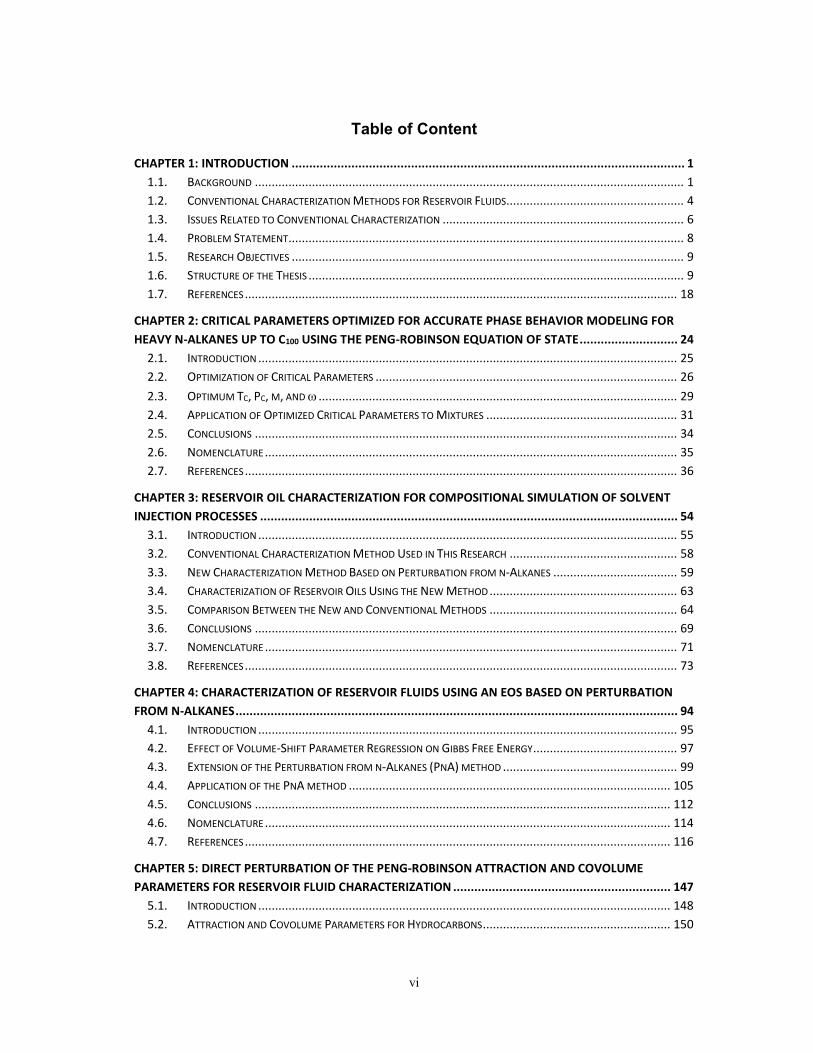
CHAPTER 1: INTRODUCTION ................................................................................................................ 1
1.1. BACKGROUND ................................................................................................................................ 1
1.2. CONVENTIONAL CHARACTERIZATION METHODS FOR RESERVOIR FLUIDS ..................................................... 4
1.3. ISSUES RELATED TO CONVENTIONAL CHARACTERIZATION ........................................................................ 6
1.4. PROBLEM STATEMENT ...................................................................................................................... 8
1.5. RESEARCH OBJECTIVES ..................................................................................................................... 9
1.6. STRUCTURE OF THE THESIS ................................................................................................................ 9
1.7. REFERENCES ................................................................................................................................. 18
CHAPTER 2: CRITICAL PARAMETERS OPTIMIZED FOR ACCURATE PHASE BEHAVIOR MODELING FOR
HEAVY N-ALKANES UP TO C100 USING THE PENG-ROBINSON EQUATION OF STATE ............................ 24
2.1. INTRODUCTION ............................................................................................................................. 25
2.2. OPTIMIZATION OF CRITICAL PARAMETERS .......................................................................................... 26
2.3. OPTIMUM TC, PC, M, AND ........................................................................................................... 29
2.4. APPLICATION OF OPTIMIZED CRITICAL PARAMETERS TO MIXTURES ......................................................... 31
2.5. CONCLUSIONS .............................................................................................................................. 34
2.6. NOMENCLATURE ........................................................................................................................... 35
2.7. REFERENCES ................................................................................................................................. 36
CHAPTER 3: RESERVOIR OIL CHARACTERIZATION FOR COMPOSITIONAL SIMULATION OF SOLVENT
INJECTION PROCESSES ....................................................................................................................... 54
3.1. INTRODUCTION ............................................................................................................................. 55
3.2. CONVENTIONAL CHARACTERIZATION METHOD USED IN THIS RESEARCH .................................................. 58
3.3. NEW CHARACTERIZATION METHOD BASED ON PERTURBATION FROM N-ALKANES ..................................... 59
3.4. CHARACTERIZATION OF RESERVOIR OILS USING THE NEW METHOD ........................................................ 63
3.5. COMPARISON BETWEEN THE NEW AND CONVENTIONAL METHODS ........................................................ 64
3.6. CONCLUSIONS .............................................................................................................................. 69
3.7. NOMENCLATURE ........................................................................................................................... 71
3.8. REFERENCES ................................................................................................................................. 73
CHAPTER 4: CHARACTERIZATION OF RESERVOIR FLUIDS USING AN EOS BASED ON PERTURBATION
FROM N-ALKANES .............................................................................................................................. 94
4.1. INTRODUCTION ............................................................................................................................. 95
4.2. EFFECT OF VOLUME-SHIFT PARAMETER REGRESSION ON GIBBS FREE ENERGY ........................................... 97
4.3. EXTENSION OF THE PERTURBATION FROM N-ALKANES (PNA) METHOD .................................................... 99
4.4. APPLICATION OF THE PNA METHOD ................................................................................................ 105
4.5. CONCLUSIONS ............................................................................................................................ 112
4.6. NOMENCLATURE ......................................................................................................................... 114
4.7. REFERENCES ............................................................................................................................... 116
CHAPTER 5: DIRECT PERTURBATION OF THE PENG-ROBINSON ATTRACTION AND COVOLUME
PARAMETERS FOR RESERVOIR FLUID CHARACTERIZATION .............................................................. 147
5.1. INTRODUCTION ........................................................................................................................... 148
5.2. ATTRACTION AND COVOLUME PARAMETERS FOR HYDROCARBONS ........................................................ 150
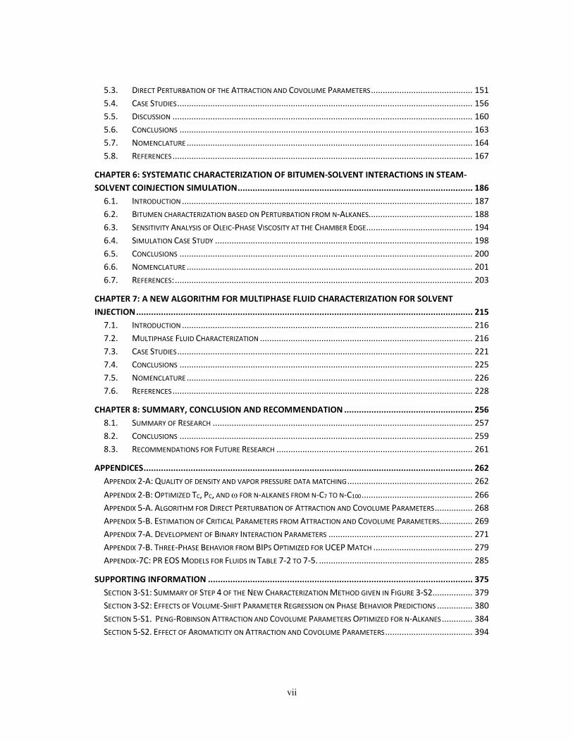
vii
5.3. DIRECT PERTURBATION OF THE ATTRACTION AND COVOLUME PARAMETERS ........................................... 151
5.4. CASE STUDIES ............................................................................................................................. 156
5.5. DISCUSSION ............................................................................................................................... 160
5.6. CONCLUSIONS ............................................................................................................................ 163
5.7. NOMENCLATURE ......................................................................................................................... 164
5.8. REFERENCES ............................................................................................................................... 167
CHAPTER 6: SYSTEMATIC CHARACTERIZATION OF BITUMEN-SOLVENT INTERACTIONS IN STEAM-
SOLVENT COINJECTION SIMULATION ............................................................................................... 186
6.1. INTRODUCTION ........................................................................................................................... 187
6.2. BITUMEN CHARACTERIZATION BASED ON PERTURBATION FROM N-ALKANES............................................ 188
6.3. SENSITIVITY ANALYSIS OF OLEIC-PHASE VISCOSITY AT THE CHAMBER EDGE............................................. 194
6.4. SIMULATION CASE STUDY ............................................................................................................. 198
6.5. CONCLUSIONS ............................................................................................................................ 200
6.6. NOMENCLATURE ......................................................................................................................... 201
6.7. REFERENCES: .............................................................................................................................. 203
CHAPTER 7: A NEW ALGORITHM FOR MULTIPHASE FLUID CHARACTERIZATION FOR SOLVENT
INJECTION ........................................................................................................................................ 215
7.1. INTRODUCTION ........................................................................................................................... 216
7.2. MULTIPHASE FLUID CHARACTERIZATION .......................................................................................... 216
7.3. CASE STUDIES ............................................................................................................................. 221
7.4. CONCLUSIONS ............................................................................................................................ 225
7.5. NOMENCLATURE ......................................................................................................................... 226
7.6. REFERENCES ............................................................................................................................... 228
CHAPTER 8: SUMMARY, CONCLUSION AND RECOMMENDATION .................................................... 256
8.1. SUMMARY OF RESEARCH .............................................................................................................. 257
8.2. CONCLUSIONS ............................................................................................................................ 259
8.3. RECOMMENDATIONS FOR FUTURE RESEARCH ................................................................................... 261
APPENDICES ..................................................................................................................................... 262
APPENDIX 2-A: QUALITY OF DENSITY AND VAPOR PRESSURE DATA MATCHING ..................................................... 262
APPENDIX 2-B: OPTIMIZED TC, PC, AND FOR N-ALKANES FROM N-C7 TO N-C100 ............................................... 266
APPENDIX 5-A. ALGORITHM FOR DIRECT PERTURBATION OF ATTRACTION AND COVOLUME PARAMETERS ................ 268
APPENDIX 5-B. ESTIMATION OF CRITICAL PARAMETERS FROM ATTRACTION AND COVOLUME PARAMETERS.............. 269
APPENDIX 7-A. DEVELOPMENT OF BINARY INTERACTION PARAMETERS ............................................................. 271
APPENDIX 7-B. THREE-PHASE BEHAVIOR FROM BIPS OPTIMIZED FOR UCEP MATCH .......................................... 279
APPENDIX-7C: PR EOS MODELS FOR FLUIDS IN TABLE 7-2 TO 7-5. ................................................................. 285
SUPPORTING INFORMATION ........................................................................................................... 375
SECTION 3-S1: SUMMARY OF STEP 4 OF THE NEW CHARACTERIZATION METHOD GIVEN IN FIGURE 3-S2................. 379
SECTION 3-S2: EFFECTS OF VOLUME-SHIFT PARAMETER REGRESSION ON PHASE BEHAVIOR PREDICTIONS ............... 380
SECTION 5-S1. PENG-ROBINSON ATTRACTION AND COVOLUME PARAMETERS OPTIMIZED FOR N-ALKANES ............. 384
SECTION 5-S2. EFFECT OF AROMATICITY ON ATTRACTION AND COVOLUME PARAMETERS ..................................... 394

viii
List of Tables
Table 1.1: PR EOS model 1 from conventional characterization. ............................................ 15 Table 1.2: PR EOS model 2 from conventional characterization. ............................................ 15 Table 1.3: PR EOS model 3 from conventional characterization. ............................................ 16 Table 1.4: PR EOS model 4 from conventional characterization. ............................................ 16 Table 1.5. Organisation of papers as chapters and features of papers ................................... 17 Table 2-1. Uncertainties in experimental data that are used in our optimization in section 2.2 40 Table 2-2. Coefficients in the correlations of Riazi and AlQaheem (2010) given in Equation 2-6.
............................................................................................................................... 40 Table 2-3. AADs in density predictions for n-alkane mixtures using the PR EOS. AADs using
Equations 2-11 to 2-13 developed in this research are compared to those using
Equations 2-8 to 2-10 of Gao et al. (2001)............................................................. 41 Table 2-4. Comparisons of density predictions using the correlations developed in this research
(Equations 2-11 to 2-13) and those using the correlations of Quiñones-Cisneros et
al. (Equations 2-14 to 2-16). Volume shift parameters are not used for these
comparisons. .......................................................................................................... 42 Table 3-1. Twenty two reservoir oils characterized in this research and converged fT, fP, and fm
values using the new characterization method ...................................................... 78 Table 3-2. Input parameters used in the 1-D simulation case study ........................................ 78 Table 4-1. Ternary fluid using the conventional characterization method with/without volume
shift in regression. ................................................................................................ 121 Table 4-2. Converged fT, fP, fm, p, and γ values for reservoir oils characterized using the PnA
method. Slim-tube MMPs are reported for these oils in the literature. ............... 121 Table 4-3. Slim-tube and calculated MMPs for eight oils from Table 4-2. .............................. 122 Table 4-4. Converged fT, fP, fm, p, and γ values for reservoir oils characterized using the PnA
method. For these oils, available data are limited to overall compositions, saturation
pressures, and liquid densities. ............................................................................ 122 Table 4-5. Converged fT, fP, fm, p, and γ values for volatile oils characterized using the PnA
method. PVT data are available for these oils, such as CVD and CCE data. .... 123 Table 4-6. Converged fT, fP, fm, p, and γ values for gas condensates characterized using the
PnA method. PVT data are available for these oils, such as CVD and CCE data.
............................................................................................................................. 123 Table 5-1. Converged fψ, fb, and p values for reservoir oils characterized using the direct PnA
method. Slim-tube MMPs are reported for these oils in the literature. ............... 183 Table 5-2. Deviations for MMP predictions for volatile oil 17 (Clark et al. 2008) based on the
direct PnA method of volatile oil. .......................................................................... 183 Table 5-3. Converged fψ, ∆c, and p values for gas condensates characterized using the direct
PnA method. CVD or CCE data are available for these oils. fb is zero for these gas
condensates. ........................................................................................................ 184 Table 5-4. Converged fψ, fb, and p values for volatile oils characterized using the direct PnA
method. CVD or CCE data are available for these oils. ...................................... 185 Table 5-5. Converged fψ, fb, and p values for heavy oils characterized using the direct PnA
method. PVT data available for these oils include swelling tests, gas solubility, and
phase envelopes. ................................................................................................. 185

ix
Table 6-1. Data used in characterization, and regressed fb and fψ values for bitumens
characterized. ....................................................................................................... 205 Table 6-2. Summary of case studies results. ......................................................................... 205 Table 6-3: Molecular weights, TC, PC, and ω for pseudo components from the proposed
characterization for JACOS bitumen .................................................................... 206 Table 6-4. Reservoir and fluid properties used in recovery simulation of JACOS bitumen. .. 206 Table 7-1. Binary interaction parameters used with the new algorithm. Numbers inside brackets
indicate the corresponding equations in this paper. ............................................ 236 Table 7-2. Characterization results for gas condensates and volatile oils with the new algorithm.
CVD or CCE data are available for these fluids. Parameters β and k are defined in
the algorithm section. Parameter p indicates the degree of freedom in the chi-
squired distribution. .............................................................................................. 237 Table 7-3. Characterization results for oils for which slim-tube MMP data are available.
Parameters β and k are defined in the algorithm section. ................................... 238 Table 7-4. Characterization results for heavy oils and bitumens with the new algorithm. ..... 238 Table 7-5. Characterization results for oils for which three phases with CO2 were reported in the
literature. .............................................................................................................. 239 Table 2-A1. Sources and T-P ranges of data used for optimizing TC, PC, ω, and AADs in density
predictions. AADs using optimum TC, PC, and ω developed in this research are
compared to those using the correlations of Gao et al. (2001). ........................... 262 Table 2-A2. Sources and T-P ranges of data used for optimizing TC, PC, ω, and AADs in vapor
pressure predictions. AADs using optimum TC, PC, and ω developed in this research
are compared to those using the correlations of Gao et al. (2001)...................... 264
Table 2-B. TC, PC, m, and optimized in this research and TC, PC, and from the correlations
of Gao et al. (2001) for n-alkanes from C7 to C100. .............................................. 266 Table 5-B1. Example of solution for TC, PC, and ω from the attraction and covolume parameters
using the EXCEL solver. The temperature is 299.81 K. ...................................... 270 Table 3-S1. Fluid model for oil 3 developed using the new characterization method with 11
components. ......................................................................................................... 375 Table 3-S2. Fluid model for oil 3 developed using the conventional characterization method with
volume shift with 11 components. ........................................................................ 375 Table 3-S3. Fluid model for oil 6 developed using the new characterization method with 11
components. ......................................................................................................... 376 Table 3-S4. Fluid model for oil 6 developed using the conventional characterization method with
volume shift with 11 components. ........................................................................ 376 Table 3-S5. Ternary fluid using the conventional characterization method with/without volume
shift in regression. ................................................................................................ 381 Table 5-S1. Estimated physical critical points for n-C100. The critical points from Kumar and
Okuno (2012) are optimized ones with the PR EOS. .......................................... 388
x
List of Figures
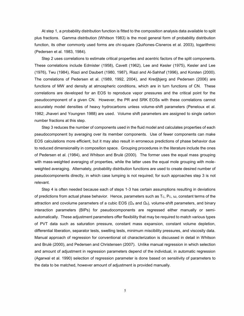
Figure 1-1. Trend of different enhanced oil recovery (EOR) projects (miscible, thermal,
immiscible, chemical and microbial). ..................................................................... 12 Figure 1-2. Temperature ranges for three hydrocarbon phases’ presence for binary mixtures
and for solvent and reservoir fluid mixture. ............................................................ 12 Figure 1-3. Non-monotonic trend for oil recovery from slim tube experiment (Mohanty et al. 1995)
for the West Sak oil. ............................................................................................... 13 Figure 1-4. Comparison of PT envelopes from four PR EOS models developed using
conventional characterization. ............................................................................... 13 Figure 1-5. Systematic change in PT phase envelope with increasing aromatic contents in
pseudocomponents. ............................................................................................... 14 Figure 2-1. The m(ω) function for the Peng-Robinson EOS as defined in Equations 2-4 and 2-
5. ............................................................................................................................ 43 Figure 2-2. Average absolute deviation (AAD) in density predictions for n-alkanes from C7 to
C100 using the correlations developed in this research and the correlations of Gao et
al. (2001). ............................................................................................................... 43 Figure 2-3. Average absolute deviation (AAD) in vapor pressure predictions for n-alkanes from
C7 to C100 using the correlations developed in this research and the correlations of
Gao et al. (2001). ................................................................................................... 44 Figure 2-4. Optimum critical temperature (TC) developed for the PR EOS in this research, and
the TC correlations of Gao et al. (2001) and Riazi and Al-Sahhaf (1996). ............. 44 Figure 2-5. Optimum critical pressure (PC) developed for the PR EOS in this research, and the
PC correlations of Gao et al. (2001) and Riazi and Al-Sahhaf (1996). ................... 45 Figure 2-6. Optimum acentric factor (ω) developed for the PR EOS in this research, and the ω
correlations of Gao et al. (2001) and Riazi and Al-Sahhaf (1996). ........................ 45 Figure 2-7. Sensitivity of density and vapor pressure predictions to TC around the optimum
values given in Equation 2-11. ............................................................................... 46 Figure 2-8. Sensitivity of density and vapor pressure predictions to PC around the optimum
values given in Equation 2-12. ............................................................................... 46 Figure 2-9. Sensitivity of density and vapor pressure predictions to the m parameter around the
optimum values given in Equation 2-13. ................................................................ 47 Figure 2-10. Comparison of bubble point pressure predictions with experimental data (Peters et
al. 1988) for C1-C16 mixtures at 300 K.................................................................... 47 Figure 2-11. Comparison of bubble point pressure predictions with experimental data (Peters et
al. 1988) for C1-C20 mixtures at 363.15 K. ............................................................. 48 Figure 2-12. Comparison of bubble point pressure predictions with experimental data (Peters et
al. 1988) for C2-C16 mixtures at 363.15 K. ............................................................. 48 Figure 2-13. Comparison of bubble point pressure predictions with experimental data (Peters et
al. 1988) for C2-C20 mixtures at 350 K.................................................................... 49 Figure 2-14. Comparison of bubble point pressure predictions with experimental data (Peters et
al. 1988) for C2-C22 mixtures at 340 K.................................................................... 49 Figure 2-15. Comparison of bubble point pressure predictions with experimental data (Peters et
al. 1988) for C2-C22 mixtures at 360 K.................................................................... 50 Figure 2-16. Comparison of bubble point pressure predictions with experimental data (Peters et
al. 1988) for C2-C24 mixtures at 330 K.................................................................... 50
xi
Figure 2-17. Comparison of bubble point pressure predictions with experimental data (Peters et
al. 1988) for C2-C24 mixtures at 340 K.................................................................... 51 Figure 2-18. Comparison of bubble and dew point predictions with experimental data (Joyce
and Thies 1998) for C6-C16 mixture at 623K. ......................................................... 51 Figure 2-19. Comparison of bubble and dew point predictions with experimental data (Joyce et
al. 2000) for C6-C24 mixture at 622.9K. .................................................................. 52 Figure 2-20. Comparison of bubble and dew point predictions with experimental data (Joyce et
al. 2000) for C6-C36 mixture at 621.8K. .................................................................. 52 Figure 2-21. AAD reduction in density predictions for 25 different reservoir oils listed in Table 2-
3. ............................................................................................................................ 53 Figure 3-1. Differences between aromatics and paraffins for critical temperature, TCA-TCP,
based on the correlations of Riazi and Al-Sahhaf (1996) and Equation 3-4. ......... 79 Figure 3-2. Differences between aromatics and paraffins for critical pressure, PCA-PCP, based on
the correlations of Riazi and Al-Sahhaf (1996), Pan et al. (1997), and Equation 3-5.
............................................................................................................................... 79 Figure 3-3. Differences between aromatics and paraffins for the m parameter, mP-mA, based
on the correlations of Riazi and Al-Sahhaf (1996), Pan et al. (1997), and Equation
3-6. ......................................................................................................................... 80 Figure 3-4. Convergence behavior for the ε function (Equation 3-13) with fm for oils 5, 6, and 9
given in Table 3-1. .................................................................................................. 80 Figure 3-5. The converged fT values for the 22 different oils in Table 3-1. .............................. 81 Figure 3-6. The converged fP values for the 22 different oils in Table 3-1. .............................. 81 Figure 3-7. The converged fm values for the 22 different oils in Table 3-1. .............................. 82 Figure 3-8. MMP calculated for Oil 6 with 100% methane at 333.15 K using CMw/oV with different
numbers of pseudocomponents. ............................................................................ 82 Figure 3-9. MMP calculated for Oil 6 with 100% CO2 at 333.15 K using CMw/oV with different
numbers of pseudo components. ........................................................................... 83 Figure 3-10. Two-phase P-T diagrams for a mixture of oil 6 10% and C2 90% based on the NM
and the CMwV. ........................................................................................................ 83 Figure 3-11. Three-phase P-T diagrams for a mixture of oil 6 10% and C2 90% based on the NM
and the CMwV. ........................................................................................................ 84 Figure 3-12. Two-phase P-T diagrams for a mixture of oil 6 10% and C3 90% based on the NM
and the CMwV. ........................................................................................................ 84 Figure 3-13. Three-phase P-T diagrams for a mixture of oil 6 10% and C3 90% based on the NM
and the CMwV. ........................................................................................................ 85 Figure 3-14. P-x diagrams for the oil-6/C1 pseudo binary pair at 333.15 K based on the NM and
CMwV with 11 components. ................................................................................... 85 Figure 3-15. P-x diagrams for the oil-6/C2 pseudo binary pair at 333.15 K based on the NM and
CMwV with 11 components. ................................................................................... 86 Figure 3-16. P-x diagrams for the oil-6/CO2 pseudo binary pair at 333.15 K based on the NM
and CMwV with 11 components. ............................................................................ 86 Figure 3-17. Saturated liquid densities for mixtures of oil 6 and the equimolar C1-C2 mixture at
333.15 K. ................................................................................................................ 87 Figure 3-18. T-x diagrams for the oil-3/C6 pseudo binary pair at 34.47 bars. .......................... 87 Figure 3-19. T-x diagrams for the oil-3/C6 pseudo binary pair at 60.00 bars. .......................... 88
xii
Figure 3-20. Two-phase PT diagrams for mixtures of oil 3 and C6 at three different C6 mixing
ratios, 0.1, 0.3, and 0.4. ......................................................................................... 88 Figure 3-21. Comparison of MMP calculations for 22 oils in Table 3-1 based on the NM with 11
components and the CMw/oV with 30 components. ................................................ 89 Figure 3-22. Comparison of MMP calculations for 22 oils in Table 3-1 based on the CMwV with
11 components and the CMw/oV with 30 components. ........................................... 89 Figure 3-23. Comparison of MMP calculations for 18 oils in Table 3-1 based on the NM with 11
components and the CMw/oV with 30 components. ................................................ 90 Figure 3-24. Comparison of MMP calculations for 18 oils in Table 3-1 based on the CMwV with
11 components and the CMw/oV with 30 components. ........................................... 90 Figure 3-25. Measured and calculated densities for oil 6 at 333.15 K. .................................... 91 Figure 3-26. Measured and calculated viscosities for oil 6 at 333.15 K. .................................. 91 Figure 3-27. Oil recovery predictions in 1-D oil displacement simulations based on the NM and
CMwV with 11 components, along with pseudo data points generated from the
CMw/oV with 30 components. ................................................................................. 92 Figure 3-28. Oil saturation profiles at 0.4 HCPVI for the oil-6 displacement with the equimolar
C1/C2 mixture at 333.15 K and 200 bars. ............................................................... 92 Figure 3-29. Concentration profiles for C1 at 0.4 HCPVI for the oil-6 displacement with the
equimolar C1/C2 mixture at 333.15 K and 200 bars. .............................................. 93 Figure 4-1. Dimensionless molar Gibbs free energy change on mixing for the ternary fluid given
in Table 4-1 at 330.4 K and 196.48 bars. ............................................................. 124 Figure 4-2. Dimensionless molar Gibbs free energy change on mixing for the ternary fluid given
in Table 4-1 at 330.4 K and 196.48 bars. ............................................................. 124 Figure 4-3. Phase envelope for the ternary fluid given in Table 4-1. ..................................... 125 Figure 4-4. Phase envelope for the ternary fluid given in Table 4-1. ..................................... 125 Figure 4-5. Chi-squared distributions for different p values in Equation 4-5. ......................... 126 Figure 4-6. Standard specific gravity (SG) calculated for aromaticity levels 10 and 60 using
uniform perturbation from n-alkanes. ................................................................... 126 Figure 4-7. Absolute deviation for standard SG calculated for two aromaticity levels 10 and 60
using uniform perturbation from n-alkanes. ......................................................... 127 Figure 4-8. Variable perturbation from n-alkanes to match the standard SG curves from
Yarborough (1979). .............................................................................................. 127 Figure 4-9. The attraction (a) parameter for three levels of aromaticity 0, 10, and 60. .......... 128 Figure 4-10. The covolume (b) parameter for three levels of aromaticity 0, 10, and 60. ....... 128 Figure 4-11. The ψ parameter (ψ = a/b2) for three levels of aromaticity based on the values for
a and b parameters in Figures 4-9 and 4-10........................................................ 129 Figure 4-12. The ψ parameter (ψ = a/b2) for three levels of aromaticity at 370.15 K. ............ 129 Figure 4-13. Trends of the fT, fP, fm, and γ parameters during iteration for oil 2 given in Table 4-
2. .......................................................................................................................... 130 Figure 4-14. Trends of the ε function and the γ parameter during iteration for oil 2 given in Table
4-2. ....................................................................................................................... 130 Figure 4-15. The ψ parameter (ψ = a/b2) for oil 1 given in Table 4-2. .................................... 131 Figure 4-16. Minimum miscibility pressures calculated for different γ values for oil 1 (Table 4-2)
at 374.85 K. .......................................................................................................... 131 Figure 4-17. The trend of the a parameter for the four pseudocomponents for each of four cases
considered in Figure 4-15. ................................................................................... 132
xiii
Figure 4-18. The trend of the b parameter for the four pseudocomponents for each of four cases
considered in Figure 4-15. ................................................................................... 132 Figure 4-19. Trend of the converged fT values with respect to the API gravity. ..................... 133 Figure 4-20. Trend of the converged fP values with respect to the API gravity. ..................... 133 Figure 4-21. Trend of the converged fm values with respect to the API gravity. ..................... 134 Figure 4-22. Trend of γ parameter with fluid API gravity. ....................................................... 134 Figure 4-23. Average gradient of ψ (Δψ/ΔM) for different fluids. ............................................ 135 Figure 4-24. Average gradient of ψ (Δψ/ΔM) with respect to γ. ............................................. 135 Figure 4-25. Comparisons of C1-MMPs for 22 oils in Table 4-4 using the PnA method and those
from pseudo data. ................................................................................................ 136 Figure 4-26. Comparisons of CO2-MMPs for 18 oils in Table 4-4 using the PnA method and
those from pseudo data. ...................................................................................... 136 Figure 4-27. CVD liquid saturation for volatile oil 1 given in Table 4-5. ................................. 137 Figure 4-28. CVD liquid saturation for volatile oil 5 given in Table 4-5. ................................. 137 Figure 4-29. CCE relative volume curve for volatile oil 6 given in Table 4-5. ......................... 138 Figure 4-30. Comparison of the ai and bi parameters for pseudocomponents for volatile oil 1
given in Table 4-5. ................................................................................................ 138 Figure 4-31. Comparison of ψ trends for pseudocomponents for volatile oil 1 given in Table 4-
5. .......................................................................................................................... 139 Figure 4-32. CCE liquid saturation for near-critical volatile oil 12 given in Table 4-5. ............ 139 Figure 4-33. CVD liquid saturation for gas condensate 20 given in Table 4-6 at 367.6 K. .... 140 Figure 4-34. CVD liquid saturation for gas condensate 5 given in Table 4-6 at 424.82 K. .... 140 Figure 4-35. Trends of ψ for gas condensates 4, 12, 20, and 26 given in Table 4-6. ............ 141 Figure 4-36. CVD liquid saturation for near-critical gas condensate 7 given in Table 4-6 at 424.82
K. .......................................................................................................................... 141 Figure 4-37. P-T phase envelope for the C7
+ fraction using the three fluid models shown in Figure
4-36. ..................................................................................................................... 142 Figure 4-38. Quality lines for near-critical gas condensate 6 given in Table 4-6. .................. 142 Figure 4-39. CVD liquid saturation for near-critical gas condensate 6 given in Table 4-6 at 422.6
K. .......................................................................................................................... 143 Figure 4-40. Oleic phase saturation data and predictions using the PnA method for heavy oil 23
given in Table 4-4 (Sharma 1990) at 299.81 K. ................................................... 143 Figure 4-41. Oleic phase saturation data and predictions using the PnA method for heavy oil 23
given in Table 4-4 (Sharma 1990) at 299.81 K. ................................................... 144 Figure 4-42. The ψ parameter (ψ = ai/bi
2) for pseudocomponents for heavy oil 23 given in Table
4-4. ....................................................................................................................... 144 Figure 4-43. Three-phase region from the PnA method is compared with pseudo data for a
mixture of 20% oil 23 (Table 4-4) and 80% CO2. ................................................. 145 Figure 4- 44. Three-phase region from the PnA method is compared with pseudo data for a
mixture of 10% oil 5 (Table 4-4) and 90% C2. ...................................................... 145 Figure 4-45. Three-phase region from the PnA method is compared with pseudo data for a
mixture of 10% oil 5 (Table 4-4) and 90% C3. ...................................................... 146 Figure 5-1. Correlation of c’/ZSATfb with (fb + fψ)/Pr using a linear function.............................. 173 Figure 5-2. Average deviations of density predictions from experimental data during the
regressions for two different fluids. ...................................................................... 173

xiv
Figure 5-3. Variation of the phase envelope in P-T space during the PnA regression for a fluid
of 42 °API. ............................................................................................................ 174 Figure 5-4. Variation of the phase envelope in P-T space during the PnA regression for a light
fluid. ...................................................................................................................... 174 Figure 5-5. The converged fb value tends to increase with increasing specific gravity of the fluid.
............................................................................................................................. 175 Figure 5-6. CVD liquid saturations measured for gas condensate 12 given in Table 5-3 (McVay
1994) at 387.59 K. ................................................................................................ 175 Figure 5-7. CCE liquid saturations measured for gas condensate 3 given in Table 5-3 (Al-
Meshari 2004) at 382.59 K. .................................................................................. 176 Figure 5-8. Comparison between the measured and predicted CVD liquid saturations for near-
critical volatile oil 14 in Table 5-4 at 424.25 K (Pedersen et al. 1988). ................ 176 Figure 5-9. Oleic phase saturation data and predictions for heavy oil 1 (Sharma 1990) given in
Table 5-5 at 299.81 K. .......................................................................................... 177 Figure 5-10. Data and predictions for saturation pressures in the swelling tests of heavy oil 2
with two injection gases; CO2 and a light gas mixture (Kredjbjerg and Pedersen
2006). ................................................................................................................... 177 Figure 5-11. Data and predictions for the gas-oil-ratios (GOR) for heavy oil 3 (Pedersen et al.
2004) at the reservoir temperature of 305.45 K. .................................................. 178 Figure 5-12. Saturation pressures measured and predicted for two mixtures with the
Lloydminster heavy oil (heavy oil 4 in Table 5-5), Feeds #4 and #5 in Li et al. (2013a).
............................................................................................................................. 178 Figure 5-13. The three-phase boundaries measured and predicted for a mixture of heavy oil 4
(Table 5-5) with CO2 and n-C4 (Feed #15 of Li et al. 2013b). .............................. 179 Figure 5-14. CVD liquid saturations predicted with different values for C for gas condensate 6 in
Table 5-3. ............................................................................................................. 179 Figure 5-15. MMPs calculated with different C values for oil 1 given in Table 5-1................. 180 Figure 5-16. Two-phase envelopes predicted with the two sets of critical parameters for an n-
alkane mixture. ..................................................................................................... 180 Figure 5-17. Saturation pressures measured and predicted for a 25-component oil with a gas at
373.15 K presented in Danesh et al. (1991). ....................................................... 181 Figure 5-18. Comparison of two-phase envelopes for ternary mixture predicted with two PR EOS
with two different set of critical parameters. ......................................................... 181 Figure 5-19. Saturation pressures measured in the swelling test of Fluid 18 (Table 5-1) with CO2
at 394 K (Negahban et al. 2010). ......................................................................... 182 Figure 6-1. Systematic development of phase envelope for a sample mixture of bitumen and
methane during regression algorithm. ................................................................. 207 Figure 6-2. Comparison of the data and predictions for ethane solubilities for (a) Cold Lake and
(b) Athabasca bitumens. For Cold Lake bitumen, solid curves show the predictions
and dashed curves show the data. ...................................................................... 208 Figure 6-3. Comparison of matched solubility with data for CO2 in Cold Lake bitumen. ........ 209 Figure 6-4. AARDs for methane and ethane solubilities in JACOS bitumen with different MWs
used in the PnA algorithm. ................................................................................... 209 Figure 6-5. Comparison of T-x diagrams at 35.0 bars for bitumen and propane mixture for two
different compositional characterizations of JACOS bitumen. ............................. 210

xv
Figure 6-6. Effective viscosity of solvents calculated at pressure 35.0 bars for solvent and
JACOS bitumen mixture. ...................................................................................... 211 Figure 6-7. Estimated trends for the L-phase viscosity at the chamber-edge conditions (μedge)
with respect to the solvent mole fraction in the L-phase (xsL). ............................. 212 Figure 6-8. Trend of viscosity gradient (∆µ/∆T) with temperature for JACOS bitumen. ......... 213 Figure 6-9. Simulated bitumen recovery with steam-solvent coinjection method for different
solvent cases (n-C3, n-C4, n-C5, and n-C6). ......................................................... 213 Figure 6-10. L-phase viscosity along the chamber edge from the simulation results: (a) propane-
steam coinjection, (b) butane-steam coinjection, and (c) hexane-steam coinjection.
............................................................................................................................. 214 Figure 7-1. Comparison of critical parameters and vapor pressure curves for hexadecane (Yaws
2010) and pyrene (Nikitin and Popov 2015). ....................................................... 240 Figure 7-2. Comparison of two-phase envelopes for 99.99% binary mixture of methane with
nonane (n-C9), propyl cyclo hexane (C9H18), and 2-propyl benzene (C9H12)....... 240 Figure 7-3. Predicted UCEP for ethane and n-C18 mixture at different BIP values. For nC18
optimized critical parameters (Kumar and Okuno 2012) are used. ..................... 241 Figure 7-4. Trend of reduced Gibbs free energy of mixing at UCEP of ethane and n-C18 mixture
at (312.45 K, 55.31 bars). .................................................................................... 241 Figure 7-5. Comparison of P-x diagram for ethane and n-C16 mixture at 363.15 K with
experimental data (Peters et al. 1988). ................................................................ 242 Figure 7-6. Comparison of P-x diagram for ethane and n-C24 mixture at 340 K with experimental
data (Peters et al. 1988). ...................................................................................... 242 Figure 7-7. Comparison of P-x diagram for hexane and n-C36 mixture at 621.8 K with
experimental data (Joyce and Gordon 2000)....................................................... 243 Figure 7-8. Comparison of P-T diagrams for quaternary mixture of methane, n-C10, n-C18, and
n-C30 with experimental data (Daridon et al. 1996). ............................................. 243 Figure 7-9. Comparison of empirically determined higher boundary correlation for critical
temperature in Equation 7-5 with data (Yaws 2010, Nikitin and Popov 2015). ... 244 Figure 7-10. Comparison of empirically determined higher boundary correlation for critical
pressure in Equation 7-6 with data (Yaws 2010, Nikitin and Popov 2015). ......... 244 Figure 7-11. Systematic changes in vapor pressure curves for pseudocomponents and P-T
envelope for fluid with changes in k parameter during regression. ..................... 245 Figure 7-12. CME liquid saturation predicted for near-critical gas condensate, Fluid 36 in Table
7-2, at 366.48 K. The molecular weight is 39.34 gram/mole. ............................. 246 Figure 7-13. CVD liquid saturation predicted for near-critical volatile oil, Fluid 54 in Table 7-2, at
424.25 K. The molecular weight is 47.84 gram/mole. ......................................... 246 Figure 7-14. Saturation pressures during the swelling test for Oil 2 in Table 7-4 at 347.15 K.
............................................................................................................................. 247 Figure 7-15. Gas-oil ratio (GOR) predictions at 305.45 K for Oil 3 in Table 7-4. ................... 247 Figure 7-16. Saturation pressures measured and predicted for two mixtures with Lloydminster
heavy oil, Oil 4 in Table 4 (Feeds #4 and #5 in Li et al., 2013a).......................... 248 Figure 7-17. Liquid-phase saturations for West Sak heavy oil (Oil 1 in Table 4) mixed with CO2
at 299.81 K. (a) Oleic (L1) phase. (b) Solvent-rich liquid (L2) phase. ................. 249 Figure 7-18. Comparison of P-x diagrams for oil 1 in Table 7-5 at 370 K predicted with EOS
models from new algorithm and Aghabsh and Ahmadi (2012). ........................... 250

xvi
Figure 7-19. Comparison of P-T envelope predicted with SRK EOS by Krejbjerg and Pedersen
(2006) with prediction from new algorithm for oil 2 in Table 7-4. ......................... 250 Figure 7-20. Comparison of three-phase boundaries for the West Sak oil and CO2 mixture. 251 Figure 7-21. Three-phase boundaries measured and predicted for a mixture of Athabasca
bitumen: 51.0% CO2, 34.7% propane, and 14.3% bitumen (Badamchi-Zadeh et al.
2009). ................................................................................................................... 252 Figure 7-22. Three-phase boundaries measured and predicted for a mixture of Peace River
bitumen: 89.90% pentane and 10.10% bitumen. ................................................. 252 Figure 7-23. Comparison of the predicted P-x diagram with data for Oil C2 (Table 7-5) of Turek
et al. (1988) with CO2 at 313.71 K. ...................................................................... 253 Figure 7-24. Comparison of the predicted P-x diagram for Oil G (Table 5) of Creek and Sheffield
(1993) with CO2 at 307.60 K. ............................................................................... 253 Figure 7-25. Comparison of the predicted P-x diagram at 313.70 K from Khan 1992 EOS model
with prediction from new algorithm for oil 5 in Table 7-5. .................................... 254 Figure 7-26. Comparison of the predicted P-x diagram at 301.48 K from Khan 1992 EOS model
with prediction from new algorithm for oil 6 in Table 7-5. .................................... 254 Figure 7-27. Comparison of the predicted P-x diagram at 316.48 K from Khan 1992 EOS model
with prediction from new algorithm for oil 7 in Table 7-5. .................................... 255 Figure 7-28. Comparison of the predicted P-x diagram at 307.60 K from Creek and Sheffield
(1993) EOS model with prediction from new algorithm for oil 9 in Table 7-5. ..... 255 Figure 5-A1. Flow chart for the direct perturbation algorithm presented in Section 3. ........... 268 Figure 7-A1. Trend of BIP with respect to ω for the heavier n-alkane for matching the UCEP
data for each binary. ............................................................................................ 274 Figure 7-A2. UCEP pressures measured for propane binaries (Peters et al. 1989, 1993). ... 274 Figure 7-A3. Comparison of physical ω (Equation 7-3) with ώ (Equation 7-4) that can be used
to match the UCEP data with the PR EOS. ......................................................... 275 Figure 7-A4. Three-phase envelope for a mixture of ethane, propane, and eicosane
(Gregorowicz et al. 1993a). .................................................................................. 275 Figure 7-A5. Trend of optimized propane BIPs with respect to CN of the heavier n-alkane. The
curve is given by Equation 7-11. .......................................................................... 276 Figure 7-A6. Comparison of predicted three-phase envelope for methane, ethane, and eicosane
mixture with data. ................................................................................................. 276 Figure 7-A7. Predicted temperature and pressure points at UCEP for butane’s mixture with
heavier n-alkane using BIP correlation Equation 7-12. ........................................ 277 Figure 7-A8. Trend of optimized CO2 BIPs with respect to CN of the heavier n-alkane. The curve
is calculated from Equation 7-8. ........................................................................... 278 Figure 7-B1. T-x projection of three-phase region in P-T-x space for CH4 and n-C7 binary mixture.
............................................................................................................................. 281 Figure 7-B2. Comparison of the optimized temperature at UCEP (shown as UCEP (UCEP
match)) with data for ethane binaries. .................................................................. 281 Figure 7-B3. Quality of matching of T-x projection of three-phase region in P-T-x space for C2H6
and n-C22 binary mixture with data. ...................................................................... 282 Figure 7-B4. Comparison of the BIP optimized for LCEP match for ethane binaries with trend of
BIP (Equation 7-10) for UCEP match. ................................................................. 282 Figure 7-B5. Comparison of the optimized temperature at LCEP (shown as LCEP (LCEP match))
with data for ethane binaries. ............................................................................... 283

xvii
Figure 7-B6. T-x projection for three-phase in P-T-x space for n-C3 and n-C44 binary with different
BIPs. ..................................................................................................................... 283 Figure 7-B7. Comparison of the BIPs optimized for LCEP match for propane binaries with the
trend of BIP (Equation 7-11) that matched the UCEP. ........................................ 284 Figure 7-B8. Comparison of the optimized temperature at LCEP (shown as LCEP (LCEP match))
with data for propane binaries is shown. .............................................................. 284 Figure 3-S1. Flow chart for the conventional characterization method (CM) in this research,
which is based on Pedersen and Christensen (2007). ........................................ 377 Figure 3-S2. Flow chart for the new characterization method (NM) developed in this research.
............................................................................................................................. 378 Figure 3-S3. Dimensionless molar Gibbs free energy change on mixing for the ternary fluid given
in Table 3-S5 at 330.4 K and 196.48 bars. .......................................................... 381 Figure 3-S4. Dimensionless molar Gibbs free energy change on mixing for the ternary fluid given
in Table 3-S5 at 330.4 K and 196.48 bars. .......................................................... 382 Figure 3-S5. Phase envelope for the ternary fluid given in Table 3-S5. ................................. 382 Figure 3-S6. Phase envelope for the ternary fluid given in Table 3-S5. ................................. 383 Figure 5-S1. Comparison of optimized and physical critical parameters. .............................. 388 Figure 5-S2. Comparison of vapor pressure curves and saturated liquid densities predicted with
optimized and physical critical parameters for n-C28. .......................................... 389 Figure 5-S3. Comparison of predicted isodensity curves with PR EOS with data (Dutour et al.
2001). ................................................................................................................... 389 Figure 5-S4. Comparison of critical densities from different correlations. .............................. 390 Figure 5-S5. Comparison of ac for PR EOS from optimized and physical critical parameters.
............................................................................................................................. 390 Figure 5-S6. Comparison of b parameter for PR EOS from optimized and physical critical
parameters. .......................................................................................................... 391 Figure 5-S7. Comparison of a parameter for PR EOS from optimized and physical critical
parametes. ........................................................................................................... 391 Figure 5-S8. Comparison of optimized and physical m-parameters. ...................................... 392 Figure 5-S9. Vapor pressures and saturated liquid densities predicted for n-C100 by use of two
sets of optimized critical parameters; one from Voutsas et al. (2006) and the other
Kumar and Okuno (2012)..................................................................................... 392 Figure 5-S10. Two liquid-phase isodensity curves (0.74 g/cc and 0.76 g/cc) in P-T space
predicted for n-C100 using the PR EOS. ............................................................... 393 Figure 5-S11. Comparison of normal boiling points from PR EOS with optimized and physical
critical parameters. ............................................................................................... 393 Figure 5-S12. Trend curves of Yarborough (1979) for standard specific gravity with respect to
CN of single CN fractions at different aromaticity levels. ..................................... 395 Figure 5-S13. Trend of attraction (a) parameters with carbon number of single carbon number
fraction for three levels of aromaticity 0, 10, and 60. ........................................... 395 Figure 5-S14. Trend of covolume (b) parameters with carbon number of single carbon number
fraction for three levels of aromaticity 0, 10, and 60. ........................................... 396 Figure 5-S15. Trend of ψ parameters (ψ = a/b2) with single carbon number fractions for three
levels of aromaticity at 370.15 K (Kumar and Okuno 2013). ............................... 396 Figure 5-S16. Chi-squared distributions for different p values. .............................................. 397
1
Chapter 1: Introduction
In this section, the area of oil and gas industry relevant to present research is recognized in the
subsection “Background”. Conventional practices in the relevant area described in “Background” are
briefly described in the subsection “Conventional Characterization Methods for Reservoir Fluid”. The
area of issues is also recognized in this subsection. Issues related to conventional characterization are
discussed in the subsection “Issues Related to Conventional Characterization”. The subsection
“Problem Statement” recognizes the issues that the present research aims to address. Finally,
“objective of the research” is explained.
1.1. Background
Hydrocarbons are major source of world energy. Hydrocarbons are present in different forms in the
reservoir, such as gas, gas condensates, oil, and bitumen. Reservoir fluids are recovered from
reservoirs using various enhanced oil recovery methods after primary recovery methods are insufficient
for economic recovery. Miscible gas injection is an important enhanced recovery method used as
secondary or tertiary recovery mechanism as shown in Figure 1.1, which presents a summary of
different enhanced recovery projects around the world for the years 2010, 2012, and 2014 from oil and
gas journal worldwide survey (Moritis 2010; Koottungal 2012, 2014).
Miscible gas injection is one of several enhanced recovery methods that is applied to reservoir
containing wide gravity range fluids such as gas condensates, volatile oils, normal oils, heavy oils.
Sänger and Hagoort (1998); Taheri et al. (2013), Abdrakhmanov (2013) studied the miscible gas
injection to recover gas condensates. Clark et al. (2008) studied the miscible gas injection for volatile
oil of Tirrawarra field of Australia. Solvent injection has been successfully implemented in West Texas
(Mizenko 1992; Stein et al. 1992; Tanner et al. 1992), the Powder River Basin (Fulco 2000), Alaska
(McGuire et al. 2001), Canada (Malik and Islam 2000), and the North Sea (Varotsis et el. 1986). For
the recovery of heavy oils and bitumen, solvent is coinjected with steam to take synergic benefit of
thermal and compositional mechanism (Gupta et al. 2005; Gupta and Gittins 2006; Dickson et al. 2011).
Reservoir fluids are held back in pore spaces because of capillary pressure resulting from interfacial
tension between two different phases. The interfacial tension can be reduced by achieving miscibility
of the injected fluid and in-situ hydrocarbon. Holm (1986) defined miscibility for reservoir fluids as the
physical condition for two or more fluids that will permit them to mix in all proportions. Miscibility at given
pressure-temperature conditions for injectant and reservoir fluid system can be either first contact
miscibility (FCM) or multi contact miscibility (MCM). In first contact miscibility, injectant and reservoir
fluids are miscible at first contact in all proportion. However, for systems that are not miscible at first
contact, miscibility can be achieved by multiple contacts between the injectant gas and reservoir fluids
either by pressure adjustment or by composition change of injection gas. At a given temperature,
minimum pressure at which miscibility through multiple contact can be achieved between a given
injection gas and a reservoir fluid is called minimum miscibility pressure (MMP) (Pedersen and
2
Christensen 2007). If reservoir pressure and reservoir temperature are kept constant, miscibility
between injection gas and reservoir fluid depends on the composition of the injection gas. Minimum
enrichment of injection gas for which miscibility can be achieved at a given pressure and a given
temperature is called minimum miscibility enrichment (MME). Enrichment gases usually contain CO2,
CH4, C2H6 and liquefied petroleum gases (C3 and C4) (Whitson and Brulè 2000), however composition
of components such as C3, C4, and higher carbon number components significantly affects the miscibility
conditions. Techno-economic feasibility of a miscible gas injection project depends on MMP and MME
factors.
Once miscibility is achieved, theoretically, 100% hydrocarbon recovery is possible, which leads to
highest possible local displacement efficiency. However, field scale implementation of miscible gas
injection does not result in such high recovery because of poor sweep efficiency from reservoir
heterogeneity and gravity override. Even though, displacement efficiency can be as high as 70-90%,
due to poor sweep efficiency, a typical additional recovery after water-flooding may be only 10-20% of
original oil in place (Sheng 2013). Nevertheless, gas flooding is well-developed technology and has
demonstrated good economic recoveries in the world (Manrique et al. 2007, Sheng 2013), and good
recovery from miscible gas injection will depend on proper understanding of the impact of key factors
on sweep and displacement efficiency (Sheng 2013).
Conventionally, enhanced oil recovery from miscible gas injection process refers to enhanced
recovery from the miscibility of liquid and vapor hydrocarbon phases for injected gas/solvent and
reservoir fluid mixture. The definitions of MMP and MME hitherto consider the miscibility of liquid and
vapor hydrocarbon phases present for a solvent and oil mixture, and these terms for miscibility may not
be suitable for use when three hydrocarbon phases are present. Experiments have confirmed the
presence of three hydrocarbon phases (oil rich liquid phase L1, solvent rich liquid phase L2, and vapor
phase V) for light gases’ (carbon dioxide, methane, ethane, propane, and butane) mixtures with heavier
n-alkanes, and with reservoir fluid.
For binary mixtures, CO2, methane, ethane, propane, and butane were studied as the solvent
component mixed with a heavier n-alkane component (Rodrigues and Kohn 1967; Kulkarni et al. 1974;
Hottovy et al. 1981a; Enick et al. 1985; Fall and Luks 1985; Fall et al. 1985; Estrera and Luks 1987;
Peters et al. 1987a, 1987b; Peters et al. 1989; Van der Steen et al. 1989; Peters 1994; Secuianu et al.
2007). For these binary mixtures, three hydrocarbon phases have been observed at extremely low
temperature (close to critical temperature of methane) to high temperature (close to critical temperature
of butane) as shown in Figure 1.2. Presence of three hydrocarbon phases for ternary mixtures has
been confirmed by Chang et al. (1966), Lin et al. (1977), Hottovy et al. (1981), Hottovy et al. (1982),
Merrill et al. (1983), Llave et al. (1986), Estrera and Luks (1988), Jangkamolkulchal and Luks (1989),
Iwade et al. (1992), and Gregorowicz et al. (1993a, 1993b).
With the presence of the components showing three hydrocarbon-phase behavior in binary or
ternary mixture (described in previous paragraph) in reservoir fluids, three hydrocarbon-phase behavior
3
is expected from its mixture with solvents. Three hydrocarbon phases have been observed for reservoir
fluids (light oil, heavy oil, bitumens) and solvents mixtures by various researchers (Shelton and
Yarborough 1977; Henry and Metcalfe 1983; Turek et al. 1988; Roper 1989; Sharma et al. 1989;
Okuyiga 1992; Creek and Sheffield 1993; DeRuiter et al. 1994; Mohanty et al. 1995; Godbole et al.
1995, Badamchi-Zadeh et al. 2009; Li et al. 2013) in temperature range of 291 K to 316 K. Multiphase
behavior (number of hydrocarbon phases ≥ 3) at very high temperature (<613 K) has been observed by
Zou et al. (2007) for Athabasca Vacuum Bottom and pentane mixture.
Discussions in previous paragraphs indicate presence of three hydrocarbon phases during oil
recovery with gas injection in practical reservoir temperature ranges. These multiple hydrocarbon
phases present complex recovery mechanism as they have different mobility and inter-phase miscibility
conditions. Miscibility in presence of three hydrocarbon phases may not be like two hydrocarbon phase
miscibility where miscibility is achieved by merging of liquid and vapor phase. Experimental studies
(Shelton and Yarborough 1977; Henry and Metcalfe 1983; Okuyiga 1992; Creek and Sheffield 1993;
DeRuiter et al. 1994; Mohanty et al. 1995) have confirmed efficient oil recoveries when two or more than
two hydrocarbon phases are present in the solvent and oil mixture.
Oil recovery amounting to 90±5% has been experimentally observed with CO2 or rich gases as
injectant gas (Shelton and Yarborough 1977; Creek and Sheffield 1993). Similar experimental
observation was made in case of displacement of the West Sak oil with gas mixture (methane, ethane,
propane, and butane). Unlike two hydrocarbon phase oil recovery where oil recovery is monotonic
function of dilution i.e. recovery decreasing with increasing dilution, researchers such as Okuyiga (1992),
DeRuiter et al. (1994), and Mohanty et al. (1995) observed non-monotonic oil recovery with increased
methane dilution in the injection gas (Figure 1.3). They observed 93% recovery at 1.2 pore volume of
injection gas with 62% methane, whereas recovery was 85% for injection gas with 51% methane.
Mohanty et al. (1995) explained the non-monotonicity of oil recovery on the degree of closeness of
density/composition of the L2 phase with V phase and with L1 phase on upstream and downstream of
the three-phase respectively. The study by Okuno and Xu (2014) has shown high displacement
efficiency in the presence of three hydrocarbon phases, when composition path approached to critical
end points of oil and solvent mixture. The local displacement efficiency depends on the components’
redistribution in the transition zone between two phases and three phases (upstream and downstream
of three-phase). For efficient displacement of oil, L2 and V phases from three-phases should merge with
non-oleic phase on upstream side, and L2 phase on downstream side should appear from oleic phase.
Experimental and analytical studies on three hydrocarbon phases and non-monotonic oil recovery,
discussed in previous paragraphs, indicate to potential use of those understandings for more efficient
oil recovery from in-situ three hydrocarbon phases’ flow conditions with proper design and simulation of
partially miscible gas injection process. Simulation of oil recovery from the miscible gas injection in
presence of two/three hydrocarbon phases is function of two important parts: phase behavior and flow
behavior. Phase behavior, which determines the miscibility of injectant fluid with the reservoir fluid at a
4
given pressure-temperature conditions, is function of fluid characterization, whereas flow behavior
depends on the properties of flow medium. Phase behavior for a given overall composition at a given
pressure-temperature condition determines some key information, such as number of phases, and
composition and amount of these phases. Combination of phase and flow behavior makes the
simulation of oil recovery complex, as overall composition becomes function of time and location
between injector and producer.
Simulating correct number of phases, their composition and volumes is important for a reliable
recovery simulation. Commonly used commercial simulators do not allow more than two hydrocarbon
phases (liquid and vapor). Although, presence of three phases depends on temperature-pressure
conditions, and asymmetric nature of injection gas and reservoir hydrocarbons; ruling out the possibility
of presence of three phases during dynamic miscibility process can lead to unreliable hydrocarbon
recovery simulation. Khan (1992) has shown the difference between simulated recoveries from two-
phase and three-phase simulators. Experimental data can be helpful to some extent but it may not be
possible to conduct experiments at all possible temperature-pressure points and compositions that may
appear during miscibility process as overall composition along the composition path from injection to
production point keeps on changing with time and place.
A reliable and robust reservoir fluid characterization is therefore, needed to simulate the number of
phases, its compositional and volumetric properties in the miscible or partially miscible displacement
process correctly. The subject of the present research is the reservoir fluid characterization, where
issues related to conventional characterization approaches are discussed and resolved by proposing a
new characterization algorithm for reliable multiphase behavior simulation.
1.2. Conventional Characterization Methods for Reservoir Fluids
Characterization of reservoir hydrocarbons is the process of representing reservoir hydrocarbons
compounds by a suitable number of pure, lumped and/or pseudocomponents and assigning them with
suitable EOS parameters so that EOS simulated phase behaviors match with experiments satisfactorily.
Reservoir fluids are characterized using conventional approaches (Pedersen and Christensen 2007)
with cubic equations of states (EOS) in commercial simulators, because of their simplicity and accuracy.
Commonly used two-parameter cubic equations of state are PR EOS (Peng and Robinson 1976, 78),
SRK EOS (Soave 1982). A typical characterization process consists of four main steps (Whitson and
Brulè 2000; Pedersen and Christensen 2007) as follows:
Step 1. Estimation of a molar distribution with respect to molecular weight (MW) or carbon number
(CN) to split the plus fraction into detailed components.
Step 2. Estimation of properties for the detailed components such as critical temperature (TC), critical
pressure (PC), critical volume (VC), acentric factor (ω), and volume-shift parameters (Peneloux
et al. 1982).
Step 3. Grouping of the detailed components into fewer pseudocomponents.
Step 4. Regression of pseudocomponents’ properties to match experimental data available.
5
At step 1, a probability distribution function is fitted to the composition analysis data available to split
plus fractions. Gamma distribution (Whitson 1983) is the most general form of probability distribution
function, its other commonly used forms are chi-square (Quiñones-Cisneros et al. 2003), logarithmic
(Pedersen et al. 1983, 1984).
Step 2 uses correlations to estimate critical properties and acentric factors of the split components.
These correlations include Edmister (1958), Cavett (1962), Lee and Kesler (1975), Kesler and Lee
(1976), Twu (1984), Riazi and Daubert (1980, 1987), Riazi and Al-Sahhaf (1996), and Korsten (2000).
The correlations of Pedersen et al. (1989, 1992, 2004), and Kredjbjerg and Pedersen (2006) are
functions of MW and density at atmospheric conditions, which are in turn functions of CN. These
correlations are developed for an EOS to reproduce vapor pressures and the critical point for the
pseudocomponent of a given CN. However, the PR and SRK EOSs with these correlations cannot
accurately model densities of heavy hydrocarbons unless volume-shift parameters (Peneloux et al.
1982; Jhaveri and Youngren 1988) are used. Volume shift parameters are assigned to single carbon
number fractions at this step.
Step 3 reduces the number of components used in the fluid model and calculates properties of each
pseudocomponent by averaging over its member components. Use of fewer components can make
EOS calculations more efficient, but it may also result in erroneous predictions of phase behavior due
to reduced dimensionality in composition space. Grouping procedures in the literature include the ones
of Pedersen et al. (1984), and Whitson and Brulè (2000). The former uses the equal mass grouping
with mass-weighted averaging of properties, while the latter uses the equal mole grouping with mole-
weighted averaging. Alternately, probability distribution functions are used to create desired number of
pseudocomponents directly, in which case lumping is not required; for such approaches step 3 is not
relevant.
Step 4 is often needed because each of steps 1-3 has certain assumptions resulting in deviations
of predictions from actual phase behavior. Hence, parameters such as TC, PC, ω, constant terms of the
attraction and covolume parameters of a cubic EOS (Ωa and Ωb), volume-shift parameters, and binary
interaction parameters (BIPs) for pseudocomponents are regressed either manually or semi-
automatically. These adjustment parameters offer flexibility that may be required to match various types
of PVT data such as saturation pressure, constant mass expansion, constant volume depletion,
differential liberation, separator tests, swelling tests, minimum miscibility pressures, and viscosity data.
Manual approach of regression for conventional oil characterization is discussed in detail in Whitson
and Brulè (2000), and Pedersen and Christensen (2007). Unlike manual regression in which selection
and amount of adjustment in regression parameters depend of the individual, in automatic regression
(Agarwal et al. 1990) selection of regression parameter is done based on sensitivity of parameters to
the data to be matched, however amount of adjustment is provided manually.

6
1.3. Issues Related to Conventional Characterization
Conventional characterization methods have been used by various researchers (Nghiem and Li 1986;
Sharma et al. 1989; Negahban and Kremesec 1989; Okuyiga 1992; Khan et al. 1992; Creek and
Sheffield 1993; Reid 1994; Mohanty et al. 1995; Godbole et al. 1995; Guler et al. 2001; Aghbash and
Ahmadi 2012) to develop EOS models to predict three hydrocarbon phases behavior for solvent-
injection cases for numerical simulation of hydrocarbon recovery. Two important observations can be
made from these approaches. First, these approaches were same as approaches for fluid
characterization for liquid-vapor phase behavior predictions, except for data type and amount of data
used in regression. This indicates that conventional approaches may not reliable for three-phase
behavior prediction if three-phase data are not used in regression. Second, these characterization
procedures were specific to the fluids studied and may not be applied to different fluid or fluid type; for
example, a characterization approach used for heavy oil may not be used for another heavy oil or a gas
condensate. These observations indicate to some fundamental issues with the conventional
characterization that need to be identified and resolved. Issues related to conventional characterization
can broadly be categorized in two sub-sections as shown below.
(1) Algorithm: Conventional characterization methods lack reliable framework, as there are no well-
defined and justified guidelines for estimation of default values for EOS parameters, selection of
regression parameters and approaches for adjustment of the selected regression parameters.
These issues are explained in the following paragraphs.
Estimation of Default Values for EOS Parameters: Default values are starting values for EOS
parameters such as TC, PC, ω, binary interaction parameters (BIPs), volume shift parameters.
The default values for parameters are estimated using several correlations as enumerated at
step 2 of conventional characterization methods for reservoir fluids. Commonly used
correlations to estimate critical properties of single carbon number fractions are empirical in
nature and are functions of experimentally measurable physical parameters such as boiling
point (Tb), specific gravity (γ) or molecular weight. These correlations represent different trends
of parameters with carbon number. Rodriguez and Hamouda (2010) have shown different
trends of parameters, such as molecular weight, Tb, TC, PC, ω, and γ, with carbon number
estimated from different correlations.
Some correlations are fluid type specific and number of phases specific, for example:
Pedersen et al. (2002) used in PVTsim (2011), Pedersen et al. (2002), Krejbjerg, and Petersen
(2006) present correlations for normal oils, highly aromatic fluids, and heavy oils respectively.
However, in the absence of any universal approach for identifying boundaries separating
different fluid types, and lack of continuity of such correlations at the boundaries, it is difficult to
make selection of correlations for a given fluid. Pedersen et al. (2006) provide two sets of
correlations, one for simulating L-V type phase behavior and other to simulate L1-L2-V type

7
phase behavior. Application of these correlations is subject to availability of experimental phase
behavior data in larger P-T-x space.
In absence of any justifiable guideline, the issue of different default values from different
correlations presents difficult task of selecting a suitable correlation.
Selection of Regression Parameters: Conventional characterization has several potential
regression parameters such as TC, PC, ω, Ωa, Ωb, BIPs and volume shift parameters. Selection
criteria for regression parameters are not known; hence, set of selected regression parameters
is subjective and may vary from user to user.
Regression: After selection of regression parameter, next important issue relates to order,
direction, and amount of regression. Order of regression determines the order in which different
parameters are to be regressed. The direction of regression indicates increase or decrease in
the regression parameter and amount of regression determines the amount of adjustment.
Conventional characterization does not provide well-defined and justified guidelines and leaves
these aspects for individuals to decide. Hence, conventional characterization can result in multiple EOS
models that have similar correlative capabilities at P-T-x points represented by data used in regression,
but different predictive capabilities at other P-T-x points.
An example to demonstrate the issues related to the selection of regression parameters and
regression approach is presented in Figure 1-4. The composition of fluid F2 and other experimental
data presented in Jaubert et al. (2002) are used in this example. The fluid is characterized using the
conventional characterization with the PR EOS (1976,1978) in PVTsim (2011). The heptane plus fraction
of the fluid split into four pseudocomponents using a logarithmic distribution function (Pedersen et al.
1983, 1984). The saturation pressure of this fluid is 117.70 bars at 372.05 K. Starting with the same
default TC, PC, and ω for pseudocomponents, the saturation pressure was matched by adjusting different
sets of regression parameters. The BIPs used are default values in PVTsim, and they are not adjusted
for matching the saturation pressure. Hydrocarbon-hydrocarbon BIPs are zero. The BIPs for N2-
hydrocarbons, CO2-hydrocarbons, and N2-CO2 are fixed to be non-zero values. They are -0.017 for N2-
CO2, 0.0311 for N2-C1, 0.0515 for N2-C2, 0.0852 for N2-C3, 0.08 for N2-C4, 0.1 for N2-C5, 0.08 for N2-Ci,
where i ≥ 6, 0.12 for CO2-Cj, where 1 ≤ j ≤ 6, and 0.1 for CO2-pseudo-components.
Four different sets of regression parameters were considered for adjustment, each resulting in a PR
EOS model. Regression was carefully performed to maintain the physical trend of EOS parameters with
molecular weight of pseudocomponents. The EOS parameters for these models are listed in Tables
1.1, 1.2, 1.3, and 1.4. Figure 1-4 shows the P-T phase envelopes from four different EOS models
(shown as EOS model 1, 2 ,3, and 4). It also shows the P-T phase envelope from the EOS model with
pseudocomponents having default values for EOS parameters. From the figure, it is evident that all
EOS models have same prediction at the temperature 372.05 K; however, at different temperature
points, predictions in P-T space are different for different EOS models. Even though all EOS models at
372.05 K have the same pressure prediction, they have different predictions in pressure-composition
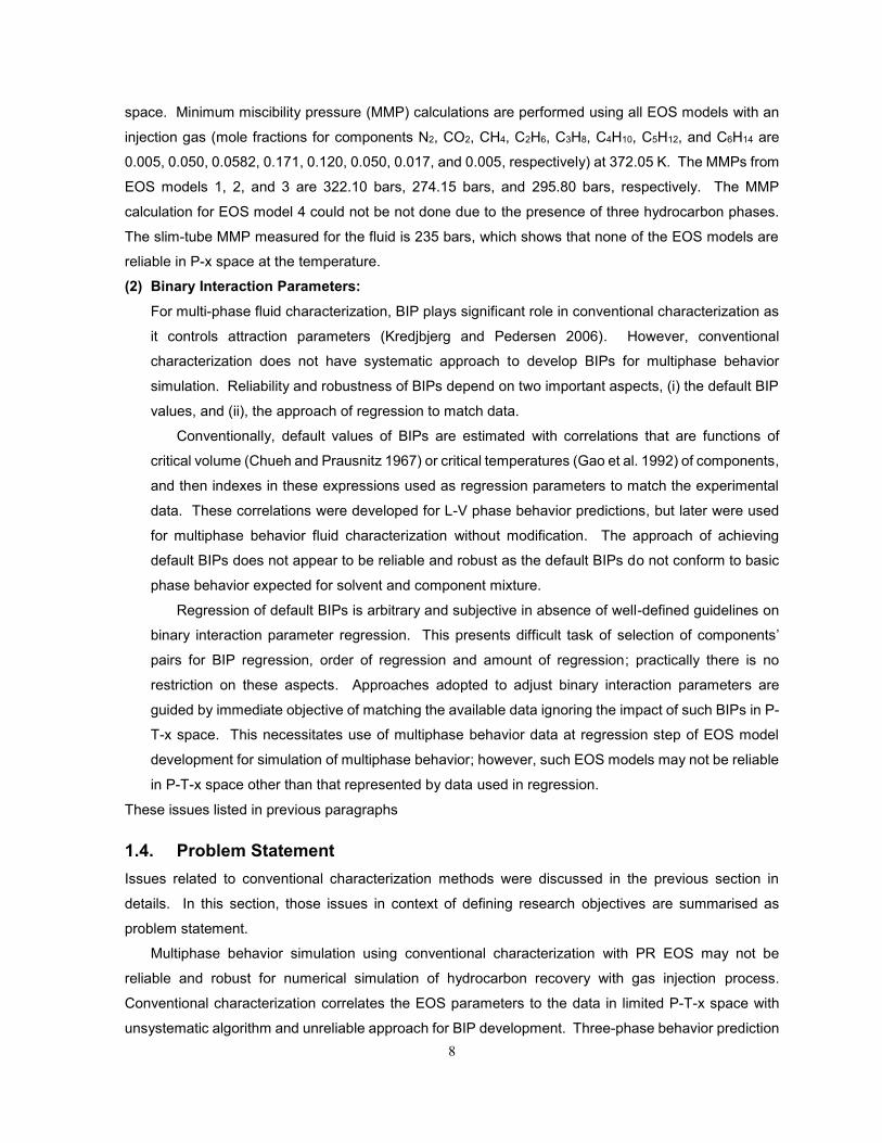
8
space. Minimum miscibility pressure (MMP) calculations are performed using all EOS models with an
injection gas (mole fractions for components N2, CO2, CH4, C2H6, C3H8, C4H10, C5H12, and C6H14 are
0.005, 0.050, 0.0582, 0.171, 0.120, 0.050, 0.017, and 0.005, respectively) at 372.05 K. The MMPs from
EOS models 1, 2, and 3 are 322.10 bars, 274.15 bars, and 295.80 bars, respectively. The MMP
calculation for EOS model 4 could not be not done due to the presence of three hydrocarbon phases.
The slim-tube MMP measured for the fluid is 235 bars, which shows that none of the EOS models are
reliable in P-x space at the temperature.
(2) Binary Interaction Parameters:
For multi-phase fluid characterization, BIP plays significant role in conventional characterization as
it controls attraction parameters (Kredjbjerg and Pedersen 2006). However, conventional
characterization does not have systematic approach to develop BIPs for multiphase behavior
simulation. Reliability and robustness of BIPs depend on two important aspects, (i) the default BIP
values, and (ii), the approach of regression to match data.
Conventionally, default values of BIPs are estimated with correlations that are functions of
critical volume (Chueh and Prausnitz 1967) or critical temperatures (Gao et al. 1992) of components,
and then indexes in these expressions used as regression parameters to match the experimental
data. These correlations were developed for L-V phase behavior predictions, but later were used
for multiphase behavior fluid characterization without modification. The approach of achieving
default BIPs does not appear to be reliable and robust as the default BIPs do not conform to basic
phase behavior expected for solvent and component mixture.
Regression of default BIPs is arbitrary and subjective in absence of well-defined guidelines on
binary interaction parameter regression. This presents difficult task of selection of components’
pairs for BIP regression, order of regression and amount of regression; practically there is no
restriction on these aspects. Approaches adopted to adjust binary interaction parameters are
guided by immediate objective of matching the available data ignoring the impact of such BIPs in P-
T-x space. This necessitates use of multiphase behavior data at regression step of EOS model
development for simulation of multiphase behavior; however, such EOS models may not be reliable
in P-T-x space other than that represented by data used in regression.
These issues listed in previous paragraphs
1.4. Problem Statement
Issues related to conventional characterization methods were discussed in the previous section in
details. In this section, those issues in context of defining research objectives are summarised as
problem statement.
Multiphase behavior simulation using conventional characterization with PR EOS may not be
reliable and robust for numerical simulation of hydrocarbon recovery with gas injection process.
Conventional characterization correlates the EOS parameters to the data in limited P-T-x space with
unsystematic algorithm and unreliable approach for BIP development. Three-phase behavior prediction

9
may not be reliable from EOS model developed using two-phase data. These fundamental issues may
render the EOS models unreliable in the P-T-x space other than that defined by the data used in the
regression. The EOS model developed from conventional characterization is fluid or fluid type or
number of phases specific, and subjective. Although, composition space for reservoir fluids is
continuous, conventional characterization lacks the capability of characterizing fluid irrespective of fluid
type or number of phases.
1.5. Research Objectives
In order to address the issues with the conventional characterization, this research aim to find a new
method for reservoir fluid characterization with following features:
1. Compatible with Peng and Robinson (1976, 1978) EOS and van der Waals mixing rule. Although
there are several modifications to the attraction and covolume parameters of the PR EOS, the
original PR EOS (1976, 78) is used without any modification throughout this research. This is to
facilitate easy implementation in PVT and hydrocarbon recovery simulators.
2. The characterization method should be applicable to hydrocarbon system irrespective of reservoir
fluid types such as gas condensates, volatile oils, normal oils, heavy oils, bitumens.
3. Characterization method should be systematic with well-defined and physically justifiable initial
values and search direction for regression parameters. The algorithm of EOS parameters
optimization should be simple, robust, and reliable.
4. Binary interaction parameters used should be reliable for multiple hydrocarbon phase prediction for
mixture of solvent and hydrocarbon system.
5. The EOS model should be capable of reliable multiphase PVT simulation using minimum amount
of phase behavior data such as composition of fluid, saturation pressure and density at reservoir
temperature.
1.6. Structure of the Thesis
This is paper-based thesis, which presents the research work in four published journal papers and two
under review papers. Introduction, problem statement, and objective of the research on the title of the
thesis were presented in the introduction section. Each paper has its own literature search, research
objective, research, discussion, conclusion, nomenclature, and references as part of research on title of
the thesis. Understanding of organization of thesis is made easier by presenting fundamental of
research in following three paragraphs.
As outlined in research objective, for systematic characterization of reservoir fluid, default values of
EOS parameters for pseudocomponents need to be well defined. Normal alkanes, among the three
prominent hydrocarbon groups i.e. paraffins, naphthenes, and aromatics, has well-defined homologous
series and has lowest critical temperature and pressure for same carbon number hydrocarbons. This
also means that the lowest value, a single carbon fractions of a reservoir fluid can have, is its n-alkane
equivalent critical parameters. Hence, PT phase envelope for a mixture of a light n-alkane with a

10
pseudocomponent changes systematically with its aromatic conent, as demonstrated in Figure 1-5.
Vapor pressure curves for propane and carbon-number-16 components (n-alkane C16H34 and aromatic
C16H10) are shown in this figure. The PT phase envelopes for the equimolar mixture of propane and a
pseudocomponent (with carbon number 16) are shown in the figure. The pseudocomponent is assumed
to be a mixture of n-C16H34 and C16H10; different cases of aromatic contents (i.e., 0, 10, 40, 50, 80 and
100%) in the pseudocomponent are considered to create PT phase envelopes. A systematic change in
the phase envelope with the aromatic content is clearly observed. The phase envelope corresponding
to the case when the pseudocomponent is totally n-alkane (i.e., 0% aromatic component) is the inner
most phase envelope. The phase envelope expands with increasing aromatic content for the
pseudocomponent. This indicates that PT phase envelope for a reservoir fluid with all of heptane plus
fractions assumed as n-alkanes may be considered as the limiting phase envelope, and actual phase
envelope of the reservoir fluid should be outside this. In this research, pseudocomponents of reservoir
fluids are first assigned n-alkane equivalent critical parameters and then higher critical parameters for
each pseudocomponent are searched that can match the experimental data such as saturation
pressure. This approach of characterization is named as perturbation from n-alkanes (PnA).
Kelser et al. (1979), Twu (1984), and Nji (2008, 2009) have presented perturbation from n-alkane
based correlations to estimate TC, PC, and ω for pseudocomponents as function of perturbation
parameters; these perturbation parameters were themselves functions of other parameters such as
boiling point, specific gravity, molecular weight. Perturbation parameters as adjustable parameters to
optimize critical pressure for pseudocomponents was used by Quiñones-Cisneros et al. (2003);
however, their objective was limited to estimating PR EOS attraction and covolume parameters for use
in their friction theory based viscosity model. In this research, PnA approach treats perturbation
parameters as adjustable parameters for all PR EOS parameters to characterize reservoir fluid to
simulate multiphase behavior for reservoir fluids.
The PnA method is applied to characterize reservoir fluid in two ways, with/without use of volume
shift parameter. When volume shift parameters are not used, saturation pressure and density, both data
are matched by regression of PR EOS; this has been used in papers presented in Chapter 2 to 6. In
Chapter 7, PnA method is applied to characterize reservoir fluids by matching saturation pressure by
regressing on PR EOS parameter and density data is matched by regressing on volume shift
parameters; however, this approach requires well-designed binary interaction parameters for three
hydrocarbon-phase predictions. All the journal papers support the reliability and efficiency of the PnA
method for multi-phase reservoir fluid characterization. Table 1.5 presents the arrangement of different
papers in the thesis.
Chapter 2: This chapter presents the content of first published paper on component level
characterization for n-alkane homologous group. Critical temperature, critical pressure, and acentric
factor for n-alkanes from n-C7 to n-C100 are optimized for Peng-Robinson EOS to match vapor pressure
and density data. These optimized parameters are used to estimate n-alkane equivalent (i.e.
11
pseudocomponents as 100% n-alkanes) PR EOS parameters for pseudocomponents in perturbation
from n-alkane (PnA) approach of reservoir fluid characterization presented in Chapter 3 to 6.
Chapter 3: The PnA approach in this research for the first time is applied mainly to heavy oils for
multiphase behavior prediction for solvent injection process. This chapter presents the paper where
algorithm has been developed for regression of EOS parameters (TC, PC, and ω) to match saturation
pressure and density data. Resulting EOS model is then used to predict phase behavior for oils. This
paper also presents difference in phase behavior predictions from EOS models developed with/without
volume shift parameters.
Chapter 4: The paper presented in Chapter 3 has limited application of PnA method to heavy oils.
Content of the Chapter 4 presents the application of PnA characterization for reservoir fluids in general
including gas condensates, volatile oils, light oils, and heavy oils. The algorithm used in Chapter 3 is
special case of algorithm used for regression of EOS parameters (TC, PC, and ω) in Chapter 4. Wherever
data are available for comparison, the PnA method has been validated by predicting three hydrocarbon
phases for heavy oils.
Chapter 5: Attraction and covolume parameters are basic units of a cubic EOS. Using attraction and
covolume parameters as regression parameters can simplify the regression algorithm and reduce the
computation time by virtue of small number of regression parameters. Numerical simulation efficiency
can improve by characterizing fluids in terms of attraction and covolume parameters for components.
Chapter 5 presents the PnA method for characterization of reservoir fluids including gas condensates,
volatile oils, light oils, and heavy oils using a new algorithm for regression of PR EOS attraction and
covolume parameters for saturation pressure and density data match.
Chapter 6: This chapter presents the characterization of bitumen by regression of PR EOS attraction
and covolume parameters. The algorithm presented in Chapter 5 is simplified further for bitumen
characterization. This algorithm successfully characterizes bitumen as single pseudocomponent, which
has similar predictive capability as multiple pseudocomponent conventional characterization. The paper
develops a mechanism, which is to be used before running the simulation, to estimate the sensitivity of
recovery simulation to bitumen characterization methods. This helps in selecting reliable and efficient
characterization method for simulation.
Chapter 7: The chapter uses PnA method of reservoir fluid characterization where saturation pressure
is matched by regression of EOS parameters (TC, PC, and ω) and density matching is done by volume
shift parameters. The approach uses well-developed binary interaction parameter for multiphase
behavior prediction. The method has been validated by successful prediction of multiphase behavior
for 90 reservoir fluids including gas condensates, volatile oils, light oils, heavy oils, and bitumens.
Chapter 8: This chapter presents an overview of the research activities presented in Chapter 2-7 in
context of research objective. Conclusion and recommendation for future research are also presented
in this chapter.
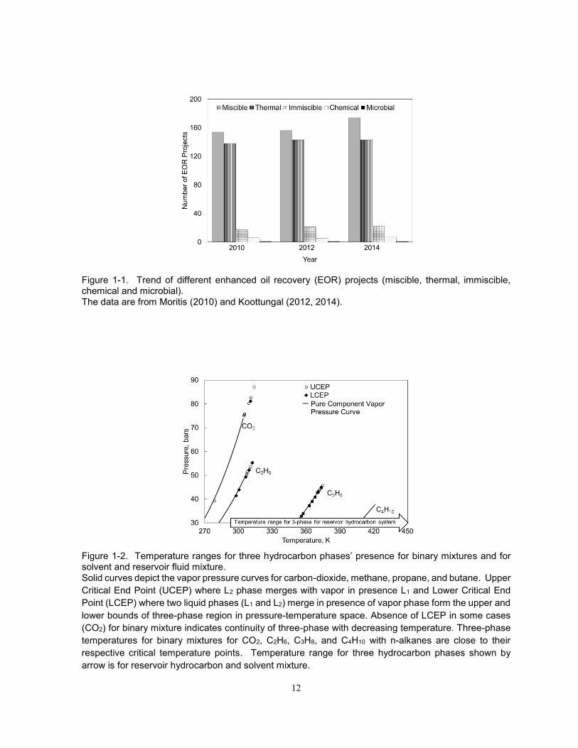
12
Figure 1-1. Trend of different enhanced oil recovery (EOR) projects (miscible, thermal, immiscible, chemical and microbial). The data are from Moritis (2010) and Koottungal (2012, 2014).
Figure 1-2. Temperature ranges for three hydrocarbon phases’ presence for binary mixtures and for solvent and reservoir fluid mixture. Solid curves depict the vapor pressure curves for carbon-dioxide, methane, propane, and butane. Upper
Critical End Point (UCEP) where L2 phase merges with vapor in presence L1 and Lower Critical End
Point (LCEP) where two liquid phases (L1 and L2) merge in presence of vapor phase form the upper and
lower bounds of three-phase region in pressure-temperature space. Absence of LCEP in some cases
(CO2) for binary mixture indicates continuity of three-phase with decreasing temperature. Three-phase
temperatures for binary mixtures for CO2, C2H6, C3H8, and C4H10 with n-alkanes are close to their
respective critical temperature points. Temperature range for three hydrocarbon phases shown by
arrow is for reservoir hydrocarbon and solvent mixture.

13
Figure 1-3. Non-monotonic trend for oil recovery from slim tube experiment (Mohanty et al. 1995) for the West Sak oil. The oil is displaced by gas mixture of methane, ethane, propane, and butane at 291.50 K. Seven gas
mixtures with different methane mole % (0, 32, 42, 51, 62, 70, and 80) are used in the slim tube oil
displacement. The phase behavior observed in the slim tube for oil and gas mixture changes from first
contact miscible at 0% methane gas mixture to multicontact miscible to three-phase immiscible to two
phase immiscible with increasing methane concentration in the injection gas. Monotonic recovery is
observed for reservoir oil and gas system with presence of two hydrocarbon phases. Non-monotonicity
is accounted for the presence of three hydrocarbon phases.
Figure 1-4. Comparison of PT envelopes from four PR EOS models developed using conventional characterization. All the EOS models have same predictive capability at data point (saturation pressure used to regress
TC, PC, and ω); however, they have different predictions at other pressure-temperature points.
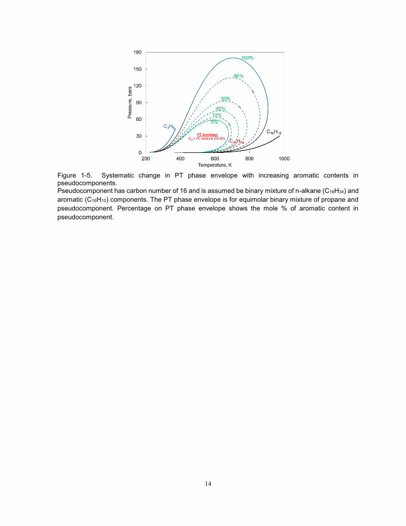
14
Figure 1-5. Systematic change in PT phase envelope with increasing aromatic contents in pseudocomponents. Pseudocomponent has carbon number of 16 and is assumed be binary mixture of n-alkane (C16H34) and
aromatic (C16H10) components. The PT phase envelope is for equimolar binary mixture of propane and
pseudocomponent. Percentage on PT phase envelope shows the mole % of aromatic content in
pseudocomponent.
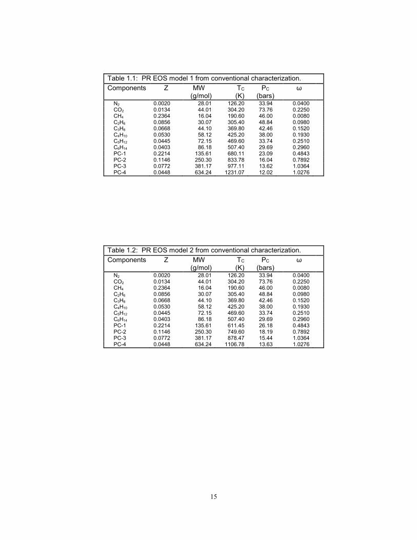
15
Table 1.1: PR EOS model 1 from conventional characterization.
Components Z MW (g/mol)
TC (K)
PC
(bars) ω
N2 0.0020 28.01 126.20 33.94 0.0400 CO2 0.0134 44.01 304.20 73.76 0.2250 CH4 0.2364 16.04 190.60 46.00 0.0080 C2H6 0.0856 30.07 305.40 48.84 0.0980 C3H8 0.0668 44.10 369.80 42.46 0.1520 C4H10 0.0530 58.12 425.20 38.00 0.1930 C5H12 0.0445 72.15 469.60 33.74 0.2510 C6H14 0.0403 86.18 507.40 29.69 0.2960 PC-1 0.2214 135.61 680.11 23.09 0.4843 PC-2 0.1146 250.30 833.78 16.04 0.7892 PC-3 0.0772 381.17 977.11 13.62 1.0364 PC-4 0.0448 634.24 1231.07 12.02 1.0276
Table 1.2: PR EOS model 2 from conventional characterization.
Components Z MW (g/mol)
TC (K)
PC
(bars) ω
N2 0.0020 28.01 126.20 33.94 0.0400 CO2 0.0134 44.01 304.20 73.76 0.2250 CH4 0.2364 16.04 190.60 46.00 0.0080 C2H6 0.0856 30.07 305.40 48.84 0.0980 C3H8 0.0668 44.10 369.80 42.46 0.1520 C4H10 0.0530 58.12 425.20 38.00 0.1930 C5H12 0.0445 72.15 469.60 33.74 0.2510 C6H14 0.0403 86.18 507.40 29.69 0.2960 PC-1 0.2214 135.61 611.45 26.18 0.4843 PC-2 0.1146 250.30 749.60 18.19 0.7892 PC-3 0.0772 381.17 878.47 15.44 1.0364 PC-4 0.0448 634.24 1106.78 13.63 1.0276
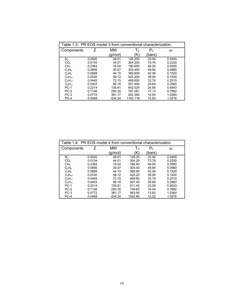
16
Table 1.3: PR EOS model 3 from conventional characterization.
Components Z MW (g/mol)
TC (K)
PC
(bars) ω
N2 0.0020 28.01 126.200 33.94 0.0400 CO2 0.0134 44.01 304.200 73.76 0.2250 CH4 0.2364 16.04 190.600 46.00 0.0080 C2H6 0.0856 30.07 305.400 48.84 0.0980 C3H8 0.0668 44.10 369.800 42.46 0.1520 C4H10 0.0530 58.12 425.200 38.00 0.1930 C5H12 0.0445 72.15 469.600 33.74 0.2510 C6H14 0.0403 86.18 507.400 29.69 0.2960 PC-1 0.2214 135.61 642.024 24.66 0.4843 PC-2 0.1146 250.30 787.081 17.13 0.7892 PC-3 0.0772 381.17 922.390 14.54 1.0364 PC-4 0.0448 634.24 1162.119 12.83 1.0276
Table 1.4: PR EOS model 4 from conventional characterization.
Components Z MW (g/mol)
TC (K)
PC
(bars) ω
N2 0.0020 28.01 126.20 33.94 0.0400 CO2 0.0134 44.01 304.20 73.76 0.2250 CH4 0.2364 16.04 190.60 46.00 0.0080 C2H6 0.0856 30.07 305.40 48.84 0.0980 C3H8 0.0668 44.10 369.80 42.46 0.1520 C4H10 0.0530 58.12 425.20 38.00 0.1930 C5H12 0.0445 72.15 469.60 33.74 0.2510 C6H14 0.0403 86.18 507.40 29.69 0.2960 PC-1 0.2214 135.61 611.45 23.09 0.4843 PC-2 0.1146 250.30 749.60 16.04 0.7892 PC-3 0.0772 381.17 993.90 13.62 1.0364 PC-4 0.0448 634.24 1502.66 12.02 1.0276
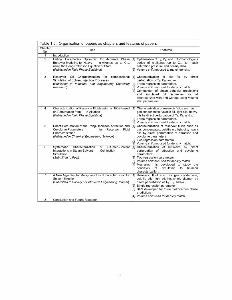
17
Table 1.5. Organisation of papers as chapters and features of papers
Chapter No.
Title Features
1 Introduction
2 Critical Parameters Optimized for Accurate Phase Behavior Modeling for Heavy n-Alkanes up to C100 using the Peng-Robinson Equation of State. (Published in Fluid Phase Equilibria)
[1] Optimization of TC, PC, and ω for homologous series of n-alkanes up to C100 to match saturation pressure and density data.
[2] Volume shift not used to match density.
3 Reservoir Oil Characterization for compositional Simulation of Solvent Injection Processes (Published in Industrial and Engineering Chemistry Research)
[1] Characterization of oils for by direct perturbation of TC, PC, and ω.
[2] Three regression parameters. [3] Volume shift not used for density match. [4] Comparison of phase behavior predictions
and simulated oil recoveries for oil characterized with and without using volume shift parameters.
4 Characterization of Reservoir Fluids using an EOS based on Perturbation from n-Alkanes (Published in Fluid Phase Equilibria)
[1] Characterization of reservoir fluids such as gas condensates, volatile oil, light oils, heavy oils by direct perturbation of TC, PC, and ω).
[2] Three regression parameters. [3] Volume shift not used for density match.
5 Direct Perturbation of the Peng-Robinson Attraction and Covolume Parameters for Reservoir Fluid Characterization (Published in Chemical Engineering Science)
[1] Characterization of reservoir fluids such as gas condensates, volatile oil, light oils, heavy oils by direct perturbation of attraction and covolume parameters
[2] Two regression parameters [3] Volume shift not used for density match.
6 Systematic Characterization of Bitumen-Solvent Interactions in Steam-Solvent Coinjection Simulation (Submitted to Fuel)
[1] Characterization of bitumens by direct perturbation of attraction and covolume parameters
[2] Two regression parameters [3] Volume shift not used for density match [4] Mechanism is developed to study the
sensitivity of simulation to bitumen characterization.
7 A New Algorithm for Multiphase Fluid Characterization for Solvent Injection. (Submitted to Society of Petroleum Engineering Journal)
[1] Reservoir fluid such as gas condensate, volatile oils, light oil, heavy oil, bitumen by direct perturbation of TC, PC, and ω.
[2] Single regression parameter [3] BIPs developed for three hydrocarbon phase
predictions. [4] Volume shift used for density match.
8 Conclusion and Future Research

18
1.7. References Abdrakhmanov, A. 2013. Modeling and Optimization of the Rich Gas-Condensate Reservoir. Master
Thesis. Norwegian University of Science and Technology, Norwey.
Agarawal, R.K., Li, Y-K., and Nghiem, L. 1990. A Regression Technique with Dynamic Parameter
Selection for Phase-behavior Matching. SPE Res Eng 5 (1): 115-120.
Aghbash, V.N. and Ahmadi, M. 2012. Evaluation of CO2-EOR and Sequestration in Alaska West Sak
Reservoir Using Four-Phase Simulation Model. Presented at the SPE Western Regional Meeting,
Bakers-field, California, 21-23 March.
Ambrose, D. and Tsonopoulos, C. 1995. Vapor-Liquid Critical Properties of Elements and Compounds.
2. Normal Alkanes. J. Chem. Eng. Data 40 (3): 531-546.
Badamchi-Zadeh, A., Yarranton, H. W., Svrcek, W. Y. et al. 2009. Phase Behavior and Physical
Property Measurements for VAPEX Solvents: Part I. Propane and Athabasca Bitumen. J Can Pet
Technol 48 (1): 54-61.
Cavett, R.H. 1962. Physical Data for Distillation Calculations, Vapor-Liquid Equilibria. Proc. Am. Pet.
Inst. Div. Refining. 42 (3): 351-357.
Chang, L.C., Hurt, L.J., and Kobayashi, R. 1966. Vapor-Liquid Equilibria of Light Hydrocarbons at Low
Temperatures and High Pressure: The Methane-n-Heptane System. AIChE J. 13 (6): 1099-1107.
Chueh, P.L. and Prausnitz, J.M. 1967. Vapor-Liquid Equilibria at High Pressures: Calculation of Partial
Molar Volumes in Non-Polar Liquid Mixtures. AIChE J. 13 (6): 1107-1113.
Clark, P., Toulekima, S., Sarma, H., 2008. A Miscibility Scoping Study for Gas Injection into a High-
Temperature Volatile Oil Reservoir in the Cooper Basin, Australia. Presented at the SPE Asia
Pacific Oil and Gas Conference and Exhibition, Perth, Australia. 20-22 Oct.
Creek, J.L. and Sheffield, J.M. 1993. Phase Behavior, Fluid Properties, and Displacement
Characteristics of Permian Basin Reservoir Fluid/ CO2 Systems. SPE Res Eval & Eng 8 (1): 34-
42. SPE-20188-PA.
DeRuiter, R.A., Nash, L.J., and Singletary, M.S. 1994. Solubility and Displacement Behavior of a
Viscous Crude with CO2 and Hydrocarbon Gases. SPE Res Eval & Eng 9 (2): 101-106. SPE-
20523-PA.
Dickson, J.L., Clingman, S., Dittaro, L.M. et al. 2011. Design Approach and Early Field Performance for
a Solvent-Assisted SAGD Pilot at Cold Lake, Canada. Presented at the SPE Heavy Oil Conference
and Exhibition, Kuwait City, Kuwait, 12-14 December. SPE-150639-MS.
Edmister, W.C. 1958. Applied Hydrocarbon Thermodynamics, Part 4: Compressibility Factors and
Equations of State. Pet. Refiner. 37: 173-179.
Enick, R., Holder, G.D., and Morsi, B.I. 1985. Critical and Three Phase Behavior in the Carbon
Dioxide/Tridecane System. Fluid Phase Equilib. 22 (2): 209-224.
Estrera, S.S. and Luks, K.D. 1987. Liquid-Liquid-Vapor Equilibrium Behavior of Certain Ethane + n-
Paraffin Mix. J. Chem. Eng. Data. 32 (2): 201-204.

19
Fall, D.J. and Luks, K.D. 1985. Liquid-Liquid-Vapor Phase Equilibria of the Binary System Carbon
Dioxide + n-Tridecane. J. Chem. Eng. Data. 30 (3): 276-279.
Fulco, G.J. 1999. Case History of Miscible Gas Flooding in the Powder River Basin North Buck Draw
Unit. Presented at the SPE Rocky Mountain Regional Meeting, Gillette, Wyoming, 15-18 April. SPE-
55634-MS.
Gao., G., Daridon, J-L., Saint-Guirons, H. et al. 1992. A Simple Correlation to Evaluate Binary
Interaction Parameters of the Peng-Robinson Equation of State: Binary Light Hydrocarbon Systems.
Fluid Phase Equilib. 74: 85-93.
Godbole, S.P., Thele, K.J., and Reinbold, E.W. 1995. EOS Modeling and Experimental Observations
of Three-Hydrocarbon-Phase Equilibria. SPE Res. Eng. 10 (2): 101-108. SPE-24936-PA.
Gregorowicz, J., De Loos, T.W., and De Swaan Arons, J. 1993a. Liquid-Liquid-Vapour Phase Equilibria
in the System Ethane + Propane + Eicosane: Retrograde Behaviour of the Heavy Liquid Phase,
Fluid Phase Equilib. 84: 225-250.
Gregorowicz, J., Smits, P.J., de Loos, T.W. et al. 1993b. Liquid-Liquid-Vapour Phase Equilibria in the
System Methane + Ethane + Eicosane: Retrograde Behaviour of the Heavy Liquid Phase. Fluid
Phase Equilib. 85, 225-238.
Gupta, S.C. and Gittins, S.D. 2006. Christina Lake Solvent Aided Process Pilot. J Can Pet Technol 45
(9): 15-18. PETSOC-06-09-TN.
Gupta, S.C., Gittins, S., and Picherack, P. 2005. Field Implementation of Solvent Aided Process. J Can
Pet Technol 44 (11): 8-13. PETSOC-05-11-TN1.
Guler, B., Wang, P., Delshad, M. et al. 2001. Three- and Four- Phase Flow Compositional Simulations
of CO2/NGL EOR. Presented at the SPE Annual Technical Conference and Exhibition, New
Orleans, Louisiana, 30 September-3 October.
Henry, R.L. and Metcalfe, R.S. 1983. Multiple-Phase Generation During Carbon Dioxide Flooding. SPE
J. 23 (4): 595-601.
Holm, L.W. 1986. Miscibility and Miscible Displacement. J Pet Technol 38 (8):817-818.
Hottovy, J.D., Kohn, J.P., and Luks, K.D. 1981. Partial Miscibility Behavior of the Methane-Ethane-n-
Octane System. J. Chem. Eng. Data. 26 (2): 135-137.
Hottovy, J.D., Kohn, J.P., and Luks, K.D. 1982. Partial Miscibility Behavior of the Ternary Systems
Methane-Propane-n-Octane, Methane-n-Butane-n-Octane, and Methane-Carbon Dioxide-n-
Octane. J. Chem. Eng. Data. 27 (3): 298-302.
Hottovy, J.D., Luks, K.D., and Kohn, J.P. 1981a. Three-phase liquid-liquid-vapor equilibriums behavior
of certain binary carbon dioxide-n-paraffin systems. J. Chem. Eng. Data 26 (3): 256-258.
Iwade, S., Katsumura, Y., and Ohgaki, K. 1992. High-Pressure Phase Behavior of Binary Systems of
Heptadecane and Octadecane with Carbon Dioxide or Ethane. J. Chem. Eng. Jpn. 26 (1): 74-79.

20
Jangkamolkulchai, A. and Luks, K.D. 1989. Partial Miscibility Behavior of the Methane + Ethane + n-
Docosane and the Methane + Ethane + n-Tetradecylbenzene Ternary Mixtures. J. Chem. Eng.
Data. 34 (1): 92-99.
Jhaveri, B.S. and Youngren, G.K. 1988. Three-Parameter Modification of the Peng-Robinson Equation
of State to Improve Volumetric Predictions. SPE J. 3 (3): 1033-1040.
Kesler, M.G. and Lee, B.I. 1976. Improve Prediction of Enthalpy of Fractions, Hydrocarbon Processing.
Hydrocarb Process 55 (3): 153-158.
Khan, S.A., Pope, G.A., and Sepehrnoori, K. 1992. Fluid Characterization of Three-Phase CO2/Oil
Mixtures. Presented at the SPE/DOE Enhanced Oil Recovery Symposium, Tulsa, Oklahoma, 22-
24 April. SPE-24130-MS.
Koottungal, Leena. 2012. Worldwide EOR Survey, Oil Gas J. 110 (4).
Koottungal, Leena. 2014. Worldwide EOR Survey, Oil Gas J. 112 (5).
Korsten, H. 2000. Internally Consistent Prediction of Vapor Pressure and Related Properties. Ind. Eng.
Chem. Res. 39 (3): 813-820.
Krejbjerg, K. and Pedersen, K.S. 2006. Controlling VLLE Equilibrium with a Cubic EoS in Heavy Oil
Modeling. Presented at 57th Annual Technical Meeting of the Petroleum Society (Canadian
International Petroleum Conference), Calgary. 13-15 June. PETSOC-2006-052.
Kukarni, A.A., Zarah, B.Y., Luks, K.D. et al. 1974. Phase-Equilbriums Behavior of System Carbon
Dioxide-n-Decane at Low Temperatures. J. Chem. Eng. Data 19 (1), 92-94.
Lee, B.I. and Kesler, M.G. 1975. A Generalized Thermodynamic Correlation Based on Three-
Parameter Corresponding States. AIChE J. 21 (3): 510-527.
Li, H., Zheng, S., and Yang. D. 2013. Enhanced Swelling Effect and Viscosity Reduction of
Solvent(s)/CO2/Heavy-Oil Systems. SPE J. 18 (4): 695-707. SPE-150168-PA.
Lin, Y-N., Chen, R.J.J., Chappelear, P.S. et al. 1977. Vapor-Liquid Equilibrium of the Methane-n-Hexane
System at Low Temperature. J. Chem. Eng. Data 22 (4): 402-408.
Llave, F.M., Luks, K.D., and Kohn, J.P. 1987. Three-Phase Liquid-Liquid-Vapor Equilibria in the
Nitrogen-Methane-Ethane and Nitrogen-Methane-Propane Systems. J. Chem. Eng. Data. 32 (1):
14-17.
Lolley, C.S. and Richardson, W.C. 1997. Compositional Input for Thermal Simulation of Heavy Oils with
Application to the San Ardo Field. Presented at International Thermal Operation & Heavy Oil
Symposium, Bakersfield, California, 10-12 Dec. SPE-37538-MS.
Malik, Q.M. and Islam, M.R. 2000. CO2 Injection in the Weyburn Field of Canada: Optimization of
Enhanced Oil Recovery and Greenhouse Gas Storage with Horizontal Wells. Presented at the
SPE/DOE Improved Oil Recovery Symposium, Tulsa, Oklahoma, 3-5 April. SPE-59327-MS.
Manrique, E.J., Muci, V.E., and Gurfinkel, M.E. 2007. EOR Field Experiences in Carbonate Reservoirs
in the United States. SPE Res Eval & Eng 10 (6): 667-686.
21
McGuire, P.L., Spence, A.P., and Redman, R.S. 2001. Performance Evaluation of a Mature Miscible
Gasflood at Prudhoe Bay. SPE Res Eval & Eng 4 (4): 318-326. SPE-72466-PA.
Merrill, R.C., Luks, K.D., and Kohn, J.P. 1983. Three-Phase Liquid-Liquid-Vapor Equilibrium in the
Methane + n-Pentane + n-Octane, Methane + n-Hexane + n-Octane, and Methane + n-Hexane +
Carbon Dioxide Systems. J. Chem. Eng. Data 28 (2): 210-215.
Mizenko, G.J. 1992. North Cross (Devonian) Unit CO2 Flood: Status Report. Presented at the
SPE/DOE Enhanced Oil Recovery Symposium, Tulsa, Oklahoma, 22-24 April. SPE-24210-MS.
Mohanty, K.K., Masino, W.H. Jr., Ma, T.D. et al. 1995. Role of Three-Hydrocarbon-Phase Flow in a
Gas-Displacement Process. SPE Res Eng 10 (3): 214-221. SPE-24115-PA.
Moritis, Guntis. 2010. Worldwide EOR Survey, Oil Gas J. 102 (14).
Negahban, S. and V. J. Kremesec Jr. 1989. Development and Validation of Equation-of-State Fluid
Descriptions for CO2-Reservoir Oil Systems. SPE 19637. Presented at the 64th Annual Technical
Conference and Exhibition, San Antonio, 8-11 March.
Nghiem, L. X. and Li, Y.K. 1986. Effect of Phase Behavior on CO2 Displacement Efficiency at Low
Temperatures: Model Studies With an Equation of State. SPE Res Eng 1 (4): 414-422.
Okuno, R. and Xu, Z. 2014. Efficient Displacement of Heavy Oil by Use of Three Hydrocarbon Phases.
SPE J. 19 (5): 956-973. SPE-165470-PA.
Okuyiga, M.O. 1992. Equation of State Characterization and Miscibility Development in a Multiple
Phase Hydrocarbon System. Presented at the SPE Annual Technical Conference and Exhibition,
Washington, DC, 4-7 Oct. SPE-24937-MS.
Pedersen, K. S. and Christensen, P. L. 2007. Phase Behavior of Petroleum Reservoir Fluids. CRC
Press, Taylor & Francis Group, Boca Raton, FL, USA.
Pedersen, K.S., Thomassen, P., and Fredenslund, Aa. 1983. SRK- EOS Calculation for Crude Oil. Fluid
Phase Equilib. 14: 209–218.
Pedersen, K.S., Thomassen, P., and Fredenslund, Aa. 1984. Thermodynamics of Petroleum Mixture
Containing Heavy Hydrocarbons. 1. Phase Envelope Calculation by Use of the Soave-Redlich-
Kwong Equation of State. Ind. Eng. Chem. Proc. Des. Dev. 23 (1): 163–170.
Pedersen, K.S., Thomassen, P., and Fredenslund, Aa. 1984. Thermodynamics of Petroleum Mixture
Containing Heavy Hydrocarbons. 1. Phase Envelope Calculation by Use of the Soave-Redlich-
Kwong Equation of State. Ind. Eng. Chem. Proc. Des. Dev. 23 (1): 163–170.
Pedersen, K.S., Blilie, A.L., and Meisingset, K.K. 1992. Calculations on Petroleum Reservoir Fluids
Using Measured and Estimated Compositional Data for the Plus Fraction. Ind. Eng. Chem. Res. 31
(5): 1378-1384.
Pedersen, K.S., Milter, J., and Sørensen, H. 2004. Cubic Equations of State Applied to HT/HP and
Highly Aromatic Fluids. SPE J. 9 (2): 186-192.
Pedersen, K.S., Thomassen, P., and Fredenslund, Aa. 1989. Characterization of Gas Condensate
Mixtures. Advances in Thermodynamics, Taylor and Francis, New York, 1, 137-152.
22
Peneloux, A., Rauzy, E., and Fréze, R. 1982. A Consistent Correction for Redlich-Kwong-Soave
Volume. Fluid Phase Equilib. 8 (1):7-23.
Peng, D.-Y. and Robinson, D.B. 1976. A New Two-Constant Equation of State. Ind. Eng. Chem. Fund.
15 (1): 59-64.
Peng, D.-Y. and Robinson, D.B. 1978. The Characterization of the Heptanes and Heavier Fractions for
the GPA Peng-Robinson Programs. GPA Research Report RR-28.
Peters, C.J. 1994. Multiphase Equilibria in Near-Critical Solvents. In Supercritical Fluids, ed. E. Kiran
and J.M.H. Levelt Sengers, 117-145. Dordrecht, The Netherlands: Springer Netherlands,
Peters, C.J., De Roo, J.L., and De Swaan Arons, J. 1987b. Three-Phase Equilibria in (Ethane +
Pentacosane). J. Chem. Thermodyn. 19 (3): 265-272.
Peters, C.J., Van der Kooi, H.J., and De Swaan Arons, J. 1987a. Measurements and Calculations of
Phase Equilibria for (Ethane + Tetracosane) and (p, 𝑉𝑚′∗ , T) of Liquid Tetracosane. J. Chem.
Thermodyn. 19 (4): 395-405.
Peters, C.J., Van Der Kooi, H.J., De Roo, J.L. et al. 1989. The Search for Tricriticality in Binary Mixtures
of Near-Critical Propane and Normal Paraffins. Fluid Phase Equilib. 51: 339-351.
PVTsim 20.0. 2011. Calsep A/S, Lyngby, Denmark.
Quiñones -Cisneros, S.E., Zéberg-Mikkelsen, C.K., and Stenby, E.H. 2003. Friction Theory Prediction
of Crude Oil Viscosity at Reservoir Conditions Based on Dead Oil Properties. Fluid Phase Equilib.
212 (1-2): 233–243.
Reid, T. 1994. Study of Hydrocarbon Miscible Solvent Slug Injection Process for Improved Recovery of
Heavy Oil From Schrader Bluff Pool, Milne Point Unit, Alaska. Annual Report for DE-FG22-
93BC14864 for the US Department of Energy. University of Alaska Fairbanks, Alaska.
Riazi, M.R. and Al-Sahhaf, T.A. 1996. Physical Properties of Heavy Petroleum Fractions and Crude
Oils. Fluid Phase Equilib. 117 (1-2): 217-224.
Riazi, M.R. and Daubert, T.E. 1980. Simplify Property Predictions. Hydrocarb. Process. 59 (3): 115-
116.
Riazi, M.R. and Daubert, T.E. 1987. Characterization Parameters for Petroleum Fractions. Ind. Eng.
Chem. Res. 26 (4): 755-759.
Rodriguez, I. and Hamouda, A.A. 2010. An Approach for Characterization and Lumping of Plus
Fractions of Heavy Oil. SPE Res Eval Eng 13 (2): 283-295.
Rodrigues, A.B. and Kohn, J.P. 1967. Three Phase Equilibria in the Binary Systems Ethane-n-
Docosane and Ethane-n-Octacosane. J. Chem. Eng. Data. 12 (2): 191-193.
Roper, M. 1989. An Experimental Study of CO2/West-Sak-Crude-Oil Phase Behavior. MS thesis,
University of Alaska Fairbanks, Fairbanks, Alaska.
Sänger, P. and Hagoort, J. 1998. Recovery of Gas Condensate by Nitrogen Injection Compared with
Methane Injection. SPE J. 3 (1): 26-33.

23
Secuianu, C., Feroiu, V., and Geana, D. 2007. Investigation of Phase Equilibria in the Ternary System
Carbon Dioxide + 1-Heptanol + n-Pentadecane. Fluid Phase Equilib. 261 (1-2): 337-342.
Sharma, A.K., Patil, S.L., Kamath, V.A. et al. 1989. Miscible Displacement of Heavy West Sak Crude
by Solvents in Slim Tube. Presented at the SPE California Regional Meeting, Bakersfield,
California, 5-7 April. SPE-18761-MS.
Shelton, J.L., and Yarborough, L. 1977. Multiple Phase Behavior in Porous Media During CO2 or Rich-
Gas Flooding. J. Pet. Technol. 29 (9):1171-1178.
Sheng, J. 2013. Enhanced Oil Recovery Field Case Studies, Gulf Professional Publishing.
Soave, G. 1972. Equilibrium Constants from a Modified Redlich-Kwong Equation of State. Chem. Eng.
Sci. 27 (6): 1197-1203.
Stein, M.H., Frey, D.D., Walker, R.D. et al. 1992. Slaughter Estate Unit CO2 Flood: Comparison between
Pilot and Field-Scale Performance. J Pet Technol 44 (9): 1026-1032. SPE-19375-PA.
Tanner, C.S., Baxley, P.T., Crump III, J.G. et al. 1992. Production Performance of the Wasson Denver
Unit CO2 Flood. Presented at the SPE/DOE Enhanced Oil Recovery Symposium, Tulsa, Oklahoma,
22-24 April. SPE-24156-MS.
Taheri, A., Høier, L., and Torsæter, O. 2013. Miscible and Immiscible Gas Injection for Enhancing of
Condensate Recovery in Fractured Gas Condensate Reservoir. Presented at the EAGE Annual
Conference and Exhibition incorporating SPE Europe, London, UK, 10-13 June.
Turek, E.A., Metcalfe, R.S., and Fishback, R.E. 1988. Phase Behavior of Several CO2/ West Texas-
Reservoir-Oil Systems. SPE Res Eng 3 (2): 505-516. SPE-13117-PA.
Twu, C.H. 1984. An Internally Consistent Correlation for Predicting the Critical Properties and Molecular
Weights of Petroleum and Coal-Tar Liquids. Fluid Phase Equilib. 16 (2): 137-150.
Van der Steen, J., De Loos, T.W., and de Swaan, A.J. 1989. The Volumetric Analysis and Prediction
of Liquid-Liquid-Vapor Equilibria in Certain Carbon Dioxide + n-Alkane Systems. Fluid Phase
Equilib. 51: 353-367.
Varotsis, N., Stewart, G., Todd, A.C. et al. 1986. Phase Behavior of Systems Comprising North Sea
Reservoir Fluids and Injection Gases. J Pet Technol 38 (11): 1221-1233. SPE-12647-PA.
Whitson, C.H. 1983. Characterizing Hydrocarbon Plus Fractions. SPE J. 23 (4): 683-694.
Whitson, C.H. and Brulè, M.R. 2000. Phase Behaviour. SPE Henry L. Doherty Series, Vol. 20, SPE,
Richardson, Texas.

24
Chapter 2: Critical Parameters Optimized for Accurate Phase Behavior Modeling
for Heavy n-Alkanes up to C100 using the Peng-Robinson Equation of State
A version of this has been published in Fluid Phase Equilibria, Year: 2012, Volume:
335, Pages: 46–59.

25
2.1. Introduction
Cubic equations of state (EOSs) are widely used in the petroleum industry to model volumetric and
compositional phase behavior of petroleum reservoir fluids. Since the original research of van der Waals
0 in 1873, many cubic EOSs have been developed including the Peng-Robinson (PR) EOS (Peng and
Robinson 1976; 1978) and the Soave-Redlich-Kwong (SRK) EOS (Soave 1972). These cubic EOSs are
used in compositional reservoir simulation to design enhanced oil recovery (EOR) using solvents. With
recent advances in the EOS compositional reservoir simulation technology, it is now possible to robustly
simulate complex gas/CO2 injection processes that involve critical endpoint behavior (Okuno et al.
2011).
Reliable predictions of EOR using compositional reservoir simulation require accurate
characterization of reservoir fluids using a cubic EOS. Such characterization methods have been
developed, and implemented in commercial software for conventional oils (Pedersen et al. 1992; Neau
and Jaubert 1993; PVTsim 2011; Riazi 2005; Pedersen and Christensen 2007; Whitson and Brule
2000). Characterization of heavy oils using an EOS, however, is more difficult than that of conventional
oils. Firstly, compositions of heavy oils are highly uncertain in terms of the concentration of each carbon
number (CN) group and the paraffins-naphthenes-aromatics (PNA) distribution within each CN group.
Secondly, critical parameters required in EOS fluid characterization are unknown for hydrocarbons
heavier than tetracosane, n-C24 (Ambrose and Tsonopoulos 1995). Thirdly, accurate prediction of heavy
oil densities is difficult using two-parameter cubic EOSs with a constant critical compressibility factor
such as the PR and SRK EOSs (Peng and Robinson 1976, 1978; Soave 1972). A cubic EOS with more
than two parameters can improve density predictions for heavy oils (Klara and Hemanth-Kumar 1987),
but at the expense of computational efficiency.
In the literature, a few different sets of correlations were proposed for critical temperature (TC),
critical pressure (PC), and acentric factor (ω) extrapolated for hydrocarbons heavier than C24 (Voulgaris
et al. 1991; Rodrίguez and Hamouda 2008). These correlations, however, were developed based on
reservoir oil samples, and do not explicitly account for effects of the PNA distribution on critical
parameters. Since a heavier CN group can contain a wider variety of compounds, more uncertainties
in phase behavior predictions arise when such generic correlations are used for heavy oil
characterization.
Cubic EOSs are incapable of accurate prediction of densities and vapor pressures for heavy
hydrocarbons even when accurate critical parameters are known and used. The volume shift approach
of Péneloux et al. (1982) (Jhaveri and Youngren (1988) for the PR EOS) is widely used to improve
density predictions with cubic EOSs. The volume shift approach, however, does not improve
compositional phase behavior predictions. Use of volume shift in EOS fluid characterization can cause
erroneous oil recovery predictions in simulation of miscible gas injection, where mass transfer among
phases is significant (Kumar and Okuno 2014).
Another approach for improving the PR EOS is to modify the alpha function (Mathias 1983; Stryjek
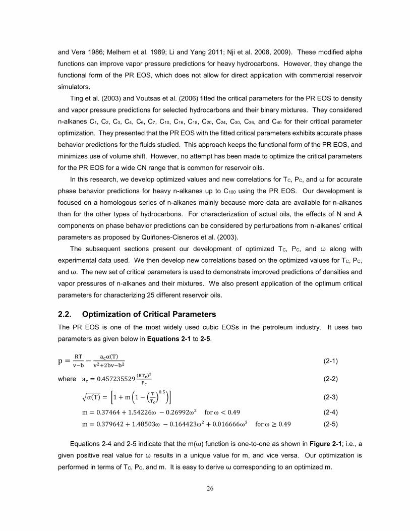
26
and Vera 1986; Melhem et al. 1989; Li and Yang 2011; Nji et al. 2008, 2009). These modified alpha
functions can improve vapor pressure predictions for heavy hydrocarbons. However, they change the
functional form of the PR EOS, which does not allow for direct application with commercial reservoir
simulators.
Ting et al. (2003) and Voutsas et al. (2006) fitted the critical parameters for the PR EOS to density
and vapor pressure predictions for selected hydrocarbons and their binary mixtures. They considered
n-alkanes C1, C2, C3, C4, C6, C7, C10, C16, C18, C20, C24, C30, C36, and C40 for their critical parameter
optimization. They presented that the PR EOS with the fitted critical parameters exhibits accurate phase
behavior predictions for the fluids studied. This approach keeps the functional form of the PR EOS, and
minimizes use of volume shift. However, no attempt has been made to optimize the critical parameters
for the PR EOS for a wide CN range that is common for reservoir oils.
In this research, we develop optimized values and new correlations for TC, PC, and ω for accurate
phase behavior predictions for heavy n-alkanes up to C100 using the PR EOS. Our development is
focused on a homologous series of n-alkanes mainly because more data are available for n-alkanes
than for the other types of hydrocarbons. For characterization of actual oils, the effects of N and A
components on phase behavior predictions can be considered by perturbations from n-alkanes’ critical
parameters as proposed by Quiñones-Cisneros et al. (2003).
The subsequent sections present our development of optimized TC, PC, and ω along with
experimental data used. We then develop new correlations based on the optimized values for TC, PC,
and ω. The new set of critical parameters is used to demonstrate improved predictions of densities and
vapor pressures of n-alkanes and their mixtures. We also present application of the optimum critical
parameters for characterizing 25 different reservoir oils.
2.2. Optimization of Critical Parameters
The PR EOS is one of the most widely used cubic EOSs in the petroleum industry. It uses two
parameters as given below in Equations 2-1 to 2-5.
p =RT
v−b−
acα(T)
v2+2bv−b2 (2-1)
where ac = 0.457235529(RTc)2
Pc (2-2)
√α(T) = [1 + m (1 − (T
Tc)
0.5
)] (2-3)
m = 0.37464 + 1.54226 − 0.269922 for < 0.49 (2-4)
m = 0.379642 + 1.48503 − 0.1644232 + 0.016666ω3 for ≥ 0.49 (2-5)
Equations 2-4 and 2-5 indicate that the m(ω) function is one-to-one as shown in Figure 2-1; i.e., a
given positive real value for ω results in a unique value for m, and vice versa. Our optimization is
performed in terms of TC, PC, and m. It is easy to derive ω corresponding to an optimized m.

27
2.2.1. Experimental Data Used for Optimization
Our optimization uses experimental data for vapor pressure and liquid density of n-alkanes. Table 2-
A1 and 2-A2 summarize the sources and T-P ranges of data used for the optimization. Table 2-1 lists
the n-alkanes for which experimental data are available for liquid densities and vapor pressures, and
data uncertainties for each of the compounds.
Saturated liquid densities estimated in Yaws (2010) are used for n-alkanes that have no liquid
density data available in the literature (Table 2-A1 shows for which n-alkanes the estimations of Yaws
(2010) are used). The estimation of saturated liquid densities is based on a modified form of the Rackett
equation (1970) using four parameters (Daubert et al. 1997). The quality of the estimations in Yaws
(2010) is difficult to judge owing to the lack of experimental data. However, the modified Rackett
equation represents experimental data very well (Poling et al. 2001). Poling et al. (2001) recommended
the modified Rackett equation for estimation of saturated liquid densities.
Vapor pressure data for many n-alkanes are not available in the literature. Therefore, vapor
pressure data for such n-alkanes are supplemented by the correlation of Riazi and AlQaheem (2010)
given by Equation 2-6. This correlation has been developed using updated (Dykyj et al. 1997) vapor
pressure data available for n-alkanes between C7 to C100.
ln Prvap
= (a1 + a2r + a3r3) + (b1 + b2r + b3r2)Tr−2 + (c1 + c2r)Tr (2-6)
In Equation 2-6, Prvap
=Pvap
Pc and Tr =
T
Tc . Coefficients a1, a2, a3, b1, b2, b3, c1 and c2 are given in Table
2-2. The r values for some hydrocarbons between C2 to C40 are available in Riazi (2005). For other
hydrocarbons up to C100, the procedure recommended by Riazi and AlQaheem (2010) has been used
to estimate the value for r. Equation 2-6 results in less than 2% deviation in vapor pressure predictions
for the CN range shown in Table 2-2. Table 2-A2 indicates n-alkanes for which the correlation of Riazi
and AlQaheem (2010) is used. For all the n-alkanes considered in our optimization, C7-C100, we ensure
use of vapor pressure data points both for Tr 0.7 and Tr 0.7. This is to ensure the accuracy of vapor
pressure predictions around Tr of 0.7, which is used in Pitzer’s definition of ω in Equation 2-7.
ω = − log10 [PSAT
PC]
(T
TC = 0.7)
− 1 (2-7)
2.2.2. Optimization Method
TC, PC, and ω are optimized considering reduction of
Average absolute deviations (AAD) in density predictions
AAD in vapor pressure predictions
Deviations of TC and PC from physical critical points,
while keeping smooth variations of TC, PC, and ω with respect to molecular weight (MW), and the
consistency with Pitzer’s definition for ω, Equation 2-7. The minimization of AADs for both density and
vapor pressure predictions can be challenging. A set of TC, PC, and ω that gives a minimum for the sum

28
of the two types of AADs does not necessarily result in a minimum for each of the AADs. When a
change in PC decreases AAD in density predictions, it can increase AAD in vapor pressure predictions.
For this reason, our optimization also considers that AAD in vapor pressure predictions should be similar
to that in density predictions.
Minimization of the AADs can have many local minima, and it is unlikely that the global minimum
always exists for this minimization. Smoothness of TC, PC, and ω with respect to MW is considered
when the minimization needs an additional criterion due to multiple local minima close to each other.
2.2.2.1. Initialization
We optimize TC, PC, and ω using the exhaustive search method, for which initial estimates are provided
using the solver function within the Excel software. The initialization using the Excel solver function
starts with TC, PC, and ω from the correlations developed for n-alkanes by Gao et al. (2001). Predictions
of vapor pressures and saturated liquid densities are sensitive to TC and PC, respectively (Voulgaris et
al. 1991). Therefore, TC and PC are primarily used to reduce AADs in vapor pressure and density
predictions. The initialization steps for a given n-alkane are as follows:
Step 1. AAD in vapor pressure predictions is reduced using TC only.
Step 2. AAD in vapor pressure predictions is reduced using m only. The m parameter is defined in
Equations 2-4 and 2-5.
Step 3. AAD in liquid density predictions is reduced using PC only.
Step 4. The sum of AADs for vapor pressure and liquid density predictions is reduced using TC and PC.
Step 5. The sum of AADs for vapor pressure and liquid density predictions is reduced using TC, PC,
and m.
Steps 1-5 are repeated until reduction of the AADs becomes marginal. During the iteration, we
confirm that TC, PC, and m with respect to MW are smooth for 94 n-alkanes from C7 through C100. The
values for TC, PC, and m that do not follow the smooth trends are replaced with values interpolated
between the neighboring CNs.
The values for TC and PC initialized above are generally greater than physical values given in the
literature. For example, the initialized critical point for C100 is (TC, PC) = (1094.0 K, 4.34 bars), and the
physical critical point is (TC, PC) = (1038.2 K, 2.71 bars) from DECHEMA (see reference). The deviation
from the physical values is reduced in the subsequent optimization using the exhaustive search method.
2.2.2.2. Exhaustive Search for Optimum TC, PC, and
An algorithm was developed for our optimization using the exhaustive search method. The algorithm
allows for simultaneous adjustment of TC, PC, and m, unlike the initialization described in Section 2.2.2.1.
The exhaustive search method defines its search domain to be (-5%, +1%) from the initial value for
TC and (-8%, +2%) from the initial value for PC for each n-alkane. This rectangular domain in T-P space
is then discretized into 6,000 grids allowing for a unit change of 0.1% in each of TC and PC. We use the
asymmetric search domain with respect to the initial point in T and P directions. This is because we
search for optimum values that are lower than the initial values set in Section 2.2.2.1.

29
For each set of TC and PC, we calculate m by minimizing AAD in vapor pressure predictions. In this
optimization of m, we consider the consistency with Pitzer’s definition of ω. For a given set of TC, PC,
and m, the PR EOS can provide a saturation pressure at Tr of 0.7 (PSAT in Equation 2-7). Equation 2-7
can then give a value for ω. However, this ω value does not necessarily match another ω value that
can be calculated from either Equation 2-4 or 2-5 with the current m value. The consistency is satisfied
when the absolute difference between these two ω values becomes smaller than a tolerance (e.g., 10-
3).
The resulting set of TC, PC, and m is then used to calculate AAD in liquid density predictions. The
AADs in vapor pressure and liquid density predictions are recorded for 6,000 sets of TC, PC, and m.
Selection of the optimum set of TC, PC, and m for each n-alkane is, in general, based on the total of the
AADs in vapor pressure and liquid density predictions. It is observed that the optimum set results in
vapor pressure and liquid density AADs that are similar to each other. Smooth curves are usually
observed for optimum TC, PC, and m with respect to MW. If a set of TC, PC, and m that gives the minimum
AADs deviates from the overall trends, it is replaced by another set of TC, PC, and m while minimizing
AADs.
2.3. Optimum TC, PC, m, and
The method discussed in Section 2.2 gives TC, PC, and m optimized for vapor pressure and liquid density
predictions using the PR EOS for 94 n-alkanes from C7 through C100. Optimized values for ω are
calculated using Equations 2-4 and 2-5. The final values for TC, PC, m, and ω are presented in Table
2-B along with TC, PC, and ω based on the correlations of Gao et al. (2001), which are given in
Equations 2-8 to 2-10.
TC = [6573.87 − 4680.77exp(−0.1831(CN0.6667 − 2.08))]1
1.276 (2-8)
PC = 42.44exp(−0.3757(CN0.5684 − 1.8672)) (2-9)
ω = [3.212102 − 2.937628exp(−0.04699(CN0.6667 − 2.08))]1
0.6851 (2-10)
In the above equations, CN is carbon number. TC and PC are in Kelvin and bar, respectively. The
accuracy (AAD) of the above correlations for TC, PC, and ω is 0.2, 0.8, and 0.4%, respectively, for n-
alkanes from C3 to C36.
Use of our optimized TC, PC, and ω with the PR EOS gives significantly improved calculations of
liquid density and vapor pressure for n-alkanes from C7 through C100 as shown in Table 2-A1 and 2-A2
respectively. Using the optimized values, the AAD is 2.8% for 3583 density data points and 1.6% for
1525 vapor pressure data points. These data points include n-alkanes from C7 to C100. Figures 2-2
and 2-3 present the comparisons of density and vapor pressure predictions using our optimized TC, PC,
and ω with those using Equations 2-8 to 2-10. Using the optimized TC, PC, and ω, AADs for both density
and vapor pressure predictions are consistently small for the wide range of CN from C7 to C100. A reason
for the smaller variation of the AADs for CN greater than 40 is the relatively consistent Tr-Pr ranges and
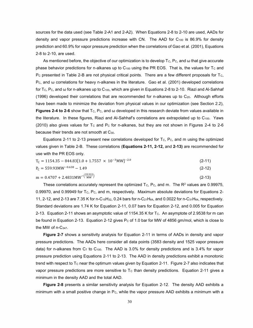
30
sources for the data used (see Table 2-A1 and 2-A2). When Equations 2-8 to 2-10 are used, AADs for
density and vapor pressure predictions increase with CN. The AAD for C100 is 86.9% for density
prediction and 60.9% for vapor pressure prediction when the correlations of Gao et al. (2001), Equations
2-8 to 2-10, are used.
As mentioned before, the objective of our optimization is to develop TC, PC, and ω that give accurate
phase behavior predictions for n-alkanes up to C100 using the PR EOS. That is, the values for TC and
PC presented in Table 2-B are not physical critical points. There are a few different proposals for TC,
PC, and ω correlations for heavy n-alkanes in the literature. Gao et al. (2001) developed correlations
for TC, PC, and ω for n-alkanes up to C100, which are given in Equations 2-8 to 2-10. Riazi and Al-Sahhaf
(1996) developed their correlations that are recommended for n-alkanes up to C20. Although efforts
have been made to minimize the deviation from physical values in our optimization (see Section 2.2),
Figures 2-4 to 2-6 show that TC, PC, and ω developed in this research deviate from values available in
the literature. In these figures, Riazi and Al-Sahhaf’s correlations are extrapolated up to C100. Yaws
(2010) also gives values for TC and PC for n-alkanes, but they are not shown in Figures 2-4 to 2-6
because their trends are not smooth at C30.
Equations 2-11 to 2-13 present new correlations developed for TC, PC, and m using the optimized
values given in Table 2-B. These correlations (Equations 2-11, 2-12, and 2-13) are recommended for
use with the PR EOS only.
TC = 1154.35 − 844.83[1.0 + 1.7557 × 10⁻³MW]−2.0 (2-11)
PC = 559.93MW−0.638 − 1.49 (2-12)
m = 0.4707 + 2.4831MW−(39.933
MW) (2-13)
These correlations accurately represent the optimized TC, PC, and m. The R2 values are 0.99975,
0.99970, and 0.99949 for TC, PC, and m, respectively. Maximum absolute deviations for Equations 2-
11, 2-12, and 2-13 are 7.35 K for n-C15H32, 0.24 bars for n-C21H64, and 0.0022 for n-C31H64, respectively.
Standard deviations are 1.74 K for Equation 2-11, 0.07 bars for Equation 2-12, and 0.005 for Equation
2-13. Equation 2-11 shows an asymptotic value of 1154.35 K for TC. An asymptote of 2.9538 for m can
be found in Equation 2-13. Equation 2-12 gives PC of 1.0 bar for MW of 4856 gm/mol, which is close to
the MW of n-C347.
Figure 2-7 shows a sensitivity analysis for Equation 2-11 in terms of AADs in density and vapor
pressure predictions. The AADs here consider all data points (3583 density and 1525 vapor pressure
data) for n-alkanes from C7 to C100. The AAD is 3.0% for density predictions and is 3.4% for vapor
pressure prediction using Equations 2-11 to 2-13. The AAD in density predictions exhibit a monotonic
trend with respect to TC near the optimum values given by Equation 2-11. Figure 2-7 also indicates that
vapor pressure predictions are more sensitive to TC than density predictions. Equation 2-11 gives a
minimum in the density AAD and the total AAD.
Figure 2-8 presents a similar sensitivity analysis for Equation 2-12. The density AAD exhibits a
minimum with a small positive change in PC, while the vapor pressure AAD exhibits a minimum with a

31
small negative change in PC. Equation 2-12 gives a minimum for the sum of the two AADs.
Figure 2-9 shows the sensitivity of the AADs to the m parameter near the optimum values given in
Equation 2-13. The vapor pressure AAD is sensitive to the m parameter, but the density AAD is nearly
constant for ±10% changes from Equation 2-13. Equation 2-13 gives a minimum for the vapor pressure
AAD and the total AAD. Figures 2-7, 2-8, and 2-9 also show that density predictions are more sensitive
to PC than to TC and the m parameter.
2.4. Application of Optimized Critical Parameters to Mixtures
In Section 2.3, we developed a new set of critical parameters for the PR EOS that can accurately predict
liquid densities and vapor pressures of n-alkanes up to C100. This section is to show that the PR EOS
with the critical parameters developed also improves phase behavior predictions for mixtures. We first
demonstrate improved phase behavior predictions for various n-alkane mixtures. Application of our
critical parameters is then presented for characterization of 25 different reservoir oils. All phase behavior
calculations in this section use the PR EOS with the van der Waals mixing rules, and zero binary
interaction between hydrocarbons.
2.4.1. Phase Behavior Predictions for n-Alkane Mixtures
We make comparisons between the PR EOS with our correlations for critical parameters (i.e., Equations
2-10 to 2-12) and the PR EOS with the correlations of Gao et al. (2001) (i.e., Equations 2-8 to 2-10). No
attempts are made to adjust parameters to obtain a better match between experimental data and
predictions.
Table 2-3 shows use of our correlations gives improved accuracy for density predictions for various
n-alkane mixtures. AADs in density predictions become greater for heavier hydrocarbons when the
correlations of Gao et al. (2001) are used. Use of our correlations for the PR EOS exhibits consistently
small AADs in density predictions for all mixtures studied.
The two sets of the correlations are also compared in terms of bubble point pressure predictions for
six different mixtures, C1-C16, C1-C20, C2-C16, C2-C20, C2-C22, and C2-C24. For C2-C22 and C2-C24
mixtures, bubble point pressures at two different temperatures are considered for the comparisons.
Predictions of bubble and dew points are compared for three n-alkane binaries C6-C16, C6-C24, and C6-
C36. As shown in Figures 2-10 to 2-20, use of our correlations gives more accurate predictions for
bubble and dew points pressures for most of the mixtures studied. Our correlations ensure that bubble
point and dew point pressures near the end points (i.e., 0.0 and 1.0 on the x axis) of the figures are
accurately predicted using the PR EOS.
Deviations from experimental data are observed for middle-range mixing ratios. Such deviations
are attributed mainly to the van der Waals mixing rules used to estimate the attraction and covolume
parameters for mixtures. The deviations can be significantly improved if a binary interaction parameter
is adjusted for each n-alkane binary. We developed the optimized critical parameters considering their
application for characterization of reservoir oils. In reservoir oil characterization, the main challenge

32
comes from uncertainties in properties and amounts of non-identifiable compounds. Adjustment of
binary interaction parameters for such a case can result in physically absurd predictions Pedersen and
Christensen (2007). That is, we do not show adjustment of binary interaction parameters to fit EOS
predictions to data in this research.
2.4.2. Density Prediction for Reservoir Oils
Different reservoir oils have different distributions of CN groups and PNA components within a given CN
group. Even for a given reservoir oil, the concentrations of PNA components likely vary with CN.
Characterization of heavy oils is more difficult than that of conventional oils because heavy oils contain
a larger amount of heavy fractions, for which CN and PNA distributions are highly uncertain.
In a typical fluid characterization using an EOS, a distribution of CN groups is estimated based on
composition analysis data available. Once a CN group distribution is specified, critical parameters are
assigned to each CN group. Correlations for critical parameters proposed in the literature are generic
in that they do not explicitly consider the concentrations of PNA components. Use of these generic
correlations is unsuitable for heavy oil characterization because a heavier CN group can have a wider
variety of compounds in it.
A potential method to address the uncertainties is to consider a PNA distribution in a reservoir oil
as perturbation from n-alkane mixtures. The critical parameters developed in this research for a
homologous series of n-alkanes can serve as a well-defined reference for the perturbation consideration.
Since TC and PC for N and A components are in general greater than those for P components within a
given CN group, TC and PC for n-alkanes developed in this research provide the lower bounds of critical
parameters for pseudocomponents for actual oils.
Quiñones-Cisneros et al. (2003, 2004a, 2005) proposed a novel fluid characterization method. In
their method, PC for a pseudocomponent is expressed as PCi = f∙PCPi, where i is a component index,
PCP is PC for paraffinic components, and f is a perturbation factor that represents deviation from PCP.
So, the f factor is 1.0 for PCPi.
In this section, we apply the critical parameters developed in this research for characterizing 25
reservoir oils (Table 2-4) on the basis of Quiñones-Cisneros et al.’s characterization method. Measured
saturation pressures are used to adjust PC through the perturbation factor f as in Quiñones-Cisneros et
al. (2003, 2004a, 2005). No other parameters are adjusted. Density predictions are then compared
with experimental data.
The characterization steps given below are applied to 25 different reservoir oils presented in Table
2-4.
Step 1. Composition. Heavy fractions are split into detailed components using a chi-square distribution.
The detailed components are then grouped into 10 components consisting of N2, CO2, C1, C2-3,
C4, C5, and four heavy pseudocomponents.
Step 2. Critical parameters. For the well-defined components (i.e., N2, CO2, and C1-C5), physical critical
parameters available in the literature are used. For the four pseudocomponents, two sets of
33
correlations are used; Equations 2-11 to 2-13 developed in this research and the correlations of
Quiñones-Cisneros et al. (2005) as given by Equations 2-14, 2-15, and 2-16.
TC = −423.587 + 210.152ln(MW) (2-14)
PC = Exp(9.67283 − 4.05288MW0.1) (2-15)
ω = Exp(8.50471 −15.1665
MW0.1 ) (2-16)
Step 3. Perturbation of PC. Adjust the perturbation factor f to match the experimental saturation pressure
at the reservoir temperature.
For all reservoir oils characterized, binary interaction parameters between non-hydrocarbon and
hydrocarbon components are 0.02 for N2-C1, 0.06 for N2-C2-3, 0.08 for N2-Ci>3, 0.12 for CO2-C1, and 0.15
for CO2-Ci>1 (Quiñones-Cisneros et al. 2005). Volume-shift parameters are zero for all components. In
the above, two fluid models are created for each of 25 reservoir oils; i.e., one using Equations 2-11 to
2-13 and the other using Equations 2-14 to 2-16 for TC, PC, and ω. Equations 2-14 and 2-16 are generic
correlations that do not consider the PNA distribution, while Equation 2-15 is the correlation for PCP
proposed by Quiñones-Cisneros et al. (2005). The two fluid models are compared in terms of density
predictions for each of the reservoir oils studied (Table 2-4).
Table 2-4 lists the resulting perturbation factors for the 25 reservoir oils. The critical parameters
developed in this research result in systematically reduced perturbation required to match saturation
pressures. All perturbation factors are calculated to be greater than 1.0 using Equations 2-11 to 2-13
except for the heavy oil oil-6. This observation is consistent with the fundamental concept of the
perturbation; i.e., the perturbation factor represents deviation from PCP, and PC is lower for the P
components than for the N and A components within a given CN group. The variation of the resulting
perturbation factors is small for oils lighter than 25˚API. A wider variation of the resulting perturbation
factors is observed for heavier oils, which likely results from higher uncertainties in heavier oils’
compositions.
Table 2-4 lists AADs in density predictions for the 25 reservoir oils using Equations 2-11 to 2-13
developed in this research and Equations 2-14 to 2-16 taken from Quiñones-Cisneros et al. (2005). As
shown in Figure 2-21, use of Equations 2-11 to 2-13 results in more accurate density predictions for
most of the reservoir oils studied. The correlations developed in this research require less perturbation
from PCP to obtain more accurate density predictions for oils lighter than 25˚API. For such lighter oils,
it is likely that the concentration of paraffinic components is relatively high.
Figure 2-21 also show that AADs in density predictions for five oils heavier than 25˚API (22.6, 13.38,
11.98, 11.63, and 9.5˚API) are larger when Equations 2-11 to 2-13 are used. Using these equations,
however, smaller perturbations of PC are required to match measured saturation pressures even for
these five heavy oils as given in Table 2-4. Reliable characterization for these low-API reservoir oils
using the PR EOS were recently developed based on a new perturbation method with the critical
parameters developed in this research (Kumar and Okuno 2014).

34
2.5. Conclusions
We developed correlations for critical temperatures (TC), critical pressures (PC), and acentric factors (ω)
that are optimized for phase behavior modeling of n-alkanes from C7 to C100 using the Peng-Robinson
(PR) EOS. Density and vapor pressure data available in the literature were used for the optimization.
The new set of TC, PC, and ω satisfies Pitzer’s definition of ω. The optimum TC, PC, and values were
applied to predict phase behavior of n-alkane mixtures and 25 different reservoir oils using the PR EOS.
The conclusions are as follows:
o Critical parameters and acentric factors for n-alkanes from C7 to C100 are optimized using 3583
density and 1525 vapor pressure data for use with PR EOS. These optimized parameters results in
2.8% AAD in density prediction and 1.6% vapor pressure prediction.
o The PR EOS with our correlations for TC, PC, and gives 3.0% and 3.4% AADs in density and vapor
pressure predictions, respectively, for n-alkanes from C7 to C100. When conventional correlations
are used for critical parameters, the PR EOS exhibits less accurate predictions for heavier n-
alkanes, and AADs can be as high as 61% for vapor pressure prediction and 87% for density
prediction for n-C100.
o The critical parameter correlations developed in this research significantly improve phase behavior
predictions for n-alkane mixtures. Use of conventional correlations for critical parameters available
in the literature results in larger AADs in density prediction and bubble-and dew-point predictions.
The errors are more significant for heavier n-alkane mixtures using the conventional correlations.
o The critical parameters for n-alkanes developed provide useful initial values for characterization of
reservoir oils using the PR EOS. Results showed that, when perturbation of PC from the n-alkane
values is used to match experimental data, resulting values for PC are greater than the n-alkane
values. This is because aromatic and naphthenic components have higher critical pressures than
n-alkanes for a given carbon number group. The new set of TC and PC correlations for a homologous
series of n-alkanes can serve as the lower bounds for TC and PC of pseudocomponents of reservoir
fluids characterized using the PR EOS.
o The PR EOS with the critical parameters developed in this research exhibits improved predictive
capability for oils lighter than 25˚API, where concentrations of aromatic and naphthenic components
are typically insignificant.
35
2.6. Nomenclature Roman symbols
b Covolume parameter in a cubic EOS
f Perturbation factor defined in Section 2.4.2
m m(ω) function in the PR EOS given in Equations 2-4 and 2-5
P Pressure, bar
PC Critical pressure, bar
PCP Critical pressure for a paraffinic component, bar
Pr Reduced pressure
Prvap Reduced vapor pressure
T Temperature, K
TC Critical temperature, K
Tr Reduced temperature
v Molar volume
Greek letters
α(𝑇) Alpha function in the PR EOS
ω Acentric factor
Abbreviations
AAD Average absolute deviation
CN Carbon number
EOS Equation of state
MW Molecular weight
NBP Normal boiling point, K
PNA Paraffins, naphthenes, and aromatics
PR Peng-Robinson
SRK Soave-Redlich-Kwong

36
2.7. References Ambrose, D. and Tsonopoulos, C. 1995. Vapor-Liquid Critical Properties of Elements and Compounds.
2. Normal Alkanes. J. Chem. Eng. Data 40 (3): 531-546.
Aucejo, A., Burguet, M.C., Muñoz, R. et al. 1995. Viscosities and Refractive Indices of Some n-Alkane
Binary Liquid Systems at 298.15 K. J. Chem. Eng. Data 40 (1): 141-147.
Banipal, T.S., Garg, S.K., and Ahluwalia, J.C. 1991. Heat Capacities and Densities of Liquid n-Octane,
n-Nonane, n-Decane, and n-Hexadecane at Temperatures from 318.15 K to 373.15 K and at
Pressures up to 10 MPa. J. Chem. Thermodyn. 23 (10): 923-931.
Coats, K.H. and Smart, G. T. 1986. Application of a Regression Based EOS PVT Program to Laboratory
Data. SPE Res Eng 1 (3): 277-299. SPE-11197-PA.
Cullick, A.S., Pebdani, F.N., and Griewank, A.K. 1989. Modified Corresponding States Method for
Predicting Densities of Petroleum Reservoir Fluids. Ind. Eng. Chem. Res. 28 (3): 340-347.
Daridon, J.L., Carrier, H., and Lagourette, B. 2002. Pressure Dependence of the Thermophysical
Properties of n-Pentadecane and n-Heptadecane. Int. J. Thermophys. 23 (3): 697-708.
Daubert, T.E., Danner, R.P., Sibel, H.M. et al. 1997. Physical and Thermodynamic Properties of Pure
Chemicals: Data Compilation, Taylor & Francis, Washington, D.C., 1997.
DECHEMA Gesellschaft für Chemische Technik und Biotechnologie http://i-
systems.dechema.de/detherm/mixture.php
Doolittle, A.K. 1964. Specific Volumes of n-Alkanes. J. Chem. Eng. Data 9 (2): 275-279.
Dutour, S., Daridon, J.L., and Lagourette, B. 2000. Pressure and Temperature Dependence of the
Speed of Sound and Related Properties in Normal Octadecane and Nonadecane. Int. J.
Thermophys. 21 (1): 173-184.
Dutour, S., Lagourette, B., and Daridon, J.L. 2001. High-Pressure Speed of Sound and Compressibilities
in Heavy Normal Hydrocarbons: n-C23H48 and n-C24H50. J. Chem. Thermodyn. 33 (7): 765-774.
Dutour, S., Lagourette, B., and Daridon, J.L. 2002. High-pressure speed of sound, density and
compressibility of heavy normal paraffins: C28H58 and C36H74. J. Chem. Thermodyn. 34 (4): 475-484.
Dykyj, J., Svoboda, J., Wilhoit, R. et al. 1997. Vapor Pressure of Chemicals. Landolt-Börnstein: Berlin,
Sub-volume A.
Elizalde-Solis, O., Galicia-Luna, L.A., and Camacho-Camacho, L.E. 2007. High-Pressure Vapor–Liquid
Equilibria for CO2 + Alkanol Systems and Densities of n-Dodecane and n-Tridecane. Fluid Phase
Equilib. 259 (1): 23-32.
Ewing, M.B. and Ochoa, J.C.S. 2005. Vapor Pressures of n-Heptane Determined by Comparative
Ebulliometry. J. Chem. Eng. Data 50 (5): 1543-1547.
Gao, W., Robinson Jr., R.L., and Gasem, K.A.M. 2001. Improved Correlations for Heavy n-Paraffin
Physical Properties. Fluid Phase Equilib. 179 (1-2): 207-216.
Goodwin, A.R., Bradsell, C.H., and Toczylkin, L.S. 1996. (p,ρ,T) of Liquid n-Octane Obtained with a
Spherical Pycnometer at Temperatures of 298.03 K and 313.15 K and Pressures in the Range 0.7
37
MPa to 32 MPa. J. Chem. Thermodyn. 28 (6): 637- 646.
Gregorowicz, J., Kiciak, K., and Malanowski, S. 1987. Vapour Pressure Data for 1-Butanol, Cumene, n-
Octane and n-Decane and Their Statistically Consistent Reduction with the Antoine Equation. Fluid
Phase Equilib. 38 (1-2): 97-107.
J. D. van der Waals, Over de Continuiteit van den Gas-en Vloeistoftoestand, Ph.D. dissertation
(excerpt), Leiden, The Netherlands, 1873.
Jhaveri, B.S. and Youngren, G.K. 1988. Three-Parameter Modification of the Peng-Robinson Equation
of State to Improve Volumetric Predictions. SPE J. 3 (3): 1033-1040.
Joyce, P.C. and Thies, M.C. 1998. Vapor-Liquid Equilibria for the Hexane + Hexadecane and Hexane
+ 1-Hexadecanol Systems at Elevated Temperatures and Pressures. J. Chem. Eng. Data 43 (5):
819-822.
Joyce, P.C., Gordon, J., and Thies, M.C. 2000. Vapor−Liquid Equilibria for the Hexane + Tetracosane
and Hexane + Hexatriacontane Systems at Elevated Temperatures and Pressures. J. Chem. Eng.
Data 45 (3): 424-427.
Khasanshin, T.S. and Shchemelev, A.P. 2002. The Thermodynamic Properties of n-Tetradecane in
Liquid State. High Temp. 40 (2): 207-211.
Klara, S.M. and Hemanth-Kumar, K. 1987. Comparisons of Computational Efficiencies of Different
Equations of State and Transport Property Correlations in a Compositional Simulator. Presented at
SPE Annual Technical Conference and Exhibition, Dallas, Texas, 27-30 September. SPE-16942-
MS.
Krejbjerg, K. and Pedersen, K. S. 2006. Controlling VLLE Equilibrium with a Cubic EoS in Heavy Oil
Modeling. Presented at Canadian International Petroleum Conference, Calgary, Alberta, 13-15
June. PETSOC-2006-052.
Kumar, A. and Okuno, R. 2014. Reservoir Oil Characterization for Compositional Simulation of Solvent
Injection Processes. Ind. Eng. Chem. Res. 53 (1): 440-455.
Li, H. and Yang, D. 2011. Modified α Function for the Peng-Robinson Equation of State To Improve the
Vapor Pressure Prediction of Non-hydrocarbon and Hydrocarbon Compounds. Energy Fuels 25
(1): 215-223
Mathias, P. M. 1983. A Versatile Phase Equilibrium Equation of State. Ind. Eng. Chem., Process Des.
Dev. 22 (3): 385–391.
Melhem, G.A., Saini, R., and Goodwin, B.M. 1989. A Modified Peng-Robinson Equation of State. Fluid
Phase Equilib. 47: 189-237
Morgan, D.L. and Kobayashi, R. 1994. Direct Vapor Pressure Measurements of Ten n-Alkanes m the
10-C28 Range. Fluid Phase Equilib. 97: 211-242.
Neau, E., Jaubert, J.N., and Rogalski, M. 1993. Characterization of Heavy Oils. Ind. Eng. Chem. Res.
32 (6): 1196-1203.
Nji, G.N., Svrcek, W.Y. and Yarranton, H. et al. 2008. Characterization of Heavy Oils and Bitumens. 1.

38
Vapor Pressure and Critical Constant Prediction Method for Heavy Hydrocarbons. Energy Fuels 22
(1): 455-462.
Nji, G.N., Svrcek, W.Y. and Yarranton, H. et al. 2009. Characterization of Heavy Oils and Bitumens 2.
Improving the Prediction of Vapor Pressures for Heavy Hydrocarbons at Low Reduced
Temperatures Using the Peng−Robinson Equation of State. Energy Fuels 23 (1): 366-373.
Okuno, R., Johns, R.T., and Sepehrnoori, K. 2011. Mechanisms for High Displacement Efficiency of
Low-Temperature CO2 Floods. SPE J. 16 (4): 751-767.
Patil, S., Dandekar, A., Khataniar, S. 2008. Project Report, DOE Award No. DE-FC26-01NT41248.
http://www.osti.gov/bridge/purl.cover.jsp?purl=/963365-YrCq8p/963365.pdf.
Pedersen, K.S., and Christensen, P.L., 2007. Phase Behavior of Petroleum Reservoir Fluids. CRC
Press, Taylor & Francis Group, Boca Raton, FL, USA.
Pedersen, K.S., Blilie, A.L., and Meisingset, K.K. 1992. Calculations on Petroleum Reservoir Fluids
Using Measured and Estimated Compositional Data for the Plus Fraction. Ind. Eng. Chem. Res. 31
(5): 1378-1384.
Peneloux, A., Rauzy, E., and Fréze, R. 1982. A Consistent Correction for Redlich-Kwong-Soave
Volume. Fluid Phase Equilib. 8 (1): 7-23.
Peng, D.-Y. and Robinson, D.B. 1976. A New Two-Constant Equation of State. Ind. Eng. Chem. Fund.
15 (1): 59-64.
Peng, D.-Y. and Robinson, D.B. 1978. The Characterization of the Heptanes and Heavier Fractions for
the GPA Peng-Robinson Programs. GPA Research Report RR-28.
Perry, R.H. and Green, D.W. 2007. Perry’s Chemical Engineers’ Handbook, 8th Edition, The McGraw
Hill Companies, Inc., New York, USA.
Peter, C.J., Spiegelaar, J., and De Arons, J.S. 1988. Phase Equilibria in Binary Mixtures of Ethane +
Docosane and Molar Volumes of Liquid Docosane. Fluid Phase Equilib. 41 (3): 245-256.
Peters, C.J., De Arons, J.S., Sengers, J.M.H.L. et al. 1988. Global Phase Behavior of Mixtures of Short
and Long n-Alkanes. AIChE J. 34 (5): 834–839.
Poling, B.E., Prausnitz, J.M., and O’Connell, J.P. 2001. The Properties of Gases and Liquids, The
McGraw-Hill, New York, NY, 2001.
PVTsim, 20.0, 2011. CALSEP International Consultants, Copenhagen, Denmark.
Queimada, A.J., Marrucho, I.M., Coutinho, J.A.P. et al. 2005. Viscosity and Liquid Density of Asymmetric
n-Alkane Mixtures: Measurement and Modeling. Int. J. Thermophys. 26 (1): 47-61.
Quiñones-Cisneros, S.E., Andersen, S.I., and Creek, J. 2005. Density and Viscosity Modeling and
Characterization of Heavy Oils. Energy Fuels 19 (4): 1314-1318.
Quiñones-Cisneros, S.E., Dalberg, A., and Stenby, E.H. 2004b. PVT Characterization and Viscosity
Modeling and Prediction of Crude Oils. Pet. Sci. Technol., 22 (9-10): 1309–1325.
Quiñones-Cisneros, S.E., Zéberg-Mikkelsen, C.K., and Stenby, E.H. 2003. Friction Theory Prediction of
Crude Oil Viscosity at Reservoir Conditions Based on Dead Oil Properties. Fluid Phase Equilib.
39
212 (1-2): 233–243.
Quiñones-Cisneros, S.E., Zéberg-Mikkelsen, C.K., Baylaucq, A. et al. 2004a. Viscosity Modeling and
Prediction of Reservoir Fluids: From Natural Gas to Heavy Oils. Int. J. Therm. 25 (5): 1353-1366.
Rackett, H.G. 1970. Equation of State for Saturated Liquids. J. Chem. Eng. Data 15 (4): 514-517.
Riazi M.R. and Al-Sahhaf, T.A. 1996. Physical Properties of Heavy Petroleum Fractions and Crude Oils.
Fluid Phase Equilib. 117 (1-2): 217-224.
Riazi, M.R. 2005. Manual 50, Characterization and Properties of Petroleum Fractions; ASTM
International: West Conshohocken, PA.
Riazi, M.R. and AlQaheem, Y.S. 2010. Predicting Vapor Pressure of Heavy Hydrocarbons from Molar
Refraction and Its Applications to Petroleum Mixtures. Ind. Eng. Chem. Res. 49 (15): 7104-7112.
Rodríguez, I. and Hamouda, A. A. 2008. An Approach for Characterization and Lumping of Plus
Fractions of Heavy Oil. Presented at SPE International Thermal Operations and Heavy Oil
Symposium, Calgary, 20-23 October. SPE-117446.
Schilling, G., Kleinrahm, R., and Wagner, W., 2008. Measurement and Correlation of the (p, ρ, T)
Relation of Liquid n-Heptane, n-Nonane, 2,4-Dichlorotoluene, and Bromobenzene in the
Temperature Range from (233.15 to 473.15) K at Pressures up to 30 MPa for Use as Density
Reference Liquids. J. Chem. Thermodyn. 40 (7), 1095-1105.
Soave, G. 1972. Equilibrium Constants from a Modified Redlich-Kwong Equation of State. Chem. Eng.
Sci. 27:1197-1203.
Stryjek, R. and Vera, J. H. 1986. PRSV: An improved peng—Robinson equation of state for pure
compounds and mixtures. Can. J. Chem. Eng. 64 (2): 323-333.
Susnar, S.S., Budziak, C.J., Hamza, H.A. et al. 1992. Pressure Dependence of the Density of n–
Alkanes. Int. J. Thermophys. 13 (3), 443-452.
Ting, P.D., Joyce, P.C., Jog, P.K. et al. 2003. Phase Equilibrium Modeling of Mixtures of Long-Chain
and Short-Chain Alkanes Using Peng–Robinson and SAFT. Fluid Phase Equilib. 206 (1-2), 267-
286.
Voulgaris, M., Stamatakis, S. and Tassios, D. 1991. Prediction of Physical Properties for Non-Polar
Compounds, Petroleum and Coal Liquid Fractions. Fluid Phase Equilib. 64: 73-106.
Voutsas, E.C., Pappa, G.D., Magoulas, K. et al. 2006. Vapor Liquid Equilibrium Modeling of Alkane
Systems with Equations of State: “Simplicity versus Complexity. Fluid Phase Equilib. 240 (2): 127-
139.
Whitson, C.H. and Brulè, M.R. 2000. Phase Behaviour. SPE Henry L. Doherty Series, Vol. 20, SPE,
Richardson, Texas.
Yaws, C.L. 2010. Yaws' Thermo Physical Properties of Chemicals and Hydrocarbons (Electronic
Edition), Knovel, 2010.
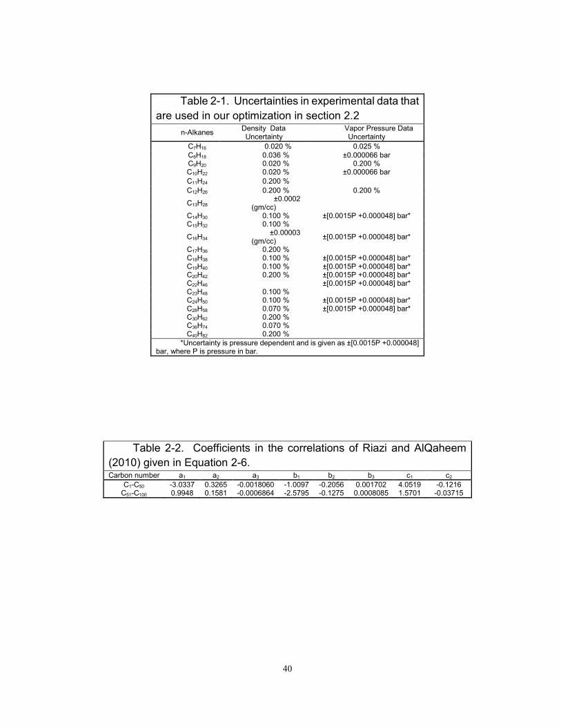
40
Table 2-1. Uncertainties in experimental data that
are used in our optimization in section 2.2
n-Alkanes Density Data Uncertainty
Vapor Pressure Data Uncertainty
C7H16 0.020 % 0.025 %
C8H18 0.036 % ±0.000066 bar C9H20 0.020 % 0.200 % C10H22 0.020 % ±0.000066 bar
C11H24 0.200 %
C12H26 0.200 % 0.200 %
C13H28 ±0.0002 (gm/cc)
C14H30 0.100 % ±[0.0015P +0.000048] bar* C15H32 0.100 %
C16H34 ±0.00003 (gm/cc)
±[0.0015P +0.000048] bar*
C17H36 0.200 % C18H38 0.100 % ±[0.0015P +0.000048] bar* C19H40 0.100 % ±[0.0015P +0.000048] bar* C20H42 0.200 % ±[0.0015P +0.000048] bar* C22H46 ±[0.0015P +0.000048] bar* C23H48 0.100 % C24H50 0.100 % ±[0.0015P +0.000048] bar* C28H58 0.070 % ±[0.0015P +0.000048] bar* C30H62 0.200 % C36H74 0.070 % C40H82 0.200 %
*Uncertainty is pressure dependent and is given as ±[0.0015P +0.000048] bar, where P is pressure in bar.
Table 2-2. Coefficients in the correlations of Riazi and AlQaheem
(2010) given in Equation 2-6. Carbon number a1 a2 a3 b1 b2 b3 c1 c2
C1-C50 -3.0337 0.3265 -0.0018060 -1.0097 -0.2056 0.001702 4.0519 -0.1216 C51-C100 0.9948 0.1581 -0.0006864 -2.5795 -0.1275 0.0008085 1.5701 -0.03715

41
Table 2-3. AADs in density predictions for n-alkane mixtures using the PR EOS. AADs using
Equations 2-11 to 2-13 developed in this research are compared to those using Equations 2-8 to 2-
10 of Gao et al. (2001).
Components No. of Data
Reference AAD
This Research AAD
Gao et al.
Heptane (C7) + Octane (C8) 11 Aucejo et al. (1995) 0.3 1.7 Heptane (C7) + Nonane (C9) 11 Aucejo et al. (1995) 0.7 2.9 Heptane (C7) + Decane (C10) 11 Aucejo et al. (1995) 1.2 4.1 Heptane (C7) + Undecane (C11) 11 Aucejo et al. (1995) 0.6 5.3 Heptane (C7) + Dodecane (C12) 10 Aucejo et al. (1995) 1.7 6.5 Heptane (C7) + Hexadecane (C16) 11 Aucejo et al. (1995) 3.1 12.6 Octane (C8) + Nonane (C9) 11 Aucejo et al. (1995) 0.9 3.8 Octane (C8) + Decane (C10) 11 Aucejo et al. (1995) 1.2 4.8 Octane (C8) + Undecane (C11) 11 Aucejo et al. (1995) 0.7 5.9 Octane (C8) + Dodecane (C12) 11 Aucejo et al. (1995) 1.9 7.3 Octane (C8) + Hexadecane (C16) 11 Aucejo et al. (1995) 3.2 12.8 Nonane (C9) + Decane (C10) 11 Aucejo et al. (1995) 1.4 5.6 Nonane (C9) + Undecane (C11) 11 Aucejo et al. (1995) 0.9 6.7 Nonane (C9) + Dodecane (C12) 11 Aucejo et al. (1995) 1.9 7.8 Nonane (C9) + Hexadecane (C16) 11 Aucejo et al. (1995) 3.3 15.2 Decane (C10) + Undecane (C11) 11 Aucejo et al. (1995) 1.3 7.6 Decane (C10) + Dodecane (C12) 11 Aucejo et al. (1995) 2.3 8.7 Decane (C10) + Hexadecane (C16) 11 Aucejo et al. (1995) 3.4 13.5 Undecane (C11) + Dodecane (C12) 11 Aucejo et al. (1995) 1.8 9.5 Undecane (C11) + Hexadecane (C16) 11 Aucejo et al. (1995) 3.0 14.1 Dodecane (C12) + Hexadecane (C16) 11 Aucejo et al. (1995) 3.7 14.7 Decane (C10) + Eicosane (C20) 24 Queimada et al. (2005) 4.2 18.0 Decane (C10) + Docosane (C22) 20 Queimada et al. (2005) 4.6 20.7 Decane (C10) + Tetracosane (C24) 16 Queimada et al. (2005) 4.9 23.5 Decane (C10) + Docosane (C22) + Tetracosane (C24) 23 Queimada et al. (2005) 4.8 21.8
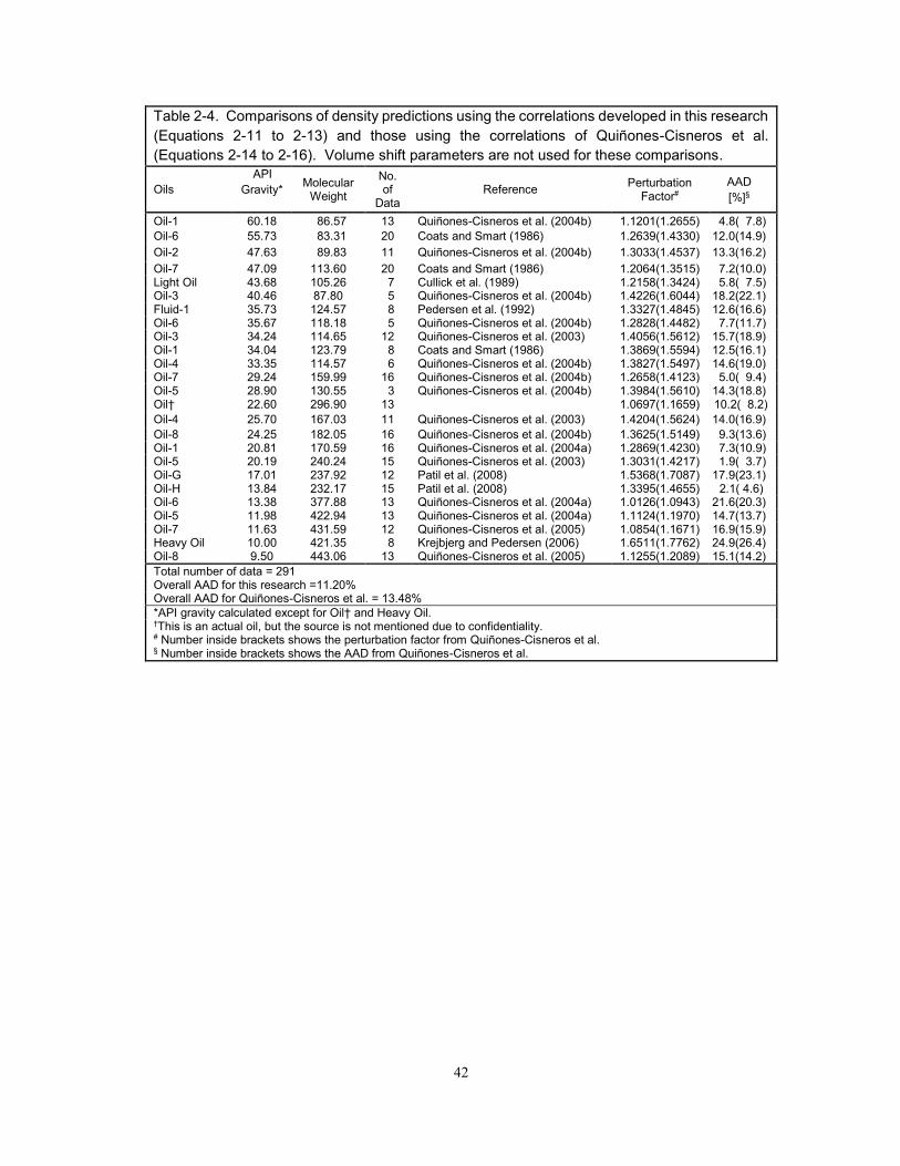
42
Table 2-4. Comparisons of density predictions using the correlations developed in this research
(Equations 2-11 to 2-13) and those using the correlations of Quiñones-Cisneros et al.
(Equations 2-14 to 2-16). Volume shift parameters are not used for these comparisons.
Oils
API
Gravity*
Molecular Weight
No. of
Data Reference
Perturbation Factor#
AAD
[%]§
Oil-1 60.18 86.57 13 Quiñones-Cisneros et al. (2004b) 1.1201(1.2655) 4.8( 7.8)
Oil-6 55.73 83.31 20 Coats and Smart (1986) 1.2639(1.4330) 12.0(14.9)
Oil-2 47.63 89.83 11 Quiñones-Cisneros et al. (2004b) 1.3033(1.4537) 13.3(16.2)
Oil-7 47.09 113.60 20 Coats and Smart (1986) 1.2064(1.3515) 7.2(10.0) Light Oil 43.68 105.26 7 Cullick et al. (1989) 1.2158(1.3424) 5.8( 7.5) Oil-3 40.46 87.80 5 Quiñones-Cisneros et al. (2004b) 1.4226(1.6044) 18.2(22.1) Fluid-1 35.73 124.57 8 Pedersen et al. (1992) 1.3327(1.4845) 12.6(16.6) Oil-6 35.67 118.18 5 Quiñones-Cisneros et al. (2004b) 1.2828(1.4482) 7.7(11.7) Oil-3 34.24 114.65 12 Quiñones-Cisneros et al. (2003) 1.4056(1.5612) 15.7(18.9) Oil-1 34.04 123.79 8 Coats and Smart (1986) 1.3869(1.5594) 12.5(16.1) Oil-4 33.35 114.57 6 Quiñones-Cisneros et al. (2004b) 1.3827(1.5497) 14.6(19.0) Oil-7 29.24 159.99 16 Quiñones-Cisneros et al. (2004b) 1.2658(1.4123) 5.0( 9.4) Oil-5 28.90 130.55 3 Quiñones-Cisneros et al. (2004b) 1.3984(1.5610) 14.3(18.8) Oil† 22.60 296.90 13 1.0697(1.1659) 10.2( 8.2)
Oil-4 25.70 167.03 11 Quiñones-Cisneros et al. (2003) 1.4204(1.5624) 14.0(16.9)
Oil-8 24.25 182.05 16 Quiñones-Cisneros et al. (2004b) 1.3625(1.5149) 9.3(13.6) Oil-1 20.81 170.59 16 Quiñones-Cisneros et al. (2004a) 1.2869(1.4230) 7.3(10.9) Oil-5 20.19 240.24 15 Quiñones-Cisneros et al. (2003) 1.3031(1.4217) 1.9( 3.7) Oil-G 17.01 237.92 12 Patil et al. (2008) 1.5368(1.7087) 17.9(23.1) Oil-H 13.84 232.17 15 Patil et al. (2008) 1.3395(1.4655) 2.1( 4.6) Oil-6 13.38 377.88 13 Quiñones-Cisneros et al. (2004a) 1.0126(1.0943) 21.6(20.3) Oil-5 11.98 422.94 13 Quiñones-Cisneros et al. (2004a) 1.1124(1.1970) 14.7(13.7) Oil-7 11.63 431.59 12 Quiñones-Cisneros et al. (2005) 1.0854(1.1671) 16.9(15.9) Heavy Oil 10.00 421.35 8 Krejbjerg and Pedersen (2006) 1.6511(1.7762) 24.9(26.4) Oil-8 9.50 443.06 13 Quiñones-Cisneros et al. (2005) 1.1255(1.2089) 15.1(14.2)
Total number of data = 291 Overall AAD for this research =11.20% Overall AAD for Quiñones-Cisneros et al. = 13.48%
*API gravity calculated except for Oil† and Heavy Oil. †This is an actual oil, but the source is not mentioned due to confidentiality. # Number inside brackets shows the perturbation factor from Quiñones-Cisneros et al. § Number inside brackets shows the AAD from Quiñones-Cisneros et al.
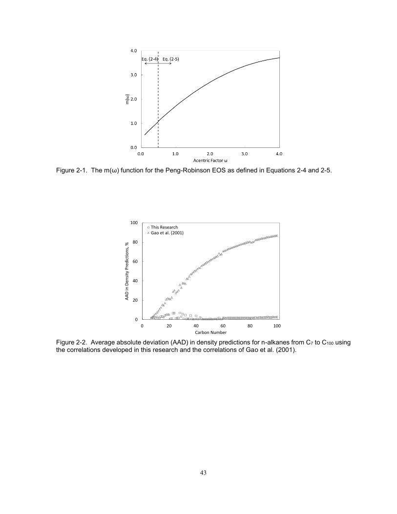
43
Figure 2-1. The m(ω) function for the Peng-Robinson EOS as defined in Equations 2-4 and 2-5.
Figure 2-2. Average absolute deviation (AAD) in density predictions for n-alkanes from C7 to C100 using the correlations developed in this research and the correlations of Gao et al. (2001).
0
20
40
60
80
100
0 20 40 60 80 100
AA
D in
Den
sity
Pre
dic
tio
ns,
%
Carbon Number
This ResearchGao et al. (2001)

44
Figure 2-3. Average absolute deviation (AAD) in vapor pressure predictions for n-alkanes from C7 to C100 using the correlations developed in this research and the correlations of Gao et al. (2001).
Figure 2-4. Optimum critical temperature (TC) developed for the PR EOS in this research, and the TC correlations of Gao et al. (2001) and Riazi and Al-Sahhaf (1996).
0
20
40
60
80
0 20 40 60 80 100
AA
D in
Vap
or
Pre
ssu
re P
red
icti
on
s, %
Carbon Number
This ResearchGao et al. (2001)
500
700
900
1100
0 20 40 60 80 100
Cri
tica
l Tem
per
atu
re, K
Carbon Number
This Research
Riazi and Al-Sahhaf
Gao et al.
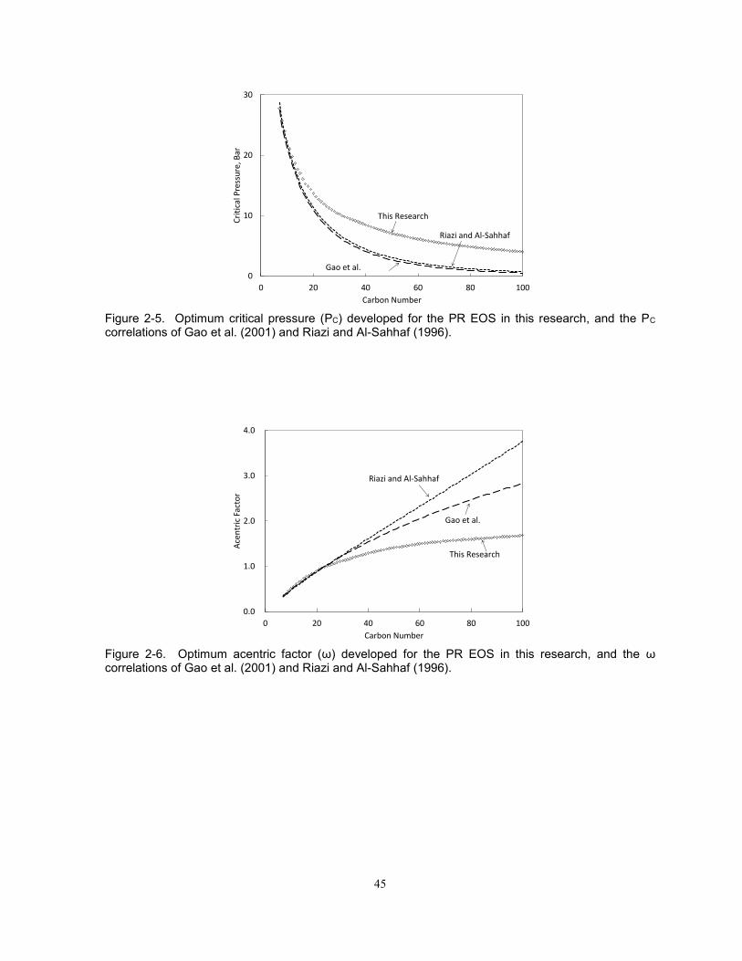
45
Figure 2-5. Optimum critical pressure (PC) developed for the PR EOS in this research, and the PC correlations of Gao et al. (2001) and Riazi and Al-Sahhaf (1996).
Figure 2-6. Optimum acentric factor (ω) developed for the PR EOS in this research, and the ω correlations of Gao et al. (2001) and Riazi and Al-Sahhaf (1996).
0
10
20
30
0 20 40 60 80 100
Cri
tica
l Pre
ssu
re, B
ar
Carbon Number
This Research
Riazi and Al-Sahhaf
Gao et al.
0.0
1.0
2.0
3.0
4.0
0 20 40 60 80 100
Ace
ntr
ic F
acto
r
Carbon Number
This Research
Riazi and Al-Sahhaf
Gao et al.
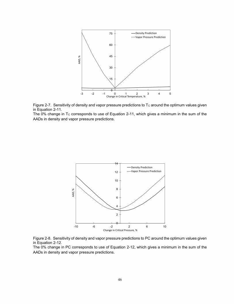
46
Figure 2-7. Sensitivity of density and vapor pressure predictions to TC around the optimum values given in Equation 2-11. The 0% change in TC corresponds to use of Equation 2-11, which gives a minimum in the sum of the
AADs in density and vapor pressure predictions.
Figure 2-8. Sensitivity of density and vapor pressure predictions to PC around the optimum values given in Equation 2-12. The 0% change in PC corresponds to use of Equation 2-12, which gives a minimum in the sum of the
AADs in density and vapor pressure predictions.
0
15
30
45
60
75
-3 -2 -1 0 1 2 3 4 5
AA
D, %
Change in Critical Temperature, %
Density Prediction
Vapor Pressure Prediction
0
2
4
6
8
10
12
14
-10 -6 -2 2 6 10
AA
D, %
Change in Critical Pressure, %
Density Prediction
Vapor Pressure Prediction
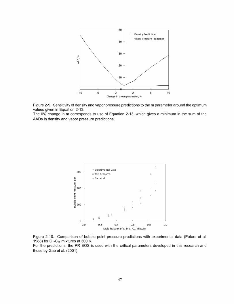
47
Figure 2-9. Sensitivity of density and vapor pressure predictions to the m parameter around the optimum values given in Equation 2-13. The 0% change in m corresponds to use of Equation 2-13, which gives a minimum in the sum of the
AADs in density and vapor pressure predictions.
Figure 2-10. Comparison of bubble point pressure predictions with experimental data (Peters et al. 1988) for C1-C16 mixtures at 300 K. For the predictions, the PR EOS is used with the critical parameters developed in this research and
those by Gao et al. (2001).
0
10
20
30
40
50
-10 -6 -2 2 6 10
AA
D, %
Change in the m parameter, %
Density Prediction
Vapor Pressure Prediction
0
200
400
600
0.0 0.2 0.4 0.6 0.8 1.0
Bu
bb
le P
oin
t P
ress
ure
, Bar
Mole Fraction of C1 in C1-C16 Mixture
Experimental Data
This Research
Gao et al.
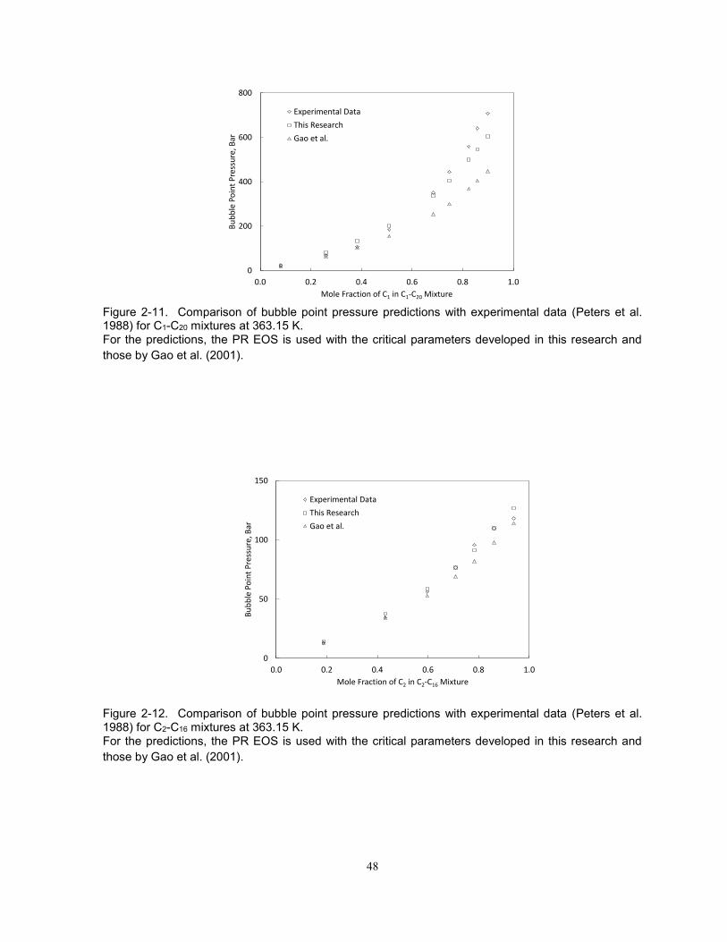
48
Figure 2-11. Comparison of bubble point pressure predictions with experimental data (Peters et al. 1988) for C1-C20 mixtures at 363.15 K. For the predictions, the PR EOS is used with the critical parameters developed in this research and
those by Gao et al. (2001).
Figure 2-12. Comparison of bubble point pressure predictions with experimental data (Peters et al. 1988) for C2-C16 mixtures at 363.15 K. For the predictions, the PR EOS is used with the critical parameters developed in this research and
those by Gao et al. (2001).
0
200
400
600
800
0.0 0.2 0.4 0.6 0.8 1.0
Bu
bb
le P
oin
t P
ress
ure
, Bar
Mole Fraction of C1 in C1-C20 Mixture
Experimental Data
This Research
Gao et al.
0
50
100
150
0.0 0.2 0.4 0.6 0.8 1.0
Bu
bb
le P
oin
t P
ress
ure
, Bar
Mole Fraction of C2 in C2-C16 Mixture
Experimental Data
This Research
Gao et al.
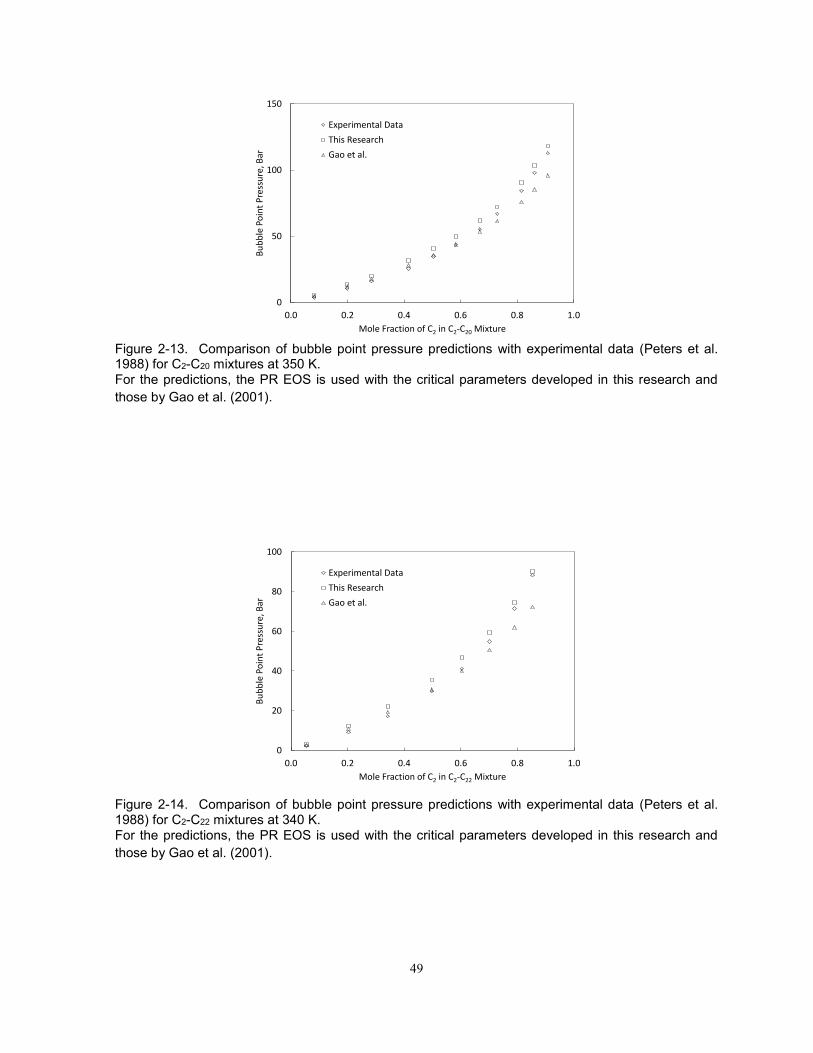
49
Figure 2-13. Comparison of bubble point pressure predictions with experimental data (Peters et al. 1988) for C2-C20 mixtures at 350 K. For the predictions, the PR EOS is used with the critical parameters developed in this research and
those by Gao et al. (2001).
Figure 2-14. Comparison of bubble point pressure predictions with experimental data (Peters et al. 1988) for C2-C22 mixtures at 340 K. For the predictions, the PR EOS is used with the critical parameters developed in this research and
those by Gao et al. (2001).
0
50
100
150
0.0 0.2 0.4 0.6 0.8 1.0
Bu
bb
le P
oin
t P
ress
ure
, Bar
Mole Fraction of C2 in C2-C20 Mixture
Experimental Data
This Research
Gao et al.
0
20
40
60
80
100
0.0 0.2 0.4 0.6 0.8 1.0
Bu
bb
le P
oin
t P
ress
ure
, Bar
Mole Fraction of C2 in C2-C22 Mixture
Experimental Data
This Research
Gao et al.

50
Figure 2-15. Comparison of bubble point pressure predictions with experimental data (Peters et al. 1988) for C2-C22 mixtures at 360 K. For the predictions, the PR EOS is used with the critical parameters developed in this research and
those by Gao et al. (2001).
Figure 2-16. Comparison of bubble point pressure predictions with experimental data (Peters et al. 1988) for C2-C24 mixtures at 330 K. For the predictions, the PR EOS is used with the critical parameters developed in this research and
those by Gao et al. (2001).
0
20
40
60
80
100
0.0 0.2 0.4 0.6 0.8 1.0
Bu
bb
le P
oin
t P
ress
ure
, Bar
Mole Fraction of C2 in C2-C22 Mixture
Experimental Data
This Research
Gao et al.
0
20
40
60
80
100
120
0.0 0.2 0.4 0.6 0.8 1.0
Bu
bb
le P
oin
t P
ress
ure
, Bar
Mole Fraction of C2 in C2-C24 Mixture
Experimental Data
This Research
Gao et al.

51
Figure 2-17. Comparison of bubble point pressure predictions with experimental data (Peters et al. 1988) for C2-C24 mixtures at 340 K. For the predictions, the PR EOS is used with the critical parameters developed in this research and
those by Gao et al. (2001).
Figure 2-18. Comparison of bubble and dew point predictions with experimental data (Joyce and Thies 1998) for C6-C16 mixture at 623K. The critical point is given as ♦. For the predictions, the PR EOS is used with the critical parameters
developed in this research and those by Gao et al. (2001).
0
20
40
60
80
100
120
140
0.0 0.2 0.4 0.6 0.8 1.0
Bu
bb
le P
oin
t P
ress
ure
, Bar
Mole Fraction of C2 in C2-C24 Mixture
Experimental Data
This Research
Gao et al.
5
10
15
20
25
30
35
40
0.0 0.2 0.4 0.6 0.8 1.0
Satu
rati
on
Pre
ssu
re, B
ar
Mole Fraction of C6 in C6-C16 Mixture
Experimental Data
This Research
Gao et al.

52
Figure 2-19. Comparison of bubble and dew point predictions with experimental data (Joyce et al. 2000) for C6-C24 mixture at 622.9K. The critical point is given as ♦. For the predictions, the PR EOS is used with the critical parameters
developed in this research and those by Gao et al. (2001).
Figure 2-20. Comparison of bubble and dew point predictions with experimental data (Joyce et al. 2000) for C6-C36 mixture at 621.8K. The critical point is given as ♦. For the predictions, the PR EOS is used with the critical parameters
developed in this research and those by Gao et al. (2001).
0
10
20
30
40
50
60
0.0 0.2 0.4 0.6 0.8 1.0
Satu
rati
on
Pre
ssu
re, B
ar
Mole Fraction of C6 in C6-C24 Mixture
Experimental Data
This Research
Gao et al.
0
20
40
60
80
0.0 0.2 0.4 0.6 0.8 1.0
Satu
rati
on
Pre
ssu
re, B
ar
Mole Fraction of C6 in C6-C36 Mixture
Experimental Data
This Research
Gao et al.
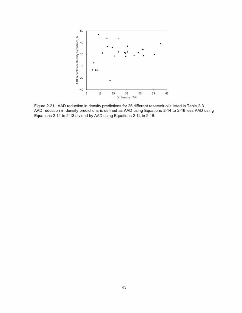
53
Figure 2-21. AAD reduction in density predictions for 25 different reservoir oils listed in Table 2-3. AAD reduction in density predictions is defined as AAD using Equations 2-14 to 2-16 less AAD using
Equations 2-11 to 2-13 divided by AAD using Equations 2-14 to 2-16.
-40
-20
0
20
40
60
5 15 25 35 45 55 65
AA
D R
edu
ctio
n in
Den
sity
Pre
dic
tio
ns,
%
Oil Density, ˚API

54
Chapter 3: Reservoir Oil Characterization for Compositional Simulation of
Solvent Injection Processes
A version of this has been published in Industrial and Engineering Chemistry Research,
Year: 2014, Volume: 53, Pages: 440-455.

55
3.1. Introduction
Solvent methods for enhanced oil recovery and heavy-oil recovery have been studied and implemented
in oil fields (e.g., Mohanty et al. 1995; DeRuiter et al. 1994). Various steam/solvent coinjection schemes
are also proposed in the literature (Hornbrook et al. 1991; Nasr et al. 2003; Gupta et al. 2003; Li et al.
2011; Gate and Chakrabarty 2008) to improve efficiency of the conventional steam-assisted gravity
drainage. Reliable design of such oil recovery processes requires compositional reservoir simulation to
model mass transfer among phases using a cubic equation of state (EOS).
Cubic EOSs are widely used in the petroleum industry to model volumetric and compositional phase
behavior of conventional oils. The most widely used cubic EOSs are the Peng-Robinson (PR) EOS
(Peng and Robinson 1976, 1978) and the Soave-Redlich-Kwong (SRK) EOS (Soave 1972). These
EOSs together with the van der Waals mixing rules are suitable for computationally efficient
representation of vapor-liquid equilibrium for hydrocarbon mixtures at a wide range of pressures (Okuno
et al. 2010).
However, application of these EOSs for modeling heavy-oil recovery is not straightforward. For
heavy-oil recovery, a typical operation range in pressure-temperature-composition (P-T-x) space is
much wider than that for enhanced recovery of conventional oil. When steam and solvent are coinjected
for heavy-oil recovery, reservoir temperatures lie between an initial reservoir temperature and steam
temperatures; e.g., between 290 K and 530 K for a typical solvent-steam-assisted gravity drainage.
Also, mixtures of solvent and heavy oils are highly size-asymmetric, resulting in a wider variety of
composition conditions. The wide operation range in P-T-x space provides technical challenges for the
traditional use of cubic EOSs with the van der Waals mixing rules.
Fluid characterization using an EOS is conducted based on experimental data available, which
typically consist of composition analysis and pressure-volume-temperature (PVT) data. However, it can
be difficult to take reliable downhole fluid samples for heavy oil (Memon et al. 2010; Zabel et al. 2010).
Even when a reliable sample is available for a heavy oil, its detailed composition is uncertain because
of high concentrations of non-identifiable compounds. Availability of experimental data in P-T-x space,
especially at different composition conditions, is often limited for heavy oil mainly because of its high
viscosity and highly uncertain composition. Laboratory measurements are performed at certain P-T-x
conditions. It is difficult to measure phase behavior along the compositional path for a given solvent
injection in the laboratory. Use of a reliable fluid characterization method is as important as use of
reliable experimental data to predict phase behavior during solvent injection processes in compositional
simulation. Heavy-oil PVT data that are measurable include saturation pressures (PSAT) and densities
at different conditions. It is not unusual that they are the only reliable PVT data for a heavy oil.
Characterization of conventional oils using an EOS has been developed, and implemented in
commercial software (Whitson and Brulè 2000; Pedersen and Christensen 2007). A typical
characterization process consists of four main steps as follows:
56
Step 1. Estimation of a molar distribution with respect to molecular weight (MW) or carbon number (CN)
to split the plus fraction (e.g., C7+) into detailed components.
Step 2. Estimation of properties for the detailed components such as critical temperature (TC), critical
pressure (PC), critical volume (VC), acentric factor (ω), and volume-shift parameters.
Step 3. Grouping of the detailed components into fewer pseudocomponents.
Step 4. Regression of pseudocomponents’ properties to match experimental data available.
In step 1, a distribution function is fitted to the composition analysis data available. Forms of
distribution functions proposed in the literature include the gamma (Whitson 1983), chi-squared
(Quiñones-Cisneros et al. 2003), and logarithmic distributions (Pedersen et al. 1983, 1984). The gamma
distribution is the most general form among the three, and reduces to the other two when certain
assumptions are used. The logarithmic distribution is a widely used form for conventional oil
characterization, where composition analysis can provide composition information for a large fraction of
the fluid. Heavy oils often require more flexible distribution functions, like the gamma and chi-squared
ones, to match their composition analysis data (Ghasemi et al. 2011). Regardless of the type of the
distribution function used, however, the reliability of the resulting molar distribution depends primarily on
how much uncertainty is left as a plus fraction in composition analysis.
Step 2 uses correlations to estimate properties of the split components because critical properties
measured for hydrocarbons heavier than C24 are not available (Ambrose and Tsonopoulos 1995).
These correlations include Cavett (1962), Edmister (1958), Kesler and Lee (1976), Riazi and Al-Sahaff
(1996), Korsten (2000), Riazi and Daubert (1980, 1987), Twu (1984), and Lee and Kesler (1975). The
correlations of Pedersen et al. (1989, 1992, 2004) are functions of MW and density at atmospheric
conditions, which are in turn functions of CN. These correlations are developed for an EOS to reproduce
vapor pressures and the critical point for the pseudocomponent of a given CN. However, the PR and
SRK EOSs with these correlations cannot accurately model densities of heavy hydrocarbons unless
volume-shift parameters (Peneloux et al. 1982; Jhaveri and Youngren 1988) are used. Krejbjerg and
Pedersen (2006) developed new correlations for TC, PC, and ω for heavy-oil characterization. Their
correlations do not attempt to model three-hydrocarbon-phase behavior, although such phase behavior
often occurs for highly asymmetric mixtures of heavy oil with solvent (Polishuk et al. 2004).
Step 3 reduces the number of components used in the fluid model and calculates properties of each
pseudocomponent by averaging over its member components. Use of fewer components can make
EOS calculations more efficient, but it can also result in erroneous predictions of phase behavior due to
reduced dimensionality in composition space. Common grouping procedures in the literature include
the ones of Pedersen et al. (1984) and Whitson and Brulè (2000). The former uses the equal mass
grouping with mass-weighted averaging of properties, while the latter uses the Gaussian quadrature
grouping method with mole-weighted averaging.
In the equal mass grouping approach, detailed split components are grouped into fewer
pseudocomponents that have an approximately same mass. The critical properties for a
57
pseudocomponent are estimated by taking the mass-weighted average of the critical properties of
member components for that pseudocomponent. In the Gaussian quadrature grouping method of
Whitson and Brulè (2000), each pseudocomponent has a wider range of molecular weights, and a
component may be present in multiple pseudocomponents (Pedersen and Christensen 2007).
Representative critical properties for a pseudocomponent are estimated by taking the mole-weighted
average of critical properties of member components for that pseudocomponent. Jørgensen and Stenby
(1995) conducted a comparative study of 12 different grouping methods and concluded that it was
difficult to single out the best grouping method.
As mentioned before, simulation of solvent methods for heavy-oil recovery requires reliable
representation of phase behavior at a wide range of composition conditions. Therefore, a reliable fluid
model for solvent/heavy-oil mixtures often requires more components than that for solvent/conventional-
oil mixtures.
Step 4 is often needed because each of steps 1-3 makes certain assumptions resulting in deviations
of predictions from actual phase behavior. Regression procedures for conventional oil characterization
are discussed in detail in Whitson and Brulè (2000), and Pedersen and Christensen (2007). Typical
parameters adjusted in this step include TC, PC, ω, volume-shift parameters, and binary interaction
parameters (BIPs) for pseudocomponents. The constant terms of the attraction and covolume
parameters of a cubic EOS, Ωa and Ωb, are sometimes adjusted, but this is not recommended as
explained by Wang and Pope (2001). These adjustment parameters offer flexibility that may be required
to match various types of PVT data such as PSAT, constant mass expansion, constant volume depletion,
differential liberation, separator tests, swelling tests, minimum miscibility pressures, and viscosity data.
Different EOS fluid models can result depending on which parameters are adjusted and how much they
are adjusted (Lolley and Richardson 1997).
As described above, each of steps 1-4 is more difficult for heavy oil than for conventional oil. The
main reason for the difficulties is that heavy-oil characterization is conducted under high uncertainties
in oil composition, components’ properties (e.g., TC, PC, and ω), and phase behavior in P-T-x space.
Also, considering direct use of EOS fluid models in compositional simulation, it is undesirable that
modeling heavy-oil/solvent mixtures often requires many components to accurately model their phase
behavior.
In this research, a new characterization method is developed for simulation of enhanced oil recovery
and heavy-oil recovery. The uncertainty issues discussed above are addressed by incorporating
physical observations into our procedures for critical parameter estimation, step 2, and regression, step
4. Since density data are easier to obtain than composition data, our method effectively uses density
data to improve phase behavior predictions in P-T-x space; i.e., volume-shift parameters are not
required in our characterization method. In the following section, the conventional characterization
method used in this research is defined. We then present a new characterization method and its
application to 22 different reservoir oils. Comparisons are made between the new and conventional

58
characterization methods in terms of phase behavior predictions in P-T-x space for actual reservoir oils
and their mixtures with solvents.
3.2. Conventional Characterization Method Used in This Research
The conventional characterization method used in this research is based mainly on Pedersen and
Christensen (2007) and Wang and Pope (2001). The method of Pedersen and Christensen (2007) has
been implemented in the PVTsim software of Calsep (2011). Descriptions are given below for the
conventional characterization steps 1-4 (see the introduction section for the definitions of the steps). All
characterizations in this research assume that PVT data available include the oil composition, the oil
PSAT at the reservoir temperature, and liquid densities and viscosities at different pressures at the
reservoir temperature. All EOS calculations in this research use the PR EOS, Equation 3-1 to 3-3, with
the van der Waals mixing rules.
p =RT
v−b−
acα(T)
v2+2bv−b2 , (3-1)
where ac = 0.457235529(RTc)2
Pc
√α(𝑇) = [1 + 𝑚 (1 − (𝑇
𝑇𝑐)
0.5
)]
𝑚 = 0.37464 + 1.54226 − 0.269922 for < 0.49 (3-2)
𝑚 = 0.379642 + 1.48503 − 0.1644232 + 0.016666𝜔3 for ≥ 0.49 (3-3)
Step 1 of the conventional method assumes a logarithmic distribution for splitting a plus fraction. In step
2, critical properties, such as TC, PC, and ω, are estimated using Krejbjerg and Pedersen (2006). Step
3 uses the equal-mass grouping with mass-weighted averaging of properties.
Although there is no well-defined regression scheme for step 4 due to its high flexibility in the
conventional method, Figure 3-S1 in the supporting information depicts the conventional regression
scheme used in this research, which is based on Pedersen and Christensen (2007) and Christensen
(1999). Adjustments are made for TC, PC, and ω of pseudocomponents to match the PSAT at the reservoir
temperature. Adjustment parameters are selected based on their sensitivities to PSAT calculation
(Voulgaris et al. 1991).
After matching the PSAT, density data at different pressures at the reservoir temperature are
matched. We consider two options here; one is to adjust TC, PC, and ω, and the other to adjust volume-
shift parameters (the temperature independent CPEN parameters in the PVTsim software). The second
option is widely used in the literature. In this paper, the conventional methods with the first option and
with the second option are referred to as the CMw/oV and CMwV, respectively. The CMw/oV and CMwV
are collectively called the CM. The CMwV will be compared with our new method (NM) developed in the
next section, both with 11 components. The CMw/oV will be used with 30 components to generate
pseudodata for the comparisons. The regression step confirms that TC and PC have physically correct
trends with respect to MW; i.e., TC monotonically increases and PC monotonically decreases with
increasing MW. VC for pseudocomponents are also adjusted to match viscosity data using the Lohrenz-
59
Bray-Clark (LBC) model (Lohrenz et al. 1964). BIPs are not adjusted in this research. These two notes
also apply for the NM described in the next section.
The PVTsim software is used as part of the CM because its flexibility enables to apply the most
prevalent characterization procedure in the literature (see Figure 3-S1 in the supporting information). It
requires step-wise manual adjustment of parameters based on engineering judgments, which can be
done with PVTsim. In the CM, TC, PC, and ω for each pseudocomponent are tuning parameters. For
example, use of four pseudocomponents results in 12 adjustment parameters. Parameter values
resulting from a regression process depend on the weights assigned to sets of experimental data, the
ranges of variation allowed for parameters, and the order of parameter adjustments. Special care must
be taken by experienced engineers to ensure smooth and physically justifiable curves for TC, PC, and ω
with respect to MW. Automated robust characterization is possible when the automatic regression
keeps physically justifiable trends of parameters, which is achieved in the NM as will be discussed. Note
that the NM also satisfies Pitzer (1955) and Pitzer et al. (1955)’s definition of acentric factor for each
component.
3.3. New Characterization Method Based on Perturbation from n-Alkanes
The new characterization method (NM) developed in this section addresses two major issues that the
CM can pose when applied for heavy-oil characterization. These issues, which are described below,
come essentially from the fact that heavy-oil characterization must be conducted under high
uncertainties in oil composition, components’ properties (e.g., TC, PC, and ω), and phase behavior in P-
T-x space. In the following subsections, we first describe the issues of the CM. Our development of the
NW is then presented in detail.
3.3.1. Issues of the Conventional Method
One of the two major issues is in step 2, estimation of pseudocomponents’ properties. Conventional
correlations for pseudocomponents’ properties in the literature are typically functions of two parameters;
e.g., MW and specific gravity. The fundamental reason for use of two types of parameters is that a CN
group contains a wide variety of compounds. One way to categorize hydrocarbon compounds is
paraffins, naphthenes, and aromatics (PNA). TC and PC of paraffins are in general lower than those of
aromatics within a given CN group (Kumar and Okuno 2012). The trend is the other way around for ω.
That is, one of the two parameters, specific gravity, is required to consider the effects of a PNA
distribution within a CN group on critical properties of the CN group. However, specific gravities of
pseudocomponents in a plus fraction are unknown. They are then estimated using a function of CN in
Pedersen and Christensen (2007). In this way, a certain PNA distribution is implicitly assumed in the
CM for property estimation, and the PNA distribution assumed is not well defined for users.
The PNA distribution implicitly set is coupled with a shortcoming of cubic EOSs in the CM. That is,
even when TC, PC, and ω of a well-defined hydrocarbon (e.g., a n-alkane compound) are given, cubic
EOSs are inaccurate in predicting its liquid densities unless a volume-shift parameter is used (Ting et

60
al. 2003; Voutas et al. 2006; Yakoumis et al. 1997). This shortcoming of cubic EOSs is more serious for
heavier hydrocarbons (Kumar and Okuno 2012). Regression in step 4 then attempts to decrease errors
caused by the coupled problem mentioned above, where adjustments of TC, PC, and ω must be
performed with little justification in a physical sense.
Another major issue addressed in this research is the separation of volumetric and compositional
behaviors using volume-shift parameters in the CMwV. For heavy oil, available experimental data are
mostly volumetric ones, instead of compositional ones. Volume-shift parameters are typically needed
when the CM is used with a small number of components to match heavy-oil density data. In such a
case, compositional behavior predictions of the resulting fluid model depend significantly on how much
one relies on volume-shift parameters to match density data.
Thermodynamically, however, volumetric phase behavior, including densities, is a consequence of
compositional phase behavior; i.e., compositional and volumetric phase behaviors should not be
modeled separately. Density data for a given fluid contain its composition information. The CMwV does
not effectively use density data to improve compositional phase behavior predictions. Although
composition analysis is often difficult for heavy oils, density data can supplement compositional data for
heavy-oil characterization by minimizing use of volume-shift parameters. Thus, our NM does not use
volume-shift parameters, which can also reduce the number of adjustment parameters. Section 3-S2
in the supporting information presents the effects of volume shift parameters on the Gibbs free energy
when used as regression parameters in reservoir oil characterization.
3.3.2. Characterization Steps in the New Method
The most important novelties of the NM lie in steps 2 and 4 as will be described below. For steps 1 and
3, the NM is based on Quiñones-Cisneros et al. (2003. 2004a, 2004b, 2005); i.e., the chi-squared
distribution is used for step 1, and the equal-mass grouping with mass-weighted averaging of properties
is used for step 3.
Step 2, estimation of TC, PC, and ω for pseudocomponents, in the NM is based on the correlations
of Kumar and Okuno (2012). The PR EOS with the correlations gives accurate predictions of liquid
densities and vapor pressures for n-alkanes from C7 to C100 without using volume-shift parameters.
These correlations were developed using the optimized critical parameters and m parameters for the
PR EOS for n-alkanes from C7 to C100. The optimized critical values do not represent the physical critical
points. In reservoir oil characterization, however, physical critical points of pseudocomponents are not
well defined at first. Only n-alkane compounds can form a well-defined homologous hydrocarbon series.
There are sufficient experimental data for the homologous series of n-alkane compounds in the
literature, which were used in Kumar and Okuno (2012).
The NM considers a PNA distribution of a plus fraction as perturbation from a limiting distribution of
100% n-alkanes. Considering the trends of TC, PC, and ω with respect to the PNA distribution, TC and
PC of a pseudocomponent should be higher than the n-alkane values from the correlations of Kumar
and Okuno (2012). Similarly, ω of a pseudocomponent should be lower than the n-alkane values. The
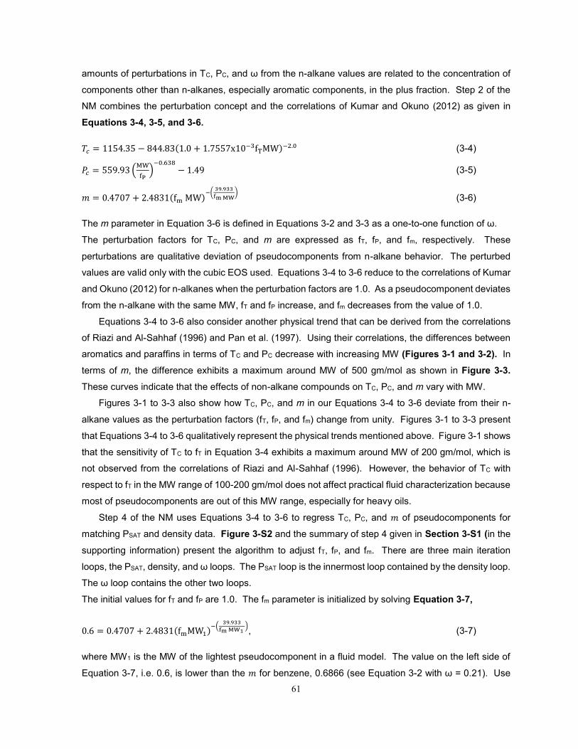
61
amounts of perturbations in TC, PC, and ω from the n-alkane values are related to the concentration of
components other than n-alkanes, especially aromatic components, in the plus fraction. Step 2 of the
NM combines the perturbation concept and the correlations of Kumar and Okuno (2012) as given in
Equations 3-4, 3-5, and 3-6.
𝑇𝑐 = 1154.35 − 844.83(1.0 + 1.7557x10⁻³fTMW)−2.0 (3-4)
𝑃𝑐 = 559.93 (MW
fP)
−0.638
− 1.49 (3-5)
𝑚 = 0.4707 + 2.4831(fm MW)−(
39.933
fm MW) (3-6)
The m parameter in Equation 3-6 is defined in Equations 3-2 and 3-3 as a one-to-one function of ω.
The perturbation factors for TC, PC, and m are expressed as fT, fP, and fm, respectively. These
perturbations are qualitative deviation of pseudocomponents from n-alkane behavior. The perturbed
values are valid only with the cubic EOS used. Equations 3-4 to 3-6 reduce to the correlations of Kumar
and Okuno (2012) for n-alkanes when the perturbation factors are 1.0. As a pseudocomponent deviates
from the n-alkane with the same MW, fT and fP increase, and fm decreases from the value of 1.0.
Equations 3-4 to 3-6 also consider another physical trend that can be derived from the correlations
of Riazi and Al-Sahhaf (1996) and Pan et al. (1997). Using their correlations, the differences between
aromatics and paraffins in terms of TC and PC decrease with increasing MW (Figures 3-1 and 3-2). In
terms of m, the difference exhibits a maximum around MW of 500 gm/mol as shown in Figure 3-3.
These curves indicate that the effects of non-alkane compounds on TC, PC, and m vary with MW.
Figures 3-1 to 3-3 also show how TC, PC, and m in our Equations 3-4 to 3-6 deviate from their n-
alkane values as the perturbation factors (fT, fP, and fm) change from unity. Figures 3-1 to 3-3 present
that Equations 3-4 to 3-6 qualitatively represent the physical trends mentioned above. Figure 3-1 shows
that the sensitivity of TC to fT in Equation 3-4 exhibits a maximum around MW of 200 gm/mol, which is
not observed from the correlations of Riazi and Al-Sahhaf (1996). However, the behavior of TC with
respect to fT in the MW range of 100-200 gm/mol does not affect practical fluid characterization because
most of pseudocomponents are out of this MW range, especially for heavy oils.
Step 4 of the NM uses Equations 3-4 to 3-6 to regress TC, PC, and 𝑚 of pseudocomponents for
matching PSAT and density data. Figure 3-S2 and the summary of step 4 given in Section 3-S1 (in the
supporting information) present the algorithm to adjust fT, fP, and fm. There are three main iteration
loops, the PSAT, density, and ω loops. The PSAT loop is the innermost loop contained by the density loop.
The ω loop contains the other two loops.
The initial values for fT and fP are 1.0. The fm parameter is initialized by solving Equation 3-7,
0.6 = 0.4707 + 2.4831(fmMW1)−(
39.933
fm MW1 ), (3-7)
where MW1 is the MW of the lightest pseudocomponent in a fluid model. The value on the left side of
Equation 3-7, i.e. 0.6, is lower than the 𝑚 for benzene, 0.6866 (see Equation 3-2 with ω = 0.21). Use

62
of Equation 3-7 assumes all pseudocomponents are heavier than C6. The value 0.6 can be unduly low
if MW1 is much greater than the MW of benzene. However, this value is recommended for robustness.
In the PSAT loop, fP is adjusted by ∆fP (e.g., +10-6) per iteration to match the PSAT by decreasing the
ψ function (Equation 3-8). Once the ψ function becomes smaller than a tolerance (e.g., 10-4), the
density loop decreases the δ function (Equation 3-9) by adjusting fT and fP. In the density loop, fP is set
to 1.0 at the beginning of each iteration, and fT is adjusted by ∆fT (e.g., +10-5) per iteration. If the fT
exceeds 3.5 or the δ function at the current iteration is greater than that at the previous iteration, then
the algorithm moves to the ω loop. The fT value can be greater than the upper bound of 3.5 when MW1
is much greater than the MW of benzene in Equation 3-7. The accuracy of density predictions is less
than 1% in AAD for all the oils tested in the next section.
𝜓 =abs(Experimental PSAT − Calculated PSAT)∗100
Experimental PSAT (3-8)
δ = ∑1
𝑘[
abs(Experimental Density−Calculated Density)∗100
Experimental Density]
𝑖
𝑘𝑖=1 (3-9)
The ω loop is to satisfy the internal consistency of TC, PC, and ω; i.e., the definition of ω given by Pitzer
(1955) and Pitzer et al. (1955) and in Equation 3-10. Equations 3-11 and 3-12 are used to back
calculate ω from the current m for each pseudocomponent. These ω values are then used in Equation
3-10 to obtain saturation pressures for pseudocomponents (PSATI) at 0.7TC.
(PSAT)at Tr=0.7 = 10−(1+)PC (3-10)
𝑚 = 0.37464 + 1.54226 − 0.269922 for ≤ 0.3984 (3-11)
𝑚 = 0.379642 + 1.48503 − 0.1644232 + 0.016666ω3 for ≥ 0.3984 (3-12)
Use of the PR EOS with the current TC, PC, and ω yields another saturation pressure at 0.7TC (PSATII)
for each pseudocomponent. The average absolute deviation ε for PSATI and PSATII for all
pseudocomponents is then calculated using Equation 3-13
ε =1
𝑛∑ Abs(PSATI − PSATII)
𝑛𝑖=1 , (3-13)
where n is the number of pseudocomponents. If fT is greater than 3.5 or the ε function at the current
iteration is smaller than that at the previous iteration, fm is increased by ∆fm (e.g., +10-3) to continue on
the ω loop. For each ω iteration, fT and fP start with 1.0. The final values for fT, fP, and fm are determined
when the ε function becomes greater than that at the previous iteration. The final set of fT, fP, and fm
gives the first minimum of the ε function encountered in the calculation.
In the regression algorithm, the initial value is 1.0 for fT and fP, corresponding to the n-alkane values
in Kumar and Okuno (2012). The search direction for fT and fP is the increasing direction from their initial
values because pseudocomponents’ TC and PC should be higher than n-alkane’s value for a given MW.
Therefore, ∆fT and ∆fP are positive to be physically justified. We set a lower bound for fm in Equation 3-
63
7, which is used as the initial fm value. Thus, ∆fm should also be positive. If the converged fm is smaller
than 1.0, it is consistent with the ω perturbation concept that pseudocomponents’ ω should be lower
than n-alkane’s value for a given MW.
The regression algorithm in the NM provides a unique set of TC, PC, and 𝑚 unlike the CM, where
the resulting TC, PC, and m depend on the selection of adjustment parameters and adjustment amounts
for them. Our regression algorithm can work with fewer adjustment parameters, compared to the CM,
because of the physical observations incorporated in its development.
Equations 3-11 and 3-12 are different from Equations 3-2 and 3-3 in terms of their ranges.
Equations 3-2 and 3-3 give the same value for 𝑚 at = 0.39839, but not at the boundary = 0.49. The
value of 0.39839 falls in the range 0.20-0.49 that is recommended for both Equations 3-2 and 3-3 by
Peng and Robinson (1978). Therefore, the value of 0.3984 is chosen as the boundary value for
Equations 3-11 and 3-12.
In general, the PR EOS overpredicts the molar volume for hydrocarbons heavier than heptane
(Søreide 1989). The values for the critical parameters must be increased to match densities and vapor
pressures regardless of the hydrocarbon compound type (i.e., P or N or A). Also, the density of an
aromatic hydrocarbon is higher than that of n-alkane for a given MW. Although the correlations used
for n-alkanes do not represent physical critical points, the search directions described above are still
valid as will be demonstrated in the next section.
The NM developed in this section uses the PR EOS. However, it can also be used with other cubic
EOSs if a new set of critical parameters is developed for the selected cubic EOS as Kumar and Okuno
(2012) did for the PR EOS. The regression algorithm assumes that densities, viscosities, and PSAT data
are the only PVT data used in characterization. More adjustment parameters may be used when more
PVT data are available, especially at different composition conditions. The regression algorithm can be
extended for such a case by using molar distribution parameters as variables and creating additional
loops. For example, the chi-squared distribution has two parameters, which influence mole fractions
and MWs of pseudocomponents. These adjustment parameters will be effective especially for heavy
oils, considering the importance of molar distributions of pseudocomponents in EOS calculations. BIPs
for pseudocomponent/non-hydrocarbon (e.g., CO2) pairs can significantly affect phase behavior
calculations. We, however, recommend that the regression step should minimize the number of
adjustment parameters to avoid physically absurd adjustment of parameters.
3.4. Characterization of Reservoir Oils Using the New Method
In this section, the NM is applied to 22 different reservoir oils ranging from 9.5˚API to 60.18˚API. The
oils are actual reservoir oils, for which data are available in the literature as shown in Table 3-1. The
number of pseudocomponents is fixed to be four for the 22 oils. Mole fractions and MWs of
pseudocomponents for oils 1-13 and 18-20 are taken directly from the corresponding references, which
are based on the chi-squared distribution. PSAT and reservoir temperature data are available in the

64
references as numerical values for the 22 oils. Many of the density data used have been obtained by
digitizing density plots in the references. The number of density data points used is given for each oil
in Table 3-1.
Figure 3-4 shows how the ε function varies with fm for oils 5, 6, and 9. Step 4 of the NM converges
to the final set of fT, fP, and fm (and corresponding TC, PC, and m) at a minimum ε value for each oil. The
same behavior of fm occurs for the other oils studied in this research.
Table 3-1 lists the converged fT, fP, and fm values for the 22 oils studied. Figures 3-5, 3-6, and 3-7 show
the relationship between the API gravity and the converged fT, fP, and fm values, respectively. For all
the oils, the converged fT and fP values are greater than 1.0, and the converged fm values are smaller
than 1.0. These results indicate that the regression algorithm successfully found the solutions that are
consistent with the perturbation concept described in the previous section.
Figures 3-5 to 3-7 also show a trend that fT, fP, and fm are converging toward 1.0 as the API gravity
becomes larger. This is likely because the paraffinic portion of the PNA distribution for a lighter oil is
greater than that for a heavier oil. The PNA distribution of a heavy oil in general can deviate significantly
from the reference distribution of 100% n-alkanes because a heavier CN group allows for a wider variety
of compounds in it.
Unlike manual adjustments performed in the CM, the regression process in the NM can be easily
codified for automation and takes only 1-3 minutes per oil using our code written in FORTRAN on the
Intel Core i7-960 processor at 3.20 GHz and 8.0 GB RAM. The algorithm presented is based on the
exhaustive search method of optimization for robustness. More rapid convergence would be achieved
if a gradient method is used with initial guesses for fT, fP, and fm based on the previous iteration steps.
3.5. Comparison Between the New and Conventional Methods
We now make comparisons between the NM and CM in terms of various types of phase behavior
predictions in P-T-x space for the oils in Table 3-1. PVT data for heavy oils are scarce as described in
the introduction section and in the literature (Kokal and Sayegh 1993; Yazdani and Maini 2010). Data
types used in this research are oil compositions; oil PSAT at reservoir temperatures, and liquid densities
and viscosities at different pressures at reservoir temperatures. Other than these measured data,
pseudo data (Merrill and Newley 1993) were generated using the CMw/oV with 30 components (see
Figure 3-S1 in the supporting information) because a complete set of data suitable for comparisons in a
wide P-T-x range is not available for heavy oils. The 30 components consist of N2, CO2, C1, C2, C3, C4,
C5, C6, and 22 pseudocomponents for the C7+ fraction.
Fluid characterization using a cubic EOS can result in deviation between predictions and data for a
few fundamental reasons; (1) the functional form of the EOS used, (2) the characterization of the
attraction (“a”) and covolume (“b”) parameters based on critical parameters, (3) the critical parameters
used, and (4) the number of components used. The focus of the comparisons in this section is on items
(3) and (4). Thus, the comparisons are made among different fluid models that have different critical
65
parameters and numbers of components for the PR EOS (i.e., for a fixed cubic EOS and a
characterization method for a and b).
If the number of components in the fluid of interest was known and used in the fluid model, there
should be no errors caused solely by reduction in composition space. We have conducted a sensitivity
analysis for the effects of the number of components used on phase behavior predictions (Figures 3-8
and 3-9). The results indicate that use of 22 pseudocomponents is appropriate for generating pseudo
data in this research. The differences in predictions are diminishing as the number of
pseudocomponents used becomes more than 16. This result is consistent with other papers in the
literature (Lolley and Richardson 1997; Egwuenu et al. 2008; Pedersen et al. 1985). Also, the CMw/oV
method used for generating pseudo data follows the method of Pedersen et al. (Pedersen et al. 1989,
1992, 2004). It has been found that this method generally has a high predictive capability (Zuo and
Zhang 2000) when properly used (see Figure 3-S1 in the supporting information).
Given the above, the pseudo data generated can be interpreted as phase behavior data for a PR
fluid, a fluid that behaves as described by the PR EOS. Global phase diagrams of binary (Mushrif 2004;
Yang 2004; Mushrif and Phoenix 2008) and ternary (Gauter 1999, Gauter et al. 1999) mixtures have
been successfully represented using the PR EOS. Their results show that the PR EOS is capable of
predicting at least qualitatively accurate phase behavior for reservoir fluids. When experimental data
are not available or measurable, use of synthetic or pseudo data has been recommended for developing
thermodynamic fluid models (Satyro et al. 2013). In the present research, the validation of the NM is
made against pseudo data for PR fluids. We believe this is a reasonable approach in the absence of
reliable experimental data other than oil compositions, densities, saturation pressures, and viscosities.
There is also an important benefit using the pseudo data. Meaningful comparisons in any conditions in
P-T-x space, particularly along the composition path for a given displacement at a given dispersion level,
may be possible only with the pseudo data.
Separately from the 30-component models created for pseudo data, two fluid models are created
for each oil using the NM and CMwV with 11 components (see Figures 3-S1 and 3-S2 in the supporting
information for the CMwV and NM algorithms, respectively). The 11 components consist of N2, CO2, C1,
C2, C3, C4-5, C6, and four pseudocomponents for the C7+ fraction.
BIPs are not adjustment parameters in this research. Fixed BIP values are used for the 22 oils.
BIPs are zero for hydrocarbon-hydrocarbon pairs. Non-zero values are used for non-hydrocarbon-
hydrocarbon and non-hydrocarbon-non-hydrocarbon pairs; i.e., N2-hydrocarbons, CO2-hydrocarbons,
and N2-CO2.
We adjust no BIPs, and set BIPs of hydrocarbon-hydrocarbon pairs to zero for the following reasons:
(1) The number of regression parameters should be minimized (Wang and Pope 2001; Egwuenu et al.
2008). Use of BIPs as regression parameters can damage the predictive capability of the resulting
fluid model (Wang and Pope 2001).
66
(2) Non-zero BIPs for hydrocarbon-hydrocarbon pairs may lead to non-physical liquid-phase split
(Pedersen et al. 1988).
(3) Use of zero BIPs can improve computational efficiency (Egwuenu et al. 2008; Michelsen 1986). It
has also been shown that fluid properties can be better predicted when most of BIPs are set to zero
(Pedersen and Christensen 2007).
(4) Use of negative BIPs, which may occur after regression, can cause non-convergence in successive
substitution for flash calculations (Heidemann and Michelsen 1995).
The BIPs for N2-hydrocarbons, CO2-hydrocarbons, and N2-CO2 are fixed to be some non-zero
values. The CM uses the default values from PVTsim as they would be the most suitable values for
PVTsim. They are -0.017 for N2-CO2, 0.0311 for N2-C1, 0.0515 for N2-C2, 0.0852 for N2-C3, 0.08 for N2-
C4, 0.1 for N2-C5, 0.08 for N2-Ci, where i ≥ 6, 0.12 for CO2,-Cj, where 1 ≤ j ≤ 6, and 0.1 for CO2-
pseudocomponents. These BIPs in the NM are based on Peng and Robinson (1976, 1978), who
properly considered effects of hydrocarbon types on BIPs for the PR EOS. They recommended 0.1 for
N2-paraffins and N2-napthenes, 0.18 for N2-aromatics, and 0.1 for CO2-hydrocarbons. Since
pseudocomponents are mixtures of PNA compounds, we use the average values in the NM, which is
[0.1 + 0.1 + 0.18] / 3 = 0.12666 ≈ 0.13 for N2-pseudocomponents, and 0.1 for CO2-pseudocomponents.
The NM uses 0.0 for N2-CO2, 0.1 for N2-Ci, where 1 ≤ i ≤ 6, 0.13 for N2-pseudocomponents, and 0.1 for
CO2-hydrocarbons.
In the following subsections, phase behavior predictions based on the NM and CMwV are compared
with the pseudo data. Tables 3-S1, 3-S2, 3-S3, and 3-S4 (in the supporting information) give the
resulting fluid models for oil 3 (13.38˚API) and oil 6 (24.25˚API) using the NM and CMwV. These models
are used in many of the comparisons presented below.
3.5.1. P-T Predictions
We first present the comparisons in terms of P-T predictions. Heavy-oil/solvent mixtures often exhibit
three hydrocarbon-phases near the vapor pressures of the solvent components. The three phases
consist of the gaseous (V), oleic (L1), and solvent-rich liquid (L2) phases (e.g., Mohanty et al. 1995;
Polishuk et al. 2004). Figures 3-10 and 3-11 show the 2-phase and 3-phase envelopes for a mixture
of 10% oil 6 and 90% C2. The CMwV gives the V-L1 and V-L1-L2 regions that are much smaller than
those predicted by the NM. The NM predictions are in good agreement with the pseudo data points.
The NM predictions are more accurate for lower temperatures. The three-phase envelope predicted by
the NM almost coincides with data.
The deviation of the CMwV predictions from the pseudo data is more significant for a mixture of 10%
oil 6 and 90% C3. Figure 3-12 shows that the CMwV results in an erroneous two-phase envelope for
this mixture. The NM correctly generates the phase behavior predictions. Figure 3-13 shows that the
NM predicts a three-phase envelope that is close to the data points. The three-phase behavior predicted
by the CMwV occurs in a much smaller P-T region apart from the correct three-phase region based on
the pseudo data and the NM.

67
The accuracy of the NM for L1-L2-V phase behavior is remarkable considering that the complex
phase behavior characteristic of highly asymmetric hydrocarbon mixtures is predicted using only four
pseudocomponents for the C7+ fraction. The reduced dimensionality in composition space does not
damage phase behavior predictions using the NM.
3.5.2. P-x Predictions A P-x prediction presents a cross section of isothermal phase behavior between two compositions. This
subsection shows P-x predictions for the oil-6/C1, oil-6/C2, and oil-6/CO2 pairs at the oil-6 reservoir
temperature 333.15 K. Figure 3-14 shows the P-x predictions along with pseudo data for the oil-6/C1
pair. The NM and CMwV are accurate at low mixing ratios of C1. This is because the 11-component
models are fitted to PSAT at the reservoir temperature at the oil composition. As the mixture composition
goes away from the oil composition, the CMwV predictions deviate from the pseudo data. The NM
accurately predicts the bubble-point pressures along the mixing line.
The advantage of the NM over the CMwV becomes more significant for P-x predictions for the oil-
6/C2 pair as shown in Fig. 15. At the C2 mixing ratio of 90%, the CMwV predicts a bubble point at 137.44
bars, which is approximately 39 bars lower than the pseudo data and the prediction by the NM.
Mixtures of CO2 and reservoir oil often exhibit continuous transition between L1-V and L1-L2 phase
equilibria (Okuno et al. 2011) at low temperatures. Figure 3-16 presents such phase behavior for oil 6
and CO2 at 333.15 K. The NM accurately predicts the upper boundary of the two-phase region in P-x
space. The CMwV erroneously gives a smaller region for the immiscible two liquid phases.
Figure 3-17 shows saturated liquid densities predicted along the mixing line between oil 6 and the
equimolar C1-C2 mixture at 333.15 K. The density at the oil composition was used to create the EOS
fluid models. Therefore, the CMwV and NM are both accurate at lower mixing ratios of the solvent. As
the mixture composition goes away from the oil composition, however, the CMwV predictions deviate
from the NM predictions and the pseudo data. The results indicate that the fluid models based on the
CMwV cannot accurately represent phase equilibrium and volumetric properties at compositions away
from the oil composition.
3.5.3. T-x Predictions
A T-x diagram presents another important cross section of phase behavior, particularly when coinjection
of solvent and steam is considered for heavy-oil recovery. Figure 3-18 shows T-x predictions for oil-
3/C6 mixtures at 34.47 bars. The CMwV overpredicts saturation temperatures except for low C6 mixing
ratios, while the NM accurately predicts them along the mixing line. If the fluid model based on the
CMwV is used in reservoir simulation of solvent/steam coinjection, propagation of the solvent in the
reservoir can be significantly underestimated, resulting in erroneous reservoir performance forecasts.
The overprediction of saturation temperatures by the CMwV becomes more significant for higher
pressures. Figure 3-19 shows T-x predictions at 60.00 bars. The NM still predicts accurately the
saturation temperatures at all mixing ratios tested. However, the CMwV predicts much higher saturation
temperatures even at low C6 mixing ratios. The deviation at the C6 mixing ratio of 0.3 is 139 K. At C6
68
mixing ratios higher than 0.3, there are no saturation temperatures predicted by CMwV because the
cricondenbar becomes lower than 60.00 bars as can be seen in Figure 3-20.
3.5.4. Thermodynamic Minimum Miscibility Pressure (MMP) Calculation
The thermodynamic MMP is the minimum displacement pressure at which complete miscibility is
developed along the composition path from the injectant to the reservoir oil for one-dimensional flow in
the absence of dispersion (John and Orr 1996). The thermodynamic MMP is a widely used parameter
for design of solvent injection. In this subsection, the thermodynamic MMPs are calculated for 18 oils
in Table 3-1 at their reservoir temperatures. Two different injectants are considered; pure C1 and pure
CO2. For the C1 cases, the MMP calculations are performed based on the method of characteristics
using PVTsim. For the CO2 cases, the mixing-cell method within PennPVT (Ahmadi and John 2011;
PennPVT) is used. MMP calculations are not shown for oils 1, 2, 4, and 18 because three phases are
present during the MMP calculations using the EOS fluid models for these oils based on the CMw/oV
with 30 components.
Figure 3-21 compares the MMPs based on the NM with the pseudo data for 18 oils with C1.
Although the C1-MMPs presented are calculated at different temperatures, the plots show that the
calculated C1-MMPs are higher for heavier oils. The accuracy of the MMPs observed for the wide variety
of oils indicates that the NM successfully retains compositional phase behavior using only four
pseudocomponents for the C7+ fraction. Figure 3-22 shows that the C1-MMPs predicted based on the
CMwV are lower than the pseudo data. The deviation is more significant for heavier oils. The maximum
deviation of the C1-MMPs is 5.3% for the NM, but it is 34% for the CMwV. Figures 3-23 and 3-24 show
the comparisons of the NM with the CMwV in terms of the CO2-MMP. The maximum deviations of the
CO2-MMPs are 6.1% and 62% for the NM and the CMwV, respectively.
Figures 3-20 and 3-22 indicate that compositional phase behavior predictions are more erroneous
for heavier oils using the CMwV. This is because the CMwV uses density corrections through volume-
shift parameters. A larger amount of volume correction is required and performed for heavier oils in the
CMwV as shown in Tables 3-S2 and 3-S4 in the supporting information (see also the Issues of the
Conventional Method subsection). However, the thermodynamic MMP considered here is a parameter
representing primarily compositional phase behavior, instead of volumetric phase behavior, of the fluid
system considered. Therefore, the separation of volumetric from compositional phase behavior
predictions causes errors in MMP predictions.
3.5.5. 1-D Displacement Simulation Case Study
Solvent injection for heavy-oil recovery is typically conducted under partially miscible conditions. In such
displacements, the oil recovery history depends on how components propagate with the throughput of
injectant. Fluid characterization can significantly affect oil recovery predictions because interaction of
phase behavior and fluid flow determines components’ propagation in a reservoir. This simulation case
study aims to compare predictions of components’ propagation using the NM and CM.
69
We present 1-D isothermal displacement of oil 6 with the equimolar C1/C2 mixture under partially
miscible conditions. The MMP calculated for this case is 412.23 bars using the CMw/oV with 30
components. Using 11 components, it is 413.34 bars and 327.23 bars based on the NM and the CMwV,
respectively (see Tables 3-S3 and 3-S4 in the supporting information for the fluid models). Input data
for the simulations using the GEM simulator of Computer Modelling Group (CMG 2011) are given in
Table 3-2. Figures 3-25 and 3-26 present predictions of density and viscosity using the NM, CMwV
and CMw/oV along with experimental data. Viscosity was matched using PVTsim by adjusting only VC
of pseudocomponents using the LBC method (Lohrenz et al. 1964). The injection and production
pressures are fixed at 203.45 bars and 200 bars, respectively. The small pressure difference is used to
make pressure variation in the reservoir small. Simulation results based on the CMw/oV with 30
components are used as pseudo data. Simulation results based on the NM and CMwV are then
compared.
Figure 3-27 shows oil recovery predictions compared to the pseudo data. The recovery curves for
0.0-0.3 hydrocarbon pore-volumes injected (HCPVI) are not shown because they nearly coincide. Oil
recovery based on the NM is almost identical to the pseudo data. However, the CMwV results in oil
recovery simulation that is significantly overpredicted by approximately 8%. The overprediction is
consistent with other comparisons made in previous subsections, where the fluid models based on the
CMwV exhibit more miscibility in their phase diagrams and MMP calculations. To see the effect of
numerical dispersion on oil recovery simulation, the number of gridblocks is decreased from 250 to 50.
Figure 3-23 shows the same advantage of the NM over the CMwV under more dispersive conditions
(The previous subsection showed comparisons for the dispersion-free case). The number of gridblocks
is fixed to be 250 for further comparisons.
The different oil recovery histories are predicted because the NM and CMwV predict different
saturation profiles as shown in Figure 3-28. Figure 3-29 shows that the C1 fronts based on the NM and
CMwV deviate from each other, resulting in different predictions of gas breakthrough as can be seen in
Figure 3-23. Figure 3-24 also indicates the CMwV erroneously predicts faster propagation of heavy
components. Since the deviation of the CMwV shown in Figure 3-24 increases with the injectant
throughput, the simulation based on the CMwV becomes more erroneous later.
3.6. Conclusions
We developed a new method for fluid characterization using the PR EOS with the van der Waals mixing
rules. The method characterizes reservoir fluids using perturbations of TC, PC, and ω from n-alkane
values. TC, PC, and ω for n-alkanes used are based on our previous research, which are optimized for
the PR EOS for predictions of vapor pressures and liquid densities without volume shift. The optimized
reference values allow for robust regression using three perturbation factors fT, fP, and fm for TC, PC, and
ω, respectively. In our regression, Pitzer’s definition of ω is properly satisfied for each component. The
new characterization method was applied to 22 different reservoir oils. Comparisons were made
between the new and conventional characterization methods in terms of predictions of various phase

70
diagrams, thermodynamic minimum miscibility pressures (MMPs), and 1-D oil displacement. The
conclusions are as follows:
o The new method (NM) exhibits significant insensitivity of phase behavior predictions to the number
of components used for a plus fraction. Two- and three-phase behavior predictions in P-T-x space
using the NM with 11 components are almost identical to those using the conventional method
without volume shift (CMw/oV) with 30 components.
o The reliability of the NM is also observed for MMP calculations and 1-D oil displacement simulations.
Oil displacement predictions based on the NM with 11 components are nearly identical to those
based on the CMw/oV with 30 components. This is true even at different dispersion levels tested.
Results indicate that the NM can reduce the dimensionality of composition space while keeping
accurate phase behavior predictions along composition paths at different dispersion levels.
o The NM does not require volume-shift parameters to accurately predict compositional and
volumetric phase behaviors. The conventional method with volume shift (CMwV) separates
volumetric phase behavior predictions from compositional phase behavior predictions. This
separation should be carefully used especially for heavy-oil characterization. Our results show that
the CMwV with 11 components yields erroneous phase behavior predictions, which typically show
significantly smaller two- and three-phase regions in P-T-x space. The advantage of the NM over
the CMwV in phase behavior predictions is more significant for P-T-x conditions away from those
used for parameter regression.
o The new regression algorithm developed searches for an optimum set of TC, PC, and ω for
pseudocomponents using physically justified search directions starting from the well-defined initial
values. Unlike in the CM, robust convergence of TC, PC, and ω does not require step-wise manual
adjustments of parameters. The automatic regression process in the NM took only a few minutes
per oil for the 22 oils characterized.
o The perturbation factors fT, fP, and fm developed in this research are unity for n-alkanes. The
perturbation factors capture physical trends that can be derived from the literature; e.g., for a given
molecular weight, TC and PC are lower and ω is larger for paraffins compared to other types of
hydrocarbon compounds. For the 22 oils characterized in this research, the converged fT and fP
values are all greater than 1.0, and the converged fm values are all smaller than 1.0. Deviations of
fT, fP, and fm from unity can be physically interpreted as deviations of the plus fractions from n-alkane
mixtures.
o The NM requires no changes in the current compositional simulation formulation because it uses
the PR EOS with the van der Waals mixing rules.

71
3.7. Nomenclature
Roman Symbols
a = Attraction parameter in a cubic equation of state
A = Aromatic
Amix = Attraction parameter for a mixture in a cubic equation of state
b = Covolume parameter in a cubic equation of state
Bmix = Covoulme parameter for a mixture in a cubic equation of state
CPEN = Peneloux volume-shift parameter
m = Parameter in the Peng–Robinson EOS (1978) defined in Equation 3-2 and 3-3
D = Dimension
fm = Perturbation factor for the m parameter
fP = Perturbation factor for critical pressure
fT = Perturbation factor for critical temperature
∆fm = Step size for fm
∆fP = Step size for fP
∆fT = Step size for fT
mA = Acentric factor for aromatics
k = Number of density data
mP = Acentric factor for paraffins
n = Number of pseudocomponents
N = Napthenes
p = Pressure, bar
P = Paraffins
PC = Critical pressure, bar
PCA = Critical pressure of aromatics, bar
PCP = Critical pressure of paraffins, bar
R = Universal gas constant
T = Temperature, K
TC = Critical temperature, K
TCA = Critical temperature of aromatics, K
TCP = Critical temperature of paraffins, K
TOL = Tolerance
𝑣 = Molar volume, gm/mol
VC = Critical volume, gm/mol
Abbreviations
oAPI = API (American Petroleum Institute) gravity

72
Greek symbols
𝛿 = Average absolute deviation for density given by Equation 3-9
휀 = Average absolute deviation for saturation pressure given by Equation 3-13
Ω𝑎 = Constant term in the attraction parameter of a cubic EOS
Ω𝑏 = Constant term in the covolume parameter of a cubic EOS
𝜓 = Absolute % deviation given by Equation 3-8
ω = Acentric factor
BIP = Binary interaction parameter
CM = Conventional (characterization) method
CMwV = Conventional (characterization) method using volume shift
CMw/oV = Conventional (characterization) method without using volume shift
CN = Carbon number
EOR = Enhanced oil recovery
EOS = Equation of state
HCPVI = Hydrocarbon pore-volume injected
MMP = Minimum miscibility pressure, bar
MW = Molecular weight, gm/mol
NM = New (characterization) method
PC = Pseudocomponent
PNA = Paraffin-napthene-aromatic
PR = Peng-Robinson
P-T-x = Pressure-temperature-composition
SRK = Soave-Redlich-Kwong

73
3.8. References
Ahmadi, K. and Johns, R.T. 2011. Multiple Mixing-Cell Model for MMP Determination. SPE J. 16 (4):
733-742.
Ambrose, D. and Tsonopoulos, C. 1995. Vapor-Liquid Critical Properties of Elements and Compounds.
2. Normal Alkanes. J. Chem. Eng. Data 40 (3): 531-546.
Cavett, R.H. 1962. Physical Data for Distillation Calculations, Vapor-Liquid Equilibria. Proc. Am. Pet.
Inst. Div. Refining. 42 (3): 351-357.
Christensen, P.L. 1999. Regression to Experimental PVT Data. J Can Petro Technol 38 (13): 1-9.
CMG, Computer Modeling Group, Calgary, Canada, 2011.
Coats, K.H. and Smart, G.T. 1986. Application of a Regression Based EOS PVT Program to Laboratory
Data. SPE Res Eng 1 (3): 277-299.
Cullick, A.S., Pebdani, F.N., and Griewank, A.K. 1989. Modified Corresponding States Method for
Predicting Densities of Petroleum Reservoir Fluids. Ind. Eng. Chem. Res. 28 (3): 340-347.
DeRuiter, R.A., Nash, L.J., and Singletary, M.S. 1994. Solubility and Displacement Behavior of a
Viscous Crude With CO2 and Hydrocarbon Gases. SPE Res Eng 9 (2): 101-106.
Edmister, W.C. 1958. Applied Hydrocarbon Thermodynamics, Part 4: Compressibility Factors and
Equations of State. Pet. Refiner. 37: 173-179.
Egwuenu, A.M., Johns, R.T., and Li, Y. 2008. Improved Fluid Characterization for Miscible Gas Floods.
SPE Res Eval Eng 11 (4): 655-665.
Gates, I.D. and Chakrabarty, N. 2008. Design of the Steam and Solvent Injection Strategy in Expanding
Solvent Steam-Assisted Gravity Drainage. J Can Pet Technol 47 (9): 12-20.
Gauter, K. 1999. Fluid Multiphase Behavior in Ternary Systems of Near-Critical CO2. PhD dissertation,
the Technical University of Berlin, Berlin, Germany.
Gauter, K., Heidemann, R.A., and Peters, C.J. 1999. Modeling of Fluid Multiphase Equilibria in Ternary
Systems of Carbon Dioxide as the Near-Critical Solvent and Two Low-Volatile Solutes. Fluid Phase
Equilib. 158-160: 133-141.
Ghasemi, M., Alavian, S.A., and Whitson, C.H. 2011. C7+ Characterization of Heavy Oil Based on
Crude Assay Data. Presented at SPE Heavy Oil Conference and Exhibition held in Kuwait City,
Kuwait, 12-24 Dec. SPE 148906-MS.
Gupta, S., Gittins, S., and Picherack, P. 2003. Insights into Some Key Issues with Solvent Aided
Process. J Can Pet Technol 43 (2): 54-61.
Heidemann, R.A. and Michelsen, M.L. 1995. Instability of Successive Substitution. Ind. Eng. Chem.
Res. 34 (3): 958-966.
Hornbrook, M.W., Dehghani, K., Qadeer, S. et al. 1991. Effects of CO2 Addition to Steam on Recovery
of West Sak Crude Oil. SPE Res Eng 6 (3): 278-286.
Jhaveri, B.S. and Youngren, G.K. 1988. Three-Parameter Modification of the Peng-Robinson Equation
of State to Improve Volumetric Predictions. SPE J. 3 (3): 1033-1040.

74
Jørgensen, M. and Stenby, E.H. 1995. Optimization of Pseudo-components Selection for Compositional
Studies of Reservoir Fluids. Presented at the Annual Technical Conference and Exhibition, Dallas,
Texas, 22-25 Oct. SPE-30789-MS
Johns, R.T. and Orr, Jr. F.M. 1996. Miscible Gas Displacement of Multicomponent Oils. SPE J. 1 (1):
39-50.
Kesler, M.G. and Lee, B.I. 1976. Improve Prediction of Enthalpy of Fractions, Hydrocarbon Processing.
Hydrocarb Process 55 (3): 153-158.
Kokal, S.L. and Sayegh, S.G. 1993. Phase Behavior and Physical Properties of CO2-Saturated Heavy
Oil and its Constitutive Fractions: Experimental Data and Correlations. J. Pet. Sci. Eng. 9 (4): 289-
302.
Korsten, H. 2000. Internally Consistent Prediction of Vapor Pressure and Related Properties. Ind. Eng.
Chem. Res. 39 (3): 813-820.
Krejbjerg, K. and Pedersen, K.S. 2006. Controlling VLLE Equilibrium with a Cubic EoS in Heavy Oil
Modeling. Presented at 57th Annual Technical Meeting of the Petroleum Society (Canadian
International Petroleum Conference), Calgary. 13-15 June. PETSOC-2006-052.
Kumar, A. and Okuno, R. 2012. Fluid Characterization Using an EOS for Compositional Simulation of
Enhanced Heavy-Oil Recovery. Presented at SPE Annual Technical Conference and Exhibition,
San Antonio, Texas, 8-10 Oct. SPE 159494-MS
Kumar, A. and Okuno, R. 2012. Critical Parameters Optimized for Accurate Phase Behavior Modeling
for Heavy n-Alkanes up to C100 using the Peng-Robinson Equation of State. Fluid Phase Equilib.
335: 46-59.
Lee, B.I. and Kesler, M.G. 1975. A Generalized Thermodynamic Correlation Based on Three- Parameter
Corresponding States. AIChE J. 21 (3): 510-527.
Li, W., Mamora, D.D., and Li. Y. 2011. Solvent-Type and –Ratio Impacts on Solvent-Aided SAGD
Process. SPE Res Eval & Eng 14 (3): 320-331.
Lohrenz, J., Bray, B.G., and Clark, C.R. 1964. Calculating Viscosities of Reservoir Fluids from their
Compositions. J. Pet. Technol. 16 (10): 1171-1176.
Lolley, C.S. and Richardson, W.C. 1997. Compositional Input for Thermal Simulation of Heavy Oils with
Application to the San Ardo Field. Presented at International Thermal Operation & Heavy Oil
Symposium, Bakersfield, California, 10-12 Dec. SPE-37538-MS
Memon, A.I., Gao, J., Taylor, S.D. et al. 2010. A Systematic Workflow Process for Heavy Oil
Characterization: Experimental Techniques and Challenged. Presented at Canadian
Unconventional Resources and International Petroleum Conference, Calgary, Alberta. 19-21 Oct.
SPE-137006-MS
Merrill, R.C. and Newley, T.M.J. 1993. A Systematic Investigation into the Most Suitable Data for the
Development of Equations of State for Petroleum Reservoir Fluids. Fluid Phase Equilib. 82: 101-
110.

75
Michelsen, M.L. 1986. Simplified Flash Calculation for Cubic Equation of State. Ind. Eng. Chem. Proc.
Des. Dev. 25 (1): 184-188.
Mohanty, K.K., Masino, W.H., Ma, T.D. et al. 1995. Role of Three-Hydrocarbon-Phase Flow in a Gas-
Displacement Process. SPE Res Eng 10 (3): 214-221.
Mushrif, S.H. 2004. Determining Equation of State Binary Interaction Parameters Using K- and L-Points.
Master thesis, the University of Saskatchewan, Saskatoon, Canada.
Mushrif, S.H. and Phoenix, A.V. 2008. Effect of Peng-Robinson Binary Interaction Parameters on the
Predicted Multiphase Behavior of Selected Binary Systems. Ind. Eng. Chem. Res. 47 (16): 6280-
6288.
Nasr, T.N., Beaulieu, G., Golbeck, H. et al. 2003. Novel Expanding Solvent-SAGD Process “ES-SAGD”.
J Can Pet Technol 42 (1): 13.
Okuno, R., Johns, R.T., and Sepehrnoori, K. 2011. Mechanisms for High Displacement Efficiency of
Low-Temperature CO2 Floods. SPE J. 16 (4): 751-767.
Okuno, R., Johns, R.T., and Sepehrnoori, K., 2010. Three-Phase Flash in Compositional Simulation
Using a Reduced Method, SPE J. 15 (3): 689-703.
Pan, H., Firoozabadi, A., and Fotland, E. 1997. Pressure and Composition Effect on Wax Precipitation:
Experimental Data and Model Results. SPE Prod & Fac 12 (4): 250-258.
Pedersen, K.S. and Christensen, P. L. 2007. Phase Behavior of Petroleum Reservoir Fluids. CRC
Press, Taylor & Francis Group, Boca Raton, FL, USA.
Pedersen, K.S., Blilie, A.L., and Meisingset, K.K. 1992. Calculations On Petroleum Reservoir Fluids
Using Measured And Estimated Compositional Data for the Plus Fraction. Ind. Eng. Chem. Res.
31 (5): 1378-1384.
Pedersen, K.S., Milter, J., and Sørensen, H. 2004. Cubic Equations of State Applied to HT/HP and
Highly Aromatic Fluids. SPE J. 9 (2): 186-192.
Pedersen, K.S., Thomassen, P., and Fredenslund, Aa. 1989. Characterization of Gas Condensate
Mixtures. Advances in Thermodynamics, Taylor & Francis, New York.
Pedersen, K.S., Thomassen, P., and Fredenslund, Aa. 1983. SRK-EOS Calculation for Crude Oils.
Fluid Phase Equilib. 14: 209-218.
Pedersen, K.S., Thomassen, P., and Fredenslund, Aa. 1984. Thermodynamics of Petroleum Mixtures
Containing Heavy Hydrocarbons. 1. Phase Envelope Calculations by Use of the Soave-Redlich-
Kwong Equation of State. Ind. Eng. Chem. Proc. Des. Dev. 23 (1): 163170.
Pedersen, K.S., Thomassen, P., and Fredenslund, Aa. 1985. Thermodynamics of Petroleum Mixtures
Containing Heavy Hydrocarbons. 3. Efficient Flash Calculation Procedures Using the SRK Equation
of State. Ind. Eng. Proc. Des. Dev. 24 (4): 948-954.
Pedersen, K.S., Thomassen, P., and Fredenslund, Aa. 1988. On the Dangers of Tuning Equation of
State Parameters. Chem. Eng. Sci. 43 (2): 269-278.
76
Peneloux, A., Rauzy, E., and Fréze, R. 1982. A Consistent Correction for Redlich-Kwong-Soave
Volume. Fluid Phase Equilib. 8 (1): 7-23.
Peng, D.-Y. and Robinson, D.B. 1976. A New Two-Constant Equation of State. Ind. Eng. Chem. Fund.
15 (1): 59-64.
Peng, D.-Y. and Robinson, D.B. 1978. The Characterization of the Heptanes and Heavier Fractions for
the GPA Peng-Robinson Programs. GPA Research Report RR-28.
PennPVT Toolkit, Gas Flooding Joint Industrial Project, Director: Dr. Russell T. Johns, EMS Energy
Institute, The Pennsylvania State University, University Park, PA.
Pitzer, K.S. 1955. The Volumetric and Thermodynamic Properties of Fluids. I. Theoretical Basis and
Viral Coefficients. J. Am. Chem. Soc. 77 (13): 3427-3433.
Pitzer, K.S., Lippmann, D.Z., Curl Jr, R.F. et al. 1955. The Volumetric and Thermodynamic Properties
of Fluids. II. Compressibility Factor, Vapor Pressure, and Entropy of Vaporization. J. Am. Chem.
Soc. 77 (13): 3433-3440.
Polishuk, I., Wisniak, J., and Segura, H. 2004. Estimation of Liquid-Liquid-Vapor Equilibria in Binary
Mixtures of n-Alkanes. Ind. Eng. Chem. Res. 43 (18): 5957-5964.
PVTsim 20.0. 2011. Calsep A/S, Lyngby, Denmark.
Quiñones-Cisneros, S.E., Andersen, S.I., and Creek, J. 2005. Density and Viscosity Modeling and
Characterization of Heavy Oils. Energy Fuels 19 (4): 1314-1318.
Quiñones-Cisneros, S.E., Dalberg, A., and Stenby, E.H. 2004b. PVT Characterization and Viscosity
Modeling and Prediction of Crude Oils. Pet. Sci. Technol., 22 (9-10): 1309–1325.
Quiñones-Cisneros, S.E., Zéberg-Mikkelsen, C.K., and Stenby, E.H. 2003. Friction Theory Prediction
of Crude Oil Viscosity at Reservoir Conditions Based on Dead Oil Properties. Fluid Phase Equilib.
212 (1-2): 233–243.
Quiñones-Cisneros, S.E., Zéberg-Mikkelsen, C.K., Baylaucq, A. et al. 2004a. Viscosity Modeling and
Prediction of Reservoir Fluids: From Natural Gas to Heavy Oils. Int. J. Therm. 25 (5): 1353-1366.
Riazi, M.R. and Al-Sahhaf, T.A. 1996. Physical Properties of Heavy Petroleum Fractions and Crude
Oils. Fluid Phase Equilib. 117 (1-2): 217-224.
Riazi, M.R. and Daubert, T.E. 1980. Simplify Property Predictions. Hydrocarb. Process. 59 (3): 115-
116.
Riazi, M.R. and Daubert, T.E. 1987. Characterization Parameters for Petroleum Fractions. Ind. Eng.
Chem. Res. 26 (4): 755-759.
Satyro, M.A., Shaw, J.M., and Yarranton, H.W. 2013. A Practical Method for the Estimation of the Oil
and Water Mutual Solubilities. Fluid Phase Equilib. 355: 12-25.
Soave, G. 1972. Equilibrium Constants from a Modified Redlich-Kwong Equation of State. Chem. Eng.
Sci. 27:1197-1203.
77
Søreide, I. 1989. Improved Phase Behavior Predictions of Petroleum Reservoir Fluids from a Cubic
Equation of State, Ph.D. dissertation, Norwegian University of Science and Technology, Trondheim,
Norway, 1989.
Ting, P.D., Joyce, P.C., Jog, P.K. et al. 2003. Phase Equilibrium Modeling of Mixtures of Long-Chain
and Short-Chain Alkanes Using Peng–Robinson and SAFT. Fluid Phase Equilib. 206 (1-2), 267-
286.
Twu, C.H. 1984. An Internally Consistent Correlation for Predicting the Critical Properties and Molecular
Weights of Petroleum and Coal-Tar Liquids. Fluid Phase Equilib. 16 (2): 137-150.
Voulgaris, M., Stamatakis, S., and Tassios, D. 1991. Prediction of Physical Properties for Non-Polar
Compounds, Petroleum and Coal Liquid Fractions. Fluid Phase Equilib. 64: 73-106.
Voutsas, E.C., Pappa, G.D., Magoulas, K. et al. 2006. Vapor Liquid Equilibrium Modeling of Alkane
Systems with Equations of State: “Simplicity versus Complexity. Fluid Phase Equilib. 240 (2): 127-
139.
Wang, P. and Pope, G.A. 2001. Proper Use of Equations of State for Compositional Reservoir
Simulation. J. Petrol. Tech. 53 (7): 74-81.
Whitson, C.H. 1983. Characterizing Hydrocarbon Plus Fractions. SPE J. 23 (4): 683-694.
Whitson, C.H. and Brulè, M.R. 2000. Phase Behaviour. SPE Henry L. Doherty Series, Vol. 20, SPE,
Richardson, Texas.
Yakoumis, I., Kontogeorgis, G.M., Voutsas, E. et al. 1997. Vapor-Liquid Equilibria for
Alcohol/Hydrocarbon Systems Using the CPA Equation of State. Fluid Phase Equilib. 130 (1-2):
31-47.
Yang, Q. 2004. Automatic Development of Global Phase Diagrams for Binary Systems in Pressure-
Temperature Space. Master thesis, the University of Saskatchewan, Saskatoon, Canada.
Yazdani, A. and Maini, B.B. 2010. Measurements and Modeling of Phase Behaviour and Viscosity of a
Heavy Oil/Butane System. J Can Pet Technol 49 (2): 9-14.
Zabel, F., Law, D.H.-S., Taylor, S. et al. 2010. Impact of Uncertainty of Heavy Oil Fluid Property
Measurements. J Can Pet Technol 49 (3): 28-35.
Zuo, J.Y. and Zhang, D. 2000. Plus Fraction Characterization and PVT Data Regression for Reservoir
Fluids near Critical Conditions. Presented at SPE Asia Pacific Oil and Gas Conference and
Exhibition, Brisbane, Australia, 16-18 Oct. SPE 64520-MS
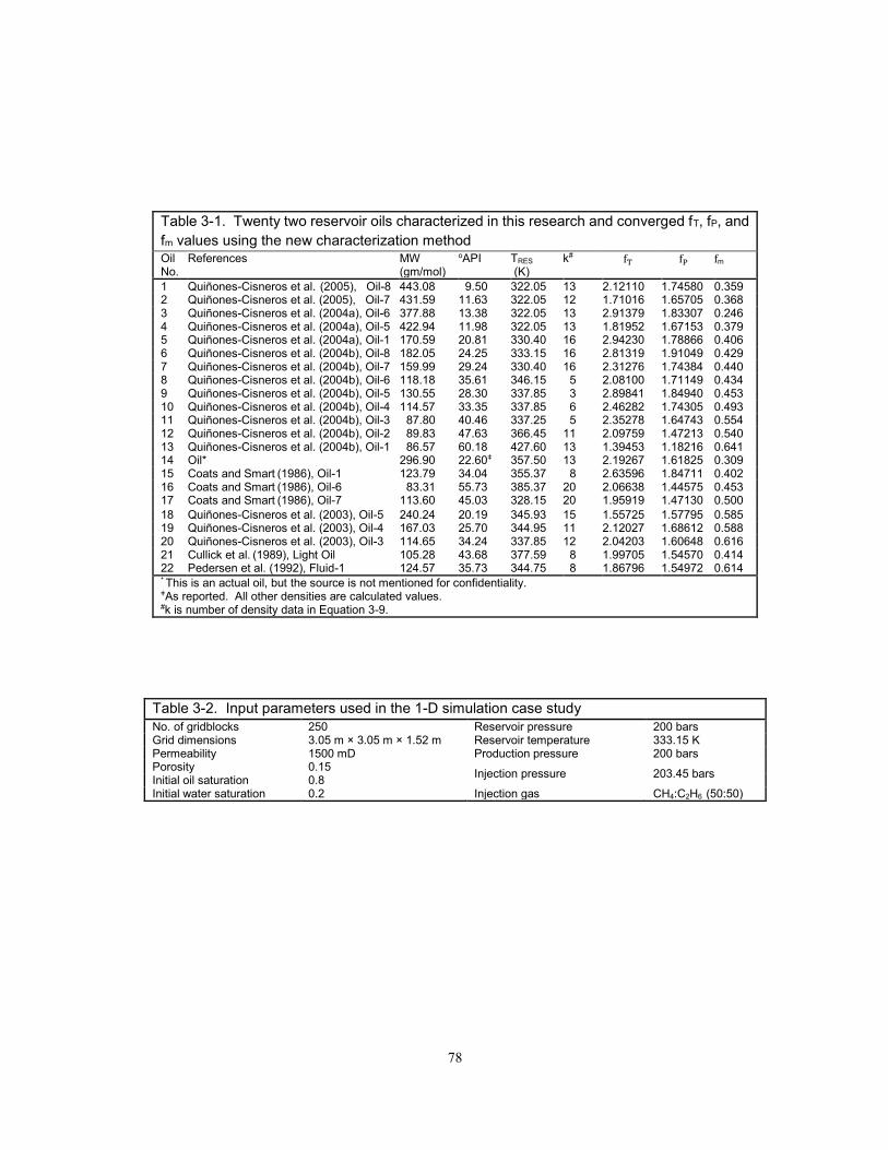
78
Table 3-2. Input parameters used in the 1-D simulation case study
No. of gridblocks 250 Reservoir pressure 200 bars Grid dimensions 3.05 m × 3.05 m × 1.52 m Reservoir temperature 333.15 K Permeability 1500 mD Production pressure 200 bars Porosity 0.15
Injection pressure 203.45 bars Initial oil saturation 0.8 Initial water saturation 0.2 Injection gas CH4:C2H6 (50:50)
Table 3-1. Twenty two reservoir oils characterized in this research and converged fT, fP, and
fm values using the new characterization method Oil No.
References MW (gm/mol)
oAPI TRES (K)
k# fT fP fm
1 Quiñones-Cisneros et al. (2005), Oil-8 443.08 9.50 322.05 13 2.12110 1.74580 0.359 2 Quiñones-Cisneros et al. (2005), Oil-7 431.59 11.63 322.05 12 1.71016 1.65705 0.368 3 Quiñones-Cisneros et al. (2004a), Oil-6 377.88 13.38 322.05 13 2.91379 1.83307 0.246 4 Quiñones-Cisneros et al. (2004a), Oil-5 422.94 11.98 322.05 13 1.81952 1.67153 0.379 5 Quiñones-Cisneros et al. (2004a), Oil-1 170.59 20.81 330.40 16 2.94230 1.78866 0.406 6 Quiñones-Cisneros et al. (2004b), Oil-8 182.05 24.25 333.15 16 2.81319 1.91049 0.429 7 Quiñones-Cisneros et al. (2004b), Oil-7 159.99 29.24 330.40 16 2.31276 1.74384 0.440 8 Quiñones-Cisneros et al. (2004b), Oil-6 118.18 35.61 346.15 5 2.08100 1.71149 0.434 9 Quiñones-Cisneros et al. (2004b), Oil-5 130.55 28.30 337.85 3 2.89841 1.84940 0.453 10 Quiñones-Cisneros et al. (2004b), Oil-4 114.57 33.35 337.85 6 2.46282 1.74305 0.493 11 Quiñones-Cisneros et al. (2004b), Oil-3 87.80 40.46 337.25 5 2.35278 1.64743 0.554 12 Quiñones-Cisneros et al. (2004b), Oil-2 89.83 47.63 366.45 11 2.09759 1.47213 0.540 13 Quiñones-Cisneros et al. (2004b), Oil-1 86.57 60.18 427.60 13 1.39453 1.18216 0.641 14 Oil* 296.90 22.60ǂ 357.50 13 2.19267 1.61825 0.309 15 Coats and Smart (1986), Oil-1 123.79 34.04 355.37 8 2.63596 1.84711 0.402 16 Coats and Smart (1986), Oil-6 83.31 55.73 385.37 20 2.06638 1.44575 0.453 17 Coats and Smart (1986), Oil-7 113.60 45.03 328.15 20 1.95919 1.47130 0.500
18 Quiñones-Cisneros et al. (2003), Oil-5 240.24 20.19 345.93 15 1.55725 1.57795 0.585 19 Quiñones-Cisneros et al. (2003), Oil-4 167.03 25.70 344.95 11 2.12027 1.68612 0.588 20 Quiñones-Cisneros et al. (2003), Oil-3 114.65 34.24 337.85 12 2.04203 1.60648 0.616 21 Cullick et al. (1989), Light Oil 105.28 43.68 377.59 8 1.99705 1.54570 0.414 22 Pedersen et al. (1992), Fluid-1 124.57 35.73 344.75 8 1.86796 1.54972 0.614 * This is an actual oil, but the source is not mentioned for confidentiality. ǂAs reported. All other densities are calculated values. #k is number of density data in Equation 3-9.

79
Figure 3-1. Differences between aromatics and paraffins for critical temperature, TCA-TCP, based on the correlations of Riazi and Al-Sahhaf (1996) and Equation 3-4. TCA using Equation 3-4 assumes three different fT values for aromatics, 1.25, 1.40, and 1.60. TCP using
Equation 3-4 uses fT of 1.0.
Figure 3-2. Differences between aromatics and paraffins for critical pressure, PCA-PCP, based on the correlations of Riazi and Al-Sahhaf (1996), Pan et al. (1997), and Equation 3-5. PCA using Equation 3-5 assumes three different fP values for aromatics, 1.75, 2.30, and 3.0. PCP using
Equation 3-5 uses fP of 1.0. The correlation of Pan et al. (1997) is used for molecular weight larger than
300 gm/mol.

80
Figure 3-3. Differences between aromatics and paraffins for the m parameter, mP-mA, based on the correlations of Riazi and Al-Sahhaf (1996), Pan et al. (1997), and Equation 3-6. The m parameter is defined in Equations 3-2 and 3-3. mA using Equation 3-6 assumes three different
fm values for aromatics, 0.60, 0.65, and 0.70. mP using Equation 3-6 uses fm of 1.0. The correlation of
Riazi and Al-Sahhaf (1996) is used for mP, and the correlation of Pan et al. (1997) is used for mA.
Figure 3-4. Convergence behavior for the ε function (Equation 3-13) with fm for oils 5, 6, and 9 given in Table 3-1. The regression algorithm (Figure 3-S2 in the supporting information) finds an optimum set of fT, fP, and
fm at the minimum shown for each oil.

81
Figure 3-5. The converged fT values for the 22 different oils in Table 3-1. The regression algorithm (Figure 3-S2 in the supporting information) starts with fT =1.0, and searches
for an optimum fT in the increasing direction. Perturbation of fT from 1.0 qualitatively represents deviation
of a plus fraction from a n-alkane mixture.
Figure 3-6. The converged fP values for the 22 different oils in Table 3-1. The regression algorithm (Figure 3-S2 in the supporting information) starts with fP =1.0, and searches
for an optimum fP in the increasing direction. Perturbation of fP from 1.0 qualitatively represents deviation
of a plus fraction from an n-alkane mixture.
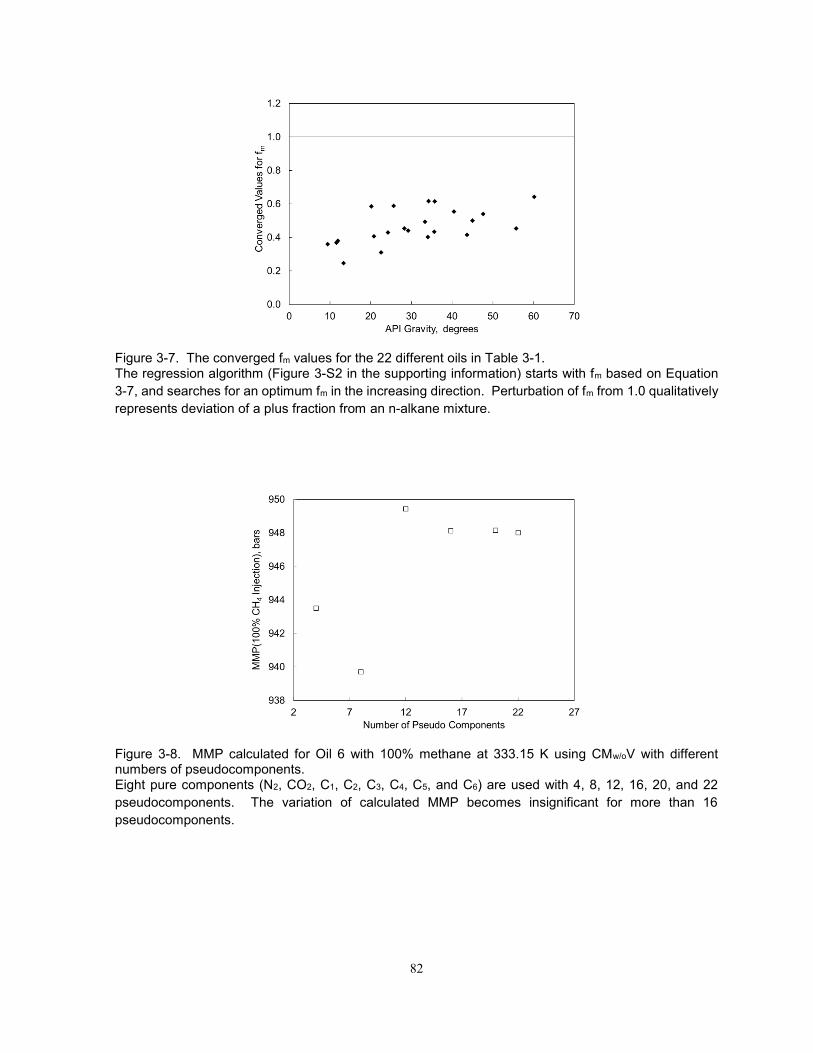
82
Figure 3-7. The converged fm values for the 22 different oils in Table 3-1. The regression algorithm (Figure 3-S2 in the supporting information) starts with fm based on Equation
3-7, and searches for an optimum fm in the increasing direction. Perturbation of fm from 1.0 qualitatively
represents deviation of a plus fraction from an n-alkane mixture.
Figure 3-8. MMP calculated for Oil 6 with 100% methane at 333.15 K using CMw/oV with different numbers of pseudocomponents. Eight pure components (N2, CO2, C1, C2, C3, C4, C5, and C6) are used with 4, 8, 12, 16, 20, and 22
pseudocomponents. The variation of calculated MMP becomes insignificant for more than 16
pseudocomponents.
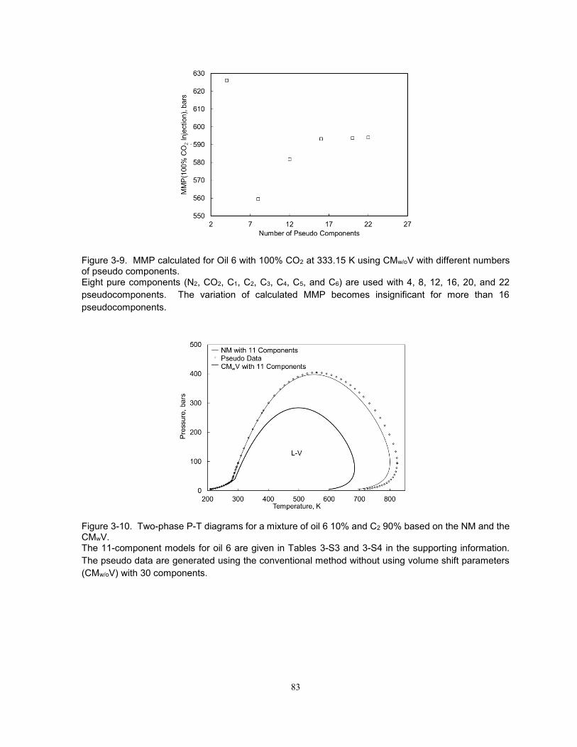
83
Figure 3-9. MMP calculated for Oil 6 with 100% CO2 at 333.15 K using CMw/oV with different numbers of pseudo components. Eight pure components (N2, CO2, C1, C2, C3, C4, C5, and C6) are used with 4, 8, 12, 16, 20, and 22
pseudocomponents. The variation of calculated MMP becomes insignificant for more than 16
pseudocomponents.
Figure 3-10. Two-phase P-T diagrams for a mixture of oil 6 10% and C2 90% based on the NM and the CMwV. The 11-component models for oil 6 are given in Tables 3-S3 and 3-S4 in the supporting information.
The pseudo data are generated using the conventional method without using volume shift parameters
(CMw/oV) with 30 components.
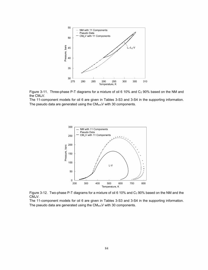
84
Figure 3-11. Three-phase P-T diagrams for a mixture of oil 6 10% and C2 90% based on the NM and the CMwV. The 11-component models for oil 6 are given in Tables 3-S3 and 3-S4 in the supporting information.
The pseudo data are generated using the CMw/oV with 30 components.
Figure 3-12. Two-phase P-T diagrams for a mixture of oil 6 10% and C3 90% based on the NM and the CMwV. The 11-component models for oil 6 are given in Tables 3-S3 and 3-S4 in the supporting information.
The pseudo data are generated using the CMw/oV with 30 components.

85
Figure 3-13. Three-phase P-T diagrams for a mixture of oil 6 10% and C3 90% based on the NM and the CMwV. The 11-component models for oil 6 are given in Tables 3-S3 and 3-S4 in the supporting information.
The pseudo data are generated using the CMw/oV with 30 components.
Figure 3-14. P-x diagrams for the oil-6/C1 pseudo binary pair at 333.15 K based on the NM and CMwV with 11 components. The 11-component models are given in Tables 3-S3 and 3-S4 in the supporting information. The pseudo
data are generated using the CMw/oV with 30 components.
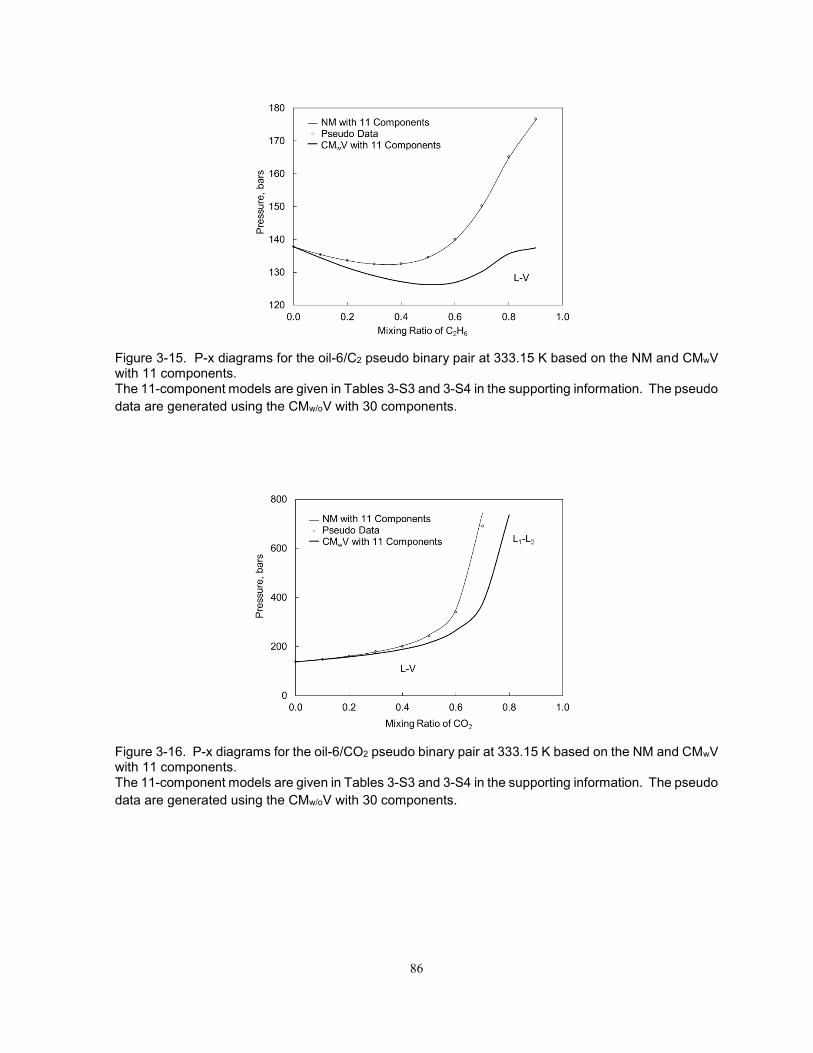
86
Figure 3-15. P-x diagrams for the oil-6/C2 pseudo binary pair at 333.15 K based on the NM and CMwV with 11 components. The 11-component models are given in Tables 3-S3 and 3-S4 in the supporting information. The pseudo
data are generated using the CMw/oV with 30 components.
Figure 3-16. P-x diagrams for the oil-6/CO2 pseudo binary pair at 333.15 K based on the NM and CMwV with 11 components. The 11-component models are given in Tables 3-S3 and 3-S4 in the supporting information. The pseudo
data are generated using the CMw/oV with 30 components.
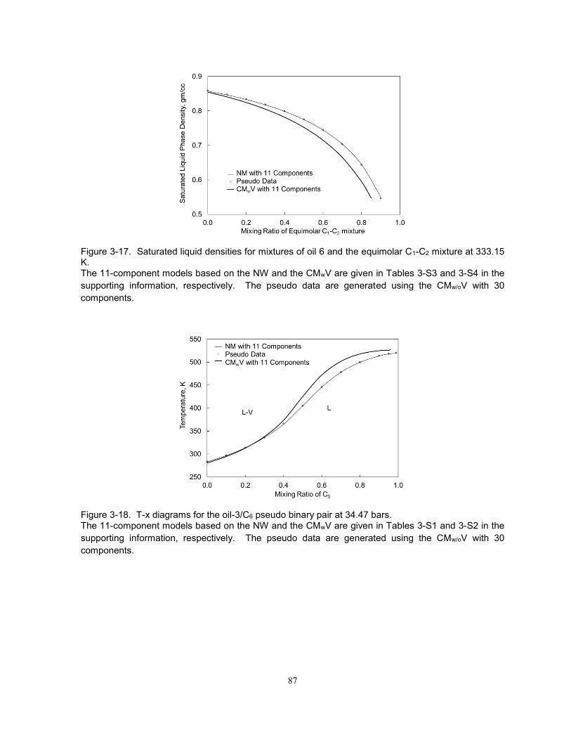
87
Figure 3-17. Saturated liquid densities for mixtures of oil 6 and the equimolar C1-C2 mixture at 333.15 K. The 11-component models based on the NW and the CMwV are given in Tables 3-S3 and 3-S4 in the
supporting information, respectively. The pseudo data are generated using the CMw/oV with 30
components.
Figure 3-18. T-x diagrams for the oil-3/C6 pseudo binary pair at 34.47 bars. The 11-component models based on the NW and the CMwV are given in Tables 3-S1 and 3-S2 in the
supporting information, respectively. The pseudo data are generated using the CMw/oV with 30
components.
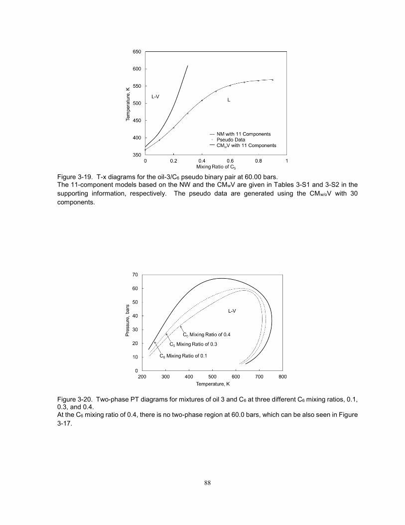
88
Figure 3-19. T-x diagrams for the oil-3/C6 pseudo binary pair at 60.00 bars. The 11-component models based on the NW and the CMwV are given in Tables 3-S1 and 3-S2 in the
supporting information, respectively. The pseudo data are generated using the CMw/oV with 30
components.
Figure 3-20. Two-phase PT diagrams for mixtures of oil 3 and C6 at three different C6 mixing ratios, 0.1, 0.3, and 0.4. At the C6 mixing ratio of 0.4, there is no two-phase region at 60.0 bars, which can be also seen in Figure
3-17.
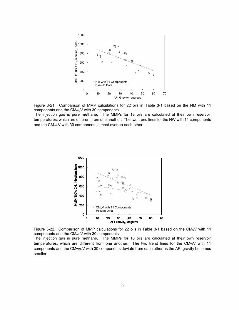
89
Figure 3-21. Comparison of MMP calculations for 22 oils in Table 3-1 based on the NM with 11 components and the CMw/oV with 30 components.
The injection gas is pure methane. The MMPs for 18 oils are calculated at their own reservoir
temperatures, which are different from one another. The two trend lines for the NW with 11 components
and the CMw/oV with 30 components almost overlap each other.
Figure 3-22. Comparison of MMP calculations for 22 oils in Table 3-1 based on the CMwV with 11 components and the CMw/oV with 30 components. The injection gas is pure methane. The MMPs for 18 oils are calculated at their own reservoir
temperatures, which are different from one another. The two trend lines for the CMwV with 11
components and the CMw/oV with 30 components deviate from each other as the API gravity becomes
smaller.

90
Figure 3-23. Comparison of MMP calculations for 18 oils in Table 3-1 based on the NM with 11 components and the CMw/oV with 30 components. The injection gas is pure CO2. The MMPs for 18 oils are calculated at their own reservoir temperatures,
which are different from one another. The two trend lines for the NW with 11 components and the
CMw/oV with 30 components are close to each other.
Figure 3-24. Comparison of MMP calculations for 18 oils in Table 3-1 based on the CMwV with 11 components and the CMw/oV with 30 components. The injection gas is pure CO2. The MMPs for 18 oils are calculated at their own reservoir temperatures,
which are different from one another. The two trend lines for the CMwV with 11 components and the
CMw/oV with 30 components deviate from each other as the API gravity becomes smaller.

91
Figure 3-25. Measured and calculated densities for oil 6 at 333.15 K. Adjustment of pseudocomponents’ TC, PC, and ω is performed for the NM with 11 components, and the
CMw/oV with 30 components. The CMwV with 11 components adjusts only volume shift parameters of
pseudocomponents to match densities.
Figure 3-26. Measured and calculated viscosities for oil 6 at 333.15 K. Adjustment of VC was performed for pseudocomponents to match viscosities using the LBC method for
the NM and CMwV with 11 components, and the CMw/oV with 30 components.

92
Figure 3-27. Oil recovery predictions in 1-D oil displacement simulations based on the NM and CMwV with 11 components, along with pseudo data points generated from the CMw/oV with 30 components. Oil 6 is displaced by the equimolar C1/C2 mixture at 333.15 K at 200 bars, which is below MMP. Input
parameters are given in Table 3-2. The recovery curves for 0.0-0.3 HCPVI nearly coincide, and they
are not shown.
Figure 3-28. Oil saturation profiles at 0.4 HCPVI for the oil-6 displacement with the equimolar C1/C2 mixture at 333.15 K and 200 bars. Predictions using the NM and CMwV with 11 components are shown along with pseudo data generated
from the CMw/oV with 30 components.
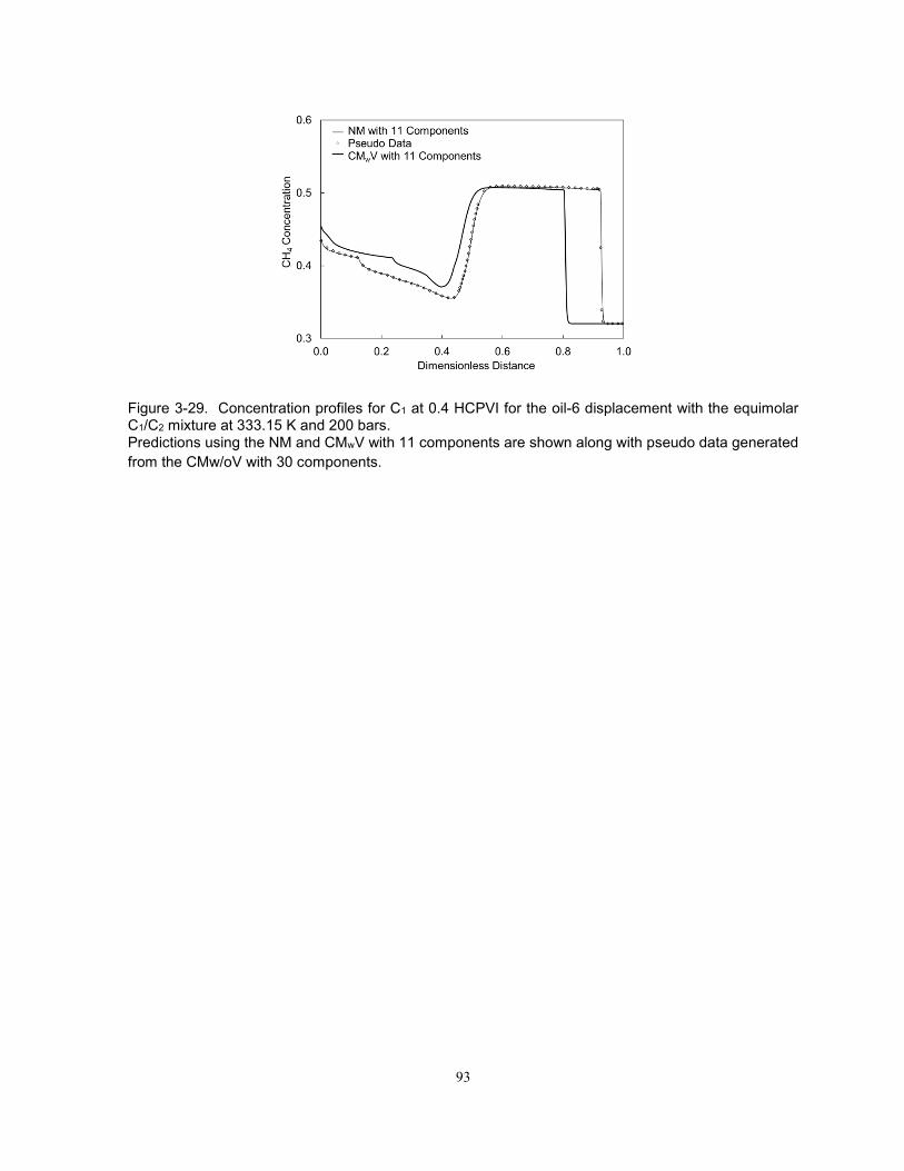
93
Figure 3-29. Concentration profiles for C1 at 0.4 HCPVI for the oil-6 displacement with the equimolar C1/C2 mixture at 333.15 K and 200 bars. Predictions using the NM and CMwV with 11 components are shown along with pseudo data generated
from the CMw/oV with 30 components.

94
Chapter 4: Characterization of Reservoir Fluids using an EOS based on
Perturbation from n-Alkanes
A version of this has been published in Fluid Phase Equilibria, Year (2013), Volume:
358, Pages: 250-271.
95
4.1. Introduction
Compositional modeling is widely used to simulate enhanced oil recovery and recovery of gas
condensates and volatile oils. Reliability of compositional simulation can depend significantly on the
phase behavior model used in the simulation. Cubic equations of state (EOSs), such as the Peng-
Robinson (PR) EOS (Peng and Robinson 1976, 1978), are used to calculate phase behavior in
compositional simulation. These cubic EOSs along with the van der Waals mixing rules give reasonable
accuracy and high computational efficiency for vapor-liquid equilibrium of reservoir fluids.
Characterization of reservoir fluids using a cubic EOS is conducted based on experimental data
available, which typically consist of composition analysis and pressure-volume-temperature (PVT) data.
Compositional analysis provides the concentrations of light components (e.g., up to C6) and a plus
fraction (e.g., C7+), and the density of the plus fraction at atmospheric conditions. The compositional
uncertainty left as a plus fraction becomes higher for heavier fluids (Kumar and Okuno 2012a). PVT
measurements are performed at selected pressure-temperature-composition (P-T-x) conditions. It is
difficult to predict and cover reservoir P-T-x conditions, which result from fluid and energy flow in a
heterogeneous reservoir, in laboratory measurements. Thus, reservoir fluid characterization is
performed under unavoidable uncertainties in composition and phase behavior data in P-T-x space.
However, theory has not been established, based on which engineers can perform reliable fluid
characterization using a cubic EOS under such uncertainties.
A typical characterization process consists of four main steps (Whitson and Brulè 2000; Pedersen
and Christensen 2007) as follows:
Step 1. Estimation of a molar distribution with respect to molecular weight (MW) or carbon number (CN)
to split the plus fraction into detailed components.
Step 2. Estimation of properties for the detailed components such as critical temperature (TC), critical
pressure (PC), critical volume (VC), acentric factor (ω), and volume-shift parameters.
Step 3. Grouping of the detailed components into fewer pseudocomponents.
Step 4. Regression of pseudocomponents’ properties to match experimental data available.
The parameter regression in step 4 is often needed because steps 1-3 make certain assumptions
causing deviations of predictions from actual phase behavior. For example, various correlations used
in step 2 were developed for an EOS to reproduce the critical point and vapor pressure for the
pseudocomponent of a given CN. Use of such correlations implicitly assumes a certain distribution of
hydrocarbon types within that CN group (e.g., paraffins, naphthenes, and aromatics, or PNA
distribution). Furthermore, unless volume shift is used, a cubic EOS is inaccurate in prediction of liquid
densities even if accurate critical parameters and acentric factor are known and used (Peneloux et al.
1982; Jhaveri and Youngren 1988; Søreide 1989).
Current best practice for step 4 is step-wise manual adjustment of parameters to match experimental
data available. Simultaneous regression of various parameters using software as a black box is not
recommended (Kumar and Okuno 2012a). The adjustment parameters often used include TC, PC, VC,

96
ω, volume-shift parameters, and binary interaction parameters (BIPs) for pseudocomponents. Special
care must be taken by experienced engineers to ensure physically acceptable trends of adjustment
parameters with respect to MW or CN (Wang and Pope, 2001). Even with this best practice, different
fluid models are created depending on selection of adjustment parameters and the adjustment amounts
(Lolley and Richardson 1997). Since parameter adjustments are conducted with little physical
justification, it is unclear whether the resulting fluid model is reliable when used in compositional
simulation to predict oil and gas recovery.
The various issues described above indicate that theory should be developed for reliable fluid
characterization using a cubic EOS under uncertainties in composition and phase behavior data in P-T-
x space. One of the main reasons for the lack of theory is likely the unknown, implicit, non-linear
relationship between phase behavior predictions and adjustment parameters such as TC, PC, VC, ω,
volume-shift parameters, and BIPs.
Different characterization methods have been proposed for different reservoir fluids (Whitson 1983;
Stamataki and Magoulas 2001; Montel and Gouel 1984; Leibovici 1984; Lomeland and Harstad 1995);
for example, gas condensates (Yarborough 1979; Lawal et al. 1985; Pedersen et al. 1988; Guo and Du
1989), volatile oils (Peneloux et al. 1979; Whitson and Torp 1983), near-critical fluids (Zuo and Zhang
2000; Al-Meshari and McCain 2006; Hosein and Dawe 2011; Hosein et al. 2013), and heavy oils
(Krejbjerg and Pedersen 2006; Ghasemi et al. 2011). However, P-T-x space that phase behavior spans
is continuous. Although size-asymmetric mixtures can be difficult to model using a cubic EOS with the
van der Waals mixing rules (Gregorowicz and De Loos 2011; Harismiadis et al. 1991), it will substantially
benefit the petroleum industry if continuous modeling of all types of reservoir fluids becomes possible
using a simple cubic EOS.
In our previous research, a method was developed for heavy-oil characterization using the PR EOS
with the van der Waals mixing rules without volume shift (Kumar and Okuno 2012a). Uncertainty issues
in heavy-oil characterization were addressed based on the concept of perturbation from n-alkanes (the
PnA method). Pseudocomponents were initially assigned TC, PC, and ω that were optimized for n-
alkanes in terms of liquid densities and vapor pressures using the PR EOS (Kumar and Okuno 2012b).
The optimized reference values allowed for well-defined directions for perturbation of
pseudocomponents’ TC, PC, and ω to match PVT data available. We presented that robust regression
using the PnA method required only three perturbation parameters to match volumetric and
compositional phase behaviors with no volume shift. Important physical considerations used in the
development of this PnA method include the following:
(1) A PNA distribution of a plus fraction is interpreted as a perturbation from the limiting distribution
of 100% n-alkanes.
(2) TC and PC of n-alkane are lower than those of other types of hydrocarbons (e.g., aromatics)
within a given CN group. The trend is the other way around for ω.

97
(3) Without using volume shift, compositional and volumetric phase behaviors are properly coupled,
and density data are effectively used.
(4) Pitzer’s definition of ω (Pitzer 1955; Pitzer et al. 1955) is satisfied for all pseudocomponents.
In this paper, we extend the PnA method to lighter fluids, such as gas condensates, volatile oils, and
near-critical fluids. The main novelty of the new PnA method is that it considers proper variations of the
attraction and covolume parameters of pseudocomponents based on the component distribution
determined in the first characterization step. This physical consideration added is more important for
lighter fluids. The new PnA method naturally reduces to the previous PnA method for heavy oils.
In the subsequent sections, we first discuss effects of volume shift on the Gibbs free energy and
phase behavior predictions. The extension of the PnA method is then discussed in detail, where the
importance of considering the interrelationship between the attraction and covolume parameters is
explained. After that, the extended PnA method is applied to 77 different reservoir fluids, consisting of
34 heavy and black oils, 12 volatile oils, and 31 gas condensates. Six fluids are near critical among
them. The universal applicability of the PnA method is conclusively shown in these applications.
4.2. Effect of Volume-Shift Parameter Regression on Gibbs Free Energy
Volume-shift parameters are widely used to correct volumetric predictions from a cubic EOS. Volume-
shift parameters alter the form of a cubic EOS, but not the form of the fugacity equations. Therefore,
volume shift can be performed separately from compositional behavior predictions (Peneloux et al. 1982;
Jhaveri and Youngren 1988). Volume shift, however, affects compositional behavior predictions when
used as regression parameters in fluid characterization.
Kumar and Okuno (2012a) conducted comparisons of phase behavior predictions from two
characterization methods using the PR EOS; one without volume shift and the other with volume shift.
Although the two characterizations were equally accurate at the P-T-x conditions used in the regression,
the latter gave erroneous phase behavior predictions at other P-T-x conditions. The deviation between
the two characterizations was more significant for heavier oils since heavier oils tend to require more
volume correction using the PR EOS.
In this section, we discuss the effects of volume shift in fluid characterization on phase behavior
predictions. Volumetric phase behavior predictions are solved for in solution of a cubic equation, which
contains volume-shift parameters (if used), TC, PC, ω, and BIPs. Thus, two different characterizations
that give the same volumetric predictions have different sets of TC, PC, ω, BIPs, and volume-shift
parameters.
Compositional phase behavior predictions are determined by the parameters that form the single-
phase Gibbs free energy (i.e., the Gibbs free energy calculated assuming a stable single-phase state
even in multiphase regions). Let us consider two characterizations for a given fluid that yield the same
volumetric predictions; one without volume shift and the other with volume shift. The parameter set is
(TC, PC, ω, k)wo for the former, and is (TC, PC, ω, k, c)w for the latter. The underlines for TC, PC, ω, and
c indicate vectors consisting of NC elements, where NC is the number of components. c is a vector for
98
NC volume-shift parameters. k is a BIP matrix consisting of kij (i = 1, 2,…, NC, and j = 1, 2,…, NC). For
the two cases, the dimensionless molar Gibbs free energy change on mixing, g, at a given T, P, and
overall composition (z) is the following:
gwo = (∆mixG
RT)
wo
= ∑ ziln [ziφi(TC,PC,ω,k,T,P,z)
wo
φi(TCi,PCi,ωi,T,P)wo ]NCi=1 (4-1)
gw = (∆mixG
RT)
w
= ∑ ziln [ziφi(TC,PC,ω,k,T,P,z)
wexp(
ciP
RT)
φi(TCi,PCi,ωi,T,P)wexp(ciP
RT)
]NCi=1 = ∑ ziln [
ziφi(TC,PC,ω,k,T,P,z)w
φi(TCi,PCi,ωi,T,P)w ]NCi=1 (4-2)
where φi is the fugacity coefficient for pure component i, and φi is the fugacity coefficient of component
i in a mixture of overall composition z. A single phase is assumed. Equations 4-1 and 4-2 show that
two different sets of parameters give two different single-phase Gibbs free energy surfaces in P-T-x
space.
For example, an oil is characterized as a ternary fluid using the PR EOS with and without volume
shift as shown in Table 4-1. Actual compositional simulation studies often require a larger number of
components. Use of only three components in this case study is to visually demonstrate the volume-
shift effects in a simple manner. The ternary fluid consists of the L, I, and H components. All BIPs are
zero for the two characterizations without loss of generality of the discussion. The two characterizations
are equally accurate in calculation of the saturation pressure, 196.48 bars, at the reservoir temperature
330.4 K and oil densities at 276.3, 258.5, 223.6, 196.5, 175.2, 144.6, 103.0, 62.3, 41.0, and 7.1 bars at
330.4 K. However, the two characterizations have different properties for the H component.
Figures 4-1 and 4-2 show gwo and gw, respectively, in composition space at 196.48 bars and 330.4
K based on the parameters given in Table 4-1 and Equations 4-1 and 4-2. The contour lines are equally
spaced. The difference between gwo and gw is not obvious in the figures, but gwo exhibits a deeper valley
than gw in this case. Although volume shift does not change the form of fugacity equations, different set
of parameters (the w and wo cases) results in different phase equilibria. For the two cases, the fugacity
equations for liquid-vapor (L-V) equilibrium at a given T, P, and overall composition is the following:
xiwoφ
i
L(TC, PC, ω, k, T, P, x)
wo= yi
woφi
V(TC, PC, ω, k, T, P, y)
wo
(4-3)
xiwφ
i
L(TC, PC, ω, k, T, P, x)
w= yi
wφi
V(TC, PC, ω, k, T, P, y)
w
(4-4)
for all i, where i = 1, 2,.., NC, and x and y are the liquid and vapor phase composition vectors, respectively.
Equations 4-3 and 4-4 are solved on the Gibbs free energy shown in Figures 4-1 and 4-2. Results are
presented in Figures 4-3 and 4-4. The two-phase envelope without volume shift is larger than that with
volume shift at 196.48 bars and 330.4 K in this case. The two characterizations give similar predictions
near the oil composition. However, the difference becomes significant in the region away from the oil
composition.
99
The different immiscibilities predicted can result in a large difference in the minimum miscibility
pressure (MMP) for the two characterizations. For example, the MMP calculated at 330.4 K for the
injection gas of 40% L and 60% I is 351.86 bars without volume shift and 250.75 bars with volume shift.
This simple case study clearly shows that the effects of volume shift can be quite significant on oil
recovery predictions. Since P-T-x conditions used in laboratory measurements cannot cover actual
reservoir conditions encountered in reservoir processes, the volume-shift effects in P-T-x space should
be considered in fluid characterization. The PnA method does not require volume shift to accurately
predict volumetric and compositional phase behaviors. Therefore, the PnA method uses no volume
shift, and properly couples the two types of phase behavior.
4.3. Extension of the Perturbation from n-Alkanes (PnA) method
The PnA method previously presented in Kumar and Okuno (2012a) successfully characterized heavy
oils with the PR EOS as described in the introduction section. It required only three adjustment
parameters fT, fP, and fm to perturb TC, PC, and ω of pseudocomponents, respectively. The fm
perturbation parameter was used for the m parameter, a one-to-one function of ω used in the
temperature-dependent term in the attraction term of the PR EOS. The perturbations were performed
in well-defined directions from the n-alkane values of Kumar and Okuno (2012b). A single value for
each of the three adjustment parameters was successfully applied for all pseudocomponents for heavy-
oil characterization.
In this section, the PnA method is extended to characterize other types of reservoir fluids without
loss of simplicity. A fourth adjustment parameter is introduced to consider proper trends of the attraction
and covolume parameters of the PR EOS with respect to MW (or CN) depending on the overall
composition of the fluid to be characterized. The main novelty of this research lies in here.
4.3.1. Overall Composition
The chi-squared distribution function is used in the composition characterization step in the PnA method.
More complicated functions like the gamma (Γ) distribution function can also be used. However, the
chi-squared distribution function can characterize the degree of skew, which is the key information
required in the new PnA method, using the p parameter in
fdis =2
−p2 e
−S2 S
(p2−1)
Γ(p
2 )
(4-5)
Equation 4-5 expresses the probability density for the S variable, which is MW or CN in the context of
composition characterization. The p parameter increases with decreasing API gravity in general. Its
practical values range between 2 and 10 (Quiñones-Cisneros et al. 2004a, 2004b). Figure 4-5 shows
chi-squared distributions for different p values. The compositional characterization method using
Equation 4-5 is described in detail in Quiñones-Cisneros et al. (2004b), and is not duplicated here.
100
4.3.2. Critical Parameters for n-Alkanes and Their Internal Consistency
A plus fraction contains a variety of compounds, such as paraffins, naphthenes, and aromatics (PNA).
Conventional characterization methods assume implicitly a certain PNA distribution in their critical
parameter estimation as described in the introduction section. In the PnA method, the PNA distribution
of a plus fraction is initially set to be the limiting distribution of 100% n-alkanes, and then characterized
explicitly in the regression algorithm. Thus, pseudocomponents are initially assigned the n-alkane
values for TC, PC, and m based on the correlations of Kumar and Okuno (2012b). The MW in the
correlations was adjusted by perturbation parameters fT, fP, and fm in Kumar and Okuno (2012a)
(Equations 4-6 to 4-8);
TC = 1154.35 − 844.83(1.0 + 1.7557 × 10⁻³fTMW)−2.0 (4-6)
PC = 559.93 (MW
fP)
−0.638
− 1.49 (4-7)
m = 0.4707 + 2.4831(fm MW)−(
39.933
fm MW) . (4-8)
The m parameter is function of ω as shown in Equations 4-9 and 4-10:
m = 0.37464 + 1.54226 − 0.269922 for < 0.3984 (4-9)
m = 0.379642 + 1.48503 − 0.1644232 + 0.016666ω3 for ≥ 0.3984. (4-10)
Equations 4-6 to 4-8 reduce to the original correlations of Kumar and Okuno (2012b) for n-alkanes
when the perturbation parameters are 1.0. These correlations were developed using TC, PC, and m
optimized for n-alkanes from C7 to C100 in terms of the vapor pressure and liquid density using the PR
EOS without volume shift. These correlations yield 3.0% and 3.4% AAD for density and vapor pressure
predictions, respectively.
Use of the correlations of Kumar and Okuno (2012b) with the PR EOS satisfies Pitzer’s definition of
ω for each n-alkane. That is, the vapor pressure (PVAPI) calculated at 0.7TC using the PR EOS with TC,
PC, and ω is equal to the vapor pressure (PVAPII) from Equation 4-11.
(PVAP)at Tr=0.7 = 10−(1+)PC (4-11)
using PC and ω. This internal consistency of TC, PC, and ω was also satisfied for each pseudocomponent
in the regression algorithm of Kumar and Okuno (2012a) by minimizing the ε function as shown in
Equation 4-12.
ε =1
𝑛∑ abs(PVAPI − PVAPII)𝑛
𝑖=1 (4-12)
where n is the number of pseudocomponents. A minimum in ε typically occurs when the m
parameter for one of the pseudocomponents falls in a range between 0.94 and 0.96. The internal
consistency is satisfied when one of the pseudocomponents has an m parameter value of 0.946 in the
new algorithm presented later.
101
4.3.3. Attraction and Covolume Parameters
Equations 4-6 to 4-8 use a single value for each of the three perturbation parameters for all
pseudocomponents. This uniform perturbation was successful in the previous PnA method for
characterizing heavy oils. In this research, the PNA distribution of a plus fraction is characterized more
mechanistically.
Yarborough (1978) presented trend curves for specific gravity (SG) at 288.15 K and 1.01325 bars
as a function of CN and “aromaticity”. The aromaticity parameter was defined as the percentage of total
carbon atoms in a molecule, which are within the benzene ring. In our opinion, however, aromaticity in
his presentation should be interpreted as deviation from n-alkanes. For example, naphthenes cannot
be well-defined using aromaticity, but their standard SG trend was shown to be much higher than that
of n-alkanes. Nevertheless, the term “aromaticity”, instead of deviation from n-alkane, is used for brevity
in this paper. In Yarborough’s presentation, CN ranged from 7 to 40, and aromaticity from 0 to 80. The
standard SG trend curves for the aromaticity levels of 10 and 60 are reproduced in Figure 4-6. The
standard SG increases with CN and aromaticity. Although the trend curves of Yarborough are based
on the standard SG, we use them here to show qualitatively how perturbation should be done in different
regions of composition space.
Figure 4-6 also shows the standard SG calculated for the aromaticity levels of 10 and 60 using the
PR EOS with uniformly perturbed critical parameters. The uniform perturbations for the two aromaticity
levels were conducted by matching the standard SG of C7. Results show that the uniform perturbation
gives deviation from Yarborough’s trend curves for higher CN. However, the deviation levels off at a
certain CN as shown in Figure 4-7.
We then match the SG trend curves for CNs from 8 to 40 using variable perturbation. Figure 4-8
shows the resulting perturbation parameters for CNs from 7 to 40 for the aromaticity level of 10. Uniform
perturbation is appropriate for the higher CN range, while sharply increasing perturbation is required for
the lower CN range. This explains why uniform perturbation can be used for heavy-oil characterization,
where CNs of all pseudocomponents are typically higher than 20. For lighter reservoir fluids, however,
a few pseudocomponents usually fall in the region of composition space where perturbation should be
increased with CN or MW.
Perturbations of critical parameters directly affect the attraction (a) and covolume (b) parameters of
a cubic EOS, which in turn affect the Gibbs free energy and volumetric predictions in P-T-x space.
Figures 4-9 and 4-10 show the a and b parameters, respectively, for three levels of aromaticity 0, 10,
and 60. The original correlations of Kumar and Okuno (2012b) are used for n-alkanes (i.e., zero
aromaticity). The fT, fP, and fm values fitted to Yarborough’s trend curves are used for the aromaticity
levels 10 and 60. The a parameter increases with CN for a fixed aromaticity level. The effect of
aromaticity on the a parameter is not systematic; i.e., the a parameter increases with aromaticity for light
hydrocarbons, and the trend is the other way around for heavier hydrocarbons. The trend of the b
parameter is more systematic. The b parameter for n-alkane is higher than those for aromatic

102
hydrocarbons for a given CN. Also, n-alkanes exhibit the largest gradient of the b parameter with respect
to CN.
Figure 4-11 shows a parameter group a/b2 (ψ) based on the values for the a and b parameters in
Figures 4-9 and 4-10. The ψ parameter for each component can be calculated using the PR EOS as
follows:
ψ =Ω𝑎
Ω𝑏2 PCα(T). (4-13)
The ψ parameter is a function of TC, PC, ω, and T as shown in Equation 4-13. The ψ parameter is
sensitive to the level of aromaticity for light and intermediate hydrocarbons, where variable perturbation
is required (see Figure 4-11). This is also true at a realistic reservoir temperature of 370.15 K as shown
in Figure 4-12. We therefore use the ψ parameter to control variable perturbation in different regions
of composition space. The ψ parameter monotonically decreases with CN for high aromaticity levels,
but exhibits a maximum for low aromaticity levels including n-alkanes. van Konynenburg and Scott
(1980) used the ψ parameter in their pioneering research on classification of binary phase diagrams
using the van der Waals EOS. The ψ parameters for two components (i.e., ψi, where i = 1, 2.) were
used to characterize size-asymmetric binary mixtures.
Figure 4-12 is useful in considering qualitatively how the ψ parameter should be characterized
depending on the fluid composition of interest. In general, heavier fractions are relatively more
naphthenic and aromatic than lighter fractions (Yarborough 1979; Nagy and Colombo 1967). This
physical trend is plausible considering that a larger number of carbon atoms allow for more variations of
hydrocarbon molecular structures; e.g., if the uniform distribution of molecular structures is considered
within individual CN groups, the concentration of n-alkane becomes lower for higher CN.
The ψ parameter changes its sensitivity to aromaticity around CN 20 as shown in Figures 4-11 and
4-12. In the CN range higher than approximately 20, the ψ parameter decreases with CN regardless of
the level of aromaticity. In the lower CN range, the ψ parameter typically increases with CN because of
the increasing aromaticity trend with respect to CN within a given fluid as just discussed in the previous
paragraph. Two trend curves for the ψ parameter are presented for these two model fluids in Figure 4-
12.
The ψ parameter typically increases with CN (like the lighter model fluid in Figure 4-12), if all
pseudocomponents are within the range of C7-C20. For some heavy oils, the lightest pseudocomponent
can be around C20, and the ψ parameter is expected to decrease almost linearly with CN (like the heavier
model fluid in Figure 4-12). For many fluids, however, the CN range of pseudocomponents contains the
boundary of the two distinct regions, which is approximately C20. For these fluids, the ψ parameter
exhibits combinations of these two model trends depending on the CN range of their pseudocomponents
and their average aromaticity. The two model trends in Figure 4-12 are shown to be linear for simplicity.
Actual trends of characterized fluids are non-linear in general as shown in the next section.
103
We assume use of four pseudocomponents based on the chi-squared compositional
characterization for discussion here. CN ranges observed for various fluids in our research can be
summarized as follows: 7-30 for gas condensates, 9-45 for light oils, 11-60 for intermediate oils, and 13-
85 for heavy oils. Light gas condensates, for which the C7+ fraction is less than 2%, can have all four
pseudocomponents within the CN range from 7 to 20. Their ψ trends can be strongly influenced by the
n-alkane curve, which exhibits a convex trend (see Figure 4-12).
The overall composition information can be obtained by the distribution function fitted to the
composition data available. The PnA method considers an expected trend of ψ in the regression
process depending on the p parameter value obtained from the fitted chi-squared distribution. Uniform
perturbation is suitable for heavy oils as presented in Kumar and Okuno (2012a). Hence, the p
parameter value of 10 corresponding to extra heavy oils is considered as the limiting value, for which
perturbation is uniform. With increasing API gravity, the p parameter value decreases below 10, and
variable perturbation is required according to the ψ trends discussed above.
4.3.4. Regression Algorithm
In this subsection, we discuss briefly how the current PnA method implements the new concept
regarding the ψ parameter presented in the previous subsection. The main difference from the
regression algorithm of Kumar and Okuno (2012a) is that the perturbation parameters fT, fP, and fm in
Equations 4-6 to 4-8 are augmented by a fourth adjustment parameter γ. We measure a deviation of
the fluid of interest from the limiting fluid with the p parameter value of 10 using constants dj, where j is
the component index for pseudocomponents. The d constants are calculated specifically to a given
fluid, and collectively serve as a fluid type indicator. Then, the d constants and the fourth adjustment
parameter γ are combined to have a desired trend of the ψ parameter.
The algorithm uses four adjustment parameters fT, fP, fm, and γ to match the saturation pressure at
the reservoir temperature and liquid densities at different pressures and the reservoir temperature.
Volume shift parameters are not used in the PnA method. BIPs are constant as described in Kumar
and Okuno (2012a). The BIPs used in the PnA method are 0.0 for N2-CO2, 0.1 for N2-Ci, where 1 ≤ i ≤
6, 0.13 for N2-pseudocomponents, and 0.1 for CO2-hydrocarbons. BIPs are zero for hydrocarbon-
hydrocarbon pairs. A step-wise description of the algorithm is presented below.
Step 1. Composition characterization: Using the composition data available, the plus fraction is split
into n pseudocomponents using the chi-squared distribution function (Equation 4-5; see
Quiñones-Cisneros et al. 2004b). This step gives the mole fractions and MWs of n
pseudocomponents and the p value of the fluid.
Step 2. Calculation of gradation constants dj: The mole fractions and MWs of n pseudocomponents are
calculated assuming that the fluid p value is 10. We calculate the ratios of the MWs from step
1 to the MWs with the assumption of p equal to 10. The resulting ratios are normalized with
respect to the ratio for the lightest pseudocomponent. These normalized ratios are the dj
constants, where j = 1, 2, …, n. That is, d1 is always 1.0.

104
Step 3. Check for the necessity of using density data. Characterize the fluid assuming that fT, fP, and
fm are equal to 1.0 in Equations 4-6 to 4-8. Compare density calculations using the PR EOS to
the experimental density data. If the average density deviation indicates overprediction of the
densities, than go to step 5. Otherwise, continue to step 4 below.
Step 4. Characterization using density and saturation pressure data.
i. fT = 1.0, fP =1.0, γ = 0.0, and k = 1, where k is the iteration index.
ii. Find fm with which TC, PC, and m are internally consistent using Equation 4-14.
mj = 0.4707 + 2.4831 (fmkMWjdjγk)
−(39.933
fmkMWjdj
γk)
(4-14)
In each iteration, fm is adjusted until one of the pseudocomponents has an m parameter value
equal to 0.946.
iii. Calculate critical parameters using Equations 4-15 and 4-16.
TCjk = 1154.35 − 844.83 (1.0 + 1.7557 × 10⁻³fTkdjΥkMWj)
−2.0
(4-15)
PCjk = 559.93 (MWj
fPk𝐝𝐣𝚼𝐤
)
−0.638
− 1.49 (4-16)
iv. Adjust fT and fP to match the saturation pressure and density data.
v. Update γ using Equation 4-17.
γk = 0.5[γk−1 + zI(3.464 + h)(fT,k−12θ + fP,k−1
2θ + fm,k−12θ ) (fT,k−1 + fP,k−1⁄ + fm,k−1)], (4-17)
where θ = (3.0 + h)/h, h is the harmonic mean of zL, zI, and zH, and
zL: Mole fraction of methane in the overall composition
zI: Sum of the mole fractions of N2, CO2, and Ci, where i = 2, 3,…, 6.
zH: Mole fraction of C7+.
fT and fP are set to 1.0, and go to step 4-ii until the difference of the γ values between two
consecutive iterations becomes below a tolerance; e.g., 10-3.
Step 5. Characterization using only saturation pressure data.
i. fT = 0.98, fP = 0.98, γ = 0.0 (for bubble point search), γ = 1.5 (for dew point search), and k =
1, where k is the iteration index.
ii. Find fm with which TC, PC, and m are internally consistent using Equation 4-14.
iii. Calculate critical parameters using Equations 4-15 and 4-16.
iv. Adjust γ until the saturation pressure is matched.
Figure 4-13 shows an example trend of the four adjustment parameters fT, fP, fm, and γ during
iteration when oil 2 (39.89°API) in Table 4-2 is characterized using the above algorithm. As γ increases
from the starting value of zero, fT, fP, and fm decrease. Convergence is achieved when the rate of
increase in γ or the rate of decrease in fT, fP, and fm becomes negligible. The internal consistency of TC,
PC, and m is evaluated by the ε function given in Equation 4-12. Figure 4-14 shows that the ε function
decreases with increasing γ and is sufficiently small on convergence. The algorithm is written in
105
FORTRAN, and takes less than two minutes on average per fluid using the Intel Core i7-960 processor
at 3.20 GHz and 8.0 GB RAM.
Gas condensates and light volatile oils behave like n-alkane mixtures due to low concentrations of
the C7+ fraction. For these fluids, density data are not required in the PnA method. The next section
shows that the correlations of Kumar and Okuno (2012b) enable the PR EOS to accurately predict
densities in such cases.
The key parameter in the PnA method is γ, which controls the ψ gradient with respect to CN (or
MW) of pseudocomponents. Hence, adjustment of γ can be carried out using more data, instead of
using Equation 4-17. For example, liquid saturation data from constant volume depletion (CVD) and
constant composition expansion (CCE), slim-tube MMPs, and three-phase data can be used to adjust
γ. For solubility data, BIPs may be adjusted for methane and heavier pseudocomponents to change
phase behavior predictions locally in composition space. As is shown in the next section, the PnA
method systematically and monotonically adjusts phase behavior predictions using a few adjustment
parameters, unlike the conventional methods.
4.4. Application of the PnA method
In this section, the PnA method is applied to 77 reservoir fluids, ranging from 9.5°API to 71.1°API, where
12 components are used altogether; N2, CO2, C1, C2, C3, C4, C5, C6, and four pseudocomponents. Data
available and used for characterization are (i) overall compositions, (ii) saturation pressures at reservoir
temperatures, and (iii) liquid densities at different pressures at reservoir temperatures, unless otherwise
stated. Other types of data available, such as MMPs, CVD, and CCE, are not used in characterization,
but are used to evaluate the reliability of characterized fluid models.
The significance of considering the ψ parameter is first presented using oils listed in Table 4-2.
Predictions from the PR EOS with the PnA characterization are then compared with data for various
fluids in the case studies subsection.
4.4.1. Significance of the ψ Parameter
In the previous section, we discussed that perturbation from n-alkanes should consider the CN range of
the pseudocomponents used. Uniform perturbation is appropriate for heavy oils since all pseudo
components usually fall in the higher CN range where the ψ parameter is insensitive to the level of
aromaticity. For lighter fluids, some of pseudocomponents are in the lower CN range where the ψ
parameter is sensitive to the level of aromaticity (see Figure 4-12). Variable perturbation should be
considered to obtain appropriate trends of the ψ parameter for these fluids.
The ψ parameter for the PR EOS is a function of TC, PC, and m at a given temperature as shown in
Equation 4-13. Obviously, different characterization schemes result in different trends of the ψ
parameter. To see this, oil 1 (35.22°API) in Table 4-2 is characterized using four different schemes;
Case 1. The PnA method with uniform perturbation (i.e., γ is fixed at zero)
106
Case 2. The PnA method with variable perturbation (i.e., the algorithm presented in the previous
section)
Case 3. The conventional method using the PVTsim software without volume shift (CMw/oV)
Case 4. The conventional method using the PVTsim software with volume shift (CMwV).
Case 1 corresponds to the previous PnA method presented in Kumar and Okuno (2012a). Cases
3 and 4 are based on step-wise manual adjustment of TC, PC, and ω as described in detail in Kumar and
Okuno (2012a). The number of components used is 12 for all cases. The CMs use the default BIP
values from PVTsim as they would be the most suitable values for PVTsim. They are -0.017 for N2-
CO2, 0.0311 for N2-C1, 0.0515 for N2-C2, 0.0852 for N2-C3, 0.08 for N2-C4, 0.1 for N2-C5, 0.08 for N2-Ci,
where i ≥ 6, 0.12 for CO2,-Cj, where 1 ≤ j ≤ 6, and 0.1 for CO2-pseudocomponents. As in the PnA
method, BIPs are zeros for hydrocarbon-hydrocarbon pairs in the CMs. For a fair comparison, the same
composition characterization based on the chi-squired distribution is used for the four cases. Saturation
pressure and density data are matched by adjusting TC, PC, and ω for cases 1-3. For case 4, volume
shift is conducted to match density data, and saturation pressure is matched using TC, PC, and ω. Then,
we calculate the MMPs for the oil with injection gas (0.48% N2, 4.97% CO2, 58.22% C1, 17.14% C2,
12.10% C3, 4.97% C4, 1.66% C5, and 0.53% C6) at the reservoir temperature 374.85 K. The
corresponding slim-tube MMP is reported to be 220 bars in Jaubert et al. (2002).
The resulting trend of ψ along with the AD on the MMP is shown for each case in Figure 4-15. The
CN range of the pseudocomponents is approximately from 11 to 40, which is similar to the entire CN
range presented in Figure 4-12. Case 1 with uniform perturbation exhibits a monotonically decreasing
trend of ψ with respect to CN for the four pseudocomponents. The calculated MMP has a large AD of
+19% compared to the slim-tube MMP. Considering the approximate CN of 11 for the lightest
pseudocomponent, the negative slope of ψ is not expected. Cases 3 and 4 present an obvious minimum
in the trend of ψ with respect to CN. Even though the MMP calculated for case 3 is relatively accurate,
it may be difficult to justify such ψ trends, considering the CN range of the pseudocomponents and that
heavier pseudocomponents are more naphthenic and aromatic than lighter pseudocomponents in
general (Yarborough 1979). Use of volume shift in case 4 makes the calculated MMP less accurate due
to the fundamental reasons presented in the section on Effect of Volume-Shift Parameter Regression
on Gibbs Free Energy. Case 2 shows a monotonically increasing trend of ψ with respect to CN. The
converged γ is 1.23. Considering the inevitable dispersion effects in slim-tube tests, the AD of -6.0% is
acceptable in this case.
Matching MMP data in fluid characterization has been proposed in the literature (e.g., Egwuenu et
al. (2008). It will be easy to implement this proposal in the PnA method. Figure 4-16 shows the MMPs
calculated for different γ values. A monotonic change in the calculated MMP is observed with respect
to γ. The slim-tube MMP of 220 bars can be predicted with γ of 1.08, and the corresponding ψ trend is
shown by a dashed line in Figure 4-15. Although matching a slim-tube MMP without considering
dispersion effects has little practical importance, this exercise shows that phase behavior predictions

107
can be adjusted systematically and monotonically with the PnA method. Similar control over phase
behavior predictions is difficult with the CM.
Figures 4-17 and 4-18 show the a and b parameters for the four pseudocomponents for each of
the four cases. The dashed curves correspond to the case for γ of 1.08. Case 4 deviates significantly
from the other cases in the a and b parameters. However, it is case 1 that has the largest error in the
MMP calculation as shown in Figure 4-15. The a and b parameters are interdependent in fluid
characterization, and the ψ parameter properly captures the interrelationship between the a and b
parameters. Cases 1-3 are similar in the trends of the a and b parameters. However, the ψ parameter
effectively makes the differences among the cases more marked.
For all oils in Table 4-2, slim-tube tests and measured MMPs are reported in the literature. Table
4-3 lists slim-tube and calculated MMPs for eight oils from Table 4-2, one of which is oil 1 discussed
above. A small amount of C7+ contained in some of the injection gases is discarded for the MMP
calculations (their C7+ concentrations are less than 0.3%). Two cases are considered for these MMP
calculations; one with variable perturbation and the other with uniform perturbation. The AAD on the
MMP calculations is 6.7% for the former case and 26.7% for the latter case. These results further
indicate the significance of considering the ψ parameter in perturbation using γ. The AAD from the new
PnA method is similar to the result of Jaubert et al. (2002), who conducted MMP calculations for the
same oils. Unlike the PnA method, they developed fluid models using various data from standard PVT
measurements, swelling tests, and multicontact tests.
4.4.2. Case Studies
The 77 different fluids considered here are 34 heavy and black oils, 12 volatile oils (including one near-
critical fluid), and 31 gas condensates (including three near-critical fluid). These fluids are listed in Table
4-2 and Tables 4-4, 4-5, and 4-6.
For oils 1-22 listed in Table 4-4, available data are limited to overall compositions, saturation
pressures, and liquid densities that are used in characterization. Most of them are heavy oils, for which
data are in general scarce in literature (Kokal and Sayegh 1993; Yazdani and Maini 2010). Therefore,
pseudo data (Merrill and Newley 1993) are generated for MMPs with pure CO2 and pure C1 and some
three-phase envelopes using 30 components (including 22 pseudocomponents) based on the CMw/oV
(Pedersen and Christensen 2007; Krejbjerg and Pedersen 2006; Pedersen et al. 1983, 1984, 1989,
1992, 2004) as explained in detail in Kumar and Okuno (2012a). Using the CMw/oV, the effects of the
number of components on phase behavior predictions diminish when more than 16 components are
used (Kumar and Okuno 2012a). Thus, use of 22 pseudocomponents is appropriate to avoid errors
caused by reduction of composition space. We directly use the compositions characterized by
Quiñones-Cisneros et al. (2004b) for oils 1-13, 18, and 22 in Table 4-4.
Tables 4-5 and 4-6 list volatile oils and gas condensates, respectively, for which PVT data are
available, such as CVD and CCE data. MMP data are unavailable for the volatile oils. Tables 4-2, 4-4,
4-5, and 4-6 present converged γ values and corresponding fT, fP and fm values, which are plotted with

108
respect to the API gravity in Figures 4-19 to 4-22. The converged fT and fP values are greater than 1.0,
and the converged fm values are smaller than 1.0. The overall trends indicate that heavier fluids tend to
require more perturbation from n-alkanes. This is consistent with the physical trend that heavier
fractions are relatively more naphthenic and aromatic than lighter fractions (Nagy and Colombo 1967;
Yarborough 1979).
The γ parameter plays an important role in the extended PnA method. It controls the gradient of ψ
with respect to MW or CN for pseudocomponents. Figure 4-22 shows that the γ parameter becomes
greater for lighter fluids. This is because a lighter fluid contains pseudocomponents lighter than C20 at
higher concentrations. The ψ parameter is sensitive to aromaticity for such lower CNs as shown in
Figure 4-12. For heavy oils, variable perturbation from n-alkanes is less significant; the importance of
the ψ and γ parameters diminishes as the API gravity becomes lower as shown in Figure 4-22. For
extra heavy oils, the PnA method reduces to the previous PnA method developed in Kumar and Okuno
(2012a).
Figure 4-23 depicts the average gradient of ψ with respect to MW of pseudocomponents (Δψ/ΔM).
This average gradient is calculated using ψ’s and MWs for the lightest and heaviest pseudocomponents.
The gradient is small for heavy fluids, and gradually increases as the API gravity increases. This is
consistent with the trends of ψ for the two model fluids presented in Figure 4-12. Figure 4-24 shows
the variation of the ψ gradient with respect to γ. As γ increases, the gradient also increases. These
figures indicate that the algorithm successfully converged as designed in the previous section. The ψ
parameter is effectively controlled by adjusting γ.
4.4.2.1. MMP Calculations
We showed that the extended PnA method gives better MMP predictions than the previous PnA method
for eight oils in Table 4-2. Here, we further test the extended PnA method for oils 1-22 in Table 4-4.
MMPs at reservoir temperatures are calculated for 100% C1 using PVTsim (2011) and for 100% CO2
using PennPVT (Ahmadi and Johns 2011; PennPVT). CO2-MMP for oils 1, 2, 4, and 18 in Table 4-4
are not considered because of the presence of three phases during the MMP calculations.
Figures 4-25 and 4-26 compare the MMPs from the PnA method and those from pseudo data.
Good agreement is observed between them for heavy oils and light oils. Some oils in the range of 30-
40°API, however, have AD of 20% (encircled in Figures 4-25 and 4-26). This is because of the
discontinuity in the CMw/oV used to generate the pseudo data. PVTsim used in the CMw/oV gives two
different characterization options, normal and heavy characterizations, based on an oil gravity criterion
of 30°API. We observed that there can be significant differences in phase behavior predictions between
these two characterization options around 30°API. Such a discontinuity in fluid characterization is
undesirable considering the continuity of phase behavior (or, more fundamentally, the single-phase
Gibbs free energy) in P-T-x space. The PnA method avoids the discontinuity by incorporating various
physical considerations in the development as explained in the previous sections; the most important

109
one is variable perturbation from n-alkanes for application to a wide variety of fluids. The AAD in C1-
MMPs and CO2-MMPs for the 22 oils is approximately 7% using the extended PnA method.
4.4.2.2. Volatile Oils
We characterize the 12 volatile oils given in Table 4-5. The types of phase behavior predicted for the
oils are presented in the table; liquid saturation in CVD and CCE, and relative volume in CCE are
indicated as 1, 2, and 3, respectively, in Table 4-5. Table 4-5 also lists the limits of measured values in
the experiments along with deviations of the predictions from data. Since these are volatile oils, liquid
saturation is 100% at the bubble points. Liquid saturation data at lowest measured pressures are listed
for data types 1 and 2. Relative volume data at lowest measured pressures are listed for data type 3.
Using the PnA method, the AD is 3.7% in CVD liquid saturation prediction, and predictions of CCE
relative volume are nearly perfect.
Figures 4-27 and 4-28 compare the CVD liquid saturation curves for volatile oils 1 and 5,
respectively. These oils were characterized using only saturation pressure data (see step 5 in the
regression algorithm subsection). The PnA method yields the small AADs given in Table 4-5 for these
oils even without using density data. The γ parameter converges to 0.62 using the algorithm given in
section 4.3.4. Figure 4-27 also shows the CVD liquid saturation with the following γ values: 0.3, 0.4,
0.5, and 0.6. The liquid saturation curve varies monotonically with the γ parameter. As an example for
CCE predictions, Figure 4-29 compares the CCE relative volume for volatile oil 6. Nearly perfect
prediction for the CCE relative volume is observed from the figure.
Figure 4-27 also shows the liquid saturation curve using the CMw/oV with 12 components. The CN
ranges for pseudocomponents in the PnA and CMw/oV are almost the same. For a fair comparison,
density matching is not conducted for both cases (Density matching actually deteriorates the CVD liquid
saturation prediction using the CMw/o in this case). A large deviation is observed in the CMw/oV case for
pressures between 250 bars and 455 bars.
To see the fundamental difference between the PnA and CMw/oV for volatile oil 1, Figure 4-30
compares the ai and bi parameters for the four pseudocomponents in the two characterizations. It is
difficult to find any abnormality in Figure 4-30. However, Figure 4-31 presents an important difference
between the two characterizations in the ψ parameter, which was defined as ai/bi2 before. The ψ trend
for the PnA method exhibits a combined trend of the two model fluids in Figure 4-12. The CMw/oV
method results in the ψ trend that exhibits a minimum for the second lightest pseudocomponent. With
this range of pseudocomponents’ CNs, the ψ value for the second lightest pseudocomponent should
not be less than that for the lightest pseudocomponent. A large deviation in the liquid saturation curve
prediction around the saturation pressure is likely attributed to this ψ behavior for the CMw/oV.
Volatile oil 12 in Table 4-5 is a near-critical fluid, for which CCE liquid saturation is predicted in
Figure 4-32. This oil is characterized at temperature of 371.6 K, and the critical temperature of the oil
is 388.1 K. The PnA method is able to reproduce quantitatively the substantial sensitivity of liquid
saturation to pressure.
110
4.4.2.3. Gas Condensates
The 31 gas condensates listed in Table 4-6 include a wide MW range from 19.75 to 54.92. Gas
condensates 6, 7, 8, 11, and 12 are near critical. As indicated in Table 4-6, CVD liquid saturation curves
(data type 1) are predicted for 26 gas condensates. CCE tests (data types 2 and 3) are predicted for
the other five gas condensates. Characterization of the gas condensates does not use density data in
regression due to low C7+ fractions. These gas condensates behave like light n-alkane mixtures, for
which the PR EOS predicts densities accurately with the correlations of Kumar and Okuno (2012b). The
AAD for density predictions is less than 4% for the gas condensates given in Table 4-6.
Table 4-6 summarizes results for phase behavior predictions using the PnA method. For gas
condensates, liquid saturation is zero at dew point. Hence, the maximum value in the experimental data
is listed for each gas condensate, along with the AAD. The PnA method is successful for these gas
condensates as indicated by the low AADs. As sample results, Figures 4-33 and 4-34 depict CVD
liquid saturation for gas condensates 20 and 5, respectively. The former exhibits low liquid saturation
with a maximum of 1.89% at the lowest measured pressure. The latter exhibits a maximum saturation
of 30.40% at a relatively high pressure in the two phase region. These results for gas condensates and
volatile oils indicate that the PnA method is quantitatively accurate in prediction of quality lines and
densities.
Figure 4-35 shows the ψ trends for gas condensates 4, 12, 20, and 26, for which the maximum
liquid saturations are 25.00%, 40.90%, 1.89%, and 69.81%, respectively. The CN range of
pseudocomponents is typically narrow for gas condensates, and the ψ parameter increases with CN as
shown in Figure 4-12. In general, the slope of ψ becomes smaller as the CN range of pseudo
components becomes wider. The four pseudocomponents for gas condensate 20 are lighter than C20.
Hence, the sharply increasing trend is conceivable since the ψ parameter is sensitive to aromaticity in
this CN region. Gas condensates 4 and 12 have CN ranges of C8-C22 and C8-C26, respectively. The ψ
parameters for these fluids exhibit convexity in the low CN region, which can be seen for n-alkanes in
Figure 4-12. Gas condensate 26 has the pseudocomponents in the CN range of C9-C30. Because of
the wide CN range, the ψ parameter shows a combined trend of the two model fluids in Figure 4-12.
Matching liquid saturation data can be difficult using the conventional fluid characterization methods.
This is true especially when liquid saturation is sensitive to pressure and temperature (e.g., see Figures
4-27, 4-32, and 4-34). Matching such liquid saturation data requires accurate prediction of dense quality
lines and liquid densities (i.e., compositional and volumetric phase behaviors) along the experimental
pressure path at a fixed temperature. However, the PR EOS is quite accurate in liquid density prediction
for light fluids using the correlations of Kumar and Okuno (2012b). Thus, adjustment of compositional
phase behavior for the small C7+ fraction is crucial for reliable prediction of condensation/vaporization
behavior of these fluids.
To show this, we characterize near-critical gas condensate 7 in Table 4-6 using the PnA and CMwV
methods. CVD liquid saturation curves from the two characterizations are compared with data points in

111
Figure 4-36. The CMwV results in large deviations near the dew point. However, the two methods
result in similar phase behavior for the C7+ fraction as shown in Figure 4-37. The converged γ value for
the PnA method is 0.820 as given in Table 4-6. The best match of the PnA characterization results in γ
of 0.930. Figure 4-37 shows that the two values of γ give essentially the same phase behavior of the
C7+ fraction. These results indicate the significant sensitivity of liquid saturation to C7+ characterization
in this case. PVT measurements for C7+ at the reservoir temperature 424.82 K and lower would not help
because the three phase-envelopes nearly coincide there as shown in Figure 4-37.
The PnA method is able to control gas condensate behavior by adjusting only one parameter (γ) to
match the dew point. The adjustment changes phase behavior predictions systematically as shown in
Figures 4-36 and 4-37. Figure 4-36 shows the CVD liquid saturation curves for different γ values. It is
evident that the predicted curve changes monotonically with varying γ and systematically in pressure
space. Gas condensate 6 is another near-critical fluid, for which Figure 4-38 shows quality lines (β is
the vapor phase mole fraction). The calculated critical point is 402.0 K and 339.2 bars. The reservoir
temperature and pressure are 422.6 K and 339.4 bars, respectively. Figure 4-39 shows that the PnA
method accurately predicts CVD liquid dropout, which results from the dense quality lines near the
critical point.
4.4.2.4. Heavy Oils
Oils heavier than 30°API listed in Table 4-4 are considered as heavy oils (Krejbjerg and Pedersen 2006).
The present PnA method reduces to the previous PnA method developed for heavy oils (Kumar and
Okuno 2012a) when γ is zero. As can be seen in Figure 4-22, the γ values for extra-heavy oils of 10°API
are nearly zero. The present PnA method performs similarly to the previous one for heavy oils. Our
focus here is on the West Sak oil (oil 23 in Table 4-4), for which gas solubility data are available in the
literature, and predictions of three hydrocarbon phases.
4.4.2.4.1. P-V Predictions
For oil 23, the oleic phase saturations for two mixtures (60% CO2 and 40% oil, and 80% CO2 and 20%
oil) are predicted at 299.81 K using the PnA method. Reasonable accuracy of the PnA method is
observed in Figures 4-40 and 4-41. The AAD is 2.7% for the 60% CO2 mixture, and 5.6% for the 80%
CO2 mixture. Figure 4-41 shows predictions with different γ values; 0.048, 0.8, 1.0, and 1.2. The
converged γ value is 0.048 using the algorithm given in section 4.3.4. A systematic change in predictions
in pressure space is observed. The change is also monotonic with the γ parameter. With available
phase saturation data, the optimum γ value can be easily selected using the PnA method.
Aghbash and Ahmadi (2012) developed a 10-component fluid model for this oil. They used all non-
zero BIPs. The PnA method does not require non-zero BIPs for hydrocarbon pairs to obtain similar
phase behavior predictions. Figure 4-42 compares the ψ parameters for pseudocomponents from
Aghbash and Ahmadi (2012) with those from the PnA method. The ψ parameter monotonically
decreases with CN for the two cases, which is in line with our discussion for heavy oils in Figure 4-12.
The non-zero BIPs used in Aghbash and Ahmadi (2012) likely did not cause absurd behavior of the

112
Gibbs free energy in P-T-x space in this case. However, special care must be taken when BIPs are
used in regression (Pedersen and Christensen 2007; Wang and Pope 2001; Egwuenu et al. 2008).
4.4.2.4.2. Three-Phase Predictions
Mixtures of oil and solvent can present complex three-hydrocarbon-phase behavior (Mohanty et al.
1995; Polishuk et al. 2004; Okuno et al. 2011). The three phases are the gaseous (V), oleic (L1), and
solvent-rich liquid (L2) phases. Here, we compare three-phase predictions from the PnA method with
pseudo data. Figure 4-43 shows the three-phase envelope for a mixture of 80% CO2 and 20% West
Sak oil. Figures 4-44 and 4-45 show the three-phase envelopes for two mixtures with oil 5 in Table 4-
4; 90% C2 and 10% oil 5, and 90% C3 and 10% oil 5. Three-phase predictions from the PnA method
nearly coincide with the pseudo data.
4.5. Conclusions
We first presented the effects of volume shift on phase behavior in P-T-x space when volume-shift
parameters are used as regression parameters in fluid characterization. Then, the PnA method
developed for heavy oils in our previous research was extended to characterize lighter fluids, such as
gas condensates, volatile oils, and near-critical fluids. Extensive case studies using 77 different
reservoir fluids demonstrated the universal applicability, reliability, robustness, and efficiency of the new
PnA method. The PR EOS with the van der Waals mixing rules was used throughout the research.
Conclusions are as follows:
o Volume-shift parameters affect compositional phase behavior predictions when used as regression
parameters in fluid characterization. P-T-x conditions used in laboratory measurements are only a
small part of actual P-T-x conditions encountered in reservoir processes. Therefore, volume shift
should be carefully performed in regression since it can substantially affect oil recovery predictions
through altered phase behavior predictions in P-T-x space. The PnA method uses no volume shift,
and properly couples volumetric and compositional phase behaviors.
o TC, PC, and ω were perturbed to match the density trend curves with respect to CN for different
levels of aromaticity presented in Yarborough (1979). Results show that uniform perturbation is
appropriate for the CN range approximately higher than 20. Sharply increasing perturbation with
CN is required for the lower CN range. This explains why the previous PnA method successfully
used uniform perturbation for characterizing heavy oils, for which pseudocomponents’ CNs are
typically higher than 20. Case studies demonstrated that perturbation from n-alkanes depends on
the CN range of pseudocomponents in the new PnA method.
o The ψ parameter defined in Equation 4-13 for the PR EOS is more sensitive to the level of
aromaticity in the lower CN range than in the higher CN range. The ψ parameter increases with CN
for fluids that have all pseudocomponents in the lower CN range, where sharply increasing
perturbation with CN is required. The trend is the other way around for fluids that have all
pseudocomponents in the higher CN range, where variable perturbation is less important. Mixed

113
trends of the ψ parameter with respect to CN are expected for fluids that have pseudocomponents
in the two CN ranges. Case studies confirmed this point. Conventional characterization methods
can exhibit unexpected trends of the ψ parameter with respect to CN.
o The regression algorithm developed in this research controls the trend of the ψ parameter with
respect to CN using a fourth adjustment parameter γ. The algorithm also considers the size of
composition space using the distribution function fitted to the composition data of the fluid to be
characterized. Case studies showed the reliability and robustness of the algorithm for all fluids
tested in this research. The algorithm written in FOTRAN takes less than two minutes on average
per fluid using the Intel Core i7-960 processor at 3.20 GHz and 8.0 GB RAM.
o The importance of the ψ and γ parameters diminishes as the API gravity decreases. For extra heavy
oils, the new PnA method naturally reduces to the previous PnA method, where γ is zero.
o The PnA method controls phase behavior predictions monotonically with parameter adjustments
and systematically in P-T-x space. This was demonstrated by quantitative prediction of
condensation/vaporization behavior of gas condensates and light oils and MMPs for various oil
displacements, which can be difficult using conventional fluid characterization. Unlike the
conventional methods, the PnA method uses only four adjustment parameters and incorporates
physical considerations in parameter adjustment.
o The PnA method requires no change in the thermodynamic model used; i.e., it can be readily
implemented in existing software based on the PR EOS with the van der Waals mixing rules.

114
4.6. Nomenclature
Roman Symbols
a Attraction parameter in a cubic equation of state
A Aromatic
b Covolume parameter in a cubic equation of state
c Peneloux volume-shift parameter for NC components
d Gradation constants
fdis Chi-squared distribution function defined in Equation 4-5
fm Perturbation factor for the m parameter
fP Perturbation factor for critical pressure
fT Perturbation factor for critical temperature
∆mixG Molar Gibbs free energy change on mixing
g Dimensionless molar Gibbs free energy change on mixing
kij Binary interaction parameter for components i and j
m Parameter in the Peng–Robinson EOS (1978) defined in Equations 4-9 and 4-10
NC Number of components
P Pressure, bar
p Parameter in the chi-squared distribution
PC Critical pressure, bar
PC Critical pressure vector for NC components
R Universal gas constant
S Parameter in the chi-squared distribution
T Temperature, K
TC Critical temperature, K
TC Critical temperature vector for NC components
TRES Reservoir temperature
𝑥 Mole fraction vector for the liquid phase
𝑦 Mole fraction vector for the gaseous phase
𝑧 Overall composition vector
zL Mole fraction of methane in fluid
zI Sum of mole fractions of non C7+ excluding methane
zH Mole fractions of C7+
Abbreviations
°API API (American Petroleum Institute) gravity
BIP Binary interaction parameter
CN Carbon number
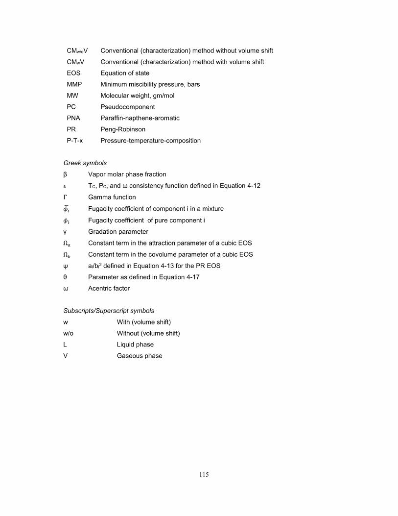
115
Greek symbols
β Vapor molar phase fraction
휀 TC, PC, and ω consistency function defined in Equation 4-12
Γ Gamma function
𝜙 Fugacity coefficient of component i in a mixture
𝜙𝑖 Fugacity coefficient of pure component i
γ Gradation parameter
Ω𝑎 Constant term in the attraction parameter of a cubic EOS
Ω𝑏 Constant term in the covolume parameter of a cubic EOS
ψ ai/bi2 defined in Equation 4-13 for the PR EOS
θ Parameter as defined in Equation 4-17
ω Acentric factor
Subscripts/Superscript symbols
w With (volume shift)
w/o Without (volume shift)
L Liquid phase
V Gaseous phase
CMw/oV Conventional (characterization) method without volume shift
CMwV Conventional (characterization) method with volume shift
EOS Equation of state
MMP Minimum miscibility pressure, bars
MW Molecular weight, gm/mol
PC Pseudocomponent
PNA Paraffin-napthene-aromatic
PR Peng-Robinson
P-T-x Pressure-temperature-composition

116
4.7. References
Aghbash, V.N. and Ahmadi, M. 2012. Evaluation of CO2-EOR and Sequestration in Alaska West Sak
Reservoir Using Four-Phase Simulation Model. Presented at the Western North American Regional
Meeting, Bakersfield, California. 19-23 March. SPE-153920-MS.
Ahmadi, K. and Johns, R.T. 2011. Multiple Mixing-Cell Model for MMP Determination. SPE J. 16 (4):
733-742.
Al-Ajmi, M.F., Tybjerg, P., Rasmussen, C.P. et al. 2011. EoS Modeling for Two Major Kuwaiti Oil
Reservoirs. Presented at the SPE Middle East Oil and Gas Show and Conference, Manama,
Bahrain, 25-28 Sept. SPE-141241-MS.
Al-Meshari, A. 2004. New Strategic Method to Tune Equation of State to Match Experimental Data for
Compositional Simulation. PhD dissertation, Texas A&M University, Texas.
Al-Meshari, A.A. and McCain, W.D. 2006. An Accurate Set of Correlations for Calculating Critical
Properties and Acentric Factors for Single Carbon Number Groups. Presented at SPE Technical
Symposium of Saudi Arabia Section, Dhahran, Saudi Arabia, 21-23 May. SPE-106338-MS.
Coats, K.H. 1985. Simulation of Gas Condensate Reservoir Performance. J Petrol Tech 37 (10): 1870-
1886.
Coats, K.H. and Smart, G.T. 1986. Application of a Regression Based EOS PVT Program to Laboratory
Data. SPE Res Eng 1 (3): 277-299.
Cullick, A.S., Pebdani, F.N., and Griewank, A.K. 1989. Modified Corresponding States Method for
Predicting Densities of Petroleum Reservoir Fluids. Ind. Eng. Chem. Res. 28 (3): 340-347.
Danesh, A. 1998. PVT and Phase Behavior of Petroleum Reservoir Fluids, Elsevier Science &
Technology Books.
Drohm, J.K., Trengove, R.D., and Goldthrope, W.H. 1988. On the Quality of Data from Standard Gas-
Condensate PVT Experiments. Presented at the SPE Gas Technology Symposium, Dallas, Texas,
13-15 June. SPE-17768-MS.
Egwuenu, A.M., Johns, R.T., and Li, Y. 2008. Improved Fluid Characterization for Miscible Gas Floods.
SPE Res Eval Eng 11 (4): 655-665.
Ghasemi, M., Alavian, S.A., and Whitson, C.H. 2011. C7+ Characterization of Heavy Oil Based on
Crude Assay Data. Presented at SPE Heavy Oil Conference and Exhibition held in Kuwait City,
Kuwait, 12-24 Dec. SPE 148906-MS.
Gregorowicz, J. and De Loos, T.W. 2011. Prediction of Liquid−Liquid−Vapor Equilibria in Asymmetric
Hydrocarbon Mixtures. Ind. Eng. Chem. Res. 40 (1): 444-451.
Guo, T.M. and Du, L. 1989. A New Three-Parameter Cubic Equation of States for Reservoir Fluids:
Part 3- Application to Gas Condensates. SPE e-library, Paper SPE-19374-MS.
Harismiadis, V.I., Koutras, N.K., Tassios, D.P. et al. 1991. How Good is Conformal Solutions Theory
for Phase Equilibrium Predictions?: Gibbs Ensemble Simulations of Binary Lennard-Jones Mixtures.
Fluid Phase Equilib. 65: 1-18.

117
Hosein, R. and Dawe, R.A. 2011. Characterization of Trinidad Gas Condensates. J Pet Sci Technol
29 (8): 817-823.
Hosein, R., Jagai, T., and Dawe, R.A. 2013. A Method for Predicting the Phase behavior of Trinidad
Gas Condensates. The West Indian Journal of Engineering 35 (2): 22-30.
Imo-Jack, O. 2010. PVT Characterization of a Gas Condensate Reservoir and Investigation of Factors
Affecting Deliverability. Presented at the Annual SPE International Conference and Exhibition,
Tinapa-Calabar, Nigeria, 31 July-7 Aug. SPE-140629-MS.
Jaubert, J-N., Avaullee, L., and Souvay, J.F. 2002. A Crude Oil Data Bank Containing more than 5000
PVT and Gas Injection Data. J Pet Sci Technol 34 (1): 65-107.
Jaubert, J-N., Avaullee, L., and Pierre, C. 2002. Is it still necessary to measure the minimum miscibility
pressure? Ind. Eng. Chem. Res. 41 (2): 303-310.
Jhaveri, B.S. and Youngren, G.K. 1988. Three-Parameter Modification of the Peng-Robinson Equation
of State to Improve Volumetric Predictions. SPE J. 3 (3): 1033-1040.
Kokal, S.L. and Sayegh, S.G. 1993. Phase Behavior and Physical Properties of CO2-Saturated Heavy
Oil and its Constitutive Fractions: Experimental Data and Correlations. J. Pet. Sci. Eng. 9 (4): 289-
302.
Krejbjerg, K. and Pedersen, K.S. 2006. Controlling VLLE Equilibrium with a Cubic EoS in Heavy Oil
Modeling. Presented at 57th Annual Technical Meeting of the Petroleum Society (Canadian
International Petroleum Conference), Calgary. 13-15 June. PETSOC-2006-052.
Kumar, A. and Okuno, R. 2012a. Fluid Characterization Using an EOS for Compositional Simulation of
Enhanced Heavy-Oil Recovery. Presented at SPE Annual Technical Conference and Exhibition,
San Antonio, Texas, 8-10 Oct. SPE 159494-MS
Kumar, A. and Okuno, R. 2012b. Critical Parameters Optimized for Accurate Phase Behavior Modeling
for Heavy n-Alkanes up to C100 using the Peng-Robinson Equation of State. Fluid Phase Equilib.
335: 46-59.
Lawal, A.S., Van derLaan, E.T. and Thambynaygam, R.K.M. 1985. Four-Parameter Modification of the
Lawal-Lake-Silberberg Equation of State for Calculating Gas-Condensate. Presented at Annual
Technical Conference and Exhibition of the Society of Petroleum Engineers, Las Vegas, Nevada,
22-25 Sept. SPE-14269-MS.
Leibovici, C.F. 1993. A Consistent Procedure for the Estimation of Properties Associated to Lumped
Systems. Fluid Phase Equilib. 87 (2): 189-197.
Lolley, C.S. and Richardson, W.C. 1997. Compositional Input for Thermal Simulation of Heavy Oils with
Application to the San Ardo Field. Presented at International Thermal Operation & Heavy Oil
Symposium, Bakersfield, California, 10-12 Dec. SPE-37538-MS
Lomeland, F. and Harstad, O. 1995. Simplifying the Task of Grouping Components in Compositional
Reservoir Simulation. SPE Comp Appl. 7 (2): 38-43.
118
McVay, D.A. 1994. Generalization of PVT Properties for Modified Black-Oil Simulation of Volatile and
Gas Condensate Reservoirs. PhD dissertation, Texas A&M University, Texas.
Merrill, R.C. and Newley, T.M.J. 1993. A Systematic Investigation into the most Suitable Data for
Development of Equation of State for Petroleum Reservoir Fluids. Fluid Phase Equilib. 82: 101-
110.
Mohanty, K.K., Masino, W.H., Ma, T.D. et al. 1995. Role of Three-Hydrocarbon-Phase Flow in a Gas-
Displacement Process. SPE Res Eng 10 (3): 214-221.
Montel, F. and Gouel, P.L. 1984. A New Lumping Scheme of Analytical Data for Compositional Studies.
Presented at the SPE Annual Technical Conference and Exhibition, Houston, Texas, 16-19 Sept.
Paper SPE 13119.
Moore, D.C. 1989. Simulation of Gas-Condensate Reservoir Performance Using Schmidt-Wenzel
Equation of State. MSc thesis, Montana College of Mineral Science and Technology, Montana..
Nagy, B. and Colombo, U. 1967. Fundamental Aspects of Petroleum Geochemistry, Elsevier,
Amsterdam.
Okuno, R., Johns, R.T., and Sepehrnoori, K. 2011. Mechanisms for High Displacement Efficiency of
Low-Temperature CO2 Floods. SPE J. 16 (4): 751-767.
Pedersen, K.S. and Christensen, P. L. 2007. Phase Behavior of Petroleum Reservoir Fluids. CRC
Press, Taylor & Francis Group, Boca Raton, FL, USA.
Pedersen, K.S., Thomassen, P., and Fredenslund, Aa. 1983. SRK- EOS Calculation for Crude Oil. Fluid
Phase Equilib. 14: 209–218.
Pedersen, K.S., Thomassen, P., and Fredenslund, Aa. 1984. Thermodynamics of Petroleum Mixture
Containing Heavy Hydrocarbons. 1. Phase Envelope Calculation by Use of the Soave-Redlich-
Kwong Equation of State. Ind. Eng. Chem. Proc. Des. Dev. 23 (1): 163–170.
Pedersen, K.S., Blilie, A.L., and Meisingset, K.K. 1992. Calculations On Petroleum Reservoir Fluids
Using Measured And Estimated Compositional Data for the Plus Fraction. Ind. Eng. Chem. Res.
31 (5): 1378-1384.
Pedersen, K.S., Milter, J., and Sørensen, H. 2004. Cubic Equations of State Applied to HT/HP and
Highly Aromatic Fluids. SPE J. 9 (2): 186-192.
Pedersen, K.S., Thomassen, P., and Fredenslund, Aa. 1989. Characterization of Gas Condensate
Mixtures. Advances in Thermodynamics, Taylor & Francis, New York.
Pedersen, K.S., Thomassen, P., and Fredenslund, Aa. 1988. Characterization of Gas Condensates.
Presented at AIChE Spring National Meeting, New Orleans, Louisiana, 6-10 March.
Peneloux, A., Jain, C., and Behar, E. 1979. Application Of The Developed Redlich-Kwong Equation Of
State To Predict The Thermodynamic Properties Of Condensate Gases. Presented at the Annual
Fall Technical Conference and Exhibition of the Society of Petroleum Engineers of AIME, Las
Vegas, Nevada, 23-26 Sept. SPE-8287-MS.

119
Peneloux, A., Rauzy, E., and Fréze, R. 1982. A Consistent Correction for Redlich-Kwong-Soave
Volume. Fluid Phase Equilib. 8 (1): 7-23.
Peng, D.-Y. and Robinson, D.B. 1976. A New Two-Constant Equation of State. Ind. Eng. Chem. Fund.
15 (1): 59-64.
Peng, D.-Y. and Robinson, D.B. 1978. The Characterization of the Heptanes and Heavier Fractions for
the GPA Peng-Robinson Programs. GPA Research Report RR-28.
PennPVT Toolkit, Gas Flooding Joint Industrial Project, Director: Dr. Russell T. Johns, EMS Energy
Institute, The Pennsylvania State University, University Park, PA.
Pitzer, K.S. 1955. The Volumetric and Thermodynamic Properties of Fluids. I. Theoretical Basis and
Viral Coefficients. J. Am. Chem. Soc. 77 (13): 3427-3433.
Pitzer, K.S., Lippmann, D.Z., Curl Jr, R.F. et al. 1955. The Volumetric and Thermodynamic Properties
of Fluids. II. Compressibility Factor, Vapor Pressure, and Entropy of Vaporization. J. Am. Chem.
Soc. 77 (13): 3433-3440.
Polishuk, I., Wisniak, J., and Segura, H. 2004. Estimation of Liquid-Liquid-Vapor Equilibria in Binary
Mixtures of n-Alkanes. Ind. Eng. Chem. Res. 43 (18): 5957-5964.
PVTsim 20.0. 2011. Calsep A/S, Lyngby, Denmark.
Quiñones -Cisneros, S.E., Zéberg-Mikkelsen, C.K., and Stenby, E.H. 2003. Friction Theory Prediction
of Crude Oil Viscosity at Reservoir Conditions Based on Dead Oil Properties. Fluid Phase Equilib.
212 (1-2): 233–243.
Quiñones-Cisneros, S.E., Andersen, S.I., and Creek, J. 2005. Density and Viscosity Modeling and
Characterization of Heavy Oils. Energy Fuels 19 (4): 1314-1318.
Quiñones-Cisneros, S.E., Dalberg, A., and Stenby, E.H. 2004b. PVT Characterization and Viscosity
Modeling and Prediction of Crude Oils. Pet. Sci. Technol., 22 (9-10): 1309–1325.
Quiñones-Cisneros, S.E., Zéberg-Mikkelsen, C.K., Baylaucq, A. et al. 2004a. Viscosity Modeling and
Prediction of Reservoir Fluids: From Natural Gas to Heavy Oils. Int. J. Therm. 25 (5): 1353-1366.
Sharma, G.D. 1990. Development of Effective Gas Solvents Including Carbon Dioxide for the Improved
Recovery of West Sak Oil, Report No. DOE/FE/61114-2, University of Alaska Fairbanks, Alaska.
Søreide, I. 1989. Improved Phase Behavior Predictions of Petroleum Reservoir Fluids from a Cubic
Equation of State, Ph.D. dissertation, Norwegian University of Science and Technology, Trondheim,
Norway, 1989.
Stamataki, S.K. and Magoulas, K.G. 2001. Characterization of Heavy Undefined Fractions. Presented
at SPE International Symposium on Oilfield Chemistry, Houston, Texas, 13-16 Feb. SPE-64996-
MS.
Van Konynenburg, P.H. and Scott, R.L. 1980. Critical Lines and Phase Equilibria in Binary Van Der
Waals Mixtures. Philos. Trans. R. Soc. Lond. 298 (1442): 495-540.
Wang, P. and Pope, G.A. 2001. Proper Use of Equations of State for Compositional Reservoir
Simulation. J. Petrol. Tech. 53 (7): 74-81.

120
Whitson, C.H. 1983. Characterizing Hydrocarbon Plus Fractions. SPE J. 23 (4): 683-694.
Whitson, C.H. and Brulè, M.R. 2000. Phase Behaviour. SPE Henry L. Doherty Series, Vol. 20, SPE,
Richardson, Texas.
Whitson, C.H. and Torp, S.B. 1983. Evaluating Constant Volume Depletion Data. J Petrol Tech 35
(3): 610-620.
Yang, T., Chan, W.-D., and Guo, T.M. 1997. Phase Behavior of a Near-Critical Reservoir Fluid Mixture.
Fluid Phase Equilib. 128 (1-2): 183-197.
Yarborough, L. 1979. Application of the Generalized Equation of State to Petroleum Reservoir Fluids,
Equation of State in Engineering and Research, in: K.C. Choa, R.L. Robinson Jr. (Eds.), Advances
in Chemistry Series, Am. Chem. Soc. 182 (1979) 386–439.
Yazdani, A. and Maini, B.B. 2010. Measurements and Modeling of Phase Behaviour and Viscosity of a
Heavy Oil/Butane System. J Can Pet Technol 49 (2): 9-14.
Zuo, J.Y. and Zhang, D. 2000. Plus Fraction Characterization and PVT Data Regression for Reservoir
Fluids near Critical Conditions. Presented at SPE Asia Pacific Oil and Gas Conference and
Exhibition, Brisbane, Australia, 16-18 Oct. SPE 64520-MS

121
Table 4-1. Ternary fluid using the conventional characterization method with/without volume
shift in regression. PR EOS with volume shift PR EOS without volume shift
Components Mole Fractions
MW (gm/mol)
TC (K)
PC (bars)
ω CPEN (cc/mol)
TC (K)
PC (bars)
ω
L 0.4219 16.10 190.86 46.07 0.0089 -5.19 190.86 46.07 0.0089 I 0.0176 31.66 315.59 47.83 0.1065 -5.85 315.59 47.83 0.1065 H 0.5605 291.30 848.33 24.18 0.4373 -110.14 1022.44 19.48 0.5108
Temperature (K) 330.40 Saturation Pressure (bars) 196.48 L = N2 + CO2 + C1, I = C2 + C3, H = C4+
Table 4-2. Converged fT, fP, fm, p, and γ values for reservoir oils characterized using the PnA
method. Slim-tube MMPs are reported for these oils in the literature.
Oil No.
References MW
(gm/mol) °API
TRES (K)
k* fT fP fm p γ
1 Jaubert et al. 2002, F1 135.24 35.22ǂ
374.85 5 1.091 1.101 0.399 4.5 1.236
2 Jaubert et al. 2002, F2 136.25 39.89 372.05 6 1.574 1.143 0.389 4.7 1.481 3 Jaubert et al. 2002, F3 82.41 39.31
ǂ 387.35 11 1.239 1.026 0.500 6.3 0.977
4 Jaubert et al. 2002, F4 63.17 40.34ǂ
388.20 7 0.959 0.959 0.545 3.0 0.770
5 Jaubert et al. 2002, F5 125.82 32.04ǂ
394.25 12 1.347 1.124 0.412 4.5 1.318
6 Jaubert et al. 2002, F6 96.25 37.73ǂ
373.15 5 1.072 1.060 0.488 4.2 1.067
7 Jaubert et al. 2002, F7 96.19 41.06ǂ
393.15 12 1.357 1.060 0.443 4.9 1.383
8 Jaubert et al. 2002,F11 82.55 38.71ǂ
373.75 11 1.172 1.066 0.501 3.8 0.921
9 Jaubert et al. 2002,F13 150.2 35.64ǂ
377.55 8 1.499 1.038 0.319 4.4 0.996
10 Al-Ajmi et al. 2011, F1 161.42 31.85 350.40 16 1.538 1.196 0.347 4.6 1.341
11 Al-Ajmi et al. 2011, F2 109.37 40.03 353.70 17 1.418 1.086 0.392 3.9 1.304 ǂAs reported. All other API gravities are calculated from density at 288.15 K and 1.01325 bars. *k is number of density data.
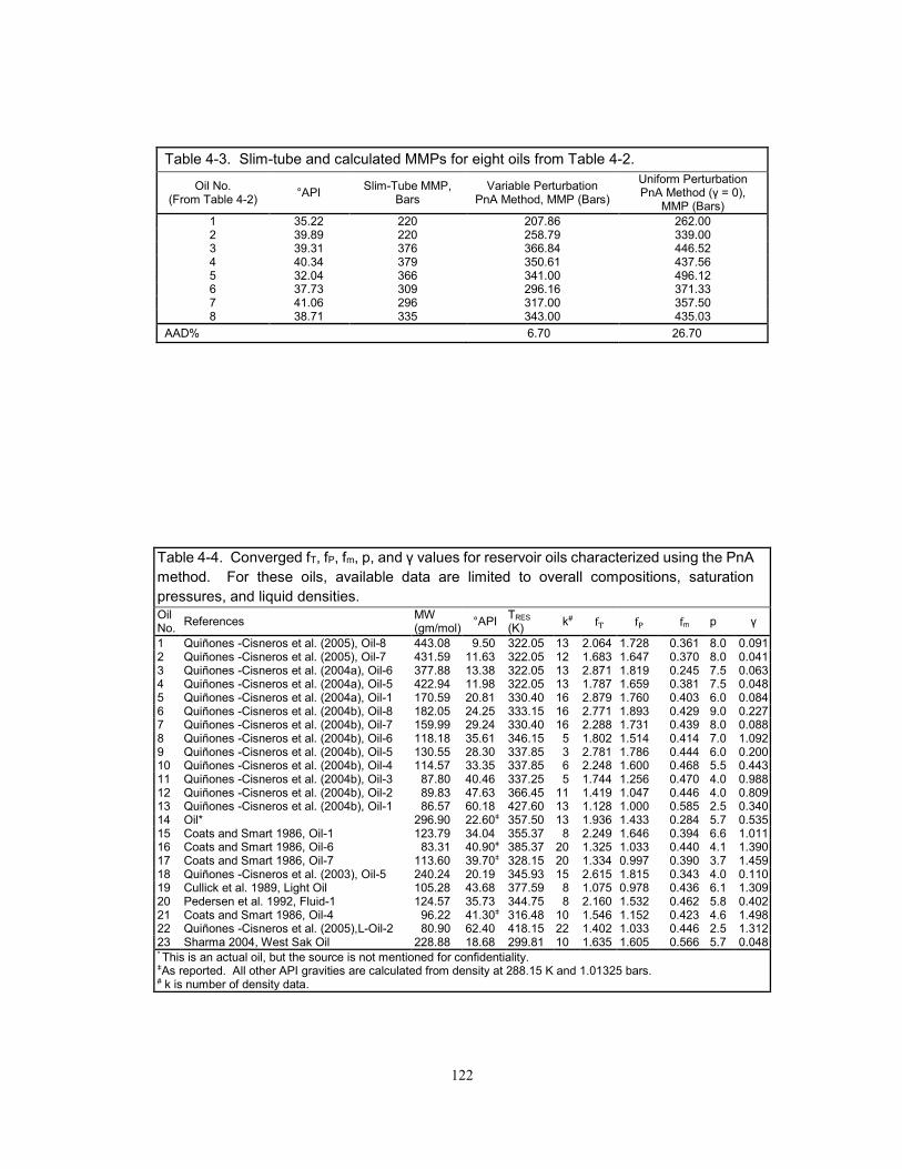
122
Table 4-3. Slim-tube and calculated MMPs for eight oils from Table 4-2.
Oil No. (From Table 4-2)
°API Slim-Tube MMP,
Bars Variable Perturbation
PnA Method, MMP (Bars)
Uniform Perturbation PnA Method (γ = 0),
MMP (Bars)
1 35.22 220 207.86 262.00 2 39.89 220 258.79 339.00 3 39.31 376 366.84 446.52 4 40.34 379 350.61 437.56 5 32.04 366 341.00 496.12 6 37.73 309 296.16 371.33 7 41.06 296 317.00 357.50 8 38.71 335 343.00 435.03
AAD% 6.70 26.70
Table 4-4. Converged fT, fP, fm, p, and γ values for reservoir oils characterized using the PnA
method. For these oils, available data are limited to overall compositions, saturation
pressures, and liquid densities.
Oil No.
References MW (gm/mol)
°API TRES (K)
k# fT fP fm p γ
1 Quiñones -Cisneros et al. (2005), Oil-8 443.08 9.50 322.05 13 2.064 1.728 0.361 8.0 0.091 2 Quiñones -Cisneros et al. (2005), Oil-7 431.59 11.63 322.05 12 1.683 1.647 0.370 8.0 0.041 3 Quiñones -Cisneros et al. (2004a), Oil-6 377.88 13.38 322.05 13 2.871 1.819 0.245 7.5 0.063 4 Quiñones -Cisneros et al. (2004a), Oil-5 422.94 11.98 322.05 13 1.787 1.659 0.381 7.5 0.048 5 Quiñones -Cisneros et al. (2004a), Oil-1 170.59 20.81 330.40 16 2.879 1.760 0.403 6.0 0.084 6 Quiñones -Cisneros et al. (2004b), Oil-8 182.05 24.25 333.15 16 2.771 1.893 0.429 9.0 0.227 7 Quiñones -Cisneros et al. (2004b), Oil-7 159.99 29.24 330.40 16 2.288 1.731 0.439 8.0 0.088 8 Quiñones -Cisneros et al. (2004b), Oil-6 118.18 35.61 346.15 5 1.802 1.514 0.414 7.0 1.092 9 Quiñones -Cisneros et al. (2004b), Oil-5 130.55 28.30 337.85 3 2.781 1.786 0.444 6.0 0.200 10 Quiñones -Cisneros et al. (2004b), Oil-4 114.57 33.35 337.85 6 2.248 1.600 0.468 5.5 0.443 11 Quiñones -Cisneros et al. (2004b), Oil-3 87.80 40.46 337.25 5 1.744 1.256 0.470 4.0 0.988 12 Quiñones -Cisneros et al. (2004b), Oil-2 89.83 47.63 366.45 11 1.419 1.047 0.446 4.0 0.809 13 Quiñones -Cisneros et al. (2004b), Oil-1 86.57 60.18 427.60 13 1.128 1.000 0.585 2.5 0.340 14 Oil* 296.90 22.60ǂ 357.50 13 1.936 1.433 0.284 5.7 0.535 15 Coats and Smart 1986, Oil-1 123.79 34.04 355.37 8 2.249 1.646 0.394 6.6 1.011 16 Coats and Smart 1986, Oil-6 83.31 40.90ǂ 385.37 20 1.325 1.033 0.440 4.1 1.390 17 Coats and Smart 1986, Oil-7 113.60 39.70ǂ 328.15 20 1.334 0.997 0.390 3.7 1.459 18 Quiñones -Cisneros et al. (2003), Oil-5 240.24 20.19 345.93 15 2.615 1.815 0.343 4.0 0.110 19 Cullick et al. 1989, Light Oil 105.28 43.68 377.59 8 1.075 0.978 0.436 6.1 1.309 20 Pedersen et al. 1992, Fluid-1 124.57 35.73 344.75 8 2.160 1.532 0.462 5.8 0.402 21 Coats and Smart 1986, Oil-4 96.22 41.30ǂ 316.48 10 1.546 1.152 0.423 4.6 1.498 22 Quiñones -Cisneros et al. (2005),L-Oil-2 80.90 62.40 418.15 22 1.402 1.033 0.446 2.5 1.312 23 Sharma 2004, West Sak Oil 228.88 18.68 299.81 10 1.635 1.605 0.566 5.7 0.048 * This is an actual oil, but the source is not mentioned for confidentiality. ǂAs reported. All other API gravities are calculated from density at 288.15 K and 1.01325 bars. # k is number of density data.
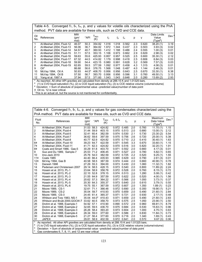
123
Table 4-5. Converged fT, fP, fm, p, and γ values for volatile oils characterized using the PnA
method. PVT data are available for these oils, such as CVD and CCE data.
Oil No.
References MW (gm/ mol)
°API TRES (K)
fT fP fm p γ Data Limits
Value (Type#)
Dev.¥
1 Al-Meshari 2004, Fluid-12 46.07 50.3 354.82 1.018 1.018 0.562 2.3 0.620 38.20 (1) 3.19 2 Al-Meshari 2004, Fluid-13 56.06 36.7 364.82 1.972 1.344 0.437 2.3 0.503 3.93 (3) 0.02 3 Al-Meshari 2004, Fluid-14 54.57 40.7 360.93 1.412 1.188 0.486 2.4 0.555 1.00 (3) 0.01 4 Al-Meshari 2004, Fluid-15 51.11 57.5 353.15 1.106 0.973 0.662 2.9 0.829 2.98 (3) 0.02 5 Al-Meshari 2004, Fluid-16 59.63 55.6 425.93 0.957 0.957 0.525 2.5 0.600 35.30 (1) 2.12 6 Al-Meshari 2004, Fluid-17 67.32 44.5 414.82 1.179 0.998 0.418 2.5 0.806 6.84 (3) 0.03 7 Al-Meshari 2004, Fluid-18 59.90 54.4 423.15 0.980 0.991 0.628 3.2 0.569 7.57 (3) 0.03 8 Al-Meshari 2004, Fluid-19 62.65 59.5 377.59 1.092 0.977 0.458 4.3 1.315 4.06 (3) 0.01 9 Oil* 86.68 56.6 376.75 1.568 1.048 0.487 4.0 1.144 2.46 (3) 0.01 10 McVay 1994, Oil A 50.93 44.5ǂ 408.70 0.956 0.956 0.643 2.5 0.670 33.30 (1) 6.38 11 McVay 1994, Oil B 57.50 56.7 393.70 0.956 0.956 0.596 3.1 0.760 49.50 (1) 3.13 12 Yang et al. 1997.ǂ 37.94 57.5 371.60 1.043 1.043 0.648 2.0 0.280 13.69 (2) 2.93 ǂ As reported. All other API gravities are calculated from density at 288.15 K and 1.01325 bars. # (1) is CVD liquid saturation (%), (2) is CCE liquid saturation (%), (3) is CCE relative volume (volume/volume) ¥ Deviation = Sum of absolute of (experimental value –predicted value)/number of data point ǂ Oil no. 12 is near critical. * This is an actual oil, but the source is not mentioned for confidentiality.
Table 4-6. Converged fT, fP, fm, p, and γ values for gas condensates characterized using the
PnA method. PVT data are available for these oils, such as CVD and CCE data.
Fluid No.
References MW (gm/mol)
°API TRES (K)
fT & fP
fm p γ Maximum
Data Value (Type#)
Dev.¥
1 Al-Meshari 2004, Fluid-3 31.53 58.3 424.82 0.972 0.485 2.0 0.760 11.70 (1) 1.15 2 Al-Meshari 2004, Fluid-4 31.44 59.9 403.15 0.970 0.513 2.0 0.680 13.00 (1) 2.12 3 Al-Meshari 2004, Fluid-5 32.41 60.4 382.59 0.974 0.530 2.1 0.730 23.30 (2) 5.54 4 Al-Meshari 2004, Fluid-7 36.62 59.6 397.59 0.975 0.756 2.6 0.720 25.00 (1) 5.38 5 Al-Meshari 2004, Fluid-8 40.77 62.9 424.82 0.970 0.710 2.2 0.410 30.40 (1) 1.63 6ǂ Al-Meshari 2004, Fluid-10 39.23 64.7 422.59 0.971 0.545 3.3 0.670 33.60 (1) 1.15 7ǂ Al-Meshari 2004, Fluid-11 41.71 62.3 424.82 0.970 0.516 3.0 0.820 32.20 (1) 1.91 8ǂ Coats and Smart 1986, Gas-5 30.29 61.8 403.70 0.971 0.552 2.0 0.660 4.17 (3) 0.01 9 Guo and Du 1989, Sample-7 25.53 71.2 406.45 0.971 0.527 2.0 0.780 5.82 (1) 0.65 10 Imo-Jack 2010 25.76 54.0 382.59 0.972 0.725 2.2 0.520 9.25 (1) 1.55 11ǂ Coats 1985 44.40 66.4 435.93 0.965 0.629 4.0 0.790 2.61 (3) 0.01 12ǂ McVay 1994, Gas B 40.58 58.5 387.59 0.974 0.444 2.0 0.660 40.90 (1) 0.78 13 Danesh 1998 27.29 55.3 394.00 0.973 0.430 2.0 1.060 11.32 (1) 1.82 14 Pedersen and Christensen 2007 29.14 58.5 428.15 0.973 0.540 2.0 0.800 11.89 (2) 2.24 15 Hosein et al. 2013, PL-1 23.64 58.9 358.78 0.972 0.528 2.0 0.760 8.15 (1) 0.72
16 Hosein et al. 2013, PL-2 22.10 52.8 378.15 0.974 0.513 2.0 1.280 5.08 (1) 0.42
17 Hosein et al. 2013, PL-3 21.55 64.9 357.59 0.972 0.622 2.0 0.520 4.00 (1) 1.56 18 Hosein et al. 2013, PL-4 20.62 57.3 364.22 0.971 0.566 2.0 1.050 3.73 (1) 0.37 19 Hosein et al. 2013, PL-5 20.30 64.3 355.37 0.973 0.640 2.0 0.610 3.79 (1) 0.55 20 Hosein et al. 2013, PL-6 19.75 55.1 367.59 0.972 0.607 2.0 1.350 1.89 (1) 0.23 21 Moore 1989, CS-1 32.61 71.1 366.48 0.972 0.690 2.5 0.350 19.90 (1) 5.21 22 Moore 1989, CS-2 35.04 59.7 410.93 0.970 0.659 2.0 0.490 21.60 (1) 2.84 23 Moore 1989, CS-3 24.45 61.4 365.37 0.971 0.721 2.0 0.930 2.17 (1) 0.48 24 Whitson and Torp 1983, NS-1 35.04 44.0ǂ 410.43 0.971 0.659 2.0 0.490 21.60 (1) 2.83 25 Whitson and Brulè 2000,GOCW-7 33.62 60.5 358.70 0.973 0.575 2.5 1.050 23.90 (1) 2.50 26 Drohm et al. 1988, Example-1 54.92 57.1 410.90 0.890 0.572 2.9 0.960 69.81 (1) 8.79 27 Drohm et al. 1988, Example-2 32.65 59.5 436.70 0.975 0.684 2.0 0.530 15.63 (1) 0.96 28 Drohm et al. 1988, Example-3 26.26 58.4 393.20 0.973 0.604 2.0 1.000 4.75 (1) 0.63 29 Drohm et al. 1988, Example-4 28.34 59.0 377.60 0.971 0.586 2.1 0.830 11.84 (1) 0.73 30 Drohm et al. 1988, Example-5 21.27 56.4 377.60 0.970 0.716 2.0 1.340 1.69 (1) 0.43 31 JAPEX 29.81 58.9 402.59 0.972 0.641 2.0 0.570 6.67 (3) 0.06 ǂ As reported. All other API gravities are calculated from density at 288.15 K and 1.01325 bars. # (1) is CVD liquid saturation (%), (2) is CCE liquid saturation (%), (3) is CCE relative volume (volume/volume) ¥ Deviation = Sum of absolute of (experimental value –predicted value)/number of data point ǂ Gas condensates 6, 7, 8, 11, and 12 are near critical
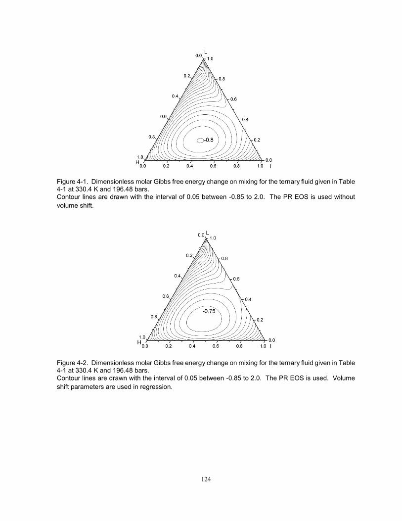
124
Figure 4-1. Dimensionless molar Gibbs free energy change on mixing for the ternary fluid given in Table 4-1 at 330.4 K and 196.48 bars. Contour lines are drawn with the interval of 0.05 between -0.85 to 2.0. The PR EOS is used without
volume shift.
Figure 4-2. Dimensionless molar Gibbs free energy change on mixing for the ternary fluid given in Table 4-1 at 330.4 K and 196.48 bars. Contour lines are drawn with the interval of 0.05 between -0.85 to 2.0. The PR EOS is used. Volume
shift parameters are used in regression.
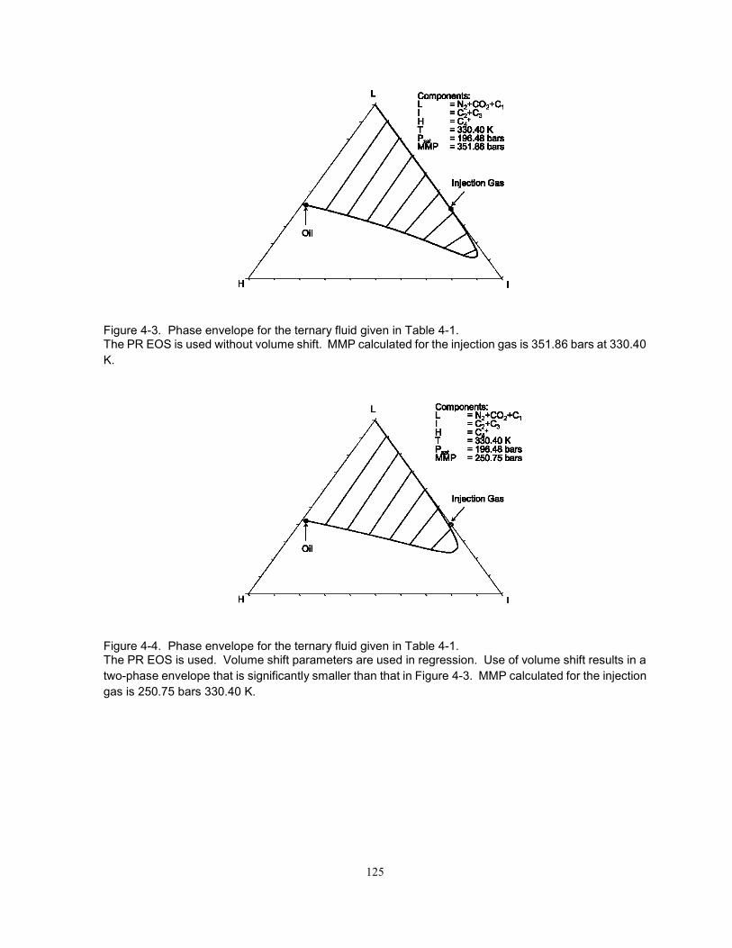
125
Figure 4-3. Phase envelope for the ternary fluid given in Table 4-1. The PR EOS is used without volume shift. MMP calculated for the injection gas is 351.86 bars at 330.40
K.
Figure 4-4. Phase envelope for the ternary fluid given in Table 4-1. The PR EOS is used. Volume shift parameters are used in regression. Use of volume shift results in a
two-phase envelope that is significantly smaller than that in Figure 4-3. MMP calculated for the injection
gas is 250.75 bars 330.40 K.

126
Figure 4-5. Chi-squared distributions for different p values in Equation 4-5. The p parameter controls the degree of skew and the size of effective composition space. A lighter fluid
tends to have a smaller p value. For light fluids, the effective CN (or MW) range is small compared to
heavy oils.
Figure 4-6. Standard specific gravity (SG) calculated for aromaticity levels 10 and 60 using uniform perturbation from n-alkanes. The perturbation was made by matching the standard SG for C7 at the two aromaticity levels given in
Yarborough (1979). Critical parameters are calculated using the correlations of Kumar and Okuno
(2012a). The plots show that the uniform perturbation gives deviation from Yarborough’s trend curves
for higher CN. However, the deviation levels off at a certain CN.
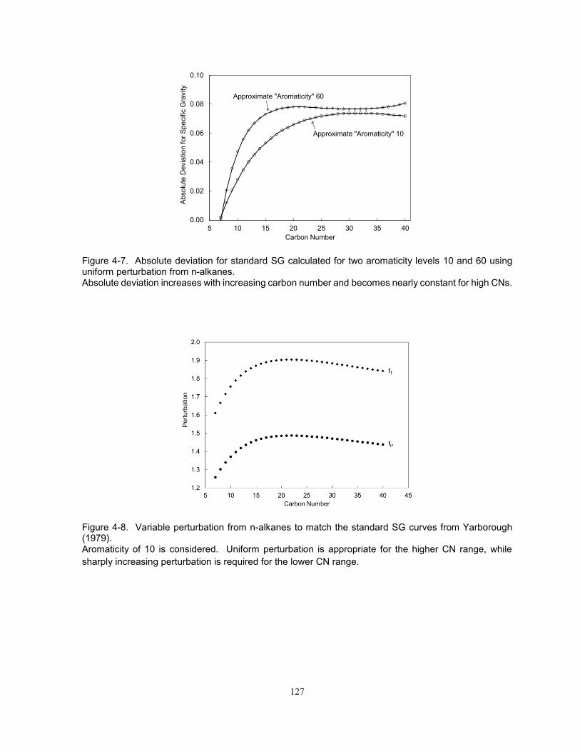
127
Figure 4-7. Absolute deviation for standard SG calculated for two aromaticity levels 10 and 60 using uniform perturbation from n-alkanes. Absolute deviation increases with increasing carbon number and becomes nearly constant for high CNs.
Figure 4-8. Variable perturbation from n-alkanes to match the standard SG curves from Yarborough (1979). Aromaticity of 10 is considered. Uniform perturbation is appropriate for the higher CN range, while
sharply increasing perturbation is required for the lower CN range.
0.00
0.02
0.04
0.06
0.08
0.10
5 10 15 20 25 30 35 40
Absolu
te D
evia
tion for
Specific
Gra
vity
Carbon Number
Approximate "Aromaticity" 60
Approximate "Aromaticity" 10
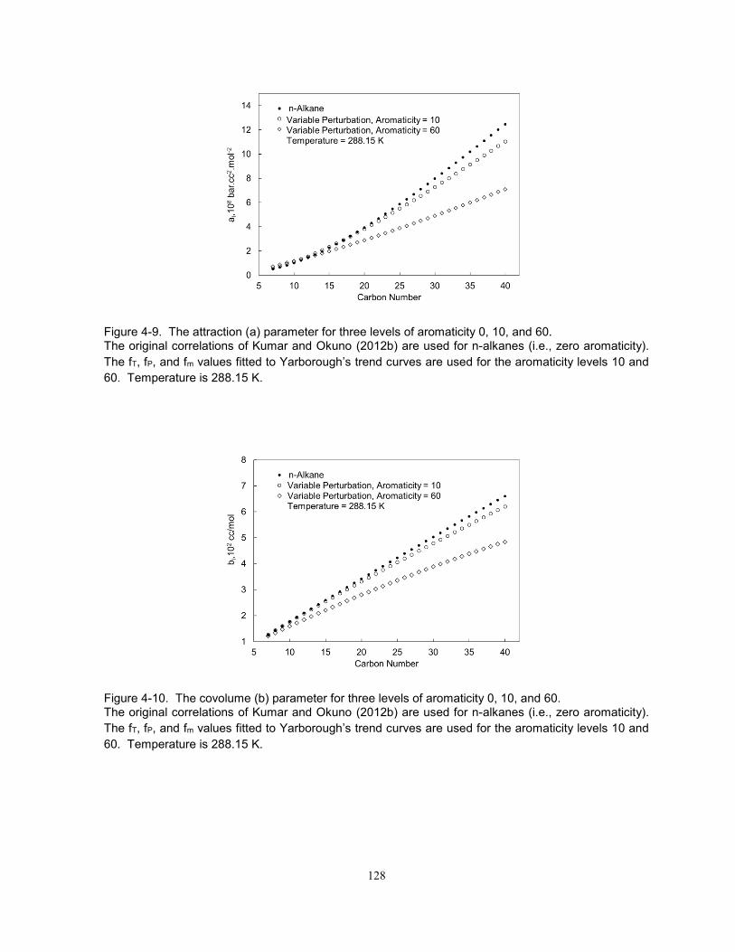
128
Figure 4-9. The attraction (a) parameter for three levels of aromaticity 0, 10, and 60.
The original correlations of Kumar and Okuno (2012b) are used for n-alkanes (i.e., zero aromaticity).
The fT, fP, and fm values fitted to Yarborough’s trend curves are used for the aromaticity levels 10 and
60. Temperature is 288.15 K.
Figure 4-10. The covolume (b) parameter for three levels of aromaticity 0, 10, and 60. The original correlations of Kumar and Okuno (2012b) are used for n-alkanes (i.e., zero aromaticity).
The fT, fP, and fm values fitted to Yarborough’s trend curves are used for the aromaticity levels 10 and
60. Temperature is 288.15 K.

129
Figure 4-11. The ψ parameter (ψ = a/b2) for three levels of aromaticity based on the values for a and b parameters in Figures 4-9 and 4-10. Temperature is 288.15 K. The ψ parameter for each component is calculated using Equation 4-13.
Figure 4-12. The ψ parameter (ψ = a/b2) for three levels of aromaticity at 370.15 K. All critical parameters and acentric factors are the same as in Figures 4-9 and 4-10. The ψ parameter
changes its sensitive to aromaticity around the CN of 20. Trend curves are given for the lighter and
heavier model fluids. For the model trends, the physical trend is also considered that heavier fractions
are relatively more naphthenic and aromatic than lighter fractions.
0.20
0.25
0.30
0.35
0.40
0.45
0.50
5 10 15 20 25 30 35 40
ai/b
i2,1
04
bars
Carbon Number
n-Alkane
Approximate Aromaticity = 10
Approximate Aromaticity =60
Variable Perturbation, Aromaticity = 10Variable Perturbation, Aromaticity = 60Temperature = 370.15 K
Lighter Model Fluid Heavier Model Fluid

130
Figure 4-13. Trends of the fT, fP, fm, and γ parameters during iteration for oil 2 given in Table 4-2. As γ increases from the starting value of zero, fT, fP, and fm decrease. Convergence is achieved when
the rate of increase in γ or the rate of decrease in fT, fP, and fm becomes negligible.
Figure 4-14. Trends of the ε function and the γ parameter during iteration for oil 2 given in Table 4-2. The ε function is defined in Equation 4-12. In our earlier work (Kumar and Okuno 2012a), the ε function
was the stopping criterion in regression. Here, the ε function is not the stopping criterion in regression.
The ε function decreases with increasing γ value, and is sufficiently small on convergence
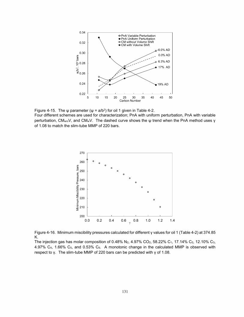
131
Figure 4-15. The ψ parameter (ψ = a/b2) for oil 1 given in Table 4-2. Four different schemes are used for characterization; PnA with uniform perturbation, PnA with variable
perturbation, CMw/oV, and CMwV. The dashed curve shows the ψ trend when the PnA method uses γ
of 1.08 to match the slim-tube MMP of 220 bars.
Figure 4-16. Minimum miscibility pressures calculated for different γ values for oil 1 (Table 4-2) at 374.85 K. The injection gas has molar composition of 0.48% N2, 4.97% CO2, 58.22% C1, 17.14% C2, 12.10% C3,
4.97% C4, 1.66% C5, and 0.53% C6. A monotonic change in the calculated MMP is observed with
respect to γ. The slim-tube MMP of 220 bars can be predicted with γ of 1.08.
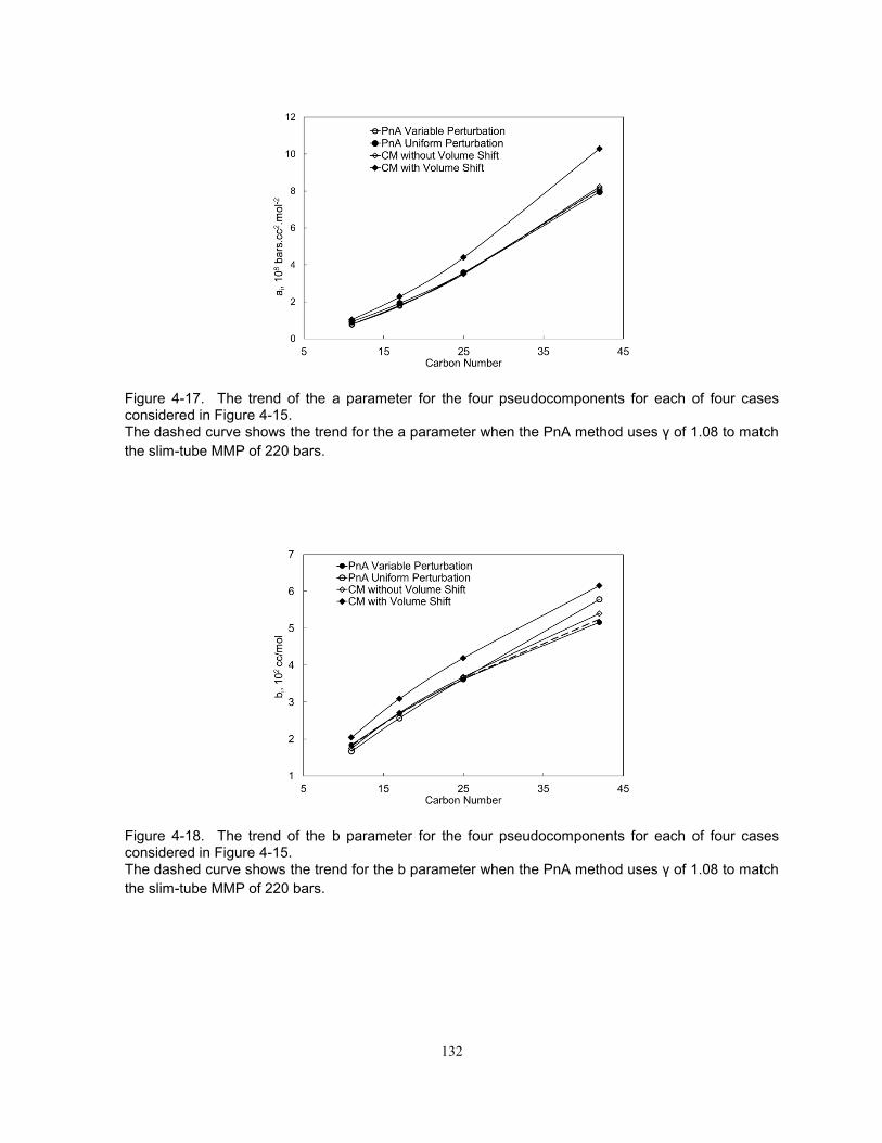
132
Figure 4-17. The trend of the a parameter for the four pseudocomponents for each of four cases considered in Figure 4-15. The dashed curve shows the trend for the a parameter when the PnA method uses γ of 1.08 to match
the slim-tube MMP of 220 bars.
Figure 4-18. The trend of the b parameter for the four pseudocomponents for each of four cases considered in Figure 4-15. The dashed curve shows the trend for the b parameter when the PnA method uses γ of 1.08 to match
the slim-tube MMP of 220 bars.
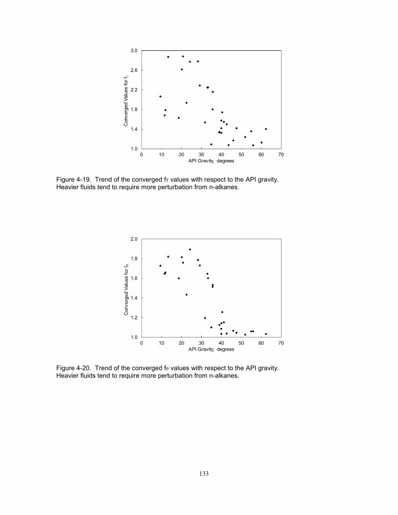
133
Figure 4-19. Trend of the converged fT values with respect to the API gravity. Heavier fluids tend to require more perturbation from n-alkanes.
Figure 4-20. Trend of the converged fP values with respect to the API gravity. Heavier fluids tend to require more perturbation from n-alkanes.
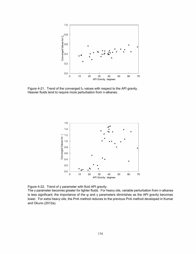
134
Figure 4-21. Trend of the converged fm values with respect to the API gravity. Heavier fluids tend to require more perturbation from n-alkanes.
Figure 4-22. Trend of γ parameter with fluid API gravity. The γ parameter becomes greater for lighter fluids. For heavy oils, variable perturbation from n-alkanes
is less significant; the importance of the ψ and γ parameters diminishes as the API gravity becomes
lower. For extra heavy oils, the PnA method reduces to the previous PnA method developed in Kumar
and Okuno (2012a).
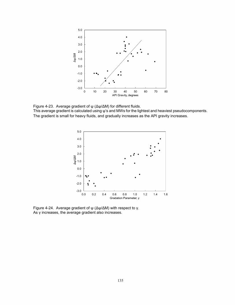
135
Figure 4-23. Average gradient of ψ (Δψ/ΔM) for different fluids. This average gradient is calculated using ψ’s and MWs for the lightest and heaviest pseudocomponents.
The gradient is small for heavy fluids, and gradually increases as the API gravity increases.
Figure 4-24. Average gradient of ψ (Δψ/ΔM) with respect to γ. As γ increases, the average gradient also increases.

136
Figure 4-25. Comparisons of C1-MMPs for 22 oils in Table 4-4 using the PnA method and those from pseudo data. Good agreement is observed except for the API gravity range between 30 and 40. This is attributed to
the discontinuity in the CMw/oV characterization used to generate pseudo data. PVTsim used in the
CMw/oV gives two different characterization options, normal and heavy characterizations, based on an
oil gravity criterion of 30°API.
Figure 4-26. Comparisons of CO2-MMPs for 18 oils in Table 4-4 using the PnA method and those from pseudo data. Good agreement is observed except for the API gravity range between 30 and 40. This is attributed to
the discontinuity in the CMw/oV characterization used to generate pseudo data. PVTsim used in the
CMw/oV gives two different characterization options, normal and heavy characterizations, based on an
oil gravity criterion of 30°API.
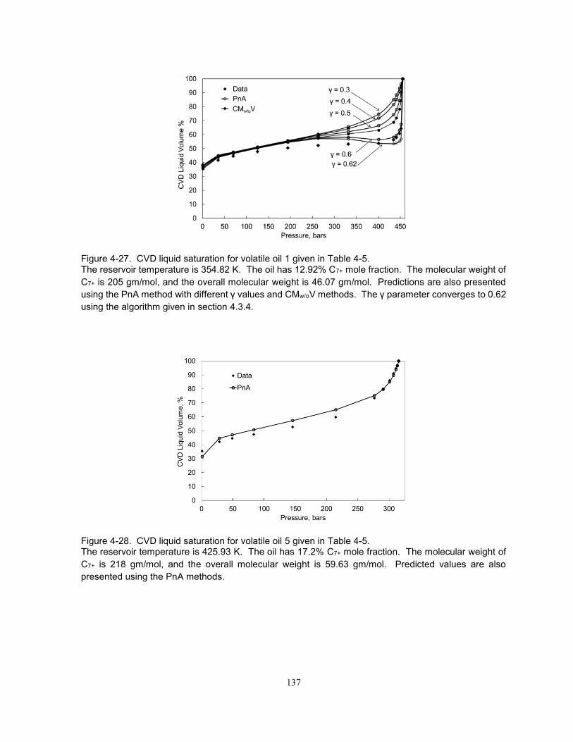
137
Figure 4-27. CVD liquid saturation for volatile oil 1 given in Table 4-5. The reservoir temperature is 354.82 K. The oil has 12.92% C7+ mole fraction. The molecular weight of
C7+ is 205 gm/mol, and the overall molecular weight is 46.07 gm/mol. Predictions are also presented
using the PnA method with different γ values and CMw/oV methods. The γ parameter converges to 0.62
using the algorithm given in section 4.3.4.
Figure 4-28. CVD liquid saturation for volatile oil 5 given in Table 4-5. The reservoir temperature is 425.93 K. The oil has 17.2% C7+ mole fraction. The molecular weight of
C7+ is 218 gm/mol, and the overall molecular weight is 59.63 gm/mol. Predicted values are also
presented using the PnA methods.

138
Figure 4-29. CCE relative volume curve for volatile oil 6 given in Table 4-5. The reservoir temperature is 414.82 K. The oil has 19.0% C7+ mole fraction. The molecular weight of
C7+ is 250 gm/mol, and the overall molecular weight is 67.32 gm/mol. Predicted values are also
presented using the PnA methods.
Figure 4-30. Comparison of the ai and bi parameters for pseudocomponents for volatile oil 1 given in Table 4-5. Characterizations were made using the PnA and CMw/oV methods.

139
Figure 4-31. Comparison of ψ trends for pseudocomponents for volatile oil 1 given in Table 4-5. Characterizations were made using the PnA and CMw/oV methods. The ψ trend for the PnA method
exhibits a combined trend of the two model fluids in Figure 4-12. The CMw/oV method results in the ψ
trend that exhibits a minimum for the second lightest pseudocomponent.
Figure 4-32. CCE liquid saturation for near-critical volatile oil 12 given in Table 4-5. Predicted values are also presented using the PnA method. The reservoir temperature is 371.6 K, and
the critical temperature is 388.1 K. The oil has 9.86% C7+ mole fraction. The molecular weight of the
C7+ fraction is 192.8 gm/mol, and the overall molecular weight is 37.94 gm/mol.

140
Figure 4-33. CVD liquid saturation for gas condensate 20 given in Table 4-6 at 367.6 K. The gas condensate has 1.62% C7+ mole fraction. The molecular weight of the C7+ fraction is 143
gm/mol, and the overall molecular weight is 19.75 gm/mol.
Figure 4-34. CVD liquid saturation for gas condensate 5 given in Table 4-6 at 424.82 K. The gas condensate has 10.87% C7+ mole fraction. The molecular weight of the C7+ fraction is 173.0
gm/mol, and the overall molecular weight is 40.77 gm/mol.

141
Figure 4-35. Trends of ψ for gas condensates 4, 12, 20, and 26 given in Table 4-6. For gas condensates, the CN range of pseudocomponents is narrow. Therefore, ψ trends are increasing
as shown in Figure 4-12. In general, the slope of ψ becomes smaller as the CN range of
pseudocomponents becomes wider.
Figure 4-36. CVD liquid saturation for near-critical gas condensate 7 given in Table 4-6 at 424.82 K. The gas condensate has 12.39% C7+ mole fraction. The molecular weight of the C7+ fraction is 158.23
gm/mol, and the overall molecular weight is 41.71 gm/mol. Predictions are presented using the CMwV
method and the PnA method with different γ values; 0.82, 0.93, 1.00, 1.10, and 1.20. The γ parameter
converges to 0.82 using the algorithm given in section 4.3.4.

142
Figure 4-37. P-T phase envelope for the C7+ fraction using the three fluid models shown in Figure 4-36.
The three models have similar phase behavior for the C7+ fraction. Liquid saturation given in Figure 4-
36 is sensitive to the C7+ phase behavior.
Figure 4-38. Quality lines for near-critical gas condensate 6 given in Table 4-6. Vapor molar phase fractions (β) are shown beside the curves. The calculated critical temperature and
critical pressure are 402.0 K and 339.2 bars, respectively. The reservoir temperature (TRes) and
pressure (PRes) are is 422.6 K and 339.4 bars, respectively.

143
Figure 4-39. CVD liquid saturation for near-critical gas condensate 6 given in Table 4-6 at 422.6 K. The gas condensate has 12.27% C7
+ mole fraction. The molecular weight of the C7+ fraction is 154.93
gm/mol, and the overall molecular weight is 39.23 gm/mol.
Figure 4-40. Oleic phase saturation data and predictions using the PnA method for heavy oil 23 given in Table 4-4 (Sharma 1990) at 299.81 K. This is a mixture of 40% oil and 60% CO2.
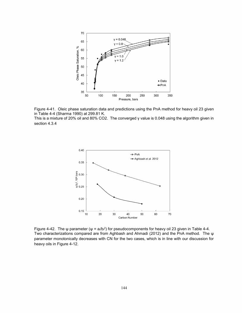
144
Figure 4-41. Oleic phase saturation data and predictions using the PnA method for heavy oil 23 given in Table 4-4 (Sharma 1990) at 299.81 K. This is a mixture of 20% oil and 80% CO2. The converged γ value is 0.048 using the algorithm given in
section 4.3.4
Figure 4-42. The ψ parameter (ψ = ai/bi2) for pseudocomponents for heavy oil 23 given in Table 4-4.
Two characterizations compared are from Aghbash and Ahmadi (2012) and the PnA method. The ψ
parameter monotonically decreases with CN for the two cases, which is in line with our discussion for
heavy oils in Figure 4-12.
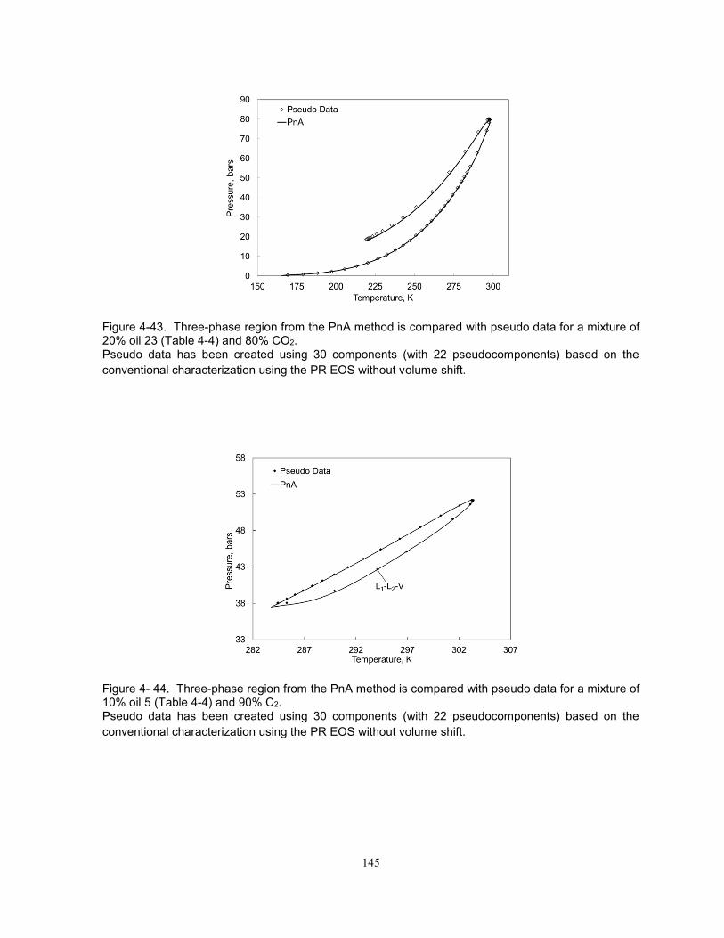
145
Figure 4-43. Three-phase region from the PnA method is compared with pseudo data for a mixture of 20% oil 23 (Table 4-4) and 80% CO2. Pseudo data has been created using 30 components (with 22 pseudocomponents) based on the
conventional characterization using the PR EOS without volume shift.
Figure 4- 44. Three-phase region from the PnA method is compared with pseudo data for a mixture of 10% oil 5 (Table 4-4) and 90% C2. Pseudo data has been created using 30 components (with 22 pseudocomponents) based on the
conventional characterization using the PR EOS without volume shift.
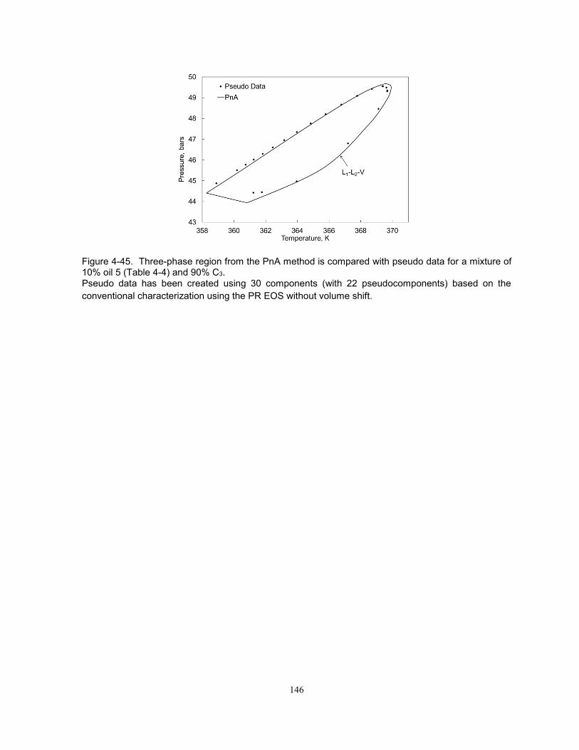
146
Figure 4-45. Three-phase region from the PnA method is compared with pseudo data for a mixture of 10% oil 5 (Table 4-4) and 90% C3. Pseudo data has been created using 30 components (with 22 pseudocomponents) based on the
conventional characterization using the PR EOS without volume shift.
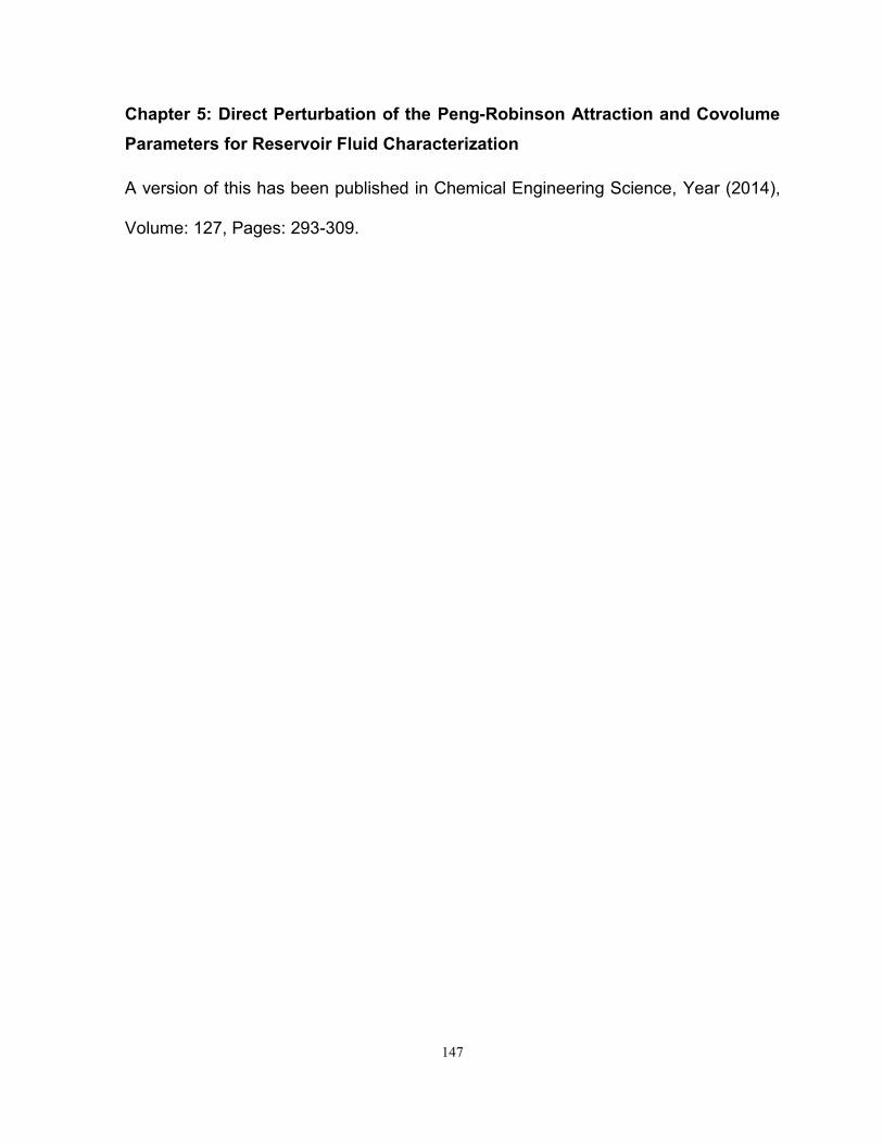
147
Chapter 5: Direct Perturbation of the Peng-Robinson Attraction and Covolume
Parameters for Reservoir Fluid Characterization
A version of this has been published in Chemical Engineering Science, Year (2014),
Volume: 127, Pages: 293-309.

148
5.1. Introduction
The interaction of fluid flow with phase behavior can be significant in many petroleum reservoir
processes, such as hydrocarbon-gas, CO2, and steam injection. Reliable design of these reservoir
processes requires compositional simulation, where the fluid system is characterized using a cubic
equation of states (EOS). Widely used EOSs in the petroleum industry include the Peng-Robinson (PR)
EOS (1976, 1978) and the Soave-Redlich-Kwong (SRK) EOS (1972). These EOSs along with the van
der Waals (vdW) mixing rules, when properly used, give reasonable accuracy and high computational
efficiency (Ikeda and Schaefer 2011).
Reservoir fluids contain a large number of compounds, most of which are non-identifiable. They
are reported as single carbon number (SCN) fractions and a lumped fraction (a plus fraction; e.g., the
heptane-plus fraction or C7+) in a compositional analysis. The uncertainties associated with non-
identifiable compounds are more significant for heavier reservoir fluids because their fractions are
higher. Even for a well-defined series of n-alkanes, for example, critical points are uncertain for carbon
numbers (CNs) higher than 36 (Niktin et al. 1997). Also, different types of hydrocarbons are present
within each SCN fraction, such as paraffins (P), napthenes (N) and aromatics (A). Their concentrations
and critical properties are unknown.
A conventional procedure for reservoir fluid characterization using an EOS is to adjust various EOS-
related parameters to match the experimental data available, such as bubble- and dew-points and
densities. The adjustment parameters often used include critical temperature (TC), critical pressure (PC),
acentric factor (ω), volume-shift parameters, and binary interaction parameters (BIPs). The constant
terms for the attraction (a) and covolume (b) parameters, Ωa and Ωb, are also sometimes used as
adjustment parameters. Since the relationship between these EOS-related parameters and phase
behavior predictions is rather implicit and non-linear, matching the experimental data available does not
always yields a reliable fluid model that is accurate at thermodynamic conditions away from experimental
conditions. This is true especially when many EOS-related parameters are simultaneously regressed
to the available experimental data. Thus, the correlative accuracy of a fluid model does not necessarily
mean the predictive capability.
How phase behavior predictions can be controlled through a cubic EOS is not fully understood in
the literature. Phase behavior predictions using a cubic EOS depend on the attraction (a) and covolume
(b) parameters. When BIPs are used for a mixture, they affect the phase behavior predictions through
the mixing rules used. It is obvious that phase behavior predictions can be controlled more directly by
the attraction and covolume parameters than by TC, PC, and ω. Current practice of reservoir fluid
characterization mentioned above does not effectively utilize the original simplicity of cubic EOSs.
For single-component fluids, various researchers conducted direct adjustment of the attraction and
covolume parameters. Thodos (1955a) estimated the attraction and covolume parameters of the vdW
EOS for n-alkanes using a group contribution method. The approach was later applied to unsaturated
aliphatic, naphthenes, and aromatics (Thodos 1955b, 1956, 1957). Deriving TC and PC from the

149
attraction and covolume parameters is straightforward in this case since the vdW attraction parameter
does not depend on temperature. Tsonopoulos and Wilson (1983), Heidman et al. (1985), Enick et al.
(1987), and Economou et al. (1997) directly adjusted the attraction and covolume parameters of an EOS
to match the vapor pressure and liquid density data for water. They used the Zudkevitch and Joffe
modification of the Redlich-Kwong EOS (Zudkevitch and Joffe 1970). Optimization of components’
parameters to match vapor pressure and liquid density data has been also performed with other types
of EOSs (Voutsas et al. 2006, Aparicio-Martínez and Hall 2006).
Ahmed and Meehan (2010) developed correlations for the attraction and covolume parameters of
the PR EOS for the C7+ fraction as a single component. They generated 49 hypothetical plus-fractions
based on the correlations of Riazi and Daubert (1986) for molecular weight (MW), boiling point (Tb), and
specific gravity (γ). For each fraction, 100 densities were specified in pressure-temperature space. The
attraction and covolume parameters adjusted to match the densities were correlated with MW, Tb, and
γ. Their correlations were recommended for density prediction of crude oil and gas condensate. Their
EOS models exhibited significant improvement in phase behavior predictions for gas condensates and
oils without volume shift. They concluded that splitting of a plus fraction was not required. Although
saturation pressures were matched by adjusting BIPs, their approach was not tested in term of the
predictive capability of compositional phase behavior, such as minimum miscibility pressures, swelling
test, and gas solubilities.
Characterization of a plus fraction using multiple pseudocomponents becomes important when an
EOS model is used not only to predict phase densities, but also to simulate vaporization and
condensation of intermediate components in various enhanced oil recovery processes. To the best of
our knowledge, however, no method has been presented in the literature that directly adjusts the
attraction and covolume parameters of a cubic EOS to characterize volumetric and compositional phase
behavior of petroleum reservoir fluids.
The attraction and covolume parameters have been indirectly adjusted through TC, PC, and ω in
prior characterization methods. This is likely because the attraction and covolume parameters are not
measurable and EOS-specific. However, this is also true for TC, PC, and ω for non-identifiable
compounds in fluid characterization using an EOS. Each of SCNs and plus fractions contains a number
of different compounds, such as the paraffinic, naphthenic, and aromatic compounds, with unknown
concentrations. Furthermore, these fractions are grouped into a few pseudocomponents so that EOS
computations are efficient in reservoir flow simulation. Therefore, apparent properties (e.g., TC, PC, and
ω) of pseudocomponents are only estimated, and even extrapolated for high-CN fractions. It is difficult
to justify the reliability of the estimated critical properties in the absence of measured values. Also, the
parameter values estimated for pseudocomponents are usually adjusted to correlate experimental data
based on the EOS used. Thus, the properties of these components eventually become EOS-specific.
A characterization method was recently presented in our previous publications (Kumar and Okuno
2013) based on the concept of perturbation from n-alkanes (PnA). Instead of attempting to estimate

150
apparent critical properties of pseudocomponents, the PnA method first assigned the
pseudocomponents the optimized TC, PC, and ω values with which the PR EOS gives accurate
predictions of vapor pressures and liquid densities for n-alkanes. Then, they were perturbed from the
n-alkane values in well-defined directions until the saturation pressure and liquid density data at the
reservoir temperature were matched. The perturbation was conducted in the increasing direction for TC
and PC, and in the decreasing direction for ω to make the pseudocomponents gradually more aromatic.
The perturbation also controlled the qualitative trend of the ψ parameter (ψ = a/b2) with respect to CN.
This ensured that the attraction (a) and covolume (b) parameters for each pseudocomponent had proper
interrelationship depending on the CN range of pseudocomponents. Extensive testing of the PnA
method by use of 77 different reservoir fluids showed that various types of phase behavior were
accurately predicted once the saturation pressures and liquid densities were matched.
The PnA method did not require volume shift to match densities for the fluids studied. This is
desirable for the following reasons; i) when used as adjustment parameters, volume shift affects phase
behavior predictions at the thermodynamic conditions that the available PVT data do not cover (Kumar
and Okuno 2013, 2014), and ii) volume shift parameters cannot be canceled out from the fugacity
equations, if the effect of capillary pressures is significant on the equations. The second reason is
becoming important considering the increasing interests in hydrocarbon recovery from tight/shale
reservoirs, where pore geometries affect phase behavior (Schulte 1980; Whitson and Belery 1994;
Nojabaei et al. 2013).
In this research, the PnA method is simplified by directly perturbing the attraction and covolume
parameters, instead of TC, PC, and ω, for reservoir fluid characterization by use of the PR EOS. The
development of the direct PnA method begins by establishing the attraction and covolume parameters
for n-alkanes up to n-C100. The effects of aromaticity on the a, b, and ψ parameters are then discussed.
A new algorithm developed for reservoir fluid characterization controls phase behavior predictions
through direct perturbation of the b and ψ parameters. The algorithm is applied to 84 different reservoir
fluids, for which phase behavior data are available in the literature. Results show the reliability,
robustness, and simplicity of the direct PnA method.
5.2. Attraction and Covolume Parameters for Hydrocarbons
TC, PC, and ω for n-alkanes from n-C7 through n-C100 were optimized in terms of liquid densities and
vapor pressures by use of the PR EOS (Kumar and Okuno 2012). As presented in the Supporting
Information (Section 5-S1), it has been confirmed that the PR attraction and covolume parameters for
n-alkanes based on Kumar and Okuno (2012) are suitable for the direct perturbation in this research.
In the previous PnA method (Kumar and Okuno 2013), the perturbations of TC, PC, and m were
conducted from the n-alkane values towards a higher level of aromaticity to match the saturation
pressure and liquid densities at a given reservoir temperature. This is essentially to perturb the attraction
and covolume parameters from n-alkane values in the direction of increasing level of aromaticity, but
only indirectly. The effect of aromaticity on the parameters and proper interrelationship between the

151
attraction and covolume parameters (Kumar and Okuno 2013) are briefly explained in the Supporting
Information (Section 5-S2). The term “aromaticity” was defined by Yarborough (1979) as the percentage
of total carbon atoms in a molecule, which are within the benzene ring. Yarborough (1979) presented
trend curves for specific gravity at 288.15 K and 1.01325 bars as a function of CN and aromaticity. In
his presentation, CN ranged from 7 to 40, and aromaticity from 0 to 80, as reproduced in the Supporting
Information (Section 5-S2, Figure 5-S12).
In Kumar and Okuno (2013), these trend curves were successfully used to explain how perturbation
of critical parameters (equivalently, the attraction and covolume parameters) should be done for the
different CNs. Details were presented in Kumar and Okuno (2013) and summarized in the Supporting
Information (Section 5-S2). In the current paper, the same knowledge is used to guide the direct
perturbation of the attraction and covolume parameters.
The attraction parameter increases with CN for a fixed aromaticity level (Figure 5-S13). The effect
of aromaticity on the attraction parameter is not systematic; i.e., the attraction parameter increases with
aromaticity for light hydrocarbons, and the trend is the other way around for heavier hydrocarbons. The
trend of the covolume parameter is more systematic (Figure 5-S14). The covolume parameter for n-
alkane is higher than that for aromatic hydrocarbons for a given CN. Also, n-alkanes exhibit the largest
gradient of the covolume parameter with respect to CN. Note that aromaticity should be interpreted as
qualitative deviation from n-alkanes within this research.
One of the most important parameters in the PnA method is ψ (Equation 5-1).
ψ =a
b2 =Ωa
Ωb2 PC(1 + m[1 − (T TC⁄ )0.5])2 (5-1)
on the basis of the PR EOS. The ψ parameter is sensitive to the level of aromaticity for light and
intermediate hydrocarbons (Figure 5-S15). The ψ parameter monotonically decreases with CN for high
aromaticity levels, but exhibits a maximum for low aromaticity levels, including n-alkanes. The ψ
parameter for a fixed CN increases with increasing level of aromaticity, and changes its sensitivity to
aromaticity around CN 20. The ψ parameter is useful in controlling variable perturbation at different
CNs.
5.3. Direct Perturbation of the Attraction and Covolume Parameters
The development of the direct PnA method was motivated by the question as to how many parameters
are required to represent phase behavior of reservoir fluids on the basis of the PR EOS with the vdW
mixing rules. A detailed investigation of phase behavior predictions from the PR EOS has indicated that
the volumetric and compositional phase behaviors are largely determined by the covolume and ψ
parameters, respectively. Also, these parameters for the pseudocomponents of a given fluid can be
controlled systematically by a few adjustment parameters. The objective of this section is to present a
fluid-characterization algorithm that reflects our findings regarding systematic control over phase
behavior predictions through the PR EOS.

152
In the subsequent subsections, a new set of equations is first presented for perturbation of the
covolume and ψ parameters in MW space. Then, a new algorithm is presented that uses the equations
to match experimental data in reservoir fluid characterization.
5.3.1. Equations for Direct Perturbation
Figure 5-S14 in the Supporting Information shows the covolume parameters calculated on the basis of
Equations 5-S8 and 5-S9. The covolume values for n-alkanes can be correlated with MW as shown in
Equation 5-2:
b = –14.6992113939827 + 1.36977232166027(MW) – 9.12089276536298 × 10⁻⁵(MW)2 (5-2)
As shown in Figure 5-S14, the covolume parameter for a given pseudocomponent tends to decrease as
it becomes more aromatic. Also, the effect of aromaticity on the covolume parameter tends to be more
significant for a heavier component. The following equation can accommodate these desired trends with
respect to the fb perturbation parameter (Equation 5-3):
bi = –14.6992113939827 + 1.36977232166027(MW i/mbi) – 9.12089276536298 × 10⁻⁵(MW i/mbi)2
(5-3)
where i is the index for pseudocomponents and mbi = (MW i/86.0)fb. The fb perturbation parameter is
zero for n-alkanes, and increases with increasing level of aromaticity in terms of volumetric phase
behavior. The mbi parameter increases with MW for a given fb value. When a pseudocomponent has a
MW of 86.0, which corresponds to the MW of n-hexane, the mbi parameter is unity regardless of the fb
value applied uniformly to all pseudocomponents within a given fluid.
Figure 5-S15 shows the qualitative trends of the ψ parameters for two model fluids. The lighter
model fluid exhibits an increasing trend, while the heavier model fluid exhibits a decreasing trend with
respect to MW. The indirect PnA method of Kumar and Okuno (2013) resulted in non-linear ψ curves
with respect to MW. However, an extensive testing of the method has indicated that the ψ parameter
can be linear with respect to MW (Equation 5-4) without loss of reliability. Thus,
ψi = g(MW i – MW1) + Cψn1, (5-4)
where MW1 is the MW of the lightest pseudocomponent (i = 1), and g is the gradient of ψ with respect
to MW. Cψn1 represents the ψ parameter for the lightest pseudocomponent as a product of the C
multiplier and the ψ parameter for the lightest pseudocomponent as an n-alkane (ψn1). The value of ψn1
is calculated by use of Equation 5-1 with TC, PC, and m from Kumar and Okuno (2012); that is, MW i and
ψn1 are constants for a given fluid once the compositional characterization is conducted. Then, the ψ
parameter in MW space can be perturbed through g and C.
Perturbation of the ψ parameters is not as straightforward as that of the covolume parameters
through Equation 5-3. This is because the ψ trend depends on the CN range of pseudocomponents,
the level of aromaticity, and temperature. Therefore, a perturbation scheme for ψ has been developed
153
on the basis of a set of the fb, g, and C parameters that were optimized for 74 different reservoir fluids.
Four pseudocomponents were used for their plus fractions as in Kumar and Okuno (2013). The gradient
(i.e., g in Equation 5-4) was represented by the summation of fb and fψ. The C multiplier in Equation 5-
4 was split into two parts; c that is independent of fb, and c’ that is linear with fb with zero intercept.
Out of the 74 fluids, 54 fluids were light, where density data were well represented by fb of zero.
Thus, they behave as n-alkanes in terms of volumetric phase behavior. The C parameters optimized
for these 54 light fluids correspond to the c part, which is considered to represent the effects of the CN
range of pseudocomponents and temperature on the C multiplier. They were correlated with MW1 and
temperature as shown in Equation 5-5:
c = 0.1088[(Tr)1.0405 + (Mr)1.2656] + 0.5825, (5-5)
where Tr is the reservoir temperature (TRES) in Kelvin divided by 277.0, and Mr is MW1 divided by the
MW of n-heptane (100.2 gm/mol). The absolute average deviation (AAD) of Equation 5-5 from the c
values for the 54 fluids is 4.5%. Equation 5-5 does not need to be very accurate since it will be part of
the regression algorithm that has a few adjustable parameters to match experimental data. This is also
true for the c’ part of the C multiplier to be described below.
For the 20 heavier fluids out of the 74 reservoir fluids, fb was positive, representing the effect of
aromaticity on volumetric behavior predictions. To extract the c’ part from the C multipliers optimized
for these 20 fluids, the c values calculated by use of Equation 5-5 were subtracted from the optimized
C multipliers. Then, the resulting c’ part, which is considered to represent the aromaticity effect on the
C multiplier, was correlated as shown in Equation 5-6.
c’ = [1.0998(fb + fψ)/Pr + 0.1763]ZSATfb. (5-6)
ZSAT is the liquid compressibility factor calculated at the experimental saturation pressure (PSAT) at TRES.
Pr is the saturation pressure at TRES under the assumption that the pseudocomponents are n-alkanes,
divided by PSAT. The calculation of Pr requires the PR EOS with TC, PC, and m from Kumar and Okuno
(2012) and PSAT. Figure 5-1 shows the quality of Equation 5-6 in correlating c’/ZSATfb with (fb + fψ)/Pr.
Although the AAD of Equation 5-6 for the 20 fluids is 35%, it is successfully used in the regression
processes with fb and fψ as will be shown later.
Equation 5-4 is then rewritten as Equation 5-7.
ψi = g(MW i – MW1) + Cψn1 = (fb + fψ)(MWi – MW1) + (c + c’)ψn1 (5-7)
in this research. Obviously, this is only one of many possible ways to use the linear form of the ψ
parameter in MW space. Equations 5-3 and 5-7 are simple, but flexible enough for perturbation of the
fb, g, and C parameters in reservoir fluid characterization as presented in the next subsection.
A single value is assigned to each of the perturbation parameters fb, g, and C for a given fluid.
However, the different levels of aromaticity for different components within a fluid have been considered

154
in the development of Equation 5-3 for covolume by using mbi. As shown in the Supporting Information
(Section 5-S2), the aromaticity effect on the attraction parameter through ψ is not as systematic as that
on covolume. As will be also shown in Section 5.4, this is likely because the trend of pseudocomponents’
attraction parameters depends not only on aromaticity, but also on temperature and CNs.
5.3.2. Algorithm
The algorithm presented in this research is kept as simple as possible. The covolume parameters are
perturbed by use of Equation 5-3 through fb. The ψ parameters are perturbed by use of Equation 5-7
through g and C, or through fb, fψ, and c. Note that c is adjustable to some extent because it is not exact
as the C multiplier when fb is zero, as mentioned previously. The data to be matched are the PSAT at
TRES and liquid density data at TRES at different pressures. Other available data are saved for testing
the predictive capability of the resulting fluid models, such as minimum miscibility pressures (MMPs),
and liquid saturation curves from constant volume depletion (CVD) and constant composition expansion
(CCE).
The algorithm consists of two nested loops as shown in the flow chart, Figure 5-A1, in Appendix
5-A. The inner loop is to match the PSAT by adjusting fψ in Equation 5-7 for a set of fb and c given by the
outer loop. The initial value for fψ is zero, and fψ is adjusted by Δfψ per iteration (e.g., Δfψ = 0.0001). The
sign for Δfψ (i.e., + Δfψ or – Δfψ) is negative if the saturation pressure is calculated to be higher than the
experimental value. Otherwise, it is positive.
The outer loop is to match density data by adjusting either c in Equation 5-7 or fb in Equations 5-3
and 5-7. Adjustment of c is first attempted to see if the deviation of density predictions is entirely
attributed to the c correlation (Equation 5-5); that is, fb is always zero when c is adjusted. Adjustment of
c is made by Δc (e.g., Δc = 0.001) in each iteration. The sign for Δc (i.e., + Δc or – Δc) is determined to
make the average deviation (AD) of density predictions smaller. Once the sign is determined in the first
iteration step, it can be kept for the subsequent iteration steps until the AD changes its sign because the
relationship between the density AD and c is monotonic within the range of investigation in this research.
Figure 5-2 shows the monotonic change of the density AD with respect to c for two example cases.
The zero deviation can be obtained by either + Δc or – Δc.
It is not always possible to achieve zero density AD by adjusting c with zero fb. This is because the
covolume parameters should be adjusted for heavy hydrocarbon mixtures, for which the PR EOS tends
to underpredict liquid densities (Søreide 1989; Kumar and Okuno 2014). It has been observed that,
with the fluids examined, c is between 0.75 and 1.20 when the correction of c with zero fb can achieve
zero density AD. If this does not occur, c is overwritten by the original value based on Equation 5-5,
and adjustment of fb is initiated. The initial value for fb is zero, and fb is increased by Δfb per iteration
(e.g., Δfb = 0.0001).
The example values given for ∆fb, ∆c, and ∆fψ in previous paragraphs are sufficient to match the
PSAT and densities. To reduce the number of iterations, however, these values can be made proportional
to the AD during regression.

155
A step-wise description of the algorithm is as follows:
Step 1. Composition characterization
On the basis of the compositional data available, the plus fraction is split into n
pseudocomponents using the chi-squared distribution function. Details can be found in
Quiñones-Cisneros et al. (2004). The i subscript is the index for pseudocomponents; i = 1, 2,
…, n.
Step 2. Calculation of c, Pr, ZSAT, and ψn1
Equations 5-5, 5-6, and 5-7 require c, Pr, ZSAT, and ψn1 to be calculated. The definitions of
these variables were given in subsection 5.3.1.
Step 3. Adjustment of the covolume and ψ parameters for the pseudocomponents
The iteration index is j for fψ and k for fb. j = k = 1.
(1) fb = fψ = 0.0
(2) Calculate the covolume parameters (bi,k) by use of Equation 5-3.
(3) Calculate the ψ parameters (ψi,j,k) by use of Equations 5-6 and 5-7.
(4) Calculate the attraction parameters (ai,j,k) as ai,j,k = ψi,j,k (bi,k)2.
(5) Calculate the saturation pressure (PSATCAL) at TRES. Calculate ε = |PSATCAL – PSAT|/ PSAT. If
ε < εTOL, go to Step 3(6) with j = 1. Otherwise, fψ is adjusted. fψ = fψ + Δfψ if PSATCAL – PSAT
< 0. Otherwise, fψ = fψ – Δfψ. j = j + 1 and go to Step 3(3). εTOL is 0.0001 in this research.
(6) Calculate densities at TRES and the experimental pressures. Calculate the AAD (δ) of the
densities calculated. If δ < δTOL, stop. Otherwise, adjust either c or fb as described earlier
in this subsection; go to Step 3(1) with c = c ± Δc, or Step 3(2) with fb = fb + Δfb, fψ = 0, and
k = k + 1. δTOL is 0.1% in this research.
The algorithm does not require TC, PC, and ω for the pseudocomponents in the fluid model of
interest, in contrast to the indirect PnA algorithm (Kumar and Okuno 2013). The new algorithm took
approximately 3 seconds to conduct characterization of a fluid, while the previous algorithm for the
indirect PnA method took a few minutes. Both algorithms were written in FORTRAN and based on
exhaustive search methods, instead of gradient-based methods. The computations were performed on
the Intel Core i7-960 processor at 3.20 GHz and 8.0 GB RAM. Appendix 5-B describes the approach
to derive TC, PC, and ω from the attraction and covolume parameters for pseudocomponents. This is
useful when one uses commercial software that requires these parameters as input information.
5.3.3. Variation of Phase Behavior during Regression
The direct PnA algorithm systematically controls the attraction and covolume parameters for the
pseudocomponents through fψ and fb, or fψ and c. This subsection shows how two-phase behavior in
P-T space for a given fluid varies with the adjustment parameters during the regression process. Figure
5-3 shows an example for a fluid of 42°API. Curve 1 represents the phase envelope at the initialization
of the algorithm, where fψ and fb are zero. Curve 2 is the phase envelope when PSAT is matched by
adjusting fψ (i.e., densities have not been matched yet). Curve 3 shows the final phase envelope when
156
PSAT and densities are matched, as indicated by the value of δ. Curves 1, 2, and 3 are also compared
with the solid curve that represents the phase envelope when the pseudocomponents are assumed to
be n-alkanes with TC, PC, and ω from Kumar and Okuno (2012). As the regression proceeds, the critical
point becomes higher, and the phase envelope accordingly becomes greater in P-T space.
Figure 5-4 shows a similar example for a light fluid, where densities are matched by adjusting c with
fb = 0.0. Unlike in the previous example, the variation of the critical point is irregular as the regression
proceeds from curve 1 to 3. This may be because this particular fluid behaves as an n-alkane mixture
in terms of volumetric phase behavior, and the effect of aromaticity on two-phase behavior is not as
obvious as the previous example fluid. Nevertheless, curve 3 entirely contains the n-alkane envelope,
as in the previous example. This is the common observation made in all fluids examined so far.
5.4. Case Studies
In this section, the direct PnA method is applied to 84 different reservoir fluids, for which experimental
data are available in the literature. They are 47 gas condensates, 33 conventional oils, and 4 heavy
oils. As mentioned previously, the direct PnA algorithm is to match the PSAT at TRES and liquid densities
at TRES and different pressures using fψ and fb, or fψ and c. Matching of densities tends to be conducted
by c for light fluids, and by fb for heavier fluids. fψ mainly controls compositional phase behavior, which
consequently affects volumetric phase behavior. Available data other than those used in the regression
process are used to test the predictive capability of the resulting fluid models. For example, CVD liquid
saturation data are available for 34 gas condensates and 7 conventional oils. The other 18 conventional
oils have MMP data, one of which is a corrosive volatile oil containing 19% CO2. For the heavy oils
used, swelling test and phase envelope data are available.
For characterization of light fluids with fψ and c, density data for the liquid phase that is equilibrium
with the gaseous phase have been found to be more important than single-phase density data. This is
plausible because the equilibrium liquid phase is richer in heavy components and more aromatic than
the equilibrium gaseous phase and liquid phases in a single-phase region. Capturing the deviation from
n-alkanes in the PnA method is more effective with density data of the denser phase. Therefore,
simulated liquid density data have been created in two-phase regions for the gas condensates and a
few volatile oils on the basis of the fluid models with optimized g and C (see Section 5.3.1). These
optimized models accurately reproduce measured single-phase density data with an AAD of less than
1%; that is, the consistency has been retained between the measured and simulated density data for
each of these light fluids.
The number of components is 12 throughout this research, four of which are pseudocomponents
for C7+. The others are N2, CO2, C1, C2, C3, C4, C5, and C6, where grouping of n- and i-alkanes is based
on the conventional mass-based mixing rule (Pedersen and Christensen 2007). Unless otherwise
stated, the BIPs are kept constant as described in Kumar and Okuno (2014); 0.0 for N2-CO2, 0.1 for N2-
Ci, where 1 ≤ i ≤ 6, 0.13 for N2-pseudocomponents, 0.1 for CO2-hydrocarbons, and 0.0 for all
hydrocarbon-hydrocarbon pairs.
157
The converged values for fψ and fb are listed for all tested fluids in separate tables as will be
discussed later. fb is representative of the aromaticity level; it is zero for n-alkanes and increases with
increasing aromaticity level. Figure 5-5 presents the overall trend that the converged fb tends to
increase with increasing specific gravity of the fluid characterized. However, such a clear trend is not
observed for fψ. This is because it controls g and C through Equations 5-6 and 5-7, which are dependent
on temperature, aromaticity, and the MW range.
5.4.1. MMP Calculation
The direct PnA method has been applied to characterize the 18 oils given in Table 5-1. MMP data are
available for these oils in the literature. For fluids 14, 16, and 17 in Table 5-1, MMPs with multiple
injection gases were measured. This subsection compares MMPs calculated by the fluid models from
the direct PnA method with the corresponding MMP data. This serves as a severe test of the predictive
capability of the direct PnA method since an MMP is affected by phase behavior in a wide region of
composition space between the oil and injection gas compositions (Egwuenu and Johns 2008). The
PnA method uses the PSAT and liquid densities at TRES only at the composition of the fluid characterized.
Thus, MMPs calculated in this subsection are predictions from the fluid models developed based on the
limited data at a point in composition space.
The gravities of the 18 oils range from 31°API to 61°API. Table 5-1 shows the converged values
for fψ and fb. The slope of the ψ parameters with respect to MW is g = fψ + fb as given in Equation 5-7.
Table 5-1 presents positive slopes except for Fluid 9. The negative slope of Fluid 9 is expected since
only one of the pseudocomponents is in the CN range less than 20 (see Figure 5-S15, and Kumar and
Okuno 2013).
MMP calculations were performed by use of the PVTsim version 19.2 (PVTsim 2010) and PennPVT
(Ahmadi and Johns 2011) software. The calculations with PVTsim based on the method of
characteristics were unsuccessful for Fluids 10, 11, 16, and 18. The mixing-cell method within PennPVT
was used for these fluids and Fluid 17. AADs of the calculated MMPs are listed in Table 5-1. Table 5-
2 presents ADs for all injection gases for Fluid 17. For the cases given in Tables 5-1 and 5-2, the
calculations resulted in an overall AAD of 6.4%, which is reasonable considering uncertainties such as
the effect of dispersion on the experimentally determined MMPs. Adjustment of BIPs can improve the
calculated MMPs especially when non-hydrocarbon components are present at high concentrations.
This will be discussed in Section 5.5.
5.4.2. Gas Condensates
Table 5-3 presents the 47 gas condensates tested, for which MWs range from 19.75 g/mol to 54.92
g/mol. Gas condensates 6, 7, 8, 11, 12, 36, and 38 are near critical at their reservoir conditions. The
regression was conducted by fψ and c with zero fb for all the gas condensates. The values listed as Δc
are the adjustments in c required to match density data. The pseudocomponents of these gas
condensates are in a relatively low CN range between 7 and 30. Therefore, positive slopes of ψ with
158
respect to MW are observed for 42 gas condensates in Table 5-3. Note that g = fψ + fb = fψ since fb is
zero for these fluids.
Data types available for the gas condensates are indicated as 1 for CVD liquid saturations, 2 for
CCE liquid saturations, and 3 for CCE relative volumes. The maximum value in these experimental data
is listed for each of the gas condensates. For example, Figure 5-6 shows CVD liquid saturations
measured for gas condensate 12 at 387.59 K. It is zero at the dew point of 333.0 bars. The maximum
value, 40.90, at 283.7 bars is the value listed for this gas condensate in the second right-most column
of Table 5-3. Figure 5-6 shows that the predictions from the resulting fluid model are in good agreement
with the data. The AAD is calculated to be 0.94 for this case, which is listed in the right-most column of
Table 5-3. Figure 5-6 also presents the CVD liquid volume predictions with the conventional
characterization method based on Pedersen and Christensen (2007), in which volume shift is used to
correct density predictions. This conventional method with volume shifting is referred to as CMwV, which
were described in detail in Kumar and Okuno (2014). The AAD for CMwV with 12 components is 1.9%
for Figure 5-6.
Figure 5-7 depicts the CCE liquid saturations measured for gas condensate 3 at 382.59 K. The
data indicate that the CCE liquid volume first increases gradually, and then decreases with decreasing
pressure. The predictions from the EOS fluid model are reasonably accurate, although the deviation at
289.57 bars is relatively large. The AAD is 1.71% with the direct PnA method and 3.7% with CMwV.
Accurate predictions of volume ratios in CVD and CCE require accurate predictions of both
compositional and volumetric phase behavior. The AADs summarized in Table 5-3 indicate that the
fluid models developed by the direct PnA method are reasonable in predicting gas condensates.
5.4.3. Volatile Oils
The direct PnA method has been used to characterize the 15 volatile oils given in Table 5-4. Oils 10,
12, and 14 are near critical at their reservoir conditions. As mentioned previously in this section,
simulated density data for the equilibrium liquid phase were used in the regression for oils 1, 5, 10, 11,
13, 14, and 15. The regression resulted in positive slopes of ψ with respect to MW for all cases except
for oil 12 as indicated in Table 5-4.
Three types of data available for these oils are given in the second right-most column as 1 for CVD
liquid saturations, 2 for CCE liquid saturation, and 3 for CCE relative volumes. This column also shows
the measured value at the lowest measured pressure for each fluid. The fluid models developed based
on the direct PnA method are able to accurately predict the measured phase behavior. The right-most
column of Table 5-4 indicates the AAD for each fluid. The predicted CCE relative volumes are nearly
perfect. The AADs for CVD liquid saturations are relatively large. However, their overall AD is only
1.4%. As a sample result, Figure 5-8 gives the comparison between the measured and predicted CVD
liquid saturations for near-critical volatile oil 14 at 424.25 K. The value, 42.20, at the lowest measured
pressure is listed in the second right-most column for this oil in Table 5-4. The critical point was
measured at 426 K and 388 bars, but it is calculated to be 433.00 K and 389.95 bars by the fluid model
159
based on the PnA method. Although the calculated TC is 7 K higher than the measured TC, the CVD
liquid saturations are accurately predicted. Figure 5-8 also shows the predictions from CMwV. The
critical point calculated with CMwV is 437.43 K and 393.18 bars. The two methods are reasonably
accurate for this case.
5.4.4. Heavy Oils
Four different heavy oils have been characterized by use of the direct PnA method. As shown in Table
5-5, their API gravities are 19°, 28°, 11°, and 11° for heavy oils 1 to 4, respectively. Heavy oil 2 was
classified as a heavy oil on the basis of the definition of Pedersen and Christensen (2007). The heaviest
oil considered in this paper is heavy oil 4 with a MW of 482, and the p value in Equation 5-S11 is as high
as 9.0 for this oil. Table 5-5 shows that the slope of ψ with respect to MW is negative for this heavy oil.
For heavy oil 1, swelling test data are available for two mixtures at 299.81 K; 60% CO2 and 40% oil,
and 80% CO2 and 20% oil. Figure 5-9 presents predictions of the oleic phase saturation in comparison
with the corresponding data for the latter mixture. The AAD for this mixture is 5.2% with the direct PnA
method and 6.15% with CMwV. For pressures higher than 100 bars, the AAD is 2.71% with the direct
PnA method and 6.71% with CMwV. For the former mixture, the AAD with the direct PnA method is
2.2%. CMwV erroneously predicts a single liquid phase at the highest and second highest pressures.
For the lower pressures, the AAD with CMwV is 5.89%.
For heavy oil 2, saturation pressures measured in swelling tests with CO2 and a light gas mixture
are considered. Figure 5-10 compares the predictions with the data presented in Kredjbjerg and
Pedersen (2006). The AAD is 3.9% for the CO2 case and 2.8% for the gas mixture case with the direct
PnA method. With CMwV, it is 5.7% for the two injection gases. For heavy oil 3, gas-oil-ratio (GOR)
data are available at the reservoir temperature 305.45 K. Figure 5-11 shows that the fluid model based
on the direct PnA method can accurately predict the GOR for this case. The deviation is relatively high
only near the saturation pressure. The AAD is calculated to be 2.9%. The predictions with CMwV are
close to those from the direct PnA method in this case.
For heavy oil 4, the regression in the direct PnA method used the PSAT of 56.64 bars at 347.67 K for
the live oil reported (Feed #5 in Li et al. 2013a). Density data for this live oil were unavailable, and,
therefore, generated on the basis of the EOS model given by Li et al. (2013a). Figure 5-12 presents
saturation pressures measured at different temperatures for two mixtures (Feeds #4 and #5 in Li et al.
2013a). Feed #4 is 38.6% CO2, 36.2% C3, and 25.2% heavy oil 4 on the molar basis. Feed #5 is 31.7%
CO2, 34.3% n-C4, and 34.0% heavy oil 4. The fluid model developed by the direct PnA method is
reasonably accurate in predicting the saturation pressures in spite of the uncertainties due to the
simulated density data that were not validated against any data. The AAD of the saturation pressure
predictions is 13.7% for Feed #4 and 6.0% for Feed #5. If the BIPs for CO2 with the pseudocomponents
are altered from 0.10 to 0.15, the AAD is reduced to 7.6% for Feed #4 and to 0.4% for Feed #5.
Li et al. (2013b) presented P-T conditions for three-phase behavior for the mixture of 83.2% CO2,
11.8% n-C4, and 5.0% heavy oil 4 on the molar basis (Feed #15 in Li et al. 2013b). Figure 5-13

160
compares the predicted phase boundaries with the data points given in Li et al. (2013b). Although the
lower pressure boundary is overestimated, the higher pressure boundary is predicted quite accurately
with no further adjustment of the fluid model from the direct PnA algorithm.
5.5. Discussion
The direct PnA method is simpler than the previous PnA method (Kumar and Okuno 2013), but exhibits
equivalent or improved predictive capability. For example, the previous PnA method resulted in an AAD
of 6.7% in MMP calculation for 8 fluids tested in Kumar and Okuno (2013), which is higher than the AAD
of 6.4% obtained for MMPs of the cases given in Tables 5-1 and 5-2 (see Section 5.4.1). The AAD for
CVD liquid saturation for 34 gas condensates (data type 1 in Table 5-3) was 1.06% using the direct PnA
method, but it was 1.8% for 27 gas condensates tested in Kumar and Okuno (2013). The AAD for CVD
liquid saturation for volatile oils calculated with the direct PnA method was 2.7% (data type 1 in Table
5-4), but it was 3.7% for 4 fluids tested in Kumar and Okuno (2013). The oleic phase saturations
calculated for the swelling test for the West Sak heavy oil showed the AAD of 3.6% with the direct PnA
method (see Table 5-5) and 4.1% with the previous PnA method (Kumar and Okuno 2013). In the
preceding section, the improved predictions with the direct PnA method were also shown in comparison
with CMwV (Figures 5-6 to 5-11).
In this section, a few fundamental aspects of the direct PnA method are discussed. Section 5.5.1
discusses systematic control of phase behavior predictions through Equation 5-7. Section 5.5.2
presents the advantage of the optimized critical parameters (Equations 5-S8, 5-S9, and 5-S10) over
estimated physical critical parameters for n-alkanes in reservoir fluid characterization. Section 5.5.3
discusses adjustment of BIPs with the direct PnA method.
5.5.1. Systematic Control of Phase Behavior Predictions
The unique feature of the direct PnA method is that it systematically controls phase behavior predictions
through three key parameters. As discussed in section 5.3, fb is able to monotonically change volumetric
phase behavior predictions from the PR EOS through Equation 5-3. The ψ parameter as a linear
function of MW is adjusted by g and C in Equation 5-7, which controls compositional phase behavior
predictions. These three key parameters, fb, g, and C, are not component-specific, and applied to all
pseudocomponents for the fluid of interest. This is the fundamental reason for the systematic control of
phase behavior predictions in the direct PnA method.
In the algorithm presented in the current paper, a mechanism was developed for adjustment of g
and C through fψ for a given fb, or for a given c in characterization of light fluids for which fb is zero.
However, it is also possible to control compositional phase behavior predictions by adjusting C, which
uniquely gives a corresponding value for g through the constraint ε < εTOL; matching of PSAT for the fluid
of interest. This is useful to match other phase behavior data, such as CVD liquid saturations and
MMPs.

161
Figure 5-14 presents CVD liquid saturations predicted with different values for C for gas condensate
6 in Table 5-3. Note that C is equal to c for this fluid because fb is zero. A monotonic variation of the
CVD liquid saturation curve with the C parameter is evident in the figure. An optimum value for C, which
is 0.91 in this case, is easy to find because of the monotonic, systematic change of the CVD liquid
saturation curve.
Figure 5-15 shows MMPs calculated with different C values for oil 1 in Table 5-1. The calculated
MMP decreases monotonically with decreasing C. It is not difficult to find the value for C with which the
measured MMP is matched.
5.5.2. Phase Behavior Predictions in Composition Space with Optimized Critical
Parameters
In the PnA methods of Kumar and Okuno (2013) and in this research, the initializations of the attraction
and covolume parameters are based on the TC, PC, and m parameters optimized for n-alkanes by use
of the PR EOS (Equations 5-S8, 5-S9, and 5-S10). The differences from physical critical parameters
estimated by Constantinou and Gani (1994) were discussed in the Supporting Information (Section 5-
S1). In general, the optimized critical parameters tend to be higher than estimated physical values for
n-alkanes; e.g., the sets of critical parameters from Constantinou and Gani (1994) and Gao et al. (2001).
The higher critical parameters result in extended two-phase lines in P-T space for pure components. To
show the effect of the higher critical parameters on phase behavior predictions in composition space,
Kumar and Okuno (2012) compared bubble- and dew-point predictions for n-alkane binaries by using
two sets of critical parameters; i.e., the optimized parameters from Kumar and Okuno (2012) and the
estimated physical parameters from Gao et al. (2001). BIPs were set to zero for systematic
comparisons. Predictions of bubble- and dew-points for nine n-alkane binaries were closer to
experimentally measured data points when the optimized parameters were used. It was also shown
that critical points of three n-alkane binaries (n-C6 with n-C16, n-C24, and n-C36) were more accurately
predicted by use of the optimized parameter set.
This subsection gives further comparisons of phase behavior predictions for more than two
components by using the optimized parameters of Kumar and Okuno (2012) and the physical parameter
estimated by Constantinou and Gani (1994). For both cases, BIPs for hydrocarbon pairs are set to zero
for systematic comparisons. Figure 5-16 presents the two-phase envelopes predicted with the two sets
of critical parameters for an n-alkane mixture consisting of 44.0% C1, 45.8% n-C10, 6.8% n-C18, and
3.4% n-C30. The bubble-point data were taken from Daridon et al. (1996). The two-phase envelope is
predicted to be greater in P-T space when the optimized parameters are used. This is in line with the
comparisons made for n-alkane binaries in Kumar and Okuno (2012). The PR EOS with the optimized
critical parameters gives more accurate predictions in composition space than with the estimated
physical critical parameters.
Figure 5-17 shows saturation pressure predictions in a swelling test for a 25-component oil with a
gas at 373.15 K presented in Danesh et al. (1991). The oil consists of 90.68% n-alkanes from C1 through
162
n-C20, 0.72% toluene, 1.79% xylene, 2.20% cyclo-hexane, 2.25% methyl-cyclo-pentane, and 2.36%
methyl-cyclo-hexane. The injection gas consists of 69.82% C1, 13.09% C2, 11.10% C3, and 5.99% n-
C4. The AAD of the saturation pressure predictions is 11% when the physical parameter set is used,
whereas it is 4% with the optimized parameter set.
Figure 5-18 depicts the two-phase envelopes predicted in composition space for a ternary system
of CO2, C3, and n-C20 at 338.65 K and 69.92 bars. Experimental data were taken from Al-Marri (2006).
As recommended by Peng and Robinson (1978), 0.10 is used for the BIPs of CO2 with the n-alkanes.
The optimized parameter set results in more accurate predictions of two-phase equilibrium for the n-
alkane mixtures containing CO2. When the CO2 BIPs are set to 0.0, the two-phase region is predicted
to be smaller in composition space.
The results presented in this subsection show that the PR EOS gives reasonably accurate
predictions for n-alkane mixtures even with zero BIPs when the optimized set of critical parameters is
used. When non-zero BIPs are required for CO2-n-alkane mixtures, required deviations from zero are
smaller with the optimized critical parameters than with estimated physical critical parameters. However,
these results are limited by the availability of experimental data. Note that the optimized critical
parameters were developed for use in reservoir fluid characterization, as described in this paper and
Kumar and Okuno (2012, 2013). If they were used for pure n-alkanes with the PR EOS, the altered
critical points would give extended vapor-pressure curves for heavy n-alkanes, as shown in Figure 5-
S1.
5.5.3. Adjustment of BIPs
The extensive testing of the PnA methods of Kumar and Okuno (2013) and in this research has indicated
that the PR EOS gives satisfactory predictions of reservoir fluid phase behavior with zero BIPs for all
hydrocarbon pairs. Recommended values have been used for non-hydrocarbon components, such as
N2 and CO2, as constants (Peng and Robinson 1978). However, these default BIPs may be adjusted
especially for non-hydrocarbon components with pseudocomponents.
Figure 5-19 shows saturation pressures measured in the swelling test of Fluid 18 (Table 5-1) with
CO2 at 394 K (Negahban et al. 2010). The experimental MMP for this oil with CO2 is 178 ± 2 bars at
394 K. The fluid model developed based on the direct PnA method gives an MMP of 188 bars with the
default BIPs of CO2 with pseudocomponents as 0.10. Although it correctly predicts the transition from
bubble- to dew-point at CO2 concentration of 0.69, this fluid model gives progressively higher saturation
pressures than the experimental values with increasing CO2 concentration. When the BIPs of CO2 with
pseudocomponents are reduced from 0.10 to 0.05, the model is much improved in saturation pressure
predictions as shown in Figure 5-19. The MMP predicted is 174 bars, which is still close to the
experimental result.
163
5.6. Conclusions
A new method was developed for reservoir fluid characterization that directly perturbs the attraction and
covolume parameters of pseudocomponents from n-alkanes’ values (direct perturbation from n-alkanes,
or direct PnA). The direct PnA method was successfully applied to 84 different reservoir fluids, such as
gas condensates, volatile oils, black oils, and heavy oils. The regression algorithm used only the PSAT
at TRES and liquid densities at TRES at different pressures for each fluid. Other available data, such as
MMPs, liquid saturations in CVD and CCE, and gas solubilities, were used to test the predictive
capability of the fluid models developed by the direct PnA method. The PR EOS with the vdW mixing
rules was used throughout this research. Conclusions are as follows:
o The reservoir fluids tested were reliably characterized by systematic adjustment of the attraction
and covolume parameters of pseudocomponents. The covolume parameters were perturbed from
n-alkane values by fb in Equation 5-3. The fb parameter monotonically changes volumetric phase
behavior predictions. As in our previous research, the ψ (= a/b2) parameter was used to ensure
proper interrelationship between the attraction (a) and covolume (b) parameters. A new approach
to adjustment of the ψ parameters was developed with a linear ψ function of MW. The g and C
parameters in Equation 5-7 control compositional phase behavior predictions in a regular manner
in the regression algorithm presented.
o The three key parameters, fb, g, and C, are not component-specific, and applied to all
pseudocomponents for the fluid of interest. This enables to control phase behavior predictions in a
systematic, monotonic manner in the direct PnA method. The direct PnA method does not require
estimation or extrapolation for apparent critical parameters of heavy fractions, which are mixtures
of non-identifiable compounds.
o The direct PnA method substantially simplifies the characterization of reservoir fluids by use of the
PR EOS. The simplification was possible because of the inherent accuracy and simplicity of the PR
EOS and the adjustment parameters found in this research. The regression process of the PnA
method requires only a few seconds per fluid using a personal computer.
o One of the important data types required for the direct PnA method is liquid densities that capture
the level of aromaticity in the fluid system of interest. Results indicated that densities of equilibrium
liquid phases in a multiphase region are more effective than densities in a single-phase region for
capturing the level of aromaticity in the PnA method.
o No change is required for the functional form of the EOS and mixing rules. The method can be
readily implemented in existing software based on the PR EOS with the vdW mixing rules.
164
5.7. Nomenclature
Roman Symbols
a = Attraction parameter defined in Equation 5-S2
ac = Attraction parameter at a critical temperature defined in Equation 5-S3
α = Temperature dependent parameter defined in Equation 5-S4.
A = Aromatics
b = Covolume parameter defined in Equation 5-S5
c = Parameter defined in Equation 5-5
c' = Parameter defined in Equation 5-6
C = c + c'
fψ = Perturbation factor for the ψ parameters
fb = Perturbation factor for the covolume parameters
fm = Perturbation factor for the m parameters in Equation 5-S10
fP = Perturbation factor for PC in Equation 5-S9
fT = Perturbation factor for TC in Equation 5-S8
mbi = Parameter defined with Equation 5-3
g = Slope of the ψ parameter in MW space
m = Parameter defined in Equations 5-S6 and 5-S7
Mr = Molecular weight of the lightest pseudocomponent divided by 100.20
n = Number of pseudocomponents
N = Napthenes
ei = Objective function for the ith pseudocomponent defined in Equation 5-B4
p = Pressure, bar
P = Paraffins
PC = Critical pressure, bar
Pr = Ratio of the saturation pressure calculated as n-alkanes to PSAT
PSAT = Experimental saturation pressure at reservoir temperature
PSATCAL = Calculated saturation pressure
Pvap = Vapor pressure
R = Universal gas constant
S = Parameter in the chi-squared distribution function given in Equation 5-S11
T = Temperature, K
Tb = Boiling point temperature, K
TC = Critical temperature, K
Tr = T in Kelvin divided by 277.0
TRES = Reservoir temperature
v = Molar volume, gm/mol (Equation 5-S1)
165
VC = Critical volume, gm/mol
Ya = Aromaticity as defined by Yarborough (1979)
ZSAT = Liquid compressibility factor at the saturation pressure at TRES
Greek symbols
ε = Absolute average deviation for saturation pressure calculations
δ = Deviation for density calculations
γ = Standard specific gravity
Γ = Gamma function
ρLS = Saturated liquid density
ρSAT = Density at saturation pressure
Ωa = Constant term (= 0.45723552892138219) in the attraction parameter of the PR EOS
Ωb = Constant term (= 0.0777960739038884574) in the covolume parameter of the PR EOS
ψ = Parameter given by Equation 5-1
ψn1 = Normal-alkane equivalent ψ for the lightest pseudocomponent
ω = Acentric factor
Abbreviations
oAPI = API (American Petroleum Institute) gravity (= 141.5/γ -131.5)
AAD = Average absolute deviation
AD = Average deviation
BIP = Binary interaction parameter
CMwV = Conventional fluid characterization method with volume shifting (Pedersen and
Christensen 2007)
CN = Carbon number
CVD = Constant volume depletion
CCE = Constant composition expansion
CP = Critical point
EOS = Equation of state
GOR = Gas oil ratio
LL = Liquid-liquid
LLV = Liquid-liquid-vapor
LV = Liquid-vapor
MMP = Minimum miscibility pressure, bar
MW = Molecular weight, g/mol
MWavg = Average molecular weight
PC = Pseudocomponent

166
PnA = Perturbation from n-alkanes
PR = Peng-Robinson
P-T = Pressure –temperature
SCN = Single carbon number fraction
SRK = Soave-Redlich-Kwong
Tol. = Tolerance
vdW = van der Waals
Subscripts
i = Index for pseudocomponents
j = Index for the iteration loop for matching the saturation pressure by adjusting fψ
k = Index for the iteration loop for mating densities by adjusting fb

167
5.8. References
Ahmed, T. and Meehan, D. N., 2010. A Practical Approach for Calculating EOS Coefficients. Presented
at SPE Russian Oil & Gas Technical Conference and Exhibition held in Moscow, Russia, 26-28 Oct.
SPE-132455-MS
Ahmadi, K. and Johns, R.T. 2011. Multiple Mixing-Cell Model for MMP Determination. SPE J. 16 (4):
733-742.
Al-Ajmi, M.F., Tybjerg, P., Rasmussen, C.P. et al. 2011. EoS Modeling for Two Major Kuwaiti Oil
Reservoirs. Presented at the SPE Middle East Oil and Gas Show and Conference, Manama,
Bahrain, 25-28 Sept. SPE-141241-MS.
Al-Marri, S.S. 2006. PVT, Phase Behavior and Viscosity Measurements and Modeling of the Ternary
and Binary Systems of Carbon Dioxide +Heavy Hydrocarbon (n-Eicosane) + Light Gas (Ethane or
Propane). PhD. Dissertation, University of Southern California, USA.
Al-Meshari, A. 2004. New Strategic Method to Tune Equation of State to Match Experimental Data for
Compositional Simulation. PhD dissertation. Texas A&M University, Texas. USA.
Al-Subai, K.O., 2001. Compositional Gradient Calculations for a Saudi Arabian Gas Condensate
Reservoir. M.Sc. Thesis. King Fahd University of Petroleum & Minerals, Saudi Arabia.
Ambrose, D., 1978. Correlation and Estimation of Vapour-Liquid Critical Properties. I: Critical
Temperatures of Organic Compounds. NPL Technical Report. Chem. 92, (Nat. Physical Lab.,
Teddington, UK, 1978).
Ambrose, D. and Tsonopoulos, C. 1995. Vapor-Liquid Critical Properties of Elements and Compounds.
2. Normal Alkanes. J. Chem. Eng. Data 40 (3): 531-546.
Anselme, M.J., Gude, M., and Teja, A.S., 1990. The Critical Temperatures and Densities of the n-
Alkanes from Pentane to Octadecane. Fluid Phase Equilib. 57 (3): 317-326.
Aparicio-Martínez, S. and Hall, K.R., 2006. Phase Equilibria in Water Containing Binary Systems from
Molecular Based Equation of State. Fluid Phase Equilib. 254 (1-2): 112-125.
PVTsim, 19.2, 2010. Calsep International Consultants, Copenhagen, Denmark.
Clark, P., Toulekima, S., Sarma, H., 2008. A Miscibility Scoping Study for Gas Injection into a High-
Temperature Volatile Oil Reservoir in the Cooper Basin, Australia. Presented at the SPE Asia
Pacific Oil and Gas Conference and Exhibition, Perth, Australia. 20-22 Oct.
Coats, K.H. 1985. Simulation of Gas Condensate Reservoir Performance. J Petrol Tech 37 (10): 1870-
1886.
Coats, K.H. and Smart, G.T. 1986. Application of a Regression Based EOS PVT Program to Laboratory
Data. SPE Res Eng 1 (3): 277-299.
Constantinou, L. and Gani, R., 1994. New Group Contribution Method for the Estimating Properties of
Pure Compounds. AIChE J. 40 (10): 1697-1710.
168
Constantinou, L., Gani, R., and O’Connell, J.P. 1995. Estimation of the Acentric Factor and the Liquid
Molar Volume at 298 K Using a New Group Contribution Method. Fluid Phase Equilib. 103 (1): 11-
22.
Danesh, A., Xu, D.-H., and Todd, A.C. 1991. Comparative Study of Cubic Equation of State for
Predictive Phase Behavior and Volumetric Properties of Injection Gas-Reservoir Oil Systems. Fluid
Phase Equilib. 63 (3): 259-278.
Danesh, A. 1998. PVT and Phase Behavior of Petroleum Reservoir Fluids, Elsevier Science &
Technology Books, 1998.
Daridon, J.L., Xans, P., and Montel, F. 1996. Phase Boundary Measurement on a Methane + Decane
+ Multiparaffins System. Fluid Phase Equilib. 117 (1-2): 241-248.
Drohm, J.K., Trengove, R.D., and Goldthrope, W.H. 1988. On the Quality of Data from Standard Gas-
Condensate PVT Experiments. Presented at the SPE Gas Technology Symposium, Dallas, Texas,
13-15 June. SPE-17768-MS
Dutour, S., Lagourette, B., and Daridon, J. L., 2001. High-Pressure Speed of Sound, Density and
Compressibility of Heavy Normal Paraffins: C28H58 and C36H74. J. Chem. Therm. 33 (7): 765-774.
Economou, I.G., Heidman, J.L., Tsonopoulos, C. et al. 1997. Mutual Solubilities of Hydrocarbons and
Water : III. 1-Hexene, 1-Octene, C10-C12 Hydrocarbons. AIChE J. 43 (2): 535-546.
Egwuenu, A.M., Johns, R.T., and Li, Y. 2008. Improved Fluid Characterization for Miscible Gas Floods.
SPE Res Eval Eng 11 (4): 655-665.
Ekundayo, J. M. 2012. Configuration of Slim Tube Apparatus for Consistent Determination of Minimum
Miscibility Pressure (MMP) Data, M.Sc. Thesis. The Petroleum Institute, Abu Dhabi, UAE.
Enick, R.M., Holder, G.D., and Mohamed, R. 1987. Four-Phase Flash Equilibrium Calculations Using
the Peng-Robinson Equation of State and a Mixing Rule for Asymmetric Systems. SPE Res. Eng.
2 (4): 687-694.
Fawumi, O.K., 1999. Effect of Liquid Drop-out on the Productivity of a Rich Gas Condensate Reservoir.
M.Sc. Thesis. King Fahd University of Petroleum & Minerals, Saudi Arabia.
Flory, P.J., Orwell, R.A., and Vrij, A. 1964. Statistical Thermodynamics of Chain Molecule Liquids. I. An
Equation of State for Normal Paraffin Hydrocarbons. J. Am. Chem. Soc. 86 (17): 3507-3514.
Gao, W., Robinson Jr., R.L., and Gasem, K.A.M. 2001. Improved Correlations for Heavy n-Paraffin
Physical Properties. Fluid Phase Equilib. 179 (1-2): 207-216.
Graue, D.J. and Zana, E. T., 1981. Study of a Possible CO2 Flood in Rangely Field. J Pet Technol 33
(7): 1312-1318.
Guo, T.M. and Du, L. 1989. A New Three-Parameter Cubic Equation of States for Reservoir Fluids:
Part 3- Application to Gas Condensates. SPE e-library, Paper SPE-19374-MS.
Heidman, J.L., Tsonopoulos, C., Bardy, C.J. et al. 1985. High-Temperature Mutual Solubilities of
Hydrocarbons and Water. AIChE J. 31 (3): 376-384.

169
Høier, L., 1997. Miscibility Variation in Compositional Grading. PhD. dissertation. Norwegian University
of Science and Technology, Norway.
Hosein, R., Jagai, T., and Dawe, R.A. 2013. A Method for Predicting the Phase behavior of Trinidad
Gas Condensates. The West Indian Journal of Engineering 35 (2): 22-30.
Ikeda, M. and Schaefer, L. 2011. Examining the Effect of Binary Interaction Parameters on VLE
Modelling Using Cubic Equations of State. Fluid Phase Equilib. 305 (2): 233-237.
Imo-Jack, O. 2010. PVT Characterization of a Gas Condensate Reservoir and Investigation of Factors
Affecting Deliverability. Presented at the Annual SPE International Conference and Exhibition,
Tinapa-Calabar, Nigeria, 31 July-7 Aug. SPE-140629-MS.
Jacoby, R.H., Koeller, R.C., and Berry, V.J. 1959. Effect of Composition and Temperature on Phase
Behavior and Depletion Performance of Rich Gas-Condensate Systems. J Pet Technol 11 (7): 58-
63.
Jacoby, R.H. and Yarborough, L. 1967. Reservoir Fluids and Their Uses. Applied Thermodynamics
Symposium. 59, 49-62.
Jaubert, J-N., Avaullee, L., and Souvay, J.F. 2002. A Crude Oil Data Bank Containing more than 5000
PVT and Gas Injection Data. J Pet Sci Technol 34 (1): 65-107.
Joback, K.G. and Reid, R.C. 1987. Estimation of Pure-Component Properties from Group Contributions.
Chem. Eng. Commun. 57 (1-6): 233-243.
Kesler, M.G. and Lee, B.I. 1976. Improve Prediction of Enthalpy of Fractions, Hydrocarbon Processing.
Hydrocarb Process 55 (3): 153-158.
Kilgren, K.H. 1966. Phase Behavior of a High-Pressure Condensate Reservoir Fluid. J Pet Technol
18 (8): 1001-1005.
Kontogeorgis, G.M. and Tassios, D.P. 1997. Critical Constants and Acentric Factors for Long-Chain
and Short-Chain Alkanes Suitable for Corresponding State Applications. A Critical Review. Chem.
Eng. J. 66 (1), 35-49.
Krejbjerg, K. and Pedersen, K.S. 2006. Controlling VLLE Equilibrium with a Cubic EoS in Heavy Oil
Modeling. Presented at 57th Annual Technical Meeting of the Petroleum Society (Canadian
International Petroleum Conference), Calgary. 13-15 June. PETSOC-2006-052.
Kumar, A. and Okuno, R. 2012. Critical Parameters Optimized for Accurate Phase Behavior Modeling
for Heavy n-Alkanes up to C100 using the Peng-Robinson Equation of State. Fluid Phase Equilib.
335: 46-59.
Kumar, A. and Okuno, R., 2013. Characterization of Reservoir Fluids Using an EOS based on
Perturbation from n-Alkanes. Fluid Phase Equilib. 358: 250-271.
Kumar, A. and Okuno, R., 2014. Reservoir Oil Characterization for Compositional Simulation of Solvent
Injection Process. Ind. Eng. Chem. Res. 53 (1): 440-455.
Lee, B.I. and Kesler, M.G. 1975. A Generalized Thermodynamic Correlation Based on Three-
Parameter Corresponding States. AIChE J. 21 (3): 510-527.
170
Li, H., Zheng, S., and Yang. D. 2013a. Enhanced Swelling Effect and Viscosity Reduction of
Solvent(s)/CO2/Heavy-Oil Systems. SPE J. 18 (4): 695-707.
Li, X., Li, H., and Yang, D. 2013b. Determination of Multiphase Boundaries and Swelling Factors of
Solvent(s)−CO2−Heavy Oil Systems at High Pressures and Elevated Temperatures. Energy Fuels
27 (3): 1293-1306.
Lindeloff, N., Mogensen, K., Pedersen, K. S. et al. 2013. Investigation of Miscibility Behavior of CO2
Rich Hydrocarbon Systems- With Application for Gas Injection EOR. Presented at the SPE Annual
Technical Conference and Exhibition, New Orleans, Louisiana, USA, 30 Spet.-2 Oct. SPE-166270-
MS
Magoulas, K. and Tassios, D. 1990. Thermophysical Properties of n-Alkanes from C1 to C20 and Their
Prediction for Higher Ones. Fluid Phase Equilib. 56: 119-140.
McVay, D.A. 1994. Generalization of PVT Properties for Modified Black-Oil Simulation of Volatile and
Gas Condensate Reservoirs. PhD dissertation. Texas A&M University, Texas, USA.
Moore, D.C., 1989. Simulation of Gas-Condensate Reservoir Performance Using Schmidt-Wenzel
Equation of State. MSc Thesis. Montana College of Mineral Science and Technology, Montana,
USA.
Negahban, S., Pedersen, K.S., Baisoni, M.A. et al. 2010. An EoS Model for a Middle East Reservoir
Fluid with an Extensive EOR PVT Data Material. Presented at Abu Dhabi International Petroleum
Exhibition & Conference, Abu Dhabi, UAE, 1-4 Nov. SPE-136530-MS
Nikitin, E.D., Pavlov, P.A., and Popov, A.P. 1997. Vapour-Liquid Critical Temperature and Pressure of
Normal Alkanes with from 19 to 36 Carbon Atoms, Napthalene and m-Terphenyl Determined by the
Pulse-Heating Technique. Fluid Phase Equilib. 141 (1-2): 155-164.
Nojabaei, B., Johns, R.T., and Chu, L., 2013. Effect of Capillary Pressure on Phase Behavior in Tight
Rocks and Shales. SPE Res Eval Eng 16 (3): 281-289.
Pedersen, K.S. and Christensen, P.L. 2007. Phase Behavior of Petroleum Reservoir Fluids. CRC
Press, Taylor & Francis Group, Boca Raton, FL, USA.
Pedersen, K.S., Thomassen, P., and Fredenslund, Aa. 1989. Characterization of Gas Condensate
Mixtures. Advances in Thermodynamics, Taylor & Francis, New York.
Pedersen, K.S., Milter, J., and Sørensen, H. 2004. Cubic Equations of State Applied to HT/HP and
Highly Aromatic Fluids. SPE J. 9 (2): 186-192.
Peng, D.-Y. and Robinson, D.B. 1976. A New Two-Constant Equation of State. Ind. Eng. Chem. Fund.
15 (1): 59-64.
Peng, D.-Y. and Robinson, D.B. 1978. The Characterization of the Heptanes and Heavier Fractions for
the GPA Peng-Robinson Programs. GPA Research Report RR-28.
PVTsim, 19.2, 2010. CALSEP International Consultants, Copenhagen, Denmark.
Quiñones-Cisneros, S.E., Zéberg-Mikkelsen, C.K., Baylaucq, A. et al. 2004. Viscosity Modeling and
Prediction of Reservoir Fluids: From Natural Gas to Heavy Oils. Int. J. Therm. 25 (5): 1353-1366.

171
Renner, T.A., Metcalfe, R.S., Yellig, W. F. et al. 1989. Displacement of Rich Gas Condensate by
Nitrogen: Laboratory Corefloods and Numerical Simulations. SPE Res Eng 4 (1): 52-58.
Reudelhuber, F.O. and Hinds, R.F. 1956. A Compositional Material Balance Method for Prediction of
Recovery from Volatile Oil Depletion Drive Reservoirs. Pet. Trans. AIME. 210: 19-26.
Riazi, M.R. and AlQaheem, Y.S. 2010. Predicting Vapor Pressure of Heavy Hydrocarbons from Molar
Refraction and Its Applications to Petroleum Mixture. Ind Eng Chem Res 49 (15): 7104 -7112.
Riazi, M.R. and Al-Sahhaf, T.A. 1996. Physical Properties of Heavy Petroleum Fractions and Crude
Oils. Fluid Phase Equilib. 117 (1-2): 217-224.
Riazi, M.R. and Daubert, T.E. 1987. Characterization Parameters for Petroleum Fractions. Ind. Eng.
Chem. Res. 26 (4): 755-759.
Rowley, R.L., Wilding, W.V., Oscarson, J.L. et al. 2006. DIPPR Data Compilation of Pure Chemical
Properties Design Institute for Physical Properties. Provo, UT: Brigham Young University.
Schulte, A.M. 1980. Compositional Variation within a Hydrocarbon Column due to Gravity. Presented at
the SPE Annual Technical Conference and Exhibition, Dallas. 21-24 Sept. SPE-9235-MS
Sharma, G.D. 1990. Development of Effective Gas Solvents Including Carbon Dioxide for the Improved
Recovery of West Sak Oil, Report No. DOE/FE/61114-2. University of Alaska Fairbanks, Alaska,
USA.
Soave, G. 1972. Equilibrium Constants from a Modified Redlich-Kwong Equation of State. Chem. Eng.
Sci. 27:1197-1203.
Spivak, A. 1971. Mathematical Simulation of Condensate-Gas Reservoirs. PhD. dissertation, University
of Texas at Austin, Texas, USA.
Søreide, I., 1989. Improved Phase Behavior Predictions of Petroleum Reservoir Fluids from a Cubic
Equation of State. Ph.D. dissertation, the Norwegian Institute of Technology, Norway.
Subero, C.L., 2009. Numerical Modeling of Nitrogen Injection into Gas Condensate Reservoir. M.Sc.
Thesis. West Virginia University, Morgantown, West Virginia, USA.
Teja, A.S., Lee, R.J., Rosenthal, D.J. et al. 1990. Correlation of the Critical Properties of Alkanes and
Alkanols. Fluid Phase Equilib. 56: 153-159.
Thodos, G., 1955a. Critical Constants of Saturated Aliphatic Hydrocarbons. AIChE J. 1 (2): 168–173.
Thodos, G., 1955b. Critical Constants of Unsaturated Aliphatic Hydrocarbons. AIChE J. 1 (2), 165–
168.
Thodos, G., 1956. Critical Constants of Naphthenic Hydrocarbons, AIChE J. 2 (4): 508–513.
Thodos, G., 1957. Critical Constants of Aromatic Hydrocarbons, AIChE J. 3 (3): 428–431.
Ting, P.D., Joyce, P.C., Jog, P.K. et al. 2003. Phase Equilibrium Modeling of Mixtures of Long-Chain
and Short-Chain Alkanes Using Peng–Robinson and SAFT. Fluid Phase Equilib. 206 (1-2), 267-
286.
Tsonopoulos, C. and Tan, Z. 1993. The Critical Constants of Normal Alkanes from Methane to
Polyethylene II. Application of the Flory Theory. Fluid Phase Equilib. 83: 127-138.
172
Tsonopoulos, C. and Wilson, G.M. 1983. High-Temperature Mutual Solubilities of Hydrocarbons and
Water. AIChE J. 29 (6): 990-999.
Vogel, J.L. and Yarborough, L. 1980. The Effect of Nitrogen on the Phase Behavior and Physical
Properties of Reservoir Fluids. Presented at First Joint SPE/DOE Symposium on Enhanced Oil
Recovery, 20-23 April. Tulsa, Oklahoma. SPE-8815-MS.
Voutsas, E.C., Pappa, G.D., Magoulas, K. et al. 2006. Vapor Liquid Equilibrium Modeling of Alkane
Systems with Equations of State: “Simplicity versus Complexity. Fluid Phase Equilib. 240 (2): 127-
139.
Whitaker, C.A. and Kim, J.S., 1993. Application of Extended Equation of State Work to Optimize the
Pegasus Devonian Field Unit No. 3 Gas Cycling Operation. Presented at SPE Annual Technical
Conference and Exhibition, Houston, Texas. 3-6 Oct. SPE-26656-MS.
Whitson, C.H. and Brulè, M.R. 2000. Phase Behaviour. SPE Henry L. Doherty Series, Vol. 20, SPE,
Richardson, Texas
Whitson, C.H. and Torp, S.B. 1983. Evaluating Constant Volume Depletion Data. J Petrol Tech 35 (3):
610-620.
Whitson, C.H. and Belery, P., 1994. Compositional Gradients in Petroleum Reservoirs. Paper
presented at the University of Tulsa Centennial Petroleum Engineering Symposium, Tulsa, OK, 29-
31 Aug. SPE-28000-MS.
Wijaya, Z. 2006. CO2 Injection in an Oil Reservoir with Gas Cap (Compositional Simulation Case at
Heidrum Field Norway). M.Sc. Thesis. Norwegian University of Science and Technology, Norway.
Yang, T., Chan, W.-D. and Guo, T.M. 1997. Phase Behavior of a Near-Critical Fluid Mixture. Fluid
Phase Equilib. 128 (1-2): 183-197.
Yarborough, L. 1979. Application of a Generalized Equation of State to Petroleum Reservoir Fluids.
Advances in Chemistry, 182, 385-439.
Yaws, C. L., 2010. Yaws' Thermo Physical Properties of Chemicals and Hydrocarbons (Electronic
Edition), Knovel.
Zudkevitch, D. and Joffe, J., 1970. Correlation and Prediction of Vapor-Liquid Equation with the Redlich-
Kwong Equation of State. AIChE J. 16 (1): 112-119.
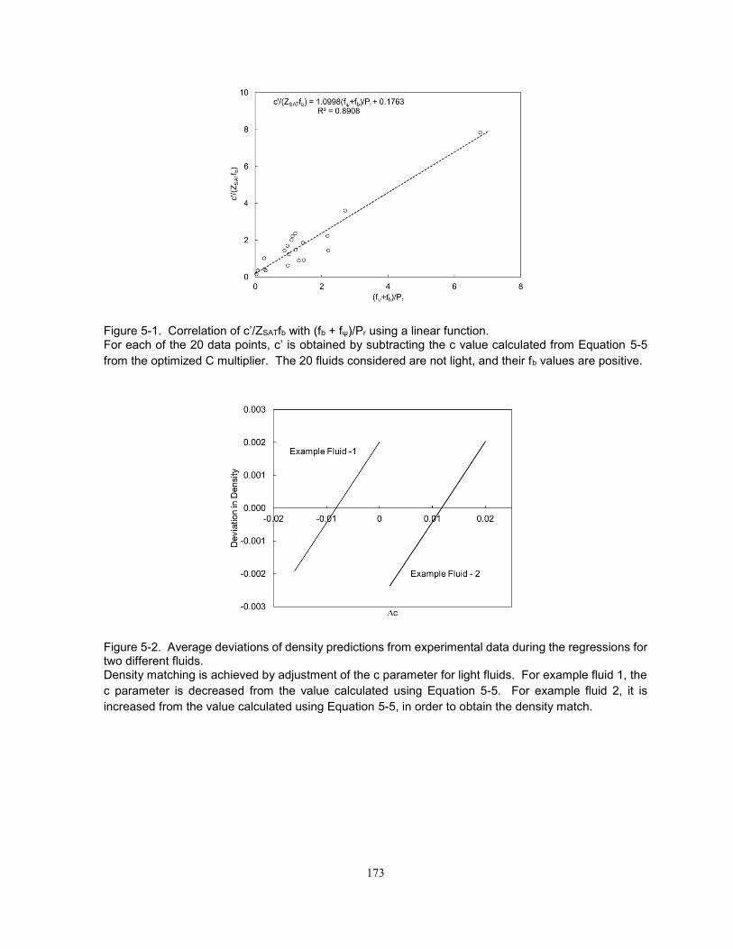
173
Figure 5-1. Correlation of c’/ZSATfb with (fb + fψ)/Pr using a linear function. For each of the 20 data points, c’ is obtained by subtracting the c value calculated from Equation 5-5
from the optimized C multiplier. The 20 fluids considered are not light, and their fb values are positive.
Figure 5-2. Average deviations of density predictions from experimental data during the regressions for two different fluids. Density matching is achieved by adjustment of the c parameter for light fluids. For example fluid 1, the
c parameter is decreased from the value calculated using Equation 5-5. For example fluid 2, it is
increased from the value calculated using Equation 5-5, in order to obtain the density match.
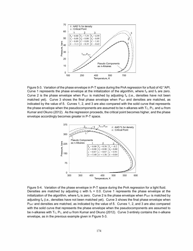
174
Figure 5-3. Variation of the phase envelope in P-T space during the PnA regression for a fluid of 42 °API. Curve 1 represents the phase envelope at the initialization of the algorithm, where fψ and fb are zero.
Curve 2 is the phase envelope when PSAT is matched by adjusting fψ (i.e., densities have not been
matched yet). Curve 3 shows the final phase envelope when PSAT and densities are matched, as
indicated by the value of δ. Curves 1, 2, and 3 are also compared with the solid curve that represents
the phase envelope when the pseudocomponents are assumed to be n-alkanes with TC, PC, and ω from
Kumar and Okuno (2012). As the regression proceeds, the critical point becomes higher, and the phase
envelope accordingly becomes greater in P-T space.
Figure 5-4. Variation of the phase envelope in P-T space during the PnA regression for a light fluid. Densities are matched by adjusting c with fb = 0.0. Curve 1 represents the phase envelope at the
initialization of the algorithm, where fψ is zero. Curve 2 is the phase envelope when PSAT is matched by
adjusting fψ (i.e., densities have not been matched yet). Curve 3 shows the final phase envelope when
PSAT and densities are matched, as indicated by the value of δ. Curves 1, 2, and 3 are also compared
with the solid curve that represents the phase envelope when the pseudocomponents are assumed to
be n-alkanes with TC, PC, and ω from Kumar and Okuno (2012). Curve 3 entirely contains the n-alkane
envelope, as in the previous example given in Figure 5-3.

175
Figure 5-5. The converged fb value tends to increase with increasing specific gravity of the fluid. The regression parameter fb is representative of the aromaticity level; it is zero for n-alkanes and
increases with increasing aromaticity level.
Figure 5-6. CVD liquid saturations measured for gas condensate 12 given in Table 5-3 (McVay 1994) at 387.59 K. The gas condensate has 11.72 mol% C7+. The MW of the C7+ fraction is 169 g/mol, and the overall MW
is 40.58 g/mol.
0
10
20
30
40
50
0 50 100 150 200 250 300 350
CV
D L
iqu
id V
olu
me
,%
Pressure, bars
Direct PnA
CMwV
Data
CMwV

176
Figure 5-7. CCE liquid saturations measured for gas condensate 3 given in Table 5-3 (Al-Meshari 2004) at 382.59 K. The gas condensate has 1.81 mol% C7+. The MW of the C7+ fraction is 152.80 g/mol, and the overall MW is 32.41 g/mol.
Figure 5-8. Comparison between the measured and predicted CVD liquid saturations for near-critical volatile oil 14 in Table 5-4 at 424.25 K (Pedersen et al. 1988). The critical point was measured at 426 K and 388 bars, but it is calculated to be 433.00 K and 389.95
bars by the fluid model based on the direct PnA method. Although the calculated TC is 7 K higher than
the measured TC, the CVD liquid saturations are accurately predicted.
0
5
10
15
20
25
0 50 100 150 200 250 300 350
CC
E L
iqu
id V
olu
me
, %
Pressure, bars
Direct PnA
CMwV
Data
CMwV
0
10
20
30
40
50
60
70
80
90
100
100 150 200 250 300 350 400
CV
D L
iqu
id V
olu
me
, %
Pressure, bars
Direct PnA
CMwV
Data
CMwV

177
Figure 5-9. Oleic phase saturation data and predictions for heavy oil 1 (Sharma 1990) given in Table 5-5 at 299.81 K. This is a mixture of 20% oil and 80% CO2. The AAD for these oleic phase saturation calculations is 5.2%
with the direct PnA method.
Figure 5-10. Data and predictions for saturation pressures in the swelling tests of heavy oil 2 with two injection gases; CO2 and a light gas mixture (Kredjbjerg and Pedersen 2006). The AAD is 3.9% for the CO2 case and 2.8% for the gas mixture case with the direct PnA method.
35
40
45
50
55
60
65
70
75
50 100 150 200 250 300 350
Oile
ic P
ha
se
Sa
tura
tio
n, %
Pressure, bars
Direct PnA
CMwV
Data
CMwV
200
250
300
350
400
450
500
0 50 100 150 200 250
Satu
ration P
ressu
re, bars
Mole % of gas added
Direct PnA CMwVData ( Injection Gas )Data (Injection Gas Mixture)
CO2
CMwV
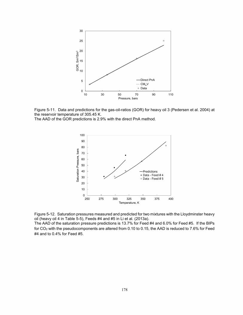
178
Figure 5-11. Data and predictions for the gas-oil-ratios (GOR) for heavy oil 3 (Pedersen et al. 2004) at the reservoir temperature of 305.45 K. The AAD of the GOR predictions is 2.9% with the direct PnA method.
Figure 5-12. Saturation pressures measured and predicted for two mixtures with the Lloydminster heavy oil (heavy oil 4 in Table 5-5), Feeds #4 and #5 in Li et al. (2013a). The AAD of the saturation pressure predictions is 13.7% for Feed #4 and 6.0% for Feed #5. If the BIPs
for CO2 with the pseudocomponents are altered from 0.10 to 0.15, the AAD is reduced to 7.6% for Feed
#4 and to 0.4% for Feed #5.
0
5
10
15
20
25
30
10 30 50 70 90 110
GO
R, S
m3/S
m3
Pressure, bars
Direct PnA
CMwV
Data
CMwV

179
Figure 5-13. The three-phase boundaries measured and predicted for a mixture of heavy oil 4 (Table 5-5) with CO2 and n-C4 (Feed #15 of Li et al. 2013b).
Figure 5-14. CVD liquid saturations predicted with different values for C for gas condensate 6 in Table 5-3. C is equal to c for this fluid because fb is zero. An optimum value for C, which is 0.91 in this case, is
easy to find because of the monotonic, systematic change of the CVD liquid saturation curve.

180
Figure 5-15. MMPs calculated with different C values for oil 1 given in Table 5-1. The calculated MMP decreases monotonically with decreasing C. It is not difficult to find the value for
C with which the measured MMP is matched.
Figure 5-16. Two-phase envelopes predicted with the two sets of critical parameters for an n-alkane mixture. The mixture contains 44.0% C1, 45.8% n-C10, 6.8% n-C18, and 3.4% n-C30. The optimized critical
parameters of Kumar and Okuno (2012) and the estimated physical critical parameters of Constantinou
and Gani (1994) are used with the PR EOS. The BIPs are zero for both cases. The bubble-point data
were taken from Daridon et al. (1996). Use of the optimized critical parameters results in a more
accurate P-T envelope.
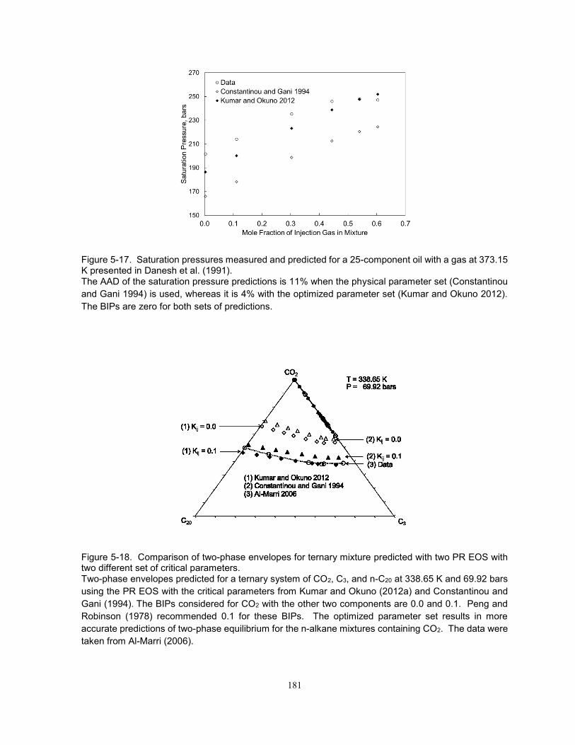
181
Figure 5-17. Saturation pressures measured and predicted for a 25-component oil with a gas at 373.15 K presented in Danesh et al. (1991). The AAD of the saturation pressure predictions is 11% when the physical parameter set (Constantinou
and Gani 1994) is used, whereas it is 4% with the optimized parameter set (Kumar and Okuno 2012).
The BIPs are zero for both sets of predictions.
Figure 5-18. Comparison of two-phase envelopes for ternary mixture predicted with two PR EOS with two different set of critical parameters. Two-phase envelopes predicted for a ternary system of CO2, C3, and n-C20 at 338.65 K and 69.92 bars
using the PR EOS with the critical parameters from Kumar and Okuno (2012a) and Constantinou and
Gani (1994). The BIPs considered for CO2 with the other two components are 0.0 and 0.1. Peng and
Robinson (1978) recommended 0.1 for these BIPs. The optimized parameter set results in more
accurate predictions of two-phase equilibrium for the n-alkane mixtures containing CO2. The data were
taken from Al-Marri (2006).
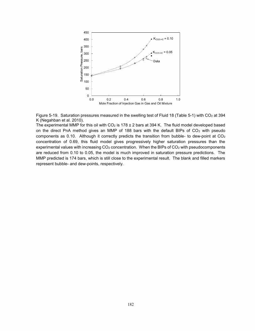
182
Figure 5-19. Saturation pressures measured in the swelling test of Fluid 18 (Table 5-1) with CO2 at 394 K (Negahban et al. 2010). The experimental MMP for this oil with CO2 is 178 ± 2 bars at 394 K. The fluid model developed based
on the direct PnA method gives an MMP of 188 bars with the default BIPs of CO2 with pseudo
components as 0.10. Although it correctly predicts the transition from bubble- to dew-point at CO2
concentration of 0.69, this fluid model gives progressively higher saturation pressures than the
experimental values with increasing CO2 concentration. When the BIPs of CO2 with pseudocomponents
are reduced from 0.10 to 0.05, the model is much improved in saturation pressure predictions. The
MMP predicted is 174 bars, which is still close to the experimental result. The blank and filled markers
represent bubble- and dew-points, respectively.

183
Table 5-1. Converged fψ, fb, and p values for reservoir oils characterized using the
direct PnA method. Slim-tube MMPs are reported for these oils in the literature.
Oil No.
References MW (gm/mol)
°API TRES (K)
k fψ fb p % AD MMP
Prediction
1 Jaubert et al. (2002), F1 135.24
35.22ǂ 374.85 5 0.4223 0.1411 4.5 5.60
2 Jaubert et al. (2002), F2 136.25
39.89 372.05 6 1.0947 0.1051 4.7 14.28
3 Jaubert et al. (2002), F3 82.41 39.31ǂ 387.35 11 0.8280 0.0690 6.3 1.27
4 Jaubert et al. (2002), F4 63.17 40.34ǂ 388.20 7 0.1683 0.074x 3.0 0.09
5 Jaubert et al. (2002), F5 125.82
32.04ǂ 394.25 12 0.8105 0.1171 4.5 0.55
6 Jaubert et al. (2002), F6 96.25 37.73ǂ 383.15 5 0.6294 0.1151 4.2 5.76
7 Jaubert et al. (2002), F7 96.19 41.06ǂ 393.15 12 1.6151 0.0520 4.9 1.29 8 Jaubert et al. (2002), F11 82.55 38.71ǂ 373.75 11 0.6737 0.0921 3.8 8.96 9 Jaubert et al. (2002), F13 150.2 35.64ǂ 377.55 8 -0.2542 0.0701 4.4 2.65 10 Al-Ajmi et al. (2011), F1 161.4
2 31.85 350.40 16 0.6427 0.1341 4.6 12.45
11 Al-Ajmi et al. (2011), F2 109.37
40.03 353.70 17 0.7924 0.1061 3.9 14.56 12 Ekundayo (2012) 86.57 51.60 402.59 7 1.1011 0.0671 4.6 3.03
13 Wijaya (2006) 113.90
44.00 302.59 17 1.3260 0.0701 4.5 9.94
14 Høier (1997), System 1¥ 97.0 39.40 368.15 6 0.6933 0.1121 4.4 8.01
Høier (1997), System 2¥ 97.0 39.40 368.15 6 4.4 4.54
Høier (1997), System 3¥ 97.0 39.40 368.15 6 4.4 4.81
Høier (1997), System 4¥ 97.0 39.40 368.15 6 4.4 5.37
15 Lindeloff et al. (2013),Oil A 148.24
30.00ǂ 329.26 10 1.0253 0.1301 4.6 12.25
16 Graue and Zana (1981)#
177.0 42.10 344.26 1 4.8227 0.0971 7.7 5.15 Graue and Zana (1981)#
177.0 42.10 344.26 1 7.7 9.16
17 Clark et al. (2008) 53.87 47.00 413.70 12 0.7289 0.1591 3.0 6. 80* 18 Negahban et al. 2010 101.9
0 40.00 394.00 16 1.1901 0.0491 4.8 5.62
x ∆c value (fb is zero). ǂ As reported. All other API gravities are calculated from the density at 288.15 K and 1.01325 bars. ¥ Oil composition and saturation data used were taken from Whitson and Belery (1994). Systems 1-4
indicate four different injection gases. # %ADs of 5.15 and 9.16 are for injection gases 1 and 2 respectively. * AAD for 26 different injection gases is 6.8 %. Deviations for these injection gases are shown in Table
5-2.
Table 5-2. Deviations for MMP predictions for volatile oil 17 (Clark et al. 2008) based on the
direct PnA method of volatile oil.
Injection gas (Mole %)*
Dev. %
Injection gas (Mole %)*
Dev. %
Injection gas (Mole %)*
Dev. %
Injection gas (Mole %)*
Dev. %
CO2 (100) 5.26 CO2 (95) + C2 (5) 4.85 CO2 (95) + C5 (5) -7.83 CO2 (95) + N2 (5) 0.18
CO2 (95) + C1 (5) 6.47 CO2 (90) + C2 (10) 4.53 CO2 (90) + C5 (10) -17.34 CO2 (90) + N2 (10) -3.44
CO2 (90) + C1 (10) 6.47 CO2 (85) + C2 (15) 5.35 CO2 (85) + C5 (15) -20.67 CO2 (85) + N2 (15) 0.48
CO2 (85) + C1 (15) 6.94 CO2 (80) + C2 (20) 5.70 CO2 (80) + C5 (20) -1.56 CO2 (80) + N2 (20) 3.57
CO2 (80) + C1 (20) 6.87 CO2 (75) + C2 (25) 7.62 CO2 (75) + C5 (25) 5.67 CO2 (75) + N2 (25) 7.59
CO2 (75) + C1 (25) 6.86 CO2 (70) + C2 (30) 9.55 CO2 (70) + C5 (30) 6.30 CO2 (70) + N2 (30) 10.78
CO2 (70) + C1 (30) 5.00 N2 (100) 13.75
* Numbers inside bracket shows mole % of the component in injection gas.
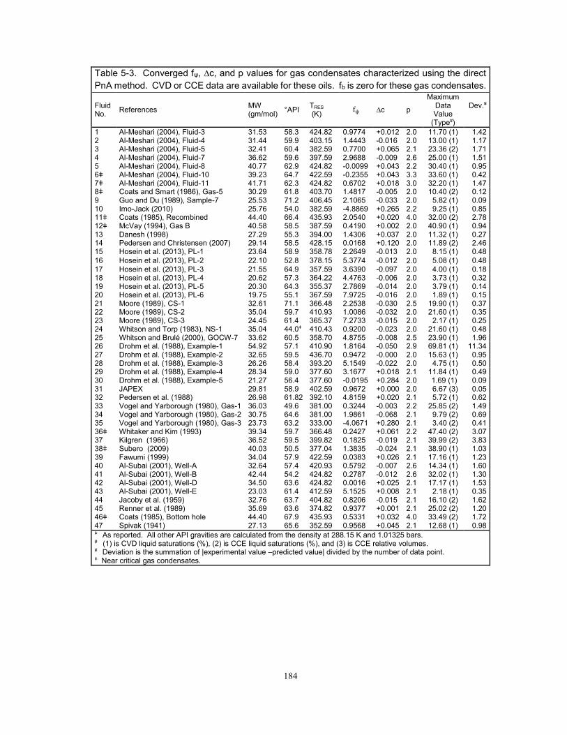
184
Table 5-3. Converged fψ, ∆c, and p values for gas condensates characterized using the direct
PnA method. CVD or CCE data are available for these oils. fb is zero for these gas condensates.
Fluid No.
References MW (gm/mol)
°API TRES (K)
fψ ∆c p
Maximum Data Value
(Type#)
Dev.¥
1 Al-Meshari (2004), Fluid-3 31.53 58.3 424.82 0.9774 +0.012 2.0 11.70 (1) 1.42 2 Al-Meshari (2004), Fluid-4 31.44 59.9 403.15 1.4443 -0.016 2.0 13.00 (1) 1.17 3 Al-Meshari (2004), Fluid-5 32.41 60.4 382.59 0.7700 +0.065 2.1 23.36 (2) 1.71 4 Al-Meshari (2004), Fluid-7 36.62 59.6 397.59 2.9688 -0.009 2.6 25.00 (1) 1.51 5 Al-Meshari (2004), Fluid-8 40.77 62.9 424.82 -0.0099 +0.043 2.2 30.40 (1) 0.95 6ǂ Al-Meshari (2004), Fluid-10 39.23 64.7 422.59 -0.2355 +0.043 3.3 33.60 (1) 0.42 7ǂ Al-Meshari (2004), Fluid-11 41.71 62.3 424.82 0.6702 +0.018 3.0 32.20 (1) 1.47 8ǂ Coats and Smart (1986), Gas-5 30.29 61.8 403.70 1.4817 -0.005 2.0 10.40 (2) 0.12 9 Guo and Du (1989), Sample-7 25.53 71.2 406.45 2.1065 -0.033 2.0 5.82 (1) 0.09 10 Imo-Jack (2010) 25.76 54.0 382.59 -4.8869 +0.265 2.2 9.25 (1) 0.85 11ǂ Coats (1985), Recombined 44.40 66.4 435.93 2.0540 +0.020 4.0 32.00 (2) 2.78 12ǂ McVay (1994), Gas B 40.58 58.5 387.59 0.4190 +0.002 2.0 40.90 (1) 0.94 13 Danesh (1998) 27.29 55.3 394.00 1.4306 +0.037 2.0 11.32 (1) 0.27 14 Pedersen and Christensen (2007) 29.14 58.5 428.15 0.0168 +0.120 2.0 11.89 (2) 2.46 15 Hosein et al. (2013), PL-1 23.64 58.9 358.78 2.2649 -0.013 2.0 8.15 (1) 0.48
16 Hosein et al. (2013), PL-2 22.10 52.8 378.15 5.3774 -0.012 2.0 5.08 (1) 0.48
17 Hosein et al. (2013), PL-3 21.55 64.9 357.59 3.6390 -0.097 2.0 4.00 (1) 0.18 18 Hosein et al. (2013), PL-4 20.62 57.3 364.22 4.4763 -0.006 2.0 3.73 (1) 0.32 19 Hosein et al. (2013), PL-5 20.30 64.3 355.37 2.7869 -0.014 2.0 3.79 (1) 0.14 20 Hosein et al. (2013), PL-6 19.75 55.1 367.59 7.9725 -0.016 2.0 1.89 (1) 0.15 21 Moore (1989), CS-1 32.61 71.1 366.48 2.2538 -0.030 2.5 19.90 (1) 0.37 22 Moore (1989), CS-2 35.04 59.7 410.93 1.0086 -0.032 2.0 21.60 (1) 0.35 23 Moore (1989), CS-3 24.45 61.4 365.37 7.2733 -0.015 2.0 2.17 (1) 0.25 24 Whitson and Torp (1983), NS-1 35.04 44.0ǂ 410.43 0.9200 -0.023 2.0 21.60 (1) 0.48 25 Whitson and Brulé (2000), GOCW-7 33.62 60.5 358.70 4.8755 -0.008 2.5 23.90 (1) 1.96 26 Drohm et al. (1988), Example-1 54.92 57.1 410.90 1.8164 -0.050 2.9 69.81 (1) 11.34 27 Drohm et al. (1988), Example-2 32.65 59.5 436.70 0.9472 -0.000 2.0 15.63 (1) 0.95 28 Drohm et al. (1988), Example-3 26.26 58.4 393.20 5.1549 -0.022 2.0 4.75 (1) 0.50 29 Drohm et al. (1988), Example-4 28.34 59.0 377.60 3.1677 +0.018 2.1 11.84 (1) 0.49 30 Drohm et al. (1988), Example-5 21.27 56.4 377.60 -0.0195 +0.284 2.0 1.69 (1) 0.09 31 JAPEX 29.81 58.9 402.59 0.9672 +0.000 2.0 6.67 (3) 0.05 32 Pedersen et al. (1988) 26.98 61.82 392.10 4.8159 +0.020 2.1 5.72 (1) 0.62 33 Vogel and Yarborough (1980), Gas-1 36.03 49.6 381.00 0.3244 -0.003 2.2 25.85 (2) 1.49 34 Vogel and Yarborough (1980), Gas-2 30.75 64.6 381.00 1.9861 -0.068 2.1 9.79 (2) 0.69 35 Vogel and Yarborough (1980), Gas-3 23.73 63.2 333.00 -4.0671 +0.280 2.1 3.40 (2) 0.41 36ǂ Whitaker and Kim (1993) 39.34 59.7 366.48 0.2427 +0.061 2.2 47.40 (2) 3.07 37 Kilgren (1966) 36.52 59.5 399.82 0.1825 -0.019 2.1 39.99 (2) 3.83 38ǂ Subero (2009) 40.03 50.5 377.04 1.3835 -0.024 2.1 38.90 (1) 1.03 39 Fawumi (1999) 34.04 57.9 422.59 0.0383 +0.026 2.1 17.16 (1) 1.23 40 Al-Subai (2001), Well-A 32.64 57.4 420.93 0.5792 -0.007 2.6 14.34 (1) 1.60 41 Al-Subai (2001), Well-B 42.44 54.2 424.82 0.2787 -0.012 2.6 32.02 (1) 1.30 42 Al-Subai (2001), Well-D 34.50 63.6 424.82 0.0016 +0.025 2.1 17.17 (1) 1.53 43 Al-Subai (2001), Well-E 23.03 61.4 412.59 5.1525 +0.008 2.1 2.18 (1) 0.35 44 Jacoby et al. (1959) 32.76 63.7 404.82 0.8206 -0.015 2.1 16.10 (2) 1.62 45 Renner et al. (1989) 35.69 63.6 374.82 0.9377 +0.001 2.1 25.02 (2) 1.20 46ǂ Coats (1985), Bottom hole 44.40 67.9 435.93 0.5331 +0.032 4.0 33.49 (2) 1.72 47 Spivak (1941) 27.13 65.6 352.59 0.9568 +0.045 2.1 12.68 (1) 0.98 ǂ As reported. All other API gravities are calculated from the density at 288.15 K and 1.01325 bars. # (1) is CVD liquid saturations (%), (2) is CCE liquid saturations (%), and (3) is CCE relative volumes. ¥ Deviation is the summation of |experimental value –predicted value| divided by the number of data point. ǂ Near critical gas condensates.

185
Table 5-4. Converged fψ, fb, and p values for volatile oils characterized using the direct PnA
method. CVD or CCE data are available for these oils.
Oil No.
References MW (gm/ mol)
°API Res. Temp. (K)
fψ fb p Data Limits
Value (Type#)
Dev.¥
1 Al-Meshari (2004), Fluid-12 46.07 50.3 354.82 0.8544 +0.033x 2.3 38.20 (1) 2.80 2 Al-Meshari (2004), Fluid-13 56.06 36.7 364.82 0.2188 0.1091 2.3 3.93 (3) 0.02 3 Al-Meshari (2004), Fluid-14 54.57 40.7 360.93 0.3069 0.1081 2.4 1.00 (3) 0.01 4 Al-Meshari (2004), Fluid-15 51.11 57.5 353.15 1.5275 0.0581 2.9 2.98 (3) 0.01 5 Al-Meshari (2004), Fluid-16 59.63 55.6 425.93 0.0591 -0.006x 2.5 35.30 (1) 2.29 6 Al-Meshari (2004), Fluid-17 67.32 44.5 414.82 0.2061 0.0920 2.5 6.84 (3) 0.04 7 Al-Meshari (2004), Fluid-18 59.90 54.4 423.15 0.2876 0.0591 3.2 7.57 (3) 0.04 8 Al-Meshari (2004), Fluid-19 62.65 59.5 377.59 1.2666 0.0540 4.3 4.08 (3) 0.00 9 Oil* 86.68 56.6 376.75 1.7416 0.0360 4.0 2.46 (3) 0.01 10ǂ McVay (1994), Oil A 50.93 44.5 408.70 1.1997 +0.000x 2.5 33.30 (1) 4.38 11 McVay (1994), Oil B 57.50 56.7 393.70 1.0877 +0.000x 3.1 49.50 (1) 2.60 12ǂ Yang et al. (1997)ǂ 37.94 57.5 371.60 -0.6776 +0.085x 2.0 6.06 (2) 2.12 13 Jacoby and Yarborough (1967) 54.32 63.7 346.48 1.1580 0.0540 2.8 24.29 (1) 1.60 14ǂ Pedersen et al. (1988) 47.84 52.5 424.25 0.2597 -0.013x 2.3 42.20 (1) 3.87 15 Reudelhuber and Hinds (1957) 42.55 49.1 374.82 0.6933 -0.024x 2.3 34.50 (1) 1.60 x ∆c value (fb is zero). ǂ As reported. All other API gravities are calculated from density at 288.15 K and 1.01325 bars. # (1) is CVD liquid saturation (%), (2) is CCE liquid saturation (%), and (3) is CCE relative volume. ¥ Deviation is the summation of |experimental value –predicted value| divided by the number of data point. ǂ Near critical volatile oil. * Data source is not mentioned for confidentiality.
Table 5-5. Converged fψ, fb, and p values for heavy oils characterized using the direct PnA
method. PVT data available for these oils include swelling tests, gas solubility, and phase
envelopes.
Oil No.
References MW (gm/ mol)
°API TRES (K)
k# fψ fb p AAD
% Type of Data
1 Sharma (1990), West Sak Oil 228.88 18.68 299.81 10 0.0568 0.1491 5.7 3.62 Swelling Test 2 Krejbjerg and Pedersen (2006),Fluid-1 125.72 28.00ǂ 347.15 13 0.2762 0.2341 5.5 3.40 Swelling Test 3 Pedersen et al. (2004), Fluid-22 311.06 10.87 305.45 11 -0.0607 0.1592 5.5 3.13 GOR 4 Li et al. (2013a), Lloydminster Oil 482.00 10.80 294.15 1 -0.3409 0.1320 9.0 9.30 Swelling Test ǂ As reported. All other API gravities are calculated from density at 288.15 K and 1.01325 bars. # k is number of density data
186
Chapter 6: Systematic Characterization of Bitumen-Solvent Interactions in
Steam-Solvent Coinjection Simulation
A version of this has been submitted to Fuel for publication. The manuscript is under
review.

187
6.1. Introduction
Steam-assisted gravity drainage (SAGD) is a widely-used method for in-situ bitumen recovery (Butler
1991, Lake et al. 2014). The most important mechanism in SAGD is the reduction of oleic-phase
viscosity owing to the heat that the injected steam releases when condensing into hot water near the
steam-chamber edge. The main drawback of SAGD is the substantial usage of steam, which may also
cause various environmental concerns.
Coinjection of solvent with steam, such as expanding-solvent-steam assisted gravity drainage (ES-
SAGD), has been proposed and pilot-tested to improve the efficiency of SAGD (Nasr et al. 2003, Gupta
and Gittins 2006). In ES-SAGD, a small amount of hydrocarbon solvent is coinjected with steam. It aims
to reduce oleic-phase viscosity by diluting bitumen with condensed solvent, in addition to the thermal
mechanism, along the chamber edge.
Unlike SAGD, ES-SAGD involves multiphase behavior of solvent/bitumen mixtures at a wide range
of temperature and its interaction with non-isothermal flow under heterogeneities. The efficiency of ES-
SAGD is substantially dependent on pressure, temperature, and composition near the chamber edge,
in which condensation of steam and solvent and the mixing of solvent with bitumen take place through
gravity drainage (Keshavarz et al. 2014).
Due to the complexity, design of ES-SAGD requires numerical simulation that accommodates the
compositional effect on non-isothermal reservoir flow. Numerical simulation studies have been
presented in the literature to understand various aspects of this complex process (Nasr and Ayodele
2006, Nasr et al. 2003, Jha et al. 2013, Keshavarz et al. 2015). However, the effect of fluid
characterization on ES-SAGD simulation has not been investigated in detail, although such simulations
are directly affected by how the fluid is characterized.
Fluid characterization for ES-SAGD is challenging because it requires a reliable method for modeling
phase properties that does not give physically absurd values at a wide range of composition and
temperature for the operating range of pressure. For example, the temperature range in ES-SAGD can
be from 300 K to 500 K. The oleic-phase composition can vary widely from nearly 100% solvent to
100% bitumen in the vicinity of the chamber edge.
Even with such a reliable method, however, it is still important to ensure that the simulation results
are not sensitive to the phase-behavior model used. This is because fluid characterization for ES-SAGD
is performed under inherent uncertainties in terms of experimental data. It would not be easy to measure
phase properties at the thermodynamic conditions that occur during ES-SAGD, even if such conditions
could be precisely predicted. Different fluid models created under such uncertainties may give a similar
level of correlative accuracy for the limited experimental data available; however, they do not necessarily
give similar results in numerical reservoir simulation, in which phase behavior should be predicted at a
variety of thermodynamic conditions. Currently, there is no method for assessing the sensitivity of
simulation results to the phase-behavior model without performing actual flow simulations.

188
There are two main objectives in this research. The first is to show reliable characterization of
bitumen by using the method that was developed by the authors (Section 6.2). The second is to develop
a novel method for analytically assessing the sensitivity of ES-SAGD simulation to the phase behavior
model used (Section 6.3). The analytical method is validated in the simulation case study (Section 6.4).
6.2. Bitumen characterization based on Perturbation from n-Alkanes
This section presents characterization of six different bitumen samples using the Peng-Robinson
equation of state (PR EOS) (1976, 78) along with the van der Waals mixing rules on the basis of
perturbation from n-alkanes (PnA). The PnA method of reservoir fluid characterization was successfully
applied to a number of reservoir fluids (Kumar and Okuno 2015), but not yet to any bitumen. The main
difference between the PnA method and the conventional method of bitumen characterization lies in
how pseudo components’ properties are adjusted during the regression of an EOS model to phase-
behavior data. Before presenting the PnA method for bitumen characterization in Section 6.2.1, the
conventional method is briefly explained below.
Several researchers presented EOS models to represent bitumens and their gas solubilities (James
and Malhotra 1988, Malhotra and Svrcek 1988, Malhotra et al. 1989, Kariznovi et al. 2010). The three
main steps of bitumen characterization in their papers are (1) representation of bitumen by a user-
defined number of pseudo components, (2) estimation of pseudo components’ parameters, such as
critical temperature (TC), critical pressure (PC), acentric factor (ω), and critical volume (VC), using various
correlations, and (3) regression of the parameters to match experimental data.
Step 1 of the conventional method uses atmospheric and vacuum distillation data. Bitumens are
represented by SARA (saturate, aromatic, resin, and asphaltene) fractions or by pseudo components
obtained from a certain probability distribution function, such as the gamma distribution function
(Whitson 1983). Step 2 of the conventional method is often based on the correlations with normal boiling
point (Tb) and specific gravity (γ). Binary interaction parameters (BIPs) are also estimated as functions
of one or more parameters, such as TC, PC, VC, and ω. Step 3 of the conventional method is to reduce
the deviation of EOS predictions from experimental phase behavior data because the general
correlations used in step 2 tend to be in substantial error when extrapolated to high carbon numbers
(CNs) relevant to bitumen components. Therefore, many parameters, such as TC, PC, VC, ω, BIP, and
volume shift, for pseudo components are adjusted to match various data, such as gas solubilities and
densities.
The conventional method described above is concerned mainly with the correlative accuracy for the
experimental data available. Due likely to a high level of uncertainties in bitumen data, the number of
pseudo components required for the conventional method to match experimental data ranges up to 6
(Fu et al. 1985, Lu et al. 1986, Mehrotra and Svrcek 1988a, Mehrotra et al. 1989, Kariznovi et al. 2010).
With the conventional method, use of one pseudo component was unsuccessful for matching bitumen
data (Mehrotra and Svrcek 1988a, Mehrotra et al. 1989). No approach to predicting the number of
pseudocomponents representing bitumen for reliable recovery simulation has been developed. The

189
general approach to representing the plus fraction by multiple pseudocomponents is based on the
understanding that lumping of components results in loss of information and flexibility (Leibovici 1993).
It is unknown in the literature whether characterization of bitumen/solvent mixtures, although
challenging, requires as many as 6 pseudo components for thermal flow simulation. Use of more
components certainly offers the flexibility in matching experimental data; however, the correlative
accuracy obtained with a large number of pseudo components does not necessarily yield accurate
predictions of phase behavior during thermal flow simulation due to a wide range of thermodynamic
conditions encountered. As will be shown later in this paper, a proper number of pseudo components
in bitumen characterization cannot be determined without consideration of compositional effects in the
oil recovery process of interest, which is ES-SAGD in this paper.
6.2.1. Algorithm for Bitumen Characterization
The PnA method begins with a PR-EOS model calibrated for n-alkanes; hence, pseudo components
are initially assumed to be n-alkanes. Then, the a and b parameters for pseudo components are
adjusted in the direction of increasing aromaticity from n-alkanes (i.e., zero aromaticity) until a saturation
pressure and densities at a given temperature are matched for the fluid of interest. Volumetric and
compositional phase behavior are corrected largely by adjusting the b parameter to match densities and
by adjusting the ψ parameter to match a saturation pressure, respectively. The ψ parameter is
expressed as Equation 6-1.
ψ = a/b2, or Ωa
Ωb2 PC(1 + m[1 − (T TC⁄ )0.5])2 (6-1)
on the basis of the PR EOS. Details of the original PnA method can be found in (Kumar and Okuno
2015).
The two types of experimental data, density and saturation pressure, are important in the PnA
method since the b and ψ parameters are adjusted specifically for volumetric and compositional
predictions, respectively. In this research, such experimental data are taken from a bitumen/gas
mixture, because a bitumen sample often exhibits no obvious saturation pressure even at 450 K, which
is near the highest operating temperature of the conventional phase-behavior experimental setup. More
specifically to this paper, we use the saturation pressure and density data for the bitumen saturated with
methane around 373.15 K (100°C), although the selection of gas and temperature is arbitrary in
principle. The BIPs of methane with bitumen components are set to zero in this paper, although other
default values are also possible.
As presented in Kumar and Okuno (2015), the adjustment of the b parameter for matching density
data is performed using Equation 6-2.
bi =– 14.6992113939827 + 1.36977232166027 (MWi
mbi) – 9.12089276536298 × 10⁻⁵ (
MWi
mbi)
2
(6-2)

190
where i is the index for pseudo components, mbi = (MW i/86.0)fb, and MW i is the molecular weight of
component i. The fb perturbation parameter is zero for n-alkanes, and increases with increasing level
of aromaticity in terms of volumetric phase behavior. The mbi parameter increases with MW for a given
fb value.
The a parameter is adjusted through the ψ parameter for a given b parameter (i.e., a = ψb2). Unlike
in the original PnA method (Kumar and Okuno 2015), however, the adjustment of ψ can be conducted
using a simplified equation:
ψi = −0.9415MWi + 2495.8fψ. (6-3)
Coefficients in Equation 6.3 corresponds to temperature of 373.15 K. Equation 6.3 represents the n-
alkane case when the fψ perturbation parameter is the initial value of 1.0. The simplification is possible
because a large fraction of bitumen components are heavier than CN 20, in which ψ linearly decreases
with MW as shown in (Kumar and Okuno 2015). The ψ function can be systematically increased by
increasing the fψ perturbation parameter, which increases the y-intercept of the function. When only one
pseudo component is used, the ψ parameter is adjusted by changing the fψ perturbation parameter in
Equation 6-4.
ψ = Ψnfψ = (−0.9415MW + 2495.8)fψ (6-4)
where ψn is the ψ parameter calculated for an n-alkane with MW.
Unlike the conventional method, the PnA method systematically changes the vapor pressure curves
of all pseudo components through direct adjustment of the two parameters. Figure 6.1 shows the
change in phase envelope for an example mixture of bitumen and methane, in which bitumen is
represented by a single pseudo component. The solid curve in this figure is the initial phase envelope
for which the bitumen is assumed to be an n-alkane (i.e., fb = 0.0 and fψ = 1.0). The other curves
correspond to positive level of aromaticity of the bitumen (i.e., fb > 0.0 and fψ > 1.0). The step-wise
description of the algorithm is given below.
Step 1. Compositional characterization
This step is required only when bitumen is to be represented by multiple pseudo components.
The chi-squared distribution function (Quiñones-Cisneros et al. 2004) is applied to split bitumen
into pseudo components. Quiñones-Cisneros et al. (2004) observed in their study that degree
of freedom of 10 was sufficient for heavy oils used. In this work, a degree of freedom of 12 is
assumed for bitumen. The C7+ molecular weight is taken from the molar mass reported for the
bitumen sample of interest. The bitumen is split into a desired number (n) of pseudo
components with equal mass fractions. In this paper, four pseudo components (i.e. n = 4) are
used for multicomponent representation of bitumen. Set fb = 0.0, and fψ = 1.0.
Step 2. Initialization of the a and b parameters for each pseudo component
191
Equation 6.2 is used for covolumes, bi, for i = 1, …n. Equation 6.3 is used for ψi (i = 1,.n) if n >
1. Otherwise, Equation 6.4 is used. Then, the attraction parameter is calculated by a i = ψibi2
for each pseudo component.
Step 3. Perturbation of fψ to match the saturation pressure
Calculate δ = (PS – PS_EOS)/PS, where PS is the saturation pressure measured for a
bitumen/methane mixture at 373.15 K as discussed previously. PS_EOS is the calculated
saturation pressure, and δ is the average absolute relative deviation (AARD) in saturation
pressure. If δ < δTOL (e.g., 10-4), go to Step 4. Otherwise, increase fψ (i.e. fψ = fψ + ∆fψ ; ∆fψ =
10-4) and go to Step 2.
Step 4. Perturbation of fb to match the saturated liquid density
Calculate the AARD in density, ε, as (DN – DN_EOS)/DN, where DN is the density at the saturation
point used in step 3, and DN_EOS is the calculated density. If ε < εTOL (e.g., 10-3), stop. Otherwise,
increase fb (i.e., fb = fb + ∆fb; ∆fb = 10-4), reset fψ to 1.0, and go to Step 2.
Step 5. Conversion of the final set of the a and b parameters to TC, PC, and ω
This step uses the procedure of Kumar and Okuno (2015), in which a physically reasonable set
of TC, PC, and ω is back calculated from the final set of the a and b parameters from the PnA
method. This calculation also gives Tb and γ for each pseudo component as it uses the Lee-
Kesler (1975) and Kesler-Lee (1976) correlations. The correlation of Riazi and Daubert (1987)
can be used along with the Tb and γ to calculate VC for each pseudo component.
6.2.2. Case Studies for Bitumen Characterization.
The algorithm presented in the previous subsection is used to characterize six bitumens: Athabasca
(Svrcek and Mehrotra 1982, Mehrotra and Svrcek 1985a), Cold Lake (Mehrotra and Svrcek 1988b),
Peace River (Mehrotra and Svrcek 1985b), Wabasca (Mehrotra and Svrcek 1985c), JACOS (Kariznovi
2013, Nourozieh 2013) and Surmont (Kariznovi 2013, Nourozieh 2013). For each bitumen, data are
available for methane/bitumen mixtures so that the algorithm can use the density at the methane-
saturation pressure near 373.15 K (100°C) in Steps 3 and 4. As mentioned previously, the BIPs for
methane with pseudo components are set to zero for all cases in this paper.
The systematic change in pseudo components’ properties during the regression allows to conduct
a comparative study of bitumen characterization in terms of the number of pseudo components used.
Hence, each bitumen is characterized by using four pseudo components (the 4-PC case) and one
pseudo component (the 1-PC case). Table 6.1 shows the data used for the characterization and the
converged values for fb and fψ for each bitumen. The densities of methane-saturated bitumens, DN, at
PS are similar to each other; therefore, no correlation is obvious for DN and fb. However, it is relatively
clear that fψ increases with PS, which comes from the systematic change in phase envelope in the PnA
method; that is, the two-phase envelope for a bitumen/methane mixture gradually expands in pressure-
temperature space as the perturbation proceeds (see Figure 6.1).
192
For each bitumen, additional data available for methane solubilities are used to test the predictive
accuracy of the resulting EOS model. Table 6.1 summarized the AARDs for these additional data. The
AARD in methane solubility predicted for 99 temperature-pressure points for six bitumens is 10.75%
with the 4-PC case and 10.44% with the 1-PC case. The difference is insignificant between the 4-PC
and 1-PC cases likely because the relative volatility of methane to each pseudo component is not much
different due to the substantial asymmetricity between methane and bitumen.
As reported by Mehrotra and Svrcek (1988a), some data are unreliable. For example, Table 6.1
shows that the PnA method yields the AARD of 9.24% in the 4-PC case and 11.05% in the 1-PC case
for methane solubilities for Athabasca bitumen. However, if the four unreliable data are excluded from
the evaluation, the AARD reduces to 5.77% in the 4-PC case and 5.86% in the 1-PC case. Mehrotra
and Svrcek (1988a) showed their characterizations of the same bitumen excluding the four unreliable
data. The characterization of Mehrotra and Svrcek (1988a) resulted in the AARD of 4.9% using five
pseudo components. Kariznovi et al. (2010) reported the AARD of 7.95% using 6 pseudo components
EOS model.
A bitumen sample usually does not contain gas components, such as N2, CO2, and hydrocarbon
gases. This is why the density at a saturation pressure for a gas/bitumen mixture is required for the
PnA method to capture the compositional and volumetric phase behavior of bitumen through the a and
b parameters. Although the density at a methane-saturation pressure was matched with zero BIPs for
methane with bitumen components in this section, matching solubilities of a gas in a bitumen generally
requires adjustment of their BIPs because the gas is not a part of the characterized bitumen. Such
adjustment of BIPs is presented here for matching gas solubilities: N2, CO2, and C2 for Athabasca
(Svrcek and Mehrotra 1982, Mehrotra and Svrcek 1985a), Cold Lake (Mehrotra and Svrcek 1988b),
Peace River (Mehrotra and Svrcek 1985b), Wabasca (Mehrotra and Svrcek 1985c), C2 for JACOS
bitumens, and C2, C3, and C4 for Surmont bitumen (note that results for methane solubilities were
presented in Table 6.1).
Table 6.2 shows the optimized BIPs and AARDs for the solubility data for these gases. As in Table
6.1, results for the 4-PC and 1-PC cases are shown in this table. The AARDs in the two cases are
similar to each other; that is, bitumen characterization by the PnA method is insensitive to the number
of pseudo components used for the cases tested. For comparison purposes, the last column of Table
2 presents the AARDs reported by Kariznovi et al. (2010) using the PR EOS with six pseudo
components. The comparison shows that use of one pseudo component may be sufficient, at least, for
correlating experimental data using the PR EOS. However, a proper number of pseudo components
should be evaluated in the context of flow in a specific reservoir process, which is ES-SAGD in this
research. This will be discussed in detail in the next section.
The AARD for ethane solubilities at 107 pressure-temperature points is 7.38% in the 4-PC case and
7.25% for the 1-PC case. Mehrotra and Svrcek (1989) reported that at least three data points for
Wabasca bitumen were unreliable. When these unreliable points are excluded, the AARDs for the

193
ethane solubility in Wabasca bitumen are 4.06% and 3.96% for 1-PC and 4-PC respectively with the
PnA method, 4.1% by Mehrotra and Svrcek (1989) using 3 pseudo components. Kariznovi et al. (2010)
reported AARD of 6.56% using 6 pseudo components. Figure 6.2 compares the ethane solubilities
calculated based on the PnA method and the corresponding data for Cold Lake (Figure 2a) and
Athabasca (Figure 2b). This figure indicates that the bitumen model has been better calibrated at higher
temperatures likely because the methane saturation pressure, PS, used is near 373 K.
The AARD for CO2 solubilities at 91 pressure-temperature points is 6.05% in the 4-PC case and
6.06% in the 1-PC case. For Athabasca, the AARD is 5.6% with PnA method for 1-PC and 4-PC, 7.3%
with the characterization by Mehrotra and Svrcek (1988a) with five pseudo components, and 9.34% by
Kariznovi et al. (2010) with six pseudo components. For Wabasca, the AARD is 6.9% with PnA method
for 1-PC and 4-PC, 4.1% by Mehrotra and Svrcek (1989), and 8.88% by Kariznovi et al. (2010).
Experimental data for the Cold Lake bitumen shows that the CO2 solubility levels off at an increased
pressure along some isotherms, and that some solubility isotherms cross each other. Figure 6.3
compares the CO2 solubilities calculated based on the PnA method with the corresponding data for the
Cold Lake bitumen. The above-mentioned characteristics are observed for the data and predictions for
288 K and 299 K.
The gas-solubility data for JACOS (Kariznovi 2013, Nourozieh 2013) and Surmont (Kariznovi 2013,
Nourozieh 2013) bitumens contain the liquid-liquid (L-L) equilibrium in addition to the liquid-vapor (L-V)
equilibrium. It was observed in this research that a positive BIP was required to match L-L data using
the PnA method, but the use of a positive BIP did not affect the L-V predictions significantly. For
example, the optimized BIP between propane and the single bitumen component is 0.066 for Surmont
bitumen as given in Table 6.2. The L-L data could not be matched with zero BIP for propane and the
bitumen component.
It is important to analyze the sensitivity of bitumen characterization to the MW used in Step 1,
considering the inherent uncertainty in the quality of bitumen samples. JACOS bitumen is re-
characterized using the 1-PC PnA method assuming different MWs from perturbation of the MW
between -15% and +15%. Then, predictions are made for methane and ethane solubilities. The BIP
for methane with the bitumen is zero, and that for ethane with the bitumen is 0.01. Figure 6.4 shows
the variation of AARDs with respect to MW deviation. The variation in AARD is quite small; e.g., it is
less than 1.2% and 2.25% between -15% and +15% deviation in MW for the methane and ethane
solubilities respectively. Higher AARD in case of ethane may be because of used BIP of 0.01 for all
cases of MW variation. The results indicate that the PnA method of bitumen characterization is not
much affected by the uncertainty of bitumen MW. However, it is important to use reliable data for the
density at a saturation pressure for a gas-saturated bitumen because it directly affects the a and b
parameters in the PnA method.

194
6.3. Sensitivity Analysis of Oleic-Phase Viscosity at the Chamber Edge
Results in the previous section indicate that the usage of one pseudo component (the 1-PC case) yields
a similar level of accuracy to that of four pseudo components (the 4-PC case) in terms of gas solubility
calculations. However, they may still exhibit substantial differences when used in flow simulation of
steam-solvent coinjection for bitumen recovery. This is because bitumen recovery in such processes is
dependent mainly on the L-phase viscosity near the steam-chamber edge. Currently, however, the
effect of bitumen characterization on bitumen recovery simulation can be evaluated only by running
multiple flow simulations with different sets of fluid models, which is time-consuming. This section
presents a new analytical method to evaluate the sensitivity of coinjection simulation results to bitumen
characterization, without running actual flow simulations.
The main idea is to see if there is a substantial difference between the lightest and heaviest pseudo
components of a multi-component model in terms of viscosity when they are treated as a single-
component bitumen and mixed with solvent at the chamber-edge conditions. If the difference is small,
the pseudo components (bracketed by the lightest and heaviest) likely behave similarly in thermal flow
simulation, and may be modeled as a grouped single component. Otherwise, use of multiple
components is recommended for proper representation of bitumen for steam-solvent coinjection
simulation.
6.3.1. Temperature, Oil-Phase Composition, and Viscosity at the Chamber Edge
The first step is to estimate the temperature and oil-phase composition at the steam-chamber edge,
which significantly affect oil recovery in coinjection. A chamber edge is defined where the phase
transition occurs between the oil-water (L-W) and vapor-oil-water (V-L-W) phase equilibria; hence, it is
where the V phase (dis)appears. A brief description of the L-phase composition at a chamber edge is
given below. More details of similar calculations can be found in Keshavarz et al. (2013).
The thermodynamic formulation is based on the following assumptions as conventionally done in
this area of research: (a) ternary mixtures of water, a solvent component, and a bitumen component; (b)
complete immiscibility between the W and L phases; (c) Raoult’s law for partitioning of the water
component between the W and V phases; and (d) hydrocarbon K values based on the PR EOS. The
water, oil, and solvent components are labeled with indices i = w, o, and s, respectively. The W, L, and
V phases are expressed using indices j = W, L, and V, respectively. xij is the mole fraction of component
i in phase j. Then, phase equilibrium for such a ternary three-phase system at a given temperature (T)
and pressure (P) is given by Equations 6-5 to 6-9.
Pwvap
= xwVP (6-5)
xoV = KoxoL (6-6)
xsV = KsxsL (6-7)
xoL + xsL = 1.0 (6-8)
xwV + xoV + xsV = 1.0 (6-9)

195
where Pwvap
is the vapor pressure of water at T, and Ki is the K value for component i. Equation 6-5 is
for the V-W equilibrium, and Equations 6 and 7 are for the V-L equilibrium. Equations 8 and 9 are
summation constraints. Note that the W phase consists of only water, and the L phase contains no
water, due to assumption (b).
Using the multiphase Rachford-Rice procedure (Okuno et al. 2010) as used in Keshavarz et al.
(2015), it is easy to solve for the L-phase composition (xiL; i = o, s) at a given P and T because the
compositions of three equilibrium phases are uniquely determined for a ternary system at a given P and
T. The L-phase composition so obtained corresponds to the one at the chamber-edge temperature (Te)
at a given P; that is, the specified T is taken as Te. This procedure gives the relationship between the L-
phase composition and temperature at the chamber edge for a given operating pressure for a specified
solvent-bitumen system.
Once the relationship between Te and the L-phase composition at P is set, the second step is to
calculate the L-phase viscosity through a certain model. The following viscosity model has been
implemented in the STARS (2012) reservoir simulator:
lnμmix = ∑ xilnμiNCi=1 , (6-10)
which is used in this section in order to keep the consistency with the simulation case study given in
Section 6-4. In Equation 6-10, xi and μi are the mole fraction and the effective viscosity of component
i, respectively. NC is the number of components in the phase for which the viscosity, μmix, is calculated
(NC = 2 in this section because only the o and s components are present in the L phase). Note that an
effective viscosity is in general different from the viscosity of that component because it is determined
by matching experimental viscosity data for mixtures using Equation 6-10.
Experimental data are used for μo for the 1-PC bitumen. For the 4-PC case, μo for each pseudo
component is determined by fitting Equation 6-10 to that of the 1-PC bitumen using the known overall
composition. An effective viscosity for a gas or solvent (e.g., methane and solvent components used in
steam-solvent coinjection) is determined by fitting Equation 6-10 to experimental viscosity data for a
given composition. Viscosity data is available only for mixture of methane with JACOS bitumen. As
evident from Table 6-1, JACOS and Surmont bitumens’ molecular weights, methane solubilities, and
characterization parameters (fb and fψ) are not significantly different. Hence, viscosity data for propane’s
mixture with Surmont bitumen (Nourozieh 2013) is used for JACOS. Effective viscosity for methane and
for propane is estimated at isobaric (35 bars) temperature points using Equation 6-10 and their
respective mixture viscosity data. When experimental data are not available for the bitumen/gas system
of interest, correlations shown in Equation 6-11 (e.g., the corresponding state viscosity model (Lindeloff
et al. 2004)) can be used to obtain a reasonable estimation of an effective viscosity for the gas/solvent,
as in the next subsection.
μs,eff = [Tc,mix
Tc,ref]
(−1
6)
[Pc,mix
Pc,ref]
(2
3)
[Mmix
Mref]
(0.5)
(μs,pure
μC3,pure)
0.5
μC3,eff (6-11)
196
Like corresponding state viscosity model (Lindeloff et al. 2004), Equation 6-11 establishes the
relationship between two sets of information; one set is Tc,ref, Pc,ref, Mref, μC3,pure, μC3,eff, and other set is
Tc,mix, Pc,mix, Mmix, μS,pure, μS,eff. In Equation 6-11, subscripts ref and mix show reference and mixture
states. Reference state indicates to propane (C3) and its mixture with bitumen. The terms Tc,ref, Pc,ref,
Mref refers to pseudo critical temperature, pseudo critical pressure, molecular weight of mixture of
bitumen and propane; and Tc,mix, Pc,mix, Mmix refers to pseudo critical temperature, pseudo critical
pressure, molecular weight of mixtures of bitumen and solvent (other than propane). The terms μC3,pure
and μC3,eff are pure C3 viscosity and effective C3 viscosity (in bitumen and C3 mixture), respectively, at
pressure P and temperature T; μs,pure and μS,eff are pure solvent (other than propane) viscosity and
effective solvent viscosity (in bitumen and solvent mixture), respectively, at pressure P and temperature
T. Liquid phase viscosity for pure solvents, such as n-C6, n-C7, n-C8, and n-C10, are available from the
literature (Dymond and Øye 1994); for other solvents, liquid phase viscosity is found by extrapolation
and interpolation.
In the third, last step, two curves for μmix at Te for an operating P with a specific solvent coinjected
with steam are plotted along the mixing line between 100% solvent and 100% bitumen; one with the
lightest pseudo component, and the other with the heaviest pseudo component, in a multi-component
representation of bitumen. Note that Te varies with the L-phase composition, through the temperature
dependency of K values. That is, the resulting μmix function has taken into account the effect the varying
temperature on μmix. If a large difference is observed for the two curves along the mixing line between
the solvent and bitumen, use of multiple pseudo components is recommended for proper representation
of bitumen in the steam-solvent coinjection of interest. Otherwise, a single-component bitumen model
is likely sufficient. For further explanation, an example calculation will be shown using JACOS Bitumen
in the next subsection.
6.3.2. Application to JACOS Bitumen
The analytical method given in section 6.3.1 is applied to JACOS bitumen. The sensitivity of the L-
phase viscosity at Te at a typical operating pressure (35 bars) to the number of components used in
bitumen characterization is studied for different single-component solvents, n-alkanes from C3 to C10.
The 4-PC and 1-PC representations are compared.
JACOS Bitumen was characterized in Section 6.2. However, it is re-characterized here using
unequal mass fractions, in place of the equal mass used previously. This is to have a wider variety of
pseudo components in terms of volatility, which is expected to amplify the difference in terms of μmix
among pseudo components in the analytical method. Table 6.3 presents the resulting 4-PC model
along with the original 4-PC and 1-PC models from Section 6.2. The mass fraction is 0.85 for the
heaviest and 0.05 for the lightest pseudo component.
Figure 6.5 compares the temperature-composition (T-x) diagrams for binary mixtures of C3 with
different pseudo components. Figure 6.5a uses 4 pseudo components on the equal mass basis (from
Section 6.2) and the 1-PC model. Figure 6.5b uses 4 pseudo components on the unequal mass basis

197
and the 1-PC model. As expected, the latter shows a larger difference between the lightest (4-PC-L)
and heaviest (4-PC-H) pseudo components in terms of two-phase envelope with C3.
BIPs of solvents with pseudo components are based on the correlation developed using
experimental data as follows:
ksb = 0.0349 ln (Vc,s
Vc,b) + 0.1329 (12)
where ksb is the BIP between the solvent and bitumen components. Vc,s and Vc,b are the critical volumes
of the solvent and bitumen components, respectively. They can be obtained from Step 5 of the PnA
algorithm (see Section 6.2.1). As discussed earlier, JACOS and Surmont bitumen do not appear to be
significantly different, hence, Equation 6-12 has been developed using optimized BIPs for propane and
butane solubility in Surmont bitumen.
Then, K values are obtained for water and hydrocarbon components at 35 bars, as described in the
previous section. Raoult’s law is used for partitioning of water between the V and W phases. The PR
EOS model is used for L-V equilibrium for binary systems, each of which consists of a solvent component
and a pseudo component (the lightest or the heaviest pseudo component). The K values are then used
to obtain the relationship between Te and the L-phase composition. Since the L phase does not contain
the water component, Te is given as a function of xsL for each of the lightest and heaviest pseudo
components.
On the basis of experimental data, the effective viscosities for methane and propane have been
obtained at 35 bars at different temperatures. Effective viscosities for other solvent components are
estimated by using a corresponding state method, which is similar to Lindeloff et al. (2004). Figure 6.6
shows the effective viscosities with varying temperature at 35 bars obtained for different solvents. The
number next to each curve is the solvent CN.
Finally, Equation 6.10 is used with the effective viscosities and the relationship between Te and xsL
at 35 bars for the lightest and heaviest pseudo components for each solvent. This gives the L-phase
viscosity at the chamber-edge conditions (μedge) as a function of xsL for each solvent/pseudo-component
pair. Figure 6.7a, b, and c respectively present the results for C3, C4, and C6. In each figure, μedge for
the 1-PC model is also given as a reference. The difference between the μedge curves for the lightest
and heaviest pseudo components is the largest for the C3 coinjection case, and diminishes as the solvent
becomes heavier. In Figures 6.7a, b, and c, μedge at lower and higher ends of xsL are mainly determined
by viscosity of bitumen components (i.e. 1-PC, 4-PC-L, 4-PC-H) and solvents respectively. It is
important to analyze the trends in mid-range of xsL.
Difference in µedge trends in mid-range of xsL is mainly because of two factors: (1) difference in
chamber edge temperatures (Te), and (2) varying viscosity gradient (Δµ/ΔT) with temperature. Volatility
decreases with increase in carbon number of solvents. For a given bitumen component, Te increases
with increasing carbon number of solvent. Gradient of viscosity (Δµ/ΔT) is significantly higher in lower
temperature range than that at higher temperatures; for example, viscosity data for JACOS bitumen

198
show gradients (Figure 6-8) of -115 cP/K at 345 K and -0.45 cP/K at 445 K at 35 bars. The impact of
varying gradient of viscosity on μedge becomes less significant with increasing Te or carbon number of
solvent.
Let us consider the liquid phase with 0.5 mole fraction of propane which exists at Te of 391 K for 1-
PC, 401 K for 4-PC-L, and 390 K for 4-PC-H; viscosities at these temperatures for propane are 0.97 cP,
0.94 cP, and 0.97 cP, and for 1-PC, 4-PC-L, and 4-PC-H are 96.3 cP, 61.0 cP, and 100.6 cP
respectively. Corresponding temperatures (Te) for butane as solvent are 440 K, 451 K, and 438 K, and
viscosities at these temperatures for butane are 1.16 cP, 1.12 cP, and 1.17 cP, and for 1-PC, 4-PC-L,
and 4-PC-H are 19.84 cP, 15.14 cP, and 21.13 cP respectively. The Te and viscosity for 1-PC and 4-
PC-H cases are not significantly different; hence, the trends of µedge with xsL for these are not significantly
different. The difference in trends for 4-PC-L and 4-PC-H is caused by difference in viscosities; for 11
K difference in their temperatures (Te), the difference in viscosities is 39.6 cP for propane solvent in
temperature range of 390-401 K, whereas for 13 K difference in temperature (Te), the difference in
viscosities for 4-PC-L and 4-PC-H is 5.99 cP for butane solvent in temperature range of 438-451 K. Due
to decreasing volatility with increasing carbon number of solvent, Tes increases and impact of varying
viscosity gradient becomes less significant. Hence, highest contrast in trends of μedge with xsL for 4-PC-
L and 4-PC-H is observed in case of propane, and this contrast increasingly diminishes with increasing
carbon number of solvent.
6.4. Simulation Case Study
This section shows the simulation case study for steam-solvent coinjection for JACOS bitumen based
on the reservoir model used in Keshavarz et al. (2014). The simulation is performed using the STARS
(2012) simulator with the phase behavior models from the 4-PC and 1-PC cases (see Table 6.3).
Results from Section 6.3 indicate that the simulation of C3-steam coinjection for JACOS bitumen may
be sensitive to the number of pseudo components used for bitumen characterization; that is, use of the
4-PC model may result in different simulation results than that of the 1-PC model. This is validated in
this section.
The reservoir and fluid properties are summarized in Table 6.4. This is a vertical-cross-sectional 2-
D reservoir with 70 (horizontal) × 20 (vertical) grid blocks. The uniform grid-block size is 1.0 × 37.5 × 1
m. Grids are numbered from left to right in the horizontal direction, and from top to bottom in the vertical
direction. The injector is located at the grid bock (1, 14), and the producer is at (1, 18); i.e., only a half
of a steam chamber is simulated.
The gas-to-oil ratio is assumed to be 4 Sm3/Sm3, for which the reservoir oil consists of 91 mol%
JACOS bitumen and 9 mol% methane. The solvents tested are n-alkanes between C3 and C10. The
coinjection pressure is 35 bars, at which the saturation temperature of water is 515.86 K. The K values
for water, solvents, and pseudo component(s) of bitumen are generated using the Winprop software
(CMG 2012) for 80 mol% reservoir-oil and 20 mol% solvent. The injectant consists of 2 mol% single-
component solvent and 98 mol% water.
199
The viscosity model used was given in Section 6.3. The density data are available for mixtures of
bitumen with methane and propane. Densities for mixtures of bitumen and other solvents can be
calculated by using the EOS models (Table 6.3). However, the STARS simulator uses
1
ρL= ∑
XiL
ρiL
NCi=1 (13)
to calculate the L-phase density. Therefore, the L-phase density values from experimental data and
EOS models are used to calculate the effective densities of components in the L phase using Equation
6.13. In this equation, ρL is the molar density of the L phase, xiL is the mole fraction of component i in
the L phase, and ρiL is the effective molar density of component i in the L phase. The starting value for
ρiL is obtained from the a and b parameters for component i with the PR EOS at the pressure and
temperature. Then, ρiL are regressed to match ρL with Equation 6-13. Other parameters, such as liquid
compressibility, coefficients of thermal expansion, enthalpy, are generated using the Winprop software
(CMG 2012) with the EOS models.
Production starts after six months of preheating for achieving the thermal communication between
the injector and the producer. Figure 6-9 presents the bitumen production histories for four cases of
coinjection: C3, C4, C5, and C6. For each solvent coinjection case, two curves are given for the 4-PC
and 1-PC bitumen models. The recovery histories for heavier solvent cases are too close to the C6
coinjection case, and not shown in Figure 6-9. In general, bitumen production is more rapid in coinjection
of heavier solvent because of higher Te and dilution of bitumen. Although an optimum solvent should
be selected based on economic evaluations of the entire process, Figure 6-9 indicates the effect of
solvent on bitumen production may diminish at CN 5 in these simple simulations.
Figure 6-9 shows that the difference between the 4-PC and 1-PC cases is pronounced for the C3-
steam coinjection case. This is because different pseudo components behave differently in the
coinjection simulation in terms of the L-phase viscosity, which is the primary factor affecting bitumen
production. The difference in phase behavior can be quantified by looking at the difference between the
lightest and heaviest pseudo components (4-PC-L and 4-PC-H). The results given in Figure 6-9 is in
line with the observation from the previous section that the μedge curves for the 4-PC-L and 4-PC-H
exhibit more deviation for the C3 coinjection case than for coinjection of heavier solvents. This simulation
case validates the simple procedure developed for assessing the sensitivity of coinjection simulation to
the number of bitumen components.
Figure 6-10 shows μedge observed along the chamber edge in the C3, C4, and C6 coinjection cases
using the 4-PC and 1-PC models after 580 days of production. The horizontal axis in the figure is the
number of grid block from the reservoir top. Note that the plots for the 4-PC cases come from the mixing
of all components, including the coinjected solvent and 4 pseudo components. The simulated μedge
shows the largest difference between the 4-PC and 1-PC cases for the C3 coinjection case. The
difference diminishes as the coinjected solvent becomes heavier. The absolute average deviation
200
(AAD) for μedge between the 4-PC and 1-PC cases is 1.64 cp for C3 coinjection, 0.31 cp for C4 coinjection,
and 0.21 cp for C6 coinjection.
6.5. Conclusions
In this paper, a new analytical method was presented for assessing the sensitivity of ES-SAGD
simulation to the number of components used for bitumen characterization. The method was compared
with the flow simulation based on experimental phase behavior data and reliable bitumen
characterization. The PnA method of fluid characterization was applied for the first time to bitumen
characterization. Conclusions are as follows:
o The analytical method for assessing the effect of bitumen characterization on ES-SAGD
simulation results was successfully validated in the simulation case study. Use of multiple
pseudo components is recommended if the lightest and heaviest pseudo components from a
multi-component representation of bitumen behave differently in terms of the L-phase viscosity
at the chamber-edge conditions. The analytical method can detect the sensitivity of ES-SAGD
simulation to bitumen characterization without performing multiple flow simulations using
different sets of fluid models.
o The PnA method was successfully applied to characterization of six different bitumens. With
the PnA method, no obvious difference was observed between the one-component and four-
component representations of bitumen in terms of the correlative accuracy for gas solubilities
and densities using the PR EOS.
o A proper number of pseudo components for bitumen characterization for ES-SAGD simulation
cannot be determined without considering the effect of phase behavior on the L-phase viscosity
at the chamber-edge conditions. Results show that the one-component representation of
bitumen may be sufficient for correlating gas solubilities and densities, but may not for reliable
ES-SAGD simulation. This is because ES-SAGD simulation is substantially affected by the L-
phase viscosity near the chamber edge, in which the gravity drainage of oil takes place.
o Matching L-L equilibrium data required positive BIPs between solvent and bitumen. The L-V
equilibrium for bitumen and solvent was not sensitive to the BIPs used. Therefore, use of
positive BIPs improved the accuracy of L-L representation without significantly affecting the
accuracy of L-V representation.
o Bitumen characterization with the PnA method was not much affected by the uncertainty of
bitumen MW. However, it is important for the PnA method to use accurate phase behavior data
for saturation pressure and densities for gas-saturated bitumen.
o Bitumen can be characterized as single pseudo component with the PnA method, with predictive
capability similar to multiple pseudocomponents conventional characterization. Unlike
conventional characterization which requires multiple data sets, the PnA method requires only
molecular weight, one saturation pressure, and one density data for reliable characterization of
bitumen.

201
6.6. Nomenclature
AARD : Average absolute relative deviation =𝟏
𝐌∑ |
𝐩𝐫𝐞𝐝𝐢𝐜𝐭𝐢𝐨𝐧−𝐝𝐚𝐭𝐚
𝐃𝐚𝐭𝐚|
𝐣
𝐌𝐣=𝟏
AAD : Average absolute deviation =1
M∑ |prediction − data|j
Mj=1
BIP : Binary Interaction Parameter
CN : Carbon number
ES-SAGD : Expanded Solvent-Steam Assisted Gravity Drainage
L-L : Liquid (L)-liquid (L) phase equilibrium
L-V : Liquid (L)-vapor (V) phase equilibrium
NC : Number of components
PC : Pseudo components
PR EOS : Peng and Robinson (1976, 78) equation of state
SAGD : Steam Assisted Gravity Drainage
T-x : Temperature-composition
Greek Symbols:
δ : Deviation of calculated saturation pressure from experimental value
δTOL : Tolerance set for deviation (δ)
ε : AARD for density prediction
εTOL : Tolerance for density prediction for density data match.
μ : Viscosity
μedge : Viscosity of oleic phase in equilibrium with other two HC phases at chamber edge.
ρL : Molar density of liquid phase (Equation 12)
ρiL : Effective molar density of ith component in liquid phase (Equation 12)
γ : Specific gravity
ψ : Parameter defined in Equation 1.
xSL : Solvent mole-fraction in oleic phase in equilibrium with other two HC phases.
ω : Acentric factor
Roman Symbols:
a : Attraction parameter in Equation of State
b : Covolume parameter in Equation of State
fb : Regression perturbation parameter for covolume parameter in PR EOS
fψ : Regression perturbation parameter for ψ as shown in Equations 3 and 4.
DN : Experimental density data
DN_EOS : Predicted density with PR EOS

202
KSb : Binary interaction parameter for solvent and bitumen pair (Equation 11).
MW : Molecular Weight
n : Number of pseudocomponents
m : Parameter in PR EOS as function of acentric factor
mb : Parameter defined in Equation 2.
PC : Critical pressure
PC : Pseudo components
PS : Experimental saturation pressure
PS_EOS : Calculated saturation pressure with the PR EOS
Tb : Boiling point
TC : Critical temperature
Te : Chamber edge three-phase temperature
VC,b : Critical volume of bitumen
VC,S : Critical volume of solvent
Subscripts:
i : Index for pseudocomponent
mix : Mixture property
s : Solvent
L : Liquid hydrocarbon phase with solvent and bitumen components
w : Water
W : Liquid water phase
V : Vapor phase
Superscript:
Vap : Vapor pressure

203
6.7. References:
Butler, R.M. 1997. Thermal Recovery of Oil and Bitumen. Calgary, Alberta: Black book series, GravDrain
Inc.
Computer Modelling Group (CMG) Ltd. Version 2012. Calgary, Alberta, Canada, 2012.
Dymond, J.H. and Øye, H.A. 1994. Viscosity of Selected Liquid n-Alkanes. J Phys Chem Ref Data 23
(1):41-53.
Fu, C.-T., Puttagunta, V.R., and Vilcsak, G. 1985. Vapour-Liquid Equilibrium Properties for Pseudo-
Binary Mixtures of CO2-Athabasca and N2-Athabasca Bitumen. AOSTRA J. Research, 2 (2): 73-
81.
Gupta, S. and Gittins, S.D. 2006. Christina Lake Solvent Aided Process Pilot. Journal of Canadian
Petroleum Technology 45 (9): 15-18.
James, N.E. and Mehrotra, A.K. 1988. V-L-S Multiphase Equilibrium in Bitumen-Diluent Systems. Can
J Chem Eng 66 (5): 870-878.
Jha R.K., Kumar, M., Benson, I. et al. 2013. New Insights into Steam/Solvent-Coinjection-Process
Mechanism. SPE J. 18 (5): 867-877.
Kariznovi, M. 2013. Phase Behaviour Study and Physical Properties Measurement for Athabasca
Bitumen / Solvent Systems Applicable for Thermal and Hybrid Solvent Recovery Processes. Ph.D.
Thesis. University of Calgary, Alberta, Canada.
Kariznovi, M., Nourozieh, H., and Abedi, J. 2010. Bitumen Characterization and Pseudo Components
Determination for Equation of State Modeling. Energy Fuels 24 (1):624-633.
Keser, M.G. and Lee, B.I. 1976. Improved Prediction of Enthalpy of Fractions, Hydrocarb Process. 55,
153-158.
Keshavarz, M., Okuno, R., and Babadagli, T. 2014. Optimal Application Conditions for Steam/Solvent
Coinjection. SPE Res Eng Eval 18 (1):20-28.
Keshavarz, M., Okuno, R., and Babadagli, T. 2015. A Semi-Analytical Solution to Optimize Single-
Component Solvent Coinjection with Steam during SAGD. Fuel 144: 400-414.
Kumar, A. and Okuno, R. 2015. Direct Perturbation of the Peng-Robinson Attraction and Covolume
Parameters for Reservoir Fluid Characterization. Chem Eng Sci 127: 293-309.
Lake, L.W., Johns, R., Rossen, B., and Pope, G. 2014. Fundamentals of Enhanced Oil Recovery.
Society of Petroleum Engineers, Richardson, Texas, USA.
Lee, B.I. and Kesler, M. G. 1975. A Generalized Thermodynamic Correlation Based on Three-
Parameter Corresponding States. AIChE J. 21, 510-527.
Leibovici, C.F. 1993. A Consistent Procedure for the Estimation of Properties Associated to Lumped
Systems. Fluid Phase Equilib. 87 (2): 189-197.
Lindeloff, N., Pedersen, K.S., Ronningsen, H.P. et al. 2004. The Corresponding States Viscosity Model
Applied to Heavy Oil Systems. J Can Petro Technol 43 (9):47-53.
Lu, B.C.-Y, Chung, W.K., Adachi, Y. et al. 1986. Correlation and Prediction of Solubilities of Gases in
Athabasca Bitumen. AOSTRA J. Research, 2 (3): 139-146.
Mehrotra, A.K. and Svrcek, W.Y. 1985a. Viscosity, Density and Gas Solubility Data for Oil Sand
Bitumens. Part I: Athabasca Bitumen Saturated with CO and C2H6. AOSTRA J. Res 1 (4): 263-268.

204
Mehrotra, A.K. and Svrcek, W.Y. 1985b. Viscosity, Density and Gas Solubility Data for Oil Sand
Bitumens. Part II: Peace River Bitumen Saturated with N2, CO, CH4, CO2 and C2H6. AOSTRA J.
Res 1 (4):269-279.
Mehrotra, A.K. and Svrcek, W.Y. 1985c. Viscosity, Density and Gas Solubility Data for Oil Sand
Bitumens. Part III: Wabasca Bitumen Saturated with N2, CO, CH4, CO, and C2H6. AOSTRA J. Res
2 (2):83-93.
Mehrotra, A.K. and Svrcek, W.Y. 1988b. Properties of Cold Lake Bitumen Saturated with Pure Gases
and Gas Mixtures. Can J Chem Eng 66 (4):656-665.
Mehrotra, A.K., Patience, G.S., and Svrcek, W.Y. 1989. Calculation of Gas Solubility in Wabasca
Bitumen. J Can Pet Technol 28 (3):81-83.
Merotra, A.K. and Svrcek, W.Y. 1988a. Characterization of Athabasca Bitumen for Gas Solubility
Calculations. J Can Pet Technol 27 (6):107-110.
Nasr, T.N. and Ayodele, O.R. 2006. New Hybrid Steam-Solvent Processes for the Recovery of Heavy
Oil and Bitumen. Presented at Abu Dhabi International Petroleum Exhibition and Conference, Abu
Dhabi, U.A.E., 5-8 Nov. SPE-101717-MS.
Nasr, T.N., Beaulieu, G., Golbeck, H, et al. 2003. Novel Expanding Solvent-SAGD Process “ES-SAGD”.
J Can Pet Technol 42 (1):13-16.
Nourozieh, H. 2013. Phase Partitioning and Thermo-physical Properties of Athabasca Bitumen / Solvent
Mixtures. Ph.D. Thesis. University of Calgary, Alberta, Canada.
Okuno, R., Johns, R.T., and Sepehrnoori, K. 2010. A New Algorithm for Rachford-Rice for Multiphase
Compositional Simulation. SPE Journal 15 (2): 313-325.
Peg, D.-Y. and Robinson, D.B. 1976. A New Two-Constant Equation of State. Ind. Eng. Chem. Fund.
15 (1): 59-64.
Peng, D.-Y. and Robinson, D.B. 1978. The Characterization of the Heptanes and Heavier Fractions for
the GPA Peng-Robinson Programs. GPA Research Report RR-28.
Quiñones-Cisneros, S.E., Zéberg-Mikkelsen, C.K., Baylaucq, A. et al. 2004. Viscosity Modeling and
Prediction of Reservoir Fluids: From Natural Gas to Heavy Oils. Int. J. Therm. 25 (5): 1353-1366.
Riai, M.R. and Daubert, T.E. 1987. Molecular Weight of Heavy Fractions from Viscosity. Oil Gas J 58
(2):110-113.
Svrcek, W.Y. and Mehrotra, A.K. 1982. Gas Solubility, Viscosity and Density Measurements for
Athabasca Bitumen. J Can Pet Technol 21 (4):31-38.
Whitson, C.H. 1983. Characterizing Hydrocarbon Plus Fractions. SPE J. 23 (4): 683-694
Yazdani, A., Alvestad, J., Kjonsvik, D., et al. 2011. A Parametric Simulation Study for Solvent Co-
injection Process in Bitumen Deposits. Presented at the Canadian Unconventional Resources
Conference, Calgary, Alberta, Canada, 15-17 November. SPE-148804-MS.

205
Table 6-1. Data used in characterization, and regressed fb and fψ values for bitumens characterized. AARDs shown are for prediction of methane solubility at pressure and temperature points other than that used in characterization.
Data used in characterization 1-PC
(PnA Characterization) 4-PC
(PnA Characterization) Conventional
Characterization
Bitumen MW.
(g/mol) XCH4 (%)*
PS
(bars) DN at PS
(gram/CC) fb fψ
AARD (%)
fb fψ AARD
(%) AARD (Kariznovi et al. 2010) (%)
Athabasca 594.6 26.17 94.40 0.9510 0.1420 1.2494 11.05 0.1353 1.2196 9.24 7.95 Cold Lake 533.0 18.95 51.60 0.9384 0.1517 1.0046 5.72 0.1447 1.0329 7.22 3.74 Peace River 527.5 25.19 76.50 0.9660 0.1718 1.0637 11.08 0.1643 1.0797 11.75 10.14 Wabasca 446.6 28.33 93.50 0.9310 0.1688 1.0857 8.35 0.1651 1.1056 11.23 7.51 JACOS 530.0 27.00 81.00 0.9440 0.1573 1.0378 15.78 0.1502 1.0588 16.76
Surmont 540.0 27.00 80.00 0.9410 0.1585 1.0228 7.58 0.1513 1.0473 7.33
* Mole fraction of methane in methane saturated bitumen at 373.15 K and PS shown. Temperature in case of Athabasca is 372.95 K.
Table 6-2. Summary of case studies results.
The AARDs for solubility data match for optimized BIPs are presented and compared with conventional characterization methods.
1-PC
(PnA Characterization) 4-PC
(PnA Characterization) Conventional
Characterization
Bitumen Gas Optimized
BIP AARD
(%) Optimized
BIP AARD
(%) AARD (Kariznovi et
al. 2010) (%)
Athabasca (Svrcek and Mehrotra 1982, Mehrotra and Svrcek 1985a) N2 0.078 11.51 0.079 11.50 10.57 CO2 0.088 5.60 0.088 5.60 9.34 C2H6 0.012 4.78 0.013 4.82 5.52 Cold Lake (Mehrotra and Svrcek 1988b) N2 0.175 6.00 0.175 5.94 5.62 CO2 0.096 4.34 0.096 4.30 8.89 C2H6 0.031 7.50 0.032 7.35 7.64 Peace River (Mehrotra and Svrcek 1985b) N2 0.068 11.78 0.068 11.79 14.40 CO2 0.098 7.89 0.098 7.89 8.77 C2H6 0.050 8.68 0.050 8.62 9.47 Wabasca (Mehrotra and Svrcek 1985c) N2 0.230 16.03 0.000 16.93 19.91 CO2 0.094 6.91 0.084 6.90 8.88 C2H6 0.028 6.65 0.028 6.55 6.56 JACOS (Nourozieh 2013) C2H6 0.010 9.83 0.010 9.84 Surmont (Kariznovi 2013, Nourozieh 2013) C2H6 0.000 6.94 0.000 7.31 C3H8 0.066 6.83 0.063 6.52 C4H10 0.076 8.74 0.076 7.77
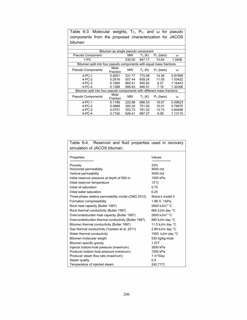
206
Table 6-3: Molecular weights, TC, PC, and ω for pseudo
components from the proposed characterization for JACOS
bitumen
Bitumen as single pseudo component
Pseudo Component MW TC (K) PC (bars) ω
1-PC 530.00 847.17 10.64 1.0406
Bitumen split into four pseudo components with equal mass fractions
Pseudo Components Mole
Fraction MW TC (K) PC (bars) ω
4-PC-1 0.4001 331.77 775.08 14.36 0.81599 4-PC-2 0.2616 507.44 859.24 11.05 1.03422 4-PC-3 0.1995 665.41 905.82 9.27 1.16443 4-PC-4 0.1388 956.63 946.51 7.16 1.32306
Bitumen split into four pseudo components with different mass fractions
Pseudo Components Mole
Fraction MW TC (K) PC (bars) ω
4-PC-1 0.1189 222.88 686.53 18.07 0.59623 4-PC-2 0.0868 305.20 751.60 15.01 0.76675 4-PC-3 0.0751 353.73 781.52 13.73 0.84498 4-PC-4 0.7192 626.41 887.27 9.58 1.13115
Table 6-4. Reservoir and fluid properties used in recovery
simulation of JACOS bitumen.
Properties
Porosity
Values
33% Horizontal permeability 4000 md
Vertical permeability 3000 md
Initial reservoir pressure at depth of 500 m 1500 kPa
Initial reservoir temperature 13°C
Initial oil saturation 0.75
Initial water saturation 0.25
Three-phase relative permeability model (CMG 2012) Stone’s model II
Formation compressibility 1.8E-5 1/kPa
Rock heat capacity (Butler 1997) 2600 kJ/m3 °C
Rock thermal conductivity (Butler 1997) 660 kJ/m day °C
Over/underburden heat capacity (Butler 1997) 2600 kJ/m3 °C
Over/underburden thermal conductivity (Butler 1997) 660 kJ/m day °C
Bitumen thermal conductivity (Butler 1997) 11.5 kJ/m day °C
Gas thermal conductivity (Yazdani et al. 2011) 2.89 kJ/m day °C
Water thermal conductivity 1500 kJ/m day °C
Bitumen molecular weight 530 kg/kg-mole
Bitumen specific gravity
Injector bottom-hole pressure (maximum)
Producer bottom-hole pressure (minimum)
Producer steam flow rate (maximum)
Steam quality
Temperature of injected steam
1.077
3500 kPa
1500 kPa
1 m3/Day
0.9
242.71oC
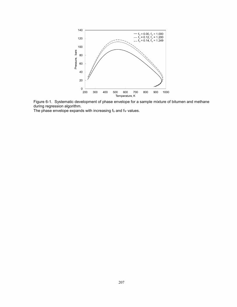
207
Figure 6-1. Systematic development of phase envelope for a sample mixture of bitumen and methane during regression algorithm. The phase envelope expands with increasing fb and fΨ values.

208
(a)
(b)
Figure 6-2. Comparison of the data and predictions for ethane solubilities for (a) Cold Lake and (b) Athabasca bitumens. For Cold Lake bitumen, solid curves show the predictions and dashed curves show the data.
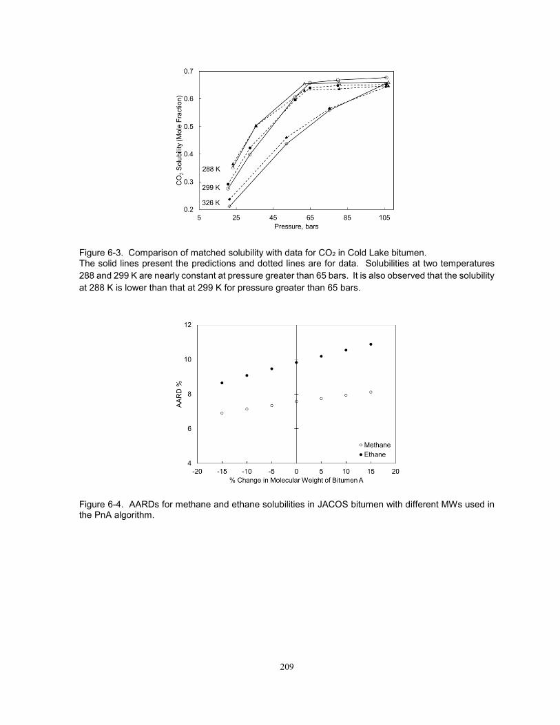
209
Figure 6-3. Comparison of matched solubility with data for CO2 in Cold Lake bitumen. The solid lines present the predictions and dotted lines are for data. Solubilities at two temperatures
288 and 299 K are nearly constant at pressure greater than 65 bars. It is also observed that the solubility
at 288 K is lower than that at 299 K for pressure greater than 65 bars.
Figure 6-4. AARDs for methane and ethane solubilities in JACOS bitumen with different MWs used in the PnA algorithm.
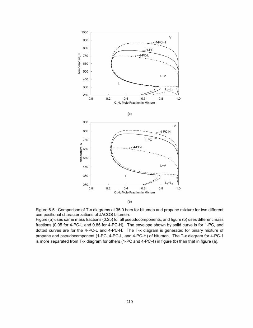
210
(a)
(b)
Figure 6-5. Comparison of T-x diagrams at 35.0 bars for bitumen and propane mixture for two different compositional characterizations of JACOS bitumen. Figure (a) uses same mass fractions (0.25) for all pseudocomponents, and figure (b) uses different mass
fractions (0.05 for 4-PC-L and 0.85 for 4-PC-H). The envelope shown by solid curve is for 1-PC, and
dotted curves are for the 4-PC-L and 4-PC-H. The T-x diagram is generated for binary mixture of
propane and pseudocomponent (1-PC, 4-PC-L, and 4-PC-H) of bitumen. The T-x diagram for 4-PC-1
is more separated from T-x diagram for others (1-PC and 4-PC-4) in figure (b) than that in figure (a).
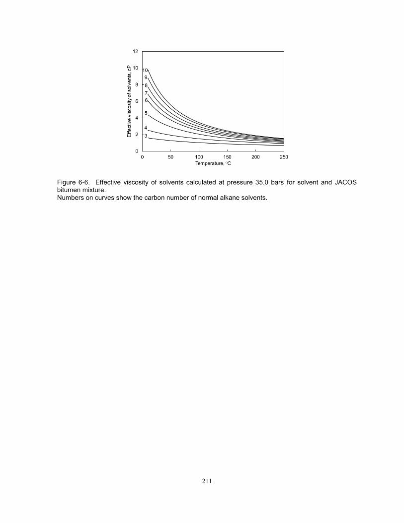
211
Figure 6-6. Effective viscosity of solvents calculated at pressure 35.0 bars for solvent and JACOS bitumen mixture. Numbers on curves show the carbon number of normal alkane solvents.
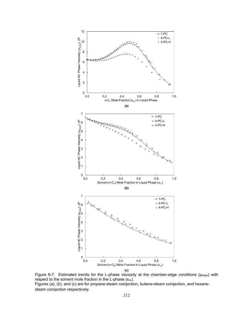
212
(a)
(b)
(c)
Figure 6-7. Estimated trends for the L-phase viscosity at the chamber-edge conditions (μedge) with respect to the solvent mole fraction in the L-phase (xsL). Figures (a), (b), and (c) are for propane-steam coinjection, butane-steam coinjection, and hexane-
steam coinjection respectively.

213
Figure 6-8. Trend of viscosity gradient (∆µ/∆T) with temperature for JACOS bitumen.
Figure 6-9. Simulated bitumen recovery with steam-solvent coinjection method for different solvent cases (n-C3, n-C4, n-C5, and n-C6).

214
(a)
(b)
(c)
Figure 6-10. L-phase viscosity along the chamber edge from the simulation results: (a) propane-steam coinjection, (b) butane-steam coinjection, and (c) hexane-steam coinjection. The number on the horizontal axis shows the grid's location from the reservoir top.

215
Chapter 7: A New Algorithm for Multiphase Fluid Characterization for Solvent
Injection
A version of this has been submitted to SPE J for publication. The manuscript is under review.
216
7.1. Introduction
Solvent injection has been successfully implemented for enhanced oil recovery; e.g., in the Western
United States (Mizenko 1992; Stein et al. 1992; Tanner et al. 1992; Fulco, G. J. 1999; McGuire et al.
2001), Canada (Malik and Islam 2000), and the North Sea (Varotsis et el. 1986). Field pilot tests were
also reported for coinjection of solvent with steam for bitumen recovery in Canada (Gupta et al. 2005;
Gupta and Gittins 2006; Dickson et al. 2011).
Solvent injection can involve complex phase behavior, which consists of three hydrocarbon phases,
the oleic (L1), gaseous (V), and solvent-rich liquid (L2) phases. Such phase behavior has been reported
for various mixtures in the literature. For binary mixtures, CO2, methane, ethane, and propane were
studied as the solvent component mixed with a heavier n-alkane component (Rodrigues and Kohn 1967;
Kulkarni et al. 1974; Hottovy et al. 1981a; Enick et al. 1985; Fall and Luks 1985; Fall et al. 1985; Estrera
and Luks 1987; Peters et al. 1987a, 1987b; Peters et al. 1989; Van der Steen et al. 1989; Secuianu et
al. 2007). Ternary mixtures were studied by Horn and Kobayashi (1967), Hottovy et al. (1981b), Hottovy
et al. (1982), Llave et al. (1986), Jangkamolkulchal and Luks (1989), and Gregorowicz et al. (1993a,
1993b). Mixtures of solvents with reservoir oils were also studied by various researchers (Shelton and
Yarborough 1977; Henry and Metcalfe 1983; Turek et al. 1988; Roper 1989; Sharma et al. 1989;
Okuyiga 1992; Creek and Sheffield 1993; DeRuiter et al. 1994; Mohanty et al. 1995; Godbole et al.
1995).
Three-hydrocarbon-phase behavior was characterized by use of a cubic equation of state (EOS) for
specific solvent-injection cases (Nghiem and Li 1986; Sharma et al. 1989; Negahban and Kremesec
1989; Okuyiga 1992; Khan et al. 1992; Creek and Sheffield 1993; Reid 1994; Mohanty et al. 1995;
Godbole et al. 1995; Guler et al. 2001; Aghbash and Ahmadi 2012). The EOSs used by them include
the Peng-Robinson (PR) EOS (Peng and Robinson 1976, 1978) and the Soave-Redlich-Kwong EOS
(Soave 1972). Their results indicate that these EOSs are capable of correlating three-hydrocarbon-
phase behavior quantitatively. However, their characterization procedures were specific to the fluids
studied. No systematic knowledge has been presented of how three-hydrocarbon-phase behavior can
be reliably characterized for solvent injection (Okuno and Xu 2014)
This paper presents a new algorithm for characterization of multiphase behavior with the PR EOS.
The term “multiphase behavior” in this paper refers to volumetric and compositional behavior of
equilibrium phases consisting of at most three hydrocarbon phases. Hence, the algorithm
accommodates the traditional vapor-liquid phase behavior as a subset of the research scope. The next
section describes the algorithm developed. Then, case studies are presented for 90 reservoir fluids, for
which experimental data are available in the literature.
7.2. Multiphase Fluid Characterization
Fluid characterization consists of three major steps: (i) compositional characterization of the plus
fraction; (ii) initial estimates for components’ properties, such as critical temperature (TC), critical

217
pressure (PC), and acentric factor (ω); and (iii) regression to the PVT data available. The current
research uses the method of Quiñones-Cisneros et al. (2004) for step i.
Steps ii and iii broadly follow the methodology of Kumar and Okuno (2013), which is referred to as
perturbation from n-alkanes (PnA). In the PnA method, step ii assumes that pseudocomponents are n-
alkanes; that is, they are assigned TC, PC, and ω of equivalent n-alkanes in terms of carbon number
(CN). This assumption is based on well-defined thermo physical properties of three important
hydrocarbon groups i.e. paraffins, napthenes, and aromatics present in pseudocomponents. For same
carbon number, paraffins have lowest TC and PC, and highest acentric factor among these three groups.
Figure 7-1 presents the comparison of critical parameters and resulting vapor pressure curves for
hexadecane (n-C16) and pyrene (C16H10). Vapor pressure curve for pyrene is below the vapor pressure
curve for n-C16 and extended to higher TC and PC in P-T space. As a result, among the P-T envelopes
for mixtures of same carbon number paraffin, napthene, and aromatic component with a given light
component, paraffin’s P-T envelope is innermost. This is shown in Figure 7-2, which presents the P-T
envelopes for 99.99% binary mixture of methane with nonane (n-C9), propyl cyclo hexane (C9H18), and
2-propyl benzene (C9H12). The P-T envelope for n-C9 is inside the P-T envelopes for C9H18 and C9H12.
The analysis presented here supports assumption that lower limits for TC and PC for pseudocomponents
are determined by its n-alkane equivalent values in fluid characterization. Then, step iii systematically
adjusts the properties of all pseudocomponents in the direction of increasing aromaticity from n-alkanes
(i.e., zero aromaticity). In the initial stage of this research, the validity of this methodology for three
phases was confirmed with the data for ternary mixtures of methane, ethane, and tetradecylbenzene
(C20H34) given in Jangkamolkulchal and Luks (1989).
In step ii of Kumar and Okuno (2013, 2015), the n-alkane properties were taken from Kumar and
Okuno (2012), in which TC, PC, and ω of n-alkanes were optimized for the PR EOS to accurately predict
vapor pressure and liquid density. Hence, the PR EOS was initially calibrated with vapor pressure and
liquid density of n-alkanes prior to characterizing reservoir fluid. For the current research, however, step
ii requires that the PR EOS be calibrated with binary three-phase behavior. To this end, binary
interaction parameters (BIPs) have been optimized for the PR EOS to represent binary three-phase data
taken from the literature, such as those for CO2, methane, ethane, and propane with heavier n-alkanes.
The three-phase data mainly included upper critical end point (UCEP) for binary mixtures. At UCEP,
solvent rich liquid phase becomes critical with the vapor phase in presence of oil rich liquid phase. The
UCEP for binary mixtures of CO2, methane, ethane, and propane with heavier n-alkanes were matched
adjusting only BIP; physical critical parameters for components not changed. Appendix A presents the
details of optimization process and development of correlations for BIPs. Appendix B presents the
predictive capability of optimized BIPs for three-phase prediction for binary mixtures of CO2, methane,
ethane, and propane with heavier n-alkanes.
It was observed that UCEP match for pairs like ethane and n-C18 could not be achieved by BIP
adjustment when physical critical parameters for n-C18 was replaced with its optimized critical

218
parameters (Kumar and Okuno 2012). Figure 7-3 shows the predicted temperatures at UCEP at
different BIPs for ethane and n-C18 pair. The UCEP for this binary mixture is 312.45 K and 55.31 bars
(Peters et al. 1986). The best match that could be achieved with BIP adjustment was 307.03 K and
50.21 bars at BIP of 0.01. Figure 7-4 shows the trend of reduced Gibbs free energy for ethane and n-
C18 mixture at UCEP temperature and pressure. The dotted curve is prediction with physical critical
parameters for n-C18 and optimized BIP (that matched UCEP); this curve is taken as reference. Solid
curves are for optimized critical parameters (Kumar and Okuno 2012) for n-C18 and different BIPs
(shown on the curves). Optimized critical parameters could not match the desired trend of reduced
Gibbs free energy for UCEP match i.e. the trend of reference curve. Hence, the BIP was optimized by
using physical critical parameters from Gao et al. (2001) correlations (Equation 7-1 and 7-2).
TCP = [6573.87 − 4680.77exp(−0.1831(CN0.6667 − 2.08))]1
1.276 (7-1)
PCP = 42.44exp[−0.3757(CN0.5684 − 1.8672)], (7-2)
for n-alkanes (or paraffins) heavier than hexane. Gao et al. (2001) also presented a correlation for ω
for n-alkanes (Equation 7-3),
ωP = [3.212102 − 2.937628exp(−0.04699(CN0.6667 − 2.08))]1
0.6851 (7-3)
As discussed in Appendix A, however, the correlation presented in Equation 7-4 has been found to
perform better for the BIP optimization in this research. The deviation of Equation 7-4 from Equation 7-
3 is minor as presented in Appendix A (see Figure 7-A3).
ώP = 0.217066 + 5.27405CN−(14.8147
CN). (7-4)
Equations 7-1 and 7-2 are used for the initialization of pseudocomponents in step ii. The initial values
for ω are all zero for pseudocomponents.
A comparative study is done on the predictive capability of two sets of EOS parameters (1) optimized
BIP and physical critical parameters (Gao et al. 2001), (2) zero BIP and optimized critical parameters
(Kumar and Okuno 2012). Predicted pressure-composition (P-x) diagrams for binary and quaternary
mixture of n-alkanes from these two sets of EOS parameters are compared with experimental data.
Figures 7-5 and 7-6 present comparison for P-x diagrams for ethane with n-C16 at 363.15 K and with
n-C24 at 340 K respectively. Figure 7-7 presents similar comparison for hexane mixture with n-C36 at
621.8 K, however, due to unavailability of any optimized BIP for n-C6-n-C36 pair, BIP is kept zero for first
set of EOS parameter also. Figure 7-8 presents comparison of predicted P-T phase envelopes for
quaternary mixture of n-alkanes with data. Though first set of EOS parameter satisfactorily matched
the P-x diagrams in Figure 7-5 and 7-6, its predictions in Figure 7-7 and 7-8 deviated from data
significantly. Attempts were made to improve these predictions by adjusting BIPs. However, such
attempts did not show significant improvement. It is observed that BIPs (with physical critical
parameters) have limited potential to improve two-phase behavior by their adjustment, whereas
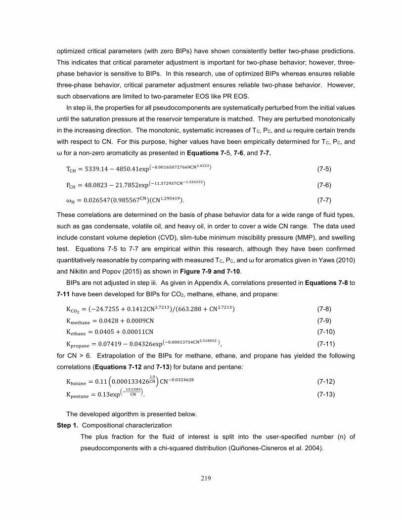
219
optimized critical parameters (with zero BIPs) have shown consistently better two-phase predictions.
This indicates that critical parameter adjustment is important for two-phase behavior; however, three-
phase behavior is sensitive to BIPs. In this research, use of optimized BIPs whereas ensures reliable
three-phase behavior, critical parameter adjustment ensures reliable two-phase behavior. However,
such observations are limited to two-parameter EOS like PR EOS.
In step iii, the properties for all pseudocomponents are systematically perturbed from the initial values
until the saturation pressure at the reservoir temperature is matched. They are perturbed monotonically
in the increasing direction. The monotonic, systematic increases of TC, PC, and ω require certain trends
with respect to CN. For this purpose, higher values have been empirically determined for TC, PC, and
ω for a non-zero aromaticity as presented in Equations 7-5, 7-6, and 7-7.
TCH = 5339.14 − 4850.41exp(−0.001650727669CN1.4223) (7-5)
PCH = 48.0823 − 21.7852exp(−11.372937CN−1.326532) (7-6)
ωH = 0.026547(0.985567CN)(CN1.295419). (7-7)
These correlations are determined on the basis of phase behavior data for a wide range of fluid types,
such as gas condensate, volatile oil, and heavy oil, in order to cover a wide CN range. The data used
include constant volume depletion (CVD), slim-tube minimum miscibility pressure (MMP), and swelling
test. Equations 7-5 to 7-7 are empirical within this research, although they have been confirmed
quantitatively reasonable by comparing with measured TC, PC, and ω for aromatics given in Yaws (2010)
and Nikitin and Popov (2015) as shown in Figure 7-9 and 7-10.
BIPs are not adjusted in step iii. As given in Appendix A, correlations presented in Equations 7-8 to
7-11 have been developed for BIPs for CO2, methane, ethane, and propane:
KCO2= (−24.7255 + 0.1412CN2.7213)/(663.288 + CN2.7213) (7-8)
Kmethane = 0.0428 + 0.0009CN (7-9)
Kethane = 0.0405 + 0.00011CN (7-10)
Kpropane = 0.07419 − 0.04326exp(−0.00013754CN2.518052 ), (7-11)
for CN > 6. Extrapolation of the BIPs for methane, ethane, and propane has yielded the following
correlations (Equations 7-12 and 7-13) for butane and pentane:
Kbutane = 0.11 (0.0001334261.0
CN) CN−0.0324628 (7-12)
Kpentane = 0.13exp(−15.5385
CN). (7-13)
The developed algorithm is presented below.
Step 1. Compositional characterization
The plus fraction for the fluid of interest is split into the user-specified number (n) of
pseudocomponents with a chi-squared distribution (Quiñones-Cisneros et al. 2004).

220
Step 2. Deviation in saturation pressure
The initial deviation in saturation pressure is calculated as the ratio of the measured saturation
pressure (PS) to the calculated saturation pressure (PS_EOS) by use of the PR EOS with
equations 7-1, 7-2, and 7-4. The ratio is denoted as β.
Step 3. Incremental values for TC, PC, and ω
Incremental values for TC, PC, and ω during the regression are determined using Equations 7-
14, 7-15, and 7-16 respectively.
∆TC,i = [TCH,i – TCP,i]/(βN) (7-14)
∆PC,i = [PCH,i – PCP,i]/N (7-15)
∆ωi = ωH,i/N, (7-16)
for i = 1, 2, …, n, where N is an integer to be specified by the user (e.g., N = 104 as used in this
research). Set the iteration-step index k to be one.
Step 4. Update of TC, PC, and ω using Equations 7-17, 7-18, and 7-19 respectively.
TC,i = TCP,i + k∆TC,i (7-17)
PC,i = PCP,i + k∆PC,i (7-18)
ωi = k∆ωi (7-19)
Step 5. Convergence test
Calculate δ = (PS – PS_EOS)/PS. Go to step 6 if |δ| < δTOL (e.g., δTOL = 10-4). Otherwise, go to
step 4 after increasing k by one; k = k + 1.
Step 6. Volume shift
Volume shift parameters are adjusted to match liquid density data, as required.
Critical parameters and acentric factors are perturbed as monotonic functions of the iteration-step
index, k. It has been consistently observed in this research that the calculated PS increases with
increasing k during the iteration. Figure 7-11a depicts that vapor pressure curves for all
pseudocomponents change systematically and monotonically as the iteration proceeds for an example
case of light oil. Figure 7-11b shows the two-phase envelopes corresponding to the three sets of vapor
pressure curves given in Figure 7-11a. Figure 7-11c shows the monotonic change in saturation
pressure with iteration parameter (k).
Volume shift is performed to match liquid density data only after the model is set in terms of
compositional phase behavior. This is because a change in compositional behavior prediction affects
volumetric predictions, as discussed in detail in Kumar and Okuno (2013). For fluid characterization
with a PnA-based approach, density data for a liquid phase that is equilibrium with the V phase are more
important than those from a single-phase fluid or equilibrium V phase (Kumar and Okuno 2015). This
was confirmed also in this research. Hence, it is recommended that step 6 use density data from an
equilibrium liquid phase.
221
7.3. Case Studies
The algorithm is applied to 90 reservoir fluids in this section, which are gas condensates, volatile oils,
heavy oils, and bitumens. The fluids tested are characterized as 12 components, which consist of N2,
CO2, C1, C2, C3, C4, C5, C6, and four pseudocomponents, by use of the PR EOS with the van der Waals
mixing rules. The regression algorithm uses only PS and saturated liquid density data, as shown in the
previous section. The EOS models for the 90 fluids developed with new algorithm are listed in Appendix
7-C. For each fluid, two separate tables are presented, one contains composition, molecular weight, TC,
PC, ω, volume shift parameters for components, and other table contains the BIP matrix.
TC, PC, and ω for well-defined pure components are taken from Yaws (2010), and they are not
adjusted. Table 7-1 gives the BIPs used in this section. Note that BIPs are not adjusted in the
regression algorithm developed. However, it is possible to adjust them individually when specific data
are to be matched. TC, PC, and ω for pseudocomponents are adjusted to match PS. Volume shift
parameters are adjusted to match saturated liquid density data at the final step of the algorithm. Then,
the quality of prediction from the resulting EOS model is demonstrated with other types of data, such as
three hydrocarbon phases, CVD, constant mass expansion (CME), and MMP for V-L.
7.3.1. L-V Phase Behavior
This subsection shows results for two-phase predictions. Table 7-2 lists 55 light fluids for which CVD
and CME data are available in the literature. In the table, fluids 1 to 48 are gas condensates and the
others are volatile oils. The fifth, sixth and seventh columns show the value of β, the number of iterations
(i.e., k in the previous section) and the degree of freedom in the chi-squired distribution, respectively.
The eighth column indicates CVD data as data type 1 and CME as data type 2. This column also
indicates the limiting value from measured data. The right-most column gives the average absolute
deviation (AAD) for the data type indicated for each fluid.
Before performing step 6, the AAD for saturated liquid densities for all the fluids in Table 7-2 was
less than 2%, indicating the accuracy of the PR EOS for light fluids. They were eventually matched in
step 6.
The results given in Table 7-2 show that the new algorithm is capable of predicting CVD and CME
liquid saturations well. The deviation tends to be high for near-critical fluids (No. 6, 7, 8, 12, 13, 14, 36,
38, 48, 51, and 54). This is because liquid saturation is sensitive to pressure near saturation pressure
for those fluids. The AADs for 42 CVD and 13 CME liquid saturation predictions are 1.5 and 2.5%
respectively. Figure 7-12 shows the CME liquid saturation for Fluid 36, which gives the highest AAD in
Table 7-2. Fluid 54 is also a near-critical fluid. However, Figure 7-13 shows satisfactory predictions of
CVD liquid saturations for this near-critical fluid. Pedersen and Christensen (2007) presents an SRK
EOS model (Pedersen and Christensen 2007) with 6 pseudocomponents model that was developed to
match the CVD and saturation pressure data. A comparison of predicted P-x diagram at 424.25 K with
this EOS model (injection gas: 0.005 N2, 0.050 CO2, 0.582 CH4, 0.171 C2H6, 0.120 C3H8, 0.050 C4H10,
0.017 C5H12, and 0.005 C6H14) shows good match with that predicted with the new algorithm. The MMPs

222
predicted at 424.25 K are 251.32 bars and 245.71 bars respectively for the new algorithm and SRK EOS
model. This comparison further validates the reliability of new algorithm for phase behavior predictions
at P-T-x conditions different from data used in characterization.
Table 7-3 shows reservoir oils for which MMP data from slim-tube tests are available in the literature.
MMP prediction serves as a severe test for fluid characterization since it requires accurate prediction of
compositional phase behavior away from the original oil composition in multicomponent composition
space. Thermodynamic MMPs are calculated with the method of characteristics within PVTsim (Calsep
2012), and compared with data. The calculated MMPs likely correspond to the V-L miscibility,
considering their reservoir temperatures and that PVTsim did not indicate any difficulty associated with
three phases in the calculations. The average absolute relative deviation (AARD) for all 26 MMP
predictions is 4.57%. Some level of deviation of thermodynamic MMP from slim-tube MMP is inevitable
due to the presence of dispersion in real displacement of oil by gas. However, the present algorithm
shows improved MMP predictions, as the AARDs with earlier characterizations were 6.7% (Kumar and
Okuno 2013) and 6.4% (Kumar and Okuno 2015).
The algorithm was also tested in terms of other types of phase behavior. Table 7-4 lists heavy oils
for which swelling test data, GOR, and V-L boundary in P-T space are available in the literature. Oil 1
in Table 7-4 is West Sak oil (Sharma 1990), for which the AARD in GOR prediction is 7%.
Swelling test data are available for Oil 2 with a gas mixture of 14% CO2, 17% methane, 60% ethane,
4% propane, 3% butane, and 2% pentane (Krejbjerg and Pedersen 2006). The saturation pressures for
different gas-oil mixing ratios were predicted satisfactorily as shown in Figure 7-14. The AARD for the
predictions is 3.4%. Pedersen et al. (2004) showed GOR data for Oil 3, for which the PR-EOS model
with the current characterization algorithm gives an AARD of 4.42%. As shown in Figure 7-15, the GOR
predictions are in good agreement with the data.
PVT data for Lloydminster heavy oil were presented in Li et al. (2013a) (oil 4 in Table 7-4). The
dead oil composition was characterized with four pseudocomponents on the basis of the chi-squired
distribution with a degree of freedom of 9. The saturation pressure of 56.64 bars at 347.67 K for feed
#5 (31.7% CO2, 34.3% butane, and 0.34% heavy oil) was used for characterization with the new
algorithm. The characterized oil was then used to predict the saturation pressure for feed #4 (38.6%
CO2, 36.2% propane, and 25.2% heavy oil). Figure 7-16 shows that the predictions are close to the
reported data, yielding an AARD of 5.60% for the seven data points.
7.3.2. L-L-V Phase Behavior
In this subsection, the new algorithm is tested by comparing three-phase behavior predictions with
experimental data. Note that the algorithm matches only PS at the oil composition as far as
compositional phase behavior is concerned; that is, no parameter is adjusted for matching three-phase
data for oil/solvent mixtures to be presented here.
Apart from the three-phase predictions for fluids with PR EOS model developed with the new
algorithm and optimized BIP, this subsection, also present predictions when fluids are characterized
223
with the new algorithm but with zero hydrocarbon-hydrocarbon BIPs. In this case, all hydrocarbon-
hydrocarbon BIPs are set to zero, and the BIP of CO2 with pseudocomponents are set to 0.1 (Peng and
Robinson 1978). No other change in the BIP matrix shown in Table 7-1 is made. Predictions with zero
BIP case in the figures are shown as “Prediction with zero BIP”. The objective of this additional
demonstration is to show the importance of non-zero optimized BIPs for reliable three-phase predictions.
Three-phase data are available for oils 1, 4, 5, and 6 from Table 7-4. Three phases were reported
for the mixture of 20% oil 1 and 80% CO2 at 299.81 K. Figure 7-17 compares predicted saturations for
the L1 (Figure 7-17a) and L2 (Figure 7-7b) phases with experimental data. The AARD for the L1-phase
saturations is 5.61%. With the new algorithm, the PR EOS correctly predicts the presence of three
phases for this mixture; i.e., they were experimentally observed between 77.20 and 83.75 bars, and
predicted between 76.46 and 82.47 bars. Similar prediction with zero hydrocarbon-hydrocarbon BIPs
shows the presence of three-phases in comparatively small pressure range (79.21- 83.0 bars). Figure
7-17b also shows the three-phase prediction from Aghbash and Ahmadi (2012) EOS model. Ranges
of pressure for three-phase predicted from new algorithm and Aghbash and Ahmadi are nearly same.
A comparison of P-x diagrams at 370 K with equimolar mixture of methane, ethane, propane, and butane
as injection gas predicted with EOS models from new algorithm and that from Aghbash and Ahmadi
(2012) is presented in Figure 7-18. The two models show significantly different predictions for P-x
diagrams. The possible reason for this difference is non-zero BIPs used for pseudocomponent-
pseudocomponent pairs by Aghabsh and Ahmadi; these BIPs are zero for the new algorithm. The
MMPs with this injection gas at 370 K are 72.77 bars, and 68.66 bars respectively for the new algorithm
and Aghbash and Ahmadi. Although, MMP predictions which depend on the composition paths, are
nearly same, significantly different P-x diagrams indicate to careful use of non-zero BIPs for
pseudocomponent – pseudocomponent pairs.
Figure 7-19 shows the comparison of predicted P-T diagram with SRK EOS from Krejbjerg and
Pedersen (2006) with the prediction from new algorithm for oil 2 in Table 7-4. Both the predictions match
significantly except for high temperature two-phase envelope. Figure 7-20 shows phase boundaries
between two and three phases in P-T space for feeds 14 (Figure 7-20a) and 15 (Figure 7-20b) with oil
4 in Table 7-4. Feed 14 is 23.6% propane, 67.2% CO2, and 9.2% oil, and feed 15 is 11.8% butane,
83.2% CO2, and 5.0% oil. The results show that the PR-EOS models with the new characterization
algorithm give satisfactory predictions for these complex mixtures. This also validates the reliability of
the BIP correlation (equation 7-12) for butane, which was developed by extrapolation of BIP values for
methane, ethane, and propane. However, the predictions with zero hydrocarbon-hydrocarbon BIPs
show narrow three-phase area close to LL-LLV boundary.
Oil 5 given in Table 7-4 is Athabasca bitumen, for which Badamchi-Zadeh et al. (2009) presented
three-phase data. The dead-oil composition was characterized with four pseudocomponents on the
basis of the chi-squired distribution with a degree of freedom of 12. The algorithm was applied with the
saturation pressure, 10.82 bars, reported for a mixture of 59.3% bitumen with 40.7% propane at 333.15
224
K. The resulting fluid model was then used to predict three-phase behavior for the mixture of 51.0%
CO2, 34.7% propane, and 14.3% bitumen. Figure 7-21 shows satisfactory predictions of phase
boundaries in spite of the large amount of CO2 present in the predicted mixture. Prediction from zero
hydrocarbon-hydrocarbon BIPs shows the presence of larger three-phase region.
Oil 6 given in 7-4 is Peace River bitumen. The molecular weight (MW) used in the characterization
is 527.5 g/mol according to Mehrotra and Svrcek (1985). This bitumen was characterized using the
saturation pressure, 50.50 bars, reported by Mehrotra and Svrcek (1985) for a mixture of 21.83%
methane and 78.17% bitumen at 326.65 K. The resulting fluid model was then used to predict three
phases in P-T space for another mixture, 89.94% pentane and 10.06% bitumen. The predicted three-
phase behavior was compared with three-phase behavior for this mixture composition simulated by
Agrawal (2012). Figure 7-22 presents that the predicted three-phase region is narrower than in Agrawal
(2012) in P-T space. The difference is inevitable due to the lack of comprehensive data; i.e., the bitumen
MW in the characterization by Agrawal (2012) was 580 g/mol. Nevertheless, the successful prediction
of three phases indicates the validity of the BIP correlation (equation 7-13) for pentane, which was
developed by extrapolation of BIP values for methane, ethane, and propane. Prediction with zero
hydrocarbon– hydrocarbon BIPs case did not show presence of three-phase region.
Table 7-5 lists reservoir oils for which three phases with CO2 were reported in the literature. Results
show that the new algorithm gives reasonable predictions for these fluids. As an example, Figure 7-23
presents phase boundaries in P-x space for oil C2 with CO2 at 313.71 K, for which the data were taken
from Turek et al. (1988). Although the EOS gives higher immiscibility than the data in this diagram, their
agreement is remarkable considering that only PS and liquid density data at the oil composition were
used in the characterization. Also, the regression was conducted only for TC, PC, and ω of
pseudocomponents. That is, the effect of oil aromaticity on the interaction between oil and CO2 was not
explicitly considered in the algorithm. The prediction from zero hydrocarbon-hydrocarbon BIPs for this
reservoir oil did not show presence of three-phase. All the fluids in Table 7-5 were characterized with
the new algorithm and zero hydrocarbon-hydrocarbon BIPs. Out of 9 oils, the presence of three-phase
was shown for only three oils (oil nos. 6, 8, and 9). Figure 7-24 presents one such example for Oil G
(Table 7-5) where zero hydrocarbon-hydrocarbon BIPs could predict the three phase successfully.
However, predicted three phase area is detached from the single-phase boundary.
The predictions from EOS models developed using new algorithm with zero hydrocarbon-
hydrocarbon BIPs either failed to show the presence of three phases or predicted three phases were
significantly deviated from the data in P-T-x space. This shows that non-zero hydrocarbon-hydrocarbon
BIPs are required to model the interaction among PR EOS attraction parameters for components for
multiphase behavior. Optimized BIPs, on the other hand, reliably predicted the presence of three-
phases for all fluids with satisfactory accuracy.
Figures 7-25 to 7-28 show the comparison of prediction of P-x diagrams from PR EOS models
developed by Khan (1992) for mixture of CO2 and oil 5, 6, 7, and 8 with the predictions from new

225
algorithm. Khan (1992) adjusted the BIPs to match the three-phase region on the P-x diagrams. Turek
et al. (1988) observed that three-phase boundaries are difficult to determine, and reported boundaries
may be reliable within ±1.7 bars. The new algorithm predicts the three-phase region correctly only by
matching saturation pressure in all cases. This indicates to reliability of the regression algorithm and
the optimized BIPs.
The analysis of multiphase behavior predictions in this research has indicated that the simple
algorithm is reliable even with the limited PVT data used (PS and liquid density). However, further
adjustment of parameters may be required if additional phase behavior data are to be matched. Obvious
candidates are BIPs for solvents with pseudocomponents. In particular, CO2 BIPs may be adjusted to
accommodate the effects of oil aromaticity and reservoir temperature on compositional phase behavior
for CO2 flooding. In addition, the parameters, N and β, in the algorithm can be flexible; e.g., N can be
different for TC, PC, and ω.
7.4. Conclusions
A new algorithm was presented for characterization of multiphase behavior for solvent injection
simulation. The PR EOS was used with the van der Waals mixing rules. The developed algorithm
requires only the saturation pressure and liquid density for a given composition and reservoir
temperature, in its simplest form. Case studies were conducted for 90 reservoir fluids and their mixtures
with solvents for up to three hydrocarbon phases. Conclusions are as follows:
o The algorithm with the BIPs developed in this research enables the PR EOS to give reliable
predictions of multiphase behavior for reservoir fluids. The PnA method was found to be applicable
for multiphase characterization; that is, the effect of aromaticity on phase behavior can be modeled
through TC, PC, and ω of pseudocomponents as monotonic functions of a single parameter in the
regression algorithm developed.
o Results show that positive BIPs are required for the PR EOS to properly represent three-
hydrocarbon-phase behavior of reservoir fluids. The fundamental reason comes from the necessity
for accurate predictions of binary three-phase curves. This is in contrast to the usage of zero BIPs
for hydrocarbon pairs that has been recommended for simpler two-phase characterization in the
literature.
226
7.5. Nomenclature
AARD : Average absolute relative deviation =1
M∑ |
prediction−data
Data|
j
Mj=1
AAD : Average absolute deviation =1
M∑ |prediction − data|j
Mj=1
BIP : Binary interaction parameter
CEP : Critical endpoint
CME : Constant mass expansion
CN : Caron number
CVD : Constant volume depletion
EOS : Equation of state
LCEP : Lower critical end point
L-V : Liquid (L)-vapor (V) phase equilibrium
MMP : Minimum miscibility pressure
PR EOS : Peng and Robinson (1976, 1978) equation of state
PT : Pressure-temperature
p : Degree of freedom in the chi-squared distribution
ST : Swelling test
UCEP : Upper critical endpoint
Greek Symbols: β : PS/PS_EOS; PS_EOS is calculated assuming pseudocomponents as n-alkanes.
δ : Deviation of calculated saturation pressure from experimental value
δTOL : Tolerance set for deviation (δ)
ω : Acentric factor
ώP : Acentric factor calculated from Eq. 7-4
ωP : Acentric factor calculated from Eq. 7-3
ωH : Acentric factor calculated from Eq. 7-7
Roman Symbols:
A : Aromatics
k : Number of iterations in the algorithm
K : Binary interaction parameters (Eqs. 7-8 to 7-13)
L1-L2-V : Three hydrocarbon phases (L1: oleic, L2: solvent-rich liquid, and V: Gaseous)
L-V : Liquid (L)-vapor (V) phase equilibrium
n : Number of pseudocomponents
PC : Critical pressure
PCP : Critical pressure calculated from Eq. 7-2
PCH : Critical pressure calculated from Eq. 7-6

227
PS : Experimental saturation pressure
PS_EOS : Calculated saturation pressure with the PR EOS
TC : Critical temperature
TCP : Critical temperature calculated from Eq.7-1
TCH : Critical temperature calculated from Eq. 7-5
Subscript:
i : Index for pseudocomponent
228
7.6. References
Aghbash, V.N. and Ahmadi, M. 2012. Evaluation of CO2-EOR and Sequestration in Alaska West Sak
Reservoir Using Four-Phase Simulation Model. Presented at the SPE Western Regional Meeting,
Bakers-field, California, 21-23 March. SPE-153920-MS.
Agrawal, P. 2012. Measurement and Modeling of the Phase Behavior of Solvent Diluted Bitumens. MS
Thesis. University of Calgary, Alberta, Canada.
Akpabio, J.U., Udofia, E.E., and Ogbu, M. 2014. PVT Fluid Characterization and Consistency Check
for Retrograde Condensate Reservoir Modeling. Presented at SPE Nigeria Annual International
Conference and Exhibition, Lagos, Nigeria, 5-7 August. SPE-172359-MS.
Al-Meshari, A. 2004. New Strategic Method to Tune Equation of State to Match Experimental Data for
Compositional Simulation. PhD Thesis. Texas A&M University, Texas. USA.
Al-Subai, K.O. 2001. Compositional Gradient Calculations for a Saudi Arabian Gas Condensate
Reservoir. MS Thesis. King Fahd University of Petroleum & Minerals, Saudi Arabia.
Badamchi-Zadeh, A., Yarranton, H. W., Svrcek, W. Y. et al. 2009. Phase Behavior and Physical
Property Measurements for VAPEX Solvents: Part I. Propane and Athabasca Bitumen. J Can Pet
Technol 48 (1): 54-61.
Chang, H.L., Hurt, L.J., and Kobayashi, R. 1966. Vapour-Liquid Equilibria of Light Hydrocarbons at Low
Temperatures and High Pressures: The Methane-n-Heptane System. AIChE J. 12 (6): 1212-1216.
Calsep. 2012. PVTsim Version 19.2.0. Lyngby, Denmark: Calsep International Consultants,
Choi, E. and Yeo, S. 1998. Critical Properties for Carbon Dioxide + n-Alkane Mixtures Using a Variable-
Volume View Cell. J. Chem. Eng. Data. 43 (5): 714-716.
Cismondi, M., Nuñez, D.N., Zabaloy, M.S. et al. 2006. GPEC: A Program for Global Phase Equilibrium
Calculations in Binary Systems. Presented at EQUIFASE VII Iberoamerican Conference on Phase
Equilibria and Fluid Properties for Process Design, Morelia, Mexico, 21-25 Oct.
Coats, K. H. 1985. Simulation of Gas Condensate Reservoir Performance. J Pet Technol 37 (10):
1870-1886. SPE-10512-PA.
Coats, K.H. and Smart, G. T. 1986. Application of a Regression Based EOS PVT Program to Laboratory
Data. SPE Res Eng 1 (3): 277-299. SPE-11197-PA.
Creek, J.L. and Sheffield, J.M. 1993. Phase Behavior, Fluid Properties, and Displacement
Characteristics of Permian Basin Reservoir Fluid/ CO2 Systems. SPE Res Eval & Eng 8 (1): 34-
42. SPE-20188-PA.
Danesh, A. 1998. PVT and Phase Behavior of Petroleum Reservoir Fluids. Elsevier Science B.V.,
Amsterdam, The Netherlands.
Daridon, J. L., Xans, P., and Montel, F. 1996. Phase Boundary Measurement on a Methane + Decane
+ Multiparaffins System. Fluid Phase Equilib. 117 (1-2), 241-248.
229
DeRuiter, R.A., Nash, L.J., and Singletary, M.S. 1994. Solubility and Displacement Behavior of a
Viscous Crude with CO2 and Hydrocarbon Gases. SPE Res Eval & Eng 9 (2): 101-106. SPE-
20523-PA.
Dickson, J.L., Clingman, S., Dittaro, L.M. et al. 2011. Design Approach and Early Field Performance for
a Solvent-Assisted SAGD Pilot at Cold Lake, Canada. Presented at the SPE Heavy Oil Conference
and Exhibition, Kuwait City, Kuwait, 12-14 December. SPE-150639-MS.
Drohm, J.K., Trengove, R.D., and Goldthrope, W.H. 1988. On the Quality of Data from Standard Gas-
Condensate PVT Experiments. Presented at the SPE Gas Technology Symposium, Dallas, Texas,
13-15 June. SPE-17768-MS.
Ekundayo, J.M. 2012. Configuration of Slim Tube Apparatus for Consistent Determination of Minimum
Miscibility Pressure (MMP) Data, MS Thesis. The Petroleum Institute, Abu Dhabi, UAE.
Enick, R., Holder, G.D., and Morsi, B.I. 1985. Critical and Three Phase Behavior in the Carbon
Dioxide/Tridecane System. Fluid Phase Equilib. 22 (2): 209-224.
Estrera, S.S. and Luks, K.D. 1987. Liquid-Liquid-Vapor Equilibrium Behavior of Certain Ethane + n-
Paraffin Mix. J. Chem. Eng. Data. 32 (2): 201-204.
Fall, D.J. and Luks, K.D. 1985. Liquid-Liquid-Vapor Phase Equilibria of the Binary System Carbon
Dioxide + n-Tridecane. J. Chem. Eng. Data. 30 (3): 276-279.
Fall, D.J., Fall, J.L., and Luks, K.D. 1985. Liquid-Liquid-Vapor Immiscibility Limits in Carbon Dioxide +
n-Paraffin Mixtures. J. Chem. Eng. Data. 30 (1): 82-88.
Fawumi, O.K. 1999. Effect of Liquid Drop-out on the Productivity of a Rich Gas Condensate Reservoir.
MS Thesis. King Fahd University of Petroleum & Minerals, Saudi Arabia.
Firoozabadi, A. and Khalid, A. 1986. Analysis and Correlation of Nitrogen and Lean-Gas Miscibility
Pressure. SPE Res Eng 1 (6): 575-582. SPE-13669-PA.
Firoozabadi, A., Hekim, Y., and Katz, D. L. 1978, Reservoir Depletion Calculations for Gas Condensates
Using Extended Analyses in the Peng-Robinson Equation of State. Can. J. Chem. Eng., 56 (5):
610–615.
Fulco, G.J. 1999. Case History of Miscible Gas Flooding in the Powder River Basin North Buck Draw
Unit. Presented at the SPE Rocky Mountain Regional Meeting, Gillette, Wyoming, 15-18 April. SPE-
55634-MS.
Gajda, M. 2014. Comparison of Black Oil Tables and EOS Fluid Characterization in Reservoir
Simulation. MS Thesis. University of Miskolc, Hungary.
Gao, W., Robinson Jr., R.L., and Gasem, K.A.M. 2001. Improved Correlations for Heavy n-Paraffin
Physical Properties. Fluid Phase Equilib. 179 (1-2): 207-216.
Godbole, S.P., Thele, K.J., and Reinbold, E.W. 1995. EOS Modeling and Experimental Observations
of Three-Hydrocarbon-Phase Equilibria. SPE Res. Eng. 10 (2): 101-108. SPE-24936-PA.
Graue, D.J. and Zana, E.T. 1981. Study of a Possible CO2 Flood in Rangely Field. J Pet Technol 33
(7): 1312-1318. SPE-7060-PA.
230
Gregorowicz, J., De Loos, T.W., and De Swaan Arons, J. 1993a. Liquid-Liquid-Vapour Phase Equilibria
in the System Ethane + Propane + Eicosane: Retrograde Behaviour of the Heavy Liquid Phase,
Fluid Phase Equilib. 84: 225-250.
Gregorowicz, J., Smits, P.J., de Loos, T.W. et al. 1993b. Liquid-Liquid-Vapour Phase Equilibria in the
System Methane + Ethane + Eicosane: Retrograde Behaviour of the Heavy Liquid Phase. Fluid
Phase Equilib. 85, 225-238.
Guler, B., Wang, P., Delshad, M. et al. 2001. Three- and Four- Phase Flow Compositional Simulations
of CO2/NGL EOR. Presented at the SPE Annual Technical Conference and Exhibition, New
Orleans, Louisiana, 30 September-3 October. SPE-71485-MS.
Guo, T.M. and Du, L. 1989. A New Three-Parameter Cubic Equation of State for Reservoir Fluids.
Parts-III, Application to Gas Condensates, SPE 19374-MS.
Gupta, S.C. and Gittins, S.D. 2006. Christina Lake Solvent Aided Process Pilot. J Can Pet Technol 45
(9): 15-18. PETSOC-06-09-TN.
Gupta, S.C., Gittins, S., and Picherack, P. 2005. Field Implementation of Solvent Aided Process. J Can
Pet Technol 44 (11): 8-13. PETSOC-05-11-TN1.
Heidemann, R.A. and Khalil, A.M. 1980. The Calculation of Critical Points. AIChE J., 26 (5): 769–779.
Henry, R.L. and Metcalfe, R.S. 1983. Multiple-Phase Generation During Carbon Dioxide Flooding. SPE
J. 23 (4): 595-601. SPE-8812-PA.
Høier, L. 1997. Miscibility Variation in Compositional Grading. PhD. Thesis. Norwegian University of
Science and Technology, Norway.
Horn, L.D.V. and Kobayashi.R. 1967. Vapor-Liquid Equilibria of Light Hydrocarbons at Low
Temperatures and Elevated Pressures in Hydrocarbon Solvents. Methane-Propane-n-Heptane,
Methane-Ethane-n-Heptane, and Methane-Propane-Toluene Systems. J. Chem. Eng. Data. 12
(3):294-303.
Hosein, R., Jagai, T., and Dawe, R.A. 2013. A Method for Predicting the Phase Behaviour of Trinidad
Gas Condensates. WIJE. 35:22-30.
Hottovy, J.D., Kohn, J.P., and Luks, K.D. 1981b. Partial Miscibility Behavior of the Methane-Ethane-n-
Octane System. J. Chem. Eng. Data. 26 (2): 135-137.
Hottovy, J.D., Kohn, J.P., and Luks, K.D. 1982. Partial Miscibility Behavior of the Ternary Systems
Methane-Propane-n-Octane, Methane-n-Butane-n-Octane, and Methane-Carbon Dioxide-n-
Octane. J. Chem. Eng. Data. 27 (3): 298-302.
Hottovy, J.D., Luks, K.D., and Kohn, J.P. 1981a. Three-phase liquid-liquid-vapor equilibriums behavior
of certain binary carbon dioxide-n-paraffin systems. J. Chem. Eng. Data 26 (3): 256-258.
Jacoby, R.H. and Yarborough, L. 1967. PVT Measurements on Petroleum Reservoir Fluids and Their
Uses. Ind. Eng. Chem. 59 (10): 48-62.
231
Jacoby, R.H., Koeller, R.C., and Berry, V.J. Jr. 1959. Effect of Composition and Temperature on Phase
Behavior and Depletion Performance of Rich Gas-Condensate Systems. J Pet Technol. 11 (7): 58-
63. SPE-1093-G.
Jangkamolkulchai, A. and Luks, K.D. 1989. Partial Miscibility Behavior of the Methane + Ethane + n-
Docosane and the Methane + Ethane + n-Tetradecylbenzene Ternary Mixtures. J. Chem. Eng.
Data. 34 (1): 92-99.
Jaubert, J-N., Avaullee, L., and Souvay, J-F. 2002. A Crude Oil Data Bank Containing More Than 5000
PVT and Gas Injection Data. J. Pet. Sci. Technol. 34 (1-4): 65-107.
Kato, K., Nagahama, K., and Hirata, M. 1981. Generalized Interaction Parameters for the Peng—
Robinson Equation of State: Carbon Dioxide—n-Paraffin Binary Systems, Fluid Phase Equilib. 7
(3–4): 219-231.
Kenyon, D.E. and Behie, G.A. 1987. Third SPE Comparative Solution Project: Gas Cycling of
Retrograde Condensate Reservoirs. J Pet Technol 39 (8): 981-997. SPE-12278-PA.
Khan, S.A., Pope, G.A., and Sepehrnoori, K. 1992. Fluid Characterization of Three-Phase CO2/Oil
Mixtures. Presented at the SPE/DOE Enhanced Oil Recovery Symposium, Tulsa, Oklahoma, 22-
24 April. SPE-24130-MS.
Kilgren, K.H. 1966. Phase Behavior of a High-Pressure Condensate Reservoir Fluid. J Pet Technol 18
(8): 1001-1005. SPE-1277-PA.
Koch, H.A. and Hutchinson, C.A. 1958. Miscible Displacements of Reservoir Oil Using Flue Gas. Pet.
Trans. AIME, 213: 7-10.
Kordas, A., Tsoutsouras, K., Stamataki, S. et al. 1994. A generalized correlation for the interaction
coefficients of CO2—hydrocarbon binary mixtures, Fluid Phase Equilib. 93: 141-166.
Krejbjerg, K. and Pedersen, K. S. 2006. Controlling VLLE Equilibrium with a Cubic EoS in Heavy Oil
Modeling. Presented at Canadian International Petroleum Conference, Calgary, Alberta, 13-15
June. PETSOC-2006-052.
Kukarni, A.A., Zarah, B.Y., Luks, K.D. et al. 1974. Phase-Equilbriums Behavior of System Carbon
Dioxide-n-Decane at Low Temperatures. J. Chem. Eng. Data 19 (1), 92-94.
Kumar, A. and Okuno, R. 2012. Critical Parameters Optimized for Accurate Phase Behavior Modeling
for Heavy n-Alkanes up to C100 using the Peng–Robinson Equation of State, Fluid Phase Equilib.
335: 46-59.
Kumar, A. and Okuno, R. 2013. Characterization of Reservoir Fluids using an EOS based on
Perturbation from n-Alkanes. Fluid Phase Equilib, 358, 250-271.
Kumar. A. and Okuno, R. 2015. Direct Perturbation of the Peng–Robinson Attraction and Covolume
Parameters for Reservoir Fluid Characterization. Chem. Eng. Sc. 127: 293-309.
Lee, J.I. and Reitzel, G.A. 1982. High Pressure, Dry Gas Miscible Flood Brazeau River Nisku Oil Pools.
J Pet Technol 34 (11): 2503-2509. SPE-10243-PA.
232
Li, H., Zheng, S., and Yang. D. 2013a. Enhanced Swelling Effect and Viscosity Reduction of
Solvent(s)/CO2/Heavy-Oil Systems. SPE J. 18 (4): 695-707. SPE-150168-PA.
Li, X., Li, H., and Yang, D. 2013b. Determination of Multiphase Boundaries and Swelling Factors of
Solvent(s)−CO2−Heavy Oil Systems at High Pressures and Elevated Temperatures. Energy Fuels.
27 (3): 1293-1306.
Lin, H. 1984. Peng-Robinson Equation of State for Vapor-Liquid Equilibrium Calculations for Carbon
dioxide + Hydrocarbon Mixtures. Fluid Phase Equilib., 16 (2): 151-169.
Lin, Y.-N., Chen, R. J.J., Chappelear, P.S. et al. 1977. Vapor-Liquid Equilibrium of the Methane-n-
Hexane System at Low Temperature. J. Chem. Eng. Data. 22 (4): 402-408.
Llave, F.M., Luks, K.D., and Kohn, J.P. 1987. Three-Phase Liquid-Liquid-Vapor Equilibria in the
Nitrogen-Methane-Ethane and Nitrogen-Methane-Propane Systems. J. Chem. Eng. Data. 32 (1):
14-17.
Malik, Q.M. and Islam, M.R. 2000. CO2 Injection in the Weyburn Field of Canada: Optimization of
Enhanced Oil Recovery and Greenhouse Gas Storage with Horizontal Wells. Presented at the
SPE/DOE Improved Oil Recovery Symposium, Tulsa, Oklahoma, 3-5 April. SPE-59327-MS.
McGuire, P.L., Spence, A.P., and Redman, R.S. 2001. Performance Evaluation of a Mature Miscible
Gasflood at Prudhoe Bay. SPE Res Eval & Eng 4 (4): 318-326. SPE-72466-PA.
McVay, D.A. 1994. Generalization of PVT Properties for Modified Black-Oil Simulation of Volatile and
Gas Condensate Reservoirs. PhD Thesis. Texas A&M University, Texas, USA.
Mehrotra, A.K. and Svrcek, W.Y. 1985. Viscosity, Density and Gas Solubility Data for Oil Sand
Bitumens; Part II, Peace River Bitumen Saturated with N2, CO, CH4, CO2, and C2H6. AOSTRA
Journal of Research 1 (4): 269-279.
Metcalfe, R.S. and Raby, W.J. 1986. Phase Equilibria for a Rich Gas Condensate-Nitrogen System.
Fluid Phase Equilib. 29: 563-573.
Mizenko, G.J. 1992. North Cross (Devonian) Unit CO2 Flood: Status Report. Presented at the
SPE/DOE Enhanced Oil Recovery Symposium, Tulsa, Oklahoma, 22-24 April. SPE-24210-MS.
Mohanty, K.K., Masino, W.H. Jr., Ma, T.D. et al. 1995. Role of Three-Hydrocarbon-Phase Flow in a
Gas-Displacement Process. SPE Res Eng 10 (3): 214-221. SPE-24115-PA.
Moore, D.C., 1989. Simulation of Gas-Condensate Reservoir Performance Using Schmidt-Wenzel
Equation of State. MS Thesis. Montana College of Mineral Science and Technology, Montana,
USA.
Mushrif, S.H. 2004. Determining Equation of State Binary Interaction Parameters Using K- and L-Points.
MS Thesis, the University of Saskatchewan, Saskatoon, Canada (October 2004).
Negahban, S. and V. J. Kremesec Jr. 1989. Development and Validation of Equation-of-State Fluid
Descriptions for CO2-Reservoir Oil Systems. SPE 19637. Presented at the 64th Annual Technical
Conference and Exhibition, San Antonio, 8-11 March. SPE 19637-PA.
233
Negahban, S., Pedersen, K.S., Baisoni, M.A. et al. 2010. An EoS Model for a Middle East Reservoir
Fluid with an Extensive EOR PVT Data Material, Presented at Abu Dhabi International Petroleum
Exhibition & Conference, 1-4 Nov. Abu Dhabi, UAE. SPE-136530-MS.
Nghiem, L. X. and Li, Y.K. 1986. Effect of Phase Behavior on CO2 Displacement Efficiency at Low
Temperatures: Model Studies with an Equation of State. SPE Res Eng 1 (4): 414-422. SPE-13116-
PA
Nikitin, E.D. and Popov, A.P. 2015. Critical point measurement of some polycyclic aromatic
hydrocarbons. J. Chem. Thermodyn. 80 :124-127.
Okuno, R. and Xu, Z. 2014. Mass Transfer on Multiphase Transitions in Low-Temperature Carbon-
Dioxide Floods. SPE J. 19 (6):1005-1023. SPE-166345-PA.
Okuno, R. and Xu, Z. 2014. Efficient Displacement of Heavy Oil by Use of Three Hydrocarbon Phases.
SPE J. 19 (5): 956-973. SPE-165470-PA.
Okuyiga, M.O. 1992. Equation of State Characterization and Miscibility Development in a Multiple
Phase Hydrocarbon System. Presented at the SPE Annual Technical Conference and Exhibition,
Washington, DC, 4-7 October. SPE-24937-MS.
Pedersen, K. S. and Christensen, P. L. 2007. Phase Behavior of Petroleum Reservoir Fluids. CRC
Press, Taylor & Francis Group, Boca Raton, FL, USA.
Pedersen, K. S., Milter, J., and Sørensen, H. 2004. Cubic Equations of State Applied to HT/HP and
Highly Aromatic Fluids. SPE J. 9 (2): 186-192. SPE-88364-PA.
Pedersen, K.S., Thomassen, P., and Fredenslund, Aa. 1989. Characterization of Gas Condensate
Mixtures. Advances in Thermodynamics, Taylor and Francis, New York, 1, 137-152.
Peng, D.-Y. and Robinson, D.B. 1976. A New Two-Constant Equation of State. Ind. Eng. Chem. Fund.
15 (1): 59-64.
Peng, D.-Y. and Robinson, D.B. 1978. The Characterization of the Heptanes and Heavier Fractions for
the GPA Peng-Robinson Programs. GPA Research Report RR-28.
Peters, C.J. 1994. Multiphase Equilibria in Near-Critical Solvents. In Supercritical Fluids, ed. E. Kiran
and J.M.H. Levelt Sengers, 117-145. Dordrecht, The Netherlands: Springer Netherlands.
Peters, C.J., De Roo, J.L., and De Swaan Arons, J. 1987b. Three-Phase Equilibria in (Ethane +
Pentacosane). J. Chem. Thermodyn. 19 (3): 265-272.
Peters, C.J., de Roo, J.L., and De Swaan Arons, J. 1992. Measurements and Calculations of Phase
Equilibria in Binary Mixtures of Propane + Tetratriacontane. Fluid Phase Equilib. 72: 251-266.
Peters, C.J., de Roo, J.L., and De Swaan Arons, J. 1993. Phase Equilibria in Binary Mixtures of Propane
and Hexacontane. Fluid Phase Equilib. 85: 301-312.
Peters, C.J., Lichtenthaler, R.N., and De Swaan Arons, J. 1986. Three Phase Equilibria in Binary
Mixtures of Ethane and Higher n-Alkanes. Fluid Phase Equilib. 29: 495-504.

234
Peters, C.J., Van der Kooi, H.J., and De Swaan Arons, J. 1987a. Measurements and Calculations of
Phase Equilibria for (Ethane + Tetracosane) and (p, 𝑉𝑚′∗ , T) of Liquid Tetracosane. J. Chem.
Thermodyn. 19 (4): 395-405.
Peters, C.J., Van Der Kooi, H.J., De Roo, J.L. et al. 1989. The Search for Tricriticality in Binary Mixtures
of Near-Critical Propane and Normal Paraffins. Fluid Phase Equilib. 51: 339-351.
Quiñones-Cisneros, S.E., Zéberg-Mikkelsen, C.K., Baylaucq, A. et al. 2004. Viscosity Modeling and
Prediction of Reservoir Fluids: From Natural Gas to Heavy Oils. Int. J. Therm. 25 (5): 1353-1366.
Reamer, H.H. and Sage, B.H. 1963. Phase Equilibria in Hydrocarbon Systems. Volumetric and Phase
Behavior of the n-Decane-CO2 System. J. Chem. Eng. Data. 8 (4): 508-513.
Reid, T. 1994. Study of Hydrocarbon Miscible Solvent Slug Injection Process for Improved Recovery of
Heavy Oil From Schrader Bluff Pool, Milne Point Unit, Alaska. Annual Report for DE-FG22-
93BC14864 for the US Department of Energy. University of Alaska Fairbanks, Alaska.
Renner, T.A., Metcalfe, R.S., and Yellig, W.F.Jr. et al. 1989. Displacement of Rich Gas Condensate by
Nitrogen: Laboratory Corefloods and Numerical Simulations. SPE Res Eng 4 (1): 52-58. SPE-
16714-PA.
Reudelhuber, F.O. and Hinds, R.F. 1957. A Compositional Material Balance Method for Prediction of
Recovery from Volatile Oil Depletion Drive Reservoirs. Pet. Trans. AIME. 210: 19-26.
Rodrigues, A.B. and Kohn, J.P. 1967. Three Phase Equilibria in the Binary Systems Ethane-n-
Docosane and Ethane-n-Octacosane. J. Chem. Eng. Data. 12 (2): 191-193.
Roper, M. 1989. An Experimental Study of CO2/West-Sak-Crude-Oil Phase Behavior. MS thesis,
University of Alaska Fairbanks, Fairbanks, Alaska.
Secuianu, C., Feroiu, V., and Geana, D. 2007. Investigation of Phase Equilibria in the Ternary System
Carbon Dioxide + 1-Heptanol + n-Pentadecane. Fluid Phase Equilib. 261 (1-2): 337-342.
Sharma, A.K., Patil, S.L., Kamath, V.A. et al. 1989. Miscible Displacement of Heavy West Sak Crude
by Solvents in Slim Tube. Presented at the SPE California Regional Meeting, Bakersfield,
California, 5-7 April. SPE-18761-MS.
Sharma, G.D. 1990. Development of Effective Gas Solvents Including Carbon Dioxide for the Improved
Recovery of West Sak Oil. Report No. DOE/FE/61114-2. University of Alaska Fairbanks, Alaska,
USA.
Shelton, J.L. and Yarborough, L. 1977. Multiple Phase Behavior in Porous Media During CO2 or Rich-
Gas Flooding. J Pet Technol 29 (9): 1171-1178. SPE-5827-PA.
Soave, G. 1972. Equilibrium Constants from a Modified Redlich-Kwong Equation of State. Chem. Eng.
Sci. 27 (6): 1197-1203.
Spivak, A. 1971. Mathematical Simulation of Condensate-Gas Reservoirs. PhD. Thesis, University of
Texas at Austin, Texas, USA.
Stein, M.H., Frey, D.D., Walker, R.D. et al. 1992. Slaughter Estate Unit CO2 Flood: Comparison between
Pilot and Field-Scale Performance. J Pet Technol 44 (9): 1026-1032. SPE-19375-PA.
235
Subero, C.L. 2009. Numerical Modeling of Nitrogen Injection into Gas Condensate Reservoir. MS
Thesis. West Virginia University, Morgantown, West Virginia, USA.
Tanner, C.S., Baxley, P.T., Crump III, J.G. et al. 1992. Production Performance of the Wasson Denver
Unit CO2 Flood. Presented at the SPE/DOE Enhanced Oil Recovery Symposium, Tulsa, Oklahoma,
22-24 April. SPE-24156-MS.
Turek, E.A., Metcalfe, R.S., and Fishback, R.E. 1988. Phase Behavior of Several CO2/ West Texas-
Reservoir-Oil Systems. SPE Res Eng 3 (2): 505-516. SPE-13117-PA.
Uzunov, D.I. 1993. Introduction to the Theory of Critical Phenomena. Singapore, World Scientific
Publishing.
Van der Steen, J., De Loos, T.W., and de Swaan, A.J. 1989. The Volumetric Analysis and Prediction
of Liquid-Liquid-Vapor Equilibria in Certain Carbon Dioxide + n-Alkane Systems. Fluid Phase
Equilib. 51: 353-367.
Varotsis, N., Stewart, G., Todd, A.C. et al. 1986. Phase Behavior of Systems Comprising North Sea
Reservoir Fluids and Injection Gases. J Pet Technol 38 (11): 1221-1233. SPE-12647-PA.
Vogel, J.L. and Yarborough, L. 1980. The Effect of Nitrogen on the Phase Behavior and Physical
Properties of Reservoir Fluids. Presented at First Joint SPE/DOE Symposium on Enhanced Oil
Recovery, Tulsa, Oklahoma, 20-23 April. SPE-8815-MS.
Whitaker, C.A. and Kim, J.S. 1993. Application of Extended Equation of State Work to Optimize the
Pegasus Devonian Field Unit No. 3 Gas Cycling Operation. Presented at SPE Annual Technical
Conference and Exhibition, Houston, Texas, 3-6 October. SPE-8815-MS.
Whitson, C.H. and Torp, S.B. 1983. Evaluating Constant-Volume Depletion Data. J Pet Technol 35 (3):
610-620. SPE-10067-PA.
Whitson, C.H. and Belery, P. 1994. Compositional Gradients in Petroleum Reservoirs. Presented at
University of Tulsa Centennial Petroleum Engineering Symposium, Tulsa, Oklahoma, 29-31 August.
SPE-28000-MS.
Whitson, C.H. and Brulè, M.R. 2000. Phase Behaviour. SPE Henry L. Doherty Series, Vol. 20, SPE,
Richardson, Texas.
Winzinger, R., Brink, J.L., Patel, K.S. et al. 1991. Design of a Major CO2 Flood, North Ward Estes Field,
Ward County, Texas. SPE Res Eng 6 (1): 11-16.
Yaws, C. L. 2010. Thermo Physical Properties of Chemicals and Hydrocarbons (Electronic Edition),
Knovel, 2010.

236
Table 7-1. Binary interaction parameters used with the new algorithm. Numbers inside brackets
indicate the corresponding equations in this paper.
N2 CO2 CH4 C2 C3 C4 C5 C6 PC-1 PC-2 PC-3 PC-4 N2 0.0000 CO2 0.0000 0.0000 CH4 0.1000 0.1000 0.0000 C2 0.1000 0.1450 0.0420 0.0000 C3 0.1000 Kato et al.# 0.0420 0.0400 0.0000 C4 0.1000 Kato et al.# 0.0420 0.0400 0.0300 0.0000 C5 0.1000 Kato et al.# 0.0420 0.0400 0.0300 0.0116 0.0000 C6 0.1000 Kato et al.# 0.0420 0.0400 0.0300 0.0155 0.0058 0.0000 PC-1 0.1300 (7-8) (7-9) (7-10) (7-11) (7-12) (7-13) 0.0000 0.0000 PC-2 0.1300 (7-8) (7-9) (7-10) (7-11) (7-12) (7-13) 0.0000 0.0000 0.0000 PC-4 0.1300 (7-8) (7-9) (7-10) (7-11) (7-12) (7-13) 0.0000 0.0000 0.0000 0.0000 PC-4 0.1300 (7-8) (7-9) (7-10) (7-11) (7-12) (7-13) 0.0000 0.0000 0.0000 0.0000 0.0000 # Equations 11, 12, 13, and 14 of Kato et al. (1981)
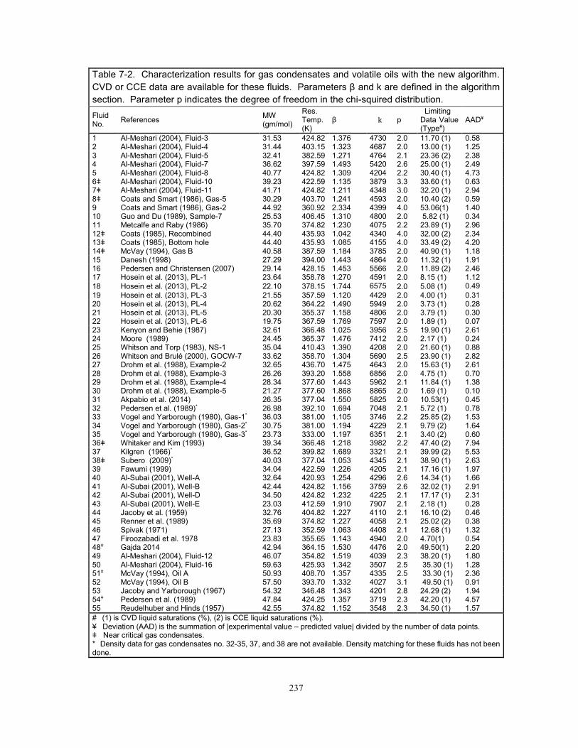
237
Table 7-2. Characterization results for gas condensates and volatile oils with the new algorithm.
CVD or CCE data are available for these fluids. Parameters β and k are defined in the algorithm
section. Parameter p indicates the degree of freedom in the chi-squired distribution.
Fluid No.
References MW (gm/mol)
Res. Temp. (K)
β k p Limiting Data Value (Type#)
AAD¥
1 Al-Meshari (2004), Fluid-3 31.53 424.82 1.376 4730 2.0 11.70 (1) 0.58 2 Al-Meshari (2004), Fluid-4 31.44 403.15 1.323 4687 2.0 13.00 (1) 1.25 3 Al-Meshari (2004), Fluid-5 32.41 382.59 1.271 4764 2.1 23.36 (2) 2.38 4 Al-Meshari (2004), Fluid-7 36.62 397.59 1.493 5420 2.6 25.00 (1) 2.49 5 Al-Meshari (2004), Fluid-8 40.77 424.82 1.309 4204 2.2 30.40 (1) 4.73 6ǂ Al-Meshari (2004), Fluid-10 39.23 422.59 1.135 3879 3.3 33.60 (1) 0.63 7ǂ Al-Meshari (2004), Fluid-11 41.71 424.82 1.211 4348 3.0 32.20 (1) 2.94 8ǂ Coats and Smart (1986), Gas-5 30.29 403.70 1.241 4593 2.0 10.40 (2) 0.59 9 Coats and Smart (1986), Gas-2 44.92 360.92 2.334 4399 4.0 53.06(1) 1.40 10 Guo and Du (1989), Sample-7 25.53 406.45 1.310 4800 2.0 5.82 (1) 0.34 11 Metcalfe and Raby (1986) 35.70 374.82 1.230 4075 2.2 23.89 (1) 2.96 12ǂ Coats (1985), Recombined 44.40 435.93 1.042 4340 4.0 32.00 (2) 2.34 13ǂ Coats (1985), Bottom hole 44.40 435.93 1.085 4155 4.0 33.49 (2) 4.20 14ǂ McVay (1994), Gas B 40.58 387.59 1.184 3785 2.0 40.90 (1) 1.18 15 Danesh (1998) 27.29 394.00 1.443 4864 2.0 11.32 (1) 1.91 16 Pedersen and Christensen (2007) 29.14 428.15 1.453 5566 2.0 11.89 (2) 2.46 17 Hosein et al. (2013), PL-1 23.64 358.78 1.270 4591 2.0 8.15 (1) 1.12
18 Hosein et al. (2013), PL-2 22.10 378.15 1.744 6575 2.0 5.08 (1) 0.49
19 Hosein et al. (2013), PL-3 21.55 357.59 1.120 4429 2.0 4.00 (1) 0.31 20 Hosein et al. (2013), PL-4 20.62 364.22 1.490 5949 2.0 3.73 (1) 0.28 21 Hosein et al. (2013), PL-5 20.30 355.37 1.158 4806 2.0 3.79 (1) 0.30 22 Hosein et al. (2013), PL-6 19.75 367.59 1.769 7597 2.0 1.89 (1) 0.07 23 Kenyon and Behie (1987) 32.61 366.48 1.025 3956 2.5 19.90 (1) 2.61 24 Moore (1989) 24.45 365.37 1.476 7412 2.0 2.17 (1) 0.24 25 Whitson and Torp (1983), NS-1 35.04 410.43 1.390 4208 2.0 21.60 (1) 0.88 26 Whitson and Brulé (2000), GOCW-7 33.62 358.70 1.304 5690 2.5 23.90 (1) 2.82 27 Drohm et al. (1988), Example-2 32.65 436.70 1.475 4643 2.0 15.63 (1) 2.61 28 Drohm et al. (1988), Example-3 26.26 393.20 1.558 6856 2.0 4.75 (1) 0.70 29 Drohm et al. (1988), Example-4 28.34 377.60 1.443 5962 2.1 11.84 (1) 1.38 30 Drohm et al. (1988), Example-5 21.27 377.60 1.868 8865 2.0 1.69 (1) 0.10 31 Akpabio et al. (2014) 26.35 377.04 1.550 5825 2.0 10.53(1) 0.45 32 Pedersen et al. (1989)* 26.98 392.10 1.694 7048 2.1 5.72 (1) 0.78 33 Vogel and Yarborough (1980), Gas-1* 36.03 381.00 1.105 3746 2.2 25.85 (2) 1.53 34 Vogel and Yarborough (1980), Gas-2* 30.75 381.00 1.194 4229 2.1 9.79 (2) 1.64 35 Vogel and Yarborough (1980), Gas-3* 23.73 333.00 1.197 6351 2.1 3.40 (2) 0.60 36ǂ Whitaker and Kim (1993) 39.34 366.48 1.218 3982 2.2 47.40 (2) 7.94 37 Kilgren (1966)* 36.52 399.82 1.689 3321 2.1 39.99 (2) 5.53 38ǂ Subero (2009)* 40.03 377.04 1.053 4345 2.1 38.90 (1) 2.63 39 Fawumi (1999) 34.04 422.59 1.226 4205 2.1 17.16 (1) 1.97 40 Al-Subai (2001), Well-A 32.64 420.93 1.254 4296 2.6 14.34 (1) 1.66 41 Al-Subai (2001), Well-B 42.44 424.82 1.156 3759 2.6 32.02 (1) 2.91 42 Al-Subai (2001), Well-D 34.50 424.82 1.232 4225 2.1 17.17 (1) 2.31 43 Al-Subai (2001), Well-E 23.03 412.59 1.910 7907 2.1 2.18 (1) 0.28 44 Jacoby et al. (1959) 32.76 404.82 1.227 4110 2.1 16.10 (2) 0.46 45 Renner et al. (1989) 35.69 374.82 1.227 4058 2.1 25.02 (2) 0.38 46 Spivak (1971) 27.13 352.59 1.063 4408 2.1 12.68 (1) 1.32 47 Firoozabadi et al. 1978 23.83 355.65 1.143 4940 2.0 4.70(1) 0.54 48ǂ Gajda 2014 42.94 364.15 1.530 4476 2.0 49.50(1) 2.20 49 Al-Meshari (2004), Fluid-12 46.07 354.82 1.519 4039 2.3 38.20 (1) 1.80 50 Al-Meshari (2004), Fluid-16 59.63 425.93 1.342 3507 2.5 35.30 (1) 1.28 51ǂ McVay (1994), Oil A 50.93 408.70 1.357 4335 2.5 33.30 (1) 2.36 52 McVay (1994), Oil B 57.50 393.70 1.332 4027 3.1 49.50 (1) 0.91 53 Jacoby and Yarborough (1967) 54.32 346.48 1.343 4201 2.8 24.29 (2) 1.94 54ǂ Pedersen et al. (1989) 47.84 424.25 1.357 3719 2.3 42.20 (1) 4.57 55 Reudelhuber and Hinds (1957) 42.55 374.82 1.152 3548 2.3 34.50 (1) 1.57
# (1) is CVD liquid saturations (%), (2) is CCE liquid saturations (%). ¥ Deviation (AAD) is the summation of |experimental value – predicted value| divided by the number of data points. ǂ Near critical gas condensates. * Density data for gas condensates no. 32-35, 37, and 38 are not available. Density matching for these fluids has not been done.

238
Table 7-3. Characterization results for oils for which slim-tube MMP data are available.
Parameters β and k are defined in the algorithm section.
Parameter p indicates the degree of freedom in the chi-squired distribution.
Oil No. References MW (gm/mol)
Res. Temp. (K)
β k p % AARD MMP Prediction
1 Jaubert et al. (2002), F1 135.24 374.85 1.329 3413 4.5 2.76
2 Jaubert et al. (2002), F2 136.25 372.05 1.528 4126 4.7 13.19
3 Jaubert et al. (2002), F3 82.41 387.35 1.438 4050 6.3 0.91
4 Jaubert et al. (2002), F4 63.17 388.20 1.387 3883 3.0 3.17
5 Jaubert et al. (2002), F5 125.82 394.25 1.523 4073 4.5 2.29
6 Jaubert et al. (2002), F6 96.25 383.15 1.324 3731 4.2 3.27
7 Jaubert et al. (2002), F7 96.19 393.15 1.318 4191 4.9 3.17
8 Jaubert et al. (2002), F11 82.55 373.75 1.401 3947 3.8 6.47
9 Ekundayo (2012) 86.57 402.59 1.334 4152 4.6 0.94 10 Høier (1997)* Injection Gas (System-1)¥ 97.0 368.15 1.551 4165 4.4 12.35 Injection Gas (System-2)¥ 97.0 368.15 1.551 4165 4.4 6.03 Injection Gas (System-3)¥ 97.0 368.15 1.551 4165 4.4 6.70 Injection Gas (System-4)¥ 97.0 368.15 1.551 4165 4.4 8.53 11 Graue and Zana (1981)#
177.0 344.26 1.493 4874 7.7 7.38
Graue and Zana (1981)#
177.0 344.26 1.493 4874 7.7 14.14
12 Negahban et al. 2010 101.90 394.00 1.279 3822 4.8 1.96
13 Firoozabadi and Aziz 1986, XA 51.58 444.26 1.288 3795 3.1 0.46
14 Firoozabadi and Aziz 1986, XB 67.33 366.48 1.516 4236 3.4 1.45
15 Firoozabadi and Aziz 1986, XC 86.25 380.37 1.764 4087 3.2 0.54
16 Firoozabadi and Aziz 1986, XD 89.07 423.71 1.647 3969 3.3 3.18 17 Lee and Reitzel 1982, A 78.35 376.15 1.320 4247 4.5 2.27 18 Lee and Reitzel 1982, D 79.85 375.15 1.280 3829 4.1 8.64 19 Lee and Reitzel 1982, E 54.33 379.15 1.358 4193 3.2 3.40 20 Koch and Hutchinson 1958, A Injection Gas-1 64.97 333.15 1.582 4604 3.1 7.02 Injection Gas-2 64.97 333.15 1.582 4604 3.1 1.73
Injection Gas-3 64.97 333.15 1.582 4604 3.1 2.75
Injection Gas-4 64.97 333.15 1.582 4604 3.1 3.53
¥Oil composition (System VOA) and saturation data used were taken from Whitson and Belery (1994). Systems 1-4 indicate four different injection gases. The MMPs reported were simulated. #Two different injection gases have been used. Details are available in the reference.
Table 7-4. Characterization results for heavy oils and bitumens with the new algorithm.
PVT data for these oils include swelling tests, gas solubility, and phase envelopes.
Parameters β and k are defined in the algorithm section. Parameter p indicates the degree of
freedom in the chi-squired distribution. Oil No.
References MW (gm/mol)
Temp. (K)
β k p AARD
% Type of Data*
1¥ Sharma (1990), West Sak Oil 228.88 299.81 1.783 3350 5.7 3.45# ST 2 Krejbjerg and Pedersen (2006),Fluid-1 125.72 347.15 1.705 4272 5.5 3.40 ST 3 Pedersen et al. (2004), Fluid-22 311.06 305.45 2.291 3587 5.5 4.42 GOR 4¥ Li et al. (2013a), Lloydminster Oil 482.00 347.67 1.352 3166 9.0 5.60 PT 5¥ Badamchi-Zadeh et al. (2009) Athabasca Bitumen 552.00 333.15 1.060 2870 12.0 PT 6¥ Mehrotra and Svrcek (1985),Peace River Bitumen 527.50 326.65 1.541 2625 12.0 PT
* ST and GOR stand for Swelling Test and Gas Oil Ratio, respectively. PT stands for 2- and 3-phase Pressure- Temperature data. # Includes oleic phase saturation prediction for 60% and 80% CO2 mixtures. For 60% CO2 mixture only, it is 1.53%. ¥ For Oils 1, 4, 5, and 6, three-phase P-T envelopes are shown in separate figures.

239
Table 7-5. Characterization results for oils for which three phases with CO2
were reported in the literature.
Parameters β and k are defined in the algorithm section. Parameter p
indicates the degree of freedom in the chi-squired distribution.
Oil No.
References MW (gm/mol)
Temp. (K)
β k p
1 Turek et al. (1988), Oil B1 149.62 314.26 1.550 4921 6.0 2 Turek et al. (1988), Oil B2 151.22 314.26 1.184 3302 6.1 3 Turek et al. (1988), Oil C2 140.30 313.71 1.454 4477 6.1 4 Turek et al. (1988), Oil D 182.42 313.71 1.551 4577 6.9 5 Khan et al. (1992), Oil BSB 148.88 313.70 1.458 4826 5.6 6 Winzinger et al. (1991), Oil NWE 138.45 301.48 1.325 4037 5.8 7 Khan et al. (1992), Oil JEMA 156.72 316.48 1.113 3092 5.2 8 Shelton and Yarborough (1977), Oil-B 161.47 307.60 1.470 4536 7.5 9 Creek and Sheffield (1993), Oil-G 113.13 307.59 1.311 4290 5.8
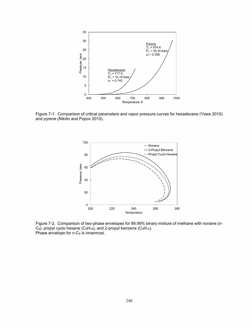
240
Figure 7-1. Comparison of critical parameters and vapor pressure curves for hexadecane (Yaws 2010) and pyrene (Nikitin and Popov 2015).
Figure 7-2. Comparison of two-phase envelopes for 99.99% binary mixture of methane with nonane (n-C9), propyl cyclo hexane (C9H18), and 2-propyl benzene (C9H12). Phase envelope for n-C9 is innermost.
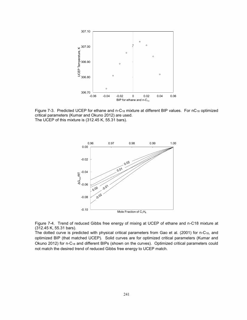
241
Figure 7-3. Predicted UCEP for ethane and n-C18 mixture at different BIP values. For nC18 optimized critical parameters (Kumar and Okuno 2012) are used. The UCEP of this mixture is (312.45 K, 55.31 bars).
Figure 7-4. Trend of reduced Gibbs free energy of mixing at UCEP of ethane and n-C18 mixture at (312.45 K, 55.31 bars). The dotted curve is predicted with physical critical parameters from Gao et al. (2001) for n-C18, and
optimized BIP (that matched UCEP). Solid curves are for optimized critical parameters (Kumar and
Okuno 2012) for n-C18 and different BIPs (shown on the curves). Optimized critical parameters could
not match the desired trend of reduced Gibbs free energy to UCEP match.

242
Figure 7-5. Comparison of P-x diagram for ethane and n-C16 mixture at 363.15 K with experimental data (Peters et al. 1988). Predictions are made from (1) optimized critical parameters (Kumar and Okuno 2012) and zero BIP and,
(2) physical critical parameters (Gao et al. 2001) and optimized BIP (Kumar and Okuno 2015).
Figure 7-6. Comparison of P-x diagram for ethane and n-C24 mixture at 340 K with experimental data (Peters et al. 1988). Predictions are made from (1) optimized critical parameters (Kumar and Okuno 2012) and zero BIP and,
(2) physical critical parameters (Gao et al. 2001) and optimized BIP (Kumar and Okuno 2015).
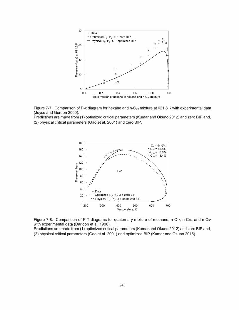
243
Figure 7-7. Comparison of P-x diagram for hexane and n-C36 mixture at 621.8 K with experimental data (Joyce and Gordon 2000). Predictions are made from (1) optimized critical parameters (Kumar and Okuno 2012) and zero BIP and,
(2) physical critical parameters (Gao et al. 2001) and zero BIP.
Figure 7-8. Comparison of P-T diagrams for quaternary mixture of methane, n-C10, n-C18, and n-C30 with experimental data (Daridon et al. 1996). Predictions are made from (1) optimized critical parameters (Kumar and Okuno 2012) and zero BIP and,
(2) physical critical parameters (Gao et al. 2001) and optimized BIP (Kumar and Okuno 2015).

244
Figure 7-9. Comparison of empirically determined higher boundary correlation for critical temperature in Equation 7-5 with data (Yaws 2010, Nikitin and Popov 2015). N-alkane equivalent values from Gao et al. (2001) for pseudocomponents form the lower boundary.
Figure 7-10. Comparison of empirically determined higher boundary correlation for critical pressure in Equation 7-6 with data (Yaws 2010, Nikitin and Popov 2015). N-alkane equivalent values from Gao et al. (2001) for pseudocomponents form the lower boundary.
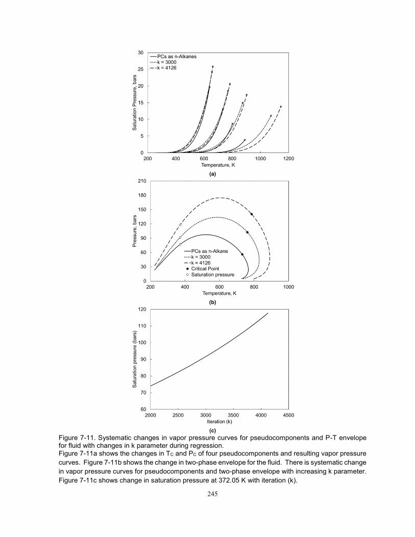
245
(a)
(b)
(c)
Figure 7-11. Systematic changes in vapor pressure curves for pseudocomponents and P-T envelope for fluid with changes in k parameter during regression. Figure 7-11a shows the changes in TC and PC of four pseudocomponents and resulting vapor pressure
curves. Figure 7-11b shows the change in two-phase envelope for the fluid. There is systematic change
in vapor pressure curves for pseudocomponents and two-phase envelope with increasing k parameter.
Figure 7-11c shows change in saturation pressure at 372.05 K with iteration (k).

246
Figure 7-12. CME liquid saturation predicted for near-critical gas condensate, Fluid 36 in Table 7-2, at 366.48 K. The molecular weight is 39.34 gram/mole. The mole fraction and molecular weight of the heptane plus are 0.1003 and 172.0 gram/mole
respectively.
Figure 7-13. CVD liquid saturation predicted for near-critical volatile oil, Fluid 54 in Table 7-2, at 424.25 K. The molecular weight is 47.84 gram/mole. The mole fraction and molecular weight of the heptane plus are 0.1417 and 194.0 gram/mole
respectively. The critical point was measured at 426 K and 388 bars. The critical point predicted with
the characterized EOS is at 434.65 K and 391.43 bars.
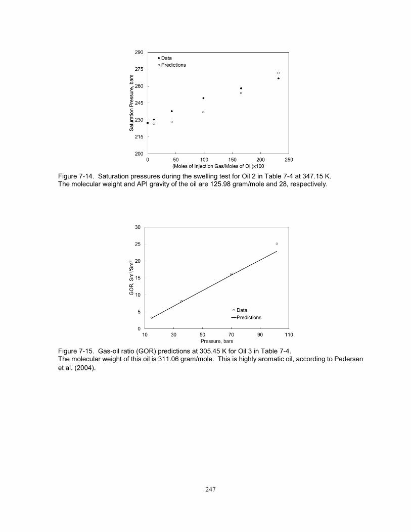
247
Figure 7-14. Saturation pressures during the swelling test for Oil 2 in Table 7-4 at 347.15 K. The molecular weight and API gravity of the oil are 125.98 gram/mole and 28, respectively.
Figure 7-15. Gas-oil ratio (GOR) predictions at 305.45 K for Oil 3 in Table 7-4. The molecular weight of this oil is 311.06 gram/mole. This is highly aromatic oil, according to Pedersen
et al. (2004).
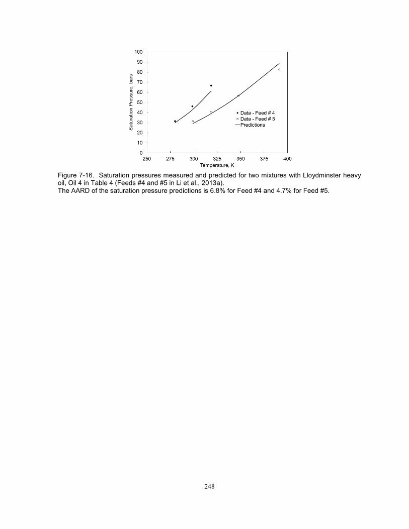
248
Figure 7-16. Saturation pressures measured and predicted for two mixtures with Lloydminster heavy oil, Oil 4 in Table 4 (Feeds #4 and #5 in Li et al., 2013a). The AARD of the saturation pressure predictions is 6.8% for Feed #4 and 4.7% for Feed #5.

249
(a)
(b)
Figure 7-17. Liquid-phase saturations for West Sak heavy oil (Oil 1 in Table 4) mixed with CO2 at 299.81 K. (a) Oleic (L1) phase. (b) Solvent-rich liquid (L2) phase. Three phases prediction with zero BIP for hydrocarbon-hydrocarbon is also shown.

250
Figure 7-18. Comparison of P-x diagrams for oil 1 in Table 7-5 at 370 K predicted with EOS models from new algorithm and Aghabsh and Ahmadi (2012).
Figure 7-19. Comparison of P-T envelope predicted with SRK EOS by Krejbjerg and Pedersen (2006) with prediction from new algorithm for oil 2 in Table 7-4.
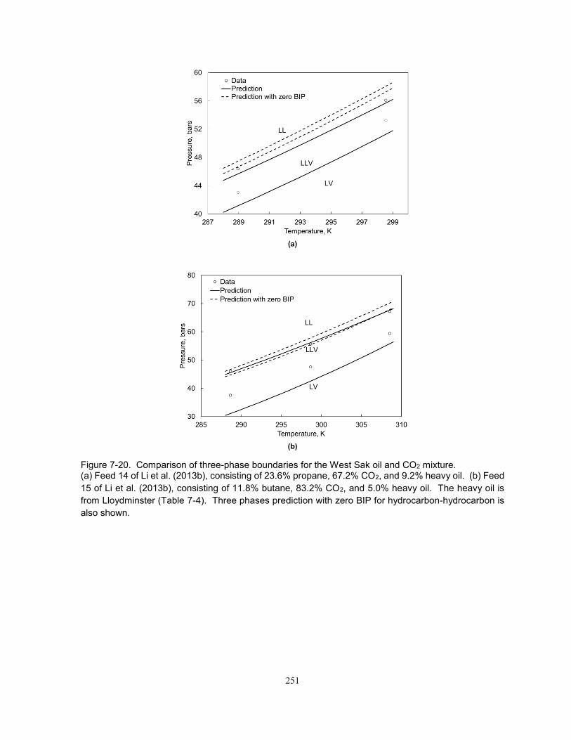
251
(a)
(b)
Figure 7-20. Comparison of three-phase boundaries for the West Sak oil and CO2 mixture. (a) Feed 14 of Li et al. (2013b), consisting of 23.6% propane, 67.2% CO2, and 9.2% heavy oil. (b) Feed
15 of Li et al. (2013b), consisting of 11.8% butane, 83.2% CO2, and 5.0% heavy oil. The heavy oil is
from Lloydminster (Table 7-4). Three phases prediction with zero BIP for hydrocarbon-hydrocarbon is
also shown.

252
Figure 7-21. Three-phase boundaries measured and predicted for a mixture of Athabasca bitumen: 51.0% CO2, 34.7% propane, and 14.3% bitumen (Badamchi-Zadeh et al. 2009). Three phases prediction with zero BIP for hydrocarbon-hydrocarbon is also shown.
Figure 7-22. Three-phase boundaries measured and predicted for a mixture of Peace River bitumen: 89.90% pentane and 10.10% bitumen. The bitumen was characterized using the data from Mehrotra and Svrcek (1985). Three-phase
boundaries simulated by Agrawal (2012) are also shown. Prediction with zero BIP for hydrocarbon-
hydrocarbon did not show presence of three phases.
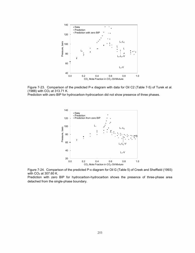
253
Figure 7-23. Comparison of the predicted P-x diagram with data for Oil C2 (Table 7-5) of Turek et al. (1988) with CO2 at 313.71 K. Prediction with zero BIP for hydrocarbon-hydrocarbon did not show presence of three phases.
Figure 7-24. Comparison of the predicted P-x diagram for Oil G (Table 5) of Creek and Sheffield (1993) with CO2 at 307.60 K. Prediction with zero BIP for hydrocarbon-hydrocarbon shows the presence of three-phase area
detached from the single-phase boundary.
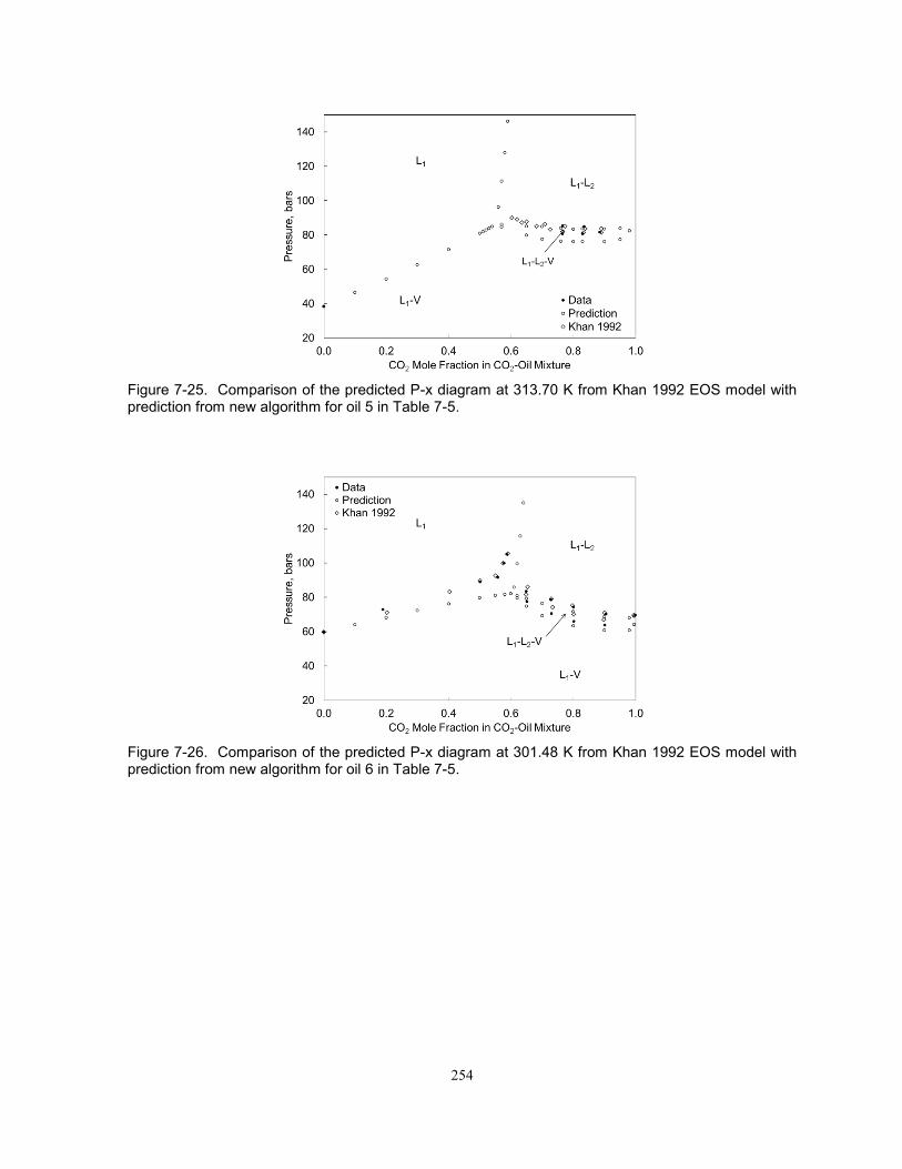
254
Figure 7-25. Comparison of the predicted P-x diagram at 313.70 K from Khan 1992 EOS model with prediction from new algorithm for oil 5 in Table 7-5.
Figure 7-26. Comparison of the predicted P-x diagram at 301.48 K from Khan 1992 EOS model with prediction from new algorithm for oil 6 in Table 7-5.
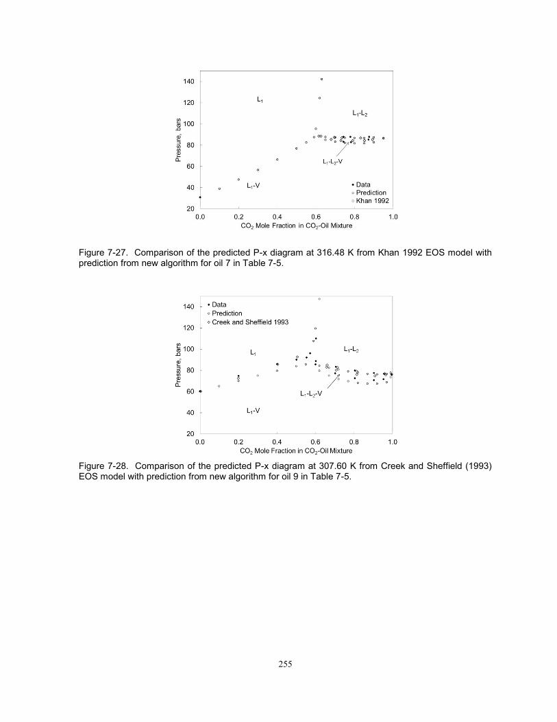
255
Figure 7-27. Comparison of the predicted P-x diagram at 316.48 K from Khan 1992 EOS model with prediction from new algorithm for oil 7 in Table 7-5.
Figure 7-28. Comparison of the predicted P-x diagram at 307.60 K from Creek and Sheffield (1993) EOS model with prediction from new algorithm for oil 9 in Table 7-5.

256
Chapter 8: Summary, Conclusion and Recommendation

257
8.1. Summary of Research
Basic objective of this research was to develop a characterization method for multiphase PVT simulation
applicable to a hydrocarbon system irrespective of its composition range using systematic approach and
reliable BIP. Systematic approach implies well-defined and physically justifiable initial (default) values
and search direction for EOS parameters. The approach of perturbation from n-alkane (PnA) has
essential features ensuring systematic reservoir fluid characterization; hence, this approach forms the
fundamental of the reservoir fluid characterization proposed in this research.
Fundamental of PnA approach is based on well-known systematic behavior of thermo- physical
properties of three main hydrocarbon groups of compounds i.e. paraffins, naphthenes, and aromatics.
For same carbon number components, paraffins have lowest TC, and PC; and highest ω among the three
hydrocarbon groups of compounds. Pseudocomponents may be considered as mixture of these three
hydrocarbon groups; hence, the lowest TC, the lowest PC and the highest ω values for a
pseudocomponent correspond to respective values estimated with assumption that pseudocomponent
is 100% paraffin. Higher TC and PC values and lower ω values for pseudocomponents are then found
to match saturation pressure data.
The n-alkane equivalent critical parameter values are estimated in two ways corresponding to two
approaches for reservoir fluid density matching i.e. density matching either by critical parameters’
adjustment or by volume shift parameters’ adjustment. The PnA approaches for reservoir fluid
characterization presented in Chapter 3 to 6 adjust attraction and covolume parameters for density
match. Normal alkane equivalent critical parameters for pseudocomponents in these approaches are
estimated with correlations developed using optimized critical parameters and acentric factors, which
match vapor pressure and density data for n-alkanes from n-C7 to n-C100 with PR EOS; development of
these correlations is described in Chapter 2. The optimized TC and PC are greater than corresponding
physical values; optimized acentric factors are smaller than respective physical values. Chapter 7
presents the PnA approach for reservoir fluid characterization, where physical critical parameters from
Gao et al. (2001) are used to assign n-alkane equivalent critical parameters for pseudocomponents. In
this approach, density matching is done by adjusting temperature independent volume shift parameters
like conventional characterization methods.
This research is presented in six different papers with different objectives in line with the research
goals presented in the introduction section. Chapter 2 presents correlations to estimate critical
parameters for n-alkanes optimized for vapor pressure and density data matching with PR EOS.
Development of algorithm for reservoir fluids was at initial stage and limited to verification of perturbation
parameter being greater than the minimum value allowed. In Chapter 3, PnA method was developed
with three variables and applied to 22 oils. This chapter also compares the phase behavior predictions
from characterization with/without using volume shift to match density. Application of PnA approach in
Chapter 3 was limited to few oils; hence, the approach needed to be validated by including more fluids.
In Chapter 4, the characterization is validated with 77 reservoir fluids comprising of 31 gas condensates,
258
12 volatile oils and 31 other oils. Application of the approach, particularly to light fluid types, required
modification of algorithm developed in the Chapter 3; however, the algorithm in Chapter 3 was special
case of algorithm in Chapter 4. This chapter also presented the trend of parameter ψ (= a/b2) with single
carbon number fractions at different aromaticity level, which is distinctive for a given range of carbon
number of components present in a reservoir fluid. This trend has been used to verify conformity of
attraction and covolume parameters for a characterized reservoir fluid to desired physical trends.
The Chapter 5 presents PnA approach for characterizing 84 reservoir fluids (47 gas condensates,
15 volatile oils, 18 oils, and 4 heavy oils) by direct perturbation of attraction and covolume parameters
maintaining characteristic trends defined by ψ parameter as described in Chapter 3 and 4. The
regression algorithm, which has two regression parameters, was simpler than that used in Chapter 4
and showed similar or improved phase behavior prediction including prediction for three hydrocarbon
phases. Chapter 6 presents application of algorithm presented in Chapter 5 in simple form to 6
bitumens. This algorithm results in similar phase behavior predictions for single pseudocomponent
bitumens as compared to multi component conventional characterization. This chapter presents a
mechanism for sensitivity of bitumen recovery simulation to characterization methods. Such sensitivity
analysis, carried out before running simulation of bitumen recovery with ES-SAGD process, can provide
important guidelines for selection of reliable and efficient bitumen characterization method.
Chapter 7 presents a well-developed reservoir fluid characterization using PnA approach for
multiphase behavior prediction for 90 reservoir fluids (48 gas condensates, 7 volatile oils, 29 other oils,
4 heavy oils, and 2 bitumens). Similar to the algorithm presented in Chapter 4, algorithm presented in
this chapter also directly perturbs TC, PC, and ω for pseudocomponents for reservoir fluid
characterization. However, the algorithm presented in Chapter 7 differs from that in Chapter 4 in
followings ways:
(1) Single parameter is used to adjust TC, PC, and ω.
(2) The BIPs are used for components like N2, CO2, CH4, C2H6, C3H8, C4H10 and C5H12. The BIPs for
CO2, CH4, C2H6, C3H8, C4H10 and C5H12 with heavier n-alkanes are developed using multiphase
behavior data for binary and ternary mixtures.
(3) Saturation pressure is matched by TC, PC, and ω adjustment and density matching is done using
volume shift parameters.
Predictive capability of the algorithm presented in this Chapter 7 is better than that presented in
Chapter 4. The average absolute deviation for CVD liquid saturation, CME liquid saturation, and
average absolute relative deviation for MMP predictions in Chapter 4 were 2.10%, 3.57% and 6.7 %
respectively; corresponding deviations in Chapter 7 are 1.5%, 2.5%, and 4.57% respectively. Chapter
7 included maximum number of fluids for three-phase predictions (9 oils, 2 heavy oils, and 2 bitumens)
and for all these cases, three hydrocarbon phases have been predicted satisfactorily.

259
8.2. Conclusions
This research presents a simple, robust, and reliable fluid characterization for multiphase behavior
simulation for hydrocarbon system irrespective of fluid type. Conclusions are the following:
(1) Perturbation from n-alkane approach provides reliable and robust framework for multiphase
reservoir fluid characterization because of well-defined initial PR EOS parameters values for
pseudocomponents and physically justified search direction for regression parameters.
(2) Irrespective of density matching either by using volume shift parameter or by adjusting critical
parameters, the PnA method was found to be applicable for multiphase characterization; that is, the
effect of aromaticity on phase behavior can be modeled by adjusting TC, PC, and ω of
pseudocomponents as monotonic functions of regression parameters.
(3) The regression parameters in the PnA approach, unlike the conventional characterization, are not
component specific, which makes the algorithm simple and easy in retaining the physical trend of
the PR-EOS parameters with carbon number of pseudocomponents during regression. The
regression of adjustable parameters is well defined and physically justified, unlike undefined manual
regression approach in the conventional characterization.
(4) The PnA approach used for reservoir fluid characterization is systematic and simple. The phase
behavior change during the regression of adjustable parameters is systematic; hence, saturation
pressure varies monotonically with the regression parameters in all algorithms developed.
(5) Parameters such as γ (Chapter 4), C (Chapter 5), β (Chapter 7) are presented as correlations;
however, these parameters can be used as adjustable variables, if needed, to match other types of
PVT data such as CVD liquid saturation, minimum miscibility pressure etc. As shown (Chapter 4
and 5), predictions of other types PVT measurements (apart from saturation pressure) are
monotonic functions of these parameters; matching of these PVT measurements may not be
possible with conventional approach.
(6) The PnA based fluid characterization algorithms presented in Chapters 2 to 7 were able to achieve
the specific objectives set in these chapters. Phase behavior simulation for n-alkanes' mixture is
recommended with the optimized TC, PC, and ω developed in Chapter 2. The optimized parameters
can reliably predict two-phase behavior with zero BIPs. The algorithm presented in Chapter 3 is a
specific case of the algorithm presented in Chapter 4, and uses perturbation of TC, PC, and ω. The
algorithm using direct perturbation of the attraction and covolume parameter is presented in Chapter
5, and its simplified form is applied to bitumens in Chapter 6. The algorithms presented in Chapters
5 and 6 have additional benefit of having fewer regression parameters. All these algorithms use
zero BIPs for hydrocarbon-hydrocarbon pairs, zero volume shift parameters and optimized TC, PC,
and ω. These algorithms are recommended for reliable two-phase behavior simulation. Three-
phase behavior simulation from these algorithms may not be reliable because of the following
reasons:

260
o Algorithms in Chapter 4 and Chapter 6 are based on the PR EOS calibrated for two-phase
behavior using optimized TC, PC, and ω for n-alkanes.
o Three-phase behavior is more reliable with physical critical parameters and non-zero
hydrocarbon-hydrocarbon BIPs as examined in Chapter 7.
o The amount of three-phase data used for validation of three-phase behavior in Chapter 4
to Chapter 6 is limited.
The algorithm presented in Chapter 7 is reliable for multiphase behavior simulation. This
algorithm uses BIPs that are optimized for multiphase behavior prediction. The algorithm has been
validated by using 90 reservoir fluids, including 13 fluids that are used for validation of three-phase
behavior simulation. Hence, the characterization approach presented in Chapter 7 is recommended
for EOS-model development for multiphase PVT simulation. However, since density matching in
this algorithm is same as that for the conventional characterization, it is important that volume shift
parameters be properly modeled for reliable density prediction in range of pressure, temperature,
and composition that are expected in reservoir oil displacement during gas injection.
(7) The PnA characterization uses a small amount of data (saturation pressure and density data);
however, it does not undermine the importance of including more phase behavior data in fluid
characterization. Particularly for gas injection, predictions from the PnA characterization should be
validated by using more compositional and volumetric phase behavior data.
(8) The algorithm presented for multiphase behavior predictions uses unmodified form of PR EOS;
hence, application of the characterization method requires no change in commercial software.
261
8.3. Recommendations for Future Research
Recommendations for future research are as follows:
(1) The impact of three-phase PnA characterization on multiphase flow simulation could not be studied
in this research due to the unavailability of detailed data for multiphase oil displacement.
(2) Systematic characterization of critical end points for reservoir fluid and solvent mixture is
recommended for future study. Although the condition, under which high displacement efficiency in
the presence of three hydrocarbon phases is possible, is known, no systematic approach to
achieving that is known.
(3) Heptane plus fractions in the PnA approach are modeled by using the chi-squared distribution
function. It is not known how splitting of the plus fraction with a more general form of probability
distribution function (i.e. gamma distribution) and a simpler form (i.e. logarithmic distribution) will
affect the present characterization. This work can be done, and the present approach may be
modified accordingly.
(4) This research did not include the impact of the number of components on phase behavior predictions
with the PnA method. A study may be done on the impact of using more pseudo components. This
may be helpful for phase behavior prediction for near critical fluids, such as near critical gas
condensates or volatile oil.
(5) The correlation for BIP of CO2 with heavier n-alkanes presented in this research is independent of
temperature. However, prior publications show that BIP of CO2 is sensitive to temperature. A
research on this may be conducted using phase behavior data with a wide temperature range.
(6) The SRK EOS is simpler than the PR EOS. The expression of fugacity with the SRK EOS is smaller
than that with the PR EOS, which can contribute to computational efficiency. It is possible to develop
a fluid characterization method using the PnA approach for the SRK EOS.
(7) Systematic study of aromaticity on fluid characterization has not been carried out. This is because
of the unavailability of suitable data for aromatic components. A research of experimental work
combined with analytical study to find EOS parameters as function of aromaticity of fluid mixtures
containing paraffins, naphthenic and aromatics may be undertaken.
(8) The attraction and covolume parameters developed in Chapter 5 and Chapter 6 may be used for
the friction theory based viscosity model developed by Quiñones-Cisneros et al. (2004). The friction
theory based viscosity model uses the attraction and covolume parameters. Since the algorithm
presented in Chapter 5 yields the attraction and covolume parameters for heavy oils and bitumens
for compositional as well as volumetric phase behavior predictions, it is expected that their use in
viscosity model will improve the correlative accuracy for viscosity data for heavy oils and bitumens.
(9) Heavy oils have been split into SARA (Saturates, Aromatics, Resin, and Asphaltene). A possibility
may be looked into for applying the PnA approach for these fractions for heavy oil characterization.
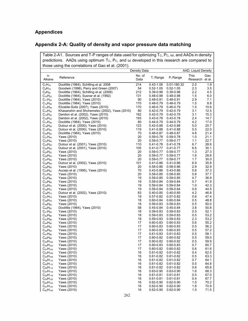
262
Appendices
Appendix 2-A: Quality of density and vapor pressure data matching
Table 2-A1. Sources and T-P ranges of data used for optimizing TC, PC, ω, and AADs in density
predictions. AADs using optimum TC, PC, and ω developed in this research are compared to
those using the correlations of Gao et al. (2001). Density Data AAD, Liquid Density
n-Alkane
Reference No. of Data
Tr Range Pr Range This Research
Gao et al.
C7H16 Doolittle (1964), Schilling et al. 2008 214 0.43-1.06 0.01-180.32 2.0 1.9 C8H18 Goodwin (1996), Perry and Green (2007) 54 0.52-1.05 0.52-1.05 2.3 3.5 C9H20 Doolittle (1964), Schilling et al. (2008) 212 0.39-0.98 0.39-0.98 2.2 4.5 C10H22 Doolittle (1964), Susnar et al. (1992) 131 0.48-0.98 0.48-0.98 1.5 6.0 C11H24 Doolittle (1964), Yaws (2010) 90 0.48-0.91 0.48-0.91 2.9 7.1 C12H26 Doolittle (1964), Yaws (2010) 170 0.48-0.79 0.48-0.79 1.5 8.8 C13H28 Elizalde-Solis (2007), Yaws (2010) 170 0.46-0.79 0.46-0.79 1.5 10.6 C14H30 Khasanshin and Shchemelev (2002), Yaws (2010) 80 0.42-0.79 0.42-0.79 3.1 12.5 C15H32 Daridon et al. (2002), Yaws (2010) 162 0.42-0.79 0.42-0.79 3.1 15.3 C16H34 Daridon et al. (2002), Yaws (2010) 193 0.43-0.78 0.43-0.78 2.4 14.7 C17H36 Doolittle (1964), Yaws (2010) 80 0.44-0.79 0.44-0.79 4.2 17.0 C18H38 Dutour et al. (2000), Yaws (2010) 123 0.42-0.88 0.42-0.88 5.0 20.7 C19H40 Dutour et al. (2000), Yaws (2010) 119 0.41-0.88 0.41-0.88 5.5 22.0 C20H42 Doolittle (1964), Yaws (2010) 70 0.48-0.87 0.48-0.87 4.8 21.4 C21H44 Yaws (2010) 20 0.59-0.78 0.59-0.78 1.0 21.1 C22H46 Yaws (2010) 20 0.59-0.77 0.59-0.77 1.1 22.7 C23H48 Dutour et al. (2001), Yaws (2010) 110 0.41-0.78 0.41-0.78 6.7 28.6 C24H50 Dutour et al. (2001), Yaws (2010) 105 0.41-0.77 0.41-0.77 6.6 30.1 C25H52 Yaws (2010) 20 0.59-0.77 0.59-0.77 1.3 27.3 C26H54 Yaws (2010) 20 0.59-0.77 0.59-0.77 1.6 28.6 C27H56 Yaws (2010) 20 0.59-0.77 0.59-0.77 1.7 30.0 C28H58 Dutour et al. (2002), Yaws (2010) 101 0.41-0.86 0.41-0.86 6.9 35.8 C29H60 Yaws (2010) 20 0.58-0.86 0.58-0.86 2.9 32.9 C30H62 Aucejo et al. (1995), Yaws (2010) 70 0.43-0.86 0.43-0.86 5.6 37.3 C31H64 Yaws (2010) 20 0.58-0.85 0.58-0.85 0.8 37.7 C32H66 Yaws (2010) 19 0.59-0.85 0.59-0.85 4.7 36.9 C33H68 Yaws (2010) 19 0.59-0.84 0.59-0.84 0.7 41.9 C34H70 Yaws (2010) 19 0.59-0.84 0.59-0.84 1.0 42.3 C35H72 Yaws (2010) 19 0.59-0.84 0.59-0.84 0.6 44.5 C36H74 Dutour et al. (2002), Yaws (2010) 83 0.40-0.85 0.40-0.85 4.2 46.8 C37H76 Yaws (2010) 19 0.57-0.82 0.57-0.82 0.6 47.4 C38H78 Yaws (2010) 18 0.60-0.84 0.60-0.84 0.5 48.8 C39H80 Yaws (2010) 18 0.59-0.83 0.59-0.83 0.5 50.0 C40H82 Doolittle (1964), Yaws (2010) 58 0.45-0.84 0.45-0.84 3.8 50.8 C41H84 Yaws (2010) 18 0.59-0.83 0.59-0.83 0.5 52.1 C42H86 Yaws (2010) 18 0.59-0.83 0.59-0.83 0.5 53.2 C43H88 Yaws (2010) 18 0.59-0.83 0.59-0.83 2.3 53.2 C44H90 Yaws (2010) 17 0.60-0.83 0.60-0.83 0.6 55.2 C45H92 Yaws (2010) 17 0.60-0.83 0.60-0.83 0.5 56.2 C46H94 Yaws (2010) 17 0.60-0.83 0.60-0.83 0.5 57.2 C47H96 Yaws (2010) 17 0.61-0.83 0.61-0.83 0.5 58.1 C48H98 Yaws (2010) 17 0.60-0.82 0.60-0.82 0.5 59.0 C49H100 Yaws (2010) 17 0.60-0.82 0.60-0.82 0.5 59.9 C50H102 Yaws (2010) 17 0.60-0.83 0.60-0.83 0.7 60.7 C51H104 Yaws (2010) 17 0.60-0.82 0.60-0.82 0.6 61.6 C52H106 Yaws (2010) 16 0.61-0.82 0.61-0.82 0.4 62.5 C53H108 Yaws (2010) 16 0.61-0.82 0.61-0.82 0.5 63.3 C54H110 Yaws (2010) 16 0.61-0.82 0.61-0.82 0.7 64.1 C55H112 Yaws (2010) 16 0.61-0.82 0.61-0.82 0.5 64.8 C56H114 Yaws (2010) 16 0.61-0.82 0.61-0.82 0.6 65.6 C57H116 Yaws (2010) 16 0.63-0.90 0.63-0.90 1.6 68.3 C58H118 Yaws (2010) 16 0.61-0.81 0.61-0.81 0.5 67.0 C59H120 Yaws (2010) 16 0.61-0.81 0.61-0.81 0.4 67.7 C60H122 Yaws (2010) 16 0.62-0.90 0.62-0.90 1.5 70.2 C61H124 Yaws (2010) 16 0.62-0.90 0.62-0.90 1.8 70.9 C62H126 Yaws (2010) 16 0.62-0.90 0.62-0.90 1.5 71.5

263
C63H128 Yaws (2010) 15 0.64-0.90 0.64-0.90 1.8 72.2 C64H130 Yaws (2010) 15 0.64-0.90 0.64-0.90 1.6 72.8 C65H132 Yaws (2010) 15 0.64-0.89 0.64-0.89 1.8 73.4 C66H134 Yaws (2010) 15 0.64-0.89 0.64-0.89 1.6 73.9 C67H136 Yaws (2010) 15 0.64-0.89 0.64-0.89 1.7 74.5 C68H138 Yaws (2010) 15 0.64-0.89 0.64-0.89 1.6 75.0 C69H140 Yaws (2010) 15 0.64-0.89 0.64-0.89 1.7 75.5 C70H142 Yaws (2010) 15 0.64-0.89 0.64-0.89 1.6 76.0 C71H144 Yaws (2010) 15 0.64-0.89 0.64-0.89 1.7 76.5 C72H146 Yaws (2010) 15 0.63-0.89 0.63-0.89 1.6 77.0 C73H148 Yaws (2010) 15 0.63-0.89 0.63-0.89 1.7 77.4 C74H150 Yaws (2010) 15 0.63-0.89 0.63-0.89 1.6 77.9 C75H152 Yaws (2010) 15 0.63-0.89 0.63-0.89 1.8 78.3 C76H154 Yaws (2010) 15 0.63-0.88 0.63-0.88 1.6 78.8 C77H156 Yaws (2010) 15 0.63-0.89 0.63-0.89 1.9 79.2 C78H158 Yaws (2010) 15 0.63-0.88 0.63-0.88 1.7 79.6 C79H160 Yaws (2010) 15 0.63-0.88 0.63-0.88 1.7 80.1 C80H162 Yaws (2010) 15 0.63-0.88 0.63-0.88 1.7 80.5 C81H164 Yaws (2010) 15 0.61-0.80 0.61-0.80 1.6 79.6 C82H166 Yaws (2010) 14 0.62-0.80 0.62-0.80 2 80.0 C83H168 Yaws (2010) 14 0.62-0.79 0.62-0.79 1.7 80.4 C84H170 Yaws (2010) 14 0.65-0.88 0.65-0.88 2.2 82.1 C85H172 Yaws (2010) 14 0.65-0.88 0.65-0.88 1.9 82.4 C86H174 Yaws (2010) 14 0.65-0.88 0.65-0.88 1.9 82.8 C87H176 Yaws (2010) 14 0.65-0.88 0.65-0.88 2.2 83.1 C88H178 Yaws (2010) 14 0.65-0.88 0.65-0.88 2.0 83.4 C89H180 Yaws (2010) 14 0.65-0.88 0.65-0.88 2.0 83.8 C90H182 Yaws (2010) 14 0.64-0.88 0.64-0.88 2.3 84.1 C91H184 Yaws (2010) 14 0.64-0.88 0.64-0.88 2.1 84.4 C92H186 Yaws (2010) 14 0.64-0.88 0.64-0.88 2.2 84.7 C93H188 Yaws (2010) 14 0.64-0.88 0.64-0.88 2.6 85.0 C94H190 Yaws (2010) 14 0.64-0.88 0.64-0.88 2.3 85.3 C95H192 Yaws (2010) 14 0.64-0.88 0.64-0.88 2.2 85.6 C96H194 Yaws (2010) 14 0.64-0.88 0.64-0.88 2.2 85.8 C97H196 Yaws (2010) 14 0.64-0.88 0.64-0.88 2.7 86.1 C98H198 Yaws (2010) 14 0.64-0.88 0.64-0.88 2.3 86.4 C99H200 Yaws (2010) 14 0.64-0.88 0.64-0.88 2.3 86.6 C100H202 Yaws (2010) 14 0.64-0.88 0.64-0.88 2.8 86.9

264
Table 2-A2. Sources and T-P ranges of data used for optimizing TC, PC, ω, and AADs in vapor
pressure predictions. AADs using optimum TC, PC, and ω developed in this research are
compared to those using the correlations of Gao et al. (2001). Vapor Pressure Data AAD Vapor Pressure
n-Alkane
Reference No. of Data
Tr Range This
Research Gao et al.
(2001)
C7H16 Perry and Green (2007), Ewing and Ochoa (2005) 35 0.69-0.95 0.5 0.5 C8H18 Perry and Green (2007), Gregorowicz et al.(1987) 27 0.53-0.95 0.5 1.7 C9H20 Perry and Green (2007) 12 0.54-0.91 1.3 2.1 C10H22 Perry and Green (2007), Gregorowicz et al.(1987) 28 0.50-0.92 1.1 3.8 C11H24 Riazi and AlQaheem (2010) 10 0.60-0.90 2.0 19.3 C12H26 Perry and Green (2007) 14 0.53-0.93 4.1 2.0 C13H28 Riazi and AlQaheem (2010) 10 0.60-0.90 3.2 16.9 C14H30 Morgan and Kobayashi (1994) 20 0.60-0.79 1.6 0.9 C15H32 Riazi and AlQaheem (2010) 10 0.59-0.90 5.1 15.0 C16H34 Morgan and Kobayashi (1994) 19 0.55-0.80 4.0 0.7 C17H36 Riazi and AlQaheem (2010) 10 0.59-0.89 4.5 13.5 C18H38 Morgan and Kobayashi (1994) 20 0.60-0.88 3.8 1.1 C19H40 Morgan and Kobayashi (1994) 20 0.59-0.88 4.1 1.2 C20H42 Morgan and Kobayashi (1994) 20 0.59-0.87 2.8 2.1 C21H44 Riazi and AlQaheem (2010) 20 0.59-0.78 1.8 1.3 C22H46 Morgan and Kobayashi (1994) 22 0.57-0.88 3.9 5.5 C23H48 Riazi and AlQaheem (2010) 20 0.59-0.78 2.3 1.4 C24H50 Morgan and Kobayashi (1994) 20 0.59-0.77 2.0 1.4 C25H52 Riazi and AlQaheem (2010) 20 0.59-0.77 1.0 1.4 C26H54 Riazi and AlQaheem (2010) 20 0.59-0.77 2.7 1.3 C27H56 Riazi and AlQaheem (2010) 20 0.59-0.77 0.6 1.3 C28H58 Morgan and Kobayashi (1994) 20 0.58-0.86 3.0 1.4 C29H60 Riazi and AlQaheem (2010) 20 0.58-0.86 1.4 1.4 C30H62 Riazi and AlQaheem (2010) 20 0.58-0.86 1.1 1.5 C31H64 Riazi and AlQaheem (2010) 20 0.58-0.85 1.4 1.5 C32H66 Riazi and AlQaheem (2010) 19 0.59-0.85 1.8 1.6 C33H68 Riazi and AlQaheem (2010) 19 0.59-0.84 0.8 1.9 C34H70 Riazi and AlQaheem (2010) 19 0.59-0.84 1.3 2.3 C35H72 Riazi and AlQaheem (2010) 19 0.59-0.84 0.9 2.8 C36H74 Riazi and AlQaheem (2010) 18 0.60-0.85 2.3 3.3 C37H76 Riazi and AlQaheem (2010) 17 0.60-0.82 0.9 3.9 C38H78 Riazi and AlQaheem (2010) 18 0.60-0.84 1.0 4.4 C39H80 Riazi and AlQaheem (2010) 18 0.59-0.83 1.1 5.0 C40H82 Riazi and AlQaheem (2010) 17 0.61-0.84 1.4 11.3 C41H84 Riazi and AlQaheem (2010) 17 0.61-0.83 0.9 13.3 C42H86 Riazi and AlQaheem (2010) 17 0.61-0.83 1.0 13.8 C43H88 Riazi and AlQaheem (2010) 17 0.61-0.83 0.8 14.4 C44H90 Riazi and AlQaheem (2010) 17 0.60-0.83 1.4 15.0 C45H92 Riazi and AlQaheem (2010) 17 0.60-0.83 1.2 15.6 C46H94 Riazi and AlQaheem (2010) 16 0.62-0.83 1.5 15.8 C47H96 Riazi and AlQaheem (2010) 16 0.62-0.83 1.6 16.5 C48H98 Riazi and AlQaheem (2010) 16 0.61-0.82 1.6 17.3 C49H100 Riazi and AlQaheem (2010) 16 0.61-0.82 2.3 18.1 C50H102 Riazi and AlQaheem (2010) 16 0.62-0.83 1.0 17.8 C51H104 Riazi and AlQaheem (2010) 16 0.61-0.82 3.0 18.9 C52H106 Riazi and AlQaheem (2010) 15 0.62-0.82 0.7 19.2 C53H108 Riazi and AlQaheem (2010) 15 0.62-0.82 0.7 20.3 C54H110 Riazi and AlQaheem (2010) 15 0.62-0.82 0.7 21.3 C55H112 Riazi and AlQaheem (2010) 15 0.62-0.82 0.7 22.4 C56H114 Riazi and AlQaheem (2010) 15 0.62-0.82 0.7 23.5 C57H116 Riazi and AlQaheem (2010) 16 0.63-0.90 1.0 22.2 C58H118 Riazi and AlQaheem (2010) 15 0.62-0.81 0.7 25.6 C59H120 Riazi and AlQaheem (2010) 15 0.63-0.81 0.5 26.8 C60H122 Riazi and AlQaheem (2010) 16 0.62-0.90 1.0 25.2 C61H124 Riazi and AlQaheem (2010) 16 0.62-0.90 1.1 26.2 C62H126 Riazi and AlQaheem (2010) 16 0.64-0.90 0.9 27.3 C63H128 Riazi and AlQaheem (2010) 15 0.64-0.90 1.0 27.0 C64H130 Riazi and AlQaheem (2010) 15 0.64-0.90 1.0 28.0 C65H132 Riazi and AlQaheem (2010) 15 0.64-0.89 1.0 29.0

265
C66H134 Riazi and AlQaheem (2010) 15 0.64-0.89 0.9 30.0 C67H136 Riazi and AlQaheem (2010) 15 0.64-0.89 1.1 31.1 C68H138 Riazi and AlQaheem (2010) 15 0.64-0.89 0.8 32.1 C69H140 Riazi and AlQaheem (2010) 15 0.64-0.89 1.1 33.2 C70H142 Riazi and AlQaheem (2010) 15 0.64-0.89 0.9 34.2 C71H144 Riazi and AlQaheem (2010) 15 0.64-0.89 1.0 35.3 C72H146 Riazi and AlQaheem (2010) 15 0.63-0.89 0.9 36.3 C73H148 Riazi and AlQaheem (2010) 15 0.63-0.89 1.0 37.4 C74H150 Riazi and AlQaheem (2010) 15 0.63-0.89 0.9 38.4 C75H152 Riazi and AlQaheem (2010) 15 0.63-0.89 1.1 39.5 C76H154 Riazi and AlQaheem (2010) 15 0.65-0.88 0.8 40.6 C77H156 Riazi and AlQaheem (2010) 14 0.65-0.89 1.3 38.2 C78H158 Riazi and AlQaheem (2010) 14 0.65-0.88 0.9 39.3 C79H160 Riazi and AlQaheem (2010) 14 0.65-0.88 1.0 40.5 C80H162 Riazi and AlQaheem (2010) 14 0.65-0.88 0.9 41.6 C81H164 Riazi and AlQaheem (2010) 12 0.65-0.80 0.5 46.3 C82H166 Riazi and AlQaheem (2010) 12 0.65-0.80 0.4 47.4 C83H168 Riazi and AlQaheem (2010) 12 0.65-0.79 0.4 48.6 C84H170 Riazi and AlQaheem (2010) 14 0.65-0.88 1.3 46.0 C85H172 Riazi and AlQaheem (2010) 14 0.65-0.88 1.1 47.1 C86H174 Riazi and AlQaheem (2010) 14 0.65-0.88 1.2 48.2 C87H176 Riazi and AlQaheem (2010) 14 0.65-0.88 1.3 49.3 C88H178 Riazi and AlQaheem (2010) 14 0.65-0.88 1.4 50.4 C89H180 Riazi and AlQaheem (2010) 14 0.65-0.88 1.8 51.4 C90H182 Riazi and AlQaheem (2010) 14 0.64-0.88 1.6 52.5 C91H184 Riazi and AlQaheem (2010) 14 0.64-0.88 1.8 53.6 C92H186 Riazi and AlQaheem (2010) 14 0.64-0.88 2.2 54.6 C93H188 Riazi and AlQaheem (2010) 14 0.64-0.88 2.6 55.6 C94H190 Riazi and AlQaheem (2010) 14 0.64-0.88 2.3 56.7 C95H192 Riazi and AlQaheem (2010) 14 0.64-0.88 2.5 57.7 C96H194 Riazi and AlQaheem (2010) 14 0.64-0.88 2.9 58.7 C97H196 Riazi and AlQaheem (2010) 14 0.64-0.88 3.0 59.7 C98H198 Riazi and AlQaheem (2010) 13 0.66-0.88 3.3 59.0 C99H200 Riazi and AlQaheem (2010) 13 0.66-0.88 3.6 59.9 C100H202 Riazi and AlQaheem (2010) 13 0.66-0.88 4.2 60.9

266
Appendix 2-B: Optimized TC, PC, and for n-alkanes from n-C7 to n-C100
Table 2-B. TC, PC, m, and optimized in this research and TC, PC, and from the
correlations of Gao et al. (2001) for n-alkanes from C7 to C100.
n-Alkanes Optimized Values in This Research Correlations of Gao et al. (2001)
TC /K PC/ Bar m TC /K PC /Bar
C7H16 542.48 27.73 0.8687 0.3407 540.40 27.497 0.3474 C8H18 570.59 25.74 0.9465 0.3986 569.44 25.142 0.3936 C9H20 595.96 23.97 1.0187 0.4536 595.30 23.097 0.4389 C10H22 618.54 22.35 1.0888 0.5043 618.53 21.304 0.4833 C11H24 628.90 21.03 1.1436 0.5456 639.55 19.717 0.5269 C12H26 657.99 19.81 1.2205 0.6042 658.69 18.302 0.5696 C13H28 666.68 18.65 1.2705 0.6426 676.19 17.034 0.6116 C14H30 694.01 17.65 1.3197 0.6808 692.28 15.891 0.6529 C15H32 698.81 17.01 1.3955 0.7401 707.12 14.856 0.6934 C16H34 723.05 16.06 1.4277 0.7657 720.86 13.915 0.7333 C17H36 729.58 15.23 1.4737 0.8024 733.61 13.057 0.7725 C18H38 751.46 14.86 1.5157 0.8358 745.48 12.271 0.8112 C19H40 764.37 14.31 1.5481 0.8618 756.56 11.549 0.8492 C20H42 777.28 13.66 1.5936 0.8988 766.91 10.884 0.8866 C21H44 787.93 13.09 1.6271 0.9261 776.61 10.271 0.9235 C22H46 796.83 12.67 1.6672 0.9589 785.71 9.704 0.9599 C23H48 810.48 12.30 1.6956 0.9824 794.27 9.178 0.9957 C24H50 821.85 11.95 1.7157 0.9990 802.33 8.690 1.0310 C25H52 830.97 11.58 1.7429 1.0216 809.92 8.235 1.0659 C26H54 841.21 11.26 1.7738 1.0474 817.09 7.812 1.1002 C27H56 849.96 10.96 1.7900 1.0609 823.87 7.417 1.1341 C28H58 859.36 10.70 1.8281 1.0930 830.28 7.048 1.1675 C29H60 867.48 10.41 1.8433 1.1058 836.35 6.702 1.2005 C30H62 876.02 10.27 1.8600 1.1200 842.11 6.378 1.2331 C31H64 883.77 9.98 1.8733 1.1313 847.58 6.074 1.2652 C32H66 891.11 9.81 1.8948 1.1496 852.77 5.788 1.2970 C33H68 899.07 9.67 1.9179 1.1693 857.71 5.519 1.3283 C34H70 905.91 9.43 1.9433 1.1911 862.41 5.266 1.3593 C35H72 911.58 9.29 1.9665 1.2110 866.88 5.028 1.3898 C36H74 918.25 9.16 1.9750 1.2184 871.14 4.803 1.4200 C37H76 924.99 8.98 2.0001 1.2400 875.21 4.591 1.4499 C38H78 930.93 8.81 2.0173 1.2549 879.08 4.390 1.4794 C39H80 936.66 8.64 2.0326 1.2683 882.79 4.200 1.5085 C40H82 940.00 8.43 2.0596 1.2918 886.32 4.021 1.5373 C41H84 946.66 8.28 2.0681 1.2993 889.71 3.851 1.5657 C42H86 951.88 8.16 2.0835 1.3127 892.94 3.690 1.5939 C43H88 955.98 8.02 2.1014 1.3285 896.03 3.537 1.6217 C44H90 961.81 7.88 2.1121 1.3379 899.00 3.391 1.6492 C45H92 965.59 7.69 2.1282 1.3521 901.84 3.254 1.6764 C46H94 970.20 7.59 2.1433 1.3655 904.56 3.123 1.7033 C47H96 974.00 7.44 2.1602 1.3805 907.16 2.998 1.7299 C48H98 978.03 7.30 2.1714 1.3904 909.66 2.879 1.7562 C49H100 982.25 7.16 2.1832 1.4009 912.06 2.767 1.7822 C50H102 985.00 7.03 2.1947 1.4112 914.37 2.659 1.8080 C51H104 990.33 6.93 2.2088 1.4238 916.58 2.557 1.8334 C52H106 993.20 6.83 2.2092 1.4242 918.70 2.459 1.8586 C53H108 996.97 6.77 2.2185 1.4325 920.75 2.366 1.8836 C54H110 1000.64 6.69 2.2267 1.4398 922.71 2.277 1.9082 C55H112 1003.20 6.56 2.2404 1.4521 924.60 2.192 1.9327 C56H114 1006.68 6.48 2.2475 1.4585 926.42 2.111 1.9568 C57H116 1009.06 6.36 2.2610 1.4707 928.16 2.033 1.9808 C58H118 1012.36 6.28 2.2669 1.4760 929.85 1.959 2.0044 C59H120 1014.56 6.17 2.2800 1.4878 931.47 1.888 2.0279 C60H122 1017.69 6.10 2.2853 1.4926 933.03 1.820 2.0511 C61H124 1020.75 6.08 2.2938 1.5003 934.53 1.755 2.0741 C62H126 1022.71 5.94 2.3037 1.5093 935.98 1.693 2.0968 C63H128 1025.62 5.91 2.3112 1.5161 937.38 1.633 2.1193 C64H130 1027.42 5.79 2.3216 1.5255 938.73 1.576 2.1416 C65H132 1030.20 5.75 2.3275 1.5309 940.02 1.521 2.1637
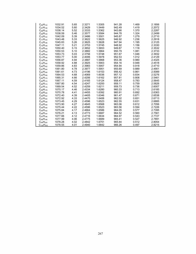
267
C66H134 1032.91 5.65 2.3271 1.5305 941.28 1.469 2.1856 C67H136 1034.52 5.60 2.3429 1.5449 942.49 1.419 2.2072 C68H138 1038.14 5.52 2.3333 1.5362 943.66 1.370 2.2287 C69H140 1038.59 5.46 2.3577 1.5584 944.78 1.324 2.2499 C70H142 1042.09 5.39 2.3486 1.5501 945.87 1.279 2.2710 C71H144 1043.48 5.33 2.3622 1.5625 946.92 1.236 2.2918 C72H146 1045.83 5.26 2.3625 1.5628 947.94 1.195 2.3125 C73H148 1047.11 5.21 2.3753 1.5745 948.92 1.156 2.3330 C74H150 1050.40 5.15 2.3652 1.5653 949.87 1.118 2.3532 C75H152 1050.53 5.10 2.3882 1.5864 950.79 1.081 2.3733 C76H154 1053.73 5.03 2.3756 1.5748 951.67 1.046 2.3932 C77H156 1053.77 5.00 2.4006 1.5978 952.53 1.012 2.4129 C78H158 1056.87 4.94 2.3887 1.5868 953.36 0.980 2.4325 C79H160 1058.92 4.88 2.3925 1.5903 954.16 0.948 2.4518 C80H162 1059.86 4.83 2.3983 1.5957 954.94 0.918 2.4710 C81H164 1061.80 4.78 2.3977 1.5951 955.69 0.889 2.4901 C82H166 1061.61 4.73 2.4196 1.6153 956.42 0.861 2.5089 C83H168 1064.53 4.68 2.4069 1.6036 957.12 0.834 2.5276 C84H170 1065.31 4.66 2.4206 1.6162 957.81 0.808 2.5461 C85H172 1067.11 4.59 2.4165 1.6124 958.47 0.783 2.5645 C86H174 1067.80 4.54 2.4247 1.6200 959.11 0.759 2.5826 C87H176 1069.54 4.52 2.4259 1.6211 959.73 0.736 2.6007 C88H178 1070.17 4.46 2.4334 1.6280 960.33 0.713 2.6185 C89H180 1070.78 4.41 2.4455 1.6392 960.91 0.692 2.6363 C90H182 1072.40 4.39 2.4405 1.6346 961.47 0.671 2.6538 C91H184 1072.92 4.33 2.4470 1.6406 962.02 0.651 2.6713 C92H186 1073.45 4.29 2.4596 1.6523 962.55 0.631 2.6885 C93H188 1073.90 4.27 2.4645 1.6568 963.06 0.612 2.7056 C94H190 1075.44 4.22 2.4596 1.6523 963.56 0.594 2.7226 C95H192 1075.84 4.17 2.4664 1.6586 964.05 0.577 2.7395 C96H194 1076.21 4.13 2.4773 1.6687 964.52 0.560 2.7561 C97H196 1077.66 4.12 2.4716 1.6634 964.97 0.543 2.7727 C98H198 1077.99 4.06 2.4775 1.6689 965.41 0.527 2.7891 C99H200 1078.28 4.02 2.4842 1.6751 965.84 0.512 2.8054 C100H202 1078.55 4.01 2.4940 1.6842 966.26 0.497 2.8215

268
Appendix 5-A. Algorithm for Direct Perturbation of Attraction and Covolume
Parameters
Figure 5-A1. Flow chart for the direct perturbation algorithm presented in Section 3. The dotted line shows the adjustment of fb for matching densities. This path is taken when the
adjustment of c is unsuccessful in matching densities (See Section 3.2 for details). For the dotted path,
the c value calculated in Step 2 is used and kept constant during the regression with fb and fψ.
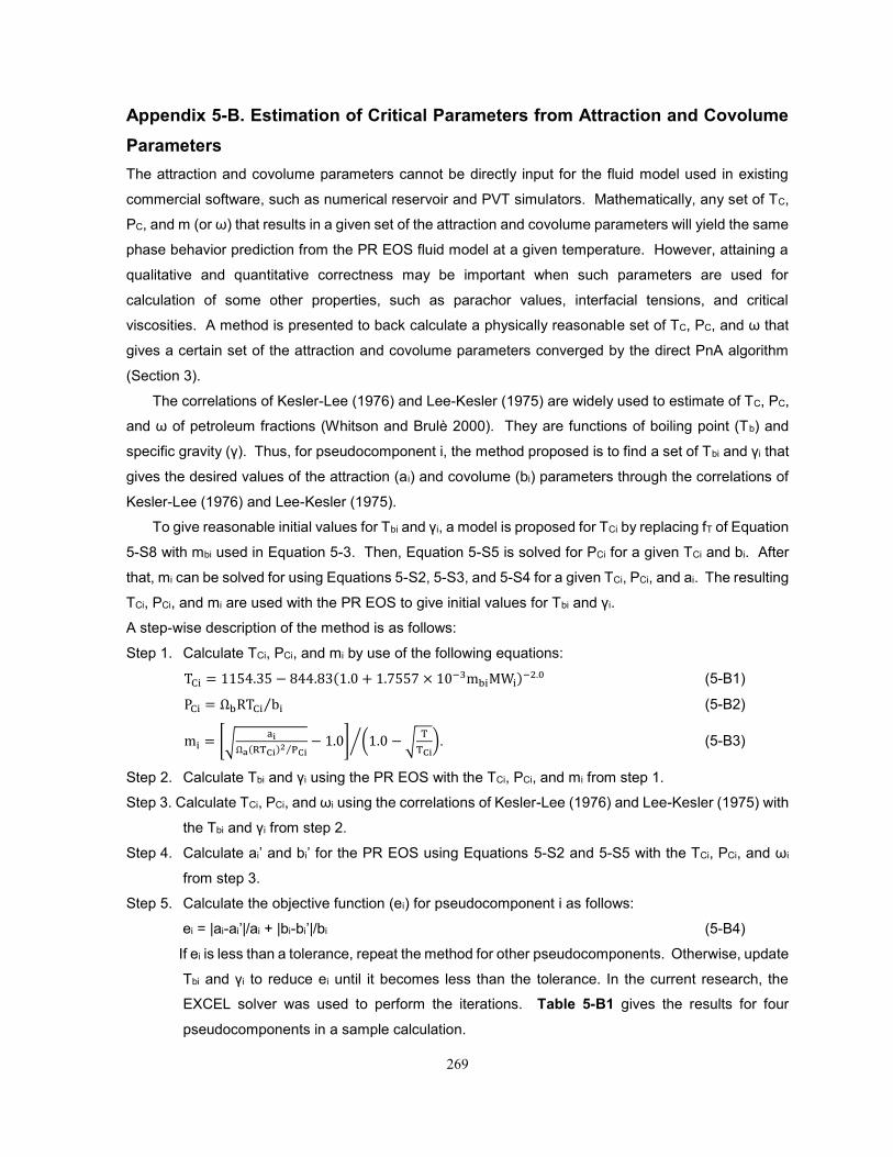
269
Appendix 5-B. Estimation of Critical Parameters from Attraction and Covolume
Parameters
The attraction and covolume parameters cannot be directly input for the fluid model used in existing
commercial software, such as numerical reservoir and PVT simulators. Mathematically, any set of TC,
PC, and m (or ω) that results in a given set of the attraction and covolume parameters will yield the same
phase behavior prediction from the PR EOS fluid model at a given temperature. However, attaining a
qualitative and quantitative correctness may be important when such parameters are used for
calculation of some other properties, such as parachor values, interfacial tensions, and critical
viscosities. A method is presented to back calculate a physically reasonable set of TC, PC, and ω that
gives a certain set of the attraction and covolume parameters converged by the direct PnA algorithm
(Section 3).
The correlations of Kesler-Lee (1976) and Lee-Kesler (1975) are widely used to estimate of TC, PC,
and ω of petroleum fractions (Whitson and Brulè 2000). They are functions of boiling point (Tb) and
specific gravity (γ). Thus, for pseudocomponent i, the method proposed is to find a set of Tbi and γi that
gives the desired values of the attraction (ai) and covolume (bi) parameters through the correlations of
Kesler-Lee (1976) and Lee-Kesler (1975).
To give reasonable initial values for Tbi and γi, a model is proposed for TCi by replacing fT of Equation
5-S8 with mbi used in Equation 5-3. Then, Equation 5-S5 is solved for PCi for a given TCi and bi. After
that, mi can be solved for using Equations 5-S2, 5-S3, and 5-S4 for a given TCi, PCi, and ai. The resulting
TCi, PCi, and mi are used with the PR EOS to give initial values for Tbi and γi.
A step-wise description of the method is as follows:
Step 1. Calculate TCi, PCi, and mi by use of the following equations:
TCi = 1154.35 − 844.83(1.0 + 1.7557 × 10⁻³mbiMWi)−2.0 (5-B1)
PCi = ΩbRTCi bi⁄ (5-B2)
mi = [√ai
Ωa(RTCi)2 PCi⁄− 1.0] (1.0 − √
T
TCi)⁄ . (5-B3)
Step 2. Calculate Tbi and γi using the PR EOS with the TCi, PCi, and mi from step 1.
Step 3. Calculate TCi, PCi, and ωi using the correlations of Kesler-Lee (1976) and Lee-Kesler (1975) with
the Tbi and γi from step 2.
Step 4. Calculate ai’ and bi’ for the PR EOS using Equations 5-S2 and 5-S5 with the TCi, PCi, and ωi
from step 3.
Step 5. Calculate the objective function (ei) for pseudocomponent i as follows:
ei = |ai-ai’|/ai + |bi-bi’|/bi (5-B4)
If ei is less than a tolerance, repeat the method for other pseudocomponents. Otherwise, update
Tbi and γi to reduce ei until it becomes less than the tolerance. In the current research, the
EXCEL solver was used to perform the iterations. Table 5-B1 gives the results for four
pseudocomponents in a sample calculation.

270
Table 5-B1. Example of solution for TC, PC, and ω from the attraction and covolume
parameters using the EXCEL solver. The temperature is 299.81 K. Target ai (bar.cc2.mol-2)
Target bi (cc.mol-1)
γi Tbi
(K) TCi
# (K)
PCi#
(bar) ωi
# ei
152780160.65 225.96109 0.82984 517.749 700.347 20.049 0.5680 3.64E-07 415755584.46 371.98724 0.94476 670.127 853.779 14.847 0.8738 2.83E-06 809603339.61 518.89867 1.04283 797.501 982.191 12.244 1.0646 1.79E-06 1893146362.73 796.38678 1.21313 1006.301 1199.746 9.745 1.2633 9.37E-06
# TCi, PCi, and ωi are calculated using the correlations of Kesler-Lee (1976), and Lee-Kesler (1975) with the listed γi and Tbi. The target ai and bi values are sample values for the attraction and covolume parameters for pseudocomponent i. Four pseudocomponents are listed.

271
Appendix 7-A. Development of Binary Interaction Parameters
BIPs were optimized for CO2, methane, ethane, and propane with heptane and heavier n-alkanes by
use of three-phase data, including critical endpoints (CEPs). A CEP is where two phases merge in the
presence of the other immiscible phase (Uzunov 1993). For a three-phase region bounded by two
CEPs, two liquid phases are critical in the presence of V phase (L1=L2-V) at the lower CEP (LCEP). At
the upper CEP (UCEP), the V and L2 phases are critical in the presence of the L1 phase (L1-L2=V). The
optimization was concerned primarily with UCEP predictions in this research.
Experimental data are available for UCEPs for the methane binaries with hexane (Lin et al. 1977)
and heptane (Chang et al. 1966), for the ethane binaries with n-C18, n-C19, n-C20, n-C22, n-C23, and n-
C24 (Estrera and Luks 1987; Peters et al. 1986; Peters et al. 1987a), and for the propane binaries with
n-C32, n-C34, n-C36, n-C38, n-C40, n-C44, n-C46, n-C50, and n-C60 (Peters et al. 1989; Peters et al. 1992;
Peters et al. 1993). These data were matched with the PR EOS by use of an in-house FORTRAN code
based on the algorithms of Heidemann and Khalil (1980) and Mushrif (2004). Critical parameters and
ω for CO2, methane, ethane, and propane were taken from Yaws (2010). The critical parameters of n-
alkanes heavier than hexane were from Equations 7-1 and 7-2 (Gao et al. 2001).
It was observed that matching UCEPs with the PR EOS requires minor deviations from the ω
correlation of Gao et al. (2001). To find a smooth ω trend with respect to CN that can be used for
matching UCEPs, different pairs of ω and BIP were found for each binary as shown in Figure 7-A1. In
this figure, the number below a curve indicates the CN of the heavier n-alkane. The curves follow the
same trend except for the propane binaries with n-C46 and n-C60. The irregularity for these binaries
appears to be caused by the fluctuation in the UCEP data measured near the asymptotic limit defined
by the critical point of propane, as shown in Figure 7-A2. This type of irregularity was also observed in
terms of measured UCEP temperature, although not shown here.
Equation 7-4 gives the smooth trend obtained for non-physical acentric factor (ώ) with respect to
CN in this research. Although this equation was found by use of non-physical and physical ω, the non-
physical values used were chosen to be as close to the corresponding physical value as possible. The
ω shown by the filled circles in Figure 7-A1 have been calculated from Equation 7-4. For n-C32, n-C34,
n-C36, n-C38, and n-C40, these are nearly equal to their respective physical values as given in Equation
7-3 (< 0.015 AAD). Figure 7-A3 shows the comparison between Equations 7-3 and 7-4.
The trend of optimized BIPs for the ethane binaries with n-C18, n-C19, n-C20, n-C22, n-C23, and n-C24
is linearly correlated by Equation 7-10. Development of a trend for propane BIPs used three-phase data
given in Gregorowicz et al. (1993b), in addition to the UCEP data mentioned previously, in order to add
an optimized BIP for propane with n-C20. The data by Gregorowicz et al. (1993b) are 12 P-T envelopes
for 12 different mixtures of ethane, propane and n-C20. The BIP of ethane with n-C20 was calculated
with Equation 7-10. The TC, PC, and ω for n-C20 were calculated from Equations 7-1, 7-2, and 7-4,
respectively. Then, three-phase data were matched by adjusting the propane BIPs with ethane and n-
C20. The optimized BIP is 0.017 for ethane-propane and 0.041 for propane-n-C20. Even though three-
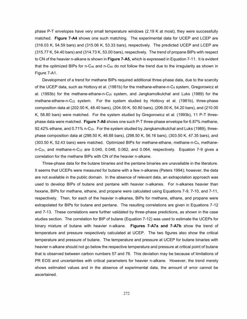
272
phase P-T envelopes have very small temperature windows (2.19 K at most), they were successfully
matched. Figure 7-A4 shows one such matching. The experimental data for UCEP and LCEP are
(316.03 K, 54.59 bars) and (315.06 K, 53.33 bars), respectively. The predicted UCEP and LCEP are
(315.77 K, 54.40 bars) and (314.73 K, 53.00 bars), respectively. The trend of propane BIPs with respect
to CN of the heavier n-alkane is shown in Figure 7-A5, which is expressed in Equation 7-11. It is evident
that the optimized BIPs for n-C46 and n-C60 do not follow the trend due to the irregularity as shown in
Figure 7-A1.
Development of a trend for methane BIPs required additional three-phase data, due to the scarcity
of the UCEP data, such as Hottovy et al. (1981b) for the methane-ethane-n-C8 system, Gregorowicz et
al. (1993b) for the methane-ethane-n-C20 system, and Jangkamolkulchal and Luks (1989) for the
methane-ethane-n-C22 system. For the system studied by Hottovy et al. (1981b), three-phase
composition data at (202.00 K, 48.40 bars), (204.00 K, 50.80 bars), (206.00 K, 54.20 bars), and (210.00
K, 58.80 bars) were matched. For the system studied by Gregorowicz et al. (1993b), 11 P-T three-
phase data were matched. Figure 7-A6 shows one such P-T three-phase envelope for 6.87% methane,
92.42% ethane, and 0.71% n-C20. For the system studied by Jangkamolkulchal and Luks (1989), three-
phase composition data at (298.50 K, 46.88 bars), (298.50 K, 56.16 bars), (303.50 K, 47.35 bars), and
(303.50 K, 52.43 bars) were matched. Optimized BIPs for methane-ethane, methane-n-C8, methane-
n-C20, and methane-n-C22 are 0.040, 0.048, 0.062, and 0.064, respectively. Equation 7-9 gives a
correlation for the methane BIPs with CN of the heavier n-alkane.
Three-phase data for the butane binaries and the pentane binaries are unavailable in the literature.
It seems that UCEPs were measured for butane with a few n-alkanes (Peters 1994); however, the data
are not available in the public domain. In the absence of relevant data, an extrapolation approach was
used to develop BIPs of butane and pentane with heavier n-alkanes. For n-alkanes heavier than
hexane, BIPs for methane, ethane, and propane were calculated using Equations 7-9, 7-10, and 7-11,
respectively. Then, for each of the heavier n-alkanes, BIPs for methane, ethane, and propane were
extrapolated for BIPs for butane and pentane. The resulting correlations are given in Equations 7-12
and 7-13. These correlations were further validated by three-phase predictions, as shown in the case
studies section. The correlation for BIP of butane (Equation 7-12) was used to estimate the UCEPs for
binary mixture of butane with heavier n-alkane. Figures 7-A7a and 7-A7b show the trend of
temperature and pressure respectively calculated at UCEP. The two figures also show the critical
temperature and pressure of butane. The temperature and pressure at UCEP for butane binaries with
heavier n-alkane should not go below the respective temperature and pressure at critical point of butane
that is observed between carbon numbers 57 and 76. This deviation may be because of limitations of
PR EOS and uncertainties with critical parameters for heavier n-alkane. However, the trend merely
shows estimated values and in the absence of experimental data, the amount of error cannot be
ascertained.

273
BIPs for CO2 with n-alkanes were optimized by Kato et al. (1981), Lin et al. (1984), Kordas et al.
(1994); however, they did not use three-phase data or CEP data. In this research, therefore, BIPs of
CO2 with n-alkanes were optimized to match the UCEP data for CO2-n-alkanes, n-C13, n-C14, n-C15, n-
C19, n-C20, and n-C21 (Hottovy et al. 1981a; Fall and Luks 1985; Fall et al. 1985). In order to make the
trend more reliable, L=V critical-point data for n-C8, n-C9, and n-C10 (Choi and Yeo 1998; Reamer and
Sage 1963) were also used in the BIP optimization. Figure 7-A8 shows that the optimized BIPs show
an increasing trend with increasing CN, but they become nearly constant beyond n-C15. However,
higher BIP values were required when matching experimental data for heavy oils for the development
of Equations 7-5, 7-6, and 7-7. This observation may be because of the effect of oil aromaticity on
phase behavior with CO2, and was considered for the development of Equation 7-8.
The BIPs developed for the PR EOS in this research are designed for n-alkanes; however, they are
used for pseudocomponents in this research. Although these BIPs were successful in predicting three-
phase behavior in this research, they can be used as initial guesses if BIP adjustment is needed.
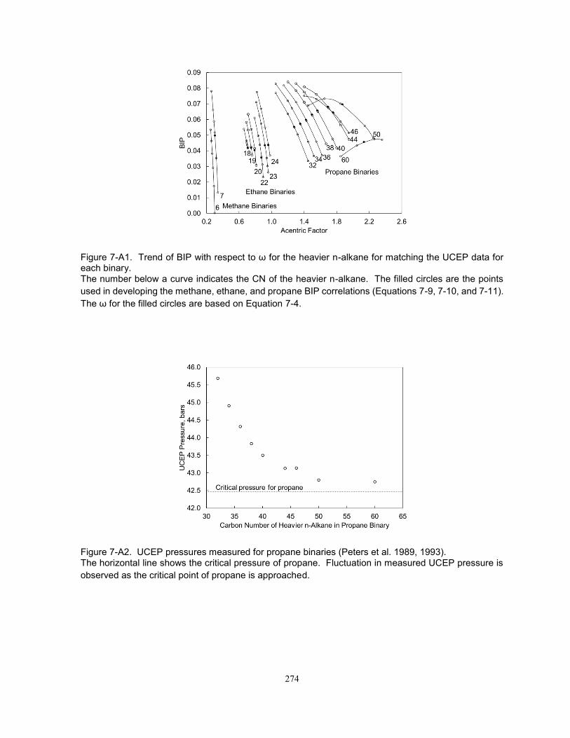
274
Figure 7-A1. Trend of BIP with respect to ω for the heavier n-alkane for matching the UCEP data for each binary. The number below a curve indicates the CN of the heavier n-alkane. The filled circles are the points
used in developing the methane, ethane, and propane BIP correlations (Equations 7-9, 7-10, and 7-11).
The ω for the filled circles are based on Equation 7-4.
Figure 7-A2. UCEP pressures measured for propane binaries (Peters et al. 1989, 1993). The horizontal line shows the critical pressure of propane. Fluctuation in measured UCEP pressure is
observed as the critical point of propane is approached.
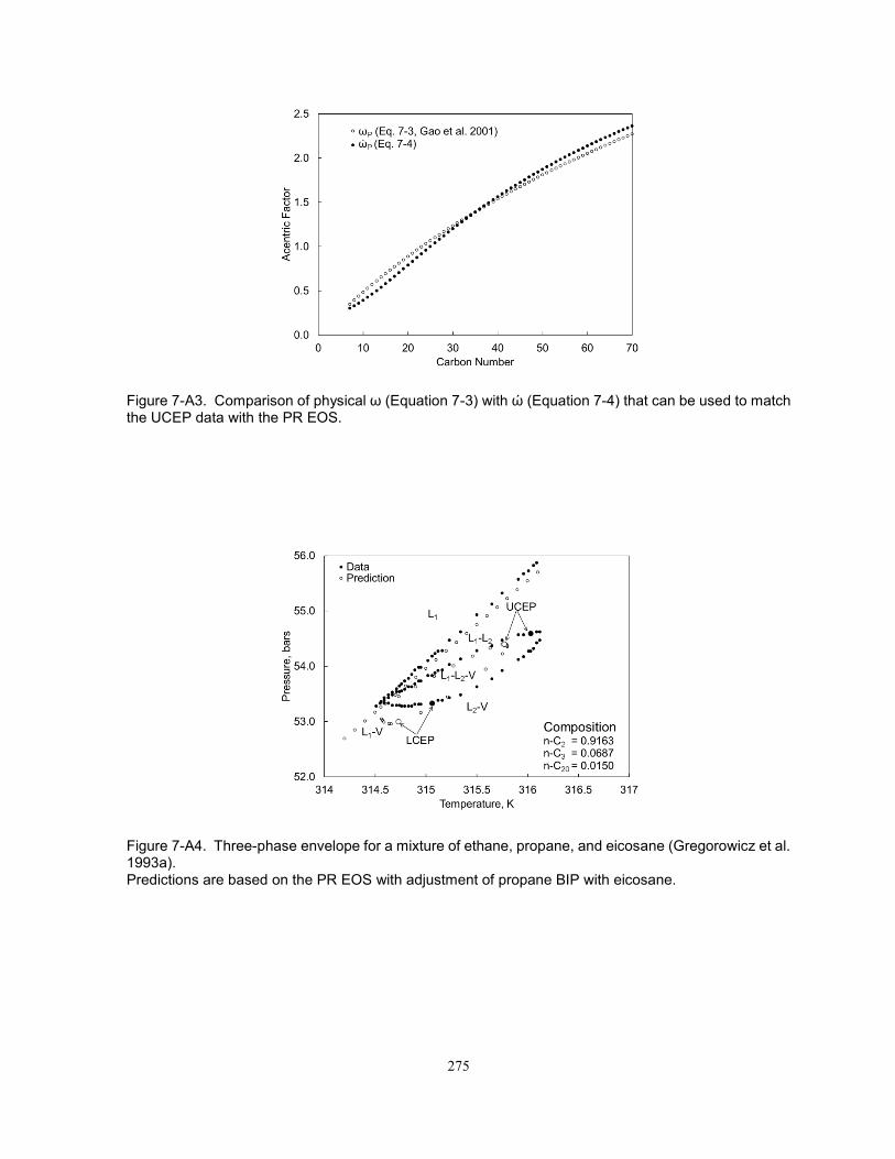
275
Figure 7-A3. Comparison of physical ω (Equation 7-3) with ώ (Equation 7-4) that can be used to match the UCEP data with the PR EOS.
Figure 7-A4. Three-phase envelope for a mixture of ethane, propane, and eicosane (Gregorowicz et al. 1993a). Predictions are based on the PR EOS with adjustment of propane BIP with eicosane.
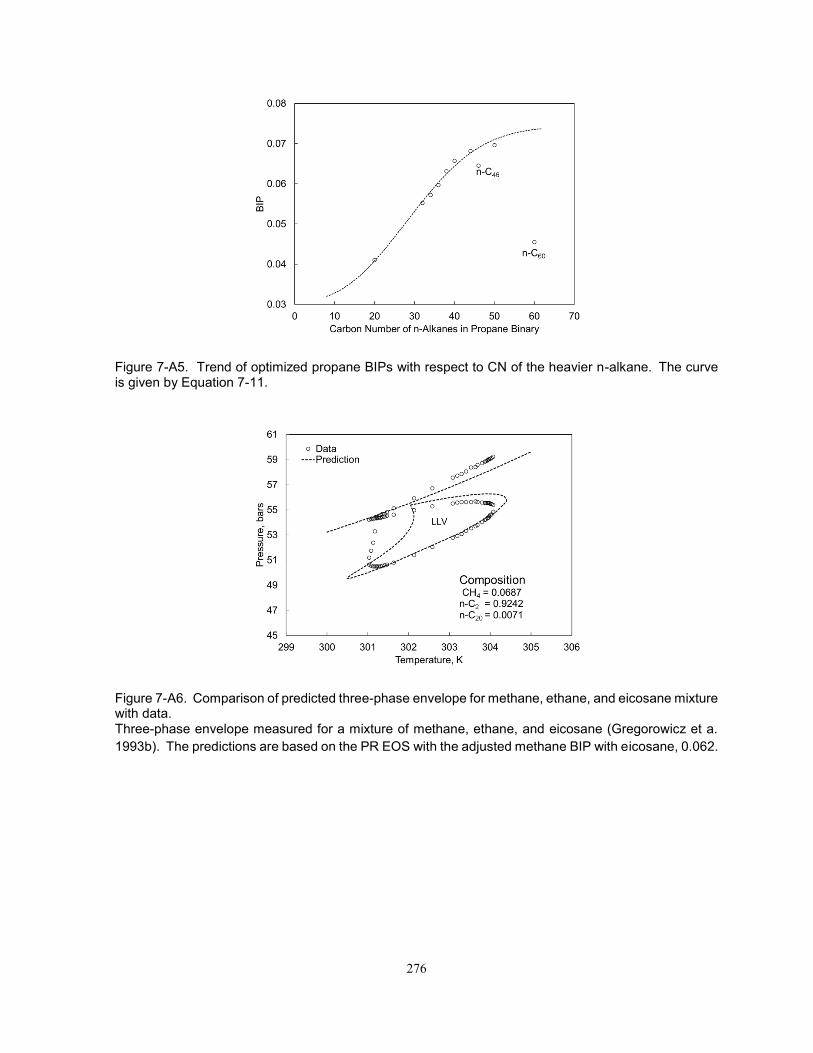
276
Figure 7-A5. Trend of optimized propane BIPs with respect to CN of the heavier n-alkane. The curve is given by Equation 7-11.
Figure 7-A6. Comparison of predicted three-phase envelope for methane, ethane, and eicosane mixture with data. Three-phase envelope measured for a mixture of methane, ethane, and eicosane (Gregorowicz et a.
1993b). The predictions are based on the PR EOS with the adjusted methane BIP with eicosane, 0.062.
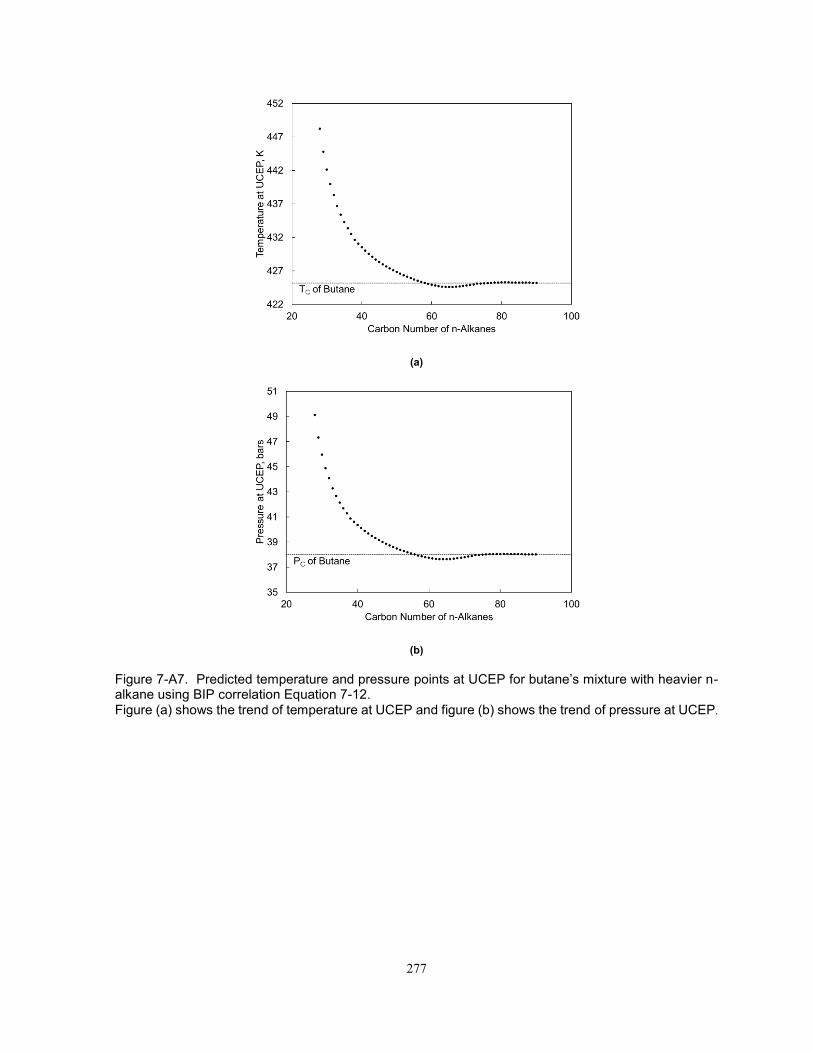
277
(a)
(b)
Figure 7-A7. Predicted temperature and pressure points at UCEP for butane’s mixture with heavier n-alkane using BIP correlation Equation 7-12. Figure (a) shows the trend of temperature at UCEP and figure (b) shows the trend of pressure at UCEP.

278
Figure 7-A8. Trend of optimized CO2 BIPs with respect to CN of the heavier n-alkane. The curve is calculated from Equation 7-8.
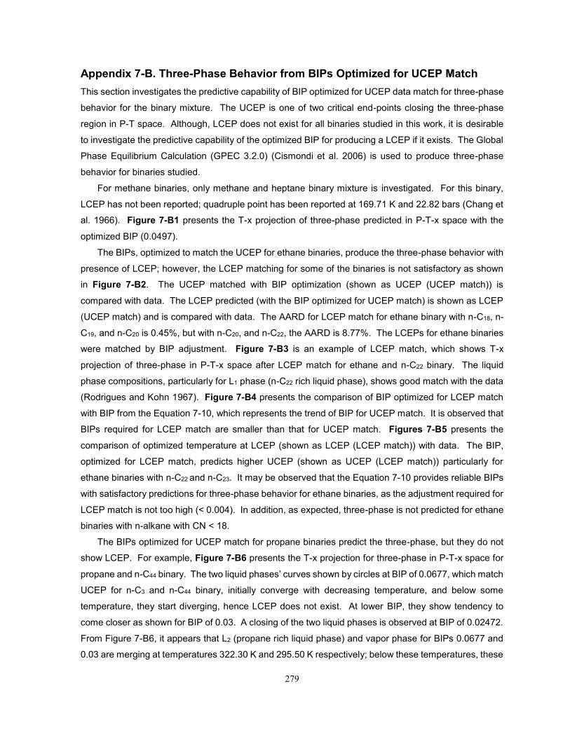
279
Appendix 7-B. Three-Phase Behavior from BIPs Optimized for UCEP Match
This section investigates the predictive capability of BIP optimized for UCEP data match for three-phase
behavior for the binary mixture. The UCEP is one of two critical end-points closing the three-phase
region in P-T space. Although, LCEP does not exist for all binaries studied in this work, it is desirable
to investigate the predictive capability of the optimized BIP for producing a LCEP if it exists. The Global
Phase Equilibrium Calculation (GPEC 3.2.0) (Cismondi et al. 2006) is used to produce three-phase
behavior for binaries studied.
For methane binaries, only methane and heptane binary mixture is investigated. For this binary,
LCEP has not been reported; quadruple point has been reported at 169.71 K and 22.82 bars (Chang et
al. 1966). Figure 7-B1 presents the T-x projection of three-phase predicted in P-T-x space with the
optimized BIP (0.0497).
The BIPs, optimized to match the UCEP for ethane binaries, produce the three-phase behavior with
presence of LCEP; however, the LCEP matching for some of the binaries is not satisfactory as shown
in Figure 7-B2. The UCEP matched with BIP optimization (shown as UCEP (UCEP match)) is
compared with data. The LCEP predicted (with the BIP optimized for UCEP match) is shown as LCEP
(UCEP match) and is compared with data. The AARD for LCEP match for ethane binary with n-C18, n-
C19, and n-C20 is 0.45%, but with n-C20, and n-C22, the AARD is 8.77%. The LCEPs for ethane binaries
were matched by BIP adjustment. Figure 7-B3 is an example of LCEP match, which shows T-x
projection of three-phase in P-T-x space after LCEP match for ethane and n-C22 binary. The liquid
phase compositions, particularly for L1 phase (n-C22 rich liquid phase), shows good match with the data
(Rodrigues and Kohn 1967). Figure 7-B4 presents the comparison of BIP optimized for LCEP match
with BIP from the Equation 7-10, which represents the trend of BIP for UCEP match. It is observed that
BIPs required for LCEP match are smaller than that for UCEP match. Figures 7-B5 presents the
comparison of optimized temperature at LCEP (shown as LCEP (LCEP match)) with data. The BIP,
optimized for LCEP match, predicts higher UCEP (shown as UCEP (LCEP match)) particularly for
ethane binaries with n-C22 and n-C23. It may be observed that the Equation 7-10 provides reliable BIPs
with satisfactory predictions for three-phase behavior for ethane binaries, as the adjustment required for
LCEP match is not too high (< 0.004). In addition, as expected, three-phase is not predicted for ethane
binaries with n-alkane with CN < 18.
The BIPs optimized for UCEP match for propane binaries predict the three-phase, but they do not
show LCEP. For example, Figure 7-B6 presents the T-x projection for three-phase in P-T-x space for
propane and n-C44 binary. The two liquid phases’ curves shown by circles at BIP of 0.0677, which match
UCEP for n-C3 and n-C44 binary, initially converge with decreasing temperature, and below some
temperature, they start diverging, hence LCEP does not exist. At lower BIP, they show tendency to
come closer as shown for BIP of 0.03. A closing of the two liquid phases is observed at BIP of 0.02472.
From Figure 7-B6, it appears that L2 (propane rich liquid phase) and vapor phase for BIPs 0.0677 and
0.03 are merging at temperatures 322.30 K and 295.50 K respectively; below these temperatures, these

280
phases have same composition as that of pure propane. This indicates existence of another UCEP
(vapor phase merging with propane rich liquid phase i.e. L2) at lower temperature; however, existence
of such phase behavior for propane binaries may not be realistic.
It is observed that with decrease in BIP to match LCEP for propane binaries, the temperature at
UCEP increases. This is in line with observation in case of ethane binaries, which required smaller BIP
for LCEP match that increased UCEP. Such adjustments were done for other propane binaries also for
LCEP match. However, it is observed that in case of n-C44 and n-C46, BIP adjustment could not bring
the LCEPs close to data. Figure 7-B7 compares the adjusted BIP for LCEP match with the trend of BIP
for UCEP match represented by Equation 7-11. Unlike the case of ethane binary in Figure 7-B4,
significant difference in BIPs matching UCEPs and matching LCEPs are observed in case of propane
binaries. Figure 7-B8 compares the optimized temperature at LCEP (shown as LCEP (LCEP match))
with the data. It also compares the UCEP predicted with BIP optimized for LCEP match (shown as
UCEP (LCEP match)) with data. It is observed that the temperatures at UCEP are significantly higher
than respective data. The three-phase prediction for propane binaries with BIP from Equation 7-11
should stop for n-alkanes with CN< 32; however, it was observed that this takes place for n-alkanes with
CN< 29.
Three-phase bounded by UCEP and LCEP exist in case of CO2 and n-C13 binary only. The BIP
optimized for UCEP match for this binary predicts the three-phase, but it does not have LCEP like
propane binary case described earlier. At BIP of 0.10, the predicted UCEP is (315.26 K and 86.14 bars),
whereas data (Fall and Luks 1985) is (314.00 K and 87.20 bars). When BIP is reduced to 0.088, the
predicted LCEP is (312.74 K and 80.72 bars), which is close to LCEP data (Fall and Luks 1985) of
(310.80 K, 81.10 bar); however, the UCEP now changes to (319.24 K and 91.89 bars). For other CO2
binaries, three-phase behavior is predicted correctly with no LCEP.
Following observations can be made from the analysis of the three-phase behavior from BIP
optimized for UCEP match:
UCEP and LCEP matching may require different BIPs for a given binary. This observation is
significant particularly in case of propane BIPs, which may be possibly because of inaccurate critical
parameters for higher n-alkanes, and limitations of PR EOS.
LCEP match requires smaller BIP compared to that for UCEP match. Hence, while characterizing
reservoir fluids with BIPs developed with UCEP match as default BIPs, adjustment of BIPs should
lead to smaller values greater than respective BIPs optimized for LCEP match.

281
Figure 7-B1. T-x projection of three-phase region in P-T-x space for CH4 and n-C7 binary mixture. L1 phase is n-C7 rich liquid phase, and L2 is CH4 rich liquid phase.
Figure 7-B2. Comparison of the optimized temperature at UCEP (shown as UCEP (UCEP match)) with data for ethane binaries. Comparison for predicted temperature at LCEP with BIP optimized for UCEP match (shown as LCEP
(UCEP match)) with data is also presented.
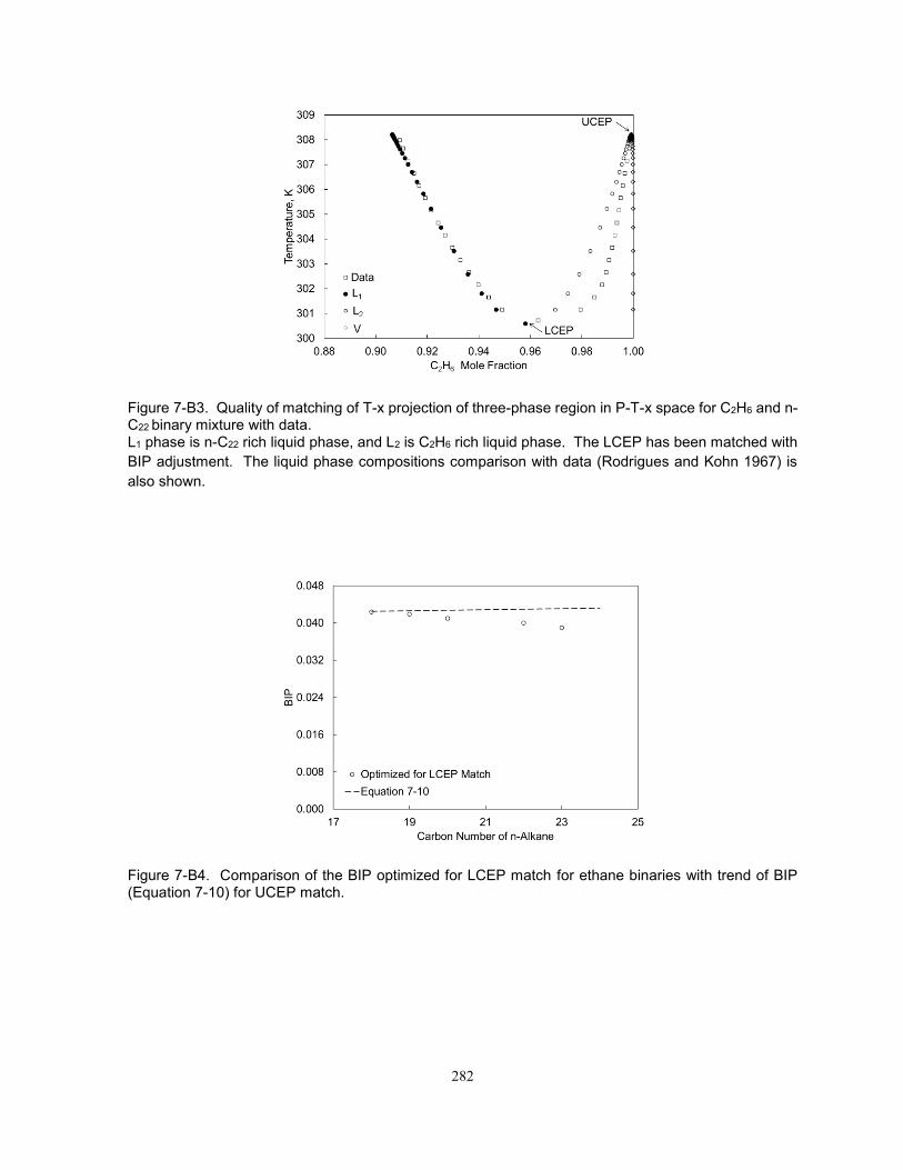
282
Figure 7-B3. Quality of matching of T-x projection of three-phase region in P-T-x space for C2H6 and n-C22 binary mixture with data. L1 phase is n-C22 rich liquid phase, and L2 is C2H6 rich liquid phase. The LCEP has been matched with
BIP adjustment. The liquid phase compositions comparison with data (Rodrigues and Kohn 1967) is
also shown.
Figure 7-B4. Comparison of the BIP optimized for LCEP match for ethane binaries with trend of BIP (Equation 7-10) for UCEP match.

283
Figure 7-B5. Comparison of the optimized temperature at LCEP (shown as LCEP (LCEP match)) with data for ethane binaries. Comparison for predicted temperature at UCEP with BIP optimized for LCEP match (shown as UCEP
(LCEP match)) with data is also presented.
Figure 7-B6. T-x projection for three-phase in P-T-x space for n-C3 and n-C44 binary with different BIPs. BIP of 0.0677 matches UCEP but predicted three-phase has no LCEP. Leftmost curve shown with circle
is L1 phase rich in n-C44, L2 phase rich in propane is very close to vapor phase, hence could not be
shown clearly. L1 (leftmost) and L2 (middle) phases for BIP of 0.03 is shown by dotted line;
corresponding curves for BIP of 0.02472 are shown by solid lines. Vapor curves for all BIP cases are
very close to each other and are shown on rightmost. The LCEP matching requires smaller BIPs, but it
increases the UCEP.

284
Figure 7-B7. Comparison of the BIPs optimized for LCEP match for propane binaries with the trend of BIP (Equation 7-11) that matched the UCEP.
Figure 7-B8. Comparison of the optimized temperature at LCEP (shown as LCEP (LCEP match)) with data for propane binaries is shown. Comparison for predicted temperature at UCEP with BIP optimized for LCEP match (shown as UCEP
(LCEP match)) with data is also presented. It is seen that LCEP matching achieved using smaller BIP
increases the UCEP significantly.

285
Appendix-7C: PR EOS Models for Fluids in Table 7-2 to 7-5.
Table 7C.1a : PR EOS model from PnA characterization for fluid 1 in Table 7.2. Saturation pressure for this fluid is 412.86 bars at 424.82 K.
Components Z MW (g/mol)
TC (K)
PC
(bars) ω CPEN
(CC/Mol) N2 0.0312 28.01 126.20 33.94 0.04000 -4.230 CO2 0.0323 44.01 304.20 73.76 0.22500 -1.640 CH4 0.6976 16.04 190.60 46.00 0.00800 -5.200 C2H6 0.0903 30.07 305.40 48.84 0.09800 -5.790 C3H8 0.0402 44.10 369.80 42.46 0.15200 -6.350 C4H10 0.0225 58.12 419.04 37.45 0.18690 -6.738 C5H12 0.0115 72.15 464.80 33.79 0.23850 -5.683 C6H14 0.0096 86.18 507.40 29.69 0.29600 1.390 PC-1 0.0237 111.55 593.84 30.97 0.16500 3.310 PC-2 0.0186 142.42 645.11 27.93 0.21400 7.770 PC-3 0.0139 189.93 735.69 23.79 0.31220 16.090 PC-4 0.0084 315.17 910.92 18.94 0.52110 39.500
Table 7C.1b : BIPs for PR EOS model from PnA characterization for fluid 1 in Table 7.2
N2 CO2 CH4 C2H6 C3H8 C4H10 C5H12 C6H14 PC-1 PC-2 PC-3 PC-4 N2 0.0000 CO2 0.0000 0.0000 CH4 0.1000 0.1000 0.0000 C2H6 0.1000 0.1450 0.0420 0.0000 C3H8 0.1000 0.2605 0.0420 0.0400 0.0000 C4H10 0.1000 0.2223 0.0420 0.0400 0.0300 0.0000 C5H12 0.1000 0.1824 0.0420 0.0400 0.0300 0.0116 0.0000 C6H14 0.1000 0.1597 0.0420 0.0400 0.0300 0.0155 0.0058 0.0000 PC-1 0.1300 0.0166 0.0500 0.0414 0.0320 0.0337 0.0186 0.0000 0.0000 PC-2 0.1300 0.0417 0.0518 0.0416 0.0328 0.0418 0.0275 0.0000 0.0000 0.0000 PC-3 0.1300 0.0814 0.0554 0.0420 0.0353 0.0534 0.0428 0.0000 0.0000 0.0000 0.0000 PC-4 0.1300 0.1206 0.0635 0.0430 0.0443 0.0674 0.0662 0.0000 0.0000 0.0000 0.0000 0.0000

286
Table 7C.2a : PR EOS model from PnA characterization for fluid 2 in Table 7.2 Saturation pressure (dew point) for this fluid is 424.70 bars at 403.15 K.
Components Z MW (g/mol)
TC (K)
PC
(bars) ω CPEN
(CC/Mol) N2 0.0679 28.01 126.20 33.94 0.04000 -4.230 CO2 0.0135 44.01 304.20 73.76 0.22500 -1.640 CH4 0.6869 16.04 190.60 46.00 0.00800 -5.200 C2H6 0.0812 30.07 305.40 48.84 0.09800 -5.790 C3H8 0.0376 44.10 369.80 42.46 0.15200 -6.350 C4H10 0.0219 58.12 419.73 37.51 0.18760 -6.710 C5H12 0.0124 72.15 465.30 33.79 0.23980 -5.630 C6H14 0.0099 86.18 507.40 29.69 0.29600 1.390 PC-1 0.0253 106.68 594.59 30.92 0.16360 8.780 PC-2 0.0198 136.77 645.93 27.87 0.21220 10.580 PC-3 0.0148 183.09 715.32 24.59 0.28540 13.280 PC-4 0.0089 305.13 895.91 19.22 0.49490 21.270
Table 7C.2b : BIPs for PR EOS model from PnA characterization for fluid 2 in Table 7.2
N2 CO2 CH4 C2H6 C3H8 C4H10 C5H12 C6H14 PC-1 PC-2 PC-3 PC-4 N2 0.0000 CO2 0.0000 0.0000 CH4 0.1000 0.1000 0.0000 C2H6 0.1000 0.1450 0.0420 0.0000 C3H8 0.1000 0.2252 0.0420 0.0400 0.0000 C4H10 0.1000 0.1942 0.0420 0.0400 0.0300 0.0000 C5H12 0.1000 0.1620 0.0420 0.0400 0.0300 0.0116 0.0000 C6H14 0.1000 0.1439 0.0420 0.0400 0.0300 0.0155 0.0058 0.0000 PC-1 0.1300 0.0166 0.0500 0.0414 0.0320 0.0337 0.0186 0.0000 0.0000 PC-2 0.1300 0.0417 0.0518 0.0416 0.0328 0.0418 0.0275 0.0000 0.0000 0.0000 PC-3 0.1300 0.0731 0.0545 0.0419 0.0346 0.0510 0.0393 0.0000 0.0000 0.0000 0.0000 PC-4 0.1300 0.1183 0.0626 0.0429 0.0431 0.0663 0.0642 0.0000 0.0000 0.0000 0.0000 0.0000

287
Table 7C.3a : PR EOS model from PnA characterization for fluid 3 in Table 7.2 Saturation pressure (dew point) for this fluid is 348.46 bars at 382.59 K.
Components Z MW (g/mol)
TC (K)
PC
(bars) ω CPEN
(CC/Mol) N2 0.0020 28.01 126.20 33.94 0.04000 -4.230 CO2 0.0077 44.01 304.20 73.76 0.22500 -1.640 CH4 0.7209 16.04 190.60 46.00 0.00800 -5.200 C2H6 0.0636 30.07 305.40 48.84 0.09800 -5.790 C3H8 0.0623 44.10 369.80 42.46 0.15200 -6.350 C4H10 0.0407 58.12 417.43 37.31 0.18530 -6.800 C5H12 0.0177 72.15 464.61 33.79 0.23800 -5.710 C6H14 0.0128 86.18 507.40 29.69 0.29600 1.390 PC-1 0.0264 104.57 596.05 31.02 0.16650 5.800 PC-2 0.0208 133.04 647.52 27.99 0.21590 15.870 PC-3 0.0156 176.65 717.59 24.72 0.29040 32.430 PC-4 0.0095 290.96 882.94 19.79 0.48110 81.380
Table 7C.3b : BIPs for PR EOS model from PnA characterization for fluid 3 in Table 7.2
N2 CO2 CH4 C2H6 C3H8 C4H10 C5H12 C6H14 PC-1 PC-2 PC-3 PC-4 N2 0.0000 CO2 0.0000 0.0000 CH4 0.1000 0.1000 0.0000 C2H6 0.1000 0.1450 0.0420 0.0000 C3H8 0.1000 0.1968 0.0420 0.0400 0.0000 C4H10 0.1000 0.1718 0.0420 0.0400 0.0300 0.0000 C5H12 0.1000 0.1463 0.0420 0.0400 0.0300 0.0116 0.0000 C6H14 0.1000 0.1322 0.0420 0.0400 0.0300 0.0155 0.0058 0.0000 PC-1 0.1300 0.0166 0.0500 0.0414 0.0320 0.0337 0.0186 0.0000 0.0000 PC-2 0.1300 0.0417 0.0518 0.0416 0.0328 0.0418 0.0275 0.0000 0.0000 0.0000 PC-3 0.1300 0.0731 0.0545 0.0419 0.0346 0.0510 0.0393 0.0000 0.0000 0.0000 0.0000 PC-4 0.1300 0.1156 0.0617 0.0428 0.0419 0.0652 0.0620 0.0000 0.0000 0.0000 0.0000 0.0000

288
Table 7C.4a : PR EOS model from PnA characterization for fluid 4 in Table 7.2 Saturation pressure (dew point) for this fluid is 415.39 bars at 397.59 K.
Components Z MW (g/mol)
TC (K)
PC
(bars) ω CPEN
(CC/Mol) N2 0.0011 28.01 126.20 33.94 0.04000 -4.230 CO2 0.0001 44.01 304.20 73.76 0.22500 -1.640 CH4 0.6893 16.04 190.60 46.00 0.00800 -5.200 C2H6 0.0863 30.07 305.40 48.84 0.09800 -5.790 C3H8 0.0534 44.10 369.80 42.46 0.15200 -6.350 C4H10 0.0348 58.12 419.55 37.50 0.18740 -6.720 C5H12 0.0178 72.15 464.79 33.79 0.23850 -5.680 C6H14 0.0173 86.18 507.40 29.69 0.29600 1.390 PC-1 0.0370 106.56 595.23 31.83 0.18940 -1.010 PC-2 0.0286 137.96 646.62 28.91 0.24560 -2.710 PC-3 0.0213 185.04 738.16 24.96 0.35840 -5.720 PC-4 0.0129 304.96 898.70 20.73 0.57290 -13.360
Table 7C.4b : BIPs for PR EOS model from PnA characterization for fluid 4 in Table 7.2
N2 CO2 CH4 C2H6 C3H8 C4H10 C5H12 C6H14 PC-1 PC-2 PC-3 PC-4 N2 0.0000 CO2 0.0000 0.0000 CH4 0.1000 0.1000 0.0000 C2H6 0.1000 0.1450 0.0420 0.0000 C3H8 0.1000 0.2171 0.0420 0.0400 0.0000 C4H10 0.1000 0.1877 0.0420 0.0400 0.0300 0.0000 C5H12 0.1000 0.1574 0.0420 0.0400 0.0300 0.0116 0.0000 C6H14 0.1000 0.1404 0.0420 0.0400 0.0300 0.0155 0.0058 0.0000 PC-1 0.1300 0.0166 0.0500 0.0414 0.0320 0.0337 0.0186 0.0000 0.0000 PC-2 0.1300 0.0417 0.0518 0.0416 0.0328 0.0418 0.0275 0.0000 0.0000 0.0000 PC-3 0.1300 0.0814 0.0554 0.0420 0.0353 0.0534 0.0428 0.0000 0.0000 0.0000 0.0000 PC-4 0.1300 0.1183 0.0626 0.0429 0.0431 0.0663 0.0642 0.0000 0.0000 0.0000 0.0000 0.0000

289
Table 7C.5a : PR EOS model from PnA characterization for fluid 5 in Table 7.2 Saturation pressure (dew point) for this fluid is 360.23 bars at 424.82 K.
Components Z MW (g/mol)
TC (K)
PC
(bars) ω CPEN
(CC/Mol) N2 0.0030 28.01 126.20 33.94 0.04000 -4.230 CO2 0.0435 44.01 304.20 73.76 0.22500 -1.640 CH4 0.6255 16.04 190.60 46.00 0.00800 -5.200 C2H6 0.0999 30.07 305.40 48.84 0.09800 -5.790 C3H8 0.0500 44.10 369.80 42.46 0.15200 -6.350 C4H10 0.0351 58.12 418.82 37.43 0.18670 -6.750 C5H12 0.0196 72.15 464.77 33.79 0.23840 -5.690 C6H14 0.0147 86.18 507.40 29.69 0.29600 1.390 PC-1 0.0422 111.44 592.24 30.33 0.14690 -0.800 PC-2 0.0312 150.51 667.06 25.93 0.21250 -2.290 PC-3 0.0224 209.99 753.43 22.13 0.29960 -4.730 PC-4 0.0129 364.76 954.99 16.87 0.52060 -12.200
Table 7C.5b : BIPs for PR EOS model from PnA characterization for fluid 5 in Table 7.2
N2 CO2 CH4 C2H6 C3H8 C4H10 C5H12 C6H14 PC-1 PC-2 PC-3 PC-4 N2 0.0000 CO2 0.0000 0.0000 CH4 0.1000 0.1000 0.0000 C2H6 0.1000 0.1450 0.0420 0.0000 C3H8 0.1000 0.2605 0.0420 0.0400 0.0000 C4H10 0.1000 0.2223 0.0420 0.0400 0.0300 0.0000 C5H12 0.1000 0.1824 0.0420 0.0400 0.0300 0.0116 0.0000 C6H14 0.1000 0.1597 0.0420 0.0400 0.0300 0.0155 0.0058 0.0000 PC-1 0.1300 0.0166 0.0500 0.0414 0.0320 0.0337 0.0186 0.0000 0.0000 PC-2 0.1300 0.0532 0.0527 0.0417 0.0334 0.0452 0.0317 0.0000 0.0000 0.0000 PC-3 0.1300 0.0886 0.0563 0.0422 0.0360 0.0556 0.0461 0.0000 0.0000 0.0000 0.0000 PC-4 0.1300 0.1259 0.0662 0.0434 0.0480 0.0702 0.0715 0.0000 0.0000 0.0000 0.0000 0.0000

290
Table 7C.6a : PR EOS model from PnA characterization for fluid 6 in Table 7.2 Saturation pressure (dew point) for this fluid is 339.41 bars at 422.59 K.
Components Z MW (g/mol)
TC (K)
PC
(bars) ω CPEN
(CC/Mol) N2 0.0343 28.01 126.20 33.94 0.04000 -4.230 CO2 0.0275 44.01 304.20 73.76 0.22500 -1.640 CH4 0.6783 16.04 190.60 46.00 0.00800 -5.200 C2H6 0.0449 30.07 305.40 48.84 0.09800 -5.790 C3H8 0.0267 44.10 369.80 42.46 0.15200 -6.350 C4H10 0.0268 58.12 419.52 37.50 0.18740 -6.720 C5H12 0.0185 72.15 465.37 33.79 0.24000 -5.620 C6H14 0.0203 86.18 507.40 29.69 0.29600 1.390 PC-1 0.0450 105.73 593.72 29.93 0.13560 -5.120 PC-2 0.0349 136.03 644.98 26.75 0.17580 -14.040 PC-3 0.0264 180.22 713.96 23.29 0.23640 -28.400 PC-4 0.0164 289.08 873.61 18.02 0.39170 -71.100
Table 7C.6b : BIPs for PR EOS model from PnA characterization for fluid 6 in Table 7.2
N2 CO2 CH4 C2H6 C3H8 C4H10 C5H12 C6H14 PC-1 PC-2 PC-3 PC-4 N2 0.0000 CO2 0.0000 0.0000 CH4 0.1000 0.1000 0.0000 C2H6 0.1000 0.1450 0.0420 0.0000 C3H8 0.1000 0.2566 0.0420 0.0400 0.0000 C4H10 0.1000 0.2192 0.0420 0.0400 0.0300 0.0000 C5H12 0.1000 0.1801 0.0420 0.0400 0.0300 0.0116 0.0000 C6H14 0.1000 0.1579 0.0420 0.0400 0.0300 0.0155 0.0058 0.0000 PC-1 0.1300 0.0166 0.0500 0.0414 0.0320 0.0337 0.0186 0.0000 0.0000 PC-2 0.1300 0.0417 0.0518 0.0416 0.0328 0.0418 0.0275 0.0000 0.0000 0.0000 PC-3 0.1300 0.0731 0.0545 0.0419 0.0346 0.0510 0.0393 0.0000 0.0000 0.0000 0.0000 PC-4 0.1300 0.1156 0.0617 0.0428 0.0419 0.0652 0.0620 0.0000 0.0000 0.0000 0.0000 0.0000

291
Table 7C.7a : PR EOS model from PnA characterization for fluid 7 in Table 7.2 Saturation pressure (dew point) for this fluid is 312.73 bars at 424.82 K.
Components Z MW (g/mol)
TC (K)
PC
(bars) ω CPEN
(CC/Mol) N2 0.0345 28.01 126.20 33.94 0.04000 -4.230 CO2 0.0273 44.01 304.20 73.76 0.22500 -1.640 CH4 0.5771 16.04 190.60 46.00 0.00800 -5.200 C2H6 0.1072 30.07 305.40 48.84 0.09800 -5.790 C3H8 0.0599 44.10 369.80 42.46 0.15200 -6.350 C4H10 0.0345 58.12 419.95 37.53 0.18780 -6.700 C5H12 0.0184 72.15 465.25 33.79 0.23970 -5.630 C6H14 0.0172 86.18 507.40 29.69 0.29600 1.390 PC-1 0.0453 108.21 594.94 30.51 0.15190 -1.650 PC-2 0.0353 138.84 646.31 27.41 0.19710 -3.300 PC-3 0.0267 183.71 715.87 24.05 0.26500 -4.940 PC-4 0.0166 294.82 878.50 18.96 0.43910 -6.590
Table 7C.7b : BIPs for PR EOS model from PnA characterization for fluid 7 in Table 7.2
N2 CO2 CH4 C2H6 C3H8 C4H10 C5H12 C6H14 PC-1 PC-2 PC-3 PC-4 N2 0.0000 CO2 0.0000 0.0000 CH4 0.1000 0.1000 0.0000 C2H6 0.1000 0.1450 0.0420 0.0000 C3H8 0.1000 0.2605 0.0420 0.0400 0.0000 C4H10 0.1000 0.2223 0.0420 0.0400 0.0300 0.0000 C5H12 0.1000 0.1824 0.0420 0.0400 0.0300 0.0116 0.0000 C6H14 0.1000 0.1597 0.0420 0.0400 0.0300 0.0155 0.0058 0.0000 PC-1 0.1300 0.0166 0.0500 0.0414 0.0320 0.0337 0.0186 0.0000 0.0000 PC-2 0.1300 0.0417 0.0518 0.0416 0.0328 0.0418 0.0275 0.0000 0.0000 0.0000 PC-3 0.1300 0.0731 0.0545 0.0419 0.0346 0.0510 0.0393 0.0000 0.0000 0.0000 0.0000 PC-4 0.1300 0.1156 0.0617 0.0428 0.0419 0.0652 0.0620 0.0000 0.0000 0.0000 0.0000 0.0000

292
Table 7C.8a : PR EOS model from PnA characterization for fluid 8 in Table 7.2 Saturation pressure (dew point) for this fluid is 334.86 bars at 403.71 K.
Components Z MW (g/mol)
TC (K)
PC
(bars) ω CPEN
(CC/Mol) N2 0.0034 28.01 126.20 33.94 0.04000 -4.230 CO2 0.0217 44.01 304.20 73.76 0.22500 -1.640 CH4 0.7064 16.04 190.60 46.00 0.00800 -5.200 C2H6 0.1076 30.07 305.40 48.84 0.09800 -5.790 C3H8 0.0494 44.10 369.80 42.46 0.15200 -6.350 C4H10 0.0302 58.12 425.20 38.00 0.19300 -6.490 C5H12 0.0135 72.15 469.60 33.74 0.25100 -5.120 C6H14 0.0090 86.18 507.40 29.69 0.29600 1.390 PC-1 0.0211 106.55 595.72 30.81 0.16050 6.190 PC-2 0.0169 133.35 647.16 27.75 0.20820 15.490 PC-3 0.0129 174.58 717.07 24.44 0.27990 31.070 PC-4 0.0079 283.21 881.60 19.45 0.46380 78.030
Table 7C.8b : BIPs for PR EOS model from PnA characterization for fluid 8 in Table 7.2
N2 CO2 CH4 C2H6 C3H8 C4H10 C5H12 C6H14 PC-1 PC-2 PC-3 PC-4 N2 0.0000 CO2 0.0000 0.0000 CH4 0.1000 0.1000 0.0000 C2H6 0.1000 0.1450 0.0420 0.0000 C3H8 0.1000 0.2261 0.0420 0.0400 0.0000 C4H10 0.1000 0.1948 0.0420 0.0400 0.0300 0.0000 C5H12 0.1000 0.1625 0.0420 0.0400 0.0300 0.0116 0.0000 C6H14 0.1000 0.1443 0.0420 0.0400 0.0300 0.0155 0.0058 0.0000 PC-1 0.1300 0.0166 0.0500 0.0414 0.0320 0.0337 0.0186 0.0000 0.0000 PC-2 0.1300 0.0417 0.0518 0.0416 0.0328 0.0418 0.0275 0.0000 0.0000 0.0000 PC-3 0.1300 0.0731 0.0545 0.0419 0.0346 0.0510 0.0393 0.0000 0.0000 0.0000 0.0000 PC-4 0.1300 0.1156 0.0617 0.0428 0.0419 0.0652 0.0620 0.0000 0.0000 0.0000 0.0000 0.0000
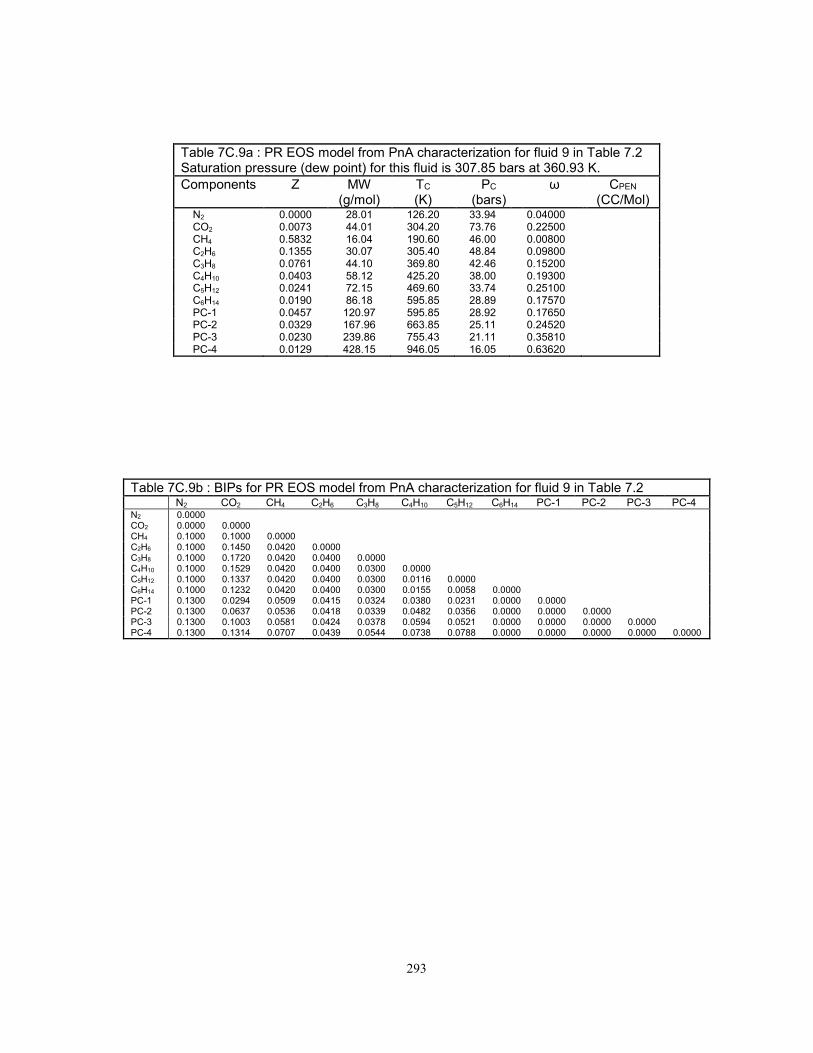
293
Table 7C.9a : PR EOS model from PnA characterization for fluid 9 in Table 7.2 Saturation pressure (dew point) for this fluid is 307.85 bars at 360.93 K.
Components Z MW (g/mol)
TC (K)
PC
(bars) ω CPEN
(CC/Mol) N2 0.0000 28.01 126.20 33.94 0.04000 CO2 0.0073 44.01 304.20 73.76 0.22500 CH4 0.5832 16.04 190.60 46.00 0.00800 C2H6 0.1355 30.07 305.40 48.84 0.09800 C3H8 0.0761 44.10 369.80 42.46 0.15200 C4H10 0.0403 58.12 425.20 38.00 0.19300 C5H12 0.0241 72.15 469.60 33.74 0.25100 C6H14 0.0190 86.18 595.85 28.89 0.17570 PC-1 0.0457 120.97 595.85 28.92 0.17650 PC-2 0.0329 167.96 663.85 25.11 0.24520 PC-3 0.0230 239.86 755.43 21.11 0.35810 PC-4 0.0129 428.15 946.05 16.05 0.63620
Table 7C.9b : BIPs for PR EOS model from PnA characterization for fluid 9 in Table 7.2
N2 CO2 CH4 C2H6 C3H8 C4H10 C5H12 C6H14 PC-1 PC-2 PC-3 PC-4 N2 0.0000 CO2 0.0000 0.0000 CH4 0.1000 0.1000 0.0000 C2H6 0.1000 0.1450 0.0420 0.0000 C3H8 0.1000 0.1720 0.0420 0.0400 0.0000 C4H10 0.1000 0.1529 0.0420 0.0400 0.0300 0.0000 C5H12 0.1000 0.1337 0.0420 0.0400 0.0300 0.0116 0.0000 C6H14 0.1000 0.1232 0.0420 0.0400 0.0300 0.0155 0.0058 0.0000 PC-1 0.1300 0.0294 0.0509 0.0415 0.0324 0.0380 0.0231 0.0000 0.0000 PC-2 0.1300 0.0637 0.0536 0.0418 0.0339 0.0482 0.0356 0.0000 0.0000 0.0000 PC-3 0.1300 0.1003 0.0581 0.0424 0.0378 0.0594 0.0521 0.0000 0.0000 0.0000 0.0000 PC-4 0.1300 0.1314 0.0707 0.0439 0.0544 0.0738 0.0788 0.0000 0.0000 0.0000 0.0000 0.0000

294
Table 7C.10a : PR EOS model from PnA characterization for fluid 10 in Table 7.2 Saturation pressure (dew point) for this fluid is 389.90 bars at 406.45 K.
Components Z MW (g/mol)
TC (K)
PC
(bars) ω CPEN
(CC/Mol) N2 0.0082 28.01 126.20 33.94 0.04000 -4.230 CO2 0.0143 44.01 304.20 73.76 0.22500 -1.640 CH4 0.7985 16.04 190.60 46.00 0.00800 -5.200 C2H6 0.0840 30.07 305.40 48.84 0.09800 -5.790 C3H8 0.0319 44.10 369.80 42.46 0.15200 -6.350 C4H10 0.0146 58.12 418.17 37.38 0.18600 -6.490 C5H12 0.0056 72.15 464.84 33.79 0.23860 -5.120 C6H14 0.0041 86.18 507.40 29.69 0.29600 1.390 PC-1 0.0136 115.89 621.80 29.45 0.19260 5.890 PC-2 0.0112 141.58 646.89 28.04 0.21750 10.760 PC-3 0.0087 181.13 716.68 24.78 0.29260 19.900 PC-4 0.0055 285.20 880.60 19.86 0.48470 47.480
Table 7C.10b : BIPs for PR EOS model from PnA characterization for fluid 10 in Table 7.2
N2 CO2 CH4 C2H6 C3H8 C4H10 C5H12 C6H14 PC-1 PC-2 PC-3 PC-4 N2 0.0000 CO2 0.0000 0.0000 CH4 0.1000 0.1000 0.0000 C2H6 0.1000 0.1450 0.0420 0.0000 C3H8 0.1000 0.2303 0.0420 0.0400 0.0000 C4H10 0.1000 0.1981 0.0420 0.0400 0.0300 0.0000 C5H12 0.1000 0.1649 0.0420 0.0400 0.0300 0.0116 0.0000 C6H14 0.1000 0.1461 0.0420 0.0400 0.0300 0.0155 0.0058 0.0000 PC-1 0.1300 0.0294 0.0509 0.0415 0.0324 0.0380 0.0231 0.0000 0.0000 PC-2 0.1300 0.0417 0.0518 0.0416 0.0328 0.0418 0.0275 0.0000 0.0000 0.0000 PC-3 0.1300 0.0731 0.0545 0.0419 0.0346 0.0510 0.0393 0.0000 0.0000 0.0000 0.0000 PC-4 0.1300 0.1156 0.0617 0.0428 0.0419 0.0652 0.0620 0.0000 0.0000 0.0000 0.0000 0.0000

295
Table 7C.11a : PR EOS model from PnA characterization for fluid 11 in Table 7.2 Saturation pressure (dew point) for this fluid is 362.66 bars at 374.81 K.
Components Z MW (g/mol)
TC (K)
PC
(bars) ω CPEN
(CC/Mol) N2 0.0223 28.01 126.20 33.94 0.04000 -4.230 CO2 0.0045 44.01 304.20 73.76 0.22500 -1.640 CH4 0.6568 16.04 190.60 46.00 0.00800 -5.200 C2H6 0.1170 30.07 305.40 48.84 0.09800 -5.790 C3H8 0.0587 44.10 369.80 42.46 0.15200 -6.350 C4H10 0.0295 58.12 425.20 38.00 0.19300 -6.490 C5H12 0.0142 72.15 469.60 33.74 0.25100 -5.120 C6H14 0.0098 86.18 507.40 29.69 0.29600 1.390 PC-1 0.0334 109.59 592.96 30.17 0.14240 6.710 PC-2 0.0251 145.83 667.93 25.74 0.20590 19.410 PC-3 0.0182 201.62 754.90 21.91 0.29040 40.800 PC-4 0.0105 348.74 942.02 16.90 0.48660 103.970
Table 7C.11b : BIPs for PR EOS model from PnA characterization for fluid 11 in Table 7.2
N2 CO2 CH4 C2H6 C3H8 C4H10 C5H12 C6H14 PC-1 PC-2 PC-3 PC-4 N2 0.0000 CO2 0.0000 0.0000 CH4 0.1000 0.1000 0.0000 C2H6 0.1000 0.1450 0.0420 0.0000 C3H8 0.1000 0.1872 0.0420 0.0400 0.0000 C4H10 0.1000 0.1645 0.0420 0.0400 0.0300 0.0000 C5H12 0.1000 0.1413 0.0420 0.0400 0.0300 0.0116 0.0000 C6H14 0.1000 0.1285 0.0420 0.0400 0.0300 0.0155 0.0058 0.0000 PC-1 0.1300 0.0166 0.0500 0.0414 0.0320 0.0337 0.0186 0.0000 0.0000 PC-2 0.1300 0.0532 0.0527 0.0417 0.0334 0.0452 0.0317 0.0000 0.0000 0.0000 PC-3 0.1300 0.0886 0.0563 0.0422 0.0360 0.0556 0.0461 0.0000 0.0000 0.0000 0.0000 PC-4 0.1300 0.1244 0.0653 0.0433 0.0468 0.0693 0.0698 0.0000 0.0000 0.0000 0.0000 0.0000

296
Table 7C.12a : PR EOS model from PnA characterization for fluid 12 in Table 7.2 Saturation pressure (dew point) for this fluid is 214.78 bars at 435.93 K.
Components Z MW (g/mol)
TC (K)
PC
(bars) ω CPEN
(CC/Mol) N2 0.0567 28.01 126.20 33.94 0.04000 -4.230 CO2 0.0201 44.01 304.20 73.76 0.22500 -1.640 CH4 0.4679 16.04 190.60 46.00 0.00800 -5.200 C2H6 0.1265 30.07 305.40 48.84 0.09800 -5.790 C3H8 0.0587 44.10 369.80 42.46 0.15200 -6.350 C4H10 0.0604 58.12 425.20 38.00 0.19300 -6.490 C5H12 0.0392 72.15 469.60 33.74 0.25100 -5.120 C6H14 0.0478 86.18 507.40 29.69 0.29600 1.390 PC-1 0.0423 107.64 570.11 30.50 0.15170 0.570 PC-2 0.0348 131.00 621.84 27.39 0.19670 1.310 PC-3 0.0276 164.93 670.10 25.02 0.24200 2.380 PC-4 0.0184 247.51 803.17 20.42 0.37490 5.510
Table 7C.12b : BIPs for PR EOS model from PnA characterization for fluid 12 in Table 7.2
N2 CO2 CH4 C2H6 C3H8 C4H10 C5H12 C6H14 PC-1 PC-2 PC-3 PC-4 N2 0.0000 CO2 0.0000 0.0000 CH4 0.1000 0.1000 0.0000 C2H6 0.1000 0.1450 0.0420 0.0000 C3H8 0.1000 0.2807 0.0420 0.0400 0.0000 C4H10 0.1000 0.2385 0.0420 0.0400 0.0300 0.0000 C5H12 0.1000 0.1944 0.0420 0.0400 0.0300 0.0116 0.0000 C6H14 0.1000 0.1691 0.0420 0.0400 0.0300 0.0155 0.0058 0.0000 PC-1 0.1300 0.0166 0.0500 0.0414 0.0320 0.0337 0.0186 0.0000 0.0000 PC-2 0.1300 0.0417 0.0518 0.0416 0.0328 0.0418 0.0275 0.0000 0.0000 0.0000 PC-3 0.1300 0.0637 0.0536 0.0418 0.0339 0.0482 0.0356 0.0000 0.0000 0.0000 0.0000 PC-4 0.1300 0.1050 0.0590 0.0425 0.0387 0.0610 0.0548 0.0000 0.0000 0.0000 0.0000 0.0000

297
Table 7C.13a : PR EOS model from PnA characterization for fluid 13 in Table 7.2 Saturation pressure (dew point) for this fluid is 208.58 bars at 435.93 K.
Components Z MW (g/mol)
TC (K)
PC
(bars) ω CPEN
(CC/Mol) N2 0.0567 28.01 126.20 33.94 0.04000 -4.230 CO2 0.0226 44.01 304.20 73.76 0.22500 -1.640 CH4 0.4574 16.04 190.60 46.00 0.00800 -5.200 C2H6 0.1147 30.07 305.40 48.84 0.09800 -5.790 C3H8 0.0759 44.10 369.80 42.46 0.15200 -6.350 C4H10 0.0638 58.12 425.20 38.00 0.19300 -6.490 C5H12 0.0431 72.15 469.60 33.74 0.25100 -5.120 C6H14 0.0592 86.18 507.40 29.69 0.29600 1.390 PC-1 0.0359 109.83 596.63 30.27 0.14520 8.210 PC-2 0.0300 131.36 648.16 27.14 0.18830 17.370 PC-3 0.0242 162.83 695.76 24.73 0.23160 30.580 PC-4 0.0164 239.95 804.52 20.67 0.33820 66.250
Table 7C.13b : BIPs for PR EOS model from PnA characterization for fluid 13 in Table 7.2
N2 CO2 CH4 C2H6 C3H8 C4H10 C5H12 C6H14 PC-1 PC-2 PC-3 PC-4 N2 0.0000 CO2 0.0000 0.0000 CH4 0.1000 0.1000 0.0000 C2H6 0.1000 0.1450 0.0420 0.0000 C3H8 0.1000 0.2807 0.0420 0.0400 0.0000 C4H10 0.1000 0.2385 0.0420 0.0400 0.0300 0.0000 C5H12 0.1000 0.1944 0.0420 0.0400 0.0300 0.0116 0.0000 C6H14 0.1000 0.1691 0.0420 0.0400 0.0300 0.0155 0.0058 0.0000 PC-1 0.1300 0.0166 0.0500 0.0414 0.0320 0.0337 0.0186 0.0000 0.0000 PC-2 0.1300 0.0417 0.0518 0.0416 0.0328 0.0418 0.0275 0.0000 0.0000 0.0000 PC-3 0.1300 0.0637 0.0536 0.0418 0.0339 0.0482 0.0356 0.0000 0.0000 0.0000 0.0000 PC-4 0.1300 0.1003 0.0581 0.0424 0.0378 0.0594 0.0521 0.0000 0.0000 0.0000 0.0000 0.0000
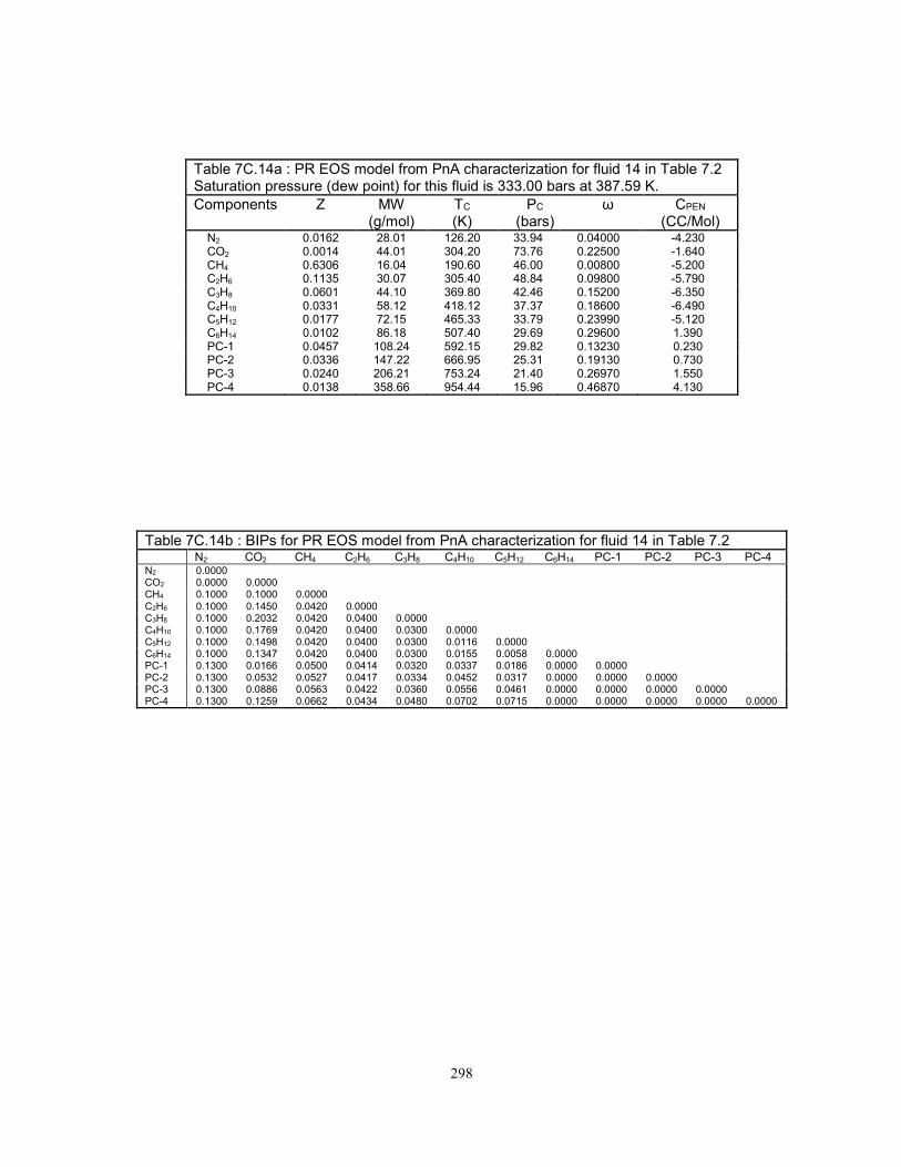
298
Table 7C.14a : PR EOS model from PnA characterization for fluid 14 in Table 7.2 Saturation pressure (dew point) for this fluid is 333.00 bars at 387.59 K.
Components Z MW (g/mol)
TC (K)
PC
(bars) ω CPEN
(CC/Mol) N2 0.0162 28.01 126.20 33.94 0.04000 -4.230 CO2 0.0014 44.01 304.20 73.76 0.22500 -1.640 CH4 0.6306 16.04 190.60 46.00 0.00800 -5.200 C2H6 0.1135 30.07 305.40 48.84 0.09800 -5.790 C3H8 0.0601 44.10 369.80 42.46 0.15200 -6.350 C4H10 0.0331 58.12 418.12 37.37 0.18600 -6.490 C5H12 0.0177 72.15 465.33 33.79 0.23990 -5.120 C6H14 0.0102 86.18 507.40 29.69 0.29600 1.390 PC-1 0.0457 108.24 592.15 29.82 0.13230 0.230 PC-2 0.0336 147.22 666.95 25.31 0.19130 0.730 PC-3 0.0240 206.21 753.24 21.40 0.26970 1.550 PC-4 0.0138 358.66 954.44 15.96 0.46870 4.130
Table 7C.14b : BIPs for PR EOS model from PnA characterization for fluid 14 in Table 7.2
N2 CO2 CH4 C2H6 C3H8 C4H10 C5H12 C6H14 PC-1 PC-2 PC-3 PC-4 N2 0.0000 CO2 0.0000 0.0000 CH4 0.1000 0.1000 0.0000 C2H6 0.1000 0.1450 0.0420 0.0000 C3H8 0.1000 0.2032 0.0420 0.0400 0.0000 C4H10 0.1000 0.1769 0.0420 0.0400 0.0300 0.0000 C5H12 0.1000 0.1498 0.0420 0.0400 0.0300 0.0116 0.0000 C6H14 0.1000 0.1347 0.0420 0.0400 0.0300 0.0155 0.0058 0.0000 PC-1 0.1300 0.0166 0.0500 0.0414 0.0320 0.0337 0.0186 0.0000 0.0000 PC-2 0.1300 0.0532 0.0527 0.0417 0.0334 0.0452 0.0317 0.0000 0.0000 0.0000 PC-3 0.1300 0.0886 0.0563 0.0422 0.0360 0.0556 0.0461 0.0000 0.0000 0.0000 0.0000 PC-4 0.1300 0.1259 0.0662 0.0434 0.0480 0.0702 0.0715 0.0000 0.0000 0.0000 0.0000 0.0000
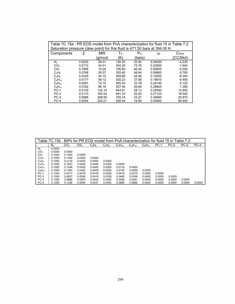
299
Table 7C.15a : PR EOS model from PnA characterization for fluid 15 in Table 7.2 Saturation pressure (dew point) for this fluid is 471.50 bars at 394.00 K.
Components Z MW (g/mol)
TC (K)
PC
(bars) ω CPEN
(CC/Mol) N2 0.0030 28.01 126.20 33.94 0.04000 -4.230 CO2 0.0172 44.01 304.20 73.76 0.22500 -1.640 CH4 0.7908 16.04 190.60 46.00 0.00800 -5.200 C2H6 0.0748 30.07 305.40 48.84 0.09800 -5.790 C3H8 0.0329 44.10 369.80 42.46 0.15200 -6.350 C4H10 0.0177 58.12 420.23 37.56 0.18810 -6.490 C5H12 0.0091 72.15 465.93 33.78 0.24140 -5.120 C6H14 0.0162 86.18 507.40 29.69 0.29600 1.390 PC-1 0.0135 132.14 644.61 28.13 0.22040 10.850 PC-2 0.0110 162.04 691.33 25.83 0.27120 18.540 PC-3 0.0085 208.06 755.74 23.27 0.34660 30.870 PC-4 0.0054 329.21 926.64 18.89 0.55900 68.400
Table 7C.15b : BIPs for PR EOS model from PnA characterization for fluid 15 in Table 7.2
N2 CO2 CH4 C2H6 C3H8 C4H10 C5H12 C6H14 PC-1 PC-2 PC-3 PC-4 N2 0.0000 CO2 0.0000 0.0000 CH4 0.1000 0.1000 0.0000 C2H6 0.1000 0.1450 0.0420 0.0000 C3H8 0.1000 0.2120 0.0420 0.0400 0.0000 C4H10 0.1000 0.1837 0.0420 0.0400 0.0300 0.0000 C5H12 0.1000 0.1546 0.0420 0.0400 0.0300 0.0116 0.0000 C6H14 0.1000 0.1383 0.0420 0.0400 0.0300 0.0155 0.0058 0.0000 PC-1 0.1300 0.0417 0.0518 0.0416 0.0328 0.0418 0.0275 0.0000 0.0000 PC-2 0.1300 0.0637 0.0536 0.0418 0.0339 0.0482 0.0356 0.0000 0.0000 0.0000 PC-3 0.1300 0.0886 0.0563 0.0422 0.0360 0.0556 0.0461 0.0000 0.0000 0.0000 0.0000 PC-4 0.1300 0.1226 0.0644 0.0431 0.0455 0.0684 0.0680 0.0000 0.0000 0.0000 0.0000 0.0000

300
Table 7C.16a : PR EOS model from PnA characterization for fluid 16 in Table 7.2 Saturation pressure (dew point) for this fluid is 388.00 bars at 428.15 K.
Components Z MW (g/mol)
TC (K)
PC
(bars) ω CPEN
(CC/Mol) N2 0.0060 28.01 126.20 33.94 0.04000 -4.230 CO2 0.0334 44.01 304.20 73.76 0.22500 -1.640 CH4 0.7416 16.04 190.60 46.00 0.00800 -5.200 C2H6 0.0790 30.07 305.40 48.84 0.09800 -5.790 C3H8 0.0415 44.10 369.80 42.46 0.15200 -6.350 C4H10 0.0215 58.12 419.55 37.50 0.18740 -6.490 C5H12 0.0119 72.15 465.50 33.78 0.24030 -5.120 C6H14 0.0081 86.18 507.40 29.69 0.29600 1.390 PC-1 0.0204 105.32 596.65 32.01 0.19450 0.130 PC-2 0.0163 131.67 648.17 29.12 0.25230 0.330 PC-3 0.0125 172.22 718.52 26.01 0.33920 0.650 PC-4 0.0077 279.05 865.50 21.80 0.53540 1.530
Table 7C.16b : BIPs for PR EOS model from PnA characterization for fluid 16 in Table 7.2
N2 CO2 CH4 C2H6 C3H8 C4H10 C5H12 C6H14 PC-1 PC-2 PC-3 PC-4 N2 0.0000 CO2 0.0000 0.0000 CH4 0.1000 0.1000 0.0000 C2H6 0.1000 0.1450 0.0420 0.0000 C3H8 0.1000 0.2664 0.0420 0.0400 0.0000 C4H10 0.1000 0.2270 0.0420 0.0400 0.0300 0.0000 C5H12 0.1000 0.1859 0.0420 0.0400 0.0300 0.0116 0.0000 C6H14 0.1000 0.1624 0.0420 0.0400 0.0300 0.0155 0.0058 0.0000 PC-1 0.1300 0.0166 0.0500 0.0414 0.0320 0.0337 0.0186 0.0000 0.0000 PC-2 0.1300 0.0417 0.0518 0.0416 0.0328 0.0418 0.0275 0.0000 0.0000 0.0000 PC-3 0.1300 0.0731 0.0545 0.0419 0.0346 0.0510 0.0393 0.0000 0.0000 0.0000 0.0000 PC-4 0.1300 0.1126 0.0608 0.0427 0.0408 0.0639 0.0598 0.0000 0.0000 0.0000 0.0000 0.0000
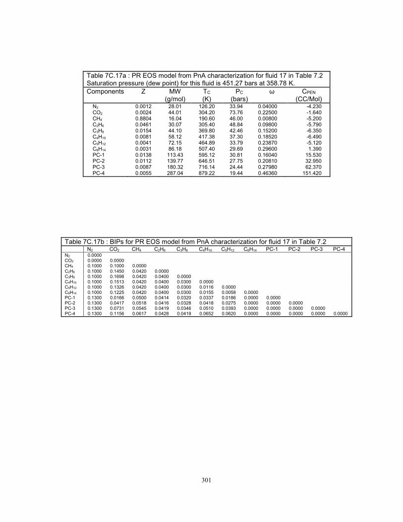
301
Table 7C.17a : PR EOS model from PnA characterization for fluid 17 in Table 7.2 Saturation pressure (dew point) for this fluid is 451.27 bars at 358.78 K.
Components Z MW (g/mol)
TC (K)
PC
(bars) ω CPEN
(CC/Mol) N2 0.0012 28.01 126.20 33.94 0.04000 -4.230 CO2 0.0024 44.01 304.20 73.76 0.22500 -1.640 CH4 0.8804 16.04 190.60 46.00 0.00800 -5.200 C2H6 0.0461 30.07 305.40 48.84 0.09800 -5.790 C3H8 0.0154 44.10 369.80 42.46 0.15200 -6.350 C4H10 0.0081 58.12 417.38 37.30 0.18520 -6.490 C5H12 0.0041 72.15 464.89 33.79 0.23870 -5.120 C6H14 0.0031 86.18 507.40 29.69 0.29600 1.390 PC-1 0.0138 113.43 595.12 30.81 0.16040 15.530 PC-2 0.0112 139.77 646.51 27.75 0.20810 32.950 PC-3 0.0087 180.32 716.14 24.44 0.27980 62.370 PC-4 0.0055 287.04 879.22 19.44 0.46360 151.420
Table 7C.17b : BIPs for PR EOS model from PnA characterization for fluid 17 in Table 7.2
N2 CO2 CH4 C2H6 C3H8 C4H10 C5H12 C6H14 PC-1 PC-2 PC-3 PC-4 N2 0.0000 CO2 0.0000 0.0000 CH4 0.1000 0.1000 0.0000 C2H6 0.1000 0.1450 0.0420 0.0000 C3H8 0.1000 0.1698 0.0420 0.0400 0.0000 C4H10 0.1000 0.1513 0.0420 0.0400 0.0300 0.0000 C5H12 0.1000 0.1326 0.0420 0.0400 0.0300 0.0116 0.0000 C6H14 0.1000 0.1225 0.0420 0.0400 0.0300 0.0155 0.0058 0.0000 PC-1 0.1300 0.0166 0.0500 0.0414 0.0320 0.0337 0.0186 0.0000 0.0000 PC-2 0.1300 0.0417 0.0518 0.0416 0.0328 0.0418 0.0275 0.0000 0.0000 0.0000 PC-3 0.1300 0.0731 0.0545 0.0419 0.0346 0.0510 0.0393 0.0000 0.0000 0.0000 0.0000 PC-4 0.1300 0.1156 0.0617 0.0428 0.0419 0.0652 0.0620 0.0000 0.0000 0.0000 0.0000 0.0000

302
Table 7C.18a : PR EOS model from PnA characterization for fluid 18 in Table 7.2 Saturation pressure (dew point) for this fluid is 539.52 bars at 378.15 K.
Components Z MW (g/mol)
TC (K)
PC
(bars) ω CPEN
(CC/Mol) N2 0.0006 28.01 126.20 33.94 0.04000 -4.230 CO2 0.0087 44.01 304.20 73.76 0.22500 -1.640 CH4 0.8922 16.04 190.60 46.00 0.00800 -5.200 C2H6 0.0355 30.07 305.40 48.84 0.09800 -5.790 C3H8 0.0168 44.10 369.80 42.46 0.15200 -6.350 C4H10 0.0103 58.12 417.38 37.30 0.18520 -6.490 C5H12 0.0046 72.15 464.89 33.79 0.23870 -5.120 C6H14 0.0037 86.18 507.40 29.69 0.29600 1.390 PC-1 0.0093 115.89 622.55 31.79 0.26380 -20.530 PC-2 0.0078 138.16 647.69 30.53 0.29800 -35.400 PC-3 0.0063 172.40 717.83 27.64 0.40070 -62.910 PC-4 0.0041 262.40 844.00 24.18 0.60040 -131.640
Table 7C.18b : BIPs for PR EOS model from PnA characterization for fluid 18 in Table 7.2
N2 CO2 CH4 C2H6 C3H8 C4H10 C5H12 C6H14 PC-1 PC-2 PC-3 PC-4 N2 0.0000 CO2 0.0000 0.0000 CH4 0.1000 0.1000 0.0000 C2H6 0.1000 0.1450 0.0420 0.0000 C3H8 0.1000 0.1912 0.0420 0.0400 0.0000 C4H10 0.1000 0.1676 0.0420 0.0400 0.0300 0.0000 C5H12 0.1000 0.1434 0.0420 0.0400 0.0300 0.0116 0.0000 C6H14 0.1000 0.1300 0.0420 0.0400 0.0300 0.0155 0.0058 0.0000 PC-1 0.1300 0.0294 0.0509 0.0415 0.0324 0.0380 0.0231 0.0000 0.0000 PC-2 0.1300 0.0417 0.0518 0.0416 0.0328 0.0418 0.0275 0.0000 0.0000 0.0000 PC-3 0.1300 0.0731 0.0545 0.0419 0.0346 0.0510 0.0393 0.0000 0.0000 0.0000 0.0000 PC-4 0.1300 0.1091 0.0599 0.0426 0.0398 0.0625 0.0574 0.0000 0.0000 0.0000 0.0000 0.0000

303
Table 7C.19a : PR EOS model from PnA characterization for fluid 19 in Table 7.2 Saturation pressure (dew point) for this fluid is 355.77 bars at 357.59 K.
Components Z MW (g/mol)
TC (K)
PC
(bars) ω CPEN
(CC/Mol) N2 0.0008 28.01 126.20 33.94 0.04000 -4.230 CO2 0.0035 44.01 304.20 73.76 0.22500 -1.640 CH4 0.9189 16.04 190.60 46.00 0.00800 -5.200 C2H6 0.0183 30.07 305.40 48.84 0.09800 -5.790 C3H8 0.0121 44.10 369.80 42.46 0.15200 -6.350 C4H10 0.0088 58.12 417.78 37.34 0.18560 -6.490 C5H12 0.0046 72.15 464.75 33.79 0.23830 -5.120 C6H14 0.0039 86.18 507.40 29.69 0.29600 1.390 PC-1 0.0099 110.25 597.53 30.61 0.15480 14.010 PC-2 0.0083 131.86 649.14 27.52 0.20070 29.340 PC-3 0.0066 165.17 696.99 25.16 0.24690 52.150 PC-4 0.0043 252.65 827.73 20.59 0.38260 121.350
Table 7C.19b : BIPs for PR EOS model from PnA characterization for fluid 19 in Table 7.2
N2 CO2 CH4 C2H6 C3H8 C4H10 C5H12 C6H14 PC-1 PC-2 PC-3 PC-4 N2 0.0000 CO2 0.0000 0.0000 CH4 0.1000 0.1000 0.0000 C2H6 0.1000 0.1450 0.0420 0.0000 C3H8 0.1000 0.1687 0.0420 0.0400 0.0000 C4H10 0.1000 0.1504 0.0420 0.0400 0.0300 0.0000 C5H12 0.1000 0.1321 0.0420 0.0400 0.0300 0.0116 0.0000 C6H14 0.1000 0.1221 0.0420 0.0400 0.0300 0.0155 0.0058 0.0000 PC-1 0.1300 0.0166 0.0500 0.0414 0.0320 0.0337 0.0186 0.0000 0.0000 PC-2 0.1300 0.0417 0.0518 0.0416 0.0328 0.0418 0.0275 0.0000 0.0000 0.0000 PC-3 0.1300 0.0637 0.0536 0.0418 0.0339 0.0482 0.0356 0.0000 0.0000 0.0000 0.0000 PC-4 0.1300 0.1050 0.0590 0.0425 0.0387 0.0610 0.0548 0.0000 0.0000 0.0000 0.0000 0.0000

304
Table 7C.20a : PR EOS model from PnA characterization for fluid 20 in Table 7.2 Saturation pressure (dew point) for this fluid is 441.61 bars at 364.22 K.
Components Z MW (g/mol)
TC (K)
PC
(bars) ω CPEN
(CC/Mol) N2 0.0009 28.01 126.20 33.94 0.04000 -4.230 CO2 0.0032 44.01 304.20 73.76 0.22500 -1.640 CH4 0.9165 16.04 190.60 46.00 0.00800 -5.200 C2H6 0.0333 30.07 305.40 48.84 0.09800 -5.790 C3H8 0.0122 44.10 369.80 42.46 0.15200 -6.350 C4H10 0.0065 58.12 416.90 37.26 0.18470 -6.490 C5H12 0.0028 72.15 464.55 33.79 0.23780 -5.120 C6H14 0.0019 86.18 507.40 29.69 0.29600 1.390 PC-1 0.0076 114.82 597.79 32.49 0.20790 -3.370 PC-2 0.0064 135.14 649.41 29.65 0.26960 -6.750 PC-3 0.0052 166.40 697.34 27.51 0.33170 -10.120 PC-4 0.0035 248.47 828.48 23.44 0.51390 -13.500
Table 7C.20b : BIPs for PR EOS model from PnA characterization for fluid 20 in Table 7.2
N2 CO2 CH4 C2H6 C3H8 C4H10 C5H12 C6H14 PC-1 PC-2 PC-3 PC-4 N2 0.0000 CO2 0.0000 0.0000 CH4 0.1000 0.1000 0.0000 C2H6 0.1000 0.1450 0.0420 0.0000 C3H8 0.1000 0.1754 0.0420 0.0400 0.0000 C4H10 0.1000 0.1555 0.0420 0.0400 0.0300 0.0000 C5H12 0.1000 0.1353 0.0420 0.0400 0.0300 0.0116 0.0000 C6H14 0.1000 0.1243 0.0420 0.0400 0.0300 0.0155 0.0058 0.0000 PC-1 0.1300 0.0166 0.0500 0.0414 0.0320 0.0337 0.0186 0.0000 0.0000 PC-2 0.1300 0.0417 0.0518 0.0416 0.0328 0.0418 0.0275 0.0000 0.0000 0.0000 PC-3 0.1300 0.0637 0.0536 0.0418 0.0339 0.0482 0.0356 0.0000 0.0000 0.0000 0.0000 PC-4 0.1300 0.1050 0.0590 0.0425 0.0387 0.0610 0.0548 0.0000 0.0000 0.0000 0.0000 0.0000

305
Table 7C.21a : PR EOS model from PnA characterization for fluid 21 in Table 7.2 Saturation pressure (dew point) for this fluid is 334.05 bars at 355.37 K.
Components Z MW (g/mol)
TC (K)
PC
(bars) ω CPEN
(CC/Mol) N2 0.0008 28.01 126.20 33.94 0.04000 -4.230 CO2 0.0028 44.01 304.20 73.76 0.22500 -1.640 CH4 0.9299 16.04 190.60 46.00 0.00800 -5.200 C2H6 0.0183 30.07 305.40 48.84 0.09800 -5.790 C3H8 0.0117 44.10 369.80 42.46 0.15200 -6.350 C4H10 0.0079 58.12 417.74 37.34 0.18560 -6.490 C5H12 0.0041 72.15 464.97 33.79 0.23890 -5.120 C6H14 0.0033 86.18 507.40 29.69 0.29600 1.390 PC-1 0.0070 112.01 598.91 31.08 0.16790 15.580 PC-2 0.0060 130.98 650.64 28.05 0.21780 30.020 PC-3 0.0049 160.21 698.87 25.74 0.26790 51.580 PC-4 0.0033 236.82 810.46 21.86 0.39120 111.710
Table 7C.21b : BIPs for PR EOS model from PnA characterization for fluid 21 in Table 7.2
N2 CO2 CH4 C2H6 C3H8 C4H10 C5H12 C6H14 PC-1 PC-2 PC-3 PC-4 N2 0.0000 CO2 0.0000 0.0000 CH4 0.1000 0.1000 0.0000 C2H6 0.1000 0.1450 0.0420 0.0000 C3H8 0.1000 0.1665 0.0420 0.0400 0.0000 C4H10 0.1000 0.1488 0.0420 0.0400 0.0300 0.0000 C5H12 0.1000 0.1310 0.0420 0.0400 0.0300 0.0116 0.0000 C6H14 0.1000 0.1214 0.0420 0.0400 0.0300 0.0155 0.0058 0.0000 PC-1 0.1300 0.0166 0.0500 0.0414 0.0320 0.0337 0.0186 0.0000 0.0000 PC-2 0.1300 0.0417 0.0518 0.0416 0.0328 0.0418 0.0275 0.0000 0.0000 0.0000 PC-3 0.1300 0.0637 0.0536 0.0418 0.0339 0.0482 0.0356 0.0000 0.0000 0.0000 0.0000 PC-4 0.1300 0.1003 0.0581 0.0424 0.0378 0.0594 0.0521 0.0000 0.0000 0.0000 0.0000 0.0000

306
Table 7C.22a : PR EOS model from PnA characterization for fluid 22 in Table 7.2 Saturation pressure (dew point) for this fluid is 408.38 bars at 367.59 K.
Components Z MW (g/mol)
TC (K)
PC
(bars) ω CPEN
(CC/Mol) N2 0.0009 28.01 126.20 33.94 0.04000 -4.230 CO2 0.0059 44.01 304.20 73.76 0.22500 -1.640 CH4 0.9164 16.04 190.60 46.00 0.00800 -5.200 C2H6 0.0352 30.07 305.40 48.84 0.09800 -5.790 C3H8 0.0131 44.10 369.80 42.46 0.15200 -6.350 C4H10 0.0069 58.12 417.82 37.34 0.18570 -6.490 C5H12 0.0032 72.15 465.03 33.79 0.23910 -5.120 C6H14 0.0023 86.18 507.40 29.69 0.29600 1.390 PC-1 0.0052 110.91 599.93 34.52 0.26550 34.610 PC-2 0.0045 127.41 626.35 33.15 0.30480 58.550 PC-3 0.0038 152.80 676.34 30.95 0.38390 98.510 PC-4 0.0026 219.17 791.23 27.46 0.58010 206.620
Table 7C.22b : BIPs for PR EOS model from PnA characterization for fluid 22 in Table 7.2
N2 CO2 CH4 C2H6 C3H8 C4H10 C5H12 C6H14 PC-1 PC-2 PC-3 PC-4 N2 0.0000 CO2 0.0000 0.0000 CH4 0.1000 0.1000 0.0000 C2H6 0.1000 0.1450 0.0420 0.0000 C3H8 0.1000 0.1790 0.0420 0.0400 0.0000 C4H10 0.1000 0.1582 0.0420 0.0400 0.0300 0.0000 C5H12 0.1000 0.1371 0.0420 0.0400 0.0300 0.0116 0.0000 C6H14 0.1000 0.1256 0.0420 0.0400 0.0300 0.0155 0.0058 0.0000 PC-1 0.1300 0.0166 0.0500 0.0414 0.0320 0.0337 0.0186 0.0000 0.0000 PC-2 0.1300 0.0294 0.0509 0.0415 0.0324 0.0380 0.0231 0.0000 0.0000 0.0000 PC-3 0.1300 0.0532 0.0527 0.0417 0.0334 0.0452 0.0317 0.0000 0.0000 0.0000 0.0000 PC-4 0.1300 0.0949 0.0572 0.0423 0.0369 0.0576 0.0492 0.0000 0.0000 0.0000 0.0000 0.0000

307
Table 7C.23a : PR EOS model from PnA characterization for fluid 23 in Table 7.2 Saturation pressure (dew point) for this fluid is 237.36 bars at 366.48 K.
Components Z MW (g/mol)
TC (K)
PC
(bars) ω CPEN
(CC/Mol) N2 0.0194 28.01 126.20 33.94 0.04000 -4.230 CO2 0.0121 44.01 304.20 73.76 0.22500 -1.640 CH4 0.6599 16.04 190.60 46.00 0.00800 -5.200 C2H6 0.0869 30.07 305.40 48.84 0.09800 -5.790 C3H8 0.0591 44.10 369.80 42.46 0.15200 -6.350 C4H10 0.0517 58.12 417.30 37.30 0.18510 -6.490 C5H12 0.0269 72.15 464.23 33.80 0.23700 -5.120 C6H14 0.0181 86.18 507.40 29.69 0.29600 1.390 PC-1 0.0226 102.22 596.85 30.03 0.13820 5.190 PC-2 0.0187 123.30 623.21 28.33 0.15870 12.280 PC-3 0.0149 155.09 672.62 25.57 0.19990 23.910 PC-4 0.0098 236.39 805.08 20.30 0.32200 60.100
Table 7C.23b : BIPs for PR EOS model from PnA characterization for fluid 23 in Table 7.2
N2 CO2 CH4 C2H6 C3H8 C4H10 C5H12 C6H14 PC-1 PC-2 PC-3 PC-4 N2 0.0000 CO2 0.0000 0.0000 CH4 0.1000 0.1000 0.0000 C2H6 0.1000 0.1450 0.0420 0.0000 C3H8 0.1000 0.1778 0.0420 0.0400 0.0000 C4H10 0.1000 0.1573 0.0420 0.0400 0.0300 0.0000 C5H12 0.1000 0.1365 0.0420 0.0400 0.0300 0.0116 0.0000 C6H14 0.1000 0.1252 0.0420 0.0400 0.0300 0.0155 0.0058 0.0000 PC-1 0.1300 0.0166 0.0500 0.0414 0.0320 0.0337 0.0186 0.0000 0.0000 PC-2 0.1300 0.0294 0.0509 0.0415 0.0324 0.0380 0.0231 0.0000 0.0000 0.0000 PC-3 0.1300 0.0532 0.0527 0.0417 0.0334 0.0452 0.0317 0.0000 0.0000 0.0000 0.0000 PC-4 0.1300 0.1003 0.0581 0.0424 0.0378 0.0594 0.0521 0.0000 0.0000 0.0000 0.0000 0.0000

308
Table 7C.24a : PR EOS model from PnA characterization for fluid 24 in Table 7.2 Saturation pressure (dew point) for this fluid is 278.87 bars at 365.37 K.
Components Z MW (g/mol)
TC (K)
PC
(bars) ω CPEN
(CC/Mol) N2 0.0058 28.01 126.20 33.94 0.04000 CO2 0.1166 44.01 304.20 73.76 0.22500 CH4 0.7533 16.04 190.60 46.00 0.00800 C2H6 0.0544 30.07 305.40 48.84 0.09800 C3H8 0.0249 44.10 369.80 42.46 0.15200 C4H10 0.0127 58.12 419.58 37.50 0.18740 C5H12 0.0068 72.15 465.14 33.79 0.23940 C6H14 0.0041 86.18 507.40 29.69 0.29600 PC-1 0.0069 100.34 577.63 35.93 0.22110 PC-2 0.0060 115.02 631.61 32.90 0.29740 PC-3 0.0050 137.65 657.38 31.71 0.33590 PC-4 0.0035 196.75 755.73 28.29 0.49010
Table 7C.24b : BIPs for PR EOS model from PnA characterization for fluid 24 in Table 7.2
N2 CO2 CH4 C2H6 C3H8 C4H10 C5H12 C6H14 PC-1 PC-2 PC-3 PC-4 N2 0.0000 CO2 0.0000 0.0000 CH4 0.1000 0.1000 0.0000 C2H6 0.1000 0.1450 0.0420 0.0000 C3H8 0.1000 0.1766 0.0420 0.0400 0.0000 C4H10 0.1000 0.1564 0.0420 0.0400 0.0300 0.0000 C5H12 0.1000 0.1359 0.0420 0.0400 0.0300 0.0116 0.0000 C6H14 0.1000 0.1247 0.0420 0.0400 0.0300 0.0155 0.0058 0.0000 PC-1 0.1300 0.0040 0.0491 0.0413 0.0317 0.0289 0.0141 0.0000 0.0000 PC-2 0.1300 0.0294 0.0509 0.0415 0.0324 0.0380 0.0231 0.0000 0.0000 0.0000 PC-3 0.1300 0.0417 0.0518 0.0416 0.0328 0.0418 0.0275 0.0000 0.0000 0.0000 0.0000 PC-4 0.1300 0.0814 0.0554 0.0420 0.0353 0.0534 0.0428 0.0000 0.0000 0.0000 0.0000 0.0000

309
Table 7C.25a : PR EOS model from PnA characterization for fluid 25 in Table 7.2 Saturation pressure (dew point) for this fluid is 466.42 bars at 410.93 K.
Components Z MW (g/mol)
TC (K)
PC
(bars) ω CPEN
(CC/Mol) N2 0.0031 28.01 126.20 33.94 0.04000 -4.230 CO2 0.0237 44.01 304.20 73.76 0.22500 -1.640 CH4 0.7319 16.04 190.60 46.00 0.00800 -5.200 C2H6 0.0780 30.07 305.40 48.84 0.09800 -5.790 C3H8 0.0355 44.10 369.80 42.46 0.15200 -6.350 C4H10 0.0216 58.12 419.58 37.50 0.18740 -6.490 C5H12 0.0132 72.15 465.14 33.79 0.23940 -5.120 C6H14 0.0109 86.18 507.40 29.69 0.29600 1.390 PC-1 0.0319 118.56 617.20 28.66 0.16880 0.008 PC-2 0.0236 159.73 688.00 24.82 0.23460 0.010 PC-3 0.0169 223.12 770.49 21.42 0.32130 0.012 PC-4 0.0097 390.34 979.53 16.32 0.55720 0.020
Table 7C.25b : BIPs for PR EOS model from PnA characterization for fluid 25 in Table 7.2
N2 CO2 CH4 C2H6 C3H8 C4H10 C5H12 C6H14 PC-1 PC-2 PC-3 PC-4 N2 0.0000 CO2 0.0000 0.0000 CH4 0.1000 0.1000 0.0000 C2H6 0.1000 0.1450 0.0420 0.0000 C3H8 0.1000 0.2373 0.0420 0.0400 0.0000 C4H10 0.1000 0.2037 0.0420 0.0400 0.0300 0.0000 C5H12 0.1000 0.1689 0.0420 0.0400 0.0300 0.0116 0.0000 C6H14 0.1000 0.1492 0.0420 0.0400 0.0300 0.0155 0.0058 0.0000 PC-1 0.1300 0.0294 0.0509 0.0415 0.0324 0.0380 0.0231 0.0000 0.0000 PC-2 0.1300 0.0637 0.0536 0.0418 0.0339 0.0482 0.0356 0.0000 0.0000 0.0000 PC-3 0.1300 0.0949 0.0572 0.0423 0.0369 0.0576 0.0492 0.0000 0.0000 0.0000 0.0000 PC-4 0.1300 0.1285 0.0680 0.0436 0.0506 0.0718 0.0746 0.0000 0.0000 0.0000 0.0000 0.0000

310
Table 7C.26a : PR EOS model from PnA characterization for fluid 26 in Table 7.2 Saturation pressure (dew point) for this fluid is 276.81 bars at 358.71 K.
Components Z MW (g/mol)
TC (K)
PC
(bars) ω CPEN
(CC/Mol) N2 0.0013 28.01 126.20 33.94 0.04000 0.0013 CO2 0.0018 44.01 304.20 73.76 0.22500 0.0018 CH4 0.6172 16.04 190.60 46.00 0.00800 0.6172 C2H6 0.1410 30.07 305.40 48.84 0.09800 0.1410 C3H8 0.0837 44.10 369.80 42.46 0.15200 0.0837 C4H10 0.0443 58.12 421.42 37.66 0.18920 0.0443 C5H12 0.0243 72.15 466.16 33.78 0.24200 0.0243 C6H14 0.0179 86.18 507.40 29.69 0.29600 0.0179 PC-1 0.0238 102.96 600.43 32.17 0.19880 0.0238 PC-2 0.0195 125.54 626.86 30.62 0.22830 0.0195 PC-3 0.0153 159.76 700.94 27.11 0.31720 0.0153 PC-4 0.0099 247.85 836.22 22.95 0.49160 0.0099
Table 7C.26b : BIPs for PR EOS model from PnA characterization for fluid 26 in Table 7.2
N2 CO2 CH4 C2H6 C3H8 C4H10 C5H12 C6H14 PC-1 PC-2 PC-3 PC-4 N2 0.0000 CO2 0.0000 0.0000 CH4 0.1000 0.1000 0.0000 C2H6 0.1000 0.1450 0.0420 0.0000 C3H8 0.1000 0.1698 0.0420 0.0400 0.0000 C4H10 0.1000 0.1512 0.0420 0.0400 0.0300 0.0000 C5H12 0.1000 0.1326 0.0420 0.0400 0.0300 0.0116 0.0000 C6H14 0.1000 0.1225 0.0420 0.0400 0.0300 0.0155 0.0058 0.0000 PC-1 0.1300 0.0166 0.0500 0.0414 0.0320 0.0337 0.0186 0.0000 0.0000 PC-2 0.1300 0.0294 0.0509 0.0415 0.0324 0.0380 0.0231 0.0000 0.0000 0.0000 PC-3 0.1300 0.0637 0.0536 0.0418 0.0339 0.0482 0.0356 0.0000 0.0000 0.0000 0.0000 PC-4 0.1300 0.1050 0.0590 0.0425 0.0387 0.0610 0.0548 0.0000 0.0000 0.0000 0.0000 0.0000

311
Table 7C.27a : PR EOS model from PnA characterization for fluid 27 in Table 7.2 Saturation pressure (dew point) for this fluid is 471.05 bars at 436.70 K.
Components Z MW (g/mol)
TC (K)
PC
(bars) ω CPEN
(CC/Mol) N2 0.0056 28.01 126.20 33.94 0.04000 -4.230 CO2 0.0264 44.01 304.20 73.76 0.22500 -1.640 CH4 0.7416 16.04 190.60 46.00 0.00800 -5.200 C2H6 0.0768 30.07 305.40 48.84 0.09800 -5.790 C3H8 0.0352 44.10 369.80 42.46 0.15200 -6.350 C4H10 0.0215 58.12 419.71 37.51 0.18750 -6.490 C5H12 0.0126 72.15 465.51 33.78 0.24030 -5.120 C6H14 0.0093 86.18 507.40 29.69 0.29600 1.390 PC-1 0.0268 117.57 618.06 29.24 0.18630 5.720 PC-2 0.0204 154.28 666.52 26.58 0.23460 12.640 PC-3 0.0150 210.81 752.52 22.89 0.33090 24.930 PC-4 0.0088 359.86 952.28 17.81 0.57500 62.110
Table 7C.27b : BIPs for PR EOS model from PnA characterization for fluid 27 in Table 7.2
N2 CO2 CH4 C2H6 C3H8 C4H10 C5H12 C6H14 PC-1 PC-2 PC-3 PC-4 N2 0.0000 CO2 0.0000 0.0000 CH4 0.1000 0.1000 0.0000 C2H6 0.1000 0.1450 0.0420 0.0000 C3H8 0.1000 0.2822 0.0420 0.0400 0.0000 C4H10 0.1000 0.2397 0.0420 0.0400 0.0300 0.0000 C5H12 0.1000 0.1953 0.0420 0.0400 0.0300 0.0116 0.0000 C6H14 0.1000 0.1698 0.0420 0.0400 0.0300 0.0155 0.0058 0.0000 PC-1 0.1300 0.0294 0.0509 0.0415 0.0324 0.0380 0.0231 0.0000 0.0000 PC-2 0.1300 0.0532 0.0527 0.0417 0.0334 0.0452 0.0317 0.0000 0.0000 0.0000 PC-3 0.1300 0.0886 0.0563 0.0422 0.0360 0.0556 0.0461 0.0000 0.0000 0.0000 0.0000 PC-4 0.1300 0.1259 0.0662 0.0434 0.0480 0.0702 0.0715 0.0000 0.0000 0.0000 0.0000 0.0000

312
Table 7C.28a : PR EOS model from PnA characterization for fluid 28 in Table 7.2 Saturation pressure (dew point) for this fluid is 344.72 bars at 393.20 K.
Components Z MW (g/mol)
TC (K)
PC
(bars) ω CPEN
(CC/Mol) N2 0.0102 28.01 126.20 33.94 0.04000 -4.230 CO2 0.0108 44.01 304.20 73.76 0.22500 -1.640 CH4 0.7394 16.04 190.60 46.00 0.00800 -5.200 C2H6 0.1019 30.07 305.40 48.84 0.09800 -5.790 C3H8 0.0568 44.10 369.80 42.46 0.15200 -6.350 C4H10 0.0266 58.12 419.03 37.45 0.18690 -6.490 C5H12 0.0114 72.15 465.16 33.79 0.23940 -5.120 C6H14 0.0063 86.18 507.40 29.69 0.29600 1.390 PC-1 0.0124 104.03 600.68 33.61 0.23960 8.770 PC-2 0.0104 124.06 627.11 32.17 0.27500 18.780 PC-3 0.0083 154.89 677.24 29.85 0.34650 34.890 PC-4 0.0055 235.89 815.07 25.61 0.55810 81.630
Table 7C.28b : BIPs for PR EOS model from PnA characterization for fluid 28 in Table 7.2
N2 CO2 CH4 C2H6 C3H8 C4H10 C5H12 C6H14 PC-1 PC-2 PC-3 PC-4 N2 0.0000 CO2 0.0000 0.0000 CH4 0.1000 0.1000 0.0000 C2H6 0.1000 0.1450 0.0420 0.0000 C3H8 0.1000 0.2108 0.0420 0.0400 0.0000 C4H10 0.1000 0.1828 0.0420 0.0400 0.0300 0.0000 C5H12 0.1000 0.1540 0.0420 0.0400 0.0300 0.0116 0.0000 C6H14 0.1000 0.1378 0.0420 0.0400 0.0300 0.0155 0.0058 0.0000 PC-1 0.1300 0.0166 0.0500 0.0414 0.0320 0.0337 0.0186 0.0000 0.0000 PC-2 0.1300 0.0294 0.0509 0.0415 0.0324 0.0380 0.0231 0.0000 0.0000 0.0000 PC-3 0.1300 0.0532 0.0527 0.0417 0.0334 0.0452 0.0317 0.0000 0.0000 0.0000 0.0000 PC-4 0.1300 0.1003 0.0581 0.0424 0.0378 0.0594 0.0521 0.0000 0.0000 0.0000 0.0000 0.0000

313
Table 7C.29a : PR EOS model from PnA characterization for fluid 29 in Table 7.2 Saturation pressure (dew point) for this fluid is 396.48 bars at 377.60 K.
Components Z MW (g/mol)
TC (K)
PC
(bars) ω CPEN
(CC/Mol) N2 0.0050 28.01 126.20 33.94 0.04000 -4.230 CO2 0.0206 44.01 304.20 73.76 0.22500 -1.640 CH4 0.7617 16.04 190.60 46.00 0.00800 -5.200 C2H6 0.0774 30.07 305.40 48.84 0.09800 -5.790 C3H8 0.0357 44.10 369.80 42.46 0.15200 -6.350 C4H10 0.0196 58.12 425.20 38.00 0.19300 -6.490 C5H12 0.0113 72.15 469.60 33.74 0.25100 -5.120 C6H14 0.0102 86.18 507.40 29.69 0.29600 1.390 PC-1 0.0212 98.31 571.04 34.28 0.17780 24.040 PC-2 0.0171 122.22 625.18 30.98 0.23920 28.960 PC-3 0.0131 158.87 698.70 27.53 0.33240 36.360 PC-4 0.0082 254.91 831.41 23.46 0.51510 58.230
Table 7C.29b : BIPs for PR EOS model from PnA characterization for fluid 29 in Table 7.2
N2 CO2 CH4 C2H6 C3H8 C4H10 C5H12 C6H14 PC-1 PC-2 PC-3 PC-4 N2 0.0000 CO2 0.0000 0.0000 CH4 0.1000 0.1000 0.0000 C2H6 0.1000 0.1450 0.0420 0.0000 C3H8 0.1000 0.1906 0.0420 0.0400 0.0000 C4H10 0.1000 0.1671 0.0420 0.0400 0.0300 0.0000 C5H12 0.1000 0.1431 0.0420 0.0400 0.0300 0.0116 0.0000 C6H14 0.1000 0.1298 0.0420 0.0400 0.0300 0.0155 0.0058 0.0000 PC-1 0.1300 0.0040 0.0491 0.0413 0.0317 0.0289 0.0141 0.0000 0.0000 PC-2 0.1300 0.0294 0.0509 0.0415 0.0324 0.0380 0.0231 0.0000 0.0000 0.0000 PC-3 0.1300 0.0637 0.0536 0.0418 0.0339 0.0482 0.0356 0.0000 0.0000 0.0000 0.0000 PC-4 0.1300 0.1050 0.0590 0.0425 0.0387 0.0610 0.0548 0.0000 0.0000 0.0000 0.0000 0.0000

314
Table 7C.30a : PR EOS model from PnA characterization for fluid 30 in Table 7.2 Saturation pressure (dew point) for this fluid is 283.35 bars at 377.60 K.
Components Z MW (g/mol)
TC (K)
PC
(bars) ω CPEN
(CC/Mol) N2 0.0054 28.01 126.20 33.94 0.04000 -4.230 CO2 0.0314 44.01 304.20 73.76 0.22500 -1.640 CH4 0.8354 16.04 190.60 46.00 0.00800 -5.200 C2H6 0.0663 30.07 305.40 48.84 0.09800 -5.790 C3H8 0.0268 44.10 369.80 42.46 0.15200 -6.350 C4H10 0.0121 58.12 425.20 38.00 0.19300 -6.490 C5H12 0.0055 72.15 469.60 33.74 0.25100 -5.120 C6H14 0.0025 86.18 507.40 29.69 0.29600 1.390 PC-1 0.0046 99.90 575.59 37.58 0.26440 -41.580 PC-2 0.0041 113.02 603.14 36.09 0.30980 -85.450 PC-3 0.0035 133.21 655.25 33.75 0.40180 -159.680 PC-4 0.0025 185.80 752.25 30.73 0.58620 -348.720
Table 7C.30b : BIPs for PR EOS model from PnA characterization for fluid 30 in Table 7.2
N2 CO2 CH4 C2H6 C3H8 C4H10 C5H12 C6H14 PC-1 PC-2 PC-3 PC-4 N2 0.0000 CO2 0.0000 0.0000 CH4 0.1000 0.1000 0.0000 C2H6 0.1000 0.1450 0.0420 0.0000 C3H8 0.1000 0.1906 0.0420 0.0400 0.0000 C4H10 0.1000 0.1671 0.0420 0.0400 0.0300 0.0000 C5H12 0.1000 0.1431 0.0420 0.0400 0.0300 0.0116 0.0000 C6H14 0.1000 0.1298 0.0420 0.0400 0.0300 0.0155 0.0058 0.0000 PC-1 0.1300 0.0040 0.0491 0.0413 0.0317 0.0289 0.0141 0.0000 0.0000 PC-2 0.1300 0.0166 0.0500 0.0414 0.0320 0.0337 0.0186 0.0000 0.0000 0.0000 PC-3 0.1300 0.0417 0.0518 0.0416 0.0328 0.0418 0.0275 0.0000 0.0000 0.0000 0.0000 PC-4 0.1300 0.0814 0.0554 0.0420 0.0353 0.0534 0.0428 0.0000 0.0000 0.0000 0.0000 0.0000

315
Table 7C.31a : PR EOS model from PnA characterization for fluid 31 in Table 7.2 Saturation pressure (dew point) for this fluid is 471.04 bars at 377.04 K.
Components Z MW (g/mol)
TC (K)
PC
(bars) ω CPEN
(CC/Mol) N2 0.0010 28.01 126.20 33.94 0.04000 -4.230 CO2 0.0062 44.01 304.20 73.76 0.22500 -1.640 CH4 0.8099 16.04 190.60 46.00 0.00800 -5.200 C2H6 0.0664 30.07 305.40 48.84 0.09800 -5.790 C3H8 0.0341 44.10 369.80 42.46 0.15200 -6.350 C4H10 0.0187 58.12 413.96 37.00 0.18180 -6.490 C5H12 0.0088 72.15 463.92 33.80 0.23620 -5.120 C6H14 0.0085 86.00 507.40 29.69 0.29600 1.390 PC-1 0.0164 108.23 596.12 32.33 0.20360 6.360 PC-2 0.0133 133.61 647.60 29.48 0.26400 14.670 PC-3 0.0103 172.69 717.70 26.43 0.35500 28.380 PC-4 0.0064 275.55 863.59 22.31 0.56030 65.350
Table 7C.31b : BIPs for PR EOS model from PnA characterization for fluid 31 in Table 7.2
N2 CO2 CH4 C2H6 C3H8 C4H10 C5H12 C6H14 PC-1 PC-2 PC-3 PC-4 N2 0.0000 CO2 0.0000 0.0000 CH4 0.1000 0.1000 0.0000 C2H6 0.1000 0.1450 0.0420 0.0000 C3H8 0.1000 0.1899 0.0420 0.0400 0.0000 C4H10 0.1000 0.1665 0.0420 0.0400 0.0300 0.0000 C5H12 0.1000 0.1427 0.0420 0.0400 0.0300 0.0116 0.0000 C6H14 0.1000 0.1295 0.0420 0.0400 0.0300 0.0155 0.0058 0.0000 PC-1 0.1300 0.0166 0.0500 0.0414 0.0320 0.0337 0.0186 0.0000 0.0000 PC-2 0.1300 0.0417 0.0518 0.0416 0.0328 0.0418 0.0275 0.0000 0.0000 0.0000 PC-3 0.1300 0.0731 0.0545 0.0419 0.0346 0.0510 0.0393 0.0000 0.0000 0.0000 0.0000 PC-4 0.1300 0.1126 0.0608 0.0427 0.0408 0.0639 0.0598 0.0000 0.0000 0.0000 0.0000 0.0000

316
Table 7C.32a : PR EOS model from PnA characterization for fluid 32 in Table 7.2 Saturation pressure (dew point) for this fluid is 399.40 bars at 392.10 K.
Components Z MW (g/mol)
TC (K)
PC
(bars) ω CPEN
(CC/Mol) N2 0.0071 28.01 126.20 33.94 0.04000 CO2 0.0864 44.01 304.20 73.76 0.22500 CH4 0.7085 16.04 190.60 46.00 0.00800 C2H6 0.0853 30.07 305.40 48.84 0.09800 C3H8 0.0495 44.10 369.80 42.46 0.15200 C4H10 0.0201 58.12 418.82 37.43 0.18670 C5H12 0.0081 72.15 464.94 33.79 0.23890 C6H14 0.0046 86.18 507.40 29.69 0.29600 PC-1 0.0101 116.66 625.38 32.42 0.28270 PC-2 0.0086 137.27 650.72 31.20 0.31940 PC-3 0.0070 168.84 698.97 29.21 0.39290 PC-4 0.0047 251.47 831.98 25.50 0.60890
Table 7C.32b : BIPs for PR EOS model from PnA characterization for fluid 32 in Table 7.2
N2 CO2 CH4 C2H6 C3H8 C4H10 C5H12 C6H14 PC-1 PC-2 PC-3 PC-4 N2 0.0000 CO2 0.0000 0.0000 CH4 0.1000 0.1000 0.0000 C2H6 0.1000 0.1450 0.0420 0.0000 C3H8 0.1000 0.2093 0.0420 0.0400 0.0000 C4H10 0.1000 0.1816 0.0420 0.0400 0.0300 0.0000 C5H12 0.1000 0.1532 0.0420 0.0400 0.0300 0.0116 0.0000 C6H14 0.1000 0.1372 0.0420 0.0400 0.0300 0.0155 0.0058 0.0000 PC-1 0.1300 0.0294 0.0509 0.0415 0.0324 0.0380 0.0231 0.0000 0.0000 PC-2 0.1300 0.0417 0.0518 0.0416 0.0328 0.0418 0.0275 0.0000 0.0000 0.0000 PC-3 0.1300 0.0637 0.0536 0.0418 0.0339 0.0482 0.0356 0.0000 0.0000 0.0000 0.0000 PC-4 0.1300 0.1050 0.0590 0.0425 0.0387 0.0610 0.0548 0.0000 0.0000 0.0000 0.0000 0.0000
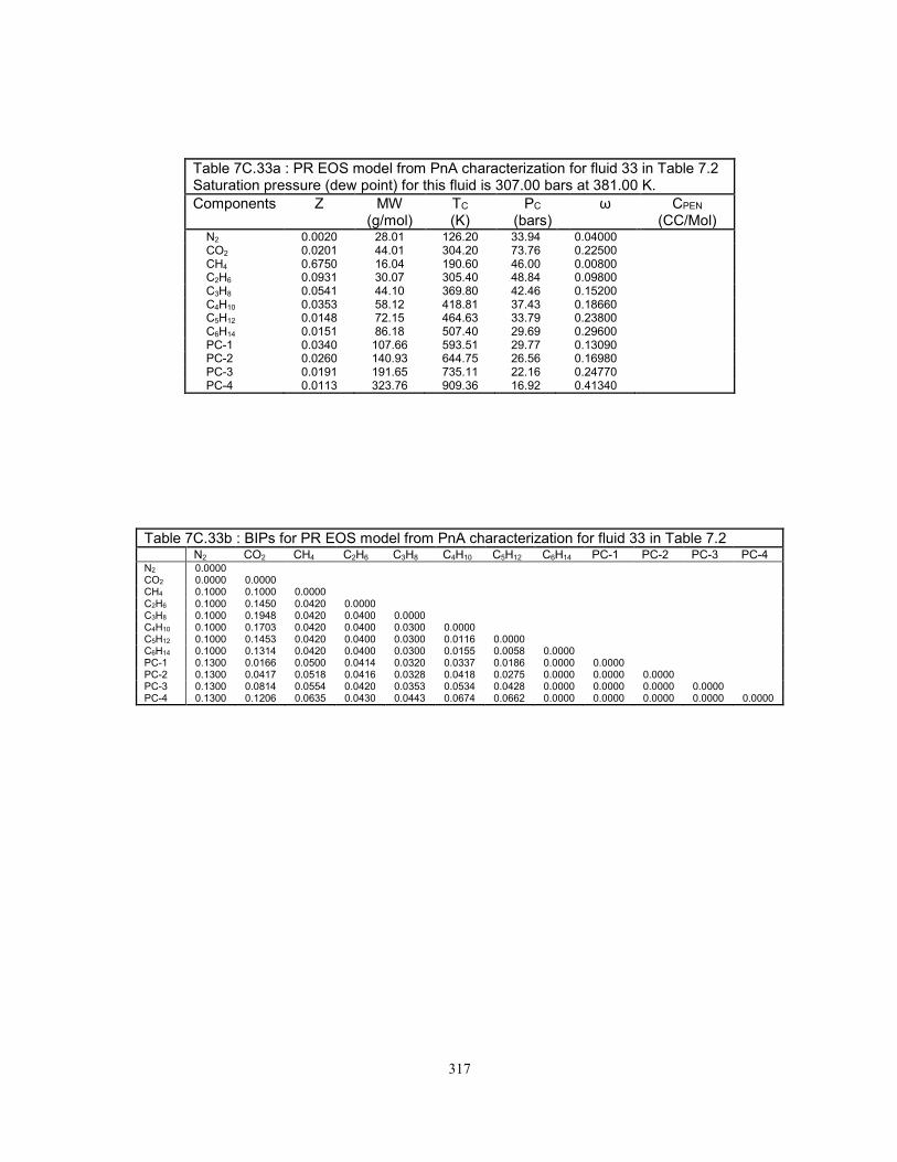
317
Table 7C.33a : PR EOS model from PnA characterization for fluid 33 in Table 7.2 Saturation pressure (dew point) for this fluid is 307.00 bars at 381.00 K.
Components Z MW (g/mol)
TC (K)
PC
(bars) ω CPEN
(CC/Mol) N2 0.0020 28.01 126.20 33.94 0.04000 CO2 0.0201 44.01 304.20 73.76 0.22500 CH4 0.6750 16.04 190.60 46.00 0.00800 C2H6 0.0931 30.07 305.40 48.84 0.09800 C3H8 0.0541 44.10 369.80 42.46 0.15200 C4H10 0.0353 58.12 418.81 37.43 0.18660 C5H12 0.0148 72.15 464.63 33.79 0.23800 C6H14 0.0151 86.18 507.40 29.69 0.29600 PC-1 0.0340 107.66 593.51 29.77 0.13090 PC-2 0.0260 140.93 644.75 26.56 0.16980 PC-3 0.0191 191.65 735.11 22.16 0.24770 PC-4 0.0113 323.76 909.36 16.92 0.41340
Table 7C.33b : BIPs for PR EOS model from PnA characterization for fluid 33 in Table 7.2
N2 CO2 CH4 C2H6 C3H8 C4H10 C5H12 C6H14 PC-1 PC-2 PC-3 PC-4 N2 0.0000 CO2 0.0000 0.0000 CH4 0.1000 0.1000 0.0000 C2H6 0.1000 0.1450 0.0420 0.0000 C3H8 0.1000 0.1948 0.0420 0.0400 0.0000 C4H10 0.1000 0.1703 0.0420 0.0400 0.0300 0.0000 C5H12 0.1000 0.1453 0.0420 0.0400 0.0300 0.0116 0.0000 C6H14 0.1000 0.1314 0.0420 0.0400 0.0300 0.0155 0.0058 0.0000 PC-1 0.1300 0.0166 0.0500 0.0414 0.0320 0.0337 0.0186 0.0000 0.0000 PC-2 0.1300 0.0417 0.0518 0.0416 0.0328 0.0418 0.0275 0.0000 0.0000 0.0000 PC-3 0.1300 0.0814 0.0554 0.0420 0.0353 0.0534 0.0428 0.0000 0.0000 0.0000 0.0000 PC-4 0.1300 0.1206 0.0635 0.0430 0.0443 0.0674 0.0662 0.0000 0.0000 0.0000 0.0000 0.0000

318
Table 7C.34a : PR EOS model from PnA characterization for fluid 34 in Table 7.2 Saturation pressure (dew point) for this fluid is 359.00 bars at 381.00 K.
Components Z MW (g/mol)
TC (K)
PC
(bars) ω CPEN
(CC/Mol) N2 0.0023 28.01 126.20 33.94 0.04000 CO2 0.0212 44.01 304.20 73.76 0.22500 CH4 0.7315 16.04 190.60 46.00 0.00800 C2H6 0.0939 30.07 305.40 48.84 0.09800 C3H8 0.0486 44.10 369.80 42.46 0.15200 C4H10 0.0180 58.12 418.97 37.45 0.18680 C5H12 0.0109 72.15 464.54 33.80 0.23780 C6H14 0.0093 86.18 507.40 29.69 0.29600 PC-1 0.0235 111.00 594.60 30.36 0.14780 PC-2 0.0185 141.05 645.94 27.24 0.19170 PC-3 0.0139 187.12 737.04 22.97 0.27960 PC-4 0.0085 307.85 895.95 18.30 0.44700
Table 7C.34b : BIPs for PR EOS model from PnA characterization for fluid 34 in Table 7.2
N2 CO2 CH4 C2H6 C3H8 C4H10 C5H12 C6H14 PC-1 PC-2 PC-3 PC-4 N2 0.0000 CO2 0.0000 0.0000 CH4 0.1000 0.1000 0.0000 C2H6 0.1000 0.1450 0.0420 0.0000 C3H8 0.1000 0.1948 0.0420 0.0400 0.0000 C4H10 0.1000 0.1703 0.0420 0.0400 0.0300 0.0000 C5H12 0.1000 0.1453 0.0420 0.0400 0.0300 0.0116 0.0000 C6H14 0.1000 0.1314 0.0420 0.0400 0.0300 0.0155 0.0058 0.0000 PC-1 0.1300 0.0166 0.0500 0.0414 0.0320 0.0337 0.0186 0.0000 0.0000 PC-2 0.1300 0.0417 0.0518 0.0416 0.0328 0.0418 0.0275 0.0000 0.0000 0.0000 PC-3 0.1300 0.0814 0.0554 0.0420 0.0353 0.0534 0.0428 0.0000 0.0000 0.0000 0.0000 PC-4 0.1300 0.1183 0.0626 0.0429 0.0431 0.0663 0.0642 0.0000 0.0000 0.0000 0.0000 0.0000

319
Table 7C.35a : PR EOS model from PnA characterization for fluid 35 in Table 7.2 Saturation pressure (dew point) for this fluid is 207.00 bars at 333.00 K.
Components Z MW (g/mol)
TC (K)
PC
(bars) ω CPEN
(CC/Mol) N2 0.0220 28.01 126.20 33.94 0.04000 CO2 0.0006 44.01 304.20 73.76 0.22500 CH4 0.7417 16.04 190.60 46.00 0.00800 C2H6 0.1127 30.07 305.40 48.84 0.09800 C3H8 0.0575 44.10 369.80 42.46 0.15200 C4H10 0.0298 58.12 417.51 37.32 0.18540 C5H12 0.0099 72.15 465.88 33.78 0.24130 C6H14 0.0058 86.18 507.40 29.69 0.29600 PC-1 0.0063 91.57 579.74 34.72 0.18940 PC-2 0.0056 103.92 607.12 32.98 0.22190 PC-3 0.0047 122.90 633.66 31.50 0.25480 PC-4 0.0034 172.32 734.80 27.28 0.38710
Table 7C.35b : BIPs for PR EOS model from PnA characterization for fluid 35 in Table 7.2
N2 CO2 CH4 C2H6 C3H8 C4H10 C5H12 C6H14 PC-1 PC-2 PC-3 PC-4 N2 0.0000 CO2 0.0000 0.0000 CH4 0.1000 0.1000 0.0000 C2H6 0.1000 0.1450 0.0420 0.0000 C3H8 0.1000 0.1481 0.0420 0.0400 0.0000 C4H10 0.1000 0.1355 0.0420 0.0400 0.0300 0.0000 C5H12 0.1000 0.1232 0.0420 0.0400 0.0300 0.0116 0.0000 C6H14 0.1000 0.1167 0.0420 0.0400 0.0300 0.0155 0.0058 0.0000 PC-1 0.1300 0.0040 0.0491 0.0413 0.0317 0.0289 0.0141 0.0000 0.0000 PC-2 0.1300 0.0166 0.0500 0.0414 0.0320 0.0337 0.0186 0.0000 0.0000 0.0000 PC-3 0.1300 0.0294 0.0509 0.0415 0.0324 0.0380 0.0231 0.0000 0.0000 0.0000 0.0000 PC-4 0.1300 0.0731 0.0545 0.0419 0.0346 0.0510 0.0393 0.0000 0.0000 0.0000 0.0000 0.0000

320
Table 7C.36a : PR EOS model from PnA characterization for fluid 36 in Table 7.2 Saturation pressure (dew point) for this fluid is 314.97 bars at 366.48 K.
Components Z MW (g/mol)
TC (K)
PC
(bars) ω CPEN
(CC/Mol) N2 0.0042 28.01 126.20 33.94 0.04000 CO2 0.0050 44.01 304.20 73.76 0.22500 CH4 0.6146 16.04 190.60 46.00 0.00800 C2H6 0.1485 30.07 305.40 48.84 0.09800 C3H8 0.0529 44.10 369.80 42.46 0.15200 C4H10 0.0367 58.12 423.20 37.82 0.19100 C5H12 0.0210 72.15 465.92 33.78 0.24140 C6H14 0.0168 86.18 507.40 29.69 0.64960 PC-1 0.0384 112.27 592.66 30.06 0.13920 PC-2 0.0288 149.60 667.57 25.60 0.20120 PC-3 0.0209 206.48 754.29 21.74 0.28380 PC-4 0.0122 354.52 957.55 16.39 0.49310
Table 7C.36b : BIPs for PR EOS model from PnA characterization for fluid 36 in Table 7.2
N2 CO2 CH4 C2H6 C3H8 C4H10 C5H12 C6H14 PC-1 PC-2 PC-3 PC-4 N2 0.0000 CO2 0.0000 0.0000 CH4 0.1000 0.1000 0.0000 C2H6 0.1000 0.1450 0.0420 0.0000 C3H8 0.1000 0.1778 0.0420 0.0400 0.0000 C4H10 0.1000 0.1573 0.0420 0.0400 0.0300 0.0000 C5H12 0.1000 0.1365 0.0420 0.0400 0.0300 0.0116 0.0000 C6H14 0.1000 0.1252 0.0420 0.0400 0.0300 0.0155 0.0058 0.0000 PC-1 0.1300 0.0166 0.0500 0.0414 0.0320 0.0337 0.0186 0.0000 0.0000 PC-2 0.1300 0.0532 0.0527 0.0417 0.0334 0.0452 0.0317 0.0000 0.0000 0.0000 PC-3 0.1300 0.0886 0.0563 0.0422 0.0360 0.0556 0.0461 0.0000 0.0000 0.0000 0.0000 PC-4 0.1300 0.1259 0.0662 0.0434 0.0480 0.0702 0.0715 0.0000 0.0000 0.0000 0.0000 0.0000

321
Table 7C.37a : PR EOS model from PnA characterization for fluid 37 in Table 7.2 Saturation pressure (dew point) for this fluid is 857.75 bars at 399.82 K.
Components Z MW (g/mol)
TC (K)
PC
(bars) ω CPEN
(CC/Mol) N2 0.0019 28.01 126.20 33.94 0.04000 CO2 0.0102 44.01 304.20 73.76 0.22500 CH4 0.8673 16.04 190.60 46.00 0.00800 C2H6 0.0248 30.07 305.40 48.84 0.09800 C3H8 0.0127 44.10 369.80 42.46 0.15200 C4H10 0.0108 58.12 413.96 37.00 0.18180 C5H12 0.0034 72.15 463.92 33.80 0.23620 C6H14 0.0019 86.18 507.40 29.69 0.29600 PC-1 0.0276 179.23 697.92 22.39 0.20240 PC-2 0.0192 257.57 802.18 17.93 0.30320 PC-3 0.0131 377.36 914.50 14.65 0.42560 PC-4 0.0072 690.90 1164.42 10.95 0.67670
Table 7C.37b : BIPs for PR EOS model from PnA characterization for fluid 37 in Table 7.2
N2 CO2 CH4 C2H6 C3H8 C4H10 C5H12 C6H14 PC-1 PC-2 PC-3 PC-4 N2 0.0000 CO2 0.0000 0.0000 CH4 0.1000 0.1000 0.0000 C2H6 0.1000 0.1450 0.0420 0.0000 C3H8 0.1000 0.2203 0.0420 0.0400 0.0000 C4H10 0.1000 0.1902 0.0420 0.0400 0.0300 0.0000 C5H12 0.1000 0.1592 0.0420 0.0400 0.0300 0.0116 0.0000 C6H14 0.1000 0.1418 0.0420 0.0400 0.0300 0.0155 0.0058 0.0000 PC-1 0.1300 0.0731 0.0545 0.0419 0.0346 0.0510 0.0393 0.0000 0.0000 PC-2 0.1300 0.1091 0.0599 0.0426 0.0398 0.0625 0.0574 0.0000 0.0000 0.0000 PC-3 0.1300 0.1273 0.0671 0.0435 0.0493 0.0710 0.0731 0.0000 0.0000 0.0000 0.0000 PC-4 0.1300 0.1384 0.0878 0.0460 0.0710 0.0810 0.0953 0.0000 0.0000 0.0000 0.0000 0.0000

322
Table 7C.38a : PR EOS model from PnA characterization for fluid 38 in Table 7.2 Saturation pressure (dew point) for this fluid is 241.72 bars at 377.04 K.
Components Z MW (g/mol)
TC (K)
PC
(bars) ω CPEN
(CC/Mol) N2 0.0168 28.01 126.20 33.94 0.04000 CO2 0.0023 44.01 304.20 73.76 0.22500 CH4 0.5609 16.04 190.60 46.00 0.00800 C2H6 0.1348 30.07 305.40 48.84 0.09800 C3H8 0.0845 44.10 369.80 42.46 0.15200 C4H10 0.0514 58.12 417.65 37.33 0.18550 C5H12 0.0228 72.15 464.48 33.80 0.23760 C6H14 0.0145 86.18 507.40 29.69 0.29600 PC-1 0.0410 102.37 554.69 30.51 0.15180 PC-2 0.0320 131.13 606.40 27.40 0.19690 PC-3 0.0241 174.15 677.72 24.04 0.26480 PC-4 0.0148 283.26 849.59 18.95 0.43880
Table 7C.38b : BIPs for PR EOS model from PnA characterization for fluid 38 in Table 7.2
N2 CO2 CH4 C2H6 C3H8 C4H10 C5H12 C6H14 PC-1 PC-2 PC-3 PC-4 N2 0.0000 CO2 0.0000 0.0000 CH4 0.1000 0.1000 0.0000 C2H6 0.1000 0.1450 0.0420 0.0000 C3H8 0.1000 0.1899 0.0420 0.0400 0.0000 C4H10 0.1000 0.1665 0.0420 0.0400 0.0300 0.0000 C5H12 0.1000 0.1427 0.0420 0.0400 0.0300 0.0116 0.0000 C6H14 0.1000 0.1295 0.0420 0.0400 0.0300 0.0155 0.0058 0.0000 PC-1 0.1300 0.0166 0.0500 0.0414 0.0320 0.0337 0.0186 0.0000 0.0000 PC-2 0.1300 0.0417 0.0518 0.0416 0.0328 0.0418 0.0275 0.0000 0.0000 0.0000 PC-3 0.1300 0.0731 0.0545 0.0419 0.0346 0.0510 0.0393 0.0000 0.0000 0.0000 0.0000 PC-4 0.1300 0.1156 0.0617 0.0428 0.0419 0.0652 0.0620 0.0000 0.0000 0.0000 0.0000 0.0000

323
Table 7C.39a : PR EOS model from PnA characterization for fluid 39 in Table 7.2 Saturation pressure (dew point) for this fluid is 354.65 bars at 422.59 K.
Components Z MW (g/mol)
TC (K)
PC
(bars) ω CPEN
(CC/Mol) N2 0.0349 28.01 126.20 33.94 0.04000 -4.230 CO2 0.0270 44.01 304.20 73.76 0.22500 -1.640 CH4 0.6507 16.04 190.60 46.00 0.00800 -5.200 C2H6 0.1050 30.07 305.40 48.84 0.09800 -5.790 C3H8 0.0497 44.10 369.80 42.46 0.15200 -6.350 C4H10 0.0282 58.12 419.44 37.49 0.18730 -6.490 C5H12 0.0155 72.15 465.03 33.79 0.23910 -5.120 C6H14 0.0125 86.18 507.40 29.69 0.29600 1.390 PC-1 0.0284 111.29 593.80 30.33 0.14690 0.780 PC-2 0.0220 143.49 668.94 25.93 0.21250 2.050 PC-3 0.0164 192.87 735.62 22.93 0.27800 3.960 PC-4 0.0098 322.24 910.74 17.87 0.46410 9.910
Table 7C.39b : BIPs for PR EOS model from PnA characterization for fluid 39 in Table 7.2
N2 CO2 CH4 C2H6 C3H8 C4H10 C5H12 C6H14 PC-1 PC-2 PC-3 PC-4 N2 0.0000 CO2 0.0000 0.0000 CH4 0.1000 0.1000 0.0000 C2H6 0.1000 0.1450 0.0420 0.0000 C3H8 0.1000 0.2566 0.0420 0.0400 0.0000 C4H10 0.1000 0.2192 0.0420 0.0400 0.0300 0.0000 C5H12 0.1000 0.1801 0.0420 0.0400 0.0300 0.0116 0.0000 C6H14 0.1000 0.1579 0.0420 0.0400 0.0300 0.0155 0.0058 0.0000 PC-1 0.1300 0.0166 0.0500 0.0414 0.0320 0.0337 0.0186 0.0000 0.0000 PC-2 0.1300 0.0532 0.0527 0.0417 0.0334 0.0452 0.0317 0.0000 0.0000 0.0000 PC-3 0.1300 0.0814 0.0554 0.0420 0.0353 0.0534 0.0428 0.0000 0.0000 0.0000 0.0000 PC-4 0.1300 0.1206 0.0635 0.0430 0.0443 0.0674 0.0662 0.0000 0.0000 0.0000 0.0000 0.0000

324
Table 7C.40a : PR EOS model from PnA characterization for fluid 40 in Table 7.2 Saturation pressure (dew point) for this fluid is 382.31 bars at 420.93 K.
Components Z MW (g/mol)
TC (K)
PC
(bars) ω CPEN
(CC/Mol) N2 0.0307 28.01 126.20 33.94 0.04000 -4.230 CO2 0.0292 44.01 304.20 73.76 0.22500 -1.640 CH4 0.6877 16.04 190.60 46.00 0.00800 -5.200 C2H6 0.0977 30.07 305.40 48.84 0.09800 -5.790 C3H8 0.0409 44.10 369.80 42.46 0.15200 -6.350 C4H10 0.0223 58.12 419.76 37.52 0.18760 -6.490 C5H12 0.0119 72.15 465.19 33.79 0.23950 -5.120 C6H14 0.0090 86.18 507.40 29.69 0.29600 1.390 PC-1 0.0261 112.99 593.77 30.45 0.15010 0.000 PC-2 0.0203 145.27 668.90 26.07 0.21710 0.000 PC-3 0.0151 194.74 735.57 23.08 0.28410 0.000 PC-4 0.0091 324.37 910.60 18.06 0.47410 0.000
Table 7C.40b : BIPs for PR EOS model from PnA characterization for fluid 40 in Table 7.2
N2 CO2 CH4 C2H6 C3H8 C4H10 C5H12 C6H14 PC-1 PC-2 PC-3 PC-4 N2 0.0000 CO2 0.0000 0.0000 CH4 0.1000 0.1000 0.0000 C2H6 0.1000 0.1450 0.0420 0.0000 C3H8 0.1000 0.2538 0.0420 0.0400 0.0000 C4H10 0.1000 0.2169 0.0420 0.0400 0.0300 0.0000 C5H12 0.1000 0.1785 0.0420 0.0400 0.0300 0.0116 0.0000 C6H14 0.1000 0.1566 0.0420 0.0400 0.0300 0.0155 0.0058 0.0000 PC-1 0.1300 0.0166 0.0500 0.0414 0.0320 0.0337 0.0186 0.0000 0.0000 PC-2 0.1300 0.0532 0.0527 0.0417 0.0334 0.0452 0.0317 0.0000 0.0000 0.0000 PC-3 0.1300 0.0814 0.0554 0.0420 0.0353 0.0534 0.0428 0.0000 0.0000 0.0000 0.0000 PC-4 0.1300 0.1206 0.0635 0.0430 0.0443 0.0674 0.0662 0.0000 0.0000 0.0000 0.0000 0.0000

325
Table 7C.41a : PR EOS model from PnA characterization for fluid 41 in Table 7.2 Saturation pressure (dew point) for this fluid is 311.71 bars at 424.82 K.
Components Z MW (g/mol)
TC (K)
PC
(bars) ω CPEN
(CC/Mol) N2 0.0345 28.01 126.20 33.94 0.04000 -4.230 CO2 0.0273 44.01 304.20 73.76 0.22500 -1.640 CH4 0.5771 16.04 190.60 46.00 0.00800 -5.200 C2H6 0.1072 30.07 305.40 48.84 0.09800 -5.790 C3H8 0.0599 44.10 369.80 42.46 0.15200 -6.350 C4H10 0.0345 58.12 419.95 37.53 0.18780 -6.490 C5H12 0.0184 72.15 465.25 33.79 0.23970 -5.120 C6H14 0.0172 86.18 507.40 29.69 0.29600 1.390 PC-1 0.0471 107.91 592.54 29.78 0.13140 0.710 PC-2 0.0355 143.33 667.42 25.27 0.19000 2.140 PC-3 0.0259 196.25 733.38 22.18 0.24850 4.250 PC-4 0.0154 330.70 922.26 16.57 0.43200 11.230
Table 7C.41b : BIPs for PR EOS model from PnA characterization for fluid 41 in Table 7.2
N2 CO2 CH4 C2H6 C3H8 C4H10 C5H12 C6H14 PC-1 PC-2 PC-3 PC-4 N2 0.0000 CO2 0.0000 0.0000 CH4 0.1000 0.1000 0.0000 C2H6 0.1000 0.1450 0.0420 0.0000 C3H8 0.1000 0.2605 0.0420 0.0400 0.0000 C4H10 0.1000 0.2223 0.0420 0.0400 0.0300 0.0000 C5H12 0.1000 0.1824 0.0420 0.0400 0.0300 0.0116 0.0000 C6H14 0.1000 0.1597 0.0420 0.0400 0.0300 0.0155 0.0058 0.0000 PC-1 0.1300 0.0166 0.0500 0.0414 0.0320 0.0337 0.0186 0.0000 0.0000 PC-2 0.1300 0.0532 0.0527 0.0417 0.0334 0.0452 0.0317 0.0000 0.0000 0.0000 PC-3 0.1300 0.0814 0.0554 0.0420 0.0353 0.0534 0.0428 0.0000 0.0000 0.0000 0.0000 PC-4 0.1300 0.1226 0.0644 0.0431 0.0455 0.0684 0.0680 0.0000 0.0000 0.0000 0.0000 0.0000

326
Table 7C.42a : PR EOS model from PnA characterization for fluid 42 in Table 7.2 Saturation pressure (dew point) for this fluid is 355.29 bars at 424.82 K.
Components Z MW (g/mol)
TC (K)
PC
(bars) ω CPEN
(CC/Mol) N2 0.0349 28.01 126.20 33.94 0.04000 -4.230 CO2 0.0270 44.01 304.20 73.76 0.22500 -1.640 CH4 0.6507 16.04 190.60 46.00 0.00800 -5.200 C2H6 0.1050 30.07 305.40 48.84 0.09800 -5.790 C3H8 0.0497 44.10 369.80 42.46 0.15200 -6.350 C4H10 0.0282 58.12 419.44 37.49 0.18730 -6.490 C5H12 0.0153 72.15 465.03 33.79 0.23910 -5.120 C6H14 0.0125 86.18 507.40 29.69 0.29600 1.390 PC-1 0.0285 111.82 593.80 30.36 0.14760 0.000 PC-2 0.0220 144.36 668.94 25.96 0.21350 0.000 PC-3 0.0164 194.23 735.62 22.96 0.27930 0.000 PC-4 0.0098 324.87 910.73 17.91 0.46620 0.000
Table 7C.42b : BIPs for PR EOS model from PnA characterization for fluid 42 in Table 7.2
N2 CO2 CH4 C2H6 C3H8 C4H10 C5H12 C6H14 PC-1 PC-2 PC-3 PC-4 N2 0.0000 CO2 0.0000 0.0000 CH4 0.1000 0.1000 0.0000 C2H6 0.1000 0.1450 0.0420 0.0000 C3H8 0.1000 0.2605 0.0420 0.0400 0.0000 C4H10 0.1000 0.2223 0.0420 0.0400 0.0300 0.0000 C5H12 0.1000 0.1824 0.0420 0.0400 0.0300 0.0116 0.0000 C6H14 0.1000 0.1597 0.0420 0.0400 0.0300 0.0155 0.0058 0.0000 PC-1 0.1300 0.0166 0.0500 0.0414 0.0320 0.0337 0.0186 0.0000 0.0000 PC-2 0.1300 0.0532 0.0527 0.0417 0.0334 0.0452 0.0317 0.0000 0.0000 0.0000 PC-3 0.1300 0.0814 0.0554 0.0420 0.0353 0.0534 0.0428 0.0000 0.0000 0.0000 0.0000 PC-4 0.1300 0.1206 0.0635 0.0430 0.0443 0.0674 0.0662 0.0000 0.0000 0.0000 0.0000 0.0000

327
Table 7C.43a : PR EOS model from PnA characterization for fluid 43 in Table 7.2 Saturation pressure (dew point) for this fluid is 381.76 bars at 412.59 K.
Components Z MW (g/mol)
TC (K)
PC
(bars) ω CPEN
(CC/Mol) N2 0.0345 28.01 126.20 33.94 0.04000 -4.230 CO2 0.0279 44.01 304.20 73.76 0.22500 -1.640 CH4 0.7798 16.04 190.60 46.00 0.00800 -5.200 C2H6 0.0884 30.07 305.40 48.84 0.09800 -5.790 C3H8 0.0288 44.10 369.80 42.46 0.15200 -6.350 C4H10 0.0131 58.12 417.89 37.35 0.18570 -6.490 C5H12 0.0052 72.15 464.12 33.80 0.23670 -5.120 C6H14 0.0032 86.18 507.40 29.69 0.29600 1.390 PC-1 0.0062 120.53 625.23 33.56 0.31720 -24.600 PC-2 0.0054 138.88 650.56 32.40 0.35840 -37.610 PC-3 0.0045 167.03 698.76 30.54 0.44080 -58.860 PC-4 0.0031 240.57 810.26 27.54 0.64360 -114.380
Table 7C.43b : BIPs for PR EOS model from PnA characterization for fluid 43 in Table 7.2
N2 CO2 CH4 C2H6 C3H8 C4H10 C5H12 C6H14 PC-1 PC-2 PC-3 PC-4 N2 0.0000 CO2 0.0000 0.0000 CH4 0.1000 0.1000 0.0000 C2H6 0.1000 0.1450 0.0420 0.0000 C3H8 0.1000 0.2400 0.0420 0.0400 0.0000 C4H10 0.1000 0.2058 0.0420 0.0400 0.0300 0.0000 C5H12 0.1000 0.1704 0.0420 0.0400 0.0300 0.0116 0.0000 C6H14 0.1000 0.1504 0.0420 0.0400 0.0300 0.0155 0.0058 0.0000 PC-1 0.1300 0.0294 0.0509 0.0415 0.0324 0.0380 0.0231 0.0000 0.0000 PC-2 0.1300 0.0417 0.0518 0.0416 0.0328 0.0418 0.0275 0.0000 0.0000 0.0000 PC-3 0.1300 0.0637 0.0536 0.0418 0.0339 0.0482 0.0356 0.0000 0.0000 0.0000 0.0000 PC-4 0.1300 0.1003 0.0581 0.0424 0.0378 0.0594 0.0521 0.0000 0.0000 0.0000 0.0000 0.0000

328
Table 7C.44a : PR EOS model from PnA characterization for fluid 44 in Table 7.2 Saturation pressure (dew point) for this fluid is 385.44 bars at 404.82 K.
Components Z MW (g/mol)
TC (K)
PC
(bars) ω CPEN
(CC/Mol) N2 0.0042 28.01 126.20 33.94 0.04000 CO2 0.0157 44.01 304.20 73.76 0.22500 CH4 0.7498 16.04 190.60 46.00 0.00800 C2H6 0.0634 30.07 305.40 48.84 0.09800 C3H8 0.0319 44.10 369.80 42.46 0.15200 C4H10 0.0295 58.12 415.99 37.18 0.18380 C5H12 0.0171 72.15 463.87 33.80 0.23600 C6H14 0.0135 86.18 507.40 29.69 0.29600 PC-1 0.0280 111.64 593.22 30.22 0.14360 PC-2 0.0215 145.09 668.24 25.79 0.20770 PC-3 0.0159 196.36 734.59 22.77 0.27180 PC-4 0.0095 330.69 925.81 17.31 0.47240
Table 7C.44b : BIPs for PR EOS model from PnA characterization for fluid 44 in Table 7.2
N2 CO2 CH4 C2H6 C3H8 C4H10 C5H12 C6H14 PC-1 PC-2 PC-3 PC-4 N2 0.0000 CO2 0.0000 0.0000 CH4 0.1000 0.1000 0.0000 C2H6 0.1000 0.1450 0.0420 0.0000 C3H8 0.1000 0.2278 0.0420 0.0400 0.0000 C4H10 0.1000 0.1961 0.0420 0.0400 0.0300 0.0000 C5H12 0.1000 0.1634 0.0420 0.0400 0.0300 0.0116 0.0000 C6H14 0.1000 0.1450 0.0420 0.0400 0.0300 0.0155 0.0058 0.0000 PC-1 0.1300 0.0166 0.0500 0.0414 0.0320 0.0337 0.0186 0.0000 0.0000 PC-2 0.1300 0.0532 0.0527 0.0417 0.0334 0.0452 0.0317 0.0000 0.0000 0.0000 PC-3 0.1300 0.0814 0.0554 0.0420 0.0353 0.0534 0.0428 0.0000 0.0000 0.0000 0.0000 PC-4 0.1300 0.1226 0.0644 0.0431 0.0455 0.0684 0.0680 0.0000 0.0000 0.0000 0.0000 0.0000

329
Table 7C.45a : PR EOS model from PnA characterization for fluid 45 in Table 7.2 Saturation pressure (dew point) for this fluid is 362.68 bars at 374.82 K.
Components Z MW (g/mol)
TC (K)
PC
(bars) ω CPEN
(CC/Mol) N2 0.0223 28.01 126.20 33.94 0.04000 -4.230 CO2 0.0045 44.01 304.20 73.76 0.22500 -1.640 CH4 0.6568 16.04 190.60 46.00 0.00800 -5.200 C2H6 0.1170 30.07 305.40 48.84 0.09800 -5.790 C3H8 0.0587 44.10 369.80 42.46 0.15200 -6.350 C4H10 0.0295 58.12 425.20 38.00 0.19300 -6.490 C5H12 0.0142 72.15 469.60 33.74 0.25100 -5.120 C6H14 0.0098 86.18 507.40 29.69 0.29600 1.390 PC-1 0.0331 110.54 592.92 30.15 0.14180 -5.150 PC-2 0.0251 145.98 667.87 25.72 0.20510 -14.400 PC-3 0.0183 200.28 754.80 21.87 0.28910 -30.000 PC-4 0.0107 342.54 941.75 16.86 0.48460 -76.180
Table 7C.45b : BIPs for PR EOS model from PnA characterization for fluid 45 in Table 7.2
N2 CO2 CH4 C2H6 C3H8 C4H10 C5H12 C6H14 PC-1 PC-2 PC-3 PC-4 N2 0.0000 CO2 0.0000 0.0000 CH4 0.1000 0.1000 0.0000 C2H6 0.1000 0.1450 0.0420 0.0000 C3H8 0.1000 0.1873 0.0420 0.0400 0.0000 C4H10 0.1000 0.1645 0.0420 0.0400 0.0300 0.0000 C5H12 0.1000 0.1413 0.0420 0.0400 0.0300 0.0116 0.0000 C6H14 0.1000 0.1285 0.0420 0.0400 0.0300 0.0155 0.0058 0.0000 PC-1 0.1300 0.0166 0.0500 0.0414 0.0320 0.0337 0.0186 0.0000 0.0000 PC-2 0.1300 0.0532 0.0527 0.0417 0.0334 0.0452 0.0317 0.0000 0.0000 0.0000 PC-3 0.1300 0.0886 0.0563 0.0422 0.0360 0.0556 0.0461 0.0000 0.0000 0.0000 0.0000 PC-4 0.1300 0.1244 0.0653 0.0433 0.0468 0.0693 0.0698 0.0000 0.0000 0.0000 0.0000 0.0000

330
Table 7C.46a : PR EOS model from PnA characterization for fluid 46 in Table 7.2 Saturation pressure (dew point) for this fluid is 254.57 bars at 352.59 K.
Components Z MW (g/mol)
TC (K)
PC
(bars) ω CPEN
(CC/Mol) N2 0.0050 28.01 126.20 33.94 0.04000 CO2 0.0062 44.01 304.20 73.76 0.22500 CH4 0.7433 16.04 190.60 46.00 0.00800 C2H6 0.0871 30.07 305.40 48.84 0.09800 C3H8 0.0527 44.10 369.80 42.46 0.15200 C4H10 0.0282 58.12 419.93 37.53 0.18780 C5H12 0.0167 72.15 465.17 33.79 0.23940 C6H14 0.0106 86.18 507.40 29.69 0.29600 PC-1 0.0172 97.28 571.14 32.51 0.13150 PC-2 0.0143 116.98 625.28 28.93 0.17680 PC-3 0.0114 147.00 675.07 26.23 0.22280 PC-4 0.0074 225.00 788.80 21.77 0.33660
Table 7C.46b : BIPs for PR EOS model from PnA characterization for fluid 46 in Table 7.2
N2 CO2 CH4 C2H6 C3H8 C4H10 C5H12 C6H14 PC-1 PC-2 PC-3 PC-4 N2 0.0000 CO2 0.0000 0.0000 CH4 0.1000 0.1000 0.0000 C2H6 0.1000 0.1450 0.0420 0.0000 C3H8 0.1000 0.1639 0.0420 0.0400 0.0000 C4H10 0.1000 0.1469 0.0420 0.0400 0.0300 0.0000 C5H12 0.1000 0.1298 0.0420 0.0400 0.0300 0.0116 0.0000 C6H14 0.1000 0.1207 0.0420 0.0400 0.0300 0.0155 0.0058 0.0000 PC-1 0.1300 0.0040 0.0491 0.0413 0.0317 0.0289 0.0141 0.0000 0.0000 PC-2 0.1300 0.0294 0.0509 0.0415 0.0324 0.0380 0.0231 0.0000 0.0000 0.0000 PC-3 0.1300 0.0532 0.0527 0.0417 0.0334 0.0452 0.0317 0.0000 0.0000 0.0000 0.0000 PC-4 0.1300 0.0949 0.0572 0.0423 0.0369 0.0576 0.0492 0.0000 0.0000 0.0000 0.0000 0.0000

331
Table 7C.47a : PR EOS model from PnA characterization for fluid 47 in Table 7.2 Saturation pressure (dew point) for this fluid is 281.03 bars at 355.65 K.
Components Z MW (g/mol)
TC (K)
PC
(bars) ω CPEN
(CC/Mol) N2 0.0008 28.01 126.20 33.94 0.04000 -4.230 CO2 0.0244 44.01 304.20 73.76 0.22500 -1.640 CH4 0.8210 16.04 190.60 46.00 0.00800 -5.200 C2H6 0.0578 30.07 305.40 48.84 0.09800 -5.790 C3H8 0.0287 44.10 369.80 42.46 0.15200 -6.350 C4H10 0.0179 58.12 413.96 37.00 0.18180 -6.490 C5H12 0.0112 72.15 463.92 33.80 0.23620 -5.120 C6H14 0.0072 86.00 507.40 29.69 0.29600 1.390 PC-1 0.0103 98.85 572.45 33.12 0.14730 19.780 PC-2 0.0088 116.53 626.55 29.63 0.19820 39.560 PC-3 0.0071 143.74 676.58 27.02 0.24960 59.330 PC-4 0.0048 215.15 791.69 22.72 0.37720 79.110
Table 7C.47b : BIPs for PR EOS model from PnA characterization for fluid 47 in Table 7.2
N2 CO2 CH4 C2H6 C3H8 C4H10 C5H12 C6H14 PC-1 PC-2 PC-3 PC-4 N2 0.0000 CO2 0.0000 0.0000 CH4 0.1000 0.1000 0.0000 C2H6 0.1000 0.1450 0.0420 0.0000 C3H8 0.1000 0.1668 0.0420 0.0400 0.0000 C4H10 0.1000 0.1490 0.0420 0.0400 0.0300 0.0000 C5H12 0.1000 0.1312 0.0420 0.0400 0.0300 0.0116 0.0000 C6H14 0.1000 0.1215 0.0420 0.0400 0.0300 0.0155 0.0058 0.0000 PC-1 0.1300 0.0040 0.0491 0.0413 0.0317 0.0289 0.0141 0.0000 0.0000 PC-2 0.1300 0.0294 0.0509 0.0415 0.0324 0.0380 0.0231 0.0000 0.0000 0.0000 PC-3 0.1300 0.0532 0.0527 0.0417 0.0334 0.0452 0.0317 0.0000 0.0000 0.0000 0.0000 PC-4 0.1300 0.0949 0.0572 0.0423 0.0369 0.0576 0.0492 0.0000 0.0000 0.0000 0.0000 0.0000

332
Table 7C.48a : PR EOS model from PnA characterization for fluid 48 in Table 7.2 Saturation pressure (dew point) for this fluid is 467.00 bars at 364.15 K.
Components Z MW (g/mol)
TC (K)
PC
(bars) ω CPEN
(CC/Mol) N2 0.0057 28.01 126.20 33.94 0.04000 -4.230 CO2 0.0144 44.01 304.20 73.76 0.22500 -1.640 CH4 0.6878 16.04 190.60 46.00 0.00800 -5.200 C2H6 0.0671 30.07 305.40 48.84 0.09800 -5.790 C3H8 0.0403 44.10 369.80 42.46 0.15200 -6.350 C4H10 0.0273 58.12 413.96 37.00 0.18180 -6.490 C5H12 0.0164 72.15 463.92 33.80 0.23620 -5.120 C6H14 0.0099 86.18 507.40 29.69 0.29600 1.390 PC-1 0.0524 113.11 590.22 30.67 0.15640 0.090 PC-2 0.0375 158.11 687.02 25.23 0.24960 0.280 PC-3 0.0263 225.23 768.82 21.89 0.34180 0.560 PC-4 0.0150 396.07 990.10 16.67 0.61130 1.450
Table 7C.48b : BIPs for PR EOS model from PnA characterization for fluid 48 in Table 7.2
N2 CO2 CH4 C2H6 C3H8 C4H10 C5H12 C6H14 PC-1 PC-2 PC-3 PC-4 N2 0.0000 CO2 0.0000 0.0000 CH4 0.1000 0.1000 0.0000 C2H6 0.1000 0.1450 0.0420 0.0000 C3H8 0.1000 0.1753 0.0420 0.0400 0.0000 C4H10 0.1000 0.1554 0.0420 0.0400 0.0300 0.0000 C5H12 0.1000 0.1353 0.0420 0.0400 0.0300 0.0116 0.0000 C6H14 0.1000 0.1243 0.0420 0.0400 0.0300 0.0155 0.0058 0.0000 PC-1 0.1300 0.0166 0.0500 0.0414 0.0320 0.0337 0.0186 0.0000 0.0000 PC-2 0.1300 0.0637 0.0536 0.0418 0.0339 0.0482 0.0356 0.0000 0.0000 0.0000 PC-3 0.1300 0.0949 0.0572 0.0423 0.0369 0.0576 0.0492 0.0000 0.0000 0.0000 0.0000 PC-4 0.1300 0.1296 0.0689 0.0437 0.0519 0.0725 0.0761 0.0000 0.0000 0.0000 0.0000 0.0000

333
Table 7C.49a : PR EOS model from PnA characterization for fluid 49 in Table 7.2 Saturation pressure (bubble point) for this fluid is 455.38 bars at 354.82 K.
Components Z MW (g/mol)
TC (K)
PC
(bars) ω CPEN
(CC/Mol) N2 0.0088 28.01 126.20 33.94 0.04000 -4.230 CO2 0.0018 44.01 304.20 73.76 0.22500 -1.640 CH4 0.6801 16.04 190.60 46.00 0.00800 -5.200 C2H6 0.0740 30.07 305.40 48.84 0.09800 -5.790 C3H8 0.0475 44.10 369.80 42.46 0.15200 -6.350 C4H10 0.0276 58.12 420.80 37.61 0.18860 -6.490 C5H12 0.0175 72.15 466.13 33.78 0.24190 -5.120 C6H14 0.0135 86.18 507.40 29.69 0.29600 1.390 PC-1 0.0533 124.28 614.53 28.44 0.16205 0.890 PC-2 0.0369 179.57 705.57 23.55 0.24620 1.500 PC-3 0.0252 262.90 818.25 19.31 0.36889 2.600 PC-4 0.0139 477.66 1047.17 14.64 0.63035 3.500
Table 7C.49b : BIPs for PR EOS model from PnA characterization for fluid 49 in Table 7.2
N2 CO2 CH4 C2H6 C3H8 C4H10 C5H12 C6H14 PC-1 PC-2 PC-3 PC-4 N2 0.0000 CO2 0.0000 0.0000 CH4 0.1000 0.1000 0.0000 C2H6 0.1000 0.1450 0.0420 0.0000 C3H8 0.1000 0.1660 0.0420 0.0400 0.0000 C4H10 0.1000 0.1484 0.0420 0.0400 0.0300 0.0000 C5H12 0.1000 0.1308 0.0420 0.0400 0.0300 0.0116 0.0000 C6H14 0.1000 0.1213 0.0420 0.0400 0.0300 0.0155 0.0058 0.0000 PC-1 0.1300 0.0294 0.0509 0.0415 0.0324 0.0380 0.0231 0.0000 0.0000 PC-2 0.1300 0.0731 0.0545 0.0419 0.0346 0.0510 0.0393 0.0000 0.0000 0.0000 PC-3 0.1300 0.1091 0.0599 0.0426 0.0398 0.0625 0.0574 0.0000 0.0000 0.0000 0.0000 PC-4 0.1300 0.1335 0.0734 0.0442 0.0581 0.0755 0.0823 0.0000 0.0000 0.0000 0.0000 0.0000

334
Table 7C.50a : PR EOS model from PnA characterization for fluid 50 in Table 7.2 Saturation pressure (bubble point) for this fluid is 315.62 bars at 425.93 K.
Components Z MW (g/mol)
TC (K)
PC
(bars) ω CPEN
(CC/Mol) N2 0.0065 28.01 126.20 33.94 0.04000 -4.230 CO2 0.0019 44.01 304.20 73.76 0.22500 -1.640 CH4 0.5318 16.04 190.60 46.00 0.00800 -5.200 C2H6 0.1156 30.07 305.40 48.84 0.09800 -5.790 C3H8 0.0762 44.10 369.80 42.46 0.15200 -6.350 C4H10 0.0500 58.12 419.01 37.45 0.18680 -6.490 C5H12 0.0260 72.15 465.32 33.79 0.23980 -5.120 C6H14 0.0199 86.18 507.40 29.69 0.29600 1.390 PC-1 0.0721 129.93 638.75 26.23 0.15890 4.860 PC-2 0.0488 192.13 725.30 21.76 0.23190 5.850 PC-3 0.0330 284.34 850.75 17.28 0.35420 7.350 PC-4 0.0181 518.05 1084.33 12.89 0.58450 11.770
Table 7C.50b : BIPs for PR EOS model from PnA characterization for fluid 50 in Table 7.2
N2 CO2 CH4 C2H6 C3H8 C4H10 C5H12 C6H14 PC-1 PC-2 PC-3 PC-4 N2 0.0000 CO2 0.0000 0.0000 CH4 0.1000 0.1000 0.0000 C2H6 0.1000 0.1450 0.0420 0.0000 C3H8 0.1000 0.2625 0.0420 0.0400 0.0000 C4H10 0.1000 0.2238 0.0420 0.0400 0.0300 0.0000 C5H12 0.1000 0.1836 0.0420 0.0400 0.0300 0.0116 0.0000 C6H14 0.1000 0.1606 0.0420 0.0400 0.0300 0.0155 0.0058 0.0000 PC-1 0.1300 0.0417 0.0518 0.0416 0.0328 0.0418 0.0275 0.0000 0.0000 PC-2 0.1300 0.0814 0.0554 0.0420 0.0353 0.0534 0.0428 0.0000 0.0000 0.0000 PC-3 0.1300 0.1156 0.0617 0.0428 0.0419 0.0652 0.0620 0.0000 0.0000 0.0000 0.0000 PC-4 0.1300 0.1350 0.0761 0.0446 0.0615 0.0769 0.0854 0.0000 0.0000 0.0000 0.0000 0.0000

335
Table 7C.51a : PR EOS model from PnA characterization for fluid 51 in Table 7.2 Saturation pressure (bubble point) for this fluid is 302.67 bars at 408.70 K.
Components Z MW (g/mol)
TC (K)
PC
(bars) ω CPEN
(CC/Mol) N2 0.0000 28.01 126.20 33.94 0.04000 -4.230 CO2 0.0584 44.01 304.20 73.76 0.22500 -1.640 CH4 0.5043 16.04 190.60 46.00 0.00800 -5.200 C2H6 0.0965 30.07 305.40 48.84 0.09800 -5.790 C3H8 0.0875 44.10 369.80 42.46 0.15200 -6.350 C4H10 0.0589 58.12 418.35 37.39 0.18620 -6.490 C5H12 0.0295 72.15 464.67 33.79 0.23810 -5.120 C6H14 0.0229 86.18 507.40 29.69 0.29600 1.390 PC-1 0.0554 117.36 618.51 28.86 0.17470 -6.590 PC-2 0.0407 159.75 689.76 25.04 0.24280 -16.780 PC-3 0.0291 223.20 773.46 21.68 0.33250 -32.760 PC-4 0.0169 385.02 988.48 16.64 0.57660 -82.110
Table 7C.51b : BIPs for PR EOS model from PnA characterization for fluid 51 in Table 7.2
N2 CO2 CH4 C2H6 C3H8 C4H10 C5H12 C6H14 PC-1 PC-2 PC-3 PC-4 N2 0.0000 CO2 0.0000 0.0000 CH4 0.1000 0.1000 0.0000 C2H6 0.1000 0.1450 0.0420 0.0000 C3H8 0.1000 0.2338 0.0420 0.0400 0.0000 C4H10 0.1000 0.2009 0.0420 0.0400 0.0300 0.0000 C5H12 0.1000 0.1669 0.0420 0.0400 0.0300 0.0116 0.0000 C6H14 0.1000 0.1476 0.0420 0.0400 0.0300 0.0155 0.0058 0.0000 PC-1 0.1300 0.0294 0.0509 0.0415 0.0324 0.0380 0.0231 0.0000 0.0000 PC-2 0.1300 0.0637 0.0536 0.0418 0.0339 0.0482 0.0356 0.0000 0.0000 0.0000 PC-3 0.1300 0.0949 0.0572 0.0423 0.0369 0.0576 0.0492 0.0000 0.0000 0.0000 0.0000 PC-4 0.1300 0.1285 0.0680 0.0436 0.0506 0.0718 0.0746 0.0000 0.0000 0.0000 0.0000 0.0000

336
Table 7C.52a : PR EOS model from PnA characterization for fluid 52 in Table 7.2 Saturation pressure (bubble point) for this fluid is 313.15 bars at 393.70 K.
Components Z MW (g/mol)
TC (K)
PC
(bars) ω CPEN
(CC/Mol) N2 0.0011 28.01 126.20 33.94 0.04000 -4.230 CO2 0.0214 44.01 304.20 73.76 0.22500 -1.640 CH4 0.5559 16.04 190.60 46.00 0.00800 -5.200 C2H6 0.0870 30.07 305.40 48.84 0.09800 -5.790 C3H8 0.0589 44.10 369.80 42.46 0.15200 -6.350 C4H10 0.0405 58.12 419.46 37.49 0.18730 -6.490 C5H12 0.0253 72.15 465.35 33.79 0.23990 -5.120 C6H14 0.0197 86.18 507.40 29.69 0.29600 1.390 PC-1 0.0765 119.41 617.17 28.42 0.16160 -22.280 PC-2 0.0539 169.32 687.97 24.54 0.22450 -44.550 PC-3 0.0379 240.96 789.61 20.43 0.32780 -66.830 PC-4 0.0219 416.17 1011.00 15.43 0.56630 -89.100
Table 7C.52b : BIPs for PR EOS model from PnA characterization for fluid 52 in Table 7.2
N2 CO2 CH4 C2H6 C3H8 C4H10 C5H12 C6H14 PC-1 PC-2 PC-3 PC-4 N2 0.0000 CO2 0.0000 0.0000 CH4 0.1000 0.1000 0.0000 C2H6 0.1000 0.1450 0.0420 0.0000 C3H8 0.1000 0.2115 0.0420 0.0400 0.0000 C4H10 0.1000 0.1834 0.0420 0.0400 0.0300 0.0000 C5H12 0.1000 0.1544 0.0420 0.0400 0.0300 0.0116 0.0000 C6H14 0.1000 0.1381 0.0420 0.0400 0.0300 0.0155 0.0058 0.0000 PC-1 0.1300 0.0294 0.0509 0.0415 0.0324 0.0380 0.0231 0.0000 0.0000 PC-2 0.1300 0.0637 0.0536 0.0418 0.0339 0.0482 0.0356 0.0000 0.0000 0.0000 PC-3 0.1300 0.1003 0.0581 0.0424 0.0378 0.0594 0.0521 0.0000 0.0000 0.0000 0.0000 PC-4 0.1300 0.1306 0.0698 0.0438 0.0532 0.0732 0.0774 0.0000 0.0000 0.0000 0.0000 0.0000

337
Table 7C.53a : PR EOS model from PnA characterization for fluid 53 in Table 7.2 Saturation pressure (bubble point) for this fluid is 280.98 bars at 346.48 K.
Components Z MW (g/mol)
TC (K)
PC
(bars) ω CPEN
(CC/Mol) N2 0.0155 28.01 126.20 33.94 0.04000 -4.230 CO2 0.0029 44.01 304.20 73.76 0.22500 -1.640 CH4 0.5197 16.04 190.60 46.00 0.00800 -5.200 C2H6 0.1172 30.07 305.40 48.84 0.09800 -5.790 C3H8 0.0923 44.10 369.80 42.46 0.15200 -6.350 C4H10 0.0413 58.12 419.46 37.49 0.18730 -6.490 C5H12 0.0182 72.15 465.35 33.79 0.23990 -5.120 C6H14 0.0159 86.18 507.40 29.69 0.29600 1.390 PC-1 0.0713 114.89 591.65 30.33 0.14680 5.060 PC-2 0.0504 162.58 688.96 24.81 0.23420 10.120 PC-3 0.0352 232.31 791.52 20.75 0.34200 15.190 PC-4 0.0202 406.11 1000.67 16.05 0.57370 20.250
Table 7C.53b : BIPs for PR EOS model from PnA characterization for fluid 53 in Table 7.2
N2 CO2 CH4 C2H6 C3H8 C4H10 C5H12 C6H14 PC-1 PC-2 PC-3 PC-4 N2 0.0000 CO2 0.0000 0.0000 CH4 0.1000 0.1000 0.0000 C2H6 0.1000 0.1450 0.0420 0.0000 C3H8 0.1000 0.1585 0.0420 0.0400 0.0000 C4H10 0.1000 0.1429 0.0420 0.0400 0.0300 0.0000 C5H12 0.1000 0.1274 0.0420 0.0400 0.0300 0.0116 0.0000 C6H14 0.1000 0.1191 0.0420 0.0400 0.0300 0.0155 0.0058 0.0000 PC-1 0.1300 0.0166 0.0500 0.0414 0.0320 0.0337 0.0186 0.0000 0.0000 PC-2 0.1300 0.0637 0.0536 0.0418 0.0339 0.0482 0.0356 0.0000 0.0000 0.0000 PC-3 0.1300 0.1003 0.0581 0.0424 0.0378 0.0594 0.0521 0.0000 0.0000 0.0000 0.0000 PC-4 0.1300 0.1296 0.0689 0.0437 0.0519 0.0725 0.0761 0.0000 0.0000 0.0000 0.0000 0.0000

338
Table 7C.54a : PR EOS model from PnA characterization for fluid 54 in Table 7.2 Saturation pressure (bubble point) for this fluid is 389.30 bars at 424.25 K.
Components Z MW (g/mol)
TC (K)
PC
(bars) ω CPEN
(CC/Mol) N2 0.0046 28.01 126.20 33.94 0.04000 -4.230 CO2 0.0336 44.01 304.20 73.76 0.22500 -1.640 CH4 0.6223 16.04 190.60 46.00 0.00800 -5.200 C2H6 0.0888 30.07 305.40 48.84 0.09800 -5.790 C3H8 0.0530 44.10 369.80 42.46 0.15200 -6.350 C4H10 0.0298 58.12 419.98 37.54 0.18780 -6.490 C5H12 0.0158 72.15 465.35 33.79 0.23990 -5.120 C6H14 0.0104 86.18 507.40 29.69 0.29600 1.390 PC-1 0.0584 117.59 615.12 28.02 0.14920 5.080 PC-2 0.0404 169.86 685.22 24.06 0.20740 14.220 PC-3 0.0276 248.61 802.47 19.25 0.32130 31.610 PC-4 0.0152 451.58 1038.65 14.09 0.56660 83.260
Table 7C.54b : BIPs for PR EOS model from PnA characterization for fluid 54 in Table 7.2
N2 CO2 CH4 C2H6 C3H8 C4H10 C5H12 C6H14 PC-1 PC-2 PC-3 PC-4 N2 0.0000 CO2 0.0000 0.0000 CH4 0.1000 0.1000 0.0000 C2H6 0.1000 0.1450 0.0420 0.0000 C3H8 0.1000 0.2595 0.0420 0.0400 0.0000 C4H10 0.1000 0.2215 0.0420 0.0400 0.0300 0.0000 C5H12 0.1000 0.1818 0.0420 0.0400 0.0300 0.0116 0.0000 C6H14 0.1000 0.1592 0.0420 0.0400 0.0300 0.0155 0.0058 0.0000 PC-1 0.1300 0.0294 0.0509 0.0415 0.0324 0.0380 0.0231 0.0000 0.0000 PC-2 0.1300 0.0637 0.0536 0.0418 0.0339 0.0482 0.0356 0.0000 0.0000 0.0000 PC-3 0.1300 0.1050 0.0590 0.0425 0.0387 0.0610 0.0548 0.0000 0.0000 0.0000 0.0000 PC-4 0.1300 0.1329 0.0725 0.0441 0.0569 0.0749 0.0812 0.0000 0.0000 0.0000 0.0000 0.0000

339
Table 7C.55a : PR EOS model from PnA characterization for fluid 55 in Table 7.2 Saturation pressure (bubble point) for this fluid is 331.63 bars at 374.82 K.
Components Z MW (g/mol)
TC (K)
PC
(bars) ω CPEN
(CC/Mol) N2 0.0027 28.01 126.20 33.94 0.04000 -4.230 CO2 0.0024 44.01 304.20 73.76 0.22500 -1.640 CH4 0.6683 16.04 190.60 46.00 0.00800 -5.200 C2H6 0.0828 30.07 305.40 48.84 0.09800 -5.790 C3H8 0.0515 44.10 369.80 42.46 0.15200 -6.350 C4H10 0.0331 58.12 425.20 38.00 0.19300 -6.490 C5H12 0.0204 72.15 469.60 33.74 0.25100 -5.120 C6H14 0.0185 86.18 507.40 29.69 0.29600 1.390 PC-1 0.0470 116.43 617.57 27.79 0.14230 4.940 PC-2 0.0344 158.90 688.50 23.79 0.19780 12.960 PC-3 0.0246 222.46 771.33 20.24 0.27090 25.850 PC-4 0.0142 384.52 982.07 14.87 0.46980 67.660
Table 7C.55b : BIPs for PR EOS model from PnA characterization for fluid 55 in Table 7.2
N2 CO2 CH4 C2H6 C3H8 C4H10 C5H12 C6H14 PC-1 PC-2 PC-3 PC-4 N2 0.0000 CO2 0.0000 0.0000 CH4 0.1000 0.1000 0.0000 C2H6 0.1000 0.1450 0.0420 0.0000 C3H8 0.1000 0.1873 0.0420 0.0400 0.0000 C4H10 0.1000 0.1645 0.0420 0.0400 0.0300 0.0000 C5H12 0.1000 0.1413 0.0420 0.0400 0.0300 0.0116 0.0000 C6H14 0.1000 0.1285 0.0420 0.0400 0.0300 0.0155 0.0058 0.0000 PC-1 0.1300 0.0294 0.0509 0.0415 0.0324 0.0380 0.0231 0.0000 0.0000 PC-2 0.1300 0.0637 0.0536 0.0418 0.0339 0.0482 0.0356 0.0000 0.0000 0.0000 PC-3 0.1300 0.0949 0.0572 0.0423 0.0369 0.0576 0.0492 0.0000 0.0000 0.0000 0.0000 PC-4 0.1300 0.1285 0.0680 0.0436 0.0506 0.0718 0.0746 0.0000 0.0000 0.0000 0.0000 0.0000

340
Table 7C.1a : PR EOS model from PnA characterization for oil 1 in Table 7.3 Saturation pressure (bubble point) for this fluid is 96.90 bars at 374.85 K.
Components Z MW (g/mol)
TC (K)
PC
(bars) ω CPEN
(CC/Mol) N2 0.0018 28.01 126.20 33.94 0.04000 -4.230 CO2 0.0082 44.01 304.20 73.76 0.22500 -1.640 CH4 0.2292 16.04 190.60 46.00 0.00800 -5.200 C2H6 0.0721 30.07 305.40 48.84 0.09800 -5.790 C3H8 0.0737 44.10 369.80 42.46 0.15200 -6.350 C4H10 0.0681 58.12 421.23 37.65 0.18910 -6.490 C5H12 0.0585 72.15 466.06 33.78 0.24180 -5.120 C6H14 0.0484 86.00 507.40 29.69 0.29600 1.390 PC-1 0.1871 151.53 661.61 24.76 0.17250 7.100 PC-2 0.1207 234.84 781.28 19.31 0.27780 18.530 PC-3 0.0831 341.02 912.58 15.49 0.40760 35.930 PC-4 0.0491 577.74 1145.28 11.98 0.62340 77.260
Table 7C.1b : BIPs for PR EOS model from PnA characterization for oil 1 in Table 7.3
N2 CO2 CH4 C2H6 C3H8 C4H10 C5H12 C6H14 PC-1 PC-2 PC-3 PC-4 N2 0.0000 CO2 0.0000 0.0000 CH4 0.1000 0.1000 0.0000 C2H6 0.1000 0.1450 0.0420 0.0000 C3H8 0.1000 0.1873 0.0420 0.0400 0.0000 C4H10 0.1000 0.1645 0.0420 0.0400 0.0300 0.0000 C5H12 0.1000 0.1414 0.0420 0.0400 0.0300 0.0116 0.0000 C6H14 0.1000 0.1286 0.0420 0.0400 0.0300 0.0155 0.0058 0.0000 PC-1 0.1300 0.0532 0.0527 0.0417 0.0334 0.0452 0.0317 0.0000 0.0000 PC-2 0.1300 0.1003 0.0581 0.0424 0.0378 0.0594 0.0521 0.0000 0.0000 0.0000 PC-3 0.1300 0.1244 0.0653 0.0433 0.0468 0.0693 0.0698 0.0000 0.0000 0.0000 0.0000 PC-4 0.1300 0.1368 0.0806 0.0451 0.0661 0.0788 0.0898 0.0000 0.0000 0.0000 0.0000 0.0000

341
Table 7C.2a : PR EOS model from PnA characterization for oil 2 in Table 7.3 Saturation pressure (bubble point) for this fluid is 117.70 bars at 372.05 K.
Components Z MW (g/mol)
TC (K)
PC
(bars) ω CPEN
(CC/Mol) N2 0.0020 28.01 126.20 33.94 0.04000 -4.230 CO2 0.0134 44.01 304.20 73.76 0.22500 -1.640 CH4 0.2364 16.04 190.60 46.00 0.00800 -5.200 C2H6 0.0856 30.07 305.40 48.84 0.09800 -5.790 C3H8 0.0668 44.10 369.80 42.46 0.15200 -6.350 C4H10 0.0530 58.12 421.17 37.64 0.18900 -6.490 C5H12 0.0445 72.15 465.92 33.78 0.24140 -5.120 C6H14 0.0403 86.00 507.40 29.69 0.29600 1.390 PC-1 0.1954 149.10 662.72 25.82 0.20850 -3.930 PC-2 0.1252 232.78 783.69 20.61 0.33590 -10.240 PC-3 0.0863 337.73 902.06 17.34 0.47420 -18.690 PC-4 0.0512 569.16 1145.01 13.82 0.74120 -39.400
Table 7C.2b : BIPs for PR EOS model from PnA characterization for oil 2 in Table 7.3
N2 CO2 CH4 C2H6 C3H8 C4H10 C5H12 C6H14 PC-1 PC-2 PC-3 PC-4 N2 0.0000 CO2 0.0000 0.0000 CH4 0.1000 0.1000 0.0000 C2H6 0.1000 0.1450 0.0420 0.0000 C3H8 0.1000 0.1840 0.0420 0.0400 0.0000 C4H10 0.1000 0.1620 0.0420 0.0400 0.0300 0.0000 C5H12 0.1000 0.1397 0.0420 0.0400 0.0300 0.0116 0.0000 C6H14 0.1000 0.1274 0.0420 0.0400 0.0300 0.0155 0.0058 0.0000 PC-1 0.1300 0.0532 0.0527 0.0417 0.0334 0.0452 0.0317 0.0000 0.0000 PC-2 0.1300 0.1003 0.0581 0.0424 0.0378 0.0594 0.0521 0.0000 0.0000 0.0000 PC-3 0.1300 0.1226 0.0644 0.0431 0.0455 0.0684 0.0680 0.0000 0.0000 0.0000 0.0000 PC-4 0.1300 0.1365 0.0797 0.0450 0.0653 0.0784 0.0890 0.0000 0.0000 0.0000 0.0000 0.0000

342
Table 7C.3a : PR EOS model from PnA characterization for oil 3 in Table 7.3 Saturation pressure (bubble point) for this fluid is 255.60 bars at 387.35 K.
Components Z MW (g/mol)
TC (K)
PC
(bars) ω CPEN
(CC/Mol) N2 0.0045 28.01 126.20 33.94 0.04000 -4.230 CO2 0.0164 44.01 304.20 73.76 0.22500 -1.640 CH4 0.4585 16.04 190.60 46.00 0.00800 -5.200 C2H6 0.0715 30.07 305.40 48.84 0.09800 -5.790 C3H8 0.0674 44.10 369.80 42.46 0.15200 -6.350 C4H10 0.0395 58.12 421.56 37.68 0.18940 -6.490 C5H12 0.0268 72.15 466.06 33.78 0.24180 -5.120 C6H14 0.0252 86.00 507.40 29.69 0.29600 1.390 PC-1 0.1211 129.45 640.30 26.98 0.18330 -3.530 PC-2 0.0809 193.79 727.84 22.66 0.26740 -9.310 PC-3 0.0558 280.81 839.32 18.81 0.38900 -18.320 PC-4 0.0324 483.29 1072.22 14.48 0.64570 -42.450
Table 7C.3b : BIPs for PR EOS model from PnA characterization for oil 3 in Table 7.3
N2 CO2 CH4 C2H6 C3H8 C4H10 C5H12 C6H14 PC-1 PC-2 PC-3 PC-4 N2 0.0000 CO2 0.0000 0.0000 CH4 0.1000 0.1000 0.0000 C2H6 0.1000 0.1450 0.0420 0.0000 C3H8 0.1000 0.2029 0.0420 0.0400 0.0000 C4H10 0.1000 0.1766 0.0420 0.0400 0.0300 0.0000 C5H12 0.1000 0.1497 0.0420 0.0400 0.0300 0.0116 0.0000 C6H14 0.1000 0.1346 0.0420 0.0400 0.0300 0.0155 0.0058 0.0000 PC-1 0.1300 0.0417 0.0518 0.0416 0.0328 0.0418 0.0275 0.0000 0.0000 PC-2 0.1300 0.0814 0.0554 0.0420 0.0353 0.0534 0.0428 0.0000 0.0000 0.0000 PC-3 0.1300 0.1126 0.0608 0.0427 0.0408 0.0639 0.0598 0.0000 0.0000 0.0000 0.0000 PC-4 0.1300 0.1341 0.0743 0.0444 0.0592 0.0760 0.0834 0.0000 0.0000 0.0000 0.0000 0.0000

343
Table 7C.4a : PR EOS model from PnA characterization for oil 4 in Table 7.3 Saturation pressure (bubble point) for this fluid is 320.20 bars at 388.15 K.
Components Z MW (g/mol)
TC (K)
PC
(bars) ω CPEN
(CC/Mol) N2 0.0035 28.01 126.20 33.94 0.04000 -4.230 CO2 0.0314 44.01 304.20 73.76 0.22500 -1.640 CH4 0.5426 16.04 190.60 46.00 0.00800 -5.200 C2H6 0.0857 30.07 305.40 48.84 0.09800 -5.790 C3H8 0.0572 44.10 369.80 42.46 0.15200 -6.350 C4H10 0.0321 58.12 421.15 37.64 0.18900 -6.490 C5H12 0.0195 72.15 466.06 33.78 0.24180 -5.120 C6H14 0.0153 86.00 507.40 29.69 0.29600 1.390 PC-1 0.0889 121.73 615.55 28.23 0.15580 -3.350 PC-2 0.0599 180.66 707.12 23.30 0.23670 -9.820 PC-3 0.0409 264.90 821.51 19.01 0.35460 -20.630 PC-4 0.0230 470.89 1056.93 14.28 0.60590 -50.990
Table 7C.4b : BIPs for PR EOS model from PnA characterization for oil 4 in Table 7.3
N2 CO2 CH4 C2H6 C3H8 C4H10 C5H12 C6H14 PC-1 PC-2 PC-3 PC-4 N2 0.0000 CO2 0.0000 0.0000 CH4 0.1000 0.1000 0.0000 C2H6 0.1000 0.1450 0.0420 0.0000 C3H8 0.1000 0.2040 0.0420 0.0400 0.0000 C4H10 0.1000 0.1775 0.0420 0.0400 0.0300 0.0000 C5H12 0.1000 0.1502 0.0420 0.0400 0.0300 0.0116 0.0000 C6H14 0.1000 0.1350 0.0420 0.0400 0.0300 0.0155 0.0058 0.0000 PC-1 0.1300 0.0294 0.0509 0.0415 0.0324 0.0380 0.0231 0.0000 0.0000 PC-2 0.1300 0.0731 0.0545 0.0419 0.0346 0.0510 0.0393 0.0000 0.0000 0.0000 PC-3 0.1300 0.1091 0.0599 0.0426 0.0398 0.0625 0.0574 0.0000 0.0000 0.0000 0.0000 PC-4 0.1300 0.1335 0.0734 0.0442 0.0581 0.0755 0.0823 0.0000 0.0000 0.0000 0.0000 0.0000

344
Table 7C.5a : PR EOS model from PnA characterization for oil 5 in Table 7.3 Saturation pressure (bubble point) for this fluid is 145.80 bars at 394.25 K.
Components Z MW (g/mol)
TC (K)
PC
(bars) ω CPEN
(CC/Mol) N2 0.0045 28.01 126.20 33.94 0.04000 -4.230 CO2 0.0207 44.01 304.20 73.76 0.22500 -1.640 CH4 0.2658 16.04 190.60 46.00 0.00800 -5.200 C2H6 0.0789 30.07 305.40 48.84 0.09800 -5.790 C3H8 0.0673 44.10 369.80 42.46 0.15200 -6.350 C4H10 0.0538 58.12 420.48 37.58 0.18830 -6.490 C5H12 0.0444 72.15 465.59 33.78 0.24050 -5.120 C6H14 0.0335 86.00 507.40 29.69 0.29600 1.390 PC-1 0.1838 144.13 662.45 25.72 0.20530 -1.380 PC-2 0.1181 224.25 764.65 21.16 0.31020 -3.510 PC-3 0.0812 326.21 900.87 17.21 0.46700 -6.870 PC-4 0.0479 553.33 1128.92 13.80 0.71720 -14.360
Table 7C.5b : BIPs for PR EOS model from PnA characterization for oil 5 in Table 7.3
N2 CO2 CH4 C2H6 C3H8 C4H10 C5H12 C6H14 PC-1 PC-2 PC-3 PC-4 N2 0.0000 CO2 0.0000 0.0000 CH4 0.1000 0.1000 0.0000 C2H6 0.1000 0.1450 0.0420 0.0000 C3H8 0.1000 0.2123 0.0420 0.0400 0.0000 C4H10 0.1000 0.1840 0.0420 0.0400 0.0300 0.0000 C5H12 0.1000 0.1548 0.0420 0.0400 0.0300 0.0116 0.0000 C6H14 0.1000 0.1385 0.0420 0.0400 0.0300 0.0155 0.0058 0.0000 PC-1 0.1300 0.0532 0.0527 0.0417 0.0334 0.0452 0.0317 0.0000 0.0000 PC-2 0.1300 0.0949 0.0572 0.0423 0.0369 0.0576 0.0492 0.0000 0.0000 0.0000 PC-3 0.1300 0.1226 0.0644 0.0431 0.0455 0.0684 0.0680 0.0000 0.0000 0.0000 0.0000 PC-4 0.1300 0.1362 0.0788 0.0449 0.0644 0.0781 0.0882 0.0000 0.0000 0.0000 0.0000 0.0000

345
Table 7C.6a : PR EOS model from PnA characterization for oil 6 in Table 7.3 Saturation pressure (bubble point) for this fluid is 172.90 bars at 383.15 K.
Components Z MW (g/mol)
TC (K)
PC
(bars) ω CPEN
(CC/Mol) N2 0.0000 28.01 126.20 33.94 0.04000 -4.230 CO2 0.0077 44.01 304.20 73.76 0.22500 -1.640 CH4 0.3620 16.04 190.60 46.00 0.00800 -5.200 C2H6 0.0974 30.07 305.40 48.84 0.09800 -5.790 C3H8 0.0675 44.10 369.80 42.46 0.15200 -6.350 C4H10 0.0496 58.12 424.46 37.93 0.19230 -6.490 C5H12 0.0389 72.15 462.98 33.81 0.23370 -5.120 C6H14 0.0329 86.00 507.40 29.69 0.29600 1.390 PC-1 0.1429 132.44 640.32 26.53 0.16880 3.630 PC-2 0.0955 198.14 727.86 22.12 0.24630 9.360 PC-3 0.0664 284.84 856.51 17.71 0.37620 19.210 PC-4 0.0392 482.42 1072.36 13.74 0.59480 42.810
Table 7C.6b : BIPs for PR EOS model from PnA characterization for oil 6 in Table 7.3
N2 CO2 CH4 C2H6 C3H8 C4H10 C5H12 C6H14 PC-1 PC-2 PC-3 PC-4 N2 0.0000 CO2 0.0000 0.0000 CH4 0.1000 0.1000 0.0000 C2H6 0.1000 0.1450 0.0420 0.0000 C3H8 0.1000 0.1975 0.0420 0.0400 0.0000 C4H10 0.1000 0.1724 0.0420 0.0400 0.0300 0.0000 C5H12 0.1000 0.1467 0.0420 0.0400 0.0300 0.0116 0.0000 C6H14 0.1000 0.1325 0.0420 0.0400 0.0300 0.0155 0.0058 0.0000 PC-1 0.1300 0.0417 0.0518 0.0416 0.0328 0.0418 0.0275 0.0000 0.0000 PC-2 0.1300 0.0814 0.0554 0.0420 0.0353 0.0534 0.0428 0.0000 0.0000 0.0000 PC-3 0.1300 0.1156 0.0617 0.0428 0.0419 0.0652 0.0620 0.0000 0.0000 0.0000 0.0000 PC-4 0.1300 0.1341 0.0743 0.0444 0.0592 0.0760 0.0834 0.0000 0.0000 0.0000 0.0000 0.0000

346
Table 7C.7a : PR EOS model from PnA characterization for oil 7 in Table 7.3 Saturation pressure (bubble point) for this fluid is 153.90 bars at 393.15 K.
Components Z MW (g/mol)
TC (K)
PC
(bars) ω CPEN
(CC/Mol) N2 0.0000 28.01 126.20 33.94 0.04000 -4.230 CO2 0.0213 44.01 304.20 73.76 0.22500 -1.640 CH4 0.3128 16.04 190.60 46.00 0.00800 -5.200 C2H6 0.0751 30.07 305.40 48.84 0.09800 -5.790 C3H8 0.0693 44.10 369.80 42.46 0.15200 -6.350 C4H10 0.0626 58.12 424.46 37.93 0.19230 -6.490 C5H12 0.0474 72.15 462.98 33.81 0.23370 -5.120 C6H14 0.0437 86.00 507.40 29.69 0.29600 1.390 PC-1 0.1461 126.76 618.26 28.63 0.16770 -5.290 PC-2 0.1025 180.82 711.28 23.78 0.25480 -13.830 PC-3 0.0738 251.06 811.51 20.12 0.36120 -26.260 PC-4 0.0454 407.94 1003.21 16.01 0.57100 -57.050
Table 7C.7b : BIPs for PR EOS model from PnA characterization for oil 7 in Table 7.3
N2 CO2 CH4 C2H6 C3H8 C4H10 C5H12 C6H14 PC-1 PC-2 PC-3 PC-4 N2 0.0000 CO2 0.0000 0.0000 CH4 0.1000 0.1000 0.0000 C2H6 0.1000 0.1450 0.0420 0.0000 C3H8 0.1000 0.2108 0.0420 0.0400 0.0000 C4H10 0.1000 0.1828 0.0420 0.0400 0.0300 0.0000 C5H12 0.1000 0.1539 0.0420 0.0400 0.0300 0.0116 0.0000 C6H14 0.1000 0.1378 0.0420 0.0400 0.0300 0.0155 0.0058 0.0000 PC-1 0.1300 0.0294 0.0509 0.0415 0.0324 0.0380 0.0231 0.0000 0.0000 PC-2 0.1300 0.0731 0.0545 0.0419 0.0346 0.0510 0.0393 0.0000 0.0000 0.0000 PC-3 0.1300 0.1050 0.0590 0.0425 0.0387 0.0610 0.0548 0.0000 0.0000 0.0000 0.0000 PC-4 0.1300 0.1296 0.0689 0.0437 0.0519 0.0725 0.0761 0.0000 0.0000 0.0000 0.0000 0.0000

347
Table 7C.8a : PR EOS model from PnA characterization for oil 8 in Table 7.3 Saturation pressure (bubble point) for this fluid is 245.70 bars at 373.75 K.
Components Z MW (g/mol)
TC (K)
PC
(bars) ω CPEN
(CC/Mol) N2 0.0027 28.01 126.20 33.94 0.04000 -4.230 CO2 0.0293 44.01 304.20 73.76 0.22500 -1.640 CH4 0.3828 16.04 190.60 46.00 0.00800 -5.200 C2H6 0.0722 30.07 305.40 48.84 0.09800 -5.790 C3H8 0.0574 44.10 369.80 42.46 0.15200 -6.350 C4H10 0.0511 58.12 419.95 37.53 0.18780 -6.490 C5H12 0.0411 72.15 469.50 33.74 0.25070 -5.120 C6H14 0.0315 86.18 507.40 29.69 0.29600 1.390 PC-1 0.1327 123.84 617.78 28.57 0.16600 -2.070 PC-2 0.0926 177.39 710.53 23.71 0.25220 -5.610 PC-3 0.0663 247.89 810.11 20.04 0.35750 -10.810 PC-4 0.0403 407.20 999.67 15.91 0.56510 -23.720
Table 7C.8b : BIPs for PR EOS model from PnA characterization for oil 8 in Table 7.3
N2 CO2 CH4 C2H6 C3H8 C4H10 C5H12 C6H14 PC-1 PC-2 PC-3 PC-4 N2 0.0000 CO2 0.0000 0.0000 CH4 0.1000 0.1000 0.0000 C2H6 0.1000 0.1450 0.0420 0.0000 C3H8 0.1000 0.2244 0.0420 0.0400 0.0000 C4H10 0.1000 0.1935 0.0420 0.0400 0.0300 0.0000 C5H12 0.1000 0.1616 0.0420 0.0400 0.0300 0.0116 0.0000 C6H14 0.1000 0.1436 0.0420 0.0400 0.0300 0.0155 0.0058 0.0000 PC-1 0.1300 0.0294 0.0509 0.0415 0.0324 0.0380 0.0231 0.0000 0.0000 PC-2 0.1300 0.0731 0.0545 0.0419 0.0346 0.0510 0.0393 0.0000 0.0000 0.0000 PC-3 0.1300 0.1050 0.0590 0.0425 0.0387 0.0610 0.0548 0.0000 0.0000 0.0000 0.0000 PC-4 0.1300 0.1296 0.0689 0.0437 0.0519 0.0725 0.0761 0.0000 0.0000 0.0000 0.0000 0.0000

348
Table 7C.9a : PR EOS model from PnA characterization for oil 9 in Table 7.3 Saturation pressure (bubble point) for this fluid is 202.08 bars at 402.59 K.
Components Z MW (g/mol)
TC (K)
PC
(bars) ω CPEN
(CC/Mol) N2 0.0027 28.01 126.20 33.94 0.04000 -4.230 CO2 0.0293 44.01 304.20 73.76 0.22500 -1.640 CH4 0.3828 16.04 190.60 46.00 0.00800 -5.200 C2H6 0.0722 30.07 305.40 48.84 0.09800 -5.790 C3H8 0.0574 44.10 369.80 42.46 0.15200 -6.350 C4H10 0.0511 58.12 419.95 37.53 0.18780 -6.490 C5H12 0.0411 72.15 469.50 33.74 0.25070 -5.120 C6H14 0.0315 86.18 507.40 29.69 0.29600 1.390 PC-1 0.1327 123.84 617.78 28.57 0.16600 -2.070 PC-2 0.0926 177.39 710.53 23.71 0.25220 -5.610 PC-3 0.0663 247.89 810.11 20.04 0.35750 -10.810 PC-4 0.0403 407.20 999.67 15.91 0.56510 -23.720
Table 7C.9b : BIPs for PR EOS model from PnA characterization for oil 9 in Table 7.3
N2 CO2 CH4 C2H6 C3H8 C4H10 C5H12 C6H14 PC-1 PC-2 PC-3 PC-4 N2 0.0000 CO2 0.0000 0.0000 CH4 0.1000 0.1000 0.0000 C2H6 0.1000 0.1450 0.0420 0.0000 C3H8 0.1000 0.1860 0.0420 0.0400 0.0000 C4H10 0.1000 0.1635 0.0420 0.0400 0.0300 0.0000 C5H12 0.1000 0.1407 0.0420 0.0400 0.0300 0.0116 0.0000 C6H14 0.1000 0.1281 0.0420 0.0400 0.0300 0.0155 0.0058 0.0000 PC-1 0.1300 0.0417 0.0518 0.0416 0.0328 0.0418 0.0275 0.0000 0.0000 PC-2 0.1300 0.0814 0.0554 0.0420 0.0353 0.0534 0.0428 0.0000 0.0000 0.0000 PC-3 0.1300 0.1126 0.0608 0.0427 0.0408 0.0639 0.0598 0.0000 0.0000 0.0000 0.0000 PC-4 0.1300 0.1341 0.0743 0.0444 0.0592 0.0760 0.0834 0.0000 0.0000 0.0000 0.0000 0.0000

349
Table 7C.10a : PR EOS model from PnA characterization for oil 10 in Table 7.3 Saturation pressure (bubble point) for this fluid is 246.00 bars at 368.15 K.
Components Z MW (g/mol)
TC (K)
PC
(bars) ω CPEN
(CC/Mol) N2 0.0027 28.01 126.20 33.94 0.04000 -4.230 CO2 0.0079 44.01 304.20 73.76 0.22500 -1.640 CH4 0.4562 16.04 190.60 46.00 0.00800 -5.200 C2H6 0.0609 30.07 305.40 48.84 0.09800 -5.790 C3H8 0.0443 44.10 369.80 42.46 0.15200 -6.350 C4H10 0.0313 58.12 420.46 37.58 0.18830 -6.490 C5H12 0.0236 72.15 465.87 33.78 0.24130 -5.120 C6H14 0.0210 86.18 507.40 29.69 0.29600 1.390 PC-1 0.1491 134.58 639.30 27.14 0.18850 -0.340 PC-2 0.0969 207.11 745.83 22.05 0.29640 -0.940 PC-3 0.0668 300.45 869.23 18.16 0.43970 -1.850 PC-4 0.0394 509.87 1090.03 14.44 0.69340 -3.970
Table 7C.10b : BIPs for PR EOS model from PnA characterization for oil 10 in Table 7.3
N2 CO2 CH4 C2H6 C3H8 C4H10 C5H12 C6H14 PC-1 PC-2 PC-3 PC-4 N2 0.0000 CO2 0.0000 0.0000 CH4 0.1000 0.1000 0.0000 C2H6 0.1000 0.1450 0.0420 0.0000 C3H8 0.1000 0.1797 0.0420 0.0400 0.0000 C4H10 0.1000 0.1587 0.0420 0.0400 0.0300 0.0000 C5H12 0.1000 0.1374 0.0420 0.0400 0.0300 0.0116 0.0000 C6H14 0.1000 0.1258 0.0420 0.0400 0.0300 0.0155 0.0058 0.0000 PC-1 0.1300 0.0417 0.0518 0.0416 0.0328 0.0418 0.0275 0.0000 0.0000 PC-2 0.1300 0.0886 0.0563 0.0422 0.0360 0.0556 0.0461 0.0000 0.0000 0.0000 PC-3 0.1300 0.1183 0.0626 0.0429 0.0431 0.0663 0.0642 0.0000 0.0000 0.0000 0.0000 PC-4 0.1300 0.1350 0.0761 0.0446 0.0615 0.0769 0.0854 0.0000 0.0000 0.0000 0.0000 0.0000

350
Table 7C.11a : PR EOS model from PnA characterization for oil 11 in Table 7.3 Saturation pressure (bubble point) for this fluid is 22.10 bars at 344.26 K.
Components Z MW (g/mol)
TC (K)
PC
(bars) ω CPEN
(CC/Mol) N2 0.0034 28.01 126.20 33.94 0.04000 -4.230 CO2 0.0025 44.01 304.20 73.76 0.22500 -1.640 CH4 0.0407 16.04 190.60 46.00 0.00800 -5.200 C2H6 0.0311 30.07 305.40 48.84 0.09800 -5.790 C3H8 0.0488 44.10 369.80 42.46 0.15200 -6.350 C4H10 0.0567 58.12 425.20 38.00 0.19300 -6.490 C5H12 0.0551 72.15 469.60 33.74 0.25100 -5.120 C6H14 0.0551 86.18 507.40 29.69 0.29600 1.390 PC-1 0.2821 142.71 643.85 28.16 0.22130 -20.810 PC-2 0.1915 210.24 754.33 23.30 0.34800 -29.460 PC-3 0.1410 285.55 869.48 20.03 0.49320 -39.510 PC-4 0.0920 437.58 1057.62 16.96 0.72540 -56.770
Table 7C.11b : BIPs for PR EOS model from PnA characterization for oil 11 in Table 7.3
N2 CO2 CH4 C2H6 C3H8 C4H10 C5H12 C6H14 PC-1 PC-2 PC-3 PC-4 N2 0.0000 CO2 0.0000 0.0000 CH4 0.1000 0.1000 0.0000 C2H6 0.1000 0.1450 0.0420 0.0000 C3H8 0.1000 0.1566 0.0420 0.0400 0.0000 C4H10 0.1000 0.1416 0.0420 0.0400 0.0300 0.0000 C5H12 0.1000 0.1266 0.0420 0.0400 0.0300 0.0116 0.0000 C6H14 0.1000 0.1186 0.0420 0.0400 0.0300 0.0155 0.0058 0.0000 PC-1 0.1300 0.0694 0.0518 0.0416 0.0328 0.0418 0.0275 0.0000 0.0000 PC-2 0.1300 0.1115 0.0563 0.0422 0.0360 0.0556 0.0461 0.0000 0.0000 0.0000 PC-3 0.1300 0.1291 0.0617 0.0428 0.0419 0.0652 0.0620 0.0000 0.0000 0.0000 0.0000 PC-4 0.1300 0.1376 0.0716 0.0440 0.0557 0.0744 0.0800 0.0000 0.0000 0.0000 0.0000 0.0000

351
Table 7C.12a : PR EOS model from PnA characterization for oil 12 in Table 7.3 Saturation pressure (bubble point) for this fluid is 142.00 bars at 394.00 K.
Components Z MW (g/mol)
TC (K)
PC
(bars) ω CPEN
(CC/Mol) N2 0.0036 28.01 126.20 33.94 0.04000 -4.230 CO2 0.0299 44.01 304.20 73.76 0.22500 -1.640 CH4 0.2907 16.04 190.60 46.00 0.00800 -5.200 C2H6 0.0716 30.07 305.40 48.84 0.09800 -5.790 C3H8 0.0658 44.10 369.80 42.46 0.15200 -6.350 C4H10 0.0608 58.12 420.01 37.54 0.18780 -6.490 C5H12 0.0514 72.15 465.53 33.78 0.24040 -5.120 C6H14 0.0410 86.18 507.40 29.69 0.29600 1.390 PC-1 0.1552 128.84 616.91 28.14 0.15290 -2.930 PC-2 0.1071 186.78 730.04 22.27 0.25210 -8.270 PC-3 0.0764 261.80 825.88 18.87 0.34810 -15.470 PC-4 0.0466 429.35 1024.47 14.72 0.55130 -34.160
Table 7C.12b : BIPs for PR EOS model from PnA characterization for oil 12 in Table 7.3
N2 CO2 CH4 C2H6 C3H8 C4H10 C5H12 C6H14 PC-1 PC-2 PC-3 PC-4 N2 0.0000 CO2 0.0000 0.0000 CH4 0.1000 0.1000 0.0000 C2H6 0.1000 0.1450 0.0420 0.0000 C3H8 0.1000 0.2120 0.0420 0.0400 0.0000 C4H10 0.1000 0.1837 0.0420 0.0400 0.0300 0.0000 C5H12 0.1000 0.1546 0.0420 0.0400 0.0300 0.0116 0.0000 C6H14 0.1000 0.1383 0.0420 0.0400 0.0300 0.0155 0.0058 0.0000 PC-1 0.1300 0.0294 0.0509 0.0415 0.0324 0.0380 0.0231 0.0000 0.0000 PC-2 0.1300 0.0814 0.0554 0.0420 0.0353 0.0534 0.0428 0.0000 0.0000 0.0000 PC-3 0.1300 0.1091 0.0599 0.0426 0.0398 0.0625 0.0574 0.0000 0.0000 0.0000 0.0000 PC-4 0.1300 0.1314 0.0707 0.0439 0.0544 0.0738 0.0788 0.0000 0.0000 0.0000 0.0000 0.0000

352
Table 7C.13a : PR EOS model from PnA characterization for oil 13 in Table 7.3 Saturation pressure (bubble point) for this fluid is 328.50 bars at 444.26 K.
Components Z MW (g/mol)
TC (K)
PC
(bars) ω CPEN
(CC/Mol) N2 0.0025 28.01 126.20 33.94 0.04000 CO2 0.0360 44.01 304.20 73.76 0.22500 CH4 0.5686 16.04 190.60 46.00 0.00800 C2H6 0.0937 30.07 305.40 48.84 0.09800 C3H8 0.0548 44.10 369.80 42.46 0.15200 C4H10 0.0407 58.12 419.07 37.45 0.18690 C5H12 0.0259 72.15 465.34 33.79 0.23990 C6H14 0.0126 86.00 507.40 29.69 0.29600 PC-1 0.0659 114.86 590.34 29.83 0.13250 PC-2 0.0471 160.74 687.18 24.17 0.21150 PC-3 0.0332 227.97 788.10 20.00 0.30880 PC-4 0.0191 395.73 990.98 15.15 0.51800
Table 7C.13b : BIPs for PR EOS model from PnA characterization for oil 13 in Table 7.3
N2 CO2 CH4 C2H6 C3H8 C4H10 C5H12 C6H14 PC-1 PC-2 PC-3 PC-4 N2 0.0000 CO2 0.0000 0.0000 CH4 0.1000 0.1000 0.0000 C2H6 0.1000 0.1450 0.0420 0.0000 C3H8 0.1000 0.2968 0.0420 0.0400 0.0000 C4H10 0.1000 0.2515 0.0420 0.0400 0.0300 0.0000 C5H12 0.1000 0.2041 0.0420 0.0400 0.0300 0.0116 0.0000 C6H14 0.1000 0.1768 0.0420 0.0400 0.0300 0.0155 0.0058 0.0000 PC-1 0.1300 0.0166 0.0500 0.0414 0.0320 0.0337 0.0186 0.0000 0.0000 PC-2 0.1300 0.0637 0.0536 0.0418 0.0339 0.0482 0.0356 0.0000 0.0000 0.0000 PC-3 0.1300 0.1003 0.0581 0.0424 0.0378 0.0594 0.0521 0.0000 0.0000 0.0000 0.0000 PC-4 0.1300 0.1296 0.0689 0.0437 0.0519 0.0725 0.0761 0.0000 0.0000 0.0000 0.0000 0.0000

353
Table 7C.14a : PR EOS model from PnA characterization for oil 14 in Table 7.3 Saturation pressure (bubble point) for this fluid is 327.81 bars at 366.48 K.
Components Z MW (g/mol)
TC (K)
PC
(bars) ω CPEN
(CC/Mol) N2 0.0058 28.01 126.20 33.94 0.04000 CO2 0.0032 44.01 304.20 73.76 0.22500 CH4 0.5450 16.04 190.60 46.00 0.00800 C2H6 0.0809 30.07 305.40 48.84 0.09800 C3H8 0.0582 44.10 369.80 42.46 0.15200 C4H10 0.0295 58.12 420.68 37.60 0.18850 C5H12 0.0259 72.15 466.26 33.78 0.24230 C6H14 0.0239 86.00 507.40 29.69 0.29600 PC-1 0.0939 126.84 615.48 28.71 0.17010 PC-2 0.0640 186.24 727.54 22.99 0.28040 PC-3 0.0443 269.16 838.71 19.20 0.40780 PC-4 0.0255 467.26 1056.28 15.11 0.66160
Table 7C.14b : BIPs for PR EOS model from PnA characterization for oil 14 in Table 7.3
N2 CO2 CH4 C2H6 C3H8 C4H10 C5H12 C6H14 PC-1 PC-2 PC-3 PC-4 N2 0.0000 CO2 0.0000 0.0000 CH4 0.1000 0.1000 0.0000 C2H6 0.1000 0.1450 0.0420 0.0000 C3H8 0.1000 0.1778 0.0420 0.0400 0.0000 C4H10 0.1000 0.1573 0.0420 0.0400 0.0300 0.0000 C5H12 0.1000 0.1365 0.0420 0.0400 0.0300 0.0116 0.0000 C6H14 0.1000 0.1252 0.0420 0.0400 0.0300 0.0155 0.0058 0.0000 PC-1 0.1300 0.0294 0.0509 0.0415 0.0324 0.0380 0.0231 0.0000 0.0000 PC-2 0.1300 0.0814 0.0554 0.0420 0.0353 0.0534 0.0428 0.0000 0.0000 0.0000 PC-3 0.1300 0.1126 0.0608 0.0427 0.0408 0.0639 0.0598 0.0000 0.0000 0.0000 0.0000 PC-4 0.1300 0.1335 0.0734 0.0442 0.0581 0.0755 0.0823 0.0000 0.0000 0.0000 0.0000 0.0000

354
Table 7C.15a : PR EOS model from PnA characterization for oil 15 in Table 7.3 Saturation pressure (bubble point) for this fluid is 319.53 bars at 380.37 K.
Components Z MW (g/mol)
TC (K)
PC
(bars) ω CPEN
(CC/Mol) N2 0.0000 28.01 126.20 33.94 0.04000 CO2 0.0000 44.01 304.20 73.76 0.22500 CH4 0.5039 16.04 190.60 46.00 0.00800 C2H6 0.0882 30.07 305.40 48.84 0.09800 C3H8 0.0591 44.10 369.80 42.46 0.15200 C4H10 0.0417 58.12 421.55 37.68 0.18940 C5H12 0.0223 72.15 465.72 33.78 0.24090 C6H14 0.0136 86.18 507.40 29.69 0.29600 PC-1 0.1201 140.90 636.43 27.04 0.18530 PC-2 0.0748 226.19 758.77 21.20 0.31220 PC-3 0.0492 344.09 902.17 16.93 0.48830 PC-4 0.0271 625.69 1153.82 13.30 0.78180
Table 7C.15b : BIPs for PR EOS model from PnA characterization for oil 15 in Table 7.3
N2 CO2 CH4 C2H6 C3H8 C4H10 C5H12 C6H14 PC-1 PC-2 PC-3 PC-4 N2 0.0000 CO2 0.0000 0.0000 CH4 0.1000 0.1000 0.0000 C2H6 0.1000 0.1450 0.0420 0.0000 C3H8 0.1000 0.1940 0.0420 0.0400 0.0000 C4H10 0.1000 0.1697 0.0420 0.0400 0.0300 0.0000 C5H12 0.1000 0.1449 0.0420 0.0400 0.0300 0.0116 0.0000 C6H14 0.1000 0.1311 0.0420 0.0400 0.0300 0.0155 0.0058 0.0000 PC-1 0.1300 0.0417 0.0518 0.0416 0.0328 0.0418 0.0275 0.0000 0.0000 PC-2 0.1300 0.0949 0.0572 0.0423 0.0369 0.0576 0.0492 0.0000 0.0000 0.0000 PC-3 0.1300 0.1244 0.0653 0.0433 0.0468 0.0693 0.0698 0.0000 0.0000 0.0000 0.0000 PC-4 0.1300 0.1375 0.0833 0.0455 0.0683 0.0797 0.0920 0.0000 0.0000 0.0000 0.0000 0.0000

355
Table 7C.16a : PR EOS model from PnA characterization for oil 16 in Table 7.3 Saturation pressure (bubble point) for this fluid is 314.71 bars at 423.71 K.
Components Z MW (g/mol)
TC (K)
PC
(bars) ω CPEN
(CC/Mol) N2 0.0046 28.01 126.20 33.94 0.04000 CO2 0.0134 44.01 304.20 73.76 0.22500 CH4 0.4901 16.04 190.60 46.00 0.00800 C2H6 0.0704 30.07 305.40 48.84 0.09800 C3H8 0.0493 44.10 369.80 42.46 0.15200 C4H10 0.0347 58.12 420.48 37.58 0.18830 C5H12 0.0268 72.15 465.62 33.78 0.24060 C6H14 0.0334 86.00 507.40 29.69 0.29600 PC-1 0.1195 145.09 660.18 25.59 0.20080 PC-2 0.0769 225.64 760.33 21.00 0.30340 PC-3 0.0517 335.46 891.13 17.02 0.45670 PC-4 0.0292 593.77 1140.82 13.23 0.73750
Table 7C.16b : BIPs for PR EOS model from PnA characterization for oil 16 in Table 7.3
N2 CO2 CH4 C2H6 C3H8 C4H10 C5H12 C6H14 PC-1 PC-2 PC-3 PC-4 N2 0.0000 CO2 0.0000 0.0000 CH4 0.1000 0.1000 0.0000 C2H6 0.1000 0.1450 0.0420 0.0000 C3H8 0.1000 0.2586 0.0420 0.0400 0.0000 C4H10 0.1000 0.2207 0.0420 0.0400 0.0300 0.0000 C5H12 0.1000 0.1813 0.0420 0.0400 0.0300 0.0116 0.0000 C6H14 0.1000 0.1588 0.0420 0.0400 0.0300 0.0155 0.0058 0.0000 PC-1 0.1300 0.0532 0.0527 0.0417 0.0334 0.0452 0.0317 0.0000 0.0000 PC-2 0.1300 0.0949 0.0572 0.0423 0.0369 0.0576 0.0492 0.0000 0.0000 0.0000 PC-3 0.1300 0.1226 0.0644 0.0431 0.0455 0.0684 0.0680 0.0000 0.0000 0.0000 0.0000 PC-4 0.1300 0.1371 0.0815 0.0452 0.0669 0.0791 0.0906 0.0000 0.0000 0.0000 0.0000 0.0000

356
Table 7C.17a : PR EOS model from PnA characterization for oil 17 in Table 7.3 Saturation pressure (bubble point) for this fluid is 210.00 bars at 376.15 K.
Components Z MW (g/mol)
TC (K)
PC
(bars) ω CPEN
(CC/Mol) N2 0.0092 28.01 126.20 33.94 0.04000 CO2 0.0032 44.01 304.20 73.76 0.22500 CH4 0.4125 16.04 190.60 46.00 0.00800 C2H6 0.0868 30.07 305.40 48.84 0.09800 C3H8 0.0727 44.10 369.80 42.46 0.15200 C4H10 0.0490 58.12 420.42 37.58 0.18820 C5H12 0.0289 72.15 465.24 33.79 0.23960 C6H14 0.0429 86.18 507.40 29.69 0.29600 PC-1 0.1160 122.65 618.55 28.70 0.17000 PC-2 0.0826 172.17 711.71 23.87 0.25830 PC-3 0.0597 238.35 793.15 20.82 0.34500 PC-4 0.0365 389.37 988.75 16.39 0.56110
Table 7C.17b : BIPs for PR EOS model from PnA characterization for oil 17 in Table 7.3
N2 CO2 CH4 C2H6 C3H8 C4H10 C5H12 C6H14 PC-1 PC-2 PC-3 PC-4 N2 0.0000 CO2 0.0000 0.0000 CH4 0.1000 0.1000 0.0000 C2H6 0.1000 0.1450 0.0420 0.0000 C3H8 0.1000 0.1888 0.0420 0.0400 0.0000 C4H10 0.1000 0.1657 0.0420 0.0400 0.0300 0.0000 C5H12 0.1000 0.1422 0.0420 0.0400 0.0300 0.0116 0.0000 C6H14 0.1000 0.1291 0.0420 0.0400 0.0300 0.0155 0.0058 0.0000 PC-1 0.1300 0.0294 0.0509 0.0415 0.0324 0.0380 0.0231 0.0000 0.0000 PC-2 0.1300 0.0731 0.0545 0.0419 0.0346 0.0510 0.0393 0.0000 0.0000 0.0000 PC-3 0.1300 0.1003 0.0581 0.0424 0.0378 0.0594 0.0521 0.0000 0.0000 0.0000 0.0000 PC-4 0.1300 0.1285 0.0680 0.0436 0.0506 0.0718 0.0746 0.0000 0.0000 0.0000 0.0000 0.0000

357
Table 7C.18a : PR EOS model from PnA characterization for oil 18 in Table 7.3 Saturation pressure (bubble point) for this fluid is 204.80 bars at 375.15 K.
Components Z MW (g/mol)
TC (K)
PC
(bars) ω CPEN
(CC/Mol) N2 0.0098 28.01 126.20 33.94 0.04000 0.0098 CO2 0.0037 44.01 304.20 73.76 0.22500 0.0037 CH4 0.4179 16.04 190.60 46.00 0.00800 0.4179 C2H6 0.0887 30.07 305.40 48.84 0.09800 0.0887 C3H8 0.0711 44.10 369.80 42.46 0.15200 0.0711 C4H10 0.0522 58.12 420.39 37.57 0.18820 0.0522 C5H12 0.0288 72.15 465.61 33.78 0.24060 0.0288 C6H14 0.0430 86.18 507.40 29.69 0.29600 0.0430 PC-1 0.1143 127.07 616.92 28.15 0.15330 0.1143 PC-2 0.0798 181.94 709.22 23.20 0.23290 0.0798 PC-3 0.0567 256.15 825.91 18.89 0.34890 0.0567 PC-4 0.0340 427.75 1024.54 14.74 0.55260 0.0340
Table 7C.18b : BIPs for PR EOS model from PnA characterization for oil 18 in Table 7.3
N2 CO2 CH4 C2H6 C3H8 C4H10 C5H12 C6H14 PC-1 PC-2 PC-3 PC-4 N2 0.0000 CO2 0.0000 0.0000 CH4 0.1000 0.1000 0.0000 C2H6 0.1000 0.1450 0.0420 0.0000 C3H8 0.1000 0.1876 0.0420 0.0400 0.0000 C4H10 0.1000 0.1648 0.0420 0.0400 0.0300 0.0000 C5H12 0.1000 0.1415 0.0420 0.0400 0.0300 0.0116 0.0000 C6H14 0.1000 0.1287 0.0420 0.0400 0.0300 0.0155 0.0058 0.0000 PC-1 0.1300 0.0294 0.0509 0.0415 0.0324 0.0380 0.0231 0.0000 0.0000 PC-2 0.1300 0.0731 0.0545 0.0419 0.0346 0.0510 0.0393 0.0000 0.0000 0.0000 PC-3 0.1300 0.1091 0.0599 0.0426 0.0398 0.0625 0.0574 0.0000 0.0000 0.0000 0.0000 PC-4 0.1300 0.1314 0.0707 0.0439 0.0544 0.0738 0.0788 0.0000 0.0000 0.0000 0.0000 0.0000

358
Table 7C.19a : PR EOS model from PnA characterization for oil 19 in Table 7.3 Saturation pressure (bubble point) for this fluid is 339.90 bars at 379.15 K.
Components Z MW (g/mol)
TC (K)
PC
(bars) ω CPEN
(CC/Mol) N2 0.0069 28.01 126.20 33.94 0.04000 CO2 0.0038 44.01 304.20 73.76 0.22500 CH4 0.5941 16.04 190.60 46.00 0.00800 C2H6 0.0815 30.07 305.40 48.84 0.09800 C3H8 0.0499 44.10 369.80 42.46 0.15200 C4H10 0.0371 58.12 419.90 37.53 0.18770 C5H12 0.0197 72.15 465.07 33.79 0.23920 C6H14 0.0317 86.18 507.40 29.69 0.29600 PC-1 0.0692 120.91 617.61 28.63 0.16780 PC-2 0.0498 168.21 688.55 24.78 0.23320 PC-3 0.0355 236.06 790.73 20.72 0.34050 PC-4 0.0208 401.52 998.44 16.01 0.57120
Table 7C.19b : BIPs for PR EOS model from PnA characterization for oil 19 in Table 7.3
N2 CO2 CH4 C2H6 C3H8 C4H10 C5H12 C6H14 PC-1 PC-2 PC-3 PC-4 N2 0.0000 CO2 0.0000 0.0000 CH4 0.1000 0.1000 0.0000 C2H6 0.1000 0.1450 0.0420 0.0000 C3H8 0.1000 0.1925 0.0420 0.0400 0.0000 C4H10 0.1000 0.1685 0.0420 0.0400 0.0300 0.0000 C5H12 0.1000 0.1441 0.0420 0.0400 0.0300 0.0116 0.0000 C6H14 0.1000 0.1305 0.0420 0.0400 0.0300 0.0155 0.0058 0.0000 PC-1 0.1300 0.0294 0.0509 0.0415 0.0324 0.0380 0.0231 0.0000 0.0000 PC-2 0.1300 0.0637 0.0536 0.0418 0.0339 0.0482 0.0356 0.0000 0.0000 0.0000 PC-3 0.1300 0.1003 0.0581 0.0424 0.0378 0.0594 0.0521 0.0000 0.0000 0.0000 0.0000 PC-4 0.1300 0.1296 0.0689 0.0437 0.0519 0.0725 0.0761 0.0000 0.0000 0.0000 0.0000 0.0000

359
Table 7C.20a : PR EOS model from PnA characterization for oil 20 in Table 7.3 Saturation pressure (bubble point) for this fluid is 191.30 bars at 333.15 K.
Components Z MW (g/mol)
TC (K)
PC
(bars) ω CPEN
(CC/Mol) N2 0.0000 28.01 126.20 33.94 0.04000 CO2 0.0000 44.01 304.20 73.76 0.22500 CH4 0.4270 16.04 190.60 46.00 0.00800 C2H6 0.1250 30.07 305.40 48.84 0.09800 C3H8 0.1020 44.10 369.80 42.46 0.15200 C4H10 0.0620 58.12 425.20 38.00 0.19300 C5H12 0.0380 72.15 469.60 33.74 0.25100 C6H14 0.0330 86.18 507.40 29.69 0.29600 PC-1 0.0841 120.96 619.70 29.19 0.18470 PC-2 0.0604 168.39 691.36 25.43 0.25670 PC-3 0.0431 236.03 796.10 21.49 0.37480 PC-4 0.0254 400.07 1013.67 16.95 0.62870
Table 7C.20b : BIPs for PR EOS model from PnA characterization for oil 20 in Table 7.3
N2 CO2 CH4 C2H6 C3H8 C4H10 C5H12 C6H14 PC-1 PC-2 PC-3 PC-4 N2 0.0000 CO2 0.0000 0.0000 CH4 0.1000 0.1000 0.0000 C2H6 0.1000 0.1450 0.0420 0.0000 C3H8 0.1000 0.1482 0.0420 0.0400 0.0000 C4H10 0.1000 0.1356 0.0420 0.0400 0.0300 0.0000 C5H12 0.1000 0.1232 0.0420 0.0400 0.0300 0.0116 0.0000 C6H14 0.1000 0.1168 0.0420 0.0400 0.0300 0.0155 0.0058 0.0000 PC-1 0.1300 0.0294 0.0509 0.0415 0.0324 0.0380 0.0231 0.0000 0.0000 PC-2 0.1300 0.0637 0.0536 0.0418 0.0339 0.0482 0.0356 0.0000 0.0000 0.0000 PC-3 0.1300 0.1003 0.0581 0.0424 0.0378 0.0594 0.0521 0.0000 0.0000 0.0000 0.0000 PC-4 0.1300 0.1296 0.0689 0.0437 0.0519 0.0725 0.0761 0.0000 0.0000 0.0000 0.0000 0.0000

360
Table 7C.1a : PR EOS model from PnA characterization for oil 1 in Table 7.4 Saturation pressure (bubble point) for this fluid is 117.54 bars at 299.81 K.
Components Z MW (g/mol)
TC (K)
PC
(bars) ω CPEN
(CC/Mol) N2 0.0003 28.01 126.20 33.94 0.04000 -4.230 CO2 0.0002 44.01 304.20 73.76 0.22500 -1.640 CH4 0.3825 16.04 190.60 46.00 0.00800 -5.200 C2H6 0.0086 30.07 305.40 48.84 0.09800 -5.790 C3H8 0.0036 44.10 369.80 42.46 0.15200 -6.350 C4H10 0.0018 58.12 425.20 38.00 0.19300 -6.490 C5H12 0.0006 72.15 469.60 33.74 0.25100 -5.120 C6H14 0.0020 86.18 507.40 29.69 0.29600 1.390 PC-1 0.2748 201.93 734.23 20.65 0.23870 13.200 PC-2 0.1560 355.66 897.81 15.03 0.41480 22.180 PC-3 0.1059 523.98 1036.19 12.37 0.56970 31.110 PC-4 0.0636 872.32 1263.45 10.23 0.76240 45.860
Table 7C.1b : BIPs for PR EOS model from PnA characterization for oil 1 in Table 7.4
N2 CO2 CH4 C2H6 C3H8 C4H10 C5H12 C6H14 PC-1 PC-2 PC-3 PC-4 N2 0.0000 CO2 0.0000 0.0000 CH4 0.1000 0.1000 0.0000 C2H6 0.1000 0.1450 0.0420 0.0000 C3H8 0.1000 0.1313 0.0420 0.0400 0.0000 C4H10 0.1000 0.1249 0.0420 0.0400 0.0300 0.0000 C5H12 0.1000 0.1192 0.0420 0.0400 0.0300 0.0116 0.0000 C6H14 0.1000 0.1166 0.0420 0.0400 0.0300 0.0155 0.0058 0.0000 PC-1 0.1300 0.0886 0.0563 0.0422 0.0360 0.0556 0.0461 0.0000 0.0000 PC-2 0.1300 0.1259 0.0662 0.0434 0.0480 0.0702 0.0715 0.0000 0.0000 0.0000 PC-3 0.1300 0.1355 0.0770 0.0447 0.0625 0.0773 0.0864 0.0000 0.0000 0.0000 0.0000 PC-4 0.1300 0.1397 0.0995 0.0474 0.0738 0.0835 0.1016 0.0000 0.0000 0.0000 0.0000 0.0000

361
Table 7C.2a : PR EOS model from PnA characterization for oil 2 in Table 7.4 Saturation pressure (bubble point) for this fluid is 227.20 bars at 347.15 K.
Components Z MW (g/mol)
TC (K)
PC
(bars) ω CPEN
(CC/Mol) N2 0.0049 28.01 126.20 33.94 0.04000 -4.230 CO2 0.0031 44.01 304.20 73.76 0.22500 -1.640 CH4 0.4401 16.04 190.60 46.00 0.00800 -5.200 C2H6 0.0384 30.07 305.40 48.84 0.09800 -5.790 C3H8 0.0112 44.10 369.80 42.46 0.15200 -6.350 C4H10 0.0133 58.12 417.36 37.30 0.18520 -6.490 C5H12 0.0104 72.15 463.50 33.81 0.23510 -5.120 C6H14 0.0101 86.00 507.40 29.69 0.29600 1.390 PC-1 0.2019 141.88 637.91 27.30 0.19350 -2.470 PC-2 0.1260 227.35 779.98 20.88 0.34750 -7.450 PC-3 0.0874 327.83 894.67 17.64 0.49060 -13.530 PC-4 0.0530 540.80 1101.11 14.42 0.73990 -26.890
Table 7C.2b : BIPs for PR EOS model from PnA characterization for oil 2 in Table 7.4
N2 CO2 CH4 C2H6 C3H8 C4H10 C5H12 C6H14 PC-1 PC-2 PC-3 PC-4 N2 0.0000 CO2 0.0000 0.0000 CH4 0.1000 0.1000 0.0000 C2H6 0.1000 0.1450 0.0420 0.0000 C3H8 0.1000 0.1591 0.0420 0.0400 0.0000 C4H10 0.1000 0.1433 0.0420 0.0400 0.0300 0.0000 C5H12 0.1000 0.1277 0.0420 0.0400 0.0300 0.0116 0.0000 C6H14 0.1000 0.1193 0.0420 0.0400 0.0300 0.0155 0.0058 0.0000 PC-1 0.1300 0.0417 0.0518 0.0416 0.0328 0.0418 0.0275 0.0000 0.0000 PC-2 0.1300 0.1003 0.0581 0.0424 0.0378 0.0594 0.0521 0.0000 0.0000 0.0000 PC-3 0.1300 0.1226 0.0644 0.0431 0.0455 0.0684 0.0680 0.0000 0.0000 0.0000 0.0000 PC-4 0.1300 0.1358 0.0779 0.0448 0.0635 0.0777 0.0873 0.0000 0.0000 0.0000 0.0000 0.0000

362
Table 7C.3a : PR EOS model from PnA characterization for oil 3 in Table 7.4 Saturation pressure (bubble point) for this fluid is 107.30 bars at 305.45 K.
Components Z MW (g/mol)
TC (K)
PC
(bars) ω CPEN
(CC/Mol) N2 0.0105 28.01 126.20 33.94 0.04000 -4.230 CO2 0.0006 44.01 304.20 73.76 0.22500 -1.640 CH4 0.3050 16.04 190.60 46.00 0.00800 -5.200 C2H6 0.0003 30.07 305.40 48.84 0.09800 -5.790 C3H8 0.0002 44.10 369.80 42.46 0.15200 -6.350 C4H10 0.0005 58.12 425.20 38.00 0.19300 -6.490 C5H12 0.0008 72.15 469.60 33.74 0.25100 -5.120 C6H14 0.0033 86.00 507.40 29.69 0.29600 1.390 PC-1 0.3105 245.95 778.03 19.01 0.30990 -2.300 PC-2 0.1753 435.53 940.26 14.21 0.51870 -6.820 PC-3 0.1200 636.50 1080.81 11.97 0.69550 -13.600 PC-4 0.0730 1046.09 1285.03 10.41 0.85940 -28.400
Table 7C.3b : BIPs for PR EOS model from PnA characterization for oil 3 in Table 7.4
N2 CO2 CH4 C2H6 C3H8 C4H10 C5H12 C6H14 PC-1 PC-2 PC-3 PC-4 N2 0.0000 CO2 0.0000 0.0000 CH4 0.1000 0.1000 0.0000 C2H6 0.1000 0.1450 0.0420 0.0000 C3H8 0.1000 0.1332 0.0420 0.0400 0.0000 C4H10 0.1000 0.1260 0.0420 0.0400 0.0300 0.0000 C5H12 0.1000 0.1192 0.0420 0.0400 0.0300 0.0116 0.0000 C6H14 0.1000 0.1160 0.0420 0.0400 0.0300 0.0155 0.0058 0.0000 PC-1 0.1300 0.1050 0.0590 0.0425 0.0387 0.0610 0.0548 0.0000 0.0000 PC-2 0.1300 0.1314 0.0707 0.0439 0.0544 0.0738 0.0788 0.0000 0.0000 0.0000 PC-3 0.1300 0.1377 0.0842 0.0456 0.0690 0.0800 0.0927 0.0000 0.0000 0.0000 0.0000 PC-4 0.1300 0.1403 0.1103 0.0488 0.0742 0.0849 0.1057 0.0000 0.0000 0.0000 0.0000 0.0000

363
Table 7C.4a : PR EOS model from PnA characterization for oil 4 in Table 7.4 Saturation pressure (bubble point) for 31.7% CO2, 34.3% butane, and 34% oil mixture is 56.64 bars at 347.67 K.
Components Z MW (g/mol)
TC (K)
PC
(bars) ω CPEN
(CC/Mol) N2 CO2 CH4 C2H6 C3H8 C4H10 C5H12 C6H14 PC-1 0.4270 282.77 827.18 17.09 0.30450 PC-2 0.2592 465.87 1025.15 12.62 0.49400 PC-3 0.1891 638.54 1168.25 10.93 0.61380 PC-4 0.1247 968.53 1399.00 9.51 0.74290
Table 7C.4b : BIPs for PR EOS model from PnA characterization for oil 4 in Table 7.4
N2 CO2 CH4 C2H6 C3H8 C4H10 C5H12 C6H14 PC-1 PC-2 PC-3 PC-4 N2 0.0000 CO2 0.0000 0.0000 CH4 0.1000 0.1000 0.0000 C2H6 0.1000 0.1450 0.0420 0.0000 C3H8 0.1000 0.1595 0.0420 0.0400 0.0000 C4H10 0.1000 0.1437 0.0420 0.0400 0.0300 0.0000 C5H12 0.1000 0.1279 0.0420 0.0400 0.0300 0.0116 0.0000 C6H14 0.1000 0.1194 0.0420 0.0400 0.0300 0.0155 0.0058 0.0000 PC-1 0.1300 0.1126 0.0608 0.0427 0.0408 0.0639 0.0598 0.0000 0.0000 PC-2 0.1300 0.1335 0.0734 0.0442 0.0581 0.0755 0.0823 0.0000 0.0000 0.0000 PC-3 0.1300 0.1377 0.0842 0.0456 0.0690 0.0800 0.0927 0.0000 0.0000 0.0000 0.0000 PC-4 0.1300 0.1401 0.1049 0.0481 0.0741 0.0842 0.1038 0.0000 0.0000 0.0000 0.0000 0.0000
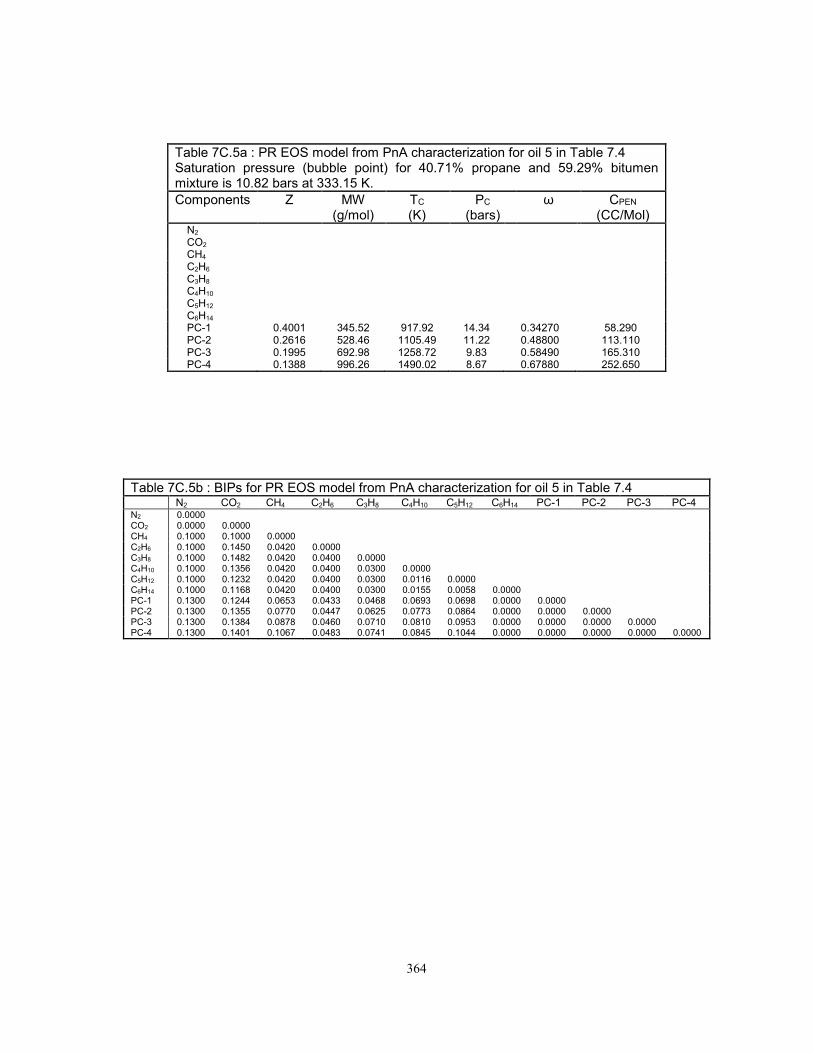
364
Table 7C.5a : PR EOS model from PnA characterization for oil 5 in Table 7.4 Saturation pressure (bubble point) for 40.71% propane and 59.29% bitumen mixture is 10.82 bars at 333.15 K.
Components Z MW (g/mol)
TC (K)
PC
(bars) ω CPEN
(CC/Mol) N2 CO2 CH4 C2H6 C3H8 C4H10 C5H12 C6H14 PC-1 0.4001 345.52 917.92 14.34 0.34270 58.290 PC-2 0.2616 528.46 1105.49 11.22 0.48800 113.110 PC-3 0.1995 692.98 1258.72 9.83 0.58490 165.310 PC-4 0.1388 996.26 1490.02 8.67 0.67880 252.650
Table 7C.5b : BIPs for PR EOS model from PnA characterization for oil 5 in Table 7.4
N2 CO2 CH4 C2H6 C3H8 C4H10 C5H12 C6H14 PC-1 PC-2 PC-3 PC-4 N2 0.0000 CO2 0.0000 0.0000 CH4 0.1000 0.1000 0.0000 C2H6 0.1000 0.1450 0.0420 0.0000 C3H8 0.1000 0.1482 0.0420 0.0400 0.0000 C4H10 0.1000 0.1356 0.0420 0.0400 0.0300 0.0000 C5H12 0.1000 0.1232 0.0420 0.0400 0.0300 0.0116 0.0000 C6H14 0.1000 0.1168 0.0420 0.0400 0.0300 0.0155 0.0058 0.0000 PC-1 0.1300 0.1244 0.0653 0.0433 0.0468 0.0693 0.0698 0.0000 0.0000 PC-2 0.1300 0.1355 0.0770 0.0447 0.0625 0.0773 0.0864 0.0000 0.0000 0.0000 PC-3 0.1300 0.1384 0.0878 0.0460 0.0710 0.0810 0.0953 0.0000 0.0000 0.0000 0.0000 PC-4 0.1300 0.1401 0.1067 0.0483 0.0741 0.0845 0.1044 0.0000 0.0000 0.0000 0.0000 0.0000

365
Table 7C.6a : PR EOS model from PnA characterization for oil 6 in Table 7.4 Saturation pressure (bubble point) for 21.83% methane and 78.17% bitumen mixture is 50.50 bars at 326.65 K.
Components Z MW (g/mol)
TC (K)
PC
(bars) ω CPEN
(CC/Mol) N2 CO2 CH4 C2H6 C3H8 C4H10 C5H12 C6H14 PC-1 0.4001 330.22 865.14 14.20 0.30170 65.690 PC-2 0.2616 505.03 1001.44 10.98 0.42850 124.980 PC-3 0.1995 662.27 1113.86 9.40 0.52240 183.160 PC-4 0.1388 952.11 1268.28 8.15 0.61330 274.900
Table 7C.6b : BIPs for PR EOS model from PnA characterization for oil 6 in Table 7.4
N2 CO2 CH4 C2H6 C3H8 C4H10 C5H12 C6H14 PC-1 PC-2 PC-3 PC-4 N2 0.0000 CO2 0.0000 0.0000 CH4 0.1000 0.1000 0.0000 C2H6 0.1000 0.1450 0.0420 0.0000 C3H8 0.1000 0.1439 0.0420 0.0400 0.0000 C4H10 0.1000 0.1326 0.0420 0.0400 0.0300 0.0000 C5H12 0.1000 0.1217 0.0420 0.0400 0.0300 0.0116 0.0000 C6H14 0.1000 0.1161 0.0420 0.0400 0.0300 0.0155 0.0058 0.0000 PC-1 0.1300 0.1226 0.0644 0.0431 0.0455 0.0684 0.0680 0.0000 0.0000 PC-2 0.1300 0.1346 0.0752 0.0445 0.0604 0.0764 0.0844 0.0000 0.0000 0.0000 PC-3 0.1300 0.1381 0.0860 0.0458 0.0701 0.0806 0.0940 0.0000 0.0000 0.0000 0.0000 PC-4 0.1300 0.1400 0.1040 0.0480 0.0740 0.0841 0.1034 0.0000 0.0000 0.0000 0.0000 0.0000
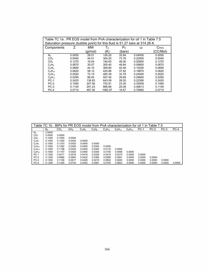
366
Table 7C.1a : PR EOS model from PnA characterization for oil 1 in Table 7.5 Saturation pressure (bubble point) for this fluid is 51.27 bars at 314.26 K.
Components Z MW (g/mol)
TC (K)
PC
(bars) ω CPEN
(CC/Mol) N2 0.0050 28.01 126.20 33.94 0.04000 0.0050 CO2 0.0040 44.01 304.20 73.76 0.22500 0.0040 CH4 0.1270 16.04 190.60 46.00 0.00800 0.1270 C2H6 0.0670 30.07 305.40 48.84 0.09800 0.0670 C3H8 0.0690 44.10 369.80 42.46 0.15200 0.0690 C4H10 0.0620 58.12 420.86 37.62 0.18870 0.0620 C5H12 0.0520 72.15 465.39 33.79 0.24000 0.0520 C6H14 0.0290 86.00 507.40 29.69 0.29600 0.0290 PC-1 0.2420 136.83 643.09 28.20 0.22266 0.2420 PC-2 0.1590 207.56 752.91 23.35 0.35009 0.1590 PC-3 0.1140 291.23 866.68 20.09 0.49613 0.1140 PC-4 0.0710 467.50 1082.97 16.67 0.76665 0.0710
Table 7C.1b : BIPs for PR EOS model from PnA characterization for oil 1 in Table 7.5
N2 CO2 CH4 C2H6 C3H8 C4H10 C5H12 C6H14 PC-1 PC-2 PC-3 PC-4 N2 0.0000 CO2 0.0000 0.0000 CH4 0.1000 0.1000 0.0000 C2H6 0.1000 0.1450 0.0420 0.0000 C3H8 0.1000 0.1370 0.0420 0.0400 0.0000 C4H10 0.1000 0.1282 0.0420 0.0400 0.0300 0.0000 C5H12 0.1000 0.1198 0.0420 0.0400 0.0300 0.0116 0.0000 C6H14 0.1000 0.1157 0.0420 0.0400 0.0300 0.0155 0.0058 0.0000 PC-1 0.1300 0.0417 0.0518 0.0416 0.0328 0.0418 0.0275 0.0000 0.0000 PC-2 0.1300 0.0886 0.0563 0.0422 0.0360 0.0556 0.0461 0.0000 0.0000 0.0000 PC-3 0.1300 0.1156 0.0617 0.0428 0.0419 0.0652 0.0620 0.0000 0.0000 0.0000 0.0000 PC-4 0.1300 0.1335 0.0734 0.0442 0.0581 0.0755 0.0823 0.0000 0.0000 0.0000 0.0000 0.0000

367
Table 7C.2a : PR EOS model from PnA characterization for oil 2 in Table 7.5 Saturation pressure (bubble point) for this fluid is 47.00 bars at 314.26 K.
Components Z MW (g/mol)
TC (K)
PC
(bars) ω CPEN
(CC/Mol) N2 0.0052 28.01 126.20 33.94 0.04000 CO2 0.0056 44.01 304.20 73.76 0.22500 CH4 0.1543 16.04 190.60 46.00 0.00800 C2H6 0.0726 30.07 305.40 48.84 0.09800 C3H8 0.0614 44.10 369.80 42.46 0.15200 C4H10 0.0459 58.12 423.38 37.84 0.19120 C5H12 0.0405 72.15 466.51 33.78 0.24290 C6H14 0.0361 86.00 507.40 29.69 0.29600 PC-1 0.2393 140.79 640.11 25.94 0.14960 PC-2 0.1572 214.39 766.57 19.80 0.25200 PC-3 0.1120 300.73 872.49 16.41 0.34880 PC-4 0.0699 481.87 1070.39 12.74 0.52690
Table 7C.2b : BIPs for PR EOS model from PnA characterization for oil 2 in Table 7.5
N2 CO2 CH4 C2H6 C3H8 C4H10 C5H12 C6H14 PC-1 PC-2 PC-3 PC-4 N2 0.0000 CO2 0.0000 0.0000 CH4 0.1000 0.1000 0.0000 C2H6 0.1000 0.1450 0.0420 0.0000 C3H8 0.1000 0.1370 0.0420 0.0400 0.0000 C4H10 0.1000 0.1282 0.0420 0.0400 0.0300 0.0000 C5H12 0.1000 0.1198 0.0420 0.0400 0.0300 0.0116 0.0000 C6H14 0.1000 0.1157 0.0420 0.0400 0.0300 0.0155 0.0058 0.0000 PC-1 0.1300 0.0417 0.0518 0.0416 0.0328 0.0418 0.0275 0.0000 0.0000 PC-2 0.1300 0.0949 0.0572 0.0423 0.0369 0.0576 0.0492 0.0000 0.0000 0.0000 PC-3 0.1300 0.1183 0.0626 0.0429 0.0431 0.0663 0.0642 0.0000 0.0000 0.0000 0.0000 PC-4 0.1300 0.1341 0.0743 0.0444 0.0592 0.0760 0.0834 0.0000 0.0000 0.0000 0.0000 0.0000
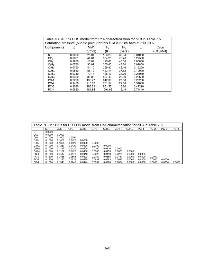
368
Table 7C.3a : PR EOS model from PnA characterization for oil 3 in Table 7.5 Saturation pressure (bubble point) for this fluid is 63.85 bars at 313.70 K.
Components Z MW (g/mol)
TC (K)
PC
(bars) ω CPEN
(CC/Mol) N2 0.0000 28.01 126.20 33.94 0.04000 CO2 0.0001 44.01 304.20 73.76 0.22500 CH4 0.1830 16.04 190.60 46.00 0.00800 C2H6 0.0780 30.07 305.40 48.84 0.09800 C3H8 0.0790 44.10 369.80 42.46 0.15200 C4H10 0.0540 58.12 423.14 37.82 0.19090 C5H12 0.0340 72.15 465.17 33.79 0.23950 C6H14 0.0380 86.00 507.40 29.69 0.29600 PC-1 0.2220 138.27 642.36 27.58 0.20280 PC-2 0.1450 210.83 751.54 22.60 0.31880 PC-3 0.1030 298.23 881.55 18.80 0.47290 PC-4 0.0630 484.84 1091.63 15.49 0.71440
Table 7C.3b : BIPs for PR EOS model from PnA characterization for oil 3 in Table 7.5
N2 CO2 CH4 C2H6 C3H8 C4H10 C5H12 C6H14 PC-1 PC-2 PC-3 PC-4 N2 0.0000 CO2 0.0000 0.0000 CH4 0.1000 0.1000 0.0000 C2H6 0.1000 0.1450 0.0420 0.0000 C3H8 0.1000 0.1368 0.0420 0.0400 0.0000 C4H10 0.1000 0.1280 0.0420 0.0400 0.0300 0.0000 C5H12 0.1000 0.1197 0.0420 0.0400 0.0300 0.0116 0.0000 C6H14 0.1000 0.1157 0.0420 0.0400 0.0300 0.0155 0.0058 0.0000 PC-1 0.1300 0.0417 0.0518 0.0416 0.0328 0.0418 0.0275 0.0000 0.0000 PC-2 0.1300 0.0886 0.0563 0.0422 0.0360 0.0556 0.0461 0.0000 0.0000 0.0000 PC-3 0.1300 0.1183 0.0626 0.0429 0.0431 0.0663 0.0642 0.0000 0.0000 0.0000 0.0000 PC-4 0.1300 0.1341 0.0743 0.0444 0.0592 0.0760 0.0834 0.0000 0.0000 0.0000 0.0000 0.0000

369
Table 7C.4a : PR EOS model from PnA characterization for oil 4 in Table 7.5 Saturation pressure (bubble point) for this fluid is 42.20 bars at 313.70 K.
Components Z MW (g/mol)
TC (K)
PC
(bars) ω CPEN
(CC/Mol) N2 0.0000 28.01 126.20 33.94 0.04000 CO2 0.0000 44.01 304.20 73.76 0.22500 CH4 0.1262 16.04 190.60 46.00 0.00800 C2H6 0.0380 30.07 305.40 48.84 0.09800 C3H8 0.0480 44.10 369.80 42.46 0.15200 C4H10 0.0401 58.12 420.55 37.59 0.18840 C5H12 0.0340 72.15 465.43 33.79 0.24010 C6H14 0.0244 86.00 507.40 29.69 0.29600 PC-1 0.2881 147.74 664.84 26.47 0.23100 PC-2 0.1849 230.24 788.27 21.43 0.37208 PC-3 0.1324 321.51 894.50 18.62 0.50445 PC-4 0.0839 507.08 1111.46 15.41 0.76189
Table 7C.4b : BIPs for PR EOS model from PnA characterization for oil 4 in Table 7.5
N2 CO2 CH4 C2H6 C3H8 C4H10 C5H12 C6H14 PC-1 PC-2 PC-3 PC-4 N2 0.0000 CO2 0.0000 0.0000 CH4 0.1000 0.1000 0.0000 C2H6 0.1000 0.1450 0.0420 0.0000 C3H8 0.1000 0.1368 0.0420 0.0400 0.0000 C4H10 0.1000 0.1280 0.0420 0.0400 0.0300 0.0000 C5H12 0.1000 0.1197 0.0420 0.0400 0.0300 0.0116 0.0000 C6H14 0.1000 0.1157 0.0420 0.0400 0.0300 0.0155 0.0058 0.0000 PC-1 0.1300 0.0532 0.0527 0.0417 0.0334 0.0452 0.0317 0.0000 0.0000 PC-2 0.1300 0.1003 0.0581 0.0424 0.0378 0.0594 0.0521 0.0000 0.0000 0.0000 PC-3 0.1300 0.1206 0.0635 0.0430 0.0443 0.0674 0.0662 0.0000 0.0000 0.0000 0.0000 PC-4 0.1300 0.1350 0.0761 0.0446 0.0615 0.0769 0.0854 0.0000 0.0000 0.0000 0.0000 0.0000

370
Table 7C.5a : PR EOS model from PnA characterization for oil 5 in Table 7.5 Saturation pressure (bubble point) for this fluid is 39.02 bars at 313.70 K.
Components Z MW (g/mol)
TC (K)
PC
(bars) ω CPEN
(CC/Mol) N2 0.0040 28.01 126.20 33.94 0.04000 CO2 0.0297 44.01 304.20 73.76 0.22500 CH4 0.0861 16.04 190.60 46.00 0.00800 C2H6 0.0739 30.07 305.40 48.84 0.09800 C3H8 0.0764 44.10 369.80 42.46 0.15200 C4H10 0.0722 58.12 422.95 37.80 0.19080 C5H12 0.0543 72.15 466.91 33.77 0.24400 C6H14 0.0406 86.00 507.40 29.69 0.29600 PC-1 0.2324 138.61 644.14 28.07 0.21845 PC-2 0.1539 209.40 754.86 23.19 0.34347 PC-3 0.1092 295.15 870.52 19.90 0.48674 PC-4 0.0673 478.67 1092.38 16.46 0.75214
Table 7C.5b : BIPs for PR EOS model from PnA characterization for oil 5 in Table 7.5
N2 CO2 CH4 C2H6 C3H8 C4H10 C5H12 C6H14 PC-1 PC-2 PC-3 PC-4 N2 0.0000 CO2 0.0000 0.0000 CH4 0.1000 0.1000 0.0000 C2H6 0.1000 0.1450 0.0420 0.0000 C3H8 0.1000 0.1368 0.0420 0.0400 0.0000 C4H10 0.1000 0.1280 0.0420 0.0400 0.0300 0.0000 C5H12 0.1000 0.1197 0.0420 0.0400 0.0300 0.0116 0.0000 C6H14 0.1000 0.1157 0.0420 0.0400 0.0300 0.0155 0.0058 0.0000 PC-1 0.1300 0.0417 0.0518 0.0416 0.0328 0.0418 0.0275 0.0000 0.0000 PC-2 0.1300 0.0886 0.0563 0.0422 0.0360 0.0556 0.0461 0.0000 0.0000 0.0000 PC-3 0.1300 0.1156 0.0617 0.0428 0.0419 0.0652 0.0620 0.0000 0.0000 0.0000 0.0000 PC-4 0.1300 0.1335 0.0734 0.0442 0.0581 0.0755 0.0823 0.0000 0.0000 0.0000 0.0000 0.0000

371
Table 7C.6a : PR EOS model from PnA characterization for oil 6 in Table 7.5 Saturation pressure (bubble point) for this fluid is 59.87 bars at 301.48 K.
Components Z MW (g/mol)
TC (K)
PC
(bars) ω CPEN
(CC/Mol) N2 0.0019 28.01 126.20 33.94 0.04000 CO2 0.0044 44.01 304.20 73.76 0.22500 CH4 0.2028 16.04 190.60 46.00 0.00800 C2H6 0.0592 30.07 305.40 48.84 0.09800 C3H8 0.0590 44.10 369.80 42.46 0.15200 C4H10 0.0559 58.12 420.73 37.60 0.18860 C5H12 0.0492 72.15 464.86 33.79 0.23860 C6H14 0.0436 86.00 507.40 29.69 0.29600 PC-1 0.2150 139.57 642.10 26.97 0.18282 PC-2 0.1433 209.36 751.06 21.83 0.28746 PC-3 0.1023 293.39 863.05 18.33 0.40737 PC-4 0.0635 472.23 1074.09 14.63 0.62949
Table 7C.6b : BIPs for PR EOS model from PnA characterization for oil 6 in Table 7.5
N2 CO2 CH4 C2H6 C3H8 C4H10 C5H12 C6H14 PC-1 PC-2 PC-3 PC-4 N2 0.0000 CO2 0.0000 0.0000 CH4 0.1000 0.1000 0.0000 C2H6 0.1000 0.1450 0.0420 0.0000 C3H8 0.1000 0.1318 0.0420 0.0400 0.0000 C4H10 0.1000 0.1252 0.0420 0.0400 0.0300 0.0000 C5H12 0.1000 0.1192 0.0420 0.0400 0.0300 0.0116 0.0000 C6H14 0.1000 0.1164 0.0420 0.0400 0.0300 0.0155 0.0058 0.0000 PC-1 0.1300 0.0417 0.0518 0.0416 0.0328 0.0418 0.0275 0.0000 0.0000 PC-2 0.1300 0.0886 0.0563 0.0422 0.0360 0.0556 0.0461 0.0000 0.0000 0.0000 PC-3 0.1300 0.1156 0.0617 0.0428 0.0419 0.0652 0.0620 0.0000 0.0000 0.0000 0.0000 PC-4 0.1300 0.1335 0.0734 0.0442 0.0581 0.0755 0.0823 0.0000 0.0000 0.0000 0.0000 0.0000

372
Table 7C.7a : PR EOS model from PnA characterization for oil 7 in Table 7.5 Saturation pressure (bubble point) for this fluid is 30.82 bars at 316.48 K.
Components Z MW (g/mol)
TC (K)
PC
(bars) ω CPEN
(CC/Mol) N2 0.0038 28.01 126.20 33.94 0.04000 -4.230 CO2 0.0135 44.01 304.20 73.76 0.22500 -1.640 CH4 0.0694 16.04 190.60 46.00 0.00800 -5.200 C2H6 0.1006 30.07 305.40 48.84 0.09800 -5.790 C3H8 0.0739 44.10 369.80 42.46 0.15200 -6.350 C4H10 0.0771 58.12 422.54 37.76 0.19040 -6.490 C5H12 0.0631 72.15 466.46 33.77 0.24280 -5.120 C6H14 0.0545 86.00 507.40 29.69 0.29600 1.390 PC-1 0.2276 148.17 665.80 25.75 0.20634 -1.380 PC-2 0.1487 226.75 771.06 21.19 0.31175 -1.950 PC-3 0.1043 323.35 898.28 17.62 0.45059 -2.730 PC-4 0.0633 532.71 1135.18 14.11 0.69431 -4.300
Table 7C.7b : BIPs for PR EOS model from PnA characterization for oil 7 in Table 7.5
N2 CO2 CH4 C2H6 C3H8 C4H10 C5H12 C6H14 PC-1 PC-2 PC-3 PC-4 N2 0.0000 CO2 0.0000 0.0000 CH4 0.1000 0.1000 0.0000 C2H6 0.1000 0.1450 0.0420 0.0000 C3H8 0.1000 0.1381 0.0420 0.0400 0.0000 C4H10 0.1000 0.1289 0.0420 0.0400 0.0300 0.0000 C5H12 0.1000 0.1200 0.0420 0.0400 0.0300 0.0116 0.0000 C6H14 0.1000 0.1156 0.0420 0.0400 0.0300 0.0155 0.0058 0.0000 PC-1 0.1300 0.0532 0.0527 0.0417 0.0334 0.0452 0.0317 0.0000 0.0000 PC-2 0.1300 0.0949 0.0572 0.0423 0.0369 0.0576 0.0492 0.0000 0.0000 0.0000 PC-3 0.1300 0.1206 0.0635 0.0430 0.0443 0.0674 0.0662 0.0000 0.0000 0.0000 0.0000 PC-4 0.1300 0.1355 0.0770 0.0447 0.0625 0.0773 0.0864 0.0000 0.0000 0.0000 0.0000 0.0000

373
Table 7C.8a : PR EOS model from PnA characterization for oil 8 in Table 7.5 Saturation pressure (bubble point) for this fluid is 55.35 bars at 307.60 K.
Components Z MW (g/mol)
TC (K)
PC
(bars) ω CPEN
(CC/Mol) N2 0.0048 28.01 126.20 33.94 0.04000 CO2 0.0011 44.01 304.20 73.76 0.22500 CH4 0.1630 16.04 190.60 46.00 0.00800 C2H6 0.0403 30.07 305.40 48.84 0.09800 C3H8 0.0297 44.10 369.80 42.46 0.15200 C4H10 0.0365 58.12 423.51 37.85 0.19130 C5H12 0.0373 72.15 465.70 33.78 0.24080 C6H14 0.0332 86.00 507.40 29.69 0.29600 PC-1 0.2648 140.17 642.41 27.67 0.20553 PC-2 0.1767 210.11 751.65 22.70 0.32316 PC-3 0.1290 287.66 864.20 19.33 0.45796 PC-4 0.0836 444.23 1045.98 16.16 0.67352
Table 7C.8b : BIPs for PR EOS model from PnA characterization for oil 8 in Table 7.5
N2 CO2 CH4 C2H6 C3H8 C4H10 C5H12 C6H14 PC-1 PC-2 PC-3 PC-4 N2 0.0000 CO2 0.0000 0.0000 CH4 0.1000 0.1000 0.0000 C2H6 0.1000 0.1450 0.0420 0.0000 C3H8 0.1000 0.1341 0.0420 0.0400 0.0000 C4H10 0.1000 0.1264 0.0420 0.0400 0.0300 0.0000 C5H12 0.1000 0.1193 0.0420 0.0400 0.0300 0.0116 0.0000 C6H14 0.1000 0.1159 0.0420 0.0400 0.0300 0.0155 0.0058 0.0000 PC-1 0.1300 0.0417 0.0518 0.0416 0.0328 0.0418 0.0275 0.0000 0.0000 PC-2 0.1300 0.0886 0.0563 0.0422 0.0360 0.0556 0.0461 0.0000 0.0000 0.0000 PC-3 0.1300 0.1156 0.0617 0.0428 0.0419 0.0652 0.0620 0.0000 0.0000 0.0000 0.0000 PC-4 0.1300 0.1322 0.0716 0.0440 0.0557 0.0744 0.0800 0.0000 0.0000 0.0000 0.0000 0.0000

374
Table 7C.9a : PR EOS model from PnA characterization for oil 9 in Table 7.5 Saturation pressure (bubble point) for this fluid is 60.21 bars at 307.60 K.
Components Z MW (g/mol)
TC (K)
PC
(bars) ω CPEN
(CC/Mol) N2 0.0029 28.01 126.20 33.94 0.04000 -4.230 CO2 0.0119 44.01 304.20 73.76 0.22500 -1.640 CH4 0.1756 16.04 190.60 46.00 0.00800 -5.200 C2H6 0.0992 30.07 305.40 48.84 0.09800 -5.790 C3H8 0.1257 44.10 369.80 42.46 0.15200 -6.350 C4H10 0.0793 58.12 421.40 37.66 0.18920 -6.490 C5H12 0.0507 72.15 465.73 33.78 0.24090 -5.120 C6H14 0.0377 86.00 507.40 29.69 0.29600 1.390 PC-1 0.1713 130.86 643.85 27.32 0.19420 1.820 PC-2 0.1157 193.74 733.63 23.06 0.28333 3.630 PC-3 0.0813 275.65 851.10 19.29 0.41216 5.450 PC-4 0.0487 460.10 1073.72 15.40 0.65271 7.260
Table 7C.9b : BIPs for PR EOS model from PnA characterization for oil 9 in Table 7.5
N2 CO2 CH4 C2H6 C3H8 C4H10 C5H12 C6H14 PC-1 PC-2 PC-3 PC-4 N2 0.0000 CO2 0.0000 0.0000 CH4 0.1000 0.1000 0.0000 C2H6 0.1000 0.1450 0.0420 0.0000 C3H8 0.1000 0.1341 0.0420 0.0400 0.0000 C4H10 0.1000 0.1264 0.0420 0.0400 0.0300 0.0000 C5H12 0.1000 0.1193 0.0420 0.0400 0.0300 0.0116 0.0000 C6H14 0.1000 0.1159 0.0420 0.0400 0.0300 0.0155 0.0058 0.0000 PC-1 0.1300 0.0417 0.0518 0.0416 0.0328 0.0418 0.0275 0.0000 0.0000 PC-2 0.1300 0.0814 0.0554 0.0420 0.0353 0.0534 0.0428 0.0000 0.0000 0.0000 PC-3 0.1300 0.1126 0.0608 0.0427 0.0408 0.0639 0.0598 0.0000 0.0000 0.0000 0.0000 PC-4 0.1300 0.1329 0.0725 0.0441 0.0569 0.0749 0.0812 0.0000 0.0000 0.0000 0.0000 0.0000
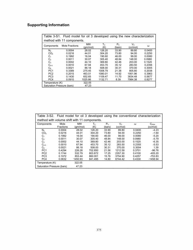
375
Supporting Information
Table 3-S1. Fluid model for oil 3 developed using the new characterization
method with 11 components.
Components Mole Fractions MW
(gm/mol) TC (K)
PC (bars)
VC (cc/mol)
ω
N2 0.0004 28.02 126.20 33.90 89.80 0.0400 CO2 0.0216 44.01 304.20 73.80 94.00 0.2250 C1 0.1992 16.04 190.60 46.00 99.00 0.0080 C2 0.0011 30.07 305.40 48.84 148.00 0.0980 C3 0.0002 44.10 369.80 42.46 203.00 0.1520 C4-5 0.0010 67.94 453.70 35.12 283.50 0.2356 C6 0.0021 86.18 508.00 30.31 370.00 0.3005 PC1 0.3389 275.45 1008.79 21.38 805.80 0.2038 PC2 0.2015 463.51 1080.01 14.92 1951.96 0.3963 PC3 0.1430 652.65 1109.47 11.70 3834.48 0.5677 PC4 0.0910 1025.86 1132.71 8.39 7984.38 0.8277
Temperature (K) 322.05 Saturation Pressure (bars) 47.23
Table 3-S2. Fluid model for oil 3 developed using the conventional characterization
method with volume shift with 11 components. Components Mole
Fractions MW
(gm/mol) TC (K)
PC (bars)
VC (cc/mol)
ω CPEN
(cc/mol)
N2 0.0004 28.02 126.20 33.90 89.80 0.0400 -4.23 CO2 0.0216 44.01 304.20 73.80 94.00 0.2250 -1.64 C1 0.1992 16.04 190.60 46.00 99.00 0.0080 -5.20 C2 0.0011 30.07 305.40 48.84 148.00 0.0980 -5.79 C3 0.0002 44.10 369.80 42.46 203.00 0.1520 -6.35 C4-5 0.0010 67.94 453.70 35.12 283.50 0.2355 -5.53 C6 0.0021 86.18 508.00 30.31 370.00 0.3004 1.39 PC1 0.4294 226.26 702.850 21.56 1212.59 0.3701 -96.76 PC2 0.1744 532.79 803.872 17.25 2357.30 0.4100 -405.20 PC3 0.1072 853.44 860.001 15.76 3754.90 0.4257 -753.83 PC4 0.0632 1450.93 841.495 14.80 6744.42 0.4330 -1458.94
Temperature (K) 322.05 Saturation Pressure (bars) 47.23
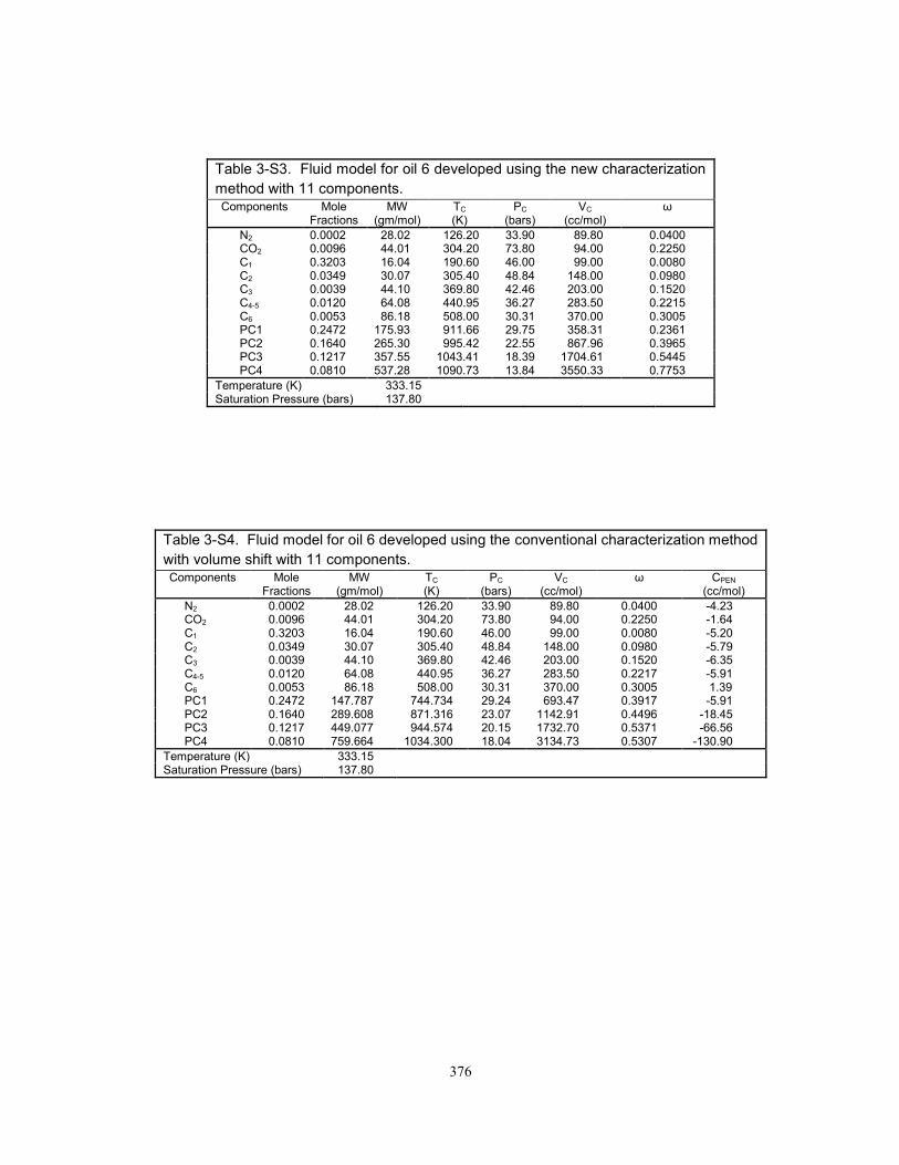
376
Table 3-S3. Fluid model for oil 6 developed using the new characterization
method with 11 components. Components Mole
Fractions MW
(gm/mol) TC (K)
PC (bars)
VC (cc/mol)
ω
N2 0.0002 28.02 126.20 33.90 89.80 0.0400 CO2 0.0096 44.01 304.20 73.80 94.00 0.2250 C1 0.3203 16.04 190.60 46.00 99.00 0.0080 C2 0.0349 30.07 305.40 48.84 148.00 0.0980 C3 0.0039 44.10 369.80 42.46 203.00 0.1520 C4-5 0.0120 64.08 440.95 36.27 283.50 0.2215 C6 0.0053 86.18 508.00 30.31 370.00 0.3005 PC1 0.2472 175.93 911.66 29.75 358.31 0.2361 PC2 0.1640 265.30 995.42 22.55 867.96 0.3965 PC3 0.1217 357.55 1043.41 18.39 1704.61 0.5445 PC4 0.0810 537.28 1090.73 13.84 3550.33 0.7753
Temperature (K) 333.15 Saturation Pressure (bars) 137.80
Table 3-S4. Fluid model for oil 6 developed using the conventional characterization method
with volume shift with 11 components. Components Mole
Fractions MW
(gm/mol) TC (K)
PC (bars)
VC (cc/mol)
ω CPEN
(cc/mol)
N2 0.0002 28.02 126.20 33.90 89.80 0.0400 -4.23 CO2 0.0096 44.01 304.20 73.80 94.00 0.2250 -1.64 C1 0.3203 16.04 190.60 46.00 99.00 0.0080 -5.20 C2 0.0349 30.07 305.40 48.84 148.00 0.0980 -5.79 C3 0.0039 44.10 369.80 42.46 203.00 0.1520 -6.35 C4-5 0.0120 64.08 440.95 36.27 283.50 0.2217 -5.91 C6 0.0053 86.18 508.00 30.31 370.00 0.3005 1.39 PC1 0.2472 147.787 744.734 29.24 693.47 0.3917 -5.91 PC2 0.1640 289.608 871.316 23.07 1142.91 0.4496 -18.45 PC3 0.1217 449.077 944.574 20.15 1732.70 0.5371 -66.56 PC4 0.0810 759.664 1034.300 18.04 3134.73 0.5307 -130.90
Temperature (K) 333.15 Saturation Pressure (bars) 137.80

377
Figure 3-S1. Flow chart for the conventional characterization method (CM) in this research, which is based on Pedersen and Christensen (2007). The shaded blocks show the input data. The CM with volume-shift parameters is referred to as the
CMwV (the right branch of the flow chart). The CMw/oV is the CM without volume-shift parameters (the
left branch of the flow chart). See the Introduction section for the definitions of steps 1-4.
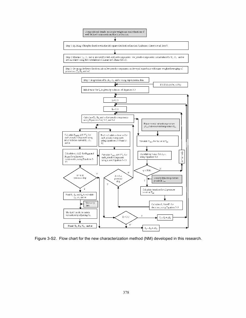
378
Figure 3-S2. Flow chart for the new characterization method (NM) developed in this research.
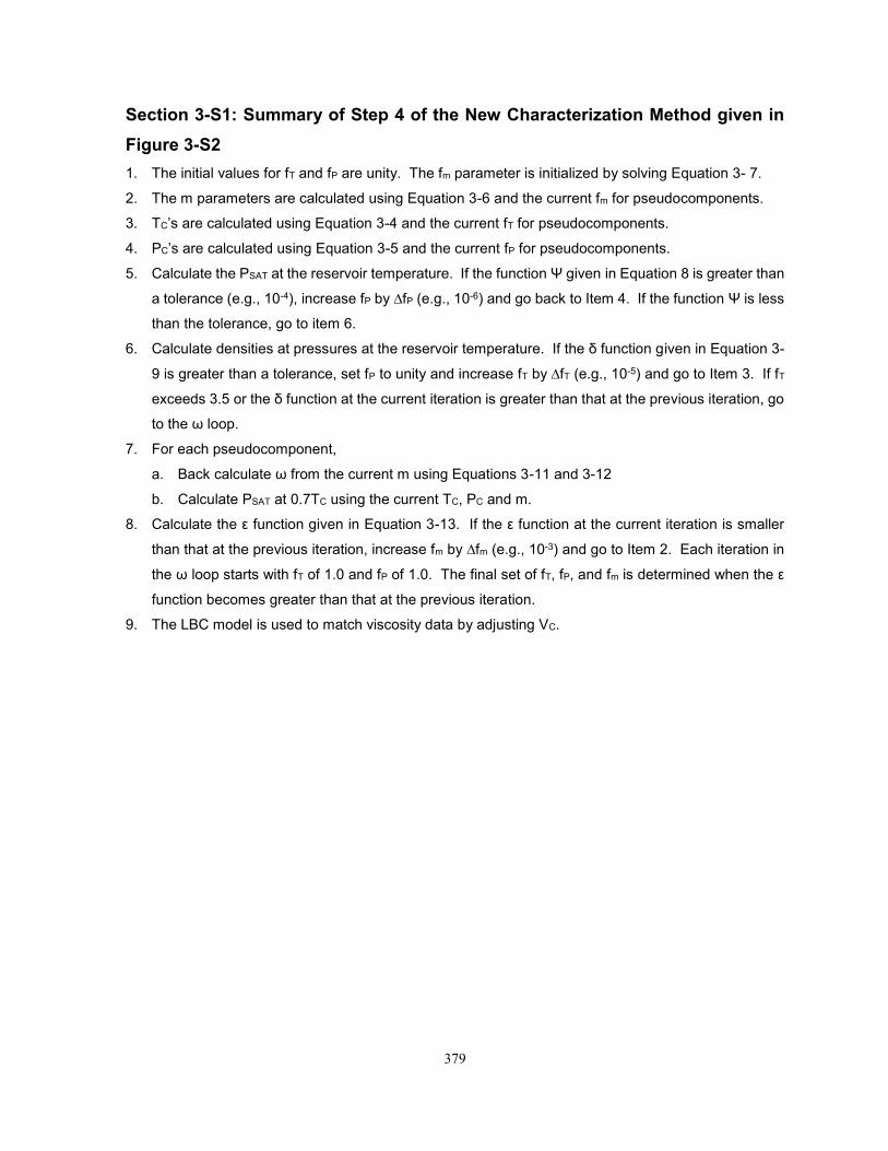
379
Section 3-S1: Summary of Step 4 of the New Characterization Method given in
Figure 3-S2
1. The initial values for fT and fP are unity. The fm parameter is initialized by solving Equation 3- 7.
2. The m parameters are calculated using Equation 3-6 and the current fm for pseudocomponents.
3. TC’s are calculated using Equation 3-4 and the current fT for pseudocomponents.
4. PC’s are calculated using Equation 3-5 and the current fP for pseudocomponents.
5. Calculate the PSAT at the reservoir temperature. If the function Ψ given in Equation 8 is greater than
a tolerance (e.g., 10-4), increase fP by ∆fP (e.g., 10-6) and go back to Item 4. If the function Ψ is less
than the tolerance, go to item 6.
6. Calculate densities at pressures at the reservoir temperature. If the δ function given in Equation 3-
9 is greater than a tolerance, set fP to unity and increase fT by ∆fT (e.g., 10-5) and go to Item 3. If fT
exceeds 3.5 or the δ function at the current iteration is greater than that at the previous iteration, go
to the ω loop.
7. For each pseudocomponent,
a. Back calculate ω from the current m using Equations 3-11 and 3-12
b. Calculate PSAT at 0.7TC using the current TC, PC and m.
8. Calculate the ε function given in Equation 3-13. If the ε function at the current iteration is smaller
than that at the previous iteration, increase fm by ∆fm (e.g., 10-3) and go to Item 2. Each iteration in
the ω loop starts with fT of 1.0 and fP of 1.0. The final set of fT, fP, and fm is determined when the ε
function becomes greater than that at the previous iteration.
9. The LBC model is used to match viscosity data by adjusting VC.
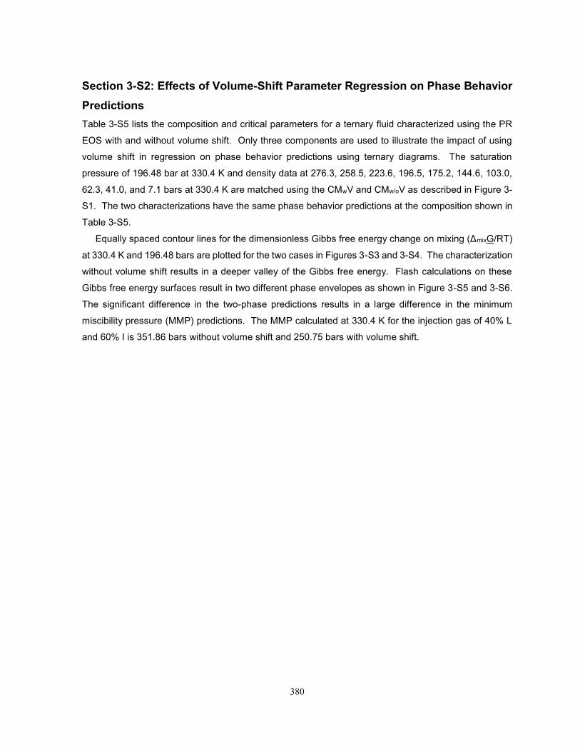
380
Section 3-S2: Effects of Volume-Shift Parameter Regression on Phase Behavior
Predictions
Table 3-S5 lists the composition and critical parameters for a ternary fluid characterized using the PR
EOS with and without volume shift. Only three components are used to illustrate the impact of using
volume shift in regression on phase behavior predictions using ternary diagrams. The saturation
pressure of 196.48 bar at 330.4 K and density data at 276.3, 258.5, 223.6, 196.5, 175.2, 144.6, 103.0,
62.3, 41.0, and 7.1 bars at 330.4 K are matched using the CMwV and CMw/oV as described in Figure 3-
S1. The two characterizations have the same phase behavior predictions at the composition shown in
Table 3-S5.
Equally spaced contour lines for the dimensionless Gibbs free energy change on mixing (ΔmixG/RT)
at 330.4 K and 196.48 bars are plotted for the two cases in Figures 3-S3 and 3-S4. The characterization
without volume shift results in a deeper valley of the Gibbs free energy. Flash calculations on these
Gibbs free energy surfaces result in two different phase envelopes as shown in Figure 3-S5 and 3-S6.
The significant difference in the two-phase predictions results in a large difference in the minimum
miscibility pressure (MMP) predictions. The MMP calculated at 330.4 K for the injection gas of 40% L
and 60% I is 351.86 bars without volume shift and 250.75 bars with volume shift.

381
Table 3-S5. Ternary fluid using the conventional characterization method with/without
volume shift in regression.
PR EOS with volume shift PR EOS without volume shift
Comp. Mole Fractions
MW (gm/mol)
TC (K)
PC (bars)
ω CPEN (cc/mol)
TC (K)
PC (bars)
ω
L 0.4219 16.10 190.86 46.07 0.0089 -5.19 190.86 46.07 0.0089 I 0.0176 31.66 315.59 47.83 0.1065 -5.85 315.59 47.83 0.1065 H 0.5605 291.30 848.33 24.18 0.4373 -110.14 1022.44 19.48 0.5108
Temperature (K) 330.40 Saturation Pressure (bars) 196.48
L = N2 + CO2 + C1, I = C2 + C3, H = C4+
Figure 3-S3. Dimensionless molar Gibbs free energy change on mixing for the ternary fluid given in Table 3-S5 at 330.4 K and 196.48 bars. Contour lines are drawn with the interval of 0.05 between -0.85 to 2.0. The PR EOS is used without
volume shift.
382
Figure 3-S4. Dimensionless molar Gibbs free energy change on mixing for the ternary fluid given in Table 3-S5 at 330.4 K and 196.48 bars. Contour lines are drawn with the interval of 0.05 between -0.85 to 2.0. The PR EOS is used. Volume
shift parameters are used in regression.
Figure 3-S5. Phase envelope for the ternary fluid given in Table 3-S5. The PR EOS is used without volume shift. MMP calculated for the injection gas is 351.86 bars at 330.40
K.

383
Figure 3-S6. Phase envelope for the ternary fluid given in Table 3-S5. The PR EOS is used. Volume shift parameters are used in regression. Use of volume shift results in a
two-phase envelope that is significantly smaller than that in Figure 3-3. MMP calculated for the injection
gas is 250.75 bars 330.40 K.

384
Section 5-S1. Peng-Robinson Attraction and Covolume Parameters Optimized
for n-Alkanes
This part presents a critical review for various sets of the attraction and covolume parameters presented
in the literature. They are categorized into three types; i) the parameter sets that are based on estimated
physical critical points, ii) the optimized parameter sets from Ting et al. (2003) and Voutsas et al. (2006),
and iii) the optimized parameter set from Kumar and Okuno (2012). This part is concerned with the
suitability of the optimized parameter set from Kumar and Okuno (2012) for use in the direct perturbation
from n-alkanes (PnA) in this research.
The Peng-Robinson equation of state (PR EOS) used throughout this paper is given below.
p =RT
v−b−
a
v2+2bv−b2 , (5-S1)
where a = aCα(Tr) (5-S2)
aC = Ωa (RTC)2 PC⁄ (5-S3)
α(Tr) = [1 + m(1 − (T TC⁄ )0.5)]2 (5-S4)
b = Ωb RTC PC⁄ (5-S5)
m = 0.37464 + 1.54226 − 0.269922 for < 0.3984 (5-S6)
m = 0.379642 + 1.48503 − 0.1644232 + 0.016666ω3 for ≥ 0.3984 (5-S7)
Critical points were measured for C1 through n-C24, n-C26, n-C27, n-C30, and n-C36 (Nikitin et al.
1997). Although there are many correlations proposed for critical parameters, not all of them are reliably
extrapolated to heavier n-alkanes. For example, the correlations of Gao et al. (2001), Riazi and Al-
Sahhaf (1996) give a normal boiling point (Tb) that is greater than TC of a given compound. The
correlation of TC by Joback and Reid (1987) yields physically absurd values; 32130 K for n-C73 and –
189113 K for n-C74. Their correlation for Tb gives 2487.60 K for n-C100. Kontogeorgis and Tassios
(1997) presented a critical review of various correlations for critical points. They recommended
Magoulos and Tassios (1990) for n-alkanes up to n-C40 and Constantinou and Gani (1994) for more
general application to heavier n-alkanes. In this paper, the group-contribution method of Constantinou
and Gani (1994) is used when physical critical points are required in phase behavior computations for
n-alkanes from C7 to C100.
Kumar and Okuno (2012) optimized TC, PC, and m for n-alkanes from n-C7 through n-C100 in terms
of liquid densities and vapor pressures by use of the PR EOS. The optimized critical parameters deviate,
to some extent, from the physically measured critical points, and give extended two-phase lines in P-T
space. Therefore, a comprehensive analysis of the deviation and its impact on phase behavior
prediction has been made by comparing with various estimations of physical critical points presented in
the literature. Table 5-S1 presents TC and PC of n-C100 from various sources in the literature. The
optimized values by Kumar and Okuno (2012) are 1084 K and 4.01 bars, and are within the variation
ranges (950 – 1215 K for TC and 0.48 – 4.43 bars for PC) presented in Table 5-S1. The deviation of the
optimized TC from the value of Constantinou and Gani (1994) is within the experimental uncertainty of

385
3% (Rowley et al. 2006). Compared to Constantinou and Gani (1994), the optimized TC is lower for n-
alkanes lighter than n-C15, but becomes higher for heavier n-alkanes. The deviation from Constantinou
and Gani (1994) in terms of PC is higher than the experimental uncertainty of 25% (Rowley et al. 2006).
The optimized PC is higher than the value from Constantinou and Gani (1994) for all n-alkanes from n-
C7 to n-C100. Figure 5-S1 compares the two sets of the critical parameters and vapor pressures.
Densities calculated by the PR EOS tend to increase when values of critical parameters are
increased. Figure 5-S2 shows data and predictions for saturated liquid densities (ρL S ) and vapor
pressures (Pvap) for n-C28. The data were taken from Yaws (2010) and Riazi and AlQaheem (2010).
The predictions were made by the PR EOS with two different sets of critical parameters; Constantinou
and Gani (1994) and Kumar and Okuno (2012). The PR EOS underpredicts ρL S when physical values
from Constantinou and Gani (1994) are used. Figure 5-S2 clearly shows that ρL S predictions are
increased by use of higher TC and PC, and lower ω from Kumar and Okuno (2012). However, vapor
pressure predictions are kept nearly the same along the data.
In this figure, the predictions with the parameter set of Constantinou and Gani (1994) deviate
substantially from the density data (Yaws 2010), due to the well-known shortcoming of the PR EOS in
liquid density predictions. However, they agree well with the vapor pressure data (Riazi and AlQaheem
2010). The availability of vapor pressure data for light n-alkanes allows for better fitting of the α(Tr)
function (Equation 5-S4), which results in improved vapor pressure prediction.
Figure 5-S3 presents data and predictions for three isodensity curves in P-T space for n-C28. The
three curves represent P-T conditions at which measured densities are 0.78 g/cc, 0.76 g/cc, and 0.74
g/cc. The PR EOS gives density predictions along the three curves that depend significantly on the
critical-parameter values used. They are respectively 0.74 g/cc, 0.73 g/cc, and 0.72 g/cc with Kumar
and Okuno (2012), and 0.50 g/cc, 0.49 g/cc, and 0.48 g/cc with Constantinou and Gani (1994). The
comparisons in Figures 5-S2 and 5-S3 show that the density predictions from the PR EOS are much
improved by using the critical parameters of Kumar and Okuno (2012), as compared to the physical
critical parameters estimated by Constantinou and Gani (1994).
The optimization of critical parameters for n-alkanes in Kumar and Okuno (2012) did not consider
critical volume predictions. Figure 5-S4 compares critical densities calculated with the PR EOS with
the optimized critical parameters from Kumar and Okuno (2012) with those with the physical critical
parameters from Constantinou and Gani (1994). It also shows estimated critical densities by use of the
correlations of Teja et al. (1990), Tsonopoulos (1993), Constantinou and Gani (1994). Teja et al. (1990)
and Tsonopoulos and Tan (1993) developed the correlations by use of experimental critical density data
for n-alkanes up to n-C18 (Anselme et al. 1990, Ambrose and Tsonopoulos 1995). Critical densities
estimated by Teja et al. (1990) tend to zero with increasing CN, which may be unlikely (Tsonopoulos
and Tan 1993). Critical densities estimated by Constantinou and Gani (1994) do not follow the data
trend; however, they are kept at the same level for higher CNs, unlike those from Teja et al. (1990). The
correlation of Tsonopoulos and Tan (1993) is based on a modified Flory theory (Flory et al. 1964) of the

386
statistical thermodynamics for chain molecules applied to n-alkanes. The critical densities from the PR
EOS with the optimized critical parameters from Kumar and Okuno (2012) exhibit a minimum. For large
CNs, they remain nearly constant, and are close to the values estimated by Tsonopoulos and Tan
(1993). The average absolute deviation (AAD) in the critical density predictions from the PR EOS with
the critical parameters from Kumar and Okuno (2012) is less than 10%, compared to the available data.
This is within the experimental uncertainty for critical density; for example, the experimental uncertainty
is 14% for n-C18 (Ambrose and Tsonopoulos, 1995).
The review given above for the critical parameters of Kumar and Okuno (2012) showed how density
predictions of the PR EOS can be improved while keeping vapor pressure predictions by adjusting TC,
PC, and m. Ting et al. (2003) and Voutsas et al. (2006) also conducted the indirect optimization of the
PR attraction and covolume parameters for n-alkanes by matching vapor pressures and liquid densities
through TC, PC, and m. Voutsas et al. (2006) also presented correlations for aC (Equation 5-S3) and
covolumes. However, the CN range used by them does not cover many reservoir fluids. C1, C2, C3, C4,
C6, C7, C10, C16, C18, C20, C24, C30, C36, and C40 were considered in Ting et al. (2003) and Voutsas et al.
(2006), while C7 through C100 in Kumar and Okuno (2012). Nevertheless, these three publications
commonly showed that phase equilibrium predictions for n-alkane mixtures were also improved when
the optimized critical parameters were used with the PR EOS.
Here, a comparison is made between the optimized sets of Voutsas et al. (2006), Kumar and Okuno
(2012). Figure 5-S5 presents the aC values based on three different sets of TC, PC, and m; two optimized
sets from Kumar and Okuno (2012) and from Voutsas et al. (2006), and the other one from the method
of Constantinou and Gani (1994) and Constantinou et al. (1995) as a physical-value set. The same
comparison is presented for the covolume parameter in Figure 5-S6 and for the attraction parameter at
350 K in Figure 5-S7. For each of the three parameters shown, the optimized set of Kumar and Okuno
(2012) results in a value that is lower than when the physical-value set is used for a given MW. The
parameters are well correlated with a linear function of MW. The small deviations between Kumar and
Okuno (2012) and Voutsas et al. (2006) are likely due to the different ranges of n-alkanes used. The
attraction parameter at 350 K from Voutsas et al. (2006) is greater than that from Kumar and Okuno
(2012) for CNs higher than 40. The deviation becomes greater for higher CNs.
The m parameter (Equations 5-S6 and 5-S7) in the PR EOS is significant in vapor pressure
prediction at sub-critical temperatures. Figure 5-S8 compares the m parameter estimated by the
method of Constantinou et al. (1995) with the optimized m parameters by Voutsas et al. (2006) and by
Kumar and Okuno (2012). The optimized m parameter of Kumar and Okuno (2012) is approximately
equal to the estimated physical value up to n-C21. For higher CNs, the optimized m parameter is smaller
than the estimated physical value for each CN. The trends from Voutsas et al. (2006), Kumar and Okuno
(2012) start deviating from each other approximately at the MW of 550 g/mol. This is likely attributed to
the fact that Voutsas et al. (2006) only considered n-alkanes up to n-C40, which corresponds to a MW
of 563 g/mol.

387
The attraction and covolume parameters calculated based on Voutsas et al. (2006) may not be
satisfactory for predictions of vapor pressures and liquid phase densities for CNs higher than 40. Figure
5-S9 presents a comparative analysis of predictive capabilities of Voutsas et al. (2006), and Kumar and
Okuno (2012) for n-C100. Saturated liquid density data were taken from Yaws (2010), and vapor
pressure data were reproduced using the correlation of Raizi and AlQaheem (2010). Use of the
parameter set from Voutsas et al. (2006) results in significant overprediction of the vapor pressures and
underprediction of the saturated liquid densities. Use of the parameter set from Kumar and Okuno
(2012) results in good agreement with data. Figure 5-S10 shows isodensity curves with liquid phase
density values of 0.74 g/cc and 0.76 g/cc for n-C100 in P-T space. The density predictions based on
Kumar and Okuno (2012) and Voutsas et al. (2006) are widely apart from each other.
Figure 5-S11 shows the normal boiling points for n-alkanes based on the parameter set of Voutsas
et al. (2006) and that of Kumar and Okuno (2012). The comparison with data indicates that the
parameter set of Voutsas et al. (2006) is not satisfactory for normal boiling point predictions for CNs 7
through 11 and 40 and higher. The trends of the parameters from Voutsas et al. (2006), and Kumar and
Okuno (2012) are qualitatively similar and quantitatively close to each other for CNs lower than 40.
However, the small differences in the parameters can result in significant differences in phase behavior
predictions.
This part presented a critical review for three different types of the PR attraction and covolume
parameters available in the literature; i.e., i) the physical parameter sets, ii) the optimized parameter
sets from Ting et al. (2003) and Voutsas et al. (2006), and iii) the optimized parameter set from Kumar
and Okuno (2012). The first type is not suitable for the direct PnA method primarily because they do
not give accurate density predictions. As explained in Kumar and Okuno (2013, 2014), use of volume
shift as adjustment parameters in reservoir fluid characterization can result in erroneous phase behavior
predictions at the thermodynamic conditions that the available phase behavior data do not cover. The
first type also showed less accurate phase equilibrium predictions for n-alkane mixtures in comparison
with the optimized parameters from Kumar and Okuno (2012), as shown in Kumar and Okuno (2012)
and Figures 5-16 and 5-17 in the current paper. The second type was not satisfactory for phase behavior
predictions for CNs higher than 40, as discussed previously in this section. That is, this is not suitable
for use in characterization of reservoir fluids, many of which contain hydrocarbons heavier than C40.
Therefore, the direct PnA method is applied with the optimized parameter set from Kumar and Okuno
(2012) in this research.

388
Table 5-S1. Estimated physical critical points for n-C100.
The critical points from Kumar and Okuno (2012) are
optimized ones with the PR EOS.
TC (K) PC (bars)
Gao et al. 2001 966.26 0.50 Riazi and Al-Sahhaf 1996 963.20 0.69 Yaws 2010 1215.25 1.51 Ambrose 1978 1049.30 2.66 Constantinou and Gani 1994 1058.70 2.10 Magoulos and Tassios 1990 950.30 0.48 Tsonopoulos and Tan 1993 989.31 4.43 Kumar and Okuno 2012 1084.00 4.01
Figure 5-S1. Comparison of optimized and physical critical parameters. Comparison of optimized critical parameters (Kumar and Okuno 2012) is presented with the estimated
physical critical parameters from Constantinou and Gani (1994) for n-alkanes from n-C7 through n-C100.
Vapor pressure curves for n-C7 through n-C100 are drawn using the correlations of Raizi-AlQaheem
(2010).

389
Figure 5-S2. Comparison of vapor pressure curves and saturated liquid densities predicted with optimized and physical critical parameters for n-C28. Vapor pressures and saturated liquid densities predicted for n-C28 by use of the optimized critical
parameters from Kumar and Okuno (2012) and the physical critical parameters from Constantinou and
Gani (1994). The optimized TC and PC are higher than the estimated physical values. Use of the
optimized parameters increases the saturated liquid density curve systematically, while keeping the
vapor pressure curve along the vapor pressure data, which are shown by the filled squares.
Figure 5-S3. Comparison of predicted isodensity curves with PR EOS with data (Dutour et al. 2001). Liquid-phase isodensity curves for n-C28 from experimental data (Dutour et al. 2001) and from the PR
EOS with the optimized (Kumar and Okuno 2012) and estimated physical critical parameters
(Constantinou and Gani 1994). The three isodensity curves represent different density values. Along
the left-most isodensity curve, for example, the measured value is 0.78 g/cc (1), but the PR EOS gives
0.74 g/cc with the critical parameters of Kumar and Okuno (2012) and 0.50 g/cc with the critical
parameters of Constantinou and Gani (1994).

390
Figure 5-S4. Comparison of critical densities from different correlations. Critical densities of n-alkanes from three correlations (Teja et al. 1990, Constantinou and Gani 1994,
and Tsonopoulos and Tan 1993) and the PR EOS with two sets of critical parameters (Kumar and Okuno
2012, and Constantinou and Gani 1994). Data were taken from Ambrose and Tsonopoulos (1995). The
critical densities calculated by the PR EOS with the parameters of Kumar and Okuno are in good
agreement with Tsonopoulos and Tan (1993) for extended CNs.
Figure 5-S5. Comparison of ac for PR EOS from optimized and physical critical parameters. The figure presents comparison of aC for the PR EOS using two sets of optimized critical parameters;
one from Kumar and Okuno (2012) and the other from Voutsas et al. (2006). The values calculated with
the physical critical parameters from Constantinou and Gani (1994) are also presented. For a given CN,
the optimized aC values are smaller than that from the estimated physical critical parameters. The
optimized aC values are well correlated with linear functions of MW. The optimized aC parameter from
Voutsas et al. (2006) starts deviating from that from Kumar and Okuno (2012) at CN 40.
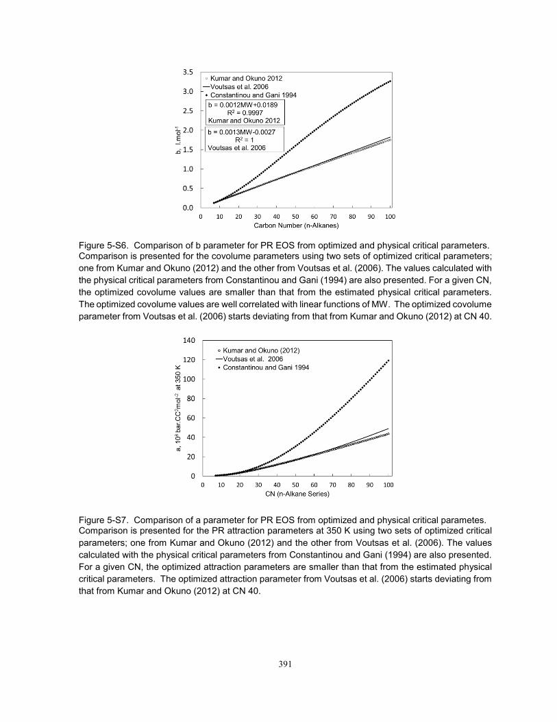
391
Figure 5-S6. Comparison of b parameter for PR EOS from optimized and physical critical parameters. Comparison is presented for the covolume parameters using two sets of optimized critical parameters;
one from Kumar and Okuno (2012) and the other from Voutsas et al. (2006). The values calculated with
the physical critical parameters from Constantinou and Gani (1994) are also presented. For a given CN,
the optimized covolume values are smaller than that from the estimated physical critical parameters.
The optimized covolume values are well correlated with linear functions of MW. The optimized covolume
parameter from Voutsas et al. (2006) starts deviating from that from Kumar and Okuno (2012) at CN 40.
Figure 5-S7. Comparison of a parameter for PR EOS from optimized and physical critical parametes. Comparison is presented for the PR attraction parameters at 350 K using two sets of optimized critical
parameters; one from Kumar and Okuno (2012) and the other from Voutsas et al. (2006). The values
calculated with the physical critical parameters from Constantinou and Gani (1994) are also presented.
For a given CN, the optimized attraction parameters are smaller than that from the estimated physical
critical parameters. The optimized attraction parameter from Voutsas et al. (2006) starts deviating from
that from Kumar and Okuno (2012) at CN 40.
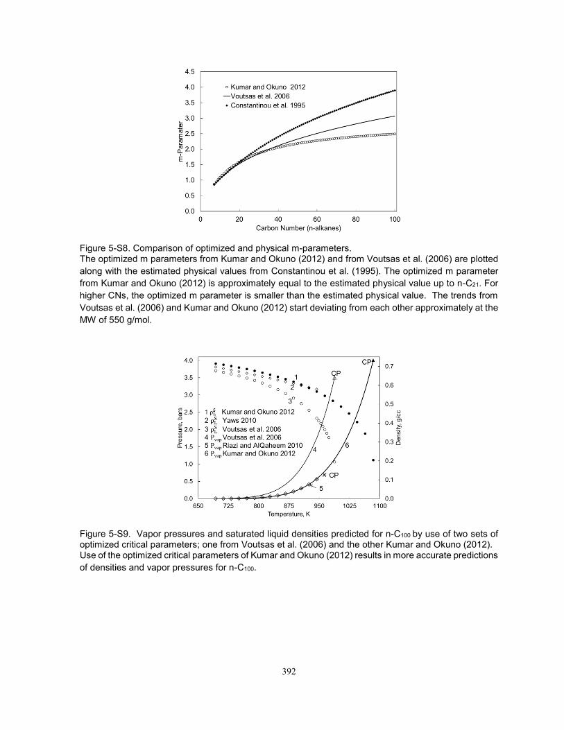
392
Figure 5-S8. Comparison of optimized and physical m-parameters. The optimized m parameters from Kumar and Okuno (2012) and from Voutsas et al. (2006) are plotted
along with the estimated physical values from Constantinou et al. (1995). The optimized m parameter
from Kumar and Okuno (2012) is approximately equal to the estimated physical value up to n-C21. For
higher CNs, the optimized m parameter is smaller than the estimated physical value. The trends from
Voutsas et al. (2006) and Kumar and Okuno (2012) start deviating from each other approximately at the
MW of 550 g/mol.
Figure 5-S9. Vapor pressures and saturated liquid densities predicted for n-C100 by use of two sets of optimized critical parameters; one from Voutsas et al. (2006) and the other Kumar and Okuno (2012). Use of the optimized critical parameters of Kumar and Okuno (2012) results in more accurate predictions
of densities and vapor pressures for n-C100.

393
Figure 5-S10. Two liquid-phase isodensity curves (0.74 g/cc and 0.76 g/cc) in P-T space predicted for n-C100 using the PR EOS. The two sets of optimized critical parameters used are from Kumar and Okuno (2012) and Voutsas et
al. (2006). Large differences are observed between the sets of predictions.
Figure 5-S11. Comparison of normal boiling points from PR EOS with optimized and physical critical parameters. Normal boiling points predicted for n-alkanes by use of the PR EOS with the optimized critical
parameters from Kumar and Okuno (2012) and from Voutsas et al. (2006). Data were taken from Yaws
(2010). Use of the optimized critical parameters from Kumar and Okuno (2012) gives good agreement
with the data. Voutsas et al. (2006) optimized the critical parameters for up to n-C40. They correlated
the aC and covolume parameters as linear functions of MW. However, these linear correlations may
not be accurate when extrapolated to higher CNs.
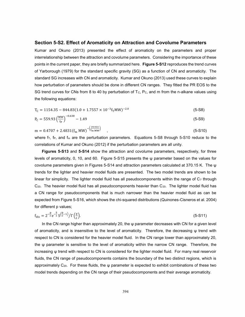
394
Section 5-S2. Effect of Aromaticity on Attraction and Covolume Parameters
Kumar and Okuno (2013) presented the effect of aromaticity on the parameters and proper
interrelationship between the attraction and covolume parameters. Considering the importance of these
points in the current paper, they are briefly summarized here. Figure 5-S12 reproduces the trend curves
of Yarborough (1979) for the standard specific gravity (SG) as a function of CN and aromaticity. The
standard SG increases with CN and aromaticity. Kumar and Okuno (2013) used these curves to explain
how perturbation of parameters should be done in different CN ranges. They fitted the PR EOS to the
SG trend curves for CNs from 8 to 40 by perturbation of TC, PC, and m from the n-alkane values using
the following equations:
TC = 1154.35 − 844.83(1.0 + 1.7557 × 10⁻³fTMW)−2.0 (5-S8)
PC = 559.93 (MW
fP)
−0.638
− 1.49 (5-S9)
m = 0.4707 + 2.4831(fm MW)−(
39.933
fm MW) , (5-S10)
where fT, fP, and fm are the perturbation parameters. Equations 5-S8 through 5-S10 reduce to the
correlations of Kumar and Okuno (2012) if the perturbation parameters are all unity.
Figures 5-S13 and 5-S14 show the attraction and covolume parameters, respectively, for three
levels of aromaticity, 0, 10, and 60. Figure 5-S15 presents the ψ parameter based on the values for
covolume parameters given in Figures 5-S14 and attraction parameters calculated at 370.15 K. The ψ
trends for the lighter and heavier model fluids are presented. The two model trends are shown to be
linear for simplicity. The lighter model fluid has all pseudocomponents within the range of C7 through
C20. The heavier model fluid has all pseudocomponents heavier than C20. The lighter model fluid has
a CN range for pseudocomponents that is much narrower than the heavier model fluid as can be
expected from Figure 5-S16, which shows the chi-squared distributions (Quinones-Cisneros et al. 2004)
for different p values;
fdis = 2−p
2 e−S
2 S(p
2−1) Γ (
p
2 )⁄ . (5-S11)
In the CN range higher than approximately 20, the ψ parameter decreases with CN for a given level
of aromaticity, and is insensitive to the level of aromaticity. Therefore, the decreasing ψ trend with
respect to CN is considered for the heavier model fluid. In the CN range lower than approximately 20,
the ψ parameter is sensitive to the level of aromaticity within the narrow CN range. Therefore, the
increasing ψ trend with respect to CN is considered for the lighter model fluid. For many real reservoir
fluids, the CN range of pseudocomponents contains the boundary of the two distinct regions, which is
approximately C20. For these fluids, the ψ parameter is expected to exhibit combinations of these two
model trends depending on the CN range of their pseudocomponents and their average aromaticity.
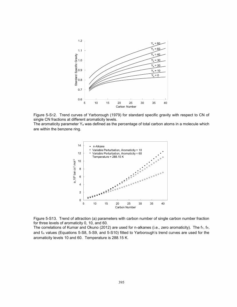
395
Figure 5-S12. Trend curves of Yarborough (1979) for standard specific gravity with respect to CN of single CN fractions at different aromaticity levels. The aromaticity parameter Ya was defined as the percentage of total carbon atoms in a molecule which
are within the benzene ring.
Figure 5-S13. Trend of attraction (a) parameters with carbon number of single carbon number fraction for three levels of aromaticity 0, 10, and 60. The correlations of Kumar and Okuno (2012) are used for n-alkanes (i.e., zero aromaticity). The fT, fP,
and fm values (Equations 5-S8, 5-S9, and 5-S10) fitted to Yarborough’s trend curves are used for the
aromaticity levels 10 and 60. Temperature is 288.15 K.
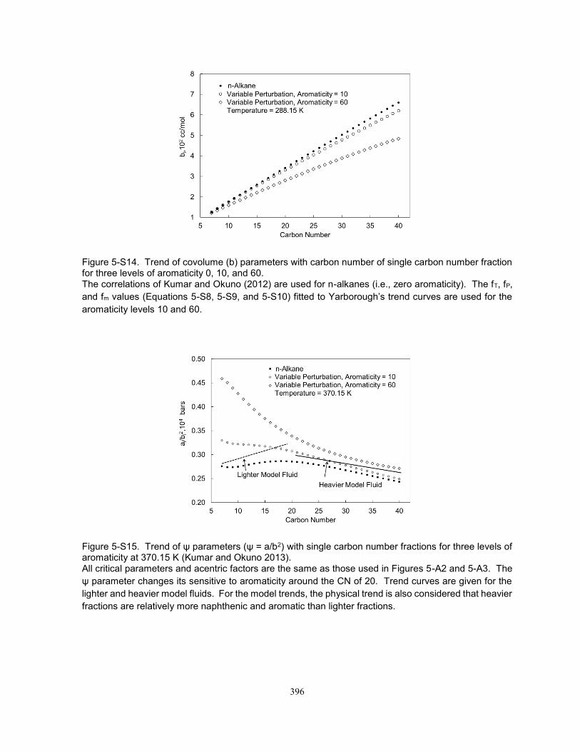
396
Figure 5-S14. Trend of covolume (b) parameters with carbon number of single carbon number fraction for three levels of aromaticity 0, 10, and 60. The correlations of Kumar and Okuno (2012) are used for n-alkanes (i.e., zero aromaticity). The fT, fP,
and fm values (Equations 5-S8, 5-S9, and 5-S10) fitted to Yarborough’s trend curves are used for the
aromaticity levels 10 and 60.
Figure 5-S15. Trend of ψ parameters (ψ = a/b2) with single carbon number fractions for three levels of aromaticity at 370.15 K (Kumar and Okuno 2013). All critical parameters and acentric factors are the same as those used in Figures 5-A2 and 5-A3. The
ψ parameter changes its sensitive to aromaticity around the CN of 20. Trend curves are given for the
lighter and heavier model fluids. For the model trends, the physical trend is also considered that heavier
fractions are relatively more naphthenic and aromatic than lighter fractions.
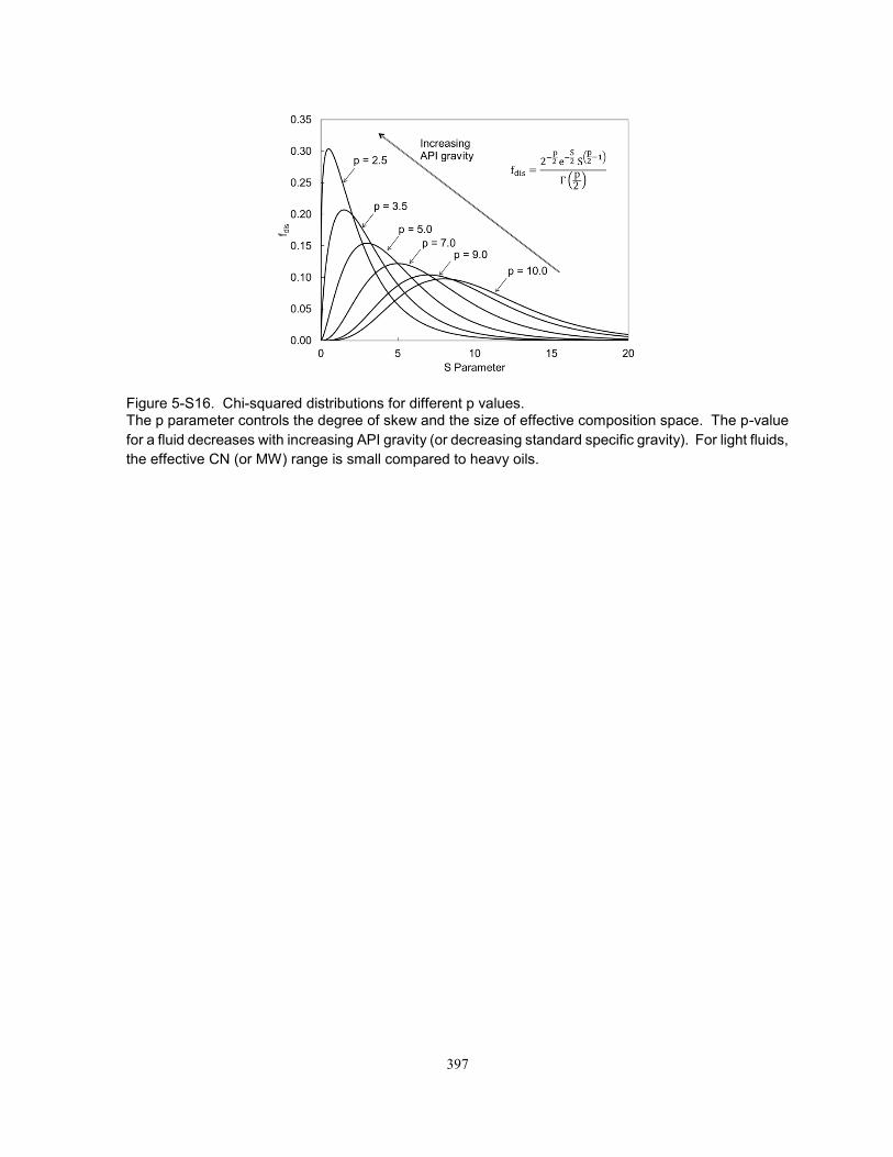
397
Figure 5-S16. Chi-squared distributions for different p values. The p parameter controls the degree of skew and the size of effective composition space. The p-value
for a fluid decreases with increasing API gravity (or decreasing standard specific gravity). For light fluids,
the effective CN (or MW) range is small compared to heavy oils.


![Thanking you, Yours faithfully, [Naresh Kumar]](https://static.fdokumen.com/doc/165x107/6326bdd4051fac18490de8c7/thanking-you-yours-faithfully-naresh-kumar.jpg)