Hazard assessment of waste disposal sites. Part 1: literature review
Upload
khangminh22Category
view
2download
0

i II I I

Hydrogeology, Waste Disposal, Scienceand Politics
Engineering Geology and Geotechnical Engineering30th Symposium, 1994
Paul Karl Link, editor
1994 Symposium Committee
Lee Robinson Paul Link Spencer WoodSymposium Chairman Proceedings Editor On.Site CoordinatorCollege of Engineering Department of Geology Department of GeosciencesIdaho State Umvermty Idaho State University Boise State University
The Engineering Geology and Geotechnicai Engineering Symposiumis an annual event, s.ponso.red by:
Idaho State UmvermtyBoise State University
University of IdahoUtah State University
University of Nevada-Reno
Copies of this volume and previous symposium volumes may be ordered fromDr. Lee RobinsonCollege of Engineering
Box 8060Idaho State University
Pocatello, Idaho 83209- Phone (208) 236-2902
FAX (208) 236-4538
Correct citation of artides in this bookin Link, P.K., editor, 1994, Hydrogeolo.gy, Waste Disposal, Science and Politics,
Proceedings of the 30th Symposmm on Engineering Geology and Geotechnical: Engineering, College of Engineering, Idaho State University, Pocatello, Idaho.--
Cover illustrations:_ Front Location map of Idaho National Engineering Laboratory and Wells drilled near the
Idaho Chemical Processing Plant (ICPP)Back: Stratigraphicunits beneath the ICPP
_- Both figures from McCurry and others, this volume
MASTER- _._,
-- _E;TRIBUTION C_ _ DOCUMENT |S UNLIMITED

ii
Hydrogeology, Waste Disposal, Science and Po Iit ic s
1994 Symposium on Engineering Geology and Geotechnical Engineering
Compiled and edited by Paul Karl Link, Idaho State University
Table of ContentsL Site Characterization..Pocateilo Area
Hydrogeologyof the Poeateilo Aquifer:.ImplicationsforWellheadProtectionStrategiesJ. Welhan, and C. Meelmn 1
Impactof LeachableSulfateOn the Qualityof C_undwater in the PocatelloAquiferC. Meehan and J. Welhan 19
Interpretationof ShallowSeismic RefractionDataUsing RaytracingInversion:A SimpleExample fromaGroundwaterResourceStudyin Poeatello, IdahoJ.R. Pelton, M.E. Dongherty, and J.A. Welhan 37
FrazierHall: The FoundationFailureThatDidn'tLee Robinson 45
A Mise-A'-La-MasseMethod ForLandftilContaminantPlumeEvaluationT.H. Rowley, P.R. Donaldson, J.L. Osiemky, and J.A. Welhan 83
II. Site Chamcterlzatlon--Bobe AreaGroundwaterdevelopmentin graniticterrain_Bogus Basin SkiResort,Boise, Idaho
William C.B. Gates, Craig L. Parklmen and Kevin L. Schroeder 55A ProposedDeg:riptiveMethodologyforEnvironmentalGeologic
(Envimgeologic) Site CharacterizationDavid L. Schwarz, and Walter S. Snyder 67
HI. Site AssessmentHotspots& OtherHiddenTargets: Probabilityof Detection,Number,FrequencyandArea
Charles L. Vlta 95The Relationshipof Seismic Velocity SWdctureand SurfaceFractureCharacteristics
of Basalt Out_3ps to RippabilityEstimatesS.E. Kay, M.E. Dougherty and J.R. Pelton 107
Geologic andGeotechnicalInvestigationof theWindsor ParkSubdivisionNorthLas Vegas, NevadaLorraine M. LInnert,James L. Werle, Alan N. StUley,and Brad E. Olsen 121
FailureAnalysis of BuriedTanksReynoid King Watklm 137
ErosionControlTest Facilitiesat the UtahWaterResearchLabC. Earl Israelsen and Gilberto Urroz 147
IV. Idaho National Engineering LaboratoryPre-anthropogenicGroundwaterEvolutionat the IdahoNationalEngineeringLaboratory,Idaho
Travis L. McLing and Robert W. Smith 151IdahoNationalEngineeringLaboratoryIntegratedField Scale Pumpingand InfiltrationTest
T.R. Wood, G.T. Norreli, A.W. Wylie, KJ. Dooley, G.S. Johnson and E.R. Neher 152Mineralogyof andDepositionalSourcesof SedimentaryInterbedsBeneath theIdaho
NationalEngi_g Laboratory; EasternSnakeRiverPlain, IdahoMichael F. Reed 154
ConcentrationsandCompositionsof ColloidalParticlesin GroundwaterNearthe ICPP,IdahoNationalEngineeringLaboratory,IdahoMason Estes and Mike McCurry 165
HydrostratigraphicInterpretationof the UpperPortionof the SnakeRiverPlainAquifernearthe IdahoChemicalProcessingPlantatthe INELW. Bah'ash, R.H. Morin, S.H. Wood, and W. Bennecke 181
Hydrostratigraphyof the SnakeRiverPlain AquiferBeneath the RadioactiveWasteM_.agement Complexat the IdahoNationalEngineeringLaboratory,A PreliminaryReportMary J. Hegnmnn and Spencer H. Wood 195

111
IV. Idaho National Enptneedn8 Laboratory (continued)Three-dimensionalChemicalStructureof the IN'ELAquiferSystemNear the
IdahoChemicalProcessingPlantMichael McCurry, Mason Estes, Jeanne Fromm, John Welhanand Warren Barrash 207
IdahoChemical Ph3cessingPlant(ICPP) InjectionWell: Operationstlistory andliydrochemical Inventoryof the Waste StreamJ. Frmmn, J. Welhan,M. McCurry and W. tlackett 221
StraddlePackerSystem Design andOperationforVerticalCharacterizationof OpenBore Holes, James K. Olsen 238
HydrologicTestingin Wells Near the IdahoChemical ProcessingPlantat theIdahoNational EngineeringLaboratoryGary S. Johnson, J. IIhan Olsen and Dale R. Ralston 253
VerticalVariationin GroundwaterChemistryInfesTedfromFluidSpecific-ConductanceWell Logging of the SnakeRiverPlainBasalt Aquifer, IdahoNationalEngineeringLaboratory,SoutheasternIdahoSpencer IL Wood and WIIHamBennecke 267
IV. Geophysical MethodsEnvironmentalGeophysics: Locatingand EvaluatingSubsurfaceGeology,
Geologic Hazards,GroundwaterContamination,Etc.Alvin K. Bemon 285
Effects of Shale andContaminantson (Vs/VP) Ratiosin Transversely-lsotropicGeologyAlvin K. Benson 305
A Comparisonof GroundPenetratingRadarMethods: Multi-FoldDataVs. Single Fold DataLee M. Liberty and John R. Pelton 321
A New GeophysicalMethod toMeasure Soil Profilesfor DynamicAnalysisof Soil EmbankmentsPaul Mfchaeis • 331
GroundPeneUatingRadarAnd Seismic RefractionInvestigationof FracturePatterns in theBasalt of LuckyPeakNearBoise, IdahoM.E. Dougherty, W.K. Hudson, S.E. Kay and R.J.Vincent 345
Resultsof a DowulmleFormationMicroscannerStudyin a Juro-Triassic-agedSedimentaryDeposit(PassaicFormation)Joseph A. Fischer, Joseph J. Fischer, and Robert J. Bullwlnkel 359
The Identificationof Basalt PhysicalFeaturesFrom BoreholeTelevision LogsWilliam Bennecke 371
Ste_logical Samplingof RockMasses for EngineeringPurposesStanley M. MUler,Bryan D. Martin and John K. Owens 385
V. RemedlationDisposalOptionsforScrapTires
C.W. "Bill" Lovell 395Selected Remedyat the QueenCity FarmsSuperfundSite: ARisk ManagementApproach
E.F. Weber, J. Wilson and M. Kirk 413]Bi0ventingFeasibilityStudyof'Low PermeabilitySoils forRemediationof
PetroleumContaminationKevin M. Bracimey 429
EnhancedEndogenousBiological Attenuationof AromaticHydrocarbonsin Groundwater:.A'Case Study(PreliminaryResults)Christopher Lammer 445
ivVL Geotechnlcal Engineering
Diffusion Through Statically Cmnpacted ClayCaHion L. Ho and Maher A.-A. Shebl 461
The Effect of Freeze-Thaw Cycles on the Hydraulic Conductivity of Compacted ClayDavid Waite, Loren Anderson, JoSeph Caliendo and Michael McFarland 475
From Lab to Held: Geotechnical Properties for Predicting Embankment Settlement onLake Bonneville DepositsKevln..C. Hoagland, Casan L. Sampaco, Loren R. Anderson, Joseph A CaHendo,
• Loren Rausher and Edward Keane 491Contaminant Fluxes Through Site Containmefit Barriers: Performance Assessment
and Illustrative ResultsCharles L. Vlta 505
F'mite Element Analysis of A Soft Nailed WallJoseph A. Callendo, Kevln C. Womack, Huey S. l_am and Loren R. Knderson 523
A Modified Cap Model Implemented in D_NA-3DIsam G. Jardaneh, Thomas H. Fronk and Loren R. Anderson 539
Effect of Geogrid Reinforcement of Seepage through Earth-Fill Dam CoresG,IL Gregory and S. Bang 555
Design of Flexible Pavement Subgrades. with GeosyntheticsG.H. Gregory and S. Bang 569
Proposing an Alternative Landf'fllLiner: A Successful ExampleDale Ortman 583
VII. Hydrogeology, Northern and Western IdahoEvaluation of the Ground Water Resources Within The Le_ston Basin
Gary R. Stevens and Dale Ralston 601Evaluation of Ground Water Nutrient Loading to Priest Lake, Boundary Co., Idaho
K,M. Freeman anti D.R. Ralston 615Characterization of a Shallow Canyon Aquifer Contaminated by Mine Tallings and
Suggestions for Constructed Wetland TrealmentJohn C. Houck and L,L. (Roy) Mink 621
Pages removed by authors'request just prior to printing 622VIH. The Last Paper to Arriv¢ (Geotechnlcal Engineering)
Modeling of the Pullout Characteristics.of Wetded Wire Mats Embexkl_ in SandCasan L. Sampaco, Loren R, Anderson and Mark R. Nielsen 637
Author Index
Aaiderson,Loren 475, 491,523, 539, 637 Kay, S.E. 107, 345 Pelton, J.R. 37, 107, 321Bang, S. 555,569 Keane,Edward 491 Ralston,D.R. 253, 601,615Bah'ash,Warren 181,221 Kirk,M. 413 Rausher,Loren 491Bennecke William 181, 267, 371 Lammer,Christopher 445 Reed, M.F. 154Benson, A.K. 285, 305 Liberty,L.M. 321 Robinson, Lee 45Brackney,K.M. 429 Linnert,L.M. 121 Rowley, T.H. 83BuUwinkel,R.J. 359 LoveU,C.W. 395 Sampaco,C.S. 491,637Caliendo,J.A. 475, 491,523 Martin,B.D, 385 Shebl, M.A.-A 461Donaldson,P.R. 83 McFarland,Michael 475 Schroeder,K.L. 55Dooley, K.J. 152 McCurry,Michael 165, 207, 221 Smith,R.W. 151Dougher_y,M.E. 37, 107,345 McLing,T.L. 151 Snyder,W.S. 67Estes, Mason 165, 207 Meehan,Chris 1, 19 Stevens,G.R. 601Fischer, J.A. 359 Michaels, Paul 331 Stilley, A.H. 121Fischer,J.J. 359 Miller,S.M. 385 Urroz,Gilberto" 147Freeman,K.M. 615 Mink,L,L. 621 Vincent,R.J. 345Fromm,Jeanne 207, 221 Morin,R.H. 181 Vita, C.L. 95, 505Fronk,T.H. 539 Neher,E.R. 152 Waite,David 475Gates,W.C.B. 55 Nham, H.S. 523 Watkins,R.K. 137Gregory,G.H. 555,569 Nielsen, M.R. 637 Weber,E.F. 413Hackett,W.R. 221 Norrell,G..T. 152 Welhan,J.A. 1, 19, 37, 83, 207, 221Hegmann, M.J. 195 Olsen,B.E. 121 Werle,J.L. 121He, C.L. 461 Olsen,J.K. 238 Wilson,J. 413Hoasl_nd, K.C. 491 Olsen, J.H. 253 Womack,K.C. 523Houck,J.C. 621 Ortman,Dale 583 Wood,S.H. 181,195,267Hudson,W.K. 345 Osiensky,J.L. 83 Wood,T.R. 152Israelsen,C.E. 147 Owens,J.K. 385 Wylie, A.W. 152Jardaneh,I.G. 539 Parkinson,C.L. 55Johnson,G.S. 152, 253 Pelton, J.R. 37, 107,321

i
Hydrogeology, Waste Disposal, Scienc_ and PoliticsProceedings 30th Symposium 1Engineering Geology and Geotechnical Engineering, 1994
HYDROGEOLOGY OF THE POCATELLO AQUIFER:IMPLICATIONS FOR _VELLHEAD PROTECTION STRATEGIF_
J. Welhan (Idaho Geological Survey)C. Meehan (Department of Geology, Idaho State University)
both at: 325 Physical Sciences, Idaho State University,Pocateilo, ID 83209-0009 208-236-3235
ABSTRACT
A well head protection (WHP) demonstration project focusing on the PocateUo municipal watersupply aquifer was initiated in 1992 to provide a preliminary characterization of the aquifer'shydrogeology and to develop a well head protection plan that could serve as a test of the State'sdraft WHP. Phase I of the program has focused on defining the geologic and hydrologiccharacteristics of the southern portion of the aquifer. Phase II is aimed at developing capture zonemodels for wells in the central part of the well field that are threatened by TCE contamination.
The shallow strip aquifer (1:6 width:length aspect ratio) in which the southern well field issituated comprises coarse, well-sorted fluvial gravels andis bounded laterally by low-permeabilitymargins. It is characterized by very high transmissivities (0.1 - 10 ft2/day) and linear velocities(6 to >60 ft/day). The effect of such high ground water flow velocities is to produce markedlyelongated pumping well capture zones, with one year time-of-travel distances of the order ofkilometers. Migration of contaminants laterally across the aquifer due to pumping stress shouldbe minimized because of the rapid longitudinal nature of ground water flow along the valley,thereby facilitating interceptor well design. However, the elongated capture zones imply thatspecial consideration will need to be given to distant up-valley land use and recharge areas.
INTRODUCTION AND SCOPE
The City of Pocatello is situated on a highly prolific, alluvial valley-fill aquifer which supplies100% of the city's annual water demand (approximately 20 billion liters). Water demand hasgrown steadily with increasing population, to a present per capita de,,nand of approximately 105gallons/person/year. The aquifer is vulnerable to contamination and _s currently threatened byseveral contamination sources, including trichloroethylene (TCE) which has closed two of thecity's 20 active production wells. However, knowledge of the aquifer's water sources, dynamics,
- and susceptibility to present and potential contaminant threats has been limited until recently.A program of hydrogeologic characterization of the aquifer was initiated by the Idaho
- Geological Survey in mid-1992, through a grant from the Idaho Water Resources ResearchInstitute. A well head protection (W) demonstration project, funded by the Environmental
_ Protection Agency (EPA), was also begun in 1992 in cooperation with the City of Pocatello andthe state Division of Environmental Quality (DEQ). The goal of this work was to provide apreliminary characterization of the aquifer's hydrogeology and to develop a well head protectionplan for the aquifer that could serve as a test of the state's Draft WHP Plan. In particular, theguidelines for valley fill-type aquifers in the Draft WHP Plan are being evaluated from thestandpoint of general applicability in similar valley-fill aquifer situations where hydrogeological
t
4
2 J. Welhan and C. Meehan
POCATELLOMUNICIPALWELLFIELD
WHP DEMONSTRATION GRANTSTUDY AREA
• 8 TCE,ppb
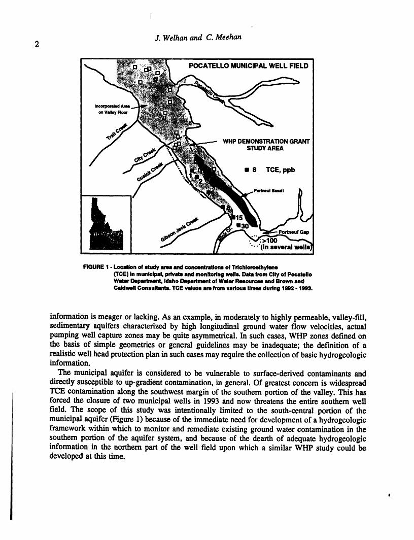
FIGURE 1 - Location of study area and ooncentratloM of Tdohloroethylene(I"CE) in munioipal, private and monitoring wells. Data from City of PocatelloWater Department, Idaho Department of Water RNouroee and Brown andCaldwell Consultants. TCE valuos am from vadous Umm dudng 1992 - 1993.
information is meager or lacking. As an example, in moderately to highly permeable, valley-fill,sedimentary aquifers characterized by high longitudinal ground water flow velocities, actualpumping well capture zones may be quite asymmetrical. In such cases, WHP zones defined onthe basis of simple geometries or general guidelines may be inadequate; the def'mition of arealistic well head protection plan in such cases may require the collection of basic hydrogeologicinformation.
The municipal aquifer is considered to be vulnerable to surface-derived contaminants anddirectly susceptible to up-gradient contamination, in general. Of greatest concern is widespreadTCE contamination along the southwest margin of the southern portion of the valley. This hasforced the closure of two municipal wells in 1993 and now threatens the entire southern wellfield. The scope of this study was intentionally limited to the south-central portion of themunicipal aquifer (Figure 1) because of the immediate need for development of a hydrogeologicframework within which to monitor and remediate existing ground water contamination in thesouthern portion of the aquifer system, and because of the dearth of adequate hydrogeologicinformation in the northern part of the well field upon which a similar WHP study could bedeveloped at this time.

Pocatello Aquifer: Wellhead Protection Strategies
3PREVIOUS WORK AND DATA SOURCES
Geologic Work
Geologic information on the area has been published by Ludlum (1943), Trimble (1976), Scott(1982), Scott et al. (1982), LaPoint (1977), Rember and Bennett (1979), Ore (1982), Link et al.(1985), Burgel et al. (1987) and Houser (1992). McDole (1969), McDole et al.(1973) and Jasmer(1987) described and mapped surficial loess deposits in the area. Several M.S. geology theseshave been done in and around the Pocatello area, including Muller (1978), LeFebre (1984) andBush (1980). A wealth of unpublished bedrock and surficial geologic data have been madeavailable by Idaho State University's Geology Department (D.W. Rodgers, H.T. Ore and P.K.Link, pers. comm., 1992, 1993).
• Figure 2 summarizes the geology of the area. The valley is defined by a half-graben Basin andRange structure, with a basin-bounding normal fault along 'its eastern margin dipping at 20-25 °basinward and estimated to have at least 6 km of offset (D.W. Rodgers, pers. comm. 1990).Bedrock in the study area is of Late Proterozoic age, and is dominated by argiUite and quartzite.Cambrian rocks, predominantly quartzite, argillite, and limestone, occur south of Cusick Creekand extend southward to Mink Creek, dipping to the east and northeast, towards the Portneufvalley and Mink Creek. Tertiary sediments and volcanics of the Starlight Formation are exposedin the southern part of the graben, as well as in outcrop to the northeast and northwest ofPocateUo. The Tertiary section in the southern part of the lower Pormeuf valley is dominated bysedimentary materials, characterized by poorly sorted conglomerates, alluvial and colluvialbouldery gravel and sedimentary breccia (Trimble, 1976; Ore, 1982).
The Quatemary/Holocene geology of the lower Portneuf river valley is dominated by fluvialand alluvial gravels which occur over the valley floor, in most areas blanketed by several 1O'sof feet of river silt and loess. Along the eastern side of the southern part of the valley, twosuperimposed basalt flows form a 50 foot-high tableland on the eastern side of the valley whichoverlooks the floor of the western half of the valley. This basalt, known as the basalt of PortneufValley (or Portneuf basalt, in this report), is of middle Pleistocene age (583,000 yrs BP, G.B.Dalrymple in Scott et al., 1982) and flowed into the lower Portneuf valley from vents in GemValley, 40 miles east, through the Pormeuf Gap. As such, it predates the gravels and siltsexposed on the floor of the western side of the valley which it overlooks.
- The valley gravels are believed to be predominantly of fluvial origin, having been depositedwithin the past 15,000 years. Northwest of City Creek the Michaud Gravel, as mapped byTrimble (1976), fans out into the Snake River Plain and overlies the lake beds of American FallsLake (72 + 14 kyr BP). The Michaud gravels are bel_.ved to have been deposited by the floodfrom pluvial Lake Bonneville as it debouched onto the Snake River Plain approximately 15,000yrs BP (Scott et al., 1982). This event was responsible for scouring the surface of the basalt andthe pre-existing valley flu along the western margin of the basai_ and depositing extensive well-sorted, coarse gravels and sands along the lower Pormeuf River valley. Much of what is believedto be equivalent of the Michaud Gravel southeas_tof City Creek has been covered by a mantleof post-flood river silt and loess.
Hydrologic Work
Hydrogeologic conditions in the northwestern portionof the aquiferhave been described byMansfield (1920), Stearns et al. (1938), Crosthwaite (1957) and West and Kilbum (1963). Those

,7.Welhan and C.Meehan4
FIGURE 2 - Geology of the lower Portneuf River valley summerlzed fromTrlmble (1976) and Rodgers (unpubl. data).
Reese
27 34 29 30 28 13a pmwl Norton A'A C3 C2 26 10 2/3 13bCA 32 31 16 12 14 Pein m
4500 " _ _ _ ....... MlchaudMlchllud _. I... s _ Gravel?
..... _ _J r .t.. -._ _ K =10" ft/s /"hl-h ": _ _ ...W._ ... _. _ t .... /L _ "IMIil__m_lll_imm'_.": "_ __ --- I''_''ee°'_su°! _ I
-, ?_..,_hmm_mm_---- -_a.- ', ' -- ' ",'-.-.,--LakeClayf ".... n --""'I• UPPERGRAVEL , 111n,m,
"] - _;_.'::1:"_:',,':. c.;,_' "_ _ '..,,:". :_... ". ,': _ ,'_, _ u
" It :1."'" "" ' ! t
- : ' f Ti11 ; I , K=I_'w0
? , / "'_o@" _ ,
nn
. i ? : .Ii
I I I I I I Iw
0 (vertk:al exaggeraUon - 100:1) 50,000 Feet 1/14
FIGURE3 - Geologic cross sectionA-A' through the lower PortneufRiver valleyfrom northwest(A) to southeast (A'), showing principle correlativefeaturesend structures. Datafrom Pocatelloend Chubbuck Municipalwells andselected private wellsshown at top of section,

Pocatello Aquifer: Wellhead Protection Strategies5
sources deal primarily with conditions in the Fort Hall Bottoms and Michaud Flats areas, as doeswork by Iacobsen (1982, 1984) and Goldstein (1981). Corbett et al. (1980) describezl thehydrogeology ofthe Tyhee area as it pertained to the geothermal resource potential of the area.The hydrogeology of a portion of the Pocatello Creek tributary drainagehas been described byCH2M-Hill (1992), as has the nature of inorganic salt contamination in that drainage.
To our knowledge, no published hydrogeologic information exists on the aquifer beneath thePocatello-Chubbuck city limits or that portion southeast of Pocatello to the Portneuf Gap.Norvitch and Larson (1970) and Seitz and Norvitch (1979) published reconnaissance data on thesurface and ground water of the upper Pormeuf River Valley drainage basin, south of thePortneuf Gap. Kindel et al. (1991) and Brown and Caldwell (1992) presented hydrogeologic dataon the mouth of Fort Hall Canyon, a tributaryvalley aquifer at the south end of the valley. Workby Brown and Caldwell and by CH2M-Hill on hydrogeologic characterization and contaminationremediation in the Fort Hall Canyon area and the southern Pocatello well field, respectively, isin progress.
Data Sources
A large amount of previously uncollated data on subsurface lithology, water level conditionsand water quality has been assembled from records of the City of Pocatello's Water Department,the City of Chubbuck's public Works Department, the IDWR, and the DEQ. Meteorological datawere obtained from the Department of Transportation meteorological station located at thePocateUo airport, approximately 6 miles west of the city. Data base development efforts in thisstudy have included collection of continuous water level records to evaluate aquifer storage andresponses to hydrologic events; well interference tests and conventional pumping tests tosupplement transmissivity estimates obtained from specific capacity and well development da_;drilling of observation wells to better define aquifer lithology and stratigraphy; and major andtrace element chemical analyses and water balance calculations to identify and quantify rechargesources.
AQUIFER CHARACTERIZATION AND CONCEPTUAL MODEL
Geologic Model
Locations of wells used to constrain subsurface geology are shown in Figure 2. Interpretedgeologic cross sections A-A', B-B' and C-C' are shown in Figures 3, 4 and 5. Almost all wellsshown in Figure 1 are municipal wells and observation wells drilled specifically for the WHPstudy, although subsurface data for the area southeast of section C-C' are derived solely fromselected private and county monitoring wells.
Figure 3 represents a synthesis of subsurface geology along transect A-A', from northwest tosoutheast, based on key units. The lack of any borehole geophysical correlative control at thisstage makes this interpretation necessarily tentative. However, in creating the geologicinterpretation of Figure 3, only those units that were considered to be consistently identifiableby a conscientious driller (namely: gdck clay beds; basalt and basalt rubble units; and crystallinebedrock) were used for correlation purposes.
Perhaps the most striking feature of Figure 3 is the presence of a bedrock high which separatesthe aquifer into sou*hem and northern portions. Henceforth, these portions of the aquifer system

Y. Welhan and C. Meehan6
will be referred to as the southern and the northern aquifers. The bedrock high may be amanifestation of the splaying of the basin-bounding fault about mid-way down the lower Portneufvalley (Figure 2) which distributed the total fault offset over numerous subsidiary faults (D.W.Rodgers, pers. comm., 1992). Similar basement highs have been mapped in other Basin andRange valleys in eastern Idaho (Link et al., 1985; Rodgers, pers. comm., 1992).
In contrast to the southern aquifer, where excellent water yields historically have been derivedfrom coarse, clean gravels at depths less than 100-150 feet below surface, the northern aquifer'sstratigraphy is characterized by much more poorly-sorted sediments (silty gravels and sands, clay)in which many more deep wells have been drilled to obtain adequate yields. Of the numeroussilty and clayey zones described in various well logs, only three are considered to have beenreliably described: a 5-10 ft thick clay (or mixed gravel and clay) bed at ca. 4380-4400 ft amslelevation; a light-colored clay unit 10-20 ft thick (possibly thickening to greater than 50 feet tothe northwest), at elevations of ca. 4200 - 4300 ft amsl.; and several occurrences of basalt lavaand/or volcanic rubble (cinders, scotia) between 4200 and 4400 ft amsl.
Of these units, the upper clay is believed to represent the late Pleistocene American Falls Lakebeds, exposed 2 miles WNW of Chubbuck wel t (24, at a maximum elevation of 4400 ft (Trimble,1976). The extent, thickness and attitude of the deep clay unit is far more tentative, as it has beenvariously logged as undifferentiated clay in excess of 90 feet thick (well 32); massive hard clayintercalated over 50 feet with thin gravel seams (well 26); sticky clay (wells C4, 27, 29); stickyyellow clay and sandy yellow clay (wells 18, 34); and sticky brown clay (well 31). It is shownin Figure 3 with a fairly uniform thickness, dipping at ca. 4°, but may thicken northward and/ordip less steeply. This unit cannot be identified with any certainty in well l0 (although it may bepresent) since this well was logged as a series of sandy clays from 4300 ft down to 4113 ft amsl.
Correlations between the basalt occurrences identified in these wells has not been attempted.Discontinuous basalt flows intercalated with sediments in the sectior, are a general feature of thesubsurface lithology in the Snake River Plain (Corbett et al., 1980; Scott et al., 1982). It is notknown whether the basalt logged in wells 16 and 30 is correlative with the other basaltoccurrences identified in wells to the north.
Cross-section B-B' _igure 4) shows the inferred subsurface lithology of the section of theaquifer above the bedrock high. This section is perhaps the most well-constrained of any in thesystem, being based on five boreholes (four of which define bedrock depth) and seismicrefraction profiles on both margins of the valley at this location. The upper part of the sectionis characterized by clean, well-sorted gravels and sands (which are considered equivalent to theMichaud gravels exposed just north of this section) mid capped by 5-20 feet of silt. Gravels andsands beneath 4360 fi amsl are much less well-sorted and are dominated by clay, possiblyreflecting a separate stratigraphic unit.
Unlike the eastern margin of the section, which is defined by what appears to be a planar(possibly fault-derived) bedrock scarp of dense, massive Proterozoic quartzite (Caddy Canyon),the western margin's bedrock limits are unknown. Based on the location of inferred CaddyCanyon quartzite bounding the western valley margin immediately south of section B-B', theextent of the sedimentary section west of well 7 is believed to be relatively minor. Sedimentsencountered in four wells clustered around well 7 are dominated by clay, silt and boulders,indicating their predominantly alluvial affinity and derivation from City Creek. Based on well7's specific capacity, the alluvial fan sediments appear to be one tenth to one hundreth aspermeable as the clean gravels in the upper part of the section in the southern aquifer (seediscussion of hydraulic data in a later section). The cross-sectional area available for ground

Pocatello Aquifer: Wellhead Protection Strategies
B B' - 7
West
Bench
Pediment1
Gravels
K1 PortneufRiver
Wldl#7 PIIAV-$ ,IL
W4dl#301 WMIs#12,16
City Creek =' _.Alluvial Fan
? Sediments"•. K1
ee
FIGURE4 - Geologiccrosssection B-B'across nerromt portion of valley,over the Proterozoic bedrockhigh. Inferredrelativehydraulicconductivitiosshown:KO: impermeable;K1, K2: lowto intennedhde;K3n very high.
C C'
PALEOZOIC& ._/./- PROTEROZOIC : i
BEDROCK _ Bannock S. 5th Ave .• Highway 1-16 (Well #15)
%i "
4460 ft ares, '. I Grady. !!?
_r".. :iJ.
•.. K1,2? ::.JL NOTE:e• _ m
.._/i Well #1S.'o..I.og
? raised,mn In• this ©ross-eection
- ., Clay,eand, to coincide with
"? ': .... volcanlcash KI:? I I Iocalsurfaceo
KO K1,2? Basin.? I "Clay"Vertk:al bounding IExaggeration Fault +13:1 L..... ! I , ! I I Shale
5000 feet J"
FIGURES. Geologiccross section C-C' acrossthe southernaquifer. Inferredrelativeperrmmbilitles:KO: Impermeable;K1, K2: lowto intermediate;K3= vtry high•

:7.Welhan and C. Meehan
8
water underflow through B-B' within the saturated gravels above the basalt is 2 x l0 s _.Including the clay-rich gravels below the basalt, the total potential cross-sectional area of flowis ca. 3.5 x los ft2.
Section C-C' (Figure 5) is perhaps the most speculative lithologic interpretation, based as itis on only one reliable observation well log (PMW-1) and several private wells whose lithologicinformation is, at best, only suggestive. In addition, the section has been created by ratherliberally projecting available geologic data from both north and south of C-C' to arrive at atentative synthesis of the southern aquifer's geology. The location of the basin-bounding faultrepresented in the cross-section was estimated based on surface mapping information, fault planeattitude and consistency with borehole lithology.
The Pormeuf basalt is shown in cross-section as resting on a presumably sedimentary sectionwhich represents v.dley fill that predates t,_e Bonneville flood and, hence, the uppermost(Michaud-equivalent) gravels in the western side of the valley. A deep municipal well (15),located approximately 1.5 miles north of this section provides the only reliable evidence of thesubsurface lithology east of the basalt. In that well, a narrow alluvial aquifer of relatively poorlysorted bouldery gravel and coarse sand overlies a 135 ft section _._fdense "clay" with competen_shale recorded in the bottom 10-20 feet. Since this well was drilled with a cable tool _ig, it isuncertain whether the "clay" represents unindurated, soft sediment or incorrectly identifie(weathered shale or fault-gouge.
Observation well PMW-1 was terminated in a hard, cemented gravel which is suggested to becorrelative with Tertiary (Starlight Formation) cemented gravel outcropping approximately 0.5miles south of well 33 at the foot of the western valley margin. Since a lithologic log for well33 is unavailable, the only other structurally meaningful data are from a recently drilled irrigationwell (Reese) which bottomed in 55 feet of red quartzite (likely late Proterozoic). No othercorrelatable units were identified in well logs in the southern aquifer, with the exception of a hardclay or hardpan unit identified in several private wells in the vicinity of Well 13 and in Well 14itself. Cemented gravel has been identified in several wells: PMW1, the Norton well at the mouthof Mink Creek and in monitoring wells drilled in the alluvial fan of Fort Hall Canyon (S. Howe,pets. comm., 1994). Unpublished seismic refraction data collected by Brown and Caldwellconsultants over the Fort Hall Canyon alluvial fan indicates that this unit may be fairly extensive,areally, as least in localized portions of the basin.
The well-sorted gravels of the upper section shown in Figure 5 are presumed to be equivalentto the Michaud gravels exposed at the surface farther down the valley. At an elevation of ca.4395 ft amsl (in well PMW-1)t they abruptly give way to a series of partially indurated sand,silty sand and intercalated clays, a hard, grey volcanic ash or tuff and a sticky clay unit whichoverlies the cemented gravel. Like the abrupt lithologic change observed in wells 12 and 16(Section B-B'), this lithologic transition may represent a separate, pre-Michaud, stratigraphic unit.The clay bed (elevation of top of bed = 4350 ft amsl) which occurs at the top of the cementedgravel may be of American Falls Lake origin (H.T. Ore, D.W. Rodgers, pets. comm., 1993); itselevation would not be expected to be strictly diagnostic in this setting, but it is within ca. 50 feetof the lake bottom's elevation on the Snake Plain. Radiometric dating of the ash unit immediatelyabove the clay is planned to better constrain this interpretation.
A simple structure contour interpretation, based on the average dip of the basin-bounding faulton the north side of the graben and the average stratigraphic dip of the Paleozoic bedrock unitson the south side, suggests that the Tertiary sedimentary section in the southern aquifer may be
_._| , , ill , ,, i , _ ,," _ , , ,r , i J , . i , , i , , i . i i, i . , i _ I I

PocateUo Aquifer: Wellhead Protection Strategies9
as thick as 3000-d000 feet (D.W. Rodgers, 1993). The sole evidence in support of such anhypothesis is the 580 ft private well located just sou_ of the mouth of Gibson Jack Creek (Peinwell). This well was logged as a monotonous sequence of sand, silt and clayey gravel, not unlikethe Tertiary Starlight section described outcropping in the Mink Creek - Gibson Jack Creek area(Trimble, 1976). A gravity survey of the southern aquifer, currently being designed for the 1994field season, should provide additional information on the Tertiar,,, sedimentary section in thisarea, as well as the basin's underlying bedrock topography.
At this point in our understanding of the basin, it is proposed that part or all of the clay-richsection underlying the presumed Michaud gravel, together with the underlying cemented gravel,is of Tertiary age and that it is of significantly lower permeability than the uppermost gravels.Well development data from the deep Pein well indicate that the bulk hydraulic conductivity ofthe 80-390 ft interval is several orders of magnitude lower than that of the upper, Michaud-likegravels (see Figure 3). Therefore, assuming that the lateral boundaries of this portton of theshallow aquifer are defined by low permeability bedrock on the west and pre-existing sedimentsof unknown permeability beneath the Portneuf basalt on the east, the area available for groundwater flow through the saturated section above the Tertiary sediments"could be as much as 2.5x 10s ft2. The to_ potential area for flow above the Tertiary cemented gravel (assuming itextends eastward) could be as much as 4.5 x 105 ft2.
/
Hydrologic Model
Based on patterns of snowpack density, geologic structure and relative tributary valleystreamflows and estimated cross-sectional areas, the principal sources of aquifer recharge arebelieved to be (from southeast to northwest): underflow from Marsh Valley through the PormeufGap, Portneuf River seepage losses (Norvitch and Larson, 1970), Mink Creek underflow, andPocatello Creek underflow. In addition, lateral ground water inflow to the valley through thepediment gravels along the southwest margin of the valley and from small tributary streamsprovides an unknown amount of recharge. Of unknown significance are several wells located onthe pediment gravels south of Cusick Creek, some 40-80 feet above the valley floor, which areflowing artesian. At least in one instance, the artesian head is associated with Proterozoicquartzite (Caddy Canyon?). The chemical composition of these waters is uniformly lower in TDS,CI and other major ions. Their place in the regional hydrogeologic framework is currentlyunknown.
Figure 6 summarizes "static" well water level data (used here to refer to measurements takenduring non-pumping periods following variable recovery times after pumping ceased) over thepast 20 years in Pocatello municipal wells. Despite the noise introduced by the measurementprocedure, the data reveal a fairly regular hydraulic gradient along the length of the aquifer, withthe overall gradient along the valley axis ofthe order of 0.0015, but varying significantly fromsoutheast to northwest. As shown clearly in Figure 3, the hydraulic gradient appears to increaseabruptly in the vicinity of the bedrock high (approximately mid-way between sections B-B' andC-C ') and then to return to close to average values on either side of the bedrock high. This hasbeen corroborated by measurements of water levels in private wells east of the Portneuf Gap tothe southern City boundary and by a recently completed domestic well survey performed byCI-I2M-Hill in the southern municipal well field area. As shown in Figure 6, water levelsdecreased by more than 5 feet between 1986 and 1991.
Figure 7 is a comparison of fluctuations in static well water levels over 22 years, with average

,I. Welhan and C. Meehan
10
D diD" lm
lOD?
, I0
804O
S0
FEETABOVE4,_)0'DATUM
Year:. Gap .life . •
1N1 -"
FIGURE6 - SIMic water level olevMionsin munlcil_l wlls, infeet above
4400 fl datum, for wintor, 1986 and 1991.Rokdive hydraulic,gradients oils.southof GibIon JIck Creekare from 1993 mNsuremems in pnvIto w
440 . _l" _ •
. _,_ ".:':L.,:,. : "4 . .._;_" "':..,,.,_ 4420 .:'tr"_ ".."" " _,,:. _,;J' " " :.. .... WELL 10Iii • • • _ "Jr, ' • _t, Ib -I e _ko e
I "'-'' ' "'"2'-':'":'4410 - _ q "_/_ _ _ "_I'e" WELL 18 " 70
_/) " _ J _{ .SNOWFALL " 50_Yeer Average "
4400 / I , , o ' I , , , , I , "i301970 1980 1990
FIGURE7 - Water kmvelo_vstk)ns in munk:lpalwoIMcomparedto three-yearmmdngaverageannual snowfall total at Pocato.o airport meteorologicalstatk_n. All water bvo_ shownwere measureddudng non-pumpingpedodI.
Pocatello Aquifer: Wellhead Protection Strategies
11snowfall amounts recorded at Pocatello airport. The data reveal that the uppermost sand/gravelaquifer is stron_y influenced by long-term (5-6 year) variations in precipitation and basinrecharge (superimposed on seasonal water level fluctuations of the order of 2-6 feet, due toseasonal imbalance between recharge and pumping). Water levels in wells completed in the uppergravel aquifer (eg: wells 28, 16 and 10) display pronounced secular variations of 10 feet or morebetween periods of normal and below-normal precipitation.
Well 18 is the only well known to be completed solely in the deep gravel aquifer (locatedbeneath the deep clay unit shown in Figure 3). As shown in Figure 7, it displays a markedlysubdued long-term hydrograph amplitude in comparison with wells completed in the shallowaquifer. The lower gravel aquifer is tapped by sever_ deep wells, but all but well 18 areperforated in multiple aquifer zones. These wells are characterized by hydrograph amplitudes .which are intermediate between those of the shallow aquifer and that of Well 18, indicating theirwater levels represent a weighted average of upper and lower aquifer hydrauli,: heads. Takentogether with the stratigraphic interpretation discussed in the previous section, th¢_ Data supportthe existence of a deep aquifer in the _,orthernwell field. On the basis of well Ig's water levelrecord, the hydraulic head of this deep unit appears to be significantly lower than that of theupper unit, with a .downward vertical hydraulic gradient implied. This would be surprising if thedeep aquifer were considered part of the valley hydrologic system, since upward hydraulicgradients are expected in valley disch_ge settings. Alternatively, the observed head in the deepgravel aquifer may reflect conditions in the regional Snake River Plain aquifer.
Figure 8 shows continuous water level variations recorded in several wells located in thecentral and southern aquifer areas, over a portion of 1993, together with Pormeuf River discharge(plotted as approximate stage, in feet). Several features are noteworthy. First, hydrographs fromwells over a large area track remarkably closely, indicating aquifer storage is sensitive toupgradient recharge sources. Secondly, water levels in some wells display a pronounced diurnalo_illation, suggestive of a barometric response under conf'med aquifer conditions. Third and mostsignificant, is the lack of evidence for direct forcing of aquifer storage by river seepage. Thisindicates that river losses may not be as significant a source of recharge in the Lower Portneufaquifer's water budget as implied by the work of Norvitch and Larson (19_]0) in the upperPortneuf basin above the Pormeuf Gap.
To date, transmissivity (T) estimates for the aquifer system have been derived for the most partfrom specific capacity data on production wells. Data were interpreted using the method ofBradbury and Rothschild (1985), with corrections for partial penetration effects. Pumping tests
- have been conducted in two areas, one in each of the northern and southern aquifers; a thirdpumping test is scheduled to occur in the southern aqu@er during the Spring of 1994.
Figure 9 summarizes the statistical variation of over 50 T estimates derived from welldevelopment tests, specific capacity, and pumping tests. Figure I0 shows the spatial distribution
_ of mean T values. Comparison of T obtained from specific capacity (not corrected for well loss)and T derived from observation well response in pump tests indicates that the effects of well lossare appreciable, as expected in perforated well casing. Transmissivities estimated from specificcapacity data therefore are expected to be low, by up to one In unit.
- Analysis of drawdown responses in wells 26, 27, 31 and 34 indicates an apparent T of 2.9 (±1.7) fta/sec with an apparent storativity of 0.000002'0.000009. This is consistent with theconfined nature of the upper and lower water-bearing zones tapped by these wells (Figure 3). Themean T determined for these wells is approximately one In unit higher than the mean of all
- available T estimates (Figure 9). Analysis of drawdown responses in wells 36, 13, 28 and PMW-

J. Welhan and C. Meehan
12 Well Woll33: 7: 12:
13: 28: 36: Feet above4400 datum38 26 40 49 19 18
28
33
37 25 39 48 18 17
7
36 24 38 47 17 16
13
35 23 37 46 16 15
28
36 Portneuf River stage (It)
34 22 38 90 110 130 150 170 190 45 15 14
Dayssince1/1/93' FIGURE 8 - Continuous water level measurements In wells completed In the hlgh
gravels of the southern aquifer. Portneuf River data mpreesnts total discharge(cfs) transformed to approximate stage height (feet) and plotted relative to anarbitrary datum.
2OALL AVAILABLET VALUES
EntireAquifer
Southern15 Aquifer
MEANT, EACHWELL
_] Southern=_ 10 Aquiferg
0-4 -3 -2 -1 0 1 2 3
In T(ft=/s)
FIGURE 9 - Distribution of all available calculated transmissivity values,expressed as natural logarithm o_T in _ INc.
J
Pocatello Aquifer: Wellhead Protection Strategies
13
1 provided the highest transmissivity e_timates in the entire aquifer system, with T = 10 ft2/secand S = 0.005. This test also corroborated the presence of an impermeable flow boundary at adistance from the pumping well that is consistent with the presence of the inferred western ,bedrock margin (eg: Figure 5) Furthermore, the test indicated no direct influence of riverrecharge in the immediate vicinity of the pumping well (possibly because of the major channeldiversions the river has experience_), corroborating the surprisingly limited influence that riverlevels hpve on aquifer storage (cf. Figure 8).
Most surprisingly, the pumping test on well 36 indicated that the aquifer in that area isconfined or semi-confined, although fithologic data strongly suggest unconfined conditions.However, the well hydraulics interpret_tior| is consistent with the apparent barometric responsesobserved in wells 36, 13 and, to a lesser degree, well 28 (Figure 8). Therefore, despitestratigraphic evidence that suggests otherwise, an effective confining condition apparently existsin the vicinity of well 36. This may be a reflection of the tendency of the basin to haveaccumulated river silt periodically over widespread areas in the area between City Creek and thePortneuf Gap. This in turn may be due to periodic flooding enhanced by the narrow neck of thevalley at section B-B' and the flood plain's relatively narrow width over **heentire southernportion of the valley.
Pending acquisition of more data and aquifer test results, therefore, it is tentatively suggesteAthat the southeTn aquifer is effectively confined, at least in the area immediately south of sectionB-B'. Howew:'.r,it must be rated that the geologic conditions necessary to develop such anaquifer may no_.Abe consistent with the current interpretation of the valley's Quatemary/Holocenehistory. "ltrot is, if relatively thin lenses or layers of silt in the gravel section are required toexplain the confined nature of the hydraulic response, depositing such layers in a Bonneville
= flood-based sedimentation model will be difficult. Ore (1982; pers. comm., 1993) has suggestedthat the upper gravel section in the southern valley may be due to braided fluvial depositionrather than a Michaud equivalent.
Utilizing a T range of 1 - 10 ft2/sec, a hydraulic gradient of 0.0015, a mean total saturatedthickness of 100 ft, and a total cross-sectional area for undertow through section B-B' of 3.5 xl(f ft2, estimated ground water undertow past B-B' is 5 - 50 fP/sec. Assuming an effectiveporosity of 0.2, this is equivalent to a linear flow velocity of 6 - 60 fgday! Comparing this fluxwith the current annual well field pumping rate of ca. 5 x 10⁹ gallons/year (20 fP/sec continuous)indicates that pumping withdrawals have a major impact on the aquifer's water balance andstorage potential.
Using the same T, saturated thickness and a total cross-sectional flow area of 5.5 x l0 s ft2 forsection C-C', the hydraulic gradient at C-C' would have to be 65% of that at B-B' (on the
- assumption that total undertow through section C-C' equals that through section B-B'). This isalmost exactly equal to the hydraulic gradient change seen in Figure 3 between the southernaquifer and the northern aquifer as ground water moves across the bedrock high. If theseestimates are born out by more extensive and accurate water level map data, it would suggest thatthe system's lateral hydraulic boundaries and its effective thickness may be adequately definedby the geologic model proposed in this report.
- IMPLICATIONS FOR WELL HEAD PROTECTION STRATEGIES
Following the development of the hydrogeological model presented above, Phase 1I of the wellhead protection demonstration study is aimed at def'ming pumping well capture zones and time
l

J. Welhan and C. Meehan
14
of travel (TOT) zones for well head protection purposes. The focus of this effort is to I) evaluatereasonable well capture zones for selected production wells in the Pocatello municipal well field
• based Onthe hydrogeologic parameters and boundary conditions identified in Phase I; 2) comparethese capture zones with simpler ones derived from application of the state's Draft WHP Planguidelines to assess the feasibility of utilizing simpler capture zone delineation methods wherethe necessary hydrogeologic data are unavailable; and 3) assess the implications of captvre_zonegeometries on the design of a rationale well head protection plan for an aquifer of this ty_-_.Thisreport briefly summarizes work in progress along these lines.
The extremely high linear ground water velocities estim_tted for the southern aquifer (6 - 60ft/day) pose a special set of problems for well head protect_c:_planning. Such high velocities ateconsistent with the spread of TCE contamination observed in the southern aquifer 01. Noble,pers. comm., 1994) and indicate an intmediate need for development of realistic well headprotection strategies.
The delineation of well capture zones can be done by mapping recharge zones contributingwater to a well field or by computing capture zone shapes for individual wells with analyticalor numerical methods, utilizing the equations of grou,ld water flow. In the present approach, ananalytical model was used to calculate the shape and extent of capture zones for wells 36 and13. An idealized confined strip aquifer bounded by impermeable boundaries and with no river
• influence was assumed. Th, position of the western boundary was determined by the radius tothe impermeable boundary calculated in well 36's pumping test. This coincides with bedrockposition reasonably inferred from geologic data; in_restingly, such a boundary coincides withthe position of known flowing artesian wells. Also assumed in this modelling: a saturatedthickness of 100 ft, an effective porosi_, of 0.1 - 0.3, and transmissivity of 1 - 10 ft:/sec. TheEPA 'WHPA v.2.0' code with the analytical GPTRAC routine was used for modelling capturezones, for wells 36 and 13 puroning concurrently at 2000 and 1000 gpm, respectively.
Figure 11 shows the nature of the calculated capture zones for the most extreme cases of lowT and high porosity vs high T and low porosity. The capture zone geometries are clearly verysensitive to the aquifer transmissivity. Note that the time of travel (TOT) zones shown for the_.wocases are for different periods of time. In the high-T, low porosity case, a one year TOTzone for well 36 would extend more than 10 km in the up-gradient direction! Since the stateDraft WHP Plan calls for the delineation and management of 2- and 5-year TOT zones, theimplication is that, in such highly permeable aquifers, a well head protection plan based on suchextremely distal TOT boundaries would not be feasible. In the higher porosity/lowertransmissivity scenario, 5-year TOT zones would be manageable (involving up-gradient distancesof the order of 4-5 kin), although in well fields situated in narrow strip aquifers, the entireupgradient width of the aquifer could conceivably require WHP management out to a distancedictated by the TOT zones. This work is continuing, in order to define the range of capture zonegeometries and TOT boundaries that will need to be considered in Pocatello's HP planningstrategy.
CONCLUSIONS
The hydrogeology of the Pocatello aquifer has been defined in preliminary fashion, in orderto facilitate further data gathering and aquifer characterization work. Although the focus ofcurrent work is on the southern aquifer, the geology and history of the entire basin need to beintegrated so as to develop the highest confidence in subsurface geologic interpretations.

Ii I " uI i ..... IL
T=10ft2/S n=0.1 T=lft2/s n=0.3,000" ; ',, , c_.o_;;
I • I
O1._ B I / 36 (l_md) ,t I !
E:i 1.0 lifO'4 I •II IIil I
0 eotl I I6000" 'b. I I
L',,I!l t
• tim _ I O
,11 : II
i LI ::II
r;,' ,'
2000 _ l I |1
In(T, ft 2Is) '' ,,! I
,, _, i! | I year
C] no data _'"i \ " ' T.O.T.
1 tI |
map of the. _ CONFUSEDAaun:ER:FI m | ,, _ T.O.T.
Pocatello aqu,fe,. Values represent '0_ 14mean of svmlable T values at each , Thickness: 100ftwell. Dotted rr._langle represents rrler Well Q, gpm
capture zone modelling area in Figure 11. Boundaries 36 200013 1000
Figure 11 - Capture zones for wells 36 and 13, modelled withWHPA v.2.0 code, usinganalytical GPTRACoption; "n" : porosity. Note thatcapture zones shown are for I month and I year time of travel (TOT) periods.

J. Welhan and C. Meehan
16
Most of the interpretationsof aquifer characteristics at this point in time are criticallydependenton the underlyinggeologic model of the aquifer.Majorfeaturesof the hydrogeologythat have been identified in this report follow:
- the Pocatello aquifer should be regardedas an aquifer system, comprised of northern andsouthernsubsystems which areseparated by a bedrock high.- the northernsubsystemappearsto consistof at least two majorwater-bearingzones: a shallow,
confined gravel aquiferdeveloped in late Pleistocene gravels beneath the American Falls Lakebeds;and a deep confined gravelaquifer.Thehighly permeableMichaud graveldepositedby the.Bonneville flood is, for the most part,unsaturatedin this part of the system.- the northernsubsystem may gradenorthwardinto the Snake Plainaquifer. Hydraulicheads in
the deepgravel aquiferareanomalouslylow when viewed in the context of the Pormeufvailey'sdischarge setting,butmay be.reconcilablewith hydraulicheads in the deep, regional Snake Plain
. aquifer.- the subsurfacegeology of the southernaquifersystem, particularly the deeper sec_tionbelow100-150 ft depth, is poorly defined south of the bedrock high. Based on surface mapping,structuralconsiderationsand a single deep well, the Tertiarysedimentarysection southof GibsonJack Creek may be of considerable thickness. Its bulk hydraulic conductivity may be threeormore ordersof magnitudelower than the uppermostgravels in the section, which are tentativelyconsidered to be equivalentto the Michaudgravelto the north(ie. depositedby Bonneville floodwaters).Alternatively, partor all ot the upper,permeablegravels in the southernaquifermay beof post-flood, braidedchannelfluvial origin.- cross-sectionalareasavailablefor groundwaterflow throughthe southernaquifer and through
the narrowest,bedrock-constrained"neck"of the aquiferwere estimated and of the orderof 5 -50 fP/sec. It was shown that the difference in these cross-sectionai areas could account forchanges in the hydraulicgradientobserved along the length of the southern aquifer.- pumping tests conducted in both the northern and southern aquifers indicated confined
conditions. This was wholly unexpected in the southern aquifer in light of available lithologicinformation. It is suggested that this conclusion, if corroborated,would requirerevision of theBonneville flood depositionalmodel for the uppergravels (tentatively considered as Michaud-equivalent) in the southernaquifer.- best estimates of transmissivity(1 - 10 ft2/sec)in the southernaquiferwere used to examine
pumpingwell capturezone,geometriesand timeof travelzones for well headprotectionplanningpurposes.It was found that, because of the high transmissivitiesand the extremely high groundwatervelocities (6 - >60 ft/day) that arecharacteristicof the southernaquifer,capturezones maybe drastically elongated, with a one year time of travel zone extending more than 10 kmupgradientof the pumping well in the high-T case. This has serious implications for anymunicipality'sability to devise and adequately manage a well head protection programin sucha hydrologicenvironment.
ACKNOWLEDGEMENTS
The authors wish to thank the City of Pocatello for its supportand involvement in this andrelated hydrogeologic research. Fred Ostler, currentWater Department Supervisor and hispredecessor, Gary Thornton, have given active encouragement and support for this work.

PocateUo Aquifer: Wellhead Protection Strate&ies
17
Numerous men_bers of the City Water Department have been extremely helpful in assemblingbackground data and assisting in field data collection and logistics, including Larry Thomsen,Tom Dekker, Kevin Ferry and others. Mark Reid, Direcwr of Community Development andResearch, was instrumental in obtaining federal funding and managing the WHP project.
Steve Smart, City of Chubbuck Public Works Director, kindly provided well log and historicalinformation on Chubbuck municipal wells.
We also are very grateful for the encouragement and assistance provided by Division ofEnvironmental Quality officials in Boise and Pocatello, including Elizabeth Cody for help inobtaining the WHP grant and George Spinner and Walt Poole for providing access to waterquality data.
The office of the Idaho Department of Water Resources in Idaho Falls provided domestic well1_gs and drilling permit assistance; we especially thank Dennis Dunn for his assistance.
REFERENCES CITED
Bradbury, K.R. and Rothschild, E.R. 1985. A computerized technique for estimating the hydraulicconductivity fo aquifers from specific capacity data; Ground Water, 23, pp. 240-246.
Brown and Caldwell 1992. Preliminary Hydrogeologic Assessment in the Vicinity of Fort HallCanyon Landf'fll, Bannock County, Idaho; 20 pp.
Burgel, W.D., Rodgers, D.W. and Link, P.K. (1987). Mesozoic and Cenozoic :_nlctures of thePocatello Region, Southeastern Idaho; in W.R. Miller (ed.), The Thrust Belt Revisited,Wyoming Geol. Assoc., 38th Field Conference Guidebook, pp. 91-1(30.
Bush, R.R. 1980. Gravity survey of the Tyhee area, Bannock Co., Idaho; M.S. thesis, Idaho StateUniversity, 33 pp.
CH2M-I-Iill 1992. Ph_e I Site Assessment Report, Pocatello Creek Landfill HydrogeologicInvestigation, Pocatello, Idaho; 61 pp.
Corbett, M.K., Anderson, J.E. and Mitchell, J.C. 1980. An evaluation of thermal wateroccurrences in the Tyhee Area, Bannock County, Idaho; Idaho Department of WaterResources, Water Information Bulletin N. 30, Geothermal Investigations in Idaho, Part10, 67 pp.
Crosthwaite, E.G. 1957. Ground water possibilities south of the Snake River between Twin Fallsand Pocatello, ID; USGS Water Supply Paper 1460-C.
Goldstein, F.J. 1981. Hydrogeology and water quality of Michaud Hats, Southeast Idaho; IdahoState Univ., M.S. thesis, 80 pp.
Houser, B. (1992) Quaternary stratigraphy of an area northeast of American Falls in theeastern Snake River Plain; Geol. Soc. America Memmoir 179, pp. 269-288.
Jacobsen, N.D. 1982. Ground water conditions in the eastern part of Michaud Flats, Fort HallIndian Reservation; USGS Open File Rept. 82-570, 35 pp.
Jacobsen, N.D. 1984. Hydrogeology of eastern Michaud Flats, Fort Hall Indian Reservation;USGS Water Resources Investigations Rept. 84-4201, 31 pp.
Jasmer, R.M. 1987. Hydrocompaction hazards due to collapsible loess in Southeastern Idaho;M.S. thesis, Idaho State University, 129 pp.
Kindel, G. and others 1991. Geological and hydrogeological characterization of the Fort HallCanyon landfall site, Bannock County, Idaho; Proc., 27th Engineering Geology and

J. Welhan and C. Meehan
18
GeologicalEngineering Syrup., Logan, Utah, pp. 33-1 to 33-8.LaPoint, P.J. 1977. Preliminary photogeological map of the eastern Snake River Plain; USGS
Misc. Field Studies Map MF-850, 1:250000.LeFebre, G.B. !984. Geology of the Chinks Peak area, Pocatello Range, Bannock County, Idaho;
Idaho State Univ., M.S. thesis, 61 pp.Link, P.K., LeFebre, G.B, Pogue, K.R. and Burgel, W.D. (1985). Structural geology between the
Putnam Thrust and tghe Snake River Plain, Southeastern Idaho; in Utah Geol. Assoc.Publ. 14, Orogenic Patterns and Stratigraphy of North-Central Utah and southeasternIdaho, pp. 97-117.
Ludlum, J.C. 1943. Structure and stratigraphy of part of the Bannock Range, Idaho; Geol. Soc.America Bull. 54.
Mansfield, G.IL 1920. Geography, geology and mineral resources of the Fort Hall IndianReservation; USGS BulL 713.
McDole, 1_.E. 1969. Loess deposits adjacent to the Snake River Plain in the vicinity of Pocatello;Univ. Idaho, Ph.D. dissertation, 231 pp.
McDole, R. and others 1973. Identification of paleosols and the Fort Hall geosol in SoutheastIdaho loess deposits; Soil Sci. Soc. Am. 37, 611-616.
Muller, S.C. 1978. The geology and distribution of base-metal deposits in the Fort Hall miningdistrict, Bannock County, Idaho; M.S. thesis, Idaho State University, 194 pp.
Non, itch, R.F. and Larson, A.L. 1970. A reconnaissance of the water resources in the PortneufRiver Basin; Idaho Dept. Water Resources, Water Information qull 16, 58pp.
Ore, H.T. 1982. Tertiary and Quaternary evolution of the landscape in the Pocatello, Idaho, area;Northwest Geology 11, pp. 31-36.
ParUman, D.J. 1982. Ground water quality in east-central Idaho valleys; USGS Open File Rept.81-1011, 55pp.
Parliman, D.J. 1987. Hydrogeology and water quality of areas with persistent ground watercontamination near Blackfoot, Bingham County, Idaho; USGS Water Res. InvestigationsRept. 87-4150, 102 pp.
Rember, W.C. and Bennett, E.H. 1979. Geologic map of the Pocatello quadrangle, Idaho; IdahoBur. Mines Geology, Geologic Map Series, Pocatello 2 deg quadrangle, 1:250000.
Scott, W.E. 1982. Surficial geology map of the eastern Snake River Plain and adjacent areas;USGS Misc. Investigations Series. Map I - 1372.
Scott, W.E., Pierce, K.L., Bradbury, J.P. and Forester, R.M. 1982. Revised Quaternarystratigraphy and chronology in the American Falls Area, southeastern Idaho; in CenozoicGeology in Idaho, B. Bonnichsen and R.M. Breckenridge, eds., Idaho Bureau of Minesand Geology Bull. 26, pp. 581-595.
Seitz, H. and Norvitch, R. 1979. Ground water quality in Bannock, Bear Lake, Caribou and partof Power Counties, Southeast Idaho; USGS Water Resources Investigations 79-14, 51 pp.
Stearns, H.T. and others 1938. Geology and water resources in the Snake River Plain in SoutheastIdaho; USGS Water Supply Paper 774.
Trimble, D.E. 1976. Geology of the Michaud and Pocatello quadrangles; USGS Bull.1400, 88pp.West, S.W. and Kilbum, C. 1963. Ground water for irrigation in part of the Fort Hall Indian
Reservation; USGS Water Supply Paper 1576-D.

Hydrogeology,Wutz Disposal,Science andPoUtl¢s |Proceedings30tb SympoilumEngineeringOeology andOeotecbnlcalEngineering,1994
I_L_ACT OF LEACHABLE SULFATE ON THE QUALITYOF GROUNDWATERINTHE POCATELLOAQUIFER
C. Meehan, Department of Geology, Idaho StateUniversity,Pocatello,Idaho83209J. Welhan, Idaho Geological Survey, Idaho State University,P0catello,Idaho83209
AbstractDuring the summerof 1993, groundwatersandsurfacewaterswerefoundto haveanomalous
sulfate concentrations in the Southern Pocatello municipalaquiferinanareaknownas theHighway Ponds. Leach tests performedona largepileo¢ roadaf,_gregatestockpilednear theHighway Ponds have been identified as the most likelysourceforthe sulfate.
Correlatingtrends of sulfate and chlorideconcentrationscanbe foundbothin themainPocatello aquiferand in Pocatello Creekgroundwaters.Thechloride contaminationatPocatelloCreek has previously been suggested to be derivedfromroadsalt. It is hypothesizedthataggregateused in roadbedconsm_ctionmaybe responsibleforelevatedsulfateintheareasgroundwater.
Chemicalmodeling has eliminatedcarbonateprecipitation/dissolutionreactionsin bufferingthe chemistt3,of sulfate-impaled groundwater.Ion-exchangewith claysis hypothesizedto be amoresignificant process and is being investigated further.
IntroductionThe city of Pocatello, located in SoutheastIdaho,dependsentirelyongroundwaterfor its
municipal water supply. The IdahoGeological Survevand IdahoState Universityareworkingwith the city of Pocatello to develop a well headprotectionplanforthemunicipalwell field.Partofthe initial aquiferstudy involves creatinga waterbalancethat utilizesthe chemicalsignaturesof the aquifer and its rechargesourcesin an attemptto calculaterechargefluxesto thelowerPortneufRiverValley aquifersoutheastof thecity (FigureI). Duringthe summerof1993, s_tes of watersamples were collected andanalyzedformajorcationandanionconcentrations. It has been well documented inchemicalanalysesof Pocatello'smunicipalwellwaters thatchloride and sulfate concentrationsare linearlycorrelated(Cityof Pocatello,WaterDept., unpublisheddata). This relationbetween chlorideandsulfatesuggeststhattheirintroductionto the Pocatello Aquifermaybe relatedin someway.
In the course of the study,severa!surfacewaterand groundwatersamplesexhibitedanomalous concentrationsof sulfate in the vicinity of a large borrowpit locatedapprox/nmtelyone mile south of the city limits and2 miles upgradientof themunicipalwell field. Furtherinvestigation identified a largepile of roadaggregateasthepossiblesourceforthe anomalouswaters. The Idsho State Departmentof Transportationhas identifiedthe substanceas slagtheyhadcrushed for use as roadaggregate. Because thismaterialmayrepresenta potentialsourceofionic constituents that may be importantin the waterbalancestudy,furtherinvestigationswereinitiated to evaluate its impacton the groundwater.
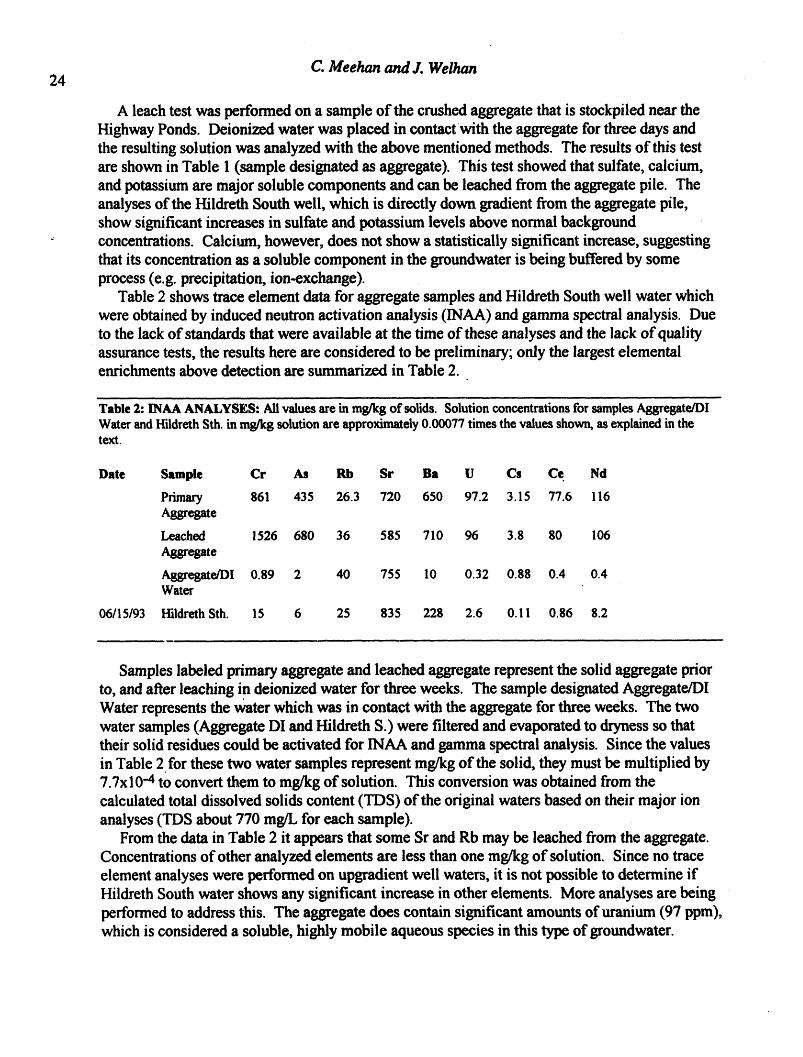
In the areaof Pocatello Creek,a tributaryvalleyimmediatelyeast of Pocatello(Figure2),chlor/de and sulfate also arecorrelatedwitha slopesimilar to thatrecognizedin themainPocatello Aquifer. In a studyof PocatelloCreekbyCH2M-Hill,it waspostulatedthatroadsaltused for winter de-icing was responsibleforthe chloridecontaminationin thatarea(CH2M-HiII,1992; Noble, 1993), but a source for the observedsulfateenrichmentwas notidentified. With

20 C. Meehan and Z Welhan
the discovery of the above mentioned road aggregate as a source of leachable sulfate in theborrow pit area, it was speculated that it may also be responsible for sulfate contamination atPocatello Creek• A casual inspection of the roadbeds in Pocatello Creek revealed that similar
road aggregate was used in their construction.Further studies were conducted to see if the chloride and sulfate trends recognized at
Pocatello Creek and in the main Pocatello aquifer may be related by similar processes. This
paper describes the initial results of this investigation and evaluates possible chemical reactionpathways which may be influenced by aggregate-derived chemical constituents.
Geologic SettingThe city of Pocatello is situated in an alluvial valley between the Pocatello Range to the north
and the Bannock Range to the south (Figure 1). These ranges consist of allocthanous upperProterozoic and Cambrian strata of the Pocatello formation and Brigham Group that were thrustfaulted during the Jurassic to Paleocene Sevier orogeny (Link et el., 1987). During theCenozoic, south-east Idaho has extended along north trending normal faults that arecharacteristic of the Basin and Range Province. In the case of the Pocatello valley this processhas resulted in a sediment filled half-graben structure. Pediment gravel terraces flanking the
valley imply several valley sedimentary filling and downcutting episodes that are thought to beLate Tertiary to Pleistocene in age (Ore, 1982).

I I
Impact of Leachable Sulfate on the Quality of Groundwater in the PocateUo Aquifer 21
Wafer BalanceUnderflow of the
Tributary Figure 2: Pocatello_::...... _ Underflow MunicipalAquifer
____ Rechargeareasto the Pocatelio
/ _ia_:: Municipal aquifer being used in the
water balance study are designated '
Bannock /_!! e_:il_neu f Rlver Losses by arrows. Also locatedonthisRange t/" _ - map arethe locationsof Pocatello
_)_'_. Highway . Creek and the Highway Ponds
_l_ _ / Portne_ Ond$ 1( studyarea. Municipal wells aredesignatedby opensquares.
Lateral __Discharge Flow ............:.:.;.:.:•:.:.:•:•:.;.:.:.:•:.:.:.::
i cho£V_v uap Recharge '
t I ' andTributary 15,000 ft. UnderflowUnderflow
iii
• . • . .
,.,.- :. Porineu f: .. ". • .- ,: IVQ
Grady ...,....: Flow Figure3:LocationMap for• .," ...
......... Highway PondsStudyArea:,'" •
North :-..... .:' .• . .
Hildreth ....: .: : :,. Map of the Highway Pondsarea..
South • Slag :::.. whereanomalouslevelsof high
Pile q_ ._. sulfate concentrations wereobserved in both surface waters and
ground waters. Located hereNorth are the samplingpoints(closed
circles),Portneuf River, surfaceSouth waters(slantedlines),Portneuf
Pit (_ Lava Flow (speckled), and the slagpile (vertical fines) thought to be thesource of the sulfate• The Union
Pacific rail line separates theind Portneuf River and the Highway
Ponds area•

22 C. Meehan and J. Welhan
The southemboundaryof the Pocatello Valley is definedbythe PortneufGap,sometimescalled the PortneufNarrows,wherethe PortneufRivercuts throughthe north-trendingBannockrange. This narrowgapis thoughtto be a superposedcanyonthat was cut by the ancestralBearRiver duringthe LakeBonneville flood as it flowed intothe Snake River(Link, 1982). Thisflood completelyerodedanearlierbasaltflow within the gap, but left scouredremnantswithinthevalley nearPocatello. Drillinghas shownlhat this flow, knownas the PortneufLavaFlow, is50 feet thick and its base is at the same level as the valley floor (Trimble, 1976). Bouldersofbasaltgreaterthan2 metersin diametercan be foundin the Bonneville flood deposits thatunderliedowntown Pocatello (Link, 1982).
Quaternaryalluviumand flood plain silts cover most of the valley floor (Trimble,1976). Thevalley strataconsists of Pleistocenelacustrineandfluvialdeposits relatedto boththe ancestralAmericanFalls Lakeand the LakeBonneville flood (See Welhanand Meehan, this volume).
Implications For Water Balance StudyThe areacurrentlybeing studied for waterbalance modelingpurposesis locatedin a small
portionof the LowerPortneufRiverBasin and extendsfrom Red Hill to the PortneufGap(SeeFiguresI and 2). The five componentsof rechargeto this valley aquiferthat arebeingexaminedare: 1) underflowthroughthe PortneufGap;2) underflowfromMink Creek; 3) infiltrationfromthe PortneufRiver; 4) lateralunderflowfrom the east dippingstrataof the BannockRange,westof the aquifer; 5) underflowfroman adjacentalluvialaquifereast of the Portneuflava flow.
As previouslymentioned,chemical characterizationof the mainaquifer_sgroundwaterandrechargesources has been undertaken. The amountof watersupplied to the aquiferbyeachsource may be calculatedusing the concentrationsof certainconstituents(i.e. sulfate,nitrate,
• chloride) in the variousrechargesources contributingto the main aquifer. The concentrationsof these constituentsin the mainaquifershouldreflectonly theiramounts as deliveredby thepreviouslydefined rechargesources. It is therefore importantto understandthe chemical impactthat roadaggregatemay have on aquiferchemistry, if the chemical mass balancemethodis toproperlyquantifyrechargefluxes.
Sampling and Analytical MethodsThe results of the chemical analysesfor the borrowpit area areshown in Table 1. Sampling
locationsareshown in Figure3. The samples labeledNorthPit, South Pit, and Pondrefertosmall bodiesof water,known as the Highway Ponds, that lie withina large gravelpit excavatedforroad aggregateduringthe constructionof InterstateHighway 15. The chemicalsignatureofthese ponds, as well as theirwater level elevations, indicatethatthey representthe surfaceexpressionof local groundwater.This is furthersupportedby the emergenceof these ponds onlyduringperiodsof above-normalprecipitationandhigh groundwaterlevels.
Regionally,groundwaterflow in the areais alongthe axis of the valley, approximatelyfromsoutheastto northwest. The sampledesignated Katsilometesrefers to an irrigationwellupgradientfrom theborrowpits and representsbackgroundaquifer waterquality. The PortneufRiveradjacentto the irrigationwell was also sampled. HildrethNorth, HildrethSouth,andOradyare residentialwells located downgradientof the aggregatepile. The sampledesignatedCate is a waterwell owned by a heavy equipmentcompany. It is located in what is consideredto
J be a separateaquifer,east of the Portneuflava flow, which is known to be locally contaminated.

Impact of Leachable Sulfate on the Quality of Groundwater in the Pocatello Aquifer 23
All samples were collected in one liter polyethylene containers and analyzed in the field forpH and specific conductance. Samples from residential wells were taken from household watertaps in which the water was allowed to run for several minutes to ensure the sample wasrepresentative of the well water. Total alkalinity for each sample was analyzed on the day ofcollection by titration with standardized acid.
After filtering samples through a 0.45 micron filter, major ion analyses were performedwithin one week of collection. Of these, sulfate, chloride, nitrate, silica, andmagnesium wereanalyzed with a HACH DR/2000 spectrophotometer, using standardized procedures and multipleruns to ensure the accuracy and precision were well defined. In some cases, dilution withdeionized water was necessary to place a sample within the detection limits of a particulartest.When this became necessary, several analyses were made at varying dilution ratios and thedeionized water itself was tested to insure its integrity. Total hardness was analyzed by EDTAtitration. Calcium was calculated by subtracting the magnesium concentrations determined fromthe spectrophotometric analyses from total hardness. Sodium and potassium were analyzed byflame atomic absorption spectroscopy. Multiple runs of analyses using the spectrophotometerhave shown the relative standard deviation at the I sigma level is less than 4 mg/l for allelements except magnesium, which was 7 mg/l. The standard deviation at the 1 sigma level forcalcium is 10 mg/l.
TABLE 1: CHEMICAL ANALYSIS FOR WATER WELLS IN THE POCATELLO AQUIFER
Concentrations of ions are all given as mg/kg of solution. Alkalinity is represented as HCO3" in mg/kg of solution.Specific conductance (S.C.) is in umho/cm. (Note: this table represents selected analyses only, and is not a completelisting of all background water compositions and other wells in the southern Pocatello aquiferfor which data areavailable)
DATE SAMPLE Ca M8 Na K SO4 CI NO$ Si AIk pH S.C.Highway Pond Area and Downgradient Wells:06115193 Hildreth S 77.0 38.4 53.7 22.2 127 54.2 14.9 24.9 356 7.6 NA12/06/93 Hildreth S 70.7 25.8 46.2 14.8 60 45 8.8 27.6 301 7.6 NA06/04/03 Pond 78 38.4 NA NA 90 50 1.3 17 376 7.5 NA06/21/93 Pond 68 38.4 43.4 10.3 100 45.2 3.08 35.6 373 8.2 72506/04/93 North Pit 74 32.4 NA NA 42 32 7.48 22.1 333 7.2 60006/21/93 North Pit 73 27 36. I 6.76 44 34.5 7.04 23.8 328 7.7 47512/06/93 North Pit 93 31.1 43.5 5.8 39 41.5 7.48 ,,,4.7 341 7.64 NA06/04/93 South Pit 66 28.8 NA NA 42 33,5 7.04 13.8 301 8.2 57506121193 South Pit 50.7 26.4 _ 30 5.26 44 42.2 3.52 11.7 290 8.2 47512/06/93 South Pit 85.7 28.7 44 5.73 38 33.5 7.04 22.3 296 8.14 NA06/15/93 Hildreth N 71 30.6 45.6 6.7 53 36.5 10.5 25.7 339 7.6 NA12/06/93 Hildreth N 77.9 23.8 38.1 6.3 43 36 8.4 25.1 305 7.5 NA
06/15/93 Grady 76 28 35.8 6.6 47 44.7 8.4 27 339 7.5 NA12/06/93 Grady 75 22 37 5.9 37 33 8.4 25 306 7.5 NABackground Water Quality:06121/93 Portneuf 61.3 20.8 24 5.03 27 27.7 2.6 21.1 253 8.3 37512/06/93 Portneuf 96.2 38.7 48.4 8.26 45 36 7.04 25.9 364 8.4 NA06/15/93 Katsilomet 66.4 27.8 45.1 7.36 44 43.5 6.16 25.2 336 7.5 406East of PortneufLava Flow:06/21/93 Care 128 58.8 69 6.62 ! l0 252 38.3 22.2 298 7.4 110012/06/93 Care 153 53.3 80 8.38 105 207 38.2 21.4 296 7.6 NA
Aggregate Leach Test:3 Days Aggregate 196 4.8 8.6 17.7 500 2.25 !.76 38.4 0.00 8.2 750
C. Meehan and J. Welhan24
A leach test was performed on a sample of the crushed aggregate that is stockpiled near theHighway Ponds. Deionized water was placed in contact with the aggregate for three days andthe resulting solution was analyzed with the above mentioned methods. The results of this testare shown in Table 1 (sample designated as aggregate). This test showed that sulfate, calcium,and potassium are major soluble components and can be leached from the aggregate pile. Theanalyses of the Hildreth South well, which is directly down gradient from the aggregate pile,show significant increases in sulfate and potassium levels above normal backgroundconcentrations. Calcium, however, does not show a statistically significant increase, suggestingthat its concentration as a soluble component in the groundwater is being buffered by someprocess (e.g. precipitation, ion-exchange).
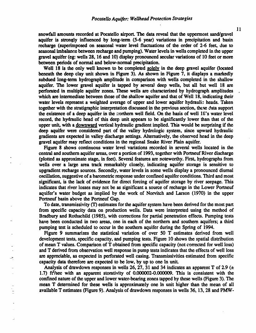
Table 2 shows trace element data for aggregate samples and Hildreth South well water whichwere obtained by induced neutron activation analysis (INAA) and gamma spectral analysis. Dueto the lack of standards that were available at the time of these analyses and the lack of qualityassurance tests, the results here are considered to be preliminary; only the largest elementalenrichments above detection are summarized in Table 2.
Table 2: INAA ANALYSES: All values are in mg/kg of solids. Solution concentrations for samples Aggregate/DlWater and Hildreth Sth. in mg/kg solution are approximately 0.00077 times the values shown, as explained in thetext.
Date Sample Cr As Rb Sr Ba U Cs Ce Nd
Primary 861 435 26.3 720 650 97.2 3.15 77.6 116Aggregate
Leached 1526 680 36 585 710 96 3.8 80 106
Aggregate
Aggregate/DI 0.89 2 40 755 10 0.32 0.88 0.4 0.4Water
06/15/93 Hildreth Sth. 15 6 25 835 228 2.6 0. I I 0.86 8.2
Samples labeled primary aggregate and leached aggregate represent the solid aggregate priorto, andafter leaching in deionized water for three weeks. The sample designated Aggregate_IWater represents the Waterwhich was in contact with the aggregate for three weeks. The twowater samples (Aggregate DI and Hildreth S.) were filtered and evaporated to dryness so thattheir solid residues could be activated for INAA and gamma spectral analysis. Since the valuesin Table 2 for these two water samples represent mg/kg of the solid, they must be multiplied by7.7x10 "4to convert them to mg/kg of solution. This conversion was obtained from thecalculated total dissolved solids content (TDS) of the original waters based on their major ionanalyses (TDS about 770 mg/L for each sample).
From the data in Table 2 it appears that some Sr and Rb may be leached from the aggregate.Concentrations of other analyzed elements are less than one mg/kg of solution. Since no traceelement analyses were performed on upgradient well waters, it is not possible to determine ifHildreth South water shows any significant increase in other elements. More analyses are beingperformed to address this. The aggregate does contain significant amounts of uranium (97 ppm),which is considered a soluble, highly mobile aqueous species in this type of groundwater.

25Impact of Leachable Sulfate on the Quality of Groundwater in the Pocatello Aquifer
performed to address this. The aggregate does contain significant amounts of uranium(97 ppm),which is considered a soluble, highly mobile aqueous species in this type of groundwater.However, the concentration of ura_t,un in solution for the prolonged leach test was less than 0.3ppb. It appears that it is not readily _..,aobilizedand does not pose a threat to groundwater.
The pile of aggregate in question appears to be heterogeneous in its bulk composition.Contraryto what was expected, the leached aggregate had higher concentrations for most of theanalyzed elements than the sample of unleached slag. Two other leaching tests performed byother parties on slag have shown different amounts of leachable sulfate. A leach test performedby CH2M-Hill yielded twice as much sulfate as our test ( R. Noble, personal comm., 1993),while another test performed by FMC on uncrushed slag had a sulfate concentration of less than1 ppm (P. French, pers. comm. 1994). These results suggest that grain size may be an importantfactor in controlling the amount of leachable sulfate.
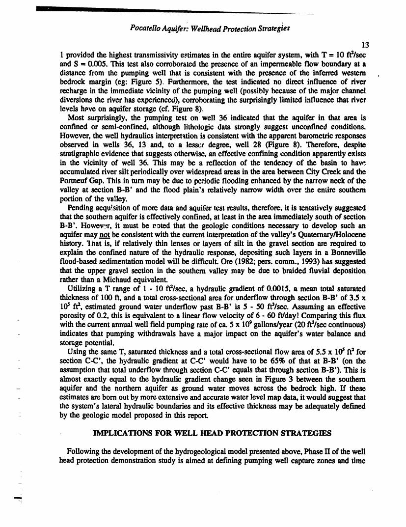
Interpretations of Highway Ponds Area DataFigure 4 is a Piper diagram that depicts the relative concentrations of the major cations
(calcium, magnesium, sodium and potass.lum) and anions (chloride, sulfate, carbonate andbicarbonate) in waters from the Highway Poi-A area, the PortneufRiver, and wells east of thePortneuf Basalt and main municipal aquifer. The lower right hand portion of this figure depictstwo trends of increasing chloride and sulfate proportions which deviate from the fight clusteringof main aquifer background water. One trend observed in wells east of the Portneuf Basalt(plotted as "-" symbols), suggests that those waters are affected by chloride alA sulfate additionin a proportion that differs from the main aquifer. The second trend shown in }_',ure 4 (as "_"symbols), reflects the addition of only sulfate in the Highway Ponds area.
Neither trend in anion compositions in Figure 4 is associated with a cation trend. Sulfate andchloride are expected to behave conservatively in these groundwaters; their concentrationschange only due to additions and source dilution. In contrast the cationic constituents (includingheavy metals) would not be expected to behave conservatively, since their concentrations areaffected by common mineral dissolution reactions, precipitation reactions, and ion exchange onclays.
It has been brought to our attention that the Highway Department may add sulfate-containingsalts to road aggregate to augment winter de-icing capabilities. However road salt used by theHighway Department contains more than 95 percent sodium chloride (P. French, pers. comm.,1994), and there has been no significant sodium or chloride observed in the leach tests on theaggregate that have been run to date. The Idaho State Department of Transportation andBannock Paving (who provided the Department of Transportation with the crushed aggregate atthe Highway Ponds) both confirmed that no additives were introduced to the stockpile inquestion (K. Magleby, pers. comm., 1994; U Robson, pets. comm., 1994).
As previously mentioned, sulfate was found to be readily leachable from the aggregatesource, and could explain the enrichment of sulfate observed in groundwater near the HighwayPonds. It is possible that the Highway Ponds area is connected hydrologically under the Portneuflava flow with the eastern aquifer, which is known to be locally contaminated with chloride,sulfate, and nitrate (see Care Well analysis, Table 1). However, our aggregate leach testproduced high-sulfate, low-chloride water, which is more characteristic of the type of watersobserved at the Highway Ponds. If the area east of the basalt were the source of sulfate for theHighway Ponds, then increased concentrations of chloride and nitrate would also be expected.
26 C. Meehan and J. Welhan
@ HighwayPonds
+ Main Aquifer A Leachate FIGURE 4
- East of Basalt ////:
Stdfate ' __Basalt ,
• ca , , , , , , , ; ; ; ; ; Q
Figure 4: Piper diagram of groundwuters from the Southern Pocatello Aquifer, Highway Ponds, and area east of
the Portneuf Lava Flow. This figure depicts two regional trends of increasing CI and SO4 proportions which
deviatefrom the main aquifer background water. Wells east of the Portneuf Basalt suggest CI and SO4 addition in
propottionsthat differ from the addition of only sulfate at the Highway Ponds. Leachate refers to the solution
derived from the lea_t_L
- " Joh FIGURE 5
_ \_ Buckskin 26_ IF X)
_ 1qa , , , , , , , , , , , , 91• ..
Figure 5: Piper Diagram of groundwaters from Pocatello Creek. This diagram displays the trend of sulfate and
chloride enrichment in Pocatello Creek groundwaters. This trend is hypothesized to be from CI derh,ed from
roadmlt and SO4 leae,hed from toed aggregate. Buckskin26 and 29 are upgradient in relation to the rest of the
waters in this diagram.

ImpactofLeachableSulfateontheQualityofGroundwaterinthePocatelloAquifer 27
couldexplainthehighsulfatelevelsinthepondthatisdirectlyadjacenttotheUnionPacificRailroad..FurtherevidenceofsulfateleachingbysurfacewatersisprovidedbythedramaticdecreaseinsulfateandpotassiumconcentrationsintheI-lildrethSouthwellbetweenJune1993andDecember 1993.Suchavariationwouldbeconsistentwitha surfacesourceofsulfatethat
was mobilizedduringspringrunoff.Percolationofthissulfate-r/chsurfacewatertothewatertablewouldraiselocalgroundwatersulfatelevelsinspring,butbyDecember,asthepulseofvadosezonerechargediminished,thelocalsulfateinputtothewatertablewouldalsobeexpectedtodecrease,withanensuingdecreaseingroundwatersulfatelevelsduetonormalgroundwaterdilutionprocesses.
Implications of Sulfate Leaching at Poeatello CreekFigure 5 is a Piper diagram displaying the relative concentrations of ions in groundwaters in
residential wells at Pocatello Creek, analyzed by the Division of Environmental Quality and theDistrict Health Department. This figure also displays a trend of chloride and sulfate enrichment(compare to Figure 4).
It has been hypothesized that road salt used for de-icing may be responsible for the chloridecontamination in Pocatello Creek ground waters(CH2M-Hill, 1992; Noble, 1993). Groundwaterat Pocatello Creek shows a direct correlation between sodium and chloride, which is alsoobserved in the Southern Pocatello main aquifer. This may suggest a similar scenario for theintroduction of chloride into the Pocatello Aquifer.
It is widely accepted that material similar to the aggregate stockpiled in the Highway Pondborrow pits has been widely used in road and rail bed construction throughout Bannock County(G. Brown, pets. comm., 1993). We suggest that features constructed with this aggregate mayprovide a source of leachable sulfate to groundwaters. After finding similar aggregate in acasual inspection of the Pocateilo Creek roadbeds, it was hypothesized that aggregate may beresponsible for the high sulfate levels observed in groundwaters in that area.
Figures 6(a) and 6(b) illustrate the linear correlation between chloride and sulfate in theSouthern Pocatello Aquifer and Pocatello Creek. Figure 6(a) shows the two trends displayed inthe Piper diagram in Figure 4 (sulfate addition and groundwater east of the Pormeuf Basalt). Athird trend in Figure 6(a) shows coupled chloride-sulfate addition that is characteristic of themain Southern Pocatello aquifer. The chloride-sulfate trend in Pocatello Creek ground waters(Figure 6(b)) is almost identical to the third trendobserved in the main aquifer in Figure 6(a).
On the basis of these data, it is hypothesized that chloride and sulfate enrichments observedin local groundwaters may be due to a combination of road salting and road bed leaching.Infiltration of runoff along roadbeds in the spring may introduce salt derived from winter de-icing applications; this chloride-enriched water may subsequently acquire sulfate from thedissolution of road bed material. Such a coupled mechanism for the introduction of road salt-derived chloride and road bed-derived sulfate would explain the observed correlation of elevatedchloride and sulfate in area groundwaters, and would imply that road runoff may be apotentially significant point of introduction for surface-derived contaminants to the aquifer. Thehypothesis for a coupled chloride-sulfate enrichment from roadbed runoff and leaching wasfurther examined by modeling the possible chemical processes and reaction paths which may beinvolved in such a scenario.
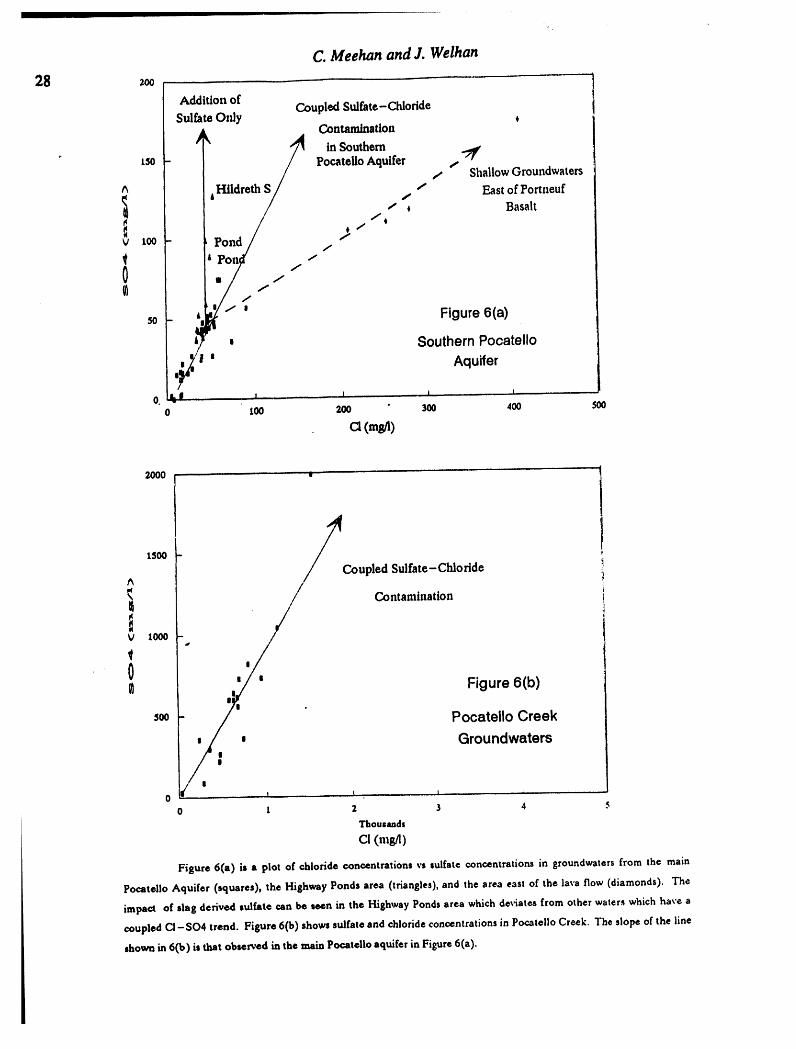
C. Meehan and J. Welhan
28 2O0 {
i Addition of Coupled Sulfate-Chloride
l / 'SulfateOnly Contamination
inSouthern" tso PocateUo Aquifer ._
t Shallow Groundwaters
, /| t), . SouthernPocatello
,_1, AquiferO. IL.i , , i i
0 tOO 20o ' 300 400
a (m_)
2000 I t
/_ xSOOL /Coupled Sulfate-Chloride
Contamination
v 100o
0_1 Figure6(b)
s00 PocatelloCreekGroundwaters
o t t _ '0 t 2 3 4 5
Thousands
C!(mgl)
Figure 6(a) is a plot of chloride concentrations vs sulfate concentrations in groundwaters from the main
Pocatello Aquifer (squares), the Highway Ponds area (triangles), and the area east of the lava flow (diamonds). The
impact of slag derived sulfate can be teen in the Highway Ponds area which de_4ates from other waters which have a
coupled CI-SO4 trend. Figure 6(b) shows sulfate and chloride concentrations in Pocatello Creek. The slope of the line
shown in 6(b) is that observed in the main Pocatello aquifer in Figure 6(a).

29Impact of Leachable Sulfate on the Quality of Oroundwater in the Pocatello Aquifer
_000 - ,, ' ' " "" "
FigUre7
NaandCi Concentrationsat PocatelloCreekI
1_00 -
f_
-I_ I I
I0_ -V I
, Sodium.' ' ' DeficitI I
II _ ...... _ _._,__ _.._w
m I
Molar1:1 Na-CIo ,,, L I • I , -
o too 2oo $0o 40o
N, (m_)
PilpJre 7: Correlation of sodium sad chloride st PocateUo Creek. These concenttstiom are
compared with a molar 1:1 ratio of sodlum vs chloride. There appears to be a deficit of sodium,
if they are mutually de_ from road mlt. This may be explained by ion-exc_nBe with days.
Reaction Path ModelingIf the changem-watercompositionsalonga hydrologicflow pathbetweenarbitrarystarting
andendingpoints is dueto theeffects of ohemicalreactionsor mixing, then the reac._onsresponsibleCotthe changecanbe quantifiedbya chemical mass balance model (Plat,truerandBack, 1980). Suchanapproachonly identifies the possible phasesand/orcomponents involvedin a set of reactions. Incontrast,chemicalreagtionpath modelingis usedto determine (1) theconditionsunderwhichthe reactionshave occurred(e.g. openvs. dosed system) (2) how thewatercompositionchangesin response to perturbationsin the system. The modelingof anaqueoussystem in this fashionis facilitated by calculations of equilibrium speciation and massbalance (Phunmeret el, 1983). Twocomputerprograms,HZrPATH (Plummerand others,1991)andMINTEQA2(Allison and others, 1991),were usedto incorporateboth of thesecalculations.
HETPATHwas used forthe massbalance calculationsto determinethe amountsof"plausiblephases"thatmustdissolve and/orprecipitateto accountfor the observedwatercompositions. Themass balanceapproachconsistsof balancing a net chemicalreactionin theform:
Initial solutioncomposition+ "ReactantPhases"=Final solution composition+ "ProductPhases"
"ProductPhases"representthose constituentsthatmust physicallyleave the aqueousphaseduringthe reaction,while "ReactantPhases"representchemical constituentsthatmust physically
30 C. Meehan and J. Welhan
"Product Phases" represent those constituents that must physically leave the aqueous phaseduring the reaction, while "Reactant Phases" represent chemical constituents that must physicallyenter the aqueous phase. The term "plausible phases" represents the reasonable choices forpossible reactants and products based on the modeler's geochemical insight and as constrainedby equilibrium speciation calculations (Plummer et al, 1983).
MINTEQA2 is a geochemical equilibrium speciation model for dilute aqueous systems.MINTEQA2 was used to evaluate models suggested by NETPATH and determine if they wereplausible in terms of their thermodynmnic requirements.
The first step was to determine the "plausible phases" that may be present and responsible forthe observed chemical changes at the Highway Ponds and PocateUo Creek. Gypsum (CaSO4)was used in modeling the sulfate component, since calcium and sulfate were derived fromleached aggregate in a 1:1ratio (Table 1). The addition of NaCI (road salt), was used to accountfor the level of chloride concentrations observed in the groundwater. Figure 7 showsconcentrations of sodium and chloride in wells at Pocatello Creek compared with the trendexpected for a molar 1:1 ratio of sodium and chloride. If sodium and chloride are from a singlesource, namely road salt, there appears to be a sodium deficiency. Ion exchange of sodium withclays may account for this deficiency. Such reactions would be of the form:
CaX + 2Na + --,Ca 2. + Na2X (1)
MgX + 2Na . _ Mg 2. +Na2X (2)
Reaction 2 could also account for the magnesium increases observed at both the Highway Pondsand Pocatello Creek (magnesium was not found to be a major constituent in the aggregate leachtest). Another plausible source of magnesium may be from the dissolution of dolomite. Forthese reasons a calcium-sodium and a magnesium-sodium exchanger, along with dolomite, werealso considered to be "plausible phases" in the modeling. Calcite and CO2 gas were also addedas phases, considering that carbonate reactions are an important chemical process for these typesof ground waters and may help explain the reaction(s) buffering Calcium. A KSO4 phase wasassumed to be a component of the aggregate and was used to model the observed potassiumincreases.
The initial NETPATH models were run using the June 1993 analyses of Katsilometes wellwater as the initial background water and Hildreth South as the final endpoint. The elementscarbon, sulfur, calcium, magnesium and potassium were used as constraints to fix the masses ofthe chosen phases that can enter or leave the aqueous solution. Initially, NaCI was not used inmodel runs, so sodium and chloride were not entered as constraints. NETPATH yielded ninepossible models that could account for the chemical signature of the water found at HildrethSouth.
Table 3 summarizes the nine possible models calculated by NETPATH. Positive valuesindicate dissolution of the particular phase, while negative values indicate precipitation. For theexchangers, positive values mean that reactions 1 and 2 are occurring as they are written; anegative value indicates the reaction is occurring in the reverse direction, so that sodium wouldbe released as free ions to solution.

31Impact of Leachable Sulfate on the Quality of Groundwater in the Pocatello Aquifer
When NaCI was included as a plausible phase (and sodium and chloride as constraints), onlymodels that contained exchangers were produced. Since sodium and chloride arc not in a molar1:1 ratio at the HildrC&well as they arc in the phase NaCI, the exchangers provide the only othersourc_ and or "sinks" for sodium. Table 3 indicates only one model (Model # 1) in which noexchangers are required.
T'ble 3" N_TIPATH"MoDEI_" _n HIGHWAY _NDs _: All values repre_, the amomlt of each P_in mmois that enters (+) or leaves (-) the solution. A (+) sign for exchangers means that reactions I and 2 occur astheyare writtenabove. Theyarereversediftheyare(-).
Mod. l Mod. 2 Mod.$ Mod. 4 ModS Mod. 6 Mod. 7 Mod. 8 Mod. 9Gypmlm 0.4901 0.4901 0.4901 0.4901 0.4901 0.4901 0.4901 0.490i 0.4901KSO4 0.3798 0.3798 0,3798 0.3798 0.3798 0.3798 0.3798 0.3798 0.3798Calcite -0.6601 .0.2252 -0.5391 0.3306 -0.7810
CO2 (8) 0.1209 0.5558 -0.5391 0.3306 0.7810Dolomite 0.4349 0.4349 0.5558 .4349 -0.2252 0.1653Ca-Exch -0.1209 -0.5558 -0.6601 -0.2252 -0.3905
Ms-Exch 0.4349 0,4349 -0.1209 0,4349 0.6601 0,2696
MINTEQA2 can be used to test whether the precipitation/dissolution reactions proposed byNETPATH are feasible given the constraints of thermodynamic equilibrium. The mass balancemethod is generally an elimination process in which calculations that identify reactions thatcannot occur are eliminated. Proof of a reaction is never positive with the mass balanceapproach, but by the process of elimination there may remain only a limited number of modelsthat are consistent with the observed chemical data (Plummet and Back, 1980).
Initially, one may use geochemical insight to eliminate certain models in Table 3. Both theHildreth South water and Katsilometes are saturated with respect to calcite. Thus Model 4 inTable 3 can be eliminated since it requires the dissolution of calcite. Model 8 is probably alsounreasonable because it requires the precipitation of dolomite, an unrealistic process for thesetypes of waters.
If the same processes influencing the Hildreth South well are also occurring in PocatelloCreek, their impact in the latter'ssetting is much greater. Groundwateranalyses of residentialwells by the Division of Environmental Quality and the District Health Department showconcentrations of major ions one to two orders of magnitude greater than in waters at theHighway Ponds. Since the combined effects of road salt and roadbed leaching seem morepronounced at Pocatello Creek, these waters were also examined to eliminate models that werenot consistent with chemical equilibrium requirements.
The samples labeled Buckskin 29 and 26 in Figure 5 refer to wells that are upgradient fromother wells in the diagram. Because these waters are upgradient and appear to be an endmember type water on the Piper diagram, they were considered to represent the initialbackground water for Pocatello Creek. The sample labeled Johnson appears to be the other end-member, most heavily impacted by chloride-sulfate addition. The Buckskin 29 and Johnsonwells were used as the initial and final wells respectively, for chemical modeling. The watercompositions used for the modeling are given in Table 4.
NETPATH was first used without sodium and chloride as constraints, and without NaCI as aphase. This produced only one model as shown in Table 5. MINTEQA2 was then used to
32 C Meehan andJ.Welhan
gypsum and 24.12 mmols ofdolomite as "finite solids." The partial pressure of CO2 was fixed atthe amount speciated in the original Buckskin water. The assumption here is that the partialpressure of CO2 at the Buckskin well is the same in the Johnson well, i.e. the system is openwith respect to CO2.
Table 4: CHEMICAL ANALYSIS FOR WELLS USED IN CHEMICAL MODELING
All concentrations given u ms/ks of mlution. Total alkalinity is given as mg/kg of HCO 3
Sample Ca M| Na . K C! S04 Tot Alk pH TempBuck 29" 49 17 20 I. I 34 27 201 7.0 15°CJohnson 590 600 376 5.3 1563 1988 590 7. I 15°C
* Note: analysis for Buckskin 29 was obtained l_om U.S.G.S. Water.Resourc._ Investigations 79-14 Open-File
Report............................................. _II I I II I III II I IIIIIII III IlmilI I I
Table 5: NETPATH MODEL FOR POEATELLO CREEK (without NsCI)All values represent the amount ofuch phase in mmols that enters (+) or leaves (-) the solution. A (+) sign for
exchangers mean# that reactions I and 2 occur as they are written above. They are reversed if they are (-).Model1
Gylmum 20.42KSO4 0.108Calcite -30.96CO2 Gas -10.3Dolomite 24.12
The final concentrations of ions in solution predictedbyM1NTEQA2 are displayed as ModelIA in Figure 8(a) as a percent of their concentrations in the Johnson well. The final equilibriumpH calculatedby MINTEQA2 was 7.04 as comparedto 7.1 at the Johnson well. However, figure8(a) shows that there is a deficit in most of the ions in the model run, compared to the observedconcentrations. Not enough gypsum or dolomite was able to dissolve to produce the amount ofsulfate, magnesium and calcium observed in the Johnson water. In addition the alkalinity(represented by HCO3 ) is much lower in the modeled water than in the Johnson water. Simplystated, this is because insufficient gypsum and dolomite were able to dissolve, as required by theNETPATH model.
An alternative reaction path consisting of two reaction steps had similar results. Model IBbogus with Buckskin water with only gypsum added as a finite solid at first. Dolomite was thenadded to the resultant water as step 2 and allowed to equilibrate. Even less gypsum dissolved inModel IB as compared to IA, because with the initial absence of dolomite dissolution, noaqueous CO3 was added to the solution, and no calcite precipitated in the first step of the model.Therefore there was no "sink" for calcium as the gypsum dissolved. The equilibrium pH for thefinal model was 7.1.
Additional mass balance models were run using sodium, chloride, and NaCI as constituents.Table 6 displays the results of the NETPATH Models with chloride as the constraint for NaCl.It should be noted that Model 2 in table 6 is the same as Model I in Table 5, with the exceptionof the NaCI phase. Two equilibrium models were again constructed with MINTEQA2 using thesame procedures as stated above, this time with 43.38 mmols of NaCI added as a finite solidphase. The results of the one step (Model 2A) and two step model (Model 2B) are displayed inFigure 8(b).

I
COMPARISON OF MINTEQ MODELs AT POCATELLO CREEK 33
t_
Figure8(a) WithoutN•CI
Diaolution
tOO
i.
o¢1 Ni Cl SOl lulI tlOO3
DISSOLVED CONS'ITIIJEI¢_
Lt- Dbtolution of Dolomite 2A: Dbmlution of CaSO4
and CdO4 in one step foUowde by Dolomite Stepwim
t
s=e i F_ure 8(b) withN•Cl
too
o
(_ Nil Ca IO4 M8 HCO3
DISSOLVED CONSTITUENTS
.oo2A Moo2B
2A: Diuolutiono[ CaSO4, 2B: DitmlutionofCaSO4 +
Dol., and NaCI in one step NaCi followed by Dol. ,tepwite
Filum 8 (a) modeb the dissolution of CaSO4 anG dolomite only. Dismh'ed ion ¢on_ntrationt are represented
as • percent of the concentrations of the utme ions in the Johnson Well at Pocatello Creek. Figure 8(b) reprments the
tame models and conditions with NaCl added as another phase.

34 C. Meehan and L Wdhan
All values represent the amount of each phase in retools that enterm(+) or leaves (-) the _lution. A (+) siSn forexchangersmeansthat reactionsI end2 occuru they erewritten above. They arereversedif'theyare (-).
Phase Mod 2 Mod 3 Mod 4 Mod S Mod fl Mod 7 Mod 8 Mod 9 Mod 10
Gypsum 20.42 20.42 20.42 20.42 20.42 20.42 20.42 20.42 20.42KSO4 0.1081 0.1081 0.1081 0.1081 0.1081 0.1081 0.1081 0.1081 0.1081
NaCI 43.38 43.38 43.38 43.38 43.38 43.38 43.38 43.38 43.38Calcite -30.96 -6.84 -41.3 6.93 -20.62CO2 Gas -10.3 13.77 -41.3 6.94 20.62Dolomite 24.12 24.12 13.78 24.12 -6.84 3.46Ca-Exeh 10.3 -13.78 -30.96 -6.84 -10.31
Mipgxch 24.12 24.12 10.34 24.12 30.96 20.65
The results are simil_ to the previous models Withthe notable exception of a large surplus ofsodium. All four reaction path models indicate that dissolution and precipitation, alone, cannotexplain the chemical evolutionary trend of the water at Pocatello Creek. Thus, it is likely thatother processes, such as ion-exchange reactions are important, as suggested by the originalNETPATH models (Table 6). This would also explain the recognized deficit of sodium inPocatello Creek waters relative to chloride. Future work on ion-exchange modeling withMINTEQA2 may yield more conclusive models. Laboratorytests are also in progress to
empirically evaluate the cation exchange capacity of local soils.
, ConclusionsSurface waters at the Highway Ponds borrow pit are the surface expression of local
groundwater for that portion of the Southern Pocatello aquifer. Well and surface waters near theborrow pits have been found to have elevated levels of dissolved sulfate. The postulated sourcefor this sulfate is a large pile of crushed slag located in the borrow pits that is used as roadaggregate by the State Department of Transportation. Leach tests performed on this aggregateyielded high concentrations of calcium and sulfate in a molar 1:1 proportion, with lesseramounts of potassium. Although the aggregate contains significant amounts of uranium (97ppm) and other trac,e metals, none were leached in significant quantities during a prolongedthree-week-long leach test. The wide spread use of crushed aggregate in road and rail bedconstruction throughout Bannock County may be providing a souw,e of readily leachable sulfateto local groundwater.
Sulfate and chloride levels in groundwaters from both the Pocatello Municipal Aquifer andPocatello Creek are correlated in very similar proportions. The coupled sulfate-chlorideenrichments observed in these waters implies a related source for both. Road salt is a likelyorigin for the chloride considering that sodium and chloride concentrations in these waters alsoshow a direct correlation.
Elevated sulfate in groundwater associated with aggregate and the coupled sulfate-chloridetrends may be related by a single process. It is hypothesized that infiltration of salt derived,chloride-rich water along roads in the spring and dissolution of soluble sulfate in roadbedaggregate as this water percolates to the water table is the mechanism by which the coupledchloride-sulfate enrichments originate.
Modeling of some of the possible chemical reactions which may be involved with sulfateaddition from aggregate leaching revealed that dissolution/precipitation reactions alone can not

Impact of Leachable Sulfate on the Quality of Groundwater in the Pocatello Aquifer 35
accountfor the observed groundwaterchemistries. Ion-exchangewithclays is likely to be animportantprocessandwould explain the deficit of sodium concentrationsin PocatelloCreekgroundwaters.Workis continuingto test the above hypothesesandto understandthe natureofthechemical processesinvolved.
Acknowledgments
The authorsgratefullyacknowledgeIdahoStateUniversityfor laboratoryspace andequipmentused in the analysespresentedhere. We would also like to thankthe CityofPocatello for its supportandcooperationin the ongoing hydrogeologicstudyof theirmunicipalaquifer. Special thanksaredue to Mr.H. Hildreth,Mr.M. Grady,BannockCounty,andthemanyotherresidentsof Pocatellowho haveallowed us to sampletheirwell waters.
Ken MaglebyandGlennGriffithof the StateDept. of TransportationalongwithLarryRobsonof BannockPavingprovidedmuchuseful informationaboutthe aggregatepile attheHighwayPonds.
We arcalso gratefulto PamFrenchand Jim ScversonfromFMCfor providinginformationaboutthe compositionandchemical characteristicsof FMCslag.
Reference# Cited
Allison, J.D., Brown, D.S., aM Novo-Grada¢, K.J., 1991. MINTEQA2/PKODEFA2, a geochemical assessmentmodel for envimnmeatal systems: version 3.0 user's manual, EPA/600/3-91/021.
CH2M-HilI, 1992. Site assessment report, Phase I, Pocatello Creek Landfill Hydmgeologic Investigefion.
Link, P.K., 1982. Idaho-Wyomin8 thrust belt: regional geology, Northwest Geology, v. ! 1, p. 1-12.
Link, P.K., Jansen, S.T., Halimdihardja, P., and Zahn, P., 1987. Stratigraphy of the Brigham group (late Proterozoic-Cambrian), Bannock, Porme_ and Bear River Ranges, Southeastern Idaho; Thirty-eighth Field Conference-1987,Wyoming Geological Association Guidebook, p. 133-148.
Noble, R., 1993. Idaho State University Geology Colloquium on 8eotechnical and hydrogeologic results of thePocatello Creek Landfill site investigation, Spring, 1993, Pocatello, Idaho.
Ore, H.T., 1982, Tertiary and quaternary evolution ofthe landscape in Pocatello, Idaho, area; Northwest Geology, v.11, p. 31-36.
Phunmer, N.L., and Back, W., 1980. The mass balance approach: application to interpreting the chemical evolutionof hydrologic systems, American Journal of Science, vol. 280, p. 130-142.
Plummer, N.L., Parkhurst, D.L., and Thorstenson, D.C., 1983. Development for reaction models for groundwatersystems, Geochim. Cosmochim. Acta 47, p. 665-686.
Plummet N.L., Prestemon, E.C., and Parkhurst, D.L., 1991. An interactive code (NETPATH) for modeling net
geochemical reactions alon8 a flow path, U.S. Geological Survey, Water-Kesources Investigations Report 91-4078.
Trimble, D.E., 1976. Geology ofthe Michaud and Pocatello quadrangles, Bannock and Power Couaties, Idaho: U.S.Geological Survey Bulletin 1400, 88p.

I
36

Hydrogeology,Ware iYmpmal,Science andPolitkaPmceedlnp 30th SymposiumEngineeringGeology andGeoteclmicalEngineering,1994 37
Interpretation Of Shallow Seismic Refraction Data Using
Raytracing Inversion: A Simple Example From A
Groundwater Resource Study In Pocatello, Idaho
J. R. Pelton
M. E. DoughertyJ. A. Welhan*
Center for Geophysical Investigation of the Shallow SubsurfaceBoise State University, Boise, Idaho 83725
*Idaho Geological Survey, Branch Office at Idaho State UniversityPocatello, Idaho 83209
ABSTRACT
Raytracing inversion of seismic refraction data acquired on the northeast side of the PortneufRiver valley at the base of Red Hill in Pocatello shows that the thickness of Quaternary and Ter-tiary sediments above much older quartzitebedrock is 46-53 m. This estimate, which was derivedindependently of any borehole data, is consistent with the lithologic log of a recently drilled mon-itoring well (PMW-3) drilled about 1 km northwest of the seismic line. The water table is hori-zontal at a depth of 22-29 m beneath a gently rising topography (20 m/km to the southeast) in thevicinity of the seismic line. The top surface of the quartzite bedrock is either horizontal or dipsslightly (1.2 degrees) to the southeast. Unsaturated sediments are characterized by a strong verti-cal velocity gradient (13-16 s"t)probably caused by compaction of the near-surface materials.Seismic P-velocities are estimated as follows: unsaturated sediments (320-780 m/s), saturatedsediments (1,670 m/s), andquartzite bedrock (2,950-3,050 m/s).
INTRODUCTION
The seismic refraction method is a well-established technique used to image subsurface inter-faces separating materials of strongly contrasting seismic velocity (a recent tutorial is in Lank-ston, 1990). Although the method has been applied to a wide variety of problems, it has made itsgreatest contribution in two geophysical specialties which aim to map the Earth's uppermoststructureat vastly different scales: engineering or groundwater seismology (upper 0.2 kin), andcrustal seismology (upper 50 kin). The principles and field procedures of both specialties are sim-ilar, but crustal seismologists have developed interpretation strategies which take advantage ofpowerful computer resources historically not available in most geotechnical or hydrogeologicalconsulting firms. As a result, refraction studies of shallow structure rely on analyses that have theadvantage of being computationally simple, but suffer from disadvantages such as the inability touse later arrivals or velocity gradients, and the lack of well-defined procedures for statistical esti-

I I i
38 J.R.Pelionand others
mationoftheresolutionandvarianceofmodel.parameters.Recentimprovementsindesktopcomputer technology have changed this situation, so that it is now appropriateto investigate theadditional capabilities offe, edby the tools of,the crustal seismologist.
We present here an example of seismic refraction interpretation of depth to bedrock usingraytracing inversion based on a two-dimensional subsurface model. The inversion algorithm wasdeveloped by Zelt andSmith (1992) and is commonly used in crustal seismology. It provides esti-mates of the random errorin model parameters that result from timing errors, and also investi-gates the degree to which individual parameters are free from the well-known trade-off betweendepth and velocity. Our data set consists of seismic travel times from a standard refraction lineacquired in PocateUo, Idaho as part of a groundwater resource study. The refraction work wasundertaken to define the thickness of water-bearing Quaternary andTertiary sediments underlainby relatively impermeable Paleozoic and Precambrian bedrock. Figure 1 shows the location ofthe refraction line on the northeast side of the Portneuf River valley at the base of Red Hill andnear the Idaho State University campus.
N
ater I
FIGURE 1. Location map showing study area. Base map is USGS Pocatello South Quadrangle (7.$ MinuteSeries, 1971, Photoinspected 1974). Scale given by length of section lines. Refraction line indicated byheavy black line at southeast end of Mountain View Cemetery. A nearby monitoring well (PMW-3 shownas black dot with cross) was drilled in 1993 (after the acquisition and interpretation of the refraction data)and encountered massive red quartzite at a depth below land surface of about 40 m.
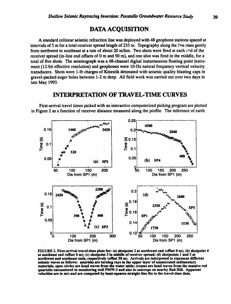
ShallowSeLonicRaytracin&Inversion:PocatelloGroundwaterResourceStudy 39
DATA ACQUISITION
A standard colinear seismic refraction line was deployed with 48 geophone stations spaced atintervals of 5 m for a total receiver spread length of 235 m. Topography along the line rises gentlyfrom northwest to southeast at a rate of about 20 m/kin. Two shots were fired at each c,d of the
receiver spread (in-line end offsets of 0 m and 50 m), and one shot was fired in the middle, for atotal of five shots. The seismograph was a 48-channel digital instantaneous floating point instru-ment (12-bit effective resolution) and geophones were 10-Hz naturalfrequency vertical velocity.transducers. Shots were 1-lb charges of Kinestik detonated with seismic quality blasting caps ingravel-packed auger holes between 1-2 m deep. All field work was carried out over two days inlate May 1993.
INTERPRETATION OF TRAVEL-TIME CURVES
First-arrival travel times picked with an interactive computerized picking program are plottedin Figure 2 as a function of receiver distance measured along the profile. The inference of earth
...... 0.25 .....L . , ,i . ..H.'_+ 4300
o.15 ,. __. :_zo o.2? _o.150.1 r
E _ EiT. 0.1_0_ 520
0.05 _ 0.05/ (a) SP2 (b) SP4
; ....... , ,, ,so 200 % loo1so2oo2soDisfrom SP1(m) DisfromSP1 (m)
,, , . .... .,....
o.2 +_.0.15 24S , (d) "-+_
._. _o.le,.-. _ . 2350m 0.1 • _ SP5
J= 39o ,toe _ s
0.05 k 0.14
) SP3 ,._/1730 1530 "_•00 100 200 300 0.12 ,_ 100 150 200 250
DisfromSP1(m) DisfromSP1 (m)
FIGURE 2. First-arrival travel-time plots for: (a) shotpolnt 2 at northwest end (offset 0 m); (b) shotpoint 4at southeast end (offset 0 m); (c) shotpoint 3 In middle of receiver spread; (d) shotpoints I and $ atnorthwest and southeast ends, respectively (offset $0 m). Arrivals are interpreted to represent differentseismic waves as follows: asterisks are turning rays in the upper layer of unsaturated sedimentarymaterials; open circles are head waves from rite water table; crosses are head waves from the massive redquartzite encountered in monitoring well PMW-3 and also in outcrops on nearby Red Hill. Apparentvelocities are in m/s and are computed by least.squares straight-line fits to the travel-time data.

40 J.R. Peltonand others
structure from these data requires correlation of different branches of the travel-time curves withthe arrival of different types of seismic waves. In problems characterized by sediments over bed-rock, the two interfaces which usually dominate first-arrival travel times are the boundarybetween unsaturated and saturated sediments (i.e., the water table) and the boundary between bed-rock and the overlying saturated sediments. Thus, a simple two-layer over a half-space model issuggested in which the first arrivals are (in order of increasing time and increasing distance fromthe seismic source): (i) the direct P-wave through the unsaturated sediments; (ii) the P-head wavefrom the water table; and (iii) the P-head wave from the top of the bedrock. The travel-timecurves in Figure 2 support the existence of all three of these waves at reasonable apparent veloci-ties. The discrepancies between the apparent velocities for similar arrivals on different shotrecords can be explained by dip, the effects of near-surface topography and velocity irregularities,timing errors, and incorrect choice of crossovers points between arrivals. In addition, slight cur-vature in the direct P-wave curves (difficult to see in Figure 2) suggests that the unsaturated sedi-ments are characterized by a vertical velocity gradient (velocity increasing with depth), probablycaused by compaction. A vertical velocity gradient will cause rays representing the direct P-waveto be curved and turn at a depth depending on the source-receiver distance.
RAYTRACING INVERSION
Raytracing is the computation of seismic wave paths and travel times through an earth modelusing Snell's law. In geophysical parlance, raytracing solves the forward problem of computingthe travel time between source and receiver for a seismic wave in a defined velocity structure.Geophysical interpretation requires solution of the corresponding inverse problem, wherein thetravel-time data are measured, and the objective is to infer the velocity structure from the traveltimes. Raytracing inversion solves the inverse problem by perturbing an initial velocity model ina systematic way until theoretical travel times (computed by raytracing) match observed times insome best-fit sense. The velocity model which provides the best fit to theseismic travel times andwhich also satisfies other known criteria such as geologic plausibility is considered to be the mostlikely interpretation.
As mentioned above, we apply here an iterative least-squares raytracing inversion algorithmdeveloped by Zelt and Smith (1992). Although this algorithm is formulated for the interpretationof crustal refraction profiles on length scales of tens to hundreds of kilometers, it is easily adaptedfor use on engineering and groundwater refraction data. A "layer-stripping" method is the bestway to proceed, in which one first inverts for the parameters describing the first layer (i.e., theunsaturated sediments), and then those parameters are fixed during inversion for the parameters ofthe second layer, and so on. In our example, we proceed as follows, using the entire data set fromall five shots (180 first-arrival travel times):
• A simple starting model is formulated based on the initial interpretation of the travel-timecurves (Figure 2) and raytracing tests; no inversions are performed at this stage. The velocityof the near-surface sediments is set equal to the average of the velocities computed along theslant path from each buried source to the nearest receiver (within I0 m).
• Parameters which control the velocity gradient in the unsaturated sediments are allowed tovary. The water table is constrained to be horizontal but its depth below a horizontal datumand the velocity of the unsaturated sediments just above the water table are allowed to vary.

Shallow Seismic Raytracing Inversion: PocateUo Groundwater Resource Study 41
After inversion, values on the diagonal of the resolution matrix are nearly unity, indicating thatno significant averaging of the true model parameters is represented in the inverse solution(Menke, 1989). In other words, the travel-time data are sufficient to resolve the trade-off 'between velocity in the unsaturated sediments and their thickness.I
• The velocity of the saturated sediments, assumed uniform both laterally and vertically, isallowed to vary. The top surface of the bedrock is constrained to I_ehorizontal, but the depth tobedrock below a horizontal datum is allowed to vary. Again, the resolution matrix indicatesthat the travel-time data are sufficient to resolve the expected trade-off between velocity of thesaturated sediments and their thickness.
• Depth to bedrock below the horizontal datum andbedrock velocity are allowed to vary. At thispoint in the inversion, adjustment of these parametershas little impact on the goodness of fit tothe observed data.
• An additional node is inserted in the model to permit the top of the bedrock to dip either to thenorthwest or southeast, and the bedrock velocity is also allowed to vary. This additional com-plexity does result in a dipping bedrock surface and a marginal improvement in the goodnessof fit, but the improvement is not statistically significant (see discussion below).
The final earth models with traced rays, observed first-arrival travel times, and calculatedfirst-arrival travel times are shown in Figure 3 for both a horizontal and dipping upper bedrocksurface.
DISCUSSION
Our interpretation indicates that the unsaturatedsediments are 22-29 m thick under therefraction line and are characterized by a vertical velocity gradient of 13-16 s"t which must be aresult of near-surface compaction. Although P-velocities for the unsaturated materials are withinnormal limits (320-780 m/s), the gradient is large and needs to be checked for consistency withamplitude information for the direct arrivals. The velocity estimate for saturated sediments is avery reasonable 1,670 m/s. In another test (not described above), we inserted an additional nodein the model to allow the water table to dip, but there was no tendency for the inversion process toforce a non-zero dip on the water table.
The first-arrival travel-time data are consistent with both a horizontal and dipping (1.2degrees southeast) upper bedrock surface beneath the refraction line. The fit to the observedtravel times is somewhat better for the dipping bedrock model, but this improvement may be theresult of random error in the travel times. To see this, a statistical model is constructed in whichthe discrepancy between any observed travel time and the corresponding theoretical travel time(computed by raytracing) is assumed to be a normally distributed random variable. The sum ofthe squared discrepancies (with each squared discrepancy normalized by its variance) is propor-tional to a random variable with a chi-square ()_2) distribution. The ;_2 for the horizontal and dip-ping bedrock models is 16.4 and 15.6, respectively, each with 178 degrees of freedom. Using thestatistical F test, we conclude that the improvement in fit (smaller ;2) shown by the dippingmodel can be reasonably attributed to random error in the observed travel times. Thus, we haveno compelling evidence that the bedrock is other than a horizontal interface. We note in passing
2that X is much greater than unity because only good quality travel-time picks have been included
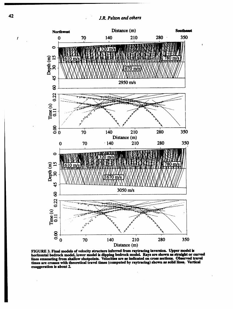
42 . J.R.Pelionandothers
Northwest Distance(m) Soulbewtt 0 70 140 210 280 , 350
I '2950 m/s
$
/ Y \0 7() IN 21'0 2i0 350
Distance(m)0 70 ' 140 210 280 350
l
780 m/s
cS -',. I-_. •
I I I I
d 0 70 140 210 280 350Distance(m)
FIGURE 3. Final models of velocity structure interred from raytracing inversion. U_per model ishorizontal bedrock model, lower model is dipping bedrock model Rays are shown as straight or curvedlines emanating from shallow shotpoints. Velocities are as indicated on cross sections. Observed traveltimes are croues with theoretical travel times (computed by raytracing) shown as solid lines. Verticalexaggeration is about 2.

ShallowSeismicRaytracIn&Inve_ion:PocarelloGroundwaterResourceStudy 43
in the inversion, and the rays are sampling more heterogeneities than have been included in themodel (Zelt and Smith, 1992).
Both bedrock models (Figure 3) indicate that the bedrock is 44-46 m below the ground sur-face at the northwest end of the refraction line. A recently drilled monitoring well (PMW-3)located about 1 km to the northwest (Figure 1) encountered massive red quartzite at a depth ofabout 40 m. This suggests that we correlate the quartzite encountered in PMW-3 with the bedrockrefractor;the velocity near 3,000 m/s is entirely consistent with this correlation.
Finally, we note that raytracing inversion yields advantages in the interpretation of the Poca-tello refraction data when compared to standard techniques such as the reciprocal method. In par-ticular, it enables us to characterize the unsaturated sedimentary layer with a vertical velocitygradient, it provides the means to investigate the trade-off between velocity and layer thickness,and it lends itself to statistical evaluation of the results.
ACKNOWLEDGMENTS
We are grateful to the numerous helpers who participated in the Pocatello field work, and tothe caretakers of Mountain View Cemetery for their assistance. Boise State University Center forGeophysical Investigation of the Shallow Subsurface contribution 0028.
REFERENCES
Lankston, R. W., High-resolution refraction seismic data acquisition and interpretation, in Geo-technical and Environmental Geophysics, S. H. Ward,editor, Investigations in GeophysicsNo. 5, v. 1, Society of Exploration Geophysicists, Tulsa, Oklahoma, 45-73, 1990.
Menke, W., Geophysical data analysis: discrete inverse theory, International Geophysics Series, v.45, Academic Press, San Diego, California, 289 pp., 1989.
Zelt, C. A., and R. B. Smith, Seismic traveltime inversion for 2-D crustal velocity structure, Geo-phys. J. Int., 108, 16-34, 1992.

I
44
. I
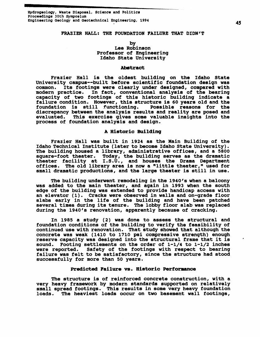
_drogeology, Waste Disposal, Science and PoliticsProceedings 30th _mposlumE_ineerlng Geolo_ and Geotechnical _glneerlng, 1994
• 45
I_ZIER HALL: THE FOUNDATION FAILURE THAT DIDN'T
byLee Robinson
Professor of EngineeringIdaho State University
Abstract
Frazier Hall is the oldest building on the Idaho StateUniversity campus--built before scientific foundation design wascommon. Its footings were clearly under designed, compared withmodern practice. In fact, conventional analysis of the bearingcapacity of two footings of this historic building indicate afailure condition. However, this structure is 60 years old and thefoundation is still functioning. Possible reasons for thediscrepancy between the analysis results and reality are posed andevaluated. This exercise gives some valuable insights into theprocess of foundation analysis and design.
A Historic Building
Frazier Hall was built in 1924 as the Main Building of theIdaho Technical Institute (later to become Idaho State University).The building housed a library, administrative offices, and a 5800square-foot theater. Today, the building serves as the dramatictheater facility at I.S.U., and houses the Drama Departmentoffices. The old llbrary area is now a "little theater," used forsmall dramatic productions, and the large theater is still in use.
The building underwent remodeling in the 1940's when a balconywas added to the main theater, and again in 1993 when the southedge of the building was extended to provide handicap access withan elevator (1). Cracks were observed in walls and on-grade floorslabs early in the life of the building and have been patchedseveral times during its tenure. The lobby floor slab was replacedduring the 1940's renovation, apparently because of cracking.
In 1985 a study (2) was done to assess the structural andfoundation conditions of the building to verify the feasibility ofcontinued use with renovation. That study showed that although theconcrete was weak (1410 to 1710 psi compressive strength) enoughreserve capacity was designed into the structural frame that it is 'sound. Footing settlements on the order of 1-1/4 to 1-1/2 incheswere reported. Safety of the footings with respect to bearingfailure was felt to be satlsfactory, since the structure had stoodsuccessfully for more than 50 years.
PTediated Failure vs. Historic Performance
The structure is of reinforced concrete construction, with avery heavy framework by modern standards supported on relatlvelysmall spread footings. This results in some very heavy foundationloads. The heaviest loads occur on two basement wall footings,

46 Lee Robinson
btlmated Sol1 Strength
Shear tests were not performed as a part of geotechnlcaiinvestigations for Frazier Hall. Shear tests on similar sites onthe I.S.U. campus in the author's file indicate a typlcal frictionangle of 28 to 30 degrees for the silt soil beneath the building,and slight cohesion of about 150 psf. Conventionally, the smallcohesion of the silt is neglected, on the basis that it is notpermanent. Analysis with a friction angle of 32 degrees, themaximum recorded in our files for Pocatello silts, did not resultin a significant increase in friction angle. However, including acohesion of 150 psf increased the factor of safety to about 1.2,using the UBC estimated loads.
In the on-slte silts, the cohesion results from very weakcarbonate cementation and capillarybonds. These mechanisms act solong as the soil is not wetted to above about 90 to 95 percentsaturation. Since groundwater levels are very deep at the site,the only realistically possible way the soils beneath the footingscould become wet, is from over-irrigation or broken waterutilities. The probability of such events wetting a significantzone beneath these deep footings is unlikely.
Boundary Condltlone In Conventlonal Bearlng Computations
To examine the effects of boundary conditions, the footingswere modelled using an elastic finite element method with thecomputer program ANSYS (6). The elastic modulus of the soil foruse in the model was computed from consolidation test data using amethod proposed by McCarthy (7). This method of selecting anelastic modulus is appropriate for estimating settlements, but notfor predicting failure. The settlements predicted by the finiteelement model (about 2 inches) compare favorably with thoseobserved and predicted by consolidation theory (about 1-1/2inches). The elastic model also allows the soil to experiencetensile stresses, which becomes a significant error at or nearfailure. Within these limltations, it is still possible to drawsome qualitative conclusions about the effects of boundaryconditions.
The results of the finite element analysis are summarized bystress contour plots in the figures below. In comparing these
• plots, note that the contour interval set by the software variesfrom plot to plot. To make it easier to see the relatively smalldisplacements, values 10 times the actual values are plotted. Theanalyses for both footings were made for a wall load of 15 kips perfoot, intermediate between the actual loads to+ allow directcomparison of the results for the two walls.
The Central Basement Wall--The central basement wall is embedded2.0 feet below the top of the basement floor slab. The finiteelement solution for this case, together with the Boussinesq caseis shown in Fig. 1. The average vertical stress beneath thefooting is plotted as a function of depth for these cases as lines

Frazier Hal1: The Foundation Failure Chat Didn'C47
loaded at an estimated 4500 and 5_00 psi. Conventional Terzaghi-Vesic bearing capacity analysis (3) predicts failure of each ofthese footings, at factors of safety of 0.76 and 0.57,respectively:
Several reasons have been suggested for the apparentcontradiction between the analysis and performance. These include
(1) Estimated loads may be conservative;(2) Redistribution of loads by the frame may have lowered the
actual bearing pressure;(3) Soil strength nay have been underestimated.(4) Boundary condition effects not considered by conventional
theory may have resulted in under predicting failure capacity, suchas e_d_nt of the footings, and backfill against the westbasement wall.
Each of these factors are addressed below.
btlaated Loads
The loads consist of about 70 to 76 percent dead load, and 20to 24 percent live load estimated from Unlfora Building Code (UBC)tables (4), and Idaho snow load tables (5). On the west basementwall, about 1/3 of the llve load is snow load, whereas snow load isinsignificant on the east wall. Based on risk levels assumed inthe snow load tables, there is about a 2/3 probability that thedesign snow has occurred or been exceeded once during thebutldtng's existence. The remaining live load is largely from thestage of the naln theater, the seating of the little theater, andaudiences leaving and entering the theaters. These loads arebelieved to be quite conservative since performances are neverscheduled simultaneously in both theaters simultaneously, and theaudience cannot be in the halls and the seating at the same time.We estlmatethatthe actual naxlmumllve load is probably about 1/2to 2/3 of the total predicted by UBC. This would result in atleast a16 parcentunder-estlmate of the bearing capacity computedusing UBC live load.
Load Redietribution
Several lightly loaded concrete spur walls intersect theheavily loaded walls. Observed cracks in these spur walls suggestthat the intersections acted as "Tee" colunns, with foundationloads redistributed perhaps 3 feet or so down the spur walls.Lightly loaded walls at the ends of the corridors act in a similarfashion. On this basis, we estimate that load redistribution hasincreased the effective footing area by about 20 percent, on eachof the two heavily loaded walls. This would result in about a 20percent over-estlmate of the bearing capacity, for computationsbased on the direct bearing area.
li , ,I

m
48 Lee Robinson
........................ ii iii.Ul nnl iii n I III I lnllll II I I
-- [ I nnuu j
WALLWITH NOEHBEDHENT(BOUSSINESQCONDITION) Feb 3, 199411'18:41
MINDr.1ZU =1DIST=18,479
_ -13.KltiI -U, 1_1
-9,19_
-5,331
Fig. 1--Vertical stress beneath the central basement wall (embedded2 ft) and for no embedment (Boussinseq condition). Displacementsare shown multlplled by 10.

Frazier Hal1: The Foundation Failure that Di dn°t 49
VERTICAL STRESS iksFl0 1 2 3 4 5
IZl ' '//4"6 "t KEY:10.5 'F£ BACKFILL. ONE SIDE
3 ' A- BRACED TOP CI'4LY
DEPTH B- BRACED TOP AND BQTTOMAND UNBRACED
[ F L] BACKFILL ON BOTH SIDES
6 C - 1.5 FL EMBE[:::II_NTD - I',EI EI_BEDMENT
(BOUSS]NESQ)
......
Fig. 2--Average vertical stress beneath wall footings for 15 kip/ftwall loads for various boundary conditions. I
i • 2. Note that the bearing pressure at the. base ofC and D on F g . _ _ about 67 percent tna_ o_d foorin is predicted to be
the e_dde g we assume this ratio applies to thethe unembedded case. IfTerzaghi analysis, a depth correction factor of 1.43 results. Incomparison, Vesic uses the Brinch-Hansen correction factor whichcomputes to be 1.14. In comparison, Meyerhof's depth c°rre?ti°n-factor computes as 1.4, closely corresponding to the finite element
his basis, it appears that the Brinch-Hansen correctionvalue, uOs_dtin our original bearing capacity analysis appears to befactorsomewhat conservative for this case. Use of the larger depthcorrection in the analysis would result in an increase in predictedbearing capacity of about 20 percent.
The West Basement Wall--The west basement wall has backfill againstone side and a concrete floor on the other. If the concrete floorwere strong enough and well enough bonded to the wall and footing,the two basement wall footings and the slab would act as a mat
. This ssibility was analyzed as shown in Fig. 3.foundation ___ .._..po tensile stress in the floor slab at theNotlce _ne 9
ootin --well above the tensile strength of theedge of the f . g- - o crack at the edge of the
Thus the sl-b is predicted t sconcrete. . , ..... an of tt.e wall load •footing and lS not exp,uted to support YIndeed, the floor slab of the actual structure has uracked at theedge of the footing as predicted.
This wall is well braced at its top and partially braced atits base by the cracked basement floor slab. We modelled the wallfor the fully braced top and bottom (at-rest condition), and the

50 Lee Robinson
1 FULLY BRACEDWALLTIED TO FLOORSLAB Jan 31,, 199411:51:85
MlNll=lZ9 --1DIST=11.55XF --13.5'tF -18.5
-118.5"/'-1BB._I9-81.927
Jl_aLsenentvail
Fig. 3--West basement wall, with concrete floor actingmonolithically with the footing.
fully braced at the top and unbraced at the bottom (archingcondition), as shown in Fig. 4. The actual condition with partialbracing at the bottom would be expected to fall between these twolimiting cases. Because of the bracing, this wall would not beexpected to develop the active condition, shown for comparison inFig. 5.
For both conditions shown in Fig. 4, some of the wall load istransferred to the backfill by friction between the wall and thebackfill, which will reduce the effective vertical pressure beneaththe footing. This results in an increased vertical stress to theleft of the wall in comparison to the cases shown in Fig. 1, but areduced vertical stress beneath the footing. This effect is shownin Fig. 2. on curves A and B. The fully braced and unbraced casesresult in essentially the same vertical stresses beneath thefooting, but the wall braced at the top has slightly lower verticalstress immediately beneath the footing.

I
Frazier Hall: The Foundation Failure that Didn't 51
basement IF_g_ _a----West basement wall modelled for the at-rest condition.
The cracked floor slab would be expected to allow some lateralAccording to the finite element model, a lateralmovement.
displacement of only about 0.I inch is sufficient to reach thearching condition of Curve B. The appearance of cracking in thefloor slab suggests that there has been sufficient displacement toachieve the arching condition.
The conventional application of bearing capacity theory to awall with backfill ignores the effect of the additional backfilloutside of the wall but does reduce the bearing capacity for the' (2 feet, in this case). If we. ment of the two sideslesser embed ..... ,.... _.._tion in effective bearing
that _ne relative L_-_aain assume ........ I.._^. a-nlies- an increase ing fro TM the finite element _u_u_,v,, r_ _ • ..... ---pressure -'_- -" about 25 percent results Erom the 9acK_Dearlng capacity uL
_ e effect of the conservatism of the Brlncn Hanseneffect. If th an increase of about 55 percentdepth correction is included,
- results.
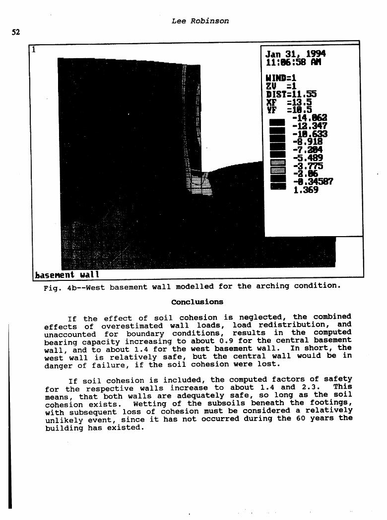
wall
Fig. 4b--West basement wall modelled for the arching condition.
Conclusions
If the effect of soil cohesion is neglected, the combinedeffects of overestimated wall loads, load redistribution, andunaccounted for boundary conditions, results in the computedbearing capacity increasing to about 0.9 for the central basementwall, and to about 1.4 for the west basement wall. In short, thewest wall is relatively safe, but the central wall would be in
danger of failure, if the soil cohesion were lost.
If soil cohesion is included, the computed factors of safetyfor the respective walls increase to about 1.4 and 2.3. Thismeans, that both walls are adequately safe, so long as the soilcohesion exists. Wetting of the subsoils beneath the footings,with subsequent loss of cohesion must be considered a relativelyunlikely event, since it has not occurred during the 60 years thebuilding has existed.

, Frazier Hall : The Foundation Failure that Didn 't 53
- [1 UNBRACEDWALL (ACTIVECONDITION) Jan 28, 199411:57:25 All
MIND-1ZU --1BIST=11,55XF =13,5VF =10.5
-28,568m -25.142
-21.716-18.289-14.863-11,437-8.011-4,584
kaseemnt wall
Fig. 5--West basement wall modelled for the active condition.
If Frazier Hall were being constructed today, undoubtedly
lar@er, safer footings would be used. Based on history, however,It is evident that the existing footzngs are probably adequate forthe remaining life of the structure.
This study illustrates that typically we as engineers tend tobe conservative in estimating loads and their redistributionthrough the structural frame, soil strength properties, and in
development_f computation methods. When the combination of theseconservatlsm accumulate, significant error can result.

54 Lee Robinson
References
(1) Robinson, Lee, G@otechnical Investiaation. Frazier Hall TowerIK1_, Chen-Northern, Inc., Boise, ID, February 1992.
(2) Narkiewicz, S.N., GeotechnicalEvaluatlon and Concrete Testina.Frazier Hall. ISU, Northern Engineering and Testing, Inc., Boise,ID, March 1985.
(3) Fang, H. S., Foundation Engineering Handbook, 2nd. ed., VanNostrand Reinhold, New York, 1991. pp. 144-165.
(4) Uniform Buildlna Code--1988 Edition, International Conferenceof Building Officiais, Whittier, CA. 1988.
(5) Sack, R. L. and A. Sheikh-Taheri, Ground and Roof Snow Loadsfor Idaho, University of Idaho, Department of Civil Engineering,Moscow, ID, 1986.
(6) DeSalvo, G. J. and R. W. Gorman, ANSYS Engineering Analysls_, Revision 4.4A, Swanson Analysis Systems, Inc., Houston, PA,1990.
(7) McCarthy, D. F., Essentials of Soil Mechanics and Foundations,4th. ed., Regents/Prentice Hall, Inc., Englewood Cliffs, NJ, 1988,p. 427.
I I
Hydrogeolosy, Wast_ Disposal. Science andPolitics 55Proceedings30thSymposiumEngineeringGmlogy and GeotechnicalEngineering,1994
GROUNDWATER DEVEIX)PMENT IN GRANITIC TERRAINBOGUS BASIN SKI RESORT
BOISE, IDAHO
ByWilliam C.B. Gates, P.E., P.G.
Manager, Water Resources Engineering ProgramCraig L. Parkinson, P.G., Hydrogeologist
Kevln L. Schroeder, GeologistKlein/elder, Inc.3189 Mill StreetReno, NV 89502
ABSTRACT
Groundwater development in the Bogus Basin Ski Area of the Idaho-Sawtooth batholith hasbeen largely ignored because of the assumption that granitic terrain produces littlegroundwater.
This l_per demonstrates the contrary is true. Groundwater in the Bo_us Basin area is largelyfracture controlled and daylights the basin headwalls as springs ano seeps. Bogus Creek,Sharer Creek and Pine Creek receive their base flow from these springs.
Fracture trace analysis combined with structural mappin_ demonstrated a high potential fordeveloping groundwater. The fracture trace analysls and geologic mapping of thediscontinuities (fractures, joints, faults, etc.) in the bedrock show there are three major jointsets (NT0°W, N20°W, and N20°E) intersecting the rock mass of Sharer Butte. Throughdifferential erosion, Bogus Basin has opened up along one of these fracture zones. Thesefractures are the primary producers of groundwater in the Bogus Basin area.
Test wells targeted at the intersection of these major joint or fracture .sets exhibit _ficcapacities ranging from 0.54 gpm/ft to 0.96 gpm/ft with estimated sustained yields of aboutI00 gpm. These values are acceptable for gramtic _r_... The results of the hydrogeologicalinvestigation indicate Bogus Basin groundwater is pnmarily fracture controlled. There appearsto be sufficient water resources for a small well field to Support snowmaking operations.Analysis of the groundwater demonstrates the water is of excellent quality.
INTRODUCTION
Since 1942, Bogus Basin Ski Resort in Idaho has provided magnificent long _o_ of na.tt_ralsnow to skiers. Unfortunately, mother nature doesn't always work with these winterwonderlands in producing the preciseweather for these ski-filled days. Bogus Basin decidedto do something about it by looking into the feasibility of developing groundwater resourcesfor snowmaking.
Bogus Basin Ski Resort is located 16 miles north of Boise on the shoulders of Sharer Butte(Figure I). It is the second largest night siding resort in the pacific northwest, with five miles
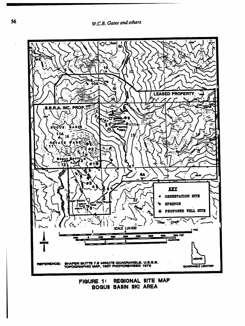
56 W.C.B.Gates and others
FIGURE 1: REGIONAL SITE MAPBOGUS BASIN SKI AREA

Groundwaterdevelopment,BogusBasinSkiResort 57
of Ughtednightruns,nllowingthenever-tiredskierto ski 13continuoushours. BogusBasinoffe_ 46sld runsand over 1,800 feet of verticaldropon 2,640 acres.
Up until the 1992/93 ski season: many of the ski areas suffered with ski visits drasticallyreduced below normal, a reflection of past droughts throughout the western United States.During this time, Bogus Basin peri'odicallycollected surface water,from the springs off themountain to aid in their mowmaking..They currentlyhave water nghts to the surface waterfrom November through March to provide the water for portable snowmaking fan jet guns.theycurrentlyhave in-place. Fortunately,they.are able to impound some of the.waterm a 48-inch culvert for storage. The man-madesnow ts used to cover up some of the high volume skiareas and provide patchwork at variouslocations on the mountain.
The bedrock g_logy of .BogusBasin Ski Area is composed of granites of the IdahoBatholith.Typically, gramtic terrmnsuch as this produces little groundwater, therefore, groundwaterweus were neverdrilled in Bogus Basin.
METHODOLOGY
To conduct the groundwaterresources feasibility investigation, fracture trace analysisof aerialphotographswas combined with mappingof the discontinuitiesin the graniticoutcropsexposedat the ski area. Fracturetrace analysis was conductedon both color and black and white aerialphotography. To verify .whiCh fracture traces were indeed fractures (joints, faults), thediscontinmfies in the gramttc outcrops surroundingBogus Basin were also mapped. Thesefractureattitudes were thenplottedon "equatorialequal-areas.tereonets"as poles to the planes.Great circles normal to the pole clusters representthe location of major fracture sets. Thelocation of the major fracture sets were verified by overlaying the stereonets on the aerialphotographs and .topographicmaps. The goal was to target intersecting fracture sets for thetest wells. These intersectionshave provento producehigh yielding wells.
GEOMORPHOLOGY
Bogus Basin Ski Resort lies completely in the northern Rocky Mountain physiographicprovince. Shafer Butte is the highest peak in the Bogus Basin area, attaining an elevation of7,582 feet. The main topographic featuresin the region are the granitic peaks trendingnorthto northeast, reachingelevationsabove 7,500 feet.Specifically, the resort occupies a portionof Boise Ridge which is partof the Atlantasection of the IdahoBatholith.
STITIGRArSY!
The oldest rocks in the region are Cretaceous age graniticrocks of the Idaho Batholith. In theBogus Basin area, and specifically Shafer Butte, the rocks are mainly biotite-moscovitegranodiorites(Mitchelland Bennett, 1979).
Southwe_t of Bogus Basin, remnants of the ColumbiaRiver basalt flows cap the granites assmall butt_ and mesas. These are of little importancein the Bogus Basinarea.
Younger (Quaternary .age) unconsolidated alluvial, colluvial, and residual deposits mantlesome of the lar_gerbasins such as Bogus Creek Basra and Pine Creek drainage. Depth andextent of these deposits are unclear.

58 W.¢.B.Gatesandothers
STRUCTURE
T_ age faulting formed the dominant features of the Boise area. Boise _occuPiesthegraben basin of a downthrown block similar to the Basin and Range _ to _ south.Thefaulttracestrikesnorthwest,approximatelyattheeasternedgeofthecitylimits.Mostofthefaultsarenolongeractive,
According to Lewis and Young (1982), several majornorth, northwest, and nc_he_ trendingfault systems have been .mapped.in the Boise River Basin southeast of SharerButte andBasin, and the Payette RiverBasin to the northwest. These faults appearto be high angle andhave dipslip movement.
Field m.apl?ingof the Bogus Basin area indicates the granitic rock as very shattered withthr?ugh-gomgfractures. Lineamentsand fracturetracesno.tedon the topographic mapand theaerial pho._.gmphs suggest thrpe major _frapturezones (Figure 2). The zones est_li_ anaverage stoke of N70°W, N2WW, and N'20°E.
During the field mapping, 1,153 fractureattitudesat 12 stations were obtained (Figtm_ I).Analy._s of the Schmidt.net verifies there are three major steeply dipping fracture sets withassocmtedsmallersets (Figure3).
FractureSet Attitudeand Dio Direction
loint Set I N70°W - 60°SW
Joint Set 2 N20°W- 60°NE
loint Set 3 N'20°E- 6(PNW
Some of the fracture sets appear to be parallel _ zones wi._. _ appa_t offsets andslickens_des. However, there are no apparentmajor offsets indicating major faulting. Thefracture sets are more likely joints..Width between fracturesranges from 1 inch, suggestingplaty cleavage, to 5 feet. The w_dth of ,fracturmrange between .<1/4 inch to2 feet.Observation of the fractures at various stattons suggest the subordinate fracttue sets areactually subsetsof the same dominantsetsand overall system.
In some areas, quartz and basalt dikes were noted inflliing the fractures. One esveciallyprominentbasaltdike (approximately2 feet wide) strikeseast-west and _els Joint ,_etNo.I near Suicide Gully (Figure I).
The apparentjoint sets compare and overlay favorablywith some of the major _ tracesobserved on the air photos (Figures2 and 3).
S Creek within Bogus Basin lies at the. in_..on of these three fracture sets. Int/on, Bogus Basinopens to the west following the _ of Joint Set No. 1, after which the
creek bends to the northand follows the.northwest stfildng loint Set No. 2. At the base ofShowcase chairareaand Mornmgstarchairarea, all threejoint sets appearto inmaect.

59
FIGURE 2: FRACTURE TRACE ANALYSISBOGUS BASIN SKI AREA
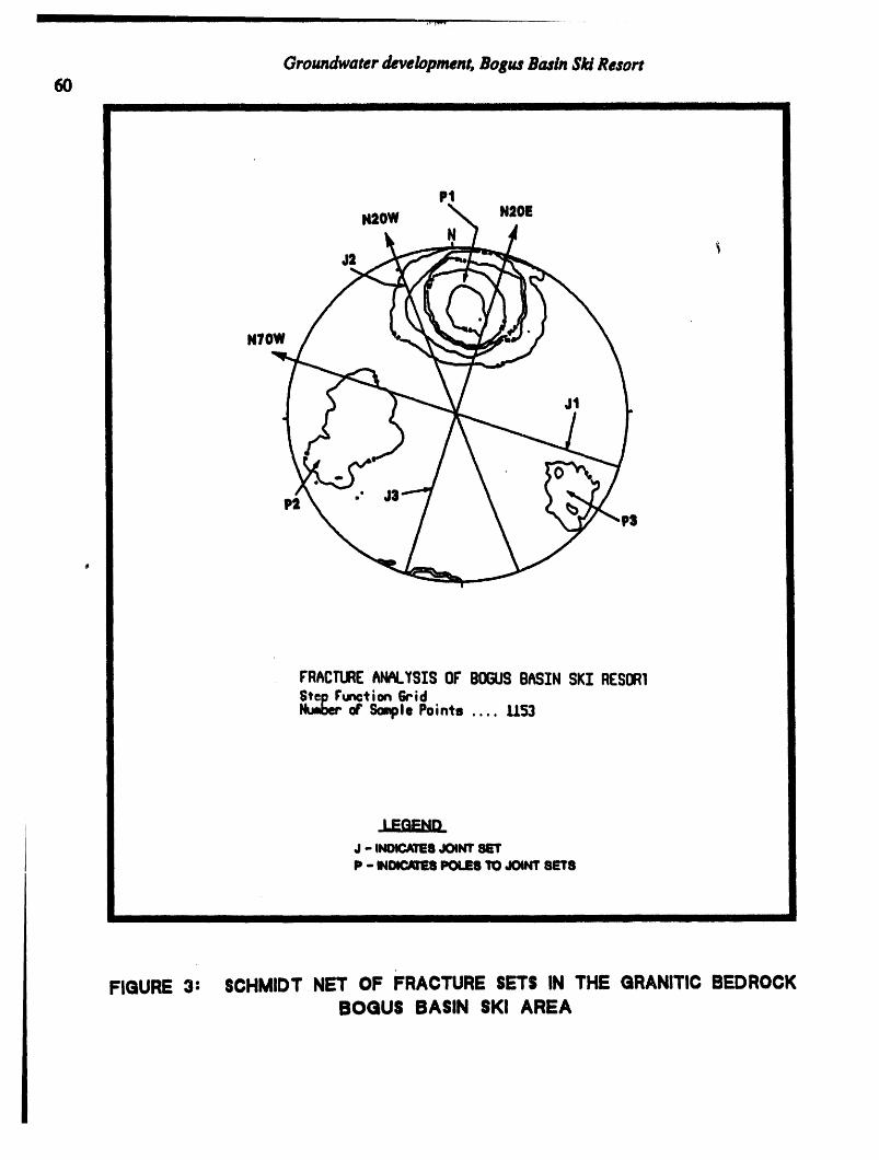
Groundwaterdevelopment,BogusBasinSkiResort6O
P1N20W N20E
NJ2
NTOW
J1
FRACTURE&I_I.Y$[SOF'BOGUSI_,SINSKI RESOR1runct ion Grid
or SamplePoints .... 1153
d- INOICATE8JOINT8E1"P- IN0CRT:8POLES10 JOINT8ET8
FIGURE 3: SCHMIDT NET OF FRACTURE SETS IN THE GRANITIC BEDROCKBOGUS BASIN SKI AREA

W.C.B.Gates and others 6!
HYDROGEOLOGY
During the aerial photographyreview, several w with apparent springs and seeps wereidentified. The locations of these springswere verified during the field rec_.nnaissance. Thereare at l.e_t 12 spring,sites around the Sharer Butte area. These spring and seep areascharacteristicallyhave mcreased vegetation (mountainalder, maple, ash, etc.) around them.Ma:,.yof the springs and seeps follow lineartrendssuggestin,g they are frac_re controlled_ Allof these fracture sets have some shallow dipping planes, re.eludedas part'of the set. Theseplanes appearto intersect and daylightthe slow_ forming spnngs and seeps,
In addition, the densely fracturednature of the rock provides storage and a _oir forgroundwater. This is especially true in Bogus Creek Basin where all three sets mters_,t.Moreover, the surficial deposits overlying the fracturedgranite may provide a good reservotr.
PRIMARY AREAS FOR TEST WELLS
Three test well locations were located in the n..arrowvalley bottom of Bogus Creek(Figure 1). According to Pari_k (1976), tn.'butaryvalleys (such as the Bogus Creekheadwaters)may be controlled or localized bydifferential weathering _ong zones of fractureconcentrations revealed by fracture traces.. Moreover, the results of._he, structuralmappingverified the concentrationof joint sets in this location. Therefore, verti_d water wells locatedwithin narrow valley bottom settings have an increased probability of penetrating zones offracture concentra..fions. These zones, because of the fractures, have a .higher degree ofhydraulic conductivity and porosity. Thus, they provide an ex.cellentaquifer System. Thefracture sets leading to the concentration offr_turesactas "ptpe conduits" for additionalgroundwaterflowage to the area.
Test Well #i (Showcase Chairlift)
The lithologic log for Test Well #I indicatedabout 42 feet of alluvium overlies moderatelytohighly weathered Cretaceousgranodiorite. The 6-inch test well was drilled to a total depth of500 feet. Multiple fractureswere encounteredthroughoutthe depth.
Groundwater was encounteredat about 75 feet below the surface. AirLiftyields started atabout 3 to 4 gpm and increasedwhen additionalfractureswere intersected for a total of about45 gpm. The majority of water was encounteredbetween 325 to 500 feet in the highlyfracturedand weathered zones of the granodiorite.
Test Wen _ (Morning Star Chairlift)
Test Well Y2 was drilled to about 350 feet without intersecting water and, therefore, wasabandoned.
Test Well #3 (Showcase Chairlift)
Test Well #3 is approximately 220 feet southeast of Test Well #1 and 26 feet higher inelevation. Therefore, the litho!.ogicsections for these wells are quite similar, exhibitinghighlyfracturedand weathered granodlonte.
I
Groundwater was first encountered at about 25 f_t and yields increased with increasingfracture density, similar to Test Well #I. Total ]held by airlift was about 80 gpm. Themajorityof the groundwaterfromTest Well #3 was from fracturesbetween 220 to 400 feet.
| H I . I IIII
Oro_ater development,Bo&_ BaslnSkiResort62
STEP-DP_4WDOWNPUMPING TEST
Step-drnwdown and Recovery Test
TestWell#Iand#3 lieon thesamefracturesetSeval(FiL_eua_2). Becauseofthis,anextendedstep-drawdown pump test was conducted to the hydraulic characteristics of therock aquifer. Prior to the test, the static waterlevels (SWL) for Test Well #I and t'3
were 12.42 feet and 32.87 feet. Discharge rates during the st,p-test ranged from about 30gpm to 200 Spin. Once the SteP-testwas complete, the discharge rate was reduced to asustainedrateof apprommately45 Spin for the next 20.6 hours.
After the pumping test, Test Well #1 recovered to within 49.6 feet (22M) of the SWL 60minutesafterstopping the pumpand recovered to within 7.7 feet (88_) of SWL at the end ofthe recovery test.
The test data indicated the specific capacity.(rate of discharge per unit drawdown) for TestWell #3 ranged from 0.96 gpm/.fiat a pumping rateof 30 Spin to 0.84 gpm/ft at a rateof 60Spin.. Calculated specific capacstiesranged from approxima_ly 0.78 gpm/ft at a theoreticalpumping rateof 80 Spin to 0.54 spm/ft at a rate of 200 gpm.
Aquifer Characterkt|cs
To assess the aquifer transmissivi_, the .authors used .the Jacob straight-line method.TranSmissivity('13is the rate at which an aquifercan transnutwater througha unit width of an_lui.fer under a unit hydraulic gradient. This method is based on an approximation of theThins equation derived by la_. and Cooper (Driscoll, 1989). The assumptionsfor the Theisequationare summarizedby Dnscoll (1989) as follows:
1. The water-bearingformationis uniform in characterand the hydraulic conductivity isthe same in 'all directions. _ghiy fracturedrock approximatesporous media in thisaspect of groundwaterhydratdics.
2. The formationis uniform in thicknessand infinite in areal extent.
3. The formation receives no rechargefrom any source.
4. The.pumped well penetratesand receives water from the full thickness of the water-bearing formation.
5. The water removed from storage is discharged instantaneously when the head islowered.
6. The pumping well is 100% efficient.
7. All water removed from the well comes from aquifer storage.
8. Laminarflow exists throughoutthe well and aquifer.
9. The water table or potentiometricsurfacehas no slope. ,
The hydraulic characteristics of the aquifer and wells satisfy these assumptions enough toobtainreliableT values.

W.C.B. Gates and others 63
The Jacob straight-.linemethodinvolv..plotting the drawdo.wndataversus time on a semilogscale to form a straightline. From thss line, T was solved using the following equation:
T,_ 4S
_/here"
T - transm.issivity(glxi/ft)Q - pumpingrate (gpm)As - drawdownduringone log cycle (ft)
The T of the aquifer was calculated using data from the first step of the st._rawdownpumpingtest.
Therefore:
Test Well No. 3:
T -,. (264)(30 gpm) =, 474 gt_ft or 63.4 ft2/d16.7 ft
where:Q =30 gpm (pumpingrateduringfirst step of steP-drawdowntest)AS= 16.7 feet (from drawdownversus time graph)
The transmissivi_ of the aquifer is estimatedat 474 glxi/ft (63.4 fl2/d), which is typical forfracture flow aqmfers m graniticbedrock.
, Applying ideal groundwa.te.rflow equations to fracture-flowsystems may !..e_tdto significanterrors because flow velocittes m fracturescan exceed the laminarflow conditions assumed byideal flow equations. Additionally, irregularfracturezones 1_ groundwatermovementand devia_..ft:om the homogenous and isotropic conditions in typscal sedimentaryaquifers.However, if the fracturesare narrow, closely-spaced, and interconnected, the fractured.rockmass approximatesa .coar_.._.greed porous mediumwith small in_ula.r openings (lVleiserand Earl, 1982). Takingthis into consideration,the T value obtained from the Jacob me.tl]odwill give a general indication of the transmissive be_vior of the fracture flow aquifer.Therefore, the transmissivitycalculated for the aqmfer gsves a reliableapproximation of howmuch water the fracturesmay yield.
The storativity of the aquiferpenetratedby the test wells was also estima.tCd.Storativityis thevolume ot water an aquifer releases from or takes into storage per umt surface area.of theaquifer per unitchange in head @riscoll, 1989). We estimated the aquifer has a storativityo_0.38, which indicates theaquifer ss unconfined.
Potential Yields
The potential yield for Test Well #3 was estimated using the aquifer test data and data fromother wells ¢ ,mpleted in fracture aquifers. Potential yield is typically estimated using theconcept of specmc capacity.
Specific capacity is the pumping rate divided by the amount of drawdown at that rate and ismeasured as gallons per minute per foot, gpm/ft. The potential yield of a well can be

64 Groundwater development, Bogus Basin Ski Resort
estimated by multiplying the specific capacity of the well by the available drawdown: gpm/flx fl = gpm. However, stressing an aquifer by increasing pumping will almost alwayssignificantly increase the drawdown, thereby decreasing the specific capacity. Accordingly,using the specific capacities calculated for low test pumping rates will result in too high anestimate of potential yield.
To estimate the potential yield of a well it is necessary to calculate how much head is availablefor withdrawal from the well. This value is the total amount of drawdown available, which isthe interval from the SWL to 20 feet above the pump intake setting. In Test Well #3, the finalpump intake will likely be set about 10 feet from the bottom of the well. Therefore, the totaldrawdown available is from the SWL to 30 feet above the bottom of the well. The SWL isapproximately 30 feet and the well is 400 feet deep, which indicates the total drawdownavailable is approximately 340 feet.
The step-drawdown test data was used to estimate the drawdown at higher pumping rates thanthose achieved during the actual pumping test. The results are then used to determine potentialsustained yields. A pumping rate of190 gpm was calculated to produce a drawdown of 340feet, which is the total available drawdown. Therefore, the maxtmum potential yield of TestWell #3 is lg0 gpm. However, pumping at this rate will probably dewater the well rapidlyand cause cavitation of the pump. The authors recommended pumping the well at no morethan 100 gpm for a period of 8 hours, followed by a 16-hour recovery period.
Impact of Wells on Groundwater and Springs
Groundwater production from Test Wells #1 and #3 is fracture controlled. These two testwells are located within the same fracture system and exhibit a strong hydraulic influenceupon each other. This hydraulic connection was demonstrated during the step-drawdown testwhen drawdown in Test Well #I was observed while pumping Test Well #3. However, thetest wells were installed in an area which appears to be an unique flow regime based on thefracture trace analysis. Wells and springs which are not located along the same fracturesystem as Test Wells #1 and #3 will not be significantly affected by pumping the test wells. ,
CONCLUSIONS
Based on the results of the investigation, there are several potential well locations offeringfavorable conditions for groundwater development in the Bogus Basin area. Bedrock is highly_fracturedgranitic rock. Groundwater is primarily by fracture flow and controlled by the majorfracturesetsstrikingNT0°W, N20°W, and N20°E. The followingisa summary of thehydrogeologic investigation conducted at Bogus Basin:
• Test Well #1 and #3 rely on fracture flow for groundwater production;
• Groundwater production from Test Well #3 is from discrete local fractures that do notappear to have a significant hydraulic connection with surrounding streams or springs;and
• Potential production from a completed well at Test Well #3 site appears to beapproximately 100 gpm for a period of 8 hours followed by a 16-hour recovery period.

65
REFERENCES CITED
Alt, David D., and Hyndman, Donald W., 1989, RoadsideGeolo2y of Idaho: MountainPressPublishingCo., Missoula, Mr, 394 p.
Driscoll, Fletcher G., 1989, Gmu_ldwaterand Wells: Johnson Filtration Systems, Inc., St.Paul, Minn., 1089 p.
Fetter, C. W., 1988, Applied HydmEeolo_y, Second Ed., Merrill Publishing Company,Columbus, OH, 592 p.
Hoek, E., and Bray, J., 1981, Rock Slope Ent,ineefin_ (3rd Edition): Instituteof Mining andMetallurgy, London, pp. 37-63.
Kleinfelder, 1992, Phase I GroundwaterFeasibility Study, Bogus Basin, Boise, Idaho.
Kleinfelder, 1993, Summary of Phase II, Hydrogeological Services, Installation and AquiferTesting, Test Wells Nos. 1, 2, and 3, Bogus Basin Ski ltesort, Boise, Idaho.
Lewis, R.E., and Young, H.W., 1980, Thermal Springs in the Payette River Basin, West-CentralIdaho: U.S. Geological Survey Water lCe_urces Investigation_Open-File Report 80-1020, 23 p.
Lewis, R.E., and Young, H.W., 1982, Thermal Springs in the Boise River Basin, South-CentralIdaho: U.S. Geological Survey WaterResourcesInvestigations 82-40_, 22 p.
Meiser & Earl, 1982, Use of FractureTraces in WaterWell Location: A Handbook: OWRTTr/82 1, US Departmentof Interior, Office of WaterResearchand Technology, WashingtonD.C., 55 p.
Mitchell, Victoria E., and Bennett, Earl H., 1979, Geologic Map of the Boise Quadrangle,Idaho, Scale 1:250,00, Geologic MapSeries, Boise 2° Quadrangle.
parizek, Richard R., 1976, on The Natureand Significanceof FractureTraces andLineamentsin Carbonateand OtherTerranes, Yerjevich, R. ed., KarstHvdrogeoloEy: WaterResourcesPublications, Fort Collins, CO., pp. 47-108.
Young, H.W., 1985, Geochemistry and Hydrogeology of Thermal Springs in the IdahoBatholith and Adjacent Areas, Central Idaho: U.S. Geological Sui'vey Water ResourcesInvestigations Report 85-4172, 28 p.

66

Hydrogeology,WasteDisposal,ScienceandPoliticsProceedings30thSymposiumEngineeringGeologyandGeotechnicalEngineering,1994
67A PROPOSED DESCRIP31VEMETHODOLOGY FOR ENVIRONMENTAL
GEOLOGIC (ENVlROGEOLOGIC) SITE CHARACTERIZATION
David L. Schwarz and Walter S. Snifder, Department of Geosclencea,Boise State Unlvereity, 1910 University Drive, BolN Idaho, 83725
ii i L i ii i i i i Li, i i i i i ll,i llll i i ii
ABSTRACTWe proposea descriptivemethodologyfor use In environmentalgeologic
(envirogeologic)site characterization.The methoduses traditionalsedimentologicdescriptionsaugmentedby environmentaldata needs, and faciesanalysis. Most otherenvironmentalmethodologiesfor soiland sedimentcharacterizationuse soilengineeringand engineeringgeologytechniquesthatclassifyby textureandengineeringproperties. This techniqueis Inadequatefor envirogeologiccharacterizationof sediments. In part, this inadequacyis due to differencesin thegrain-sizesbetweenthe UnifiedSoilClassificationandthe Udden-Wentworthscales.Use of the soilgrain-sizeclassificationcouldeasilycause confusionwhen attemptingto relatedescriptionsbasedon thisclassificationto our basicunderstandingofsedimentarydepositionalsystems. The proposedenvirogeologicmethodusesdescriptiveparametersto characterizea sedimentsample,suggestsspecifictests onsamplesfor adequate characterization,and providesa guidelinefor subsurfacefaciesanalysis,basedon data retrievedfrom shallowboreholes,that will allow betterpredictivemodelsto be developed. This methodologyshouldallowfor both a morecompletesite assessment,and providesufficientdata for selectionof the appropriateremediationtechnology,includingbioremediation.
INTRODUCTIONEnvironmentalsite characterizationrequiresidentificationof the contaminant
source(s)includingthe waste(s) involved,and assessmentof the media impactedbythe waste. The environmentalg¢jlogic (envirogeologic)mediasof interestaresediment(withinbothvadoseand saturatedzones) and fluids(e.g., water, air, lighter-and denser-than-waternon-aqueousphase liquids). Bothenvironmentalsitecharacterizationandcontaminantremediationdependon undemtandingthe processesthat controlwaste or chemicaltransportin the subsurface,with emphasisondeterminingthe distributionof contaminantsand the processescontrollingtheirtransport. Such informationcomesfrom the assessmentof the impactedarea.Obviously,data collectionis the key to a successfulsiteassessment. Unfortunately,some site characterizationsare whollyor partly re-donebecausethe initialstudyfailedto supplythe necessaryinformationfor adequatecharacterizationand/or forselectionof applicableremediationtechnologies(D.M. Miller,pars. comm., 1992).Part of this failure is causedby.assumptionsconcemingsubsurfacegeology. Mostenvironmentalprofessionalsnow recognizethat the subsurfacecannotbe simplifiedand assumedto be a homogenousmedium(e.g., Anderson,1992). Geologicheterogeneitiesare the norm,andare of great interestin characterizingshallowsubsurfacecontaminantmigration.
We proposea methodologyfor envirogeologicsitecharacterizationofsiliciclasticsedimentsthat uses traditionalsedimentologicdescriptionsaugmentedby
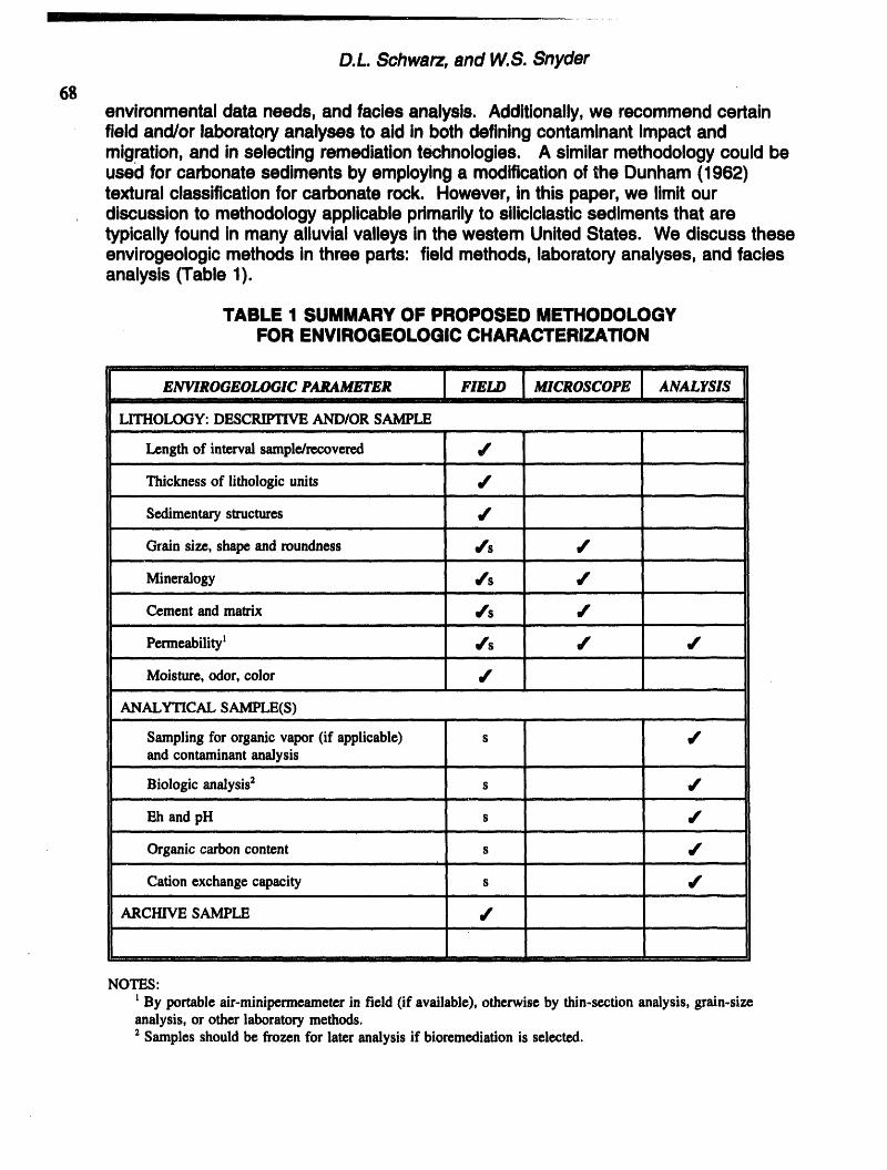
D.L. Schwarz, and W.S. Snyder
68environmentaldata needs, and faciesanalysis. Additionally,we recommendcertainfieldand/or laboratoryanalysesto aid in bothdefiningcontaminantimpactandmigration,and inselectingremediationtechnologies. A similarmethodologycouldbeusedfor carbonatesedimentsby employinga modificationof the Dunham(1962)texturalclassificationfor carbonaterock. However, inthispaper, we limitourdiscussionto methodologyapplicableprimarilyto siliciclasticsedimentsthat aretypicallyfound in manyalluvialvalleysin the westem UnitedStates. We discusstheseenvirogeologicmethodsin three parts: fieldmethods,laboratoryanalyses,and faciesanalysis(Table 1).
TABLE 1 SUMMARY OF PROPOSED METHODOLOGYFOR ENVIROGEOLOGIC CHARACTERIZATION
, i, i ,,,, ,,,,
ENVIROGEOIJTGIC PARAMETER FIE_ MICROSCOPE ANALYSISi i'i ' Ii
LITHOLOGY: DESCRIPTIVEAND/OR SAMPLE
Length of intervalsample/recovered _'
Thicknessof lithologic units J
Sedimentarystructures _',, ,, , ,.,, , -
Grainsize, shape androundness wfs /
Mineralogy wes /
CementandmaULs _¢s /i i i , ,,
Permeability' _s _' It'
Moisture, odor, color it'
ANALYTICALSAMPLE(S)
Sampling fororganic vapor (if applicable) s _'and contaminant analysis
,, , , ,, , ,,, , ..,,i
Biologic analysis2 s _',. . , .,,,. , ,.
Eh and pH s It'
Organiccarboncontent s _'I , ,,us ,, ,,, ,.,
Cation exchange capacity s J
ARCHIVESAMPLE /
I i i 11illl ii i ii i
NOTES:
By portableair-minipermeameterin field (if available),otherwiseby thin-section analysis, grain-sizeanalysis, or other laboratorymethods.2 Samples should be frozen for later analysis if bioremediationis selected.
Descriptive Methodology for Env/rogeolog/c Site Characterization69
SamplesSamplesshouldbe taken for: contaminantsof concem; additionalchemical
/physicaland biologicanalyses; thin-sectionanalysis; and archivalpurposes. _Thin-sectionanalysisof samples(petrography)Is standardprocedurefor most
geologicoutcropstudies(Boggs,1992) and subsurfacepetroleumstudies( Ethddge,1992). In contrast, these petrographictechniquesare rarelyused in hydrogeologicstudies(Younger,1992) butwouldprovidecriticaldata importantto solvinga vadetyofcharacterizationand remediationproblems. We recommendthat criticalfacies (e.g.,contaminant-impactedsands) be sampledfor petrographicanalysis. An "undisturbed"sEimplefrom the coreor split,barrel samplercan be solidifiedin the fieldwith bluecoloredepoxyresinvia a methodmodifiedfromAtkinsand McBride(1992). Cut thebottomout of a disposablecupand gentlypushthe cup Intothe sample. Supportthebottomof the sample/baseof cupwitha flexiblespatulawrapped In aluminumfoil.Pourthe resinintothe cup. Gentlyremovethe foil from the spatulaand form intoacover over the base of the cup. Place the cup withthe resin-drenchedsample intoanothercup. The solidifiedsamplecan be storedfor laterpetrographicanalysis, ifwarranted. When samplesolidificationis not feasible, samplesof loosesedimentaggregateshouldbe carefullytaken in clean, markedsamplebags. These "loose"samplescan be petrographicallyassessedundera binocularmicroscopefor many, butnotall of the features visiblein thinsectionundera petrographicmicroscope.
Remainingportionsof samplesshouldbe "archlved"by storingirtplasticbags orretaininga smallamountof each definedunitor specificintervalin seParatecompartmentsof a plasticrotaryrock-chipstoragetray. These trays allowforconvenientre-examinationwhen questionsadse.
Sampling LimitationsMany envirogeologicsite investigationsoccurin looselyconsolidatedalluvial
sediments,such as foundin the BoiseValley. These are not soilsin a geologicsense,althoughthey are sometimesreferedto as suchin many studies. For shallow(less than 50 meter)subsurfaceevaluationsin suchsediments,the preferreddataretrievalmethoduseshollow-stemauger boringtechnology,in large part becauseofthe ease of retrievingrepresentative,relativelyundisturbedsedimentsamples(U.S.EPA, 1986). The hollowstem of the augerallowsthe collectionof samplesby twomethods. The "standard"samplemethodusesa split-barrelsamplerdriven 18 to 24inchesbeyondthe auger bit by a hammerdropsystem(Hackett, 1987). Sampleintervalsvary, but generallyoccurat five foot intervalsor less. The secondsamplemethodusesa continuoussamplingtube to retrievea sedimentcoreas the augercolumnis rotatedand advanced. A continuouscore is "cut" untilthe augercolumnhas advancedfor a specificinterval,generallytwoand one half to five feet. Thesampletube is then retrievedto the surfaceby a wire-linesystem(CME, 1987).
BACKGROUND ON FIELD DESCRIPTIVE TECHNIQUES-
Geologic fielddescriptionsof shallowboreholesamples,summarizeinTable 1, aredevelopedfrom standardmethodsused to describeoutcropand hand-specimensamplesof sedimentaryrock; this is the realm of classicsedimentology.Techniquesare well describedin manytexts (e.g., Boggs,1992). In contrast,mostexisting
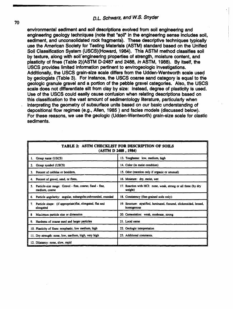
i
D.L. $chwarz, and W.S. Snyder70
environmentalsedlmentand soildescriptionsevolvedfromsoilengineeringandengineeringgeologytechniques(note that "soil"Inthe engineedngsense includessoil,sediment,and unconsolidatedrockfragments). These descriptivetechniquestypicallyuse the AmedcanSocietyfor TestingMatedals(ASTM) standardbasedon the UnifiedSoil ClassificationSystem(USCS)(Howard, 1984). ThisASTM methodclassifiessoilby texture,alongwith soil'engineedngpi'opertlesof strength,moisturecontent,andplasticityof fines (Table 2)(ASTM D-2487 and2488, in ASTM, 1988). By itself,theUSCS provideslimitedinformationpertinentto envimgeologioinvestigations.Additionally,the USCS grain-sizescale differsfromthe Udden-Wentworthscale usedby geologists(Table3). For Instance,the USCS coarsesand categoryis equal to thegeologicgranulegraveland a portionof the pebblegravelcategodes. Also, the USCSscale does notdifferentiatesiltfromclayby size: Instead,degree of plasticityis used.Use of the USCS couldeasilycause confusionwhen relatingdescdptlonsbased onthisclassificationto the vast amountof sedimentologyliterature,particularlywheninterpretingthe geometryof subsurfaceunitsbasedon our basicunderstandingofdepositionalflow regimes(e.g., Allen, 1985 ) and faciesmodels(discussedbelow).For these reasons,we use the geologic(Udden-Wentworth)grain-sizescale for clasticsediments.
II'r '11 I" ' Irl I I III III I" ' I'1
TABLE 2: ASTM CHECKLIST FOR DESCRIFI'ION OF SOILS
(ASTM D 2488,1984)
I. Group name (USCS) 13. Toughness: low, medium,high
2. Groupsymbol (USCS) 14. Color(in moist condition)
3. Percentof cobbles or boul_rs, 15. Odor(mentiononly if organic or unusual)1=,1 11 , H ,lie. i ,| , 11 ,11
4. Percentof gravel, sand,or f'mes, 16. Moisture: dry,moist, wet
5. Particle-sizerange: Gravel - fine, coarse;Sand. fine, 17. Reactionwith HCf: none, weak, strongor all three (by drymedium,coarse weight)
6. Particleangularity: angular,subangular,subrounded,rounded 18. Consistency(flne-grednedsoils only):
7. Panicle shape: (if appropdate)flaz,elongated,fiat and 19. Structure:slTatified,leum/nated,fissured,slickensided, lensed,elongated homogenous
1|.
8 Maximum panicle size or dimension 20. Cementation: weak, moderate,strong
9. Hardnessof coarse sand and largerpanicles 21. Localname
I0. Plasticityof fines; nonplastic, low medium,high 22. Geologic interpretationH H i,
I I. Dry strength:none, low, medium,high, very high 23. Addillonal comments.1,,11|1 ................. 11IlL , ,111|
12. Dilatuncy: none, slow, rapidI I' . ' 'I 'II | I 'III I I' IIII '
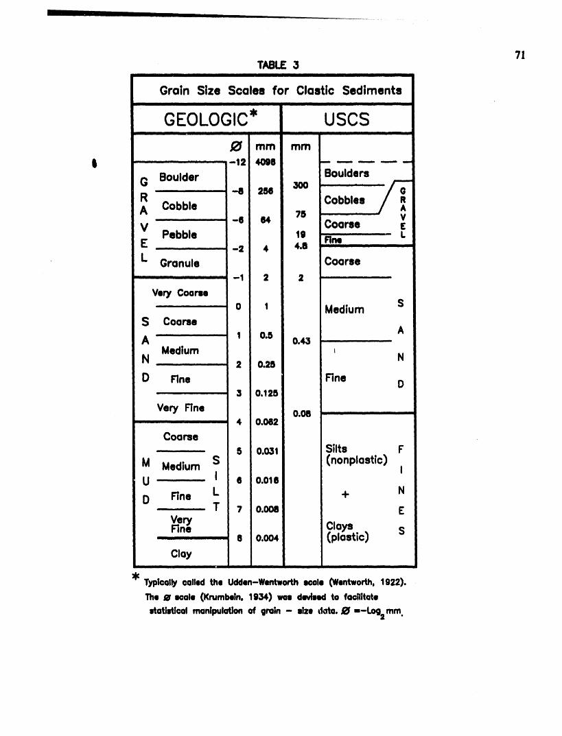
| I
71TABLE3
_ _ _ ,_,_ t ,, , __ _ ,,,_ _ . _ , _ q, ,, ,, , , _ , _ , II Ill I I [ I[
Grain Size Scalee for Clastlc SedimentsII I ........
GEOLOGIC* USCS_ __ L I I __ IIIIII I 111 I I [ IIII III IIII
._ mm mm
t ....'.......... 1= 4see .....
(3 Boulder Boulders
R Cobble -e =se _ ----'_'---_-e (14 75 V
Coarse EV Pebble 1¢ _ LE -= 4 4.eL Granule Coarse
..... -1 2 2
Very CoarseS
o 1 MediumS Coarse
AA _ 1 0.5 0.43
MediumN 2 o.25 ND Rne Rne D
3 0.125
Very Fine 0.08 ...._," , , 4 0.082
Coarse..... 5 o.o31 Silts F
M Medium S (nonplastic) IU I e o.o16
D Rne L + N,, _ T 7 o.oos E
_enrY Clays .• S8 0.0o4 (plastic)
Cloyi , .............
Typl©Qlly©ailed the Udden-Wentworth =cole (Wentworth, 1922).
The 8 =,=ale (Krumbein. 1934) was devised to fa©llitate
statistlGal manipulation of grain - =ize dM¢ _ ,,-Log=ram.

D.L. Sohwarz, and W.8. 8nyder
72Deeorlptlve Pammetere
Some of the pammetemof Table I havebeen usedto characterlzeenvironmentalsites (e.g., Ball and others, 1990), thoughstandardlzstlonIs lacklng. The followlngsuggestedmethodologyfor descdblngspllt-barrelor coresedlmentsamples is derlvedfrom standardsample iogglngdescriptionstyploallyused In the petroleumIndustry(Swanson, 1981), traditlonalsedlmentologlcoutcropdescdptlons(e.g., Boggs,1992),solldescdptlonsfor englneedngpurposes(ASTM D 2488), andfrom personalexperiencefrom envlrogeologlcchamctedzatlon. Vlsuslcomparatorscan be usell tohelp estimate manyof the attributesdiscussedbelow. These can be made byphotocopyingpublishedcompamtors(e.g., Dietrich,and others,1982) ontotransparencies. The wdttenunitdescriptionshouldincludeall visuallyidentifiableattributes. The writtenorderof descriptiveattributesdependson personalpreferences.
Length of Interval Sampled Versus RecoveredThe amountof informationavailablewillbe at leastpartlygovernedby the sample
intervallengthand the sample lengthrecovered. Thus, these lengthsshouldalwaysbe recorded upon retrievaland disassemblyof the sampler(if required). Note thatthe initialfew inchesof sedimentin the split-barrelsampleror the core tube may bedrillslough. A poor recoverymay dictatethat all of the samplebe immediatelycontainerizedfor analysisof contaminant(s).
Organic Vapor Analysis and Contaminant SamplingIf the site is presumedor knownto be contaminatedby volatileorganiccompounds,
then the initialeffortmust focuson organicvaporanalysisand samplingforcontaminantsof concern. These samplesmustbe quicklypreservedto insureaccrateanalyses. First, the sampleshouldbe split lengthwiseintoequal halves. The coreshouldthen be subdividedintocrudelithologlcunitsbasedon a visualscanandeasily-definableattributessuch as grainsize (i.e., sand vs. mud). Quicklypackageand label two sub.samplesof each "crude"unitintoappropriatecontainers; onecontainermust immediatelybe placed intoan ice-filledcooler,whilethe othercan beallowedto warmto roomtemperaturefor vaporanalysiswith appropriatefieldinstruments(e.g., flame ionizationdetector,Sensidyne,1992). Detailedsamplehandlingprotocolare documentedin EnvironmentalProtectionAgency (EPA)publications(e.g., EPA, 1986).
Lithologic Units: Thickneos, Sedimentary StructuresLithologlcunitsare a fundamentalcharacteristicof sedimentaryrocks. Although
seldomanalyzedfor enviromentalstudiesuntilnow (e.g., Anderson,1992), theirgeometry,thickness,sedimentarystructuresand lithologiccharacteristics(e.g., grainsize, grain rounding,etc.) fundamentallycontrolsubsurfacefluidmovement. Theimportanceof these unitsis discussedlater, in the sectionon faciesanalysis.
Lithologicunits(facies)are typicallydefinedby grain-sizeor mineralogychangesand characteristicsedimentarystructures. Oncethese unitsare thusdefined,thethicknessof each unitshouldbe recorded. Sedimentarystructuresare manytimesnot easilydiscemablefromsamplesrecoveredfrom split-barrelor core samplers.

Descriptive Methodology for Envirogeologio Site Characterization 73
However, they are extremelyImportantandfundamentalfeatures. Beddingsurfacesshouldbe describedas: parallelor nonparallel;even, wavy,or curved; andcontinuousor discontinuous.Graded beddings(gradual,distinctverticalchange Ingroinsize) shouldbe descdbedas normal(coarserparticlesat the base gradingtofiner at the top) or inverse(finerparticlesat the basegradingto coarserat the top).Note that split-barrelsamplingwillcause distortionof structuresalongthe wall of thesampler. Lackof any sedimentarystructuresshouldbe descdbedas massive.Uncommonlysampledfeatures includeburrows(horizontal,vertical,or both)andchaos (churnedappearancecaused by bioturbationor fluidescape. Note that fluid-escape structurescan be createdby the samplingprocedure,particuladynear thewater table).
Grain Size, Sorting, RoundingThe grainsize for each unitshouldbe describedas boththe average grainsize and
range of grainsizes each definedunit(e.g., very fine to coarsewith an averageoffine). For sand sizes, use a handlensto visuallycomparethe sampleto a grain-sizecomparatorthat is basedon the Udden-Wentworthgrain-sizescale. Gravelsizegroinscan be measuredwitha see-throughruler.
Sorting is a measureof dispersionof the size frequencyof grains {notethat sortingis oppositeof gradingin the USCS). Visuallyestimateby directcomparisonto asortingcomparator,or by Payne's (1942) classification:Good: 90% in 1 or 2 classes;Fair: 90% in S or 4 classes;Poor: 90% in 5 or more classes.
Grain roundnessconcernsthe curvatureof graincomers. Visualestimatescan bequicklymade with a handlens,binocularor petrographicmicroscopeby directcomparisonto a roundnesscomparator. Describeas very angular,angular,subangular,subrounded,rounded,or well-rounded.
MineralogySome may argue that mineralogyis of little importancein environmentalsite
characterization,and that laboratorymodelsof glassbeads can properlymimicanaturalsetting. However,for contaminanttransportmigration,mineralogymay be a
- majorcontrolon contaminantretardationvia mineraladsorptionin the absence oforganicmatedal (Anderson,1992). Estimationof mineralogycan be done inthe fieldwith a hand lens, _ndera binocularmicroscopeor by thin-sectionanalysiswith apetrographicmicroscope. Each methodrepresentsan increasein the accuracyof thedetermination.
Many alluvialsedimentswillconsistpredominantlyof quartz, with lesseramountsoffeldspar,rockfragmentsderivedfromvolcanicor metamorphicrock,and accessoryconstituentssuchas mica (biotite,muscovite)and plantremains. Visuallyestimatepercentageof majorconstituentsby directcomparisonto a percentagecomparator.Use the majorconstituentto namethe sediment,e.g., quartz sandwith minorfeldspar
_ and rare biotite. Detaileddescriptionsandclassificationscan be derivedat a later- time by thin-sectionanalysis,if appropriate.
Petrographicthin-sectionanalysisalso allowsfor directmeasurementof grainsize,__ pore size, and porosity(Atkinsand McBride,1992; Younger, 1992). Typically,
hydraulicparametersthemselvesare measured(i.e., pumptest), whilethe geologic
D.L. Schwarz, and W.S. Snyder
74parameterswhichgovernthem are igno_-ed(Younger,1992). When pumptests arefinanciallyimpossible(whichthey typicall_am), numed¢modelerstend to estimatehydraulicconductivity.'This shouldbe avoided:hydmuiicparameterscan besuccessfully(and cheaply)estimatedfromthin.sectionanalysisby methodsoutlinebyYounger(1992).
Cement and MatrixCement is depositedchemicallyaroundgrainsand in intersticesof sediment. A
commoncement in aridalluvialvalleysis calcitethat formsdudcrust(caliche). Matdxis depositedmechanicallywiththe sedimentand consistsof small individualgrainsthat fillIntersticesbetweenlargergroins(especiallyevidentwithgrovels). Cement andmatdxdeterminationis importantfor understandingsubsurfacefluidmovement
A dropof weak hydrochloricor aceticacid willcause calciteto effervescewhereasothercementsare best determinedin the laboratoryvia thin-sectionstudy. Therelativeindurationof the sediment(a functionof cementand compaction)shouldbeestimated;typicalterms are: strongly,weakly,or unconsolidatedif non-cemented.
The compositionof the matdxmustbe described (e.g., clay,silt). Forgravel,descdbeif grainsare matrix-supported(grains"floating"in matrix)or groin-supported(grainstouchingeach other).
PermeabilityPermeability can be measuredrapidlyon numeroussamplesin the fieldby a
portableair-rninipermeameter(Davis andothers,in press). This instrumenthas beensuccessfullyused on outcropsamples(Davis and others,1993) and similartechniquescan be usedfor boreholesamples. The air-minipermeametercan be assembledfromcomponentsthat cost about$1,300.00 (Davis,pers. comm., 1994). Other permeabilityestimatescan be attainedby thin-sectionor grain-sizeanalysis(discussedbelow).
Permeabilitycan also be estimatedfromthin-sectionanalysis,but this is generallyamore time consumingprocess. If neitherthe portableair-minipermeameteror thin-sectionmethodhas been undertaken,then grain-sizeanalysescan providepermeabilityestimates. Suchpermeabilityestimatescan be producedby solvinganequationderivedfromthe interceptof a straightlinefitted to a grain-sizedistributioncurve and the differencebetweenthe averageand effectivegraindiameters(Alyamaniand Sen, 1993). However,we believethat permeabilityestimatesdprivedsolelyfromdistributioncurveswillnotcorrelateto in situ measurementsbecausegrainsizeanalysiscannotaccountfor the effectsof mineralogy,texture,and diagenesis. Forexample,Hartkampand others(1993) showedthat permeabilityvaded betweentopset, foreset,and bottomsets of cross-bedsdue to contrastsin average pore sizeand contrastsin mineralogiccoml_osition.Traditional,moreexpensivelaboratorymethodsfor permeabilitycan also be performed,thoughthin-sectionanalysishasprovidedgood estimatesthat comparefavorablyto laboratory-derivedresults(Younger, 1992).
Moisture, Odor, and ColorDescribethe moistureconditionas dry (absenceof moisture),moist(damp, but no
visiblewater), or wet (visiblefree water). Beforesmellingany sample,screenthe

D.L. 8¢hwarz, and W.8. Snyder 75
sample for organic vapomwith appropdatefield Instruments(preferablyby heedspecetechniques). Do notsmellany s_llment sample that reglstemthe pmsance of organicvapomgreater than backgroundlevels (5 ppm). Forbeckground-reglsteredsamples,smell and de_dbe the odor(e.g., gasoline)as strong,weak, or omit if no odorIspresent. Boththe wet and d_/color shouldbe descdbed (if possible). General termssuch as lightgray, darkbrown,etc., shouldsuffice; however,If moreconcisedesignationsare required,determinethe colorby compedngto a soil or rockcolorchart (e.g., Goddardand othem,1980). Recordmottlu/stalns (patchesor lensesofone color In a matdxof anothercolor)as to: abundance(rare, common,many) ;size; ana contrast (faint,distinct,prominent).
LABORATORY ANALYSE8SedimentsImpactedby contaminantsneed additionalchemicaland physical
analysesIn orderto select applicableenvironmentalremedlationtechnologies. Asnotedabove, data on permeability, porosity, and groin-size are needed todetermine if the sedimentmatrixwill allowadequatemovementof fluid,such as:vapomfor vaporextraction; fluidscontainingnutrientsand/or oxygenforblodegradation;or flushingsolutionfor sedimentflushingof contaminants.Applicationof the proposedenvirogeologlcmethodologyshouldsupplymostof this type of datavia routinein house-work. However,additionalanaysles usingoutsidelaboratoriesmay be necessaryto assess the effectsof sedimentsorptionon contaminantmigrationand remedialremovalefficiency. Additionallaborartoryanalysesthat shouldbeperformedon Impactedsedimentincludeorganiccarboncontent,cationexchangecapacity, graindensity, Eh, and ,nil. We suggestthat each facies(definedbelow)impactedby contaminatio_shouldbe characterizedby & suiteof suchdata. For ageographicallysmallsite, thiswouldequateto onlyone analysisfor each of thefollowingparameters.
Eh and pHFactorsaffectingcontaminantsorptionon sedimentand soil includeoxidation-
reductionpotential(measuredby Eh) and hydrogenionconcentration(measuredbypH). Both Eh and pH partlycontrolselectivityand competitionamong"contaminant"ions(particularlyfor trace metals)for surfacesites in sediments(McComishand Ong,198e).
Peril©Is DensityParticledensityof sedimentand soilrefersto the densityof the solidparticles
collectively(Blake, 1965). Particledensityis used in mathematicalequationstodeocdbeaspects of contaminant transport(e.g., Feenstmandothers, 1991; Bjergand others, 1993).
Organl©Carbon ContentIt is assumedthat sorptionof contaminantson sedimentsresultsfromsorptionon
sedimentorganiccarbonthat occuras graincoatings,organicdebds, and condensedhumlcmatedal (KinniburghandJackson,1981). For instance,complexationof metalionswith sedimentsIncreasesat higherpH's and higherorganiccarbon

I r
Descriptive Methodology for Envlrogeoioglc Site Characterization"16
concentrations,and hydrophobicorganiccontaminantsshowa highaffinityforassociationwith organicmacromolecules(i.e., humi¢material; Huling,1989). In loworganiccarbonsediments,suchas in the BoiseValley, sorptionon mineralsurfacesmay be of equalor more importance( Feenstraand others,1991). It shouldbenotedthat organiccarboncontentcan varyconsiderably. In the horizontaldimensionit may vary by a factorof 10 or less,while it can vary by a factorof 10 to 100 in theverticaldimension(Piwoniand Keeley, 1990).
Cation Ex©hsngeCapacityCationexchangecapacitycan providesan estimatefor the totalnegatively-charged
sites availableinsoil or sediment.Thisis importantfor assessingthe rate ofcontaminantretardationthrougha sediment. It is determinedby measuringthe massof a standardcation(usuallyammonia)that displacesanothercationheld by thesediment. In naturalconditions,these receptorsites willbe occupiedby cationscommonto flowingor percolatingwater (e.g., Na+,ca_+). Largerorganiccationsandhigh!y-chargedmetal ions(e.g., Cr_) can be exchangedat these sites with theirnormaloccupants. Thus a highcationexchangecapacityof a sedimentwouldsuggestthat largeorganiccationsor heavy metalswouldnot normallybe expected tomovefar (Piwoniand Keeley, 1990).
Biologic Analyses For BioremedlatlonRecently,bioremediationhas emergedas an extremelyattractivealtemative
technologyfor the economicaltreatmentof numerouscontaminants.Underthe rightconditions,it appearsthat mostorganiccompounds,and many inorganiccompoundscan be brokendownby microbesintonon-toxiccompounds,(Chapelle,1993). Evenhighlycontaminatedsiteshave been knownto harborindigenousmicrobesthat havebecome acclimatedto the contaminant. To assessa site's potentialfor in situbiorernedlation,specializedtest(s)for microbeviabilitywithin the contaminatedzonemustbe performed.
To test for microbeviability,an aseptic,subsurfacesedimentsamplemustberecoveredfor laboratoryanalysis. Even ifsamplingtoolsare properlysterilized,thepossibilityexistsfor recontaminationby othermicrobewhile placingthe tool backdownthe hollowstem ot the augers. Therefore,upon retrievalof the sedimentsample, theoutsideportionof the sedimentsampleshouldbe discarded(Chapelle, 1993). Theremainderof the sampleshouldbe immediatelyplacedin a sterilecontainersuch as awidemouthglassjar withtightlysealingteflon-linedscrewtop. The samplemay needto be frozen beforebeingtransportedto an appropriatemicrobiologylaboratoryforanalysisof phospholipidfattyacids(PLFA). PLFAanalysisdefinesthe viablebiomass,communitystructure,andnutritionalstatusof microbes,informationnecessaryto assessthe potentialof in situ bioremediation.A "standard"PLFA assaycan cost$300.00 per sample. Dependingon the contaminantof concern,thefollowingadditionalanalyses(cost in brackets)may be necessary: (1) polybeta-hydroxyalkanoate(PHA)for furtherrefinementof communitynutritionalstatus[$50.00];(2) steroidsto furtherdefinemicroeukaryotecommunitystructure[$50.00];lipopolysacchaddelipidA hydroxyfattyacidsfor identificationof gram-negativebacteria[$250.00]; (3) diglyceddesfor evidenceas to whichcommunitiesare viable
D.L. Schwarz, and W.S. Snyder??
and whichones are not[$100.00]; and (4) tdglyceddeeto measureeukaryotenutritionalstatus [$100.00] (summarizedfrom Informationobtainedfrom MicrobialInsights,Inc., Nashville,Tennessee). Arguably,suchcosts(up to $850.00 persample)are prohibitivefor many sitecharacterizations.Yet, if bloremedlatlonbecomesthe onlyviable remedlatlontechnologyfora site, the costof retrievingsubsurfacesamplesat a laterdate can be even more prohibitivethan an Initialmicrobeanalysis. A solutionmay be to routinelyfreeze a numberof sedimentcomeor samplesfor analysesthat may be needed laterwhen the scope of the problemisfully known(suggestedby D.M. Miller,SubsurfaceRestorationConference, 1992).
FACIES ANALYSISWhy Facies Analysis for Site Characterization?
Subsurfacefluidmigrationis controlledin part by geologicfeaturesdevelopedduringsedimentdeposition. Thisdepositionproduceshetemgeneitlesthat complicatethe predictionof fluidbehaviorand hencethe effectivenessof proposedremedlationprogramsfor each specificsite. These depositionalhetemgeneitlesare not randomlydistributed,ratherthey occuras predicablegroupsof featureswithingenetically-relatedsedimentaryunits. Faciesanalysis,as appliedhere is a descriptivemethodologythat allowsgroupsof these genetically-relatedsedimentunitsto besummarizedintoa conceptualmodelof a particulardepositionalsystem(e.g., Walker,1992; Boggs,1992). Such"faciesmodels"allowsedimentologiststo comparetheirdetailedsite-specificinformationagainstthe idealcase (the faciesmodel). In contrast,environmentalgeologistsmay be able to use the conceptualfacies modeltoextrapolatelimitedfield data and therebyavoid the time and expenseof obtainingdetailedsite-specificinformationnecessaryto characterizeenvirogeologicheterogeneity(modifiedfrom Anderson,1989).
History of Facies TerminologyThe term facieswas introducedby Gressly(1838, fide Selley, 1988) to define
sedimentaryunitsof rockthat were characterizedby similarlithologicandpaleontologicattributes. Over the years, Gressley'sterm "facies"has been expandedto includealmostall scalesof everythinggeologic,bothdescriptiveand interpretive.Faciesscalesand typesrange from micmfaciesdescriptions(defined by petrographicthin-sectionanalysis)to individualIithofaciesdescriptions(e.g., individualsand bed) tolarge-scaledepositionalenvironmentinterpretations(e.g., fluvialfacies). The faciesconcepthas also been appliedto metamorphicrocks(Eskola,1915, fide Selley, 1988),mineralassemblages(Eskola, 1922, fide Krumbeinand Sloss, 1963); post-depositionalbiologicaleffectson sedimentarydeposits(ichnofacies,e.g., Seilacher,1967); geological,technical,and economicfactors connectedwiththe formationofcollieryspoilfrom coal mining("geologic-technical"faciesof Wiggering,1993), andmanyothers.
Today, there is no generalagreementon the usageof the termfacies. Manysuggestthat the term faciesshouldbe restrictedto its odginaldescriptiveapplication(e.g., Selley, 1988; Walker, 1992), whileothersbelieve Interpretiveusagesareacceptableif clearlydefined (e.g., tidal-fiatmud facies to interpreta depositionalenvironment,or storm-generatedsand-ridgefaciesto interpreta depositionalprocess;
78 Descriptive Methodology for Envirogeoiogic Site Characterization
Anderton,1985). In summary,facies remainsa viableterm, thoughone must be clearwhether it is beingapplieddescriptivelyor interpretively.
Application to Envirogeolgle CharacterizationFaciesmodelscan be developedfor envirogeologiccharacterizationby using
depositionalarchitecturalelementanalysis. Architecturalelementsare morphologicsubdivisionsof a particulardepositionalsystemcharacterizedby a distinctiveassemblageof faciesunits (Allen,1983). These individualfaciesare also knownasdepositionalelementsor architecturalunits (Miall, 1991). Architecturalelementanalysisprovidesa means of studyingsedimentarydepositsat scalesrangingfrommillimetersto kilometers; its geologicsignificanceis well documented(e.g., Allen,1983; Miall, 1985,1991,1992; Einsele,1992;Jordanand Pryor, 1992; Dreyer andothers, 1993; Shanleyand McCabe, 1993). The virtueof thismethod is that it revertsto the purelydescriptiveand frees the geologistfromrigidadherenceto anypreconceivedconceptualmodel. A frameworkfor carryingout suchan analysisisprovidedby Miall (1985).
From a purelyhydrogeologicperspective,architecturalelementanalysisdefineslarge-scalehydrogeologictrends,hydrogeologiceffective properties,and, whencombinedwithpermeabilitystudies, providesthe most comprehensivesourceof two-and three-dimensionalinformationon hydrogeologicheterogeneity(e.g., Anderson,1989; Chandlerandothers, 1989; Blairandothers, 1991; Davis and others, 1993;Hartkamp-Bakerand Donselaar,1993). Forexample,architecturalelementanalysisprovidedthe frameworkto delineatedissolvedpentachlorophenolmovementwithinanaquiferat a site inCalifornia(Blairand others,1991). At thissite, detailedlithologicdescriptionsfrom29 boreholeswere augmentedwith rare surfaceoutcropstocharacterizeaquiferheterogeneityand PrOVidea basisfor accuratemodellingof thecomplexgroundwatersystem. .
Architecturalelementanalysisrequiresdatafrom a substantialnumberof boreholesalongwith either coevalsurfaceexposuresor outcropanalogs. Surface exposuresoroutcropanalogsmustbe studiedto provideguidesor models for the interpretationofsubsurfacedata whichare dedvedfromcores,drillcuttings,and a varietyofgeophysicalmethods. Withoutinformationderivedfromthesesurfaceanalogs,solutionsto subsurfaceanalysesare notunique. Unfortunately,mostenvirogeologicsite investigationsdo not have the luxuryof relevantoutcropsto studyor largenumbersof boreholesfromwhichcontinuousdata can be retrieved. Despite thesesamplinglimitations,facies analysisfor predictivepurposescan stillbe undertaken.
-
Envirogeologic Facies Analysis for Shallow BoreholesThe followingfivefacies analysisguidelinesfollowAnderton(1985), with
modificationswhere appropriatefor hollow-stemaugersample limitations.(1) Fromthe shortcoreor split-barrelsample,descdbethe lithologyof each
_" convenientunit. Followingfielddescription,dividethe loggedsectionby lithologies(generally)intoa small numberof facies. The remainingguidelinescan be performedin the office.
(2) Compilea generaldescriptionof the featuresfoundin the vadousexamplesofeach faciesfrom each borehole. Use propermodifiersfor descriptionsof features,

D.L. Schwarz, and W.S. Snyder
79
suchas: always, usually,sometimes,and Occasionally.Do not interpret- justdescribe.
(3) Interpreteach faciesin isolationfromthe otherfacies. Forexample, can anydeductionsbe madeaboutsedimentaryprocess? Again, use appropriatemodifiers,suchas indicates,suggests(stronglyto weakly),compatible,inconclusive,andcontradicts.
(4) Look at the relationshipbetweenfacies. Lookfor simplepatternsor variationsof patternssuch as fining-,thickening-,or coarsening-upwardsequences. Suchrelationshipsdefinefacies associationsand architecturalelements. Draw cross-sections,or preferably,fencediagrams.
(5) Attemptto relate any faciesassociationsto a simple,publishedconceptualmodel. Excellentsourcesof faciesmodelsincludeEinsele (1992) and Walker (1992).With limitedboreholedata, thisprocessis very interpretive. The advantageof tryingto definea model is in usingits predictivepowerto extrapolatesuch limitedfielddata.Rememberto favora simplemodelovera complexone: subsurfacedata alone doesnot allow uniquesolutions.
SUMMARYIt is becomingincreasinglyobviousthat there is no widelyused standardto analyze
shallowbore holedrillingprograms. ASTM descriptionsof soilsare good butinadequatefor thistask. Table 1 summarizesthe proposeddescriptivemethodologyfor envirogeoiogiccharacterizationof bore holes. The proposedstandardcannotbeuniversallyappliedto all sitecharacterizations;for each site,the numberofrecommendedanalyseswillbe limitedby siteconditionsandthe projectbudget.Nevertheless,the proposedmethodologyis inexpensiveand rapid; mostof thetechniquesare part of a geologist'sstandardundergraduateeducation. Duringinitialsite characterization,it may not seem necessaryto conductsuchdetailedassessments. This wouldbe a mistake; the time requiredto make the descriptionsand/ortake the samplesis minorcomparedto the possiblecostsassociatedwith re-sampl;ingat a laterdate. In effect,usingthe proposedmethodologymay reducesoverallsite assessmentcosts.
We hopethat introducingsomeideasfor standardizationwill stimulatediscussionand result in the routinegatheringof higherqualityand largeramountof data for site=
characterizations.
,r _,rl ' ' '
80 Descri_ive Methodology for Envirogeologic Site Characterization
REFERENCESAllen,J.R.L.' 1983, Studiesin fluvlatilesedimentation:bars, bar complexesand sandstone
sheets(low-sinuositybraidedstreams)in the B¢ownstones(L. Devonian),Welsh Borders:SedimentaryGeology,v. 33, p. 237-293.
Allen,J.R.L., 1985, Principlesof Physical8edimentology: GeorgeAllen and Unwin,London,272p.,
Alyamani,M.S., and Sen, Z., 1993, Determinationof hydraulicconductivityfrom complete grain-size distributioncurves: GroundWater, v. 31, p. 551-555.
Anderson,M.P., 1992, Basicsciencerequiredfor decisionmaking: Geologicalsetting, in:SubsurfaceRestorationConferenceProceedingsVolumefor 1992,, NationalCenter forGroundWater Research,Rice University,Dept.of EnvironmentalScience andEngineering,Houston,Texas, p. 5-7.
Anderson,M.P., 1989, Hydrogeologicfacies modelsto delineatelarge-scalespatialtrendsinglacialand glaciofluvialsediments: GeologicalSocietyof AmericaBulletin,v. 101, no. 4, p.501-511.
Anderton,R., 1985, Clasticfaciesmodels andfacies analysis,in Brenchley,P.J., and Williams,B.P.J., eds., Sedimentology:Recent DevelopmentsandAppliedAspects: The GeologicalSociety (London),Alden Press,Oxford, p. 31-47.
ASTM (AmericanSocietyforTestingand Matedals),1988, AnnualBookof ASTM Standards,Section4, Construction,Volume04.08, Soil and Rock,BuildingStones,Geotextiles,ASTM,Philadelphia,Methods D-2487 and 2488.
Atkins,J.E., and McBride, E.., 1992, Porosityand packingof Holoceneriver,dune, and beachsands: AmericanAssociationof PetroleumGeologistsBulletin,v. 76, p. 339-355.
Ball, W.P., Buehler,C.H., Harmon, T.C., Mackay,D.M., and Roberts,P.V., 1990,Characterizationof a sandyaquifermaterialat the grainscale: Journalof ContaminantHydrology,v. 5, p. 253-295.
Bjerg,P.L., and Chdstensen,T.H., 1993, A fieldexperimenton cationexchange-affectedmulticomponentsolutetransportin a sandyaquifer: Joumalof ContaminantHydrology,v.12, p. 269-290.
Blair,T.C., Baker, F.G., and Turner,J.B., 1991, Cenozoicfluvial-faciesarchitectureand aquiferheterogeneity,Oroville,CaliforniaSuper Fundsite and vicinity,in Miall,A.D., and Tyler, N.,eds., The Three-dimensionalFaciesArchitectureof TerrigenousClasticSedimentsand itsImplicationsfor HydrocarbonDiscoveryand Recovery: SEPM (Society of SedimentaryGeology)Concepts in sadimentologyand paleontology,Volume3, p. 148-159.
Blake,G.R., 1965, ParticleDensity, in Black,C.A., editor-in-chief,Methods of Soil Analysis,Part1, Physicaland MineralogicProperties,IncludingStatisticsand Measurementsof Sampling:Amedcan Society of Agronomy,Inc., Madison,Wisconsin,p. 371-373.
Boggs,S. Jr., 1992, Petrologyof SedimentaryRocks: MacmillanPublishingCompany, NewYork,707p.
Chandler,M.A., Kocurek,G., Goggins,D.J., and Lake, L.W., 1989, Effects of stratigraphicheterogeneityon permeabilityin eoliansandstonesequence,Page Sandstone,northemArizona: AmericanAssociationof PetroleumGeologistsBulletin,v. 73, p. 658-668.
Chapelle,F.H., 1993, Ground-waterMicrobiologyand Geochemistry:John Wiley and Sons,New York, 424p.
CME (CentralMine EquipmentCo.), 1987, Catalogof product literature: St. Louis,Missouri,12p.
Davis,J.M., Wilson, J.L., and Phillips,F.M., in press,A portableair-minipermeameterfor rapidin-situfield measurements: GroundWater.
Davis,J.M., Lohman,R.C., Phillips,F.M., Wilson,J.L., and Love,D.W., 1993, Architectureofthe Sierra LadronesFormation,central New Mexico: Depositionalcontrolson the
11 ,
D.L. 8chwarz, and W.8. 8nyder 81
permeabilitycorrelationstructure: GeologicalSocietyof Amedca Bulletin,v. 105, p. 998-1007.
Detdech, R.V., Dutro, J.T., Jr., and Foose, R.M. (compilers),1982, AGI Data Sheets: forGeologyin the Reid, Laboratory,and Office: AmedcanGeological Institute,Falls Church,Virginia.
Dreyer, T., FaR,L.-M., Hoy, T., Knarud,R., Steel R., and Cuevas,J.-L., 1993, Sedimentaryamhltectumof fieldanaloguesfor reservoirinformation(SAFARI): a case study of thefluvial EscanillaFormation,SpanishPyrenees,in Rint, S,S., and Bryant, I.D. (ede.), TheGeologicalModellingof HydrocarbonReaervoirsand OutcropAnalogs,IntemattonalAssociationof SedimentologistSpecialPub,cation Number15, BleckwellScientificPublications,Oxford,p. 3-20.
Dunham,R.J., 1962, Classificationof carbonaterocksaccordingto depceitionaltexture, in Hem,W.E., ed., Claseificstionof carbonaterocks: Amedcan Aseoclationof PetroleumGeologistsMemoir 1, p. 108-121.
Einsele,G., 1992, Sedimentary Basins,Spdnger-Vedeg,Bedin,628p.Feenstm, S.D., Mackay, M., and Cherry, J.A., 1991, Presenceof residualNAPL basedon
organicchemicalconcentrationsin soil: GroundWater MonitoringReview,v. Xl, p. 128-- 138.
Goddard, E.N., chairman,and five committeemembers,1980, Rock-colorchart: GeologicalSocietyof Amedca, Boulder,Colorado.
Hackett,G., 1987, Drillingand constructingmonitoringwellswith hollow-stemaugers, pert hddllingconsiderations: GroundWater MonitoringReview,v. 7, p. 51-2.
Ha_t(amp,C.A., Ardbas,J., and Tortosa,A., 1993, Groinsize, composition,porosityendpermeabilitycontrastswithincross-beddedsandstonesin Tertiaryfluvialdeposits,centralSpain: Sedimentology,v. 40, p. 787-799.
Hartkamp-Baker,C.A., and Donselaar,M.E., 1993, Permeabilitypatternsin pointbar deposits:Tertiary Lomnca Basin,centralSpain,in Flint,S.S., and Bryant,I.D. (ede.), The GeologicalModellingof HydrocarbonReservoirsand OutcropAnalogs,InternationalAssociationofSedimentologistSpecialPublicationNumber 15, BlackwellScientificPublications,Oxford,p.157-168.
- Howard,A.K., 1984, The revisedASTM standardon the UnifiedClassificationSystem:GeotechnicalTestingJournal,v. 7, p. 216-222.
Huling,S.G., 1989, Facilitatedtransport,EPA SuperfundGroundwaterIssue, Officeof SolidWaste and EmergencyResponse, Officeof Reseamh and Development,United States
_ EnvironmentalProtectionAgency,EPA/540/4-89/003, 5p.Jordan,D.W., and Pryor,W.A., 1992, Hierarchicallevelsof hsterogeneityin a MississippiRiver
meanderbelt and applicationto reservoirsystems: AmedcanAssociationof PetroleumGeologistsBulletin,v. 76, p. 1601-1624.
Kinniburgh,D.G., and Jackson,M.L., 1981, Cationadsorptionby hydrousmetal oxidesandclays,in Anderson,M.A., and Rubin,A.J., ads., Adsorptionof Inorganiceat Solid-LiquidInterfaces: Ann ArborScience Publishers,Ann Arbor,Michigan,p. 91-160.
:. Krumbein,W.C., 1934, Size frequencydistributionsof sediments: Joumal of SedimentaryPetrology,v. 4, p. 65-77.
Krumbein,W.C., and Slose, L.L., 1963, Stratigraphyand Sedimentation,SecondEdition: W.H.- Freemanand Company,San Francisco,660.
McComish,M.F., and Ong, J.H., 1988, Chapter7: Trace Metals,i_.nBodek, I., ed.,EnvironmentalInorganicChemistry: PergamonPress, New York,p 7.1-7.15-10.
Miall,A.D., 1985, Amhitectural-elementanalysis: a new methodof facies analysisappliedto- fluvialdeposits: Earth Science Reviews,v. 22, p. 261-308.- Miall,A.D., 1991, Hierarchiesof architecturalunitsinterdgenousclasticrocks,and their
Descriptive Methodology for Envirogeologic Site Characterization82
relationshipto sedimentationrate, in Miall,A.D., and Tyler, N., ads., The Three-dimensionalFacies Architectureof TerdgenousClastic Sedimentsand itsImplicationsfor HydrocarbonDiscoveryand Recovery: SEPM (Societyof SedimentaryGeology)Conceptsinsadimentologyand paleontology,Volume3, p. 6-12.
Miall,A.D., 1992, Chapter7, AlluvialDepositsinWalker, R.G., and James, N.D., ads., FaciesModels,responseto sea level change: GeologicalAssociationof Canada, St. John's,Newfoundland,p. 119-142.
Payne, T.G., 1942, Stratigraphicalanalysisand environmentalreconstruction:AmericanAssociationof PetroleumGeologistsBulletin,v. 26, p. 1697-1770.
Piwoni,M.D., and Keeley,J.W., 1990, Basicconceptsof contaminantsorptionat hazardouswastesites, EPA GroundWater Issue: Officeof SolidWaste and EmergencyResponse,Office of Researchand Development,UnitedStates EnvironmentalProtectionAgency,EPA/540/4-90/053, 7p.
Seilacher,A. 1967, Bathymetryof tracefossils: Marine Geology,v. 5, p. 413-428.Selley, R.C., 1988, AppliedSedimentology:AcademicPress, London,446p.Sensidyne,Inc., 1992, OperationManualforportableFlame IonizationDetector(FID), Sixth
Edition,RevisionB, October,1992.Shanley,K.W., and McCabe, P.J., 1993, Alluvialarchitecturein a sequencestratigraphic
framework: a case historyfromthe UpperCretaceousof southernUtah, USA, in Flint,S.S., and Bryant, I.D. (ads.), The GeologicalModellingof HydrocarbonReservoirsandOutcropAnalogs,IntemationalAssociationof SedimentologistSpecialPublicationNumber15, BlackwellScientificPublications,Oxford,p. 21-56.
Swanson, R.G., 1981, Sample Examir]atlonManual: America _sociationof PetroleumGeologistsMethods in ExplorationSeries,Tulsa,Oklahoma,118p.
U.S.EPA (EnvironmentalProtectionAgency), 1986, RCRA Ground-watermonitoringtechnicalenforcementguidancedocument: Office of Waste ProgramsEnforcement,Office of SolidWaste and EmergencyResponse,OSWER-99501.1, UnitedStates EnvironmentalProtectionAgency,317p.
Walker, R.G., 1992, Facies,facies modelsand modernstratigraphicconcepts,inWalker, R.G.,and James, N.P., eds., Facies Models: Responseto Sea Level Change: GeologicalAssociationof Canada, p. 1-14.
Wentworth,C.K., 1922, A scaleof gradeand classtermsforclasticsediments: JournalofGeology,v. 30, p. 377-392.
Wiggering,H., 1993, Sulfideoxidation- an environmentalproblemwithincollieryspoildumps:EnvironmentalGeology,v. 22, p. 99-105.
Younger,P.L., 1992, The hydrogeologicaluse of thin sections: inexpensiveestimatesofgroundwaterflowand transportparameters: Quartedy Joumalof EngineeringGeology(London),v. 25, p. 159-164.
I
Hydrogeology, Waste Disposal, Science and Politics .Proceedings 30th SymposiumEngineering Geology and Geotechnlcal Engineering, 1994 83
A MISZ-A'-LA-MASSE MITHOD FOR LANDFILL CONTAMINANT PLUME
EVALUATION
T.H. Rowlo¥ and Paul R. Donaldgon, Department o£ Googciences,
Boise State University, James L. Oglengky, Hydrology
Program, _nlver|It¥ of Idaho, and John A. Welham, Idaho
Geological Survey, Pooatello.
ABSTRACT
A mise-a'-la-masse surv_was conducted dow_ gradient of theBannock County Landfill, in Fort Hall Canyon, Idaho in 1993.Data collected during the survey were compared to seismicrefraction data also collected at the site. The site at themouth of Fort Hall Canyon is ideal for use of the mise-a'-la-masse method to characterize a contaminant plume under actualfield conditions. A contaminant plume is believed to emanatefrom the Bannock County Landfill. The plume contains highconcentrations of _enseHon-Aqueous _Phase Liquids (DNAPLs) plusinorganic groundwater contaminants. These DNAPLs and inorganicshave been detected in nearby domestic and municipal water supplywells. The field site is relatively free of culturalinterference that would adversely affect electrical-potentialfields.
The mise-a'-la-masse method of plume identification, first
suggested by Osiensky and Donaldson (1994) has not been appliedat the scale of an actual contaminant plume prior to thisinvestigation. The method is much easier to use and the datainterpretation is less subjective than other electrical methods;however, it does not yield depth information. The mise-a'-la-masse method was used successfully to identify electric-fieldanomalies near the Bannock County Landfill. A seismic refraction
survey suggested that three large buried channels meander acrossan old alluvial fan beneath the site. The alluvial fan isunderlain by an undulating bedrock surface. The electric-fieldmap correlates very well with the interpretation of the seismicsurvey in those areas where the data sets coincide. Mostelectric-field highs are located above areas seismicallyinterpreted as buried channels or basins. These features mayprovide preferential flow path_ for the contaminated groundwaterand DNAPLs.
Ongoing work involves a second phase mise-a'-la-masse surveyenlarging the area of investigation to include more of the areacovered by the seismic survey. _zese data will be correlatedwith existing surface geophysical data sets and with currentgeological studies to better understand the hydrogeology of thesite.
INTRODUCTION
The Bannock County Landfill, like many pre-subtitle Dlandfills in Idaho, and in the United States in ge_eral, arelocated in sand and grnvel deposits of fluvial origin. From the
standpoint of ground water quality protection, these landfillsare located inappropriately due to the lack of a low hydraulic-conductivity geologic unit to protect aquifers Used for domesticand municipal water _upplies.
Ground water monitoring in complex fluvial deposits is
complicated by the fact that ground water contaminants oftenmigrate along preferred pathways caused by lateral and verticalheterogeneity within a stratigraphic unit. Delineation ofpreferential flow paths historically has required the
84 T.H. Rowley and otherm
construction of numerous ground water monitoring wells at greatexpense (Osiensky and others; 1984). Surface geophysics can addimportant information on the shape, character, and spatialdistribution of heterogeneities within fluvial hydrostratigraphicunits thereby reducing the uncertainty and expense in groundwater monitoring programs.
Surface electrical resistivity has been used to identifysubsurface lithologic variations including buried stream channels(Zhody and others, 1974; Urish, 1983; Ayers, 1989), altered andsaturated zones _n bedrock (Applegate and Donaldson, 1977) andother geotechnical parameters (Donaldson, 1975). Electricalresistivity has also been used by many investigators to locatevariations in ground water quality and to delimit zones of groundwater contamination. Recent examples of these uses include thework of Ringstad and Bugenig (1984), Weber and others (1984), andRudy and Caoile (1984). White (1988) described a field study inNew Zealand where the method of Fried (1975) was used todetermine the direction of movement and velocity of a salt-waterslug injected into an aquifer.
Surface electrical resistivity measurements can bemanipulated to gain understanding of the geologic conditions thatexist at a site. Resistivity data typically are collected usingone or more electrode arrays that have been developed over theyears for various geologic conditions. Examples of these
• electrode arrays include the Wenner array (Wenner, 1916),Schlumberger array (Compagnie Generale de Geophysic, 1955),Dipole-Dipole array (Al'pin, 1950), etc. Resistivity surveysusually include both electrical sounding and horizontalprofiling. Electrical sounding is the process for performingdepth investigations and horizontal profiling is the process fordetecting lateral variations in resistivity (Zhody and others,1974). According to Zhody and others (1974), the probability ofcorrect interpretation of the resistivity data can be improved bycorrelating several sounding curves, making crossed soundings,sounding with different arrays, traversing the area withhorizontal resistivity profiles, knowing the general geology, andidentifying the electrical properties of the rocks in the studiedarea. The electrical resistivity arrays mentioned above aresomewhat cumbersome and time consuming to use. In addition, thequality of the interpretations is dependent on the qualificationsand experience of the investigators.
The mise-a'-la-masse method was first suggested bySchlumberger (1920). Information derived with this method is notas complete as with the typical resistivity array. However, themethod is much easier to use and the data interpretation is lesssubjective. The mise-a'-la-masse method has been usedsuccessfully in the mining industry to delineate partiallyexposed ore bodies. Originally the method was designed to mapconductive orebodies by passing an electric current into anoutcrop and recording electrical potential measurements at landsurface (figure 1).
The mise-a'-la-masse method has direct application to theevaluation and interpretation of inorganic (conductive)contaminant plumes that emanate from known sources (e.g., leaking

I
l
85Mise-A'-La-Masse Method For Contaminant plume Evaluation

T.H. Rowley and otherm
86
underground tanks, landfills, etc.). If the source ofcontamination isn't known the contaminant plume can beelectrically excited via monitoring wells. The configuration ofthe equipotentials derived by exciting the formation (plume) viaboreholes (monitoring wells) should be nearly identical to thosegenerated by exciting the source directly if the formation is anexcellent electrical conductor (Parasnis, 1975). The resultingequipotentials may be used to help identify the contaminantsource as well to help delineate extent and continuity of thecontaminant plume.
The organic solvents that are denser than, and immisciblein, water such as perchloroethylene ('perc') andtetrachloroethylene (TCE) are referred to as _ense _on_queous_hase liquids (DNAPLs) . The unique physical and chemicalproperties of DNAPL chemicals often limit the effectiveness ofcommon remediation and monitoring methods.
The resistive DNAPL chemical can exist in multiple phases(Schwille, 1988). The residual phase of DNAPL chemicals areevident in unsaturated zones after a spill has migrated to the
' isaturated zone leaving mlcroscop c droplets attached to soils orsmall grains. The gaseous phase exists as a product ofevaporation of the liquid or "free" phase. The liquid phase willseek paths of least resistance along geologic structures such asdipped strata, faults and fractures without regard to saturation.The dissolved phase moves with the ground water gradient.Because it is possible for the liquid phase to move in adifferent direction than that of the dissolved phase, contaminantmigration can be difficult to determine. The DNAPL liquid phasecan pool on geological strata (i.e. clay lenses, unfracturedbedrock). Thus, knowledge of the geologic and hydrologic units,if available, would assist in the development of a remediationplan.
Surface geophysical methods such as the mise-a'-la-massemethod show promise for the delineation of DNAPL waste plumes byrecording electrical anomalies. Currently, wells located downgradient of the Bannock County Landfill have detected highconcentrations of TCE. Annan and others (1991) used surfaceelectrical resistivity successfully to detect migration patterns
, of a controlled DNAPL plume.
Controlled Field Test
The following discussion is taken from Osiensky andDonaldson (1994). A field research site was developed within thefloodplain of the Boise River, a_ Eagle Island State Park,approximately 24 kilometers west of Boise, Idaho in 1991. Thesite consists predominantly of coarse grained river gravels thatare typical of many abandoned gravel pits which historically havebeen used as landfill sites. The research site was selectedbecause of the undeveloped nature of the land (open field) andthe existence of a shallow water table (less than 1.5 metersbelow land surface).
A backhoe trench was excavated approximately .5 meters belowthe water table for use as the source for the tracer experiment.

Mise-A'-La-Masme Method For Contaminant Plume Evaluation87
The background electrical potential field between the trench andthe pumping well was measured with a 'gradient array" by usingthe trench as a current electrode (i.e., the current electrodewas driven into the bottom of the trench). The distant electrode(i.e., current sink) was driven into the edge of a swimming lakelocated 100 meters east of the trench. The gradient arrayconsisted of disposable potential electrodes placed on 2 metercenters between the trench and the pumping well. Electricalpotential measurements were taken one at a time at each potentialelectrode by completing an electrical circuit to a receiversystem and a reference electrode.
The potential electrodes were placed above the zone whereconvergent tracer migration was being inducedby ground waterpumping. The electrical equipotentials were contoured for acomparative analysis through the time period of the tracerexperiment (figure 2).
Electrical potentials within the test well field weremeasured at selected intervals during the tracer test todetermine if the migration of tracer could be tracked with themodified mise-a'-la-masse method.
The controlled field test results prove that the modifiedmise-a'-la-masse method is very sensitive to changes in thespecific-electrical-conductance of ground water. The nextlogical step is to apply the modified mise-a'-la-masse method toa larger field scale investigation.
FIILD APPLICATION
A field research site was surveyed within the alluvial fanbelow Fort Hall Canyon, Bannock County, approximately 5 milessoutheast of Pocatello, Idaho. The site consists predominantlyof a shallow rocky soil layer underlain by coarse grained rivergravels. The research site was selected because of theundeveloped nature of the land (open fields) and the detection ofhigh concentrations of DNAPLs in nearby water supply wells.Figure 6 shows the location of the site.
The site was surveyed using monitoring well MW3 (figure 3)as an origin for a grid of potential electrode stations every 50meters within the test area. The current source electrode was an8" steel well casing (T , figure 3) that extends below the watertable. The distant electrode (i.e., current sink) was locatedapproximately 1200 meters North of MW3 in Fort Hall Canyon. Theelectrodes were connected to the transmitter with insulatedcopper wire.
For this investigation, a Zonge GGT-3 transmitter and ZongeXMT-16 transmitter controller powered by a smell 400-Hz generatorwere used for the current source. A Zonge Engineering GDP-16receiver recorded the data. The transmitter-controller was used
to ensure proper synchronization. The transmitted signal was atypical 4-second period time-domain signal. The electricalpotentials were measured relative to a fixed reference electrodelocated north of MW3. Non-polarizing porous pots filled withapproximately .2 liters of copper sulfate solution were used forthe reference electrode and potential electrodes. Electrical

88 T.H. Rowley and otherm
Z = • PUMPING WELL
,_ .
IW NORTH_)
._ONTOURINTERVAL0.5 MILLIVOLTS
• P/I WEST
TRENCH
'0 2 4 tl p METERSI, i I
Figt_e 2. =leotEiasl eqnipotenti&l lineo foe the pe:£od 153 tolSS houz= (9180 to 9300 minutes) &£to: =:soot £n_eot£on.(£romOm£eno_tmdDonaldmon, 1994)
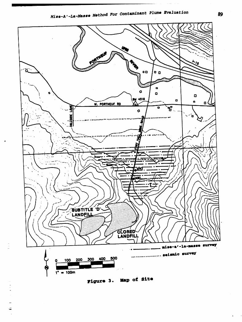
Mime-A,-J_a-Manme Her:hod rot Cont:aminant: Plume A'va.luaCton 89
LANDFILL
• s _
f 0 100 200 300 500 ..................... se£nmio suz'_rey1" -- 100m
]figure 3. Nap of site
=
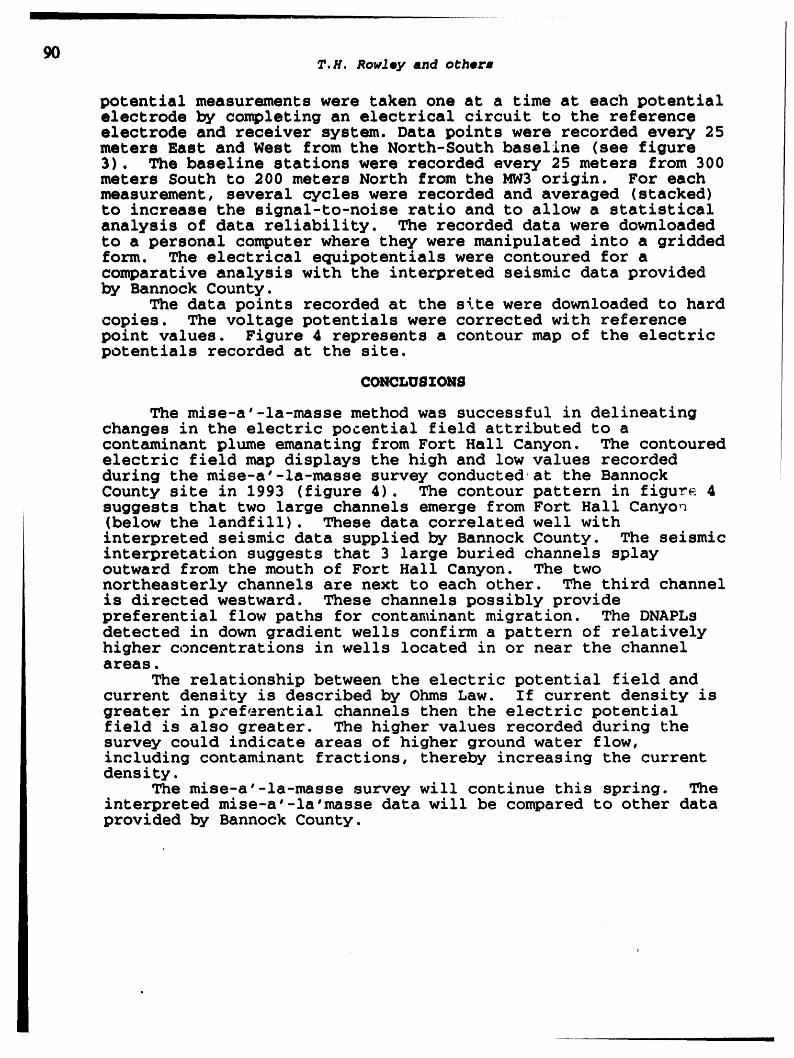
gOT.H. Rowley an_ o_herm
potential measurements were taken one at a time at each potentialelectrode by completing an electrical circuit to the referenceelectrode and receiver system. Data points were recorded every 25meters East and West from the North-South baseline (see figure3). The baseline stations were recorded every 25 meters from 300meters South to 200 meters North from the MW3 origin. For eachmeasurement, several cycles were recorded and averaged (stacked)to increase the signal-to-noise ratio and to allow a statisticalanalysis of data reliability. The recorded data were downloadedto a personal computer where they were manipulated into a griddedform. The electrical equipotentials were contoured for acomparative analysis with the interpreted seismic data providedby Bannock County.
The data points recorded at the s_te were downloaded to hardcopies. The voltage potentials were corrected with referencepoint values. Figure 4 represents a contour map of the electricpotentials recorded at the site.
CONCLUSIONS
The mise-a'-la-masse method was successful in delineatingchanges in the electric potential field attributed to a
'ncontaminant plume emanatl g from Fort Hall Canyon. The contouredelectric field map displays the high and low values recordedduring the mise-a'-la-masse survey conducted at the Bannock
' rCounty site in 1993 (flgu e 4). The contour pattern in figu_ 4suggests that two large channels emerge from Fort Hall Canyon(below the landfill). These data correlated well withinterpreted seismic data suppliedby Bannock County. The seismicinterpretation suggests that 3 large buried channels splayoutward from the mouth of Fort Hall Canyon. The twonortheasterly channels are next to each other. The third channelis directed westward. These channels possibly providepreferential flow paths for contaminant migration. The DNAPLsdetected in down gradient wells confirm a pattern of relativelyhigher concentrations in wells located in or near the channelareas.
The relationship between the electric potential field andcurrent density is described by Ohms Law. If current density isgreater in p_ef_rential channels then the electric potentialfield is also greater. The higher values recorded during thesurvey could indicate areas of higher ground water flow,including contaminant fractions, thereby increasing the currentdensity.
The mise-a'-la-masse survey will continue this spring. Theinterpreted mise-a'-la'masse data will be compared to other dataprovidedby Bannock County.
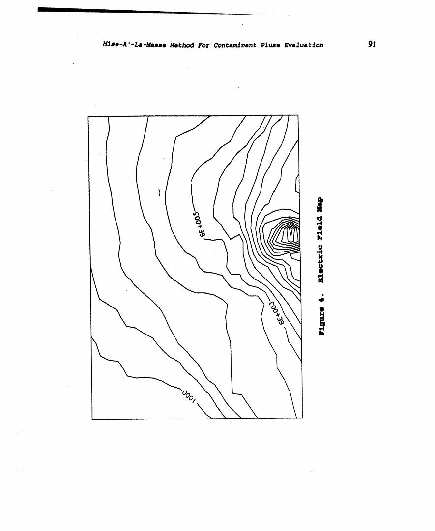

o_ __
_"////./.,e/N°
_J"o ,,,, _e_._,,-.
__ BY I:::IPPL'rEDTMI:IOE, INC, _


92 T.H. Rowley and others
REFERENCES
Al'pin, L. M., 1950, The Theory of Dipole Sounding. Moscow,Gostoptekhizdat, 89p., (Translation in Dipole methods formeasuring earth conductivity): New York, Plenum Press, 1966,p.60.
Annan, A.P., Bauman, P., Greenhouse, J.P., and Redman, J.D.,1991, Geophysics and DNAPLs, Ground Water Management No.5,Proceedings of the Fifth National Outdoor Action Conference onAquifer Restoration, Ground Water Monitoring and GeophysicalMethods, May 13-16, 1991, Las Vegas, Nevada, P. 963-977.
Applegate, J.K. and Donaldson, P.R., 1977, GeophysicalInvestigation of Rock Properties Near Silver Creek, BoiseNational Forest, Idaho, Department of Geology and Geophysics.Boise State University, Geoscience Contribution, n.107, 31p.
Ayers, J.F., 1989, Conjunctive Use of Ge_hysical and GeologicalData in the Study of an Alluvial Aquifer, Ground Water, v.27, No.5, pp. 625-632.
Compagnie Generale de Geophysique, 1955, Abaques de SondageElectrique: Geophysical Prospecting, v. 3, supplement 3.
Fried, J.J., 1975, Groundwater Pollution, Theory, Methodology,Modelling and Practical rules. Elsevier, New York, p. 330.
Donaldson, P.R., 1975, Geotechnical Parameters and TheirRelationship to Rock Resistivity, Proceedings of theThirteenthAnnual Engineering Geology and Soils Engineering Symposium,p.169-185.
Osiensky, J.L., Winter, G.V., and Williams, R.E., 1984,Monitoring and Mathematical Modeling of Contaminated Ground-WaterPlumes in Fluvial Environments, Ground Water, v.22, p.298-306.
Osiensky, J.L., and Donaldson P.R., 1994 "The Modified Mise-A-La-Masse Method for Contaminant Plume Delineation," Ground Water,in-press.
Parasnis, D.S., 1975, Mining geophysics: methods in geochemistryand geophysics series (3), Elsevier, Amsterdam, p.395.
Ringstad, C.A., and Bugenig, D.C., 1984, Electrical ResistivityStudies to Delimit Zones of Acceptable Ground Water Quality,Ground Water Monitoring Review, v.4, n.4, p.66-69.
Rudy, R.J., and Coile, J.A., 1984, Utilization of ShallowGeophysical Sensing at Two Abandoned Municipal/Industrial WasteLandfills on the Missouri River Floodplains, Ground WaterMonitoring Review, v.4, n.4, p.57-65.

Mise-A'-La-Masse Method For Contaminant Plume Evaluation 93
Schlumberger, C., 1920, Etude Sur la Prospection Electrique duSous-sol, Gauthier-Villars, Paris, p. 94.Schwille, F. 1988. Dense Chlorinated Solvents in Porous andFractured Media; Model _xperiments. Translated by J.F. Pankow.Lewis Publishers. -
Urish, D.W., 1983, The Practical Application of SurfaceElectrical Resistivity to Detection of Ground-water Pollution,Groundwater, v.21, n.2, p.144-152.
Weber, D.D., Scholl, J.F., LaBrecque, D.J., Walther, E.G., andEvans, R.B., 1984, Spatial Mapping of Conductive Ground WaterContamination with Electromagnetic Induction, v.4, n.4, p.70-77.
Wenner, Frank, 1916, A Method of Measuring Earth Resistivity,U.S. Bureau of Standards Bulletin, v. 12, pp. 469-478.
White, P.A., 1988, Measurement of Ground-water parameters usingsalt-water injection and surface resistivity, Ground Water, v.26,no. 2, pp. 179-186.
Zhody, A.A., Eaton, G.P., and Mabey, D.R., 1974, Application ofSurface Geophysics to Ground-Water Investigations, U.S.Geological Survey Techniques of Water-Resources Investigations,Book 2, Chapter DI, l16p.

4_
Hydrogeology, Waste Disposal, Science and PoliticsProceedings 30th Symposium 95Engineering Geology and Geotechnical Engineering, 1994
HOTSPOTS & OTHER HIDDEN TARGETS:Probability of Detection, Number, Frequency and Area
by
Charles L Vita, Ph.D., P.E., G.E._ cemeg_
Environmental Science & Engineering, Inc. (E.SE)15444m_ 95thSt, 4244,Redmond,Washiagton90O52,206/86O-8220
ABSTRACT
Concepts and equations are presented for making probability-based estimates of thedetection probability, and the number, frequency, and area of hidden targets, includinghotspots, at a given site. Targets include hotspots, which are areas of extreme orparticular contamination, and any object or feature that is hidden from direct visualobservation--including buried objects and geologic or hydrologic details or anomalies.Being Bayesian, results are fundamentally consistent with observational methods.Results are tools for planning or interpreting exploration programs used in siteinvestigation or characterization, remedial design, construction, or compliancemonitoring, including site closure. Used skillfully and creatively, these tools can helpstreamline and expedite environmental restoration, reducing time and cost, making siteexploration cost-effective, and providing acceptable risk at minimum cost.
INTRODUCTION
Purpose and Organization
Very simply, this paper alms to answer the question: given that hidden targets ofsome particular importance (such as hotspots) could exist at a site, wh_: is theprobability of detecting those targets, and what is the probable number_frequency, andarea of targets? To that end, this paper presents conceptual and analytical tools formaking probability-based estimates of the detection probability, number, frequency, andarea of hidden targets in a given site or area of exploration. The tools are rigorous yetflexible and fundamentally consistent with observational methods and continuousimprovement processes and strategies [9-14]. The purpose of these tools is to help makeexploration program design, implementation, and data interpretation, efficient, rational,and technically defensible. When skillfully integrated with project requirements andconditions, these tools can help streamline and expedite environmental restoration,reducing time and cost, making site exploration cost-effective, and providing acceptablerisk at minimum cost.
This paper is organized into this introductory section and five principal sectionsthat follow. This introductory section defines targets and identifies fundamentalassumptions and concepts, including statistical strata, random sampling, and probabilitymodels. The probability of target detection, Pd, is discussed second. The number of

96 C.L. Vita
undetected targets, U, is discussed third. Target areas are discussed fourth. GeneralBayesian updating is discussed fifth. The final section summarizes general conclusions.
Hot,_ots and Targets
Hotspots are areas of extreme or particular contamination. Targets is a moregeneral concept that includes hotspots as a special case. That is, targets can includehotspots, as well as any object or feature that is hidden from direct visualobservation==includingburied objects and geologic or hydrologic details or anomalies.The tools presented in this paper apply to targets in general and hotspots in particular.Furthermore, the results presented here can be extended to quantify measures of targetintensity or magnitude-=for example, contaminant concentrations in hotspots.
Assumptions and Background
Estimates make three basic assumptions: (1) that the site (area being explored)has been divided into statistical strata; (2) that efficient random sampling is used; and(3) that target locations are spatially random or randomly clumped. Note that the thirdassumption implies that the probability, before exploration, that one or more targetsexist, P_ is not zero; if PT=0, exploration is unnecessary because no targets exist, withcertainty. The three basic assumptions are discussed further in the following paragraphs.
Statistical Strata
A site is divided into statistical strata (strata) [3-6] based on interpretation ofavailable information, including project requirements. Strata reflect significantdifferences in target conditions, including conditions that create, or can create, targets.Strata are located so that within each stratum there are no expected significant,systematic differences in target conditions; thus, possible targets have equal probability ofbeing anywhere in the stratum. Conversely, strata not having significant differences canbe combined into one stratum. In certain situations, one stratum may cover multiplesites-=thus allowing information to be transferredbetween sites, increasing explorationefficiency. Because strata are always defined based on available information, strataboundaries may require updating to reflect new information, as it becomes available.
Contamination targets may be distributed within a stratum in several ways: asuniformly random concentrations; as random hotspots of contamination in an otherwiseclean area; or as random variations of concentration about a non-random continuoustrend or "background" level of contamination. For example, absent contrary information,each of the following could be one stratum: a fuel spill soil stain; a waste pile from asingle waste stream; sediment in a lagoon; a parking lot; a subsurface area of potentialDNAPL pools; a transformer storage yard; an empty field; an uncontrolled landfill; a firetraining area; a fuel storage yard; an aqueous=phasebenzene plume; an LNAPL plume;an area of potential NAPL zones above a capillary fringe; a pipeline alignment; a sectionof railroad; a stream; a highway; a reach of fiver downstream from an outfall; adischarge zone; an air emission zone. Where significant systematic variations incontamination conditions are expected, the site is divided into multiple strata; for

Hotspots & Other Hidden Targets97
example, a site consisting of product storage, waste storage, and a process area may bedivided into three strata.
Because the importance and needed accuracy of information within a stratum mayvary across the stratum, a stratum may be subdivided into zones requiring greater orlesser exploration to meet project requirements. And new information found duringexploration may indicate, for example, that a stratum is composed of significant andsystematically different target conditions, and should therefore be subdivided into strata;or vice versa, that strata are similar and can be combined. Thus, strata boundaries maychange and evolve over time.
Random__
Sampling within a stratumusing a regular rectangular grid having a random startlocation provides random sampling [3-6] that is practical, efficient, uniform, andconsistent with common geoscience grid sampling approaches. For given samplingdensity, the sampling grid used should provide uniform coverage over the stratum, to theextent practical for the site conditions. Within each grid the sampling point locationP(,,y)is the same, but it is chosen randomly. For a uniform sample spacing of Bx in the
x-dfi'ection and By in the y-direction, P(,.y)is located a distance B_ and ByRyfromgrid origin (any comer of the grid), where 1_ and Ry are any two ran0om numbers, esampling locations will thus be regular rectangular and randomized (random sampling inthree or four dimensions follows the same logic). Notice that for the common case of asquare grid, the stratum sampling area, A, number of samples, N, and grid or samplespacing, B, are related by B-Sqrt{A/N}; for a one-dimensional linear grid B=L/N,where L is the stratum length. Because sampling density should be based on projectrequirements, a given stratum may be subdivided into zones requiringgreater or lessersample spacing; in each zone, sampling should provide uniform coverage to the extentpractical.
J
Probability_Models
Absent contrary information, target locations are Poisson events having anuncertain (or variable) average occurrence frequency following a gamma probabilitydistribution function (pdf); the number of targets in a stratum thus follows a negativebinomial pdf [10]. The target detection probability follows a beta pdf [10]. Each pdf ischaracterized by an expected value, E[ ], and coefficient of variation, CV[ ].
These probability models are consistent with the maximum-entropy principle [7];they are therefore expected to provide robust, least-biased (maximum-entropy) estimates.The negative binomial pdf allows targets to be spatially random or randomly clumped.Assuming targets follow a negative binomial pdf is both reasonable and consistent withfield observations from, and search theory used in, various geological, and biological,applications [2,8,9]. Furthermore, the models are Bayesian--making themmaximally-consistent with phased-sampling and continuous updating of estimates, andcombining information from multiple, independent exploration methods [1,8-14].
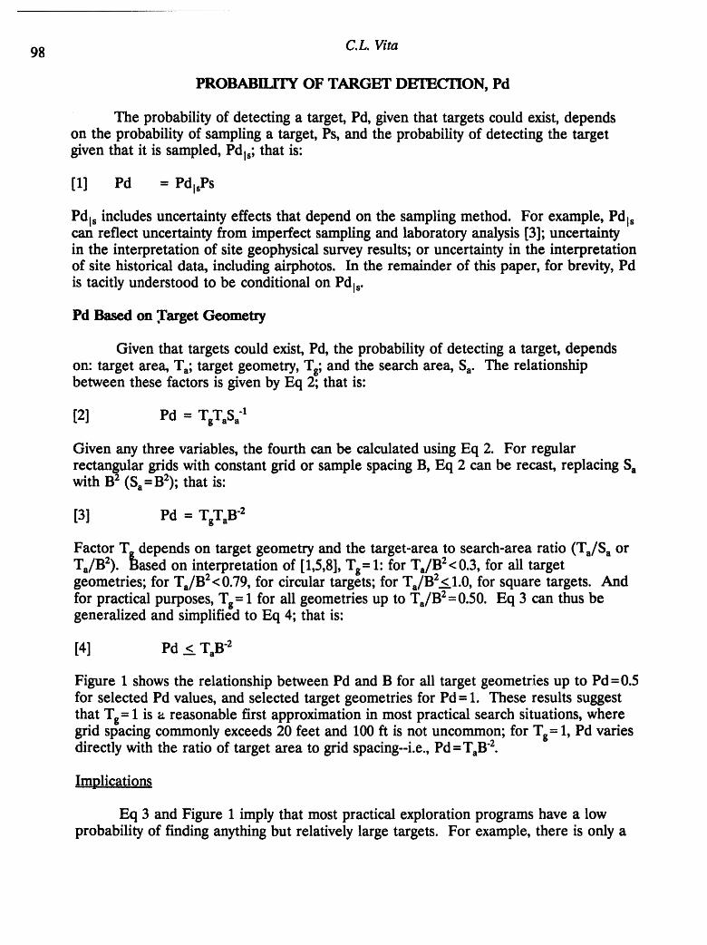
98 C.L Vita
PROBABILITY OF TARGET DETECTION, Pd
The probability of detecting a target, Pd, given that targets could exist, dependson the probability of sampling a target, Ps, and the probability of detecting the targetgiven that it is sampled, Pdls; that is:
[1] Pd = PdlsPs
Pdls includes uncertainty effects that depend on the sampling method. For example, Pdlscan reflect uncertainty from imperfect sampling and laboratory analysis [3]; uncertaintyin the interpretation of site geophysical survey results; or uncertainty in the interpretationof site historical data, including airphotos. In the remainder of this paper, for brevity, Pdis tacitly understood to be conditional on Pdls.
Pd Based on Target Geometry
Given that targets could exist, Pd, the probability of detecting a target, dependson: target area, Ta; target geometry, Tg;and the search area, Sa. The relationshipbetween these factors is given by Eq 2; that is:
[2] Pd = TgT,S_"1
Given any three variables, the fourth can be calculated using Eq 2. For regularrectangular grids with constant grid or sample spacing B, Eq 2 can be recast, replacing Sawith B 2 (Sa=B2); that is:
[3] Pd = TgTaB"2
Factor T. depends on target geometry and the target-area to search-area ratio (Ta/Sa orTa/B2). _3asedon interpretation of [1,5,8], Tg=1: for Ta/B 2<0.3, for all targetgeometries; for Ta/B2< 0.79, for circular targets; for Ta/B2<I.0, for square targets. Andfor practical purposes, Tg= 1 for all geometries up to Ta/B2=0.50. Eq 3 can thus begeneralized and simplified to Eq 4; that is:
[4] Pd < TaB"2
Figure 1 shows the relationship between Pd and B for all target geometries up to Pd=0.5for selected Pd values, and selected target geometries for Pd = 1. These results suggestthat Tg= 1 is _ reasonable first approximation in most practical search situations, wheregrid spacing commonly exceeds 20 feet and 100 ft is not uncommon; for Tg= 1, Pd variesdirectly with the ratio of target area to grid spacing--i.e., Pd =T_B"z.
Implications
Eq 3 and Figure 1 imply that most practical exploration programs have a lowprobability of finding anything but relatively large targets. For example, there is only a
Hotspots & Other Hidden Targets
991% probability of finding a 100-ft2 target using a grid spacing of 100 ft. Conversely, agrid spacing approaching the target size is necessary to achieve a high .findprobability.For example, finding a square 100-ft 2 target with 95°7..0probability requires a grid spacingof no more than 10.3 ft; and finding 100-ft2 targets with certainty requires a grid spacingof 10 ft or less, depending on target geometry. After exploration, no undiscovered,nearly-square targets of area exceeding B2 exist; and no circular targets exceeding 1.57B 2exist; and so on.
These results indicate that small targets or hotspots are likely to go undetected incommon exploration programs; and that not detecting a target or hotspot does notnecessarily provide confidence that there are none. Importantly, however, other relevantsite information that can be combined with grid-sampling information may be available.Combining independent information from different kinds of exploration can, in effect,increase Pd; the following section expands on this.
Pd Based On Sampling Results Or Combined Information Sources
Estimates of Pd can be based on sampling results. Imagine that an explorationprogram has identified D targets (D_>0) from N independent sampling points in astratum. Assuming that Pd-estimates, Pro[pal],follow a beta pdf between the limits ofone and zero, Ppo[pd],the expected value of Pd, E[Pd], and the coefficient of variation ofPd, CV[Pd], are given by Eq 5; that is:
[Sa] Ppd[Pd] = (a-l)![(b-l)l(a-b-l)!]'tpdb'1(l-pd)a'b'l
[5b] E[Pd] = b/a
[5c] CV[Pd] = Sqrt{(b-a)/(ab+a)}
wherea=N +2 andb=D +1.Parametersa andb includeallactualsamplingresults.BecauseEq 5 isBayesian,parametersa andb may includerelevantinformationnotcontainedinN andD; inwhichcase,a=N +2+a'andb--D +1+b',wherea'andb'
representtheadditionalinformationrelevanttoestimatingPd. Intermsoftargetgeometry,Eq 5 canbeusedwithEqs2 and3 toestimateparametersorvariables,includingtargetareas,Ta.Thus,parametersa andb may combinesamplingdataandtargetgeometryinformation.Parametersa'andb'may alsoincludeadditionalinformationfromsitehistoricalknowledgeorexperiencewithsimilarsites[10,11].Ifabetapdfisinappropriate,estimatesofPd canbebasedon anydesiredpdfusingthetotalprobabilitytheorem[7].
NUMBER OF UND_ TARGETS, U
Giventhatan explorationprogramoverareaAehasidentifiedD targets(D>0) ina stratum,how many undetectedtargets,U (U>0),remain?UnlessPd=I(makingU =0),U isunknown,andmustbe estimated.EstimatesofU dependon whetherPd isknownorestimated,asdiscussedinthissection.

100 ¢.L Vim
U, Number of Undetected Targets, Given Pd
Given that D and Pd are known, estimates of U follow a negative binomial pdf,with pdf Pu[u], expected value, E[U], and coefficient of variation, CV[U], given by Eq 6;that is:
[6a] Pu[u] = (u+ V)!(u!Dl)'lPd v+ l(1.Pd)U[6b] E[U] = (D + 1)(1-Pd)Pd"1
[6c] CV[U] = Sqrt{(E[U]Pd) "1}
Eq 6 has three special cases that are useful simplifications. Case 1.(U>01D=0): giventhat no targets were discovered (Dr0), the probability that undiscovered targets remain,Pu[ulD=0], and E[U] and CV[U] are given by Eq 7. Case 2.(Uf01D>0): given that Dtargets have been discovered, the probability that all actual targets have been discovered,and none remain, Pu[Uf01D>0], is given by Eq 8. Case 3.(Uf01D=0): given that notargets were discovered (D=0), the probability that no undiscovered targets remainPu[Uf01D=0] is given by Eq 9 (which is the same as Eq 8 with D=0 or Eq 7a withU=O). That is:
[7a] Pu[uID=0] = Pd(1-Pd)u[To] E[UID=0] = (1-Pd)Pd "1
[7c] CV[UID=0] ffi Sqrt{(1-Pd)"1}[8] Pu[Uf01D>0] = Pdv.l[9] Pu[Vffi0lDffi0] ffi Pd
Eqs 6-9 say that the probable number of undetected targets increases as the number ofdetected targets increases or the probability of detection decreases. Figure 2 plots E[U]by Eq 6b for D=0, 1, and 10. Figure 3 plots Pu[ulD=0] by Eq 7a for u=0 through u=5.Figure 4 plots Pu[U =0] by Eq 8 for D=0, 1, 2, 3, 4 and 10. Note that D may come fromone or more sampling phases in a given stratum.
Im!)lications
Interpretation of Eqs 6-9 amplify the implications related to Pd, the targetdetection probability: to find all targets, or hotspots, requires a high Pd. For example, toclaim a 95% probability that all targets have been found after finding no targets requiresPd=95%; and ff Pd= 1%, the expected number of remaining, undiscovered targets is 100.As another example, in terms of target areas, concluding with 95% probability that alltargets have been found after finding two targets is only accurate for targets having areasgreater than 98% of the sample spacing area, B2.
Yet finding all targets or making high-confidence conclusions may or may not benecessary, depending on site conditions and project requirements. That is, explorationeffectiveness should be consistent with project requirements. For example, high Pd's canbe limited to areas requiring high confidence; lower Pd's can be used in areas requiringi

Hotspots & Other Hidden Targets101
less confidence. Exploration that is optimally consistent with project requirements iscost-effective and provides acceptable risk at minimum COSt.
Tgrget Frequency; T.
Estimates of the total target frequency, Tf, over explored area Ae follows a gammapdf with PTt[tf],E[Tf] and CV[Tf] estimated by Eq 10; that is:
[10a] PTf[tf] = (AetfPd)D+lD!'lexp{-ActfPd}[10b] E[Tf] = (D+ 1)(AePd)"1[10C] CV[Tf] = Sqrt{(D+1)"1} <
Tfisthesum ofdiscoveredandundiscoveredtargetfrequencies:Taj,theundiscoveredtargetfrequency,beingTf(1-Pd);andTfD,thediscoveredtargetfrequency,beingTfPd.NotethatTfDisknown(CV[Tm]=0),whereasTfuisuncertain,withCV[Tfu]=CV[Tf].
Number of Targets in Unexplored Areas. A._
Estimates of U., the number of targets in unexplored portions of a stratum, A_,can be based on results from the explored portion A. of that stratum. Importantly, A_and A_ need not be contiguous or even part of the same site, provided they are from-thesame stratum. Estimates of U. follow a negative binomial pdf, with Pu.[U], E[U_] andCV[U.] given by Eq 11; that is:
[11a] Puu[U] = (u+D)!(u!D!)'x(PdA.)D+IA_"(PdA_+A_) "D'u'l
[11b]E[U.] = (D+ 1)Au(AePd)"I
[11c]CV[U.] = Sqrt{(D+1)"I+ E[U,,]"I}
wherePd isforAe.Notethatinbothexploredandunexploredareas(ofthesamestratum)targetsoccuratthesamefrequency.Therefore,thetotaltargetfrequency,Tf,canalsobeusedtoestimateE[U.];thatis:
[12] E[Uu] - AuE[Tf]
, U, Number of Undetected Targets, With Pd Uncertain/
Eqs 6-12 estimate U or Uu on the condition that Pd is known. They can alsoestimate U or Uu when Pd is uncertain using the total probability theorem (by summingthe conditional U-estimates times the probability of each Pd value) or other estimationmethods [7]. For the case of Pd following a beta pdf (Eq 5), Pu[u], E[U], and CV[U]are given by Eq 13, where l,arameters a and b are discussed following Eq 5; that is:
[13a] Pu[u] - (u+i))!(a-1)!(D+b)!(u+a-b-1)!{u!D!(b-1)!(a-b-1)!(u+D+a)!} 4[13b] E[U] = (D+ 1)(a-b)(b-1) "_

102 C.L. Vita
[13c] CV[U] = Sqrt{(a-1)(D-1)'lE[U] "1}
Eq 13, which is Bayesian, may be used to estimate targets in unexplored areas (Au) bysynthesizing estimates of parameters a, b, and D from interpretation of all available andrelevant data.
TARGET AREAS, TA
The areas of individual targets, I"., can be estimated from Eq 3, solving for T.:Ta=PdTilB 2. Then, Err.] and CV[T.] can be estimated from Eq 14, where Pr¢_ is thecorrelation coefficient between Pd and T s (which is always negligible for Pd< 0.5); thatis:
[14a] E[Ta] = E[Pd]E[Tt'I]B 2 (l+Prd,TsCV[Pd]CV[Ts])[14b] CV[T,] Sqrt{(CV[Pd]2+ 1)(CV['_s]2+ l)+2pl, d.TsC[Pd]CV[Tg]-!}
After exploration, the total area of discovered targets, TAD, is the sum of theindividual areas of the D discovered targets: TAD-SumD{Ta}, with E[TAD] and CV[TAD]estimated from Eq 15; that is:
[15a] E_AD] = E[TolD[1Fo] CV[TAD] = Sqrt{CV[T,]_/V}
Similarly, the total area of undiscovered targets, TAu, is the (random) sum of theindividual areas of U undiscovered targets: T^u=Sumu{Ta}, with E[T^u ] and CV[TAu]estimated from Eq 16; that is:
[16a] E[TAu] ffi E[Ta]E[U][16b] CV[TAu] = Sqrt[CV[T,]_/E[U] + CV[U] 2}
The total area of targets, T^, is the sum of discovered and undiscovered target areas:TA=TAD+ TAu. Then, E[TA] and CV[TA] can be estimated from Eq 17, where PTAU,TAD
is the correlation coefficient between TAUand TAD; that is:
[17a] E[TA] = E[TAv]+E[TAD][1To] CV[TA] =Sqrt{[V[T^v]+ V[TAD]+ 2PTAu,TAD(V[TAu]V[TAD])'5]E[TA] "2} •
\where V[TAu ] =(E[TAu]CV[TAu]) 2 and V[TAD] =(E[TAD]CV[TAD])_are the variances of
T^u and TAD. Estimates of Ta, TAD,T^u, or T^ can also be based on simulation or otherestimation techniques [7].
COMBINING EffIIMATES FROM INDEPENDENT EXPLORATION METHODS
In general, estimates of any variable (including Pd, U or U u, and TAD, T^u or T_may be based on multiple, independent exploration methods using Bayesian updatir/g[5,7-13]. Independent exploration methods may include information from other similar

Hotspots & Other Hidden Targets " 103
sites or site-specific information from, for example, historical data, terrain analysis,geophysical surveys, different sample-testing methods, exploration results from other s_temedia or strata, or information from physical or analytical modeling. By making use ofall available and relevant site data, plus relevant data from others sites, Bayesianupdating can reduce exploration costs and increase the accuracy of data interpretationsand decisions that use those interpretations. However, skill, good judgment, imagination,knowledge and consideration of all potentially relevant data, and understanding ofproject requirements, are all necessary for success.
GENERAL CONCLUSIONS
The forgoing concepts and equations are tools that can be used in projectplanning, analysis or design--at any project stage, from initial site investigation to finalsite closure. A general conclusion is that finding hidden targets, or hotspots, with highconfidence requires a high detection probability, Pal--which,using the tools presentedhere, can be maximized given available data. Yet finding all targets may be costly, andmay or may not be necessary, depending on project requirements.
Exploration that is optimally consistent with project requirements is cost-effectiveand provides acceptable risk at minimum cost. The fundamental practical implication isthat, at each project stage, field program design, implementation and interpretation,should be systematic and integrated with project requirements [11-14]. Explorationshould be focused, with sampling effort concentrated where it is most needed.Therefore, site conditions and history, together with project requirements, have to beskillfully and insightfuLlyassessed and synthesized to optimize strata definition andsampling effort. For any total level-of-effort, phased-approaches, using evolutionary,Bayesian updating and observational methods, can provide the best allocation ofexploration resources. Each phase should aim to maximize Pd for the area andgeometry of targets or hotspots that are important, consistent with the minimum-neededPal--whichwill generally vary across a site, even within a given stratum. At each phase,exploration should be done with the least-costly appropriate detection method available;for example, geophysical surveys can help optimize sampling locations and increase Pd,and field screening methods and field labs can help expedite and focus phased-samplingefforts. Systematic exploration increases the probability of finding all important targetsand controlling risk at minimum cost. The tools presented here, like all tools, can bemisapplied. Yet, when appropriately used with skill, imagination, and insight, they canhelp streamline and expedite environmental restoration, and help control risk at_nimnm cost.
CITED REFERENCF_#
1. Baecher, G.B. 1970 Site Exploration: A ProbablTisticApproach, Ph.D. dissertation,Dept. of Civil Engr., MIT, Cambridge, MA.
2. Elliot, J.M. 1973 Statistical Analysis of Samples of Benthic Invertebrates, FreshwaterBiological Association, England.
3. EPA 1987 Data Quality Objectives for Remedial Response Activities,EPA/540/G-87/003,4.

CL Vita104
4. EPA 1989 Methods for Evaluating the Attainment of Cleanup Standards,EPA/230/02-89-042
5. Gilbert, R.O. 1987 Statistical Methods For Environmental Pollution Monitoring, VanNostrand Reinhold, New York, N.Y.
6. The Hazardous Waste Consultant 1992 "Soil Sampling and AnaJysis--PracticesandPitfalls," 10(6) 4.14.26, Nov/Dec., McCoy and Assoc., Lakewood, CO.
7. Harr, M.E. 1987 Reliability-Based Design in Civil Engineering, McGraw-Hill, NewYork, N.Y.
8. Koch G.S. Jr. and R.F. Link 1980 Statistical Analysis of Geological Data, Dover, New oYork, N.Y.
9. Mangel, M. 1985 Decision and Control in Uncertain Resource Systems, Academic_ess, Orlando, FL.
10. Raiffa, H. and R. Schlalfer 1961Applied Statistical Decision Theory, HarvardUniversity Press, Cambridge, MA.
11. Vita, C.L i984 '_RouteGeoteclmical Characterization and Analysis,"Journal ofGeotechnical Engineed_, ASCE 110(12) 1715-34, Dec.
12. Vita, C.L 1985Arctic Route Geotechnical Characterization and Analysis: A SystemsApproach, Ph.D. dissertation, Dept of Civil Engr., University of Washington, Seattle,WA.
13. Vita, c.L. 1986 "Project Geotechnical Engineering: Systems MethodologyConsiderations," Civil Engineed_ Systems 3(3).
14. Vita, C.L i987 "Risk-Based Decision Making for Hazardous Waste Sites," InProceedings HMCRI 4th Nat. Conf. on Hazardous Waste & Hazardous Materials.

Hotspots& OtherHiddenTargets
•lOS
FIGURE I: FIGURER:PROBABILITY OF DETECTION, Pd EXPECTEDNUMBEROF UNDETECTEDTARGETS,E[U]
P4fO.IS--_
II_o_ T_IT Pd=IoOITII--I)'--_ _ DwNilMIIil Or DITICTrD T_EI_
._ ._n Pd,.._Te,2/_)-1 _
omQi=T.mnPd-t.o<_,,o.io)-; I I_ -o,o //"n't //-n't°,+,, ,oucr_.,.,, ,, • lo,,,ram,| _+L-- " = ] , , ,,' i i rl
r _ s ! _ sml .... w +wi .i i i_u xw , _ i'll' ' ' ' '"" "''""" "_-Pd._., _ "_'_ ;;;; _'_ _ ,,,,, _"I l I I IVIIi #11 Ill [If&l . IIIII ill
[._ ioc too ]
: - \: I!!!P\ i i_1_ I if I 1 rl#1l_ W • I 1 1,11 _-_:o,ol llll I% '_ lllll _L ' ' 'ii•m I Z I i, A'I#II A/! i lJil _, Illl I ", "_11111+_ ] .
II '1_111/ V I IXII! 'm' ',
l/I_ ll]__/!,tXl[[[ I][!I +t/; ....... I/I ; Ill" ;;;; ', , . -. I'I
/ I//,YII.'IIIII /I l l,,rlll IIII I IIIII . M ill
/ ,_/I II,IIIIoVI t/rllll Illl "+_!i....... I U .
_'_._o_ ,oo o.om o.ot o., ,, s.oSAMPLEGRIDSPACING,BPROBABILITY OF DETECTION, Pd
FIGURE 3: FIGURE4:PROBABILITY OF UNDETECTED TARGETS PROBABIlITyOF NO UNDETECTEDTARGETS,PU[U=O]
GIVEN NO DETECTED TARGETS, Pu[ulD=O]
Pu[u:,+-o]7LO - - ,:+
,.o. ' .... ' ]ii_l!t I _-P:,+. ,,,,, ,,,,,, "+,+-' ";+++'+;"'"'' iiiii'- '"" '"'" "+"I i I l llil I I ] t lltll I + u=O 111II IIIIII . . / lJl_lll
! !!!!!!!iilllio,- ' i .... _'" u=2 o,o-"=: = i iii',',',ii',_::i iii_iii+t il, II 11llillllII!11 I] _l_J'fll . 1 _ _l_mi_.---u=4 A I 1 I IIIIii A IIIIII /I I/Ylllll|, I I I Illlil i II_llll I \ _1 II 111111 _ IIII111 /I ,<_l_lllllI
" '"'"" J'' '"" ' 'i_"=_ L IIIIIII+_IIIII!/j/j/!!l!!l
++o! + !!!!!I 00'l 1 1 1/11111 I Illlll !1 !111 1 !I1|1
l ' ', IXIIll , .... : 1 I 1/111111 IVI II I I IlllllllI IIIIt ]/111111 :IIIII I VII IIIII ; I VIlli I II If IIIIIIIi /_z_ !llitl I /71111111 i I/lllll/ )_llllllll
, / ,,,,,, ll,II _ IIlllll! zrlllllIZtlLIIll]itl1oo, ' o. _.. oo, I.. o!,\\ "--,+, ,• i)=0 " Dml " \ '-- D-:i \ .0
O.OOt O.Ot l 0 DuNUiI_II OF DrrgcTID TARGL'T_ _-Dmli _-DmIO
PROBABILITY OF DETECTION. Pd PROBABILITYOF DETECTION,Pd

I06
Hydmgeology, Wute DisposM,Science and Politics
Proce_ings 30thSymposium 107EngineeringGeology andOeotechrdcalEngineering,1994
THE RELATIONSlIIP OF SEISMIC VELOCITY STRUCTURE AND
SURFACE FRACTURE CHARACTERISTICS OF BASALT OUTCROPS
TO RIPPABILITY ESTIMATES
S.E. Kay, M.E. Dougherty, and J.R. Pelton
Center for Geophysical Investigation of _he Shallow Subsurface,
Boise State Univer_ty, Boise, Idaho
ABSTRACT
Seismic velocity has been shown in previous engineering studies to be related to the fracturecharacteristics andrippability of rock outcrops. However, common methods of measuring seismicvelocity in outcrops do not take into account the many possible travel paths for wave propagationand the fact that velocity zones may exist within an outcrop. Presented here are the results ofusing raytracing inversi.on of first-arrivaltravel-time datato map P-velocity structure in basaltoutcrops, and also the investigation of the relationship of the mapped velocities to observed sur-face fractures and hand-sample P-velocities. It is shown that basalt outcrops commonly consist ofan irregularnear-surface low-velocity zone underlain by higher velocity material; _at velocitygradients can exist in outcrops; that hand-sample velocity measurements are typically higher thanoutcrop-scale measurements; and that the characteristics of surface fractures are empiricallyrelated to near-surface P-velocity. All of these findings are relevant to the estimated rippability ofrock in geotechnical engineering. The data for this study are derived from eleven sites on basaltoutcrops of the Troodos Ophiolite in Cyprus. The basalt types include pillow basalts, massiveflows, and a pillow breccia. A commonly available raytracing inversion program (RAYINVR)was used to produce a velocity profile of each outcrop. Different velocity zones were detailed byinverting observed travel times to produce a model of outcrop velocity structure which producesrippability profiles for each outcrop.
INTRODUCTION
The rippability of a rock or soil depends on its elastic moduli [Konya and Walter, 1990].Compressional seismic velocity (which will be referredto as the seismic velocity throughout thispaper) also depends on the elastic moduli of the medium. A direct correlation can be madebetween rippability and seismic velocity of rock (Figure 1). To some extent, the rippability of themedium depends on the equipment used for ripping. A Caterpillar D9N ripper copes with basaltof seismic velocity up to 2.3 kilometers per second, while a D 11N ripper can rip up basalt withseismic velocity up to 2.6 kilometers per second.
In Cyprus, a variety of basalt outcrops were selected for detailed study. Co-ordinated seismicand geologic investigations were executed to compare the seismic characteristics of the sites andtheir fracture patterns. Outcrop mapping involved measuring the size and shape of lithologies;density and aspect ratios of fractures; and the evolution of fracture filling. Seismic refractionexperiments were performed to understand the relationship between lithology, fracture densityand seismic velocity. Since the area of study in Cyprus is an ophiolite (oceanic crust emplaced

S.E. Kay and others108
above sea level), the primary objective of the parent study was to understand the relationshipbetween fractures and basalt velocity in upper oceanic crust. However, results from the Cyprusstudy have a much broader applications, one of which is presented here. The very high quality,three component data collected earl be used for engineering studies of the relationship betweenfractured rock and seismic velocity. Any study which discusses this relationship is applicable toconsiderations of rippability. Seis,rnic exploration as a means to estimate rippability has a lot ofpotential, especially with the availability of 24 and 48 channel seismographs.
Rippability is directional in nature. Fractures in the rock can create planes of weakness.Basalts, in general, show preferred fault orientation while lacking preferred crack orientation.Massive flows display colonnades, which do have a preferred fracture orientation. Where frac-tures are oriented, one particular direction would be more susceptible to ripping than another.Other formations with fractures show slower seismic velocities perpendicular to the fracture ori-entation [Stephen, 1985], though these results are on a much larger scale than outcrops. Increasedfracturing after blasting can also be detected through changes in seismic velocity [McCann et al.,1986]. Other seismic parameters, such as seismic attenuatien spectra, can be used to characterize
Seismic Velocity 0 1 2 3 4
Meterspersecondx 1000 I I . I I I I I I I
FeetpersecondxlO00 0 1 2 3 4 S 6 7 8 9 10 11 12 13 14 lS
RIPPABLE l ' MARGINAL_ NON-RIPPABLEI
Figure I. The dppability of a rock may be expressed interms of its compressional seismic velocity.For each different dpper the range ot rippable velocities changes. The plot shown here is for a Caterpil-lar D9N ripper [from Kenya andWalter, 1990,courtesy of Caterpillar Tractor Company]. It can onlycope with basalts with velocities up to 2.3 krn/s. Larger rippers can be used on outcrops with fastervelocities.
rock mass [Young and Hill, 1986]. It is possible to investigate the best ripping direction by exam-ining the seismic characteristics of a site. The possible volume that can be excavated, the specifi-cations of the ripper needed, and the best direction for ripping, can be interpreted using a detailedseismic survey
Site investigations often rely on geophysical logging of selected blast holes [Hendricks et al.,1992] or in simple seismic investigations using a limited number of geophenes. As the use of por-

Seismic Velocity Structure and Surface F_actures Related to Rippability of Basalt 109
table 24 and 48 channel seismographs increases, the amount of definition that a seismic site inves-tigation can provide will increase proportionally. Where surveys using four, eight, or twelvegeophones give only an overall seismic velocity for each velocity layer, it will be shown in thispaper that expanded geophone coverage combined with detailed modelling can give a much moredetailed picture of subtle variations in depth and velocity.
Another important aspect of seismic velocity is the disparity of field seismic velocity mea-surements and laboratory measurements of velocity in hand samples. Figure 2 is one example ofthis relationship as seen in the Cyprus outcrops. Laboratory measurements of velocity are plottedagainst the velocities observed in the field refraction results. One controlling factor on seismic
1l,S
1.0i.o l.s 2.o zs xo _ 4_ 4_ 5.0
Fieldvelocities(km/s)
Figure2. Laboratorymeasurementofhandsamplevelocitiescomparedtofieldmeasurements(undersurfacepressureconditions).Allthelaboratorymeasurements,exceptforonevalueforsite6, arehigherthanthemeasuredfieldvelocities.Samplevelocitiesfromeachsitearcconnectedbya solidline,indicatingthe rangeofmeasuredlaboratoryvalues.Fieldvelocitiesareanaverageofthe reciprocalvelocitlescalculatedforeachsite.Thesolidlineat45degreesisthelinealongwhichthetwovelocitieswouldlineupifhandsampleandfieldvelocitiesagreed.
velocity is the presence of fractures in the field. Correlations can be made between lower seismicvelocities and increased fracture densities [Kuster and Toksoz, 1974, O'Connell and Budiansky,
- 1974], and is directional in nature [Peacock et al., 1994]. At the present time, however, an under-standing of the exact relationship has not been reached and theoretical predictions are poor in allbut ideal conditions where rock with only one set of fractures is considered.
In this paper, the vafiatio!_pf velocity within outcrops will be considered. It will be shownthat velocities can vary within homogeneous basalt layers, and on seemingly unifo,-m outcropsthere is often a slow velocity present layer atthe surface. This has a profound effect Gn the rippa-bility of an outcrop. The need for good quality seismic data, along with geologic infocmation, toproduce a model in which confidence can be placed will be discussed. Outcrop seismic velocitiesare shown to be lower than those in measured hand samples, and to be locally variable. Variationsare related to the observed fracture densities. Seismic velocities can be used to identify localchanges in elastic moduli, thus giving a more detailed rippability profile of an outcrop.

110 S.E. Kay and others
GEOLOGIC SETTING
The Troodos Ophiolite Complex lies in the south western thirdof Cyprus. A wide variety ofbasalt volcanic units are present in the complex, including pillow lavas, massive and sheet flows,hyaloclastites and volcanic breccias. River canyons expose cross-sections through the volcanicsequence along the northern flank of the ophiolite. Within these canyons, volcanic units may betraced up to a few hundred meters both laterally and vertically. Sites included in this study cov-ered the complete range of lithological types [Dougherty et al., 1992a,b]. At each site, a detailedgeologic study was carried out, including fracture density measurements [Gillis et al., 1993].
Analysis of two sites from the Cyprus study are presented in this paper. These two sites havecontrasting geology and topography. Site 6 consists of._ differentiated massive flow that is greaterthan 10 meters thick and extends for at least 100 meters along strike. Towards the eastern end ofthe flow, pillow lavas begin to dominate th_ outcrop. Two sets of cooling fractures can be seen,:ertical fractures which define the margins of the columns, and horizontal fracturing across a fewof the columns. One seismic line was run near the crest of the outcrop, with an additional parallelline lower on the slope (Figure 3). In this paper, the upper line, qu, is modelled.
Figure3. Plotofsite6 showingboththeupperandlowerseismiclines.Thegeophoneandshotlocationsarebothshownasblackdots.Seismicresultsandmodelsofthe linetowardsthebottomof thefigurearepresentedbelow.Theoutcropconsistedof a ridge,witha gentlydippingslopetotheeast.Onthewesterlyfacingedge,columnarjointingisclearlyseeninoutcrop,aswellasthecappiogentablatureontheexposedface oftheflow
Site 8, the second site presented here, is located in an abandoned copper mine at Kampia. Theline was laid out along a flat bench along the northern edge of the open pit. Hyaloclastite makesup the major par_ of the outcrop, with pillows, massive flows and cross cutting sheeted dikes.Sheet flows have irregular orientations with regular jointing patterns, and locally appear to flowover hyaloclastite mounds. Where dikes cross cut the hyaloclastite, it is highly competent, proba-bly due to heating and metamorphism during emplacement. Weathering was limited at this site,and overburden had been removed in the course of mining. At the mine, two lines were laid out onadjacent benches, but in this paper only the lower line will be considered (the upper line was des-ignated Site 9).

Seismic Velocity Structure and Surface Fractures Related to Rippability of Basalt 111
DATA ACQUISITION
One of the original intentions of the project was to obtain a high quality engineering seismicdata set which could be applied to a variety of studies involving the relationship between frac-tured rock and seismic velocities. At each site, five 1/3pound dynamite shots were acquired withthe seismic line laid out at 3-5 meter station spacing. Total spread lengths ranged from 48 metersto 112 meters, measuring from end shot point to end shot point. Three-component, 10-Hz geo-phones were used at each of 16 stations, recording a total of 48 channels for each shot record. Thedata were recorded on a 48-channel, digital, floating point seismograph. Hand samples were takenfor la[ Jratory measurement of rock matrix P-velocities, and fracturemapping was carded outover each outcrop by field and laboratory analyses of high-resolution photographs.
In the field, each shot record was printed to ensure that the record had been properly stored.Originally, five shots had been planned for each site, but due to misfiring, or a failure of the triggermechanism, some lines only had four records. First arrivals were picked and some idea of veloci-ties was obtained by taking the slope of the first picks against distance to geophone. Reciprocalvelocities [Hawkins, 1961] at each site were calculated (Table 1). Also, the three component datafor each site was isolated and velocities worked out for the transverse, longitudinal and verticalcomponents. The vertical component was utilized for the raytracing profiles. Most field experi-ments are carried out using arrays of vertical component geophones, so in for most data sets onlyvertical velocitieswill be available.There is _ wide rangein basaltvelocitymeasuredat thedif-ferentsites,from 1.64 km/sat site2 to 3.12 kan/sat site7.
Table 1"Average P-wave velocitiesobtainedusingthe reciprocalmethod.
1 Akaki pillows 4 2.09
2 Akaki pillow breccia 2 1.64
3 Akaki pillows - west side 8 2.42
4 Akaki pillows- low T 2 2.78
5 Eucalyptus massive flow 2 2.48
6 Marki weathered massive 6 2.61flow
7 Analiondas pillows, low T 8 3.12
8-9 Kampia hyaloelastites, sheet 8 2.51Mine flows, dikes
10 Mathiati altered pillows 4 2.18mine
11 Delikipo pillows 8 3.03

$.E. Kay and others
112MODELS AND INVERSION
Model construction
Many raytracingprogramsareavailablefor modellingthepropagationof seismicenergythroughan outcrop.RAYINVRwas originallydesignedforthe modellingof deep crustalseismicdata [Zeltand Ellis, 1987].It is used hereto model outcropson the scale of tens of meters.Thefundamentalfeatureof RAYINVRis its simple,layered, large-blockvelocity model parameter-ization, whichallows for efficientraytracing.The modelerconstructsa two dimensionalprofilefor a seismic line, consistingof distance, depthandvelocity values forthe layersthat are expectedin the model.Initially,the profileis usedto forwardmodel the arrivalsthathave beenpickedfromthe seismic data (Figure4). It is importantto havea clear view of how the arrivaltravelled,fromwhich layerand type of seismicenergy it originated.For the Cyprus sites, a detailed surveywascarded out to give preciselocationsfor the geophonesand shot points. At largersites, a gridsur-vey was car_,iedout so that topographicplots, such as Figure3, could be produced.
DL_ANCE (in)0 18 36 $4 72 90
- 2.0 I . , , . I lI
Directarrivals
. Head waves [
i l,f£f]/,Tfrr t/f . lrr,ir/.lllfl.!t/fl.lWlTifflT,
i
I.S- yerl - 1.2_ Inn/. :///:
_y.rz. Zsoi_. : :
_ 36 / Head waves24 Directarrivals _ I-_I_t_+_ ....
_-.._'t"_'_ _ "
I ! ! 'r j
0 18 36 $4 72 90
DISTANCE (m)
Figure 4. RAYINVR model for site 8, located on the north face of Kampia mine.The upper portionof the diagram contains the profile model for this site, with direct arrivals and head waves from the top ofthe second layer plotted. Dashed lines indicate the boundaries of the blocks into which the model isdivided. Velocity and depth values are entered for each comer of these blocks, and may be changed dur-ing the inversion process.The lower plot shows the actual picked arrival times as crosses with the calcu-lated travel times as solid lines. The first layer is a uniform two meters thick for the entire line, with auniform velocity of 1.25 km/s. Velocity of the second layer, 2.50 km/s, was taken directly from Table 1.This model fits the data fairly closely, with calculated time being slightly slower than real times. Only theray paths for one shot are shown here, whereas in the forward modelling stage all shots are considered.
When a model has been adjusteduntil the rootmean squareresidualtraveltime error(RMS)value is reasonablylow, aninversioncan be attempted.RMSerror is a measureof the errorbetween the pickedarrivaltimes andthe calculatedarrivals,andis calculatedby summingthesquareddifferencesbetween real and modelledarrivalsand dividingby the total numberof datapoints.A "reasonable"value of RMSerrorvariesfrommodel to model, but in general,the morecomplicatedthe model, the harderit is to reducetheerror.Forthe two following examples, Site 8producedlowererrorvalues than Site 6, butcontainedone less layer.Inversionsinvolve changes
Seismic Velocity Structure and Surface Fractures Related to Rippability of Basalt
either in the depth or the velocity of a layer (Figure 5), or both simultaneously (Figure 6). Inver- 113sions are performed after close agreement with the field data has been reached, and involve aseries of damped iterations. If the forward model is too far from a reasonable representation of thesite which produces the field data, the fiist inversion will abort.
f
Site $ Results
Site 8 is located along a bench cut into the northernedge of an abandoned Kampia mine. Aledge ran parallel and below the ledge along which the seismic line was laid out, so a detailed pic-ture of the geology underlying the line was available. The surface of the bench is flat, with littleevidence of surface weathering. Initial modelling centered around one layer with velocity gradi-ents, but the data were poorly matched by such a treatment of the site. A model then was con-structed with a very thin, 25 centimeter, slow velocity or weathered layer at the surface. Thisproved to give a very poor fit to the data until the slow velocity layer was increased to 200 centi-meters as shown in Figure 4, the RAYINVR profile which was the starting point for the inver-sions. From the first arrivals, a velocity of 1.25 km/s was established for the first layer, and avelocity of 2.50 km/s was established for the second layer. Real time picks are shown as crosses inthe lower portion of Figure 4, with the calculated travel times shown as a solid line. Figure 4shows the ray paths for the second shot at this site, which was offset five meters from the first geo-phone. Direct waves in the first layer and head waves from the top of the second layer were tracedas the observed arrivals.
A series of inversions were'then carried out for Site 8, using Figure 4 as the starting model.Figure 5a shows the result of an inversion which allowed the depth of the first layer to change.Considerable differences exist between the inverted and original model, chiefly being an overallincrease in depth of the slow velocity layer. The ends of the seismic line show a decreased depthof the slow velocity layer. Since no actual field data are available at the end of the line, the thin-ning is questionable. Figure 5b shows the result of an inversion which allows only velocity inlayer 2 to vary. Damping of the allowable change in velocity was greater in this inversion than forthe depth inversion. Increases in velocity were observed along most of the line, with a fewdecreases. Calculated range of velocities in this inversion was 2.45 km/s to 2.79 kin/s, with twovalues at 65 and 70 meters remaining at 2.50 km/s. Both inversions reduced the RMS value con-siderable, showing statistically a better fit to the data.
It is reasonable however to assume that both the depth and velocity values vary from thestarting model. Figure 6 displays the result of an inversion allowing both parameters to vary. Raysare traced for shot point two again so the variations in the depth can be clearly seen. Variations invelocity and depth are slightly reduced. Velocities vary from 2.47 km/s to 2.72 krrdsin the model.Damping was increased for this inversion, and the number of iterations increased. RMS value islowest for this final model. Two distinct dips in the slow velocity layer can be seen, one at l0meters and one at 50 to 60 meters.
Site 6 Results
Site 6 consists of a massive differentiated basalt flow. Originally, site 6 was modelled usingrays refracted through a single continuous layer, with topography accounting for the change inslope of arrival times. It was soon obvious that it was impossible to use this model to fit theobserved data without using unrealistic velocity gradients. Once a two layer model using headwaves was considered, a closer fit emerged. This came close to modelling the outcrop, butobserved arrivals near the end of each record were faster than calculated. At this stage, the veloc-ity was considered as if the first arrivals from each shot were direct arrivals. This suggested thepresence of a much lower velocity zone at the surface. Once this was added, an inversion was pos-sible, as good fits could be achieved for all the time picks. The starting model contained a meter

I14 $.E. Kay and others
DISTANCE (m)
0 18 36 54 72 90
.2.0' i ,, L L ,/
] i! ! !._o_ i! i z_,i Is.o, ili i!iiil i ii i : ! i i
_ + Headwsves
48
24
i 0 18 36 $4 72 90
DISTANCE(m)
0 18 36 54 72 90-2,0! l , t l ....... ,
2_.._0i:m/_ : : ::: : i i ! : 258kni/Iss.o[ _:'s°,k'_', .: i i i. !ii ! : : ,, i i': : J60 ....... _ b.
0 18 36' _4 '_2 _)
DISTANCE (m)
Figure S. Inversions, allowing depth (a) and velocity (b) to vary, for Site 8. When depth of the firstlayer is allowed to vary (a) two distinct areas of thickening occur and in a few areas thinning occursallowing the calculated times to decrease and better fit the field data. In (b), the velocity of the secondlayer was allowed to vary, but not depth or velocity in the first layer. For the majority of the second layer,velocities are slightly increased except in the areas where in the depth inversion layer I was increased.For both inversions, there are two picks which RAYINVR discarded due to the fact they lay far outsidethe normal range expected for the arrival times for the geophones. Rays from all the shots are shownhere for both inversions.

Seismic Velocity Structure and Surface Fractures Related to Rippability of Basalt
D__ (,.) 1150 18 36 54 72 90I __
• 2.0 , j i , .......
z z !,, , : .soku_s, t , i n __
$,0 ' '" ' '6O
36- Headwaves
12-
0 , i0 18 36 54 72 90
DISTANCE (In)
Figure 6. Inversion for Site 8, allowing both velocity and depth to vaFy.The same trends seen inthe previous inversions are present here. The depths of the low velocity layer vary, thickening around10 and 48 meters, and thinning slightly,especially towards the ends of the line. Veloci_ areless than before, with most values remaining near 2.50 km/s. Ray paths for shot pointll_l_ shownhere, and when compared to Figure 4, it can be seen that the agreement between the calculated andfield data is much improved over the initial model.
thick slow velocity zone of 1.25kin/s, a ten to twelve meterthick intermediatevelocity zone of2.55 knVs,on top of a bottom fastzone of 3.20 knVs.Figure7 shows this model with raystracedfor the centershot. Again,crossesshow the arrivalspickedfromthe fielddata,andsolid lines thecalculatedtraveltimes. Fit between calculatedandreal datais poorerhere than in the previousmodel which is in partdue to the addedcomplexity of a thirdlayer.
As in the examplefor site 8, two inversionswerecarriedoutusing firstchanges in depth, andthen changes in velocity.The depthvaryinginversion,asseen in Figure8a,came close to the fielddata, tendingto increase the depth of the slow velocity layer.The inversionallowing velocityvariationsalone was notas successful,producinga model using unrealistic velocity gradients,asseen in Figure 8b.Finally,a combinedinversionwhichallowedboth velocity and depth to varywas carriedout (see Figure9). The overalldampingwas increasedbutthe numberof iterationswas increasedto achieve asimilarRMSvalue as the previousdepthinversion.Velocitieschangedslightly,but stayed within :1:0.20knVsof their originalvalues. Therearesimilar changes in layerthicknesses as there was in the inversionallowingonly depthto vary.For the centershot, theagreementon the lowerend of the seismic line is muchbetter than for the uppergeophones. Thisis truethroughoutthe dataat this site, uppergeophonearrivalstendingto be slowerin reality thanthose calculated.
DISCUSSION
Each one of the above models began with the surfacetopography,a full descriptionof thegeology, andan estimationof the thicknessof slow velocity layerat the site. The startingmodelsrely onreciprocalvelocities workedout fromthe fieldrefractiondata.Assumptionshave to bemade aboutthe depthto bedrock,the errorpresentin pickingfirstarrivals,even to the type _f ,.

116 $.F.. Kay and others
DISTANCE (m)
0 18 36 54 72 90
"_O'e] ' _ ' ' 'lDirect arrivsls Head waves - layer 2
.$.0- _ x,| * i i
_ : , ,
1o.o :: 3 3.o i60
0 18 36 54 72 90DISTANCE (m)
Figure 7. The initial RAYINVFIImodel for site 6. Three layers are included, and rays are traced fordirect arrivals, head waves from the second layer and head waves from the third layer. As in the previ-ous RAYINVR plots, actual arrival times are shown as crosses, and calculated times as solid lines.Here, layer 3 is split into fewer velocity blocks than the other layers, since it is less constrained by ray-paths. For this model, all the calculated times are slower than the field data. Compared to Site 8, thestarting RMS value is higher indicating greater misfit for the Site 6 model.
arrival assigned to each arrival time, whether they are refracted, reflected or head waves. How-ever, as numerous variations are u_iedat each site, certain parameters become more defined.
Modelling of site 8 revealed the presence of a slow velocity layer along the surface of the out-crop. Initial modelling failed to fit:the calculated rays to the data until this layer was added. Inver-sions of the model that showed two distinct areas of thickening occur at 10 and 50 meters. Thiswould allow more of the outcrop 1_obe ripped than could be judged by the starting model.Veloci-ties from the hand samples for this site were the highest measured (Figure 2), being in the region3.60 km/s to 4.80 km/s. Reciprocal velocities for the outcrop are much lower (Table 1), averagingonly 2.51 km/s. Within the second layer, there are velocity gradients. Across the outcrop, veloci-ties increase and decrease both horizontally and vertically (Figure 6). It was only through apply-
• ing raytracing to the data, that these details emerged. Modelling produced a good fit to the data,and the combined inversion matched the observed arrival times for each shot record very closely.The velocity variation found in the second layer (Figure 6) lies outside the range of rippabilityseen in Figure 1. A high degree of confidence can be placed in the final inverted model for thissite.
Originally, site 6 was modelled using refracted rays through a single layer. It soon becameobvious that it was impossible to use this model to fit the observed data. Once a two layer modelusing head waves was considered, a closer fit emerged, but again this only agreed with the data toa degree. At this stage, the velocity was considered as if the first arrivals from each shot weredirect arrivals. This showed the presence of a much lower velocity zone. Once this was added, aninversion was possible. It should be ne_ed that the geologic description of site 6 includes referenceto columnar jointing being present between a very weathered capping layer, and a base of minorflows and pillows. The second layer very likely represents the columnar jointed basalt, capped byan entablature. This kind of detail picked up by modelling the seismic data is very important, as it

Seismic Velocity Structure and Surface Fractures Related to Rippability of Basalt 117
DISTANCE (m)0 18 36 54 72 90
- 20.0 i i t L I
- 15.0-
10.0 ' ' " ....... a.6O
48 Head waves
12
0 ,0 18 36 54 72 90
DISTANCE (m)
0 18 36 54 72 90
-20.0 J .... L , _ ' iI
i ". s.o "_-
10.q i :...... : ' ; ' b.60
48 t_-___. Head waves ._j_
o| , , , , '7,0 18 36. 54 72 90
DISTANCE (m)
Figure 8. Site 6, the RAYINVR inversions varying both depth (a) and velocity (b). For the depthinversion (a), the first layer was increased in thickness across the whole of the seismic line, this effectbeing especially pronounced at 5 meters. The overall shape of the adjusted layers f'dswell with geologicmapping of the site. Velocities in the second inversion (b) are unrealistically low for the top of layer two,and vary considerably more than they did in the inversion for site 8, and produce unrealistic velocity gra-dients.
marks the first stage of relating f_acturepatterns to outcrop velocities. It should be noted in Figure2, Site 6 had the lowest hand sample velocities. These hand samples represent the weatheredlayer. Velocities variations for the second layer of this outcrop vary between 2.23 km/s and 2.55km/s. From Figure 9, it can be seen that the lower section of the seismic line, between 0 and 50meters, overlies rippable rock in layer 2 as defined in Figure 1. The upper section of the line,
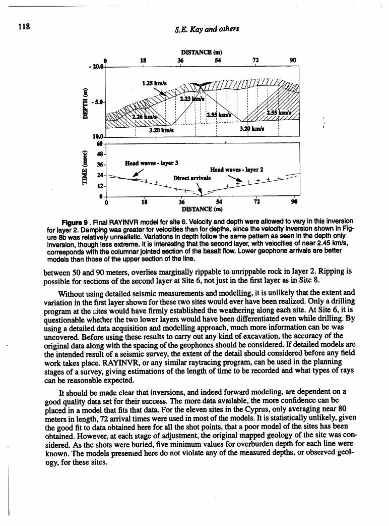
118 S.E. Kay and others
DISTANCE (m)0 18 36 54 72 90
- 20.0' I I l I ,
• . " i i t t
i i , i i , i. - t i i i i
, , , : , ,
50 _" ' , ' '
' i - " l ! i
i _e--v .,.,_._ -- t o
10.0 ' , ' : . ' '60
36- Head waves - layer 3
_ 24- _ DirectarrivalsHead waves "layer 2
o 18 36 s4 iz 90DISTANCE (m)
Figure 9. FinalRAYINVRmodelforsite6. Velocityanddepthwereallowedtovaryinthisinversionforlayer2. Dampingwasgreaterforvelocitiesthanfordepths,sincethevelocityinversionshowninFig-ure8bwasrelativelyunrealistic.Variationsindepthfollowthesamepatternasseeninthedepthonlyinversion,thoughlessextreme.It isinterestingthatthesecondlayer,withvelocitiesof near2.45krn/s,correspondswiththecolumnarjointedsectionofthebasaltflow.Lowergeophonearrivalsarebettermodelsthanthoseoftheuppersectionoftheline.
between 50 and 90 meters, overlies marginally rippableto unrippable rock in layer 2. Ripping ispossible for sections of the second layer at Site 6, not just in the first layer as in Site 8.
Without using detailed seismic measurements and modelling, it is unlikely that the extent andvariation in the first layer shown for these two sites would ever have been realized. Only a drillingprogram at the _ites would have firmly established the weathering along each site. At Site 6, it isquestionable whether the two lower layers would have been differentiated even while drilling. Byusing a detailed data acquisition and modelling approach, much more information can be wasuncovered. Before using these results to carryout any kind of excavation, the accuracy of theoriginal dataalong with the spacing of the geophones should be considered..If detailed models arethe intended result of a seismic survey, the extent of the detail should considered before any fieldwork takes place. RAYINVR, or any similar raytracing program, can be used in the planningstages of a survey, giving estimations of the length of time to be recorded and what types of rayscan be reasonable expected.
It should be made clear that inversions, and indeed forward modeling, are dependent on agood quality data set for their success. The more data available, the more confidence can beplaced in a model that fits that data. For the eleven sites in the Cyprus, only averaging near 80meters in length, 72 arrival times were used in most of the models. It is statistically unlikely, giventhe good fit to data obtained here for all the shot points, that a poor model of the sites has beenobtained. However, at each stage of adjustment, the original mapped geology of the site was con-sidered. As the shots were buried, five minimum values for overburden depth for each line wereknown. The models presented here do not violate any of the measured depths, or observed geol-ogy, for these sites.

Seismic Velocity Structure and Surface Fractures Related to Rippability of Basalt119
One of the results of modelling both these sites was the realization of the importance of goodquality seismic data. Reductions in the availability and quality of seismic data carry through to themodelling stage. In this study, datacollection was carded out with a high degree of precision,, butstill, one shot which was not recorded at Site 6 resulted in a subsequent reduction of the resolutionpossible for this site. Site 6 is a complicated outcrop that differs from Site 8 in that three layers arepresent. With a smaller data set as well, it follows that it is not possible to have as much confi-dence in the inversion for Site 6 as in Site 8. However, clearly Site 6 is composed of three velocitylayers which are quite closely approximated in Figure 9. Errors in the arrivals times for both thesemodels are in the region of two milliseconds, so it is unreasonable to push the inversions to fit thepicked times exactly.
Rippability, along with seismic velocity, is highly dependent on the fracture patterns in a rockmass. In some circumstances, prior to any excavation, it could be cost effective to conduct adetailed seismic study first. Where a simple analysis of the seismic data could lead to the conclu-sion that ripping is not an option, a raytracing model of the site may uncover that sufficient varia-tion exists in the outcrop to make it worthwhile. In each of the models presented, velocities anddepths vary across an outcrop, bringing sections of the outcrop into and out of the range of rippa-bility. Planning a more effective excavation of a site may be possible with the kind of detailedseismic survey outlined here. In areas that are environmentally sensitive, a seismic survey couldbe used to investigate the subsurface while having minimal impact on the land. Instead of a drill-ing program, a detailed seismic refraction survey could obtain the same information.
CONCLUSION
It has been shown in this paper that detailed seismic data acquisition and modelling at a_?out-crop scale can provide a detailed velocity profile of on outcrop. On all outcrops it revealed theunsuspected presence of a slow velocity layer, even on rock outcrops with no overburden. Such amodel is extremely useful when considering the rippability of a particular site, and can provideinformation on the best direction of ripping since seismic velocities tend to be lower perpendicu-lar to fracture orientations. Velocities and depths have been shown to display sufficient variationin sites that the rock may vary between rippable and unrippable.The importance of good qualityseismic data, with reasonable coverage for the scale of detail required can not be overstated. Withthe availability of 24 and 48 channel portable seismographs, seismic evaluation is a viable alterna-tive to drilling for site assessment Such a survey can provide much more detail on subsurface con-ditions with far less impact on the environment.
ACKNOWLEDGEMENTS
This research was funded by the Office of Navel Research Grant #N00014-92-J-1143 toBoise State University. Boise State University Center for the Geophysical Investigation of theShallow Subsurface contribution 0026.
REFERENCES
Curfman, J.E., Ripping of ores and overburden, Can. Min. Metall. Bull., $8, 645 - 648, 1964.
Dougberty, M.E., S.E, Kay, J.R. Pelton, and K.M. GiUis, Predictions of fine scale seismic structureof the upper oceanic crust, Transactions, EO$, 74, 426, 1993.
Dougherty, M.E., K.M. Gillis, and J.R. Pelton, Heterogeneity and Permeability of the upper oce-anic crust, Troodos Ophit_liteComplex, Cyprus, Center for Geophysical Investigation of the

120 S.E. Kay and others
Shallow Subsurface Technical Report BSUCGISS #92-05, Boise State University, 72 pp,1992a.
Dougherty, M.E., K.M. Gillis, J.R. Pelton, and K. Sapp, A geological and seismic study of the up-per oceanic crust in the Troodos Ophioiite, Cyprus, Transactions, EOS, 73, 355, 1992b.
Gillis, K.M., K. Sapp, and M.E. Dougherty, Distribution of porosity in the upper oceanic crust ex-posed in the Troodos Ophiolite, Cyprus, Transactions, EOS, 74, 241, 1993.
Hawkins, L.V., The reciprocal method of routine shallow seismic refraction investigations, Geo-physics, 26, 806 - 819, 1961.
I-Iendricks,C., J. Peck, and M.J. Scoble, Machine performance monitoring in surface mines, Min.Eng., 44, 243 - 250, 1992
Konya, Calvin J., and Edward J. Walter, Surface Blast design, Prentice Hall, Englewood Cliffs,New Jersey, 303 pp, 1990.
Kuster, G.T. and M.N. Toksoz, Velocity and attenuationof seismic waves in two-phase media: Part2 Experimental results., Geophysics, 39, p 607-618, 1974.
McCann, D.M., R. Baria, P.D. Jackson, and A.S.P. Green, Application of cross-hole seismic mea-surements in site investigation surveys, Geophysics, $1, 914 - 929, 1986.
O'Connell, R.J. and B. Budiansky, Seismic velocities in dry and saturatedcracked solids, J. Geo-phys. Res., 79, 5412-5426, 1974.
Peacock, S., C. McCann, J. Sothcott, and T.R. Astin, Seismic velocities in fractured rocks: an ex-perimental verification of Hudson's theory, Geophys.Prospect., 42, 27 - 80, 1994.
Savely, James P., A comparison of rippability with shear strength of a boulder conglomerate, Pro-ceedings of the 28th US Symposium on Rock Mechanics, 927 - 934, 1987.
Stephen, Ralph A., Seismic anisotropy in the upper oceanic crust, Y.Geophys. Res., 90, 11,383 -11,396, 1985.
Young, R.P. and J.J. Hill, Seismic attenuation spectra in rock mass characterization; a case study inopen-pit mining, Geophysics, 51, 302 - 323, 1986.
Zelt, C.A. and R.M. Ellis, Practical and efficient ray tracing in two-dimensional media for rapidtraveltime and amplitude forward modelling, J. Can. Soc. Expl. Geophys., 24, 16-31, 1988.

Hydroseolosy, Waste Disposal, Science and Politics 121_ings 30th SymposiumEngineering Geology and Geotechnical Engineering, 1994
GEOLDGICAND _CAL INVES'IIGATIONOF THRWINDSORPARK SUBDIVISION
NORTH LAS VEGAS, NEVADA
M. _ James L. Wede, C.E.G.,AlanN. Stilley, P.E. and BradL. Ohm, E.I.T.
Converse C.om_t,mts Southwest, Inc., Lu Vegas, Nevada
ABSTRACT
The Windsor Park subdivision in North Las Vegas, Nevada has received wide-spreadattentionfor damage to the homes and infrastructurefrom fissures, land subsi-dence and adverse soil conditions. Between Marchand July, 1992, Converse Consul-tants Southwest, Inc. conducted a geologic and geotechnical investigation for theWindsor Park RevitalizationProject. The purpose of the work was to investigate theprobablefactors contributingto the reporteddamage and distress in the area, evaluatethe potential for future damage, and assess the feasibility of possible mitigation andrepair.
The site is constructed on the juncture of at least two subsidence-related faultscarps, and earth fissures have been extensively maplx_ in the Windsor Park andsurroundingarea. A total of twenty-one trenches and fifteen borings were locatedwithin the subdivision and aroundthe perimeter to observe subsurfacegeologic featuresand to collect samples for laboratorytesting. The primary causes of damagewithin thedevelopmentwere foundto be (1) earth fissuringand (2) expansiveclays.
The risk of future damage to structuresat the Windsor Park site was also evaluat-ed. A high potential for fissuringwas found at the site, and future structuraldistress inthe area will likely be similar to past damage. Although engineering upgrades willreduce the risk posed by underlyingexpansive clays, they cannot totally eliminate therisk from fissuring.
INTRODUC'HON
The Windsor Park subdivisionis a residentialdevelopmentconsisting of 246 homesin the central portion of North Las Vegas, Nevada. The homes were built between1964 and 1965 and consist of single-story, wood-frame construction supported byeither slab-on-gradefoundationsor perimeter footingswith elevated wood floors (crawlspaces). Damage to homes and infrastructurein the area has been documented sincethe early 1980's, and numerousstudies have been performedsince 1984 to assess theseproblems and determinepossible causes for damage and fissures in the subdivision.However, conclusions made in previous investigations were often contradictory
_
=__
_

122
hM. Linnert and others
indicating that the problem is very complicated as multiple and possibly interrelatedproblems may coexist at the site.
In February, 1992, Converse Consultants Southwest, Inc. was contracted by theCity of North Las Vegas to conduct a geologic and geotechnical investigation for theWindsor Park Revitalization Project. The purpose of the work was to determine theprobable cause of distress to the neighborhood homes and infrastructure, evaluate therisk for future damage and provide recommendations for mitigation accordingly. Thescope of work consisted of compilation and review of previous investigations andgeologic literature for the area, extensive subsurface explorations, laboratory testing,and assessment of our fmdings.
GEOIJ3GIC SEITING
Geologic and Hydrologic Cmu]itions
The Windsor Park subdivision in North Las Vegas, Nevada lies in the north-centralportion of the Las Vegas Valley in the Basin and Range physiographic province. Thedistinctive features of the province are isolated, nearly parallel mountain rangesseparated by long, wide valleys. The Valley is filled with Tertiary and QuaternaryAge unconsolidated alluvial and lacustrine (playa-like) sediments derived from thesurrounding mountains. It is approximately 50 miles long and 5 to 25 miles wide.Figure 1 shows the location of the site within the Valley.
c_ _. • N
P_
I \_m,om _. ^rE_ I
FIGURE1:WlND80R PARKLOCATIONMAP

123Windsor Park Subdivision North Las Vegas, Nevada
Two _mrate aquifers exist in the Las Vegu Valley: a shallow relatively uncon-fined aquiferand a series of deep confining water-bearingzones (Plume, 1984). Eachzone typically containsgranularsedimentsthat are containedby low permeabilitysiltsand clays. The fine-grainedsediments occur as lenses or layers which act as semi-con-fining barriersor aquitardsthatimpede vertical flow. The majority of the groundwaterwithdrawn in the Valley is from the deeper aquifer zone at depths greater than 200feet.
The aquifers are faulted as a result of differentialconsolidation of the interbeddedfine-grained sediments. The features termed subsidence-related faults significantlyaffect the movement of groundwater, both laterally and between aquifers. Prior toartesian head decline as a result of heavy pumping, flowing springs were often ob-served along these faultscarps (Bell, 1981).
Site Qmditioas
Near-surface soils at the site consisted of man-made fall and playa-like depositsincluding silts, clays and fine sands overlying clays, clayey sands and cemented(calicbe) soils. The majorityof soils containedvarious amountsof gypsum in the formof crystallizedgypsum layersand gypsiferousclays.
C,eok_ic ConstraintsGeolo2ic Faults
The site is constructedon the junctureof two fault scarpstrendingsouthwest-north-east across the Windsor Park Subdivision(IVIatti,et. al., 1987). The location of thesefault scarps is shown on Figure 2. These fault scarpsare generally believed to tope-graphic expressions of subsidence-relatedfaults that extend throughoutthe Las VegasValley. They are generally thought to be nontectonic features of QuaternaryAge(Cibor, 1983). Although several authors (Bell and Price, 1991) have noted that thefaultescarpments may be tectonic in origin (from faultsextending up from the bedrockbasement underlyingthe valley and capable of generatingseismic events), these faultscarpsare most commonly thought to be the surfaceexpressions of prehistoricdifferen-tial consolidation or compaction of alluvial and playa-like sediments having dissimilargrain-size and compressibility characteristics. Therefore, the faults are not capable ofgeneratingearthquakesalthough they may be partially inducedby an earthquakeevent(Bell, 1981).
Subsidence-relatedfaults may be historically reactivated due to differential landsubsidenceas a result of groundwaterwithdrawal. They are also associatedwith earthfissures, formersprings and adverse geotechnicalconditions.

GRAPHIC 8GALE:250 0 250 5OO fooo
EXPLANATION." (In re,t)
._B'I APPROXIMATE SOIL I" = 500'BORING LOCATION
MAPPED SUBSIDENCE--e- RELATED FAULT (MATTI, 1987) _ LOCATION OF
SUBSURFACE EXPLORATIONS--?-- INFERRED FAULT AND FAULTS.
FAULT (FIELD VERIFIED-TRENCH EVIDENCE)
APPROXIMATE TRENCH LOCATION
...... IH,III

Windsor Park SubdivisionHorthLasVegas,Nevada 125
Land Subsidence
The principal cause of historical land subsidence in the Las Vegas Valley is theregional extraction of groundwaterresources. The Las Vegas Valley soils containmuch silt and clay sediments which are very conducive to consolidation upon fluid(water) extraction.
Evidence for land subsidence is based upon regional land level surveys conductedover years; in some areas near downtown Las Vegas, a total subsidenceof more that5feet has been reported since land subsidence was first documented in 1940 (Bell,1981). Elevation surveys conductedbetween 1963 and 1986/87 show the patternforvalley-wide subsidence as one large subsidence bowl punctuatedby three secondary,1_ zones. At present, the 1_ bowl in the northwest part of the valley isthe most actively subsidingof the three and presents the greatest subsidence hazardtourbanizationin the valley. The maximum surface subsidenceof the northwest areaisgreaterthan 5 feet as measuredbetween 1963 and 1986/87 (Bell and Price, 1991).
Land subsidencenear the subjectsite is interpolatedas 11/_total feet between 1963and 1986/87 (Bell and Price,_1991). In addition, the site is directly between thenorthwestand downtown subsidencebowls (see Figure 4). In the period between 1978and 1991, approximately0.8 foot ofvertical subsidence has occurredalong a land level line which crossesthe fault zone about 1,00o feetnortheastof WindsorPark. Approx-imately 0.6 foot of differentialsubsidence between adjacent bench-marks I00 feet apart has beenobserved in the same period. Thissuggests that differential movementalong the fault zones at WindsorPark is actively occurring. Fissuring(see next section) and structuraldamage in Windsor Park a_ tobe concentratedalong the upthrownside of the fault roughly thought thecenter of the site, closest to thenorthwesternsubsidencebowl.
Figure3. Fissurelocated balcalhcaliche cap in treachT-5.

126
- 0
i1.1
t!
i i!
ContourinteNi: O.RIt, =.exceogfor0.1 It ¢amour. .; '
' i 19elLAllcontoursamaogmximiteJy located. :_i
o 2 4 6kilometersI !il li 1 II tl
0 1 2 3 4miles
t
FIGURE4: APPROXIMATELANDSUBSIDENCE(1963-1986/87)

Windsor Park SubdivisionNorth Las Vegas, Nevada 127
EarthFissures
Earth fissures in the LasVqpuValleyareusuallyformedin the subsurface by tensionalstresses associated with ground-water withdrawal (Helm, 1992).They are commonly expressedasgroups of short, discontinuous,dendritic cracks or as a single,continuous, linear crack. Bothtypes have been observed in theWindsor Park area. A fissure is
s
believed to originate u atensional crack approximatelyI/8 to I/4 inch wide in relativelyloose sediment (W'erle andStilley, 1991). Infiltration ofsurface runoff widens the crack,and collapse of overlyingsedimentsexposes the fissure tothe ground surface. Surfacewaterfurthererodes and enlarsesthe feature. Evenly thefeature may be temporarilyfilledor obscured (Bell, 1981).
Groundfissuresat theWind-Figure 5. Fissure _ at the sor Parkdevelopmentwere surfi-surface at Trm_ T-9 location, cially mappedby Western Tech-
nologies, Inc. (1988) and MifflinInternational,Inc. (1992). Nearly 3,200 linear feet of fissureswere documentedin thelatter study. Surficial expressionswere 0. I to 3 feet wide and up to 3 feet deep. Theywere preferentially oriented subparaUelto the surfacedrainagechannels and subparallelto the fault scarps. In addition, fissuring in the area appeared to be active andaccelerating with time as there was a significant increase in the number of newunrecordedfissuresas mappedin 1991 (Mifflin, 1992).
INVESTIGATIONS
SutnurfitceExploration
A total of twelve trencheswithinthe WindsorParksubdivisionand nine trenchesinthe area surroundingthe development were ex_tvated using a Case 580K rubber-tired

128 LM. IJnnertandothers
backhoe and a Case 1088 trackhoe, Excavations were logged, photographed andvideotaped, and then backfllled and tampeddown with a backhoe. Nine exploratoryborings were drilled with a truck-mountedair-rotarydrill rig equil_d for soil sam-piing and were logged by a field geologist. (See Figure 2 for approximate trench andboring locations at the site.) Soil sampleswere collected from the exploratory trenchesand borings for laboratorytesting.
L,mgA variety of evidence for faults, fissuresand spring conduits was observed in the
trenches. Monoclinesor gently folded stratigraphicunits wereencounteredacross faultescarpments and were interpretedto be possible indicatorsof a fault zone at depth.Western Technologies (1988) . .notedtheexistence of an addi-tional fault scarp northwest ofthe subdivision. An inferredfault was mapped; the extent ofdamage to the homes in this areawould support the existence ofthisfaultnear thislocation.
Accuratepositioningof thesefaults was critical to risk assess-ment for the development.
A fine-grained quartz sandwas observedin two trenches
south of the development. It isbelieved to be located in aconduit for an extinctspring el,stand on the downthrown side of
the fault systemwhich extendsthrough the subdivision. Thisloose sand was foundin lensesand nearly vertical "pipes"extending below the base of thetrench. Stratigs_hic soil layerswere observed folding down intothe spring conduit or werevertically displacedup to 1_/2feetin a collapse feature. One largefissure, southof thesubdivision, Figure6. Subsurfaceexpressionwas located80 feet west and of fissure in Trench T-9. Noteparalleled the spring conduit the desiccationcracks.
Wind_orPark Subc_visionNorth Las Vegas, N_ula129
found in Trenches T-4 and T-$. This may infer a r,,_onshtp betwe_ the fissure,formerspringconduitand faults nmpl_ in the locale.
Most fissures encounm_ in the trencheswere surflcially expressed. In addition,most were encountor_ in uso_._floa with highly de_ed clays. Highly fractured,desiccatedclays were encounteredin several trencheswithin the subdivisionand in thearea surroundingthe site. Fissures most often were found to extend down to a highlydesiccated fat clay up to 8 feet below ground surface but rarely continuedbelow thatlayer. Fiss_ displayed a tensional or horizontal displacement; no vertical dis-placement was observed. Occasionally fissures were filled with soil from overlyingunits (TrenchesT-3, T-4, T-7, TS2-12). Two. fissures mcountered within vacant lotsin the subdivision paralleled the existing exmior footings from previous homes(Trenches TS2-20 and TS2-16). Mifflin International (1992) had postulated thepresence of an extensive, subsurface fissure network in the area. Evidence could notbe found to substantiatethis concept.
Soils observed at the site consisted primarilyof surficialsilts (ML), sands (SM andSC) and clays (CL and CH) ovcrlyins clays of variable plasticity and gypsum content.Cemented soils (caliche) were encounmed in many trenches. Figure 7 is a graphicalrepresentationof trenchT-9. Beds were horizontal to geatly dipping over most of thesite area except in areas of faults and springs. In some cases, trenches were verticallyexaggerated to show more detail, however, some stratigraphicfeaturm may appearexaggeratedinthecross-sections.
xmeLaboratorytestresultsindicatetheon-siteandimmediatevicinitysoilshave(I)
low tomoderatedrydensities,(2)a moderatetohighpotentialforhydro-collapse(rapidsettlementuponsaturation),(3)a lowtohighdegreeofgypsumsolubility,(4)amoderate to critical clay swell potential, (5) a low to moderatechemical (salt) heavepotential and (6) contain sulfate salts in sufficient concentrationsto be severely corro-sive to metal and harmfulto concrete. Criticallyexpansive soils were encounteredatvarious depths throughoutthe entire subdivision. Some of the laboratoryswell pres-sures, determinedfrom confined swell tests, were in excess of 10 feet of equivalentoverburdenswell pressures.
It should be noted that adverse soil conditions can be found throughoutthe LasVegas Valley; however, the conditionsencounteredduring the investigation at WindsorPark were such that nearly all adverse soils: expansive clays, hydro-collapsibleandgypsiferoussoils were found to be at nearlycritical levels. It is highly unusual to findso many adverse soil types at one location. Table I provides selected laboratorytestdata.
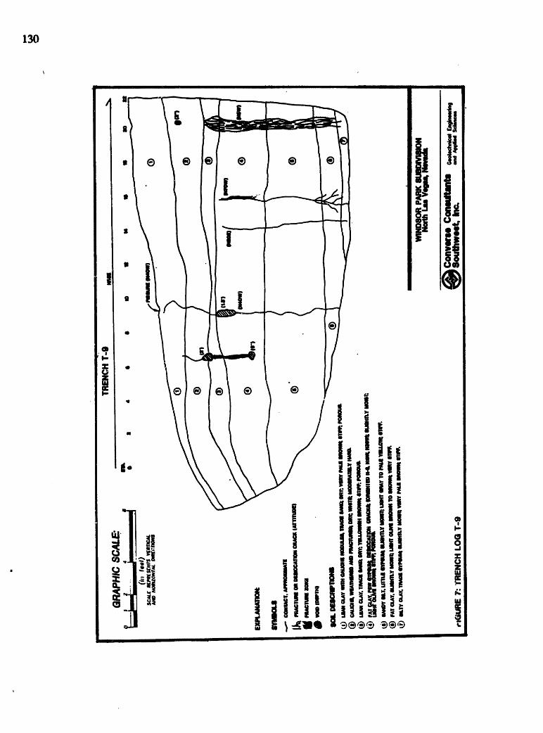

131
WindsorParkSubdivisionNorthLasVegas,Nevada
Table. 1 - Selected _ T_t:m_ _m ....
Atte_ Limits (ASTM 1M318_
Exploration Sample Liquid Plastic Plasticity Unified Soils....Location Death. ft. Limit. _ Limit. S Index Classification
TS2-6, STA 20 4-6 143 47 96 CH
T52-7, eTA 0 1_-4 71 37 34 CH
TS2-7, STA 0 4-6_ 247 65 182 CH
T52-7, eTA 10 8-11 83 30 53 CH
TS2-10, Pit 1_-4_ 63 25 38 CHT-lb, Pit 5-10 169 55 114 CH
_lubility*
ExpLoration SampLe Depth Soil Solubility
Locatio n ........... {feet) DescriDt!on (Dercent by dry weight)
TS2-1 Pit 1-2_ GYPSlFEROUSLEAN CLAY 1.5
TS2-6 STA 20 4-6 GYPSIFEROUSFAT CLAY 10.5
T52-6 eTA 20 6-8 GYPSlFEROUSFAT CLAY 3.8
T52-7 STA 0 1_-4 GYPSIFEROUSFAT CLAY 5.8
T52-7 STA 20 4-7 GYPSlFEROUSFAT CLAY 9.0
TS2-11STA 15 0-4 SANDYLEAN CLAY few gyp 1.4TS2-15 eTA 25 1_-2_ 6YPSUN 0.8
T52-15 eTA 25 4-5 GYPSIFEROUSLEAN CLAY 3.2
* About 2.0 Liters of tap water was passed through each oven-dried sample.
Consolidafion/I-Ivdro-collavse*
Exploration Sample Depth Soil Hydro-collapse
_ocatlQn ..... (feet) Oeacrlotton (nercent) .
T-3 STA 1000 1-2 LEAN CLAY 1.4T-3 STA 1010 1-2 LEAN CLAY 7.3
T-4 STA 0 _-1 CLAYEY SAND 2.8
*Sample saturated with a Load of 1 kips per square foot (ksf)

132
LM. Linnertandothers
Tab I(connu
Moisture Content
ExpLoration Depth Soil (percent) PercentLocation (feet) Description FieLd Air-Dry Final SweLL
TS2-6 STA 20 4-6 GYPS. FAT CLAY 19 2 43 20
TS2-7 STA 0 1_-4 FAT CLAY 15 2 27 10TS2-? STA 20 4-7 GYPS. FAT CLAY 31 N/A 46 10tTS2-15 STA 25 11-12 FAT CLAY 56 13 95 >25
T-1 STA 450 3-4 FAT CLAY 33 2 ?0 >223T-lb Pit 5-10 FAT CLAY 27 1 67 253T-4 STA 100 0-1 GYPS. FAT CLAY 16 6 22 12"T-6 STA 0 5-6 FAT CLAY 23 5 50 14"*T-6 STA 20 6_-10_ FAT CLAY 34 13 ?8 29:T-9 STA 14 4_-7 FAT CLAY 15 § 46 14:
B-8 9-10 FAT CLAY 70 4 68 10"*
Each sample was confined under a normal pressure of either 60, 120, or $00 poundsper square foot (psf)
* Undisturbed sample** Undisturbed sample confined under s normal pressure of 120 psf.: Remotded sample confined under s normal pressure of 500 psf. Some
of the samples also exhibited saturated sweLL pressures of about 7kips per square foot (ksf)(TS2-7) and 1.1 ksf (T-4).
: Remotded sample confined under a normal pressure of 120 psf.
Fig.: 8. P.esideedamagedbyexpmvcclays.Trm_ TS2-7 located in front of house.

133• Windsor Park Subdivision North Las Ve&as,Nevada
DISCUSSION
The subsurfaceinvestigation, laboratorytesting and assessment revealed that theproblem at the Windsor Park subdivisionis indeed complex. Previous work had beencentered on identifying one or two potential causes without considering the entiregeologic framework,and the conclusions havebeen contradictory.
The primarycauses of damage within the development were found,to be (1) earthfissuring and (2) expansive clays. Several other causes are present at the site but theyare not as significant as these two. Fissures have been extensively mapped in theWindsor Park and surroundingarea. Expansive clays were encountered at variousdepths throughoutthe subdivisionduringour field work.
The potential for future damage at the site was assessed. The potential for fissur-ing at the site was considered high based on the offsite (regional) factors controUilagfissure developmentand local factors such as soil type, proximity of faulting, drainagecharacteristicsand the presence of existing fissures. Since underlying expansive claywas prevalent at the site, the potential for future clay expansion was also consideredlikely.
Future structuraldamage to the residences, utilities and streets from the variousfactors will likely be similar to the damage in the past. Without any form of mitiga-tions whatsoever, it was believed that thedamage from these factors would continue ata similaror fasterrate throughthe next ten to fifteenyears.
Engineering upgrades such as regrading of each lot and replacement with specialhouse foundations as well as control of surface water drainagewould reduce the riskposed by underlying expansive clays and other geotechnical conditions found at the
= site. However, they cannot totally eliminate the risk from fissuring. Engineeringtechnology is not currentlypractical for solving such an extensive fissure problem asexists st Windsor Park given the nature of the development. Therefore, abandonmentor alternativeuse of the site (i.e., parkor mobilehome community) was consideredthebest solution for eliminating all risks posed by fissuring and underlying expansiveclays.
By 1992, approximately $2 million in federal and state funds were allocated formitigation and/or relocation of the subdivision. However, the Uni_tedStates Depart-ment of Housing and Development (HUD), the City of North Las Vegas and the arearesidents needed assurancethat damagewould not continue after upgradesand repairswere completed. Evaluationof the data indicated fissuringand damage might continueat the site.
Since it was not economically feasible for the City of North Las Vegas to abandonor relocate all 200+ homes in the immediate future, Converse ConsultantsSouthwest,Inc. used a statistical analysis (Bell and Price, 1991) and availabledata from previousdamage surveys (I-_D, 1988 and Mifflin, 1992) to develop 4 risk zones for Cityplanning purposes. The intention was to relocate the homes in phases, and the resi-dences at highest risk and with greatest damage would receive priority. Homes at
134 LM. Linnertandothers
highest risk were pl__d in Zone I and:_those with the least risk in Zone 4. Approxi-mately56 percent of the fissures in the Windsor Park area were located within 400 feetof a subsidence-related fault. Zones 1 and 2 (136 lots) were positioned roughly withinthis 400 foot boundary_ and it was believed that the potential for continued damage inthese areas was extremely high. Zones 3 and 4 (I I0 lots) were generally located alongthe northwest and southeast margins of the development farther than 400 feet from thefault. Fissures and structural damage were less concentrated in these areas.
A relocation site was chosen by the City of North I.as Vegas, approximately 1,000feet east of the existing subdivision. By late 1993, relocation of homes from WindsorPark to the new site was under way.
_CF._
Bell, J.W., 1981, "Subsidence in Las Vegas Valley," Nevada Bureau ofMines and Geology, University of Nevada, Reno, Nevada, Bulletin 95, 84p.
Bell, LW. and Price, LG., 1991, "Subsidence in Las Vegas Valley,1980-91: Final FTojectReport," Nevada Bureau of Mines and Geology, Univer-sity of Nevada, Reno, Final Project Report to a Consortium of 11 City, County,State and Federal Agencies.
Cibor, L M., 1983, "Geotechnical Considerations of Las Vegas Valley,"Special Publication on Geological Environment and Soil Properties, ASCEOeotechnical Hngineering Division, ASCIi. Convention, Houston, TX, October17-21, 1983, pp. 351-373.
.
Helm, D. C., 1992, "Hydraulic forces'that play a role in generating fissures atdepth" in Proceedings of the Association of Engineering Geologists, Long Beach,California, October 2-9, 1992, p. 7-16.
Matti, J.C., Bachhuber, F.W., Morton, D.W. and Bell, J.W., 1987, Las
Vegas NW Quadrangle, Geologic Map, Map 3Dg, Nevada Bureau ofMines & Geology, Scale 1:24,000.
Mifflin International, Inc., 1992, 1991 Inventory of Earth Fissures andAssociated Damage at Windsor Park (Draft), for the City of North Las Vegas,Windsor Park Revitalization Project, February, 1992.
Plume, R.W., 1984, "Ground-water Conditions in the Las VegasValley, Clark County, Nevada: Part 1. Hydrogeologic Framework," U.S. Geolog-ical Survey, Open-File Report 84-130, 25p.
Windsor Park Subdivision North Los Vegas, Nevada 135
U.S. Department of Housing and Urban Development (H), 1988, "Reportof Windsor Park," October, 1988, 9p.
Werle, J.L. and Stilley, A.N., 1991, "Hffects of Ground Fissures onDevelopment in the I.as Vegu Valley, Nevada," tn Proceedings of the 27thSymposium on Engineering Geology and Geotechnical Engineering, Utah StateUniversity, Logan, Utah, 15p.
Western Technologies, 1988, "Geotechnical/Geologic Evaluation, WindsorPark Development, North Las Vegas, Nevada," Project No. 4128,1266, November9, 1988, 35 pp.

t_

Hydrogeology, Waste Disposal, Science and PoliticsProceedings 30th _mposium
Engineering Geolo_ and Geotechnical Engineering, 1994 137
7&ILltmB]L1H_YBZ8 07 BORIBD TL1H'K8
by' ReynoZd King Watk/ns, Professor Rmez/tusDept of OLviland Bnvizonuental Bngineez£ngUtah Btate UntvozJity, Logtn, UT 84322-4110
(801) 7S0-2864
ABSTRACT
Failure of a buried tank can be hazardous. Failure may be aleak through which product is lost from the tank; but also throughwhich contamination can occur. Failures are epidemic -- becauseburied tanks are out of sight, but also because designers of buriedtanks have adopted analyses developed for pressure tanks. So whydo pressure tanks fail when they are buried?
Most failures of buried tanks are really soil failures. Soilcompresses, or slips, or llquefies. Soll is not only a load, it isa support without which the tank deforms. A high water table addsto the load on the tank. It also reduces the strength of the 8oil.
Based on tests, structural analyses are proposed for emptytanks buried in soils of various quality, with the water table at
various levels, and with internal vacuum. Failure may be collapsedue to vacuum in the tank, or equivalent flood level above th_tank. Such collapse is a sudden, audible inversion of the cylinde_when the sidefill soil sllps. Failure may be flotation. Failuremay be a leak. Most leaks are fractures in the welds in overlapseams at flat spots. Flat spots are caused by a hard bedding or aheavy surface wheel load. Because the tank wa11 is double thick atthe overlap, shearing stress in the weld is increased. Other weld
failures occur when an end plate shears down past a cylinder; orwhen the tank is supported only at its ends like a beam.
These, and other, failures can be analyzed with justifiableaccuracy using basic principles of mechanics of materials.

R.K. Watkins138
Zr_RODU_TION
Failure of buried tanks has become a major environmental issuebecause of leaks that allow contents of the tank to contaminate thesoil and groundwater, or allow groundwater to contaminate contentsof the tank. See Nomenclature and Notation, Figure I and Table I.
Because the design of a tank to contain pressure is understoodby tank designers and by manufacturers, rupture is infrequent --that is, until the tank is buried. Most failures of buried tanks
are really failures of the soil. Sol1 is complex -- not Just aload on the tank, but also a support; not Just a homogeneous minglephase medium, but a complex three phase environment; not Just awell-controlled/engineered material, but a variety of materialswith deviations in properties and boundaries. Unlike the pressuretank, a buried tank is a composite, the performance of which isanalyzed by soil-tank interaction mechanics.
Failure of a buried tank is a performance limit defined as anylimit beyond which the tank does not perform as intended. Intendedperformance usually includes leak-proof containment over a designlife without excessive distortion of the tank or movement of thesoil. A safety factor is required for design.
Performance limits are excessive displacement or deformation.Displacement Includes unacceptable settlement of the tank or
of the ground surface over the tank, and possible flotation of thetank when the water table rises.
Deformation includes excessive distortion of the tank, orrupture of the tank. Ruptures (leaks) are also deformations.
Table I. NotationD - mean diameter of the circular shellL - length of the tankt - thickness of the tank wall (and head?)r - maximum radius of the shell to the neutral surface of wall
ro - radius of the circular shell to the neutral surface of wallrx = radius of curvature (minimum?) of the deflected ring at B
- radius of curvature (maximum) of deflected ring at A or CrY - transition length of arc of the shell from point of maximum
to point of minimum radius of curvaturew = width of the overlap in a seamR = radius of curvature of the head (membrane theory)c = cord length for finding radius of curvature, r, of the shelle = mid-ordinate from cord to shell
d - ring deflection = A/DA = decrease in vertical diameter of the deflected shellP - external pressure on the tankP' = critical internal pressure, or vacuum, at incipient collapseu = external water pressure on the shellW - load per unit length of tankS - yield strength from an axial test (compression or tension)Ss - shearing yield strength of the tank or weld materlalso - normal stress in the tank wall or weld
- shearing stress in the tank wall or weldE - modulus of elasticlty of the tank material

f
Failure Analysis of Buried Tanks
139_YTZ_I_ NOD_|
In the following cases, analytical models are free-body-diagTams in static equilibrium. Performance limit is deformation.The limiting tank deformation may be a fracture at yield stress;
but it may also be .a flexural inversion of the cylinder ring.Inversion (collapse} is a function of ring stiffness -- not stress.For worst case collapse analysis, two models are proposed: one inunsaturated soil, and one in saturated soil with the water table ator above the ground suface. The tank is a horizontal cylinder(shell) with flat end plates (heads}. The soil is ooheslonless; itis placed in full contact with the tank; but it is not necessarilycompacted. Soil failure is sllp or liquefaction of the soil at thesides of the tank. Upon lo8s of support, the shell may invert.Loads on the tank Include _Internal pressure (or vacuum) andexternal pressure due to soil, water table, and traffic loads.
X
Intez_al Pressure analysis
The design of tanks to resist internal pressure applies to alltanks -- includlng buried tanks. External pressure of the 8o11 andgroundwater could be deducted from internal pressure at rupture.But usually the deduction is not significant or dependable, and isneglected. Figure 2 i8 the free-body-diagram for internal pressureanalysls. The primary performance limit is a longitudinal split inthe shell where circumferential stress, by the Barlow formula, is,a = P'r/t. Rupture occurs at yield stress, S. Therefore, criticalinternal pressure i8,
P' = St/r RUPTURE ANALYSIS .... • . • . .... (I)
_ternal Pressure _nalysis
If the tank is held in circular shape by good backfill, thefree-body-diagram is Figure 3a or its equivalent, 3b. At wallcrushing, the critical vacuum (or flood pressure) is,
P - St/r RING COMPRESSION ANALYSIS . . . . . . . . (2)
Clearly, the critical vacuum is reduced as the radius of curvature,r, is increased. The radius increases during backfilling as thering deflects into an oval or develops flat spots -- for example,on the bottom when the tank is on a flat bedding without adequatecompaction of soil under the haunches. Therefore, in Equation (2),
radius r is maximum radius, usually ry. See Figure 4.
DefozwLtion Lna17sis
Figure 5 is the free-body-diagram for predicting stress inoverlap seams where the wall thickness is doubled, but where theplates are fastened by a single circumferential weld. Due to thechange in radius of curvature from ro to r (at A, B and C for mostring deflections) the maximum normal circumferentlal stress on the

R.K. WatkinS
140
"-- " u - P' r/t - Boop STRESSj j_| ii
Figure 2. Free-body-dia¢Iram for internal pressure a_alysis of ashell (cylinder) showing the rupturing force P'D resisted by thehoop strength, 2ut of the walls.
P P
Pr Pr PIT
(a) RADZAL P_SSURE (b)_UZVAU_T V_TZCAL P_essunz
o-_It-RIWa__sszo. s_ss
Figure 3. Free-body-diagram for external pressure analysis of ashell with radial pressure P acting on it. Pressure P is resistedby ring compression, Pr, in the walls.

Figure 4. Tank shell ovalisod during backfiliing; in this c.sse, anellipse. Radius of ourvature oan be found fr.om a R.ld-ordinate, e...,,.red tr-- a cordot x.ov. 1.-_, o,_o _: __.,r- _" ooT"nay _ positioned either inside or as a _angen_ ou_sxae unu nnw._.
Figure 5. Change in radius of curvature in a typical overlap Jta.

R.K. Watkins
142
surfaces of the tank wall Is 2o - Et/ro - Et/r, but in the overlap(double thick) wall the stress is twice as great, i.e.,
o - Et/r o - Et/r WALLCZRCUMF_ZAL STRESS. . (3)
Because steel can yield without fracture, normal stress is usuallynot a probla eventhough the deformation may be permanent.
Sheering stress is maximum at the neutral surface of the shellwall in the transition from maximum to minimum radius of curvature;e.g. at the ends of a flat spot. See Figure 5. If x is the len91_hof transition, shearing stress in the wall is,
t m Et 2/8_ WALL SHEARING STRESS . . . . . (4)
Of greater concern is shearing stress in a weld at an overlapseam. See Figure 5. Shearing stress occurs throughout the lengthof the transition, x, (from the maximum to the minimum radius ofcurvature). If the shell is deflected into an ellipse, the maximumchange in moment is from B to C (or A to B) over transition length
x m fro/2. Change in moment i8 N - EI(i/rx-I/r¥). From mechanics,
f - (Ewt/.ro)(l/rx-l/ry ) WELD SHEARING STRESS . . (5)
In case of line load, F, on the bottom of the pipe, shearingstress in the weld of the overlap seam of Figure 5, is,
This is a significant cause of leaks in buried tanks -- especiallywhen F is the reaction to the combined weights of: the tank, thecontents, a wedge of sell on top, and a surface live load -- andmore especially if the line load F is concentrated at one or twohigh spots in the bedding under the tank. This weld shear failureis particularly objectionable because it occurs on the bottom ofthe tank where the entire contents can leak out.
Another cause of leaks is shear in a circumferential weldwhere the stiff head shears down past the flexible shell. SeeFigure 6. A head picks up 8oil load for at least one diameterfrom the end of the shell. As the flange buckles, the weld issubjected to both shearing and flexural stresses.
Longitudinal analTsis
Longitudinal stresses can open cracks in circumferentialwelds. Due to internal pressure only, longitudinal stress Is halfas great as the circumferential (hoop) stress; o - P'r/2t. Butadded to this may be longitudinal stresses due to tamperaturedecrease, Polsson effect of internal pressure, and longitudinalbeam ];_nding.
But the principal cause of longitudinal stress is beau bendingdue to non-uniform bedding. See worst case, Figure 7. At point C,from mechanics of a simply supported beam, longitudinal stress i8,
o = W(L/r)2/8_t WALL LONGITUDINAL STRESS . . . (7)

Failure Analysis of Buried Tanks 143
SOIL I_RESS_RE
;
' TT'T T
,A.G_(K.,CKL_) "_'|
J
BEFORE WELD FAILURE AFTER WELD FAILURE(o_ sL_a() (mm_ BUCKLZ)
Figure 6. Mechanism for failure of a circumferential weld due toa stiff head that shears down past a flexible shell. UnderwritersLaboratory code calls for a minimum 1.5 inch flange and 0.5 inchpenetration into the shell.
TAL HEIGHT PER UNIT LENGTH
|,|
HELD ,
----. L _J_z
Figure 7. Typical conditions for longitudinal (tension) failure ofa weld due to mounds in the bedding at the ends of the tank used tolevel the tank. The tank becones a simply supported bean.

]44 R. K. Watkins
Head Aaalysls
Even though external pressure on the head varies from top tobottom, an assumption that pressure is uniform i8 accurate withintwo percent for typical steel tanks. A classlcal analysls to findmaximum moment by plate theory is available, but i8 not justifiedbecause the ratio of thickness to diameter is small and yleldstress is not failure. Membrane theory Is adequate, if headanalysis should be of any concern. Tension stress in the head isa - PR/2t, where R is the radius of curvature of the pressurizedspherical head and can be calculated by the strain as the headdeforms from a disc to a sphere under average pressure P.
Shell AnalTs£s -- UnJaturated Boil Bnvelope
With a good soil backfill, the shell is essentially circular.Few problems are encountered. Longitudinal stress is not criticalexcept when the tank is a simply supported beam. Wlth poor sol1backfill, the ring deflects down. Ring deflection is nearly equalto settlement of sidefi11 soil. Soil compaction is recommended.With less than minimum sol1 cover, a wheel load over the top of the
J tank can invert the top of the shell. Live load pressure on thetank should be checked. Conditions for deformation are worstenedif soil is not compacted under the haunches. At worst, for a tankwith no soil support, subjected to internal vacuum, the classicalanalysls of collapse is plotted on Figure 8. Noteworthy is thestiffener effect of the heads in the term L/D.
Shell Analysts -- Saturated Sotl Bnvelope
Figure 9 is the free-body-diagram for analysis of a buriedtank after the water table rises. Buoyant water pressure on thebottom of the tank is critical -- not soil load on top. In fact,soil on top becomes a reaction to the buoyant tank. Analysis isequilibrium of horizontal stresses on the Inflnitesimal sol1 cubeat B where pressure of the. tank against sell is r eslsted byeffective passive soil strength. It is assumed that the sol1 iscoheslonless, placed dry, then saturated.
In case the backfill is mud -- the worst case scenario --results of tests on 12,000 gallon service station tanks are shownin Figure 10. The worst-case soil is seventy percent fine sand andthirty percent silt. The effect of shortened tank length is offsetby greater depth of the _uoyant uplift water pressure.
Flotation
In saturated soil, an empty tank will not float if the soilcover is at least half of the tank diameter. However, this rule isbased on the assumption that the backfill sol1 is coheslonless andis compacted to a density greater than 80% ASTM Method D698. Loosesoil may liquefy due to earth shock waves or to soil movement. Acommon practice below water table is to tie the tanks down to heavyconcrete foundations with straps that avoid stress concentrations.
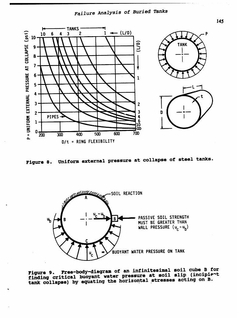
F_ilure Analysis of Buried Tanks
145
TANKS ,
_.-,._ 1 _',-_ _ 18
0" 200 300 400 500 600 /00
D/t = RING FLEXIBILITY
Figure 8. Uniform external pressure at collapse of steel tanks.
..--" " IL REACTION
•PASSIVESOIL STRENGTHUb MUST BE GREATERTHAN
WALL PRESSURE(uc-ub)
BUOYANTWATER PRESSUREON TANK
Figure 9. Free-body-diagram of an infinitesimal soil cube B forfinding critical buoyant water pressure at soil slip (incipienttank collapse) by equating the horizontal stresses acting on B,
_
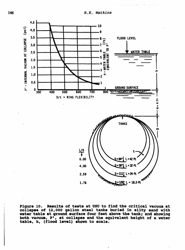
]46 R.K. Watkins
TANKS
C:
1.76 L - 18.5ft
Figure 10. Results of tests at USU to find the critical vacutm atcollapse of 12,000 gallon steel tanks buried in silty sand withwater table at ground surface four feet above the tank; and showingboth vacuum, P', at collapse and the equivalent height of a watertable, h, (floo4 level) shown to scale.

Hydrogmlogy, Wute Disposal, Science andPoliticsProceedings30th SymposiumEngineeringGeology andGeotechnicalEngineering,1994
EROSION CONTROL TEST FACILITIES AT THE 147UTAH WATER RESEARCH LABORATORY
C. EaH Israelsen, ProfessorCivil and Environmental Engineering Department
• Utah State University, Logan, UT 84322
Gilberto Urroz, Assistant ProfessorCivil and Environmental Engineering Department
Utah State University, Logan, UT 84322
ABSTRACT
Facilities have been developed at the Utah Water Research Laboratory in Logan, Utah,for determining the effectiveness of a variety of erosion control products including mulches,blankets, mats, rovings, chemicals, blocks, and vegetation. This paper describes in detail arainfall simulator, a tiltable test bed, a sunlight simulator, a wind generator, twin large-scalehigh-velocity test channels, and a glass-walled flume for measuring shear.
INTRODUCTION
In the late 1970's, the Utah Water Research Laboratory in Logan, Utah, recognized theneed for evaluating the effectiveness of a continually-increasing number of erosion controlproducts and practices, and adapted some of its laboratory equipment to accommodate this need.Since that time, the equipment has undergone periodic upgrading and. improvement until at thepresent time it is probably second to none in the nation. Present erosion control test facilitiesinclude a rainfall simulator and accompanying test flume, sunlight simulator, wind generator,high-velocity test flume, and a flume for mea,:uring shear.
RAINFALL SIMULATOR '
The rainfall simulator is a drip-type device in which raindrops are formed by wateremitting from the ends of small-diameter brass tubes. The rate of flow is controlled byadmitting water into manifold chambers through fixed orifice plates under constant hydraulicpressure. Five separate inlet orifices are used in each chamber or simulator module. The ratiosof the areas of the orifices are 1:2:4:8:16. By controlling the water flow to the orifices withelectrically operated solenoid valves, and the water pressure with a movable head tank, it ispossible to vary rainfall rate up to approximately 25 inches per hour. Outlet from the chambersor modules is through equally spaced brass tubes on the undersides of the modules. Eachmodule is a 24-inch square completely enclosed box about l-inch deep and oriented so that theends of the tubes or needles form a horizontal plane to let the water drip to test plots below.Each module has 576 needles spaced on a l-inch square grid pattern.
The rainfall simulator consists of 100 modules that are supported adjacent to each otherto make a continuous simulator 400 square feet in area. Each module can be controlledseparately. The 500 electrical control switches are manually operated.

. C.£. Israelsen and G. Urroz
148Raindrop sizes about 4 mm in diameter are representative of typical high intensity storms.
The spatial distribution of rain is essentially uniform, and the control of application rates iswithin the accuracy requirement of most experiments.
1 TEST FLUME
The square test flume measures 20 feet on each side and can be tilted to any angle fromhorizontal up to more than a 1 1/2:1 slope. The rainfall simulator is supported over the flumeso that rain falls directly onto the test plots. The plots contain a 1-foot depth of soil, supportedby a metal grating which is covered with a filter cloth through which water can drain.
The flume can be divided into six 2 ft x 19.5 ft test plots, or three 4 fi x 19.5 ft testplots. The plots are separated from each other and from the side walls by 2-foot widewalkways. The rainfall simulator can be controlled to rain only on the plots and not upon thewalkways.
SUNLIGHT SIMULATOR
A balance of radiant energy needed for good growth of plants is provided to the test plotsby a sunlight simulator which utilizes incandescent as well as fluorescent lamps. It has the samedimensions as the tilting flume, is square, and measures 20 feet on a side. It is rolled on andoff the test plots on wheels riding on horizontal rails mounted on top of the side walls of thetilting flume. When in position, it is about 3 ft above the test plot surfaces and providesillumination at a photon flux density of 216 _,E • m2 . sec_ (measured with a LaCor 190 Squantum sensor on a Model L1-185 quantum radiometer/photometer). The sunlight simulatoris used for germinating seed and growing plants, and also to shorten the time for drying soilbetween runs.
WIND GENERATOR
A 24-inch diameter squirrelcage fan driven by a 15 HP, 440 VAC motor is mountedngidly on a wall near the lower end of the testing flume. When the flume is positioned at a 2:1slope, three 10-inch diameter metal ducts direct wind from the fan through the end of the flumeonto the test plots. The wind blows upslope, parallel to the sloping surface, and impinges onthe plots at approximately their midpoints. Wind enters the flume at a velocity of approximately60 mph (88 fps), disperses to about 30 mph (44 fps) at the point of impingement, and slows to10 mph (15 fps) at the upper ends of the plots. This uni-directional constant velocity wind doesnot simulate all of the conditions found in a field setting, but does enable a comparison of theperformance of erosion control products under similar conditions.
HIGH VELOCITY TEST FLUME
This flume, which is 8 ft wide, 6 fi deep, and 570 fi long, is supplied with water under35 ft of head from a nearby reservoir through a 3-ft diameter pipe. A spreader at the outlet endof the supply pipe uniformly distributes water over the 8-fi width of the channel. A plywoodpartition and end gates in the flume provide two test sections, each measuring 4 ft in width and50 ft in length. A 20-fi long plywood-lined smooth approach to the test sections allow
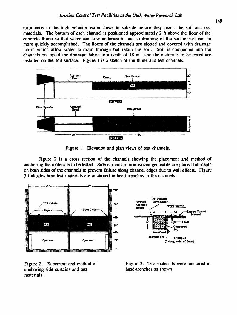
Erosion Control Test Facilities at the Utah Water Research Lab149
turbulence in the high velocity water flows to subside before they reach the soil and testmaterials. The bottom of each channel is positioned approximately 2 ft above the floor of theconcrete flume so that water can flow underneath, and so draining of the soil masses can bemore quickly accomplished. The floors of the channels are slotted and covered with drainagefabric which allow water to drain through but retain the soil. Soil is compacted into thechannels on top of the drainage fabric to a depth of 18 in., and the materials to be tested areinstalled on the soil surface. Figure 1 is a sketch of the flume and test channels.
,_p,o_h Tut., I_.
18"
t24"i
B_devlevt
Flov Spreader AppeoechReach Test Section
dee
4'
I so' 1 so............... Ii ;_'rrk:F'4-_
Figure 1. Elevation and plan views of test channels.
Figure 2 is a cross section of the channels showing the placement and method ofanchoring the materials to be tested. Side curtains of non-woven geotexfile are placed full-depthon both sides of the channels to prevent failure along channel edges due to wall effects. Figure3 indicates how test materials are anchored in head trenches in the channels.
40..... .L ,m-.. a•r 11
_- 16"l:>m_ePlywood OIo_ CoverMamrml 30" Appxoach _-/
,l, 4/ _ :__. g'u Mad
q J_'- _-'M _1r
Ups_om End L== 6" Saeples2Aa" (5 elon[ vtdth of flume)
Figure 2. Placement and method of Figure 3. Test materials were anchored inanchoring side curtains and test head-trenches as shown.materials.

C.E. Israelsen and (7. Urroz
150
A "test" in this unit consists of two replications of several runs, each at a different waterflow amount and velocity. Normally there would be flows of 20, 32, 45, 60, and 75 cfs for 30minutes each which translate to velocities of approximately 3, 5, 10, 15, and 20 fps. We canalso run in excess of 100 cfs at approximately 25-30 fps when necessary. On durable materials,the runs may start at 10 to 15 fps and extend through 25 fps. Centerline velocity and flow-depthmeasurements are made of each run at stations 0, 5, 15, 30, and 45. After every run, cross-sectional measurements are made at each 1-ft width across the channels and every 5 ft alongtheir lengths to determine erosion depths. Extended runs at any velocity and for any, length oftime are made when warranted.
FLUME FOR MEASURING SHEAR
Valid calculations of shear on channel linings cannot be made in erodible channelsbecause the values change with time as well as with velocity as the soil erodes. Toaccommodate the many requests to determine shear values of particular lining materials, a thirdtest facility has only recently been constructed. This consists of a 2 ftx 2 ft x 24 ft glass-walledflume supplied with water through a 10-inch diameter pipe and a spreader nozzle. In the floorof the flume is a 2 ft x 5 ft section to which materials to be tested are fastened with stainless
steel staples that are anchored into the floor section at a 45 degree angle. This section rests onstainless steel ball bearings set in teflon pockets. From the underside of this section, a steel armextends through the floor of the channel and is connected to a load cell that has a digital readout.The shear that is generated on the material by water flowing over it is imparted directly to theload cell where it is displayed as a force on the readout. These values are then recorded asforce per unit area (lbs/ft2). Even shear from the slightest flows can be detected. The shearincreases as velocity increases (unless the liner fails first) up to the limit of the system whichis approximately 20 ft per second, or until it reaches an equilibrium value.
The test is started at a low velocity and allowed to stabilize. The velocity is increasedin incremental steps until the material fails or until the limit of the test unit is reached,whichever comes first. At each setting, the velocity and flow depth at the beginning and endof the test section are measured and recorded along with the corresponding shear.
Three replications are run of each test, and the results are averaged and plotted. Shearvalues at any velocity can then be read directly from the graph.
The regular utilization of these ,mique testing facilities can result in a continualimprovement in the effectiveness of erosi, m control products throughout the industry.
!

Hydrogeology,WasteDisposal, Science andPoUtic,Proceedings30th Symposium
EngineeringGeology andGeotechnicalEngineedns, 1994 | 51
Pre-anthopogenicgroundwaterevolutionat the Idaho NationalEngineering
Laboratory,Idaho
MCLING, Travis L., and SMITH, Robert W., Idaho National Engineering
Laboratory, P.O. Box 1625, Idaho Falls, ID 83415-2110
The Snake River PlainaquiferIs the mostimportantgroundwatersourcein
Idaho. Overlyingthe aquiferin eastern Idahois the Department of Energy's
Idaho NationalEngineeringLaboratory(INEL). Activitiesat the INEL include
reactor research,nuclearfuel reprocessing,and nuclearwastestorage. Past
activitiesat the INEL have locallyaffectedgroundwaterquality. To assessthe
geochemicalcontrolson waterquality,waterchemistriesfrom approximately75
US GeologicalSurveywellswere evaluatedusingthe MINTEQA2 and
NETPATH computercodes.
Greaterthan 95 percentof the solutebudgetin the aquifer is compdsed
of eight ions: calcium,magnesium,sodium,potassium,silica,bicarbonate,
chloride,andsulfate. Basedon MiNTEQA2 calculationscalcite is the only
significantsecondarymineralprecipitatinginthe aquiferat the INEL.
Commonlyoccurringmineralsthat are under-saturatedinthe aquifer are
plagioclase,pyroxene,and olivine. The pH in the aquiferrangesfrom 7.6 to 8.6
and increaseswithresidencetime, primarilydue to a lossof CO2.
The resultsof thisstudyshowthatthe aquiferchemistryis strongly
controlledby groundwatermixingand minorbasaltweathering. In addition,this
studywillaid in the,establishmentof a groundwaterstandardto be used in
remediationand aid waste migrationmodelingactivitiesat the INEL.

Hydmseology, WasteDisposal, Science andPolltiesProceedings30thSymposium
152 EngineeringGeology andOebtechnicalEngineering,1994
DESIGN OF THE IDAHO NATIONAL ENGINEERINGLABORATORY INTEGRATED FIELD SCALE
PUMPING AND INFILTRATION TEST
T. R. Wood 1, G. T. Norreli 1, A. W. Wylie 1,K. J. Dooley 1 G. S. Johnson2 and F_ R. Neherl
1. Idaho National Engineering Laboratory,P. O. 1625, Idaho Fails, ID 83415
2. University of MahoMaho Fails, IX} 83405
ABSTRACT
The high de_,ree of heterogeneity present in the Snake River Plain subsurfaceprecludes utilization of small or intermediate scale observation alone forhydrologic and geochemical characterization efforu.,.s..The mimmumrepresentative elemental volume for the fractured, intercalated sequence ofbasalt flows and sedimentary interbeds is considered to be in the 105 to 107m3 range. An integrated program of large scale field experiments, along withsupporting laboratory investigations, has been initiated at the INEL to providethe most reliable information obtainable regarding aquifer flow andcontaminant transportthrough the vadose zone.
An aquifer pum.pingtest has been designed which will involve pumping theSnake River Plam aquifer (SRPA) at approximately 3000 gpm for a periodof four weeks. Previous aquifer tests have been conducted at comparativelylowpump rates over shorter time intervals. This increased scale is intendedto edlow for stressing a sufficiently large volume of the SRPA to effectivelyaverage out heterog.eneities which cause wide variations in the results fromsmaller scale experiments. The water generated during the extended pumptests will be piped - two kilometers to the southwest to a seven acreinf'dtrationbasin. Conservative and reactive tracerswill be added to the
inf'dtratingwater for assessing actinide and fission product surrogateretardationfactors and dispersion parameters. Infiltrating water wall bemonitored with several overlapping systems, including -60 wells screenedat various transmissive layers within the first 200 ft depth, and geophysicaltechniques. Water and tracer migration will be tracked with down-holenuclear moisture logging and gamma spectroscopy, as well asgeophysically. The State of Idaho INEL Oversite Program will conduct adetailed characterization of the aquifer test observations wells using asophisticated straddle-packer system. Additionally, the State will performdepth-discrete sampling to the base of the aquifer for stable and radiogenicisotopic analyses.
The field site was constructed (including well installation during the 1993field season). Geological characterization has provided baseline data forpredictive modeling of experimental results. The field experiments arescheduled to be performed during the 1994 field season. Results from theintegrated program of field and laboratory experiments will be used toestimate projected contaminant travel times through the vadose zone to theSnake River Plain aquifer. As such, results will ultimately determine whichremediation alternatives are most appropriate.
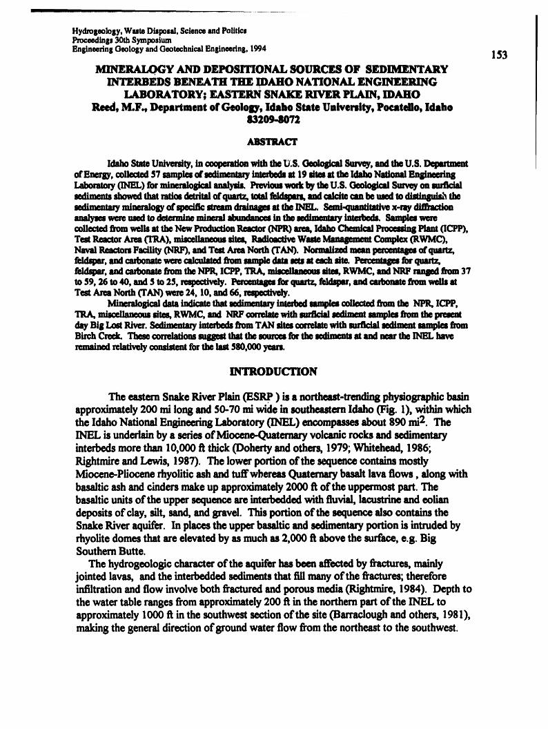
Hydroseology,WasteDisposal,ScienceandPolitiesProceedings30thSymposium
EngineeringGeologyandGeotechnicslEngineering,1994 153
MINERALOGY AND DEPOSIT/ONAL SOURCES OF SEDIMENTARYINTERBEDS BENEATH _ IDAHO NAT/ONAL ENGINEER/NG
LABORATORY; EASTERN SNAKE RIVER PLAIN,/DAHOReed, M.F., Department of Geology,Idaho State University, Poeatello,idaho
S3209.S072
ABSTRACT
IdahoStateU_ty, incoclm_ withtheU.$.Oeolosi_Swvey,andtheU.S.of Energy, collected57 samplesof sedime_my intefoedsm 19 sitesat the Idaho Nalimud P__xw_ _) tot mine_osic_m_/L Pmiuwerkby t_U.S. _ _eyon_sed_ sl_ that ratim detrJtalof quartz, totalEld_ andci_te canIx_naedto dJadnB_ thesedimentaryminmlosy of specificmum d_ attin n4E[.. Seml-qumtttttivex-ray8n_ werereedtodmermtneminm_ahmdana_intin mdin_ _ San_ werecollectedfromwellsattheNewProductionReactor_) areLIdahoChemical1_ Plant(ICYP),TestReactorAreaGRA),miscenanamsites, RadioactiveWine ManqememCoaplex0tWMC),NavalReactorsFacility(NRF),mxlTestAreaNm_ (TAN). Normallz_ mmnpacema_ of qum_feldsper,andcarbonatewereceladmalfl_mmnple dm ms ateachslte. Pacema_ forquarU,lhldspsr, and carboasle from the NPR, ICPP, "IRA, _ sllu, RWMC, stud NRF _ from 37to 59, 26 to 40, ud $ to 2S, mqx:clively. Pemree_e_ for qumlz, feldqxu', and _ horn well_ atTest Area North (TAN) were 24, 10, and 66, reqx_ively.
Minm'alogical data indicate that sulimealmy _ _ collated from the NPR, ICPP,mtsce_zom sit_ RWMC,and NP.Ycorrelatewith suracl_sedtazm mnplu f_m thepsmm
day Big Loa lltvcr. Salimmtmy intmbals from TAN sitm axvelat_ with muflctal mlimmst munplm f_omBirch Crock.These_mlations sugl_ tlmtthe_ forthe sedtnm_ at andneartheDEL _
relativelyconsistentfor thelast 580,000yea.
INTRODUCTION
The eastern Snake River Plain (ESRp) is a no_esst-trending physiographic basin
approximately 200 mi long and 50-70 mi wide in southeutern Idaho (Fig. 1), within whichthe Idaho National Engineering Laboratory (INEL) encompasses about 890 miz. TheINEL is underlainby a series of Miocene-Quaternary volcanic rocks and sedimentm_interbeds more than I0,000 fl thick (Doherty and others, 1979; Whitehead, 1986;Rightmire and Lewis, 1987). The lower portion ofthe sequence contains mostlyMiocene-Pliocene rhyolitic ash and tuffwbereas Quaternarybasalt lava flows, along withbasaltic ash and cinders make up approximately 2000 fl of the uppermost part. Thebasaltic units of the upper sequence are interbedded with fluvial, lacustrine and eoliandeposits of clay, silt, sand, and gravel. This portion of the sequence also contains theSnake River aquifer. In places the upper basaltic and sedimentm_ portion is intruded byrhyolite domes that are elevated by as much as 2,000/1 above the surface, e.g. BigSouthern Butte.
The hydrogeologic character ofthe aquifer has been affected by fractures, mainlyjointed lavas, and the interbedded sediments that fill many of the _es; thereforeinfiltrationand flow involve both fractured and porous media (Rightmire, 1984). Depth tothe water table ranges from approximately 200/t in the northern part of the INEL toapproximately 1000/1 in the southwest section of the site (Barraclough and others, 1981),making the general direction of ground water flow from the northeast to the southwest.

154
IX)N.ANATION
.... BOUNDARYOF IDAHO NATIONALENGINEERINGLABORATORY
= SELECTEDFACILITIESAT THE IDAHO NATIONALENGINEERINGLABORATORY
ANL-W ARGONNE NATIONAL LABORATORY-WEST NRF NAVALREACTORSFACILITY
CFA CENTRALFAClLmES AREA PBF POWER BURSTFACILITY
CTF CONTAINEDTEST FACILITY(formerlycalled RWMC RADIOACTIVEWASTELoss of Fluid Test Facility-LOFT} MANAGEMENTCOMPLEX
EBR-1 EXPERIMENTALBREEDERREACTORNO. 1 TAN TESTAREANORTH
ICPP IDAHO CHEMICAL PROCESSINGPLANT TRA TEST REACTORSAREAI I I
Figure I. Locations ofthe Idaho National EngineeringLaboratqry,selectedfacilidea,andcore samplesites.

MineralogyandSourcesofSedimentaryInterbeds,INEL
155
"['henorthernpartoftheINELisinato_hicaldollbasinthatincludmtheBigLost River Sinks,LittleLost River Sinks;BirchCreekSink_ Big Lost RiverPlayu 1,2,and 3; and the BirchCreekPlaya(Fig.1). Big Lost River,LittleLost River,andBirchCreekterminatein the BirchCreekPlaya_n ando_ 1974). The _ alsocontsinsseveralsmallisolateddosedbasins.S_ flowhm LittleLostRiverandBirch Creek is presently being diverted for irflsation andpower _on md does notreachthe playasexcept duringyearsof hlgh runoff. Themsjorityof the mrfbzewater atthe INEL is derivedfrom flow in the Big Lost Riverwhich ultimatelyrechargestheaquifer.Relativeabundancesof detfitalminaab in mrflcialsedimentsfrom the Big lostRiver drainagewerepresentedbyBartholomayandothers(I989). Mineralogicaldataformrflcialsedimentsfrom theLittleLost RiverandBirchCreekdrainageswerepresentedbyBartholomayandIf,nobel(I989). A sunmm_of these resultsby Bartholomay(I990)indicatesthatthethreedrainagesystemsthatflowontotheINELcambesepmatedbasedonmeannormalizedper_es ofquartz,totalfeldspar,andcarbonate.
Previously publishedmineralogicaldataareusedto correlatesurflcialsedimentsflomthe threedifferentdrainageswith the dataof sedimentinterbed8fi_m this study.As inpreviousstudies,quantitativeX-raydiflh_on analysiswas used inthis studyto determinethe mineralogyof all interbedsedimentsamples. A modificationof the methoddescribedby Dieboldandothers (1963) ar_ ._¢hultz(1964) was used to obtainthe relativemineralpercentages.
METHODSSamnleC91lecflon
Sediment intesbedswere collectedfrom 19 sites for mineralogicalanalysisfromFebruary1993 throughDecember1993 (Fig. 2). Samp"lmgsiteswere selected based onthe availabilityat the USGS fithologiccorelibraryat the INEL. Sedimentaryinterbedsamples(approximately20 grams)werecollected from 17 sites in theBig Lost Riverbasin:10 samplesfrom3 sites(DC-I, DC-4, andWO-2) atthe New ProductionReactor(I_R) area;10 samplesfrom 5 sites(PW-7, PW-11, TRA-5, TRA-8, andUSGS 80) nearthe TRA; 13 samplesfrom 3 sites (USGS 81, 121, and 123)nearthe ICPPfacih'ty;8samplesfrom 2 sites (RWMC-CIAandUSGS 118) nearthe RWMC; 5 samplesfrom 3sites (NRF-6P,NRF-TP,andUSGS 99) nearthe NavalReactorFacility(NRF); 1 samplefromUSGS 103;and I samplefrom USGS 104. Sedimentmyinterbedsfromthe BirchCreekbasinwere representedbyninesamplesfrom 2 sites( TAN CH-I, andTAN CH-2)nearthe Test AreaNorth (rAN) facility. Depthsof samplescollectedareshownon Table1.Samole Prenaratten and Analysis
X-raydiffractionanalysison the sedimentaryinterbedswas used to determinebulktttineralogyandday particlesless than0.004 mm in diameter. Analysesof clay separateswere madeonlyon samplesthathadclaypresentin the bulkanalysis. Forbulkmineralogya representativesampleapproximately3 g of samplewas groundfor 8 minutesin a bail-and-milldevice to reducegrainsize andto homogenizethe sample. The samplewassubsequentlygroundusing a mortarandpestle untilallof the samplepassedthrougha0.062 mmsieve. The powderedsamplewas packedintoan aluminumholderand scannedwitha PhilipsNorelco X-raydiffractometer.Thegeneratorwas operatedat 35 kilovolts,

156
EXPLANATION---,---- BO_ OF IDAHONATIONALENGINEERINGLABORATORY
• Im LOCATIONOF CORESAMFLE-EnUy.103. ill aim idenlfller
0 6 10 MILESt !
o 6 lO
I t
Figure2.-Location of coreholessampled at the Idaho National EngineeringLaboratory.

MineralogyandSourcesofSedimentaryInterbeds,INEL157
and]S_s. DifhctoSmmwemprepamd atamdeetctorof],amultlpl_of0.S,andtimecomsntor2.
inthesumplu. A modificationofthemethoddescribedbyDieboldandothms(]963)andS_ (]964)wuusedtoobtaintherdafivemism_pemnnlp's.Thoraw__® oreach_ wasdetamlsmlbydlvidi_theUstms_ofeachmim_ peakheightby qle intensityofits pare _. Therawperc_tq_wem nonmlizedto 100peremt. Theintensitiesof the purestandardswere ealmlated fkomstandardminm_providedbythe iSU Departm_ of Geology. Sdmltz (1964, p.C1) reporteduncertaintiesof+ 10 percentfor mineralsthatmakeup at least 1$ percentof the sample. Dieboldandothers(1963, table 5, p.130) calculatedweightpercmtwithin+ 8 percmt of thetrueconcentrationsusinga95percentconfidenceinterval.
For samples thathadclaypresentinthe bulkmineralogyamlysts,a qualitativeidentificationof individualday mineralswas undertaken.Clay separationfollowedguidelinesdescribedby Ellees(1987). Firstthe organicmatterwas removedbyusinga30% 14202 mlution, thenradium Itexs-metephosphatewu addedto aid in _ dayparticles. The< 45 micronfl'actionwas thenisolatedbyusing a 325 meshsieve. Isolationof the clayparticlesin the < 2 micron_'actionwas accomplisl_ using the principleofStoke'sLawthatpredictsthe finestsilt-sizeparticlesettles below the top 5 an ofsuspensionafter3.5 hours. The suspendedclaysizepmicles were m_ on afilter,thenthe filtratewas transferredto a glass slideand allowedto drybeforebeinganalyzedby X- ray _o_
The slideswere wannedwitha diflh_ometer usingthe aforementionedoperating_ers withascalefkctorof Ito 0.5.The sampleswere glymlatedandrescanmdtodifferentiatebetweensmectite andchloritedays. Smectiteexpandsfi-om14to 17 A whenethyleneglycolreplaceswater in the crystallattice. Theeqmmon was achievedbyexposingtheclay slidesto anethyleneglycol atmospherefor at least 24 hours.
- The resultsreportedby the ISU X-raydiflh_on laboratoryfor the 43 samplesanalyzedfor claymineralogy(Table2) yieldqualitativeestimatesof the abundanceof daymineralsin the samples. The estimateswere basedon the relativeintens_es of the claymineral's001 crystalface. Five catesoriesweredesignatedin order of decreasingabundance:dominant,major,minor,trace,andpossiblypresent.
Bulk Mlneralotv of Sediment luterbedsA summaryof thequantitativebulkmineralogyfor the _limentary interbedsis
given in table I. A mmmmryof the qualitativestudyof the claymineralogyis given intable2. Statisticalparametersfor quantitativemineralanalysesfor the sedimentaryinterbeds(table3) show thatquartz,totalfeldspar, pymxene, andtotal day mineralsarerelativelyabundantF r the NPg-test_ TRA, ICPP,NIt,F, andRWMC _ilitiesthey areabsenceor in low abundancesforthe TAN/kility. Interbedsfi_m NPlt-test arerepresentedby 10 samplesthathavemeanpercmteSesof 34 for quartz,30 for totalfeldspar,3 for pyroxene,and 30 fortotal day minerals. InterbedsfromTRA arerepresentedby 10 samplesthathave meanpercen_es of 31 for quartz,18 for totalfeldspars,10 for pyroxene,and 17 for total clay minerals. Interbedsfi_m ICPParerepresentedby 13 samplesthathave meanpercentagesof 38 for qum_ 31 for total

or)
Table 1. Semiquaru'tative mineralogy of bulk samples by x-ray d_on for the
sedimentary interbed intervals. Symbols: nd indicates not detected.Bulk Analyses
Interval sampled ( in percent mineral abundance)
Sample ( feet below Date Plagioclas Potassium TotalIdentifier land surface) collected Quartz Feldspar Feldspar Calcite Pyroxene Olivine Dolomite Clays HematiteDC-1 238 2/24/93 44 26 5 15 nd nd nd 10 ndDC-4 112.9-113.3 2/24/93 15 9 13 52 nd nd nd 11 ndDC-4 241.7 2/24/93 33 23 5 15 nd nd nd 25 ndWo-2 560-564 2/24/93 62 19 19 nd nd nd nd nd ndWo-2 600 2/24/93 21 15 15 6 nd nd nd 42 ndWo-2 719 2/24/93 39 13 18 3 nd nd 1 26 ndWo-2 815 2/24/93 30 25 6 8 6 6 nd 20 ndWo-2 871 2/24/93 34 9 5 36 nd nd nd 16 ndWo-2 932.3 2/24/93 32 27 18 2 11 nd 1 8 ndWo-2 1001.5 2/24493 31 20 13 1 8 nd nd 28 ndPW-7 219.3 6/9/93 45 17 nd nd nd nd nd 38 ndPW-7 230 6/9/93 44 19 14 3 6 nd _1 13 ndPW-11 139.4 6/9R3 26 12 10 6 46 nd nd nd nd ._TRA-5 69 6/9/93 31 6 rid 13 6 nd nd 43 nd ._TRA-5 172-173 6/9/93 29 4 15 40 11 nd nd nd ndTRA-8 116.5 6/9/93 25 13 13 11 nd nd nd 38 ndTRA-8 204.5 6/9/93 23 5 nd 33 13 nd nd 26 nd _.USGS 80 165 2/24/93 49 19 18 nd 7 nd nd 6 ndUSGS 80 175 2/24/93 35 14 13 nd 9 nd nd 28 ndUSGS 81 27 2/24/93 29 16 19 10 7 nd 1 17 ndUSGS 81 107 2/24493 43 23 23 10 nd nd nd nd ndICPP 121 33-34.5 6/9/93 40 28 6 nd 18 nd nd 8 ndICPP 121 401 6/9/93 39 23 8 nd 11 nd nd 19 ndICPP 121 410.8 6/9/93 31 21 6 16 9 nd 2 15 ndICPP 123 10.0-12.0 6/9/93 56 15 nd 10 10 nd nd 8 ndICPP 123 112.4 6/9/93 42 10 8 10 10 nd nd 20 ndICPP 123 117 6/9/93 39 19 nd 15 8 nd nd 19 ndICPP 123 420 5/14493 40 27 9 nd 9 nd nd 15 ndICPP 123 502 1/25/94 22 12 8 32 8 nd nd 17 ndICPP 123 563.6 5/26/93 54 19 18 nd 9 nd nd nd nd

Table I cont.
Bulk AnalysesIntervalsampled ( inpercentmineralabundance)
Sample (feet below Date Plagloclas Potassium TotalIdentifier land surface) collected Quartz Feldspar Feldspar Calcite Pyroxene Olivine Dolomite Cloys HematiteICPP 123 690 5/14/93 20 46 18 nd 6 nd nd 10 nd
ICPP 123 741.7 6/9/93 39 31 10 nd nd nd nd nd 20RWMC CIA 229.7 11/30/93 42 28 17 nd 13 nd nd nd nd _,RWMC CIA 291.5 11/30/93 37 34 20 nd 9 nd nd nd nd
332.5 11/30/93 40 16 11 9 7 nd nd 18 nd _'RWMC CIARWMC CIA 745.7 11/30/93 39 20 15 nd 12 nd nd 14 nd
RWMC CIA 971 11/30/93 35 12 nd 24 nd nd rid 29 nd _.RWMC CIA 1072.3 11/30/93 39 16 11 nd 11 nd nd 23 ndUSGS 118 9.4 2/24/93 44 25 13 nd 4 nd nd 14 I1(I _1=USGS 118 237.9 2/24/93 39 11 16 16 6 nd nd 13 ndNRF-6P 97.8 6/9/93 31 13 11 30 11 nd 3 nd nd _-,NRF-6P 354 6/9/93 36 27 20 nd 16 nd nd nd ndNRF-TP 93 6/9/93 36 25 22 nd 8 nd nd 9 ridNRF-7P 156 6/9/93 15 9 nd 75 nd nd nd nd ndUSGS 99 25-30 2/24/93 43 19 18 6 4 nd nd 10 nd
USGS 103 15 2/24/93 36 17 13 4 12 nd nd 17 '. rid _.USGS 104 142 2/24/93 64 28 nd 5 3 nd nd rid ridTAN CH-1 401 6/9/93 20 nd nd 80 nd nd nd nd nd _'TAN CH-1 411 6/9/93 11 4 4 82 nd nd nd nd nd R
TAN CH-1 444.5 6/9/93 8 2 nd 81 nd nd nd 8 nd _.TAN CH-1 446.5 6/9/93 9 8 nd 72 nd nd 2 9 ndTAN CH-2 245.5 6/9/93 22 3 3 56 nd nd nd 14 ndTAN CH-2 449 6/9/93 44 9 nd 46 nd nd nd nd ndTAN CH-2 471.5 6/9/93 2 nd nd 98 nd nd rid nd ndTAN CH-2 735 6/9/93 23 19 nd 27 13 rid 13 4 ndTAN CH-2 977.7 6/9/93 47 13 11 10 nd nd nd 19 nd

M. F. Reed160_
Table2. br_ma_osy ofthe clay_ psrtioles.Symbols:dom indicatesdominate,majindicatesmajor,miaindiostesminor,tr indicms trs_ poss indicatespossiblypresent,endnd indicatesnot indicated.
Intervalsampled(feet below Sample
Sample landsurface) collected mixlayer smectite biollnlte Illite Chlorite Quartz Feldspar Calcite
,:30-1 238 2/2493 tr maJ rain maJ poss rain tr ndDC.4 112-113.3 2/2493 nd nd tr rain nd rain poss doraDC.4 241.7 272493 nd dora rain dora nd min tr ndWO-2 600 2/2493 nd dora rain maJ poss rain nd ndWO-2 719 2r24R3 tr dora rain maJ tr rain tr ndWO-2 818 2,/24R3 tr maJ rain ma| rain rain tr ndWO-2 87.1 2724/93 tr nd tr dora nd rain tr trWO-2 932,3 2/24/93 nd nd nd tr nd msJ dorn ndWO-2 1001.5 2/24/93 min poss nd dom nd rain poss ndPW-7 219,3 6/W93 tr dora rain maJ poss rain nd trPW-7 230 6/993 tr dom rain maJ lOSS rain lOSS ndTRA-6 69 6/9/93 tr min mln dom mln maj tr ndTRA-8 118.5 6/9/93 poss dora rain rnaJ nd maJ tr ridTRA-80 204.8 6fgR3 tr dora rain maJ na rain nd ndUSG880 165 2/24R3 tr nd nd rain nd maJ maJ ndUSG880 175 2/24/93 tr dora tr maJ nd rain nd ndUSGS81 27 22493 tr nd nd dora nd maJ tr ndICPP121 83-34.8 5/9R3 poss maJ rain dom tr rain tr ndICPP121 401 6R/93 nd msJ tr maJ poss min tr ndICPP121 410.8 6/9/93 nd dora rain min nd maJ tr trICPP123 10.0-12.0 6/9/93 poss dora m!n maJ tr rain tr ndICPP!23 112.4 6R/93 tr nd nd maJ nd maJ maJ ndICPP123 117 6/9R3 nd nd ndr 1118j 114 dom nd ndICPP123 420 5/14/93 min rain nd dom rain maJ poss ndICPP123 502 5/14/93 tr dora rain rain tr maJ poss rainICPP123 680 5/14/93 poss nd nd poss nd maJ dora ndRWMC-CIA 332.5 11/30R3 nd dora tr tr nd tr poss ndRWMC.C1A 745.7 11/30/93 poss rxl nd dora nd nd nd ndRWMC.CIA 971 11/30/93 poss dom rain maJ poss maJ tr possRWMC-CIA 1072 11/30/93 poss nd nd min IX)SS maJ dora ndUSG8 118 9.4 224R3 tr rain rain maJ poss maj tr ndUSG8 118 237.9 224/93 tr dora tr min nd rain poss ndNRF-Tp 93 _ tr nd nd dora nd nd nd ndU8G8 89 25-30 224/93 rain min tr dom nd maJ tr ndUSG8 103 18 224R3 tr rain tr maJ poss maj tr ndTANCH-1 444.8 6/9/93 nd dora nd nd min nd nd minTANCH-I 446.5 6/9R3 poss maJ nd tr nd tr nd domTANCH-2 245.5 6/993 nd dora nd nd poss min rain ndTANO,1-1-2 735 6;9/93 poss dora nd tr poss rain tr ndTANOH-2 977.7 6/9/93 tr dora min maJ poss rain tr nd

b
Mineralogyand SourcesofSedlmentaryInterbeds,INEL161
Table3. SummaryofstatisticalparametersforbulkminersiosyofselectedsedimentaryinterbedsattheNationalEnSinm'h8Lsbomon/,Idsho.
8mp,,
Qumtz 21 62 34 10Ptqiod_ 9 27 19 1oPoeushnnFeldspar $ 19 12 10ToldFddspst 14 45 30 l0Cldcilo 0 52 14 10Pymmm 0 !i 3 10Ddmnito 0 1 0 10Oiivfao 0 6 0 10ToldClayMinu_ 8 42 19 10
TRAFacilitiesQuartz 23 45 31 10Plq_.lsso 4 19 II 10PomsJm Fddsper 0 18 9 10TotalFddspst $ 37 18 10Cdc/to 0 4O Ii 10Pysomn 0 46 10 10ToulClayMhts_ 6 43 17 10
ICPPF_Quartz 2o 56 38 13Phjiochso 12 46 22 13_ Fddspm' 0 23 22 13Tots/Pddspm' _$ 64 31 13Calcite 0 32 8 13
0 18 8 13Ddml_ 0 2 0 13l'JmnJto 0 20 1.5 13ToldCtsyMhlmls 0 20 11 13
RWMCFacflitim
Qusrtz 35 44 39 811 28 20 8
PolasshnmFddspm' 0 17 13 8TotdFddspm' 12 54 31 8Caloho 0 2.4 6 8PysmGmo 0 13 8 8TeedC_y_ 0 29 14 8
dzoNRFF_
Qusrtz I5 43 31 5R,ljodmm 9 27 19 $
Feldspw !1 22 14 ST_ldFddJpa' 9 47 33 SC,k_to 0 75 22 S
0 16 8 SDdmnito 0 3 0 $ToedCby Mimab 0 10 4 S
TANPs_a,Qum'tz 2 47 21 9PtsSioclaso 0 19 6 5)Pomsl_ Fddsp,r 0 4 2 9ToaslFeldsp,r 0 24 8 9C81cllo 10 98 61.5 9Ppoxmo 0 13 1 9Ddmnito 0 13 2 9ToedClayMinalds 0 19 6 9
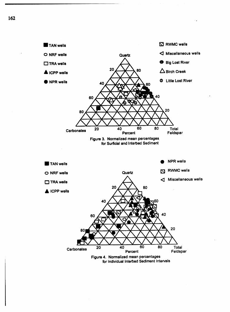
162
1 TAN wells _ RWMC wells
O NRF wells Quartz <_ Miscellaneous wells
I--I TRA wells Q Big Lost River
A ICPP wells 20 80 Z_ Birch Creek
O Little Lost River• NPR wells 40 60
60 40
80 20
Carbonates 20 40 60 80 TotalPercent Feldspar
Figure 3. Normalized mean percentagesfor Surftcialand Interbed Sediment
1 TAN wells Q NPR wells
O NRF wells Quartz I_ RWMC wells
I--I TRA wells <] Miscellaneous wells20 8O
ICPP wells
:) 60
60 40
80 20
Carbonates 20 40 60 80 TotalPercent Feldspar
Figure 4. Normalized mean percentagesfor IndividualInterbed Sediment Intervals

Mineralogy and Sources of Sedimentary Interbeds, INEL 163
feldspar, 8 for pyroxene, and 11 for total day minerals. Interbeds from RWMC arerepresented by 8 samples that have mean percentages of 39 for quartz, 31 for totalfeldspars, 8 for pyroxene, and 14 for total clay minerals. Interbeds from NRF arerepresented by 5 samples that have mean percentases of 32 for qtmrtz, 33 for totalfeldspars, 8 for pyroxene, and 4 for total clay minerals. Interbeds from TAN arerepresented by 9 samples that have mean percentages of 21 for quartz, 8 for totalfeldspars, i for pyroxene, and 6 for total day minerals.
Carbonates, calcite and dolomite, are not abundant in samples from interbeds atNPR-test, TRA, ICPP, NRF, and RWMC whereas are the dominate mineral phase at theTAN facility. Mean percentages for carbonates are 14, I I, 8, 6, 22, and 63.5 respectively.
CONCLUSION
Following Bartholomay (I 990), semiquantitative dii_action analysis can be usedto correlate the sedimentary interbeds to with the surficial sediment. The low abundanceof calcite, and dolomite in the sedimentary interbeds from NPR, ICPP, TRA, RWMC,NRF, and miscellaneous well sites (Fig.2) along with the relatively high amount of feldsparand pyroxene, indicate that the sedimentary interbeds are from a source area similar to thatthe present day Big Lost River drainage. The large amount of calcite and dolomitecombined with the relativity low amount of feldspar the absences of pyroxene in the TANsedimentary interbeds indicate that these are similar to the surfical sediments from theBirch Creek drainage. A summary of the normalized mean percentages and normalizedpercentages of all the interbed from this study are shown in Figure 3a-b. This suggests thatthe historical drainage basin ofthe area contained within the INL is similarto thepresent. Two anomalous intervals, TAN CH-2 at 735 and977.7 ft, has a mineralogicalsignature similarto the surifical sediments from the Big Lost River. This may indicate atime interval when Birch Creek was diverted from the present day flow path, but morework on the basalt stratigraphy needs to be done to determine the validity of theargument. Age dates have been performed on basalts beneath the INEL which indicatesthat sedimentary interbeds are at least 580,000 years old. This along with themineralogical data sets suggests that the historical drainage basin of the area is similartothe present day deposition basin, with the major sedimentary source being the Big LostRiver.
ACKNOWLEDGMENTS
The author gratefully acknowledges the ISU Department of Geology -- Dr. DavidRodgers Chairperson-- for providing X-ray diffraction equipment and laboratory. Spe_althanks are due to U.S. Geological Survey, Roy Bartholomay, Judith J. Kreig, JeanneFromm, and Dr. Scott Hughes for demonstrating the proper use of the x-ray equipment,and providing discussions on this project.
ReferencesBarraclough,J. T., Lewis, B.D., andJensen,R.G., 1981,Hydrologicoonditionsat the Idaho
NationalEngineeringLaboratory,Idaho:Emphasis:1974-1978: U.S. Geological SurveyWater-ResourcesInvestigationsOpen-FileReport81-526 (IDO-22060), p.77.

M. F. Reed164
Bartholmnay, R.C., andKnobd, L.L., 1989,Mlnmmlouand8rainsize oftlm surflcialsedinm_frmntheLittleLost RiverandBirchCreek_, IdahoNalimal F._Laboratory,Idaho::U.S. GeologicalSurveyOpen-FileReport89-385 (DOFAD-22082),p.19.
Bartholcamy,R.C., Kn¢_l, L.L.,andDavis, L.C., 1989,Mineralogyandgrainsize of the.ur_¢i__ _ theBisLot roverdramp andvicini_,witha_i_ mdphysical characteri_'cs ofpologic nmefiab fl'mnselectedsites at the IdahoNatimalP_,zerin8 Laboratory,Idaho::U.S.eeologicaSurveyOpen-FileReport89-384(DOF.AD-22081),p.V4.
Bartholomay,R.C., 1990,MinendogicalCormlafimof SurficialSedimentfromAreaDminai_withSclea_Sedinmm_ InmrbedsattimIdahoNatimalF.af_oerin8Laboratory,Idaho:U.S. GeologicalSurveyOpen.FileReport90-4147 (DOE/ID-22092),p.17.
Diebold,F.E.,_ J.,andHiltrop, C&.,1963,Determilmtionofcalcite,dolomite,quartz,andclay contentof cadmmte rocks:Journalof Sedim_lmy Petrology,v. 33, p.124-139.
Doimrty,DJ., MoBroome,L.A., andKuntz,M.A., 1979,Preliminary8eologic_dinterpret_on andlithologiclogofthe ExploratoryGeothermalTestWell0NEL-I),IdahoNationalReginee_ tabomm_,ememSnakeRiverPt_ Idaho:U.S.Oeologic_Sm_ Opeo-File Report79-1248, p.8.
Ellen, M., 1987,Standardoperafin8 procahues fortheexaminatioaof clay- sizedmineralsby X-my _oa, MS thesis,NorthDakotaStateUnivemity.
_, C.T.,1984,Dmcri_oaandhydrogeok_icimplicslimsofcoredsalimanrynmm_ecologicalSurvWW_er-Rmurces_cstig_iomReport87-4071(DOF./[D-220_7),p.33.
Rightmire,C.T., andfinds, B.D.,1987, Hydroseologyandgeochemistryofthe unsaturatedzone,RadioactiveWaste ManagementComplex, IdahoNationalEngi_ Laboratory,Idaho:U.S. GeologicalSurveyWat_-l_sour_ Inv_dgatiom Report 87-4198 (DOFAD-22073), p.89.
Robertsoa,J.B., Sdsom, 11.,andBarracloogh,J.T., 1974, Theinfluenceof liquidwaste disposalca the8e0chemistryof the waterattheNationReactorTestin8Station,Idaho:1952-1970:U.S. GeologicalS_ Open-FileReport 73-238 (IDO-22053), p.231.
Schultz,L.G. 1964, Quantitativeinterpretativeof mineralogical_ition fromX-rayandchanical datafor thePierreShale:U.S. GeologicalSurveyProfessionalPaper39I-C,p.33.
Whitehead,R.L., 1986,Geohydrologicfrmneworkofthe SnakeRiverPlain,IdahoandeasternOregon:U.S. Geological SurveyHydrologicInvestigationsAtlas HA-681, 3 sheets.
i
I_dr_eolo_, Waste Disposal,Scienceand PoliticsProceedings30th _mposiumEngineeringGeology and OeotechnicalEngineering,1994 |65
OONCZNTRATZONB RJD CONPOBITION80P OOLLOZDAL PRJtTIOLM8 INGROUNDWATER BM_R THN ZCPP, IDItHO NATIONAL BNGIHBRZNG
, LABORATORY, IDeS
Uason lstos and Xiko XoCuzz7DopaEtaont o£ Goolo_
Idaho Brats Un£vorslt¥Pooatollo, ID 83Z09
BRBBION8 HYDROGROLOG¥, ID]U[O NATIONALBHGINBBRZHG LRJORATORY
Abstraot
The presence of colloidal material i8 beinginvestigated in groundwater near the ICPP to determinewhether the concentrations and chemical compositions aresuitable to have an impact on the transport of Sr-90.Colloids are proposed as a viable transport mechanism, andmay have an influence on the chemical trends observed inthree wells near the ICPP. Ultrafiltration of groundwatersarples has been performed on different intervals in USGSwells 45, 46, and Site 14, has provided filtrate samples foranalyses by ICP-MS, and filters for analyses by SEM/EDS.Preliminary results indicate that concentrations of colloids
are from 2.1-1.8 ppm for the >0.45 _m size fraction, and
2.3-9.8 ppm for the <0.45 _m size fractions. Compositionsconsist of calcite, 8iliolc acid, ferrlhydrite,clay, andpossibly dolomite. Calcium was shown to have the largestcontribution from both EDS and ICP-MS. Magnesium andsilicon were also found to filter out in largeconcentrations. Iron and aluminum are minor constituents of
the colloidal mass and contain concentrations of <10ppb and<lppb, respectively.
These results indicate that if colloids are going tohave a major impact on contaminant migration then thecoprecipitation of Sr-90 with calcite and dolomite wouldhave to be a sorption mechanism. Sorption onto Fe and A1colloids probably does not have a major impact because ofthe low concentrations. Clay colloids were noted to berelatively abundant and may also have an impact on Sr-90migration, due to the exchange of Sr with other cations inthe clay structure.
Introduotion
An on going study, referred to as the Straddle PackerProject, has been administered by the State OversightProgram for the past two years and intends to quantify the

Mason Estes and Mike McCurry
166
three dimensional hydrostratigraphy of the aquifer near theICPP. The Project utilizes a straddle packer to sealpredetermined intervals and extract water samples. Detailson the methodology of sample collection can be found inOlsen (1994). Ultimately, sampling of monitoring wellssurrounding the ICPP will provide an evaluation of howconcentrations of analytes, especially 1-129, St-90, and H-3, vary in concentration with depth. Results of the projectfor the wells USGS-44, 45, and 46 show a distinct chemicalheterogeneity in these analytee and a decoupling of St-90chemical trends with 1-129 and H-3 (McCurry et.al.,1993,1994).
We propose that the observed deooupling of St-90 withH-3 and 1-129 is a result of differences in b@havior betweenthe different species. Strontium-90 is known to adsorb ontomineral phases such as ferrihydrite, diffuse into clays viacation exchange, and to coprecipitate with calcium carbonate(Dragun, 1989; Dozombac, 1991; McCarthy, 1993). Tritium and1-129 are conservative in nature and do not adsorb
slgniflcantly. The concentration trends in the upper 42 m ofthe aquifer between Sr-90 and H-3/I-129 indicate that asource of contamination still exists at the ICPP.
Modeling of contaminant transport requires a thoroughunderstanding of the mechanisms of transport. It is oftenassumed that contaminants are transported in the dissolvedstate. However, this may not always be true due to the
presence of colloids smaller than the EPA cut off of 0.45 _mfor dissolved versus particulate phases. Severalinvestigators, (Degueldre et. al, 1989; Payne, 1992), haveshown the potential for colloid migration. Reimus (1993)describes colloids as the dominant transport mechanism inthe migration of Pu isotopes at the Los Alamos NationalLaboratory. The potential for colloidal transport of Sr-90is being investigated as part of the Straddle Packer Projectfor two principle reasons: 1) colloids could be acceleratingthe transport of Sr-90 from perched zones near the ICPPinjection well resulting in new inputs into the aquifer; and2) colloids could be accelerating the migration of St-90 inthe upper portion of the aquifer without retardation, ineffect simulating the migration of conservativeradionuclides such as H-3 and 1-129. This paper presents theresults of the first study performed at the INEL regardingcolloidal partlcle concentration and composition. This papercovers preliminary results of experiments designed todetermine colloids in the aquifer beneath the ICPP, as wellas a description of the role that they may have in thetransport of contaminants.
In order to substantiate this hypothesis, theconcentrations and compositions of the colloids must beknown, Certain compositions of colloids will have a greaterimpact on contaminant migration than others. For example,amorphous Fe oxyhydroxides colloids will have the greatest

IColloidal Particles in Groundwater Near the ICPP, INEL
167
adsorption capability due to the extremely large surfacearea to mass ratio (Dozombac, 1991).
MethodologT
Concentrations and compositions of colloids can bedetermined by two different methods. Several authors(McCarthy, 1993; Payne, 1992) have used Inductively CoupledPlasma-Mass Spectrometry (ICP-MS) analysis as the primarymethod of inferring colloid concentrations. Theseinvestigators utillzed hollow core fiber filters which workby the tangential flow of water across the filter. Thistype of filtration has the benefit of allowing for efficient£ield filtration, but is not useful for Scanning ElectronMicroscopy/ Energy Dispersive X-ray Spectroscopy(SEM/EDS)work. Other investigators (Degueldre et. al, 1989)have used flat filters similar to the ones used in thisstudy. The benefit of this approach is that it allows forthe textural analysis of colloids. The concentrations andcompositions of colloids using this technique involves pointcounting of particles and EDS to determine the elementalcompositions.
This study represents an integrated approach to thestudy of colloids. Both analytical methods were used andwill provide for a comparison of results. Figure 1.0illustrates a flow chart of experimental procedures.Groundwater samples were taken from the well head andcollected in one liter polyethylene bottles (A). Sampleswere taken to the ISU geochemistry laboratory for filtratlon(B). Two duplicate samples and one field filtration samplewere collected for comparison of results in the laboratoryand in the field (C). The samples were filtered with two
coarse filters >0.45 _m, and were weighed before and afterfiltration to determine the mass of particulates extracted
(D). Smaller filters consisted of 0.2, 0.1, and 0.02 _m poresizes, and were filtered with a specially designed device.The filters produced were stored and analyzed with SEM todetermine the particle concentration by point counting (D).SEM analyses allows for determination of the texture andmorphology as well as the distribution of the different typeof colloids. EDS analyses was performed to determine theelemental spectrum, which was used to deduce the compositionof the material. Filtrate samples analyzed by ICP-MS(D)were collected, acidified, for each filtration todetermine the composition of each filtrate. Each filtrationproduced four filtrate samples.
Samples of water were taken from the target wells atpredetermined intervals. Two to three target intervals weresampled per well for filtration. Two intervals at 145.4-150m and 157.2-161.8 m in well 45 were sampled, and threeintervals at 185.4-190.6 m, 180-185.45 m, and 160.9-166.36 mwere sampled in INEL-46. Samples from the deeper portions ofINEL-45 were not taken because of difficulty in access. TWo
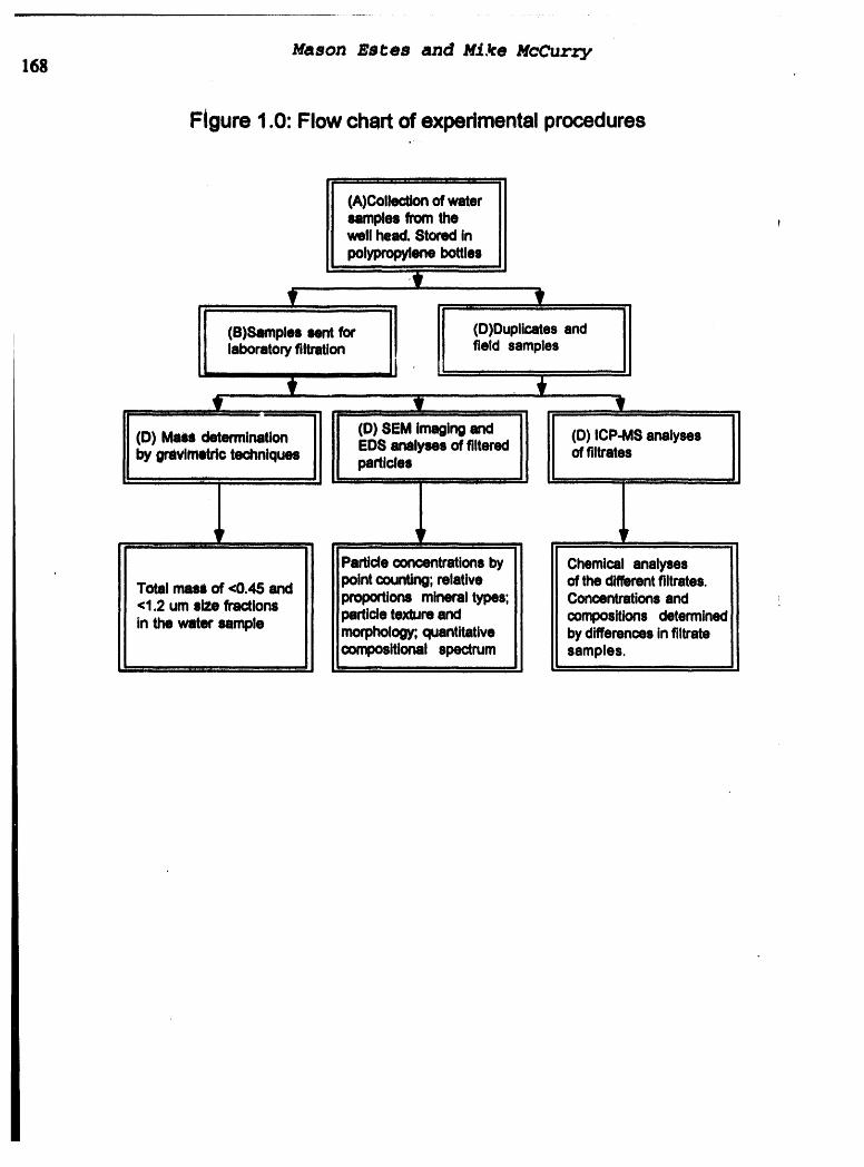
Mason Estes and Mi,_e McCurry168
Figure 1.0: Flow chart of experimental procedures
(A)Collectlonof watersamplesfrom thewell head.Storedinpolypropylenebottles
ii IJIHl, ,I, ,
'I
(B)Smnplessentfor (D)Duplicatesandlaboratoryfiltration field samples
(D) 8EM Imagingand (D) ICP-MSanalyses(D) Male determlnatlon EDS analysesof filteredbygravlmetdotechniques offiltrates
particles
/
i i ,1 _ r ,,, , ,, , , ,, ,. ,
Chemicalanalyses
Totalmassof <0.45 and ofthedifferentfiltrates.<1.2 um sizefractions ; Concentrationsandin the watersample compositionsdetermined
bydifferencesinfiltratesamples.
i ,] ii H - H , ,,H. , , ,

Colloidal Particles in Groundwater Near the ICPP, INEL
169additional samples were taken at the Slte-14 well at 113.36m and 212.12 m by thief sampler. Approximately one to twoliters of water were taken for each sample.
The smaller sized filters were Anoteo, A1 oxide filters
with a surface area of 3.14 _2, and the 1.2 and 0.45filters were _onstructed of cellulose nitrate. Water was
Inltlally flltered through the 1.2 _m and 0.45 _tm filterusing a standard Nalgene hand vacuum filtratlon unit. Afterpassage through the coarser filt&rs, the water was placed in
the filtration unit and sequentlally filtered with the 0.2
m filter, followed by the 0.1 9m, and finally the 0.02_mfilter.
The ultrafiltration unit devised consisted of a one
llter, glass, modified separatory funnel. The filters areplaced in a housing attached to the bottom of the funnelwith polyethylene tubing. Argon gas was used to pressurisethe chamber from 5 to 9 psi gauge pressure. The gas had anonline constant pressure regulator located close to thefunnel and was used to assure that during filtration aconstant pressure was provided during filtration. The devicewas scrubbed thoroughly before each filtratlon and ahydrogen peroxide wash was used to kill any bacteria. Afinal rinse of deionized water was used to assur_ noresidual contamination existed., The device was rinsed afterfiltration of each size fraction.
The concentrations of colloids can be estimated from the
ICP-MS data by assuming an average diameter of collolds ineach size range (r), and a specific density (p). Equation1.0 shows the conversion from mass difference determinedfrom the ICP-MS data to the number of particles/L:
(I.0) Mass Difference (in _g/l)+(4/3_r3)p (in 9g/particle) -
Concentration in part/L
The denominator in this equation is the mass of eachindividual colloid and the numerator is the mass of colloids
extracted. For this study colloids in the 0.45-0.2 _m range
were assumed to have a average diameter of 0.3 _m, in the
0.2-0.1 _m a diameter of 0.15 _m was used, and lastly for
the 0.i -0.02 9m a average diameter of 0.07 _m was assumed.A density of 2 grams/cm3 was assumed based onrecommendations of McCarthy (1993). Concentrations ofcolloids can also be determined with SEM analyses. Byassuming an average diameter for colloids it is possible todetermine the number of particles that it would take tocover the observed coverage on the filters. A series ofestimation charts were developed for the estimation ofpercent coverage.
Results

Mason Estes and Mike McCurry170
Preliminary results are given in Table 1.0 for three samplesin INEL-46. Two analysis are given for the 185.4-190 minterval since a duplicate was run on this sample. Results£or the 180-185.4 interval are also given. The tablesprovide the results of the major elements thought to formcolloids. These elements consist of Mg, Si, and Ca,although Fe and A1 have been shown to be importantconstituents of colloids. Un£ortunately, the results forthe latter two elements were found to be unsatisfactoryusing ICP-MS. The filters are uonstructed of A1 andleaQhing of this element from the filter caused varlableconcentrations of A1 in the water. ICP-MS analysis of otherwater samples showed that the A1 concentration wasconsistently less than one ppb, hence the contribution of A1to the mass of collolds is probably very small. Thedetection limits Eor Fe were 10 ppb. Analysls of thecolloid and groundwater samples showed that Fe was alwaysless than this amount. Iron is still a likely constituentof colloids based on SEM/EDS analysls.
Results of the 180-185.45 ft interval show that the
concentrations of collolde determined by ICP-MS, are on theorder of 2.3E+09, 7.8E+10, and 1.72E+12 parti=les/L for the
0.2, 0.1, and 0.2 _n filters, respectively. Thiscorresponds to a concentration of 1.0, 2.7, and 5.1 ppm forthe same filter sizes. The amount of material between 1.2
and 0.45 _m was about 1.2 ppm, and that <1.2 was about 1.5ppm. Note that Ca is the largest constituent. Results ofthe two 185.45-190.6 analyses show aoncentrations of2.63E+09 to 4.55E+09, 1.6E+10 to 2.4E+I0, and 2.7E+II to
2.48E+11 particles/L for the 0.2, 0.1, and 0.02 _m filters,respectively. This corresponds to 940 to 1630, 450 to 670,and 710 to 790 ppb for the filter sizes. The amount of
material between 1.2 and 0.45 _m was about 1.6 ppm and for
the fraction <1.2 _m, 2.1 ppm was measured. Calcium wasalso the dominant element detected in these samples. Figure2.0 illustrate graphically the concentrations inparticles/L. Note the linear pattern on the log graph,which show that the smaller colloids consistantly have thehighest concentrations.
Results of analyses using SEM are partially representedin Figure 3.0. The top photo in figure 3.0 is a SEM photo of
the 0.2 _m filter surface for the intervals 140-146.3 m inUSGS-46, and provides an example of three different types ofcolloids. Minor Fe and Ca colloids are noted by the roundedmorphology, whereas the bottom Jagged collold is a clayparticle. Note the pattern o_ the filter surface. Based onpoint counting, this interval contained concentrations ofcolloids estimated at about 750, 600, and 800 ppb for the
0.02, 0.1, and 0.2 _m filter, respectively (Table 4.0). The
<1.2 _m size fraction was 2.0 ppm and the 0.45-1.2 _m

Colloidal Particles in Groundwater Near the ICPP, INEL 171
0.2urn................. I - ,I, I0.1 urn,, - 12.39E+101 I 1 I0.o2 urn_' ............ ! 2.48E+il I I .... I i .....
Table]'".0:Resuitsof WaterFi_ for '"180-t88.48 m _rval
0.2.m' J,i.72s+121 I I .....

Mason Estes and Mike McCurry
172
Total Colloid Conoentratlons for the 185.45-190.6 m
Duplloate Interval of Well 46
1E+12__.._......-e
1E+I 1 ____....----- .....1E+10 _ "_
_ 1E+I_1E+08 : To_I
_ 1E+071E+06
100O0O
10000 ' '0.2 um 0.1urn 0.02 um
Fibr 8_.e
Total Oolloid Oonoentrations fez the 180-185.45 mInteEval of Well 46
1E+13
1E+12 _ __-4
1E+11
1E+10 _ _
1E.09 I : T_sll_ 1E.081E+07
1E+06
1OOO0O10000 , ,
02 um 0.1urn 0.02 um
_br 8be
Total Oolloid OonoentEations _n the 185.45-190.6 mInterval of W_ll 46
1E+12____.....-e1E+11 ..--
, ,,,1E+10 v
11 +" l 11E+08 --4--- TO_I
1E.07
1E+06
100000
10000 , ,
0.2 um 0.1urn 0.02 um
FIHersize
Figure 2.0: Total Concentration of Colloids in Intervalsof We.l146nearthe ICPP.

Colloidal Particles in Groundwater Near the ICPP, INEL
173
fraction was 1.8 ppm. The bottom photo in figure 3.0
illustrates colloids on the 0.I _m filter for the 147.8-153.3 interval in USGS 46. Concentrations were estimated at
600, 750, 800 ppb for the 0.02, 0.i, and 0.2 _m
filter,respectively. The <1.2 _m size fraction was 2.1 ppm
and the 0.45-1.2 _m fraction was 1.9 ppm. The concentrationsof colloids covered isolated areas of the filter, but in afew instances colloids were observed to bunch up.
Table 2.0: Results of SEM point counting of two filters
0 2 m. 750 600600 750
0.1 _m800 800
0.02 _m
The EDS analysis performed on random colloids on the J
filter surfaces showed that much of the colloidal material( ~60%)was composed of Ca. When present the Ca colloids werecharacterized by a rounded morphology. Iron colloids werealso observed and the Fe peak showed very strongly when a Fecolloid was found. These colloids also had a rounded
morphology. The concentrations of Fe colloids(~5%)we re muchsmaller than the Ca colloids. Certain colloids with a more
jagged morphology showed strong peaks of Mg, Fe, Ca, Si, andA1 indicating that they are possibly clays. The peakpattern for Si and A1 was difficult to determine because theA1 peak showed every time as a result of the A1 constructionof the filter. The Si peak is next to the A1 peak and wasoften overlapped by the A1 peak. However, on many of thecolloids the Si peak did show up distinctly. A few of thecolloids were observed to be Ti, although the concentrationwas less than one percent that of Ca. The Ti peak was verydistinct when this type of colloid was observed.
Particulate material <0.45 _m was observed under the
SEM/EDS unit. Much of the material had a rounded morphologyand was composed of Fe, Ca and clay minerals. The EDS peak
for Fe was very strong for many of the 0.45 Bm filtersindicating that a higher percentage of Fe is in the largerparticulate sizes than the smaller. Distinct peaks for A1,Si, Fe, Mg, and Ca were also observed when clay mineralswere encountered.
Discussion
The EPA 0.45 Bm distinction between dissolved versus
particulates phases is an arbitary cut off limit. This

Mason Estes and Mike McCurry_174
/ _ __ , ....
Fillure3.0: SEM plmtosofthe 0.2 pm filterfor the 139.69- 146.3 m interval(top) and the 180-185.4_,mimmal (bouom).Seethetextfordescriptions

Colloidal Particles in Groundwater Near the ICPP, INEL
175
study has shown that particulates do occur in 0.45 Bmfiltered water which are not dissolved. These colloids havebeen observed in the groundwater and consist of primarilycalcite and clays. The amorphous mineral ferrihydrite hasalso been observed in colloidal form, but in smallconcentrations. Most of the ferrihydrite appears to be in
the larger size fractions >0.45 _m. This has been observedin several of the samples that have been viewed underSEM/EDS. Calcite is observed as a dominant component inalmost all size fractions. The presence of calcite andferrihydrite is consistent with the equilibration,speciation modeling by the computer code MINTEQA2/PRODEFA2(1991), which shows these minerals to be oversaturated inthe waters near the ICPP. It is also consistent with XRDanalysis by Fromm (per. comm.) and Reed (per. comm.) thatcalcite is often as much as 40 percent of the material thatfills cracks and fissures in the basalts. Iron mineralshave also been observed in this material.
The clays that are observed have a jagged morphologyand probably are detrital in origin. The source for clayparticulates is likely the sedimentary interbeds as well asthe Big Lost River alluvium, which covers the surface of theICPP. Silicic acid colloids are likely responsible for partof the observed decrease in Si with filtration. Clays maybe partially responsible for the drop in Mg, Si, and Ca.Although Ca-Mg smectites have not been verifiedspecifically, smectites clays have been dete_ted, and watersappear to be thermodynamically in equilibrium with the clayphases Mg and Ca nontronite. Dolomite colloids are alsopossible, and may be partially responsible for the Mg and Cadecrease. Results of the MINTEQA2 equilibration modelingalso indicate that amorphous Si and dolomite areoversaturated.
Colloids do exist, but after preliminary determinationof the compositions it is unlikely that ferrihydritecolloids will play a major role in the transport of Sr-90 inthe saturated zone because of low concentrations. Aluminum
oxyhydroxide colloids are equally as unlikely to have amajor impact on contaminant migration. Ferrihydrite is inhigher concentrations in the fracture filling, and is likelythe primary phase for retardation of St-90 along the flowpath (Arnett, 1993). The role that calcite colloids willplay in the migration of Sr-90 is unknown. The adsorptioncapabilities of calcite are not as great as ferrihydrite,but it is much more abundant. It may have a significanteffect as a result of coprecipitation. Strontium is capableof substituting for Ca in calcite will easily fit into theCa site, due to the similarity in ionic radii. The presenceof clays may also impact St-90 migration. The role thatclay colloids will play is unknown, but it is possible thatSr-90 will diffuse into the clays via cation-exchange andbecome retarded in the basalt fractures.

Mason Estes and Mike McCurry
176
The concentrations of colloids determined in this studyare likely much higher than the true ambient condition.Other investigations on colloids have been conducted at theYucca Mountain Site in Nevada and the Grimsel Site in
Switzerland (Degueldre et al., 1989; Degueldre C. andSmith, 1993). Geologically these sites are similar in therespect that the groundwater migrates via fractures and thewater chemistries are similar. Concentrations of colloids
in these areas have been determined at 500 ppb and 600 ppb,
for the <0.45 _m size fractions. One of the primaryproblems in conducting a filtration experiment is theagitation caused by the pump. The stress imposed on theformation likely frees particulates that would normally beattached to the fracture walls. This was especially evidentwhen sampling INEL-45. The water from this well had to bepurged for more than the standard three borehole volumesbecause of the high concentration of large particulates,which gave the water a brownish tint. Better methods ofwater collection would involve slow pumping at rates ofml/min to avoid agitation (McCarthy, 1993).
We propose that the reason for the chemical trend inthe upper portion of the aquifer is a result of new inputsto the system. The highest concentrations of ra_4onuclidesare found in US&S-46 which is the closest to th_ o,jectionwell. The trends in USGS-45 and 44 are equally c_ose to theinjection well and both have lower concentrations ofradionuclides (Mccurry et. al., 1994). Strontium-90 shouldnot have the same chemical trend as H-3 of 1-129, unlesstheir was continued input into the system. Colloids couldbe aiding the transport of St-90 from the disposal wellperched zone and residual injected wastes. The decouplingwithin the deeper, tighter zones of the wells may be aresult of the adsorption onto the ferrihydrite and clayswithin fractures and vesicle walls.
Figure 7.0 represents an idealized cross sectionbeneath the ICPP showing the spatial separation of Wells 4S,46, 44, and the CPP injection well. The arrows indicatepotential pathways for Sr-90 migration. In this model it isassumed that the perched waters beneath the percolationponds do not have an influence on the concentrations of St-90 in the target wells. This assumption is based on thelocation of the perched zones, which are 600 m down gradientof the wells. The most likely source for the concentrationsof Sr-90, 1-129, and H-3 observed in the upper intervals ofthe sampled wells is the inferred perched zone surroundingthe ICPP injection well. This well has been documented tohave collapsed several times during its operational historywithin the vadose zone, and subsequent effluents formed aperched zone 100 ft above the regional aquifer. Modelingperformed by Robertson (1977) and Arnett (1993) both predictthat Sr-90 will not migrate to the regional aquifer becauseof adsorption in the interbeds. However, new inputs to theaquifer appear to continue. It is likely that colloids are

I i
W -" t_
_'Vell _ USGSWell#45 LISGSWell#.46 CPPDisposalWell(1953-1989) I-.,I_.
0 BigLostRiveraguvium n__ets 0
lava flows interbeds Probable zone _I_.
- until 1961.
Table WaterTable I..,.- ®
EThin,highlyfracturedandbrecciatedlavaflows C_
T'I"
450 ................
* Based upon down-hole electric andTV logs anddrillerlogs; ICPP interpretationandbasalt flow unit designations baseduponAnderson, 1991; injection well history work in progressby Fromm_
pathwaysof Sr-90.(A)MigrationfromtheICPP-03_ zoae_(B_ migmtimtofSr-90intheupperportionsof theaquiferby colloid_(C)Restrictedmigrationin thelesspermeablezonescausesincreaseH-3and1-129.Sr-90migrationbycolloidslessthanintheupperzones, Sr-90adsorbsontothebasaltmatrixand_,__nda_ryminendsandistakenoutof thegroendwam'. ,-,
-,d

Mason_ Estes and Mike McCurry178
adsorbing St-90 and migrating through fracture systemswithout retardation and forming the new inputs to thesystem. Contaminants migrate downward from the perched zonesand enter the regional aquifer.
List of Referenoes
Arnette R.C. and M.J. Rohe, 1993, Predicted Consequences onthe Snake River Plain Aquifer of Alternative Actions 1 and2, EGG-XXX-Draft, EG&G Idaho Inc.
Degueldre C. and P.A. Smith,1993, Colloid-facilitatedtransport of radionuclides through fractured media, J.of
Contaminant Hydrology,k
Deguelare C., B.Baeyens and W. Goerlich,1989, Colloids inwater _rom a subsurface fracture in granitic rock, GrimselTest Site, Switzerland, Geochimlca et Cosomochimica Acta,V.53, pp. 603-610.
Dragun J.,1988, The soil chemistry of hazardous materials,pub. by the Hazadous Materials Control Research Institute.
Dozombac J., 1991, Surface Complexation Modeling on IronOxyhydroxides, Oxford Press
McCarthy J.F. and C. Degueldre, 1993, Sampling andcharacterization of colloids and particles in groundwaterfor studying their role in contaminant transport, inEnvironmental Particles, Vol.2, pp. 2-31.
McCurry M., J. Welhan, J.Fromm, M.Estes,1993, Threedimensional chemical structure of the INEL aquifer near theIdaho Chemical Processing Plant(ICPP), Abstracts of AGU 1993Meeting.
McCurry M., J. Welhan, J.Fromm, M.Estes,1994, Threedimensional chemical structure of the INEL aquifer near theIdaho Chemical Processing Plant(ICPP), this volume.
MINTEQA2/PRODEFA2 A geochemical assessment model forenvironmental systems: version 3.0 user's manual, EPA 600-3-91-021. 1991, A
Olsen J.,1994, Straddle packer system design and operation,this volume.
Payne T.E., R. Edis, T. Seo,1992, Radionuclide transport bygroundwater colloids at the Koongarra uranium deposit, Mat.Res. Soc. Symp. Proc., V. 257pp. 481-488.
B

I
Colloidal Particles in Groundwater Near the ICPP, INEL]79
Ramsay J.D.,1988, The role of colloids in the release ofradionuclides from nuclear waste, Radiochimica Acta. V. 44,pp. 167-170.
Reimus, P.W., 1993, Transport of synthetic colloids throughsingle saturated fractures: A literature review: LANL Report11-22, pp 1-74.
Robertson J.B., 1977, Numerical Modeling of subsurfaceradioactive solute transport from waste-seepage ponds at theIdaho National Engineering Laboratory, USGS open file report76-717.

t,...L

181
Hydrosmlogy, Waste Disposal, Science and PoHtlc_Pme.a_ings _ SymposiumEngineeringGeology and OeotechntcalEngineering,1994
HYDROSTRATIGRAPHIC INTERPRETATION OF THE UPPER
PORTION OF THE SNAKE RIVER PLAIN AQUIFER NEAR THE IDAHO
CHEMICAL PROCESSING PLANT AT THE INEL
W. Barrash,
Center for Geophysical Investigation of the Shallow Subsurface,
Boise State University, Boise, Idaho
R.H. Morln,
U.S. Geological Survey, Denver, Colorado
S.H. Wood and W. Bennecke,
Department of Geosclences,
Boise State University, Boise, Idaho
ABSTRACT
The Snake River Plain aquifer (SRPA) is one of the most transmissive aquifers known. At theIdaho National Engineering Laboratory (INEL), the upper portion of the SRPA consists of numer-ous basalt flow groups and interbeddedsediments which have been tentatively traced across muchof the site. Three wells about 500 to 700 ft aparthave been logged through 190 ft of open intervalin the SRPA near the Idaho Chemical Processing Plant (ICPP). The wells exhibit the same lithos-tratigraphy and intersect much of the E-H and I flow groups of Anderson (1991). Geophysicallogs run in wells near the ICPP were: caliper, neutron porosity, gamma-gamma density, naturalgamma activity, acoustic televiewer, television, temperature, fluid conductivity, and flowmeters.
Logging results identify two hydrostratigraphic units for the upper portion of the SRPA withcontrasting borehole fluid velocities, permeabilities and lithologic characteristics. The upperhydrostratigraphicunit includes the E-H anduppermost partof the I flow groups. Intervals of highpermeability are mostly confined to interflow zones. The lower hydrostratigraphicunit consists ofthe interior of the I group where rubbly interflow zones do not occur and permeability is low.
Borehole fluid velocity fluctuations and direction reversals occur in less than one minute inresponse to pumping cycles at a production well 0.5 miles away which is screened in the E-H andI flow groups, respectively. This hydraulic communication indicates lateral continuity of hydros-tratigraphicunits and confined aquifer conditions in the SRPA in the vicinity of the Idaho Chemi-cal Processing Plant at the INEL. Data from walls 48 and 123 to the south indicate that the lowerhydrostratigraphic unit can be correlated with a thick flow in those wells. Another flow groupbelow the I group in wells 48 and 123 may be continuous beneath wells 44, 45 and 46 and may bea third hydrostratigraphic unit with relatively high transmissivity.
182 It'.Barrashandothers
INTRODUCTION
The Snake River Plain aquifer (SRPA) consists of numerous basalt flows and sedimentaryinterbeds. Early investigations at the INEL recognized that the SRPA is highly transmissive over-all, but heterogeneous. Reported values of transmissivity from monitoring wells in the upper partof the SRPA range over nearly six orders of magnitude (Ackerman, 1991). Also, where deepmeasurements have been made at the INEL (well INEL-Ia) permeability decreases with depth inthe SRPA (Mann, 1986). And, on a smaller scale, permeability varies with depth in any givenwell due to vertical changes in flow structures of the different basalt flows present.
Previous workers recognized vertical variability of head, hydrochemistry and in-hole flow(both magnitude and direction) in wells at the INEL, and at the ICPP in particular (e.g., .Jones,1961; Barraclough et al., 1967). Recent efforts to characterize contamination and evaluate reme-diation alternatives have increased the interest in quantifying vertical changes in hyd_'aulicparam-eters and water chemistry to determine if the SRPA is well mixed or layered. This paper presentsresults from stratigraphic andborehole geophysical logging investigations which are part of anon-going program to understand vertical and lateral variations in hydraulic properties, hydro-chemistry (including contaminant chemistry), and flow within and between wells in the SRPA atthe INEL.
STUDY AREA
Three wells (44, 45 and 46) immediately west of the ICPP (Figures 1 and 2) were selected fordetailed investigation because they: (a) have 190 ft of open interval to the SRPA; (b) have identi-cal well construction; (c) are in close proximity (within 700 ft of each other); (d) have longrecords of water level and water chemistry measurements; (e) have similar histories of contamina-tion with liquid wastes originating from the ICPP; and (f) are administratively available for inves-tigation. That is, wells 44, 45 and46 provide the opportunity to see if vertical changes occur over190 ft of the SRPA, and if any such changes can be traced 500 to 700 ft laterally to adjacent wells.
For the interpretive purposes of this paper,the study area is extended beyond wells 44, 45 and46 to the north and south at the ICPP to include wells CPP1, CPP2, 48 and 123. These additionalfour wells were not investigated in the field for this study. However, observed hydraulic interac-tions and detailed stratigraphic information permit tentative correlations to the north and southbased on findings in wells.44, 45 and 46.
STRATIGRAPHIC FRAMEWORK
Anderson (1991) identified about 40 flows and23 flow groups in the unsaturatedzone and theupper SRPA in the ICPP area between land surface and about 750 ft below land surface (BLS).He was able to correlate flow groups in the ICPP area with equivalents in the area of the Radioac-tive Waste Management Complex (Anderson and Lewis, 1989; Kuntz et al., 1980) about 7 mi tothe southwest of the ICPP, and with equivalents at the NPR test well 3 mi to the northeast of theICPP (Champion et al., 1988). These correlations were based largely on naturalgamma logresponses (see Anderson, 1991, Fig. 8). Golder Associates (1990) report on core from well 123;Lanphere et al. (1993) add detailed flow descriptions for well 123, and place individual flow units
"Hydrostratisraphic interpretation, ICPP, INEL 183
and flows into the regional stratigraphic nomenclature.
The three wells that were investigated in detail here (wells 44, 45 and 46,) are open to basaltsand sediments of flow groups E-H, I (Anderson, 1991) and the recently recognized J flow group(S.R. Anderson, personal communication, 1994) in the saturated portions of these wells (Figure3). Geophysical logs that were most useful for lithostratigraphic interpretation (identification andcorrelation of flows, flow units and flow groups) in these wells are: naturalgamma, caliper andtelevision logs.
Caliper logs showed locations of enlarged borehole diameters in the wells. These enlargedborehole diameters commonly occurred at flow tops and are abundant in the upper 120 ft of wells44, 45 and 46. The lower 70 ft of these boreholes are smooth at the nominal drilled diameter (Fig-ure 4). Television logs complement the na:ural gamma and caliper logs by providing flow struc-ture information helpful for recognition of individual flow units or flows, and relative verticalpositions within them based on flow structures (Bennecke, 1994).
From these logs and from stratigraphic interpretations by Anderson (1991), the change tosmooth borehole at about 580 ft BLS (4340 + 4 ft elevation) in 44, 45 and 46 occurs below several(two to four) relatively thin flow units or _lows in the upper portion of the I flow group (Figure 3).Lanphere et al. (1993) identified two thin flow units above a ll0-fl-thick flow (together formingtheir flow 12) in the I flow group in well 123 about 0.5 mi south of wells 44, 45 and 46 (Figure 2).Two relatively thin flows or flow units overlie a 100-fl-thick flow at comparable elevation andstratigraphic position in well 48 (Bennecke, unpublished data). The smooth borehole segments inthe bottom 70 ft of wells 44, 45 and 46 appear to be the main portion of one thick flow (startingbelow the flow top) which is correlated here with the number 12 flow of Lanphere et al. (1993).
The thick flow in the I group is underlainby a sedimentary interbed at comparable elevationsin wells 48 and 123 (Lanphere et al.,"1993; Bennecke, unpublished data). This interbedmarks thecontact with the J basalt flow group below (S.R. Anderson, personal communication, 1994) whichconsists of several flows above another interbed at about 4170 + 4 ft elevation (Figure 3).
To the north, in wells CPP1 and CPP2, the best stratigraphic information comes from naturalgamma log interpretation (Anderson, 1991) and drillers' logs which: (a) locate the contactbetween the E-H flow groups and the I flow group about 45 ft higher than in wells 44, 45 and 46(Figure 3); and (b) indicate that no flows occur in the I group there with thickness approaching100 ft. Television logs are not available for wells CPP1 and CPP2. It is uncertain if individualflows (such as the thick flow in the I flow group in wells 44, 45, 45, 48 and 123) continue north towells CPP1 and CPP2 or if flows thin northward. Also it is not clear if the elevation difference ofthe contact between E-H and I is due to paleotopography, structuraloffset or both.
HYDROSTRATIGRAPHY
Responses to geophysical logging in wells 44, 45 and 46 indicate that the basalt aquifer pene-tratedby these wells can be divided into two hydrostratigraphic units: an upper unit with numer-ous high-permeability zones and a lower unit with very low permeability throughout. The contactbetween these two hydrostratigraphic units occurs at about 4340 ft elevation (580 ft BLS) wherethe lithologic change occurs from numerous flows with enlarged borehole diameters at flow topsto the interior of the thick flow in the I flow group.

184 W. Barrash and others
Logs most useful for characterizinghydrostratigraphy are flowmeter logs from heat.pulseand impeller tools, and the temperature log (Bennecke and Wood, 1992; Morin et al., 1992).
' Fluid specificconductance logging also can provide valuable information on locationsof changesin hydrochemistry in open boreholes in the SRPA (e.g., Hegmann and Wood, 1994; Wood andBennecke, 1994).
Flowmeter logging in wells 44, 45 and 46 (Bennecke and Wood, 1992; Morin et al., 1992)has demonstrated that significant in-hole flow (generally 0.9 to 8.4 g_.l/min)occurs in the upperhydrostratigraphic unit, andthat little or no in-hole flow (<0.1 to 0.7 gal/min) occurs in the lowerhydrostratigraphic unit (Table 1). Temperature logs in wells 44, 45 and 46 show approximatelyisothermal conditions in the upper hydrostratigraphic unit due to strong vertical in-hole flow;increase of temperaturewith depth in the lower hydrostratigraphic unit indicates little or no in.hole flow there (Figure 5). High in-hole flow rates and magnitudes in the upper hydrostrati-graphic unit correlate with high estimates of hydraulic conductivity (generally >100 to >10,000 ft/day) from flowmeter logging while pumping (Moria et al., 1992), and from hydraulic tests withthe straddle-packer system (Monks et al., 1993).
Hydraulic Indications of Hydrostratlgraphic Continuity
Under "static" conditions, in-hole flow has an upwardgradient in wells 44, 45 and 46 (Figure4) including upward gradient in the lower stratigraphic unit where slight in-hole flow can bedetected (Morin et al., 1992). Measurements of flow rates and directions during flow logging(Table 1, Figure 5) also demonstrate that changes occur when an ICPP production well 0.5 miaway (either CPP1 or CPP2) is turnedon or off (Bennecke and Wood, 1992; Morin et al., 1992).These changes occurred in less than 30 seconds, as determined when close coordination withoperations staff at the production wells provided accurate times that a production well was turnedon.
The upper production zone in the E-I-Iflow groups in CPP1 and CPP2 (screened intervals andidentified producing zones from drillers' logs) and the contact of the E-H flow groups over the Iflow group in CPP1 and CPP2 are at higher elevations than comparable features in wells 44, 45and 46 (Figure 3). The lower production zone in CPP1 and CPP2 occurs in the I flow group(Anderson, 1991) at an elevatioii higher than the base of wells 44, 45 and46. Also the interveningthickness between screened intervals is less than 100 ft (Figure 2). Rapid changes in head and in-hole flow rate and direction noted above that occurred in response to pumping at wells CPP1 andCPP2 0.5 mi away indicate that there is hydraulic connection to these wells and that the aquifersystem is under confined conditions (Bennecke and Wood, 1992; Barrash et al., 1993). Theupward gradient in wells 44, 45 and 46 is consistent with a system in hydraulic communicationwith higher head regions under confined conditions.
In addition, preliminary review of transient responses to pumping at CPP1 in the lowerhydrostratigraphic unit in well 46 suggest hydraulic communication with a high permeability unitbelow the base of well 46. Head changes were recorded in the lox .r 10 ft of well 46 (isolatedfrom the well above with a packer) beginning <15 seconds after pumping was started in wellCPP1, but it appears that no response or a more muted or delayed response occurred in thepacked-off interval above. Because the horizontal permeability in the lower hydrostratigraphicunit of well 46 is quite low (Table 1, Figure 5), such a rapid response to pumping 0.5 mi away isnot likely unless the response occurs by vertical leakage communication with a high permeabilityzone below that is hydraulically connected to CPPI.

Hydrostratl&raphlc Interpretation, ICPP, INEL 185
To explain these conditions, it has been suggested that the upper hydrostratigraphic unit inwells 44, 45 and 46 may be continuous with the upper screened producing zones in the E-H flowgroups in CPP1 and CPP2, and that a higher permeability unit may exist below the bottoms ofwells 44, 45 and 46 (J flow group?) that is hydraulically connected to the lower screened produc-ing zones in the I flow group in CPP1 and CPP2 (Matin et al., 1992; Barrash et al., 1993). Tenta-tive correlation of the thick flow (flow 12 of Lanphere et al. [1993] in well 123) in the I groupwith a thick flow in well 48 and with the lower region of wells 44, 45 and 46 allows us to specu-late that a higher permeability unit may occur up to 25 to 35 ft below wells 44, 45 and 46 based onprojection of the base of the thick flow from wells 48 and 123.
This interpretation of a three-layered hydrostratigraphy at the ICPP can be tested by investi-gating well 48 with geophysical logging and also with hydrologic and hydrochemical testing andsampling with the straddle-packer system described in this volume (Olsen, 1994) -- as has beenemployed at wells 44, 45 and 46. Such investigation has not occurred to date for logistical rea-sons (well 48 is inside the security area of the ICPP) and because administrative issues surround-ing management of contaminated water generated by the straddle-packer system have not yetbeen resolved. New data on vertical variability in hydrostratigraphy in the upper portion of theSnake River Plain aquifer have significant implications for the vertical distribution of contamina-tion in the aquifer (McCurry et al., 1993; 1994), and hence for ground water monitoring, riskassessment and modeling of aquifer flow and contaminant transport.
ACKNOWLEDGMENTS
This paper was improved by discussions with staff of the U.S. Geological Survey at theINEL, especially S.R. Anderson and R.G. Jensen, and by the reviews of G. Johnson and M.McCurry.
REFERENCES
Ackerman, D.J., Transmissivity of the Snake River Plain aquifer at the Idaho National EngineeringLaboratory, Idaho, U.S. Geological Survey Water-Resources Investigations Report 91-4058,1991.
Anderson, S.R., Stratigraphy of the unsaturatedzone and uppermost part of the Snake River Plainaquifer at the Idaho Chemical Processing Plant and Test Reactors Area, Idaho National Engi-neering Laboratory, Idaho, U.S. Geological Survey Water-Resources Investigations Report91-4010, 1991.
Anderson, S.R. and B.D. Lewis, Stratigraphy of the unsaturated zone at the Radioactive WasteManagement Complex, Idaho National Engineering Laboratory,Idaho, U.S. Geological Sur-vey Water-Resources Investigations Report 89-4065, 1989.
Barraclough, J.T., Teasdale, W.E. and Jensen, R.G., Hydrology of the National Reactor Testing Sta-tion, Idaho: Annual Progress Report 1965, U.S. Geological Survey Open-File Report, IDO-22048, 1967.


186 W. Barrash and others
Barrash, W.,+R.H. Morin, S.H. Wood, S.R. Anderson, R.G. Jensen and W. Bennecke, Geophysicallogging evidence for stratigraphic controls on hydrology in the Snake River Plain aquifer atthe Idaho National Engineering Laboratory (INEL), southeastern Idaho, EOS, 74, 283-284,1993.
Bennecke, W.M., The identification of basalt physical features from borehole television logs, Pro-ceedings of the 1994 Annual Symposium on Engineering Geology and Geotechnical Engi-neering, Boise, Idaho, 1994.
Bennecke, W.M. and S.H. Wood, Impeller flow-meter logging of vertical cross flow between basaltaquifers through wells at the Idaho National Engineering Laboratory, eastern Snake River |
Plain, Idaho, Borehole Geophysics Research Program, Boise State University, Progress Re- .port: June 22, 1992, 1992.
Champion, D.E., Lanphere, M.A. and Kuntz, M.A., Evidence for a new geomagnetic reversal fromlava flows in Idaho: Discussion of short polarity reversals in the Brunhes and late Matuyamapolarity chrons, Journal of Geophysical Research, 93, 11,667-11,680, 1988.
Golder Associates, Final well completion report for wells 121,122 and 123 at the Idaho ChemicalProcessing Plant, Report to EG&G Idaho, Contract C86-131159, Task 6, 1990.
Hegmann, M.J. and S.H. Wood, Hydrostratigraphy of the Snake River Plain aquifer beneath theRadioactive Waste Management Complex at the Idaho National Engineering Laboratory,southeastern Idaho, Proceedings of the 1994 Annual Symposium on Engineering Geology andGeotechnical Engin'eering, Boise, Idaho, 1994.
Johnson, G.S., H. Olsenand D.R. Ralston, Hydrologic testing in wells USGS 44, 45 and 46 nearthe ICPP at the Idaho National Engineering Laboratory, Proceedings of the 1994Annual Sym-posium on Engineering Geology and Geotechnical Engineering, Boise, Idaho, 1994.
Jones, P.H., Hydrology of waste disposal, National Reactor Testing Station, Idaho -- An interimreport, U.S. Geological Survey Report ID0-22042, 1961.
Kuntz, M.A., G.B. Dalrymple, D.E. Champion and D.J. Doherty, 1908, Petrography, age and pa-leomagnetism of volcanic rocks at the Radioactive Waste Managemnent Complex, Idaho Na-tional Engineering Laboratory, Idaho with an evaluation of volcanic hazards, U.S. GeologicalSurvey Open-File Report 80-388, 1980.
Lanphere, M.A., D.E. Champion and M.A. Kuntz, Petrography, age and paleomagnetism of basaltlava flows in coreholes Well 80, NRF 89-04, NRF 89-05 and ICPP 123, Idaho National En-gineering Laboratory, U.S. Geological Survey Open-File Report 93-327, 1993.
Mann, L.J., Hydraulic properties of rock units and chemical quality of water for INEL-la; 10,365ft deep test hole drilled at the Idaho National Engineering Laboratory, Idaho, U.S. GeologicalSurvey Water-Resources Investigations Report 86-4020.
McCurry, M., J. Fromm, J. Welhan and W. Barrash, Vertical profiling of aquifer hydrochemistry atthe INEL, Idaho: Implications for hydrostratigraphy (abs.), EOS, 74, 284, 1993.
McCurry, M., M. Estes, J. Fromm, J. Welhan and W. Barrash, Three-dimensional chemical struc-ture of the INEL aquifer system near the Idaho Chemical Processing Plant, Proceedings of the1994 Annual Symposium on Engineering Geology and Geological Engineeriizg, Boise, Ida-ho, 1994.

Hydrostratigraphic Interpretation, ICPP, INEL187
Monks, J.I., D.R. Ralston, G.S. Johnson, J.K. Olsen andW. Barrash, Straddle-packer determinationof vertical variations in aquifer properties in the Snake River Plain aquifer at the Idaho Na-tional Engineering Laboratory (abs.), EOS, 74, 284, 1993.
Morin, R.H., W. Barrash, F.L. Paillet and Taylor, T.A., Geophysical logging studies in the SnakeRiver Plain aquifer at the Idaho National Engineering Laboratory - Wells 44, 45 and 46, U.S.Geological Survey Water-Resources Investigations Report 92-4184, 1993.
Olsen, J.K., Straddle packer system design and operation for vertical characterization of open bore-holes, Proceedings of the 1994 Annual Symposium on Engineering Geology and Geotechni-cal Engineering, Boise, Idaho, 1994.
Wood, S.H. and W. Bennecke, Vertical variation in groundwater chemistry in the Snake River Plainbasalt aquifer inferrred from fluid specific-conductivity (electrical) well logging at the IdahoNational Engineering Laboratory, southeastern Idaho, Proceedings of the 1994 Annual Sym-posium on Engineering Geology and Geotechnical Engineering, Boise, Idaho, 1994.
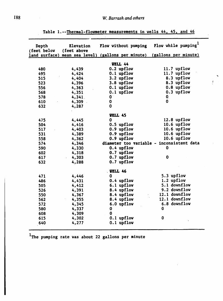
188 W. Barrash and others
Table 1.--Thermal-flo_nneter measurements in wells 44 t 451 and 46
Depth Elevation Flow without pumping Flow vhilepumplng 1(feet below (feet aboveland surface) mean sealevel) (gallons per minute) (gallons perminute)
.WELL 44
480 4,439 0.2 upflov 11.7 upflov495 4,424 0.1 upflov 11.7 upflov ,515 4,404 3.2 upflow 8.3 upflov523 4,396 3.8 upflow 8.3 upflov556 4,363 0.1 upflow 0.8 upflov568 4,351 0.1 upflov 0.3 upflov578 4,341 0 0610 4,309 0 0632 4,287 0
tELL 45
475 4,445 0 12.8 upflow504 4,416 0.5 upflov 10.6 upflow517 4,403 0.9 upflov 10.6 upflov531 4,389 0.9 upflov 10.6 upflov558 4,362 0.9 upflov 10_6 upflow574 4,346 diameter too variable - inconsistent data590 4,330 0.4 upflow 0602 4,318 0.7 upflov617 4,303 0.7 upflov 0632 4,288 0.7 upflov
WELL 46
471 4,446 0 5.3 upflov486 4,431 0.4 upflow 1.2 upflow505 4,412 6.1 upflow 5.1 dovnflow526 4,391 8.4 upflow 9.2 downflow550 4,367 8.4 upflow 12.1 downflow562 4,355 8.4 upflow 12.1 downflow572 4,345 6.0 upflow 6.8 downflow580 4,337 0 0608 4,309 0615 4,302 0.I upflow 0640 4,277 0.1 upflow
1The pumping rate was about 22 gallons per minute

189q
Hydrostratigraphic Interpretation, ICPP, INEL
Figure 1. Location map of the Idaho National Engineering Laboratory.

190W. Barrash and others
112_'7"30"" 112°56"............. ,............. .- !
Figu_ 2. Location map of wells in the vicinity of the IdahoCliem_cal Processing Plant which penetrate the Snake RiverPlain aquifer. Wells CPPI and CPP2 are production wells.

CPP1 CPP2 44 45 46 48 " 123• .
Land _tt Land4913 Surface 491S 4919 • 4_0 117• .
441114470 4474
44m4463 4447
HighT? 44U
' _ "_" " High T HighT HighT -_High T ? 44004400 Low T "-. -
".?
-" L_wT ' _"
FlighT " - ,_
4300 • 4_1 _s • ? '_, LowT LowT LowT 4300- R_. Low1"?. ._
"
- '_?..................... ._.."................. ?.. . .........
g_ HighT ?
4200 _ Above E-H Flow Groups 42o0 _"t'%
- ["-] E-H Flow Groups Contact between hydrostratigraphic " ¢'_
1 I Flow Group units; queried where speculative41711 4177
['-'] J Flow Group Water levels in 44, 45, 46 and 48 taken 10190, _L"z'ilevels unavailable for CPPI, CPP2 and 123 C-_
Screened intervals in CPP1 and CPP2shown with hachures
Figure 3. Interpreted iithostratigraphic and hydrostratigraphic cross section
in the um3er _ion of the Snake River Plain aquifer in the ICPP area.

192 W. Barrash and others
-- I4500 "
Well44 Well45 Well46480-"
!!
..,F,,?_.
b
i ,_, _m0- _ •
_. aim
_ _ ._.,, ._1 J,_. w
_H u _ , ' i' "-Eo FlowGroups l'.-- , m
-----,s_,----_-- ,- ----_ '- -'"_'"*_ _l_ow _. _'Group _ _"
A
4320"•
, i|, E4300-- • " W
• m
_.. ., -, __ I , I __ I. , I , I , I , 0
0 _ 10 150 S 10 15 0 5 10 15 ...I
Caliper,ininches
Figure 4. Sketches of fluid circulation patterns in we]is 44, 45 and 46 based onheat-pulse flowmeter measurements. In-hole flow direction indicated by ar-rows. U]_ward_radient was present when production wells were off.(After _orm e_ai., 1992)


194
JIt

Hydrogeology, Waste Disposal, Science and PoliticsProceedings 30th SymposiumEngineering Geology and Geotechnical Engineering, 1994 195
]lrJ'JDROS'JL_I_TZ(_IRA]P]i[¥OF 'JL_[Z_ RZ%tIM ]PLAZN AQUZ]r]_BlC]N]CA'2_i['JL*]i_]U_ZOJ_T:rVll HAS'JL']I_lOlt]D_ CON]PL]r.X
AT _ IDAHO NATIONAL _ZHZERZNG _]KKTORYzA PI_LZB[ZHARY RIPORT
.
Naz_ _. Hegnann and _er H. WoodGeolc:l.emoe Doparl:nm_t
Boime State Un£vezm£tyBO4ie, X]:) 83725
ABSTRACT
Geophysical logs for 6 wells which penetrate the Snake RiverPlain aquifer at the Radioactive Waste Management Complex (RWMC)were analyzed for preliminary information on the hydrostratigraphy.Using stratigraphic correlation of flow groups worked out byAnderson and Lewis (1989), and by Anderson (pers.comm., 1994), aswell as gamma signatures of flows within these flow groups,correlation of individual flows is attempted. Within these flows,
probable permeable zones, suggested by density and caliper logs,are identified, and zones of hydraulic connection are tentativelycorrelated. In order to understand the response of density andneutron logs in basalt, the geological characteristics arequantified for the 150-ft section of the well CIA core, from depth550 to 710 ft.
ZN'2_ODUCTZON
The Radioactive Waste Management Complex (RWMC) is located inthe southwest corner of the Idaho National Engineering Lab (INEL)in eastern Idaho (Fig. i). The RWMC was established in 1952 as adisposal site for solid radioactive waste and is situatedapproximately 600 ft above the Snake River Plain aquifer. The siteis underlain by a complex series of basalt flows and sedimentaryinterbeds, and horizontal movement through the aquifer is believedto occur chiefly through interflow zones (Ackerman, 1991)o Thegroundwater generally flows from northeast to southwest, and itsvelocity is estimated at between 5 and 20 ft/d (Robertson andothers, 1974). Because of the potential for migration ofcontaminants through the aquifer, it is important to identify zonesin the aquifer which are likely to be permeable.
APPROACH
Six of the deeper wells located at the RWMC were chosen for ahydrogeologic cross-section beneath the water table (Fig. i).Using primarily gamma logs, as well as core descriptions,geomagnetic properties, K-Ar age dates, and location and thicknessof sedimentary interbeds, Anderson and Lewis (1989) have correlatedstratigraphic units in 2 of these wells (RWMC-Prod. and 120) tofive wells previously described by Kuntz and others (1980).

196 M. J. Hegmann and S. H. Wood
N,--..,..
. flier.
_.r I ,., ,-,,r'-.. _ I /
! !I . !_..._ __. "-__ _
, ,! _L .......... _-- --_'IL
g.I. fill
t
10oo ft
Fig. 1. Location of the Radioactive Waste Management Complex and
hydrogeologic cross-section through 6 wells.

Hydrostratigraphy, SRP Aquifer, Beneath RWMC, INEL199
Anderson has since correlated stratigraph$c units in the 4remaining wells in this cross-section (OW-2, M4D, M10S, and CIA).These stratigraphic units are termed "flow groups", originallydefined as petrographically similar flows extruded from the samesource during eruptive events of less than 200 years (Kuntz andothers, 1980).
For this study, gamma, caliper, and density logs were examinedto identify possible permeable zones and individual flows withinAnderson's time-equivalent flow groups. Gamma logs were studied toidentify gamma signatures. By comparing signatures of individualflows, correlation between wells of some of these flows washypothesized. Density logs and caliper logs were studied toidentify zones of low density and caved zones, which may indicatepermeability. The core of well CIA, the only core available withinthe cross-section, was inspected and compared to its density andneutron logs to identify the characteristics which causedeflections on density and neutron logs.
LOG 331TIRlqUBT&TZOW
Gamma z_oga
By identifying sedimentary interbeds and by examining gammasignatures, Anderson and Lewis (1989), and Anderson (pers.comm.,1994) correlated sequences of basalt flows in wells OW-2, 120, M4D,M10S, RWMC-Prod., and CIA, to other wells in the area. These time-equivalent sequences were termed "flow groups" , and thealphabetical naming convention for these groups, originated byKuntz and others (1980), is retained for this report.
Natural gamma logs were used in this * study in an attempt tocorrelate individual basalt flows within Anderson's flow groups.An analysis of eastern Snake River plain basalts of Pleistocene agedemonstrated that flows vary from 0.26% to 2..71% K20 (Kuntz andothers, 1992), and this is thought to be responsible for variationsin natural gamma response (Anderson, pers. commun., 1994). Gammaemissions are believed to be uniform in related flows of similar
age and source at the site (Anderson and Lewis, 1989; Anderson,pers.comm., 1994).
Natural gamma logs were inspected, and signatures weretentatively identified. These signatures were used to divideAnderson's original flow groups into "gamma units", or sequences ofbasalt flows believed to have erupted from the same source. Eachgamma unit retains its original group name, but because gammasignatures within some of Anderson's groups varied significantly,they were identified as separate gamma units.
For example, Anderson believes that flow group H in well M4Dprobably correlates with flow group H in other wells. But becausegroup H in M4D contains three distinctly different gammasignatures, it may contain flows of 3 different sources (Anderson,pets.comm., 1994). These 3 gamma units were named H I, H_, and H 3because they are the first, second, and third gamma units (countedfrom the surface) to occur in this well, within what Anderson andLewis (1989) originally called group H. Note that subscripts are

M.J. Hegmann and S.H. Wood198
used only to order uammaunits stratiuraDhicallv within a urOUD inan individual well: the same subscriDt does not imply correlation
l__r_2___.. Also, to simplify correlation, it wasided that gamma unlts could contain more than a single flow, but
could not contain interbeds. An accumulation of sediment wouldtend to indicate a long period of time passed between flows andwould make itunlikely that the flows were part of the same event.
Because the base of flow group F is known with certainty, andit is uniquely characterized by reversed polarity and high gammaemission (Anderson and Lewis, 1989; Anderson, Fers. comm., 1994),its gamma signature was utilized as the basis for correlatingindividual flows beneath it.
Figure 2 illustrates the manner in which gamma signatures wereidentified and correlated_ For example, because Anderson hastentatively correlated all G groups with respect to time, thesimilarity of gamma units GI in OW-2, GI in 120, and G2 in M4D mayindicate correlation of individual flows within the gamma unit.Density and caliper logs indicate there may be 2 flows within GI of120, and 2 flows within G2 of M4D. It might be hypothesized thenthat the 2 flows in GI of 120 correlate to the 2 flows in G2 of M4D.It is important to note that this was a loose, qualitativecomparison, because some of the wells were logged with uncalibratedtools, and caving of sediments, drilling fluid, and wellconstruction can each affect the gamma log.
CallpozLog8
Caved zones as expressed on caliper logs were used to identifypossible flow tops within gamma units. Flow tops are likely to bepermeable zones because they are usually very vesicular andsometimes rubbly (Whitehead, 1992). Caved zones are also caused bythe presence of unconsolidated sedimentary interbeds, which may ormay not be permeable. These major interbeds were previouslyidentified byAnderson and Lewis (1989), and Anderson (pets.comm.,1994). Several zones where minor interbeds might exist, such as atelevations 4325 ft and 4383 ft in well M4D, were identified byexamining natural gamma logs. It is important to note that theseexcursions on the gamma log are not as strong as those of knowninterbeds, and they may be due to conditions other than thepresence of sediment.
Caved zones within a gamma unit may also be caused by zones offrscture. Unfortunately, it appears they, cannot be positivelydistinguished from flow tops except by examining cores, which arerarely collected, or by examining the borehole with a televiewer.Caved zones which did not appear to contain interbeds, and whichoccurred within a gamma unit, were assumed to be flow tops. Forexample, caved zones occur at elevation 4410 ft in RWMC-Prod., andbetween elevations 4288 and 4268 ft in OW-2.; natural gamma logs donot indicate sediment. In logging OW-2 with spinner-flowmeter,Wood and Bennecke (this volume) have determined that flow is
occuring in this caved zone. Such zones were assumed to bepermeable as long as the density log did not indicate otherwise.
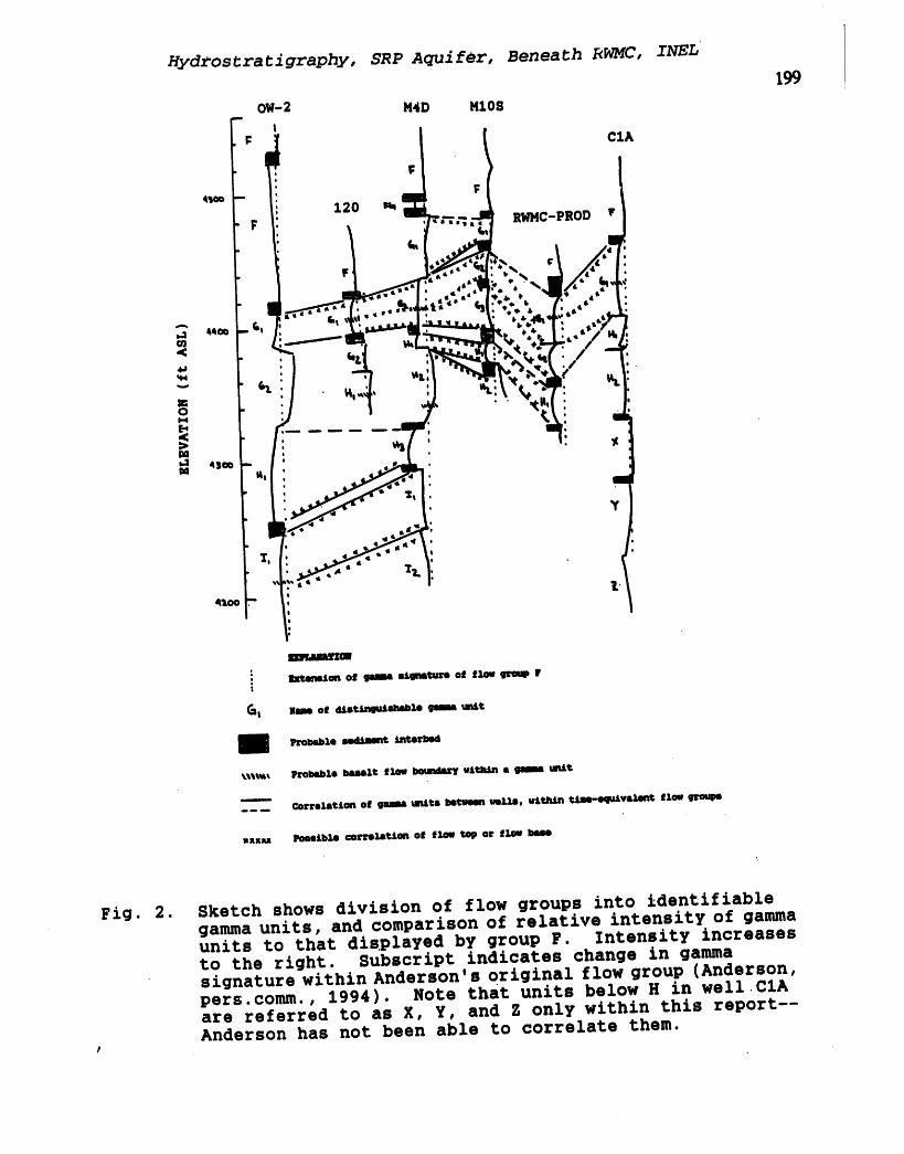
Hydrostratigraphy, SRP Aquifer, Beneath RWMC, INEL 199
OW-2 M4D MIOS
| CIA
_ 120r'_',_ RWMC-PRODv
F
Fig. 2. Sketch shows division of flow groups into identifiablegamma units, and comparison of relative intensity of gammaunits to that displayed by group F. Intensity increasesto the right. Subscript indicates change in gammasignature within Anderson's original flow group (Anderson,pers.comm., 1994). Note that units below H in well ClAare referred to as X, Y, and Z only within this report--Anderson has not been able to correlate them.
p

200 M.J. Hegmann and S.H. Wood
DenslCyLo2s
The gamma-gamma or density log is used as a measure of bulkdensity or porosity (Keys and MacCary, 1971). The excursions onthe gamma-gamma logs displayed in this report are not directlyproportional to formation density as explained in the appendix. Inthis study the density log was used in a qualitative manner toidentify permeable zones such as fracture zones and flow tops,which sometimes are not expressed on the caliper log. Zones of lowdensity in the absence of caving were interpreted as a flow top andadjacent flow base. For example, at elevations 4414 ft and 4356 ftin well 120, the density log displays marked drops in density, butthe caliper log does not show caving. These zones were interpretedas vesicular flow tops, although it is possible they may befracture zones within an individual flow. Marked drops in density,especially in combination with a caved zone, were tentativelyidentified as flow tops.
ClA Core ana Logs
In comparing the sketch of a 150-ft section from depth 550 ftto 710 ft of the CIA core to the density and neutron logs, it canbe seen that certain characteristics of the core cause deflections
on both logs (Fig. 3). For example, the neutron log shows a zoneof very low porosity, and the density log displays high densitybetween elevations 4456 and 4444 ft. An examination of the core inthis zone revealed it to be very dense and practically unfractured.
Between elevations 4433 and 4430 ft, the neutron log displaysa marked deflection to the left, indicating high water-filledporosity; the density log shows a gradual, then very sharp drop indensity. The core was poorly recovered in this zone, but nosediment is indicated on the gamma log. The caliper indicates acaved zone. This was interpreted as a rubble zone between flows,within a single gamma unit, mostly because of the gradual characterof the density log, but it is possible that the zone is highlyfractured flow basalt.
In studying the remainder of the core between elevations 4470and 4320 ft, it is seen that features such as vesicularity, degreeof fracturing, and presence of sedimentary interbeds producedistinct deflections on both logs. The rock quality designation(RQD), which is a modified core-recovery percentage (Bieniawski,1989), and roughly estimated porosity also appear to be at leastcrude indications of the relative degree of density and porosity.For example, the RQD shows a high degree of core recovery, nearly100 percent, between elevations 4454 and 4442 ft (Fig. 3). Thedensity log displays a zone of high density, and the neutron logindicates low saturated porosity. Estimated porosity tends to dropin zones where the density log indicates high density, betweenelevations 4402 and 4385 ft for example.

• 201
Hydrostratigraphy, SRP Aquifer, Beneath RWMC, INEL
iII l IiI: I i '
i !i ;_U
0
@0i
, jm__Jl_ __r,,__/l r'l ,o "-t- O_
m_
.... _1,4o,-,, F_, I , r -'t_ .t-,-_"o,_, -_u_ o -OT-O _ W
,, k4_
U° 0@
, ,_::j_- NI I,,I
_ i_I _'l_ _'_ ,,, m ,11 ' . .'. i_i ;"_', r _{ ........
_* - O®
--'- I i I i I I I I i, I i I I I I I
('18¥ ':l,J) HOLLVA|'I|

202 M. J. Hegmann and S. H. Wood
]ln12ROGZOLOGZC _2ROBB-SZCTZO_
Groundwater flows vertically through fractures, faults, andjoints in basalts. Horizontal movement occurs through interflowzones, which are zones of fractured, vesicular basalt and cindersbetween adjacent lava flows (Whitehead, 1992). Assuming thatindividual lava flows may be correlated between wells in the mannersuggested above, then one may speculate that the permeable zoneswithin these flows, especially flow tops and rubble zones, may becorrelated. It should be noted, however, that not all flow topswill be permeable, nor is it e._pec_:ed that permeable zones becontinuous over the area. Figure 4 displays possible hydraulicconnections between wells, based on stratigraphic correlationmethodology described above.
The hydrogeologic cross-section displays likely zones ofpermeability as inferred from low-density zones on density logs,and caved zones on caliper logs. Flows are labeled according totheir original flow group designation as F, G, H, and I (Andersonand Lewis, 1989; _nderson, pers.comm., 1994). Units below H inwell CIA are referred to as X; Y, and Z only for the purpose ofthis report. Anderson has not been able to correlate these units.
CO_LUBZOW
Caliper and density logs appear to be useful foridentification of possible zones of groundwater flow in wells atthe RWMC. It is possible to speculate on the correlation ofindividual basalt flows. It appears to be very difficult topositively identify hydraulic connections between wells using onlycaliper, density, and gamma logs. Nevertheless, the hydrogeologicsection of this report presents a framework for more detailedinvestigations, including re-logging of existing wells withborehole TV, flowmeter, and temperature logs to verify permeablezones.

i i i' i ii, t
204 M. J. Hegmann and S. H. Wood
Rm_Sr_]R_Bg CZ'L'I_
Ackerman, D. J., 1991, Transmissivity of the Snake River plainaquifer at the Idaho National Engineering Laboratory, Idaho:U.S. Geological Survey Water-Resources Investigations Report91-4058, 35 p.
Anderson, S. R., and Lewis, B. D., 1989, Stratigraphy of theunsaturated zone at the Radioactive Waste Management Complex,Idaho National Engineering Laboratory, Idaho: U.S. GeologicalSurvey Water-Resources Investigations Report 89-4065, 54 p.
Bieniawski, Z. T., Engineering rock mass classifications, 1989:John Wiley & Sons, Inc., 251 p.
Keys, W. S., and MacCary, L. M., 1971, Application of boreholegeophysics to water-resources investigations: Techniques ofWater-Resources Investigations of the U.S. Geological Survey,Book 2, ch. El, 126 p.
Kuntz, M. A., Dalrymple, G. B., Champion, D. E., and Doherty, D.J., 1980, Petrography, age and paleomagnetism of volcanicrocks at the Radioactive Waste Management Complex, IdahoNational Engineering Laboratory, Idaho, with an evaluatio_ ofpotential volcanic hazards: U.S. Geological Survey Open-FileReport 80-388, 63 p.
Kuntz, M. A., Covington, H. R., and Schorr, L. J., 1992, Anoverview of basaltic volcanism of the eastern Snake RiverPlain, Idaho, _I Link, P. K., Kuntz, M. A., and Platt, L. B.,eds., Regional Geology of Eastern Idaho and Western Wyoming:Geological Society of America Memoir 179.
Robertson, J. B., Schoen, R. N., and Barraclough, J. T., Theinfluence of liquid waste disposal on the geochemistry ofwater at the national reactor testing station, Idaho--1952-1970: _.S. Geological Survey Open-File Report (IDO-22053),231 p.
Whitehead, R. L., 1992, Geohydrologic framework of the Snake RiverPlain regional aquifer system, Idaho and eastern Oregon: U.S.Geological Survey Professional Paper 1408-B, 32p.
Serra, 0., 1984, Fundamentals of well-log interpretatien (v. 1),the acquisition of logging data: Pau, France, Elf-Acquataine;or Amsterdam, Elsevier, 423 p.

Hydrostratigraphy, SRP Aquifer, Beneath RWMC, INEL 205
AP_4mDXX
Formation density is _ directly proportional to counts persecond (I) recorded by the gamma-gamma density logs shown in thisreport. Rather, density is proportional to the logarithm of thecounts per second. The equation used as a basis for calibration oftool response is give by Serra (1984, p. 196) :
I = Io exp[-_1OeL]
where I = tool response in counts per secondIo = intensity of gamma-ray source (usually a 137Cs szource, of
about 20 mCi).
Oe = electron density of formation (i.e. no. of electrons perunit volume: for most ._ock forming minerals and water,electron density is approximately proportional to bulkdensity, oh, so that we can express bulk density as ob =bae, where b varies from about 0.9 to 1.0 for mostminerals and water, but varies somewhat as indicated inSerra (1984, p. 197).
= a number characteristic of the source and detector(tool specific) which is determined empirically when
calibrating tool response to blocks of known density.L = source-detector spacing.
Taking the natural logarithm of the above equation and substitutingfor Me, 0b = boe, one obtains the following equation used as a basisfor calibrating density tools: .
ob = -[b/_L]-In[I] + [b/_L]- in [Io]
which is of the form o = A in I + B , where A is the slope, and Bis the intercept value for ob vs. I plotted on semi-logarithmicpaper. In practice one is not concerned with values of b, _, L,and Io, since they are just components of constants determinedempirically.


Hydroseology,Waste Disposal, Science andPoliticsProceedings30th SymposiumEngineeringGeology andGeotechnicalEngineering,1994 207
THREE-DIMENSIONAL CHEMICAL STRUCTURE OF THE INEL AQUIFERSYSTEM NEAR THE IDAHO CHEMICAL PROCESSING PLANT
M. McCurry, M. Estes and J. FrommDepartment of Geology, Idaho State University, Pocatello, ID 83209
J. WelhanIdaho Geological Survey, Idaho State University, Pocatello, ID 83209
Warren BarrashCenter for Geophysical Investigation of the Shallow Subsurface
Boise State University, Boise, ID 83725
Sampling and analysis from the Snake River Plain aquifer using a stainless-steel and teflonconstructed straddle-packer system has established detailed vertical profiles of aquifer chemistryfrom three wells near a major source of low-level waste injection at the Idaho ChemicalProcessing PI_. Multiple intervals, varying from 4.6 to 6.1 m in length, were sampled betweenthe water table. (14('5 mbls - meters below land surface), and approximately 200 mbls to obtaina wide specuum of metals, anions, radiological and organic components analyses.Measurements were also made at the well sites of important transient parameters (T, Eh, Fe3+,Fe2+, DO and SC). The principal purpose of this ongoing work is to improve our understandingof the third (i.e. verti¢_) dimension of aquifer chemistry at the INEL as a basis for criticallyevaluating site-wide monitoring procedures, and, ultimately, for improving fate and transportmodels for aquifer contaminants within basalt-hosted aquifers.
Chemical an.dradioiogical data indicates that substantial syst_-.maticvertical and lateralvariations occur m the aquifer hydrochemistry - in particularfor conservative radiologicalnuclide concentrations. Radiological data define a three-layered zonation. Ground water withinupper and lower zones contain up to 10 times higher concentrations of H-3 and I-129 than in themiddle zone. Sr-90 activity is decoupled from H-3 and I-129--relatively high activity wasdetected within the upper zone nearest the ICPP, but activities elsewhere are very low.Concentrations of radiological constituents within the upper two zones decrease systematicallyaway from the ICPP whereas there is no systematic decline within the lower zone. Otherprobable contaminants, including Na, CI and NO3, exhibit similar systematic behaviors.
Vertical _qd spatial variations in upper zone chemistry suggests an ongoing input to theaquifer from within the ICPP of H-3 and Sr-90, perhaps from perched zones or from percolationponds at that site. The origin of anomalously high H-3 and 1-129 at the base of the wells is moreambiguous, and may be related to any of the following: 1. inputs from other sites (e.g. "IRA orNRF); 2. relicts of past, larger plumes which have been preferentially retained within porous butrelatively impermeable basalt strata; or 3. upward leakage from a deeper contaminated aquiferzone below the level penetrated by the monitoring wells. Decoupling of Sr-90 from H-3 and 1-129 can be accounted for by their differing sorbtive behaviors. However, the inferred flux of St-90 is higher than expected and may indicate a significant role for colloidal transport for that (andpossibly other) sorbtive metals (Estes and McCurry, 1994). Our preliminary data suggest that nobetter than order-of-magnitude results can be expected from fixed-depth, open-hole samplingmethods for radiological constituents at the INEL.
Introduction:
Statement of Problem:
The ICPP was a localized source of low-level radioactive waste disposal for over 30 years.Between 1953 and 1989 over 104 Ci of waste, mostly as H-3, but also including a wide variety ofother radionuclides, were disposed of to the aquifer via an injection well (Figure 1). Additionalwaste was disposed of to the vadose zone in a -5 meter deep hole (CPP603) and percolationponds. Over much of this time aquifer plumes associated with disposal at this and other sites

208 M. McCurry and others
Location and Geologic Sketch Map of the INEL and Surroundings
Idaho Nil/lid ._, "CPn Sllia-" Sml®"" "Ilitrl ._ _._l - • • r
•-_...u,_ _* _'_ US_Mo.,.to.qo o.s I k.,_" ' " _i "_i_/\ I Wd_,
. 4x/ "*" o _ "'_11ICPP Distal
;_ , .J_W'U (CPF'J)44 ; l-_ I"s2
•. ed _-_( _,"_-J"-=( ' "L..,•... _ "6"/•
_ lil A "_' • "111
Figure 1. Sketch maps of the INEL illustrating outline of the site and surroundinggeographic features (left); ICPP and nearby monitoring wells, including wells sampled forthis study (# 44, 45 and 46).
have been monitored via a network of wells, principally by the USGS (e.g., Mann and Cecil,1990; Lewis and Jensen, 1984). Almost all of the sampling has been from open holes by thiefsampler or submersible pumps at fixed depths near the top of the aquifer.
Part of the rational for this sampling strategy is that qualitative and semiquantitative tracer,and hydrologic studies suggest that effluent is generally confined to upper parts of the aquifer(e.g., Schmalz, 1959), and that there is a general upward gradient of vertical flow in the aquifer(Mann, 1986). However, tracer studies conducted to date have been qualitative, and could bemisleading because of cross-mixing from the existing monitoring well system, which probablyattenuated chemical stratification near the ICPP monitoring wells ((Jones, 1961)). In addition,previous thief sampling and hydrologic vertical profiling of wells near the ICPP indicatecomplex smaller scale upward and downward movements of water and radioactive effluent (e.g.,(Barraclough et al., 1966); (Robertson et al., 1974)), which along with the heterogeneous,fractured nature of the host rocks suggest that injected solutes may have pathways to even deeperparts of the aquifer. Significant reversal of the usual upward hydraulic gradient may have beeninduced near the CPP injection well during periods of high discharge (Mann, personalcommunication, 1993). There is therefore considerable uncertainty as to the vertical distributionand transport of contaminants within the aquifer system.
The pri:,cipal purpose of this ongoing study is to employ state-of-the-art sampling andanalysis methods from a network of wells surrounding the ICPP, that are open through largeintervals, to establish for the first time a detailed three-dimensional chemical and isotopiccharacterization of plume geometry in that area. This work will ultimately form the basis formaking recommendations, as needed, for changes in modeling and sampling practices,reconstruction of existing wells, and/or location and construction of additional wells to improvethe regional aquifer monitoring system. In this paper we present preliminary results ofradiological and major anion and cations analyses from sampling of three wells (INEL #44, 45and 46) located west of the ICPP (Figure 1).
Three-dimensional Chemical Structure, INEL Aquifer System Near ICPP 209
Previous Work, Geologic and Hydrologic Setting:
Idaho National Engineering Laboratory (INEL) is located on the eastern Snake River Plain,approximately 60 km west of Idaho Falls. The readeris referred to excellent recent summariesemphasizing the volcanic geology and stratigraphy of the 1NEL area by Hackett and Smith, 1992(1992) and Kuntz et al., 1992 (1992). Additional general geologic, physiographic, andme_orological surveys of the INEL are provided by Nace et al. (1972; 1975). The overallstratigraphic framework for the INEL, to a depth of 200-300 meters has been established byAnderson (1991), based primarily upon detailed examination of numerous geophysical well logs
. (Figure 2).The study area is underlain by approximately 1-kin of interlayered, nearly flat-lying, thin
Quarternary basalt and polygenetic elastic sedimentary rocks, and minor amounts of silicic tuff.These in turnoverlie several kilometers of late Tertiary silicic ignimbrites associated with theYellowstone volcanic track (Pierce and Morgan, 1992). The basalt-sediment sequence isintruded in some areas by sil_.cicdomes andlaccoliths, some of which may be buried beneath theINEL (Anderson, personal communication, 1992). It may also be intruded by numerous NNWtrending basalt dikes (cf. Rodgers et al., 1990), although none are exposed at the surface. Few, ifany major faults cross the SRP, in contrast to fault bounded ranges on either side (Rodgers et al.,1990).
The sample wells penetrate the upper portion of an aquifer hosted within a stratigraphicallycomplex assemblage of 1 to 10-meter-thick, lobate, highly fractured basaltic lava flows andminor, thin sediment interbeds (Figure 2) (Chase, et al., 1964; Morin et al., 1993;(Bartholomay,1990). Fractures within the flows are commonly choked with fine-grained sediment similar toand probably elutriated from sediment interbeds. Most flows are separated by vesicular brecciazones which are the primary conductive zones within the aquifer (Barrash et al., 1994).
Alteration and authigenic mineralization of the basalts within the upper 100 meters of theaquifer is minimal. Authigenic calcite is common, though volumetrically minor, particularlyalong tops and bottoms of flows in fractures and vesicles. Additional authigenic mineralsinclude hematite(?), goeth[te and quartz. Clays are common, but with the possible exception ofcolloidal clays, are apparently allogenic (of. Estes and McCurry, 1994).
The base of the wells penetrate into a sequence of unusually thick and massive flows definedby Anderson as the 1-flow group (Figure 2). Based on downhole televiewer log thick parts ofthis group contain few fractures, and are dense-looking. However, they contain prominenthorizontal and vertical vesicular zones which are apparently not associated with flow contacts.In addition, based upon examination of correlative parts of the I-group exposed in core fromWell #123, the dense appearing pans of the flow group have zones of high intergranular (i.e.diktytaxitic) porosity. Knutson, et al., 1990, have documented porosities as high as 15% insimilar rocks elsewhere at the INEL; therefore these apparently "massive" basalts may havesignificant water-bearing capacity, and conductivity.
Major hydrologic and water chemistry features of the region are described by Wood andLow (1986), and more specifically for the INEL area by Robertson (1974), Mann (1989),Olmsted (1962) and Lewis and Goldstein (1982). Site-wide background (i.e. natural)concentrations for a variety of radiological and chemical constituents are documented by On', etal. (1991) and McLing (ISU M.S. Thesis, in progress, 1994), and specifically for the ICPP areaby Fromm (ISU M.S. Thesis, in progress, 1994). Estimates for selected solutes are listed inFigure 3.
Major features of the background major-solute hydrochemistry are consistent withderivation from ranges bordering the northwest and north part of the INEL, and recharge zonesconcentrated along the Big Lost River, Little Lost River, Birch Creek and Mud Lake (Busenberget al. 1993; On"and Cecil, 1991; Rogers, et al., 1974). Spatial variations, based uponreconnaissance two-dimensional modeling of the aquifer, are documented by Olmsted (1962) andMcLing ('ISU M.S. Thesis, in progress, 1994), and are better explained by mixing of waters from

Im,a
Injection Well, Monitoring Wells and Stratigraphy Near the ICPP*W - _E
iUSGSWell #44 USGSWell#45 USGSWell #46 CPPDisposalWell (1953-1989)
0 - Big Lost Riveralluvium4 ac
.wd_.o_.m :_7._, no,,+ i,t,mmm 'm.o_m,,_+u zone _ _-. urn,ram,
Secondwellcoilatse_
1972and|981; ._
WaterTable WaterTable
e..m,,q,n,,-, I"-.*JSGSsubmen'sl_ pump s:::
,200• I-ampb,,, ._
kkx'e massive,thic_ bva flows _.Thin, highlyfractured, lobate lava flows, and flow breccia (_
• * • mm"v'aD'lm't,o. ,,,, ,n_''_'a''' -
Inf_e'red,high permeability !""_,,_ ''_ _ breccia----_-"r'"*"""_*"-l
andhighIX)rosKyconlUnminatedzone I "1_ _ ..'_" I.._.. .... ............ one.. I .... -._r.,ff:,_..... :'-• I
_ I 51 u
Figure2. A simplifiedrepresentationof stratigraphywestof theICPPbasedutx)ndown-boleelectricandTV logs anddrillerlogs; ICPPinterpretationandbasaltflow unitdesignationsbaseduponAnderson,1991;injectionwell historyworkin progressby Fromm(andFromm,et al., 1994). Insetfig.ureschematicallyillustratesthelobatenatureof lavaflows, andshowsapossibleverticalflow pathforgroundwateralonghighlytransmissivebreccxazonesatflow contacts---verticalflow is possiblethroughsuchzones,evenff fractm'e-flowis impededby inftlU'ationof siltandclay. WellsareprojectedalonganE-Wline through the ICPP and are space approximately to scale.

Three-dimensioru_l Chemical Structure, INEL Aquifer System Near ICPP211
different recharge zones and _ep basin water than from water-rock interactions (cf. Wood andLow, 1986, 1988).
Busenberg et al. (1993) used CFC-dating methods to suggest a range in groundwaterresidence times of from 4 to >50 years, with relatively young recharging water being thedominant type sampled by the INEL monitoring well system--consistent with other evidence forrelative innermess of the aquifer for major solutes. Their data also are interpreted to indicate thatthe younger water has not equilibrated with deep vadose zone gas, but has retained signaturesinherited from water-vapor equilibration with near-surface soil zone.
Barrash, et al. (1994) and Monks, et al. (1993) recently characterized the hydrostratigraphyof wells 44 through 46 as having a two-layer zonation: 1. a highly conductive upper zoneconsisting of numerous, highly permeable zones (conductivities of about 3000 meters/day); 2. alower zone of much lower conductivity (conductivities of about 0.03 meters/day). Contactbetween the zones occurs at a depth of-177 meters and correlates with a lithologic transitionfrom thinly layered to more massive flows of the I-group. Vertical flow is stagnant in the lowerzone and upward in the upper zone in all the wells. Barrash, et al. (1994) also infer that a third,highly permeable zone exists below the depth penetrated by wells 44-46.
Methodology:
Sampling was undertaken during June-August 1982 (wells 44) and Iuly-October 1983 (wells45, 46) using a specially designed stainless-steel and teflon constructed straddle-packer system(Olsen, 1994). Duplicate samples were taken of selected intervals by thief sampler and in-situU.S. Geological Survey submersible pumps, for comparison of open-hole sampling techniqueswith the packer samples. Sampled intervals were selected on the basis of several criteria: 1.ground water pwducing zones; 2. packer seal integrity; 3. risk to packer (e.g., the lower parts ofwell #45 were not sampled because of excessive risk of losing the packer from debris in andtormosity of the well); 3. complete well coverage. They are illustrated in Figure 3.
Standardoperational procedures were established for sampling, filtering, preservation andsample storage, and are outlined in the project QA/QC report. Field measurements wereobtained for transient parameters including water temperature, pH, Eh, dissolved oxygen (DO),specific conductance (SC), alkalinity, total filtered and unfiltered ferric and ferrous iron.Measurements of parameters sensitive to exposure to air (T, pH, Eh, SC and DO) were madeusing electrodes inserted into an enclosed flow cell. Alkalinity and DO (duplicate) weredetermined with titration procedures.
All samples were taken directly at the well-head though a teflon valve off the stainless steelriser pipe (Olsen, 1994). Subsamples were prepared for the following analyses: 1. major cationsand silica; 2. trace elements (by ICP-MS); 3. major anions and nutrients; 4. VOC's; 5. BNA's;6. radiologicals (I-I-3,St-90,1-129, CI-36, U-235; Pu-239/40; Pu-238; Co-60; Cs-137; gross a, b,g); 7. s_ble isotopes (O-18, H-2o C-13). No significant activities were found in the sampledwells for a variety of these constituents (e.g., CI-36, U-235; Pu-239/40; Pu-238; Co-60, Cs- 137,VOC's and BNA's). This report focus' on the major solute, H-3, 1-129 and St-90 hydrochemistryof the target wells.
An important assumption made in the following discussion regarding comparisons of watersamples from well 44, with those of wells 45 and 46, is that the aquifer chemistry has not variedsubstantially during the one year gap in time between sampling. There is no simple way ofevaluating this problem: previous work based upon open-hole sampling me_ods are not reliablefor this purpose for reasons stated later in this report. However, the highly conductive nature ofparts of the aquifer indicate it would respond rapidly to fluctuations in input, etc. This is an openquestion which we believe should resolved by a dedicated straddle-packer-based samplingprogram.

tO
TABLE I. Water quality analyses (_tg/L; pCi/L)*
Method DP DP DP TS TS TS UP P P P P P P P DP TS
...... INEIA5 t_,,,, i _ "me_5 emL_ a_'eL_ IneLA5i _ e,'eL_ emL,_ _ _a_L,_ _L44 _ _ n,a_LA4INeLA5_.....i'_....V_i_........... i_ ........ i'_ .........i_ ...........i6_ ............i"_ ......'......i_" ..........."/_i,i. ......i_ ...._.......i'_ .........../_" ............i_ ............i_;_............i'_/_.............i_/_..........."i_ .....(feet) 499'" 503 502 500 500 500 499 467-482 495-515 " 519-534 535-555 '557-577 580;600 580-base* .......499 ..... 500
Ca 58,000 58,500 60,.r_O 60,000 61,000 61,000 59,500 62,000 60,000 58,700 60,167 59,000 49,333 52,000 56,000 155,000
Or 6.4 6.5 _""6."7 6.3 6.3 6.0 5.4 5.9 5.'] 6.0 ..... 6_'2............. 5"8.............. 5-'6 ........................... 5-.._...... (_."0".........
M[8 " 14,900 15,1100" 16,300 15,000 15,.q)O 16.000 15,000 15,000 15o000 15,000 " 15,100 15,750 " 16,000 16,000 14,3_ 14,600K _._o 2_o -2._-"_-T///6........._/ ........_ .........._.7_........_ ............_ .........._ ......i....i_.3_i........._5_..........__ ............__............_-_...._-_......5iO2 2io400 23,500 21,400 22000 21,000 21,I00 20,600 21.200 21.000 21,300 21,400 25,200 24,400 22400 23,000
............m.mo '--m--.o_o.....i_ ........To"_''"-i'//.o_......i'i;i/6b.........i_;//66........."_'._0..........i6_.........ii.'/_........./i$_........_._..........i'i:'_.........ii;/fi$".......-/i3T_......"]5_ ....295 .... 315...... 290 290 310 280 305 '" 300 305 303 310 315 293 290 240 340
_-......_-T'o6....-___.......___o_........,i..........._i_......._/ .........i_._"{_/_-"-"/_i/_.........2_._........._6:_......._ ........._ ..........._o.........._._.....i-_._-'........
•-- 200 200 200 200 200 300 200 190 200 240 230 300 300 160 160
so4(2-) ....:u_ ........._3-_-- 2-_ ............ _-6_ ........_-_o.......-_T,_......_ .....g_ ........._ ........_i_,i"-2-_,_o........._ ........_ .......__-_'-.......-_-._ ....AIk (SL) 279,000 276,000 279,000 .......... 272,000 266,1)00 279,000 280,001) 276,000 278,000 279,000 284,000 251,000 261,000 264°000 267,000_L(n,__ .... _.6oo 2.so,_oo"_ ........................i'_'_ .... _ ......"_'_'_'- 2.s6.ooo -- -
",_,-"-'_.__ ..... _ .... ""_3..... "_..... _ ....... _ "--_ ........ _- ..... _ ............_ ............_ ........._/ .... 2o . 2o ,o 6o _
[-1-3_) 400 ..... !,!00 3,100 1,100 800 4,000 950 1300 ..... 500 750 400 3_ 73.50 6,.500 1,600 l,_uo[.1"-_..... _ ....... ."_" "'--':- .......... _ .......--" ..... "0"._- ..... -0.'2i".......... i]'_ ....... "6-_-."i1-'-'0._3 ......... 0.-_............ b-_........ - ...........
•St-90 4.1 16.9 17.8 3.2 1.0 13.1 7.9 9.8 8.8 8.5 5.5 4.9 4.3 6.1 3.7
M[ethod P p p P P TS P P P P P P P P P
_ .......... i-s_rJ...........ig#'J-_ z993 zg_ _r_ _99_ _993 z_ _9_3 _993 _99_ _99_ z993 _9_ _3_lh (__fi___)462-477 480-495 500-$i5 519_$34 538-553 505 464-_3 488-506 507-525 531-549 553-571 575-593 594-612 595-613 612-629 .
_Z,200 _2300 5S300 _3,000 55,OOO 55,2OO 58,6OO 60,000 57.5OO 56,2OO 58,3OO 58,900 56,7OO 34,5OO 34,8OO _.......................6.9- - $_ - 6.9 5.3 $.7 6.9 6.9 6.4 8.4 _ 7.9 ..........8.5 9.8 3.4 5.2
14,500' 14,4100 15,000 i4,600 1_,000 14,700 i5,700 15,600 15JO0 ' iSAO0 15,.q_ 16,300 l&700 15,330 15,..100I_................... 2,520" 2,500 2,640 2,600 - 2,400............ 2,_- "_2,240_-- 2,-"1'50..... 2,160 ---'2,230 .... _--"_7.,3--_)0 .... "_I-0 ....... 2,_)0---- 2,340
SiO2 " ' 24,500 23,500 "24,000' 24,000'" 22_0 23,000 21,000 20,000 20,000 21_00 ..... _ 23,000 23,400 27,100 '27A00........ zz,.soo zz,.soo zo.soo zz,soo z0.200 s,.sgo z4,voo "i3',_......"i'6",_........._ ......."-_;_............ _,_4_....... _',._ .........s230 s,020
s_ 3_0 _ ' 3_0' _0' _90 29o 29o 3m _20 _0_ _os 3s2 30s 2m 2mC_--.................. _,iI00-........2],.S00 "_--_"- 21"-'_..... "23,000 15,800 27,'7_---_24-,_0......"19_--- 19,000 19,300....19,300 19,100 13,400 13,900, ,, .,, .....
.,. 20_ lye 2so 2m 160 2oo _35 150 s40 no 12o -m,(2-) _ 24.5oo z_._ _"_ .... zs..ooo......- ...... _._oo-""-'_.ooo "--_';aTo.................. ":_-" 2v_0o .... -(SL) _ _.oooz_ ,__....2___...................2v,.__,z_6._....__.........___.ooo__.L,2._............,_,_o -..................=_ . -......................,__
_ (_ae___ - . . . _. - ........... "..._L- z,s60' 1,2,90 z,_o ....L290 ' 1,240 4,83o 3,270 1,63o 1,350 L4'70 1,300 -e,,.,.. -- zz-=-"W--" u'_ ...... _-' __" s20 - ,o <5o <5o 8o 9o _o..........
•3,(ecg,.)(.soo 3_....z_oo._oo....__._..........___s.°°°_,ooo__._._..,2-_°°_oo 2.ooo.-----"_°°,._oo 9oo ,_3o[-129 .... " ., " .... " .... "_-90 3.7 2.7 2,4'" 3.5 4.9 5.2 22.0 [ 16.5 8.6 6,5 8.9 4.9 7_ 2.8
• All _tratioas in IJqg/L;radiological activities are in pCi/L. Symbols: P- straddle-packer; UP - uninflated packer, TS - thief sampler, DP - 8.5U.S. Geological Survey submersible pump.Year is indicated to indicate times rumples were taken (1992: July - August; 1993: June - November). Alkalinities (as HCO3) are listed as d163(X)etermined by field titration (Alk. (field)) andby a contract iaboratmy (AIk. (SL)); disa)nlanass between field and lab data are not well understood at this ti..me. Depths are in feet below lan2320d surface. 580-bese: indicates upper packerwas inflated, lower packer was uninflated (samples interval from 580 to base of well---640 feet). Hypnens mmcam no data was obtained. Total nitrogen (Nit.) and phosphorus (Phos.) are as Nand P, respectively. Accuracy and lxecision of the data, based upon duplicate analyses and laboratory data, is estimated at < 10% RSD (excluding alkalinity).

Three-dimensional Chemical Structure, INEL Aquifer System Near IcPP
Aquifer Chemistry:
Metals and Anions: 213
Metal and anion hydrochemistry of ground waters from wells 44 through 46 exhibit avariety of systematic variations. Data are listed in Table I and a representative group of solutesare illustrated in Figure 3. Two prominent patterns emerge from these data: 1. there is adistinctive three-layered pattern to the data for many solutes, in particular Na, CI and NO3(expressed in the Figures and Table as N), while other solutes exhibit little or no systematicvertical variation. These are defined from top to bottom, respectively, as Zone 1, Zone 2 andZone 3. 2. The same solutes exhibit a systematic decline in concentration away from the ICPP
Sampled Intervals Major Solute Concentrations
Sunpled Intervals Solute conoentrations in mlCL:n - well 44; o - well 45; I_ - well 46.
(by well) Ca iMg4 Na SiO2 CI- N*444546 30 40 50 60 14 15 16 8 lO 20 1
j Topoi' : plaquifer ,i
'_ I [ i
TSandDP ")l-ee_l" I_-....I....4
> I c_ [ t I
,i CICI t
t
\,[' "1_ l I,D1 ' '* t
' i[
t*
: :] "_ t I_1 -
190 I_ I_ t .I I_.t
Figure 3. Selected major solutes are plotted against depth sampled by the straddle-packer system. Solute :on:enm,0on_ _ _nmsK,; total phosphorous is plotted as P; total nitrosen as N. Sampled intervals are shown with solid bars. Estimates of natural(background) solute ¢oncenlralions are shown inparentheses and with range bars at the top of each plot. Thief and USGS pumpsamples (500') are illustrated wi_ filled symbols for the respective wells.
within the upper zone, but exhibit no systematic variation in concentrations with respect to theICPP in the lower two zones. Zone 2 has the greatest consistency among the wells and isdescribed first.
Zone 2, from 158 to 175 mbls (meters below land surface), is characterized by essentially flatvertical gradients in solute components. Concentrations are near inferred background (BK) forsome (e.g., SiO2 and NO3). Significant exceptions include Ca (10-50% above BK), Mg (20-30% above BK), Na (20% above BK) and CI (100% above BK). Although uncertainties for our

214 M. McCurry and others
inferred background values have not been figoronsly quantified we believe these deviations aresignificant and assume therefore that direct or indirect anthropogenic processes have played arole in elevating their values.
Several constituents (e.g., SiO2 and Mg) exhibit vertical variations greater than would beexpected from analytical uncertainties. Although trends are subtle, concentrations of bothincrease slightly with depth.
Zone 1, from 140 to 158 mbls, is distinguished by steep upward gradients in Na, CI andNO3. The upward gradients decrease systematically to the west (in projection) from the ICPP,from wells 46 to 44. These variations are shown in Table 2 as concentration ratios. Nearest theICPP (well 46) NO3 increases by nearly a factor of 3.6, while Na and CI increase upward byabout 50%. These gradient decrease by about half at well 45, and are essentially flat at well 44.Little variation is exhibited by other constituents.
Zonel concentrationratios
Component Weft 44 Well 45 Well 46Na 0.90 1.1 1.5
0 1.00 1.2 1.5
N 0196 i.3' 3.6
Table 2. This table lisls ratiosof concenh'mions ofNa, CI and NO2+ NO3 asN between the topof Zone Imd top of Zone 2 for INELWells 44-46.
Zone 3, from 175 to base in well #44 and from 180 to base in well #46, is distinguishe_ bystep-wise increases and decreases in solution concentrations, and by a lack of correlation inconcentrations with distance to the ICPP. Several constituents exhibit systematic patterns ofvariation, e.g., Ca decreases downward by 15% and 40% in wells 44 and 46; SiO2 increasesdownward by 20% in both wells. Nitrate also increases downward in well 44, but no analysesare yet available for comparison with the other wells.
However, discordant variations occur among other solutes. For example, Na decreasesdownward by about 20% in well 46 (to inferred background concentration), while it increasesdownward by 75% in well 44.
Comparisons are made between datagathered by the packer with analyses obtainedsampling from the open-borehole with the U.S. Geological Survey dedicated submersible pump,and thief sampler. As illustrated in Figure 3, samples taken from the same depth (160 meters)are comparable for many solutes, particularly those most likely to consist partially of wasteproducts (i.e. Na, CI and NO3). Note, however, that those concentrations are not reflective of thecomplex aquifer formation (i.e. host rock) hydrochemistry, particularly near the ICPP.
Thief samples were taken at widely separated time intervals (-1 year) from wells 44 and 45,to evaluate possible temporal variations in aquifer chemistry (Table 1). Although most data aresimilar within uncertainties associated with analytical and sampling errors, some significantdifferences were observed: 1. Na and CI decrease by --15% in well 44 (but not in well 45); 2.2. H-3 activity increases by --200% in well 45. Interpretation of these data is complicatedbecause we now have clear indications of vertical variations in aquifer chemistry which exceedthese ranges. Variations in vertical flow rates (e.g., in response to production pumping cycles atthe ICPP) could induce changes in borehole water chemistry at any particular depth by mixingfrom various levels, producing a possible artifact of the type observed. This is a seriouslimitation of open-borehole sampling methods near the ICPP.

Three-dimensional Chemical Structure, INEL Aquifer System Near ICPP 215
Radiological Activities:
Patterns among radiological constituents are similar to those of the major solutes, andevenbetter define the proposed three-layer zonation in hydrochemistry. Only three radionuclideswere detected, in decreasing order of activity: H-3 >> St-90 > 1-129. Data are listed in Table 1,along with major solutes concentrations, and are plotted in Figure 4. Zone boundaries occur at
the same depths as previously described for the major solutes.Zone 2 is characterized by flat gradients in radiological concentratior_,_.However, incontrast to the major solutes, there is a systematic decline in activities of H-3, and possibly St-90,away from the ICPP (I-129 is not included because no analyses are available from either of wells45 or 46). The pattern is best demonstrated by H-3; concentrations decline from about 2500pCi/L in well 46 to approximately 500 pCi/L in well 44.
Strontium-90 may also decrease slightly away from the ICPP. The St-90 data arecomplicated by a cross-over of well 44 and 45 data near the top of Zone 2. However, weinterpret this as a result of disturbance of the well rather than reflecting changes in formationchemistry. Note that thief and dedicated pump (U.S. Geological Survey) samples taken shortlybefore installing the packer into the well, are much lower than those obtained by the packer. Wetentatively suggest that the "anomalously" high St-90 data from the packer samples is a result ofdetachment of particles from near the borehole (because of disturbance to the formation bypumping from the confined interval), which had adsorbed Sr-90 during peak periods of plumeactivity, effectively doubling the actual aquifer Sr-90 activity.
Zone 1 is characterized by steep upward increasing gradients in H-3 and Sr-90concentrations. The break in activity occurs at the same depth as described above for somemajor solutes. They also exhibit a decline in gradient in westward projection from the ICPP, tothe flat "background" of Zone 2. Maximum H-3 concentrations decrease from 8000 pCi/L (well46), to 4500 pCi/L (well 45), to 1300 pCi/L (well 44). Maximum St-90 concentrations decreasefrom 22 pCi/L (well 46) to -4 pCi/L (well 45). St-90 concentrations is Zone 1 from well 44 arecomplicated for the same reasons stated above for Zone 2. However, thief and U.S. GeologicalSurvey pump data suggest that it is approximately the same as for well 45.
Curiously, there is no increase in I-129 through Zone 1, at least at well 44. H-3 increases byabout a factor of two, resulting in a decrease in 1-129/H-3 activity ratio from -4 to 2x10"3..Variations in 1-129 activities are within analytical uncertainties. I-129 and H-3 should havenearly identical, nonreactive (i.e. conservative) behaviors during transport. Both occur at abovebackground levels: The decoupling of their concentration patterns in Zone 1 would thereforeseem to require a nearby mixing source of contaminants characterized by a very high H-3/I- 129ratio (Fromm, ISU M.S. Thesis, in progress, 1994).
In contrast to Zone 1, Zone 3 is distinguished by a prominent step-wise increase in both H-3and 1-129. The increases are by about a factor of 10 in H-3 activity for well 44, and are moremodest (-SX) for well 46. 1-129/H-3 activity ratios decrease downward from Zone 2 to Zone 3from -4 to 1.3x 10⁻³--similar to the transition to Zone 1. St-90 exhibits no change from Zone 2.Two salient aspects of these preliminary data are that: I. the vertical patterns of nonconservative(Sr-90) and conservative (H-3, 1-129) radionuclides activities are decoupled; 2. there is not adecline in radionuclides activities away westward from the ICPP (H-3 activities are about 15%higher in well 44 than in well 46).
Summary and Discussion:
Vertical and horizontal patterns in ground water hydrochemistry def'me a three-fold zonationof the aquifer west of the ICPP: 1. an upper zone (Zone 1), extending approximately 15 metersdownward from the water table; 2. a middle zone approximately 15 meters thick; 3. a lowerzone extending from a depth of-171 meters to the base of the wells (-200 meters).

M. McCurryandothers216
Radionuclides (pCi/L) Iw'u4'wwdl#45#46...... "Metersbelow --Feetbelowlandmrf_e tarotsurr_.e Sr-90 1-129 H-3
0 10 20 0.1 0.3 0.4 0.6 0.8 0 2000 4000 6000 8NO
TabIe ............. I
tl P-480 _ _ '/J
1504 Oeiatlated I I
..USUSprop i 'I_ '_-Thlef.mple(To) / _-
¢1-520
160"I t
- !, ' i ,i
170 _ -560
-580
1so, i--600
;
190.,I-620 ]
_,40 i!
200,1,660
Figure 4. Plots of H-3, 1-129 and Sr-90 yrs. depth for wells 44 through 46. Units are in pCFL. Thief (TS)and U.S. Geological Survey open-hole submersible pumps sample (DP) analyses also plotted for comparisonas follows: Open square, circle and triangle - USGS pump, uninflated packer and thief sampler, respectivelyfor Well #44; Th45 and DP45, DP46 - thief and dedicated pump analyses for wells 45 and 46 (analyses plotat center of symbols).
Zone 1 is characterized by steep upward gradients in H-3 and Sr-90 (and possibly 1-129)activities and by increases in Na, CI and NO3. All of these constituents are principal componentsof the ICPP waste stream (Fromm, ISU M.S. Thesis, in progress, 1994). They also exhibit asystematic horizontal decline away from the ICPP.
A constraint on the of the source of contamination can be obtained by analyzing ratios ofcontaminants, and is described in this volume by Fromm et al., 1994. In addition, steepconcentration gradients, extending to the top of the water table, suggest that the source is from thevadose zone (i.e. perched zones or percolation ponds within the ICPP) rather than from theinjection well (CPP3 was deactivated in 1989).
Although infiltration from known perched zones and from percolation ponds is qualitativelyconsistent with much of our data there are significant anomalies. Fromm et al. (1994) describeseveral. In addition, it is curious that significant Sr-90 is still present in the upper part of the

Three-dimensional Chemical Structure, INEL Aquifer System Near ICPP
217
aqu.ifer;past St-90 plumes were related to inj,ectionof low levels of St..90 directly into theaqu'.tferfrom the C.PP3 injection wel!: SI:.90 is strongly adsorbed to mineral surfaces;preluninary modehng suggests that htt_e lf.,an,y. should reach the aquifer from the inferred surfacesources. This suggests the interesting possibility that Sr-90 may have either another source or, adifferent tj_. sport mechanism (such as via colloidal particles, Estes _d McCurry,' 1.994).
Zone 2 is characterized by flat gradlents.m concentrations and activities. H-3 activity dropssystematically away from the ICPP, suggesting that waste from that site has at least someinfluence on the chemistry of the zone. However, m contrast to the upper zone, no otherconstituents exhibit systematic spatial variations. Fl.at concentration gradients within Zone 2may be a result of strong verticalflow and cross-mixing over that interval.
The most intriguing patterns in aquifer hydrochemistry occur in Zone 3. This zone ischaracterized.by a step-wise chan_e in a wide variety of solute concentrations and activities,several of which are of opposite dwection between wells, and none of which appear to correlatewith distance to the ICPP. Conservative radiologlcal constituents (H-3 and I-129) exhibitconcordant order-of-magnitude downward increases. In well 44 these correlate with increases inNa, CI and NO3. This pattern is similar to increase observed in Zone 1. Prominent exceptionsare the lack of increase in St-90, and proportionate increases in I-129 and H-3 activities.
Samples from well 46 are distinguished from well 44 by significant downward decre_es inNa and CI. Na and CI concentrations generally correlate closely with radiological activities inICPP waste plumes. Such correlations are to be expected because of the relatively conservativenature of the solutes, and composition of the waste stream from the ICPP (Fromm, ISU M.S.Thesis in progress, 1994). The inverse correlation within Zone 3 of well 46 is thereforesurprising, and cannot be accounted for by any simple mixing or sorbtion mechanisms.
The boundary between Zones 2 and 3 correlates with a significant change in host rocklithology. Above the contact the host rocks are dominantly, thin, highly fractured basalts andb_alt breccia: hydraulic conductivites are up to 3000 m/day. Below the contact the basalts aremuch more massive (although no necessarily dense, as previously described); conductivity is-0.03 m/day (Barrash, et al., 1994). These features would suggest a much greater residence timefor possible intergranular water (i.e. in diktytaxitic cavities), and water-rock reaction mayaccount for the increase in SiO2 observed at this depth.
Three possible mechanisms have been examined for the anomalous features of Zone 3: 1.inputs of contaminants from distant sources (e.g., TRA or NRF); 2. residual contaminantstrapped in porous but relatively impermeable basalt during higher periods of plume activities; 3.inputs from a possible porous and transmissive zone located below the level penetrated by themonitoring wells. Preliminary analyses of these mechanisms suggests that none are adequate forexplaining all aspects of Zone 3 three hydrochemistry. However, many aspects of the chemistrycould be accounted for most simply by inputs from a relatively highly contaminated, highlytransmisswe zone (scenario 3). The existence of such a zone has been proposed on the basis ofindependent hydrological information (e.g., Barrash et al., 1994). However, additional work isneeded to better define extent and magnitudes of anomalies which are not accounted for by thismodel, and to verify that this infencd zone does in fact exist.
Conclusions:
Significant vertical heterogenities, on the scale of 10-20 meters, occur in major componentsand radiological concentrations within the aquifer system. Steep vertical concentration gradientsoccur within the aquifer despite cross-mixing through the monitoring wells and general upwardconvective flow within the system. These indicate continued input of low-level waste to the topof the aquifer from the ICPP, and hint at the existence of a more contaminated zone at depth.Decoupling of Sr-90 from H-3 and 1-129 near the base of the wells, and relatively high St-90activities near the top of the aquifer suggests a possible nonaqueous transportmechanism for thatsolute.
Straddle-packer data suggest that open-hole measuring techniques could bc expected to yieldno better than order of magnitude estimates of radionuclide concentrations for aquifer plumes.

218
Acknowledgments:
We acknowledge funding from the State of Idaho, Dept. of Health and Welfare, INEL OversightProgram; J. Fromm acknowledges funding from a DOE EPSCoR Apprenticeship 1_.ogr.am. We.gratefully acknowledge Dr.Bdl Hackett and Dr. Dick Smith, EG&G, Idaho, for their assistance mobtaining sam,pies of well core, and for their interaction and guidance in attacking the problem ofbasalt alteratton.
List of References:
Anderson, S. R., 1991, Stratigraphy of the unsaturated zone and uppermost part of the SnakeRiver Plain aquifer at the Idaho Chemical Processing Plant and Test Reactors Area, IdahoNational Engineering Laboratory, Idaho: U.S. Geological Survey, 91-4010.
Barraclough, L T., Teasdale, W. E., Robertson, J. B., and Jensen, 1966, Hydrology of theNational Reactor Testing Station, Idaho, 1966, IDO-22049-03.
Barrash, W., Morin, R. H., Wood, S. H., Bennecke, W., Anderson, S. R., and Jensen, R. G.,1994, Hydrostratigraphic interpretation of the upper portion of the Snake River Plain aquifer nearthe Idaho Chemical Processing Plant at the INEL, Proceedings of the 1994 Annual Symposiumon Engineering Geology and Geotechnical Engineering.
Bartholomay, R. C., 1990, Mineralogical correlation of surficial sediment from areadrainages with selected sedimentary interbeds at the Idaho National Engineering Laboratory,U.S. Geological Survey Water-Resources Investigations Report 90-4147, 18 p.
Busenberg, E., Weeks, E. P., Plummer, L. N., and Bartholomay, R. C., 1983, Age datingground water by use of chlorofluorocarbons (CC13F+ CC12F2), and distribution ofchlorofluorocarbons in the unsaturated zone, Snake River Plain aquifer, Idaho NationalEngineering Laobratory, Idaho, U.S. Geological Survey Water-Resources Investigations Report93-4054, 47 p.
Estes, M., and McCurry, M., 1994, Concentrations and compositions of colloidal particles ingroundwater, near the ICPP, Idaho National Engineering Laboratory, Idaho, Proceedings of the1994 Annual Symposium on Engineering Geology and Geotechnical Engineering.
Fromm, J., McCurry, M., Hackett, W. R., and Welhan, J., Idaho Chemical Processing Plant(ICPP) injection well: Operation, history and hydrochemical inventory of the waste stream,Proceedings of the 1994 Annual Symposium on Engineering Geology and GeoteehnicalEngineering.
Hackett, W. R., and Smith, R. P., 1992, Quaternary volcanism, tectonics, and sedimentationin the Idaho National Engineering Laboratory arera, in Wilson, J. R., eds., Field Guide toGeologic Excursions in Utah and Adjacent Areas of Nevada, Idaho, and Wyoming: Salt LakeCity, Utah Geological Survey, p. 1-18.
Jones, P. H., 1961, Hydrology of waste disposal National Reactor Testing Station Idaho:Prepared on behalf of the U. S. Atomic Energy Commission, Idaho Operations Office, IdahoFalls, Idaho, IDO-22042-USGS.
Knutson, C. F., McCormick, K. A., Smith, R. P., Hackett, W. R., O'Brien, J. P., Crocker, J.C., 1990, FY 89 report RWMC vadose zone basalt characterization, Informal Report EGG-WM-8949 prepared by EG&G, Idaho, for the U.S. Department of Energy, 126 p.
Kuntz, M. A., Covington, H. R., and Schorr, L. J., 1992, An overview of basaltic volcanismof the eastern Snake River Plain, Idaho, in Link, P. K., Kuntz, M. A., and Platt, L., eds., Regionalgeology of eastern Idaho and western Wyoming, Geological Society of America Memoir, p. 227-267.
Lewis, B. D., and Goldstein, F. G., Evaluation of a predictive ground-water solute-transportmodel at the Idaho National Engineering Laboratory, Idaho, U.S. Geological Survey WaterResources Investigations 82-25 (IDO-22062), 71 p.
219
Lewis, B. D.,.and Jensen, R. O., Hydrologic conditions at the idaho National Engineering! Laboratory, Idaho. 1979-1981 update, U.S. Geological Survey Open-File Report 84-1981.,_ Mann, L. J., 1986, Hydrauhc propeN..es of rock units and .chemical quality of water for
INEL-1 - A 10,365-foot deep test hole drilled at the Idaho Nauonal Engineering Laboratory,Idaho, U.S. Geological Survey Water-Resources Investigations Report 86-4020, 23 p,
Monks, J, I., l]alston, D. "R.,Johnson, G. S., Olsen, J. K., and Barmsh, W., 1993, Straddle-/ packer determination of vertical variations in aquifer properties in the Snake River Plain aquifer
at the Idaho Naional Engineering Laboratory (abs.), EOS, 74, 284.Morin, R. H., Barrash, W., PaUlet, F. L., and Taylor, T. A., 1993, Geophysical logging
studies in the Snake River Plain aquifer at the Idaho National Engineering Laboratory - Wells 44,45, and 46: U. S. Geological Survey, 92-4184.
Nace, R. L., Deutsch,. M., V.oegeli, p. T., and Subi_ky, S., 1972, Physical environment ofthe National Re.actorTesting Station, idaho--A summary: Washington, D.C., U.S. GeologicalSurvey Professlonai Paper, 38 p.
Nace, R. L., Voesell, P. T., Jones, J. R., and Deutsch, M., 1975, Generalized geologic.framework of the Nat.tonalReactor Testing Station, Idaho: Washington, D.C., U.S. GeologicalSurvey Professional Paper, 49 p.
Olsen, J. K., 1994, Straddle packer system design and operation for vertical characterizationof open boreholes, Proceedings of the 32nd Annual Symposmm on Engmeenng Geology andGeotechnicai Engineering.
Olmsted, F.H., 1962, Chemical and physical character.of ground water in _e NationalReactor Testing Station, Idaho, U.S. Atomic Energy Commission, Idaho Operations OfficePublication, IDO-22043-USGS, 142 p.
..Orr,B. R., and Cecil, D., 1991, Hydrologic conditions.and distributions of selected chemicalconstituents in water, Snake River Plain aquifer, Idaho National Engineering Laboratory, Idaho,1986-1988, U.S. Geological Survey Water-Resources Investigations Report 91-4047.
On', B. R., Cecil, L. D., and leatobel, L. L., 1991, Background concentrations of selectedradionuclides: organic components, and chemical constituents in ground water in the vicinity ofthe Id.ahoNational Engineering Laboratory, U.S. Geological Survey Water-ResourcesInvestigations Report 91-4015, 53 p.
Pierce, K. L., and Morl_an, L. A., 1992, The track of _e Yellowstone hot spot: Volc_ism,faulting, and uplift, Geologtcal Society of America Memoir 179: Boulder, Geological Society ofAmerica, p. 1-53.
Robertson, J. B., Sc.hoen, R., and Barraclough, J. T., 1974, The influence of liquid wastedisposal on the geochemistry of water at the National Reactor Testing Station, Idaho: 1952-70:U. S. Geological Survey, IDO-22053.
Rodgers, D. R., Hackett, W. R., and Ore, H. T., 1990, Extension of the Yellowstone plateau,eastern Snake River Plain, and Owyhee plateau: Geology, v. 18, p. 1138-1141.
Schmalz, B. L., 1959, Interim.report of liquid waste disposal in the vicinity of the IdahoChemical Processing Plant (ICPP). U. S. Geological Survey, ID-12011.
Wood, W. W., and Low, W. H., 1986, Aqueous geochemistry and diagenesis in the easternSnake River Plain aquifer system, Idaho, Geological Society of Amenca Bulletin, 97, 1456-1466.
i ,, III i i I i

.1
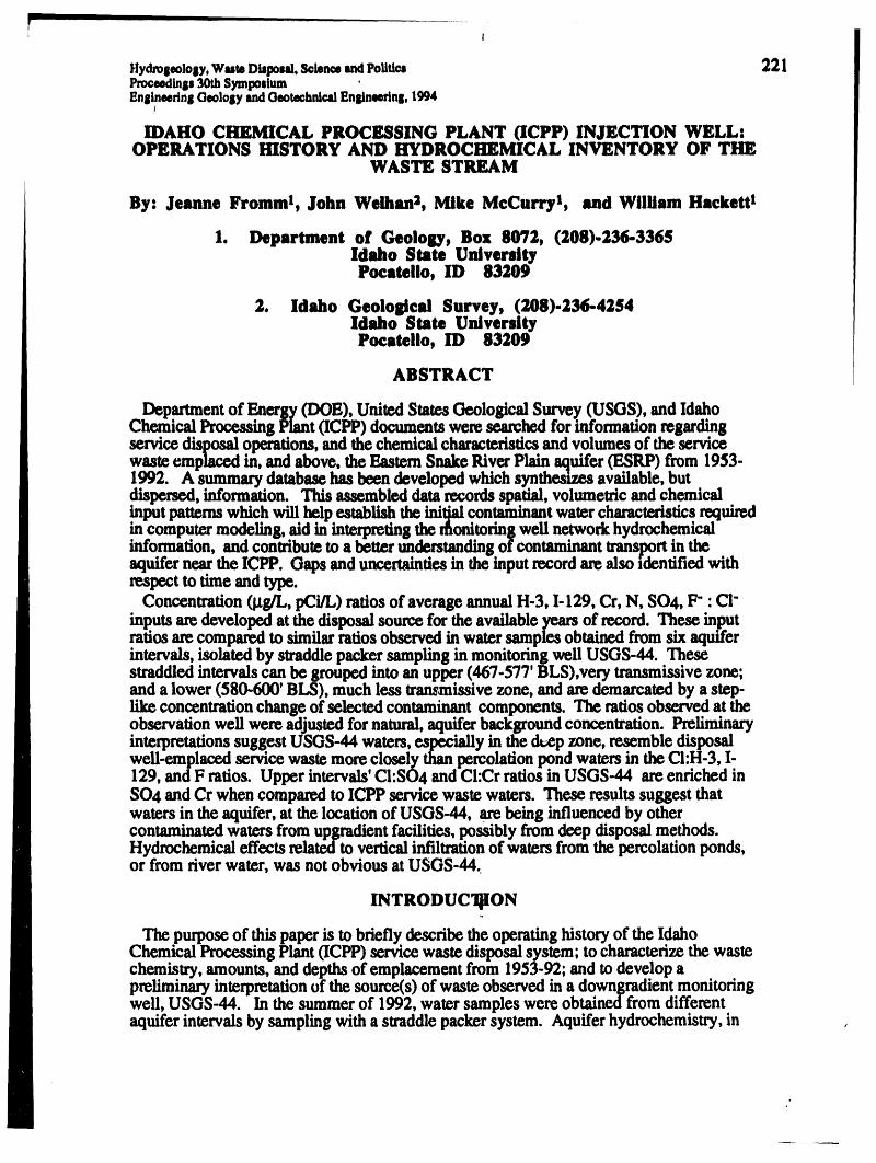
I
Hydrolmloly,WuteDisposal,ScienceandPolitics 221Proceedings30thSymposiumBnsineerinsGeologyandOeotechnlcslEnldneerin|,1994
/
IDAHO CHEMICAL PROCESSING PLANT (ICPP) INJECTION WELL:OPERATIONS HISTORY AND HYDROCHEMICAL INVENTORY OF THE
WASTE STREAM
By: Jeanne Fromm 1, John Welhan 2, Mike MeCurry z, and William Hackettl
1. Department of Geology, Box 8072, (208).236-3365Idaho State UniversityPocatello, ID 83209
2. Idaho Geological Survey, (208)-236-4254Idaho State UniversityPocateilo, ID 83209
ABSTRACT
Departmentof Energy (DOE), United States Geological S_.y CUSGS), and id._.oChemical Processing Plant (ICPP) documents were searched for information regardingservice disposal operations, and the chemical characteristi.cs,and volumes of the servicewaste emplaced in, and above, the EasternSnake River Plain aquifer (ESRP) from 1953-1992. A summary database has been developed which synthesizes available, butdispersed, information. This assembled datarecords spatial, volumetric and chemical.input patternswhich will help establish the initj/tlcon_ant water characteristicsreqmred
computer modeling, aid in interpreting the rfionitormgwell network hydrochemlcalinformation, and contribute to a betterunderstandingof contaminant transportin the .aquifer near the ICPP. Gaps and uncertainties in the input record are also identified withrespect to time and type.
Concentration (ttg_, pCi/L) ratios of average annual H-3, I-129, Cr, N, SO4, F- : CI"inputs are developed at the disposal source for the available years of record. These inputratios are compared to similar ratios observed in water samples obtained from six aquiferintervals, isolated by straddle packer sampling in monitoring well USGS-44. Thesestraddled intervals can be grouped into an upper (467-577' BLS),very transmissive zone;and a lower (580-600' BLS), much less wansmissive zone, and are demarcated by a step-like concentration change of selected contaminant components. The ratios observed at theobservation well were adjusted for natural, aquifer b.ackgroundconcentration. Prefiminaryinterpretations suggest USGS-44 waters, especially m the dvep zone, resemble dis_posalwell-emplaced service waste more closely than percolation pond waters in the CI.H-3, I129, and F ratios. Upper intervals' C1:SO4 and CI:Cr ratios in USGS-44 are enriched mSO4 and Cr when compared to ICPP service waste waters. These results suggest thatwaters in the aquifer, at the location of USGS-44, are being influenced by othercontaminated waters from upgradient facilities, possibly from deep disposal methods.Hydrochemical effects related to vertical infiltration of waters from the percolation ponds,or from river water, was not obvious at USGS-44.
INTRODUC'I]ION
The purpose of this paper is to briefly describe the operating history of the IdahoChemical Processing Plant (ICPP) service waste disposal system; to characterize the wastechemistry, amounts, and depths of emplacement from 1953-92; and to develop apreliminaryinterpretationof the source(s) of waste observed in a down_radient monitoringwell, USGS-44. In the summer of 1992, water samples were obtainedfrom differentaquifer intervals by sampling with a straddle packer system. Aquifer hydrochemistry, in
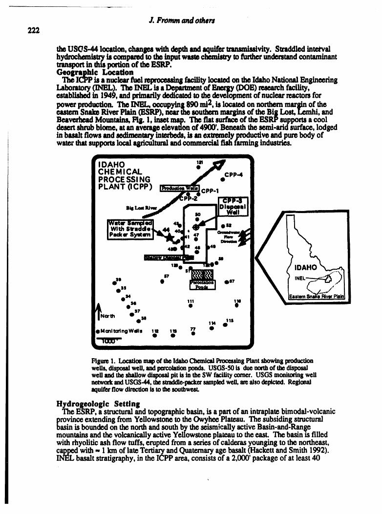
J. Frommando_,rs222
the USOS-44 location,changeswithdepthandaquifertransm_vity. Straddledintervalhydrochemistryis ¢om_ to the inputwastec_ tofurtherunderstandcontaminant
in thisportionof theESRP.Geographic Location
The ICPPis a nuclearfuel rewoomd_ facilitylocatedonthe IdahoNationalEngineeringLaboratory(INBL). The _h aDe_ meritof _ (Ix)E) researchfacility,establtsl_ in 1949,and_y dedicatedto thedevelopmentof nuclearreactorsforpowerproduction.TheINBL, (¢cupying890 mt2, is locatedon northernmarl_ of theeasternSnakeRiverPlain(ESRP),nearthesou_ marginsof the Big Lost,Izmhi, andBea_ Mountains,Pill. 1, insetmap. The flat surfaceof theESRPsupportsa cool
shrubbiome, at an averalteelevation of 4900'. Beneaththe semi-aridSurface,lodgedin basaltflows and __ interbeds,is an extremelyproductiveand purebody ofwaterthatsupportslocal agriculturalandcommercialfishfarmingindustries.
CHEII_DAHO""""""RocEMICALssING' I ,1,, _:PP4 ....... ILANT OCPP)_c,,-_
I ..1 -I [_ it. ! .,,
i Pa_er Syetm'l _-_. ,! , .,,,,._...r_i "-'- F%p, , ,,..,,._i 4m ¢ m t
i = ,,
i taSoo" o"
i_N ese •
ose==T 1isa.th
lt4 •
•III II IIIII II
Rll=re1. Locationmapof theIdahoChemicalPrate,in8Plantshowingproductionwells,disposalwen,andpercolationponds.USOS-50is duenorthofthedispo_wellandtheshallowdisposalpitis intheSWfacilitycorner.USGSmonitoringwellnetwogkandUSGS-44.thestraddle-peckersampledwell,arealsodepicted.ReBionalaquiferflowdirectionis tothesouthwest.
Hydrogeologlc Setting ....The ESRP,a structuralandtopographicbasm,ts a partof an intraplatebtmodal-volcanic
provinceextendingfromYellowstoneto the OwyheePlateau.The subsidingstructuralbasin is boundedon thenorthandsouthby theseismicallyactiveBasin-and-RangemountainsandthevolcanicallyactiveYellowstoneplateauto theeast. Thebasinis filledwithrhyoliticash flow tufts, eruptedfroma seriesof calderasyounging to the northeast,cappedwith - 1 kmof late TertiaryandQuatern,aryage basalt(Hackettand Smith 1992).1NELbasaltstratigraphy,in the ICPParea,conststsof a 2,000' packageof at least40
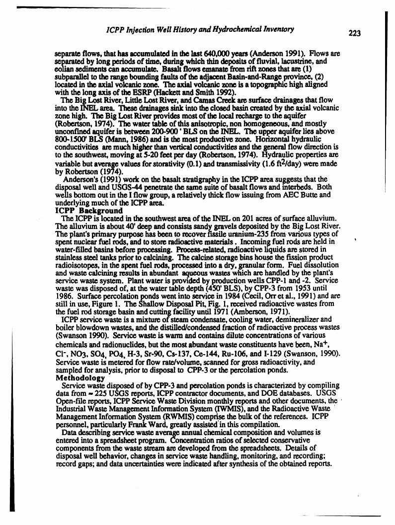
ICPP InjectionWellHistoryandHydrochemicalInventory 223
separate flows, that has accumulated in the last 640,000 years (Anderson 1991). Flows areseparated by long periods of time, during which thin deposits of fluvial, lacustrine, andeolian sediments can accumulate. Basalt flows emanate from rift zones that are (1)subparallel to the range bounding faults of the _jacent Basin-and-Range province, (2)located in the axial volcanic zone. The axial volcanic zone is a topographichigh alignedwith the long _ of the ESRP (Hackett and Smith 1992).
The Big Lost River, Little Lost River, andCamas Creek are surface dmina_..s.that flowinto the INEL area. _ drainages sink into the closed basin created by the axtal volcaniczone high. The Big Lost River provides most of the local recharge to the aquifer(Robertson, 1974). The water table of this anisotropsc, non homogeneous, and mostlyunconfined aquifer is between 200-900 ' BLS on the INEL. The up.peraquifer lies above800-1500' BLS (Mann, 1986) and is the most productive zone. Horizontal hydraulic
conductivities are much hiatgherthan vertical conductivities and the general .flow direction isto the southwest, moving 5-20 feet per day (Rohertson, 1974.). Hydraulic properties arevariable but average values for storativity (0.1) and transmissiwty (1.6 ftZ/day) were madeby Robenson (1974).
Anderson's (1991) work on the basalt stratigraphy in the ICPP area su_ggeststhat thedisposal well and USGS-44 penetrate the same suite of basalt flows and mterbeds. Bothwells bottom out in the I flow group, a relatively thick flow issmng from AEC Butte andunderlying much of the ICPP area.ICPP Background
The ICPP is located in the southwest areaof the INEL on 201 acres of surface alluvium.
The alluvium .is about 40' deep and consists sandy gravels deposited by the Big Lost River.The plant's prtmarypurpose has been to recover fissile uranium-235 from various types ofspent nuc_..arfuel rods, and to store radioacuve materials. Incoming fuel rods are held in 'water-filled basins before p_g. Ih'ocess-related, radio.activeliquids are stored instainless steel _ priorto calcining. The calcine storage bins house the fission productradioisotopes, m the spent fuel rods, proc_ into a dry, granular form. Fuel dissolutionand waste calcining results in abundant aqueous wastes which are handled by the plant'sservice waste system. Plant water m provided by production wells CPP-I and -2. Servicewaste was disposed of, at the water table depth (450' BLS), by CPP-3 from 1953 until1986. Surface percolation ponds went into service in 1984 (Cecil, Orret al., 1991) and arestill in use, Figure 1. The Shallow Disposal Pit, Fig. 1, received radioactive wastes fromthe fuel rod storage basin and cutting facility until 1971 (Amberson, 1971).
ICPP service waste is a mixture of steam condensate, cooling water, demineralizer andboiler blowdown wastes, and the distilled/condensed fraction of radioactive process wastes(Swanson 1990). Service waste is warm andcontains dilute concentrations of variouschemicals andradionuclides, but the most abundant waste constituents have been, Na+,
CI-, NO3, SO4, PO4, H-3, Sr-90, Cs-137, Ce-144, Ru-106, and I-129 (Swanson, 1990).Service waste is metered for flow rate/volume, scanned for gross radioactivity, andsampled for analysis, prior to disposal to CPP-3 or the percolation ponds.Methodology
Service waste disposed of by CPP-3 and percolation ponds is characterized by compilingdata from 225 USGS reports, ICPP contractor documents, and DOE databases. USGSOpen-file reports, ICPP Service Waste Division monthly reports and other documents, theIndustrial Waste Management Information System (1WMIS), and the Radioactive WasteManagement Information System (RWMIS) comprise the bulk of the references. ICPPpersonnel, particularly FrankWard, greatly assisted'in this compilation.
Data describing service waste average annualchemical composition and volumes isentered into a spreadsheet program. Concentration ratios of selected conservativecomponents from the waste stream are developed from the spreadsheets. Details ofdisposal well behavior, changes in service waste handling, monitoring, and recording;record gaps; and data uncertainties were indicated after synthesis of the obtained reports.

J. Fromm and others224
The autho.rs were members of the reae,arch team thatvertically sampled the waters ofUSGS-44 gath a straddle packer sy.s_m. A wd'.ttenrel_..rtof this work is in.the reviewstages and contains the hydrochemlcal information used m this report. Specificmethodologies (Johnson, Olsen et al. 1993) and some results (McCurry, Estes et ai. 1993)are presented at this meeting.
SERVICE WASTE DISPOSAL TIMELINE
This section isa brief chronological presentation of CPP-3's operating history and thoseevents at the ICPP that influenced the chemical nature and/or volumes of service wastereleased to CPP-3. It includes the documented, atypical releases to the well, planned ICPP
eerO_mgchanges,and modifications to service waste monitoring methods andrecord
1951 Disposal well, CPP-3, is in_stalledand completed.1953 ICPP begins operation and CPP-3 is disposing plant service waste. Waste
is monitored for gross _ activity and discharge volume (King, 1956).1956 There are several perched water bodies in the vadose zone below the ICPP
and they are encountered during monitoring well installation (Robertson,Schoen et al., 1974) in late 1950's and early 1960's.
1958 Largestannualtritiumrelease(3,504Ci)inthisyear1967;(MannandCecil1990).Plantprocesschamgesreleaseless1-131andmorelong-livedisotopes to service waste. Fluorescein dye and salt slug tracer test at CPP-3.29Ciaccidentallyreleasedandregistersinmonitoringwells(Schmalz,1959).Saltandgrossbetaactivityplumesmai_pedforICPP.
1959 Firstinstanceoffissionproducts(Ru-106)inICPPproductionwellwater(Horan and Others 1960). Line to CPP-3 has disintegrated and is replaced(Ayers and Bum 1960). Second largest annual H-3 release in this year(2,565 Ci) (Mann and Cecil 1990).
1960 Tritium is discovered in ICPP service waste (Hawkins and Schmalz, 1965).Na+ concentration map of aquifer around ICPP contoured (Horan andOthers 1960)
1961 Monitoring service waste for H-3 begins (Barraclough, Teasdale et al.,1967). 209 Ci released in Dex_mber (Horan and Others 1962). Tritium(Horan and Others, 1962) and Na + (Jones, 1961) isoconcentration linesdrawn around ICPP. ,
1962 More activity released to ICPP disposal pit than CPP-3 (Robertson, Schoenet al., 1974). Tritium plume mapped.
1963 Clinoptilofite ion exchange column installed at ICPP to remove cationicradioisotopes (Sr-90, Cs-137, Ce-144) (Robertson, Schocn et al., 1974).Large tritium release in June (Barraclough, Teasdale et al., 1967). Tritiumplume mapped.
1965 Tritium plume mapped (Barraclough, Teasdale et al., 1967).1967 High levels of H-3 andCI- in ICPP production wells (Hawkins, 1968).
CPP-3 fails in this year or 1968 (Robertson, Schoen et al., 1974). 20%error in volume estimates (Schmalz, 1968).
1968 Waterlevels,andtritiumconcentrations,inUSGS-50 riseabruptly(Hawkins,1968).
1969 19 Ci tritiuminadvertently released to CPP-3 in September.1970 New ion exchange column (Amberlite-200 resin) installed at ICPP to
remove cationic radioisotopes (Amberson, 1970). CPP-3 is found tohave collapsed and filled to 225' BLS (Gildersleeve, 1971). Well repairbegins.
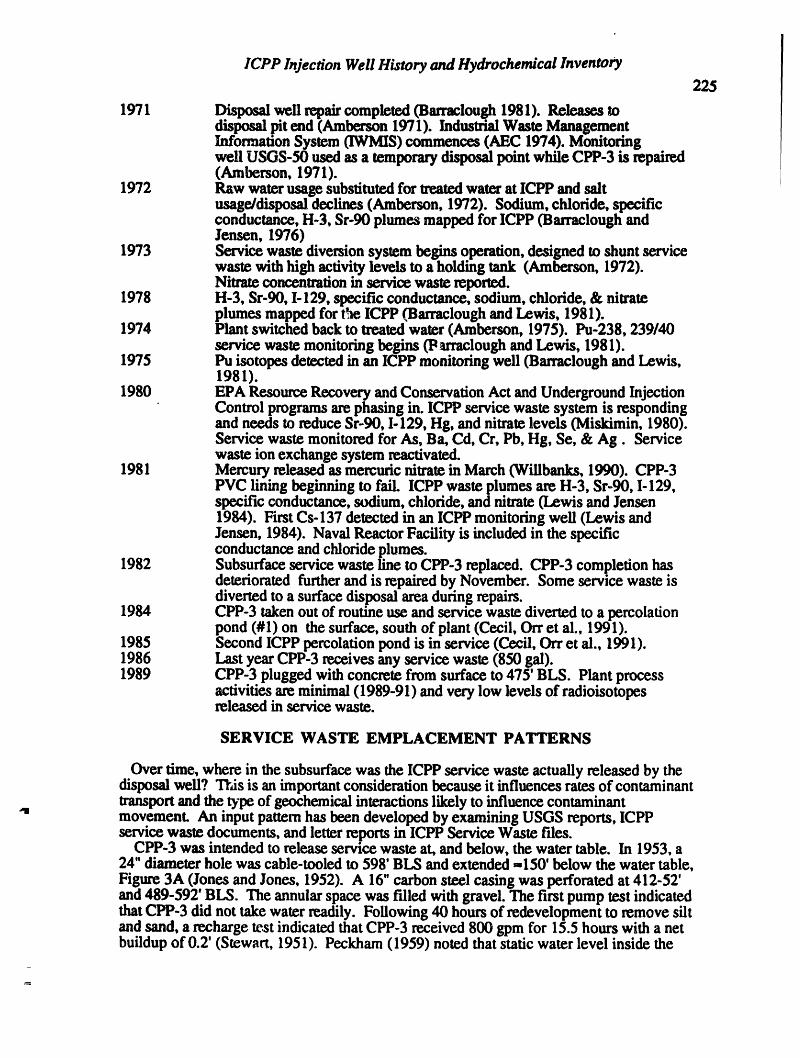
ICPP Injection Well History and Hydrochemical Inventory225
1971 Disposal well repaircompleted (Banaclough 1981). Releases todisposal pit end (Amberson 1971). IndustrialWaste ManagementInformation System (IWMIS)commences (AEC 1974). Monitoringwell USGS-50 used as a temporary disposal point while CPP-3 is repaired(Amberson, 1971).
1972 Raw water usage substituted for treatedwater at ICPP and saltusage/disposal declines (Amberson, 1972). Sodium, chloride, specificconductance, H-3, St-90 plumes mapped for ICPP (Barraclough andJensen, 1976)
1973 Service waste diversion system begins operation, designed to shunt servicewaste with high activity levels to a holding tank (Amberson, 1972).Nitrate concentrationin service waste reported.
1978 H-3, Sr-90, I-129, specific conductance, sodium, chloride, & nitrateplumes mapped for the ICPP (Barraclough and Lewis, 1981).
1974 Plant switched back to treated water (Amberson, 1975). Pu-238, 239/40service waste monitoring begins (P_raclough and Lewis, 1981).
1975 Pu isotopes detected in an ICPP monitoring well (Barraclough and Lewis,1981).
1980 EPA Resource Recovery andConservation Act andUnderground InjectionControl programs are phasing in. ICPP service waste system is respondingand needs to reduce Sr-90,1-129, Hg, and nitrate levels (Miskimin, 1980).Service waste monitored for As, Ba, Cd, Cr, Pb, Hg, Se, & Ag. Servicewaste ion exchange system reactivated.
1981 Mercury released as mercuric nitrate in March (Willbanks, 1990). CPP-3PVC lining beginning to faiL ICPP waste plumes are H-3, Sr-90, I-129,specific conductance, sodium, chloride, and nitrate(Lewis and Jensen1984). Ftrst Cs-137 detected in an ICPP monitoring well (Lewis andJensen, 1984). Naval Reactor Facility is included in the specificconductance and chloride plumes.
1982 Subsurface service waste line to CPP-3 replaced. CPP-3 completion hasdeteriorated furtherand is repaired by November. Some service waste isdiverted to a surface disposal area during repairs.
1984 CPP-3 taken out of routine use and service waste diverted to a percolationpond (# 1) on the surface, south of plant (Cecil, On"et al., 1991).
1985 Second ICPP percolation pond is in service (Cecil, Orr et al., 1991).1986 Last year CPP-3 receives any service waste (850 gai).1989 CPP-3 plugged with concrete from surface to 475' BLS. Plant process
activities are minimal (1989-91) and very low levels of radioisotopesreleased in service waste.
SERVICE WASTE EMPLACEMENT PATTERNS
Over time, where in the subsurface was the ICPP service waste actually released by thedisposal well? Tl-,isis an importantconsideration because it influences rates of contaminanttransportand the t_e of geochemical interactions likely to influence contaminantmovement. An input patternhas been developed by examining USGS reports, ICPPservice waste documents, and letter reports in ICPP Service Waste files.
CPP-3 was intended to release service waste at, and below, the water table. In 1953, a24" diameter hole was cable-tooled to 598' BLS and extended _150' below the water table,Figure 3A (Jones and Jones, 1952). A 16" carbon steel casing was perforated at 412-52'and 489-592' BLS. The annular space was filled with gravel. The first pump test indicatedthatCPP-3 did not take water readily. Following 40 hoursof redevelopment to remove siltand sand, a recharge test indicated that CPP-3 received 800 gpm for 15.5 hours with a netbuildup of 0.2' (Stewart, 1951). Peckham (1959) noted that static water level inside the

.I. Fromm and others

ICPP Injection Well History and Hydrochemical Inventory
227well was 18' above the water table but the elevation of the recharge mound outside the wellwas 0.6 feet. Water level mea._,lrementswere made by the USGS until 1959 and occurredmostly at 450', but levels inc_ to 419' in 1959.
The first failure of CPP-3 was I_ in 1970 when the well was found to be filled to225' BLS (Gildersleeve, 1971), and had a water level that fluctuated between 204-156'BLS. The well received water up to, and after, the failure was discovered. Workersestimated thatCPP-3's steel casing had a service life of only 3-5 years because of the salty,aerated characteristics of service waste. The casing slowly dissolved away, developingnumerous water table and vadose zone "perforations",which allowed the gravel pack todrain from the annular space into the well bore and slowly filled the borehole up. Sometimein 1967-8, the casing became so eroded that a discrete break occurred and the well rapidlyfdled to the 225' level. A large perched water body was created by this event and
eventually contaminated the production wells, CPP-1 and -2, with H-3 and CI-. 12"The f'u,st repair of CPP-3, Fig. 3C, was a long and frustrating affair. In 1971, a steelcasing was finally in place and lined with 10" PVC pipe. USGS-50 disposed of servicewaste for about one month while well repairs were made and this practice maintained theperched water body created by disposal well failure.
When the well completion began to disintegrate a second time, in 1981, a flow meter waslowered through the borehole until it met an obstruction, or the fill level, at 534' BLS(Barraclough, 1982). The log indicated that most of the waste was leaving the well at 472-505'BLS. Once again, the well had continued to dispose of the service waste influx as its
casings and linings deteriorated. The well configuration, after0'thel-second repairWasl2,,finished in 1982, was similar to the first repair completion- a PVC liner inside asteel casing, except that the finer was perforated to a shallower depth, Fig. 3E. Atemporary surface disposal area, to the east of the well, received = 7 million gallons ofservice waste while well is repaired.
By 1985, most service waste was released to the percolation ponds. Pump testsperformed in 1986 indicated that the CPP-3's specific capacity declined to the values it hadbefore redevelopment (Ackerman, 1991). When the well is plugged with concrete, in1989, it was noted that the borehole has silted in to 475' BLS.
Observations and tests suggest that CPP-3 emplaced service waste at approximately the450-505' BLS for most of its service life. Intervals of vadose zone emplacement occurredin 19677-71, and 1982. Surface release commenced in 1984. Releases to the shallowdisposal pit, Fig. 1, were a source of vadose zone water and contaminants until 1971. The24" Lineto CPP-3 was occasionally a source of shallow leaks and contaminants, and it wasreplaced twice during the 1953-84 period. While the disposal well was operating, basaltflow groups DE7, DE8, F, EF, E, FG, and possibly the top of I group received themajority of ICPP service waste. The I flow received less waste over time because the wellfailures tended to block the bottom portions of the well, and the well perforation zonebecame shallower with time.
DISPOSAL VOLUMES
King (1956) gives a description of the ICPP system that (1) measures service wastevolume, (2) monitors flow-by activity level, and (3) obtains aliquot samples for subsequentchemical analysis. This system is in place when the plant begins to operate in 1954.Production well flow meters are installed in 1959 (Robertson, Schoen et el., 1974). Therecord, Figure 3, indicates that total service waste volume, disposed of by,CPP-3 over itsoperating life, is 10,623,470,765 gallons, for an average of 331,981,904 gallons per year.Disposal rates ranged from 356 to 1,135 gpm and averaged 632 gpm. These volumevalues must be qualified, however. Their accuracies are at least + 10%, could be :!:30%,and are commonly treated as 4-15%. Percolation pond annual releases are similar todisposal well releases.

228 J.Vromm andothers
i iiiiirlll
Annual Service Waste Volumes
600,000,000 .v-l-v-rT_'V"rv-t-c-rv-l-r"rv_-¢"rv_-v-r• _'v"r, _.-,-r,II I l I II I l i l500,000,000'I-I-,-Fl-l-,-_I-I-,-FI-I-,-tI-I-,-_I-I-,-_I-E-:_,-_{
0 0 0 m I., 0 o a m.II J
400,000,000:llt,._'-l.!-l-,-l-14-_,,.l-l-,l-t-l-..-__.l.-l-,,,_,_I-_I-,-_I300,000,000. -,, " • ,-, --=,,u _, , ,_-,_5-n_-Fj_,]-FI_,,,_,_-rIt_,-FI_-',-___I:-F_
T3 200,000,000..'..P.t.'.A.J.It,'t.,.J.LAJ.t.LAS.t._AJ.'.LA.P.'.LtJ.V.L_l ll ll llW#l ll ll II ll II II II II II II II II
I I I I I I I I 0 1 1 1 1 1 1 I I I I I I I I I I I_I I
0 aa,,,_ ................... ,,,,,'
Year
i
Rgure 3: AnnualtotalsofICI_servicewastesentto CPP-3
SERVICE WASTE CHEMICAL COMPONENT RECORD
The identity and amounts of the anthropogenic components in the service waste stream
were determined by analysis of the composite sample. Gross [_and y were analyzed dailyand the composite sample was analyzed monthly. Total mass additions are determined bymultiplying concentration values with measured service waste volume. The uncertaintyassociated with the volume measurements will also influence the amounts of mass addition.Records of monthly salt, sulfuric acid, and other chemicals usage have been kept byvarious ICPP divisions from 1954 to present, but the record is incomplete. Tables 2 and 3
• illustrate the type of chemical input records available for the radioactive and nonradioactivecomponents of serd_ waste. The record becomes more complete with time andisexpanded dramatically with the advent of the Resource Conservation and Recovery Act in1980. Anthropogenic additions to the service waste stream occur as pulses of varyingfrequency and magnitude. Tritium, which accounts for - 95% of the radioisotopes in theICPP aqueous wastes, is not monitored until 1961. Annual tritium additions have beenestimated for the pre-1961 period by calculations based upon kilograms of fuel rod uraniumprocessed.
USGS-44 HYDROCHEMICAL ZONES
Figure 4 shows the concentration of selected analytes in water samples obtained fromstraddled intervals in USGS-44. Sampling intervals were chosen because they wereregions of active borehole flow. These intervals were isolated with inflatable packers andsampledafterpurgingthestandingboreholewaterwithintheisolatedinterval. Theintervalsabove577'werelocatedinverytransmissive,activelyflowingpartsoftheaquifer.TheseupperstraddledintervalsoccurredinflowgroupsE-H,andthetopoftheIgroup.The 580-600'intervalwas locatedintheleasttransmissiveportionoftheaquifersampledandoccursintheIflowgroup.ThedeepestsampledintervalcontainswaterwiththehighestcodcentrationlevelsofH_3,1-129,NO3" + NO2" asN,andCI-.F-,SO4,andCrshowmoreuniformconcentration-with-depthbehavior,butCrconcentrationsare2-2.5timesbackgroundconcentrationthroughout.SiO2,Mg, Na,andK arenotshown,buttheir concentrations are also highest in the 580-600' interval. Sr-90, and Ca concentrationsare highest in the 467-82' interval.


ICPP Injection Well: Operations History and Hydrochemical Inventory 231
'=== " ' ' II I IIIIII I IIIII III I III II Ill I I IIII I II I J l I II II I
S,raddled Ch_/_de Fl#_de S_ Chromium N Tritium 1-129Interval pg/L pg/L pCi/L pCi/L _'
'",,"ii:"'' ",',, ,,!--"t.t.,,
::A - Jll _l .k.,.495-515 -,i4 -', +4 ,., " " ::, ,I, , , :i ' ' Ii'''' '' '
il l| I l II i _s i I s iI* ' i' 'I ' ' '
, I l :I I I I I I' * , !l- JilJ .4-- Jlli -i- - J - i ,!_19-53_II,-!i-_,-,+-I,_ _,,,, i ,ill,,' --r--i "-
li , ' i, 'I ' I 'lli ' ' ' 'ii , ' :!' 'I' I 'II_' ' ' '' _, ,i, I ,II_, o ,
I , i i i I i I qlli i i:;I[ , , ;' '.If' ' '--- 4-- .#i!-_-- J
''ll, ,,i ' ' !:* ' I ' I 'II! * ' ' '_i ' ' "_'"' I ',I'_'' ' ' II.!!
' I 'ilil'' , , i, ,!i' I:_' 'I ' I '!fi' ' ' l:i " " _' 'I ' ,!!_ , ' '
580-600 "":_""'" -" !_ ,_,-_,- _., ....
.,........,,............Background ConcentrationI II I I II I I IIIII I
Figure 4. Diagram of concentration values from the USGS-44 swaddled intervals for selected analytes.Depth, in feet, of the straddled interval is given on the left and basalt flow group designations are indicatedon me right of figure. Background concentration zone shown with stippled band.
The waters from the tight interval in the I group (580-600') have a contaminant signaturethat is different from the more transmissive portions of the aquifer. The lowest straddledinterval contains higher concentrations of anthropogenic additions to the aquifer, except forCr and SO4. These waters may be remnant from a previous time interval when the entireupper aquifer had similar contaminant chemistry derived from a common source. Theactive zones may have been flushed of contaminants preferentially over the less permeablezone. Alternatively, the waterin the tight I flow may have received contaminants from acontaminant source other than CPP-3.
The analytes selected for inclusion in Figure 4 will be compared to CI-, on aconcentration basis. These components, except for Cr, were selected because they areanionic, elevated with respect to natural background concentration at some well interval,and are known components of the ICPP service waste stream.
COMPARISON OF CONSERVATIVE COMPONENT RATIOS IN USGS-44 INTERVALS AND ICPP SERVICE WASTE STREAM
The ICPP disposal well and/or percolation pond historically has always been consideredto be the primarysource of the contaminant chemistry in USGS-44. When USGS-44 wasinstalled in 1957, it was expected to be a sensitive indicator of aquifer contaminant levels.It was placed directly downgradient of USGS-40, a well that contained high concentrationsof anthropogenic chemicals and responded quickly to inadvertent releases of highcontaminant levels to the service waste system. Historically, USGS-44 does show the

_t
J.Fronun and others
232
-___nent _
__........... Chll'3 CId429 ! Cl:80i cliN['cl_- ci:cr
1959
I_0...... , , ,._
1961
1962 3 I0,169
_963 ! 6_89.1964 .1 |.0_2i_s 14 is,o89
.......!966. 4 1.1,437 _ ..........1967 1 9,842........ ,.......... -
1968 2 10,549
.... 1969 6 = 10,8911970 14 15,354
1971 13 12,127 7.3 24,679....
19_2 2 lO,ZT7_ 6.5 ..... _2o,__93_!1973 7 4,041 2.3 7 8,2241974 1 8,485 3.6 U l l 17,267.............. = .......
1975 13 11,069 7.9 35 22,5251976 16 31,967 34 27,W/3
-- 1977 1 12,352. 5.8 14 __ 25,1______' i978 ' 2 2,360 4.8 II 33,621
!,979 2 7,.505 5.3 9 27,1861980 6 .. 2!,721 ' 5.7 11 ..........7,4151981 3 14,127 6.8 19 211 20,820I_ 3 20,028 4. ! 12 246 ! 6,705
1983 ..... I .._ 8,441 135 14,6841984 42 4.0 16 267
_,.,u;iv, 7 t2a37 s_ 17 2ts 26,sso__ II ...... II
1985 1 2.7 15 3351986 ' 3 8.7 " 23 547 _
1987 3 67,837 4.5 40 4.27 32,738
IS_8 8 4.3 _-3-6--[-___-9_-ii_i._i-_-__-----_i.-_1989 1102 3.8 57 271
1990 1476 261,990 ,-....7.5___ 1,315
"_ 1991 -267 261,,350 9.9 i 111 1_6_33....'",,,',p_u,_,4e9 ,,,t97_9 6 I_o 7_ 3_,738
USGS:44 I _ J ......' Straddled Intervalsand Background Ratios
........................F-=:-:---_-:=_L_:L---:___...........r:.........
Intervals _ t t-467-82, 8 43,478 .......1:4 ......__ 71_ i.....i'i'I_i.2,__1
495-515 18= 37,735 1.5 [ [ / 2,540
ss_-w 39 78.78__ 2.0 48._-_x.-_-3.o30Upper ZoueAve 21 49176 2 b'7 [.292 . 2825
_.6oo 2 ,8.04, s.o i ,s !,781 s.'_I ! _I
B_.d ...._ o.5 I I _oI 4.,_

ICPP Injection Well: Operations History and Hydrochemical Inventory233
effects of waste USGS-40disposal'but.it has been relatively "clean', in spite of its proximity to thedisposal well and
at thefuncti6n disposal point and the contaminant concentrationsm the sam led sis inUSOS-44, ratios of conservative components were developed for the stradSed intervals inUSGS-44 and service waste over time. _ two sets of ratios arecompared for similar,or disparate pattm_ and the ratio values are listed in T..able5.
The concentration ratios in the monitoring well are adjustedfor background (pre-an,thmpopenic) concentrations in the aquifer. Background aquifer hydrochemlstry isestimated, Table 1, by comp..m'mg"values reported from several sources. The ICPP
production (CPP-1, -2) and¢iC_pSalwells were sampled after completion anddevelopment, but before the . facility began to operate. These common ion analysesare listed in reportsby the Umted States Geological Survey (USGS) (Nace, Jones et al.,1951) (Bagby, White et SI., 1985). In addition, raw water analyses, from five yearsduring the late 1960s and early 1970s, and taken from CPP-I and-2, are also available.Background values for radioisotopes and trace metals are taken from recent USGS reports(Orr,CeciletSI.,1991)(Knobel,On"etel.,1992).
The set of ratios for conservative components in the service waste are based on annualaverage concentration values recorded in waste monitoring records. The effect of an annualavera_, will be to "smooth"the considerable monthly variability in the input function,especially for the radioisotopic components. What is observed, at a point in time, in theUSGS-44 straddled intervals may be the pulsed, not the averaged, signal from the disposalsource. The annual tritiumconcentrations have been reducedfrom their initial input levelsto "decayed" 1992 concentrations, because tritium has a short half-life (12.3 years). TheH-3 and 1-129: CI ratios are in pCi/L:_tg/L units. The blank positions in the USGS-44interval ratios table are the result of negative values in the N and F- concentrations afterbackground concentrations are subtracted. Background concentration values are higherthan measured concentrations in these intervals.
Table 5 shows that there is a great deal of variability in the inputconcentration ratios andthere are significant gaps in the service waste record. For purposes of comparison, thecomponent ratios for service waste disposed of to the well and the percolation ponds havebeen grouped and averaged. Grouping and averaging has been performed on themonitoring well component ratios also- the lower, tight interval (580-6003 is separatedfrom the more transmissive, upper (>5779 intervals. These averages are plotted in Figure5. The larger the ratio values, the more enriched the service waste stream is in H-3, I-129,N, SO4, F, and Cr components.
Preliminary interpretations of this approach suggest thatCI:H-3, I-129, F and N ratios,in USGS-44 lower interval water, most closely resemble disposal well water (<1984). CI:H-3,1-129, and F ratios from upper interval waters in USGS-44 plot closer to servicewaste disposal well ratiosthan percolation pond ratios,butthey are more intermediary thanthe deep zone waters. The N:CI ratio in USGS-44 upper intervals is similar to the servicewaste percolation pond ratio. The monitoring well CI:Crratio does not resemble the CI:Crratio in the ICPP service waste, from either th_ disposal well or pond disposal periods.C1:SO4 ratios for service waste are higher than the ratios calculated for USGS-44. Fconcentrations in theupper three intervals in USGS-44 are close to background inconcentration. Nitrogen concentrations are also close to background in two intervals fromthe upper, permeable intervals in USGS-44.
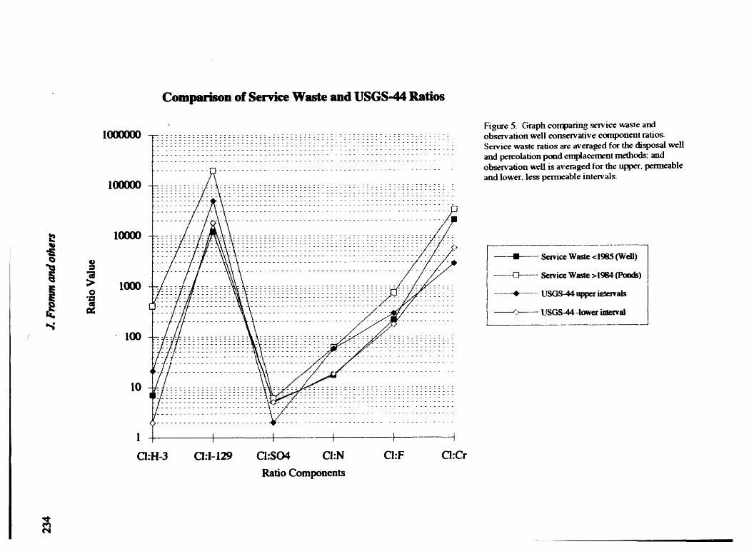
Comparison of Service Waste and USGS-44 Ratios
I0
1 l I _ ) )
ChH-3 CI:I-129 C1:SO4 CI:N ChF ChCr
Ratio Components
,q.¢q

I
ICPP Injection Well History and Hydrochendcal Invenm_ 235
CONCLUSIONS
The ICPP hm added anthropogenic chemicals to a complex, mt_otropic, nonhomogenom aquifer in a manner that has chimged over time in many rmpecm. Plant
" processes affect thechemical conmu of service waste and radtotsotoptcreleases varyconsiderably in concentration, and content, overlime.Method of service wute disposalhm changed from mosdy watertabletopercolationpond releases..I_.posalwelldisintegration and lineJvalve leaks have crea_d perched water bodies m the vicinity of thedispo_ well.ICPPservicewasterecordscontaindataonvolumesreleasedandchemicalcontentbuttheyarein.completeandofuncertainaccuracyoversomeofthetimeintervals.Local, preanthropogemcaquiferwaterchemistry can be estimatedfortheICPP areafromvarioussources.
Straddlepackersamplingtechniqueswereappliedtoanearbymonitoringwell:USGS-44, in the summer of 1992, to characterize the aquifer hydroche.n_try. Aquifer mhydroc,heroically stratified with respect to depth. Le_ transmissive and/or deeper zonescontain higher concentrations of certain contaminants (H-3, I-129, N, F, Cl, Na). Thereare interesting exceptions to this trend(Cr, SO4, St-90). Ratios of conservativecomponents observed in the observation well andin the ICPP service waste stream.,werecalculated and compared. These ratios were adjusted for natural,background aquiferconcentration. Preliminary interpretations suggest USGS-44 waters, especially .inthe deepzone, resemble disposal well-emplaced service waste more closely than percolatmn pondwaters in the ChH-3,1-129, and F ratios. The upper intervals' ChSO4 and ChCr ratios inUSGS-44 are enriched in SO4 and Crwhen compared to ICPP service waste waters.These results suggest thatwaters in the aquifer, at the location of USGS-44, are beinginfluenced by waters containing Cr andSO4, perhapsfrom upgrad.ientfacilities, orpossibly from deep disposal methods. Based on the same comparison of componentratios, hydrochenucal effects related to.vertical infiltration of waters from the percolationponds, or from river water, cannot be Identified in USGS-44.
236 L Fromm and o_ers
Acknowledgments:
This work has been supported by the DOE-EPSCoR progrmn and the State of Idaho INELOversight ManagementProsr_. Idaho Chemical Processing Plant documents anddatabases wereprovided by FrankWard, LeRoy LewtJ, and Tim McKenna. Theirtechnicalexperuseandcooperationhave contributedimmensely to this work. Dr. BillHackeu and Dr. Dick Smith have served as DOE-_SCoR mentors. Steve Anderson andLarryMann, USGS, have helped with basalt stratigraphy and supplied practical,comprehensive knowledge about the INEL and the ESRP aquifer.
REFERENCES
Ackerman, D. J. (1991). Tmnmfl,mivity of the Sn_a_eRiver Plain Aquifer at the IdahoNational Engineering Laboratory,Idaho. Uni.ted States Geological Survey. 35.
AEC (1974). NRTS Waste Management Informauon System.Aton_cEnergyCommission.
Amberson, C. B. (1970). CPP Production Monthly Report. ICPP.Amberson, C. B. (1971). ICPP Operations Branch Monthly Report. ICPP.Amberson, C. B. (1972). ICP Operations Branch Monthly Report. ICPP.Amberson, C. B. (1975). ICPP Production Monthly Report. ICPP.Anderson, S. R. (199.1). Stratigraphy of the Unsaturated Zone and Uppermost Part of the
Snake River Plain Aquifer at the Idaho Chemical Processing Plant andTest ReactorsArea, Idaho National Engineering Laboratory, Idaho. United States Geological Sm'v.ey.
Ayers, A. L. and P. Burn (1960). Waste Management At The Idaho Chemical proce_mgPlant. Phillips Petroleum Company.
Bagby, J. C., L. J. White, et al. (1985.). Water-Quality Data For Selected Wells On orNear the Idaho National Engmeerm8 Laboratory, 1949 Through 1982. United StatesGeological Survey. 799.
Barraclough, J. (1981). ICPP Disposal Well--current conditions and proposed futuremodifications. USGS.
Barraclough, J. (1982). ICPP Disposal Well-Deterioration of the 10-inch PVC liner.USGS.
Barraclough, J. T. and R. G. Jensen (1976). Hydrologic Data For The Idaho NationalEngineering Laboratory Site, Idaho: 1971 to 1973: United States Geological Survey.
Barraclough, J. T. and B. D. Lewis (1981). Hydrologtc Conditions at the Idaho NationalEngineering Laboratory, Idaho Emphasis: 1974-1978. United States GeologicalSurvey. 77.
Barraclough, J. T., W. E. Teasdale, et al. (1967). Hydrology Of The National ReactorTesting Station Area, Idaho: Annual Progress Report 1965. United States GeologicalSurvey. 107.
Barraclough, J. T., W. E. Teasdale, et al. (1967). Hydrology of the National ReactorTesting Station, Idaho, 1966. USGS.
Cecil, L. D., B. R. Orr,et al. (1991). Formation of Perched Ground-water Zones andConcentrations of Selected Chemical Constituents in Water, Idaho NationalEngineering Laboratory, Idaho, 1986-88. United States Geological Survey.
Gildersleeve, R. P. M. (1971). Repair of CPP Disposal Well: Problem Analysis. ICPP.Hackett, W. R. andR. P. Smith (1992). Quaternary Volcanism, Tectonics, and
Sedimentation in.the Idaho National Engineering Laboratory Aw.a. Field Guide ToGeolomc Excursmns In Utah and Adjacent Areas Of Nevada. Idaho, and Wyoming,Boulder, Geological Society of Ame/'ica. 1-18.
Hawkins, D. B. and B. L. Schmalz (1965). Environmental Tritium At The NationalReactor Testing S_fion. Health and Sffety Division, AEC. 38.
Hawkins, M. (1968). Sttuatton Report- Tritium in ICPP Production Wells. AEC.

I
J
ICPP InjectionWell:OperatlonsHistoryandllydrochen_calInventory237
Horan, J. R. and Others (1960). Annual Report of the Health and Safety Division, 1959.Health and Safety Division, Atomic Energy Commission. 152.
Horan, j. R. and..Ot.h.e,rs (1962). Health and Safety Division Annual Report, 1961. Healthand Safety Division, Atomic Energy Commission.
Jones, J. R. and S. L. Jones (1952). Logs of Water Wells, Reactor Testing Station, Idaho.United States Geological Survey, Water,Resources Division. 38.
Jones, P. H. (1961). Hydrology Of Radioactive Waste Disposal At The Idaho ChemicalProcessmg Plant National Reactor Testing Station, Idaho. United States GeologicalSurvey, Water Resources Division, Ground Water Branch. 8.
King, W. C. (1956). Monitoring The Liquid Wastes Discharged From The Idaho ChemicalProcessing Plant. Atomic Energy Commission (AFt) Research and Development
Report Prepared by Phillips Petm,leum Company, Atomic Energy Division. 29.Knobel, L., B..R. Orr, et al. (1992).' Summary of Background Concentrations of Selected
Radiochermcal and Chemical Constituents in GroundwaterFrom the Eastern SnakeRiver Plain Aquifer, Idaho: Estimated From An Analysis of Previously PublishedData." Journalof the Idaho Academy of Science 28(I): 48-59.
Lewis, .B.D. and R. G. Jensen (i984). l:ly_logic Conditions at the Idaho NationalEngineering Laboratory, Idaho: 1979-1981 Update. United States Geological Survey.61.
Mann, L. (1986). Hydraulic Properties of Rock Units and Chemical Quality of Water forINEL-I: A 10,365-foot Deep Test Hole Drilled at the Idaho National EngineeringLaboratory, Idaho. United States Geological Survey. 23.
Mann, L. and D. Cecil (1990). Tritium in Groundwater at the Idaho National EngineeringLaboratory, Idaho. United States Geological Survey. 35.
Miskimin, P. A. (1980). RCRA and UIC Programs. ICPP.Nace, R. L., J. R. Jones, et al. (1951). Geology and Groundwater in the Central
Conslruction Area, Reactor Testing Station, Idaho. United States Geological Survey,ater Resources Division, GroundWater Branch.
On', B. R., L. D. Cecil, et al. (1991). Background Concentrations of SelectedRadionuclides, Organic Compounds, and Chemical Constituents In Ground Water Inthe Vicinity of the Idaho National Engineering Laboratory.United States GeologicalSurvey. 51.
Robertson, J. B. (1974). Digital Modeling of Radioactive and Chemical Waste Transport inthe Snake River Plain Aquifer at the National Reactor Testing Station, Idaho. UnitedStates Geological Survey. 41.
Robertson, J. B., R. Schoen, et al. (1974). The L-dluence of Liquid Waste Disposal on theGeochemistry of Water at the National Reactor Testing Statton, Idaho: 1952-1970.Preparedby the United States Geological Survey, Water Resomr,es Division, for theU.S. Atomic Energy Commission. 231.
Schmalz, B. L. (1959). Interim Report of Liquid Waste Disposal in the Vicinity of IdahoChemical Processing Plant (ICPP). Analytical Branch of the Health and Safety Divisionof the Idaho Operations Office-Atomic Energ_ Commission.
Schmalz, B. L. (1968). Liquid Waste At The National Reactor Testing Station, Idaho.Health Services Laboratory, Atomic Energy Commission.
Stewart, J. W. (1951). Results Of Tests On Wells At Sites 3 and 7, Reactor TestingStation, Idaho. United States Geological Survey, Water Resources Division, GroundWater Branch. 28 plus charts.
Swanson, D. S. (1990). ICPP Plant Safety Document: Aqueous Liquid WasteManagement. WINCO.
WiUbanks, J. (1990). Closure Plan For LDU CPP-23 Injection Well (MAH-FE-304).Westinghouse Idaho Nuclear Company, Inc. 63.
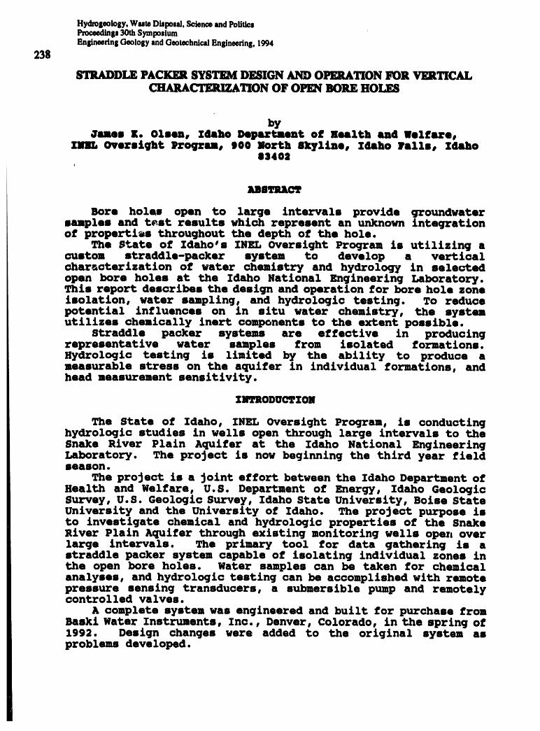
Hydrogeololy,WuteDlspoHl,SciencewndPolltiesPmceedlnp_ SymposiumEnEineedniOeologylindGeotechnlcalEnglneerlns,1994
238
STRADDLE P&CKER SYSTEM DESIGN AN]) OPEBATION FOR VERTICALCHAR__TION OF OPEN BORE HOLES
by_smeJ K. Oleea, Idaho Depsrtment of Health and gelfsre,
XIlBL Ovezoight Program, 900 North 8_71tne, :Idaho Falls, Xdaho8340R
![
UBTRIaT
Bore holes open to large intervals provide groundwatersamples and t_st results which represent an unknown integrationof properties throughout the depth of the hole.
The State of Idaho's INEL Oversight Program is utilizing aaustom straddle-packer system to develop a verticalcharv,cterization of water chemistry and hydrology in selectedopen bore holes at the Idaho National Engineering Laboratory.This report describes the design and operation for bore hole zoneisolation, water sampling, and hydrologic testing. To reducepotential influences on in situ water chemistry, the systemutilizes chemically inert components to the extent possible.
Straddle packer systems are effective in producingrepresentative water samples from isolated formations.Hydrologic testing is limited by the ability to produce ameasurable stress on the aquifer in individual formations, andhead measurement sensitivity.
Z]I'210DU_TZO]I
The State of Idaho, INEL Oversight Program, is conductinghydrologic studies in wells open through large intervals to theSnake River Plaln Aquifer at the Idaho National EngineeringLaboratory. The project is now beginning the third year fieldseason.
The project is a Joint effort between the Idaho Department ofHealth and Welfare, U.S. Department of Energy, Idaho GeologicSurvey, U.S. Geologic Survey, Idaho State University, Boise StateUniversity and the University of Idaho. The project purpose isto investigate chemical and hydrologic properties of the SnakeRiver Plain Aquifer through existing monitoring wells open overlarge intervals. The primary tool for data gathering is astraddle packer system capable of isolating indivldual zones inthe open bore holes. Water samples can be taken for chemicalanalyses, and hydrologic testing can be accomplished with remotepressure sensing transducers, a submersible pump and remotelycontrolled valves.
A complete system was engineered and built for purchase fromBaeki Water Instruments, Inc., Denver, Colorado, in the spring of1992. Design changes yore added to the original system asproblems developed.
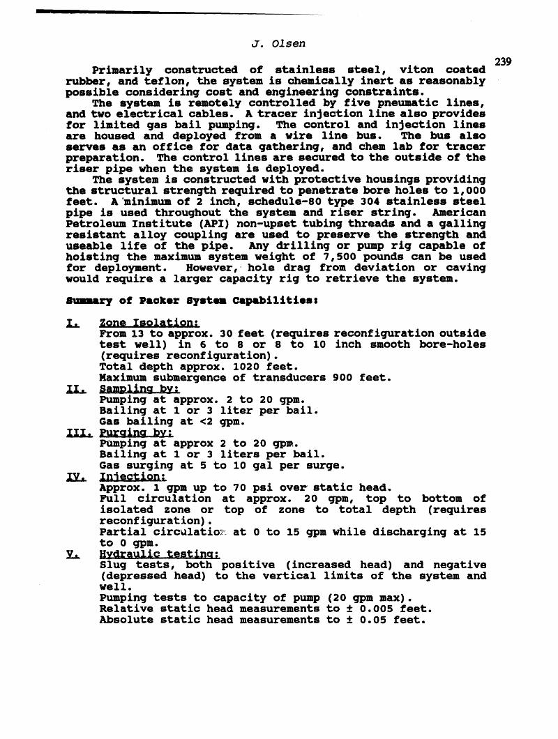
J. Olsen
239Primarily constructed of stainless steel, vlton coated
rubber, and teflon, the system is chemically inert as reasonablypossible considering cost and engineering constraints.
The system is remotely controlled by five pneumatic lines,and two electrical cables. A tracer injection line also providesfor llmlted gas ball pumping. The control and injection linesare housed and deployed from a wire line bus. The bus alsoserves as an office for data gathering, and chem lab for tracerpreparation. The control llnes are secured to the outside of theriser pipe when the system i8 deployed.
The system is constructed with protective housings providingthe structural strength required to penetrate bore holes to 1,000feet. A 'minimum of 2 inch, schedule-80 type 304 stainless steelpipe is used throughout the system and riser string. AmericanPetroleum Institute (API) non-upset tubing threads and a gallingresistant alloy coupling are used to preserve the strength anduseable life of the pipe. Any drilling or pump rig capable ofhoisting the maximum system weight of 7,500 pounds can be usedfor deployment. However, hole drag from deviation or cavingwould require a larger capacity rig to retrieve the system.
8unary of pecker eyeta Captbilttteos
IL Zone Isolation:From 13 to approx. 30 feet (requires reconflguratlon outsidetest well) in 6 to 8 or 8 to 10 inch smooth bore-holes(requires reconfiguration).Total depth approx. 1020 feet.Maximum submergence of transducers 900 feet.Sampling bv:Pumping at approx. 2 to 20 gpm.Bailing at 1 or 3 llter per bail.Gas bailing at <2 gpm.
_ Puraina by:Pumping a-t approx 2 to 20 gpm.Bailing at 1 or 3 llters per bail.Gas surging at 5 to 10 gel per surge.
IV. Injection:Approx. 1 gpm up to 70 psi over static head.Full circulation at approx. 20 gpm, top to bottom ofIsolated zone or top of zone to total depth (requiresreconfiguration).Partlal circulatio_ at 0 to 15 gpm while discharging at 15to 0 gpm.
Y-L Hydraulic testina:Slug tests, both positive (increased head) and negative(depressed head) to the vertical limits of the system andwell.
Pumping tests to capacity of pump (20 gpm max).Relative static head measurements to ± 0.005 feet.Absolute static head measurements to ± 0.05 feet.

Straddle Packer System, Characterization of Open Bore Holes
24O
]mZ]IC3ZPL]IB 01 OPBR&TZOm
saz£ptLon of nontss
The straddle packer system described in this report cons2stsof aoa_onent parts vhlch york together as a system. Without a
thorough understanding of each conponent and how the systemfunctions as a unit, the operation of the systen is not possible.
Following ££guze one below fron top to bottom, each componentpart and it's functions are described.
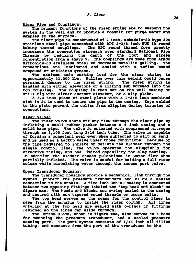
J. Olsen241
Riser Pipe and CouDlinas:
The primary functi0ns of the riser string are to suspend thesystem in the well and to provide a conduit for purge wa_er andsamples to the surface.
The riser plpe is constructed of 2 inch, schedule-80 type304stalnless steel pipe connected with API 2-3/8 inch NUE 10 roundtubing thread couplings. The API round thread form greatlyincreases the =ormectlon strength over standard National PipeThreads by reducing the depth of the root and stressconcentration from a sharp V. The couplings are made £romArmcoNitronics-60 stalnless steel to decrease metallic galling. Theconnections are lubricated and sealed with a teflon based
compound or antlsleze grease.The maximum safe working load for the rimer string is
approximately 31,000 1be. Pulling over this weight could causepermanent damage to the riser string. The riser string ishandled with either elevators or a llftlng sub eGrewed into thetop coupling. The coupling is then set on the well casing ordrill rig with either another elevator, or a sllp plate.
A 3/4 inch piece of steel plate with a 2-3/8 inch machinedslot in it is used to secure the pipe tot he casing. Keys weldedtot he plate prevent the collar from slipping during torquing ofconnections.
Riser Valve:
The riser valve shuts off any flow through the riser pipe byinflatlng a small rubber packer between a 4 inch casing and asolid base pipe. The valve is actuated with compressed nitrogenthrough an 1,100 foot long 3/16 inch tube. The valve is capableof forming a competent seal even when subjected to silt or sand,and is used as a backup valve under those =ondltlons. Because ofthe time required to Inflate or deflate the bladder through thesingle control line, the valve operates too sluggishly foreffective timing, and has limited capability for slug testing.In addition the bladder causes pulsations in water flow whenpartially inflated. The valve is useful for holdlng a full risercolumn while circulating water through the access port valve.
UDDer Transducer Houslna:
The transducer housings provide a mechanical link through thesystem, protect the pressure transducers and allow a sealedconnection to the annuls. A five inch Sch-80 casing is connectedbetween two opposing fittings labeled the "top head and block" onfiguze one. The heads and blocks are o-rlng sealed to the casingand secured with non tapered round threads or cross bolts.
The top head serves as the means for the control lines topass from the annulus to inside the riser column. All llnesentering at the top head are sealed with o-rlngs in fittings_eeigned so the lines can slide through."
The Bottom Block, shown in flguze two, also serves as a basefor mounting the pressure transducer, and a sealed pressuresensing port. The port system consists of 1/16 inch o11 filledtubing, and connects from the port of the transducer to the

Straddle Packer System, Characterization of Open Bore Holes
242
annulus through a 1/2 inch hole drilled through the block. Aplug seals the hole ._ the bottom and a 1/16 inch tubing to 1/4inch NPT fitting seals the top. The tube passes through thefitting, and terminates about 3/4 of the way down the hole. A1/16 inch hole drilled through the block dlrectly below thefitting aligns with a 1/4 inch hole through the housing toprovide a water connection to the annulus.
TRANSDUCER
I
OIL FILLED
LINE ---_ _ _-HOUSINGI
--- FITTING
--SENSING PORT
7 _-PLUGRISER PIPE
Figure Two: Transducer Housing Bottom BlockShowing Pressure Sensing System
This system provides a simple bubble free pressure connectionfrom the transducer to the annulus. All the air in the tubingand transducer port is expelled by sillcone oil with a syringe.Then the block cavity is filled with deionized and degassed waterby the same method.
Control Lines:
Eight 1100 foot flexible control lines accompany the riserstring from the surface to the packer system. There are fivetype 304 stainless steel pneumatic lines: two 1/4 inch llnes forpacker inflation, a 3/16 line for riser valve inflation, and two3/16 inch lines for the access port valve opening and closing.In addition a 1/2 inch Tefzel llne for tracer injection, a fourconductor transducer cable, and a four wire 14 gauge power cablefor the pump. To reduce the volume of control lines within thehousings and riser at qhe top head, the power cable converts to3 wires bydropping the ground, and the injection line reduces to1/4 inch. Quick connector couplings are provided to attach thepneumatic lines to a regulated nitrogen supply, transducer cableto computer hardware, and power to the pump cable.
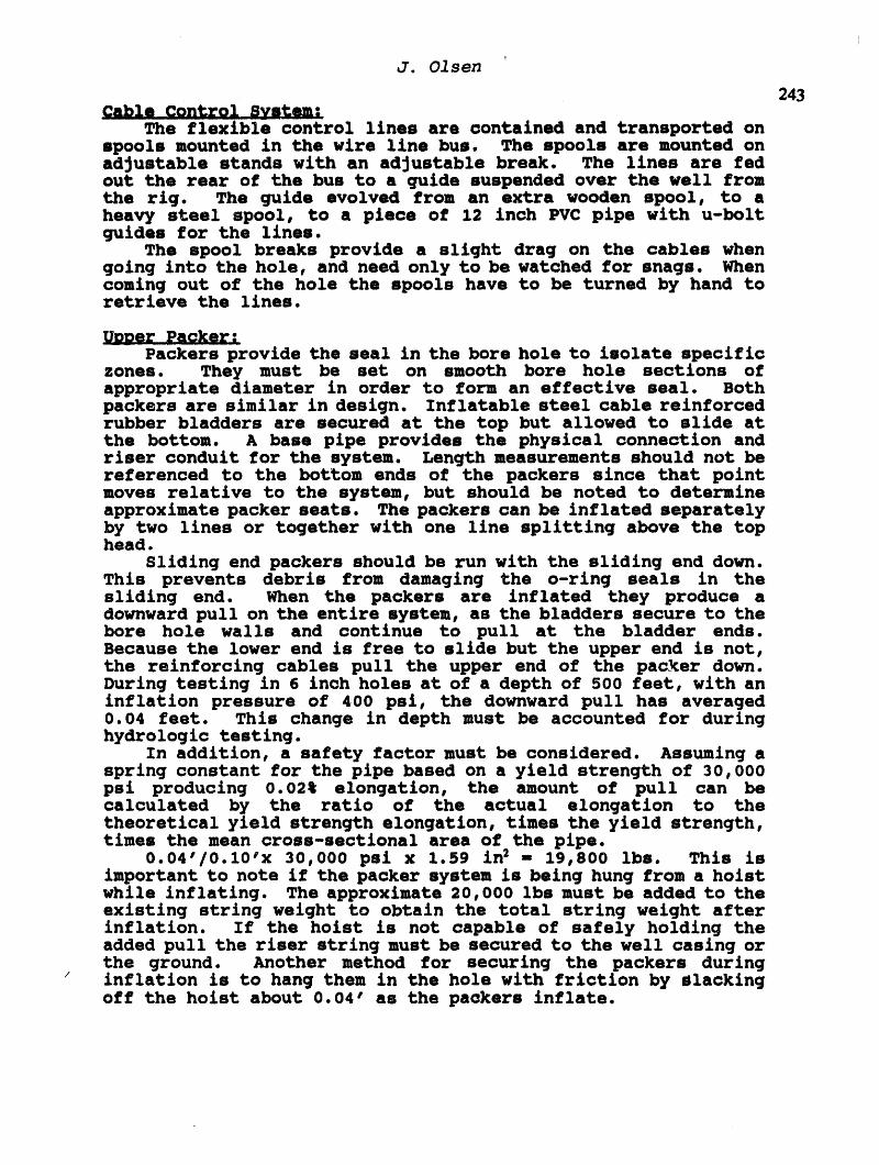
J!
J. Olsen
243Cable Control System:
The flexible control lines are contained and transported onspools mounted in the wire line bus. The spools are mounted onadjustable stands with an adjustable break. The lines are fedout the rear of the bus to a guide suspended over the well fromthe rig. The guide evolved from an extra wooden spool, to aheavy steel spool, to a piece of 12 inch PVC pipe with u-boltguides for the lines.
The spool breaks provide a slight drag on the cables whengoing into the hole, and need only to be watched for snags. Whencoming out of the hole the spools have to be turned by hand toretrieve the lines.
V_Der Packer|Packers provide the seal in the bore hole to isolate specific
zones. They must be set on smooth bore hole sections ofappropriate diameter in order to form an effective seal. Bothpackers are similar in design. Inflatable steel cable reinforcedrubber bladders are secured at the top but allowed to slide atthe bottom. A base pipe provides the physical connection andriser conduit for the system. Length measurements should not bereferenced to the bottom ends of the packers since that pointmoves relative to the system, but should be noted to determineapproximate packer seats. The packers can be inflated separatelyby two lines or together with one llne splitting above the tophead.
Sliding end packers should be run with the sliding end down.This prevents debris from damaging the o-rlng seals in thesliding end. When the packers are inflated they produce adownward pull on the entire system, as the bladders secure to thebore hole walls and continue to pull at the bladder ends.Because the lower end is free to slide but the upper end is not,the reinforcing cables pull the upper end of the packer down.During testing in 6 inch holes at of a depth of 500 feet, with aninflation pressure of 400 psi, the downward pull has averaged0.04 feet. This change in depth must be accounted for duringhydrologic testing.
In addition, a safety factor must be considered. Assuming aspring constant for the pipe based on a yield strength of 30,000psi producing 0.02% elongation, the amount of pull can becalculated by the ratio of the actual elongatlon to thetheoretical yield strength elongation, times the yield strength,times the mean cross-seotlonal area of the pipe.
0.04'/0.10'x 30,000 psi x 1.59 in2 - 19,800 lbs. This isimportant to note if the packer system is being hung from a hoistwhile inflating. The approximate 20,000 lbs must be added to theexisting string weight to obtain the total string weight afterinflation. If the hoist is not capable of safely holding theadded pull the riser string must be secured to the well casing orthe ground. Another method for securing the packers during
/ inflation is to hang them in the hole with friction by Slaokingoff the hoist about 0.04' as the paokers inflate.

Straddle Packer SyStem, Characterization of Open Bore Holes
244Pressure Relief Valve System:
When an isolated zone within a well is incapable of producingthe full flow rate of the pump, flow can be throttled with asurface valve. However, sufficient flow must be maintained toadequately cool the pump motor. To throttle the discharge belowthe minimum pump flow, a pressure relief valve allows circulationbypass of the water back to the pump by way of the annulus. Thevalves are Swageloc adjustable relief valves, which are availablein a variety of pressure ranges. The valves are mounted in across drilled block, with tubing threads connecting to the risersystem through the center.
Static tests performed in a test tank provide the dataillustrated in £19_ure thzee. The unmodified pump curve followsthe upper line, from A to C. The curve modified by the pressurerelief valve follows the lower line from B to D. As the head
pressure rises and discharge flow decreases from A to B bothcurves are the same. At point B (16 gpm, 300 psi) the pressurerelief curve begins to diverge from the pump curve. From pointsB to D the circulated volume increases as the discharged volumedecreases. At any point E along the modified curve the dischargerate is the value of X. The total flow, discharge pluscirculation, is the value of X along the unmodified curveadjacent to point E of equal value Y, point F. The circulationrate is the difference between the total and discharge.
A pressure gauge and discharge flow meter are used toregulate the circulation and discharge flow. The gauge and metercan also identify washed-out or plugged pressure valves, systemleaks, and pump performance. The pressure relief system allowscontinual mixing of the isolated zone during purging.
FLOW (Q} GPMo ,_ _ _ _ _ _ _ _ _ _ _ _
0
iL !i
i i il Ij
i

J. Olsen245
Access Port Valve and Houslna:
The access port valve (APT) provides open circulation betweenthe riser pipe and the annulus of the isolated zone. It is usedfor rapid mixing of tracer in the isolated zone before purging,and in combination with the pump check valve for slug tests. Inoperation the valve acts very quickly after a predictable delay.The valve is actuated with two pneumatic lines, which act onopposite sides of a vertical piston. The piston seals the riserfrom the annulus with o-ring seals against the valve body. Theo-rings are subject to leakage, damage, and failure from sand andpebbles. Care should be taken to clear the valve of sedimentbefore closing. The valve is very compact, helping to reduce theminimum length of the isolated zone. The access port valve iscontained in a separate 5-1/2 inch sch-80 housing to provide therequired mechanical link and riser seal. Sealed with o-rlngs andsecured by threads to the pump head and cross bolts to the valvebody. The top of the access port valve attaches to the pressurerelief valve by a tubing nipple. The access port valve housingis the main connection where the packer system breaks into theupper and lower half. The original housing was increased inlength from 12 inches to 18 inches to ease assembly of thecontrol line connections also contained there.
Pump and Middle Transducer Housinq:The pump housing, directly below the APV housing is 5-1/2
inch sch-80 stainless steel pipe. The pump is hung from the pumphead within the housing by a 1-1/4 inch NPT nipple. The housingattaches to the head with cross-bolts and o-ring seals. Cablesand tubing pass through the pump head and are sealed by fittingswith o-rings. The bottom block serves as the mount for themiddle transducer similar to the upper transducer.
PumD and Check Valve:
A Grunfoss 16 gpm 5 hp pump with a 3-ph 460v Franklin motoris used for purging and sampling. Because the system wasdesigned to operate at 1000 foot depths, a pump with adequatelift capacities was chosen. A 3-ph 460v motor was chosen toallow smaller gauge power cable to be used, (14 ga). However, avariety of 4 inch pumps could fit in the housing with the properfittings. Custom stabilizers were installed on the pump tomaintain alignment and reduce _tress on the pump nipple when theunit is laid down.
The pump check valve supplied with the pump is essential whenholding a column of water for slug testing, and beginning pumpingtests with a constant discharge. The check valve is subject toleakage when clogged with sand, and care must be taken to flushpump and valve clean before depending on a seal.
Extension Zone PUP Joints:
The isolated zone between packers can be adjusted bysubstituting various length pup joints between the pump housingand the lower packer. The connecting threads are the same as theriser string so joints are interchangeable throughout the system.The transducer cable extensions continue through the joints,

Straddle Packer System, Characterization of Open Bore Holes
246
while the lower inflation line runs tot he outside. There is nolimlt to the length of the isolated zone, up to the limits of thesystem, however, 13 feet is the minimum length, and 25 feet hasbeen the maximum length used to date.
Lower Packer:
The lower packer is similar to the upper packer except thatpump intake holes are provided in the upper (fixed) end. Placingthe intake holes in the packer head reduces the minimum length ofthe isolated zone. The intake holes in the packer head at thebottom of the zone insure through mixing when water is circulatedthrough the access port valve or pressure relief valve. Areplacement packer was modified from the original design toincrease the base pipe from Sch-80 to She-160. The first packerbase pipe suffered some crushing damage from a wrench.
Lower Transducer Houslna:
The lower transducer housing is interchangeable with theupper housing except for the top head. A solid plug seals theblock from the bore hole. Pipe lengths could be used instead ofthe plug to extend the pump intake into smaller hole diametersthan could be accessed with the entire system. In that case thepump intakes in the lower packer would be plugged.
Pressure Transducers:Three Paroscientific, Inc. "Digiquartz" RS-232 depth sensors
provide temperature and temperature compensated pressure readingsfor the packer system. The temperature sensor is internal to thetransducer and is used primarily for temperature compensation ofthe pressure reading. Although temperature readings arerelatively slow to respond, water temperature data can beobtained if enough time is allowed for equilibration.
The transducers have a pressure range of 0 to 400 psi with anover pressure rating of 1.2 times full scale. The repeatabilityand hysteresis are both listed at ± 0.005% full scale, orapproximately ± 0.046 feet of head. The resolution orsensitivity can be controlled by adjusting the integration timebetween the internal counter and the oscillators monitoringtemperature and pressure. The integration time is adjustable in0.003 second steps up to 45 seconds. Resolution is increasedwith integration time, but maximum sampling speed is reduced.For most tests a default setting of 0.7 seconds per reading isadequate and provides resolution of one part per million. Thetemperature compensated pressure is then calculated with amicroprocessor that loads the data onto the RS-232 bus. Thetransducers are fully programmable and data is recorded withbasic programs to a data file on a portable computer. In teststo date background noise has limited the useful resolution toapproximately 0.005 feet. The transducers are linked with asingle transmission cable in a serial loop. As many as fourtransducers have been run together with the fourth used at thesurface for a barometer.
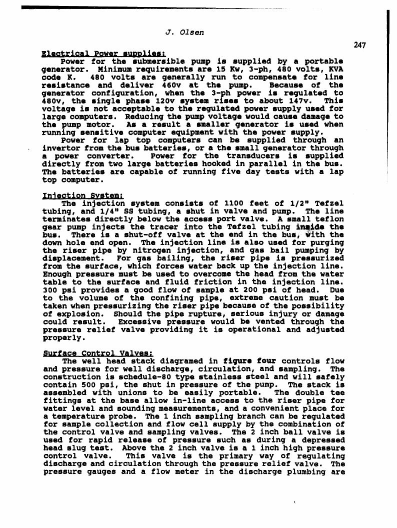
J. Olsen
247Ellotrlcal Power suDpllesz
Power for the submersible pump is supplied by a portablegenerator. Minlmumrequlrements are 15 Kw, 3-ph, 480 volts, KVAcode K. 480 volts are generally run to compensate for lineresistance and deliver 460v at the pump. Because of thegenerator configuration, when the 3-ph power Is regulated to480v, the slngle phase 120v system rises to about 147v. Thisvoltage is not acceptable to the regulated power supply used forlarge computers. Reducing the pump voltage would cause damage tothe pump motor. As a result a smaller generator Is used whenrunning sensitive computer equipment with the power supply.
Power for lap top computers can be supplled through anInverter from the bus batteries, or a the small generator througha power converter. Power for the transducers is supplieddlrectly from two large batteries hooked in parallel in the bus.The batteries are capable of running five day tests with a laptop computer.
InJgction System:The injection system consists of ii00 feet of 1/2" Tefzel
tubing, and 1/4" SS tubing, a shut in valve and pump. The llneterminates directly below the access port valve. A small teflongear pump injects the tracer into the Tefzel tubing IM_de thebus. There i8 a shut-off valve at the end in the bus, _ith thedown hole end open. The injection line is a18o used for purgingthe riser pipe by nitrogen injection, and gas bail pumping bydisplacement. For gas bailing, the riser pipe is pressurizedfrom the surface, which forces water back up the injection line.Enough pressure must be used to overcome the head from the watertable to the surface and fluid friction in the injection line.300 psi provides a good flow of sample at 200 psi of head. Dueto the volume of the confining pipe, extreme caution must betaken when pressurizing the riser pipe because of the possibilityof explosion. Should the pipe rupture, serious injury or damagecould result. Excessive pressure would be vented through thepressure relief valve providing it is operational and adjustedproperly.
Surface Control Valves:
The well head stack diagramed in £iguze fouz controls flowand pressure for well discharge, circulation, and sampling. Theconstruction i8 schedule-80 type stainless steel and will safelycontain 500 psi, the shut in pressure of the pump. The stack isassembled with unions to be easily portable. The double teefittings at the base allow in-line access to the riser pipe forwater level and sounding measurements, and a convenient place fora temperature probe. The 1 inch sampling branch can be regulatedfor sample collectlon and flow cell supply by the combination ofthe control valve and sampling valves. The 2 inch ball valve isused for rapid release of pressure such as during a depressedhead slug test. Above the 2 inch valve is a 1 inch high pressurecontrol valve. This valve i8 the primary way of regulatingdischarge and circulation through the pressure rellef valve. Thepressure gauges and a flow meter in the discharge plumbing are

Straddle Packer System, Characterization of Open Sore Holes
both used to adJumt the valve. A flow regulator Installed Justpast the I inch valve can also be used. However, the availablepremmure may exoeed the range of the regulator. In that case,decreasing the available pressure with the control valve maycause cavitation, affecting the stability of the regulator.Another tee im included to allow injection of nitrogen into therimer pipe. The nitrogen Im used £or depressing the head forslug tests, or gas bail pumping through the injection line.
_FLOWMET_,j ,,, ,,,
Figura Fo_zS_face Control
REGULA_R Valvem
_2" BALL V_
_ION 1" SAMP_ LINEF-I'CONTROL V_ P-7
ACCE$_ ON _- _$AMPLING V_S
t _ RIS_ _SLIP PLATE
R_DROLOGIC TISTING
Statto mead pzoflltngs
Although the Paroacientific pressure transducers employed inthe Idaho packer system are potentially capable of tremendoussensitivity to less than 0.001 foot, the accuracy of the systemIs limited to ± 0.05 feet. Sensitivity, precision or relativemeasurement is not the same as accuracy, repeatability orabsolute measurement. Testing to date in the Snake River PlainAquifer at the INEL has detected vertical head profiles in theorder of ± 0.01 feet. While that range is within the capacity ofthe system to detect relative changes, there are many factorswhich contribute background noise of over 0.1 feet. The resultis that absolute head measurements are not possible to theaccuracy required, and relative head measurements are alsollmited. Listed below in order of magnitude are the prlnclpal

j. 01sen
249factors affecting absolute accuracy _ relative precision whichhave been documented in actual field tests.
I Regional aquifer changes over months ± 1 footCalibration drift over months ± 0.5 feet
III Barometric effects over days ± 0.1 to 0.3 feetIV Production well pumping over hours + 0.01 to 0.1 feetX Physical movement on packer inflation/deflation ± 0.03
to 0.05 feetVI Vertical bore hole flow restriction head loss around
packers in small dianeter (6 inch) holes ± 0.01 to 0.1feet
VII Physical measurement errors of system depth ± 0.01 to0.5 foot
Because complete testing and sampling of wells, near theIdaho Chemical Processing Plant has typically taken one to twomonths each, accurate absolute head measurements have not beenpossible. The calibration drift conbined with regional aquiferchanges has contributed the greatest error. Barometric effectscan be accounted for if the baronatric efficiency of thk intervalcan be measured. However, only with monitoring over days canbarometric efficiency be deternined by conparing atnoopheriochanges with interval head. The production wells at the ICPPproduce 3300 gpm and cycle throughout the day. The result isthat static conditions in the nearby monitoring wells within onenile are never achieved, and draw down and recovery are notconsistent throughout the saturated interval being tooted.
An alternative method to measure relative head gradients isproposed and will be tested on wells far enough away to not bedirectly affected by the production pumping. Should the methodIs perfected it will be applied in future tests near theproduction wells at the ICPP.
Before the packers are Inflated, static heads will bemonitored and the calibration of the transducers checked by thephysical length between sensing ports. Transducers arecalibrated to a barometric reference in the bore hole beforegoing under water. A steel tape and sounding weight will be usedto measure from the surface to a measuring point at the top ofthe riser valve. Transducer sensing ports are also referenced tothe same point. With the access port valve open to allow treeflow to the riser, an electrical tape will be used to measur& thestatic head level of the open bore-hole. The measuring tapeswill then be left in the riser and static head monitored with thetransducers while the packers are inflated. The actual headchange of the isolated interval, relative to the open bore hole,is the change recorded by the e-tape. The physical movement ofthe packers will be the change in head on the middle transducerminus the e-tape change. For a check, the relative head changecan also be obtained by directly measuring the change in depth oninflation with the steel tape and sounder, then subtracting thatvalue from the change on the middle transducer. A map of headprofiles relative to the open bore hole can then be plotted forthe intervals tested. The assumption on which the method is

Straddle Packer System, Characterization of Open Bore Holes
25Obased is that the head profile will be constant over the leng_chof testing, approxlmately one month. That assumption isreasonable provided there are no major changes in the reglonalaquifer water table, there is no detectable production wellInfluence, and barometric efficiency is falrly consistentthroughout the saturated Interval. It would also be helpful ifa head gradient of sufficient magnitude to measure actuallyexists. The finished profile could be further checked bycomparing to flow logs for the well, or to near by nested wellscompleted at discrete Intervals, provided they exist.
Slug Tosts8
Slug tests for determining aquifer transmisslvity canaccomplished by one of two methods, either by releasing astabilized depressed head or instantaneously inducing anincreased head. However, the effectiveness of the test dependson the abillty of the testing system to produce a measurablestress on the aqulferbeing tested. If the aquifer being testedcan accept water at a rate much higher than can be dellvered, ameasurabl_ response may not be posslble. In tests with the Idahosystem, a 460 foot induced head will produce a maximum flow ratethrough the APV of approximately 200 9_m. That range limitseffective slug testing to approximately half of the formationstested at the INEL. Fluid friction in the 2 inch riser pipe over500 feet has been determined to be the most limiting factor. Inaddition, the upper section of the packer system contains controlllnes in the riser which increases restriction. With therestrictions in mind, slug testing has been an effective tool formeasuring medium to low conductivitiesbythe following methods.A slngle Basic test program with variable sampling rates can berun to monitor the transducer readings throughout the entiresequence. Being able to slow down sample rates at times whenfast readings are not needed allows you to reduce the size oft heresulting data file to a more manageable size, while preservinga large enough time span to recognize any antecedent trends.
First a rough estimate of conductivity can be made byinflatlng the packers at a desired test zone and observing thepressure change on the three transducers as during the first testfor static head relative measurements. If the zone isolatedincreases dramatlcally over the other two on packer inflation,the approximate draw down at 20 gpm will be 150 times thepressure spike minus the pull down of 0.04 feet. Because usingexcessive head for a slug test can cause damage to the well andequipment, and can waste time waiting for conditions to stabillzean estimate of the size of slug needed is valuable.
An example would be, if on Inflation the center transducerrises 0.15 feet then stabilizes within a minute, the expecteddraw down from the zone would be about 16.5 feet. This method is
very imprecise and could actually be 10 to 50 feet. However itserves the purpose to design the magnitude of the test. A 500foot slug would be much too much and would probably take hours toaccomplish stable conditions. A slug of about 50 feet would bemuch more reasonable. Under such conditions the packers should

J. 01sen
251be deflated to reduce draw dOwnwhenthe pump Is used to flll thoriser, or when the head is depressed.
Induced Head Slum Test:The riser pips can be filled with the submersible pump. The
access port valve must be closed and the riser valve open to dothis. The pump is turned off when the water level reaches thepredetermined mark. By using an e-tape, the induced head can beaoourately measured above the static head of the zone, orapproximated by timing the pump rate. Continue monitoring thewater level in the pipe to make sure the pump chec_ valve oraccess port valve are not leaking as they might if the watercontains much silt or sand. If no leakage occurs, the riservalve can be ignored. If leakage does occur, close the riservalve.
Inflate the packers and monitor the transducers untilconditions stabilize to a pre-test state. The slug test oanthonbegin by opening the riser valve (if used) and then open theaccess port valve. A standard test timing sequence and pressuresettingswas developed during field testing. Remember the riservalve must be fully open before the APV opens or it will causewild oscillatlon and unusable data.
At time 0 open riser valve, release pressure.At time 25 seconds release pressure from APV close side.At time 45 seoonds pressurize AFV open side.At time 60 seconds riser valve is fully open.At time 70 seconds APV opens instantly test begins.
T_ne slug height can be checked again prior to the test withthe e-tape if desired, or read directly on the PC as the APVopens. When the APVopens the slug is delivered tot he isolatedzone usually within one second. By monitoring the transducersuntil the head returns to the pre-test state the test Iscompleted, and the data can be examined.
Depressed Head Slum Tests:_
Depressed head slug tests can be used as long as the zonebeing tested has sufficient head to depress. The followingmethod has proven successful in field testing. The riser valvecannot be used effectively in this case because it opens tooslugglshly and cause wild oscillations in head measurements.Instead of the riser valve the 2 inch ball valve onthe stack isused to control the test. All fittings above the 2 inch valveshould be removed to allow full volume flow when the head isreleased.
With the packers deflated and theAPV open, depress the headin the riser by injecting nitrogen through the stack (fi_refour). Monitor the pressure dlreotly by the gauge on the stackuntil the desired head is reached. The supply regulator can beset to provide a constant head should leaks occur, or the stackshut in completely if leaks are not a problem. The packers canthen be Inflated and transducers monitored untll conditionsstabillze again. An e-tape measurement of the depressed head

Straddle Packer System, Characterization of Open Bore Holes
252 cannot be made at this time because the stack is sealed, ho_evero-tape readings should be made prior and after a test as a chock.The head magnitude will be recorded within a second or two afterthe 2 inch surface is opened. Continue monitoring untll headsrecover. The data can then be analyzed.
Pumping Tests t
Pumping tests require a constant discharge rate throughoutthe test to produce accurate results. A reasonable pumping rateshould be estimated from the inflation test to prevent excessivedraw down in tight formations. Set up the test with the packersdeflated, APV closed and riser valve open. Start pumping andadjust the flow to the desired level with the surface controlvalves and regulators. Note if any excessive draw down occurs onthe transducers. If draw down occurs in the whole well or
central zone with the packers deflated, the pump must be stoppedafter setting the discharge and the head allow to recover. Ifthe pump is turned off and leakage occurs through the check valveor APV the test will be compromised. The riser valve can be usedas a back up but must be completely deflated before starting thepump or oscillations will occur. Should the check hold and APVhold the full column without leaking, the pump can be started assoon as conditions stabillze. If no draw down occurs the packerscan be inflated with the pump running and the test begun. Thepull down of 0.04 feet on all _ee transducers must besubtracted from the test readings. The variable rate samplingprogram allows slowing the readings after the initial draw downduring long tests.
Tracer In, coting, nixings
Tracers are injected directly into the pump stream below theAPV and mixed throughout the isolated zone back to the pumpintakes (Eigttre one). The tracer should be injected and mixedwith the APV open and pump clrculatlng. The riser valve can beused if a full column constant discharge is desired for pumpingtests or other reasons until mixing is completed. Then the pumpmust be shut off while the APU is closed first then the riser
valve opened. Purging the zone at the predetermined dischargerate can then began with the pump. Allowing some clrculationthrough the pressure roller valve while purging eliminates deadspots in the Isolated zone. The tracer is monitored in thesurface discharge stream with either ion specific or specificconductance instrumentation untll background levels areapproached or reached. Background levels can be determined whenpro-setting the Jischarge rate.

_dr_eology, Waste Disposal, Science and Politics
Proce_ings 30th Symposium
Engineering Geolo_ and Geotechnical Engineering, 1994253
FZDIOLOGIO TIBTZ_G IN WllLL8 _ 'JLIZZDI_O 01DINZo]ur_ _OOBBBZ_G PZ_UflT AT 'ERR
ZD.%RO I_TZO_ BIIGZlfllI_.Z_G Z_BOR_.TORY
byG_"7 B. _olmson
_o l_am OlsenDale R. Ralston
Untvezstt7 of Idaho, Geolog3, and Geologto Bngz. Dept.Idtho Depaztnent of Ketlth and Welfaze, ImllL Ovezsight Pzogzsn
ABS'I'RACT
The Snake River Plain aquifer beneath the INEL is often viewedas a 2-dimensional system, but may actually possess 3-dimensionalproperties of concern. A straddle-packer system is being used bythe State's INEL Oversight Program to isolate specific aquiferintervals and define the 3-dimensional chemical and hydrologiccharacteristics of the aquifer. The hydrologic test results fromwells USGS 44, 45, aLnd 46 near the Idaho Chemical Processing Plantindicate that: 1) Vertical variation in static head is less than0.3 feet, 2) barometric efficiencies are _etween 25 and 55 percent,and 3) the system responds to distant pumping as a multi-layered,but interconnected system.
INTRDDOCTION
The State of Idaho INEL Oversight Program is evaluating theground-water monitoring system at the Idaho National EngineeringLaboratory (INEL). The project includes use of a straddle-packersystem to isolate, sample, and hydraulically test discreteintervals of the Snake River Plain aquifer. The program willultimately improve knowledge of the three-dimensionalcharacteristics of the aquifer system and the efficacy of currentsampling programs in wells open to the aquifer over largeintervals.
The straddle-packer apparatus has been used to test threewells in the vicinity of the Idaho Chemical Processing Plant (ICPP)at the INEL. Wells USGS 44, 45, and 46 were selected forstraddle-packer testing based on location, well diameter, openinterval, and long history of water quallty data. All three wellsare open from the water table, at about 460 feet below land surface(bls) to the bottom of the well at about 650 feet bls. The wellsare located in about a 400 foot radius, just west of the ICPP(figure i).
The straddle-packer isolates specific intervals of the aquiferby closing-off the open borehole with inflatable rubber packers.The system components of interest to this paper are, from top tobottom: a) an upper pressure transducer, b) the upper packer, c)the middle transducer, d) the lower packer, and e) the lowertransducer. A pump is also located between the two packers. Thesystem components are described in detail in 01sen (1994).

254 G.S. Johnson and others
11TPSI_11_ Irr' s_' ,,I III I II I I I I I I I I
LrKlPtANATION
Q _1p
I ,, I • z_ , • _ ,0 _ 6OO 76O Metem
_U' - "
¢PP-3 • oCPP-1IdaheCtlemkmlI_reeeulngIqam
43"34' -
DD
Figure i. Location of wells CPP-I, CPP-2, USGS 44, 45, and 46Relative to the Idaho Chemical Processing Plant (after Anderson,
1991) • i
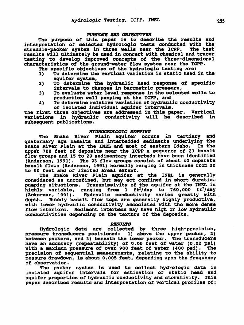
"nHydrologic Testl g, ICPP, INEL 255
PURPONZANDO_Z_rz8
The purpose of this paper is to describe the results andinterpretation of selected hydrologic tests conducted with thestraddle-packer system in three wells near the ICPP. The testresults will ultimately beused in concert wlthchemical and tracertesting to develop improved concepts of the three-dimenslonalcharacteristics of the ground-water flow system near the ICPP.
The specific objectives of the hydrologic testing are:1) To determine the vertical variation in static head in the
aquifer system,2) To determine the hydraulic head response of specific
intervals to changes in barometric pressure,3) To evaluate water level response in the selected wells to
production well pumping at the ICPP, and4) To determine relative variation of hydraulic conductivity
of isolated indlvldual aquifer intervals.The first three objectives are addressed in this paper. Verticalvariations in hydraulic conductivity will be described insubsequent publications.
BYDROGEOLOGIC SETTING
The Snake River Plain aquifer occurs in tertiary andquaternary age basalts and Interbadded sediments underlying theSnake River Plain at the INEL and most of eastern Idaho. In the
upp6r 700 feet of deposits near the ICPP a sequence of 23 basaltflow groups and 15 to 20 sedlmentaryinterbeds have been identified(Anderson, 1991). The 23 flow groups consist of about 40 separatebasalt flows (Anderson, 1991) normally ranging in thickness from 20to 50 feet and of limited areal extent.
The Snake River Plaln aquifer at the INEL is generallyconsidered as unconfined, but may act confined in short durationpumping situations. Transmissivity of the aquifer at the INEL ishighly variable, ranging from 1 ft2/day to 760,000 ft2/day(Ackerman, 1991). Hydraulic conductivity varies greatly withdepth. Rubbly basalt flow tops are generally highly productive,with lower hydraulic conductivity associated with the more denseflow interiors. Sediment Interbeds may have high or low hydraullcconductivities depending on the texture of the deposits.
RESULTS
Hydrologic data are collected by three high-precision,pressure transducers positioned: 1) above the upper packer, 2)between packers, and 3) beneath the lower packer. The transducershave an accuracy (repeatability) of 0.05 feet of water (0.02 psi)with a maximum pressure of over 900 feet of water (400 psi). Theprecision of sequential measurements_ relating to the ability tomeasure drawdown, is about 0.005 feet, depending upon the frequencyof observation.
The packer system is used to collect hydrologic data inisolated aquifer intervals for estimation of static head andaquifer properties of hydraulic conductivity and storatlvity. Thispaper describes results and interpretation of vertical profiles of:

G.S. Johnson and others255
1} Static head data,2) Barometric pressure response, and3) Response to the ICPP production wells about 0.5 miles
away.Straddle-packer testing was conducted on multiple intervals in
wells USGS 44, 45, 46. Table 1 provides a list of tested intervalsdiscussed in this paper.
i i i
Table i. Straddle-Packer Tested Intervals.
....... (depth, in feet below land surface} ..........467-482 462-477 465-483480-495 480-495 507-525495-515 500-515 531-549500-515 519-534 553-571519-534 575-593580-600 594-612600-620 612-629
illlli llllmll|IIII
Well USGS 45 was not tested below 534 feet due to borehole
deviation which prevented access with the packer system.
Temporal Variation in Water LevelsTrue static conditions are non-existent in the Snake _iver
Plain aquifer near the ICPP. Hydraulic head is continuouslychanging as a result of production well pumping at the ICPP andchanging barometric pressure. Conditions appear static if short-term variations in head are less than the resolutlon of the
measuring device. The continuously variable nature of "static"head is apparent in observations with the straddle-packer systemdue to the high transducer resolution. Examples of variations inhydraullc pressure with time ar_ shown in figures 2 and 3 for thewater table to 483 foot interval and 553 to 571 foot interval (bls)in well USGS 46. The graphs show the response of the threesubmerged transducers and variations in barometric pressure withtime. The transducer observations have been adjusted for elevationand an average barometric pressure, but are not compensated forinstantaneous barometric pressure. Only two transducers areplotted in figure 2 because the upper transducer was above thewater table.
Production well pumping at the ICPP results in about an 11hour cyclic response in the graphs of figures 2 and 3. Theduration of the pumping cycle varies somewhat with the operation ofthe facility. All three transducers show response of generallyless than 0.I feet of drawdown to ICPP pumping. The responseappears more a_tenuated in the upper transducers, and is affectedby superimposed barometric effects. The Initial transducerresponse generally occurs I0 to 15 seconds after the ICPP wellbegins pumping, some 2400 to 3100 feet away. A relationship isalso apparent between aquifer head and barometric pressure infigures 2 and 3. Aquifer response to ICPP pumping and barometric
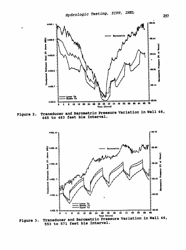
Hydrologic Testing, ICPP, INEL 257
4466. I - RB.64
04o4-0 Lower Yd----- Middle Td
4.155.6 _lWtWlWW,lVlW iVWilil,ll,Vlll.l,W _ 28.040 4 O 18 16 20 24 28 _ 30 40 44 40 62 68 80 44 M
Time (llo.rs)
Figure 2. Transducer and Barometric Pressure Variation in Well 46,465 to 483 feet bl8 Interval.
4456. • - - 28.'70
=
.u:_ 44r_.7 ,28.40 u
44_. 6 28.30
w e.e • e.e Lower Td14idd|e Td
.eeeo Upper Td
44C_,_ ww,l,,,li,Vle,WllV,lV1,1,,Vl,V,lVV, I,, ,l,.,l,,,l,,,l,,,l,, d 20._00 4 O 12 I0 20 24 28 32 30 40 44 46 62 M 80
Time (llo.rll)
Figure 3. Transducer and Barometric Pressure Variation in Well 46,553 to 571 feet bls Interval.
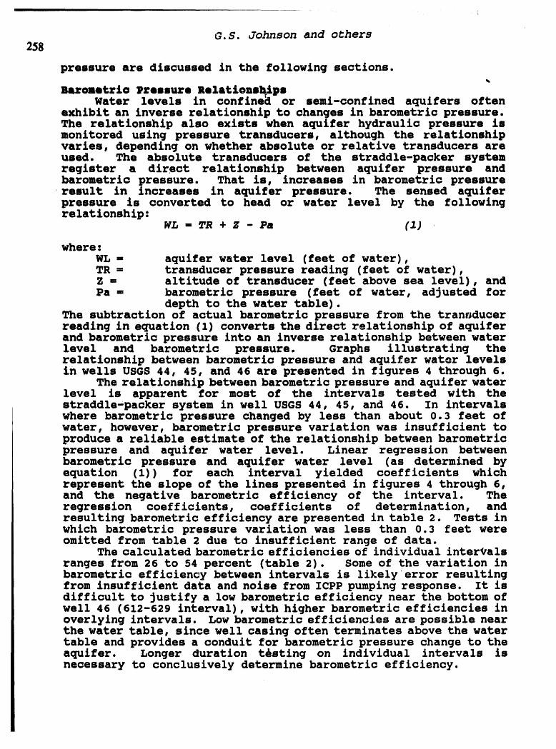
G.S. Johnson and others258
pressure are discussed in the followlng sections.
Bazomotrio Pzeesure Relationsh_poWater levels in confinea or semi-confined aquifers often
exhibit an inverse relationship to changes in barometric pressure.The relationship also exists when aquifer hydraulic pressure ismonitored using pressure transducers, although the relationshipvaries, depending on whether absolute or relative transducers areused. The absolute transducers of the straddle-packer systemregister a direct relationshlp between aquifer pressure andbarometric pressure. That is, increases in barometric pressureresult in increases in aquifer pressure. The sensed aquiferpressure is converted to head or water level by the followingrelationship:
WL - TR + Z - Pa (i)
where:
WL = aquifer water level (feet of water),TR = transducer pressure reading (feet of water),Z = altitude of transducer (feet above sea level), andPa = barometric pressure (feet of water, adjusted for
depth to the water table).The subtraction of actual barometric pressure from the transducerreading in equation (1) converts the direct relationship of aquiferand barometric pressure into an inverse relationship between waterlevel and barometric pressure. Graphs illustrating therelatlonship between barometric pressure and aquifer watar levelsin wells USGS 44, 45, and 46 are presented in figures 4 through 6.
The relationship between barometric pressure and aquifer waterlevel is apparent for most of the intervals tested with thestraddle-packer system in well USGS 44, 45, and 46. In intervalswhere barometric pressure changed by less than about 0.3 feet ofwater, however, barometric pressure variation was insufficient toproduce a reliable estimate of the relationship between barometricpressure and aquifer water level. Linear regression betweenbarometric pressure and aquifer water level (as determined byequation (1)) for each interval yielded coefficients whichrepresent the slope of the lines presented in figures 4 through 6,and the negative barometric efficiency of the interval. Theregression coefficients, coefficients of determination, andresulting barometric efficiency are presented in table 2. Tests inwhich barometric pressure variation was less than 0.3 feet wereomitted from table 2 due to insufficient range of data.
The calculated barometric efficiencies of individual intergals
ranges from 26 to 54 percent (table 2). Some of the variation inbarometric efficiency between intervals is likely_error resultingfrom insufficient data and noise from ICPP pumping response. It isdifficult to justify a low barometric efficiency near the bottom ofwell 46 (612-629 interval), with higher barometric efficiencies inoverlylng intervals. Low barometric efficiencies are possible nearthe water table, since well casing often terminates above the watertable and provides a conduit for barometric pressure change to theaquifer. Longer duration t_sting on individual intervals isnecessary to conclusively determine barometric efficiency.

7
4457.6, !
Figure 4 Aquifer Water Level Relationship to Barometric Pressure for InTervals in Well 44.

Figure 5. Aquifer Water Level Relationship to Barometric Pressure for Intervals in Well 45.

Figure 6. Aquifer Water Level Relationships to Baroletric Pressure for Intervals in Well 46.

G.S. Johnson and others
262lJ " i iiii iii l i ii I i iiiiiii
Table 2. Results of Linear Regression of BarometricPressure and Aquifer Water Level.
Regression Barometric__;JF_ Coifflclent R2 Efficilncv (%_
44 500-515 -0.35 0.65 3545 519-534 -0.54 0.90 5446 465-483 -0.30 0.53 3046 507-525 -0.52 0.81 5246 553-571 -0.40 0.45 4046 594-612 -0.47 0.96 4746 612-629 -0.26 0.52 26
,i i i i iiiii i ,LIIII iiiii i , i iiii IIHI H i i
Vertioal Variations in 8ratio HeadLittle variation of hydraulic head with depth is apparent in
wells USGS 44, 45, and 46. The relatively small degree ofdifference in water level between Intervall Is shown by the smallvertical offset of the Interval data sets presented in figures 4through 6. The calculated head difference between intervals withina well ranges between 0.15 to 0.3 feet. The vertlcal offset Is notconsidered to be representative of head difference betweenintervals due to inconsistency when compared to pressuredifferences among the three transducers .during 81multaneousreadings. The offset el thought to be the cumulative relult of a)inaccuracy in transducer readings, b) inaccuracy in measurement ofsystem depth, and c) seasonal variations in aquifer water levell.The data indicate only that vertlcal head variation in the 170 feetof submerged, open borehole is leas than 0.3 feet.
zoPP punping ResponseWater levels in wells USGS 44, 45, and 46 respond to pumping
in the ICPP production wells about 0.5mile to the northeast. Thetwo production wells, CPP-1 and CPP--2, provide water for thefaoillty at a rate of about 3000 Spa. The two wells are rotatedinto production on a monthly basis and currently cycle on and offabout every 11 hours. Both of the wells are completed in two
' intervals in the aquifer, at depths ranging from 460 to 600 feetbelow land surface. The completlon zones correspond to two basaltflow groups: 1) the E through H group, and 2) the I flow group,according to the stratigraphy defined by Anderson (1991). Anderson(1991) determined that these same basalt flow groups intersectwells 44, 45, and 46 at the depths llsted in Table 3.
The drawdown in wells USGS 44, 45, and 46 from pumping at theICPP production wells ranges from 0.02 to 0.10 feet, depending onthe well and Interval. The drawdown Is apparent from cycllcresponse of the graphs of figures 2 and 3. The magnitude of thedrawdown in specific packer intervals can be used as a qualitativemeasure of the degree of hydrologic connection between the Intervaland the pumping zones of the ICPP well.
Hydrologic Testing, ICPP, INEL263
__ i . I I [ 11 FB IlIIIilIR IIIII Ill I llllll I IIIII I l I ii ii IIBN_II III IIIIIHIIlIIII I I l _ --.....
Table 3. Depth of Basalt Flow Groups Intersecting theSaturated Portion of Wells USGS 44, 45, and 46 (afterAnderson, 1991).
...... W ll ..................F10w Group 44 45 . 46E through H ...... (feet below land surface) ......
Top 441 446 450Bottom 550 550 547
I Flow
Top 440 550 550Bottom >650 >651 >648
i i i iiii ii i Ulll ii I.i ii iiii ] ii . ii i iii lllil i . - _ iii
ICPP production well drawdownvarles with depth in wells USGS44, 45, and 46 (figure 7). The drawdown is determined graphicallyas the amplitude of the drawdown cycle in figures 2 and 3 andslmilar graphs fo: other intervals. Small vertlcal variations indrawdown are apparent in the lower transduder, with the generaltrend indicating the minimum response near the water table. Theresponse of the middle and upper transducers varies signiflcantlywith depth. The trend is toward maximum response near the bottomof the wells, generally within the I flow group deflnedbyAnderson{1991).
The relative difference between upper, mlddle, and lowertransducer response in figure 7 is more meaningful than theabsolute magnitudes of the drawdown. Drawdown is consistentlylowest in the upper transducer (above the upper packer) compared tothe middle and lower transducers, separated by inflated packers.The consistently low relatlve readings of the upper transducer maybe the result of either of two conditions: a) the uppertransducer may be representing unconfined conditions, and b) theupper saturated intervals are not as well connected to the ICPPproduction wells. In most intervals, the drawdown in the middletransducer is also less than or equal to drawdown in the lowertransducer , reflecting diminishing drawdown nearer the water table.
The relative differences in drawdown among the threetransducers varies with depth of the Isolated interval. Figure 7shows that there is little difference in drawdown from the ICPPwell in the middle and lower transducers for intervals near thebottom of the wells. This indicates that the wells may be dividedinto two units based on their hydrologic response to ICPP pumping.In well 44, the middle and lower transducer register approximatelythe same magnitude of drawdown in all Intervals below 515 feetbelow land surface. In intervals above 515 feet the response ofthe middle transducer is attenuated relative to the lower unit,implylng that the lower portion of the well is hydrologically morestrongly connected with the ICPP wells. Wells 45 and 46 showsimilar conditions, with the transition zones at depths of 500 and550 feet below land surface, respectively.
The qualitative grouping of drawdown response may define twoflow systems with differing degrees of connection to the ICPP

264 G.S. Johnson and others
, Wlllll UIQII 44
(P'¢blo)HI[Ill I I IIII[ III IIII I , I II I I IIIIII
].UI.J_.__lL......LJ.J...........$.1_:i
010,,4114
uNoo 1..... I
" : ]11 " - ii ii li_n_;- I ,,i ......
o O,Ol 0,04 O,Otl 0.Ol 0.1taPPOrmn (Pll
WellUSG846
(Ftblo)
wY-41ry
41o-4ml
Ioo-tll
1irlt-184
0 0.0| 0.04 0.01 0.01 0.tIOPPDrlwdown(Pt)
Well USG8 40
(Ft biB)
wr-4. :__L........_._...................
::::..:..... .......... , ij I
' ,,, ,, i ' ,:: I
uH_ ,_............_,,:'!_..........,,-.:......:,:,.....::_:.,:..!!-_......_,:.:,:..:.:...-:..::: ii
m-Ira _- .........._.................::::...-_..................:..............................;
011410
0 0.0| 00,4 O,OO O.Ol 0.1IOOIIiOqriwdownIPl)
Figure 7. Interval Specific Drawdown at Wells USGS 44, 45, and 46in Response to Pumping at CPP-I and CPP-2.

Hydrologic Testing, ICPP, INEL
265production wells. A layer of lower vertical permeability couldconceivably separate the two units. In well USGS 46 the transitionapproximately corresponds to tho sediment interbed at thelithomtratigraphic contact between basalt flow groups E-H and I asdetermined by Anderson (1991). In wells USGS 44 and 45 thetransition appears at a higher llthostratlgraphic point in theprofile, somewhere within the E-H basalt flow group. Within the Iflow group, and within the lower depths of the E-H flow group inwells 44 and 45, a nearly homogeneous response is observed toproduction well pumping for the ICPP.
The straddle-packer system Is effective for determiningvertical variations in hydrologic characteristics of the SnakeRiver Plaln aquifer within certain limitations. It has beendetermined that. 1) Vertical variation of static head within theupper 170 feet of aquifer near the ICPP Is less than 0.3 feet, 2)the tested wells respond as 8eml-confined with a barometricefficiency ranging between 0.25 and 0.55, and 3) response to ICPPproduction wells indicates a multi-layer hydrologic system with ahydraullc interconnection of the two layers. These results will beconfirmed and expanded as testing progresses into additional wellsnear the ICPP and as hydrologic, geochemical, and geophysicalinformation are pieced together as components of the conceptualflow system puzzle.
RIFERENCESAckerman, n.J., 1991, Transmlssivity of the Snake River Plain
aquifer at the Idaho National Engineering Laboratory, Idaho_U.S. Geological Survey Water Resources Investigations Report91-4058, 35 p.
Anderson, S.R., 1991, Stratigraphy of the Unsaturated Zone andUppermost Part of the Snake River Plain aquifer at the IdahoChemical Processing Plant and Test Reactors Area, IdahoNational Engineering Laboratory, Idaho: U.S. GeologicalSurvey Water Resources Investigation 91-4010, 71 p.
Olsen, James K., 1994, Straddle-Packer Design and Operation forVertical Characterization of Open Bore Holes: 1994 Symposiumon Engineering Geology and Geoteahniaal Engineering, Boise,Idaho.

Hy&ogeology, WasteDisposal, Science andPoliticsProceedings30th Symposium 2(57EngineeringGeology andGmtechnical Engineering,1994
VERTICAL VARIATION IN GROUNDWATER CHEMISTRY INFERRED FROM
FLUID SPECIFIC-CONDUCTANCE WELL LOGGING OF THE SNAKE RIVER
PLAIN BASALT AQUIFER, IDAHO NATIONAL ENGINEERING LABORATORY,SOUTHEASTERN IDAHO
Spencer H. Wood and William Bennecke
Departmentof Geosciences
Boise State University
Boise, Idaho 83725
ABSTRACT
Wellloggingofelectricalfluidspecificconductance(C.)showsthatpermeablezonesyieldingground water to intrawell flows and the water columns in some wells at INEL have highlydifferent chemistry, with as much as a two-fold variation in C,. This suggests that dedicated-pump sampling of ground water in the aquifer may not be representative of the chemistry ofthe waste plumes migrating south-west of the nuclear facilities. Natural background C, inbasalt-aquifer ground water of this part of the Snake River Plain aquifer is less than325pS/cm (microSiemans/cm), and total dissolved solids in mg/L units, (TDS) = 0.6C,. Thisrelationship underestimates TDS for waters with chemical waste, when C, is above 800pS/cm.
At well 59 near the ICPP water of 1115 pS/cm (-670+ mg/L TDS) enters the wellfrom a permeable zone between 521 and 537 ft depth; the zone being 60 ft below the waterlevel and water of 550 pS/cm. At the time of logging (9/14/93) the 1115pS/cm water wasflowing down the well, mixing with less concentrated waters and exiting at 600 or 624-ftdepth. Waste water disposed of down the injection well at ICPP until 1984 was estimated tohave a Q of 1140 pS/cm, identical to the water detected in logging.
At well OW2, the highest C, water (760pS/cm) is in the upper 30 feet of the watercolumn: water from two flow zones below have different chemistry with lower values of C,.The Site 14 well and USGS 83 show uniform values throughout the water column. The watercolumn in Site 14 is dominated by a downward flow of 50 gal/min probably entering between475 and 500 ft depth and exiting near the bottom of the well at 700 ft depth.
Impeller flowmeter and precision temperature logging are used to define and quantifytemperature variations and intrawell flows. At well 59 (depth=657 ft) and OW2 (depth=996ft), are downward decreasing temperatures in the bottom zones of no flow, suggesting thatmajor flow zones lie beneath the deepest parts of these wells.
INTRODUCTION
Fluid temperature, electrical specific conductance, and spinner-flowrneter logs were run infour wells within the saturated zone of the eastern Snake River Plain basalt aquifer (Figures 1

268 $.H. Wood and W. Bennecke
and 2). This reconnaissance logging was done to identify wells in which to deploy packersystems to hydraulically test and sample ground water from the aquifer - a project of the Stateof Idaho Oversight Programof U.S. Government nuclear facilities at the Idaho NationalEngineering Laboratory. Identification of the majorpermeable conduits in the stack ofQuaternary lavas, sediments and basalt bodies that make up the aquifer is a major goal of theproject. Knowledge of'the major permeable zones, and determining the position of wastewater in the aquifer is important to monitoring plumes of waste water, and to design a
' strategy for diverting plumes or recovering and reprocessing waste waters should that becomenecessary or feasible in the future.
Thickness of the Quaternarybasalt section exceeds 2,500 ft (760 m) beneath parts ofthe Idaho National Engineering Laboratory(Figure 3). A K-Ar age of 820 Ma is obtainedfrom basalt at 2321-ft (708 m) deep in well NRF 89-04, and ages of 200-650 Ma are commonfor the sequence (Lanphereand others, 1993. The lava sequence that comprises the saturatedaquifer contains several thin but very transmissive zones which we believe to be mostly lava-flow tops - although not all flow tops are highly permeable. Well tests of the upper 150 to500 ft (45 to 150 m) of the aqu!fer show very small drawdowns for large flows, from whichare derived some of the highest transmissivity values known in the world, ranging up to2,400,000 ft2/day (220,000 m2/day) (Garabedian, 1992, p. F12). Typical value is 60,000ft2/day (5580 m2/day) (Ackerman, 1991). We do not yet know the typical thickness of thehighly transmissive zones, but we suspect that several zones of only a few meters of fracturedor rubbly flow-top basaltmay dominate the response of the wells to pumping. Much of theeastern Snake River Plain basalt is near-vent and tube-fedpahoehoe lava (Kuntz and others,1992). We have been impressed by the apparentpermeability of coarse rubble and sequencesof shelly pahoehoe in the upperfew meters of flows with partings typically spaced a fewcentimeters. Downgradient ground water velocities areestimated at 4 to 20 ft/day at agradient of 10 ft,/mile (0.0019) (Robertson and others, 1974).
The wells are situated on the Quaternarybasalt fields of the eastern plain and weredrilled for various groundwatermonitoring and experimentalprogramsassociated with nuclearfacilities at the Idaho National Engineering Laboratory(INEL). The Site 14 well is upgradientof injection wells, disposal ponds and waste ponds that have introducedlow-level wasteradionuclides and other constituents into the southwest migratinggroundwater. Well 59 iswithin a plume of waste constituents attributedmostly to the injection well at the IdahoChemical Processing Plant (ICCP), a disposal-well practicethat was discontinued in 1984.Well 83 is down gradient,within the track of the waste water plume area, but shows lowTritium (0.1:k0.3 pCi/mL)in contrastto surroundingwells which are above 2 pCi/mL (Knobeland Mann, 1988). [(note that 1 pCi/mL - 312 TU = 2.25 3H-disintegrations/min/mL),where1 TU = isotope ratio 3H/2H of lif ts = = 0.0032 pCi/mL 07_hodehameland others, 1971; p. 4),and thatvalues of less than 5 TU areconsidered natural,pre-almospherictesting ofthermonuclear devices in the period 1953-69 (Freeze and Cherty, 1979)]. Well OW-2 wasdrilled in 1993 south of the Radioactive Waste ManagementComplex (RWMC) for thepurpose of monitoring the saturatedzone duringa large scale infiltrationexperiment (Norelland Wood, 1993).
METHODS
Well logging was conducted with Boise State University's Series 3000 Mount SoprisInstruments Company 4-conductor wireline unit with dataacquisition using the ACQUIRE

Vertical Variation in Groundwater Chemistry, Snake River Plain Basalt Aquifer, INEL
269software and interface electronics. We used the bi-dir_tional Halliburton (formerly Gearhart-Owen, Mineral Logging Service) 1 7/16-inch-06.5 mm)-diameter impeller flowmeter with alow-density plastic impeller spinning on jewelled pivots (Figure 4). The impeller has anembedded magnet that allows the electronics in the sonde to sense the direction of spin andchange polarity of the pulses according to spin direction. The impeller has a stall speed ofabout 11 ft/minute for down-wash flow, and about 8 ft/minute of up-wash flow. _[_order todetect small flows the tool is trolled at speeds of 15 to 25 feet/minute. The least noisy signalis obtained on down trolled runs (up-wash). Noise level is about 2 to 3 feet per minute(Figures 6 to 9) on account of the somewhat jerky nature of the revolutions of the impeller.Calibration is obtained by trolling at various speeds in casing. Counts per second [cps]response have a Hnear relationship to troll speed in the range 15 ft/min to 25 ft/min. Foruptroll (downwash): ft/min ffi 8.00fcps] + 11.00, and for downtroll (upwash): ft/min =6.06.[cps] + 6.80.
Intrawell flows detected by flowmcter, in terms of ft/min can be converted tovolumetric flow, by multiplying by the cross-sectional area of the borehole, which for a 6-inch well is 0.20 ft_, and for an 8-inch well is 0.35 fta to give flow in terms of ftS/min. Onecubic foot is 7.5 gallons, so that for a 6-inch well, 1 ft/min = 1.5 gaYmin; and for an 8-inchwell, 1 ft/min = 2.6 gaYmin. A uniform volumetric flow fluctuates with borehole diameter,so that in break-out intervals or constrictions seen on caliper logs, the flow will vary onaccount of borehole size.
Fluid electrical resistivity and temperature are recorded simultaneously by logging with theMount Sopris Instruments MLP-4280 probe. Temperature and fluid resistivity response of thetool is calibrated by immersing the sonde in 6-gallon buckets of waters for which thetemperature and resistivity have been determined using a Prestotech Corp. meter previouslycalibrated to an ASTM thermometer to an accuracy of + 0._ °C and to standard solutions sothat absolute resistivity is :1:2.0 ohm-meters. When fluid resistivity is converted to specificconductance (Cx), the absolute values are accurate to :1:20 pS/cm (microSiemans/cm) over therange 100 to 1300 pS/cm.
The logged values of fluid resistivity are corrected for temperature to the standard 25°Cusing the Arps' equation (Serra, 1984, p. 9): Rw(TI) = 1_ (Tz)_(Tl + 21.5)/(T 2 + 21.5)],where temperature (T2) and resistance l_(Tz) are the pair of logged values. Units on theformula are degrees centigrade, and resistivity is in ohm-meters. The resulting R,,(Tt) isconverted to specific conductance (C,) in pS/cm units by the formula: C, = 10,000/R,). Thesecalculations are most simply done for the entire log by importing the ASCII-format well-logfiles into a spread-sheet program.
The reported temperatures on the log are accurate to :1:0.2°C, and the values of C, to :1:20pS/cm, and relative changes of 0.02°C and 10pS/cm are reproducible on repeated loggingruns. As discussed later, (2, is about 1.6 x (.totaldissolved solids expressed in rag/L). Thisimplies that relative changes in electrolyte concentrations of about 10 mg/L are detectablewith the calculated C, log from the MLP logging tool.
TEMPERATURE PROFILES
Temperature gradients observed in wells at INEL are of three types. The simplest is one,inwhich the temperature increases with depth as is expected for solid conduction of the heat ofthe earth vertically outward to the surface. Variations in gradients of this type can occur in a
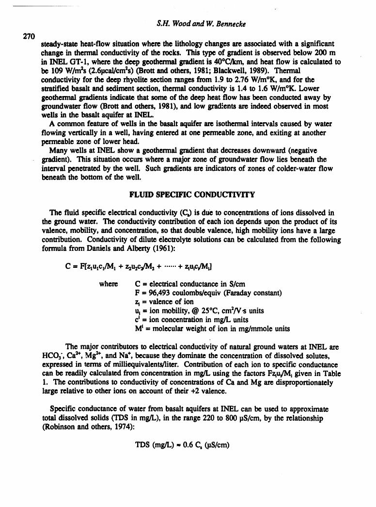
$.H. Wood and W. Bennecke
27Osteady-stateheat-flow situationwhere the lithology changesare associatedwith a significantchange in thermal conductivityof the rocks. This type of gradientis observed below 200 min INEL GT-1, where the deep geothermalgradientis 40°C_ and heat flow is calculated tobe 109 W/m2s(2.6pcal/cm2s) (Brottand others, 1981; Blackwell, 1989). Thermalconductivity for the deep rhyolite section rangesfrom 1.9 to 2.76 W/m°K, and for thestratifiedbasaltand sediment section, thermal conductivity is 1.4 to 1.6 W/m°K. Lowergeothermalgradients indicate that some of the deep heatflow has been conductedaway bygroundwaterflow (Brott and others, 1981), and low gradientsare indeed observedin mostwells in the basalt aquifer at INEL.
A common featureof wells in the basaltaquifer are isothermal intervalscaused by waterflowing verticallyin a well, having enteredat one permeable zone, and exiting at anotherpermeablezone of lower head.
Many wells at INEL show a geothermal gradientthat decreasesdownward(negativegradient). This situationoccurs where a majorzone of groundwaterflow lies beneath theinterval penetratedby the well. Such gradientsare indicatorsof zones of colder-waterflowbeneath the bottom of the well.
FLUID SPECIFIC CONDUCTIVITY
The fluid specific electricalconductivity (C_)is due to con_ntrations of ions dissolved inthe ground water. The conductivity contributionof each ion depends upon the productof itsvalence, mobility, and concentration,so that doublevalence, high mobility ions have a largecontribution. Conductivityof dilute electrolytesolutions can be calculatedfrom the followingformulafrom Daniels and Alberty (I96I):
C ffiF[z_ulc,/Ml+ z_u2cJM2+ ...... + _usc/M_]
where C = electricalconductancein S/cmF = 96,493 coulombs/equiv(Faradayconstant)
= valence of ionus= ion mobility, @ 25°C, cm2/Vs unitscs= ion concentrationin mg/L unitsMS= molecular weight of ion in mg/mmole units
The majorcontributorsto electrical conductivityof naturalgroundwaters at INEL areHCO3",Ca2+,Mg_, and Na+, because they dominatethe concentrationof dissolved solutes,expressed in termsof milliequivalents/liter. Contributionof each ion to specific conductancecan be readily calculatedfrom concentrationin mg/L using the factors Fz_u/Mlgiven in Table1. The contributionsto conductivityof concentrationsof Ca and Mg aredisproportionatelylarge relative to other ions on accountof their +2 valence.
Specific conductanceof water from basaltaquifersat INEL can be used to approximatetotal dissolved solids CIDSin rag/L), in the range 220 to 800 pS/cm, by the relationship(Robinsonand others, 1974):
TDS (rag/L),, 0.6 C, (pS/cm)

L
Vertical Variation in Groundwater Chemistry, Snake River Plain Basalt Aquifer, INEL271
At higher values of C,, (>800 pslcm) which are in most cases influenced by waste water, theabove equation underestimates TDS by as much as 200 mg/L.
Table1. Contributionto specificconductance(C,)of major solutesinground water.
solute _ M _ x 10s F _ u, / Mspecks
mequiv m8 ionmobility contributiontoper per @ 25°Cin conducWce_Slcm)mmole mmol¢ cm=/V,s s permg/L
concentration
HCOiI 1 61.0 46 0.73SOi= 2 96.0 82.7 1.66CI" 1 35.5 79.0 2.15Ca+= 2 40.1 61.6 2.96Na+' 1 23.0 52.0 2.18K+! 1 39.1 76.2 1.88M8+2 2 24.3 55 4.37"SiO_ - - 0.0"
1fromMamnandLando(1974,p. 516)
F = Faradayconstant= 96,493coulombs/equiv
"SiO=is notsignificantlyionizedforpHbelow8.5. At low pHSiO2is entirelyas undisassociatedH4SiO,°. Fromequalionsin Krauskopf(1979,p. 133)itcanbe shownthatat 25°C,the pHdependencyof themoleratioof ionizedsilica to non-ionizeds_ica is expressedas: {H_SiO;i}/lI-14SiO.°} = 1011_'9'*}.
The highestpHfor_maltaquiferwatersat INELis pH=8.3,so thattheratioof ionizedto non-ionizedsilicais 1/40.
VARIATIONS IN WATER CHEMISTRY
Spatial variation in groundwater chemistry at INEL was systematically mapped byRobert Schoen in the study by Robertson and others (1974). He speculated that the rechargewater from the northwest mountains is enriched in Ca, Mg, and HCO3 on account of beingderived from mountains underlain by Paleozoic carbonate rocks, whereas recharge water fromthe northeast is enriched in Na, F, and SiO2. These waters appear to mix along a northeast-striking zone through central INEL. Recharge water from the Mud Lake area has highdissolved solids (300 to 500 + mg/L) on account of evaporation of irrigation water, beingparticularly high in Ca, Mg, K, Na, CI, SO4, and NO3 as shown by concentration lobesextending from Mud Lake to about well no. 21.
Schoen (in Robenson and others, 1974, p. 74-76) was aware that significant changes inwater chemistry occur vertically in the aquifer in some wells. He recognized in some wells, abody of relatively fresh water (C, of 100 to 200 pS/cm) at the top of the water table, as muchas 50 feet thick, though usually much thinner, underlain by normal groundwater with a (2, of
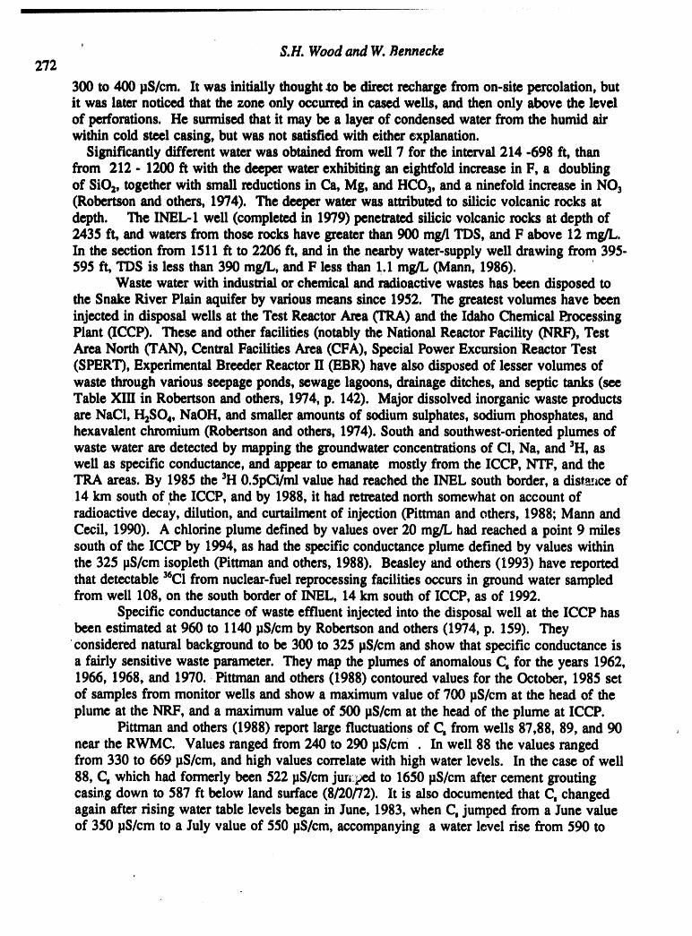
' $.H. Wood and W. Bennecke272
300 to 400 pS/cm. It was initially thought w be direct recharge from on-site percolation, butit was later noticed that the zone only occurred in cased wells, and then only above the levelof perforations. He surmised that it may be a layer of condensed water from the humid airwithin cold steel casing, but was not satisfied with either explanation.
Significantly different water was obtained from well 7 for the interval 214 -698 ft, thanfrom 212 - 1200 ft with the deeper water exhibiting an eightfold increase in F, a doublingof SiO2, together with small reductions in Ca, Mg, and HCO3, and a ninefold increase in NO3(Robertson and others, 1974). The deeper water was attributed to silicic volcanic rocks atdepth. The INEL-1 well (completed in 1979) penetrated silicic volcanic rocks at depth of2435 ft, and waters from those rocks have greater than 900 rag/1 TDS, and F above 12 mg/L.In the section from 1511 ft to 2206 ft, and in the nearby water-supply well drawing from 395-595 ft, TDS is less than 390 mg/L, and F less than 1.1 mg/l., (Mann, 1986).
Waste water with industrial or chemical and radioactive wastes has been disposed tothe Snake River Plain aquifer by various means since 1952. The greatest volumes have beeninjected in disposal wells at the Test Reactor Area (TRA) and the Idaho Chemical ProcessingPlant (ICCP). These and other facilities (notably the National Reactor Facility (NRF), TestArea North (TAN), Central Facilities Area (CFA), Special Power Excursion Reactor Test(SPERT), Experimental Breeder Reactor II (EBR) have also disposed of lesser volumes ofwaste through various seepage ponds, sewage lagoons, drainage ditches, and septic tanks (seeTable XIII in Robertson and others, 1974, p. 142). Major dissolved inorganic waste productsare NaCI, H2SO4,NaOH, and smaller amounts of sodium sulphates, sodium phosphates, andhexavalent chromium (Robertson and others, 1974). South and southwest-oriented plumes ofwaste water are detected by mapping the groundwater concentrations of CI, Na, and 3H, aswell as specific conductance, and appear to emanate mostly from the ICCP, NTF, and theTRA areas. By 1985 the 3H 0.5pCi/mi value had reached the INEL south border, a diste, lce of14 km south of the ICCP, and by 1988, it had retreated north somewhat on account ofradioactive decay, dilution, and curtailment of injection (Pittman and others, 1988; Mann andCecil, 1990). A chlorine plume defined by values over 20 mg/L had reached a point 9 milessouth of the ICCP by 1994, as had the specific conductance plume defined by values withinthe 325 pS/cm isopleth (Pittman and others, 1988). Beasley and others (1993) have reportedthat detectable UCl from nuclear-fuel reprocessing facilities occurs in ground water sampledfrom well 108, on the south border of INEL, 14 km south of ICCP, as of 1992.
Specific conductance of waste effluent injected into the disposal well at the ICCP hasbeen estimated at 960 to 1140 pS/cm by Robertson and others (1974, p. 159). They
considered natural background to be 300 to 325 pS/cm and show that specific conductance isa fairly sensitive waste parameter. They map the plumes of anomalous C, for the years 1962,1966, 1968, and 1970. Pittman and others (1988) contoured values for the October, 1985 setof samples from monitor wells and show a maximum value of 700 pS/cm at the head of theplume at the NRF, and a maximum value of 500 pS/cm at the head of the plume at ICCP.
Pittman and others (1988) report large fluctuations of C, from wells 87,88, 89, and 90near the RWMC. Values ranged from 240 to 290 pS/cm . In well 88 the values rangedfrom 330 to 669 pS/cm, and high values correlate with high water levels. In the case of well88, C, which had formerly been 522 IJS/cmjur_ to 1650 pS/cm after cement groutingcasing down to 587 ft below land surface (8/20/72). It is also documented that C, changedagain after rising water table levels began in June, 1983, when C, jumped from a June valueof 350 pS/cm to a July value of 550 I_S/cm,accompanying a water level rise from 590 to

Vertical Variation in Groundwater Chemistry, Snake River Plain Basalt Acluifer, INEL.273
580 feet below land surface. Over the next 2 years water level rose to 520 feet and thendropped to 550 feet, and the specific conductance has remained above 500 pS/cm. Theyattributed the high value in 1972 to effects of the cement chemistry, but allowed that some ofthe chemical fluctuation may be the result of waste material buffed at the Radioactive WasteManagement Complex that migrated to the water table as a result of local flooding of the areain 1982.
INTRAWELL FLOWS
It has been established that many wells at INEL have significant intrawell flows, up to20 feet/minute (and up to 60 gallons/minute) between vertically separated permeable zoneswith small head differences (Morris and others,1963; Morris and ofliers, 1964; Barracloughand others, 1965; Bennecke and Wood, 1992, Bennecke and others, 1993; Morin and others,1993; Barrash and others, 1993). The flows enter and exit in intervals that are permeablezones less than 20 feet thick, and in some cases the intervals are less than the 1-foot depthresolution of the impeller flowmeter.
In the vicinity of the large production well at ICPP (=,3,000 gallon/minute)intrawellflows reverse direction of flow and establish a constant flow magnitude within tens ofseconds of the pump turning on or turning off (Bennecke and others, 1993). Away fromlarge pumping wells the intrawell flows are thought to be steady, and possibly due to naturalvertical-head gradients within the aquifer system, but we have not studied the intrawell flowsextensively at these distant sites for more than a few hours.
Where these ambient intrawell flows are present, the flowmeter logs clearly identifypermeable zones within a well. One also pump the well to induce flow, and troll the impellerflowmeter to identify permeable zones. It is tempting to try to derive hydraulic conductivityor transmissivity over narrow intervals using a flowmeter, and measuring pumpage (Moltzand others, 1989; Morin and others, 1993); however, one does not know the vertical headprof'flein the well - and the assumption of a uniformly distributed head drop throughout thewell bore may not be always be appropriate. Nevertheless, the flowmeter is a useful tool tolocate and determine relative permeability of zones.
SITE 14 WELL
The Site 14 well was cable-tool drilled to 717 ft in 1956. Well construction is
important to interpreting the logs run in the afternoon of 9/13/93 (Figure 5b). Water flowsinto the well at the top of an 8-inch-casing riser at 315 ft and flows down the casing anddown the open interval at a rate of 20 fVmin (50 gaVmin) and exits into an enlarged diameterzone 701 to 717 ft (exceeding 35 inches diameter as shown on the caliper log [a 1960 caliperlog is published by Bartholomay, 1990, p. 331]. A slight shift in the temperature of 0.1°C inthe zone 475 to 500 fi suggests that water enters at that point and flows upward in theannulus between the 8-inch casing and the borehole wall.
The temperature log shows an abrupt increase downward starting at 652 feet and a smallpeak at 670 ft, and then increases in the lower part of the hole about 2°C to 18.4°C (Figure5a). There is a slight increase in downward flow at 685 it, which is apparently warmer waterentering at that point and mixing with the downward flow. The downward flow exits abrupt.tyat 702 ft. Water appears to be stagnant below 702 feet to the total depth logged of 716 feet.
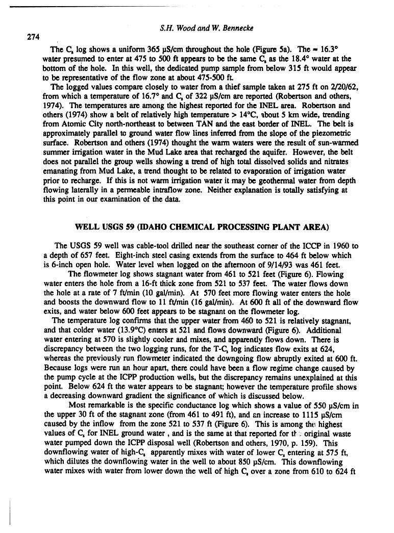
S.H. Wood and W. Bennecke274
The C, log shows a uniform 365 pS/cm throughout the hole (Figure 5a). The - 16.3°water presumed to enter at 475 to 500 ft appears to be the same (2, as the 18.4 ° water at thebottom of the hole. In this well, the dedicated pump sample from below 315 ft would appearto be representative of the flow zone at about 475-500 ft.
The logged values compare closely to water from a thief sample taken at 275 ft on 2/20/62,from which a temperature of 16.7 ° and (2, of 322 pS/cm are reported (Robertson and others,1974). The temperatures axe among the highest reported for the INEL area. Robertson andothers (1974) show a belt of relatively high temperature > 14°C, _bout 5 km wide, trendingfrom Atomic City north-northeast to between TAN and the east border of INEL. The belt isapproximately parallel to ground water flow lines inferred from the slope of the piezometricsurface. Robertson and others (1974) thought the warm waters were the result of sun-warmedsummer irrigation water in the Mud Lake area that recharged the aquifer. However, the beltdoes not parallel the group wells showing a trend of high total dissolved solids and nitratesemanating from Mud Lake, a trend thought to be related to evaporation of irrigation waterprior to recharge. If this is not warm irrigation water it may be geothermal water from depthflowing laterally in a permeable intraflow zone. Neither explanation is totally satisfying atthis point in our examination of the data.
WELL USGS $9 (IDAHO CHEMICAL PROCESSING PLANT AREA)
The USGS 59 well was cable-tool drilled near the southeast corner of the ICCP in 1960 to
a depth of 657 feet. Eight-inch steel casing extends from the surface to 464 ft below whichis 6-inch open hole. Water level when logged on the afternoon of 9/14/93 was 461 feet.
The flowmeter log shows stagnant water from 461 to 521 feet (Figure 6). Flowingwater enters the hole from a 16-ft thick zone from 521 to 537 feet. The water flows downthe hole at a rate of 7 ft/min (10 gal/min). At 570 feet more flowing water enters the holeand boosts the downward flow to 11 ft/min (16 gal/min). At 600 ft all of the downward flowexits, and water below 600 feet appears to be stagnant on the flowmeter log.
The temperature log confirms that the upper water from 460 to 521 is relatively stagnant,and that colder water (13.9°C) enters at 521 and flows downward (Figure 6). Additionalwater entering at 570 is slightly cooler and mixes, and apparently Cows down. There isdiscrepancy between the two logging runs, for the T-C, log indicates flow exits at 624,whereas the previously run fowmeter indicated the downgoing flow abruptly exited at 600 ft.Because logs were run an hour apart, there could have been a flow regime change caused bythe pump cycle at the ICPP production wells, but the discrepancy remains unexplained at thispoint. Below 624 ft the water appears to be stagnant; however the temperature profile showsa decreasing downward gradient the significance of which is discussed below.
Most remarkable is the specific conductance log which shows a value of 550 pS/cm inthe upper 30 ft of the stagnant zone (from 461 to 491 ft), and v.n increase to 1115 pS/cmcaused by the inflow from the zone 521 to 537 ft (Figure 6). This is among the highestvalues of (2, for INEL ground water, and is the same at that reported for t?: original wastewater pumped down the ICPP disposal well (Robertson and others, 1970, p. 159). Thisdownflowing water of high-C, apparently mixes with water of lower C, entering at 575 ft,which dilutes the downflowing water in the well to about 850 pS/cm. This downflowingwater mixes with water from lower down the well of high C, over a zone from 610 to 624 ft
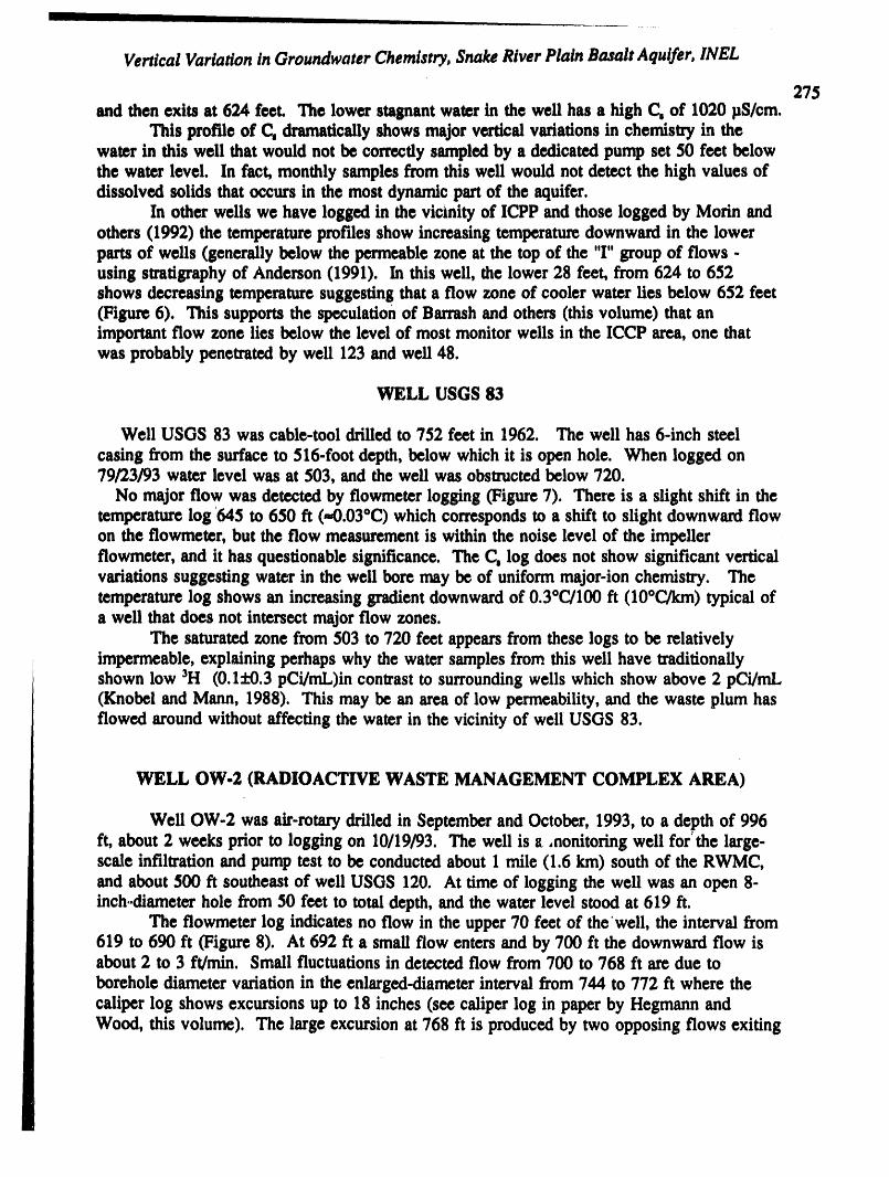
Vertical Variation in Groundwater Chemistry, Snake River Plain Basalt Aquifer, INEL
275and then exits at 624 feel The lower stagnant water in the well has a high C0 of 1020 pS/cm.
This profile of C, dramatically shows major vertical variations in chemistry in thewater in this well that would not be correctly sampled by a dedicated pump set 50 feet belowthe water level. In fact, monthly samples from this well would not detect the high values ofdissolved solids that occurs in the most dynamic part of the aquifer.
In other wells we have logged in the vicinity of ICPP and those logged by Morin andothers (1992) the temperature profiles show increasing temperature downward in the lowerparts of wells (generally below the permeable zone at the top of the 'T' group of flows -using stratigraphy of Anderson (1991). In this well, the lower 28 feet, from 624 to 652shows decreasing temperature suggesting that a flow zone of cooler water lies below 652 feet(Figure 6). This supports the speculation of Bah'ash and others (this volume) that animportant flow zone lies below the level of most monitor wells in the ICCP area, one thatwas probably penetrated by well 123 and well 48.
WELL USGS 83
Well USGS 83 was cable-tool drilled to 752 feet in 1962. The well has 6-inch steel
casing from the surface to 516-foot depth, below which it is open hole. When logged on79/23/93 water level was at 503, and the well was obstructed below 720.
No major flow was detected by flowmeter logging (Figure 7). There is a slight shift in thetemperature log 645 to 650 ft (,,0.03°C) which corresponds to a shift to slight downward flowon the flowmeter, but the flow measurement is within the noise level of the impellerflowmeter, and it has questionable significance. The C, log does not show significant verticalvariations suggesting water in the well bore may be of uniform major-ion chemistry. Thetemperature log shows an increasing gradient downward of 0.3°C/100 ft (10°CJkm) typical ofa well that does not intersect major flow zones.
The saturated zone from 503 to 720 feet appears from these logs to be relativelyimpermeable, explaining perhaps why the water samples from this well have traditionallyshown low SH (0.II-0.3 pCi/mL)in contrast to surrounding wells which show above 2 pCi/mL(Knobel and Mann, 1988). This may be an area of low permeability, and the waste plum hasflowed around without affecting the water in the vicinity of well USGS 83.
WELL OW-2 (RADIOACTIVE WASTE MANAGEMENT COMPLEX AREA)
Well OW-2 was air-rotary drilled in September and October, 1993, to a depth of 996ft, about 2 weeks prior to logging on 10/19/93. The well is a ,nonitoring well for_the large-scale infiltration and pump test to be conducted about 1 mile (1.6 kin) south of the RWMC,and about 500 ft southeast of well USGS 120. At time of logging the well was an open 8-inch..diameter hole from 50 feet to total depth, and the water level stood at 619 ft.
The flowmeter log indicates no flow in the upper 70 feet of thewell, the interval from619 to 690 ft (Figure 8). At 692 ft a small flow enters and by 700 ft the downward flow isabout 2 to 3 ft/min. Small fluctuations in detected flow from 700 to 768 ft are due to
borehole diameter variation in the enlarged-diameter interval from 744 to 772 ft where thecaliper log shows excursions up to 18 inches (see caliper log in paper by Hegmann andWood, this volume). The large excursion at 768 ft is produced by two opposing flows exiting

$.H. Wood and W. Bennecke
276
at that point in the well. Below 768 is an upward flow of 3 ft/min, which enters the holegradually over the interval 805 to 790 ft. Below 805 feet the water appears stagnant. Thusflows set up by a lower head in the 768-ft zone are coming from 805-790, and from 692-700ft.
The temperature log shows that the water entering at 692 is 10.7°C, and the waterentering at 790 ft is 10.6°C, a small but detectable difference (Figure 8). Below 790 ft thewell shows a negative geothermal gradient profile with inflections possibly related to smallflows at 835 and at 895 ft. Temperature of the bottom of the hole is 9.2°C
The specific conductance log shows that the relatively stagnant water in the topinterval from the water level down to about 650 ft has a high value, up to 760 pS/cm, at thewater level (Figure 8). Water entering and flowing down from the 692-700 ft interval has alower value of 520 pS/cm, and water entering at 805 and flowing up has a still smaller value
of 430 pS/cm. Below 805 ft, [he water has the same unifo.rm,value of 430 pS/cm. All ofthese values are above the value of 300 to 325 pS/cm considered background by Robertsonand others (1974). The vertical variations in (2, show that a dedicated pump samplingprogram in this well would not obtain a sample representative of the aquifer, because threeintervals have different chemistry.
The negative temperature gradient from 805 to the bottom of the hole at 996 ft suggeststhat a major flow zone lies beneath 996 ft (Figure 8). It has been suggested that the negativegeothermal gradient may be an artifact of drilling; however, water introduced into the wellduring drilling in September and October would most likely have been warmer that theground water, and would have warmed the lower part of the hole, rather than cooled thelower hole, as the temperature log shows.
CONCLUSIONS
Flowmeter, temperature, and specific conductance logging of borehole fluid show thatthe chemistry of ground waters varies vertically from flow zone to flow zone in many wellsthe penetrate 300 feet or less into the Snake River Plain aquifer beneath INEL. Monitoringthe aquifer with dedicated pump samples is only meaningful if one knows the permeable flowzone from which the water actually entered the well. In wells 59 and OW-2 che value ofspecific conductance varies vertically by a factor of 2. This would suggest that historicsampling and mapping of the waste plumes may not be showing the maximum waste level incertain zones of the aquifer.
The Site 14 borehole fluid is entirely fluid entering from one zone and flowing down thewell. Well 83 appears to be in a relatively less permeable section and does not showsignificant flow zones or variations in specific conductance.
Profiles of downward decreasing temperatures are observed at the bottom of wells 59and OW-2 suggesting that a major flow zone lies beneath the bottoms of these wells.
It is recommended that flowmeter, temperature, specific conductance logs combined withpreviously obtained caliper, natural gamma, and calibrated- density logs be used to design amonitoring program using a downhole wireline thief sampler to obtain ground water foranalysis from specific flow zones encountered 0y wells. Fluid specific conductance logs givean indication of chemical variation, but the actual constituents need to be analyzed from watersamples taken by thief sampler or from zones isolated by packers.
Ve_cal Variation in Groundwater Chemistry, 5rake River Plain Basalt Aquifer, INEL277
ACKNOWLEDGEMENTS
We wish to thank W. Barrash, J. Olsen, S,R. Anderson, and R. J'ensen for providingdata, discussions, and advice which contributed to this study. Niel Smith and Curtis Baker ofMt. SopHs Instruments have helped us improve our logging instrumentation over the yearsand we are most appreciative of their efforts.
REFERENCESl
Ackerman, D.J., 199 I, Transmlsslvity of the Snake River Plain aquifer at the Idaho NationalEngineering Laboratory,Idaho: U. S. Geological Survey Water.Resourc6s InvestigationsReport 91-4058, 35 p.
Anderson, S.R., 1991, Stratigraphyof the unsaturatedzone and uppermostpart of the Snake RiverPlain aquifer at the Idaho Chemical Processing Plant and test area, Idaho National EngineeringLaboratory, Idaho: U.S. Geological Survey, Water-ResourcesInvestigations Report 91-.
Bartholomay, R.C., 1990, Digitized geophysical logs for selected wells on or near the Idaho NationalEngineering Laboratory, Idaho: U. S. Geological Survey Open-File Report 99-366, 347 p.
Bah'ash, W., Morin, R.H., Wood, S.H., and Bennecke, W., 1994, Hydmstratigraphic interpretationofthe upper portion of the Snake River Plain aquifex near the Idaho Chemical Processing Plant atthe idaho National Englneering Laboratory (this volume).
Barrash, W., Morin, R.H., Wood, S.H.,Anderson, S.R., Jensen, R.G., and Bennecke, W., 1993,Geophysical logging evidence for stratlgraphlc control of hydrology in the Snake River Plainaquifer at the Idaho National EngineeringLaboratory(INEL), southeastern Idaho: EOS, v. 74,No.43,p.283-284.
Beasley,T.M.,Cecil,L,D,,Sharma,P.,Kubik,P,W.,Fehn,U.,Mann,LJ.,andGove,H.E.,1993,Chlorine-36intheSnakeRiverPlainaquiferattheIdahoNationalEngineeringLaboratory:originandimplications:GroundWater,31,V.302-310.
Bermecke,W., Wood, S.H., 1992oImpellerflow.meterloggingofvertical
crossflowbetweenbasaltaquifersthroughwellsattheIdahoNationalEngineeringLaboratory,easternSnakeRiverPlain,Idaho:aprogressreport:Boreholegeophysicsresearchprogram,DepartmentofGeosciences,BoiseStateUniversity,23p.
Bermecke,W., Wood, S.H.,Olsen,J.,andBarrash,W.,1993,Verticalcross-flowsinducedin
observationwellsbydistantpmnpingoftheSnakeRiverbasaltaquifer,easternIdaho:GeologicalSocietyofAmericanAbstractswithPrograms,v.25.no.5(Reno,Nevada,May1992).
Brott,C.A.,BlackweU,D.D.,andZiagos,J.P.,1981,ThermalandtectonicimplicationsofheatflowintheeasternSnakeRiverPlain,Idaho:JournalofGeophysicalResearch,86,11,709-I1,734.
BlackweIl,D.D.,1989,RegionalimplicationsofheatflowintheSnakeRiverPlain,northwesternUnitedStates:Tectonophysics,v.164,p.323-343.
Daniels,F.andAlberty,R.,1961,PhysicalChemistry(2ridEdition):New York,JohnWHey andSons,744 p.
Freeze, R.A., and Cherry, J.A., 1979, Groundwater:Englewood Cliffs, New Jersey, Prentice-Hall, Inc.,604 p.
Garabedian, S.P., 1992, Hydrology and digital simulation of the regional aquifer system, eastern Snake'River Plain, Idaho: U.S. Geological Survey Professional Paper 1408-F, 102 p.
Hegmann, M., and Wood, S.H., 1994, Hydrostratigraphyof the Snake River Plain aquifer beneath theRadioactive Waste Management Complex at the Idaho National Engineering Laboratory: apreliminary report: (this volume).
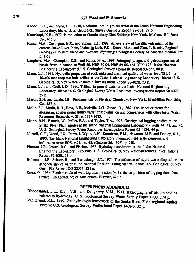
278 $.H.Wood andW. Bennecke
Knobel, L.L., and Mann,L.J., 1988, RadionucUdesin ground water at the Idaho National EngineeringLaboratory,Idaho:U. S. Geological Survey Open.file Report 88-731, 37 p.
Krauskopf, K.B., 1979, Introductionto Geochemistry(2nd Edition): New York, McGraw.HUl BookCo.,617p.
Kuntz,M.A.,Covington,H.R.,andSchorr,L.J.,1992,An overviewofbasalticvolcanismoftheeastern SnakeRiver Plain, Idaho: in Link, P.K., Kuntz, M.A., and Plait, L.B. eds., RegionalGeology of Eastern Idaho and Western Wyoming: Geological Society of America Memoir 179,p. 1-53.
Lanphere, M.A., Champion,D.E., and Kuntz, M.A., 1993, Petrography,age, and paleomagnetism of' basalt flows in coreholes Well 80, NRF 89-04, NRF 89-05, and ICPP 123, Idaho National
Engineering Laboratory:;U. S. Geological Survey Open.File Report 93-327, 40 p.Mann, L.J., 1986, Hydraulicproperties of rock units and chemical quality of water for INEL-1. a
10,356-foot deep test hole drilled at the Idaho National Engineering Laboratory, Idaho: U. S.Geological Survey Water-ResourcesInvestigationsReport 86-4020, 23 p.
Mann, L.J., and Cecil, L.D., 1990, Tritium in groundwater at the Idaho National EngineeringLaboratory, Idaho:U. S. Geological Survey Water-ResourcesInvestigations Report 90-4090,35p.
Maron,S.H.andLando,J.B.,FundamentalsofPhysicalChemistry:New York,MacMillanPublishingCo.,853p.
Moltz,F.J.,Morin,R.H.,Hess,A.E.,Melville,J.G.,G{Iven,O.,1989,The impellermeterformeasuringaquiferpermeabilityvariations:evaluationandcomparisonwithothertests:WaterResourcesResearch,v.2.5,p.1677-1683.
Morin,R.H.,Barrash,W.,Paillet,F.A.,andTaylor,T.A.,1993,GeophysicalloggingstudiesintheSnakeRiverPlainaquiferattheIdahoNationalEngineeringLaboratory-wells44,45,and46:U. S.GeologicalSurveyWater-ResourcesInvestigationsReport92-4184,44 p.
Norrell,G.T.,Wood,T.R.,Porto,I.Wylie,A.H.,Dunnivant,F.M..Newman,M.E.,andDooley,K.J.,1993, The Idaho National Engineering Laboratory integrated field scale pumping andinfiltrationtests: EOS, v.74, no. 43, (October 26, 1993), p. 240.
Pittman, J.R., Jensen, R.G., and Fischer, 1988, Hydrologic conditions at the Idaho NationalEngineering Laboratory 1982-1985. U.S. Geological Survey Water-Resources InvestigationsReport 89-4008, 73 p.
Robenson, J.B., Sc_oen, R., and Barraclough,J.T., 1974, The influence,of liquid waste disposal on the, geochemistry of waterat the National ReactorTesting Station, Idaho: U.S. Geological Survey
Open-File ReportID0.22054, 231 p.Se,,'ra,O., 1986, Fundamentalsof well.log interpretation(v. I), the acquisition of logging data: Pau,
France, E1f.Acquitalne;or Amsterdam,Elsevier, 423 p.
REFERENCES ADDENDUM
Rhodehamel, E.C., Kron, V.B., and Dougherty, V.M., 1971, Bibliography of tritium studies
related to hydrology: U. S. Geological Survey Water-Supply Paper 1900, 174 p.Whitehead, R.L., 1992, Geohydrologic framework of the Snake River Plain regional aquifer
system: U.S. Geological Survey Professional Paper 1408-b, 32 p.
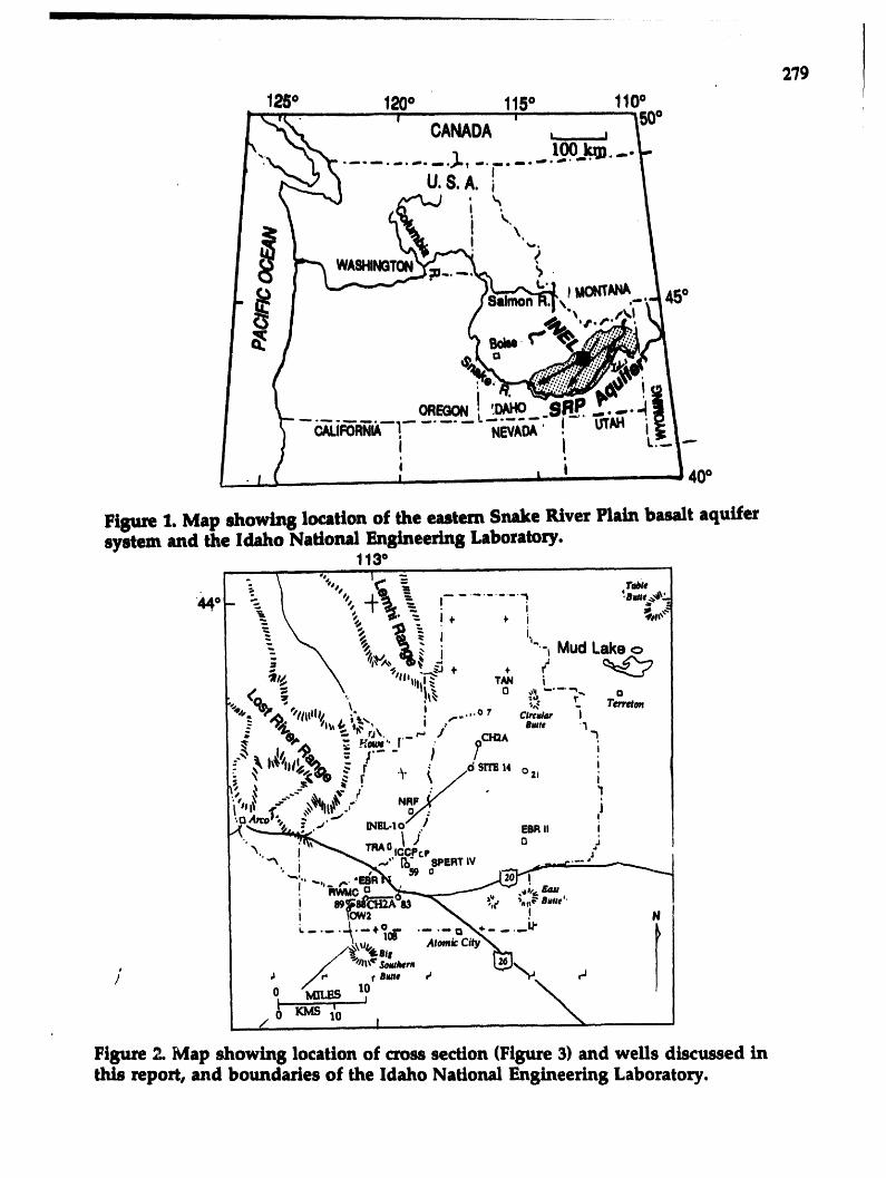

2808W NE
_ [ 11 II r [ lllUllrl I II I I UIIi lli II I[ I ....
i I i__ __ _ _ _ ]
I ........
6 KMS_
Fisure 3. Generalized seolosic cross section of selected wells at INEL (exa88eratedvertical scale). Water'level in wells indicated by dotted line (depth of basalt southof 8t8 Southern Butte ts from resistivity soundings reported by Whitehead (1992).
Fisure 4. Photogsaph ofHalliburton (Gearhart-Owen)bi-directlonal impellerflowmeter (36.5 nun diameter),and the thermistor.housin8 endof the Mr. Sopris combinationfluid-resisitivity andtemperature 1o88in8 tool (51mm diameter).


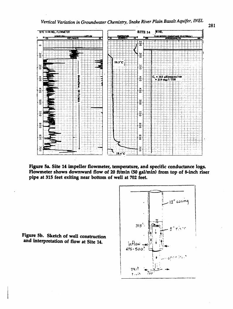
Figure Sa. Site 14 impeller flowmeter, temperature, and specific conductance logs.Flowmeter shows downward flow of 20 ft/min (SO8al/min) from top of 8-inch riserpipe at 315 feet exiting near bottom of well at 702 feet.
,.
+_+'.i_, !_.L.--+_"r/_+'rFigure Sb. Sketch of well construction I '_' ,?i\
!Iand interpretation of flow at Site 14. in_:10_ -_- i _,,.-
' ++_,
'+ +I+ +,, ?'_+_+'+"4. ,+_.+. +
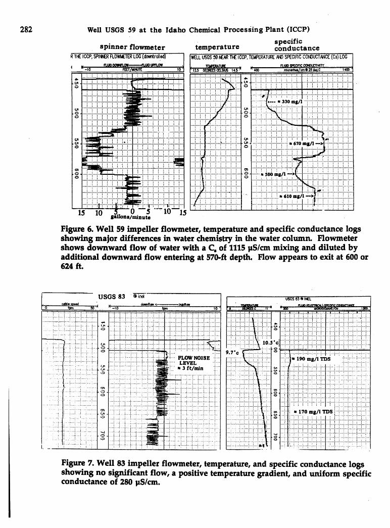
282 Well USGS 59 at the Idaho Chemical Processing Plant (ICCP)
specificspinner flowraeter temperature conductance
RTHEICCP,SPINNERFLO_dETERLOG (d(x_t_led) ] WELLUS_ 59NEARTHEICCP,T_RATURE/V,IDSPECIFICCONDUCTN_CE(Cs)LOGFLUl)_anc CONOUC11_ITY
_ T_m_ ._ _ 4oo _c,_w_/_o_c _o
! '..........L...I....f,__ .!....!....L...!........_...!....!....!....!....L..!....L...!....!
....I....L...I...L...!..L...!....!....!....0 ....!....!....!....:...:....!....!...L...!........!....L...L...!....!....!....!....!....!.... •
_ .... • • ....L,L..!....L..,i....i....L...L..i....
...._:....::.q....':....i....::....i....":....":........ i....!....!....i....':...._:...._....i....:.._ ' .-',...!....!....!....i....i..-i...._....i....
....b"i"":'"i""i'"'i'"i'"'b"i....= ....ff"::"'i'"'i'"i"b"i""i':........i""i'"'::'"':..""ff"i"':_'"i""i....
l__!i!'!!!"!!! ............i..!........i....!....':....!....!....oo...._...,_oo,_/_',.':........!....!...._,....i...._:....i....!....!....!....o '_ii_ii ....!....i.,.L..i....i....i....i....i....i........i....=._...._...._.....=.!....!...._....i....i..._i....i....i....!....!....i....i....
....!'"'!'"!""!'"'i'"i"'"!"'!'"'!....• ""!'"'!'"'bi'"'i";;'_;_i"-_[_'i'"i'"'i'"'i'"'i""i'_"IT..T..T..._....;...T..T..T...;........;....;...._...._...._.,I_,..;...._...;...._...._..._...._...
15 I0 5 "- ''I 'T-iiiiiiii.... i!i"!i!!!! _!i,:!!!!!!"!..../minute
Figure 6. Well 59 impeller flowmeter, temperature and specific conductance logsshowing major differences in water chemistry in the water column. Flowmetershows downward flow of water with a C. of 1115 laS/cm mixing and diluted byadditional downward flow entering at 570-ft depth. Flow appears to exit at 600 or624 ft.

Figure 8. Well OW2 spinner flowmeter, temperature, and specific conductance logs.Opposing intrawell flows exit at 768-depth. Water of three different chemistries
• are apparent from the specific conductance log, with the highest value at the top ofthe water column. The negative temperature gradient suggests a major flow zonelies beneath the bottom of the well (996 ft deep)

tOOo

Hydrogeology , Waste Disposal, Science and PoliticsProceedings 30th Symposium
EngineeringGeologyandGeotechnicalEngineering,1994 28_
ENVIRONMENTAL GEOPHYSICS: LOCATING AND EVALUATING
SUBSURFACE GEOLOGY, GEOLOGIC HAZARDS, GROUNDWATERCONTAMINATION, ETC.
Alvin K. Benson
Department ofGeology, Brigham Young UniversityProvo,UT 84602
ABSTRACT
Geophysical surveys can be used to help delineate and map subsurface geology,including potential geologic hazards, the water table, boundaries ofcontaminant plumes,etc.The depth to the water table can be determined using seismic and ground penetrating radar(GPR) methods, and hydroge_logic andgeologic crosssections ofshallow alluvial aquiferscanbe constructed from these data. Electrical resistivityand GPR data arc especially sensitive tothe quality of thewater and other fluids in a porous medium, and these surveyshelpto identifythe stratigraphy, the approximate boundaries of contaminant plumes, and the source andamount of contamination in the plumes. Seismic, GPR, electromagnetic CCLF),gravity, andmagnetic data help identify and delineate shallow, concealed faulting, cavities, and othersubsurface hazards. Integration of these geophysical data sets can help pinpoint sources ofsubsurfacecontamination, identify potential geological hazards,and optimize the location ofborings, monitoring wells, foundations for building, dams, etc. Casestudies from a varietyoflocations will illustrate these points.
INTRODUCTION
Geophysical methods can play a veryimportant rolein environmental and engineeringapplications that involve shallow subsurfacemapping studies. These methods areapplicableto the study of groundwater contamination, underground cavities (natural or man-made),subsurfacefaulting, buriedpipes, cables, barrels,etc., allof which pose potentially dangerousgeological hazards(Benson, 1993). Geophysical exploration is a nondestructive,cost effectiveway to help locate and characterize these hazards.
In addition to helping locate the water table, characterization of subsurfacecontamination produced by hazardous materials has become an important application ofgeophysical methods. The objectives of subsurface investigations at sites containingcontamination caused byhazardous materialsinclude:(a) the location of buriedmaterial; (b)the determination of the presenceof contaminant plumes, their source(s), and geometry; and(c) the assessment of associated hydrogeologic conditions. The purpose for locating buried
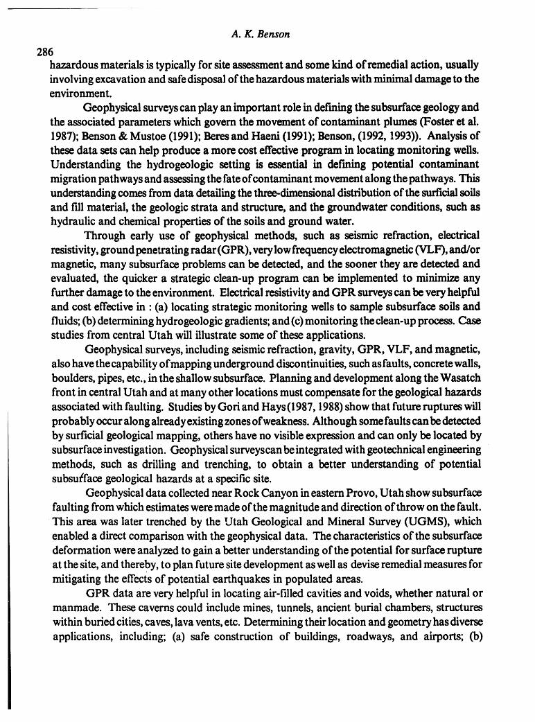
A. K. Benson
286hazardous materialsis typically for site assessment and some kind of remedial action, usuallyinvolving excavation and safedisposal of the hazardous materials with minimaldamage to theenvironment.
Geophysical surveyscan play animportant role in defining the subsurface geology andthe associated parameterswhich govern the movement of contaminant plumes (Foster et al.1987);Benson & Mustoe (1991); Beresand Haeni (1991); Benson, (1992, 1993)). Analysis ofthese data sets can help produce a more cost effective program in locating monitoring wells.Understanding the hydrogeologic setting is essential in def'ming potential contaminantmigration pathwaysand assessing the fateofcontaminant movement along the pathways. Thisunderstandingcomes from data detailingthe three-dimensionaldistribution of the surfidal soilsand fill material, the geologic strata and structure, and the groundwater conditions, such ashydraulic and chemical properties of the soils and ground water.
Through early use of geophysical methods, such as seismic refraction, electricalresistivity, ground penetrating radar(GPR), verylow frequencyelectromagnetic (VLF), and/ormagnetic, many subsurface problems can be detected, and the sooner they are detected andevaluated, the quicker a strategic clean-up program can be, implemented to minimize anyfurtherdamage to the environment. Electrical resistivity and GPR surveyscan be very helpfuland cost effective in : (a) locating strategic monitoring wells to sample subsurface soils andfluids; (b) determining hydrogeologic gradients;and (c) monitoring the clean-up process. Casestudies from central Utah will illustrate some of these applications.
Geophysical surveys, including seismic refraction, gravity, GPR, VLF, and magnetic,also have the capability ofmapping undergrounddiscontinuities, such asfaults, concretewalls,boulders, pipes, etc., in the shallow subsurface. Planning and development along the Wasatchfront in central Utah and at manyother locations must compensate for the geological hazardsassociated with faulting. Studiesby Gori and Hays(1987, 1988)show that future ruptures willprobablyoccuralong alreadyexisting zonesofweakness. Although somefaultscan bedetectedby surficial geological mapping, others have no visible expression and can only be located bysubsurfaceinvestigation. Geophysical surveyscanbe integrated with geotechnical engineeringmethods, such as drilling and trenching, to obtain a better understanding of potentialsubsutface geological hazards at a specific site.
Geophysical data collected nearRock Canyon in eastern Provo, Utah show subsurfacefaulting from which estimates weremade of the magnitude and direction of throw on the fault.This area was later trenched by the Utah Geological and Mineral Survey (UGMS), whichenabled a direct comparison with the geophysical data. The characteristicsof the subsurfacedeformation wereanalyzed to gain a better understanding of the potential for surfaceruptureat the site, and thereby, to plan future site development aswell as devise remedialmeasures formitigating the effects of potential earthquakes in populated areas.
GPR data arevery helpful in locating air-filled cavities and voids, whether natural ormanmade. These caverns could include mines, tunnels, ancient burial chambers, structureswithin buriedcities, caves, lava vents, etc. Determining theirlocation and geometry has diverseapplications, including; (a) safe construction of buildings, roadways, and airports; (b)

Uses of Environmental Geophysics
287archaeological excavations; and (c) mineral investigations.
A case study to determinethe locationof an undergroundlaboratoryat BrighamYoungUniversity will be examined. Good contrast exists between the dielectric constants for theoverlying soil, the concrete ceiling, floors, and walls, and the large air-Idled cavity.Consequently, GPR was successful in outlining this underground cavity. In addition, amagnetic surveywas successful in locating underground piping at BrighamYoung University.
CONTAMINATED GROUNDWATER STUDIES
Fresh, clean groundwater is becoming an increasingly valuable resource around theworld. In some area, supplies have been greatly decreased by careless management and/ordisposal ofhazardous materials. Hydrogeologists requiremethods to map the soil stratigraphyat sites where contaminants are in the subsurface.
The first site of investigation is associated with leaking fuel tanks at a site in UtahCounty, near Provo, Utah. The general layout of this site is shown in Figure 1. Theunderground storage tanks leaked hydrocarbons (gasoline and diesel fuel) into thegroundwater which flowed to the southwest following the water-table gradient of about 1.1meters/100 meters. Basedupon maps by Hintze(1988) and ourwelland GPR data, the geologyat this site was determinedto consist of threemain layers: (1) an asphalt/sand layer(0.9 to 1.3meters thick);(2) a layer of silty-clay and sand (1.7-2.4 meters thick); (3) asand and gravel layer(1.1-1.8 meters thick); and (4) a water-bearing, sandy-gravel layer. The water table atmonitoring wells l and 2 was 3.2 and 3.6. meters, respectively.
This site is currently undergoing bioremcdiation to recoverthe contaminated soft andground water. Contaminated ground water is being pumped out of the subsurface and thenreinjectedafter it iscombined withnitrate andphosphate nutrientsfromcommercial fertilizers,as well as with hydrogen peroxide, to help the microorganisms (bacteria) digest thegroundwatercontaminationin situ. The nutrientsadd nitrate (NO3) and Phosphate (IK)_')ionsto the subsurface, and the degradation of the hydrocarbons adds carbonate (CO3_),sulfate(SO4"),and chlorine (CI) ions. Although hydrocarbon plumesmight typically be mapped asresistivityhighs, these additional ions could decrease the electricalresistivity and outline thecontaminant plume as a resistivity low.
Electrical resistivity data were collected at the site using a Bison Offset SoundingSystem (BOSS) in a Wenner arrayconfiguration. In Particular, the sounding centered nearMW- 1willbe analyzed (Figure 1). These data are plotted in Figure 2 as a function ofelectrode
spacing. The data were modeled for subsurface structure using the BOSSIX software fromInterpex. Initial layer thicknesses and internal resistivitieswereconstrained by the geologicaldata from MW-I. Table l shows the initial model and the final computed model after twoiterations. The first layer (.91 meters thick) corresponds to the asphalt/sand layer, the second(1.44 meters thick) to the silty-clay, sand layer, the third (1.08 meters thick) to a sand,gravel/cobble layer,and the fourthtoalayer ofwater-saturated sediments. This correlates withthe stratigraphic data cited above from MW-1. Adding up the thicknesses of the upper three
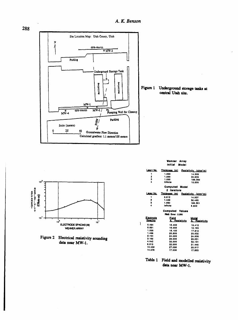
A. K. Benton
288ii i i ii i iii i i
Sit=L=c=r.iouM.,p: UmhCmm_, Ut_
N
Gpp .tlo..,.,.p_ _ __- e ._W-3 __
.... -]- l-
---i' --L.....----Unde_grouP.d Sm_g_ Tank
Figure 1 Underground storage tanks atcentralUtah site.
.... Ivt_-t
, ¢O_-So_r.="MW 2 / ' _pin$ W¢_ for ClequxupMW4
' Zo, ...... , i GroundwaterFlow Dkectiou[
I Caicubt_ gradle._ 1.I meters/lO0meu_x's!i i i i
Wonner Array' Initial Model
Thickne. (m) Resletivi_ (ohm'el1 1.ooo 14.sooa 1.ooo 3o.0oo3 1.000 110.300
101 4 infinite I0,000
R Computed ModelA E 2 Iterationsp S _ Thickness(m_ Resistivity (ohm'm_P' ,_ , 0.012 14.937F_TSE , 1.43, ,0.4,S
+ ,o,o ,...o,N . 4 Infinite fi,053
T , _ ' Computed Valuesij RM8Error:2.288
Electrode _ Mod_101 r ' ' ' ' '_ i110 10 _ _- _ A. Resistivity
W_XlN_,q_y o.ool +e.ooo 1e.le31.ooo 18.1oo 17.o121.4ee 2o.soo 2o.03a•.,s, _4.ooo ,,.,o0
Figure 2 Electrical resistivity sounding +.10. .ooo ..o014.04, 3,.ooo s2.1=1data n_r MW'I. 0,813 am,000 31.446
lo.ooo 27.ooo 20..,1714.078 17.000 17.803
Table I Field and modelled resistivitydata near MW-I.
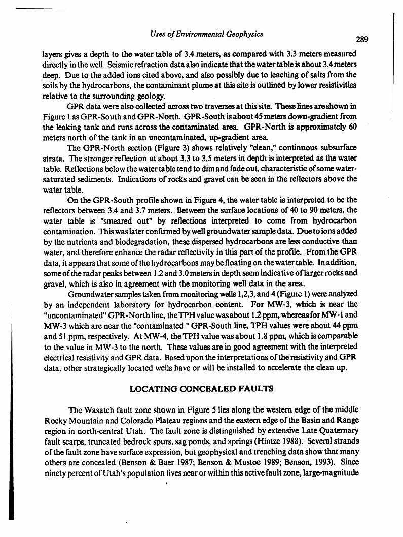
Uses of Environmental Geophysics 289
layers gives a depth to the water table of 3.4 meters, as compared with 3.3 meters measureddirectly inthe well. Seismicrefraction dataalso indicate that the water table is about 3.4metersdeep. Due to the added ions cited above, and also possibly due to leaching of salts from thesoils by the hydrocarbons, the contaminant plume at this site is outlined by lower resistivitiesrelative to the surrounding geology.
GPR data werealso collected across two traversesat this site. These lines areshown in
Figure I asGPR-South and GPR-North. GPR-South isabout 45 meters down-gradient fromthe leaking tank and runs across the contaminated area. GPR-North is approximately 60meters north of the tank in an uncontaminated, up-gradient area.
The GPR-North section (Figure 3) shows relatively "clean,"continuous subsurfacestrata. The stronger reflection at about 3.3 to 3.5 meters in depth is interpreted as the watertable. Reflections below the water table tend to dimand fade out, characteristic ofsome water-saturated sediments. Indications of' rocks and gravel can be seen in the reflectors above thewater table.
On the GPR-South profile shown in Figure 4, the water table is interpreted to be thereflectors between 3.4 and 3.7 meters. Between the surface locations of 40 to 90 meters, the
water table is "smeared out" by reflections interpreted to come from hydrocarboncontamination. This was later confirmed bywellgroundwater sampledata. Due to ions addedby the nutrients and biodegradation, these dispersedhydrocarbons are less conductive thanwater, and therefore enhance the radar reflectivity in this part of the profile. From the GPRdata, it appears that some of the hydrocarbons may be floating on the water table. In addition,some ofthe radarpeaks between 1.2and 3.0meters in depth seemindicative oflarger rocksandgravel, which is also in agreement with the monitoring well data in the area.
Groundwater samplestaken from monitoring wells 1,2,3,and 4 (Figu_ 1)wereanalyzedby an independent laboratory for hydrocarbon content. For MW-3, which is near the"uncontaminated" GPR-North line, theTPH value wasabout 1.2ppm, whereas for MW-I andMW-3 which are near the "contaminated "GPR-South line, TPH values were about 44 ppmand 51 ppm, respectively. At MW-4, the TPH value was about 1.8 ppm, which is comparableto the value in MW-3 to the north. These values are in good agreement with the interpretedelectrical resistivity and GPR data. Based upon the interpretations ofthe resistivity and GPRdata, other strategically located wells have or will be installed to accelerate the clean up.
LOCATING CONCEALED FAULTS
The Wasatch fault zone shown in Figure 5 lies along the western edge of the middleRocky Mountain and Colorado Plateau regions and the eastern edge of the Basin and Rangeregion in north-central Utah. The fault zone is distinguished by extensive Late Quaternaryfault scarps, truncated bedrock spurs, sag ponds, and springs (Hintze 1988). Severalstrandsof the fault zone have surface expression, but geophysical and trenching data show that manyothers are concealed (Benson & Baer 1987; Benson & Mustoe 1989; Benson, 1993). Sinceninety percent of Utah's population livesnearor within this activefault zone, large-magnitude
i
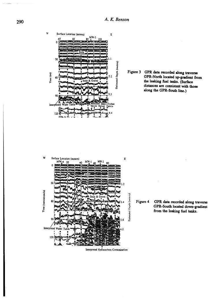
290 A. K. Benson
W SurfacsLocation(meters) , E
,t5 _ 65 85 _W-3 105o
30 " " l.l
O I -L_'-- 4--- II
.. rt._e_.a _ • _.,. , _, __ __ Figure 3 GPR data recorded along traverse• I--_.-- I-- s-- _I -- I
= _o__2'z _ GPR-North locat_ up-grmlientfrom.......... , , - the leaking fuel tanks. (Surface
_ distancesare consistentwith those
, , along the GPR-Southline.)90 m . "33
Wa_ar Tab1_
c.r___ ..&,;, , _ r
,,u,t '.--,- _-n"--_"-q--_--__l'l_._t ¢'_ , "at : m _ _t_.._ . .,.31_.
W SurfaceLocation (meters) EMW-4 20 MW.I MW.2
_ _ 4o_o
30: , ; _' _-2 ....... 1",
60' "___ L_"____"_1"_ 2.4 Figure 4 OPR data recorded along traverse
,_ _,_,_, _t ._'t'__. _-_i_A__ GPR-South located down-gradient.__- , _ ' _ from the leakingfuel tanks.
' 3.6
Interp 4.2
I I • II., _I
120 ' " _ ' r J " "_
InterpretedHydrocarbonContamhaation
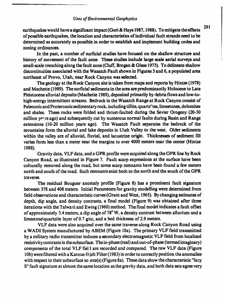
Uses of Environmental Geophysics
291earthquakeswould have a significant impact (God &Hays 1987,1988). To mitigate the effectsofpossible earthquakes, the location and characteristicsof individual fault strands need to bedeterminedas accurately as possible in orderto establish and implement building codes andzoning ordinances.
In the past, a number of surficial studies have focused on the shallow structure andhistory of movement of the fault zone. These studies include large scale aerial surveys andsmall.scale trenching along the fault zone (Cluff, Brogan & Glass 1973). To delineate shallowdiscontinuities associated withthe Wasatch Fault shown in Figures 5 and 6, a populated areanortheast of Provo, Utah, near Rock Canyon was selected.
The geology at the Rock Canyon site is takenfrom maps and reports by Hintze (1978)and Machette (1989). The surficialsediments in the areaarepredominantly Holocene to LatePleistocene alluvial deposits (Machette 1989),deposited primarilyby debrisflows and low-to-high-energy intermittent streams. Bedrock in the Wasatch Range at Rock Canyon consist ofPaleozoic andProterozoic sedimentary rock, including tillite,quartz;tes, limestones, dolomitesand shales. These rocks were folded and thrust-faulted during lhe Sevier Orogeny (20-30million y_,_.rsago) and subsequently cut by numerous normal faults during Basin and Rangeextensions (10-20 million years ago). The Wasatch Fault separates the bedrock of themountains form the alluvial and lake deposits in Utah Valley to the west. Older sedimentswithin the valley are of alluvial, fluvial, and lacustrine origin. Thicknesses of sediment fillvaries form less than a meter near the margins to over 4000 meters near the center (Hintze1988).
Gravity data, VLF data, and a GPR profile were acquired along the GPR line by RockCanyon Road, as illustrated in Figure 7. Fault scarp expressions at the surface have beenculturally removed along the road, but some scarp remnants have been found a few metersnorth and south of the road. Such remnants exist both to the north and the south of the GPRtraverse.
The residual Bouguer anomaly profile (Figure 8) has a prominent fault signaturebetween 378 and 408 meters. Initial Parameters for gravity modelling were determined fromfield observations and characteristic curves (Grant and West, 1965). By changing estimates of
depth, dip angle, and density contrasts, a final model (Figure 9) was obtained after threeiterations with the Talwani and Ewing (1960) method. The final model indicates a fault offsetof approximately 3.4 meters, a dip angle of 78*W, a density contrast between alluvium and alimestone\quartzite layer of 0.7 g/co, and a bed thickness of 2.9 meters.
VLF data were also acquired over the same traverse along Rock Canyon Road usinga WADI System manufactured by ABEM (Figure 10a). The primary VLF field transmittedby a military radio transmitter induces a secondary electromagnetic VLF field from localizedresistivity contrasts in the subsurface. The in-phase (real) and out-of-phase (termed imaginary)components of the total VLF fiel] are recorded and compared. The raw VLF data (Figure10b)were filtered with a Karo us-FIielt Filter (1983)in order to correctly position the anomalieswith respect to their subsurface so _rce(s)(Figure 8a). These data show the characteristic "lazyS" fault signature at almost the same location as the gravity data, and both data sets agree very

A. K. Benson
292-- II,¢'':" _ _'_" _:: -- _r
"'° J. Z'l 'l!
i J [ Iv)U)_.,T t",,,,-_,'(,, =m |E i ,||"
I XIDDL[_oc_MOUrrAZNSi
., = _-I !|
|
. ,/ !
! / COLORADOPI.ATF.AU iI
i / i! / !_-"I Ii /'
t I !i ' !
|0 lOO l*J.lell l
I I I(_.... I I 1100 g.i.l_llllte]r I ; .
ICoet_ Imm_:50eatm
0 1000 S_0 10000 Metro
Figure'5 Regional location mapshowing the o--- ,0we a_o ....'"' _ l,,,,Wuatch Fault andphydographic
, provinces (afterI-Iintze(1988), Figure 6 Mapof the Prove, Utaharea showingp.80), the traceof the WasatchFaultand
the Rock Canyon site (fromU.S.GeologicalSurvey 30x60 minutemetrictopographicmap of Provo, Utah, 1986).
/
I
Rock Canyon Site: Provo, Utah N I
/II-;I.,e.,ioo:,.50m.,o. T,o.o .o,,,,,of
Surface Localio. (,ncters)
Figure 7 Map of Rock CanyonRoadshowinglocation of the GPR (& VLF & Gravity) traverse,observed fault scarp trace, and the UGMS trench. The dashedsection of the faultscarp indicates thatmuch of it has been culturallyremovedacross Rock CanyonRoad.
Uses of Environmental Geophysics
well with the fault scarp location observed in the field. 293The GPR profile over the same traverse (Figure 11)also suggests a high-angle normal
fault in the subsurface, whose surface exposure is probably the ex_rp to the north and southof the roadway. Some of its surface expression was probably removed when Rock CanyonRoad was built. The upper layers in the GPR profile are interpreted to be road fill, soils, rocks,and gravel. Some of the rocks and gravel are probably from post-fault debris fJow out of thecanyon. Using an average dielectric constant of 2.5 for dry soils and rocks near Rock Canyon,the fault offset is estimated to be 3.3 meters, and the dip angle of the interpreted fault isestimated to be 75"W. Above the fault plane between surface locations 385-395meters, aradarreflection is seen which we interpret to come from the colluvial wedge ofmaterials associatedwith the faulting.
After the geophysical work was completed, the Utah Geological and Mineral survey(UGMS) dug a 30-meter long trench across the fault scarpapproximately 5meters due northofour GPR line. In going north form the GPR traverse to the trench location, the north sideof Rock Canyon Road slopes down a gradient of about 1.5meters, and most of this materialappearsto be road fill and gravel base, with some rock debris from Rock Canyon.
A schematic diagramof the trench is shown in Figure 12fW.R. Lurid,UGMS, personalcommunication, 1991). The trench indicates a single-event rupturewith 3.5 meters of throw,dipping at 76"W beneath the scarp. Comparing the GPR data (Figure 11) with the trenchcross-section suggests that the fault reflections are probably coming from the rock layerbetween the upper and middle soil horizons. Examination of natural exposures in the trenchshowed competent rock between these two horizons, consisting of fractured limestone andquartzite, as well as some debris-flow deposits from the canyon. The gravity,VLF and GPRdata are all in good agreement with the geology of this subsurface faulting.
OUTLINING UNDERGROUND CAVITIES
The effectiveness of GPR in locating and outlining the boundaries of an undergroundcavity was tested by running some traverses over an underground physics laboratory locatedon the campus of Brigham Young University, Provo, Utah. The surveys were conducted andinterpretations made knowing only the general area where the lab was located. To avoid bias,comparisons with lab blueprints were not made until the geophysical work was completed. AnE-W cross section of the lab taken from the blueprints is sketched in Figure 13a, and aschematic of the experimental setup is shown in Figure 13b.
The air cavity and floor of the lab can be clearly seen on the GPR profile inFigure 14. This traverse was taken over the central portion of the lab ceiling. The overlyingsoil, concrete ceiling, and associated multiple reflections are in the upper 40nanoseconds ofthisprofile. Since the relative dielectric constant of air is I and from Figure 14 the time intervalbetween the interpreted ceiling and floor is 60nanoseconds, the average depth form the ceilingto the floor is 9.1 meters. This is the same value as found on the blueprints for the lab.Between the surface positions at 6 and 9 meters, the larger amplitudes along the floor ofthe lab

Gravity Fault ModelM E
JSSo
-- 1S.II0, :_.
vt,e (_ _ Gmv_,t _ VLe(_) f
340 3S0 380 370 380 30O 400 41O 420 430 440Dlatenee (m) o ...........................................................
C 0.0 L .... -i y ...... 2- );_i-2L
_)._o VLF FaultModel
"": *:u_,__ _ Figure9 Faultmodelsconsmgtedfromgravity • :"_Im_ irmuP_
i ...... t ....a :."_._.".", . . , ........ , - . . and VLF cbt_ shownin Figu_ 8. _ _ -_- ,m
Sunh__ (mam)S,_ace_ (roans)
Figme 8 Ralichud Ipmvitychemmid filte_VLF _ _ Figure10b OriginalVLF fielddataacquiredalongdata along the GPR traverseshown in \ theGPR line shown in Figure 7.Figure 7.
|Figure 10a lllustration of VLF principle. As the
operator walks along traverse A-B, theWADI VLF system detects the phase lagbetweenthe primaryand secondarywaves.

Uses of Environmental Geophysics
w ' e 2954"" ...e
s_zrface
I0
I I
t_.O
6.7
390 39S tOO _S 4t0 41S
Surface Location (me".n)
Figure 11 GPR profile along Rock Canyon Road. Vertical dashed lines represent adistance of about 3 meters. Horizontal lines are 20 nanoseconds
ap_,a. The m fault is clearly visible.
W E
15.15 ----- tim,, s,,, w,,, Rock Canyon Trench .Lill&lie fell IlOf|lm
.... tmmr kit Itoellm. Fault Plnno
""Lt_
157.5....... .......... . ............ . ..... -....... , .... 4--370 375 380 385 390 395
Sttrfnce Locnlio. (meters)
Figure 12 Schematic diagram of the stratigraphy in the UGMS trench along Rock CanyonRoad. Three mapped soil horizons are shown. Heavy black lines representfaults; arrows show directions of relative movement. The upper soilhorizon is on a debris flow, the middle soil horizon is on a matrix-
supported debris flow, and the lower soil horizon is on a high-energyfluvial deposit.
A.K.Benson|
296areinterpretedtobetheapproximatelocationofaVandeGraaffgeneratorhousedinthelab.Thislocationwaslaterconfirmedbyinspectingtheblueprintsandthelabitself.
AnotherGPR traversewasrecordedacrossU.S.Highway6 neartheEureka,Utah
locationshowninFigure5.Eurekaisanoldminingtowndatingbacktothe1890'shavingnumerousmineshaftsandtunnelsunderthetownandsurroundingareas.Locationsofmany
oftheolderundergroundexcavationsareunknownsincetheywereneverrecordedon any
maps.MostoftheminesareinCambrianandOrdovicianlimestone,andtheareaisrichinoresofgold,silver,copper,iron,andothermetals.Tertiaryintrusionshavebroughtinore-
bearingsolutionswhichhavesolidifiedinthecracks,vugs,andfissuresinthelimestone.Inmany placesthegroundiscrackedorcollapsedfromtheminingactivity,andsomeminesare
now justcone-shapedcave-ins(Chronic,1990).Two areas of apparent subsidence in the upper strata can be seen in Figure 15. Any
surfaceexpressions of this slumping were most likely filledin manyyearsago when the highwaywas resurfaced. Some nearby cracking and warping in the highway may be clues that somesubsurface movement is still occurring. Almost directly below each area of subsidence is ahyperbolic diffraction pattern that is characteristic of reflections from localized objects orcavities in the subsurface. The hyperbolae in Figure 15most likely originate from man-madecavities, such as amine shaft or a tunnel, but could also arise from sinkholes carvedout in thelimestone. Cavity diameters appear to be on the orderof 2-4 meters.
Whatever the source of the apparent subsurface cavities and possible associatedsubsidence, the important point isthat GPR can often be successfulin locating these potentialhazards. This information is veryuseful in planning and site development. Earlydetection ofsuch cavities or the mechanism causingsubsidence canresult in substantial savings in time andmoney.
UNDERGROUND PIPING
Magnetic exploration can be used to locate and characterize subsurface features thatdiffer in magnetic susceptibilityfrom thesurrounding material. Someexamples include buriediron objects, ore bodies, and rock units containing magneticminerals. A magnetic surveywasconducted on the Brigham Young University (BYU) campus to determine the location anddepth to some underground high-temperature water pipes. The experimental setup isillustrated in Figure 16a.
The residual magnetic values measured with a proton-precession magnetometer areplotted in Figure 16b. The maximt,m magnetic field intensity correlates with the location ofthe subsurface pipe.
The depth to thecenter of a hollow cylinder (Telfordet al., 1984)can be approximatedby solving the following equation for r:
F, = 2kFoxDt / r2 , (1)

297
Uses of £nvironmenml Geophysics
$udm I_n_m (mueu_l
Sieve'/
_"_ 4b-._' m_""_ _M°DIlePower Supply.
Af*',el Vm ile_l_nmflf(:}emntlm*
(_.j. 3 4LJ Figure 13b Illustrationof the GPRexplorationsetup.Sclte main)
Figure 13a Schematicdiagram c:ftheImderlFotrodphysicslaboratory '_ the_mpus ofBrighlmYoung t_niven6ty,Provo, U_ah.

298 A. K. Benson
#
MeasuredMagneticFieldIntensity
/_ s4-
t 53.5-
"_ 53 "_-_ ,.....
o 52-
C
51"
5°S._o .i'o o 1'o ioFigure 162t Illustration of magneticexplorationsetup. Distance(m)
Figure 16b Reduced magnetic filed data collected overunderground piping on Bdgham YoungUniversity campus.
_ sw_ _ Hollow C dinderModelX (mlMeasures C='.c'.dlzod FI 1400' I---..
-18 S3,1¢5 _05 2.38-IS ,_33e0 _0 3.4,1 | Diameter(m) 0.254i 1200-._2 s_e _ s._ ITh_. (m)O.Oml,_I _ 1000-
•6 83058 58 21.15 800"4 _ _ eo.Ts | |,slnno uaso 1= 12o.o6 _o.$ t4.118 1310 !10.7_ _ 400"8 _ 20S 21AS iT.. r'_
9 82796 404 9.4_S _ 20012 52e65 .t05 5.3S c1_ s2teO .t12 =._ _ O _ - - ;- .... \_ o c =
18 S2egS _ 2.38 ,s _m- ---at21 524N .S04 135 -200-24 IJ2_42 -_8 1.3427 82400 .¢tO 1.06 -400 ....30 S2C'eS ._S 0._ -20 -15 -10 -5 0 5 10 15 2033 S1610 .1390 0.71 Distance (m)38 scece .2194 0.60
-,,- Measured Anomaly _ Calculated Anomaly
Table 2 Modelled magnetic data over a hollow pipe.Figure 17 Modelled magnetic data superimposed on the
reduced magnetic field data.
i rql , i
UsesofEnvironmentalGeophysics 299
where F, is the anomaly value, k isthe magneticsusceptibility contrast, F, isthe strength of theearth'smagnetic field (53,000 nanoTeslas at thissite), D is the diameterof the pipe, t isthe pipethickness, and r is thcdepth to the centerof the pipe. Since the BYU utilities departmenttoldus that the piping used was 10inches in diameter and 0.36 inches thick, and since k for this steelisabout I, the depth to thecenterof the pipe isestimated fromequation (I) to be0.76 m, which
" was later confirmed by BYU utilities. Table 2 shows the calculated anomaly values over thepipe using the above equation. These modelled values are compared with the measuredanomaly values in Figure 17. Since the steel pipe is quite shallow, one would expect a narrowanomalous peakasshown by themodelled data. However, dueto a nearbyundergroundcableand steel supports for the piping, the measuredanomaly is broadened. These effects werenotaccounted for in the magneticmodelling, but verygood resultswere still obtained for locatingand estimating the depth to this subsurface piping.
CONCLUSIONS
Depending on the geological setting, geophysical surveys are reliable, rapid, andeconomical formappingshallowsubsurfacesediments andassessinghydrogeologic conditions.The thickness of the sediments, the depth to the water table, the presence of groundwatercontamination, the location ofsubsurface faults,undergroundcavities, and subsurface pipingcan all be reliably mapped at field sites where subsurface geometries are not too complex andwhere sufficient contrasts exist in the physical properties being measured. The surfacegeophysical methods for general investigation of the shallow subsurface are summarized inTable 3 and the common borehole geophysical methods aresummarized in Table 4. Morespecifically, the surface geophysical methods effective for locating and mapping buried wastesand utilities aresummarizedin Table 5, with detailed specifications for mapping contaminantplumes summarized in Table 6.
In particular,electrical resistivity and GPR data from sites in central Utah have beenhelpful in mapping groundwater contamination produced byleaking underground fuel tanks.Based upon the estimated depths to the areas of subsurface contamination from the resistivityand GPR data, the lateralextent ofthe contaminant plumes areoutlined and monitoring wellsinstalled at strategic locations at the sites. Analysis of the monitoring well data shows thatestimated water table depths and qualitative assessments of contamination location andconcentrations inferred from the resistivity and GPR data are in good agreement with thedepths and contamination levels found in the wells.
Gravity, VLF, and GPR data collected in east Provo, Utah demonstrate the r_:liabledetection of shallow concealed faulting in appropriate geologic settings. Interpretations ofthese geophysical data sets coincide with manyfeatures observed in a recently opened nearbytrench. The net offset and dip of the fault correlate quite well. Determining the characteristicsand distribution of subsurface faulting and folding can provide useful information forestablishing and implementing building codes and zoning ordinances in the Provo area.
Cavity detection is another challenging exploration problem that requires good

Table 3 Common surface/subsurface geophysical methods
300 (after Melvin, 1993).
SURVEY METHOD APPLICATIONS
Magnetic Locate buried metallic objects and utilities,map buried channels and depth to bedrock ifmagnetic minerals are present and locatefaults and fractures.
Electromagnetic (EM) Locate contaminant plumes, boundaries oflandfills, buried metallic objects or ut.itities andi
, locate fractures and faults•
Electrical Resistivity i Locate contaminant plumes, the water table and
[ locate fractures and fa_.Its.
Gravity I Determine overburden thickness, map bedrock
I
] topography and locate fractures and faults.
Seismic (Reflect.ion I Determine overburden thickness, locate the
i
and Refraction) i water table, lithologic boundaries, fracturest and faults.I
Ground Penetrating i Locate buried objects whether metallic orstrucv.tresorboundariesoflandfillsand can
Radm-{GPR} [ assistinlocatingcontaminantplumes,fracturesfaultsand karsttopography.
Table 4 Common borehole geophysical methods(after Melvin, 1993).
i,,,lit! I
SURVEY METHOD ! APPLICATIONS
Caliper Logs I Determine llthologlc and stratlgraphlc
I correlations, fractures and solution openingsI and theconstructionofexlsr.tngwells.i ,,, __
Electric (Resistivity ! Determine lithologlc and stratigraphicand Spontaneous correlations, grain size and effective porosityPotential} .Logs I and locate water level and saturated zones.
Natural Gamma Determine depth and concentxation of clayor shale.
,,,, ,, __
Gamma-Gamma ! Determine total porosity or bulk densl .ty, locatewater level and saturated zones and the
constructionofexistingwells."
Neutron i Determine total porosity or bulk density, specificI yields of unconfined aquifers, moisture content,
infiltration, and to locate water level andi
saturated zones.,,,, I
ii i i i ' '' i
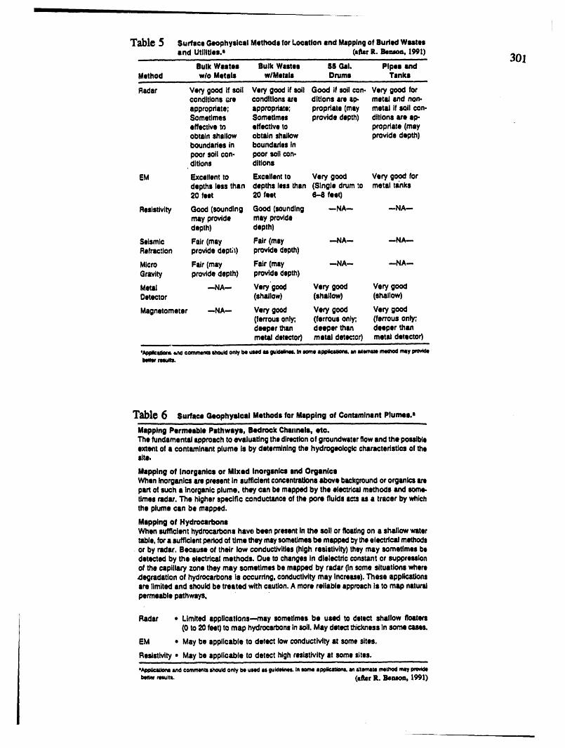
'l"ab|(_ _ Surface GeophysicalMethodsforLocationend Mappingof Bulled W_tel
and Utilities... ; (ifter g. bees, 1991)- 301........ ..,k;..,.. e.,kw..,.. . a.,. ,,,...dMethod wlo Metals w/Metals Drum Tanks
i, i i | _ -
Radar Vew goodif soil Very goodif soil Good if soilcon. Very good forconditions_re conditions_e ditions ares_. metal and non-appropriate; appropriate; propdale (may metal if soil con-Sometimes Somedmu provide depth) ditionsate .p-effectivetn effectiveto propdate (mayobtainshallow obtainshaJlow providedepth)boundariesin bounds'assinpoorsoil con- poorsoilcon-ditions ditlons
EM Excellentto Excellentto Very good Very good fordepthslessthan depthsless than (Single drumto metal ts_nks20 feet 20 feet 6-8 feet)
Resistivity Good(sounding Good(sounding --NA-- --NA-..may provide may providedepth) depth)
Seismic Fair (may Fair (may ..-NA-. -.NA--.Rob'action providedepth) providedepth)
Micro Fair (may Fair (may --NA-- --NA--Gravity providedepth) providedepth)
Metal -.NA-- Very'good Very good Very goadDetector (shallow) (shallow) (shallow)
Magnetometer --NA-- Very good Very good Very good(ferrous0nly; (ferrousonly;, (ferrousonly:deeperthan deeper than deeper thanmetal detector) metal detec'.cr) metal detector)
i , ,i
'Ap_k:mSom__n4commentsshout4onlybevasdas9uld411netInI_XTIO,p_ anMemmmethodmy wOrSe_ rasuns.
'l?ab|o 6 surface Geophysical Methods for Mapping of ContaminantPlumes.e
MappingPermeable Pathways, BedrockChmmels,etc.ThefundamentalapproachtOevaluatingthedirectionof groundwaterflowandthe possibleextentof a contaminantplume is by determiningthe hydrogeeloglccharacteristicsof theSite,
Mappingof Inorganics or Mixed Inorganlcsend OrganicsWhenInorganicsam presentin sufficientconcentrationsabovebackgroundororganicsmpartof sucha inorganicplume, th_f san bemappedby the electricalmethodsand some.timesradar.The higherspecificconductanceof the pore fluidsac'.su a tracer bywhichthe plumecan be mapped.
Mappingof HydrocarbonsWhensufficienthydrocarbonshlve been presentIn the sell or floatingon a shallowwatertable,fora sufficientperiodof tJmetheymaysometimesbe mapped_ytheelectricalmethods
• or byradar. Becauseof their low conductJvitlss(high resistivity)theymay sometimesbedetectedby the electricalmethods, Due tochangesin dlelecfficconstantorsuppressionof the capillaryzonethey may sometimesbe mappedby radar (insomesituationswhere_legredationof hydrool,,bonsia occurflng,conductivitymay increMe).These applicationsare flmitedand shouldbe treated withcaution.A more reliableapproachis to mapnaturalpermeablepathways.
Radar • Limitedapplications--may sometimesbe used to detect shallowflcatanl(0 to20 feet)to map hydrocad_nlinsolhMay detectthicknessinsomecases.
EM • May be applicableto detect lowconductivityat somesites.
Resistivity* May be applicableto detect highresistivityat somesites.
•_ and commen_l Should Only be used as _ide_n4s. In Iome III)Pl_ an .,1ornate morned may ix_Me
_.w mol.L (abr R. Ikmoa, 1991)

A. K. Benson
302
resolution and good depth penetration. GPR can be successful in detecting near-surfacecavities when the host rock has a relatively low electromagnetic wave attenuation factor. Thegeometrical i'eaturesof an underground laboratory at Brigham Young University weresuccessfully outlined and specified in depth using GPR surveys. Interpretations of the ceiling,floor, and aircavity are in good agreement with the blueprintsof the laboratory. GPR dataalso provided useful information about the location and approximatedepths for two apparent,:avities and associated areas of subsidence under U.S. Highway 6 near Eureka, Utah.
Magnetic exploration is a primary method for locating subsurface pipes, cables, orebodies, archaeological artifacts, and metal objects in general. The location and depth toundergroundhigh-temperaturewater pipesat BrighamYoung Universityweredelineated usinga proton-precession magnetometer. Likewise, this method can locate buffed barrelsand oldwell casingsthat pose significant contamination hazards, as well as map the metal objects ina buried landfill.
In sure.mary,in appropriate geology, geophysical s_jrveyscan provide useful, cost-effective 'data which can help assess potentially dangerous geological hazards, includinggroundwater contamination, concealed faulting, undergroundcavities and piping. Planningand remedial measures based upon these data can then be implemented to hell, protecthumanlife and produce minimal threat to the environment.
_ REFERENCES
Benson, A.K., 1993. Case Studies Using Ground Penetrating Radar to Help AssessGroundwater Contamination, Shallow Faulting, andCavities: Proceedings ofthe 29thSymposium on Engineering Geology and Geotechnical Engineering, 63-89.
Benson, A.K., 1992. Integrating Seismic,Resistivity, and Ground Penetrating RadarData toDelineate the Water Table and Groundwater Contamination: in Water-RockInteraction. Vol. 1,Low TemperatureEnvironments. A.A. Balkema, Rotterdam, 359-366.
Benson, A.K. and Mustoe, N.B., 1991. Ground Penetrating Radar, Electrical Resistivity, andWater Quality Studies Integrated to Determine the Source(s) and Geometry ofHydrocarbon Contamination at a Site in North-central Arizona: Proceedings of the27th Symposium on Engineering Geology and Geotechnical Engineering, 38.1-38.18.
Benson, A.K. and Mustoe, N.B., 1989. Seismicand Gravity Surveys asTools in DelineatingSubsurface Geology and Assessing Some Geologic Hazards: Proceeding of the 25thSymposium on Engineering Geology and Geotechnical engineering, 25-30.
Benson, A.K. & Baer,J.L., 1987. Close OrderGravity Surveys: A Means of Fault Delineationin Valley Fill Sediments: Proceedingsofthe 23rdSymposium on EngineeringGeologyand Soils Engineering, 219-240.
Benson, R.C., 1991. Remote Sensing and Geophysical Methods for Evaluation of SubsurfaceConditions: in Practical Handbook of Ground-Water Monitoring: D.M. Nielsen, ed.,Lewis Publishers, Chelsea, Michigan, 143.194.
Uses of Environmental Geophysics3O3
Beres, M. and Haeni, F.P., 1991. Application of'Ground-Penetrating-Radar Methods toHydroseologic Studies: Ground Water, 2,_,375-386.
Chronic, H., 1990. Roa&qideGeology of Utah: Mountain Press Pub;ishing Company,Missoula, Montana, 336 p.
Cluff, L.S., Brogan, G.E. &Glass, C.E., 1973. Wasatch Fault, SouthernPortion: Woodward-Lundgren and Associates, Oakland, California. Report preparedfor Utah Geologicaland Mineral Survey, Salt Lake City, Utah.
Foster, A.R., Veatch, M.D., and Baird, S.L., 1987. Hazardous W_te Geophysics:Geophysics, The Leading Edge, 6, 8-13.
Gori, P.L. and Hays, W.W. (eds.), 1987. Earthquake Hazards Along the Wasatch Front,Utah: U.S. Geological Survey Open File Report 87.154.
Gori, P.L. and Hays, W.W. (eds.), 1988. Assessment of Regional Earthquake Hazards andRisk Along the Wasatch Front, Utah, Volume HI: U.S. Geological Survey Open FileReport 88-680.
Grant, F.S. and West, G.F., 1965. Interpretation Theory_in Applied Geonhysics: McGraw-Hill, New York, 282-287.
Hintze, L.F., 1988. Geologic History of Utah: BrighamYoung University Geology Studies.Special Publication 7, 7-10, 29-32, 77-89.
Hintze, L.F., 1978. Geologic Map of the Y Mountain Area, East of Provo, Utah and CrossSections of the Y Mountain: Brigham Young University Geology Studies, SpecialPublication 5. Map scale is 1:24,000.
Karous, M. and Hjelt, S.E., 1983. Linear Filtering of VLF dip-angle measurements:Geophysical Proslxx:ting,31, 782-794.
Machette, M.N., 1989. Preliminary Surficial Geologic Map of the Wasatch Fault Zone,EasternPartof Utah Valley, Utah Country, and Partsof Salt Lakeand Juab Countries,Utah: USGS Misc. Field Studies Map and Pamphlet MF-2109. Map scale is 1:50,000.
Melvin, R.J., 1993. Geologic Skills Used in the Site Characterization ofEnvironmental/HazardousWaste Projects:TheProfessional Geologist, September, 12-15.
Talwani, M. and Ewing, M., 1960. Rapid Computation of Gravitational Attraction of Three.Dimensional Bodies of ArbitraryShape: Geophysics, 25, 203-225.
Telford, W.M., Geldart, L.P., Keys, D.A., and Sheriff, R.E., 1984. Applied Geophysics.Cambridge University Press, New York, New York, 161-162.

Hydrogeology, Waste Disposal, Science and PoliticsProceedings 30th SymposiumEngineering Geology and Geotechnical Engineering, 1994
EFFECTS OF SHALE AND CONTAMINANTS ON (V./Vr) RATIOS IN 305TRANSVERSELY- ISOTROPIC GEOLOGY
ALVIN K. BENSON
Department of Geology, BrighamYoung University, Provo, Ut 84602
ABSTRACT
Themechanicalpropertiesof rocksandsoils can be calculatedfromthe shear-wavevelocity,Vs,the compressional-wavevelocity,V_,andthe density,or from(Vs/Vl,)ratiosandthe density.Therefore,determinationof (Vs/Vp)ratios is an importanttool to assistwithlithologicalidentificationandmanyassociatedapplications.
In mostgeologicsettings,mixturesof differentmaterialsarequitecomraon,andit isimportantto understandthe effect of thin laminationson measured(Vs/Vp)ratios. Anequationisderivedfor(Vs/Vp)in transversely-isotropicmaterials.Itis foundthatevensmallamountsof a secondcomponent,suchas 10%shale,can change(Vs,'F) ratiossignificantlyfromthat ofapureendmember,suchassandstone.Casestudieswillillustratesomepracticalapplications.
INTRODUCTION
Foranelasticearthmodel,onecanpredictthe occurrenceof two distinct body-wavetypes:(1) acompressionalwavewithparticlemotionin linewiththe directionof propagationand(2)a shearwavewithparticlemotion perpendicularto the directionof propagation.Ateachboundaryof themodel,anyincidentbodywaveis transmittedand reflectedasbothwavetypes. The Zoeppritzequations(Telfordet al., 1976)predict the amplitudeand wavefrontdirectionof the resultingP- andS-wavesignalsasa functionofthe angleof incidenceforanincident P- or S- waveat eachboundary.
It is possible to generateand receivepolarizedversionsof these elastic signalsbyconfiningthegroundmotion at the sourceto emphasizeacertainpolarizationandbyusingasensorthat issensitiveto particlemotionin onlyonedirection (Garotta, 1983). In additionto compressionalsources,sevealshearwavesourceshavebeendeveloped.Conocodevelopeda S- wavevibratoralong with the P- wavevibratorin the 1950's. In a laterdevelopment,CompagnieGeneralede Geophysique(CGG)developeda transversehammersourcecalledSEISLAPR. With SEISLAP,CCGdemonstratedhow explosivesourcescould becombinedwithtransversereceiversforreceptionofhorizontallypolarizedshear-wavesignals.Stilllater,Prakla-Seismosdevelopeda techniquewhich usestwo 180° out-of phaseP-wavevibratorsplacedside-bysideandperpendicularto the seismicline,knownasSHOVER.TM (SeeWaters1987;Danbom and Domenico, 1987).

A.K.Benson
3O6Two uses of shear-wavedata have beome readily apparent(Danbom and Domenico,
1987). First,since shear waves arenot propagatingunder the influenceof the fluid in the porespace of the rock, measured propertiesof shear waves having gone through or reflected fromrocks with anomalous pore fluids will be different when compared with the response ofcompressional waves. Secondly, by measuringthe velocity ratio Vs/VP for a sequence in thestratigraphiccolumn, some of the physical characteristicsof that zone can be described. Inaddition, Poisson's ratio can be directly calculated from Vs/Vr. Indeed, if one uses eitherGardner'sequation (Gardneret al., 1974)with the variableV_,or the relationship establishedby Ludwig et al. (1970) with Poisson's ratio as the variable, the density of the formation canbe empirically estimated. With the availability of Vv.V,, density and Poisson's ratio, theremainingelastic constants, namely Young's modulus, bulk modulus, and shearmodulus canbecalculated. In other words, compressional and shear wave datatogether form a synergisticsystem. Some applications of compressional plus shear wave data have been discussed byPol.qkov,et al. (1980), Meissnerand Hegazy(198 l), Helbig and Mesdag (1982), Heidell (1985),and Ahmed 0989).
Gregory (1976a) showed a relationship between the pore fdler and the Vs/Vpratio forporous sedimentary rocks. Pickett 0963) and Domenico 0983, 1984)showed a separation oflithology as a function of the Vs/Vv ratio. Tatham and Stoffa 0976) and Tatham 0982)discussed Vs/V_,ratios as possible lithology and hydrocarbon indicators, and Tatham andGoolsbee (1983)extended these ideasto themarineenvironment. Brownet al. (1989) describedusage of Vs/Vpratios for finding oil and gas. Most of these are empirical relationships whichshould be used subject to the conditions established by the original author(s), since universalapplication of empirical formulaccan be inaccurate. This paper considers the effect of thinlayers of shale or contaminants, such as hydrocarbons, on (Vs/Vv)ratios in otherwise puresedimentary rocks, such as sandstone or limestone.
VELOCITIES IN TRANSVERSELY-ISOTROPIC MEDIA
Thinly laminated materials arequite common in most geological settings, with manysedimentary sections consisting of thin layers of contrasting properties. Hence, it is animportant problem to understandtheeffect thst thin laminations have on physicalproperties,such as measured (Vs/Vp) ratios. Laminated materials consist of a number of isotropiccomponents in layers parallel to a horizontal plane, with variablethicknesses, such as layersof shale in sandstone or in limestone, or layersof sandstone or limestone contaminated withhydrocarbons in other layers of sandstone or limestone.
In order for the layered material to approximate a homogeneOusmedium, its averagepropertiesmust be the samethroughout anyelementaryvolume in the medium. An elementaryvolume must have its largest dimensions small in comparison to the shortest probingwavelength of seismicenergy. Therefore, ,'_helayers need not be identical for each elementaryelement, but the average properties must be the same. This implies that the fractionalconcentration of the various components (hit, N2, N3,...) are the same for each elementary

EffectsofShaleandConmnu'nantson(VslVP)Ratios
307element,wherethenumbersrefertodifferentgeolosicalconstituents.
Bysymmetry,itcanbeshownthatalaminatedmaterialshouldbehaveasatransversely
-isotropicmediumwiththeverticalaxisbeingtheuniqueaxis.Hence,asshownbyWhite(1965),theP-andS-wave(horizontal-shear)velocitiesareexpressedas
Vs = {(Nsin2Y.+ Lcos2Y,)/0}_and
Vp = {(Asin2T.+ C cos2T,+ L + D)/2p}_, (I)
where
D=(G+ H)_,
O = {(A-L)sin2(y_)-(C- L)cos=(¥,)}2,
H = 4(F+ L)sin2(%)cos_(¥_),
A,C,F,L,Naredependentonthepropertiesofthetransversely-isotropicmedium,andT=istheanglebetweenthedirectionofwavepropagationandtheverticalZ-axis.Whiteshowsthatfor
alaminatedmaterialwithN componentsthatC,F,L,N,A,andp aregivenbythefollowingexpressions:
A = R + (T2/W),
c =(i/w),
F = (T/W),
N
R = _ [4 _n_(7._+ _)] / (_.,+ 2_,),i=l
N
W = _ (ni) / (;'i + 2Pt),i=l
N
T = _ (rile.i) / (_'i + 2p|),i=l
N

A.K. Benson
N
308 N = _ n_l_i,i=l
N
p = E ni Pl, (2)l=!
where n_,pi,k_,I_arethe fractionalconcentration, density, and Lame'sconstants, respectively,for the ithconstituentof the laminated medium. Thedensity of each component is
p,= 0.(1-@+ Pr, (3)
where p, is the density of the matrixgrains, ptis thedensity ofpore fluids,and _ is theporosity.
COMPOSITE (VJVr) DERIVATION
Since (Vs/Vr) data from verticalseismicprof'fles,checkshots, and CDP stacked seismicsectionsessentially simulatewavepropagation in theverticaldirection, let's takeT. = 0. Hence,the expressions for Vs and Vpin equation (I) simplify to
Vs = (L/p)_ and Vv = (C/p)_. (4)
Consequently, the (Vs/VPr) ratio for a transversely-isotropic (composite) material is given byequation (4) as
= (5)
asin White (1965), Lcv'm(1979), and Melia and Carlson(1984). Fora two-component system,L is the geometric mean of the shearmoduli,
L = {(n,/It,) + (n2/It2)}" and
C = {(nJ(k, + 2_,) + n2/(k2+ 2p2)}", (6)
where n,, t_l, _'l and 112,t_2,_.2are the fractional concentrations and elastic parameters for thetwo components, respectively. After some extensive algebra, equations (5) and (6) yield
(Vs/Vt,)__ = (ttl/(k, + 21t,))v.(i_2/(k2+ 2_2))v.yr., (7)
whereY = (n_(_2+ 21_2)+ n2(k_+ 2ttt)/(n_tt2+ n2ttl).
However, from equations (2) and (4) for a one-component system,

Effects of Shale and Contaminantson (VslVP) Ratios
Vs' = (p/p_),, 309
and
VPl= ((_.l + 2Pl)/Pl) 'a'
for the first component, and
v_ =(t,jp,)_,
and
v_ =((x_+2tt_)/p_)'* (s)
for the second component. Combining the results of equations (7) and (8),
(VdV,.).m_,= (V,/V,,)(VdV,OZ",. (9)
where Z = (n_P2V_ + n2 p_V_)/(n_ p=V_ + n2p_V2s,),
which isthe equation for the (Vs/Vp)ratio for atransversely-isotropic,two-component system.Using the bulk and shear moduli of the rock components, this can also be written as
(vdv,.)_,.,. = (v,,/v,,,)Ordv,OQ_, 0o)
where Q = (nl(k2 + (4/3) P2)+ n2(kt + (4/3) pt))/(n, P2+ n2Pt),
where k is the bulk modulus (or incompressibility), and p is the shear modulus. Thus, thecomposite (Vs/V_,)ratio is the product of the (Vs/V_) ratios of the individual componentsmultiplied by a factor involving the percentagesof individual components and the shearandbulk moduli. Note that equation (9) is a function of the square root of the shale content, as isan empirical relationship determinedby Eberhart-Phillipset al. (1989) using lab data from 64different water-saturated sandstones, including clean quarry sandstones, other well-consolidated sandstones from quarries and boreholes, tight-gas sands, and samples (somepoorly consolidated) from offshore wells in_the Gulf of Mexico.

A.K.Benson
310 CASE STUDY EXAMPLES
Using equation (9) or equation (10), the effect of thin shale laminations on the (Vs/VP)ratio in limestones and sandstones can beestimated. First, let's consider some vertical seismicprofile data tabulated by Omnes (1980) for the ParisBasin, approximately 50miles southwestof Paris, France. Both compressional and shear wave events wererecorded. Table 1 showsparametersselected from the Kimmeridgian shal_ and the Lusitanian li_',_stones, which areadjoining strata at about 1000 meters deep. Figure 1 shows a plot of the composite (Vs/Vp)data calculated from equation (9) and shown in Table 1. Note the rapid change from the valueof the (VJVp) ratio for Lusitanian limestones when they arecontaminated with rathersmallamounts of laminated shale. For example, for the shaley limestone, only 10%shale gives acomposite (Vs/Vr) of.529, whereas the Lusitanianlimestone has a VJVp of.550, and 20%shaledrops the ratio to .515, which is a change of 6.4%. Thus, the composite (Vs/Vs,)ratio may bea good indicator of shale as the Kimmeridgian shales grade into the Lusitanian limestones.
As a second case, let's applyequation (9) to some Gulf Coast well log data compiled byGregory (1976b). Parameters selected for some brine-saturated Gulf Coast sands and shalesat a depth of5,182 metersareshown in Table 2. The averagesandstone porosity at this depthis 17.8%,while for the shales it is 15.3%. These porosities are kept fLxedas the shale contentvaries, and the resulting composite (Vs/Vr) data in Table 2 are plotted in Figure 2. Again,significant changes occur in the (Vs/VP) ratio of clean, saturated sands as they grade intolaminated shaley, sands. These results agree favorably with lab findings of Mann and Fatt(1960). These changesarea good indication ofcontent and are probably important estimatorsto help correctly determinethe subsurface lithology. Of course, this could be very critical inhydrocarbonreservoirevaluation or in soil and groundwatercontaminationevaluation. If fielddata and lab resultsaregood quality, thencombined with the geology and experience in agivenarea, the data can be modeled and correlated to point out regions where hydrocarbons andcontaminants most likely exist.
A third example is the basin hinge-line model of Tatham et al. (1977). They considershalegrading into shaley limethen into limestone atabout 1100meters deep. Parameterstakenfrom their compressional and shearwavemodels areshown in Table 3. The effect ofthe facieschange can be seen directly from thenonlinear drop in the composite (Vs/VF)ratio as shalinessincreases. Similar results to those shown in Figures 1-3 arealso found from equation (9) forBereasandstone data (Porosity- 10.3%)compiled byWinkler(1985)and for Ottawa sandstonedata (Porosity - 37.74%)compiled by Domenico (1976) by letting the shale content vary from0%to 100%. J
As another example, let's considera shallow, transversely-isotropi¢medium consistingof a sand partially saturated with acontaminating fluid, such as leaking oil, layeredwith a drysand. What happens to the (Vs/VF)ratio as the amount of contaminated sand increases? Theparameters selected for the two sands are taken fromdata reported byMcLamore et al. (1978),and are shown in Table 4. The composite (Vs/Vp)ratio decreases rapidly as the amount ofcontaminated sand increases (Figure 4). The same phenomena occurs as the amount of clay

EffectsofShaleandContaminantson(VslVP)Ratios
311Paris Basin
Lusitanian Limestone gimmeridtian shale
Vp - 4,745 m/see Yp,, 3,195 m/sec
V s - 2,610m/sec Vs.. i,502 m/see
Vs/Y_ - .550 VI/V , - .470
Density= 2.60 Ii/cc Density- 2.32 8/co
Fractional Shale Concentration V(._._) comDoslte
0.0 .5500.1 .$290.2 .5150.3 ._040.4 .4960.5 .4590.6 .4840.7 .4500.8 .4760.9 .4731.0 .470
Table 1 Parametersand calculation of (VJVp) compositefor shaly limestonesin the Paris Basin. The depth considered is approximately l,000meters.
Ns/Vp)
.560
.550
.540
.530
.52O
.510
.500
.49(
.480
.470 '_,
0.0 0.1 0.2 0.3 0.4 0.5 0.6 0.7 0,8 0.9 1.0ShaleFraction
Figure 1 (Vs/Vp) compositeasa function of fractional shaleconcentrationfor limestonesinthe
Paris Basin.
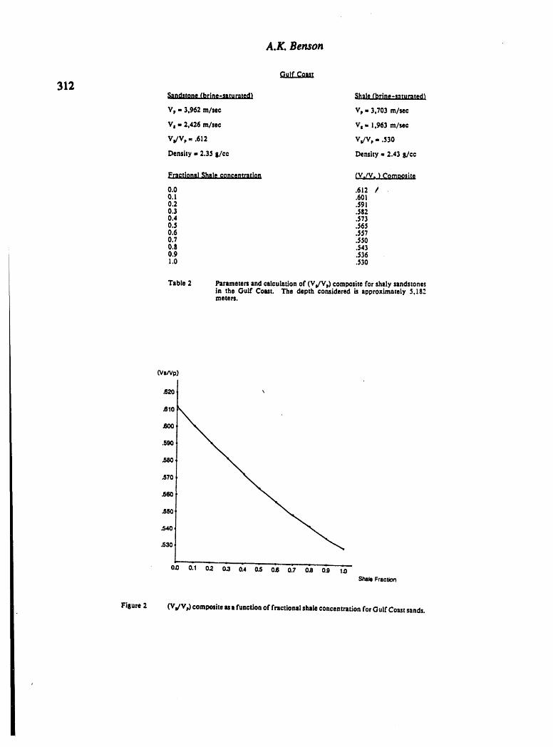
A.K,Benson
Gulf'Coast
312Sandstone (brjpe-saturatedl Shale(brine-s=turated_
Vp - 3,962 m/see Vt ,, 3,703 m/see
Vs - 2,426 m/see Vs - 1,963 m/see
V_/V, -, .612 Vs/V , - .530
Density ,, 2.35 8/cc Density - 2.43 g/co
Fractional Shale concentration _V./V. ) Composite
0.0 .612 /O.l .6010.2 .$910.3 .5820.4 .5730.5 .5650.6 .5570.7 .5500.8 .5430.9 .5361.0 .530
Table 2 Parameters and calculation of (Vs/V P)composite for shaly sandstonesin the Gulf Coast. The depth considered is approximately 5,182metees.
(Va/Vp)
.620
.610
.BOO
.590
.580,
.570
.560
.55O
.540,
.530
0.0 0.1 0.2 0.3 0_4 0_5 0'.6 0."_' 0.8 0.9 1.0ShaleFraction
Fillure 2 (Vs/Vp) composite asa function of fractional shale concentration for Gulf Coast sands.

Effec_of Stmle andContaminantson(Vo'VP)Ratios
.,,t. - Hi., Li,,c_odel 313
V,- 3,4"/5 m/sec Vv = 2,743 m/sec
Vs - 1.91? m/sec YS - 1,382 m/sec
V#V, - .552 V#V, = .504
Density • 2.37 g/cc Density • 2.25 g/cc
Fractional _hale _oncentratiojl CV.IV._Comngsite
0.0 .5520.1 .5430.2 .5360.3 .5300.4 .5250.5 .$200.6 .$160.7 .$130.8 .5090.9 .$061.0 .$04
Table 3 P:zrsmetersand Calculationof (VJV r) compositefor shaly limestonesin a basin-hinge line model. The approximazedepth is i,i00 me:era.
(vs/yp)
.54O
-520
.51o
.500
--
o.o o:I o_,o-_0:4o-_o.e 0:7 o.e o:9 I.oShaleFraction
Figure 3 (Va/V p)compositeasa function of fractional shaleconcentration for limestonesin a
buin hlnse line model.
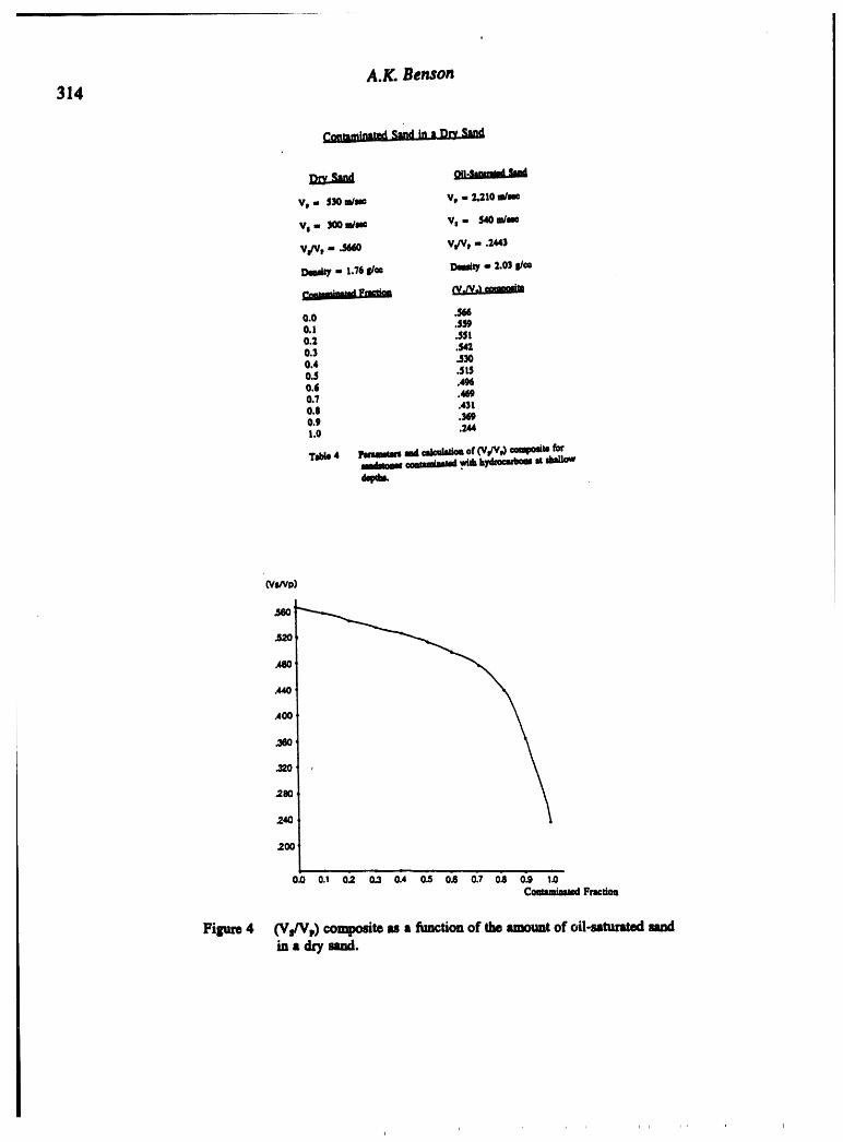
A.K.Benton314
Conmmt_,*t_$_ndinlDry S_ld
Vp,, 530_lm Vp- 2,210m/ue
VI ,,, 300m/me Vs ,, _ m/_
V,N_ - .S660 V,/V_- .2443
- 1.76I_ Oemty- 2.O3i_co
.5660.0 .SS90.1 .5,510.2 .5420.3 .S300.4o.s .5150.6 .496.4690.7 .4310.8 .3690.9 ._1.0
T_ 4 pmmmn mdc._n_s or(V_Vp)comtmt*totrod.raMausmi,_ _ 8 _
(vs/v_)!
.s2o
_o
_t4o
_o ,
28o
2.4o
2oo
CommimmiFraction
Pigum4 (Vs/Vp)compositeasstfunctionof themount of oil-_ sandin s ch7msd.

EffectsofShaleandContaminantson(Vs/VP)Ratios
315contaminatedwithleakingoilisinc_asedinadry,cleansand(Table5,Figure5).However,whentheamountofoil-saturatedclayisincreasedinabrine-saturatedsandthereisamuch
smallerdecreaseinthecomposite(VJVv)ratio(Table6,Figure6).The decreaseinthecomposite(Vs/Ve)ratioisalmostlinearforthiscase,and itwouldtakeveryhighquality
compressionalandsheardatatodetectthecontaminationfromthecomposite(Vm/Vv)ratio.Noticethatforeachofthethreecasesofhydrocarboncontaminatedlayersthatthe
composite(VJVr)ratiodecreasesasaconvex-shapedcurve,whereasforthepreviousthree
casesofshalecontaminatingapuresandstoneorlimestonethatthecomposite(VJVp)ratio
decreases as aconcave.shaped curve. Thus, for some cases,this shape differencemight beusedas an indicator of hydrocarbon contaminated layers versus shale contaminated layers. Inaddition, since the f'wstthreeexamples werefor d_"-Izr,consolidated sediments and the lattertwo were for shallow, unconsolidated sediments, thisshape differencemight be an indicator ofdepth and type of sediments involved.
The accuracy of equation (9) was tested by using lab data from Kowallis et al. (1984)for sandstone cores obtained from three Gulf'wells drilled in the West Delta Block, Plaque-Mines County, Louisiana. The sandstone at3863.9.meterscontains I1%clay,mostly kaolinite,and has a porosity of 21.7%. At a confining pressureof 48.3 MPa, lab measurements on thewet sandstone core yielded Vv = 3,630 m/sec and V, = 2,080 m/sec, so that the composite(Vs/Vp)= .573. From Tathamet al., the average Gull'Coast sandstone density at this depth is2.27 g/cc, Vp = 3,551 m/sec, and v s = 2,109 m/sec, and for shale, Vv= 3,414 m/see and V, =1,809 m/sec. The average density of ke_,linite from well logs is 2.42 g/cc (Doveton, 1986).Using this data in equation (9), the composite (Vs/Vp)= .583, a difference of 1.7%with themeasured value of.573. Obviously, other factorsalso needto beconsidered, such as degreeandtype ofcementation, how the shale is distributed, porosity changes, fluid saturations, pressuregradients, etc., but it is obvious that shalecontent is a first-ordereffect in the determination of(Vs/Vp)and that equation (9) appears to model this variable reasonably well.
CONCLUSIONS
The (VJVv) ratio is a very useful parameter to help identify rock matrixtype and fluidsaturation. A relationship was derived for transversely-isotropicmedia showing the effect ofthin laminations (stringers) of contaminants on the (Vs/V_,)ratio of clean sedimentary rocks.This relationshipestimates variations in (Vs/Vp)ratios forshaley sandstones, shaley limestones,limey sandstones, sandy limestones, limey shales, oily sandstones, etc.
Severalcase studies using publisheddata wereexamined showing theeffect ofshale andhydrocarbon content on (Vs/Ve)ratios in sandstones and limestones. Small amounts ofshalecan change this ratiosignificantly. The composite (Vs/Ve)ratio is afunction of the square rootof theclay content, bulk moduli, and shearmoduli, and of the (Vs/Vp)ratios of the individualclean lithologies making up the rock. This relationship yields reasonably accurate (Vs/Vv)ratios when compared withlab valuesfor shaley sandstone cores. With good quality fielddata,combined with the geology of the area and available lab results, the derived expressions in

A.K.Benson316
Cemamt_t_l L"I_ tn a _ Samtl
vp,- _ _m Vp- 1,700Wm
v, - 300a/m V, - _tgOWm
V,/% - _ Vd% - ._
o.oo.1 .JS30,2 .1'38O.3 ,,5210.4 .J01O.S .4780.4 .4SO0.7 .4160.8 .3730.9 .$I$1.0 .229
Tat_S 1_nmem mi_.datm _r(vj_v_)ooapou_
CVaNp)
.520
.480
.440
.400
_60
.,32O
280
240
2O0
o_ 02,O_o3 o14o_ i.6' o:7o-_o:9_oComminatedFracuon
Figure $ (Vs/Ve) composite as a function of the amount of oil-ssturated clay

E._ecuo/ShaleandContaminantson(Vu'VP)Ratios
317
BriM.S_ _
Vp - 2,210m/_ Vps 1,'_0 m/_
vdv,. ,:Am vJv, - .2294
0.0 .2440.1 .2420.2 .2400.3 .2380.4 .234O.J0.6 .2330.7 .2320.8 .231O.9 .2301.0 .229
Figure6 (VdV:,)composiu:u a fim_tiouof timamountofoi1_ clayin • brinHatumted sand.

A.IL Benson
318equation (9) or equation (10) can be used to help model the data to point out regions wherehydrocarbons, geothermalreservoirs,groundwater,soil and groundwatercontamination, etc.might best be located.
I_BFEIUINCI_
Ahmed, H. 1989, Application of mode-converted shear waves to rock-property estimationfrom vertical seismic profiling data. Geoph_ics 54, 478-485.
Brown, R.L., Cook, R.N., and Lynn, D. 1989. How useful is Poisson's ratio for fmding
oil/gas? World Oi1209, 99-106.Danbom, S. and Domenico, S.N. 1987. Shear Wave Exploration. SEG, Tulsa, OK.Domenico, S.N. 1976. Effect of Brine-Gas Mixture on Velocity in an Unconsolidated Sand
Reservoir. Geonhysics 41,882-894.Domenico, S.N. 1983. Sandstone and Limestone Porosity Determinations from Shear- and
Comp_ional-Wave Velocity. 53rd SEG meeting, Las Vegas, Nevada.Domenico, S.N. 1984. Rock lithology and porosity determination from shear and
compressional wave velocity. Geophysics 49, 1188-1195.Doveton, J.H. 1986, Lo_ Analysis ofgubsurface Geolot 7. John Wiley & Sons, New York,
N.Y.Eberhart-Phillips, D., Han, D.H., and Zoback, M.D. 1989. Empirical relationships among
seismicvelocity, effectivepressure,porosity, andclaycontent in sandstone.54, 82-89.
Gardner,G.H.F., Gardner,L.W., and Gregory, A.R. 1974. Formation Velocity and Density-The Diagnostic Basis for StratigraphicTrust. Geophysics 39, 770-780.
Garotta, R. 1983. Comparisons Between P, SH, SV, and Converted Waves. CompaganieC_n_ale de G6ophysique, Technical Series No. 521.82.08, Massy, France.
Gregory, A.R. 1976a. Fluid Saturation Effectson Dynamic ElasticProperties of SedimentaryRocks. Geophysics, 41,895-921.
Gregory, A.R. 1976b. Some Aspects of Rock Physics from Laboratory and Log Data that areImportant to Seismic Interpretation. Notes distributed at AAPG-SEG School onStratigraphic Interpretation ofseismic Data, September 20-25, 1976, Houston, Texas.
Helbig, K. and Mesdag, C.S. 1982. The Potential of Shear-Wave Observations. Geoph_icalPro._ectin_ 30, 413-431.
Kowallis, B.H., Jones, L.E.A., and Wang, H.F. 1984. Velocity-Porosity-Clay ContentSystematics of Poorly consolidated Sandstones. Journal of Geophysical Research 89,10,355-10,364.
Levin,F.K. 1979. SeismicVelocities in TransverselyIsotropic Media. Geophysics 44, 918-936.Ludwig, W.J., Nafe, J.E., Drake, C.L. 1970. Seismic Refraction in The _a, Vol. 4, Part I,pp.
53-84, A.E. Maxwell (ed). John Wiley and Sons, N.Y.Mann, R.L. and Fatt, I. 1960. Effect of Pore Fluids on the Elastic Properties of Sandstone.

EffectsofShaleandContaminantson(VslVP)Ratios
Geophysics 25, 433-444. 319McLamore, V.R., Anderson, D.G., and Espansa,C. 1978. CrosaholeTesting Using explosive
and Mechanical Energy Sources. Dynamic Geotechnical Testing, ASTM STP 654:ASTM, 30-50.
Melia, P.J. and Carlson, R.L. 1984. An ExperimentalTest ofP-Wave Anisotropy in StratifiedMedia. Geophysics 49,374.
Meissner, R. and Hegazy, M.A. 1981. The Ratio ofthe PP. to the SS- Reflection Coefficientas a Possible Future Method to estimate Oil and Gas Reservoirs. GeophyRicalProsgecting 29, 533-540.
Neidell, N.S. 1985. Land applications ofshear waves. The Leading Edge, November, 1985,32-44.
Omnes, G. 1980. Logs From P and S Vertical Seismic Profiles. Journal of petroleumTechnolot,y. 1843-1849.
Pickett, G.R. 1963. Acoustic characterLogs andTheirApplications in Formation Evaluation.Journal Petroleum Technolotw. 659-667.
PolAkov,M.K., Brodov, L. Ju.,Mironova, L.V., Michon, D., Garotta, R., Layotte, P.C., andCoppens, F. 1980. Utilisation Combin_e Des Ondes Lognitudinales et Transversalesen Sismique Reflexion. _.leophy.qicalPros_nectin_28, 185-207.
Tatham, R.H. and Stoffa, P.L. 1976. Vv/Vs--APotential Hydrocarbon Indicator. Geoph_vsic_.41,837-849.
Tatham, R.H., Danbom, S.H., Tyce, R.C., and Omnes, G. 1977. Seismic Parameters andTheft Estimation: Progress in Estimation and Determination. Notes distributed atSEG Continuing Education Symposium, November 27-28, 1977, Houston, Texas.
Tatham, R.H. 1982. Vv/Vs and lithology. Geophysics 47, 336-344.Tatham, R.H. and Goolsbee, D.V. 1983. Separation of Shear-Wave and P-Wave Reflections
Offshore Western Florida. 53rdSEG Meeting, Los Vegas, Nevada.Telford, W.M., Sheriff, R.E., Geldardt, L.P., and Keys, D.A. 1976. Applied Geophysics.
Cambridge University Press, London.Waters, K.H. 1987. l_eflection Seismolo_, John Wiley & Sons, New York, N.Y.White, J.E. 1965. SeismicWaves: Radiation, Transmission, and ,Attenuation. McGraw-Hill,
New York, N.Y.Winkler, K.W. 1985. Dispersion Analysis of Velocity and Attentuation in BereaSandstone.
Journal of Geophysical Research 90, 6793-6800.

320
Hydmgmlogy,WasteDisposal,ScienceandPolitics' Pm_ings _ Symposium
EngineeringGeologyandC_otechnicalEngineering,1994 321
A COMPARISON OF GROUND PENETRATING RADAR METHODS:
MULTI-FOLD DATA VS. SINGLE FOLD DATA
Lee M. Liberty and John R. PeltonCenter for Geophysical Investigation of the Shallow Subsurface (CGISS)
Boise State University, Boise, ID 83725
ABSTRACT
Ground penetrating radar(GPR) data has been used since the 1970's in geotechnical andengineering problems to image the soil and bedrock strata of the near surface. GPR data has tradi-tionally been acquired as analog, single-fold, fixed source/receiver offset data. The reasons forthis included quick, simple acquisition and processing of the data to arrive at an interpretation inthe field for the client, and the limitations of digitally recording high frequency data (> 100 MHz).In the 1980's, significant advances were made with personal computers and GPR systems. Realtime digitizing became possible, resulting in enhanced processing of the data. Optimization ofacquisition parameters, including the source/receiver offset and field stacking, also improved theresults. Now, enhanced acquisition and processing steps are becoming more common, using stan-dard techniques developed by the oil industry for seismic reflection data. With detached radarsource and receiver antennas now readily available for GPR systems, common mid-point (CMP)experiments are possible.
A comparison of the single fold method vs. the multifold method for acquisition and process-ing of GPR data is presented. Data are shown from an old lumber mill site on a river flood plainwhich has undergone excavation and backfilling. Results show an improved image can be attainedby compensating for the problems related to complex geology, a complex wavefield and culturalnoise. The results also show that in regions with a complex near-surface, multi-fold radar sectionsare the preferred method over single fold coverage. Steeply dipping horizons are placed in a cor-rect spatial position and reflections are better imaged in the section by reducing coherent noise.Additional time and computing resources are needed for acquisition and processing of the data,but the costs are justified by an improved and more accurate radar section.
t
INTRODUCTION
Acquisition and processing of GPR data has recently evolved in much the same way as seis-mic reflection techniques evolved since the 1960's. Technologica! advancements have alloweddigitization at faster sample rates to keep up with the high frequencies used in radar(20-500MHZ). Also, GPR designs have improved, now allowing for the separation of the source andreceiver antennas as a standard feature. The CMP method for datacollection was patented in 1956by Henry Mayne, who recognized the benefits of collecting seismic reflection data at variable off-sets. With this technique, a better understanding of the wavefield and a more improved image ofthe subsurface was possible and, in return, more complex structures were imaged. The techniquewas adopted by the oil industry in the 1960's and is still standard practice today. The CMP methodin radaris just now gaining in popularity, but multi-offset data acquisition has been used in the

L.M. Liberty and J.R. Pelton
322
past with analog systems. Separating so,_rce and receiver antennas have been used to determinevelocity models (Annan and Davis, 1976), analyze lateral waves (Clough, 1976), and study dis-persion of electromagnetic waves (Arcone, 1984). Only recently has the implementation of seis-mic reflection processing techniques been used to study digital radardata (Fisher andothers,1992, where common receiver gathers were used).
ACQUISITION OF RADAR DATA
Single Channel Radar (SCR)
The traditional SCR method for data acquisition involves moving the source and receiverantennas along the ground at fixed intervals (Figure 1A). The selection of antenna frequency, sta-
A)SI RI $2 R2 $3 R3 $4 R4 $5 R5
B)SI Rl R2 R3 R4 R5 ..... S2 R! R2 R3 R4 R5 .....
Figure1. (A)TraditionalSCRacquisitionstyle,sourceandreceivermoveinfixedintervals ,alongtheprofile.(B)CSRGacquisition,whereonesourcelocationisusedformanyreceiverloca-tions.Onceallreceiversarecollected,thesourceismovedtothenextstationlocation.
t
tion spacing and sample interval are all important to ensure the target is not spatially or tempo-rally aliased. Other parameters that affect the data quality include antenna separation, fieldstacking and the time window. Commonly, many parameters are fine tuned by performing CMPgather tests to estimate velocity and depth for a given target. Once CMP's have been collected at afew stations, appropriate SCR parameters are chosen and data are collected.
Radar data are typically summed and stacked at the same location within the field computerto increase the sign._alto noise ratio. Commonly, 64 traces are averaged to attenuate random noiseby a factor of 8 ( _/n, where n=64 in this case). The field stacking can be performed in a few sec-onds for each source/receiver location.
The source/receiver antenna separation is important because reflection amplitudes are inci-
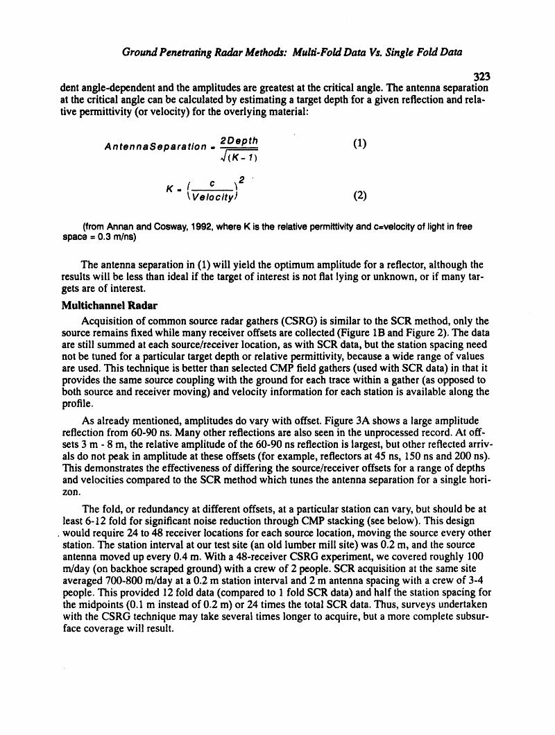
GroundPenetratingRadarMethods:Mulg-FoldDataVs.SingleFoldData
323dentangle-dependentandtheamplitudesaregreatestatthecriticalangle.The antennaseparationat the critical angle can be calculated by estimating a target depth for a given reflection and rela-tive permittivity (or velocity) for the overlying material:
AntennaSeparation . 2Depth (1)
K-( c _2 "_Velocity) (2)
(fromAnnanandCosway,1992,whereK istherelativepermittivityandc=velocityof lightinfreespace= 0.3 rains)
The antenna separation in (1) will yield the optimum amplitude for a reflector, although theresults will be less than ideal if the target of interest is not flat lying or unknown, or if many tar-gets are of interest.
Multichannel Radar
Acquisition of common source radargathers (CSRG) is similar to the SCR method, only thesource remains fixed while many receiver offsets are collected (Figure 1B and Figure 2). The dataare still summed at each source/receiver location, as with SCR data, but the station spacing neednot be tuned for a particulartarget depth or relative permittivity, because a wide range of valuesare used. This technique is better than selected CMP field gathers (used with SCR data) in that itprovides the same source coupling with the ground for each trace within a gather (as opposed toboth source and receiver moving) and velocity information for each station is available along theprofile.
As already mentioned, amplitudes do vary with offset. Figure 3A shows a large amplitudereflection from 60-90 ns. Many other reflections are also seen in the unprocessed record. At off-sets 3 m - 8 m, the relative amplitude of the 60-90 ns reflection is largest, but other reflected arriv-als do not peak in amplitude at these offsets (for example, reflectors at 45 ns, 150 ns and 200 ns).This demonstrates the effectiveness of differing the source/receiver offsets for a range of depthsandvelocities compared to the SCR method which tunes the antenna separation for a single hori-zon.
The fold, or redundancy at different offsets, at a particularstation can vary, but should be atleast 6-12 fold for significant noise reduction through CMP stacking (see below). This design
• would require 24 to 48 receiver locations for each source location, moving the source every otherstation. The station interval at our test site (an old lumber mill site) was 0.2 m, and the sourceantenna moved up every 0.4 m. With a 48-receiver CSRG experiment, we covered roughly 100m/day (on backhoe scraped ground) with a crew of 2 people. SCR acquisition at the same siteaveraged 700-800 m/day at a 0.2 m station interval and 2 m antenna spacing with a crew of 3-4people. This provided 12 fold data (compared to 1 fold SCR data) and half the station spacing forthe midpoints (0.1 m instead of 0.2 m) or 24 times the total SCR data. Thus, surveys undertakenwith the CSRG technique may take several times longer to acquire, but a more complete subsur-face coverage will result.

LM. Liberty and J.R. Pelton
324 PROCESSING
Noise Attenuation and Muting
CSRG data have the advantage of separating out many different arrivals on a radargram,giv-ing information not attainable from SCR acquisition (Figure 2). There are three kinds of signal
1S v_ 2 "- Air
,,G
: 4d Layer 1
Layer 2
0 Xc Offset (X)
o : 1) Direct air wave (constantvelocity = 0.3 m/ns)
2) Critically refracted air1 wave (lateral wave)
3) Direct ground wave
4) Reflected wave
Region generally freefrom reflections.
Region containingthe reflections
Figure2. Raypathsandarrivaltimesfora flat,two-layermodel(modifiedfromAnnanandCosway,1992).Fourarrivalsareshown.Thefirstarrivalina radarsectionwillalwaysbetheairwave(event1). Thearrivaltimewillequaldistance/c,wherec=0.3m/ns.Arrival2 isa criticallyrefractedairwaveorlateralwave,observedpastthecriticaldistancefora reflection.Thisarrivalalsotravelsat0.3 m/sandiscausedbytheinversevelocityrelationshipbetweentheair/groundinterface.Thedirectgroundwave(event3)travelsthroughthenear-surfacedirectlyfromsourcetoreceiverandevent4 representsa reflection.Thereflectionhashyperbolicmoveoutandasymptoticallyapproachingthedirectwavearrival.Sincevelocitiestendtodecreasewithincreasingdepth,reflectionsusuallydonotcrossthegroundwavearrival.
that can be recorded with a digital system" random noise, coherent noise and desired signal (orreflections, in this case).
Random noise is energy which does not exhibit correlation between distinct receiver chan-

Ground Penetrating Radar Methods: Multi-Fold Data Vs. Single Fold Data
325nels (Sheriff, 1984). Random noise can be attenuated by averaging traces in the field at the samesource/receiver location, as is done for both single channel and multiehannel methods. Multichan-nel processing allows additional attenuation of the random noise by adding more traces to averageand allowing different averaging techniques (weights) during processing to remove specific noise(for example, removing noise bursts by averaging traces without the maximum and minimumamplitudes for a given time). Random noise can appear at any frequency and a bandpass filtermay aid in attenuating the noise andboosting the signal. If random noise still persists in a traceafter filtering and/or averaging techniques have been tested, traces can be completely removedfrom the processing flow. With 12-fold data, the removal of a few bad traces may greatly increasethe quality of a final stack.
Coherent noise appears as laterally continuous arrivals that are not reflections across the mul-tichannel records. These arrivals can be generated from the radarsource or from other culturalsources and are hard to distinguish from reflections on SCR records. Standard processing tech-niques allow attenuation or complete removal of the coherent noise on multi-offset radargrams.There is no way to conclusively separate reflections from coherent noise with SCR data becauseapparent velocity information is not available. Undesired coherent noise includes the direct airwave, ground waves, lateral waves, multiples and out of plane energy (Figures 2 and 3A). Theseevents are of no interest when plotting a final stack of the data, but contain information regardingthe site and subsequent processing steps.
The air wave is beneficial in radar data because the velocity is a known physical constant.CSRG data can be aligned to the air wave because the arrival will always be first on the radar-grams with a constant linear velocity of 0.3 m/ns (Figures 2 and 3). This provides the initial sys-tem statics, allowing the data to be lined up in the case of system errors (possibly related to fiberoptic cable problems). The system static shift can also be performed on SCR data with a knownsource/receiver offset.
The direct ground wave travels through the near surface directly from the source antenna tothe receiver antenna (Figure 2). This arrival can appear very strong on the section or can bemasked by different arrivals (compare Figure 3A with Figure 3B). With SCR data, the groundwave may be misinterpreted as a reflector in the radargram, depending on the complexity of thenear surface. If the near-surface conditioas change drastically across the line, the ground wavemay also appear to have topography across the radargram with SCR data. The apparent topogra-phy is caused by changes in the near-surface velocity (or permittivity). With CSRG data, theground wave arrival is usually easily distinguished, even if masked by other arrivals. With simplefiltering techniques, the ground wave can be enhanced, allowing direct measurement of the near-surface velocity (Figure 3B). The ground wave is beneficial if near-surface statics are to beapplied to the data. Although it is possible to perform a few CMP tests along a single channel lineto acquire the ground wave velocity, this arrival may still interfere with reflected arrivals in thesection and near-surface velocities may also change between CMP locations.
Generally, the zone of reflections appears below the ground wave (Figure 2). The area abovethe ground wave is free from reflections, provided velocities decrease with depth, as is commonfor electromagnetic waves (because the dielectric permittivity generally increases with depth insoil and in bedrock). Above the ground wave on a CSRG lies critically refracted arrivals oftentravelling through air after a critical distance (Figure 2), due to the inverse velocity relationshipbetween the air and the ground. Processing to remove the refracted arrivals and direct arrivalsincludes muting the region between the air wave and the ground wave. In a SCR section, if thesource/receiver antenna separation is tuned to image deeper arrivals (wide aperture), arrivals

L.M.LibertyandZR.Pelion
326
A_)ffset )o o o o o B) o o o o o Offset(m)(m _ _ _ _ ..: _ _ _ o_0 0
20 20
40 40
_,so so
_ 80 80
i:::: 10o
i_ 120
140I180
180
200
)220
240 240
Figure3. A) CSRGfromthe lumbermilltestsite.Thegatherhassystemanddatumstaticsappliedandanautomaticgaincontrol(AGC)windowof80 ns.Notethechangeinamplitudesforthedifferentreflectionswithrespecttooffset.B)Thesamegatherwitha filtertoremovecoherentenergyattheairwavevelocity.Thefilterhastheeffectof highlightingthegroundwavearrival(0.15m/ns)andothercoherentenergy.Thenoiseinthelowersectionisenergyfromout-of-planearrivals.Theenergyisout-of-planebecauseoftheanomalousapparentvelocitiesofthearrivals(<-0.4m/sorgreaterthanthe(negative)airwavevelocity).
abovethe tuneddepthwill appearat anomalouslyfasttimes, and all amplitude informationwill belostbecausetherefractedair wave energyappearsinsteadof thereflection.
Other undesiredcoherentarrivals thatappearin a radargramincludeout-of-planenoiseandmultiples. Figure 3A shows a strong arrival at 220-230 ns that has a negative apparentvelocity.This arrival is anomalous and its source is from out of the plane. On a single channel radargather,the arrival could be not easily be distinguished from a reflection. Coherent noise that is in theplane of the radar line can usually be identified as noise if travelling through air (will appear at theair wave velocity on SCR data), but out-of-plane noise can have any apparent velocity, making itharder to conclude coherent noise is present. With multi-offset data, out-of-plane noise be noticedand attenuated through processing.
Multiples are another common source of coherent noise, especially where large impedancecontrasts are found. The only way to determine if multiples are a problem in radar data is to recordthe velocity information and measure travel paths. Multiples will appear at an anomalous velocitydue to their repeated reflected raypaths. These arrivals may be hard to separate from primaryarrivals, but their presence can be noted in the stacked section.

Ground Penetrating Radar Methods: Multi-Fold Data Vs. Single Fold Data
327Statics
System statics have already been mentioned as a necessary tool to ensure that data are col-lected and processed properly. Datum (or elevation) statics can also benefit from the CSRGmethod of data acquisition. Datum statics involve shifting the data to a common datum (or eleva-tion) to account for topography of the surface and near-surface lateral velocity changes. Since ele-vation statics are velocity dependent (3), this information is only possible by calculating thevelocity of the direct arrival and applying this velocity to the static calculations. If the velocity is
(Es-Ed) (Er-Ed) (3)Tota/Static ,, SourceStatic + ReceiverStatic = +Vs Vr
where:
Es=elevationof thesource
Er=elevationof thereceiver
Ed=datumelevation
Vs=near-surfacevelocityatthesource
Vr=near-surfacevelocityatthereceiverantenna.
nearly constant across the section, a constant velocity can be assumed for both Vs and Vr. Also, ifthe topography is flat, no static correction may be necessary.
Velocity Measurements and Corrections
If the subsurface changes across the section, velocities should be measured every 10-20 sta-tions. This is necessary to place the reflectors at their proper two-way travel time and for depthcalculations. A useful and easy way to perform velocity analyses is to stack CSRG data at differ-ent constant velocities and display them side by side (figure 4). When the reflection appears fiat,the best root mean square (RMS) velocity is attained for a given time and this is the proper normalmoveout (NMO) velocity for the arrival. By analyzing gathers with this method, it is easy tonotice out-of-plane events and multiples. These events often attain the greatest RMS stackingvelocity at anomalously high or low velocities.
Anomalous velocity measurements may also occur if there are steeply dipping reflections inthe section. Dip moveout (DMO) is essential in the case of steeply dipping events (see Hale,1984). DMO is a change in the arrival time for a reflection because of the dip of the reflector(Sheriff, 1984). The DMO correction migrates the dipping reflector to a zero offset reflector for agiven velocity. DMO makes the stacking velocities become independent of dip, enabling eventswith conflicting dips to be properly imaged. The velocity model used with DMO should be esti-mated by a generalized velocity model from the original velocity tests. The data can then be rean-alyzed to attain a higher degree of accuracy in picking proper velocities.
Sorting and Stacking
CMP sorting is the process of moving traces with the same midpoint locations into onegather, and is performed before velocity analyses. Once the velocity analyses and corrections arecomplete, the traces for each mid-point can be averaged at each station an__stacked. Stackingtraces with different offsets will attenuate coherent events not associated with reflections, reducerandom noise, and highlight the reflections pinpointed in the velocity analyses. Figure 5 shows acomparison between SRG and CSRG stacks for the same profile. Note the strong reflection in fig-\

L.M. Liberty and J.R. Pelton ,
328
CV
EE
200 2000
Figure4. Constantvelocitystacksfora CMPgatherfromthelumbermillsite.TheRMSvelocitycanbefoundbyfindingtheflatarrivals(shownatthetopsofthegathersinm/ns).Ifthevelocityistooslow,thearrivalwillbeovercorrected(slopingup),whenthevelocityistoofast,thearrivalisundercorrected(slop-ingdown).Notethegeneraldecreaseinvelocitywithdepthandtheanomalousstackingvelocityforthecoherentnoise.
ure 5B at 50 ns does not clearly appear in the SCR stack (Figure 5A). This is because the antennaseparation is not tuned for this depth. With a 2 m antenna separation for the SCR data and an esti-mated near-surface velocity of 0.15 m/ns, the tuned depth is 1.7 m (from equation 1) and thisreflector depth is estimated at 3.75 m (assuming a constant velocity of 0.15 m/s). Even reflectedarrivals above 50 ns in the CSRG stack appear more coherent than the SCR stack because there isless interference from coherent noise in the section. Also note the presence of diffractions below100 ns on the SCRG stack. These arrivals are much less coherent on the SCR stack (Figure 5A)where background noise begins to dominate the radargram below 140 ns.
CONCLUSIONS
The CSRG technique involves collecting GPR data at different source/receiver offsets to sep-arate the different components of the wavefield, to look at the velocity structure at each location,to increase the signal to noise ratio, to account for steeply dipping structures, and to removeanomalous arrivals from the radargrams. The increase in data collected and processed comparedto single channel acquisition allows a significant increase in resolution and confidence in interpre-tation of the profile in complex regions, but at a cost of additional time. Although fewer fieldhands are needed (commonly 1=2people for CMP collection, instead of 3-4 people for fixed offsetcollection), one should expect 2-3 times longer in the field for the same surface coverage. Thisincreased coverage and repetition may only b_eneeded if the subsurface is complex or if the objec-i

GroundPenetratingRadarMethods:Multi-FoldDataVs.SingleFoldData
329
B) oA)o
g
"_ 100 100
200 200
Figure5. (A)SCRstackfromthe lumbermilltestsite.Processingincludedsystemanddatumstatics(assuminga near-surfacevelocityof0.13 m/ns)andsubtractionofa meantraceacrossthesec-tiontoremovelaterallycoherentarrivals,liketheairwave(appliedbeforedatumstatics).Also,an80 nsAGCwindowwasused.(B)CSRGstackforthesameprofileas.A.Notethestrong,laterallycontinuousreflectionsintheupper50 nscomparedtoA andtheincreaseincoherentenergyclownto200ns.Thelowersectioncontainsdiffractions,possiblyfromlargecobblesintheriverchannelsequence.Process-ingissummarizedinthetextwithan80 nsAGCappliedafterstacking.
tive includes more than one reflector. If a single horizon with little topography is known to be thetarget, SCR acquisition may suffice.
Interpreting a single fold GPR line as a cross section of the earth must be done with caution.Often, ground waves, multiples and out-of-plane events appear in the section. These noise trainscan cause a misinterpretation of the data. In regions of a complex near surface (e.g. disturbedzones and river channels), steeply dipping arrivals and diffractions may appear. A complex regionmay also contain dramatic lateral and vertical velocity changes. All of these problems can beaddressed by collecting multi-fold CSRG data. Processing steps, including muting, trace editing,velocity analyses, dip filtering, dip-moveout, sorting and stacking are all available to increase the-clarity of the radar section.
• Acknowledgments
The authors are grateful to Mark Petteys for help with the CSRG field work and EnvirosearchInternational for permission to collect and publish the data. CGISS contribution 25.

LM. l_ben_andLR.Pelion
330 References
Annan,A.P.andCosway,S.W., 1992, Groundpenetratingradarsurvey design:SAGEEPAnnualMeeting,2, 329-351.
Annan,A.P.andDavis J.L., 1976, Impulseradarsoundingin permafrost,RadioScience, 11,383-394.
Arcone, S.A., 1984, Field observationsof electromagnetic pulse propagationin dielectric slabs:Geophysics, 49, 1763-1773.
Clough, J.W.,Electromagneticlateralwaves observedby earth-soundingradars:Geophysics, 41,1126-1132.
Fisher,E., McMechan,G.A., and Annan,P., 1992, Acquisitionand processingof wide-aperturegroundpenetratingradardata:Geophysics,S7, 495-504.
Hale,D., 1984, Dip-moveoutby fouriertransform:Geophysics,49, 741-757.
Mayne,W.H.,1962,Commonreflectionpointhorizontaldatastackingtechniques:Geophysics,27,927-938.
Sheriff, R.E., 1984, Encyclopedic dictionaryof exploration geophysicists,2rided., Societyof Ex-ploration Geophysicists,Tulsa, Ok., 323 p.

N
Hydro|_lo|y,Wmu DiJlx_xl,_ mdPolJlJaFe0m,dinls_ Symposium
BngtnR_4n|OmlosyendOeot_chnJcxlBnllneerins,1994 331
A New Geophysical Method to Measure Soil Profilesfor Dynamic Analysis of Soll Embankments
PaulMlchaels
CenterforGeophyslealInvestlsatlonoftheShallowSubsurface' BoiseState University
Boise,Idaho8372S
ABSTRACT
Following the February9th, 1971 San Fernandoearthquake(and near collapse of theSan Femando Dams), there hu been an inc_ awarenessfor the need tO evaluate damsafety in the engineering community. Partof that evaluationis the dynamic analysis ofthe soil embankmentstructure. This analysisrequiresa soil profile.
A problemwith alluvium embankmentshas been the measurementof soft profiles.Traditionalblow count methods often producescatteredresults due tO the very localizednatureof the measurement. This paperdescribes an alternativegeophysical approachtomeasuringthe soil profile.
The method is to acquireshear-waveboreholedatafollowing blow count measure-ments. Measurementsof the shear wave amplitudesand velocity dispersionare jointlyinvertedto produce a soil profile of the elastic and inelastic propertiesneeded fordynamic analysis by computerprogramssuch as SHAKE or DESRA-2. Since themeasuredprofilescorrespondexactly to the parametersneeded by the computerpro-grams,improveddynamic evaluationscan be made without employing conversionchartsor empiricalformulae. The resultingprofiles will be valid over a broadrange offrequencies,since the correctdifferential equationis used in place of simpler constant Qmodels. Furthermore,since geophysical measurementsprobea larger volume of soil, lessscattercan be expected in the measuredsoil profiles.
INTRODUCTION
The evaluationo_"embankmentdam safety includes an assessmentof the dam'sdynamic behavior when exposed to an earthquakehazard. Such a dynamic analysis canbe performed using currentlyavailable software. However, the quality of the computeranalysis depends significantly on the qualityof the soil profile.
What is needed is a profile of the elastic and inelastic propertiesof the soil.Geophysical measurementof these propertiesby seismic methods is highly desirablewhen the final objective is to evaluate the seismic responseof the embankment.However, it has become apparentthat seismic measurementsmade in the limitedfrequencyband of engineering seismology may not accuratelypredictthe seismicbehavior in the broader frequencyband of naturallyoccurringearthquakes.
This issue was recentlyraised by Jongmansand Campillo (1993). In their work, theydemonstratedthatmeasurementsof the inelastic propertiesof soils at high frequencieswere in conflict with a low frequencymeasurementsextractedfrom surface waves.
P. Michael:
332 Specifically, they examined the apparentfrequencyvariation in quality factor,Q.In my view, the apparentcontradictionis causedby assumptionsmade in the analysis
of the seismic observations. Specifically, the spectralratiomethod should not beinterpretedin terms of the constantQ model. Rather,the spectralratioshould beinterpreted in terms of a model consistentwith the differential equation used by thedynamic analysis software.
A computer programsuch as DESP,A.2 (Lee andFinn, 1982) presupposesthat Q isnot constant with respect to frequency. This observationfollows from the matrixform ofthe differential equation that is used in DESRA-2. Since the stiffness and dampeningmatricesare invariantwith respect to frequency, it is Q that will have to vary predict-ably with frequency.
This paperpresentsan alternativeto the traditionalconstantQ analysis. I will showhow it is possible to interpret engineeringseismogramsin a mannerconsistent with theeventualuse of the soil profile. Two key advantages of this approachare:
1). The solution is for soft parametersthat areexactly those parametersneededby the dynamic analysis software. Thus, no empirical or other correctionsneedbe made.
2). The solution is appropriatefor a broadrange of frequenciessince it honorsthe differential equation currentlyacceptedby engineering practice.
METHOD i
Geophysical Data AcquisitionTherearea numberof ways to acquiregeophysicalmeasurementssuitable for
determinationof soil profiles. Because the intendedapplicationis primarilyfor evalua-tion of soft embankments,I will presentthe method in the context of boreholemeasure-ments.
Figure 1 shows a classic boreholeexperimentas describedby Kudo and Shima(1970). A shallow reference geophone is planted in hole A where it remains fixed. Asoundinggeophone is clamped at different levels in the deeper borehole, B. The seismicsource consists of a wooden plate struck on edge to produce verticallypropagatingSH-waves which are then recordedby both geophones. The shallow referencegeophone iscritical, since it provides a way to monitorany variationsin the seismic source that mayoccurduring the course of the experiment.
The elastic and inelastic propertiesof the soil are determinedby comparingseismo-gramwaveforms recordedat the different depths in boreholeB. The details of howwaveform variationsareconvertedto a soil profile follows next.
The Inelastic Model
The key to the method is to use the same differential equationin both the analysis ofthe geophysical data and the dynamic analysis of the embankment. Figure2 shows howthe soil dynamics are modeled in a programsuch as SHAKE or DESRA-2. The soil ismodeled as a Voigt solid (springand dashpot in parallel). In the limit of continuous
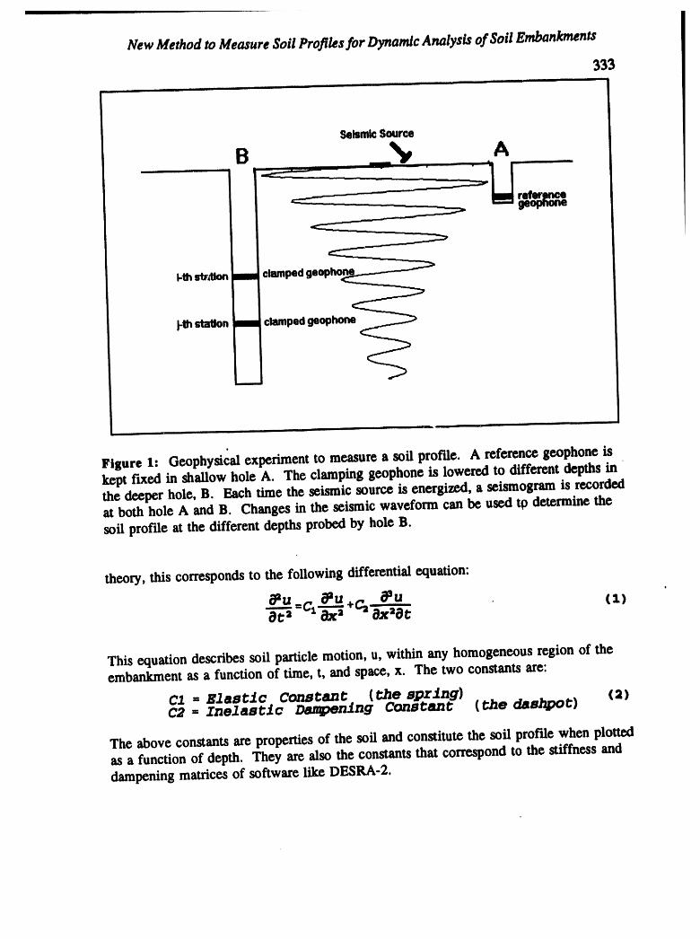
New MethodtoMeasureSoilPro/llesforDynamicAnalysbofSoilEmbankments
333
i im__
Figure 1: Geophysical experiment to measure a soil profile. A reference geophone iskept fixed in shallow hole A. The clamping geophone is lowered to different depths inthe deeper hole, B. Each time the seismic source is energized, a seismogram is recordedat both hole A and B. Changes in the seismic waveform can be used tO determine the
soil profile at the different depths probed by hole B.
theory, this corresponds to the following differential equation:
____u__u ... _u . (1)st:'- c_.._-._+_ c_x2c_t
This equation describes soil particle motion, u, within any homogeneous region of theembankment as a function of time, t, and space, x. The two constants are:
C2 = Elastic Constant (the spring) (2)C2 = Inelastic _ning Constant (the dashpot)
The above constants are properties of the soil and constitute the soft profile when plottedas a function of depth. They are also the constants that correspond to the stiffness anddampening matrices of software like DESRA-2.

P. Michaels
334
Seismic Source Soil Model
_-- . _.__._ _
Geophone
Figure 2: The model used to _escribe the elastic behavior of soft. The wave propagatesby transferring energy from one mass to the next via the spring/dashpot connection. Inthe continuous limit, the dynamics of this model (a Voigt solid) are describexi by thedifferential equation (1) in the text. This is the same kind of model used by SHAKE andDESRA-2.
The elastic constant, C1 is actually equivalent to the square of the S-wave velocity for anelastic case,
C....G shearmodulusI--_= (3)densi Cy
The dampening term, C2, corresponds to the frictional resistance of the dashpot and cansignificantly alter the resonant characteristics of a soft embankment. A single value ofC2 is sufficient to describe both the frequency variation in S-wave velocity and the
amplitude attenuation.For example, ff a solution of the form

New Method to Measure Soil Profiles for Dynamic Analysis of Soil Embankments
335
ulx, C)=exp (-gx)'cos(w (-_-e)) (4)
is substituted into equation (1), then we may solve for C1 and C2 in terms of amplitudedecay, ot, and phase velocity, v. The result is
2 [ 2.__][ (_) -a2].w2c_: , _: (s)[g2+(_) 2] [,,+ (_) 2]
Note that u and v are both functions of angular frequency, ¢o. However, they vary insuch a way that both C1 and C2 are constant over all frequencies. By specifyingconstant values for C1 and C2, the frequency dependent behavior of the soil in a givenregion is completely described by equation (5).
The connection to loss factor, Q, is as follows:
0 - o ' (6)2._-v
Thus, Q also is a function of frequency because of its dependence on decay and phasevelocity.
A typical situation can be visualized by examining Figure 3. Here, equations (5)have been inverted to show the frequency behavior for ¢_, v, and Q for a region whosesoil constants are C1=12000 m2/sec2 and C2=10 m2/sec. The increase in phase velocitywith frequency is due to the increased frictional resistance to motion of the soil at higherfrequencies. This increase in friction causes the soil to appear stiffer, resulting in fasterwave propagation.
The increase in decay constant, or,with increasing frequency shown in Figure 3 is aconsequence of the decrease in wavelength at high frequencies. Since the energy lost perwavelength is constant, propagation losses accumulate faster with shorter wavelengths.This causes a loss of higher frequencies as the wave propagates.
The spectral effects predicted by equation (1) and illustrated in Figure 3 are measur-able in the borehole experiment. These effects cause a propagating wave to changeamplitude and shape (see Figure 4). That change in shape can be easily quantified in thefrequency domain (see Figure 5). The next section shows how the changing amplitudeand shape of the seismic wave can be used to compute the soil profile.
Computing the Soil ProfileThe method'begins with the traditional spectral ratio method. The recorded signal at
the ith station in the borehole, B, can be expressed as a product of transfer functions inthe frequency domain:
s_(u) : s_(w).s_ ((_).¢_(w)_ (c_) (7)
where o) is angular frequency and the other terms are as follows:
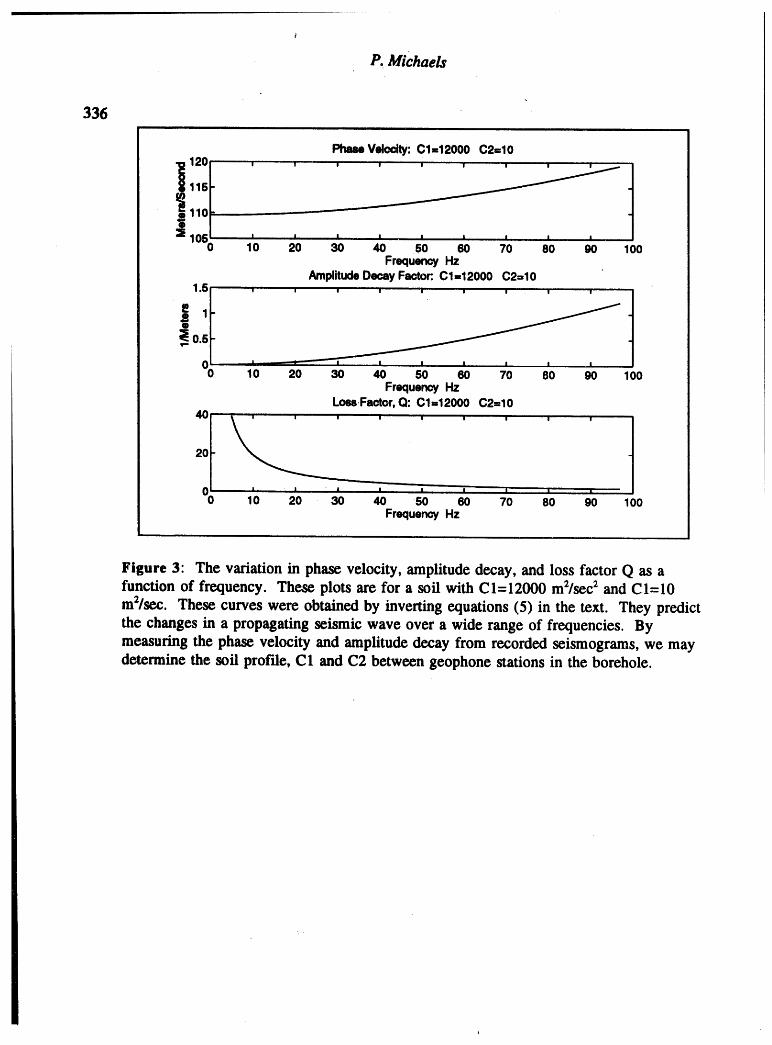
P. Michaels
336
Ph_ V¢o_: C1-12000C2-10
i"_120/ ' ' ' ' ' ' ' ' ' _1
t
1151 ____
!,,°F_ I I I , I I I I I I10 10 20 30 40 50 60 70 80 90 1O0
Frequency HzAmplitudeDecayFactor:.C1,,12000 C2=,10
!o.+[0 l I I I I I I I I
0 10 20 30 40 50 60 70 80 90 100Frequency Hz
Loss.Factor,Q: C1=12000 C2=1040
2O
00 10 20 30 40 +50 60 70 80 90 100
FrequencyHz
Figure 3: The variation in phase velocity, amplitude decay, and loss factor Q as afunction of frequency. These plots are for a soil with C1=12000 m2/sec2 and CI=10m2/sec. These curves were obtained by inverting equations (5) in the text. They predictthe changes in a propagating seismic wave over a wide range of frequencies. Bymeasuring the phase velocity and amplitude decay from recorded seismograms, we maydetermine the soil profile, C1 and C2 between geophone stations in the borehole.
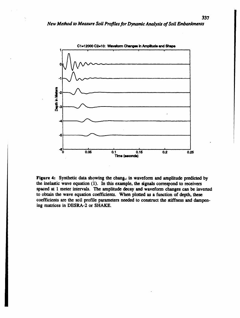
-. 337
New MethodtoMeasureSoilPro.filesforDynamicAnalysis of Soil Embankments
C1-12000 C2-10: Wawfoml _ inAmplitudorand
1__ ....
_._ _ - ,,t
._ I ,, I . I . , i.0.06 0.1 0.16 0.2 0.25l".ne(mx._)
Figure4: Syntheticdatashowingthechang,;inwaveformandamplitudepredictedbytheinelasticwave equation(I).Inthisexample,thesignalscorrespondtoreceiversspaced at 1 meter intervals. The amplitude decay and waveform changes can be invertedto obtain the wave equation coefficients. When plotted as a function of depth, thesecoefficients are the soil prof'fleparameters needed to construct the stiffness and dampen-ing matrices in DESRA-2 or SHAKE.

.. P.Michaels338
C1=12000C2=10: FrequencySpectraof Figure4 Signals1
0 50 100 150FrequencyHz
Figure S: Amplitude spectrum of waveforms in Figure 4. The near receiver spectrumhas been normalized to unity. As the source to receiver separation increases, the peakamplitude of the spectrum decreases. In addition, the shape of the spectrum changes dueto bodywave dispersion. Both the change in amplitude, and the change in spectral shapecan be measured between any two receiver depths. The soil profile can be computedfrom these spectral measures (see text).

New MethodtoMemure SoilProfilesforDy_m[¢ AnalysbofSoil£mbanJ_nen_ 339
B,(¢o) = Seismogram SpectrumSt(m)= SourceSpectrumHb|((0 ) -- Soil Transfer Function (source to station "i")Cb(m) = Instrument Transfer FunctionGbi(ffl ) -- Geometric Spreading (beam divergence)
Similarly, the seismogram obtained from the reference geophone for the ith source effortis given by:
_(w) = s_(w) .x.(w).c.(w) %(w) (e)
Since the reference phone is fixed, the medium and geometric spreading terms areconstant for all "i'.
The traditional method of spectral ratios can be used to determine the amplitudedecay rate, ¢x,between the ith and jth stations in hole B. In this method, one computesthe ratio of the amplitude spectra for the ith and jth seismograms. Variations in thesource spectrum are corrected for by solving (8) for S(¢e) and substituting into thespectral ratio. The result is:
B_(.) _ Ht_((o).[At(¢o).G._(¢¢) ] . (9)
To obtain the spatial amplitude decay rate, we begin by solving (9) for the ratio of thesoil transfer functions in terms of the measured spectra,
The spatial amplitude decay is given as an exponentialdecay (seeequation(4)). Thusthe final step is to take the natural logarithm of the spectral ratio of the soil transferfunctions in (10) and divide by the distance separating the ith and jth station,
og. / "L (,.,)z (o_) = (x_-x_)
_)eparture from Traditional PracticeIt is at this point that my method deviates from traditional practice. Under the
constant Q assumption, traditional analysis would be to assume that a(ca) is a linearfunction of frequency, co. This would be true if the phase velocity were constant(nondispersive). Recall equation (6) and solve for spatial amplitude decay,
g (O}) = [ 2.1..- _,v.rwI "CO (Z2)
As long as phase velocity, V, and loss factor, Q, are constant, linearity is expected. Thus

P. Michaels
traditionalanalysis has been to fit a straightline to the resultsobtainedin (11) by a340 method such as least squares.
This linearityis in conflict with the inelastic wave equation(1). The SH-waveshould be dispersive. Thus, both V and Q will also vary with frequency (see Figure3for example). My method is to least squarefit equation(1l) results with a nonlinearcurveof the shape shown in Figure 3. Furthermore,since phase velocity is also afunctionof frequency,V(co)may also be measuredand used to furtherconstrainthesolution in a way consistent with the inelastic wave equation.
The ForwardProblemThe solutionfor a((o) can be found by takingthe ratio of equations (5) and using that
to eliminatephase velocity from the C2 equation. The resultis as follows:
- .......[ 2+sa]
(13)
where B = 2"CI+2_C1 z+ez.C2Z
Solving equation(13) at any given frequency yields the spatialamplitude decay at thatfrequency.
The ratio of equations (5) can also yield an expressionfor the phase velocity disper-sion,
V- 2"°)a'C2 (14)B'g -"
Once _m) has been determined at a desired frequencyby (13), thenthat resultcan beused in (14) to compute phase velocity, V(o)).
The InverseProblenlThe procedure is to start with an initial guess at C1 and C2. Based on the
difference between the observed and cor.tputed(x(¢o)and V(¢o),sensible corrections to C1and C2 are made. The nonlinearnature,of the problemcan be overcome by the use ofTaylor's series expansion, retainingon;y the first orderterms. For each frequencyforwhich a measurementof _(oi) and V(¢%)can be made, we have two equations. At theith frequencywe have,
8 v(e_).Acz + 8 v(e_).Ac2 = Av(e_) (16)8 C2 8 02
a _ (e_).ACl + 8 _ (e_)"AC2 = Ag (e_) (IS)8 Cl 8 C2 .

New MethodtoMeasureSoilProfilesforDynamicAnalysisofSoilEmbankments341
Here, AC1 and AC2 are the changes in C1 and C2 which will reduce the differencebetweentheobservedandcalculatedo_((o)andV((o).Thatis,
Aa (w,,) = _ ((0.()_ - a (W.O,,,,.zo,,z,t,,,a (17)
If there are measures of _o)) and V(o)) at N frequencies, the above can be writtenas an N x 2 matrix equation. The least squares solution for this system is well known(Menke, 1984 for example) and is given by
t
Gz,_-_ = (O="O) "_'O_' (xg)
where
! !
a • (w.() a a ((or)a c1 "a c2"
G = ! _ (20)a v((o._) a v(w.()ac_ .... ac2
! !
The derivatives in matrix G can be computed numerically or analytically. I was able toderive the derivatives using the symbolic processing software known as MAPLE. Theresulting formula are quite long, but can be easily implemented in a computer program.
Practical Considerations
Although the computational procedure is straight forward, there are a number ofpractical matters to be considered:
1). The separation between stations must be large enough to permit an accuratemeasurement of the phase velocity dispersion.
2). The separation between the source and the stations must be small enough sothat the loss of high frequencies is not so large as to adversely reduce the useablebandwidth.
If the station separation is too small, there will not be a significant difference inarrival time between different frequencies. Fortunately, shear waves are some of theslowest traveling seismic waves. This permits one to work at a finer resolution than withP-waves. A good experimental design will insure that a measurable dispersion curve ispossible. However, it is not absolutely required. As long as the sampled spectrumcaptures enough curvature in the spatial decay measurement (spectral ratio), a solution ispossible.

P. Michaels
342 The desirability of large station spacings in the dispersion measurement is temperedby the need to retain as much bandwidth as possible. If too much of the high frequencyenergy is lost, one will not be able to measure either the spatial decay or velocitydispersion over a sufficient bandwidth. Thus it becomes a compromise betweenmeasurement precision and retention of bandwidth.
CONCLUSIONS
The proposed new method to measure soil profiles is designed to overcome asignificant inconsistency between engineering and geophysical practice. By making thegeophysical analysis subject to the same differential equation as is used in engineeringpractice, this inconsistency is overcome. Furthermore, two major advantages are realized:
1). The soil profiles produced consist of the same parameters that will be laterused in the dynamic analysis of an embankment or foundation site.
2). The resulting soil profiles should better predict soil dynamics beyond thespectral bandwidth of the geophysical measurements. The realization of this lastpoint will be subject to measuring a sufficient bandwidth for determining thenonlinear spatial decay factor, a(¢o), or velocity dispersion, V(¢o).
REFERENCES
Futterman, W.I. (1962). Dispersive Body Waves, Jour. of Geophysical Research, Vol 67,No. 13, pp5279-5291.
Hardin, B.O., and V.P. Drnevich (1972a). Shear modulus and damping in soils:measurement and parameter effects, J. Soil Mech. Foundations Div.ASCE 98, pp603-624.
Hardin, B.O., and V.P. Drnevich (1972b). Shear modulus and damping in soils:design equations and curves, J. Soil Mech. Foundations Div.ASCE 98, pp667-692.
Jongmans D., and M. Campino (1993). The determination of soil attenuation bygeophysical prospecting and the validity of measured Q values for numericalsimulations, Soil Dynamics and Earthquake Eng., 12, pp. 149-157.
Kudo, K., and E. Shima (1970). Attenuation of shear waves in soil, Bull. EarthquakeResearch Institute, v. 48, p.145-158.
343
Lee, M.K.W. and W.D.L. Finn (1982). Dynamic effective stre_ response analysis of soildeposits with energy transmitting boundary including assessment of liquefactionpotential, Rev., Dept. of Civil Eng., Soil Mechanics Series, No. 38, Univ. of BritishColumbia, Van_,_uver, Canada.
Menke, W. (1984). Geophysical data analysis, discrete inverse theory, Academic Press,San Diego.
Michaels, P. and R_B. Smith (1992). Recurrent neural network representation of theinelastic wave equation and full-waveform inversion without local minima, 5EG
Annual Meeting Expanded Abstracts, New Orleans, AI1.7, pp22-25.
Seed, H.B., and IJvl. Idriss (1970). Soil moduli and damping factors for dynamicresponse analyses, Report EERC 70-10, Earthquake Engineering Research Centre,University of California, BerkeleT.
Seed, H.B, K.L. Lee, and FI. Makdisi (1973). Analysis of the slides in theSan Fernando dams during the earthquake of Feb. 9, 1971, Report No. EERC 73-2,University of California, Berkeley.
Tonn, R. (1991). The determination of the seismic quality factor from VSP data: Acomparison of different computational methods. Geophys. Prospecting, 1991,vol. 39, 1-29.
ACKNOWLEDGEMENTS
I would like to acknowledge Phillip Sirles at the Bureau of Reclamation who broughtthe work of Jongmanns and Campillo to this author's attention. This paper is CGISScontribution 29.


n
Hydrovmlogy, Wum Disposal, Science andPoliticsProceedinp 30thSymposiumEnlpineerin$Oeolo|y andGeotechnlcalEngineerlns,1994
345GROUND PENETRATING RADAR AND SEISMIC REFRACTION
INVESTIGATION OF FRACTURE PATTERNS IN THE BASALT OF
LUCKY PEAK NEAR BOISE, IDAHO
M.E. Dougherty, W.K. Hudson, S.E. Kay, and R.J. Vincent
Center for Geophysical Investigation of the Shallow Subsurface,
Boise State University, Boise, Idaho
ABSTRACT
In hard rock environments, fluid flow and basement integrity are often controlled by thedegree and connectivity of fracturing on an outcrop scale, ratherthan strictly by laboratory valuesof the permeability and competence of the matrix rock. Therefore, in many cases it is important tohave a subsurface image of fracture characteristics of rock units in addition to an image of grossrock type. Fortunately, within a single rock type, many physical properties on outcrop scale aregreatly influenced by fracturing, and changes in these physical properties should be detectablethrough the innovative use of geophysical methods. Work presented here is an attempt to use sur-face geophysical methods to delineate areas within a basalt flow which display different fracturecharacteristics and which have different electrical and seismic properties,
The Basalt of Lucky Peak is an intracanyon basalt flow exposed in cliffs around Lucky PeakReservoir and in a terrace downstream from Lucky Peak Dam near Boise, Idaho. Visible in theface of the terrace below Lucky Peak Dam are the colonnade and entablature structures character-istic of differential cooling rates within basalt flows. Exposure of structuralunits within the cliffface is used to ground truth results from ground penetrating radar(GPR) and seismic refractiondata collected along a line running perpendictdar and away from the top edge of the cliff.
GPR data were collected using 25, 50, and 100 MHz antennas with the best results obtainedwith the 25 and 50 MHz antennas. Very little, if any information is contained in the 100 MHzGPR records from the 35-40 m thick basalt flow. One seismic refraction line with seven sledgehammer shotpoints was run along the same line as the GPR data collection line. In general, thereis excellent agreement between the results obtained with the two methods. Two overburden layersand three basalt layers can be identified in the results. Arrivals from the bottom of the flow werenot successfully obtained due to attenuationof the GPR signal and insufficient line length of theseismic refraction line. Results from this simple study warrant furtherresearch into the simulta-neous use of electrical and seismic methods to image fracture systems in terrestrial basalts.
INTRODUCTION
Non-invasive characterization of the shallow subsurface is becoming an invaluable aspect ofmany hydrogeologic and geological engineering studies. In hard rock environments, fluid flowand basement integrity are often controlled by the degree and connectivity of fracturing on an out-crop scale, rather than strictly by laboratory values of the permeability and competence of thematrix rock. Therefore, in many cases it is important to have a subsurface image of fracture char-acteristics of rock units in addition to an image of gross rock type. Fortunately, within a singlerock type, many physical properties on outcrop scale are greatly influenced by fracturing, andchanges in these physical properties should be detectable through the innovative use of geophysi-cal methods.

M.£.Dougher_ ando_ers
346 Ultimately, individual geophysical methods measure only a limited set of physical properties.Ground penetrating radar(GPR) is most sensitive to changes in the electromagnetic properties ofa medium (particularly the electrical properties of conductivity andpermittivity at the frequenciesused in most GPR surveys), while seismic techniques respond only to contrasts in the elasticparameters of density, bulk modulus, and shear modulus. Either of these techniques can individu-ally provide a wealth of subsurface information given proper environmental conditions. If achange in geologic structure, such as porosity or fracture pattern, results in a perturbation of bothelectrical and elastic properties, then independent verification of this structurecan be obtained byeach of the two techniques. Previous work suggests thatfracture characteristics may indeed affect
' high frequency electrical properties through scattering [Olhoefl, 1990] and also that cooling zoneswithin a basalt flow exhibit unique petrographic textures [Long and Wood, 1986] which mayaffect electrical properties. Seismic velocities are known to be fairly sensitive to fracture densityas well as porosity [Kuster and ToksiJz, 1974; Cheng and ToksOz, 1982; O'Connell and Budiansky,19741.
Work presented here is an attempt to use surface geophysical methods to delineate areas withina basalt flow which display different fracture characteristics and which presumably have differentelectrical and seismic properties. Imaging of the top and bottom of the flow is an additional goudofthis work. The basalt of Lucky Peak is exposed in a canyon along the Boise River just east of Boise,Idaho and displays zones of entablature and upper and lower colonnades (see Figure l). Relativeabundances of these zones vary spatially along the canyon walls. We present here the results of aground penetrating radar and seismic refraction study of a small portion of the Lucky Peak basaltflow in a area where three distinct zones of upper colonnade, entablature, and lower colonnade areexposed in the canyon wall. GPR and seismic lines were run on the relatively smooth upper surfaceof the flow above the cliff face. Profiles were run perpendicular to the cliff and ended at the cliffface for absolute ground-truth of at least one end of the line.
GEOLOGIC SEI"HNG
The basalt of Lucky Peak is exposed as a single flow unit, approximately 40 meters thick,forming terraces downstream from the Lucky Peak Dam (see Figure 2). This flow is one of aseries of intra-canyon basalt flows erupted along the Boise River and its tributaries over the past 2million years [Howard, et al., 1982]. Flow age is estimated between 0.572 Ma and 0.730 Ma[Mankinen and Dalrymple, 1979; Berggren, et al., 1985]. Buried beneath the flow are two formersurfaces consisting of relatively unweathered alluvial gravel deposits: (1) the active flood plain atthe time of eruption, and (2) a secondary terrace approximately 18.5 meters (60 feet) above thefloodplain [Othberg and Burnham, 1990]. Alluvial fan deposits cover the surface of the flow.Sand and granule gravels eroded from the granite of the Idaho batholith are the major constituentsof the alluvium in this area. Loess 1-2 meters thick discontinuously covers the alluvial fans. Soilshave formed in both the thin loess and_in the upper part of the fan gravel. The soils have clayeyand calcic Bh-orizons[Collett, 1980].
The basalt of Lucky Peak is a Type III basalt flow as defined by Long and Wood [ 1986], dis-playing a distinct upper colonnade, entablature, and lower colonnade (see Figure 1). Below thepoint of the experiment, the upper colonnade is approximately 10 meters thick. Below this, thehackly jointed entablature is approximately 14 meters thick. A lower colonnade is exposed for 10meters at the base of the flow. A talus pile obscures the absolute base of the flow in the study area.Boundaries and thicknesses of these zones shift in both directions away from the study area. In
some places, the entablature disappears completely and the lower colonnade extends to the top of
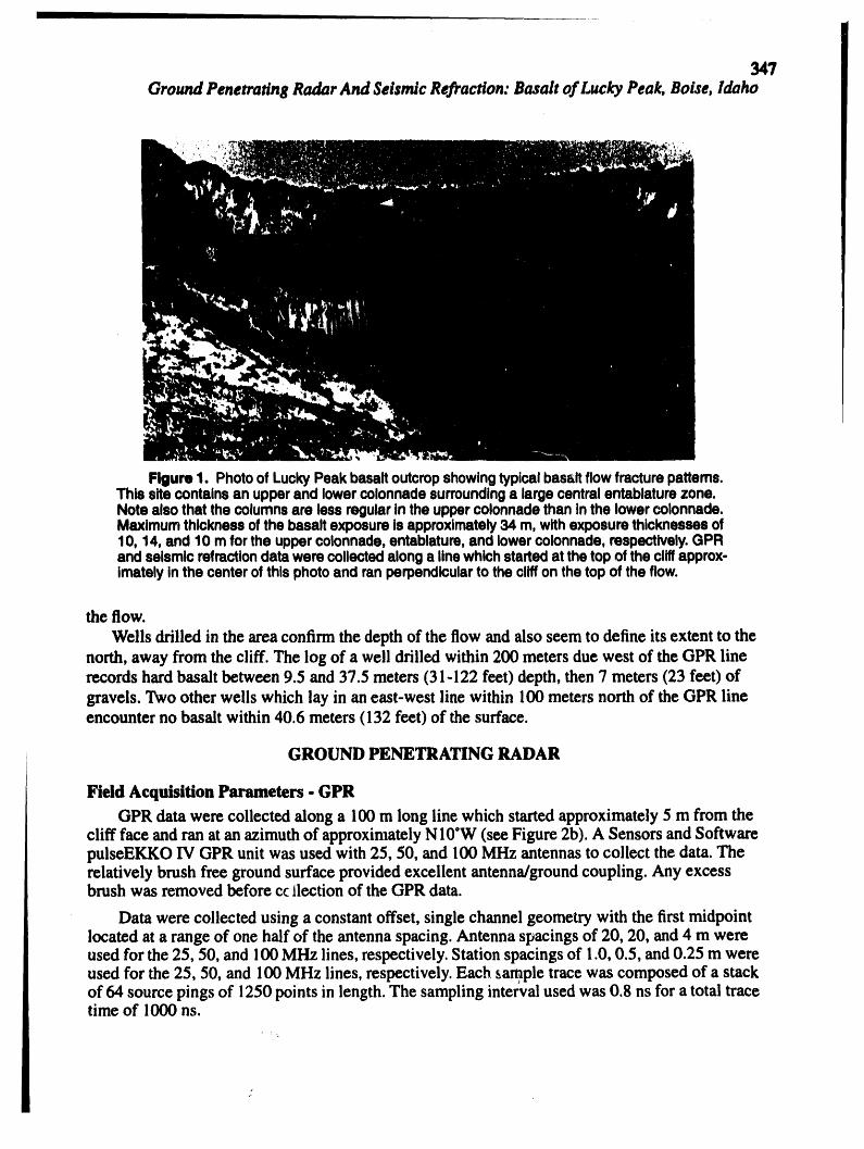
I
347
GroundPeneu'atlngRadarAndSeisn_cRefraction:Basaltofl_ckyPeak,Boise,Idaho
Figure1. PhotoofLuckyPeakbasaltoutcropshowingtypicalbasaltflowfracturepatterns.Thissitecontainsanupperandlowercolonnadesurroundinga largecentralentablaturezone.Notealsothatthecolumnsarelessregularintheuppercolonnadethaninthelowercolonnade.Maximumthicknessofthebasaltexposureisapproximately34m,withexposurethicknessesof10,14,and10mfortheuppercolonnade,entablature,andlowercolonnade,respectively.QPRandseismicrefractiondatawerecollectedalongalinewhichstartedatthetopofthecliffapprox-imatelyinthecenterofthisphotoandranperpendiculartothecliffonthetopoftheflow.
the flow.Wells drilled in the areaconfirmthe depthof the flow andalso seem to define its extent to the
north,awayfrom the cliff. Thelog of a well drilledwithin 200 metersdue west of the GPR linerecordshard basaltbetween9.5 and37.5 meters(31-122 feet) depth, then7 meters (23 feet) ofgravels.Twoother wells which lay in aneast-west line within 100metersnorthof the GPRlineencounterno basalt within 40.6 meters(132 feet) of the surface.
GROUND PENETRATINGRADAR
Field Acquisition Parameters- GPRGPR datawerecollected along a 100m long linewhich startedapproximately5 m fromthe
cliff face andran at anazimuthof approximatelyN10°W (see Figure2b).A Sensors andSoftwarepulseEKKOIV GPRunit was used with 25, 50, and 100 MI-Izantennasto collect the data.Therelativelybrushfree groundsurfaceprovidedexcellent antenna/groundcoupling.Any excessbrush was removedbeforeccllection of the GPRdata.
Data werecollectedusing a constantoffset, single channelgeometry with the firstmidpointlocated at a range of one half of theantennaspacing.Antennaspacingsof 20, 20, and4 m wereused for the 25, 50, and 100MHzlines, respectively.Stationspacingsof 1.0,0.5, and0.25 m wereused forthe 25, 50, and 100MHz lines, respectively.Each sampletracewas composedof a stackof 64 sourcepings of 1250points in length.The samplingintervalused was 0.8 ns for a total tracetime of 1000 ns.

M.E.Dousher_ andothers348
too
o
bo
aR
Figure2. (a) Locationof LuckyPeakBasaltGPRandseismicrefractionstudynearBoise,Idaho.LuckyPeakReservoirandtheBoiseRiverareshownbytheshadedregions.Inset(b)showslocationofGPR/seismiclinerelativeto cliffface.Zeropointof lineisonthesouthendofthelinenearcliffface.Contourintervalin(b)is2 mwiththeelevationoftheuppercliffedgeatapproximately3080m.
Data - GPR
Processed25, 50, and 100 MHz datafrom the GPR line arepresentedin Figure 3. While rawdata taken directly from the pulseEKKO system can usually provide a fairly complete initial viewof the subsurface, additional post-processing is often necessary to take full advantage of the col-lected data [Gerlitz, et al., 1993; Fisher, et al., 1992; Dougherty, et al., 1994, Liberty and Pelton,1994]. This is particularly true for these Lucky Peak basalt data which have relatively low ampli-tude reflected arrivals. While a thorough explanation and display of the inherent trade-offs in pro-cessing is beyond the scope of the paper, a brief description of final processing steps used withthese data is presented below.
A DC shift of each trace for all records in Figure 3 exists and is due to recording offsets of anunknown origin. The magnitude of the DC shift seems to drift somewhat from trace to trace and ismore dramatic in the 25 and 50 MHz data than in the 100 MHz data. Removal of the DC shift is
carded out as the first processing step and is a straight forward subtraction of the mean value ofeach trace for times before arrival of the direct wave. All traces in each record section are nextbandpass filtered with a Butterworth filter in order to remove any residual low-frequency 'WOW'effects [Gerlitz, et al., 1993] and random high frequency noise. Bandpass cutoffs were set at 5-50MHz, 10-100 MHz, and 10-200 MHz for the 25, 50, and 100 MHz data, respectively. 'WOW'effects are manifested by a time-varying DC shift in the data following the direct air wave and aredue to swamping of the system by the high amplitude direct wave. These effects are most preva-lent when using small-offset geometries and were not a major problem with the 20 m offsets usedwhile collecting the 25 and 50 MHz data. Some 'WOW' can be seen in the 100 MHz data, but
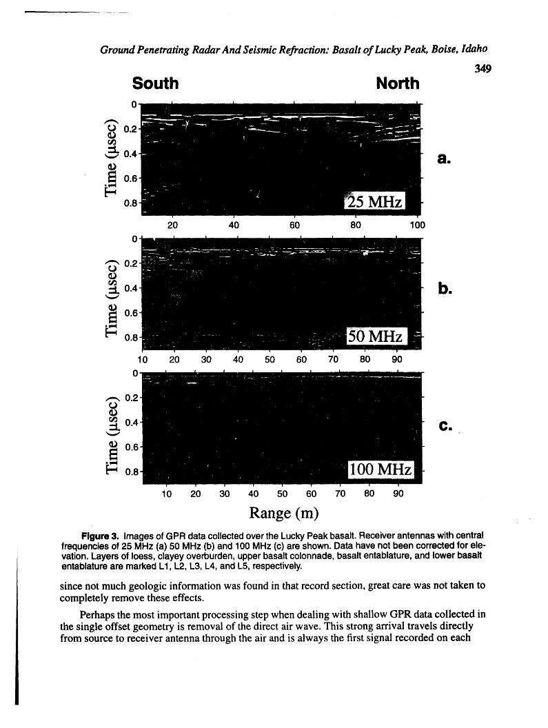
Ground Penetrating Radar And Seismic Refraction: Basalt of Lucky Peak, Boise, Idaho
349
South NorthO-
_0.2
0.4 b,
0.6-
_ 0,8-
10 20 30 40 50 60 70 80 90
0-
0.2-
r_ 0.4=L C.
0.6
_ 0.8
10 20 30 40 50 60 70 80 90
Range (m)Figure 3. Imagesof GPR data collectedovertheLuckyPeak basalt.Receiverantennaswithcentral
frequenciesof 25 MHz (a) 50 MHz (b) and 100MHz (c) are shown.Data havenot been correctedfor ele-vation.Layersof loess,clayeyoverburden,upperbasaltcolonnade,basaltentablature,and lowerbasaltentablatureare markedL1, L2, L3, L4, andL5, respectively.
since not much geologic information was found in that record section, great care was not taken tocompletely remove these effects.
Perhaps the most important processing step when dealing with shallow GPR data collected inthe single offset geometry is removal of the direct air wave. This strong arrival travels directlyfrom source to receiver antenna through the air and is always the first signal recorded on each

M.E. Dougherty and others
35Otrace. Fortunately, since the arrival is traveling a constant distance through a relatively homoge-neous medium (air), its arrival time and waveform are relatively invariant. Reflections from veryshallow strata may interfere with the latterpartof this waveform, but generally this does not affectthe main lobes of the arrival. Various methods have been proposed to dampen the affects of thisarrival and we have found that the subtraction of a normalized 'average' trace is sufficient to pre-vent this arrival from dominating the record sections. The 'average' trace is calculated by firstaligning all traces by first arrival (to correct for instrument timing errors) then summing all of thetraces in a record section. This has the effect of cancelling out most geological arrivals (exceptcontinuous horizontal arrivals) and enhancing the direct wavelet. Finally, the 'average' trace isnormalized in amplitude to the maximum amplitude of the direct arrival in each individual traceand subtracted from each trace. After subtraction of the air wave arrival, the data are scaled lin-early with time (depth) to recover the effects of spherical spreading of the wavefronts.
Arrivals seen in the GPR data include signal returnedfrom geological features, instrumentinterference, and signal returned from cultural features. In general, because of the presence of thecliff, clayey overburden, and field vehicles, there is a fair amount of cultural and geologic noise inthe record sections. The most obvious non-geological arrivals are large diffractions which extendover the entire range of the 25 and 50 MHz data lines and have their peaks beyond the northernend of the line. Velocities of the branches of these diffracted arrivals indicate an origin of air wavereflections from field vehicles parked approximately 30 meters from the northernend of the line.Diffractions with peaks on the southern (cliff) end of the line originate by scattering off the cliffface itself. Other diffractions in the center of the line are most likely due to scattering from therough basalt surface and thus can be considered to contain some geologic information. Diffrac-tions are often collapsed in seismic datathrough a migration process. However, migration was notcarried out here because of the rr_.xof geological diffractions and out-of-plane surface air wavediffractions which have widely different velocities, and hence make the migration process diffi-cult. Coherent horizontal noise which is prevalent after about 600 ns in the 25 and 50 MI-Izdata ismost likely background instrument noise which has been increased in amplitude through the lin-ear gain function used to correct for spherical spreading.
Once the origins of noise in the GPR records are realized and understood, a number of geo-logically relevant arrivals and layers can be identified. Rather than label individual arrivals in theGPR data plots, layers have been labeled and assigned geological significance based on detailsseen in the cliff exposure (see Figure 3) and well log results from nearby wells. In order ofincreasing depth, these layers are: L1, thin surface loess layer which thins below resolution of thewide aperture collection geometry near the center of the line; L2, clayey overburden which gener-ally increases in thickness with range; L3, upper colonnade portion of exposed Lucky Peak basalt;L4, entablature portion of exposed basalt flow; and L5, lower colonnade of exposed basalt flow.These same layers can be seen in both the 25 and 50 MHz GPR records and are slightly moreobvious in the 25 MHz record section. Very little, if any, useful information can be obtained fromthe 100 MHz line. There is a slight hint of scattering off the top of the flow at ranges where theoverburden is not thick (ranges less than 40 meters). The 100 MHz section also suffers from lowfrequency 'WOW' effects directly following the direct wave as described above.
Data images in Figure 3 are plotted with respect to two-way travel time instead of depthbecause of poor constraints on subsurface electromagnetic velocity. A few common midpoint(CMP) experiments were run unsuccessfully near the center of the line in order to obtain accuratevelocity information. However, using an estimated velocity of 0.13 m/ns within the basalts and a20 m antenna spacing would put the upper colonnade/entablature contact at approximately 9-10meters depth and the entablature/lower colonnade contact at approximately 24-25 meters depth atthe cliff face. These depths correspond very closely (within measuring error) to the depths of
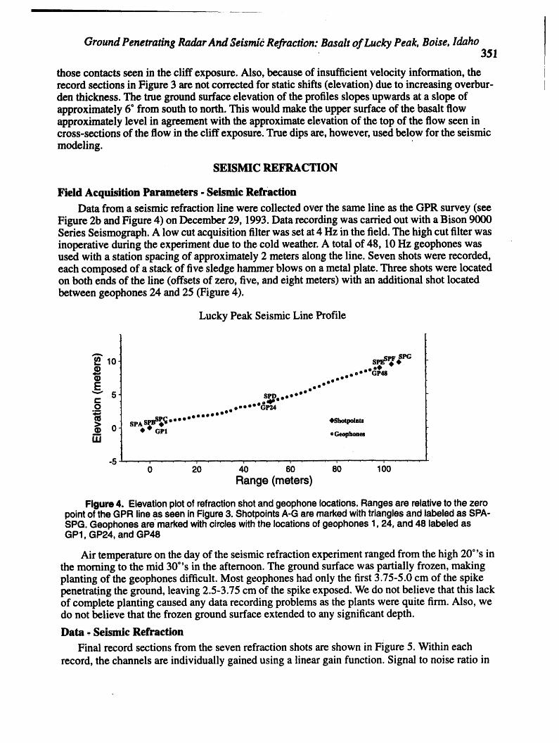
Ground Penetrating Radar And Seismic Refraction: Basalt of Lucky Peak, Boise, Idaho351
those contacts seen in the cliff exposure. Also, because of insufficient velocity information, therecord sections in Figure 3 are not corrected for static shifts (elevation) due to increasing overbur- =den thickness. The true ground surface elevation of the profiles slopes upwards at a slope ofapproximately 6" from south to north. This would make the upper surface of the basalt flowapproximately level in agreement with the approximate elevation of the top of the flow seen incross-sections of the flow in the cliff exposure. True dips are, however, used below for the seismicmodeling.
SEISMIC REFRACTION
Field Acquisition Parameters - Seismic Refraction
Data from a seismic refraction line were collected over the same line as the GPR survey (seeFigure 2b and Figure 4) on December 29, 1993. Data recording was carried out with a Bison 9000Series Seismograph. A low cut acquisition filter was set at 4 Hz in the field. The high cut filter wasinoperative during the experiment due to the cold weather. A total of 48, 10 Hz geophones wasused with a station spacing of approximately 2 meters along the line. Seven shots were recorded,each composed of a stack of five sledge hammer blows on a metal plate. Three shots were locatedon both ends of the line (offsets of zero, five, and eight meters) with an additional shot locatedbetween geophones 24 and 25 (Figure 4).
Lucky Peak Seismic Line Profile
_PF SPG
=0 R_
._ ooee °" GP48
5 eoee e°e°°°°°eA
o0JO ooO/_
"_ OQooOOO 0
sPAsr_ °""""" .s_,tpo_u0 • '¢ GPI • Geophonesmmm
LU
-s • . 6 2'o ' 4o 6'o..... 8'o 16oRange (meters)
Figure4. Elevationplotof refractionshotandgeophonelocations.Rangesarerelativetothezeropointof theGPRlineasseeninFigure3. ShotpointsA-Garemarkedwithtrianglesandlabeledas SPA-SPG.Geophonesare"markedwithcircleswiththelocationsofgeophones1,24, and48 labeledasGP1,GP24,andGP48
Air temperature on the day of the seismic refraction experiment ranged from the high 200's inthe morning to the mid 30°'s in the afternoon. The ground surface was partially frozen, makingplanting of the geophones difficult. Most geophones had only the first 3.75-5.0 cm of the spikepenetrating the ground, leaving 2.5-3.75 cm of the spike exposed. We do not believe that this lackof complete planting caused any data recording problems as the plants were quite firm. Also, wedo not believe that the frozen ground surface extended to any significant depth.
Data, Seismic Refraction
Final record sections from the seven refraction shots are shown in Figure 5. Within eachrecord, the channels are individually gained using a linear gain function. Signal to noise ratio in

M.E.Doughertyandothers
352eachoftherecordsbecomesfairlylowbeyondrangesofapproximately50-60m.Confidenceinpicksbeyondthoserangesisgivenalow valueinsubsequentanalyses.Inanefforttofacilitatepickingfirstarrivals,thedataarefilteredwitha 50-150I-IzbandpassButterworthfilter.Thishastheeffectofremovingsomeofthelowfrequencynoiseandallofthehighfrequencynoise.Afterfiltering,itispossibletopickfirstarrivalsforafewmorechannelsineachrecord,buttheconfi-denceinthesepicksislow.
Fourmainrefractionbranchescanbeseeninthefinalseismicdata.Whiledatafromonlyoneshotpoint(shotpointC,seeFigures4 and5)showalloftherefractionbranches,individualrecordsectionsshowvariouscombinationsofthefourarrivals.Thesebrancheswerepickedaccordingtocrossoversinthefirstarrivalcurvesandlabeledbasedonsimilarslopes(reciprocalvelocities).Slopeswereroughlycorrectedfordipofrefractorsbasedonasimplelayeredmodelandtherecip-rocalmethod[Hawkins,1961;Burger,1992]beforeassigninglabels.ArrivalsRI,R2,R3,andR4correspondtoadirectwavethroughthethinloesslayer,andheadwavesalongthetopsoflayersofclayeysoil,upperbasaltcolonnade,andbasaltentablature,respectively,asseenintheGPRdataandinthecliffexposureforthebasaltcontacts.
Models - Seismic Refraction
Forward and inverse raytracing models were constructed in order to confirminterpretation ofthe seismic refraction results. Construction of the models was also aided by preliminary interpre-tation of the GPR data. RAYINVR, a seismic raytracing inversion program, was used for all of themodel development and inversions [Zelt and Ellis, 1988]. Inputs to the RAYINVR models includeseismic velocities (compressional and shear, if desired), surface elevation, shot locations, and sub-surface layer structure. Once seismic field data are available, arrival times with uncertainties andarrival type can also be entered for inversion of the field data. A preliminary model based on GPRresults and expected seismic velocities was calculated before the seismic refraction experiment.Results from this model were used to determine the resolution of the refraction method and alsoas an aid in laying out the seismic line.
After acquisition of the refraction data, a refined starting model was developed based on theGPR results and preliminary velocities obtained by using the reciprocal method [Hawkins, 1961].As seen in Figure 6a, this model contains many of the geologic features as seen in the GPR results(Figure 3) including two overburden layers and two basalt layers. Figure 6 is an example of theoutput of the RAYINVR modeling program.The upper portion of both Figures 6a and 6b are plotsof the model geometry and rays traced through the model. Layer boundaries are shown withdashed lines and seismic rays are shown by the solid lines. Ground surface elevations wereobtained from a survey of the seismic line and shot locations. Subsurface information wasinferred form the GPR results and reciprocal method reduction of the refraction data. Depths andranges are relative to zero being at the edge of the cliff face in these diagrams. The lower portionof the plots in Figures 6a and 6b are plots of the seismic arrival times for both the model and fieldresults. Solid lines ifidicate model travel time results and crosses indicate actual arrival timesobserved in the field.
Figure 6a shows results of the starting model compared to field data from shotpoint B of therefraction line. In general, agreement between the model and the field data is quite good, indicat-ing that the model is a good fit to the actual field conditions (within the constraints of non-unique-ness). Arrivals from layers 2, 3, and 4 are found in the data, as seen in Figure 5b. Althoughpreliminary model-data comparisons are only shown here for shotpoint B, comparisons for all ofthe shotpoints were calculated and all show a high degree of agreement.
Once general agreement is made between the preliminary RAYINVR forward model andfield data, inversions of the field data can be carried out with the program. This technique is useful

353
Ground Penetrating Radar And Seismic Refraction: Basalt of Lucky Peak, Boise, Idaho
0.1 i 0.1 " -
0.05 ,, __ ._'0.05
- 20 40 60 80 IO0 20 40 60 80 1O0distancefromshot(meters) distancefromshot(meters) ..
0.1 ........
0.11
o.o+l/l/l iliil++o0 -40 -20 0 20 40
distancefrom shot (meters) distancefromshot(meters_
+oo++++++,+,,+,+,+++::io_+'''''''''''''''''''''''+''+'+.,,'oo.80+o -,o .+,o-80 -60 -40 -20 0distancefromshot(meters) distancefromshot(meters)
+o, 'iiiiiIIi0.
-100 -80 -60 -40 -20distancefromshot(meters)
Figure 5, Seismicdatafromall shotsof the LuckyPeak basaltrefractionline.Arrivalsfromsimilarrefractorsare labelledon eachplot.See Figure4 forlocationof shotpoints.
for investigations of the trade-off between depth to layers and their velocity. Inversions were car-ded out on the Lucky Peak basalt refraction data by using arrival time picks from all of the shot-points simultaneously. This overconstrains the inversion calculation given the number of freevariables (grid node locations and/or velocity values) used in these models (node locations givenby crossing dashed lines in model geometry plots of Figure 6).
Three separate inversions were obtained from the refraction data, each allowed different setsof variables to vary. In general, travel time variations can be caused by variations in layer veloci-ties or thicknesses. Inversions with varying layer depths, velocities, and a combination of varying
velocities and depths were calculated. Results from the inversion which allowed both velocities

354 _ M.E. Dougherty and others
DISTANCE (m)0 2O 40 60 8O 100
I I . I I I-10.0
SPB Layer 1 - 0.20 km/s [_l_II]
!?.::zs 70 km/s
La er 3 - 1.50 km/s i'_'_--- a.
,, !: La,yer 4 - _.S0 km/s ,
15.0 , , , ,, ,
ve - Layer 40 ! , Mean wave -/_ayer ._
0 20 4O 6O 8O 100
DISTANCE (m)
DISTANCE (m)0 _ 40 60 80 lflO
....... I I I 1 I-10.0-
.... 0 19 km/s 0.20 km/s - -,_,,_ _l_-•_l Kn11/S ", _ . _I_I_U _f\_ I
/,
i i' i: z.so , z.s0kns15.0 ', ', ',, , , ', 'I_1_
_..
_'120- "...... _.-Head Wave - Layer 2
-.... ..........................32 Head Wave - Layer 4 - ++++++_
0 26 46 60 80 10() " -
DISTANCE (m)
Figure 6. (a) StartingRAYINVRmodelderivedfromthe interpretedGPR recordsshowingraystraced fromshotpointB (SPB) of the LuckyPeak basaltrefractionexperiment.Modelgridboundaries(dashedlines)and tracedrays (solidlines)showninthe upperportionof the plot.Observed(crosses)andcalculated(solidline)arrivalsshowninthe lowerportionof the plot.(b) FinalinvertedRAYINVRmodelshowingraystraced fromshotpointF (SPF) of the LuckyPeak basaltrefractionexperiment.Velocitiesanddepthsto layershavebeenallowedto varyfor thisinversion.Althoughonlyrays andarrivaltimesfromshotpointF areshownforclarity,allshotsandarrivalswere usedforcalculationof theinversions.

GroundPenetratingRadarAnd SeismicRefraction:BasaltofLuckyPeak,Boise,Idaho 355
anddepthstov_y areshowninFigure6b.Thisfinalmodelincorporatesmostofthefeaturesseenin the inversions with only one variable parameter. As can be seen in Figures 6a and 6b, since thestarting model produces arrival times that are relatively close to the observed data, very littlechange in the model is seen upon three iterations of inversion. The main features that change arethe thickness of the loess layer and some very slight velocity variations within layers 1 and 2(loess and clayey overburden, respectively). Variable thickness of the loess layer in the seismicmodel corresponds well with the general characteristics of that layer as seen in the GPR data.
DISCUSSION
Although the ground penetrating radarresults exhibit a relatively low signal to noise ratio,most of the important geological features can still be identified in the GPR images (Figure 3).Depths to the boundaries between internal flow structures (entablature and colonnades) agreeclosely to the corresponding boundaries seen in the cliff exposure. We believe that attenuation dueto the presence of clayey overburden limits the ability of the GPR to see into the basalts exceptwhere the overburden is relatively thin on the cliff end of the line. Scattering from fractures con-tributes additional propagation losses once the signal has entered the basalts. These loss mecha-nisms prevent the bottom of the flow from being imaged at this site.
The seismic refraction line was originally proposed as a mechanism to constrain overburdenthickness. Results presented here contain the added information of internal structural layeringwithin the basalt flow. Velocity variations within the basalt flow could be due to weathering and/ordiffering degrees of fracturing in the different structuralunits. Since the upper colonnade is rela-tively less fractured than the entablature, one would expect its seismic velocity to be relativelyfaster based on fracture density/velocity relationships. However, compressional velocities ofapproximately 1.5 km/s indicate that the upper colonnade probably has experienced greaterweathering than the rest of the flow. A velocity difference between the entablature and lower col-onnade could not be resolved within the constraints of the experiment geometry used for thisrefraction line. A longer line oriented perpendicular to the refraction line presented here wouldpossibly be more effective at resolving all layering within the basalt flow.
It is clear in data from both geophysical methods presented above that layering exists withinthe Lucky Peak basalt flow as seen in the cliff exposure, and that this layering is detectable usingsurface geophysical methods. A thinning of the upper colonnade is typical for these types ofbasalt flows [Long and Wood, i986] as the cooling structuresare often not laterally continuousover any great distance. This can be seen in lateral cross-sections of the Lucky Peak basalt cliffexposure as well. Differential weathering throughout the flow with a higher degree of weatheringtowards the top of the flow is to be expected as well and can account for the relatively low seismicvelocities seen in the refraction data [Dougherty, et al., 1992; 1993]. It is not clear, however, whydistinct seismic arrivals are not seen for the entablature and lower colonnade layers. One factor isthat the length of the line and source strength may not have been sufficient to resolve these twolayers.
Interpretation of data from GPR in combination with that from seismic techniques is a power-ful tool and allows for a high degree of confidence in the final model presented above. While GPRcollected in the single offset geometry used here can give a quick first lock at the geological envi-ronment, seismic refraction can add additional depth constraints to the model. Also, since the twotechniques essentially measure different physical properties, independent confirmation of the geo-logic structure is obtained by the two methods. This assumes, of course, that the respective physi-cal properties measured by the two tech_iques are unique in different geologic structures. Also, it
/
/
,,1
M.E. Dousherty and others356
suggests that joint inversion of data collected by these two techniques should provide a well con-strained model of fracture structure within basalts.
Data presented here are the result of two days of opportunistic fieldwork carried out in timewindows when geophysical equipment was available. A limited amount of planning and recon-naissance time was available prior to days when it was necessary to carry out the fieldwork. Giventhe success of these initial results, we feel that this study could benefit greatly by additional datacollection from other portions of the Lucky Peak basalt. Specifically, areas where less overburdenis present and where longer lines could be runat a greater distance from the cliff face are availablein close proximity to the line used for this study.
CONCLUSIONS
We have presented here the results from a geophysical investigation of the Lucky Peak basaltflow using ground penetrating radarand seismic refraction techniques. In general, agreement ofthe results between the two techniques and between the geophysical models and structure seen inthe adjacent outcrop exposure is excellent. Structures within the overburden as well as fromwithin the basalt flow itself can be distinguished with both methods. However, attenuation of theGPR signal due to absorption in clayey sediments and scattering from cracks in the basalt, as wellas insufficient seismic source strength and line length, prevent the base of the flow from beingimaged by either geophysical method used here. Results from this study warrant further researchinto the simultaneous ose of electrical and seismic methods to image fracture systems in terrestrialbasalts.
ACKNOWLEDGEMENTS
This work was supported by the Idaho State Board of Education and the Office of NavalResearch Grant #N00014-92-J-1143. Boise State University Center for Geophysical Investigationof the Shallow Subsurface contribution #0027.
REFERENCES
Burger, R.H, Exploration Geophysics of the Shallow Subsurface, Prentice Hall, Englewood Cliffs,NJ, 489 p., 1992.
Berggren, W. A., D.V. Kent, J.L Flynn, and J.A. Van Couvering, Cenozoic geochronology, Geol.Soc. Am. Bull., 96, 1407-1418, 1985.
Cheng, C.H., and M.N. Toks6z, Elastic wave propagation in a fluid-filled borehole and syntheticacoustic logs, Geophysics, 46, 1042-1053, 1981.
Collett, R. A., Soil survey of Ada County area, Idaho, U.S. Department of Agriculture, Soil Con-servation Service, 1980.
Dougherty, M.E., Gillis, K.M., Pelton, J.R., and Sapp, K., A geological and seismic study of theupper oceanic crust in the Troodos Ophiolite, Cyprus, Transactions, EOS, 73, 355, 1992.
Dougherty, M.E., Kay, S.E., Pelton, J.R., and Gillis, K.M., Predictions of fine scale seismic struc-ture of the upper oceanic crust, Transactions, EOS, 74, 426, 1993.
Dougherty, M.E., Enhancement of ground penetrating radar data through signal processing, sub-mitted to the Proceedings of the Symposium on the Application of Geophysics to Engineeringand Environmental Problems, SAGEEP '94, 1994.

Ground Penetratin8 Radar And Seisnffc Refraction: Basalt of Lucky Peak, Boise, Idaho 357
Fisher, E., G.A. McMechan and A.P. Annan, Acquisition and processing of wide-aperture ground-penetrating radardata, Geophysics, 57, 495-504, 1992.
Geditz, K., M.D. Knoll, G.M. Cross, R.D. Luzitano and R. Knight, Processing ground penetratingradar datato improve resolution of near-surface targets, Proceedings of the Symposium on theApplication of Geophysics to Engineering and Environmental Problems, SAGEEP '93, 2,561-574, 1993.
Hawkins, L.V., The reciprocal method of routine shallow seismic refraction investigations, Geo-physics, 26, 806-819, 1961.
Howard, K.A., J.W. Shervais, and E.H. McKee, Canyon-filling lavas and lava dams on the BoiseRiver, Idaho, and their significance for evaluating downcutting during the last two millionyears, in Bill Bonnichsen andR.M. Breckenridge, editors, Cenozoic Geology ofldaho, IdahoBureau of Mines and Geology Bulletin, 26, 629-641, 1982.
Kuster, G.T., and M.N. ToksSz, Velocity and attenuation of seismic waves in two-phase media, I.Theoretical formulations, Geophysics, 39, 607-618, 1974.
Liberty, L.M., and J.R. Pelton, A comparison of ground penetrating radar: Multi-fold data vs. sin-gle fold data, this volume, 1994.
Long, P. E., and B.J. Wood, Structures, textures, and cooling histories of Columbia River basaltflows, Geol. Soc. Am. Bull., 97, 1144-1155, 1986.
Mankinen, E.A., and G.B. Dalrymple, Revised geomagnetic time scale for the interval 0-5 m.y.B.P., J. Geophys. Res., 84, 615-626, 1979.
Olhoeft, G.R., Tutorial: High frequency electrical properties, United States Geological SurveyOpen File Report 0FR-90.0414, 48, 1990.
O'Connell, R.J. and B. Budiansky, Seismic velocities in dry and saturated cracked solids, J. Geo-phys. Res., 79, 5412-5426, 1974.
Othberg, K. L., and W. L. Burnham, Geologic map of the Lucky Peak quadrangle, Ada County,Idaho, Idaho Geological Survey Technical Report 90-4, 1990.
Zclt, C.Z., and R.M. Ellis, Practical and efficient ray tracing in two-dimensional media for rapidtraveltime and amplitude forward modelling, Canadian Journal of Exploration Geophysics,24, 16-31, 1988.

t_
ClO

!
Hydrogeology, Waste Disposal, Science and PoliticsProceedings 30th SymposiumEngineering Geology and Geotechnical Engineering, 1994
•' 359RESULTS OF A_LEFORltATIORMICROSCANNER x STUDY IN A
JURO-TRiASSIC-ACED SEDIMENTARY DEPOSIT (PASSAIC FORMATION)
byJoseph A. Fischer, Geoscience ServicesJoseph J. Fischer, Geoscience Services
Robert J. Buliwinkel, Schlumberger Wireline & Testing Services
ASSTP£CT
Studies to determine the structural and geohydrological properties of thePassaic Formation were performed at two sites. Both sites are located in north-eastern New Jersey, within the Juro-Triassic-aged Newark Basin. The PassaicFormation rocks are described in the literature as a reddish brown, thin to mas-
sively bedded, sedimentary deposit with lithology ranging from claystone throughconglomerate. A fractured "layer cake" model has been proposed (and is general-ly accepted) to describe the prevailing geohydrological conditions.
The Formation MicroScanner tool was used in four wells drilled for these
projects (two at each site). In addition to this microresistivity tool, a suiteof other oil field geophysical tools (Gamma, Induction, Dipmeter, Temperature,and Neutron probes) were also utilized. The data collected with the FormationMicroScanner were correlated with detailed logs and the continuous core retrievedfrom three of the wells. Pump test data was also obtained at both sites. Thegeophysical data obtained at both sites allowed the direct identification offractures and their orientation in relation to bedding. Fracture and bedding ap-erture size and orientation were measured. The results, as presented in this pa-per, show a high degree of inhomogeneity at both sites rather than the conven-tional layer cake model. For appropriate site analyses it was necessary to sig-nificantly refine the previously assumed Passaic Formation geohydrological andstructural model.
INTRODUCTION
The role of geophysical instrumentation in various geotechnical disciplines
is well accepted. While many geophysical tools are extremely useful, they haveoften been oversold or misapplied. While recognizing this concern, the authorswould like to describe the use of the Formation MicroScanner tool in Passaic
Formation rocks at two sites in New Jersey.The Passaic Formation underlies some 3000 square miles of New Jersey. Sim-
ilar rocks are found in all the Juro-Trlasslc-aged basins of the eastern United
States. Bordered by major northeast trending faults along the western margin,
the Newark Basin of New Jersey is filled with thick, clastic sediments transport-
ed from the west. Igneous events have resulted in dikes, extrusive units, sillsand plutons.
As a result of its' extent in New Jersey, the Newark Basin is a source of
potable water as well as a repository for hazardous waste. Many large structuresare built upon and within the basin and many more are planned for the future.
Hence, a thorough understanding of its physical characteristics is necessary
whether one wishes to i) locate a potable water supply, 2) cleanup a hazardouswaste site, or 3) build upon or within it.
_Trademark of Schlumberger Well Services

J. A, Fimcher and others
36OAt the two sites described herein, both the structural and hydrogeologlcal
properties of the Passaic Formation were of significance. Traditional fleldtechniques (hlgh-quallty coring, detailed logs and pump test data) were used tocharacterize the formation. In addition, a new oll field geophysical tool, a
downhole mlcroreslstlvlty (MR) tool was employed in four borings ranging in depthfrom 105 to 500 feet below the ground surface. The available geologlc informa-
tion for each site was expanded and enhancedbycorrelatlng FMS data with the re-
sults of continuous and careful corln8 and logglng in three boreholes at thesetwo sites.
FORMATIONMICRO$CANNER_TOOL
The MR tool images the borehole wall by utillzing a four pad array of six-
teen mlcroconductlvlty electrodes each. The electrodes examine 0.1 inch vertlcal
increments laterally around the borehole wall as the tool is pulled uphole. Atrlaxial accelerometer and threemagnetometers are used to determine tool orien-
tation and subsequently, attitudes of bedding planes.Variations in currents for each of the electrode buttons are recorded in
a series of traces. These variations in mlcroreslstlvlty can be caused by
changes in porosity, graln-slze, mlneralogy, cementation, and fluld type. Theresistivity traces are converted to a sixteen channel white, black or gray image
with white denoting the highest resistivity and black the lowest resistivity.
Data processing is required to correct for variations in tool movement,
voltage output and button contact. The image Is converted from gray shades toa 256 channel color image, on a specially designed workstation, in order to im-
prove analysis capabilities.
Figures i and 2 show typlcal black and white copies of workstation displaystaken from the two sites discussed. Bed thickness can be identified to an order
of I mm. Bedding planes and fluld-filled fractures are readily seen and can be
selected for true dip and strike calculations. A three dimensional display aids
the interpreter in visualizing in sltu characteristics at varying orientations.
Stratlgraphlc patterns can be measured and described with an unusual degree of
confidence. Lithologlcal features such as grain-size, porosity and mineralogycan be identified to a relative degree. With the use of a calibrated resistivity
curve and borehole fluld salinity measurements, the fracture aperture can bemeasured within a fraction of an inch.
PASSAIC FORMATION - NEW JERSEY
The Newark Basin shows two fundamental depositlonal patterns (Schllsse and
Olsen, 1990). The first is fluvial, formed in a hydrologically open basin and
characterized by i) baslnwlde channel systems; 2) lentlcular bedding; 3) con-
glomerate intervals; 4) paleocurrent patterns that are often axlal or trend inone direction across the basin (indicating extensive subsurface drainage); and
5) the lack of evidence of large lakes, although some pond or paludal depositshave been noted. The second is a lacustrine pattern that would be consistent
with a hydrologlcally closed basin model. These criteria include (from Smoot,
1985): I) increases in graln-size toward the basin boundaries; 2) paleocurrentpatterns away from the basin borders; 3) local coarse-gralned strata near the ba-
slnmarglns; 4) evaporltes or evaporlte crystal clasts; and 5) cycllclty of fine-Erained sedimentary rocks'in the central basin. Cyclically deposited lacustrine
beds extend over large areas (Oisen, in press), and the basin margins show sig-
nificant deposits of lake-margln fluvial and deltaic sequences, as well as allu-vlal fans. Within the basin, these two generalized depositlonal systems are very

Downhole Formation Microscanner Study, Pasmalc Formation
361
persistent through time and are the largest stratiaraphlc elements of the Newark
Basin, although Igneous extrusive and intrusive flows are common, particularlynear the border fault.
From a structural standpoint, the Newark Basin may be considered a half-
graben bounded by northeast trendln 8, southeasterly dipping faults (the Ramapoborder fault system) to the west and gently westward dlppln 8 strata to the east.
Numerous faults, both synthetic and antlthetfc to the border fault in nature, are
recoKnlzed throughout the basin. Numerous, generally northwest trending thrust
features have been mapped across the border fault and wot_td probably be foundwithin the basin itself if further InvestIKatlon were undertaken.
The available literature did not indicate any faulting in the vicinity ofeither site discussed herein, although shear zones and/or Jointing could be ex-
pected anywhere as a result of the major movements that have taken place in thisrift basin.
The current in situ stress system is believed to be generally consistentwith that of much of the northern Atlantic coastline. The minor principal stressis vertical, with the major and intermediate principal stresses of a compressivenature. Thus, the in situ stress system would tend to open any uncemented sub-horizontal bedding planes. With the major principal stress oriented to thenortheast, one would also expect that shallowly dipping fracture zones orientedin a northwest/southeast direction would be those most susceptible to movement.
PASSAIC FORMATION - SITE SPECIFIC
General
In the literature (New Jersey Geological Survey Atlas Sheets and Summaries,and Monteverde, in press), the structure and litholoay of the two sites in ques-tion (although separated by some lO miles) are relatively similar. Site A hadtwo wells logged with the Formation MicroScanner tool, with one well cored witha triple-tube, wireline, split barrel. Site B had two wells cored with a triple-cube, wireline, conventional barrel and were logged in a similar manner. The Pas-saic Formation (formerly known as the Brunswick Formation or Brunswick Shale) was
believed to be relatively thinly-bedded and presumed to be a primarily sandy sec-tion at Site A, while at Site B, the section was presumed to be more silty. Bed-ding was reported to dip about 15 ° northwest with a N±30°E strike at Site A anddip at about 8 ° tO 10 ° northwest with a N±40°E strike at Site B.
Table 1, below, prepared from as yet unpublished (New Jersey GeologicalSurvey) information, summarizes the range of hydrogeologic characteristics mea-sured in various tests within the Passaic at a number of locations throughout theNewark Basin. As may be seen from Table 1, the large variations in propertiesfrom the many sites would seem to indicate the non-uniformity of the formation,perhaps indicating the typical, current assumption of uniform anisotropy is, atbest, a local condition.
TABLE 1
HYDJtOGEOLOGICESTIMATES . PASSAI(_ FORMATION
Transmissivity - 400 to 88,200 gpd/ft
Storatlvlty - ix10-6 to 4.5xi0-6
Hydraulic Conductivity- 0.15 to 90 it/day

J. A. Fischer and others
362From a structural standpoint, the rocks can be considered to be relatively
weak, brittle sediments, sometimes with open bedding planes and joints. Although
not necessarily noted in the literature, fractures are often closed with second-
ary mlneralization. Soft rock tunnellngmachines generally would be appropriate
for controlled excavation. Ordinarily, blasting is necessary for conventionalexcavation below some !10 feet beneath the varying depth weathered zone. Excava-
tion in fault zones has proceeded, easily, to the maximum reach of the available
equipment.
Hydrogeologically, a series of papers have described the Passaic sediments
somewhat differently, but perhaps in a more definitive manner with time and in-creased information. The earlier papers on the subject, by a number of geolo-
gists in New Jersey (e.g., Vecchioli, 1965, and Vecchioll, et al, 1969), dis-
cussed the non-homogeneity of the aquifer system in the Passaic. These earlier
studies and evaluations were a cooperative effort of the USGS and the forerunner
of the NJGS. It was generally accepted by these investigators that drawdownalong strike was greater than drawdown parallel to strike.
In the Vecchioll, 1965 paper, transmissivltles were reported at sites in
Kenilworth, Linden, New Brunswick, Nyckoff, and Flemington. T values ranged from
about 400 to 88,200 gallons/day/foot (gpd/ft) apparently using Theis, 1935 as-
sumptions to analyze the test results. "Always, cross-strike T's were less thanalong strike T's". The 1969 Vecchloli, et al paper concluded that the Passaic
had "anisotropic hydraulic properties everywhere. The degree of anisotropy var-
ies from place to place. In some areas it is considerably less; in fact, it may
even approach isotropy. Where mildly anisotroplc conditions exist, one could
conclude that discrete producing zones do not occur, but that the formation is
thoroughly dissected by interconnecting fractures resulting in hydraullc continu-ity in all directions. Nonetheless, drawdown is always greatest along strike".
In a later paper, Michalski (1990) concluded: "Ground water flow in the
Passaic appears to be influenced primarily by partings along bedding and by the
contrast in degree of fracturing between beds. A lingering belief that near ver-tical fractures oriented parallel to the strike of the beds dominates the flow
is not supported by field data.
"On a scale typical of most ground wate_ contamination studies, the Passaic
hosts a multiunit, leaky ground water system in which individual water bearing
units are relatively thin and parallel to the bedding. A large scale anisotropicflow pattern results from the inherent heterogeneity of the multlunit system.
Along strike flow direction is favored within the saturated reaches of individual
water-bearing units, and vertical flow across intervening aquitards is produced
by head differences in the water bearing units".
Boyle's (1991) study of a well field in Pennington had a number of inter-esting conclusions, as follows:
i. There was a "general trend of !.ncreaslng water level depth with
increases in well depth".
2. The hydrogeologic analysis in the paper supported an earlier the-orization of a fault fracture system "complicity" in measured wellinterference effects.
Rather than the more conventional Theis analysis, Boyle utilized (apparent-
ly successfully) the Jenkins and Prentice, 1982 analyses which presumes a domi-
nant fracture system as the major influence on water movement.If one were to attempt to summarize the literature available in 1993 for
the Passaic Formation, both sites would be presumed to be geohydrologically sim-ilar, as follows:
A multi-layered aquifer system with low primary porosity and rela-
Downhole Formation Microscanner Study, Passaic Formation
363
tively high secondary porosity. Water could be found under bothconfined and unconfined conditions. Secondary porosity would be
primarily composed of major bedding plane partingsand near-vertical
joints. If existing at a site, faults or fracture zones could also
influence water movement. However, in the absencb of faulting a
"uniform anisotropy" could be presumed in evaluating test data.
Site A
Figure 3 shows 20 feet of core run taken from the 311 foot deep well at
Site A (correlative with the MR log, Figure l). The recovered core is consistent
with the generic description of the Passaic Formation except, perhaps, for therelatively interbedded nature of the rocks encountered in this borehole which,
in effect, results in massively- rather than a thinly-beddednature. Additional-
ly, far fewer sandstone layers were encountered throughout the borehole than
might be assumed from the available local information. The interbedded natureof the formation at this location is quite evident on both Figures 1 and 3.
Fractures, bedding plane partings and mineralization were noted on the core logs
throughout the full depth of the borehole.
Our interpretation of the MR log of this hole was completely consistent
with the core log in relation to type and thickness of the various beds and majorfracture locations. In addition, the MRlog indicated that structural dip gener-
ally ranged from 10 ° to 12° to the west-northwest (although some dips as high as
20° were measured). The log also indicated uncorrected depositional flow to the
west-northwest. Porosity was estimated to be in the 6_ to IOZ range in theshales and 16Z to 21Z in the sandstones and conglomerate zones.
In general, fracture aperture was small (<0.1 mm) and dipped at an angle
of 60 ° to 80°0 Partial healing was apparent in most fractures. Fracture orien-
tation was predominantly east and southeast in the deep well and random in the
shallow (105 foot) well. Some indication of bedding displacement is visible inboth boreholes. This could have resulted from nearby faulting. However, any
fault orientation is not readily identifiable from the MR images.
A pump test on the deep well yielded a transmissivlty value of about 0.0005
ftZ/min (5 gpd/ft) using the "confined leaky" assumptions described in Hantush,1956. The shallower well had a measured transmissivity of 0.016 ft2/min (170
gpd/ft) in the same multi-well pump test with the same Hantush, 1956 aquifer as-
sumptions. Other wells at the site had T values as high as 0.19 ft2/ min (2,000
gpd/ft). One high T well was only 150 feet from the 311 foot deep, low T well.
Thus, there is no evidence of any homogeneity or uniform anisotropy from the mul-ti-well pump test performed at the site.
Site B
Two deep (500 foot) holes were cored at this site using a triple-tube,wireline, split core-barrel. The core log for the 481 to 489 foot depth in one
of the boreholes is provided as Figure 4 (see also the MR log of this interval
on Figure 2). In general, the logs show thinly- to massively-bedded shales, '
siltstones and sandstones. Porosity ranged from about 10Z in the shales to 16Z
to 18Z in the siltstones and sandstones. Calcareous fracture fillings were notedthroughout both the core and the photoelectric factor (PEF) curve.
Bedding planes dipped i0 ° to 15" to the northwest, with again, an apparent
(uncorrected) northwest sediment transport direction. Fracture aperture ranges
from about 0.I nun to 1.0 mm. Many fractures are healed. Fracture orientation
was predominantly to the southeast at about 90° to the structural trend. Addi-
tional fractures were detected in a west-northwest direction dipping at about 20°to 30 °, which would be consistent with the present regional stress regime.

J. A. Fischer and others
364Using the structural information for the two borings at this site (spaced
some 700 feet apart) a N±30°E striking fault, dipping ±45 ° to the southeast canbe postulated. As interpreted, this fault would pass quite close to thenorther-
ly we11_
A pump test in the more southerly well yielded transmissivity values of
0.05 ft2/min (500 gpd/ft) with the "confined" aquifer assumptions of Theis, 1935
and similar, but slightly lower values with the Moench, 1984 fractured rock aqui-fer assumptions.
ENGINEERING GEOI/)GYASSESSMENT
From an engineering geology standpoint, several concerns were quite evident
from the investigations at these two sites. First and perhaps most important isthe extreme variability of the Passaic Formation over relatively short vertical
and horizontal distances. Even in relatively close boreholes (essentially on-
strike at Site B), all with full core recovery and a suite of geophysical logs,
lithologic correlation was impossible. The borings are fully representative ofthe lithology described in the literature and often seen in outcrop, but defini-
tive, contlnuou_ marker beds are rare and geophysical signatures are probably the
most suitable (albeit questionable) means of correlating between borings. In
fact, the attempts to draw a cross section at Site B were finally predicated upon
bedding plane dip variations, uranium-thoriummeasurements and volumetric analy-ses rather than upon conventional lithology or gamma ray signatures.
This variability probably results in the need to make conservative simpli-
fications in subsurface assumptions in designing structures on or through the
Passaic. Additionally, fracture zones, which will certainly influence supporting ,capacity, slope stability, as well as tunnelling procedures and lining, are prob-
ably quite common. Obviously, investigations, planning, design, and construction
must consider the likelihood of major or minor fractures through the brittle
rocks of the Newark Basin. Perhaps even more important in subsurface construc-tion is that these fractures will be the primary conduits for water or contami-nant movement.
HYDROGEOLOGIC ASSESSMENT
The results of the various evaluations at these two site8 indicate thatstudies performed within Passaic Formation rocks must be conducted with care and
with the knowledge that the hydrogeologic characteristics of the formation may
vary rapidly over short horizontal distances. At both locations, determining thestrike and dip of the bedding would have been difficult (if not impossible), evenwith oriented core, because of the lack of obvious marker beds.
Bedding plane openings (size and frequency) were extremely variable from
location to location, and even from well to well at Site A. Thus, the pervasive-ness of bedding plane openings that might be presumed to exist from some of the
available literature was not found at these sites. It is important to note that
only the MR logs could show the nature of the bedding planes in situ, i.e.,
tightness, aperture size and filling.
The estimates of porosity made from the MR logs are also unique to theseprocedures. Alternate methods of measuring porosity would likely require labora-
tory testing.
The MR logs also provided a much better understanding of the fracture sys-
tems at each site than could have been obtained in any other manner, even withoriented core.
Downhole Formation Microscanner Study, Passaic Formation
365
SUMMARY AND CONCLUSION
The quality of the subsurface data developed in these projects is a result
of the use of old fashioned, good drilling and core logging combined with so-phisticated, high-resolution geophysical technology. The combination of tech-
niques allowed a far better understanding of the physical properties of the Pas-
saic Formation than was available in the past. It was recognized in the past
that the Passaic (Brunswick) was not homogeneous (e.g., Vecchioll, 1965), but
neither can it be accurately described as a simple(?) uniform anlsotropy model(e.g., Michalski, 1990), except perhaps in localized areas.
While the Formation HicroScanner log provided information not available
from conventional drilling techniques, modern core barrels and careful core log-glng, the authors wish to emphasize that it does not replace conventional proce-
dures, but we do believe that it is an invaluable complementary tool.By combining conventional and geophysical techniques at the two sites de-
scribed herein, a somewhat different subsurface picture than commonly presumed
was defined at both sites. Of the extensive geohydrologlcal literature availablo
on the Passaic Formation of the Newark Basin, Boyle's (1991) conclusions appearclosest to those actual sampled at Sites A and B.
BIBLIOGRAPHY
Boyle, J., 1991. A Case Study of Well Interference at Pennlngton, New Jersey,draft NJGS Tech. Memo. 91-?.
Hantush, H.S., 1956. Analysis of Data from Pumping Tests in Leaky Aquifers,
Amer. Geophys. Union Trans., v. 57.
Jenkins, D.N. and J.K. Prentice, 1982. Theory ofAqulfer Test Analysls in Frac-
tured Rocks Under Linear (Nonradlal) Flow Conditions, Ground Water, v. 20,no. 1.
Michalski, A., 1990. Hydrogeology of the Brunswick (Passaic) Formation andlmpli-
catlonsfor GroundWater MonitorlngPractlce, Ground Water Monitoring Rev.,Fall, 1990.
Moench, A.F., 1984. Double-Poroslty Models for a Fissured Groundwater ReservoirWith Fracture Skin, Water Resources Res., v. 20, no. 7.
Monteverde, D., in press. Bedrock]Capplng in the WeehawkenQuadrangle, NJGS.
New Jersey Dept. of Conservation and Economic Development, 1957. Topographic
Series Sheet 28 with Geologic Overlay, NJGS.
New Jersey Geologlcal Survey, in press. Tables of Hydrologic Properties of Se-lected Formations.
Olsen, P.E., in press. Tectonic, Climatic, and Biotic Modulation of LacustrineEcosystems - Examples from Newark Supergroup of North America, Lamont-Doherty Geol. Obs.
Schlisse, R.W. and P.E. Olsen, 1990. Quantitative FillingModel for ContinentalExtensional Basins With Applications to Early Mesozoic Rifts of EasternNorth_erica, J. of Geology, v. 98.
J. A. Fischer and others
366
Smoot, J.P., 1985. The Closed Basin Hypothesis and the Use of Working Models inFacies Analysis of the Newark Supergroup, Proc. of the 2nd USGS Workshopon the Early Mesozoic Basins of the Eastern U.S., USGS circ. 946.
Theis, C.V., 1935. The Relation Between the Lowering of the Piezometric Surfaceand the Rate and Duration of Discharge of a Well Using Groundwater Storage,Am. Geophys. Union Trans., v. 16.
Vecchioll, J., 1965. Directional Hydraulic Behavior of a Fractured-Shale Aquifer
in New Jersey, Proc. of Symp. of Dubrovnik, Int. Assoc. of Scientific Hy-drology.
Vecchioli, J., L.D. Carswell, and H.F. Kasabach, 1969. Occurrence and Movement
of Ground Water in the Brunswick Shale at a Site Near Trenton, New Jersey,USGS Prof. Paper 650-B.
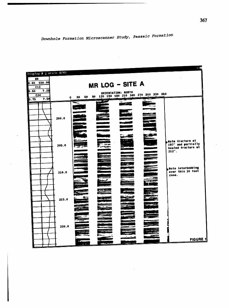
367
Downhole Formation Microscanner Study, Passaic Formation
6R
.0o 150_. MR LOG - SITE A5.5o 7.2_
ORIENTATION:NORTHC24
.75 7.50 0 30 GO 90 120 150 180 210 240 270 300 330 3GO
/_ _ _ _Note lnterbeddlng210.0 _ _ _ over this 20 foot
-- ( zone •
/ _.
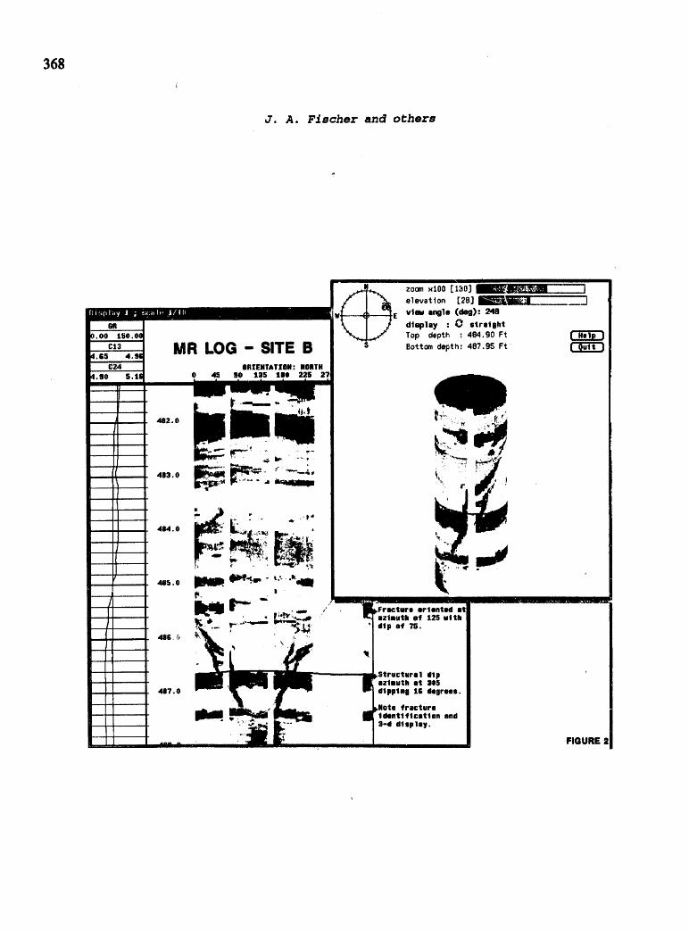
368
J. A. Fischer and others

Downhole Formation Microscanner Study, Passaic Formation
369
.... 1p F
SER R R
I T N E E J EDN S AES S C C R OQE A NTI ¥ O O Q IUP F M D R S M DESCRIPTION R V D _ N ETE P AAT B E E TNHE L RTA 0 R C
T E DIN L Y YOCNE
--195------- --Brown shale grading to grayish red mad sandstone (195' - 196.2'-- 196.2') Run 19-- Lt red, fresh, competent, med sandstone, unweathered-- Ipartings at 3" - 2.5'(196.2' - 201.2')
200-- Mineralized Joint plane at 70" to 75" (197') 97.5Z 83Z 0-- --Brown shale (201.2' - 202.5')
- -- Lt red, mad sandstone w/ vertical mlneral-filled veins- (202.5' - 204.5)
205--_ -- Brown shale grading to mad, red/brown sandstone, open,---- mineralized fractures (204.5' - 207.5') 206.2'
Run 20 205.0
-- --Miceceous brown shale, silt stringers, mineral filled to
-- ipartings at 4" - 6" (207.5' - 210.2) 206.2210-- --Interbedded shale, siltstone, sandstone, graded, sediment at
- deformation (210.2' - 211.5) I00_ 90_ 80°
- -- Competent pi_ish red to gray/red, laminated a_dstone,- partings at ehaley laminations, fresh (211.5' - 215.2')
215-_ Turbidites of sand to shale, partings at <1" - 8",---- fresh (215.2' - 217.5') 216.2'
Run 21 223.5
-- -- Fairly competent Interbedded, grayish red sandstone, to-- brown/red siltstone, & stringers of brown & gray shale, 991 89_ 224.2
220-- partings at 6" - 15" - 18", usually at shale stringers, at
some of whlch are mineralized (217.5' - 226.2') 80"--i ....... ...........
FIGURE,,, ........
J
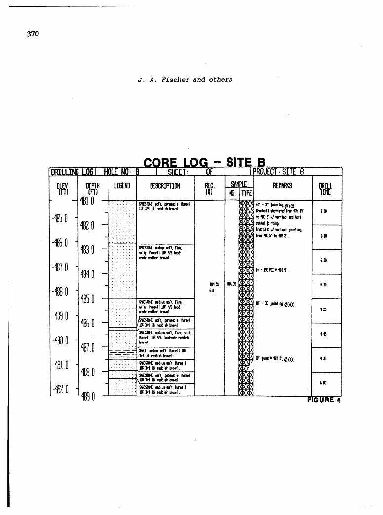
370
J. A. Fischer and others
_ILL_G LOG{HOLENO:B SHEET OF PROJECTSITEB
NO.T/P[ lit[- -'{810- .. . ... ' _s,,_,_,,m" ","" ,r-_' {o',,'_¢)oc .....
- .i,i.. "ii.i .. _ 4e05'N/vlrti=l _I:Il_ri-
"ij;:;;'.::::;:;;;.; frxtur_ _/_t0ml joinli__;;i:lll:l:l:l;i:;:l frm_0.{'_ _1.2'. |.=
-41_0- ..........•. '. ' ,.. ;,. • .:. '. •. •
• . ......... stl_ l_r_ll ll_ _ Imod-
........ Ie, 1%I_Io_3.9'.
48_0- , , , ,., ,
• , ,. • , . . , •
41_0- ....:::.: .;: :. ::..; _I_ _d,,_ _rt, rir_, lit - E join_i,_}O (..:...i.;-i-.i .. _iltl 1_lll_4/_le
:: :,.: :;:::::; "__, p_e_t, nun_tt....
_i....:i.:'-....:.:.. "_Tm[ _hu, _r,, r,_. oit_ 4,_
__ __ _ w_h,mloftllu,_llII_
-49]0'18_.0- .......•.............I_OST_..=it..1_-_,.ru=l{ I
- ii• l_ _q Id_r_:li_ lun_l.-qL0 _89.0 _i i _'0""_'_" FIGURE 4

HydroseolosY,WasteDisposal, Science and Politics_ro=_tnss30ths_posium 371En_In_ring Geology andOeotechnicalEngineerin$,1994
THE IDENTIFICATIONOF BASALT FLOW FEATURES FROM BOREHOLETELEVISION LOGS
Wllllam Bennecke, Bolee State Unlverslty, Bolse Idaho
ABSTRACTThis study investigated whether basaltflowfeaturesfoundinoutcropsandcores
couldbe identifiedin openboreholewallsbythe useof the boreholetelevis;oncamera.Toanswerthisquestiondetailedoutcropsurveyswere carriedoutinseverallocationsinthe SnakeRiverPlain, Idaho. A similartype of surveywas also doneonseveralcoresfromthe Idaho NationalEngineeringLaboratory,southeastidaho. Boreholetelevisionlogswereviewedto find similarbasaltfeaturesthat were notedincoresandoutcrops.Fromthesestudiesitwas foundthat basaltfeaturescan be identifiedinopenboreholeWallsbythe boreholetelevisioncamera. Thebasaltflowscan be dividedintofourzones:an uppervesicularzone;a columnarzone;a centralzone;and a lowervesicularzone.The uppervesicularzonecan be furthersubdividedintofoursubzones:an uppervesicu-larsubzone;a transitionalsubzone;a lowervesicularsubzone;anda bubbletrainsub-zone. Somespecificfeaturesfoundinthe borehole"IV logswere:bubble-trains,vesicleplumes,boreholeextensions,andpipevesicles.
The overalldistinctionsfor the zoneswerebasedon theirvesicularity.An overallpat-ternof vesicleswasfoundto be a progressionof smallnumerousvesiclesat the topof aflowwhichincreasein size, butdecreasein number,towardsthe centerof the flow. Theoppositeistruestartingatthe bottomof the basaltflowwheresmallvesiclesare numer-ous,but increaseinsize whiledecreasingin numbertowardsthe centerpartof the flow.
INTRODUCTIONBoreholetelevisioncamerashavebeenusedto inspectthe insideof pipes,tubing,
andboreholeswhichcouldnototherwisebe satisfactorilyobserved(LeRoy,et al., 1977).A typicalborehole"IV camera is madeof a longpipehousinga TV camerawithits ownsourceof illuminationinthe form of an internallamp;operationof the toolis accom-plishedbyloweringthe cameradownthe borehole. The speedat whichthe cameraislowered,the lamps'intensity,camerascanning,focusingpower,irisadjustments,andsensitivityare all controlledbyequipmentonthe surface. As the camerais loweredinformationgatheredby the TV camerais recordedsimultaneouslyby a video-cassette-recorder(VCR) ontoa videotape. Real-timeviewingof what the boreholecameraimagescan be seen bythe operatorona TV monitor.Underwaterviewingas wellasopenair recordscan be made inthe borehole.
Boreholetelevisionlogswere obtainedfrom morethanthirtywells bythe U. S. Geo-logicalSurveyat the IdahoNationalEngineeringLaboratory(INEL). The INEEis locatedinthe easternSnake RiverPlain(ESRP), Idaho. Basalticandsedimentarysequencesunderliethe INEL andare thenunderlainbyrhyoliticlava flows,ignimbrites,andpyro-clasticdeposits.Basaltsfoundinthe ESRP are chieflyolivinetholeiitebasaltsthatshowlittleevidenceof differentiationor contaminationconsistingof normativeolivineandhypersthene,a singleclinopyroxene,plagioclase,titanomagnetite,ilmenite,and brownglass(Kuntz,et al., 1992). Basaltrocksinthe TV logsare of Quaternaryage fromtheSnakeRiverGroupand IdahoGroup(Malde,lg87 andWhitehead,1992). The detailsof

IN.Bennecke
3"/2thebasalticfeaturesfoundintheserockscanbeobservedintheboreholetelevision
logs,coresfromthearea,andoutcrops.
METHOD
A numberofoutcropswereexaminedintheSnakeRiverPlainarea.Examinationentailedmeasurementsandobservationsoffractures,vesicles,color,andotherphysicalfeaturesobservedatoutcrops.A similartypeofexaminationwas carriedouton coresfromtheINEL.Followingthesetwotypesofexaminations,boreholetelevisionlogswereinspectedfromtheboreholesthathavecoresandfromotherboreholesthroughouttheINELarea.
Table 1: TV Logs and Cores at the INEL
BORE BORE BORETV TV TV
HOLE CORE HOLE CORE HOLE CORELOG LOG LOG
NAME NAME NAME, = ,| ,,
VVE- 1 X USGS 5"]........ X DD-33 X
VVE-3 X usGs 70 X DG1 X
VVEol0 X USGS 80 X X DC.2 X Xt
USGS 41 X' USGS 81 X X DC-3 X ' x
USGS 42 X ! 23 X X DC-'4 X X
USGS 43 X ID-8 X .... S!-13 X X
USGS 44 X ID-9 X S1-14 X X
USGS 45 X' ID-II ..........X " si-i6 x x
USGS 46 X DD-22 X IC-5 X X
USGS 47 X DD-23 X IC-7 X X
USGS 48 X DD-24 X IC-I 0 X
j USGS 50 X DD-25 'X IC-i 2 X X
Borehole TV logs are watched on a television from a VCR; the view recorded by thecamera is one looking down the borehole with a fish-eye view that is distorted from a per-pendicular view of the borehole wall. Still photographs are usually taken from TV logs,which are also distorted. Relativecorrections can be made knowing how much distortionoccurs to a reference unit as recordedon the picture. Two measuring devices (a 7 cm by2.5 cm rod with 5 cm taped increments and a 61 m by 6 mm steel tape with taped 2 cmsections) were used as standards and were lowered down a 15 centimeter diameter cas-ing. They were then recorded by a borehole TV camera on a VHS tape. This tape wasthen processed into a photograph and the relative distortion was measured (Plate 1).
t

I
Identification of Basalt Physical Features From Borehole Television Logs373
Plate1. Calibrationpictureshowingstandardof referenceand sketch.
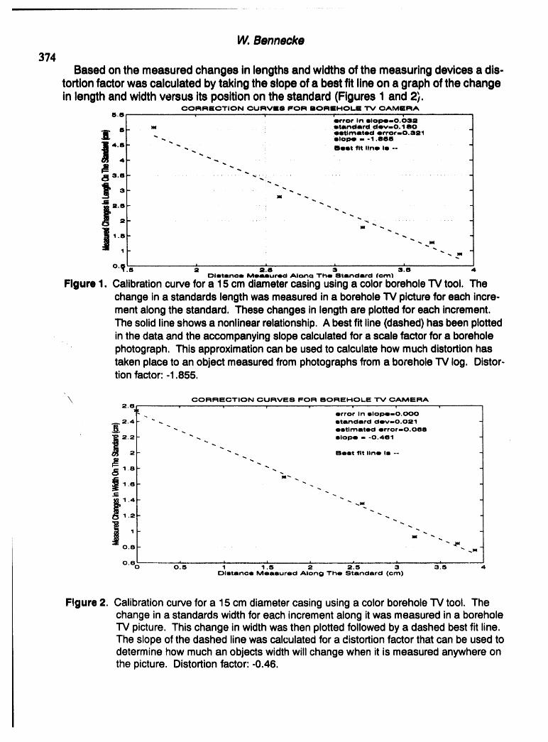
W. Bennecke
374
Based on the measured changes in lengths and widths of the measuring devices a dis-tortion factor was calculated by taking the slope of a best fit line on a graph of the changein length and width versus its position on the standard (Figures 1 and 2).
CORRHCTION CURVE[8 FOR IBORIEHOLE "rv OAMERAIS.IS , , ,
.r.o.,o.,o.-o
6 m Itandard ¢lev,,0.1 aoestimated error,,0.821" -. lllOpO m -1 .aBle
-- Beat fit line lib --
"4
3.6 ......... "_.' ." ............-_,
-}: --2. i ",,
1 "1.8 _,,.
0._l_ ,r i ............2 2.,, _ 3:, .|. E,3l
C)imtmrtoe Measured Aloha The Standard fore)
Figure 1. Calibrationcurvefora 15 cm diametercasingusinga colorboreholeTV tool. Thechange in a standards length was measured in a borehole TV picture for each incre-ment along the standard. These changesin lengthare plottedfor eachincrement.The solid line shows a nonlinear relationship. A best fit line (dashed) has been plottedin the data and the accompanying slope calculated for a scale factor for a boreholephotograph. This approximation can be used to calculate how much distortionhastaken place to an objectmeasuredfrom photographsfrom a boreholeTV log. Distor-tionfactor: -1.855.
\ CORRECTION CURVES FOR BOREHOLE "IV CAMERA2.6 , , , , • , ,
it _ error In elope--0.000
._. 2.4 " -. standard devm0.021
i _ _ .. emtlmated error-0.OeIS
2. "" ,.. slope -- -O.461
" -. Belt fit line iS --
I "
|} '-I 15 Io 0:5 1 1. 2 =2:_ ; _,,' ,,DIBtmnoe Measured Along The Stendarcl (Grn)
Figure 2. Calibration curve fora 15 cm diametercasingusinga colorboreholeTV tool. Thechangein a standardswidthforeach incrementalongitwas measuredina borehole"IV picture. Thischange inwidthwasthen plottedfollowedbya dashedbestfit line.The slopeof the dashedlinewascalculatedfora distortionfactorthat canbe usedtodeterminehow muchan objectswidthwillchangewhen it is measuredanywhereonthe picture. Distortionfactor:-0.46.

Identification of Basalt Physical Features From Borehole Television Logs
375A distortionfactorof -1.855 forthe change inthe lengthand -0.46 factor in the changeinwidthof an objectwas calculated. Toobtainthe correctdimensionsof an objectsimplymeasure itsdimensionsonthe photograph,multiplybythe distortionfactor,thentake theoriginalmeasuredvalue andsubtractfrom it the valuemultipliedby the distortionvalue.
The distortionfactoris accurateonlyforthe 15centimeterdiameterportionof theboreholesand can notbe usedfor otherwellsof differentdiameters. Fifteencentimetercasingis verycommoninthe INEL andthe distortionfactorfor it can be usedwithminorlossof accuracywhen lookingat diametersfrom 12.7 cm to 15.24 cm.
A darkcirclecan usuallybe seen inthe middleof the photographtakingfroma bore-holeTV camera;thisobjectis nota featurefoundonthe basaltboreholewall. It isa 5.4cmdiametermetalcap forthe lightingunitthat is positionedunderthe camera.Nomenclature
Based on observationsof boreholeTV logsa modelof whata typicalbasaltflowwouldlooklikewas generatedfor reference (Figure3).
',91--"
-- " "._;_.i..,_" _] UPPERVESlCULARSUBZONE
UPPER _ --] TRANSITIONAL SUBZONEVESICULAR
zone _ -,B :'-"-'F -- -7 LOWER..,_.O ,, ..- / VESICULAR
(Row Top) _ 1 SUBZONE
"_ _ --7 BUBBLE, "- [ TRAIN
COLUMNARSUBZONEZONE
(Upl_rColonnade_...L..0_" L"_._
vesiculated
area Larse VesicleCENTRAL _ avg. diameter -3.2 cm
!
zoNE 7 _(Ent=blaluR) B
| '---
" Medium Vesicle
_ /.';_ avg. diameter-l.lcm, ._': ..II .._'/ ,_ _ vesicle f _
I o.I--, _'_ _X 0 _vesicles Small Vesicle
VESICULARLOWER_ -1.8 m_ _ avg.diametero-.0.3cm . 1ZONE
(FlowBo(tom)
Figure 3. SchematicdiagramofanidealbasaltflowintheeasternSnakeRiverPlain,basedon"IVcameralogs. Averagediametersfor large,mediumandsmallvesiclesandgen-eralshapearealsoshown.

Centimeter1 2 3 4 5 6 7 8 9 10 11 12 13 14 15 mm
1 2 3 4 5
Inches 1.0 ,_
I 111'-' ,IIII'2lU'_ IIII1_Illll_
%
e_/_ NI::INUFI:ICTURED TO I::IT'I'N STlaNDI:::IRDS _<_


W. Bennecke
3?6The model is based on the work of George Faust in the Watchung Basalt Flows (Faust,1978). An upper vesicular zone, columnar zone, central zone, and lower vesicular zonemake up an idealized basalt flow. The upper zone is further subdivided by four subzonesan upper vesicular subzone, transitional subzone, lower vesicular subzone, and bubbletrain subzone. Entablature is a term used for the central massive zone while the upperand lower vesicular zones can be labeled colonnades. These zones may be absent in agiven basalt flow.
Typically the entablature occupies the interior one-third to upper one-half of a flow(Long, et al., 1986) and maybe the thickest portion of the lava flow. A basalt flow alsomay have colonnades; either an upper or lower, or both may be present. Colonnadestypically occur in the lower or upper third of a flow with the entablature between the twocolonnades (Long, et al., 1986). Well spaced, near-vertical columnar jointing is verycommon in colonnades and this differentiates them from the entablature.
UPPER VESICULAR ZONEUpper Vesicular Subzone
The upper vesicular subzone makes up the smallest portion of the upper vesicularzone and has the greatest vesicularity. The size of the vesicles are very small (averagediameter 0.3 cm), but they are nearly perfectly spherical in shape (Plate 2).
Plate 2. Borehole"IV picture of the upper vesicularsubzone. Notice the many vesicles present(Picture from borehole TV log of well WE-3 RWMC, INEL).

Identification of Basalt Physical Features From Borehole Television Logs3?7
Vesicles are small round cavities in the basalt and are the result of gasses beingexsolved from cooling lava. Numerous fractures found in this subzone have a charac-teristic light colored material filling them. Based on observations from the TV logs at theINEL this subzone commonly ranges from 15 cm to one meter in thickness. In the uppersubzone of the upper vesiculation zone red colored basalt with white coating of vesiclesand fractures are very contrasting to the center part of a basalt flow. Most of the whitecolor comes from alteration of the basalt in the form of calcite with zeolites possibly fromwater transport through the fractures and vesicles in the rock (Lanphere, et al., 1993)and secondary mineral precipitation. Red discoloration is most likely the result of oxida-tion of the rock during the initial deposition of the lava flow and possibly baking from anoverlying flow (Lanphere, et al., 1993)oTransitional Subzone
The mostprominentfeatures found in the borehole"IV logs in the transitionalsubzoneof the uppervesicularzoneare vesicles. Boththe size and numberof the vesiclesarechangingtowardsthe centerof a flow. The overallvesicularityor densityof vesiclesisintermediatebetweenthe uppervesicularsubzoneandthe lowervesicularsubzone.Largeandsmallvesiclescan be foundtherebutmediumsized vesiclesare the predomi-nate types (averagediameter1.1 cm); largeandmediumvesiclesoutnumbersmallerones. Themediumsizedvesiclestend to occurtowardsthe centerof theflowandabovethe largervesiclesinthe lowervesicularsubzone. Mediumvesicleshapesare oblatespheroids,andare moresphericalin shapethanthe largervesicles. Thissubzoneisusuallythickerthanthe uppervesicularsubzonebutthinnerthan the lowervesicularsub-zoneandthe bubbletrainsubzonebelow.Lower VesicularSubzone
Vesiculationis lessinthe lowervesicularsubzonethan inthe uppervesicularsubzoneandthe transitionalsubzone. Thesevesiclesare larger(averagediameter3.2 cm), butsmallandmediumvesiclescanalso be present(Plate3).
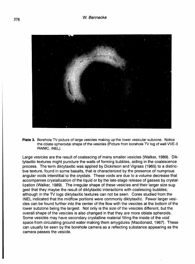
3?8 W. Bennecke
Plate 3. Borehole TV picture of large vesicles making up-the lower vesicular subzone. Noticethe oblate spheroidal shape of the vesicles (Picture from borehole TV log of well VVE-3RWMC, INEL).
Large vesicles are the result of coalescing of many smaller vesicles (Walker, 1989). Dik-tytaxitic textures might puncture the walls of forming bubbles, aiding in the coalescenceprocess. The term diktytaxitic was applied by Dickinson and Vigrass (1965) to a distinc-tive texture, found in some basalts, that is characterized by the presence of numerousangular voids interstitial to the crystals. These voids are due to a volume decrease thataccompanies crystallization of the liquid or by the late-stage release of gasses by crystal-lization (Walker, 1989). The irregular shape of these vesicles and their larger size sug-gest that they maybe the result of diktytaxitic interactions with coalescing bubbles;although in the TV logs diktytaxitic textures can not be seen. Cores studied from theINEL indicated that the midflow portions were commonly diktytaxitic. Fewer larger vesi-cles can be found further into the center of the flow with the vesicles at the bottom of the
lower subzone being the largest. Not only is the size of the vesicles different, but theoverall shape of the vesicles is also changed in that they are more oblate spheroids.Some vesicles may have secondary crystalline material filling the inside of the voidspace from circulating ground water making them amygdules (Macdonald, 1967). Thesecan usually be seen by the borehole camera as a reflecting substance appearing as thecamera passes the vesicle.

Identification of Basalt Physical Features From Borehole Television Logs379
Bubble Train SubzoneThe bubble train subzone is the lowermost and thickest (around 2 meters) subzone
making up the upper vesicular zone. Bubble trains are thin (ranging from 0.1 to 2 cmthick) tabular laminae of small vesicles that are parallel to the top of a flow (Plate 4).
Plate 4. Borehole "IV picture showing a bubble train in the bubble train subzone (Picture fromborehole TV log of well WE-3 RWMC, INEL).
Termed "micro-vesicular lamina" or "vesicle sheets" by McMillan, et al. (1987) representvesiculation in melt within the crystal framework of the rock or they might be the result ofthe liberation of gases from residual crystals at the point of solidification. In outcropthese vesicle rich laminae form a crude line across a basalt surface which can be easilyseen. These trains occur within an area of diktytaxitic texture; furthermore, they crosscutlarge vesicles meaning that they formed after the larger vesicles. The trains are verycommon in the upper portion of this subzone; however, the number of trains decreasestowards the center of the flow becoming very rare in the dense central zone. Spacingbetween trains varies greatly from 3 cm to 3 m or more. In outcrop the bubble trains maybe traced along the entire length of the flow.
COLUMNAR ZONE
The thickness of the columnar zone can vary greatly and usually makes up only asmall portion of the flow. The relative location of this zone within a basalt flow is alsohighly variable; it commonly occurs in the colonnades just under the flow tops or occa-sionally at flow bottoms. In some basalt flows it is completely absent. The zone is more

W. Bennecke38O
common in ponded basalt flows and can attain great thickness. Columnar joints formfive or six sided polygonal columns with five sided pentagons being most common(Beard, 1959). These columns can range from 40 cm in diameter to 19 m in height(Beard, 1959). The origin of these features has well been studied and their formationhas been attributed to contraction due to cooling which has overcome the tensilestrength of the cooling rocks (James, 1920).
Boreholes have problems as due cores with their smaller diameters not being able tosample the larger polygons; however, evidence for their presence are found in TV logs.What can be distinguished is a regular jointing seen in the borehole wall and a juttingstep-like pattern which is reminiscent of columns in outcrops. In some TV logs, hexago-nal-like blocks with vertical fractures make up the sides of the borehole (Plate 5). Largecavernous areas are also common in these places which could be the result of the drill-ing of the columns.
Plate 5. Borehole TV picture of the columns in the columnar zone. Jointing distinguishes thecolumns (Picture from borehole TV log of USGS well 44 ICPP, INEL).
CENTRAL MASSIVE ZONEThe central massive zone makes up the thickest portion of the basalt flow. These
zones are easily identifiable both in cores, outcrops and in the "IV logs as a very smoothtextured surface lacking vesicles or many fractures. The thickest zone identified by mein the "IV logs of wells at the INEL is 21 meters. Occasionally a very pronounced area ofvesicles is encountered in this zone; these areas can range up to 0.3 meters in thick-ness. Above and below these areas vesicles commonly are absent throughout the cen-tral massive zone. More rare are areas of extreme vesiculation called vesicle plumes or"vesicle cylinders" by McMillan et al., (1987). Plume is a more accurate term inthat theirshapes are very irregular. Such as irregular amoebid-like shapes with long linear vesicu-
Identification of Basalt Physical Features From Borehole Television Logs38]
lar arms coming out of the general mass. Unlike the trains, the plumes are not very long,with the longest being approximately 1.8 m (while the trains can go the entire length of alava flow). The origin of these vesicles plumes is unknown. They are found more com-monly in the lower part of the flow and thus could be the result of a lava flowing over abody of water.Fractures and Borehole Extensions
Borehole extensions are areas where the borehole wall extends outward (maximumdiameter measured by calipers is 53 cm) from the normal diameter. Fracture zones andborehole extensions can be found throughout a basalt flow. Fractures are most numer-ous in the upper vesicular zone, but longer fractures are found in the central zone.These extensions contain numerous fractures and rubble material. Extensions have
very regular fractures to jumbled blocks in appearance. Many possible mechanisms cangenerate these fractures and extensions; blasting, the drilling process, tectonic adjust-ments, lava tubes, shelly pahoehoe flow tops, and others could be the cause of thesefeatures. In outcrops certain pockets of abundantly fractured rock occur that are not verylarge (only several meters) or deep into the rock itself; these pockets are very angularand broken up, yet lack any other indication that they are special to the surrounding rock.These features could be borehole extensions.
LOWER VESICULAR ZONEVesicles
Vesicles in the lower vesicular zone have an opposite arrangement when compared tothe upper vesicular zone. The vesicle size decreases closer to the bottom of the flow ascompared to the increase in size of the vesicles towards the center of the flow. Overallsize of the vesicles is smaller than in the upper vesicular zones, and most of the vesiclesare irregular in shape compared to those near the top of the flow. Vesicularity increasestowards the bottom of the lower vesicular zone opposite to the upper vesicular zonewhere the vesicularity is the greatest at the top and decreases towards the bottom. Atthe bottom of this zone many small vesicle are present, yet the relative number is fewerthan the vesicles found at the flow top. Ranging from 0.3 to 1.8 meters thick this is usu-ally the thinnest zone that can be found in a basalt flow; only the columnar zone can pos-sibly be smaller. The overall color of this zone is also different in that it is usually adarker color than the rest of the basalt flow.
Pipe VesiclesPipe vesicles are usually found just at the lowest point of the central massive zone or
at the top of the lower vesicular zone; typically they range in size from 3 to 8 mm wideand are in the shape of hollow tubes. These tubes exhibit a rounded top and a taperedbottom. Pipe vesicles differ from vesicle plumes because they are hollow compared tothe plumes which are just areas in the basalt made up of vesicles. Magmatic gasexsolved from the lava as it crystallizes is one possible source for the generation of thepipes vesicles rather than trapped air or steam generated beneath the lava (Walker,1987).
SUMMARYUpon completing an outcrop and core analysis of basalt rocks common to the INEL a
further study was carried out on over thirtysix borehole "IV logsof boreholes at the INEL.

W. Bennecke382
A distortionfactor was determined for a 15 cm diameter boreholeso accurate measure-ments of basalt features could be made from the TV logs. From the study of the TV logsa generic section for a basalt flow was put forward as a model. This generic section wassubdivided into separate zones with the upper zone further subdivided into four sub-zones. The marked change in shape and changes in vesicularity are the main criteriathat distinguishes the four subzones from each other and is used as one of the mainbases for breaking the column into separatezones. Vesicles, fractures, and boreholeextensionswere easily identified by the use of the borehole TV camera. The detail of thelogs enabled direct measurements of these features. These same features also aredirectly comparable to outcrops and cores. A great potential exists for this tool to betterour understanding of subsurface geology.
REFERENCES CITED
Beard, N. C., 1959, Quantitative study of columnar jointing: The Geological Society ofAmerica Bulletin, vol. 70, p. 379-382.
Dickinson,W. R., and Vigrass, L. W., 1965, Geology of the Suplee-lzee area, Crook,Grant and Harney Counties, Oregon: Oregon Department of Geological MineralResources Bulletin, vol. 46, p. 69-94.
Faust, G., 1978, Joint Systems in the Watchung Basalt Flows, New Jersey: U. S. Geo-logical Survey Professional Paper,864-B, p.1-45.
James, A. V.G., 1920, Factors producing columnar structure in lavas and its occurrencenear Melbourne, Australia: Journal of Geology, vol. 28, p. 458-469.
Kuntz, M. A., Covington, H. R., and Schorr, L. J., 1992, An overview of basaltic volcan-ism of the eastern Snake Rive Plain, Idaho: Geological Society of America Mem-oir 179, p. 227-267.
Lanphere, M.A., Champion, D. E., and Kuntz, M. A., 1993, Petrography, age and paleo-magnetism of basalt lava flows incoreholes Well 80, NRF 89-04, NRF 89-05, andICPP 123, Idaho National Engineering Laboratory: U. S. Geological Survey,Open-File Report 93-327, p. 2-40.
LeRoy, L. W., LeRoy, D. O., and Raese, J. W., 1977, $_bsurf_ce Geology: 4th ed., Colo-rado School of Mines, Golden, Colorado.
Long, P.E., and Wood, B. J., 1986, Structures, textures, and cooling histories of Colum-bia River basalt flows: Geological Society of America Bulletin, vol. 97, p. 1144-1155.
Macdonald, G. A., 1967, Forms and structures of extrusive basaltic rocks. In .ThePolder-vaart Treatise on rocks of basaltic composition, H. H., Hess and A. Poldervaart(eds.): vol. 1, Interscience, New York, p. 1-61.
Identification of Basalt Physical Features From Borehole Television Logs383
Malde, H. E., 1987, A guide to the Quaternary geology and physiographic history of theSnake River Birds of Prey area, Idaho, in Field Trip Guidebook: American Associ-ation of Petroleum Geology & Society of Economic Mineralogists and Paleontolo-gist, Rocky Mountain Section, Meeting, September 10-18, 1987, Boise Idaho, p.234-246.
McMiilan, K., Cross, R. W., and Long, P. E., 1987, Two-stage vesiculation in the Cohas-sett flow of the Grande Ronde Basalt, south-central Washington: Geology, vol. 15,p. 809-812.
Walker, G. P. L., 1987, Pipe vesicles in Hawaiian basaltic lavas: their origin and potentialas paleoslope indicators: Geology, 15, p. 84-87.
Walker, G. P. L., 1989, Spongy pahoehoe in Hawaii: a study of vesicle-distribution pat-terns in basalt and their significance: Bulletin of Volcanology, vol. 51, p. 199-209.
Whitehead, R. L., 1992, Geohydrologic framework of the Snake River Plain RegionalAquifer system, Idaho and eastern Oregon: U. S. Geological Survey ProfessionalPaper 1408-B, p. 1-32.

t_O0

|
Hydrogeology, Waste Disposal, Science and PoEtics 385Proceedings 30th SymposiumEngineering Geology and Geotechnical Engineering, 1994
STEREOLOGICAL SAMPLING OF ROCKMASSES FOR ENGINEERING PURPOSES
Stanley M. MillerBryan D. Martin
Department of Geology andGeologicalEngineeringUniversity of Idaho, Moscow, Idaho 83844
John K. OwensU.S. Bureau of Mines Spokane Research Center
Spokane, Washington 99207
ABSTRACT
Stereological analysis of observations made in drill ho!es or along the walls of under-ground excavations can provide two- and three-dimensional measures that help characterizediscontinuous rock masses for engineering and hydrogeologic purposes. The approach isbased on sampling methods developed previously in stereology for the analysis of micro-structures in the fields of biology and materials science.
Input information for a stereological analysis of a rock mass is best obtained by scanning(imaging) the walls of clean drill holes using a borescope or other video device. Two classesof features are investigated: 1) lithologic types that comprise the overall rock mass, and 2)structural discontinuities (e.g., joints, foliation, bedding planes) within a given lithologic unit.For the former case, the volume fraction of a given lithologic entity in regards to the entire rockmass can be estimated. For the lattercase, the intact-block size distribution, the mean interceptlength between adjacent structures, and the surface area density (say, area in m2 per unitvolume in m3) of the geologic slructurcscan be estimated.
Example samplings and computations are pre,_entedfor several situations based on drillholes associated with underground mining activity. Extensions of the methodology areproposed for larger diameter borings or tunnels and for exposed rock faces.
INTRODUCTION
The origins of stereology can be traced to petrological applications proposed by theFrench geologist, Delesse, in the mid 1800's [3], but recent developments and applicationshave been primarily in the fields of biology and materials science [2, 10, 11]. Stereologyprovides a mathematical protocol for relating simple measurements made along test probes (oron planar sections) to three-dimensional geometric properties of the body being sampled.
Although stereological principles have been applied rarely to the engineering study ofdiscontinuous rock masses [7], they have been used to assess large-scale fracturing on theearth's surface [5, 6] and to analyse the crack geometry in stressed concrete [4, 9]. Theprimary difficulty in obtaining representative stereological samples for site-specific engineeringwork is that continuous, linear probes of the rock mass are possible only in competent rockwhere drill-core recovery is effectively 100 percent. Planar, two-dimensional sections forsampling rock exposures also are rare in nature;consequently, such faces must be blasted andcleaned to allow for stereological measurement of its structuralfeatures. This extensive effortprobably will not be justified at the exploration and site investigation stages of most projects.
S.M. Miller and others
386
However, recent technological developments in miniature video equipment .and fiber-optics now make it possible to record video images of the inside w,'dls of drill holes in the rockmass, regardless of whether any drill core was recovered. Of course, the holes must be cleanenough to observe discontinuities and any changes in rock type or physical characteristics,such as zones of dike material, breccia, fault gouge, or alteration/weathering. By obtainingfundamental stereological measurements from such images, we can derive useful informationto help characterize discontinuous rock masses for engineering purposes.
0
STEREOLOGICAL RELATIONSHIPS
When line probes are used to sample the structures within a three-dimensional body forstereological purposes, care must be taken to assure that the probes are chosen randomly froma uniform and isotropic population of all such probes in the sampling space. This implies thatthe line probes must sample all positions and orientations uniformly. An important advantageof having line probes along the walls of a cylindrical hole (in our case, a drill hole) is that thecylindrical surface of the hole automatically samples uniformly all orientations about the axis ofthe hole [1].
Practical guidelines for such sampling include the following [1]:1. Sample uniformly; draw observations that are uniformly distributed in position;2. It is better to sample the entire population lightly, rather than concentrate on detailed
samples at only a few locations; i3. A systematic sampling plan can reduce the statistical variance of observations and,
thus, increase the precision of stereological estimates, provided a random startingpoint is used for the plan layout.
For stereological measurements, the braces <...> around an attribute denote the "expectedvalue" or mean of that attribute. In this sense, the stereological attributes are consideredrandom variables, and each sample mean is assumed a reasonable estimate of the populationmean. The following attributes can be measured from line probes and are relevant to our studyof rock masses:
<Pp> Point Fraction -- The ratio of ni to n, where n = total number of points on acounting grid that covers the sampling image and ni = the number of points contained in the i-thconstituent of the rock mass as counted along the sampling grid.
<LL> Line Fraction -- The ratio of Li to L, where L = total length of a sampling linethat covers the sampling image and Li = the summed length of segments of the sampling linecontained in the i-th constituent of the rock mass.
<PL> Line Intercept Count -- The ratio of nij to L, where L = total length of asampling line that covers the sampling image and nij = the number of interfaces (boundaries)between constituents i and j in the rock mass as counted along the sampling line.
The point fraction and the line fraction essentially provide the same measure, because asthe point grid spacing is reduced to zero, the ratio ni"n will approach the limit L i • L. Decidingwhich parameter to measure depends on the selected sampling procedures and on the available
. equipment used for sampling and analysis.The point fraction and the line fraction both provide unbiased estimates of the volume
l'raetlon Vv, which repesents the fraction (similarly, the percentage) of the total volumesampled that consists of tJ_especified constituent [10, 11]:
<Pp> = <LL> = Vv (1)

Sterzological Sampling of Rock Masses 387
The line intercept count for a specified type of interface or boundary is related to the surfacearea density Sv of that type contained in the sampled volume, as expressed in units of areaper unit volume (say, m21m3) [I0,I I]:
<PL>= (el2)Sv (2)
These are but a few of the fundamental stereological parameters and relationships thathave been applied in the fields of biology, medicine, and materials science. Basic point countsor line measurements often are performed automatically by computerized imaging systems orsemi-automatically using some type of human delineation of features [8].
STEREOLOGICAL SAMPLING IN DRILL HOLES
The stereological parameters reported above are the most applicable ones forchsxacterizing fractured rock masses, particularly when using drill holes as the samplingprobes. However, some modifications and orientation corrections are needed when the drillholes are parallel to each other and constitute a set of directed line probes. Such is the casewhen using rock-bolt holes drilled in the roof of an underground mine.
The line intercept count obtained from such parallelsampling lines provides an unbiasedestimate of the total projected area Av of the specified interface type onto a planeperpendicular to the sampling lines [2, 10]. The corresponding stere_flogical relationship is [1]:
<PL>ori = Av (3)
whom <PL>od isthe_ interceptcountobtainedfromparallel,orientedsamplinglines.
The cosine of the angle _ between the sampling-line direction and the normal to anintersected surface (interface) relates the actual surface areato the projected area of the surface.That is, for the i-th interface encountered:
Avi = (cos _'0Svi (4)
Thus, by averaging all such cosines of angles for all surfaces (interfaces) encountered,we obtain the following:
Av = (cOSavs¢)Sv= '<PL>ori (5)
Sv= <PL>o./(cOSav) (6)
The mean interceptlengthofa specifiedconstituentintherockmassasmeasuredinthereferencedirectionofthesamplinglinesisgivenas[I]:
< _.>ori = 2Vv / Av = 2Vv / <PL>ori (7)
It is important to note that when sampling to estimate the volume fraction of a constituent(feature), such a volume does not possess an orientation as do line or surface features. Thus,sampling to obtain the point fraction and line fraction does not require an isotropic array ofsampling lines to yield unbiased estimates of the volume fraction [1]. Consequently, suchstereologicalsamplingfrom paralleldrillholeswillsufficeinthisregard.

S.M. Miller and others
388EXAMPLES
Estimatin2 Volume Fractionsv
Estimating the volume fractionof a given constituent in a discontinuous rock mass can behelpful in assessing its engineering performance, especially if the constituent is a structurallyweak component of the overall rock mass. Also, ff ore dilution was a concern in a proposedmining operation, knowledge of the volume fraction of non-ore materials would yield theexpected amount of such dilution when mining througha specified volume of rock.
For example, consider a situation where mudstone layers and lenses in a sedimentaryformation overlying a coal seam could cause potential stability problems in mining excavations.To estimate the volume fraction of mudstone, 12 rock-bolt holes (each 2.5-m long) in the mineroof have been imaged by a videoscope, and pertinent measurements collected regarding theline intercept lengths of mudstone encountered (Table 1).
i
Table 1. Line intercept measurements for mudstone example.
Sum of MudstoneHole Number InterceptLengths (L0, m Line Fraction (LL),m/m
1 0.62 0.2482 1.00 0.4003 1.25 0.5004 0.43 0.1725 1.18 0.4726 0.00 0.0007 1.37 0.5488 1.09 0.4369 1.12 0.448
10 1.76 0.70411 1.45 0.580
0.856Mean = 0.45
n = 12 SD = 0.23
Given the mean and standard deviation (SD) for the line fraction, we now can calculatethe volume fraction of mudstone according to Equation 1, as well as define a 0.95 confidenceinterval (CI) for the estimate.
Volume fraction of mudstone, Vv = < LL > = 0.45, or 45%
95% CI for the mean volume fraction: 0.45 5: t.o_, 11(SD/c-ff) = 0.45 + 2.201(.066)
=0.45:1:0.15
where t.ozs,tl = value of appropriate Student's-t statistic = 2.201.
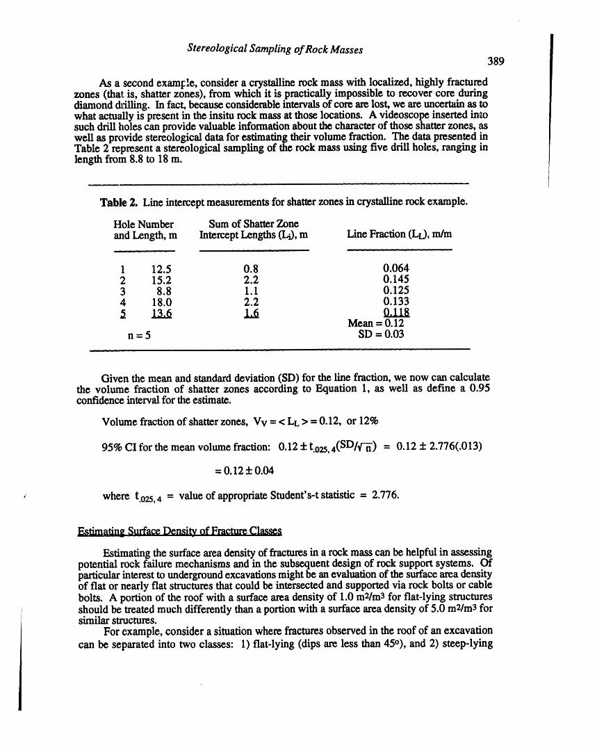
Stereological Sampling of Rock Masses389
As a second examl:le, consider a crystalline rock mass with localized, highly fracturedzones (that is, shatter zones), from which it is practically impossible to recover core duringdiamond &LSlling.In fact, because considerable intervals of core are lost, we are unce'rtainas towhat actually is present in the insitu rock mass at those locations. A videoscope inserted intosuch drill holes can provide valuable information about the character of those shatter zones, aswell as provide stereological data for estimating their volume fraction. The data presented inTable 2 represent a stereological sampling of the rock mass using five drill holes, ranging :inlength from 8.8 to 18 m.
Table 2. Line intercept measurements for shatter zones in crystalline rock example.
Hole Number Sum of ShatterZoneand Length, m Intercept Lengths (Li), m Line Fraction (LL), m/m
1 12.5 0.8 0.0642 15.2 2.2 0.1453 8.8 1.1 0.1254 18.0 2.2 0.133_. 13.6 1.6 0.118
Mean = 0.12n = 5 SD = 0.03
Given the mean and standard deviation (SD) for the line fraction, we now can calculatethe volume fraction of shatter zones according to Equation 1, as well as define a 0.95confidence interval for the estimate.
Volume fraction of shatter zones, Vv = < LL > = 0.12, or 12%
95% Clfor the mean volume fraction: 0.12 + t.ozs,4(SD//'-ff) = 0.12:1: 2.776(.013)
=0.12+0.04
, where t.o_,4 = value of appropriate Student's-t statistic = 2.776.
F,stimatin_ Surface Density of FractureClassesw
Estimating the surface area density of fractures in a rock mass can be helpful in assessingpotential rock failure mechanisms and in the subsequent design of rock support systems. Ofparticularinterest to undergroundexcavations might be an evaluation of the surface area densityof flat or nearly flat structures that could be intersected and supported via rock bolts or cablebolts. A portion of the roof with a surface area density of 1.0 m_tm3 for flat-lying structuresshould be treated much differently than a portion with a surface area density of 5.0 m2/m3 forsimilar structures.
For example, consider a situation where fractures observed in the roof of an excavationcan be separated into two classes: 1) flat-lying (dips are less than 45°), and 2) steep-lying

390 S.M.Miller andothers
(dips exceed 45°). To estimate the surface area density of the two fracture classes, 10 verticalrock-bolt holes (each 4-m long) in the roof have been imaged by a video_ope, and pertinentmeasurements collected regarding line interceptcounts (Table 3).
Table 3. Line intercept counts for twofracture classes.
No. of Fractures Observed < PL >oriHole Number Flat (._45o) Steep (>45o) Flat Steep
1 9 2 2.25 0.502 11 3 2.75 0.753 8 1 2.00 0.254 12 4 3.00 1.005 I0 2 2.50 0.506 13 2 3.25 0.507 II 0 2.75 0.008 9 1 2.25 0.259 8 3 2.00 0.75
10 .9. _4 2.25 1.00Mean = 2.50 0.55
n = 10 cOSavs#= 0.887 0.462 SD = 0.425 0.329
Given the mean and standard deviation (SD) for the oriented line intercept counts, wenow can calculate the surface area density for each fracture class according to Equation 6, aswell as define a 0.95 confidence interval for each estimate.
Fla_fracturea: Sv = <PL>ori/(COSavg _) = 2.50/0.887 = 2.82 m2/m3
SvSD = 0.425 / 0.887 = 0.479 m2/m3
95% CI for the surface areadensity: 2.82 + t.o25,9(SD/_n ")k_
= 2.82 :!:2.262(0.479 / 3.162) = 2.82 :!:0.34 m2/m3
where t.o25,9 = value of appropriate Student's-t statistic = 2.262.
Steep fractures: Sv = <PL>ori/ (COSavg#) = 0.55 / 0.462 = 1.19 m2/m3
SvSD = 0.329 / 0.462 = 0.712 m2/m3
95% CI for the surface area density: 1.19 + t.o25,9(SD/'/"n)
= 1.19± 2.262(0.712/3.162)= 1.19± 0.51m2/m3

Stereological Sampling of Rock Masses391
This example illustrates how the orientation (directional) bias that causes undersamplingof steep fractures in vertical holes is taken care of automatically in the stereological calculationsused to estimate the surface area density of such structures. The averaged line intercept count<Pt.>ori for thesteep fractures was approximately one-fifth of that for the flat fractures, yet theresulting surface area density for the steep fractures was about half of that for the flat fractures.For this particular stereological procedure, the cosine term contained in Equation 6appropriately corrects for the undersampling of steep structures in vertically oriented drillholes.
If the stereological sampling for this example also included the point fraction or linefraction (to estimate Vv), then Equation 7 could be used to calculate the mean vertical interceptlength as megsured between adjacent flat fractures or adjacent steep fractures. This term wouldbe equivalent to the mean fracture spacing between adjacent flat fractures or adjacent steepfractures.
Estimadn_ Intact-Block Size Distributionsv
In some engineering projects, estimates of core-piece size distributions are useful forpredicting fragmentation and for characterizing overall rock-mass deformation under loading.If certain geometrical conditions reasonably can be assumed for intact block shapes, then acore-piece size distribution can be converted to a volumetric, intact-block-size distributionusing stereological methods.
When measuring line intercept distances from one fracture to the next in a borehole, weare, in fact, measuring the core-piece lengths that would be observed in drill core if it had beenrecovered from the hole. The cumulative relative frequency plot of these lengths provides anestimate of the core-piece length probability distribution. However, if we were interested inrelating such data to the entire rock mass volume, we could divide the length intercepts into sizecategories and then use the LL for each category to estimate the volume fraction Vv for each ofthe intact-block size categories. The information presented in Table 4 illustrates this procedurefor a set of 20 drill holes (each approximately 60 inches long) in the siltstone roof of anunderground coal mine, covering an area of approximately 6 by 18 meters (108 sq. m).
Table 4. Intercept lengths for intact siltstone and corresponding volume fractionsfor selected size categories (total length of sampling lines was 1220 in.).
Intact Rock Sum of Intact Rock Line Fraction (LL)Size Category, in. Intercept Lengths (Li), in. = Vol. Fraction (Vv)
0-4 192 0.164- 8 305 0.258- 12 312 0.2612- 16 283 0.2316 - 23 129 0.10
To determine whether the position of the sampling line in drill holes affects thestereological results, a chi-squared statistical procedure (5 x 2 contingency tables) was used on

S.M. Miller and others
392this data set to compare the volume fractions predicted by two sampling line positions locatedon opposite sides of the drill holes. The results indicated that the two sets of volume fractionsthus obtained did not differ significantly. Consequently, the positioning of the scanning deviceha drill holes probably is not critical when conducting line scans for most stereological studies.
Another statistical comparison (chi-squared goodness of fit) was conducted for thissiltstone data set to estimate the minimum number of drill holes required to provide repeatableresults in regard to intercept length distributions. Subsets of 6 randomly selected drill holesfrom the original 20 were compared to one another using the chi-square test; this was repeatedfor randomly selected subsets of 5 holes, 4 holes, and 3 holes. Significant differences in thepredicted size distributions began to show up with 4 holes and were common with 3 holes.Thus, intact-rock size distribution repeatability becomes questionable when less than 4 drillholes are used. This implies that as long as geologic conditions do not vary significantly, aminimum of 4 roof-bolt holes per 100 square meters of roof need to be sampled to providerepresentative stereological results in regards to intercept length measurements.
In situations where the fracturesin a rock mass divide it into fairly equidimensional intactblocks (i.e., blocks shaped more like spheres than plates or columns), stereological procedurescan be used to adjust size distributions of intact-rock intercept lengths to volumetric sizedistributions of three-dimensional blocks [8]. The method we developed to accomplish thistransformation is b_d on three steps:
1) Describe the cumulative relative frequency distribution (cr0 of the measured interceptlengths;
2) Convert this crf to one describing the distribution of the diameters of correspondingspherica.!particlesizes (i.e., spherical blocks pierced by the drill hole);
3) Convert the derived crf of spherical particles to one describing the distribution ofcorresponding polyhedral shapes (such as dodecahedraor icosahedra) using a ratio of1.08 for their mean tangent diameter to that of a sphere of equal volume [8].
Output from an example set of computations for intercept lengths (core-piece lengths)measured in three exploration drill holes (each approximately60 m long) in a rhyolite formationare given in Figure 1. The measured intercept length distribution is skewed right andprobablycan be modeled by a lognormal probability distribution. The resultant cumulative distributionof polyhedral mean tangent diameters is less skewed and covers a wider range of sizes. It isworthy to note that this latter distribution is a volumetric particle size distribution,rather than aweight-percent particle size distribution as is commonly reportedfor soils and crushed rock.
InterceptLengths Polyhsd'aTangentOiametem1-
oa. -""""
0-0 0.5 1 1.5 2 2.5 3 3.5 4
IntactBkx:kSize(m)
Figure 1. Intact rock size distributions estimated from three drill holes in rhyolite.

i
Stereological Sampling of Rock Masses
393
CONCLUSIONS
With recent advances in hardware development for imaging drill holes, applications ofstereology to rock mass sampling and characterizationare feasible. More comprehensive three-dimensional characterizations of rock masses are now possible, ones that include volu_n_fractions of various lithologic constituents (of rock engineering interest, these might includealtered or weathered zones, veins, shatter zones, fault breccia and gouge), surface areadensities of fractures (particularly of interest are those with orientations critical to rockengineering projects), and intact-rock volumetric size distributions. Such measures provide anenhanced understanding of a rock mass over such descriptors as RQD and fracturedensity.
Stereological sampling lines can he used on tunnel walls or on exposed rock faces. Caremust be taken to avoid alignin.g such probes in the same plane, because our experience hasshown that many more sampling lines are needed to produce representative and repeatablestereological results for this case. If sampling into the rock mass is desired, then relativelyshort holes can be drilled economically with percussion drillingequipment.
Additional field work is needed in discontinuous rock masses to investigate relationshipsbet_,een traditional rock engineering descriptors and stereological descriptors. One clearadvantage of stereology is that recovered drill core is not required, provided that a boreholevideo imaging system is available.
ACKNOWLEDGMENTS
Much of the funding for this research work was provided by the U.S. Bureau of Mines,Spokane Research Center. The authors also express their appreciation to the engineeringpersonnel at the Center who shared techrdcal information and field data during the course ofthis investigation.
REFERENCES
1. DeHoff, R.T., 1993, Use of Bolt Holes as Stereological Sampling Probes; unpubl, reportto U.S. Bureau of Mines, Spokane Research Center, Spokane, WA.
2. DeHoff, R.T. and Rhines F.N., 1968, Quantitative Microscopy; McGraw-Hill, NewYork.
3. Delesse, A., 1848, Pour Determiner la Composition des Roches; Ann. des Mines, v. 13,Fourth Series, p. 379.
4. Hong, T., 1991, Quantitative Characterization of Crack Geometry in Concrete CompressedUniaxially at High Strain Rate; unpubl. M.S. thesis, Dept. of Matl. Sci. andEngrg., Univ. of Florida, Gainesville, FL.
5. Karcz, I., 1977, Rapid Determination of Lineament and Joint Densities; Tectonophysics,44, p. T29-T33.
6. Karcz, I. and Dickman, S.R., 1979, Determination of Fracture Intensity; Tectonophysics,56, p. T1-T7.
7. Kanatani, K., 1985, Measurement of Crack Distribution in a Rock Mass from Observationof its Surfaces; Soils and Foundations (Japanese Soc. Soil Mech.), 25 (1), p. 77-83.
8. Russ, J.C., 1986, Practical Stereology; Plenum Press, New York.9. Stroeven, P., 1976, Application of Various Strereological Methods to the Study of the
Grain and the Crack Structure of Concrete; Proc. of 4th Intl. Congress for Stereology,Natl. Bureau of Standards Special Publ. 431, p. 281-286.
10. Underwood, E.E., 1970, Quantitative Stereology; Addsion Wesley, Reading, MA.11. Weibel, E.R., 1979-80, Stereological Methods, Vol. I and II; Academic Press, New
York.

4_

Hydroseology,WasteDisposal, Science andPoliticsProceedings30th SymposiumEngineeringGeology and GeotechnicalEngineering,1994
DISPOSAL OPTIONS FOR SCRAP TIRES 395
by C. W. 'Bill' Lovell, Research EngineerSchool of Civil EngineeringPurdue UniversityW. Lafayette, IN 47907.1284
ABSTRACT
Scrap tires have been a high profile waste oecause of improper disposal in the past.
They have been mandated for use in crumb form in asphaltic pavements by FederalISTEA legislation. In addition, useful disposal options have been developed for shreds asa lightweight geomaterial for embankments or backfills. In these later cases, problems ofexcessive deformability may be countered by mixing with sand.
Tires may also be reduced to basic constituents in a process known as pyrolysis. Aprincipal byproduct of this process is an impure form of carbon black, which may be usefulas a filler in asphaltic concrete. There are limited applications for whole tires in restrainingstructures, and for linkages of tire beads or tire sidewalls as reinforcing elements in soils.In addition, tires yield a high BTU return when burned.
The paper summarizes research experiences of the author in research on scrap tires,and recommends future uses of these materials, particularly in highway applications. In anumber of instances, use of the scrap rubber produces performance superior to or moreeconomical than that for conventional materials.
INTRODUCTION
Solid wastes produced in the U.S. in decreasing order of quantity are: (1)agricultural (most); (2) mining; (3) industrial; and (4) domestic (least). Scrap tires areconsidered a part of the domestic waste, and therefore are exceeded in quantity by anumber of others. Yet, scrap tire disposal has received as much or more national attentionthan any solid waste. Why is this so7
Careless and uncontrolled storage and disposal seems the obvious answer. Outdoortire dumps have the following unfavorable features: unsightly; fire hazard; and breedingground for rodents and insects.
Many states prohibit the outdoor storage of whole tires. The disposal of whole firesin solid waste landfills is also usually forbidden.
Used tires are accumulated in small quantities by tire dealers, who pay tire haulers(recyclers) to periodically truck them away. The recycler will have an indoor
C.W.. Lover396
storagesorting processing facility. Useable tires are retrieved and sold to primarily Asianmarkets. The other tires are either cut or shredded for market or disposal. The latteroption involves hauling, tipping fees, and wasting of a potentially valuable engineeringmaterial. However, present markets are very limited and in great need of expansion.
Some of the rubber may be mechanically ground or cryogenically reduced to crumbsize. As such it has a variety of uses including incorporation into asphaltic mixes. Theexperiences of state highway agencies with these mixes varies widely. Many conclude thatsuch mixes almost double the cost without significant improvement in the performance ofthe paving.
Another market exists as fuel in the generation of power. Indeed, the tires producemore BTU's than coal. However, special combustion features are needed and air emissionsalso require extraordinaryattention.
Reduction of the tire to basic components of oil, gas, steel and "carbon black" in thepyrolysis process is quite promising. A major obstacle to success of this recovery processis finding a market for the rather impure carbon black accumulated from it.
Tire shredding through mechanical cutting and tearing actions may be accomplishedby a variety of fixed or mobile devices...some commercial, others "homemade". Successivepasses through the shredding operation produce smaller sizes, and pieces which are morenearly equal in length/width dimensions.
Tire shreds have a much higher bulk unit weight than whole tires and hence aremuch more convenient to store or haul. The product is referred to as "shreds"or "chips"ofa maximum length or width dimension. There seem to be a variety of potential civilengineering uses for such materials, including fills, backfills and drainage media. They maybe used alone or in mixtures with soil.
BACKGROUND
Scrap tires are generated in the U.S. at the rate of about a tire/person/year (EPA,1991). This quantity of about a quarterbillion tires per year is added to an estimated prioraccumulation of about 2 billion tires. The high visibility of this waste (and associatedhazards cited earlier) has caused national and state legislative bodies to mandate studies orapplications of various reuse options.
Fortunately, tire rubberis an excellent civil engineering material, being both strongand durable. Environmental constraints seem to be minimal for certain usage, e.g.,shred/chip forms, although applications are being pursued with appropriate caution.
Figure 1(Ahmed, 1993b) s_ows the scrap tire generation cycle. The recyclingportionis followed on Figure 2 (Ahmed, 1993b). Note that a variety of options exist for (a) wholetires or tire sidewalls, (b) shredded tires, and crumb rubber.

TIRE MANUFACTURINGPLANTS !
I DISTRIBUTORS 1
DEALERS OF DIFFERENT CATEGORIESOF TIRES (i.e., automobile, truck/bus, construction machinery, etc.
EXPORTING (resource recovery) C>
I LANDFILLING/ SCRAP TIRES INCINERATIONSTOCKPILING (sorting at tire processing
facilities}
TI-D'VED !MONOFILLS
(separation of tlre sidewalls,shredding, grinding, etc. )
RECLADU_G/
I • RECYCLING PYROLYSIS
(hlghway & non-highwayapplications)
Figure 1 Tire manufacturing, retreading, and discards (Ahmed, 1993b)

OO
TIRE S IDEUklJ_Ii
FILLS ASPHALT RUBB ,_R
crack/joint sealantasphalt-rubber hot
SOIL RETAINING GRAVEL SUBSTITUTE stress absorbing meLbranes (SAM)stress absorbing membranes interlayers
, _ EROSION CONTROL I _ OIL SPILI_ ] _
_ SOUND BARRIERS ] -_ COMPOSTING/MUIEH I _ RUBBER MODIFIEDASPHALT
_ CRASH BARRIERS I _ BUILDING PRODUCTS I
ARTIFICIAL REEFS I _ STORAGE/MONOFILLS ] PYROLYSIS I
Figure 2 A summary of recycling options for scrap tires (Ahmed, 1993b)

Disposal Optionsfor Scrap Tires399
Whole tires are bulky and expensive to transport,but may require no processing priorto use. Some applications are not uncommon, such as retaining structures and crashbawiers, but have intrinsic limitations. Use to form artificial reefs (fish holding structure)requires only linking and weighting, but source and market are often geographicallyseparated.
The inner rim of the tire contains a wire hoop (the bead) which may be cut out andhas potential usage. The same is true for the tire sidewalls. When linked into mats, thebeads or the sidewalls form a layer of high tensile strength which can be used to reinforcesoil masses (very low tensile strength). Fabrication of the mats, as well as transportationand placement of them, involves significant cost.
Shredding i° a relatively inexpensive operation and may simply constitute aconditioning which allows the rubber to be used as a raw material for other purposes, e.g.,pyrolysis. In other cases, the shred or chip is directly used as a flU, backfill or drainagelayer. Because of minimal preparation and extra construction costs, this option is attractive.This paper provides additional details on the use of shreds as a lightweight geomaterial.
Production of crumbrubber as an additive to asphalt is expensive. Such additive hasproduced best success in crack/joint sealants and in stress absorbing membranes. Whenused as an additive to asphaltic mixes, the experience is mixed. In Indiana for example, thebenefits do not seem to warrant the added costs.
Reduction of the tire to basic ingredients in the pyrolysis process (oil, gas, steel,carbon black) is promising,but depends upon identifying a market for the pyrolyzedcarbonblack. While pure carbon black may be useful in asphalt mixes, the pyrolyzed product issufficiently impure to cause doubts. Research to identify the effects of pyrolyzed carbonblack on asphaltic binders and in asphaltic mixes is currently under way in Indiana.
LIGHTWEIGHTGEOMATERIALS
A number of studies have indicated the potential benefits of using tire shreds aslightweight geomaterial (Ahmed, 1992; Ahmed, 1993a; Ahmed and Lovell, 1993). Whensuch materials are used, settlements are reduced and stability is increased. A variety ofmaterials may be used for the above purpose, and these are summarized in Table 1.
Manufactured products tend to be relatively expensive, while waste products areessentially free at the source. This is because the recycler thus avoids disposal costs. Thus,only transportation costs must be borne by the user.
Qualification of a waste material for routine use in a highway system would ideallyinvolve the following steps:
(1) chemical/mineralogical characterization;
(2) physical/mechanical characterization in the laboratory;

C W.. Lovell4OO
Material Unit Commentsweight_0
II I I HI I I Hi|
Bark 35-64 Waste material used relatively rarely as it is difficult to compact. The risk of(Pine & Fir) leachates can be reduced by using material initially stored in water and then
allowed to air dry for some months. The compacted/loose volume ratio is in theorder of $0%. Long term mttlemant may be around 10% of compacted thickness.
I II
Sawdust 50-64 Waste material commonly used below permanent groundwater level but(Pine & Fsr) occasionally employed for embankments with asphalt or geotoxtile sealed side
slopes.III I IIIII I lll I I I
Peat: Air dried Found particularly umful in Ireland for repairing existing roads by replacingMilled 19-32 gravel fill with baled peat.BaledHorticultural 13
Compreseedbalee $1-64
Fuel ash, slag, 64-100 Waste materials such as pulverized fuel ash (PFA) are generally placed at least Icinder, etc. /t above maximum flood level. Such materials may have cementing properties
producing a significant increase of strength with time. Some may absorb water(e.g. furnace slag) and increase in density.
Scrap cellular 64 Significant volume decrease during compaction. Excessive compaction reducesconcrete material to powder.
Expanded clay 20-64 Physical properties such as density, resistance and compressibility ate appropriateor shale for use as a lightweight fill, although properties are affected by manufacturing(lightweight process. The material is relatively expensive. A 20 in. soil cover on the slopesaggregate) and 2 ft. road base thickness are minimal requirements for embankment
construction.
Shell (oyster, 70 Commercially minedor dredged shells are available on Gulf and Atlantic coasts.clam, etc.) Size: 0.5 to 3 in. When loosely dumped, shells possess low density and high
bearing capacity due to interlock.t
Expanded 1.3-6 Superlight material used in Norway, Sweden, U.S.A. and Canada withPolystyrene satisfactory performanceand increasing popularity. Thickness varies between 0.5
and 1 m, depending on traffic loads. Very expensive but attractive due to itsvery low density.
Low-density Manufactured with Portlandcement, water and a foaming agent ('Elastizell El:').cellular concrete, Six different categories (I to V1) of engineered fill are produced with varyingElastizeU: compressive strengths of 10, 40, 80, 120, 160, 300 psi and bearing capacities ofClass I 24 0.7, 2.9, 5.8, 8.6, 11.5 and 21.6 tsf, respectively. The material is cast in-situClass II 30 and has been used in highway embankments, bridge approaches, foundations, etc.Class 1TI 36 (ELeati,_llCorp. of America, Ann Arbor, Michigan, 1992)Class IV 42Class V $0Class VI 80
Tire chips 20-45 Has been widely used in the U.S.A. Benefits include: reduced weight of fill, freedraining medium, inexpensive, and recycling of tires. Potential problems includemetal and hydrocarbon leachate, high compressibility and fire hazard.Recommended in unsaturatedzones of embankments. Requires top and side capagainst fire and for confinement (Authors).
ii
Table 1 Lightweightembankmentfill materials(adaptedfrom Holtz, 1989; OECD, 1979;Merdes, 1992; Elastizell, 1992; andothersources)
Disposal Options for Scrap Tires401
(3) ! preparaZ'an of guidelines/standards/specifications for demonstration projects,including monitoring as needed;
(4) construction of demonstration projects, short term observation of behavior;
(5) modification of guidelines/standards/specifications for routine use, andobservation of longer term behavior.
Following this procedure, the Indiana Department of Transportation (INDOT) hasreached step (4) for fills of tire shred or tire shred/soil mixes. Other states already havedemonstration projects in place, including Minnesota (Lamb, 1992), Oregon (Read et al,1991), Wisconsin (Bosscher et al, 1992), and others. While the laboratory studies precedingthese projects was limited, performance of them has been good. The Minnesota workincorporates tire shreds above the water table, but wood chips below, as a guard againstunknown long-term effects on the ground water. Other studies have indicated that the lowresilient modulus of tire shreds (Ahmed, 1993b) makes it desirable to interpose 3-5 feet ofconventional materials between the rubber and the pavement sm£ace. Side slopes must becovered with soil to protect against combustion of the rubber.
As reported in subsequent sections of this paper, properties of a tire shred fill maybe improved by mixing the shreds with sand.
GEOTECHNICKL CHAR&CTERIZATION OF TIRESHREDS AND SHRED/SOIL MIXTURES
The characterization reported herein results from laboratory study by Ahmed(1993b). The shred gradations used are shown on Figure 3. Limitation to 2 in. sizes was
dictated by the usual requirement that min. sample size > 6. The soils used in shred/soilmax. particle size
mixes are shown in Table 2.
Both vibration and Proctor type compaction techniques were tried in the laboratory.Compaction had only minor effects on unit weight of shreds only as shown in Figure 4.Note the range in unit weights of about 24-36 pcf.
Compressibility of the tire shreds can be predicted to be a problem. Accordingly,mixtures of shreds and both sandy and clayey soils were studied. As more soil is added, theunit weight increases, for example as shown in Figure 5 for clayey soft. A mixture of about40% by weight of chips seems to be one where the soil effectively fills the inter shredspaces. Vibration was the most effective compactive mode for sands and shred-sandcombinations, whereas Proctor type compaction was somewhat more effective for days, clay-shred mixtures, and shreds alone.
Compressibility testing was accomplished with large sized equipment. As expected,1-D vertical strains of the tire shreds alone were quite high, e.g., Figure 6 shows about 14%at a loading of 10 psi and about 21% at a loading of 20 psi. On the other hand, a mix of


Disposal Options for Scrap Tires 403
I I I ii _ , , I Ill
Physical Properties Crosby Till Ottawa Sand
,, ,,, • , , , , ,m i i i i i i | i
Liquid Limit (%) 19. S -
Plastic Limit (%) 15.5 NP
Plasticity Index (%) 4.3 NP
Maximum Dry Density: - -
Modified Proctor (pcf) 130:25 -
Standard Proctor (pcf) 124.1 -
Vibration Method (pcf) - 118.75
Optimum Water Content: - -
Modified Proctor (%) 9.3 -
Standard Proctor (%) 10.6 -
Soil Classification:
Unified Soil Classification CL-ML (Sandy SP (Poorly
Silty Clay) Graded
AASHTO Soil Classification A-4 (0) Sand)
A-3 (0)
I I II ,. , ,. i,, , , , ,,
Table 2 Index values for test soils (Ahmed, 1993b)

404 C W.. LoveU
,o I35 m
• Modified + Standard _ 50% Standard
-3+ Vibration =B No Compaction
Figure 4 Minor effects of compaction on tire shreds (chips) (Ahmed 1993b)
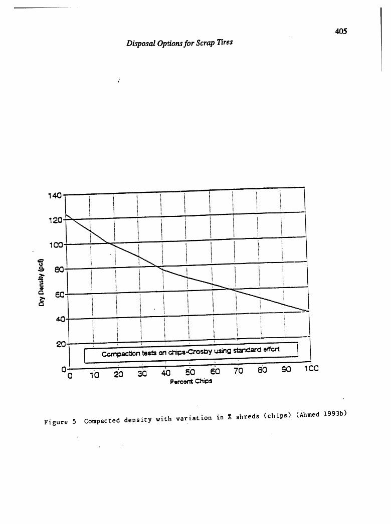
405
Disposal Options for Scrap Tires
Figure 5 Compacted density with variation in % shreds (chips) (Ahmed 1993b)

406 C.W.. Lovell
COMPRESSION OF l-INCH CHIPS
(Mlriablo CompactJve Effort=/1st Cycle)
• Modified + Standard
50% of standard _- No Compactioni
Figure 6 Compression of shreds (chips) for various compactive efforts(Ahmed 1993b)
Disposal Options for Scrap Tires
4O7
sand + 37% shreds by weight produced only 3% strain at 10 psi and 4% strain at 20 psi.Similar data were produced fo_ shred/clay mixtures, where a mix of clay +40% shredsproduced 4% strain at 10 psi and 6% at 20 psi.
Obviously, the problems of excessive settlements can be offset by the mixtureapproach. The lightweight feature is still present in the mixtures trending from a 2/3'sreduction in weight with shreds only, to a 1/3 reduction with a proper mix of shreds andsoil.
Shear testing also required large triaxial cells with special features. Samples ofshreds only did not demonstrate any definite shear failure, and required that strengthparameters be selected for a limiting strain of 20%. As shown in Table 3, values of thestrength intercept c = 4.8 psi and the strength angle _ = 25° might be expected. A mixtureof sand and 39% shreds by weight would yield values of c = 5.2 psi and _ = 38°. Thus atlower confinements (4 to 5 psi), the shred_ increase strength with respect to sand only. Thisis well illustrated in Figure 7. The shreds produce a reinforcing effect in the sand that canbe quite beneficial.
Table 3 also shows that shred collections have a high hydraulic conductivity. Mixingsand with rubber shreds is seen to moderately increase the conductivity with respect to sandalone. Mixing rubber shreds and clay produces a major increase in the conductivity withrespect to clay only.
Resilient modulus testing revealed significantly lower values of the modulus for evenrubber soil mixtures compared to natural subgrade soils (Ahmed, 1993b). Accordingly, tireshreds alone or mixed with soils should probably not be used in highway pavement coursesor even in the subgrade layer. A separation of 3 to 5 ft from the surface of the pavementis likely advisable.
SUMMARY AND CONCLUSIONS
Disposal options for scrap tires are numerous. One particular promising use is thatof a lightweight geomaterial involving tire shreds or tire shred-soil mixtures.
Use of these materials in fill or backfills is recommended based upon theexperimental evidence reported in this paper. Such use can eliminate landfill disposal forvery large numbers of discarded tires.
Some states have reached the demonstration or implementation stage for suchlightweight geomaterial applications. It is likely that many additional states will follow thislead in the very near future.
ACKNOWLEDGEMENTS
The author is grateful to his graduate researcher, Dr. Imtiaz Ahmed, for thededicated experimental effort reported herein. He also thanks the Indiana Department of
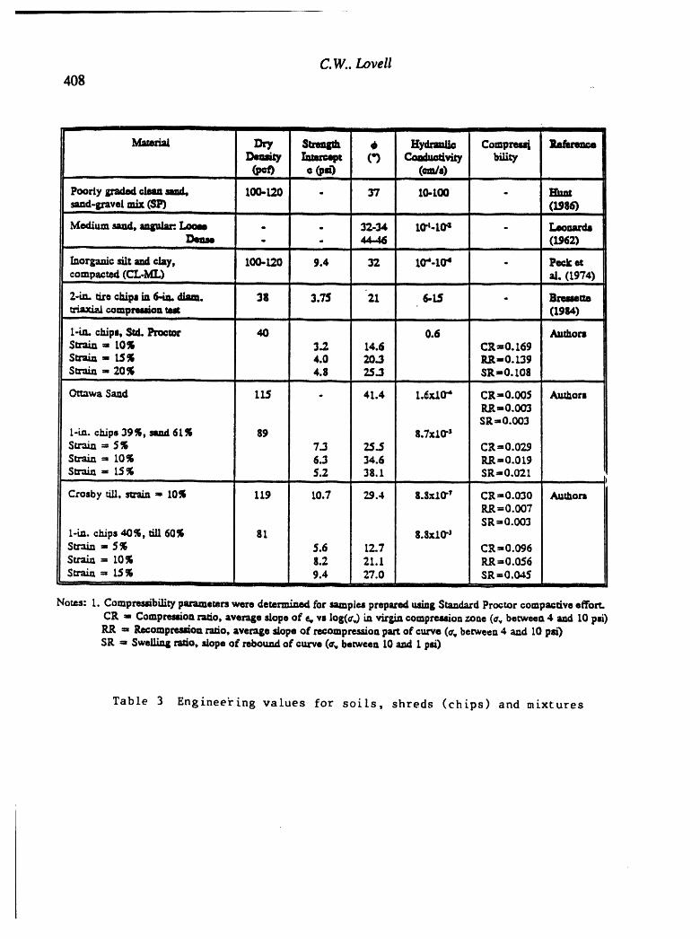
C.W.. Lovell408
,.
IIII I III Ill
Dry $_ 6 HycLTa_ta Compr_i
• (pa3 (_a)ii ii ii ii i,Jl i i
Poorly gradedclean sand, 100-120 . 37 10-100 -sand-gravel mix (SP) (1986)
Sill I I i III IIIII I i laB
Medium sand, angular:..Loom - - 32-34 I0":-t0_ - Leoeard8I),,,m . . 4,t-t6 (L_2)
I I I I i I I i i ii i
rnorganic silt and clay, 100-120 9.4 32 104-104 - Peck stcompacted (CL-ML) aL (1974)
I I I
2-;- _re chips ;I, 6-in. diam. 38 3.75 21 6-13 - grammecompression test (1984)
i I I II iiii ii I
l-in. chlpe, SM. Proctor 40 0.6 Author=Strata = 10_ 3.2 14.6 CR=0.169Stn/a - _% 4.0 20.3 P,_-0.139Strain :, 20% 4.8 25.3 SR=0.108
OttawaSand 115 - 41.4 l._xl0" CR--0.00$ AuthorsP,_=0.0O3SR:0.003
I-in. chips 39%, sand61_ 89 8.7x10⁴Strata : $_ 7.1 25.$ CR=0.029Su'a_ : 10% 6.3 34.6 I_:0.019SlrJm : 15% 5.2 38.1 SR:O.021
I ii i j I
Crosbyr_l, strain1, 10% 119 10.7 29.4 8.$x10" CR:0.030 Au_ortRR=O.O07SR: 0.003
L-in. chips 40_, dU 60_ 81 S.gxlO4Strain : 5_ 5.6 12.7 CR=0.096Sr.ra_ : 10'_ 8.2 21.1 RR=0.056
$tra/= : 15_ 9.4 27.0 SR=0.0,t5i il i .........
Noum: 1. Compressibilityparameterswere determined for samples preparedus/rigStandard Proctor compactive effort.CR - Compression ratio,average slopeof _, vslog(o,)invirgincompressionzone (0,between 4 and I0psi)RR = 17_compre,_ou ratio, average slope of recompressioa part of curve (0, between 4 and 10 pm_)SR : Swelliag ratio,slope or"reboundofcurve (o, between tOand1 psi)
Table 3 Engineering values for soils, shreds (chips) and mixtures

Disposal Options for Scrap Tires 409
TRIAXIAL TESTS ON RUBBER - SAND
40 ..... _ Sand +_" _ ---- 40%"-" 30- / ...... Chips¢t}
ca 25 ...... '
•_ 10 _,sand Only _a 5 _ , ,
i i
00 5 10 15 20 25
Vertical Strain (%)
Figure 7 Increased strength of sands with shreds (chips); confining
pressures of 4-5 psi
C W..LoveU
410
Transportation and the Federal Highway Adminlstrat/on who provided finandal supportthroughthe Joint Highway Research Project,School of CivilEngineering, Purdue University.
REFERENCES
Ahmed, I. (1992), "LaboratoryStudyon Properties of Rubber Softs-Interim Report", ReportNo. FHWA/IN/JHRP.92/11, School of Civil Eng/neering, Purdue University, WestLafayette, Indiana, 145 pp.
Ahmed, I. (1993a), "Use of Waste Materials in Highway Construction",Ist Ed., Noyes DataCorporation (ndc), Park Ridge, New Jersey, 114 pp.
Ahmed, I. (1993b), "Laboratory Study on Properties of Rubber-Soils", FHWA/IN/JHRP-93/4, School of Civil Engineering, Purdue University, W. Lafayette, Indiana, 348 pp.
Ahmed, I. and C. W. Lovell (1993), "Rubber-Soils as Lightweight Geomaterials", Preprintfor January 1993 Transportation Research Board Meeting, TRB, Washington, D.C., 22 pp.
Bosscher, P. J., Edil, T. B., Eldin, N. N. (1992), "Construction and Performance of aShredded Waste-Tire Embankment",Department of Civil and Environmental Engineering,University of Wisconsin-Madison, Wisconsin, 17 pp.
Bressette, T. (1984), "Used Tire Material as an Alternative Permeable Aggregate",ReportNo. FHWA/CA/TL.84/07, C._ficeof Transportation Laboratory, California Department ofTransportation, Sacramento, California, 23 pp.
Elastizell (1992), "Engineeringand Research Reports on Elastizell Engineered Fill",SalesLiterature, Elastizell Corporation of America, Ann Arbor, Michigan.
EPA (1991), "Markets for Scrap Tires", Report No. EPA/530-SW-90-074A, United StatesEnvironmental Protection Agency, Office of Solid Waste, Washington, D.C. 115 pp.
Holtz, R. D. (1989), 'Treatment of Problem Foundations for Highway Embankments",NCHRP Synthesis of Highway Practice No. 147, National Research Council, Washington,D.C. 72 pp.
Hunt, R. H. (1986), "Geotechnical Engineering Techniques and Practices", McGraw-Hill,Inc., New York, 729 pp.
Lamb, R. (1992), "Using Shredded Tires as Lightweight Fill Material for Road Subgrades",Draft Report Dated April 28, 1992, Materials and Research Laboratory, Minnesota DOT,Maplewood, Minnesota, 18 pp.
Leonards, G. A. (1962), "Engineering Properties of Soil",in Foundation Engineering, G. A.Leonards, ed., McGraw-Hill Book Company, New York, pp. 66-240.

I | --r
DisposalOptlonsforScrapTSres411
Merdes,R.S.(1992a),PersonalCommunication,DatedMarch 15,1992.
OECD (1979),"Comtru_onofRoadsinCompressibleSoils',Orlpm_ationforEconomicCooperation and Development, Paris, France, 148 pp.
Peck, R. B., Hanson, W. E. and Thomburn, T. H. (1974), Foundation Englneerin_ 2nd Ed.,John Wiley & Sons, Inc., New York, 514 pp.
Read, j., Dodson, T., and Thomas, J. (1991), "Use of Shredded Tires for L/_tweisht Fill,Report No. DTFH-71-90-$01-OR-I I, Oregon DOT, HighwayD/v/slon, Road Section, Salem,OR, 13pp.

I'0

Hydrogeology,Waste Disposal, Science and PoliticsProceedings 30th SymposiumEngineeringGeology and OeotechnicalEngineering,1994 4_
8RLECTED _'/' AT _ QUKIfllCITY FARMS 8_ER,11'OND SITE:A AISK .u___u_s_ APPROACH
Webe=, u.r., J. Wilson, and X. KizkLandau Alloalatel, ZmO., ldlloncL8, Washington
Toc_Lko, 8., The Boeing CcILwm¥, Seattle, Washington
ABSTRACT
A risk management approach at a former industrial wastedisposal site in western Washington resulted in a selected remedythat is cost-effective and that meets the CERCLA thresholdcriterion of protecting human health and the environment. Theproposed remedy, which addresses contamination in soil andgroundwater, does not require an AR3LRS waiver and received stateand community acceptance. By analyzing the current and potentialrisk at the site, a proposed remedy was chosen that would controlthe source and naturally attenuate the groundwater plume. Sourcecontrol will include removal and treatment of some light nonaqueous
phase liquid (LNAPL) and some soil, followed by isolation of theremaining soil and LNAPL within a slurry wall and beneath amultilayer cap. A contingent groundwater extraction and treatmentsystem was included to address uncertainty in the riskcharacterization.
Implementing source control is predicted to result in a steadydecline in volatile organic compound levels in the drinking wateraquifer through adsorption, degradation, and dispersion. Exposureto groundwater during the period of natural attenuation will becontrolled by monitoring, institutional controls, and a thoroughcharacterization of the plume and receptors.
i

414
E.F. Weber and others
\,
ZNTAODUCTZON
A selected remedy for groundwater and soil contamination isbeing implemented at the Queen City Farms (QCF) Superfund site inwestern Washington by the Potentially Responsible Parties (PRPs),in accordance with the requlrements of the ComprehensiveEnvironmental Response and Claims Liability Act (CERCLA). Thescope of the remedy is the result of a.decision making process byEPA documented in the Record of Decislon (ROD) and based on theresults of a Remedial Investigation (RI), Baseline Risk Assessment(BRA), and Feasibility Study (FS) conducted by the PRPs.
Three small ponds on the property received industrial wastesfrom the mid-1950s to 1968. The QCF site was entered on theNational Priorities List (NPL) in 1984. Initial Remedial Measures(IRM) were completed in 1986, following a focused remedialinvestigation by the PRPs. One purpose of the IRM was to remediateand isolate the original waste ponds. The IRM actions, includinga multilayer cap that covered the former ponds, are an integralpart of the selected remedy.
A site-wide RI (including BRA) and FS, initiated in 1988 andcompleted in 1992, was intended to characterize the risk to humanhealth and the environment and to provide a basis for evaluating !and formulating a remedial response. The FS and ROD issued by theEPA in December 1992 are the result of a risk management approachused to evaluate and select a remedy. The risk management approachprovided a context for balanced decision making based on multiplefactors, including: the results of the baseline risk assessment andits inherent uncertainty; site characteristics and likely futureland use; statutory requirements; and economic, social, andpolitical factors. Site waste disposal and environmentalregulatory actions are summarized in Table I.
SITE CHARACTERISTICS (REMEDIAL INVESTIGATION)
The QCF site is a 320-acre parcel located in a rural setting
directly east of the Seattle-Tacoma metropolitan area: The RI atQCF provided a thorough characterization of the sate that isrelevant to environmental decision making. Elements of thischaracterization are as follows: a history of the site, includinghazardous waste disposal activities; a description of sitefeatures; a conceptual model of the site hydrology andhydrogeology; a characterization of the nature and extent ofcontamination; and a conceptual model of contaminant migration.
The QCF site has been used for a variety of activities,including: a pig farm, an industrial waste disposal site (at formerponds 1,2 and 3), an airstrip, a gravel mine (beginning in themid-1970s), and recently a yard waste composting facility. Theextent of these activities at the site is delineated on a plan view(Figure 1). Also shown on Figure 1 is the approximate location ofthe IRM multilayer cap, which was placed over the industrial waste
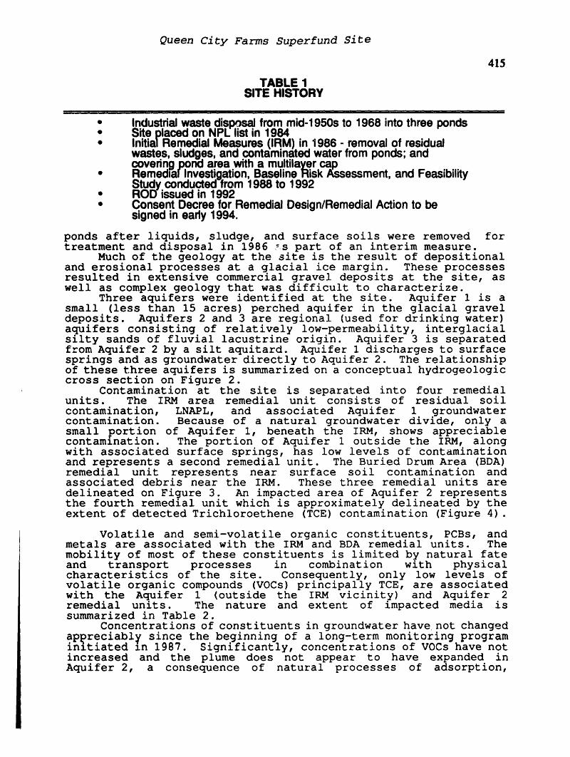
Queen City Farms Superfund Site
415
TABLE 1SITE HISTORY
' ,', ii, ,, ,i ' J , , , ,, ,, J'J ,' ' ' "
• Industrialwastedisl:_.,s_, frommid-1950sto 1968 intothree ponds• Site placedon NPI.:list in 1984• InitialRemedialMeasures(IRM) in 1986- removalof residual
wastes,sludges,and contaminatedwater fromponds;and_covering,pp.nd area with a multilayer
• Hemeomi investigation,uaseiineRisk Assessment,and FeasibilityStudyconductedfrom 1988 to 1992
• ROD'issued in 1992• ConsentDecree for RemedialDesign/RemedialActionto be
signedin early 1994.
ponds after liquids, sludge, and surface soils were removed fortreatment and disposal in 1986 .s part of an interim measure.
Much of the geology at the site is the result of depositionaland erosional processes at a glacial ice margin. These processesresulted in extensive commercial gravel deposits at the site, aswell as complex geology that was difficult to characterize.
Three aquifers were identified at the site. Aquifer 1 is asmall (less than 15 acres) perched aquifer in the glacial graveldeposits. Aquifers 2 and 3 are regional (used for drinking water)aquifers consisting of relatively low-permeability, interglacialsilty sands of fluvial lacustrine origin. Aquifer 3 is separatedfrom Aquifer 2 by a silt aquitard. Aquifer 1 discharges to surfacesprings and as groundwater directly to Aquifer 2. The relationshipof these three aquifers is summarized on a conceptual hydrogeologiccross section on Figure 2.
Contamination at the site is separated into four remedialunits. The IRM area remedial unit consists of residual soilcontamination, LNAPL, and associated Aquifer 1 groundwatercontamination. Because of a natural groundwater divide, only asmall portion of Aquifer i, beneath the IRM, shows appreciablecontamznation. The portion of Aquifer 1 outside the IRM, alongwith associated surface springs, has low levels of contaminationand represents a second remedial unit. The Buried Drum Area (BDA)remedial unit represents near surface soil contamination andassociated debris near the IBM. These three remedial units aredelineated on Figure 3. An impacted area of Aquifer 2 representsthe fourth remedial unit which is approximately delineated by theextent of detected Trichloroethene (TCE) contamination (Figure 4).
Volatile and semi-volatile organic constituents, PCBs, andmetals are associated with the IBM and BDA remedial units. Themobility of most of these constituents is limited by natural fateand transport processes in combination with physicalcharacteristics of the site. Consequently, only low levels ofvolatile organic compounds (VOCs) principally TCE, are associatedwith the Aquifer 1 (outside the IBM vicinity) and Aquifer 2remedial units. The nature and extent of impacted media issummarized in Table 2.
Concentrations of constituents in groundwater have not changed
appreciabl_ since the beginning of a long-term monitoring programznitlated zn 1987. Significantly, concentratzons of VOCs have notincreased and the plume does not appear to have expanded inAquifer 2, a consequence of natural processes of adsorption,

I
NV"id :IllS
I. eJn6!-I

r...
- Figure 2
CONCEPTUAL HYDROGEOLOGIC CROSS SECTION
soul_
NORTH
(l) "_ Or_nal Ground Surlace Prior
===================================='i"xxtll v x 14 x x tl x Ii x x x x x x ii II tit tl II w X Ill Iii II X x •
,: x J[xXx x " •
- -,,v,b, ---_,u6_a"_, '= oo OOoo oar, ..... .-..:".-..'..-:.+-• . .- Pl,,_-a+-,y...o+o¢
[_ "" .+ . ... +.+ +. + ..+. • . ..: ...- +. ;:_.-..." .... ""_" " " +' ' " "" ...... I+ .... " ." "._.- +"+" • ' +...+ +.-'-'. *t+ ._£. . ..: ;.".+; ,:'..
4,.I
",_ | ' Aquifer 3 --
rj " ___ _ _ - , __/Z/Z-/_zzzTzTz7777777wzzzzz-zJ.... ......-,7+.,...:C.._,-2Z_____Z,I.Z27__ZZ//_ZZ/j_z.z_ _ _.
q)_EY_ Gr oul_dwol er or
Till _ Surface ValorLev=l
Groundwot or
Sill Ioyor _ (Iow path
SUI race 1101It
Upper Aquifer ] _ flow pathglSlOlUrOl ed
•-_1-- -- ---- groundlol or
,iri as pathUnll F polrl_onOf' Aqul firEast AIrIIrlp

Figure3
AQUIFER 1, IRM, AND BURIED DRUM AREA
CEDAR HILLS LANDFILL
OUEEN CITY FARHS
KEY
r-21 IRM Area Remedial UnitNOTE _ Buried Drum Area Remedial Unit
The'LNAPLZone'klheoreomlhevidenceof _ Aquifer I Remed,ol Unil
0 300 600 o4..t,her o=re=dualot rree-i_ .e _. (_ Spr in 9ThiszoneincbJe=Ihe reskluololl benoozhthe Formerponds.l_ch is uhovethe _jh /_ Dr o i np i p• ou I I • t,=uler levelScale in feel
O0

_, Figure 4
DISTRIBUTION OF TCE IN AQUIFER 2

Table 2IMPACTED MEDIA
Media Source of Contamination Extent Constituents of Concern
IRM Area Soils • Originaldisposal pondsthat • Area beneath the IRM cap • Volatile and semivolatile(IRM Remedial Unit) were remediated in 1986 extending down to the organiccompounds
• Existing LNAPL layer in Aquifer I aquitard • MetalsAquifer 1 • PCBs
Buried Drum Area (BDA) • Burieddrums and associ- • Near surfacesoils beneath • Volatile and semivolatile¢n Soils ated soils the BDA organic compounds
(BDA Remedial Unit) • Metalsq) • PCBs.z::4,JO
'_ Aquifer I Groundwater in • Residualsoil contamination • Limitedextent of Aquifer I • Volatile and semivolatilein the direct vicinityof the organiccompounds
the Vicinity of the IRM • LNAPL layer Metals ,h (IRM Remedial Unit) IRM •• PCBs(1)
_: Aquifer I Groundwater • Aquifer I groundwaterin ° All of Aquifer I outsidethe • Chlorinated volatile
Outside the Vicinity of the vicinity of the IRM vicinityof the IRM, which organic compoundsthe IRM includesthe majority of the
r_ (Aquifer I Remedial Unit) aquifer
Surface Water Springs • Aquifer I groundwater • Two spring dischargeareas • Chlorinatedvolatile(Aquifer I Remedial Unit) limited in areal extent organic compounds
Aquifer 2 Groundwater • Aquifer I groundwater • Plume extending radially • Chlorinatedvolatile(Aquifer 2 Remedial Unit) from groundwatermound organiccompounds
located inAquifer 2beneath Aquifer I and theMain Gravel Pit Lake
¢N

Queen City Farms Superfund Site
421
degradation, and dispersion, and the effect of the IRM sourcecontrol in 1986.
SITE RISKS (BASELINE RISK ASSESSMENT)
The BRA conducted by the PRPs formed a basis for remedyselection. The BRA consisted of four stages of analysis:
hazard assessment, toxicity assessment, exposure evaluation, andrisk characterizatlon. Risk characterlzation represents thesynthesis of the preceding three analyses into a conclusion as tothe baseline risk to humans at the site. A summary of the BRAprocess performed at QCF is presented in Table 3. Estimated sitecancer and non-cancer risks are summarized in Figures 5 and 6.
The results of risk characterization indicate that relativelyfew constituents and exposure pathways were found to contribute tothe majority of estimated human health risk. Most estimated sitecancer and non-cancer risk is due to Aquifer 1 groundwater directlybeneath the IRM, along with BDA surface and subsurface soils.Consequently, the selected remedy focused most resources on the IBMand BDA remedial units. Remedial actions being implemented includetreatment and containment technologies. Estimated site cancer andnon-cancer risk is limited due to exposure to Aquifer I groundwateroutside the IRM and associated surface water springs, as well asAquifer 2. Consequently, institutional co_,trols and naturalattenuation were deemed appropriate response actions for theAquifer 1 and Aquifer 2 remedial units.
SELECTED REMEDY
The selected remedy in its simplest form consists of sourcecontrol and aquifer restoration. The BDA and IRM areas are thesource areas for groundwater contamination. Implementation ofsource control measures in these areas is predicted to result in asteady decline in VOC concentrations in Aquifer 1 and Aquifer 2 bynatural processes of dispersion, degradation, and adsorption.
The application of source control at QCF will consist of thefollowing approach:
• Remove and treat sludges, soils and LNAPLexhibiting high levels of contamination
• Leave soils with low levels of contamination inplace
• Apply containment options to prevent exposure toand migration of soil contaminants
• Apply institutional controls to protect containmentoptions and limit exposure to soils left in place.
The majority of remedial resources will be applied to sourcecontrol treatment and containment actions, which included extendingthe multilayer cap to cover part of the BDA, as well asinstallation of a slurry wall that, when completed, surrounds theIRM and part of the BDA remedial units to the bottom of Aquifer i.Extension of the cap and installation of the slurry wall willresult in dewatering the mosu contaminated portion of the aquifer.
The application of aquifer restoration at QCF will consist ofthe following approach:
• Remove and isolate the potential sources ofgroundwater contamination (IBM and BDA soils)
• Achieve long-term restoration of groundwaterthrough natural remedial processes of degradation,adsorption, and dispersion

Table 3SUMMARY OF BASELINE RISK
ASSESSMENT PROCESS AT QCF
Hazard Assessment
Metals and organic compounds were found to be present in soil,I..i® groundwater,and surface water springs as a result of onsite waste disposal.4.1
o ExposureAssessment"O
Three exposurescenarioswere evaluated • Onsite occupational• Onsite residential
® • Onsite recreationalExposure Pathway Evaluated:
r_ • Dermal contactwith and incidental ingestion of soilr_ • Use of groundwateras a potable water source (dermal contact, inhalation of
vapors, and ingestion)• Ingestionof food crops grown onsite• Soil particulateinhalation• Ingestionof surfacewater
ToxicityAssessment
EPA-derivedtoxicitycriteriawere used./
RiskCharacterization
Relativelyfew constituentsand exposurepathwayswere found to contributeto the majorityof estimatedhuman healthrisk.

SurfaceWsler SurfaceSoil Sudaceand AquiferI Aquifer2(AquilerI RU) (BDARU) SubaudaceSoil Groundwater Groundwaler .IX
(IRM RU) (IRM RU) (Aquifer2 RU)

424E.F. Weber and others
Risk Below Level of Concern Need for Remedial ActionDepends on Site Conditions
Queen City Farms Superfund Site
425
• Evaluate the effectiveness of natural attenuationthrough statistical trend analyses of groundwatermonitoring data
• Control short-term exposure to contaminatedgroundwater through institutional controls,groundwater monitoring, and possible use ofremedial contingencies.
Because of uncertainties in predicting the rate and effectivenessof natural attenuation processes, contingent extraction (pumping)and treatment systems were included in the remedy, as was acontingent alternative water supply for private drinking waterwells. The contingent remedy may be triggered based on an interimevaluation of the effectiveness of natural attenuation. Aquifer 1is targeted to meet risk-based cleanup goals in 5 years andAquifer 2 to meet maximum contaminant levels (MCLs) within 10years.
RXSK I)GUIAGIDm]IIT APPLZCJLTZON8 Z]ll TEE SITE RRMIIIDT
Risk management is the process of regulatory decision makingonce a problemhas been identified through risk assessment. At theQCF site this process involved balanced application of CERCLAdecision making criteria in the FS and ROD. Risk management usesthe results of the risk assessment and other information, includingstatutory, economic, and political considerations. The result isa balanced remedy that is cost-effective, protective of humanhealth, consistent with applicable laws and statutory preferences,and received community acceptance. The risk management process atQCF involved eight ?lements. A summary of the risk managementprocess and its appllcation at the QCF slte is presented in Figure7.
The BRA established site risks at QCF based on standardizedprocedures. This element of the risk management processestablished the extent and scope of the problem. The BRA is aquantitative and qualitative assessment based on a data base thatis incomplete, which leads to potential uncertainty in thefollowing areas:
• Accuracy and representativeness of sampling data• Accuracy and representativeness of exposure
scenarios• Accuracy and representativeness of toxicological
data.Where uncertainty was identified to be relatively high, the BRAapproach was to apply conservative (protective) assumptions thattend to overestimate risk. This approach invariably leads to theselection of a remedy that is also conservative. A goal of the RIwas to reduce uncertainty where possible. For example, theuncertainty associated with the accuracy and representativeness ofsampling data was considered to be fairly small due to thoroughcharacterization of contaminant migration pathways and rigorousQA/QC program. A goal of the FS and ROD was to identify andaccount for areas where conservative risk as.sumptions were appliedFor example, exposure to Aquifer 1 and Aqulfer 2 is based in parton future residential use. A_uifer i residential use is veryunlikely, due to its limited ability to supply potable water to ahousehold year-round. This limitation supported the use of anatural attenuation remedy that might take longer than anextraction and treatment remedy. Scenarios involving long-termexposure to soil are probably conservative because exposure

E.F. Weber and others
426
Figure7SUMMARY OF THE RISK
MANAGEMENT PROCESS AT QCFL ...... II [[11 IIIII I IIIII I
Developmentof Major Elements of theRegutatory Risk ManagementOptions Process at QCF
I • BaselineRisk AssessmentRisk Management I
Evaluationof: I • Uncertaintyin RiskAssessment
• PublicHealth t . Short-TermRisksNot• Economic Addressedin RiskAssessment• Statutory• Site • Cost Effectiveness
Characteristics • Considerationof Currentand• Uncertainty PotentialFutureLand Use that• Socialand AffectsPotentialfor Exposure
PoliticalFactors• Considerationof Site
Characteristicsthat AffectPotentialfor Exposure
AgencyDecisions • StatutoryPreferencesandActions(The ROD) • CommunityPerceptions
Queen City Farms Superfund Site
427
concentrations are based on hot-spot sampling, thereby supportingthe effectiveness of containment and isolation of some soils inlace. The uncertainty associated with the natural variability inydrogeology makes it difficult to completely characterize
physical, chemical, and biological parameters that controlcontaminant fate and transport. Consequently, there is someuncertainty associated with the effectiveness of naturalattenuation, uncertaint_ that was addressed by implementation oflong-term monitoring ana the specification of contingent remedialactions.
Remedy selection at QCF considered short-term risks associatedwith the remedy. Complete excavation and treatment of allcontaminated soil at the site was eliminated as a consideration, inpart because of the associated health risk to workers and thecommunity.
A cornerstone of the risk management approach is therealization that typically, only finite resources are available toaddress risk. Therefore, the decision maker is concerned about thecost-effectiveness of the selected remedy. At QCF, more resourceswere allocated to media and p_thways that represented higher risksin order to achieve the most risk reduction for a given cost.
Consideration of current and future land use was also a partof the remedy selection process. The location of a landfill alongthe site's northern boundary, for example, makes future residentialexposure to Aquifer 2 unlikely, supporting natural attenuatlon.Future residential exposure was also considered less likely becauseof the existing gravel mine and composting facility.
In addition, site characteristics influenced remedy selection.For example, it was determined that Aquifer 2 recharge anddischarge patterns and low permeability limit the likelihood offuture offsite exposure and favor natural attenuation processes.These characteristics were a factor in selecting naturalattenuation as part of the remedy.
Finally, effective risk management should also include theconsideration of legal, social and political factors. Accordingly,elements of the QCF site remedy specifically address statutorypreferences. LNAPL and soil removal and treatment address thepreference for treatment. A passive soil venting pilot testaddresses the preference for innovative technologies. And based onthe mandate and guidelines for community involvement, locallandowners were informed about the risks and the remedialalternatives and accepted the selected remedy.
SUMMARYBalanced application of remedy evaluation and selection
criteria in the FS and ROD results in a risk management approach toremedy selection. This approach, as applied at the QCF site,results in the following:
• A remedy that is consistent with the NCP• A context for balanced decision making• More efficient and consistent risk reduction
policies• Efficient allocation of resources to address site
risks" A more effective and implementable remedy• Consideration of the concerns of all affected
parties within the constraints of thresholdcriteria.

428
III I

Hydrogeology, Waste Disposal, Science and Port,k:.Proceedings 301h SymposiumEngineering Geology and Geotechnical Engineering, 1994 429
BIOVEN'ITNG FEASIBILITY STUDY OF LOW PERMEABILITY SOILS FORREMEDIATION OF PETROLEUM CONTAMINATION
Kevin M. Brackney, M.S., P.G.University of Idaho Center for Hazardous Waste Remediation Research
Moscow, ID 83844-1052
ABSTRACT
A site characterization of leaking underground gasoline and diesel storage tanks at theUniversity of Idaho, West Farm Operations Center, identified approximately 800 cubic yards ofpetroleum-contaminated soil exceeding regulatory action limits of 100 ppm TPH. Bioventing, acombination of in situ soil vapor extraction and microbial degradation, was selected as a remedialalternative on the basis of the presumably unsaturated paleo-soil with a 45-foot depth togroundwater, and a microbial study which concluded that indigenous petroleum-degradingmicroorganisms existed throughout the contamination. Soil vapor extraction tests wereconducted by applying a 60-inch water column vacuum to a soil vapor extraction well andmonitoring pneumatic pressure drawdown in 12 adjacent pneumatic piezometers andverticallydistributed piezometer clusters. Pressure drawdown vs time data plots indicated that airpermeabilityis inadequate everywhere at the site except at 20 feet below ground surface. Lowsoil permeability creates conditions for a perched water table that was documented during theinvestigation, resulting in unsatisfactory conditions for in situ bioventing.
SITE INVESTIGATION
Two 1500-gallon gasoline and diesel underground storage tanks (USTs) were excavatedat the University ofIdaho (LrDWest Farm Operations Center in December of 1990. The tankshadbeen abandoned a decade earlierwhen water began contaminatingthe fuel. When the twoUSTs were excavated at the UI West Farm site, several four-inch-diameter holes were observedin the tanks. Strong odors were noticed, and concentrations exceeding 2000 parts per million(ppm) were determined with a hand-held photo ionization detector (PID) (Chen-Northern, 1991).
A site investigation was conducted by drilling 17 hollow-stem auger boreholes (Fig. 1)which were sampled by drilling 3 feet, then driving a split-spoon sampler lined with brass sleevesinto the soil for 2 feet. Drilling and sampling continued to an average 25-foot depth for eachborehole. One six-inch core _om each sample was analyzed by the UI Analytical Laboratory fortotal petroleum hyd_'ocarbons(TPH)-gas and TPH-diesel by EPA Method 8020, volatile organicsby EPA Method 8260, and total lead by EPA Method 3050. A hand held PID calibrated toisobutylene was used to assist in field contaminant characterization. Geologic cross-sections wereconstructed in the field and plotted with PID concentrations to guide the investigation. Theboreholes were terminated where geologic evidence sugge_ed the limits of contamination hadbeen reached and PID readings were <100 ppm.
Approximately 800 yd3of petroleum-contaminated soil exceeding regulatory action limitsof 100 ppm TPH as gasoline or 1000 ppm TPH as diesel were identified in an area approximately35 × 50 × 20 feet deep (Fig. 1.) (Ralston et al. 1992.) Interestingly, the highest contaminationwas not found under the tank but offset _40 feet downhill, suggesting a component oflateral

K.M. Brackney
430subsurface flow. Sample values ofup to 2,900 ppm TPH-gas and 54,000 ppm TPH-diesel werecofiected from 10-20 feet below ground surface in borehole WF-6 in this area. No volumetricestimate ofleaked fuel is available, since inventory control records were not maintained.
Mean lead concentration at the site was 20 ppm with background lead concentrations of10 ppm. One borehole immediately adjacent to the regular gasoline tank location (WF-3) had
15 feet of gasoline contaminated soil averaging 226 ppm total lead, a concentration consideredhigh enough to fail the toxicity leaching control procedure (TCLP) for lead, thereby potentiallycharacterizingthe soil as hazardous waste,/fexcavated This lead-contaminated borehole waslater twinned by drilling a second borehole (WF-16) 1.5 feet south which contained a mean leadconcentration of 28 ppm total lead and<3.5 ppm leachable lead based on TCLP results.
General Geologic/Hydrologic Setting
At the West Farm site, surface geology consists of silt and clay of the Palouse formation,mostly wind-derived sediments (loess.) Soils have been mapped by the University of IdahoAgricultural Experiment Station as Palouse Series soils consisting of silt loam and grading intosilty clay loam at 52 inches. The Palouse soils are characterized as being very deep, well drainedsoils on upland positions with 7% to 12% slopes. Depth to water is >6 feet. The available water-holding capacity of the soil is high (0.19-0.21 irwin)with a permeability of 0.6 to 2.0 inches perhour. Of potential significance is the tendency of the soil to develop severe pipin8 characteristicsdefined as the formation of tunnels or pipe-like cavities by moving water. The soil texture isblocky to prismatic with many very fine to medium-fine tubular pores. Some soil horizons haveup to 20% old vertical worm channels (McDole and Peterson, 1989). Locally, erosion hasexposed flows of the underlying Columbia River Basalt Group.
A downward groundwater gradientexists within the Moscow area. Shallow wells (<20feet) located at the University of Idaho Groundwater Research Site (located 1000 feet north ofthe UST site) have static water levels 5-10 feet below land surface. Deeper wells (80-150 feet)completed in the basalt have depth-to-water values in the range of 10 to 20 feet. Nearby city anduniversity water supply wells draw water from depths of 600 to 1,200 feet and have static depth-to-water values of 250-300 feet. Based on available information, the estimated depth to theshallowest groundwater underlying the UST site is >45 feet (Ralston, et al, 1992.)
Site Stratigraphy
Although the fine-grained silty clay loess soils at the site were difficult to characterize,relative soil density was one of the more significant stratigraphic characteristics. Total blowcounts to pound a 2-foot split-spoon sampler with a 140 pound safety hammerat approximate
5-foot intervals in each borehole indicate relative soil density. A mean value was calculated foreach 5-foot interval, representing the relative density for that interval over the site. The relativesoil density at 5 feet below ground surface Cogs)was 43 blows. A dense silty clay from 10-20 feetbgs averaged 73 blows, with maximum values of>100 blows. In contrast, the mean blow countto penetrate 2 feet at 25 feet bgs was 37 blows. This dense silty clay present from about 10-20feet represents a paleo-"B" soil horizon that may have formed during the Pleistocene. Two buffedlenticular paleo-stream channels consisting of quartz feldspar sand and gravel were intercepted at30 feet bgs. These paleo-stream channels were surrounded on at least three sides by loess. "e
Bioventing Low Permeability Soils431
deeper of the two OVF-2) was not fully penetrated, while the shallower lenticular sand wasunderlain by loess. When borehole WF-2, which bottomed in gravel at 30 feet bgs, stood openovernight; no water was present in the borehole the following morning. Two other boreholes hadminor water seeps that appeared to be entering the holes on top of the dense clay horizon.
Basaltic bedrock or boulders were intercepted in two boreholes at the site. Depth to thebasalt at the UST site increases from 14 feet bgs in VE-I southwest of the site (Fig. 2), to 27.5feet on the northeast side of the contamination (WF- 17), to >31 feet on the north end of the site.This deepeningof basalt intercept_is believedto reflectbasaltledgesburiedbyloessstairsteppingdownto thevalleyof ParadiseCreeklocatedabout1000 feetnorthof thesite.
SOIL VAPOR EXTRACTIONfBIOVENTING FEASIBILITY STUDY
A literature review of possible remediation methods covered landfarming, low-temperature thermal desorbtion, and soil vapor extraction/bioventing. The advantages of treatingthe petroleum contaminated soil by in situ bioventing are potentially lower cost, avoidance of"generating" hazardous waste (e.g. lead) by excavation, andability to remediate under buildings,roads, utility conduits, etc. Some of the disadvantages of excavating contaminated soil are thatadditional non-agricultural land is needed for landfarming, and landfarmedsoils are only suitablefor construction backfill or disposal as solid waste.
In situ soil vapor extractionfoioventing seeks to take advantage of two processes:
1. The removal ofvolatile phase hydrocarbons from the soil by establishing a pressuregradient and venting the effluent to the surface for subsequent disposal.
2. Supplying oxygen and nutrients to petroleum-degrading microbes.
The combination of these two processes is very effective for landfarmingpetroleum contaminatedsoils where oxygen, nutrients, and microbes can be manipulated to enhance volatilization andmicrobial degradation. In situ soil vapor extraction/bioventing utilizes these same processes, butcontrol of the critical variables is more difficult in subsurface geologic materials that must beaccessed from the surface via wells and trenches. The main distinction between bioventing andsoil vapor extraction (SVE) is that bioventing attempts to degrade contaminants in situ byminimizing the amount ofvolatiles extracted, while soil vapor extraction attempts to maximize themass transport aspects of remediation. Essentially, they are end members of the same process.
In sandy soils with high air permeabilitythere are many well documented examples of soilventing of volatile organic fluids (e.g. gasoline) (Hutzler et al, 1989). However, organicmolecules larger than Cl0 do not readilyvolatilize and are logical targets for microbialdegradation (Johnson, 1990.)
The diesel- and gasoline-contaminated West Farm site soils consist of silt loam to silt clayloam. Although soils of this size fraction are less amenable to bioventing due to low airpermeability values, the presence of soil macropores suggested that natural permeability might besufficient for effective bioventing. The possibilities for permeabilityenhancements by utilizingvapor extraction trenches to increase surface contact of the vacuum with the soil and the potentialfor hydraulically or pneumatically fracturingthe sediments further supported possible bioventingat this site. Johnson (1990) identified the need for a well-documented case history of soil vaporextraction in low-permeability soil. These combined factors led to the university's conclusion thatthe advantages ofbioventing at the West Farm site outweighed the disadvantages of the low
• K.M. Brackney432
permeability soil. With the encouragement of the Idaho Department of Environmental Quality,we began evaluating the in situ soil air permeability and potential for microbial degradation.
Pneumatic Well Field Design and Installation
A pneumatic well field and piezometer cluster network was designed to characterize thevertical and horizontal distribution of air permeability within a 10 foot radius around a vaporextraction well (Fig. 2.) Proposed testing included a constant pumping test and monitoringchange in pneumatic pressure and soil gas concentrations (TPI-I,02) with respect to time atvarying radisl distances and depths from a pumping or vapor extraction well. Oxygen content ofextracted soil gas from the contaminant zone was to be compared with a background well todetermine if oxygen uptake (an indication of microbial respiration) was occurring.
During the vapor extraction well drillingit was observed that significant formation damageoccurred with the buildup of a clay wall cake on the borehole wall. Removal of the clay wall cakewas considered necessary since it would inhibitthe characterization of the natural soil airpermeability. Two methods of open borehole well development were attempted, utilizingcompressed air and oversize borehole reaming. The compressed air seemed to have the highestlikelihood of success but the results were erratic and difficult to control. Lack of visibility downthe borehole, combined with either ineffective removal or significant erosion of the borehole wall,prevented consistent removal of the wall cake. Oversize reaming with a short piece of 6 inchdiameter steel casing studded with sharpened bolts was moderately effective at tearing the claywall cake off without smearing the clay.
To complete the vapor extraction wells, we used groundwater monitor well constructiontechniques, including 20 slot (0.020 inch spacing) well screen, a pea gravel filter pack surroundingthe screen, and a minimum of 4 feet of non-shrinkconstruction grout to form an impermeable sealfrom the surface to prevent short-circuiting of the well to the atmosphere. Piezometer clusterswere constructed similarly except that 5 c"e-inch PVC standpipes were installed in a singleborehole from 5-25 feet. Each O.5-foot screened interval had an individualgravel pack and wassealed from adjacent piezometers with 3 feet of non-shrink construction grout. The wells andpiezometers were then sealed and plumbed with hose barbs, narrow flexible tubing, and valves toallow the measurement of soil air pressure with Dwyer differential air pressure gages.
Well and piezometer installations appeared to be very effective at isolating zones fromeach other and the atmosphere. Indeed, both positive and negative differential pressures weremeasured under ambient (non-pumping) conditions in a single borehole at variable depths. Thisdecouplement of soil air pressure from atmospheric air pressure was later determinedto be someof the more significant data used to characterize the air permeability at the site.
Soil Vapor Extraction Tests
The extraction test was conducted using an explosion-proofRotron regenerative blower(Model DR 505) capable of producing a maximumof 6G-inchwater column (wc) vacuum, air-water separator tank, Dwyer differential air pressure gages ranging from 2- to 80-inch wc, pietotube and gage to measure exhaust air velocity, and a recording microbarographto correctdifferential soil pressures to actual pressure.
I
Bioventing Low Permeability Soils
433
Four vapor extraction tests were conducted with limited success. Test I pumped wellVE-2 (Fig. 2) and was abandoned after 6 hours because short circuiting was occurring and allextracted air was being withdrawn from a 0.25 inch sand layer correlated with one of thepreviously described sand channels. This short circuiting of air was determined when pressuredrawdown was occurring only at the 20-foot pneumatic piezometer level at a radial distance of 5feet from the extraction well. The vapor extraction blower was then moved to well VE-4. Test 2pumping well VE-4 was abandoned because of technical difficulties. Test 3 pumping well VE-4collected the most useful data (see below). Test 4 repeated Test 3 but an impermeable soil coverand the substitution of the totalizing gas flow meter for the pieto tube. Very low flow velocitiesfrom the extraction well wero below the design tolerances for the pieto tube. Because therecording microbarograph operated by the State Climatologist at I3I failed during Test 4, theinterpretation of data is seriously inhibited by lack of barometric data.
Soil Vapor Extraction Data Analysis (Test 3)
Vapor extraction test 3 operated for about 5.6 days at a 60 inch we vacuum that produceda flow of 0.17 standard cubic feet of air per minute (SCFI_. Passage of an atmospheric frontthrough the Moscow area during the test complicated the interpretation of the data. A review ofthe soil pressure drawdown vs time data from the two piezometer clusters at 5-and 10-foot radialdistances from the pumping well (clusters VE-5 andVE-6, respectively) illustrates the horizontaland vertical heterogeneities of air permeabilityat the West Farm site (Fig. 2.) At the 5, 10, and15 foot depths in both piezometer clusters soil air pressures generally exceeded atmosphericpressures (Figs. 3-8.) Negative differential soil air pressures (i.e., less than atmospheric pressure)were only seen at 20-foot depths in both clusters (Figs. 9 and 10) Soil air pressure in VE-5 at 25foot depth exceeded atmospheric pressure at most time increments (Fig. 11), while the highestpositive differential pressures observed on the site occurred in VE-6 at 25 fl (Fig. 12).
The highest permeabilities at the site were found at the 20-foot soil depth, repeating thepressure response observed in Test 1. This increased permeability may be correlated with anerosional period and lateral deposition of stream channels from ancestral Paradise Creek. Thevery dense paleo-"B" soil horizon does not appear to have sufficient natural air permeabilitytosupport bioventing.
A limitation of the above data set is that insufficient ambient soil pressure monitoring(non-pumping) data was collected. This would have been useful in an attempt to calculate thebarometric efficiency of the individual pneumatic piezometers. Preliminary data suggests thatbarometric efficiency ranges from 50 to 100%. However, it is not clear that the relationship islinear, and factors other than air permeability may be significant.
Microbial Degradation
Zhou (1993) investigated the microbiology of the West Farm site and conducted microbialdegradation experiments on petroleum contaminated soils collected during the site investigation.Figure 13 shows the results of biodegradation experiments in a microcosm at various levels ofpetroleum contamination at a constant temperature (25°C). He concluded that (1) Indigenouspetroleum-degrading microorganisms existed throughout the contaminated area, and (2) soilmicrobial populations were affected by contamination level, oxygen availability, and nutrient
434 K.M. Brackney
availability. If these environmental factors could be appropriately manipulated throughbioventing, the microbial communities could be adapted to the contaminated environment anddegrade the hazardous contaminants.
Soil Gas Monitoring
The background vapor extraction well VE-1 was completed in a previously unidentifiedwater-saturated loess and was useless for collecting background soil air quality data. The wellwas maintained as a groundwater piezometer and is discussed below.
TPH and oxygen were monitored during Test 4, with the results probably comparable tothose of Test 3. Over the 24-day testing period, continuous vapor extraction from well VE-4produced 6,600 SCFM of air, a volume representing _ 1 contaminated soil pore volume, assuming30% porosity. Zhou reported (personal communication) that gas chromatographic analysis of 15samples of soil vapor extraction off-gas showed that total petroleum hydrocarbons in air rangedfrom 20 to 470 ppm Oxygen content of the off-gas ranged from 3 to 7%, with no discernibletrend from the beginning to the end of the test. Kittel et al. (1993) report that typicalhydrocarbon content of soil gas beneath a contaminated site is <100 ppm, while oxygen content isusually 0 to 2%. Oxygen content of soil gas at uncontaminated sites is typically 15 to 20%.
Perched Water Table
Piezo:Jeters VE-5 at 10 ft, andVE-5 at 15 fi bgs became saturated with groundwaterduring test 3 or 4. With the exception of well VE-1 all other piezometers and wells remainedunsaturated during the testing; no water or condensing water vapor was produced from the vaporextraction well or the air water separator tank. A drive point piezometer (VE-7, Fig. 2) wasinstalled in the petroleum tank excavation to monitor what was interpreted to be rainwater fillingthe sand-backfilled excavation. It was assumed that groundwater had been drawn in laterally bythe 60-inch water column vacuum induced by the vapor extraction well. Later, an additionalI
groundwater piezometer cluster (VE-9) was installed upgradient from the site and the presence ofa perched water table was documented and monitored throughout the following year.
Groundwater monitor well hydrographs are shown in Figure 14. The monitor wells arearrangedin the legend from south to north through the site. The hydrographs show a distinctdecline in hydrostatic head with increasing depth, indicative of a groundwater recharge zone. Forexample, in early July, 1993, the groundwater elevation of piezometer cluster VE-6 at 5 ft was2588 feet, at VE-6 at 10 ft it was 2587 tt, and at VE-6 at 15 ft it was 2577 ft. Interestingly, VE-6at 15 ft had previously been unsaturated (dry), and the groundwater elevation rose 6 feet over thenext 3 months. These hydrographs appear to be documenting groundwater recharge occurring inthe vadose zone. However, it should be remembered that the piezometers at 20 and 25 feet wereunsaturated during this same period.
The hydrographs document the effectiveness of the impermeable soil cover placed overthe site before the start of test 4 during the fall of 1992. VE-6 at 5 ft is on the uncovered edge ofa plastic cover. Before February 1993, the piezometer was unsaturated until the wet spring of1993. However, VE-5 at 5 ft was under plastic during this same period and remained unsaturatedthroughout the measurement period. This observation underscores the need to address bothgroundwater inflow and surface water infiltration in any attempt to dewater the remediation site.
Bioventing Low Permeability Soils 435
Capillary Pressure
Soil capillary pressures within the vadose zone have a significant role in understanding therelationship between soil vapor pressure and soil water movement. Corey (1990) describescapillary pressure (Pc) as equal to the pressure of the non-wetting phase (Pnw) minus pressure ofthe welting phase (Pw); that is, Pc = Pnw - Pw. He states (1990, p. 13.)
In a system in contact with the atmosphere, such as soil, either the wetting phase (water)or the non-wetting phase (air) will normallybe at atmospheric pressure. If the soil issufficiently desaturated for an interconnected air phase to exist, the air will be atatmospheric pressure and the liquid will be at less than atmospheric pressure. This is thereason that soil scientists refer to water as being under 'suction'or 'tension.'... In awater-gas system, water tends to be preferentiallyadsorbed by the solid surfaces and thegas is compressed if it is entirely surroundedby water. The gas pressure is higher thanthe water. In an water-oil-gas system, the gas will usuallybe the highest pressure, the oilat the next highest and water at the lowest pressure when equilibriumexists.
The presence of groundwater in piezometers VE-5 and VE-6 provides a partialexplanation for the air pressures above atmospheric pressure in these wells. Air trapped beneath aperched water table would become compressed. Air contained in an enclosed piezometer columnabove the water table would also become compressed as water levels increased. This does notprovide an explanation for the positive soil air pressures observed in the unsaturated wells.Obviously, the vertical air conductivity of the sediments is a limiting factor. It may be that soil airpressures exceeding atmospheric pressure are related to a lag time phenomenon created by thepassage of an atmospheric pressure from. It may also be related to the high vapor pressures ofthe volatile organics. Headspace analysis of contaminated soil sample occasionally exceeded 2000ppm TPH so that physical measurement of soil pressures exceeding atmospheric pressures may bepartly attributable to petroleum contaminants.
One commonly reported result of negative capillary forces applied to soil during soil vaporextraction is that water is raised by reducing the pressure of the air, a phenomenon believed tohave occurred at the West Farm site. Water in piezometer VE-5 was first identified during soilgas sampling with a vacuum pump. The relatively high vacuum is believed to have drawn water inlaterally from the adjacent rain saturated sand backfill from the petroleum tank excavation. Thefirst two water level measurement in VF-5 at 10 ft drop nearly 2 feet at_erthe sampling inducedvacuum dissipates (Fig. 14.) Piezomet ;r cluster VE-6 was 10 feet further downgradient from thebackfilled tank basin and remained un'_aturatedat all levels untill the following year.
Applying a vacuum to soils with high soil matric suction such as silty clays has thetendency to pull moisture out from the soil and artificiallyraise the water table further reducingthe already limited pore space available for air flow. However, capillary forces could also bereduced by increasing the soil air pressure anddriving water out of the soil. This has importantimplications, since dry soil has the highest air permeability.

K.M. Brackney436
CONCLUSIONS AND RECOMMENDATIONS
The combination of low-permeability silty clay soils and groundwater inflow creatingperched water table conditions at the West Farm site are not conducive to soil vapor extractionwithout significant engineering modifications. The most importantof these would be thediversion of groundwater flow around the site by the construction of a groundwater interceptiontrench. This trench would need to be about 15 feet deep to intercept the observed groundwaterinflow. An impermeable or low permeability cover is also necessary to prevent precipitation frominfiltratingand reducing air permeability.
Applying a positive pressure head instead of a vacuum to supply oxygen would be anappropriate application ofbioventing technology. This has the benefit of forcing water out of thesoil, omitting costly off-gas treatment if excessive volatiles are produced. At the West Farm sitethere are no sensitive subsurface receptors such as basements or utility conduits that would beimpacted by volatile organics. If this were a concern, vapor interception trenches or positivepressure barrierscould be installed to protect sensitive receptors. An additional caution is thatenhanced groundwater recharge by pressurizingthe vadose zone might also increase thevulnerability of groundwater from impacts by dissolved organics such as benzene.
The dense paleo-"B" soil horizon would need to be artificially fractured to increase thevery low permeability of this zone. This dense horizon is a logical candidate for hydraulic orpneumatic soil fracturing. These and other engineering solutions are quite expensive relative toexcavation and conventional landfarming. In certain situations, the expense of bioventing siltyclay soils would be justified. If the entire West Farm site had permeabilities similar to thoseexperienced at the 20 foot depth without the perched water, the situation would be significantlyenhanced. As a prudent manager, I would not recommend bioventing in this situation if savingmoney is an objective. However, Kittel et al. (1993) reported that in the US Air Force bioventinginitiative, out of over 100 fuel-contaminated sites evaluated for bioventing only 3 were found tohave unacceptable air permeabilities. The West Farm site has an unfortunate combination offactors working against successful bioremediation.
REFERENCES
Chen-Northern, Inc. 1991. Limited environmental site assessments for tank closures. NorthIdaho Tank Closure Project. University of ldaho, unpublished report preparedfor IdahoDepartment of Public Works, 36 p.
Cory, A.T. 1990. Mechanics of immiscible fluids in porous media. Water P.,esourcesPublications, Littleton, Colorado, 255 p.
Hutzler N. J., B. E. Murphy, and J. S. Oierke. 1989. State of technology review, soil vaporextraction systems. U.S. EPA, CR 814319-01-1, EPA/600/2-89/024.
Johnson P.C., C .C. Stanley, M. W. Kemblowski, D. L. Byers, and J.D. Colthart. 1990 Apractical approach to the design, operation, and monitoring of in situ soil venting systems.Ground Water Monitoring P,,eview, Spring 1990.
Kittel, J. A., P,. E. Hinchee, R. M. Miller, C. V. Vogel, and K. Hoeppel. 1993,. In situ respirationtesting: A field treatability test for bioventing, in Proceedings of the 1993 PetroleumHydrocarbons and Organic Chemicals in Groundwater: Prevention, Detection, and
Bioventing Low Permeability Soils437
Restoration, November 10-12, 1993, Houston Texas. American Petroleum Institute andNational Groundwater Association.
McDole, R. E., and P. N. Peterson. 1989. Soil Survey of the University of Idaho AgriculturalExperiment Station and Campus, Moscow, Idaho. Bulletin no. 698, AgriculturalExperiment Station, University of Idaho, College of Agriculture, 52 p.
Ralston D., J. Kaufinan, and K. Brackney. 1991. Site assessment report, West Farmsunderground storage tank (UST) site. University of Idaho, Site Assessment ConsentOrder 39-108.
Zhou, E. 1993. Physical, chemical, and microbiological factors affecting bioremediation of apetroleum hydrocarbon contaminated soil. M.S. Thesis, University of Idaho, Moscow,Idaho.
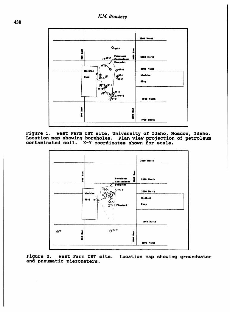
K.M. Brackney438
i illl m
|040 Norlk
<_4Ut:-7
O._._r c_si..," sos,Xo.h-L_ P._lwl,,*
Idoehls, ...1 _ Jeee Neigh
8hod ' .
8hop
(_--tF-g 11)40North
1 I1900 North
Figure 1. West Farm UST site, University of Idaho, Moscow, Idaho.Location map showing boreholes. Plan view projection of petroleumcontaminated soil. X-Y coordinates shown for scale.
1060 North
i 1! Potrelooll ! 31130 ]NOrth
jd" ¢oolIIIlIoI...... [ + .+ Footprtll
,/'_+- \ -6 2000 North....,..+.
1940 North
"" 11100 North
Figure 2. West Farm UST site. Location map showing groundwaterand pneumatic piezometers.


442 K.Mr.Brackney
VE-_20
:iiii....... iL "li,,,iill I 111,--'Jillillt itlill
_,o I!ill I!!111IIIIr_lilil1.1_ 10.00 1111LI_ 1000.00 II_X_._
Time {mbmtee)
Figure 9. Piezometer VE-5 at 20 feet bgs. Radius from pumping well equals 5 feet.
VE-@20
]030.0 I I ::::: I :I I I!111 0-.i ..,_......
I I ::::i • : jdi ', ....... llw
""""u_u.v '- • : ::" : _--._ .i: :-.,., •
: ::ll :
920.0 .........
j| ....... 0 ,.m: ::::: : ,,,
: ::::: i: : : :. ---o--- VE-O-20
'_""_ 815.0 : ::::: II: : :::: II ;, ;;11 i.
: Ii111 '.
: :::: :
010.0 _ " ::::_ : 1! ::::: : _ .--I._
u: : :11 I
905.0 .... '
1 10 100 1000 10000
Time (mJnutee)
Figure 10. Pi, zometer VE-6 at 20 feet bgs. Radius from pumping well equals 10 feet.

Bioventing Low Permeability Soils 443
VE-5-25
930 _ tI
..... i _::n.., i ,928 , L,'i i:
i ::: '-"_"_ i.. ._ d,
920 - i : ,1" !
924 .i i . i: _ _ VE-5-25L • • I.. ..
922 n j _I I
' " " |' i
920 1 ii i, r
918
10 100 1000 10000
Time(minutes)
Figure 11. Piezometer VE-5 at 25 feet bgs. Radius from pumping well equals 5 feet.
VE-6-25
I ' I I945.0 !!!!!! _ !!::: "1
-' I _ ' 'I' iii::: ..... I.....
940.0 ...... I ! i i iii i , :• !!!!! !I I I!1 I
iii:::a,.,...... .= _',: :;;:: : :
... I ! III 14_3 _ : ,935.0 jii,,, lllll I _ "............ ii
i iiii; iiiii i : :
_ I '''I','',. _]_ i : : : P-atm930.0 lllll !iiii ] i iI'"" iiii " i .j;,
d;:E i i t Ill i I in==_-_ ' ! ----o---- VE-0-25ii''"' .e,,
025.0 liill iiiii "_ II,_ !"1 1Jill'" iiiii ,. _. i] :• [[[!! "_:: i :
; i ilJJJl ! !iiii ! i
i iiiij]'' i ii::: i...... : ::
• . . : :::::
91s.o I i i i i iii i i i_-_ i
1.00 10.00 100.00 1000.00 10000.00
Time(minutes)
Figure 12. Piezometer VE-6 at 25 feet bgs. Radius from pumping well equals 10 feet.
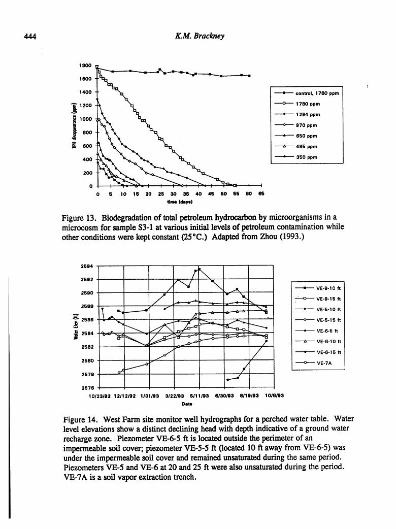
444 K.M. Brackney
1800
1600
1400 = control, 1780 ppm
.__1200 ---o---- 1780 ppm* 1294 ppm
1000
970 ppm
800 * 650 ppm
600 A . 485 ppm
400 : 350 ppmi
200 L_0 I ....... : :
0 5 10 16 20 25 30 35 40 46 50 66 60 65
dine (days)
Figure 13. Biodegradation of total petroleum hydrocarbon by microorganisms in amicrocosm for sample $3-1 at various initial levels of petroleum contamination whileother conditions were kept constant (25"C.) Adapted from Zhou (1993.)
2594
2592 /__
2590 / ,lrj_ " w__--- VE-9-10 ft_, _ VE-9-15 ftJ .2588
=,,_....._........_ r _ VE-5-10 It"" " " _ VE-5-15 ft
_ VE-6-10 ft
2582
_J'/ ----0-----: VE-6-15 tt2580 / VE-7A
2578 - OJ /e--"
2576
10/23/92 12/12/92 1131193 3122193 5/11/93 6/30/93 8/19/93 10/8/93Date
Figure 14. West Farm site monitor well hydrographsfor a perched water table. Waterlevel elevations show a distinct declining head with depth indicative of a ground waterrecharge zone. Piezometer VE-6-5 ft is located outside the perimeter of animpermeable soil cover; piezometer VE-5-5 ft (located 10 ft away from VE-6-5) wasunder the impermeable soil cover and remained unsaturated during the same period.Piezometers VE-5 and VE-6 at 20 and 25 ft were also unsaturated during the period.VE-TA is a soil vapor extraction trench.

Hydrogeology, Waste Disposal, Science and PoliticsProceedings 30th SymposiumEngineeringGeologyandGeotechnical Engineering,1994 44_
ENHANCED ENDOGENOUS BIOLOGICALATTENUATION OF AROMATICHYDROCARBONS IN GROUNDWATER: A CASE STUDY
(Preliminary Results)
Christopher Lammer, P.E.EnvlroSearch Intematlonal
1605 N. 13th StreetBolse, Idaho 83702
ABSTRACT
EnviroSearchInternationalhas designedand is currentlyoperatinga groundwatertreatmentsystemto addressa release of petroleumhydrocarbonsat a site in Meridian,Idaho. Amongthese hydrocarbons,the principalcompoundof concern,benzene, wasreportedat concentrationsof up to 4.0 mgl£ prior to systemoperation. The systemisdesigned to reduce hydrocarbonconcentrationsin groundwaterand saturated soilthroughenhancementof naturallyoccurringaerobicmicrobialactivity.
An in situ treatment system was selected in order to simultaneouslyaddresshydrocarbonsdissolved in groundwaterand adsorbed to the saturated soil matrix.Petroleum-utilizingbacteria were identifiedin groundwatersamples collectedfromtheprojectsite. The in situ systemwas designedto create conditionsmoreconducivetoaerobic microbialactivityby increasingthe initially low concentrationsof dissolvedoxygenandthe nutrientsnitrogenandphosphorus.
_'__ration of the in situ treatment system was initiated in August 1993. A_ ', significantdecline in concentrationsof the aromatichydrocarbonsbenzene, toluene,
_ ethylbenzene,and xylenes was observedover the first seventeen weeks of systemoperation;concentrationsof these compoundswere reportedas less than or equal todrinkingwater maximumcontaminant limits in November 1993. These preliminaryresults suggest that in situ biologicaltreatment is a practical approach to shallowaquiferpetroleum contaminationinthe TreasureValley.
INTRODUCTION
Biologicaldegradationof petroleumhydrocarbons,particularlybenzene, has beena recognizedphenomenondocumentedin the literatureover recent years (Delfino,1985 and Urano, 1986). Applicationof this process to in situ treatment of soil andgroundwaterimpactedby petroleumhydrocarbonreleases has also been documentedat a varietyof sites (Wilson, 1989 and USEPA, 1993). EnviroSearchInternationalhasappliedthistechnologyto an industrialfacilityin Meridian, Idahoto address impactstogroundwaterfroma hydrocarbonreleaseat this location.
Biologicalgroundwatertreatmentutilizesindigenousbacteria and other microbesto degrade hydrocarbons. These hydrocarbons,which can providea substrate (i.e.,energy source)for certain microorganisms,are metabolizedinto harmlesscompoundssuch as carbondioxideandwater. This type of hydrocarbondegradationoften occursnaturally at contaminatedsites, but can be severely limitedby a lack of oxygen and

C. Lammer446
nutrients. The in situ groundwatertreatmentsystemwas designedto accelerate thisnaturalbiologicalprocessby providingthesepotentiallyrate-limitingcompounds.
J Traditional "pump and treat" approaches to groundwatertreatment are oftenlimitedintheir abilityto removehydrocarbonsadsorbedto saturatedsoil, often leadingto long treatmenttimes (McCarty, 1988). An in situ treatmentsystemwas selected inorderto simultaneouslyaddresshydrocarbonsdissolvedin groundwaterand adsorbedinthe saturatedsoilmatrix. Petroleum-utilizingbacteriawere identifiedin groundwatersamples collected from the project site, indicatingthat conditionswere favorable forbiologicaltreatment. The in situ systemwas designed to create conditions moreconduciveto aerobicmicrobialactivityby increasingthe initiallylow concentrationsofdissolvedoxygenandthe nutrientsnitrogenand phosphorus.
The in situ treatmentsystemoperates by pumpinggroundwaterfrom a shallowwell upgradientof the impactedarea. This water is then augmentedwith hydrogenperoxide, nitrogen, and phosphorusand injected in the impactedarea. Hydrogenperoxide reacts with groundwater to increase the dissolvedoxygen concentration(Huling, 1990) The increased availability of oxygen and nutrients then leads toincreasedmicrobialactivity. The resultingincreasedpopulationof petroleum-utilizingmicroorganismswas expectedto reducethe concentrationof hydrocarbons,boththosedissolvedin groundwaterandadsorbedinthe soilmatrix.
SITE HISTORY
The projectsite is an industrialfacilityin Meridian, Idaho (Figure 1). Petroleumhydrocarbonswere released from leakingundergroundstoragetanks (USTs) removedfrom the site in 1991. These tanks were used to store both diesel fuel and regulergasoline;the quantitiesof each fuel releasedare unknown. EnviroSearchInternationalconducteda UST closureinvestigationand subsequenthydrogeologicassessmentatthe facilityin early 1992. Thoughmostof the unsaturatedsoil impactedby the releasewas removedwith the USTs, dissolvedhydrocarbonswere detected in groundwatersamples collected from monitoringwells downgradientof the former UST location.Amongthese hydrocarbonsbenzene was reportedat concentrationsup to 4,000 I_g/£.Site cleanupwas complicatedby aqueoustransportof dissolvedhydrocarbonsunderalarge buildingadjacentto the formerUST location,limitingaccessto the contaminatedarea.
HYDROGEOLOGY
The projectsite is locatedwithinthe BoiseRiver Valley. The valley's landformsconsistof sixterrace levels of alluvialgravel deposits. The Projectsite is located onthe second terrace above the current channel of the Boise River. The shallowsubsurfacecontains100 to 500 ft of Quaternaryalluviumthat consistsof interfingeredand interlayeredsands,silts,clays,and gravels(Othberg,1992). This shallowalluviumunconformablyoverlays the Quaternary-Tertiary age Idaho group deposits whichconsistof severalthousandfeet of moderatelyto poorlyconsolidatedclasticsedimentsand basalticvolcanics. The Idaho Groupsedimentsconsistsof sands, silts, and claysof variablethicknessand lateralextent(Maids, 1962).

44"1Biological Attenuation of Aromatic Hydrocarbons in Groundwater
i i , i ii ii ii ii ii
.gin--- f'OdCl: ---,Im-
m
I ,• mr--4
o o _ o __ o
® ®o o o o
' I I....We/-! '
I Z,_xz} I
I o i,-,-,,_ _-- I• _ lu. U0_mNm ! , I _-,
m li i li i i l
Figure I -Site Plan
_ Two aquifersare knownto existin the area. Throughoutmuch of the valley, anuncOnfinedwater table aquiferis foundwithinthe shallowalluvium,normallyat a depthof less than 15 ft. Slug testingof monitoringwells at the project site indicates ahydraulicconductivityin the vicinityof 2 ft/day. Groundwaterelevations in monitoringwells at the project site have rangedfrom6.7 to 13.5 ft below groundsurfacesince ourinitialmeasurementsin January 1992 (Figure 2). In the immediatearea of the sitegroundwaterin the shallow,unconfinedaquifergenerallyflowsto the northwesttowardthe Boise River (approximately4.5 miles away). Seepage losses from the NinemileDrainage lateral canal (less than 500 ft to the north of the site) creates seasonalfluctuationsin localgroundwaterflowdirections. Potentiometricsurface diagramsfromthe period prior to systemstartupare presentedas Figures 3 and 4. These show agenerallyconsistent northto northwesterlygroundwatergradientover the 18 monthspriorto the mid1993 systemstartup.
At a depth of approximately300 to 500 ft below ground surface, the region'sprincipal water supply aquifer is contained within the Upper Idaho Group strata.Towardthe northwesternend of the BoiseRiverValley severalhundredfeet of siltsandclays separate the water supply and water table aquifers, thereby reducing thepotentialfor flow betweenthe aquifer. However,subsurfacedata recentlycompiledbySquires et al (1992) suggest that the boundaries between aquifer units andhydrogeologicsettingsare gradational,and flow may exist across the system. Thisappears to be mostevidentthroughpumptestdata obtainedfrom the east Boisearea(Squires et al, 1992). Due to an incompletedata base, an adequate hydrogeologic
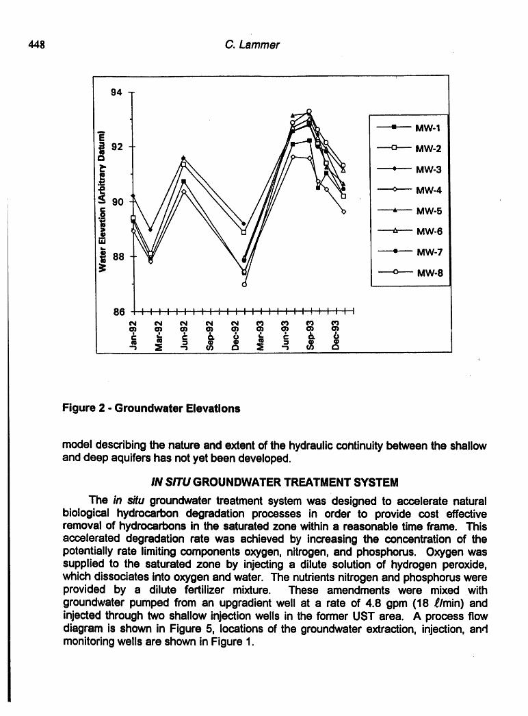
448 C. Lammer
94 T
---o-.-- MW-1
92 ---o---- MW-2
,_ = MW-3
_ MW-4so
._ " MW-5
i_i " MW-6I,,,
_ 88 MW-7
_: -----o---- MW-8
86 ] I I I I I I I I I : ; ', : : : : : : : : : ; ', : : :
m m m, o_ m m m, m m
i ,
, ,
Figure 2 - Groundwater Elevations
modeldescribingthe nature and extentof the hydrauliccontinuitybetweenthe shallowand deep aquifershas notyet been developed.
IN SlTU GROUNDWATER TREATMENT SYSTEM
The in situ groundwatertreatment systemwas designed to accelerate naturalbiological hydrocarbon degradation processes in order to provide cost effectiveremovalof hydrocarbonsin the saturatedzone withina reasonabletime frame. Thisaccelerated degradation rate was achieved by increasing the concentration of thepotentiallyrate limitingcomponentsoxygen,nitrogen,and phosphorus. Oxygenwassupplied to the saturated zone by injecting a dilute solutionof hydrogen peroxide,which dissociatesintooxygen andwater. The nutrientsnitrogenand phosphoruswereprovided by a dilute fertilizer mixture. These amendments were mixed withgroundwaterpumped from an upgradientwell at a rate of 4.8 gpm (18 _lmin) andinjected throughtwo shallow injectionwells in the former UST area. A process flowdiagram is shown in Figure 5, locationsof the groundwaterextraction, injection,andmonitoringwellsare shownin Figure 1.

Biological Attenuation of Aromatic Hydrocarbons in Groundwater 449

450 C. Lammer
i ii iiiiii
R£1IOH_
i! --"
iW
IIi
I_ -m
...- __
m U
i I iii i _
Figure 5 - Process Flow Diagram
Subsurfacemonitoringwas conductedinthe sevenmonitoringwellsat the projectsite to allow evaluationof system performance. Baselinedata was collected prior tothe systemstartup. No monitoringwas conductedduringthe first seven weeks ofsystemoperation,since it was consideredunlikelythat effectsfrom systemoperationwould reach the subsurface monitoringwells during this early period of systemoperation. After this initialhiatus, systemperformancewas monitoredon a monthlybasis. Parameterstracked in these monthlymonitoringevents includedwater levels,dissolvedoxygenconcentrations,microbialpopulations,and nutrient concentrations.Concentrationsof the petroleumhydrocarbonsbenzene, toluene, ethylbenzene, andxylenes(BTEX) were measuredona quarterlybasis.
All parameterstracked as part of systemperformancemonitoringwere measuredprior to system startup in order to provide baseline data. In addition to baselinemeasurements made in July 1993, water levels and petroleum hydrocarbonconcentrationswere periodicallymeasuredover the previouseighteenmonthsas partof site assessmentactivities. These data, included as Figures 3 and 4, provideinformatio;Iregardingconditionsprior to operationof the treatment system. Theseshowa generallyconsistentnorthto northwesterlygroundwatergradientpriorto systemstartup.
Baseline concentrations of hydrocarbonS;,dissolved oxygen, nutrients, andmicrobialpopulationsare includedwith operationaldata in Figures 10 through 14.Hydrocarbonconcentrationswere followedfor 19 monthsprior to system startup to

Biological Attenuation of Aromatic Hydrocarbons in Groundwater 451
allowfor potentialseasonaleffects. Concentrationsless than methoddetectionlimitsare reportedas the detectionlimitin the figures.
Performance Monitoring Results
Operation of the in situ treatment systemwas initiatedon August 2, 1993; thesystemhas operated continuouslysince that time. The first performancemonitoringeventwas completedon September21, 1993, seven weeks after systemstartup. Thismonitoring included field measurements of water levels and dissolved oxygenconcentrationsand collection of samples for laboratorymeasurement of microbialpopulationsand nutrientconcentrations.This routinemonitoringwas then repeatedona monthlybasis. On November 26, 1993, seventeen weeks after system startup,groundwatersamples were collectedfor laboratoryanalysisof BTEX compoundsbyGCIMS. Dissolvedoxygen,microbialpopulations,nutrientconcentrations,and waterlevelswere also measuredas inthe previousmonitoringevents.
(_r0undwaterEle..vations
Potentiometricsurface diagrams measured at approximately5 week intervalsduring system operationare presented as Figures 6 through 9. Static water levelelevationsin monitoringwellsat the projectsite over22 monthsare shownin Figure2.These water levels showseasonalvariationstypicalof the Boise valley; groundwaterelevationsin the second half of 1993 have been slightlyhigherthan those measuredpreviously. The mostrecentpotentiometricsurfacediagram(January20, 1994) showssomeinfluencefromthe injectionwellsonwater levelsin nearbymonitoringwells. Thismoundingsuggeststhat groundwaterand injectedconstituentsmay be migratingin amorewesterlydirectionnear the southernextentof the building. The gradientthroughthe remainderofthe impactedarea continuesto be northwesterlyaswas typicalpriortostartupof the treatmentsystem.
HydrocarbonConcentrations
The November26, 1993, s_'.nplingevent providedthe first BTEX concentrationdata after systemstartup. Water samples were collectedfrom all seven monitoringwells at the projectsite and analyzed for BTEX by EPA Method624. Among thesecompoundsbenzene was of primary concern due to the low 5 _g/_ drinking watermaximumcontaminant limit (MCL). The maximum benzene concentrationreportedamong the November samples was 5 I_g/t in well MW-4; all other benzeneconcentrationswere reported as below methoddetection limits (Figures 10 and 11).This detectionlimitfor benzenewas 1 I_glt in all wellsexceptfor MW-6, whichwas setat 10 I_g/t. The detection limit for MW-6 was elevated due to potential interferencefromxylene isomers,reportedat 238 Ilg/_ inthissample.

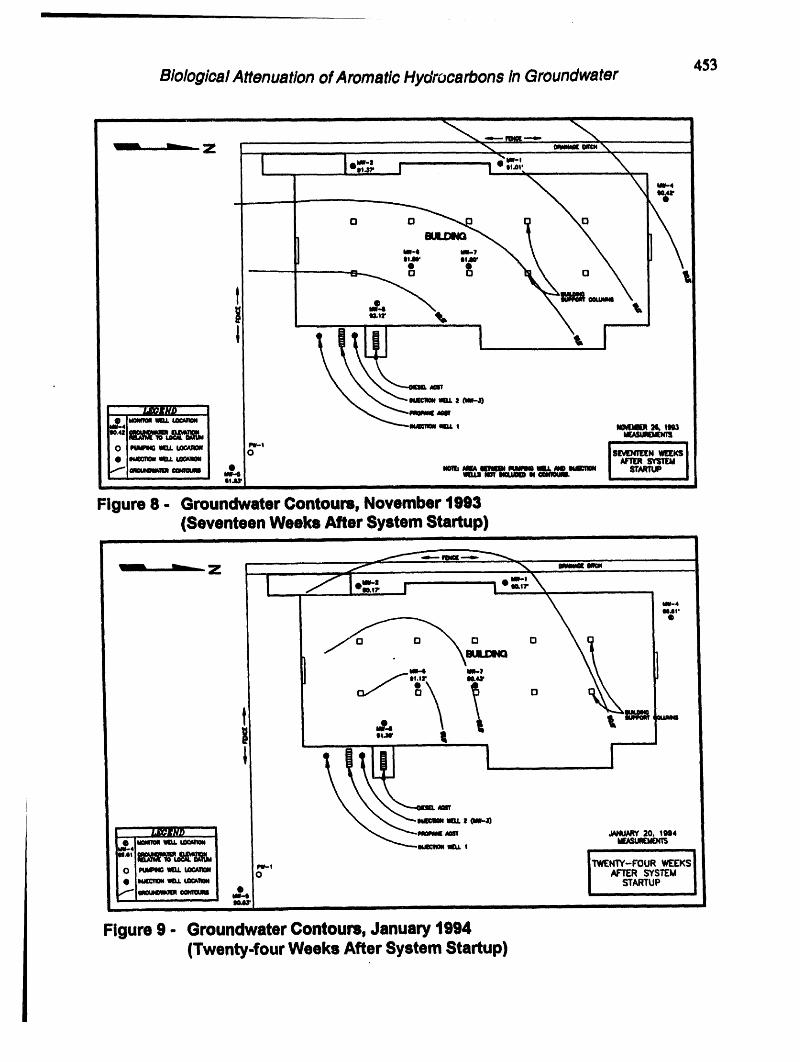
453Biological Attenuation of Aromatic Hydrocarbons In Groundwater
C. Lamrner454
BTEX concentrationsIn samples collected from all wells other than MW-4 andMW-6 were reported as below analytical method detection limits. These reportedconcentrations are significantly lower than the July 1993 basellne BTEXmeasurements,where benzene concentrationswere reported to be as high as 2,800l_g/_(in well MW-8). The increasein reportedBTEX concentrationsIn well MW.4 maybe due to som_"downgradienttransportof hydrocarbonsdue to hydrauliceffectsof thewater injectedIn the former UST area (Flgure 1I). Althoughdetectableconcentrationsof some BTEX compoundsremain In bothwells MW-4 and MW..6, concentrationsofthese compoundsare not above drinkingwater MCLs. The two wells located to thewest of the injectionwells, MW-I and MW-2, continue to be free of detectableconcentrationsof BTEX compoundsas in the baselineanalytlcalresults.
MicrobialpoDulations
Populationsof heterotrophlcbacteriahave been measured in samples collectedon a monthlybasis (Figure 12). In the first of these performancemonitoringsamplingevents,conductedin September1993, populationswere higher thanthose reported inbaselinesamplescollectedinJune 1992, priorto systemstartup. Microbialpopulationsgenerally decreased in all wells from September through the November samplingevent. The January1994 sampleresultsyieldedmixedresults.
Some variationsmay be due to th_ lack of precisionof the laboratoryanalysisused to measure microbialpopulations. Variations in reported microbialpopulationsbetween blind duplicate samples submittedto the same laboratorywere 150% end156% in the two instancesthat duplicateswere submitted.
DissolvedO_aen
The primary purpose of equipment installed as part of the in situ groundwatertreatmentsystemwas to increase the amountof oxygen available for use by aerobicmicroorganismsin the impactedarea. These microorganismswere expectedin turn todegradepetroleumhydrocarbonsat an increasedrate due to the increasedavailabilityof oxygen. However,the expenseof the hydrogenperoxideused as ranoxygensourcecomprisesthe majorityof systemoperatingcosts. Therefore, the hydrogenperoxideinjectionrate was set at a level expectedto foster robustmicrobialpopulationswhileminimizingany excessreleasedfromthe treatmentarea.
Dissolvedoxygenconcentrationswere measuredin monitoringwellson a monthlybasis (Figure 13). Oxygen concentrationsin the three wells located closest to theimpacted area (MW-6, MW-7, and MW-8) have consistently been lower thanconcentrationsmeasuredin outlyingwells. The oxygen concentrationin well MW-4,locateddowngradientof the former UST area, declinedrapidlyover the first 17 weeksof systemoperationand has remainedat a very lowlevel sincethe Novembersamplingevent.

Biological Attenuation of Aromatic Hydrocarbons in Groundwater 455
Figure 10 - Tots! BTEX Concentrations in Groundwater
Figure 11 - Total BTEX Concentrations in Groundwater(ExcludingWellsMW-6andMW-8)

456 C.Lammer
_ _ _ z_ illl I i
1.0E + 07
1,0E + 06 " : MW-1
-----o---- MW-21.0E + 06
-" MW-4i ,OE+ 04
---.o---- MW-51,0E + 03
..... "- MW-61,0E + 02
':' - MW-7
1,0E + 01 _ MW-8
1.0E+00 : " , /
t
Figure 12 - Mi©roblalPopulations in Groundwater
Figure 13. Dissolved Oxygen Concentrations in Groundwater
Biological Attenuation of Aromatic Hydroca_ons in Groundwater457
Despite continuous injection of hydrogen peroxide solution from August throughOctober only a slight increase in oxygen concentrations was observed in wells MW-6,MW-7, and MW-8. This slight increase was reversed in the November measurements,which were even lower than baseline concentrations.
NutrientsOver the course of system operation concentrationsof both nitrogen and
phosphorushave been graduallyincreasingin MW-8, the monitoringwell closestto theinjectionwells. Nitrogen(as nitrate) concentrationtrends are presentedin Figure 14.Nutrientconcentrationsinthesewellshaveconsistentlybeen lowerthan thosereportedfor the outlyingwellsMW-1, MW-2, and MW-5. Nutrientsin MW-4 fell duringsystemoperationin a trendsimilarto that discussedaboveregardingdissolvedoxygen.
Nitrogenconcentrationsin the outlyingwellsMW-1, MW-2, and MW-5 havebeensignificantlyhigher than those reported in the wells closer to the foyer UST area.Baseline concentrationsin these wells were near the 10 mgl£ MCL, the nitrateconcentrationin well MW-2 was reportedas 32 mgl£ in the September1993 samplingevent. It is not likelythat these highnitratelevelsare a resultof nutrients,applied aspart of this project as the nitrogen concentrationin the nutrient-amended injectedgroundwateris only8 mgl£. Also, concentrationsin wellscloser to the injectionwellshave consistentlybeen reportedas less than2 mgl£.
CONCLUSIONS
A significant decline in BTEX concentrationswas observed over the firstseventeenweeks of systemoperation. Immediatelyprior to systemstartupbenzeneconcentrationswere as high as 2,800 I_g/_ (MW-8, July 1993). Results of theNovember samplingevent indicate that benzene concentrationsare at or below thedrinkingwater MCL of 5 I_gl_in all wells at the projectsite. The methoddetectionlimitfor benzene in MW-6 was 10 I_g/£ because the presence _!__240 I_g/_ xylenesnecessitatedsampledilutionfor BTEX analysis. Therefore, thoughno benzene wasreportedin thissample, it is possiblethat up to 10 I_gl£benzene was present. Exceptfor this detection limit issue, it appears that Idaho Divisionof EnvironmentalQuality(DEQ) waterqualityguidelineshavebeen satisfiedat the projectsite.
Residual concentrationsof xylenes in wells MW-4 and MW-6 were higherthanthoseof benzene, toluene,and e_hylbenzene.The maximumreportedconcentrationofxyleneisomerswas 240 I_gl£inwell MW-6. It is commonfor xyleneisomersto be moreresistantto biologicaldegradationthan benzene, toluene, and ethylbenzene (Tabak,1991). Althoughxyleneswere reportedat detectableconcentrationsinthese twowells,theseconcentrationswere well belowthe maximumcontaminantlimitof 10,000 I_g/£.

4.58 C. Lammer
35I" = MW-1
3O---o--- MW-2
25* MW-4
20_ MW-5
z, 15
/ ,, ,w.o10 i z_ MW-7
I
5 ' =' MW-8
01 - i@ o3 ¢_ o3 "13
m _ rj 0I_ m 0 z
Figure 14 - Nitrogen (as Nitrate) Concentrations in Groundwater
The concentrationof both benzene and xylenesincreasedin well MW-4 over thefirst seventeen weeks of systemoperation. The benzene concentration in this wellincreasedfrombelowthe I Ilg/_ methoddetectionlimitto 5 I_g/l. Well MW-4 is locateddowngradientof the injection wells and former UST location. Elevated benzeneconcentrationsas highas 16 I_gl_had previouslybeen measuredin samplescollectedfrom this well in both January 1992 and March 1992. Benzene concentrationsinsubsequentsamplescollectedfromthiswell inJanuary 1993 and July1993 were belowmethoddetection limits. The recent increase in benzene concentrationcould be theresultof hydraulictransportfromthe impactedarea and/ornaturalseasonalvariations,as suggestedby earlier variationsin reportedconcentrations. A sharpdecline in bothdissolvedoxygen and nutrient concentrations in this well suggest that hydraulictransportof oxygen-and nutrient-depletedwater fromthe impactedarea is takingplaceand, therefore, is likely responsiblefor at least some of the observed increase inbenzene and xylene concentrations. Since reported concentrations of thesecompoundsare notabove drinkingwaterMCLs, and the shallowwater table is notusedas a drinkingwater supply,thispotentialfor somehydraulictransport is not considereda major concem. Two wells located west of the impacted area, MW-1 and MW-2,remain free of detectable concentrations of BTEX compounds, indicating thesehydrocarbonsare notbeingtransportedoff-sitein thisdirection.
Microbialpopulationsdeclined in all wells from Septemberto November. Sincethiseffectis commonto all of the monitoringwells, includingthe upgradientwell MW-5,
i
Biological Attenuation of Aromatic Hydrocarbons in Groundwater 459
it appears to be a regional trend rather than the result of system operation. Thisapparentregionaltrendcouldbe due to decreasedintrusionof surfacewaterduringthewinter months. Populationsin MW-6, MW-7, and MW-8, the three monitoringwellslocatedclosestto the injectionwells,either increasedslightlyor decreasedat a slowerrate than the other, moredistant,monitoringwells. This suggeststhat operationof thein situ groundwater treatment system was having a positive effect on microbialpopulationsin contrastto a regionaldecline. Microbialcountsin samplescollectedinJanuary, 1994, remained low,with somewells showingminordeclineswhile samplesfromother wellscontainedslightlyhigherpopulationsthan in earlier samples. Becausethere were significantvariations between microbial counts for duplicate samples,microbialpopulationmeasurementsmustbe interpretedas only a rough indicatorofactualmicrobialpopulations.
Despite lowmicrobialpopulations,decreasingBTEX concentrationsindicatethatan active microbialpopulationis present. These apparentlyconflictingdata could bean indicationthat the microbialcommunityis largelyheld in the soil matrixin the areabetweenthe injectionwellsand the monitoringwells.
Despitecontinuousinjectionof hydrogenperoxidesolutionfrom August throughOctober only a slight increase in oxygen concentrationswas observed in the threemonitoringwells locatedclosestto the injectionwells (MW-6, MW-7, and MW-8). Thisslight increasewas reversed in subsequentmeasurements,which were even lowerthan baseline concentrations. Dissolvedoxygen concentrationsin these three wellshave consistentlybeen lowerthan thosemeasuredin outlyingwells. This is mostlikelydue to oxygen demand exhibitedby aerobic microorganismsin the presence of anample carbon substrate (i.e., hydrocarboncompounds) as is available in thecontaminatedarea.
The microbialcommunityis apparently increasingin populationas rapidly asoxygen becomesavailable (i.e., the oxygen supplyis limitingthe microbialpopulationand therefore the rate of hydrocarbondegradation). The slight rise in oxygenconcentrationsmeasured in October followed by the very low values measured inNovembermay have been causedby a lag in the microbialpopulationcatchingup withthe increasingavailabilityof dissolvedoxygen.
Nutrientconcentrationshave been gradually increasingin the monitoringwellslocatedclosestto the injectionwells. This indicatesthat nutrientshave been suppliedat a rate slightlyin excessof the demandimposedby the microbialpopulation.
FUTURE ACTIVITIES
Exceptfor MW-6, where the 10 pg/£ detectionlimitfor benzene was higher thanthe 5 I_g/£drinkingwaterMCL, it appearsthat DEQ waterqualityguidelineshave beensatisfiedat the projectsite. If BTEX concentrationscontinueto be reportedas belowdrinkingwater MCLs, systemoperationbe terminated. If ongoi_'lggroundwaterqualitymonitoringsupportsthe promisingresultsof the initialBTEX analysespresentedin thisreport, in situ biological treatment may offer a relatively rapid and cost effective

C. Lammer46O
treatment alternative for additional petroleum release sites in the Treasure Valleyregion.
LITERATURE CITED
Delfino, J.J. and Miles, C.J. "Aerobic and anaerobic degradation of organiccontaminantsin Florida groundwater" Soil and Crop Science Society of Florida,Proceedings44 (1985): 9-14
Dion, N.P. "Some effects of land use changeson the shallowgroundwatersysteminthe Boise-Nampaarea, Idaho" Idaho Department of water Administration, WaterInformationBulletin No. 26 (1972); 47
Huling, S.G., Bledsoe, B.E., and White, M.V. "Enhanced bioremediationutilizinghydrogenperoxide as a supplementalsourceof oxygen:a laboratoryand fieldstudy" U.S. Environmental ProtectionAgency Report EPN60012-90/006 (1990)
Malde, H.E. and Powers,H.A. "Upper Cenozoicstratigraphyof Western Snake RiverPlain" Idaho: Geological Society of America Bulletin 73 (1962): 1197-1220.
McCarty, P.L. "Bioengineeringissuesrelating to in situ remediationof contaminatedsoilsandgroundwater" EnvironmentalBiotechnology(1988): 153-156
Othberg, K.L. and Stanford, L.R. "GeologicMaps of the BoiseValley and adjoiningareas, Western Snake River Plain, Idaho, Scale 1:100,000" Idaho GeologicSurvey Map Series (1992)
Squires, E., Wood, S.H., and Osiensky, J.L. "Hydrologicframework of the Boiseaquifer system,Ada County, Idaho" Idaho Water Resources Research Institute,Research Technical Completion Report 14-08-0001-G1559-06 (1992): 109
Tabak, H.H., Desai, S., and Govind,R. "Developmentand applicationof a multilevelrespirometricprotocolto determinebiodegradabilityand biodegr_dationkineticsoftoxic organicpollutantcompounds" On-Site Bioreclamation. Ed. Hinchee, R.E.,and Olfenbuttel,R.F. Butterworth-Heinemann,Stoneham,Massachusetts,!991.325-39.
United States. Environmental Protection Agency. Bioremediation in the field.EPN540/N-93/001, 8 (1993)
Urano, K. and Kato, Z. "Evaluation of biodegradationranks of priority organiccompounds"Journal of Hazardous Materials 13 (1986): 147-159
Wilson, J.T., et al. "In situ bioremediationof spillsfrom undergroundstorage tanks:new approaches for site characterization, project design, & evaluation ofperformance" U.S. Environmental Protection Agency Report EPN60012-891042(1989)
Hydmgeology, Waste Disposal, Science andPoliticsProceedings30th Symposium
EngineeringGeology andGeotechnicalEngineering,1994 461
DIFFUSION THROUGH STATICALLY COMPACTED CLAY
by Carlton L. Ho, M. ASCE I and Maher A.-A. Shebl, S.M. ASCE 2o,
ABSTRACT :
This paper presents experimental work on the effect of compaction on contaminant flowthrough clay liners The experimental program included evaluation of soil properties, compaction,permeability and solute diffusion. A permeameter was built of non reactive materials to testsamples compacted at different water contents and compactive efforts. The flow of a permeatingsolute, LiCI, was monitored. Effluent samples were collected for solute concentrationmeasurements. The concentrations were measured by performing atomic adsorption tests. Theanalyzed results showed different diffusion characteristics when compaction conditions changed.At each compactive effort, permeability decreased as molding water content increased.Consequently, transit time (measured at relative concentration 50%) increased and diffusivitydecreased. As compactive effort increased for soils compacted dry of optimum, permeability and
diffusion decreasec_. On the other hand, as compactive effort increased for soils compacted wetof optimum, permeability and diffusivity increased. Tortuosity factor was indirectly measuredfrom the diffusion and retardation rate. Tortuosity factor also decreased as placement watercontent was increased from dry of optimum to wet of optimum. These decreases were morepronounced for low compactive effort tests.
Keywords: clay, clay liner, compaction, diffusion, laboratory, solute transport.
INTRODUCTIONClay is commonly used as a liner material for hazardous wastes containment. These clay
liners are used to contain the wastes and to minimize contamination of the groundwater. Clay ischosen because of its low permeability and stability. In order to use clay as a liner, the clay mustbe compacted in place. The method of compaction influences the properties of the clay. Thisstudy is intended to emphasize the effect of compaction on clay as well as to emphasize theeffect of compaction on contaminant flow properties.
Compaction produces volumetric and structural changes in the clay soil. Dry of optimumcompaction reduces the voids between the clay particles (Lambe, 1958a, 1958b, Seed and Chan,1959), which can be expressed as a volumetric change. Compaction wet of optimum rearrangesthe clay particles into a parallel structure (Lambe, 1958a, 1958b), which can be expressed asstructural changes. Permeability is dependent upon soil structure (Mesh and Olsen, 1971), andthe pore size (Garcia-Bengochea, et al., 1979). When the soil is compacted wet of optimum orat a high compactive effort, the permeability decreases. Also, permeability depends on theproperties of the permeating fluid (Kozeny, 1972, Carman, 1937, 1941).
Since flowing contaminants consist mostly of water and salt solutions, the flow must beexpressed as a coupled movement (Greenberg, et al., 1973). It is therefore important tounderstand the mechanisms that control the flow of water and solute through clay. Water flow
Asst. Prof., Dept. of Civ. and Env. Engrg., Wash. St. Univ., Pullman, WA 99164-2910.
: Res. Asst., Dept. of Civ. and Env. Engrg., Wash. St. Univ., Pullman, WA 99164-2910.

CL Ho andM. A.-,4.Shebl462
is controlled by the soil properties. Solute transport mechanisms (diffusion, advection, dispersion,and adsorption) are controlled by soil properties as well as by the fluid properties and speciesproperties. For low permeability of clays subjected to low gradient, the diffusion appears to bethe most dominant contaminant transport mechanism (Goodall and Quigley, 1977; Dessaulinier,et al., 1981; Crook and Quigley, 1984, Folkes, 1982, Barone, et al., 1989; Barone, et al., 1990).So the analysis of the obtained experimental data will show the significance of compactionvariables on the transport mechanisms. Also, it will show the effect of compaction variables ondiffusion.
This paper presents an experimental study on the effect of compaction method on solutetransport through clay. The solute chosen for this study was of LiCI, with an initial concentrationof 500 mg/l. LiCI was used because, Li+ has a low potential to be adsorbed to the negativelycharged clay particles. This allows for easier evaluation of diffusion. This study investigated theeffect of compactive effort and molding water content on permeability and diffusivity (Shebl,1990).
MODEL AND ASSUMPTIONS
The three-dimensional constitutive model used in this work is composed of a solid phasewith an open void domain. The solid phase consists of soil particles. The open domain consistsof the void space which can contain liquid and gas phases. For fully saturated soils, the opendomain is completely occupied by liquid. The concept of conservation of mass was applied toderive the governing differential equation for the continuum model. The model was built on thefollowing assumptions:
- Homogeneous medium- Isotropic medium.- Saturated medium.
- Steady state flow- Darcy's law is valid.- No biological transformations.- No radioactive reactions.- Isothermal conditions.
- The coefficient of diffusion assumed to be constant over the migration profile.- Solute of single species (no chemical reaction between different species).- Sufficiently diluted solute.- Conservation of mass.
- Conservation of energy.No chemical reaction between different species into the medium was assumed. The measureddiffusion differ from field conditions. The diffusion coefficient obtained from a leachate modelis typically lower than that obtained from a single salt model (Barone, et al., 1989).
The one-dimensional dispersion differential equation can be expressed as,
D _c Oc Oc
where D_ equals the coefficient of hydrodynamic dispersion in the x direction, C equals theconcentration of the solute, and (V,)x equals the seepage velocity in the x direction.
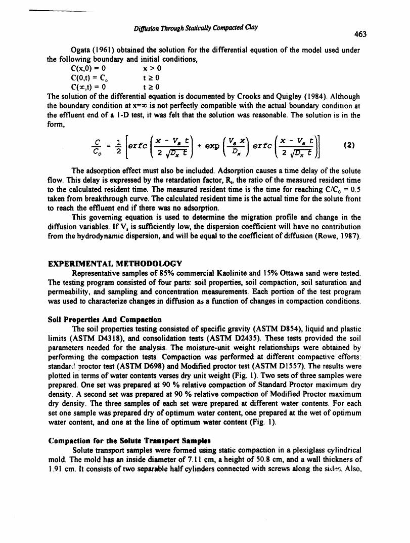
Di.O_sionThroughStaticallyCompactedClay463
Ogata (1961) obtained the solution for the differential equation of the model used underthe following boundary and initial conditions,
C(x,O) = 0 x > 0C(O,t) - Co t _>0C(_,t) = 0 t 2 0
The solution of the differential equation is documented by Crooks and Quigley (1984). Althoughthe boundary condition at x=_ is not perfectly compatible with the actual boundary condition atthe effluent end of a I-D test, it was felt that the solution was reasonable. The solution is in theform,
co 2 2--" ) ezc 121
The adsorption effect must also be included. Adsorption causes a time delay of the soluteflow. This delay is expressed by the retardation factor, R, the ratio of the measured resident timeto the calculated resident time. The measured resident time is the time for reaching C/C0 - 0.5taken from breakthrough curve. The calculated resident time is the actual time for the solute frontto reach the effluent end if there was no adsorption.
This governing equation is used to determine the migration profile and change in thediffusion variables. If V, is sufficiently low, the dispersion coefficient will have no contributionfrom the hydrodynamic dispersion, and will be equal to the coefficient of diffusion (Rowe, 1987).
EXPERIMENTAL METHODOLOGY
Representative samples of 85% commercial Kaolinite and 15% Ottawa sand were tested.The testing program consisted of four parts: soil properties, soil compaction, soil saturation andpermeability, and sampling and concentration measurements. Each portion of the test programwas used to characterize changes in diffusion as a function of changes in compaction conditions.
Soil Properties And CompactionThe soil properties testing consisted of specific gravity (ASTM D854), liquid and plastic
limits (ASTM D4318), and consolidation tests (ASTM D2435). These tests provided the soilparameters needed for the analysis. The moisture-unit weight relationships were obtained byperforming the compaction tests. Compaction was performed at different compactive efforts:standarc__proctortest (ASTM D698) and Modified proctor test (ASTM D1557). The results wereplotted in terms of water contents verses dry unit weight (Fig. 1). Two sets of three samples wereprepared. One set was prepared at 90 % relative compaction of Standard Proctor maximum drydensity. A second set was prepared at 90 % relative compaction of Modified Proctor maximumdry density. The three samples of each set were prepared at different water contents. For eachset one sample was prepared dry of optimum water content, one prepared at the wet of optimumwater content, and one at the line of optimum water content (Fig. i).
Compaction for the Solute Transport SamplesSolute transport samples were formed using static compaction in a plexiglass cylindrical
mold. The mold has an inside diameter of 7.11 cm, a height of 50.8 cm, and a wall thickness of1.91 cm. It consists of two separable half cylinders connected with screws along the sides. Also,

C.L Ho and M.A.-A.Shebl464
it had a 0.64 cm thick rubberdisk and a 0.64 cm thick aluminum plate with diameters the sameas the inside diameter of the cylinder.
The soil was prepared for compaction in the following manner. The soil specimensdimensions were approximately !.27 cm tall and 7.11 cm in diameter. Since the dry density andthe volume of the specimen were predetermined, the mass of soil solids required for eachspecimen could be calculated. This mass of soil solids and water were mixed to thepredetermined water contents required for each test. Each batch of soil sat overnight in a sealedcontainer to allow for even hydration. Then, the soil was placed in the mold for compaction. Thesample was covered with the rubber disk and the aluminun' disk. A steel loading rod (55.9 cmtall and 6.91 cm diameter) was placed at the top of the aluminum plate. The mold and itscontents were placed between compression plates and compacted under continuous pressure.
The soil was compressed between the loading plates until the desired thickness wasobtained. At that point, the load on the sample remains for about 1/2 hour to limit any soilswelling of the sample upon removal from the mold. Zero swell was confirmed by measuring thethickness of the specimen with a dial gage.
Falling Head Permeameter DesignThe permeameter consists of a sample confining chamber, flow reservoirs and control
panel (Fig. 2). The arrow._,in Fig. 2 indicate the fluid flow during the solute transport phase ofthe test. A triaxial cell is used as a confining chamber. There are three stainless steel 2 literreservoirs. The first cylinder is used as an influent water reservoir. The second cylinder is aninfluent solution reservoir. The third cylinder is an effluent water reservoir. A 6 mm diametereffluent sampling septum is placed near the bottom platen T-valve, between the T-valve and theeffluent reservoir. This T-valve controls the flow to the septum, and allows for change of theseptum when necessary.
Two pressure regulators are mounted on a control panel. One regulator controls fluid backpressure. A second regulator controls confining pressure. One differential pressure transducermeasures effective confining stress. A second differential pressure transducer is used to measurevolume changes. The transducer measures the pressure difference between the top and bottom ofa standard volume change burette. Changes in the transducer output relate to changes in fluidvolume.
Fittings and tubes were selected to minimize any chemical reactions. All fittings,connectors and valves were made of stainless steel. 0.635 cm i.d. TEFLON tubes were used forthe pressure lines. 0.318 cm i.d. TEFLON tubes were used for the flow lines.
Sample preparation and permeability testingThe soil specimen was placed between two glass filter papers and two fretted glass porous
plates. This combination was placed between the two stainless steel platens and confined witha latex membrane. The membrane was sealed to each platen with two O-rings. The triaxial cellwas closed and filled with water to approximately 2.0 cm above the top of the upper platen toprovide a hydrostatic isotropic pressure. Confining pressure and back pressure were incrementallyincreased to 345 kPa and 276 kPa respectively in increments of 34.5 kPa. This provided a net
effective stress of 69 kPa. Back pressure is necessary to saturate the sata_ie. B (= Au/Aa3) wasgreater than or equal to 0.96. After the saturation, the inflow and outflow valves were closed inpreparation for the permeation stage.

DiffusionThroughStaticallyCompactedClay465
At the beginning of the permeation stage the effluent valve was opened for about 6 hoursto allow for stabilization of the pore water flow. Once the flow rate stabilized, the solution wasthen allowed to flow through the soil column. The flow direction was from the top to the bottomof the soil column. This simulated actual field situation. The flow driving head was the differencebetween the elevated solution tank head and the volume change burette head. The head differencewas kept at 290 mm+ 5 mm during most of the test period. Volume change readings were takenevery 3 to 6 hours during the test period (2 to 4 weeks). The soil permeability was calculatedusing these readings. The entire test was conducted in a temperature controlled room at 20° C.Replicate tests were conducted to confirm reliability of results.
Sampling and Samples Concentration MeasurementsSamples of the effluent were taken at 3 hour intervals up to 12 hours, then at 12 hour
intervals thereafter. A 1.0 ml syringe was used to extract the effluent solution through thesampling septum. As the effluent solution was extracted, the volume change burette headdecreased. 1.0 to 2.0 ml of the solution were extracted until the head difference between theinfluent reservoir and the volume change burette was the same as at the beginning of the test.This was to keep the head constant. The samples were stored in sealed vials and kept at 4° Cuntil the solute concentrations could be analyzed.
The solute concentrations were determined by atomic adsorption tests. For the testspresented in this paper, two atomic adsorption spectrophotometers were used, a Perkin-Elmer 303and a Varian SpectrA-A300, Sample concentrations were determined by comparison of thesample reading with standard concentration calibration curve.
DATA ANALYSISThe test soil was a mixture of 85% kaolinite and 15% Ottawa sand. Fig. 1 shows the
StandardProctor and Modified Proctor compaction curves. Identified on the curves are the pointschosen for the permeability testing samples. Three points were for the low compactive effort (Ydof 14.4kN/m3): A (at dry of optimum), B (at optimum) and C (at wet of optimum). These werecompacted at water contents of 10.4, 24,8 and 28.8% respectively. Another three points were forthe high compactive effort (Ydof 15.1 kN/m3): D (at dry of optimum), E (at optimum) and F (atwet of optimum). These were compacted at water contents of 9.4, 23.0 and 26,7% respectively.Although it is known that a liner should always be compacted wet of optimum (Reades, et al.,1987), the entire range of water contents (from dry of optimum to wet of optimum) wasconsidered because there is always the possibility of placement error resulting in a dry ofoptimum, or optimum water content.
The results obtained from the permeability and atomic adsorption tests appear in Table1. The table presents the following data: coefficient of per-, eability; seepage velocity; retardationfactor; coefficient of diffusion; and tortuosity. Fig. 3 shows the coefficient of permeability atdifferent water contents. For both high compactive effort and low compactive effort, coefficientof permeability decreased with an increase in water content. This phenomenon was observed byothers (Lambe, 1958b; Mitchell et al., 1965). This variation in coefficient of permeability isattributed to the dependency of soil structure on the placement water content. Soils compacteddry of optimum tend to exhibit a more flocculated structure. Soils compacted wet of optimumtend to exhibit a more dispersed structure (Lambe, 1958b). It is important to note that Ydfor eachcompactive effort series was constant. Hence, porosity was also constant. Therefore, the variationin permeability is a function of the orientation of the soil particles and size cf macropores
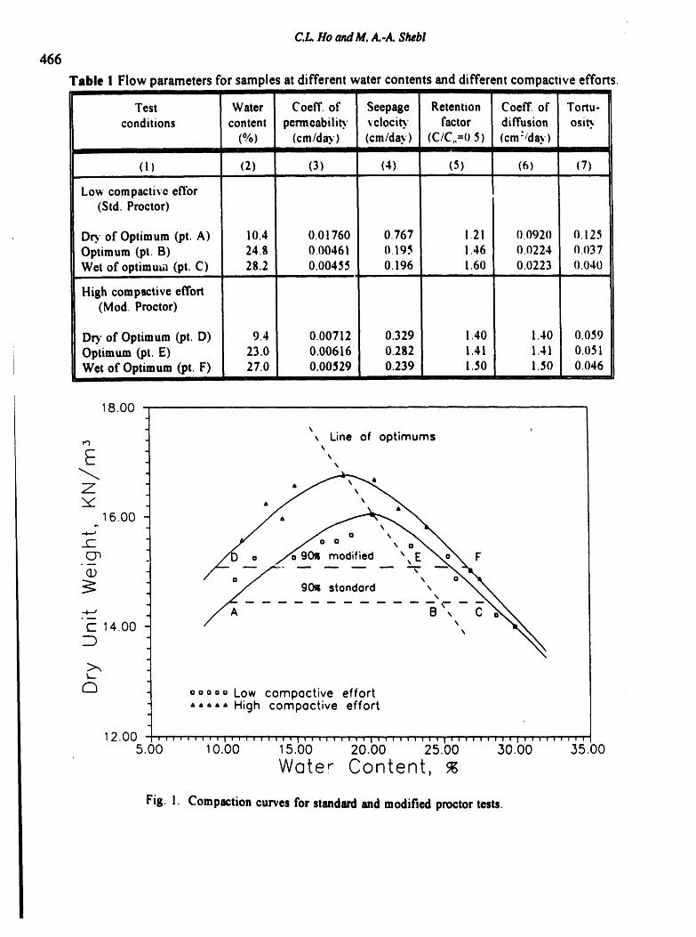
C.L. Ho and M, A.-,4.Shebl
466
Table I Flow parameters for samples at different water contents and different compactive efforts.I IIII I I I [ I IIIIIIII !llll I II IIIIIII I
Test Water Coeff. of Seepage Retentton Coeff. of Tortu-conditions content permeabilit3." vclocit3.' factor diffusion osi_
(%) (cm/day) (era/day) (C/C,,=0.5) (cm:/day)Jill I I Illl I Ill I I '
(I) (2) (3) (4) (5) (6) (7)u i i ,ul=,
Low compactivc eft'or
(Std. Proctor)
DW or"Optimum (pt. A) 10.4 0.01760 0.767 !.21 0.0920 0.125Optimum (pt. B) 24.8 000461 0.193 1.46 0.0224 0037Wet ofoptimuua (pt. C) 28.2 0.00455 0,196 1.60 0.0223 _ 0.040
i i i ,I i iiI ,ii4
High compactive effort(Mod. Proctor)
Dr3'of Optimum (pt. D) 9.4 0.00712 0.329 1.40 1.40 0.039Optimum (pt. E) 23,0 0.00616 0.282 1.41 1.41 0.031Wet of Optimum (pt. F) 27.0 0.00329 0.239 1.30 1,30 0.046
_ t i iiii i
18.00
,, Line of optimums
7" A "
.16.00
C- "
(l)
c- 14.00
o ° ==0 Low compoctive effort,,,,, High compoctive effort
12.00 .... ,',,,,t ..... ',,,,1, .... ,_,,i ...... ,,,i, ...... ,,1,,,,,_,,,5.00 10.00 15.00 20.00 25.00 30.00 35.00
Wate Content,
Fig. 1. Compaction curves for standard and modified proctor tests.

, D_sion _rou#h StaticaUyCompacted Clay 467
Fig. 2. Schematic of diffusimeter/permeameter: 1) compressed air: 2) Pressure gauge; 3) confiningpressure regulator; 4) back pressure regulator; 5) T-valve; 6) volume change pressure transducer; 7)volume change burette; 8)effective stress pressure transducer; 9) sampling septum; 10) sample confinedin membrane; 11) confining chamber; 12) influent water reservoir; 13) influent solute water reservoir; 14)effluent water reservoir.
_-_10 -'>,,C3
-0
Fo
>_ _.
10 -="
""A
(D "s- - -a¢'1
0=_e low compactive effort"=-_=-_ high compoctive effort
o 10"' , __b" :;6bb' :_,bb'o.oo...."_'.66"......lO.OO'............_. . ' .... . " .....3o.ooWater Content, (_)
Fig. 3. bttect ot changes m water content at different compactive efforts on the coefficient ofpermeability.
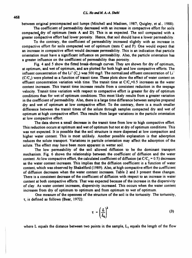
C.LHeandM.A.,,4.Shebl468
betweenoriginal precompactedsoil lumps(Mitchell andMadisen, 1987; Quigley, et al., 1988).The coefficientof permeabilitydecreasedwith an increasein compsctiveeffort for soils
compacted_dryof optimum (tests A and D). This is as expected.The soil compactedwith agreatercompactiveeffort had lower porosity. Hence, that soil shouldhavea lower permeability.
To the contrary, the coefficient of permeability increasedslightly with an increaseincompactiveeffort for soils compactedwet of optimum (testsC and F). One would expectthatan increasein compactiveeffort would decreasepermeability.This is an indicationthatpanicleorientation must have a significant influence on permeability. Also, the particle orientation hasa greater influence on the coefficient of permeability than porosity.
Fig. 4 and 5 show the fitted break-through curves. They are shown for dry of optimum,at optimum, and wet of optimum, and are plotted for both high and low compactive efforts. Theinfluent concentration of the Li+(Co) was 500 mg/I. The normalized effluent concentration of Li"(C/Co) were plotted as a function of transit time. These plots show the effect of water content oneffluent concentration variation with time. The transit time at C/Co=0.5 increases as the watercontent increases. This transit time increase results from a consistent reduction in the seepagevelocity. Transit time variation with respect to compactive effort is greater for dry of optimumconditions than for wet of optimum conditions. This most likely results from a greater variationin the coefficient of permeability. Also, there is a large time difference between samples prepareddry and wet of optimum at low compactive effort. To the contrary, there is a much smallerdifference between the transit times of the solute through samples compacted dry and wet ofoptimum at high compactive effort. This results from larger variations in the particle orientationat low compactive effort.
The data shows a small decrease in the transit time from low to high compactive effort.This reduction occurs at optimum and wet of optimum but not at dry of optimum conditions. Thiswas not expected.It is possiblethat thesoil structureis more dispersedat low compactionandhigher water content.This is most unlikely. Another possibleexplanation is that adsorptionreducesthe solutetransport.Variationsin particle orientationmay affect the adsorptionof thesolute.The effect may have beenmoreapparentin wetter soil.
The low permeability of the soil allowed diffusion to be the dominant transportmechanism.Fig. 6 showsthe relationshipbetween the coefficient of diffusion and the watercontent.At low compactiveeffort, the calculatedcoefficientof diffusion(at C/Co= 0.5) decreasesas the water contentincreases.This impliesthat the diffusion coefficient is a functionof watercontent,whichwasobservedby Shakelford(1989). Also,athigh compactiveeffort thecuefficientof diffusion decreaseswhen the water contentincreases.Table 2 and 3 presentthesechanges.Thereis a consistentdecreaseof the coefficientof diffusionwith respectto an increasein watercontentat bothcompactiveefforts. That was expectedbecauseof the increasein thedispersivityof clay. As water contentincreases,dispersivityincreased.This occurswhen the water contentincreasesfrom dry of optimumto optimumand from optimumto wet of optimum.
One measureof the opennessof thestructureof thesoil is the tortuosity.The tortuosity,z, is defined as follows (Bear, 1972):
where L equals the distance between two points in the sample, L0 equals the length of the flow

.o_o.6o0t,.
C0.40¢D
CO
(..) _ at dry of optimumot optimum
(D 0.20 %EU.P ot wet of optimum>
..m,b
-4.-'
O(D
EE 0.00o.oo _o.oo 20.00 30.00 40.00Tronsit Time, (doys)
Fig. 4. Break-through curves for Li+ at different water contents at low oompactive effort.
1.00
O
(D
_'0.80
c".o_0.600L.
(--
(D 0.40rjC0
O ...9.._._.=ot dry of optimumot optimum
Q.)0.20 _ ot wet of optimum>
._
.4--'
O....,.
I_ 0.00 '-_ ' ........ 4()0.00 10.00 20.00 30.00 .00
Transit Time, (days)
Fig. 5. Break-through curves for Li+ at different water contents at high compactive effort.

C.L. !!o andM..4...4.$1_bl
470
Table 2 Results of nonlinear least square regression analysis for the diffusion coefficient fromthe observed concentration data.
L i i ii i iii i ii i i i i iiii
Test NO IDCV R.square T-value LB for UB forconditions (cm:/day) 95% 95%
confidence confidenceIII III I IIIIIIIIIIIIIII I I I II II I IIIII IIIII IIIIIII III IIIIII III I I IIIIII
(I) (2) (3) (4) (5) (6) (7),,, ii ii i! i if i iiiiii
Low compactive effort(Std. Proctor)
Dry of Optimum (pt, A) 49 0,326 0.987 14.50 0.281 0,371 iOptimum (pt, B) 90 0,121 0,969 12.20 0,101 0,141Wet of optimum (pt. C) 87 0,082 0,972 14,90 0,071 0,093
i L [ I I I III I II I I
High compactive effort(Mod. Proctor)
Dry of Optimum (pt. D) 90 0,657 0,957 7,73 0,488 0,825Optimum (pt. E) 53 0,058 0.985 12.40 0,049 0,068Wet of Optimum (pt. F) 45 0.114 0,992 16,40 0,100 0.129
i i i i i iii i ii i
Table 3 Resultsof nonlinear least square regressionanalysis for the retentionfactor fromthe observed concentrationdata.
iiii i iii ii ii ii _ iiii
Test NO IRFV R.square T-value LB for UB forconditions 95% 95%
confidence confidenceI i IIII i I I r.......
(1) (2) (3) (4) (5) (6) (7)iii i
Low compactive effort(Std. Proctor)
Dry of Optimum (pt, A) 49 2.60 0,987 54.4 2.50 2.70Optimum (pt. B) 90 2.13 0.969 42.6 2,03 2.22Wet of optimum (pt, C) 87 2.03 0.972 52.5 !.95 1.10
i i
High compactive effort(Mod. Proctor)
Dry of Optimum (pt. D) 90 4.00 0.957 14.4 3.45 4.55Optimum (pt, E) 53 1.66 0.985 66.8 1,61 1.71Wet of Optimum (pt. F) 45 2.05 0,992 60.8 1.98 I, 12
i i
(IDCV) Interpolated diffusion coeffecient value.(IRFV) Interpolated retention factor value.(LB) Lower bound.(UB) Upper bound.

+@ _
BY APPLIED +_

DiffusionThroughStaticallyCompactedClay473
Evaluation of the tortuosity indicated that there is a variation in soil structure with respectto placement water content. Soils placed dry of optimum have a higher tortuosity (less tortuousflow path) than soils placed at optimum or wet of optimum. That variation is less significant forsoils placed with high compactive effort.
These conclusions are based upon experimentation with one type of soil at two typicalcompactive efforts. The trends inferred from the test data indicate the dependence of solutetransport mechanisms upon the method of conipaction. Other soil types may have more or lessdependence than the Kaolinite and Ottawa sand mixture used in the experimentation describedin this paper.
ACKNOWLEDGMENTS
The authors would like to express their appreciation for the technical advice given by Dr.Richard Fragaszy, Dr. Yavuz Corapcioglu, Dr. David Mulla and Dr. David Yonge. The authorsalso thank the Office of Graduate and Research Development and the Department of Civil andEnvironmental Engineering at Washington State University for their financial support of thisresearch.
REFERENCES
Barone, F. S., Rowe, R. K., and Quigley, R. M. (1990), "Laboratory determination of chloridediffusion coefficient in an intact shale," Can. Geotech. J., 27, pp. 177-184.
Barone, F. S., Yanful, E. K., Quigley, R. M., and Rowe, R. K. (1989), "Effect of multiplecontaminant migration on diffusion and adsorption of some domestic waste contaminantsin a natural clayey soil," Can. Geotech. J., 26, pp. 189-198.
Bear, J. (1972), Dynamics of Fluids in Porous Media, American Elsevier, New York.Carman, P.C. (1937), "Fluid flow through a granular bed," Trans. Inst. Chem. Engrg., London,
15, 150-156.Carman, P.C. (1941), "Capillary size and capillary movement of moisture in fine sands," Soil Sc.,
52, 1-14.Crooks, V.E. and Quigley, R.M. (1984), " Saline leachate migration through clay: a comparative
laboratory and field investigation," Can. Geotech. J., 21, 349-362.Dessaulinier, D.E., Cherry, J.A. and Fritz, P. (1981), "Origin, age and movement of pore water
in argillaceous quaternary deposits at four sites in southwestern Ontario," J. of Hydrology,231-257.
Folkes, J.d. (1982), "Control of contaminant migration by the use of liners," Fifth Can. Geotech.Colloquium, Can. Geotech. J., 19, 320-344.
Garcia-Bengochea, J., Lovell, C.W. and Altschaeffl, A.G. (1979), "Pore distribution andpermeability of silty clays," J. Geotech. Engrg. Div., ASCE, 105(7), 839-856.
Gilham, R. W., Robin, M. J. L., and Dytynyshyn, D. J. (1984), "Diffusion of non-reactive andreactive solutes through fine grained barrier material," Can. Geotech. J., 21, pp. 541-550.
Goodall, D.C. and Quigley (1977), "Pollutant Migration from Two Sanitary Landfill Sites NearSarina, Ontario", Can. Geotech. J., 14(27), 223-236.
Greenberg, J.A., Mitchell, J.K. and Witherspoon, P.A. (1973), "Coupled salt and water flows ina groundwater basin," J. Geophys. Res., 78(27), 6341-6353.
Kozeny, J. (1927), "l]ber kapillar leitung des wassers im boden," Akad. Wiss. Wiener, Abt. lla,136, 271-306.

C.L.Ho and M.A..A. Shebl
474
Lambe, T.W. (1958a), "Compacted clay: engineering behavior," J. of the Soil Mech. and Found.Div., ASCE, Paper 1655, May, 1958.
Lambe, T.W. (1958b), "Compacted clay; structure,"J. of the Soil Mech. and Found. Div., ASCE,Paper 1654.
Mesri, G. and Olson, R.E. (1971), "Mechanisms controlling the permeability of clays," Clays andClay Minerals, 19, Pergamon Press, Great Britain, 151-158.
Mitchell, J. K., Hooper, D. R., and Campanella, R. G. (1965), "Permeability of compacted clay,"J. Soil Mech. and Foundations Div., ASCE, 92(7), pp. 41-65.
Mitchell, J. K., and Madisen, F. T. (1987), "Chemical effect on clay hydraulic conductivity,"Proc. ASCE Spec. Conf. Geotech. Aspects of Waste Disposal, Ann Arbor, pp. 87-116.
Ogata, A. and Banks, R. B. (1961), "A solution of the differential equation of longitudinaldispersion in porous media," U.S.G.S. Prof. Paper 41 I-A, 7 pp.
Parker, J.C. and Van Genuchten, M. Th. (1984), "Determining transport parameters fromlaboratory and field tracer experiments," Virginia Agr. Exper. Sin., Bulletin 84-3.
Quigley, R. M., Fernandez, F., and Rowe, R. K. (1988), "Clayey barrier assessment forimpoundment of domestic waste leachate (southern Ontario) including clay--leachatecompatibility by hydraulic conductivity testing," Can. Geotech. J., 25, pp. 574-581.
Reades, D. W., Poland, R. J., Kelly, G., and King, S. (1987), disc. (of "Hydraulic conductivityof two prototype clay liners," _ Geotech. Engrg., 111(8), pp. 957-970), J. Geotech.Engrg., 113(7), pp. 809-813.
Robinson, R. A. and Stokes, R. H. (1959), Electrolyte Solutions, 2nd ed., Butterworth's ScientificPublications, London, 559 pp.
Rowe, R. K. (1987), "Pollutant transport through barriers," Proc. ASCE Spec. Conf. Geotech.Aspects of Waste Disposal, Ann Arbor, pp. 159-181.
Seed, H.B. ,_LndChan C.K. (1959), "Structure and strength characteristics of compacted clays,"ASCE, J. of the Soil Mech. and Foundation Engrg. Div., 85(5), Paper 2216.
Shakelford, C. D. (1989), "Diffusion of contaminants through waste contaminant barriers,"Trans.Res. Rec., 1219, pp. 169-182.
Shebl, M.A. (1990), "Effect of compaction technique on the diffusion characteristics in clayliners," M.S. Civ. Engrg. thesis, Wash. St. Univ., Pullman, WA, 83 pp.

Hydrogeology, W_ste Disposal. Science and PoliticsProceedings 30th SymposiumEngineering Geology and Geotechnical Engineering, 1994 475
THE EFFECT OF FREEZE-THAW CYCLES ON THE
HYDRAULIC CONDUCTIVITY OF COMPACTED CLAY
David Walte
Bingham Environmental, Salt Lake City, UtahLoren Anderson, Joseph Caliendo, and Michael McFarland
Department of Ci_ and Enrlronmental Engineering,Utah State University, Logan, Utah
ABSTRACT: A study was conductedto investigatethe detrimentaleffects of freeze-thawon the hydraulic conductivity of compacted clay. The purpose of this study was todetermine the effect that molding water content has on the hydraulic conductivity of acompactedclay soil thatis subjectedto freeze-thawcycles, andto determinetherelationshipbetween the numberof freeze-thaw cycles andthe hydraulicconductivityof the compactedclay soil. Clay soils compacted and frozen wet of optimumexperienced an increase inhydraulic conductivity of approximately 140 fold. The hydraulic conductivity of claycompacteddry of optimum increasedten fold. These results are consistent with recentresearchwhich suggests thatclay compactedwet of optimumexperienceslarge increases inhydraulicconductivitywhile the hydraulicconductivityof clay compacted dry of optimumincreasesto a lesser extent.
INTRODUCTION
Solid and hazardous waste containment is a major environmental problem that only
promises to escalate. In light of this dilemma, long-term integrity of the liners and covers thatcontain these wastes is of paramount importance to Engineers. Landfill covers are expected toisolate municipal and hazardous waste from the surrounding environment by promoting runoffand minimizing infiltration of surface water into the waste materials (Landreth, 1990). Landfillcovers are commonly constructed of low-permeability compacted clay which is susceptible tomany long-term problems such as; effects of freeze-thaw, differential settlement, anddesiccation. One of the primary reasons for landfill cover failure in northern climates iscracking of the cover due to freeze-thaw (Miller, 1992). If hydraulic conductivity increasessignificantly the cover will not perform the intended function. Review of current literatureshows that the hydraulic conductivity of fine-grained soils subjected to freeze-thaw increasesdramatically (Chamberlain, 1990) (Kim, 1992) (Zimmie, 1992). Thus an understanding of theeffects that freeze-thaw has on hydraulic conductivity is crucial in the design of waste
containment systems.Taber (1930) was one of the first to observe the increase in hydraulic conductivity of clay
due to freeze-thaw. Subsequent researchers have observed an increase of 2 to 300 fold in thehydraulic conductivity of clay that has been exposed to freeze-thaw (Chamberlain, 1990), CKim,1992), (Zimmie, 1992). Soil conditions that promote or negate the detrimental effects of freeze-thaw have not been precisely identified or quantified. But it is clear that water content and

D. Waite and others476
number of freeze-thaw cycles that the clay is exposed to, influences the hydraulic conductivityof compacted clay.
A study was conducted to investigate the detrimental effects of freeze-thaw on thehydraulic conductivity of compacted clay. The purpose of this study was to:
• determine the effect that molding water content has on the hydraulic conductivity of acompacted clay soil that is subjected to freeze-thaw cycles
• determine the relationship between the number of freeze=thaw cycles and the hydraulicconductivity of the compacted clay soil
Compacted clay samples were frozen and thawed at various water contents and varyingnumbers of cycles. Falling head permeability tests were performed on a set of clay samplesprior to freezing, then on other sets of samples that had been subjected to freeze-thaw cycles.Water content and the number of freeze-thaw cycles were varied to ascertain the importance ofthese factors. All other parameters were held constant.
Because of the small size of the clay samples used in this test, predicting field hydraulicconductivities from this data would be inappropriate. However, the relative increase inhydraulic conductivity with respect to water content and number of freeze-thaw cycles isimportant. This will help identify the factors that influence this phenomenon and may lead todesign and construction techniques that will help mitigate the effects of freeze-thaw. Mitchell(1990), states that clay liners/covers should always be protected from freezing. With frostpenetration reaching a depth of 6 feet in northern climates, the economic ramifications ofburying a compacted clay cover under this depth of soil can be significant (Kim, 1992). Factorsthat influence the increase in hydraulic conductivity, and solutions that are economically feasible,must be identified.
PREVIOUS RESEARCH
General
Chamberlain (1990) states that all engineering properties of soils containing a significantamount of clay particles are affected by the process of freeze-thaw: structure, strength,compressibility, and hydraulic conductivity are all influenced. Taber (1930) was one of the firstto recognize there was a correlation between freeze-thaw cycles and a corresponding increasein the hydraulic conductivity of clay. This increase in hydraulic conductivity has been attributedto macrofractures that develop in the soil structure, which then function as conduits for liquidto readily pass through the soil matrix (Chamberlain, 1990). A drawing of the macrofracturepattern is shown in Figure 1.
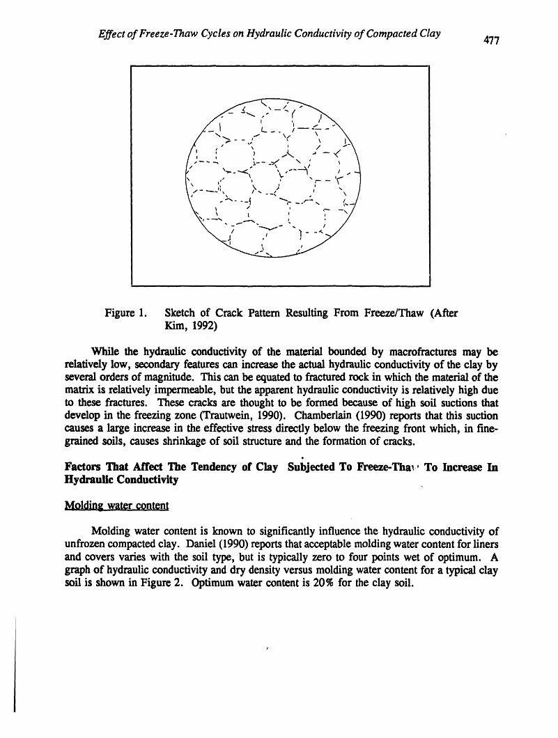
Effect of Freeze-Thaw Cycles on Hydraulic Conductivity of Compacted Clay 477
Figure 1. Sketch of Crack Pattern Resulting From Freeze/Thaw (AfterKim, 1992)
While the hydraulic conductivity of the material bounded by macrofractures may berelativelylow, secondary features can increase the actual hydraulic conductivity of the clay byseveral orders of magnitude. This can be equated to fracturedrock in which the materialof thematrix is relatively impermeable, but the apparent hydraulic conductivity is relatively high dueto these fractures. These cracks are thought to be formed because of high soil suctions thatdevelop in the freezing zone (Trautwein, 1990). Chamberlain (1990) reports that this suctioncauses a large increase in the effective stress directly below the freezing front which, in fine-grained softs, causes shrinkage of soil structure and the formation of cracks.
Factors That Affect The Tendency of Clay Subjected To Freeze-Thaw To Increase InHydraulic Conductivity
Moldin2 water¢Qntent
Molding water contentis known to significantly influence the hydraulicconductivity ofunfrozencompactedclay. Daniel (1990) reportsthat acceptablemoldingwatercontentfor linersand covers varies with the soil type, but is typically zero to four points wet of optimum. Agraphof hydraulicconductivityand dry density versus molding watercontent for a typicalclaysoil is shown in Figure 2. Optimumwater contentis 20% for the clay soil.

D. Waite and others478
Ill II I
1E..7. 90
I]F,-l 0 ' , ,, , , m , 8214 16 18 20 22 24 26 28
Z4old_,SWaterC_e=_ (',,;)
Figure 2. Variation of Hydradic Conductivity And Dry Density WithMolding Water Content
While it is well known what the effect of molding water content on the hydraulicconductivity of unfrozen compacted clay is, how molding water content effects the hydraulicconductivity of clay that has been exposed to freeze-thaw is inconclusive. Zimmie (1992)reports that there is no significant difference in hydraulic conductivity increase, due to freeze-thaw, between clay samples compacted dry of optimum and wet of optimum clay samples.Chamberlain (1990) studied four clays that were frozen after being compacted at typical landfillcover molding water content and compactive effort. The increase in hydraulic conductivity,after freeze-thaw, ranged from a ratio of 35 to 300. Kim (1992) tested clay samples at varyingmoisture contents and determined that wet of optimum specimens realize an increase in hydraulicconductivity of 70 to 300 fold, while the hydraulic conductivity of dry of optimum samplesincreased in hydraulic conductivity by a factor of 2 to 6. Kim concluded that molding watercontent was the single most important variable that affected the tendency of compacted clay toundergo an increase in hydraulic conductivity when subjected to freeze-thaw. Kim's data isshown in Figure 3; optimum water content is 15% and the clay was compacted at 100% ofstandard proctor.
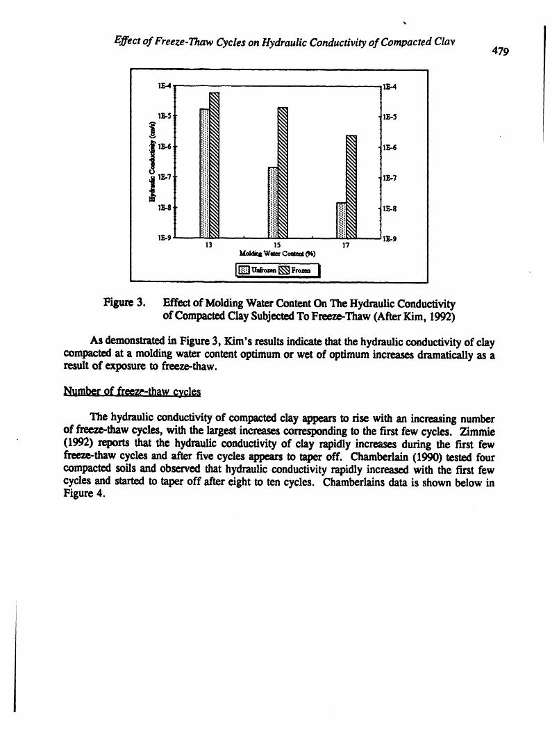
%
Effect of Freeze-Thaw Cycles on Hydraulic Conductivity of Compacted Clay479
i . i,
IE-4 15-4
IB.61 IE-6
1E-7_- _ IE-7
I Jlii!J:ii[
1_9 ' ' 12[..913 15 17
w_ ¢ommt_)
l,,Di,u_°mg_lV'°'= Ii i i i
Figure 3, Bffe_'tof Molding Wstex ContentOn The HydraulicConductivityof Compacted Clay Subjected To Freeze-Thaw (After Kim, 1992)
As demonstrated in Figure 3, Kim's results indicate that the hydraulic conductivity of claycompacted at a molding water content optimum or wet of optimum increases dramatically as aresult of exposure to freeze-thaw.
Humber of freeze-lhaw cycles
The hydraulic conductivity of compacted clay a_ to rise with an increasing numberof freeze-thaw cycles, with the largest increases corresponding to the first few cycles. Zimmie(1992) reports that the hydraulic conductivity of clay rapidly increases during the first fewfreeze-thaw cycles and after five cycles appears to taper off. Chamberlain (1990) tested fourcompacted soils and observed that hydraulic conductivity rapidly increased with the first fewcycles and started to taper off after eight to ten cycles. Chamberlains data is shown below inFigure 4.
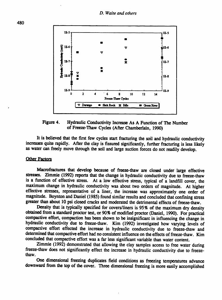
D. Waite and others
480
IF,-3 s lg-32
• 0+.
I
" + t,lg-7 1 E..7
m-8 _m-e
.=
+
IF.,-9 • i , , , , ' ' 1_,-90 2 4 '6 8 10 12 14
_rem-_ @j_es
Figure 4. Hydraulic ConductivityIncreaseAs A Function of The Numberof Freeze-Thaw Cycles (After Chamberlain,1990)
It is believed that the first few cycles startfracturingthe soil and hydraulic conductivityincreases quite rapidly. After the clay is fissured significantly, furtherfracturing is less likelyas water can freely move through the soil and large suction forces do not readily develop.
OtherFactors
Macrofraetures that develop because of freeze-thaw are closed under large effectivestresses. Zimmie (1992) reports that the change in hydraulicconductivity due to freeze-thawis a function of effective stress. At a low effective stress, typical of a landfill cover, themaximum change in hydraulic conductivity was about two orders of magnitude. At highereffective stresses, representative of a liner, the increase was approximately one order ofmagnitude. Boynton and Daniel (1985) found similar results and concluded that confining stressgreater than about 10 psi closed cracks and moderatedthe detrimentaleffects of freeze-thaw.
Density that is typically specified for covers/liners is 95 % of the maximum dry densityobtained from a standard proctor test, or 90% of modified proctor (Daniel, 1990). For practicalcompaetive effort, compaction has been shown to be insignificant in influencing the change inhydraulic conductivity due to freeze-thaw. Kim (1992) investigated how varying levels ofcompaetive effort effected the increase in hydraulic conductivity due to freeze-thaw anddetermined that compactive effort had no consistent influence on the effects of freeze-thaw. Kimconcluded that compactive effort was a far less significant variable than water content.
Zimmie (1992) demonstrated that allowing the clay samples access to free water duringfreeze-thaw does not significantly effect the increase in hydraulic conductivity due to freeze-thaw.
One dimensional freezing duplicates field conditions as freezing temperatures advancedownward from the top of the cover. Three dimensionalfreezing is moreeasily accomplished

Effect of Freeze-Thaw Cycles on Hydraulic Conductivity of Compacted Clay481
in the lab though, and for this reason there has been testing to determine if there is a significantdifference between one dimensional and three dimensional freeze-thaw effects in hydraulicconductivity. Zimmie (1990) investigated this factor and found the same rate of increase inhydraulic conductivity for fine-grained soil exposed to one dimensional freezing and threedimensional freezing.
MATERIAI3 AND METHODS
Approach
Where possible, conditions typical of a landfill cover were used while compacting,freezing, and performing falling head permeability tests on the clay samples. These conditionsinclude;
• an overburden that is comparable to the overburden that a landfill cover would besubjectedto
• no access to free water during freeze-thaw as the cover typically will not be saturated
• densities and compaction methods that would be typical of that which would be usedin the construction of a landfill cover
The variables in the freeze-thaw tests were molding water content, and the number offreeze-thaw cycles. The molding water content of the samples in the test was 4- 3 percent ofoptimum, which resulted in molding water contents of 23.5 % and 29.:_%. The Clay sampleswere frozen in groups of 0, I, 3, 5, and I0 cycles. A minimum of three tests were performedfor each combination of molding water content and number of freeze-thaw cycles. The claysamples were compacted and frozen in consolidorneters which were also used as thepermeameters for the falling head permeability test.
Soft Properties and Preparation
The soil used in this test was acquired from the Utah State University Drainage Farm andis ladce Bonneville lacustrine deposits. The soil is a inorganic silt-highly plastic clay and isclassified a MH-CH, according to the Unified Soil Classification System. Soil properties areprovided in Table I.

D. Waite and others482
TABLE 1SOIL PROPERTIES
Plastic Limit 30%
Liquid Limit 51
Plasticity Index 21%
Specific Gravity 2.63
Optimum Water Content 26.5 %
Maximum Dry Density 93.5 lb/fta l
Proctor tests were performed to determine the optimum moisture content of the soil usedin the testing. Results from the standard proctor tests are shown in Figure 5.
uP+-- ilu, i ii
" 96 +
92 92m um • •
90 ,, 90
_' 88 98
86 " 86
84 ,, I I I l ..... I I I I I 84
16 18 20 22 24 26 28 30 32 34 36
i,, i
Figure 5. Results From Standard Proctor Tests
In preparation for testing, the soft was brought into the lab and allowed to air-dry for twodays. After the soil was air-dried, the clods in the soil were broken down and the soil waspassed through a #4 sieve. Soil passing the #4 sieve was thoroughly mixed and quartered to getsmaller samples that were representative of the soil. The air-dried clay was slowly mixed withwater to achieve the desired water content. The sample was then allowed to stabilize for 24hours, enough time for all the soil particles to hydrate.
After the soft moisture had stabilized it was compacted into the consolidometer. The claywas compacted in three lifts, with 3 blows per layer. The hammer constructed for compactionof the samples had a weight of 0.6178 lbs, and a drop of six inches. The volume of the clay

Effect of Freeze-Thaw Cycles on Hydraulic Conductivity of Compacted Clay483
' samplewas0.00284i_.Thisproceduregavea compactiveeffortof12,400ft-lb/i_whichisequivalent to the compa_ve effort of a standardproctor. Care was takento compactclose tothe sides of the consolidometerto minimize thepotential for piping. Clods thathad formeddueto the additionof water, and were larger thenthe openings in the # 4 sieve, were broken downbefore compaction. Comlmctedclay pmlmrtiesare shownin Table 2.
TABI_ 2PROI_RTIES OF COMPACTED SOIL
MOLDING WATER CONTENTPROPERTY _23.5_ 26.5_ 29.5_
II III II
DryDensity(pc0 92.5 93.5 S9.9l I I I II
Moist Density (pcf) 114.2 118.3 116.4i I i ii i i
Void Ratio 0.77 0.76 0.83 _I II Illi Ill
_t _u_ 79.9 92.3 94.0m I IH i ii i
The goal of laboratoryfteeze-tlmw testing was to simulate field conditions. Of course]abomtm'ycmditiom are, at best, only an approximationof actual field conditions. Many ofthe conditionsof freeze-thawthatan actualcover would be subjectedto arereproduciblein the ramry though.
An overburdenstress of 2.4 psi was placed on the com_ clay and remained thereduringfreeze-thaw. This was believed to best simulate field conditions where the clay wouldbe subjectedto a relatively constantoverburden. Municipal waste landfill covers are oftensubjectedto an overburdenstress thatranges from 2 to 3 psi. This h based on a topsoil coverdepth of approximatelytwo feet and a one foot sanddrainagelayer.
While the landfillcover would generallybe frozenunder one dimensionalconditions, fromthe topdown, studieshaveshownthatfi'cczingsamples in a threedimensional mannerproducesthe same resultsas freezing one dimensional(Zimmie, 1992). For this reason the clay samples
frozen _onally as freezing all-around is more readily performed in thet xm-y.
The consolidometerswere _ in aluminumfoil to prevent any dryingduringfreeze-thaw. Samples in this test were frozen at moldingwater content with no access to water.
Prof_ure
The clay samples were frozenin a large chest freezer, then the freezer compressor wasturnedoff and the samples w_e thawed. After the sampleswere frozen, the compressor wasshutoff and a timerturnedon heatlampsthat hadbeen placed in the freezer. The freezerused
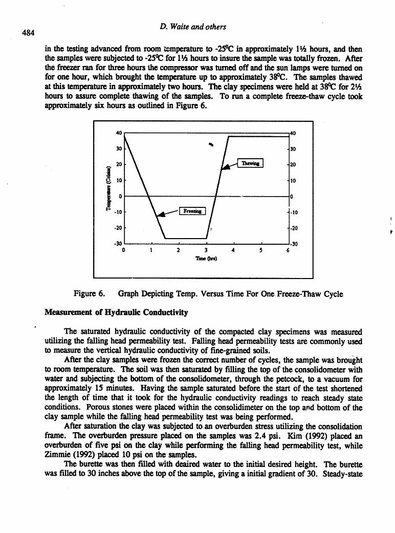
D. Waite and others484
in the testingadvancedfrom room _mperatureto -25°C in approximatelyl_h hours, and thenthesampleswere subjectedto -25°Cfor l_h hoursto insure the samplewas totally frozen. Afterthe freezerranfor three hoursthe compressorwas turnedoff and the sun lampswere turned onfor one hour, which brought the temperatureup to approximately38°C. The samples thawedatthis temperaturein approximatelytwo hours. The clay specimenswere held at 38°C for 2_hhours to assure complete thawingof the samples. To run a complete freeze-thaw cycle tookapproximatelysix hours as outlined in Figure 6.
i i
40 40
'b3O 30
10 10
]o o-Io I Fro,,=.. ]-_o
-20 I"20-30 i , , , i -300 1 2 3 4 5 6
"Z'w (!=.)
, i
Figure 6. GraphDepicting Temp. Versus Time For One Freeze-Thaw Cycle
Measurement of Hydraulic ConductivityB
The saturatedhydraulic conductivity of the compacted clay specimens was measuredutilizingthe falling head permeability test. Falling head permeability tests are commonly usedto measure the vertical hydraulicconductivity of fine-grained soils.
After the clay samples were frozen the correctnumberof cycles, the sample was broughtto room temperature. The soil was then saturatedby filling the top of the consolidometer withwater and subjecting the bottom of the consolidometer, through the pe_ock, to a vacuum forapproximately 15 minutes. Having the sample saturatedbefore the startof the test shortenedthe length of time that it took for the hydraulic conductivity readings to reach steady stateconditions. Porous stones were placed within the consolidimeteron the top a_ndbottomof theclay sample while the falling headpermeability test was being performed.
After saturation the clay was subjectedto an overburdenstress utilizing the consolidationframe. The overburden pressure placed on the samples was 2.4 psi. Kim 0992) placed anoverburden of five psi on the clay while performing the falling head permeability test, whileZimmie 0992) placed l0 psi on the samples.
The burette was then filled with deairedwater to the initial desired height. The burettewas filled to 30 inches above the topof the sample, giving a initial gradientof 30. Steady-state
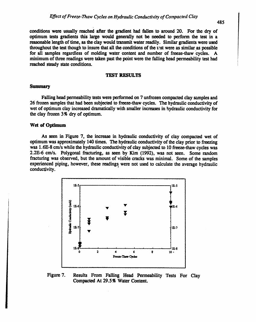
Effect of Freeze-Thaw Cycles on Hydraulic Conductivity of Compacted Clay485
conditions were usually reached after the gradient had fallen to around 20. For the dry ofoptimum tests gradients this large would generally not be needed to perform the test in areasonablelength of time, as the clay would transmitwaterreadily. Similargradientswere usedthroughoutthe test though to insure that all the conditionsof the t_t were as similar as possiblefor all samples regardlessof molding water content and number of freeze-thaw cycles. Aminimumof three readingswere takenpastthe point were the falling headpermeability test hadreached steady state conditions.
TEST RESULTS
Summary
Fallingheadpermeability tests were performed on 7 unfrozen compactedclay samplesand26 frozen samplesthat hadbeen subjectedto freeze-thawcycles. The hydraulicconductivityofwet of optimumclay increaseddramaticallywith smallerincreases in hydraulic conductivity forthe clay frozen 3 % dry of optimum.
Wet of Optimum
As seen in Figure 7, the increase in hydraulicconductivity of clay compacted wet ofoptimum was approximately140 times. The hydraulic conductivityof the clay prior to freezingwas 1.6E-8 cm/s while the hydraulicconductivityof clay subjectedto 10 freeze-thawcycles was2.2E-6 cm/s. Polygonal fracturing,as seen by Kim (1992), was not seen. Some randomfracturingwas observed, but the amountof visible cracks was minimal. Some of the samplesexperiencedpiping, however, these readings were not used to calculate the average hydraulicconductivity.
i i i IL
g,
"_" IFIE.6 V Y _E-6
-J1_7V
0 2 4 • 6 8 lO-
Frem-_ _s
i i i lll i i
Figure 7. Results From Falling Head Permeability Tests For ClayCompactedAt 29.5 % Water Content.

.°L
D.WaiteandOthers
486DryofOptUnum
The hydraulicconductivity of dry of optimumclay increased by a ratio of 11 a_ 10freez_th_w cycles as shownin Figure 8.
1F_4 1_4
i r
ts,.5 lS-5F
V pqF
l, iii 1"I i , i , t , IF.-"/0 2 4 6 8 10
•_rm,-_Cycb,
i
Figure 8. Results From Falling Head Permeability Tests For ClayCompactedAt 23.5 % Water Content.
The hydraulicconductivityof theclay priorto freezing was 8.3E-7 cm/s and the hydraulicconductivityof clay subjectedto 10 freeze-thawcycles was 9.1E-6 cm/s. Polygonal fracturing,as with the wet of optimumsamples, was not seen. Some randomfracturingwas observed, butthe amountof visible cracks was minimal. Some of the samplesexperiencedpiping, however,these readings were not used to calculate the average hydraulicconductivity. A minimum of
samples, with no testing anomalies, was recorded for each freeze-thaw cycle.
Number of Cycles
As seen in Figure 9, increases in hydraulic conductivity tapered off with increasingnumbersof freeze-thaw cycles. However, the hydraulicconductivity was still increasingafter10 freeze-thawcycles. _

Effect of Freeze-Thaw Cycles on Hydraulic Conductivity of Compacted Clay
487ii i it i i i
1000 1000
10 40
1', ................ 10 2 4 6 8 10
l:reeze-_w Cydes
Figure 9. Ratioof HydraulicConductivityIncrease
ANALYSIS/CONCLUSIONS
Molding Water Content
Hydraulicconductivityof clay compactedwet of optimuminc_ greatly as a result offreeze-thaw. Clay samplescompacteddry of optimumalso experiencedanincreasein hydraulicconductivitybut to a lesser extent. Possible reasons for this difference are:
• Wet of optimum samples were frozen at 94% of saturation while dry of optimumsampleswere frozen at 80% of saturation.
• The initial hydraulicconductivityof wet of optimumclay was muchlower thendry ofopt clay whichcould lead to higher suction forces in front of the freezing front in wetof optimum clay, due to the diminishedfreedom of movementof the free water.
Wet of optimum samples in this experiment experienced an increase in hydraulicconductivityof approximatelya factorof 140, after 10 cycles. This leads to the conclusionthatclay compactedwet of optimum, and exposed to a least 10 freeze-thaw cycles, will increase inhydraulic conductivityby a factorof roughly two orders of magnitude. Results from this testwere comparable to the findings of other researchers. Kim's (1992) tests suggestedan increasein hydraulic conductivityin wet of optimumclay of approximatelya factorof 110 after5 freeze-thaw cycles. Chamberlain(1990) tested four clays at typical landfill design molding watercontents and observed that the ratio of increasein hydraulicconductivity, after9 cycles, rangedfrom 24 to 269 with an average of 100.
Clay compacteddry of optimumdidnot increasein hydraulicconductivityas muchas clay
D. Waite and others
488
compactedwet of optimum. Clay compacted3% dry of optimum in this experiment increasedin hydraulic conductivity by a factor of II, after ten freeze-thaw cycles. The increase inhydraulicconductivity after five cycles was threefold, which is similar to the results of Kim(i992). Kim tested clay compacted at various moisture contents and determined that claycompacteddryof optimum experiencedan increasein hydraulicconductivity,after5 freeze-thawcycles, of a factor of four.
Number of freeze-thaw cycles
Hydraulicconductivityincreasesdramaticallywith thefirsttwo tothreefreeze-thawcycles,with a rapidtaperivg off with increasing numbersof freeze-thawcycles. The possible reasonsfor this are:
* Conduitsareopened in the soil matrixallowing for the permeantto flow freely. Afterseveral freeze-thawcycles the soil would be so fracturedthat large suctionforces couldnot develop and there would be no significantadditionalfracturing.
• Voids t_evelopin the soil which act as pockets for the release of the suctionforces thatdevelop.
The tapering off of hydraulic conductivity increases is well documented in previousresearch. The results from this investigation,which demonstratethe decrease in the effects offreeze-thawwith an increase in the numberof cycles, agree well with results from Chamberlain(1990), Kim (1992), and Zimmie (1992).
Conclusions
Molding water content and the numberof freeze-thawcycles that a fine-grainedsoil isexposed to, significantlyaffect the hydraulic conductivityof the soil used in this test. Resultsfrom this investigation clearly demonstratethe sensitivity of compactedclay to these factors.
The hydraulicconductivity of compactedclay increased when exposed to freeze-thaw.Clay compactedwet of optimum was effected significantlyby freeze-thawand experiencedlargeincreases in hydraulicconductivity. Clay compacteddry of optin,um experienced increases inhydraulicconductivity, but to a lesser extent. The largest increases in hydraulic conductivitywere seen in the first few freeze-thawcycles that the soft was exposed to. A summary of theresults is outlined below:
• Molding watercontentaffectsthe tendencyof a fine-grainedsoil to experienceincreasesin hydraulic conductivity,due to freeze-thaw.
• Landfillcovers typicallymustbe compactedat a moldingwatercontentoptimumor wetof optimum to achieve the required hydraulic conductivity. It appears that clayscomIgictedat these water contentsare most susceptibleto freeze-thaw
J
• Molding water contentis the single most importantvari2_bleinfluencing the effects offreeze-thawon the hydraulic conductivity of compactedclay.

i
Effect of Freeze-Thaw Cycles on Hydraulic Conductivity of Compacted Clay
489
* The hydraulic conductivity of a fine-gr_ined soil increases with the number of freeze-thaw cycles. The increase in hydraulic conductivity tapers of rapidly with an increasein the number of cycles.
• Landfill covers must be protected from the effects of freeze-thaw if the low hydraulicconductivity of the cover is to be maintained.
Results of this test support the conclusions of previous research which suggests that landfillcovers are susceptible to the effects of freeze-thaw. Once the factors that effect the hydraulicconductivity increase due to freeze-thaw are idenfilied, solutions to the problem can beidentified.
REFERENCES
Boynton, S. S., and Daniei, D. E. (1985). "Hydraulic Conductivity Tests on Compacted Clay," J.Geotech. Engrg., ASCE, i 11(4), 465-478
Chamberlain, E., Iskand_r,I., andHunstcker S. E. (1990). "Effect of Freeze-Thaw Cycles On ThePermeability And Macrostructure of $otls, _ Proc., Int. Symp. on Frozen Soil Impacts on Agric.,Range, and Forest Lands, CRREL Special Report 90-1, U.S. Army Corps of Engineers, ColdRegions Research & Engineering Laboratory, Hanover, N.H., 145-155.
Daniel, D. E., and Benson, C. H. (1990). "Water Content-Density Criteria For Compacted SoilLiners," J. Geotech. Engrg., ASCE, 116(12), 1811-1830
Day, S.,R., and Daniel D. E. (1985). "Hydraulic Conductivity of Two Prototype _ Liners,"J. Geotech. Engrg., ASCE, 111(8), 957-970
Kim, Woon-Hyung, and Daniel D. E. (1992). "Effects of Freezing On Hydraulic Conductivity ofCompacted C/ay," J. Geotech. Engrg., ASCE, 118(7), 1083-1097
Landreth, R. E. (1990). "Landfl//Containment Systems Regulations," Waste ContainmentSystems:Construction, Regulation, andPe,rformance, R. Bonaparte(ed.), ASCE Geotech. Spec. Pub. No. 26.
Miller, C. J., and Lee J. Y. (1992). "Effects of Freeze-Ihaw on Clay Cover Liner Performance,"EnvironmentalGeotechnology, Usmen andAcar (ed.), Proceedings of theMediterraneanConferenceon EnvironmentalGeotechnology/CSME/Turkey/May 25-27 1992, 205-211
Mitchell, J. K. and Jaber, M. (1990). "Factors Controlling the Long-Term Properties of ClayLiners," Waste Containment Systems: Construction, Regulation, and Performance, R. Bonaparte(ed.), ASCE Geotech. Spec. Pub. No. 26.
Taber, S. (1930). "The Mechanics of Frost Heaving," J. Geology (38), 303-317

D. Waite and others49O
Trautwein, S. J. and Williams, C. E. (1990). "Petfotwzance Evaluation of Earthen Liners," WasteContainment Systems: Constru_ion, Regulation, and Performance, R. Bonaparte (ed.), ASCEGeotech. Spe¢. Pub. No. 26.
Zimn_, T. F., LaPlante C. M., ,rodBronson, D. (1992). "The Effects of Freezing And Thawin_On The Permeability of Comptwted Clay Landfill Covers And Liners," EnvironmentalGeotex.hmlogy, Usmen and Acar (ed.), Proceedings of the Mediterranean Conference onEnvironmental Geotechnology/CSME/Turkey/May 25-27, 1992, 213-217
Zimmie, T. F. and LaPlante, C. M. (1990). "TheEffects of Freeze-Thaw Cycles on the Permeabilityof a Fine-Grained Soil," Proc., 22nd Mid-Atlantic Industrial Waste Conf., Drexel Univ.,Philadelphia, Pa., 580-593

Hydrogeology,WasteDisposal, Science andPoliticsProceedings30th SymposiumEngineeringGeology andGeotechnicalEngineering,1994 491
FROM LAB TO FIELD:. GEOTECHNICALPROPERTIF._FOR PREDICTINGEMBANKMENT SEITLEMENT ON LAKE BONNEVILLE DEPOSITS
Kevin C. H_d, Graduate StudentCamn L. Sampsco, Graduate Reseerch & Teaching Assistant
Loren R. Anderson, Department Head & ProfessorJoseph A. Cailendo, Assistant ProfessorCivil and Environmental Enaineerin3
Utah State University, Logan Utah 84322Loren Itsusher and F.dwardKeane
Geotechnicsl Engineers, Utah Department of TnmsportstionSalt Lake City, Utah 84119
ABSTRACT
The results el a laboratoryanalysis, to determine geotechnical properties oflacustrine Lake Bonneville deposits, within the 1-15 corridor of Salt Lake C/ty, Utah, ispresented. _r_ory vertical and horizontal consolidation coefficients are comparedwith those back-calculated from observed, field settlement data and linear relationshipsestablished. The results are used to select vertical and horizontal field coefficients andpredict settlement rate of an existing embankment, scheduled for enlargement.
INTRODUCTION
Geotechnical engineering of earth embankments, requires accurately predictingslope and foundation stability, and magni'tudeand rate of settlement, for proper designand construction scheduling. In the 13_ Rankine Lecture, Lambe (1973) referred to thegeotechnical engineer, as the "masterpredictor." He points out, that predictions areoften based on insufficient, inaccurate and varying data, due to the complexity of naturaldeposits, limitations in the theories used to make predictions, and that sound engineeringjudgement is essential, if predictions are to be useful. He further suggests, the need forsimple techniques to make type A predictions, i.e., before the events occur.
The Utah Department of Transportation 0._DOT) proposes widening the existinghighway embankments, within the 1-15 corridor of Salt Lake City, Utah, to accommodateadditional travel lanes. Settlement rate predictions are required in order to coordinateembankment construction and paving, to avoid differential settlement in the new surface.
This paper presents the results of a laboratory analysis on five soil samplessupplied by UDOT. The samples ranged in depth from twenty-seven te sixty-._wofeetand are typical of the stratified, lacustrine Lake Bonneville deposits. Consolidati_ncoefficients from one-dimensional consolidation tests, on vertically and horizonta_,lytrimmed specimens, are compared with those back-calculated from observed se_ementdata. Linear relationships were developed between the vertical and horizontalconsolidation coefficients, obtained from the laboratory and the field data. The linearequations are used to determine field consolidation coefficients, from those acquired inthe laboratory. A settlement prediction is made for an embankment scheduled forenlargement, using one-dimensional theory. The use of vertical drains is considered.
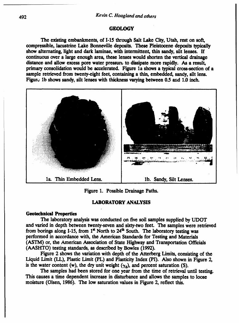
492 Kevin C. Hoagland and others
GEOLOGY
The existing embankments, of 1-15 through Salt Lake City, Utah, rest on soft,compress_le, lacustrine Lake Bonneville deposits. These Pleistocene deposits typicallyshow alternating, light and dark laminae, with intermittent, thin sandy, silt lenses. Ifcontinuous over a large enough area, these lenses would shorten the vertical drainagedistance and allow excess pore water pressur_ to dissipate more rapidly. As a result,primary consolidation would be accelerated. Figure l a shows a typical cross-section of asample retrieved from twenty-eight feet, containing a thin, embedded, san¢_, silt lens.Figur,_ lb shows sandy, silt lenses with thickness varyingbetween 0.5 and 1.0 inch.
::iii
J m •,.IIIIP o."i :': ....
":: : i!i: ": _ , I : i : _ : .... : ' . . • r'
.... :: _:::_.,.: .......
la. Thin Embedded Lens. lb. Sandy, Silt Lenses.
Figure 1. Poss_le Drainage Paths.
LABORATORYANALYSIS
Geotechnical PropertiesThe laboratory analysis was conducted on five soil samples supplied by UDOT
and varied in depth between twenty-seven and sixty-two feet. The samples were retrievedfrom borings along 1-15,from 1= North to 24_ South. The laboratory testing wasperformed in accordance with, the AmericanStandards for Testing and Materials(ASTM) or, the American Association of State Highway and Transportation Officials(AASHTO) testing standards, as described by Bowles (1992).
Figure 2 shows the variation with depth of the Atterberg Limits, consisting of theLiquid Limit (LL), Plastic Limit (PL) and Plasticity Index (PI). Also shown in Figure 2,is the water content (w), the dry unit weight (3'd),and percent saturation (S).
The samples had been stored for one year from the time of retrieval until testing.This causes a time dependent increase in disturbance and allows the samples to loosemoisture (Olsen, 1986). The low saturation values in Figure 2, reflect this.

Predicting Embankment Settlement on Lake Bonneville Deposits493
I II II I I I Ill Illl II II I II I Ill Illl II I
, ,, ,,,
-10 .....
-20 .............
-,o-50
-70 .......
-80 : .....0 10 20 30 40 50 60 70 80 90 100
w (%) _ LL (_) _ PL (_.)
PI (_) _ S (_.) --4k-- Dry Density (pcf)
Figure 2. Variation with Depth of Laboratory Oeotechnical Properties.
Mechanical and hydrometer particle size analyses were conducted on each of thefive samples and the sandy, silt lenses shown in Figure lb, in accordance with ASTM D421 and ASTM D 422. Fiwtre 3 shows the particle-size distnl_utionsfor a typicalclaysample and the sandy, silt lenses of Figure lb.
ii iii ii i ii i iiiii i i i i ii i ill i i ii iiii • iiii iiill i i ii ii
|0_ ,, |m ,
,ol IIII/ III!iIN:I:I_Ilii ]1111111 _! 1!,111i Ii!111Ii!!!1!II_lil_ lllllllll
:!1 ' .,, .Vlllllillllmli lilllll _.I l llllla! :IIIIIIl iilllHl'[IIIIIII l llllalllllH[litllll/lllllll l llilllll llllHl ..I l llllli ] _IIIIIII IIIIIHIIIIIIIIIl llllllg
I IIIIIN[llili[ i llllli l lllllili lllllll _ .I IIIIII| ] IIIIIIl lllllii IIIIIII! l lilillH°° llllli IIIIHI IIIIIII IIIIIIII l llllllg i .I l llllli i IIIIII IIIIII| IIIIIIII JJIIIIIH
lllllg[IL$1Illlllll lllilill illiml ._L.llllllli illlHlllllllillllllllll [llllllgllill| [_lllil i llllil i llilllll llllfli .I l illll! lllllllI IIHIHl illM i JJllllgJ]lllla.._II[IIIIl llllli IIIIIIII i lllllIg .I IIIIII! i !lllHll_llllgIIIIIIII l illlllglilIY'[ll$1l l llllli I IIIM l llllfll ,.I IIIIII! illlliL,,_llllNl lllllll l llllflg
,,,IIM ill[filll llllli l i[lllilI IHIIIH ._I!!!!_.. _ 111111l lllllll l llllilg
3a. Typical Clay. 3b. Sandy, Silt Lenses.
Figure 3. Particle-Size Disml_utions.
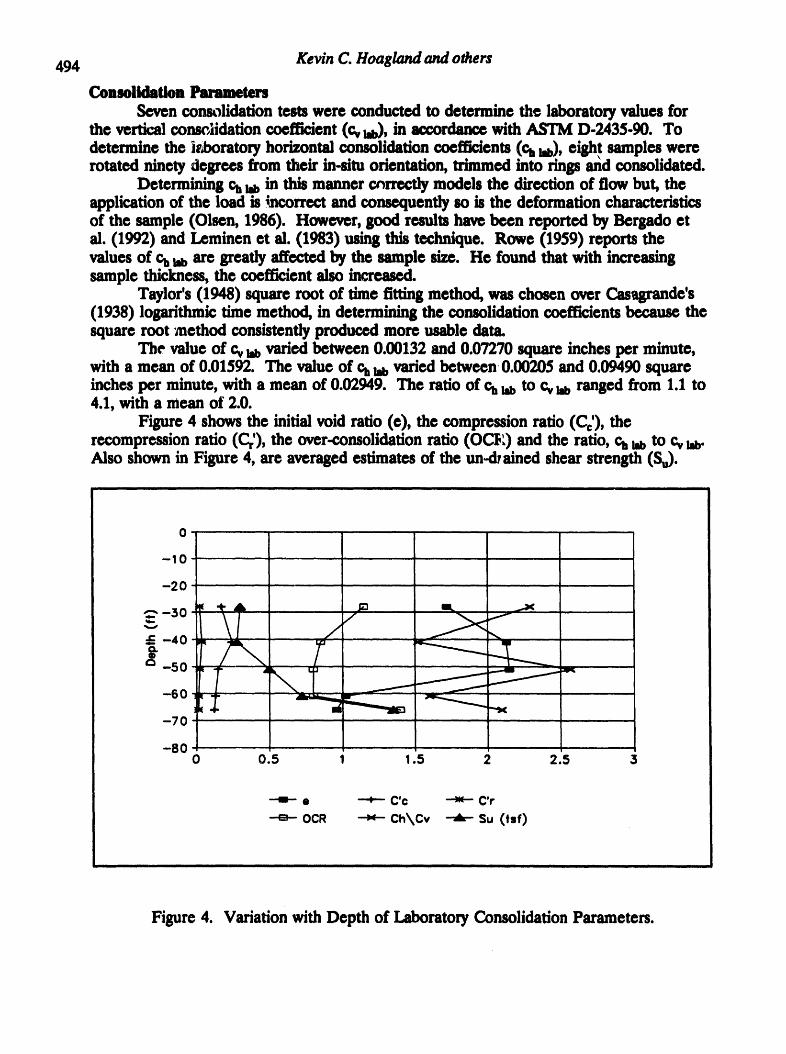
494 Kevin C. Hoasland and others
Con_ildatlonm__Seven consolidation tests were conducted to determine the laboratoryvalues for
the vertical consc,lidation coefficient (_ td,), in accordance with ASTM D-2435-90. Todetermine the b,boratoryhorizon.talconsolidation coef_ents (oh_b), eight samples wererotated ninety degrees from their m-situ orientation, trimmed into rings and consolidated.
Determining chm, in this manner cnrrectly models the direction of flow but, theapplication of the load is/sw.orrect and consequently so is the deformation characteristicsof the sample (Olsen, 1986). However, good results have been reported by Bergado etal. (1992) and Leminen et al. (1983) using this technique. Rowe (1959) reports thevalues of cb_b are greatly affected by the sample sizeo He found that with increasingsample thickness, the coefficient also increased.
Taylor's (1948) square root of time fitting method, was chosen over Cas_de's(1938) logarithmic time method,in determining the consolidation coefficients bexause thesquare root method consistently produced more usable data.
The value of cvm,varied between 0.00132 and 0.07270 square inches per minute,with a mean of 0.01592. The value of chm, varied between 0.00205 and 0.09490 squareinches per minute, with a mean of 0.02949. The ratio of ch_b tOCv_b ranged from 1.1 to4.1, with a mean of 2.0.
Figure 4 shows the initial void ratio (e), the compression ratio (Co'),therecompression ratio (Cr'), the over-consolidation ratio (OCt:) and the ratio, ch_b tOCvm,.Also shown in Figure 4, are averaged estimates of the un-d_ained shear strength (S0.
i i iiii i i iiii
0t-10 ........
-20 .............
"_-30 _ _" A J= m._ ..,,..._
-50 f. • _ =_-70
-800 0.5 1 .5 2 2.5 3
---m- • -'-P-- C'c _ C'r
OCR ---N-- Ch\Cv _ Su (tsf)
Figure 4. Variation with Depth of Laboratory Consolidation Parameters.
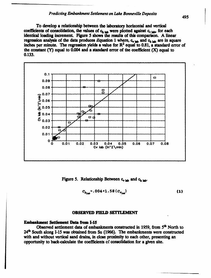
PredictingEmbankn_ntSettlementonLakeBonnevilleDeposits 495 I
fTo develop a relationship between the laboratoryhorizontal and verticalcoefficients of consolidation, the values of ch _ were plotted asainst c, m,, for eachidentical loading increment. F_ 5 shows the results of this comparison. A linearregression analysis of the data produce8 Equation I where, cq,_ and _ nabare in squareinch_ ,perminute. The regression yields a value for R2 equal to 0.81, a standard error ofthe constant (Y) equal to 0.004 and a standarderror of the coefficient (X) equal to0.133.
I I I I III [l I I [ [ II llll lI [ II l I I I
.1 ° ................
/ =-- , ,l, ,
o.o9. ,_ /Jl
0.08 -r _ J#"
.-o.07I..... == /' ' ' " _ r ' "'
_1 0.06 " i/¢
o.o5._, , _ _- .....
_o.O4o.o3 .....y _v'_c,c_ .......
0.02 _ .........0.01 ..............
O.il _ ....0 0.01 0.02 0.03 0.04 0.05 0.06 0.07 0.08
Cv lob (In"2\mln)
Figure 5. Relationship Between _ _b and chlb.
oh_ =, 004 +1,58 (ova) (1)
OBSERVED FIELD SEFILEMENT
EmbanlumentSettlement Data froml-ISObserved settlement data of embankments constructed in 1959, from 5thNorth to
24e_South along 1-15was obtained from Su (1966). The embankments were constructedwith and without vertical sand drains, in close proximityto each other, presenting anopportunity to back-calcolate the coefficients of consolidation for a given site.

KevinC.Hoaglandandothers
496
Bsck-Cf_lculsfln8 Consolkilstlon PnmmelcTs.The observational method of Asaoka (1978), as d_'bed by Magnan et al. (1983)
and Holtz et al. (1991), was used to back-calculatevalues of the coefficients ofconsolidation, cv _d and ct rod. The method consists of conveniently dividing thesettlement versus time curves into equal time intervals (At). The correspondingsettlement (Sn)is then determined for each time increment (in) and the Cartesiancoordina':es,(sn-l, %) are plotted. The slope (B) of the straight line formed by the points(sn-l, sffi)is used in Equation 2, to determine cvrod, from embankments without verticaldrainsor Equation 3 to determine chSdd,from embankments with vertical drains,
4 (lnp) {a}c_=- .2(A t:)
(de)'(F(n))(in_) (3)cb=- 8(At)
where, in Equation 2, Cvis the vertical coefficient of consolidation and HDp is the heightof the drainage path. In Equation 3, chis the horizontal coef_ent of consolidation, deis the diameter of an equivalent soil cylinder and F(n) is a drain spacing factor.
The intersection of the line with slope 0 and a line formed at 45°, represents themagnitude of primaryconsolidation for that loading increment. Equation 2 is based onTerzaghi's (1923) theory for vertical flow and Equation 3 in based on Barton's (1948)theory for horizontal flow. The value of F(n) is shown in Equation 4 (I-Iansbo,1979),
d. 3F(n) ,,ln (-_v) -_ {4}
where, dwis the equivalent diameter of a vertical drain.Good results have been reported by Bergado et al. (1992) and Magnan et al
(1981) using Asaoka's method to back-calculate field consolidation coefficients.Gilani (1993) back-calculated the average drainage distance, under double-drained
conditions, from observed settlement data of embankments in the vicinity and estimatesvalues between 1.5 and 5 feet. A value of 3 feet was selected for back-calculating cvmdand represents the mean of the values determined by Gilani. A triangular drain spacingpattern was assumed for calculating,de and is equal to 1.05 times the drain spacing.
The value of cv am varied between 0.00110 and 0.01410 square inches per minute,with a mean of 0.00695. Notice the mean Cv_b is 2.29 times greater than the meanCvera. The value of cheetdvaried between 0.00594 and 0.29200 square inches per minute, 'with a mean of 0.05084. The ratio of chaetdtOCvaetdranged from 2.2 to 22.2, with amean of 9".0.
Similarly to the laboratory results, the back-calculatedvalues of cheetdand Cveetdwere plotted, as shown in Figure 6. The linear regression analysis of the data in Figure6, yields Equation 5 where, cvmd and cheektare in square inches per minute. Theregression generated a value for R 2 equal to 0.89, a standarderror of the constant (Y)equal to 0.022 and a standard error of the coefficient (X) equal to 0.545.
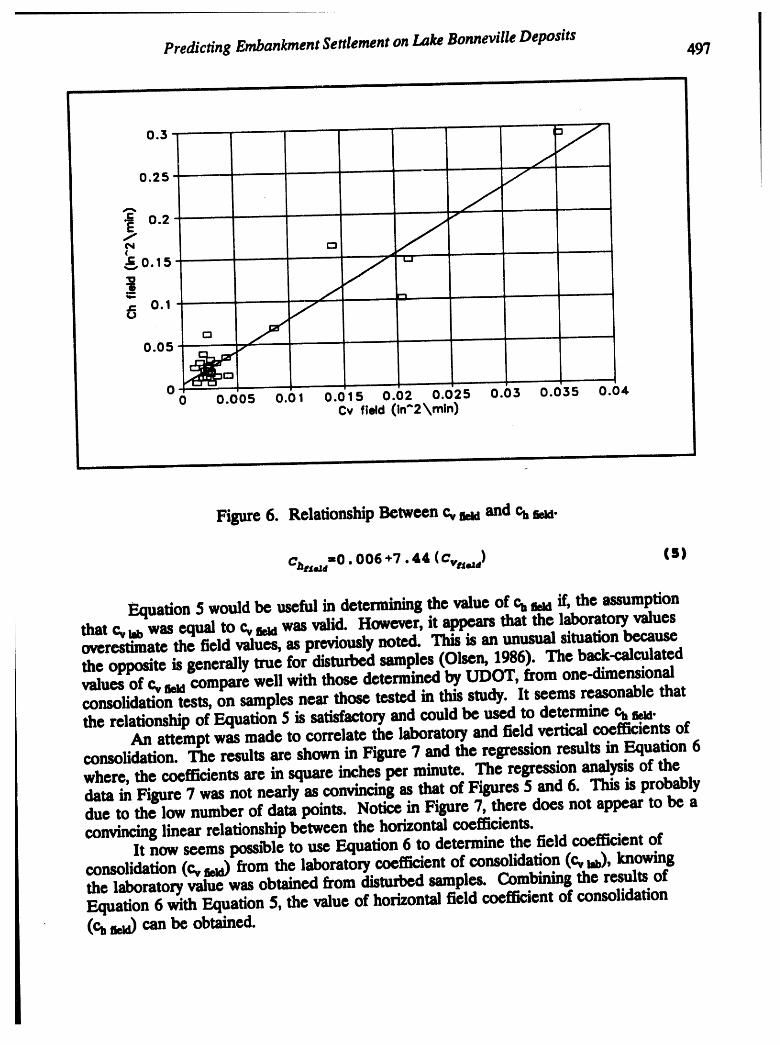
Predicting Embankment Settlement on Lake Bonneville Deposits 49'7
.,,I0.25 _
c 0.2 "I",,,, =
•_ 0.15 /
0.1 /
° J0.05 F
0 0 0.005 0.01 0.015 0.02 0.025 0.03 0.055 0.04Cv field (in"2\min)
Figure 6. Relationship Between cvmd and c_ _d.
Ch_.,4=O .006 +7.44 (Cv,i,_4) {S }
Equation 5 would be useful in determining the value of chfradif, the assumptionthat cv_b was equal to _ md Wasvalid. However, it appears that the laboratoryvaluesoverestimate the field values, as previously noted. This is an unusual situationbecausethe opposite is generally tree for dismd_ samples (Olsen, 1986). The back-calculatedvalues of cveetdcompare well with those determined by UDOT, from one-dimensionalconsolidation tests, on samples near those tested in this study. It seems reasonable thatthe relationship of Equation 5 is satisfactory and could be used to determine chaetd.
An attempt was made to correlate the laboratory and field vertical coefficients ofconsolidation. The results are shown in Figure 7 and the regression results in Equation 6where, the coefficients are in square inches per minute. The regression analysis of thedata in Figure 7 was not nearly as convincing as that of Figures 5 and 6. This is probablydue to the low number of data points. Notice in Figure 7, there does not appear to be aconvincing linear relationship between the horizontal coefficients.
It now seems posu'ole to use Equation 6 to determine the field coefficient ofconsolidation (cvaeu) from the laboratory coefficient of consolidation (cv_b), knowingthe laboratoryvalue was obtained from disturbed samples. Combining the results ofEquation 6 with Equation 5, the value of horizontal field coef_ent of consolidation(cheeu) can be obtained.

498 Kevin C. Hoagland and others
0.04ti
0.035 -!-
0.03 ; .
0.025"0"6
0.02 .¢.J
0.015.4-
0.01m __._
0.005 -- _ __-'B m
00 0.01 0.02 0.03 0.04 0.05 0.06 0.07 0.08
C lab
m CV + Ch
Figure 7. Relationship Between Cv_b and Cvksa.
Cvt:Z,,ld=O.003 +0.04 (cvl,_) (6)
EMBANKMENT SETFLEMENT PREDICTION
Settlement MagnitudeTo illustrate the use of the previously described relationships, a settlement
prediction was made for an embankment addition at the Junction of 1-15_I-80East.Using the one-dimensional metbod proposed by Karl Terzaghi (1925), the settlementmagnitude was calculated accordingto Equation 7 for the normally consolidated deposit,
AH=_, (Ho) (C_)log ( _'°+"k_'_) (7)0 o
where, Ho is the depth of the compress_le layers or each subdivision, Cc'is thecompression ratio and represents the slope of the virgincompression portion of the logof pressure versus strain curve, _'o is the initial vertical effective stress and A_ o is theincrease in vertic_ effective stress due to the embankment enlargement.
The compressl'ole layer was determined to be sixty feet in depth and wassubdividedinto six layers. The value of Co'was chosen to be 0.152, and represents the

Predicting Embankment Settlement on Lake Bonneville Deposits499
mean value determined from consolidation tests, on rumples fzom the site. The values of _o
and A_ e were determined at the center of each subdivisionusing Osterberg's (1957)integration of the Boussinesq (1885) equations, for an infinitely long embankment.Overburden stresses were calculated assuming the water table was located at 3.0 feet andthe dry unit weight ('Yd)of the soil was 110 pounds per cubic foot. The unit weight ofthe embankment was assumed to be 125 ixmnds per cubic foot.
Gilani (1993) concluded that this method provides reasonably accurate results andcompares favorablywith solutions by other methods, for embankments constructedkradly. The effective stresses and corresponding settlement were calculated for variouslocation below the embankment. The settlement results are shown in Figure 8.
!
EXISTING 'I
0 i
/, ,"0.5 / '* ........
I-1-
-1.5 ....
-20 so _00 _50 200 250
[I_ANKIW(N'rWID'IH(fi')
Figure 8. Predicted Settlement Magnitude Below Embankment.
Set_©_nt RateTerzaghi's (1923) differential equation descn_oingthe time rate of one-dimensional
consolidation is given in Equation 8, in terms of the excesspore water pressure,
_u au

500 Kevin C. Hoagland and others
where, cv is the coefficient of consolidation due to vertical flow, u the excess pore waterpressure at any time t and z the depth from the top of the compress_le layer to a pointwithin the layer under consideration. The solution to the differential equation ispresented in terms of the average degree of consolidation (13,) and the time factor (Tv)shown in Equation 9.
T.-c_(C) (')
To predicted settlement rate, Equation 9 is solved for the time (t) required for100 percent consolidation to occur (Tv=I). Equation 9 is then solved successively for thetime (t), corresponding to each of the well known time factors (Tv), that are related tothe average degree of vertical consolidation (0v), from ten to ninety percent. Thesettlement (S) at time (t) is expressed as follows in Equation 10,
s-(D_)(Am (,o)
where, _ is the magnitude of settlement from Equation 7.A settlement rate comparison was made under the shoulder of the enlarged
embankment as shown by position (h) in Figure 8. The magnitude of settlement at this.location was 0.7 feet. The average value of _ _b, for the range of effective stresses theembankment will undergo due to loading, was 0.0165 square inches per minute. Usingthe linear relationship of Equation 6, Cvem is equal to 0.00366 square inches per minute.
Figure 9 shows the time-rate of settlement, in months, for two double drainedconditions, to 90 percent consolidation. They are, case (1), HDr equal to 30 feet,assuming the lenses are ineffective and case (2) HDe equal 3 feet, as determined byGilani (1993), and the sandy, silt lenses are effective. The time required to ninetypercent consolidation for case (1) is 20850 days, about 57 years or 695 months and forcase (2), 209 days or about 7 months.
Aecountin,_for the sandy, silt lenses, primaryconsolidation will occur 100 timesfaster. This can easily be shown by the selection of HD1,in Equation 9, going from 30feet in case (1), to 3 feet in case (2), or one-tenth the drainage path length squared,which is one, one-hundredth the time for case (1). This solution is simplified andassumes evenly dism'outed sandy, silt lenses at six foot intervals or averaged values.More complex strata require the use of computer programs.
Often the error associated with underestimating settlement rate predictions isatm'outed to the value selected for the coefficient of consolidation. Attempts are madeto correct the laboratory coefficient by multiplyingit by some factor, assuming this willresult in an accurate field value for the consolidation coefficient. This approach may bein error, when in fact, the problem may be in the selection of the drainage path length.
Concluding that primarysettlement will occur in 209, days the embankment couldbe enlarged one season and surfaced the following. However, if complete constructionwas required in one season, the use of vertical drainsshould be considered as onealternative to accelerate primaryconsolidation. An estimate was made that primaryconsolidation would need to take place in 100 days to complete construction in oneseason.
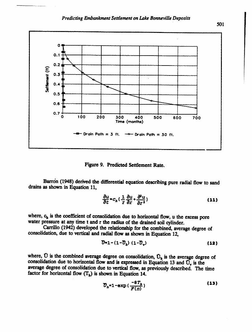
Predicting Embankment Settlement on Lake Bonneville Deposits501
ii i i i i i i i
O ....
0.1 _i_Br " , i ....
\0.2 , . .
] ..........I
0.4 m _ ....
0.5 " _ , ..
, _0.6 .... ,,, , _
0.7 .......0 100 200 300 400 500 600 700
Time (months)
-m--Orain Path = 3 ft. --.4--Drain Path = 30 ft.
i ii ii i i i
Figure 9. Predicted Settlement Rate.
Barrc_n(1948) derived the differential equation descn"oingpure radial flow to sanddrains as shown in Equation 11,
au 1 au+__..u.u) (xx)"_'ch (¥'a_ az2
where, c_ is the coefficient of consolidation due to horizontal flow, u the excess porewater pressure at any time t and r the radius of the drained soil cylinder.
Carrillo (1942) developed the relationship for the combined, average degree ofconsolidation, due to vertical and radial flow as shown in Equation 12,
T_-I- (1-_)h) (1-_v) (la)
where,. O is.the. combined, average degree,on consolidation, Oh is the average degree ofconsohdation due to horizontal flow and ts expressed in Equation 13 and Ov is theaverage degree of consolidation due to vertical flow, as previously descn'oed. The timefactor for horizontal flow (Tu) is shown in Equation 14.
-e2'h (13)_b-l-ex_ (F(n) )
502 KevinC.Hoaglandandothers
T,.,(c,)(t) (3.4)(d.) a
In order to determine the required drain spacing that will allow consolidation tooccur in 100 days, accounting for vertical and horizontal flow, Tv is solved for inEquation 9, with t equal 100 days. Hoe and c, md have been pre_ously determined.The value of Or, corresponding to the resulting Tv, equals 0.407, b ,_p_atdy 70percent. Equation 12 is then solved for in terms of the requ/red average degree ofconsolidation due to horizontal flow (Oh) and designing for the combined, averagedegree of consolidation (O), equal to 90 percent. The result is Oh approximately 70percent.
Finally, we combine Equations 13, 14 and 4 and solve for time (t). The result isshown in Equation 15 and represents the ideal case, that is, the effects of smear anddrain resistance are not accounted for.
t:= (d')a d. 3 1[Zn(--_)-_-] [Xn((i_]7h) ] (IS)8oh
Solving Equation 15, w/th t equal to 100 days, by trail and error for de,wh/ch isapproximately the drain spacing and considering dwequal to 0.16 feet, which represents acommon prefabricated vertical drain size, results in the desired drain spacing, The valueof Chrod,USingEquations 6 and 5 is 0.0332 square inches per minute. The result is adrain spacing of 8.5 feet after converting units. More detailed/nformation on the use ofvertical drains can be found in the U.S. Department of Transportation'smanual onprefabricatedvertical drains (R/xner eL al, 1986) and in Holtz et al. (1991).
t
CONCLUSIONSI
In the 27thKarl Terzagh/Lecture, Duncan (1993) discusses the _tiesassociated w/th estimating settlement magn/tude and rate. Among those discussed, erethe selection of consolidation coeff_ents and the effects of internal drainage byembedded sand layers. He states, "the prime prerequiSite for any analysis is a gooddefinition of soll pmpert/es that reflect the behavior of the undisturbed clay in s/tu." Theuse of back-calculated field _eters might assist in accomplishing this prerequim'te.The use of disturbed samples will not.
The use of linear relationships appear to prov/de a mechanism, for obtaining fieldconsolidation coefficients, from the laboratory coefficients. This technique maycontn'oute to simplif_g settlement predictions, as suggested by Lambe (1973) in theintroduction of this paper.
The following conclusions are drawn from the results of this study on lacustrineLake Bonneville deposits and may be useful in correlating consolidation permneters forsimilar deposits, when making settlement predictions.
1) The use of undisturbed soil samples is imperative if geotechnical propertiesarc to be determined accurately in the laboratory.

Predicting Embankment Settlement on Lake Bonneville Deposits 503
2) Not accounting for the thin sandy, silt lenses will lead to inaccuratesettlement rate predictions.
3) The one-dimensional consolidation tests, conducted on vertically andhorizontally trimmed specimens, suggest a linear relationship exists betweenthe laboratoryconsolidation coefficients.
4) Asaoka's method was useful in back-calculating field consolidationcoefficients from observed field settlement data.
5) Linear relationship appear to exist between the back-calculated, vertical andhorizontal consolidation coefficients, obtained from field settlement data.
6) If linear relationship can be established between the consolidationcoefficients from laboratory and field data, they may be useful in determininga reasonably accurate consolidation coefficient, on which to base settlementrate predictions.
Q
REFERENCES
Asaoka, A. 1978. Observational Procedure of Settlement Prediction. Japanese Society ofSoil Mechanics and Foundation Engineering. 18 (4):87-101.
Barton, R. A. 1948. Consolidation of Finc-Cn'aincdSofts by Drain Wells. AmericanSociety of Civil Engineers Transactions. 113:718-754.
Bcrgado, D. T., Em-iquez, A. S., Sampaco, C. L., Alfaro, M. C. and Balasubramaniam,A.S. 1992. Inverse Analyses of Gcotcchnical Parameters on Improved Soft BangkokClay. Journal of Geotcchnical Engineering. 118 (7):1012-1030.
Boussinesq, J. 1885. Application des Potentiels/t L°l_tudcde L'_quilibre et dueMouvcment des Solides l_lastiques, Gauthier-Vallars, Paris. (referenced in, Dunn,Anderson and Kiefer, 1980).
Bowles, J. E. 1992. Engineering Properties of Soils and their Measurement. 4m ed.McGraw-Hill, Inc., Hightstown, New Jersey. 241 p.
_1o, N. 1942. Simple Two and Three Dimensional Cases in the Theory ofConsolidation of Soils. Journal of Math and Physics. 21:1-5.
Casagrande, A. 1936. The Determination of the Pre-Consolidation Load and Its PracticalSignificance. Proceedings, First International Conference of Soil Mechanics andFoundation Engineering. Cambridge. Vol. III. p. 60-64. (referenced in, Holtz andKovacs, 1981).
Casagrande,A. 1938. Notes on Soil Mechanics-First Semester. HarvardUniversity(unpublished). 129 p. (referenced in, Holtz and Kovacs, 1981).
Duncan, M. J. 1993. Limitations of Conventional Analysis of Consolidation Settlement.27mTerzaghi Lecture, Journal of Geotechnical Engineering. 119 (9):1332-1359.
Dunn, I. S., Anderson L. R. and Kiefer, F. W. 1980. Fundamentals of Geotcchnical

504 Kevin C. Hoagland and others
Analysis. John Wiley and Sons, New York. 414 p.Gilani, S. H. 1993. Observed and Pzedicted Settlements of Highway Embankments on
Soft I.atcustrineDeposits. Report, Utah State University, Logan, Utah. 80 p.Hansbo, S. 1979. Consolidation of Clay by Band-Shaped Prefabricated Drains. Ground
Engineering.(12)5:16-25.Holtz, R. D., Jamiolkowski, M. B., Iauw,ellotta, R. and Pedroni, R. 1991. Prefabricated
Vertical Drains: Design and Performance. Butterworth-Heinemaun, Ltd., JordanHill, Oxford. 130 p.
Holtz, R. D. and Kovacs, W. D. 1981. An Introduction to Geotechnical Engineering.Prentice-Hall, Inc., Englewood Cliff& New Jersey. 733 p.
Lmbe, T. W. 1973. Prediedons in Soil Engineering. G6otechnique 23 (21):155-205.Leminen, K. and Rathmayer, H. 1983. Experience on Horizontal Oedometer Tests to
Determine the Parameter ch.Proceedings, of the 8*hEuropean Conference on SoilMech_ and Foundation Engineering. Helsinki, Vol. 2. p. 647-651.
Magnan, J. P. 1981. An Inverse Problem Approach to Settlement Prediction. Discussion,Japanese Society of Soil Mechanics and Foundation Engineering. (21) 4:117-120.
Magnan, J. P., Pilot, G. and Queyroi, D. 1983. Back Analysis of Soil ConsolidationAround Vertical Drains. Proceedings, 8thEuropean Conference on Soil Mechanicsand Foundation Engineering. Helsinki, Vol. 2. p. 653-658.
Olsen, R. E. 1986. State of the Art: Consolidation Testing. in, Consolidation of Softs:Testing and Evaluation, ASTM STP 892. Yong, R. N. and Townsend, F. C., Eds.American Society For Testing And Materials. Philadelphia, Pennsylvania.p. 7-68.
Osterberg, J. O. 1957. Influence Values for Vertical Stresses in a SemMnfinite MassDue to an Embankment Loading. Proceeding of the Fourth InternationalConference on Soil Mechanics and Foundation Engineering. London. Vol. I p.393-394. (referenced in, Holtz and Kovacs, 1981).
Rixner, J. J., Kraemer, S. R. and Smith, A. D. 1986. Prefabricated Vertical Drains.U. S. Department of Transportation, Federal Highway Administration, McLean,Virginia. No. FHWA/RD-86/168, 107 p.
Rowe, P. W. 1959. Measurement of the Coefficient of Consolidation of Lacustrine Clay.G6otechnique 7 (3):107-119.
Su, T. R. 1966. The Investigation of Sand Drain Installation in Interstate HighwayConstruction in Salt Lake a_d Box Elder Counties, Utah. Thesis, University ofUtah, Salt Lake City, Utah. 82 p.
Taylor, D. W. 1948. Fundamentals of Soil Mechanics. John Wiley and Sons, New York.700 p.
Terzaghi, K. 1923. Die Berechnun8 der Durchiassigkeitsziffer des Tones aus dem Verlaufder HydrodynamischenSpannungserscheinungen.Akademie der Wissenschaften inWien. Sitzungsberichte. Mathematisch-naurwissenschaftlicheKlasse 132 (3/4):125-138. (reprinted in Terzaghi, 1960).
Terzaghi, K. 1925. Erdbaumechanikauf Bodenphysikalischer Grundlage. Franz Deuticke,Leipzig und Wein. 399 p. (referenced in, Dunn, Anderson and Kiefer, 1980).
Tetzaghi, K. 1960. From Theory to Practice in Soil Mechanics, Selections from theWritings of Karl Terzaghi. Bjerrum,L, Casagrande, A., Peck, R. B. andSkempton, A. W., contn_tors. John Wiley and Sons, Inc., New York. 425 p.

Hydroseology,WasteDisposal, Science and PoliticsProceedings30th SymposiumEngineeringGeology andGeotechnicalEngineering,1994 505
CONTAMINANT FLUXES THROUGH SITE CONTAINMENT BARRIERS:Performance Aasessment and Illustrative Results
by
Charles I.. Vita, Ph.D., P.E_ G.E._ ce,=attm
Environmental Science & Eng/ncerin& Inc., (ESE)_ 95thst. _244,aedmeed,W_ _ _6/_
ABSTRACT
Contaminant mass flux by advective and diffusive transport is predicted for fivecontainment barriers that use one or more clay liners, flexible membrane liners (FMLs),or liquid collection and removal systems (LCRS)s. Barriers are engineered systemsintended to contain and isolate site contaminants from the environment. Barriersinclude liners, caps, and cutoff walls. Barriers may be used in contaminated-sitecleanups (including CERCLA and RCRA), RCRA landfills, or other RCRA TSDFs.Concepts are provided for barrier performance assessment, including analysis andoptimization, for meeting performance requirements and controlling risk at minimumcost. Concepts and results can help in planning, designing or evaluating, andcommunicating, the use or effectiveness of proposed or existing barriers for site cleanupsor waste containment.
INTRODUCTION
Purpose and Organization
Very simply, this paper aims tohelp answer the question: given an existing orproposed barrier, what is the contaminant flux out the barrier, and how can risks becontrolled at mira'mumcost? To that end, this paper: (1) introduces methodology forbarrier performance assessment, including analysis and optimization, for meetingperformance requirements and controlling risk at minimum cost; and (2) providesillustrative results on the relative flux performance of five different barrier systems.These concepts and results can help in planning, designing or evaluating, andcommunicating, the use or effectiveness of proposed or existing barriers for site cleanups ,or waste containment. Furthermore, these efforts can fit within a systems approach[11,12] to environmental protection or restoration, including streamlined and innovativeapproaches to site cleanup.
The paper is organized into three main sections and one appendix. First, is abrief background discussion on barriers and contaminant transport through barriers.Second, barrier performance assessment methodology is summarized. Third, flux resultsfor five selected barriers are presented and discussed. Appendix 1 provides modelingdetails on advective transport through FMLs and composite liners.
C.L V/ta
5O6
Site Containment Barriers
Site containment barriers are engineered structuresused to isolate waste bodiesor contain contaminated media, including groundwateror NAPL plumes, and limitcontaminant migration into the environment. Contaminated media typically includesolids (soil, sediments, stabilized material, or debris), Hquids(NAPLs, groundwater, orleachate), or both.
Barriers include liners, caps, and cutoff walls that may be used incontaminated-site cleanups (including CERCI_ remedial actions and RCRA correctiveactions), RCRA landfills, or other RCRA TSDFs [6,7]. Barriers may provide totalcontainment, as for RCRA landfills, or partial containment, as for vertical cutoff walls.
Barriers are composed of one or more components that may include clay liners(using natural or geosyntheflc clays); FMLs (flem_olemembrane liners) orgeomembranes; composite liners (an FML placed directly on an underlying clay liner);sheet pile walls, made of steel or plastic; or pavement liners (typically asphalt orportland cement concrete). Barrier designs may also include injected grout curtains,auger-cast walls, frozen ground curtains, or other containment technologies.
Barriers may also provide for liquid control using (1) covers, (2) pumping, or (3)LCRSs (liquid collection and removal systems). Covers use surface water control,LCRSs, and liners to limit infiltration and percolation into waste bodies or affectedmedia, thereby limiting leachate creation and hydraulic heads that drive advectivecontaminant migration. Groundwater or leachate pumping can create an inwardhydraulic gradient through contaminant barriers that limits or prevents contaminantmigration through the barrier. Depending on needs, _Ss can be designed to collectand remove surface water, percolation, leachate, NAPL, or groundwater. Barriers mayalso include soil or landfill gas control, typically using gas extraction wells, passive vents,interceptor trenches, or collection blankets.
Advect/ve and Diffm/ve Contaminant TransportThrough Barriers
Commonly,contaminant transport through barriers is due to advecfion anddiffusion, which occurs to the extent contaminants contact the barrier. Advectivetransport is due to contaminated liquid flow through the barrier, and in the direction ofdecreasing hydraulic head. Diffusive transport is due to molecular diffusion ofcontaminants through the barrier, and occurs in the direction of decreasing contaminantconcentration. Diffusion through barriers is outward. Advection is outward when head
, decreases through the barrier, and inward when head increases, as when groundwater orleachate is pumped from within the barrier enclosure. Inward advection counteractsdiffusion; high inward advection can overcome diffusion, creating a zero-flux condition.
Effective Diffusion Coefficient and ]-IvdrauliqConductivity_
A barrier's effective coefficient of diffusion (D) and hydraulic conductivity (K)directly influence the diffusive and advective transport through the barrier. D and Kvalues are generally variable and depend on: barrier design, including materials andthicknesses; barrier construction, including construction QA/QC (CQA/QC);

Contan_'nantFluxesThroughSiteContainmentBarriers507
contaminant chemistry, including barrier.contaminant and co-contaminant chemical. effects; temperature, thermal and frost effects; and barrier structural integrity.
Saturated K-values for high-quality liners generally range from IE-7 to IE-9cm/sec. Lower-quality liners have higher K-values; high-quality geosynthetic clay orpavement liners may have lower K-values. Intact FMLs have negligible K [5] forpractical purposes.
K-values can change over time. K-values can increase from loss of barrierintegrity. Barrier rupture, fractures, or cracks can come from site instability or groundmovement (including earthquake effects), frost effects, weathering or aging effects,adjacent construction, flooding, or other hazards. K-values can also change from various
chemical or physical barrier-con.um_nt effects, including sorption [3,8,10].Saturated D-values for soils generally range from 1E-5 to IE-8 cm2/sec, or less,
depending on contaminants an.dsorption effects [5,8]. Results presented by Lord et al.[9], imply D-values of approxunately IE-8 to 2E-8 cm_/sec for an HDPE FML. D valuesfor common chlorinated solvents and HDPE composite liners could range from 1E-6 to1E-7 cm2/sec. Co-contaminant effects can increase D in both softs and FMI.s.
Barrier systems with partially saturated components will have decreased K and Drelative to fully saturated systems. For example, well-functionlng LCRSs that remain dryor nearly dry can greatly decrease K and D.
Adv©ction (Leakage) Through FMLs
Advection through FlVH.soc_,s by leakage through FML holes (any kind ofmacroscopic discontinuity). Most FIVILholes occur in field seams. For RCRA (HSWASubtitle C) landfills, EPA [5] recommends an FML "standardhole" area and frequencyof 1 cm' per acre for design calculations and liner leakage analysis. EPA's "standardhole" covers all FML defect types (including those from operations) and requireshigh-quality design and construction, including intensive CQA/(K_. Leakage throughFML holes strongly depends on the FlVlL.subgradecontact compliance and subgrade K[13,14]. Advection through intact FM].s is negligible.
BARRIER PERFORMANCE ASSESSMENT METHODOLOGY
Precise barrier contaminant-containment performance is uncertain, even withhigh-quality design and construction. This section provides analytical and conceptualtools for dealing with that uncertainty and the risk it creates--includingreliability/risk-based barrier design that controls risk at minimum cost.
Contaminant Flux Estimates: q(t)
Barrier performance is inversely proportional to q(t), where q(t) is the predictedcontaminant mass flux through the barrier system and into the external environment (perunit area and time). Low q(t) means high performance, and vice versa, q(t) is estimatedusing the one-dimensional advection-dispersion equation with dispersion due tomolecular diffusion only [1,2]; that is, q(t), is calculated from Eqs 1 and 2:
C.L Vlta5O8
[I] q(t) = n (CV- D dC/dx) [M/L2/t][2] dC/dt= V/r dC/dx+ D/r d_C/clx2-zC
Eqs 1 and 2 apply throughout the barrier, where: C is the contaminant concentration, afunction of time and location; V is the effective average (uniform) advective flow; D isthe effective average coeffident of diffusion; n is effective average porosity; r is theeffective average retardation factor for the contaminant; and z is a contaminantdecay-rate factor that accounts for chemical or biological degradation (ff any) of thecontaminant as it passes through the barrier. Because each parameter (V,D,r,z) andvariable (q(t) and C) is spatially variable, each represents spatial averages; parametersV, D, r and z also represent temporal averages. Eq 1 is evaluated at the exterior face ofthe barrier.
The initial and boundary conditions for Eqs I and 2 assume that time, t, ismeasured from the beginning of contaminant contact with the barrier interior face; thatC=0 throughout the barrier system at t=0; and that for t>_.0,the contaminant is incontinuous barrier contact at a constant concentration of Ci at the barrier interior face,and C, at the barrier exterior face. Because q(t) is linear with C1 (e.g., doubling Ctdoubles q(t)), effects of time-varying Ct can be estimated by summing independentsolutions of Eqs 1 and 2 using (positive or negative) increments of Ci(t) appropriatelytime-lagged to account for the contact-time variation.
Eq 1. says q(t) is proportional to n, V, D, and C and dC/dx at the exterior barrierface. Since barrier performance increases as q(t) decreases, Eqs 1 and 2 predict thatbarrier performance (1) decreases with time, until reaching steady state, q(ss), and (2)increases with either decreased n, V, D, or Ct, increased Ce, or increased barrierthickness. Through its inverse, Eq 1 also predicts the time to any level of flux, includingbreakthrough.
Barrier Advective Flow Velocity. V
Advective flow through the barrier, V, is conservatively assumed uniform,neglecting the time required to achieve the steady state hidraulic gradient. Estimates ofV depend on barrier design, as summarized in Appendix 1. For most common barriers,V can be reasonably approximated by Eq 3; that is:
[3] V = L K i/n [L/t]
where:K isaveragebarrierhydraulicconductivityforthecontaminantofconcern;iisaveragehydraulicgradientthroughthebarrier(totalheadlossthroughbarrierdividedbytotal barrier thickness); and L is the barrier FML/LCRS factor (0<L<I). Estimates ofL, K, and n, can be calculated using the relationships in Appendix 1.
FML/LCRS-factor L measures FML and LCRS effectiveness as the ratio ofbarrier leakage to leakage through the same barrier without FMLs or tERSs (i.e., aclay-only barrier). As developed in Appendix 1, L depends principally on the number,size, and flow effects of FML holes, as well as barrier LCRS performance.

ContaminantFluxesThrough51teContainmentBarriers 509
BarrierEff,_etiveDIHu_onCoefficient.D
Formultiple-componentbarriers,theaverageeffectivediffusioncoefficientcanbeestimated using Eq 4 [9]; that is:
[4] D .. SUM[T_]/ SUM[(T/D)t] [L2/t]
The T, and Dl are the thickness and diffusion coefficient for each barrier component(natural or synthetic). The D, are contaminant-dependent.
Performance Uncertainty, Risk, Relialdlity & Optind._tton
q(t) estimates the actual flux throush the barrier, which is unknown. As with allpredictions and estimates, q(t) is uncertain to the extent available information and itsinterpretation is imperfect. Risk is created by this uncertainty and the potentialconsequences of q(t), recognizing that project-specific risk covers many issues [11,12],including costs, regulatory requirements, community relations, and possible adverseaffects on human health or the environment.
Optimization meets performance requirements and controls risk at minimum cost.. That is, the optimum barrier meets performance reliability criteria using the most
cost-effective design, as discussed in the following paragraphs.
Uncertainwina(t)
Total uncertainty in q(t) consists of parameter uncertainty and model uncertainty.Parameter uncertainty stems from the impracticabilityof precisely predicting V(L,K,t,n),D, r and z. Model uncertainty comes from the assumptions and approximations, explicitand implicit, in the formulation and solution of Eqs 1-4-including possible contaminanttransport effects not represented in the advective-difftmionequation [1-3].
Uncertainty is modeled using engineering probability and reliability [11-13].Parameter uncertainty is modelled with each parameter, as well as q(t), lognormallydistributed, characterized by an expected value, El], and coefficient of variation, CV[].Model uncertainty (including bias-effects) is included implicitly, by appropriatelyadjusting parameter uncertainty, and explicitly, using multiplicative or additive factors orgeneral Bayesian methods [13].
Unnecessary complexity and analysis costs can be eliminated by allowing aparameter, modelin8 detail, or effect, to be uncertain, and modeled probabilistically,within the bounds of available information and resources, even though it could bedetermined more accurately with greater effort or cost. Conversely, "conservativeassumptions" can be avoided by probabilistically modeling the uncertainty related to theassumption. As in all aspects of the performance assessment process, skill and judgmentare necessary for effective modeling.
This approach to uncertainty is practical, flexible, and defensible-provided it isbased on available site-specific, design.specific in,Oormation and project requirements.Used systematically, important assumptions, hypothesizes, and their effects, are madeexplicit and documented, open to appropriate interpretation and negotiation, with

C.L Vita
510
analysis, design and performance criteria updated as needed to reflect new information,including evolving or changing project requirements [11,12].
Performance Probabilities and Reliabilitiess
The Iognormal distribution of q(t) is used to calculate the barrier performancemeasures PN[q(t)] and R[qL(t)]. PN[q(t)] is the q(t) value having non-exceedanceprobability N-i.e., the value of q(t) having a probability of "N"of not being exceeded bythe actual (and unknown) flux. For example, Pg0[q(t)]is the q(t) value having 90%probability of not being exceeded by the actual flux at time t.
R[qL(t)] is the probability that q(t) is below qL(t),a specified flux limit (e.g., 1.0mg/mZ/yr). R[qL(t)] thus estimates the probability, R, that the actual flux will notexceed qL(t). R[qL(t)] and PN[q(t)]are identical if N=R and PN[q(t)]=qL(t). Forexample, ff R[qL(t)]=N, then PN[q(t)]=qL(t), and vice versa. And because higher barrierperformance means lower q(t), as performance increases: PN[q(t)] decreases and R[qL(t)]increases, for given N and qL(t).
Proposed or existing barriers are evaluated based on PN[q(t)]or R[qL(t)]. Criteriafor acceptable barrier performance requires (I) a specified flux limit, qL(t),and (2) acorresponding acceptable reliability level, R,, or non-exceedance probability, N, (whereN,= R,). This performance acceptance criteria is called R-criteria, to emphasize thereliability interpretation of the criteria. An example R-criteria is that barrierperformance, to be acceptable, must have a maximum contaminant flux of 1.0 mg/m2/yrat steady state (flux limit) with 90% reliability (Ra). Therefore, acceptable barrierperformance means that the performance reliability is at or above an acceptable level forthe specified flux limit: R[qL(t)]>R,; or equivalently, that PN,[q(t)]<qL(t), where N,=R r
R-criteria equate with acceptable risk. That is, the flux limit and reliability levelshould be set (in combination) to meet the acceptable risk. For example, ff possiblehealth effects drive the R-criteria, the flux limit and acceptable reliability level should beconsistent with the acceptable health risk to downgradient receptors from flux throughthe barrier.
In practice, project-specific R-criteria may involve multiple issues and opposingviewpoints or goals. To build consensus, good communication is essential, withpragmatic tradeoffs and compromises likely. Provided time and resources are available,an open, honest, evolutionary process of communication, understanding, and negotiation,which includes all active stakeholders, can build consensus and achieve agreeablecriteria, Any strategy to reach consensus in a contentious environment must be flexible.
Optimization: Reou/red Performance at Minimum Cost
The optimum barrier achieves required performance at minimum cost using acreative design/analysis/evaluation process consistent with project-specific requirements[11,12]. Required performance means the barrier meets project-specific R-criteria: thepredicted flux is below a specified flux limit at a given reliability level. Minimum costmeans the design meets the R-criteria and is the most cost-effective available alternative.A design is cost-effective when each design variable affecting cost and reliability hasequal marginal cost-reliability. The optimum barrier for a given project, consistent with
Contaminant Fluxes Through Site Containment Barriers511
practical constraints, (1) meets the R-criteria and (2) is the most cost-effective availablealternative. Equivalently, the optimum barrier meets R-criteria at least cost. Thatbarrier controls risk at minimum cost.
BARRIER PERFORMANCE ANALYSIS RF.SULTS
Performance analysis results of five high-quality contmninant-containment barriersusing the methodology discussed in this paper are presented in Tables 1 through 5 andFigures 1 through 6. Analysis inputs are illustrative of data interpretations that arepracticable for a given design-recognizing that any project-specific interpretation,analysis, design or decision must be consistent with project-specific conditions, data, andgoals.
The analyses use a contaminant (or group of contaminants) with (total)concentration at the interior barrier face (Ci) of 1 mg/L. Although Ct= 1 mg/L has nospecific representation, because q(t) is linear with Ci, the q(t) results do correctlyindicate relative barrier performance. Furthermore, the q(t) results can be transformedto any specific Ci (or Ct distribution) simply by multiplying q(t) and Ci (normalized forunits). The analyses also use a zero contaminant concentration at the exterior face(Ce=0); and a retardation factor of one (r= 1.0) and contaminant decay-rate of zero(z=0), which are representative of mobile, stable compounds--e.g., halogenated solvents.
Representative Barrier Systems
Each barrier assumes: high-quality design and construction on stable sites;consistency with EPA recommendations for FMI.s [5]; clays of continuous, :miformlyvery-low, hydraulic conductivity, K; barrier constructabilityand structural integrity. Thefive barriers are summarized as follows.
Case 1.-Single Clay-Liner Or Cutoff-Wall Barrier: 91-cm [3-ft] clay liner. Thisbarrier represents a cutoff wall design for contaminated site cleanup or TSDF sitecontainment. Case l(a) is a low-gradient (low-head) situation, potentially representativeof operating conditions where groundwater pumping is not used to create an inwardgradient. Case l(a) could also represent an operating or closed landfill having limitedhead on the finer system-because of an effective landfill cover, liner LCRS (with orwithout pumping), or both. Case l(b) represents a potential uncontrolled (high-head)condition where the cutoff wall (or landfall) has created a site '"oathtubeffect" with arelatively-high outward gradient through the barrier. Case l(c) simulates groundwaterbeing pumped within the cutoff wall (or landfill), creating a continuous andrelatively-high inward gradient through the barrier. Inputs and results are presented inTable 1; q(t) results are plotted in Figure 1.
Case 2.-Single Composite-Liner Or Cutoff-Wall Barrier: 1 composite FML/91-cm[3-ft] clay liner. This barrier could be used as a cutoff wall or other barrier system forsite containment. It also represents a common design for current RCRA/HSWASubtitle D (MSW) landfills. Cases 2(a), 2(b) and 2(c) are similar to Cases l(a), l(b) and1(c). For landfills, Case 2(b) potentially represents long-term (high-head) conditionsafter post-closure; it assumes cover leakage and non-functioning LCRSs. Case 2(c)simulates groundwater being pumped to create a continuous inward gradient through the

512 C.L. V/ta
barrier, assuming the FML is on the exterior of the barrier. Inputs and results arepresented in Table 2; q(t) results are plotted in Figure 2.
Case 3.-Double Composite-Liner Barrier: 2 composite FML/91-cm [3-ft] clayliners separated by a 30-cm [1-ft] I.L_S. This barrier represents a common design forcurrent RCRA Subtitle C (hazardous waste) landfills. Cases 3(a) and 3(b) are similar toCases 2(a) and 2(b). Case 3(a) assumes well-functioning I.L'RSs. Case 3(b),representing potential long-term (high-head) conditions after post-closure, assumesnon-functioning I.L'RSsand a leaking cover. Case 3(bl) represents possible (extreme)long-term FML degradation; it is the same as Case 3(b) except the number of FMLholes has been increased 1,000% and D includes no benefit from the FMI.s. Inputs andresults are presented in Table 3; q(t) results are plotted in Figure 3.
Case 4.--Single FML or Cutoff-Wall Barrier: 1 FML over relativelyhigh-permeability soils. This barrier could be used as a cutoff wall or other barriersystem for site containment. It also represents a possible single-FML design for landfills.Cases 4(a), 4(b) and 4(c) are similar to Cases 2(a); 2(b) and 2(c). Case 4(c) simulatesgroundwater being pumped to create a continuous negative gradient on the FMLeffecting an inward gradient on FML holes (advection through an intact FML beingessentially zero). Inputs and results are presented in Table 4; q(t) results are plotted inFigure 4.
Case 5.-Single Geosynthetic Composite-Liner Or Cutoff-Wall Barrier: 1composite FML/10-cm [0.3-ft] geosynthetic-clay liner. This barrier could be used for sitecontainment or landfills. Cases 5(a), 5(b), and 5(c) are similar to Cases 2(a), 2(b), and2(c). Inputs and results are presented in Table 5; q(t) results are plotted in Figure 5.
Results and Impfications
Results presented for each case analyzed include: the expected values andcoefficients of variation for the FML/I.L_S factor, L, barrier advective velocity, V, andsteady state contaminant flux, q(ss); E[q(t)], the expected values of the (unknown) flux;Pg0[q(t)],the 90% non-exceedance fluxes, q(t) values having an estimated 90%probability of not being exceeded by the actual flux; and R[qL(ss)], the steady statebarrier performance reliabilities, the estimated probabilities that the actual steady stateflux would not exceed specified qL(SS)values of 1, 5 and 10 mg/m2/yr.
The analytical results suggest several implications to barrier selection, design, oroperation. How these implications are interpreted and applied in practice would dependon project-specific conditions and requirements.
Performance
One potentially important implication is that composite liners generally providethe highest performance barriers, particularly for uncontrolled (high-head) situations.Tables 1 through 5 show this general superiority in terms of E[q(t)], Pg0[q(t)],andR[qL(ss)]. Figure 6a illustrate relative barrier performance for operating (low-head)coaditions, based on Case (a) results for each barrier. Figure 6b illustrates relativebarrier performance for long-term, uncontrolled (high-head) conditions, based on Case(b) results for each barrier.

Contaminant Fluxes Throu&hSite Coolant Barriers513
In particular is the superior performance of the double composite-liner barrier,both for operating and uncontrolled, post-operating conditions. The doublecomposite-liner barrier has the lowest flux for all times, including steady state; and it hasthe longest breakthrough time, for any level of breakthrough. It has the lowest averageflux, E[q(t)]. It has the lowest Pg0[q(0];and it would have the lowest PN[q(0] for any N.It has the h/ghest reliability, R[qL(ss)], for each qL(SS);and it would have the highestrel/abil/ty for any qL(SS)or any qL(t). Furthermore, the high performance is maintainedeven under extreme FML degradation.
The high performance of composite liners occurs because FMLs and clay linerscomplement each other. Advection decreases substantially when FMLs are underlain byhigh-quality clay liners--based on comparison of V-results for Cases 2(a) and 2(b) vs.Cases 4(a) and 4(b). The FML limits advective transport, particularly under high heads.Diffusive transport is controlled by the clay components (and not FM1.s--as comparisonof Case 4(c) and Case l(a) results suggest)--provided the clay is not too thin, as indicatedby comparison of Cases 2(a) and 2(b) vs. Cases 5(a) Case 5(b).
There are important exceptions to the generality that composite liners make themost effective barriers. One exception is that a thick clay-onlybarrier, of uniformlylow-K, may be more effective under low heads than a thin composite liner. That is,there is increased diffusive transport through thin composite liners relative to thick clayliners-as a comparison of Case l(a) and Case 5(a) results suggest. Greater contaminanttransport occurs through the thin composite liner even though there is more leakage andadvective transport through the thicker clay-only liner.
However, as a comparison of Case l(b) and Case 5(b) suggests, thedecreased-diffusion advantage of thicker clay is swamped under high heads--because ofincreased advection through the clay-only liner. Higher clay K leads to the sameconclusion. Of course, a clay-only barrier of adequate thickness, with low-enough K,could be constructed to also control h/gh heads.
Under high inward hydraulic gradients, clay-only barrier performance can exceedcomposite-liner barrier performance. The inward advection counteracts the outwarddiffusion. The high inward advection of clay-only barriers counteracts more diffusionthan composite liners, which have reduced advection because of the FML. This effectcan be seen by comparing Case l(c) and Case 2(c). Thus, with an adequate inwardgradient, clay-only barriers are more effective than composite-liner barriers. If highenough, the inward advection can prevent diffusion, creating a zero-flux condition, withtotal contaminant containment.
I
Cost
Potential cost-effectiveness and cost-minimization implications are also apparent,as the following simple examples suggest. A single composite-liner design can performas well as a double-composite liner that meets R-criteria by adequately increasing T (claythickness); and if less costly, it would be a more cost-effective alternative. Similarly witha clay-only barrier, T and K could be adjusted and balanced to achieve R-criteria withequal marginal cost-reliability, to make the design cost-effective; and if it were also theleast-costly barrier alternative, it would be the optimum barrier, controlling risk atminimum cost. And at the hypothetical extreme of a site with continuous, uniformly
• CLVita
514
very-low permeability soft (e.g., unfractured clay), a relatively low-performance barriermay meet R-criteria; if the design was cost-effective and the least-costly barrieralternative, it would be the optimum barrier for that situation. For a given project, costis minimized by that design meeting R-criteria most cost-effectively--using compositeliners, clay liners, FMLs, or other barrier technology, singly or in combination, and withor without LCRSs, pumping, or covers. The value of insightful, creative design andrigorous analysis to cost and risk control is evident.
Conclusion
To conclude, recall that, because q(t) assumes Ci= 1 mg/L and risk isproject-specific, conclusions are limited to relative barrier performance. However, tohelp evaluate potential barrier performance, it is enlightening to gain some perspectiveon possible health-risk implications or perceptions of flux rates. Therefore, imagine abarrier having a total area of 10,000 m_ and an average contaminant flux of 10mg/m2/yr. The resulting flux could yearly contaminate 100 million liters of groundwaterto an average concentration of I ug/L. If the contaminant was PCE, that groundwatercould have a worst-case potential to expose more than 100,000 people to a cancer riskexceeding 1E-6, based on maximum exposure assumptions in EPA health riskassessments. This implies that, in actual situations and to the extent practicable: barrierperformance should be rigorously assessed--with siting, design, operation, andcommunication, used to control the risks and costs involved. This paper has introducedtools to help achieve that end.
SITED REFERENCF_
1. Bear, J. 1972 Dynamics of Fluids in Porous Media, American Elsevier, New York,N.Y.
2. Bear, J. and A. Verruijt 1987, Modeling Groundwater Flow and Pollution, D.Reidel,Holland.
3. Cherry, J.A., R.W. Gillham and J.F. Barker 1984 "Contaminants in Groundwater:Chemical Processes," Groundwater Contamination, National Academy Press,Washington, D.C.
4. Daniel, D.E., C.D. Shackelford, and W-P. Liao 1988 "transport of InorganicCompounds Through Compacted Clay Soil," IN EPA/600/9-98/021.
5. EPA 1987 Bac_und Document on Bottom Liner Performance in Double-LinedLandfills and Surface Impoundments, EPA/530-SW-013.
6. EPA 1989 Requirements for Hazardous Waste Landfill Design, Construction, andClosure, EPA/625/4-89/022.
7. EPA 1990 Design and Construction of RCRA/CERCLA Final Covers,EPA/625/4-91/025.
8. Johnson, R.L, J.A. Cherry, and J.F. Pankow 1989 "Diffusive Contaminant Transportin Natural Clay..."ES&T 23, 340-349.
9. Lord, A.E., R.M. Koerner, and R.H. Swan 1988 "Chemical Mass TransportMeasurements to Determine Flexible Membrane Liner Lifetimes," GeotechnicalTesting Journal, 11(2) 83-91.

Contanu'nantFluxes Through Site Containment Barriers
515
10. Roy, W.R. and R.A. Griffin 1985 "Mobility of Organic Solvents in Water-SaturatedSoft Materials," Envir Geol Water Sci, 7(4) 241-247, Springer-Verlag, New York,N.Y.
11. Vita, C.L. 1986 "Project Geotechnical Engineering: Systems MethodologyConsiderations," Civil Engineering Systems 3(3).
12. Vita, C.L. 1987 "Risk-BasedDecision Making for Hazardous Waste Sites,"Proceed/nss HMCRI 4th Nat. Conf. on Hazardous Waste & Hazardous Materials.
13. Vita, C.L. and K. Haskel 1987 "Flexible Membrane Liner Reliability AnalysisMethodology," 4 vols., U.S. EPA Contract No. 68-034040.
14. Vita, C.L. 1988 "Reliability-Based Design of Secure Landfills,"Proceed/nssSymposium on Reliability-Based Design in Civil Engineering, Lausanne,Switzerland.
15. Vita, C.L. 1989 "Secure Landfills: Reliability-Based Analysis and Design,"Proceed/n_ 5th International Conference on StructuralSafety and Reliability,ASCE, New York, N.Y.
APPENDIX 1: Advection Through Comtmsite-Liner Barriers
A general approximation for flow (leakage) through a barrier system, Qb,consisting of multiple FMI_, soil layers, and LCRSs can be developed assumingsteady-state flow continuity through the barrier; that is, for a barrier system having bFMLs (b > 1) and c soil layers (c> 1): 0
[AXa] Ob = (fNSFKh)e_.t= (fKh/T),_ = (fNSFKh)e_.a= (fKh/T),_ea= ... = (NSFKh)_ = (Kh/T),_e_
where: N,S,F are the number, size, and flow-effects factor of FML holes [13-15]; K is theFML subgrade or soil layer hydraulic conductivity; h is the head above FML holes orhead loss through soil layers; T is soil layer thickness; and f, for each FML and soil layer,is the total proportion of leakage not removed by downgradient _Ss (0<f<l). Foreach FML (l,2,...,b): (NSFKh)fmlestimates the flow (leakage) [L3/t] per unit areathrough the FML [13-15].-where F and K are for the FML subgrade in the flowdirection. For each soil layer (I,2,...,c), including natural or 8e.osynthetic clays ordrainage materials: (Khfr)_l estimates the flow [L3/t] per umt area using Darcy'sequation. The total head loss through a barrier system, H, is the sum of head lossesthrough each barrier component h; that is:
[Alb] H = hzue.1+ hme.l+ hum4+ lime4+ ... + hu_ +
Substituting Eq Ala into the rhs of Eq Alb and solving for Qb yields Eq Alc:
[AIc] Ob = H{(fNSFIQeua.{t+(IKpr)mu.{'+(fNSFK)e_4q+(fK/T),ou4"'+... +(NSFK)emn4,"+(X/T)m_'t} "'
Eq A1c can be solved for any given barrier system. The average uniform advective flowthrough the barrier, V, can then be calculated from V=Qb/n, where n is the averageeffective porosity of the barrier system: n=SUMFFi]/SUM[(T/n),], i= 1,2,...,b+c (hi= 1 foreach FML).
For a barrier system having two identical composite liners and onehigh-permeability LCRS (giving negligible head loss) between the composite Liners,EqA1c yields Eq Ald; that is:

C.L. Vita516
[Ald] Ob = H NSFK f{(I+NSFI'd)(1+0}"I
where:K =IQmI= I_.; Td iscompositelinerthickness;and fistheproportionofleakagenotremovedby the_I_S. For high-quality(HQ) doublecompositelinersNSFrcl< < I;inwhich caseEq Aid simplifiestoEq Ale; and forHQ singlecompositeliners
(NSFrc_< < I),Eq Ale simplifiestoFXlAll. And forsingleclayliners,Eq Ale simplifiestoEq Alg,where T istotalbarrierthickness.Thatis:
[Ale] Qb = H NSFK(f/1 +f) [HQdoublecompositeliner][Alf] Ob = H NSFK [HO singlecompo_teliner][AIg] Ob-day = H Kfr [Clay-onlyliner] t
The FML/LCRS Factor, L, is the ratio of Qb to leakage through the same barrierwithout, FMLs or LCRSs (clay only); that is: L=Ob/Qb-clay. In general 0<L<I, withL= 1 for clay-only barriers. For barriers having two identical HQ _(high-quality:NsFrc_ < < 1) composite lineis, L is the ratio of Eq Ale to Eq Alg, which simplifies toEq Alh; and for HQ single composite liners, L is estimated by Eq All. That is:
[Alh] L = NSFT(f/l+ f) [HQ doublecompositeliner]' [Ali] L = NsFr [HQsinglecompositeliner]
Both L and Qb, and, therefore,' V, depend on N, S, and F (the number, size, andflow factor of FML holes) which, realistically, cannot be accurately predicted--they arethus probabilistically estimated as follows, where E[] is the expected value and CV[] isthe coefficient of variation. L is a random sum with holes occurring as Poisson eventswith a variable hole rate (per unit area), Hr, following a gamma distributioncharacterized by parameters E[Hr] and CV[Hr] [13-15]. The Poisson-event assumptionuses the maximum entropy principle to provide a least-biased assignment of probabilities.E[L] and CV[L] can be estimated following [13-15]; if the variables are reasonablyindependent, E[L] and CV[L] can be estimated by Eqs A2j,k:
[Alj] ElL] - E[Hr]E[S]ElF]E[T]E[f/X+fl[Alk] CV[L] = Sqrt{CV[Hr]2+(CV[S]2+1)(CV[F]2+1)(CV[T]2+1)(CV[f/l+f]2+1)E[Hr]._}
Factor L is expected to be approximately lognormal for high-quality barriers.Variables S, F, and T are generally expected to be approximately lognormal; andvariable N (although theoretically negative binomial) is also approximately lognormal.Factor L is lognormal if S, F, T and N are lognormal. Then, if L, K, i and n arelognormal, it follows that V is lognormal; in which case E[V] and CV[N] are calculatedby Eqs A21,m; that is:
[All] E[V] = E[L]E[K]E[i] / E[n][Alto] CV[V] = Sqrt{(CV[L]2+1)(CV[K]2+1)(CV[i]2+1)(CV[n]2+1)-1}

Case 1. - Single Clay Liner Or Cutoff Wall BarrierTable 1 Figure 1
Case1 (a) Case1Co) Case1 (c) q(t) q(ss)Eli cv0 E0 CV{l P-.0 cv0
T[cm! = 91 0.05 91 0.05 91 0.05 f,_
i- o.10 0_ 7.00 0_ -zoo _ " Poe[q(t)]0.10 0.35 0.10 0.35 0.10 , _ l'ctsz lenffi O.35
K[cul/sec]-- 2.00E-08 1.00 2.00E-08 1.00 Z00E418 1.00 _"
D[cm2/sec]= 2.00E-_ 0.50 2.00E-(_ 0.50 2.00E4_ 0_50 /! _.o.qam !H[cm| = 9 0.30 183 030 -183 0.30L= 1.00 0.00 1.00 0.00 1.00 0.00
V[cm/sec]= 5.7E.09 LI0 1.1E,.07 1.10 -L1E-07 1.10 / _ E[q(t)]
q(m)ffilkfMjlim: ?,73 0.41 12.65 0.65 0.59 1.42 i / _ [
P4qL(m)=Sl o.96 <.m 0.99P4qL(u)=ml >m o.46 >m
I FzamteaFlea,q(t)lmg/mZ/yrl I 9 /T'nne,t[ym] E[q(t)] Pge[q(t)] E[q(t)] Psdq(t)] E[q(t)] Pge[q(t)] • /10 0.66 1.34 4.74 9.61 0.18 0.41 / _"
20 1.61 3.10 10.81 20.63 0.42 0.94 7 / :_, _f_30 2.11 3.80 11.99 22.35 0.51 1.14 e40 2.36 4.05 12.31 22.56 0.55 1.23 [ .50 2.50 4.14 12.45 22.61 0.57 1.26 5 r
60 2.58 4.16 12.53 22.63 0_58 L28 4 ,• Pgo[q(t)]CtSB tt
80 2.67 4.17 12.60 22.64 0.58 1.29 a _ ._- E[q( t )]90 z_9 4.18 v.62 2z64 0_9 xa9 /_ _ ?100 2.70 4.18 12.63 22.64 0.59 1.30 2 - ,,, ck_ IA "s
150 2.72 4.17 12.65 27.64 0.59 1.30 l _ e_200 2.73 4.17 12.65 22.64 0.59 130 _ _ _-----q(x_) 2.73 4.17 12.65 22.64 0.59 1.30 o E[q(t)]ct_ t¢
0 tO 20 30 40 50 m
Case (a): - Low head (operating) conditions TIME (t) [yrs]CaseCo):- Highhead(IXSt-opera_)con_nsCase (c): - Inward hydraulic gradient
S_mbels List. - Eli:Expected value; CV[]:Coefficicnt of variation; T:Barner thickness; i:Hydraulicgradient through ba_,_z;, n:Poresity; K:Hydraulkconductivity;,D-.FMeaive diffusioncoefficient; H:Head loss through barrier, V-.Advectionvelocity;, q(t):Predicted contaminant flux through barrier, q(ss):q(t) at steady state; qL(sS):Specifiedsteady state flux limit;R[qL(sS)]:Reliabilitythat q(ss) <qL(sS); Pgdq(t)]:q(t) with 90% probabilityof noneaccedance.
t_
,,d

t_i,,.,too
Case 2. - Single Composite Liner Or Cutoff Wall BarrierTable 2 Figure 2
cue 2 (a) Case2 fo) Case2(c) q(t) q(ss)eli cvo eli cv[I eli evil
T[cm]= 92 o.o5 92 o.05 92 o.o5Sire] = 1.128 1.00 1.128 1.00 1.128 1.00Hr[acre-_]= 1.00 1.00 1.00 1.00 1.00 1.00F= 2,500 0.50 2,500 o_so 2,500 1.00i= 0.10 0-_0 5.00 0.30 -ZOO 0__0n = 0.35 0.10 0.35 0.10 035 0.10
K[cm/sec]= 2.00E-08 1.00 Z00E-_ 1.00 2.00E-08 1.00 1oD[em2/see]= 1.$7E-06 050 1SPE_ 0.50 l_qTE-06 0.50 9O,qa_H[cm] = 9 0.30 458 0.30 -183 0.30 a
L= &4E,,03 1.87 6.4E-03 1.87 6.4E.,03 Z24 f_V[cm/sec]= 3.7E-11 Z97 l_B-09 Z97 -73B.10 3.48 v _'*q(ss)ffi 1,88 0.44 1.96 0.42 1_5 0.45 • "
R[qL(m) ffi1] <.10 < .10 < .10 elqqL(m)=5] o.99 0.99 0.99 4 ctsffi28Rib(m)=10] >0.99 >0.99 >0.99 c_Qk_C
! ._ated lqux,q(t)[mg/malyrl I s dr,=== Pm[q(t)]T'nne, t[ym] E[q(t)] Vee[q(t)] E[q(t)l rge[q(t)] E[q(t)] Pg0[q(t)] 2 _ ___"10 0_7 056 0_8 0_8 0_7 055 E[q(t)]20 0.90 1.78 0.92 1,83 0.89 1.76 l _ F_ 2A
"" C.t_ 2C30 1.28 7.43 1212 Z50 1.26 ?.40 _ [^40 1.50 Z73 1.56 2.81 1.48 Z70 o50 1.63 2.86 1.69 2.94 1.61 2.8360 1.71 2.92 1.78 3.00 1.69 2.88 o lo 2o so ,to 50 .s
70 1.76 2.94 1.83 3.03 1.74 2.91 TIME (t) [yrs]80 1_0 Z95 1M7 3.03 1.77 2.9290 1_2 Z95 1_0 3.04 1.79 292100 1,84 2.95 1.91 3.04 1.81 2.92
150 I_7 7.95 L95 3.03 1.84 7.92 Case (,y - Lowhad (opemtiq) o0edieo_200 1_8 ?.95 1.96 3.03 1.85 2.92 CAme(b): - High had (po_-opemfiag) coaditk3mq(m) 1.88 2.95 1.96 - 3.03 1.85 2.92 C.me(c):- ]awanJ I_lmulic gnulieat
s_,td. Lkt.- EI]:_ value;CVIl:Coemciema vttittioe;T:Banierthidma_S_SizecrFMLhok,;Hr.FMLhole_ I_.FMLflowfEtar;_ sradiemtt_o_h•K:H_draulk amdmiv_, IT_Hective diffmkm coefficient; H:Head Iota thmul_ bavde_, "I,:FML/I,CRSFuct_, V'.Advectioaveloc_, q(t_ matamimmt flux thnx_
q(m):q(t) at mtemdlymate;qL(m):Spedfied steady mate flux limit; R[qL(m)l:Reliabil_ that q(m)<qc(m); Pge[q(t)]:q(t) with 909l,_ _ mmem_d_

Case 3. - Composite Double, Liner Barrier W/LCRSTable 3 Figure 3
case 3 (a) Case3 Co) case3 fez)_m_ Eli cv[] r_l cv[] Eli cv[] q(t) q(ss)T[cm] = 213 0.05 213 0.05 213 0.05S[cm]= 1.128 1.00 LL28 Z.00 1.128 1.00
Ht[actc-]]= 1.00. 1.00 1.00 1.00 10.00 L00 f_F= 2,5O0 0_0 ZS00 0.S0 2,5O0 Z.00i= 0.04 02D0 115 0__0 Z15 0.30n= 0_35 0.10 0.35 0.10 0-35 0.10 t x _ _
K[cm/scc]= Z00FA}8 1.00 Z00F_A_L00 Z00EA_ 1.00 _.D[cm2/sec]= 8.00E.07 0.50 L62F_.,-060.50 Z00F_4}6 0.50fD+f= o_o o_o o_o o.oo o._o o.oo '
H[cm] = 9 0210 458 0.30 458 0.30L= 3_0E.03 1.90 7.4E-03 L87 0.074 1.18 7 b]V[cm/sec]= 7__E-12 3.02 9.1E-10 2.99 9.1E.09 2.07 eq(ss)= 0.41 0.45 0_7 0.44 1_$8 0.42
R[_(ss)=Xl 0.99 0.7o oarR[qt.(ss)=5] >0.99 >0.99 >0.99 4R[_(_)=X0] >0.99 >0.99 >0.99 s
I ..... EstimatedFlux, q(t)[mg/mZ/yr] I j pE[q(t)]Tune, t[yrs! E[q(t)] Pgo[q(t)] E[q(t)] Pm[q(t)] E[q(t)] P_[q(t)] 2 - ctsz aBt t_10 0.00 0.00 0.00 0.00 0.00 0.00 t20 0.00 0.00 0.00 0.00 0.01 0.0230 0.00 0.00 o.o2 0.04 0.07 0.]5 o _.40 0.00 0.00 0.06 0.12 0.18 0.37 cA_ se
50 0.00 0.01 0.11 023 030 0.62 o lo 2o so 4o 5o -- t)]60 0.01 0.02 0.17 0-35 0.42 0.86 TIME (t) [yrs]
70 0.02 0.03 0.23 0.47 0.54 Lo9 E[q(t)]80 u.03 0.05 0.29 0.59 0.64 1.28 "t90 0.04 0.08 0.34 0.69 0.74 1.45 ctsE _t ¢_:_LZOO 0.05 0.11 02;9 0.78 0,83 1.60150 0.12 0.25 0.57 1.09 1.14 ?_04250 0.23 0.46 0.74 1.31 1.42 2.32 Case (a): - Low head (operatia_ coaditio_500 035 0.63 0.85 137 1.56 2.42 - Case Co):- High head (pcm-operatiaK)mnditk_
q(ss) 0.41 0.66 0.87 1.37 1AS 2.43 Case Col): - Case Co)with extreme FML degmdatim
S_bok Lilt - Eli:Expectedvalue;CVl]:Coefficientofvadati_ T:Barrierthicknes__SizeofFMLhote_I_.FMLhoteramP.E_ flowfact_,i:_ gndieatthroeShbamen,=Por_, tCH,a=_c co_m_, _ect_ mmmo_coan_-n_e_ _o_ notremo_ byLC_ _tHe_ _ _ _ t_FML/LCSSFme_ v-._avmmq(t):.Predictedconmminam fluxthrough barrier;q(tm):.q(t)at steadystate; qL(m):Specifiedsteadystate flux limit;RtqL(m)l:Senabmtythatq(1)<qL(S);e_m[q(t)l:q(t)with9096
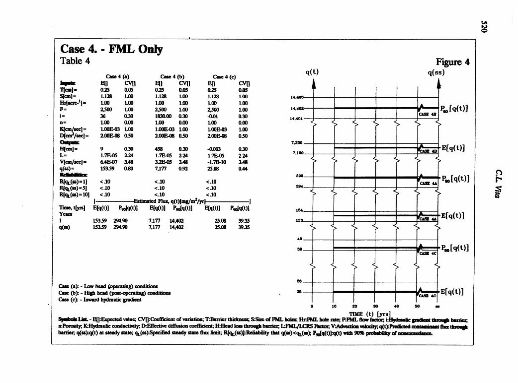
tA
f
Case 4. - OnlyTable 4 Figure 4
Came4 (a) Ca_ 4 Co) Cue 4 (c) q(t) q(ss)e[l cv[! el] CVl] El] cv[]
TIll = o_ o_ 025 o_ o_ 0.o5 iS[¢m]= 1.128 1.00 1.128 1.00 1.128 1.00Hr[acmJ] = 1.00 1.00 1.00 1.00 1.00 1.00 •F= _ 1.00 7.500 1.00 2.500 1.00 f Peo[q(t)]i= 36 030 1830.00 030 -0.01 0__0 cak_n= 1.00 0.00 1.00 0.00 1.00 0.00
K[cm/_c]= 1.00E4)3 1.00 1.00E4B 1.00 1.00E-03 1.00D[cm2/mcl= Z00E-_ 0.5O Z00B_ 0.50 Z00F_ 0.50
7,2ooHtcml= 9 0.30 458 o3o _.oo3 o_o .E[q(t)]L= 1.7F_,.05 2..24 1.7E.05 2.24 1.7E.05 2.24
V[cmfle¢]= &4P_AT/ 3L48 3OJffAl5 3L48 -1.TB-10 3.48q(u)= 153.59 0.80 7,177 0.92 25.08 0.44
R[qL(m)= 1! <.10 <.10 <.10 Pro[q(t)] P'R[qL(_)=5 ] <.10 <.10 <.10 e_R[qL(s) = 10] < .10 < .10 <.10
I .]EstimatedFlux,q(t)[m_m2/yr] ITune, t[ymi E[q(t)l Pm[q(t)] E[q(t)] P_e[q(t)] E[q(t)] P_e[q(t)lYeam1 153.59 294.90 7,177 14,402 25.08 39.35q(m) 153.59 294.90 7,177 14,402 25.08 39.35
P.[q(t)]

Case 5.- FML/GeosyntheticOayTable 5 Figure 5
c,,e5 (.) cme 5(b) crees (e) q(t) q(ss)
eli CVl] eli CVl] eli CVl]T[cm]= 10.25 0.05 10.25 005 10.25- 0.05S[em]ffi 1.128 1.00 L128 L00 L128 1.00 _,
Hr[ac_-l] = I_I) 1.00 1.00 100 L00 1.00Pm[q(t)] !i= 0.91 030 45.70 030- -18,_ 0.30 _ _ ..W
n= 0_ 0.10 0._6 (L10 036 0.10 .fKlau/_c}= L0_09 1.00 L00e_ L00 L0m_09 L00 . _"_ _V[cm2/s_c]= 6L_EA)7 0.50 Tx_ 050 _ 030 s
H=[em] 9.328 0__i0 468,425 0._ -187.575 0__I0 7 _ sc
L+ 7.1B-04 1.87 7.1F.04 137 ?.1E_ _ _ _ _ _. E[q(t)] _]V]cm/sec]= 1_.,-12 2.99 9.1E-11 2.99 -3.6_11 _ " _ _ ec
q(m); _1 o45 _ _4s _sl _4s s / _a-itelialmTmim:
R[qL(sS)ffiI] <.I0 <.10 <.10 ' ,
R[qL(=)=ml 0.SS 0_ 0_I ._ Flux,q(t)/mg/m2/yr] I e . ..
Tune,t[_] l_q(t)l P_q(t)i Elq(t)! r_q(t)] Ell(0] r_dq(t)l1 4..56 8.66 4.56 8.66 4.56 8.66 ! -i _.2 6.04 10.34 6.05 10.34 6.04 10.34 • /x_ |3 6.42 10.47 6.42 10.48 6.42 10.47
4 6_54 10.48 6.55 10.48 6.54 10.48 o lo zo 80 40 so ,= _15 6.59 m.48 e_s9 _48 _ _4_6.61 I(L48 6.60 10.47 TIME (t) [.W's]6 6.60 10.48
7 6.61 10.47 6.61 10.48 6.61 10.47
q(m) 6.61 io.47 6.61 10.48 es_ _0.4v
case (-_ -t,_wbrad(_ _c_ (b_-ms_ hma(eou-oeumi_mnaiammC_ (e):-Uremia_ zmak_
Sj_ Lm.-_ vaU_CV[l._.oemc_mo_o_ T'J_m_ertt_tam_ S_ _FML_m_ Hr.Pt_ t_e m_ _ ao,_am_ t_tm,_p,Smt em=_ _uim___, _ _ _._ _ _ t_tkad kmauuu_ _ L_m./LC_SX_em_V-.t_S_em_ q(t_ =mmimma._e,,_._bmier, q(m):q(t) at steady ate; ch.(m_ steady state flux limit; R[q_(m)]:Rgliabaity that q(m)<qL(m); P_q(t)]:q(t) writ 90_ laOlmblttyof
tObm.t

C.L Vito
522
Figure 6.
Case (a)-Low head(operatlns)conditions Case(b)-High head (post-operating)conditions
E[q(t)] E[q(ss)]
?,NO
F
E[q(t)] E[q(es)] " .......... _ J""_il
,o.... / ....... ..... /o '/
X
7 ? J cam g
/ -6 . ...... _ _.....
,dr
4 4 _ ......
$ $ ....
i
0 0 -- ,
0 10 80 30 40 04) u 0 tO 80 80 40 60 Jm
TIME (t) [yrs] TIME (t) (yr*]_v_
P.o[q(t)] "" P.o[q(ss)]
P.o [q_t)] , Poo [q(ss)].... /- --
fCJdlB49
ak
, , • /r,,
. f C_.,X /
6 / , _ It&
r ,o r .r0 ,, • 9 /
..... 8
4 ...... • 4
: s
_ v'C_8 sa8 _ ,,,--- YcAn _ s
f_ vo i._.,.-" o -'-' _"
0 10 _0 30 40 60 so o IO 30 _0 40 60 88
TIME (t) [yrs] TIME (t) [yrs]vC_vw eL R
SS = STEADY STATE; E[q(t)] = EXPECTED VALUES; Peo[q(t)] = 90_ NON-EXCEEDANCE VALUES
q(t) in mi[/m2/yr (Cl=l ml/L);

ea_s O,otosytadOooum_mSastnmas,t_523
FINITE ELEMENTANALYSISOF A SOIL NMLED WAIA,
JosephA.Calbndo,KevlnC.WemsekHuey 8. Nhan_ Loren R. Anderson
All. Utah State Uelventty,Depertmentot QvU& EnvJro EnSJneer
ABSTRACT
Soil naris are flndin8 increased use by Transportation Departments on wldentn8project_ where a vertical wall stabill_d with nails is used to replace soil benin at bridgeabutments. Soil nails provide an economic "top down" method for widening roadwaysbeneath existing bridges.
A sou nailed wall was constructed to accommodate the widenin8 of Intenttate$ northof Portland Oregon. The total length of the wall is 256 feet, 165 feet of which is locatedunder an existing bridge. The height is 19 feet. Five rows of nalb were installed at ahorizontal spacing of 4.5 feet and a vertical 5pacingof 3 feet and were approximately 18 feetin length. The soil nailed wall was instrumented with slope tn¢linometers, strain geges, andelectric load cells to measure and record lateral wall deflections and stress distributionalongthe nail lengths. t
The finite element computer program SOILSTRUCT (Filz, Cloush, and Duncan,1990) was used to analyze the soil structureinteraction of the wall/nail system. Quadrilateralelements were used to model the soil mass and hyperbolic soil parameters described the soilproperties. Bar elements with interface elements modeled the nails. Both quadrilateral andbeam elements were used for the wall itself. A complete report on the finite elementanalysis is provided by Nham, (1993). Wall deformations predicted by the finite elementmodel compared well with the measured results.
SOIL NAILING
A complete discussion on the principals of soil nailing is provided by Elias and Juran,(1991). The soil nallin8 process consists of a reinforced shotcrete facing constructedincrementally from the top down. Soil nails (often referred to as "inclusions")are driven orgrouted into the wall face at predetermined locations. These provide tensile, shear, andbending stress resistance. The procedure is summarized as follows:
(1) An initial unsupported cut is made.(2) Drainage materials are provided.

J.A. Callendo and others524
(3) The expmed face is covered with reinforced shotcrete.(4) Naris are ImtaUed at predetermined locations.(5) Repeat steps 1.4 through the final elevation.(6) The nails may be prestressed to a relatively low level.(7) A cast in place or prefabricated facing may be connected
to the final shotcrete face.
An increasingly popular application of soil nailing technology in the highwayindustryisto replaceexitingm/lterm belowbridges at the abutments thus providing additionalroadwayw/dt
CASE HISTORY DESCRIM'ION
The soil nailing case history used for this study provided subsurface siteparameters and wall response measurements and is well documented by Sakr andBarrom, (1991) and Dumas, (1991). The soil nailed wall was constructed toaccommodate the widening of Interstate 5 (Swift-Delta Highway), north of Portland,Oregon under the existing Oregon Slough Bridge (M.P. 307.46). Figure I shows therelative position of the soil nailed wall and the bridge. The existing abutment is pilesupported by a single row of 14 inch diameter concrete titled steel pipe piles at 4 foot 5inch centers. Soil nails were installed between the piles. The end slope fill consisted of afine sand with traces of silt.
The wall is located under the south end of the Oregon Slough bridge Theconstruction process required that the w/dening profess from the top down. Thereforea son nailed wall was utilized for lateral earth support. Other methods were not usedbecause of restricted space, and economic considerations. In order to evaluate theperformance of th_ wall, it was instrumented with slope inclinometers, strain gauges,and electric load cells to measure and record lateral wall deflections and the force
distributiom along the length of the nail. These measuring devices were implemented intwo monitoring sections.
This paper will focus on the deflection measurements obtained at section #2located west of the pile.supported bridge abutment. Section #1 was not analyzed with afinite element analysis because it is located adjacent to the bridge abutment, where thepiles complicate the interaction of the soil nailed wall.
Soft Nailed Wall Description
The total length of the soil nailed wall is 256 feet, 165 _eet of which is locatedunder the Oregon Slough Bridge. The maximum height of the wall is 19 feet. Based onthe stability analysis and physical constraints, a horizontal nail spacing of 4.5 feet and avertical nail spacing of 3 feet were used. There were a total of 5 rows of nails. The topfour rows were oriented at 15 degrees from horizontal; the bottom row was installed at25 degrees. The nail lengths ranged from 17 feet to 18 feet. The wall geometry is shownon Figure 2.

|
, FiniteKlememAnalydjo/A_olINailedWall 525
Submrfkce ConditionsThe soil west of the bfldge abutment near section #2 was generally loose silty fine
sand with varying amounts of moisture. Large concrete pieces, rock boulders, and metaldebris up to two feet in diameter were encountered during test p/t excavation of the topsix feet, The ground water table was located five to six feet below the bottom of thewall.
Construction MethodsThe construction of the soft ha/led wall consistedof the following sequence:(I) Testin_ the pre.product/on naristo verify the Contractor's ddlflng
p_dure, the proposed maximum 5 inch diameter nall hole, and the_outing method.
(2) Excavation of the end berm in stages.(3) InstalHngthe steel welded w/re mesh.(4) Apply/ng the structural shotcrete materials.(5) Drilling nail holes with the "cased hole drilling method".(6) Installing the epmy-coated #9 Dywiclagbars and grouting the nail holes.(7) Placing the six inch by six inch steel b-_g plate and tightening the
bearing nut.(8) Repeating step (I) through (7) for the subsequent excavation steps until
the desired elevat/on is reached.
InstrumentationVibrating wire strain gauges, electr/c load cells, and slope inclinometers were all
used on the project. The vibrating w/re strain gauges were mounted in pairs and equallyspaced along the length of each nail. The strain gauges were used to evaluate the axialforce dism'bution along the length of each rows of nails. Three electr/c load celts wereinstalled on the nails of rows I, 3 and 5 to mon/tor nail load buildup at the nailanchorage. The ground movement in the vicinity of station two was monitored with twoslope inclinometers installed 10 feet and 38 feet west of the bridge, and approx/mately3.5 feet behind the wall.
HNITE ELEMENT ANALYSIS
Computer ProgramThe computer program SORM'RUCT (Filz, Clough, and Duncan, 1990) was used
for the finite element analysis. This program has been widely used in both academic andengineeringpracticeto model lateral support systems. SORM'RUCT can simulatearbitrarysequences of/ncremental construction and loading steps under plane strainconditions. The different functions of the program allow various Oeotechnicalengineering projects to be modeled. The following incremental comtruction steps maybe simulated:

526 J.A.CaHendoandothers
(I) Excavating.+(2) Fmi.8. ,,(3). -watering.,+(4) Installing struts, tie-backs or nails for excavation support systems.(5) Removing excavation support systems.(6) Applying a specified sequence of loads, such as concentrated loads,
boundary pressures, and loads induced by a change in temperatures.(7) Installing beam elements, and (hanging material types in a construction
step.SOH.STRUCT utifizes+ahyperbolic relationship suggested by Duncan et al. (1980)
to model the non-linear stress strain properties of the soils. A piece-wise linear stress-strain response is used to approximate the nonlmear stress-strain response of so/Is.
" SOH.STRUCT utilizes an incremental load analysis to create the piece-wise linear stress-strain response. The incremental process may result in a divergence from the true stress-strain curve. Chang and Duncan (1970) have ind/cated that the accuracy may beimproved through the iterative analysis of load increment. For this process, an incrementis analyzed at least two times. The modulus values are evaluated using the averagevalues of stress from the previous increment and the first iteration during the secondanalysis of the load step. The SOH..STRUCT program allows the user to specify thenumber of iterations for each increment and the number of increments associated witheach load step. During the iterations, the unload/reload modulus is used when thedeviator stress decreases until the deviator stress for the current element exceeds the
maximum past value.Four different element types were used to model the soil, wall, and nails. These
elements were:
(1) A two dimensional, .-ubparametricoquadrilateral element (soft and wall).(2) A one dimensional, two-node bar or spring element (nail).(3) A one dimensional interface or slip element (nail/soil interface).(4) An Euler-Bernoulli beam element (wall).
Ouadrilateral Element. Doherty et al. (1969) developed a two dimensionalsubparametric (OM5) quadrilateralelement to represent soils and some structuralmaterials. The geometry of this element is defined by four external nodes, while thedisplacement functions include an internal fifth node. This fifth node improves theflexural response of the element. Aumrding to Tsui (1974), the quadrilateral element isbetter than a beam element when doing fin/te element analysis because the beamelement has no thickness. Therefore, no mesh space is allocated for the actual walllocation. By using a quadrilateralelement to model the wall, there is no problem withincompat_ility between adjacent elements since they are the same element type.
Bar Element. One dimensional bar or spring elements are used to model thebehavior of braces or tiebacks. In this study, two node bar elements are used to simulate

FiniteElementAnalysisofA SoilNailedWall 527
thereinforcingnail.Thesebarelementsarenotincludedinthefiniteelementsmeshinitially.Theyareplacedduringtheconstructionsteps.The _)_UCT usercanspecifya certaindisplacementtosimulateslackinthenailspriortoresistingtheloads.No pre-displacementconditionswereplacedonthebarelementsinthisfiniteelement
study.
Interface Element. One dimensional interface or slip element elements wereplaced between the quadrilateral elements (soil) and the bar elements (nails) to perm/trelative movement between the two. Four nodes are used to defme the element with
two adjacent nodes having the same _inates. This element possesses no thickness.D/fferent relative movements ranging from complete slippage to no slippage can bemodeled at the interface depending on the specified interface element st/ffness.
Beam element. An Eulcr-Bernoulli beam element using hermite interpolationfunct/om was ut/lized in place of the quadrilateral elements to model the soilcrete wallfacing for the FEA. In addition to resisting axial stresses, the beam elements providebending resistance. In SOILSI'RUCT, the connection between beam elements is fixed,providing bending moment continuity between elements.
Finite Element Model. Three finite element models were used in the study. Twomeshes consisted of 296 nodes and 275 elements. The third mesh had 312 nodes and
290 elements. Sixty interface elements were included in each of the meshes. Thedifferent meshes resulted from different approaches in modeling the shotcrete wall.Mesh #I models the wall with a single column of quadrilateral elements. Mesh #2 usesbeam elements; and mesh #3 contains two columns of two dimensional quadrilateralelements. Mesh #3 is shown on Figure 3.
SIXbar elements are used to model one reinforcing nail. Accompanying the barelements, twelve interface elements are placed at the soil-nail interface. No interfaceelements are positioned at the soil-wall interface.
Construction StepsIn order to simulate the actual construct/on progress of the soil nailed wall, six
loading steps were applied sequent/ally in the _n/te element model. These steps are thefoUow/ng:
(I) Excavate the first two rows of elements as shown in Figure 3 and installthe first row of nails.
(2) Excavate the next four rows of elements, and install second row of nails.(3) Excavate the next one row of elements, and install third row of nails.(4) Excavate the next two rows of elements, and/nstall fourth row of nails.(5) Excavate the next two rows of elements, and install fifth row of nalis.(6) Excavate the next row of elements to a depth of 19 feet.
, , r_ II " I[I

528 J.A.Caliendoandothers
Allthesoilelementsareinitiallyinthemesh andremainevenafterexcavation.However,astheyareexcavated,SOH..STRUCT assignsthem thephysicalpropertiesofair (Le weightless and no stiffness)
Wall ModelingThe shotcrete wall was represented in the finite element mesh as a single column
of two dimensional quadrilateral elements (model #1), by beam elements (model #2)and by a double column of two dimensional quadrilateral elements (model #3). The wallis assumed to behave elastically and homogeneously. A Young's modulus was calculatedfrom the _ equation: E ffi 57000 x f'© where f© ffi 3,000 psi
For the beam element wall, the moment of inertia (I), cross section area (A), andheight or thickness must be entered along with E. Based on an assumed wall thicknessof 6 inches, an I of 216 in4 per foot of wall was used with an area of 72 in2 per foot ofwall.
The a_tml Young's modulus of the third wall model must be adjusted toaccommodate the two column thick model. The model Young's modulus (En) isobtained by first determining the model moment of inertial (Im)based on the width andunit length of t_,e modeled wall, then the rigidityof the model (EI), is set equal to therigidity of the actual wall (EI),. An Emof 390,000 psi was used for this modeL
Soft ModelingIn order to correctly model the soil response, SO_UCT requires that both
conventional and hyperbolic parameters be included in the input. The conventional soilstrength parameters used in the actual design were used for the finite element analysis.These consist of: cohesion 100 psf, friction angle of 330, soil unit weight of 115 pcf and alateral earth pressure coefficient of 0.43.
The hyperbolic parameters are used to define the non-linear (i.e. hyperbolic)stress - Strainresponse of the soil mass. These values are determined from a series ofsteps using data from either unconsolidated-undrained or drained triaxial tests. Detailedinformation for developing these parameters are provided by Duncan et al. (1980). Alsoshown in this reference is a compilation of hyperbol/c parameters recommended whentr/axial results are not available (as was the case for this study).
Nail Reinforcement ModelingSix bar elements were used to model the reinforcing nails. The bar elements are
connected end to end to form a nail. The orientation of the nails are shown on Figure 3.The top four rows of bar elements and the bottom row of bar elements are inclined at 15degrees and 25 degrees from the horizontal respectively.
The composite grout-steel reinforcing nails are assumed to behave elastically andhave perfect bonding between steel and grout. Therefore, an equivalent steel crosssectional area can be used in the finite element model. For this model, with a steel bar

FiniteElementAnalysisofA SoilNalli_dWall529
areaofI in2andgroutingareaof19.6in2,an equivalentareaof3 in2wasusedformodelnail,The calculationsareasfollows:
@ n ffi _c = 29000000 psi_122018.6 psi = 9.289@ Area_'= AreaJn = (18.63 in2)/9.289 = 2.0 in2@ Total equivalent steel area -- Area_ + Area,'@ Total equ/valent steel area = (2.0 + 1.0)in2 -- 3.0 in2
The stiffness (AE/L) of the actual nails are divided by the nails' spacing toaccommodate the plain strain conditions. The model nail st/ffness (AE/L).. is set equalto the actual nail stiffness (AF_JL)a.The nail st/ff_ess that were used for the finiteelement analysis are shown below in table 1.
Table 1. Model bar element st/ff_ess for the model ha/Is (Ib/ft/ft).II I ,, . H
AF./L AE/L AE/L AF3L AFJLNAIL #1 NAIL #2 NAIL #3 NAIL #4 NAIL #5
6.787F_J5 6.787E6 6.445E6 6.807E6 6.458E6
Soft.Nail Interfhee MedeHngA total of sixty interface elements are utilized at the soil-nail interface. The
interface elements are placed on the top and bottom of the bar elements, and areinitially in the finite element mesh. An interface element does not have any thickness;consequently, it appears like a bar element with only two nodes.
COMPARISON OF FEA WITH FIELD RESULTS
Measured Deflections
As discussed previously, there were two monitoring stations, SD129 and SD130, atsection #2 where wall displacements were measured. The displacements at differentconstruction stages were recorded. Figure 4 shows the displacements which occurred atSD129. The maximum outward displacement of the wall occurs at the top and decreaseswith depth.
Predicted ResultsSinele Column - Ouadr/lateral Element Wall Model. The lateral wallv
displacements, at the end of each construction step, predicted by SOILSTRUCT for awall modeled with a single column of quadrilateralelements are shown in Figure 5.Steps one to five involved excavation and installation of each sequential nail row. Stepsix is the final excavation.
Beam Element Model. The predicted deflection of the beam element wall modelat the end of each construction step is shown on Figure 6. Steps one to five involvedexcavation and installation of each sequential nail row. Step s/x is the final excavat/on.

530 J.A.Caliendoandothers
The beam elements are rigidly connected. This, combined with the outward deflectionof the top of the wall and the inward pressure of the unexcavated soft at the base of thewaft result in an inward (negat/ve) displacement of the wall during the first two phases ofthe construction modeling. Modeling the whole shotcrete wall/nitially in the soil does notrepresent the actual condition since the shotcrete wall is constructed after the staged soilexcavations. In spite of this limitation, the beam element model prov/des satisfactorydisplacement results at the end of construction. The bean_ elements provide flexural orbending resistance to the shotcrete wall, whereas the quadrilateral elements do not.
Double Column - Ouadrilateral Element Wall Model. The predicteddisplacements of the double column quadrilateralelement wall are shown on Figure 7.This mesh results in a smoother wall deflection as compared with the single columnmodel.
Conclusion
The end of construction wall displacements for the three wall models arecompared to the measured results (SD129 & SD130) on Figure 7. Overall, the beamelements did a better job of modeling the displaced wall (at end of construction) than dideither combination of quadrilateral wall elements. The quadrilateral element wall modelswere much too flexible in the lower parts of the wall and provided accurate walldisplacements only at the very top of the wall. The beam elements, on the other hand,modelled the stiffness of the wall extremely well indicating that the shotcrete wall hadsignificant bending stiffness. The only exception to this is near the top of the wall wherethe beam element model is stiffer than the actual wall and underestimates the top of walldisplacements. This is most likely due to cracking in the upper portions of the shotcretewall, resulting in "hinges" that allows these large displacements to occur.
If SOILSTRUCT allowed for the modification of rigid beam joints to includesome flexibility,and the upper two joints in this wall model were so modified, this beammodel would be very capable of modeling quite accurately the displacements for theentire wall.
Finite Element Analysis of A Soil Nailed Wall 531
BIBUOGR&PBY
Chang, C-Y. and Duncan, J.M. Nonlinear Analysis of Stress and Strain in Soft. Journalof Soil Mechanics and Foundations Division, ASCE, Vol. 96, No. SM5,; September, 1970.
Dumas, Christopher. Permanent Soil Nailed Wall I-5 Portland, Oregon. 1991; 41 poTraining Report to the Federal Highway Administration.
Duncan, J.M.; Byrne, P.; Wong K.S.; Mabry, P. Strength, Stress-Strain and Bulk ModulusParameters For Finite Element Analyses of Stresses and Movements in Soil Masses.Geotechnical Engineering. 198_, 70 p. Department of Civil Engineering, University ofCalifornia, Berkeley.
Elias V.; Juran I. Soil Nailing For Stabilization of Highway Slopes and Excavations.Federal Highway Administration, Publication # FHWA A-RD-89-193, June 1991.
Filz, G.; Clough, G. W.; Duncan, J.M. Draft User's Manual For Program Soilstruct(Isotropic) Plane Strain With Beam Element. 199_, 50 p. Virginia Polytechnic Instituteand State University, Department of Civil Engineering.
Juran, I.; Elias, V.; M. ASCE. Soft Nailed Retaining Structures: Analysis of CaseHistories. Geotechnical Special Publication No. 12. 232-244; 1990.
Nham, Huey S. Finite Element Analysis of a Soiled Nailed Wall and Case HistoryComparison. Master of Science Report. 1993;90 p. Department of Civil and Environmental Engineering, Utah State University, Logan,Utah.
Sakr, T. C. Soft Nailing: Its Applicability To Bridge Embankment Retention. Report-Oregon Department of Transportation, Highway Division, Bridge Section. 1991; 12 p.
Tsui Y. A Fundamental Study of Tied-Back Wall Behavior. Phl) Dissertation. DukeUniversity. 1974. 258 p.

532 J,A.Caliendoandothers
Figure I. Oregon Slough Bridge(Source: Sakr e_ al., 1991)
Figure 2. Soil nailed wall geometry at sect/on #2(Source: Sakr et aL, 1991)
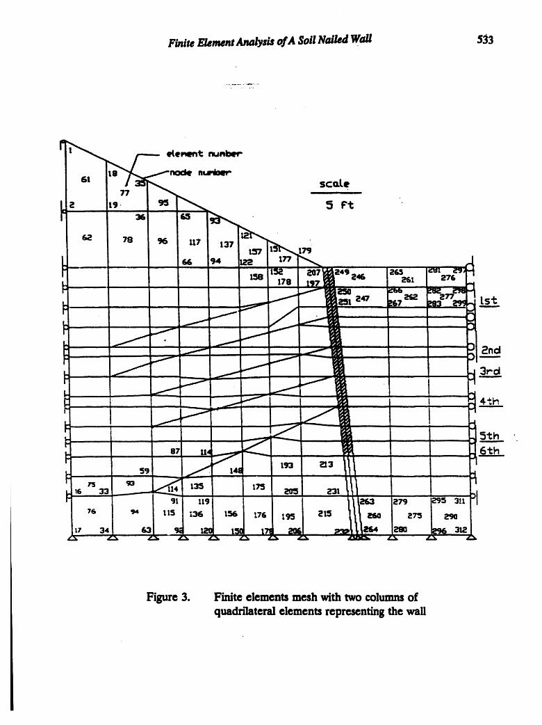
Finite ElementAnalysimofA SoilNailedWall 533
elementnunlm_
nuu,_loerSt sccLe
77
e tg. 5 _t
36 G5 _ •
G2 78 56 117 1371_-_''=r7 1t'_ _
d
158 1_?. LmO7_249;_4G 2% 1 _:uz27G_7
, I;,o ,,7__ z' '_ %__"'
¢i' _ .... 2nd
__ , ImI.' , - _,--'_ _I_ , _ 4.-':..,._..,..h.__
: , 59 _f . 148
" 91 119 279 295 3It
76 94 115 ;36 156 _7G t_ _| Z75
17 34 63 . _ 12C 150 |7_ 2QG . 280 _ 312
Figure 3. Finite elements mesh with two columns of
quadrilateral elements representing the wall

534 LA.Caliendoandothers
27.0026.0025.0024.00 "
23.00 "22.00 "21.00 "20.0019.00 "18.0017.00 "
16.OO /..15.1111
._ 14.111113.OO
ml_OO ..11.00
IO.O0 •9.1111
8.1111
7.OO ",8.1111 _
5.1111" _
4.1111 " _3.1111-I
2.OO 4
1.1111_
0.1111 ,
0 0.5 1 1.5 2Displacement(in)
--41---12-9-90 -4-- 12-15-90 -a_ 1..5-91 _ 1-12-91 _ 1-23-91 _ 2-2-91I I I I I I
Figure 4. Measured displacements, SD129

Elevation(ft)-.-= --= _ --= --= --= -.-= I_ I_ I_ I_
t,A

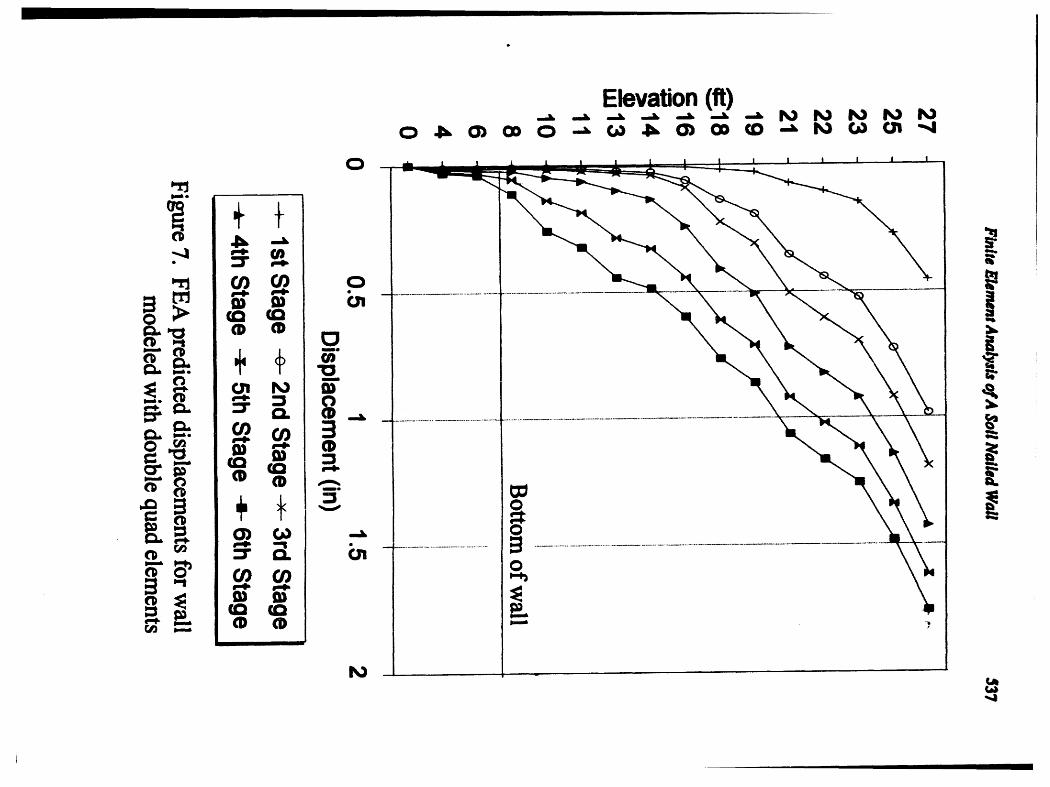
_ Illll

538 JjL Co//endoando=_urrs
..... i,
E18 - b i=16 _ _ I +
j14 i i i13 + 1 I+m-- i , +11 i ! '10
8 G/ ! i+ Bottomof wall
i ! J t •
6 I ! +4 ! Ji i
0 - I i t i
-0.2 0 0.2 0.4 0.6 0.8 1 1.2 1.4 1.6Displacement(in)
-+- One-2D -e- Beam -x- Two-2D -_- SD129 -x- SD130I I
Figure 8. FEApredicteddisplacementsvs. measureddisplacements,endof construction

Hydroseolosy, Wits Disposal,Science s_ Politics_p 3o_ s_po._m 539
AMoJnedCapModdIml__ in DYNA.3D
ham G. Iardanohn, Thomas H. Fronk2, Loren 1_ Anderson_
AImmct
In 1957, Drucker, Gibson and Henkel [1] were the first to introduce the concept of work-hardening theories of phmicity into the soil mechanics, and using the hardening cap to controldilatency. This cap model and all of the recent ones are based on Drucker's stability postulates.Good results have been found using cap models. Most of these versions of cap models have been
implemented in many specialized finite element codes, as well as general purpose finite elementcedes, such as DYNA-3D. A cap model is included in DYNA-3D, but there are problemsmodeling certain materials. The cap model is considered as a complicated material model dueto the fact that it consists of three surfaces (the yield surface, the hardening cap, and the tensioncutoff), which are intersecting in an nonsmooth fashion. In this paper, a modified cap modelbased on Hofstetter et al. 1993 [2] implemented in DYNA-3D is presented. The modified capmodel incorporates a return mapping algorithm of Simo et al, 1988 [3] end Simo and Taylor,1985 [4]. Koiter's generalized flow rule, Koiter, 1960 [5]. Kuhn.Tucker optimization conditionsare also applied to the modified cap model. The Newton iteration technique for solving thenonlinear equations is used. This makes the convergence quadratic, i.e. faster and less computertime consuming. Finally, evaluation of the model is presented by comparing the results to theoriginal DYNA-3D cap model which was developed by Simo et al, 1988 [6], and to test results.
1.0 Introduction
The cap model is based on classical incremental theory of work hardening plasticity. Itwas developed as part of a constitutive model to account for important characteristics ofgeological materials such as compaction, hardening, end failure. The cap model differs fromother geological elasto-plastic models, in that the hydrostatic stresses are limited by capping thefrictional failure envelope.
DiM_,gio and Sendler [7] first introduced the cap model in 1971, and since then severalversions of cap models have been successfully developed [8-16], as _own in Table (1). As a
mammm
1Research Assistant, Civil and Environmental Engineering, Utah State University,Logan, Utah.
2Assistant Professor, Mechanical and Aerospace Engineering, Utah StateUniversity, Logan, Utah.
aProfessor and Department Head, Civil and Environmental Engineering, Utah StateUniversity, Logan, Utah.

540 I.G. Jardaneh and others
Table 1 Featuresand Shortcomingsof Cap Models.
ii i ii i i i I
.Developers/Year Features Shortcomings RefII ii I I
DiMaggio, _mdler The t'u_tcap model, INucker- Linear elastic. [7]1971 Presar yield surface with an Not 8enerelizod.
elliptical hardenins cap.i |1 ii i I i i
Sandier, DiMq_o, and Oeneralizod cap, nonlinear elastic, Numerical problems. [8]Baladi and tension behaviors are specified.1976
ii , i
Sandier, _88io, and Vertical _ cap. For rocks of low porosity, and [8]Baladi lcadins and unloadin$ bulk1976 modulus are thesame.
i | , i
•mdler,DiMauio, and Extensionofthecapmodel to Same astheorisinaloapmodel. [9]
Baron include pore pressure and1984 kimmmio _ effects.
I,[II I ii i,
Ketone ViK_oplasti©type cap model. Numerical solution problems, [I0]1984 tension cutoff and viscous
tension dama8e index need, andalso hardening/softeningfunction need modifications.
H m , ,,,
Remmda and Martin Dmcker-Praser cap model. It my Stability problems under certain [11]1985 harden or soften and coupled to the conditions.
yield surface.iinll| ii ,i
Faruqus and Chans Same parameters for both failure Still under improvements. [12]1986 surface and the yield cap.
ii ill
Baladi and Schuster Cap model with strain-dependent Can_ be used for all 8eolosiaal [13]1987 elastie moduli, materials.
i| iii i
Faruque Cap model for plain concrete. Plain For concrete only. [ 14]1987, concrete failure surface inelmiin8
thehardeninscap.i ii i i ii iiii
Simo et al DYNA-3D eap model. Consistent Doesn_ work as advertised. [6]1988 numerical solution (elosNt- point
projection), with viseoplufioextension (rste-dependent).
li ii
General Atomic Failure envelope and hardenin8 cap Still under improvements. [15]1989 are represented by on curve. Permit
8radual yieldin8 at the cap.,,,,
• Abduljawwad et al Modified the orisinal cap model to Just appeared. [16]1992 include the third invariant sereu
tensorand also the kinematic
hardeningrule.

A Mochfied Cap Model Implemented in DYIVA-3D541
result of these investigations, more sophisticated cap models have evolved with a number offeatures which can be included or excluded in specific problems. These features includeanistorpy, rate-dependency, pore pressure effects, and elasto-viscoplastic modelling.
The cap model has been used to study various geotechnical problems, such as groundshock effects from explosive sources, and soil-structure interactions problems, including buriedpipeline, retaining walls, foundations, embankments, in situ tests, etc. Good results have beenobtained using the cap model which make it well known and commonly used for solvinggeo_chnical problems.
However, like other models, the cap model has some shortcomings such as, it is usuallyassumed that the isotropic model is independent of the third invariant of stress, a discontinuityis created at the intersection of the failure curve and the hardening cap, a non-continuous yieldsurface will cause computational difficulties, and the hardening cap is not defined in terms ofboth the shear and the normal plastic displacements.
In this paper a modified cap model that is implemented in DYNA-3D is presented, withits new features. Including return mapping algorithm, Koiter's generalized flow rule, Kuhn-Tucker optimization condition, and Newton iteration technique to solve nonlinear equation_.Conclusion and recommendations are also presented.
2.0 Cap Model
In this section a description of the modified cap model features are presented; the capmodel surfaces, Koiter's generalized flow rule applied to these surfaces, Kuhn-Tuckeroptimization conditions that will specify the activation of each mode, return mapping algorithmthat will determine the value of the final stress for each increment, and finally, thecharacterization of the six different modes of this modified cap model.
2.1 Cap Model Surf_es
The surfaces of the modified model are plotted in stress space, as shown in Fig. (1) [2],in which the coordinates are the Ji (the first invariant of the stress tensor), and I sl (the norm ofthe deviatoric stress tensor s). Three surfaces characterize the cap model. These are, the fixedfailure envelope surface, the cap surface, and the tension cutoff surface. Details of these surfacesare presented below.
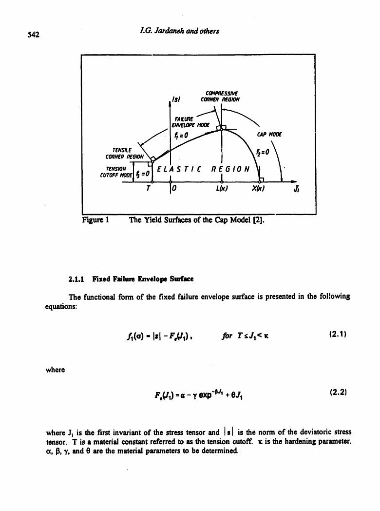
542 LG. Jardaneh and others
COMI_£$$1VEIs/ COnN_n_mON
FA_mE _ _
. X+:o\r,Ns,o,I. _ELASTIC REGION _ I"
lO L(_) X(x)T
Figure I TheYield Surfaces of theCap Model [2].
2.1.1 Fixed FailureEnvelope Surface
The functionalform of the fixed failure envelope surface is presentedin the followingequations:
_(a) ..Isl- F.(J',), for T<JI<¢ (2.1)
where
F.(J1)=a - t' exp"lU'+ 0,/1 (2.2)
where J_is the first invariantof+the stress tensor and Is] is the norm of the deviatoric stresstensor. T is a materialconstant referredto as the tension cutoff'. K is the hardeningparameter.(x, [3,Y,and 0 are the materialparametersto be determined.

A ModifiedCap ModelImplementedinDYNA-3D $43
2.1J Hsnleaing Cap
The functional form for representing the hardening caps are presented in the followingequations:
/=(o,,=)-F,,(I.I,J_,_=)- F.(,=) .forI: ":'/t < XO¢) (2.3)
where
1 ['/1-L(K)]e (2.4)F,(l,l.,rl._)= Isla+
X(K) is the intersection point of the cap the J! axis. R is the shape factor which is the ratio ofmajor to minor axes ofthe ellipse. L(K) is the value of J! at the intersection of the cap and the fixed failure envelopesurface. It is defined as
where Kis the hardening parameter.
The point of intersection of the cap with the J! axis is defined as follows:
X0¢)==¢ , RF.(K) (2.6)
2.1.2.1 Hnnlening Behavior of rise Cap
The parameters required for the hardening behavior of the cap are presented in thefollowing equation:
= W(1-exO_'x(_)}) (2.7)
D, W, and Z are the material parameters which govern the hardening behavior of the caps;
. LG. Jardaneh and others544
where W characterizes the maximum plastic volumetric strain, D denotes the total volumetricplastic strain rate which controls the initial loading moduli, andZ determines the initiation of thevolumetric plastic deformation under hydrostatic loading conditions, s, P is the effectivevolumetric plastic strain corresponding to the point X(K), defined by integrating the followingdiscontinuous equation
or I¢>0 and it>J1} (2.8)
Where _,P is the incremental plastic strain. The last equation was suggested is to avoid softeningbehavior, accordingly if the stress point is at the compressive comer point, movement of the capis prevented and the model behaves as perfect plasticity.
2.1.3 Tension Cutoff Sud'ace
The functional form of the tension cutoff is
fs(o) = T-J1, :for J1 = T (2.9)
where T is as defined above, a material constant referring to the tension cutoff.
2.2 Koiter's Normality Law for Singular Yield Surfaces
Koiter, 1960 [5] proposed an associated flow rule for both elastic perfectly plastic, andwork hardening materials. Singular yield surfaces with edges or comers are considered as a finitenumber of regular yield surface functions f,(o), such that the elastic domain is given by
f,,(o) <0, where (z = 1,2,... (number of surf_cs) (2.10)
The yielding will occur as soon as at least one of the functions f_(o) is equal to zero, allthe other yield functions being negative (i.e., at least one yield surface is provoked).
The associated flow rule for elastic perfectly plastic materials, as proposed by Koiter, thatwill give the value of the plastic strain rate is as follows:

A ModifiedCapModelImplementedinDYIVA-3D 545
J
where (2.11 )
AX,-0 W J'.<0 o_oZ,o tr S.-0. _.- _" _< 0;ao
AX._0 _f f.-0 and_.-0.
From the above equation,loading occurs if the stress rates are such that f_>O. Whileunloadingoccursif f_<O. Thiswill define _ as follows: it is alwaysnon-negativeand it is non-zero only if the state of stress is at the yield limit andno unloading occurs. It is noteworthytomentionthat_ is anindeterminateparameter,of dimension(time)"1.Time may be replacedbyany other parameterprovidedit increasesmonotonouslywith time. _ is not a materialconstant.
2.3 Knhn-Tueker¢onditiom
Plastic loading or elastic loading/unloadingis formulated in Kulm-Tuckerform. Theplastic strainrate is given by the associatedflow rule in the form of Koiter'sgeneralizedflowrule as shown above. It is satisfied Kuhn-Tuckercomplementaryconditions for cc-l,2,...,m:
A).,z 0j'.(o)_o
A)., f,(o)= 0 (2.12)
A_.j,(o)-o
The last equationis known asthe consistencyconditions.
From the above equation,the discreteKuhn-Tuckerconditions that governs the changeof the discrete consistency parameterA_. s are
A).t,,+1_ 0, /i,,_1_0 and (2.13)
A)-I,.+I /i, .+1 : 0 t:1,2,3
546 LG.Jardanehandothers
2.4 Return Mapping Algoflflun
In this model a general closest-point-projection algorithm [3,4] for multi-surface plasticityis used, which is unconditionally convergent, and is capable of accommodating an arbitrarynumber of yield surfaces intersecting in a nonsmooth fashion. The algorithm is basically consistsof two major steps, the formulation of the elastic trial stress, also referred to an elastic predictorand the return mapping to the yield surface, which is the closest point projection of the trial stressonto the yield surface, also referred to as a plastic corrector. For multisurface plasticity, usingKoiter's generalized flow rule yields the following return mapping algorithm
.D p p r _ (3_'_+1 (2.14)(.+1 = (. + A em+l = e. + 1-1 A _'i,.+1 u_Om.1
D/dO.+1 = C" (£.+1 - £ap) (2.1 5)
J, r,_ p (2.16)ol+1: C ' ((,+1-(,.1) = o,.s - C: A(,. 1
where AZ=.Z_i At and C is the elastic tensor.
The trial functional forms of the cap model surfaces can be calculated as follows
_ _ Ytfa/,,,.,I, )( I J'l, _+1_ TAd
12,.+1 =l_...+1 ( I*.-* I s J1, .+is K.) (2.17)rn_ _ rdd
.J_,..l r.l_, ..1 ( Ji, ..1)
where
s,.s = 2 G (e,.l - e_) (2.18)
Ji,_.l =3 -Jl_)
where G is the shear modulus, K is the bulk modulus, e is the devaitoric strain tensor, J! is thevolumetric strain, the subscript n+l and n refer to the time, and the superscript P refers to theplastic component.

A ModifiedCap ModelImplementedinDI'NA.3D. 547
The final stresses are obtained from
23 Implemenliq lhe Cap Model
Applying the return mapping algorithm and Kuhn-Tucker conditions for multisurfaceplasticity, six different modes of behavior are possible.
Depending on the trial stress, Kulm-Tucker conditions will specify the mode that isinvoked. Applying return mapping algorithm the final stress can be calculated.
2.&l mastic Mode
Elastic behavior occurs when the stress is within the failure envelope and deformationsare recoverable. This mode is characterized by the following equation
TaalJ_.l < O'P.fk...l < 0"_ A_'b,.q =0 t=1,2,3 (2.20)
Various types of linear and nonlinear elastic behavior can be implemented. However,most models only allow linearly elastic behavior. For linear elastic behavior a constant bulkmodulus, K, and a constant shear modulus, G, are required.
2.&2 Failure Mode
Failure occurs wh6n the stress point lies on the failure envelope. This mode ischaracterized by
J_,x-.l > 0, _Xl,_.,. 1 • 0 _ _'_'P..,x.,.1= A_'8,..1 = 0 (2.21)
Failure envelope may be either, fixed or movable (hardening) but are generally assumedto be fixed.
I.G. Jardaneh and others548
2.5.3 Cap Mode
The cap mode is initiated when the stress point lies on the movable cap and pushes itoutward. The motion of the cap is due to the plastic strain and models material hardening (thecap does not move during purely elastic deformation). This mode is characterized by
•f_l > 0, A_,2,m.1 > 00_ A_,I.:. 1 : A _,8.m.1 : 0 (2.22)
Although various geometric shapes can be used for the cap, elliptical surfaces have been foundacceptable for wide range of geological materials.
The compaction resulting from the associated flow rule leads to an increase in thehardening. Therefore the cap moves to the right, increasing the extent of the elastic region insidethe new yield surface.
The behavior of the cap depends on whether a soil model or rock model is used.
2.5.4 Tension Cutoff Mode
This mode is characterized by
•_,m.l > 0, A_,8,m.1 > 00_ A_,1_.1 : _'R,m*l : 0 (2.23)
The tension cutoff procedure may take various forms. For simplicity, the tension cutoffcriterion is chosen as Jl= T, in which T represents the maximum allowable hydrostatic tension.
2.5.5 Tensile Corner Mode
This mode invoke if the trial stress fall in the tension cutoff corner. This mode is
characterized by
A_I,,. 1 > 0, _'8,,.1 > 0 _ A_,_sJs.l : 0 (2.24)
Since both the failure envelope and the tension cutoff surfaces behave as ideal plasticity,the return stress point is the intersection of these two surfaces.
2.5.6 Compressive Corner Mode
This mode invoke if the trial stress fall within the compressive corner. This mode ischaracterized by
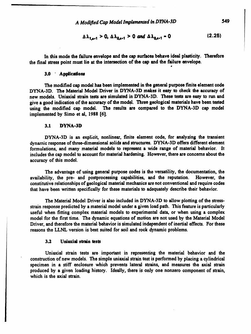
A ModifiedCap Mode!ImplementedInDYNA-JD 549
A).I,.. 1 > 0, A).l,.. 1 > 0 and A2,s,..1 -0 (2.25)
In this mode the failure envelope and the cap surfaces behave ideal plu_icity. Thereforethe final stress point must lie at the intersection of the cap and the failure envelope.
O
3.0 "Applications
The modified cap model hu been implemented in the general purpose finite element codeDYNA-3D. The Material Model Driver in DYNA-3D makes it easy to check the accuracy ofnew models. Unio, ial strain tests ere simulated in DYNA-3D. These tests are easy to run and
give a good indication of the accuracy of the model. Three geological materials have been testedusing the modified cap model. The results see compared to the DYNA-3D cap modelimplemented by Simo et al, 1988 [6].
3.1 DYNA-3D
DYNA-3D isan expl;cit,nonlinear,finiteelementcode,foranalyzingthetransientdynamicresponseof'three-dimensionalsolidsandstructures.DYNA-3D offersdifferentelementformulations,and many materialmodelstorepresenta widerangeof materialbehavior.Itincludesthecapmodeltoaccountformaterialhardening.However,thereseeconcernsabouttheaccuracyof'thismodel.
The advantageofusinggeneralpurposecodesistheversatility,thedocumentation,theavailability,the pre-and postprocessingcapabilities,and the reputation.However, theconstitutiverelationshipsofgeologicalmaterialmechanicsarenotconventionalandrequirecodesthathavebeenwrittenspecificallyforthesematerialstoadequatelydescribetheirbehavior.
The MaterialModel DriverisalsoincludedinDYNA-3D toallowplottingofthestress-
strainresponsepredictedbyamaterialmodelundera givenloadpath.Thisfeatureisparticularlyuseful when fitting complex material models to experimental data, or when using a complexmodel for the first time. The dynamic equations of motion see not used by the Material ModelDriver, and therefore the material behavior is simulated independent of inertial effects. For thesereasons the LLNL version is best suited for soil and rock dynamic problems.
3.2 Uniaxial strain tests
Uniaxial strain tests are important in representing the material behavior and theconstruction of new models. The simple uniaxial strain test is performed by placing a cylindricalspecimen in a stiff enclosure which prevents lateral strains, and measures the axial strainproduced by a given loading history. Ideally, there is only one nonzero component of strain,which is the axial strain.

550 I.G.Jardanehandothers
3.3 Examples
Geologicalmaterialsof threedifferenttypesareusedto verify the modifiedcapmodel.Soil material [7] (MaCormickRanch Sand), high strength concrete material [6] (TerraTekResearchDynamicConcreteTest), enfl rock material[17] (LimestoneRock). The parametersofthe above materialsare given in Table (2).
Table 2 Parameters for Uniaxial StrainTest Materials. .IIII HI .... _ ,,,,,,s,
8oil/lto_ B v a p y e it D W ZT_ _J x_ x_ tncsi X_ IJX_ X_
Ow'_) (MP,) (tn_a,,) Ow',) On,mP,) (_)ii i i i i i i i iili i iii iii iii iii
M.com t_ too. ._ .25 .67 .ts o.o 2.s .e7 .o_ .17slt,Mh Sad (ag.) (n._3) (.o9_ (I.24) (.097)[7]
iiiii i ii, • , ,,,, ii i iii i i ii .
TmsTek 6000 .22 Z! .30 1.3 .I i6 9.7 .006 .3 $6.0Kesua_th (41340) (14.47) (.0454) (8.957) (8.71B.4) (385.84)Dynmt,CeaemWTest[eli H i f H, illlJ i i H ,H
Limestone 3261 ._q3 I00.1 _ZTB-3 17.011 0.0 5.5 .01 .20 67.71Rock m4_ ((;9o.) (3.rW.4) (m).) (1.4ss.3) (,m.)[17]
I I I I I I I I I! I
3.4 ResulW
Figures (2),(3) and (4) show the _comparisonbetween the DYNA-3D cap model and themodified cap model. Figure(2) compare_the MaCormickRanchSandsample. The axialstressvs. the axial strainis plotted. Experiment]d dataare also shown. These data are scaled fromRef.[7]. The modified cap model fits the experimentaldata betterespecially on the hardeningcap.Unloadingbehaviorof both models arenotclose to the experimentaldata,however,the modifiedcap model results are closer. DYNA-3D cap model predicts the maximum axial stressbetter.Both models have similar initial elastic behavior,failure envelope, and tension cutoff.
Figure (3) compares the two models for the high strength concrete sample. Goodagreementbetweenthe two modelsis shown. Themaximum axial stressesarevery close in bothmodels, andalso the tensioncutoff values. The initial elastic andthe elastic unloadingbehaviorsof both models are similar. The failure envelope predictions are slightly different. Noexperimentaldataare available.

T
!
A ModifiedCapModelImplementedInDYNA-3D551
' j_mmO.B ..... -
/A"m
| 0.4
- /j--0.2 .........
--0.03 -.0.0 ! 0.01 0.03 0.05 0.07AxialStroin(in/In)
_ ModifiedCap Modal _ DYNA-3DCapModel m _pi'Imimtd l_la I
i ii i i i i i i iiiii ii iiiii i ] ii
Figure 2 MaCormick RanchSand Unlaxlal Strain Test.
25
2O
v
0
-50 0.001 0.002 0.003 0.004 0.005 0.006 0,007 0.006 0.009 0.01
AxlaiStrain (in/in)
--m-- ModifiedCapModal -"(- OYNA-3DCapModal J
Figure 3 Hsc concrete Uniaxlal Strain Test.
Figure(4)comparesthe limestone rock sample. It alsoshows good agreement between DYNA-3D cap model and the modified model. The initial elastic behavior is similar. The hardeningcap behavior for the modified cap model is lower than the DYNA-3D cap model. The elastic
I. G. Jardansh and ot&rra552
m
unloading predictions are also slightly different for both models. And the tension cutoffpredictionsareNearlydifferentdue to thedifferencesin the maximumaxial stresspredlcted. Noexperimentaldataare available.
I I - [ IIIII IIII ] II I _I iii lllll I
250 ................................
200
,,o ...... E .............100 ......
.-5O
,,,-100 ....... _ ............
-150 ........... _ ....-o.oos o 0.0'05 o._t o.ols 0.02Axl_tStrain(m/m)
+ Modlfl_lCapModd -'_ DYNA-3DCopModelJ
Figure 4 ...... LimestoneROckuniaXlal strain Test.
4.d Conclusions and RecommendaUons
The following conclusionscanbestated
I- Goodagreement has been found between the DYNA-3D cap model and the modified capmodel.2- From the only availableexperimentaldata, the modifiedcap model shows a betterfit of thehardeningcap.3- Froma programmingpoint of view, the modified cap model is simple and easy to follow.4- The nonlinearequationsare solved using Newton iterationmethod. This method convergesquadratically,i.e. the modified cap model is faster.5- New featuresare implementedin the modifiedcap model, includingKoiter'sgeneralizedflowrule, Kuhn-Tuckerconditions,and returnmappingalgorithm.
More tests and simulationsusing DYNA-3D and the modified cap models need to becarded out. These simulationswould allow furtherexaminationof the model and verificationof computertime. A dynamiccompactionsimulation(finite elementanalysis) will be modeledand tested by both models.
A ModifiedCap ModelImplementedinDIWA.3D 553
$,0 llefereneu
I. Drucker,D. C.,Gibson,R. E.,and Henkel,D. J.,1955.SollMechanicsand Wovk-
Havdenln$TheoriesofPlasticity.Trmsactlom ASCIg.PaperNo. 2864.
2. Hofstetter,G.,$imo,J.C.,and Taylor,R. L.,1993.A ModifiedCap Model: ClosestPointSolutionAl$orithms.Compumn and 81ructmw.Voi.46,No. 2,pp 203-214.
3. Simo, J. C., Kennedy, J. g., and GovintUee, S., 1988. Non-Smooth Multtsu_faee Plmticityand Vtsooplasttotty. LoadingUnloading Conditions and Numerical Algorithms.International Journal for Nmmedealaad Analytical Me,hods in Geeme¢lumles. Vol. 26, pp2161-2185.
4. Simo, J. C., and Taylor, R. L., 1985. Consistent Tangent Operators for Rate,lndependentElastoplastictty. Computer Methods in Apldied Meclumlcs and Enltineedng. Vol 48, pp101-118.
5. Koiter, W. T., 1960. Genend Theorems for Elastic-Plastic Solid. Proven in SolidMechmies. Edited by Sneddon, I. N., and Hill, R., Vol. I, pp 167-218.
6. Simo, J. C., JU J.-W., Pister, K. S., and Taylor, R. L., 1988. Assessment of Cap Model:Consistent Return Algorithms and Rate-Dependent Extension. Jounml of MechanicalEngineedn|, ASCE, Vol. 114, No. 2, February, pp 191-218.
7. DiMauio, F. L., and Sandier, I. S., 1971. Material Model for Granular Soils. Journal efEngineering Mechanics Division, ASCE, Vol. 97, No. EM3, June, pp 935-950.
8. Sandier I. S., DiMaggio F. L., and Baladi G. I., 1976. Generalized CAP Model forGeological Materials. Journal of the Geote¢lmieal En|ineedng Division, ASCE, GTT,July, pp 683-699.
9. Sandier, I. S., DiMaggio, F. L., and Baron, M. L., 1984. A n Extension of the Cap Model-Inclusion of Pore Pressure Effects and Kinematic Hardening to Represent an AntsotroptcWet Clay. Mechanics of Engineering Materials. Edited by Desai, C. and Gallagher R.John Wiley and Sons Ltd.
10. Katona, M. G., 1984. Evaluation of Viscoplastic Cap Model, Journal of GeotechnicalEngineering, ASCE, Vol. 110, No. 8, August, pp 1106-1125
11. R.esende, L., and Martin, B., 1985. Formulation of Drucker-Prager Cap Model. Journalof Mechanical Engineering, ASCE, Vol. 111, No. 7, July, pp 855-881.
12. Faruque, M. O., and Chang, C. J., 1986. New Cap Model for Failure and Yielding ofPressure-Sensitive Materials. Journal of Mechanical Engineering, ASCE, Vol. 112, No.10, October, pp 1041-1053.

L G. Jardaneh and others
554
13. Baladi, G. Y., and Schuster S. H., 1987. A Cap Model with Strain-Dependent ElasticModuli. Preceedings of the 2"' _temationai Cenference on ComUtutive Laws forEngineering Materials. Desai, C. S. et. al. (ed.), University of Arizona, Tucson, Arizona,
14. Faruque, M. O., 1987. A Cap Type Constitutive Model for Plain Concrete. Preceedingsof the 2 'dIntenudionai Conference on Censiitufiv® Laws for Engineering Materials. Desai,C. S. et. al. (ed.), University of Arizona, Tucson, Arizona.
15. Pelessone, D., 1989., A Modified Formulation of the Cap Model. Draft presented toDefence Nuclear Agency. General Atomic.
16. Abduljauwad, S. N., AI-Buraim, I., and AI-Ghanmady, H. H., 1992. Mixed Hardening,Three-Invav_ants Dependent Cap Model. Jounmi of Mechanical Engineering, ASCE, Vol.118, No. 3, March, pp 620-637.
17. Chu, H. S., and Brandt, H., 1987. Short Communication "Constants for an Elastic.PlasticCAP ModeIJor Limestone". Int. J, Num. Analy. Meth. Geenx Vol. 11, pp 193-202.
Hydrogeology,WasteDisposal,ScienceandPoliticsProceedinss30th Symposium 555EngineeringGeology andGeotechnicalEngineering,1994
EFFECT OF GEOGRID REINFORCEMENT ON SEEPAGETHROUGH EARTH-FILL DAM CORF_
G. H. Gregory and S. Bang
Department of Civil and Environmental _ri_South Dakota School of Mines and Technology
Rapid City, SD 57701
ABSTRACT
A conceptual model was developed to define the restrictions on soil processing and compaction,and potential seepage mechanisms related to the inclusion of geogrids in a dam core. Hydraulicconductivity tests were performed using rigid-wall permeameters. The tests covered three soiltypes normally used for dam cores. They included tests with and without geogrids and differentlevels of soil processing and compaction. Hydraulic conductivity values were slightly tomoderately higher for the test specimens which included the geogrid. The test results wereanalyzed statistically and normalized values were used as input data for a finite element methodof analysis of seepage through a hypothetical earth-fill dam core, with and without geogrids.The analysis showed an increase in phreatic surface elevation and increased flow through thedam core, however these increases were relatively small. The results of this study indicate thatthese increases should be in a range that cart be appropriately managed and accommodated indesign and construction.
INTRODUCTION
Geogrids offer a significant potential for reinforcement of earth-fill dams. Large savingsin cost and construction time are possible by utilizing geogrid reinforcement to achieve steeperside slopes (and thus less fill) than for the non-reinforced cases. In.cases where ideal soilmaterials are not available on or near the site, geogrids may allow the use of available soils,while maintaining acceptable factors of safety against the slope failures.
In order to realize the maximum practicalbenefit of geogrid reinforcement in dams, it willoften be necessary to include geogrids in the low-permeability soil core zones. There currentlyexists a widespread reluctance among dam designers to penetrate the impervious core zones withgeogrid materials because little information is available on the seepage effects of geogrids insuch applications.
The scope of this study consisted of a laboratory testing program, statistical analysis andcorrelation of laboratory test results, and a finite element method _ of computer analysisof seepage through a hypothetical earth-fill dam core, with and without geogrid reinforcement.
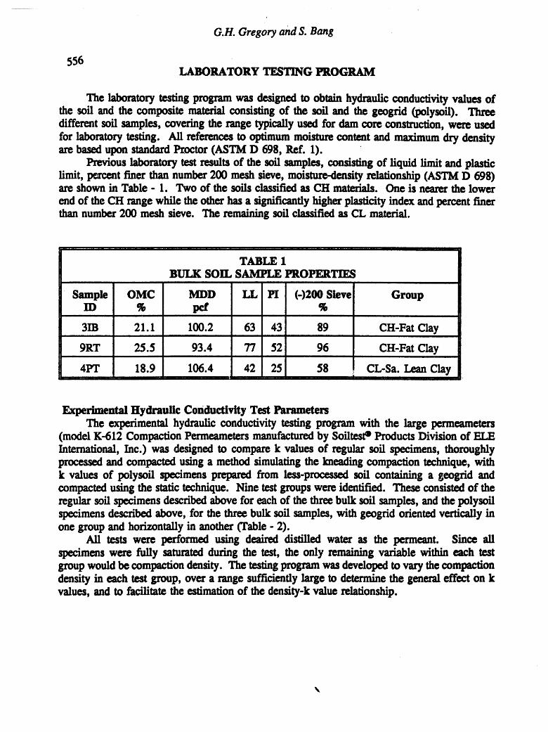
G.H.Gregoryand$.Bang
556LABORATORY TESTING PROGRAM
The laboratorytesting programwas designed to obtainhydraulicconductivityvalues ofthe soil and the composite material consistingof the soil and the geogrid (polysoil). Threedifferentsoil samples, covering the range typic_y used for damcore construction,were usedfor laboratory testing. All references to optimummoisturecontent and maximumdry densityarebased upon standardProctor(ASTM D 698, Ref. I).
Previous laboratory test results of the soil samples, consistingof liquid limit and plasticlimit, l_.xcentfiner than number200 mesh sieve, moisture-densityrelationship (ASTMD 698)are shownin Table - I. Two of the soils classifiedas CH materials. One is nearerthe lowerendof the CH range while the other has a significantlyhigher plasticityindex and percent finerthannumber200 mesh sieve. The remaining soil classified as CL material.
TABLE 1BULK SOIL SAblPLE PROPERTIES
Sample OMC MDD LL PI 0200 Steve GroupIV % pet
3IB 21.1 100.2 63 43 89 CH-Fat Clay
9RT 25.5 93.4 77 52 96 CH-Fat Clay
4PT 18.9 106.4 42 25 58 ! CL-Sa. Lean Clay|
I
Experimental Hydraulic Conductivity Test ParametersThe experimental hydraulic conductivity testing program with the large Im'meameters
(model K-612 CompactionPermeametersmanufacturedby Soiltes_ ProductsDivision of ELEInternational,Inc.) was designed to comparek values of regular soil specimens, thoroughlyprocessedand compacted using a method simulatingthe kneadingcompaction technique, withk values of polysoil specimens prepared from less-processed soil containing a geogrid andcompactedusing the static technique. Nine test groupswere identified. These consistedof theregularsoil specimensdescribedabove for each of the three bulk soft samples, and the polysoilspecimensdescribedabove, for the threebulk soil samples, with geogrid orientedvertically inone groupand horizontallyin another (Table- 2).
All tests were performed using deaired distilled water as the permeant. Since allspecimens were fully saturatedduring the test, the only remaining variable within each testgroupwould be compactiondensity. The testingprogramwas developed to vary the compactiondensity in each test group, over a range sufficiently large to determinethe general effect on kvalues, and to facilitate the estimation of the density-kvalue relationship.
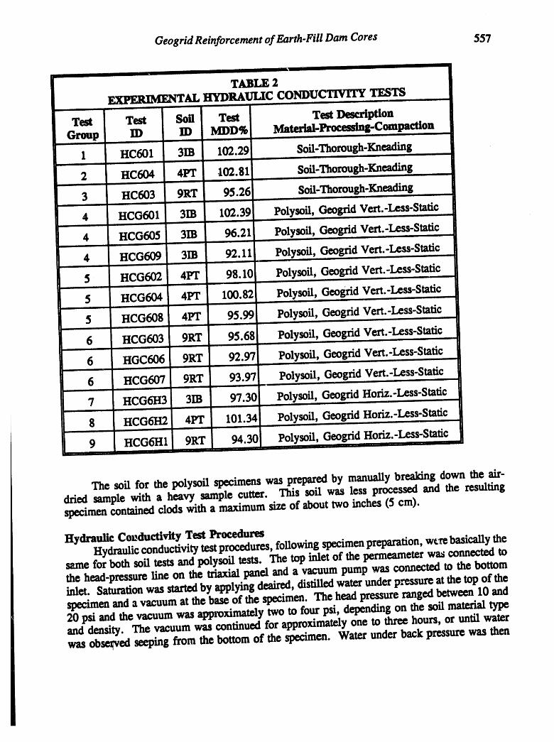
Geogrid Reinforcement of Earth-Fill Dam Cores 557
TABLE 2
EXPER/MENTAL ItYDI_ULIC CONDUCTIVITY TESTS
Test Test Soil Test Test DescriptionGroup ID ID MDD% MatedabProeemtns-Compaction
1 HC601 3IB 102.29 Soft-Thorough-Kneading
2 HC604 4PT ,102.81 Soft-Thorough-Kneading
3 HC603 9RT 95.26 Soft-Thorough-Kneading
4 HCG601 3IB 102.39 Polysoil, Geogrid Vert.-Less-Static
4 HCG605 3IB 96.21 Polysoil, GeogridVert.-Less-Static
4 HCG609 3IB 92.11 Polysoil, GeogridVert.-Less-Static
5 HCG602 4PT 98.10 Polysoil, Geogrid Vert.-Less-Static
5 HCG604 4PT 100.82 Polysoil, Geogfid Vert.-Less-Static
5 HCG608 4PT 95.99 Polysoil, GeogridVert.-Less-Static
6 HCG603 9RT 95.68 Polysoil, GeogridVert.-Less-Static
6 HGC606 9RT 92.97 Polysoil, Geogrid Vert.-Less-Static
6 HCG607 9RT 93.97 Polysoil, GeogridVert.-Less-Static
7 HCG6H3 3IB 97.30 Polysoil, GeogridHoriz.-Less-Static
' 8 HCG6H2 4PT 101.34 Polysoil, GeogridHoriz.-Less-Static
9 HCG6HI 9RT 94.30 Polysoil, GeogridHoriz.-Less-Static
The soil for the polysoil specimens was preparedby manuallybreaking down the air-dried sample with a heavy sample cutter. This soil was less processed and the resultingspecimen containedclods with a maximumsize of about two inches (5 cm).
Hydraulic Couductivity Test ProceduresHydraulicconductivitytestprocedures,following specimenpreparation,w_'rebasicany the
ssme for both soft tests and polysoil tests. The top inlet of the permeameterwas connectedtothe head-pressureline on the triaxial panel and a vacuum pump was connected to the bottominlet. Saturationwas startedby applyingdeaired,distilledwaterunderpressureat the top of thespecimenand a vacuumat the base of the specimen. The headpressurerangedbetween 10 and20 psi and the vacuum was approximatelytwo to four psi, dependingon the soft materialtypeand density. The vacuum was continued for approximatelyone to three hours, or until waterwas obse_ed seeping from the bottom of the specimen. Water underback pressurewas then

G.H. Gregory and S. Bang558
applied to the bottom of the specimen and a hydraulic gradient was established across thespecimen. Hydraulic gradients used in the various tests ranged from 20 to 141.
The saturation process continued until no air bubbles were observed in the back pressureline from the bottom of the specimen. Saturation was then checked by closing the valve on theback pressure line and leaving the head pressure line open. The pore pressure change on thebottom of the sample was then observed. If the pore pressure on the base of the specimenequalized with the head pressure in a few minutes, the specimen was assumed to be saturated.Each test was continued until four consecutive k-value readings had a maximum variation of 95percent from the average of the four values for specimens with k values in the E-09 cm/secrange, or a maximum variation of 50 percent from the average of the four values for specimenswith k values in the E-08 to E-06 cm/sec range.
The ratio of outflow to inflow was also required to be between 0.75 and 1.25 for each ofthe final four readings. The k value was then taken as the average of the four consecutivereadings meeting the above criteria. A summary of the experimental hydraulic conductivity testresults is presented in Table - 3. _
STATISTICAL ANALYSIS AND CORRELATION
The laboratory test resvlts from this study and the previous test resu+ ,_ere analyzedstatistically and correlated to produce normalized values for comparative purposes and for theFEM analysis. The statistical analysis included confidence interval estimation, linear regressionand best-fit curve analysis. Correlations were made between the previous test results and thoseof this study, between various test groups in this study, and among various compacted densitieswithin each test group.
The linear regression comparison described above for soil sample 3IB indicates a k valueof 4.652E-08 cm/sec for soil (HC tests) and a k value of 5.335E-08 cm/sec for polysoil (HCGtests), at a density of 91 percent of maximum. The k values at a density of 102 percent are2.96E-09 cm/sec and 7.88E-09 cm/sec for soil and polysoil, respectively. The linear regressioncomparison for soil sample 4PT indicates k values of 3.64E-08 cm/sec and 1.82E-06 cm/sec forthe soil and polysoil, respectively, at a density of 91 percent of maximum. The k values at 104percent of maximum density are 1.30E-08 cm/sec and 4.312E-07 cm/sec for the soil andpolysoil, respectively. The best-fit curve comparison for soil sample 9RT indicates a k valueof 4.f'/£-09 cm/sec for soil and a k value of 7.82E-08 cm/se¢ for polysoil at 93 percent density.The k values at 103 percent density are 1.4E-09 cm/sec and 3.6E-09 cm/sec for soil andpolysoil, respectively. Comparisons for all three soil samples indicate a smaller difference ink values between soil and polysoil as the density increases.
The polysoil test results, with the geogrid oriented horizontally (I-ICGH tests), fall betweenthe best-fit lines for soil and polysoil on each of the graphs, as expected.
FINITE ELEMENT METHOD OF SEEPAGE ANALYSIS
A program, designated as X8202 by the U.S. Army Corps of Engineers, WaterwaysExperiment Station, Vicksburg, Mississippi (Ref. 3 - 7) is capable of solving two dimensional

Geogrid Reinforcement of Earth-Fill Dam Cores 559
[
.SUMMARY OF EXPERIMENTAL HYDRAULICCONDUCTIVTIYTEST RESULTS
., i m tl ,,.. ,. i ,ll ,i i
Test iD Soil ID Description k- cm/secill Illl I II I I I ' I I I I Ill l , I
HC601 31B Soil 3.04E-09................ , ,,, i i ,i ,,
HC603 9RT Soil 2.71E-09i i ii ii i ii i . ii i ,, i i
HC604 4PT Soil 1.52E-08H , 'I I I , I ,I II il I
HCG_I 31B PolysoiI.Vertic_l 8.82E-09[ i,i, i, ii i ii ii . i ii ,
HCG602 4PT PolysoiI.Vertical 8.25E-07i i II I Illll I'1 II I II I I III
HCG_3 9NT PolysoiI-Vertic_l 1.19E-08u im, , nmm
HCG604 4PT PolysoiI.Vertic.al 8.77E-07iii IIIIL I I III I III I
HCG605 31B PolysoiI-Vertical 2.55E-08iii I I II i i ii ii ii i i ii Ill I. II Illll
HCG606 9RT PolysoiI-Vertical 7.50E-08i i i iv i i
HCG607 9RT PolysoiI-Vertical 2.62E-08H i i i i i H,| i ,
HCG6t_ 4PT Po_soii-Vertical 1.42E-06i i I i | I I i iii i ii i ii i |111i i ii ii I i i i ii ,il
HCG609 31B PolysoiI-Vertical 5.27E-08i I i1 I II i II I ii i i i iii ii
HCG6H1 9RT Polysoil-Horizonta_ 2.06E-08i i i i
HCG6H2 4FT PolysoiI-Horizo_al 2.66E-07i ii i I i i iii lUl i i iii iiiii
HCG6H3 31B PolysoiI-Horizontal 2.47E-08i I I ill i i I , _ , , i
TABLE - 3 Hydraulic Conductivity,Test Results
G.H. Gregoryand S. Bang560
steady-state,unconfinedseepage problemswithoutan initialestimateof the free surfaceandalsohas good graphics capabilities. The program solves the seepage problem using four-nedequadrilateralelements. Following generation of the grid, the required input includes theboundarycondition codes, and the knownhead conditions on the boundaries. The position ofthe free surface is found throughan interpolation process between nodes with positive andnegative pressureheads, and successive iterations are performeduntil the position of the freesurfacehas essentiallystoppedmoving. The coordinatesof the nodes very nearthefree surfaceare temporarilyadjustedto coincide with the free surface. Programoutputincludes an echo ofthe input, the head at each node, percentageof availablehead, flow, and whether the node isabove, on or below the _ surface, with coordinates of those nodes on the free surface.Additionaloutputvalues include the unit fl0w volume and the horizontal,verticaland resultantelement flow velocities and direction of flow.
Grid GeometryThe finite-element grid was generatedto conform to the geometry of the damcore developedin the conceptual model (Figs - 1 and 2). The grid consists of 10 elements in the horizontaldirectionand 17 elements in theverticaldirection. The verticalspacingwas selectedto coincidewith the polysoil strips. The grid contains198 nodes and 170 elements, as shown in Fig - 3.The same grid was used for both the non-reinforcedand reinforcedcases, to prevent a bias inthe FEM analysis due to a different grid geometry. For the non-reinforcedcase, identical kvalues were assigned to the thinsoil layers (polysoil strips in the reinforced case) as the thickersoil layers.Input Boundary ConditionsA datumof zero was selected at the level of the base of the core. Initial input values of totalheadfor each node were as follows: h - 45 feet (13.7 m) on the upstreamface from the head-watersurface to the base; h ---45 feet (13.7 In)across the top of the truncatedcore; h - 5 feet(1.52 m) on the downstream face from the tail-water surface to the base; h --- z on thedownstream face above the taft-watersurface;h -- 0 along the imperviousbase; and h - 0 forall internal nodes.
Hy&_ulie Conductivity Input ValuesThe normalized k values from the laboratory test results were adjustedto realistic field valuesfor use as input into the FEM program. The assigned field k values used in the computeranalysis are sum_:-_,_-izedin Table - 4.
Conditions AnalyzedNine differentconditionswere analyzed with the FEM program. Each of the threesoil
material types were analyzed for the non-reinforced case, assuming isotropic hydraulicconductivity. For the reinforced case, each soil material type was first analyzed assuming
isotropic k values in the polysoil, using the higher adjustedk (HCG) values for flow parallel tothe grid (assumingk, - k0. Theneach soil materialtypewas analyzed for the reinforcedcaseassuminganisotropichydraulicconductivity in the polysoil, and using the adjustedk, (HCGH)and kh (HCG) values. The soil portion of the core was assumed to have isotropic hydraulicconductivity in all analyses.

G Ieo&ridReinforcementofEarth-Fill Dam Cores 561
,,.,,,,i i , iL i u ,, ..i.,,,., i ullLII i, I
' .... _ ' Shell "'"Core' _
Not to Soale
RGURE 1 HYPOTHETICAL EARTH-FILLDAM
I_0------ 30 ft ----I_(gin)
.,"
"' Truncated P_'tl_ of•"" ', Core Not In(:luded in• ..
//_2_.................
,,,m) ,/2"Z--Z__.--_---....._..__oeee m i_dle_lNN_SrAB4N _e_ o_elN_N, e4NNeeee_lN_NN_N, meeoge m
14r:-_::;::::: _m__BllmmmUNDm_mleqNIq)
Impervlou;l_llS. ' 90 ft 127m) ..... _ _IL
FIGURE 2 HYPOTHETICAL EARTH-FILLD/II.MCORE

562 G.H. Gregory and S. Bang
i;o,144,, ,...............,..,4,o_k,o,oo_k,FisV 'i_21i_3I 154 '=5slse ls7_1'5e_,'_ leo\
I_a_i _3_/_i331__34_3s _3el _37_3e_ _ "'
1 /'!12f113 i14 i15 116 117[."ile\ 119\ 120\
/_o,/,o,/1./,o,,oo,o°,o,/,0.t,oo\,,0\9i "'/9_ /9_ • ......°"'" " °"'/\ \°°"'°°'I.,! .,I._1,, .° .° .,I- .° oo
/.. 71 /7_ / 7:3 I 7.4 7,s 7e 177I 7e _. 79 \ eoi._
/o,/o./°,/... °,lo.looi,olIs1 I sa I 53 ! 54 ss s8 s7 ._R _ oo
L_ 31 /'"3_i'"'I' 33" / _1 _t_3 36 37 "_R ,..\. _.q 4
1 ' ' i5 " 16 [.. 17 ' 18 't9 20
FIGURE 3 FINITE ELEMENT SOLUTION GRID
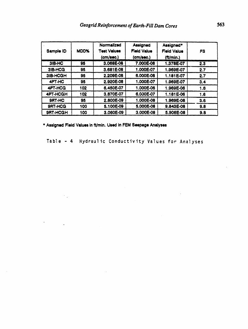
Geogrid Reinforcement of Earth-FiU Dam Cores 563
......... Normalized A,,lgned A.Igned"Sample ID MDD% Test Values Reid Value Reid Value FS
(em/ze¢.) (om/se¢.) Ift,/min.)I II Bill II I I I I I| I III 11I! III I / III IIII I1 ' I III I IIII [ Ill
31B-HC 95 3.068E-06 7.000E-08 1.378E-07 2.3I IIII I I I II II I I I1 iiii il
31B-HCG 95 3.681E-08 1.000E-07 1.969E-07; "" 2.7i i , i i .,,. i .....................
3,,.HCC;H .og.os e.ooo .o81.181e.o7 a.74PT-Hc 95 ' 2.920E-08 .... 1.000E-07 1.96gi_-07 '3.4 .......
I I I I ii III I I IIII II i II iii
4PT-HCG 102 6.450E-07 1.000E-06 1.969E-06 1.6I i iii iiiii I iiii i i ii I
4PT-HCGH 102 3.870E-07 6.000E-07 1,181E-06 1.6i iiiii ii_i I I ii I II IIII I I llU ii iiiii I II I iiii
9RT-HC 95 2.800E-09 1.000E-08 1.969E-08 3.6iii I Iiii ii iii ii II i I ii i ii i I I i i i i ii ii i ii i
9RT-HCG 1O0 5.100E-09 S.000E-08 9.843 E-08 9.8I iii II I ii ii i L l --
9RT-HCGH 100 3.060E-09 3.000E-08 5.906E-08 9,8.......... i iiiii l i ii iii I i
"Assigned Reld Values inft/min. Used in FEM Seepage Analyses
Table - 4 Hydraulic Conductivity Values for Analyses

564 G.H. Gregoryand $. Bang
Analysis ResultsThe resultsof the FEM analysisare summarizedin Table - 5. The soft materialtype is
identifiedby the sample !D containedin the analysisnumber(e.g., 3IB). The last digit in theanalysis number, for each soft material type, identifies the analysis condition u follows: I =non-reinforcedcase; 2 = reinforcedcase with isotropichydraulicconductivity in the polysoil;and 3 = reinforced case with anisotropic hydraulicconductivity in the polysoil. The thirdcolumn containsthe average flow rate for each analysis.
II i .... , J
TABLE $SUMMARY OF FEM ANALYSIS RESULTS
Analysis Output Ave. Flow Rate Flow VolumeNumber F'fleName (ft3/mtn/ft_ (ft3/day/1000 fl dam)
iiiii i i i I
S3IBN1 S3IBP1 2.0920E-06 68
S3IBN2 S3IBP2 2.2494E-06 76
S3IBN3 S3IBP3 2.2422E-06 75
$4FI_1 S4PTP1 2.9807E-06 101
S4PT_ S4PTF2 8.5286E-06 362
S4FI'N3 S4PTP3 7.7602E-06 324
SgRTN1 S9RTPl 2.9855E-07 10i i iii i
S9RTN2 S9RTP2 5.1297E-07 21
S9RTN3 S9RTP3 5.0850E-07 20I
The fourth column contains the total flow quantityper day based on the height of theseepage face and assuming a damlength of 1000 feet (305 In), for illustrationpurposes.
Eachof the nine analyses generatetwo plots. One plot shows the portionof the damcorebelow the phreaticsurface and containsequipotentiallines. The other plot shows the portionof the damcore below the phreaticsurfaceand containsflow velocity vector arrows. Figs - 4and 5 show the typical plots from the output. The plot with the equipotentiallines for thereinforced case have the phreaticsurface of the non-reinforcedcase shown with dashed lines.The dashedlines were addedto the plots to facilitatecomparisonof the phreaticsurfacepositionfor the reinforcedand non-reinforcedcases. The summarizedFEM results in Table - 5 and thecomputerplots discussed above indicate only modest increases in flows and phreaticsurfaceelevationsfor the reinforced cases (cases including the polysoil strips).
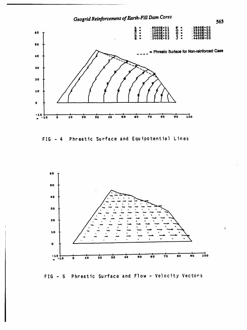
GeosridReinforcen_nto/Earth-FlUDam Cores 56Sk " .|000E+01 F " .21100E*02II ,, .1200E*02 O " .320011:+02
tO C a .ttOOE_'02 H " .:1600E+02D " .20OOE.02 Z " .4000E*02
, E u ,2400E+02 _3 " .4400E+02
SO
- PhreaticSurfaceforNon.reinforcedCase4O
3O
20
10
0
-10 I i ! I " I I I .... I 1 |-L0 0 10 20 30 40 gO 60 Y0 e0 90 100
FIG -4 Phreatic Surface and Equipotential Lines
6O
60
40
30
20
t10
0
-1C I I I I I I I I I : _. -_0 0 10 20 30 40 gO 60 70 80 90 luO
FIG - 5 Phreatlc Surface and Flow- Velocity Vectors

566 G.H. Gregory and $. Bang
CONCLUSIONS AND RECOMMENDATIONS
Conclusions developed during the currentstudy include those relating to FEM analysisresults and design and construction.
1. The increase in unit flow rates for the reinforcedcore with polysoil stripswas a maximumof 7.5 percentfor sample3IB, 286 tmrcentfor sample 4PT, and 172 percent for sample9RT. Although the increases may sound considerable for samples 4PT and 9RT, theactualincrease in flow volumes is very modest, as shown in Table - 5, for a 1,000-footdamlength. The maximum increase in exit-seepage volume for the above configurationwu 261 cubic feet per day for sample4PT. The maximumincrease for sample3IB waseight cubic feet per day and for sample 9RT, 11 cubic feet per day. These are verymodest incre_. The phreaticsurfaceconfigurationwas virtuallythe same for an threeanalyseson sample 3IB. The maximumincrease in phreaticsurface elevation for sample4PT was approximately three feet and that for sample 9RT was about 1.8 feet. Thephreadcsurfacewas virtuallythe samefor isotropicandanisotropichydraulicconductivityvalues in the polysoil, withineach softmaterialtype. Again, these increases areminimal,or modestat most.
2. The use of geogrid reinforcement through an earth-fill dam core will likely v.sult inincreased seepage throughthe core and a higher phreaticsurface. With a well designedlaboratorytesting program that carefully models the field condition, the magnitudeof theincreasedseepage and phreaticsurface can be predicted. These data, with application ofappropriate safety factors can be used to develop design parameters for a geogridreinforced dam, including the core.
3. Rigid constructiondocumentsand a high level of qualitycontrolduringconstructionwill berequiredto produce a final product in the field that will perform as modeled in thelaboratory.
4. The relatively small increase_,in Seepageand phreaticsurface rise indicated in this study,resultingfrom the use of g_ogriclreinforcementin earth-filldam cores, should be withina rangethatcan be appropris,t_ly managedand accommodatedin design and construction.
ACKNOWLEDGEMENTS
' Theauthor wishes to gratefully acknowledge theefforts and contributionsof the followingindividuals:Dr. Iames G. CoUinand Mr. RonaldAndersonof TensarEarthTechnologies, Inc.,who provided funding for the large permeametersused in this study, the geogrid materials fortesting, and advice and technical literature;Mr. Thomas D. Bakerof EMCON/Balmr-Shifiett,Inc., who provided the bulk soil samplesand previous laboratorytes_ ,esuits.

Geogrid Reinforcement of Earth-Fill Dam Cores 567
lt.EFER_t'J_CES
I. AmericanSociety for Testing and Materials(ASTM), 1993 Annual Bookof Standards.2. Bang, S. and Shao, L. (1993). "Analysisof UnconfinedFlow with InclinedBoundaries
by Finite Difference Method." Canadian Societyfor _vU Engineering, 1993 AnnualConferenceProceedings, 119-128.
3. Tracy,FredT. (1973a). "AThree-DimensionalFinite ElementProgramfor Steady-Stateand TransientSeepage Problems." Miscellaneous PaperK-73-3, U.S. Army EngineerWaterwaysExperimentStation,Vicksburg, MS.
4. Tracy,FredT. (1973b). "APlaneand AxisymmetricFinite ElementProgramfor Steady-State and Transient Seepage Problems." Miscellaneous Paper K-73-4, U.S. ArmyEngineer WaterwaysExperimentStation, Vicksburg,MS.
5. Tracy,FredT. (1977a). "AnInteractiveGraphicsFinite ElementMethod GridGeneratorfor Two-Dimensional Problems." Miscellaneous Paper K-77-5, U.S. Army EngineerWaterwaysExperimentStation, Vicksburg, MS.
6. Tracy, Fred T. (19T/b). "An Interactive Graphics Post-Processor for Finite ElementMethod Results." Miscellaneous Paper K-774, U.S. Army Engineer Waterwaysl_xperimentStation, Vicksburg, MS.
7. Tracy, FredT. (1991). "Applicationof Finite Element, GridGeneration,and ScientificVis_aliT_tionTechniquesto 2-D and 3-D SeepageandGroundwaterModeling." TechnicalReportITL-91-3, U.S. Army Engineer WaterwaysExperimentStation, Vicksburg, MS.

_ _o__/' _NU_CTU_OTO _TONO_O___ __.IMRGE, INC.
BY RPPLIED I., _


568

Hydrogeology, Waste Disposal, Science and PoliticsProceedings 30th SymposiumEngineering Geology and Geotechnical Engineering, 1994 569
DESIGN OF FLEXIBLE PAVEbIENT SUBGRADES WITH GEOSYNTHETICS
G. H. Gregory and S. Bang
Department of Civil and Environmental EngineeringSouth Dakota School of Mines and Technology
Rapid City, SD 57701
ABSTRACT
The objective of this study is to develop design guidelines for incorporatingthe soil subgradeimprovementfunctionsof geosyntheticsinto a conventionalflexiblepavement designmethod thatuses the California BearingRatio criteriaas design input. The study incorporatesa series oflaboratorytests, including the standardCBR tests on weak subgradessoils andthe modified CBRtests using crushedstone surchargesand geosynthetics. The laboratory CBR test results havebeen correlatedwith existing data to produce a design method that includes the effect of soilimprovementdue to geosynthetics. The proposed design method combines the conventionalflexible pavement thickness designprocedurewith the geosynthefic improvementfactors.
INTRODUCTION
The purpose of this study is to develop guidelines for incorporating the soil subgradeimprovementfunctions of geotextiles and geogrids (geosynthetics) into a conventional flexiblepavement design method which uses CaliforniaBearing Ratio (CBR) criteria as design input.The scope consisted of the following; (1) researchingand compiling existing relevant data, (2)performing laboratorytestingincludingseriesconsisting of standardCBR tests on weak-subgradesoils and modified CBR tests using crushed stone surchargesand geosynthetics (geotextile onlyand geotextile-geogrid combination) to determine subgrade improvement factors, and (3)correlatinglaboratory test data with existing data combininga conventional pavement thicknessdesign procedure with the geosynthetic improvement factors.
LABORATORY TESTING PROGRAM
The laboratorytesting programwas designed to providetest resultswhich, whencorrelatedwith existing data, would indicate subgrade improvement factors for the soil-geosynthetic-pavement base interaction. The series included crushed stone, geotextile and geogridmaterials.This study was, of necessity, limited in scope and multiple testing of all specimen types andcombinations was not possible. However, multiple tests were performed on selected specimensand combinations to obtain an indication of the spread in test results.

570 G.H. Gregory and S. Bang
CBR Soil SeriesThe CBR soil series was performed using two different types of soft in the "weak
subgrade"range (CBR less that, 10). The softs were obtainedfrom anotherprojectsource andhad been previously tested in accordance with ASTM (Ref.1) procedures for classification(ASTM D 2487) and StandardProctor density (ASTM D 698). The soil properties aresummarizedin Table - 1.
TABLE- 1
Sample Description Maximum LL PI -200Number Dry Density SIEVE
31:!3 Lt. Br. Clay (CH) 100.2 per 63 43 89%
4PT Br. Sa. Clay (CL) 106.4 pcf 42 25 58%
The geotextileused in the tests was Trevira® 1125. The geotextile properties were selected tomeet or exceedminimumpavementdesign and survivabilitycriteria(Ref. 2 and 3). The geogridused in the tests was Tensar*BX 1200 (SS2). The TensarBX 1200 was selectedfor this studybecause this product has performed well in numerous applicable projects and the geogridpropertiesmeet or exceed the minimumpavementdesign and survivability criteria(Ref. 2 and3).
Conventional CBR tests were performed on the two soil samples in generalaccordancewith ASTM D 1883, except only ore eompactiveeffort and moisture content (ASTM D 698)was used in preparing the specimens. These test results were then compared to the StandardProctorvalues. The compactedspecimenswere in the range of 95 to 100 percentof maximumdry density and optimum to plus 4 points wet of optimummoisture content. The specimenswere soakedunderwater for a minimumof 96 hoursprior to CBR testing. The CBR tests wereperformed with steel surchargeweight of approximately15 pounds.
CBR test results on soil sample 3IB are presentedin Fig - 1. This specimen had a CBRvalue of 1.81. The results on sample4171'are presentedin Fig - 2. This specimen had a CBRof 3.14. Both values were takenat a penetrationof 0.1 inch. The 4PT specimen had a slightlyhigher CBR value (3.52) at 0.2 inch penetration.
Modified CBR Testing With Crushed Stone SurchargeThe crushed stone material used as a surcharge in CBR tests consisted of two different
gradationsof crushed limestonebase materials. The gradationsof these materialswere similarto ASTMD 448, Size Number8 (3/8 inch to No. 8 sieve) and Size Number57 (1 inch to No.4 sieve).
Modified CBR tests were performedon additionalspecimensof the two soil samples. Thesoil specimenswere preparedand compactedin the CBR molds as described previously. The2-inch extension collar was then placed on the mold and filled with crushed limestone. SizeNumber57 was used in the lower portion of the moldand Size Number 8 was used in the upper

Design of Flexible Pavement Subgrades with Geosynthetics571
BEAfilNG RATIO TEST .......
PR0_IECT:Ge0syntheiics in Pavement Subgrades JoB'No.:CE790-1 ' ......LOCATION: South Dakota Schoolof Mines and Technology ......SAMPLE No.: 31B-1 DESCRIPTION: Lt. ar.,,Ciay(CH) ...............DATI=OF TEST: 2-il-93 REMARKS:PENETR. DIAL LOAD STRE_SS CBR SCBR GCBR GGcBR
Inches .0001 in. " Lbs. psio.ooo o.ooo o.ooo o.ooo .... 1.............
o.o2s 3.00o 2419_ 8._ ..............,,,, ,,,,,
olos0 5.ooo 41.ees _3.8_,,, ,i
o.oTs e.ooo 49._e 16.eee I_ 011oo e.soo s4._es le.oss ' _.el.............
1
, ,, ,, ,,i ,, , ,,,,
0.125 7.000 58.331 19.444 . ,o._so _.2oo sR.99e _9.999 ......0.175 7.500 62.498 20.833
' 0.200 8.000 .... 66.664 22.221 .... 1.48' 0.300 9'500 79.164 26.388 " '['.39 "
0_400 :1:1".100 92.496 30.832 1.34ol 5_ ..................
OiBoo .................., , .... ,,, , ,,,
0'700, , ,
o.eoo,, ,,, , ,, ,,,
o.go0, ,, , ,, ,, .....
1.000 .........
CALIFORNIA BEARING RATIOLOAD-PENETRATIONCURVE
50 ] :.A__............._............._.............t............._...........$............_............_............*.............,.............
3s1.............!............._.............!............i...........-:.".............i............,.............,............._.............,_,,,_o1.............i............._........._ ...........t............!.............i.............i.............i.............
/20_...........!.-,_-_--i............i............+.............i.............!.............;..............i..............
_o-,._ ......i..........:.............:.............'.............:............'............
........i............i.............i...........i...........i...........i............i.............i............i.............:31 : : : : : : , . ,
0 0,1 0.2 0.3 0,4 0.5 0.6 0.7 0.e 0.9 1PENETRATION-INCHES
FIG - l CBR Test Resultsof 31B Soil

572 G.H. Gregory and S. Bang
BEARING RATIO TEST
PROJECi': Ge0synthetics in Pavements ubgrades. , '_JOBNo.:CE790-1 ..........LOCATION: South Dakota School of Minesand Technology ....SAMPLE No.: 4PT-1 .DI_SC'R,!PTION:Br. Sa,:Clay(CL) ...... .iDATE OI_TEST: 2-11-93 REMARKS:PENETRI DIAL LOAD STRESS CBR' SCBR (_CBR GGCI3R
....Inches .OOO1 in. Lbs. .PS! . . 'o,ooo o.ooo o.ooo o.ooo
'o.o2s '3'.060....241099e._3........, ,,,1,,i, ,,,, l, 'I " " ' ' ""
0.050 6.000 49.998 16.666,, . ., ,,.,,,. i , = i , i , L .
0.075 8.750 72.914 24.305 L."'(3.10(311.300'" 94'."163'31.388 3'.I4 ......i0.125 13.500 i121_$96 "37.499 .....
o.lr,6 _s.soo" 129._62 ....,_.6_ .....0.175' 1'7.000 141.661 47.22'0 ............0.200 19.060 158.327...... 52.776 3_52 ......."0.300 25.000 "' 2081325' 69.442 .... 3.65 ....
ii, , ,,
0.400 30.000 249.990 83.330 3.62o.5oo 34.oo02s3.32294.441 3.63 .....
J ,, , i, ,, i ,
0.600,,,i i ,, , ,, ,, , ,,, ,
0.700, | m=,, ,| ,, , , , i
0.8OO,, , , ,
0.9001,000 .............
......
CALIFORNIA BEARING RATIOLOAD-PENETRATION CURVE
100 i _ "901,......... I'......... T..........."T......... T'"""_'_" ......... I- .......-T......... T.... T.........
8oI.........._........4........_-;:.........-............i...........':,:-........._........::-.......";-........,o.,........,...........,........._i ..........,.............,............,...........,.........oo........-:".........:..;........._............!.......!............_............;..........!........._.........,o---_...i ]]iii-i_i.........._............,.........,.........._........'°1....._ ......t..........i...........t--t.............".........t.........t.......¢......3Ol --:.:----.-.-.;..-.-..-;.- ........-;...---;.!........-:::...........::"..........¢......_;.........._........._......._........_ ......
'::--ii i i i'-" --........................................i0 0.1 0,2 0.3 0.4 0.5 0.6 0.7 0.8 0.g
PENETRATION-INCHES
FIG - 2 CBR Test Resultsof 4PT Soil

Design of Flexible Pavement Subgrades with Geosynthetics573
portion. A 16-pound steel disc was temporarily placed on top of the crushed stone and struckwith a rubber mallet to level the stone. The stone was then compacted by striking the steel discwith 40 blows with a ten-pound hammer (ASTM D 1557 type) dropping 18 inches. Thiscompaetive effort in the confined collar mold was estimated to be roughly equivalent to thatwhich is achieved in the field with eight passes of a ten-ton vibratory roller per 6-inch lift ofpavement base material. The CBR tests were then performed on the composite specimens withthe piston loading applied to the crushed stone. Steel surcharge weight of approximately 15pounds was applied to the crushed stone during the tests. The resulting CBR values are shownin Fig - 3 under the heading "SCBR."
Modified CBR Testing With Crushed Stone and GeosyntheticsModified CBR tests were performed on additional specimens of the two soil samples
including tests with geotextile only and geotextile-geogrid combination. A crushed stonesurcharge was necessary for these tests as previously discussed. In all cases the geosyntheticswere placed directly on the soil specimen at the bottom of the stone surcharge. Geotextile-geogrid combination tests were performed with the geogrid on top of the geotextile.
A modification to the CBR testing apparatus was necessary to accommodate thegeosyntheties. In developing the geosynthetic-subgrade model, a near fully-anchored conditionof the geosynthetics in the pavement structure was assumed. During the laboratory tests, aclamping device was required to anchor the geosynthetics. The clamping device was fabricatedfrom a heavy duty PVC pipe flange assembly for a nominal 6-inch diameter pipe. The flangeassembly has a bolt circle containing eight 3/4-inch diameter bolts and inner groovedcompression ring. The assembly was modified to fit over the top of the basic CBR mold andto accommodate the 2-inch CBR extension coUar on top. The geosynthetic materials (geotextile,geogrid or both) can be clamped in the flange assembly and then placed on top of the CBR basemold so that the geosynthetic material rests directly on the soil specimen surface. The CBRextension collar is then clamped on top of the apparatus to accommodate the crushed stone. Thecrushed stone for this series of tests again consisted of the Size Number 57 in the lower portionof the collar and Size Number 8 in the top portion. A schematic drawing of the modified CBRapparatus with geosynthetics in place is depicted in Fig - 4.
On the 3IB specimens, one test was performed with geotextUe and three tests withgeotextile-geogrid combination. On the 4PT specimen, two tests were performed with geotextileand one test with geotextile-geogrid combination. The test results are included in Fig - 3. Thecolumns headed "GCBR" contain the test results for the tests with geotextile only and thecolumns headed "GGCBR" contain the test results for the geotextile-geogrid combination tests.
TEST RESULTS AND SUMMARI_
Load-Penetration Curves
The virgin stress-penetration data from the CBR tests were summarized and a compositeaverage was obtained for each sample. These composite averages were then plotted ascomposite load-penetration curves for each sample material. These graphs are presented in Figs- 5 and 6. Below the 0.2-inch penetration level a distinct pattern of behavior is not evident. At
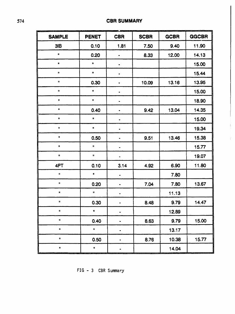
574 CBR SUMMARY
I I H _ ,t I J mi
SAMPLE PENET CBR SCBR GCBR GGCBRi ii ,. i i
31B 0.10 1.81 7.50 9.40 11.90
" 0.20 - 8.33 12.00 14.13i i
" " - 15.00i i
" " - 15.44,
" 0.30 - 10.09 13.16 13.95ii i, , i
" " - 15.00i rail
" " - 18.90.. i i
" 0.40 - 9.42 13.04 14.35i
" " - 15.00i
" " - 19.34i ,i i i
" 0.50 - 9.51 13.46 15.38i i, i i
" " - 15.77H i ii i
" " - 19.07i i
4PT 0.10 3.14 4.92 6.90 11.80ii
" " - 7.80i= l Ill
" 0.20 - 7.04 7.80 13.67
" " - 11.13.... i i H,
" 0.30 - 8.48 9.79 14.47ii
" " - 12.89
" 0.40 - 8.63 9.79 15.00= i
" " - 13.17i
" 0.50 - 8.76 10.38 15.77, ii
" " - 14.04i,
ml i n i i n i
FIG - 3 CBRSummary

Design of Flexible Pavement Subgrades with Geosynthetics 575b
CRUSHED STONE
CLAMPINGDEVICE , '
! !
_ ,
MODIFIED CBR APPARATUS
NTS
FIG - 4 Modified CBR Apparatus

576
CBR LOAD-PENETRATIONCURVE31BLt. Br. Clay (CH) COMPOSITE
_o4_/ i i i
0 0.1 0.2 0.3 0.4 0.5 0._PENETRATION-IN CHES
-'l-CBR --'_-SCBR _GCBR -e-GGCBR
FIG - 5 Load - Penetrationof 31B Soil
CBR LOAD-PENETRATIONCURVE4PT Br.Sa. Clay (CL) COMPOSITE
450' { _ i i i.......
400" _ i i i
i ! ,,,'
...... ! .....0 0.1 0.2 0.3 0.4 0.5 0.0
PENETRATION-INCHES
FIG - 6 Load - Penetrationof 4PT Soil

Design of Flexible Pavement Subgrades with Geosynthetics 577
and above the 0.2-inch penetration level, however, a very obvious pattern is present. Anincreasingly larger stress level for the same penetration is evident for the stone surcharge-onlytests (SCBR), geotextile tests (GCBR), and geotextile-geogrid (GGCBR) tests, in ascendingorder. The only case where this is not clear at the 0.2-inch penetration is for the 4PT sample(Fig - 6), where it appears that the SCBR and GCBR curves almost coincide. However, this ispartly due to the large stress-axis scale required to depict all results on the same graph. Anexamination of the actual stress-penetration values for the 0.2-inch penetration point will showaa approximate 14 percent increase in stress value for the GCBR test over the SCBR test. Alsothe 4PT sample is the stronger soil and would be expected to have a higher resistance topenetration at _'helower deformation than the weaker soft sample.
CBR Correlations and SummariesThe CBR values from all tests were summarized and correlated with each other for the
various types of tests. A summary of CBR test results is presented in Fig - 3. The basic CBRvalues (CBR) were summadz_ and averaged only for the 0. l-inch penetration since that valuerepresents the conventional CBR value for the basic material (soft only).
The SCBR, GCBR and GGCBR results were summarized m_d averaged for the 0.I, 0.2,0.3, 0.4 and O.5-inch penetration points. The average improvement in CBR value was thendetermined at each of the above penetrations between SCBR and GCBR results and betweenGCBR and GGCBR results. The most consistent improvement factors when considering bothGCBR and GGCBR values occurred at the O.2-inch penetration level.
GEOSYNTHETIC-SUBGRADE MODEL
The correlations and summaries of the laboratory test results discussed previously wereanalyzed and correlated with data from the previous study to develop the current geosyntheticsubgrade model involving both geotextiles and geogrids.
Correlation With Previous GeotextHe-Subgrade ModelThe 1987 study (Ref. 4) involved 12 flexible pavement projects on which a geotextile was
used on all or a portion of each project. All 12 pavements were constructed on relatively weaksubgrade soils (CBR between 2 and 10). Actual pavement thicknesses on all projects weredeficient for the traffic loads, based upon CBR values of the subgrades, without considerationof the geotextile. The portions of the projects on which a geotextile was used did not fail, evenwith the apparentdeficiency in thickness. The portions of the projects on which a geotextile wasnot used all experienced significant failures within a relatively short time after being put intouse. It was then postulated that the geotextile was providing a measurable improvement to thesubgrade. To estimate the magnitude of the improvement, required CBR values based upon thetraffic loads and actual pavement thicknesses were back-calculated. This value of required CBRwas termed the "apparent CBR" of the subgrade. The difference between the actual CBR valueof the subgrade and the "apparent CBR" value was the improvement factor attributed to thegeotextile. Thus the apparent CBR value was designated as the get>textile-modified CBR or"GEOMOD" CBR and the improvement factor was termed the GEOMOD factor. The 12

G.H. Gregory and S. Bang578
pavement projects provided a unique opportunity to study the effects of geotextiles in flexiblepavements and involved a relatively well balanced distribution of subgrade CBR values for weaksoils. A model for the GEOMOD CBR was developed by plotting the subgrade CBR valuesversus the difference between the apparent CBR and actual CBR values. This resulted in theplotted GEOMOD CBR curve shown in Fig - 7. The curve indicates a trend toward zeroimprovement at a CBR value of 11 at the fight hand end of the curve and a trend toward zeroimprovement at a CBR of zero. This curve confirmed actual experience and observations wherethe subgrade improvement using a geotextile is lower for very weak soils (CBR less than about2), increases in the intermediate range (CBR of about 2 to 7) and again is lower for morecompetent soils (CBR of about 7 to 11). This holds true for permanent pavement structureswhere deformations must be limited. In temporary haul roads and similar facilities, wheresignificant deformations are acceptable, the improvement factors would also be high in the rangeof CBR below 2 (but would still be zero for zero CBR).
Using the GEOMOD CBR Curve, a GEOMOD factor can be obtained for any particularsubgrade between zero and 11. This GEOMOD factor is then added to the subgrade CBR toobtain the GEOMOD CBR. The GEOMOD CBR can be used in any conventional pavementthickness design procedure in lieu of the subgrade CBR. This allows conventional proceduresto be used to design flexible pavements with geotextiles. The observation of numerousconstructed pavement projects, designed by the author since 1987, have continued to confirmthe validity of the curve.
CBR Test-GEOMOD Model Correlations
The summarized CBR test results from the current study were correlated with theGEOMOD model to establish a relationship between the GEOMOD factors from the 1987 studyand the improvement factors for the geogrid observed in the CBR tests. Once this relationshipwas established it could be used to extrapolate GEOMOD factors for the geogrid, based uponthe improvement factors for the geogrid observed in the CBR tests. This procedure couldsignificantly mitigate the scale effects of the laboratory tests by correlations with the full-scaletest projects of the 1987 study. To accomplish this correlation, the following steps wereperformed:1. GEOMOD factors were determined from the mathematical model for each average
conventional CBR value from the laboratory tests(samples 3IB and 4PT), at the 0.1, 0.2,0.3, 0.4 and 0.5-inch penetration levels.
2. The above GEOMOD factors were then divided by the difference between the averages ofthe SCBR tests and GCBR tests at the above penetration levels. This produced a"correlation coefficient" which could be used as a multiplier to adjust the geogridimprovement factors from the laboratory tests to the full-scale field condition based on the1987 study.
The values obtained in the above analysis, including correlation coefficients, are presented onFig- 8.
Geotextfle-Geogrid-Subgrade ModelThe geotextile-geogrid-subg_, ade model, referred as the GEOMOD2 model, was developed
in the following steps:

m _ co GEOMODFACTORO_ ..,.
• . . _ . .
__...... 0_-, _ _- _._._ ,
to- _.:.., _.
O0
IT1
0
___ _ooo_o o ,0 o::,- _ ,_ _'-" o° _"
w
"< "o "_ _"
- /-.,. c:: C_
_. _. _, 0 _ 0 0 -" 0 -" _i _1
-. ,J
4-
U_
_O
580 G.H. Gregory and S. Bang
1. The differences between the averagesof the GCBR and GGCBRtests at the 0.1, 0.2, 0.3,0.4 and 0.5-inch penetration levels were multiplied by the correlation coefficientsdiscussedin previous section. The resultingvalues were the improvementfactorsfor thegeogrid adjusted to the full-sc_e field conditions observed in the 1987 study.
2. The above values were thenadded to the appropriateGEOMOD factors previouslyobtainedfor the geotextile-only condition. Each sum was then divided by the appropriateGEOMOD factor to obtain an "improvementcoefficient" for the geotextile-geogridcomb'marion,over the geotextile alone. It was found thatthe improvementcoefficients atthe 0.2-inch penetration level were the most consistent. These values had a standarddeviationof 0.185 and a coefficient of variation (standarddeviation + mean)of 0.10.
3. The original 12 datapoints (GEOMODfactors)from the 1987 study, which were used toproducethe GEOMOD model curve, were multipliedby the improvementcoefficients atthe 0.2-inch penetration level to establish 12 new extrapolated data points for thegeotextile-geogrid combination. The 0,0 and 11,0 coordinatesof the ends of the curvewere also included in the data set.
The above analysis resulted in the new GEOMOD2 model for the geotextile-geogridcombination. The results of the analysis are also presented in Fig - 8 and a graph of theGEOMOD2curve is included in Fig - 9.
DiscussionThe GEOMOD2 model was developed from the SCBR, GCBR and GGCBR test data at
the 0.2-inch penetrationlevel. For permanentpavementstructuresit is necessary to establishdesign values at a low deformation. Larger deformationlevels obviously would show a largerimprovement factor for the geosynthetic materials, but would likely involve unacceptabledeformations in the pavement structure. The test results indicated a significant, relativelyconsistent improvement factor at the 0.2-inch penetration level. This deformationis alsoacceptable in permanent flexible pavement structures. Accordingly, the correlatedtest resultsfrom the 0.2-inch penetrationlevel were used to develop the model.
CONCLUSIONS
The following general conclusions were developed during this study:1. Laboratory CBR tests can be used to model the effects of geosynthetic improvement of the
subgradeby using a modified CBR apparatus.2. The geosynthetic-subgradeimprovementfactors (GEOMOD and GEOMOD2 factors)
indicate a significant improvementat the 0.2-inch penetrationlevel. The factors at the0.2-inch penetrationlevel should be used in the design of permanentflexible pavementsto limit deformations. Improvementfactors at a higher deformation could be used fortemporary facilities such as haul roads.
3. The raw geosynthetic-subgradeimprovementfactors from the laboratory tests with thegeotextile show a larger level of improvement than that observed in the full-scalepavements in the 1987 study. This is likely due to obvious scale effects in the laboratorytests. The revised GEOMODand GEOMOD2factorsdevelopedin the currentstudy werecorrelatedwith the full-scale conditionsof the 1987 study to limit the scale effects of the

DesignofFlexiblePavementSubgradeswithGeosynthetics581
IDEALIZED GEOMOD2 CBR CURVE,,
oO -_
I"', _4 ,, ,,, _ ,,
- /_ -
- / __ .....
0 -_,, If) ....
_ _ \,,,o \0
(,,_ I_') ,i ..... _, ,
("4 -i_____/_ _ ,,,
0 1 2 3 4 5 6 7 8 9 10 11$UBGRADECBR
FIG - 9 GEOMOD2CBR Curve

G.H. GregoryandS.Bang582
laboratory tests. The GEOMOD and GEOMOD2 factors should be used in designapplications rather than the raw laboratory test results.
4. Conventional pavement-thickness design procedures, which use the subgrade CBR as adesign basis, may be readily used to design pavements with geotextiles or geotcxtile-geogrid combinations by using the GEOMOD or GEOMOD2 CBR in lieu of the subgrade
CBR. IACKNOWLEDGEMENTS
The authors wishes to gratefully acknowledge the following individuals and firms whoprovided technical assistance, information or materials related to the current study: Mr. RonaldP. Anderson, P.E. and Tensar Ear'.hTechnologies, Inc., who provided geogrid materiall forlaboratory testing, and technical information; Mr. Les Neumann, P.E., Mr. Keith A. Miller _,ndContech Construction Products, Inc., who provided the geotextile for laboratory testing, andtechnical information; and Mr. Thomas D. Baker, P.E., and EMCON/Baker-Shiflett, Inc., whoprovided the soil samples and previous laboratory classification and Standard Proctor test resultson the samples.
REFERENCES
1. American Society for Testing and Materials (ASTM), 1993 Annual Book of Standards,Volume 4.08, Soil and Rock: Dimension Stone: Geosynthetics.
2. Koemer, Robert M., Desi_inE With Geosynthetics. Prentice-Hall, 2nd Edition, 1990.
3 Fluet, Joseph E., Jr., Editor, Geotextile Testin_ and the Design ]_n_ineer. ASTM STP952.
4. Gregory, Garry tL, Desitm of Flexible Pavements with Geotextile_, 1987. AmericanSociety of Civil Engineers, Fall Meeting, Geotechnical Session, Houston, Texas, October 2,1987.

Hydrogeology,WasteDisposal,ScienceandPoliticsProceedings30thSymposium 583EngineeringGeologyandGeotechnicalEngineering,1994
PROPOSING AN ALTERNATIVE LINERA SUCCESSFUL EXAMPLE
Dale Ortman, P.E.Huntingdon Chen-Northern, Inc.
P.O. Box 4699Helena, MT 59604
ABSTRACT
The mandated Sub-TitleD landfill liner designwhich meets the basic Sub-TitleDperformancerequirement(noexceedanceof groundwaterqualitystandardsat the landfillboundaryin30 years)specifiesconstructionof a two foot thickclaylayerwitha hydraulicconductivityno greaterthan 10.7cm/sec anda 60 milHDPE membrane. Thismandateddesigniseasilyacceptedby the regulatorycommunitybutvery difficultandexpensivetoproperlyconstruct. Fundamentalproblemsariseconstructinga clay linerthat meetsthe10.7cm/sec hydraulicconductivityrequirementand, incoldclimates,protectingthe clayfromfreezecracking.Geosyntheticclayliners(GCL)providea remedyto theseproblemsbut their use requires obtainingspecial approvalfor an "alternativeliner" from theappropriateregulatoryagency. Thispaper presentsa simpleexampleof an "alternativeliner" proposal that has been accepted by the Montana Department of Health andEnvironmentalSciencesfora newlandfill.Theargumentspresentedfor the useof a GCLcombine site-specificparameterswith easilyunderstoodcalculationsto demonstratecompliancewiththe basic Suo-TitleD performancerequirement.
FORWARD
The intention of this presentation is to provide an example of both form andcontent of a successful application for an "alternative liner", therefore it is a slightly editedversion of the original submittal to the regulatory agency. The specific details of theproject are not important and there is no attempt to elaborate on them, instead it is hopedthat the form of the developed argument will be useful to both designers and regulatorswhen dealing with "alternative liners."
This paper attempts to show how the use of simple mathematical models may bepreferable to complex analyses, providing the situation warrants their use. In most realworld landfill design and permitting projects the available information, not to mention thebudget, does not support the use of complex numerical modelling tools,also suchapproaches are often skepticallyreceivedby agencies. Therefore, when possible, it ispreferableto use a more common sense approach to develop a preponderanceofevidenceto supportthe proposedalternative.
The GCL presentedin thisproposalis identifiedby brand name. This is not meant toendorsethisproductin favorof otherGCL'savailableonthe market. The structureof thepresentedproposalis applicableto allGCL's.
D. Ortman584
INTRODEICTION
The purpose of this document isto propose an alternativeliner systemfor Cell # 1of the proposed landfill. To fulfill this purpose the following itemsare presented:
• Descriptions of:• The "standard"SubtitleD compositeliner system• The proposed alternativecompositeliner system
• Excerptsfromthe EPA'sdraft "Reportof Workshopon GeosyntheticClayLiners"(Daniel& Boardman,1992).
• An estimateof the time for leakage breakthroughfor:• The "standard" SubtitleD compositeliner system• The proposed alternativecompositelinersystem
• An estimateof the amountof leakagethroughthe linersystemsfor the8 acre, Cell #1.
• An estimateof the time for leakagethrough the foundationsoil to reacheitherthe knownwater table (approximately80 feet belowthe baseofCell #1) or a hypotheticalwater transmissionzone at a lesserdepth.
• An estimateof the groundwaterflow velocityin the water-bearingzonesbeneaththe siteand an estimateof the timefor landfillleakageto crossthelandfillsite boundary once it reaches the groundwater.
LINER SYSTEM DESCRIPTIONS
This section presents descriptionsof:• The "standard"SubtitleD compositelinersystem• The proposedalternativecompositelinersystemBoth the Subtitle D liner system and the proposed alternativeliner system
incorporatea leachatecollectionsystemthatwillbe designedto ensurethatnomorethanone foot (30.5 cm) of leachate head may be present on the upper high-densitypolyethylene(HDPE)membrane.Therefore,thefollowingdescriptionsfocusonthe HDPEmembraneand clay portionsof the linersystems.
General Considerations
It is wellknownthat the long-termperformanceof any well-designedlinersystemis a functionof: (1) the constructionpracticeused during installation,(2) the QA/QCprogramperformedduringinstallation,and (3) the protectionprovidedthe linersystemduring the operationalphase of the landfill. The final design of the liner systemwillincorporateprovisionsthat address all three of these vital aspects of liner design,thereforethe detailsconcerningthese itemsare notdiscussedinthis report. However,the bureau shouldbe assuredthat the final designwillincludethe following:
Pre-qualificationof the installer to ensure the liner is placed by anexperiencedconstructor
• A third-partyQA/QC program• An adequateprotectionlayeroverthe proposedalternativecompositeliner• An operational inspection program to ensure the proposed alternative
compositelineris not damagedduringlandfilloperations.

Alternative Landfill Liner585
The "Standard" Subtitle D Composite Liner SystemThis linersystemconsistsof a 60 rail HDPE membraneplaced over two feet of
recompactedsoilhavinga permeabilityof no greaterthan 1 x 10.7cm/sec (Figurela)
The Proposed Alternative CompotJIteLiner SystemThe proposedlinersystem consistsof a 60 rail HDPE membraneplaced over
Gundseal®(Figurelb). Inadditionto thisbasiclinerconfiguration,the followingitemswillbe includedinthe finaldesign:
• Gundseal® will have sufficientoverlap of its unweldedjointsto preventthermal shrinkage from reducing the overlap distance to less than thespecifiedlength.
• Subgrade preparation for placementof the Gundseal® will include:• Inspectio._of the subgrade and removal and replacement of any
sand lenses with suitable compacted clayey material.• Exploratory drilling of the subgrade to a depth of five feet at a
suitablespacingto identifyany large, neargrade, sand lensesthatextend beyondthe cell boundary.
• if any such sand lenses are identified, they will be further drilled todetermine their extent and, depending on the site-specific condition,
either:(1) The sand will be excavated and replaced with suitable
compacted clayey material, or(2) A two-foot thick, recompacted soil layer having a permeability
no greater than 10.7cm/sec and extending ten feet outsidethe perimeter of the sand within the cell boundary, will beplaced over the sand lens.
• Scarification and recompaction of the upper six inches of the finalsubgrade to provide structural support for the liner system. This willinclude inspection for and removal of any oversized or sharp-edgedmaterials in the subgrade.
EXCERPTS FROM EPA's WORKSHOP REPORT ONGEOSYNTHETIC CLAY LINERS
This section presents:• Excerpts from the EPA's draft "Report of Workshop on Geosynthetic Clay
Liners" (Daniel & Boardman, 1992).Emphasis is added to the quoted text to highlight significant points. Explanatory
notes are included where appropriate.
Page ii: "Theinformationin this document.., hasbeensubjectto the AFency'speer andadministrativereviewandhasbeenapprovedforpublicationasa U.S.EPAdocument."
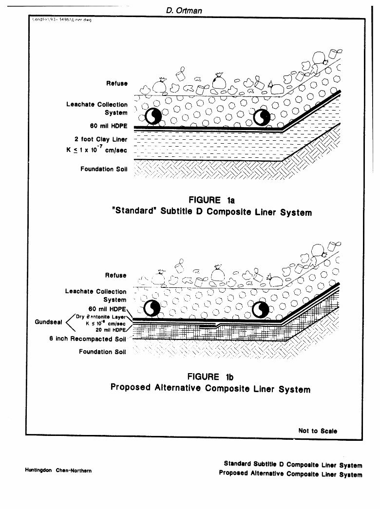
D. Ortman!_ondfm\,cl.3 - _496\,LinPr dwg I ii
FIGURE la
"Standard' Subtitle D Composite Liner System
FIGURE lb
Proposed Alternative Composite Liner System
Not to Scaleiii ii
Standard Subtitle D Composite Liner System
HuntingdonChen-Northern Proposed Alternative Composite Liner System

Alternative Landfil! Liner 58"1q
Page iv: '_ workshop was held at the Risk Reduction EngineerinD Laboratory inCincinnati, Ohio, on June 9-10, 1992 to discuss geosynthetic clay liners(GCLs). The purpose of the workshop was to present and discuss the mostrecent information available on the use of GCLs. This Information will be ##n tOEPAnroFramandruionRI official#,state r_ulatorv officials,nrmit writer#, andd_ianerl of we#t# dlsnoul f_llitlu,"
Page v: "The issue of equivalency of a GCL to a CCL (compacted clay liner) wasdiscussed. A number of criteria might be appfled, but only a few seem trulyrational. Stnd¥.#tate Waterfluxand #olut¢ flux are obviou#ran#r/ur criterimthe##huld ut#al!y be #art of an ewuivmlenovurn!re1# Othercriteria an be rope!ledbutrout are muchless muni_ul t.. terets of #ddroninF ruulmtorv co#reliance,"
NOTE: This report specifically addresses "$tudy.#tato w#ter flux _od #otut_f_/_q_'to demonstrate the equivalency or ,,_uperiorityof the proDosedalternative composite liner system to the "standard" Subtitle D liner.
"Finally, regulatory acceptance of GCLs was discussed. Although numeroussite-specific approvals of GCLs have been given by regulatory agencies, noblanket approvals or disapprovals were identified."
Page 21-22:"2.4.1.1 Hydraufic Conductivity"
"The hydraulic conductivity of an intact specimen of Gundseal ®has been reportedto be less than 4x10"_ cm/s. Researchers at the University of Texas (Daniel &Shan, 1992) and at GeoSyntec Consultants (1991) have reported that the bentoniteelement of Gundseal ® alone has a hydraulic conductivity between lx10 _ andlx10 "t°cm/s. Therefore,the 1/0inch thick lav#r of Imnto#iti wheneon#ideredby itself, isequivalentto,at lea#t twelve,,,!.nohuof Ix10 _era# clay. The#undn_[ #¥#ten_¢on#i#tinFofthe geomembraneand the layer of bentonite,I# equivalent to well over three feet of 1x10;am# clay,,
NOTE: "The 8un_nl* #V#tem"only refers to the Gundseal ® itself. It does notinclude the overlying 60 mil HDPE in the proposed alternative liner system.
"2.4.1.2 Overlapped Se_ms"
'When Gundseal ®panels are overlapped, close contact is developed between thebentonite portion of one panel and the geomembrane portion of the other.Researchers at the University of Texas (Estornell, 1991) investigated theeffectiveness of this overlap by performing large scale tests on two separateoverlapping specimens. One sample had an overlap of 1.5 inches, while the othersample had an overlap of 3 inches. Two feet of gravel and one foot of water wereplaced over each of the specimens. During the five.month.lon_xtest. no outflow Wa#noted through either of the overla#pino#lledmM¢ Additional tuting ha# beenperformedby

D. Ortman588
6eesyntecConsultants(lggll and no flow was noted thrauahthe overlannodsaanwaftor a#ohundredhours."
NOTE: The recommended overlap for Gundseal®is 3 - 6 inches.
"2.4.1.3 Composite Action"
"The effectiveness of the overlapped seams indicates that a good composite actionis formed between a geomembrane and the hydrated bentonite. AdditionalrE ,earch at the University of Texas (Estornell, 1991) has shown that the bentoniteportion of Gundseal ® is able to seal off defects in an overlying geomembrane.tho Universityof Texas,#/its andholes woreout into a woomombrsno,rhi# goomombrs#aw_#plated on top of the bonton!toportion of Bud#of. and tho #v#temw## aov#rsdwtth aravola_pdwater. Thesetest# were nrformod for flVOmonth#,d#rin_awhioh timo no flow w_robservedthrau_ahthe my#tern,After five month#,th# test# worodi#montlod#nd tho oMdltlo#of the 8CLwas observed.Around the ler_aestholef3 l##hdiomotor/in tho !oomombrsn& onlya 6 inch diameterarsa Waswetted on tho bentonite,thu#/ndleatlnwoxaollantl#timate co#tootand aompesiteaction,"
"The effectiveness of intimate contact between Gundseal ® and an overlyinggeomembrane was also invest/gated by the engineers at GeoSyntec Consultants(1991). Tbsir result# indicatod that the hydratedbsntonitacan affectivo!v SaMa dafest inan overlyingwesmembrano.Water contents were taken from the bentonite portion ofGundseal ®directly beneath a O.1 mm diameter hole. The water content testsindicated a significant reduction in the water content of the bentonite radially awayfrom the hole."
Page 26:"2.4.3 Conclusion"
"Researchhu indicated that Sun_ul ®i# an affectivo rollaeamont for clay in landfill linersy#tamsand covers. Co#earnhas beenaxpresse_unon oecuio& by on_ai#oors,contractor#,and regulators that tho thin uaesyntbstieclay liners, such es 6undsu! ®. are s#no#tiblo todamaaaduringinstallation, Howovor.the installation of aaesvnthetloclay liners is m#eheasierthan tbs constructionof tom#actedclay liners, and whenthe contractors utilize the #e_a carethat is neededto install a gaomambrana,an offectiva liner or covor#¥stamis in nloea andprotectin_athe environment."
NOTE: The final design will include both pro-qualification of the installer and athird-party QA/QC program to ensure ."the cutraoto_ utilize tbs _ameoars t/tat isnndad to iestMI a wesmmbrsn". In addition, the design will incorporate both anadequate protective layer over *,hecomposite liner and an operational inspectionprogram to ensure the proposed alternative liner system is not damaged duringlandfill operations.

Alternative Landfill Liner589
Page 84:"7.1 5.1 Freeze/Thaw Resistance"
"Compacted clay liners are known to be vulnerable to large increases in hydraulicconductivity from freeze/thaw. Limited laboratory data indicate that GCLs do notundergo increases in hydraulic conductivity as a result of freeze/thaw (Shan andDaniel, 1991). In addition, for those GCLs that contain a geomembrane, thegeomembrane is unaffected by freeze/thaw. Thu. frcB theavMImbl¢dmt&#¢_ Ullurto he##neriorto CClJIn ternmof frNzWthewr_htuce,"
NOTE: The site's climateis particularlyconduciveto freeze/thaw of liners.
"7.1.5.?.. Wet/Dry_Effects"
'lNe=tingand drying of CCLs and GCLs can cause either type of clay liner to sweflor shrink. Themain concern with clay liners that are wet and then dry out, is thatdesiccation can lead to cracking and an increase in hydraulic conductivity."
"Limited laboratory data indicate that when dry, cracked CCLs are rewetted, theclay swells and any cracks are partially closed, leading to partial recovery of theoriginal, low hydraulic conductivity. In contrast, theJavailable data show that thehigh swelling of bentonite results in full self healing and full recovery of theoriginal, low hydraulic conductivity when dried, cracked GCLs are rewetted. Inaddition, for those GCLs that contain a geomembrane, the geomembrane isinsensitive to wet/dry effects. The. #eL#unenr to bemorethmnNeivalentto Ct_l_in_¢rnmof ability to nff.hul ff themmterimlh wetted driedaddthemrewetted."
Page 87-88:"7.1.6.3 Ease of Placement or Construction"
I
"A GCL will always be easier to place than a CCL, unless weather conditions areadverse (e.g., constant rain), in which case even a CCL will also be difficult toconstruct. In FenerM.8¢1J ere eu#ivMenttOqr I_etterth## eeLsin term of N#e #nleoementof ¢on#tr#otion."
"7.1.6.4 Speed of Construction"
"eeo#vntheti¢¢levliner#canhenlmeedmuchmore #aiot(!wthu ¢¢_. EauivMenqvh obvio_,"
"7.1.6.6 weather Constraints"
"compacted clay liners are difficult to construct when soils are wet, heavyprecipitation is occurring, the weather is extremely dry (clay desiccates), the soilis frozen, or the temperature is below freezing. Geosynthetic clay liners aredifficult to construct during precipitation. Weather¢on#trM#t#FenerMl_vf#vor 8Cl.e."
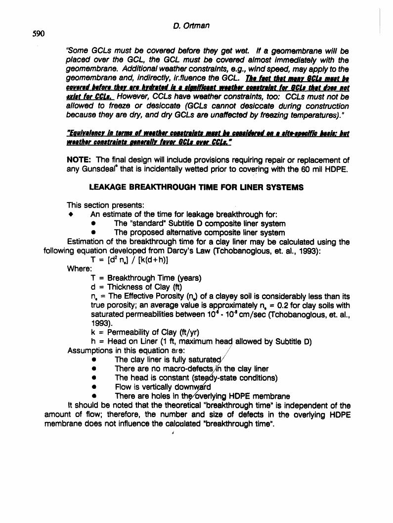
D. Ortman590
"Some GCLs must be covered before they get wet. If a geomembrane will beplaced over the GCL, the GCL must be covered almost immediately with thegeomembrane. Additional weather constraints, e.g., wind speed, mayapply to thegeomembrane and, indirectly, influence the GCL. Thef_t that mmr 8C1.#m_t h¢coveredbeforetheratehr_ated h a #1FnM_ntweathercmtrNntfor8CLsthati_ea#Or,axhtforCC_. However,CCLs haveweatherconstraints,too:CCLs mustnotbe
allowed to freeze or desiccate (GCLs cannot desiccate during constructionbecause they are dry, and dry GCLs are unaffected by freezing temperatures')."
"EauiwlMcrin ternuofweatherea_trNntt /n_t lleconalderedona #1tc_rnmffioImeh:b_tweathorOon#trNn_rnnerMIr fmvort/t_ #vwrOOIJ."
NOTE: The finaldesignwillincludeprovisionsrequiringrepairor replacementofany Gunsdeal"that is incidentallywetted priorto coveringwiththe 60 mil HDPE.
LEAKAGEBREAKTHROUGH TIME FOR LINER SYSTEMS
This sectionpresents:• An estimateof the time for leakagebreakthroughfor:
• The "standard"SubtitleD compositelinersystem• The proposedalternativecompositelinersystem
Estimationof the breakthroughtime for a clay linermay be calculatedusingthefollowingequationdevelopedfrom Darcy'sLaw (Tchobanoglous,et. al., 1993):
T = [d=n,] / [k(d+h)]Where:
T = BreakthroughTime (years)d = Thicknessof Clay (ft)n, = The EffectivePorosity(n,)of a clayeysoilis considerablylessthan itstrue porosity;an averagevalueis approximatelyn, = 0.2 for claysoilswithsaturatedpermeabilitiesbetween10"e- 10"ecm/sec (Tchobanoglous,et. al.,1993).k = Permeabilityof Clay (ft/yr)h = Head on Liner(1 ft, maximumheac_allowedby SubtitleD)
Assumptionsin this equationare: /• The clay lineris fullysaturatec_/• There are no macro-defects_nthe clay liner• The head is constant(steely-state conditions)• Flow is verticallydownward• There are holes inthe//overlyingHDPE membrane
It shouldbe notedthat the theoretical"breakthroughtime" is independentof theamount of flow; therefore, the number and size of defects in the overlyingHDPEmembranedoes not influencethe calculated"breakthroughtime".

Alternative Landfill Liner591
The "Star,tdard" SubtlUe D Composite Uner SystemUsingthe equationgivenaboveand assuminga holeexistsinthe 60 railHDPE,
the breakthroughtimefor the standardSubtitleD lineris:T = [22ftx 0.2] / [0.103 ft/yr x (2 + 1)]
Where:d = 2 feetn. = average0.2 forclayeysoilwithpermeabilitybetween10"e- 10acm/sec,(Tchobanoglous,st. al., 1993)k = 10̀ 7cm/sec = 0.103 ft/yr
Therefore:T = 2.6 years
The ProposeO Alternative Composite Liner SystemUsingthe equationgivenaboveand assumingalignedholesexistin boththe 60
railHDPEprimarylinerandthe 20 railHDPEbackingforthe Gundseal®, the breakthroughtimefor the proposedalternativelinersystemis:
T = [0.012ft x 0.2] / [0.001 ft/yr x (0.01 + 1)]Where:
d = 0.01 feet (1/8_ inchunhydratedthickhessof bentonitecoating = 0.01ft)n. = average0.2 for clayeysoilwithpermeabilitybetween10e- 10.8cm/sec,(Tchobanoglous,G., Theisen,H., Vigil,S., 1993)k = 10"gcm/sec = 0.001 ft/yr
Therefore:T = 0.02 years ,_ 1 week
The breakthroughtimefor the overlapseam inthe Gundseal® may be estimatedusingthe sameequationby substitutingthe minimumoverlaplength(3 inches = 0.25 ft)for the clay thickness(d) and assumingthe hole in the overlying60 rail HDPE occursexactly on the edge of the upper Gundseal® panel. For this case, the calculatedbreakthroughfor the minimumGundseal®overlapseam is:
T = [0.252ftx 0.2] / [0.001 ft/yr x (0.25 + 1)]Where:
d = 0.25 feet (minimumrecommendedoverlapof 3 inches= 0.25 feet)n, = average0.2for clayeysoilwithpermeabilitybetween10e- 10s cm/sec,(Tchobanoglous,st. al., 1993)k = 10"scm/sec = 0.001 ft/yr
"Therefore:T = 10 years
Itshouldbe rememberedthattheseestimatesassume:(1) the maximumallowablehead existsonthe linersystem,(2)there isa sufficientsupplyof leachateto maintainthismaximumhead,and (3) the permeabilityof the bentonitelayerisconstantat 10.9cm/sec.In reality,the laboratorytestingof the Gundseal® indicatesthat the effectivepermeabilityof the I_ydratedbentoniteisless than10"gcm/sec andthe amountof leakageis so smallthat the real-worldleakage is essentiallyimmeasurableonce the dry bentonitelayer ishydrated(Daniel& Boardman,1992).

592 D. Ortman
AMOUNT OF LEAKAGE THROUGH LINER SYSTEMS
Thissectionpresents:• An estimateof the amountof leakagethroughthe linersystemsfor the
8 acre, Cell #1 for:• The "standard"SubtitleD compositelinersystem• The proposed alternativecompositelinersystem
Theamountof leakagethrougha compositelineris controlledby the numberandsize of constructiondefects in the membrane and the effectivepermeabilityof theunderlyingclay. An accepted approachto predictingthe performanceof a compositeliner is to calculatethe leakage through the expected number of holes in the uppermembraneand assumethisamountexitsthe bottomof the linersystem.
The followingequation has been developedby J.P Giroud for calculatingtheleakage through a hole in a membraneoverlyinga clay secondaryliner;it has beenaccepted by the EPAin lieuof BernouUli'sEquationand has been incorporatedin therecent3.0 versionof EPA's HELP model (Giroud,1993).
Q = 0.21 a°'1h°-gk,0"74Where:
Q = LeakageRate (m3/sec)a = Area of the LinerHole (mz)h = Head on the Liner(m)k, = SaturatedPermeabilityof the UnderlyingClay (m/sec)
For predictinglinerperformancethe followingparametershave been proposed(Giroud,1993):
• A "standard hole" is 0.2 cm in diameter;thereforethe area = 3.1 x 10e m2• The number of "standard holes" per acre may be estimatedbased on:
• 1 standard hole per acre if the membrane is placed by a goodinstaller and there is a QA,/QC proaram
• 30 standard holes per acre if the membrane is placed by a goodinstaller but there i.sno QAJQCDrogram
Table 1 presents the results of using Giroud's equation to calculate both the annual and30 year leakage amounts from the eight acres of Cell #1 for various combinations of"Number of Standard Holes (holes/acre)" in the membrane and "Controlling ClaySaturated Permeability (k,)" for the underlying clay.
The final design will include pre-qualification of membrane installers to ensure a"good installer" is selected and a QA/QC program will be in force during construction ofthe entire liner and leachate collection system. Therefore, the leakage results for1 standard hole per acre represent Cell #1.
,

Alternative Landfill Liner 593
TABLE 1i , ' , , , i i L , , , .... ' '
LEAKAGE FOR 8 ACRE CELL #1 USING GIROUD'S EQUATION")Q gal/yr : [0.21 aL' ht' k,t" ml/sec] x 31,536,000 sec/yr x 35.3 flP/m' x 7.48 gal/_ x n,
holes/acre x 8 acresi i 'T I I I II I I I
Numberof ControllingClaySaturatedPermeability(k,)StandardHoles '
(holes/acre) " SuMIUe_.,_ D _ Alternative10_ cm/sec 10.7¢m/uc 1o• cm/sec lO" ¢m/sec10" m/sec : 1:0"m/a¢ lO"1°m/sec . 10'"
m_i 1 i 1 ' ' i • , i i ii. " i ' i
I m 1625 gal/yr 296gal/yr 54 gal/yr 10gal/yrGood_ImdaHer .
r , .
• with _/QC .... 48,750 gal/30yr 8880 goV30yr 1620 gal/30yr 300gal/30yr
5 8125 gal/yr 1480 gel/yr 270 gal/yr 50 gal/yr, ,,
10 16,250gal/yr 2960 gal/yr 540 gal/yr 100 gal/yr,
20 32,500 gal/yr 5920 gal/yr 1080 gal/yr 200 gal/yr,,, , ,, ........
300) 48,750 gal/yr 8880 gal/yr 1620 gal/yr 300 gal/yrGood Installer 1,462,5000
withoutQA/QC gal/30yr 266,400 gal/30yr 48,600 gal/30yr 9000 gal/30yr
a = Area of Standard Hole (3.1 x 10"°m=)h = Head (0.305 m = 1 ft, MaximumHead Allowedby SubtitleD)k,= SaturatedPermeabilityof ControllingClay (m/sec)
_1) Leakagerepresentsthe amountthat passesthroughthe "standardholes"inthe upperHDPEliner,assumingthe underlyingclay is saturated.
_1 Giroud(1993)
The "Standard" SubtlUe D Composite Liner SystemThe standard Subtitle D composite liner system is expected to have the following
leakage amounts:• Total Annual Leakage == 296 gallons
Total 30 Year Leakage ,= 8880 gallons
The Proposed Alternative Composite Uner SystemThe proposed alternative composite liner system is expected to have the following
leakage amounts:Total Annual Leakage == 10 gallonsTotal 30 Year Leakage == 300 gallons
It should be noted that this estimate of total leakage through the proposedalternative liner system ignores the 20 mil HDPE membrane incorporated in theGundseal®; the actual leakage for the proposed alternative liner system should beconsiderably less than that predicted by these calculations.
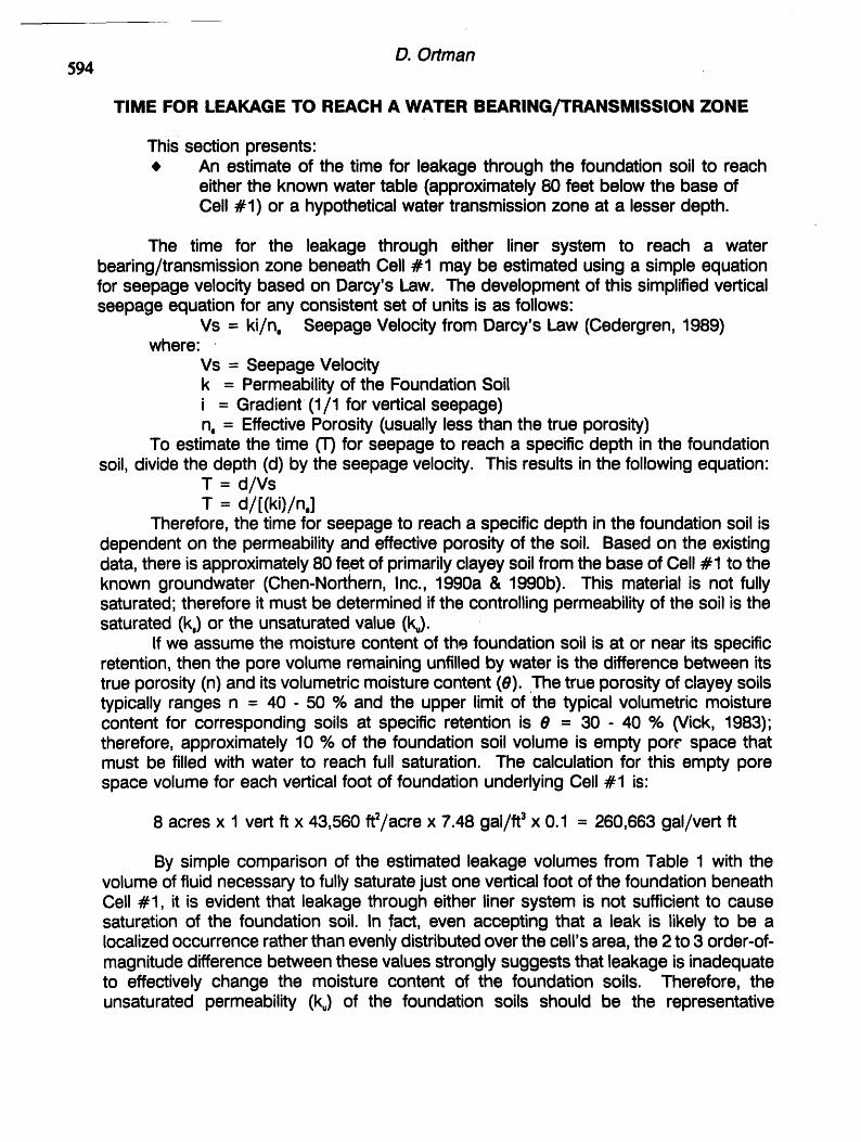
D. Ortman594
TIME FOR LEAKAGETO REACH A WATER BEARING/TRANSMISSION ZONE
Thissectionpresents:An estimateof the time for leakage throughthe foundationsoil to reacheitherthe knownwatertable (approximately80 feet belowthe base ofCell #1) or a hypotheticalwater transmissionzone at a lesserdepth.
The time for the leakage through either liner system to reach a waterbearing/transmissionzone beneathCell #1 may be estimatedusinga simpleequationfor seepagevelocitybased on Darcy'sLaw. The developmentof thissimplifiedverticalseepageequationfor any consistentset of unitsis as follows:
Vs = ki/n. SeepageVelocityfrom Darcy'sLaw (Cedergren,1989)where:
Vs = SeepageVelocityk = Permeabilityof the FoundationSoili = Gradient_(1/1 for verticalseepage)n, = EffectivePorosity(usuallylessthan the true porosity)
To estimatethe time (T) for seepage to reach a specificdepth inthe foundationsoil,dividethe depth(d) by the seepagevelocity. Thisresultsinthe followingequation:
T = d/VsT = d/[ (ki)/n.]
Therefore,the timefor seepageto reach a specificdepthinthe foundationsoilisdependenton the permeabilityand effectiveporosityof the soil. Basedon the existingdata,thereis approximately80 feetof primarilyclayeysoilfromthe baseof Cell# 1 to theknown groundwater(Chen-Northern,Inc., 1990a & 1990b). This materialis not fullysaturated;thereforeitmustbe determinedifthe controllingpermeabilityof the soil isthesaturated (k,) or the unsaturated value (k,).
If we assume the moisture content of the foundation soil is at or near its specificretention, then the pore volume remaining unfilled by water is the difference between itstrue porosity (n) and its volumetric moisture content (8). The true porosity of clayey soilstypically ranges n = 40 - 50 % and the upper limit of the typical volumetric moisturecontent for corresponding soils at specific retention is 8 = 30 - 40 % (Vick, 1983);therefore, approximately 10 % of the foundation soil volume is empty pore space thatmust be filled with water to reach full saturation. The calculation for this empty porespace volume for each vertical foot of foundation underlying Cell #1 is:
8 acres x 1 vert ft x 43,560 ft2/acre x 7.48 gal/ft 3x 0.1 = 260,663 gal/vert ft
By simple comparison of the estimated leakage volumes from Table 1 with thevolume of fluid necessaryto fully saturate just one vertical foot of the foundation beneathCell #1, it is evident that leakage through either liner system is not sufficient to causesaturation of the foundation soil. In fact, even accepting that a leak is likely to be alocalizedoccurrence rather than evenly distributed over the cell's area, the 2to 3 order-of-magnitude difference between these valuesstrongly suggests that leakage is inadequateto effectively change the moisture content of the foundation soils. Therefore, theunsaturated permeability (k,) of the foundation soils should be the representative
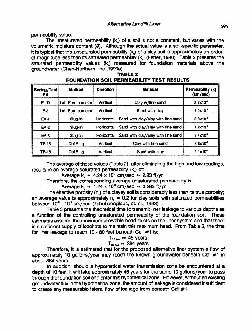
Alternative Landfill Liner 595
permeabilityvalue.The unsaturatedpermeability(k,) of a soil is not a constant,but varieswith the
volumetricmoisturecontent (8). Althoughthe actualvalue is a soil-specificparameter,it is typicalthat the unsaturatedpermeability(k,) of a claysoilis approximatelyan order-of-magnitudelessthan its saturatedpermeability(k,) (Fetter,1980). Table2 presentsthesaturated permeabilityvalues (k,) measured for foundation materials above thegroundwater(Chen-Northern,Inc.,1990a).
TABLE 2FOUNDATION SOIL PERMEABILITY TEST RESULTS
j _ T i i _ ill i i i i ,i , : I ' • , ,,,ira iJ i ii ,
Boring/Test Method Direction Material Permeability (k)Pit (cm/ac)
,,, , , ,, , , , , , ,
E-1D Lab Permeameter Vertical Clayw/fine sand 2.2<10_, , , i , , , i| i
E-3 Lab Permearneter Vertical Sand withclay 1.0x10⁷i
EA-1 Slug-In Horizontal Sandwith clay/claywithfine sand 6,8x10"7,,, , , • , , ,,, ,,, ,,
EA-2 Slug-In Horizontal Sand with clay/claywithfine sand 1.2x10"7, i , , , -
EA-3 Slug-In Horizontal Sand with clay/claywith fine sand 3,4x10⁷,, ,, , i, ,, ,
TP-15 DbI.Ring Vertical Claywith fine sand 8.8x10.7, , ,i , , ,
TP-18 Dbi.Ring Vertical Sandwith clay 2.lx10"s,,, _ ,, i , i , i, i ..... i , ,
The average of these values(Table2), aftereliminatingthe highand lowreadings,resultsin an averagesaturatedpermeability(k,) of:
Averagek, - 4.24 x 10.7cm/sec - 2.83 ft/yrTherefore,the correspondingaverageunsaturatedpermeabilityis:
Averagek, - 4.24 x 10"lcm/sec _, 0.283 ft/yrThe effectiveporosity(no)of a clayeysoilis considerablylessthanitstrueporosity;
an averageva!ue is approximatelyn, = 0.2 for clay soilswith saturatedpermeabilitiesbetween 10e- 1l_° cm/sec (Tchobanoglous,et. al., 1993).
Table3 presentsthe theoreticaltimeto transmitlinerleakageto variousdepthsasa function of the controllingunsaturatedpermeabilityof the foundationsoil. Theseestimatesassumethe maximumallowablehead existson the linersystemandthatthereis a sufficientsupplyof leachateto maintainthismaximumhead. FromTable3, the timefor linerleakageto reach 10 - 80 feet beneathCell #1 is:
T1o,.,- 45 yearsT,,,, - 364 years
Therefore,it is estimatedthat for the proposedalternativelinersystema flow ofapproximately10 gallons/year may reach the known groundwaterbeneath Cell #1 inabout364 years.
In addition,shoulda hypotheticalwater transmissionzone be encounteredat adepthof 10 feet, itwilltake approximately45 yearsfor the same 10 gallons/yearto passthroughthe foundationsoilandenterthishypotheticalzone. However,withoutan existinggroundwaterfluxinthe hypotheticalzone,theamountof leakageisconsideredinsufficientto createany measurablelateralflowof leakagefrom beneathCell #1.
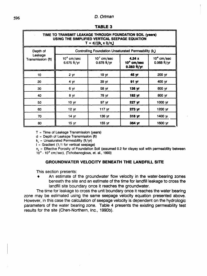
596 D. Ortman
TABLE 3
TIME TO TRANSMIT LEAKAGETHROUGH FOUNDATION SOIL (years)USING THE SIMPLIFIED VERTICAL SEEPAGE EQUATION
T : d/[(k, x i)/n.]., .,, , i i,
. . i I I
Depthof ControllingFoundationUnsaturatedPermeability(1%)Leakage ..................
Transmission(ft) 10e cm/sec 10̀ 7cm/sec 4,24 x 10_ cm/sec6.675 ft/yr 0.678 ft/yr 104era/ram 0.068 ft/yr
.... , ,, , .....10 2 yr , 19 yr _ yr.... . : 200 yr
20 4 yr 39 yr 91 yr 400 yr.... : I I Ii Ill I] Ill , ,
30 6 yr 58 yr 136 yr 600 yri ,ii , l i .ill ii I I i
40 8 yr 78 yr 162 yr 800 yr11 LII tLtL]Li Ii_l . ± Jill
50 10 yr 97 yr 2_. yr 1000 yri, 
I
A/temative Landfill Liner 597
TABLE 4WATER BEARINGZONE PERMEABILITY TEST RE,I;ULTS
,, i , , _, , ,, ,,., , ,, i , ' ', ,,. ,,, ,, ,, ' ' ,,, i -.
Boring/ Method Direction Material SaturatedTest Pit Permeability (k,)
(cm/sec)i , , , , , , ,,,, ,, , ..
E-1D Slug-Copper Horizontal Sand/Gravel,80'-9G' 3x10⁴..... i , i., ,,,, , , L. , ,.
E-ID Slug-Hvorslev Horizontal Sand/Gravel,80'-90' lx104, . , ,, ,,
E-1D Bailer Recovery-Cooper Horizontal Sand/Gravel,80'-90' 4.0x10⁴, |. i . , ,,,,
E-2 Slug-Cooper Horizontal Sand/Gravel, 85'-90' 3x10⁴' ' ' '' " I
E-3 Slug-Cooper Horizontal Sand/Gravel,67'-77' 6x10.6
E-3 BailerRecovery-Cooper Horizontal Sand/Gravel,67'-77' 4.lx10 .5, , , , ,.,. ,
E-6 Slug-Cooper Horizontal Sand/Gravel, 154'-164' 8.2x10.6,,. , ,, ,, ,.,
E-7 Slug-Cooper Horizontal Sand/Gravel,150'-160' 2.8x10.3,,
E-8 Slug-Cooper Horizontal Sand/Gravel, 128'-134' 3.3x10⁴, ,,, . ,, . ,
E-9 Slug-Cooper Horizontal Sand/Gravel, 143'-157' 3.3x10_• , ,, ., '- , . .,, . ,. , ,,
The averageof thesevalues(Table4), aftereliminatingthe highand lowreadings,resultsin an averagesaturatedpermeabilityof:
Averagek, _=2.3 x 104 cm/sec ==238 ft/yearThe other pertinenthydrologicparametersare:
i = 0.02- 0.04 (Chen-Northern,Inc., 1990b)n, = 0.25 (assumedfor Sand/Gravelwithk, _ 10.4cm/sec; Note:AlthoughTable4 liststhe materialas "Sand/Gravel",theremustbe a finesizefractionto accountfor the low measuredvaluesof k,)
Therefore,the velocityof groundwaterflow beneaththe siteranges:V, = k,i/n,V, = (238 ft/year x 0.02)/0.25 to (238 ft/year x 0.04)/0.25V, = 19 - 38 ft/year
In the vicinityof Cell #1, the general groundwaterflow is toward the east unitboundary (Chen-Northern,Inc., 1990b). Table 5 indicatesthe range of times for thegroundwaterto reachthe east unitboundaryfrom variousstartinglocationswithinCell #1., the range is:
T = 3 - 37 years (dependingon startinglocationand hydraulicgradient(i))
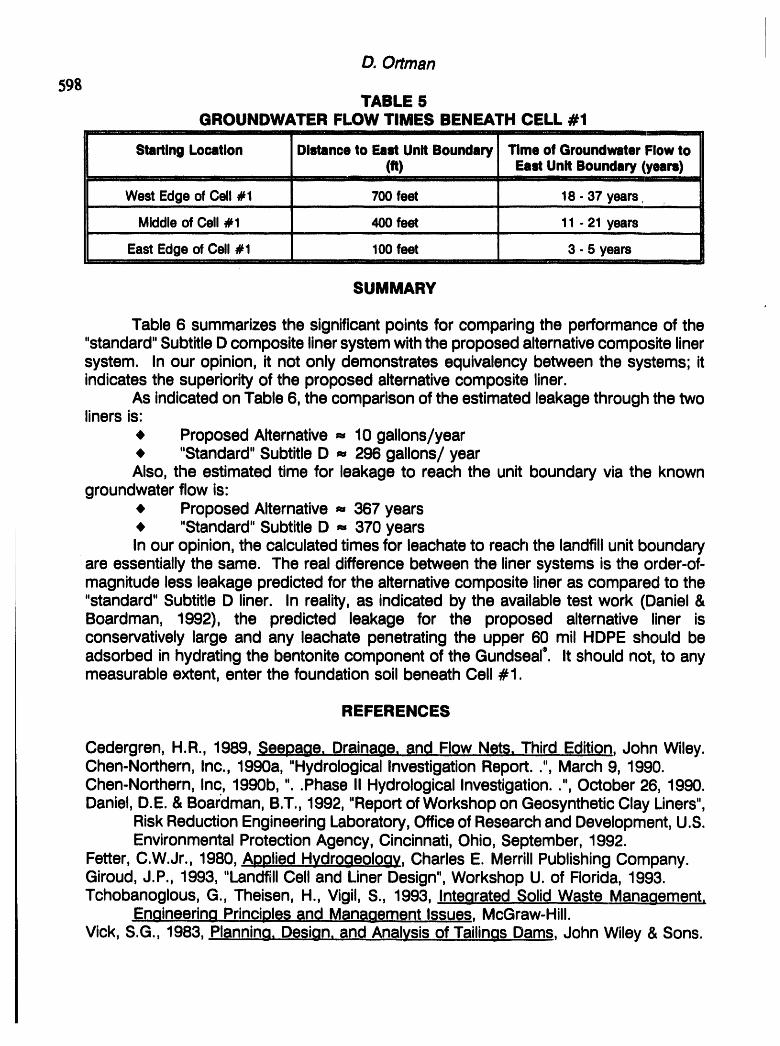
D. Ortman598
TABLE 5GROUNDWATER FLOW TIMES BENEATH CELL #1
, l I I III I 'rl'Hl'' :
Starting Location Distance to East Unit Boundary Time of Groundwater Flow to(it) East Unit Boundary (years)
i LI
West Edge of Cell #1 700 feet 18 - 37 yearsi i i i ill i.i,H i i ,ill i,==,l i ii
Middleof Cell #1 400 feet 11 - 21 years
EastEdge of Cell #1 100feet 3- 5 years' r
SUMMARY
Table 6 summarizesthe significantpointsfor comparingthe performanceof the"standard"SubtitleDcompositelinersystemwiththe proposedalternativecompositelinersystem. In our opinion,it not only demonstratesequivalencybetweenthe systems;itindicatesthe superiorityof the proposedalternativecompositeliner.
As indicatedonTable6, the comparisonof the estimatedleakagethroughthe twolinersis:
• ProposedAlternative==10 gallons/year• "Standard"SubtitleD ==296 gallons/yearAlso, the estimatedtime for leakage to reach the unit boundaryvia the known
groundwaterflow is:• ProposedAlternative==367 years• "Standard"SubtitleD ==370 yearsIn ouropinion,the calculatedtimesfor leachateto reach the landfillunitboundary
are essentiallythe same. The realdifferencebetweenthe linersystemsis the order-of-magnitudelessleakagepredictedfor the alternativecompositelineras comparedto the"standard"SubtitleD liner. In reality,as indicatedby the availabletest work (Daniel&Boardman, 1992), the predicted leakage for the proposed alternative liner isconservativelylarge and any leachate penetratingthe upper 60 mil HDPE should beadsorbedin hydratingthe bentonitecomponentof the Gundseal®. It shouldnot, to anymeasurableextent,enterthe foundationsoilbeneathCell #1.
REFERENCES
Cedergren,H.R., 1989, Seepage, Drainaae. and FlowNets, Third Edition,John Wiley.Chen-Northern,Inc., 1990a, "HydrologicalInvestigationReport..", March9, 1990.Chen-Northern,Inc, 1990b, "..Phase II HydrologicalInvestigation..",October 26, 1990.Daniel,D.E.& Boar'dman,B.T., 1992, "Reportof WorkshoponGeosyntheticClayLiners",
RiskReductionEngineeringLaboratory,Officeof ResearchandDevelopment,U.S.EnvironmentalProtectionAgency,Cincinnati,Ohio,September,1992.
Fetter,C.W.Jr., 1980, AppliedHydrogeology,CharlesE. MerrillPublishingCompany.Giroud,J.P., 1993, "LandfillCell and LinerDesign",WorkshopU. of Florida,1993.Tchobanoglous,G., Theisen, H., Vigil, S., 1993, IntegratedSolidWaste Management,
EnoineerinoPrinciplesand ManagementIssues,McGraw-Hill.Vick, S.G., 1983, Planning,Design,and Analysisof TailingsDams, JohnWiley& Sons.

TABLE 6
COMPARATIVE SUMMARY OF MAJOR ITEMS FOR THE "STANDARD" SUBTITLE O LINERAND THE PROPOSED ALTERNATIVE LINER
,,L
ITEM "STANDARD"SUBTITLEO PROPOSEDALTERNATIVELINER SYSTEM COMPOSnE UNER SYSTEM
|!
To_ Leakage 2_S_ear 10gaUons,_/ear TotaJleakageamo..tIsconsldmblylessformeanemaUveUner.Amount tnreamy,UdsamountmuwwmbeadmbedIn_ me
UOOganons_years 3OOganonsneyears bentonneandwmnotmdyescapemeUner_ toanYmeasurd_ extent, tn addlUon,me _ Ignoresme 20 ndll
_PE_me_
2.syears t weJ (Um_h _kj_d _ _ born The_r k_ I_._i_ Urn.¢J:uWMdtotme_mmm_B_ IHDPE _) liner requk_ lhat open holiesezlst dlrocUyoppoedlMeach other inTime bo__ An onset of only 3 Inches beewNn holes results :)_
10years (Uu'oughovedap seam In a _ t_ne skmUar_ome ovedap seam. _nlsassum_ a hok,Inm* upp_HDPE conskSer_hig_. unak_ UmU., b,r,/Uw,_ Un.,_x U.,_ atmeedgeofmeovedap) aj,_._,eU_rwmbetnWkmUmtorme'smdard'SubU_D, m
Tbne for Leakage Hy1?o_ Water SeadngZone Same The known water beadng zo_ Is at least OOfeet below me Cell _ r-.to Reach a Water @ t0 feet - 4s years k merofor_ the Umefor leakage1o rmch me edsOngieeadngZo_ne _ is qnlnroximnate_364 years,, The eslnaim for me
Known Water Seadng Zone @ eo hyl_heUc_ w_er be_r_g zone at 10 feet Lsprovk_ k)r _feet- 364 years c0mpeds_ puqx:e_; even ff such a zone _ It would take
amroxm_,s yea. _ .,,, mlum tor._ ". .r-:(b
Tlme for Leakage 3 - 37 years dqpendlngon slartMg Same The general gro4md_der flow befmath Cell gt is toward the eastem "_to Cross the Unn IocatkmandWdVaudnlcgradlent unnboundarywnhagradlentramgeof0.02-0.O4. The_Boundary Once It Umeassumes Um leak occun at me eastern edge of Ceil #t (100Has Reached the feet from me unit boundary) and has a gradient of 0.04. The longestGroundwater time assumes the leak occurs M the wedem edge of Cd tl (70O
feet from me unn boundan/) and has a gradient of 0.02.
Total TIme for HypolhetlcalWalMrBearingZone _Watm'BearingZone@ 10 BollhestbemtesassumelheleaklsatbciosestlocadlontoUteunltLeakageto Reach • 10 feet - 2.6_15.3 - 51 years feet - 4,5+3-, 48 years boundalryarldlhe _lllVel underlhe bdkJeltCeofthethe Unit Boundary greatest hydraulic gradlenL
Known Water 6earing ZmJe@OO Known WatK 6eadng Zone @aOfeet-- 2.6'_'-'-'-'-'-'-'-'-'-__..3 -- 370 years - 364+3 - 367 years,,,
Fr_ Vulnerable to large Increases In No increase In pm'meabHnyfrom Freeze/Thaw has no effect on the _ liner sYstm_ but wglR-u'._nce _ lrrom__.,_haw fmeze/Umw ,,. cause large Increases In the Pen_labltY of llhe SubUh D clay liner-
'Wet4)ry Effects Vulnerable to deslccaUoncrad(b_ No b_.ease Jnpemeabany from Wet4_ has no effect on me _ Uner_ but may causeand Incr______In _ wet/dry effects an increase In tlhe penemabity of Ute SubUUeD clay IMer.
, • "_' , ,,,


Hydrogeology, Waste Disposal, Science and PoliticsProceedings 30_h SymposiumEngineering Geology and Go.technical Engineering, 1994
•VALUATION OF THE GROUND WATER RESOURCES 601WITHIN THE LEWXSTON BASIN
Gary R. Stevens, College of Mines and Earth Resources,University of Idaho, Moscow, ID 83843
Dr. Dale Ralston, College of Mines and Earth Resources,University of Idaho, Moscow, ID 83843
ABSTRACT
The Lewiston Basin located in North Idaho covers approximately 550 squaremiles and includes the cities of Lewiston, Idaho and Clarkston, Washington.The deep aquifer in the Lewiston Basin has been declared a sole source
aquifer. This system provides the primary water supply for the City ofClarkston Washington and a partial water supply for the City of Lewiston andthe Lewiston Orchards Irrigation District. Questions have been raised relativeto the maximum yield of the aquifer system with the continued growth of thearea. This study addresses the hydrogeology of the basin, along with thelocations and mechanisms for recharge and discharge.
The geology of the Lewiston Basin consist of Miocene-Pllocene basalt flowsoverlain by quaternary sediments. The basalt flows were structurally deformedduring and after emplacement, thus creating a structural basin with numerousfaults. The lower most basalt unit of the Lewiston Basin is the Imnaha Basalt,
which is overlain by the Grande Ronde and Wanapum Basalts. The boundaries ofthe ground water flow system are the same as the structural basin.
The Lewiston Basin, based on static water levels, appears to have threeseparate aquifer systems, the sedimentary aquifer, the Wanapum Basalt aquiferand the Grande Rondo Basalt aquifers. The aquifers, composed of dipping basaltunits, are most likely recharged where they intersect the Snake River in the
southern part of the basin and also along a portion of the Clearwater Riverand its tributary creeks in the eastern part of the basin. The discharge areaappears to be just west of the Snake River and Clearwater River confluence.
The Grande Rondo Basalt aquifer is utilized by the cities of Lewiston andClarkston, while the shallower sedimentary and Wanapum Basalt aquifers areused for domestic wells. Compilation and analysis of pump and water level datafrom the major ground water users of the Lewlston Basin from 1960 to 1993 showno apparent long term water level decline.
INTRODUCTIONStatement oE Problem
The Lewiston Basin covers approximately 550 square miles and includes theC'.ties of Lewiston, Idaho and Clarkston, Washington (figure 1). The Lewiston
Basin is a broad, shallow syncline with an axis that strikes east-west withboth ends plunging towards the center of the Basin. The Snake River flows from
south to north through the center of the study area (defining the Idaho-Washington border) and intersects the west flowing Clearwater River, near thenorthern boundary of the Lewiston Basin.
The three largest water management agencies within the Lewiston Basin arethe: 1) As.tin County Public Utilities District (APUD), which serves the Cityof Clarkston and surrounding areas; 2) City of Lewiston; 3) Lewiston OrchardsIrrigation District (LOID). The latter two agencies supply water to the Cityof Lewiston and vicinity. The APUD and LOID use mostly ground water for theirneeds while the City of Lewiston acquires almost all of its water from theSnake and Clearwater Rivers. Most of the wells were completed in the 1950s and1960s. Other smaller public water management agencies within the study areainclude the Cities of Lapwai, Idaho and As.tin, Washington. The Port of Wilmaalong the Snake River in Idaho also has its own wells. Industry in the studyarea have developed their own wells; these include: the Potlatch Corporation,Blount Industries and Twin Cities foods. The United States Army Corps ofEngineers manages a well that supplies water for Chief Timothy Park on theSnake River. A number of small domestic and agricultural wells are completedwithin the Lewiston Basin, mostly in the Lewiston Orchards and ClarkstonHeights areas. Most of the shallow wells are completed in the alluvial and

N

EvaJuation of _he Oround Mater Resources Within The Lewiston Easin
603shallow basalt aquifers, and the larger municipal wells are completed withindeeper basalt a_ifers.
Continued population and economic growth within the Lewiston Basin willnecessitate greater ground water pumpage and the future construction of moreproduction wells. This will be accelerated if the City of Lewiston partiallyswitches away from surface water supplies.
Purpose end Ob_eotivegThe purpose of this report is to serve as a technical guide for the LOID
and other water supply entities in the development of additional wellsconstructed into deep basalt aquifers within the Lewiston Basin. The generalobjectives are to 1) describe the hydrogeology of the Lewiston Basin, and 2)the potential for the additlonal development of high yield production wellsand the impacts that future wells might have on existing wells.
Water PEoduction WellsAll the information regarding the aquifer characteristics discussed in
this report came from data on existing water wells. The discussion og wherethese wells are located, and the details of well construction are imperativeto the description of the hydrogeology. The APUD has a total of seven wellsdrilled in and around the Clarkston, Washington area (see figure 1). The wellsare completed with a range of depths -76 to -183 feet ms1. The wells havereported yields of 1350 gpm to 4200 gpm.
The City of Lewiston has a total of five water production wells. The wellsare located within and near the City of Lewiston, Idaho. The wells have depthsof 460 to -5 feet msl and reported yields of 295 gpm to 1677 gpm. The City ofLewiston acquires most of its water from the Snake and Clearwater Rivers. Thewells are only used during the summer months when water demands are at thepeak. The two additional major wells located in the eastern portion of theLewiston Basin, belong to the Lewiston Orchards Irrigation District. LOIDwells, #1 and #2 have depths of -353 and -219 feet ms1 respectively. LOID #ihas a reported yield of approximately 870 gpm, and LOID #2 has reported yieldof 935 gpm.
A wildcat oil well (Konen well) is located near the LOID wells. The oilwell is presently used for irrigation of a parcel of farm land adjacent to theTammney School on Waha Road in the Lewiston Orchards. The well was reported tohave been drilled to a depth of approximately 3000 feet.
Other wells in the study area belong to the City of Asotin, City of Lapwaiand Chief Timothy Park along the Snake River. There are a number of othersmall irrigation and domestic wells spread out over the study area; most ofthese wells are less than 500 feet dee_.
RYDROGEOLOGZC SITTINGIntroduction
The thickness and lateral extent of individual basalt flows, physicalproperties of the aquifers, and the presence of any 8tructural deformation orlateral no-flow boundaries, all can have significant impacts on ground waterflow and on water level changes related to pumping of water wells. The deeperaquifers within the Lewiston Basin are composed of a series of basalt flowcontact units. The hydraulic properties and 8tructural configuration of theseunits control ground water flow characteristics.
Geologic Stratigraphy_mnaha Basalt
The Imnaha Basalt is the oldest basalt sequence of the Columbia RiverBasalt Group within the Lewiston Basin (see figure 2). The Imnaha Basalt,which is approximately 500 to 1000 feet thick, forms the hydrogeologicalbasement within the Lewiston Basin.Grands Rends BasaltThe Grands Rends is the most voluminous sequence of flows in the ColumbiaRiver Basalt Group, with a maximum thickness of approximately 2000 feet withinthe Lewiston Basin. The Grands Ronde has four alternating paleomagneticintervals, showing remanent magnetism with both normal and reversed fields
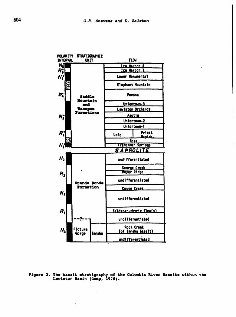
O.R. $¢even$ and D. Ra2mt:on
POLARITYSTRATIliUPHICINTERVAL UNIT FLOW
RN4* LowerMonumental
Elephmnt_untatn
Iladdle PomnaNountain
andIhmaPUa LewtstonOrchards
roz'matLonmtn •
Untontown-ZUntont0wn-1
Lolo Pr|est
b;
i
N2 undtfferent| itad
R2und|fferenttated
Grande mondeFonmtLon
NLund|fferent|ited
RI
-?-- undtfferenttated
RockCreekNO Picture
Gorge of Imnihl basil!und4fferenttated
]r£gure 2. The basalt atratLgraphy of the Colombia River Basalte w£th£n theLew_nton Basin (cmp, 1976).

Evaluation of the Ground Water Resources Within The Lewiston Basin
6O5(relative to the present earth magnetic field). The lowermost interval isreversed and is designated R1. This interval is overlain by the next threepaleomagnetic sequences designated N1, R2 and N2 respectively. All of thebasalts which overlie the N1 thicken toward the center of the basin.SaDrolite Laver
The significant period of quiescence that followed the extrusion of theGrands Ronde Basalt is expressed as a saprolite layer. The saprolite is a red-grey clay formed by weathering of the N2 basalt layer. The saprolite iswidespread throughout the Lewiston Basin and forms a marker between the GrandsRonde Basalt and the overlying formations_anaDum Basalt
The Wanapum Basalt overlies the Grands Ronde Basalt and consists of a
number of flows which include from oldest to youngest: the Dodge Member, RozaMember, and two flows of the Priest Rapids Member. The most extensive of thesebasalts is the uppermost Priest Rapids Member which averages 150 feet throughout most of the Lewiston Basin (Camp, 1976). The Priest Rapids Member overliesthe saprolite everywhere except along the western boundary of the study area.The lower most Dodge Member and the middle Roza Member are not found withinthe Lewiston Basin, but do exist extensively elsewhere in the ClearwaterEmbayment.Saddle Mountain Basalt
The Saddle Mountain Basalt consists of a number of basalt flows separatedabove and below by interbeds. There are a total of eight flows that consist offour different magnetic polarities. The lower five flows (Uniontown-1,Uniontown-2, Asotin, Lewlston Orchards, and Uniontown-3 flows) are laterally
extensive and cover the Lewiston Basin, while the upper three (Pomona,Elephant Mountain and Lower Monumental flows) occur as intracanyon basalts.The Saddle Mountain Basalts rest upon the Sweetwater Creek Interbed, whichseparates it from the Priest Rapids Member. The Sweetwater Creek interbedconsist of fine sands, silts clays and coarse detritus, and can be over 200feet thick.
0uaternary SedimentsThe Lewiston Basin contains a thick sequence of Quaternary stream gravels
which thicken toward the present confluence of the Snake and Clearwaterconfluence (Kehew, 1977). The gravels are composed of basalt and basementdetritus and reach a thickness of 400 feet. The gravel deposits can be foundsouthwest of the City of Clarkston, Washington and also both north and southof the Clearwater River near Lewiston, Idaho. The gravels are most likelyfluvial deposits of pleistocene age formed by the aggradation of the gravelswithin ancestral channels of the Snake and Clearwater Rivers.
Structural GeologyOne of the most significant features of the area is the doubly plunging
syncline found just south of Lewiston, Idaho and Clarkston, Washington (seefigure 3). The syncline strikes east-west, with each end of the axis plungingapproximately one to two degrees toward the central low point which is nearthe present Snake River Canyon. The limbs of the syncline dip approximately 2degrees toward the central axis.
The northern extent of the study area is defined by the ClearwaterEscarpment, which has almost 1800 feet of relief from top to bottom. At thebase of the Clearwater Escarpment is the east-west striking Gaging StationAnticline, an asymmetrical anticline bounded by the Wilma fault to the southand the Vista fault to the north. The Wilma fault extends west along the Snakeand Clearwater Rivers, crossing the Snake River just east of Chief Timothy
Park and terminates near the western boundary of the study area. The Wilmafault is believed to be the northern major structural barrier that controlsground water flow (Cohen, 1979).
A major structure found in the southern portion of the study area is theUniontown Anticline. The Uniontown Anticline, Lewiston Syncline and theClearwater Escarpment are believed to be the expression of a north-southcompressional regime which created the major structures of the area. Thecompression most likely occurred during the Miocene and was followed bysubsidence of the Lewiston Basin during the Miocene-Pleistocene period. Thesubsidence beneath the Lewiston Basin is probably due to withdrawal of magma

SCALE
B 2 4 6 8
Figure 3. Structural feature8 of the Lewlston Basin.

Evaluation of the Ground Water Resources Within The Lewiston Basin
607
from reservoirs and isostatic adjustment to the load of basalt flows imposedon the crust (Bond, 1963).
The southern limit of the study area is defined by both the Limekiln Faultand the Grande Ronde Fault. The Limekiln Fault strikes northeast from the
Limekiln Rapids on the Snake River to Mission Creek. The rest of the southernboundary is defined by the Grande Ronde Fault. This structural feature runsfrom Anatone Butte striking east-west paralleling the Grande Ronde River to anarea just north of the Limekiln Rapids. At this site, it runs northeast,follows the Limekiln Fault and terminates near Captain John Rapids on theSnake River.
The western boundary is formed in part by a northeast striking fault,which intersects the Wilma Fault approximately two miles southwest of ChiefTimothy Park. The southwest-northeast trending fault extends for approximatelyten miles, intersecting a monocline structure that strikes north-south anddips to the east, which forms the rest of the western boundary. The easternboundary of the study area is formed by a northwest-southeast fault thatfollows Cottonwood Creek.
Dosaription of AquifersIntroduction
Aquifers occur in all of the basalts units within the Lewiston Basin. Thecompleted sections of the major municipal wells are for the most part limitedto the R2 and N1 of the Grande Ronde Basalt; the LOID #2 well which is
completed in the RI. Many of the shallow domestic wells found in LewistonBasin are completed in the alluvium and upper basalt units.Wanap_m.and Saddle Mountain Aquif_r_
Most of the wells completed in the Wanapum and Saddle Mountain Basaltsare shallow domestic and irrigation wells. The wells have yields averaging 10
to 20 gpm. The recharge for aquifers in the Saddle Mountain and WanapumBasalts is believed to be from irrigation and precipitation mainly in theLewiston Orchards area in Idaho and the Clarkston Heights area in Washington(Salami, 1978). Salami (1978) also states that the Wanapum Aquifer dischargesin the form of seeps and springs along the valley slopes above the GrandeRonde Basalts.
Grande Ronde Basa!_ Aquif%rsAll of the large wells in the study area are completed opposite aquifers
in the Grande Ronde Basalts. Most of these wells have static water elevations
near the river level elevations and have large yields (greater than 1000 gpm).The water elevation of LOID well #2 is approximately 480 feet higher than theother wells completed in the Grande Ronde Basalts. Alternative explanationsfor this discrepancy are presented later in the report.
PRESENTATION ANDANALYSIS OF PUMPAGE, WATER LEVEL,
AND WATER QUALITY DATA.
IntroduQtion
Pumpage and water level data from production wells provide significantinformation with respect to the characteristics of the ground water flowsystem in the study area. Correlation of water levels from area wells helpidentify isolated aquifers and define the ground water gradients within theaquifers. Large decreases in water levels with pumping over a number of yearsare indicative of the physical properties of the aquifer, particularly thepresence of lateral no-flow boundaries and confining layers or that pumping is
in excess of recharge. Conversely, constant water levels in the aquifers withsignificant pumpage usually indicate hydraulic interconnection of the aquiferwith surface water systems.
Histori_ Pumpago and Water Level DataPresentation of PumDaae Data
The Lewiston Orchards Irrigation District, Asotin PUD, and City ofLewiston collect the pumpage data on a daily basis. These pumpage data have
been compiled on a yearly basis for the all the major municipal wells withinthe Lewiston Basin.

G.R. Stevens and D. Ralston
608
The amount of water pumped differs dramatically between the water
management agencies. The user that pumps the least amount of groundwater isthe City of Lewiston, with a yearly average of 2.1 x 10" gallons over the
period of rscord. The LOID pumpage is next in magnitude with a yearly averageof 4.6 x 10° gallons. The LOID pumps water for irrigation and domestic use.
The largest user of ground wa_er within the Lewiston Basin is the APUDwith a yearly average of 1.9 x 10_ gallons. The APUD derives almost all of its
water from ground water. The APUDprovides irrigation and domestic water forthe City of Clarkston and the surrounding areas.Presentation of Water L_vel Data
None of the APUD wells show significant water level decline with time. TheAPUD wells 1,2,4,5, and City of Lewiston Wells 1A and 5 show an increase inwater levels during 1975 (average of 20 feet), achieving a new equilibrium(Cohen, 1979). The new static water level is attributed to the filling of theLower Granite Dam (Bond and Ralston, 1977). The water levels for City ofLewiston wells IA, 2, 3, and 5 all appear to be stable with time.
Recorded static water levels for the R2-N1 basalt units within the
Lewiston Basin during April of 1988 show that ground water is flowing from thesouth-southeast to the northwest. The ground water flow path suggests that adischarge area exists between Chief Timothy Park and the confluence of theSnake and Clearwater Rivers.
Relationship of Pumpage to Water LevelsThe nature of the ground water system in the Lewiston Basin can be
examined by studying the historic pumpage and temporal water levelfluctuations in response to the pumpage. The primary area of pumpage in thebasin is in Clarkston, centered on the APUD wells. The combined annual pumpagefrom_these wells, plus other production wells in the basin, averaged about 2.1x 10⁹ gallons in the period of 1960 to 1991. The APUD wells have had no
discernable pattern of water level decline over the same period. This level ofpumpage with no major water level decline is possible only if the ground watersystem is hydraulically connected to a surface water body either in therecharge or discharge areas. The combined pumpage and water level data confirmthe hypothesis that the aquifer system in the Grande Ronde Basalts ishydraulically connected to the Snake and/or the Clearwater Rivers.
The pumpage record and associated water level hydrograph for LOID well #2show a different pattern. The pumpage from LOID well #2 has caused asignificant water level decline with apparent equilibrium conditions after1988. The pumpage/water level data show that LOID well #2 obtains water froman aquifer that is separate from other municipal production wells in thebasin.
Water ChemistryIntroduction
Eight wells were sampled within the Lewiston Basin and tested forspecific chemical components. The purpose of the ground water sampling projectwas to: 1) describe the groundwater flow paths based on the hypothesis thatthe chemical composition of the water will change with an increase inresidence time and/or distance traveled along the flow path and 2) delineatedifferent aquifers.
Ground water in general will evolve in basalt from a Calcium-Magnesium-Bicarbonate type to a Sodium-Potassium-Bicarbonate type (Steinkampf, 1985).The presence and distribution of ions in the ground water indicate the stateof evolution.
Wells Sampled and Samplinq ProcedureThe wells sampled were based on a conceptual ground water flow model with
recharge and discharge areas supported by static water levels and structuralconfiguration of the basin. Relatively shallow wells were selected inhypothesized discharge and recharge areas and deeper wells were selected inthe mid-portion of the ground water flow system. The specific wells selectedwere: LOID #I, LOID #2, City of Lapwai well #5, City of Lewiston well #5, APUDwells #2, #3 and #5, City of Asotin well #2, Chief Timothy Park well, and theKonen well.

Evaluation of the Ground Water Resources Within The Lewiston Basin609
The samples at each well were taken from water using the existing pump,and collected only after the temperature had stabilized. The temperature wasnoted and the pH was taken using a Hydac pH tester. The unfiltered samples
were placed in plastic bottles and acidified to a pH of 2 or less with nitric
acid (HNO3). The sample bottles were stored in a cooler with ice untildelivered to the lab. Holding time never exceeded eight hours for any of the
samples. All of the samples were analyzed by Anatek Labs in Moscow, Idaho.Presentatio_ and A_.alTsis of Wate_ Qualit7 Dat_
Each water sample was analyzed in the lab for the following parameters:
Ca + , Na +, K +, Mg _+, HC03., Cl', Fe(total), SiC 2. The anion and cation resultswere plotted on a Piper diagram, which shows the distribution of the majorcations and anions by percent composition in miliequvalents per liter (seefigure 4). The central diamond shaped diagram, shows a distinct lineardistribution in relation to the Na+K and Ca+Mg content. The lineardistribution extends from LOID#1 (sample 1) in the lower right with a high Na
content (85%) and low M g-Ca content, to Chief Timothy Park Well (sample 8)with a much higher Ca and Mg content (52% and 27% respectively).Interpretation
The chemistry shows that the City of Lapwai, the City of Asotin and ChiefTimothy Park wells tap ground water that is relatively younger. These wellsare most likely located in recharge areas. The Lapwai and Asotin areas werepostulated to be recharge sites by Cohen (1979) based on the structuralsettings of the basin. The Chief Timothy area probably was a regionaldischarge site prior to the initiation of municipal well pumping. The area iscurrently believed to be a recharge area because hydraulic gradients have beenreversed by extensive pumping in the Clarkston area. The LOID #1 well yieldsground water that is significantly older probably representing the deeperportions of the ground water flow system. The Konen well (previous oil well)shows a water chemistry characteristic of a shallower well, probably due tomixing of deep water and shallow water within the largely uncased well. LOID#2 water chemistry most likely represents ground water from a separate aquifersystem, since it is completed at approximately the same depth as LOID #1.
FLOW SYSTEM DESCRIPTION
Alternative Hydrogeologlc Conceptual ModelsThe aquifers of primary interest in this report are within the Grande
Ronde basalts. The geologic, water level and water chemistry indicate that twohydraulically isolated aquifers and/or flow systems are present in the area.All of the wells except LOID #2 and the Konen well appear to penetrate asingle aquifer system. The LOID #2 well and the Konen well have water levelelevations that are approximately 480 feet higher than the other wells. These
two wells appear to be within a different aquifer system.Two alternative hydrogeologic conceptual models have been formulated to
explain the apparent two aquifer system within the Grande Ronde basalts in theLewiston Basin. The first conceptual model is based on horizontalstratification that isolates the two aquifers. The second conceptual modelutilizes approximately vertical discontinuities to explain the water leveldifferences. These two conceptual models are described in the followingparagraphs.
First, the two separate aquifers in the Grande Ronde basalts may becorrelatable to paleomagnetic sub-units of this formation. The postulatedupper Grande Ronde aquifer would correlate with the N1 and R2 units and havecharacteristic water level elevations in the range of 720 to 740 feet. The
postulated lower Grande Ronde aquifer would correlate with the R1 unit andhave characteristic water level elevations of about 1,200 feet. This
conceptual model is supported by the fact that the LOID #2 is the only wellknown to be completed in the R1 unit. However, APUD #2 (oil test well) wasreported to be drilled to depths sufficient to have penetrated the R1 unit.The 1,200-foot static water level elevation for this aquifer would haveproduced dramatic flowing well conditions. The original records for this welldo not indicate that this occurred. The APUD #2 data suggest that a continous
R1 aquifer does not exist on the west side of the Snake River. Also, thedischarge of water characteristics of LOID #2 (warmer temperature) has not

610
G.R. Stevena and D. Ralston
No. TDS Samp_S.e1 231 LOID#12 266 LOID#23 279 I_ONBq
e0 80 4 273 LAPWAI#55 268 LEWISTONQ5
TDS- roOMper inch ? _ 6 271 ASOTIN #2I ! l ' CI SOCm 7 268 ASOTIN#38 463 CHIEFTIMOTHY
+ . 9 250 CITYOF ASOTIN#20 2000 SO4 Mg
40 40
2O 2O
BO 80
/., R°\SO4Mg
40 40
20 2O
80 60 40 20 20 1 40 60 80_k----Ca CI
Cations % meq/I Anions
Figure 4. Piper diagrams for wells sampled in the Lewlston Basin.

_al.atton of the Ground Wa_er Remourcem Within The Lewis_on BaBi.
611
been found to occur at an outcrop of the R1 unit along the Clearwater Rivereast of the study area that is below 1,200 feet elevation or an outcrop of theR1 unit along the Snake River at an elevation of about 820 feet. The geologic,water level and water quality data indicate that separate aquifers based onpaleomagnetic sub-units of the Grande Ronde basalts probably is not a validconceptual model.
In the second conceptual model, a single aquifer in the Grande Ronde
basalts is postulated to be separated into semi-isolated compartments byroughly north-south trending geologic discontinuities. One discontinuity wouldseparate the LOID #2 and Konen wells from LOID #1 and the other wells to thewest. A second discontinuity would isolate the LOID #2 area from the LapwaiValley and Grande Ronde basalt outcrops to the east. The structural featuresthat form the Clearwater Escarpment would bound the aquifer on the north. Thisconceptual model fits with all of the available hydrologic information. Thewestern discontinuity would separate this system from interconnection with theSnake River and the water level elevations near river level. The eastern
discontinuity would isolate the system from interconnection with theClearwater River. The lack of hydraulic connection with these major surfacewater systems is consistent with the major water level decline experienced inLOID #2 in contrast with the relatively constant water levels in the otherwells.
DemGription of Ground Water Flow PatternsThe recorded water levels from wells completed in the Grande Ronde
formation in the Lewiston Basin (excluding the LOID #2 and Konen wells) shows
a gradient toward the northwest. This ground water system probably dischargedto the Snake River between the Snake and Clearwater Rivers confluence and the
Chief Timothy prior to well development in the area. The location of theoriginal discharge area is supported by early reports of lack of ice alongthis portion of the free flowing river (Cohen, 1979). The lack of ice would beindicative of a discharge area, where warmer ground water is discharging into
the river. The present indicated direction of ground water flow probably iscentered on the cone of depression created by pumpage of the APUD wells. Water
quality data suggest that the Chief Timothy area now receives recharge fromthe Snake River; this original discharge area has been converted to a rechargearea because of limited water level declines caused by pumpage.
Water chemistry data show that the areas near the Cities of Lapwai andAsotin have relatively young ground water. This supports Cohen,s hypothesisthat ground water recharge occurs in these areas. The water level elevationsof all the Grande Ronde aquifer wells (except LOID #2 and Konen) are
compatible with the elevations of the Grande Ronde outcrop areas along reachesof the Snake and Clearwater Rivers.
The static water level in the LOID #2 well (1,213 feet) is higher thanthe elevations of any of the identified river recharge areas. The recharge forthe eastern portion of the Lewiston Basin is most likely derived from arealprecipitation and possibly some contributions from along the Limekiln Fault.There is no evidence for significant ground water discharge from the portionof the Grande Ronde aquifer penetrated by the LOID #2 well.
Ground Water gquilibriumConditionsThe western portion of the Grande Ronde aquifer in the Lewiston Basin
appears to be in equilibrium with the present rate of pumpage. The hydrographsof the municipal wells in this area show no long-term pattern of water leveldecline because of the hydraulic connection with the Snake River and possiblythe Clearwater River. The rivers act as positive boundaries this limiting thewater level decline in the area.
The eastern portion of the Grande Ronde aquifer in the Lewiston Basinhas undergone significant historic water level decline based on records fromLOID #2. At this time, the pumpage from LOID #2 apparently has been balancedby an increase in recharge and/or a decrease in discharge; the water levels inLOID #2 have been stable for about the last 5 years. The recharge anddischarge characteristics and controls for the eastern portion of the GrandeRonde aquifer in which LOID #2 is completed are poorly understood.
The potential for future well development and additional pumpage from

G.R. Stevens and D. Ralston
612
the Grande Ronde aquifer in the Lewiston Basin is much greater in the westernportion than in the eastern portion based on available hydrogeologic data. Thewestern portion has a demonstrated hydraulic connection to major surface watersystems. Additional pumpage in this area will likely be balanced by increasedrecharge with little change in water levels. Additional pumpage in the easternportion of the area will likely result in additional water level decline. The
recharge to this area is likely to be less then the pumpage and probably willnot increase significantly with lowered water levels.
CONCLUSIONS
The Lewiston Basin is composed of a number of Miocene flood basalts whichwere structurally altered forming a doubly plunging syncline, which defines
the Lewiston Basin. The boundaries of the basin which is delineated by anumber of folds and faults, also define the boundaries of the ground waterflow system.
The ground water system of the Lewiston Basin consist of aquifers in theSaddle Mountain Basalts, Wanapum Basalts, and the Grande Ronde Basalts. The
Grande Ronde Basalts are the primary source of water for large municipalitieswithin the Lewiston Basin. Most of the deep wells are completed in the R2 andN1 units and are located near or west of the Snake River. LOID well #i which
is farther east is believed to be part of this group. All of these wells havesimilar static water level elevations. Yields range from approximately 200 gpmto 4200 gpm. LOID well #2 is located in the eastern portion of the area andhas a static water level elevation almost 450 feet higher than the otherwells. The yield of this well is 1000 gpm. The LOID well #2 is hypothesized tobe different from the other wells because: 1) the R1 unit is a separateaquifer relative to the R2-N1 units or 2) a lower transmissivity zone islocated between LOID wells #1 and #2. The recharge regions for the aquifers ofthe R2-N1 and R1 units are believed to be these areas where these basalt units
intersect sections of the Snake River approximately 3 to 9 miles south o_Lewiston, and along portions of the Lapwai and Sweetwater creeks. The Ca T and
Na + data show that the Chief Timothy Park, City of Lapwai, and City of Asotin
wells appear to be in recharge areas.The pre-development ground water discharge area for the Lewiston Basin
appears to be a section of the Snake River between the Snake River -Clearwater River confluence and Chief Timothy Park. The discharge area wasevidenced by the lowest water levels in the Lewiston Basin and reports ofrelatively warmer waters within this section of the Snake River. The pumpingof municipal wells however, now has reversed flow to make this a rechargearea. Water chemistry of the Chief Timothy Park well suggests relatively youngwater.
The lack of long-term water level decline in the major municipalproduction wells of APUD, City of Lewiston and LOID well #1 provide additionalevidence for hydraulic connection to the rivers. These data indicate that
additional well development is possible with little major water level decline.
REFERENCES
Bond, J.G., 1963, Geology of the Clearwater Embayment in Idaho: Ph.D.dissertation, University of Washington, Seattle, Washington, 193 p.
Bond, J.G., and D.R. Ralston, 1977, Lewiston Orchards Groundwater Potential
and Well Site Location Study: Unpublished Consulting Report, Moscow, Idaho,17p.
Camp, V.E., 1976, Petrochemical Stratigraphy and Structure of the ColumbiaRiver Basalt, Lewiston Basin Area, Idaho-Washington: Ph.D. dissertation,Washington State University, Pullman, Washington, 201 p.
Cohen, P.L., 1979, Reconnaissance Study of the "Russell" Basalt Aquifer in theLewiston Basin of Idaho and Washington: M.S. thesis, University of Idaho,163 p.

Evaluation of the Ground Water Resources Within The Lewiston Basin
613
Kehew, A., 1977, Environmental Geology of the Lewiston and Vicinity: Ph.D.dissertation, University of Idaho, Moscow, Idaho, 210 p.
Salami, S.O., 1978, A Reconnaissance Study of the Ground Water of theLewiston-Clarkston Area, Idaho-Washington: M.S. Thesis, University of Idaho,
Moscow, Idaho, 105 p.
Steinkampf, W.C., Hearn, P.P., Bortleson, G.C., Drost, B_W., GeochemicalControls on Dissolved Sodium in Basalt Aquifers of the Columbia Plateau,
Washington: U.S.G.S, Water Resources Investigations Report 84-4304, 38 p.

614

Hydrogeolo_, Waste Disposal,Science and PoliticsProceedings30th _mposiumEngineeringGeolo_ and GeotechnicalEngineering,1994 615
&_ILU&TION OF GRoDlfDW3&TIR _IINT LOADING TO PRIIBT L_KR,BO_ QOUHTYt IDJLHO
K. M. Freeman and D. R. Ralston
College of Mines and Earth ResourcesUniversity of Idaho, Moscow, ID 83844-3022
I_L'RODOOTIONThe quality of Idaho lakes is of increasing concern,
particularly when related to waste disposal and land usepractices within the watersheds. Priest Lake, located innorthern Idaho, is one of the highest quality water bodies inIdaho. However, there are concerns about preserving the existingquallty of Priest Lake. The Priest Lake Project was funded bythe 1992 Idaho State Legislature with the overall objective ofpreserving existing water quality while allowing the continuationof nonpoint nutrient sources.
One portion of the general nutrient study of Priest Lake isdetermining the nutrient loading via ground water from wastedisposal practices near the shore llne. This portion of thestudy was directed by the "Groundwater/Wastewater Program Unit"of the Priest Lake Project. The stated objectives of the unitare:
Develop a program of groundwater sampling and/orestimation methods which would allow: I) a lakenutrient value from groundwater, and 2) determine ifgenerated septic effluent is percolating to potablewells, aquifers, and lake bays at unacceptable nutrientand bacteria concentrations. (IDHW-DEQ, 1993)
Two areas of Priest Lake (Figure 1) were selected by theGroundwater/ Wastewater Program Unit as representative of thetypes of waste disposal practices that may impact the lake. Thetwo study areas selected are: 1) the Kalispell Bay area and 2)the Granite Creek area. Two sewage lagoon systems in theKalispe11 Bay area are septic sources of nutrients that might betributary to the lake. The septic sources for nutrients in theGranite Creek area are on-site resldential subsurface disposalsystems. The Kalispell Bay area and Granite Creek area aretypical of point and non-point nutrient loading sources presentin the Priest Lake area.
BTDROGBOLOGIC SETTINGIntzoduatlon
Priest Lake is a glacially formed lake situated in thenorthwest corner of the Idaho panhandle. The rock types presentin the area surrounding the lake are quartzites and argillites ofthe Belt Supergroup and granite of the Kanlksu Bathollth.Weathering of the granite produced alluvial deposits of verycoarse to fine granitic sands. Weathering of the very resistantBelt rock types produces sediments ranging in size from gravelsto large cobbles. Belt rock clasts are found in the associatedalluvial sands adjacent to Belt outcrops.

616 K.M. Freeman and D.R. Ralston
Kalispell Bay Az'eaA review of available driller's logs for wells located in
the Kallspe11 Bay study area describe aquifer units of coarse tofine granitic alluvlal sands to depths of 80 feet, which can beinterbedded with thin clay layers. However, the clay layers donot appear to be stratlgraphlcally continuous across the studyarea. To provide a measure of the depth to bedrock, surfaceresistivity surveys were performed at various locatlon8 in thearea. Analysis of the surveys indicate a sediment thickness ofapproximately 250 feet. Field data was collected andobservations made during construction of 12 shallow ground watersampling wells in the study area. Analysis of these data andobservations characterize the upper 20 feet of the aquifer as arelatively homogeneous, very coarse to fine sand with occasionalsilt-clay lenses. From these investigations, a conceptualhydrogeological model for the Kalispell Bay area was developed.The characteristics of the conceptual model for the area are anunconfined, thick sequence of.homogeneous sands averaging coarseto medium in grain size overlying an impervious graniticbasement.
Granite Creek_ea
Available well logs for the Granite Creek study area reportthe aquifer as composed of coarse to fine grained alluvialgranitic sands interbedded with occasional, thin units of gravelto cobble-sized Belt clasts to depths of 70 feet. The Belt clastlayers do not appear to be stratigraphically continuous throughthe study area, but are discrete occurrences at individual sites.A surface resistivity survey was conducted in the area to providean estimate of the sediment thickness. Analysis of the data fromthe survey indicates a sediment thickness of approximately 200feet across the area. Field data and observations collectedduring construction of 15 shallow ground water sampling wellsdetermined that coarse to fine granitic sands with abundantgravel to cobble Belt clasts comprised the upper 20 feet of thealluvial sediment. Additionally, gravel to cobble Belt clastsappear as discrete but discontinuous units throughout the area.However, the occurrence of the distinct clast layers appears todecrease with depth. Through these examinations, a conceptualhydrogeologic model for the Granite creek study area wasconstructed. The characteristics of the conceptual model for theGranite Creek area are a thick, unconfined homogeneous aquifercomposed of coarse to fine alluvial granitic sands with numerousgravel to cobble quartzite fragments overlying an imperviousbasement of granite and/or quartzite.
GROUHDW'ATBR 7LOW 8¥8T/DI8Kal_spell Bay kcea
Preliminary evaluation of the data suggest ground water flowdirection in the Kalispell Bay area is toward Priest Lake. Inthe western portion of Kalispell Bay there an abrupt change intopographic relief with significantly lower elevations toward thelake. In this area of lower elevation, static water levels inwells increase with increasing well depth, indicating an upward

Ground Water Nutrient Loading: Priest Lake, Idaho617
hydraulic gradient as well as horizontal flow. in the easternportion of the study area, water levels demonstrate strictlyhorizontal flow.
Granite Creok_oaIn the Granite Creek study area, evaluation of the collected
water level data is indicative of strictly horizontal flowtowards Priest Lake. Future evaluation of the collected data
will yield an estimation of ground water discharge to Priest Lakefrom both the Kalispell Bay and Granite Creek study areas.
gnommuaTn QVALZTTIntroduotion
The ground water quality of the Kalispell Bay and GraniteCreek study areas was investigated with regards to nutrientenrichment of the ground water and possible contributions ofnutrient through septic tank and/or sewage system percolation. Asampling program of the constructed shallow wells and selectedprivate wells in both areas began in September of 1993. Watersamples taken from these wells were analyzed for total nitrogen(NOz + NO3) , phosphates (ortho-P and total-P), selected cationsand anions, total iron, pH, Eh, conductivity, temperature, TDS,coliform bacteria, and presence of E. coll. Chemical samplingwas performed by Idaho Division of Environmental Quality andanalyzed by Idaho Department of Health and Welfare. Biologlcalsamples were collected and analyzed by the Department ofMicrobiology, Molecular Biology, and Biochemistry at theUniversity of Idaho. Samples were collected over two day periods
during the m_nths of September, October, and November of 1993.
Kallspell BaT_eaAn analysis of the ground water quality data collected from
the Kalispe11 Bay area indicates elevated nitrogen content inparticular sites. Wells (Figure 2) K08, K09, K03, and KIO,completed in the shallow portion of the aquifer system, andprivate wells THOMPSON and RUDIE2, completed in the deeperportion of the aquifer all exhibit elevated (>0.01 mg/L) totalnitrogen content (Table 1). All anomalous wells are located inthe area showing upward hydraulic gradient.
Table i. Total Nitrogen (mg/L) for selected Kalispell Ba_ wellsI
Well Beptember October November AverageII I I III I I
K08 0.064 0.056 0.064 0.061,_
K09 0.353 0.334 0.488 0.392 _i i i
K03 0.180 0.178 0.289 0.216i i iii i
KIO 0.341 0.257 0.266 0.288ii i ii i iiiii
THOMPSON 0.170 0.146 0.167 0.161i|i ii i i
RUDIE2 0.093 0.081 0.094 0.089I i I

K.M. Freeman and D.R. Ralston6]8
Qr_tto Orook 1,iresAnalysis of ground water samples collected from the Granite
Creek study area indicates an elevation of total nitrogencombined with the presence of E. coii bacteria within thesouthern portion of the study area. Wells (Figure 3) G15, G14,G12, G02, and Gll exhibit an increase in total nitrateconcentration (>0.1 mg/L) while wells G15, G14, G13, G01, GO2,and Gll test positive for presence of E. cell bacteria (Table 2).
, Table 2. Total Nitrogen and E. Cell presence for selected GraniteCroak wells.
lU,ll ii hill nn I i I li [
Well Ileptmntber Ootobo: Bovenber Average B. ooI:L
- t '4" " eI, l,G15 0.676 0.640 0.678 0.665 +
-- i iiiii ii iiiii [ - iiii ii i i]11i] i i i iiiii1 i i i i iiiiliiii
G14 0.233 0.281 0.282 0.259 +lilil ii] III ill ill II Ill tt tatHill i I III
G13 0.0i9 O. 007 0. 128 O. 051 +I II I llnlnlii i i ill ill IIl l Ul IT Hill I
G01 0. 025 0. 025 0. 010 O. 020 +i i ii iii ,1, t - ii ii ii]| i i ii i i ii
G12 0.183 0.142 0.185 0.163 -i] i i iii I iii iiiii ii iiii [11 i 1[ i i
!
G02 O. 252 0. 110 0. 102 O. 155 +-- i iiiill ii i i --- i iiiiiii i IINIInlnl _ i i inlnn IIIN]IINIINNII I
Gll 0. 108 0. 106 0. 194 O. 135 +Ill tttii I t[ I II tt It t t t HI ,t t t I I
n
OONOLUBZON|
Preliminary conclusions from investigation of the KalispellBay and Granite Creek study areas are:
1) Both study areas demonstrate direction of ground watertowards Priest Lake. The Kalispell Bay area displayshorizontal ground water flow throughout the entire areawith an upward hydraulic gradient over a portion of thearea. The Granite Creek area displays strictlyhorizontal flow.
2) Both study areas contain particular sub-areas whichdisplay nutrient enrichment, particularly nitrogen, ofground water.
3) The Granite Creek study area contains a sub-areadisplaying both elevated nitrogen concentrations andpositive tests for E. cell bacteria.
Currently, work is being performed which will provideestimation of ground water flow volume to Priest Lake from bothstudy areas. This estimation will be used with conclusionsreached from the water quality portion of the study to describethe amount of nutrient loading to Priest Lake via the groundwater pathway from both study areas.
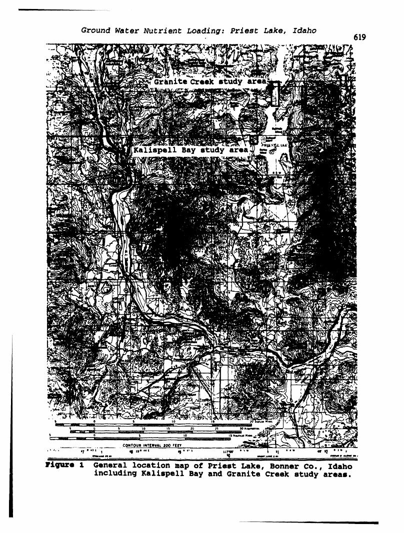
Ground Water Nutrient Loading: Priest Lake, Idaho. 619
"',_ nlte Creak study area
l
i
ini I
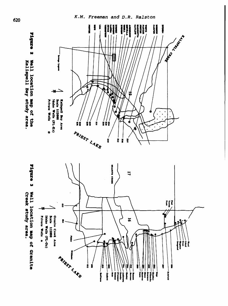
Hydmgeology,WroteDispmml,ScienceandPoliticsercceed_s. _ Sympo.ium 62lEngineeringGeologyandGeotechnicalEngineerin8, 1994
CI'IARACTI_ZSA, T'roN OF A 8_LOW CANYON AQUIFER COIgTAMZNA'I_D BY MINI|
TAILING8 AND SUGGESTION8 FOR C0NSTRUCTZD WETLANDS TRI__
by
John C. Houck, Hydrology Graduate Btudents, Univ. of Idaho
and
Dr. L.L. (Roy) M4nk, Director, Idaho Water Resources ResearchInstitute (INNRZ) • University of Zdaho
ABSTRACT
A shallow aquifer consisting of mine tailings mixed withalluvial sediments is being investigated by the University ofIdaho. The shallow aquifer is located in the lower Canyon Creekdrainage in the Coeur d'Alene Mining District of northern Idaho.Canyon Creek is a major contributor of dissolved heavy metal loadsto the South Fork of the Coeur d'Alene River. Problem metalsinclude zinc, lead, and cadmium.
A total of 16 new monitoring wells were constructed in a 2.5by .5 mile study area during summer of 1993 to map the water tableconfiguration and collect water samples. A monitoring network ofwells has been established in the Lower Canyon Creek valley whichincludes these 16 new monitoring wells, 5 monitoring wellsinstalled previously, 10 domestic wells, and 7 wells located neartailing ponds.
Water quality analyses for ground and surface water samplescollected during low creek flow conditions are presented along withgeologic, geophysical and geohydrological information.
Creek flow measurements show that Canyon Creek gains waterfrom the subsurface in the lower section of the study area,
adjacent to and downstream from the community of Woodland Park.
The dissolved con_cntratins of zinc, cadmium, and lead are
33.9 mg/L, 0.26 mg/L, and 1.45 mg/L respectively for ground watersampled from recently installed shallow monitoring wells.
Two methods are proposed for consideration as methods ofdecreasing the input of heavy metals into Canyon Creek. These are:1) restricting creek losses to the ground water system in theupper part of the study area and 2) construction of bench andpilot-scale anaerobic wetlands prior to large-scale constructedanaerobic wetlands.

Pages 622-636
These pages were removed at
Authors' request just prior to printing.

Hydropololff,WssWDisposal.ScienceandPolitics_gs _)thSymposium 637Eal_'dng GeologyandGmteclmtcdEngineering,1994
MODEUNG THE PULLOUT CHARACIYRISTICS OF WELDED WIRE MATSEMBEDDED IN SILTY SAND
Casan L. Sampa_o, Loren R. Anderson andMark R. Nielsen
Dept ot Civil& EnvironmentalUtah Stale University,Logan,Utah 84322
ABSTRACT:This paper is an outgrowthof the on-goingresearchon discretefinite element modelingofweldedwiremeshreinforcedsoftstructuressuchastheweldedw/reandRSEwalls.The stiffnesscharacteristicsof the w/re mesh-softinterfacesare modeledby a nonlinearhyperboUcrebtionshlp between the appliedpullout stress and the associatedmat placement.The relevantparametersare estimatedfrom laboratorypullout tests that wereconductedforweldedwire matsembeddedon silty sand.Sincethe bulkof the pulloutresistanceof welded wire mesh reinforcementsis derived from the bearingresistance of the transversemembers,an attemptis madeto correlatetheback-figuredparameters to the numberof transversewiresthatconstitutethe test mats. This featurepermitsproperevaluatlonof actualinterfaceparameters for the actualreinforcedsoft structuresin whichthe actual lengthsof the mats are longer(Le.more transversemembers)thanthe specimenused inthe laboratorypullouttests.The resultingpulloutstress.displacementformulationsare then verified by comparing the predicted pulloutresistanceto the existing specificationsand designmethodsfor estimatingthe pulloutcapacitiesof gridreinforcements.
INTRODUCTION
Twogeneralapproachesare currentlyused in the finite elementmodelingof reinforcedsoil walls.TheI_rstapproachis the compositematerialapproachwhereinthe reinforcedsoil massis modelledasa compositematerialwitheach elementhavingpro_rties representativeof the compositesoil and reinforcementmatrix.The second approachis a discrete formulationwherein the reinforcedsoil mass is modelled as discreteelements thatcaninteractwith eachother.Althoughthecompositerepresentationhasbeen usedsuccessfullyto predictstressesin a numberof full scalestructures,the discreteapproachis consideredto be more realisticandappropriatefordetailed investigationof reinforcedsoilwellbehaviorbecausethe propertiesand responsesof the soil-reinforcementinterfacesaredirectlyquantifiable(RoweandHo, 1988).
The most commonlyused procedureto model the relativemovementof soil-reinforcementinterfaceinthe discretefiniteelement modelingis by the use of joint (interface)elements. In this procedure,a pair ofnodes is usuallyintroducedat the same geometriclocationwithin the structuralelement;one attachedto thereinforcement,and the other to the soil. The nodes are linked by a pair of nonlinear springsnormalandtangentialto the reinforcement.The relativedeformationof thesoil andreinforcementpriorto fa/lureat theinterfaceare controlledby the stiffnessof thesesprings.The normalspringstiffnessis usuallyassigneda veryhigh valuewhile the shearstiffnessis usuallygovernedbyan assumedconstitutivelaw.Manyof the existingcodes that were developed for finite element analysisof soil-structureinteraction problemsemploy thehyperbolicconstitutivemodel developedby CloughandDuncan(1971)to representthe shearstiffnessof theinterface(Andraweset al, 198_,Adibet al, 199(Y,Seedet al, 1986;Sdunenmannet al, 1989_,SeedandDuncan1984). The parametersassociatedwith this model are usually estimatedfromlaboratorytests that closelysimulate the antidpated conditions in the field. In finite element analysis of reinforcedsoil walls, theseparameterscan be realisticallyestimated frompullout test results.
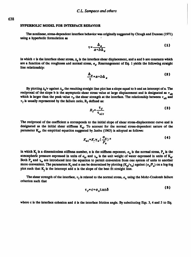
C.L. Samgaco and others
638
HYPERBOLIC MODEL FOR INTERFACEBEHAVIOR
The nonlinear, stress-dependent interfacebehaviorwas originally suggested by Clough and Duncan (1971)using a hyperbolic formulation m
A. (x)a+bA,
in which 5-is the interface shear stress, As is the interface shear displacement, and a and b are constants whichare a function of th©roughness snd normal stress, %. Rearrangement of Eq. 1 yields the following straightline relationship:
A,=a+bA" (a)
By plotting AS/5-against AS,the resulting straight line plot has a slope equal to b and an intercept of a. Thereciprocal of the slope b is the asymptotic shear stress value at large displacement and is designated as _'uttwhich is larger than the peak value _'v the shear strength at the interface. The relationship between I-.,t and_-fis usually represented by the failure ratio, Rf defined as:
'or (3)R r= ,6ul"----_t
The reciprocal of the coefficient a correspondsto the initial slope of shear stress-displacement curve and isdesignated as the initial shear stiffness Kit. To account for the normal stress-dependent nature of theparameter Ksl, the empirical equation suggested by Janbu (1963) is adopted as follows:
o. (4)
in which I_ is a dimensionless stiffness number, n is the stiffness exponent, on is the normal stress, P, is theatmospheric pressure expressed in units of %, and "Ywis the unit weight of water expressed in units of K,i.Both Pa and 7w are introduced into the equation to permit conversion from one system of units to another
more convenient. The parameters I_ and n can be determined by plotting (Ksl/.yw)against (on/Pa)on a log-logplot such that I_ is the intercept and n is the slope of the best fit straight line.
The shear strength of the interface, Tf is related to the normal stress, on using the Mohr-Coulomb failurecriterion such that
_r=c+o.tan 6 (S)
where c is the interface cohesion and _5is the interface friction angle. By substituting Eqs. 3, 4 and 5 to Eq.

Pullout Characteristics of Welded Wire Mats Embedded in Sand
639
1, the shear stress.displacement relationship of the interface can be expres,¢_ as follows:
A.'g=
1 + R_, {e}On
K:jy,,(_ )" c+o.tan8
In an incremental finite element analysiswhich employs the generalized Hooke's law and piecewise linearelastic algorithm, the value of the instantaneous slope of the shear stress.displacement relationship is used.The instantaneous slope, usually called the tangent stiffness value (Kit), can be derived by differentiating Eq.6 with respect to Asto obtain
Rr_ o. RrT {7)K,,==K,,i(I- c+o,tan8 )2=KJ¥'('_a)" (I- c+ont._8 )a
The above nonlinear formulation was developed by Clough and Duncan (1971) as an improvement to theone-dimensional linear elastic "interfaceelement"originally developed by Goodman et al (1968). The interface
element has zero thickness and essentially consists of two parallel nodal links, each controlled bya normal anda shear spring as illustrated in Fig. la. The properties of the interface element consist of a normal stiffness(Kn) and a tangent shear stiffness (Ku) which are related to the normal stress (on) and shear stress (v) actingon the element by the following equations:
o:2=K.A . (8)
=K,=A, (s)
in which _ is the average relative normal displacement across the element. The normal spring is assumed tobe linear elastic and controls the opening and compressing of the interfaceelement between two adjacent two-dimensional elements. During compression, overlappingof two-dimensional elements canbe minimized in theanalysis by using a very large value of Kn. In the case of tension loading, the normal spring stiffness is set tozero. The shear behavior of the interface described by the shear stiffness (Ku) can be modelled by a hyperbolicrelationship (Fig. lb) which is given by Eq. 7 for primary lOadingand reloading. In the case of unloading, thefollowing equation is usually used
o. " (:tO)}
in which Ktu is the unloading shear spring coefficient. During shear failure or tension failure, the shearstiffness (K,t) value is reduced to a certain fraction of the stiffness just prior to failure (Boulanger et al, 1991).
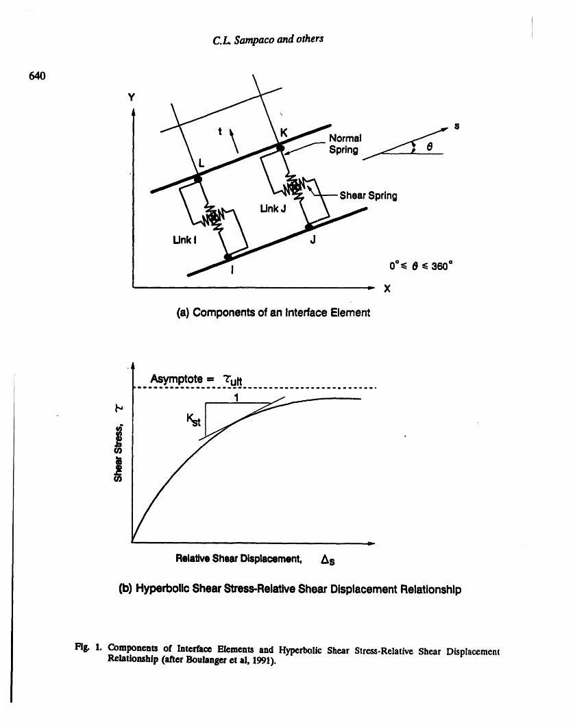
C.L 5ampaco and others
64O
Y\
t _ sNormalSpring _ 0
ShearSpringUnkJ
UnkI J
I 0°<_6 <_360°
_- X
(a) Componentsof an InterfaceElement
Asymptote= "Z'ult_oo,men_ u, en _ e..n ,o ,o ,m e. _ _ ,m ,m _, ,u, ,m _ ,m m,.eo .o u, .J, _ _ _ o _ •
1 "
b,
I '
RelativeShearDisplacement, Bs
(b) HyperbolicShearStress-RelativeShear DisplacementRelationship
Fig. 1. Components of Interface Elements and Hyperbolic Shear Stress-Relative Shear DisplacementRelationship (after Boulanger et a], 1991).

Pullout Characteristics of Welded Wire Mats Embedded in Sand
641
PULLOUT RESISTAHCE EVALUATION
This section presents the three most commonly used expressions to evaluate the pullout resistance of gridreinforcements, such as the welded wire mesh. These methods are presented and adopted in this paper tovalidate the use of the hyperbolic relationship to model the pullout resistance of welded wire mats embeddedin silty sand.
Nielsen & Anderson f1984_ EmolHcal IDmatlon
From the series of laboratory pullout tests that were conducted by Nielsen and Anderson (1984),prediction equations were developed based on statistical analysis to evaluate the total pullout resistance perunit width of the mat. The equations were expressed as a function of the overburden pressure, length and sizeof the wires, and the number of longitudinal and transverse bars that constitute the test mats. Differentequations were developed for welded wire mats embedded in silty sand, washed sand and pea gravel The
pullout capacities were taken at 0.75 in. of displacement. The pullout resistance per unit width (Pr) of weldedwire mats embedded on silty sand can be estimated using the equations listed below. For NonDT > 113.6 lb/ft:
P:=-_=2143_Fc lb +o.Dr (zLeMtan6 +17 .61N) (lX)
For N%D T < 113.6 lb/ft, the following equation is recommended
Pz=-_Fe=o.DT(_Lebltan6+36 .47N) IX2)
in which % is the overburden pressure (psf), DT is the bar diameter (ft), Le is the embedment length (ft), Mis the number of longitudinal wires per unit width (ft'l), W is the width of the wire mat sample (ft), tan _5isthe friction factor between soil and reinforcement, and lq is the number of transversemembers. Equations 11
and 12were developed on the assumption that the longitudinal and transversemembers are of the same sizes.
Federal HI2hwnvAdministrmtlon fChrlstonher et al. 1989_
Christopher et al (1989) developed a general procedure to evaluate the pullout resistance which can beapplied to different soil reinforcement systems, nor reinforcements capable of transmitting both frictional andpassive soil resistance such as the welded wire nesh and bar mat systems, the pulkmt resistance per unit widthof reinforcement (Pr) can be expressed as:
Pz=F*ao.Le c 1 (13)
where F° is a factor that accounts for the combined effect of friction and passive (bearing) resistance,a is thescale effect correction factor and is defined as the fractionof reinforcement area that resists direct shear with
the soft, % is the overburden pressure, Le is the embedment length, and c is the effective perimeter of thereinforcement which has a value of 2 for grids. The factor F* for welded wire mesh was derived by adoptingsome of the experimental results reported by Nielsen and Anderson (1984). The resulting expression becomes:
F*=18"5D"D--r+0'475"_S_ IX4)

C.L Sampacoandothers
642
in which ST is the spacing of transverse wires, DL is the diameter of longitudinal members, and SL is thelateral spacing of longitudinal wires.
AASHTO Task Force 27 Stz_eiflcatloqs
The AASHTO Task Force 27 (1990) specified that the pullout resistance evaluation for mechanicallystabilized earth structures shall be based on load capacity at 0.5 in. of displacement or residual strength,whichever is less. For grid-reinforcingsystems, with transverse member spacing of greater than or equal to 6
in., the pullout capacity per mat (Pp) can be evaluated as:
PpfHp' b (XS)
where Np is the passive resistance factor, z is the depth to reinforcement, ? is the unit weight of soil, m is thenumber of transverse bearing members behind the failure plane, and Ab is the surface area of transverse
reinforcement in bearing (A b ---DT * width of mat). The passive resistance (Np) varies from a value of 30 atthe top of the wall and decreases linearly to a value of 15 at a depth of 20 ft. Aconstant value of 15 is usedfor a depth of 20 ft. and below.
LABORATORYPULLOUT TEST DATA
A total of 33 pullout tests using different sizes of welded wire mats embedded in silty sand were conductedby Nielsen and Anderson (1984) using the buried structures test facility at Utah State University. The testswere carried out using a 6 ft. wide by 5 ft. long by 4 ft. high test cell which is constructed with 12 in. reinforcedconcrete on three sides and steel gates closing the fourth side. Sixteen high capacity hydraulicrams which arecapable of simulating up to 120 ft. of overburden pressure are used to apply normal pressure to the soft massthrough a steel plate. Other details of the test cell are reported by Nielsen and Anderson (1984).
The silty sand used in the test has 40% passing sieve No. 200 and a Ds0 of 0.15 ram. Moisture-densityrelationship indicates a maximum dry density of 125 lb/ft3 and an optimum water content of 9.5%. Trlaxtaltest results yielded an angle of internal friction of 36° for specimens compacted at 95% relative compaction.The soils were compacted in the pullout test cell to at least 90% relative compaction density with watercontent near the optimum.
The welded wire mats were fabricated using two wire sizes of 1/4 in. and 3/8 in. with six longitudinalmembers spaced at 6 in. on centers and varying number of transverse members. The mats were laid in placeas soon as the test cell was filled with compacted soil up to about 4 ft. An additional 1 ft. of soft was addedto cover the mats. Two 1/2 in. thick steel plates were bolted on each side of the portion of the mat extendingfrom the test cell and were,attached to a large hydraulic ram by means of a clevis and a 3/4 in. diameter pin.The hydraulic ram was run oy a hydraulic pump which was independent of the overburden hydraulic systemand was capable of supplying 3000 psi pressure to the cylinder. The pullout force applied to the mats were
monitored using a strain gage load cell mounted on opposite sides of the pullout rod. The displacement ofthe mats were measured by a dial gage mounted near the face of the mat. All the tests were run at adisplacement rate of approximately 4 in/hr until the mats pulled out of the soil at a total displacement of 1in.
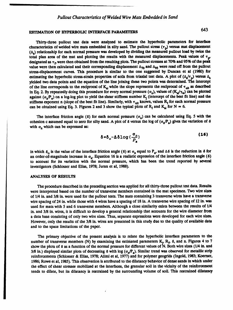
Pullout Characteristics of Welded Wire Mats Embedded in Sand
ESTIMATION OF HYPERBOLIC INTERFACE PARAMETERS 643
Thirty-three pullout test data were analyzed to estimate the hyperbolic parameters for interface
characteristics of welded wire mats embedded in silty sand. The pullout stress (v_ versus mat displacement(L_) relationship for each normal pressure was developed by dividing the measured pullout load by twice thetotal plan area of the mat and plotting the results with the measured displacements. Peak values O°Vp,designated as vr,were then obtained from the resulting plots. The pullout stresses at 70% and 95% of thevalue were then calculated and their corresponding displacement _'y0and A75were read off from the pulloutstress-displacement curves. This procedure is similar to the one suggested by Duncan et al (1980) forestimating the hyperbolic stress.strain properties of soils from trlaxlal test data. A plot of (L_/Vp)versusyielded two data points and the equation of the line joining these two points was determined. The interceptof the line corresponds to the reciprocal of Ksiwhile the slope represents the reciprocal of _ultas describedin Eq. 2. By repeatedly doing this procedure for every normal pressure (On),values of (Kti/-fw)can be plotted
against (On/Pa)on a log-log plot to yield the shear stiffness number gl (intercept of the best fit fine) and thestiffness exponent n (slope of the best fit line). Similarly,with 'rult known, values Rf for each normal pressurecan be obtained using Eq. 3. Figures 2 and 3 show the typical plots of Rf and Ktl for N = 6.
The interface friction angle (6) for each normal pressure (%) can be calculated using Eq. 5 with thecohesion c assumed equal to zero for silty sand. A plot of 6 versus the log of (On/Pa)gives the variation of 6with % which can be expressed as:
on (16}
in which 6o is the value of the interface friction angle (6) at on equal to Pa, and A6 is the reduction in 6 foran order-of-magnitude increase in on. Equation 16 is a realistic expression of the interface friction angle (6)to account for its variation with the normal pressure, which has been the trend reported by severalinvestigators (Schlosser and Elias, 1978; Juran et al, 1988).
ANALYSES OF RESULTS
The procedure described in the preceding section was applied forall thirty.three pullout test data. Resultswere interpreted based on the number of transverse members contained in the mat specimen. Two wire sizesof 1/4 in. and 3/8 in. were used for the pullout tests. The mats containing 3 transverse wires have a transversewire spacing of 24 in. while those with 4 wires have a spacing of 18 in. A transverse w/re spacing of 12 in. wasused for mats with 5 and 6 transverse members. Although a close similarity exists between the results of I/4in. and 3/8 in. wires, it is difficult to develop a general relationship that accounts for the wire diameter froma data base consisting of only two wire sizes. Thus, separate expressions were developed for each wire sizes.However, only the results of the 3/8 in. wires are presented in this study due to the quality of available dataand to the space limitations of the paper.
The primary objective of the present analysis IS to relate the hyperbolic interface parameters to the
number of transverse members (N) by examining the estimated parameters gj, Rt_ 6, and n. Figures 4 to 7show the plots of 6 as a function of the normal pressure fordifferent values of N. Both wire sizes (I/4 in. and3/8 in.) displayed similar plots of decreasing 6 with log (on/Pa)"Similar trend was observed for metallic stripreinforcements (Schlosser & Elias, 1978; Aliml et al, 1977) and for polymer geogrids (Ingold, 1983; Koerner,
1986; Rowe et al, 1985). This observation is attributed to the dilatancy behavior of dense sands in which underthe effect of shear stresses mobilized at the interfaces, the granularsoil in the vicinity of the reinforcementtends to dilate, but its dilatancy IS restrained by the surrounding volume of soft. This restrained dilatancy

¢,L $_aco and othersi i i iii,
HYPERBOLICINTERFACEPROPERTIESSILTY SAND, 6 TRANSVERSEWIRES(N=6)
10000 ,
B I I
1000 ' ,
_ _ _ , , ,,
1000.1 1 10
_3t,tA/Po
I -, 3/B"WRES Iiii
Flg. 2. Typical Plot of (IC_Jyw)and (%/P,) on a Log.Log Scale for N = 6.
HYPERBOLICINTERFACEPROPERTIESSILTYSAND, 6 TRANSVERSEWIRES(N=6)
21.8
1.4
1.2, 1 • -- =
_0.8 . m
0.60.40.2
I i I I
0.1 10aGMA/Pa
i" I,i
Fig. 3. Typical Plot of Failure Ratio (Rg) as a Function of log (crn/P,)for N = 6.

Pullout CharacterJsdcs of Welded Wire Mats Embedded in Sand
645
HYPERBOLICINTERFACEPROPERTIESSLTY SAND, .I TRANSVERSEWIRES(N = ,3)
wBE
i
....... i,
0.1 1 10• _,_/Po
a OATA(3/8" wlr.m)"---- BI._ FiT /
Fig. 4. Plot of Interface Friction Angle (_) as a Function of Normal Pressure for N - 3.
1 10O.1 SIGMA/Pa
Fig. 5. Plot of Interface Friction Angle (6) as a Function of Normal Pressure for N = 4.
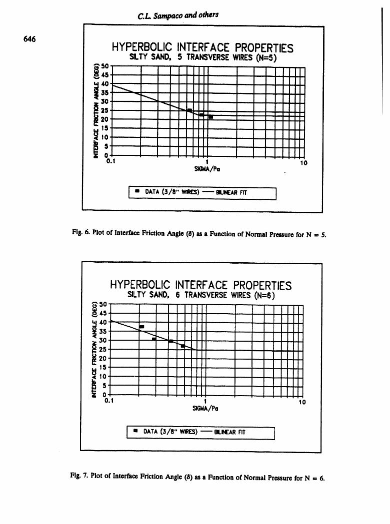
¢.L $cm,.p_coandothersi i I_ITI I IIIIIIII 11 I I
646 HYPERBOLICINTERFACEPROPERTIESSILTYSAND, 5 TRANSVERSEWIRES(N=5)
"" 50 ,,
r,,
_ ........ , .... I
,,,
.....
, ,,
......
0.i 1 10S_MA/Po
[ - 0AT,C_/,"w,_)--- ,,.,o, r,T ]i ii i i,iiin ii ii i i i
Fig. 6. Plot of Interface Friction Angle (8) as a Function of Normal Preuure for N ,, 5.
HYPERBOLICINTERFACEPROPERTIESSILTYSAND,6 TRANSVERSEWIRES(N=6)
35 ....30 "_ -25 -----""1_ I20
10.900.1 1 10
_,,A/Po
[ m DATA (3/8" WIRES)-----BILINEARFIT ]
Fig. 7. Plot of Interface Fdction Angle (8) as a Function of Normal Pressure for N = 6.
Pullout Characteristics of Welded Wire Mats _dded in Sand
647
results In a normal stress concentration at the soil.reinforcement interlkes, thereby incressinil the pulloutresistance of the inclusion (Juran et al, 1988). As a result, the apparent interbce friction anille can sijniflcantlyeweed the friction Shill©of the soil at low normal pressures. Futthermor_ the effect is also Idilhlydependentupon the surface texture of the reinforcement. $chlceser and Elias (1978) reported that ribbed strips mobilizesoil-to4oft friction which in dense granular soils can result In a high dilatan_ effect, whereas smooth stripemobilize soil.to.reinforcement friction resulting to a very low volume change and consequently small dilatan_effects.
Based on this premise, welded wire mesh reinforcements can result in a high dllaumcy effect due to themanner in which friction is mobilized by the transverse bearinll members (Peterson and Anderson, 1980). Toaccount for this phenomenon, a bilinear relationship was fitted in the pious of FIp. 4 to 7. At a value of
(oo/Ps) of 0.80 and lower, all points can be fitted using A_ Of 18° and yielded 6o values of 11.5°, 20°, 21°, and23' for 3, 4, 5, and 6 transverse members, respectively. A linear reilression anL_ysisyielded the followingrelationship with a correlation coeMcient of 0.91.
6o=2.9°+3.55N (27)
in which N is the number of transverse members.The Interface friction angle can. therefore, be estimated forany number of transverse wires using F..qs.16and 17 such that 6_5is equal to 18° at (on/Ps) value of leas thanor equal to 0.80. At higher normal pressures (odP a > 0.80) the interface friction angle (45)remains constant(AS = O) at a value evaluated by Eq. 16 at (o./Pa) = 0.80.
On the other hand, no definite relationships were observed from the plots of failure ratio (1_)and s_exponent (n) such that simple averaging was used to obtain an 1_ of 0.95 and an n value of 1.0. This p_of forcinil Rf and n to be constant would naturally affect the accuracy of the estimates. This was compensatedby the waythe values of the initial shear stiffness (I_) were established. Each pullout stress.displacement datawas then fitted using Rf = 0.95, n =, 1, and 6 calculated from Eq. 16. Adjustments were madeto fit the databy varying the values of Ksl. The new set of values of 0f_/'Yw) were then replotted against (%/Pa) on anarithmetic scale (since n - 1) and the slope g1 is obtained for different values of N. Reilression analysis ofthe interface stiffness number (I_) versus the number of transverse members (N) yielded a corr_lationcoefficient of 0.95 using the follow_lngrelationship
X'j=180 +712N (:L8)
From the empirical equations defined by Eqs. 17 and 18, a plot of the pullout load versus displacementcan be made for any number of transverse members by manipulating Eq. 1. Figure 8 depicts the pullout load-displacement curves for 4 transverse wires and the corresponding hyperbolic model fit based on the equationsdeveloped in this study. The pullout resistance can also be estimated at any displacement At for any value ofon and N using Eq. 1. Figures 9 to 12 show the computed pullout capacities at a displacement (A,) of 0.5 in.for different values of N. Also shown on the plots are the pullout resistances calculated from the equationsdeveloped by Nielsen and Anderson (1984), AASHTO Task Force 27 (1990), and Federal HighwayAdministration (FHWA) (Christopher et al, 1989). The measured pullout capacities at 0.5 in. of displacementare also included. It must be noted that the empirical equations developed by Nielsen and Anderson (1984)are based on 0.75 in. displacement. From these comparisons, the hyperbolic model seems to provide reasonablepredictions of the pullout resistance for all values of N.

CL. Sampacoandothersm,,, ,,, I IRII I I I II iiiii i ii ii IIIIIiI i I III ii
648
HYPERBOLICPIT (4 WIR£5, S/8" DIASETER)16 .................
i-° _...____, ....
_.__-1.----' ' -.".... "'[r"-
0 'o 0.2 0.4 o.e o.o + _.z_UmT Om::HES)
'm DATA(O.6OSk|t). DATA_I.ZOgkSf)o DATA_I.814ksf) 1x DAT_2.41Bkst)-- HYPIERB_ICFIT
i i i nil I I
Fig. 8. Predicted and Measured Pullout Resistance-Displacement Curves for N = 4.
ii i
3 TRANSVERSEWIRES14......
12 ........ "-"
10 Q
I 8 ' _A+ _.4=
6
4 / "' x
2 R' .........
00 0.5 1 _.s 2 2.5 3 3.5 4 4.5 5
Fig. 9. Predicted and Measured Pullout Resistance at 0.5 in. Displacement for N = 3.

I
Fig.10.PredictedandMeasuredPulloutResistanceat 0,5in.DisplacementforN = 4.
Fig. 11. Predicted and Measured Pullout Resistance at 0.5 in. Displacement for N = 5.

C.L Sampaco and others
650
6 TRANSVERSEWIRES10 ....
9 ....8 A '7 '
6 __.
z _D__ ,,,,,
_ 2 x
0'
0 0.25 0.5 0.75 1 1.25 1.5 1.75NO_ _[ss_ (k,O
I i MEASURED _HYPERBOLIC (::314E]..SEN(1984) Ix A/13HTO(1990) • F14WA(1989) J
Fig. 12. Predicted and Measured Pullout Resistance at 0.5 in. Displacement for N = 6.
8 TRANSVERSEWIRES50"
'k ----"
45 HYPERBOLIC
°4o N(L.S_(19S4)
35 xAASZ,n'O(199o)
30 ,k, ( •
:'5 , F'HWA(19.)
2O f/
5, ::
O, !0 1 2 3 4 5 6
Noe_,_.m:ssm((_)
Fig. 13. Predicted Pullout Resistance for an Actual Size Mat With N = 8.

Pullout Characteristics of Welded Wire Mats Embedded in Sand
651
To extend the problem beyond the mat sizes studied in the laboratory pullout teats, a field mat size waschosen for analysis. A 15 fl long by 4 fl wide mat with a transversewire spacing of 2 ft and a longitudinal wirespacing of 0.5 fi was used. This mat configuration results to 9 longitudinal and 8 transverse membem with eachmember assumed to be 3/8 in. in diameter. Figure 13 illustrates the predicted pullout resistance using the fourdifferent methods. It is evident that the hyperbolic model can predict reasonable values of the pulloutresistance which are within the range of values predicted by the existing specifications and empiricalprocedures.
CONCLUSIONS
The use of nonlinear hyperbolic stress-displacement relationship to model the characteristics of soil.structure interfaces seems to offer a promising application in discrete finite element modeling of reinforcedsoft structures. From the analyses conducted in this study, the parameters estimated from laboratory pullouttests can provide a reliable prediction of the pullout resistance which compares well with the actualmeasurements. The empirical equations developed in this paper to account for the number of transverse
members and dilatancy effects at low normal pressures, further extended the applicability of the model toprovide reasonable evaluation of the pullout resistance of full-scale reinforcing mats.
REFERENCES
Adib, M.E., Mitchell, J.IL, and Christopher, B.R. (1990). "Finite Element Modeling of Reinforced Soil Wallsand Embankments'. Proc. Design and Performance of Earth Retaining Structures, ASCE GeoteclmicalSpecial Publication No. 25, P.C. Lambe and L.A. Hansen (eds.), pp. 409-423.
Alimi, I., Bacot, J., P. Long, N.T., and Schlosser, F. (1977). "Etude d radherence sol-armatures." Proc. 9thInternational Conference on Soil Mechanics and Foundation Engineering, Tokyo, Japan, pp. 11.14.
Andrawes, K.Z., McGown, A., Mashhour, M.M., and Wilson-Fahmy, R.F. (1980). "TensionResistant Inclusionin Soils'. Journal of Geotech. Eng'g. Dlv., ASCE, Vol. 106, No. GT12, pp. 1313-1326.
Boulanger, R.W., Bray, J.D., Chew, S.H., Seed, R.B., Mitchell, J.K., and Duncan, LM. (1991). "SSCOMPPC:
A Finite Element Analysis Program for Evaluation of Soft-Structure Interaction and Compaction Effects."Geotechnical Eng'g. Research Report No. UCB/GT/91.02, Dept. of Civil Eng'&, University of California,Berkeley, California.
Christopher, B.R., Gift, S.A., Oiroud, J.P., Juran, I., Mitchell, J.K., Schlosser, F., and Dunnicllff, J. (1989)."ReinforcedSoil Structures, Design and Construction Guidelines: VoL 1".FHWA Report No. RD-89-043,Federal Highway Administration, Springfield, Virginia.
Ciough, G.W. and Duncan, J.M. (1971). "Finite Element Analysis of a Retaining Wall Behavior'. Journal ofGeotech. Eng'g. Div., ASCE, Vol. 97, No. 12, pp. 1657-1673.
Collin, J.G. (1986). "EarthWall Design'. Thesis Submitted in Partial Satisfaction of the Requirements for theDegree of Doctor of Philosophy, Dept. of Civil Engineering, University of California, Berkeley, California.
Duncan, J.M., Byrne, P.M., Wong, K.S., and Mabry, P. (1980). "Strength, Stress-Strain, and Bulk ModulusParameters for Finite Element Analysis of Stresses andMovements in Soil Masses'. Report No. UCB/GT/80-01, University of California, Berkeley, California.
Goodman, R.F_.,Taylor, R.L., and Brekke, T.L. (1968). "A Model for the Mechanics of Jointed Rocks'. Journalof the Soil Mech. and Foundations Division, Vol. 94, No. SM3, p. 637.
Ingold, T.S. (1983). "Laboratory Pull-out Testing of Grid Reinforcements in Sand." Geoteclmical TestingJournal, Vol. 6, No. 3, pp. 101-111.
Janbu, N. (1963). "SoilCompressibility as Determined by Oedometer and TrlaxtalTests." Proc. European Conf.on Soil Mechanics and Foundation Eng'g., Weisbaden, Germany, Vol. 1, pp. 19-25.
C.L. Sampaco and others
652
Juran,L, Knochenmus, G., Acar, Y.B., and Arman, A. (1988). "]PulloutResponse of Geotextfles and Geofgrl_(Synthesis of Available Experimental Data)'. Geosynthetics for Soil Improvement, ASCE Geotech. SpecialPub. No. 18, R.D. Holtz (ed.), pp. 92-111.
Koerner, It. (1986). "Direct Shear/Pull.Out Tests on Geogrids." Report No. 1, Department of CivilEngineering, Drexel University, Philadelphia, Pennsylvania.
Nielsen, M.R. and Anderson, L.R. (1984). "Pullout Resistance of Wire Mats Embedded in Soil'. ResearchReport Submitted to the l-I/lflkerRetaining Wall Co., Dept. of Civil and EnvLEng'g., Utah State University,Logan, Utah.
Peterson, L.M. and Anderson, L,R. (1980). "Pullout Resistance of Welded Wire Mats Embedded in SoIL"Research Report Submitted to the l-lllflker Retaining Wall Company, Dept. of Civil and EnvironmentalEalfg., Utah State University, Logan, Utah.
Rowe, R.K., Ho, S.K., and l_her, D.G. (1985). "Determination of Soil-Geotextile interface StrengthPropertiet" Second Canadian Symposium on Geotextlles, pp. 23-34,
Rowe, R.K. and Ho, S.K. (1988). "Application of Finite Element Techniques to the Analysis of ReinforcedSon Walls'. 'I'neApplication of Polymeric Reinforcements in Soil Retaining Structures, P.M. Jarrett and A.McGown (eds.), pp. 541-553.
_hl_, F. and Elias, V. (1978). "Friction in Reinforced Earth."Proc. Symposium on Earth Reinforcement,ASCE, Pittsburgh.
Sclunertmann, G.R., Chew, S.H. and Mitchell, J.K. (1989). "Finite Element Modeling of Reinforced Soil WallBehavior'. Rep. No. UCB/GT/89.01, Dept. of Civil Eng'f,., University of California, Berkeley, California.
Seed, R.B. and Duncan, J.M. (1984). "SSCOMP:A Finite Element Analysis Program for Evaluation of Soil-Structure Interaction and Compaction Effects'. Geotech. Eng'g. Research Rep. No. UCB/GT/84-0ZUniversity of California, Berkeley, California.
Seed, R.B., COlIIn,J.G. and Mitchell, J.K. (1986). "FEMAnalysis of Compacted Reinforced Soil Walls'. Proc.2rid Intl. Syrup.on Numerical Models in Geomechanics, Ghent, Belgium, pp. 553-562.
Task Force 27 (1990). "Design Guidelines for Mechanically Stabilized Earth (MSE) Walls in PermanentApplications'. AASHTO-AGC-ARTBA Joint Committee, Washington, D.C.

m mI I 0

Copyright © 2022 FDOKUMEN