Desalination and Water Purification Research and Development Program Report No. 123 (Second Edition)

Membrane Concentrate Disposal: Practices and Regulation Mickley & Associates Agreement No. 98-FC-81-0054

U.S. Department of the Interior Bureau of Reclamation April 2006

REPORT DOCUMENTATION PAGE Form Approved OMB No. 0704-0188

Public reporting burden for this collection of information is estimated to average 1 hour per response, including the time for reviewing instructions, searching existing data sources, gathering and maintaining the data needed, and completing and reviewing this collection of information. Send comments regarding this burden estimate or any other aspect of this collection of information, including suggestions for reducing this burden to Department of Defense, Washington Headquarters Services, Directorate for Information Operations and Reports (0704-0188), 1215 Jefferson Davis Highway, Suite 1204, Arlington, VA 22202-4302. Respondents should be aware that notwithstanding any other provision of law, no person shall be subject to any penalty for failing to comply with a collection of information if it does not display a currently valid OMB control number. PLEASE DO NOT RETURN YOUR FORM TO THE ABOVE ADDRESS.

T1. REPORT DATE (DD-MM-YYYY)T

April 2006 T2. REPORT TYPET

Final T3. DATES COVERED (From - To)T

Final 5a. CONTRACT NUMBER

Agreement No. 98-FC-81-0054 5b. GRANT NUMBER

T4. TITLE AND SUBTITLE Membrane Concentrate Disposal: Practices and Regulation (Second Edition)

5c. PROGRAM ELEMENT NUMBER

5d. PROJECT NUMBER

5e. TASK NUMBER

6. AUTHOR(S) Michael C. Mickley, P.E., Ph.D.

5f. WORK UNIT NUMBER

7. PERFORMING ORGANIZATION NAME(S) AND ADDRESS(ES) Mickley & Associates, 752 Gapter Road, Boulder CO 80303

8. PERFORMING ORGANIZATION REPORT NUMBER

10. SPONSOR/MONITOR’S ACRONYM(S)

9. SPONSORING / MONITORING AGENCY NAME(S) AND ADDRESS(ES)

U.S. Department of the Interior, Bureau of Reclamation, Technical Service Center, Environmental Services Division, Water Treatment Engineering and Research Group, 86-68230, PO Box 25007, Denver CO 80225-0007

11. SPONSOR/MONITOR’S REPORT NUMBER(S)

Report No. 123 12. DISTRIBUTION / AVAILABILITY STATEMENT

Available from the National Technical Information Service (NTIS), Operations Division, 5285 Port Royal Road, Springfield VA 22161 13. SUPPLEMENTARY NOTES T

14. ABSTRACT (Maximum 200 words) The project objective was to provide the membrane utility industry with a valuable and useful reference source focusing on characterizing the municipal membrane industry and documenting membrane residuals disposal practices and regulations. The project objective was accomplished though the following tasks: Survey Task: All (422) U.S. municipal membrane facilities built through 2002 of size 25,000 gpd and greater were identified and tallied. A detailed survey of 149 membrane plants in the 1st edition was extended to 300 plants in the 2nd edition. It provided a characterization of the membrane utility industry, in general, and the concentrate and backwash disposal practices, in particular. This included treatment of concentrate and backwash prior to disposal and disposal of cleaning wastes. Regulatory task: Federal regulations were documented to provide the framework for a subsequent state-by-state review of disposal regulations. Cost model task: Design and cost issues associated with the various concentrate disposal options were discussed and for four disposal options (deep well injection, spray irrigation, evaporation pond, and zero liquid discharge), preliminary level cost models were developed. Database development task: A stand-alone executable database was developed to permit viewing, manipulation, and printing of the survey information. CD deliverable task: The stand-alone database, the project final report, and the preliminary cost models were made available in an easy to use, menu-driven CD format. 15. SUBJECT TERMS

membranes, drinking water, concentrate, backwash, cost, regulations, survey 16. SECURITY CLASSIFICATION OF:

UL 19a. NAME OF RESPONSIBLE PERSON T

Scott Irvine a. REPORT

b. ABSTRACT

c. THIS PAGE

17. LIMITATION OF ABSTRACT

18. NUMBER OF PAGES

298 19b. TELEPHONE NUMBER (include area code)

303-445-2253 SS Standard Form 298 (Rev. 8/98)

P Prescribed by ANSI Std. 239-18

Desalination and Water Purification Research and Development Program Report No. 123 (Second Edition)

Membrane Concentrate Disposal: Practices and Regulation Mickley & Associates Agreement No. 98-FC-81-0054

U.S. Department of the Interior Bureau of Reclamation Technical Service Center Environmental Resources Team Water Treatment Engineering and Research Group Denver, Colorado April 2006

Disclaimer Information contained in this report regarding commercial products or firms was supplied by those firms. It may not be used for advertising or promotional purposes and is not to be construed as an endorsement of any product or firm by the Bureau of Reclamation. The information contained in this report was developed for the Bureau of Reclamation; no warranty as to the accuracy, usefulness, or completeness is expressed or implied.

MISSION STATEMENTS

The mission of the Department of the Interior is to protect and provide access to our Nation's natural and cultural heritage and honor our trust responsibilities to Indian tribes and our commitments to island communities.

The mission of the Bureau of Reclamation is to manage, develop, and protect water and related resources in an environmentally and economically sound manner in the interest of the American public.

iii

Preface The reasons for compiling a second edition of this report included:

• To more accurately identify the total number of municipal membrane plants that have been built in the 50 States of the United States of size 25,000 gpd and above

• To increase the number of plants in the database. o To update the database to include plants built and beginning

operation in the years 2000 and 2001.

o To survey plants not previously surveyed

o To include plants built prior to 1993 (part of a 1993 survey)

• To extend the data analysis to include statistics on the treatment of concentrate and backwash prior to disposal

• To extend the data analysis to include statistics on the disposal of cleaning wastes.

A benefit of producing a second edition was to correct errors present in the first edition. These included a handful of incorrect entries in the cost worksheets, a wrong formula used in one of the cost models, and limitations associated with the search function working with the interactive database.

As a result of the above, the database now contains information on approximately 300 plants (up from 150 in the first edition), the data analysis chapter (Chapter 5) has been expanded from 17 pages to 45), and the search function for the database is fully functional.

Most report chapters went unchanged. Text that was changed included:

• Preface (new)

• Executive Summary (revised)

• Chapter 2 Conclusions and Recommendations (revised)

• Chapter 5 Plant Survey Results (revised)

v

Acknowledgements The author of this report is indebted to the research and development tasks undertaken by the following individuals:

• Jorge Briceno, Ph.D. (database survey, state regulations, general support of other tasks)

• Jeffrey Truesdall (database survey, general support of other tasks)

• Patrick Fitzgerald (database development and programming)

• Gary Fehr (final database packaging and production of CDs)

In addition, the author wishes to thank the many individuals from over 150 utilities, many membrane and membrane equipment original equipment manufacturers who provided information about individual membrane plants. Dick Smith, editor of Water Desalination Report, was especially helpful in identifying the status and contacts for several membrane plants. Ed Geishecker of Ionics and Paul Johnson of Memcor were especially helpful in identifying plants using their membrane technologies.

The project benefited from conversations with Scott Irvine, Project Manager for the Bureau of Reclamation, and Kevin Price, manager of the Desalination and Water Purification Research Program under which this project was funded.

vii

Table of Contents

Page

Glossary and Abbreviations .................................................................... xvii

1. Executive Summary ........................................................................ 1

2. Conclusions and Recommendations................................................ 5 2.1 Conclusions ........................................................................... 5 2.1.1 Number of Plants in the Membrane Plant Tally and Survey .................................................... 5 2.1.2 Survey (Concentrate Disposal Aspects).................... 7 2.1.3 Backwash Disposal Options...................................... 8 2.1.4 Disposal Options in General ..................................... 8 2.1.5 Treatment of Concentrate and Reject/Backwash Before Disposal ...................................................... 8 2.1.6 Disposal of Cleaning Wastes..................................... 9 2.1.7 Regulations................................................................ 9 2.1.8 Disposal Methods and Cost Models.......................... 10 2.1.9 Low-Pressure Membrane Systems............................ 11 2.2 Recommendations ................................................................. 11 2.2.1 Plant Surveys............................................................. 11 2.2.2 Regulations................................................................ 12 2.2.3 Preliminary Level Disposal Cost Models ................. 13 2.2.4 General Aspects......................................................... 13

3. Background Information ................................................................. 15 3.1 Background ........................................................................... 15 3.1.1 Membrane Drinking Water Industry......................... 15 3.1.2 Concentrate Disposal Changes.................................. 15 3.2 Purpose of the Project Work ................................................. 17 3.3 Research Objectives .............................................................. 18 3.4 Report Content ...................................................................... 19

4. Research Conducted........................................................................ 21 4.1 Introduction ........................................................................... 21 4.2 Survey Task........................................................................... 21 4.2.1 Identifying Plants ...................................................... 21 4.2.2 Contacting Plants....................................................... 23 4.3 Database Program Task......................................................... 25 4.3.1 Database Software..................................................... 25 4.3.2 Programming............................................................. 25 4.3.3 Final User Interface................................................... 26 4.4 Regulatory Task .................................................................... 27 4.5 Analysis Task ........................................................................ 27 4.6 Cost Modeling Task .............................................................. 29

viii

Table of Contents (continued)

Page

4.6.1 Cost Estimates ........................................................... 29 4.6.2 Cost Model Objectives .............................................. 30 4.6.3 Recommendations for Use of the Models ................. 30 4.6.4 Development of Worksheet Models.......................... 30

5. Plant Survey Results........................................................................ 39 5.1 Introduction ........................................................................... 39 5.2 Total Number of Membrane Plants in the United States ...... 40 5.2.1 Tabulation of Plants in the United States Through 2002 ......................................................... 41 5.3 Results from Surveys – Desalting Plants .............................. 45 5.3.1 Plant Size................................................................... 45 5.3.2 Plant Location ........................................................... 64 5.3.3 Plant Types................................................................ 65 5.3.4 Method ...................................................................... 66 5.3.5 Treatment of Concentrate Before Disposal ............... 68 5.3.6 Disposal of Cleaning Waste ...................................... 71 5.4 Results from Surveys – Low-Pressure Plants ....................... 75 5.4.1 Number of Plants....................................................... 75 5.4.2 Disposal Methods (From Survey Results) ................ 78 5.4.3 Treatment of Drinking Water Plant Reject/Backwash Before Disposal ......................... 81 5.4.4 Disposal of Cleaning Waste from Drinking Water Plants ........................................................... 82

6. Regulation – Federal Perspective.................................................... 85 6.1 Introduction ........................................................................... 85 6.1.1 Membrane Wastes ..................................................... 85 6.1.2 General Classification and Regulation of Membrane Concentrate and Backwash .................................... 85 6.2 Overview ............................................................................... 87 6.2.1 Laws and Regulation................................................. 87 6.2.2 Federal Acts Affecting Disposal of Membrane Wastes .................................................. 87 6.2.3 Impact of Drinking Water Requirements on Discharge Regulations............................................ 89 6.2.4 Federal and State Regulatory Interface ..................... 90 6.2.5 State and Local Programs.......................................... 92 6.3 Surface Water Discharge....................................................... 93 6.3.1 General Considerations ............................................. 93 6.3.2 Federal Programs....................................................... 94 6.3.3 Federal Guidelines – General .................................... 95 6.3.4 Federal Guidelines – Specific ................................... 96

ix

Table of Contents (continued)

Page

6.3.5 EPA WET Program................................................... 97 6.3.6 Surface Water Discharge Permitting Process............ 100 6.4 Disposal to Sewer.................................................................. 104 6.5 Disposal to Deep Well........................................................... 105 6.5.1 Classification of Injection Wells ............................... 106 6.5.2 Municipal Class I Injection Wells............................. 106 6.6 Disposal by Other Methods................................................... 107 6.7 Special Topics: Radionuclides, MF/UF Backwash, Contaminated Concentrate, Toxic and Hazardous Waste............................................................. 108 6.7.1 Ground Water Based Membrane Processes .............. 108 6.7.2 Regional Problems Occurring with Ground Water ... 108 6.7.3 MF and UF Backwash............................................... 109 6.7.4 Future Concentrate Challenges ................................. 109 6.7.5 Toxicity and Hazardous Labels................................. 109

7. Regulation – State Perspective........................................................ 111 7.1 Background ........................................................................... 111 7.2 Survey of WTP Disposal Options ......................................... 111 7.2.1 California................................................................... 112 7.2.2 Florida ....................................................................... 113 7.2.3 Texas ......................................................................... 113 7.3 Survey of NPDES-Related State Regulations....................... 114 7.3.1 California................................................................... 114 7.3.2 Florida ....................................................................... 116 7.3.3 Texas ......................................................................... 118 7.4 Summary of Regulatory Requirements for Selected States .. 120

8. Surface Water and Sewer Disposal ................................................. 127 8.1 Background ........................................................................... 127 8.2 Design Considerations for Disposal to Surface Water.......... 127 8.2.1 Ambient Conditions .................................................. 127 8.2.2 Discharge Conditions ................................................ 128 8.2.3 Regulations................................................................ 128 8.2.4 The Outfall Structure................................................. 129 8.2.5 Dilution Levels.......................................................... 129 8.2.6 Diffuser Characteristics and Design Variables ......... 130 8.2.7 CORMIX and Other Software................................... 130 8.2.8 General Design Approach for Diffusers.................... 131 8.3 Cost Considerations for Disposal to Surface Water.............. 132 8.3.1 Consideration of Shared Outfall Structures .............. 133 8.4 Disposal to Sewer.................................................................. 133

x

Table of Contents (continued)

Page

9. Deep Well Disposal......................................................................... 135 9.1 Background ........................................................................... 135 9.1.1 Deep Well Disposal in Southern Florida................... 136 9.1.2 Geology of Southern Florida..................................... 137 9.2 Design Considerations........................................................... 138 9.2.1 Siting ......................................................................... 138 9.2.2 Construction .............................................................. 139 9.2.3 Design Basis – Flow Versus Tubing Diameter ......... 141 9.3 Cost Factors........................................................................... 142 9.3.1 Pretreatment .............................................................. 142 9.3.2 Pumps........................................................................ 143 9.3.3 Site Tests – Logging, Surveying, and Testing .......... 143 9.3.4 Injection Well Formation .......................................... 143 9.3.5 Monitoring................................................................. 146 9.3.6 Other Considerations................................................. 152 9.3.7 Operating Costs ......................................................... 152 9.4 Design Approach for the Deep Well Disposal Cost Model ...................................................................... 155 9.5 Deep Well Disposal Worksheet and Example ...................... 156 9.6 Deep Well Disposal Regression Model ................................ 156

10. Evaporation Pond Disposal ............................................................. 159 10.1 Background ........................................................................... 159 10.2 Design Considerations........................................................... 160 10.2.1 Sizing of Evaporation Ponds ..................................... 160 10.3 Cost Parameters..................................................................... 163 10.3.1 Land Costs................................................................. 165 10.3.2 Earthwork .................................................................. 165 10.3.3 Miscellaneous Costs.................................................. 174 10.3.4 Operating Costs ......................................................... 179 10.4 Design Approach for the Evaporation Pond Cost Model .............................................................................. 180 10.5 Evaporation Pond Worksheet and Example.......................... 181 10.6 Evaporation Pond Regression Model.................................... 183

11. Spray Irrigation Disposal ................................................................ 185 11.1 Background ........................................................................... 185 11.2 Design Considerations........................................................... 186 11.2.1 Salt, Trace Metals, and Salinity ................................ 186 11.2.2 Site Selection............................................................. 187 11.2.3 Preapplication Treatment .......................................... 187 11.2.4 Hydraulic Loading Rates........................................... 188 11.2.5 Land Requirements ................................................... 189

xi

Table of Contents (continued)

Page

11.2.6 Vegetation Selection ................................................. 190 11.2.7 Distribution Techniques ............................................ 190 11.2.8 Surface Runoff Control ............................................. 191 11.3 Cost Factors........................................................................... 191 11.3.1 Land........................................................................... 191 11.3.2 Distribution................................................................ 194 11.3.3 Pumping .................................................................... 196 11.3.4 Storage....................................................................... 196 11.3.5 Underdrains ............................................................... 201 11.3.6 Operational Costs ...................................................... 201 11.4 Design Approach for Spray Irrigation Model ....................... 201 11.5 Spray Irrigation Model Worksheet and Example.................. 206 11.6 Spray Irrigation Regression Model ....................................... 206

12. Zero Liquid Discharge Disposal ..................................................... 209 12.1 Background ........................................................................... 209 12.1.1 Single- and Multiple-Effect Evaporators .................. 209 12.1.2 Vapor Compression Evaporator Systems (Brine Concentrators)............................................. 211 12.1.3 Crystallizers............................................................... 214 12.1.4 Spray Dryers.............................................................. 216 12.2 Model for Interaction of Membrane and Thermal Systems............................................................................ 217 12.3 Design Considerations........................................................... 219 12.3.1 Sizing of Zero Discharge Systems Evaporation........ 220 12.4 Cost Parameters..................................................................... 220 12.4.1 Brine Concentrators................................................... 220 12.4.2 Crystallizers............................................................... 224 12.4.3 Spray Dryers.............................................................. 224 12.4.4 Energy ....................................................................... 227 12.5 Design Approach for the Zero Liquid Discharge Cost Model ...................................................................... 227 12.6 Zero Liquid Discharge Worksheet and Example .................. 231 12.7 Zero Liquid Discharge Regression Model ............................ 231

13. Analysis of Cost Models ................................................................. 235 13.1 Introduction ........................................................................... 235 13.2 Sensitivity Analysis............................................................... 235 13.2.1 Relative Importance of Design Parameters ............... 235 13.2.2 Spray Irrigation ......................................................... 236 13.2.3 Zero Liquid Discharge .............................................. 236 13.2.4 Evaporation Pond ...................................................... 237 13.2.5 Deep Well Injection .................................................. 238

xii

Table of Contents (continued)

Page

13.2.6 Summary ................................................................... 238 13.3 Model Comparison................................................................ 238 13.3.1 Spray Irrigation ......................................................... 239 13.3.2 Zero Liquid Discharge .............................................. 239 13.3.3 Deep Well Injection .................................................. 240 13.3.4 Evaporation Pond ...................................................... 240 13.3.5 Summary ................................................................... 240

14. Instructions for Using CD ............................................................... 243 14.1 Format of the CD................................................................... 243 14.1.1 A Front-End Menu for Accessing These Individual Parts of the CD...................................... 243 14.1.2 The Stand-Alone Database........................................ 243 14.1.3 The Complete Text Report........................................ 244 14.1.4 Worksheets for Use in Developing Cost Estimates of Disposal Options ............................... 244 14.1.5 Calculation Pages for Capital Costs of Disposal Options .................................................... 245 14.1.6 Glossary..................................................................... 245 14.2 Installation of the CD ............................................................ 245

Reference List ......................................................................................... 249

Appendix 1 – SI Metric Conversion Table ............................................. 251 Appendix 2 – Survey of State Regulations Regarding Drinking Water Waste Disposal ..................................................................... 253 Appendix 3 – State NPDES-Related Regulations Comments ................ 285

List of Figures

Figure Page

4.1 Regression Estimates as Function of Input Values ............... 37 4.2 Regression Residuals as Function of Estimated Value ......... 38 5.1 Cumulative Number of Municipal Membrane Plants by Year ............................................................................ 43 6.1 NPDES Implementation Procedure for Whole Effluent Toxics Control Program.................................................. 99 6.2 Diagram of a Stream Mixing Zone ....................................... 101 9.1 Schematic Diagram of a Three-Transition Injection Well with Packer...................................................................... 140 9.2 Logging, Testing, and Survey Costs as Function of Tubing Diameter ............................................................. 144

xiii

List of Figures (continued)

Figure Page

9.3 Drilling and Reaming Cost as Function of Tubing Diameter .......................................................................... 147 9.4 Installed Tubing Cost as Function of Tubing Diameter .......................................................................... 148 9.5 Installed Packer Cost as Function of Tubing Diameter .......................................................................... 149 9.6 Installed Casing Cost as Function of Tubing Diameter .......................................................................... 150 9.7 Installed Grouting Cost as Function of Tubing Diameter .......................................................................... 151 9.8 Monitoring Well Cost as Function of Well Depth ................ 153 9.9 Mobilization and Demobilization Cost as a Function of Well Depth .................................................................. 154 10.1 Rate of Precipitation in Evaporation Pond (After Office of Saline Water, 1970) .................................................... 164 10.2 Area Correction Factor as Function of Evaporative Area (1 to 10 Acres)................................................................. 166 10.3 Area Correction Factor as Function of Evaporative Area (10 to 100 Acres)............................................................. 167 10.4 Dike Cost as Function of Evaporative Area (1 to 10 Acres)................................................................. 169 10.5 Dike Cost as Function of Evaporative Area (10 to 100 Acres) ....................................................................... 170 10.6 Schematic Diagram of a Baffled Evaporation Pond ............. 171 10.7 Liner Cost as Function of Evaporative Area (1 to 10 Acres) ......................................................................... 172 10.8 Liner Cost as Function of Evaporative Area (10 to 100 Acres) ....................................................................... 173 10.9 Fence Cost as Function of Evaporative Area (1 to 10 Acres) ......................................................................... 175 10.10 Fence Cost as Function of Evaporative Area (10 to 100 Acres) ....................................................................... 176 10.11 Road Cost as Function of Evaporative Area (1 to 10 Acres) ......................................................................... 177 10.12 Road Cost as Function of Evaporative Area (10 to 100 Acres) ....................................................................... 178 11.1 Land Requirements as a Function of Flow and Loading (Flows Up to 1.2 mgd) .................................................... 192 11.2 Land Requirements as a Function of Flow and Loading (Flows Up to 3.5 mgd) .................................................... 193 11.3 Schematic Diagram of a Typical Spray Irrigation Distribution System......................................................... 195

xiv

List of Figures (continued)

Figure Page

11.4 Distribution System Piping Cost as Function of Area (Up to 50 Acres).............................................................. 197 11.5 Distribution System Piping Cost as Function of Area (Up to 200 Acres)............................................................ 198 11.6 Sprinkler, Valves, and Control System Cost as Function of Area.............................................................. 199 11.7 Cost of Low-Head Pumps as Function of Flow Rate............ 200 11.8 Storage Tank Cost as Function of Flow Rate (Up to 0.5 mgd) ............................................................... 202 11.9 Storage Tank Cost as Function of Flow Rate (Up to 5 mgd) .................................................................. 203 12.1 Schematic Diagram of Brine Concentrator Processor Flow—Pumps Not Shown............................................... 213 12.2 Schematic Diagram of Forced-Circulation, Vapor Compression Crystallizer Process Flow.......................... 215 12.3 Schematic Diagram of a Typical Spray Dryer ...................... 217 12.4 Capital Cost of Skid-Mounted Brine Concentrator as Function of Flow Rate (0 to 200 gpm)............................ 221 12.5 Capital Cost of Nonskidded Brine Concentrator as Function of Flow Rate (0 to 1.2 mgd)............................. 222 12.6 Capital Cost of Nonskidded Brine Concentrator as a Function of Flow Rate (1 to 2.5 mgd)............................. 223 12.7 Capital Cost of Crystallizer as a Function of Flow Rate (5 to 50 gpm) .................................................................. 225 12.8 Capital Cost of Spray Dryer as a Function of Flow Rate (1 to 12 gpm) ................................................................... 226 12.9 Energy Requirements for the Brine Concentrator as Function of Flow Rate (Up to 1 mgd) ............................. 228 12.10 Energy Requirements for the Brine Concentrator as a Function of Flow Rate (1 to 3 mgd)......................... 229 12.11 Energy Requirements for the Crystallizer as a Function of Flow Rate .................................................................... 230 14.1 Menu for Accessing CD files ................................................ 244

List of Tables

Table Page

4.1 Arrangement of Data in Database ......................................... 22 4.2 1992 Survey of 140 Plants .................................................... 23 4.3 Data Analysis Categories ...................................................... 28 4.4 Worksheet for Evaporation Pond Disposal Capital Costs..... 33

xv

List of Tables (continued)

Table Page

5.1 Number of Municipal Membrane Plants Constructed in the 50 States of the United States by Year ................. 42 5.2 Location by State of Desalting Plants ................................... 44 5.3 Location by State of Low-Pressure Plants ............................ 44 5.4 Municipal Membrane Plants in the 50 States........................ 46 5.5 Selected Survey Results – Number of Desalting Plants by Category Built During 1993–2001.................................. 62 5.6 Desalting Plant Size by Year of Startup................................ 64 6.1 Characteristics of Concentrate and Backwash Streams ........ 86 6.2 Delegation Status of States for Federal Programs................. 90 7.1 Description of Specific Legislative Rules in the Porter-Cologne Water Quality Control Act .................... 115 7.2 List of Specific Regulations (Title 62 Florida Administrative Code) that Cover the Currently Accepted Disposal Options in the State of Florida ........................................ 117 7.3 Description of Regulations and Corresponding Legislative Sections of the Texas Administrative Code Applicable to Membrane Disposal Options........... 119 7.4 Permitting Constraints on Waste Disposal Options for Selected States ........................................................... 121 9.1 Relationship Between Pipe Diameter and Flow Rate ........... 142 9.2 Logging, Surveying, and Testing Events from Florida 3400-foot Well ................................................................ 145 9.3 Worksheet for Deep Well Disposal Capital Costs ................ 157 10.1 Worksheet for Evaporation Pond Disposal Capital Costs ................................................................... 182 11.1 Site Selection Factors and Criteria ........................................ 188 11.2 Worksheet for Spray Irrigation Disposal Capital Costs ........ 207 12.1 Schematic of Membrane/Thermal System and Mathematical Relations to Calculate System Flows ............................................................................... 218 12.2 Flows for Membrane and Membrane/Thermal Systems....... 219 12.3 Worksheet for Zero Liquid Discharge Disposal Costs.......... 232

xvii

Glossary and Abbreviations A irrigation area, acre

ADA American Desalting Association

ALR annual hydraulic loading rate (feet per year)

AMS advanced membrane systems

AMTA American Membrane Technology Association

AWWA American Water Works Association

AWWARF American Water Works Association Research Foundation

BOD biological oxygen demand

BRO brackish reverse osmosis

BTU British thermal unit

C concentration of constituent (milligrams per liter)

Ca calcium

CAA Clean Air Act

CD compact disk

CERCLA Comprehensive Environmental Response, Compensation and Liability Act

CFD computational fluid dynamics

CFR Code of Federal Regulations

CRWQCB California Regional Water Quality Control Board

CWA Clean Water Act

d day

DO dissolved oxygen

DOE Department of Energy

DOT Department of Transportation

DW drinking water

ED/EDR electrodialysis/electrodialysis reversal

EPA U.S. Environmental Protection Agency

EPCRA Emergency and Community Right-to-Know Act

EPRI-CEC Electric Power Research Institute – Community Environmental Center

ESA Endangered Species Act

ET evapotranspiration

F fetch (straight line distance the wind can blow without obstruction)

FAC Florida Administrative Code

FDEP Florida Department of Environmental Protection

xviii

FFDCA Federal Food, Drug, and Cosmetic Act

FIFRA Federal Insecticide, Fungicide and Rodenticide Act

Fl Florida

FOIA Freedom of Information Act

FQPA Food Quality Protection Act

fps feet per second

FS Florida Statutes

ft feet

ft2 square feet

ft3 cubic feet

FWPCA Federal Water Pollution Control Act

gal gallon

gpd gallons per day

gpm gallons per minute

GPO Government Printing Office

HDPE high density polyethylene

HLR hydraulic loading rate

hr hour

Hw wave height (feet)

I.D. inside diameter

IMS integrated membrane system

in inch

kW kilowatt

LAS land application system

lb pound

Lc loading rate of constituent (lb/acre-yr)

LOEL lowest observed effects level

MCL maximum contaminant level

meq/L milliequivalent per liter

MF microfiltration

Mg magnesium

mgd million gallons per day

mg/L milligram per liter

mils thousandths of an inch

mph miles per hour

Na sodium

NEPA National Environmental Policy Act of 1969

xix

NF nanofiltration

NOI notification of intent

NPDES National Pollutant Discharge Elimination System

NWRI National Water Research Institute

OEM original equipment manufacturer

ONRW Outstanding National Resource Waters

OPA Oil Pollution Act of 1990

OSHA Occupational Safety and Health Administration

% percent

PER percolation

POTW publicly owned treatment work

PPA Pollution Prevention Act

ppm parts per million

PPT part per thousand

psi pounds per square inch

psig pounds per square inch gauge

Q concentrate flow (gallons per day)

RCRA Resource Conservation and Recovery Act

RO reverse osmosis

SAR sodium adsorption ratio

SARA Superfund Amendments and Reauthorization Act

SDWA Safe Drinking Water Act

SID State Indirect Discharge

SRO seawater reverse osmosis

TCC total capital cost

TDS total dissolved solids

THMFP trihalomethane formation precursor

TMDL total maximum daily load

TPDES Texas Pollutant Discharge Elimination System

TRC total residual chlorine

TRE toxicity reduction evaluation

TSCA Toxic Substance Control Act

TSS total suspended solids

UF ultrafiltration

UIC Underground Injection Control

U.S. United States

USDW underground source of drinking water

xx

VOC volatile organic compounds

W wind velocity (miles per hour)

WET whole effluent toxicity

WETC whole effluent toxics control

WQ water quality

WQS water quality standards

WTP water treatment plant

WWTP waste water treatment plant

yd3 cubic yard

yr year

1

1. Executive Summary The major objective of the project was to provide the membrane utility industry with a valuable and useful reference source focusing on characterizing and documenting concentrate (from membrane desalting processes), backwash (from low-pressure membrane processes), and cleaning waste disposal practices and regulations.

The project objective was accomplished through the following tasks:

♦ Identification task: An effort was made to identify all municipal membrane plants that have been built in the 50 United States through 2002 and to produce a list of these plants. A total number of 422 plants were identified consisting of 234 desalting plants (reverse osmosis, nanofiltration, and electrodialysis) and 188 low-pressure (microfiltration and ultrafiltration) plants. Of these, about 30 plants operate at waste water facilities in water reuse situations. Most of the plants produce drinking water.

The identification of utility plants and the survey provide statistics to characterize the water and waste water utility’s use of membrane processes by startup date, size, location, type of process, and several other parameters. The dramatic growth of membrane use in the utility industry is documented, along with the equally dramatic increase in size of the membrane plants and the increased number of States that now have membrane plants. Statistics are provided about concentrate, backwash, and cleaning waste disposal practices, and results of the survey are compared with the results of a 1992 survey (Mickley et al., 1993).

♦ Survey task: A detailed survey of 150 membrane plants was made and combined with results from a previous survey to provide a database of 300 plants that included 97 percent (%) of the utility desalting plants built in the United States from 1967 through 2001 above a size of 25,000 gallons per day (gpd). It also included 91 percent of the utility low-pressure membrane plants built in the United States of a size greater than 1 million gallons per day (mgd). The survey provided a detailed characterization of the membrane utility industry, in general, and the concentrate and backwash disposal practices, in particular.

The survey results are stored in a “run-time” version of Microsoft Access. This is a stand-alone version that does not require the user to have Access to run. This database is made available in compact disk (CD) form, along with a pdf file containing the entire project report, the capital cost worksheets, and the closed form equations that can also be used to calculate preliminary level capital costs for the disposal options. Upon installation, a convenient menu provides several options for interfacing with the database and accessing the other items.

2

♦ Regulatory task: Federal regulations were documented to provide the framework for a subsequent State-by-State review of disposal regulations.

A review of the Federal and State-by-State regulations affecting concentrate and backwash disposal is presented. Major ion toxicity (Mickley, 2000) that has occurred in several ground water membrane systems in Florida appears not to have been documented elsewhere. This seems to be because whole effluent toxicity tests are not routinely part of surface discharge (National Pollutant Discharge Elimination System [NPDES]) permits in States other than Florida. Where surface discharge permits are used in other States, the mysid shrimp used in the Florida whole effluent toxicity (WET) tests may not be used. Backwash from low-pressure membrane systems frequently (depending on the application) has elevated levels of microorganisms. Presently, there are no water quality criteria for microorganisms that hinder discharge to receiving waters. Such regulation is only a matter of time, however.

♦ Cost model task: Design and cost issues associated with the various concentrate disposal options were discussed, and preliminary level cost models were developed for four disposal options (deep well injection, spray irrigation, evaporation pond, and zero liquid discharge).

The design parameters and cost factors associated with several concentrate (and backwash) disposal methods are discussed in detail. The disposal methods (listed in order of decreasing frequency of use) include:

• Surface water discharge • Discharge to sewer • Deep well injection • Evaporation ponds • Spray irrigation • Zero liquid discharge

Preliminary level capital cost models are presented for the final four disposal methods in both worksheet form and closed form equation. In the case of discharge to surface water, the large number of site-specific variables makes it difficult to formulate a meaningful general model. In the case of disposal to the sewer, the only cost other than pipeline conveyance to the disposal site is a negotiated fee payable to the waste water plant. These fees can range from zero to very high.

♦ Database development task: A stand-alone executable database was developed to permit viewing, manipulation, and printing of the survey information.

♦ CD deliverable task: The stand-alone database, the project final report, and the preliminary cost models were made available in an easy to use, menu-driven CD format.

3

The project CD provides the user with a broad and valuable resource that characterizes the membrane utility industry, its concentrate and backwash disposal practices, the regulations that govern disposal, and the costs associated with disposal options.

5

2. Conclusions and Recommendations 2.1 Conclusions

2.1.1 Number of Plants in the Membrane Plant Tally and Survey ♦ The tally of 422 municipal membrane plants built in the United States (U.S.)

of 25,000 gallons per day (gpd) and greater through the year 2002 is substantially.

♦ Desalting plants (reverse osmosis [RO], nanofiltration [NF], electrodialysis/electrodialysis reversal [ED/EDR]) are used in water treatment plants (WTPs) to provide new sources of potable water via the treatment of lower quality water resources.

♦ Low-pressure membrane plants (microfiltration [MF] and ultrafiltration [UF]) are used in WTPs to help meet the Safe Drinking Water Act (SDWA) amendment requirements for higher quality, and in waste water treatment plants (WWTPs) to provide a polishing treatment step in water reuse situations.

♦ Several aspects of the use of membrane technology in the drinking water and waste water utilities have changed significantly since the last (1993) survey. Others remain similar.

♦ With regard to the number of plants:

• A total of 234 desalting plants was identified and listed in tables 5.1 and 5.2.

• Of these, only seven desalting plants were not included in the survey and database.

• A total of 188 low-pressure plants were identified and listed in tables 5.1 and 5.2.

• Of these, only three low-pressure plants built of 1 million gallons per day (mgd) or greater were not surveyed.

• The database contains information on a total of 300 of the 422 plants. Most of the identified plants not in the survey and database are low-pressure plants less than 1 mgd.

• The number of utility desalting plants in the United States of 25,000 gpd and higher has increased from approximately 133 in 1992 to 234 in 2002.

• The number of utility low-pressure MF and UF plants in the United States of 25,000 gpd and higher has increased from 1 in 1992 (operating at a State park) to 188 in 2002.

6

• Based on the yearly increases in the different plants of this size and larger, the number of MF and UF plants should surpass the number of desalting plants by the end of 2004.

• With one early exception, there were no integrated membrane plants (using MF as pretreatment to RO or NF) built until 1995. Now, there are 11 integrated plants primarily used in water reuse situations.

♦ With regard to the location of plants:

• A higher percentage of plants are being built in States other than Florida. About 30 percent (%) of the desalting plants built between 1992 and 2002 are in Florida, with the remainder scattered throughout 24 States, with 13% in California and 9% in Texas. This is in contrast to the results of the 1992 survey, when about 61% of the desalting plants were in the State of Florida and the rest of the plants were located in about 13 States, with 9% in California and Texas, respectively.

• The geographic distribution of low-pressure MF plants is considerably different from that of desalting plants. For MF plants, the leading States are California (with 22% of the plants as of 1999), Colorado (with 12% of the plants), and Virginia (with 10% of the plants). The rest of the plants are scattered throughout 28 other States.

♦ With regard to size:

• Although dependent on the particular plants surveyed, an increase in the size of desalting plants is striking. In the project surveys conducted, 16% of the plants were greater than 6 mgd (compared to 4% for the 1992 survey). Also, only 4% of the plants in the project surveys were less than 0.1 mgd, as opposed to 33% in the 1992 survey.

• From 1993 through 1997, 29% of the desalting plants (15 of 52) built were 3 mgd or greater. From 1998 through 2001, the percentage increased to 44% (20 of 45).

• Many of the larger desalting plants are being built in Florida. About 34% of the desalting plants built in Florida since 1992 are 6 mgd or greater, whereas about 7% of desalting plants built elsewhere in this same timeframe were greater than 6 mgd.

• The size and number of MF plants has increased dramatically since 1995. Before 1996, 1 of 17 plants (6%) built were 1 mgd or larger. Since 1996 and through 2001, 54 of 137 plants (39%) were greater than 1 mgd, with 24 (18%) being greater than 3 mgd.

♦ With regard to the types of plants:

• The percentage of plants of different types built since 1992 is roughly the same as plants operating in 1992. Brackish water RO (BRO) plants

7

account for about 65% of all plants, with NF plants (13%), ED/EDR (8%), seawater RO (3%), and integrated plants, MF/RO and MF/NF, (11%) making up the rest.

• In spite of the large numbers of membrane plants in Florida, most ED/EDR plants are not in Florida (as in 1992).

• Most of the NF plants are in Florida (as in 1992).

• With one early (1980) exception, there were no integrated plants before 1995. Most of the integrated plants are in California.

♦ With regard to membrane systems providers:

• Until 1999, nearly all of the MF plants were Memcor systems. Since then, Pall has made a significant entry into the marketplace.

• Since 1999, three strong companies have emerged to provide UF systems (Aquasource, Koch, and Zenon).

2.1.2 Survey (Concentrate Disposal Aspects) ♦ The relative use of different means of concentrate disposal has changed

somewhat since the previous survey (comparison of plants built between 1992 and 2002 to plants operating in 1992):

• A somewhat decreasing percentage dispose concentrate to surface water: 41% versus 48%.

• A significantly higher percentage dispose concentrate to sewer: 31% versus 23%.

• A higher percentage dispose concentrate to deep wells: 17% versus 12%.

• A lower percentage dispose concentrate by evaporation pond and spray irrigation: for evaporation pond, the percentages are 2% as opposed to 6%; and for land applications, the percentages are 2% compared to 12%.

♦ The relative use of different concentrate disposal options shows similar trends, with plant size as in the previous survey:

• Disposal to surface water is an option used at approximately the same relative frequency regardless of plant size, with an exception of less use at sizes of 10 mgd and greater.

• Disposal to sewer is used more frequently for smaller sized plants (< 1 mgd product).

• Disposal to deep well injection is primarily used for larger plants (> 1 mgd).

• Disposal via evaporation pond and land applications is used primarily with smaller plants (< 1 mgd).

8

• As in the previous survey, with few exceptions, deep well disposal of concentrate has been practiced only in the State of Florida

2.1.3 Backwash Disposal Options • Disposal of backwash from MF and UF plants does not follow any trend

with plant size (likely because backwash is of considerably smaller volume than concentrate, due to much greater recoveries).

• Disposal to surface water (39%) and sewer (24%) are the most widely used disposal options.

• Unlike concentrate disposal, deep well injection has not been used for backwash disposal. This is due to the small number of low-pressure membrane systems in Florida, the only State presently using deep well disposal for concentrate to any significant degree, as well as the small volume of backwash relative to concentrate.

• Recycle of backwash from low-pressure plants accounts for 16% of the disposal cases. [With one exception, it is not used for desalting plants.]

• Recycle of backwash is used in 15% of the drinking water plants and 33% of the waste water plants.

2.1.4 Disposal Options in General ♦ Together, disposal to surface water and to sewer account for 72% of desalting

disposal cases, 64% of the MF cases, and 61% of the UF cases.

♦ Recycle accounts for 0% of the desalting disposal options, 13% of the MF cases and 28% of the UF cases.

2.1.5 Treatment of Concentrate and Reject/Backwash Before Disposal ♦ Of 112 desalting plants (mostly built since 1992) providing information, the

treatment of concentrate before disposal consists of:

• None 78% • Aeration 8 • pH adjustment 5 • Disinfection 4 • Degasification 3 • Air stripping 1 • Defoaming 1

♦ Of 29 low-pressure plants providing information, the treatment of reject/backwash before disposal consists of:

9

• None 79% • pH adjustment 10 • Settling 7 • Sand/gravel filter 3

2.1.6 Disposal of Cleaning Wastes ♦ Of 110 desalting plants (mostly built since 1992) providing information, the

means of disposal of membrane cleaning wastes included:

• Sewer 61% • Surface water 22 • Land application 7 • Injection 6 • Evaporation pond 2 • Recycle 1 • Hauling 1

♦ In 59% of the cases, cleaning wastes were disposed in the same manner as the concentrate.

♦ Of 42 low-pressure plants providing information, the means of disposal of membrane cleaning wastes included:

• Sewer 51% • Land application 19 • Surface water 17 • Septic tank 6 • Evaporation pond 4 • Recycle 2

♦ In 55% of the cases, the cleaning waste was pH adjusted before disposal.

♦ In 62% of the cases, cleaning wastes were disposed in the same manner as the reject/backwash.

2.1.7 Regulations ♦ Many more States have membrane system sites and must regulate disposal of

membrane concentrate and backwash (38 as of 2002 versus 14 as of 1992)

♦ The most widely regulated disposal options are disposal to surface water and sewer. They both involve National Pollutant Discharge Elimination System (NPDES) permits, either for the WTP discharging the concentrate or backwash or the WWTP plant receiving the concentrate or backwash.

10

♦ There have been no major changes in Federal regulations over the past 8 years; total maximum daily loads (TMDLs), which may come into play in NPDES permits, are more of a burden for States than for individual surface water dischargers.

♦ A major surface water disposal issue in the State of Florida since 1992 has been the occurrence of major ion toxicity (Mickley, 2000) in several concentrates from desalting plants using ground water sources.

♦ Very few States require whole effluent tests on membrane concentrate discharged to surface waters. This explains, in part, why major ion toxicity problems associated with brackish RO concentrate appear to have occurred only in Florida.

♦ Some regulatory distinction has been given to drinking water membrane concentrate in the State of Florida. Although it is still regulated as an industrial waste, it is called “potable water byproduct” where produced by plants 50,000 gpd or less. Pending legislation may extend this to plants of larger size.

♦ Most regulations are not specific to municipal membrane concentrate and reject/backwash.

♦ Deep well disposal of industrial wastes (including membrane concentrate and backwash) is not permitted in many States.

2.1.8 Disposal Methods and Cost Models ♦ The costs of different disposal methods for concentrate disposal are very site

dependent; consequently, the cost models developed are to be considered for preliminary level estimates only.

♦ The major factors influencing deep well injection costs are the depth of the well and the diameter of the well tubing and casing strings. The diameter has surprisingly low influence on the cost; drilling, reaming, cementing, and testing costs are much more significant than material costs. The minimal cost of a well is high enough that these wells are typically used only with large concentrate flow rates.

♦ Spray irrigation of concentrate usually requires blending to decrease the salinity to an acceptable range. The method is land intensive, although the irrigation need may exist and the land need not be purchased. This disposal method is limited by the climate and the soil uptake rates. The major cost elements include the distribution system material cost, the cost of installation, and the storage tank cost. This method is usually used only for small concentrate flow rates.

♦ Evaporation ponds are also land intensive, and land usually needs to be purchased for use. In general, net evaporation rates are lower than soil uptake

11

rates; thus, evaporation ponds require more land than spray irrigation for a given volume flow. This disposal method is limited by climate and evaporation rate. The major capital cost element is usually the liner material required in most States.

♦ Zero liquid discharge is not typically an economical disposal option. It has not yet been used for disposal of concentrate from a drinking water membrane plant. The major capital cost elements are the installed equipment costs of the brine concentrator and crystallizer. However, the high annual energy cost is usually equal to a sizable portion of the capital cost; thus, on an annualized cost basis (assuming an equipment life of 20 to 30 years), the energy cost is, by far, the major element.

2.1.9 Low-Pressure Membrane Systems ♦ Low-pressure membrane systems offered by different system suppliers differ

significantly from each other. For instance, the systems may have different membrane configurations (spiral wound, hollow fiber, tubular). The hollow fiber systems can differ in whether the high-pressure side is inside or outside the fiber, and the means of backwashing the membranes (with air, with water, other variables) can also differ considerably. There is also a lack of standards for system components. Much of this is due to the relative youth of the technology and a variety of successful system designs.

♦ Low-pressure systems are in sharp contrast to equipment used in desalting membrane systems where components made by different manufacturers must meet various industry standards. Most of the components are thus, to a high degree, interchangeable. For a given system, several original equipment manufacturers (OEMs) may be involved in providing the system components.

2.2 Recommendations

2.2.1 Plant Surveys ♦ Surveys should be conducted periodically as a means to:

• Monitor and document the trends and changes within the utility membrane industry, particularly concentrate disposal.

• Identify industry challenges and needs.

• Provide information and understanding to existing and future utility membrane plants that can result in the improved use of the technology and associated cost savings.

• Provide information and understanding to regulators, legislators, decisionmakers, and the public to facilitate and support the growing use of membrane technology in meeting drinking water and water reuse challenges.

12

♦ Future surveys of the type presented here might be conducted in the following manner:

• Minimum size cutoff for desalting plants be kept at 25,000 gpd to avoid small systems serving truck stops, mobile home parks, etc.

• Minimum size cutoff for low-pressure membrane plants be set at 1 mgd to make the survey manageable given the rapidly growing numbers and sizes of these plants.

• Include plant startup dates so that information trends can be followed with time.

• For low-pressure membrane plants, obtain plant lists from the major system suppliers as a means of gathering general statistics on numbers, locations, and sizes of plants. [This cannot be done for desalting plants because the systems are supplied in parts from many different suppliers.]

• Continue to get more than the minimum sampling of plants typical of mailed surveys. The reasons for doing this include: 1) the population of plants contains several subpopulations, making it difficult to get a meaningful representative sampling; and 2) the relatively small total number of these plants still makes it possible to take the more accurate approach to obtain survey information.

• In the next survey, update the operating condition of all plants, as some of the plants listed are no longer in operation.

2.2.2 Regulations ♦ To avoid future problems, utilities in other States should be made aware of the

major ion toxicity issues and the resolution of those issues that are affecting many BRO plants in Florida (Mickley, 2000).

♦ Utilities should be aware of forthcoming regulations that may affect their concentrate of backwash disposal. It is anticipated that water quality standards will tighten as a result of increased drinking water standards. Although the relation is not a direct one, as the water quality requirements for certain parameters of potable water increase, further efforts will be made to limit contamination of water resources for these same parameters. A case in point is that of microorganisms. The SDWA Amendments require increased removal levels of microorganisms (among other things) from drinking water. The dramatic increase in use of low-pressure membrane systems in WTPs is, in part, in response to this requirement. Microorganism removal by MF and UF processes results in concentration of the microorganisms in the backwash from these processes. There are, however, no water quality standards prohibiting or limiting discharge of such backwash to surface waters. Such standards, however, are inevitable. Other water quality standards may follow future changes in drinking water standards.

13

♦ Reclassification of municipal membrane concentrate from “industrial” to “municipal plant byproduct,” or a similar term, should be sought and supported.

♦ Federal and State regulations specific to municipal membrane concentrate and reject/backwash should be sought and supported.

2.2.3 Preliminary Level Disposal Cost Models ♦ Actual disposal costs for new membrane plants should be gathered as the

plants come into operation. It is difficult to obtain historical costs, and more recent costs are the pertinent ones. This information can be used to further test and validate the usefulness of the preliminary level disposal cost models presented.

♦ Before using the disposal cost models, one should carefully read the supporting text chapters to understand the limitations, assumptions, and general basis for these cost models. The disposal chapters, together with the models, are best used to provide an understanding of the issues, design parameters, and cost factors involved with each of the disposal options. From this understanding, site-specific cost models can be more easily developed. Care should be taken to not use the models beyond the purpose for which they were intended.

♦ As with all models, feedback on their usefulness and general validity should be used to refine and improve the models.

2.2.4 General Aspects ♦ This reference manual should be made as visible and available as reasonably

possible so it can benefit the utility community for which it is intended.

15

3. Background Information 3.1 Background

3.1.1 Membrane Drinking Water Industry The relatively young membrane drinking water industry has grown dramatically, particularly since the late 1980s. Membrane processes are the technology of choice where lower quality water sources need to be desalted and for several application areas where specialized treatment is required by the Safe Drinking Water Act Amendments of 1986.

An earlier work (Mickley et al., 1993) provided a unique opportunity to see the membrane drinking water industry from several different perspectives. Interactions and interviews took place with several groups involved in matters concerning membrane drinking water plants. This included utilities, regulators, legislators, engineering design firms, OEMs, decisionmakers (city councils, etc.), and the public.

From such a broad or all-encompassing viewpoint, it becomes evident that matters such as providing the best technology to meet a treatment need are not simply ones of technology and economics. All of the above-mentioned groups play some role in the consideration of and feasibility of various treatment options.

The membrane drinking water industry and the complexity of technical, economic, environmental, political, and social interplay involved with bringing a new membrane plant into operation have grown dramatically. In spite of this growth and the reality of the cost-effective, environmentally safe, technically sound capabilities of the technology, many of the above groups (regulators, legislators, decisionmakers, public) carry misconceptions and mistaken perceptions about the technology.

This situation has affected how the tremendous potential of membrane technology to provide drinking water has unfolded. It acts as a block or limiting constriction to the realization of this potential.

The previous work (Mickley et al., 1993) provided definition of and recommendations for addressing disposal issues and challenges. It also provided useful design, cost, regulatory, and statistical information for utilities to use in their planning, design, and operation.

3.1.2 Concentrate Disposal Changes Since the previous report (Mickley et al., 1993), concentrate disposal has become an accepted and routine session topic at the American Water Works Association (AWWA) Membrane Conference, the American Membrane Technology Association (AMTA) conference, and international conferences. The role and importance of concentrate disposal in membrane plant considerations have been

16

recognized. However, the subject is not static. In the time since the original information-gathering effort, the industry has grown and changed, bringing new disposal challenges to be addressed. These changes include:

♦ The impact of the SDWA Amendments:

• The commercialization (in the United States) of UF and MF plants

• The consideration of integrated membrane systems (employing two or more different types of membrane processes)

• The resultant increased focus on surface water applications

♦ Increased awareness, relevance, and importance of European efforts:

• As leaders in surface water membrane applications

• Reflected in increased mutual participation in United States and European membrane-related conferences

• Reflected in increased joint projects and research studies

• Reflected in the appearance of European and Canadian membrane technologies in the United States plants

♦ Increased number of NF, RO, and ED/EDR plants

♦ Increased number of States becoming aware of membrane applications and beginning to form disposal regulatory policies

♦ Increased degree of regulation (example: more stringent monitoring requirements)

♦ Significant research undertaken, particularly in areas of surface water discharge of concentrate:

• Investigation of major ion toxicity (Mickley et al., 2000)

• Development of new mixing zone models for surface water discharge (Electric Power Research Institute-Community Environmental Center [EPRI-CEC], 1994)

♦ The increased pro-active involvement by many groups in addressing important concentrate issues (Bureau of Reclamation [Reclamation], American Water Works Association Research Foundation [AWWARF], National Water Research Institute [NWRI], EPRI-CEC, Florida Department of Environmental Protection [FDEP], etc.)

The needs highlighted by the above situation include:

♦ Communication and education (based on gathering and analysis of information)

17

♦ Appropriate technical research to provide new information

This report focuses on communication and education. One project goal is to document the current understanding and practice involved with concentrate disposal, including State-by-State regulation of the various disposal options.

3.1.2.1 Appearance of MF and UF Plants in the United States In 1992, the time of the last extensive membrane drinking water plant survey, there were no utilities using ultrafiltration or microfiltration technology in the United States. Since then, there have been many MF installations, several UF installations, and a great number of plants in the planning stages; all reflecting the promise and success of these processes in meeting SDWA Amendment water quality requirements. It is likely that the number of these plants will increase at a dramatic rate—a rate greater than the increase in NF, RO, and ED/EDR plants. Whereas concentrate from NF, RO, and ED/EDR processes is characterized by some degree of concentration of total dissolved solids (TDS), which limits recovery to generally less than 85 to 90%, the concentrate (or the backwash) from UF and MF processes does not concentrate TDS and the recovery is frequently greater than 90%. The differing nature of this concentrate/backwash from “conventional” concentrate raises new disposal issues. There is also new interest in integrated membrane systems (IMS) that employ more than one type of membrane process. These systems result in multiple concentrates to be disposed.

3.2 Purpose of the Project Work

New issues evolve out of the changing nature of industry and, thus, it is important to periodically redefine and document the nature of the industry and its issues. The product of such research is primarily knowledge leading to understanding. This hard copy includes a CD containing the project report and 1) the membrane drinking water plant survey database in a user-friendly form suitable for sorting and manipulating the data records but not allowing for data entry, 2) a State-by-State review of disposal regulations, and 3) concentrate disposal cost models.

The membrane plant survey and documentation of each State’s disposal regulations are the direct means of gathering information that allows definition and documentation of concentrate and backwash disposal issues but also provides valuable information for other purposes.

♦ Determining, documenting, and representing the status of the membrane drinking water industry:

• To document industry growth • To define industry trends • To define industry problems and needs

♦ Communicating such information to interested parties:

18

• To highlight the viability and feasibility of membrane-produced drinking water

• To represent the size, growth, and strength of the industry

• To reflect the importance of the industry and, consequently, the importance of addressing and settling issues surrounding membrane-produced drinking water

♦ Enabling utilities to set up a network of similar membrane plants that can result in cost reductions and savings during planning, design, and operation

♦ (More generally) Planning, designing, and operating membrane facilities—to avoid past shortcomings and capitalize on successes of existing facilities.

The survey in this report provides the industry with a detailed self-portrait: a quantitative description of existing practices that reflects patterns and trends not only of the entire industry but by geographical area, plant size, membrane process, year of startup, etc. Since this survey is the second one done in this manner, a comparison can be made of changes in practices, patterns, and trends with those found in the original survey (Mickley et al., 1993). The survey provides a detailed portrait, not just a “representative” one. While Reclamation, NWRI, AWWA, AWWARF, and other organizations and groups refer to the membrane drinking water utility industry and characteristics about it such as practices, growth, etc., this survey is the only means of documenting and thereby portraying these aspects in a statistical sense. The survey and its results become a firm basis from which to better represent issues, concerns, and needs. There is a need for educating many groups about the existing benefits and the great potential of membrane drinking water plants to provide new sources of drinking water and improved treatment to meet SDWA requirements. The survey provides a factual, quantitative basis for describing and explaining the growing industry. It is, thus, a tool to help frame communication and educational efforts and energies. The survey can also provide a basis for defining industry research needs.

The survey and documentation of regulatory practices can also help individual utilities to see and appreciate the “big picture”' of membrane drinking water plants, providing a degree of confidence in the technology. Finally, the survey provides utilities with a cost-savings tool for planning, designing, and operating membrane treatment plants.

3.3 Research Objectives

The project objectives are:

♦ To develop a detailed characterization and representation of the membrane drinking water industry in general and concentrate disposal practices in particular [through a plant survey and analysis of results]

19

♦ To document and characterize the regulation of membrane concentrate disposal through a review of Federal and State regulations

♦ To provide preliminary level cost models for various concentrate disposal options

♦ To make this information readily available through a CD format that includes:

• Report text

• Membrane plant database

• Worksheets for developing preliminary level cost estimates of disposal option costs

• Mathematical models for calculating preliminary level cost estimates

These objectives led to five general areas of effort:

♦ Survey tasks ♦ Regulatory tasks ♦ Analysis tasks ♦ Cost modeling tasks ♦ Routine project administrative and management tasks

3.4 REPORT CONTENT

Chapter 4 presents the project methodology information through a discussion of the research conducted. It describes the technical approach taken to accomplish the project tasks. Chapter 5 presents the results of the detailed membrane plant survey that covers over 150 plants. In chapter 6, the regulation of membrane concentrate is documented from a Federal perspective. This is followed by the State’s perspective in chapter 7. Chapter 8 begins the first of several chapters devoted to modeling the capital cost of different concentrate disposal options. Chapter 8 focuses on disposal to surface water and to sewer. Chapter 9 looks at disposal by deep well injection. Disposal by evaporation pond is discussed in chapter 10, followed by disposal by spray irrigation in chapter 11. Disposal by thermal zero liquid discharge is the subject of chapter 12. Chapter 13 provides an analysis of the cost models, and chapter 14 contains instructions for using the stand-alone CD containing the membrane plant database, the full report text, worksheets for calculating disposal costs, and closed-form equations for calculating these disposal costs. Appendices contain an SI Metric conversion table and State-by-State discussions of concentrate regulation with State contacts provided.

21

4. Research Conducted 4.1 Introduction

The project research effort was divided into several tasks:

♦ Survey task ♦ Database program task ♦ Regulatory task ♦ Issue-related task (analysis of survey and other information) ♦ Cost modeling task

This chapter discusses the technical approach taken to accomplish these tasks.

4.2 SURVEY TASK

The general technical approach was to efficiently and effectively gather, analyze, and report information using methods and procedures that the researchers have successfully used in past project work. The intended technical approach was to contact each and every membrane drinking water plant above a 25,000 gpd. While statistically representative surveys that use blanket mailings serve a purpose, the degree of detail sought in this project was high, and it was felt that personal contact and repeated interactions with plants were necessary for obtaining the information. All interactions with the membrane drinking water plants were done by telephone or fax. The requested information is listed in table 4.1. The items marked by an asterisk (*) are the new items that were not included in the 1992 survey and database.

4.2.1 Identifying Plants The initial and significant challenge was to locate and contact the plants. The previous survey (Mickley et al., 1993) listed contact names and telephone numbers. There was a surprising number of changes in both area codes and local numbers, such that the list was much less useful than anticipated. Individual membrane manufacturers and membrane system suppliers were contacted. In contrast to the considerable help and assistance given in the previous survey, most of these groups were not forthcoming with information. This was taken to be an indication of the high level of competitiveness that exists in the industry. This also was not anticipated. Attempts were also made through the State regulatory agencies to obtain lists and contacts of plants. In most instances, membrane drinking water plants were not culled out as a separate group within these agencies, and lists were not available. The most effective source of information was the Water Desalination Report published by Maria Carmen Smith. Issues of this weekly newsletter, going back to 1990, were reviewed for plant names and locations.

22

Table 4.1 Arrangement of Data in Database

Plant Identification - State - County - Plant name - Address

General Plant - Type of plant - Reason for plant - Plant status - Initial capacity * Present capacity - Build-out capacity * Basis for capacity (include blending?) - Start-up date

Feedwater - Source * TDS * Removal requirements

Pretreatment - Process steps

Concentrate - Treatment - Method of disposal

Engineering Design, Contractor - Other disposal, and options considered - Disposal permits obtained * Disposal permit conditions (mixing zones, etc. *Disposal permit monitoring requirements - Difficulties obtaining permits

Other Information * Operating, equipment, permitting changes within last 3 years * Reason for changes * Date of last major membrane replacement * Problems encountered within last 3 years * Most frustrating operating aspect * Information they would use network for (needs basis) * Information they would be willing to network with (advice basis) - Other comments including identification of issues that plant operators feel the industry should address

Information Contact - Date of contact - Name - Title - Telephone number * Fax number

Membrane - Material - Manufacturer - Type * Model * Configuration

Membrane Process - Feed operating pressure - System recover * Number of process trains * Train capacity

Permeate Post-Treatment * Process steps * Blending? Ratio

Membrane Cleaning Solutions - Cleaning solutions used - Method of disposing of cleaning wastes

OEMs - Engineering design firm - Contact name - Contact address * General contractor * OEMs

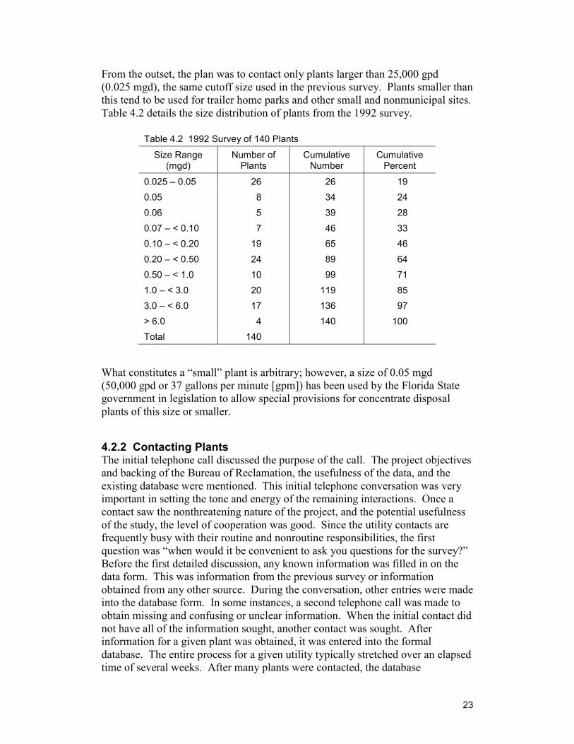
23

From the outset, the plan was to contact only plants larger than 25,000 gpd (0.025 mgd), the same cutoff size used in the previous survey. Plants smaller than this tend to be used for trailer home parks and other small and nonmunicipal sites. Table 4.2 details the size distribution of plants from the 1992 survey.

Table 4.2 1992 Survey of 140 Plants

Size Range (mgd)

Number of Plants

Cumulative Number

Cumulative Percent

0.025 – 0.05 26 26 19 0.05 8 34 24 0.06 5 39 28 0.07 – < 0.10 7 46 33 0.10 – < 0.20 19 65 46 0.20 – < 0.50 24 89 64 0.50 – < 1.0 10 99 71 1.0 – < 3.0 20 119 85 3.0 – < 6.0 17 136 97 > 6.0 4 140 100 Total 140

What constitutes a “small” plant is arbitrary; however, a size of 0.05 mgd (50,000 gpd or 37 gallons per minute [gpm]) has been used by the Florida State government in legislation to allow special provisions for concentrate disposal plants of this size or smaller.

4.2.2 Contacting Plants The initial telephone call discussed the purpose of the call. The project objectives and backing of the Bureau of Reclamation, the usefulness of the data, and the existing database were mentioned. This initial telephone conversation was very important in setting the tone and energy of the remaining interactions. Once a contact saw the nonthreatening nature of the project, and the potential usefulness of the study, the level of cooperation was good. Since the utility contacts are frequently busy with their routine and nonroutine responsibilities, the first question was “when would it be convenient to ask you questions for the survey?” Before the first detailed discussion, any known information was filled in on the data form. This was information from the previous survey or information obtained from any other source. During the conversation, other entries were made into the database form. In some instances, a second telephone call was made to obtain missing and confusing or unclear information. When the initial contact did not have all of the information sought, another contact was sought. After information for a given plant was obtained, it was entered into the formal database. The entire process for a given utility typically stretched over an elapsed time of several weeks. After many plants were contacted, the database

24

information was printed out in a concise form. This form was faxed to the plant for their verification and modification if necessary. Frequently the returned form contained additional information. Perhaps 20 percent of the faxed forms were returned with comments, new information, or corrected information.

It should be noted that no attempt was made to gather cost information from the survey. This was not an objective, in large part due to the difficulties and challenges associated with obtaining this type of information, particularly when several different types of plants are involved. While utilities are willing to describe their process, they are much less willing to share cost information. Not only is the reliability of such information in question, but it is difficult to get cost data from different plants on the same basis—conforming to predefined cost categories. In addition, much of the capital cost information is not recent and not well documented. In a separate project task, cost models of different disposal options were developed. The information needed for these models was not addressed in the interactions with the individual utilities.

During the course of the survey task, some changes were made in the data-gathering effort. First, the size of the minimum plant surveyed was increased from 0.025 mgd to 0.05 mgd. As can be seen in table 4.2, plants in this size range constituted almost 20 percent of the 1992 survey. Most of these plants were from Florida, and several of these plants are no longer in existence. Several small plants operating in 1992 are no longer operating, having been shut down in favor of more economical options for providing drinking water and because of problems with obsolescence and concentrate disposal. Furthermore, most plants of this size have a part-time operator who is typically not easily contacted and, when reached, not very interested in participating in the survey. In some instances, these smaller systems were found to have become part of larger systems. Because of the general trend in new membrane plants becoming larger, it was decided to focus the data-gathering efforts on larger utilities. As explained in the data analysis discussion of chapter 4, the effect of this change on the concentrate disposal statistics was both definite and predictable.

Another change involved limiting the number of microfiltration plants contacted. The primary reason for this was that nearly all of the microfiltration plants used Memcor microfiltration systems (the survey cutoff date for MF plants was 1999). Microfiltration systems are much more similar from site to site than are reverse osmosis, nanofiltration, or electrodialysis systems, and many sites were producing similar data. It was assumed that the data obtained were representative of many plants not contacted. Similarly, it was decided to set the minimum size cutoff for MF plants at 0.50 mgd, as MF plants tend to be larger than other membrane plants and, like other plants, their typical size is increasing.

A handful of plants in Florida declined to participate in the survey, saying that they did not want to jeopardize their ongoing permit-related challenges with the Florida Department of Environmental Protection.

25

The net result of these changes on the plants surveyed was that several plants are not included in the survey. In the 1992 survey that included 140 plants, it was estimated that as many as 95 percent of the candidate plants were contacted and included in the survey. In the present case, it is estimated that the number of candidate RO, NF, and ED/EDR systems surveyed was about 70 percent and the number of candidate MF plants surveyed was about 50 percent. The 1999 survey includes 150 plants.

4.3 Database Program Task

The 1992 survey information was summarized in an EXCEL spreadsheet. This form was convenient at the time for tabular display of the information. The 1999 survey contains considerably more information, thus requiring a change in format away from displaying all data from several plants on a single page. More important, the EXCEL format is not convenient for sorting and searching for information, and in general, for data analysis.

4.3.1 Database Software Various relational databases were reviewed to determine which most closely suits the intended purposes. Development of the database software for different platforms (Windows 32-bit, Windows 16-bit, Mac, UNIX, etc.) involves somewhat separate efforts. Because of this, it was decided to develop the database software only for the Windows 32-bit platform, as this platform is the one that is most widely used and whose usage is increasing. The database software may be considered to have a “front end” that the user sees and a “back end” which is the database itself. It was decided to use a Microsoft back end so that others on the research team can interact with it or visit it using the popular Microsoft program Access. It was also decided to use Access, itself, for the back end. With purchase of the Access 97 Developers Toolkit, distribution of the resulting program can be done without paying a royalty fee to Microsoft. This product easily handles the relatively small size of the database (a maximum of 200 plants and 150 pieces of information per plant).

4.3.2 Programming Programming of the database included customizing (defining input and output formats and forms) and manipulation (how information is retrieved and sorted). Programming aspects included:

♦ Designing the tables where the data will be held

♦ Designing the input form and the front end interface

♦ Designing a report (output form) so the input information can be printed out for immediate use

26

♦ Designing the reports and query mechanisms for the final product

♦ Modifying this to make an executable product which does not have input

♦ Creating a menu-driven user interface

The initial step was to develop a listing of information to be included in the database. Table 4.1 was developed for this purpose. Next, the nature and format of possible entries for each of these data were identified. After a dozen or so plants were contacted and the information from the plants was reviewed, database tables were constructed to house the individual data entries. A means of linking the data for each plant to that plant was developed. The end result was a series of interlinked tables.

To facilitate easy entry of data into these tables, an input form was created as the user-program interface. Data obtained from the survey were then entered into the database using this form. Creation of an output form allowed a hardcopy printout of the input data such that it could be sent to the individual plant for their review of accuracy and completeness.

A simple demonstration database software program was developed to demonstrate all the functions and capabilities of the final project database software program, albeit in a limited form. The intent of the demonstration effort was to encounter each of the different program design and CD formatting steps and challenges early in the project. A very simple database of limited information was thus developed that allowed data input, data query, data manipulation, report generation, and printing just as the project database software program would later do.

The database program to this point was all created in Microsoft Access. The creation of a stand-alone executable program that did not require Access software to run requires further programming. Microsoft Office products allow for some code to be written in Visual Basic. No separate software is required because the Visual Basic is accessed from within the Microsoft Office product software. The stand-alone version of the database was created using these Microsoft Access capabilities.

The next priority was to program the query mechanism. The programming step involved defining what types of queries would be made, how the queries would be made, and how the results of the queries would be displayed. Since the user creates the queries, some programming was required to provide this interface. An installation program, using the software INSTALLSHIELD, was created for this purpose.

4.3.3 Final User Interface The database is included along with other project products in a CD format. The contents of the CD include:

27

♦ A front-end menu providing choices to the user ♦ The stand-alone database program ♦ The full project text report ♦ The preliminary level disposal cost model worksheets ♦ The preliminary level disposal cost regression models

The front-end menu was created using Visual Basic. The stand-alone database program was simply written onto the CD. The report text was converted into a pdf file for inclusion into the CD format. The worksheets were also provided as pdf files. The regression models allow for some calculation to be done by the user. These files were written in Visual Basic also.

4.4 Regulatory Task

The regulation of concentrate and backwash disposal from membrane systems is an important consideration in the planning and design of a membrane drinking water system. Fifteen years ago, however, the meeting of regulatory requirements was a relatively minor challenge, as requirements were minimal. Since then, regulatory requirements have evolved considerably, as reflected in NPDES permit requirements in Florida. These have gone from the 1985 consideration of about six parameters to 1) an increase in the number of specific chemical parameters considered, 2) more stringent limits for many of these specific chemical parameters, and 3) use of whole effluent toxicity tests. While much of the historical membrane activity has been in the State of Florida, this situation has been changing. In addition to documenting the Federal regulatory structure and framework for concentrate disposal, the goal of the present work was to document State-by-State regulation. This was accomplished through contact with regulatory agencies from each State and discussing the regulatory requirements for the different types of concentrate disposal options. Many of the States now have Internet web sites that facilitate information gathering.

4.5 Analysis Task

There are several levels of data analysis. The first level of analysis was the compiling of lists such as plants by type of membrane process, treatment goals, and disposal method. The second level of analysis was the breakdown of these lists by other parameters, such as plant size, year of startup, etc. The number of possible different responses was limited, and the analyses at these levels were a simple matter of adding up plant responses.

The third level of analysis involves responses that required interpretation to fit them into categories. Examples included descriptions of disposal difficulties, of permit changes, of areas where networking advice would be given or sought after,

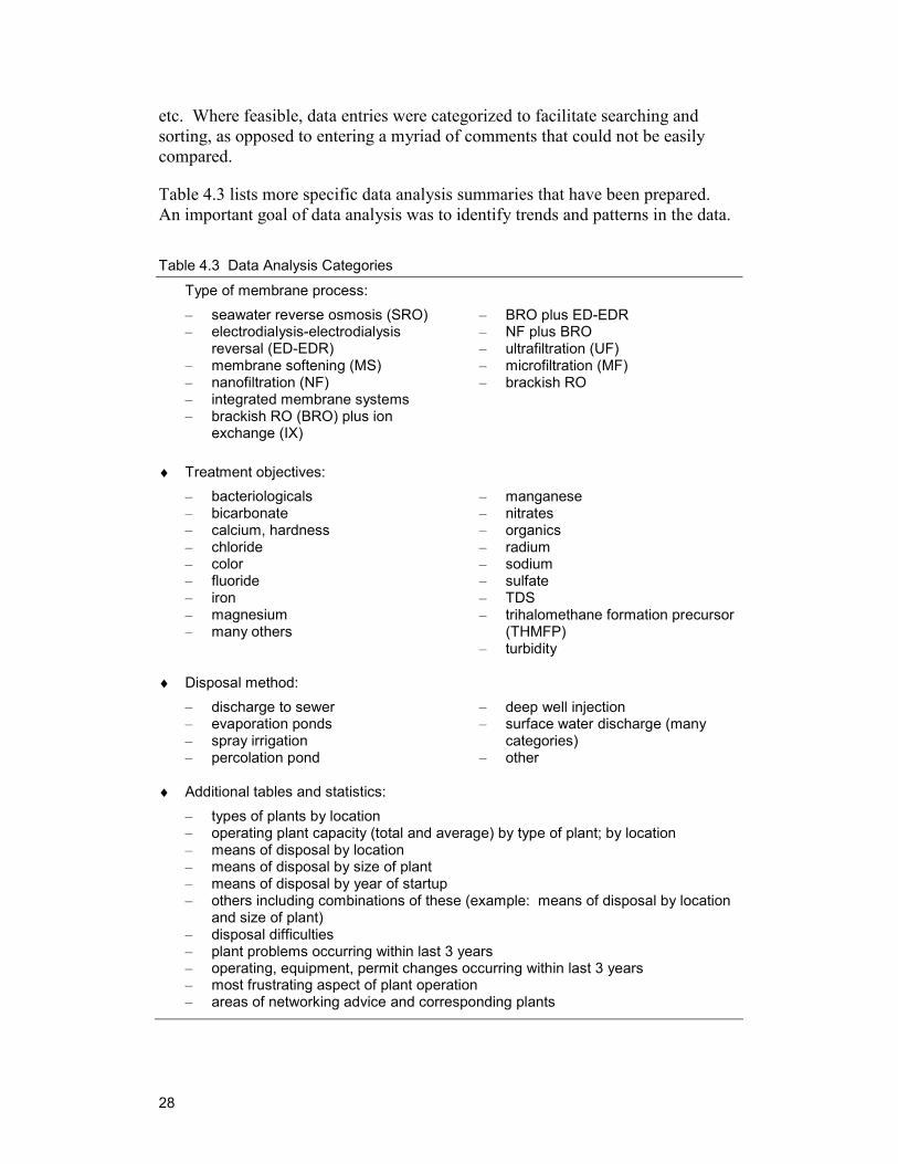
28

etc. Where feasible, data entries were categorized to facilitate searching and sorting, as opposed to entering a myriad of comments that could not be easily compared.

Table 4.3 lists more specific data analysis summaries that have been prepared. An important goal of data analysis was to identify trends and patterns in the data.

Table 4.3 Data Analysis Categories

Type of membrane process: – seawater reverse osmosis (SRO) – electrodialysis-electrodialysis

reversal (ED-EDR) – membrane softening (MS) – nanofiltration (NF) – integrated membrane systems – brackish RO (BRO) plus ion

exchange (IX)

– BRO plus ED-EDR – NF plus BRO – ultrafiltration (UF) – microfiltration (MF) – brackish RO

♦ Treatment objectives: – bacteriologicals – bicarbonate – calcium, hardness – chloride – color – fluoride – iron – magnesium – many others

– manganese – nitrates – organics – radium – sodium – sulfate – TDS – trihalomethane formation precursor

(THMFP) – turbidity

♦ Disposal method: – discharge to sewer – evaporation ponds – spray irrigation – percolation pond

– deep well injection – surface water discharge (many

categories) – other

♦ Additional tables and statistics: – types of plants by location – operating plant capacity (total and average) by type of plant; by location – means of disposal by location – means of disposal by size of plant – means of disposal by year of startup – others including combinations of these (example: means of disposal by location

and size of plant) – disposal difficulties – plant problems occurring within last 3 years – operating, equipment, permit changes occurring within last 3 years – most frustrating aspect of plant operation – areas of networking advice and corresponding plants

29

In addition to using the survey results to identify trends and, thus, issues affecting the membrane drinking water industry, discussions with various utility, regulatory, and other industry people frequently provided insights into issues that were affecting them.

4.6 Cost Modeling Task

4.6.1 Cost Estimates In general, the approach taken to develop cost estimates depends on the degree of accuracy desired and the amount of information available, including whether cost estimation programs are available. Cost estimates may be made at several stages of process design ranging from conceptual or preliminary stage to a final detailed stage. In this sequence, the accuracy desired may range from 50% at the preliminary stage to 10 to 15% at the design stage.

The most accurate cost estimates are developed using a “ground up” approach where costs for individual items are determined and then summed to arrive at the total cost. This approach is absolutely necessary to obtain the most accurate and meaningful cost projections. It takes into account regional and site-specific factors and all details required for vendors to issue quotes. For some well-established technologies and applications, there are cost estimation programs available, such as for a brackish reverse osmosis system (Bureau of Reclamation, 1999). The accuracy of these programs may approach that of a final design estimate, depending on the sophistication of the model and the quality of the input data. This is particularly true of technologies that are equipment oriented and whose equipment is substantially the same regardless of site location. Although membrane processes themselves fit this category, disposal options, in general, do not. For instance, whereas membrane processes can be used almost anywhere, most disposal options are location- and climate-dependent, and these site-dependent features must be considered for accurate disposal cost estimates. As a result, disposal cost estimation programs similar to those available for membrane processes do not exist.

Another approach to developing cost estimates involves studies undertaken to determine the range of costs encountered in the field. Cost information is gathered from existing facilities, typically new facilities where cost information is available. This approach has been used (Adham et al., 1996; Leitner et al., 1997) to determine rough costs and cost trends with plant size, etc. This approach must deal with the challenge of conforming cost information from different sources into a standard and usually arbitrary format and is not appropriate for meeting the present objectives.

30

4.6.2 Cost Model Objectives The objectives of the modeling effort are two fold:

1) To provide a simple means of developing preliminary cost estimates for different disposal options; this also allows the user to compare relative costs among different disposal options.

2) To do so in a manner that illustrates the different individual cost elements.

This allows the user to explore the influence of different design parameters on the total cost and to understand the equipment and operational aspects of the disposal options. The descriptive model can serve as a template for the user to develop more precise site-specific cost estimates.

These objectives have led to the development of two different types of cost-estimation models: worksheet models and simple closed-form regression models. The worksheet approach requires the user to choose design parameter values, to look up the individual cost factor values from figures, and to enter the values in a worksheet. The worksheet and the associated figures make the design parameters and cost factors explicit and provide a means of understanding the technical and economic aspects of the disposal option. The relative importance of the different cost factors can be seen easily. This calculation framework also provides the user a basis from which to develop more accurate cost estimates. The calculation process is, however, labor intensive. The regression models are closed-form mathematical relations developed from the worksheet models and, thus, represent approximations to them. They require the user to choose design parameter values and to make a simple calculation of the total capital cost. The regression models are much easier to use. They do, however, obscure any understanding of individual cost factors and their relative importance in determining the total cost.

4.6.3 Recommendations for Use of the Models User understanding is best served by reading about the individual model cost factors to appreciate the nature of the disposal option and also to appreciate the assumptions and limitations of the model. When some level of understanding is at hand, the regression models offer a means of developing quick relative comparison of costs for the different disposal options and analyzing cost sensitivities and trends with design parameter values. The worksheet calculations should be used when more accurate estimates are required.

4.6.4 Development of Worksheet Models The following worksheet models are developed for six disposal options and for the transport of concentrate from the membrane plant to the disposal site:

♦ Deep well disposal ♦ Evaporation pond ♦ Spray irrigation

31

♦ Surface water disposal ♦ Discharge to sewer ♦ Zero liquid discharge ♦ Transport

The worksheet models, especially for the first three items, borrow heavily from a previous work the author participated in (Mickley et al., 1993). More specifically, this includes the cost factor approach and some of the descriptive text from that work. Cost factor values have been updated from the previous work.

The worksheet models were developed in several steps as described below.

4.6.4.1 Step 1: Identification of Cost Factors Cost factors are the independent cost items that, in sum, make up the total capital cost for each disposal option (Mickley, 1996). As an example, the cost factors for the evaporation pond disposal option include:

♦ Land ♦ Land clearing ♦ Dike ♦ Pond liner ♦ Perimeter fence ♦ Road ♦ Engineering ♦ Contingency

4.6.4.2 Step 2: Identification of Design Parameters The capital cost of each cost factor is dependent on the design parameters necessary to characterize the cost factor. For instance, in the case of a pipeline, the design factors might include the pipe material, wall thickness, length of the pipe, and diameter of the pipe. Not all combinations of these parameters are considered in the models; in some cases, parameters are restricted; for instance, in setting values of pipe material and wall thickness. Values are chosen to be most representative and typical of field use. In situations where other values are required at a site, the model user will need to adjust the calculations accordingly. The choice of design parameters is dependent on the design approach taken in the model. The design parameters that determine the independent cost factors for the evaporation pond model are:

♦ Land acreage ♦ Land type ♦ Dike height ♦ Total pond liner thickness

32

4.6.4.3 Step 3: Identification of Values for Cost Factors Costs were developed through interaction with equipment vendors in various parts of the country to ensure that costs were not biased by regional differences. The assignment of values or curves to the resulting data was somewhat arbitrary, given differences in cost values found from different sources. Values were chosen which were judged to be representative.

4.6.4.4 Step 4: Development of Worksheet Table 4.4 presents the worksheet for the evaporation pond disposal model. There are five design parameters called variables in the worksheet. In the example provided, values are chosen of 10 acres for the evaporative surface, 8 feet for the dike height, 60 milliliters (mil) for the total liner thickness, $5,000 per acre for the land purchase cost, and $4,000 per acre for the clearing of medium wooded land. From these five variable values, the values of several cost factors are determined from the appropriate figures listed in the worksheet. The worksheet contains room for additional calculations. Similar worksheets are developed for the other disposal options.

4.6.5 Development of Regression Models The total capital cost (TCC) for a disposal method is equal to the sum of several individual cost factors. Each of these cost factors (such as pipe, pump, pond liner, land, etc.) may be represented by the size or amount of the cost element times its unit cost factor. The cost factor for land, for instance, is determined by the acres of land required times the cost per acre of the land. The cost curves presented in figures represent these individual cost factors as a function of design parameters (number of acres, for example) for set values of the unit cost factors.

For the cost models, the TCC (a dependent variable) is thus dependent on design parameters (independent variables). A closed form mathematical relationship expressing this dependency is of the form:

TCC = function (independent variables) (1)

In a multilinear regression model with three independent variables, this function is linear in the independent variables such as:

TCC = a + b*IV1 + c*IV2 + d*IV3 + … (2)

Where a, b, c, and d are constants determined by the regression algorithm and IV1, IV2, and IV3 are the three independent variables.

Once values of the four constants are determined, the total capital cost, TCC, may be calculated by inserting particular values for the three independent variables, IV1, IV2, and IV3, into this relationship.

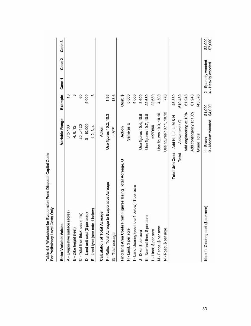
33

34

It is obvious from the figures of cost factor values as a function of the independent variables that the relationships are not always linear. However, there is no reason to assume that a linear regression model for the total capital cost will not be adequate; and, in any case, this needs to be evaluated as a first step in developing the regression relation.

The regression algorithms require several sets of data comprised of values for each of the independent variables and the corresponding value for the dependent variable. From statistical considerations, 30 sets of data are sufficient to estimate regression relation constants with high confidence, providing a meaningful linear relation exists. This is the first of several steps in the development of a regression model.

4.6.5.1 Step 1: Calculation of 30 Sets of Values for the Independent Variables To guarantee that the 30 sets of data cover the full range of independent variable values (ranges of the design parameters) and are randomly distributed over these ranges, values of the independent variables are chosen using the following approach:

♦ Thirty (30) sets of random numbers, between the values of zero and one, are developed for each independent variable.

♦ These random numbers are then used to calculate values for the independent variables. For example, if the flow rate variable is assumed to go from 0 to 5 mgd, then the flow rate is determined from multiplying the random number times the full range of the variable, which in this case is 5. A random number of 0.48 gives a flow rate of 0.48 * 5 or 2.40. For a variable such as the number of casing transitions that can take on a value of 3 or 4, the value of 3 is used if the random number is 0 to 0.5, and a value of 4 is used if the random number is > 0.5 to 1.0. Problematic cases are thrown out, such as flow rates below 0.1 mgd.

♦ The resulting sets of independent variable values are then checked for autocorrelation; that is, to see if the values for one variable are correlated, through chance, to the values of another variable. The variable values are also checked to make sure the range of possible values is adequately represented. If there are problems with the values, either from autocorrelation or from value bias, a new set of random numbers is generated until 30 suitable sets of data are obtained.

4.6.5.2 Step 2: Calculation of the Total Capital Costs The worksheets previously discussed are used to calculate 30 total capital costs using the 30 sets of parameter values.

4.6.5.3 Step 3: Multiple Regression on the 30 Data Sets The software used to perform the regression calculations is SYSTAT 9, a powerful statistical and graphical analysis system marketed by SPSS, Inc. The

35

program calculates the constant and coefficient values, such as a, b, c, and d, in the above relation and various indicators of degree of regression success such as regression coefficients, confidence intervals in the coefficients, and residuals (the difference between data values for total capital cost and calculated or predicted values for total capital cost using the regression relation).

The primary indicator of regression success is taken as the adjusted squared multiple R, where R2 is the familiar regression coefficient that expresses the fraction of the total variability in the data that is explained by the regression relation. The adjusted value takes into consideration the number of data sets considered. When a regression model is based on relatively few cases, the multiple squared R tends to be an optimistic estimate of how well the model fits the population from which the data are assumed to come.

At this point in the procedure, a closed form mathematical relation such as equation (2) exists. A standard procedure in determining the adequacy of the model is an analysis of residuals. This will indicate the presence of outliers, curvature, or other forms of nonlinearity in the data.

4.6.5.4 Step 4: Analysis of Model Residuals The residual for a given set of data (i.e., for a given set of independent variable values) is the difference between the total capital cost used in the regression and the total capital cost predicted by the regression equation. A comparison between each of the 30 sets of values (the worksheet calculated total capital costs and the regression equation total capital costs) yields 30 residual values. Patterns in residuals are studied to determine if there is a consistent trend of residual values with high or low or certain combinations of design variable values. Ideally, the magnitude of the residuals would be fairly constant and normally distributed without any outlier values. Where residual patterns deviate from this ideal, it may mean that:

1) A worksheet calculation mistake was made in certain values (particularly where outliers exist).

2) Outliers exist for some other reason.

3) The linear model is not necessarily the best to use to fit the data.

As an illustration of these considerations, the regression model for the evaporation pond (total cost per unit area) is considered. The model coefficients, a, b, c, and d were determined to be:

a = 5406 b = 465 c = 1.07 d = 0.931 e = 217.5

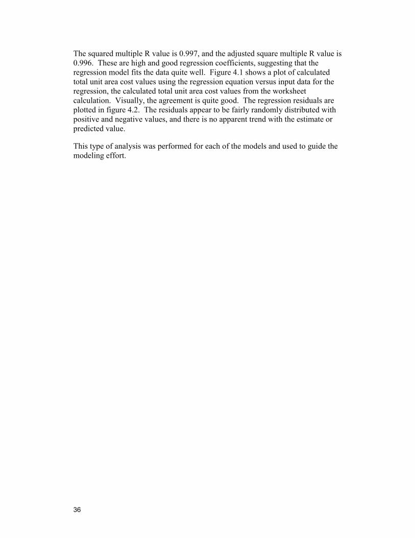
36

The squared multiple R value is 0.997, and the adjusted square multiple R value is 0.996. These are high and good regression coefficients, suggesting that the regression model fits the data quite well. Figure 4.1 shows a plot of calculated total unit area cost values using the regression equation versus input data for the regression, the calculated total unit area cost values from the worksheet calculation. Visually, the agreement is quite good. The regression residuals are plotted in figure 4.2. The residuals appear to be fairly randomly distributed with positive and negative values, and there is no apparent trend with the estimate or predicted value.

This type of analysis was performed for each of the models and used to guide the modeling effort.

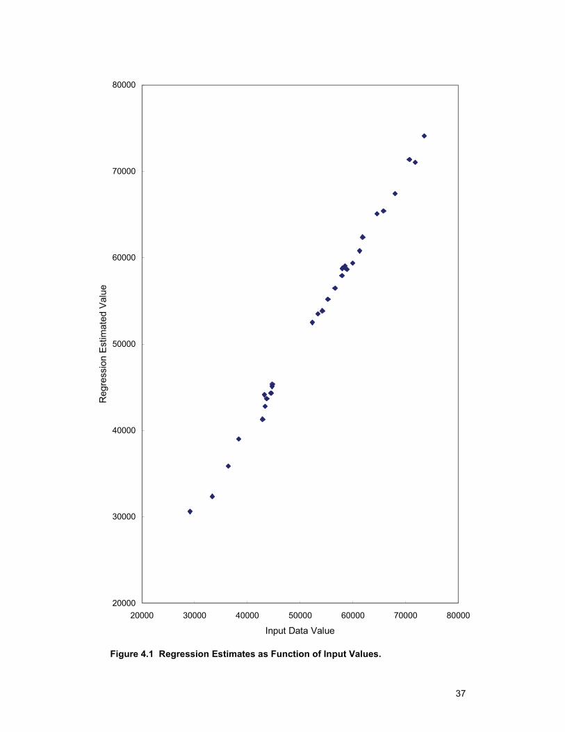
37

20000

30000

40000

50000

60000

70000

80000

20000 30000 40000 50000 60000 70000 80000

Input Data Value

Reg

ress

ion

Est

imat

ed V

alue

Figure 4.1 Regression Estimates as Function of Input Values.

38

-2000

-1500

-1000

-500

0

500

1000

1500

2000

20000 30000 40000 50000 60000 70000 80000

Regression Estimated Value

Res

idua

l Val

ue

Figure 4.2 Regression Residuals as Function of Estimated Value.

39

5. Plant Survey Results 5.1 Introduction

This chapter presents observations and results from analysis of the plant data collected in the survey. It contains new information obtained after publication of the first edition. The new information is a result of 1) a membrane plant survey conducted in 2002 to extend the 2000 report database to include municipal plants beginning operation in 2000 and 2001 and to include plants beginning operation from 1993 through 1999 that were left out of the previous (1999) survey, and 2) inclusion of pre-1993 plants from a previous project.

Pre-1993 plants were mostly eliminated from the 2002 and previous (1999) survey, as the pre-1993 plants were the focus of a previous 1992 survey (Mickley et al., 1993). All membrane plants included in the 1992 survey conducted for AWWARF (Mickley et al., 1993) are now included in the database. In this recent survey, as well as in previous surveys, membrane plants were contacted by telephone and, in most cases, by a series of faxes, emails, and telephone calls.

As a result of these efforts, the updated database now includes:

♦ Nearly all (97 percent) desalting plants (BRO, SRO, NF, EDR, MF/RO, and NF/RO) that could be identified in the 50 States that were built through 2001 to produce drinking water or treat municipal waste water and that are 25,000 gpd and above.

♦ Nearly all (91 percent) low-pressure plants (MF and UF) that could be identified in the 50 States that were built through 2001 to produce drinking water or treat municipal waste water that are 1 mgd and above.

♦ Other plants: some smaller desalting and low-pressure membrane plants.

In addition to the database that contains substantial information about most of these plants, a numerical tally of all municipal membrane plants (of 25,000 gpd and above) that could be identified in the 50 States is provided. This list includes plants built through 2002.

Information about total number of plants is provided in section 5.2. This is followed by a discussion of the surveyed plants, beginning in section 5.3.

Low-pressure MF and UF plants are considered separately from the desalting plants because of their natural differences. Foremost is the fact that MF and UF plants do not concentrate salts and other dissolved solids, and, consequently, the reject/backwash from MF and UF plants is not of a higher TDS than the feed—unlike desalting plant concentrate. The low-pressure reject/backwash is typically a much lower percentage of the feed volume than is desalting plant concentrate. Thus, for a same-sized plant, the reject/backwash is of much lower

40

volume than is the corresponding concentrate. As a result of these differences, the disposal of reject/backwash is different than disposal of concentrate. At the time of a previous survey (Mickley et al., 1993) there were no MF or UF plants identified as operating at municipal sites. The 1992 survey included only desalting plants. Separation in the present survey into desalting and low-pressure portions allows direct comparison of the desalting plants built since 1992 with the 1992 survey plants.

It will be seen that the numbers used in tables and figures are not always consistent. Such differences are due to missing information in the case of one or more plants. A few cases of missing information does not significantly alter the statistical picture presented.

5.2 Total Number of Membrane Plants in the United States

There were several reasons for identifying the total number of membrane plants in water and waste water facilities in the United States. The first was to accurately document the number of plants of each type, as this is important information in its own right. The second reason was to determine how feasible a periodic membrane survey of all plants would be. As a result of the identification of the total number of plants, it was decided that:

♦ All desalting plants 25,000 gpd and above, not previously surveyed, could be surveyed

♦ Due to the relatively low number of new desalting plants appearing each year (typically between 5 and 15), in the future it would be reasonable to periodically update the database

♦ Due to the large number of low-pressure plants being built each year (on the order of 35), and due to many older low-pressure plants yet to be surveyed, not all low-pressure plants could be surveyed.

♦ It would be best to raise the size limit of low-pressure plants to be surveyed to 1 mgd. This would allow a reasonable effort to bring the database completely up to date for low-pressure plants of that size and also allow reasonable efforts for future updates to the database.

These decisions bring about the difference between the number of plants in the total plant tally and in the database. The total plant tally identifies all municipal membrane plants (desalting and low-pressure) of 25,000 gpd and above. The database contains a subset of these plants: all the desalting plants built but only those low-pressure plants 1 mgd and above. Because some survey effort, both past and present, was made before this decision, there are some smaller low-pressure plants in the database.

41

The following tabulation provides an indication of how representative the database is, showing the number of plants included in the database versus the number of plants identified.

Identified In

Database

Number of membrane plants, .025 mgd or above (through 2002)

422 300

Number of desalting plants, .025 mgd or above (through 2002)

124 227

Number of low-pressure plants, 1 mgd or above, (< 2002)

53 48

Number of low-pressure plants, 025 mgd or above (through 2002)

188 74

As can be seen, only seven desalting plants are missing from the database and only five large low-pressure plants (through 2001).

5.2.1 Tabulation of Plants in the United States Through 2002 Table 5.1 is a tabulation of operating municipal membrane plants by year and by membrane technology. It was developed based on data from the 1992 survey (Mickley et al., 1993), the 1999 survey, and the more recent 2002 survey. This and all such plant tallies have minimum size cutoffs that influence the numbers of plants listed. For this tabulation, a size cutoff of 25,000 gpd was used for both desalting plants and low-pressure plants. This cutoff eliminates most smaller plants that serve truck stops, mobile home parks, hospitals, campgrounds, etc. In the highlighted columns of table 5.1, the total number of desalting plants and low-pressure plants is tallied for each year, as well as the grand totals and cumulative number of plants.

Figure 5.1 shows the cumulative number of plants by year beginning in 1965. The total number of all types of plants, the number of low-pressure plants, and the number of desalting plants are shown separately.

Several important observations can be made from table 5.1 and figure 5.1. These include:

♦ Most (167, or 71%) of the 234 desalting plants are BRO plants with a lesser number of NF and ED/EDR plants (26, or 11% and 18, or 8%, respectively) and a few (10, or 4%) SRO plants. There are now 13 (6%) integrated (MF/RO or MF/NF) membrane plants, which in this report are considered only as desalting plants.

♦ The early plants were BRO and ED/EDR plants, with the first NF plant coming online in 1988.

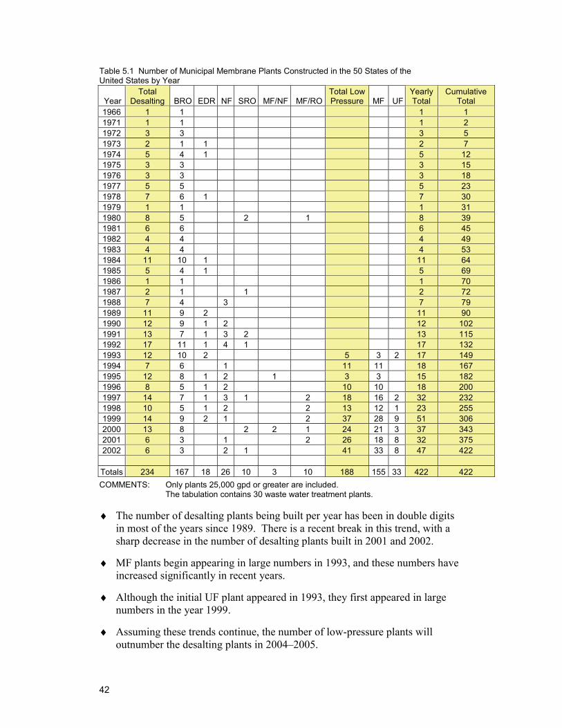
42

♦ The number of desalting plants being built per year has been in double digits in most of the years since 1989. There is a recent break in this trend, with a sharp decrease in the number of desalting plants built in 2001 and 2002.

♦ MF plants begin appearing in large numbers in 1993, and these numbers have increased significantly in recent years.

♦ Although the initial UF plant appeared in 1993, they first appeared in large numbers in the year 1999.

♦ Assuming these trends continue, the number of low-pressure plants will outnumber the desalting plants in 2004–2005.

Table 5.1 Number of Municipal Membrane Plants Constructed in the 50 States of the United States by Year

Year Total

Desalting BRO EDR NF SRO MF/NF MF/ROTotal LowPressure MF UF

Yearly Total

Cumulative Total

1966 1 1 1 1 1971 1 1 1 2 1972 3 3 3 5 1973 2 1 1 2 7 1974 5 4 1 5 12 1975 3 3 3 15 1976 3 3 3 18 1977 5 5 5 23 1978 7 6 1 7 30 1979 1 1 1 31 1980 8 5 2 1 8 39 1981 6 6 6 45 1982 4 4 4 49 1983 4 4 4 53 1984 11 10 1 11 64 1985 5 4 1 5 69 1986 1 1 1 70 1987 2 1 1 2 72 1988 7 4 3 7 79 1989 11 9 2 11 90 1990 12 9 1 2 12 102 1991 13 7 1 3 2 13 115 1992 17 11 1 4 1 17 132 1993 12 10 2 5 3 2 17 149 1994 7 6 1 11 11 18 167 1995 12 8 1 2 1 3 3 15 182 1996 8 5 1 2 10 10 18 200 1997 14 7 1 3 1 2 18 16 2 32 232 1998 10 5 1 2 2 13 12 1 23 255 1999 14 9 2 1 2 37 28 9 51 306 2000 13 8 2 2 1 24 21 3 37 343 2001 6 3 1 2 26 18 8 32 375 2002 6 3 2 1 41 33 8 47 422

Totals 234 167 18 26 10 3 10 188 155 33 422 422 COMMENTS: Only plants 25,000 gpd or greater are included. The tabulation contains 30 waste water treatment plants.

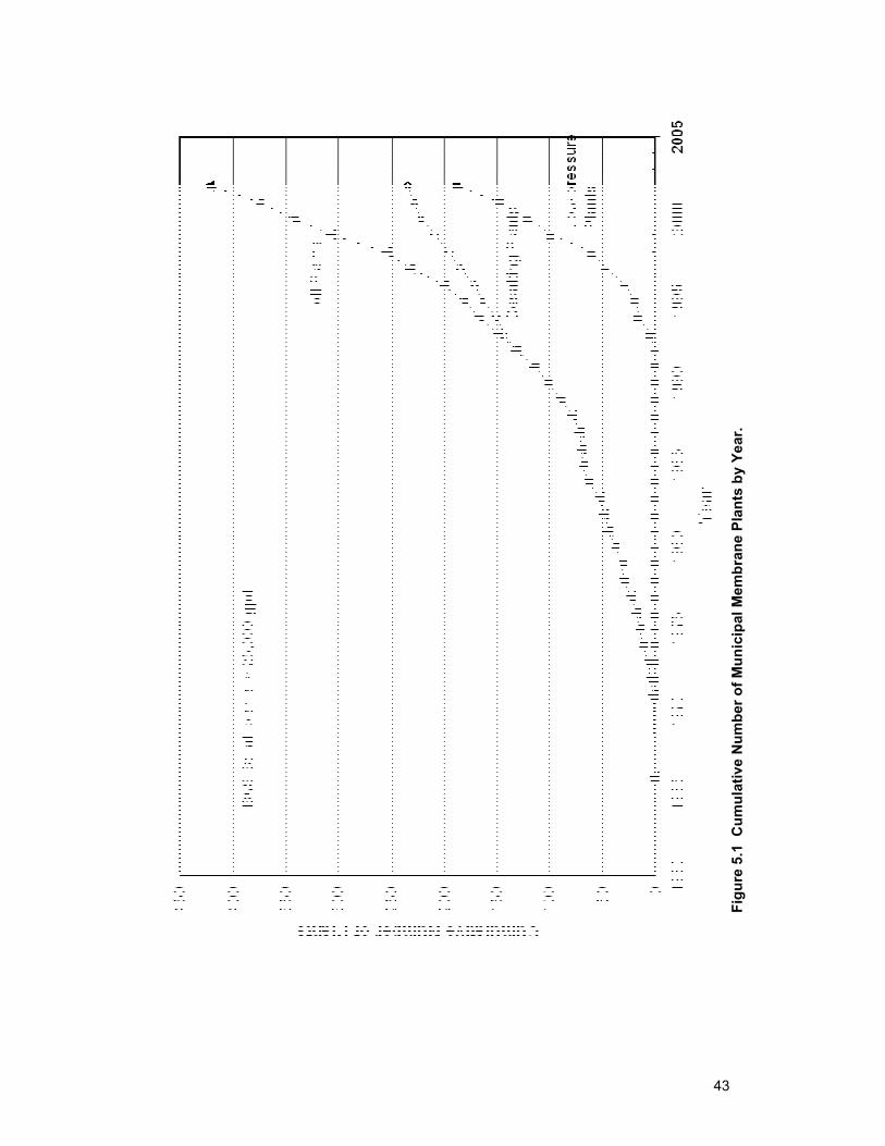
43

Figu

re 5

.1 C

umul

ativ

e N

umbe

r of M

unic

ipal

Mem

bran

e Pl

ants

by

Year

.

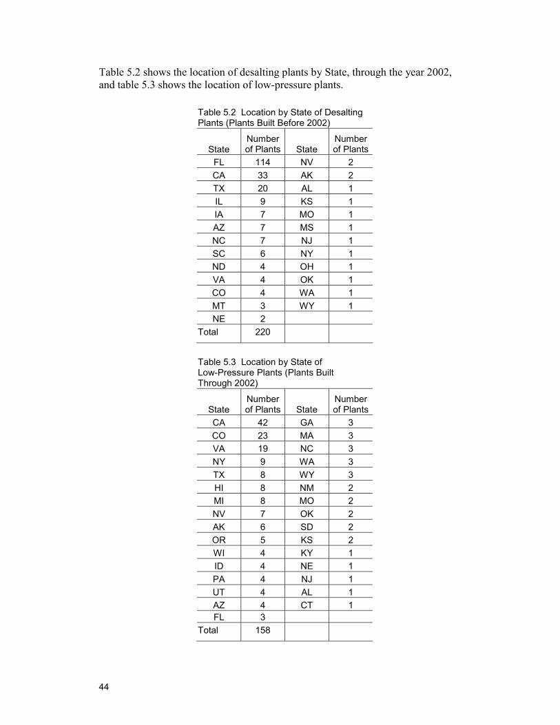
44

Table 5.2 shows the location of desalting plants by State, through the year 2002, and table 5.3 shows the location of low-pressure plants.

Table 5.2 Location by State of Desalting Plants (Plants Built Before 2002)

State Number of Plants State

Number of Plants

FL 114 NV 2 CA 33 AK 2 TX 20 AL 1 IL 9 KS 1 IA 7 MO 1 AZ 7 MS 1 NC 7 NJ 1 SC 6 NY 1 ND 4 OH 1 VA 4 OK 1 CO 4 WA 1 MT 3 WY 1 NE 2

Total 220

Table 5.3 Location by State of Low-Pressure Plants (Plants Built Through 2002)

State Number of Plants State

Number of Plants

CA 42 GA 3 CO 23 MA 3 VA 19 NC 3 NY 9 WA 3 TX 8 WY 3 HI 8 NM 2 MI 8 MO 2 NV 7 OK 2 AK 6 SD 2 OR 5 KS 2 WI 4 KY 1 ID 4 NE 1 PA 4 NJ 1 UT 4 AL 1 AZ 4 CT 1 FL 3

Total 158

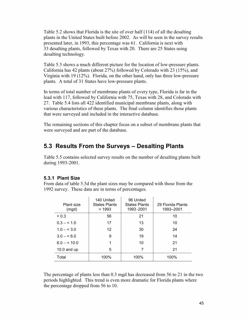
45

Table 5.2 shows that Florida is the site of over half (114) of all the desalting plants in the United States built before 2002. As will be seen in the survey results presented later, in 1993, this percentage was 61. California is next with 33 desalting plants, followed by Texas with 20. There are 25 States using desalting technology.

Table 5.3 shows a much different picture for the location of low-pressure plants. California has 42 plants (about 27%) followed by Colorado with 23 (15%), and Virginia with 19 (12%). Florida, on the other hand, only has three low-pressure plants. A total of 31 States have low-pressure plants.

In terms of total number of membrane plants of every type, Florida is far in the lead with 117, followed by California with 75, Texas with 28, and Colorado with 27. Table 5.4 lists all 422 identified municipal membrane plants, along with various characteristics of these plants. The final column identifies those plants that were surveyed and included in the interactive database.

The remaining sections of this chapter focus on a subset of membrane plants that were surveyed and are part of the database.

5.3 Results From the Surveys – Desalting Plants

Table 5.5 contains selected survey results on the number of desalting plants built during 1993-2001.

5.3.1 Plant Size From data of table 5.5d the plant sizes may be compared with those from the 1992 survey. These data are in terms of percentages.

Plant size (mgd)

140 United States Plants

< 1993

96 United States Plants 1993–2001

29 Florida Plants 1993–2001

< 0.3 56 21 10 0.3 – < 1.0 17 13 10 1.0 – < 3.0 12 30 24 3.0 – < 6.0 9 19 14 6.0 – < 10.0 1 10 21 10.0 and up 5 7 21

Total 100% 100% 100%

The percentage of plants less than 0.3 mgd has decreased from 56 to 21 in the two periods highlighted. This trend is even more dramatic for Florida plants where the percentage dropped from 56 to 10.

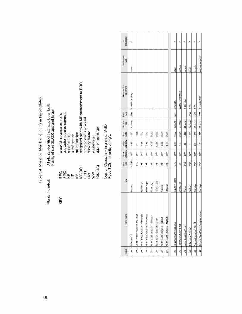
46

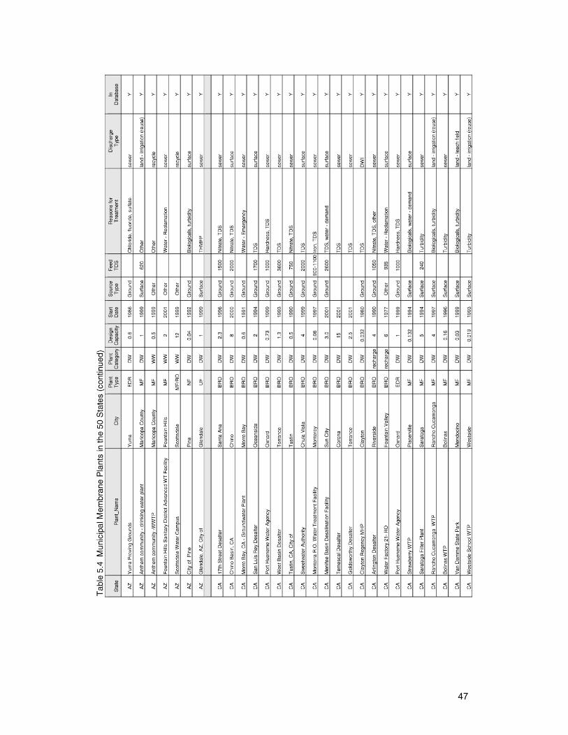
47

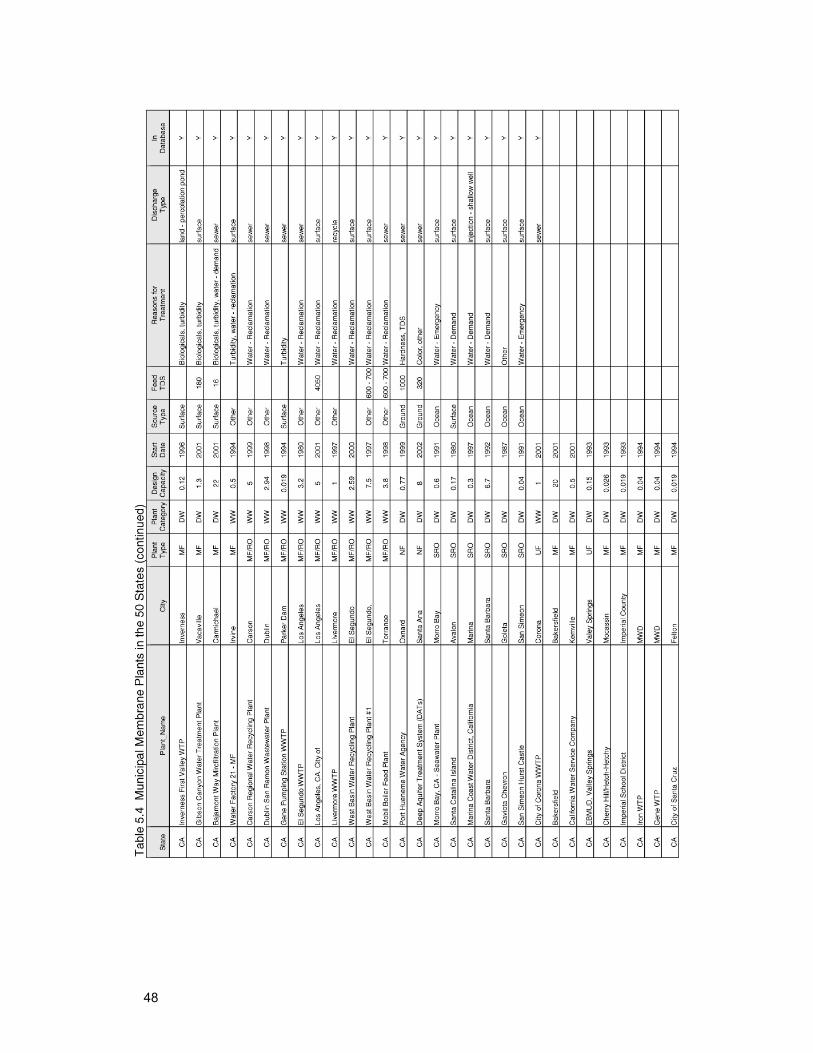
48

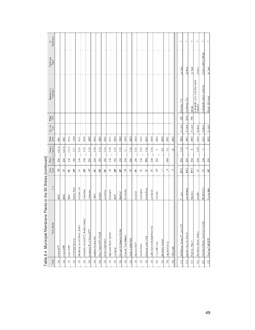
49

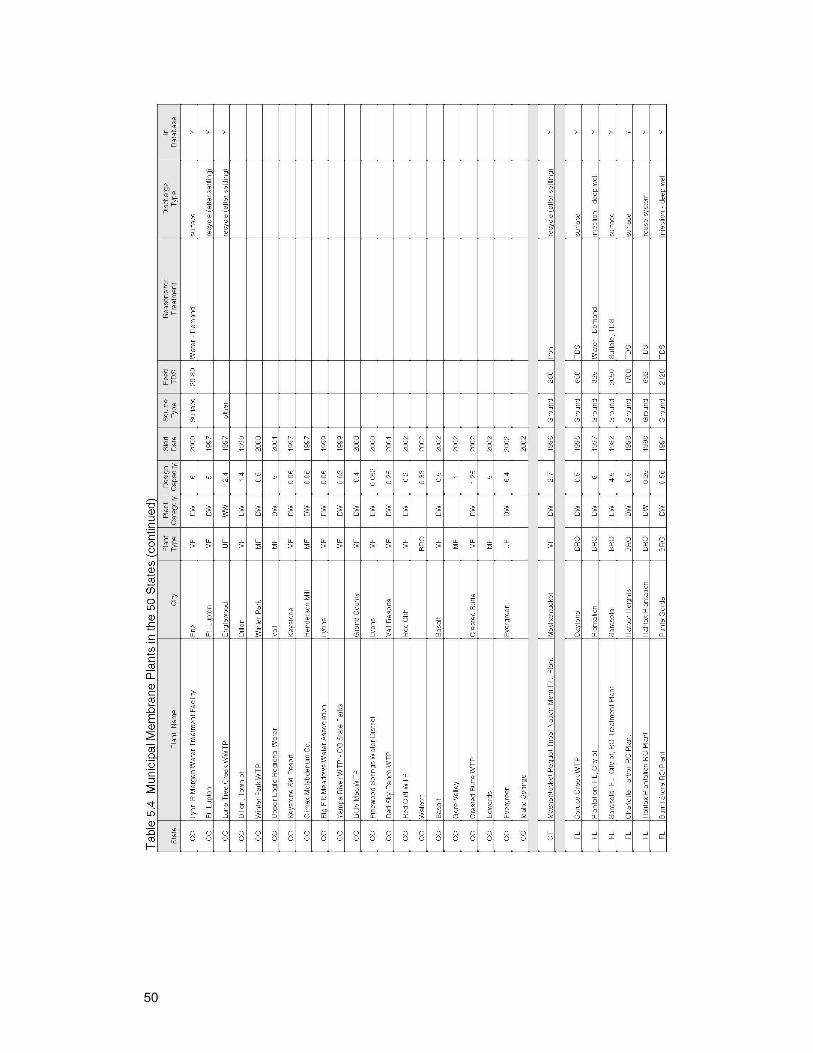
50

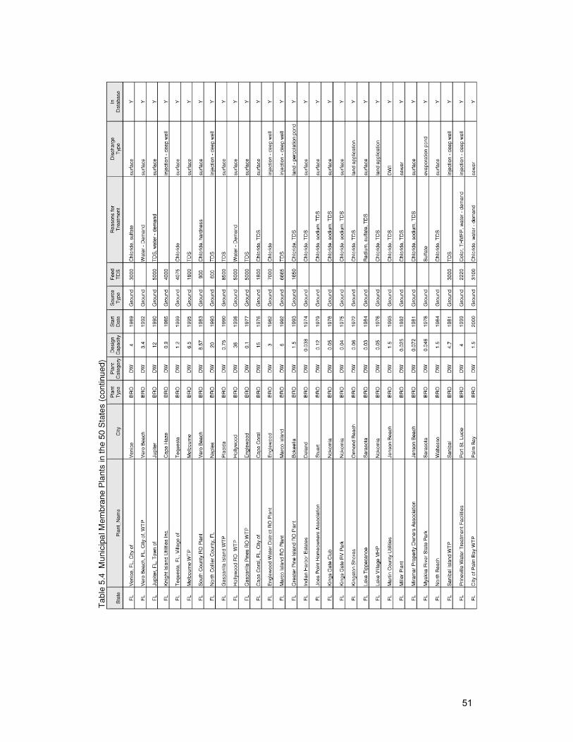
51

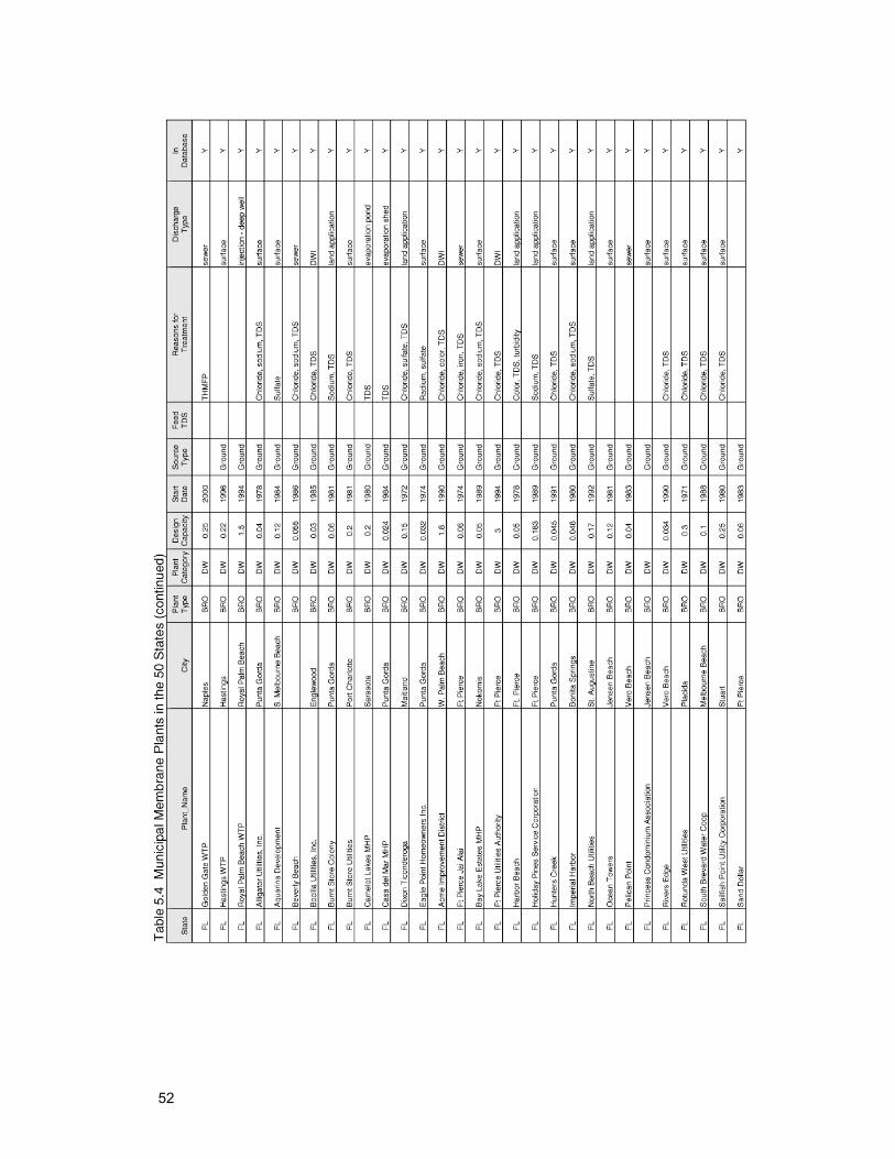
52

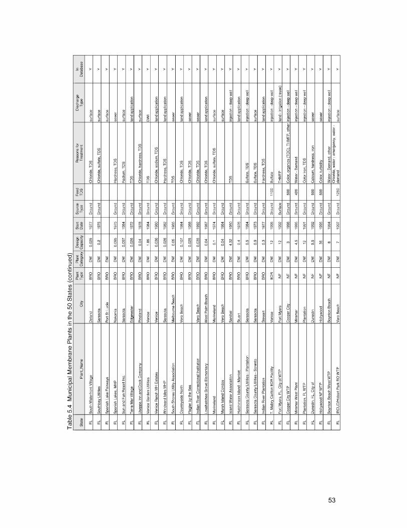
53

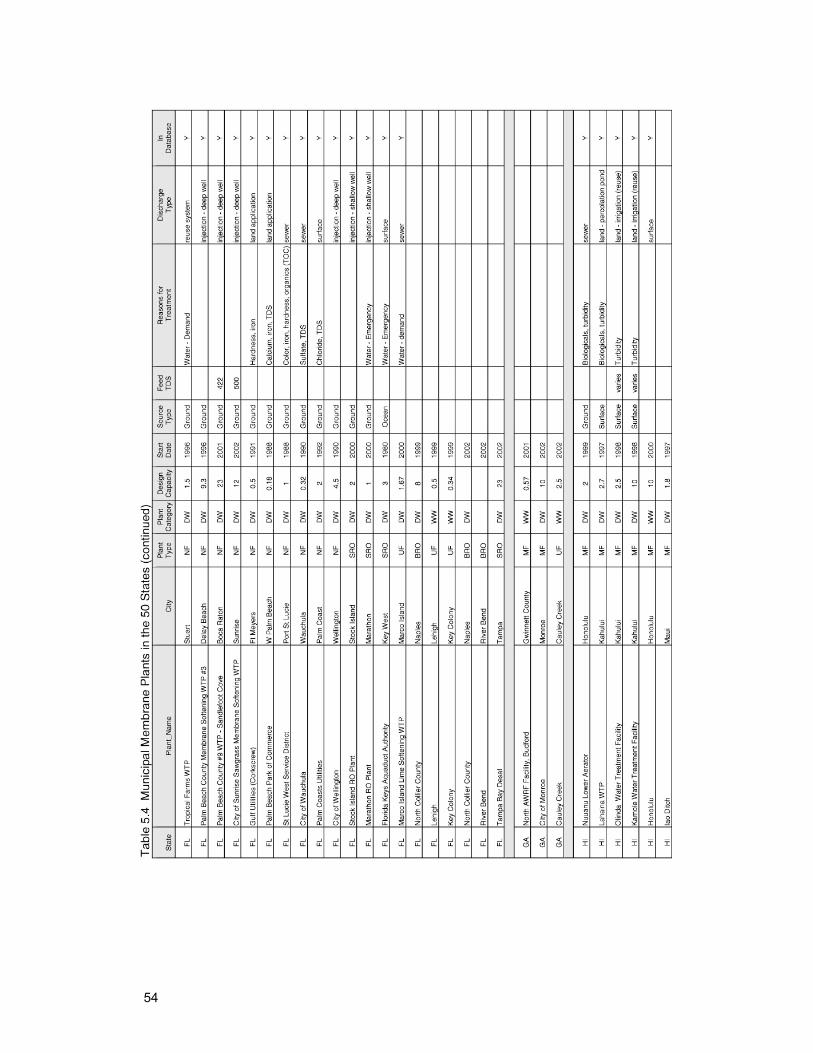
54

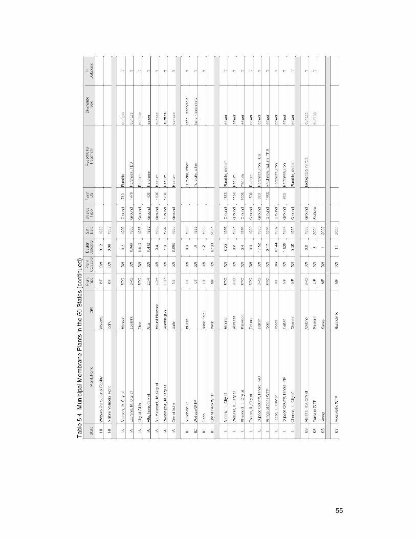
55

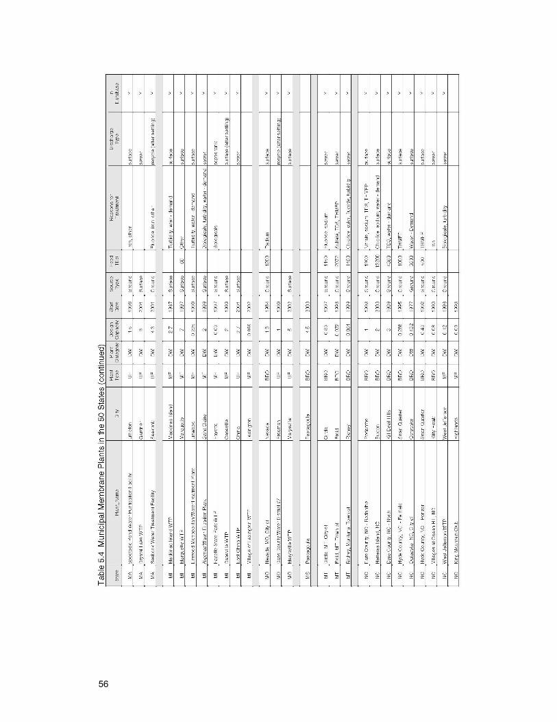
56

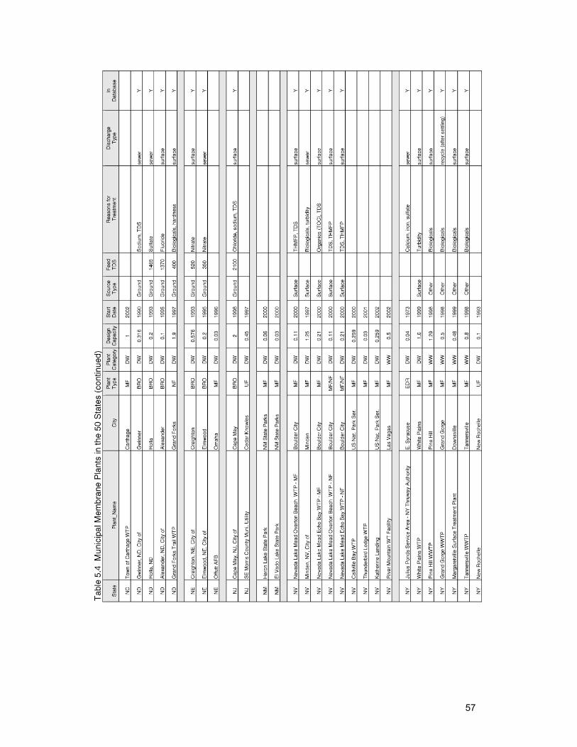
57

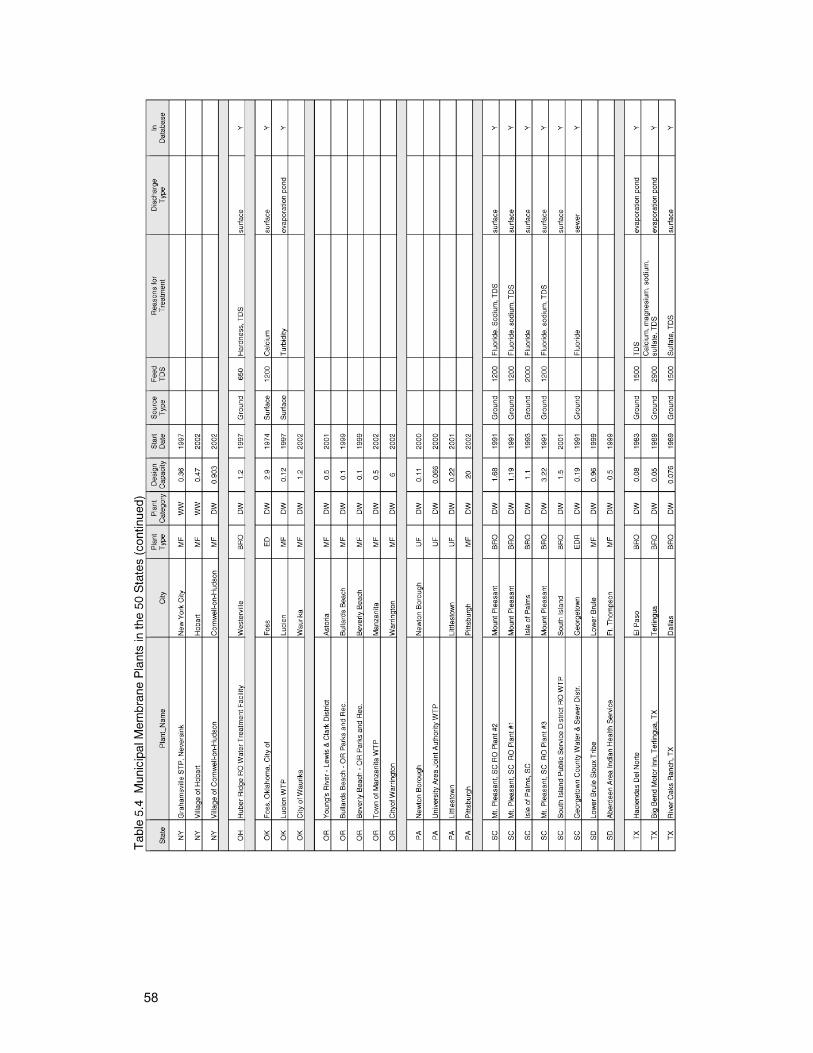
58

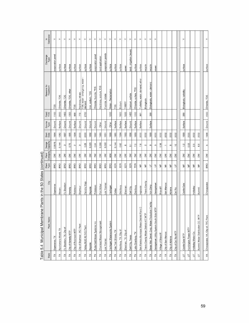
59

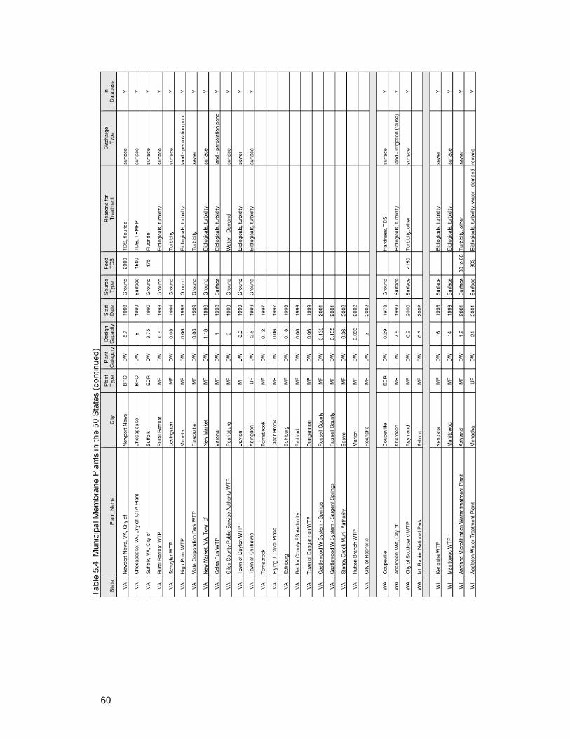
60

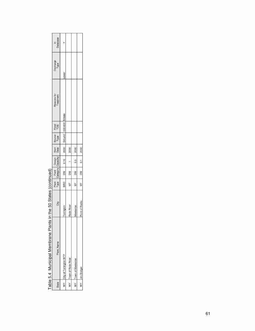
61

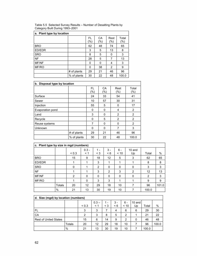
62

Table 5.5 Selected Survey Results – Number of Desalting Plants by Category Built During 1993–2001

a. Plant type by location FL

(%) CA (%)

Rest (%)

Total (%)

BRO 62 48 74 65 ED/EDR 3 5 13 8 SRO 8 5 0 3 NF 28 5 7 13 MF/NF 0 0 4 3 MF/RO 0 38 2 9 # of plants 29 21 46 96 % of plants 30 22 48 100.0 b. Disposal type by location FL

(%) CA (%)

Rest (%)

Total (%)

Surface 24 33 54 41 Sewer 10 57 30 31 Injection 55 5 0 17 Evaporation pond 0 0 4 2 Land 3 0 2 2 Recycle 0 5 2 2 Reuse systems 7 0 0 2 Unknown 0 0 7 3 # of plants 29 21 46 96 % of plants 30 22 48 100.0 c. Plant type by size in mgd (numbers)

< 0.3 0.3 - < 1

1 - < 3

3 - < 6

6 - < 10

10 and Up Total %

BRO 15 9 18 12 5 3 62 65 ED/EDR 1 1 3 1 1 1 8 8 SRO 0 1 2 0 0 0 3 3 NF 1 1 3 2 3 2 12 13 MF/NF 2 0 0 0 0 0 2 3 MF/RO 1 0 3 3 1 1 9 9 Totals 20 12 29 18 10 7 96 101.0 % 21 13 30 19 10 7 100.0 d. Size (mgd) by location (numbers)

< 0.3 0.3 – < 1

1 - < 3

3 - < 6

6 - < 10

10 and Up Total %

FL 3 3 7 4 6 6 29 30 CA 2 3 8 5 2 1 21 22 Rest of United States 15 6 14 9 2 0 46 48 Totals 20 12 29 18 10 7 96 100.0 % 21 13 30 19 10 7 100.0

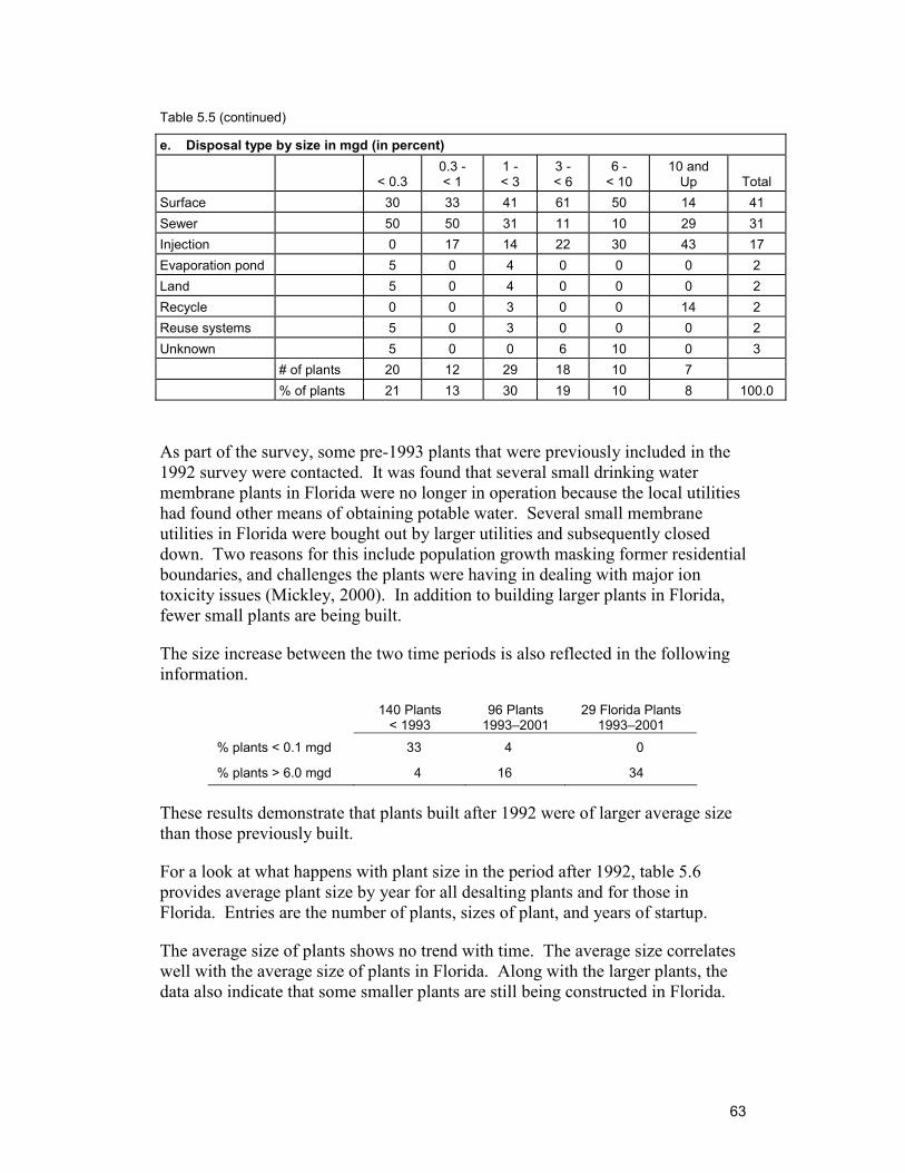
63

Table 5.5 (continued)

e. Disposal type by size in mgd (in percent)

< 0.3 0.3 - < 1

1 - < 3

3 - < 6

6 - < 10

10 and Up Total

Surface 30 33 41 61 50 14 41 Sewer 50 50 31 11 10 29 31 Injection 0 17 14 22 30 43 17 Evaporation pond 5 0 4 0 0 0 2 Land 5 0 4 0 0 0 2 Recycle 0 0 3 0 0 14 2 Reuse systems 5 0 3 0 0 0 2 Unknown 5 0 0 6 10 0 3 # of plants 20 12 29 18 10 7 % of plants 21 13 30 19 10 8 100.0 As part of the survey, some pre-1993 plants that were previously included in the 1992 survey were contacted. It was found that several small drinking water membrane plants in Florida were no longer in operation because the local utilities had found other means of obtaining potable water. Several small membrane utilities in Florida were bought out by larger utilities and subsequently closed down. Two reasons for this include population growth masking former residential boundaries, and challenges the plants were having in dealing with major ion toxicity issues (Mickley, 2000). In addition to building larger plants in Florida, fewer small plants are being built.

The size increase between the two time periods is also reflected in the following information.

140 Plants < 1993

96 Plants 1993–2001

29 Florida Plants 1993–2001

% plants < 0.1 mgd 33 4 0

% plants > 6.0 mgd 4 16 34

These results demonstrate that plants built after 1992 were of larger average size than those previously built.

For a look at what happens with plant size in the period after 1992, table 5.6 provides average plant size by year for all desalting plants and for those in Florida. Entries are the number of plants, sizes of plant, and years of startup.

The average size of plants shows no trend with time. The average size correlates well with the average size of plants in Florida. Along with the larger plants, the data also indicate that some smaller plants are still being constructed in Florida.

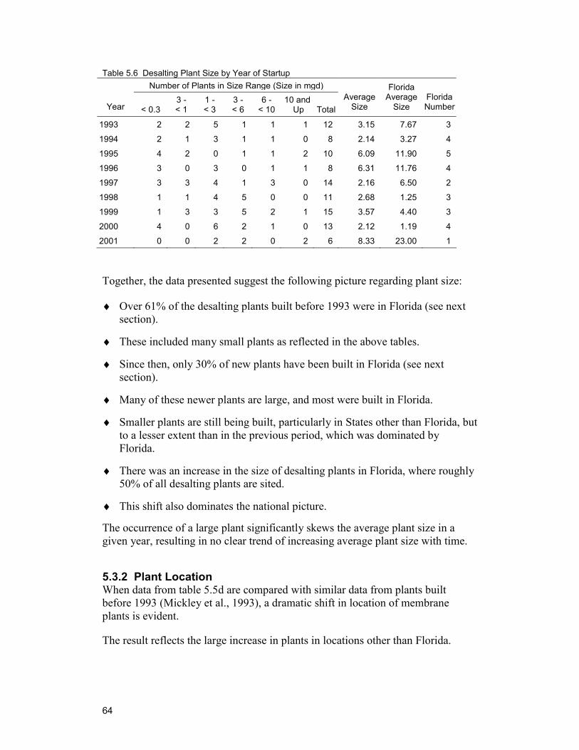
64

Table 5.6 Desalting Plant Size by Year of Startup Number of Plants in Size Range (Size in mgd)

Year < 0.3 3 - < 1

1 - < 3

3 - < 6

6 - < 10

10 and Up Total

Average Size

Florida Average

Size Florida Number

1993 2 2 5 1 1 1 12 3.15 7.67 3

1994 2 1 3 1 1 0 8 2.14 3.27 4

1995 4 2 0 1 1 2 10 6.09 11.90 5

1996 3 0 3 0 1 1 8 6.31 11.76 4

1997 3 3 4 1 3 0 14 2.16 6.50 2

1998 1 1 4 5 0 0 11 2.68 1.25 3

1999 1 3 3 5 2 1 15 3.57 4.40 3

2000 4 0 6 2 1 0 13 2.12 1.19 4

2001 0 0 2 2 0 2 6 8.33 23.00 1

Together, the data presented suggest the following picture regarding plant size:

♦ Over 61% of the desalting plants built before 1993 were in Florida (see next section).

♦ These included many small plants as reflected in the above tables.

♦ Since then, only 30% of new plants have been built in Florida (see next section).

♦ Many of these newer plants are large, and most were built in Florida.

♦ Smaller plants are still being built, particularly in States other than Florida, but to a lesser extent than in the previous period, which was dominated by Florida.

♦ There was an increase in the size of desalting plants in Florida, where roughly 50% of all desalting plants are sited.

♦ This shift also dominates the national picture.

The occurrence of a large plant significantly skews the average plant size in a given year, resulting in no clear trend of increasing average plant size with time.

5.3.2 Plant Location When data from table 5.5d are compared with similar data from plants built before 1993 (Mickley et al., 1993), a dramatic shift in location of membrane plants is evident.

The result reflects the large increase in plants in locations other than Florida.

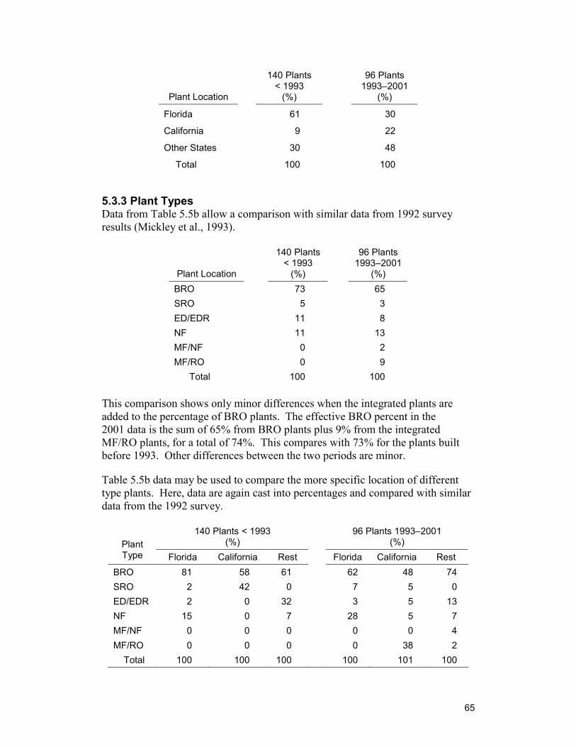
65

Plant Location

140 Plants < 1993

(%)

96 Plants 1993–2001

(%)

Florida 61 30

California 9 22

Other States 30 48

Total 100 100

5.3.3 Plant Types Data from Table 5.5b allow a comparison with similar data from 1992 survey results (Mickley et al., 1993).

Plant Location

140 Plants < 1993

(%)

96 Plants 1993–2001

(%) BRO 73 65 SRO 5 3 ED/EDR 11 8 NF 11 13 MF/NF 0 2 MF/RO 0 9 Total 100 100

This comparison shows only minor differences when the integrated plants are added to the percentage of BRO plants. The effective BRO percent in the 2001 data is the sum of 65% from BRO plants plus 9% from the integrated MF/RO plants, for a total of 74%. This compares with 73% for the plants built before 1993. Other differences between the two periods are minor.

Table 5.5b data may be used to compare the more specific location of different type plants. Here, data are again cast into percentages and compared with similar data from the 1992 survey.

140 Plants < 1993 (%)

96 Plants 1993–2001 (%) Plant

Type Florida California Rest Florida California Rest BRO 81 58 61 62 48 74 SRO 2 42 0 7 5 0 ED/EDR 2 0 32 3 5 13 NF 15 0 7 28 5 7 MF/NF 0 0 0 0 0 4 MF/RO 0 0 0 0 38 2 Total 100 100 100 100 101 100

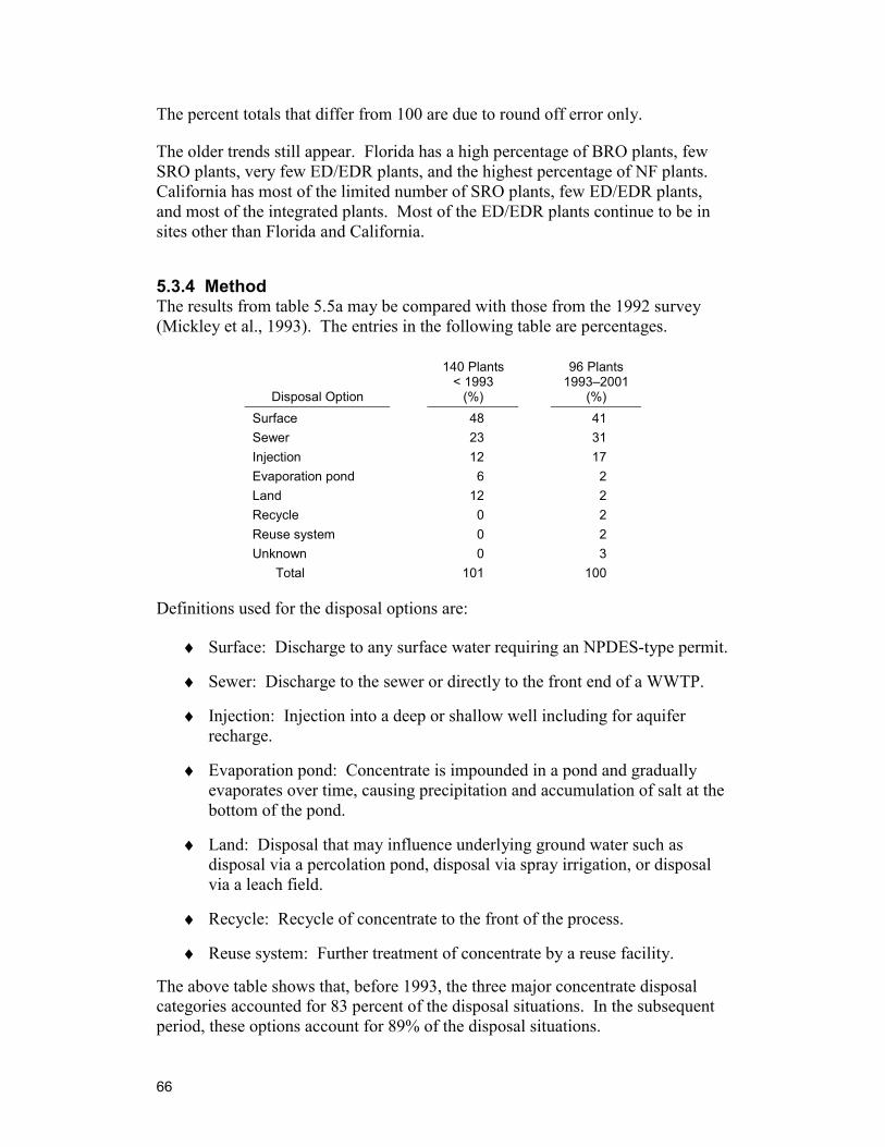
66

The percent totals that differ from 100 are due to round off error only.

The older trends still appear. Florida has a high percentage of BRO plants, few SRO plants, very few ED/EDR plants, and the highest percentage of NF plants. California has most of the limited number of SRO plants, few ED/EDR plants, and most of the integrated plants. Most of the ED/EDR plants continue to be in sites other than Florida and California.

5.3.4 Method The results from table 5.5a may be compared with those from the 1992 survey (Mickley et al., 1993). The entries in the following table are percentages.

Disposal Option

140 Plants < 1993

(%)

96 Plants 1993–2001

(%) Surface 48 41 Sewer 23 31 Injection 12 17 Evaporation pond 6 2 Land 12 2 Recycle 0 2 Reuse system 0 2 Unknown 0 3 Total 101 100

Definitions used for the disposal options are:

♦ Surface: Discharge to any surface water requiring an NPDES-type permit.

♦ Sewer: Discharge to the sewer or directly to the front end of a WWTP.

♦ Injection: Injection into a deep or shallow well including for aquifer recharge.

♦ Evaporation pond: Concentrate is impounded in a pond and gradually evaporates over time, causing precipitation and accumulation of salt at the bottom of the pond.

♦ Land: Disposal that may influence underlying ground water such as disposal via a percolation pond, disposal via spray irrigation, or disposal via a leach field.

♦ Recycle: Recycle of concentrate to the front of the process.

♦ Reuse system: Further treatment of concentrate by a reuse facility.

The above table shows that, before 1993, the three major concentrate disposal categories accounted for 83 percent of the disposal situations. In the subsequent period, these options account for 89% of the disposal situations.

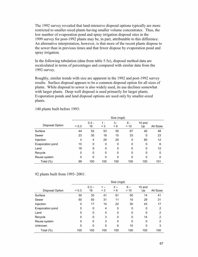
67

The 1992 survey revealed that land-intensive disposal options typically are more restricted to smaller-sized plants having smaller volume concentrates. Thus, the low number of evaporation pond and spray irrigation disposal sites in the 1999 survey for post-1992 plants may be, in part, attributable to this difference. An alternative interpretation, however, is that more of the recent plants dispose to the sewer than in previous times and that fewer dispose by evaporation pond and spray irrigation.

In the following tabulation (data from table 5.5e), disposal method data are recalculated in terms of percentages and compared with similar data from the 1992 survey.

Roughly, similar trends with size are apparent in the 1992 and post-1992 survey results. Surface disposal appears to be a common disposal option for all sizes of plants. While disposal to sewer is also widely used, its use declines somewhat with larger plants. Deep well disposal is used primarily for larger plants. Evaporation ponds and land disposal options are used only by smaller-sized plants.

140 plants built before 1993:

Size (mgd)

Disposal Option < 0.3 0.3 - 16

1 - < 3

3 - < 6

6 - < 10

10 and Up All Sizes

Surface 44 52 53 55 67 40 48 Sewer 23 35 18 15 33 0 23 Injection 4 4 29 25 0 60 12 Evaporation pond 10 0 0 0 0 0 6 Land 18 9 0 5 0 0 12 Recycle 0 0 0 0 0 0 0 Reuse system 0 0 0 0 0 0 0 Total (%) 99 100 100 100 100 100 101

92 plants built from 1993–2001:

Size (mgd)

Disposal Option < 0.3 0.3 –

16 1 – < 3

3 – < 6

6 – < 10

10 and Up All Sizes

Surface 30 33 41 61 50 14 41 Sewer 50 50 31 11 10 29 31 Injection 0 17 14 22 30 43 17 Evaporation pond 5 0 4 0 0 0 2 Land 5 0 4 0 0 0 2 Recycle 0 0 3 0 0 14 2 Reuse system 5 0 3 0 0 0 2 Unknown 5 0 0 6 10 0 3 Total (%) 100 100 100 100 100 100 100

68

5.3.5 Treatment of Concentrate Before Disposal The following sections of information are taken from the surveys conducted in 1999 and 2002. They include a few plants built before 1993. Thus, the data are primarily for plants built since 1992.

5.3.5.1 BRO Plants Information in this area was provided by 78 of 93 plants.

♦ Surface water disposal: • Of the 78 plants, 46 dispose concentrate to surface waters. The different

treatments include:

33 None 8 Aeration 3 Degasification 1 with ph adjustment 2 Disinfection 1 with ph adjustment

♦ Sewer disposal: • Of the 78 plants, 23 dispose concentrate to the sewer with no treatment:

23 None ♦ Injection disposal:

• Of the 78 plants, 6 dispose concentrate by injection. The different treatments include:

3 None 2 Disinfection 1 Aeration

♦ Evaporation pond disposal: • Of the 78 plants, 3 dispose concentrate to evaporation ponds with no

treatment:

3 None

5.3.5.2 Summary of BRO Plant Concentrate Treatment Information in this area was provided by 78 of 93 plants. The types of treatment along with the number of plants having these treatments are:

62 None 9 Aeration 3 Degasification 1 with ph adjustment 4 Disinfection 1 with ph adjustment

5.3.5.3 NF Plants Information in this area was provided by 16 of 20 plants.

♦ Surface water disposal:

69

• Of the 16 plants, 2 dispose concentrate to surface waters. The different treatments include:

1 None 1 Air stripping plus chlorine

♦ Sewer disposal: • Of the 16 plants, 6 dispose concentrate to the sewer. The different

treatments include:

4 None 1 pH adjustment 1 Defoaming agent added

♦ Injection disposal: • Of the 16 plants, 7 dispose concentrate by injection. The different

treatments include:

6 None 1 Disinfection

♦ Reuse system disposal: • Of the 16 plants, 1 disposes concentrate to a reuse system. The different

treatments include:

1 pH adjustment

5.3.5.4 Summary of NF Plant Concentrate Treatment Information in this area was provided by 16 of 20 plants. The types of treatment along with the number of plants having these treatments are:

11 None 2 pH adjustment 1 Disinfection 1 Air stripping plus chlorine 1 Defoaming agent added

5.3.5.5 EDR Plants Information in this area was provided by 13 of 16 plants.

♦ Surface water disposal: • Of the 13 plants, 7 dispose concentrate to surface waters. The different

treatments include:

4 None 3 pH adjustment

♦ Sewer disposal: • Of the 13 plants, 4 dispose concentrate to the sewer. The different

treatments include:

70

3 None 1 pH adjustment

♦ Evaporation pond disposal: • Of the 13 plants, 1 disposes concentrate to evaporation ponds with no

treatment:

1 None ♦ Land disposal:

• Of the 13 plants, 1 disposed concentrate to the land with no treatment: 1 None

5.3.5.6 Summary of EDR Plant Concentrate Treatment Information in this area was provided by 13 of 16 plants. The types of treatment along with the number of plants having these treatments are:

9 None 4 pH adjustment

5.3.5.7 Integrated Plants (Both MF/NF and MF/RO) Information in this area was provided by 7 of 12 plants.

♦ Surface water disposal: • Of the seven plants, four dispose concentrate to surface waters with no

treatment:

4 None ♦ Sewer disposal:

• Of the seven plants, two dispose concentrate to the sewer with no treatment:

2 None ♦ Recycle:

• Of the seven plants, one recycled concentrate to the front of the process with no treatment:

1 None

5.3.5.8 Summary of Integrated Plant Concentrate Treatment Information in this area was provided by 7 of 12 plants. None of these concentrates has any treatment:

7 None

71

5.3.5.9 Summary of Concentrate Treatment for All Desalting Plants Information in this area was provided by 112 of 141 plants. The types of treatment along with the number of plants having these treatments are:

87 None 9 Aeration 6 pH adjustment 5 Disinfection With ph adjustment 3 Degasification 1 with ph adjustment 1 Air stripping With chlorine addition 1 Defoaming agent

added It is possible and probable that the question of concentrate treatment, where answers were provided, was not completely answered in every case. (The number of cases of pH adjustment is suspiciously low.)

5.3.6 Disposal of Cleaning Waste In this section, survey information from all plants responding to cleaning waste questions is included.

5.3.6.1 BRO plants Information in this area was provided by 74 of 93 plants.

♦ Surface disposal of concentrate (Note: Not cleaning waste): • Of these plants, 44 responded with cleaning waste information. The

different means of disposing of cleaning waste from these plants include:

28 Sewer 8 of these with ph adjustment 14 Surface water 7 with ph adjustment and 1 of

these with settling 2 Land – lagoons

♦ Sewer disposal of concentrate: • Of these plants, 20 responded with cleaning waste information. The

different means of disposing of cleaning waste from these plants include:

20 Sewer 3 of these with ph adjustment ♦ Injection disposal of concentrate:

• Of these plants, seven responded with cleaning waste information. The different means of disposing of cleaning waste from these plants include:

2 Sewer 1 of these with pH adjustment) 2 Surface water 3 Injection

72

♦ Evaporation pond disposal of concentrate: • Of these plants, two responded with cleaning waste information. The

different means of disposing of cleaning waste from these plants include:

2 Evaporation pond ♦ Land (percolation pond) disposal of concentrate:

• Of these plants, one responded with cleaning waste information. The way of disposing of cleaning waste from this plant was:

1 Hauled off by independent contractor

5.3.6.2 Summary of BRO Cleaning Waste Disposal Information in this area was provided by 74 of 93 plants. The disposal methods along with the number of plants using this disposal method are:

50 Sewer 12 with pH adjustment 16 Surface 7 with ph adjustment; 1 of

these with settling 3 Injection 2 Land Lagoons 1 Evaporation pond 1 Hauling With chlorine addition

5.3.6.3 NF Plants Information in this area was provided by 13 of 20 plants.

♦ Sewer disposal of concentrate: • Of these plants, seven responded with cleaning waste information. The

different means of disposing of cleaning waste from these plants include:

7 Sewer 1 with pH adjustment ♦ Injection disposal of concentrate:

• Of these plants, four responded with cleaning waste information. The different means of disposing of cleaning waste from these plants include:

1 Sewer 12 with pH adjustment 3 Injection 1 with pH adjustment

♦ Land (irrigation) disposal of concentrate: • Of these plants, one responded with cleaning waste information. The

means of disposing of cleaning waste from this plant was:

1 Land – irrigation After pH adjustment ♦ Reuse system disposal of concentrate:

• Of these plants, one responded with cleaning waste information. The method of disposing of cleaning waste from this plant was:

1 Sewer

73

5.3.6.4 Summary of NF Cleaning Waste Disposal Information in this area was provided by 13 of 20 plants. The disposal methods along with the number of plants using this disposal method are:

9 Sewer 1 with pH adjustment 3 Injection 1 with pH adjustment 1 Land Irrigation after pH adjustment

5.3.6.5 EDR plants Information in this area was provided by 15 of 16 plants.

♦ Surface disposal of concentrate: • Of these plants, nine responded with cleaning waste information. The

different means of disposing of cleaning waste from these plants include:

4 Surface 2 with pH adjustment 1 Sewer With pH adjustment 4 Land – lagoons 1 with pH adjustment

♦ Sewer disposal of concentrate: • Of these plants, four responded with cleaning waste information. The way

of disposing of cleaning waste from these plants was:

4 Sewer 2 with pH adjustment ♦ Injection disposal of concentrate:

• Of these plants, one responded with cleaning waste information. The way of disposing of cleaning waste from this plant was:

1 Injection ♦ Land (irrigation) disposal of concentrate:

• Of these plants, one responded with cleaning waste information. The way of disposing of cleaning waste from this plant was:

1 Sewer

5.3.6.6 Summary of EDR Cleaning Waste Disposal Information in this area was provided by 15 of 16 plants. The disposal methods along with the number of plants using this disposal method are:

6 Sewer 4 with pH adjustments 4 Land – lagoons 1 with pH adjustment 4 Surface 2 with pH adjustments 1 Injection

74

5.3.6.7 Integrated Plants (MF/NF and MF/RO) Information in this area was provided by 8 of 12 plants.

♦ Surface disposal of concentrate: • Of these plants, four responded with cleaning waste information. The way

of disposing of cleaning waste from these plants was:

4 Surface 2 to dry tributaries ♦ Sewer disposal of concentrate:

• Of these plants, two responded with cleaning waste information. The different means of disposing of cleaning waste from these plants include:

1 Sewer 1 Land – lagoons

♦ Recycle disposal of concentrate: • Of these plants, two responded with cleaning waste information. The

different means of disposing of cleaning waste from these plants include:

1 Sewer 1 Recycle After pH adjustment

5.3.6.8 Summary of Integrated Plant Cleaning Waste Disposal Information in this area was provided by 8 of 12 plants. The disposal methods along with the number of plants using this disposal method are:

4 Surface 2 to dry tributaries 1 Sewer 1 Land Lagoon 1 Recycle After pH adjustment

5.3.6.9 Summary of Desalting Plants Cleaning Waste Disposal In summary, 110 of the 141 plants provided information in this area. The number of plants disposing cleaning wastes by the different means is:

67 Sewer disposal 14 with pH adjustment 24 Surface water

disposal 9 with pH adjustment; 1 of these with settling; 2 to dry tributaries

8 Land disposal 7 lagoons (1 with pH adjustment) 1 spray irrigation

7 Injection 1 with pH adjustment 2 Evaporation pond

disposal

1 Recycle After pH adjustment 1 Hauling

75

5.4 Results From the Surveys – Low-Pressure Plants

At the time of the 1992 survey (Mickley et al., 1993) there was only one MF plant, and there were no UF plants operating in WTPs and WWTPs. At the end of 2002, there were 33 UF plants and 155 MF plants.

5.4.1 Number of Plants Aided by records of the low-pressure membrane system suppliers (Aquasource, Koch, Memcor, Pall, and Zenon), we have identified the number of municipal low-pressure membrane systems 25,000 gpd and greater that have began operation in the 50 States. This does not include pilot or demonstration units. The number of MF and UF plants in the drinking water (DW) facilities and waste water (WW) facilities was determined to be:

Total DW WW MF Plants Through 2002 155 142 13 UF Plants Through 2002 33 27 6 Total 188 169 19 Note: There are 11 MF/RO WW plants for a total of 30 WW plants

Relative to the total of 188 low-pressure plants, the percentages for the different low-pressure plant categories are:

MF plants 82% UF plants 18% DW plants 90% WW plants 10%

The following tabulation lists the number of MF plants by year of beginning operation. Columns three and four list the number of drinking water plants and waste water plants respectively. Columns five and six give the number of plants that are Memcor and Pall systems, respectively. The final column gives the average size of the plants for that year in mgd.

Several patterns are noticeable from the tabulation:

♦ The number of MF plants built per year has increased dramatically from the initial MF plant in 1991.

♦ The average size of these plants has similarly increased with time.

♦ Before 1999, Memcor supplied all MF plants.

♦ Pall has rapidly become a major system supplier since 1999. Not evident from this tabulation is the fact that both suppliers have supplied or are supplying systems of 20 mgd and larger.

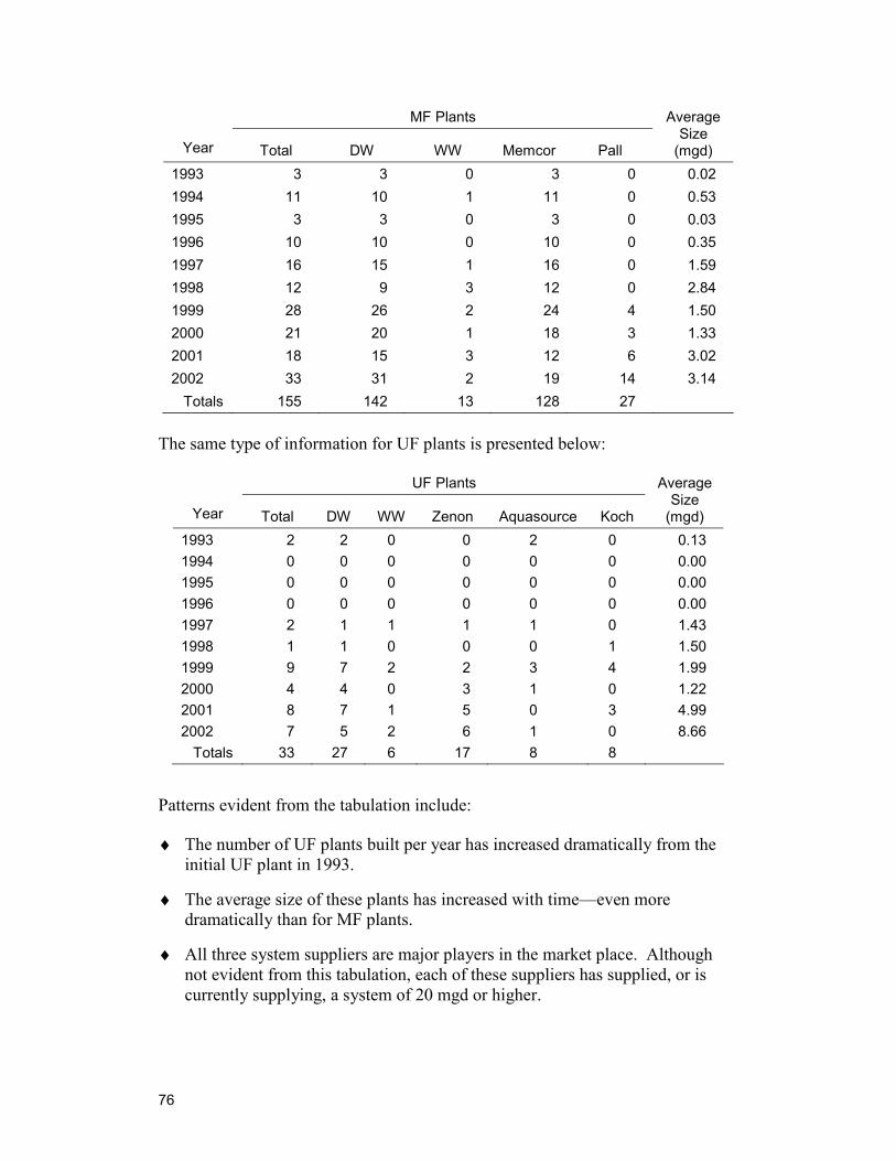
76

MF Plants

Year Total DW WW Memcor Pall

Average Size

(mgd) 1993 3 3 0 3 0 0.02 1994 11 10 1 11 0 0.53 1995 3 3 0 3 0 0.03 1996 10 10 0 10 0 0.35 1997 16 15 1 16 0 1.59 1998 12 9 3 12 0 2.84 1999 28 26 2 24 4 1.50 2000 21 20 1 18 3 1.33 2001 18 15 3 12 6 3.02 2002 33 31 2 19 14 3.14 Totals 155 142 13 128 27

The same type of information for UF plants is presented below:

UF Plants

Year Total DW WW Zenon Aquasource Koch

Average Size

(mgd) 1993 2 2 0 0 2 0 0.13 1994 0 0 0 0 0 0 0.00 1995 0 0 0 0 0 0 0.00 1996 0 0 0 0 0 0 0.00 1997 2 1 1 1 1 0 1.43 1998 1 1 0 0 0 1 1.50 1999 9 7 2 2 3 4 1.99 2000 4 4 0 3 1 0 1.22 2001 8 7 1 5 0 3 4.99 2002 7 5 2 6 1 0 8.66 Totals 33 27 6 17 8 8

Patterns evident from the tabulation include:

♦ The number of UF plants built per year has increased dramatically from the initial UF plant in 1993.

♦ The average size of these plants has increased with time—even more dramatically than for MF plants.

♦ All three system suppliers are major players in the market place. Although not evident from this tabulation, each of these suppliers has supplied, or is currently supplying, a system of 20 mgd or higher.

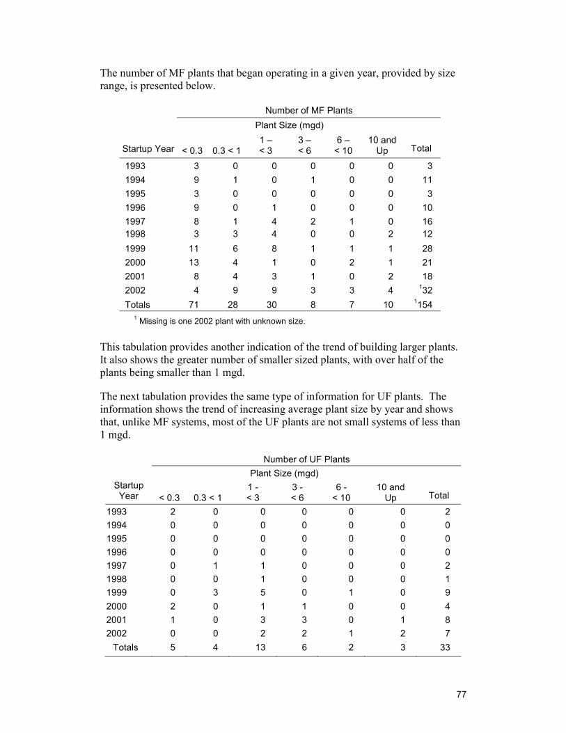
77

The number of MF plants that began operating in a given year, provided by size range, is presented below.

Number of MF Plants Plant Size (mgd)

Startup Year < 0.3 0.3 < 1 1 – < 3

3 – < 6

6 – < 10

10 andUp Total

1993 3 0 0 0 0 0 3 1994 9 1 0 1 0 0 11 1995 3 0 0 0 0 0 3 1996 9 0 1 0 0 0 10 1997 8 1 4 2 1 0 16 1998 3 3 4 0 0 2 12 1999 11 6 8 1 1 1 28 2000 13 4 1 0 2 1 21 2001 8 4 3 1 0 2 18 2002 4 9 9 3 3 4 132 Totals 71 28 30 8 7 10 1154

1 Missing is one 2002 plant with unknown size.

This tabulation provides another indication of the trend of building larger plants. It also shows the greater number of smaller sized plants, with over half of the plants being smaller than 1 mgd.

The next tabulation provides the same type of information for UF plants. The information shows the trend of increasing average plant size by year and shows that, unlike MF systems, most of the UF plants are not small systems of less than 1 mgd.

Number of UF Plants Plant Size (mgd)

Startup Year < 0.3 0.3 < 1

1 - < 3

3 - < 6

6 - < 10

10 and Up Total

1993 2 0 0 0 0 0 2 1994 0 0 0 0 0 0 0 1995 0 0 0 0 0 0 0 1996 0 0 0 0 0 0 0 1997 0 1 1 0 0 0 2 1998 0 0 1 0 0 0 1 1999 0 3 5 0 1 0 9 2000 2 0 1 1 0 0 4 2001 1 0 3 3 0 1 8 2002 0 0 2 2 1 2 7 Totals 5 4 13 6 2 3 33

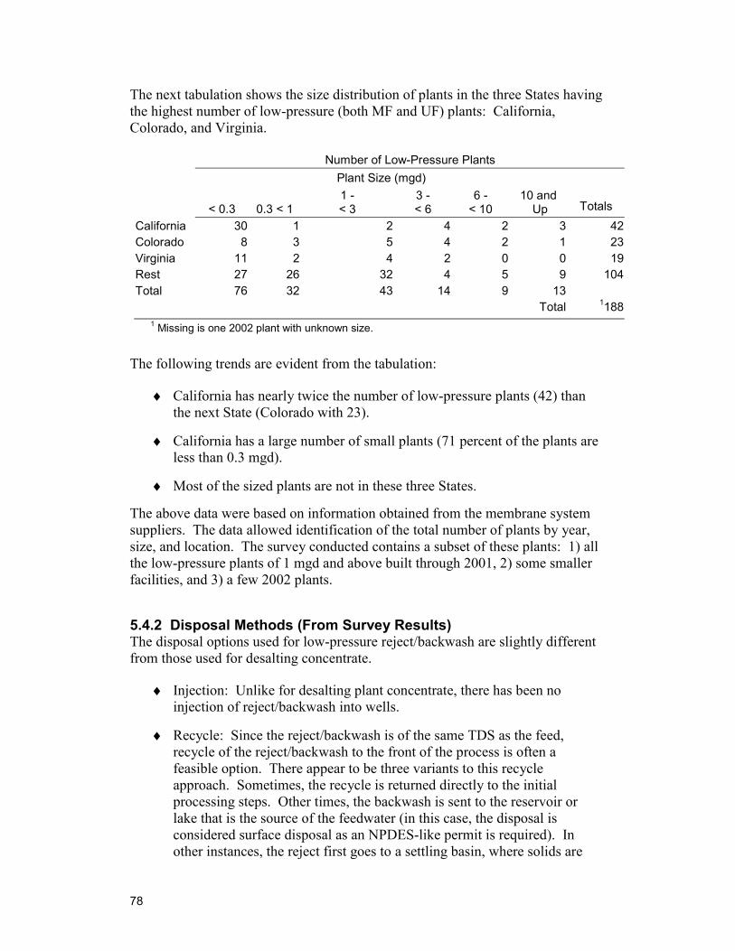
78

The next tabulation shows the size distribution of plants in the three States having the highest number of low-pressure (both MF and UF) plants: California, Colorado, and Virginia.

Number of Low-Pressure Plants Plant Size (mgd)

< 0.3 0.3 < 1 1 - < 3

3 - < 6

6 - < 10

10 and Up Totals

California 30 1 2 4 2 3 42Colorado 8 3 5 4 2 1 23Virginia 11 2 4 2 0 0 19Rest 27 26 32 4 5 9 104Total 76 32 43 14 9 13 Total 1188

1 Missing is one 2002 plant with unknown size.

The following trends are evident from the tabulation:

♦ California has nearly twice the number of low-pressure plants (42) than the next State (Colorado with 23).

♦ California has a large number of small plants (71 percent of the plants are less than 0.3 mgd).

♦ Most of the sized plants are not in these three States.

The above data were based on information obtained from the membrane system suppliers. The data allowed identification of the total number of plants by year, size, and location. The survey conducted contains a subset of these plants: 1) all the low-pressure plants of 1 mgd and above built through 2001, 2) some smaller facilities, and 3) a few 2002 plants.

5.4.2 Disposal Methods (From Survey Results) The disposal options used for low-pressure reject/backwash are slightly different from those used for desalting concentrate.

♦ Injection: Unlike for desalting plant concentrate, there has been no injection of reject/backwash into wells.

♦ Recycle: Since the reject/backwash is of the same TDS as the feed, recycle of the reject/backwash to the front of the process is often a feasible option. There appear to be three variants to this recycle approach. Sometimes, the recycle is returned directly to the initial processing steps. Other times, the backwash is sent to the reservoir or lake that is the source of the feedwater (in this case, the disposal is considered surface disposal as an NPDES-like permit is required). In other instances, the reject first goes to a settling basin, where solids are

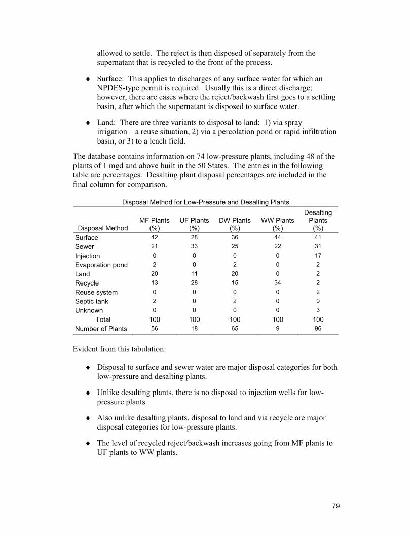
79

allowed to settle. The reject is then disposed of separately from the supernatant that is recycled to the front of the process.

♦ Surface: This applies to discharges of any surface water for which an NPDES-type permit is required. Usually this is a direct discharge; however, there are cases where the reject/backwash first goes to a settling basin, after which the supernatant is disposed to surface water.

♦ Land: There are three variants to disposal to land: 1) via spray irrigation—a reuse situation, 2) via a percolation pond or rapid infiltration basin, or 3) to a leach field.

The database contains information on 74 low-pressure plants, including 48 of the plants of 1 mgd and above built in the 50 States. The entries in the following table are percentages. Desalting plant disposal percentages are included in the final column for comparison.

Disposal Method for Low-Pressure and Desalting Plants

Disposal Method MF Plants

(%) UF Plants

(%) DW Plants

(%) WW Plants

(%)

Desalting Plants

(%) Surface 42 28 36 44 41 Sewer 21 33 25 22 31 Injection 0 0 0 0 17 Evaporation pond 2 0 2 0 2 Land 20 11 20 0 2 Recycle 13 28 15 34 2 Reuse system 0 0 0 0 2 Septic tank 2 0 2 0 0 Unknown 0 0 0 0 3 Total 100 100 100 100 100 Number of Plants 56 18 65 9 96

Evident from this tabulation:

♦ Disposal to surface and sewer water are major disposal categories for both low-pressure and desalting plants.

♦ Unlike desalting plants, there is no disposal to injection wells for low-pressure plants.

♦ Also unlike desalting plants, disposal to land and via recycle are major disposal categories for low-pressure plants.

♦ The level of recycled reject/backwash increases going from MF plants to UF plants to WW plants.

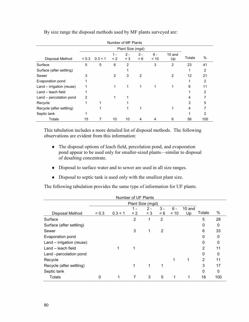
80

By size range the disposal methods used by MF plants surveyed are:

Number of MF Plants Plant Size (mgd)

Disposal Method < 0.3 0.3 < 1 1 - < 2

2 - < 3

3 - < 6

6 - < 10

10 and Up Totals %

Surface 5 5 6 2 3 2 23 41 Surface (after settling) 1 1 2 Sewer 3 2 3 2 2 12 21 Evaporation pond 1 1 2 Land – irrigation (reuse) 1 1 1 1 1 1 6 11 Land – leach field 1 1 2 Land – percolation pond 2 1 1 4 7 Recycle 1 1 1 3 5 Recycle (after settling) 1 1 1 1 4 7 Septic tank 1 1 2 Totals 15 7 10 10 4 4 6 56 100

This tabulation includes a more detailed list of disposal methods. The following observations are evident from this information:

♦ The disposal options of leach field, percolation pond, and evaporation pond appear to be used only for smaller-sized plants—similar to disposal of desalting concentrate.

♦ Disposal to surface water and to sewer are used in all size ranges.

♦ Disposal to septic tank is used only with the smallest plant size.

The following tabulation provides the same type of information for UF plants.

Number of UF Plants Plant Size (mgd)

Disposal Method < 0.3 0.3 < 11 - < 2

2 - < 3

3 - < 6

6 - < 10

10 and Up Totals %

Surface 2 1 2 5 28 Surface (after settling) 0 0 Sewer 3 1 2 6 33 Evaporation pond 0 0 Land – irrigation (reuse) 0 0 Land – leach field 1 1 2 11 Land –percolation pond 0 0 Recycle 1 1 2 11 Recycle (after settling) 1 1 1 3 17 Septic tank 0 0 Totals 0 1 7 3 5 1 1 18 100

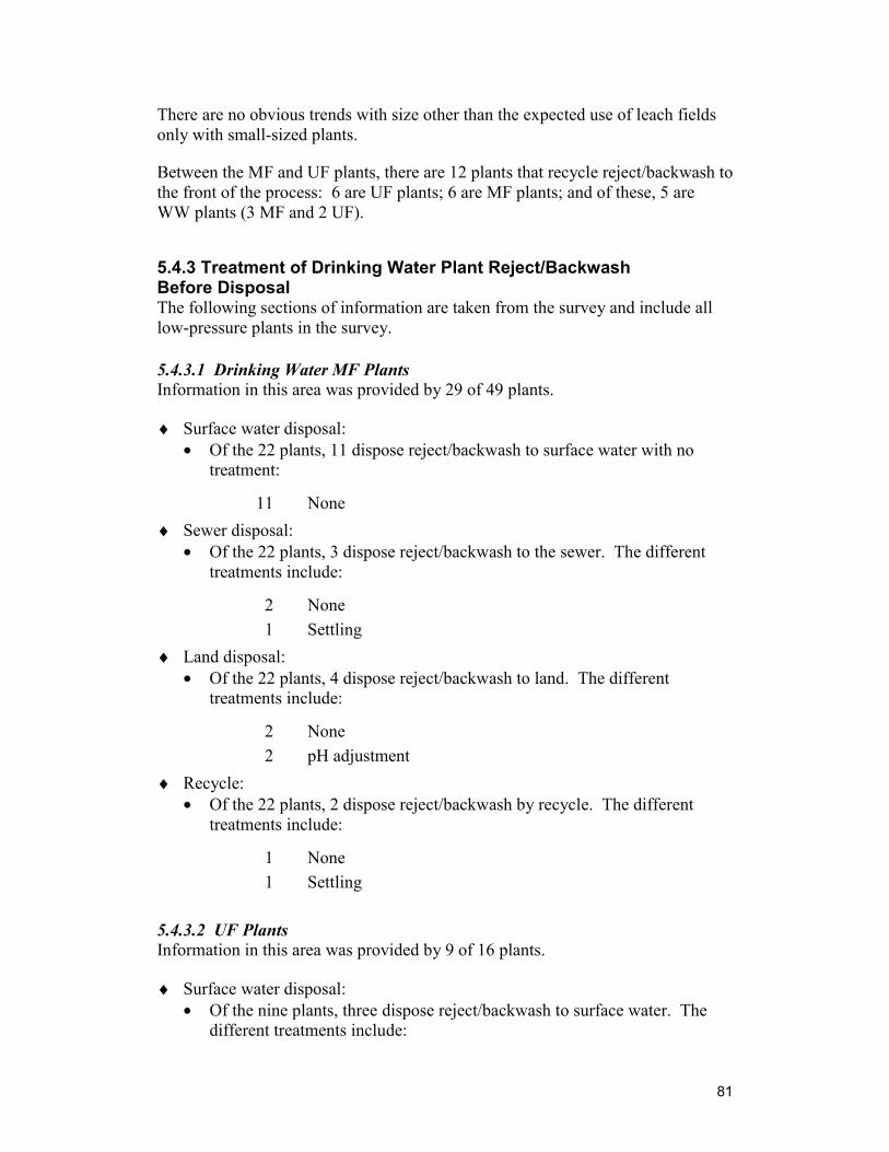
81

There are no obvious trends with size other than the expected use of leach fields only with small-sized plants.

Between the MF and UF plants, there are 12 plants that recycle reject/backwash to the front of the process: 6 are UF plants; 6 are MF plants; and of these, 5 are WW plants (3 MF and 2 UF).

5.4.3 Treatment of Drinking Water Plant Reject/Backwash Before Disposal The following sections of information are taken from the survey and include all low-pressure plants in the survey.

5.4.3.1 Drinking Water MF Plants Information in this area was provided by 29 of 49 plants.

♦ Surface water disposal: • Of the 22 plants, 11 dispose reject/backwash to surface water with no

treatment:

11 None ♦ Sewer disposal:

• Of the 22 plants, 3 dispose reject/backwash to the sewer. The different treatments include:

2 None 1 Settling

♦ Land disposal: • Of the 22 plants, 4 dispose reject/backwash to land. The different

treatments include:

2 None 2 pH adjustment

♦ Recycle: • Of the 22 plants, 2 dispose reject/backwash by recycle. The different

treatments include:

1 None 1 Settling

5.4.3.2 UF Plants Information in this area was provided by 9 of 16 plants.

♦ Surface water disposal: • Of the nine plants, three dispose reject/backwash to surface water. The

different treatments include:

82

1 None 1 pH adjustment 1 Sand/gravel filter

♦ Sewer disposal: • Of the nine plants, two dispose reject/backwash to the sewer. The

treatment in these plants was: 2 None

♦ Recycle: • Of the nine plants, two recycle the reject/backwash. The treatment in

these plants was:

2 None ♦ Land disposal:

• Of thesenine plants, two dispose reject/backwash to land with no treatment:

2 None

5.4.3.3 Summary of Reject/Backwash Treatment for Low-Pressure Drinking WaterPlants Information in this area was provided by 29 of 65 plants. The types of treatment along with the number of plants having these treatments are:

23 None 3 pH adjustment 2 Settling 1 Sand/gravel filter

It is possible and probable that the question of reject/backwash treatment, where answers were provided, was not completely answered in every case.

5.4.4 Disposal of Cleaning Waste from Drinking Water Plants In this section, survey information from all plants responding to cleaning waste questions is included.

5.4.4.1 MF Plants Information in this area was provided by 36 of 49 plants.

♦ Surface disposal of reject/backwash (Note: Not cleaning waste): • Of the 20 plants, 17 responded with cleaning waste information. The

different means of disposing of cleaning waste from these plants include:

83

10 Sewer 1 trucked to WWTP; 5 with pH adjustment

5 Surface water 3 with pH adjustment; 2 to dry tributaries after settling

1 Land – lagoons 1 Septic tank Followed by periodic contract hauling

♦ Sewer disposal of reject/backwash: • Of the 11 plants, 7 responded with cleaning waste information. The way

of disposing of cleaning waste from these plants was:

7 Sewer 5 with pH adjustment ♦ Recycling of reject/backwash:

• Of the five plants, two responded with cleaning waste information. The way of disposing of cleaning waste from these plants was:

2 Sewer 2 after pH adjustment ♦ Land disposal of reject/backwash:

• Of the 11 plants, 8 responded with cleaning waste information. The different means of disposing of cleaning waste from these plants include:

6 Land 3 to irrigation of which 2 have pH adjustment; 3 to percolation ponds after pH adjustment

Septic tank Followed by periodic hauling to Hazwaste landfill

♦ Evaporation pond disposal of reject/backwash: • Of the one plant, one responded with cleaning waste information. The

way of disposing of cleaning waste from this plant was:

1 Evaporation pond After pH adjustment ♦ Septic tank disposal of reject/backwash:

• Of the one plants, one responded with cleaning waste information. The way of disposing of cleaning waste from this plant was:

1 Septic tank

5.4.4.2 UF Plants Information in this area was provided by 11 of 16 plants.

♦ Surface disposal of reject/backwash: • Of the four plants, three responded with cleaning waste information. The

way of disposing of cleaning waste from these plants was:

3 Surface water 3 with pH adjustment; 2 of these to mixed bed filter

84

♦ Sewer disposal of reject/backwash: • Of the six plants, three responded with cleaning waste information. The

way of disposing of cleaning waste from these plants was: 3 Sewer 1 with pH adjustment and

dechlorination ♦ Recycle of reject/backwash:

• Of the four plants, three responded with cleaning waste information. The different means of disposing of cleaning waste from these plants include:

1 Recycle After lagoon and pH adjustment and dechlorination

1 Evaporation pond 1 Sewer

♦ Land disposal of reject/backwash: • Of the two plants, two responded with cleaning waste information. The

way of disposing of cleaning waste from these plants was: 2 Land Leach fields; after pH adjustment and

storage

5.4.4.3 Summary of Low-Pressure Drinking Water Plants Cleaning Waste Disposal In summary, 47 of the 65 plants provided information in this area. The methods of disposal of cleaning wastes include:

24 Sewer disposal 13 with pH adjustment; 1 with dechlorination; 1 waste is trucked to WWTP

8 Surface water disposal

6 with pH adjustment; 2 with mixed bed filters; 2 to dry tributaries

9 Land disposal 2 leach fields after pH adjustment and storage; lagoon 3 irrigation (2 with pH adjustment)

3 percolation ponds (all with pH adjustment)

3 Septic tank disposal

With periodic hauling to landfill; 1 to hazwaste landfill

2 Evaporation pond disposal

1 after pH adjustment

1 Recycle After pH adjustment and dechlorination, from lagoon

85

6. Regulation – Federal Perspective 6.1 Introduction

6.1.1 Membrane Wastes Membrane systems separate feedwater into a cleaner product water and a more concentrated stream that is called concentrate in RO, NF, and EDR systems and backwash in UF and MF systems. In the former systems, TDS and most constituents of the feed stream are concentrated; and in the latter systems, TDS is not concentrated, but larger-sized species and particles are concentrated. The portion of the feedstream which ends up as concentrate or backwash varies considerably among the membrane processes ranging from as much as 70% in some seawater systems to as little as 1% in some MF and UF systems. Table 6.1 summarizes the characteristics of the different concentrates and backwash streams.

Because of these different characteristics, and as seen in the survey results of chapter 4, the disposal options used for the various concentrate and backwash streams also vary with membrane process. Consequently, the regulations that come into play with the different membrane processes vary.

Cleaning wastes, usually much lower in volume and generated only periodically, represent another membrane system waste. Most often, cleaning wastes are either blended into the concentrate or backwash streams or are handled separately through bleeding to the sewer. The present study focuses on the concentrate and backwash streams generated in membrane processes.

6.1.2 General Classification and Regulation of Membrane Concentrate and Backwash In Federal regulations, wastes are either industrial or municipal. The designation “municipal” is restricted to waste water treatment plant effluents that may contain bacteria and other microorganisms. Thus, membrane concentrate and backwash are, by definition, industrial wastes.

For small plants of 50,000 gpd or less, the State of Florida classifies membrane concentrate as “potable water byproduct” instead of industrial waste water. Present proposed legislation will extend this classification to larger plants. In addition, the proposed legislation will create a technical advisory committee to assist in rule development regarding permit applications for concentrate disposal, specific options and requirements for concentrate disposal, requirements for evaluating mixing of effluents in receiving waters, and permitting requirements relating to major ion toxicity in concentrate (Mickley, 2000). This effort recognizes the nature and characteristics of membrane concentrate which stand in contrast to those of most industrial effluents that are characterized primarily by process-added contaminants.

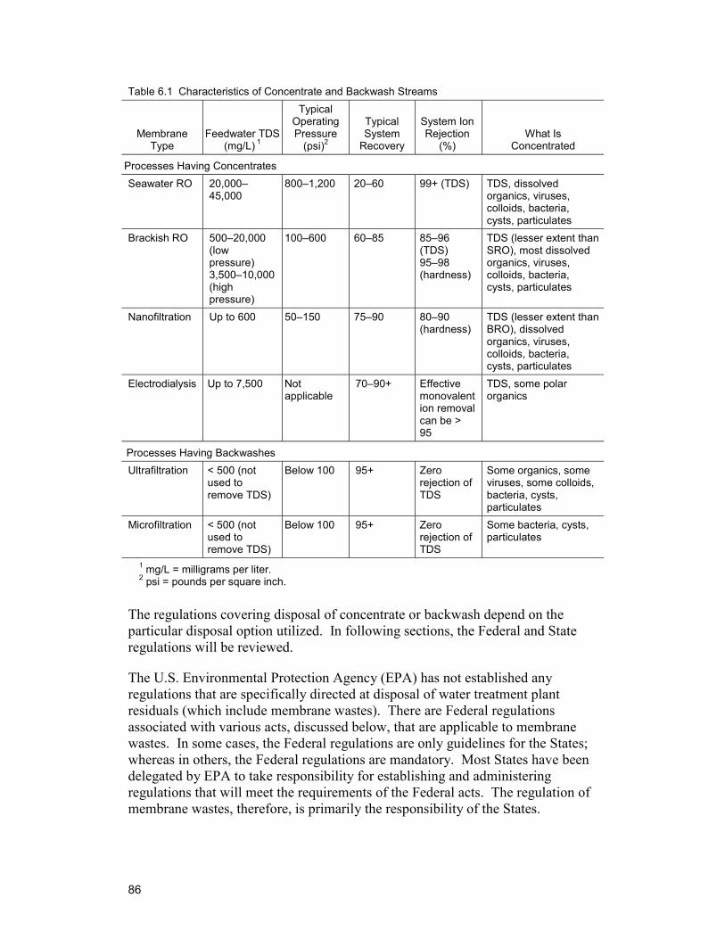
86

Table 6.1 Characteristics of Concentrate and Backwash Streams

Membrane Type

Feedwater TDS (mg/L) 1

Typical Operating Pressure

(psi)2

Typical System

Recovery

System Ion Rejection

(%) What Is

Concentrated

Processes Having Concentrates Seawater RO 20,000–

45,000 800–1,200 20–60 99+ (TDS) TDS, dissolved

organics, viruses, colloids, bacteria, cysts, particulates

Brackish RO 500–20,000 (low pressure) 3,500–10,000 (high pressure)

100–600 60–85 85–96 (TDS) 95–98 (hardness)

TDS (lesser extent than SRO), most dissolved organics, viruses, colloids, bacteria, cysts, particulates

Nanofiltration Up to 600 50–150 75–90 80–90 (hardness)

TDS (lesser extent than BRO), dissolved organics, viruses, colloids, bacteria, cysts, particulates

Electrodialysis Up to 7,500 Not applicable

70–90+ Effective monovalent ion removal can be > 95

TDS, some polar organics

Processes Having Backwashes Ultrafiltration < 500 (not

used to remove TDS)

Below 100 95+ Zero rejection of TDS

Some organics, some viruses, some colloids, bacteria, cysts, particulates

Microfiltration < 500 (not used to remove TDS)

Below 100 95+ Zero rejection of TDS

Some bacteria, cysts, particulates

1 mg/L = milligrams per liter. 2 psi = pounds per square inch.

The regulations covering disposal of concentrate or backwash depend on the particular disposal option utilized. In following sections, the Federal and State regulations will be reviewed.

The U.S. Environmental Protection Agency (EPA) has not established any regulations that are specifically directed at disposal of water treatment plant residuals (which include membrane wastes). There are Federal regulations associated with various acts, discussed below, that are applicable to membrane wastes. In some cases, the Federal regulations are only guidelines for the States; whereas in others, the Federal regulations are mandatory. Most States have been delegated by EPA to take responsibility for establishing and administering regulations that will meet the requirements of the Federal acts. The regulation of membrane wastes, therefore, is primarily the responsibility of the States.

87

The next discussion is of the general framework for Federal regulation, EPA, and Federal acts forming the basis for EPA programs. The discussion then highlights the specific Federal acts that affect the different disposal methods for membrane wastes. Finally, the relation between Federal, State, and local regulation of wastes is presented before discussion of the regulatory issues associated with each of the disposal methods. Both Federal and State regulatory aspects are brought into this discussion.

6.2 Overview

6.2.1 Laws and Regulation Laws and regulations are a major tool in protecting the environment. Congress passes laws that govern the United States. Once an act is passed, the House of Representatives standardizes the text of the law and publishes in the U.S. Code. The U.S. Code is the official record of all Federal laws. Laws often do not include all the necessary details to put those laws into effect or to make the laws work on a day-to-day basis. Congress authorizes certain government agencies to create and enforce regulations. The authorized agency typically decides a regulation may be needed, researches it, proposes it, considers public comment, revises the regulation, and issues a final rule. Twice a year, each agency publishes a comprehensive report that describes all the regulations it is working on or has recently finished. These are published in the Federal Register and the Unified Agenda of Federal Regulatory and Deregulatory Actions. Once a regulation is completed and has been printed in the Federal Register as a final rule, it is “codified” by publication in the Code of Federal Regulations (CFR). The CFR is the official record of all regulations created by the Federal Government. It is divided into 50 volumes, called titles—each of which focuses on a particular area. Almost all environmental regulations appear in Title 40. The CFR is revised yearly. The full text of CFR Title 40, known as the Protection of Environment, is available via the internet in portable document format (pdf). Text is available from a Government Printing Office Web site (www.access.gpo.gov/su_docs/aces/aaces002.html) and a Cornell University site (www4.law.cornell.edu/uscode/ index.html).

6.2.2 Federal Acts Affecting Disposal of Membrane Wastes In 1914, the United States Government issued very basic water quality standards; and in 1925, the U.S. Public Health Service was given the lead role in addressing water quality issues. This situation remained until the formation of the U.S. Environmental Protection Agency in 1970. Since then, the Federal Government, through EPA, sets water quality standards, carries out appropriate studies and research, coordinates the work of other Federal regulatory agencies, and supports the States in enforcing the standards. In a similar fashion, EPA has come to oversee the protection of air, soil, and ground water.

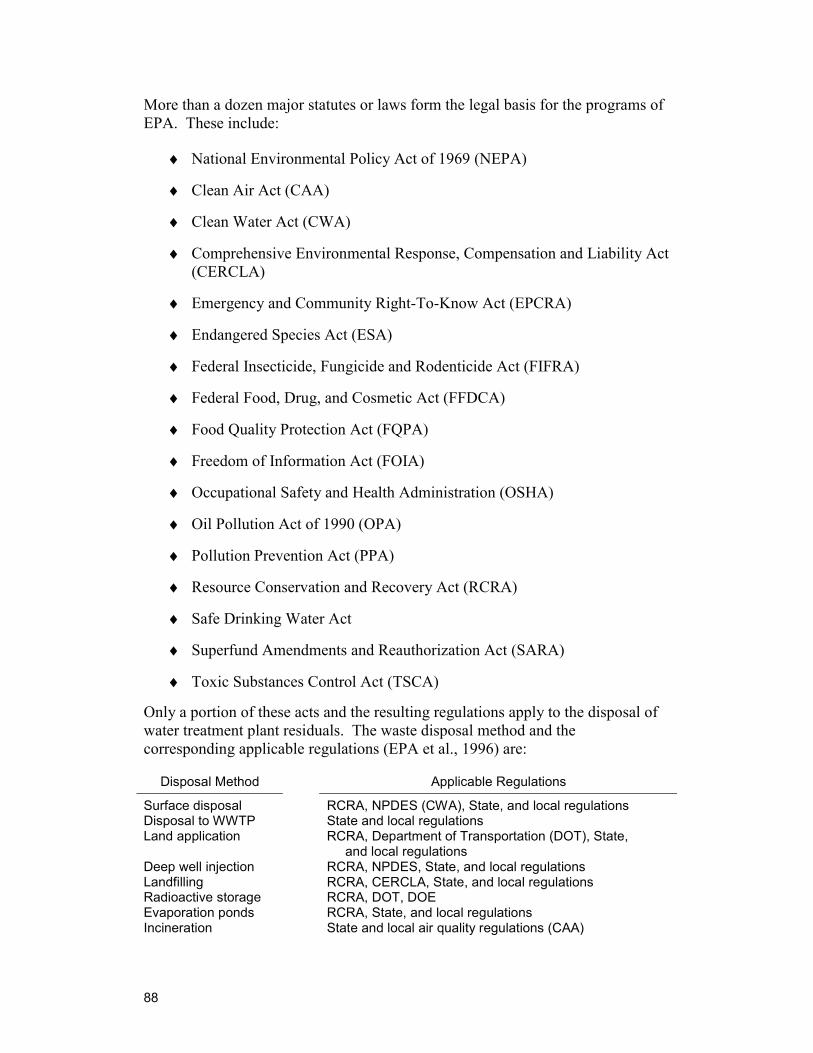
88

More than a dozen major statutes or laws form the legal basis for the programs of EPA. These include:

♦ National Environmental Policy Act of 1969 (NEPA)

♦ Clean Air Act (CAA)

♦ Clean Water Act (CWA)

♦ Comprehensive Environmental Response, Compensation and Liability Act (CERCLA)

♦ Emergency and Community Right-To-Know Act (EPCRA)

♦ Endangered Species Act (ESA)

♦ Federal Insecticide, Fungicide and Rodenticide Act (FIFRA)

♦ Federal Food, Drug, and Cosmetic Act (FFDCA)

♦ Food Quality Protection Act (FQPA)

♦ Freedom of Information Act (FOIA)

♦ Occupational Safety and Health Administration (OSHA)

♦ Oil Pollution Act of 1990 (OPA)

♦ Pollution Prevention Act (PPA)

♦ Resource Conservation and Recovery Act (RCRA)

♦ Safe Drinking Water Act

♦ Superfund Amendments and Reauthorization Act (SARA)

♦ Toxic Substances Control Act (TSCA)

Only a portion of these acts and the resulting regulations apply to the disposal of water treatment plant residuals. The waste disposal method and the corresponding applicable regulations (EPA et al., 1996) are:

Disposal Method Applicable Regulations

Surface disposal Disposal to WWTP Land application Deep well injection Landfilling Radioactive storage Evaporation ponds Incineration

RCRA, NPDES (CWA), State, and local regulations State and local regulations RCRA, Department of Transportation (DOT), State, and local regulations RCRA, NPDES, State, and local regulations RCRA, CERCLA, State, and local regulations RCRA, DOT, DOE RCRA, State, and local regulations State and local air quality regulations (CAA)

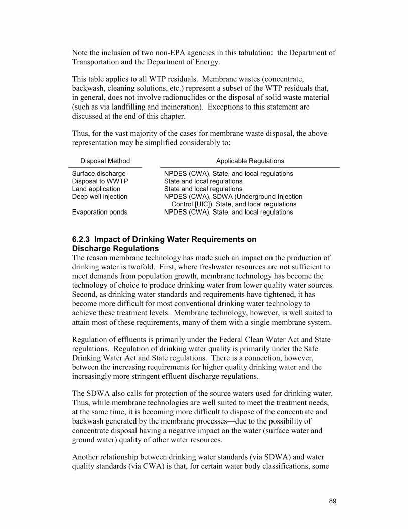
89

Note the inclusion of two non-EPA agencies in this tabulation: the Department of Transportation and the Department of Energy.

This table applies to all WTP residuals. Membrane wastes (concentrate, backwash, cleaning solutions, etc.) represent a subset of the WTP residuals that, in general, does not involve radionuclides or the disposal of solid waste material (such as via landfilling and incineration). Exceptions to this statement are discussed at the end of this chapter.

Thus, for the vast majority of the cases for membrane waste disposal, the above representation may be simplified considerably to:

Disposal Method Applicable Regulations

Surface discharge Disposal to WWTP Land application Deep well injection Evaporation ponds

NPDES (CWA), State, and local regulations State and local regulations State and local regulations NPDES (CWA), SDWA (Underground Injection Control [UIC]), State, and local regulations NPDES (CWA), State, and local regulations

6.2.3 Impact of Drinking Water Requirements on Discharge Regulations The reason membrane technology has made such an impact on the production of drinking water is twofold. First, where freshwater resources are not sufficient to meet demands from population growth, membrane technology has become the technology of choice to produce drinking water from lower quality water sources. Second, as drinking water standards and requirements have tightened, it has become more difficult for most conventional drinking water technology to achieve these treatment levels. Membrane technology, however, is well suited to attain most of these requirements, many of them with a single membrane system.

Regulation of effluents is primarily under the Federal Clean Water Act and State regulations. Regulation of drinking water quality is primarily under the Safe Drinking Water Act and State regulations. There is a connection, however, between the increasing requirements for higher quality drinking water and the increasingly more stringent effluent discharge regulations.

The SDWA also calls for protection of the source waters used for drinking water. Thus, while membrane technologies are well suited to meet the treatment needs, at the same time, it is becoming more difficult to dispose of the concentrate and backwash generated by the membrane processes—due to the possibility of concentrate disposal having a negative impact on the water (surface water and ground water) quality of other water resources.

Another relationship between drinking water standards (via SDWA) and water quality standards (via CWA) is that, for certain water body classifications, some

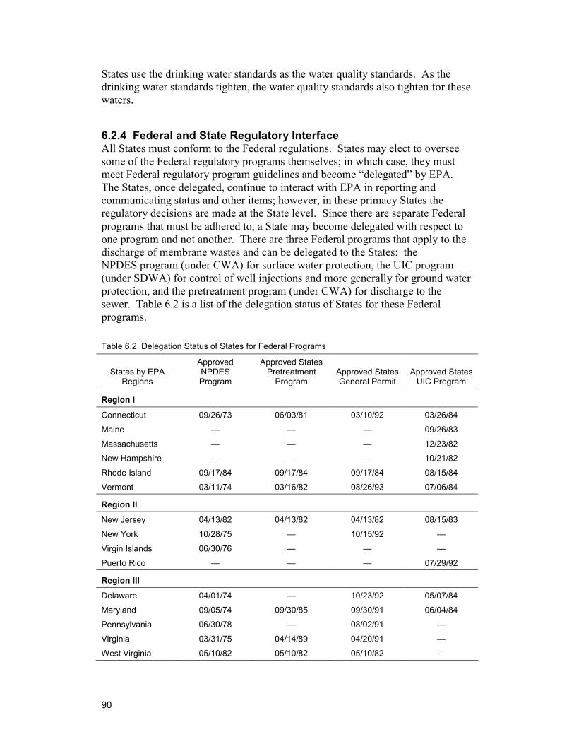
90

States use the drinking water standards as the water quality standards. As the drinking water standards tighten, the water quality standards also tighten for these waters.

6.2.4 Federal and State Regulatory Interface All States must conform to the Federal regulations. States may elect to oversee some of the Federal regulatory programs themselves; in which case, they must meet Federal regulatory program guidelines and become “delegated” by EPA. The States, once delegated, continue to interact with EPA in reporting and communicating status and other items; however, in these primacy States the regulatory decisions are made at the State level. Since there are separate Federal programs that must be adhered to, a State may become delegated with respect to one program and not another. There are three Federal programs that apply to the discharge of membrane wastes and can be delegated to the States: the NPDES program (under CWA) for surface water protection, the UIC program (under SDWA) for control of well injections and more generally for ground water protection, and the pretreatment program (under CWA) for discharge to the sewer. Table 6.2 is a list of the delegation status of States for these Federal programs.

Table 6.2 Delegation Status of States for Federal Programs

States by EPA Regions

Approved NPDES Program

Approved States Pretreatment

Program Approved States General Permit

Approved States UIC Program

Region I

Connecticut 09/26/73 06/03/81 03/10/92 03/26/84

Maine — — — 09/26/83

Massachusetts — — — 12/23/82

New Hampshire — — — 10/21/82

Rhode Island 09/17/84 09/17/84 09/17/84 08/15/84

Vermont 03/11/74 03/16/82 08/26/93 07/06/84

Region II

New Jersey 04/13/82 04/13/82 04/13/82 08/15/83

New York 10/28/75 — 10/15/92 —

Virgin Islands 06/30/76 — — —

Puerto Rico — — — 07/29/92

Region III

Delaware 04/01/74 — 10/23/92 05/07/84

Maryland 09/05/74 09/30/85 09/30/91 06/04/84

Pennsylvania 06/30/78 — 08/02/91 —

Virginia 03/31/75 04/14/89 04/20/91 —

West Virginia 05/10/82 05/10/82 05/10/82 —

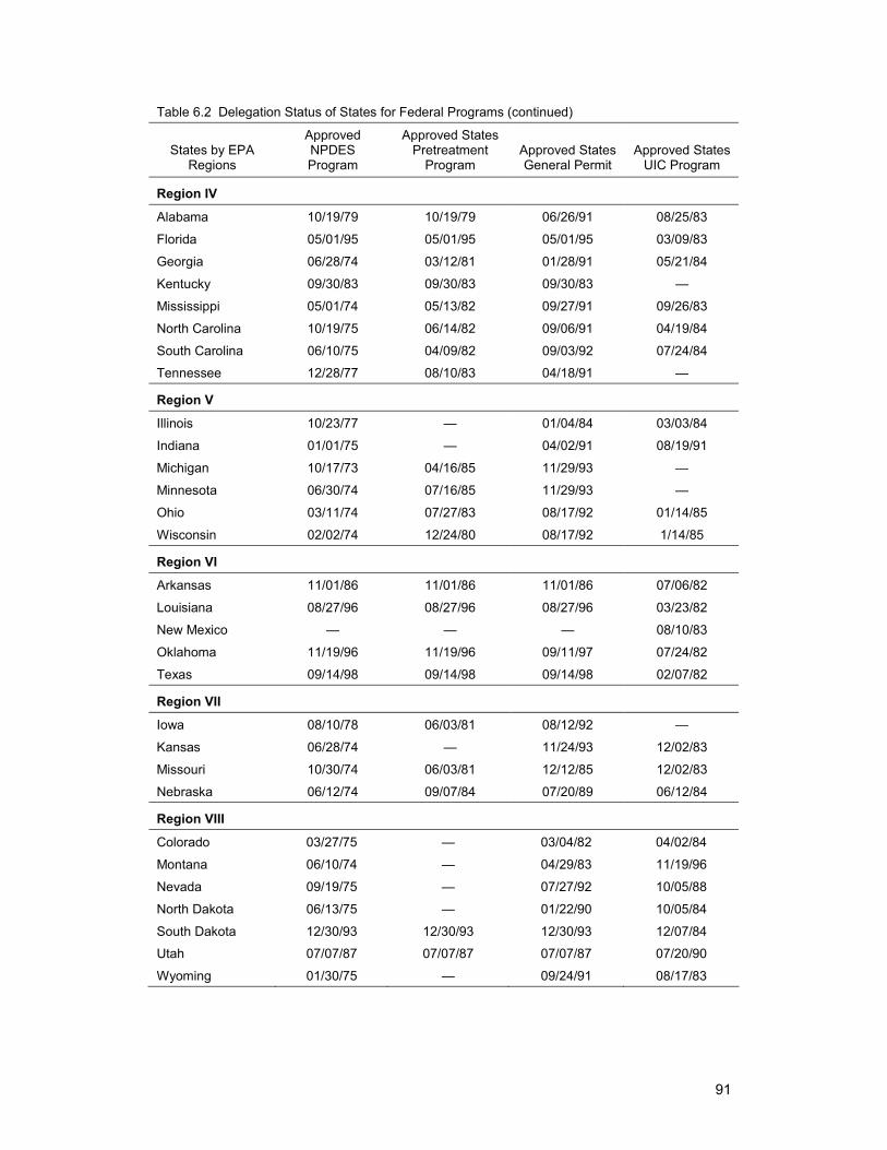
91

Table 6.2 Delegation Status of States for Federal Programs (continued)

States by EPA Regions

Approved NPDES Program

Approved States Pretreatment

Program Approved States General Permit

Approved States UIC Program

Region IV

Alabama 10/19/79 10/19/79 06/26/91 08/25/83

Florida 05/01/95 05/01/95 05/01/95 03/09/83

Georgia 06/28/74 03/12/81 01/28/91 05/21/84

Kentucky 09/30/83 09/30/83 09/30/83 —

Mississippi 05/01/74 05/13/82 09/27/91 09/26/83

North Carolina 10/19/75 06/14/82 09/06/91 04/19/84

South Carolina 06/10/75 04/09/82 09/03/92 07/24/84

Tennessee 12/28/77 08/10/83 04/18/91 —

Region V

Illinois 10/23/77 — 01/04/84 03/03/84

Indiana 01/01/75 — 04/02/91 08/19/91

Michigan 10/17/73 04/16/85 11/29/93 —

Minnesota 06/30/74 07/16/85 11/29/93 —

Ohio 03/11/74 07/27/83 08/17/92 01/14/85

Wisconsin 02/02/74 12/24/80 08/17/92 1/14/85

Region VI

Arkansas 11/01/86 11/01/86 11/01/86 07/06/82

Louisiana 08/27/96 08/27/96 08/27/96 03/23/82

New Mexico — — — 08/10/83

Oklahoma 11/19/96 11/19/96 09/11/97 07/24/82

Texas 09/14/98 09/14/98 09/14/98 02/07/82

Region VII

Iowa 08/10/78 06/03/81 08/12/92 —

Kansas 06/28/74 — 11/24/93 12/02/83

Missouri 10/30/74 06/03/81 12/12/85 12/02/83

Nebraska 06/12/74 09/07/84 07/20/89 06/12/84

Region VIII

Colorado 03/27/75 — 03/04/82 04/02/84

Montana 06/10/74 — 04/29/83 11/19/96

Nevada 09/19/75 — 07/27/92 10/05/88

North Dakota 06/13/75 — 01/22/90 10/05/84

South Dakota 12/30/93 12/30/93 12/30/93 12/07/84

Utah 07/07/87 07/07/87 07/07/87 07/20/90

Wyoming 01/30/75 — 09/24/91 08/17/83

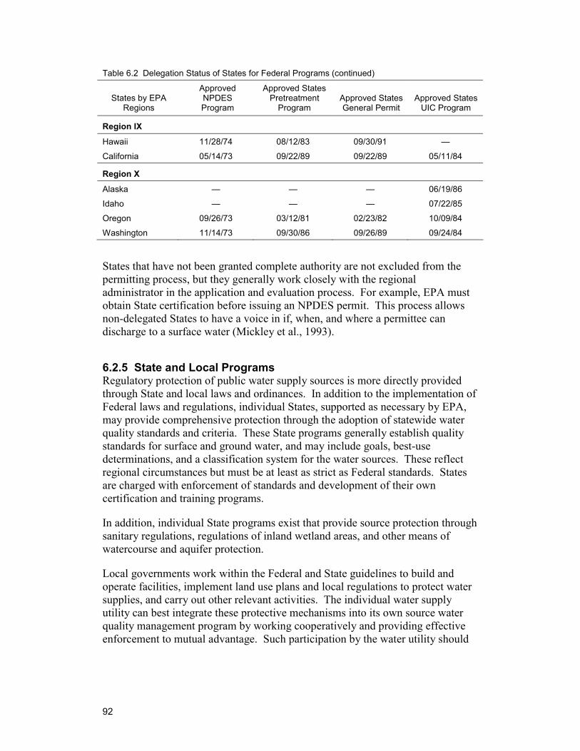
92

Table 6.2 Delegation Status of States for Federal Programs (continued)

States by EPA Regions

Approved NPDES Program

Approved States Pretreatment

Program Approved States General Permit

Approved States UIC Program

Region IX

Hawaii 11/28/74 08/12/83 09/30/91 —

California 05/14/73 09/22/89 09/22/89 05/11/84

Region X

Alaska — — — 06/19/86

Idaho — — — 07/22/85

Oregon 09/26/73 03/12/81 02/23/82 10/09/84

Washington 11/14/73 09/30/86 09/26/89 09/24/84

States that have not been granted complete authority are not excluded from the permitting process, but they generally work closely with the regional administrator in the application and evaluation process. For example, EPA must obtain State certification before issuing an NPDES permit. This process allows non-delegated States to have a voice in if, when, and where a permittee can discharge to a surface water (Mickley et al., 1993).

6.2.5 State and Local Programs Regulatory protection of public water supply sources is more directly provided through State and local laws and ordinances. In addition to the implementation of Federal laws and regulations, individual States, supported as necessary by EPA, may provide comprehensive protection through the adoption of statewide water quality standards and criteria. These State programs generally establish quality standards for surface and ground water, and may include goals, best-use determinations, and a classification system for the water sources. These reflect regional circumstances but must be at least as strict as Federal standards. States are charged with enforcement of standards and development of their own certification and training programs.

In addition, individual State programs exist that provide source protection through sanitary regulations, regulations of inland wetland areas, and other means of watercourse and aquifer protection.

Local governments work within the Federal and State guidelines to build and operate facilities, implement land use plans and local regulations to protect water supplies, and carry out other relevant activities. The individual water supply utility can best integrate these protective mechanisms into its own source water quality management program by working cooperatively and providing effective enforcement to mutual advantage. Such participation by the water utility should

93

be directed toward the adoption of practical laws and regulations that provide tangible benefits in terms of enhanced protection of source waters (Pontius, 1990).

Local public programs are also available to public water supply utilities for the enhancement of source water protection. A public education approach, both in schools and at large, can be used to increase awareness and to avoid indiscriminant disposal of harmful contaminants resulting in enhanced protection and improved community relations. Concerned individuals and groups propose additional standards through initiative processes. Such standards usually rely on public referenda, often at the State level, for adoption.

6.3 Surface Water Discharge

6.3.1 General Considerations Membrane wastes may be discharged to surface waters either directly or following passage over the soil. Ultimate disposal is by dilution in a receiving water. Such disposal by dilution in large bodies of water is by far the most common method of waste water disposal (including membrane wastes) in the United States today (Mickley et al., 1993).

A balance between plant and animal life exists in natural streams. Waters of good quality are characterized by a multiplicity of species with no dominance. Organic matter that enters the stream is broken down by bacteria to ammonia, nitrates, sulfates, carbon dioxide, etc., which are utilized by plants and algae to produce carbohydrates and oxygen. Introduction of excessive quantities of waste material can upset this natural cycle. Historically, this fundamental approach of letting nature finalize the treatment of wastes was taken. However, nature can only do so much, and the assimilative capacity of the receiving waters was exceeded resulting in pollution (Metcalf and Eddy, 1979).

The amount of natural or self-purification capacity in the receiving water depends on its flow or volume, its oxygen content and ability to reoxygenate itself, currents, sedimentation, bottom deposits, sunlight, and temperature. The proportion of the assimilative capacity that can be safely utilized in rivers, lakes, etc., depends on how the water is used elsewhere, the desires of the people, and the self-purification capacity of the receiving water system (Metcalf and Eddy, 1979).

Water pollution control is concerned with the protection of the aquatic environment and the maintenance of water quality in lakes, reservoirs, streams, rivers, estuaries, and the oceans. The desired or required water quality that must be maintained depends on the uses of the water. Therefore, water quality criteria must be available for alternative beneficial uses if the adequacy of various pollution control measures is to be assessed properly. Domestic water supply, industrial water supply, agricultural water supply, water for recreational uses, and

94

water for fish, other aquatic life, and wildlife are well established beneficial uses. Once the criteria necessary for protecting the various beneficial uses have been established, it is possible to set standards for surface waters with the stipulation that no discharge shall create conditions that violate them (Metcalf and Eddy, 1979).

6.3.2 Federal Programs The Federal program to protect the quality of the Nation’s water bodies is authorized under the Federal Water Pollution Control Act (FWPCA) of 1972. The statute has been amended several times and renamed the Clean Water Act. The CWA was the first of a series of national environmental laws; it directly regulates the introduction of contaminants into surface and ground waters.

The act and associated regulations attempt to ensure that water bodies maintain the appropriate quality for their intended uses, such as swimming, fishing, navigation, agriculture, and public water supplies (EPA et al., 1996).

The national regulatory program includes the Effluent Guidelines Program to develop limitations and standards for all facilities that discharge or may discharge directly into waterways of the United States or that indirectly discharge or may discharge into publicly owned treatment works (POTWs).

The national regulatory program also created the National Pollutant Discharge Elimination System, which sets minimum treatment standards for surface water dischargers and also establishes the framework for setting additional discharge standards.

Under section 402 of the CWA, any direct discharge to waters of the United States must have an NPDES permit. The permit specifies the permissible concentration or level of contaminants in a facility’s effluent.

Under the NPDES, the administrator of EPA may issue permits for the discharge of any pollutant or combination of pollutants upon condition that such discharge will meet all applicable requirements of the CWA relating to effluent limitation, water quality standards and implementation plans, new source performance standards, toxic and pretreatment effluent standards, inspections, monitoring and entry provisions, and guidelines establishing ocean discharge criteria. Permit holders (point sources, except for POTWs) were required to achieve, not later than July 1, 1977, effluent limitations that require the application of the best practical control technology currently available. POTWs were required to achieve secondary treatment by the same date, and all point source dischargers must comply with applicable water quality standards requirements. Point sources in this definition means any discernible, confined, and discrete conveyance, including but not limited to any pipe, ditch, change, tunnel, conduit, well, discrete fissure, container, rolling stock, concentrated animal feeding operation, vessel, or other floating craft, from which pollutants may be discharged. NPDES is the

95

system by which the administrator can issue, condition, and deny permits for the discharge of pollutant from point sources into navigable waters, the contiguous zone, and the ocean. Dischargers required to obtain permits include, among other point sources, municipal and other POTWs, industries discharging directly to navigable waters, and concentrated animal feeding operations.

States are authorized to act as the primary agent for the NPDES program, provided they meet all EPA requirements. States meeting such requirements become “delegated” States. A list of the delegated States was given in table 6.2. For States not granted primacy, EPA regional offices issue NPDES permits. State regulations controlling the discharge of membrane wastes can vary from State to State.

In general, without regard to membrane drinking water plants or water treatment plants, the NPDES permit specifies effluent levels dependent on technology-based effluent limitations, water quality standards, or both. These water quality standards may be both numeric and narrative. Under sections 301 and 304 of the CWA, EPA is required to establish national effluent limitations for major categories of industrial dischargers. These limitations take into consideration the best available technology that can economically be used to treat industrial effluent for surface water discharge. While technology-based limitations have been developed for many different industries, they have not yet been issued for WTP residuals. Federal guidelines for controlling WTP discharges were drafted but never fully implemented (EPA, American Society of Civil Engineers [ASCE], AWWA, 1996). Because of this, NPDES permits issued for WTP discharges are based only on water quality standards (numeric and narrative).

6.3.3 Federal Guidelines – General To assist States in this requirement, CWA requires EPA to publish (and update) ambient surface water quality criteria. The criteria are not legally enforceable but are intended as a guide towards developing discharge standards and in determining the potential environmental impact of a given discharge on surface water. The Water Quality Criteria include aquatic life values (fresh acute, fresh chronic, marine acute, and marine chronic lowest observed effects level [LOEO] values) and human health values (water and fish ingestion and fish consumption-only values).

The CWA lists a number of water uses for the States to consider. Those used by a given State vary, but most include: aquatic life, drinking water supply, agricultural, and recreational. Recreational standards are typically based on bacteriological values and, in some States, dissolved oxygen values. Some agricultural criteria were developed in the early 1970s. Many States use aquatic life criteria. Drinking water supply standards consider both drinking water standards developed under the SDWA and the human health part of the CWA water quality criteria.

96

Every water is classified by the State as having a designated use, and the standards that apply are dictated by the use classifications. For example, one water may have aquatic life use only, while another may be classified as having aquatic life use, drinking water use, and human health exposure. In the first case, aquatic life standards apply; whereas in the second case, several standards apply. In all cases, the most stringent value of all those State standards appropriate for the particular designated use applies. For carcinogens, the human standards are generally tighter. Part of the reason for this is that for humans, the carcinogen level protects against one in a million occurrence, and this level of concern is not applied to fish. For non-carcinogens, with a few exceptions such as nitrates, perhaps 90% of the water quality standards are tighter than drinking water standards. This is because aquatic life is more sensitive, mainly from dosage considerations. For metals, the aquatic life values are generally the tightest; for organics, it is usually the human values. There are also differences among aquatic life. For example, coho and trout streams have tighter standards than streams with other aquatic life because these fish are more sensitive.

States thus require that certain concentration levels be met in surface waters. The values vary from State to State but are at least as stringent as the Federal recommendations. These are ambient criteria; that is, they relate to the concentration of a pollutant in the surface water and not in the discharge itself. The correlation between the concentration of a particular constituent in a discharge and its effect on receiving water will depend on a number of variables, including the dilution and mixing capacity of the receiving water. Generally, the more the concentration of a particular constituent is above its criteria level (in the discharge), the higher the likelihood of environmental damage in the receiving water. More specifically, certain in-stream water quality standards must be met at the edge of a mixing zone to allow direct discharge of the effluent.

States use the water quality criteria documents published by EPA, as well as other advisory information, as guidance in setting maximum pollutant limits. EPA reviews and approves the State standards. The State standards can be more stringent than the allowable discharge that will meet EPA in-stream water quality criteria.

In addition to the numeric criteria, there are narrative criteria as developed by the EPA Whole Effluent Toxicity (WET) Program.

6.3.4 Federal Guidelines – Specific Under section 303 of the CWA, each State is required to establish ambient Water Quality Standards (WQS) for its water bodies. These standards define the type of use and the maximum permissible concentrations of pollutants for specific types of water bodies. In addition, the WQS further define the water quality goals of a water body, or portion thereof, by establishing antidegradation policies and implementation procedures that serve to maintain and protect water quality. The WQS regulations, section 131.1, also encourage States to adopt both numeric and

97

narrative criteria. Aquatic life criteria should protect against both short-term (acute) and long-term (chronic) effects.

As specified in 40 CFR 131.10, each State must identify the designated use of the individual water body for which they are set. When a water body has multiple designated uses, the criteria must protect the most sensitive designated use. In the numerical criteria, the States are recommended to establish values based on 304(a) guidance adapted for site-specific conditions or to use scientifically defensible methods. For narrative toxicity criteria, the States are recommended to establish criteria based on toxicity test methods where numeric criteria are not established or to supplement numeric criteria. Antidegradation Policy 40 CFR 131.12 ensures that once a use is achieved, it will be maintained. As part of their WQS, each State must develop and adopt an Antidegradation Policy and identify methods for implementing the policy. The policy should, at a minimum, delineate how the State shall maintain water quality in water bodies where existing uses are being met, how the State shall maintain water quality in cases where uses are exceeded, whether they will allow lower water quality in cases where it is necessary to accommodate important economic or social development in the areas, and how the State will protect Outstanding National Resource Waters. Finally the policy must be consistent with the CWA section 316 for thermal discharge. A new antidegradation requirement was recently added, and the NPDES permitting regulations were revised to implement the requirement. The changes affect discharges into water bodies that are not attaining water quality standards. These changes include revisions of the TMDL regulations so that TMDLs more effectively can contribute to improving the Nation’s water quality.

6.3.5 EPA WET Program Whole effluent toxicity tests (exposure of various test species to 100-percent effluent and various dilutions of it) have been in use as a regulatory tool in the NPDES program since the mid-1970s when EPA Region IV conducted and required on-site flow-through acute toxicity testing at selected industries as part of a section 308 (a)(4)(iii) permittee’s monitoring requirement. During the 1980s, chronic test methods were developed and included as permit requirements along with acute limits as a regulatory tool. The 1984 EPA policy addresses the technical approach for assessing and controlling the discharge of toxic substance to the Nation’s waters through the NPDES permit program. During the 1990s, the program gained experience and led State and Federal agencies to build upon successes and adjust the program as warranted. EPA manuals provide guidance for the States in using WET tests.

Previously, pollutant limits in the NPDES permits were based on treatment technology and chemical-specific standards. Overall, however, toxicity is not simply the sum of the individual pollutants. Synergistic effects can increase or decrease the toxicity of an individual pollutant. In 1984, EPA issued a new policy under which pollutant limits are based also on the quality of the receiving water.

98

To assess the toxicity of an effluent to receiving water, bioassay tests are conducted that directly expose selected test organisms to various effluent dilutions for a specified period of time. The requirement to perform bioassays has been written into many NPDES permits and is being incorporated into virtually all new permits.

WET testing is one aspect of an integrated toxics control strategy using both chemical-specific numerical limits and biologically based whole effluent procedures. Chemical-specific and whole effluent testing approaches have different advantages and limitations. An effective toxics control program, therefore, will have to include both. This integrated approach is emphasized in the new section 303(C)(2)(B) of the CWA, as amended by the Water Quality Act of 1987.

Bioassays and biomonitoring are carried out using species that occur in the receiving waters or closely related species. Fish, invertebrates, and plants may all be considered for biomonitoring. The toxicity endpoints or measurements may be acute, chronic, or both. The acute toxicity test is a measure of the organism’s survival rate. Chronic toxicity occurs when the survival, growth, or reproduction rates of the test species exposed to the effluent are significantly less than those of the control specimens. The bioassay tests are conducted at certified laboratories and can be time consuming and expensive to run. The type of toxicity test, species used, and frequency of testing vary widely.

The general NPDES implementation procedures for whole effluent toxics control (WETC) testing are described in figure 6.1. The procedures may vary slightly from State to State but are expected to be similar for all. Flexibility exists in the type of species selected (they must be of equivalent sensitivity), monitoring frequency, and exact dates for implementation by the permittee. However, any deviation from the diagram must be justified in the “statement of basis” accompanying the permit. Also, major permits must require two-species testing, completions of a toxicity reduction evaluation (TRE) if toxicity is determined, and an appropriate limitation of WET after approximately 3 years. This process may be accelerated for any discharger singled out of control. A more stringent defini-tion than is provided by the NPDES program of when chronic or acute toxicity has been demonstrated is left to the discrepancy of the State regulatory authority. A specific definition can be incorporated into the permit or it can be left to the judgment of the regulatory authorizing agency, much as it is now for all other permit limitations. In this latter case, it would be up to the permit-issuing authorizing agency to notify the permittee that the WET results had demonstrated toxicity and that the required TRE should be immediately implemented.

Actual procedures to be followed in a TRE are expected to be different for each individual site. In addition, the discharger will always be more familiar with his operation than the regulatory agency, and an excessive amount of procedural

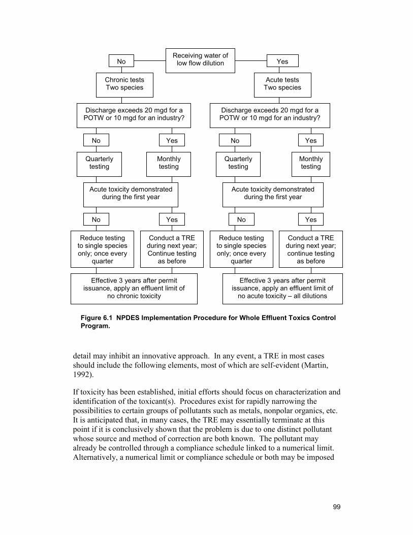
99

detail may inhibit an innovative approach. In any event, a TRE in most cases should include the following elements, most of which are self-evident (Martin, 1992).

If toxicity has been established, initial efforts should focus on characterization and identification of the toxicant(s). Procedures exist for rapidly narrowing the possibilities to certain groups of pollutants such as metals, nonpolar organics, etc. It is anticipated that, in many cases, the TRE may essentially terminate at this point if it is conclusively shown that the problem is due to one distinct pollutant whose source and method of correction are both known. The pollutant may already be controlled through a compliance schedule linked to a numerical limit. Alternatively, a numerical limit or compliance schedule or both may be imposed

No

Chronic tests Two species

No

Conduct a TRE during next year; continue testing

as before

Receiving water oflow flow dilution No Yes

Acute tests Two species

Discharge exceeds 20 mgd for a POTW or 10 mgd for an industry?

Discharge exceeds 20 mgd for a POTW or 10 mgd for an industry?

No Yes Yes

Quarterly testing

Monthly testing

Quarterly testing

Monthly testing

Acute toxicity demonstrated during the first year

Acute toxicity demonstrated during the first year

Yes No Yes

Reduce testing to single speciesonly; once every

quarter

Conduct a TRE during next year;Continue testing

as before

Reduce testing to single speciesonly; once every

quarter

Effective 3 years after permit issuance, apply an effluent limit of

no chronic toxicity

Effective 3 years after permit issuance, apply an effluent limit of

no acute toxicity – all dilutions

Figure 6.1 NPDES Implementation Procedure for Whole Effluent Toxics Control Program.

100

on the permittee following negotiation. Once the toxicant has been identified, the objective is its elimination by process controls, pretreatment, combined water stream treatment, or other means.

If the toxicity problem cannot be readily identified even with diligent effort on the part of the permittee, the authorizing agency may be persuaded to grant additional time for compliance. However, the discharger must convince the regulatory agency that a diligent and thorough TRE has been done and that more time is needed to address the problem. Only then is permit relief likely to be granted.

In some instances, concentrate dischargers have encountered discharge permit problems based on WET testing. For instance, discharge permits for new RO facilities are generally issued on a temporary basis before facility completion. Estimates are required of the quantity and quality of the concentrate eventually to be discharged. This estimation can be difficult and inexact. If available, pilot plant data are a much better source of discharge information. A temporary discharge permit is issued, and construction of the facility goes forward on the assumption that a permanent permit eventually will be issued on this basis. The tests require an actual concentrate; therefore, when the plant initiates operation, a full toxicity analysis is conducted. In at least one instance, a new plant was built based on a preliminary discharge permit and was then denied a permanent permit because it failed the WET test. Although the WETC program allowed a grace period for the effluent to be brought within standards, the extra time and expense were not anticipated or budgeted.

6.3.6 Surface Water Discharge Permitting Process The permitting process looks at all use classifications for the potential receiving water, then looks at all the standards that apply. The most stringent standard for a given pollutant applies. The calculation of the permit limit begins with the appropriate standard. A waste load calculation is made, which takes into account concentration and flow of discharge and the flow, concentration, and standard of the receiving body. A mixing zone calculation is one aspect of the waste load calculation. A chronic permit limit is the value to be met at the edge of the mixing zone. The acute value is the value met at the end of the discharge pipe. If the background concentration is greater than the standard, an ambient standard can be used, but the effluent must not be worse than the ambient standard.

6.3.6.1 Implementation Policy The WQS regulation allows the States to include in their standards State policies and provisions regarding WQS implementation. Often, these address issues such as mixing zones, variances, and low flow exemptions. It is recommended that the policy also includes information on the implementation of WET criteria, such as the use of mixing zones, test species, and methods. All policies related to criteria development should include reference to the three criteria components (magnitude, duration, and frequency). Magnitude establishes how much of a pollutant (or pollutant parameter such as toxicity) expressed as concentration is

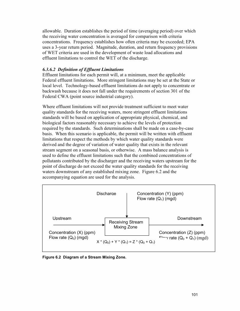
101

allowable. Duration establishes the period of time (averaging period) over which the receiving water concentration is averaged for comparison with criteria concentrations. Frequency establishes how often criteria may be exceeded; EPA uses a 3-year return period. Magnitude, duration, and return frequency provisions of WET criteria are used in the development of waste load allocations and effluent limitations to control the WET of the discharge.

6.3.6.2 Definition of Effluent Limitations Effluent limitations for each permit will, at a minimum, meet the applicable Federal effluent limitations. More stringent limitations may be set at the State or local level. Technology-based effluent limitations do not apply to concentrate or backwash because it does not fall under the requirements of section 301 of the Federal CWA (point source industrial category).

Where effluent limitations will not provide treatment sufficient to meet water quality standards for the receiving waters, more stringent effluent limitations standards will be based on application of appropriate physical, chemical, and biological factors reasonably necessary to achieve the levels of protection required by the standards. Such determinations shall be made on a case-by-case basis. When this scenario is applicable, the permit will be written with effluent limitations that respect the methods by which water quality standards were derived and the degree of variation of water quality that exists in the relevant stream segment on a seasonal basis, or otherwise. A mass balance analysis is used to define the effluent limitations such that the combined concentrations of pollutants contributed by the discharger and the receiving waters upstream for the point of discharge do not exceed the water quality standards for the receiving waters downstream of any established mixing zone. Figure 6.2 and the accompanying equation are used for the analysis.

Figure 6.2 Diagram of a Stream Mixing Zone.

Receiving Stream Mixing Zone

Discharge Concentration (Y) (ppm) Flow rate (Q1) (mgd)

Upstream

Concentration (X) (ppm) Flow rate (Q0) (mgd)

Downstream

Concentration (Z) (ppm) Flow rate (Q0 + Q1) (mgd)

X * (Q0) + Y * (Q1) = Z * (Q0 + Q1)

102

For most pollutants, the authorizing agency will assign effluent limitations defined from the mass balance analysis described above as the 30-day average value in the permit. If the pollutant has a relatively acute toxic effect, the resultant concentration will be assigned to a shorter-term average, such as a 7-day or daily maximum.

The authorizing agency will exercise its best engineering judgment in writing effluent limitations based on water quality standards and will give consideration to other regulations, as well as other factors such as mixing zone studies, seasonal low flows, bioassays, and biosurveys.

Once the discharge limits are known, they can be used to develop the design of the discharge system. Useful discharge limitations data include:

♦ Which constituents will be limited

♦ Concentrations of the limited constituent

♦ Seasonal variations allowed for the constituents

♦ Hazardous or toxic limitations for any constituents

♦ Monitoring requirements for any constituents

♦ Receiving-stream data such as flow rate, existing quality, and stream specifications

With the raw water quality data, it is possible to accurately predict the concentration of constituents in the concentrate before installation by using various methods, including computer programs and vendor data.

6.3.6.3 Monitoring, Recording, and Reporting Any discharge authorized by a discharge permit may be subject to such monitoring, record keeping, and reporting requirements as may reasonably be required in writing by the authorizing agency. All permits specify required types, intervals, and frequencies of monitoring sufficient to yield data representative of the monitored activity including, when appropriate, continuous monitoring. To assure compliance with permit limitations, at least the following will be required of the permittee:

♦ Monitoring of the mass (or other specified measurement) for each pollutant limited in the permit and of the volume of effluent discharged from each outfall

♦ The provision of access to the authorizing agency (with the appropriate credentials) to sample the discharge at a point after the final treatment process (if applicable) but before the discharge mixing with the receiving waters

103

♦ Records of monitoring activities and results, which will include for all samples:

• The data, type, exact place, and time of sampling or measurements

• The individual(s) who performed the sampling or measurements

• The data for which the analyses were performed

• The individual(s) who performed the analyses

• The analytical techniques or methods used

• The results of such analyses

♦ Retention, for a minimum of 3 years, of records of all monitoring information, including all original strip chart recordings for continuous monitoring instrumentation, all calibration and maintenance records, copies of all reports, and records of all data used to complete the application for the permit

♦ Reporting at whatever time interval the authorizing agency reasonably determines to be necessary

6.3.6.4 Permit Duration The duration of an NPDES permit is for a fixed term and will not exceed 5 years. A permit may be transferred to new permittee, if both:

♦ The current permittee notifies the authorizing agency in writing 30 days in advance of the proposed transfer data

♦ The notice includes a written agreement between the existing and new permittees giving a specific date of the transfer of permit responsibility, coverage, and liability

The permit duration is important for the applicant whose facility or process may change in less than 5 years. A decision must be made as to how the original permit will be written. For instance, the concentrate for the first 2 years of facility operation may be 25 to 30 gpm; however, the owner or operator knows that the concentrate stream will increase after 2 years to between 75 and 100 gpm. The original permit may be written for 25 to 30 gpm and then be amended when the discharge increases; or the original permit may be written for between 75 and 100 gpm from the very start. Flow rate is a simple example. More complications arise if there will be changes in the raw water quality or pretreatment, both which affect the constituent of the concentrate, or in operation of the system that affects concentrations of rejected constituents.

6.3.6.5 Generalities about NPDES Permits Dischargers from point sources (individual discrete facilities) into surface water must obtain an NPDES discharge permit from the appropriate State regulatory agency (dependent on State delegation status). The NPDES permit application

104

process in most States requires 180 days before any discharge takes place, or to renovate their permit, or the discharger will make significant changes to the existent permit. A set of forms is involved. EPA form 1, the application, is the standard form to initiate the process. Form 1 requires general facility information such as name, address, telephone, contact person, standard industrial classification codes, and nature of the business, operator information, existing environmental permit, and a topographic map that covers at least 1 mile beyond property lines.

Form 2C provides waste water discharge information. This form requires information concerning flows, source of pollution, and treatment technologies, production and improvement to reduce pollutants in the discharge point, effluent characteristics, biological toxicity data, and analytical contractor information.

Facilities that do not discharge process water will fill out EPA form 2E. This form requires information concerning the receiving waters, discharged dates, type of waste, effluent characteristics, indication if the discharge will be intermittent or seasonal, and the treatment systems.

Each State will include additional forms depending on the different programs associated with the NPDES program. For example, there are forms for discharge of storm water, combined sewer overflow, land irrigation, and injection wells that are regulated under the UIC program.

Once a draft permit is generated, the State issues notice for a public hearing providing stakeholders a copy of the draft permit. The public hearing length is subject to the level of response received by the State. In some States, this step is conditional to the level of controversy associated with the permit. After considering the public comments and a final review, the permit is either granted or denied. A site inspection is typical before the start of a new operation. The permit is valid for a maximum of 5 years. After approval, the State agency in charge of the permit has the right to inspect the facility annually or as deemed necessary, reserving the authority to revoke or suspend a permit for noncompliance of any standard, limitations, or other permit requirements. Civil penalties may also be imposed for noncompliance.

6.4 Disposal to Sewer

An NPDES permit is not required for a discharge to a POTW. Each direct discharger (e.g., a POTW) must have an NPDES permit specifying, among other things, the required waste quality and must submit regular reports to the regulatory agency. Under these regulations, a membrane treatment facility must obtain an NPDES permit to discharge directly to a surface water.

The NPDES permit requires compliance with all Federal standards and may also require additional controls based on local conditions. A POTW may have trouble meeting the NPDES permit conditions if the concentration of pollutants flowing

105

into the treatment plant is too high. One way to control the concentration of these pollutants is to require pretreatment by the individual industrial dischargers before discharge. This control was provided by the implementation of the National Pretreatment Program in 1981.

The CWA also called for EPA to develop national pretreatment standards to control industrial discharges into sewage systems. The standards are uniform national requirements that restrict the level of certain industrial waste water pollutants discharged into the sewage system. All POTWs must enforce the Federal standards. The standards in effect today consist of two sets of rules: categorical pretreatment standards and prohibited discharge standards.

Categorical pretreatment standards are organized by type of industry, and different requirements are mandated for each specific industry as part of the CWA Effluent Guidelines Program. For example, a categorical standard for the iron and steel industry limits the concentrations of ammonia, cyanide, and other specific pollutants that may be present in the waste water discharged.

Prohibited discharge standards forbid any discharge to sewer systems of certain types of waste from all sources. For example, the release of any waste waters with pH lower than 5.0 is prohibited because such wastes may corrode the sewer system.

Membrane treatment facilities are classified “industrial” by default because they are not considered POTWs (for municipal waste water treatment) and, therefore, must abide by the prohibited discharge standards when discharging into the local sewage system. Also, no point source category (e.g., steel mills) exists for membrane treatment facilities. The categorical pretreatment guidelines pertain to the primary industrial point sources. Concentrate and backwash are not regulated as a primary industrial point source.

6.5 Disposal to Deep Well

As a result of the growing concern over contamination of the Nation’s ground water resources from the estimated 300,000 injection wells in the United States, Congress included in the Drinking Water Act of 1979 a statutory mandate to establish minimum requirements for State programs designed to protect underground sources of drinking water from contamination by subsurface injection. The Underground Injection Control regulations were intended to strengthen State regulations as well as establish minimum Federal standards reflecting good engineering practices. As in the NPDES and Pretreatment programs, the delegation of authority for the UIC program has, in certain cases, been made at the State level. Currently, 40 States have primacy with regard to the UIC program (see table 6.2) for a listing of State programs and their status).

106

During formulation of the regulations, it became clear that many differences existed between States, including injection applications and geological conditions. For this reason, the regulations were worded to allow States maximum flexibility in preventing contamination of drinking water sources.

6.5.1 Classification of Injection Wells Injection wells are divided into five classes (CFR 1989a, b). Class I wells include:

♦ Wells used by generators of hazardous wastes or by owners or operators of hazardous waste management facilities to inject hazardous wastes beneath the lowermost formation containing, within 0.25 mile of the well bore, an underground source of drinking water

♦ Other industrial and domestic disposal wells that inject fluids beneath the lowermost formation containing, within 0.25 mile of the well bore, an underground source of drinking water

Classes II through V include wells for many specific uses and different fluids. Only Class I wells are pertinent to the disposal of membrane concentrate.

6.5.2 Municipal Class I injection Wells Class I injection wells include both industrial and municipal disposal wells that inject fluid beneath the lowermost formation containing an underground source of drinking water. Industrial disposal wells include those facilities that inject industrial wastes regardless of their corrosivity, toxicity, or hazard to health. Municipal waste disposal wells are not nearly as numerous as industrial waste disposal wells. Increasingly stringent controls on discharges of sewage effluents into surface water bodies have forced municipalities to seek more effective means of waste treatment and disposal. Currently, the largest, most numerous, and most sophisticated municipal Class I injection wells are in southern Florida, where the favorable hydrogeology makes the use of wells for subsurface injection of wastes possible.

Municipal waste water, a category not rigidly defined in the Federal regulations, is primarily sewage effluent that has received a minimum of secondary treatment. Municipal waste water may contain minor contributions from nonmunicipal or industrial sources. These sources must ensure that their wastes have received the required pretreatment and are compatible with the municipal waste water. For purposes of the UIC program in Florida, municipal sewage effluent that contains less than 5 percent (of its current operating capacity) contribution from non-municipal sources is considered municipal waste water.

Of particular importance to the classification of municipal wells is an exclusion that eliminates the tubing and packer requirement. A packer is a device that is placed inside the innermost casing string and holds the base of the tubing through

107

which the fluid is injected in place. The annular space between the tubing and casing string is filled with fluid, most commonly water mixed with a corrosion-inhibitor. The packer, in conjunction with the tubing, protects the casing from injection pressures, isolates the casing from the injection fluid, and provides an additional opportunity for monitoring through the tubing-and-casing annulus. Under the UIC regulations,

“All Class I injection wells, except those municipal wells injecting non-corrosive wastes, shall inject fluids through tubing with a packer set immediately above the injection zone, or tubing with an approved fluid seal as an alternative. The tubing, packer, and fluid seal shall be designed for the expected service.” (CFR 1989b, p. 734)

The tubing and packer represent additional capital costs, the largest by far being that of the tubing string. The well casings will be somewhat larger in diameter to accommodate the tubing. This represents some additional cost; however, most of the capital cost of a deep well is in labor and testing and not in materials. Solution in annular area between the tubing and the final casing is monitored 24 hours per day for pressure. Either a surface air compressor or source of nitrogen is used to keep the annulus at a pressure higher than the working pressure. In general, the tubing and packer wells required more maintenance than typical injection wells.

The UIC program responsibilities go beyond that of permitting deep well injection of wastes. All injection wells are not waste disposal wells. Some Class V wells, for instance, inject surface water to replenish depleted aquifers or to prevent salt water intrusion. In addition, some Class II wells inject fluids for enhanced recovery of oil and natural gas, and other inject liquid hydrocarbons that constitute our Nation’s strategic fuel reserves in times of crisis (EPA, 2001). Thus, the situation exists where States have UIC programs but do not allow underground injection of industrial wastes including membrane concentrate.

6.6 Disposal by Other Methods

Permits for disposal by methods other than to surface water, POTWs, and deep wells are site specific (Mickley et al., 1993).

Permits for evaporation ponds are not specifically required under either the NPDES or UIC programs. Permits may be prudent (or even required) if the potential exists for leakage to either surface water or a drinking water aquifer and no secondary containment method exists. A permit is recommended because it is very difficult to prove that a leak will not contaminate a potential source water.

An NPDES permit may be required for spray irrigation if the potential exists for runoff to reach a receiving water. To avoid this requirement, the facility must prove beyond reasonable doubt that no runoff can possibly travel to a receiving

108

water, or it must provide secondary containment. Proving that runoff will never reach a receiving water is generally more costly and time consuming than obtaining a permit.

In the zero liquid discharge scenario, such as through the use of brine concentrators and crystallizers, the waste produced is a sludge-like material or dry salts. Solids disposal methods are required including final disposal in an impervious area to eliminate the potential for contamination of surface and ground water.

6.7 Special Topics: Radionuclides, MF/UF Backwash, Contaminated Concentrate, Toxic and Hazardous Waste

There can be site-specific disposal challenges such as when the concentrate or backwash contain some material that will not meet disposal requirements.

6.7.1 Ground Water Based Membrane Processes Ground water typically contains high levels of dissolved gases that include carbon dioxide (CO2), hydrogen sulfide (H2S), and possibly ammonia (NH3). In addition, ground water is typically low in dissolved oxygen. Concentrate resulting from such ground water sources cannot be disposed to surface waters due to the aquatic toxicity that results from high H2S or NH3 and low dissolved oxygen (DO). Consequently, it is routine to post-treat concentrate using steps that might include chlorination (followed by dechlorination), degasification, and aeration. In addition, it is routine to make pH adjustments on concentrate before discharge to surface water. These situations are regularly occurring ones and do not present final disposal problems.

6.7.2 Regional Problems Occurring with Ground Water Membrane concentrate is essentially concentrated raw water. The constituents that are concentrated and the extent to which they are concentrate depend on the type of membrane process and the operating conditions. Typically, there are few process-added chemicals (acid and antiscalant); and, thus, the nature of the concentrate reflects the makeup and nature of the raw water from which it came. A detailed characterization of membrane concentrate (Mickley et al., 1993) highlights how concentrate differs in this regard from nearly all other industrial waste waters.

Historically, most membrane concentrates have been free from the presence of problematic levels of contaminants because of the low occurrence of contaminants in the raw water.

109

Sometimes, however, local raw waters will contain relatively high levels of certain constituents that become spikes of “contaminants” in the resulting concentrate. One such site-specific situation is presence of radionuclides in a raw water. In a previous survey (Mickley et al., 1993) 16 plants were identified (in Florida, Illinois, Iowa, and Missouri) that cited radium removal as one of the reasons for the membrane plant. In southwest Florida, this has frequently meant that the only viable disposal option was deep well injection.

6.7.3 MF and UF Backwash Backwash presents an emerging disposal challenge. While these processes do not concentrate salts (including radionuclides), they concentrate to varying extents suspended solids, organics, and microorganisms. The backwash may contain elevated levels of microorganisms such as giardia and cryptosporidium which common sense suggests should not be routinely disposed to surface water or sewer. At present, however, there are no water quality criteria for receiving waters with regards to surface water disposal of effluents containing these microorganisms.

6.7.4 Future Concentrate Challenges In section 6.6.2, the presence of radionuclides in concentrate is a natural occurrence due to the local raw water makeup. It is also possible, however, to have raw waters that are contaminated by human activity. Such examples will increasingly include raw waters with high levels of nitrates (from fertilizer use), pesticides (also from agricultural activity), arsenic (from mining area waters), and possibly endocrine blockers (from several sources). The concentrate resulting from treatment of these waters will have spikes of these “contaminants” that will complicate or prevent their disposal by most methods. Treatment of concentrate for pesticide and arsenic removal has occurred in Europe.

6.7.5 Toxicity and Hazardous Labels Unless the concentrate is contaminated with a toxic of hazardous substance, it is not generally toxic or hazardous (Mickley et al., 1993). Historically, the only reasons that the author is aware of for failed toxicity tests from membrane drinking water plant concentrate include:

♦ Metal leaching from pump parts

♦ High levels of H2S and NH3 from ground water source

♦ Low levels of dissolved oxygen from ground water source

♦ High levels of fluoride and or calcium from ground water source

The first case was addressed by changing pump parts. The second and third situations routinely occur and are addressed by removal of H2S and NH3 and

110

aeration of concentrate to increase the level of dissolved oxygen. The fourth case refers to major ion toxicity, which has recently been extensively studied (Mickley, 2000). This type of toxicity is different from that resulting from heavy metals or pesticides in that it is not bioaccumulative and has a threshold nature that results in the toxicity disappearing at low dilution levels. Perhaps even more important is the fact that the toxicity has occurred almost exclusively (there are exceptions) as a result of conducting the whole effluent toxicity tests using the mysid shrimp as the test organism. The mysid shrimp appears to be the most sensitive test organism routinely used for these tests.

As a result of the unusual nature of the major ion toxicity, the State of Florida is considering legislation to regulate concentrate shown to have this toxicity (in the absence of other causes of toxicity) differently than concentrate with other types of toxicity.

111

7. Regulation – State Perspective 7.1 Background

As explained in chapter 5, the States play in important role in the regulation of concentrate disposal. Federal (EPA) guidelines, directives, and framework provide starting points for State regulation. While starting with this common framework, State regulations can differ in the details of how the guidelines and directives are implemented. They can also differ in how stringent the regulatory requirements are, providing they are at least as stringent as the Federal guidelines.

Many States do not have membrane plants producing potable water. In addition, many other States that do have membrane plants have only limited experience with either very small plants or with a small number of plants.

Two different surveys were conducted to document States’ regulation of membrane concentrate disposal. Because of this limited experience of most States with membrane technology, the first survey focused on options available for disposal of WTP residuals, in general. The second survey, which was also of a similar more general nature, focused on disposal of residuals to surface waters and the NPDES-related State regulations.

Some terminology comments are in order. There are some similar terms used to describe residuals in both conventional water treatment plants and membrane water treatment plants. This can be confusing unless understood. The term “concentrate” unless referred to as “membrane concentrate” means a liquid waste/sludge before dewatering. Similarly, unless the term “backwash” is in the context of membrane plants and membrane backwash, it refers to filter backwash.

7.2 Survey of WTP Disposal Options

The first of the two surveys conducted was undertaken to document disposal options available to WTPs in different States. The more detailed results of the survey are included as appendix A. This survey is not restricted to membrane concentrate but includes information about how various WTP residuals are disposed.

Information was obtained from the Internet through checking the State environmental agency Web sites to list and document the relevant programs dealing with water quality issues for the drinking water utilities. The corresponding agency was contacted by phone and interviewed accordingly. In some instances due to the division of authority within the State, more than one agency was involved in the survey.

The questions addressed in the survey concerning the WTPs waste disposal options concerned:

112

♦ Options of liquid waste disposal ♦ Options of residue or sludge disposal ♦ Raw water source and overall quality ♦ Chemicals or technical treatment problems faced by the utilities ♦ Ground water reinjection as a waste disposal option ♦ Membrane technology use by the operating WTP ♦ Programs involved dealing with disposal options

Appendix A presents this information in a narrative form as was hand recorded during the interviews. Further technical details as well as the legal requirements for the permits or policies listed can be obtained directly from the contact person phone number or checking the agency’s corresponding Web site.

Results for the States for California, Florida, and Texas are presented here. Appendix A has results for all 50 States.

7.2.1 California California Environmental Protection Agency State Water Control Board SWRCB Division of Water Quality Los Angeles Region 4 101 Center Plaza Dr Monterrey Park CA 91754-2156

Ph: (323) 266-7557 Fx: (323) 266-7600 Web site: www.dwr.water.ca.gov/

Contact: Shirley Birosik, Division of Water Quality Abdell Shrudaji, Department of Health Services Ph: (213) 977-6808

Currently, there is no special regulation for disposal of wastes from drinking water plants; the waste generated will fall within existent programs such as NPDES permit for surface discharge. This is the most common option of disposal for liquid waste, and permit requirements are managed by the Division of Water Quality. Disposal of the concentrate or sludge to a sanitary landfill as solid waste is also allowed, and the solid waste group in the Department of Health Services handles the necessary requirements. In the State, some utilities dispose their sludge as road construction material, and no permit is involved in this process, with the exception of notification to the solid waste group. Source water is a combination of surface and ground water; the northern part of the State uses primarily surface water; whereas, in the southern portion, there is more use of ground water. In the region (Los Angeles), source water quality is acceptable; but there are frequent problems with salinity, nitrates, and volatile organic compounds. There are utilities using membrane technology such as RO and

113

microfiltration. Santa Catalina Island has an RO plant to treat salt water. There are some cases of re-injection occurring as an option for treating drinking water disposal, especially to control salt intrusion. The State has an UIC program to oversee any re-injection into ground water.

7.2.2 Florida Florida Department of Environmental Protection Division of Water Facilities Drinking Water Section 2600 Blair Stone Rd, MS 3520 Tallahassee FL 32399-2400

Ph: (850) 487-1762 Fx: (850) 414- 9031 Web site: www.dep.state.fl.us/

Contact: Richard Drew, Bureau Chief Ph: (850) 487-0563 Elsa Potts, Office of Waste Water Management Ph: (850) 921-9495 Fax: (850) 414-9031

The State of Florida issued in 1996 a set of guidelines for RO membrane utilities. This document does not elaborate on waste disposal options but describes current trends and present case studies of these membrane facilities. Currently, the State allows surface water disposal, and blending is a common practice. The concentrate is mixed with clean, treated effluent to reduce saline concentration before discharge; all water quality standards must be met. The sludge or concentrate also can be land filled, but few utilities chose this option due to the high chloride of the sludge that renders it unsuitable for land application; areas with high lime concentrations may qualify for this type of disposal. The State requires a UIC permit for deep well injection of brine or concentrate.

7.2.3 Texas Texas Natural Resource and Conservation Commission Water Utilities Water Quality Division TNRCC, P.O. Box 13087 Austin TX 78711-3087

Ph: (512) 239-6020 Fx: (512) 239 6050 Web site: www.tnrcc.texas.gov/

Contact: Jack Schulze, Public Drinking Water Section

114

Drinking water utilities are allowed to discharge their liquid waste to a receiving stream only under an NPDES permit. They also can discharge to an existing sewer system; and, in this case, no permit is required. A third practice in the State for liquid waste disposal is recycling of the waste to the head of the plant. Typically, the supernatant of the settling lagoon is recycled, reducing the volume of liquid discharge. Any sludge or residue generated after dewatering can be disposed in a permitted sanitary landfill. There is a beneficial use program that the utilities can apply for, but most utilities prefer the first option. No use of the sludge for road construction is known at this moment. The utilities also have the option of re-injecting the stream waste, but most of them do not choose this option due to the stringent UIC program requirements. There are some concerns regarding quality of raw water. Utilities located east of Interstate-35 face some color, alkalinity, iron, and manganese problems. West of Interstate-35 the situation is different involving mainly high salt content in the surface and ground water. Also in this area, there is evidence of high fluoride concentration that requires attention. Surface water presents some sporadic problems with benzene, toluene, ethylbenzene, xzylene (BTEX), and atrazine; and the utilities have problems meeting MCLs. Along the Rio Grande, the problem is TDS, salinity, and urban pollution coming from Mexico. Around Austin, the south section has excellent water quality, and no major problems occur. There are some RO systems in the State serving small communities. In west Texas, there are about five ultrafiltration and microfiltration utilities; two are under construction, and the rest (three) are approved and in final design phase.

7.3 Survey of NPDES-Related State Regulation

A second survey was undertaken to focus on disposing effluents to surface waters and the NPDES-related State regulations that govern this. As mentioned in chapter 6, about 87 percent of the surveyed desalting plants dispose membrane concentrate either directly to surface water or indirectly to surface water through disposal to the sewer. For low-pressure membrane systems and membrane backwash, the figure is 84 percent.

Survey results for the States for California, Florida, and Texas are presented here. Appendix B has results for all 50 States.

7.3.1 California There are three main pieces of legislation for regulating concentrate disposal in the State:

♦ Porter-Cologne Water Quality Control Act ♦ California Regional Water Quality Control Board Basin Plans ♦ Water Recycling Criteria

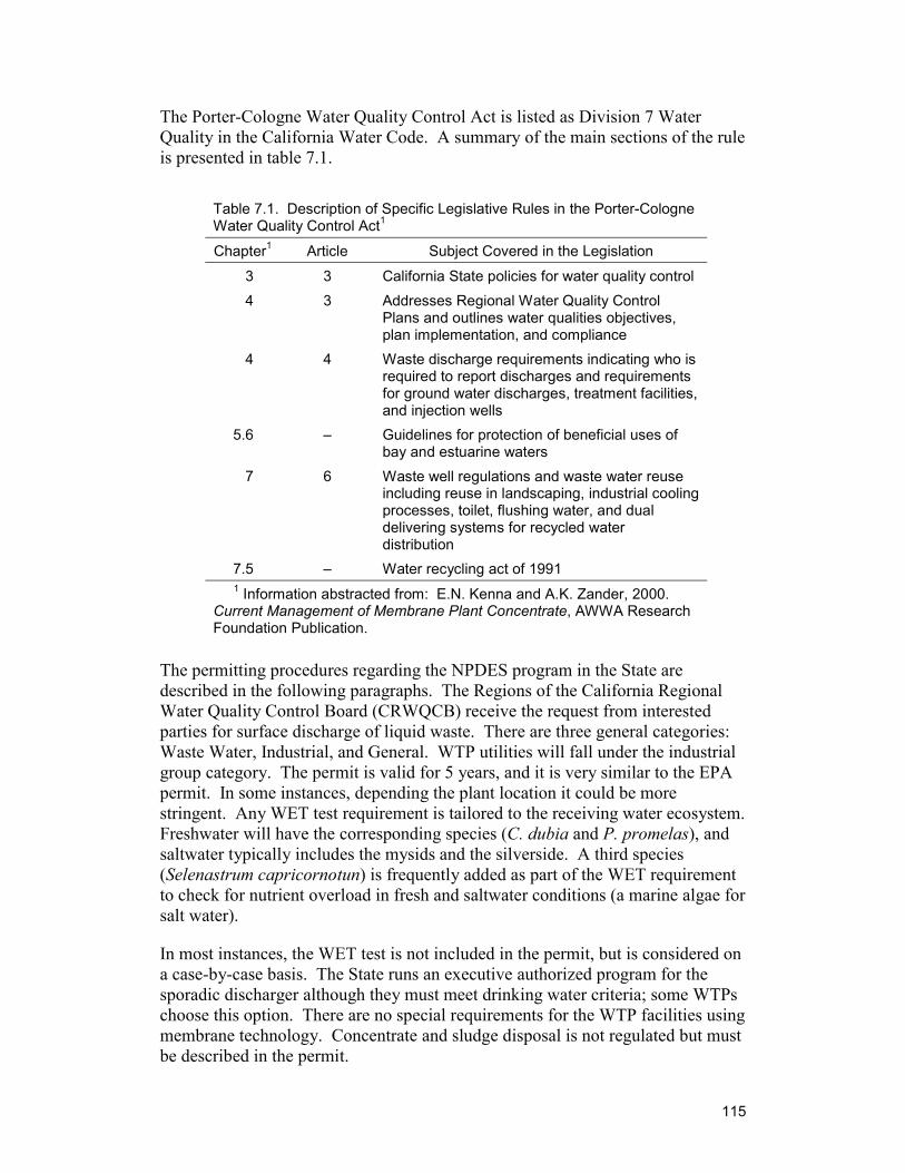
115

The Porter-Cologne Water Quality Control Act is listed as Division 7 Water Quality in the California Water Code. A summary of the main sections of the rule is presented in table 7.1.

Table 7.1. Description of Specific Legislative Rules in the Porter-Cologne Water Quality Control Act1

Chapter1 Article Subject Covered in the Legislation

3 3 California State policies for water quality control 4 3 Addresses Regional Water Quality Control

Plans and outlines water qualities objectives, plan implementation, and compliance

4 4 Waste discharge requirements indicating who is required to report discharges and requirements for ground water discharges, treatment facilities, and injection wells

5.6 – Guidelines for protection of beneficial uses of bay and estuarine waters

7 6 Waste well regulations and waste water reuse including reuse in landscaping, industrial cooling processes, toilet, flushing water, and dual delivering systems for recycled water distribution

7.5 – Water recycling act of 1991

1 Information abstracted from: E.N. Kenna and A.K. Zander, 2000. Current Management of Membrane Plant Concentrate, AWWA Research Foundation Publication.

The permitting procedures regarding the NPDES program in the State are described in the following paragraphs. The Regions of the California Regional Water Quality Control Board (CRWQCB) receive the request from interested parties for surface discharge of liquid waste. There are three general categories: Waste Water, Industrial, and General. WTP utilities will fall under the industrial group category. The permit is valid for 5 years, and it is very similar to the EPA permit. In some instances, depending the plant location it could be more stringent. Any WET test requirement is tailored to the receiving water ecosystem. Freshwater will have the corresponding species (C. dubia and P. promelas), and saltwater typically includes the mysids and the silverside. A third species (Selenastrum capricornotun) is frequently added as part of the WET requirement to check for nutrient overload in fresh and saltwater conditions (a marine algae for salt water).

In most instances, the WET test is not included in the permit, but is considered on a case-by-case basis. The State runs an executive authorized program for the sporadic discharger although they must meet drinking water criteria; some WTPs choose this option. There are no special requirements for the WTP facilities using membrane technology. Concentrate and sludge disposal is not regulated but must be described in the permit.

116

7.3.2 Florida The State of Florida has six regulatory districts in charge of issuing permits (NPDES) for discharge of waste water into waters of the State, including ground water. The districts are distributed in six different geographical regions of the State, including the northwest, northeast, central, southwest, southeast, and the south districts. Florida is a EPA delegated State since 1995 for the application of the NPDES permits and has over 20 years of experience issuing discharge permits. When the State became delegated, they combined EPA guidelines with the State requirements; therefore, EPA guidelines are included in the current Florida regulation (chapter 62 of the Florida Administrative Code). In some cases, requirements in the State are more stringent than the Federal requirements. Each facility’s permit is defined by specific constituents or conditions of the discharge and the receiving stream. The districts do not make any difference regarding the requirements for other industrial facilities and the drinking water utilities (WTPs). All requirements are tailored to the operational and waste type of the applicant to ensure that the discharge will not impact water quality standards or cause or contribute to pollution.

Regarding WET test requirements for the NPDES permit, Florida Department of Environmental Protection (FDEP) emphasizes that every permit is unique, and technical considerations for disposal of RO membrane plant concentrate are taken into account when writing the permit and the biomonitoring requirements. Typically, marine species are considered for WET testing (i.e., Menidia beryllina and Mysidopsis bahia). If the TDS of the concentrate is primarily determined by ions other than chloride and sodium, and thus the concentrate is of lower salinity, freshwater species are considered. Any surface discharge must comply with biomonitoring and chemical standards before discharge. Utilities can request variance of discharge standards filing a State form if they consider that permit constituents do not apply to their current situation (a copy of the form application can be obtained from the FDEP Web site).

The complexity of the individual permit for membrane utilities is defined by the receiving Florida water, which follows a designation system. Several of the standards and requirements are based on which type of Florida water is receiving the discharge. Waters in Class III, for example, include all recreational waters; Class II describes waters dedicated to fisheries activities and will have more requirements on pollutants than the previous one. The permit process typically takes between 6 months to a year. However, it can get lengthy if sensitive environments in the State are involved. Currently, there are some legislative initiatives to resolve the issue of WET testing requirements for the membrane utilities. In some cases, the demonstration of absence of other pollutants has been required by FDEP, although it is up to the districts to get satisfaction on this requirements since they are the ones issuing the NPDES permit.

There are no special requirements for utilities discharging to a marine environment with the caveat that they must meet all standards established for the

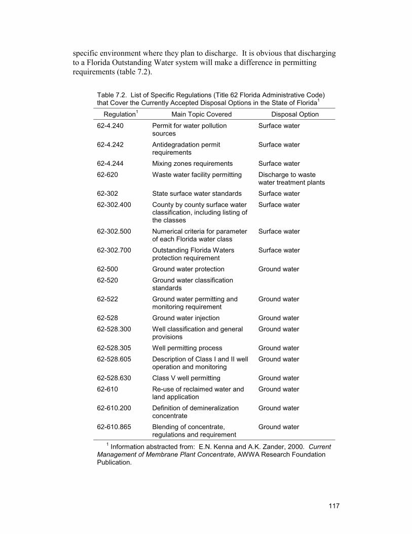
117

specific environment where they plan to discharge. It is obvious that discharging to a Florida Outstanding Water system will make a difference in permitting requirements (table 7.2).

Table 7.2. List of Specific Regulations (Title 62 Florida Administrative Code) that Cover the Currently Accepted Disposal Options in the State of Florida1

Regulation1 Main Topic Covered Disposal Option

62-4.240 Permit for water pollution sources

Surface water

62-4.242 Antidegradation permit requirements

Surface water

62-4.244 Mixing zones requirements Surface water 62-620 Waste water facility permitting Discharge to waste

water treatment plants 62-302 State surface water standards Surface water 62-302.400 County by county surface water

classification, including listing of the classes

Surface water

62-302.500 Numerical criteria for parameter of each Florida water class

Surface water

62-302.700 Outstanding Florida Waters protection requirement

Surface water

62-500 Ground water protection Ground water 62-520 Ground water classification

standards

62-522 Ground water permitting and monitoring requirement

Ground water

62-528 Ground water injection Ground water 62-528.300 Well classification and general

provisions Ground water

62-528.305 Well permitting process Ground water 62-528.605 Description of Class I and II well

operation and monitoring Ground water

62-528.630 Class V well permitting Ground water 62-610 Re-use of reclaimed water and

land application Ground water

62-610.200 Definition of demineralization concentrate

Ground water

62-610.865 Blending of concentrate, regulations and requirement

Ground water

1 Information abstracted from: E.N. Kenna and A.K. Zander, 2000. Current Management of Membrane Plant Concentrate, AWWA Research Foundation Publication.

118

7.3.2.1. Deep Well injection Current deep well injection permits in Florida are issued under provisions of Chapter 403, Florida Statutes (F.S.) and Florida Administrative Code (FAC) Rules 62-4, 62-550, 62-660, and 62-528. The permit describes all technical requirements for Class I injection wells to dispose of non-hazardous reverse osmosis concentrate. The permit specifies well inner diameter (I.D.), depth, casing, volume (mgd) allowed to be disposed, injection pressure, and required monitor wells.

In addition, the permit narrative indicates the General Conditions that are required from the permittee such as record keeping, compliance with monitoring requirements, emergency procedures etc. The Specific Conditions of the permit describe the operating requirements for the injection well such as which type of waste is allowed in the well, daily monitoring, abandonment procedures, testing and reporting requirements etc. A certification of financial responsibility is required as part of the permit to ensure that the facility has the necessary resources to close, plug, and abandon the injection and associated monitor wells, at all times.

7.3.2.2. Spray Irrigation/Land Application This type of permit is issued under the provision of chapter 403 of the Florida Statutes and applicable rules of the Florida Administrative Code (See table 1). The permit covers holding pond facilities for concentrate waste before the irrigation stage. Typically, the concentrate is blended with other raw water to meet TDS standards before irrigation in most cases to golf course facilities. The permit specifies monitoring parameters which for the land application such as flow, TDS, sodium, chloride, sulfate, and pH. Ground water protection is also specified in the permit. Discharge monitoring reporting and blending ratios of concentrate with raw water (4:1) are detailed in the permit.

7.3.2.3. Surface Discharge The outfall discharge point is specified in the permit as well as the type of waste allowed to be discharged. Monitoring parameters at the mixing zone and the dimension of the zone are detailed in the permit. The permittee must comply with the applicable FAC Rules 62-4.244 and 63-302.500 (table 1) related to the subject of mixing zones. Land application, emergency surface discharge, other methods of disposal or recycling, and further limitations of monitoring reporting are defined in the permit. A WET testing program is also described in the permit and is mandatory for surface dischargers.

7.3.3 Texas The disposal options for membrane concentrate and their regulatory requirements are specified in Title 30 of the Texas Administrative Code (TAC). Table 7.3 lists the main topics included in this piece of legislation indicating the appropriate disposal option allowed by the Texas Natural Resources Conservation Commission (TNRCC).

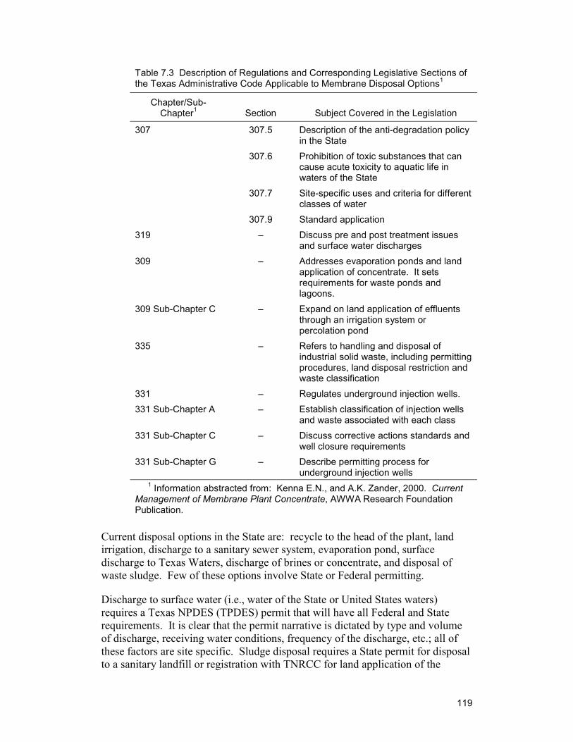
119

Table 7.3 Description of Regulations and Corresponding Legislative Sections of the Texas Administrative Code Applicable to Membrane Disposal Options1

Chapter/Sub-Chapter1 Section Subject Covered in the Legislation

307 307.5 Description of the anti-degradation policy in the State

307.6 Prohibition of toxic substances that can cause acute toxicity to aquatic life in waters of the State

307.7 Site-specific uses and criteria for different classes of water

307.9 Standard application 319 – Discuss pre and post treatment issues

and surface water discharges 309 – Addresses evaporation ponds and land

application of concentrate. It sets requirements for waste ponds and lagoons.

309 Sub-Chapter C – Expand on land application of effluents through an irrigation system or percolation pond

335 – Refers to handling and disposal of industrial solid waste, including permitting procedures, land disposal restriction and waste classification

331 – Regulates underground injection wells. 331 Sub-Chapter A – Establish classification of injection wells

and waste associated with each class 331 Sub-Chapter C – Discuss corrective actions standards and

well closure requirements 331 Sub-Chapter G – Describe permitting process for

underground injection wells

1 Information abstracted from: Kenna E.N., and A.K. Zander, 2000. Current Management of Membrane Plant Concentrate, AWWA Research Foundation Publication.

Current disposal options in the State are: recycle to the head of the plant, land irrigation, discharge to a sanitary sewer system, evaporation pond, surface discharge to Texas Waters, discharge of brines or concentrate, and disposal of waste sludge. Few of these options involve State or Federal permitting.

Discharge to surface water (i.e., water of the State or United States waters) requires a Texas NPDES (TPDES) permit that will have all Federal and State requirements. It is clear that the permit narrative is dictated by type and volume of discharge, receiving water conditions, frequency of the discharge, etc.; all of these factors are site specific. Sludge disposal requires a State permit for disposal to a sanitary landfill or registration with TNRCC for land application of the

120

sludge near the surface as it is indicated in 30 TAC Section 312.121. Re-injection is always an option for concentrate disposal but not a preferred one since it must require meeting UIC requirements. In the case of land irrigation, it will only require a permit if the discharge is above 5,000 gallons per day in which case it will require a TPDES permit. Volumes below 5,000 gallons per day do not require permits according to current rules. The on-site disposal option of sludge or concentrate (within the WTP property) also is an accepted practice, and it will be covered by the TPDES permit.

The TPDES permit is currently being implemented, and there is no indication that the WTPs are treated any different from other industrial dischargers. The drinking water utilities will fall under the category of industrial dischargers and will follow the same protocol for getting a permit. The existing process will take approximately 180 days, from the day of a declaration of administrative completeness. Due to the extensive review, it is recommended that the process should start a year in advance.

7.4 Summary of Regulatory Requirements for Selected States

Table 7.4 presents information about the waste disposal options for WTPs from States that provided detail NPDES-related information. Information is presented about 1) the NPDES-related requirements associated with surface water disposal of wastes, 2) the various disposal options available for disposal of WTP residuals, and 3) membrane concentrate disposal in particular.

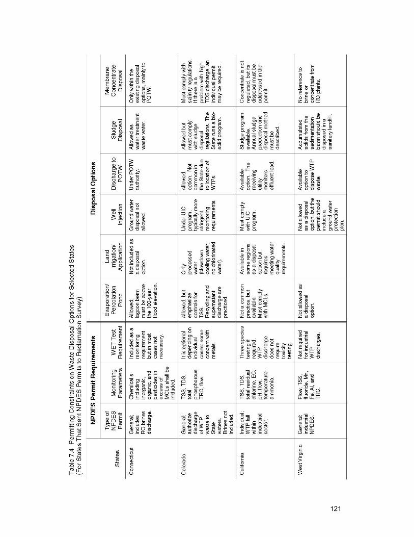
121

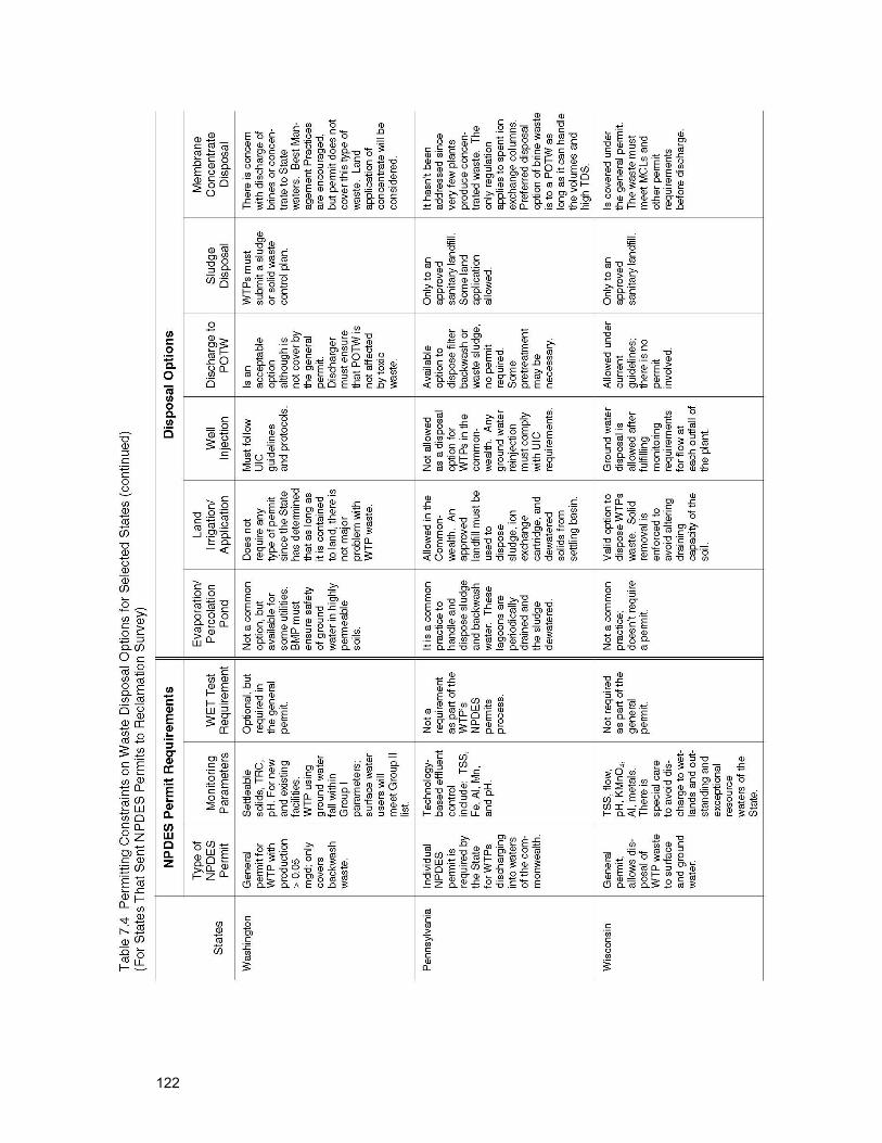
122

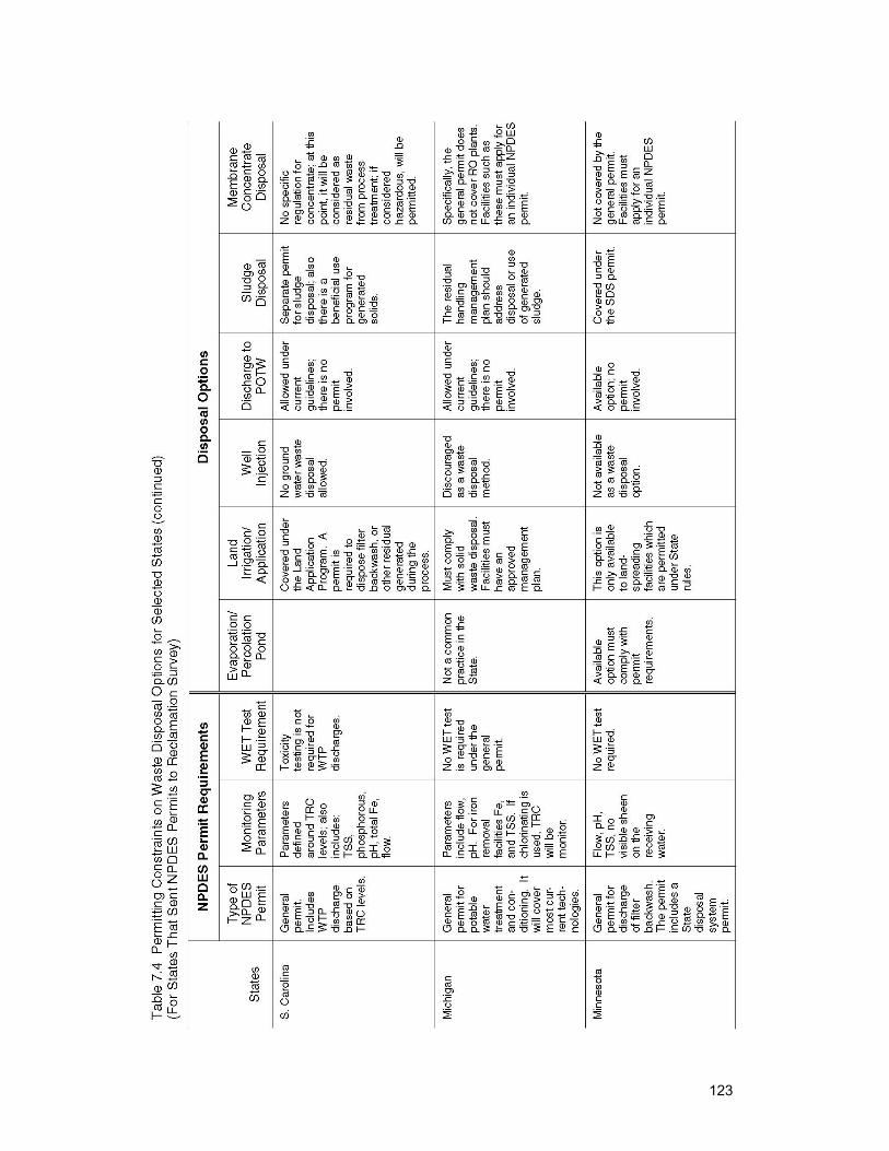
123

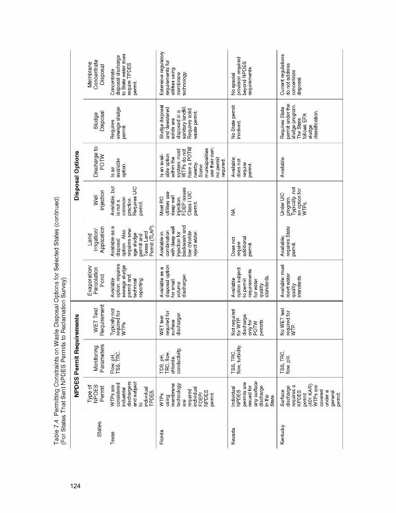
124

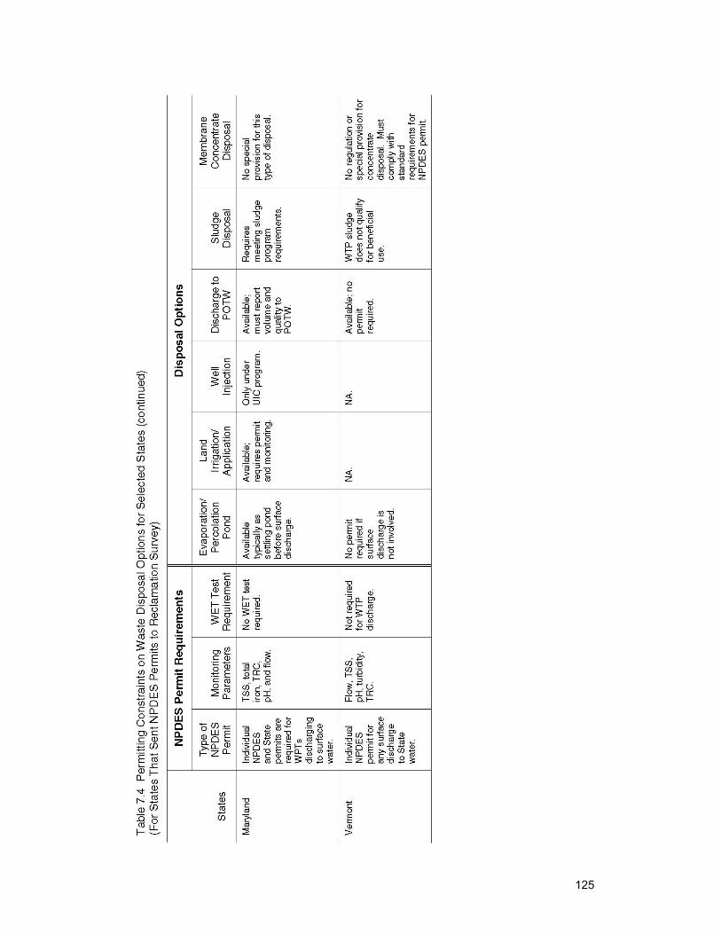
125

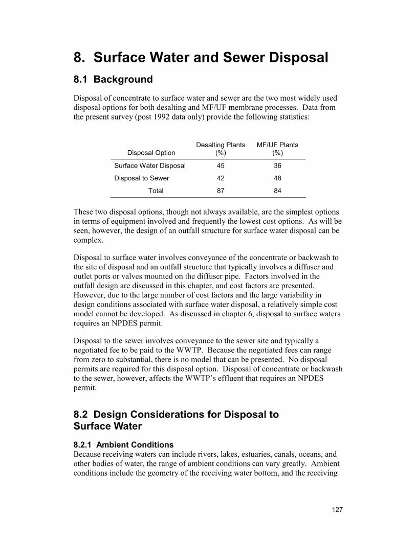
127

8. Surface Water and Sewer Disposal 8.1 Background

Disposal of concentrate to surface water and sewer are the two most widely used disposal options for both desalting and MF/UF membrane processes. Data from the present survey (post 1992 data only) provide the following statistics:

Disposal Option Desalting Plants

(%) MF/UF Plants

(%)

Surface Water Disposal 45 36

Disposal to Sewer 42 48

Total 87 84

These two disposal options, though not always available, are the simplest options in terms of equipment involved and frequently the lowest cost options. As will be seen, however, the design of an outfall structure for surface water disposal can be complex.

Disposal to surface water involves conveyance of the concentrate or backwash to the site of disposal and an outfall structure that typically involves a diffuser and outlet ports or valves mounted on the diffuser pipe. Factors involved in the outfall design are discussed in this chapter, and cost factors are presented. However, due to the large number of cost factors and the large variability in design conditions associated with surface water disposal, a relatively simple cost model cannot be developed. As discussed in chapter 6, disposal to surface waters requires an NPDES permit.

Disposal to the sewer involves conveyance to the sewer site and typically a negotiated fee to be paid to the WWTP. Because the negotiated fees can range from zero to substantial, there is no model that can be presented. No disposal permits are required for this disposal option. Disposal of concentrate or backwash to the sewer, however, affects the WWTP’s effluent that requires an NPDES permit.

8.2 Design Considerations for Disposal to Surface Water

8.2.1 Ambient Conditions Because receiving waters can include rivers, lakes, estuaries, canals, oceans, and other bodies of water, the range of ambient conditions can vary greatly. Ambient conditions include the geometry of the receiving water bottom, and the receiving

128

water salinity, density, and velocity. Receiving water salinity, density, and velocity may vary with water depth, distance from the discharge point and time of day and year.

8.2.2 Discharge Conditions Discharge conditions include the discharge geometry and the discharge flow conditions. The discharge geometry can vary from the end of the pipe to a lengthy multi-port diffuser. The discharge can be at the water surface or submerged. The submerged outfall can be buried (except for ports) or not. Much of the historical outfall design work deals with discharges from WWTPs. These discharges can be very large—up to several hundred mgds in flow. In ocean outfalls and in many inland outfalls, these discharges are of lower salinity than the receiving water, and the discharge has positive buoyancy. The less dense effluent rises in the more dense receiving water after it is discharged.

The volume flow of membrane concentrates is on the lower side of the range of WWTP effluent volumes, extending up to perhaps 15 mgd at present. Membrane concentrate, as opposed to WWTP effluent, tends to be of higher salinity than most receiving waters, resulting in a condition of negative buoyancy where the effluent sinks after it is discharged. This presents a concern of the potential impact of the concentrate on the benthic community at the receiving water bottom. Any possible effect on the benthic community is a function of the local ecosystem, the composition of the discharge, and the degree of dilution present at the point of contact. The chance of an adverse impact is reduced by increasing the amount of dilution at the point of bottom contact through diffuser design.

8.2.3 Regulations Receiving waters can differ substantially in their volume, flow, depth, temperature, composition, and degree of variability in these parameters. The effect of discharge of a concentrate or backwash to a receiving water can vary widely depending on these factors. As described in chapter 6, the regulation of effluent disposal to receiving water involves several considerations, some of which are the end-of-pipe characteristics of the concentrate or backwash. Comparison is made between receiving water quality standards (dependent on the classification of the receiving water) and the water quality of the effluent to determine disposal feasibility. In addition, in States such as Florida, the effluent must also pass WET tests where test species, chosen based on the receiving water characteristics, are exposed to various dilutions of the effluent. Because the nature of the concentrate or backwash is different than that of the receiving water, there is a region near the discharge area where mixing and subsequent dilution of the concentrate or backwash occurs.

Where conditions cannot be met at the end of the discharge pipe, a mixing zone may be granted by the regulatory agency. The mixing zone is an administrative construct that defines a limited area or volume of the receiving water where this

129

initial dilution of the discharge is allowed to occur. The definition of an allowable mixing zone is based on receiving water modeling as discussed in chapter 6. The regulations require that certain conditions be met at the edge of the mixing zones in terms of concentration and toxicity (via the WET test).

8.2.4 The Outfall Structure The purpose of the outfall structure is to assure that mixing conditions can be met and that discharge of the effluent, in general, will not produce any damaging effect on the receiving water, its lifeforms, wildlife, and the surrounding area.

In a highly turbulent and moving receiving water with large volume relative to the effluent discharge, simple discharge from the end of a pipe may be sufficient to assure rapid dilution and mixing of the effluent. For most situations, however, the mixing can be improved substantially through the use of a carefully designed outfall structure. Such design may be necessary to meet regulatory constraints.

The most typical outfall structure for this purpose consists of a pipe of limited length mounted perpendicular to the end of the delivery pipe. This pipe, called a diffuser, has one or more discharge ports along its length.

8.2.5 Dilution Levels Some examples will serve to illustrate the dilution levels sought in the use of diffusers. It has been estimated that in seawater most organisms can tolerate a departure of +/- 1 part per thousand (ppt) from the normal salinity, which represents a 3% deviation from the ambient (EPRI-CEC, 1994). For seawaters where the membrane concentrate is of 70 ppt salinity, a dilution of approximately 35 times would be required to achieve an effluent stream salinity of 1 ppt above ambient. This can be shown as follows:

Let x = receiving water salinity and y = effluent salinity. After one dilution (equal volumes) the resulting salinity is (y + x)/2. After the second dilution where another volume of the receiving water is added, salinity is (y + 2x)/3. After the ith dilution the salinity is (y + i*x)/(i+1). For the case where x = 35 and y = 70, at the 35th dilution, the final salinity is 35.97 and, thus, within 1 ppt of the receiving water salinity.

This same formula may be used to determine the effects on salinity of blending concentrate with other effluents. For instance, if membrane seawater concentrate is blended with WWTP effluent of a salinity of 1 ppt (very high), the second dilution of the seawater concentrate by the WWTP effluent will result in a combined effluent of 24 ppt. For ocean discharge, such a dilution changes the discharge from one of negative buoyancy to one of positive buoyancy. This discharge will rise rather than sink in the receiving water and, thus, avoid (minimize) any effect on the benthic community.

130

8.2.6 Diffuser Characteristics and Design Variables There are several parameters that characterize diffuser design. These include:

♦ Diameter of the diffuser pipe ♦ Length of the diffuser pipe ♦ Pipe material ♦ Length of risers (if any) between pipe and ports/valves ♦ Riser material ♦ Port or valve materials ♦ Number of diffuser ports or valves ♦ Size of the diffuser ports or valves ♦ Distance between diffuser ports or valves ♦ Angles of diffuser ports with respect to the diffuser pipe

Other characteristics of the diffuser include its orientation in relation to the receiving water boundaries and surface. This orientation may be described in terms of:

♦ Distance from shore ♦ Depth from surface ♦ Angles with respect to receiving water boundaries and flow ♦ Trenched or not

Many outfall structures are designed using software packages that take into consideration design variables such as:

♦ Effluent flow rate

♦ Hydrodynamics of the receiving water • Currents • Turbulence • Tidal influences • Velocity

♦ Shape of the receiving water boundaries (sides and bottom) including bottom slope

♦ Temperature of effluent

♦ Temperature profile of receiving water

♦ Density of the effluent relative to that of the receiving water (buoyancy)

8.2.7 CORMIX and Other Software This software development began at Cornell University in 1986 under contract from EPA. Following the development of CORMIX1 subsystem (Doneker and

131

Jirka, 1990), other systems were added in the ensuing years. CORMIX1 applies to single port discharges and CORMIX2 to multiport discharges. CORMIX 3 deals with surface level discharges. D-CORMIX extends the capabilities of CORMIX to negatively buoyant discharges. Software has also been developed for visualization of outfall design and mixing zone properties (http://steens.ese.ogi.edu).

Other modeling software includes EPA PLUMES (Visual Plumes) models that were developed primarily for waste water discharges from WWTPs. A discussion of the differences between the CORMIX and PLUMES software may be found on the Web page: http://steens.ese.ogi.edu/faq.html.

The CORMIX simulations are for steady-state constant source systems. For transient simulations, more sophisticated software is required such as various computational fluid dynamics (CFD) packages. These software packages are much more expensive (many systems are $15,000 or more) than the CORMIX system (about $500 for a single user plus $900 for the visualization tools). Several companies also offer services in providing CFD simulations.

8.2.8 General Design Approach for Diffusers The reason for diffusers is to meet dilution requirements. Sometimes dilution is not required, as when conditions at end of pipe can be met. If the diffuser cannot be designed to meet the mixing zone requirements, then there needs to be more treatment before discharge. For the intermediate cases where a design is needed and possible, there are options as to the general nature of the diffuser. One alternative is to lay the diffuser pipe on bottom surface with holes drilled in the side; this is the cheapest alternative if it can be supported and maintained in its bottom position. Another option is a buried pipeline with protection from scouring or damage (such as from a dragging anchor) with a protruding vertical riser and gooseneck elbow that would discharge horizontally. In cases where flow is intermittent, it may be prudent and even necessary to install a valve at each discharge port to prevent backflow of seawater (for instance) or to prevent organisms and even wildlife from entering the diffuser. One company (Red Valve) makes rubber valves that have no moving parts but will open and close depending on the discharge flow/pressure.

Software packages may be used to develop conceptual designs by exploring the various design variables within the constraints of the ambient conditions and the dilution requirements. Sometimes, several different designs can meet the dilution requirement, in which case, usually a design with a shorter diffuser and smaller ports will offer the less expensive option.

One design constraint is the maximum discharge velocity of about 12 feet per second (fps). Discharge velocities range from 5 to 12 fps, but most typically designs strive for a 10 fps discharge velocity. Most designs have the ports far enough apart so the plumes just barely touch. This spacing, as well as smaller

132

port diameters, leads to increased dilution. Dilution also increases with smaller density differences between the discharge and receiving water (another advantage of blending before discharge).

In general, the diameter of the diffuser is sized just like that of any pipe based on velocity and pressure drop considerations. In the case of long diffusers (which for WWTP outfalls can be several thousand feet in length), sometimes the diffuser pipe is tapered to maintain flow velocities, as flow is lost through the ports. The design length of the pipe typically would increase with flow, but this is dependent on the site-specific dilution requirements and ambient flow conditions. The size of the ports may be targeted to be a certain percentage of the diffuser diameter. The port size typically increases with the magnitude of the total flow being discharged.

8.3 Cost Considerations for Disposal to Surface Water

The design of the outfall system is influenced by more variables and larger variability in conditions than the design of any of the other concentrate disposal methods. Consequently, outfall design is much more site specific and more difficult to describe in terms of a cost model. Unlike other disposal options presented in following chapters, a cost model is not presented. Cost factors, however, are discussed in this section.

The various cost elements in disposal of concentrate to surface water include:

♦ Conveyance of concentrate to shoreline: • Pump • Pipeline • Fabrication • Trenching of pipeline

♦ Pipe from shore to outfall • Pipeline • Possible underwater fabrication • Dredging/trenching

♦ Outfall structure • Pipe (diffuser) • Risers • Ports • Fabrication • Possible trenching

The conveyance of the concentrate from membrane plant to the disposal site is an element common to all disposal options. It may be considerably more complex for surface water disposal, however, due to the portion of the conveyance pipe that is underwater. Underwater dredging and trenching can be more expensive by a factor of perhaps three or four than trenching on land. In an extreme case of an

133

ocean outfall where the water depth is greater than 60 feet, divers may be required for the pipeline work, and costs may approach $1,000 per liner foot of pipe. In most situations, however, this will not be the case. The amount and depth of underwater work is highly variable, and the major cost in most outfall systems above a relatively small size is the construction and installation of the underwater pipeline.

The cost of the actual diffuser on smaller systems is not much more than standard pipe length. Where valves are used for situations of intermittent flow, the valve costs may range from about $600 for a 3-inch valve to $1,500 for a 12-inch valve.

In the simplest of situations, the surface disposal might consist of concentrate discharged from an unsubmerged pipe extending over the receiving water. The costs in this case are simply the cost of the pipe. In the other extreme, outfall system design may result in a submerged pipeline and outfall structure at a considerable distance from shore in water perhaps more than 60 feet in depth. In this case, the outfall costs are considerable.

8.3.1 Consideration of Shared Outfall Structures Where possible, one option that should be considered is co-disposal of concentrate along with another effluent in an existing outfall. The advantages of this co-siting option include the dilution possible through mixing of the effluents, the savings of outfall costs, and the time and effort saved in modifying an existing discharge permit rather than applying for a new permit.

Assuming the concentrate to be of higher salinity than the receiving water, mixing of concentrate with waste water of salinity less than that of the receiving water can, provided the relative volumes allow enough dilution, lead to a positively buoyant discharge.

Mixing of concentrate with waste waters with densities greater than ambient but less than the concentrate will result in an effluent still having negative buoyancy; but modeling has shown that the mixing will also result in greater dilution at the point of contact with the benthic zone, and the point of contact will be further from the discharge point.

8.4 Disposal to Sewer

Where possible, this means of disposal is simple and usually cost effective. Disposal to sewer does not require a permit but does require permission from the waste water treatment plant. The impact of both the flow volume and composition of the concentrate will be considered by the WWTP, as it will affect their capacity buffer and their NPDES permit. The high volume of some

134

concentrates prohibits their discharge to the local WWTP. In other cases, concerns are focused on the increased TDS level of the WWTP effluent that results from the concentrate discharge.

The possibility of disposal to sewer is highly site dependent. In addition to the factors mentioned, the possibility is influenced by the distance between the two facilities, by whether the two facilities are owned by the same entity, and by future capacity increases anticipated. Where disposal to the sewer is allowed, the WTP may be required to pay fees based on volume and/or composition.

135

9. Deep Well Disposal 9.1 Background

Injection wells are a disposal option in which liquid wastes are injected into porous subsurface rock formations. Depths of the wells typically range from 1,000 to 8,000 feet. The rock formation receiving the waste must possess the natural ability to contain and isolate it. Paramount in the design and operation of an injection well is the ability to prevent movement of wastes into or between underground sources of drinking water.

Historically, this disposal option has been referred to as deep well injection or disposal to waste disposal wells. Because of the very slow fluid movement in the injection zone, injection wells may be considered a storage method rather than a disposal method; the wastes remain there indefinitely if the injection program has been properly planned and carried out.

Because of their ability to isolate hazardous wastes from the environment, injection wells have evolved as the predominant form of hazardous waste disposal in the United States. According to a 1984 study by EPA, almost 60 percent of all hazardous waste disposed of in 1981, or approximately 10 billion gallons, was injected into deep wells. By contrast, only 35 percent of this waste was disposed of in surface impoundments and less than 5 percent in landfills. The EPA study also found that a still smaller volume of hazardous waste, under 500 million gallons, was incinerated in 1981 (Gordon, 1984). Although RO concentrate is not classified as hazardous, injection wells are widely used for concentrate disposal in the State of Florida.

A study prepared for the Underground Injection Practices Council showed that relatively few injection well malfunctions have resulted in contamination of water supplies (Strycker and Collins, 1987). However, other studies document instances of injection well failure resulting in contamination of drinking water supplies and ground water resources (Gordon, 1984).

Injection of hazardous waste can be considered safe if the waste never migrates out of the injection zone. However, there are at least five ways a waste material may migrate and contaminate potable ground water (Strycker and Collins, 1987). Wastes may:

♦ Escape through the well bore into an underground source of drinking water because of insufficient casing or failure of the injection well casing due to corrosion or excessive injection pressure

♦ Escape vertically outside of the well casing from the injection zone into an underground source of drinking water (USDW) aquifer

136

♦ Escape vertically from the injection zone through confining beds that are inadequate because of high primary permeability, solution channels, joints, faults, or induced fractures

♦ Escape vertically from the injection zone through nearby wells that are improperly cemented or plugged or that have inadequate or leaky casing

♦ Contaminate ground water directly by lateral travel of the injected waste water from a region of saline water to a region of freshwater in the same aquifer

9.1.1 Deep Well Disposal in Southern Florida Southern Florida receives abundant rainfall of over 60 inches per year; however, 45 to 50 of those inches are lost very quickly to evaporation. There are additional losses through runoff to the ocean and percolation into the sandy Florida soil. The problem is further complicated by limited storage capacity. The majority of the rainfall occurs during a 6-month period, and the ability of lakes and reservoirs to store this water is limited by the flat topography of the state.

The rapid population growth of southern Florida, which has been second only to that of California, has stretched the existing freshwater supplies to the limit in many areas and forced many municipalities to turn to treatment of brackish sources as a supplement. Florida is exceeded only by New Mexico in dependence on ground water, with 91 percent of the total population relying on that source (Miller 1989). Southern Florida also leads the Nation in operating municipal Class I disposal wells and has more membrane drinking water plants than any other State in the Nation. Florida also has some of the best geologic formations to support deep well injection. This unique combination of characteristics has placed Florida at the center of a controversy over disposal of membrane concentrate, the resolution of which will most likely establish precedents for the Nation as a whole.

Brackish water of varying quality is available in aquifers underlying all of southern Florida. The main aquifer, in southeastern Florida, is a confined one known as the Florida aquifer; it ranges in depth from approximately 500 to 2,000 feet below sea level. The water quality of this aquifer is between 2,000 and 8,000 mg/L TDS, depending on exact locations and depths.

In southwestern Florida, the geology is much more complex; there are up to 10 separate, confined water-bearing zones. Each has a different production rate and quality of water. Feedwater for desalination is commonly withdrawn from the Hawthorn Formation of the Suwannee Limestone at depths between 250 and 900 feet. The salinity of the water from these aquifers generally ranges from 1,000 to 3,500 mg/L (Morin, 1987).

Currently in Florida, over 100 membrane plants are in operation. The majority of these plants uses surface water discharge to dispose of the concentrate generated during plant operation. Many of the early plants were small, producing less than

137

100,000 gpd of product water. These plants served mobile home parks or small communities or municipalities, or they produced water for irrigation purposes. These small facilities generated concentrate for disposal in amounts proportionate to their size. The plants being proposed today are much larger in scope. Projects currently in development will serve larger communities, producing upwards of 20 mgd of product water and a correspondingly larger amount of concentrate for disposal. It is the disposal of these larger volumes of concentrate that presents the biggest obstacle to using membrane technology. Deep well injection is an option for concentrate disposal, but the designation of concentrate as an industrial waste requires that the wells include the more expensive tubing and packer, which are not required of municipal disposal wells.

Municipal wells were excluded from the tubing and packer requirement because, at the time the regulations were published, several Florida wells then in operation were disposing of typical municipal waste water (treated sewage effluent) and were not constructed with tubing and packer. The regulations allowed the continued operation of these wells to dispose of typical municipal waste water and allowed future construction of similar wells (i.e., for typical municipal waste water). EPA has pointed out that the intent of the exemption was to limit the construction of Class I wells without tubing and packer to typical municipal waste water effluents (treated sewage plant effluent). The 5-percent limit allows for minor contributors to municipal systems but prohibits the large nonmunicipal waste water contributors from using municipal wells for disposal. EPA has emphasized that municipal wells should not serve as a disposal method for large, nonmunicipal contributors.

9.1.2 Geology of Southern Florida Southern Florida is underlain by a series of ground water-bearing strata of cavernous limestone and dolomites separated by thick and impervious layers of marls and dense limestone. Ground water in the deeper strata, generally at depths grater than 1,500 feet, is highly mineralized. Cavernous dolomite exists at a depth of approximately 3,000 feet. This zone is called the Boulder Zone of the Oldsmar Formation because oil well drillers have reported fractured dolomite fragments (boulders) falling into bore holes during drilling. Water quality is poor at this depth, and the zone has extremely high permeability and the capacity to receive large amounts of waste under low injection pressures. The Boulder Zone is isolated from overlying aquifers by thick, dense layers that act as barriers to fluid exchange, thus protecting the water quality of the overlying aquifers. Consequently, a number of Class I municipal injection wells have been developed in the area in the past decade. The water quality of this zone is similar to seawater, or about 35,000 mg/L TDS (Muniz and Skehan, 1988).

At West Palm Beach, the Boulder Zone is approximately 3,150 feet deep, 350 feet thick, and accommodates injection rates of 20 to 22 mgd (14,000 to 15,000 gpm) of sewage effluent, with peak injection rates as much as 25,000 gpm. The inner casings of injection wells in Florida typically range from 12 to 30 inches in

138

diameter, with outer casings being progressively larger. Casings are typically 0.5-inch-thick steel. Each different diameter casing is cemented after its full string is positioned. The casings are generally cemented from the bottom up to the land surface. In southeastern Florida, the final casing depth settings are around 2,700 feet with most wells drilled to a total depth of 3,300 feet (Muniz and Skehan, 1988).

In the Tampa area, several wells have been drilled for injection into the Avon Park Formation with total depths in the range of 1,300 to 2,000 feet.

9.2 Design Considerations

9.2.1 Siting Site selection is the first step, and one of the most important steps, in developing an injection well. The UIC regulations state,

“…all Class I wells shall be sited in such a fashion that they inject into a formation which is beneath the lowermost formation containing, within ¼ mile of the well bore, an underground source of drinking water.” (CFR, 1989b, p. 729)

Site selection is dependent upon geologic and hydrogeologic conditions, and only certain areas are suitable for construction of Class I wells. Suitable underground strata capable of receiving the waste must be present and separated from any underground sources of drinking water by impermeable strata. Most favorable locations are generally in the midcontinental, Gulf Coast, and Great Lakes regions of the country. Site selection involves evaluation of many conditions; most important is the determination that the underground formations possess the natural ability to contain and confine the injected waste. The ability of properly designed and operated injection wells to provide long-term confinement makes deep well disposal an environmentally acceptable option. This characteristic has allowed the entrapment and containment of naturally occurring oil and gas deposits, which have been held in place, moving little if at all, for millions of years.

Rock formations such as sandstone are highly porous and are able to take in large volumes of liquid. Other rock formations such as shales and clays are essentially impermeable and act as confining layers that make it possible to dispose of liquids underground into porous strata and prevent migration of the waste water into potable water aquifers.

Ground water quality usually deteriorates with increased depth. Although high-purity deep aquifers do exist, water sources with low salinity and mineral content (freshwater) are typically located near the surface. Deep aquifers, which are used for deep well disposal, typically have very poor water quality and are not considered potential sources of drinking water.

139

In addition to the existence of the necessary types of underground formation, it is essential that the well not be located in areas subject to earthquakes or in regions containing recoverable mineral resources such as ores, oil, coal, or gas. Any wells in the area in question, both operating and abandoned, must be investigated to assure that they are properly plugged to prevent migration of the waste to other aquifers.

9.2.2 Construction The UIC regulations require that all Class I wells be cased and cemented to prevent the movement of fluids into or between underground sources of drinking water. The casing and cement used in the construction of each well are to be designed for the life expectancy of the well. In determining and specifying casing and cementing requirements, the following factors should be considered (CFR, 1989b):

♦ Depth to the injection zone ♦ Injection pressure, external pressure, internal pressure, and axial loading

A Class I injection well is constructed in successive stages of drilling (or reaming), casing, and cementing until a well of the required depth (to reach the disposal formation) and diameter (to accommodate the required flow rate) is completed (see figure 9.1). The first step is the drilling of a pilot hole of perhaps 12 inches in diameter to either the final depth or to the setting depth of the first casing string. Next, the hole is reamed to a much larger diameter to this same depth, typically a depth of between 20 and 200 feet. The initial casing is set to this depth, and the void between the reamed borehole and the outside of the initial casing is filled with cement. Well construction service companies indicate that the single most important factor in ensuring well integrity is obtaining a satisfactory primary cementing job. Primary cementing involves placing cement in the annulus between the bore hole and the outermost casing and between the concentric strings of casing, to restrict fluid movement between formations as well as to support and to bond the casing and protect the casing pipe material from external corrosion by subsurface water.

If the original drilling did not go to final depth, then drilling is conducted to the depth where the nest casing string is set. In either case with the hole now drilled to at least this depth, the hole is reamed to this depth. This procedure is repeated, using successively smaller diameter drilling tools and casing, until the depth of disposal is reached. Casing and cementing the well as the drilling proceeds stabilizes and seals the upper strata while allowing drilling to proceed to the required depth.

The first and largest diameter casing to be installed is called the conductor casing and is used to stabilize the top of the bore hole and prevent soil from washing out around the base of the drilling rig during construction. The next casing string is called the surface casing. It protects the well from unconsolidated sediments

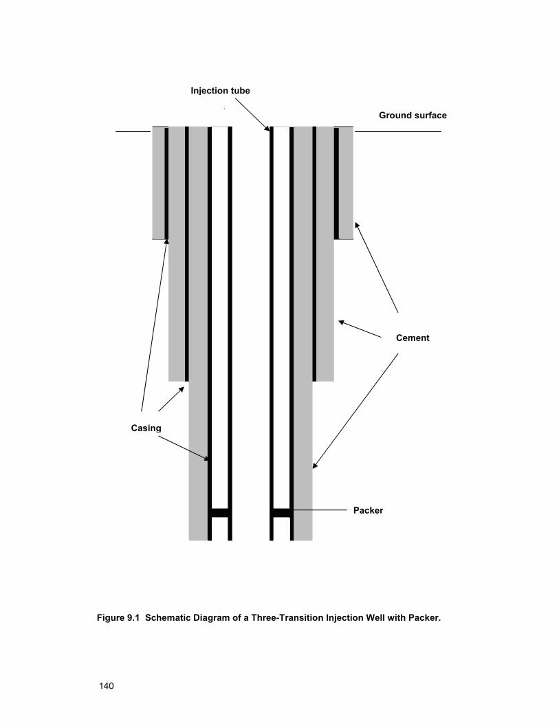
140

Packer

Casing

Cement

Injection tube

Ground surface

Figure 9.1 Schematic Diagram of a Three-Transition Injection Well with Packer.

141

caving in, and seals shallow freshwater aquifers from injection fluid contamination. The surface casing may extend as little as 200 feet or as far as 4,500 feet, depending on the well design and geologic conditions. At a minimum, the surface casing must be deep enough to reach solid formations that will not fracture or break down under the pressures imposed by the drilling fluid needed to reach the ultimate depth of the well. One or more intermediate casing strings are used to protect the bore hole at the lower depths by sealing off weak formations that could fracture under the drilling stresses. The final casing is the injection casing, which protects other formations from the injection fluid and houses the tubing and packer. Casing is distinguished from tubing with respect to its function and location in the well. Casing refers to the outer pipe string cemented in place to maintain structural integrity in the borehole and to seal upper aquifers. Tubing refers to the innermost pipe string through which injection takes place. A mechanical device called a packer seals the annular space between the tubing and casing.

Once the casing, tubing, and packer are in place, the annulus between the tubing and innermost casing is filled with a noncorrosive fluid, and positive pressure is maintained in the annulus. The presence of the tubing and packer isolates the injection fluid from the casing and, thus, provides corrosion protection to the casing. Although corrosion-resistant coating or liners may be applied to the casing, the integrity cannot be guaranteed, and these additions increase the cost of the well significantly. The annular fluid can also be monitored for pressure and analyzed periodically to detect failure of the tubing and allow corrective action to be taken before the failure is transmitted to the casing and contamination of ground water occurs.

The design of the deep well disposal system requires specification of 1) the flow rate of the concentrate or backwash stream in units of mgd, 2) the depth of the well in feet, and 3) the number of casing transitions (usually three or four). There are several independent cost factors such as the pump, the drilling and reaming, the casing, and others that are dependent on the values of these design parameters. Since the cost of the well is primarily labor and testing, the material costs and, thus, the diameter of the well are not major cost factors. Because of this, to allow for future increases in use, many wells are made of much larger diameter than required.

Depending on site conditions, deep well disposal can be an economical option. Costs of developing a disposal well are difficult to estimate for a generic site. Site-specific geological characteristics will vary, requiring different drilling depths and construction techniques (Mickley et al., 1993).

9.2.3 Design Basis – Flow Versus Tubing Diameter For most of the cost models, the size of the disposal option is based on flow rate of concentrate. For the deep well disposal, this is not always the case. Because the material costs are not the major cost factor for the deep injection wells, there

142

is relatively little penalty or additional cost for designing and building a well capable of receiving larger flows. This might be done to allow for future plant expansion or for future shared use of the well. It should be noted that if the tubing and packer requirements were not necessary for disposal of membrane concentrate, the tubing could be removed, resulting in effect in a much larger capacity deep injection well – limited by the diameter of the final casing string. Some wells in Florida are being designed and built with a larger than necessary final casing diameter for this future possibility. Because of lack of correlation between design flows and tubing size in the Florida deep wells, the cost basis was chosen to be the tubing diameter instead of the concentrate flow rate.

Correlations between flow and diameter are based on assumption of a flow formula such as the Hazen and Williams formula with a constant in the equation chosen to represent the flow-friction characteristics of different pipe materials. Specification of a maximum flow velocity then sets the correlation. For new steel pipe, table 9.1 gives the relationship between nominal internal pipe diameter and flow rate.

Table 9.1 Relationship Between Pipe Diameter and Flow Rate

Flow Rates (mgd) for Different Flow Velocities (fps)

Diameter (in) 5 fps 8 fps 10 fps

2 0.07 0.11 0.143 0.16 0.25 0.324 0.28 0.45 0.566 0.63 1.02 1.27

10 1.76 2.82 3.5212 2.54 4.06 5.0816 4.51 7.22 9.0220 7.05 11.28 14.1024 10.15 16.24 20.30

Although the design basis chosen for the following model is based on nominal tubing diameter, the above tabulation may be used to determine a correlation with allowable concentrate flow rate. For downhole injection, a velocity of 10 fps is recommended.

9.3 Cost Factors

9.3.1 Pretreatment The waste water to be injected may require pretreatment in an above-surface facility to prevent plugging in the receiving formation. When significant suspended solids are present, such as when concentrate is mixed with membrane

143

prefilter backwash and periodic cleaning waste, typical pretreatment consists of total suspended solid removal. Cartridge filters to remove 5 micron and larger particles may be required. Depending upon the specific characteristics of the waste water and receiving formation water, pH adjustment may also be necessary. When pH is adjusted, scale formation can be minimized with two incompatible waters. The cost of pretreatment cannot be estimated with general guidelines; a site-specific evaluation is necessary.

9.3.2 Pumps Pumps are used in above-surface facilities to inject the concentrate. The flow and pressure requirements are site specific. The discharge head will vary depending upon the geologic conditions and depth of the injection zone. Some municipal disposal wells operate at pressures as low as 3 to 6 pounds per square inch gauge (psig). More typical discharge pressures are in the range of 30 to 50 psig; however, much higher pressures are often required. Discharge as high as 2,000 to 5,000 psi can be encountered. To attain discharge pressures in this range, reciprocating pumps typically are used; and the pump cost increases drastically. At a 1992 installation, the cost of a reciprocating pump rated for 150 gpm at 3,180 psig was $150,000 (1992 costs). For low-head pumps, the cost would be approximately $10,000. Estimates of pumping costs for low-head pumps (less than 50 psig) can be obtained from figure 10.7. If higher-head pumps are required, a site-specific evaluation is necessary.

9.3.3 Site Tests – Logging, Surveying, and Testing Site tests are conducted following the initial drilling and throughout the repeated sequence of drilling (or reaming), setting casing, and setting cement. A final injection test is conducted before the drilling rig is disassembled. Early site tests include core samples obtained to determine the soil conditions, which indicate the most effective type of drilling. Water tests are also conducted to predict the compatibility of the formation water and the injected waste water. Based on the water tests, the required pretreatment can be established. As an example of how involved the logging and testing can be, table 9.2 lists events that took place at a disposal well in Florida.

Many of these tests are fairly independent of the well size and well depth. The total cost of logging, surveying, and testing is summarized in figure 9.2.

9.3.4 Injection Well Formation Deep injection wells are normally multicased. The use of more than one casing provides transition zones and isolates deep contaminated aquifers from the purer water contained in shallower aquifers. The injection tube is run from the surface to the deep aquifer where the water will be injected. The tube is encased in cement at least 5 inches thick to comply with environmental regulations. Intermediate depths of casing are selected based on the geological conditions at

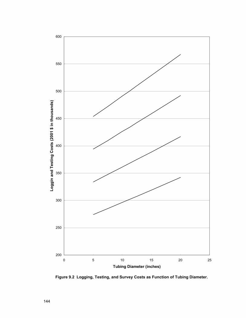
144

200

250

300

350

400

450

500

550

600

0 5 10 15 20 25

Tubing Diameter (inches)

Logg

in a

nd T

estin

g C

osts

(200

1 $

in th

ousa

nds)

Figure 9.2 Logging, Testing, and Survey Costs as Function of Tubing Diameter.

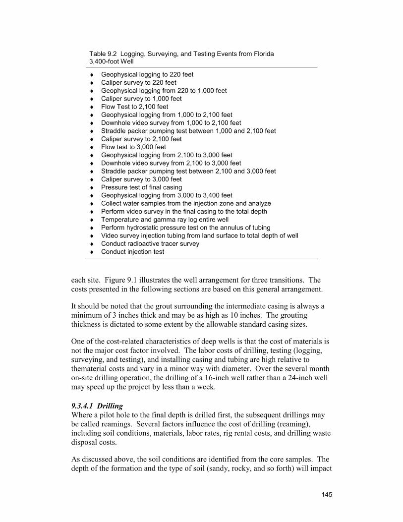
145

Table 9.2 Logging, Surveying, and Testing Events from Florida 3,400-foot Well

♦ Geophysical logging to 220 feet ♦ Caliper survey to 220 feet ♦ Geophysical logging from 220 to 1,000 feet ♦ Caliper survey to 1,000 feet ♦ Flow Test to 2,100 feet ♦ Geophysical logging from 1,000 to 2,100 feet ♦ Downhole video survey from 1,000 to 2,100 feet ♦ Straddle packer pumping test between 1,000 and 2,100 feet ♦ Caliper survey to 2,100 feet ♦ Flow test to 3,000 feet ♦ Geophysical logging from 2,100 to 3,000 feet ♦ Downhole video survey from 2,100 to 3,000 feet ♦ Straddle packer pumping test between 2,100 and 3,000 feet ♦ Caliper survey to 3,000 feet ♦ Pressure test of final casing ♦ Geophysical logging from 3,000 to 3,400 feet ♦ Collect water samples from the injection zone and analyze ♦ Perform video survey in the final casing to the total depth ♦ Temperature and gamma ray log entire well ♦ Perform hydrostatic pressure test on the annulus of tubing ♦ Video survey injection tubing from land surface to total depth of well ♦ Conduct radioactive tracer survey ♦ Conduct injection test

each site. Figure 9.1 illustrates the well arrangement for three transitions. The costs presented in the following sections are based on this general arrangement.

It should be noted that the grout surrounding the intermediate casing is always a minimum of 3 inches thick and may be as high as 10 inches. The grouting thickness is dictated to some extent by the allowable standard casing sizes.

One of the cost-related characteristics of deep wells is that the cost of materials is not the major cost factor involved. The labor costs of drilling, testing (logging, surveying, and testing), and installing casing and tubing are high relative to thematerial costs and vary in a minor way with diameter. Over the several month on-site drilling operation, the drilling of a 16-inch well rather than a 24-inch well may speed up the project by less than a week.

9.3.4.1 Drilling Where a pilot hole to the final depth is drilled first, the subsequent drillings may be called reamings. Several factors influence the cost of drilling (reaming), including soil conditions, materials, labor rates, rig rental costs, and drilling waste disposal costs.

As discussed above, the soil conditions are identified from the core samples. The depth of the formation and the type of soil (sandy, rocky, and so forth) will impact

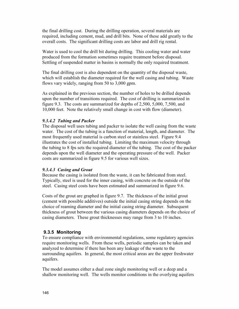
146

the final drilling cost. During the drilling operation, several materials are required, including cement, mud, and drill bits. None of these add greatly to the overall costs. The significant drilling costs are labor and drill rig rental.

Water is used to cool the drill bit during drilling. This cooling water and water produced from the formation sometimes require treatment before disposal. Settling of suspended matter in basins is normally the only required treatment.

The final drilling cost is also dependent on the quantity of the disposal waste, which will establish the diameter required for the well casing and tubing. Waste flows vary widely, ranging from 50 to 3,000 gpm.

As explained in the previous section, the number of holes to be drilled depends upon the number of transitions required. The cost of drilling is summarized in figure 9.3. The costs are summarized for depths of 2,500, 5,000, 7,500, and 10,000 feet. Note the relatively small change in cost with flow (diameter).

9.3.4.2 Tubing and Packer The disposal well uses tubing and packer to isolate the well casing from the waste water. The cost of the tubing is a function of material, length, and diameter. The most frequently used material is carbon steel or stainless steel. Figure 9.4 illustrates the cost of installed tubing. Limiting the maximum velocity through the tubing to 8 fps sets the required diameter of the tubing. The cost of the packer depends upon the well diameter and the operating pressure of the well. Packer costs are summarized in figure 9.5 for various well sizes.

9.3.4.3 Casing and Grout Because the casing is isolated from the waste, it can be fabricated from steel. Typically, steel is used for the inner casing, with concrete on the outside of the steel. Casing steel costs have been estimated and summarized in figure 9.6.

Costs of the grout are graphed in figure 9.7. The thickness of the initial grout (cement with possible additives) outside the initial casing string depends on the choice of reaming diameter and the initial casing string diameter. Subsequent thickness of grout between the various casing diameters depends on the choice of casing diameters. These grout thicknesses may range from 3 to 10 inches.

9.3.5 Monitoring To ensure compliance with environmental regulations, some regulatory agencies require monitoring wells. From these wells, periodic samples can be taken and analyzed to determine if there has been any leakage of the waste to the surrounding aquifers. In general, the most critical areas are the upper freshwater aquifers.

The model assumes either a dual zone single monitoring well or a deep and a shallow monitoring well. The wells monitor conditions in the overlying aquifers

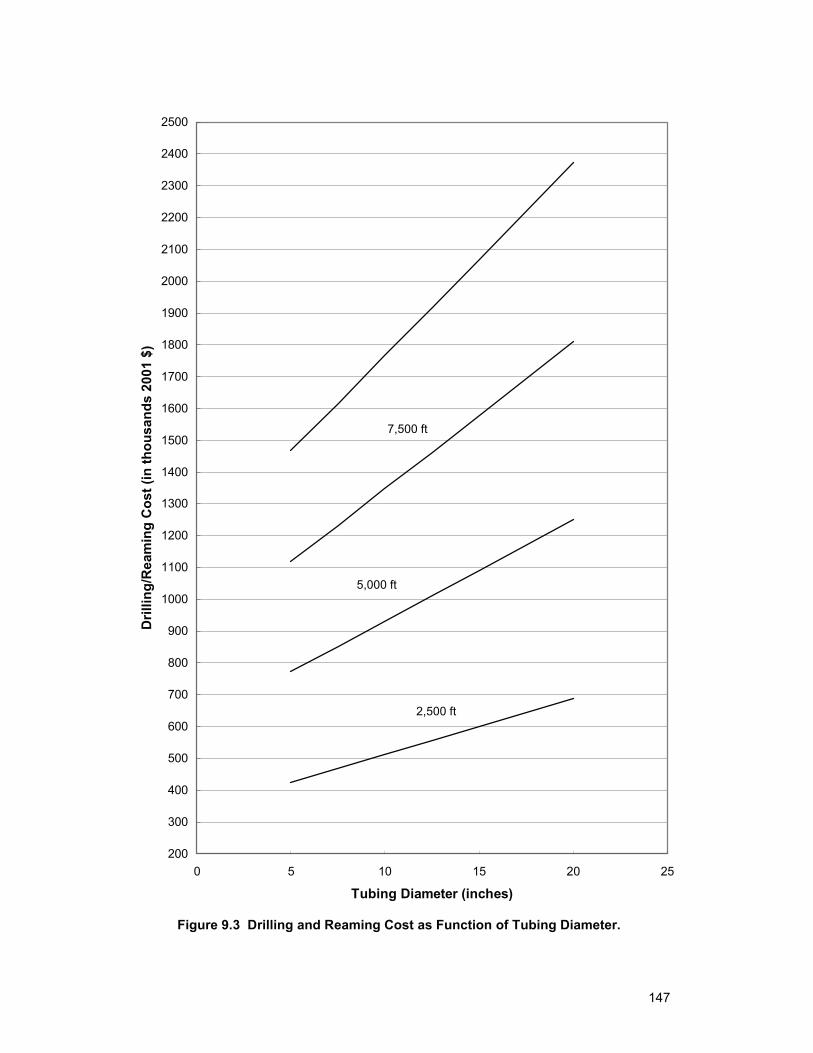
147

Figure 9.3 Drilling and Reaming Cost as Function of Tubing Diameter.

200

300

400

500

600

700

800

900

1000

1100

1200

1300

1400

1500

1600

1700

1800

1900

2000

2100

2200

2300

2400

2500

0 5 10 15 20 25

Tubing Diameter (inches)

Dril

ling/

Rea

min

g C

ost (

in th

ousa

nds

2001

$)

2,500 ft

5,000 ft

7,500 ft

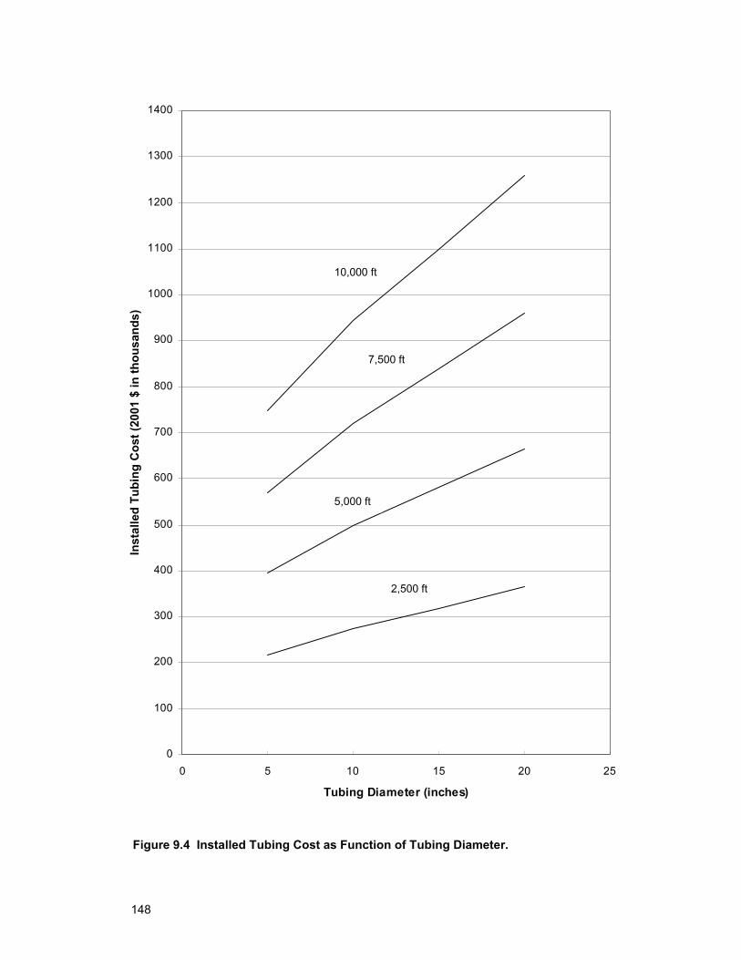
148

0

100

200

300

400

500

600

700

800

900

1000

1100

1200

1300

1400

0 5 10 15 20 25

Tubing Diameter (inches)

Inst

alle

d Tu

bing

Cos

t (20

01 $

in th

ousa

nds)

2,500 ft

5,000 ft

7,500 ft

10,000 ft

Figure 9.4 Installed Tubing Cost as Function of Tubing Diameter.

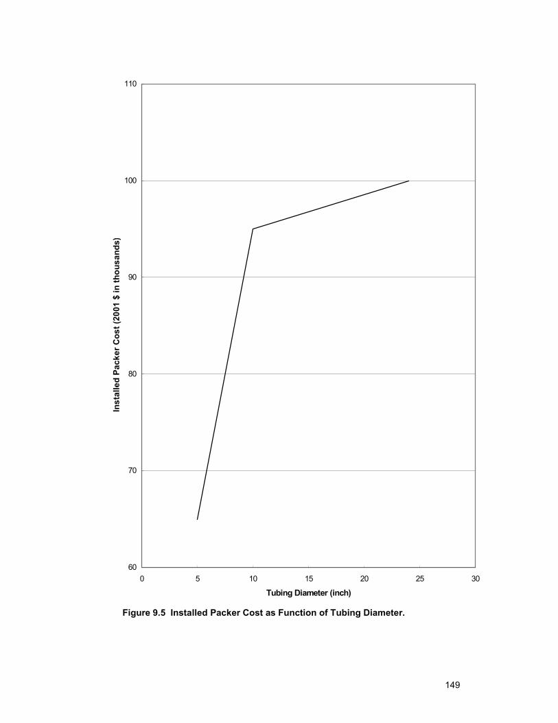
149

60

70

80

90

100

110

0 5 10 15 20 25 30

Tubing Diameter (inch)

Inst

alle

d Pa

cker

Cos

t (20

01 $

in th

ousa

nds)

Figure 9.5 Installed Packer Cost as Function of Tubing Diameter.

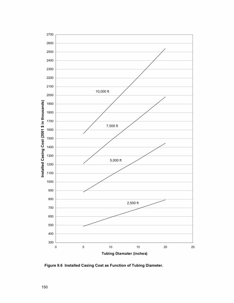
150

300

400

500

600

700

800

900

1000

1100

1200

1300

1400

1500

1600

1700

1800

1900

2000

2100

2200

2300

2400

2500

2600

2700

0 5 10 15 20 25

Tubing Diamater (inches)

Inst

alle

d C

asin

g C

ost (

2001

$ in

thou

sand

s)

2,500 ft

5,000 ft

7,500 ft

10,000 ft

Figure 9.6 Installed Casing Cost as Function of Tubing Diameter.

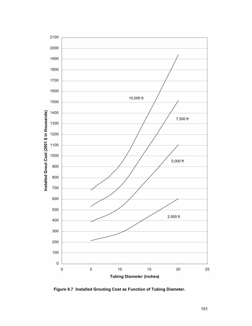
151

0

100

200

300

400

500

600

700

800

900

1000

1100

1200

1300

1400

1500

1600

1700

1800

1900

2000

2100

0 5 10 15 20 25

Tubing Diameter (inches)

Inst

alle

d G

rout

Cos

t (20

01 $

in th

ousa

nds)

10,000 ft

7,500 ft

5,000 ft

2,500 ft

Figure 9.7 Installed Grouting Cost as Function of Tubing Diameter.

152

that are structurally isolated from the confining, injection aquifer. The shallow well or upper monitoring zone of the dual zone well is to detect any changes in the upper freshwater aquifer. A deep monitoring well is also required to detect any changes in the deeper formation. The depth of the monitoring wells depends on the depths of the aquifers to be monitored, which, of course, is site specific. In Florida, most of the monitoring wells are approximately 2,000 feet in depth for deeper Boulder Zone deep injection wells and about 900 feet in depth for the Avon Park Formation shallower injection wells. Estimated monitoring costs are presented in figure 9.8.

9.3.6 Other Considerations Mobilization and demobilization will also constitute part of the total cost. The drilling rig must be assembled and then disassembled. These costs are represented in figure 9.9.

Systems handling waste water must take corrosion into account as a design consideration. Special materials can be used to minimize corrosion, but the cost of special alloys may be prohibitive. Utilization of a corrosion inhibitor is often more feasible. The corrosion inhibitors add to the operating cost but can be cost effective for flows of 200 gpm or less.

The interaction between the water and the formation water can form precipitates that plug the formation. To control this commingling, a buffer zone may need to be established. Injecting a quantity of neutral water before injecting the waste forms this buffer. This procedure has little impact on cost.

9.3.7 Operating Costs The operating costs for disposal wells are generally low. Well maintenance consists of periodically checking the casing and repairing it if required. Thus, a large capital cost (of $1,000,000 or more) can be offset by economical operating costs.

The operating costs encountered are for pumping power, chemical costs, and operating labor. Of these, the pumping power is the most significant. For the 150-gpm pump at 3,150 psig, a 350-horse power motor is required, resulting in a cost of more than $50,000 per year.

Chemical costs are normally much lower than this. For example, treating a waste flow of 150 gpm with a corrosion inhibitor would cost approximately as much as $7,000 per year. Thus, unless elaborate pretreatment is required, the chemical costs are not excessive.

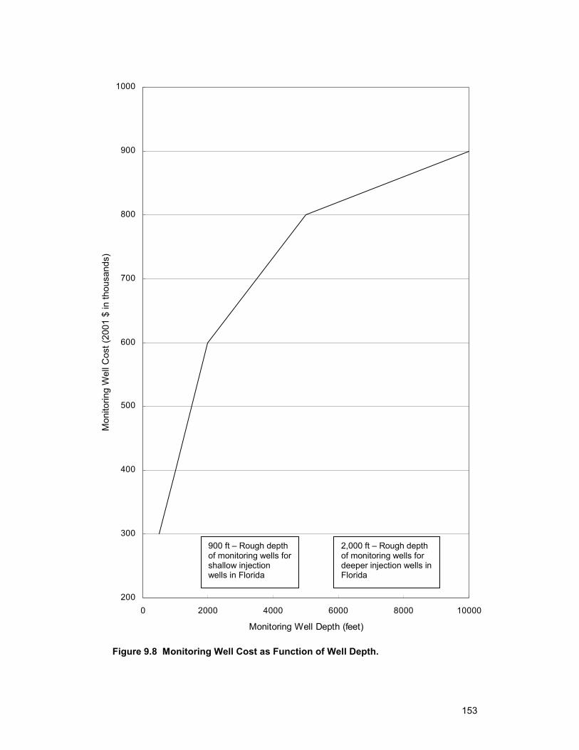
153

200

300

400

500

600

700

800

900

1000

0 2000 4000 6000 8000 10000

Monitoring Well Depth (feet)

Mon

itorin

g W

ell C

ost (

2001

$ in

thou

sand

s)

900 ft – Rough depth of monitoring wells for shallow injection wells in Florida

2,000 ft – Rough depth of monitoring wells for deeper injection wells in Florida

Figure 9.8 Monitoring Well Cost as Function of Well Depth.

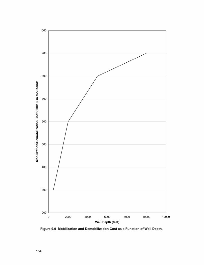
154

200

300

400

500

600

700

800

900

1000

0 2000 4000 6000 8000 10000 12000

Well Depth (feet)

Mob

iliza

tion/

Dem

obili

zatio

n C

ost (

2001

$ in

thou

sand

s

Figure 9.9 Mobilization and Demobilization Cost as a Function of Well Depth.

155

9.4 Design Approach for the Deep Well Disposal Cost Model

The costs of disposal by deep well injection are subject to many site-specific circumstances—perhaps more so than those of any other disposal method. The site terrain may vary considerably from site to site and may require substantial clearing, grading, and road building. The site may be close to a water source that can provide injection test water. Sometimes, the site can use city pumps and flow lines; other times, a series of pumps and lines might need to be set up. The costs are affected also by how many different groups are involved. The work may involve a general contractor, well driller, a group to do the packer tests, a group to do the logging, etc.; or it may involve one company tightly controlling all these elements. The work is also significantly affected by the geology of the area that determines aspects from the difficulty of drilling and reaming to the depths at which the casing strings are set.

The reader is cautioned to use the models provided only to obtain a preliminary level cost estimate. The supporting text should give the user an understanding from which to better determine, from a site-specific approach, more accurate costs involved in a deep well disposal system.

The design approach taken in the following worksheet model is straightforward but based on conditions in Florida, where nearly all of the deep well disposal of concentrate has occurred.

♦ The design approach chosen for the worksheet model is as follows: • The number of casing transitions (normally three or four in Florida) is not

broken out as a cost factor, but its influence is embedded in the other cost curves.

• The total well depth and the injection tubing diameter determine the following costs:

• Logging, testing, and survey

• Drilling and reaming

• Installed casing

• Installed grouting

• Installed injection tubing

• The diameter of the injection tubing determines the packer cost

• The injection well cost is the sum of these costs.

• The mobilization and demobilization cost is taken as 20 percent of the injection well cost.

• The monitoring well cost is determined from the monitoring well depth.

156

♦ The design variables thus include: • Total depth of the well • Diameter of the injection tubing

♦ Costs included in the capital cost model: • Drilling and reaming • Logging, testing, and survey • Installed casing • Installed grouting • Installed injection tubing • Installed packer • Mobilization and demobilization • Monitoring well

♦ Costs not included in the capital cost model: • Pretreatment • Pump

9.5 Deep Well Disposal Worksheet and Example

Based on the cost data provided in the figures, a preliminary capital cost estimate can be developed for a specific site. Such an estimate can provide an order-of-magnitude cost, but a specific site evaluation would be required to provide an accurate estimate.

The worksheet for deep well disposal is provided in table 9.3. An example calculation is provided in the column marked “example.” For this example, assume that a 16-inch nominal diameter injection tube is required. The well depth is 3,400 feet. The figures previously presented can now be applied to develop an estimated cost. From figure 9.2, a cost of $350,000 is obtained for logging of the injection well. The drilling and reaming costs, estimated from figure 9.3, are $790,000. Referring to figure 9.4, the cost is $430,000 for injection tubing in a 3,400-foot well. Based on the tubing diameter and well depth, the cost of packer, casing, and grouting are obtained from figures 9.5, 9.6, and 9.7, respectively. These costs are estimated at $97,000, $920,000, and $600,000, respectively. The monitoring well cost for a dual zone monitoring well is taken from figure 9.8 with an estimated cost of $600,000. Finally, the rig mobilization and demobilization cost is estimated from figure 9.9 to be $710,000. The total estimated cost is shown in table 9.3 to be $4,497,000.

9.6 Deep Well Disposal Regression Model

Based on about 35 cases from the worksheet, a closed form mathematical relation was developed to approximate the worksheet model. The user is reminded that the cost projections from both the worksheet model and the regression model that

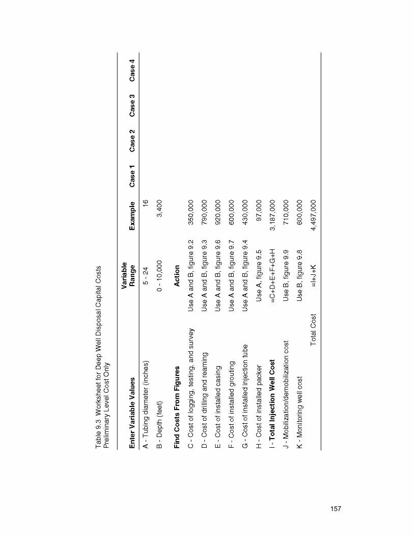
157

158

approximates the worksheet model are for preliminary level cost estimates only. The model developed below is linear in the various cost factors. The mathematical expression is:

Total Capital Cost ($) = -288,000 + 145,900 * TUBEDIAMETER + 754 * DEPTH

For the worksheet example conditions of:

TUBE DIAMETER = 16 inches DEPTH = 3,400 feet

the calculated total capital cost is $4,610,000, which compares to the worksheet result of $4,497,000.

159

10. Evaporation Pond Disposal 10.1 Background

Solar evaporation, a well established method for removing water from a concentrate solution, has been used for centuries to recover salt (sodium chloride) from seawater. There are also installations that are used for the recovery of sodium chloride and other chemicals from strong brines, such as the Great Salt Lake and the Dead Sea, and for the disposal of brines resulting from oil well operations (Office of Saline Water, 1971).

Evaporation ponds for membrane concentrate disposal are most appropriate for smaller volume flows and for regions having a relatively warm, dry climate with high evaporation rates, level terrain, and low land costs. These criteria apply predominantly in the western half of the United States—in particular, the southwestern portion.

Advantages associated with evaporation ponds are described in the following list:

♦ They are relatively easy and straightforward to construct.

♦ Properly constructed evaporation ponds are low maintenance and require little operator attention compared to mechanical equipment.

♦ Except for pumps to convey the waste water to the pond, no mechanical equipment is required.

♦ For smaller volume flows, evaporation ponds are frequently the least costly means of disposal, especially in areas with high evaporation rates and low land costs.

Despite the inherent advantages of evaporation ponds, they are not without disadvantages that can limit their application, as described in the following list:

♦ They can require large tracts of land if they are located where the evaporation rate is low or the disposal rate is high.

♦ Most States require impervious liners of clay or synthetic membranes such as polyvinylchloride (PVC) or Hypalon. This requirement substantially increases the costs of evaporation ponds.

♦ Seepage from poorly constructed evaporation ponds can contaminate underlying potable water aquifers.

♦ There is little economy of scale for this land-intensive disposal option. Consequently, disposal costs can be large for all but small-sized membrane plants.

160

In addition to the potential for contamination of ground water, evaporation ponds have been criticized because they do not recover the water evaporated from the pond. However, the water evaporated is not “lost”; it remains in the atmosphere for about 10 days and then returns to the surface of the earth as rain or snow. This hydrologic cycle of evaporation and condensation is essential to life on land and is largely responsible for weather and climate.

10.2 Design Considerations

10.2.1 Sizing of Evaporation Ponds Evaporation ponds function by transferring liquid water in the pond to water vapor in the atmosphere above the pond. The rate at which an evaporation pond can transfer this water governs the size of the pond. Selection of pond size requires determination of both the surface area and the depth needed. The surface area required is dependent primarily on the evaporation rate. The pond must have adequate depth for surge capacity and water storage, storage capacity for precipitated salts, and freeboard for precipitation (rainfall) and wave action.

10.2.1.1 Determining the Evaporation Rate Proper sizing of an evaporation pond depends on accurate calculation of the annual evaporation rate. Evaporation from a freshwater body, such as a lake, is dependent on local climatological conditions, which are very site specific. To develop accurate evaporation data throughout the United States, meteorological stations have been established at which special pans simulate evaporation from large bodies of water such as lakes, reservoirs, and evaporation ponds. The pans are fabricated to standard dimensions and are situated to be as representative of a natural body of water as possible. A standard evaporation pan is referred to as a Class A pan. The standardized dimensions of the pans and the consistent methods for collecting the evaporation data allow comparatively and reasonably accurate data to be developed for the United States. The data collection must cover several years to be reasonably accurate and representative of site-specific variations in climatic conditions. Published evaporation rate databases typically cover a 10-year or more period and are expressed in inches per year.

The pan evaporation data from each site can be compiled into a map of pan evaporation rates. Because of the small heat capacity of evaporation ponds, they tend to heat and cool more rapidly than adjacent lakes and to evaporate at a higher rate than an adjacent natural pond of water. In general, experience has shown the evaporation rate from large bodies of water to be approximately 70 percent of that measured in a Class A pan (Reclamation, 1969). This percentage is referred to as the Class A pan coefficient and must be applied to measured pan evaporation to arrive at actual lake evaporation. Over the years, site-specific Class A pan coefficients have been developed for the entire United States. Multiplying the pan evaporation rate by the pan coefficient results in a mean annual lake evaporation rate for a specific area.

161

Maps depicting annual average precipitation across the United States also are available. Subtracting the mean annual evaporation from the mean annual precipitation gives the net lake surface evaporation in inches per year. This is the amount of water that will evaporate from a freshwater pond (or the amount the surface level will drop) over a year if no water other than natural precipitation enters the pond. All these maps assume an impervious pond that allows no seepage. Note, that for some parts of the country, the results of this calculation give a negative number; and in other parts of the country, it is a positive number. A negative number indicates a net loss of water from a pond over a year, or a drop in the pond surface level. A positive number indicates more precipitation than evaporation at a particular site. A freshwater pond at one of these sites would actually gain water over a year, even if no water other than natural precipitation were added. Thus, such a site would not be a candidate for an evaporation pond.

It is important to realize that data of this type are representative only of the particular sites of the individual meterological stations, which may be separated by many miles. Climatic data specific to the exact site should be obtained if at all possible before actual construction of an evaporation pond.

The evaporation data described above are for freshwater pond evaporation. However, brine density has a marked effect on the rate of solar evaporation. Most procedures for calculating evaporation rate indicate evaporation is directly proportional to vapor pressure. Salinity reduces evaporation primarily because the vapor pressure of the saline water is lower than that of freshwater and because dissolved salts lower the free energy of the water molecules. Cohesive forces acting between the dissolved ions and the water molecules may also be responsible for inhibiting evaporation, making it more difficult for the water to escape as vapor (Miller, 1989).

The lower vapor pressure and lower evaporation rate of saline water result in a lower energy loss and, thus, a higher equilibrium temperature than that of freshwater under the same exposure conditions. The increase in temperature of the saline water would tend to increase evaporation, but the water is less efficient in converting radiant energy into latent heat due to the exchange of sensible heat and long-wave radiation with the atmosphere. The net result is that, with the same input of energy, the evaporation rate of saline water is lower than that of freshwater.

For water saturated with sodium chloride salt (26.4 percent), the solar evaporation rate is generally about 70 percent of the rate for freshwater (Office of Saline Water, 1971). Studies have shown that the evaporation rate from the Great Salt Lake, which has a TDS level of between 240,000 and 280,000 mg/L, is about 80 to 82 percent of the rate for freshwater. Other studies indicate that evaporation rates of 2-, 5-, 10-, and 20-percent sodium chloride solutions are 97, 98, 93, and 78 percent, respectively, of the rates of freshwater (Reclamation, 1969). These ratios are determined from both experiment and theory. However, there is no simple relationship between salinity and evaporation, for there are always

162

complex interactions among site-specific variables such as air temperature, wind velocity, relative humidity, barometric pressure, water surface temperature, heat exchange rate with the atmosphere, incident solar absorption and reflection, thermal currents in the pond, and depth of the pond. As a result, these ratios should be used only as guidelines and with discretion. It is important to recognize that salinity can significantly reduce evaporation rate and to allow for this effect in sizing the evaporation pond’s surface area. In lieu of site-specific data, an evaporation ratio of 0.70 is a reasonable allowance for long-term evaporation reduction. This ratio is also considered to be an appropriate factor for evaporation ponds that are expected to reach salt saturation over their anticipated service life.

10.2.1.2 Pond Depth Studies indicate that pond depths ranging from 1 to 18 inches are optimal for maximizing evaporation rate. However, similar studies indicate only a 4-percent reduction in the evaporation rate as the pond depth is increased from 1 to 40 inches. (Reclamation, 1969). Very shallow evaporation ponds are subject to drying and cracking of the liners and are not functional in long-term service for concentrate disposal. From a practical operating standpoint, an evaporation pond must not only evaporate waste water but also provide

♦ Surge capacity or contingency water storage ♦ Storage capacity for precipitated salts ♦ Freeboard for precipitation and wave action

For an evaporation pond to be a viable disposal alternative for membrane concentrate, it must be able to accept concentrate at all times and under all conditions so as not to restrict operation of the desalination plant. The pond must be able to accommodate variations in the weather and upsets in the desalination plant. The desalination plant cannot be shut down because the evaporation pond level is rising faster than anticipated.

To allow for unpredictable circumstances, it is important that design contingencies be applied to the calculated pond area and depth. Experience from the design of industrial evaporation ponds has shown that discharges are largest during the first year of plant operation, are reduced during the second year, and are relatively constant thereafter. A long-term, 20-percent contingency may be applied to the surface areas of the pond or its capacity to continuously evaporate water. The additional contingencies above the 20 percent (up to 50 percent) during the first and second years of operation are applied to the depth holding capacity of the pond.

Freeboard for precipitation should be estimated on the basis of precipitation intensity and duration for the specific site. There may also be local codes governing freeboard requirements. In lieu of site-specific data, an allowance of 6 inches for precipitation is generally adequate where evaporation ponds are most likely to be located in the United States (Office of Saline Water, 1970).

163

Freeboard for wave action can be estimated as follows (Office of Saline Water, 1970):

Hw = 0.047 * W * √(F)

Where: Hw = wave height (ft) W = wind velocity (mph) F = fetch, or straight line distance the wind can blow without obstruction (mi)

The run-up of waves on the face of the dike approaches the velocity head of the waves and can be approximated as 1.5 * Hw. Hw is the freeboard allowance for wave action and typically ranges from 2 to 4 feet. The minimum recommended combined freeboard (for precipitation and wave action) is 2 feet. This minimum applies primarily to small ponds.

Over the life of the pond (which should be sized for the same duration as the projected life of the desalination facility), the water will likely reach saturation and precipitate salts. The type and quantity of salts is highly variable and very site specific. Allowance in the pond depth for precipitate salts can be made using figure 10.1, which provides an estimate for the depth of precipitate produced as a function of the salinity of the waste water discharged to the pond (Office of Saline Water, 1970). For a given salinity, figure 10.1 provides an estimate of precipitate produced (in feet per year [ft/yr]) for each foot of waste water discharged to the pond. Multiplying the annual deposition depth times the depth of water discharged to the pond each year and then by the life of the pond will result in the necessary allowance for the life of the pond.

10.3 Cost Parameters

Although sizing of an evaporation pond is a relatively straightforward procedure once appropriate net evaporation data are available, the costs associated with pond construction are highly site specific and quite variable. Therefore, generic cost estimating of evaporation ponds from typical handbook-type data is very difficult and subject to a wide range of accuracy. However, by gathering site-specific data, a reasonably accurate cost estimate can be made.

The following section sets forth the steps necessary to accurately determine the cost of an evaporation pond. Typical cost data are used. Graphs of the various costs for an evaporation pond can be used as the basis for determining site-specific costs. For some applications, an evaporation pond can be a cost-effective disposal alternative; in other locations, the cost can be prohibitive.

In general, it is anticipated that evaporation ponds most likely will be competitive for relatively small plants in remote, inland locations with high evaporation rates. Large membrane treatment plants are typically located near large population

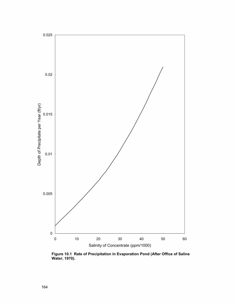
164

0

0.005

0.01

0.015

0.02

0.025

0 10 20 30 40 50 60

Salinity of Concentrate (ppm/1000)

Dep

th o

f Pre

cipi

tate

per

Yea

r (ft/

yr)

Figure 10.1 Rate of Precipitation in Evaporation Pond (After Office of Saline Water, 1970).

165

centers, where the availability of large tracts of inexpensive land will generally be limited. The major factors contributing to the cost of an evaporation pond are:

♦ Land costs ♦ Earthwork ♦ Lining ♦ Miscellaneous cost ♦ Operation and maintenance

10.3.1 Land Costs The cost of land can vary greatly from site to site. In general, however, the cost of land at locations appropriate for evaporation ponds is a small percentage of the total cost. Costs vary not only from city to city but also in the vicinity of a particular municipality itself. Land costs can easily vary by a factor of 10 or more, depending on the exact location near the city.

10.3.2 Earthwork Like the cost of land itself, the cost of earthwork is very site specific, depending on whether the terrain is flat or hilly, rocky or sandy, forested or clear, etc. In selecting a site for an evaporation pond, such factors must be considered in making the final selection. Of course, in some cases, there are only limited choices. If the desalination plant location is fixed by the proximity of the water source or the locus of the demand for the desalted water, the evaporation pond must be located reasonably close by. However, certain aspects are generic, however; typical construction features for an evaporation pond include the following:

♦ Land clearing ♦ Perimeter dikes ♦ Baffle dikes (optional) ♦ Dike covers

Land is required for the evaporative surface area and for the perimeter area that includes the dike, road, and fence. This distinction between evaporative area and total area is important in determining land requirements. Figures 10.2 and 10.3 provide an area correction factor to multiply times the evaporative area to calculate the total area. The correction factor value depends on the evaporative area and the dike height. This correction factor will be applied in determining land and land clearing costs.

10.3.2.1 Land Clearing The initial step in the construction of the pond consists of clearing the land. Land clearing can be labor intensive, and the cost is dependent upon the specific characteristics of each site. Costs can be categorized based on the type of.

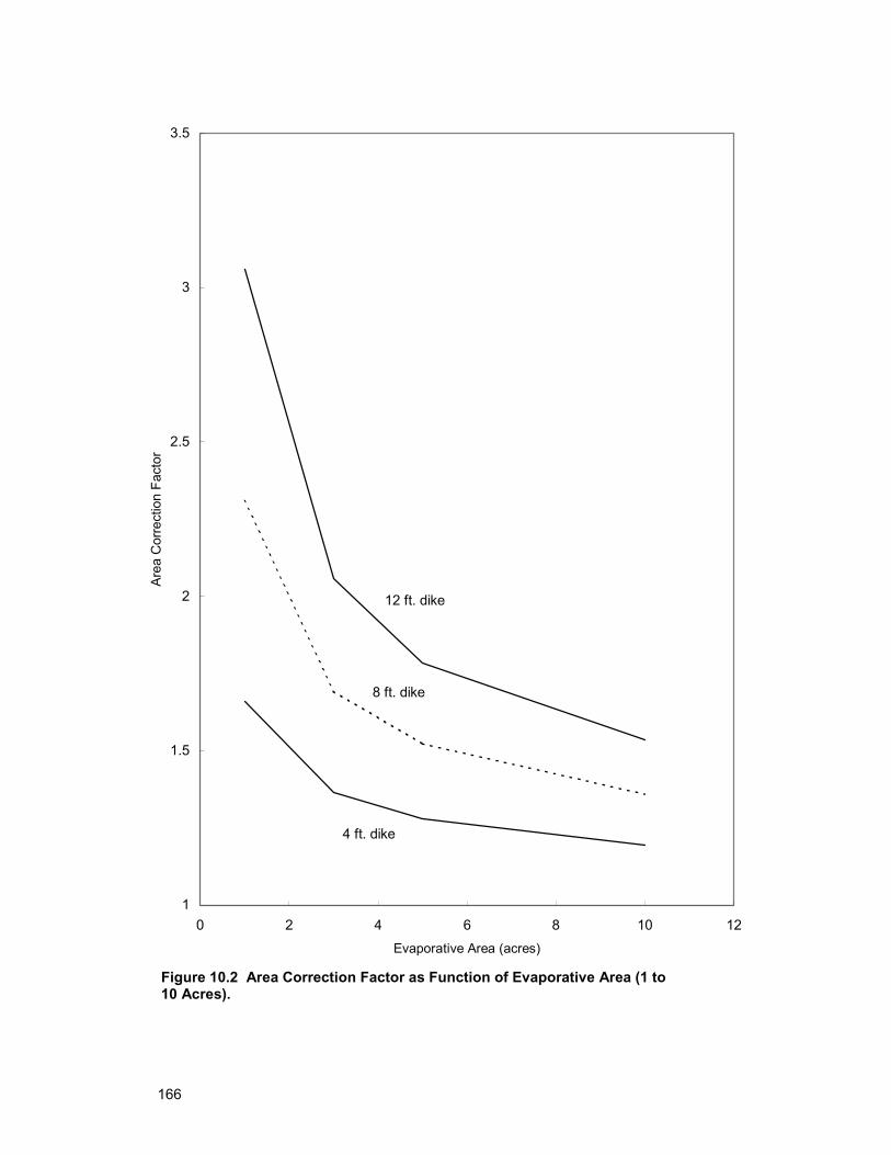
166

1

1.5

2

2.5

3

3.5

0 2 4 6 8 10 12Evaporative Area (acres)

Are

a C

orre

ctio

n Fa

ctor

12 ft. dike

8 ft. dike

4 ft. dike

Figure 10.2 Area Correction Factor as Function of Evaporative Area (1 to 10 Acres).

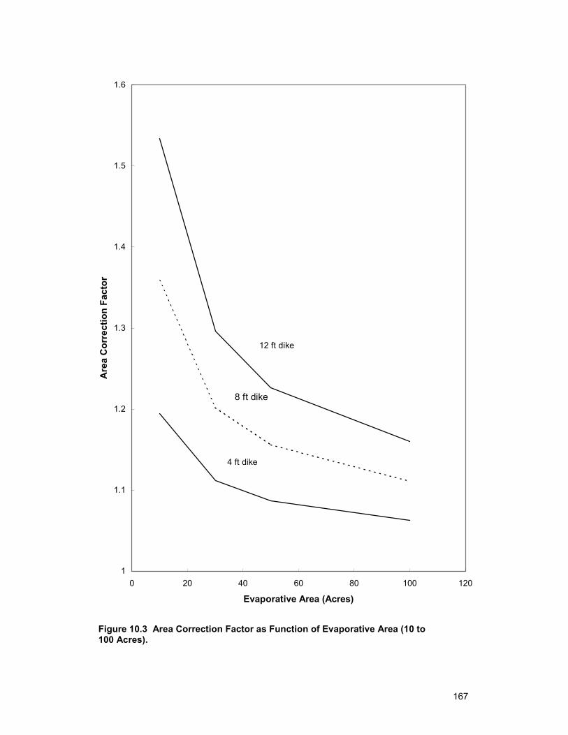
167

1

1.1

1.2

1.3

1.4

1.5

1.6

0 20 40 60 80 100 120

Evaporative Area (Acres)

Are

a C

orre

ctio

n Fa

ctor

12 ft dike

8 ft dike

4 ft dike

Figure 10.3 Area Correction Factor as Function of Evaporative Area (10 to 100 Acres).

168

vegetation at the site. The typical cost for clearing brush is $1,000 per acre; for sparsely wooded areas, $2,000 per acre; for medium-wooded areas, $4,000 per acre; and for heavily wooded areas, $7,000 per acre

10.3.2.2 Dikes Dike construction, which is also labor intensive, involves excavating part of the soil and using it for the dike. Evaporation pond dikes are typically constructed with a 2:1 to 4:1 slope and a 12-foot top width that provides for a maintenance roadway. Generally, the excavated earth is sufficient for the dike’s construction. The configuration of the pond determines the dike perimeter. To minimize the perimeter and the associated costs, the pond should be square.

The major variable in dike design is the required height. The pond depth is set by the volume required to accumulate sludge and the height required to prevent overflow due to wave action. Dike heights of 4 to 12 ft are typical. Figures 10.4 and 10.5 summarize the cost of dikes with 4-ft, 8-ft, and 12-ft heights and acreages of 1 to 10 and 10 to 100 acres. These costs include material and labor for dike construction.

Dike heights can be lower if the evaporation pond solids are periodically cleaned out. For cleanout, either a baffled single pond or multiple ponds are provided. A single pond designed for cleanout is baffled to allow sections of the pond to operate while other sections are cleaned. Figure 10.6 illustrates this arrangement. This scheme provides for a pond of smaller acreage as well as lower dike height. The water level can be lower, thus increasing the temperature, which will increase the evaporation rate and reduce the area required. The baffling will also help to settle the precipitates in a relatively uniform pattern, helping to minimize the required pond depth. Often one section is dried, and silt is placed over the salt precipitates to prevent the salts from redissolving as new waste water is introduced. This practice also increases the net evaporation rate. The disposal costs for periodic cleaning of a baffled pond can be substantial and frequently rule out this option.

10.2.2.3 Liners Evaporation ponds have been used for decades for the disposal of liquid wastes. Historically numerous unlined evaporation ponds have been used as catchall disposal sites for a variety of wastes. Dumping in unlined evaporation ponds has frequently contributed to contamination of ground water supplies with hazardous chemicals. Once contaminated, ground water supplies are very difficult and expensive to clean up.

Because the potential for ground water contamination exists with any evaporation pond, most States require impervious liners of clay or synthetic membranes, which substantially increase the cost. Where the waste discharged to the pond can be verified as nonhazardous and the ground water in the area is of poor quality or substantially distant from the pond, or both, a single liner may be acceptable. However, if the water has the potential to contain even trace amounts of

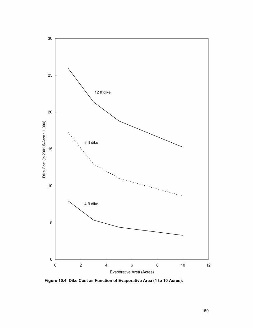
169

0

5

10

15

20

25

30

0 2 4 6 8 10 12

Evaporative Area (Acres)

Dik

e C

ost (

in 2

001

$/A

cre

* 1,

000)

12 ft dike

8 ft dike

4 ft dike

Figure 10.4 Dike Cost as Function of Evaporative Area (1 to 10 Acres).

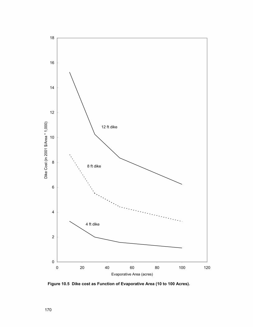
170

0

2

4

6

8

10

12

14

16

18

0 20 40 60 80 100 120Evaporative Area (acres)

Dik

e C

ost (

in 2

001

$/A

rea

* 1,

000)

12 ft dike

8 ft dike

4 ft dike

Figure 10.5 Dike cost as Function of Evaporative Area (10 to 100 Acres).

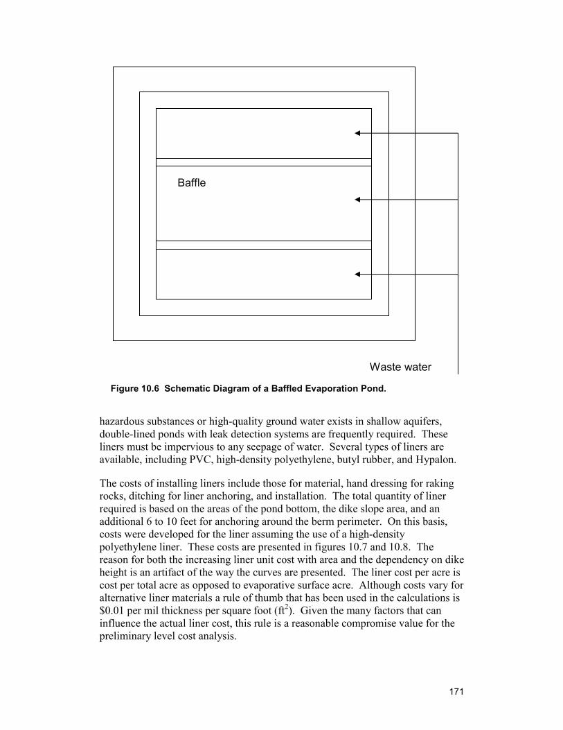
171

hazardous substances or high-quality ground water exists in shallow aquifers, double-lined ponds with leak detection systems are frequently required. These liners must be impervious to any seepage of water. Several types of liners are available, including PVC, high-density polyethylene, butyl rubber, and Hypalon.

The costs of installing liners include those for material, hand dressing for raking rocks, ditching for liner anchoring, and installation. The total quantity of liner required is based on the areas of the pond bottom, the dike slope area, and an additional 6 to 10 feet for anchoring around the berm perimeter. On this basis, costs were developed for the liner assuming the use of a high-density polyethylene liner. These costs are presented in figures 10.7 and 10.8. The reason for both the increasing liner unit cost with area and the dependency on dike height is an artifact of the way the curves are presented. The liner cost per acre is cost per total acre as opposed to evaporative surface acre. Although costs vary for alternative liner materials a rule of thumb that has been used in the calculations is $0.01 per mil thickness per square foot (ft2). Given the many factors that can influence the actual liner cost, this rule is a reasonable compromise value for the preliminary level cost analysis.

Baffle

Waste water

Figure 10.6 Schematic Diagram of a Baffled Evaporation Pond.

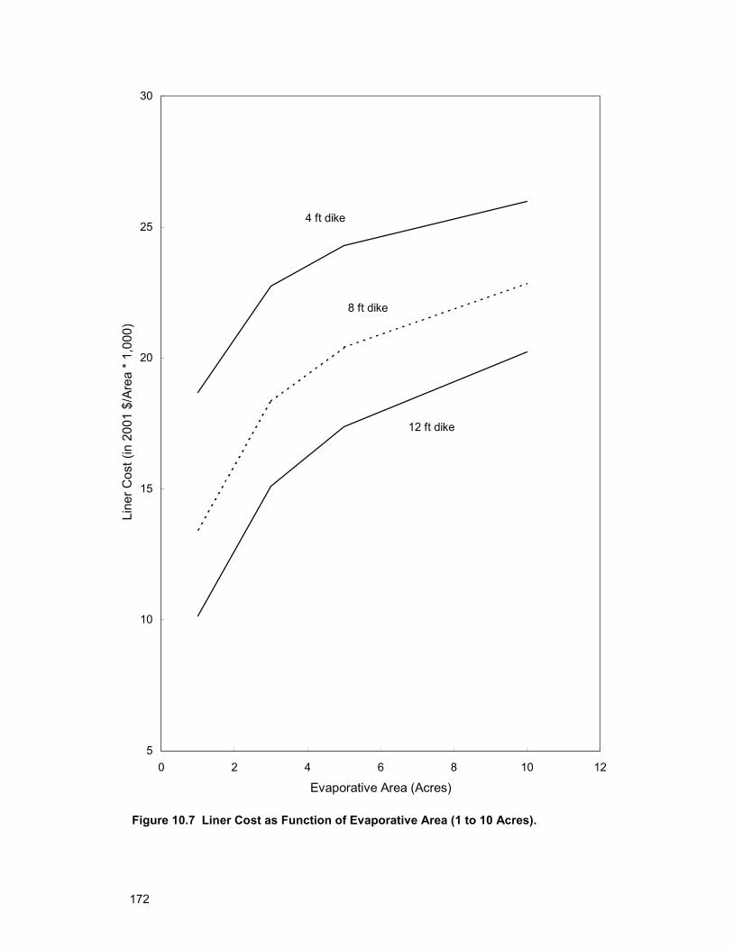
172

5

10

15

20

25

30

0 2 4 6 8 10 12

Evaporative Area (Acres)

Line

r Cos

t (in

200

1 $/

Are

a *

1,00

0)

4 ft dike

8 ft dike

12 ft dike

Figure 10.7 Liner Cost as Function of Evaporative Area (1 to 10 Acres).

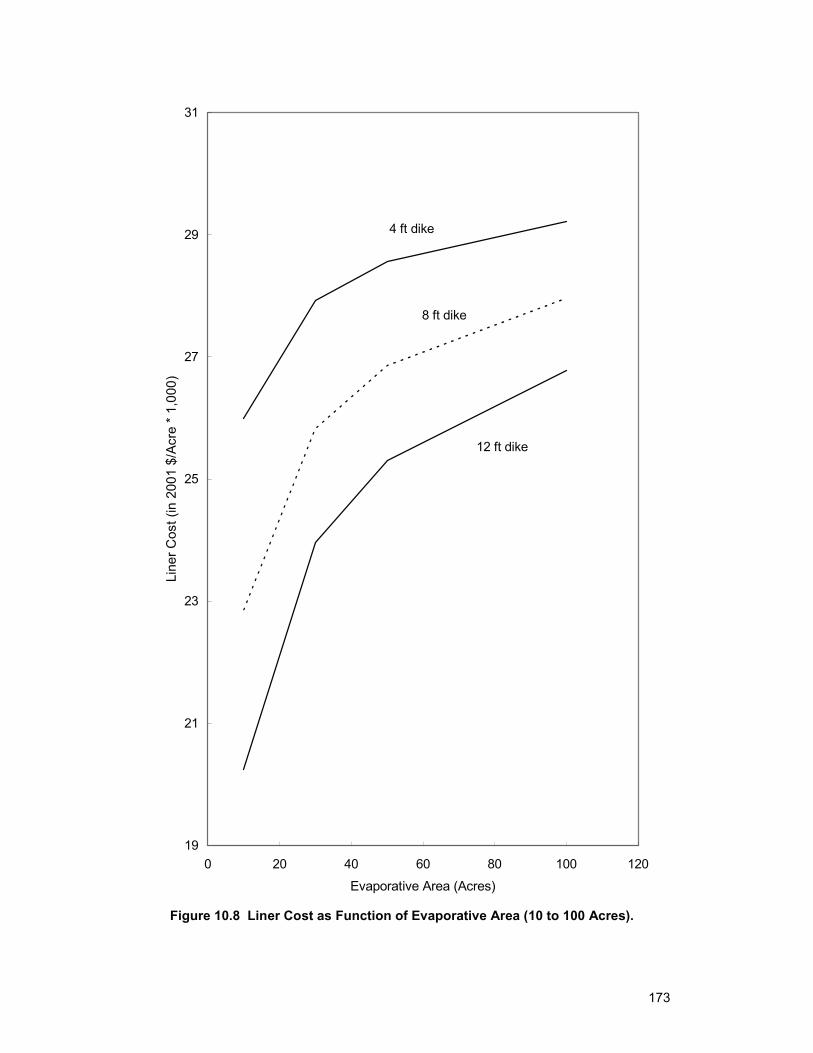
173

19

21

23

25

27

29

31

0 20 40 60 80 100 120

Evaporative Area (Acres)

Line

r Cos

t (in

200

1 $/

Acre

* 1

,000

)

4 ft dike

8 ft dike

12 ft dike

Figure 10.8 Liner Cost as Function of Evaporative Area (10 to 100 Acres).

174

10.3.3 Miscellaneous Costs The following costs depend upon the needs of the specific installation; they may constitute a significant percentage of the total cost of the evaporation pond installation. Some of these possible costs include:

♦ Fencing ♦ Maintenance roadways ♦ Disposal ♦ Seepage monitoring ♦ Contaminated ground cleanup

10.3.3.1 Fencing If the evaporation pond is not part of the main plant property, the cost of fencing should be applied to the cost of pond development. Fencing is required for several reasons. The membrane-lined sides of evaporation ponds are relatively steep and slick and pose a very real hazard for people and animals that might wander into the area. Fencing is also required for security purposes, to preclude acts of vandalism and unauthorized dumping. Installed fence costs are relatively standard and are estimated at $15 per linear foot. Figures 10.9 and 10.10 provide estimates for the cost of fencing. The height of the dike impacts the size of the perimeter slightly—and, thus, the length of fence. This factor, however, is negligible in the context of the present model.

10.3.3.2 Maintenance Roadways For large evaporation ponds, maintenance roadways facilitate security patrols and routine inspection of the pond and provide access for maintenance vehicles. In some bids, the labor for constructing a roadway may be considered as part of the dike construction. In the following, however, this cost has been separated as the labor and material for construction a gravel roadbed. Figures 10.11 and 10.12 illustrate the cost of the roadbed for various sizes of ponds based on $15 per cubic yard.

10.3.3.3 Disposal The solid precipitates collected in the pond may require periodic disposal if the pond is not large enough to hold the total volume of sludge produced during the life of the plant. This may occur either because the solids contribution to the pond is especially high (high suspended solids in the water stream, large amounts of windblown dirt, and the like), or because the pond has a shallow depth to enhance the evaporation rate or to avoid the local water table.

The cost for solids disposal include dredging the solids from the pond, transporting the solids, and landfill disposal costs. In isolated cases, the solids may require stabilization if hazardous materials (e.g., heavy metals) are present in the pond.

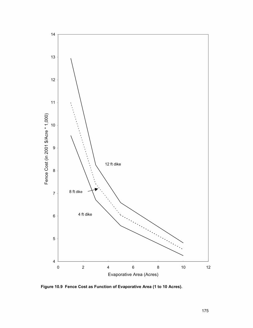
175

4

5

6

7

8

9

10

11

12

13

14

0 2 4 6 8 10 12

Evaporative Area (Acres)

Fenc

e C

ost (

in 2

001

$/A

cre

* 1,

000)

12 ft dike

8 ft dike

4 ft dike

Figure 10.9 Fence Cost as Function of Evaporative Area (1 to 10 Acres).

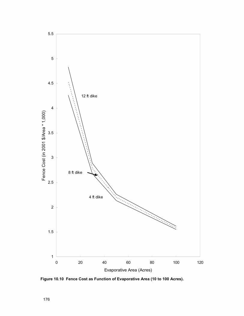
176

1

1.5

2

2.5

3

3.5

4

4.5

5

5.5

0 20 40 60 80 100 120

Evaporative Area (Acres)

Fenc

e C

ost (

in 2

001

$/Ar

ea *

1,00

0)

12 ft dike

4 ft dike

8 ft dike

Figure 10.10 Fence Cost as Function of Evaporative Area (10 to 100 Acres).

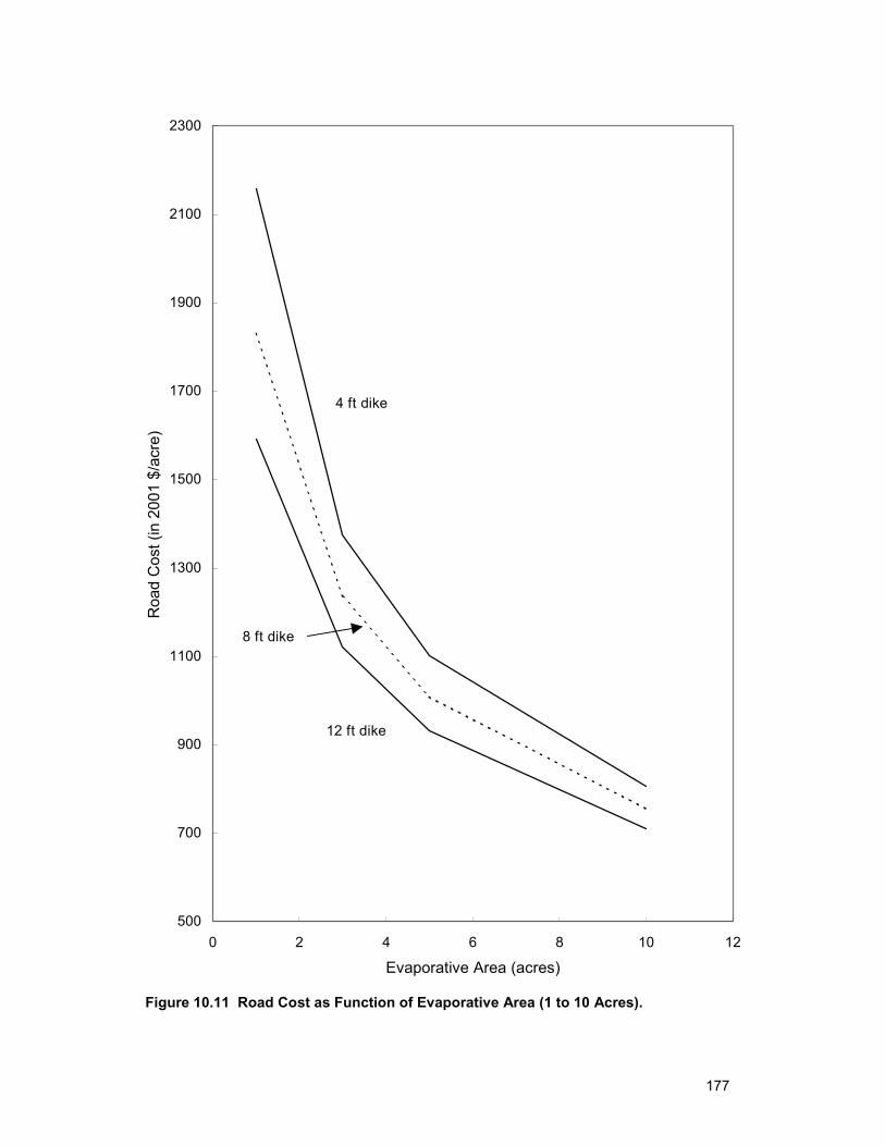
177

500

700

900

1100

1300

1500

1700

1900

2100

2300

0 2 4 6 8 10 12

Evaporative Area (acres)

Roa

d C

ost (

in 2

001

$/ac

re)

4 ft dike

8 ft dike

12 ft dike

Figure 10.11 Road Cost as Function of Evaporative Area (1 to 10 Acres).

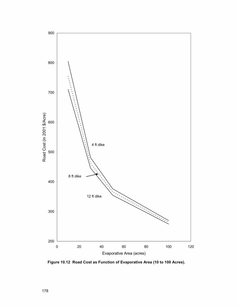
178

200

300

400

500

600

700

800

900

0 20 40 60 80 100 120

Evaporative Area (acres)

Roa

d C

ost (

in 2

001

$/Ac

re)

4 ft dike

12 ft dike

8 ft dike

Figure 10.12 Road Cost as Function of Evaporative Area (10 to 100 Acres).

179

10.3.3.4 Seepage Monitoring Seepage monitoring or leak detection may be required, depending on the pond construction, the proximity and quality of nearby aquifers, or both. Single-lined ponds allow for no direct means of detecting seepage until the water has left the pond. However, for relatively clean wastes such as most membrane concentrates, a single-lined pond used in conjunction with monitoring wells may satisfy local regulatory requirements. For contaminated wastes or in locations where high-quality aquifers are present, a double-lined pond may be required to assure the integrity of the disposal site. In double-lined ponds, a porous layer is provided between the two liners. Should the first liner leak, the waste water will pass into the porous layer and drain to a monitoring sump, where it will be detected. Until draining or repair of the pond, or both, is affected, the second liner prevents ground water contamination. For large ponds where draining of the porous layer to a sump is not practical because of the distances involved, electronic moisture detectors or lysimeters can be embedded in the porous layers at regular intervals to detect primary liner leaks.

Where evaporation ponds are located in an area of known previous ground water contamination, the owner may install monitoring wells around the pond, not to detect pond leaks but to establish a historical record of the existing ground water contamination in the area. Then, if additional contamination should occur in the area, the owner of the pond can provide water quality monitoring data from the wells, along with periodic samples of the waste water in the pond, to assure the regulatory agencies that any additional ground water contamination did not originate from the pond.

To detect seepage around the pond, several methods may be used: bore holes, monitoring wells, or moisture detectors. The costs of these depend upon the required monitoring depth.

10.3.3.5 Contaminated Ground Cleanup The earth surrounding the evaporation pond may become contaminated through contact with the waste water. The contamination could be the result of seepage or upset overflows from the pond. Cleanup of contaminated soils is becoming a cost factor in many States, but the requirements for cleanup are too varied at this time to reasonably predict the costs. Site-specific evaluations are required.

10.3.4 Operating Costs Once it has been constructed, the pond operates essentially maintenance free. Periodic maintenance is required only for the repair of the dike or liner, pipe, flow control devices, etc. Operating costs also include security and damage inspection. The annual operating costs can be estimated at 0.5 percent of the total installation costs.

180

10.4 Design Approach for the Evaporation Pond Cost Model

♦ The climatic variables are key in the determination of the effective evaporation rate. This is not a simple matter and is perhaps the most critical design variable.

♦ The model assumes that the effective evaporation rate is known.

♦ Once known, this determines the total evaporation surface required. A contingency factor of 20 percent is included in the evaporation surface required.

♦ The design challenge is to determine the suitable evaporation pond depth or conversely the dike height. This depends on the nature of the solution to be evaporated.

♦ Standard tables exist for calculating the sludge buildup with time as a function of solution salinity.

♦ The dike design variables include dike height (pond depth plus freeboard), dike slope ratio, and dike width at top.

♦ Typically, only enough earth will be excavated to build the dikes.

♦ The total earth to be moved depends on the amount of dike, and this depends on pond size. The entire evaporative surface can be from one or many ponds. Typically, the largest possible pond size is used, as this minimizes costs associated with earth moving, liner installation, road construction, and other costs.

♦ Pond size, however, depends on the wind level and the possibility of dike erosion.

♦ Dike height has a similar effect on dike cost as total system size, and both have a much greater effect on dike cost than the number of ponds.

♦ As the total pond size decreases, the dike physically makes up more of the total area of the system.

♦ The ratio of dike costs for different dike heights holds for any size system, as it is a function only of the relative sizes (volumes) of the different dikes.

♦ The design approach chosen for the worksheet model is as follows: • Excess evaporation surface of 20 percent is assumed as a design

contingency.

• The dike slope is set at 3:1.

• The design is based on a single pond.

181

• The road width is set at 12 feet.

• Excess liner for sealing and overlap is set at 2%

♦ The remaining design variables include: • Dike height (pond depth plus freeboard)

• Evaporation surface determined by net evaporation rate and total concentrate flow)

♦ Other input variables include: land type, total thickness of liner material, and unit land cost.

♦ Costs included in the capital cost model: • Land • Land clearing • Dike • Liner • Fencing • Roadway

♦ Costs not included in the capital cost model: • Disposal of sludge • Seepage monitoring • Cleanup of contaminated soil • Cost of pipeline to the evaporation pond site

10.5 Evaporation Pond Worksheet and Example

With the information provided above, the total cost of an evaporation pond can be determined. The worksheet for evaporation pond is provided in table 10.1. An example calculation is provided in the column marked “example.” The land available is assumed to be 10 medium-wooded acres. A single liner material of 60 mils thickness is assumed along with a dike height of 8 feet and a unit land cost of $5,000 per acre. The land and land clearing costs are entered into the worksheet. From figure 10.2, an area correction factor of 1.36 is determined which multiplied times the evaporative surface area required gives the total land area required as 13.6 acres. The unit dike cost is $8,600 per acre as found from figure 10.4. From figure 10.7, the liner cost is determined to be $22,680 per acre. Perimeter fence cost is determined from figure 10.9 to be $4,500 per acre. The roadbed cost is $770 per acre as shown in figure 10.11. These unit costs are entered into the worksheet and added to give the total unit cost of $45,500 per acre. For 13.6 acres, this amounts to $619,480. With engineering and contingency fees both set at 10 percent, the grand total capital cost becomes $743,376.

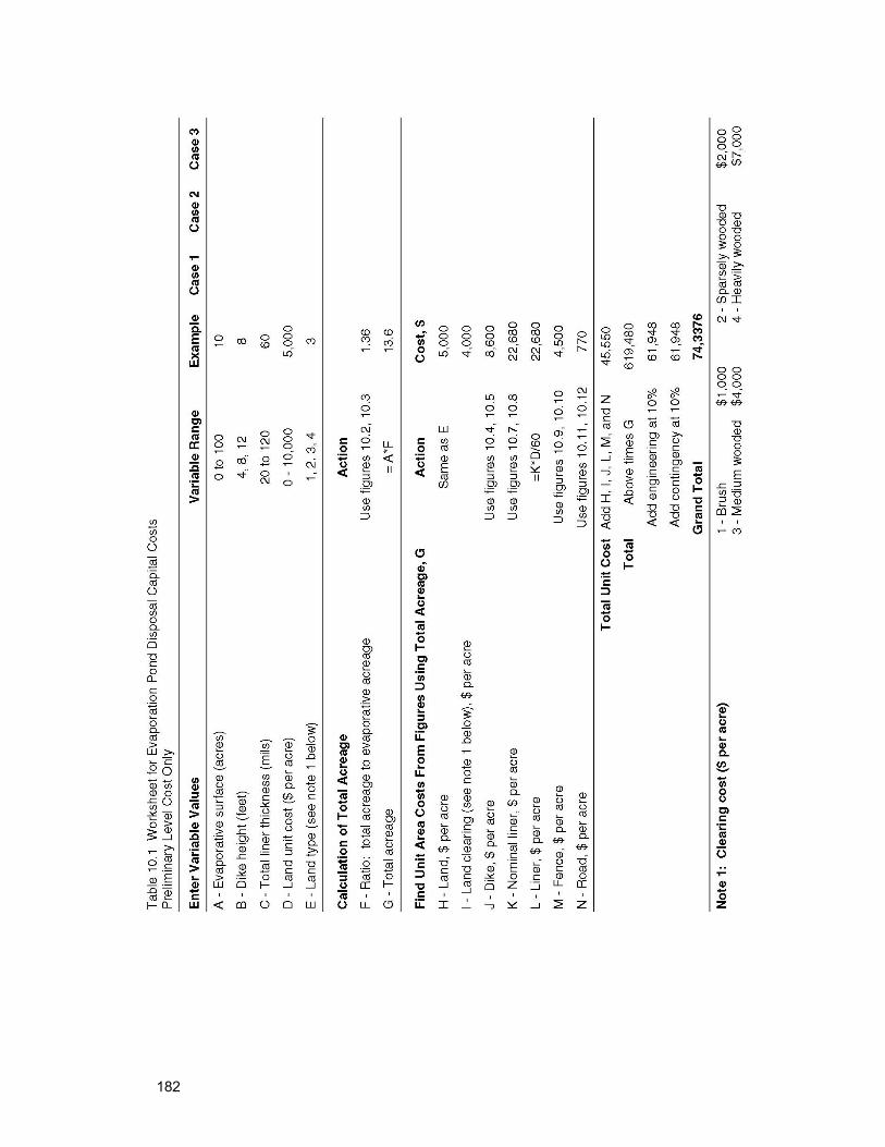
182

183

10.6 Evaporation Pond Regression Model

For convenience, it is helpful to have a simplified closed-form mathematical expression to calculate preliminary capital cost. Cautions on using the worksheet model to develop capital cost for the evaporation pond apply to the regression model. By definition, the regression model is less accurate being based on a best fit of the results from the worksheet calculations. A linear regression model is used to develop the equation for total unit area capital cost. This model is valid from 10 to 100 acres. To obtain the total capital cost, this expression is then multiplied times the total area required as well as by a 20-percent contingency factor (1.2). The expression for the total area is nonlinear taking into account the area adjustment factor as well as the evaporative surface area.

Total Unit Area Capital Cost ($/acre) = 5406 + 465 * LINER THICKNESS + 1.07 * LAND COST + 0.931 * LAND CLEARING COST + 217.5 * DIKE HEIGHT Total Area (plus contingency factor) = 1.2 * EVAP AREA * [1 + 0.155 * DIKE HEIGHT/(SQRT(EVAP AREA))

When multiplied together these two expressions yield the Total Capital Cost. For the worksheet example conditions of : LINER THICKNESS = 60 mil LAND COST = $5,000 per acre

LAND CLEARING COST = $4,000 per acre DIKE HEIGHT = 8 feet

EVAP AREA = 10 acres The calculated total capital cost is $737,045, which compares to the worksheet result of $743,376.

185

11. Spray Irrigation Disposal 11.1 Background

Land application methods include irrigation systems, rapid infiltration, and overland flow systems (Crites et al., 2000). These methods, and in particular irrigation, were originally used to take advantage of sewage effluent as a nutrient or fertilizer source as well as to reuse the water. Membrane concentrate has been used for land application in the spray irrigation mode. Using the concentrate in lieu of fresh irrigation water helps conserve natural resources; and in areas where water conservation is of great importance, spray irrigation is especially attractive. Because of the higher TDS concentration of RO and EDR concentrate, unless it is diluted, concentrate is less likely than NF concentrate to be used for spray irrigation purposes.

Concentrate can be applied to cropland or vegetation by sprinkling or surface techniques for water conservation by exchange when lawns, parks, or golf courses are irrigated and for preservation and enlargement of greenbelts and open spaces.

Where the nutrient concentration of the waste water for irrigation is of little value, hydraulic loading can be maximized to the extent possible, and system costs can be minimized. Crops such as water-tolerant grasses with low potential for economic return but with high salinity tolerance are generally chosen for this type of requirement.

Fundamental considerations in land application systems include knowledge of waste water characteristics, vegetation, and public health requirements for successful design and operation. Environmental regulations at each site must be closely examined to determine if spray irrigation is feasible. Contamination of the ground water and runoff into surface water are key concerns. Also, the quality of the concentrate—its salinity, toxicity, and the soil permeability—must be acceptable.

The principal objective in spray irrigation systems for concentrate discharge is ultimate disposal of the applied waste water. With this objective, the hydraulic loading is usually limited by the infiltration capacity of the soil. If the site has a relatively impermeable subsurface layer or a high ground water table, underdrains can be installed to increase the allowable loading. Grasses are usually selected for the vegetation because of their high nutrient requirements and water tolerance.

Other conditions must be met before concentrate irrigation can be considered as a practical disposal option. First, there must be a need for irrigation water in the vicinity of the membrane plant. If the need exists, a contract between the operating plant and the irrigation user would be required. Second, a backup

186

disposal or storage method must be available during periods of heavy rainfall. Third, monitor wells must be drilled before an operating permit is obtained (Conlon, 1989).

11.2 Design Considerations

The following design considerations are applicable to spray irrigation of concentrate for ultimate disposal:

♦ Salt, trace metals, and salinity ♦ Site selection ♦ Preapplication treatment ♦ Hydraulic loading rates ♦ Land requirements ♦ Vegetation selection ♦ Distribution techniques ♦ Surface runoff control

11.2.1 Salt, Trace Metals, and Salinity Three factors that affect an irrigation source’s long-term influence on soil permeability are the sodium content relative to calcium and magnesium, the carbonate and bicarbonate content, and the total salt concentration of the irrigation water. Sodium salts remain in the soil and may adversely affect its structure. High sodium concentrations in clay-bearing soils disperse soil particles and decrease soil permeability, thus reducing the rate at which water moves into the soil and reducing aeration. If the soil permeability, or infiltration rate, is greatly reduced, then the vegetation on the irrigation site cannot survive. The hardness level (calcium and magnesium) will form insoluble precipitates with carbonates when the water is concentrated. This buildup of solids can eventually block the migration of water through the soil.

The U.S. Department of Agriculture’s Salinity Laboratory developed a sodium adsorption ratio (SAR) to determine the sodium limit. It is defined as follows:

SAR = Na/[(Ca + Mg)/2]1/2

Where Na = sodium, milliequivalent per liter (meq/L) Ca = calcium, meq/L Mg = magnesium, meq/L

High SAR values (> 9) may adversely affect the permeability of fine-textured soils and can sometimes be toxic to plants.

Trace elements are essential for plant growth; however, at higher levels, some become toxic to both plants and microorganisms. The retention capacity for most

187

metals in most soils is generally high, especially for pH above 7. Under low pH conditions, some metals can leach out of soils and may adversely affect the surface waters in the area.

Salinity is the most important parameter in determining the impact of the concentrate on the soil. High concentrations of salts whose accumulation is potentially harmful will be continually added to the soil with irrigation water. The rate of salt accumulation depends upon the quantity applied and the rate at which it is removed from the soil by leaching. The salt levels in many brackish reverse osmosis concentrates can be between 5,000 and 10,000 parts per million, a range that normally rules out spray irrigation.

In addition to the effects of total salinity on vegetation and soil, individual ions can cause reduction in plant growth. Toxicity occurs when a specific ion is taken up and accumulated by the vegetation, ultimately resulting in damage to it. The ions of most concern in waste water effluent irrigation are sodium, chloride, and boron. Other heavy metals can be very harmful, even if present only in small quantities. These include copper, iron, barium, lead, and manganese. These all have strict environmental regulations in many States.

In addition to the influence on the soil, the effect of the salt concentrations on the ground water must be considered. The possible impact on ground water sources may be a difficult obstacle where soil saturation is high and the water table is close to the surface. The chance of increasing background TDS levels of the ground water is high with the concentrate. Due to this consideration, spray irrigation requires a runoff control system. An underdrain or piping distribution system may have to be installed under the full areas of irrigation to collect excess seepage through the soil and, thus, to protect the ground water sources. If high salinity concentrate is being used, scaling of the underdrain may become a problem. The piping perforations used to collect the water can be easily scaled because the openings are generally small. Vulnerability to scaling must be carefully evaluated before a project is undertaken.

11.2.2 Site Selection Site selection factors and criteria for effluent irrigation are presented in table 11.1. A moderately permeable soil capable of infiltration up to 2 inches per day on an intermittent basis is preferable. The total amount of land required for land application is highly variable but primarily depends on application rates.

11.2.3 Preapplication Treatment Factors that should be considered in assessing the need for preapplication treatment include whether the concentrate is mixed with additional waste waters before application, the type of vegetation grown, the degree of contact with the waste water by the public, and the method of application. In four Florida sites, concentrate is aerated before discharge, because each plant discharges to a

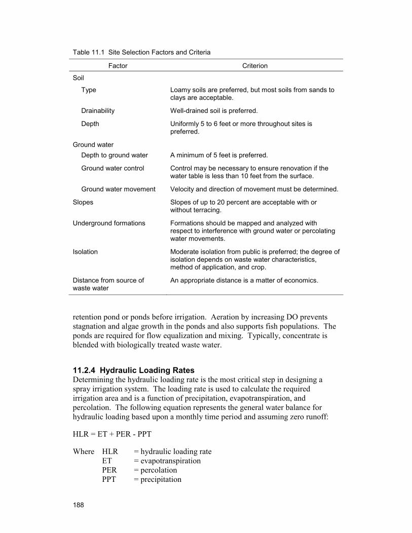
188

Table 11.1 Site Selection Factors and Criteria

Factor Criterion

Soil Type Loamy soils are preferred, but most soils from sands to

clays are acceptable.

Drainability Well-drained soil is preferred.

Depth Uniformly 5 to 6 feet or more throughout sites is preferred.

Ground water Depth to ground water A minimum of 5 feet is preferred.

Ground water control Control may be necessary to ensure renovation if the water table is less than 10 feet from the surface.

Ground water movement Velocity and direction of movement must be determined.

Slopes Slopes of up to 20 percent are acceptable with or without terracing.

Underground formations Formations should be mapped and analyzed with respect to interference with ground water or percolating water movements.

Isolation Moderate isolation from public is preferred; the degree of isolation depends on waste water characteristics, method of application, and crop.

Distance from source of waste water

An appropriate distance is a matter of economics.

retention pond or ponds before irrigation. Aeration by increasing DO prevents stagnation and algae growth in the ponds and also supports fish populations. The ponds are required for flow equalization and mixing. Typically, concentrate is blended with biologically treated waste water.

11.2.4 Hydraulic Loading Rates Determining the hydraulic loading rate is the most critical step in designing a spray irrigation system. The loading rate is used to calculate the required irrigation area and is a function of precipitation, evapotranspiration, and percolation. The following equation represents the general water balance for hydraulic loading based upon a monthly time period and assuming zero runoff:

HLR = ET + PER - PPT

Where HLR = hydraulic loading rate ET = evapotranspiration PER = percolation PPT = precipitation

189

In most cases, surface runoff from fields irrigated with waste water is not allowed without a permit or, at least, must be controlled; it is usually controlled just so that a permit does not have to be obtained.

Seasonal variations in each of these values should be taken into account by evaluating the water balance for each month as well as the annual balance. For precipitation, the wettest year in 10 is suggested as reasonable in most cases. Evapotranspiration will also vary from month to month, but the total for the year should be relatively constant. Percolation includes that portion of the water that, after infiltration into the soil, flows through the root zone and eventually becomes part of the ground water. The percolation rate used in the calculation should be determined on the basis of a number of factors, including soil characteristics underlying geologic conditions, ground water conditions, and the length of drying period required for satisfactory vegetation growth. The principal factor is the permeability or hydraulic conductivity of the least permeable layer in the soil profile.

Resting periods, standard in most irrigation techniques, allow the water to drain from the top few inches of soil. Aerobic conditions are thus restored, and air penetrates the soil. Resting periods may range from a portion of each day to 14 days and depend on the vegetation, the number of individual plots in the rotation cycle, and the availability of backup storage capacity.

To properly calculate an annual hydraulic loading rate, monthly evapotranspiration, precipitation, and percolation rates must be obtained. The annual hydraulic loading rate represents the sum of the monthly loading rates. Recommended loading rates range from 2 to 20 feet per year (Goigel, 1991).

11.2.5 Land Requirements Once a hydraulic loading rate has been determined, the required irrigation area can be calculated using the following equation:

A = Q * K1/ALR

Where A = irrigation area (acre) Q = concentrate flow (gpd) ALR = annual hydraulic loading rate (ft/yr) K1 = 0.00112 d * ft3 * acres/(hr * gal * ft2)

The total land area required for spray irrigation includes allowances for buffer zones and storage and, if necessary, land for emergencies or future expansion.

For loadings of constituents such as nitrogen, which may be of interest to golf course managers who need fertilizer for the grasses, the field area requirement is calculated as follows:

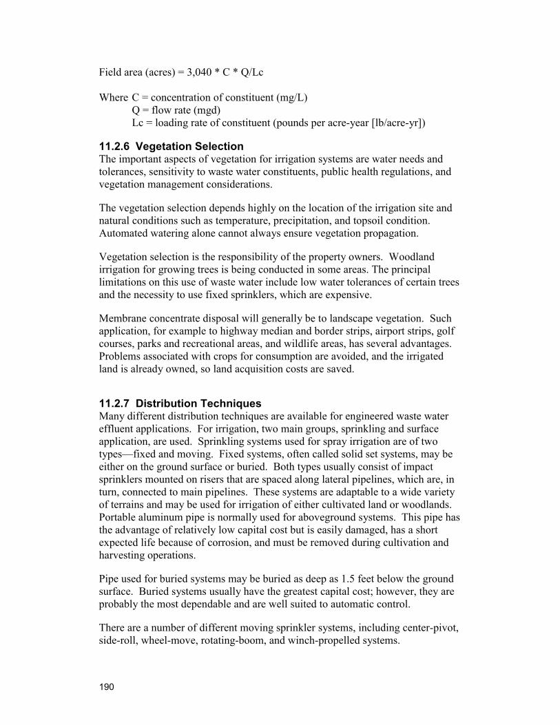
190

Field area (acres) = 3,040 * C * Q/Lc Where C = concentration of constituent (mg/L) Q = flow rate (mgd) Lc = loading rate of constituent (pounds per acre-year [lb/acre-yr])

11.2.6 Vegetation Selection The important aspects of vegetation for irrigation systems are water needs and tolerances, sensitivity to waste water constituents, public health regulations, and vegetation management considerations.

The vegetation selection depends highly on the location of the irrigation site and natural conditions such as temperature, precipitation, and topsoil condition. Automated watering alone cannot always ensure vegetation propagation.

Vegetation selection is the responsibility of the property owners. Woodland irrigation for growing trees is being conducted in some areas. The principal limitations on this use of waste water include low water tolerances of certain trees and the necessity to use fixed sprinklers, which are expensive.

Membrane concentrate disposal will generally be to landscape vegetation. Such application, for example to highway median and border strips, airport strips, golf courses, parks and recreational areas, and wildlife areas, has several advantages. Problems associated with crops for consumption are avoided, and the irrigated land is already owned, so land acquisition costs are saved.

11.2.7 Distribution Techniques Many different distribution techniques are available for engineered waste water effluent applications. For irrigation, two main groups, sprinkling and surface application, are used. Sprinkling systems used for spray irrigation are of two types—fixed and moving. Fixed systems, often called solid set systems, may be either on the ground surface or buried. Both types usually consist of impact sprinklers mounted on risers that are spaced along lateral pipelines, which are, in turn, connected to main pipelines. These systems are adaptable to a wide variety of terrains and may be used for irrigation of either cultivated land or woodlands. Portable aluminum pipe is normally used for aboveground systems. This pipe has the advantage of relatively low capital cost but is easily damaged, has a short expected life because of corrosion, and must be removed during cultivation and harvesting operations.

Pipe used for buried systems may be buried as deep as 1.5 feet below the ground surface. Buried systems usually have the greatest capital cost; however, they are probably the most dependable and are well suited to automatic control.

There are a number of different moving sprinkler systems, including center-pivot, side-roll, wheel-move, rotating-boom, and winch-propelled systems.

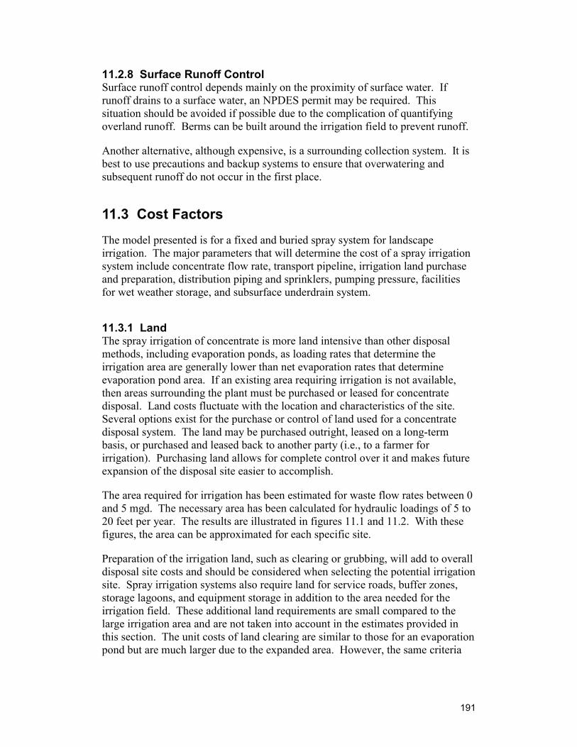
191

11.2.8 Surface Runoff Control Surface runoff control depends mainly on the proximity of surface water. If runoff drains to a surface water, an NPDES permit may be required. This situation should be avoided if possible due to the complication of quantifying overland runoff. Berms can be built around the irrigation field to prevent runoff.

Another alternative, although expensive, is a surrounding collection system. It is best to use precautions and backup systems to ensure that overwatering and subsequent runoff do not occur in the first place.

11.3 Cost Factors

The model presented is for a fixed and buried spray system for landscape irrigation. The major parameters that will determine the cost of a spray irrigation system include concentrate flow rate, transport pipeline, irrigation land purchase and preparation, distribution piping and sprinklers, pumping pressure, facilities for wet weather storage, and subsurface underdrain system.

11.3.1 Land The spray irrigation of concentrate is more land intensive than other disposal methods, including evaporation ponds, as loading rates that determine the irrigation area are generally lower than net evaporation rates that determine evaporation pond area. If an existing area requiring irrigation is not available, then areas surrounding the plant must be purchased or leased for concentrate disposal. Land costs fluctuate with the location and characteristics of the site. Several options exist for the purchase or control of land used for a concentrate disposal system. The land may be purchased outright, leased on a long-term basis, or purchased and leased back to another party (i.e., to a farmer for irrigation). Purchasing land allows for complete control over it and makes future expansion of the disposal site easier to accomplish.

The area required for irrigation has been estimated for waste flow rates between 0 and 5 mgd. The necessary area has been calculated for hydraulic loadings of 5 to 20 feet per year. The results are illustrated in figures 11.1 and 11.2. With these figures, the area can be approximated for each specific site.

Preparation of the irrigation land, such as clearing or grubbing, will add to overall disposal site costs and should be considered when selecting the potential irrigation site. Spray irrigation systems also require land for service roads, buffer zones, storage lagoons, and equipment storage in addition to the area needed for the irrigation field. These additional land requirements are small compared to the large irrigation area and are not taken into account in the estimates provided in this section. The unit costs of land clearing are similar to those for an evaporation pond but are much larger due to the expanded area. However, the same criteria

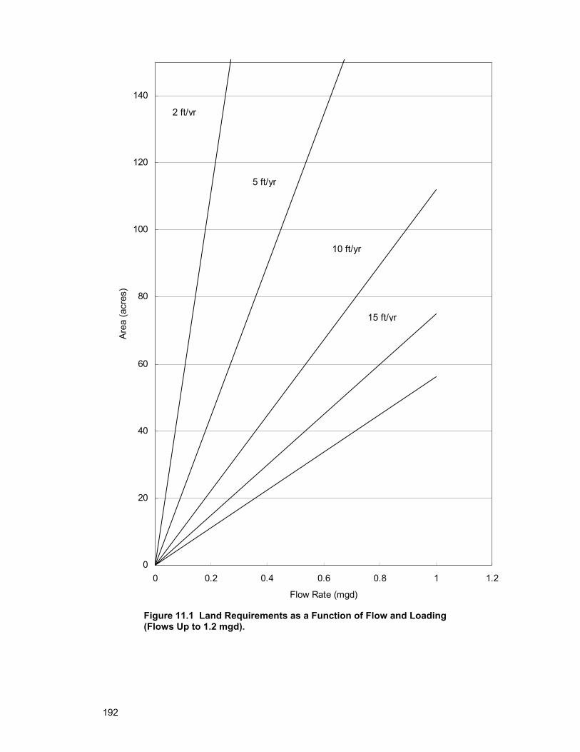
192

20 ft/yr

0

20

40

60

80

100

120

140

0 0.2 0.4 0.6 0.8 1 1.2

Flow Rate (mgd)

Area

(acr

es)

15 ft/yr

10 ft/yr

5 ft/yr

2 ft/yr

Figure 11.1 Land Requirements as a Function of Flow and Loading (Flows Up to 1.2 mgd).

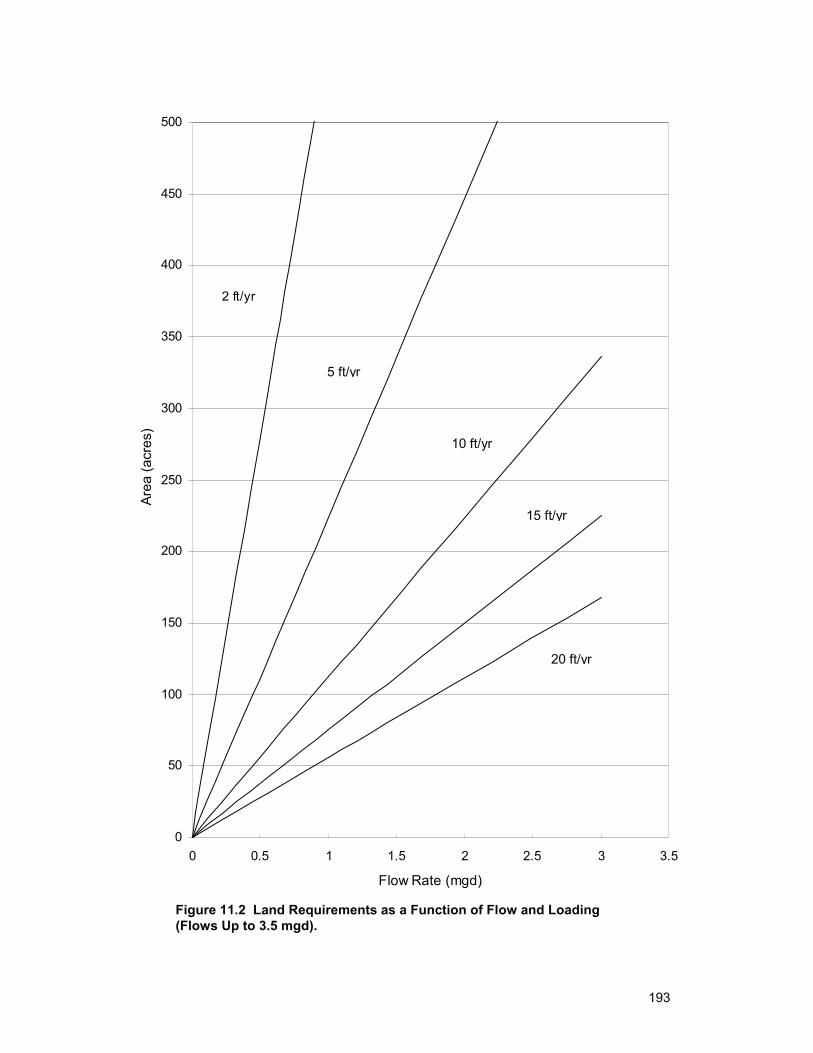
193

0

50

100

150

200

250

300

350

400

450

500

0 0.5 1 1.5 2 2.5 3 3.5

Flow Rate (mgd)

Area

(acr

es)

2 ft/yr

5 ft/yr

10 ft/yr

15 ft/yr

20 ft/yr

Figure 11.2 Land Requirements as a Function of Flow and Loading (Flows Up to 3.5 mgd).

194

can be applied: cost for clearing bushes, $1,000 per acre; sparsely wooded areas, $2,000 per acre; medium-wooded areas, $4,000 per acre; and heavily wooded areas, $7,000 per acre.

11.3.2 Distribution The cost of the distribution system includes the cost of the piping (main header, subheaders, and laterals), the cost of the sprinklers, and the cost of valves placed on the subheaders to segregate portions of the system for isolation. Figure 11.3 illustrates a distribution system with four submain headers. The size and length of the main header pipe are set by the area of land to be irrigated and the required flow rate. As the size of the area to be irrigated relative to the available flow increases, it no longer becomes feasible to irrigate the entire system at the same time due to minimum flow requirements for the individual sprinkler. The entire distribution system is segmented into several subsystems, each of which is operated in a sequential pattern. A minimum number of subsystems is required to meet the minimum flow requirements per sprinkler. The number of submain headers and the number of sprinklers per lateral are determined by the number of subsystems. Setting of the number of submain headers uniquely determines the number of sprinklers per lateral. The more submain headers, the fewer sprinklers per lateral.

Sprinklers are characterized by the wetted diameters of their coverage and their pressure/flow characteristics. The water delivered (inches per hour) by a sprinkler is greatest near the sprinkler head and decreases in a bell-shaped curve to the edge of the wetted diameter. To deliver more uniform coverage, sprinklers are typically spaced with as much as a 30- to 50-percent overlap in coverage. Thus, the spacing of the sprinklers is less than the wetted diameter of the sprinkler.

In designing the distribution system, first determine the required land area of land based on the concentrate flow and the loading rate of the land. This sets the length of the main header. Setting of the sprinkler spacing determines the total number of sprinklers required. The subsystem design may be based on meeting a minimum flow rate per sprinkler. The lengths of main header, submain header, and laterals are set at this point. The size of the piping is chosen to meet pressure drop limitations dictated by delivering a certain pressure to the sprinkler head consistent with its pressure/flow characteristics. Typically, lower acceptable diameter piping is specified to minimize pipe cost. There are choices and options in sprinkler and distribution design that may be made based on minimizing overall system cost and providing system flexibility.

The present model is for preliminary design purposes only. Because the more final design requires site-specific information and costs to be considered, the present model makes several design assumptions that are listed in the design approach section.

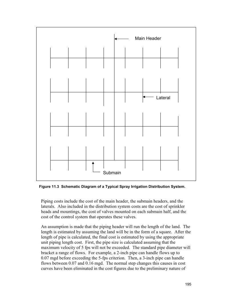
195

Piping costs include the cost of the main header, the submain headers, and the laterals. Also included in the distribution system costs are the cost of sprinkler heads and mountings, the cost of valves mounted on each submain half, and the cost of the control system that operates these valves.

An assumption is made that the piping header will run the length of the land. The length is estimated by assuming the land will be in the form of a square. After the length of pipe is calculated, the final cost is estimated by using the appropriate unit piping length cost. First, the pipe size is calculated assuming that the maximum velocity of 5 fps will not be exceeded. The standard pipe diameter will bracket a range of flows. For example, a 2-inch pipe can handle flows up to 0.07 mgd before exceeding the 5-fps criterion. Then, a 3-inch pipe can handle flows between 0.07 and 0.16 mgd. The normal step changes this causes in cost curves have been eliminated in the cost figures due to the preliminary nature of

Submain

Lateral

Main Header

Figure 11.3 Schematic Diagram of a Typical Spray Irrigation Distribution System.

196

the cost estimates. The costs presented are based on the costs of PVC piping. The submains costs are estimated by a similar procedure. Again, the submain length is assumed to be the total length of the land. The lateral cost is a function of how many sprinklers are on each lateral and the distance the sprinklers can cover.

The single main header is sized for the total flow and is the largest diameter pipe in the system. Flow in the main header goes into the submain headers mounted perpendicular to it. Valves are located on each submain half near the main header to control flow into the submain halves. The valves are either fully open or closed according to which subsystem of the distribution system is operating. For example, perhaps a system has 8 submain headers and, thus, 16 half submains. If each subsystem involves two submain halves, then the total flow in the main header flows into these two submain halves and on to the laterals and sprinkler heads associated with these submain halves. The submain header halves are sized according to the flow and velocity constraints. After this subsystem has operated for a period of time, valve closures and openings shunt the flow to another subsystem. Typically, the major piping cost is for the submain headers.

Figures 11.4 and 11.5 provide piping costs (header, submain headers, and laterals) as a function of area to be irrigated. For a given area, land with greater hydraulic loadings will receive more flow and the piping system will be of larger diameter to accommodate the greater flows. Thus the greater piping cost for the larger loading systems is reflected in these figures.

The cost of the sprinklers, valves, and control system are combined and presented in figure 11.6. The sprinkler cost is typically the largest of these cost items. The cost is dependent upon the land area.

The installed costs, which include labor and trenching for the distribution system, are taken as 1.8 times the material cost obtained from figures 11.4 through 11.6.

11.3.3 Pumping The concentrate stream is first stored in a storage facility and then pumped to the irrigation system. The head requirement of the pump is established by the pumping distance and the pressure loss through the sprinklers. Based on the flow rate and pump head, the size of the pump and estimated cost can be established. For this study, the pump heads are assumed to be less than 100 psig and would be similar in cost to the low-head pumps for deep well injection (see figure 11.7).

11.3.4 Storage Temporary storage facilities are necessary to retain concentrate during heavy rainfall periods or other circumstances when irrigation is not necessary. The need for retention facilities is particularly important in areas with large average yearly rainfall.

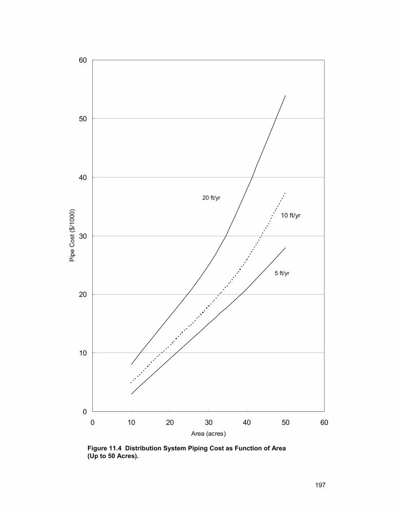
197

0

10

20

30

40

50

60

0 10 20 30 40 50 60Area (acres)

Pipe

Cos

t ($/

1000

)

20 ft/yr

10 ft/yr

5 ft/yr

Figure 11.4 Distribution System Piping Cost as Function of Area (Up to 50 Acres).

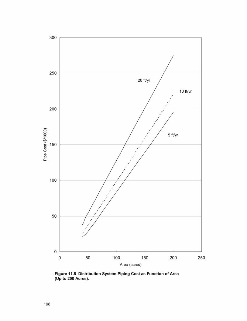
198

0

50

100

150

200

250

300

0 50 100 150 200 250Area (acres)

Pipe

Cos

t ($/

1000

)

20 ft/yr

10 ft/yr

5 ft/yr

Figure 11.5 Distribution System Piping Cost as Function of Area (Up to 200 Acres).

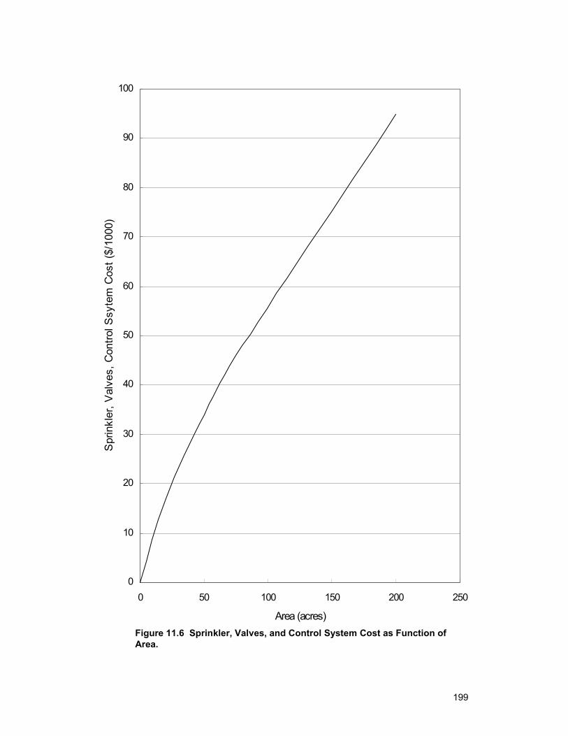
199

0

10

20

30

40

50

60

70

80

90

100

0 50 100 150 200 250

Area (acres)

Spr

inkl

er, V

alve

s, C

ontro

l Ssy

tem

Cos

t ($/

1000

)

Figure 11.6 Sprinkler, Valves, and Control System Cost as Function of Area.

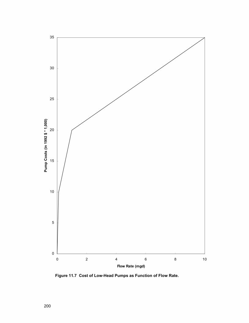
200

0

5

10

15

20

25

30

35

0 2 4 6 8 10

Flow Rate (mgd)

Pum

p C

osts

(in

1992

$ *

1,00

0)

Figure 11.7 Cost of Low-Head Pumps as Function of Flow Rate.

201

Storage tanks or lined ponds can be utilized. The volume of storage required is set by the amount of rainfall expected at the site. Historical rainfall data must be reviewed to determine the maximum number of consecutive days on which irrigation would not be necessary. Storage tank costs have been estimated based on using retention and circular tanks designed for 1-day capacity. These costs are summarized in figures 11.8 and 11.9.

11.3.5 Underdrains Irrigation systems may be required to include underdrainage to protect ground water sources. Subsurface drainage systems consist of a network of buried drainage pipes with open holes or perforations that recover the waste stream effluent that has percolated through the soil. A collection basin is used to recover the water collected by the underdrains. This water can then be reused by the irrigation system. The contribution of this water to the total flow is minor.

The cost of an underdrain system will add significantly to the overall cost of the system. The underdrain system will consist of header and subheader pipes arranged similarly to the distribution piping. For a cost estimate, use 80 percent of the piping cost as determined from figures 11.4 and 11.5.

11.3.6 Operational Costs Costs associated with the labor requirements for spray irrigation must be addressed, because the operation and maintenance of a concentrate spray irrigation system is more labor intensive than the disposal methods previously discussed. Labor requirements include sprinkler system repair and vegetative surface maintenance. The energy costs for pump operation also add to the system’s total operational costs.

11.4 Design Approach for Spray Irrigation Model

NOTE: In a site-specific design, various options for the sprinkler (sprinkler size, spacing, overlap) and distribution system (submain header, laterals, sprinklers per lateral) would be investigated. The design constraints include cost, pressure drop, available sizes, etc. In this way, the most appropriate and effective system can be defined. In addition, the variability of loading and application rates with time of day and month of the year would be examined to ensure that the design meets minimum and maximum flow, temperature, and other conditions. In the following approach to preliminary cost estimation, various assumptions are made to simplify the design process and enable cost estimates to be developed more easily.

♦ The system is a solid set buried spray irrigation system comprised of PVC piping.

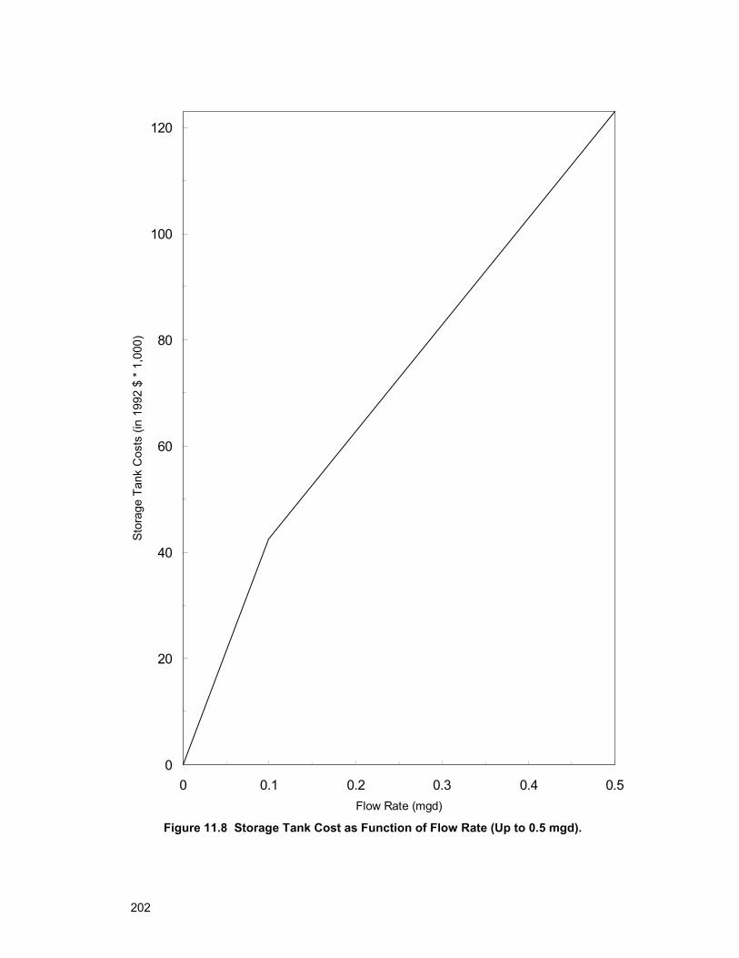
202

0

20

40

60

80

100

120

0 0.1 0.2 0.3 0.4 0.5Flow Rate (mgd)

Stor

age

Tank

Cos

ts (i

n 19

92 $

* 1

,000

)

Figure 11.8 Storage Tank Cost as Function of Flow Rate (Up to 0.5 mgd).

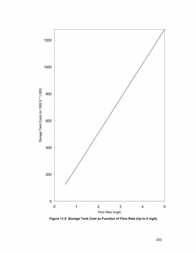
203

0

200

400

600

800

1000

1200

0 1 2 3 4 5Flow Rate (mgd)

Stor

age

Tank

Cos

ts (i

n 19

92 $

* 1

,000

)

Figure 11.9 Storage Tank Cost as Function of Flow Rate (Up to 5 mgd).

204

♦ The total flow (mgd) and loading factor (feet per year) determine the total number of acres needed to take up the water.

♦ The main header is sized to handle the total flow.

♦ The entire distribution system (main header, submain headers, laterals, sprinklers) that covers the acreage cannot be active at one time because of minimum flow requirements for the individual sprinkler.

♦ Consequently, only a portion of the system is active at any given time.

♦ Gate valves on each submain half control which submain halves are active at a given time.

♦ The hydraulics for the subsystem (portion active at any one time) determine the size of pipe for the headers and laterals. Considerations include flow, pressure, velocity, irrigation rate (inch per hour), etc.

♦ The length of time any part of the system is on is limited by the allowable application rate (inch per hour).

♦ The entire irrigation system is chosen to be in the shape of a square.

♦ The main header flows the entire length of the square (minus a portion of the wetted radius of the sprinkler at the distal end).

♦ The submain headers are perpendicular to the main header and span the entire length of the square (minus portions of the wetted radius of the sprinkler at each end).

♦ The laterals are perpendicular to the submain headers and may contain one to several sprinklers per lateral.

♦ The length of each lateral is a function of how many sprinklers are on each lateral.

♦ There is an inverse relation between the number of submain headers and the number of sprinklers per lateral. The more submain headers, the fewer sprinklers per lateral.

♦ A certain number of submain headers is necessary to allow division of the entire system into subsystems, only one of which operates at a time. This permits a minimum sprinkler flow to be met.

♦ The ground coverage from the sprinklers is highest nearest the sprinkler, having a bell curve-type distribution with distance from the sprinkler.

♦ To assure some coverage of all ground and to provide more uniformity of coverage, the spacing between sprinklers is chosen to provide an overlap in ground coverage. This overlap is typically from 30 to 50% of the wetted diameter.

205

♦ The most economical and efficient design needs be investigated for each site-specific situation.

♦ The specific design approach chosen for this model is as follows: • Number of submain headers is a variable that ranges from 1 to 16.

• This allows for up to 32 identical subsystems as there are 32 independent halves to the submain system, each of which can be active or inactive.

• Each subsystem is identical.

• The system is active for 20 hours per day.

• Each subsystem is active for an identical period of time each day.

• It is assumed that an impact sprinkler will be used that has a flow from 10 to 35 gpm per sprinkler and a wet radius ranging from 55 to 85 feet; the wet radius increases with the flow.

• The actual design is a trial and error process that involves choice of number of submain headers and number of active subsystems. These variables are exercised until a solution, where a sprinkler roughly matching the performance characteristics of the impact sprinkler just mentioned, is found. Very few combinations of the variables result in conditions matching sprinkler performance specifications.

• It is assumed that the pressure to the distribution system is 100 psi and that the pressure drop through the piping is not greater than 25 psi.

• Where design constraints dictate changes in pipe diameter from one nominal size to another, there would be step changes in the cost curves. These step changes are eliminated from the figures due to the preliminary nature of the cost estimate and to enforce the recommendation that a site-specific cost workup be done whenever any cost estimate other than a preliminary one is sought.

♦ Costs included in the capital cost model: • Land • Land clearing • Distribution systems (header, submain header, laterals, sprinklers, valves) • Pump • Storage tank • Underdrain

♦ Costs not included in the capital cost model: • Cost of blending, modifying, or pretreating concentrate to meet water

quality requirements

• Cost of pipeline to the spray irrigation site

• Cost of monitoring wells

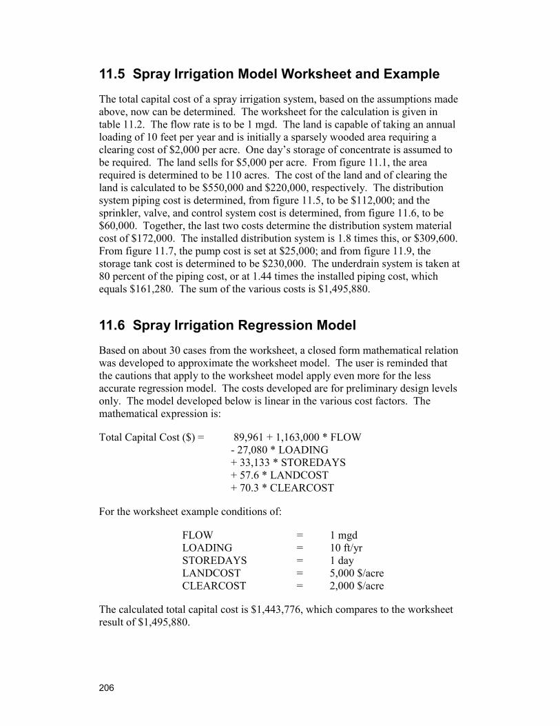
206

11.5 Spray Irrigation Model Worksheet and Example

The total capital cost of a spray irrigation system, based on the assumptions made above, now can be determined. The worksheet for the calculation is given in table 11.2. The flow rate is to be 1 mgd. The land is capable of taking an annual loading of 10 feet per year and is initially a sparsely wooded area requiring a clearing cost of $2,000 per acre. One day’s storage of concentrate is assumed to be required. The land sells for $5,000 per acre. From figure 11.1, the area required is determined to be 110 acres. The cost of the land and of clearing the land is calculated to be $550,000 and $220,000, respectively. The distribution system piping cost is determined, from figure 11.5, to be $112,000; and the sprinkler, valve, and control system cost is determined, from figure 11.6, to be $60,000. Together, the last two costs determine the distribution system material cost of $172,000. The installed distribution system is 1.8 times this, or $309,600. From figure 11.7, the pump cost is set at $25,000; and from figure 11.9, the storage tank cost is determined to be $230,000. The underdrain system is taken at 80 percent of the piping cost, or at 1.44 times the installed piping cost, which equals $161,280. The sum of the various costs is $1,495,880.

11.6 Spray Irrigation Regression Model

Based on about 30 cases from the worksheet, a closed form mathematical relation was developed to approximate the worksheet model. The user is reminded that the cautions that apply to the worksheet model apply even more for the less accurate regression model. The costs developed are for preliminary design levels only. The model developed below is linear in the various cost factors. The mathematical expression is:

Total Capital Cost ($) = 89,961 + 1,163,000 * FLOW - 27,080 * LOADING + 33,133 * STOREDAYS + 57.6 * LANDCOST + 70.3 * CLEARCOST

For the worksheet example conditions of:

FLOW = 1 mgd LOADING = 10 ft/yr STOREDAYS = 1 day LANDCOST = 5,000 $/acre CLEARCOST = 2,000 $/acre

The calculated total capital cost is $1,443,776, which compares to the worksheet result of $1,495,880.

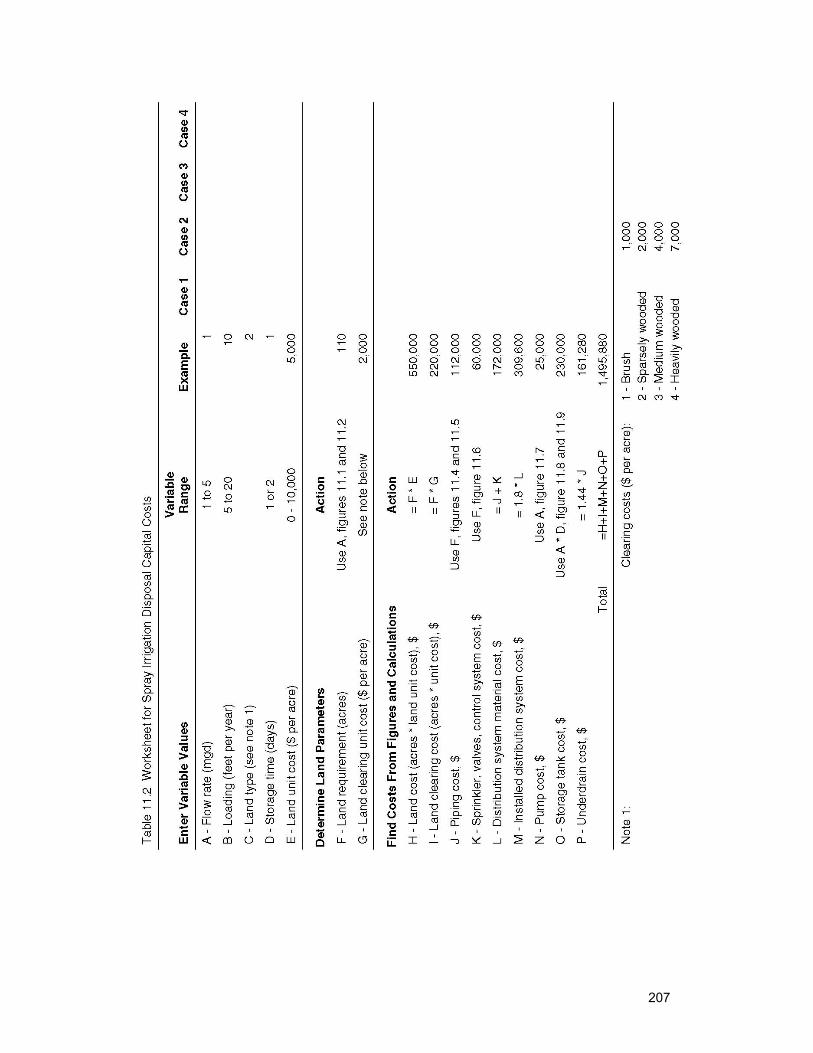
207

209

12. Zero Liquid Discharge Disposal 12.1 Background

In this approach, evaporation is used to further concentrate the membrane concentrate. In the extreme limit of processing concentrate to dry salts, the method becomes a zero discharge option. Evaporation requires major capital investment, and the high energy consumption together with the final salt or brine disposal can result in significant disposal costs.

Because of this, disposal of municipal membrane concentrate by mechanical evaporation would typically be considered when no other disposal option is feasible. Cost aside, however, there are some advantages to zero liquid discharge. These include:

♦ It may avoid a lengthy and tedious permitting process.

♦ It may gain quick community acceptance.

♦ It can be located virtually anywhere.

♦ It represents a positive extreme in recycling, by efficiently using the water source.

When this thermal process is used following an RO system, for example, it produces additional product water by recovering high-purity distillate from the concentrate waste water stream. The distillate can be used to help meet the system product water volume requirement. This reduces the size of the membrane system and, thus, the size of the membrane concentrate to be treated by the thermal process. In addition, because the product purity of the thermal process is so high (TDS in the range of 10 mg/L), some of the product water volume requirement of the system may be met by blending the thermal product with untreated source water. The usual concerns and considerations of using untreated water for blending need to be addressed. The end result may be a system where the system product requirement is met by three streams: 1) membrane product, 2) thermal process product, and 3) bypass water.

12.1.1 Single- and Multiple-Effect Evaporators Using steam as the energy source, it takes about 1,000 British thermal units (BTU) to evaporate a pound of water. In a single-effect evaporator, heat released by the condensing steam is transferred across a heat exchange surface to an aqueous solution boiling at a temperature lower than that of the condensing stream. The solution absorbs heat; and part of the solution water vaporizes, causing the remaining solution to become richer in solute. The water vapor flows to a barometric or surface condenser, where it condenses as its latent heat is released to cooling water at a lower temperature. The finite temperature differences between the steam, the boiling liquid, and the condenser are the

210

driving forces required for the heat transfer surface area to be less than infinite. Practically all the heat removed from the condensing stream (which had been generated initially by burning fuel) is rejected to cooling water and is often dissipated to the environment without being of further use.

The water vapor that flows to the condenser in a single-effect evaporator is at a lower temperature and pressure than the heating stream but has almost as much enthalpy. Instead of releasing its latent heat to cooling water, the water vapor may be used as heating steam in another evaporator effect operating at a lower temperature and pressure than the first effect.

Additional effects may be added in a similar manner, each generating additional vapor, which may be used to heat a lower-temperature effect. The vapor generated in the lowest-temperature effect finally is condensed by releasing its latent heat to cooling water in a condenser. The economy of a single- or multiple-effect evaporator may be expressed as the ratio of kilograms of total evaporation to kilograms of heating steam. As effects are added, the economy increases representing more efficient energy utilization. Eventually, added effects result in marginal added benefits, and the number of effects is thus limited by both practical and economic considerations. Multiple effect evaporators increase the efficiency (economy) but add capital cost in additional evaporator bodies.

More specifically, the number of effects, and thus the economy achieved, is limited by the total temperature difference between the saturation temperature of the heating steam (or other heat source) and the temperature of the cooling water (or other heat sink). The available temperature difference may also be constrained by the temperature sensitivity of the solution to be evaporated. The total temperature difference, less any losses, becomes allocated between effects in proportion to their resistance to heat transfer, the effects being thermal resistances in series.

The heat transfer surface area for each effect is inversely proportional to the net temperature difference available for that effect. Increasing the number of effects reduces the temperature difference and evaporation duty per effect, which increases the total area of the evaporator in rough proportion to the number of effects.

The temperature difference available to each effect is reduced by boiling point elevation and by the decrease in vapor saturation temperature due to pressure drop. The boiling point elevation of a solution is the increase in boiling point of the solution compared to the boiling point of pure water at the same pressure; it depends on the nature of the solute and increases with increasing solute concentration. In a multiple-effect evaporator, the boiling point elevation and vapor pressure drop losses for all the effects must be summed and subtracted from the overall temperature difference between heat source and sink to determine the net driving force available for heat transfer.

211

12.1.2 Vapor Compression Evaporator Systems (Brine Concentrators) A vapor compression evaporator system, or brine concentrator, is similar to a conventional single-effect evaporator, except that the vapor released from the boiling solution is compressed in a compressor. Compression raises the pressure and saturation temperature of the vapor so that it may be returned to the evaporator steam chest to be used as heating steam. The latent heat of the vapor is used to evaporate more water instead of being rejected to cooling water.

The compressor adds energy to the vapor to raise its saturation temperature above the boiling temperature of the solution by whatever net temperature difference is desired. The compressor is not completely efficient, having small losses due to mechanical friction and larger losses due to nonisentropic compression. However, the additional energy required because of nonisentropic compression is not lost from the evaporator system; it serves to superheat the compressed vapor. The compression energy added to the vapor is of the same magnitude as energy required to raise feed to the boiling point and make up for radiation and venting losses. By exchanging heat between the condensed vapors (distillate) and the product with the feed, it is usually possible to operate with little or no makeup heat in addition to the energy necessary to drive the compressor. The compressor power is proportional to the increase in saturation temperature produced by the compressor. The evaporator design must trade off compressor power consumption versus heat transfer surface area.

Using the vapor compression approach to evaporate water requires only about 100 BTU to evaporate a pound of water. Thus, one evaporator body driven by mechanical vapor compression is equivalent to 10 effects or a 10-body system driven by steam.

While most brine concentrators have been used to process cooling water, concentrators have also been used to concentrate reject from RO plants. Approximately 90 percent of these concentrators operate with a seeded slurry process that allows the reject to be concentrated as much as 40 to 1 without scaling problems developing in the evaporator. Brine concentrators also produce a distilled product water that can be used for high-purity purposes or for blending with other water supplies. Because of the ability to achieve such high levels of concentration, brine concentrators can reduce or eliminate the need for alternative disposal methods such as deep well injection or solar evaporation ponds. When operated in conjunction with crystallizers or spray dryers, brine concentrators can achieve zero liquid discharge of RO concentrate under all climatic conditions.

Individual brine concentrator units range in capacity from approximately 10 to 700 gpm of feedwater flow. Units below 150 gpm of capacity are usually skid mounted, and larger units are field fabricated. A majority of operating brine concentrators are single-effect, vertical tube, falling film evaporators that use a calcium sulfate-seeded slurry process. Energy input to the brine concentrator can be provided by an electric-driven vapor compressor or by process steam from a

212

host industrial facility. Steam-driven systems can be configured with multiple effects to minimize energy consumption.

Product water quality is normally less than 10 mg/L TDS. Brine reject from the concentrator typically ranges between 2 and 10 percent of the feedwater flow, with TDS concentrations as high as 250,000 mg/L.

Because of the corrosive nature of many waste water brines, brine concentrators are usually constructed of high-quality materials, including titanium evaporator tubes and stainless steel vessels suitable for 30-year evaporator life. For conditions of high chloride concentrations or other more corrosive environments, brine concentrators can be constructed of materials such as AL6XN, Inconal 825, or other exotic metals to meet performance and reliability requirements.

Figure 12.1 shows a schematic diagram of a typical single-effect vertical tube brine concentrator. Waste water, such as RO concentrate, enters a tank where the pH is adjusted to prepare for deaeration. The waste water then passes through a heat exchanger and enters a deaerator, where noncondensable gases are removed. From the deaerator, the waste water enters the evaporator sump, where it mixes with the brine slurry. The slurry is constantly recirculated from the sump to a floodbox at the top of the evaporator tube bundle. Water from the floodbox flows through brine distributors and moves as a thin film down the interior walls of the evaporator tubes.

Some of the brine evaporates and flows through mist eliminators before entering the vapor compressor, where additional heat is added. Vapor from the compressor then flows to the outside of the evaporator tubes, where its heat is transferred to the cooler brine falling inside the tubes. As the compressed vapor gives up heat, it condenses as product water and is collected and pumped through the feedwater heat exchanger, where it transfers its heat to the incoming feedwater.

The seeded slurry process prevents scaling of the evaporator tubes. Calcium sulfate and silica precipitates build on calcium sulfate seed crystals in the recirculation brine instead of scaling on heat transfer surfaces. With the seeded slurry system, concentrations of up to 30-percent total solids can be reached in the recirculating water without scaling.

Brine concentrator technology was developed in the early 1970s to help thermal power stations achieve zero discharge of waste water. At present, approximately 75 brine concentrators are in operation in the United States and overseas. Of these, about a dozen are being used to concentrate reject streams (RO concentrate) from industrial RO plants. The operating experiences of these plants have shown that using brine concentrator evaporators for concentration of RO concentrate is a viable application and that the systems are highly reliable. Many operating systems have achieved on-stream operating availabilities greater than 90 percent over an extended period of years.

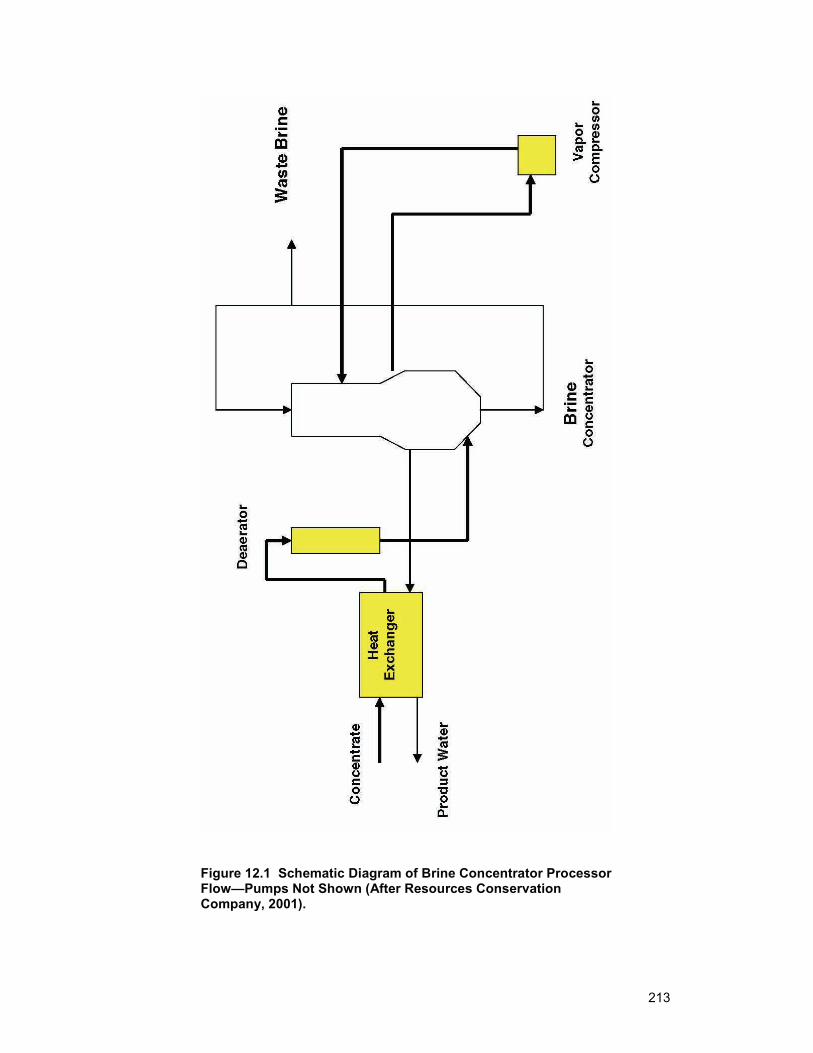
213

Figure 12.1 Schematic Diagram of Brine Concentrator Processor Flow—Pumps Not Shown (After Resources Conservation Company, 2001).

214

The specific design features and performance of brine concentrator systems are usually developed in conjunction with the equipment suppliers, based on the flow, chemistry, and economic factors involved in each case. The suppliers use proprietary methods to determine concentration factors to minimize brine concentrator blowdown rates while controlling scaling in the evaporator tubes. Process water recovery typically is limited by the formation of a double salt that is a combination of sodium and calcium sulfate. Thus, recovery is dependent on the site-specific feedwater quality but is usually in the 90- to 98-percent range.

Brine concentrators can be applied to a majority of RO concentrate streams. For such streams that are already saturated in calcium sulfate, brine concentrators operate without calcium sulfate addition. If concentrations of calcium sulfate in the concentrate stream are insufficient, calcium sulfate is added as required to support the seeded slurry process.

Blowdown from brine concentrators is high in dissolved and suspended solids and saturated in calcium sulfate. Disposal can be handled in several ways. In areas where evaporation ponds are feasible and cost effective, brine concentrator blowdown can be settled in a decant basin and then pumped to an evaporation pond. Settled solids then are removed by a front-end loader, clamshell, or other device and transported to a land disposal facility. Blowdown can also be sent directly to a disposal pond, where the solids periodically can be removed, or to a pond constructed deep enough so that solids removal will not be required during the design life of the facility.

In areas with negative net evaporation rates, or with expensive construction requirements for evaporation ponds, brine concentrator blowdown can be concentrated to a wet cake or dry powder using crystallizers or spray dryers. These technologies will be discussed in the next two sections.

The method of evaporation will be selected based on the characteristics of the RO membrane concentrate and the type of energy source to be used.

12.1.3 Crystallizers Crystallizer technology has been used for many years to concentrate feed streams in industrial processes. More recently, as the need to concentrate waste waters has increased, this technology has been applied to reject from desalination processes, such as brine concentrate evaporators, to reduce waste water to a trans-portable solid. Crystallizer technology is especially applicable in areas where solar evaporation pond construction cost is high, solar evaporation rates are neg-ative, or deep well disposal is costly, geologically not feasible, or not permitted.

Crystallizers used for waste water disposal range in capacity from about 2 to 50 gpm. These units have vertical cylindrical vessels with heat input from vapor compressors or an available stream supply. For small systems ranging from 2 to 6 gpm, steam-driven crystallizers are more economical. Steam can be supplied by

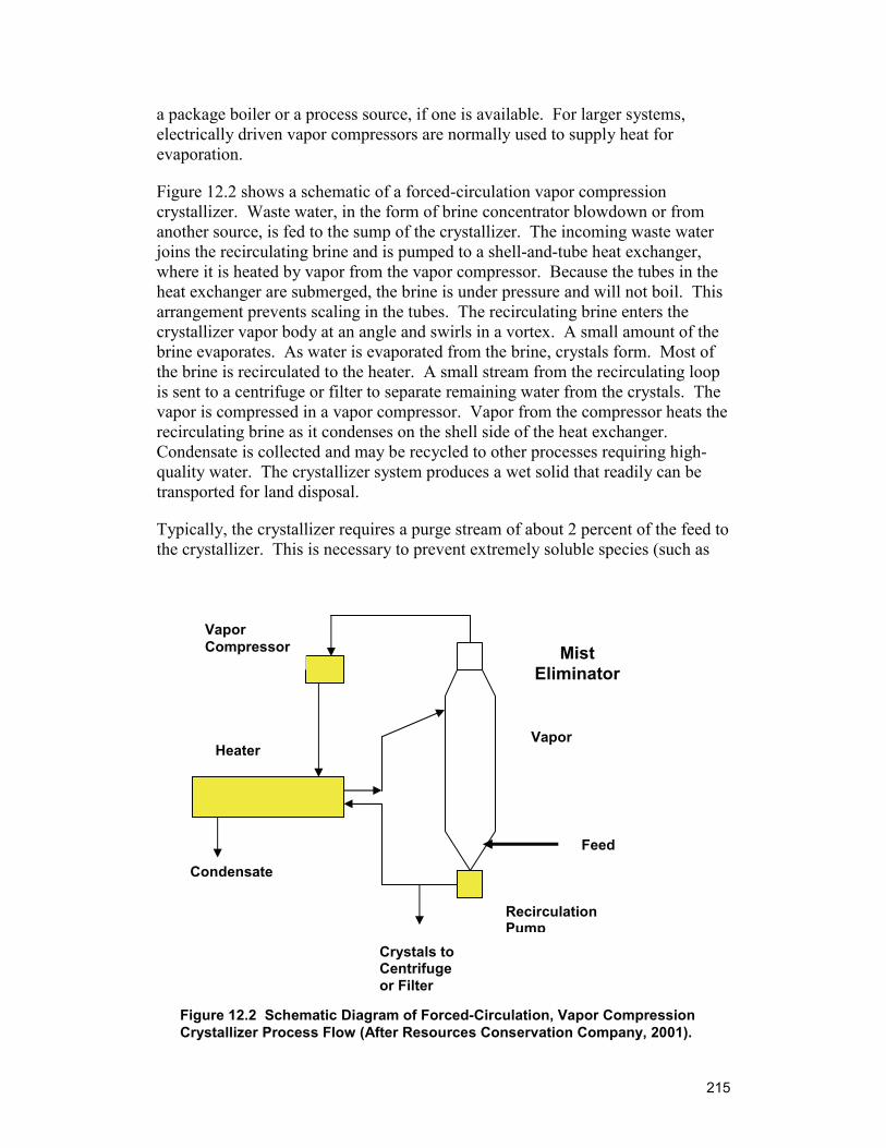
215

a package boiler or a process source, if one is available. For larger systems, electrically driven vapor compressors are normally used to supply heat for evaporation.

Figure 12.2 shows a schematic of a forced-circulation vapor compression crystallizer. Waste water, in the form of brine concentrator blowdown or from another source, is fed to the sump of the crystallizer. The incoming waste water joins the recirculating brine and is pumped to a shell-and-tube heat exchanger, where it is heated by vapor from the vapor compressor. Because the tubes in the heat exchanger are submerged, the brine is under pressure and will not boil. This arrangement prevents scaling in the tubes. The recirculating brine enters the crystallizer vapor body at an angle and swirls in a vortex. A small amount of the brine evaporates. As water is evaporated from the brine, crystals form. Most of the brine is recirculated to the heater. A small stream from the recirculating loop is sent to a centrifuge or filter to separate remaining water from the crystals. The vapor is compressed in a vapor compressor. Vapor from the compressor heats the recirculating brine as it condenses on the shell side of the heat exchanger. Condensate is collected and may be recycled to other processes requiring high-quality water. The crystallizer system produces a wet solid that readily can be transported for land disposal.

Typically, the crystallizer requires a purge stream of about 2 percent of the feed to the crystallizer. This is necessary to prevent extremely soluble species (such as

Heater

Vapor Compressor Mist

Eliminator

Vapor

Feed

Recirculation Pump

Crystals to Centrifuge or Filter

Condensate

Figure 12.2 Schematic Diagram of Forced-Circulation, Vapor Compression Crystallizer Process Flow (After Resources Conservation Company, 2001).

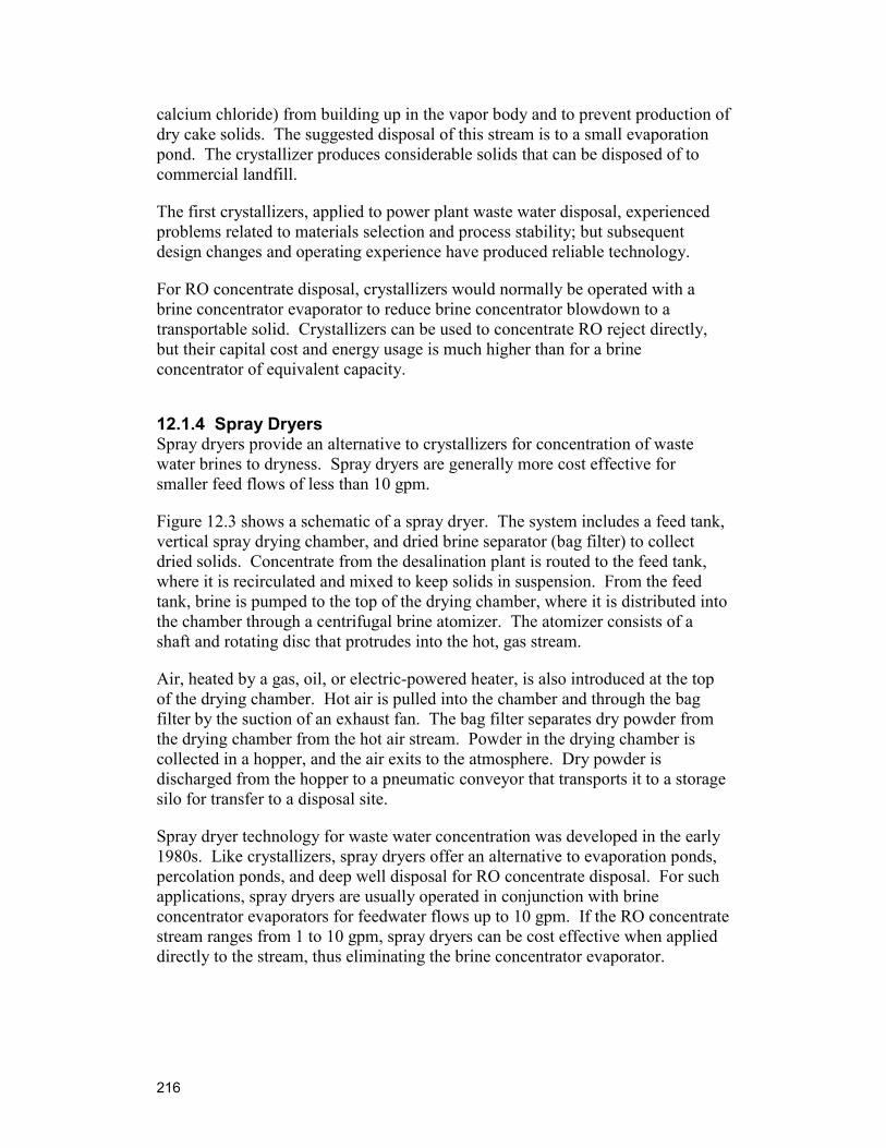
216

calcium chloride) from building up in the vapor body and to prevent production of dry cake solids. The suggested disposal of this stream is to a small evaporation pond. The crystallizer produces considerable solids that can be disposed of to commercial landfill.

The first crystallizers, applied to power plant waste water disposal, experienced problems related to materials selection and process stability; but subsequent design changes and operating experience have produced reliable technology.

For RO concentrate disposal, crystallizers would normally be operated with a brine concentrator evaporator to reduce brine concentrator blowdown to a transportable solid. Crystallizers can be used to concentrate RO reject directly, but their capital cost and energy usage is much higher than for a brine concentrator of equivalent capacity.

12.1.4 Spray Dryers Spray dryers provide an alternative to crystallizers for concentration of waste water brines to dryness. Spray dryers are generally more cost effective for smaller feed flows of less than 10 gpm.

Figure 12.3 shows a schematic of a spray dryer. The system includes a feed tank, vertical spray drying chamber, and dried brine separator (bag filter) to collect dried solids. Concentrate from the desalination plant is routed to the feed tank, where it is recirculated and mixed to keep solids in suspension. From the feed tank, brine is pumped to the top of the drying chamber, where it is distributed into the chamber through a centrifugal brine atomizer. The atomizer consists of a shaft and rotating disc that protrudes into the hot, gas stream.

Air, heated by a gas, oil, or electric-powered heater, is also introduced at the top of the drying chamber. Hot air is pulled into the chamber and through the bag filter by the suction of an exhaust fan. The bag filter separates dry powder from the drying chamber from the hot air stream. Powder in the drying chamber is collected in a hopper, and the air exits to the atmosphere. Dry powder is discharged from the hopper to a pneumatic conveyor that transports it to a storage silo for transfer to a disposal site.

Spray dryer technology for waste water concentration was developed in the early 1980s. Like crystallizers, spray dryers offer an alternative to evaporation ponds, percolation ponds, and deep well disposal for RO concentrate disposal. For such applications, spray dryers are usually operated in conjunction with brine concentrator evaporators for feedwater flows up to 10 gpm. If the RO concentrate stream ranges from 1 to 10 gpm, spray dryers can be cost effective when applied directly to the stream, thus eliminating the brine concentrator evaporator.

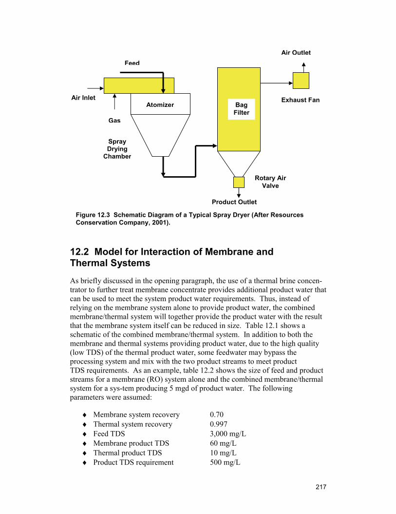
217

12.2 Model for Interaction of Membrane and Thermal Systems

As briefly discussed in the opening paragraph, the use of a thermal brine concen-trator to further treat membrane concentrate provides additional product water that can be used to meet the system product water requirements. Thus, instead of relying on the membrane system alone to provide product water, the combined membrane/thermal system will together provide the product water with the result that the membrane system itself can be reduced in size. Table 12.1 shows a schematic of the combined membrane/thermal system. In addition to both the membrane and thermal systems providing product water, due to the high quality (low TDS) of the thermal product water, some feedwater may bypass the processing system and mix with the two product streams to meet product TDS requirements. As an example, table 12.2 shows the size of feed and product streams for a membrane (RO) system alone and the combined membrane/thermal system for a sys-tem producing 5 mgd of product water. The following parameters were assumed:

♦ Membrane system recovery 0.70 ♦ Thermal system recovery 0.997 ♦ Feed TDS 3,000 mg/L ♦ Membrane product TDS 60 mg/L ♦ Thermal product TDS 10 mg/L ♦ Product TDS requirement 500 mg/L

Feed

Gas

Air Inlet Atomizer

Spray Drying

Chamber

BagFilter

Rotary Air Valve

Product Outlet

Exhaust Fan

Air Outlet

Figure 12.3 Schematic Diagram of a Typical Spray Dryer (After Resources Conservation Company, 2001).

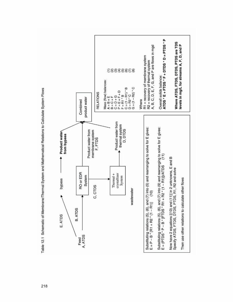
218

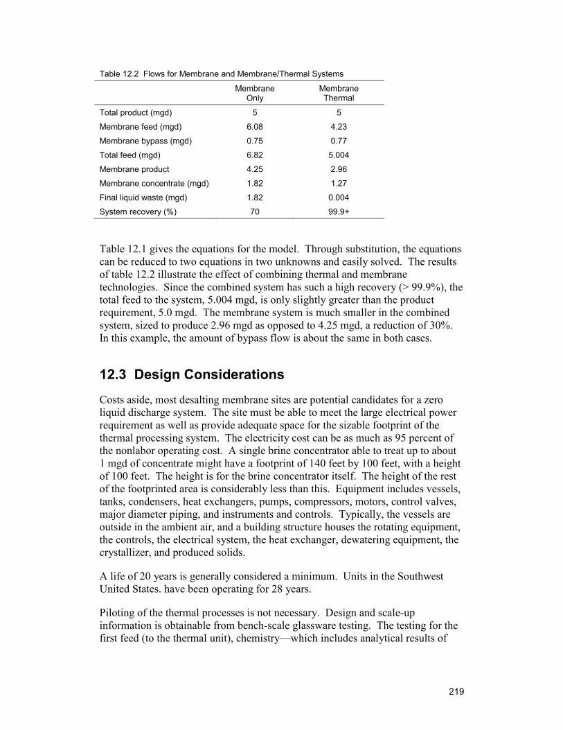
219

Table 12.2 Flows for Membrane and Membrane/Thermal Systems

Membrane Only

Membrane Thermal

Total product (mgd) 5 5

Membrane feed (mgd) 6.08 4.23

Membrane bypass (mgd) 0.75 0.77

Total feed (mgd) 6.82 5.004

Membrane product 4.25 2.96

Membrane concentrate (mgd) 1.82 1.27

Final liquid waste (mgd) 1.82 0.004

System recovery (%) 70 99.9+

Table 12.1 gives the equations for the model. Through substitution, the equations can be reduced to two equations in two unknowns and easily solved. The results of table 12.2 illustrate the effect of combining thermal and membrane technologies. Since the combined system has such a high recovery (> 99.9%), the total feed to the system, 5.004 mgd, is only slightly greater than the product requirement, 5.0 mgd. The membrane system is much smaller in the combined system, sized to produce 2.96 mgd as opposed to 4.25 mgd, a reduction of 30%. In this example, the amount of bypass flow is about the same in both cases.

12.3 Design Considerations

Costs aside, most desalting membrane sites are potential candidates for a zero liquid discharge system. The site must be able to meet the large electrical power requirement as well as provide adequate space for the sizable footprint of the thermal processing system. The electricity cost can be as much as 95 percent of the nonlabor operating cost. A single brine concentrator able to treat up to about 1 mgd of concentrate might have a footprint of 140 feet by 100 feet, with a height of 100 feet. The height is for the brine concentrator itself. The height of the rest of the footprinted area is considerably less than this. Equipment includes vessels, tanks, condensers, heat exchangers, pumps, compressors, motors, control valves, major diameter piping, and instruments and controls. Typically, the vessels are outside in the ambient air, and a building structure houses the rotating equipment, the controls, the electrical system, the heat exchanger, dewatering equipment, the crystallizer, and produced solids.

A life of 20 years is generally considered a minimum. Units in the Southwest United States. have been operating for 28 years.

Piloting of the thermal processes is not necessary. Design and scale-up information is obtainable from bench-scale glassware testing. The testing for the first feed (to the thermal unit), chemistry—which includes analytical results of

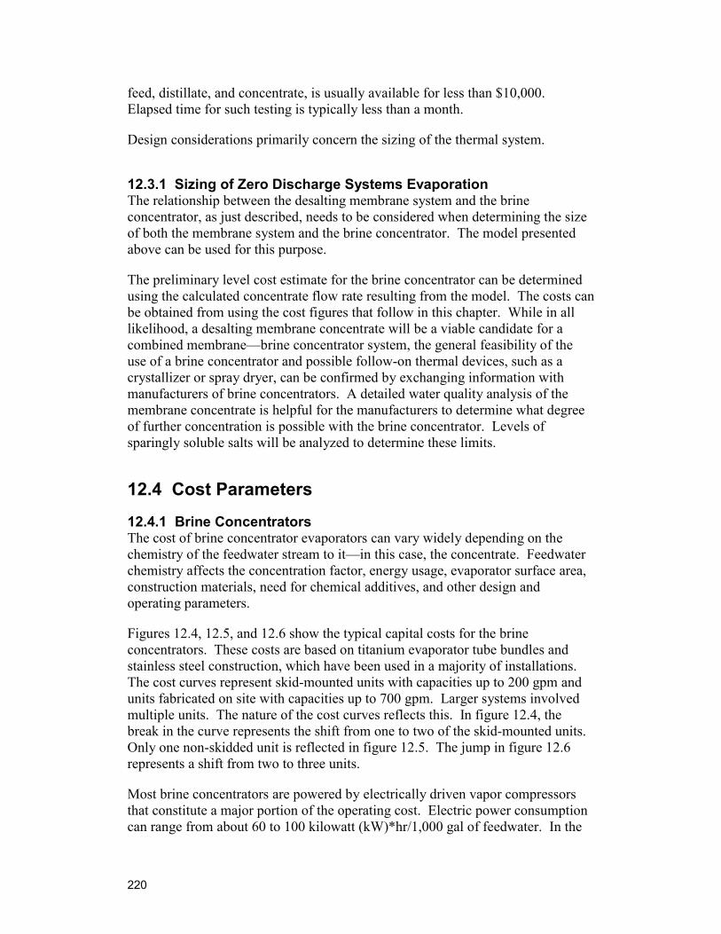
220

feed, distillate, and concentrate, is usually available for less than $10,000. Elapsed time for such testing is typically less than a month.

Design considerations primarily concern the sizing of the thermal system.

12.3.1 Sizing of Zero Discharge Systems Evaporation The relationship between the desalting membrane system and the brine concentrator, as just described, needs to be considered when determining the size of both the membrane system and the brine concentrator. The model presented above can be used for this purpose.

The preliminary level cost estimate for the brine concentrator can be determined using the calculated concentrate flow rate resulting from the model. The costs can be obtained from using the cost figures that follow in this chapter. While in all likelihood, a desalting membrane concentrate will be a viable candidate for a combined membrane—brine concentrator system, the general feasibility of the use of a brine concentrator and possible follow-on thermal devices, such as a crystallizer or spray dryer, can be confirmed by exchanging information with manufacturers of brine concentrators. A detailed water quality analysis of the membrane concentrate is helpful for the manufacturers to determine what degree of further concentration is possible with the brine concentrator. Levels of sparingly soluble salts will be analyzed to determine these limits.

12.4 Cost Parameters

12.4.1 Brine Concentrators The cost of brine concentrator evaporators can vary widely depending on the chemistry of the feedwater stream to it—in this case, the concentrate. Feedwater chemistry affects the concentration factor, energy usage, evaporator surface area, construction materials, need for chemical additives, and other design and operating parameters.

Figures 12.4, 12.5, and 12.6 show the typical capital costs for the brine concentrators. These costs are based on titanium evaporator tube bundles and stainless steel construction, which have been used in a majority of installations. The cost curves represent skid-mounted units with capacities up to 200 gpm and units fabricated on site with capacities up to 700 gpm. Larger systems involved multiple units. The nature of the cost curves reflects this. In figure 12.4, the break in the curve represents the shift from one to two of the skid-mounted units. Only one non-skidded unit is reflected in figure 12.5. The jump in figure 12.6 represents a shift from two to three units.

Most brine concentrators are powered by electrically driven vapor compressors that constitute a major portion of the operating cost. Electric power consumption can range from about 60 to 100 kilowatt (kW)*hr/1,000 gal of feedwater. In the

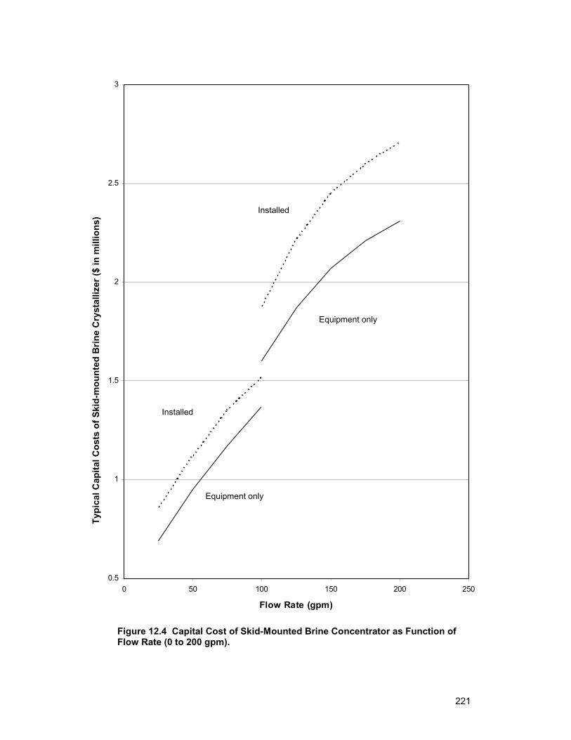
221

0.5

1

1.5

2

2.5

3

0 50 100 150 200 250

Flow Rate (gpm)

Typi

cal C

apita

l Cos

ts o

f Ski

d-m

ount

ed B

rine

Cry

stal

lizer

($ in

mill

ions

)

Equipment only

Equipment only

Installed

Installed

Figure 12.4 Capital Cost of Skid-Mounted Brine Concentrator as Function of Flow Rate (0 to 200 gpm).

222

1

1.5

2

2.5

3

3.5

4

4.5

5

5.5

0 0.2 0.4 0.6 0.8 1 1.2

Flow Rate (mgd)

Typi

cal C

apita

l Cos

ts fo

r a N

on-s

kidd

ed B

rine

Con

cent

rato

r ($

in m

illio

ns)

Installed

Equipment only

Figure 12.5 Capital Cost of Nonskidded Brine Concentrator as Function of Flow Rate (0 to 1.2 mgd).

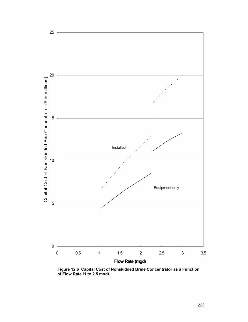
223

0

5

10

15

20

25

0 0.5 1 1.5 2 2.5 3 3.5

Flow Rate (mgd)

Cap

ital C

ost o

f Non

-ski

dded

Brin

Con

cent

rato

r ($

in m

illio

ns)

Installed

Equipment only

Figure 12.6 Capital Cost of Nonskidded Brine Concentrator as a Function of Flow Rate (1 to 2.5 mgd).

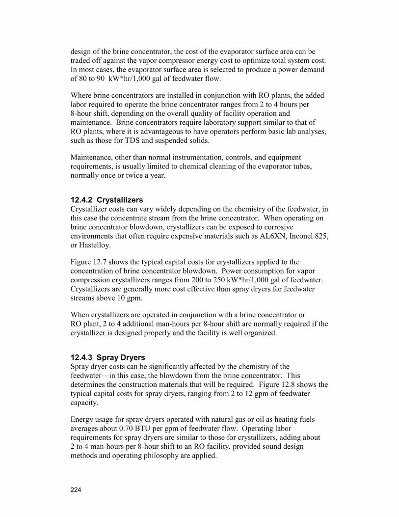
224

design of the brine concentrator, the cost of the evaporator surface area can be traded off against the vapor compressor energy cost to optimize total system cost. In most cases, the evaporator surface area is selected to produce a power demand of 80 to 90 kW*hr/1,000 gal of feedwater flow.

Where brine concentrators are installed in conjunction with RO plants, the added labor required to operate the brine concentrator ranges from 2 to 4 hours per 8-hour shift, depending on the overall quality of facility operation and maintenance. Brine concentrators require laboratory support similar to that of RO plants, where it is advantageous to have operators perform basic lab analyses, such as those for TDS and suspended solids.

Maintenance, other than normal instrumentation, controls, and equipment requirements, is usually limited to chemical cleaning of the evaporator tubes, normally once or twice a year.

12.4.2 Crystallizers Crystallizer costs can vary widely depending on the chemistry of the feedwater, in this case the concentrate stream from the brine concentrator. When operating on brine concentrator blowdown, crystallizers can be exposed to corrosive environments that often require expensive materials such as AL6XN, Inconel 825, or Hastelloy.

Figure 12.7 shows the typical capital costs for crystallizers applied to the concentration of brine concentrator blowdown. Power consumption for vapor compression crystallizers ranges from 200 to 250 kW*hr/1,000 gal of feedwater. Crystallizers are generally more cost effective than spray dryers for feedwater streams above 10 gpm.

When crystallizers are operated in conjunction with a brine concentrator or RO plant, 2 to 4 additional man-hours per 8-hour shift are normally required if the crystallizer is designed properly and the facility is well organized.

12.4.3 Spray Dryers Spray dryer costs can be significantly affected by the chemistry of the feedwater—in this case, the blowdown from the brine concentrator. This determines the construction materials that will be required. Figure 12.8 shows the typical capital costs for spray dryers, ranging from 2 to 12 gpm of feedwater capacity.

Energy usage for spray dryers operated with natural gas or oil as heating fuels averages about 0.70 BTU per gpm of feedwater flow. Operating labor requirements for spray dryers are similar to those for crystallizers, adding about 2 to 4 man-hours per 8-hour shift to an RO facility, provided sound design methods and operating philosophy are applied.

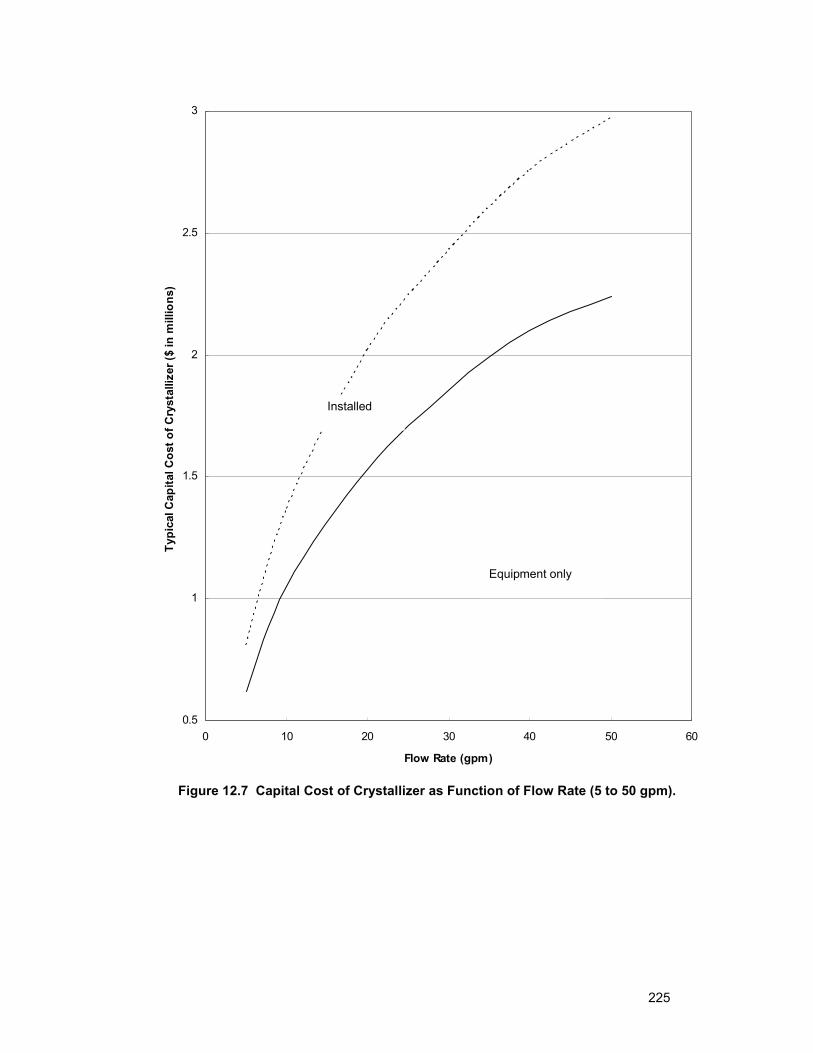
225

0.5

1

1.5

2

2.5

3

0 10 20 30 40 50 60

Flow Rate (gpm)

Typi

cal C

apita

l Cos

t of C

ryst

alliz

er ($

in m

illio

ns)

Installed

Equipment only

Figure 12.7 Capital Cost of Crystallizer as Function of Flow Rate (5 to 50 gpm).

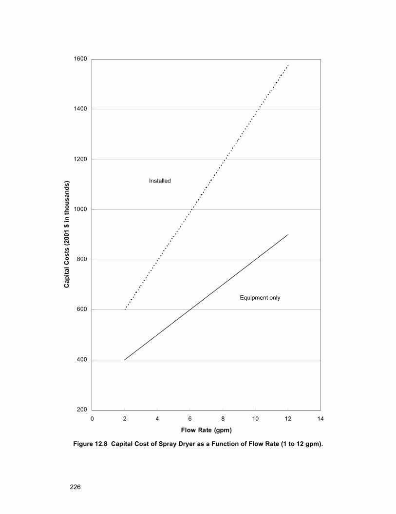
226

Equipment only

200

400

600

800

1000

1200

1400

1600

0 2 4 6 8 10 12 14

Flow Rate (gpm)

Cap

ital C

osts

(200

1 $

in th

ousa

nds) Installed

Equipment only

Figure 12.8 Capital Cost of Spray Dryer as a Function of Flow Rate (1 to 12 gpm).

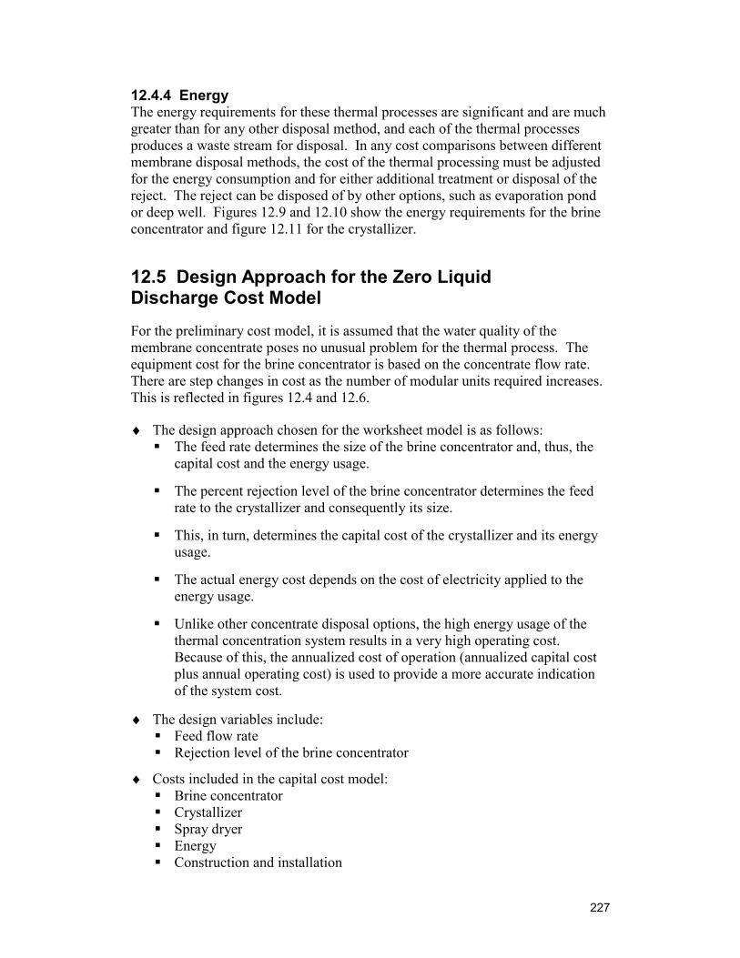
227

12.4.4 Energy The energy requirements for these thermal processes are significant and are much greater than for any other disposal method, and each of the thermal processes produces a waste stream for disposal. In any cost comparisons between different membrane disposal methods, the cost of the thermal processing must be adjusted for the energy consumption and for either additional treatment or disposal of the reject. The reject can be disposed of by other options, such as evaporation pond or deep well. Figures 12.9 and 12.10 show the energy requirements for the brine concentrator and figure 12.11 for the crystallizer.

12.5 Design Approach for the Zero Liquid Discharge Cost Model

For the preliminary cost model, it is assumed that the water quality of the membrane concentrate poses no unusual problem for the thermal process. The equipment cost for the brine concentrator is based on the concentrate flow rate. There are step changes in cost as the number of modular units required increases. This is reflected in figures 12.4 and 12.6.

♦ The design approach chosen for the worksheet model is as follows: The feed rate determines the size of the brine concentrator and, thus, the

capital cost and the energy usage.

The percent rejection level of the brine concentrator determines the feed rate to the crystallizer and consequently its size.

This, in turn, determines the capital cost of the crystallizer and its energy usage.

The actual energy cost depends on the cost of electricity applied to the energy usage.

Unlike other concentrate disposal options, the high energy usage of the thermal concentration system results in a very high operating cost. Because of this, the annualized cost of operation (annualized capital cost plus annual operating cost) is used to provide a more accurate indication of the system cost.

♦ The design variables include: Feed flow rate Rejection level of the brine concentrator

♦ Costs included in the capital cost model: Brine concentrator Crystallizer Spray dryer Energy Construction and installation

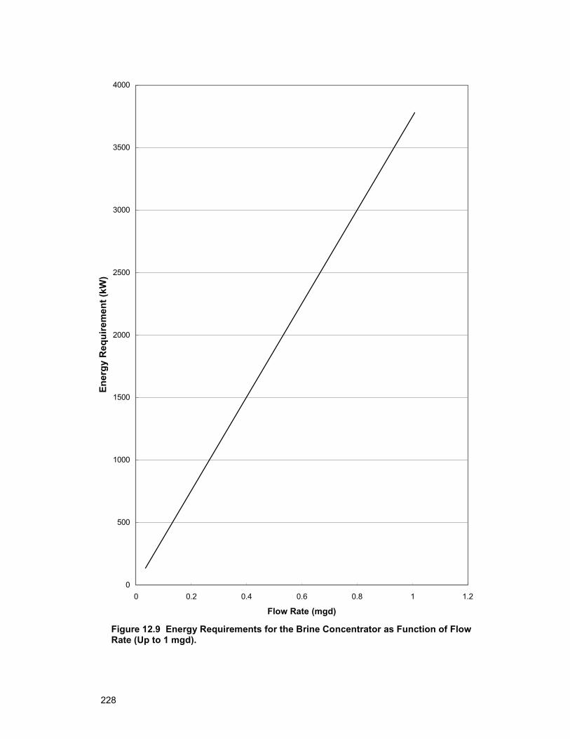
228

0

500

1000

1500

2000

2500

3000

3500

4000

0 0.2 0.4 0.6 0.8 1 1.2

Flow Rate (mgd)

Ener

gy R

equi

rem

ent (

kW)

Figure 12.9 Energy Requirements for the Brine Concentrator as Function of Flow Rate (Up to 1 mgd).

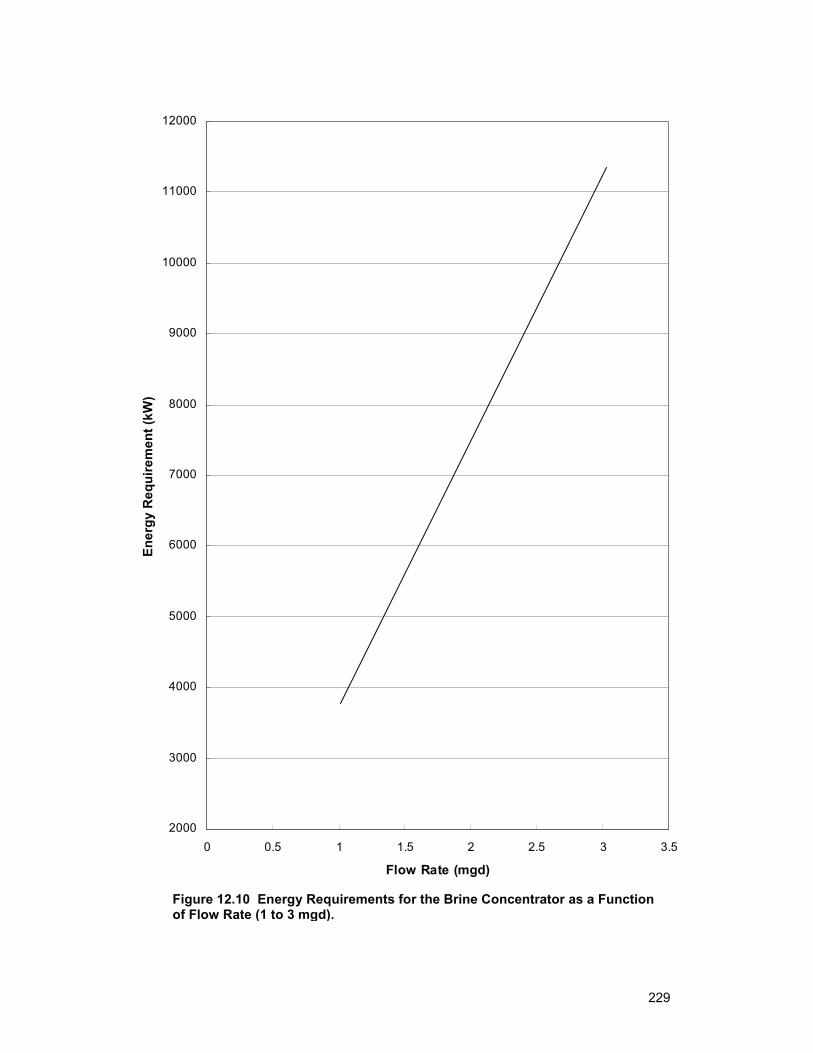
229

2000

3000

4000

5000

6000

7000

8000

9000

10000

11000

12000

0 0.5 1 1.5 2 2.5 3 3.5

Flow Rate (mgd)

Ener

gy R

equi

rem

ent (

kW)

Figure 12.10 Energy Requirements for the Brine Concentrator as a Function of Flow Rate (1 to 3 mgd).

230

0

100

200

300

400

500

600

700

800

0 10 20 30 40 50 60

Flow Rate (gpm)

Ener

gy R

equi

rem

ents

(kW

)

Figure 12.11 Energy Requirements for the Crystallizer as a Function of Flow Rate.

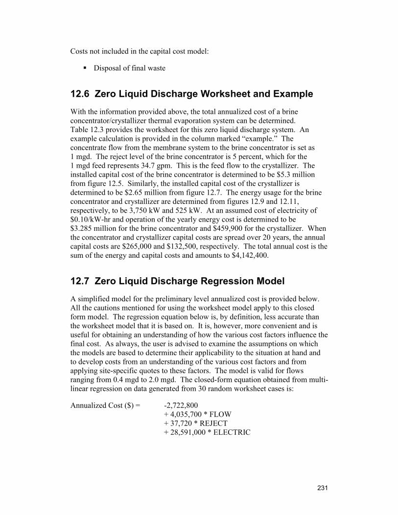
231

Costs not included in the capital cost model:

Disposal of final waste

12.6 Zero Liquid Discharge Worksheet and Example

With the information provided above, the total annualized cost of a brine concentrator/crystallizer thermal evaporation system can be determined. Table 12.3 provides the worksheet for this zero liquid discharge system. An example calculation is provided in the column marked “example.” The concentrate flow from the membrane system to the brine concentrator is set as 1 mgd. The reject level of the brine concentrator is 5 percent, which for the 1 mgd feed represents 34.7 gpm. This is the feed flow to the crystallizer. The installed capital cost of the brine concentrator is determined to be $5.3 million from figure 12.5. Similarly, the installed capital cost of the crystallizer is determined to be $2.65 million from figure 12.7. The energy usage for the brine concentrator and crystallizer are determined from figures 12.9 and 12.11, respectively, to be 3,750 kW and 525 kW. At an assumed cost of electricity of $0.10/kW-hr and operation of the yearly energy cost is determined to be $3.285 million for the brine concentrator and $459,900 for the crystallizer. When the concentrator and crystallizer capital costs are spread over 20 years, the annual capital costs are $265,000 and $132,500, respectively. The total annual cost is the sum of the energy and capital costs and amounts to $4,142,400.

12.7 Zero Liquid Discharge Regression Model

A simplified model for the preliminary level annualized cost is provided below. All the cautions mentioned for using the worksheet model apply to this closed form model. The regression equation below is, by definition, less accurate than the worksheet model that it is based on. It is, however, more convenient and is useful for obtaining an understanding of how the various cost factors influence the final cost. As always, the user is advised to examine the assumptions on which the models are based to determine their applicability to the situation at hand and to develop costs from an understanding of the various cost factors and from applying site-specific quotes to these factors. The model is valid for flows ranging from 0.4 mgd to 2.0 mgd. The closed-form equation obtained from multi-linear regression on data generated from 30 random worksheet cases is:

Annualized Cost ($) = -2,722,800 + 4,035,700 * FLOW + 37,720 * REJECT + 28,591,000 * ELECTRIC

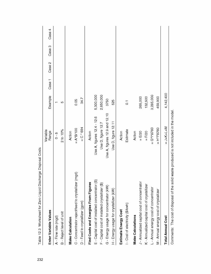
232

233

For the worksheet case where:

FLOW = 1 mgd REJECT = 5 % ELECTRIC = 0.10 $/kWhr

The calculated annualized cost is $4,360,565. This compares to the worksheet result of $4,142,400.

235

13. Analysis of Cost Models 13.1 Introduction

Four cost models (deep well disposal, evaporation pond, spray irrigation, and zero liquid discharge) are discussed individually and then compared. In this way, the sensitivity of each model to the various design parameters included in the cost models is reviewed, and the relative magnitude of costs associated with each concentrate disposal method is illustrated.

As pointed out in the chapters discussing the individual models, (chapters 9 through 12), care must be taken in interpreting and applying the model results. These models are limited in their applicability. The models make many assumptions that may not apply to a site-specific situation. Assumptions, discussed in each disposal method chapter, need to be reviewed for the user to better understand how the models apply to the situation of their concern. The models were developed to provide preliminary cost estimates only; they do not take into account regional differences in material and labor costs and the applicability of the concentrate disposal options. There may be site-specific costs that are not included in the model.

It is recommended that the model user read the chapter discussing the model in question to understand the assumptions made, the design parameters involved, and the cost factors associated with each model. By understanding the design approach and the model limitations, other costs not included in the model may be added to provide a more accurate site-specific cost estimate. The worksheet model provides a blueprint for developing more accurate, site-specific cost estimates.

The regression models provide a more rapid, but less accurate, cost estimate for these same disposal options. The range of applicability of the regressions is less than that of the worksheet models, and this further limits their applicability beyond the concerns expressed above.

13.2 Sensitivity Analysis

13.2.1 Relative Importance of Design Parameters In following sections, design parameters that appear directly in the four regression models are listed along with the Standardized Coefficient for that parameter from the regression model. The absolute magnitude of the Standardized Coefficient provides an indicator of the relative importance of the individual design parameters in the regression model. The more important the parameter, the more it affects the total cost. This indicator takes into account the full range of values each design parameter may take on and, more correctly, considers the entire “solution space” covered by the individual data sets used to develop the

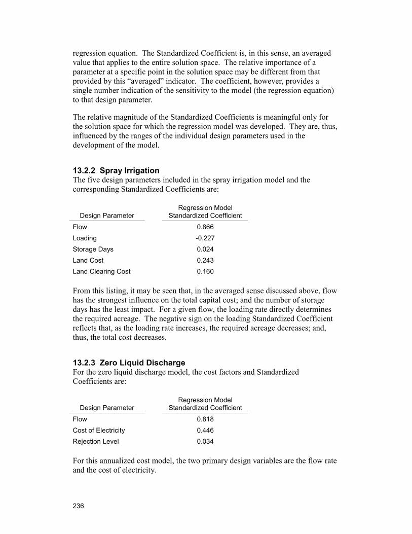
236

regression equation. The Standardized Coefficient is, in this sense, an averaged value that applies to the entire solution space. The relative importance of a parameter at a specific point in the solution space may be different from that provided by this “averaged” indicator. The coefficient, however, provides a single number indication of the sensitivity to the model (the regression equation) to that design parameter.

The relative magnitude of the Standardized Coefficients is meaningful only for the solution space for which the regression model was developed. They are, thus, influenced by the ranges of the individual design parameters used in the development of the model.

13.2.2 Spray Irrigation The five design parameters included in the spray irrigation model and the corresponding Standardized Coefficients are:

Design Parameter Regression Model

Standardized Coefficient

Flow 0.866 Loading -0.227 Storage Days 0.024 Land Cost 0.243 Land Clearing Cost 0.160 From this listing, it may be seen that, in the averaged sense discussed above, flow has the strongest influence on the total capital cost; and the number of storage days has the least impact. For a given flow, the loading rate directly determines the required acreage. The negative sign on the loading Standardized Coefficient reflects that, as the loading rate increases, the required acreage decreases; and, thus, the total cost decreases.

13.2.3 Zero Liquid Discharge For the zero liquid discharge model, the cost factors and Standardized Coefficients are:

Design Parameter Regression Model

Standardized Coefficient

Flow 0.818 Cost of Electricity 0.446 Rejection Level 0.034 For this annualized cost model, the two primary design variables are the flow rate and the cost of electricity.

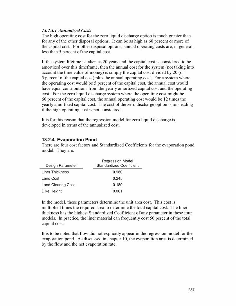
237

13.2.3.1 Annualized Costs The high operating cost for the zero liquid discharge option is much greater than for any of the other disposal options. It can be as high as 60 percent or more of the capital cost. For other disposal options, annual operating costs are, in general, less than 5 percent of the capital cost.

If the system lifetime is taken as 20 years and the capital cost is considered to be amortized over this timeframe, then the annual cost for the system (not taking into account the time value of money) is simply the capital cost divided by 20 (or 5 percent of the capital cost) plus the annual operating cost. For a system where the operating cost would be 5 percent of the capital cost, the annual cost would have equal contributions from the yearly amortized capital cost and the operating cost. For the zero liquid discharge system where the operating cost might be 60 percent of the capital cost, the annual operating cost would be 12 times the yearly amortized capital cost. The cost of the zero discharge option is misleading if the high operating cost is not considered.

It is for this reason that the regression model for zero liquid discharge is developed in terms of the annualized cost.

13.2.4 Evaporation Pond There are four cost factors and Standardized Coefficients for the evaporation pond model. They are:

Design Parameter Regression Model

Standardized Coefficient

Liner Thickness 0.980 Land Cost 0.245 Land Clearing Cost 0.189 Dike Height 0.061 In the model, these parameters determine the unit area cost. This cost is multiplied times the required area to determine the total capital cost. The liner thickness has the highest Standardized Coefficient of any parameter in these four models. In practice, the liner material can frequently cost 50 percent of the total capital cost.

It is to be noted that flow did not explicitly appear in the regression model for the evaporation pond. As discussed in chapter 10, the evaporation area is determined by the flow and the net evaporation rate.

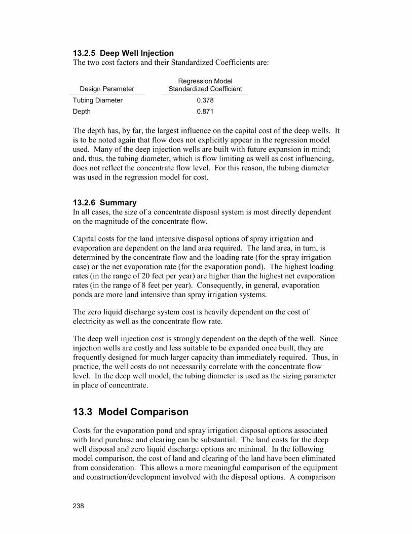
238

13.2.5 Deep Well Injection The two cost factors and their Standardized Coefficients are:

Design Parameter Regression Model

Standardized Coefficient

Tubing Diameter 0.378 Depth 0.871 The depth has, by far, the largest influence on the capital cost of the deep wells. It is to be noted again that flow does not explicitly appear in the regression model used. Many of the deep injection wells are built with future expansion in mind; and, thus, the tubing diameter, which is flow limiting as well as cost influencing, does not reflect the concentrate flow level. For this reason, the tubing diameter was used in the regression model for cost.

13.2.6 Summary In all cases, the size of a concentrate disposal system is most directly dependent on the magnitude of the concentrate flow.

Capital costs for the land intensive disposal options of spray irrigation and evaporation are dependent on the land area required. The land area, in turn, is determined by the concentrate flow and the loading rate (for the spray irrigation case) or the net evaporation rate (for the evaporation pond). The highest loading rates (in the range of 20 feet per year) are higher than the highest net evaporation rates (in the range of 8 feet per year). Consequently, in general, evaporation ponds are more land intensive than spray irrigation systems.

The zero liquid discharge system cost is heavily dependent on the cost of electricity as well as the concentrate flow rate.

The deep well injection cost is strongly dependent on the depth of the well. Since injection wells are costly and less suitable to be expanded once built, they are frequently designed for much larger capacity than immediately required. Thus, in practice, the well costs do not necessarily correlate with the concentrate flow level. In the deep well model, the tubing diameter is used as the sizing parameter in place of concentrate.

13.3 Model Comparison

Costs for the evaporation pond and spray irrigation disposal options associated with land purchase and clearing can be substantial. The land costs for the deep well disposal and zero liquid discharge options are minimal. In the following model comparison, the cost of land and clearing of the land have been eliminated from consideration. This allows a more meaningful comparison of the equipment and construction/development involved with the disposal options. A comparison

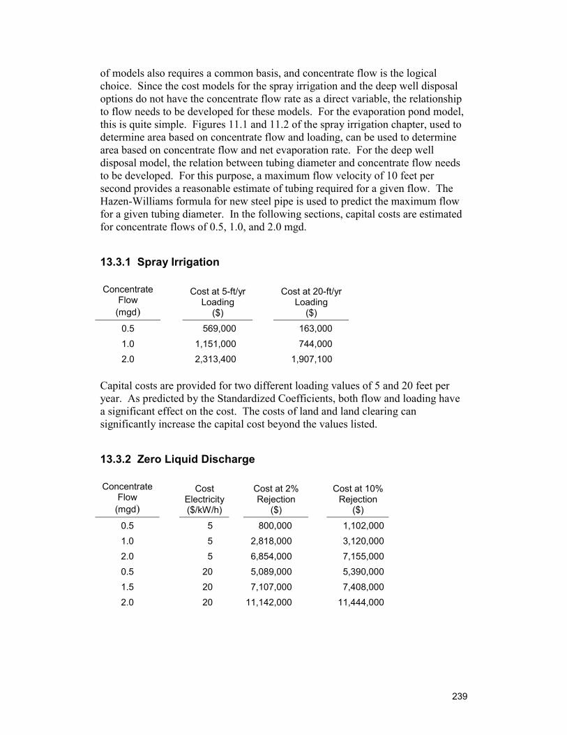
239

of models also requires a common basis, and concentrate flow is the logical choice. Since the cost models for the spray irrigation and the deep well disposal options do not have the concentrate flow rate as a direct variable, the relationship to flow needs to be developed for these models. For the evaporation pond model, this is quite simple. Figures 11.1 and 11.2 of the spray irrigation chapter, used to determine area based on concentrate flow and loading, can be used to determine area based on concentrate flow and net evaporation rate. For the deep well disposal model, the relation between tubing diameter and concentrate flow needs to be developed. For this purpose, a maximum flow velocity of 10 feet per second provides a reasonable estimate of tubing required for a given flow. The Hazen-Williams formula for new steel pipe is used to predict the maximum flow for a given tubing diameter. In the following sections, capital costs are estimated for concentrate flows of 0.5, 1.0, and 2.0 mgd.

13.3.1 Spray Irrigation Concentrate

Flow (mgd)

Cost at 5-ft/yr Loading

($)

Cost at 20-ft/yr Loading

($)

0.5 569,000 163,000 1.0 1,151,000 744,000 2.0 2,313,400 1,907,100

Capital costs are provided for two different loading values of 5 and 20 feet per year. As predicted by the Standardized Coefficients, both flow and loading have a significant effect on the cost. The costs of land and land clearing can significantly increase the capital cost beyond the values listed.

13.3.2 Zero Liquid Discharge Concentrate

Flow (mgd)

Cost Electricity ($/kW/h)

Cost at 2% Rejection

($)

Cost at 10% Rejection

($)

0.5 5 800,000 1,102,0001.0 5 2,818,000 3,120,0002.0 5 6,854,000 7,155,0000.5 20 5,089,000 5,390,0001.5 20 7,107,000 7,408,0002.0 20 11,142,000 11,444,000

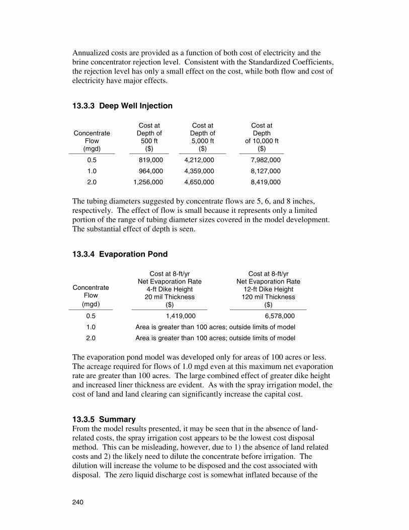
240

Annualized costs are provided as a function of both cost of electricity and the brine concentrator rejection level. Consistent with the Standardized Coefficients, the rejection level has only a small effect on the cost, while both flow and cost of electricity have major effects.

13.3.3 Deep Well Injection

Concentrate Flow (mgd)

Cost at Depth of

500 ft ($)

Cost at Depth of 5,000 ft

($)

Cost at Depth

of 10,000 ft ($)

0.5 819,000 4,212,000 7,982,000

1.0 964,000 4,359,000 8,127,000

2.0 1,256,000 4,650,000 8,419,000

The tubing diameters suggested by concentrate flows are 5, 6, and 8 inches, respectively. The effect of flow is small because it represents only a limited portion of the range of tubing diameter sizes covered in the model development. The substantial effect of depth is seen.

13.3.4 Evaporation Pond

Concentrate Flow

(mgd)

Cost at 8-ft/yr Net Evaporation Rate

4-ft Dike Height 20 mil Thickness

($)

Cost at 8-ft/yr Net Evaporation Rate

12-ft Dike Height 120 mil Thickness

($)

0.5 1,419,000 6,578,000

1.0 Area is greater than 100 acres; outside limits of model

2.0 Area is greater than 100 acres; outside limits of model

The evaporation pond model was developed only for areas of 100 acres or less. The acreage required for flows of 1.0 mgd even at this maximum net evaporation rate are greater than 100 acres. The large combined effect of greater dike height and increased liner thickness are evident. As with the spray irrigation model, the cost of land and land clearing can significantly increase the capital cost.

13.3.5 Summary From the model results presented, it may be seen that in the absence of land-related costs, the spray irrigation cost appears to be the lowest cost disposal method. This can be misleading, however, due to 1) the absence of land related costs and 2) the likely need to dilute the concentrate before irrigation. The dilution will increase the volume to be disposed and the cost associated with disposal. The zero liquid discharge cost is somewhat inflated because of the

241

interaction between the thermal treatment system and the membrane system, as discussed in section 12.2, that results in a smaller membrane system needed to produce the required product volume. Similar statements can be made for the other models. These statements exemplify why care should be taken in using the model results.

It should be kept in mind that not all disposal options are possible at a given plant because of climate (limiting land applications), geology (limiting deep well injection), chemistry (limiting surface water disposal), volume (for disposal to sewer), or several other reasons. Further, where different options are possible, they may be at different distances from the membrane plant and require different amounts of conveyance to the disposal site. In an idealized situation where all options are possible, require minimal treatment before disposal, and are located at similar distances from the membrane plant, disposal to sewer should be the least expensive disposal option—provided disposal fees are not high. Disposal to surface waters or by land application would, in most cases, be less expensive than disposal to deep well. Typically, zero liquid discharge would be the most expensive disposal option.

The inevitable exceptions to this idealized situation underscore the need to develop site-specific disposal costs. The cost models presented may be used as a means of providing preliminary cost estimates and insights into developing more accurate disposal costs.

243

14. Instructions for Using CD 14.1 Format of the CD

The CD contains the following items:

♦ The complete survey database ♦ The complete report ♦ Worksheets for use in developing cost estimates of disposal options ♦ Calculation pages for capital costs of disposal options ♦ A front-end menu for accessing these individual parts of the CD

Each of these items is discussed, in turn, before a review of the installation procedure for loading and using the CD.

There are two requirements that must be installed on the user computer system:

1. The user must have at least one printer defined on the computer, as Microsoft Access requires a printer definition in order to display certain reports. The user, however, does not need Microsoft Access software.

2. The user must have Adobe Acrobat Reader version 4.0 or higher installed on the computer. Adobe Acrobat Reader is a free software application that is needed to view certain reports in the CD. You can download a free copy from <http://www.adobe.com/prodcuts/acrobat/readstep2.html>.

14.1.1 A Front-End Menu for Accessing These Individual Parts of the CD A user-friendly menu is the starting point to use the CD. It provides several buttons that are used to access different parts of the CD. The menu is shown in figure 14.1.

14.1.2 The Stand-Alone Database The database contains the survey results from approximately 150 membrane plants in summary form of three (sometimes four) pages of information for each plant. There are several ways of accessing these summaries. The first is by viewing a list of all the plants and by first clicking on the PLANT LIST button and then clicking on a particular plant name on the list that appears. The second is by clicking on the FULL PLANT REPORT button and then by scrolling through a large single file that appears which contains summary pages for all the plants. The final way is by clicking on the SEARCH button and by specifying search parameters on the resulting screen and then clicking on the Search Now button. A list of plants will appear; and when a particular plant name in a list is clicked, the summary pages for that plant will appear.

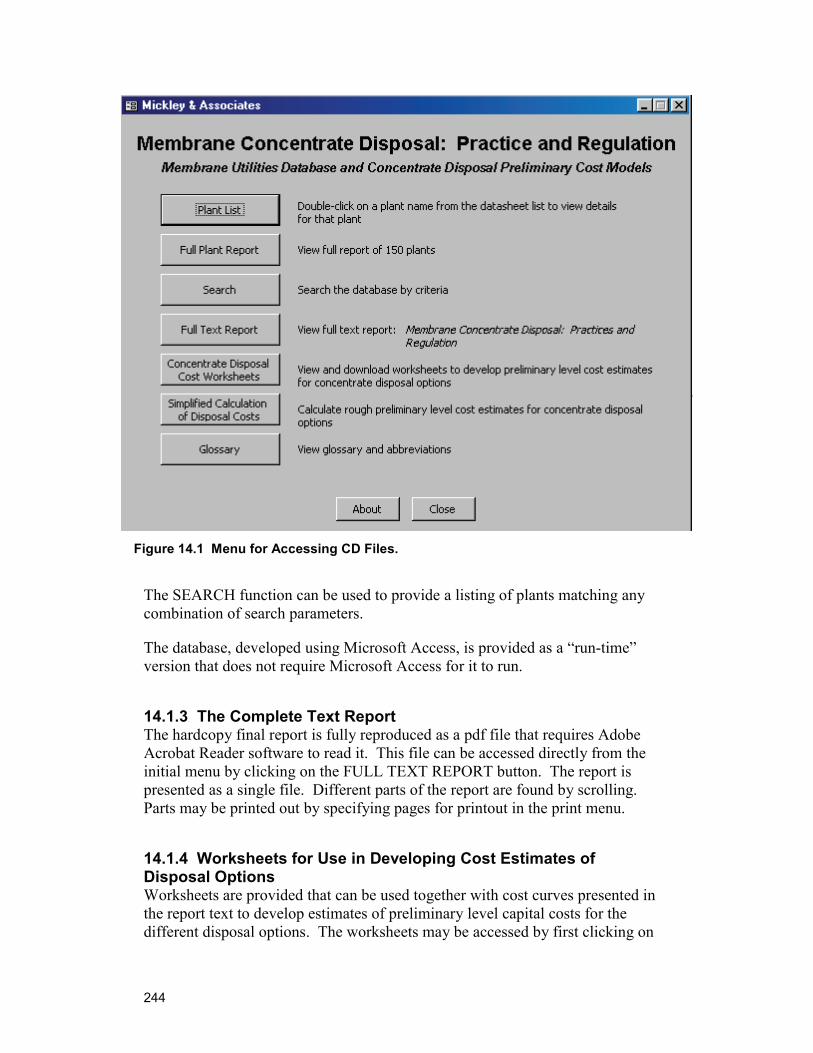
244

The SEARCH function can be used to provide a listing of plants matching any combination of search parameters.

The database, developed using Microsoft Access, is provided as a “run-time” version that does not require Microsoft Access for it to run.

14.1.3 The Complete Text Report The hardcopy final report is fully reproduced as a pdf file that requires Adobe Acrobat Reader software to read it. This file can be accessed directly from the initial menu by clicking on the FULL TEXT REPORT button. The report is presented as a single file. Different parts of the report are found by scrolling. Parts may be printed out by specifying pages for printout in the print menu.

14.1.4 Worksheets for Use in Developing Cost Estimates of Disposal Options Worksheets are provided that can be used together with cost curves presented in the report text to develop estimates of preliminary level capital costs for the different disposal options. The worksheets may be accessed by first clicking on

Figure 14.1 Menu for Accessing CD Files.

245

the CONCENTRATE DISPOSAL COST WORKSHEETS button. The particular worksheet corresponding to a disposal option can then be chosen from specifying it on the dropdown list that appears. The worksheet that appears may be printed out and used for manually calculating the capital cost for that disposal option. The user specifies certain design parameters, uses various cost curves in the text report to determine individual cost values, enters these costs on the worksheet, and performs the simple calculations described on the worksheet to develop a total cost. The text report contains separate chapters for each of the disposal options. The worksheets are discussed in these text report chapters along with design considerations and a discussion of the cost model assumptions and limitations. An example calculation is provided on each worksheet.

14.1.5 Calculation Pages for Capital Costs of Disposal Options Closed form equations were developed from regressing on 30 to 35 sets of data generated from worksheet calculations for each disposal option cost model. These calculation sheets may be accessed by first clicking on the SIMPLIFIED CALCULATION OF DISPOSAL COSTS button. A specific disposal option can then be chosen on the resulting screen by clicking on the disposal option name. The calculation page for that disposal option then appears. When the user declares values for the input variables specified on the calculation page, and then clicks on the “calculate cost” button, the total capital cost for the disposal option is calculated and displayed.

Use of the calculation page provides a simple and quick method of generating preliminary level cost estimates. The user, however, is cautioned to study the text report chapter and to work with the cost worksheets to develop an understanding of the assumptions and limitations of the cost models.

14.1.6 Glossary By clicking on the GLOSSARY button, the user can access a glossary of abbreviations and terms used in the report.

14.2 Installation of the CD

The following installation instructions are enclosed with each CD:

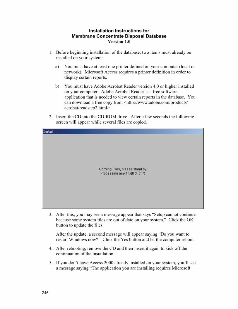
246

Installation Instructions for Membrane Concentrate Disposal Database

Version 1.0

1. Before beginning installation of the database, two items must already be installed on your system:

a) You must have at least one printer defined on your computer (local or network). Microsoft Access requires a printer definition in order to display certain reports.

b) You must have Adobe Acrobat Reader version 4.0 or higher installed on your computer. Adobe Acrobat Reader is a free software application that is needed to view certain reports in the database. You can download a free copy from <http://www.adobe.com/products/ acrobat/readstep2.html>.

2. Insert the CD into the CD-ROM drive. After a few seconds the following screen will appear while several files are copied.

3. After this, you may see a message appear that says “Setup cannot continue because some system files are out of date on your system.” Click the OK button to update the files.

After the update, a second message will appear saying “Do you want to restart Windows now?” Click the Yes button and let the computer reboot.

4. After rebooting, remove the CD and then insert it again to kick off the continuation of the installation.

5. If you don’t have Access 2000 already installed on your system, you’ll see a message saying “The application you are installing requires Microsoft

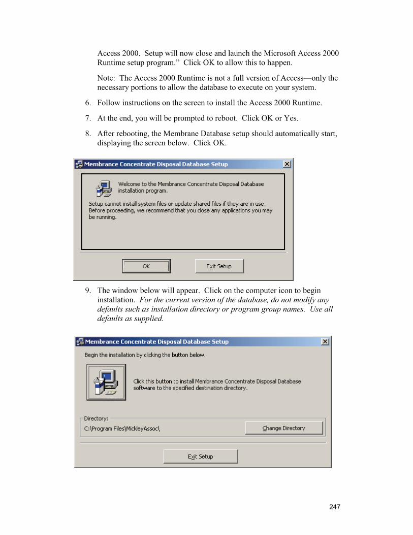
247

Access 2000. Setup will now close and launch the Microsoft Access 2000 Runtime setup program.” Click OK to allow this to happen.

Note: The Access 2000 Runtime is not a full version of Access—only the necessary portions to allow the database to execute on your system.

6. Follow instructions on the screen to install the Access 2000 Runtime.

7. At the end, you will be prompted to reboot. Click OK or Yes.

8. After rebooting, the Membrane Database setup should automatically start, displaying the screen below. Click OK.

9. The window below will appear. Click on the computer icon to begin installation. For the current version of the database, do not modify any defaults such as installation directory or program group names. Use all defaults as supplied.

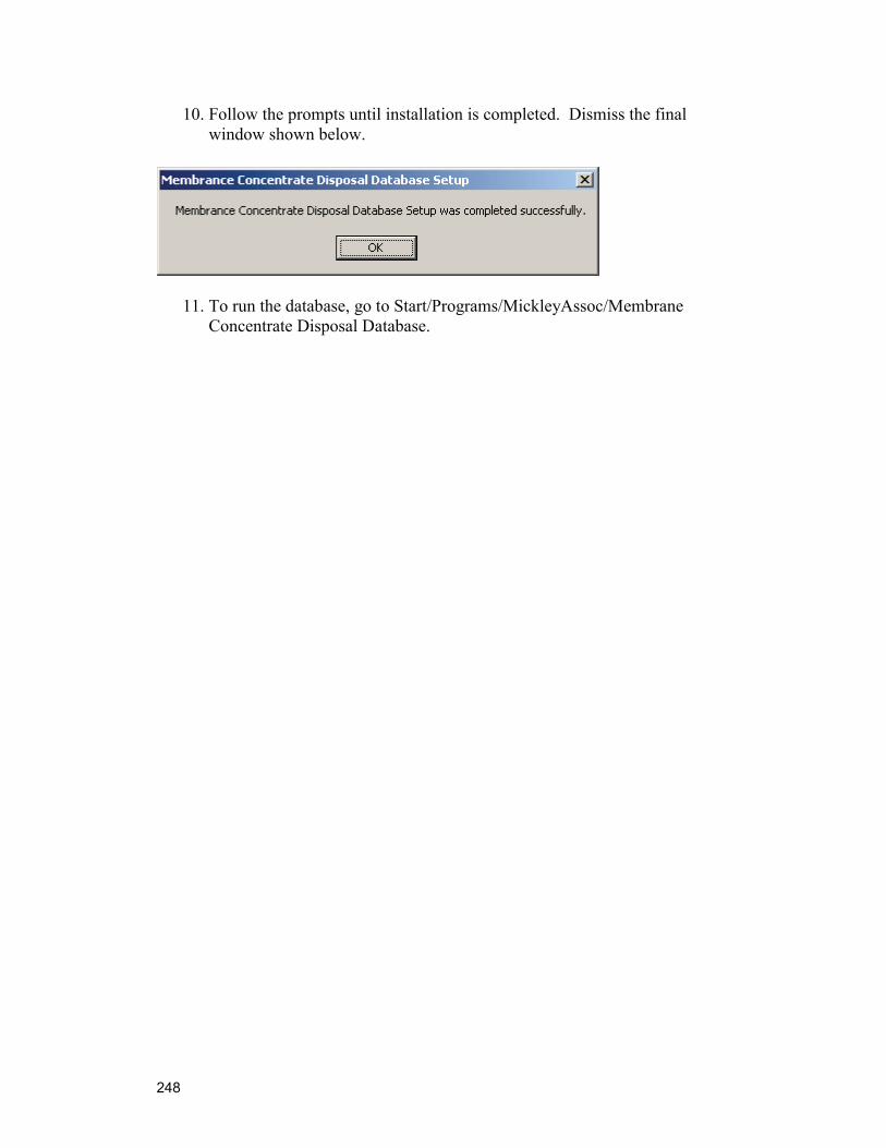
248

10. Follow the prompts until installation is completed. Dismiss the final window shown below.

11. To run the database, go to Start/Programs/MickleyAssoc/Membrane Concentrate Disposal Database.

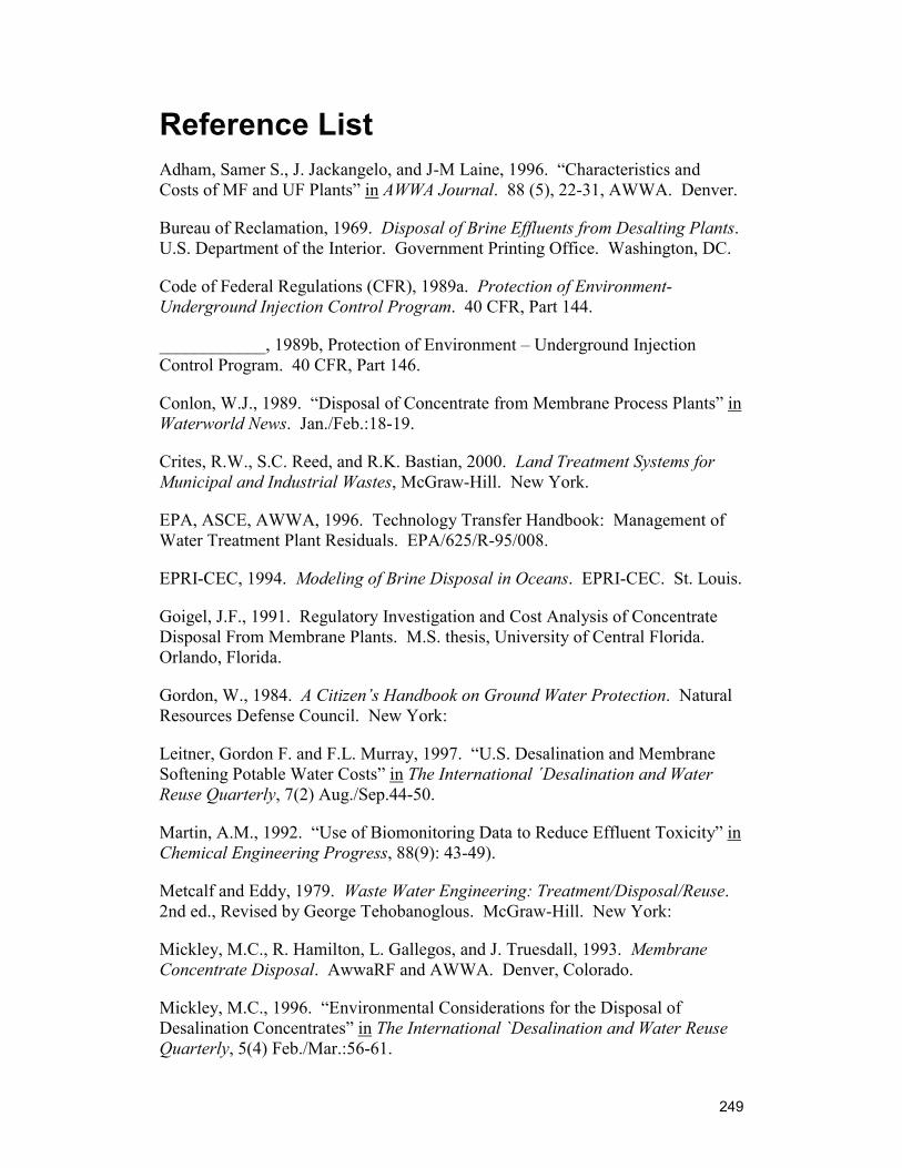
249

Reference List Adham, Samer S., J. Jackangelo, and J-M Laine, 1996. “Characteristics and Costs of MF and UF Plants” in AWWA Journal. 88 (5), 22-31, AWWA. Denver.

Bureau of Reclamation, 1969. Disposal of Brine Effluents from Desalting Plants. U.S. Department of the Interior. Government Printing Office. Washington, DC.

Code of Federal Regulations (CFR), 1989a. Protection of Environment-Underground Injection Control Program. 40 CFR, Part 144.

____________, 1989b, Protection of Environment – Underground Injection Control Program. 40 CFR, Part 146.

Conlon, W.J., 1989. “Disposal of Concentrate from Membrane Process Plants” in Waterworld News. Jan./Feb.:18-19.

Crites, R.W., S.C. Reed, and R.K. Bastian, 2000. Land Treatment Systems for Municipal and Industrial Wastes, McGraw-Hill. New York.

EPA, ASCE, AWWA, 1996. Technology Transfer Handbook: Management of Water Treatment Plant Residuals. EPA/625/R-95/008.

EPRI-CEC, 1994. Modeling of Brine Disposal in Oceans. EPRI-CEC. St. Louis.

Goigel, J.F., 1991. Regulatory Investigation and Cost Analysis of Concentrate Disposal From Membrane Plants. M.S. thesis, University of Central Florida. Orlando, Florida.

Gordon, W., 1984. A Citizen’s Handbook on Ground Water Protection. Natural Resources Defense Council. New York:

Leitner, Gordon F. and F.L. Murray, 1997. “U.S. Desalination and Membrane Softening Potable Water Costs” in The International ´Desalination and Water Reuse Quarterly, 7(2) Aug./Sep.44-50.

Martin, A.M., 1992. “Use of Biomonitoring Data to Reduce Effluent Toxicity” in Chemical Engineering Progress, 88(9): 43-49).

Metcalf and Eddy, 1979. Waste Water Engineering: Treatment/Disposal/Reuse. 2nd ed., Revised by George Tehobanoglous. McGraw-Hill. New York:

Mickley, M.C., R. Hamilton, L. Gallegos, and J. Truesdall, 1993. Membrane Concentrate Disposal. AwwaRF and AWWA. Denver, Colorado.

Mickley, M.C., 1996. “Environmental Considerations for the Disposal of Desalination Concentrates” in The International `Desalination and Water Reuse Quarterly, 5(4) Feb./Mar.:56-61.

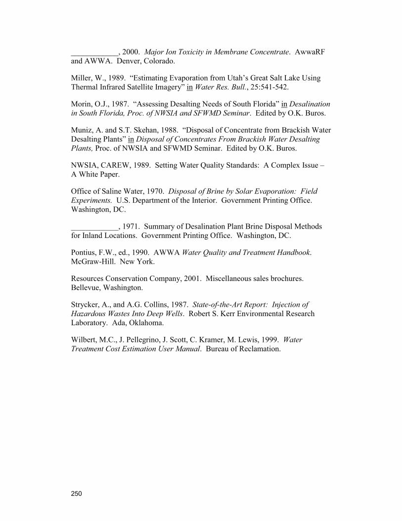
250

____________, 2000. Major Ion Toxicity in Membrane Concentrate. AwwaRF and AWWA. Denver, Colorado.

Miller, W., 1989. “Estimating Evaporation from Utah’s Great Salt Lake Using Thermal Infrared Satellite Imagery” in Water Res. Bull., 25:541-542.

Morin, O.J., 1987. “Assessing Desalting Needs of South Florida” in Desalination in South Florida, Proc. of NWSIA and SFWMD Seminar. Edited by O.K. Buros.

Muniz, A. and S.T. Skehan, 1988. “Disposal of Concentrate from Brackish Water Desalting Plants” in Disposal of Concentrates From Brackish Water Desalting Plants, Proc. of NWSIA and SFWMD Seminar. Edited by O.K. Buros.

NWSIA, CAREW, 1989. Setting Water Quality Standards: A Complex Issue – A White Paper.

Office of Saline Water, 1970. Disposal of Brine by Solar Evaporation: Field Experiments. U.S. Department of the Interior. Government Printing Office. Washington, DC.

____________, 1971. Summary of Desalination Plant Brine Disposal Methods for Inland Locations. Government Printing Office. Washington, DC.

Pontius, F.W., ed., 1990. AWWA Water Quality and Treatment Handbook. McGraw-Hill. New York.

Resources Conservation Company, 2001. Miscellaneous sales brochures. Bellevue, Washington.

Strycker, A., and A.G. Collins, 1987. State-of-the-Art Report: Injection of Hazardous Wastes Into Deep Wells. Robert S. Kerr Environmental Research Laboratory. Ada, Oklahoma.

Wilbert, M.C., J. Pellegrino, J. Scott, C. Kramer, M. Lewis, 1999. Water Treatment Cost Estimation User Manual. Bureau of Reclamation.

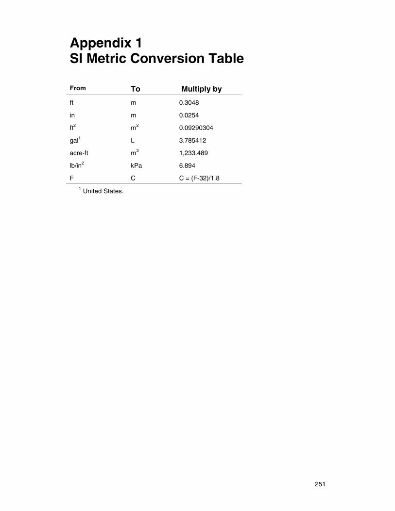
251

Appendix 1 SI Metric Conversion Table From To Multiply by

ft m 0.3048

in m 0.0254

ft2 m2 0.09290304

gal1 L 3.785412

acre-ft m3 1,233.489

lb/in2 kPa 6.894

F C C = (F-32)/1.8

1 United States.

253

APPENDIX 2 SURVEY OF STATE REGULATIONS REGARDING DRINKING WATER WASTE DISPOSAL

Background

Most of the survey was conducted from December 1998 to early 2000 with periodic checks with States that had membrane plants. Relevant information was obtained from the Internet and checking the State’s environmental agencies’ Web site to list and document the relevant programs dealing with water quality issues for the drinking water utilities. The corresponding agency was contacted by phone and interviewed accordingly. In some instances, due to the division of authority within the State, more than one agency was involved in the survey.

The key topics addressed in the survey concerning the water treatment plant’s (WTP) waste disposal options were the following:

♦ Options of liquid waste disposal ♦ Options of residue or sludge disposal ♦ Raw water source and overall quality ♦ Chemicals or technical treatment problems faced by the utilities ♦ Ground water reinjection as a waste disposal option ♦ Membrane technology use by the operating WTP ♦ Programs involved dealing with disposal options

The report that follows is presented in a narrative form as was hand recorded during the interviews. Further technical details as well as the legal requirements for the permits or policies listed can be obtained directly from the contact person phone number or checking the agency corresponding Web site.

Comments

Most States do not have membrane plants producing potable water. Several States have only small systems operating or have very few membrane plants. Consequently, the survey conducted and highlighted in this appendix refers mostly to disposal options for WTP residuals other than membrane concentrate or membrane backwash.

There are some similar terms used to describe residuals in conventional water treatment plants and membrane water treatment plants. This can be confusing unless directly addressed. In what follows, the term “concentrate,” unless referred

254

to as “membrane concentrate,” means a liquid waste/sludge prior to dewatering. The term “backwash” does not refer to “membrane backwash” as from an ultrafiltration (UF) or microfiltration (MF) process but means filter backwash.

ALABAMA Alabama Department of Environmental Management (ADEM) ADEM Montgomery Office 1751 Cong. W.L. Dickinson Dr. Montgomery, AL 36109-2608

Ph: (334) 271-7823 Fx: (334) 271-3051 Web site: www.adem.state.al.us/h2owebpg.htlm

Contact: Steve Williams, Water Supply Branch Ph: (334) 271-7788 Industrial facilities of all types, including drinking water utilities that discharge storm water and/or waste water to surface water must apply for a National Pollutant Discharge Elimination Systems (NPDES) permit. In Alabama, the preferred option is to discharge backwash waste into a retaining pond. Most utilities do not discharge, since they have enough surface area to allow evaporation to occur, and their waste volume is minimal. The few that discharge must have an NPDES permit. The State also has a permitting procedure for industrial discharger to publicly owned treatment works (POTWs) under the State Indirect Discharge (SID) permit. There is no ground water re-injection option for waste disposal, and the Underground Injection Control (UIC) program has been cancelled in Alabama. The northern section of the State relies on surface water and the southern portion on ground water as the main drinking water source. Only one reverse osmosis (RO) system is currently operating in the State on Dolphin Island; this is a small unit treating water for high chloride since ground water in the Gulf Coast is affected by saltwater intrusion.

ALASKA Alaska Department of Environmental Conservation Division of Air and Water Quality Section of Water Quality Protection 410 Willoughby Ave. Suite 105 Juneau, AK 99801-1795

Ph: (907) 465-5308 Fx: (907) 465-5274 Web site: www.state.ak.us/local/akpages/ENV.CONSERV/dawq/wqhome.htm

Contacts: Susan Braley, Section Chief Joe Cottingham, Drinking Water Program

255

The State maintains and supervises the NPDES program ensuring that water quality standards are met by industrial dischargers, including the water treatment plants. Other disposal options such as indirect discharge to a sewer system are available to the utilities. Residue is typically disposed either onsite or sent to a sanitary landfill. Raw water is mainly surface water for the large utilities, and several smaller communities use ground water. There are very few membrane plants in the State, with the exception of drilling rigs in Cook Bay, which use RO to treat drinking water for small facilities. They submit regular monitoring analytical data to the State.

ARIZONA Arizona Department of Environmental Quality (ADEQ) Water Permits 3033 North Central Ave. Phoenix, AZ 85012

Ph: (602) 207-4677 Fx: (602) 207-4634 Web site: adeq.state.az.us/water/index.htm

Contact: John Coleman, Maricopa County Ph: (602) 506-6935 The State does not have additional regulations or permitting requirements for drinking water plant waste disposal. The Engineering Department of ADEQ authorizes the construction and operation of the new facilities, and the Water Permits section monitors compliance with the NPDES program in the event of discharges to surface water. New facilities must submit an Effluent Disposal Plan that can be incorporated in the design report for residual liquid disposition. Other options available in Maricopa County and the State are dewatering of the concentrate and landfilling, indirect discharge to POTWs, and recycling of backwash; in some cases, treated waste water is permitted for agriculture irrigation. Currently, Arizona does not have a sludge classification program, but there is concern about sludge quality regarding cryptosporidium and giardia cysts. A new nuclear plant facility in Palo Verde will be using RO technology for treating drinking water. A new Phoenix utility will also be implementing MF technology. There is concern about arsenic and pesticide in membrane concentrates of these new membrane facilities, and the ADEQ Water Quality Division will be monitoring their waste streams closely.

256

ARKANSAS Arkansas Department of Pollution Control and Ecology Water Division 8001 National Dr. Little Rock, AR 72209

Ph: (501) 682-0656 Fx: (501) 682-0910

Arkansas Health Department Drinking Water Program Division of Engineering 4815 Markan St. Little Rock, AR 72205

Ph: (501) 661- 2623 Fx: (501) 661-2032 Web site: www.adeq.state.ar.us/water/main.htm

Contact: Ted Schlurter, Health Department. Dischargers must meet State regulations for water quality standards (Arkansas Pollution Control and Ecology Commission [APC&E Commission] Regulation 2) and all regulations related to the administration of the NPDES program (APC&E Commission Regulation 6). Drinking water utilities currently dispose backwash to a retaining settling pond. In some cases, they require an NPDES permit for surface discharge. The WTP residual or concentrate can be dewatered and disposed in a sanitary landfill. Land application is also a viable option. In both cases, the utility must fulfill the required documentation for sludge disposal. The State does not have a classification or sludge program for the drinking water waste, which is considered in most cases nonhazardous. The State also allows land irrigation using backwash water. The source of water for the WTP is mixed, surface and ground water. In western Arkansas, the source primarily is surface water; whereas in the eastern section of the State, it is ground water. Source water is considered of good quality with minor metal or organic concentration problems (due to the treatment process). The use of alum is common and is considered the only additive necessary for treatment in most of the WTP utilities. Only one RO system is being proposed in the State to treat deep well water for a small community in northern Arkansas.

The Water Quality Planning Branch of the APC&E Commission is in charge of ground water protection monitoring landfills and other industrial facilities that store waste water or solid waste that could potentially impact ground water; they run the UIC program. Currently, the State does not have a formal set of ground water standards; the Water Division uses Federal standards and health advisory limits to determine status of the aquifers.

257

CALIFORNIA California Environmental Protection Agency State Water Resources Control Board (SWRCB) SWRCB Division of Water Quality Los Angeles Region 4 101 Center Plaza Dr. Monterrey Park, CA 91754-2156

Ph: (323) 266-7557 Fx: (323) 266-7600 Web site: www.dwr.water.ca.gov/

Contacts: Shirley Birosik, Division of Water Quality Abdell Shrudaji, Department of Health Services Ph: (213) 977-6808 Currently, there is no special regulation for disposal of wastes from drinking water plants; the waste generated will fall within existent programs such as a NPDES permit for surface discharge. This is the most common option of disposal of liquid waste. Permit requirements are managed by the Division of Water Quality. Disposal of the concentrate or sludge to a sanitary landfill as solid waste is also allowed, and the solid waste group in the Department of Health Services handles the necessary requirements. In the State, some utilities dispose their sludge as road construction material, and no permit is involved in this process, with the exception of notification to the solid waste group. Source water is a combination of surface and ground water. The northern part of the State uses primarily surface water, whereas the southern portion of the State uses more ground water. In the Los Angeles region, source water quality is acceptable, but there are frequent problems with salinity, nitrates, and volatile organic compounds (VOCs). There are utilities using membrane technology such as RO and MF. Santa Catalina Island has an RO plant to treat saltwater. There are some cases of re-injection occurring as an option for treating drinking water disposal, especially to control salt intrusion. The State has an UIC program to oversee any re-injection into ground water.

COLORADO Colorado Department of Health and Environment Water Quality Control Division 4300 Cherry Creek Drive South Denver, CO 80222-1530

Ph: (303) 692-3546 Fx: (303) 692-0390 Web site: http://governor.state.co.us/gov_dir/cdphe_dir/

258

Contacts: Jerry Biberstaine, Primary Drinking Water Regulation Division Glen Butner, Primary Drinking Water Regulation Division Phil Hegeman (also contributed to the survey—ext. 3598) The State of Colorado has not developed any new policies concerning disposal of drinking water plant waste. The division currently has issued 79 permits for filtered backwash and other concentrate disposal, which include some membrane concentrate from RO treatment units (there is no record by technology used). The recommended procedure is to dispose the high total dissolved solids (TDS) brine into lined settling ponds and allow for evaporation. The residue is disposed of in a landfill or applied to land after compliance with sludge classification criteria and meeting State regulations for solid waste disposal. Other disposal options such as discharge to waste water treatment plants (WWTP), surface discharge, or use of nonmembrane concentrate for road base material are currently considered and permitted in a case-by-case basis.

CONNECTICUT Department of Environmental Protection 79 Elm St. Hartford, CT 06106-5127

Ph: (860) 424-3837 Fx: (860) 424-4074 Web site: www.state.ct.us/dep

Contact: Dave Cherico The State currently has about 169 towns with municipal drinking water facilities. The main water source is ground water, which is of excellent water quality requiring minimum treatment. The drinking water utilities can apply to the Waste Management Bureau for a General Disposal Permit that will mirror U.S. Environmental Protection Agency (EPA) waste disposal regulation and will cover surface discharge situations. Disposal options include discharge to an existing sewer system, landfilling after dewatering, and surface discharge. There is current concern about excess iron and some heavy metals and hardness.

DELAWARE Delaware Department of Natural Resources and Environmental Control Division of Water Resources Surface Water Discharge Section 89 King Highway Dover, DE 19901

259

Ph: (302) 739-4731 Fx: (302) 739-3591 Web site: www.dnrec.state.de.us/

Contact: Peter Hansen, Ground Water Discharge Section Ph: (302) 739-5731 The State runs a sludge disposal program under the Department of Public Health. Backwash, concentrate, and other high TDS (brines) as drinking water waste are currently regulated under the sludge disposal program with all other sludge from waste water treatment plants. All options are allowed for disposal of drinking water treatment plant waste. These include surface discharge which will go through the NPDES section under the division of Water Resources and discharge to a waste water plant. In most cases, the backwash is allowed to settle in the sump with enough retention time to separate the solids. As with all effluents, the liquid must meet the 30 milligrams per liter (mg/L) TDS State limit before surface discharge. The solids can be landfilled or land spread (reporting how many pounds per acre will be spread.) The State issues permits on a case-by-case basis for land application of concentrate. There is no ground water discharge of concentrate allowed in the State. There is an aquifer recharge project in the State where the aquifer is filled during the wet season for demand later in the summer, but no waste goes into it.

FLORIDA Florida Department of Environmental Protection Division of Water Facilities Drinking Water Section 2600 Blair Stone Rd, MS 3520 Tallahassee, FL 32399-2400

Ph: (850) 487-1762 Fx: (850) 414- 9031 Web site: www.dep.state.fl.us/

Contacts: Richard Drew, Bureau Chief Ph: (850) 487-0563 Elsa Potts, Office of Waste Water Management Ph: (850) 921-9495 Fax: (850) 414-9031 In 1996, the State of Florida issued a set of guidelines for RO membrane utilities. This document does not elaborate on waste disposal options but describes current trends and present case studies of these membrane facilities. Currently, the State allows surface water disposal, and blending is a common practice. The concentrate is mixed with clean treated effluent to reduce saline concentration before discharge; all water quality standards must be met. The sludge or

260

concentrate also can be land filled, but few utilities chose this options due to the high chloride of the sludge that renders it unsuitable for land application. Areas with high lime concentrations may qualify for this type of disposal. The State requires a UIC permit for deep well injection of brine or concentrate.

GEORGIA Department of Natural Resources Environmental Protection Division Drinking Water Program 205 Butter St., SE Suite 1362 Atlanta, GA 30334

Ph: (404) 656-2750 Fx: (404) 651-9590 Web site: www.dnr.state.ga.us/

Contact: Bill Moaries Ph: (404) 651-5158

The majority of the drinking water utilities (conventional alum precipitation plants) in the State have NPDES permits since the preferred option is surface water discharge for the supernatant after settling in a lined pond or lagoon. Raw water source is mainly surface, but wells are also used especially for the smaller utilities. No ground water re-injection is allowed in the State. Very few utilities use membrane technology. The common practice includes using sand filters and plate and press filters. Residual generated can be dewatered and sent to a landfill. Some utilities may choose to negotiate with farmers to arrange land application of the sludge; currently, this is not a common practice.

HAWAII Department of Environmental Health Safe Drinking Water Branch 919 Ala Moana Blvd. Honolulu, HI 96814

Ph: (808) 586-4258 Fx: (808) 586-4370 Web site: hawaii.gov./doh/eh/eiemdw00.htm

Contact: Lawrence Whang There are very few utilities in the State (about eight) using membrane technology. Options for waste disposal fall within the NPDES program if the utility is discharging directly to surface water. Other options available to the industry have been landfill application after dewatering. No ground water re-injection is allowed in the State. Indirect discharge to a sewer system is also allowed, but no

261

permit is required. Surface water is the main source of raw water; and, in general, quality is good requiring minimum treatment. Technology use in the larger utilities includes conventional sand filters combined with a clarifier and chlorination process. Small utilities serving campground or resort areas use membrane technology such as RO systems.

IDAHO Division of Environmental Quality (DEQ) Water Quality 1410 North Hilton Boise, ID 83706

Ph: (208) 373 0265 Fx: (208) 373 0576 Web site: www2.state.id.us/deq

Contacts: Steve Tanner, Twin Falls Regional Office Ph: (208) 769-1422 Dick Rogers, Boise DEQ Ph: (208) 373-0265

Drinking water facilities in the northern section of the State do not generate significant waste. Source water comes from reservoirs with excellent water quality. The water is chlorinated to meet health standards but no further process is usually required. In the southern portion of the State, utilities using surface and ground water generate some residuals that are permitted for land application since it has alkaline properties and helps to maintain soil pH. Direct discharge of backwash wastes to surface water falls within the NPDES permitting program. Most utilities discharge to an existing sewer system and do not require further permits. In some cases, the utility is allowed to discharge backwash water to an infiltration basin as long as it meets water quality standards. There are few utilities (one or two) using MF and UF in the State.

ILLINOIS Illinois EPA Bureau of Water Division of Public Water Supply 1021 North Grand Ave. East Springfield, IL 62702

Ph: (217) 782-3397 Fx: (217) 782-0075 Web site: www.epa.state.il.us/

Contact: Derek Rompot Ph: (217) 782-0610

262

Drinking water utilities must have an NPDES permit for surface water discharge. In other instances, the utility can discharge to a waste water treatment system, previously reporting to the permitting office for clearance. More often, direct agreement with the waste water treatment facility suffices to avoid affecting water quality in the receiving plant. Source of raw water for the WTPs in the State is surface water. Other options such as sludge disposal directly to a landfill are available once the utility meets solid waste requirements, (i.e., sludge water content). For a complete list of treatment plants in the State and technology used in each one, it is possible to submit a formal request through the Freedom of Information office to the following address:

Division of Water Pollution Control P.O. Box 19276 Springfield, IL 62794-9276 The letter should be marked “FOI request.”

INDIANA Indiana Department of Environmental Management Drinking Water Branch 100 N. Senate P.O. Box 6015 Indianapolis, IN 46206-6015

Ph: (317) 308-3308 Fx: (317) 308-3339 Web site: www.state.in.us/idem/

Contact: Steve Roush Ph: (317) 232-8706

Lagoon settling and further discharge of the supernatant is the preferred option for drinking water plants in the State to discharge their backwash or liquid waste. Any surface discharge will require an NPDES permit, but very few utilities have a permit since most of them discharge to an existing sewer system. Residual land application is allowed once the sludge meets the required standards to ensure that no hazardous material is involved. Landfill application is also an option for residual disposal. Very few RO systems are currently in operation in the State of Indiana. No re-injection to ground water is allowed as a method of waste disposal. About 95 percent (%) of the public drinking water plants use ground water as their primary water source.

263

IOWA Iowa Department of Natural Resources Public Water Supply Henry Wallace Bldg. 502 E. 9th St. Des Moines, IA 50319-0034

Ph: (515) 281-6599 Fx: (515) 281- 8895 Web site: www.state.ia.us/government/dnr/organiza/

Contact: Roy Ney Ph: (515) 281-8945

Drinking water plants dispose their waste stream into a holding pond or lagoon. In the event of surface discharge, an NPDES permit is required. The most common disposal option is to discharge into an existing sewer system for which no permit is required. Ground water re-injection is not a disposal option for liquid waste in the State. Residual disposal to a landfill is a common option; again, no permit is required with the exception of the normal landfill paperwork. Most of the utilities use surface water as the main source of raw water. In the State there are six RO systems currently operating: three electrodialysis and probably one MF. Most plants are traditional alum settling plants that follow AWWA guidance for treating drinking water.

KANSAS Kansas Department of Health and the Environment Division of Environment Bureau of Water Forbes Field Bldg. #283 Topeka, KS 66620-0001

Ph: (785) 296-5500 Fx: (785) 296-5509 Web site: www.kdhe.state.ks.us/

Contact: Iragh Pourmirza Drinking water plants must have an NPDES permit for surface discharge to streams or other surface water. For drinking water utilities, it is mandatory that they meet a TDS limit between 20 to 81 mg/L TDS (required for all effluents) and also a pH range between biological acceptable limits (6.5 to 9.0). Most of the utilities have a settling lagoon; and in few cases, they dispose their concentrate to a sanitary landfill. None of the State utilities use membrane technology in Kansas. There is no ground water discharge option available for drinking water plants.

264

KENTUCKY Kentucky Department of Environmental Protection Frankfort Office Park Division of Water 14 Reilly Rd. Frankfort, KY 40601

Ph: (502) 564-2150 Fx: (502) 564-4245 Web site: www.state.ky.us/agencies/nrepc/dep2.htm

Contact: Tom Skaggs Ph: (502) 564-2225

The State allows surface water disposal of backwash or any liquid waste stream but requires permitting by the NPDES program. Use of lagoons and holding ponds are common. The indirect discharge to POTWs is practiced by municipal drinking water plants. The State conducts supervision of sludge quality for hazardous material through the Municipal Waste branch, which permits land farming of the sludge after quality control is performed. Main source of raw water is surface, but use of ground water is common. About 250 utilities are on surface water. The State conducts a UIC program, but ground water re-injection is not allowed as a disposal option.

LOUISIANA Department of Environmental Quality Office of Water Resources Drinking Water Program P.O. Box 82215 Baton Rouge, LA 70884 -2215

Ph: (225) 342-9500 Fx: (225) 765-0635 Web site: www.deq.state.la.us/

Contact: Clay Bowes, Drinking Water Program Engineer The State allows surface water discharge from retaining ponds; the overflow discharge requires an NPDES permit. Recycling of backwash is common practice as well as indirect discharge to a sewer system. Some WTPs generate sludge that is dewatered and landfilled without further requirement. Most of the utilities operate basic technology using clarifiers, sand filters, etc. There is no RO or other membrane technology currently being used by drinking water utilities in the State.

265

MAINE Maine Department of Environmental Protection 17 State House Station Augusta, ME 04333-0017

Ph: (207) 287-7688 Fx: (207) 287-7191 Web site: www.state.me.us/dep/mdephome.htm

Contact: Charles Brown Liquid waste generated in the process by WTPs is retained in a lagoon or holding pond and can be discharged to a surface stream as long as the plant has a valid NPDES permit. Indirect discharge to a sewer system is a valid option for liquid waste disposal. The concentrate residue is typically disposed in a sanitary landfill after dewatering; in this case, it classifies as a solid waste and can be disposed as such. Source water is mainly surface water from streams and reservoirs; few ground water wells are also a source of raw water. Iron and manganese are the main chemicals of concern. Liquid waste re-injection is not allowed by the current regulations for waste disposal. The State has a UIC program that addresses other aspects of ground water protection. There are a few small membrane systems in the State.

MARYLAND Maryland Department of the Environment 2500 Broening Highway Baltimore, MD 21224

Ph: (410) 631-3706 Fx: (410) 631-3157 Web site: www.mde.state.md.us/

Contact: Barry O’Brian, Water Supply Program The drinking water utilities are allowed to dispose their liquid waste directly to a surface stream providing previous clearance with the State has been obtained through an NPDES type of permit. Although indirect discharge to a sewer system is allowed, very few utilities choose this option. No ground water re-injection is currently allowed. The sludge or residual generated is commonly disposed in a sanitary landfill. There are very few utilities applying to the State for land application of backwash waste. In the State, most of the sludge is mixed with the municipal waste water sludge as the preferred way to handle residual concentrate. Raw water source is of acceptable quality; and most of the large cities rely on surface water and the rest on ground water. There are about 500 drinking water utilities in the State—25 of them (the larger ones) use surface water from reservoirs or streams. Iron and Manganese are typical problems in surface and

266

ground water. In some communities, wells have arsenic and low radioactive contamination (mainly radium and radon). There is only one RO system in the State dealing with a high sodium concentration.

MASSACHUSETTS Massachusetts Department of Environmental Protection 1 Winter St. 2nd Floor Boston, MA 02108

Ph: (617) 574-6871 Fx: (617) 292-5696 Web site: www.state.ma.us/

Contact: Frank Niels All traditional disposal options are currently available to drinking water utilities in the State. Surface discharge will require an NPDES permit. Ground water re-injection will be regulated by the ground water program (UIC) and must report water quality before re-injecting; currently reinjection is not a preferred practice. Drinking water utilities prefer to discharge into an existing sewer system. Sludge generated can be landfilled. In 1996, the State issued a document containing guidelines for residual disposal from drinking water utilities.

MICHIGAN Michigan Department of Environmental Quality Field Operation Section 350 Ottawa NW Grand Rapid, MI 49503

Ph: (616) 356-0277 Fx: (616) 356-0298 Web site: www.deq.state.mi.us/dwr/

Contact: Dave Timm, Field Operation Section, Grand Rapid District Surface discharge under an NPDES permit is the common practice to dispose liquid waste in the State, but indirect discharge and recycling within the plant are available options. Most residue is dewatered and disposed in a landfill; some land application occurs, but it is not common. The Michigan DEQ has a sludge program that oversees any land application. Surface and ground water are used as source water for public water utilities, but surface water coming from the Grand Lakes is the main source of raw water in the State. In general, the water quality is good requiring minimal treatment. In ground water, iron and, in few cases, arsenic are chemicals of concerns. The State does not allow ground water re-injection. There are a few utilities using membrane technology in the State, mainly RO systems.

267

MINNESOTA Minnesota Pollution Control Agency Municipal and Industrial Water Quality 520 Lafayette Rd. St. Paul, MN 55155-4194

Ph: (651) 296-6300 Fx: (615) 296-8717

Department of Health Public Water Program 121 East 7th Place P.O. Box 64975 Saint Paul, MN 55164-0975

Ph: (651) 215-0770 Fx: (651) 215-0775 Web site: www.pca.state.mn.us/water/

Contact: Dick Clark Ph: (651) 215-0747

Drinking water utilities in the State can dispose waste water or backwash directly to surface water after complying with NPDES regulations. Indirect discharge to sewer systems is also common practice. The State does not allow any underground waste disposal. Sludge generated is dewatered and sent to a sanitary landfill. No land application is allowed. Few membrane utilities currently operate in the State dealing with high TDS water source. Source of water quality in the State is good, and no major issues regarding concentration of pollutants occur.

MISSISSIPPI Mississippi Department of Environmental Quality Office of Pollution Control Division of Water Supply (Department of Health) P.O. Box 10385 Jackson, MS 39289-0385

Ph: (601) 961-5171 Fx: (601) 354- 6612 Web site: www.deq.state.ms.us/

Contact: James McClellen Ph: (601) 961-5061 Fx: (601) 961-5187

Drinking water plants can apply for DEQ NPDES permits for surface discharge. Most of the utilities discharge to a retaining pond or lagoon, allowing for settling

268

time and eventual surface discharge under a DEQ permit. Indirect discharge is also common, and utilities negotiate directly with the sewer utilities about volumes and quality of the effluent. Overall, the State enforces a total TDS < 45 mg/L in any surface discharge from drinking water utilities (and from other industries). DEQ does not allow underground water re-injection since almost all utilities draw ground water for drinking purposes. Recycling of backwash is encouraged and practiced by most utilities. Only the city of Jackson is currently permitted by DEQ under the NPDES program, but it is currently under a Consent Order since they have an alum problem with their sludge. The rest of the State utilities do not require permits due to reduced amounts of waste generated. No RO utilities currently exist in the State.

MISSOURI Missouri Department of Natural Resources Division of Environmental Quality Public Drinking Water Program P.O. Box 176 Jefferson City, MO 65102

Ph: (573) 751-7428 Fx: (573) 526-5797 Web site: www.dnr.state.mo.us/deq/

Contact: Terry Timmons, Public Drinking Water Program Ph: (573) 751-1188

Drinking water utilities in Missouri have two options for waste disposal under the current NPDES program. The first is to surface discharge to main rivers such as the Missouri or the Mississippi Rivers. This option is being currently reviewed because of increasing concern regarding additives such as alum or softener used by the utilities. The second option is to discharge to a retaining pond and discarding the supernatant and concentrating the sludge that is later removed, dewatered, and landfilled. Currently, the State has over 2,000 public water treatment plants; only 100 of them use surface water as the raw water source, and the rest depend on ground water. There are no extensive uses of membrane technology among the utilities, only the city of Nevada is currently using this technology. Due to the extensive use of ground water as water source, there is no ground water re-injection program for waste disposal.

269

MONTANA Montana Department of Environmental Quality 1520 E. Six Ave. Helena, MT 59620

Ph: (406) 444-2544 Fx: (406) 444-4386 Web site: www.deq.state.mt.us/

Contact: Terry Campbell Ph: (406) 444-5311

In most cases, drinking water plants discharge to an existing sewer system or surface discharge under an NPDES permit which requires the applicant to meet water quality standards. Residue generated at the plant is sent to a sanitary landfill after being dewatered. Some land application occurs but is authorized in a case-by-case basis. There are no RO plants currently in the State. Some utilities are using different types of cartridge such as 3M bag filters in some cases with granular pre-filtering. These plants serve small communities (less than 50,000) and resort areas. Source of raw water is a combination of surface and ground water. In general, source water quality is good with few exceptions dealing with nitrate intrusion mainly in utilities relying on ground water.

NEBRASKA Nebraska Department of Environmental Quality 1200 N. Street, Suite 400 P.O. Box 98922 Lincoln, NE 68509

Ph: (402) 471-2186 Fx: (402) 471-2909 Web site: www.deq.state.ne.us/

Contact: Jack Daniels, Department of Health, Drinking Water Program Ph: (402) 471-0510

Drinking water utilities in the State discharge their liquid waste to a pond or lagoon to allow settling of the solids. The overflow can be discharged directly to a receiving body of water under an NPDES permit. Indirect discharge to a sewer system is also a common option. Raw water source for the drinking water utilities is surface and ground water. In general, water quality is good, but some iron and manganese occur and need treatment. There are very few utilities using membrane technology; at least one is using an RO system to treat a nitrate problem. There is no underground re-injection allowed in the State as an option for waste disposal, but the State has an UIC program.

270

NEVADA Department of Conservation and Natural Resources Division of Environmental Protection Bureau of Water 1550 East College Parkway, Suite 142 Carson City, NV 89706-7921

Ph: (775) 687-6353 Fx: (775) 687-5856 Web site: www.state.nv.us/cnr/ndwp/home/htm

Contact: Dana Penny The State allows surface water discharge under an NPDES permit. Indirect discharge to an existing sewer system is also allowed. Landfill disposal of concentrate generated by the drinking water utilities is also allowed. In some cases, deep well injection is permitted under the UIC program, but is not a common practice among the drinking water utilities. Source raw water is mainly surface and ground water requiring treatment to deal with high TDS. Membrane technology is used in the State on a small scale, mainly by utilities dealing with sodium and chloride problems.

NEW HAMPSHIRE New Hampshire Department of Environmental Services 6 Hazen Drive Concord, NH 03302

Ph: (603) 271-3139 Fx: (603) 271-5171 Web site: www.state.nh.us/des/descover.htm

Contact: Richard Skarinka The State allows drinking water utilities several waste disposal options. The most common options are discharge to a holding lagoon and surface water (under the NPDES program) and direct discharge to a sewer treatment system. In most cases, reports to the sewer utility are required. The residue must be dewatered and dried before land disposal. The State reviews alum content to allow this option. Iron and manganese are metals of concern. Sludge with low radioactive levels of radon is also a potential problem.

271

NEW JERSEY New Jersey Department of Environmental Protection 401 East State St. P.O. Box 029 Trenton, NJ 08625-0029

Ph: (609) 292-4543 Fx: (609) 984-7938 Web site: www.state.nj.us/dep/dwq/

Contacts: Jeffrey Reading Mary Jo Aiello

The State allows different options for waste disposal from the drinking water plants. Surface water discharge falls within the NPDES program. Sludge generated can be landfilled or used for land application once approved by the Sludge Quality Assurance program where the utility must report quantity and quality of the sludge to be applied or disposed. There is concern in some cases with the amount of chlorine left in the residual; therefore, the level of trihalomethane is closely monitored. Heavy metal concentration is also monitored. In some cities, arsenic is a major concern, especially among utilities using ground water as the raw water source. In one case, a utility is disposing sludge as construction material in a dam project. The State offers what is called Determination Program for Beneficial Use of Waste; if the utility can support any beneficial use of its waste, it can apply for a permit under this program.

NEW MEXICO New Mexico Environmental Department Surface Water Quality Bureau Harold Runnels Bldg., N. 2050

1190 St. Francis Dr. Santa Fe, NM 87502 Ph: (505) 827-0187 Fx: (505) 827-0160

Web site: www.nmenv.state.nm.us/

Contact: Steve Baumgarth Ph: (505) 827-2803

Drinking water utilities in New Mexico can discharge liquid waste to surface water if they have a current NPDES permit. Holding pond or settling lagoons are common among the drinking water industry because they generate small waste volume. The State also allows the landfill option for disposal of concentrate or sludge; no land application is practiced or permitted. Indirect discharge to a

272

sewer system is also a valid disposal option, and no permit is involved; but the utilities negotiate the terms of the disposal to maintain quality of effluent discharge. The main source of raw water for the utilities is ground water; and therefore, no re-injection of any industrial liquid waste is allowed in the State. The ground water bureau manages the UIC program.

NEW YORK New York State Department of Environmental Conservation Division of Water Bureau of Water Permit 50 Wolf Rd. Albany, NY 12233-8010

Ph: (518) 457-7464 Fx: (518) 485-7786 Web site: www.dec.state.ny.us/

Contact: Joe Callaghen Ph: (518) 457-0663

Drinking water utilities in the State discharge preferably to an existing sewer system, and no permit is required. Other utilities discharge to surface water after settling the solids, and this option will require an New York NPDES permit. Currently, there is no ground water disposal option available in the State since most of the plants obtain their source water from wells. Sludge generated by drinking water plants is typically high in alum and, therefore, must be landfilled. This option does not require special permit. Minimum land application is known to occur with the sludge generated by the drinking water utilities.

NORTH CAROLINA North Carolina Department of Environmental and Natural Resources Division of Water Quality Raleigh, NC 27626-0535

Ph: (919) 733-7015 Fx: (919) 733-2496

Web site: www.ehnr.state.nc.us/

Contact: Harold Seylor Ph: (828) 251-6786 Fx: (828) 251-6770

Surface discharge of backwash water is a disposal option in the State but requires a NPDES permit. Indirect discharge to a sewer system is available as well as recycling the waste to the front end of the plant. Sludge generated in the plant is

273

typically landfilled and, in some instances, used for land application and supervised by the solid waste group. Utilities using ground water as source water are not allowed to dispose waste into the wells. The State has an UIC program that will be involved if a utility chooses this option. So far, this situation has not occurred in the State. Public utilities use surface and ground water as their main source water. On the coast, there is problem with saltwater intrusion in the aquifers because some of them have geological fractures. This salt intrusion is aggravated by poor well design and construction. There are no major chemicals of concern in the raw water used by industry. There are several, about 12, utilities using membrane technology (RO and MF) and about 10 more waiting to be permitted.

NORTH DAKOTA North Dakota Department of Health Environmental Health Section Division of Water Quality 1200 Missouri Ave. Bismark, ND 58506-5520

Ph: (701) 328-5150 Fx: (701) 328-5200 Web site: www.health.state.nd.us/ndhd/environ/wq/

Contacts: Gerry Bracht Ph: (701) 328-5227, Dave Bergsagel

Discharge to a settling lagoon is the preferred option in the State by drinking water utilities to dispose backwash waste. For surface discharge, an NPDES permit is required, and it is issued by the Department of Health. Most utilities discharge to an existing sewer treatment system. The sludge, once dewatered, is allowed to be disposed into a sanitary landfill. In the State, land application is not an option due to poor sludge quality for such purpose. Only one or two small RO plants are currently operating in the State.

OHIO Ohio Environmental Protection Agency Division of Surface Water Lazarus Government Center 122 South Front St. Columbus, OH 43215

Ph: (614) 644-2001 Fx: (614) 644-2329 Web site: www.epa.ohio.gov/

274

Contact: Sangee Prakash, drinking and ground water engineering and operating facilities Ph: (614) 644-2752 Fx: (614) 644-2909

In the State, there is a high percentage (greater than 90%) of drinking water plants recycling backwash to the front end of the plant. In some cases, surface discharge permits are issued under the NPDES program, but the preferred method of liquid waste disposal is indirect discharge to a sewer system. Underground injection is not allowed by the State. The common technology to treat drinking water in the State is flocculation and the use of clarifiers to remove iron and manganese. There are about three to five utilities using membrane technology (RO and MF).

OKLAHOMA Oklahoma Department of Environmental Quality P.O. Box 1677 Oklahoma City, OK 73101-1677

Ph: (405) 702-8100 Fx: (405) 702-8101 Web site: www.deq.state.ok.us/

Contact: Pratap Ganti Water treatment plants can discharge their liquid waste from their holding ponds directly to a receiving body once they fulfill the requirements of the NPDES program. Few utilities choose this option, and the majority recycle to the front of the plant. Indirect discharge to a sewer system is also an option valid in the State and does not require a permit from DEQ. The residue or sludge is disposed onsite and, in some cases, sent to a sanitary landfill. The State has a sludge quality program for the POTWs. Source of raw water is ground water in the southwestern portion of the State and surface water in the eastern part. In general, the water is of good quality with few instances of iron, manganese, and nitrates. Underground waste disposal is discouraged, but there are few WTPs that re-inject their waste. The State conducts an UIC program to ensure ground water protection. There are few utilities using membrane technology, but none of the large WTPs have membrane systems.

275

OREGON Oregon Department of Environmental Quality Water Quality Division Environmental Engineering 2020 SW. 4th Ave., Suite 400 Portland, OR 97201

Ph: (503) 229-5279 Fx: (503) 229-6957 Web site: www.deq.state.or.us/

Contact: Jim Sheelz Ph: (503) 229-5310

Liquid waste generated in the WTP is typically sent to a retaining lagoon for settling of the solids and posterior overflow discharge to a stream. The State requires an NPDES permit for this option. Indirect discharge to a sewer district is another valid option in the State. Residue or sludge generated is disposed in a sanitary landfill and, in some cases, used for land application. Any land application is supervised by the waste water sludge program. Some re-injection of liquid waste is still practiced by the existing plants. The State is working to discourage this practice, but some wells come with high salt content; and the utilities choose to re-inject, especially in central Oregon. The UIC program oversees this practice. Raw water quality is good in the State, and very few utilities have problems. Recently, high nitrates have originated some concern. No membrane technology is currently operating in the State or, if so, only serving small campground locations.

PENNSYLVANIA Department of Environmental Protection (DEP) P.O. Box 2063 Harrisburg, PA 17105-2063

Ph: (717) 783-2300 Fx: (717) 783-8926 Web site: www.dep.state.pa.us/

Contact: Ed Rosky, Division of Drinking Water Ph: (717) 783-9037

Surface discharge of liquid waste (backwash, clarifier blowdown, etc.) to a receiving stream is allowed in the State under the NPDES program. Indirect discharge to a sewer system is also a valid option for waste disposal. Sludge generated by the utilities is typically disposed in a sanitary landfill. There is a sludge program. Other disposal options may be available such as land application or as filling material, but these latter options are negotiated by DEP in a case-by-

276

case basis. The utilities use both sources of raw water and surface and ground water, with most of the utilities (about 75%) on ground water. In terms of population served, the use is almost even between the two sources. Most of the utilities use traditional filtration, coagulation, and flocculation to treat the raw water. There is one MF and one UF utility in the State, but no RO systems currently operating. In general, raw water quality is good, and no major concerns beside some iron and manganese occur.

RHODE ISLAND Rhode Island Department of Environmental Management Bureau of Environmental Protection 235 Promenade Rd. Providence, RI 02908

Ph: (401) 222-6605 Fx: (401) 222-3162 Web site:www.deq.state.or.us/

Contact: Jim Scheetz Ph: (503) 229-5310

The State issues general NPDES permits for drinking water utilities that discharge to a surface water stream or creek. In Rhode Island, General Permits are issued to an industrial sector instead of an individual facility, and the permit will cover intermittent or continuous effluent discharges. Utilities must meet the corresponding water requirements described in the permit. Residual disposal after dewatering is accomplished in a sanitary landfill. This is the preferred disposal option. Land application is also allowed, and the State has a program for this option; but since the requirements are more stringent, there are not many applicants. The State does not allow ground water injection for the new facilities; however, existing facilities in high saline areas still use this option. The State maintains a UIC program to monitor these facilities. The goal is to phase out this option in the near future. There are some chemicals of concern such as nitrates in some areas, and the Health Department monitors this sector of the drinking water utilities. Also, the sludge program is managed by the Health Department.

277

SOUTH CAROLINA South Carolina Department of Health and Environmental Control Bureau of Water Water Facilities 2600 Bull Street Columbia, SC 29201

Ph: (803) 898-4300 Fx: (803) 898-4215 Web site: www.state.sc.us/dhec/eqchome.htm

Contact: Coy Waritts, water facilities Ph: (803) 898-4257

In the State, over 90% of the WTPs choose surface discharge as needed under a general discharge permit. Although some paperwork is involved, it is less stringent on the monitoring side than an individual NPDES permit. Waste streams from holding ponds or lagoons can also be discharged to a sewer system. The residue or concentrate is typically sent to a POTW and, in some cases, landfilled. The preferred option is to dispose the sludge onsite. Some WTPs sell their sludge to cement plants. Source water comes from both surface and ground water. The larger utilities use more surface water. The State allows some utilities to store excess treated water underground for future use. The UIC program is involved in these cases, and the program is called capacity use; but there are very few of these in the State. Raw water is of good quality with some specific communities dealing with natural occurrence of radioactive material, chlorides, and salts in general. Ground water is typically treated for iron and manganese. Membrane technology is used in the State on a very limited scale.

SOUTH DAKOTA South Dakota Department of Environment and Natural Resources Office of Drinking Water Joe Foss Bldg. 523 E. Capitol Pierre, SD 57501

Ph: (605) 773-3754 Fx: (605) 394-2229 Web site: www.state.sd.us/state/executive/denr/denr.html

Contact: Gerry Stephanson Direct discharge to surface water in the State is regulated under the NPDES program. This requirement applies to any industrial or drinking water utility discharge. Indirect discharge to a sewer system is also an option, and no permit is involved; but the utilities should discuss the terms to keep within the required

278

standards. No ground water re-injection is allowed for disposal of liquid waste. The State has an UIC program to monitor ground water quality and use by utilities. Most of the utilities use surface water, but the smaller ones rely on wells. There is some concern in the State for low radioactive contaminants such as radium 228.

TENNESSEE Department of Environment and Conservation Division of Water Supply 6th Floor, L&C Tower 401 Church St. Nashville, TN 37243-1549

Ph: (615) 532-0191 Fx: (615) 532-0503 Web site: www.state.tn.us/environment

Contact: Bill Hench Ph: (615) 532-0165

Direct discharge of liquid waste is allowed in the State under an NPDES permit but is not the preferred option of the drinking water utilities. The option of choice is to recycle the decanted water to the front end of the process. Discharge to a POTW is also practiced on a lesser scale. The sludge generated is, in most cases, stored onsite, landfilled, or used in a beneficial use program for land application. If the utility applies to this program, it must meet quality criteria for health and hazardous requirements before releasing the sludge. Source of raw water in the State is both ground and surface water. The middle and eastern part of the State rely more on ground water. The water is of good quality; and only very few problems are known, among them iron and manganese. Some utilities are facing VOC pollution that requires air stripping. No re-injection is allowed, and the State has an UIC program. The few membrane technology plants in the State are mainly in small communities or suburbs.

TEXAS Texas Natural Resource and Conservation Commission (TNRCC) Water Utilities Water Quality Division P.O. Box 13087 Austin, TX 78711-3087

Ph: (512) 239-6020 Fx: (512) 239 6050 Web site: www.tnrcc.texas.gov/

Contact: Jack Schulze, Public Drinking Water Section

279

Drinking water utilities are allowed to discharge their liquid waste to a receiving stream only under an NPDES permit. They also can discharge to an existing sewer system; and, in this case, no permit is required. A third practice in the State for liquid waste disposal is recycling of the waste to the head of the plant. Typically, the supernatant of the settling lagoon is recycled, reducing the volume of liquid discharge. Any sludge or residue generated after dewatering can be disposed in a permitted sanitary landfill. There is a beneficial use program that the utilities can apply for, but most utilities prefer the first option. No use of the sludge for road construction is known at this moment. The utilities also have the option of re-injection of the stream waste, but most of them do not choose this option due to the stringent UIC program requirements. There are some concerns regarding quality of raw water. Utilities located east of Interstate 35 (I-35) face some color, alkalinity, iron, and manganese problems. West of I-35, the situation is different involving mainly high salt content in the surface and ground water. Also in this area, there is evidence of high fluoride concentration that requires attention. Surface water presents some sporadic problems with BTEX, and atrazine and the utilities have problems meeting maximum contaminant levels (MCLs). TDS, salinity, and urban pollution coming from Mexico are problems along the Rio Grande. Around Austin, the south section has excellent water quality, and no major problems occur. There are some RO systems in the State serving small communities. In west Texas, there are about five UF and MF utilities; two are under construction, and the rest (three) are approved and in final design phase.

UTAH Utah Department of Environmental Quality Division of Drinking Water Utah State Office Park 1950 W. North Temple Salt Lake City, UT 84114-4830

Ph: (801) 536-4200 Fx: (801) 536-4211 Web site: www.deq.state.ut.us/

Contact: Michael Georgenson Ph: (801) 536-4197

The State runs a General Permit program that covers the situation for WTPs discharging supernatant to surface water. Typically, this discharge is intermittent and in small volumes. Indirect discharge to a sewer system is not a common option in the State. The sludge generated is disposed in a sanitary landfill or combined with POTW sludge. Source of raw water for the WTPs is a combination of surface and ground water, but the utilities depend more on ground water. Chemicals of concern in the State are iron and manganese and TDS—specifically sulfates. No re-injection of liquid waste is allowed, and the State has

280

an UIC program. In the State, there are some utilities using membrane technology; one is an UF plant, and there are several small units online using RO systems.

VERMONT Vermont Department of Environmental Conservation Water Quality Division Agency of Natural Resources 103 S. Main 10 N. Waterbury, VT 05671-0408

Ph: (802) 241-3777 Fx: (802) 241-3287 Web site: www.anr.state.vt.us/

Contact: Gregg Bostock Surface discharge of a holding pond or lagoon supernatant to a receiving stream needs to be permitted (NPDES) by the State. Indirect discharge to a sewer system is also an option. Source of raw water is a combination of surface and ground water. The water quality in the State is good, and the utilities do minimum treatment with sandbag filtration—in some cases, coagulation and flocculation—to handle iron and manganese. No liquid waste re-injection is permitted to ground water, but the State has an UIC program. The sludge is dewatered and disposed in a landfill. No land application is practiced since the sludge quality is poor for this purpose. In the State, utilities can dispose sludge as filling material. There is no knowledge of membrane technology being used by existing or upcoming utilities.

VIRGINIA Virginia Department of Environmental Quality Water Program Pollution Prevention 629 East Main St. Richmond, VA 23240

Ph: (804) 698-4108 Fx: (804) 698-4032 Web site: www.deq.state.va.us/

Contact: Martin Bergenson Ph: (804) 698-4374

Drinking water utilities have the option to discharge directly any liquid waste (i.e., supernatant from a retaining pond) to a receiving stream only if they have a current NPDES permit. The residue, once dried, can be disposed in a sanitary

281

landfill. There is also the option of land application for the solids under the State pollution abatement program. The program requires quality control of any permitted sludge. Surface water is the main source of raw water, but there are some small WTPs on ground water. One utility is permitted to re-inject treated water under the UIC program. There is only one RO plant in the State dealing with brackish water.

WASHINGTON Washington Department of Health Division of Drinking Water Air Industrial Center, Bldg. 3 P.O. Box 478222 Olympia, WA 98504

Ph: (360) 236-3153 Fx: (360) 236-2522 Web site: www.wa.gov/

Contact: Jim Rio All surface dischargers must comply with State and Federal regulations and have an NPDES permit to discharge to a surface stream. WTPs hold the liquid waste in a lagoon for settling, and the supernatant is discharged as needed. The plant can also recycle to the front end of the process as an option to reuse the supernatant. Indirect discharge to a sewer system is also a valid option in the State. Surface water is the most common raw water source in the State. Ground water is also used as source water, especially by smaller utilities. In general, source water quality is good, and only nitrate has been reported as a problem by a few utilities. The concentrate generated is typically dewatered and disposed in a sanitary landfill or onsite. The State does not allow liquid waste re-injection and just started the UIC program that will supervise any re-injection request for water reclamation. There is no information about RO or other membrane systems in the State.

WEST VIRGINIA West Virginia Department of Environmental Health Office of Environmental Engineering 815 Quarrier St. Charleston, WV 25301

Ph: (304) 558-2981 Fx: (304) 558-0691 Web site: www.dep.state.wv.us/

Contact: William Harold, Assistant Director of Environmental Engineering

282

Drinking utilities in the State discharge supernatant after settling in a lagoon to surface streams only under an NPDES permit. The most common disposal option is recycling the backwash by sending the liquid waste to the front end of the plant. Indirect discharge to a sewer system is also practiced, but in a minor proportion of the plants. The residue or sludge is mainly land applied or landfilled; this option is handled by the solid waste program. Source water for the utilities is mainly surface (70%) with few springs and wells used by small utilities. Raw water quality is good with mainly iron and manganese to be treated. In most cases, only chlorination and aeration is required to meet drinking water standards. Only one or two plants are currently using membrane technology. No ground water re-injection of liquid waste is allowed.

WISCONSIN Wisconsin Department of Natural Resources Environmental Protection Bureau of Drinking Water and Groundwater

Ph: (608) 266-9265 Fx: (608) 267-7650 Web site: www.dnr.state.wi.us/org/water

Contact: Steve Lendorff Discharge to a surface stream under an NPDES permit is one of the options available to WTPs in the State. The utility’s backwash is retained in a holding pond or is recycled to the front of the process. This is a common practice among the utilities. In few instances, they have the option of indirect discharge to a sewer system. The sludge or residue is commonly sent to a POTW as liquid waste for disposal; some WTPs choose to dewater and send their sludge to a landfill. Half of the population in the State is served by utilities using surface water and the rest by ground water. There are 20 large utilities using surface water and about 200 small plants on ground water. The State does not allow waste re-injection and closely monitors all well operation under the UIC program. Source water quality is good with few exceptions where the plants have to deal with VOC leaching from nearby landfills. There are two plants under construction with MF technology.

283

WYOMING Wyoming Department of Environmental Protection Water Quality Division 122 West 25th St., Herschler Bldg. Cheyenne, WY 82002

Ph: (307) 777-7981 Fx: (307) 777-5973 Web site: www.deq.state.wy.us/

Contact: Larry Robertson Ph: (307) 777-7075

The U.S. Environmental Protection Agency (EPA) region VIII runs from Denver several programs related to Wyoming’s water issues. At this time, EPA sets the water quality standards for the NPDES program, including the monitoring, capacity development, drinking water reporting, and confirmation of permits to the waste and drinking water utilities. The officer in charge of Wyoming in the region is Maureen Dauddy (ph: 303 312-6262).

There are only nine WTPs currently operating in the State. In most cases, they send the backwash and other liquid waste to a lagoon; and after the solids have settled, the decant could be discharged to a surface stream or recycled to the front of the process within the plant. This latter option is common practice among the utilities. Sludge or concentrate residue can be disposed to a sanitary landfill once it passes the “paint filter test” to measure the level of water content. There are some land applications of the concentrate, but it is not a popular option since the sludge must meet quality criteria (e.g., Federal sludge criteria). Source water is a combination of surface and ground water. There is no re-injection of liquid waste, and the State conducts a UIC program to monitor ground water quality. Ground water is good requiring very minimum treatment such as chlorination to control coliforms. No membrane technology is currently in use among the State’s WTPs.

285

APPENDIX 3 STATE NPDES-RELATED REGULATIONS COMMENTS Most States do not have membrane plants producing potable water. Several States have only small membrane systems operating or have very few membrane plants. The words “concentrate” and “backwash” have different meanings in nonmembrane treatment plants, and care must be taken when using these terms to denote the intended meaning. In what follows, the term “concentrate” unless referred to as “membrane concentrate” means a liquid waste/sludge prior to dewatering. Similarly, the term “backwash” means filter backwash unless specifically referred to as “membrane backwash” (from an ultrafiltration [UF] or microfiltration [MF] process). The context of the paragraph should also help to make the distinction clear.

Regulations for the States of California, Florida, and Texas are highlighted due to their high level of membrane activity. Information about regulation in the other States follows.

CALIFORNIA There are three main pieces of legislation for the regulation of concentrate disposal in the State:

♦ Porter-Cologne Water Quality Control Act ♦ California Regional Water Quality Control Board Basin Plans ♦ Water Recycling Criteria

The Porter-Cologne Water Quality Control is listed as Division 7 Water Quality in the California Water Code. A summary of the main sections of the rule is presented in table 1.

The permitting procedures regarding the National Pollutant Discharge Elimination System (NPDES) program in the State are as follows. The regions of the California Regional Water Quality Control Board (CRWQCB) receive the request from interested parties for surface discharge of liquid waste. The three general categories include waste water, industrial, and general. Water treatment plant (WTP) utilities will fall under the industrial group category. The permit is valid for 5 years, and it is very similar to the U.S. Environmental Protection Agency (EPA) permit. In some instances, depending on the plant location, it could be more stringent. Any whole efficiency toxic (WET) test requirement is tailored to the receiving water ecosystem: freshwater will have the corresponding species (C. dubia and P. promelas), and saltwater typically includes the mysids and the

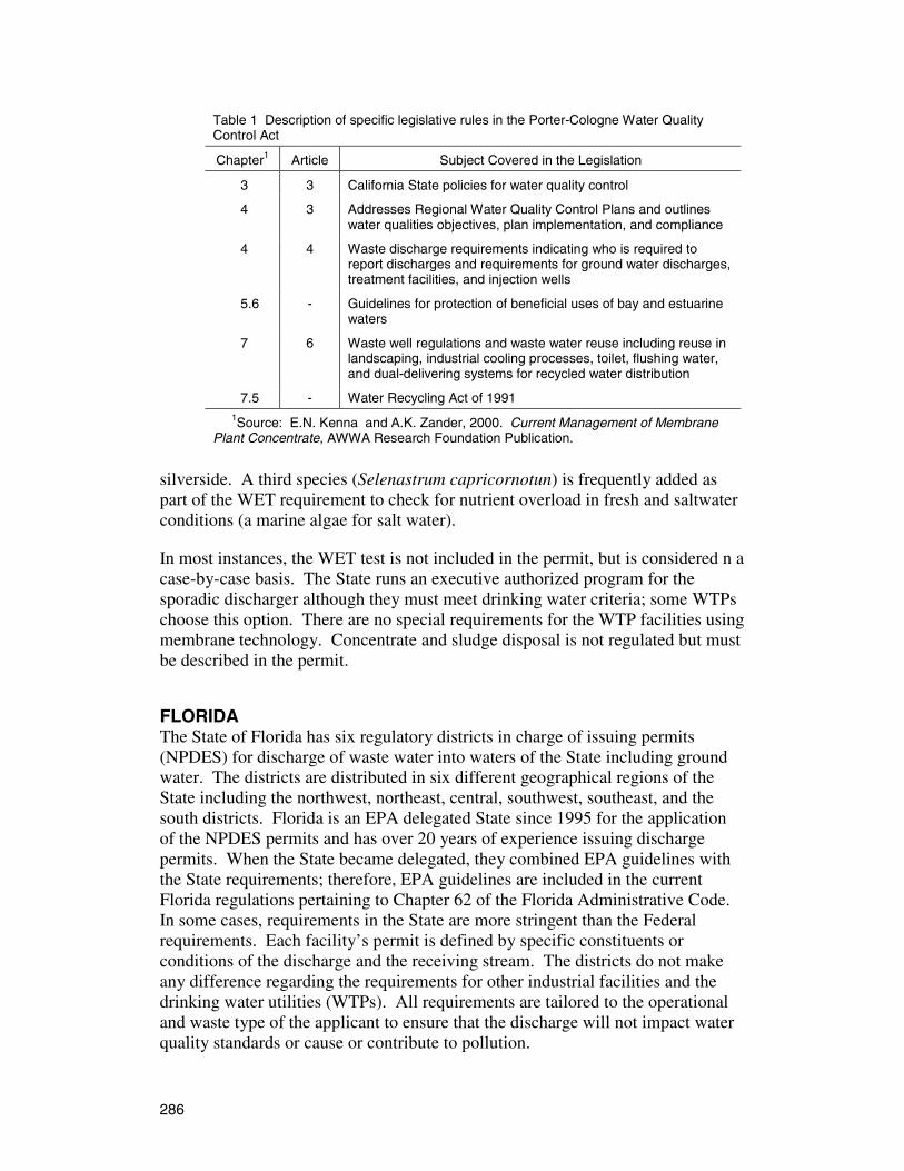
286

Table 1 Description of specific legislative rules in the Porter-Cologne Water Quality Control Act

Chapter1 Article Subject Covered in the Legislation

3 3 California State policies for water quality control

4 3 Addresses Regional Water Quality Control Plans and outlines water qualities objectives, plan implementation, and compliance

4 4 Waste discharge requirements indicating who is required to report discharges and requirements for ground water discharges, treatment facilities, and injection wells

5.6 - Guidelines for protection of beneficial uses of bay and estuarine waters

7 6 Waste well regulations and waste water reuse including reuse in landscaping, industrial cooling processes, toilet, flushing water, and dual-delivering systems for recycled water distribution

7.5 - Water Recycling Act of 1991

1Source: E.N. Kenna and A.K. Zander, 2000. Current Management of Membrane Plant Concentrate, AWWA Research Foundation Publication.

silverside. A third species (Selenastrum capricornotun) is frequently added as part of the WET requirement to check for nutrient overload in fresh and saltwater conditions (a marine algae for salt water).

In most instances, the WET test is not included in the permit, but is considered n a case-by-case basis. The State runs an executive authorized program for the sporadic discharger although they must meet drinking water criteria; some WTPs choose this option. There are no special requirements for the WTP facilities using membrane technology. Concentrate and sludge disposal is not regulated but must be described in the permit.

FLORIDA The State of Florida has six regulatory districts in charge of issuing permits (NPDES) for discharge of waste water into waters of the State including ground water. The districts are distributed in six different geographical regions of the State including the northwest, northeast, central, southwest, southeast, and the south districts. Florida is an EPA delegated State since 1995 for the application of the NPDES permits and has over 20 years of experience issuing discharge permits. When the State became delegated, they combined EPA guidelines with the State requirements; therefore, EPA guidelines are included in the current Florida regulations pertaining to Chapter 62 of the Florida Administrative Code. In some cases, requirements in the State are more stringent than the Federal requirements. Each facility’s permit is defined by specific constituents or conditions of the discharge and the receiving stream. The districts do not make any difference regarding the requirements for other industrial facilities and the drinking water utilities (WTPs). All requirements are tailored to the operational and waste type of the applicant to ensure that the discharge will not impact water quality standards or cause or contribute to pollution.

287

Regarding WET test requirement for the NPDES permit: the Florida Department of Environmental Protection (FDEP) emphasizes that every permit is unique and technical considerations for disposal of reverse osmosis (RO) membrane plant (see table 2) concentrate are taken into account when writing the permit and the biomonitoring requirements. Typically, marine species are considered for WET testing (i.e., Menidia beryllina and Mysidopsis bahia). If the total dissolved solids (TDS) of the concentrate are primarily determined by ions other than chloride and sodium and, thus, the concentrate is of lower salinity, freshwater species are considered. Any surface discharge must comply with biomonitoring and chemical standards before discharge. The utilities can request variance of discharge standards filing a State form if they consider that permit constituents do not apply to their current situation (a copy of the form application can be obtained from the FDEP Web site).

The complexity of the Individual Permit for membrane utilities is defined by the receiving Florida water, which follows a designation system. Several of the standards and requirements are based on which type of Florida water is receiving the discharge. Waters in Class III, for example, include all recreational waters; Class II describes waters dedicated to fisheries activities and will have more requirements on pollutants than the previous one. The permit process typically takes between 6 months to a year. However, it can get lengthy if sensitive environments in the State are involved. Currently, there are some legislative initiatives to resolve the issue of WET testing requirements for the membrane utilities. In some cases, the demonstration of absence of other pollutants has been required by FDEP, although it is up to the districts to get satisfaction on this requirement since they are the ones issuing the NPDES permit.

There are no special requirements for utilities discharging to a marine environment with the caveat that they must meet all standards established for the specific environment where they plan to discharge. It is obvious that discharging to a Florida Outstanding Water system will make a difference in permitting requirements.

A summary of accepted disposal options in the State for WTP (RO or conventional) includes the following:

1. Deep Well Injection Current deep well injection permits in Florida are issued under provisions of Chapter 403, Florida Statutes (F.S.) and Florida Administrative Code (FAC) Rules 62-4, 62-550, 62-660, and 62-528. The permit describes all technical requirements for Class I injection wells to dispose of nonhazardous reverse osmosis concentrate. The permit specifies well inside diameter (I.D.), depth, casing, volume (million gallons per day [mgd]) allowed to be disposed, injection pressure, and required monitor wells.

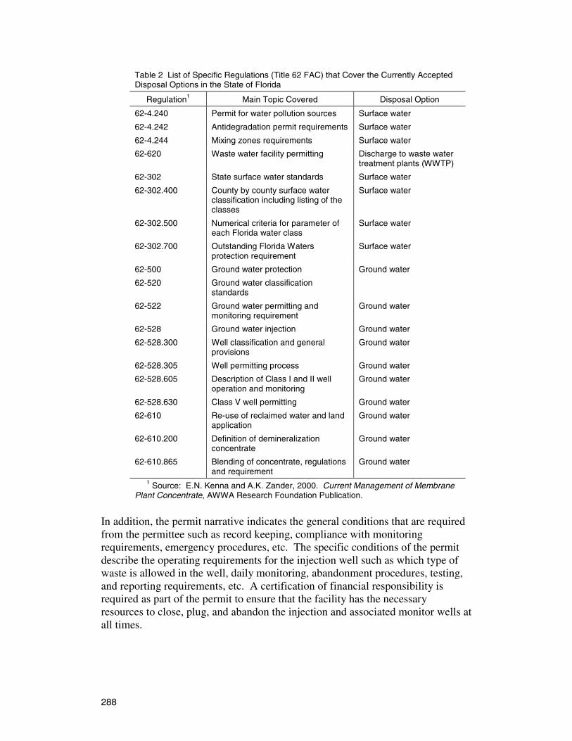
288

Table 2 List of Specific Regulations (Title 62 FAC) that Cover the Currently Accepted Disposal Options in the State of Florida

Regulation1 Main Topic Covered Disposal Option

62-4.240 Permit for water pollution sources Surface water

62-4.242 Antidegradation permit requirements Surface water

62-4.244 Mixing zones requirements Surface water

62-620 Waste water facility permitting Discharge to waste water treatment plants (WWTP)

62-302 State surface water standards Surface water

62-302.400 County by county surface water classification including listing of the classes

Surface water

62-302.500 Numerical criteria for parameter of each Florida water class

Surface water

62-302.700 Outstanding Florida Waters protection requirement

Surface water

62-500 Ground water protection Ground water

62-520 Ground water classification standards

62-522 Ground water permitting and monitoring requirement

Ground water

62-528 Ground water injection Ground water

62-528.300 Well classification and general provisions

Ground water

62-528.305 Well permitting process Ground water

62-528.605 Description of Class I and II well operation and monitoring

Ground water

62-528.630 Class V well permitting Ground water

62-610 Re-use of reclaimed water and land application

Ground water

62-610.200 Definition of demineralization concentrate

Ground water

62-610.865 Blending of concentrate, regulations and requirement

Ground water

1 Source: E.N. Kenna and A.K. Zander, 2000. Current Management of Membrane Plant Concentrate, AWWA Research Foundation Publication.

In addition, the permit narrative indicates the general conditions that are required from the permittee such as record keeping, compliance with monitoring requirements, emergency procedures, etc. The specific conditions of the permit describe the operating requirements for the injection well such as which type of waste is allowed in the well, daily monitoring, abandonment procedures, testing, and reporting requirements, etc. A certification of financial responsibility is required as part of the permit to ensure that the facility has the necessary resources to close, plug, and abandon the injection and associated monitor wells at all times.

289

2. Spray Irrigation/Land Application This type of permit is issued under the provision of Chapter 403 of the Florida Statutes and applicable rules of the Florida Administrative Code (See table 2). The permit covers holding pond facilities for concentrate waste prior to the irrigation stage. Typically, the concentrate is blended with other raw water to meet TDS standards before irrigation, in most cases, to golf course facilities. The permit specifies monitoring parameters for the land application, such as flow, TDS, sodium, chloride, sulfate, and pH. Ground water protection is also specified in the permit. Discharge monitor reporting (DMR) and blending ratios of concentrate with raw water (4:1) are detailed in the permit.

3. Surface Discharge The outfall discharge point is specified in the permit as well as the type of waste allowed to be discharged. Monitoring parameters at the mixing zone and the dimension of the zone are detailed in the permit. The permittee must comply with the applicable FAC Rules 62-4.244 and 63-302.500 (table 2) related to the subject of mixing zones. Land application, emergency surface discharge, other methods of disposal or recycling and further limitations of monitoring reporting are defined in the permit. A WET testing program is also described in the permit and is mandatory for surface dischargers.

TEXAS The disposal options for membrane concentrate and their regulatory requirements are specified in Title 30 of the Texas Administrative Code (TAC). Table 3 list the main topics included in this piece of legislation indicating the appropriate disposal option allowed by the Texas Natural Resources Conservation Commission (TNRCC).

Current disposal options in the State are: recycle to the head of the plant, land irrigation, discharge to a sanitary sewer system, evaporation pond, surface discharge to Texas Waters, discharge of brines or concentrate, and disposal of waste sludge. Few of these options involve State or Federal permitting. Discharge to surface water (i.e., water of the State or United States waters) requires a Texas NPDES (TPDES) permit that will have all Federal and State requirements. It is clear that the permit narrative is dictated by type and volume of discharge, receiving water conditions, frequency of the discharge, etc. All of these factors are site specific. Sludge disposal requires a State permit for disposal to a sanitary landfill or registration with TNRCC for land application of the sludge near the surface as it is indicated in 30 TAC Section 312.121. Re-injection is always an option for concentrate disposal but not a preferred one since it must require meeting underground injection control (UIC) requirements. In the case of land irrigation, it will only require a permit if the discharge is above 5,000 gallons per day; in which case, it will require a TPDES permit. Volumes below 5,000 gallons do not require permits according to current rules. The onsite disposal option of sludge or concentrate (within the WTP property) also is an accepted practice, and it will be covered by the TPDES permit.

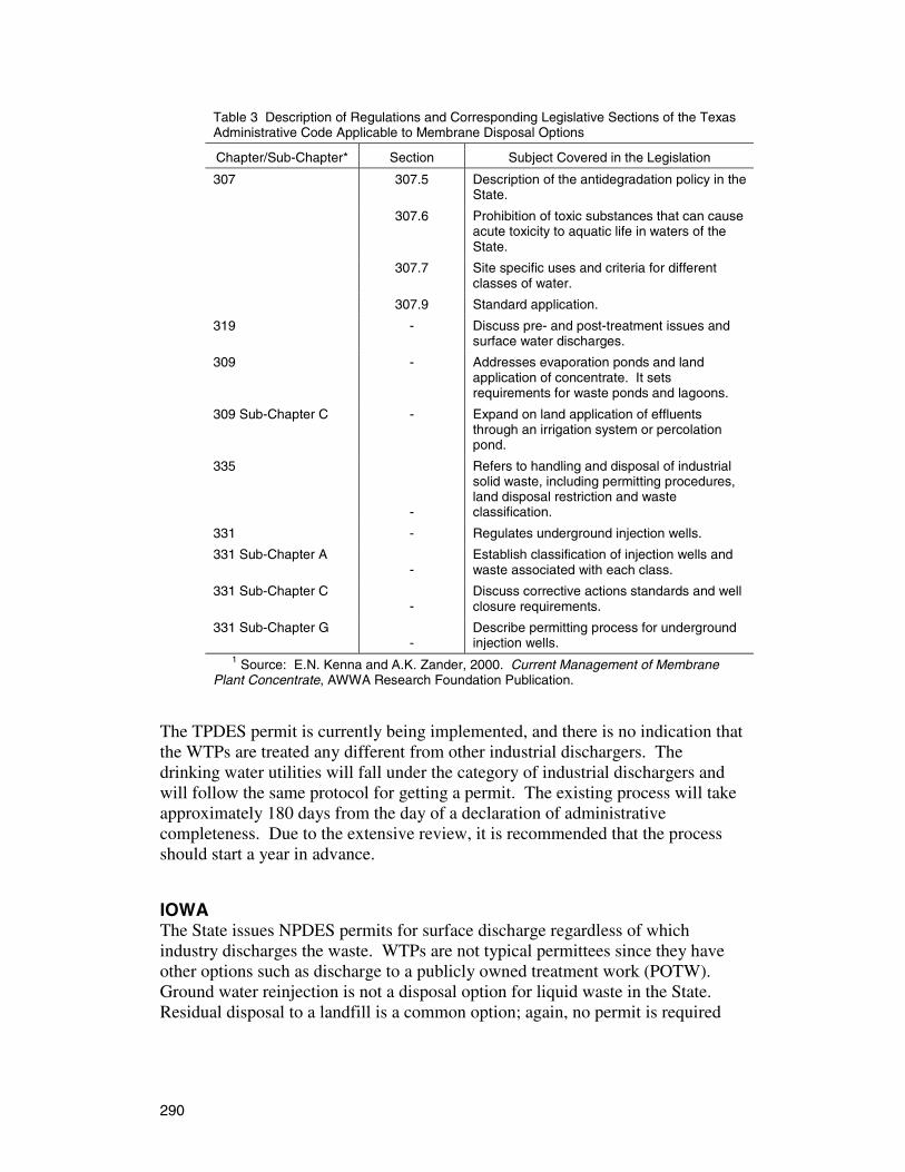
290

Table 3 Description of Regulations and Corresponding Legislative Sections of the Texas Administrative Code Applicable to Membrane Disposal Options

Chapter/Sub-Chapter* Section Subject Covered in the Legislation

307 307.5 Description of the antidegradation policy in the State.

307.6 Prohibition of toxic substances that can cause acute toxicity to aquatic life in waters of the State.

307.7 Site specific uses and criteria for different classes of water.

307.9 Standard application.

319 - Discuss pre- and post-treatment issues and surface water discharges.

309 - Addresses evaporation ponds and land application of concentrate. It sets requirements for waste ponds and lagoons.

309 Sub-Chapter C - Expand on land application of effluents through an irrigation system or percolation pond.

335

-

Refers to handling and disposal of industrial solid waste, including permitting procedures, land disposal restriction and waste classification.

331 - Regulates underground injection wells.

331 Sub-Chapter A -

Establish classification of injection wells and waste associated with each class.

331 Sub-Chapter C -

Discuss corrective actions standards and well closure requirements.

331 Sub-Chapter G -

Describe permitting process for underground injection wells.

1 Source: E.N. Kenna and A.K. Zander, 2000. Current Management of Membrane Plant Concentrate, AWWA Research Foundation Publication.

The TPDES permit is currently being implemented, and there is no indication that the WTPs are treated any different from other industrial dischargers. The drinking water utilities will fall under the category of industrial dischargers and will follow the same protocol for getting a permit. The existing process will take approximately 180 days from the day of a declaration of administrative completeness. Due to the extensive review, it is recommended that the process should start a year in advance.

IOWA The State issues NPDES permits for surface discharge regardless of which industry discharges the waste. WTPs are not typical permittees since they have other options such as discharge to a publicly owned treatment work (POTW). Ground water reinjection is not a disposal option for liquid waste in the State. Residual disposal to a landfill is a common option; again, no permit is required

291

with the exception of the normal landfill paperwork. The Municipal Solid Waste Office runs this program. An evaporation pond is not a disposal option due to weather conditions.

The NPDES program is similar to the Federal with water quality standards and biological requirements tailored to the type of waste and receiving water conditions. For WTPs, there is no WET test requirement. The normal processing time for an NPDES permit is 180 days.

ALABAMA Surface discharge of liquid waste generated by WTPs in the State will require an individual NPDES permit issued by the Permit and Compliance section of Alabama Department of Environmental Management. Currently in the State, there are not many of these permits issued since there are only about 25 WTPs that serve mostly small communities. The permit process takes about 6 months to complete and follows EPA guidelines. Constituents monitored include metals such as aluminum and iron. Other parameters such as pH, total suspended solids (TSS), total residual chlorine, and turbidity are also included.

The permit does not require WET testing. In general, few utilities are issued a permit since there are other disposal options available such as indirect discharge to a POTW.

ARKANSAS The State offers individual NPDES permits for WTPs that have been issued a construction permit by the State. The process requires submission of a notice of intent (NOI) form, a fee of $200, and corresponding maps indicating the discharge points. The process can take up to 3 months to complete including the comment period and draft review. Each utility is analyzed in a case-by-case basis. A partial priority pollutant scan must be submitted; and from the data, constituents for monitoring are defined. A WET test may be required based on the analytical report; but in most cases, it is not required. The State permit has similar requirements as the Federal NPDES, and the water quality standards correspond to the Clean Water Act (CWA) specifications.

Sludge disposal of concentrate and residual generated by the utilities are included in the permit. Landfill disposal and discharge to a POTW utility do not require a State permit.

CONNECTICUT WTP waste disposal in the State does not require an NPDES permit for surface discharge of liquid waste. The State runs a General Permit for the WTP utilities that covers disposal of residue or liquid backwash, filter rinse water, brines, and other waste generated during the process.

292

The permit describes in detail activities authorized and the type of wastes covered, such as clarifier tank sludge blowdown, filter media backwash, infiltration bed, and settling lagoon overflows, etc. The permit also specifies that the applying utility must submit, in the event of indirect discharge to a POTW, all pertinent information about the volumes and characterization of sludge and effluent.

The extent of requirements and constituents are defined after reviewing the presented information such as DMRs, process chemicals, etc. In general, WET test requirements are not required.

COLORADO The Colorado River Salinity Standards are listed in Regulation 39 and administered by the Colorado Department of Health. These standards are established to ensure that any discharge to surface water will not increase salt content (Regulation 61.8(2) (1)) in the Colorado River.

The State issues a General Permit (GP 60040000) for the WTP disposal of backwash and other liquid waste from retaining ponds. This permit will establish limits for pH, TSS, residual chlorine, flow, and other general constituents. Each utility must report their process chemicals and other treatments use to set the discharge requirements. WET testing is not typically included but is always an option based on specific constituents (chemical use in the process). The permit follows NPDES guidelines and corresponds with Federal CWA requirements regarding water quality standards. The permit is issued to utilities that have completed construction permit requirements, and it takes about 30 days to be completed. The most common disposal option currently used by the local utilities is natural percolation to the ground, which does not require a State permit.

Disposal options that require a State permit include land application of concentrate, which is regulated under the bio-solid program. Landfill disposal requires clearance with the landfill operator. No other options involve permitting.

DELAWARE Disposal options for the WTP in the State are: discharge to a POTW sewer system, landfill, onsite disposal, and, in some instances, spray or land irrigation of backwash reject. The only option that is covered under a State program is land irrigation. The others are not currently regulated. Concerning surface discharge, only one plant in the State has requested an individual NPDES permit.

The State NPDES program does not included any special regulation for WTPs. The program corresponds to EPA requirements; and, in some cases, there has been disagreement on maximum contaminant levels (MCLs) for metals since the utilities may concentrate these during the process to high levels for those constituents already existing in the source water. The State allows for a pollutant credit program, which accounts for initial level concentrations and credits the

293

utilities at the moment of disposal of the particular constituent. The State would like to provide waivers to the utilities in these situations; but the EPA region is reluctant to open this venue, and it demands the meeting of water quality standards.

There is no difference in the NPDES program for WTPs; but overall, few utilities request an Individual Permit (only one facility has initiated the permitting process). Regarding WET tests, only industrial dischargers with complex mixtures in their waste are required to submit biomonitoring data. WTPs are not required to do WET testing. The State has a set of guidelines for discharge to the marine environment, and it is site specific in the standards that the discharger has to meet, including definition of mixing zones, sensitive environment, seashell fisheries, etc.

In the event a WTP initiates the process for a NPDES permit, the time it takes from application to issuing the permit could be 6 months to 1 year. Location of the facility is the key decisive factor that might lengthen the process; in the simplest case, it can be fast (6 months).

GEORGIA Disposal options for the WTPs in the State are centered in surface discharge, land irrigation, land application of concentrate, and indirect discharge to POTW sewer system. The State permits through the NPDES program any surface discharge to State or United States surface waters; the State also runs a Land Application System (LAS) permit program that covers both land irrigation and sludge application for the municipal treated effluent and bio-solids. WTPs can apply to dispose backwash or blowdown waters, but it is not a common choice. The NPDES permit is posted on the Web. It is relatively simple for the WTP to apply for it and comply with basic requirements, such as TSS, turbidity, pH, and, in some cases, heavy metals such as ferrous ion (Fe++), and manganous ion (Mn++). The Individual Permit process is 120 days.

HAWAII Few utilities are issued NPDES permits since the main option to dispose liquid waste is the evaporation pond. In the island of Maui, the WTP utility has been issued an Individual Permit for supernatant discharge. The permit includes typical constituents such as pH, TSS, and total residual chlorine, which is the major concern to protect aquatic biota. One important aspect of the permit is that there is no marine discharge allowed—only discharge to freshwater streams.

ILLINOIS Disposal options covered by State regulations include landfill and surface discharge to State waters. All other options do not require State permits, but WTPs must comply with general guidelines (i.e., indirect discharge to a sewer system implies agreement between utilities).

294

It is common that WTPs request and obtain an NPDES permit for surface discharge. In the State, they are considered within the industrial sector and must meet all water quality standards before effluent discharging. The process is the same for all industrial facilities. WTPs using advanced technology such as RO systems or other advance filtration systems must report in detail their waste composition providing analytical data on constituents. The permit process in Illinois typically takes 180 days from the moment of submission of all pertinent documentation. There is high priority in the State for new WTP utilities. In general, the Illinois NPDES permit corresponds with the EPA permit and follows to the letter CWA standards and requirements. It is evident that the permit is tailored to individual conditions, and variations exist due to the uniqueness of each case.

The NPDES permits in the State for WTPs typically do not require WET tests, but it is possible to add this requirement based on the specific situation. Previously, the State had a General Permit for WTPs, but it has been phased out. The current policy is to allow old permits to expire and to issue a new Individual Permit that, in general, quite closely resembles the old permit. Requirements such as pH, TSS, flow, and metals are common. After reviewing analytical data of typical constituents, other MCLs may be established.

INDIANA Disposal options currently available in the State include indirect discharge to a POTW with no permit involved and surface discharge of liquid waste that does require an individual NPDES permit that follows EPA guidelines. For drinking water utilities, there are only secondary water quality standards on their key constituents but no biomonitoring or WET testing since these utilities are considered low flow and low pollutant contributors. The permit process is direct; and by statute, the State must finish the process in 180 days from submission.

Currently, WTPs are facing problems meeting chloride standards. Although there is no membrane technology treating drinking water in the State, it is expected that, as the chloride problem becomes more critical, some of the utilities will be considering advanced technology.

KANSAS Public utilities typically use retaining lagoons as a disposal option of their liquid waste; and for this, the State will issue a General Water Supply permit. There is no further requirement. The lagoon is allowed to evaporate or trickle underground. Since the water is considered relatively clean, further requirements are not necessary.

The NPDES permit for those WTPs will need to go to surface discharge proceeds as it would for any other industrial discharger, although the process is less complex. Within 6 to 8 months, the WTP can obtain a permit. The State will

295

establish the water quality standards according to process constituents. Currently, the permitting office requires TSS, pH, residual chlorine, and polymers as the main chemicals to monitor in the WTP utilities. Biomonitoring requirements with two species are only requested once at the onset of the permit to confirm no deleterious effect on aquatic biota.

KENTUCKY The State issues a General Permit for surface discharge of industrial facilities. WTPs are considered within this latter category. The permit is specifically for backwash or process water from a drinking water utility, and requirements listed include TSS, pH, residual chlorine, and, in some cases, metals such as iron and manganese.

The permitting process is direct and streamlined taking only from 30 to 60 days. All water quality standards and constituents follow CWA and EPA guidelines.

Disposal options that require a State permit include land application, which is regulated by the sludge program and the solid waste program. The permittee must meet EPA sludge criteria.

MARYLAND WTPs in the State are classified as municipal waste water plants for waste disposal regulation. For surface discharge of backwash or other liquid waste, the utility is required to apply for an individual NPDES permit. The permit defines basic constituents such as pH, TSS, coagulants used, aluminum, Iron, and total residual chlorine. WET testing requirements are not included in the permit since the utility effluent is considered to be a low pollutant contributor. There is no special requirement for discharging to State marine waters once all standards specified in the permit have been met.

The State does not allow land application of residual or concentrate from WTPs. Landfill disposal of sludge is dealt directly with the landfill operator. The permit process takes between 6 months to a year depending on the backlog in the permitting office.

MICHIGAN Currently, the State is implementing a General Permit for waste disposal of WTP residuals, specifically backwash and reject water from the drinking water treatment process. A new permit application will take between 2 to 6 months. The constituents currently monitored include TSS, pH, residual chlorine, settleable solids, and, in few cases, some metals. There are no WET test requirements involved as of this date. The metro area plants (Detroit) discharge to existing sewer systems and, therefore, avoid the NPDES permit. In the State, there are about 70 WTPs; and few of the medium to small size have chosen the General Permit route.

296

MISSISSIPPI In the State, the largest WTP is in the city of Jackson and currently is under a consent order to stop surface discharge due to frequent violation of State standards for aluminum and TDS. None of the other smaller utilities have requested an NPDES permit. In the event of surface discharge, they will be requested to comply with DEQ regulations. Most of the WTPs avoid surface discharge by negotiating with POTWs for sewer disposal and conducting onsite disposal of liquid and solid waste. The State does issue Individual Permits for other industrial dischargers. The process of applying and issuing a permit could take from 90 days to 6 months depending on data submitted in the application. All permit specifications mirror EPA guidelines, and the utilities must comply with State standards. WET testing is frequently included in these permits.

MISSOURI Disposal options for the WTP facilities include discharge to a POTW, landfill of the concentrate, and sludge disposal generally onsite. None of these options require a State permit. Only surface discharges to State waters require an NPDES permit. The State manages two types of permits: a General Permit for small utilities and Individual Permits for larger WTPs. The key characteristic that the permitting office considers as a criterion to sort out whether a utility qualifies as a small or large facility is how the WTP handles and disposes of the concentrate. Discharge of liquid waste and sludge to the Mississippi or Missouri Rivers must have an Individual Permit (large facility), which will include WET testing with two species. Constituents such as pH, TSS, settleable and suspended solids, and residual chlorine are typically included. The WET test requirement in the Individual Permit is being contested by the public utilities, and there is ongoing litigation concerning this issue. The General Permit is more flexible and does not include WET testing. Utilities that qualify for the General Permit do not dispose any sludge or residual to the rivers. The General Permit can be processed in 60 days; an individual NPDES permit can take as long as 3 years. These permits do not differ from the EPA guidelines.

MINNESOTA The State issues a general NPDES permit for surface discharge of WTP effluent including backwash, blowdown, and holding pond overflow. This General Permit is issued only to utilities already in the system (i.e., already with construction and operation permits; and, in that sense, it is a straightforward procedure that only takes 30 days). Constituents monitored in this permit are TSS, flow, pH, iron, manganese, and, in some cases, total residual chlorine. The permit also includes concentrate waste management within the facility. There is no WET testing included in the permit.

297

MONTANA Requirements for WTP surface discharge of their settling pond or backwash and liquid waste involve an NPDES Individual Permit. Typical constituents that are listed in the permit are TSS, turbidity, dissolved aluminum, and chlorine. The permit process takes about 6 months; but depending on the site location of discharge, it can be issued in 90 days. The writeup of the permit corresponds with EPA guidelines. WTP are low pollutant generators and, therefore, will not require WET testing.

NEBRASKA The State is currently reviewing the policies concerning surface discharge of liquid waste for the WTP sector. Utilities that discharge into the Missouri River are monitored for TSS, pH, flow, and residual chlorine. At this time, no WET test requirements are included in the permit. EPA guidelines are followed, and the required water quality standards meet CWA specifications. In the State, the utilities undergoing permit renewal must obtain an individual NPDES permit. The process from application to issuing the permit could take from 30 to 60 days for utilities that have completed the construction and permitting phase. The permit also covers sludge disposal and requires submission of a solid management plan. Although the State does not have a beneficial use program for concentrate, it encourages use of sludge as soil amendment in agricultural land.

NEVADA Discharge of backwash and process waste water to State waters by WTPs requires an individual NPDES permit. In most instances, pond and water tank overflow requires a permit. Typical constituents monitored in the permit are TSS, total residual chlorine, pH, settleable solids, and turbidity. The permit follows EPA guidelines and is at least as stringent as the Federal requirements.

Landfill disposal of generated sludge and indirect discharge to POTW do not require State permits. Underground waste water disposal will require a UIC permit. This latter option is not common among the utilities.

NEW JERSEY WTPs in the State are covered under a general New Jersey Pollutant Discharge Elimination System permit for surface discharge of filter backwash, cleaning operation of clarifiers, or other liquid wastes generated in the process of bringing the raw water supply to drinking water standards. In the State, most of the WTPs discharge their effluent to an outdoor infiltration-percolation lagoon that ultimately discharges to ground water. Based on the water source, either ground water or surface water, the permit constituents are defined. Whether or not the pond is lined plays a key role in writing the permit. The permit requires sampling of the accumulated sludge to characterize metal content in the sediment. The State is more concerned with problematic parameters such as dissolved metals that can

298

impact aquatic life or, in the case of surface water, trihalomethanes or other reactive chlorinated compounds. WET tests are not included in the permit. Sludge generated must be handled in a safe and legal manner. The permit has a section for reporting and describing sludge disposal procedures. The State manages a beneficial use of sludge program for which the utilities need to apply and submit qualifications.

Process time of the permit is typically 30 to 60 days. This implies that the WTP is already permitted to operate and it will only be issued a discharge permit.

NEW YORK In the State, the WTPs are classified as industrial facilities and issued an Individual Permit that is tailored to the discharge composition. The chemical composition of the discharge and the flow and category of the receiving waters dictate the constituents to be regulated. The permit process can take from 4 to 6 months.

The preferred disposal option, however, for most of the State utilities is discharge to an existing sewer system. The State does not issue any permit for the above disposal option. There is no ground water reinjection allowed for waste disposal.

OREGON Waste disposal options for WTPs include land application under the waste water sludge State program. Some utilities still have the option of ground water disposal; this option is only available to existent facilities prior to implementation of a UIC program. The Oregon Department of Environmental Quality is phasing out this practice. Surface discharge of liquid waste is covered under a general NPDES industry permit to dispose backwash waste to surface water. Currently, the State issues two types of General Permits. The first one is for utilities only discharging backwash and other liquid waste (General Permit 0100) where requirements for constituents are only TSS, pH, flow, total residual chlorine, and any other process chemical reported by the utility such as biocide, antiscalant, polymers, etc. The other permit (General Permit 0200) is issued for utilities disposing concentrate and other sludge as well as liquid waste. Neither permit requires WET testing or other biomonitoring requirement.

PENNSYLVANIA The State issues individual NPDES permits for disposal of backwash and overflow lagoons. WTPs applying for the permit must submit a series of requirements including DMRs and process stream composition, which are used to judge which monitoring requirements will be included in the permit. Typically, the process takes around 180 days, and the permit is valid for 5 years. The permit follows EPA guidelines.

299

The permit mentions waste disposal of concentrate and specifies that it must be handled and disposed of in a safe manner, but it does not enforce the utility to follow a specific way of disposal. The State runs some other programs that deal directly with sludge disposal (solid waste, beneficial use of sludge).

Constituents to be monitored include TSS, pH, total residual chlorine, and aluminum, iron, and manganese. There are no WET test requirements in the permit.

NORTH CAROLINA Regulations pertaining to surface and sewer discharges are listed in sections 2B and 2H of Title 15A of the North Carolina Administrative Code. Sections 2B.0201 and 2B.0204 present the antidegradation policies in the State and mixing zones for surface discharges. Section 2H.0100 governs the issue of NPDES permits for point source discharge.

Water utilities discharging to State waters require an individual NPDES permit in which constituents are specified for monitoring. In the case of membrane utilities, the State is issuing a new set of discharge policies and regulation to address the disposal of concentrate or residual waste. Utilities treating over 50,000 gallons per day are required to comply with WET testing. There are several membrane utilities in the State (approximately 20 to 50) with a few large RO systems on the coast over 1 million gallons per day. An Individual Permit takes about 180 days after application. For membrane utilities, it may be longer due to some environmental issues related to the source water quality.

The State has a water classification system (Section 2B0101), which determines the permit requirements in the event of discharging to receiving bodies of water that could impact sensitive fisheries areas.

NORTH DAKOTA The State issues individual NPDES permits for WTP surface discharge of backwash and supernatant or overflow from retaining lagoons. The permit includes basic monitoring parameters depending on the type of process used by the utilities. Constituents to be monitored include TSS, pH, and the metals iron and manganese. Plants that use lime-softening processes are required to monitor TSS, pH, TDS, and total residual chlorine. There is no WET testing involved in either permit. The State does not have primacy on sludge issues, which are handled by EPA Region VIII. The permit process takes about 180 days.

OHIO The State will issue NPDES Individual Permits for any WTP waste stream disposed by surface discharge. Similar requirements apply to disposal of lagoon overflow or backwash waste. The permit follows EPA guidelines, and defines the water quality standards based on State regulation. For this type of discharge,

300

basic secondary treatment parameters are monitored, among them TSS, TDS, pH, flow, chloride, total residual chlorine, and depending on the treatment process, metals such as iron, and manganese. A new facility is issued the construction and NPDES permits at the same time, and it can take from 3 to 9 months if the comments received from the notification of intent (NOI) are not complex.

The sludge or concentrate generated is also included in the permit, and the facility must present a solid or sludge management program to address this type of waste.

RHODE ISLAND Few WTP utilities in the State request a discharge permit. In the event that they require a Rhode Island Pollutant Elimination System (the NPDES version in the State) permit, this will fall within the industrial sector permit. The constituents to be monitored are TSS, pH, and residual chlorine. The main disposal option in the State is indirect discharge to an existing sewer system or onsite disposal of dry sludge.

SOUTH CAROLINA There are several types of permits depending on the constituents in the waste water. According to the interviewed officer, the permit documents address all current policies in the State concerning waste disposal for the WTP utilities.

TENNESSEE The State issues an NPDES Individual Permit for all discharge into State waters. The permit follows EPA guidelines on discharge requirements such as water quality standards. The draft for a General Permit will be posted on the State Web site for public comments. This proposal includes the secondary treatment constituents that will be monitored as well as which type of liquid discharge and process will be covered under this permit. There is no special reference to a particular process or WET test requirement. The State is simplifying the permitting process.

VERMONT The State issues individual NPDES permits for WTP surface discharge of liquid waste. The permit is a simple one with few constituents to monitor such as flow, pH, TSS, and few metals depending on the treatment process. As of this date, there is no WET testing involved in the permit; however, the State closely monitors plant additives to ensure safety for aquatic organisms. The permit process starts with completing an application and submitting all required data to the permitting office. Within about 180 days, the permit is processed including notification of intent and public review. If there is no public comment, the permit is issued within the above period.

301

Concentrate generated by the WTP is disposed in a sanitary landfill or onsite. Although the State runs a sludge program, drinking water utility sludge does not qualify for beneficial use.

VIRGINIA WTPs discharging to State surface water must have an individual NPDES permit. The permit is very basic with few constituents to monitor such as pH, TSS, total residual chlorine, and flow. This type of Individual Permit typically does not include WET testing. However, depending on the DMR results, chemicals used in the process as well as the volume of the discharge, WET tests may be required.

There is no special requirement for discharge to seawater environments except the ones specified in the State water quality standards for marine environments. The State has a surface water (fresh and saltwater) classification system.

The permit also requires concentrate and sludge management information which must be presented by the permittee to address disposal of process byproducts. The permit process can take from 4 to 6 months.

WEST VIRGINIA The State considers discharge to surface water by WTP utilities a matter requiring an individual NPDES permit. Although most of the State utilities do not discharge to surface water, there are few that do not have an option and need to obtain a permit. In the State, only Individual Permits are issued. As in other States, the WTP utilities will comply with few parameters. Parameters monitored are flow, pH, residual chlorine, and, in some cases, metals such as iron, manganese, magnesium, and aluminum. Metals are more common in facilities using ground water as source water.

The permit process can take from 90 to 180 days depending on comments received during the NOI phase.

WASHINGTON Chapter 173-220 of the Washington Administrative Code provides information on discharge limitations, monitoring, and reporting for NPDES permits in the State. Chapter 173-221 presents discharge standards and limits for waste water facilities.

WTPs with a maximum production capacity of 50,000 gallons in a 24-hour period qualify for the General Permit issued by the State to dispose backwash, lagoon overflow, and other specific liquid waste described in the rule which applies to any concentrate. There is specific language in the permit to indicate which types of liquid waste are covered. These permits have been applied mostly to traditional pants and a few filtration processes that remove TDS. These situations include filter rinse, backwash, and concentrates that resemble sludge produced in

302

the filtration/coagulation process. Parameters monitored under the General Permit follow secondary treatment criteria (TSS, total residual chlorine, pH, flow).

Although sludge disposal is mentioned in the permit, this issue is left to the permittee; and the State does not enforce submission of a waste disposal management plan.

UTAH Public drinking water utilities in the State discharging overflow, backwash, blowdown, or any other liquid waste are covered under a General Permit. This permit follows NPDES and EPA guidelines that establish constituent requirements such as pH, TDS, TSS, and total residual chlorine. Depending on the characteristics of the receiving waters, the above requirements can be expanded. The State has a surface water classification system that identifies outstanding areas to ensure special protection. There is no WET test requirement in the permit, but each facility must submit their DMR results. The permit process takes about 180 days for a new facility.

Other disposal options such as recycling at the head of the plant, landfill, or onsite disposal of residual sludge do not require State or Federal permits.

WISCONSIN Surface discharge of overflows, backwash, blowdown, and column exchange waste will require a general NPDES discharge permit. To qualify for this type of permit, the utilities must fulfill some requirements. These include submitting DMRs reports, documentation for the process for treating the raw water, waste management plans, and description of the receiving water and outfall location.

The State has in the past issued two General Permits for WTP facilities—one, for the traditional filtration/coagulation process, and the second one for plants using sodium cycling anion/cation exchange columns. This second permit is being eliminated since high chloride resulting from the process has proven toxic to aquatic life. In the State, there are about 12 plants using this cation/anion process. The General Permit currently available has typical secondary treatment facility parameters and does not include WET testing.

WYOMING The State issues individual NPDES permits to dispose backwash, filter rinse water, overflow, and other liquid waste. The permit is a standard NPDES surface discharge requirement that monitors TSS, pH, total residual chlorine, and, in some cases, ammonia, flow, and biological oxygen demand which according to EPA correspond to secondary treatment parameters. In some instances, the permit may include sludge disposal. Typically, the WET test is not included; but depending on the nature and classification of the receiving waters, it may be included. The

303

volume of the discharge also can require verifying aquatic toxicity impacts in streams with small flow. The permit takes approximately 180 days to be processed.