Investigation on Hydrodynamic Characteristics, Wave–Current ...

HYDRODYNAMIC STUDIES ON TWO PHASE INVERSE FLUIDIZATION USING NON NEWTONIAN FLUID
This report has been submitted as a part of requirement for the fulfillment
of B.Tech in Chemical Engineering of West Bengal University of Technology
By
Atanu Kumar Paul - 071550106047Ravi Shankar Mukherjee - 071550106049
Souvik Nandy - 071550106051Swarnav Mitra - 071550106031
Tapas Sen - 071550106026Trishagni Sen - 071550106040
Under The Guidance Of
Dr. Bimal DasAssistant Professor, Department of Chemical
Engineering.
DEPARTMENT OF CHEMICAL ENGINEERING
DURGAPUR INSTITUTE OF ADVANCEDTECHNOLOGY & MANAGEMENT
RAJBANDH, DURGAPUR-12.
WEST BENGAL UNIVERSITY OF TECHNOLOGY.

Certificate from the Head of the Department
This is to certify that the following students -
Atanu Kumar Paul CH/07/56
Ravi Shankar Mukherjee CH/07/02
Souvik Nandy CH/07/05
Swarnav Mitra CH/07/21
Tapas Sen CH/07/52
Trishagni Sen CH/07/32
of B. Tech., 4th year (2011), in the department of Chemical Engineering from
Durgapur Institute of Advanced Technology & Management, Durgapur, West
Bengal, have successfully completed their project work allotted to them in
stipulated time.
It is hereby approved that the project done by them is a creditable study
carried out with all the details and precisions for the fulfillment of the purpose.
I wish them all the success in future.
______________________
Dr. Ananta Kumar Das
Head of the DepartmentChemical Engineering DepartmentTel: +919433828272Email: [email protected]
DURGAPUR INSTITUTE OF ADVANCEDTECHNOLOGY & MANAGEMENT
G.T. ROAD, RAJBANDHDUGRAPUR-713212Tel: 0343-2520712/713Website: www.diatm.rahul.ac.in
Place : Durgapur
Date :

Certificate from the Project Supervisor
This is to certify that the following students –
Atanu Kumar Paul CH/07/56
Ravi Shankar Mukherjee CH/07/02
Souvik Nandy CH/07/05
Swarnav Mitra CH/07/21
Tapas Sen CH/07/52
Trishagni Sen CH/07/32
of B. Tech., 4th year (2011), in the department of Chemical Engineering from
Durgapur Institute of Advanced Technology & Management, Durgapur, West
Bengal, have successfully completed their project work allotted to them in
stipulated time.
It is hereby approved that the project done by them is a creditable study
carried out with all the details and precisions for the fulfillment of the purpose.
I wish them all the success in future.
_____________________
Dr. Bimal Das
Assistant ProfessorChemical Engineering DepartmentTel: +919007977912Email: [email protected]
DURGAPUR INSTITUTE OF ADVANCEDTECHNOLOGY & MANAGEMENT
G.T. ROAD, RAJBANDHDUGRAPUR-713212Tel: 0343-2520712/713Website: www.diatm.rahul.ac.in
Place : Durgapur
Date :

ACKNOWLEDGEMENT
We take great pleasure in submitting our final year project report on
“HYDRODYNAMIC STUDIES ON TWO PHASE INVERSE FLUIDIZATION
USING NON NEWTONIAN FLUID”.
It was an immense pleasure doing the project work which helped us to learn new
things, & improve our technical skill. This work would not have been possible without
the help of many people. We would like to take this opportunity to express our deep
appreciation to all those who helped us.
It is our proud privilege to epitomize our deepest sense of gratitude & ineptness to our
project supervisor Dr. Bimal Das, Assistant Professor, Department of Chemical
Engineering, DIATM for his valuable guidance, keen & sustained interest, intuitive ideas
& persistent endeavour. His inspiring assistance enabled us to complete our work
smoothly & successfully.
We would also like to extend our sincere gratitude to Dr. Ananta Kumar Das,
Head of the Chemical Engineering Department for granting us the opportunity to
complete this project work on such an innovative topic and for his immense guidance and
support.
Special thanks go to all the Faculty Members and Technical Assistants of the
Chemical Engineering Department and to all the members of this and other groups.
Atanu Kumar Paul (CH/07/56) _____________________________
Ravi Shankar Mukherjee (CH/07/02) _____________________________
Souvik Nandy (CH/07/05) _____________________________
Swarnav Mitra (CH/07/21) _____________________________
Tapas Sen (CH/07/52) _____________________________
Trishagni Sen (CH/07/32) _____________________________

ABSTRACT
Inverse fluidization is a technique in which solid particles having lower density
than that of the liquid are kept in suspension by the downward flow of continuous liquid
phase. Inverse fluidization has several advantages such as high mass transfer rates due to
reduced film thickness resulting from rotation due to low inertia, minimum carry over of
coated microorganisms due to less solids attrition, efficient control of bio-film thickness
and ease of re-fluidization in case of power failure. These significant advantages found
many applications of inverse fluidized beds in biochemical processes like ferrous iron
oxidation and aerobic and anaerobic biological wastewater treatment like treatment of
wine distillery wastewater. Even though, the applications of the inverse fluidized bed
technique to industrial processes are fast growing, much information on hydrodynamics,
mass transfer and chemical reaction is not yet available. Two phase (liquid – solid)
inverse fluidized beds are used for anaerobic biological processes due to their high mass
transfer potential.
The studies on the hydrodynamics and mass transfer of two-phase inverse
fluidization were performed only in the last few decades one of the most important recent
applications of inverse fluidized beds is in the field of bioreactor engineering. Inverse
fluidization is used in biotechnology as the basics of a new type of bioreactor, the so
called inverse fluidized bed bioreactor are among the most efficient application for
aerobic and anaerobic wastewater treatment Penicillin Production and Phenol
degradation.
The inverse fluidization system gained significant importance during the last few
decades in the field of environmental, biochemical engineering, and oil water separation.
The hydrodynamics of the inverse fluidization have been studies by Karamanev
and Nikolov (1996), Ulaganathan and Krishnaiah (1996), Ramos et al. (1998), Banerjee
et al. (1999), Vijaya Lakshmi et al. (2000), and Renganathan and Krishnaiah (2003, 2004,
2007) using water-solid system. They proposed empirical correlations to predict the
minimum inverse fluidization velocity. Fan et al. (1982), Karamanev and Nikolov (1992),
Biswas and Ganguly (1997), Bendict (1998), Lee (2001), Renganathan and Krishnaiah
(2005) reported the bed expansion characteristics in two phase downward fluidization
and predicted their bed expansion data in terms of Richardson and Zaki equation.
It is very much essential to study on hydrodynamic characteristics such as
pressure drop and minimum inverse fluidization velocity for successful analysis, design
and operation of inverse fluidization bed.
Experiments will be carried out using four polyethylene particles having different
densities, different diameter and sphericity with different concentrated aqueous solutions
of SCMC as fluidizing liquid. Minimum fluidization velocity will be estimated from the
experimental data. An empirical correlation will be developed for the minimum
fluidization velocity as a function of physical and dynamic variables of the system.

Contents
Content Page no.
Acknowledgement
Abstract i
Contents iii
List of tables v
List of figures vi
Chapter - 1: Introduction 1-16
1.1 Literature review 1
1.2 Objective of the project 12
1.3 Minimum fluidization velocity 13
1.3.1 Different flow regimes 13
1.3.2 The bed expansion 14
Chapter - 2: Experimental setup and technique 17-25
2.1 Experimental setup 17
2.2 Rheological properties of scmc solution 18
2.3 Solid particles 21
2.4 Experimental technique and procedure 22
Chapter - 3: Results and discussions 26-54
3.1 Evaluation of minimum inverse fluidization velocity 26
3.1.1 From pressure drop data 26
3.1.2 From bed porosity 28
3.2 Effect of rheological properties on the minimum inverse
fluidization velocity 29
3.3 Effect of column diameter on the minimum inverse
Fluidization velocity 29
3.4 Effect of sphericity 30
3. 5 Analysis of the minimum inverse fluidization velocity 30
3.5.1 Yu et al. (1968) correlation 33
3.5.2 Ulaganathan and krishnaiah (1996) 33

3.5.3 Vijaya lakshmi et al. (2000) correlation 33
3.5.4 Banerjee et al. (1999) correlation 34
3.5.5 Empirical correlation for minimum inverse
Fluidization velocity 35
3.5.6 Comparison of the different method 36
Conclusions 55
Nomenclature 56
References 57
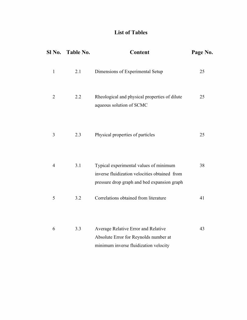
List of Tables
Sl No. Table No. Content Page No.
1 2.1 Dimensions of Experimental Setup 25
2 2.2 Rheological and physical properties of dilute
aqueous solution of SCMC
25
3 2.3 Physical properties of particles 25
4 3.1 Typical experimental values of minimum
inverse fluidization velocities obtained from
pressure drop graph and bed expansion graph
38
5 3.2 Correlations obtained from literature 41
6 3.3 Average Relative Error and Relative
Absolute Error for Reynolds number at
minimum inverse fluidization velocity
43

List of Figures
Sl No.
Figure No.
ContentPage No.
1 1.1 Inverse Fluidization and Normal Fluidization 16
2 2.1 Experimental set-up for the study of inverse fluidization 23
3 2.2 Rheogram of SCMC solution 24
4 3.1 Plot of pressure drop versus velocity 44
5 3.2 Plot of pressure drop versus velocity for sample LDPE-1 (SCMC concentration 0.2 kg/m3)
44
6 3.3 Plot of pressure drop versus velocity for sample LDPE-1 (SCMC concentration 0.4 kg/m3)
45
7 3.4 Plot of pressure drop versus velocity for sample LDPE-1 (SCMC concentration 0.6 kg/m3)
45
8 3.5 Plot of pressure drop versus velocity for sample LDPE-1 (SCMC concentration 0.8 kg/m3)
46
9 3.6 Plot of pressure drop versus velocity for sample LDPE-2 (SCMC concentration 0.2 kg/m3)
46
10 3.7 Plot of pressure drop versus velocity for sample LDPE-2 (SCMC concentration 0.4 kg/m3)
47
11 3.8 Plot of pressure drop versus velocity for sample LDPE-2 (SCMC concentration 0.6 kg/m3)
47
12 3.9 Plot of pressure drop versus velocity for sample LDPE-2 (SCMC concentration 0.8 kg/m3)
48
13 3.10 Plot of pressure drop versus velocity for sample HDPE (SCMC concentration 0.2 kg/m3)
48
14 3.11 Plot of pressure drop versus velocity for sample HDPE (SCMC concentration 0.4 kg/m3)
49

15 3.12 Plot of pressure drop versus velocity for sample HDPE (SCMC concentration 0.6 kg/m3)
49
16 3.13 Plot of pressure drop versus velocity for sample HDPE (SCMC concentration 0.8 kg/m3)
50
17 3.14 Plot of pressure drop versus velocity for sample PP (SCMC concentration 0.2 kg/m3)
50
18 3.15 Plot of pressure drop versus velocity for sample PP (SCMC concentration 0.4 kg/m3)
51
19 3.16 Plot of pressure drop versus velocity for sample PP (SCMC concentration 0.6 kg/m3)
51
20 3.17 Plot of pressure drop versus velocity for sample PP (SCMC concentration 0.8 kg/m3)
52
21 3.18 Variation of minimum inverse fluidization velocity with bed weight
52
22 3.19 Schematic diagram of variation of liquid velocity with bed porosity
53
23 3.20 Variation of minimum inverse fluidization velocity with concentration of SCMC
53
24 3.21 Dependence of Rem on Archimedes number based on minimum fluidization velocity for different correlation
54
25 3.22 Variation of the calculated Rem with the experimental Rem
54

Chapter-1 Introduction
Inverse Fluidization Using Non Newtonian Fluid

Chapter-1 Introduction
Inverse Fluidization Using Non Newtonian Fluid
Fluidization where the liquid is a continuous phase is commonly conducted with
the upward flow of the liquid in liquid –solid phase or with an upward and the liquid in
gas- signed-solid system. Under these fluidization conditions, a solid of particles with a
density figure than that of the liquid is fluidization with an upward flow of the liquid
counter to the net gravitational force of the particles when the density of the particles is
smaller than that of the liquid and the liquid is the continuous phase, however,
fluidization can be achieved by a down ward flow of the liquid counter to the net
buoyancy face of the particles. Such a type of fluidization is termed inverse fluidization.
So the main difference between the classic and inverse fluidization is that the solid
particle density in the inverse fluidization bed is less than that of the density of the
continuous fluid and therefore the bed is fluidized by a down flow of the fluid. Schematic
illustration of both classic and inverse fluidized beds is shown in Fig.1.1.
The first studies on the application, hydrodynamics and mass transfer of two-
phase inverse fluidization were performed in last few years (Nikolov et at 1981, Gsn et at
1991). One of the most important recent application of inverse fluidized beds is in
thefield of bioreactor engineering. Inverse fluidization is used in biotechnology as the
basics of a new type of bioreactor, the so called inverse fluidized bed bioreactor are
among the most efficient application for aerobic and anaerobic wastewater treatment
(Jeris et at 1981, Jewell et at 1981) Penicillin Production (on et at 1988; Endo et at 1988)
and Phenol degradation (Holladay et at, 1978, Tang and Fan 1987).
Further advantages can be founding the reactor design. If the gas distribution is
fitted above the reactor bottom, a calming zone can thus be integrated in the lower
separate the sludge from the liquid. Furthermore the friction effects between the solid
particles would helps for a better control of biofilm size and to a stronger biofilm
attachment.

Chapter-1 Introduction
Inverse Fluidization Using Non Newtonian Fluid Page 2
However, the important problem of biofilm thickness control is the main reason
for the limited industrial application for these systems. However, this inverse fluidization
technique may be advantageously used in the field of environmental engineering as
biological reactor (Legile et al., 1988). In this case, the granular solid is used as a carrier
for the microorganisms involved in the reaction. From the hydrodynamic point of view,
this configuration enables many advantages over the classical three-phase processes. In
the field of biological wastewater treatment, for instance, this kind of reactor enables to
use the gas flow as only a fluidizing agent (biological waste water treatment plant
generally work under high liquid retention times and thus low liquid velocities compared
to the minimal fluidization velocity of the solid). This point is particularly important
because this does not require any extra energy cost in aerobic processes. Further
advantages can be found in the reactor design. If the gas distributor is fitted above the
reactor bottom, a calming zone can thus be integrated in the lower section and this can act
as a settler to separate the sludge from the liquid. Furthermore, the friction effects
between the solid particles would help for a better control of the biofilm size and to a
stronger biofilm attachment. Thus the control of the bio film thickness within a narrow
range is achieved in the inverse fluidized bed bio film reactor. Three-phase fluidized bed
bioreactors have the following advantages over other bioreactors, such as suspended-
growth and trickling-filter bioreactors, used in fermentation and aerobic wastewater
treatment:
Low Wash Out rate of microbes from the system.
No Clogging of biomass in the system.
High and variable biomass concentration and large solid-liquid contacting area.
Thus the large bio-film-liquid interfacial area, high interfacial velocities and good
mass transfer characteristics are the main advantages of this type of bioreactor. In
addition to the above, aerobic wastewater treatment fluidized bioreactors exhibit
minimum recycle requirements and minimum biomass recovery at high substrate loading.
A fluidized bed provides better solids and liquid mixing, better oxygen transfer, more
CO2 removal, more stable cell population and easier cell regeneration than a hollow fiber

Chapter-1 Introduction
Inverse Fluidization Using Non Newtonian Fluid Page 3
reactor. The bio-reaction rates per unit volume of the reactor were up to 14 times higher
than those in the equivalent airlift bioreactor. The uncontrolled growth of the fixed
biomass changes the hydrodynamic characteristics of each bio particle (support particle
covered by bio-film) and the whole fluidized bed. It also affects the mass transfer of
substrate into the bio-film. As per the biofilm control is concerned, a better control is
obtained in case of fluidized bioreactors. Increasing bio film thickness reduces density
differences between the bio-particles and the liquid, thus causing entrainment of the bio-
particles into the draft tube. Inside the draft tube, extensive abrasion among the heavy
particles and the entrained light bio-particles removes excess bio-film providing a
delicate means to control bio-film thickness. It was found that this bioreactor is very
efficient when used for biological aerobic wastewater treatment both under laboratory
conditions and when scaled up (Nikolov and Karamanev, 1987; Nikolov et al., 1990).
Another important biotechnological process, ferrous iron oxidation by Thiobacillus
ferrooxidans, was also carried out with very high efficiency in an inverse fluidized bed
bio film reactor (Nikolov and Karamanev, 1987; Karamanev and Nikolov, 1988). The
bioreactor was successfully used for milk protein hydrolysis by Lactobacillus helveticus
(Dion et al., 1988). Moreover, this apparatus was found to be suitable as a laboratory tool
for bio film process research (Nikolov and Karamanev, 1990)
Chapter-1 Introduction
Inverse Fluidization Using Non Newtonian Fluid Page 4
1.1 Literature review
Fan et al. (1981) were worked on hydrodynamic characteristics of inverse
fluidization in liquid-solid and gas-liquid-solid systems. The experimental data for bed
expansion in the liquid-solid system are correlated, both empirically and semi
empirically.
The flow characteristics of inverse fluidization free stylizing low density spherical
particles experimentally investigated by L.S. Fan et. al ( 1982 ) for both the liquid, solid
and gas-liquid solid systems. The experimental data for the bed expansion in the liquid-
solid system are correlated, both empirically and semi-empirically. In the gas-liquid-solid
system in which the gas and liquid flows are countercurrent, two modes of fluidization
are examined. They are fluidization with the liquid as a continuous phase and fluidization
with the gas as a continuous phase; the former characterizes the inverse gas-liquid-solid
fluidized bed, while the latter characterizes the turbulent contacting bed. A flow regime
diagram which portrays these of fluidization is presented. Correlation of the bed
expansion and gas hold-up proposed for the inverse gas-liquid-solid fluidization.
A new apparatus, the inverse fluidized bed biofilm reactor was described by L.
Nikolov et. al ( 1986 ). Introduction of the so called inverse fluidized bed, in with low
density particles covered by a biofilm are fluidized by down flow of the liquid, allows
control of the bio-film thickness and provides a high oxygen concentration in the reacting
liquid.
Characteristics of the reactor were should by carrying out two important
biotechnological process, aerobic wastewater treatment by a mixed bacterial culture and
ferrous iron oxidation by the bacteria Thiobacillus ferrooxidans. The bio-reaction rates
per unit per unit volume of the reactor were up to 14 times higher than those in the
equipment airlift bioreactor. The structure of the liquid flow was determined by a tracer
method.
Karamanev and Nikolov (1992) studied on bed expansion characteristics of
liquid-solid inverse fluidization. They used twelve different spheres with diameters from
1.31 to 7.24 mm and densities between 75 to 930 Kg/m3 and continuous phase was water.

Chapter-1 Introduction
Inverse Fluidization Using Non Newtonian Fluid Page 5
The experimental data on the porosity was analyzed and found similar to Richardson and
Zaki (1954) model, i.e., the plot of versus U in the logarithmic scale was parallel to
those of Richardson and Zaki (1954), therefore the exponent, n were similar. However,
Umf at = 1 differed from that predicted from standard drag curve for NRe >130. This can
be explained by the fact that the drag curve of freely rising light spheres differs from that
of a falling particle. The values of Umf calculated using modified drag curve were in good
agreement with the experimental results. The difference between minimal fluidization
velocity obtained experimentally and that calculated from Ergun equation is explained by
the difference in mechanical inertia of the light and heavy particles. They also observed
that fluidized particles with densities between 100 and 200 kg/m3 have unusual expansion
characteristics – lower than the expected minimum and maximum fluidization velocities.
The experimental relation between Co & Ret for the case of Steady rising
particles was developed. The significant difference between the drag co-efficient of light
heavy particles was observed.
Experiments were conducted Krishnaiah,K. et al (1993) by to study the
hydrodynamics of inverse gas-liquid-solid fluidized beds using very light particles. The
experimental data for the minimum liquid velocity at the onset of fluidization are
correlated in terms of the physical properties of the fluids, particle characteristics and
system variables. A correlation for the friction factor is also proposed.
Nikov and Karamanev (1994) have reported mass transfer studies in liquid
inversed fluidized bed reactor. They found that the mass transfer rate is independent of
superficial velocity and strongly depends on particle density.
Ulaganathan and Krishnaiah (1995) studied the hydrodynamic characteristics of
two phase inverse fluidized bed reactor with 12.5 to 20 mm diameter in a 75 mm column.
They presented equations to predict the minimum fluidization velocity.
The volumetric effectiveness of IFFBR was studied by D.G. Karamanev et al (
1996 ) and compared with that of a chemostat shows the relation between the volumetric
glucose uptake rate in both IFFBR and chemostat. At high substrate conversion (over
80%), the fluidized bed bioreactor is 25 times more efficient than a chemostat without
Chapter-1 Introduction
Inverse Fluidization Using Non Newtonian Fluid Page 6
cell recycle; this difference increases to 0.1 as the substrate conversion decreases to 20%.
There are the most efficient design would be IFBBR tank in se.
Hydrodynamic characteristics of inverse fluidization in which low density floating
particles are fluidize with downward flow of liquid, are experimentally investigated by
Ulaganthan, N et al (1996) . The experiments are carried out with low density particles
(<534kg/m3) which allow high liquid throughputs in the system. During the operation,
three regimen, namely, packed semi-fluidization and fully fluidization are encountered.
Empirical correlations are proposed to predict the pressure drop in each regime. A
Computational procedure is developed to simulate the variation of pressure drop with
liquid velocity.
Biswas S.K et al (1997) studied on the voidage – velocity lerationship in reverse
fluidization. They showed that there a linear relationship of the plot of ln(Uf/Upr) versus
lnЄ and also shows the effect of the quality of solid on the slop of such plot.
Buffiere and Moletta (1998) investigated some hydrodynamic characteristics of
three phase fluidized bed reactor. Using two types of particles having different
characteristics (ds = 4 mm and 0.175 mm; s = 920 and 690 Kg/m3, respectively) allowed
us to observe two different expansion mechanisms :
A pseudo-fluidized state promoted by density difference between the solid and
surrounding gas-liquid mixture.
A fluidized state due to the liquid circulation induced by the rise of bubbles.
A correlation for the liquid hold-up and bed porosity could be proposed by means of a
modified gas drift flux model.
Femin Bendict,R,J et al (1998) studied hydrodynamics characteristics (bed
expansion and pressure drop) of a different type of two phase inverse fluidized bed
reactor in which low density particles are fluidized with downward flow of liquid.
Experiments conducted by using 6mm diameter spherical particles of low-density
polyethylene (LDPE) and polypropylene (PP) with water and aqueous solutions of
Carboxy methyl cellulose (CMC). It was found that the minimum fluidization velocity,
Chapter-1 Introduction
Inverse Fluidization Using Non Newtonian Fluid Page 7
Umf decreased with increase in CMC concentration and solid density. They proposed a
dimensionless correlation for the prediction of bed height at fully fluidized conditions.
Some hydrodynamic characteristics of inverse three-phase fluidized bed were
investigated Pierre Buffiere et al (1999). Using two types of particles having different
characteristics (ds = 4 mm, Ps = 920 kgm3, and ds = 0.175 mm and p1 = 690 kgm3
respectively allowed us to observe two different expansion mechanism: a pseudo-
fluidized state promoted by the density difference between the solid and the surrounding
gas-liquid mixture, and a fluidized state due to the liquid circulation induced by the rise
of the bubbles. Both contributed to the solid mixing and axial solid distribution in the
systematic holdup measurements were done on two reactor diameter and two types of gas
Spurger. A correlation for the liquid holdup and bed porosity could be proposed by
means of a modified gas drift flux definition. The latest was a function of gas velocity
only and gave a good accuracy among the range of solid amount, gas and liquid velocity
used.
Experimental data on the minimum inverse fluidization velocity, Umf was
obtained by R.Leyva Ramos et al ( 1999 ) in this work. The particles use were made of
low density polyethylene and polypropylene; the diameters and densities were in the
ranges of 0.17 to 0.91 cm and of 18 to 913 kg/m3 respectively. The experimental Umf was
values obtained in this study and Umf values reported in the literature were compare to the
values predicted from different correlations and it was found that the predicted values had
an average percent deviation above 20%. Due to this fact a new correlation was proposed
which had an average percent deviation of the order of 16.6%. It was shown that the Umf
increased with augmenting the particle diameter and with decreasing the particle density.
Suk Choi ,H. et al(1999) investigated the hydrodynamic characteristics of two
types of inverse fluidized bed reactors having different force for fluidization: aeration and
centrifugal force. They found the gas velocity at which the solid concentration is uniform
throughout the bed expansion decreases with increasing particle loads. For the application
of wastewater treatment, the inverse fluidized bed with aeration was found to be more
efficient than the second type of reactor

Chapter-1 Introduction
Inverse Fluidization Using Non Newtonian Fluid Page 8
Benerjee, J.et al (1999) studied fluidization in a cylindrical column using water
as the fluid taking various kinds of low density polythene beads, having specific gravities
lighter than water. The minimum reverse fluidization velocities (for multi-component
systems only) have been determined from the conventional plots of bed pressure drop
versus superficial fluid velocity
Vijaya Lakshmi et al. (2000) studied the hydrodynamic characteristics of LDPE
and PP in a liquid solid inversed fluidized bed reactor as a function of particle diameter,
liquid viscosity and density. They proposed empirical equations for the minimum
fluidization velocity and friction factor.
Dong Hyun Lee (2001) studied the Hydrodynamic transition experiments for tow-
phase (liquid-solid), both upward and downward, liquid flow systems in a 127-mm
diameter column. The particles used were 3.2 mm polymer (1,280 kg/m3), 5.8-mm
polyethylene (910, 930, 946 kg/m3), 5.5-mm polystyrene (1,021 kg/m3) and 6.0 mm
glass (2,230 kg/m3)spheres, with water, aqueous glycerol solution and silicon oil as
liquids. Experiment shows that the dimensionless pressure gradient increases initially
with increasing liquid velocity, but decreases gradually with increasing liquid velocity
beyond minimum fluidization velocity due to bed expansion. The non-dimensionalied
pressure gradient using the liquid/solid mixture density increases with increasing liquid
velocity and then reaches a constant value close to unity beyond minimum fluidization
velocity.
Renganathan ,T et at (2001) used Monte Carlo simulation to predict bed
expansion in inverse fluidized bed, which is an important parameter for the design of the
equipment. The simulation is carried out of various liquid velocities and number of
particles for a particular particle diameter and density. They found that the void fraction
increases with the liquid velocity and is independent of the number of particles. Very
good agreement between simulated and experimental void fraction values in obtained
Delebarre ,A et al (2003) carried out two series of fluidization tests on two test
models with catalyst, alumina and sand particles to determine the bed mass influence on
the characteristics at the minimum of fluidization. They concluded that (i) measured
Chapter-1 Introduction
Inverse Fluidization Using Non Newtonian Fluid Page 9
minimum velocities increased with the inventory whatever were the solid and the test rig
used; (ii) the measured bed porosity at minimum fluidization decreased with the increase
of the bed inventory, (iii) the definition of the minimum fluidization velocity by the
balance between weight and drag forces and some usual mathematical modeling attempts
were not able to describe the minimum fluidization increase with the bed inventory; (iv)
the addition of a complementary consolidation effect in the force balance was able to
match the obtained experimental results.
Renganathan, T. et al (2004) studied liquid phase residence time distribution in
2-phase inverse fluidized bed for the first time in the literature. They used a pulse tracer
technique and disconsolation method of analysis, RTD of the system, residence time,
Peclet number and dispersion coefficients are determined. They found the liquid phase
axial dispersion coefficient increases with increase in liquid velocity and Archimedes
number and is independent of static bed height. An empirical correlation has been
proposed for liquid phase axial dispersion coefficient in 2-phase I IFB.
Delebarre ,A et al (2003) carried out two series of fluidization tests on two test
models with catalyst, alumina and sand particles to determine the bed mass influence on
the characteristics at the minimum of fluidization. They concluded that (i) measured
minimum velocities increased with the inventory whatever were the solid and the test rig
used; (ii) the measured bed porosity at minimum fluidization decreased with the increase
of the bed inventory, (iii) the definition of the minimum fluidization velocity by the
balance between weight and drag forces and some usual mathematical modeling attempts
were not able to describe the minimum fluidization increase with the bed inventory; (iv)
the addition of a complementary consolidation effect in the force balance was able to
match the obtained experimental results.
Renganathan, T. et al (2004) studied liquid phase residence time distribution in
2-phase inverse fluidized bed for the first time in the literature. They used a pulse tracer
technique and disconsolation method of analysis, RTD of the system, residence time,
Peclet number and dispersion coefficients are determined. They found the liquid phase
axial dispersion coefficient increases with increase in liquid velocity and Archimedes

Chapter-1 Introduction
Inverse Fluidization Using Non Newtonian Fluid Page 10
number and is independent of static bed height. An empirical correlation has been
proposed for liquid phase axial dispersion coefficient in 2-phase I IFB.
Formisani et al (2007) have investigater process of fluidization of mixtures of two
spherical solids differing only in density and addresses the relationship between bed
suspension and component segregation. Fluidization properties of density-segregating
mixtures is that based on the definition of the initial and final fluidization velocity of the
binary bed.Such an alternative approach provides an effective representation of the actual
behaviour of these systems, as it correctly accounts for all the variables which affect their
phenomenology of fluidization. data for bed expansion are taken for making
dimensionless empirical or semi-empirical correlation
Jenaa et. al(2008) have studied the hydrodynamic characteristics, viz. the pressure
drop, bed expansion and phase holdup profile of a concurrent three-phase fluidized bed
with an antenna-type air sparger have been determined. Correlations for minimum liquid
fluidization velocity, bed voidage and gas holdup have been developed. The bed voidage
is found to increase with the increase of both liquid and gas velocities. The gas holdup
increases with gas Froude number, but decreases with liquid Reynolds number. The gas
holdup is a strong function of the Froude number. The experimental values have been
found to agree with the correlations.
Sowmeyan and Swaminathan (2008) also studied on Effluent treatment process in
molasses-based distillery industries. Among the different methods available, they found
that “An Inverse Anaerobic Fluidization” to be a better choice for treating effluent from
molasses-based distillery industries using an inverse anaerobic fluidized-bed reactor
(IAFBR). This technology has been widely applied as an effective step in removing 80–
85% of the COD in the effluent stream.
Sowmeyan and. Swaminathan (2008) reported on the physical characteristics of
carrier material (perlite), biomass growth on the carrier material and the biogas
production during an apparent steady state period in an inverse anaerobic fluidized bed
reactor (IAFBR) for treating high strength organic wastewater. Before starting up the

Chapter-1 Introduction
Inverse Fluidization Using Non Newtonian Fluid Page 11
reactor, physical properties of the carrier material were determined. 1 mm diameter
perlite.
Sokoł et al (2009) investigated on the biological wastewater treatment in the
inverse fluidised bed reactor (IFBR) in which polypropylene particles of density 910
kg/m3 were fluidised by an upward flow of gas. Measurements of chemical oxygen
demand (COD) versus residence time t were performed for various ratios of settled bed
volume to reactor volume (Vb/VR) and air velocities ug. The largest COD removal was
attained when the reactor was operated at the ratio (Vb/VR)m = 0.55 and an air velocity
ugm = 0.024 m/s. Under these conditions, the value of COD was practically at steady
state for times greater than 30 h. Thus, these values of (Vb/VR)m, ugm and t can be
considered as the optimal operating parameters for a reactor when used in treatment of
industrial wastewaters. A decrease in COD from 36,650 to 1950 mg/l, i.e. a 95% COD
reduction, was achieved when the reactor was optimally controlled at (Vb/VR)m = 0.55,
ugm = 0.024 m/s and t = 30 h. The pH was controlled in the range 6.5–7.0 and the
temperature was maintained at 28–30 ◦C. The biomass loading was successfully
controlled in an IFBR with support particles whose matrix particle density was smaller
than that of liquid. The steady-state biomass loading depended on the ratio (Vb/VR) and
an air velocity ug. In the culture conducted after switching fromthe batch to the
continuous operation, the steady-state biomass loading was attained after approximately
2-week operation. In the cultures conducted after change in (Vb/VR) at a set ug, the
steady-state mass of cells grown on the particles was achieved after about 6-day
operation. For a set ratio (Vb/VR), the biomass loading depended on ug. With change in
ug at a set (Vb/VR), the new steady-state biomass loading occurred after the culturing for
about 2 days.
Wang et. al. (2010) studied the Removal of emulsified oil from water by inverse
fuidization of hydrophobic aerogels. Different size ranges of surface-treated hydrophobic
silica aerogels (Nanogel®) were fuidized by a downward flow of an oil-in-water
emulsion in an inverse fuidization mode. Surface areas, pore size distributions, and pore
diameters were investigated by using BET and contact angle is measured by a

Chapter-1 Introduction
Inverse Fluidization Using Non Newtonian Fluid Page 12
goniometer. The hydrodynamics characteristics of the Nanogel granules of different size
ranges were studied by measuring the pressure drop and bed expansion as a function of
superficial water velocity. The density of the Nanogel granules was calculated from the
plateau pressure drop after the bed was fully fluidized. The oil removal efficiency of a
dilute (1000 ppm COD or lower), stabilized (using the emulsifer Tween 80) oil-in-water
emulsion and the capacity of the Nanogel granules in the inverse fluidized bed were also
studied. A model was developed to predict the inverse fluidized bed experimental results
based on equilibrium and kinetic batch measurements of the Nanogel granules and the
stabilized oil-in-water emulsion. The results showed that the major factors which affect
the oil removal efficiency and capacity are the size of the nanogel granules, bed height,
fluid superficial velocity and the proportion of emulsifier in the oil-in-water emulsion.
Das et. al. (2010) investigated Inverse fluidization using non-Newtonian liquids.
Experiments had been carried out to determine the minimum inverse fluidization velocity
using single and binary systems of four different solids of polymeric origin, and four
different non-Newtonian liquids in two different columns. Empirical correlations had
been developed to predict the minimum inverse fluidization velocity as a function of
physical and dynamic variables of the system. Statistical analysis of the correlation
suggested that is of acceptable accuracy with correlation coefficient more than 0.99.
1.2 Objective of the project
The main aim of this project work –
1. To investigate the hydrodynamic behavior of the two phase (liquid – solid)
inverse fluidized bed using non-Newtonian liquid.
2. To develop empirical correlation to predict the minimum fluidization velocity
from system parameter & also to compare the experiment minimum fluidization
velocity with the different correlation obtained from literature.
3. To develop empirical mathematical correlation to predict bed expansion as a
function of system variables.

Chapter-1 Introduction
Inverse Fluidization Using Non Newtonian Fluid Page 13
1.3 Minimum Fluidization Velocity
Theoretically, umf should be same for both up flow and inverse fluidization for the
following reason. The Ergun equation is based on the main assumption that the drag force
of the fluid moving with a superficial velocity umf is equal to the weight of the particles in
the bed:
olpo
g
1 (1)
In the bed containing light particles, the weight force should be replaced by the buoyancy
force:
oplo
g
1 (2)
Since Equations (1) & (2) are identical, the minimum fluidization velocities in both up
flow and inverse fluidized beds should be equal when parameters of the liquid phase,
particle diameters and the absolute values of lp are equal. In fact it has been
experimentally established (Karamanov and Nikolov, 1992) that an inverse fluidized bed
consisting of low-density particles has smaller umf compared to that of an up flow
fluidized bed (and that predicted by the Ergun Equation) for Remf > 50-70. This
difference is negligible when Remf is less than the critical one.
1.3.1 Different flow regimes
Static bed regime
At low superficial liquid velocity, the liquid moving down does not disturb the bed but
just percolates. The voidage of bed and the height remain constant.

Chapter-1 Introduction
Inverse Fluidization Using Non Newtonian Fluid Page 14
Partially fluidized bed regime
When uf is increased further, the liquid gains enough energy and overcomes the inertial
force of the solid particles and hence the static bed partially becomes dynamic. Only then
lower end of the bed tends to be fluidized and the upper half remains static.
Completely fluidized bed regime
This regime starts when the superficial liquid velocity equals or exceeds the minimum
fluidization velocity. The force exerted by the liquid velocity overcomes the inertial force
of all the particles in the column and thus the bed fluidizes. All the particles are in motion
during the completely fluidized bed regime.
1.3.2 The Bed Expansion
The different models for the correlation of bed expansion with the superficial
velocity can be classified into three main groups ( Fan et al., 1982). The first group is
based on correlations giving the dependence between U / Ui and . The Richardson &
Zaki model (1954) is most popular in this group. In the second group of models the drag
function for multi particle system is used. It is usually given as a function of Re and Ar.
The models of Ramamurthy and Subbaraju (1973) and Riba and Couderc (1977) are
typical for this group. The third group of models is based on the dependence between
and the main variables of the fluidized bed as in the Wen and Yu (1966) correlation.
Among all these correlations, the Richardson and Zaki model is probably the most
popular one due to its simplicity and good agreement with the experimental data.
The drag coefficient CD is determined from the standard Drag curve the
dependence ln CD – ln Ret (Den, 1980). The standard drag curve is based on experimental
data with settling heavy spherical particles in a fluid when P >l. There is no
information available regarding the validity of the standard drag curve in the case of
freely rising light spheres with P < l. The free rise of spherical particles with densities
smaller than that of the fluid is believed to obey the laws of free settling since the same
forces are applied to the particle but in the opposite directions.

Chapter-1 Introduction
Inverse Fluidization Using Non Newtonian Fluid Page 15
Additional experiments are necessary for determination of this dependence.
Nevertheless, in many publications, including one of the best monographs on particle-
fluid interactions. The assumption was made that the drag curves of free falling and rising
solid spheres are identical. This assumption was not however confirmed by the
experimental data.
Striking Features of Inverse Fluidized bed
Several specific characteristics of the two-phase inverse fluidized bed usually not
observed in “Classic” up flow fluidization must be underlined. The liquid entering the
fluidized bed often carries gas bubbles. When a bubble enters an up flow fluidized bed, it
leaves the bed rapidly because the direction of its free rise is the same as the direction of
the liquid flow and therefore it does not change significantly the hydrodynamic state of
the bed. In inverse fluidized bed, these directions are opposite to each other and the
bubble entering the bed with the liquid phase usually remains in it, provided it is not too
small. In the later case, the bubble moves downwards together with the liquid.
Consequently, since gas bubbles accumulate in the inverse fluidized bed, they affect the
hydrodynamic measurements. It is very important therefore to eliminate the gas bubbles
from the liquid entering the bed. The solid particles used in the up flow fluidized beds are
usually non-porous materials like glass, metals, sand, plastic beads, etc. Each of these
materials has a certain constant density.

Chapter-1 Introduction
Inverse Fluidization Using Non Newtonian Fluid Page 16
Normal Fluidization Particles heavier than flowing liquid
(Anti-gravity flow)
Fluidized Bed
(Upward Bed Expansion)
Liquid Stream Outlet
Liquid Stream Inlet
Dire
ctio
nof
Bed
Expa
nsio
n
Inverse Fluidization Particles lighter than flowing liquid
(Gravitational flow)
Liquid Stream Outlet
Liquid Stream Inlet
Fluidized Bed
(Downward Bed Expansion)
Figure : 1.1 Inverse Fluidization and Normal Fluidization

Chapter-2 Experimental setup and technique
Inverse Fluidization Using Non Newtonian Fluid
Chapter-2 Experimental setup and technique
Inverse Fluidization Using Non Newtonian Fluid Page 17
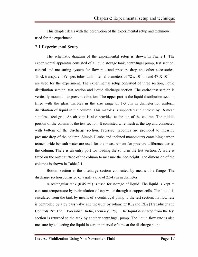
This chapter deals with the description of the experimental setup and technique
used for the experiment.
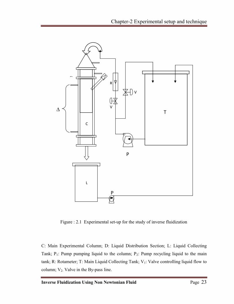
2.1 Experimental Setup
The schematic diagram of the experimental setup is shown in Fig. 2.1. The
experimental apparatus consisted of a liquid storage tank, centrifugal pump, test section,
control and measuring system for flow rate and pressure drop and other accessories.
Thick transparent Perspex tubes with internal diameters of 72 x 10-3 m and 47 X 10-3 m.
are used for the experiment. The experimental setup consisted of three section, liquid
distribution section, test section and liquid discharge section. The entire test section is
vertically mountain to prevent vibration. The upper part is the liquid distribution section
filled with the glass marbles in the size range of 1-3 cm in diameter for uniform
distribution of liquid in the column. This marbles is supported and enclose by 16 mesh
stainless steel grid. An air vent is also provided at the top of the column. The middle
portion of the column is the test section. It consisted wire mesh at the top and connected
with bottom of the discharge section. Pressure trappings are provided to measure
pressure drop of the column. Simple U-tube and inclined manometers containing carbon
tetrachloride beneath water are used for the measurement for pressure difference across
the column. There is an entry port for loading the solid in the test section. A scale is
fitted on the outer surface of the column to measure the bed height. The dimension of the
columns is shown in Table 2.1.
Bottom section is the discharge section connected by means of a flange. The
discharge section consisted of a gate valve of 2.54 cm in diameter.
A rectangular tank (0.45 m3) is used for storage of liquid. The liquid is kept at
constant temperature by recirculation of tap water through a cupper coils. The liquid is
circulated from the tank by means of a centrifugal pump to the test section. Its flow rate
is controlled by a by pass valve and measure by rotameter RL1 and RL2 [Transducer and
Controls Pvt. Ltd., Hyderabad, India, accuracy 2%]. The liquid discharge from the test
section is returned to the tank by another centrifugal pump. The liquid flow rate is also
measure by collecting the liquid in certain interval of time at the discharge point.

Chapter-2 Experimental setup and technique
Inverse Fluidization Using Non Newtonian Fluid Page 18
Four different dilute solution of sodium salt of carboxy methyl cellulose (SCMC)
are used as experimental liquid. The physical properties of the experimental liquids are
measured by standard methods.
2.2 Rheological properties of SCMC solutions
Four aqueous solutions of sodium salt of carboxy methyl cellulose (SCMC) [Loba
Cheme Pvt.Ltd., Mumbai, India] of approximate concentrations 0.2 kg/m3, 0.4 kg/m3, 0.6
kg/m3 and 0.8 kg/m3, are used as the non-Newtonian liquids. The tests liquid are prepared
by dissolving the required amount of SCMC in tap water and stirring until a
homogeneous solution is obtained. It is kept at least 12 hrs. for aging and initially a trace
amount of formalin is added to prevent biological degradation. Contents of the tank are
kept at a constant temperature (280C ± 20C) by circulating water through the copper coil.
The properties of the non-Newtonian liquids are measured by standard techniques, i.e.,
viscosity is measured by pipeline viscometer, surface tension by Dünouy tensiometer and
density by specific gravity bottle.
The SCMC solution is a time independent pseudo plastic fluid and the Ostwald
de-Waele model or the power-law model describes its rheological behavior as,/n
duK
dr
(2.1)
Where, K and n are the constants for the particular fluid with n/ < 1. The constant K is
known as the consistency index of the fluid; the higher the value of K, the more viscous
is the fluid. The constant n is called the flow behavior index and is a measure of the
degree of departure from the Newtonian behavior. The more the departure of n from
unity, the more pronounced will be the non-Newtonian properties. In the case of non-
Newtonian fluids the establishment of what constitutes a suitable viscosity in analytical
terms, is a matter, upon which there is no general agreement. A number of viscosities
have been defined such as apparent viscosity, μap, effective viscosity, μeff, and limiting
viscosity, μα. In the present analysis the term effective viscosity, μeff, has been used
throughout for calculation. It is defined as the ratio of the shear stress at the wall to the
Chapter-2 Experimental setup and technique
Inverse Fluidization Using Non Newtonian Fluid Page 19
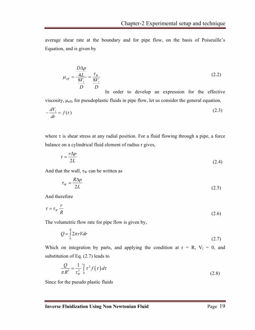
average shear rate at the boundary and for pipe flow, on the basis of Poiseuille’s
Equation, and is given by
(2.2)
In order to develop an expression for the effective
viscosity, μeff, for pseudoplastic fluids in pipe flow, let us consider the general equation,
(2.3)
where τ is shear stress at any radial position. For a fluid flowing through a pipe, a force
balance on a cylindrical fluid element of radius r gives,
2
r p
L
(2.4)
And that the wall, τW can be written as
2W
R p
L
(2.5)
And therefore
W
r
R
(2.6)
The volumetric flow rate for pipe flow is given by,
0
2R
Q rVdr (2.7)
Which on integration by parts, and applying the condition at r = R, Vl = 0, and
substitution of Eq. (2.7) leads to
23 3
0
1 W
W
Qf d
R
(2.8)
Since for the pseudo plastic fluids
48 8
Weff
l l
D pLV V
D D
( )ldVf
dr

Chapter-2 Experimental setup and technique
Inverse Fluidization Using Non Newtonian Fluid Page 20
1
nf
K
(2.9)
/
1
23 3
0
2 1 W nl
W
VQf d
R D K
(2.10)
Which on integration gives
/
1/
/
2
3 1
nl WV n
D n K
(2.11)
On rearranging,//
/
/
2 3 1nn
lW
V nK
D n
(2.12)
or
///
/
8 3 1
4
nn
lW
V nK
D n
(2.13)
Now as per the definition of μE, we have // 1 /
/
8 3 1
8 / 4
nn
W leff
l
V nK
V D D n
(2.14)
or/ /1 1 1 '8n n n
eff lV D K (2.15)
Where
//
/
3 1
4
nn
K Kn
(2.16)
Therefore, the value of μeff can be evaluated provided K and n are known.
In Eq. (2.14) it is clear that if a logarithmic plot is made between w and 8 /lV D , a linear
relation will result, the slope and intercept should of which are the values on n/ and K/
respectively.
A horizontal steel tube of 0.635 cm internal diameter is used as the pipeline viscometer
with pressure tapping at a distance of 1.85 m. Measurements on pressure drop are made
in the fully developed flow region of non-Newtonian liquids, in the laminar flow
condition. The developed flow region is ensured by providing the necessary and

Chapter-2 Experimental setup and technique
Inverse Fluidization Using Non Newtonian Fluid Page 21
sufficient straight entry length, i.e., more than 50 pipe diameter length of the tube. The
inlet end of the tube is well rounded to ensure smooth and parallel flow at the entrance.
From the data on pressure drop and flow rate, the values of w and 8 /lV D are
calculated for four different SCMC solutions. The rheogram are shown in Fig. 2.2 and
represent typical flow curves for pseudoplastic behavior in the shear rate range 32 – 950
s-1.
The values of n/, K/ and other physical properties of the liquids are shown in Table 2.2.
2.3 Solid particles
Four different particles having different diameters, shapes and densities made of
polymeric materials are used for the experiments. The representative diameters for the
non spherical particle are the equivalent diameter based on volume. Fifty random
samples are taken and its dimensions are measured by slide calipers and then average
volume is measured. The particles are spherical, cylindrical and cubical in shape. The
sphericity of these particles are measured by using the following equation
6 ps
p p
v
d S (2.17)
The diameters, density and sphericity for the binary system are measured by using the
following equations (Ganguly, 1994),
1
1
ni
Mi pi
xd
d
, (2.18)
1
n
M i ii
x
(2.19)
and, 1
n
M i sii
x
(2.20)
respectively. The physical properties of the single component solid particles are given in
Table 2.3.

Chapter-2 Experimental setup and technique
Inverse Fluidization Using Non Newtonian Fluid Page 22
2.4 Experimental Technique and Procedure
In actual experiments, a predetermined quantity of solids is admitted into the
column through the inlet port fitted at the side of the column which is subsequently
closed by a rubber cork. The fluid (aqueous SCMC solution) is fed into the column by
starting the centrifugal pump. The flow is increased to some extent till the bed of solids
starts expanding downwards. The pump is stopped to allow the solids float and
accumulate under the top strainer to form a fixed bed height which is called the initial
bed height. Finally the flow rate is increased gradually, causing the bed height to increase
in downward direction. The pressure drop, at each flow rate, has been recorded by the
manometer. The liquid flow rate is measured by collecting the liquid in certain interval of
time at the discharge point. Bed height is measured by the scale fitted on the surface of
the column. Each experiment has been repeated three times to confirm the reproducibility
of the data. The bed weight varies from 200 – 1000 gm for single component systems.
For binary mixtures, the weight has been kept at 500 gm, varying the mass fractions of
the components from 0.2 to 0.8. For all the experiments, however, actual bed pressure
drop, aP , has been determined by subtracting the blank pressure drop, blP , from the
observed pressure drop, oP , for the same fluid velocity, fu .
Hence,
a o blP P P
Chapter-2 Experimental setup and technique
Inverse Fluidization Using Non Newtonian Fluid Page 23
Figure : 2.1 Experimental set-up for the study of inverse fluidization
C: Main Experimental Column; D: Liquid Distribution Section; L: Liquid Collecting
Tank; P1: Pump pumping liquid to the column; P2: Pump recycling liquid to the main
tank; R: Rotameter; T: Main Liquid Collecting Tank; V1: Valve controlling liquid flow to
column; V2: Valve in the By-pass line.
L
TV
V
RD
C
P
P

Chapter-2 Experimental setup and technique
Inverse Fluidization Using Non Newtonian Fluid Page 24
10 100 1000
1
10
100
Symbol SCMC Conc.
Kg/m3
0.2 0.4 0.6 0.8
Fig. 2.2 Rheogram of the SCMC solution
Wal
l she
ar s
tres
s; DP
a/4L,
N/m
2
Shear rate; 8V/D, S-1

Chapter-2 Experimental setup and technique
Inverse Fluidization Using Non Newtonian Fluid Page 25
Table : 2.1 Dimensions of experimental setup
Table: 2.2 Rheological and physical properties of dilute aqueous solution of SCMC
Concentration
kg/m3
Flow behavior index
n/
Consistency index
K/
Nsn´/m2
Density
l
kg/m3
0.2 0.9013 0.0142 1001.69
0.4 0.7443 0.1222 1002.13
0.6 0.6605 0.3416 1002.87
0.8 0.6015 0.7112 1003.83
Table : 2.3 Physical properties of particles
Particle
Used
Average
diameter
dp
m
True
particle
density
ρp
kg/m3
Bulk
particle
density
ρb
kg/m3
Shape Spheri
city
p
Length/Dia
meter
LDPE 1 5.6410-3 915 0.906 Spherical 1 -
LDPE 2 4.1810-3 919 0.904 Cylindrical 0.873 0.943
HDPE 4.7910-3 944 0.913 Cylindrical 0.904 1.190
PP 3.1310-3 900 0.854 disc 0.777 -
Internal Diameter
of the Column
m
Wall Thickness
m
Total
Column
Height
m
Distance between
two Pressure
Tapings
m
72 x 10-3 3 x 10⁻³ 1.50 1.11

Chapter-3 Results and discussions
Inverse Fluidization Using Non Newtonian Fluid

Chapter-3 Results and discussions
Inverse Fluidization Using Non Newtonian Fluid Page 26
This chapter deals with the determination of the minimum inverse fluidization
velocity and its analysis.
3. Results and Discussions
3. 1 Evaluation of minimum inverse fluidization velocity
3.1.1 From pressure drop data
When a liquid is passed through a bed of particles, with the gradual and continual
increase in the superficial velocity of the liquid, a point is reached whereby the bed just
begins to loosen, though the majority of the particles are still in contact with each other.
This velocity is called the minimum fluidization velocity. The minimum fluidization
velocity is an important hydrodynamic parameter involved in the design of this type of
system. Richardson (1971) pointed out that the transition from fixed bed to fluidized bed
conditions depends on number of mechanical details like original bed structure, design of
distributor, etc. and it always occurs gradually over as range of conditions thereby
making it difficult to identify precisely for normal fluidization. In case of inverse
fluidization it is defined as the lowest superficial velocity at which the downward weight
of the particles the drag force due to downward flow of the liquid just counters the
upward buoyancy force of the solid particles, i.e., the net upward force is equal to the net
downward force. Richardson (1971) comment is also true for the inverse fluidization. The
minimum fluidization velocity is measured by visual observations of the bed as well as
by the intersection of ΔPa - uf plots in fixed and fluidized bed regimes. As expected, the
pressure drop across the bed remains essentially constant once the fluidization has begun.
Actual bed pressure drop, aP , has been measured for a particular liquid velocity, fu , by
subtracting the blank pressure drop, blP , due to liquid flow at identical liquid velocity,
fu , from the observed pressure drop, aP , with solids present. Hence,
a ob blP P P (3.1)
The determining the minimum fluidization velocity, um, involves the use of data
on the variation in bed pressure drop across a bed of particulate solids with fluid velocity.

Chapter-3 Results and discussions
Inverse Fluidization Using Non Newtonian Fluid Page 27
The trend in variation of the bed pressure drop with the superficial liquid velocity is
shown in Fig. 3.1. The transition point from the fixed bed to the fluidized bed is marked
by the onset of constant pressure. This is also the point at which the increasing trend in
the bed pressure drop (ΔPa) of a packed bed terminates. For an ideal case, liquid flow
reversal in the fluidized bed condition does not change the magnitude of ΔPa. However,
the value of ΔPa is smaller when the bed starts settling during flow reversal compared to
previous values obtained at the same velocity in the increasing flow direction. The
pressure drop method is the most popular means of determining um experimentally.
For liquid – solid inverse fluidization it is determined from the plot (Fig. 3.1) of
pressure drop versus the liquid velocity for the inverse fluidized bed system. From this
plot it is shows that as the velocity increases, the pressure drops increases (A→B) and
ultimately reaches a constant pressure drop zone (B→C). This A→B zone is static bed
zone. As increasing flow rate of the liquid pressure drop increases. The B→C zone is the
fluidized bed zone. The point (B) of intersection of the increasing part of the curve and
the constant region represents the minimum fluidization velocity. Further increasing the
liquid flow rate the particle of the bed starts to elutriate from the column. This C→ D
zone is referred as elutriation zone. In the elutriation zone the pressure drop falls off with
superficial velocity due to continual depletion of the solids in the column. The point (C)
of intersection of the constant region and the decreasing part of the curve represents the
minimum elutriation velocity.
The plots of aP versus fu for different systems are shown in Figs. 3.2 – 3.17. It
is clear from the plots that for the single component system there is a sharp transition
between fixed and fluidized bed where for binary system the transition is very gradual in
nature. The minimum inverse fluidization velocity, mu , is obtained from the point of
intersection of the fixed and fluidized bed lines. It is observed from the plots that
minimum inverse fluidization is independent of bed weight (Fig. 3.18)
Figs. 3.2 – 3.17 shows the pressure drop, aP , versus the liquid velocity, fu , at
constant bed weight but different bed compositions. It is clear from the plot that as the
amount of heavier particles increases the pressure drop also increases and the transition
Chapter-3 Results and discussions
Inverse Fluidization Using Non Newtonian Fluid Page 28
from fixed to fluidized bed is not sharp but gradual. The value of the minimum inverse
fluidization, mu , is determined by the intersection of two tangents showing the beginning
of fluidization, minimum fluidization and total fluidization velocities. The slow and
gradual change is attributed to the fact that in binary system there is change of
segregation with the smaller particles getting fluidized first, followed by larger particles
which fluidize later. In this plot two factors affecting the minimum inverse fluidization
velocity namely the particle density and size. The HDPE has higher density and larger
diameter than that of PP.
3.1.2 From bed porosity
Another way of determination of the minimum inverse fluidization velocity is
from the porosity of the bed. The determination of bed voidage, ε, for any bed height, Hfl,
is carried out as follows,
fl
s
H
H1 (3.2)
and as a special case the voidage at static bed height, εm , is determined by replacing the
term Hfl in Eq. (3.2) by Hm , Thus
1 1s sm
fl m
H H
H H
(3.3)
Where Ls represents the static bed height at zero voidage and obtained as
2
4
ps
p t
WH
d
(3.4)
The minimum inverse fluidization velocity is determined from the plot bed porosity, ε,
vs. liquid velocity, uf, on a log-log plot as shown in Fig. 3.19. From the intersection point
of packed bed region and fluidized region (point B in Fig. 3.19) the minimum inverse
fluidization velocity can be determined. Fig. 3.19 show the typical plot of bed porosity
versus the liquid velocity for single system. It is observed that for binary component
system gradual transition from packed bed to fluidized bed occurs. Typical experimental
Chapter-3 Results and discussions
Inverse Fluidization Using Non Newtonian Fluid Page 29
data of minimum inverse fluidization velocities obtained from both the procedure. The
minimum inverse fluidization velocity obtained from both the processes is practically
same.
3.2 Effect of rheological properties on the minimum inverse fluidization
velocity
The variations of minimum inverse fluidization velocity with different SCMC
solution concentrations are shown in Figs. 3.2 – 3.17. It is observed that the inverse
fluidization velocity, ,mu decreases with an increase in SCMC concentration, i.e.,
pseudoplasticity of the liquid for the both single and binary system. The observed
decrease in the minimum inverse fluidization velocity, mu is due to the decrease in
Archimedes number with increase in viscous force resulting from increase in viscosity of
liquid phase, i.e., as pseudoplasticity increases with increase in SCMC concentration
(Fig. 3.21). It is clear from the plots that the minimum inverse fluidization velocity, um,
for mixture is more than that of single sized particle due to change in mixture diameter
and density as well as sphericity. Similar results are also obtained for normal fluidization
(Fan et al., 1985) and for inverse fluidization (Bendict et al., 1998 and Vijaya Lakshmi et
al., 2000). It is also observed that the minimum inverse fluidization velocity, um, decrease
with the pseudoplasticity of the liquid.
3. 3 Effect of column diameter on the minimum inverse fluidization velocity
It is clear from the plot that with decrease in column diameter the inverse
fluidization velocity practically constant. In smaller diameter column the initial bed
height is more than that of the higher column diameter for certain amount of solid. There
is a possibility of the wall effect in the smaller diameter tube. The wall-effect becomes
prominent for low values of dt/dM. According to Wicke and Hedden (1952) if the ratio
dt/dM ≥ 10 the wall effect is negligible for the case of normal fluidization. For the present
study, this ratio is higher than that to cause any wall-effect. Happel and Byrne (1954)
attempted to correlate hindered settling velocity with dt/dM ratio, and observed that with
Chapter-3 Results and discussions
Inverse Fluidization Using Non Newtonian Fluid Page 30
decrease in this ratio, the hindered settling velocity decreases, which means greater
floatability of the particles with a consequential increase in the value of the minimum
inverse fluidization velocity, um. Clift et al. (1978) pointed out that rising a particles
generate secondary motion, including rocking, zigzag or spiral movement, producing
thereby an increase in the effective drag coefficient. According to Clift et al. (1978), the
difference increases as the ratio ρs/ρf decreases, but becomes negligible for Rep < 1000.
Chhabra (2001) pointed out that for normal fluidization using non-Newtonian liquids if
dM/dt ≤ 0.32 then the wall effect is negligible. In the present case dM/dt ≤ 0.12, hence, the
wall effect is negligible and the minimum inverse fluidization velocity is independent of
the diameter of the tube.
3. 4 Effect of Sphericity
The effect of surface irregularity of the solids has been shown earlier by Pittyjohn
and Christiansen (1948) in free fall settling velocity in the sense that lower the sphericity
(i.e. more irregularity of the surface), lower will be the settling velocity or higher will be
the value of particle rise velocity, upr. Hence, higher fluid velocity will be required to
cause the particles to be fluidized in the downward direction (higher value of Rem). Such
dependence is also reflected by the negative exponent of φM in Eq. (3.24).
3. 5 Analysis of the minimum inverse fluidization velocity
For inverse fluidization with the z-coordinate taken as positive in the upward
direction, i.e., in the direction opposite to that of the liquid flow, and with the hydrostatic
head of liquid corrected for the frictional pressure gradient, the overall pressure variation
in the vertical direction coordinated for the frictional pressure gradient is given by
lf fsl
dP dPg
dz dz
(3.5)
The frictional pressure gradient in solid - liquid inverse fluidized beds is given by
,
p lf sl
dPg
dz
(3.6)

Chapter-3 Results and discussions
Inverse Fluidization Using Non Newtonian Fluid Page 31
Substituting Eq. (3.6) into Eq. (3.5) and rearranging,
11 1p
fsll l
dP
g dz
(3.7)
In the case of a fixed bed, fsl
dP
dz
, can be expressed by the Ergun (1952) equation
applied to the liquid-solid interaction as follows:
22
2 2 2 2
150 1 1.75 1f fs f l f
fsl f p p f s p
u udP
dz d d
(3.8)
Substituting Eq. (3.8) into Eq. (3.5)
22
2 2 2 2
150 1 1.75 1f feff f l fl
sl f p p f p p
u udPg
dz d d
(3.9)
Transforming the above equation
22
2 2 2 2
150 1 1.75 11
f feff f l fsl
l f p p l f p p
dPu udz
g d g d g
(3.10)
The frictional pressure gradient at the minimum fluidization condition equal to the net
difference between gravitational and buoyancy forces per unit area. With the assumptions
of bed voidage, particle properties and the superficial velocity are all uniform over the
entire bed height, Eq. (3.7) - (3.10) can be applied if the bed height is measured and it is
assumed that voidages, particle properties and the superficial liquid velocity are all
uniform over the bed height so that the pressure gradient is also uniform over that height
interval.
22
2 2 2 2
150 1 1.75 1f feff f l fl p
sl f p p f p p
u udPg
dz d d
(3.11)
At the point of minimum inverse fluidization velocity, the above equation become
2 2
2 2 2 2
150 1 1.75 1eff mm m l mm l p
sl m p p m p p
u udPg
dz d d
(3.12)
Chapter-3 Results and discussions
Inverse Fluidization Using Non Newtonian Fluid Page 32
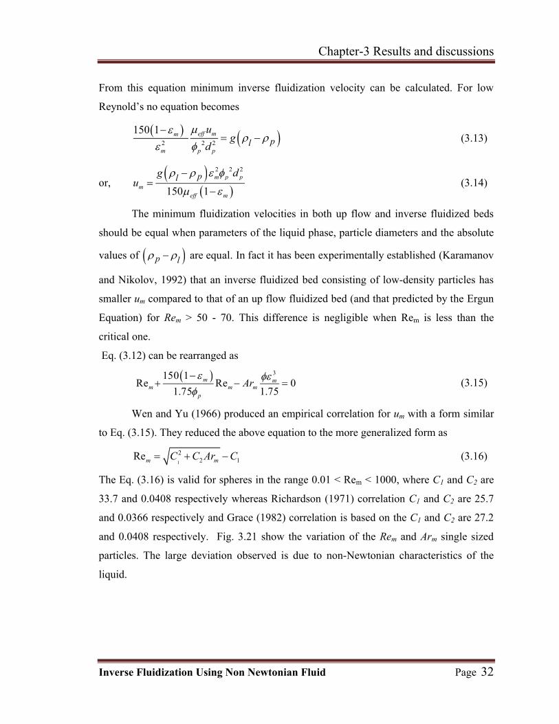
From this equation minimum inverse fluidization velocity can be calculated. For low
Reynold’s no equation becomes
2 2 2
150 1 eff mm
m p ppl
ug
d
(3.13)
or,
2 2 2
150 1
m p p
meff m
plg du
(3.14)
The minimum fluidization velocities in both up flow and inverse fluidized beds
should be equal when parameters of the liquid phase, particle diameters and the absolute
values of p l are equal. In fact it has been experimentally established (Karamanov
and Nikolov, 1992) that an inverse fluidized bed consisting of low-density particles has
smaller um compared to that of an up flow fluidized bed (and that predicted by the Ergun
Equation) for Rem > 50 - 70. This difference is negligible when Rem is less than the
critical one.
Eq. (3.12) can be rearranged as
3150 1Re Re 0
1.75 1.75m m
m m mp
Ar
(3.15)
Wen and Yu (1966) produced an empirical correlation for um with a form similar
to Eq. (3.15). They reduced the above equation to the more generalized form as
1
22 1Rem mC C Ar C (3.16)
The Eq. (3.16) is valid for spheres in the range 0.01 < Rem < 1000, where C1 and C2 are
33.7 and 0.0408 respectively whereas Richardson (1971) correlation C1 and C2 are 25.7
and 0.0366 respectively and Grace (1982) correlation is based on the C1 and C2 are 27.2
and 0.0408 respectively. Fig. 3.21 show the variation of the Rem and Arm single sized
particles. The large deviation observed is due to non-Newtonian characteristics of the
liquid.

Chapter-3 Results and discussions
Inverse Fluidization Using Non Newtonian Fluid Page 33
3. 5.1 Yu et al. (1968) correlation
Yu et al. (1968) empirically modified the Richardson – Zaki (1954) correlation
for predicting the minimum normal fluidization velocity using velocity – porosity
behavior for non- Newtonian liquid flow. They used aqueous solutions of Polyox in 100
mm diameter column, with particle size ranges from 2.5 – 9 mm. They obtained the
following expression which gives reasonable agreement between the experiment and
prediction in the range of 0.81 ≤ n ≤ 1,
2
2 1
9 3 112.5 Re
nn
m nm mn
m
nAr
(3.17)
Fig. 3.22 show the large deviation with the experimental data.
3. 5.2 Ulaganathan and Krishnaiah (1996)
Ulaganathan and Krishnaiah (1996) studied the hydrodynamic characteristics of
two-phase inverse fluidized bed with 12.5 to 20 mm diameter particle size in a 75.3 mm
diameter column. The experiments are carried out with low density particles (< 534
kg/m3) which allow high liquid throughputs in the system. During the operation, three
regimes, namely, packed, semi-fluidization and fully fluidization are encountered.
Empirical correlation is proposed to predict the minimum inverse fluidization velocity as
0.383 0.2022.93 10 /m m l p lu Ar (3.18)
A computational procedure is also developed to simulate the variation of pressure
drop with liquid velocity. Fig. 3.22 show the large deviation with the experimental data
as this expression is valid for inverse fluidization system using water.
3. 5.3 Vijaya Lakshmi et al. (2000) correlation
Hydrodynamic study of inverse fluidization experiments are carried out by Vijaya
Lakshmi et al. (2000) using low-density polyethylene and polypropylene along with
water and different concentration of aqueous solutions of carboxy methyl cellulose
(CMC) as non- Newtonian liquid. The experimental column they used, is made-up of
perspex with dimensions of 94 mm internal diameter with a maximum height of 1800

Chapter-3 Results and discussions
Inverse Fluidization Using Non Newtonian Fluid Page 34
mm and a wall thickness of 3 mm. Spherical low density polyethylene (LDPE) and
polypropylene (PP) particles of 4, 6 and 8 mm diameters are used along with water and
different concentrations of aqueous solutions of CMC as liquid. They proposed empirical
equations for the prediction of the friction factor and the minimum inverse fluidization
velocity for water and non-Newtonian liquid system separately. Minimum inverse
fluidization velocities are determined from the bed expansion and pressure drop data.
They observed that minimum inverse fluidization is independent of solid loading and
increased with an increased in particles diameter, decreases with the solid density and
pseudoplasticity of non-Newtonian liquid. They proposed the following correlation to
predict the minimum inverse fluidization velocity for non-Newtonian solution
0.041 -6mRe =1.139 10 Arm (3.19)
for 0.00875 < um < 0.0175
and 2 < dP < 8 mm.
Figs 3.21 and 3.22 show unacceptable deviation with experimental data.
3. 5.4 Banerjee et al. (1999) correlation
Banerjee et al. (1999) investigated the inverse fluidized bed using various kinds of
low density polythene beds and different shaped (spherical, cylindrical and disc) with
water as the liquid phase. The minimum inverse fluidization velocities for uni-, and
multi-component systems, as well as the beginning of fluidization and total inverse
fluidization velocities are determined from the conventional plots of bed pressure drop
versus superficial liquid velocity. They proposed three empirical correlations to three
velocities namely, minimum inverse fluidization velocity, beginning of fluidization
velocity and total inverse fluidization velocity. The proposed correlation to predict
inverse fluidization velocity as
-6 1.513m mRe = 7.68 10 Ar (3.20)
Unacceptable deviation is observed with experiment as shown in Figs 3.21 and 3.22, as
they use spheriricity, φs = 1 for cases and water as liquid.

Chapter-3 Results and discussions
Inverse Fluidization Using Non Newtonian Fluid Page 35
3.5.5 Empirical correlation for minimum inverse fluidization velocity
The minimum fluidization velocity, um, in liquid-solid inverse fluidized beds is a
function of physical and dynamic variables of the system. The following factors affect the
minimum inverse fluidization velocity,
1. Physical properties of the liquid : viscosity, eff , density, l
2. Physical properties of the solid : density, M and sphericity, M
3. Acceleration due to gravity : g
Hence, the minimum inverse velocity can be expressed as,
, , , , ,m M l M eff Mu F d g (3.21)
The use of dimensional analysis the above functional relationship can be reduced to the
following functional relationship (combining the variables),
Re ( , )m m MF Ar (3.22)
On the basis of Eq. (3.22), the multiple linear regression analysis using the
experimental data of single and binary system yielded the following correlation,
0.5490 1.8570Re 1.2790m m MAr (3.23)
The values of Rem as predicted by Eq. (3.23) have been plotted against the experimental
values as shown in Fig. 3.22. For single sized particles M = p , ρM = ρp, and dM = dp.
The ranges of variable in Eq. (3.23) are shown in Table 3.2.
Statistical Analysis of the correlation
The following statistical parameters have been calculated to test the significance
of the correlation. Sum of the squares of deviation removed by regression,
' 2 1192.66C
Residual sum of the squares of deviation, ' 21 19.05994F
Sum of the squares of deviation, ' 21 1211.72F
Correlation coefficient, 0.992104r
Variance of estimate, 2 21̂ 4.813115 10S F

Chapter-3 Results and discussions
Inverse Fluidization Using Non Newtonian Fluid Page 36
Degrees of freedom = 396
Variation of regression coefficients,
2 2 51 11 1
2 2 22 22 1
2 2 33 33 1
ˆ 1.319458 10
ˆ 3.725638 10
ˆ 2.610195 10
S y C S F
S y C S F
S y C S F
The ‘t’ value for 0.05 probability level and 396 degrees of freedom as obtained from
statistical table is 1.98 (Volk, 1958). Therefore, 95% confidence ranges on the regression
coefficients are,
21 1 1
22 2 2
23 3 3
1.98 0.5490 0.0072
1.98 1.8570 0.3821
1.98 1.0227 0.1011
y y S y
y y S y
y y S y
Significance of the correlation by F test
For checking the significance of the correlation the Null hypothesis is used, i.e., it
is assumed that the correlation is not significant. The F value for the regression equation
is, 8285.795F . The value for 396 degrees of freedom at 0.01-probability level
obtained from statistical table is, 0.01 3,396 3.83F . Since 0.01 3,396F F= , the Null
hypothesis may be rejected and it may be concluded that the correlation, i.e., Eq. (3.23) is
highly significant at 99% confidence level.
3. 5.6 Comparison of the different method
The comparison is carried out with the existing equations available in the
literature. The condition for the minimum fluidization velocity is that the pressure drop
across the bed is equal to the net buoyant force per unit area. The phenomena at the
minimum fluidization condition the classical and inverse fluidized bed is same
(Renganathan and Krishnaiah, 2003) so the equation for minimum fluidization velocity in
classical fluidized beds is to be valid in the case of inverse fluidized bed. Renganathan
and Krishnaiah (2003) observed that the Wen and Yu (1966) is valid in both classical and
inverse fluidized bed. Similarly Yu et al. (1968) have been tired in the present case to

Chapter-3 Results and discussions
Inverse Fluidization Using Non Newtonian Fluid Page 37
compare it validity. Table 3.3 presents the average absolute error and average relative
error for the Reynolds number at minimum inverse fluidization velocity by different
correlations as mentioned. The average absolute error and average relative error are
defined as
Average relative error
exp
exp
Re Re1100
Re
m m cal
m
RE XN
% (3.24)
Average absolute error
exp
1Re Rem m cal
AEN
(3.25)
It may be seen that the average relative error for the present correlation is
minimum and the discrepancy with the first correlation is the non-Newtonian nature of
the liquid used in the present study. Wen and Yu (1966), Richarson (1971), Grace (1982)
correlations are valid for Newtonian liquid flow and normal fluidization system. Yu et al.
(1968) is valid for normal fluidization using non-Newtonian liquids. 21.83% average
relative error observed with the experimental data. The other correlation are all for
inverse fluidization system using either Newtonian or non-Newtonian liquid system.
Ulaganathan and Krishnaiah (1996) correlation is valid only for spherical sized particles
and water as working fluid. Banerjee et al. (1999) correlation uses spherical, cylindrical
and disc type particles assuming sphericity is unity and water as working fluid. Vijaya
Lakshmi et al. (2000) uses spherical particle and non – Newtonian liquids for their
experiments. Table 3.2 clearly indicates that the Eq. (3.24) gives the best result.

Chapter-3 Results and discussions
Inverse Fluidization Using Non Newtonian Fluid Page 38
Table 3.1 Typical experimental values of minimum inverse fluidization velocities
obtained from pressure drop graph and bed expansion graph
Sl No.
Column
diameter
m
SCMC
conc.
kg/m3
SolidSolid
weight
gm.
Minimum inverse
fluidization velocity from
pressure drop graph um
(m/s)
1 0.072 0.2 LDPE 1 200 0.00693
2 0.072 0.2 LDPE 1 400 0.006834
3 0.072 0.2 LDPE 1 600 0.006957
4 0.072 0.2 LDPE 1 800 0.006934
5 0.072 0.2 LDPE 1 1000 0.006854
6 0.072 0.4 LDPE 1 200 0.005701
7 0.072 0.4 LDPE 1 400 0.005612
8 0.072 0.4 LDPE 1 600 0.005545
9 0.072 0.4 LDPE 1 800 0.005692
10 0.072 0.4 LDPE 1 1000 0.005588
11 0.072 0.6 LDPE 1 200 0.004528
12 0.072 0.6 LDPE 1 400 0.004952
13 0.072 0.6 LDPE 1 600 0.004873
14 0.072 0.6 LDPE 1 800 0.004847
15 0.072 0.6 LDPE 1 1000 0.004658
16 0.072 0.8 LDPE 1 200 0.003391
17 0.072 0.8 LDPE 1 400 0.003411
18 0.072 0.8 LDPE 1 600 0.003321
19 0.072 0.8 LDPE 1 800 0.003589
20 0.072 0.8 LDPE 1 1000 0.003706
21 0.072 0.2 LDPE 2 400 0.005344
22 0.072 0.2 LDPE 2 600 0.005585

Chapter-3 Results and discussions
Inverse Fluidization Using Non Newtonian Fluid Page 39
23 0.072 0.2 LDPE 2 800 0.005467
24 0.072 0.2 LDPE 2 1000 0.005348
25 0.072 0.4 LDPE 2 200 0.004663
26 0.072 0.4 LDPE 2 400 0.004469
27 0.072 0.4 LDPE 2 600 0.004505
28 0.072 0.4 LDPE 2 800 0.004897
29 0.072 0.4 LDPE 2 1000 0.004537
30 0.072 0.6 LDPE 2 200 0.003653
31 0.072 0.6 LDPE 2 400 0.003903
32 0.072 0.6 LDPE 2 600 0.003592
33 0.072 0.6 LDPE 2 800 0.003809
34 0.072 0.6 LDPE 2 1000 0.003603
35 0.072 0.8 LDPE 2 200 0.002911
36 0.072 0.8 LDPE 2 400 0.002982
37 0.072 0.8 LDPE 2 600 0.002939
38 0.072 0.8 LDPE 2 800 0.003038
39 0.072 0.8 LDPE 2 1000 0.002828
40 0.072 0.2 HDPE 200 0.006972
41 0.072 0.2 HDPE 400 0.006984
42 0.072 0.2 HDPE 600 0.006858
43 0.072 0.2 HDPE 800 0.006842
44 0.072 0.2 HDPE 1000 0.006821
45 0.072 0.4 HDPE 200 0.005282
46 0.072 0.4 HDPE 400 0.005102
47 0.072 0.4 HDPE 600 0.005187
48 0.072 0.4 HDPE 800 0.005272
49 0.072 0.4 HDPE 1000 0.005527
50 0.072 0.6 HDPE 200 0.003891
51 0.072 0.6 HDPE 400 0.00394

Chapter-3 Results and discussions
Inverse Fluidization Using Non Newtonian Fluid Page 40
52 0.072 0.6 HDPE 600 0.003851
53 0.072 0.6 HDPE 800 0.003893
54 0.072 0.6 HDPE 1000 0.004653
55 0.072 0.8 HDPE 200 0.00244
56 0.072 0.8 HDPE 400 0.002523
57 0.072 0.8 HDPE 600 0.002711
58 0.072 0.8 HDPE 800 0.002635
59 0.072 0.8 HDPE 1000 0.002453
60 0.072 0.2 PP 200 0.006416
61 0.072 0.2 PP 400 0.006679
62 0.072 0.2 PP 600 0.006316
63 0.072 0.2 PP 800 0.006567
64 0.072 0.2 PP 1000 0.006483
65 0.072 0.4 PP 200 0.005096
66 0.072 0.4 PP 400 0.005166
67 0.072 0.4 PP 600 0.005139
68 0.072 0.4 PP 800 0.005049
69 0.072 0.4 PP 1000 0.004901
70 0.072 0.6 PP 200 0.003814
71 0.072 0.6 PP 400 0.003828
72 0.072 0.6 PP 600 0.003734
73 0.072 0.6 PP 800 0.003997
74 0.072 0.6 PP 1000 0.003795
75 0.072 0.8 PP 200 0.002568
76 0.072 0.8 PP 400 0.002631
77 0.072 0.8 PP 600 0.00265
78 0.072 0.8 PP 800 0.002807
79 0.072 0.8 PP 1000 0.003706
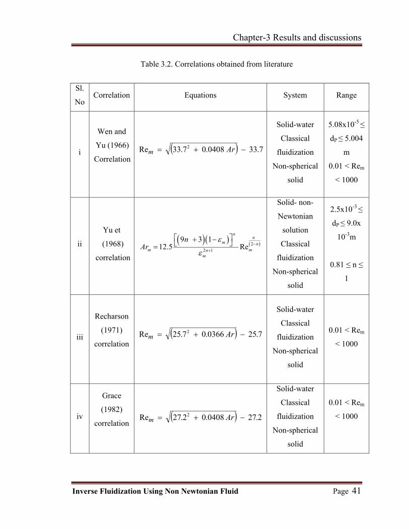
Chapter-3 Results and discussions
Inverse Fluidization Using Non Newtonian Fluid Page 41
Table 3.2. Correlations obtained from literature
Sl.
NoCorrelation Equations System Range
i
Wen and
Yu (1966)
Correlation 7.330408.07.33Re 2 Arm
Solid-water
Classical
fluidization
Non-spherical
solid
5.08x10⁻⁵ ≤
dP ≤ 5.004
m
0.01 < Rem
< 1000
ii
Yu et
(1968)
correlation
2
2 1
9 3 112.5 Re
nn
m nm mn
m
nAr
Solid- non-
Newtonian
solution
Classical
fluidization
Non-spherical
solid
2.5x10⁻³ ≤
dP ≤ 9.0x
10-3m
0.81 ≤ n ≤
1
iii
Recharson
(1971)
correlation 7.250366.07.25Re 2 Arm
Solid-water
Classical
fluidization
Non-spherical
solid
0.01 < Rem
< 1000
iv
Grace
(1982)
correlation 2.270408.02.27Re 2 Arm
Solid-water
Classical
fluidization
Non-spherical
solid
0.01 < Rem
< 1000
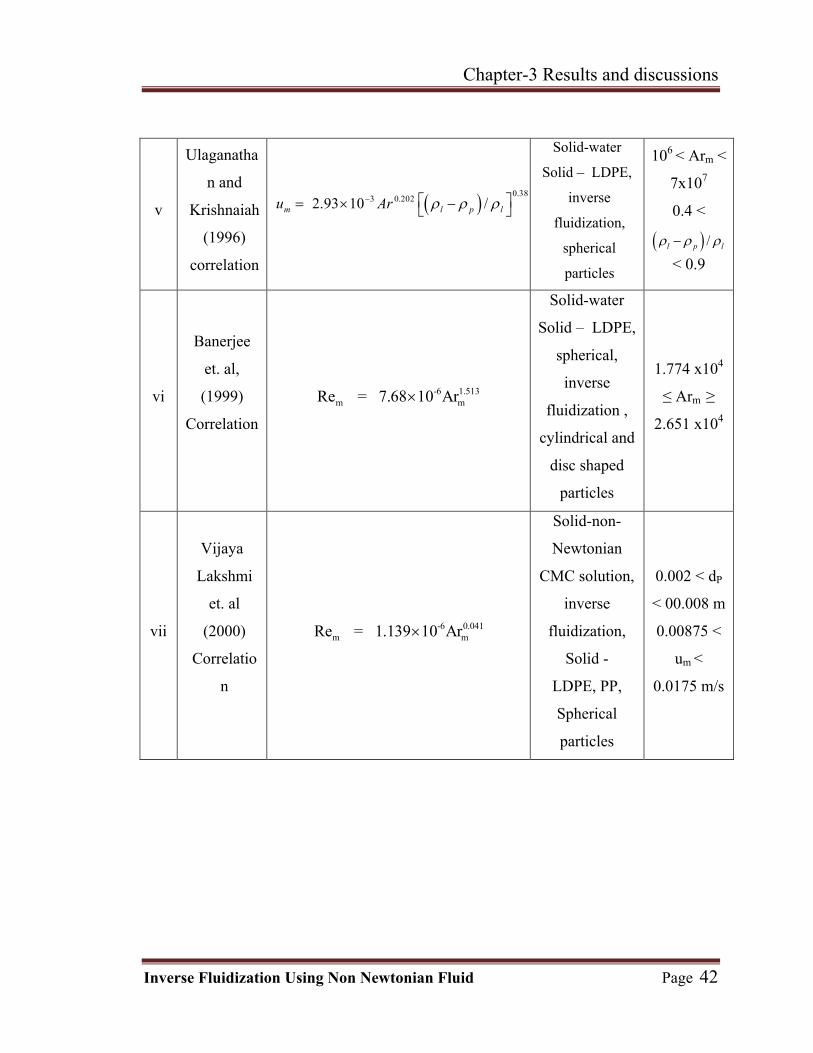
Chapter-3 Results and discussions
Inverse Fluidization Using Non Newtonian Fluid Page 42
v
Ulaganatha
n and
Krishnaiah
(1996)
correlation
0.383 0.2022.93 10 /m l p lu Ar
Solid-water
Solid – LDPE,
inverse
fluidization,
spherical
particles
106 < Arm <
7x10⁷
0.4 <
/l p l
< 0.9
vi
Banerjee
et. al,
(1999)
Correlation
-6 1.513m mRe = 7.68 10 Ar
Solid-water
Solid – LDPE,
spherical,
inverse
fluidization ,
cylindrical and
disc shaped
particles
1.774 x10⁴
≤ Arm ≥
2.651 x10⁴
vii
Vijaya
Lakshmi
et. al
(2000)
Correlatio
n
-6 0.041m mRe = 1.139 10 Ar
Solid-non-
Newtonian
CMC solution,
inverse
fluidization,
Solid -
LDPE, PP,
Spherical
particles
0.002 < dP
< 00.008 m
0.00875 <
um <
0.0175 m/s
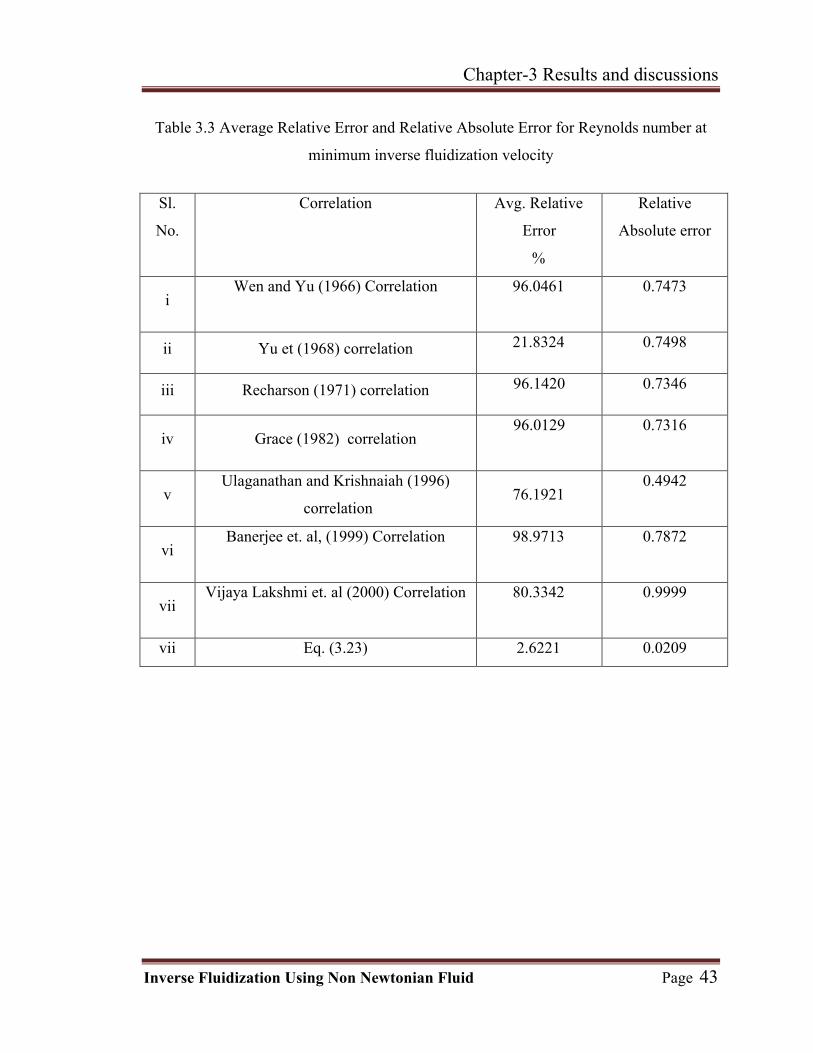
Chapter-3 Results and discussions
Inverse Fluidization Using Non Newtonian Fluid Page 43
Table 3.3 Average Relative Error and Relative Absolute Error for Reynolds number at
minimum inverse fluidization velocity
Sl.
No.
Correlation Avg. Relative
Error
%
Relative
Absolute error
iWen and Yu (1966) Correlation 96.0461 0.7473
ii Yu et (1968) correlation 21.8324 0.7498
iii Recharson (1971) correlation 96.1420 0.7346
iv Grace (1982) correlation96.0129 0.7316
vUlaganathan and Krishnaiah (1996)
correlation76.1921
0.4942
viBanerjee et. al, (1999) Correlation 98.9713 0.7872
viiVijaya Lakshmi et. al (2000) Correlation 80.3342 0.9999
vii Eq. (3.23) 2.6221 0.0209

Chapter-3 Results and discussions
Inverse Fluidization Using Non Newtonian Fluid Page 44
Pre
ssu
re d
rop
, N/m
2
Velocity, m/sFigure : 3.1 Plot of pressure drop vs velocity
0.00 0.01 0.02 0.03 0.04 0.05 0.06240
260
280
300
320
340
360
380
400
420
440
460
Pre
ssur
e d
rop,
N/m
2
Liquid velocity, uf , m/s
Figure : 3.2 Variation pressure drop across the bed with liquid velocity
Column Diameter : 0.072 mSolid : LDPE-1
SCMC Conc. : 0.2 kg/m3
Symbol Bed weight, gm 200
400 600 800 1000

Chapter-3 Results and discussions
Inverse Fluidization Using Non Newtonian Fluid Page 45
0.00 0.01 0.02 0.03 0.04 0.05 0.06
250
300
350
400
450
Column Diameter : 0.072 mSolid : LDPE-1
SCMC Conc. : 0.4 kg/m3
Symbol Bed weight, gm 200
400 600 800 1000
Pre
ssur
e d
rop,
N/m
2
Liquid velocity, uf , m/s
Figure : 3.3 Variation pressure drop across the bed with liquid velocity
0.00 0.01 0.02 0.03 0.04 0.05 0.06 0.07
250
300
350
400
450
500
Column Diameter : 0.072 mSolid : LDPE-1
SCMC Conc. : 0.6 kg/m3
Symbol Bed weight, gm 200
400 600 800 1000
Pre
ssu
re d
rop
, N/m
2
Liquid velocity, uf , m/s
Figure : 3.4 Variation pressure drop across the bed with liquid velocity
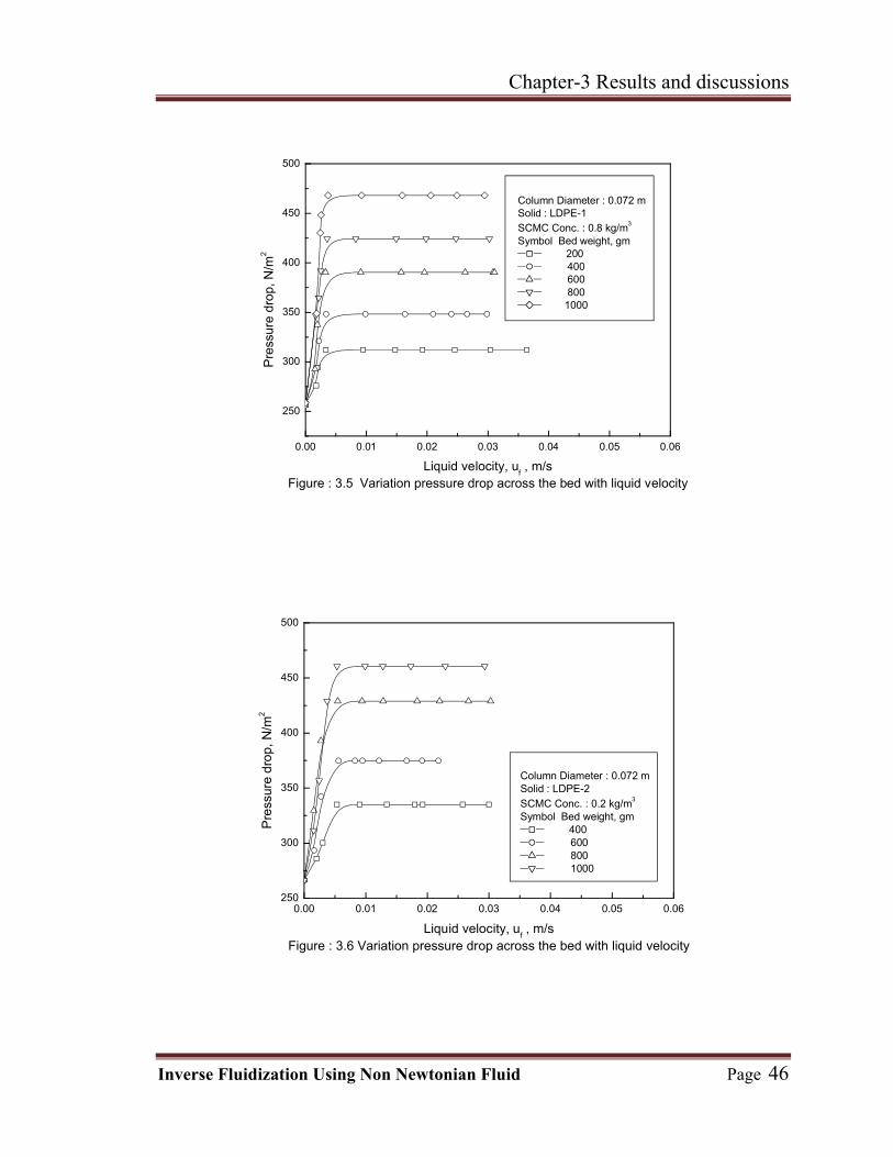
Chapter-3 Results and discussions
Inverse Fluidization Using Non Newtonian Fluid Page 46
0.00 0.01 0.02 0.03 0.04 0.05 0.06
250
300
350
400
450
500
Column Diameter : 0.072 mSolid : LDPE-1
SCMC Conc. : 0.8 kg/m3
Symbol Bed weight, gm 200
400 600 800 1000
Pre
ssu
re d
rop
, N/m
2
Liquid velocity, uf , m/s
Figure : 3.5 Variation pressure drop across the bed with liquid velocity
0.00 0.01 0.02 0.03 0.04 0.05 0.06250
300
350
400
450
500
Pre
ssur
e d
rop,
N/m
2
Liquid velocity, uf , m/s
Figure : 3.6 Variation pressure drop across the bed with liquid velocity
Column Diameter : 0.072 mSolid : LDPE-2
SCMC Conc. : 0.2 kg/m3
Symbol Bed weight, gm 400
600 800 1000

Chapter-3 Results and discussions
Inverse Fluidization Using Non Newtonian Fluid Page 47
0.00 0.01 0.02 0.03 0.04 0.05 0.06240
260
280
300
320
340
360
380
400
420
440
460
480
Column Diameter : 0.072 mSolid : LDPE-2
SCMC Conc. : 0.4 kg/m3
Symbol Bed weight, gm 200
400 600 800 1000
Pre
ssu
re d
rop
, N/m
2
Liquid velocity, uf , m/s
Figure : 3.7 Variation pressure drop across the bed with liquid velocity
0.00 0.01 0.02 0.03 0.04 0.05 0.06240
260
280
300
320
340
360
380
400
420
440
460
480
Column Diameter : 0.072 mSolid : LDPE-2
SCMC Conc. : 0.6 kg/m3
Symbol Bed weight, gm 200
400 600 800 1000
Pre
ssur
e dr
op, N
/m2
Liquid velocity, uf , m/s
Figure : 3.8 Variation pressure drop across the bed with liquid velocity

Chapter-3 Results and discussions
Inverse Fluidization Using Non Newtonian Fluid Page 48
0.00 0.01 0.02 0.03 0.04 0.05 0.06240
260
280
300
320
340
360
380
400
420
440
460
480
500
Column Diameter : 0.072 mSolid : LDPE-2
SCMC Conc. : 0.8 kg/m3
Symbol Bed weight, gm 200
400 600 800 1000
Pre
ssur
e dr
op,
N/m
2
Liquid velocity, uf , m/s
Figure : 3.9 Variation pressure drop across the bed with liquid velocity
0.00 0.01 0.02 0.03 0.04 0.05 0.06 0.07240
260
280
300
320
340
360
380
400
420
440
460
480
500
520
Column Diameter : 0.072 mSolid : HDPE
SCMC Conc. : 0.2 kg/m3
Symbol Bed weight, gm 200
400 600 800 1000
Pre
ssu
re d
rop
, N/m
2
Liquid velocity, uf , m/s
Figure : 3.10 Variation pressure drop across the bed with liquid velocity

Chapter-3 Results and discussions
Inverse Fluidization Using Non Newtonian Fluid Page 49
0.00 0.01 0.02 0.03 0.04 0.05 0.06 0.07240
260
280
300
320
340
360
380
400
420
440
460
480
500
520
540
Column Diameter : 0.072 mSolid : HDPE
SCMC Conc. : 0.4 kg/m3
Symbol Bed weight, gm 200
400 600 800 1000
Pre
ssu
re d
rop
, N/m
2
Liquid velocity, uf , m/s
Figure : 3.11 Variation pressure drop across the bed with liquid velocity
0.00 0.01 0.02 0.03 0.04 0.05 0.06240
260
280
300
320
340
360
380
400
420
440
460
480
500
520
540
Column Diameter : 0.072 mSolid : HDPE
SCMC Conc. : 0.6 kg/m3
Symbol Bed weight, gm 200
400 600 800 1000
Pre
ssur
e dr
op, N
/m2
Liquid velocity, uf , m/s
Figure : 3.12 Variation pressure drop across the bed with liquid velocity

Chapter-3 Results and discussions
Inverse Fluidization Using Non Newtonian Fluid Page 50
0.00 0.01 0.02 0.03 0.04 0.05 0.06240
260
280
300
320
340
360
380
400
420
440
460
480
500
520
540
Column Diameter : 0.072 mSolid : HDPE
SCMC Conc. : 0.8 kg/m3
Symbol Bed weight, gm 200
400 600 800 1000
Pre
ssur
e d
rop,
N/m
2
Liquid velocity, uf , m/s
Figure : 3.13 Variation pressure drop across the bed with liquid velocity
0.00 0.01 0.02 0.03 0.04 0.05 0.06240
260
280
300
320
340
360
380
400
420
440
460
480
500
Column Diameter : 0.072 mSolid : PP
SCMC Conc. : 0.2 kg/m3
Symbol Bed weight, gm 200
400 600 800 1000
Pre
ssu
re d
rop
, N/m
2
Liquid velocity, uf , m/s
Figure : 3.14 Variation pressure drop across the bed with liquid velocity

Chapter-3 Results and discussions
Inverse Fluidization Using Non Newtonian Fluid Page 51
0.00 0.01 0.02 0.03 0.04 0.05 0.06240
260
280
300
320
340
360
380
400
420
440
460
480
500
Column Diameter : 0.072 mSolid : PP
SCMC Conc. : 0.4 kg/m3
Symbol Bed weight, gm 200
400 600 800 1000
Pre
ssu
re d
rop
, N/m
2
Liquid velocity, uf , m/s
Figure : 3.15 Variation pressure drop across the bed with liquid velocity
0.00 0.01 0.02 0.03 0.04 0.05 0.06240
260
280
300
320
340
360
380
400
420
440
460
480
500
520
Column Diameter : 0.072 mSolid : PP
SCMC Conc. : 0.6 kg/m3
Symbol Bed weight, gm 200
400 600 800 1000
Pre
ssu
re d
rop
, N/m
2
Liquid velocity, uf , m/s
Figure : 3.16 Variation pressure drop across the bed with liquid velocity

Chapter-3 Results and discussions
Inverse Fluidization Using Non Newtonian Fluid Page 52
0.00 0.01 0.02 0.03 0.04 0.05 0.06240
260
280
300
320
340
360
380
400
420
440
460
480
500
520
Column Diameter : 0.072 mSolid : PP
SCMC Conc. : 0.8 kg/m3
Symbol Bed weight, gm 200
400 600 800 1000
Pre
ssu
re d
rop
, N/m
2
Liquid velocity, uf , m/s
Figure : 3.17 Variation pressure drop across the bed with liquid velocity
Figure : 3.18 Variation of minimum inverse fluidization velocity with bed weight
200 400 600 800 1000 1200
0.002
0.004
0.006
0.008
0.010
0.012
0.014Solid : LDPE-1Column diameter : 0.072 m Symbol SCMC solution Conc.
kg/m3
0.2 0.4 0.6 0.8
Min
imum
inve
rse
fluid
izat
ion
velo
city
, u m
, m
/s
Bed weight, gm.
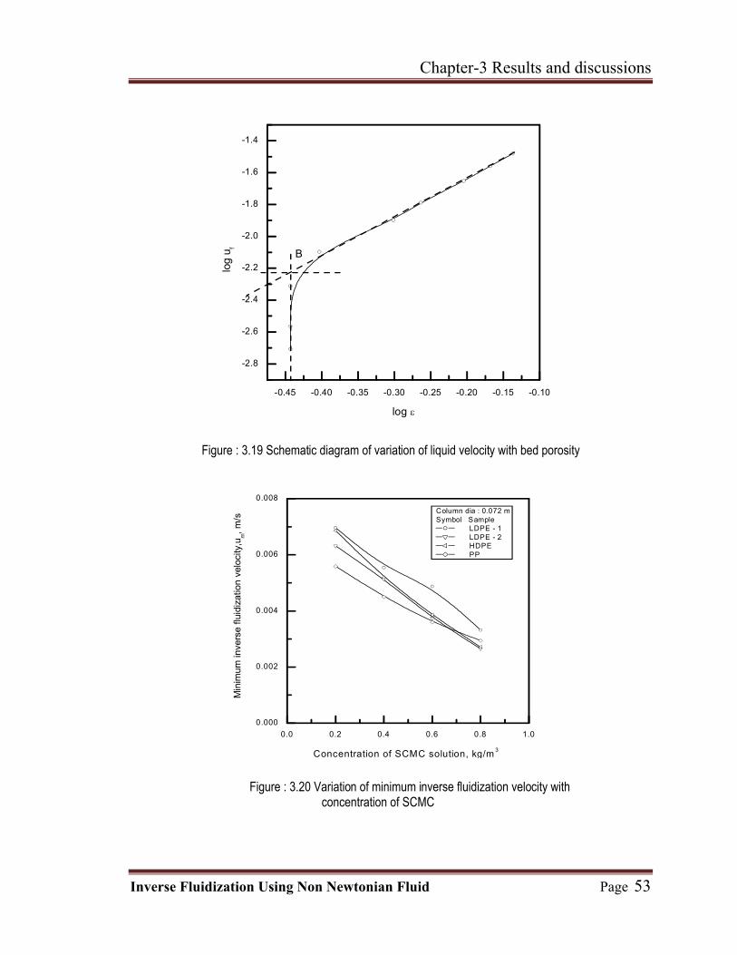
Chapter-3 Results and discussions
Inverse Fluidization Using Non Newtonian Fluid Page 53
Figure : 3.19 Schematic diagram of variation of liquid velocity with bed porosity
Figure : 3.20 Variation of minimum inverse fluidization velocity with concentration of SCMC
-0.45 -0.40 -0.35 -0.30 -0.25 -0.20 -0.15 -0.10
-2.8
-2.6
-2.4
-2.2
-2.0
-1.8
-1.6
-1.4
B
log
u f
log
0.0 0.2 0.4 0.6 0.8 1.0
0.000
0.002
0.004
0.006
0.008
Concentration of SCMC solution, kg/m 3
Min
imum
inve
rse
fluid
izat
ion
velo
city
,um,
m/s
Column dia : 0.072 mSymbol Sample
LDPE - 1 LDPE - 2 HDPE PP

Chapter-3 Results and discussions
Inverse Fluidization Using Non Newtonian Fluid Page 54
Figure : 3.21 Dependence of Rem on Archimedes number based on minimum
fluidization velocity for different correlation
Figure : 3.22 Variation of the calculated Rem with the experimental Rem
1E-6 1E-5 1E-4 1E-3 0.01 0.1 1 10 100
0.01
0.1
1
10
100
1000
Single component system Experimental; Wen and Yu (1966); Richardson (1971) Grace (1982); Banerjee et al. (1999); Vijaya Lakshmi et al. (2000) Ulaganathan and Krishnaiah (1996); Yu et al (1968); Calculated From Eq. (3.23) using
m=
s,
m=
pand d
m=d
p
Mod
ified
Arc
him
edes
num
ber,
Ar m
Reynolds number at minimum inverse fluidization velocity, Rem
1E-3 0.01 0.1 1 10
1E-3
0.01
0.1
1
10
Cal
cula
ted
Re m
Experimental Rem
single component system Binary component system

Inverse Fluidization Using Non Newtonian Fluid Page 55
CONCLUSIONS
The hydrodynamics Characteristics of the two phase inverse fluidization bed were
experimentally investigated. The experiments were carried out for four particles of
spherical and non spherical polyethylene and polypropylene and with four different
aqueous solutions of SCMS solution as non-Newtonian liquid. For two phase inverse
fluidization system, the pressure drop increases initially with increasing liquid velocity,
beyond um, it remains almost constant. The um is independent of bed weight. Empirical
correlation has been developed to determine the minimum inverse fluidization velocity as
a function of physical and dynamic variables of the system and compared with existing
correlations. The comparison shows that the developed correlation gives satisfactory
results than that of different correlations obtained from literature.

Inverse Fluidization Using Non Newtonian Fluid Page 56
NOMENCLATURE
Ar = Archimedes No. defined by dP3g(p -l )l/l
2 when p > l and by dP3g
(l -p )l/l2
CD = Particle Drag Coefficient.
D = Particle Diameter.
dP = Average Particle Diameter.
D = Column Diameter.
f = Drag Function for Multi particle system.
g = Acceleration due to Gravity.
Ga = Gallelio Number defined by gdp3 f
2/l2.
L = Distance between two pressure tapings in the column.
N = Exponent in Richardson and Zaki Correlation.
Rem = Particle Reynold’s Number at Minimum Fluidization Condition
U = Superficial Liquid Velocity.
Ui = The extrapolated value of U as approaches 1.
Umf = Minimum Fluidization Velocity.
Ut = Terminal Velocity of the solid particle.
Greek Letters
P = Pressure Drop across the Bed.
= Bed Porosity.o = Porosity of a Fixed Bed of Particles.
l = Liquid Viscosity.
l = Liquid Density.
P = Particle Density
Inverse Fluidization Using Non Newtonian Fluid Page 57
REFERENCE
Biswas, S. K., U. P.Ganguly, A preliminary Study on the Voidage – Velocity
Relationship in Reverse Fluidization, Ind. Chem. Eng., 39 303-306 (1997).
Fan, L. S., K. Muroyama, S. H. Chern, Hydrodynamic Characteristics of Inverse
Fluidization in Liquid – Solid and Gas – Liquid – Solid Systems, Chem. Eng. J., 24 143-
150 (1981).
Bendict, F., G. Kumarsan, M. Velan, Bed expansion and pressure drop studies in a liquid-
solid inverse fluidized bed reactor, Bioprocess Eng., 19 137-142 (1998).
Howley, M. A., J. G. Benjamin, A comparison of one-dimensional traveling waves in
inverse and normal fluidized beds, Physica D: Nonlinear Phenomena, 201 177-198
(2005).
Karamanev, D. G., L. N. Nikolov, Bed Expansion of liquid – solid inverse fluidization,
AIChE J,, 38 1916-1922 (1992).
Karamanev, D. G., L. N. Nikolov, Influence of some physicochemical parameters on
bacterial activity of biofilm : Ferrous iron oxidation by Thiobacillus ferrooxidans,
Biotechnol. Bioengg., 31(4) 295-299 (1988).
Li, J., T. Nakazato, K. Kato, Effect of cohesive powders on the elutriation of particles
from a fluid bed, Chem. Eng. Sci 59, 2777-2782, (2004).
Oh, D. K., C. K. Hyun, J. H. Kim, Y. H. Park, Production of penicillin in a fluidized-bed
bioreactor: Control of cell growth and penicillin production by phosphate limitation,
Biotechnol. Bioengg., 32(4) 569-573 (1988).
Ramos, R.L., L.S. Fan, L.Lopez, Velocidad minima de fluidizacion en lecho fluidizado
invertido liquido-solido, Avances en Ingenicria Quimica, 7 148-155 (1999).
Inverse Fluidization Using Non Newtonian Fluid Page 58
Renganathan, T., K. Krishnaiah, Liquid phase mixing in 2-phase liquid-solid inverse
fluidized bed, Chem. Eng. J,. 98 213-218 (2004).
Renganathan, T., K. Krishnaiah, Voidage characteristics and prediction of bed expansion
in liquid–solid inverse fluidized bed, Chem. Eng. Sci,. 60, 2545-2555, (2005).
Renganathan, T., K. Krishnaiah, Spatio-temporal evolution of void fraction in liquid–
solid inverse fluidized bed, Chem. Eng. Sci., 62, 328-338 (2007).
Sowmeyan, R. and G Swaminathan, Evaluation of inverse anaerobic fluidized bed reactor
for treating high strength organic wastewater, Bioresource Technology, 99 (9), 3877-
3880, (2008).
Sowmeyan, R. and G. Swaminathan, Effluent treatment process in molasses-based
distillery industries: A review, Journal of Hazardous Materials, 1, 453-462 (2008).
Sok´oł , W. and W. Korpal, "Aerobic treatment of wastewaters in the inverse fluidised
bed biofilm reactor", Chem. Engg. J., l 118 , 199–205 (2006).
Ulganathan, N., K. Krishnaiah, Hydrodynamic characteristics of two-phase inverse
fluidised bed, Bioprocess Eng,. 15 159-164 (1996).
Vijaya Lakshmi, A.C., M. Balamurugan, , M. Sivakumar, , T.N Samuel, M. Velan,
Minimum fluidization velocity and friction factor in a liquid-solid inverse fluidized bed
reactor, Bioprocess Eng.,. 22 461-466 (2000).
Wang D., T. Silbaugh, R. Pfeffer, Y.S. Lin, Removal of emulsified oil from water by
inverse fluidization of hydrophobic aerogels, Powder Technology J., 203 298–309 (2010)
Das, B., U. P. Ganguly, S. K. Das, Inverse fluidization using non-Newtonian liquids,
Chem. Engg. J., 49 1169–1175 (2010).
Copyright © 2022 FDOKUMEN