How to detect the Granger-causal flow direction in the presence of additive noise?

Martin Vincka,b,c,∗, Lisanne Huurdemanb, Conrado A. Bosmana,b, Pascal Friesa,d, Francesco P. Battagliaa, Cyriel M.A. Pennartzb,Paul H. Tiesingaa

aRadboud University Nijmegen, Donders Institute for Brain, Cognition and Behavior, Nijmegen, the NetherlandsbSwammerdam Institute for Life Sciences, Center for Neuroscience, University of Amsterdam, Amsterdam, the Netherlands

cYale University, School of Medicine, Department of NeurobiologydErnst Strungmann Institute (ESI) for Neuroscience in Cooperation with Max Planck Society, Frankfurt, Germany

Abstract

Granger-causality metrics have become increasingly popular tools to identify directed interactions between brain areas. However,it is known that additive noise can strongly affect Granger-causality metrics, which can lead to spurious conclusions about neu-ronal interactions. To solve this problem, previous studies have proposed to detect Granger-causal directionality, i.e. the dominantGranger-causal flow, using either the slope of the coherency (Phase Slope Index; PSI), or by comparing Granger-causality val-ues between original and time-reversed signals (reversed Granger testing). We show that for ensembles of vector autoregressive(VAR) models encompassing bidirectionally coupled sources, these alternative methods do not correctly measure Granger-causaldirectionality for a substantial fraction of VAR models, even in the absence of noise. We then demonstrate that uncorrelated noisehas fundamentally different effects on directed connectivity metrics than linearly mixed noise, where the latter may result as aconsequence of electric volume conduction. Uncorrelated noise only weakly affects the detection of Granger-causal directionality,whereas linearly mixed noise causes a large fraction of false positives for standard Granger-causality metrics and PSI, but not forreversed Granger testing. We further show that we can reliably identify cases where linearly mixed noise causes a large fractionof false positives by examining the magnitude of the instantaneous influence coefficient in a structural VAR model. By rejectingcases with strong instantaneous influence, we obtain improved detection of Granger-causal flow between neuronal sources in thepresence of additive noise. These techniques are applicable to real data, which we demonstrate using actual area V1 and area V4LFP data, recorded from the awake monkey performing a visual attention task.

Keywords: Granger-causality; phase slope index; volume conduction; reversed time series; vector autoregressive modelling

The Wiener-Granger definition of causality allows inferenceof causal relationships between interacting stochastic sources.Causality analysis methods have been applied in many fields,including physics, econometrics, geology, ecology, genetics,physiology and neuroscience (Barnett et al., 2009; Bernasconiand Konig, 1999; Bressler and Seth, 2011; Brovelli et al.,2004; Ding et al., 2006; Geweke, 1982; Granger, 1969; Gre-goriou et al., 2009; Hiemstra and Jones, 1994; Hu and Nenov,2004; Kaufmann and Stern, 1997; Lozano et al., 2009; Mari-nazzo et al., 2008; Nolte et al., 2008; Rosenblum and Pikovsky,2001; Salazar et al., 2012; Schreiber, 2000; Smirnov andMokhov, 2009; Staniek and Lehnertz, 2008; Sugihara et al.,2012). Standard Granger-causality metrics are typically basedon linear vector autoregressive (VAR) modeling, with Granger-causality fi→ j defined by examining xi’s effect on the resid-ual errors in forecasting x j(t) (Geweke (1982); Granger (1969),eqs. 4-5). In the neurosciences, Granger-causality metricshave become increasingly popular tools to identify functional,frequency-specific directed influences between brain areas (e.g.(Bernasconi and Konig, 1999; Bressler and Seth, 2011; Brovelliet al., 2004; Ding et al., 2006; Friston et al., 2014)). Two recent

∗Corresponding author.Email address: martin.vinck@yale.edu (Martin Vinck)

studies have shown interesting applications of Granger causal-ity to characterize functional interactions in the visual system.Bastos et al. (2014); van Kerkoerle et al. (2014) have shown thatgamma frequencies contribute to a feedforward flow of infor-mation, whereas alpha and beta frequencies contribute to flowof information in the feedback direction. Interestingly, Bastoset al. (2014) succeeded to reconstruct the visual hierarchy basedon anatomical tracing studies on the mere basis of examiningthe asymmetry of Granger-causality spectra, and showed thatthis cortical hierarchy was task-dependent.

Granger-causality metrics were originally developed for sys-tems whose measurements are not corrupted by additive noise.It has been shown that they can be strongly affected by bothuncorrelated and linearly mixed additive noise (Albo et al.,2004; Friston et al., 2014; Haufe et al., 2012a,b; Nalatore et al.,2007; Newbold, 1978; Nolte et al., 2008; Seth et al., 2013;Sommerlade et al., 2012). Nolte et al. (2008) showed thatadding a linear mixture of noise sources (correlated noise) of-ten leads to a misidentification of causal driver and recipientwhen using the standard Granger-causality metrics proposed byGranger (1969). This is an important issue in the neurosciences,as electric currents spread instantaneously from single brainor noise sources to multiple sensors (‘volume conduction’),

Preprint submitted to Elsevier December 5, 2014

posing a major problem especially for scalp EEG (Electro-encephalography), MEG (Magneto-encephalography), and in-tracranial LFP (Local Field Potential) signals (Nolte et al.,2004; Nunez and Srinivasan, 2006; Stam et al., 2007; Vincket al., 2011). This problem can, as far as the estimation of sym-metric, undirected connectivity (like coherence, phase lockingvalue) metrics is concerned, be adequately addressed by usingmetrics that are based on the imaginary component of the cross-spectral density (Nolte et al., 2004; Stam et al., 2007; Vincket al., 2011). In this paper, we ask whether directed connec-tivity measures like Granger-causality can be protected againstlinearly mixed noise as well.

Recently, two directed connectivity measures were intro-duced to address the volume conduction problem. Nolte et al.(2008) proposed to detect Granger-causal directionality by ex-amining whether fluctuations of one signal precede fluctuationsof another signal in time - i.e. temporal precedence - using ameasure called phase slope index (PSI). Haufe et al. (2012a,b)proposed to protect Granger-causality metrics against linearlymixed noise by comparing Granger-causality values with thosefor time-reversed signals (Haufe et al., 2012a), henceforth re-ferred to as RGT (reversed Granger testing). In terms of thetrue positives vs false positives mix, PSI was found to exhibitslightly better performance than RGT and much better perfor-mance than standard Granger-causality metrics (Haufe et al.,2012a,b; Nolte et al., 2008).

While initial results using these alternative directed connec-tivity metrics have been promising (Haufe et al., 2012a; Nolteet al., 2008), there are several critical questions that need to beaddressed. Firstly, it is unknown under which conditions PSIand RGT are in fact valid measures of Granger-causal direc-tionality, as previous work evaluated their use only for unidirec-tional, but not bidirectional VAR models (Haufe et al., 2012a;Nolte et al., 2008) (Section 2). This question is critical be-cause interactions between cortical areas are typically bidirec-tional rather than unidirectional. Secondly, it remains unclear towhat extent directed connectivity measures are affected by un-correlated noise, which occurs for example for spatially distantspike trains, current source densities and bipolarly referencedLFPs (Mitzdorf, 1985) (Section 3). Haufe et al. (2012a); Nolteet al. (2008) only considered the effect of linearly mixed noise(which is prominent for scalp EEG and MEG) but not uncor-related noise. It is thus unknown whether standard Granger-causality metrics can be safely used in the regime of uncorre-lated noise. Thirdly, it remains unclear whether PSI and RGTare indeed robust to linearly mixed noise, and how their over-all performances compare, since to date they have been evalu-ated only for finite-length data traces and unidirectional VARmodels. This is problematic, because small fractions of falsepositives may arise because of a lack of statistical power (finitedata traces) and the use of unidirectional VAR models. The per-formance of PSI and RGT should therefore also be evaluated inthe asymptotic sampling regime (i.e., infinitely long data traces)and for bidirectional VAR models (Section 4). Here, we employalgorithms to compute the various directed connectivity metricsanalytically given the VAR models of signal and noise sources.Surprisingly, we find that PSI, like standard Granger-causality

metrics, does not constrain the false positives rate at accept-able levels. In contrast, RGT yields a much smaller fraction offalse positives and much better overall performance than stan-dard Granger and PSI, although it still shows failures in a sig-nificant fraction of test cases. This paper also aims to advancethe theoretical analysis of PSI and RGT; in particular, we usetheoretical analysis to identify regimes in which RGT alwaysfails or succeeds.

We find that further performance gains are achievable beyondthose obtained by RGT, by indirectly measuring the amount oflinearly mixed noise impinging on two measurement sensors.The idea of this approach is quite simple but effective: We canexamine the degree to which there is instantaneous (i.e., zero-lag) feedback between time series by using a structural VARmodel that contains an explicit instantaneous transfer coeffi-cient. This allows us to reject cases where the instantaneoustransfer is too large compared to the transfer at other lags. Insection 5 we show that failures of Granger-causality metrics dueto linearly mixed noise can be reliably predicted and removedby examining the magnitude of the instantaneous prediction co-efficient in a structural VAR model. This provides a means toreduce the false positives rate and to improve the overall per-formance of the analysis in terms of the true and false positivesmix.

We apply these techniques to actual LFP data obtained fromareas V1 and V4 in the awake monkey performing a visual at-tention task.

1. Introduction of Granger analysis techniques and VARmodel with additive noise

In this section, we define the basic VAR model, the VARmodel with additive noise included, the various directed con-nectivity metrics, and performance measures for the differentmetrics.

1.1. The bivariate VAR model and a measure of linear Grangerfeedback

In this paper, we will be concerned with a bivariate signalx(t) described by a bivariate VAR model of order M

x(t) =

M∑τ=1

A(τ)x(t − τ) + U(t) , (1)

where innovation U(t) - the remaining error after incorporatingthe predictions from past values of x(t) - has covariance matrix

Σ ≡ CovU(t),U(t) . (2)

We refer to x1 and x2 as the signal sources. The matrices A(τ)hold the real-valued VAR coefficients. Also x(t) can be repre-sented by the restricted AR model

x(t) =

M∑τ=1

F(τ)x(t − τ) + V(t) (3)

with diagonal coefficient matrix F(τ) and Ω ≡ CovV(t),V(t).The standard measure of Granger-causal flow is defined by the

2

log-ratio of the variances of the innovation errors (Granger,1969)

f j→i ≡ ln(Ωii

Σii

), i , j . (4)

The feedback metric f j→i measures the degree to which pastvalues of x j(t) improve the prediction of future values of xi(t)relative to what can be derived from past values of xi(t). We de-fine x1 to be Granger-causally dominant over x2 if the Granger-causal directionality measure

g ≡ f1→2 − f2→1 > 0. (5)

In this paper, we study the simplified problem of detectingsgn(g), where sgn(g) is the sign function, from noisy data, asin Nolte et al. (2008); we are not concerned with the problemof estimating f2→1 and f1→2 separately. The problem is statedas providing a measure of sgn(g) that optimizes performance interms of the false and true positives mix. The precise weight-ing of false positives and true positives depends on the practicalapplication, but typically false positives outweigh true positivesin importance by an order of magnitude, which is reflected bythe common convention that the false discovery rate (FP/TP)should not exceed a low threshold (e.g. 0.05 or 0.1) (Benjamini,2010). The problem can therefore be formulated as maximizinga direction detection performance function

U ≡ −G · fracFP + fracTP (6)

where the gain G is set to 10 in this paper (as in Haufe et al.(2012b)).

1.2. The PSI (Phase Slope Index)Recently, two procedures were proposed to detect Granger-

causal directionality in the presence of additive linearly mixednoise (Haufe et al., 2012a,b; Nolte et al., 2008). PSI is defined

ψ ≡

∫=C′(ω)dω , (7)

with slope of the coherency

C′(ω) ≡ limdω→0

C(ω)C∗(ω + dω)dω

, (8)

and where = is the imaginary component. In turn, coherencyis defined

C(ω) ≡S 12(ω)

√S 11(ω)S 22(ω)

(9)

and spectral density matrix (assuming it exists) is defined

S(ω) ≡(S 11(ω) S 12(ω)S 21(ω) S 22(ω)

). (10)

PSI was motivated by the argument that causal dominance im-plies temporal precedence (Nolte et al., 2008), with a shift ofthe peak of the cross-covariance function

s12(τ) ≡ Covx1(t), x2(t + τ) (11)

by a delay of ∆τ corresponding to multiplication of its FourierTransform, the cross-spectral density S 12(ω) by eiω∆τ.

Coherency relates to linear prediction in the context of con-structing a noncausal Wiener filter (Wiener, 1949): For the lin-ear model x2(t) =

∑τ=+∞τ=−∞ h(τ)x1(t− τ), the optimal Wiener filter

kernel has Fourier Transform H(ω) = S 21(ω)/S 11(ω), such thatthe minimum error εmin =

∫S 22(ω)

(1 − |C(ω)|2

)dω, where the

squared coherence |C(ω)|2 plays a similar role as in linear re-gression analysis. Define the inverse Fourier Transform of thecoherency function c(τ) ≡ F −1[C(ω)]. If prediction errors tendto be more reduced by the τ > 0 than the τ < 0 componentof c(τ), then the coherency C(ω) will typically have a posi-tive slope, as follows from the shift/translation property of theFourier Transform.

Yet, it is not obvious that PSI ‘typically’ detects Granger-causal directionality for bidirectional VAR models, because itignores the linear feedback between sources and the predictionsof the time series by themselves.

1.3. RGT (Reversed Granger Testing)Another procedure to make a decision about Granger-causal

directionality is based on computing the Granger-causal feed-back values f j→i for time-reversed signals xrev(t) = x(−t)(Haufe et al., 2012b). For time-reversed signals, we have spec-tral density matrix Srev(ω) = S(−ω) and cross-covariance ma-trix srev(τ) = s(−τ). RGT holds that x1 is Granger-causallydominant over x2 if the inequalities

g ≡ f1→2 − f2→1 > 0grev ≡ f rev

2→1 − f rev1→2 > 0 (12)

both hold, that is if Granger-causal directionality reverses (flips)for the time-reversed signals. Note that in the definition of grev,the individual feedback terms are already sign-reversed; there-fore the signs of g and grev should be equal. No decision aboutGranger-causal directionality is taken when sgn(g) , sgn(grev),that is if Granger-causal directionality does not flip for time-reversed signals. Theoretical motivation for the RGT measurein case of additive linearly mixed noise will be given in Section4.1.1.

1.4. Additive noise modelNow suppose that additive noise

ε(t) ≡(ε1(t)ε2(t)

)≡ K z(t) (13)

is superimposed onto the signal source x(t). Here, K is a real-valued 2xS linear mixing matrix and z(t) is an S x1 vector ofS noise sources. We assume that the S noise sources are un-correlated with each other, i.e. Covzp(t), zs(t + τ) = 0 forall (s, p, τ) for which s , p. We also assume that the noisesources are each uncorrelated with the signal sources x(t), suchthat Covzs(t), xi(t + τ) = 0 for all (s, i, τ).

We refer to the additive noise ε(t) as uncorrelated (Section3) if the equality Covε1(t), ε2(t + τ) = 0 holds for all τ (e.g.if for S = 2, K is diagonal or anti-diagonal) and as linearly

3

mixed (Section 4) otherwise (e.g. if for S = 2, K is not strictlydiagonal or anti-diagonal).

The resulting time series with a superposition of additivenoise is

x(ε)(t) ≡ (1 − γ)x(t) + γε(t) , (14)

where the parameter γ determines the signal-to-noise ratio.Throughout this paper, superscript (ε) always indicates variablesthat result from mixing signal and noise. From the linearity ofthe cross-covariance function and the Fourier Transform, it fol-lows that the spectral density matrix equals

S(ε)(ω) = (1 − γ)2S(ω) + γ2Sε(ω) , (15)

and that the cross-covariance function equals

s(ε)(τ) = (1 − γ)2s(τ) + γ2sε(τ) . (16)

That is, the resulting spectral density matrix S(ε)(ω) can bewritten as a linear mixture of the original spectral density ma-trix S(ω) and the spectral density matrix of the noise sourcesSε(ω); the same holds for the resulting cross-covariance func-tion s(ε)(τ).

1.5. Difference between additive noise and innovation

It is important to note that additive noise and innovation ex-ert fundamentally different effects. The innovation process Uaffects future values x(t + τ) through A (eq. 1), whereas ad-ditive noise merely distorts the measurement of x(t) (eq. 14),such that it cannot be subsumed by the innovation U in eq. 1.

1.6. Definition of true positives and false positives

Throughout the text, the standard measure of Granger-causalfeedback sgn(g) for the noise-free VAR in eq. 1 (γ = 0) istaken as a ‘ground-truth’ reference for defining true positivesand false positives. We define false negatives, and true and falsepositives as follows.

(i) If PSI is computed analytically, then we simply examinesgn(ψ(ε)), i.e. no statistical testing has to be performed (seeFigs 2 and 4). In that case, a true positive for PSI is definedby the equality sgn(ψ(ε)) = sgn(g); a false positive by the in-equality. Let fracTP ∈ [0, 1] and fracFP ∈ [0, 1] denote the frac-tions of false positives and true positives. For PSI, the equalityfracTP + fracFP = 1 then holds, unless γ = 1 in eq. 14. Notethat with analytical computation, there are no false negatives forPSI, because PSI either yields a value that is positive or negative(since a value of zero will in practice not occur), which meansthat it either detects the G-causal directionality correctly (truepositive) or incorrectly (false positive).

(ii) If PSI is estimated from finite data traces (Fig 6), thenstatistical testing is performed to test against the null hypothesisthat ψ = 0. In this case, PSI can yield false negatives, because itcan fail to reach statistical significance, and the equality fracTP+

fracFP + fracFN = 1 holds, where a true positive requires the nullhypothesis to be rejected and the equality sgn(ψ(ε)) = sgn(g) tohold true.

(iii) If RGT is computed analytically, then it has a true posi-tive if the equalities

sgn(g(ε)) = sgn(g)

sgn(g(ε),rev) = sgn(g) (17)

both hold, and a false positive if the inequalities sgn(g(ε)) ,sgn(g) and sgn(g(ε),rev) , sgn(g) both hold; it yields a false neg-ative otherwise.

(iii-a) For RGT, the equality fracTP +fracFP +fracFN = 1 holdsin case of added noise.

(iii-b) In case of no additive noise (γ = 0 in eq. 14), theequality fracTP + fracFN = 1 holds.

(iv) If RGT is estimated from finite traces (Fig 6), then statis-tical testing is performed in addition to the requirements in eq.17.

The false discovery rate (FDR) is defined FDR ≡ fracFPfracTP

.

2. Case of no additive noise

In this section we consider the case of no additive noise, i.e.the equality γ = 0 holds, where the noise amplitude parameter γis defined in eq. 14. The case of additive noise will be discussedin Sections 3-4.

2.1. Theoretical considerations for the case of no additivenoise

We note that while the parameters of the restricted AR model(eq. 3) are invariant to a time-reversal of x(t), the full VARmodel (eq. 1) and associated metrics fi→ j (eq. 4) are not alwaysreversible.

In Appendix A, we provide a theoretical analysis showingthat RGT performs always well in the regime where cross- andauto-correlations have small magnitudes (as confirmed by Fig1A-B). This case occurs for example for near-Poissonian spiketrains from separate brain areas, which have small-magnitudeautocorrelations at all non-zero lags, and may have small-magnitude cross-correlations at all lags as well.

In Appendix A, we also perform a theoretical analysis show-ing that RGT performs always well if the autocorrelation func-tions of x1 and x2 are similar. This result is important becausewe can assume that signals from different neocortical areas of-ten have quite similar autocorrelation functions (implying sim-ilar power spectra of signals with standardized variance), a re-sult of the relatively homogeneous architecture of the neocorti-cal column. The result does not assume that the time series areoptimally described by a linear model, but merely assumes thatthe autocorrelation functions of x1 and x2 (and power spectra)are relatively similar.

2.2. Simulations for the case of no additive noise: Methods

2.2.1. Methods: Choice of priorsWe evaluated the performance of the various metrics ana-

lytically, i.e. without using finite-length signals or particularspectral estimation techniques, or making assumptions aboutthe type of probability distribution of the innovation process

4

U, i.e. P(U), beyond its covariance matrix Σ. The questionwhether the equations sgn(ψ) = sgn(g) and sgn(grev) = sgn(g)‘typically’ hold requires the specification of a prior distributionP(A(τ),Σ). This prior distribution specifies which VAR mod-els are ‘expected’ or ‘typical’ and which VAR models are ‘sur-prising’ or ’nontypical’. Simulations performed by Nolte et al.(2008) were limited to cases with unidirectional Granger-causalflow.

Here we consider classes of priors that encompass both uni-directional and relatively ‘difficult’ bidirectional VAR modelsthat are more representative of actual cortical interactions. As-suming that variables interact at a delay, we set the covariancematrix to be the identity matrix, i.e. Σ = I. We examined both anormal prior and a shrinkage prior on the space of VAR models,and evaluate a wide range of parameter settings to generalizeour results. The normal prior is defined

Ai j(τ) ∼ N(0, σ2A) , (18)

where N is the normal (Gaussian) distribution. Larger coeffi-cients σA correspond to a larger variance (i.e. magnitude) ofVAR coefficients and larger Granger feedback (and coherence)values; note that for large σA many VAR models become unsta-ble. No assumption is made about the distribution (e.g. Gaus-sian or non-Gaussian) of U(t) beyond its covariance Σ.

The shrinkage prior is a popular prior in macro-economicBayesian estimation and is defined

Ai j(τ) ∼ N(0, θ2λ2/τ2) , (19)

with the coupling parameter θ = 1 for i = j and 0 ≤ θ ≤ 1otherwise (Litterman, 1986). In this case the parameter λ (com-parable to σA in eq. 18) controls the variance of the VAR co-efficients, and θ the coupling strength. The shrinkage prior as-sumes that more recent lags carry more predictive power thandistant lags (shrinkage 1/τ2), reflecting the decay of synapticpotentials in the brain, i.e. the finite influence of an impulse inone neuronal group on another neuronal group. It also assumesthat a time series is a better forecaster of itself than of other timeseries (θ ∈ [0, 1]), reflecting the architecture of the neocortexin the sense that the majority of neuronal connections is local(Buzsaki, 2006), such that a local group of neurons generatingone LFP/EEG/MEG signal is expected to have a much greatercausal influence on itself than on a distant group of neurons thatgenerates another LFP/EEG/MEG signal. Furthermore, it en-compasses both unidirectional and bidirectional VAR models,which both occur in the nervous system. Probabilities of falseand true positives were estimated by Monte Carlo sampling anensemble of stable VAR models from the prior P(A(τ)), andcomputing the various Granger-causality metrics analyticallyas indicated in the following subsections. We note that it wouldnot be possible to evaluate a flat (noninformative) prior on A,because it would be an improper prior having infinite supportthat does not allow for Monte Carlo sampling.

Because most VAR models became unstable for large vari-ance of the VAR coefficients σA, we iteratively updated drawsby replacing the maximum squared element of A with a newrandom variate from N(0, σ2

A), until the VAR model became

stable. For the shrinkage prior we directly rejected the smallfraction of unstable VAR models.

2.2.2. Computation of the PSIPSI values were obtained by computing the spectral density

matrix S(ω) analytically and using the broad-band frequencyspectrum, sampled at 103 (without loss of generalization) fre-quencies. Starting from the VAR model in eq. 1 the spec-tral density matrix is obtained by using the stochastic spectral(Cramer) representation for the wide-sense stationary time se-ries

x j(t) =

∫ π

−π

eitωdZ j(ω) (20)

(Granger, 1969; Percival and Walden, 1993) (in analogy to theFourier Transform of a deterministic signal) such that(

a11(ω) a12(ω)a21(ω) a22(ω)

) (dZ1(ω)dZ2(ω)

)=

(dZu1 (ω)dZu2 (ω)

), (21)

where ai j is defined in terms of the Discrete Fourier Transformof the VAR coefficients

ai j(ω) ≡ δi j −

M∑τ=1

Ai j(τ)e−iωτ , (22)

and where the dZ’s are the spectral representations of x(t) andU(t). The spectral density matrix is now given as

S(ω) ≡(dZ1(ω)dZ2(ω)

) (dZ1(ω) dZ2(ω)

)= H(ω) Σ H∗(ω) (23)

where the ‘transfer function’ H(ω) ≡ a(ω)−1 and ∗ is the ad-joint operator (Hermitian conjugate). Thus, the spectral densitymatrix can be analytically computed starting from the coeffi-cients of a given VAR model. We then computed PSI, usingeq. 7, sampling at 103 frequencies (results were not affected byincreasing the number of frequencies, as the spectral functionsare relatively smooth with the model orders used, resulting inonly few peaks in the coherence spectra, see Fig 1D).

Note that using an iterative spectral factorization algorithm,the VAR model can also be obtained from S(ω) in return(Dhamala et al., 2008; Wilson, 1972). The spectral Grangervalues are now defined (Dhamala et al., 2008; Geweke, 1982)

F j→i(ω) ≡ lnS ii

S ii −

(Σ j j −

Σ2ji

Σii

)|Hi j(ω)|2

. (24)

2.2.3. Computation of RGTFor the grev metric, i.e. the Granger-causal dominance

for time-reversed signals, we computed the VAR coefficientsArev(τ) for the time-reversed signals x(−t) by (i) analyticallysolving the Yule-Walker equations

s(τ) =

M∑m=1

A(m)s(τ − m) + δτ0Σ (25)

5

for the cross-covariance function s(τ) given specified A(m) andΣ, (ii) using the equality srev(τ) = s(−τ), and (iii) analyticallysolving the Yule-Walker equations for Arev, where

srev(τ) =

M∑m=1

Arev(m)srev(τ − m) + δτ0Σrev (26)

We then used eq. 4 and 5 to compute grev. Spectral matrix fac-torization (Dhamala et al., 2008) of the spectral density matrixS(−ω) yielded quantitatively nearly identical results (data notshown).

2.3. Simulations for the case of no additive noise: Results

Fig 1A-B shows the true and false positives ratios as a func-tion of the parameters σA and λ that control the variance (i.e.,magnitude) of the VAR coefficients, and the model order M.The fraction of false negatives is not shown for RGT as forRGT, 1 − fracTP = fracFN in case of no additive noise. Forboth normal and shrinkage priors, PSI and RGT failed to iden-tify the Granger-causally dominant variable for a large fractionof simulated VAR models (Fig 1A-B). The fraction of failures[1 − fracTP] increased as a function of the magnitude of VARcoefficients (σA and λ). Because, in case of no noise, RGTdoes not yield false positives but only true positives and falsenegatives, it yielded much better performance than PSI in termsof a gain function U = fracTP − 10fracFP, except for the caseof a unidirectional prior (see Supplementary Information). Al-though PSI is a directed connectivity metric and a valid measureof the temporal ordering of signals, we conclude that it does notconstitute a valid measure of Granger-causality in general, be-cause the FDR can reach 30-40% for many priors. Thus, for PSIto be a valid measure of Granger-causality, one needs to assumethat the interaction between sources is nearly unidirectional.

RGT performed especially well in the regime of the normalprior with small variance of the VAR coefficients. The goodperformance of RGT in this regime is conform our analyticalresults presented in Appendix A. This regime yielded realisticpeak coherences (0.1-0.4) for brain signals (Fig 1C), however italso yielded signals that are too white (i.e., relatively flat powerspectrum) for the colored brain EEG/MEG signals (Bosmanet al., 2012; Brovelli et al., 2004; Buschman and Miller, 2007;Gregoriou et al., 2009; Saalmann et al., 2012; Salazar et al.,2012) (although not for e.g. near-Poissonian spike trains). Themost difficult regime for RGT that yielded both colored signalsand realistic peak coherences for MEG and EEG brain signalswas the case of the shrinkage prior with λ large (i.e., large mag-nitude of VAR coefficients) and θ small (i.e., weak coupling). Inpractice, we expect the performance of RGT to be better how-ever: In our simulations, the two variables x1 and x2 could havewidely different autocorrelation functions (and power spectra),while RGT performs better for variables having similar auto-correlation functions (Appendix A).

3. Case of uncorrelated noise

3.1. Theoretical considerations for the case of uncorrelatednoise

The case of predominantly uncorrelated noise occurs for ex-ample for spike trains, and distant current source densities orbipolarly derived intracranial signals (Mitzdorf, 1985). It re-mains unknown whether the dominant Granger-causal flow canbe reliably detected in case of uncorrelated noise, as Nolte et al.(2008) evaluated the case of correlated noise only. In case ofuncorrelated noise the equality sε1,ε2 (τ) = 0 holds for all τ, thusuncorrelated noise affects S(ε)

i j (ω) and s(ε)i j (τ) only for i = j, as

follows from eqs. 15-16. Hence, it affects PSI only weaklyand via C(ω)’s denumerator (see Fig 2A,B). In Appendix A weshow that if the magnitudes of cross- and autocorrelations arerelatively small, then sgn(g(ε)) tends to be unaffected by uncor-related noise (see Fig 2A,B) even though f (ε)

i→ j and f (ε)j→i typically

decrease at the rate of the signal-to-noise ratio (Appendix A).The behavior of the various measures in other regimes will beexplored through simulations in this Section.

3.2. Simulations for the case of uncorrelated noise: Methods

We evaluated normal and shrinkage priors by drawing an en-semble of VAR models from these priors. When the VAR coef-ficients for x(t) were drawn randomly from a normal (or shrink-age) prior, we also drew the VAR coefficients for the noisesources ε from a normal (or shrinkage) prior, except that Aε(τ),the coefficients for the noise time series, was set to be diago-nal for all τ. Values of f (ε)

j→i and f rev,(ε)j→i were obtained using the

following algorithm:(i) We analytically solve the Yule-Walker equations (eq. 25)

yielding expressions for s(τ) and sε(τ), which are combined intos(ε) = (1 − γ)2s(τ) + γ2sε(τ) (eq. 16).

(ii) We obtain an expression for A(ε), the coefficients for thesignal corrupted by noise, where

x(ε)(t) =

M(ε)∑τ=1

A(ε)(τ)x(ε)(t − τ) + U(ε)(t) , (27)

by solving the Yule-Walker equations again.(iii) From the expressions of A(ε)(τ) and U(ε)(t) we then ob-

tain the expression for the VAR coefficients of the time-reversedsignal, Arev,(ε)(τ) (see Section 2.2.3).

(iv) Because of added noise, A(ε)(τ) will typically be non-zero for τ > M, but decays at steep exponential rate. Wetherefore computed the order M(ε) by increasing M(ε) until allA(ε)(M(ε) − M + 1), . . . ,A(ε)(M(ε)) coefficients computed usingstep (iii) had absolute values <10−4 lower than the respectivecoefficients in A(ε)(1), . . . ,A(ε)(M) (where M is the original or-der of x), that is we set M(ε) such that the VAR coefficients haddecreases by a factor of 10−4. The same procedure was used forArev,(ε)(τ).

Using spectral matrix factorization (Wilson, 1972) of theanalytically computed spectral density matrix S(ε)(ω) yieldednearly identical results to those obtained with the algorithm pre-sented above, but it was much slower to compute.

6

PSI was directly computed from the expression for the spec-tral density matrix in eq. 15, sampling at 103 frequencies (asabove, results were not affected by increasing the number offrequencies).

3.3. Simulations for the case of uncorrelated noise: ResultsAs predicted theoretically in Section 3.1, we found that PSI

was minimally affected by uncorrelated noise, although, asshown in Section 2, it yielded many false positives withoutany additive noise. The standard measure of Granger-causaldirectionality sgn(g(ε)) was only weakly affected for small σA,and only moderately for large σA and γ (Fig 2A-B). For theshrinkage prior, we also observed weak effects on all measures.Thus, while the individual Granger-causal feedback measuresf (ε)2→1 and f (ε)

1→2 are typically strongly affected by noise, the stan-dard measure of Granger-causal directionality sgn(g(ε)) is quiterobust to uncorrelated noise. Overall, RGT yielded the smallestfraction of (<0.1) false positives, at the expense of a reductionin true positives. Thus, our results suggest that both RGT andstandard Granger-causality are viable options for the regime ofuncorrelated noise; which measure to choose depends on as-sumptions on the signal-to-noise ratio and the relative weight-ing of true and false positives.

We verified that our results held true across different modelorders M and for a unidirectional prior (See the SupplementaryInformation).

4. Case of linearly mixed noise

4.1. Theoretical considerations for the case of linearly mixednoise

4.1.1. PSILinearly mixed noise is common in the neurosciences (the

‘volume conduction’ problem), where electric currents fromsingle neural or noise sources spread instantaneously to mul-tiple electro-magnetic measurement sensors (Nolte et al., 2004;Stam et al., 2007; Vinck et al., 2011). For the signal componentthat is due to linearly mixed noise, the equality sε(τ) = sε(−τ)holds for all lags τ, i.e. the cross-covariance function of thenoise sources is strictly symmetric. This implies that if there areonly noise sources (γ = 1 in eq. 14), then the imaginary com-ponent of the spectral density matrix vanishes, i.e., the equation=S(ε)(ω) = 0 holds for all ω (Nolte et al., 2004), implying thatthe PSI for the noise sources equals zero, i.e. ψ(ε) = 0. It wastherefore argued that PSI should have reduced noise sensitivityin comparison to the standard measure of Granger-causal direc-tionality sgn(g(ε)) (Nolte et al., 2008). While this holds true forthe extreme case of γ = 1, it is not clear whether it also holdstrue for values of γ close to one.

PSI can, by construction, be affected by adding linearlymixed noise. First note that the real component of the co-herency, <C(ω), does play a role in the PSI metric, as theimaginary component of the slope of the coherency =C′(ω)cannot be rewritten to

limdω→0

=C(ω)=C∗(ω + dω)dω

. (28)

Second, note that adding a symmetric cross-covariance func-tion sε(τ) to an asymmetric function s(τ), the effect of addinglinearly mixed noise (eq. 16), can flip asymmetries in theopposite direction, because the cross-covariance function s(τ)can attain both negative and positive values. That is, theinequality |s12(τ)| > |s12(−τ)| does not imply the inequal-ity |s(ε)

12 (τ)| > |s(ε)12 (−τ)| (Fig 3). For example, suppose that

s12(τ) = u(τ)e−τ cos(τ) with u(τ) the Heaviside step function.In this case, all the energy in the cross-covariance function isconcentrated at positive delays. If now sε1,ε2 (τ) = −e−|τ| cos(τ),then s(ε)

12 (τ) = 0 for τ ≥ 0 and s(ε)12 (τ) = −eτ cos(τ) for τ < 0.

Suddenly, the energy in the cross-covariance function is con-centrated at negative delays.

These considerations reveal that the effect of additive noise isfundamentally different for the case of linearly mixed noise as itaffects the cross-correlation function ρ(ε)

12 (τ) in a lag-dependentmanner, as opposed to uncorrelated noise, and can flip asym-metries around τ = 0 (see Fig 3), which would then appear as aswitch of causal flow.

4.1.2. RGTGood performance of RGT is predicted in the limit of dom-

inant linearly mixed noise, as we will now prove from thespectral definition of Granger-causality (Dhamala et al., 2008;Geweke, 1982). If linearly mixed noise is dominant (i.e. γhigh), then the normalized magnitude of the imaginary compo-nent of the cross-spectral density vanishes, i.e.

|=S 12|

|<S 12|→ 0 . (29)

Define J ≡ Hrev. Now take the spectral matrix factorization

Srev(ω) = J(ω) Σrev J∗(ω) . (30)

As γ → 1, Hrev(ω) → H(ω). Hence, F j→i(ω) → Frevj→i(ω).

Since F j→i and f j→i are Fourier pairs (Geweke, 1982), it followsthat f j→i(ω) → f rev

j→i(ω). Thus, it follows that | f (ε)j→i − f rev,(ε)

j→i | →

0, and hence sgn(grev,(ε)) → sgn(g), as the relative magnitudeof linearly mixed noise increases, i.e. γ → 1. This theoreticalresult is confirmed by our simulations presented in Fig 4. Onthe other hand, although the PSI converges to zero, i.e. ψ(ε) →

0, as the relative magnitude of linearly mixed noise increases,i.e. γ → 1. However, sgn(ψ(ε)) does not necessarily converge tosgn(g) for γ close to 1, which is confirmed by our simulationspresented in Fig 4.

These theoretical considerations also reveal cases whereRGT yields false negatives in the absence of noise: If the imagi-nary component of S( f ) vanishes (i.e. zero-phase or 180 degreephase interaction), then RGT will yield a false negative; thus,similar to connectivity metrics based on the imaginary com-ponent of the cross-spectral density (Nolte et al., 2004; Stamet al., 2007; Vinck et al., 2011), RGT is esp. sensitive in detect-ing interactions occurring at a phase delay away from 0 or 180degrees.

4.2. Simulations for the case of linearly mixed noise: MethodsPrevious simulations performed by Nolte et al. (2008) were

performed for unidirectional VAR models with finite-length re-

7

alizations. The question remains whether the observed lack offalse positives for PSI (maximum ≈ 5%) (Nolte et al., 2008) wasdue to limited sampling and the use of a unidirectional prior.We set the linear mixing matrix K ∼ N(0, 1) and the numberof noise sources S = 2 (where K and S occur in eq. 13), likeNolte et al. (2008). We computed RGT, Granger and PSI valuesas outlined in Section 3.2.

We also performed simulations for the finite samplingregime. We randomly generated finite length realizations ac-cording to eq. 1 with Gaussian innovation. For PSI, the spec-tral density matrix S was estimated parametrically by first esti-mating the VAR coefficients (using the BSMART toolbox, Cuiet al. (2008)) and then using eq. 23. PSI was then computedusing sampling at 103 frequencies (as above, results were notaffected by increasing the number of frequencies). The modelorder of the VAR parameters was determined empirically us-ing the Bayesian information criterion (BIC) (Seth, 2010). TheBIC criterion was computed in iterative fashion: first findingthe optimal model order between 1 and 16; if the model or-der was equal to 16, then the optimal order between 16 and 32was searched, etc.. To compute PSI nonparametrically, we es-timated S using Bartlett-averaging with a Hann taper and 400datapoint windows, as in Nolte et al. (2008).

4.3. Simulations with analytical approximations: ResultsWe first show the results from simulations where RGT,

Granger and PSI were computed analytically from the givenVAR models of signal and noise sources. Our simulationsconfirm Nolte et al. (2008)’s observation that the standardGranger-causal directionality measure sgn(g(ε)) fails to identifythe Granger-causally dominant variable when linearly mixednoise dominates (high γ), yielding poor control of the FDR.

A surprising result of this paper is that the PSI also exhibiteda large number of false positives for high γ, with poor controlof the false discovery rate. In contrast, RGT yielded a muchsmaller fraction of false positives (maximum <0.1-0.15) acrossγ’s (Fig 4A-B). The RGT shows non-monotonous behavior, be-cause at the extremes of γ = 0 and γ = 1, there are no false pos-itives, however for intermediate values of linear mixing, therewill be acceptances that are false.

Evaluation of the performance function U = −10fracFP +

fracTP indicates that RGT has much better asymptotic perfor-mance U than both PSI and standard Granger measure sgn(g(ε))(Fig 5). RGT is the only decision procedure yielding a perfor-mance U around 0, while Granger measure sgn(g(ε)) and PSIhad a performance U far below zero. These findings contradictthe previous conclusion that PSI outperforms RGT and stan-dard Granger-causality (Haufe et al., 2012b; Nolte et al., 2008)and reveal that RGT is the most conservative control for linearlymixed noise.

We verified that our results held true across different modelorders M and for a unidirectional prior (See the SupplementaryInformation).

4.4. Simulations with finite samples: ResultsFor the finite sampling regime (Fig 6A-D), we find that with

increasing number of observations, true positives and false pos-

itives fractions converged to the asymptotic values shown in Fig4. PSI converged at a much slower rate when computed withnonparametric (Fourier) than with parametric spectral estima-tion of the spectral density matrix (Fig 6C-D). Thus, the dis-crepancy with earlier conclusions (Nolte et al., 2008) can be ex-plained by considering only finite samples (M = 5; n = 6 ·104),a unidirectional prior, and nonparametric spectral estimation ofPSI - all of these factors suppress the fraction of false positives(Haufe et al., 2012a; Nolte et al., 2008).

5. Criterion on instantaneous influence

5.1. Definition of the instantaneous influence strength measure

Our results indicate that RGT strongly improves overall per-formance relative to standard Granger-causality techniques andPSI. Nevertheless, it can still yield quite a significant fractionof false positives for intermediate levels of linearly mixed noise,such that the performance measure U = −10·fracFP+fracTP stillreaches values of about -1 for noise amplitudes γ around 0.5 to0.7 (see Fig 9). These are structural failures that do not van-ish with increasing durations of datasets. We therefore askedwhether further gains in overall performance are achievable.

PSI is based on the notion that linearly mixed noise adds asymmetric component to the cross-covariance function s12(τ)(like symmetric synchronization metrics as in Nolte et al.(2004); Stam et al. (2007); Vinck et al. (2011)), and is designedto suppress this component for estimation of directed connec-tivity, but fails to do so (Fig 4). However, there may be otherfeatures of the VAR model that are diagnostic of linear mixingand that can be used to further improve overall performance,as we will show in what follows. One consequence of addinglinearly mixed noise is that it gives rise to strong instantaneouscausality. This does not occur in the absence of linearly mixednoise, assuming delayed interactions. Thus, if linearly mixednoise dominates, it is to be expected that instantaneous influ-ence is relatively large in comparison to the feedback at otherlags in magnitude.

To formalize this notion, our strategy will be to rewritethe standard (reduced-form) VAR model to a structural VAR(SVAR) model that has a zero-lag coefficient for instantaneousinfluence. The magnitude of this coefficient can then be com-pared with the magnitude of VAR coefficients at other delays.This yields a diagnostic criterion for the relative magnitude oflinearly mixed noise that can be used to further reduce the falsepositive rate and false discovery rate. The strength of instanta-neous influence can be compared with the strength of feedbackat other lags by rewriting the reduced-form VAR model (eq. 1)to a structural VAR model

B(0)x(t) =

M∑τ=1

B(τ)x(t − τ) + W , (31)

with diagonal matrix CovW,W = Λ. The difference betweenthe reduced form VAR (eq. 1) and the structural VAR is that thestructural VAR contains a VAR coefficient B(0) that accountsfor the instantaneous influence from x(t) to x(t), such that the

8

covariance matrix of the innovation Λ = CovW,W can re-main diagonal. If the covariance matrix Σ of the innovationin the reduced form VAR (eq. 1) is diagonal, then the SVARequates the reduced form VAR. Using the SVAR representationof the data allows the noise correlations in Σ in the reduced formVAR to be put on the same scale as the VAR coefficients A(τ).

Because the SVAR has one more degree of freedom than thereduced-form VAR, B(0) cannot be uniquely determined fromthe reduced form VAR coefficients in eq. 1 without additionalconstraints. Thus, we need to estimate the instantaneous in-fluence matrix B(0) separately for the prediction of x1 and x2(recursive causal ordering) (Geweke, 1982; Sims, 1980). Forpredicting x2,

B(0) = B(12)(0) =

(1 0

b12 1

)(32)

yielding b12 = −Σ21/Σ11. For predicting x1,

B(0) = B(21)(0) =

(1 b210 1

)(33)

yielding b21 = −Σ21/Σ22. Note that B(0) does not have aunique solution without the triangular constraint. We then ob-tain a diagonal covariance matrix as the Cholesky decomposi-tion Λ = B(0)ΣBT (0), and B(τ) = B(0)A(τ), where A(τ) is theVAR coefficient matrix for the reduced-form VAR (eq. 1). Wedefine a measure of instantaneous influence strength (IIS) as

I ≡|b12| + |b21|

maxτ>0

(∣∣∣B(21)21 (τ)

∣∣∣) + maxτ>0

(∣∣∣B(12)12 (τ)

∣∣∣) (34)

The IIS measure compares the magnitude of the instantaneousVAR coefficient to the maximum magnitude of the VAR coeffi-cients at other lags. Because the magnitude of VAR coefficientsis affected by a scaling of the signals (Σ), signals should first beZ-transformed in practice. If I > 1/2, we say that the instanta-neous influence exceeds the maximum magnitude of feedbackat other lags; the value of 1/2 follows from the fact that in eq.34 we derive the SVAR(0) value for each signal by assumingthat it absorbs all the instantaneous causal influence, while wecan only assume that each channel absorbs 1/2 of that influence.

5.2. Use of the instantaneous influence strength measure as arejection criterion or diagnostic tool

Fig 7 shows the probability of obtaining a certain IIS valueas a function of γ. Low IIS values correspond with high proba-bility to low values of γ, whereas high values of IIS correspondwith high probability to high values of γ. This reveals that theIIS is strongly indicative of the signal-to-noise ratio, i.e. theamount of linearly mixed noise added.

This finding suggests that we can use the IIS as a rejec-tion criterion in order to improve overall performance, onlytaking a decision about sgn(g) if I < β, where β ≥ 0 issome threshold. That is, for RGT, a true positive would cor-respond to sgn(g)(ε) = sgn(g), sgn(g)(ε),rev = sgn(g) and I < β,while a false positive would correspond to sgn(g)(ε) , sgn(g),

sgn(g)(ε),rev , sgn(g) and I < β. The case I > β would alwaysresult in a false negative (as sgn(g) will not be zero in practice).We first examine results for β = 1/2, i.e. the criterion that theinstantaneous influence may not exceed the magnitude of feed-back at other lags. The I < 1/2 criterion strongly suppressedboth the fractions of true positives and false positives, for bothRGT and Granger (Fig 8), across all the evaluated normal andshrinkage priors. Evaluation of the gain function

U = −10 · fracFP + fracTP (35)

reveals that this rejection procedure leads to an increase in di-rection detection performance (Fig 9).

Thus, the effect of linearly mixed noise can be strongly mit-igated by not taking a decision about Granger-causal direction-ality for datasets in which the instantaneous influence coeffi-cient in a structural VAR model is too large. Different choicesof β than β = 1/2 may be possible, however. To inquire this,we evaluated the performance gain U for various levels of thethreshold β. Evaluation of the gain function U reveals thatacross the various priors there exists a different value of β that isoptimal (Fig 10). For both standard Granger and RGT, averageperformance is close to maximum around β = 1/2, althoughlower thresholds for standard Granger would yield comparablegain.

Another use of the instantaneous influence measure IIS is asa diagnostic feature for the relative magnitude of linearly mixednoise superimposed on our data, or as a confidence weightto emphasize the contribution of particular trials, channel-combinations, sessions or subjects. For example, a value ofI = 0.1 would indicate a high signal-to-noise ratio and a verygood control of the false discovery rate even for the standardmeasure of Granger-causal directionality sgn(gε) (Fig 11). Avalue of I = 10 would indicate that linearly mixed noiseis extremely dominant and that the FDR is unacceptable forall Granger-causality measures, as the signal-to-noise ratio islikely small.

For values of β ≈ 1/2, the FDR for RGT is smaller than 0.15,at least for the priors examined. For standard Granger, the FDRlies around 0.2-0.25, which may be higher than acceptable. Toconstrain the FDR for standard Granger below 0.1, one wouldhave to require a threshold of β ≈ 0.1. Thus, for RGT, a thresh-old of β ≈ 1/2 works reasonably well both in terms of FDR andaverage performance, while for standard Granger, one shouldchoose a lower threshold than β = 1/2 in order to constrain theFDR. Thus, the following decision strategy could be taken: ifI is small enough (I < 0.1), indicating low noise levels, onemay use standard Granger because it avoids the relatively largefraction of false negatives that RGT brings in case of low noise,although average detection performance is comparable to RGT;if I indicates medium noise levels (say 0.1 < I < 0.5), one canuse RGT as it still yields an acceptable FDR for all I in thisinterval; if I exceeds 0.5, indicating high noise levels, it is to beadvised to reject any decision about causal directionality.

9

6. Application to experimental data

In order to demonstrate that the discussed techniques alsowork for experimental data we applied them to simultaneousLFP recordings from area V1 and area V4 that were made fromECoG grids in an awake monkey performing a spatial visual at-tention task (Bosman et al., 2012; Rubehn et al., 2009). LFPdata was bipolarly referenced, as in Bosman et al. (2012). Herewe analyze the epoch of visual stimulation, in which two grat-ing stimuli were presented simultaneously, and the monkey wascued to attend to one of the two grating stimuli (Bosman et al.,2012). For one of the two monkeys (monkey P), we analyzedbivariate causality between area V1 sites having receptive fieldsthat overlap with the receptive fields of the area V4 sites. Weused the same sites as selected in Bosman et al. (2012). Bosmanet al. (2012) reported that in the gamma-frequency band (40-90Hz), the dominant Granger-causal flow between V1 and V4 is‘bottom-up’, i.e. runs from area V1 to area V4, likely reflectingthe feedforward projection from superficial V1 layers, in whichgamma power is known to be particularly strong (Buffalo et al.,2011), to the superficial/granular V4 layers.

Our analysis strongly suggests that this finding is unlikely tobe explained by the influence of uncorrelated or linearly mixednoise. We find that Granger feedback values in the gammarange reliably reverse when time-reversing the signals (Fig 12).For the original signals, the dominant Ganger-causal drive runsfrom V1 to V4, while for time-reversed signals, the dominantGranger-causal drive runs from V4 to V1. We then appliedour SVAR measure of instantaneous influence strength, whichyielded low values (mean±SEM = 0.1926±0.0083), indicatingthat the relative contribution of linearly mixed noise to our datawas quite small. For all priors analyzed, these values of I incombination with RGT yield FDR ratios smaller than 0.1. Insum, we conclude that the finding that gamma coherence be-tween V1 and V4 primarily serves as a substrate for feedfor-ward coherence (Bastos et al., 2014; Bosman et al., 2012) isunlikely to be an effect of linearly mixed noise or uncorrelatednoise and likely reflects a true bottom up drive.

7. Discussion

7.1. Overview of resultsIn this study, we examined the performance of various di-

rected connectivity measures, and developed a measure of therelative magnitude of linearly mixed noise that can be used toidentify VAR models with either a high or low expected falsediscovery rate. We considered the following cases: detect-ing the dominant Granger-causal flow for bidirectional VARmodels in the presence of (1) no noise, (2) additive uncorre-lated noise, or (3) additive linearly mixed noise. The lattercase models the effect of volume conduction of single sourcesto multiple sensors in EEG and MEG data. It is known thatstandard Granger-causality fails in the presence of substantialamounts of linearly mixed noise (Haufe et al., 2012a; Nolteet al., 2008). We examined the phase slope index (PSI), whichquantifies the slope of the coherency, and reversed Granger test-ing (RGT), which demands that Granger-causal directionality

flips for time-reversed signals. We evaluated these techniquesusing analytical calculations for a wide range of priors on VARmodels, including normal priors and shrinkage priors, and for awide range of parameters.

In case of no noise, we find that PSI produces many errors,yielding many false positives. RGT also produces a large num-ber of false negatives, but does not produce false positives incase of no noise. Thus, Granger-causal inferences obtainedfrom time delays (as measured by e.g. PSI) should be inter-preted cautiously. In fact, the dominant Granger-causal flowcan be reliably inferred from time delays only by making the as-sumption that the interaction between sources is unidirectional.If this assumption can be made, then sgn(g) is probably knownalready. It should be emphasized that inference of temporalprecedence is a meaningful enterprise by itself; PSI is a validmeasure of temporal precedence that has the important advan-tage of not being affected by uncorrelated noise.

We find that uncorrelated noise has only weak to moderateeffects on the standard metric of G-causal directionality g =

f j→i − fi→ j. If the SNR can be assumed to be larger than 1, thensgn(g) will typically yield a reliable measure of Granger-causaldirectionality with well-controlled FDR. We have also shownthat uncorrelated noise has negligible effects in the limiting casethat signals are close to white and coherence values are low,even though both f j→i and fi→ j can be strongly decreased.

Compared to uncorrelated noise, linearly mixed noise ex-erts much stronger effects on metrics of G-causal dominance.Our simulations show that linearly mixed noise strongly affectsthe PSI, contrary to previous results, which were obtained us-ing nonparametric spectral estimation and relatively short datatraces (Nolte et al., 2008). This discrepancy is principally ex-plained by the finding that the false positives fraction is stronglyunderestimated when using short data traces. We find that usingdata traces of similar length as in Nolte et al. (2008) but withparametric estimation of the PSI already yields a much higherfalse positives fraction. Furthermore, the false positives fractionis higher for bidirectionally coupled sources than for unidirec-tionally coupled sources. RGT has a compromised true posi-tives fraction relative to standard Granger measures (Granger,1969), but yields a much smaller fraction of false positives, re-sulting in a higher overall performance. In fact, our theoreticalanalysis shows that the fraction of false positives always (i.e.,independent of the specific VAR model) converges to zero asthe relative contribution of linearly mixed noise increases.

We then developed a means to further suppress the false pos-itive fraction and increase overall performance for all the mea-sures studied. This was achieved by examining the relativemagnitude of instantaneous transfer, by comparing the zero-lagcoefficient with the nonzero-lag coefficients in a structural VARmodel. Exclusion of cases where the zero-lag coefficient has alarger magnitude than the other coefficients yields a strong in-crease in overall performance gain.

Large values of the instantaneous influence strength measureI can also be indicative of the presence of a third neuronal driv-ing source: While the axonal outputs from one brain area can-not be transmitted to another brain area without a synaptic de-lay, a third area can simultaneously drive the activity of two

10

distant brain areas, which can cause instantaneous influence.Thus, high values of I may either indicate the abundance oflinearly mixed noise, or the presence of third driving sources,which can both lead to false conclusions about the Granger-causal flow between brain areas. Note that the effect of a thirddriving source is fundamentally different than the effect of ad-ditive noise, because the effect of a third driving source canbe explicitly modelled using a multivariate VAR, whereas ad-ditive noise cannot, since noise at time t merely affects the ob-servations at time t, but not at future time-points. Our prac-tical recommendation is to combine the use of RGT and themeasure I (with a threshold of 1/2), as it leads to a substan-tial increase in performance gain, with a strong reduction in thefraction of false positives. Furthermore, in practice, if inde-pendent replicates (trials sessions, EEG channels, subjects) areavailable within same experiment, then it may add insight to ex-plore the relationship between the measure I and the asymmetryof Granger values. One can also use the measure 1/I effec-tively as a continuous confidence weight, emphasizing the con-tribution of trails/sessions/subjects/channel-combinations witha relatively small amount of instantaneous influence (possiblyin combination with a hard inclusion criterion).

Note that computation of IIS require sufficiently fine sam-pling. If too coarse sampling is used, then strong interactions atshort lags can give rise to a high IIS value. Given that synapticdelays in the nervous system are on the order of a few to tens ofms, it is recommended to adjust the sampling frequency basedon prior knowledge about the delays of interaction between thetwo sources under consideration.

We then applied these techniques to actual neuronal data(Bosman et al., 2012), where we studied Granger-causal flowbetween area V1 and area V4. As in Bosman et al. (2012),we find that the dominant Granger-causal flow in the gamma-frequency band (40-90 Hz) is bottom-up, i.e. runs from V1 toV4, consistent with area V1 sitting lower in the cortical hierar-chy than area V4 (Markov et al., 2014). Application of RGTand the instantaneous influence strength measure indicates thatthis finding is unlikely to be explained by the contribution ofeither uncorrelated or correlated noise. Our analysis shows thatconclusions drawn based on coherence and Granger analysis ofthis dataset (Bastos et al., 2014; Bosman et al., 2012; Brunetet al., 2014) are unlikely to be affected by linearly mixed noise.

7.2. Comparison to previous workCompared to previous work (Haufe et al., 2012a; Nolte

et al., 2008), we made several advances that we believe leadto a substantial reinterpretation and revaluation of existing di-rected connectivity measures (RGT, PSI and standard Granger-causality).

Firstly, we evaluated all directed connectivity measures usinganalytical computations, without generating finite data tracesand not making any assumptions about the distribution of the in-novation noise beyond its covariance matrix. We supplementedand validated this analysis using computations based on finitedata traces. Analytical computations have - despite their com-plexity - the advantage of not underestimating the false and truepositives ratios, and of showing the measures’ behavior when

all statistical quantities can be optimally estimated from thedata. The lack of false positives observed for PSI by Nolte et al.(2008) can to a large degree be explained by Nolte et al. (2008)using only finite and relatively short data traces. This leads tothe paradoxical conclusion that PSI performs better for shortthan for very long data traces. Indeed, in terms of the perfor-mance function U = −10 · fracFP + fracTP, PSI’s performancedeteriorates as we increase the sample size (Fig 6). However, itcan also be seen from Fig 6 that parametric spectral estimationalready leads to much higher FP ratios, and that the FP ratio fora given sample size is also strongly dependent on the prior usedto generate VAR models. This suggests that repeatedly com-puting PSI over small data segments (bootstrapping) does notprovide a viable solution to the noise problem.

Our finding that RGT strongly outperforms PSI in the ana-lytical regime seems somewhat surprising given earlier conclu-sions that PSI performs slightly better than RGT (Haufe et al.,2012a,b). Importantly, a solid analytical proof was lackingshowing the behavior of PSI and RGT for low signal-to-noiseratios. Here, we gave an analytical proof that the false positiveratio for RGT indeed approaches zero as the signal-to-noise ra-tio approaches zero, while we gave counterexamples showingthat this is not the case for PSI, except in the limiting case thatthere is only correlated noise and no signal.

Secondly, compared to previous work, we did not only eval-uate the case of correlated noise, but also the case of uncorre-lated noise. We find that uncorrelated noise only weakly af-fects standard Granger-causality metrics when it comes to de-tecting the dominant Granger-causal flow, even though individ-ual Granger-causal flow values (from source 1 to 2, and from2 to 1) can be strongly affected. Thus, the conclusion thatGranger-causality metrics are strongly affected by correlatednoise (Nolte et al., 2008) should not be generalized to all formsof noise, and should not be generalized to all data types. In-tracranial measurements such as LFPs, especially when bipo-larly derived, current source densities and spike trains shouldbe much less affected by correlated noise than scalp EEG andMEG.

Thirdly, compared to previous work, we evaluated a muchbroader range of priors for generating ensembles of VAR mod-els. Nolte et al. (2008) only evaluated unidirectional priors (i.e.,one signal is the driver and one signal is the recipient), whichleads to a severe underestimation of FP ratios for low signal-to-noise ratios. Here, we used several types of priors (nor-mal and shrinkage) that include both unidirectional and bidi-rectional VAR models, and evaluated a wide range of param-eter settings to generalize our results (difference variances andmodel orders). We note that the set of priors used in this paperis not exhaustive and that other, e.g. sparse priors on the spaceof VAR models, have been considered previously (Valdes-Sosaet al., 2005). The use of a wide range of bidirectional priors iscritical as the behavior of RGT and PSI is not easily predictableeven in the case of no noise. In fact, we show that RGT canattain false negative ratios up to 40% in case of no noise. Theconsequence is that RGT may systematically fail to detect cer-tain neuronal interactions, and that the use of RGT should beavoided if the signal-to-noise ratio can be assumed to be high.

11

Yet, a more positive message follows from our theoretical resultthat RGT performs especially well if the autocorrelation func-tions of two time series are relatively similar, in other words ifthe time series have similar power spectra after z-scoring (i.e.,standardizing the variance) the signals.

Fourthly, to make further progress on the problem of lin-early mixed noise, we took a fundamentally different approachthan Nolte et al. (2008). Following the important and influ-ential result that undirected connectivity measures (like coher-ence or phase locking value) can be protected against linearlymixed noise by considering only the imaginary component ofthe cross-spectral density (Nolte et al., 2004; Stam et al., 2007;Vinck et al., 2011), the fundamental idea of Nolte et al. (2008)was to devise a directed connectivity measure that is insensi-tive to symmetric features of the cross-covariance function, aslinearly mixed noise adds a strictly symmetric component tothe cross-covariance function. RGT was proposed based on thesame rationale (Haufe et al., 2012a), and (Haufe et al., 2012a)concluded that its performance is similar to PSI. However wehave shown that it is much more effective than PSI in suppress-ing the false positives ratio, and that it has a better theoreti-cal rationale than PSI. Here, we develop the idea to explicitlymodel the instantaneous transfer between two time series, byincluding a zero-lag transfer coefficient in the VAR model (astructural VAR model). We note that, in neuroscience context,instantaneous interactions have been modelled by several pre-vious papers (Faes and Nollo, 2010; Gates et al., 2010). Thenovelty of our approach lies in an explicit quantification of themagnitude of the zero-lag transfer coefficients relative to themagnitude of transfer coefficients at other lags, and using thisas a diagnostic tool of linearly mixed noise. Compared to theSVAR model, the ‘regular’ VAR model does not contain a co-efficient to quantify instantaneous transfer between signals, butmerely absorbs the instantaneous transfer into the covariancematrix of the innovation process. We have shown that reject-ing SVAR models with a large-magnitude zero-lag coefficientleads to a large improvement in the overall performance for alldirected connectivity measures.

7.3. Combination with other techniques and extension to mul-tivariate case

We would like to emphasize that in the present paper we haveattempted to solve the common noise problem by checking forvolume conduction / linearly mixed noise, instead of reduc-ing the scale of the problem with a model, spatial filtering, ortechniques like independent component analysis. Connectivitymeasures can be directly computed on the ‘raw’ sensor level,which is a common approach for ECoG or LFP signals (e.g.Salazar et al. (2012); van Kerkoerle et al. (2014)). However,prior to computing connectivity measures, it is often desirableto first apply some form of spatial filtering or source estima-tion. For example, bipolar referencing, current source densities(CSDs) or Laplacians can be used to remove the influence of acommon reference and mitigate the influence of distal sources,thereby improving signal-to-noise ratio (e.g. Bollimunta et al.(2008); Bosman et al. (2012); Nunez and Srinivasan (2006); van

Kerkoerle et al. (2014)). Noise reduction through spatial filter-ing becomes especially important when multiple distant noisesources that are out of phase are (non-linearly) mixed (Schoffe-len and Gross, 2014; Sirota et al., 2008; Vinck et al., 2011).

A more advanced form of spatial filtering is source recon-struction or inverse modelling, e.g. using minimum-norm esti-mates or minimum-variance beamforming. Source reconstruc-tion can be used for EEG/MEG signals prior to computing con-nectivity measures (Babiloni et al., 2005; Ding et al., 2007; Huiet al., 2010; Schoffelen and Gross, 2009, 2014), although spuri-ous correlations can still be abundant after application of sourcereconstruction (Schoffelen and Gross, 2009). Future simulationstudies and theoretical work are needed to assess the perfor-mance of applying the diagnostic techniques discussed in thepresent paper (RGT, IIS) after source reconstruction / inversemodelling in comparison to either source reconstruction withstandard Granger-causality or applying RGT and ISS withoutsource reconstruction.

An alternative approach to remove uncorrelated or linearlymixed noise is a model-based approach in which one directlyattempts to model the separate contributions of the signal andnoise sources (Cheung et al., 2010; Friston et al., 2014; Nala-tore et al., 2007). Nalatore et al. (2007) used a state-spaceKalman-filter approach in which an expectation-maximizationalgorithm was developed to mitigate the effect of uncorrelated,Gaussian white noise. This algorithm may be employed to re-move uncorrelated noise sources prior to the application of stan-dard Granger causality. Although the assumption of Gaussian-ity is sensible from the perspective of Central Limit Theorem,a difficulty with this approach is that uncorrelated noise can notalways be modelled as a Gaussian white source. In this presentpaper, we have shown that estimation of G-causal directionalityis not strongly affected by uncorrelated noise sources, even ifthey are not white or Gaussian white.

For the common noise problem, it has been shown that esti-mating VAR parameters for cortical sources after first applyingsource reconstruction can lead to biased VAR estimates (Che-ung et al., 2010). To address this problem, Cheung et al. (2010);Cheung and Van Veen (2011) used a state-space modelling ap-proach in which both the VAR and the observation equation,which links sources to sensors through the lead field matrices,were considered simultaneously. Future studies should examinewhether applying RGT or IIS on the VAR estimates obtainedusing such state-space estimation yields further improvementsin detecting G-causal directionality.

Various connectivity measures have been proposed to esti-mate coherence or phase synchronization based on the imagi-nary component of the cross-spectral density, whose expectedvalue is not affected by adding linearly mixed, uncorrelatednoise sources (Nolte et al., 2004). These include the imagi-nary component of the coherence (Nolte et al., 2004) the phaselag index (PLI) (Stam et al., 2007) and the weighted phase lagindex (WPLI) (Vinck et al., 2011). While these measures weredeveloped with the idea to measure the magnitude of coherencyor strength of phase synchronization, these measures could inprincipal also be used as diagnostic measures of the amountof volume conduction. However, we believe that the discussed

12

techniques (RGT, IIS) are to be preferred for the following tworeasons: 1) If the imaginary component of the coherency (ICC)or PLI/WPLI is significantly greater than zero, it is still pos-sible that there is a strong linear mixing component that givesrise to spurious G-causal directionality estimates, especially ifthe availability of a large sample size permits the detection ofsmall coupling values. Hence, some threshold would be re-quired on the strength of e.g. ICC/PLI/WPLI; it is not clearhow to choose this threshold. 2) An advantage of IIS is that,in case of no noise, it can identify G-causal links for all VARsystems (Figure 8), while ICC/PLI/WPLI perform poorly wheninteractions occur around a 0 or 180 degrees phase relationship.

Finally, we would like to point out that in this paper we haveconsidered only the simplified bivariate VAR case. Principally,to interpret G-causality in terms of causality one needs to takea multivariate approach in which third sources are also mod-elled (Granger, 1969). It is always possible that a G-causalrelationship between two signals can be explained by a thirdsource that is not included in the VAR model. In practice, mul-tivariate approaches give rise to estimation problems due to theincreased number of model parameters. Our conclusion thatthe fraction of false positives for RGT approaches zero in thelimiting case of γ → 1 (only linear mixing) extends to mul-tivariate settings, because also in that case the cross-spectraldensity matrix is real-valued and not affected by a reversal ofthe time-series. An extension of the SVAR approach used hereto the multivariate case is called for. Because the nuisance fromthird sources, which may give rise to instantaneous interactions,can be removed using multivariate VAR models, we expect thatthe IIS approach benefits from a multivariate model. One pos-sible extension of IIS to the multivariate case is to model theinstantaneous influences for only one pair of sources at a time,and have the instantaneous influences between the other sourcesabsorbed by the covariance matrix W in eq. 31. The exact per-formance of IIS and RGT in the multivariate case needs to beexamined using future simulations.

7.4. OutlookGranger-causality has become an increasingly popular tech-

nique to study directed interactions between neuronal popula-tions in spike train, LFP, EEG or MEG signals. Yet, Granger-causality metrics can be strongly affected by the addition of lin-early mixed noise (e.g. caused by volume conduction). Here,we show that two effective, complementary control analysescan be performed to avoid spurious conclusions: 1) comput-ing Granger-causality metrics on time-reversed signals and en-suring that the directionality of Granger-causal flow reverses;2) rewriting the reduced form VAR model to a structural VARmodel containing an instantaneous influence coefficient, andensuring that the magnitude of that instantaneous influence co-efficient is relatively small. We show that, for a broad range ofpriors, a combination of these techniques yields a small frac-tion of false positives. In the limit of having only or no linearlymixed noise, these techniques give a hard performance guar-antee that no false positives emerge. However, it needs to beemphasized that false positives can, in practice, still emerge forintermediate levels of linearly mixed noise, and that for those

cases no universal performance guarantees can at present begiven outside the realm of the studied VAR priors. Future workshould generalize this conclusion by studying a broader rangeof VAR priors. However, it remains an open question whetherhard, universal performance bounds on the expected fractionsof false and true positives can be obtained for data contami-nated by linearly mixed noise.

Acknowledgements

This work was supported by EU FP7- ICT grant 270108(Goal Leaders; to CMP), a Rubicon NWO grant (to MV) andEU FP-7 grant 284801 (Enlightment; to FPB). We thank Fer-nando Lopes da Silva and Steven Bressler for useful commentson early versions of this manuscript. MV designed the study.MV and LH performed simulations and analyzed data. CABand PF contributed experimental data. All authors contributedto interpretation of results. MV drafted manuscript. All authorsedited and revised manuscript.

Appendix A

Theoretical analysis of validity reversed Granger testing

We decompose f j→i in terms of auto- and cross-correlations,revealing the limiting case where reversed Granger testing per-forms well. By dividing Ωii and Σii by the overall signal vari-ance (i.e., using the scale invariance property of G-causality),we can rewrite f j→i ≡ ln Ωii

Σiias

f j→i = − ln

1 − R2i, j→i

1 − R2i→i

, (36)

By treating the VAR model as a multiple regression model, itcan be seen that the coefficient of determination R2 (explainedvariance) (Pierce, 1979) equals

R2i, j→i = ui, j→i [Di, j→i]−1 uT

i, j→i , (37)

where

ui, j→i ≡ (ρii(1), · · · ρii(M), ρi j(1), · · · ρi j(M)) , (38)

with cross-correlation function

ρi j(τ) ≡si j(τ)√

sii(0)s j j(0). (39)

(Subscript i, j → i indicates that xi and x j are used to predictxi). The symmetric block matrix

Di, j→i ≡

(Dii Di j

DTi j D j j

)(40)

holds the correlations among the predictors, whereDii,km ≡ ρii(k − m), D12,km ≡ ρ12(m − k). Define

[Di, j→i]−1 ≡ E ≡(

Eii E12ET

12 E j j

)(41)

13

Note that E is symmetric. For the restricted model vi→i ≡

(ρii(1), · · · ρii(M)), and R2i→i = vi→i [Dii]−1 vT

i→i.We now show the behavior of reversed Granger testing in two

limiting cases.1) Suppose that the cross- and autocorrelations are small in

magnitude, that is ∀τ, |ρi j(τ)| ≤ µ << 1 (note that ρii(0) = 1).Then, Ei j ≈ 1+O(µ2) for i = j and Ei j ≈ −[Di, j→i]i j +O(µ2) fori , j. Taylor expansion of ln(z) around z = 1 (which is justifiedbecause of the low Granger values) yields

f j→i ≈

M∑τ=1

ρ212(τ) + O(µ3) ≈ f rev

i→ j . (42)

Thus, for small auto and cross-correlations, Granger values ap-proximately equal the energy of the left or right-hand side of thecross-correlation function. Indeed, for small A(τ)’s, reversedG-causality testing invariably identifies sgn(g), and tends to failfor a larger % of VAR models when the squares of A(τ)’s arelarger (corresponding to larger squared correlations) (Fig 1A-B,main text).

2) If the signals have similar autocorrelation functions, i.e. ifD11 ≈ D22, then it follows directly from eq. 36 that f j→i ≈ f rev

i→ j.

Theoretical analysis of influence uncorrelated noise

Now suppose that uncorrelated noise η(t) is added only tox1(t). Then,

ρ(ε)11 (τ) =

s11(τ) + ρηη(τ)σ2η

σ21 + σ2

η

. (43)

Suppose that, in addition, ρηη(τ) is small (i.e., nearly whitenoise). Then, ρ(ε)

11 (τ) ≈ ρ11/ϑ for τ , 0 where ϑ = (σ21+σ2

η)/σ21.

At the same time,

ρ(ε)12 (τ) =

ρ12(τ)(σ2

1 + σ2η)1/2σ2

(44)

is decreased relative to ρ12 by only 1/√ϑ, independent of the

noise’s color. As for f1→2, note that ρ(ε)22 (τ) = ρ22(τ), while

ρ(ε)21 (τ) decreases at rate 1/

√ϑ.

The impact of uncorrelated noise on Granger values can beanalyzed in the limiting case that the magnitudes of the cross-and autocorrelations are small, that is ∀τ, |ρi j(τ)| ≤ µ << 1.It follows from eq. 42 that sgn(g) (and f j→i/ fi→ j) tends to beunaffected by noise (see main text Fig 2A,B), even though f j→i

and fi→ j decrease at rate 1/ϑ.Albo, Z., Di Prisco, G. V., Chen, Y., Rangarajan, G., Truccolo, W., Feng, J.,

Vertes, R. P., Ding, M., 2004. Is partial coherence a viable technique foridentifying generators of neural oscillations? Biological cybernetics 90 (5),318–326.

Babiloni, F., Cincotti, F., Babiloni, C., Carducci, F., Mattia, D., Astolfi, L.,Basilisco, A., Rossini, P., Ding, L., Ni, Y., et al., 2005. Estimation of thecortical functional connectivity with the multimodal integration of high-resolution eeg and fmri data by directed transfer function. Neuroimage24 (1), 118–131.

Barnett, L., Barrett, A. B., Seth, A. K., Dec 2009. Granger causality and transferentropy are equivalent for Gaussian variables. Phys. Rev. Lett. 103 (23),238701.

Bastos, A. M., Vezoli, J., Bosman, C. A., Schoffelen, J.-M., Oostenveld, R.,Dowdall, J. R., De Weerd, P., Kennedy, H., Fries, P., 2014. Visual areas exertfeedforward and feedback influences through distinct frequency channels.bioRxiv.

Benjamini, Y., 2010. Discovering the false discovery rate. Journal of the RoyalStatistical Society: Series B (Statistical Methodology) 72 (4), 405–416.

Bernasconi, C., Konig, P., Sep 1999. On the directionality of cortical interac-tions studied by structural analysis of electrophysiological recordings. BiolCybern 81 (3), 199–210.

Bollimunta, A., Chen, Y., Schroeder, C. E., Ding, M., 2008. Neuronal mech-anisms of cortical alpha oscillations in awake-behaving macaques. J. Neu-rosci. 28, 9976–9988.

Bosman, C., Schoffelen, J., Brunet, N., Oostenveld, R., Bastos, A., Womels-dorf, T., Rubehn, B., Stieglitz, T., De Weerd, P., Fries, P., 2012. Attentionalstimulus selection through selective synchronization between monkey visualareas. Neuron 75, 875–888.

Bressler, S. L., Seth, A. K., 2011. Wiener–granger causality: a well establishedmethodology. Neuroimage 58 (2), 323–329.

Brovelli, A., Ding, M., Ledberg, A., Chen, Y., Nakamura, R., Bressler, S. L.,2004. Beta oscillations in a large-scale sensorimotor cortical network: direc-tional influences revealed by granger causality. Proceedings of the NationalAcademy of Sciences of the United States of America 101 (26), 9849–9854.

Brunet, N. M., Bosman, C. A., Vinck, M., Roberts, M., Oostenveld, R., Des-imone, R., De Weerd, P., Fries, P., 2014. Stimulus repetition modulatesgamma-band synchronization in primate visual cortex. Proceedings of theNational Academy of Sciences 111 (9), 3626–3631.

Buffalo, E. A., Fries, P., Landman, R., Buschman, T. J., Desimone, R., 2011.Laminar differences in gamma and alpha coherence in the ventral stream.Proc. Natl. Acad. Sci. U.S.A. 108, 11262–11267.

Buschman, T. J., Miller, E. K., 2007. Top-down versus bottom-up control ofattention in the prefrontal and posterior parietal cortices. Science 315, 1860–2.

Buzsaki, G., 2006. Rhythms of the Brain. Oxford University Press, USA.Cheung, B. L. P., Riedner, B. A., Tononi, G., Van Veen, B., 2010. Estimation

of cortical connectivity from eeg using state-space models. Biomedical En-gineering, IEEE Transactions on 57 (9), 2122–2134.

Cheung, B. L. P., Van Veen, B. D., 2011. Estimation of cortical connectiv-ity from e/meg using nonlinear state-space models. In: Acoustics, Speechand Signal Processing (ICASSP), 2011 IEEE International Conference on.IEEE, pp. 769–772.

Cui, J., Xu, L., Bressler, S. L., Ding, M., Liang, H., 2008. Bsmart: a matlab/ctoolbox for analysis of multichannel neural time series. Neural Networks21 (8), 1094–1104.

Dhamala, M., Rangarajan, G., Ding, M., 2008. Estimating Granger causalityfrom fourier and wavelet transforms of time series data. Phys. Rev. Lett.100 (1), 018701.

Ding, L., Worrell, G. A., Lagerlund, T. D., He, B., 2007. Ictal source analy-sis: localization and imaging of causal interactions in humans. Neuroimage34 (2), 575–586.

Ding, M., Chen, Y., Bressler, S. L., 2006. 17 granger causality: Basic theoryand application to neuroscience. Handbook of time series analysis, 437.

Faes, L., Nollo, G., 2010. Extended causal modeling to assess partial directedcoherence in multiple time series with significant instantaneous interactions.Biological cybernetics 103 (5), 387–400.

Friston, K. J., Bastos, A. M., Oswal, A., van Wijk, B., Richter, C., Litvak, V.,2014. Granger causality revisited. NeuroImage.

Gates, K. M., Molenaar, P., Hillary, F. G., Ram, N., Rovine, M. J., 2010. Auto-matic search for fmri connectivity mapping: an alternative to granger causal-ity testing using formal equivalences among sem path modeling, var, andunified sem. Neuroimage 50 (3), 1118–1125.

Geweke, J., 1982. Measurement of linear dependence and feedback be-tween multiple time series. Journal of the American Statistical Association77 (378), 304–313.

Granger, C. W., 1969. Investigating causal relations by econometric models andcross-spectral methods. Econometrica: Journal of the Econometric Society,424–438.

Gregoriou, G. G., Gotts, S. J., Zhou, H., Desimone, R., 2009. High-frequency,long-range coupling between prefrontal and visual cortex during attention.Science 324, 1207–1210.

Haufe, S., Nikulin, V. V., Muller, K.-R., Nolte, G., 2012a. A critical assessmentof connectivity measures for eeg data: A simulation study. Neuroimage.

14

Haufe, S., Nikulin, V. V., Nolte, G., 2012b. Alleviating the influence of weakdata asymmetries on granger-causal analyses. In: Latent Variable Analysisand Signal Separation. Springer, pp. 25–33.

Hiemstra, C., Jones, J. D., 1994. Testing for linear and nonlinear granger causal-ity in the stock price-volume relation. The Journal of Finance 49 (5), 1639–1664.

Hu, X., Nenov, V., Feb 2004. Robust measure for characterizing generalizedsynchronization. Phys Rev E Stat Nonlin Soft Matter Phys 69 (2 Pt 2),026206.

Hui, H. B., Pantazis, D., Bressler, S. L., Leahy, R. M., 2010. Identifyingtrue cortical interactions in meg using the nulling beamformer. NeuroImage49 (4), 3161–3174.

Kaufmann, R. K., Stern, D. I., 1997. Evidence for human influence on climatefrom hemispheric temperature relations. Nature 388 (6637), 39–44.

Litterman, R. B., 1986. Forecasting with bayesian vector autoregressionsfiveyears of experience. Journal of Business & Economic Statistics 4 (1), 25–38.

Lozano, A. C., Abe, N., Liu, Y., Rosset, S., Jun 2009. Grouped graphicalGranger modeling for gene expression regulatory networks discovery. Bioin-formatics 25 (12), i110–118.

Marinazzo, D., Pellicoro, M., Stramaglia, S., Apr 2008. Kernel method fornonlinear granger causality. Phys. Rev. Lett. 100 (14), 144103.

Markov, N. T., Vezoli, J., Chameau, P., Falchier, A., Quilodran, R., Huissoud,C., Lamy, C., Misery, P., Giroud, P., Ullman, S., et al., 2014. Anatomy ofhierarchy: Feedforward and feedback pathways in macaque visual cortex.Journal of Comparative Neurology 522 (1), 225–259.

Mitzdorf, U., 1985. Current source-density method and application in cat cere-bral cortex: investigation of evoked potentials and EEG phenomena. Phys-iol. Rev. 65, 37–100.

Nalatore, H., Ding, M., Rangarajan, G., 2007. Mitigating the effects of mea-surement noise on granger causality. Physical Review E 75 (3), 031123.

Newbold, P., 1978. Feedback induced by measurement errors. InternationalEconomic Review 19 (3), 787–791.

Nolte, G., Bai, O., Wheaton, L., Mari, Z., Vorbach, S., Hallett, M., 2004. Iden-tifying true brain interaction from EEG data using the imaginary part ofcoherency. Clin Neurophysiol 115, 2292–2307.

Nolte, G., Ziehe, A., Nikulin, V. V., Schlogl, A., Kramer, N., Brismar, T.,Muller, K. R., 2008. Robustly estimating the flow direction of informationin complex physical systems. Phys. Rev. Lett. 100, 234101.

Nunez, P. L., Srinivasan, R., 2006. Electric fields of the brain: the neurophysicsof EEG. Oxford University Press.

Percival, D., Walden, A., 1993. Spectral analysis for physical applications: mul-titaper and conventional univariate techniques, 583 pp.

Pierce, D. A., 1979. R 2 measures for time series. Journal of the AmericanStatistical Association 74 (368), 901–910.

Rosenblum, M. G., Pikovsky, A. S., Oct 2001. Detecting direction of couplingin interacting oscillators. Phys Rev E Stat Nonlin Soft Matter Phys 64 (4 Pt2), 045202.

Rubehn, B., Bosman, C., Oostenveld, R., Fries, P., Stieglitz, T., 2009. A mems-based flexible multichannel ecog-electrode array. J Neural Eng 6, 036003.

Saalmann, Y. B., Pinsk, M. A., Wang, L., Li, X., Kastner, S., 2012. The pulvinarregulates information transmission between cortical areas based on attentiondemands. Science 337 (6095), 753–756.

Salazar, R., Dotson, N., Bressler, S., Gray, C., 2012. Content-specificfronto-parietal synchronization during visual working memory. Science338 (6110), 1097–1100.

Schoffelen, J.-M., Gross, J., 2009. Source connectivity analysis with meg andeeg. Human brain mapping 30 (6), 1857–1865.

Schoffelen, J.-M., Gross, J., 2014. Studying dynamic neural interactions withmeg. In: Magnetoencephalography. Springer, pp. 405–427.

Schreiber, T., 2000. Measuring information transfer. Physical review letters85 (2), 461.

Seth, A. K., 2010. A matlab toolbox for granger causal connectivity analysis.Journal of neuroscience methods 186 (2), 262–273.

Seth, A. K., Chorley, P., Barnett, L. C., Jan 2013. Granger causality analysisof fMRI BOLD signals is invariant to hemodynamic convolution but notdownsampling. Neuroimage 65, 540–555.

Sims, C., 1980. Macroeconomics and reality. Econometrica 48 (1), 1–48.Sirota, A., Montgomery, S., Fujisawa, S., Isomura, Y., Zugaro, M., Buzsaki,

G., 2008. Entrainment of neocortical neurons and gamma oscillations by thehippocampal theta rhythm. Neuron 60, 683–697.

Smirnov, D. A., Mokhov, I. I., 2009. From granger causality to long-termcausality: Application to climatic data. Physical Review E 80 (1), 016208.

Sommerlade, L., Thiel, M., Platt, B., Plano, A., Riedel, G., Grebogi, C., Tim-mer, J., Schelter, B., 2012. Inference of granger causal time-dependent in-fluences in noisy multivariate time series. Journal of neuroscience methods203 (1), 173–185.

Stam, C. J., Nolte, G., Daffertshofer, A., 2007. Phase lag index: assessmentof functional connectivity from multi channel eeg and meg with diminishedbias from common sources. Human brain mapping 28, 1178–93.

Staniek, M., Lehnertz, K., Apr 2008. Symbolic transfer entropy. Phys. Rev.Lett. 100 (15), 158101.

Sugihara, G., May, R., Ye, H., Hsieh, C. H., Deyle, E., Fogarty, M., Munch, S.,Oct 2012. Detecting causality in complex ecosystems. Science 338 (6106),496–500.

Valdes-Sosa, P. A., Sanchez-Bornot, J. M., Lage-Castellanos, A., Vega-Hernandez, M., Bosch-Bayard, J., Melie-Garcıa, L., Canales-Rodrıguez, E.,2005. Estimating brain functional connectivity with sparse multivariate au-toregression. Philosophical Transactions of the Royal Society B: BiologicalSciences 360 (1457), 969–981.

van Kerkoerle, T., Self, M. W., Dagnino, B., Gariel-Mathis, M.-A., Poort, J.,van der Togt, C., Roelfsema, P. R., 2014. Alpha and gamma oscillationscharacterize feedback and feedforward processing in monkey visual cortex.Proceedings of the National Academy of Sciences, 201402773.

Vinck, M., Oostenveld, R., van Wingerden, M., Battaglia, F., Pennartz, C. M.,2011. An improved index of phase-synchronization for electrophysiologi-cal data in the presence of volume-conduction, noise and sample-size bias.Neuroimage 55 (4), 1548–1565.

Wiener, N., 1949. Extrapolation, interpolation, and smoothing of stationarytime series: with engineering applications. Vol. 9. Technology Press of theMassachusetts Institute of Technology Cambridge:.

Wilson, G. T., 1972. The factorization of matricial spectral densities. SIAMJournal on Applied Mathematics 23 (4), 420–426.

15

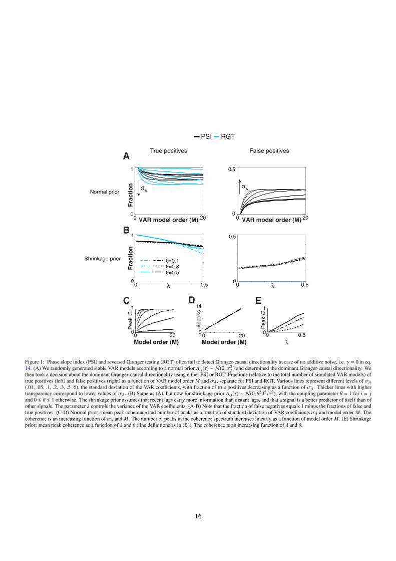
λ

0 20 0 20

0 0.5 0 0.5

Frac

tion

Frac

tion

0

1

0

1

A

B

PSI RGT

Normal prior

Shrinkage prior θ=0.1θ=0.3θ=0.5

VAR model order (M) VAR model order (M)

λ

0 200

1

0 200

14

#pea

ks

0 0.50

1

Peak

C

C D E

Model order (M) λ

Peak

C

Model order (M)

True positives False positives

0

0.5

0

0.5

σAσA

Figure 1: Phase slope index (PSI) and reversed Granger testing (RGT) often fail to detect Granger-causal directionality in case of no additive noise, i.e. γ = 0 in eq.14. (A) We randomly generated stable VAR models according to a normal prior Ai j(τ) ∼ N(0, σ2

A) and determined the dominant Granger-causal directionality. Wethen took a decision about the dominant Granger-causal directionality using either PSI or RGT. Fractions (relative to the total number of simulated VAR models) oftrue positives (left) and false positives (right) as a function of VAR model order M and σA, separate for PSI and RGT. Various lines represent different levels of σA(.01, .05, .1, .2, .3, .5 .6), the standard deviation of the VAR coefficients, with fraction of true positives decreasing as a function of σA. Thicker lines with highertransparency correspond to lower values of σA. (B) Same as (A), but now for shrinkage prior Ai j(τ) ∼ N(0, θ2λ2/τ2), with the coupling parameter θ = 1 for i = jand 0 ≤ θ ≤ 1 otherwise. The shrinkage prior assumes that recent lags carry more information than distant lags, and that a signal is a better predictor of itself than ofother signals. The parameter λ controls the variance of the VAR coefficients. (A-B) Note that the fraction of false negatives equals 1 minus the fractions of false andtrue positives. (C-D) Normal prior: mean peak coherence and number of peaks as a function of standard deviation of VAR coefficients σA and model order M. Thecoherence is an increasing function of σA and M. The number of peaks in the coherence spectrum increases linearly as a function of model order M. (E) Shrinkageprior: mean peak coherence as a function of λ and θ (line definitions as in (B)). The coherence is an increasing function of λ and θ.

16

Normal prior Model order M=4

0

1

Frac

tion

A

0 0.9

PSI Granger RGTStandard deviationVAR coefficients

0 0.90

1

Frac

tion

B

σA, λ = 0.3

Shrinkage prior Model order M=10θ=0.3

σA, λ = 0.01

Noise level (γ)

True positives False positives

0 0.9

0 0.9Noise level (γ)

0

0.5

0

0.5

Figure 2: Uncorrelated noise has very weak effects on PSI and weak to moderate effects on other Granger-causality metrics. (A) We randomly generated stableVAR models of order M = 4 according to a normal prior Ai j(τ) ∼ N(0, σ2

A) and determined the dominant Granger-causal directionality. Two uncorrelated noisesources were superimposed on the signal sources and also generated according to a stable VAR model that was again randomly generated by a normal priorAi j(τ) ∼ N(0, σ2

A). From the noisy signal, we then detected the Granger-causal directionality using either phase slope index (PSI), reversed Granger testing (RGT)or standard Granger-causality. Fractions (relative to the total number of simulated VAR models) of true positives (left) and false positives (right) as a function ofnoise amplitude γ and σA. For small σA, noise has no effects on the calculated metrics. For large σA, noise has moderate effects. (B) Same as (A), but now forthe shrinkage prior Ai j(τ) ∼ N(0, θ2λ2/τ2), with the coupling parameter θ = 1 for i = j and θ = 0.3 otherwise. The parameter λ controls the variance of the VARcoefficients. (A-B) See the Supplementary Information for generalization to higher model order and unidirectional prior.

17

Cro

ss-c

ov (a

.u.)

τ (a.u.) τ (a.u.)

A

signalnoise,

00

( )measured

= + ,

B

Figure 3: Measures that quantify the asymmetry of the cross-covariance function, like the phase slope index (PSI), are not necessarily robust against the additionof linearly mixed noise. Observed cross-covariance s(ε)

12 (B) is sum of (asymmetric) signal and (symmetric) linearly mixed noise cross-covariance (A). Here, sε1 ,ε2causes the asymmetry in s12 to flip around τ = 0.

18

A

0

1

Frac

tion

Frac

tion

B

0

1

0 0.90 0.9

0 0.9

Noise level (γ)Noise level (γ)

Normal priorModel order M=4

Shrinkage prior Model order M=10θ=0.3

PSI Granger RGTStandard deviationVAR coefficients σA, λ = 0.3

σA, λ = 0.01

True positives False positives

0 0.90

0.5

0

0.5

Figure 4: Linearly mixed (i.e., correlated noise) has strong effects on the false positives fractions of standard Granger-causality and phase slope index (PSI), butonly weak to moderate effects on the false positives fraction of reversed Granger testing (RGT). (A) We randomly generated stable VAR models of order M = 4according to a normal prior Ai j(τ) ∼ N(0, σ2

A). A linear mixture of two uncorrelated noise sources was superimposed on the signal sources. Both noise sourceswere generated according to a stable VAR model that was randomly generated by a normal prior Ai j(τ) ∼ N(0, σ2

A). Fractions (relative to the total number ofsimulated VAR models) of true positives (left) and false positives (right) as a function of noise amplitude γ. (B) Same as (A), but now for the shrinkage priorAi j(τ) ∼ N(0, θ2λ2/τ2), with the coupling parameter θ = 1 for i = j and θ = 0.3 otherwise. The parameter λ controls the variance of the VAR coefficients. (A-B)See the Supplementary Information for generalization to higher model order and unidirectional prior.

19

Granger RGT

−5−4−3−2−1

01

−5−4−3−2−1

01

−5−4−3−2−1

01

0 0.9

0 0.9

0 0.9

−5−4−3−2−1

01

−4−3−2−1

01

−4−3−2−1

01

0 0.9Noise level (γ)

0 0.9

Noise level (γ)

0 0.9

PSI

Gai

n

Gai

n

A

B

C

D

E

F

Gai

n

Gai

n

Gai

n

Gai

n

All systems

Shrinkage priorNormal prior

−5

−5

Figure 5: RGT has better overall performance than PSI and Granger. (A-C) Gain −10F(γ) + T (γ), with γ the noise level, and F and T the fractions of false positivesand true positives, respectively (Normal prior, σA = 0.01). (A-C) correspond to different variance of the VAR coefficients (σA = 0.01, 0.1, 0.3). (D-F) Same as(A-C), but now for shrinkage prior, with (A-C) corresponding to various levels of the variance of VAR coefficients (λ = 0.01, 0.1, 0.3).

20

Frac

tion

Frac

tion

4 5 60

1

Granger RGTγ = 0γ = 0.7

Nonparam.PSI

Noise level

A

B

Log10(# observations)

Frac

tion

Frac

tion

Log10(# observations)

C

D

4 5

ParametricPSI

Asympoticvalues

Finite sample estimates

Asympoticvalues

Finite sample estimates

4 5 6

4 5 6

6

True positives False positives

0

1

0

1

0

1

4 5 6

4 5 6

4 5 6

4 5 60

0.5

0

0.5

0

0.5

0

0.5

Figure 6: All metrics converge to analytically computed values with increasing number of observations. (A-B) We randomly generated stable VAR models of orderM = 4 according to a normal prior Ai j(τ) ∼ N(0, σ2

A), in this case σA = 0.1. A linear mixture of two uncorrelated noise sources was superimposed on the signalsources. Both noise sources were generated according to a VAR model that was randomly generated by a normal prior Ai j(τ) ∼ N(0, σ2

A). We then generated datatraces of finite length with normally distributed innovation noise. Jackknifing was used to estimate significance, using |µ/σµ | = 2 as cutoff. For PSI, the spectraldensity matrix was estimated parametrically via the VAR fits. (B) Same as (A), but now using σA = 0.3. (C-D) Same as (A-B), but now also estimating the spectraldensity matrix nonparametrically using Discrete Fourier Transforms of 400 datapoint segments multiplied with Hann windows, and Bartlett-averaging.

21

−1 0 1 20

1

−1 0 1 20

1

−1 0 1 20

1

−1 0 1 20

1

−1 0 1 20

1

−1 0 1 20

1

A CB

D FE

log10(I) log10(I) log10(I)

log10(I) log10(I) log10(I)

Cum

. den

sity

Prob

. den

sity

Figure 7: The instantaneous influence strength measure I provides information about the relative magnitude of linearly mixed noise. (A-C) Shown the cumulativedensity function as a function of the instantaneous influence strength measure I, for various levels of noise amplitude γ. Green-to-black color gradient correspondsto increasing levels of γ = 0, 0.1, · · · , 0.9. The variable I measures the magnitude of the instantaneous influence compared to the feedback at other lags. (A) to (C):variance of normal prior on VAR coefficients σA = 0.01, 0.1, 0.3. (D-F) As (A-C), but now shown the probability density function. (A-F) show that low values of Itend to correspond to a high signal-to-noise ratio, and that high values of I correspond to a small signal-to-noise ratio.

22

0 0.9 0 0.90

1

Frac

tion

0

0.5

0

0.8

Normal

prior

A CB

0 0.9 0.90

1

Frac

tion

0

0.5

00

0.7

Noise level (γ)Noise level (γ)

Granger RGT

λ, σΑ=0.1

λ, σΑ=0.1

D FE

Standard deviationVAR coefficients

σA, λ = 0.3

σA, λ = 0.01 σA, λ = 0.1

True positives False positives I: instantaneous interactionstrength (IIS)

Shrink

age p

rior

allI<1

/2I>1

/2I<1

/2I>1

/2all

allI<1

/2I>1

/2I<1

/2I>1

/2all

Figure 8: Using an inclusion criterion on the instantaneous influence strength I (include only I < β and reject I > β) can strongly reduce the fraction of falsepositives. (A-B) As in Fig 4, we show the fraction of true and false positives as a function of the noise amplitude γ. The difference with 4 is that in this figure,we take a decision about the Granger-causal directionality only if the instantaneous influence strength I < 1/2 (eq. 34). Thus, for I > 1/2, we always obtain falsenegatives. Note that the sum of true and false positives and false negatives equals 1. (C) The fractions of false positives (filled bars) and true positives (open bars)across all levels of noise amplitude γ, separate for all VAR models, VAR models for which I > 1/2, and VAR models for which I < 1/2 (Normal prior, σA = 0.1).The mixture of true positives and false positives is better for I < 1/2 than for I > 1/2. (D-F) Same as (A-C), but now for shrinkage prior.

23

Granger RGT

−5−4−3−2−1

01

−5−4−3−2−1

01

−5−4−3−2−1

01

0 0.9

0 0.9

0 0.9

−5−4−3−2−1

01

−4−3−2−1

01

−4−3−2−1

01

0 0.9Noise level (γ)

0 0.9

Noise level (γ)

0 0.9

PSI

Gai

n

Gai

n

A

B

C

D

E

F

Gai

n

Gai

n

Gai

n

Gai

n

Granger RGT PSIAll systemsOnly I<1/2

Shrinkage priorNormal prior

−5

−5

Figure 9: Using an inclusion criterion on the instantaneous influence strength I < 1/2 can strongly increase overall performance in terms of false and true positives,for RGT, PSI and Granger. (A-C) Gain −10F(γ) + T (γ), with γ the noise level, and F and T the fractions of false positives and true positives, respectively(Normal prior, σA = 0.01). Dashed: including only VAR models for which I < 1/2. Solid: all VAR models. (A-C) correspond to different variance of the VARcoefficients (σA = 0.01, 0.1, 0.3). (D-F) Same as (A-C), but now for shrinkage prior, with (A-C) corresponding to various levels of the variance of VAR coefficients(λ = 0.01, 0.1, 0.3).

24

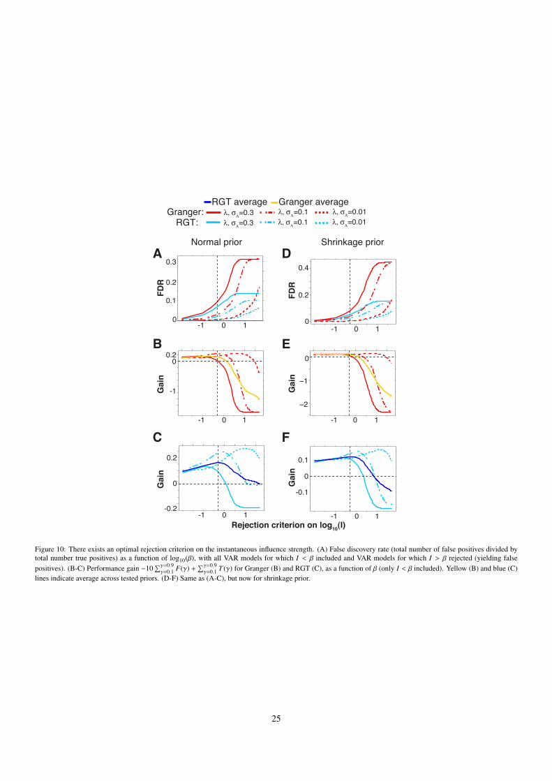
FDR

0

0.3

Gai

n

0 1-1

Rejection criterion on log10(I)0 1-1

Gai

n

0.2

-0.2

0.2

0

0

-1

0.1

λ, σΑ=0.3 λ, σΑ=0.1 λ, σΑ=0.01Granger:RGT:

A

B

C

0

0.2

0.4

−2

−1

0

0.1

-0.1

0

0 1-1

RGT average Granger average

Shrinkage priorNormal prior

Gai

n

D

E

F

λ, σΑ=0.3 λ, σΑ=0.1 λ, σΑ=0.01

0 1-1

0 1-1 0 1-1

Gai

nFD

R0.2

Figure 10: There exists an optimal rejection criterion on the instantaneous influence strength. (A) False discovery rate (total number of false positives divided bytotal number true positives) as a function of log10(β), with all VAR models for which I < β included and VAR models for which I > β rejected (yielding falsepositives). (B-C) Performance gain −10

∑γ=0.9γ=0.1 F(γ) +

∑γ=0.9γ=0.1 T (γ) for Granger (B) and RGT (C), as a function of β (only I < β included). Yellow (B) and blue (C)

lines indicate average across tested priors. (D-F) Same as (A-C), but now for shrinkage prior.

25

0 1-10

1

log10(I)

A

FDR

0 1-1 log10(I)

B

0

1

λ, σΑ=0.3 λ, σΑ=0.1 λ, σΑ=0.01Granger:RGT:

Shrinkage priorNormal prior

λ, σΑ=0.3 λ, σΑ=0.1 λ, σΑ=0.01

Figure 11: The false discovery rate is an increasing function of the instantaneous influence strength I. (A) Mean false discovery rate total number of false positivesdivided by total number true positives) for different levels of I, for the various normal priors. (B) Same, but now for shrinkage prior.

26

0 40 80 120

1

2

3

Gra

nger

-cau

sal f

eedb

ack

Frequency (Hz)−4 −2 0 2 4 6 8 10

−4−2

02468

10

Tim

e re

vers

ed

Original Granger asymmetry

x 10-3 x 10-3

x 10-3

V4->V1 originalV1->V4 original V4->V1 time reversed

V1->V4 time reversed

A B

Figure 12: Application to neuronal data. (A) Spectral Granger feedback values between V1 LFP sites and V4 LFP sites as a function of frequency. Shadingsrepresent standard error of the mean across channel-combinations. (B) Original Granger asymmetry values (defined as the difference between V1→ V4 flow minusV4→ V1 flow) vs. Granger asymmetry values for time-reversed signals (defined as the difference between V4→ V1 flow minus V1→ V4 flow.

27