urinary metabolomics to detect - OhioLINK ETD Center

URINARY METABOLOMICS TO DETECT

POLYCYSTIC KIDNEY DISEASE AT AN EARLY STAGE

A thesis submitted in partial fulfillment of the

requirements of the degree of

Master of Science

By

AMNAH MAHMOUD OBIDAN

B.S., King Abdul-Aziz University, 2010

2017

Wright State University

2

WRIGHT STATE UNIVERSITY

GRADUATE SCHOOL

December 13, 2017

I HEREBY RECOMMEND THAT THE THESIS PREPARED UNDER MY SUPERVISION BY Amnah Mahmoud Obidan ENTITLED Urinary Metabolomics to Detect Polycystic Kidney Disease at an Early Stage BE ACCEPTED IN PARTIAL FULFILLMENT OF THE REQUIREMENTS FOR THE DEGREE OF Master of Science

Nicholas V. Reo, Ph.D.

Thesis Director

Madhavi P. Kadakia, Ph.D. Chair, Department of

Biochemistry and Molecular Biology

Committee on Final Examination

Nicholas V. Reo, Ph.D. Nicholas DelRaso, Ph.D.

John Paietta, Ph.D. Barry Milligan, Ph.D.

Interim Dean of the Graduate School

iii

ABSTRACT

Obidan, Amnah Mahmoud. M.S., Department of Biochemistry and Molecular Biology, Wright State University, 2017. Urinary Metabolomics to Detect Polycystic Kidney Disease at Early Stage. Urinary metabolomics abilities in detection of biological effects (i.e., toxicity, disease)

is compounded by high background variability. Previously, we showed mild kidney

dysfunction was detectable under the stress imposed by furosemide (diuretic). Here we

tested whether furosemide (FUR) can enhance the sensitivity to detect autosomal dominant

polycystic kidney disease (ADPKD) at an early stage. ADPKD is one of the most common

inherited renal disorders and is characterized by the growth of numerous cysts in the

kidneys. Urinary metabolomics analyses, using nuclear magnetic resonance (NMR)

spectroscopy, were conducted in control (WT) and diseased mice (RC) at 7 and 24 weeks

of age. Urine samples were collected before (baseline) and after administration of

furosemide or vehicle (saline). At 7 wks of age, the WT and RC mice showed different

metabolite profiles before injection with FUR using Principle Components analysis (PCA)

and OPLS discriminant analysis of the NMR data. We found a ketoglutarate, citrate,

acetate, taurine, succinate and other metabolites that appear to be significant features that

were responsible for the separation. There are multiple urinary NMR signals of diseased

mice that have higher intensities than control mice, such as ⍺ ketoglutarate, citrate, acetate,

taurine, succinate and other unknown metabolites. Significant increases in kidney weight

per body weight ratio and cystic index in RC mice at 7 wks (D. Wallace, U Kansas)

confirmed that disease progression was rapid. Thus, FUR could not be used to produce

iv

subtle differences in urinary metabolite profiles between WT and RC mice at 7 wks. At 24

wks of age, the WT and RC mice showed very similar urinary metabolite profiles at

baseline (pre-dose), and preliminary data suggest that FUR helps to separate these groups.

The “n” value of mouse urine samples at 24 wks was too small to test statistical significance

of the work. ANOVA shows that some metabolites (⍺ ketoglutarate/TSP and citrate/TSP)

that are nearly significant (p=0.09). If n-value was larger, then these would likely be

different. To confirm the hypothesis of this study, the study should be repeated using a

larger sample size, and an animal model that develops cysts gradually, in order to show that

furosemide has the potential to detect PKD at an early stage.

v

TABLE OF CONTENTS

Page CHAPTER 1. INTRODUCTION AND SPECIFIC AIMS……………………………1

1.1 Introduction ………………………………………………………………………….1

1.2 Hypothesis …………………………………………………………………………...2

1.3 Specific Aims ……………………………………………………………………......3

CHAPTER 2: BACKGROUND …………………………………………………………4

2.1 Polycystic Kidney Disease …………………………………………………………...4

2.2 Kidney Structure and Function ………………………………………………………5

2.3 ADPKD Disease Pathology ………………………………………………………......7

2.4 Biomarkers of ADPKD …………………………………………………………….11

2.5 Diagnosis of ADPKD ………………………………………………………………12

2.6 Animal Model for Study …………………………………………………………....13

CHAPTER 3: MATERIALS AND METHODS …………………………………….18

3.1 Materials ……………………………………………………………………………18

3.2 Methods …………………………………………………………………………….19

3.2.1. Animal Model …………………………………………………………………19

3.2.2 Experimental design ……………………………………………………………20

3.2.3 Treatment compound …………………………………………………………..21

3.2.4 Experimental Groups ………………………………………………………….24

3.2.5 Preparation of NMR samples ………………………………………………….26

vi

3.2.6 NMR spectra acquisition and Data Processing ………………………………...28

3.2.7 Data Analysis ………………………………………………………………….29

CHAPTER 4: RESULTS AND DISCUSSION ………………………………………31

CHAPTER 5: SUMMARY, CONCLUSION AND FUTURE DIRECTION ………62

5.1 Summary and conclusion…………………………………………………………….62

5.2 Future direction………………………………………………………………………62

REFERENCES …………………………………………………………………………63

vii

LIST OF FIGURES Figure Page 1. Diagram of human kidney displaying the internal structure………………………….6

2. Structure of the nephrons……………………………………………………………...7

3. Mechanism of cyst formation in Polycystic Kidney Disease…………………………8

4. The role of vasopressin and the signaling in tubular cells in ADPKD……………….10

5. Masson trichrome histology sections of homozygous PKD1………………………...14

6. Graphic representations of different biochemical and physiological changes……… 15

7. Biochemical and physiological changes from 0-50 weeks of age for two different

groups…………………………………………………………………………………....17

8. Diagram showing how the micro tube fits into a 5 mm NMR tube………………….18

9. Experiment scheme and timeline…………………………………………………….20

10. Urine output rates 3-day baseline average vs. post injection with Ve/Fur at 7 weeks

of age…………………………………………………………………………………….23

11. Change in urine production: 3-day baseline average vs. post injection with Ve/Fur

for both groups, diseased and control mice……………………………………………...23

12. 1H NMR spectrum shows a urinary metabolite profile from a WT mouse………….28

13. PCA plots show diet effect………………………………………………………......33

14. PCA plots show groups effect……………………………………………………...35

15. OPLS-DA model using mice urinary NMR spectra at baseline time points for mice

at 7 wks of age fed Food B………………………………………………………………36

viii

Figure page

16. all 345 significant features from OPLS-DA for WT vs. RC at Baseline…………..37 17. An example of one NMR spectral regions identified as significant by using

visualization in MATLAB…………………………………………………………….39

18. Pathway for catabolism of propionyl-CoA………………………………………..39

19. Quantified composition of significant metabolites profiles……………………….41

20. Quantified composition of significant metabolites for taurine…………………......42

21. ANOVA statistics analysis for different metabolite profiles……………………….43

22. ANOVA statistics analysis for profiles ⍺ ketoglutarate/TSP after excluding

two data points………………………………………………………………………….44

23. PCA plot comparing two different ages together……………………………...........46

24. Different PCA plots for WT mice……………………………………………..........48

25. all 170 significant features from OPLS-DA for WT at Baseline vs. day 1 post

injection with Fur……………………………………………………………………….49

26. Different PCA plots for RC mice……………………………………………...........51

27. all 19 significant features OPLS-DA for RC at Baseline vs. day 1 post

injection with Fur……………………………………………………………………….52

28. PCA plot show effect of two different treatment Ve/Fuer………………………….54

29. PCA plots show effect of Fur at later time………………………………………….56

30. PCA plots show effect of Fur at later time by comparing two days together……….58

31. PCA plots used paired analysis too eliminate effect of diet…………………………59

32. PCA plots show effect of Fur at two different ages (7 and 24 weeks) ……………...61

ix

LIST OF TABLES

Table Page

1. The percentage of kidney weight per body weight % KW/BW, liver weight per

body weight %LW/BW at 12 months of age for WT and RC mice……………………15

2. Diet nutrient/ingredient information………………………………………………….24

3. Demonstrate how the mic fed inside and outside metabolism cage………………….26

4. Animal’s characteristics……………………………………………………………….27

5. NMR spectral regions identified as significant by OPLS-DA for WT vs. RC at Baseline…………………………………………………………………………………..37

6. NMR spectral regions identified as significant by using different analysis………….40

7. The P-value and standard error of ANOVA statistics analysis……………………….44

8. NMR spectral regions identified as significant by OPLS-DA for WT at Baseline vs. day

1 post injection with Fur for food B………………………………………………...........50

9. NMR spectral regions identified as significant by OPLS-DA for RC at Baseline vs.

day 1 post injection with Fur for food B………………………………………………...53

x

ACKNOWLEDGMENT

It is a pleasure to thank those who made this thesis possible. Special thanks for

advisor, Dr. Nicholas Reo for his guidance and advise. Also, I would like to thank Dr.

John Paietta and Dr. Nicholas DelRaso for serving as members of the thesis committee. I

am grateful to my colleague Angela Campo for her support and assistance. I owe my

deepest gratitude to my parents, sisters and husband who gave me a moral support that I

required. Special thanks for my biggest supporter in my life (my daughter Aleen).

1

INTRODUCTION AND SPECIFIC AIMS

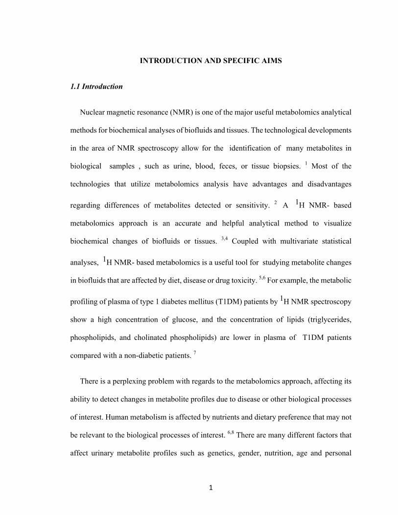
1.1 Introduction

Nuclear magnetic resonance (NMR) is one of the major useful metabolomics analytical

methods for biochemical analyses of biofluids and tissues. The technological developments

in the area of NMR spectroscopy allow for the identification of many metabolites in

biological samples , such as urine, blood, feces, or tissue biopsies. 1 Most of the

technologies that utilize metabolomics analysis have advantages and disadvantages

regarding differences of metabolites detected or sensitivity. 2 A 1H NMR- based

metabolomics approach is an accurate and helpful analytical method to visualize

biochemical changes of biofluids or tissues. 3,4 Coupled with multivariate statistical

analyses, 1H NMR- based metabolomics is a useful tool for studying metabolite changes

in biofluids that are affected by diet, disease or drug toxicity. 5,6 For example, the metabolic

profiling of plasma of type 1 diabetes mellitus (T1DM) patients by 1H NMR spectroscopy

show a high concentration of glucose, and the concentration of lipids (triglycerides,

phospholipids, and cholinated phospholipids) are lower in plasma of T1DM patients

compared with a non-diabetic patients. 7

There is a perplexing problem with regards to the metabolomics approach, affecting its

ability to detect changes in metabolite profiles due to disease or other biological processes

of interest. Human metabolism is affected by nutrients and dietary preference that may not

be relevant to the biological processes of interest. 6,8 There are many different factors that

affect urinary metabolite profiles such as genetics, gender, nutrition, age and personal

2

factors including exercise, diet, medication, tobacco, alcohol and other environmental

influences. 9 These factors , especially in humans, will result in high background noise in

urinary metabolite profiles, which can complicate data interpretation.6 Consequently,

relating metabolite profiles to health and disease is a difficult task. Some of this high

variability can be decreased by controlling factors that affect metabolite profiles such as

diet and other environmental influences, but some of these factors are uncontrollable

factors.6,10 In longitudinal studies, findings provided evidence that individual metabolic

phenotypes may exist and their detection by multiple sample collection, combined with

advanced statistical analysis, may provide a means to eliminate the daily “noise.” 9,11

HYPOTHESIS AND SPECIFIC AIMS

1.2 Hypothesis

Tissue responses under a metabolically stressed condition will increase the capability

to detect biologically relevant changes in urinary metabolite profiles. The normal daily (or

even hourly) variability in urinary metabolite profiles will be minimal in comparison to

changes that may occur under a stressed condition. In a previous metabolomics study, Reo

and coworkers9 tested this hypothesis in a rat model, using the kidney as a target organ. D-

serine (kidney toxin) was used to cause a mild tissue insult, and furosemide (diuretic drug)

was used as a metabolic tissue stressor. The sub-acute toxic dose of D- Serine (60 mg/kg)

is undetectable by standard urinary metabolomics analysis, clinical blood chemistry, and

histopathology of the kidney. Mild kidney dysfunction was detectable, however, under the

stress to the kidney imposed by furosemide.9 In this study, we tested this hypothesis using

a mouse model involving a disease state – polycystic kidney disease. Furosemide (kidney

stressor) was used to stress the kidney to determine if it could be used to detect disease at

3

an early stage.

1.3 Specific Aims

Autosomal Dominant Polycystic Kidney Disease (ADPKD) is a genetic disorder

characterized by the growth of numerous cysts in the kidneys, and is associated with

mutations in polycystin 1 and polycystin 2. The RC mouse in a disease model for ADPKD

{RC (Pkd2+/- ; Pkd1RC/RC)} with mutations occurring in two alleles of PKD1 and a one

allele knock-out of PKD2. The WT mouse is a control {WT (Pkd2+/+ ; Pkd1RC/+)} and

has normal PKD2 expression, and one mutated allele in PKD1 (more detailed information

about these animal models will be provided below).

Aim 1. Conduct NMR-based metabolomics analysis of mouse urine before and after

administration of furosemide in normal control mice {WT (Pkd2+/+ ; Pkd1RC/+)}, and

ADPKD diseased mice {RC (Pkd2+/- ; Pkd1RC/RC)} at 7 weeks of age and again at 24

weeks of age.

Aim 2. Conduct multivariate data analyses to demonstrate that ADPKD is detectable by

urinary analysis at an early stage. We will also identify the changes in metabolite profiles

that may be associated with ADPKD; we will identify specific metabolites that help to

discern diseased mice from controls.

4

CHAPTER 2: BACKGROUND

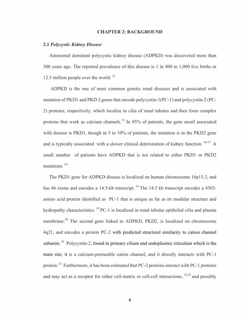
2.1 Polycystic Kidney Disease

Autosomal dominant polycystic kidney disease (ADPKD) was discovered more than

300 years ago. The reported prevalence of this disease is 1 in 400 to 1,000 live births or

12.5 million people over the world. 12

ADPKD is the one of most common genetic renal diseases and is associated with

mutation of PKD1 and PKD 2 genes that encode polycystin-1(PC-1) and polycystin-2 (PC-

2) proteins, respectively, which localize in cilia of renal tubules and then form complex

proteins that work as calcium channels.13 In 85% of patients, the gene mostl associated

with disease is PKD1, though in 5 to 10% of patients, the mutation is in the PKD2 gene

and is typically associated with a slower clinical deterioration of kidney function. 14-17 A

small number of patients have ADPKD that is not related to either PKD1 or PKD2

mutations. 14

The PKD1 gene for ADPKD disease is localized on human chromosome 16p13.3, and

has 46 exons and encodes a 14.5-kb transcript. 18 The 14.5 kb transcript encodes a 4303-

amino acid protein identified as PC-1 that is unique as far as its modular structure and

hydropathy characteristics. 19 PC-1 is localized in renal tubular epithelial cilia and plasma

membrane.20 The second gene linked to ADPKD, PKD2, is localized on chromosome

4q21, and encodes a protein PC-2 with predicted structural similarity to cation channel

subunits. 21 Polycystin-2, found in primary cilium and endoplasmic reticulum which is the

main site; it is a calcium-permeable cation channel, and it directly interacts with PC-1

protein. 21 Furthermore, it has been estimated that PC-2 proteins interact with PC-1 proteins

and may act as a receptor for either cell-matrix or cell-cell interactions, 19,22 and possibly

5

control the activity of PC-2 through their interactions. 23 However, the function of these

two proteins, PC-1and PC-2, is still unknown. ADPKD manifests itself as progressive

formation of kidney cysts that expand at the expense of the kidney tissue, which causes

renal failure correlating with abdominal fullness, hypertension, gross hematuria,

nephrolithiasis, and cyst infections. 24

2.2 Kidney Structure and Function

There are two main functional regions in the human kidney: the outer renal cortex and

the inner medulla. Renal cortex and medulla can be isolated into renal lobes consisting of

a pyramid-shaped section of the medulla and the cortex above it. The renal papilla is the

location where the renal pyramids empty urine into the minor calyx of the kidney. Several

minor calyces converge to form major calyces, at last, yielding the renal pelvis from which

the ureter emanates (Fig 1). Nephrons span across the cortex and the medulla of the kidney

and are the basic unit of structure in the kidney responsible for producing urine (Fig 2).

Ultrafiltrate (filtered liquid devoid of blood cells and blood proteins) is produced by the

glomerulus into the renal capsule. The tubules in the renal cortex are the primary site for

reabsorption of water and nutrients. The tubules reabsorb most of the filtrate, minerals and

water, and discharge extra waste into the collecting ducts that span the cortex and medulla,

and then empty into the calyx at the papilla, releasing urine. 25

6

Figure 1. Diagram of human kidney displaying the internal structure. 26

Primary cilia function in the kidney is still uncertain. It has been proposed that they are

included in mechanosensation to discover fluid flow through the tubule lumen. Also, they

may regulate cell proliferation and cell division, as well as cell-to-cell and cell-to- matrix

signaling. 27

7

Figure 2. Structure of the nephrons.26 2.3ADPKD Disease Pathology

Cyst formation relates to changes in epithelial cell proliferation and differentiation, and

fluid secretion. 28 Cysts are essentially responsible for the decrease in the glomerular

filtration rate that occurs generally late over the course of the disease. This decrease

includes anatomic disruption of glomerular filtration and urinary concentration on a huge

scale, combined with increased blood pressure and blockage by the growth of cysts in

adjacent nephrons in the cortex, medulla, and papilla (Fig 2). These cysts keep the waste

in urine from upstream tributaries, which prompts tubule atrophy and loss of working

kidney parenchyma by a mechanism like those found in ureteral obstacle. 29

8

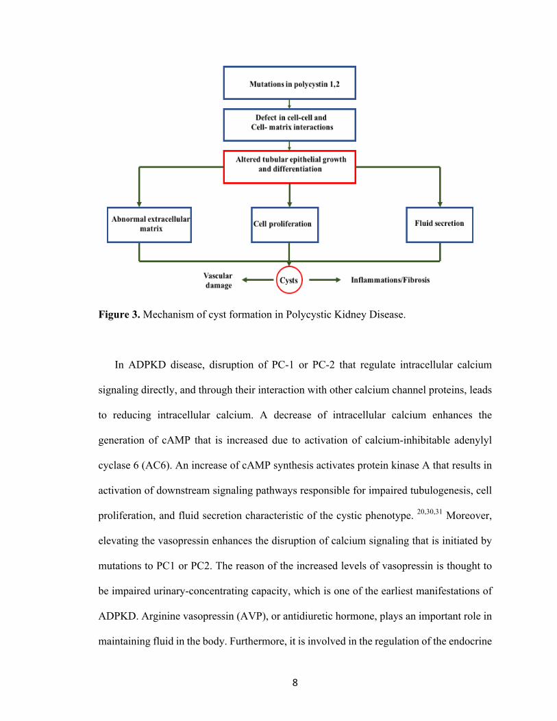
Figure 3. Mechanism of cyst formation in Polycystic Kidney Disease.

In ADPKD disease, disruption of PC-1 or PC-2 that regulate intracellular calcium

signaling directly, and through their interaction with other calcium channel proteins, leads

to reducing intracellular calcium. A decrease of intracellular calcium enhances the

generation of cAMP that is increased due to activation of calcium-inhibitable adenylyl

cyclase 6 (AC6). An increase of cAMP synthesis activates protein kinase A that results in

activation of downstream signaling pathways responsible for impaired tubulogenesis, cell

proliferation, and fluid secretion characteristic of the cystic phenotype. 20,30,31 Moreover,

elevating the vasopressin enhances the disruption of calcium signaling that is initiated by

mutations to PC1 or PC2. The reason of the increased levels of vasopressin is thought to

be impaired urinary-concentrating capacity, which is one of the earliest manifestations of

ADPKD. Arginine vasopressin (AVP), or antidiuretic hormone, plays an important role in

maintaining fluid in the body. Furthermore, it is involved in the regulation of the endocrine

9

stress response. Vasopressin has three different types of receptors: V1a-receptors, V1b –

receptors, and V2-receptors. The V2-receptor (V2R) that is located in the renal collecting

ducts has an antidiuretic effect. When vasopressin binds to V2R in the collecting duct, the

water permeability and sodium reabsorption will increase by activation of the epithelial

sodium channel.13 Increasing the level of vasopressin enhances the constant tonic effect of

vasopressin on the V2 receptors that activate downstream-signaling pathways responsible

for impaired tubulogenesis, cell proliferation, increased fluid secretion and interstitial

inflammation (Fig 4).20

Recently, treatments in ADPKD focused on lowering cAMP by inhibiting the

vasopressin V2R; it could be effective in controlling proliferation and enlargement of renal

cysts.13,31 Investigators found that treatment with the vasopressin V2R antagonist tolvaptan

has been shown to prevent disease progression in different studies. For patients with

ADPKD, the total volume of kidney decreased from 5.5 to 2.8 % and the slope of the

reciprocal of serum creatinine levels decreased from -3.81 to -2.61 mg.ml- per year.13

10

Figure 4. The role of vasopressin and the signaling in tubular cells of the collecting duct in ADPKD.20 Blue indicates molecules that are increased in PKD; yellow indicates molecules that are reduced in PKD. AC6: adenylyl cyclase 6; PDE: Phosphodiesterase; PKA: Protein kinase A. Adapted from Chibib, FT, et.al., Nature Review Neph. 11, 451-464 (2015).

11

2.4 Biomarkers of ADPKD

The most commonly used marker of renal function is serum creatinine, which is used

to measure the glomerular filtration rate (GFR). However, this is not a reliable indicator

for some renal diseases such as ADPKD. In one human biomarker study, investigators

explored 28 urinary biomarkers to observe if there were any differences between patients

with ADPKD and healthy people, and found that urinary biomarkers in ADPKD are

different in neutrophil gelatinase-associated lipocalin (NGAL), Monocyte chemoattractant

protein-1 (MCP-1), and Macrophage colony stimulating factor (M-CSF).30 NGAL belongs

to the superfamily of lipocalin proteins. It has important roles in the kidney, including

regulation of iron transport. It also plays a role in inflammation and cell proliferation.

NGAL is produced at a low level in the kidney, lung, and alimentary canal. In the kidney,

increasing the level of NGAL production in serum and urine leads to renal impairment. In

addition, some studies utilized NGAL as a biomarker for acute kidney injury (AKI).32,33

Investigators have shown a significant correlation between acute renal injury and urine /

serum concentration of NGAL at 2h, and cardiopulmonary bypass time.32 The urine

concentration level of NGAL increased from a mean of 1.6 µ /L ± 0.3 SE at baseline to

147 µ /L 2 h after cardiopulmonary bypass. The serum concentration elevated from a mean

of 3.2 µ /L ± 0.5 SE at baseline to 61 µ/L 2 h after the method.32 Elevating the level of

NGAL in urine in ADPKD show inflammation, kidney enlargement, and cell

proliferation.30 MCP-1 plays a role in permeation of monocytes and macrophages in

different types of inflammatory disease, and it is a marker of kidney inflammation. In a

previous study, investigators suggest that the role of MCP-1 in ADPKD is a development

of interstitial inflammation and renal failure.34 The concentration of MCP-1 in ADPKD

12

patients elevates in the urine along with cyst proliferation.35 M-CSF is a glycoprotein, and

it plays an important role in monocyte and macrophage proliferation, differentiation, and

survival. In the kidney, patients with chronic renal failure show an increase in M-CSF

levels in the serum.36 Thus, the three compounds in particular that they determined to be

appropriate biomarkers were all markers that were involved in inflammation and immune

response. NGAL has been shown to be useful as a marker of acute kidney injury (AKI),

and CSF is an effective marker of graft rejection in renal transplant patients. Therefore,

these biomarkers appear to be useful in severe cases of kidney injury and advanced disease

states. In the present study, we are searching for early biomarkers using a protocol that

involves stressing the kidney to induce a response.

2.5 Diagnosis of ADPKD

Ultrasound is the standard diagnosis of ADPKD and it is an inexpensive and

noninvasive way to diagnose this disease. Also, ultrasound is reliable in patients with

positive family history for ADPKD, but it is less sensitive in young adults and children.

ADPKD can be reliably detected by ultrasound after the age of 30 years.37 Furthermore,

there are advances in processes to diagnose ADPKD, such as computed tomography scan

(CT scan) and magnetic resonance imaging (MRI) that could help monitor progression of

disease by detection of small cysts that cannot be found by ultrasound. Molecular genetic

testing can be used to diagnose ADPKD, but there are some disadvantages for this test,

such as high costs and technical difficulties.38,39

A furosemide stress test (FST) is used to assess kidney function and diagnose

disease. FST is a way to differentiate which patients with AKI will progress to severe AKI

or will not. Recently, investigators demonstrated that 2 hours of urine output after a high

13

dose of furosemide (1.0-1.5 mg/kg) in ill patients with stage 1 or 2 AKI has the ability to

identify those with severe and progressive AKI. The FST showed a 3-fold increase over

baseline in serum creatinine, and an increase in urine output (0.3 ml/h per kg x 24 hours)

within 14 days of furosemide.40 The total urine output within 2 hours following furosemide

treatment is predictive for progression to stage 3 AKI. There was an improvement in risk

prediction when furosemide was combined with other biomarkers of AKI.41,42

2.6 Animal Model for Study

PKD mouse model

The PKD mouse model (Pkd2+/-; Pkd1RC/RC) has mutations in both PC1 and 2.

The PKD1 p.R3277C allele was discovered in the United States in a family of French

ancestry, and these phenotypes indicated that the p.R3277C allele was incompletely

penetrant. In the present study, we used the same model that was used in a previous study43

where the authors generated a knock-out mouse model that mimicked the same codon of

a clinical PKD1 allele for patients (Pkd1 c.9805.9807AGA>TGC). The targeting construct

and confirmation of PKD1 p.R3277C allele was described in more details in a previous

study.43 Mice homozygous for the PKD1 p.R3277C allele develop gradual cystogenesis

(Fig 5,6 and Table 1).

14

Figure 5. Representative Masson Trichrome histology sections of homozygous PKD1 p.R3277C allele and comparing between Pkd1RC/RC and WT kidneys at 1 to 12 months. It shows the cyst developed progressively with age.43 Taken from Hopp, K, et. al., J. Clinical Invest. 122, 4257-4273 (2012).

15

Table 1. Determination of the percentage of kidney weight per body weight % KW/BW

and liver weight per body weight %LW/BW at 12 months of age for WT and RC mice in

Fig 5.

Control Mice (WT) Disease Mice (RC)

% KW/BW 1.30 4.47

% LW/BW 4.05 3.45

Figure 6. Graphic representations of different biochemical and physiological changes (cAMP, BUN and %KW/BW) measured at 3, 6, 9, and 12 months for Pkd1RC/+ and Pkd1RC/RC mice. A and B are not shown in Fig 6. C) %KW/BW; the cyst increased progressively until 9 months, then decreased due to increasing fibrosis. D) cAMP levels increased with disease burden. E) BUN rose after 9 months due to increasing kidney damage because of cystogenesis/fibrosis.43 Adapted from Hopp, K, et al., J. Clinical Invest. 122, 4257-4273 (2012).

16

WT mouse model

The wild type (WT) mouse (Pkd2+/+; Pkd1RC/+) has a mutation in one allele. We

used this model as WT because it is phenotypically wild-type (not cystic) although it has

one allele Pkd1.RC/+ In a previous study, the authors used the same model with no

development of cysts for 12 months.43

Characterizations of animals

Figure 7 represents data for characterization of animals in this study and this data was

collected by our collaborators in Dr. Wallace’s laboratory, kidney institute, University of

Kansas. There were three different measurements: the percentage of kidney weight per

body weight (KW/BW %), cystic index, and blood urea nitrogen (BUN). Cystic index (%

cross sectional cystic area compared to total kidney cross sectional area) was measured

using slide images of axial kidney sections (FFPE) and ImageJ. In Fig (7- A and B), the

red line in Fig 7-A indicates control mice WT (Pkd2+/+; Pkd1RC/+), the green line in Fig

7-A and B indicates diseased mice RC (Pkd2+/-; Pkd1RC/RC), and the blue line indicates

other mice with a mutation that is not related to our study. KW/BW % and cystic index

showed that the progression of the disease was rapid at an early age (5-10 wks) and then

remained constant because the disease in the animals did not progress any further at a later

time. Figure 7-C shows that BUN was stable until 20 weeks then started to increase slowly.

17

A) B)

(C)

Figure 7. Data shows different biochemical and physiological changes from 0-50 weeks of age for two different groups (A) Kidney weight/ body weight ratio for RC and WT animals. The red line indicates control mice and it does not show any significant changes. The green line indicates diseased mice and it demonstrates a significant increase in (KW/BW %) from 5-10 weeks of age, which is then stable beyond this time point. (B) The average of cystic index (histology measurement) for diseased mice and it shows that the progression of disease was rapid from 5-10 weeks of age. (C) Measurement of blood urea nitrogen (BUN). Elevated kidney damage due to cystogenesis resulted in a significantly increased BUN after 20 weeks.

Kidney'Weight'(%'Body'Weight)

Error'bars'+/8'SEM

AS'OF'8/23/17

Age'(weeks)

0 5 10 15 20 25 30 35 40 45 50

KW/BW'(%)

0.5

1.0

1.5

2.0

2.5

3.0

3.5

4.0

Pkd1RC/+)'Pkd1RC/RC)

Pkd2+/+:Pkd1RC/RC)

183RC&CharacterizationCystic&Index&AS&OF&7/26/17

Averages&and&individual&measurements&(so&far)

Age&(weeks)

0 1 2 3 4 5 8 10 15 20

Cystic&Index&(%&Kidney&Area)

0

10

20

30

40 Avg.&CI&for&Pkd1&+/P:RC/RC&averages+/P:RC/RC&RC/RC

18

CHAPTER 3: MATERIALS AND METHODS

3.1 Materials

Chemicals: Sodium phosphate monobasic monohydrate (NaH2PO4.H2O), sodium

phosphate dibasic (Na2HPO4), 3-(Trimethylsily) Propionic-2,2,3,3-d4 acid sodium salt

(TSP), and Deuterium oxide (D2O) were purchased from Sigma-Aldrich (St. Louis, Mo).

Furosemide was purchased from Sigma F4381, and phosphate buffered saline (PBS) was

purchased from Sigma B5652 by Dr. Wallace’s lab.

NMR tubes: Micro NMR tubes 60 µL (Coaxial insert for 5mm NMR precision sample)

were purchased from Wilmad Lab Glass that located in Vineland, NJ.

Figure 8. Diagram showing how the micro tube fits into a 5 mm NMR tube.

Animals: All animal studies were conducted at the University of Kansas Medical Center,

Kidney Institute, in the laboratory of Dr. Darren Wallace. Urine samples from male mice

were frozen at -80 °C and shipped on dry ice to our laboratory at Wright State University.

19

Animal Diet: There are effectively two separate experimental groups by diet. Four animals

were fed Diet Gel Recovery + Takled 8604 Pellet Diet; all other animals were fed Diet Gel

76A from ENVIGO (see Table 1 for more details about animals).

3.2 Methods

3.2.1. Animal Model

The PKD mouse model is the RC mouse (C57Bl/6) described in the background, with

mutations in both PC-1 and -2 (Pkd2;+/- Pkd1RC/RC). There is a mutation in one Pkd2

allele (Pkd2+/-); this mutation involves disruption of exon 1 by insertion of a Neo cassette,

producing a null allele.44 The mutation is the R3277C mutation in Pkd1 (Pkd1RC/RC),

where the homozygous mutation produces a hypomorphic PC-1, rapid progressive cyst

formation at an early age (5-10 wks) and then remained constant and that is orthologous to

the model of ADPKD. The diseased mice did not behave as we saw in original paper. 43

The wild type (WT) control model possesses a mutation in one allele (Pkd2;+/+

Pkd1RC/+). However, Pkd1RC/+ has one allele and it has been shown not to develop cysts

for 12 months in a previous study.43 Thus, we used Pkd2;+/+ Pkd1RC/+ mice as our wild-

type control mice (see background for more information about this animal model).

20

3.2.2 Experimental design

Figure 9. Experimental scheme and timeline. Each box represent duration in cage, arrows

in yellow represents urine collection time, and the arrow in orange represents injection day

with Ve/Fur “see text for details”.

Figure 9 shows the time line for the experiment; each box in the figure represents a 6 h

urine collection from animals placed in metabolism cages collected over 9 days. Urine

samples were collected daily over a 9-day period (3 acclimation + 3 baseline + 3 post-

injection days) with the stat of the experiment beginning on day 4. The first three days was

an acclimation period, the next three days for baseline urine collections, and the final three

days for post-injection urine collections (Figure 9). During the collection time, one small

bag of ice was placed inside the bottom of the metabolism cage unit so that it contacted the

urine collection cup in an attempt to keep the urine cold. Prior to each collection period

(except during the acclimation period), 25 or 50 µL of chilled 1% sodium azide was added

to the urine collection cups to reduce or prevent bacterial growth. This volume of 25 or 50

µL was based on a qualitative estimate of the median urine volume excreted during the

acclimation period for two different groups of animals. All urine samples were stored at

−80°C until subsequent preparation for NMR analysis.

21

In phase 1 of the study, mice were approximately 7-weeks of age (7.21 ± 0.54 wks.;

Mean ± SD). Phase 2 of the study involved mice that were approximately 24 weeks of age

(23.74 ± 0.19 wks.; Mean ± SD).

Seven-wk old mice, wild-type (WT; n=9) and PKD (RC; n=8), were treated with vehicle

(Ve; phosphate buffered saline) or furosemide (Fur) as a metabolic stressor. Of the nine

WT mice, four were treated with Ve and five were treated with furosemide. Of the eight

RC mice, four were treated with vehicle and four were treated with furosemide. The

experimental protocol was conducted using mice at 7 weeks of age and then repeated at 24

weeks of age. For 24-wk old animals, WT (n=5) and PKD RC (n=3), mice were treated

with vehicle or furosemide as a metabolic stressor. Of the five WT mice, two were treated

with Ve and three were treated with furosemide. Of the three RC mice, one was treated

with vehicle and two were treated with furosemide.

3.2.3 Treatment compound

We administered furosemide or vehicle (10 mg/kg) by intraperitoneal (ip.) injection. The

volume for injection varied by the weight of the animal. Our collaborator (Dr. Wallace)

used a sterile-filtered 2 mg/mL solution of furosemide (and sterile-filtered vehicle).

Therefore, for a 15g mouse, 75 microliters of solution would be injected and for a 20g

mouse 100 microliters of solution would be injected.

22

The treatment compounds were given at day 7, then the urine was collected for three

days (7, 8, and 9; Figure 9). The vehicle for the treatments was phosphate buffered saline

(PBS). The furosemide was dissolved in this PBS and adjusted to pH ~ 7.3 with NaOH.

The solutions of PBS vehicle and the furosemide in PBS were sterile filtered, aliquoted,

and stored at 4 °C until used for injections.

Furosemide is a diuretic drug used as a chemical stressor targeting the kidney. In the

thick ascending limb of the loop of Henle (Figure 2) in the kidney, furosemide reversibly

binds to luminal Na+ / 2Cl- /K+ cotransport proteins resulting in decreased reabsorption of

NaCl and H2O leading to an increased urinary output. The furosemide dose of (10mg/kg)

was based upon studies showing maximal diuretic effectiveness in mice over the first 6 h

following injection.9,45,46

Figure 10 shows urine output rate of control and diseased mice after injection with Ve or

Fur at 7 weeks of age. These data were collected by our collaborators at the University of

Kansas Medical Center. Figure 10-A represents control mice {WT (Pkd2;+/+ Pkd1RC/+)}

injected with Ve/Fur. It compares change in a urine output rate between B3 (last time point

before injection) and C1 (day 1 of injection with Fur). Data shows that urine output rates

was elevated at day 1 of post injection with Fur. Figure 10-B represents diseased mice {RC

(Pkd2;+/- Pkd1RC/RC )}, and data shows that the volume of urine was also elevated at day

1 of injection with Fur. At baseline time points (before any treatments) at day 3 the urine

volume was ~ 65 µl/h and increased to 160 µl/h. Figure 11 shows change in a urine output

rate of control and diseased mice after injection with Ve or Fur at 24 weeks of age. It

compares change in a urine output rate between B3 (last time point before injection) and

23

C1 (day 1 of injection with Fur). For diseased mice, it shows a significant increased to ~

250 µl/h.

A) B)

Figure 10. Urine output rates 3-day baseline average vs. post injection with Ve/Fur at 7

weeks of age (A) control mice {WT (Pkd2;+/+ Pkd1RC/+ )}; (B) diseased mice {RC

(Pkd2;+/- Pkd1RC/RC )}.

Figure 11. Change in urine production: 3-day baseline average vs. post injection with Ve/Fur for both groups diseased and control mice.

0

50

100

150

200

-‐66 -‐42 -‐18 6 30 54

Urine ou

tput ra

tes (uL/hr)

Collection times (hours, 0 hr = injection time)

Male VEHICLE +/-:RC/RC Male FUROSEMIDE +/-:RC/RC

-‐500

50100150200250300

+/+;RC/+ +/-‐;RC/RC

CHAN

GE in urin

e ou

tput RAT

E (Δ

uL/hr)

Vehicle (PBS)Furosemide 10 mg/kg

0

50

100

150

200

-‐66 -‐42 -‐18 6 30 54

Uri

ne o

utpu

t rat

es (u

L/h

r)

Collection times (hours, 0 hr = injection time)

Male VEHICLE +/+:RC/+ Male FUROSEMIDE +/+:RC/+

24

3.2.4 Experimental Groups

There were differences in diet and urine time collection. The first group of animals were

fed a different diet from the second group of animals. The reason for the use of two different

diets in this study was that our collaborator (Dr. Wallace) used Diet Gel Recovery + Takled

8604 Pellet Diet as a preliminary test for the first four animals in the study, and they found

that the urine volume was too low to perform an analysis. They then decided to replace the

diet using Diet Gel 76A and used it for the remaining 13 animals. Diet Gel 76A has a higher

water content that helps to increase urine output better than Diet Gel Recovery. Another

difference between the first group and second group is that, instead of having the second

group in the cages for 8 hours on collection day with two urine collections like the first

group (some of which were below 100 µl), we kept the second group in the cages for the

same 6-hours period as all the other collection times (see Fig 9).

Table 2. Showing diet nutrient/ingredient information

Teklad 8604

DietGel Recovery

DietGel 76A.

Macro % Calorie

composition

Macro % Calorie

composition

Macro % Calorie

composition

Protein 32 Protein 2.0 Protein 18.1

Carbs 54 Carbs 83.8 Carbs 68.9

Fat 14 Fat 14.2 Fat 13.0

25

The two groups that have different diet and urine collection time are:

Group 1

There are four animals in Group 1, wild-type (WT; n=2), PKD (RC; n=2), and they were

fed Diet Gel Recovery + Takled 8604 Pellet Diet. Mice were placed in metabolism cages

for 6 hours per day with day 1 to 6 serving as acclimation and baseline days. Urine was

collected from (0- 6 hrs.) and then the mice were returned to their regular caging. On the

day of the injection (Day 7), one of the WT control mice was treated with vehicle (Ve) and

another one was treated with furosemide (Fur); the same process was performed for RC

mice. Mice were kept in metabolism cages for 8 hours, with urine collection occurring after

the first 4 hours (0-4 hrs) and again after the second 4 hours (4-8 hrs). Then, urine

collections from (0-6 hrs.) continued on days 8 and 9 (Fig 9).

Group 2

There are 13 animals in Group 2: wild-type (WT; n=7) and PKD (RC; n=6). All mice

were fed a Diet Gel 76A and placed in metabolism cages for 6 hours per day. All urine

collections occurred over a 6-hour timeframe (0 – 6 hrs.) for each day (acclimation,

baseline, and experimental days). On day 7, mice were injected with either vehicle or 10

mg/kg furosemide. Three WT mice were treated with vehicle (n=3), while four were treated

with the stressor (Fur; n=4). Three PKD mice received vehicle (RC; n=3), and three were

treated with furosemide (RC; n=3). Post injection urine was collected from 0-6 hrs. on all

three days (7, 8 and 9).

26

Groups 1 and 2 mice were housed individually in metabolism cages to collect urine

(Techniplast® Metabolic Single Mouse). In the cages, mice received their diets and water

(Table 2). The metabolism cages include a water bottle and food attachments that reduce

or eliminate the presence of food that may fall into the collection tubes (Table 4).

Table 3. Demonstrate how the mic fed inside and outside metabolism cage.

Cage

Group 1

Food A

Group 2

Food B

Metabolism cage Diet Gel Recovery Diet Gel 76A

Home cage Takled 8604 Pellet Diet Diet Gel 76A

3.2.5 Preparation of NMR samples

The urine samples were frozen at -80°C upon collection. They were thawed at room

temperature for five minutes before preparing the samples. A 50 µl aliquot of urine was

transferred to a microcentrifuge tube. To this was added 25 µl of sodium phosphate buffer

(0.2 M mono- and disodium phosphate; p H 7.4), and 20.5 µl of TSP solution (in D2O) was

added and the solution was mixed well. Then 60 µl of the sample was transferred into a

micro NMR tube. The final concentration of the solution of TSP in the sample was 2mM.

TSP was used as a chemical shift reference ( d = 0.00 ppm) and quantification standard,

and D2O provided a field-frequency lock for NMR data acquisition.

27

Table 4. Animal characteristics

Animal

ID

DOB Age

(wks)

Group Treatment Diet

1836a6 8/4/16 6.9&23.9 WT Ve DGel Rec +8604 Pellet

1838a4 8/5/16 6.7&23.7 WT Fur DGel Rec +8604 Pellet

1839a8 8/4/16 6.7&23.9 RC Fur DGel Rec +8604 Pellet

1846a4 8/7/16 6.4&23.4 RC Ve DGel Rec +8604 Pellet

1856a8 8/17/16 6.9&23.6 WT Ve DGel76A

1864a1 8/22/16 8 WT Ve DGel76A

1865a8 8/23/16 7.9 WT Ve DGel76A

1854a6 8/15/16 7.1&23.9 WT Fur DGel76A

1855a4 8/15/16 7.1&23.9 WT Fur DGel76A

1863a4 8/22/16 8 WT Fur DGel76A

1864a2 8/22/16 8 WT Fur DGel76A

1863a3 8/22/16 8 RC Ve DGel76A

1856a7 8/17/16 6.9&23.6 RC Fur DGel76A

1883a4 9/30/16 7 RC Ve DGel76A

1835c5 10/24/16 7 RC Ve DGel76A

1835c7 10/24/16 7 RC Fur DGel76A

1910a3 10/24/16 7 RC Fur DGel76A

28

3.2.6 NMR spectra acquisition and Data Processing

All 1H NMR spectra were acquired using a Varian INOVA NMR Spectrometer

operating at 600 MHz and a probe temperature of 25 °C. Samples were placed in a micro

NMR tube insert, which was then placed into a standard 5 mm NMR tube. Water

suppression was achieved using the first increment of a NOESY pulse sequence that

integrated 2.0 seconds of saturating irradiation at the water resonance frequency during a

2.5 s relaxation delay and again during a 50 ms mixing time. A total of 2240 transients

were collected per spectrum using an acquisition time of 4.0 s and interpulse delay of 6.55s

(Fig 12).

Figure 12. 1H NMR spectrum shows a representative urinary metabolite profile from a WT

mouse.

29

NMR data was processed using Varian software (VNMR 6.1c) and applying

exponential multiplication (line-broadening of 0.30 Hz), Fourier transformation, and phase

correction. Then baseline was corrected by flattening in MATLAB Version (2012,2014b)

by Math Works (Natick) using a spline correction function. Regions in the spectra

containing signals from TSP (0.00 ppm), the residual water signal (4.70-5.00 ppm), and

urea (5.06-5.95 ppm) were removed (zeroed). Then the data were sum normalized, such

that the peak intensities for the metabolite signals of each spectrum were summed to a

constant value (1000). After sum normalization, we applied Probabilistic Quotient

Normalization (PQN) procedure. PQN is a method that accounts for different dilutions of

samples by scaling the spectra to the same overall concentration.47 The spectra were binned

using a dynamic adaptive binning process.48 The binned spectra were manually checked

and some bin boundaries were adjusted to group together specific known multipletes

(doublets,triplets,etc.). The total number of bins per spectrum was 598. Binned data was

autoscaled using different datasets as reference depending on the effects investigated.

3.2.7 Data Analysis

Unsupervised Analysis. Principle Component Analysis (PCA) is a mathematical

algorithm used to explore and visualize the large numbers of variables in data. We build

PCA models based on specific groups to find differences between groups. For example, a

model comprising data from the PKD mouse group (RC) and control group (WT) could be

constructed to discover any metabolomics changes between these two groups of mice

during the baseline time points. Furthermore, PCA is helpful to visualize the effect of

furosemide by constructing a model of animal groups at the baseline time, pre-injection,

and post-injection with furosemide.

30

Supervised Analysis. Orthogonal Projections onto Latent Structures Discriminant

Analysis (OPLS-DA) was used to classify groups and evaluate the unique features that help

to separate (or classify) different groups. In the OPLS model, the Q2 (coefficient of

prediction) metric provides a means to evaluate how well the data can be classified into

separate groups. Q2 was calculated as follows:

𝑸𝟐 =1 −𝑷𝑹𝑬𝑺𝑺𝑺𝑺𝒀

= 𝟏 − 𝒆𝒊𝟐𝒏

𝒊/𝟏𝒚𝒊 –𝒚¯ˉ𝒊 𝟐𝒏

𝒊/𝟏 = 𝟏 − (𝒚𝒊4 𝐲�̂�

𝒏𝒊/𝟏 )𝟐

𝒚𝒊4 𝒚¯ˉ𝒊 𝟐𝒏𝒊/𝟏

Where PRESS is the Predicted Residual Sum of Squares and calculated as the residual 𝑒9

between the predicted and actual (class labels) during leave-one-out cross validation, Sum

of Squares for y (SSY), y¯ is the y mean for all samples, and ŷ9 is the y value for 𝑖<=

sample. The more predictive capability the model exhibits, the closer the 𝑄? value is to 1

(1.0 is a perfect discriminate). If the 𝑄? value is less than zero, then the model shows no

predictive power. We used a permutation test to evaluate the significance of the 𝑄? metric.

This test involved repeatedly permuting the data labels and rerunning the discrimination

analysis, and resulted in a distribution of the 𝑄?scores.9,49 Then we compare the 𝑄?from

correctly labled data to the distribution to define the significance of the model at a specified

alpha (set herein at a = 0.01).

OPLS-DA is a discriminate analysis technique that was used in this study to identify

bins responsible for significant changes in the spectra. The first permutation was repeated

500 times for each bin at a corresponding to alpha of 0.01. Those near-significant loadings

were repeated 1000 additional permutation.9

31

CHAPTER 4: RESULTS AND DISCUSSION

Abbreviations for results section BL = baseline times (B1, B2, B3) C1F = day 1 post furosemide C2F = day 2 post furosemide C3F = day 3 post furosemide C1V = day 1 post vehicle Fur = furosemide Ve = vehicle Food A = DietGel Recovery Food B = DietGel 76A Group Animal ID Diet Age (wks) Treatment WT 1838a4 Food A 7 and 24 Fur WT 1836a6 Food A 7 and 24 Ve RC 1839a8 Food A 7 and 24 Fur RC 1846a4 Food A 7 and 24 Ve WT 1854a6 Food B 7 and 24 Fur WT 1855a4 Food B 7 and 24 Fur WT 1856a8 Food B 7 and 24 Ve RC 1856a7 Food B 7 and 24 Fur WT 1863a4 Food B 7 Fur WT 1864a2 Food B 7 Fur WT 1864a1 Food B 7 Ve WT 1865a8 Food B 7 Ve RC 1835c7 Food B 7 Fur RC 1835c5 Food B 7 Ve RC 1910a3 Food B 7 Fur RC 1883a4 Food B 7 Ve RC 1863a3 Food B 7 Ve

Note. Information about animals referring in results section

32

Results and Discussion

Diet effect. Due to issues related to limited urine volumes, the animal’s diet was

changed shortly after the first series of experiments were conducted. Therefore, we have

data for mice that were fed two different diets, which are designated as Group 1 and Group

2. Group 1, wild-type (WT; n=2) and PKD (RC; n=2) were fed Diet Gel Recovery + Takled

8604 Pellet Diet (food A). Group 2 were fed a Diet Gel 76A (food B) and contains a greater

sample size (n=13); wild-type (WT; n=7) and PKD (RC; n=6).

Principal Components Analysis (PCA) was used to investigate the effects of diet. Figure

13 shows PCA scores plots (PC 1 vs. PC 2) depicting the effect of diet at 7 and 24 weeks

of age in both WT and RC mice. The major effect along PC1 is due to different diets, and

a minor effect along PC2 is due to animal groups (WT vs. RC). Food B shows a tighter

clustering likely due to larger n-values.

33

A) B)

C) D)

Figure 13. PCA modeling WT (n=9) and RC (n=8) mice fed Food A and B (A) Mean ± 2SE plot at 7 wks of age, (B) individual data points plot for figure (A). (C) Mean ± 2SE plot at 24 wks of age, and (D) individual data points plot for figure (C). PCA modeling is: (WT+RC) at BL, AS = (WT+RC) at BL. At 7 wks of age PC1 vs. PC2 represents 58% of total variance, and at 24 wks of age PC1 vs. PC2 represents 53% of total variance. Symbols and ellipses in (A and C) are centroid mean ± 2SE. Arrows show trajectories for each group (WT and RC) due to diet (Food A and Food B). Group effect. We focused on Food B because the animal numbers (n-values) are larger

than Food A. Figure 14 shows PCA plots (PC 1 vs. PC 2) depicting the effect of group at

7 and 24 weeks of age in both WT and RC mice. PCA plot modeling (A) mice at 7 weeks

(WT+RC) at BL, AS = (WT+RC) at BL. The centroid mean ± 2SE (right panel; Fig 14 A)

Centroid Mean ± 2SE

RC (diet effect)

WT (diet effect)


34

and the scores plot show all data points (left panel: B). At 7 weeks, control and diseased

mice clearly separate along PC1 before giving any treatment. About 56% of the total

variance is captured in PC1 + PC2. At 24 weeks (Figure 14 C and D) were again used a

PCA plot modeling: (WT+RC) at BL, AS = (WT+RC) at BL. Plot C shows individual

samples, while Plot D depicts the Centroid Means ± 2SE.WT and RC mice have a weaker

separation than mice at 7 weeks, but unfortunately, we have less animal numbers (n-values)

at 24 weeks; wild-type (WT; n=3) and PKD (RC; n=1).

35

A) B)

C) D)

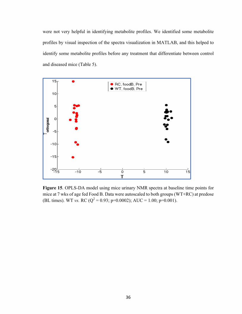
Figure 14. PCA modeling WT (n=7) and RC (n=6) mice fed Food B (A) Mean ± 2SE plot at 7 wks of age, (B) individual data points plot for figure (A), (C) Mean ± 2SE plot at 24 wks of age, and (D) individual data points plot for figure (C). PCA modeling is: (WT+RC) at BL, AS = (WT+RC) at BL. At 7 wks of age PC1 vs. PC2 represents 56% of total variance, and at 24 wks of age PC1 vs. PC2 represents 63% of total variance. OPLS discriminant analyses was used to evaluate the statistical significance, and to identify

the salient features (spectral bins) that are associated with group classification at baseline

time points. The model significance was tested at a=0.01 and the results shown in Figure

15 (T vs. T Orthogonal plot), indicate that wild-type mice are significantly different from

diseased mice at baseline (before any treatments). A total of 345 significant bins (a=0.01)

were derived from WT vs. RC at baseline OPLS-DA model and the Q2 value was 0.93 (see

Fig 16 and Table 5). The high numbers of significant features that resulted from OPLS-DA


36

were not very helpful in identifying metabolite profiles. We identified some metabolite

profiles by visual inspection of the spectra visualization in MATLAB, and this helped to

identify some metabolite profiles before any treatment that differentiate between control

and diseased mice (Table 5).

Figure 15. OPLS-DA model using mice urinary NMR spectra at baseline time points for mice at 7 wks of age fed Food B. Data were autoscaled to both groups (WT+RC) at predose (BL times). WT vs. RC (Q2 = 0.93; p=0.0002); AUC = 1.00; p=0.001).

37

Figure 16. The plot shows all 345 significant features that we got from OPLS-DA for WT vs. RC at Baseline. Arrow indicates the most important features in WT vs. RC at Baseline. Table 5. NMR spectral regions identified as significant by OPLS-DA for WT vs. RC at Baseline. Metabolite Chemical shift in ppm WT vs. RC intensity at BL unknown 1.209875 WT > RC unknown 1.017743 WT > RC unknown 1.05125 WT > RC unknown 2.623844 WT > RC unknown 1.033524 WT > RC unknown 2.617762 WT > RC unknown 0.77 WT < RC unknown 1.00577 WT < RC unknown 0.832125 WT < RC unknown 1.063 WT < RC unknown 0.714144 WT < RC unknown 0.813375 WT < RC unknown 0.75127 WT < RC unknown 1.05675 WT < RC

0

0.01

0.02

0.03

0.04

0.05

0.06

0.07

0.08

0.09

0 100 200 300 400

The most important features

38

Figure 17 shows an example of one NMR spectral regions identified as significant by

using (visualization) in MATLAB to compare WT vs. RC. The NMR signal intensity of

diseased mice (red spectrum) for ⍺ ketoglutarate at two different regions (2.45 and 3.02) is

higher than control mice (black spectrum). Table 6 shows all NMR spectral regions

identified as significant by using visualization in MATLAB, and some of regions identified

by OPLS-DA from comparing between WT and RC at baseline for food B. There are

multiple NMR signals of diseased mice that have higher intensity than control mice such

as ⍺ ketoglutarate, citrate, acetate, taurine, succinate and other unknown metabolites. Some

NMR signals of control mice have higher intensities than diseased mice, such as the NMR

signal at 1.21 ppm that is an unknown metabolite.

We expect that the signal at1.21ppm is methyl-malonic acid. One metabolic pathway

demonstrates that blocking two enzymes in degradation of propionyl-CoA, such as

defective activity of methylmalonyl-CoA mutase or of the synthesis of the

adenosylcobalamine coenzyme, leads to accumulation of methylmalonyl-CoA and exits

from cells as methyl-malonic acid (see Fig 18). This metabolic pathway leads to severe

acidosis and damages the central nervous system. It will be interesting to quantify succinate

and methyl-malonic acid and calculate the ratio for both to confirm if there is any

correlation between these metabolites and disease.

39

Figure 17. ⍺ ketoglutarate at (2.45 and 3.02) is an example of one NMR spectral regions identified as significant by using visualization in MATLAB; comparing between experimental groups WT (in black color) vs. RC (in red color).

Figure 18. Pathway for catabolism of propionyl-CoA.

Propionyl-CoA

(S)methylmalonyl-CoA

(R)methylmalonyl-CoA

Succinyl-CoA

Propionyl-CoA Carboxylase

(biotin coenzyme)

methylmalonyl-CoA epimerase

methylmalonyl-CoA mutase

(B12 coenzyme)

⍺ ketoglutarate [2.42,3.02]

40

Table 6. NMR spectral regions identified as significant by using visualization in MATLAB and OPLS-DA to compare WT vs. RC at baseline for food B.

Metabolite Chemical shift in ppm WT vs. RC intensity

Citrate 2.55, 2.69 (d) WT < RC

a Ketoglutarate 2.45, 3.01 (t) WT < RC

Acetate 1.92 (s) WT < RC

Succinate 2.43 (s) WT < RC

Taurine 3.42,3.27 (t) WT < RC

unknown metabolite 4.02 (d) WT < RC





unknown metabolite 1.21 (S) WT > RC

When we compared two metabolite profiles at baseline for each group at 7 and 24 weeks,

we identified multiple significant regions at 7 weeks by using visualization in MATLAB

41

and OPLS-DA. At 24 weeks, we used visualization in MATLAB; we could not use OPLS-

DA due to less animal numbers at 24 weeks; wild-type (WT; n=3) and PKD (RC; n=1).

NMR spectral regions of control mice and diseased mice were similar to each other and

there were no significant features between the two groups. This may be due to differences

in the progression of disease; rapid progression at 7 weeks that plateaus at 24 weeks (for

more details see Fig 7 in characterization of animal).

To further evaluate the differences between two groups WT and RC at baseline time

points, we calculated the ⍺ ketoglutarate/TSP, acetate/TSP, citrate/TSP and taurine/TSP

ratios for each sample. Figure 19 and 20 shows the average of signal amplitude for different

metabolites for mice at baseline times. Data shows no significant difference in these

metabolites, except for ⍺ ketoglutarate and citrate which were nearly significant (p = 0.09);

if n-values was larger, then these would likely be different.

(A) (B)

Figure 19. Quantified composition of significant metabolites (⍺ ketoglutarate, citrate and acetate) that were found when WT vs. RC mice were compared at baseline time points (B1, B2, B3) at 7 weeks of age that fed Food B. These graphs show (A) the average and standard error of signal amplitude for different metabolites at three time points; B1, B2, and B3. (B) the average and standard error of signal amplitude for different metabolites at the mean of three time points; (B1+ B2+B3).

0

0.05

0.1

0.15

0.2

0.25

0.3

0.35

a-KG/TSP acetate/TSP citrate/TSP

Sign

al Amplitu

de

RC B1RC B2RC B3WT B1WT B2WT B3

00.020.040.060.080.1

0.120.140.160.180.2

a-‐KG/TSP acetate/TSP citrate/TSP

Sing

le A

mpl

itude

RC (B1+B2+B3)

WT (B1+B2+B3)

42

(A) (B)

Figure 20. Quantified composition of the significant metabolites taurine that we found when were compared WT vs. RC mice at baseline time points (B1, B2, B3) at 7 weeks of age that fed Food B. These graphs show (A) the average and standard error of signal amplitude for taurine at three time points; B1, B2, and B3. (B) the average and standard error of signal amplitude for taurine at the main of three time points; (B1+ B2+B3). There are no significant differences were observed in taurine.

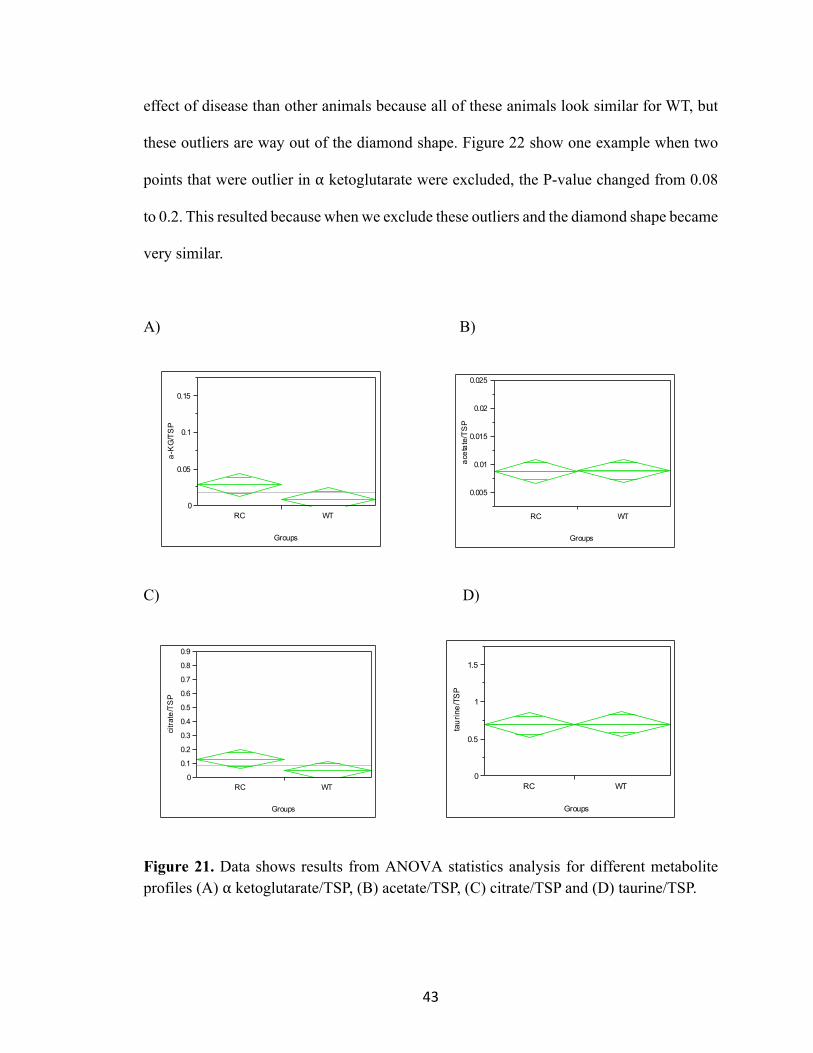
Figure 21 shows box plots; the central line in the diamond shape is the median (50th

percentile), the bottom line is 25th percentile and the upper line is 75th percentile. Y

represents metabolites (⍺ ketoglutarate, citrate, acetate, taurine), grouped by WT vs. RC

and all three times were combined (B1, B2, B3). We performed this analysis by using

ANOVA, which is an analysis of variance to determine if there is statistical difference

between these two groups or not. The results from these plots show that there are no

significant differences due to too much variance. Table 7 represents the P-value for

metabolites profiles (⍺ ketoglutarate, citrate, acetate, and taurine) and it is very obvious

from these data that there is no statistical significance; ⍺ ketoglutarate and citrate would be

different. All of the WT mice metabolite profiles are very tight and we have two outliers

at ⍺ ketoglutarate/TSP, and three outliers at citrate/TSP. The animals that are outliers in ⍺

ketoglutarate are the same that show high citrate levels. Those animals may show a greater

00.10.20.30.40.50.60.70.80.9

1

Taurine/TSP

Sign

al A

mpl

itude

RC B1RC B2RC B3

00.10.20.30.40.50.60.70.80.9

Taurine/TSP

Sing

le A

mpl

itude

RC (B1+B2+B3)

WT (B1+B2+B3)

43

effect of disease than other animals because all of these animals look similar for WT, but

these outliers are way out of the diamond shape. Figure 22 show one example when two

points that were outlier in ⍺ ketoglutarate were excluded, the P-value changed from 0.08

to 0.2. This resulted because when we exclude these outliers and the diamond shape became

very similar.

A) B)

C) D)

Figure 21. Data shows results from ANOVA statistics analysis for different metabolite profiles (A) ⍺ ketoglutarate/TSP, (B) acetate/TSP, (C) citrate/TSP and (D) taurine/TSP.

a-KG/TSP

0

0.05

0.1

0.15

RC WT

Groups

acetate/TSP

0.005

0.01

0.015

0.02

0.025

RC WT

Groups

citrate/TSP

0

0.1

0.2

0.3

0.4

0.5

0.6

0.7

0.8

0.9

RC WT

Groups

taurine/TSP

0

0.5

1

1.5

RC WT

Groups

44

Table 7. The P-value of ANOVA statistics analysis that we got from Jump program in Fig 19 for ⍺ ketoglutarate, citrate, acetate and taurine.

Figure 22. Data shows results from ANOVA statistics analysis for profiles ⍺ ketoglutarate/TSP after excluding two data points; P-value = 0.2054. In previous work, investigators found that defective glucose metabolism is correlated

with pathobiology of ADPKD.50 The authors analyzed metabolism profiles from

extracellular medium by using 1H NMR analysis, then they used unsupervised statistical

analysis and the result showed that the metabolic profile of PKD1-/- cells differed from WT

cells. This analysis showed higher lactate concentrations and lower glucose concentrations.

Consequently, PKD cells use less O2 and preferentially use anaerobic glycolysis due to

mutation of PC1 and PC2. If the TCA cycle is slowed in these cells, then maybe that results

a-KG/TSP

0

0.005

0.01

0.015

0.02

0.025

RC WT

Groups

Metabolite P-value

⍺-KG 0.0854

Acetate 0.9693

Citrate 0.0885

Taurine 0.8801

45

in elevated TCA cycle intermediates being found in urine, such as citrate and ⍺

ketoglutarate. From previous work and our study, data suggested that glucose metabolism

is the major source of energy that produced by oxidative phosphorylation that occurs in the

mitochondria.

We then combined two groups and ages in one analysis. Mice at 7 weeks contains a

greater sample size (n=13): wild-type WT (n=7) and RC (n=6); mice at 24 weeks include

WT (n=3) and RC (n=1). PCA was used to investigate the spectral profiles in one analysis;

approximately 51% of the total variance is captured in PC1 + PC2. Figure 23 shows PCA

scores plot (PC 1 vs. PC 2) at 7 and 24 weeks of age in both WT and RC mice. PCA plot

modeling WT+RC at BL for 7 and 24 weeks of age, autoscaling (WT+RC), was performed

at BL for each age group. The plot shows a large spread of the data along PC1 for mice at

7 weeks of age, but mice at 24 weeks of age are more tightly clustered together. In fact, the

RC animals at 7 weeks appear to be more variable than WT animals; this may be due to

differences in the progression of disease at 7 weeks (for more details see Fig 7 in

characterization of animal). At 24 weeks (highlighted in the oval), all the data points are

clustering together, but unfortunately, the n-value is very small. Data suggested that at 7

weeks the animals were acting different, but at 24 weeks the animal samples looked more

alike. In Figure 23, arrows show trajectories for WT (18568,18546) and RC (18567) at

baseline (before any treatments) and how these animals behaved at two different ages (7

and 24 weeks). At 24 weeks, RC animal urinary profiles were similar to WT animals, but

at 7 weeks the RC animals’ urinary profiles separated farther away from the WT animals;

more than likely due to the progression of disease. For RC 18567, it appears that this animal

46

was very different from WT animal at baseline time points at 7 weeks, but at 24 weeks, it

looks very similar for WT animals.

Figure 23. PCA scores plot (PC1 vs. PC2 representing 51% of total variance) based on mice urinary NMR spectra from the two groups (WT vs. RC) and comparing the two different ages together (7 and 24 weeks). PCA modeling (WT+RC) at BL for two different ages (7 and 24 weeks), autoscaling (WT+RC) at BL for 7&24 weeks of age. Arrows show trajectories for WT and RC animals; WT (18568,18546) and RC (18567) at BL 1-3 at both ages 7 and 24 weeks. Treatment effect (Furosemide). We used different PCA plots to investigate the effect

of furosemide, and to identify if it is a helpful drug in detecting polycystic kidney disease

at an early stage. Figure 24 shows the centroid mean ± 2SE plot modeling (A) at 7 weeks

(WT) at predose and day 1 post injection with Fur; AS = (WT) at BL, was about 57% of

the total variance captured in PC1 + PC2. Days 2 and 3 post injection were superimposed

24 wks

47

in the plot. It is very obvious that the largest effect occurred from baseline to day 1 of

injection, and demonstrates that the effect of furosemide was very fast acting; the second

and third day of injection are clustered with baseline data. Fig 24-B used a PCA plot

modeling: (WT) at predose and day 1 post injection with Fur, AS = (WT) at BL. Day1 post

injection with Ve is superimposed into the plot, AS = (WT) at BL. In Fig 6-B, data shows

that Ve treatment overlapped with predose animals. This was expected since there should

be no effect for Ve treatments animals. Fig 24-C shows OPLS discriminant analyses that

was conducted to evaluate the statistical significance in Fig 24-A. The model significance

was tested at a=0.01 and the results, showed in T vs. T Orthogonal plot that wild-type mice

at baseline are significantly different from wild-type mice at day 1 post injection with Fur.

A total of 170 significant bins (a=0.01) were derived from this OPLS-DA model where

the Q2 value was 0.88.

48

A) B)

C)

Figure 24. PCA scores plot Modeling (A) WT at predose and day 1 post injection with Fur. Data at days 2 and 3 post injection are superimposed in the plot. Data were autoscaled relative to WT at BL (PC1 vs. PC2 representing 57% of total variance). (B) The same PCA model as used in A, but now shows Ve-treated mice superimposed in the plot. (C) OPLS-DA model using mice urinary NMR spectra at baseline time points and day 1 post injection with Fur for control mice (WT) at 7 wks of age, WT (Q2 = 0.88; p=0.0002); AUC = 1.00; p=0.001).

BL Day 1 post Fur

Day 1 post Ve Day 1

BL Day 3

Day 2

49

Figure 25 and table 8 show NMR spectral regions identified as significant by OPLS-

DA from WT at Baseline vs. day 1 post injection with Fur for food B. There are multiple

NMR signals from control mice at day 1 of post injection that have higher intensity than

baseline times point. These are the significant features and the metabolites that show the

effect of FUR. When we compared these significant features with previous work from our

lab in rats,9 we saw some features that may be the same that showed the effect of Fur as

the previous study such as (tryptophan, benzoate, and formate).

Figure 25. The plot shows all 170 significant features that we got from OPLS-DA for WT at Baseline vs. day 1 post injection with Fur for food B. Arrow indicates the most important features in WT at Baseline vs. day 1 post injection with Fur.

0

0.05

0.1

0.15

0.2

0.25

0.3

0.35

0.4

0 50 100 150 200

|P|


50

Table 8. NMR spectral regions identified as significant by OPLS-DA for WT at Baseline vs. day 1 post injection with Fur for food B.

Metabolite Chemical shift in ppm

WT (predose vs. day 1post injection)

OPLS-DA aromatic amino acid 6.445961

Post > Pre


Post > Pre


Post > Pre


Post > Pre


Post > Pre


Post > Pre

Figure 26 shows PCA plots modeling at 7 weeks (RC) at predose and day 1 post

injection with Fur, AS = (RC) at BL, and about 59% of the total variance is captured in

PC1 + PC2. Days 2 and 3 post injections are superimposed in plot. RC animals do not

show the strong effect of furosemide at day 1 as WT data. Data suggested that the effects

of furosemide are short-lived in WT mice, where the maximum effect is observed at Day

1 postdose, and data at Days 2 and 3 return to the baseline profile. The data show effects

of Fur that appear to extend to later times (days 2 and 3 post injection with Fur). Figure 26-

B shows OPLS discriminant analyses that were conducted to evaluate the statistical

significance in Fig 26-A. The model significance was tested at a=0.01 and the results (T

vs. T Orthogonal plot) showed that diseased mice at baseline are significantly different

from diseased mice at day 1 post injection with Fur. A total of 37 significant bins (a=0.01)

were derived from this OPLS-DA model where the Q2 value was 0.79. Figure 26-C

51

illustrates individual samples for Fig 26-A; the RC animals are highly variable and the

animal 1835c7 behaves differently from other RC animals.

A) B)

C)

Figure 26. (A and C) PCA scores plot modeling; RC at predose and day 1 post injection with Fur (plot A shows the centroid mean ± 2SE, while plot C shows the individual data points for the same model). Data at days 2 and 3 post injection are superimposed in the plot. Data were autoscaled relative to RC at BL (PC1 vs. PC2 representing 59% of total variance). Trajectory in (Fig 26-C) indicates one of RC animals (1835c7 left side) behaves differently from other RC animals. The OPLS-DA model using mice urinary NMR spectra (B) at baseline time points and day 1 post injection with Fur for mice RC mice at 7 wks of age yielded a Q2 = 0.79; p=0.0002); AUC = 1.00; p=0.001.

RC #18357 appears different from others in the

group.

52

Figure 27 and table 9 show NMR spectral regions identified as significant by OPLS-DA

from RC at Baseline vs. day 1 post injection with Fur for food B. There are multiple NMR

signals of diseased mice at day 1 of post injection that have higher intensities than baseline

time points. They are significant features and metabolites that show the effect of FUR.

When we compare these results with WT results in Fig 22-C and 24-B, we found that the

effect of furosemide was similar in WT and RC.

Figure 27. The plot shows all 37 significant features that we got from OPLS-DA for RC at Baseline vs. day 1 post injection with Fur for food B. Arrow indicates the most important features in RC at Baseline vs. day 1 post injection with Fur.

0

0.05

0.1

0.15

0.2

0.25

0.3

0.35

0.4

0.45

0.5

0 5 10 15 20 25 30 35 40

|P|


53

Table 9. NMR spectral regions identified as significant by OPLS-DA for RC at Baseline vs. day 1 post injection with Fur for food B.

Metabolite Chemical shift in ppm

RC (predose vs. day 1post injection)


Post > Pre


Post > Pre


Post > Pre


Post > Pre


Post > Pre


Post > Pre

We then combined two groups WT vs. RC in one analysis. This analysis is suspect due

to autoscaling, which used the combined WT and RC data at BL times as reference.

Baseline data is very different for WT and RC, using the baseline as reference to scale is

not a good analysis to look at it. Figure 28 shows PCA scores plot (PC 1 vs. PC 2) at 7

weeks of age in both WT and RC mice. PCA plot modeling WT+RC at BL and day 1 post

injection with Fur and day 1 post injection with Ve is superimposed in the plot, autoscaling

(WT+RC) at BL. Data shows that the major effect was along PC1, due to group effect, and

the minor effect was along PC2, due to Fur effect. All animals treated with Ve overlapped

with baseline data in both groups, which was expected from vehicle treatment (Ve). When

we combined both groups together, RC animals that were treated with Fur day 1 post

injection showed a clear separation from baseline and Ve. We did not see a clear separation

for WT as RC animals and that because some of WT animals that treated with Fur act as

baseline and Ve samples.

54

Figure 28. PCA scores plot modeling; WT+RC at BL and day 1 post injection with Fur and day 1 post injection with Ve is superimposed in the plot. Data autoscaling included all animals at BL times (WT+RC). PC1 vs. PC2 represents 53% of total variance. From previous Figures 24 and 26, we noticed that the effect of furosemide appeared to

be at long lasting in RC animals. We conducted a ‘paired analysis’ to examine the effects

of furosemide over the total time course post-dose (3 days). This should help to investigate

whether the effects of Fur appear to last longer in RC mice than in WT mice. Figure (29-

A) shows a PCA plots (PC 1 vs. PC 2) modeling (WT+RC) at day 2 post injections with

Fur, paired-by day 1 of injection with Fur, and about 71% of the total variance is captured

in PC1 + PC2. This PCA plot shows a separation between WT vs. RC for day 2 of injection

with Fur. The RC animal 1910a3 at day 2 post injection with Fur separated along PC1 and

is different than the other two mice (1835c7 and 1856a7). In Fig (29-C), we looked at day

3 of post injection with Fur. PCA plot modeling (WT+RC) at day 3 post injections with

Day 1 post Fur

BL

55

Fur, paired-by day 2 of injection with Fur, demonstrated that about 88 % of the total

variance was captured in PC1 + PC2. This plot shows a separation between WT vs. RC for

day 3 of injection with Fur. The RC animal 1835c7 at day 3 post injection with Fur

separated along PC1 and is different than the other two mice from that treatment group

(1910a3and 1856a7). From these two plots, we can say that the effect of furosemide

appears to extend into later times.

56

A) B)

C) D)

Figure 29. (A) PCA Mean ± 2SE plot modeling (WT+RC) at day 2 post injections with Fur, AS= (WT+RC) at day 1 of injection with Fur at 7 weeks of mice age, paired-by day 1 of injection with Fur (PC1 vs. PC2 representing 71% of total variance). (B) Individual data points from Figure A. (C) PCA Mean ± 2SE plot modeling: (WT+RC) day 3 post injections with Fur, AS= (WT+RC) at BL at 7 weeks of mice age, paired-by day 2 of injection with Fur (PC1 vs. PC2 representing 88% of total variance). (D) Individual data points from Figure C.

1835c7

1910a3

1856a7

1835c7

1910a3

1856a7

57

Effect of furosemide at later times in RC mice We then looked at days 2 and 3 of injection with Fur and Ve in one analysis to confirm

that the effect of furosemide appears to occur at later times in RC animals. Figure 30 shows

a paired analysis, where data were paired-by day1 of injection with Fur as a reference point.

The analysis shows PCA plots (PC 1 vs. PC 2) modeling (WT+RC) at days 2 and 3 post

injection with Fur or Ve (C2 and C3) paired-by day 1 post injection (C1), and autoscaled

to (WT+RC) at day 1 (C1). This paired-by analysis for all animal samples resulted in

different spectrums for each time point (C2 and C3) versus the reference time (C1), and

showed changes in urinary profiles relative to C1. The data show effects of Fur that appear

to occur at later times. Data showed that all WT animals that were injected with both

treatments, and RC animals that were injected with Ve, are clustered together. RC animals

at day 2 and 3 of post injection with Fur separated and behaved differently from other

animals. Animal 1835c7 shows the big effect of furosemide at day 3 of injection along

PC1. The data suggested that there was an effect of furosemide that occurred at a later

time following injections in RC animals.

58

A) B)

Figure 30. (A) PCA Mean ± 2SE plot modeling (WT+RC) at day 2 and 3 post injections with Fur and Ve, AS= (WT+RC) at day 1 of injection with Fur at 7 weeks of mice age, paired-by day 1 of injection with Fur (PC1 vs. PC2 representing 48% of total variance). (B) Individual data points from Figure A. Arrow indicates the RC animals (1835c7) that show a big effect of Fur along PC1.

Because of the diet effect, we cannot include mice fed Food A or Food B in the same

analyses. However, using a paired-by analysis may allow us to examine the effect of Fur

without the complications of different diets; including both groups of animals in the same

analysis would increase the sample size (n-value). Thus, we attempted to use a ‘paired

analysis,’ which may help to suppress the changes due to diet and increase the animal

numbers for analyzing the effects of furosemide. Figure 31 shows a paired analysis, where

data were paired-by B3 as a reference point. Data shows a PCA plots (PC 1 vs. PC 2)

modeling (WT+RC) at day 1 post injection with Fur or Ve and paired-by B3 (last time point

of baseline). This “paired-by” analysis for all animal samples resulted in different spectrum

(C1 - B3) emphasizing the changes between these two-different times, and it might help to

eliminate the effect of diet. We expected that the animals that were treated with Ve would

separate from animals that were treatment with Fur. We observed that all animals clustered

together with the exception of two animals, 1838a4 (WT) and 1839a8 (RC). These animals

d2 RC

d3 RC

1835c7

59

were treated with Fur and fed Food A, and show a clear separation from all other animals.

Mouse 1839a8 separated along PC1 and mouse 1838a4 along PC2; approximately 78% of

the total variance is captured in PC1 + PC2. Paired analysis helped to suppress the effects

of diet, but we found another issue that was related to urine time of collection. For mice

fed Food A, we collected urine over a 4-hour time period post injection with treatments.

However, in mice fed Food B, urine was collected over a 6-hour time period following

injection. By using paired analysis, we suppress diet effects, but we could not eliminate the

issue with different time of urine collection. We observed the effect of furosemide in

animals where urine was collected at early time (4-hour) following injection and fed Food

A.

A) B)

Figure 31. The scores plots show all data points (left panel), and all data points with animal ID (right panel). PCA modeling is: (WT+RC) at day 1 post injection with Fur or Ve for mice fed Food A or Food B; AS= (WT+RC) at C1 (day 1 post injection) at 7 weeks of age mice fed Food A or B, paired-by B3 (PC1 vs. PC2 representing 78% of total variance).

60

Effect of furosemide

We then looked at both animal ages (7 and 24 wks) separately to investigate the effect

of furosemide. Figure 32 shows a PCA plots (PC 1 vs. PC 2) depicting the effect of

furosemide at 7 and 24 weeks of age in both WT and RC mice. PCA plot modeling

(WT+RC) at BL (B1, B2, and B3) and day 1 post injection with Fur, AS = (WT+RC) at

BL. At 7 weeks, the data showed that the two groups are separated from each other before

furosemide treatment, as shown in Fig 26 above and again here in Fig 32A. Thus, due to

the rapid progression of disease, RC and WT mice showed different urinary profiles at 7

wks of age (for more details about progression of disease at 7 weeks of mice age see Fig 7

in characterization of animal). At 24 weeks of age, both groups are clustering together

before Fur treatment (Fig. 32B). Subsequent treatment with furosemide induced separation

between WT and RC mice. The plots show that separation between WT vs. RC groups

occurred before injection with Fur, which is due to progression of disease at 7 weeks.

However, at 24 weeks, the animals did not progress any further at a later time and the

predosed animals for both groups became similar and clustered together following injection

with Fur that helped to separate WT and RC mice.

61

A) B)

Figures 32. PCA modeling WT and RC mice fed Food B at (A) 7 wks and (B) 24 wks of age. PCA scores plot Modeling (WT+RC) at BL (B1, B2, and B3) and PostC1F, autoscaling (WT+RC) at BL. At 7 weeks of age PC1 vs. PC2 representing 54% of total variance, and at 24 weeks of age PC1 vs. PC2 representing 78% of total variance.

WT RC

Post FUR

WT post

62

CHAPTER 5: SUMMARY AND CONCLUSION AND FUTURE DIRECTION

5.1 SUMMARY AND CONCLUSION

Our data demonstrated that the effect of diet was significant, and because of that we

focus on one food (Food B; Diet Gel 76A) that had a larger sample size than Food A. We

then noticed that the separation between the two groups (WT and RC) occurs at 7 weeks

before applying any treatments, and that was due to progression of disease at an early age.

We found multiple significant features between WT vs RC at baseline time points that

showed higher intensities in diseased mice when compared to control mice, such as ⍺

ketoglutarate, citrate and other unknown metabolites. In addition, the data appeared similar

at 24 weeks before injection with Fur, and then Fur induced the separation of the two

groups from each other. In this study, we wanted to confirm the hypothesis that the stressor

(Furosemide) helped to detect biologically relevant changes. Thus, at 24 weeks we could

not verify that this hypothesis was correct a hundred percent because we have due to the

small sample size of the diseased animal model (RC; n-value = 1).

5.2 FUTURE DIRECTION

To validate our hypothesis, it will be necessary to repeat this study at 7 and 24 weeks

with an increased sample size. We would like to explore a new mouse model that develops

cyst gradually to test our hypothesis that stress to the kidney using diuretic drug could be

helpful to detect the disease at an early stage. It would be interesting to compare metabolites

to identify if PKD can be diagnosed at an early stage by a simple urine analysis. We would

like to identify more metabolites that differentiate between control and diseased mice

before and after injection with furosemide.

63

REFERENCES

1. Smolinska A, Blanchet L, Buydens LMC, Wijmenga SS. NMR and pattern recognition methods in metabolomics: From data acquisition to biomarker discovery: A review. Analytica Chimica Acta. 2012;750:82-97.

2. Bollard ME, Stanley EG, Lindon JC, Nicholson JK, Holmes E. NMR-based metabonomic approaches for evaluating physiological influences on biofluid composition. NMR in Biomedicine. 2005;18(3):143-162.

3. Nicholson JK, Lindon JC, Holmes E. 'Metabonomics': understanding the metabolic responses of living systems to pathophysiological stimuli via multivariate statistical analysis of biological NMR spectroscopic data. XENOBIOTICA. 1999;29:1181-1189.

4. Nicholson JK, Wilson ID. High resolution proton magnetic resonance spectroscopy of biological fluids. Progress in Nuclear Magnetic Resonance Spectroscopy. 1989;21(4):449-501.

5. Xu J, Zhang J, Cai S, Dong J, Yang JY, Chen Z. Metabonomics studies of intact hepatic and renal cortical tissues from diabetic db/db mice using high-resolution magic-angle spinning 1H NMR spectroscopy. Analytical and Bioanalytical Chemistry. 2009;393(6):1657-1668.

6. Sibomana I, Delraso NJ, Mattie D, Raymer ML, Reo NV. Furosemide enhances the sensitivity of urinary metabolomics for assessment of kidney function. Springer. 2017:1-17.

7. Bervoets L, Massa G, Guedens W, Louis E, Noben J-P, Adriaensens P. Metabolic profiling of type 1 diabetes mellitus in children and adolescents: a case–control study. Diabetology & Metabolic Syndrome. 2017;9:48.

8. Martin F-P, Collino S, Rezzi S, Kochhar S. Metabolomic Applications to Decipher Gut Microbial Metabolic Influence in Health and Disease. Frontiers in Physiology. 2012;3(113).

64

9. Isaie Sibomana NJD, David Mattie, Michael L. Raymer,Nicholas V Reo. Furosemide enhances the sensitivity of urinary metabolomics for assessment of kidney function. Spriger. 2017:1-17.

10. Lenz EM, Bright J, Wilson ID, Morgan SR, Nash AFP. A 1H NMR-based metabonomic study of urine and plasma samples obtained from healthy human subjects. Journal of Pharmaceutical and Biomedical Analysis. 2003;33(5):1103-1115.

11. Assfalg M, Bertini I, Colangiuli D, et al. Evidence of different metabolic phenotypes in humans. Proceedings of the National Academy of Sciences. 2008;105(5):1420-1424.

12. Chebib FT, Torres VE. Autosomal Dominant Polycystic Kidney Disease: Core Curriculum 2016. American Journal of Kidney Diseases.67(5):792-810.

13. van Gastel MDA, Torres VE. Polycystic Kidney Disease and the Vasopressin Pathway. Annals of Nutrition and Metabolism. 2017;70(suppl 1)(Suppl. 1):43-50.

14. WILSON PD. Polycystin: New Aspects of Structure, Function, and Regulation. Journal of the American Society of Nephrology. 2001;12(4):834-845.

15. Reeders ST, Keith T, Green P, et al. Regional localization of the autosomal dominant polycystic kidney disease locus. Genomics. 1988;3(2):150-155.

16. Kimberling WJ, Kumar S, Gabow PA, Kenyon JB, Connolly CJ, Somlo S. Autosomal dominant polycystic kidney disease: Localization of the second gene to chromosome 4q13–q23. Genomics. 1993;18(3):467-472.

17. Ravine D, Forrest SM, Sheffield LJ, et al. Phenotype and genotype heterogeneity in autosomal dominant polycystic kidney disease. The Lancet. 1992;340(8831):1330-1333.

18. The European Polycystic Kidney Disease C. The polycystic kidney disease 1 gene encodes a 14 kb transcript and lies within a duplicated region on chromosome 16. Cell. 1994;77(6):881-894.

65

19. The International Polycystic Kidney Disease C. Polycystic kidney disease: The complete structure of the PKD1 gene and its protein. Cell. 1995;81(2):289-298.

20. Chebib FT, Sussman CR, Wang X, Harris PC, Torres VE. Vasopressin and interactive calcium, cyclic AMP and purinergic signaling in Polycystic Kidney Disease. Nature reviews Nephrology. 2015;11(8):451-464.

21. Cai Y, Maeda Y, Cedzich A, et al. Identification and Characterization of Polycystin-2, the PKD2 Gene Product. Journal of Biological Chemistry. 1999;274(40):28557-28565.

22. Hughes J, Ward CJ, Peral B, et al. The polycystic kidney disease 1 (PKD1) gene encodes a novel protein with multiple cell recognition domains. Nat Genet. 1995;10(2):151-160.

23. Mochizuki T, Wu G, Hayashi T, et al. <strong><em>PKD2</em></strong>, a Gene for Polycystic Kidney Disease That Encodes an Integral Membrane Protein. Science. 1996;272(5266):1339-1342.

24. Chapman AB, Devuyst O, Eckardt K-U, et al. Autosomal Dominant Polycystic Kidney Disease (ADPKD): Executive Summary from a Kidney Disease: Improving Global Outcomes (KDIGO) Controversies Conference. Kidney international. 2015;88(1):17-27.

25. Diedrich B, Dengjel J. Insights into autosomal dominant polycystic kidney disease by quantitative mass spectrometry-based proteomics. Cell and Tissue Research. 2017:1-11.

26. Koeppen BM, Stanton BA. Berne & Levy Physiology, Updated Edition E-Book. Elsevier Health Sciences; 2009.

27. Yoder BK. Role of Primary Cilia in the Pathogenesis of Polycystic Kidney Disease. Journal of the American Society of Nephrology. 2007;18(5):1381-1388.

28. Wilson PD. Polycystic Kidney Disease. New England Journal of Medicine. 2004;350(2):151-164.

66

29. Grantham JJ, Mulamalla S, Swenson-Fields KI. Why kidneys fail in autosomal dominant polycystic kidney disease. Nat Rev Nephrol. 2011;7(10):556-566.

30. Kawano H, Muto S, Ohmoto Y, et al. Exploring urinary biomarkers in autosomal dominant polycystic kidney disease. Clinical and Experimental Nephrology. 2015;19(5):968-973.

31. Yamaguchi T, Nagao S, Wallace DP, et al. Cyclic AMP activates B-Raf and ERK in cyst epithelial cells from autosomal-dominant polycystic kidneys. Kidney International. 2003;63(6):1983-1994.

32. Mishra J, Dent C, Tarabishi R, et al. Neutrophil gelatinase-associated lipocalin (NGAL) as a biomarker for acute renal injury after cardiac surgery. The Lancet. 2005;365(9466):1231-1238.

33. Kjeldsen L, Johnsen AH, Sengeløv H, Borregaard N. Isolation and primary structure of NGAL, a novel protein associated with human neutrophil gelatinase. Journal of Biological Chemistry. 1993;268(14):10425-10432.

34. Cowley BD, Ricardo SD, Nagao S, Diamond JR. Increased renal expression of monocyte chemoattractant protein-1 and osteopontin in ADPKD in rats. Kidney International. 2001;60(6):2087-2096.

35. Zheng D, Wolfe M, Cowley BD, Wallace DP, Yamaguchi T, Grantham JJ. Urinary Excretion of Monocyte Chemoattractant Protein-1 in Autosomal Dominant Polycystic Kidney Disease. Journal of the American Society of Nephrology. 2003;14(10):2588-2595.

36. Meur YL, Fixe P, Aldigier J-C, Leroux-Robert C, Praloran V. Macrophage colony stimulating factor involvement in uremic patients. Kidney International. 1996;50(3):1007-1012.

37. Kistler ADS, Andreas L.; Siwy, Justyna; Poster, Diane; Krauer, Fabienne; Torres, Vicente E.; Mrug, Michal; Grantham, Jared J.; Bae, Kyongtae T.; Bost, James E.; Mullen, William; Wüthrich, Rudolf P.; Mischak, Harald; Chapman, Arlene B. Urinary Proteomic Biomarkers for Diagnosis and Risk Stratification of Autosomal Dominant Polycystic Kidney Disease: A Multicentric Study. EMORY LIBRARIES & INFORMATION TECHNOLGY. 2013;8(1):e53016.

67

38. Cheng Xue C-CZ, Ming Wu, Chang-Lin Mei. The Clinical Manifestation and Management of Autosomal Dominant Polycystic Kidney Disease in China. Kidney Diseases. 2016:111-112.

39. Harris PC, Torres VE. Polycystic Kidney Disease. Annual review of medicine. 2009;60:321-337.

40. Chawla LS, Davison DL, Brasha-Mitchell E, et al. Development and Standardization of a Furosemide Stress Test to Predict the Severity of Acute Kidney Injury. Critical Care. 2013;17(5):R207.

41. Powell TC, Warnock DG. The Furosemide Stress Test and Predicting AKI Outcomes. Journal of the American Society of Nephrology : JASN. 2015;26(8):1762-1764.

42. Koyner JL, Davison DL, Brasha-Mitchell E, et al. Furosemide Stress Test and Biomarkers for the Prediction of AKI Severity. Journal of the American Society of Nephrology : JASN. 2015;26(8):2023-2031.

43. Hopp K, Ward CJ, Hommerding CJ, et al. Functional polycystin-1 dosage governs autosomal dominant polycystic kidney disease severity. The Journal of Clinical Investigation. 2012;122(11):4257-4273.

44. Wu G, D'Agati V, Cai Y, et al. Somatic inactivation of Pkd2 results in polycystic kidney disease. Cell. 1998;93(2):177-188.

45. Wittner M, Di Stefano A, Wangemann P, Greger R. How Do Loop Diuretics Act?

Drugs. 1991;41(3):1-13.

46. Christensen S, Steiness E, Christensen H. Tubular sites of furosemide natriuresis in volume-replaced and volume-depleted conscious rats. Journal of Pharmacology and Experimental Therapeutics. 1986;239(1):211-218.

47. Dieterle F, Ross A, Schlotterbeck G, Senn H. Probabilistic Quotient Normalization as Robust Method to Account for Dilution of Complex Biological

68

Mixtures. Application in 1H NMR Metabonomics. Analytical Chemistry. 2006;78(13):4281-4290.

48. Anderson PE, Mahle, D. A., Doom, T. E., Reo, N. V., DelRaso, N. J., & Raymer, M. L. Dynamic Adaptive Binning: an Improved Quantification Technique for NMR Spectroscopic Data. Spriger. 2011;7(2):179-190.

49. Rose J. Environmental toxicology current developments. 1998:1-11.

50. Rowe I, Chiaravalli M, Mannella V, et al. Defective Glucose Metabolism in Polycystic Kidney Disease Identifies A Novel Therapeutic Paradigm. Nature medicine. 2013;19(4):488-493.

urinary metabolomics to detect - OhioLINK ETD Center

Documents

Transcript of urinary metabolomics to detect - OhioLINK ETD Center