Development of Quality System for Additive Manufacturing

Development of Quality System for Additive

Manufacturing

By

Stephen Oluwashola Akande

The thesis is submitted in fulfilment of the requirements for the Degree of

Doctor of Philosophy

School of Mechanical and Systems Engineering

Newcastle University

March 2015

i

ABSTRACT

Selective laser sintering (SLS) and fused filament fabrication (FFF) are significant

methods in additive manufacturing (AM). As AM is increasingly being used to

manufacture functional parts, there is a need to have quality systems for AM process, to

ensure repeatability of properties or quality of part made by the process. The primary

aim of this research is to develop quality systems for SLS and FFF processes of AM.

In order to develop a quality system for SLS process based on defining a minimum set

of tests to qualify a build, two SLS materials of Nylon 11 and Nylon 12 were

investigated. Melt flow index (MFI), impact, tensile and flexural tests were assessed,

along with density, surface roughness, dimensional measurements and scanning electron

microscopic (SEM). Two benchmark parts were designed for manufacture to track

changes in key parameters from one build to another, and tests on this validated against

ISO standards.

Similarly, to develop a quality system for FFF process, the various mechanical

properties of tensile, flexural properties, notched and un-notched impact strengths and

sample mass of specimens made from biodegradable polylatic acid (PLA) FFF material

were investigated. In order to identify the tests that can be most sensitive to changes in

processing conditions and differences in interlayer bond strength which affect the

structural integrity of part made by FFF. Analysis of variance (ANOVA) was used to

compare the significance of the effect of processing parameters on the mechanical

properties, while optical microscopy was also used to investigate failure pattern.

A novel low cost method for evaluating fracture strength of FFF made parts was also

developed for low cost FFF machines. Benchmark specimens and a low cost test jig

were designed and fabricated to track changes in key quality characteristics of FFF

made parts from one build to another. Tests conducted on the test jig were validated

against those conducted on standard machine. Very good correlation was observed

between them.

On the basis of the data from experiments, impact strength was adopted as a key test of

interlayer bond strengths which determines overall structural strengths of the materials

for both SLS and FFF AM processes. A positive correlation exist between density and

modulus of SLS parts, and also between sample mass and modulus of FFF made parts.

ii

This led to the impact strength and density/mass of parts being adopted as key

indicators of mechanical integrity, with MFI a good indicator of input material quality,

and dimensional accuracy of machine calibration. These tests were thus adopted as a

quality assurance system in the respective developed quality system for AM processes

of SLS and FFF. If the quality system is implemented, repeatability of properties can be

achieved and the quality of product assured.

Keyword: FFF, SLS, quality system, Nylon, Polylactic acid (PLA), additive

manufacturing

iii

Acknowledgement

I would like to thank Prof. Kenny Dalgarno and Dr Javier Munguia for their support and

continuous guidance throughout this research and writing of this thesis. I am also

grateful to Peacock Medical Group, and their staff such as Dr Jari Pallari and Iain

Charlesworth for their help in getting specimens and using their venue to carry out some

tests in the process of my work.

I would like to thank my fellow colleagues in the Design and Manufacturing Group and

also in Robotics and MEMS group, who shared the joy and travails during this research.

I give thanks to the technical staffs in the School of Mechanical and Systems

Engineering, especially Malcolm Black, Michael Foster and Christopher Aylott for their

assistance in carrying out mechanical tests and imaging of fracture surface of specimens.

I am also very grateful to Tertiary Education Trust Fund of Nigeria for their scholarship

award which allows me to undertake this study.

Finally, I am especially grateful to my family and friends for their continuous support,

patience and understanding over the years of being far apart during this work.

iv

Table of contents

ABSTRACT ....................................................................................................................... i

Acknowledgement............................................................................................................ iii

Table of contents .............................................................................................................. iv

List of figures ................................................................................................................. xiv

List of tables ................................................................................................................... xxi

Chapter 1 INTRODUCTION .......................................................................................... 1

1.0 Background and motivation of the research ....................................................... 1

1.1 Aims and objectives ........................................................................................... 2

1.1.1 Aim of study ................................................................................................ 2

1.1.2 Objectives .................................................................................................... 2

1.2 Hypothesis .......................................................................................................... 2

1.3 Industrial collaboration and alignment to a- footprint project............................ 2

1.4 The Scope of the research................................................................................... 2

1.5 Layout of Thesis ................................................................................................. 3

Chapter 2 LITERATURE REVIEW ............................................................................... 5

2.1 Introduction ........................................................................................................ 5

2.2 Rapid prototyping ............................................................................................... 6

2.3 Rapid tooling ...................................................................................................... 6

2.4 Additive manufacturing ...................................................................................... 7

2.4.1 The basic process of Additive Manufacturing ............................................ 8

2.5 Types of AM machines .................................................................................... 10

2.5.1 Liquid- Based Processes ........................................................................... 10

2.5.2 Solid – Based Processes ............................................................................ 12

2.5.3 Powder – Based Processes ........................................................................ 14

2.6 Research in selective laser sintering (SLS) ...................................................... 17

v

2.6.1 Introduction ............................................................................................... 17

2.6.2 Polyamide 11 and 12 powders .................................................................. 20

2.6.3 Research Overview ................................................................................... 21

2.7 Research in Fused Filament Fabrication (FFF) ................................................ 27

2.8 Summary of process parameters and key quality indicators for SLS and FFF 30

2.9 Quality Systems ................................................................................................ 31

2.9.1 Quality Management ................................................................................. 31

2.9.2 Measures of Quality .................................................................................. 31

2.9.3 Statistical quality control........................................................................... 33

2.9.4 Statistical process control .......................................................................... 34

2.9.5 The mean control Chart ............................................................................. 35

2.9.6 Range control chart ................................................................................... 36

2.9.7 Melt rheology of Polyamide powder......................................................... 37

2.9.8 Impact strength characterisation and material failure ............................... 37

2.9.9 Quality System for AM ............................................................................. 38

2.9.10 Benchmark Development for AM ............................................................. 39

2.9.11 Reviews of various Benchmarking Study ................................................. 39

2.10 Statistical Analysis ........................................................................................... 46

2.10.1 Correlation and regression analysis .......................................................... 46

2.10.2 ANOVA .................................................................................................... 47

2.10.3 Design of Experiment ............................................................................... 48

Chapter 3 MECHANICAL TESTING AND MATERIALS CHARACTERISATION 49

3.1 Introduction ...................................................................................................... 49

3.2 Powder Characterisation ................................................................................... 49

3.3 Flexural part geometry and test procedures ..................................................... 50

3.4 Tensile part geometry and test procedures ....................................................... 52

3.5 Impact part geometry and test procedures ........................................................ 53

vi

3.6 Dimensional accuracies measurement .............................................................. 55

3.7 Determination of mass of specimens ................................................................ 55

3.8 Determination of Density of specimens ........................................................... 55

3.9 Imaging and Microscopy .................................................................................. 55

3.9.1 Scanning electron microscopy .................................................................. 55

3.9.2 Specimen preparation and microscopic examination ................................ 55

3.9.3 Replication of fracture surface .................................................................. 56

3.10 Surface roughness measurement ...................................................................... 56

Chapter 4 QUALITY ASSESSMENT FOR SLS PROCESS ....................................... 58

4.1 Quality System Mapping for SLS process ....................................................... 58

4.1.1 Detailed Description of SLS process ........................................................ 58

4.2 Identification of Potential Input and Output Quality Measures ....................... 61

4.2.1 Requirements for a quality assurance (QA) test ....................................... 61

4.2.2 Evaluation of Possible QA Tests............................................................... 61

4.3 Proposed Quality System and Benchmark parts for SLS ................................. 62

4.3.1 Proposed Quality System .......................................................................... 62

4.3.2 Proposed Benchmark parts ........................................................................ 65

4.3.3 Selection of Tests for Validation of Benchmarks parts ............................ 66

4.4 Materials and Methods ..................................................................................... 67

4.4.1 Experimental procedures for Nylon 12 ..................................................... 67

4.4.2 Experimental procedures for Nylon -11 .................................................... 69

4.4.3 Test Procedures for SLS Benchmark parts ............................................... 71

4.5 Nylon 12 Results and analysis .......................................................................... 72

4.5.1 Benchmark Validation against ISO Tests in Virgin Powder Build

(Duraform PA 12) .................................................................................................... 72

4.5.2 ISO flexural modulus versus benchmark flexural modulus (Duraform PA

12) …………………………………………………………………………...73

vii

4.5.3 ISO Impact strength versus benchmark Impact strength for Duraform PA

12…………………………………………………………………………..............75

4.5.4 Input Powder Property Variations over Multiple Builds (Duraform PA 12

powders)................................................................................................................... 77

4.5.5 Mechanical Property Variation over Multiple Builds (Duraform PA 12) 78

4.5.6 Variation of flexural modulus and impact strengths with builds and

benchmark for Duraform PA 12 .............................................................................. 78

4.5.7 Modulus and density correlation for Duraform PA 12 ............................. 79

4.5.8 MFI and density correlation for Duraform PA 12 .................................... 80

4.5.9 MFI and impact strength correlation for Duraform PA 12 ....................... 81

4.5.10 Variation of dimensional accuracy with builds for Duraform PA 12 ....... 82

4.5.11 Summary of Nylon 12 Results .................................................................. 83

4.6 Nylon 11 Results and Analysis ........................................................................ 83

4.6.1 Benchmark Validation against ISO Tests in Virgin Powder Build (Innov

PA 1350 ETX) ......................................................................................................... 83

4.6.2 ISO flexural modulus versus benchmark flexural modulus (Innov PA 1350

ETx)…………………………………………………………………………..........84

4.6.3 ISO Impact strength versus benchmark Impact strength for Innov PA 1350

ETX material............................................................................................................ 86

4.6.4 Variation of benchmark impact strength with locations in the build

chamber (Innov PA 1350 ETX material) ................................................................. 87

4.6.5 Input Powder Property Variation over Multiple Builds (Innov PA 1350

ETX powders) .......................................................................................................... 89

4.6.6 Mechanical Property variation over Multiple Builds (Innov PA 1350 ETx)

…………………………………………………………………………...90

4.6.7 Variation of flexural modulus and impact strengths of benchmark .......... 90

4.6.8 Variation of ISO tensile strength with builds (Innov PA 1350 ETX

material)… ............................................................................................................... 92

viii

4.6.9 Modulus, Impact strength and density correlations (Innov PA 1350 ETX)

over multiple builds ................................................................................................. 93

4.6.10 MFI and density correlation for Innov PA 1350 ETX material ................ 94

4.6.11 MFI and impact strength correlation for Innov PA 1350 ETX material ... 95

4.6.12 MFI and accuracy correlation for Innov PA 1350 ETX material ............. 96

4.6.13 Variation of surface roughness of Benchmark specimens with build (Innov

PA 1350 ETx) .......................................................................................................... 97

4.6.14 Summary of Nylon 11 Results .................................................................. 98

Chapter 5 QUALITY ASSESSMENT FOR FUSED FILAMENT FABRICATION .. 99

5.1 Introduction ...................................................................................................... 99

5.2 Quality System Mapping .................................................................................. 99

5.2.1 Detailed Description of FFF process......................................................... 99

5.3 Identification of Potential Input and Output Quality Measures ..................... 102

5.3.1 Evaluation of Possible QA Tests............................................................. 102

5.4 Proposed Quality System for FFF process ..................................................... 103

5.5 FFF Part production ........................................................................................ 105

5.5.1 Hardware ................................................................................................. 105

5.5.2 Software .................................................................................................. 105

5.5.3 Build parameters and styles .................................................................... 106

5.5.4 Experimental plan for FFF specimens .................................................... 108

5.6 Pilot Study –Flexural Properties of Hollow Beams ....................................... 112

5.6.1 Evaluations of Flexural properties of FFF specimens ............................ 112

5.6.2 Evaluation of second moment of area of non- fully dense FFF specimen

………………………………………………………………………….114

5.6.3 Geometrical modelling and evaluation of second moment of area ......... 115

5.6.4 Second moment of area modelling results .............................................. 118

5.7 Influence of Build Parameters on Accuracy ................................................... 120

ix

5.8 Influence of Build Parameters on Modulus, Strain at maximum stress and

sample mass ............................................................................................................... 122

5.8.1 Variations of Modulus with parameter sets and orientations .................. 122

5.8.2 Flexural modulus, strain at maximum stress and sample mass of

specimens processed using Axon 3 software ......................................................... 127

5.8.3 Variations of Modulus with parameter sets and fill patterns .................. 128

5.9 Influence of Build Parameters on Strength .................................................... 132

5.9.1 Variations of strengths with parameter sets and orientations.................. 132

5.9.2 Flexural strengths and impact strengths of specimens process using Axon

3 software ............................................................................................................... 135

5.9.3 Variations of strengths with parameter sets and fill patterns .................. 138

5.9.4 Correlation between Impact strength and UTS, Flexural strength and UTS

………………………………………………………………………….141

5.10 MFI of two batch of PLA filament ................................................................. 143

5.11 Surface morphology ....................................................................................... 144

5.12 Summary of FFF PLA properties tests results ............................................... 149

5.13 Low cost QA benchmark for fused filament fabrication ................................ 150

5.13.1 Introduction ............................................................................................. 150

5.13.2 Materials and methods for FFF process benchmark test ......................... 150

5.13.3 Proposed Benchmark .............................................................................. 150

5.13.4 Experimental plan ................................................................................... 151

5.13.5 Manufacture ............................................................................................ 152

5.13.6 Bending test using design test jig ............................................................ 152

5.13.7 Test specimens ........................................................................................ 153

5.14 Results and analysis for FFF QA benchmark ................................................. 154

5.14.1 Maximum load to failure of benchmark sample with notch radius of 0.25

mm…………. ........................................................................................................ 154

x

5.14.2 Maximum load to failure of single edge notched specimens with notch

radius of 2 mm and of different thickness ............................................................. 155

5.14.3 Correlation between load, thickness and mass of single edge notched

specimens ............................................................................................................... 155

5.14.4 ISO flexural, tensile and Impact strengths and benchmark flexural strength

………………………………………………………………………….156

5.14.5 Correlation analysis of ISO test results and that of benchmark test results

………………………………………………………………………….158

5.14.6 Summary of low cost benchmark test results .......................................... 162

Chapter 6 DISCUSSION ............................................................................................. 163

6.1 Summary of Key SLS Results ........................................................................ 163

6.2 SLS Mechanical properties............................................................................. 163

6.2.1 Tensile properties of laser sintered part .................................................. 163

6.2.2 Flexural properties of laser sintered part ................................................. 167

6.2.3 Impact strength of laser sintered part ...................................................... 169

6.2.4 Implication of SLS Mechanical property results for this work ............... 170

6.3 SLS Quality System ....................................................................................... 171

6.3.1 Powder properties characterisation ......................................................... 171

6.3.2 Benchmark validation for SLS specimens .............................................. 173

6.3.3 Correlations between densities and flexural modulus of benchmark

specimen made in multiple builds (PA 11 and PA 12) .......................................... 175

6.3.4 Impact strength of benchmark specimens made in multiple builds (PA 11

and PA 12) ............................................................................................................. 176

6.3.5 Correlations between MFI and density of Benchmark specimens made in

multiple builds (PA 11 and PA 12) ........................................................................ 177

6.3.6 Fracture surface morphology of SLS made benchmark part .................. 177

6.3.7 Comparison between MFI, dimensional accuracies and surface roughness

of benchmark specimens made in multiple builds ................................................. 180

6.3.8 Selection of sampling method for data collection in benchmark test ..... 181

xi

6.3.9 SPC analysis for flexural modulus, impact strength and dimensional

accuracy for benchmark (Innov PA 1350 ETx) ..................................................... 182

6.3.10 SLS quality measure threshold values .................................................... 186

6.4 Elements of a quality system for SLS process ............................................... 188

6.4.1 Quality assurance test part ...................................................................... 188

6.4.2 Procedures for using various elements of the SLS quality system ......... 191

6.5 Summary of Key FFF Results ........................................................................ 192

6.6 FFF Mechanical properties ............................................................................. 193

6.6.1 Importance of sample mass for FFF part mechanical properties ............ 193

6.6.2 Tensile properties of FFF made part ....................................................... 193

6.6.3 Flexural properties of FFF made part ..................................................... 196

6.6.4 Impact strength of FFF made part ........................................................... 198

6.7 Quality System for “Industrial”/high end FFF machine ................................ 199

6.7.1 Variation of dimensional accuracy with build parameters ...................... 200

6.7.2 Variation of strength and modulus with build parameter sets ................ 200

6.7.3 Comparison between MFI of two batch of PLA filament....................... 201

6.7.4 Correlations between Impact strength, flexural strength and UTS ......... 201

6.7.5 Selecting specimen type for modulus evaluation .................................... 202

6.7.6 Selecting specimen type for strength evaluation ..................................... 202

6.7.7 Threshold value for strength ................................................................... 204

6.7.8 Threshold value for bending stiffness/mass ............................................ 205

6.7.9 Element of a quality system for FFF process .......................................... 207

6.7.10 Quality Assurance test part for FFF process ........................................... 208

6.7.11 Procedure for using various elements of FFF Quality System for high end

machine……. ......................................................................................................... 210

6.8 Quality System for low cost FFF machine ..................................................... 210

6.8.1 Selection of low cost FFF benchmark design type ................................. 210

6.8.2 Validation of benchmark Jig test results ................................................. 211

xii

6.8.3 Correlation between ISO specimen flexural strength, UTS, Impact

strength with benchmark flexural strengths ........................................................... 212

6.8.4 Threshold value for FFF benchmark strength ......................................... 213

6.8.5 Procedure for using various elements of FFF Quality System for low cost

machine……. ......................................................................................................... 216

Chapter 7 Conclusion and recommendations for Future work .................................... 217

7.1 Conclusion ...................................................................................................... 217

7.2 Novelty ........................................................................................................... 217

7.3 Recommendation for future work .................................................................. 218

REFERENCES .............................................................................................................. 220

APPENDICES .............................................................................................................. 231

Appendix A Layout drawing for SLS Jig ..................................................................... 231

A-1 Jig assembly ....................................................................................................... 231

A-2 Bottom block of jig ............................................................................................ 231

A-3 Bottom block of jig parts drawing ..................................................................... 231

A-4 Horizontal bracket and dial gauge support ......................................................... 231

A-5 Aluminium Clamp plate ..................................................................................... 231

Appendix B Layout drawing for FFF Jig ...................................................................... 237

B-1 FFF jig Assembly ............................................................................................... 237

B-2 Support base and clip ......................................................................................... 237

B-3 Steel base plate and support ............................................................................... 237

Appendix C ANOVA table for comparison of Mechanical properties ......................... 241

C-1 Variation of tensile properties of ISO specimens with orientations ................... 241

C-2 Variation of impact strength with builds and benchmark type for SLS material

................................................................................................................................... 241

C-3 Variation of mechanical properties with parameter sets for PLA material

(ANOVA) .................................................................................................................. 242

xiii

C-4 DOE analysis for flexural properties of specimens made using Axon 3 for setting

process parameter ...................................................................................................... 244

Appendix D Publications .............................................................................................. 245

xiv

List of figures

Figure 2.1 Data flow from product idea to actual component (adapted from [35]). ..................... 9

Figure 2.2 Stereolithography (adapted from [37]). ..................................................................... 11

Figure 2.3 The Objet Polyjet process (adapted from [38]) ......................................................... 12

Figure 2.4 Fused deposition modelling process (adapted from [41]).......................................... 13

Figure 2.5 A schematic drawing of an SLS process (adapted from [50]) ................................... 14

Figure 2.6 Heat transfer in the building envelope during the laser sintering process [55] ......... 16

Figure 2.7 Three dimensional printing (adapted from [37]) ....................................................... 17

Figure 2.8 3D System sPro SLS production centre .................................................................... 18

Figure 2.9 Molecular chain structure of PA 12 ........................................................................... 20

Figure 2.10 Molecular chain structure of PA 11 ......................................................................... 20

Figure 2.11 Molecular structure of semi-crystalline polymer (from [55]) .................................. 21

Figure 2.12 Beam offset [87] ...................................................................................................... 24

Figure 2.13 Schematic illustration of sintering in the laser sintered process, with (a) showing

necking between particles in a single vector, (b) necking between two parallel vectors (c)

necking between different layers [33]. ........................................................................................ 25

Figure 2.14 Build parameters of road width, air gaps and raster angle ....................................... 28

Figure 2.15 A manufacturing model ........................................................................................... 32

Figure 2.16 The new benchmark part used by Ippolito et al. adapted from [152] ...................... 39

Figure 2.17 Specimen for measuring the roughness of inclined surfaces adapted from [153] ... 39

Figure 2.18 Benchmark part adapted from [154] ........................................................................ 40

Figure 2.19 Computer aided design of test model Bakar et al.[155] .......................................... 40

Figure 2.20 Benchmark part used by Jayaram et al. [156] .......................................................... 40

Figure 2.21 Benchmark part for dimensional accuracy and position of datum axes adapted from

[20] .............................................................................................................................................. 41

Figure 2.22 Benchmark part for comparative study adapted from [157] .................................... 41

Figure 2.23 Benchmark part used by Ippolito et al. adapted from [158] .................................... 42

Figure 2.24 Isometric view of the test part adapted from [159] .................................................. 42

Figure 2.25 Benchmark part used by Kruth et al. [149] .............................................................. 43

Figure 2.26 Benchmark part used by Muhammad and Hopkinson [160] ................................... 43

Figure 2.27 Benchmark model used by Shellabear [161] ........................................................... 44

Figure 2.28 Benchmark part used by Lart [162] ......................................................................... 44

Figure 2.29 Benchmark part used by Sercombe and Hopkinson [163] ...................................... 44

Figure 3.1 Extrusion Plastometer with tools, measuring cylinder and precision weighing balance

.................................................................................................................................................... 50

Figure 3.2 (a) Position of test specimen at start of test (adopted from [172]) (b) specimen

positioned during test .................................................................................................................. 50

Figure 3.3 Five flexural specimen parts with dimensions ........................................................... 51

Figure 3.4 Build orientations of (a) Notch impact (b) flexural & un-notch impact (c) tensile test

specimens .................................................................................................................................... 51

Figure 3.5 (a) Tensile test specimens, all dimensions are in mm (b) tensile testing using machine

.................................................................................................................................................... 52

Figure 3.6 Five impact specimen parts with dimensions ............................................................ 53

Figure 3.7 Izod notch type A (BS EN ISO 180:2001) ................................................................ 53

xv

Figure 3.8 (a) Impact testing machine (b) Vice jaws, test specimen (notched) and striking edge

shown at impact (adapted from [175]) ........................................................................................ 54

Figure 3.9 Surface roughness measurement using (a) Talysurf (b) direction of measurement ... 57

Figure 4.1 Process mapping for polymer based SLS process ..................................................... 60

Figure 4.2 Tentative Quality System for Polymer based SLS process ....................................... 64

Figure 4.3 the geometrical design for Benchmark 1 and Benchmark 2 ...................................... 66

Figure 4.4 Proposed Benchmark part .......................................................................................... 66

Figure 4.5 Refreshed, overflow and part cake powders with label ............................................. 68

Figure 4.6 Build orientations of Benchmark (a) 1 (b) 2 .............................................................. 69

Figure 4.7 Positioning of the specimen during bending (b) assembly with parts ....................... 71

Figure 4.8 Free body diagram for the bending specimen under the action of load ..................... 72

Figure 4.9 Variation of ISO and benchmark flexural modulus with orientations (Duraform PA

12) within a single build .............................................................................................................. 73

Figure 4.10 Correlation between ISO flexural modulus and benchmark flexural modulus

(Duraform PA 12) ....................................................................................................................... 73

Figure 4.11 Variation of flexural modulus specimen densities with orientations (Nylon 12)

within a single build .................................................................................................................... 74

Figure 4.12 Correlation between ISO flexural modulus and their densities (Duraform PA 12) . 74

Figure 4.13 Correlation between Benchmark modulus and benchmark densities (Duraform PA

12) ............................................................................................................................................... 75

Figure 4.14 Variations of Impact strength of ISO and benchmark specimens with orientations

(Duraform PA 12) within a single build ..................................................................................... 76

Figure 4.15 Correlation between ISO Impact strength and Benchmark impact strength

(Duraform PA 12) ....................................................................................................................... 76

Figure 4.16 Variations of Duraform PA 12 powders MFI with builds for two powder batches,

the graph shows the mean, median, lower and third quartile of the data. ................................... 77

Figure 4.17 Impact strengths variations with builds (Duraform PA 12), the graph shows the

mean, median, lower limit, upper limit, first and third quartile .................................................. 78

Figure 4.18 Variations of flexural modulus and densities of Benchmark 2 with builds

(Duraform PA 12), error bars in the figure represent standard deviation of the mean. .... 79

Figure 4.19 Variations of impact strength and densities of Benchmark 2 with builds (Duraform

PA 12), error bars in the figure represent standard deviation of the mean ................................. 79

Figure 4.20 Correlation between Flexural modulus and densities of Benchmark specimens

(Duraform PA 12) across multiple builds, error bars in the figure represent standard deviation of

the mean ...................................................................................................................................... 80

Figure 4.21 Correlation between MFI and densities of Benchmark specimens (Duraform PA 12)

across multiple builds, error bars in the figure represent standard deviation of the mean .......... 81

Figure 4.22 Correlation between MFI and Impact strength of Benchmark specimens (Duraform

PA 12) across multiple builds, error bars in the figure represent standard deviation of the mean

.................................................................................................................................................... 82

Figure 4.23 Variation of ISO and Benchmark flexural modulus with orientation (Innov PA 1350

ETx) within a single build ........................................................................................................... 84

Figure 4.24 Correlation between ISO and benchmark flexural modulus (Innov PA 1350) ........ 84

Figure 4.25 Variation of flexural modulus specimen’s densities with orientations (Nylon 11)

within a single build .................................................................................................................... 85

Figure 4.26 Correlation between ISO flexural modulus and density (Innov PA 1350ETx) ......... 85

xvi

Figure 4.27 Correlation between benchmark modulus and density of benchmark specimens

(Innov PA 1350) ......................................................................................................................... 86

Figure 4.28 Variations of Impact strength of ISO and benchmark specimens with orientation

(Innov PA 1350 ETx) .................................................................................................................. 86

Figure 4.29 Correlation between ISO and benchmark impact strengths (Innov PA 1350)......... 87

Figure 4.30 (a) Benchmark specimen with orientation (b) Build chamber set up ...................... 88

Figure 4.31 Variation of impact strengths with locations and builds (Innov PA 1350 ETx), the

figure shows 95% confidence interval for the mean ................................................................... 88

Figure 4.32 Variation of MFI with builds for Innov PA 1350 ETx refreshed powders, the

graphical summary shows the means at 95% confidence interval .............................................. 89

Figure 4.33 Variation of MFI with builds for Innov PA 1350 ETx cake and overflow powders,

the graphical summary shows the means at 95% confidence interval ........................................ 90

Figure 4.34 Variation of impact strengths with builds for Innov PA 1350 ETx powder, the figure

shows the lower and upper quartiles, and means of the data sets. .............................................. 91

Figure 4.35 Variation of flexural modulus with density and build for Innov PA 1350 ETx

(Benchmark 1), error bars in the figure represent standard deviation of the mean ..................... 91

Figure 4.36 Variation of flexural modulus with density and builds for Innov PA 1350 ETx

powder (Benchmark 2), error bars in the figure represent standard deviation of the mean ........ 92

Figure 4.37 Variation of tensile strength of specimens with builds (Innov PA 1350ETx), lower

and upper quartiles, and means of the data sets are shown in the figure .................................... 92

Figure 4.38 Correlation between Flexural modulus and density of Benchmark specimens (Innov

PA 1350 ETx powders) across multiple builds, error bars in the figure represent standard

deviation of the mean .................................................................................................................. 93

Figure 4.39 Correlation between impact strength and density of Benchmark specimens for Innov

PA 1350 ETx powder across multiple builds, error bars in the figure represent standard

deviation of the mean .................................................................................................................. 94

Figure 4.40 Correlation between MFI (Innov PA 1350 ETx) and densities of benchmark across

multiple builds, error bars in the figure represent standard deviation of the mean ..................... 95

Figure 4.41 Correlation between MFI and benchmark Impact strength (Innov PA 1350 ETx)

across multiple builds, error bars in the figure represent standard deviation of the mean .......... 96

Figure 4.42 Correlation between MFI (Innov PA 1350 ETx) and dimensional accuracy across

multiple builds, error bars in the figure represent standard deviation of the mean ..................... 97

Figure 5.1 FFF part with raft and build platform ...................................................................... 100

Figure 5.2 Process mapping for FFF process ............................................................................ 101

Figure 5.3 Tentative Quality System for FFF process .............................................................. 104

Figure 5.4 (a) 3D Touch FFF machine (b) extruder head depositing material ......................... 105

Figure 5.5 Axon software screen for assigning processing parameters .................................... 106

Figure 5.6 Different fill density for the same layer [185] ......................................................... 107

Figure 5.7 Fill patterns with descriptions for parts made using Axon 2 software .................... 107

Figure 5.8 Micrograph with raster orientations in a part (a) Internal section (b) 0o, (c) 45o, and (d)

90o angles rasters for a part made using Axon 3 software ........................................................ 108

Figure 5.9 PLA melt flow index test samples ........................................................................... 112

Figure 5.10 a) Free body diagram of three point bending test b) specimen positioned during

bending ...................................................................................................................................... 112

Figure 5.11 Fracture surface micrograph of cylindrical parameter A flexural specimen with

dimensions (Z- axis) ................................................................................................................. 113

xvii

Figure 5.12 Flexural specimens (a) first layer (b) 0% fill (c) fully build 100% fill ................. 114

Figure 5.13 Sectional view through the beam section ............................................................. 115

Figure 5.14 Variations of X-oriented flexural specimen mass ratios with fill patterns, error bars

are standard error ...................................................................................................................... 120

Figure 5.15 Dimensional accuracies for parameter settings and orientations, the graph show the

mean, median, lower limit, upper limit, first and third quartile ................................................ 121

Figure 5.16 Surface profile (a) top surface (b) bottom surface of Y-oriented parameter A

specimens .................................................................................................................................. 121

Figure 5.17 Variation of flexural and tensile modulus with parameter sets and orientations, the

graph shows the mean, median, lower limit, upper limit, first and third quartile ..................... 123

Figure 5.18 Flexural samples weight types with orientations and parameter sets, the graph

shows the mean, median, lower limit, upper limit, first and third quartile ............................... 124

Figure 5.19 Micrograph showing the internal structure of Y - oriented specimen produced using

parameter set A ......................................................................................................................... 125

Figure 5.20 Micrograph showing the internal structure of Y - oriented specimen produced using

parameter set B ......................................................................................................................... 125

Figure 5.21 Tensile samples weight with parameter sets and orientations, the figure shows the

mean, median, first and third quartile ....................................................................................... 126

Figure 5.22 Variation of (a) flexural modulus (b) sample mass with orientations and layer

thickness, the figure shows the mean, median, lower limit, upper limit, first and third quartile

.................................................................................................................................................. 127

Figure 5.23 Variation of flexural modulus for X- and Z –oriented specimens with fill styles, the

figure shows the mean, median, lower limit, upper limit, first and third quartile ..................... 128

Figure 5.24 Variation of tensile modulus for Z –oriented specimens with fill styles and

parameter sets, the figure shows the mean, median, lower limit, upper limit, first and third

quartile ...................................................................................................................................... 129

Figure 5.25 Weight of X- and Z – oriented specimens with fill styles and parameter sets, the

figure shows the mean, median, lower limit, upper limit, first and third quartile ..................... 130

Figure 5.26 Tensile sample weights with parameter sets and fill patterns for Z-oriented

specimens, the figure shows the mean, median, lower limit, upper limit, first and third quartile

.................................................................................................................................................. 130

Figure 5.27 surface micrographs for Z- oreiented flexural samples with their respective fill

patterns and specimen parameter sets ....................................................................................... 132

Figure 5.28 Variations of Impact strengths with parameter sets and orientations of specimens,

the figure shows the mean, median, first and third quartiles .................................................... 133

Figure 5.29 Variations of UTS with parameter sets and orientations of specimens, the figure

shows the mean, median, first and third quartiles ..................................................................... 133

Figure 5.30 Variations of Flexural strength with parameter sets and orientations of specimens,


Figure 5.31 Variations of notch and un-notched impact specimen weights with parameter sets,


Figure 5.32 Variation of flexural strengths with layer thickness and orientation of specimens,

the figure show the mean, median, first and third quartiles ...................................................... 136

Figure 5.33 Variation of impact strength with layer thickness and orientation of specimens, the

figure shows the mean, median, first and third quartiles .......................................................... 137

xviii

Figure 5.34 Variation of impact sample weight with layer thickness and orientation of

specimens, the figure show the mean, median, first and third quartiles ................................... 137

Figure 5.35 Variation of flexural strengths with parameter sets and fills patterns, the figure show

the mean, median, first and third quartiles ................................................................................ 138

Figure 5.36 Variations of impact strengths with parameter sets and fill pattern (Z-orient.), the

figure show the mean, median, first and third quartiles ............................................................ 139

Figure 5.37 Variations of UTS with parameter sets and fill pattern (Z-orient.), the figure show

the mean, median, first and third quartiles ................................................................................ 139

Figure 5.38 Impact samples (Z- orient.) weight with fill patterns and parameter sets, the figure

show the mean, median, first and third quartiles ...................................................................... 140

Figure 5.39 Correlation between UTS and impact strength for parameter sets A and B (X, Y &

Z orientations) samples ............................................................................................................. 142

Figure 5.40 Correlation between flexural strength and tensile strength with parameter sets A and

B specimen (X, Y & Z orient.) ................................................................................................. 142

Figure 5.41 Correlation between UTS and notched impact strength and build parameters (Z-

orient.) ....................................................................................................................................... 143

Figure 5.42 MFI of two batches of PLA filament and parts made from them .......................... 144

Figure 5.43 Surface micrographs of flexural samples with respective orientations ................. 145

Figure 5.44 Notched impact strength fracture surfaces for X, Y and Z orientations ................ 146

Figure 5.45 Un-notched impact strength fracture surfaces for X, Y and Z orientations ........... 147

Figure 5.46 Flexural sample fracture surfaces for X, Y and Z orientations .............................. 148

Figure 5.47 Fracture surface of impact specimen (Nikon SMZ 1500 optical microscope) ...... 149

Figure 5.48 Benchmark (a) specimen design (b) 2 mm thickness specimens with raft on build

table ........................................................................................................................................... 150

Figure 5.49 FFF Design jig (a) Assembly with parts (b) with specimens loaded ..................... 151

Figure 5.50 Free body diagram of three-point bending of Benchmark specimens .................. 153

Figure 5.51 Single edge notched benchmark specimens with notch radius (a) 0.25 mm (b) 2 mm

.................................................................................................................................................. 154

Figure 5.52 Correlation between maximum load, sample mass and thickness of single edge

notched specimens .................................................................................................................... 156

Figure 5.53(a) correlation between flexural strength of benchmark specimens (2 mm) tested by

standard machine and test jig and correlation between ISO (b) Impact strength (c) UTS (d)

Flexural strength with Benchmark flexural strength ................................................................. 159

Figure 5.54 (a) Correlation between flexural strength of benchmark specimens (1.5 mm) tested

by standard machine and test jig and correlation between ISO (b) Impact strength (c) UTS (d)

Flexural strength with benchmark flexural strength ................................................................. 160

Figure 5.55(a) Correlation between flexural strength of benchmark specimens (1. 3mm) tested

by standard machine and test jig and correlation between ISO (b) Impact strength (c) UTS (d)

Flexural strength with benchmark flexural strength ................................................................. 160

Figure 5.56 Fracture surfaces of benchmark specimens made with parameter sets (a) F1 (b) F2

(c) G1 (d) G2 ............................................................................................................................. 162

Figure 6.1 Variation of UTS with build directions for nylon 11 and nylon 12 polymer, the graph

shows the mean, median, lower and upper limit, first and third quartile ............................... 164

Figure 6.2 Variation of tensile modulus with build direction for nylon 11 and nylon 12 polymer,

the graph shows the mean, median, lower and upper limit, first and third quartile ............... 164

xix

Figure 6.3 Variation of elongation at break with build direction for nylon 11 and nylon 12

polymer, the graph shows the mean, median, lower and upper limit, first and third quartile 165

Figure 6.4 Tensile stress vs. strain from experimental results for PA 11.................................. 165

Figure 6.5 Tensile stress vs. strain from experimental results for PA 12.................................. 166

Figure 6.6 Variation of flexural strength with build direction for SLS nylon 11 and nylon 12


Figure 6.7 Variation of flexural modulus with build direction for SLS nylon 11 and nylon 12


Figure 6.8 Flexural stress vs. strain from experimental results for PA 11 ................................ 168

Figure 6.9 Flexural stress vs. strain from experimental results for PA 12 ................................ 169

Figure 6.10 Variation of Impact strengths with build direction for SLS nylon 11 and nylon 12

polymers, the graph shows the mean, median, lower and upper limit, first and third quartile

.................................................................................................................................................. 170

Figure 6.11 Variation of MFI of refreshed powders with builds, error bars in the figure represent

standard deviation of the mean ................................................................................................. 171

Figure 6.12 Variation of viscosity with builds for Innov PA 1350 ETx refreshed powders .... 172

Figure 6.13 Relationship between MFI, MVR and viscosity of recycled powders for Innov PA

1350 ETx powder, error bars in the figure represent standard deviation of the mean .............. 173

Figure 6.14 Impact specimen fracture surface (Innov PA 1350 ETx) ...................................... 178

Figure 6.15 SEM micrographs of fractured surface of Benchmark sample .............................. 179

Figure 6.16 Mean and range chart for impact strength of benchmark 1 (Innov PA 1350ETx) 182

Figure 6.17 Mean and range chart for impact strength of benchmark 2 (Innov PA 1350ETx) ... 183

Figure 6.18 Mean and range chart for flexural modulus of benchmark 1 (Innov PA 1350 ETx)

.................................................................................................................................................. 184


.................................................................................................................................................. 184

Figure 6.20 Mean and range chart for dimensional accuracy of benchmark 1 (Innov PA 1350ETx)

.................................................................................................................................................. 185


.................................................................................................................................................. 186

Figure 6.22 Variation of MFI and surface roughness with builds (Innov PA 1350 ETx), error

bars in the figure represent standard deviation of the mean ...................................................... 187

Figure 6.23 Benchmark parts all dimensions are in mm ........................................................... 189

Figure 6.24 Quality system for polymer based SLS process .................................................... 190

Figure 6.25 UTS of injection moulded PLA and FFF made PLA parts with build direction for

the part, error bars in the figure represent the standard deviation of the mean ......................... 193

Figure 6.26 Tensile modulus of injection moulded PLA and FFF made PLA parts with build

direction for the part, error bars in the figure represent the standard deviation of the mean .... 194

Figure 6.27 Elongation at break injection moulded PLA and FFF made PLA parts with build


Figure 6.28 Tensile stress vs. strain from experimental results for PLA .................................. 195

Figure 6.29 Schematic diagram of fabrication strategy (a) X (b) Y (c) Z orientations ............. 195

Figure 6.30 Flexural strength of injection moulded PLA and FFF made PLA parts with build


xx

Figure 6.31 Flexural modulus of injection moulded PLA and FFF made PLA parts with build


Figure 6.32 Flexural stress vs. strain from experimental results for PLA................................. 197

Figure 6.33 Schematic diagram of loading during bending test for (a) Z- (b) Y (c) X-oriented

specimens .................................................................................................................................. 198

Figure 6.34 Impact strength of injection moulded PLA and FFF made PLA parts with build


Figure 6.35 Test of equality of variances for impact strength with specimen parameter sets .. 204

Figure 6.36 Test of equality of variance for flexural modulus with specimen parameter sets . 206

Figure 6.37 Correlation between flexural modulus and flexural modulus sample mass of Z-

oriented ISO specimens ............................................................................................................ 206

Figure 6.38 Quality System for FFF process (high end machine) ............................................ 209

Figure 6.39 Test of equality of variances for benchmark flexural strength with specimen

parameter sets............................................................................................................................ 213

Figure 6.40 Quality System for FFF low cost machine ............................................................ 215

xxi

List of tables

Table 2.1 Effect of process parameters on product made by SLS process ................................. 26

Table 2.2 Effect of process parameters on product made by FFF process .................................. 29

Table 2.3 Effects of key parameters affecting the quality of parts made by SLS and FFF ......... 30

Table 2.4 Summary of the comparative analysis of the reviewed benchmark ............................ 45

Table 4.1 Number of specimens by builds and specimen types (Duraform PA 12) ................... 67

Table 4.2 SLS process parameters for parts supplied by Peacocks Medical Group ................... 68

Table 4.3 Number of specimens by builds and specimen types (Nylon 11) ............................... 70

Table 4.4 SLS process parameters for parts supplied by Peacocks Medical Group (Nylon PA 11)

.................................................................................................................................................... 70

Table 4.5 Average dimensional accuracies of Benchmark 1 specimens with builds (Duraform

PA 12) ......................................................................................................................................... 82

Table 4.6 Average dimensional accuracy of Benchmark 2 specimens with builds (Duraform PA

12) ............................................................................................................................................... 83

Table 4.7 Dimensional accuracy of benchmark specimen with builds (INNOV PA 1350 ETX) 96

Table 4.8 Variations of surface roughness with builds ............................................................... 97

Table 5.1 Experimental plan: Specimen design settings ........................................................... 109

Table 5.2 Experimental phase one and number of specimens with respective orientations ..... 110

Table 5.3 Experimental phase two and three: number of specimens with respective orientations

.................................................................................................................................................. 110

Table 5.4 General Linear Model: Flexural properties, impact strengths versus Blocks, Layer

thickness, orientations ............................................................................................................... 111

Table 5.5 Full factorial experimental design matrix ................................................................. 111

Table 5.6 Dimensions of X-oriented flexural specimens made with 100% fill density ............ 118

Table 5.7 Moment of inertia ratio of the inner and outer sections to total section of fully dense

beam X-oriented specimens ...................................................................................................... 119

Table 5.8 Mass of X-oriented flexural specimens with fill patterns fill densities ..................... 119

Table 5.9 Variation of flexural strain at maximum stress with parameter sets and orientations

.................................................................................................................................................. 123

Table 5.10 Variation of tensile maximum strain at break with parameter sets and orientations

.................................................................................................................................................. 124

Table 5.11 Full factorial experimental design with tests results from experimental runs ......... 126

Table 5.12 Variations of flexural strain at maximum stress with layer thickness and orientations

.................................................................................................................................................. 127

Table 5.13 Tensile maximum strains at break for Z-oriented specimens with fill styles and

parameter sets............................................................................................................................ 140

Table 5.14 Flexural strains at maximum stress of X- and Z – oriented specimens with fill styles

and parameter sets ..................................................................................................................... 141

Table 5.15 Processing parameters for selection of specimens with minimum thickness ......... 152

Table 5.16 Specimens parameter sets ....................................................................................... 152

Table 5.17 Benchmark sample maximum bending load to failure ........................................... 154

Table 5.18 Maximum bending loads (N) versus Sample thickness (mm) ................................ 155

Table 5.19 Variations of mechanical properties with parameter set ......................................... 157

Table 5.20 ANOVA: Flexural strength versus parameter sets .................................................. 157

xxii

Table 5.21 ANOVA: Tensile strength versus parameter sets ................................................... 158

Table 5.22 ANOVA: Impact strengths versus parameter sets ................................................. 158

Table 5.23 ANOVA: Benchmark flexural strengths versus parameter set and machine type (1.5

mm specimens) ......................................................................................................................... 161

Table 5.24 ANOVA: Benchmark flexural strengths versus parameter set and machine type (2

mm specimens) ......................................................................................................................... 161

Table 5.25 Benchmark flexural strengths versus parameter set and machine type (1.3 mm

specimens)................................................................................................................................. 161

Table 6.1 Flexural modulus and sample mass with parameter sets for Z-oriented specimens . 205

Table 6.2 Mass of Z-oriented impact specimens with parameter set ........................................ 207

Table 6.3 Build durations for FFF benchmark specimens ........................................................ 213

Table 7.1 Variation of tensile modulus with orientations ......................................................... 241

Table 7.2 Variation of UTS with orientations ........................................................................... 241

Table 7.3 Variation of elongation at break with orientations .................................................... 241

Table 7.4 Variation of flexural strength and modulus with orientations .................................. 241

Table 7.5 ANOVA: Impact strength versus Builds, Benchmark type (Nylon 12) ................... 242

Table 7.6 ANOVA: Impact strengths versus builds and benchmark types (Nylon 11) ............ 242

Table 7.7 Modulus versus specimen design and orientations (X, Y, Z) ................................... 242

Table 7.8 ANOVA: Impact strength, UTS versus parameter sets, orientations (X, Y & Z) ..... 243

Table 7.9 ANOVA: Flexural strength versus specimens parameter sets, orientation ............... 243

Table 7.10 ANOVA: Un-notched Impact strength versus specimen parameter sets, Orientation

(X, Y and Z) .............................................................................................................................. 243

Table 7.11 ANOVA table for Flexural modulus (MPa) ........................................................... 244

Table 7.12 ANOVA table for Strain at maximum stress (%) ................................................... 244

Table 7.13 ANOVA table for Flexural strength (MPa) ............................................................ 244

Table 7.14 ANOVA table for Impact strength (kJ/m2) ............................................................. 245

Table 7.15 Percentage difference between flexural properties of Axon 2 and Axon 3 processed

specimens .................................................................................................................................. 245

1

Chapter 1 INTRODUCTION

1.0 Background and motivation of the research

The two methods that have dominated manufacturing are subtractive (machining) or

formative processes such as casting, injection moulding and forging. However, more

recently the growth in three dimensional computer aided design software has enabled

the production of products directly from 3D CAD models by material consolidation in

layers without the need of tooling or jigs [1]. This has simplified 3D part production

processes to 2D layering processes [2]. This new set of manufacturing methods is called

additive manufacturing (AM). The building methods for AM includes 3-D printing

(3DP), fused filament fabrication (FFF), laminated object manufacturing (LOM),

selective laser sintering (SLS), Selective laser melting (SLM), Stereolithography (SLA)

with many machines in the market that make use of the aforementioned building

methods [3-5]. The three among them with wide commercial application are SLS, FFF

and SLA. The various processes are cost effective methods for the production of custom

made parts based on customer requirements and are also good for low volumes with

potential for medium and high volume production [6, 7].

AM has been used to manufacture various functional parts. For example, AM was used

by Boeing Company to manufacture functional parts for F18 fighter jets and 787 jet

airliners with a reduction in part count in one design from 15 to 1 [8]. The technology

has also been used in hearing aid industry to product fully fitted customized in – the -

ear hearing aids with other customised goods [9-12]. AM was also used by Boeing

Rocketdyne to manufacture low volume parts for the space lab and space shuttle [13]

and NASA jet proportion lab used it to manufacture parts that were launched into space

[14]. AM has also found application in the medical field for preoperational planning and

craniomaxillofacial interventions [15] and the production of prostheses and orthotics

[16, 17]. The technology has been claimed to have the capability to reduce the cost of

new products by 70% and time to the market by 90% [18].

However, material quality and processing conditions are very important in AM, because

of their effect on surface finish and the mechanical properties of the products that are

made by the processes. The quality of fabricated part in AM has been reported to vary

with builds and process parameters. And assessment of the quality and reliability of

2

product made by the process is not yet a solved problem. There is thus need for quality

system for AM to assure the quality of fabricated part.

1.1 Aims and objectives

1.1.1 Aim of study

The aim of this research is to develop quality systems for selective laser sintering

(SLS) and fused filament fabrication (FFF) processes of AM and monitor parts

quality from build to build.

1.1.2 Objectives

The specific objectives include the following:

(i) to determine the relationship between melt flow index, dimensional accuracy

and mechanical properties of products manufacture by SLS and FFF.

(ii) to investigate the possibility of using the melt flow index, impact strength,

stiffness and dimensional accuracy to qualify the processes (benchmarking

process capability).

1.2 Hypothesis

It is feasible to develop quality systems for SLS and FFF by extrapolating data of melt

flow index of powder polymer before and after use, to qualify the input material, impact

and bending tests and dimensional accuracy measurement of the specimens to qualify

the process and product and then integrating them to create the respective quality

systems.

1.3 Industrial collaboration and alignment to a-footprint project

The a-footprint project was a €3.7 million EU framework VII project which examined

the potential for the use of AM to produce orthotics. Both Newcastle University and a

local medical devices company called Peacocks Medical Group were partners in the a-

footprint project, and Quality Management of AM processes was a key theme. For that

reason this PhD project was closely aligned to the a-footprint project, and was carried

out in close collaboration with Peacocks Medical Group.

1.4 The Scope of the research

This research deals with the Development of Quality Systems for Additive

Manufacturing. Quality management is an essential competitive tool for any company

3

that wishes to remain afloat and successful. To fully utilize and derive benefit from the

capabilities of solid freeform manufacturing the process must be well understood, and

the quality management of the processes which has influence on the effectiveness of the

process need to be given sufficient attention which it has not been given in the past [19].

The introduction of quality management principles to rapid manufacturing is very

important. The problem is complex and there is insufficient directed scientific research

work in AM. Moreover, benchmarking tests are very important for high productive and

capital intensive equipment [20] such as that used in addictive manufacturing.

Benchmarking protocols will be developed to assess the process capability of FFF and

SLS in terms of mechanical properties and accuracy.

Although a lot of work has been done in the way of generic mechanical testing, much is

still required in terms of looking at AM as a system, with sources of variation of

mechanical properties in AM traceable to material and process. The research therefore

focus on developing quality system for two of the most commonly used AM processes;

Selective Laser Sintering (SLS) and Fused filament fabrication (FFF) which will

involve the qualification of material, process and product to achieve repeatability.

1.5 Layout of Thesis

This thesis is divided into two main sections. Section one focuses on development of

quality system for polymer based SLS process and section two focuses on development

of quality system for FFF process.

A review of AM processes and various research efforts in SLS and FFF were carried out

in Chapter 2. The measures of quality were also discussed in that chapter. The reviews

of various related research efforts in development of benchmark for AM technology

were also undertaken.

Various mechanical tests, material characterisation, imaging and microscopy

examination procedures are presented in Chapter 3. Chapter 4 discusses quality

assessment process for SLS and it includes quality system mapping, the requirements

for quality assessment tests, and the evaluation of possible test parts. Procedures for

using benchmark parts and the selection of test methods for validating benchmark test

results are also discussed. This is then followed by presentation of all the test results and

analysis. Statistical process control charts for the control of process average and process

spread were also introduced for process monitoring and control in that chapter.

4

Chapter 5 presents quality assessment for the FFF process and includes quality system

mapping for FFF, evaluations of possible QA tests, development of quality assurance

parts for high-end FFF machines and benchmark development for low-cost FFF

machines. The procedures for using benchmark and presentation of test results and

analysis are also presented in that chapter. In Chapter 6 quality systems for SLS and

FFF are described. Discussion of key experimental results and analysis are carried out

in that chapter and the measures of quality for both SLS and FFF processes are also

presented.

Finally Chapter 7 presents conclusion drawn from this studies, the novelty and value of

AM quality system and recommendation for future work.

5

Chapter 2 LITERATURE REVIEW

2.1 Introduction

The development of new products requires producing prototypes of the

desired/designed component or system. This is because of the large capital investment

that may be required to build new production lines. It also takes time to prepare

production tooling and consequently there is a need for analysis and evaluation of a

working prototype before a complex product is ready to be produced and marketed. In a

competitive market the speed in which products flow from design to a marketable item

is very important. Competition has resulted in more attention being paid to customer

satisfaction: a short product delivery time, reductions in lead time and product

customization are now the main focus. Moreover, increasing market globalization

means a reduction in product development cycles is a necessity for survival in

industrial economies [21]. High quality products that are introduced into the market

before those of their competitors enjoy more patronage and are more profitable. As a

result of these advantages great efforts are put into bringing high quality product into

the market quickly.

A technology which considerably speeds up the product development cycle is the

concept and practice of rapid prototyping (RP) or additive manufacturing (AM). The

various advantages of this technology include the ability to speed up the production of

prototypes, reduction of restrictions for designs; parts can be made inside assembly

thereby reducing total part counts, removal of the requirement for tooling and thus

reduction in product development cost and cycles. AM ability to reduced product

development cycles has made it an essential manufacturing technology in both small

and large scale industries. The direct production of finished part from 3D digital model

has been a breakthrough in technology and is increasingly being used to manufacture

functional parts with high flexibility in design changes. Parts made by these processes

initially were for prototypes, concept verifications and analysis but technical

improvements, better process control and the ability to use more materials resulted in a

shift to rapid tooling and more recently to rapid manufacturing [8, 22]. AM has been

used to fabricate functional part. However, assessment and reliability of the product

made by the process is not yet a solved problem.

6

This chapter will therefore present an overview of development in AM. Various

research efforts in improving the quality of fabricated parts and benchmarking AM

process will also be discussed. As the development of quality system for SLS and FFF

methods of AM is the subject of this investigation, it will be presented in depth than

other methods of AM.

2.2 Rapid prototyping Rapid prototyping (RP) refers to groups of prototyping technologies that are used for

producing tangible or physical model of a product directly from the 3D CAD model of

the product.

Prototyping or model making has been in existence for a long time and is an important

part of product developing cycle. It is normally used for evaluating the feasibility of a

making a product before commitment of more resources in production of the product. It

has been through three phases of development [23]: manual prototyping, soft or virtual

prototyping and finally rapid prototyping. In manual prototyping non-sophisticated

prototypes are made, through a laborious and craftsmanship dependent process with the

time to manufacture based on complexities of the part [24]. Similarly, soft or virtual

prototyping enables modification, analysis, testing of computer models as if they are

physical models [25].

RP was initially used for fabrication of prototypes from polymers as communication

and inspection tools [26]. RP reduced substantially the time required to build physical

solid models from CAD model. Simple to complex geometrical structures could be built,

which may be difficult or impossible to be made by traditional method of prototyping,

thereby reducing product development steps [6, 27].

2.3 Rapid tooling The next step in the use of AM technologies after rapid prototyping was rapid tooling

(RT). This is the building of prototype and production tools directly from 3D CAD

models. Conventional tooling is time consuming to make and expensive [28]. Rapid

tooling can reduce manufacturing lead times and cost. It has been used for low volume

tooling and it has found application in processes such as vacuum casting, die casting

and injection moulding. Low volume tools can be made from metals and plastics at a

shorter time for injection moulding and die casting as compared to conventional method.

Rapid tooling is classified into two methods: direct and indirect. An indirect method

makes use of pattern made using AM systems for creating moulds and dies. The moulds

7

or dies can then be used for the production of products in plastic or metal such as sand

casting, injection moulding, metal forming, extrusion etc. In the direct method the insert

or tool is produced directly using an AM system [29].Tooling produced by these

processes are usually lower in cost and lower in tool life compared to conventional

tooling method.

2.4 Additive manufacturing

AM is a layer based manufacturing technology that produces end use parts or final products

from a CAD model. Parts that are made may undergo post processing such as infiltration, bead

blasting, painting, plating, [9] etc. The use of RP systems in fabricating specialized final

products, can result in problems being experienced such as surface finish, dimensional

accuracy and repeatability because the processes were originally not meant for manufacturing

[9]. AM is still at a developmental stage, but has been used successfully for making reliable

parts and low volume mass production of customized products [9]. It can potentially be used

to deposit multiple materials in any location with degree of freedom for combination of

materials to produce functionally graded product [9]. The design freedom that is made

possible by the process give it the ability of making not only simple geometries but also

complex and intricate geometries that can be best created, without the requirement of tooling.

The elimination of tooling removes some of the bottlenecks of the product development cycle.

Thus the requirement for Design for Manufacture and Assembly (DFMA) [30] that is integral

part of products development cycle and manufacturing is no longer such a large constraint [31].

The cost of parts made by AM is not based on the complexity of the part. Similarly, within the

short developmental stage of AM processes it has outstripped the capability of CAD with the

challenge now in the design but not making the part [9]. A new phase in manufacturing is thus

created where making a part is much easier than designing the part. Designers are normally

trained to design for manufacture due to the absence of geometrical freedom in conventional

methods of manufacturing but the advent of AM has changed that thinking because parts that

can be designed can be made. Thus a new transition from the philosophy of ‘Design for

Manufacture’ to ‘Manufacture for Design’ is being made possible [27]. Furthermore, the

application of AM can lead to cost reductions due to the absence of tooling and enables the

customisation of products with the added advantage of increasing customer satisfaction [6].

The elimination of tooling has resulted in a change in economics of production and a

reduction in design constraints that are found in the other methods of manufacturing [6, 9, 32,

33].

8

2.4.1 The basic process of Additive Manufacturing

AM is based on the principle that liquids, powders, filament and films are layered to

build three – dimensional structures without the use of a mould.

The basic manufacturing process is as shown in Figure 2.1; it involves part modelling

by a geometric modeller such as a solid modeller, surface modeller or reverse

engineering. The part model is then converted to an STL file, that is made up of

triangulated facets of the surface to be built and a unit normal vector of the surface by

process called tessellation [34]. Binding paths are thus generated for each of the sections

which are then used to instruct the machines to produce the part by solidifying a layer of

the material. At the end of building the first layer another layer will be built on the

previous layer, this process will continue until the solid physical object is built by

consolidation of various layers of the material sequentially to produce the part [2].

9

Figure 2.1 Data flow from product idea to actual component (adapted from [35]).

P r o d u c t id e a2 D im a g e

o f o b je c tP h y s ic a l m o d e l

3 D d ig i ta lis a tio n

A S C II

F O R M AT

P o in t c lo u d

R e v e rs e e n g in e e r in gP o ly g o n is a t io n /

tr a n g u la tio n

S u rf a c e m o d e l3 D C A D

m o d e llin g

Vo lu m e m o d e l

S T E P,I G E S ,

V D A - F S f o rm a t

D X F F o rm a t

P o ly g o n is a t io n /

tr a n g u la tio n

S T L ,V R M L f o rm a t

F a c e t m o d e l

S l ic in g p r o c e ss

S l ic e d c o n to u r d a ta

A d d itiv e

fa b r ic a tio n p ro c e s s

c o m p o n e n t

R e s u lt

P r o c e s s

Da

ta a

cq

uis

itio

nD

ata

pr e

pa

ra

tio

n

10

2.5 Types of AM machines There are several types of AM machines in the market. Chua et al.[25] pointed out that

more than twenty RP processes are in existence since 1988 and one way of categorizing

them is by the use of materials that they used in making product. These include:

Liquid– based processes

Solid - based processes

Powder- based processes

The work reported in this thesis is concerned with AM of polymer materials, and so the

text below briefly describes some of the most common AM approaches for polymer

materials.

Sections 2.6 and 2.7 will provide an overview of selective laser sintering and fused

filament fabrication, the two processes investigated in details in this work.

2.5.1 Liquid- Based Processes

Stereolithography

Stereolithography (SLA) was introduced by 3D Systems and there are over 40 available

resins type with wide range of machines and vendors of the photopolymer resins [9].

The resin is photosensitive and cures or hardens on exposure to ultraviolent radiation

provided by an ultraviolet laser. The process (Figure 2.2) begins with the design of the

part in CAD software and the importation of the STL files into the machine software

which then interpret and slice the data into series of horizontal plane surfaces or layers

before conversion into machine control data and subsequent loading into the machine

for building of the part. An electronic motor drives the computer control scanning optics

which moves in X - Y directions and directs the laser beam to cure the selected area of

the resin that corresponds to the layer of the part [36]. The first layer is bonded to a

movable platform, which then lowers to a distance that corresponds to one layer

thickness. The wiper blade sweeps across the part surface recoating it with a new layer

of resin. The scanning is repeated for the next layer which then bonds to the previous

layer. The bonding of layers continues until all the part building process is completed.

Support structures are created at the same time as the part by the process to provide

supports to the various sections of the part, to prevent them from falling due to their

weight. These are later removed from the part on completion of the building process.

Post –processing of the part is then carried out in a ultraviolent or thermal oven for

curing of uncured resin [9].

11

Figure 2.2 Stereolithography (adapted from [37]).

The parts made by the process are considered to have high dimensional accuracy

compared to other processes and materials are usually transparent or translucent.

Jetting Systems

These systems use inkjet technology for creation of part from photosensitive resins. The

two with commercial applications are PolyJet process (Figure 2.3) from Object of Israel

(now part of Stratasys Inc. of US) and InVision process from 3D Systems [9]. In PolyJet

process, collections of multiple printing heads are used to deposit an acrylate – based

photopolymer selectively and simultaneously (by the movement of the print head in the

same pattern as the line printer) onto a build tray layer by layer until the part is fully

built. Each deposited thin layer (16 μm) is then cured by an ultraviolet lamp that passes

over them, thus eliminating the need for post curing that is required by the other

technologies [38]. The deposition of support materials also takes place at the same time

by collections of jets which are then cured to gel state by ultraviolet lamp before their

removal by water jet or similar on completion of the building process. Parts made by the

process have good dimensional accuracy, speed and resolution but material properties

are poor [39]. A range of about 70 materials has been introduced by Objet; with the

capability of combining the materials to produce advanced composite materials and the

specification of up to 14 materials properties in a single printed model [40].

In the InVision process materials properties are closed to that of stereolithography, it also

uses collections of jets to produce part from an acrylate – based material with the main

12

difference between the two being the support structure. The support structure in InVision is

made by jetting of wax which is removable by several methods on completion of the parts.

Parts can be made in different colours but the major limitation is in the material properties

[9].

Figure 2.3 The Objet Polyjet process (adapted from [38])

2.5.2 Solid – Based Processes

Fused Filament fabrication (FFF)

Fused filament fabrication (FFF) is a type of AM process that builds 3D physical part

by extrusion of melted filament material. The material usually passed through a set of

drive wheels into extruder head where they are heated and then extruded in semi-molten

form through nozzle onto a movable platform. The first commercial machine was made

by Stratasys in 1991 under the trademark name Fused Deposition Modelling (FDM).

The materials that can be used by this type of machine includes investment casting wax,

ABS, polyamide and methl- methacrylate acrylonitrile butadiene styrene [25],

polycarbonate (PC), PC – ABS, Polyphenylsulfone (PPSF / PPSU), Polylactic acid

13

(PLA) and PC-ISO etc., with different properties that are suitable for production of

functional parts.

Figure 2.4 Fused deposition modelling process (adapted from [41])

FFF (see Figure 2.4) is one of the most important AM processes because of ease of

operation, low cost of machinery, high modulus of part made by the process, durability

of product and easy material changeability [8, 42]. Usually, thermoplastic material in

the form of filaments is fed into extrusion heads which then soften the material raising

the temperature to about 0.5oC above the melting point [43] before extruding the

material through the nozzle. The layer thickness (thickness of the deposited extruded

filament) is determined by the size of the nozzle which can be as thin as 0.13 mm [44].

The tool paths are automatically generated by the software for driving of the extrusion

head. The motion path of the extrusion head is controlled by a computer, which moves

it horizontally tracing the profile or perimeter of the part layer in X-Y plane to create the

outside of the layer before being raster fill or vector fill to finish it. The deposited

material hardens immediately after deposition, but as soon as a layer is completed the

building bed platform moves a programmed distance downward which corresponds to

the layer height before the deposition of new layer takes place which will then cold

weld to the previous layers. These processes will be repeated until the part is fully built.

Currently, most FFF machines use different nozzles for part material deposition and

14

support structure deposition but work alternatively. The support structure is usually

made from different materials from that for building parts and allows overhang,

undercut, separated features and small features to be supported during the process and

can be easily removed from part on completion of the process by melting, dissolving or

carefully detached manually by hand.

2.5.3 Powder – Based Processes

Selective Laser Sintering (SLS)

In polymer SLS processing a CO2 laser (see Figure 2.5) is used as a source of heat for

scanning and consolidating powder particles in layers. Powders absorbed heat energy

before being joined by the following methodologies viscous – flow binding, curvature

effect, particle wetting [45] solid – state sintering, liquid – phase sintering and true

melting [46-48]. Viscous – flow binding method is usually found in materials with

temperature dependent viscosity while curvature is prominent in nano-crystalline

materials [49].

Figure 2.5 A schematic drawing of an SLS process (adapted from [50])

Theoretically, SLS can be used for sintering of any material provided it can be made

available in powder form and with tendency of the particles fusing or sintering on

application of heat [51]. But currently and practically it is not the case [33]. One of the

15

possible reasons is non-availability of material in powder form with the right particle size

and morphology for polymers. This is because they are not produced in powder form;

they therefore, need to be processed into suitable particle size and morphology for

effective sintering to take place [33]. Powder particle size and morphology have also been

reported to influenced the processing ability (e.g. deposition) and sinterability with

resultant effect on fabricated part quality such as surface roughness, part density,

accuracy and porosity among others [33, 52, 53]. There will also need to be established

machine processing parameters and sintering temperature for different polymer types.

This is because thermal transitions (glass, melting and crystallisation) are polymer

dependent and they significantly determine if a material can be successfully process by

the use of laser sintering [33].

SLS had been used to directly manufacture functional parts like bespoke parts and small

varieties of end use parts [9]. This process uses CO2 laser to sinter selectively a thin

layer of powder spread over a moving platform by heating it so that the surface tension

between particles is overcome, resulting in fusion of the particles. The process begins

with the importation of STL file of the designed part which is then sliced into a series of

planned sections by the machine software. This is followed by the settings of the build

parameters for the process by the operator. A computer directs a laser scanning mirrors

over the powder layer, sintering and attaching a new layer of the part [4]. Each time a

layer is finished, the platform is lowered and a new layer of powder is then spread over

the previously built layer by counter rotating rollers [43]. The process is repeated

sequentially until the part is fully made. The sintered product can then be separated

from un-sintered powder after the cooling down stage. It should be noted that the un–

sintered powder serves as support for features such as overhangs during the building

process and thus eliminating the need for the use of any special support materials (see

Figure 2.6). The part can then be clean using air blasting (cleaning using compressed air)

or brushed away on completion of the part building process.

In addition, the powder bed is normally heated to a temperature just below the

softening or melting point of the polymer material for minimization of distortion due to

heat and facilitations of fusion between layers [54]. The laser beam will then provide

the needed power that will cause sintering to occur at the require temperature. However,

for amorphous polymer such as polycarbonate the powder bed temperature is heated to

a temperature just below the glass transition temperature and sintering takes place at the

16

glass transition temperature [33]. While in the case of semi-crystalline material like

nylon sintering takes place at the melting temperature. Various finishing processes such

as: manual/tumble grinding, painting or coating by direct application on sandblast part,

vacuum metalizing (a thin film deposition method in which material such as metal,

alloys and other compound is evaporated onto a substrate in a vacuum) can also be

applied to improve surface and aesthetics characteristic.

Figure 2.6 Heat transfer in the building envelope during the laser sintering process

[55]

Three - Dimensional Printing (3DP)

This process (Figure 2.7) was invented at Massachusetts Institute of Technology (MIT)

but has been licensed to many companies. One company that is a key player in

manufacture of 3D printer is Z- Corporation (recently merged with 3D Systems of

USA). The current ZPrinter 850 offers 390,000 colours, 5 print heads, 1520 jets, a

resolution of 600 X 540 dpi and layer thickness of 0.09 – 0.1 mm [56]. The Z Corp 3DP

process is very similar to the SLS process but in this case a binder is used for

solidification of powder instead of a laser.

The powder is selectively joined by a binder sprayed through the nozzle of the print

cartridge that moves across the layer [43]. This results in solidification of the powder

with the remaining powder dry for reuse and also serving as support material.

The piston then lowers the build powder bed so that another layer of powder can be

spread and levelled on the previous layer. The binder will then be sprayed again in order

to solidify the current layer to the previous layer. This process will be repeated until the

part is fully built.

17

Figure 2.7 Three dimensional printing (adapted from [37])

On completion of the process the loose powder that is attached to the model is removed

and transferred by pneumatic system after filtering back to the hopper for use in the next

build. The completed part may be post process to improve the surface finish and

strength by infiltrating with secondary resins which then fills any voids in the part [57].

2.6 Research in selective laser sintering (SLS) with respect to quality

analysis

2.6.1 Introduction

As noted in Section 2.5.3 SLS is one of the most important AM processes due to its

ability to be used to fabricate parts from materials such as polymer, metals and ceramics

[58]. Mass customized parts can be fabricated, no need for support structures (as un-

sintered powders provide support for parts), good dimensional accuracy and resolution,

complete functional assemblies can also be made. An example of a commercial SLS

system is shown in Figure 2.8.

18

Figure 2.8 3D System sPro SLS production centre

When preparing polymer powder for a build the common practice in Laser Sintering-

based systems involves the blending of virgin powder with used powder to reduce cost

and increase material utilisation. However, part properties have been shown to later

reduce as a result of repeated exposure to heat [59]. This results in changed chemical

and structural properties (molecular weight and degree of crystallinity) which affect the

physical and mechanical properties of the final part [60]. There is a need to ensure that

the properties of the recycled powder are within a range that will not be detrimental to

the final part quality. A powder life study was carried out by Choren et al. [61] by

increasing laser power relative to powder age, and it was observed that although

increases in laser power can increase mechanical properties, higher powers with older

powders chemically degraded the material.

Gornet et al. [59] used an extrusion plastomer (a device that is normally used in plastic

industries to measure the quality of resins and grade polymer) to assess powder

properties with repeated use. It was observed that after several builds the melt flow rate

(MFR) or melt flow index (MFI) of the polymer decreased with increasing number of

builds, an indication that the polymer is degrading. Variations of mechanical properties

with different machines and also for the same machine in different builds were observed

by Gornet et al. [59].

Goodridge et al. [33] pointed out, that an area of concern with SLS is the numbers of

refreshes (number of times virgin powder can be mixed with old powders) possible. It is

important to find a method of determining and implementing refresh rates program for

19

powders to ensure consistency in parts under stated process parameters. There is also a

need to mitigate the risks of producing a build that will not be usable. Knowledge of

melt flow rates enables the monitoring of lot - to– lot variability of polymer samples

and variation in properties due to processing conditions [62].

Furthermore, different degrees of particle melt (which is the percentage of powder

particles that are melted by the laser) have been shown to exist in parts made by SLS.

The presence of these un-melted particles have been demonstrated to influence

mechanical properties, particularly the elongation at break [63, 64].

Various researchers have carried out work to improve the quality of fabricated parts.

Schmid and Levy [65] presented a generic model for the development of a quality

management system for additive manufacturing with the selective laser sintering

process. Real time melt pool analysis and control to achieve desired quality through the

use of a feedback control system in powder based SLS processing technology was

proposed by Berumen et al. [66] for metal parts. Krauss et al. [67] also used

thermography for monitoring of process parameter deviation in selective laser melting.

An online quality control system for selective laser melting using systems for

monitoring powder layers deposing and real time melt processing have also been

developed [68]. However, no correlation was made between the evolved material

properties and the process parameters.

The various research efforts point to the fact that a quality management system is very

important for the future of additive manufacturing as the standardization activities are

still in their infancy [65]. Overall the need of ensuring that AM processes deliver

reliable and predictable properties cannot be overemphasised. Currently, the inability to

guarantee material properties is holding back the adoption of AM technologies as

industry does not have the confidence that manufactured parts will have the required

mechanical properties for specific needs. This research will therefore look at basic

mechanical properties variation with builds, powder degradation and benchmark

development with the aim of developing quality system for polymer based SLS systems.

The details of aforementioned will be provided in Section 4.3 and subsequent chapters

of this thesis.

20

2.6.2 Polyamide 11 and 12 powders

The SLS polymers materials studied in this research are polyamide 11 and polyamide

12. Polyamide 12 molecules chain structures has chemical repeating unit as shown in

Figure 2.9, with the back bone of the chain being the covalently bonded carbon atoms.

Polyamide 12 (Nylon -12) is a semi-crystalline polymer thermoplastic consisting of

polyethylene segments (𝐶𝐻2)𝑛 separated by peptide units (𝑁𝐻 − 𝐶𝑂). It is the peptide

units or amide group that provide hydrogen bonding between polymer chains, giving

nylon some of its unique properties [69]. Through the change of amide density, one can

modify properties such as the melting point, moduli, low-temperature impact strength,

moisture absorption, and chemical resistance to metal, salts and acids [69].

Figure 2.9 Molecular chain structure of PA 12

Similarly, polyamide 11 powders (Nylon-11) is also a semi crystalline high

performance engineering thermoplastic, because of excellent mechanical properties [70].

It has the molecular chain structure or repeating unit as shown in Figure 2.10.

Figure 2.10 Molecular chain structure of PA 11

Bond strengths between polymer molecules determine the mechanical and thermal

properties of the material. Though much work has been done in injection and extrusion

moulded Nylon 11 there is insufficient research work in characterizing Nylon 11 SLS

material. Most of research in SLS polymer material to date focuses on Polyamide 12

thus there is insufficient research in Polyamide 11 (Nylon 11). Therefore, this study will

present mechanical properties characterization of Nylon 11 in addition to Nylon 12 and

ageing of the powder material due to reuse.

21

Figure 2.11 Molecular structure of semi-crystalline polymer (from [55])

Semi-crystalline polymers like nylon are made up of amorphous and crystalline regions

(see Figure 2.11). In the amorphous region the molecular chains are randomly arranged.

It is this region that also determines the toughness of the material and it is characterised

by entanglements and thermal phase transitions or relationship between melting

temperature characteristics and time. The molecular chains in crystalline region are

orderly arranged forming spherulites (radially arranged, narrow crystalline lamellae)

[71].

It is this arrangement (amorphous and crystalline regions) that determines the

mechanical properties such as the toughness and stiffness of semi- crystalline polymer.

Furthermore, the degree of crystallinity of the polymer is very important in defining

properties for polymers. Semi-crystalline polymers can vary in density, melting point

etc. based on their degree of crystallinity. Generally, the stiffness and strength of

polymer are known to increase with the degree of crystallinity [71].

2.6.3 Research Overview

A lot of work had been done on the effect of process parameters on parts made by AM.

Most of the problems that are experienced in AM are due to materials and processes but

currently, there is inadequate knowledge of mechanical behaviour of SLS and FFF

materials by AM community [72, 73].

Density of sintered parts has been shown to influenced the mechanical properties, with

part with high density also having high strength [33, 74]. Increased densification in

fabricated part is achieved with improved particle packing which will leads to reduction

in porosity [33, 52]. Processing parameters used in laser sintering such as laser energy

density and powder bed temperature also affect the density and surface roughness of

sintered parts, because increased energy density and powder temperature will lead to

22

better bonding between powder particles [72, 75-77]. Crack initiation and failure can

occur easily if there is insufficient densification of laser sintered part [33, 78], as the

presence of voids can serve as points of stress concentration which will encourage

propagation of cracks under load with the subsequent fracture of the parts even at stress

level that is below the ultimate tensile strength of the material.

Beal et al. [58] studied the effect of laser energy density on mechanical properties of

polyamide parts manufactured by SLS, they found out that low power density will cause

poor bonding between layers making them weak and easily delaminate, while too high

power might cause the layers to warp and degrade the polymer decreasing its properties.

However, sufficiently high energy density will also lead to an increase in powder

temperature thereby enhancing the effectiveness of the sintering or bonding between

layers [79].

Moreover, build time and surface accuracy are also affected by part orientation, layer

thickness and hatch space parameters [80].

Hope et al. [81] developed a method, based on surface curvature and angle of the

surface normal, to predict the difference between a sliced model and the original CAD

model when the layers have sloping boundary surfaces. This was then used in an

adaptive slicing procedure to optimize the building of layered parts for both speed and

accuracy.

Zarringhalam and Hopkinson [82] investigated the post- processing methods to improve

tensile and impact properties of SLS Nylon parts, they found a substantial increase in

impact and tensile strength of parts heated just below the melting temperature with a

problem of distortion and necking when heated close to the melt temperature, while the

surface infiltration by polymer based infiltrate was found to have little effect on

properties despite the fact that ratio of surface area to volume was quite high.

Optimal part orientation to achieve geometrical accuracy in AM was also investigated

by Ratnadeep and Sam [83].

Hill et al. [84] applied fracture mechanics to compare laser sintered parts and injection

moulded samples which were made from Nylon-12. It was observed that fracture is

thickness dependent for both samples. In the case of injection moulded sample energy

to initiate crack growth decreases with increasing thickness while that of laser sintered

23

parts increases with increasing thickness which was attributed to changes in molecular

structure (weight) during the additive manufacturing process.

Van et al. [78] studied the micro structural characterization of SLS – PA 12 specimens

subjected to dynamic compression and tension, they found temperature and density had

important effects on the fatigue life of the material, because the higher the density the

higher the fatigue life and the lower the temperature the higher the fatigue life. However,

lower density signified lower degree of sintering and hence the presence of more un-

fused powder particles which gives rises to inclusions and increases the potential for

crack initiation. Moreover, the presence of pores in sintered part act as crack initiators

and propagator of cracks. This is because of the ease of propagation of crack between

pores [85]. Though, increases in energy density and spot diameter will lead to increase

in density and strength of SLS prototypes [72]. But excessive heat will also degrade the

material and affect the surface and dimensional resolutions.

Furthermore, part accuracy is affected by shrinkage and the principal factors influencing

shrinkage in SLS are materials, the process parameters, and geometry of the made part

[52, 86]. Therefore, inaccuracy due to shrinkage needs to be control, and this is done by

calibrating and compensating for it. Calibration of beam offset and shrinkage is usually

carried out at regular interval or whenever there is a change of SLS material and laser

power. Machine calibration involves calibration for shrinkage and beam offsets. Figure

2.12 shows the beam offset in SLS process, where α is the deflection angle and h is the

distance from scanning mirror to scan surface. The beam offset is made of the diameter

of the laser spot, heat affected area and deflection angle during laser scan [87]. The

diameter of the laser spot can also be observed from the figure to be smaller than the

diameter of heat affected area or sintered zone. Laser beam is normally offset from the

boundaries of the cross sections of parts to correct dimensional inaccuracy due to laser

spot. The procedures for the calibration have been given by Wang [87]. This beam

offset varies from one SLS machine to another.

24

Figure 2.12 Beam offset [87]

Shrinkage is also dependent on the location of geometry within the building platform

and thus depends on the temperature at which the part is exposed to during sintering.

Shrinkage is also affected by cooling rate and powder layer thickness which causes

pressure to act on the part due to the weight of the powder that the part is embedded

[88]. Senthikumaran et al. [89] studied the effect of process parameters of build

orientation, laser power, scan speed and build chamber temperature on the shape

accuracy of SLS part. A second order regression model was then developed to predict

flatness and cylindricity of part that are made under the stated specific parameter

settings. Accuracy was reported to be affected by the studied process parameters and

interactions between build orientations, process parameters and geometry on accuracy

were also observed.

The anisotropy behaviour of laser sintered nylon 12 material has been acknowledged by

various researchers [33, 90-92]. For example the high value of tensile properties for X-

oriented specimens as compared to Y- and Z- orientation of specimens is due to

stronger inter particles or interlayers bonding and the direction of application of load

[90]. This anisotropy is due to the additive layer-by- layer manufacturing technique in

laser sintering. This is because as the laser heats the powder bed in a single vector, it

causes powder particles coalescence and necking between particles, which is a particle-

particle bonding mechanism as shown in Figure 2.13 (a). As the second parallel vector

is scanned, the degree of necking between particles in that vector will be similar to the

first vector scan but necking between particles in two vectors will be less as shown in

Figure 2.13 (b). This is because particles in previous vector will have cooled to some

extent while waiting for the scanning of second vector. As the laser usually switch off

25

while an increment takes place in y-axis mirror to allow the laser to scan the next vector.

On completion of sintering of a layer, a new layer of powder is normally spread over the

previously sintered layer of a part. This will again lead to bonding between particles in

different layers being less than bonding between particles in different vectors as shown

in Figure 2.13 (c) because the particles in previous layer will also have cooled to some

extent [33, 90].

Figure 2.13 Schematic illustration of sintering in the laser sintered process, with (a)

showing necking between particles in a single vector, (b) necking between two

parallel vectors (c) necking between different layers [33].

Therefore, when tensile load is applied to X- and Y-oriented specimens, it acts parallel

to powder particle bonding or interlayers bonding due to their build orientations as

shown in Figure 3.4 (c). But when the tensile load is applied to Z-oriented specimens it

acts perpendicularly to this layer to layer bonding. This explains the reason why

specimens oriented in Z-axis have the lowest tensile properties as compared to X-axis

and Y- axis oriented specimens. As the bonding between particles in different layers are

less that between particles in different vectors as aforementioned.

However, it is possible to minimise anisotropy by optimizing the laser scanning

methodology, for example instead of unidirectional vector scanning (scanning only in

X-direction) as used by Ajoku et al. [90] “cross scanning” strategy can be adopted

which involves scanning in X-direction in one layer and Y-direction in the alternate

layer until the part is fully built [33]. This will lead to reduction in material properties

variation due to orientation than when unidirectional scanning is used for scanning part

in every layer. Goodridge et al.[33] also pointed out that not all SLS machine support

scanning of part in X- and Y-directions and even with cross scanning anisotropy is not

entirely eliminated, thus there is need for designer to put into consideration the

orientation of part in a build and the mechanical properties that is needed for functional

used. The summaries of various researches work and conclusion drawn from the studies

for SLS process is as presented in Table 2.1.

26

Table 2.1 Effect of process parameters on product made by SLS process

Publication Process parameters

studies/work

Conclusion

Cooke et al. [92] Part location, orientations and

ageing (storage effect)

Materials properties was found to

be inhomogeneous in build volume,

affected by orientations and ageing.

Beal et al. [58] Laser energy density on

mechanical properties of

polyamide parts

Low energy density will cause poor

bonding between layers. Too high

power might result into warping of

the layers and degradation of

polymer.

Caulfield et al. [75] Effects of varying the energy

density on the physical and

mechanical properties of

produced specimens and

build orientations

Part accuracy depends on part build

orientation and energy density. Part

densities increases as energy density

increases. Part orientations also

affect density.

Ho et al. [77]

Moeskops et al. and

Zarringhalam et al. [63,

93]

Effect of energy density on

morphology and properties of

part processed by SLS

High energy density will result into

better fusion between layers but

excess energy will results into

degradation of polymer and increase

surface roughness.

Jain et al. [94] Delay time (time differential

between successive laser

beam exposures in a layer)

Was found to affect part strength

and is also a function of part

orientations

Cho and Samavedam

[80]

layer thickness, hatch space,

bed temperatures and laser

power

Build time, surface accuracy and

efficiency are largely determined by

orientation, layer thickness and

hatch space parameters.

Ajoku et al. [95] Compressive test and finite

element modelling of

properties of part made by

SLS was evaluated.

Porosity was found to have an effect

on the compressive properties of

parts tested which was attributed to

inhomogeneous heat distribution

and inadequate process temperature.

Zhang et al. [96] Particle size and laser energy Laser energy plays a key role in the

final density and mechanical

properties of the sintered

components.

Zarringhalam and

Hopkinson [82]

Post – processing effect on

tensile and impact properties

of SLS Nylon parts

Impact and tensile strength

increases when heated but with a

problem of distortion while

infiltration have little effect.

Bugeda et al. [97] Simulation was used to

investigate effect of

preheating of powder bed,

laser power and scanning

velocity

Preheat aid sintering at low laser

power and low scanning speed

increases sinter depth while other

parameters are kept constant.

Thrimurthulu et al. [98]

Alexander et al. [99]

Part orientation and cost of

building part

It affects mechanical properties,

surface finish, dimensional accuracy

and cost

Hitt et al. [84] Fracture mechanic was used

for comparing SLS parts and

injection moulded part

Fracture was found to be thickness

dependent.

27


studies/work

Conclusion

Van et al. [78] Micro- structural

characterization of part

subjected to dynamic loading

Fatigue life was found to be

temperature and density dependent

Choren et al. [61]

Gornet et al. [59]

Material (polymer powder)

studies

Powder degrade on exposure to

thermal heat cycles

Silverman [100] Mechanical properties and

microstructures of parts

Performance of SLS machines

varies even if they are from the

same model and optimum

parameters setting is still an

iterative process

Senthilkumaran et al.

[86]

Shi et al. [52]

Manetsberger et al. [88]

Materials, part locations

within build platform, layer

thickness and geometry

Shrinkage is affected by those

factors.

Raghunath and Pandey

[101]

Ian Gibson and

Dongping Shi [91]

Laser power, beam speed,

hatch spacing , part bed

temperature and scan length

Shrinkage was found to be

inhomogeneous along laser

scanning direction. Mechanical

properties were also affected

2.7 Research in Fused Filament Fabrication (FFF) with respect to

quality analysis The quality of products made using FFF are also affected by various processing

parameters, the presence of voids in fabricated part and thermal stresses due to heating

and cooling cycles during layering.

Sood et al. [102] investigated effect of layer thickness, part build orientations, raster

angle, raster to raster gap (air gap) and raster width on dimensional accuracy of FFF

build part. Shrinkages were observed in length and width while thickness was found to

increase. The aforementioned process parameters were reported to influence the

dimensional accuracy of FFF.

Air gap is the space between two adjacent rasters on the same layer. Raster or road

width is the width of deposited raster that is used for filling interior regions of part

curves while raster angle is the direction of orientation of the raster relative to x- axis of

the build plaform [103]. The build parameters of air gap, raster angle and road width are

shown in Figure 2.14.

28

Figure 2.14 Build parameters of road width, air gaps and raster angle

Anitha et al. [104] uses Taguchi techniques to analyse the effect of process parameters

of road width, build layer thickness and speed of deposition on surface roughness of

components produced by FFF. The most significant factors, with the order of

significance influencing the surface roughness are: layer thickness, road width (small

width) and speed of deposition (high speed) respectively.

Pandy et al. [105] also look at the effect of layer thickness in FFF on accuracy and

surface finish. They demonstrated that geometric inaccuracies and surface finish

problem on RP part can be controlled by minimizing the layer thickness. But

minimizing the layer thickness leads to maximization of the build time. The two

parameters are mutually exclusive.

Pennington et al. [106] investigated effect of the position of parts in the building

envelope, part size and envelope temperature on dimensional accuracy of parts made

from ABS material using FFF machine and reported that the studied factors have

significant effect on dimensional accuracy.

Lee et al. [107] carried out optimization of FFF process parameters of raster angle,

raster width and layer thickness using Taguchi approach. It was reported that those

parameters affect the elastic performance of ABS prototypes produced using FFF.

Thrimurthulu et al. [98] proposed a methodology using genetic algorithm to determine

part orientation of FFF process. Two mutually exclusive objectives of build time and

surface finish were considered and minimized by minimizing their weighted average.

Moreover, the quality of bond between filaments in FFF is also affected by the

temperature of the chamber, conductive heat transfer between filaments and convective

heat conditions in the building chamber [108].

Road width

Air gap

Raster angle

29

Effects of the tool path on part fabricated by FFF was studied by Qui and Langrana [109]

and Qui et al. [110]. A closed loop CAD system was developed for generating high

quality tool path, in order to eliminate voids and create defects free parts.

Equbal et al. [111] developed empirical model using central composite design for

predicting wear resistance of ABS part that was processed using FFF. They noted that

wear resistance is influenced by the strength of internal structure of the part. Sung et al.

[41] used a design of experiments approach to study the anisotropic material properties

of FFF ABS by changing five parameters of air gap, bead width, model temperature,

ABS colour and raster orientations. It was observed by the authors that tensile strength

of FFF part is affected to large extend by air gap and raster orientation, while bead or

road width, model temperature and colour have little effect. The summaries of various

researches work and conclusion drawn from the studies for FFF process are as presented

in Table 2.2.

Table 2.2 Effect of process parameters on product made by FFF process


studies/work

Conclusion

Pandey et al. [112]

Vasudevarao et al.

[113]

Orientations of part , layer

thickness

The surface roughness was found to be

affected by staircase effect, layer

thickness and part orientations

Anitha et al. [104] road width, build layer thickness

and speed of deposition

Surface roughness is affected by those

parameters. The order of significance

were layer thickness, road width,

speed of deposition respectively

Pandy et al. [105] Slicing of layer edge profile for

fused deposition modelling and

layer thickness

Geometrical inaccuracies and surface

finish are affected by layer thickness.

But minimizing the layer thickness

leads to maximization of the build

time.

Agarwala et al.

[114]

filament quality, build

temperature, feed roller speed,

flow rate and fill pattern

Structural quality of part is affected by

those parameters

Lee et al. [107]

Sood et al. [102]

Chang and Huang

[115]

Equbal et al. [111]

Masood et al. [116]

Raster angle, raster width and

layer thickness, air gap

The parameters affect elastic

performance, dimensional accuracy,

surface finish and strength

Sun et al. [108]

Zhang and Chou

[117]

Qui and Langrana

[109]

Quit et al. [110]

Heat transfer in building chamber,

road width and tool path pattern

The quality of bond is affected by heat

transfer, distortion and tool path

30


studies/work

Conclusion

Ang et al. [118] Air gap and raster width Mechanical properties are affected by

porosities due to those parameters

2.8 Summary of process parameters and key quality indicators for SLS

and FFF The key parameters affecting quality of part manufactured by AM are the material and

processing parameters. These can be further subdivided into operation specific, machine

specific, material specific and geometric specific parameters [76, 114].

The effect of key parameters on quality of part fabricated by the use of SLS and FFF are

summarized in Table 2.3.

Table 2.3 Effects of key parameters affecting the quality of parts made by SLS and

FFF

Key parameters SLS FFF Quality indicators

Operation specific Layer or slice thickness,

scan direction, part bed

temperature, part location

or position within the build

platform

Layer thickness, road

width, extrusion head

speed, extrusion

temperature, air gap,

fill pattern and density, ,

raster angle and build

chamber temperature

Dimensional accuracy,

mechanical properties

and surface roughness

Machine specific Laser power, scan spacing,

beam speed or scanning

velocity: energy density

nozzle diameter,

filament feed rate and

diameter, roller speed,

flow rate

Surface finish,

dimensional accuracy,


and density

Material specific powder characteristics:

particle size, powder density,

MFI, viscosity, thermal

conductivity and ageing

(storage effect)

filament melt viscosity,

thermal conductivity

and stiffness

Mechanical properties

Geometric Scan vector length, part

orientation

fill vector length and

support structure, part

orientation

Surface roughness,


The key quality indicators used in the literature for parts made by AM are: surface

finish, dimensional accuracy and strength [119-121]. Since input material properties

have significant effect on the mechanical properties of AM produced part, a good

31

understanding of the relationship between it and the processing parameters is very

important for obtaining quality products. Hence, there is a need for monitoring the

quality of input materials properties, especially for SLS process where powders are

usually reused after being refreshed with new powder to safe cost. There is also need to

monitor the dimensional accuracy and process stability in order to produce parts with

good internal and external quality.

2.9 Quality Systems

2.9.1 Quality Management

Quality according to ISO 8402 [122] “ the totality of features and characteristics of a

product or service that bears on its ability to satisfy implied or stated needs”. This need

may include safety in using the product, reliability and cost.

The introduction of total quality control (TQC) in the 1960s, together with the total

quality management philosophy and ISO 9000 (developed in the 1980s) has helped

improve and develop quality management system (QMS) in manufacturing enterprises

[123, 124]. Quality management System (QMS) is define as a group of co-ordinated and

directed procedures, processes and resources for improving the effectiveness and

efficiency of organization performance in the realm of continual improvement to satisfy

quality objectives [125-127].

Quality management is therefore concerned with ensuring consistency in product

quality and the methods of achieving it. Quality in product does not just happen it must

be planned for and acted upon to achieved desired objectives. The main components of

QMS are quality planning, quality control, quality assurance and quality improvement

[128]. QMS is also very important to improved organization performance and

competitive advantage [129]. Four different QMS, were identified by Yeung et al. [123]

as undeveloped, framed, accommodating and strategic quality systems which is based

on the level of development. These systems can be classified into historical

developmental stages of QMS as: inspection, quality control, quality assurance and

strategic quality management (SQM) [130]. An overview of quality management had

been given by Sousa and Voss [131].

2.9.2 Measures of Quality

Quality measurement is concern with performance or conformance measurement in an

improvement cycle [126]. Some of the reasons for making measurements includes the

32

need for ensuring customer requirements are met, the need to establish a standard for

making comparisons, pinpointing of quality problems and prioritising efforts and the

need for developing of feedback system for driving quality improvement [126].

However, there is also need of developing an appropriate measurement for assessing

and evaluating performance. Several measurement types exist such as output or input,

the cost of poor quality, customer complaints, economic data, number of remakes, time

etc. The selection of appropriate measures is also very important and must relate to the

process, be controllable and capable of being used to establish standards of

measurement [126].

Quality management (QM) was classified by Flynn et al. [132] into infrastructure and

core practices. The infrastructure practices were referred to as the non-mechanistic or

human behaviour part of the QM which focuses on commitment of senior management

to quality, customer centred thinking, human resource management and training [133].

The core aspect was defined as the mechanical part of quality management which

includes process management, statistical process control, product design process and

benchmarking [132]. This research will be looking at the core aspect of quality

management as applied to AM. Consider a manufacturing model consisting of basic

elements of manufacturing system as shown in Figure 2.15.

Customer

requirementInput Process Output

Customer

Satisfaction

Figure 2.15 A manufacturing model

It can be observed from Figure 2.15 that quality assurance (organized procedures that

ensure quality requirements for a product are satisfied) can be obtained by controlling

input to a process, optimizing the process and then monitoring of the output (product).

Moreover, there is need for the determination of input characteristics to assured

consistency in material properties. Hence, to reduce variability in process output,

variability in process input must be controlled and the process optimised. The ability to

relate process capabilities with product features as been ascribed for the enhancement of

product design integration and quality control [19]. The research will therefore,

measures quality in terms of the conformance to requirements by the input and output

33

and use statistical process control tools to monitor and optimise the process to obtain

desired output.

2.9.3 Statistical quality control

The quality of manufactured product is determined by those characteristics which are

measurable qualitatively or quantitatively and which tend to distinguished them from

others [134]. Producing products that are exactly alike in all respects is desirable.

However, irrespective of steps taken by manufacturers to control process in order to

produce uniform products they still differ among themselves in characteristics to some

extent. It may therefore, not be possible to produce product in which all the units are

one hundred per cent identical [134]. The causes of random variations may include the

quality of raw materials, wear and tear of machine, humidity, temperature, energy

density, physiological and psychological conditions of manufacturing staff or machine

operators [134] etc. Since it is impossible to eliminate all causes of variation in product

characteristics, it is therefore, imperative to eliminate those causes which produce trends,

shifts, cycles and outliers in any quality characteristics of the product.

An important tool that can be used to know when actions are supposed to be taken is

statistical quality control (SQC).

SQC is various statistical tools that are used to assured and improve the quality of a

product [135]. SQC is divided into three categories: descriptive statistics, acceptance

sampling and statistical process control (SPC). Descriptive statistics are used to describe

quality characteristics such as mean, range and variance. Acceptance sampling is a

process of randomly inspecting a sample of products and deciding whether to accept or

reject entire lot. SPC is a process of deciding whether a process is producing within

required specifications based on the inspection of a random sample of output from the

process [136]. SPC are used to monitor, maintain and improve the capability of

processes to assure product conformance [137]. Based on the SPC analysis informed

decisions can be taken to maintain the quality of the product. SPC is therefore the voice

of the process [126].

The two commonly used categories of variation in quality of a product or process are

common cause/non-assignable and special cause/assignable causes of variations.

Assignable cause of variation can be identify and eliminated. Examples of assignable

cause of variation in SLS process include the quality of the input materials, powder bed

temperature, laser energy density, degradation of the laser window etc.

34

Control charts are used in SPC methodology. There are different types of control charts

and each is used for different purpose [138]. Control chats for variables are used for

monitoring measurable quality characteristics such as weight, density, strength and

modulus. Control charts for attributes are used for monitoring quality characteristics

that have countable discrete values such as number of defects [136].

A process can be say to be statistical stable if no special cause of variation are identify

in the control charts. Special causes of variation will appear in statistical control charts

as outliers, shifts, trends and cycles. Once special causes of variation are detected the

cause of variation should be investigated and eliminated so that uniform product can be

made with deviations within the control limits.

SQC and its subcategory SPC have been shown to be effective in improving and

maintaining the quality of product and process [137, 139-141]. SPC have been used in

the manufacturing of medical accelerators and in weld process monitoring successfully

[137, 142]. MacGregor and Kourti [143] also used SPC for online monitoring and

diagnostic of continuous polymerization process.

However, since variations in quality of SLS manufactured products from one build to

another have been identified. There is this need to implement SPC in SLS process in

order to ensure repeatability in quality of product manufactured by the process.

Moreover, since the proposed quality characteristics in this research are measurable

(strength and modulus from one build to another). The control chart for measurement of

characteristics (Shewhart) is thus adopted. These charts are also known as control chart

for variable and they include the control chart for monitoring of the process average (𝑋)

and process spread that is the range (𝑅) chart, and the standard deviation chart (𝜎).

2.9.4 Statistical process control

Statistical process controls (SPC) is concern with process inspection and the use of

process control to avoid the manufacturing of products that does not meet the expected

requirements or standard [144]. Control charts are usually used for studying the

variation of the process average and variation within the process [134]. SPC attempts to

separate the special cause of variation of a process from inherent variability or common

cause of variation of the process by the use of various charts [144]. Special causes of

variation will appear in control charts as outliers, shifts, trends and cycles. Once special

causes of variation are detected the cause of variation should be investigated and

eliminated so that uniform product can be made with deviations within the control limits.

35

Control charts were thus used to in this research to study variation in the process

average and within the process in order to possibly detect unusual pattern. Moreover,

the control charts for mean (�̅�), is used to for controlling process average level while

standard deviation (𝑆) and range (𝑅) are used for controlling the process spread (within

group) when data are in subgroup [144]. However , (𝑋 − 𝑆) is less sensitive than

(𝑋 − 𝑅) in detecting special causes of variation that is due to a single value in subgroup

being unusual [145]. Range chart for checking data spread also gives a more efficient

estimate than the standard deviation when subgroup sizes are small [144, 145].

2.9.5 The mean control Chart

The averages of the subgroups, based on central limit theorem are expected to be

normally distributed, irrespective of the individual measurement distribution from

which the averages were calculated.

The action or control limits for the average chart is given as:

𝜇 ± 3�̂� 1

Where, µ is the group mean and �̂� is the standard effect or variation of the averages.

The average of each benchmark measured variables (impact and modulus) is computed

by summing the n individual measured data and dividing them by the total number of

measurement (n) for each build. The central line for the control chart is the arithmetic

mean of all the averages. The various calculations are given by Equations (2) and (3).

𝑥𝑖 =1

𝑛∑ 𝑥𝑖𝑗

𝑛

𝑗=1

2

𝜇 =1

𝑘∑ 𝑥𝑖

𝑘

𝑖=1

3

Where, 𝑥 is the mean of individual data, n is the subgroup sample size (3 in this study),

k is the subgroup numbers (11 in this study), 𝑥𝑖 averages of the subgroups

The standard deviation of the averages (�̂�) is given as:

�̂� = √𝑘 ∑ 𝑥𝑖

2− (∑ 𝑥𝑖

𝑘𝑖=1 )

2𝑘𝑖=1

𝑘(𝑘 − 1)

4

36

2.9.6 Range control chart

Range can be defined as the difference between the maximum and the minimum value

of a benchmark measured properties in a subgroup (build). The range of 𝑖𝑡ℎ subgroup

(𝑅𝑖) is given as:

𝑅𝑖 = 𝑟𝑚𝑎𝑥𝑖− 𝑟𝑚𝑖𝑛𝑖

5

Where, 𝑟𝑚𝑎𝑥𝑖 𝑎𝑛𝑑 𝑟𝑚𝑖𝑛𝑖

are the maximum and the minimum data in the 𝑖𝑡ℎ subgroup.

The average of the range 𝑅 is given by

𝑅 =1

𝑘∑ 𝑅𝑖

𝑘

𝑖

6

The control limits for the range chart is given as:

Control limits = 𝑅 ± 3�̂�𝑅 7

And it can also be expressed as [142]:

Control limits = ((1 ± 3𝑑3 𝑑2⁄ )𝑅) 8

Where, �̂�𝑅 is the standard deviation of the range, 𝑅 is the average of the ranges, k is the

subgroup numbers in the experiment (11 in this study), 𝑑2 𝑎𝑛𝑑 𝑑3 are constants of

proportionality and are dependent on the size of the subgroup and can be found in

various statistical books [138].

Furthermore, there are various rules in interpreting the control chart. Some of which are

given below. The chart can be said to show evidence of assignable cause of variations

when either of the following basic rules is violated [144]:

1. When a point is outside the action limits.

2. When two successive points are outside the same warning limit.

Wetherill and Brown [144] pointed out that other rules can be used for interpreting

control charts but they increase the chance of raising false alarm.

The presence of assignable causes of variations means that the sample is not part of

population that is being estimated for mean and range or standard deviation [144].

Therefore, the process will need to be studied, to find out the cause of the variations

with the aim of controlling it. The investigation and removal of variations are crucial in

process improvement which can only come with increasing knowledge of the process.

37

2.9.7 Melt rheology of Polyamide powder

The coalescence of polymeric particles under high temperature is an essential step in

polymer processing [146]. During the sintering of polyamide at temperature higher than

glass transition temperature there will be an increase in molecular chain movement.

This then encourages unstable side groups (free radicals) to attract more molecules to

the molecular chain [55]. The higher the thermal loading during sintering processes the

greater is the possibility of the molecular chain increasing in length. Thus, the more a

polymer powder is recycled and exposed to thermal loading the greater will be the

average chains length, due to crossing linking between the molecules with the resultant

increase in the degree of entanglement. This will lead to increase in average molecular

weight, decreased melt flow rate and increased viscosity.

However, excessive heat exposure can also degrade the material and results in

molecular chains scission instead of cross-linking. The degradation will deteriorate

mechanical properties and surface finish of fabricated part [55, 147].

2.9.8 Impact strength characterisation and material failure

The impact of a sample by a projectile or pendulum will result into straining of

deposited filaments defining the contour of the part and internal material filling or raster

and hence, structural tensile failure of the specimen. The plastic flow that occurs due to

localized yielding at the end of crack has the effect of dissipating energy of the

propagating crack.

Therefore, when the cohesive energy of polymer and energy used in dissipation forces

(rotational, chain uncoiling, etc.), are exceeded by impact energy and its rate of

application a void will be form in the polymer which will thus lead to failure [148].

Also, at high rates of strain as in the case of impact loading, fracture strains will thus

decreased, while voids and crack will propagate through the material and hence

increasing probability of failure by brittle fracture [148]. Work done to fracture the

specimen or critical energy to cause failure is given as:

𝐸𝑐 = ∫ (�̇�−𝐸𝐷)𝑑𝑡𝑡𝑓

0

9

Where, 𝐸𝑐 is the critical energy to cause failure, �̇� is the input energy, 𝑡𝑓 is time to failure,

𝐸𝐷 is the dissipated energy.

38

Therefore, on macro level the energy absorbing mechanism during the impact event will

involves straining or deformation of the extruded filaments (external contour and

internal material filling) or raster and fracturing of interlayer’s bond strengths. Interlayer

bond strengths will therefore plays a critical role in determining the structural integrity

of parts that are made of the same material and process parameters.

2.9.9 Quality System for AM

Kruth et al. [149] investigated the potential and limitations of five different SLS/SLM

processes of AM process that make use of different materials and processing conditions

for manufacturing of functional components. Variations in properties such as hardness,

density, Young’s modulus and yield strength were observed for the different processes

studied. Bourell et al. [73] pointed out, that the aerospace industry as well as other

organizations requires material and process standards that ensure part quality

consistency across machines and builds. Today, this is a serious shortcoming for AM.

The problem is complex and there is insufficient directed scientific research work in

AM. Therefore, in order for AM to effectively move from prototyping to manufacturing

of functional part, there is need of a quality system that can assure the quality of

fabricated part.

Benchmarking tests are also very important for high productive and capital intensive

equipment [20] such as that used in addictive manufacturing.

Although a lot of work has been done in the way of generic mechanical testing as

explained in Sections 2.6, much is still required in terms of looking at AM as a system,

with sources of variation of mechanical properties in AM traceable to material and

process.

The advantages of having a quality system include quick identification of problems

areas and rectifying them, standardising processes or procedures, conformance to

customer needs and expectations, consistencies in system performance, reproducibility

in parts properties, traceability of parts with input used in making the parts and process,

increased sales and profits due to enhance customer confidence and good business

reputation [150, 151] and more efficient use of input materials. Because of the

aforementioned benefits of having a quality system, and producing quality product

competitively, the need of establishing and maintaining a quality system cannot be over

emphasised and it worth the efforts required to attain good quality in FFF and SLS parts

fabrication.

39

2.9.10 Benchmark Development for AM

This section will review various related research efforts in the development of

benchmarks for AM technology. However, the eventual aim is to propose a benchmark

for use in process stability monitoring and control in SLS and FFF.

2.9.11 Reviews of various Benchmarking Study

Benchmark parts can be best understood or evaluated by looking at the intended

purpose (s). Most of the benchmark parts in AM are either for evaluation of the

capability of the process to produce certain features and their accuracy (geometric

benchmark) such as the evaluation of flatness, tolerance, straightness, roundness,

cylindricity, linear accuracy, concentricity, accuracy of slots, and repeatability while

mechanical benchmark part are for the characterization of mechanical properties such as

strength and modulus of AM part etc. Table 2.4 summarized the performance

characteristics of the reviewed benchmark parts, size, year and the purpose of the

respective benchmark is also presented; and Figure 2.18 to Figure 2.26 shows a

selection of the benchmark parts.

Figure 2.16 The new benchmark part used by Ippolito et al. adapted from [152]

Figure 2.17 Specimen for measuring the roughness of inclined surfaces adapted

from [153]

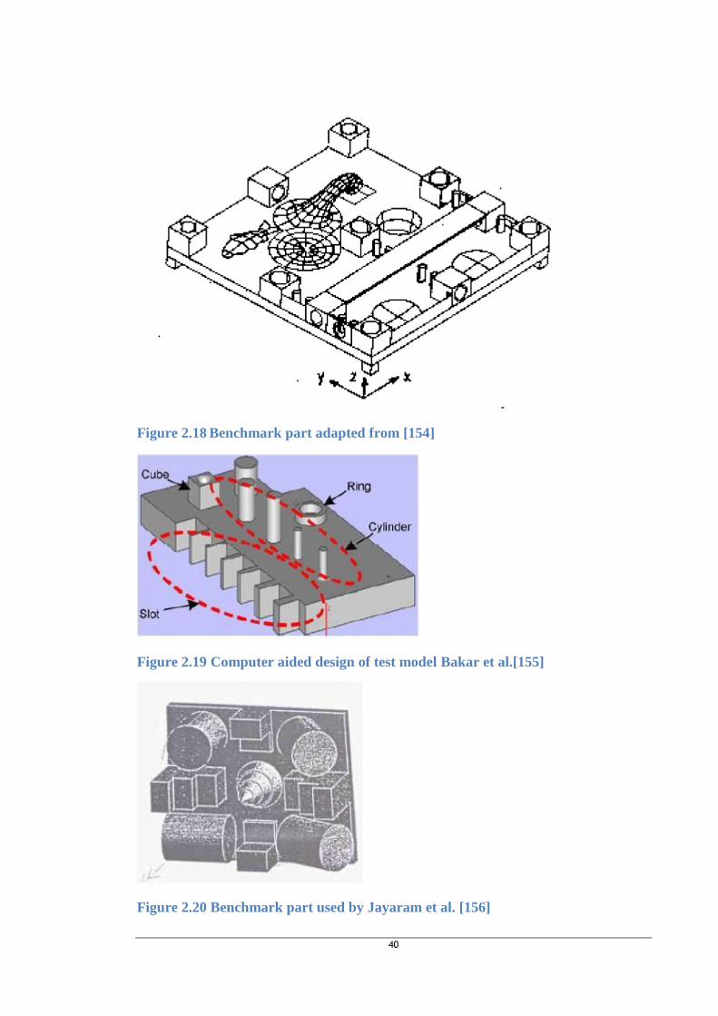
40

Figure 2.18 Benchmark part adapted from [154]

Figure 2.19 Computer aided design of test model Bakar et al.[155]

Figure 2.20 Benchmark part used by Jayaram et al. [156]

41

Figure 2.21 Benchmark part for dimensional accuracy and position of datum axes adapted

from [20]

Figure 2.22 Benchmark part for comparative study adapted from [157]

42

Figure 2.23 Benchmark part used by Ippolito et al. adapted from [158]

Figure 2.24 Isometric view of the test part adapted from [159]

43

Figure 2.25 Benchmark part used by Kruth et al. [149]

Figure 2.26 Benchmark part used by Muhammad and Hopkinson [160]

44

Figure 2.27 Benchmark model used by Shellabear [161]

Figure 2.28 Benchmark part used by Lart [162]

Figure 2.29 Benchmark part used by Sercombe and Hopkinson [163]

45

Table 2.4 Summary of the comparative analysis of the reviewed benchmark

Benchmark Size and remark Performance characteristic Purpose of the benchmark

Justers and Childs

[154]

250 x 250 mm (one fabrication

for each process) (1994)

Linear accuracy, geometric tolerances,

repeatability and resolution

Comparative study of ability of AM systems to produce

some geometry features

Kim and Oh [153] 50 x 100 x 50 mm and ASTM

sample size for mechanical test

(single fabrication for each

process) (2008)

Dimensional accuracy, surface

roughness, mechanical properties,

speed, and material cost

Performance evaluation and comparative study of AM

processes and machines

Dimitrov et al. [20] (190 x 190 x 190) mm (2006) Dimensional and geometrical accuracy Evaluating performance capability of 3D printing process

Mahesh et al. [157] (170 x 170 x 20) mm (2004) Achievable geometrical accuracy Performance characterization of different AM processes

Aubin [159] 6-inches long by 4-inches wide

(1994)

Processing and building time to fabricate

the same part, resolution and accuracy

Characterization of different AM processes with respect

to economic factor and capability

Ippolito et al. [158] (240 x 240 x 36) mm (1995) Dimensional accuracy, tolerance and

surface finish of AM processes

Evaluation of ability of different AM processes to

produce the various features

Kruth et al. [149] 50 x 50 x 9 mm3

(2005)

Accuracy precisions, roughness,

hardness, density and strength

Capability studies of five different laser based AM

machines to produced features

Shellabear [161] (71 x 75 x 52.5) mm (1999) Dimensional accuracy Investigation of capabilities of different AM processes

Jayaram et al.

[156]

-

(1994)

Straightness, parallelism, distortion of

flat surface and accuracy

Provide information about pre-processing, building and

post-processing factors in AM

Bakar et al.[155] -

(2010)

Dimensional accuracy and surface

finished

Determinations of optimum parameters setting that affect

quality for the AM machine studied.

Sercombe and

Hopkinson [163]

(90 x 90 x 105) mm

(2006)

Dimensional accuracy and shrinkage Investigation of process shrinkage and accuracy

Muhammad and

Hopkinson [160]

270 mm x 50 mm

(2012)

Accuracy and repeatability Proposed benchmark part for comparative study of AM

processes

Carolyn et al.[164] -

(2012)

Designed features resolutions with part

thickness, clearances, and build

orientations

Designer's guide for dimensioning and tolerancing parts

for use in SLS process

Proposed

benchmark

L – shape with dimensions given

in section 4.2

Dimensional accuracy, modulus, impact

strength, distortion and repeatability

Process performance stability monitoring and control

from one build to another and qualifying a build

46

It can be observed from Table 2.4 and Figure 2.18 to Figure 2.26 that the

aforementioned benchmark parts are mostly generic benchmark for making comparison

between different AM processes and for checking the process capability for a single

batch or run production on different AM machines and processes, but not for checking

long term performance. In fact, it may not be economically feasible on the long run to

do that with most of those designs. Dimensional measurement of some of the features

will be difficult to make without the use of special equipment like CMM machine which

may be suitable for research and development but may not be easy to be adopt by many

users. They are thus good for performance characterization of AM processes and

machines but may not be suitable for a quick evaluation of process performance. There

is a need of ensuring that measurements and test procedures can be made as quickly as

possible, to enables the use of the results or outputs for checking of any drift in systems

performance or quality management and control.

2.10 Statistical Analysis

2.10.1 Correlation and regression analysis

Analysis of the experimental results was done on Microsoft Excel 2010, MatLab and

Minitab R16 software. Correlation analysis is normally carried out to measure the

strength of relationship between pairs of variables by means of a single variable called

correlation coefficients or Pearson product moment coefficient of correlation [165]. It

thus measures the linear relationship between two random variables X and Y,

represented by r and given by

𝑟 =1

𝑛 − 1∑ (

𝑥𝑖 − 𝑥

𝑠𝑥) (

𝑦𝑖 − 𝑦

𝑠𝑦)

10

Where, 𝑥𝑖 and 𝑦𝑖 are values of the random samples 𝑋𝑖 and 𝑌𝑖 respectively, for 𝑖 =

1, 2, ⋯ , 𝑛 and 𝑛 is the sample size of the population. 𝑥 and 𝑠𝑥 are the means and

standard deviation for x- values, and 𝑦 and 𝑠𝑦 are for the y- values [166]. r assumes a

value between -1 to +1 with a value of r = 0 signifying the absence of linear relationship

but not absence of association. The closer the value is to 1 the greater the linear

correlation. Therefore, if a value is close to 0 it means no linear relationship. If one

variable increases as the other decreases the correlation will be negative but if both

variables tend to increase together the correlation will be positive. Correlation may thus

be low, high, positive, negative or absent [165]. P-value is used for checking if there is

47

enough statistical evidence that the correlation coefficient is not zero and it ranges from

0 to 1 [167]. If the p-value is less than the alpha (α) level (the most commonly used is

0.05) the null hypothesis (no correlation) can be rejected in favour of alternative

hypothesis [167]. Correlation was thus carried between ISO flexural modulus and

density, benchmark modulus and density, density and MFI, Impact strength and MFI

and ISO flexural modulus and impact strength with that of benchmark modulus and

strength to find out the degree of linear relationship between the variables.

2.10.2 ANOVA

Analysis of variance (ANOVA) can be used in situations where more than two groups

are under investigation. ANOVA is good for testing hypotheses of means of multiple

populations (unlike the t- test that is best suited for testing differences between two

means); it was thus adopted to test the hypothesis in this work. The estimates of total

variations due to assignable causes (between group variations) and that due to chance

(within group variations) are obtained independently and compared using F-statistics

and its P-values in order to draw conclusion, about the significant of factors being

investigated. A factor is significant if the P – value is less than the chosen alpha (α)

value [168]. F-statistic is a value obtained from standard statistical test and is used for

comparing variances between the means of two populations. Variation in data in

ANOVA is represented by sum of squares, and is computed as the summation of square

deviations. In addition, the mean square is computed for each source of variation, and is

given as the sum of squares divided by the degree of freedoms. And degree of freedoms

are also computed for each sum of squares, and are N-1 where N is the number of

observations [168]. The details of the ANOVA computation can be obtained from the

referenced statistical books.

Also ANOVA output results using Minitab are divided into two parts. The first part is

the analysis of variance table, where the total sums of squares (SS) are broken down

into two sources: the variation due to factor and variation due to random error [167].

The table consist of source, degree of freedom (DF), sum of squares (SS), mean squares

(MS), F- statistics and P- value. Source is for indication of source of variation which

may be from the factor, the interaction or the error while the total is the sum of all

sources of variations. DF is the degree of freedom from each source. SS is the sum of

squares between groups (factors) and sum of squares within groups (error). MS is

obtained by dividing the sum of squares by the degrees of freedom. F –ratio is given

48

as 𝐹 = 𝑀𝑆 𝐹𝐴𝐶𝑇𝑂𝑅 𝑀𝑆 𝐸𝑅𝑅𝑂𝑅⁄ [167]. The F- ratio will become large if the

variations between factors are larger than variations due to random error. If this occurs

the null hypothesis will have to be rejected, the p- value is use for determining if the F-

ratio is large or not. P-value ranges from 0 to 1 and is the value for the determination of

correctness of accepting or rejecting null hypothesis in a hypothesis test with reference

to the alpha level (𝛼). A commonly use alpha level is 0.05 and 0.01, if the p-value of

the test statistics is less than the chosen alpha value then null hypothesis will have to be

rejected [167] in favour of the alternative hypothesis.

2.10.3 Design of Experiment

Factorial designs of experiment (DOE) are used for simultaneous studies of factors

effects on a process. Lin and Chananda [169] used full- factorial design to obtained

optimal factors with levels that will result into improvement in the quality of injection

-moulding product. In addition, factorial design of DOE methodology is very good in

dealing with several factors in an experiment and it involves joint varying of factor

levels. Also DOE is very efficient in detecting factor effects and interactions between

factors on response value [170]. DOE therefore, saves time and cost of experiments. A

general full factorial experimental design can also be used with factors having any

number of levels. It was therefore, used in FFF experiments since the factors have

multiple levels in order to determine the effect of all combinations of factors on flexural

properties and impact strength.

Experiment plan used consists of experimental runs, blocks, replicates and was

randomized. Randomization is normally used to average out the effects of noise factors

by carrying out the trials in random manner while replication is used for obtaining

experimental error estimate or variability which will be used to check for significant of

factor effects [170]. While blocking is used for reducing or eliminating variability that

may be due to nuisance factors (factors that may influence response which the

experimenter is not directly interested) [170] for example when experiments are

conducted in different day of the week like in case of some of the FFF experiment.

Further detail about DOE methodology can be found in the referenced statistical book

by Montgomery [170].

49

Chapter 3 MECHANICAL TESTING, MATERIALS

CHARACTERISATION, DIMENSIONAL ACCURACY AND SURFACE

ROUGHNESS MEASUREMENT

3.1 Introduction The mechanical properties of a material are a measure of its response to applied load.

Specimens are usually used to carry out the characterization according to various test

standards. As the use of standard test specimens will ensure meaningful and

reproducible test results. In this research, standard test specimens were made using BS

EN ISO and ASTM standards for mechanical properties characterization. Powder

properties characterisations were also carried out for two SLS polymer materials

(Nylon-11 and Nylon-12). Other tests carried out include surface roughness

measurements, imaging and microscopic observation of fracture surfaces, density and

dimensional accuracy measurements. The tests procedures and specimens geometry

were presented in this chapter while the results of various tests will be presented in the

subsequent chapters.

3.2 Powder Characterisation The Melt flow rate (MFR) or melt flow index (MFI) and viscosity of Duraform PA and

Innov PA 1350 ETx powder materials were measured using standard MP600 Extrusion

plastometer (see Figure 3.1) that is equipped with an automatic timing switch (Tinius

Olsen of USA). MFI or MFR is defined as the rate of extrusion of a thermoplastic or

resin through an orifice of standard dimensions under prescribed temperature and

pressure [171].

The test was carried out to ASTM D 1238 – 10 procedures B (Automatically Timed

Flow Rate-type tests) [171]. The procedures involve preheating of the plastometer to a

temperature of 235oC before charging the heated cylinder with a measured quantity of

powder (10 mL, or 4 - 6 g) with the aid of funnel and charging tool. The material is then

extruded under a load of 2.16 kg and weighed with a precision weighing balance

(KERN PFB 200-3) with division size of 0.001g and accuracy +/-0.1%. The value was

then imputed into the machine for the computation of MFI and viscosity. An average of

five measurements was taken for each powder sample and the mean and standard

deviation were then computed. The test was carried out for virgin, refreshed, powder

cake and overflow powders from one build to another.

50

Figure 3.1 Extrusion Plastometer with tools, measuring cylinder and precision weighing balance

3.3 Flexural part geometry and test procedures Flexural test samples were made in accordance with BS EN ISO 178:2010 as shown in

Figure 3.3 and were oriented in X, Y and Z directions as shown in Figure 3.4 (b) to

study the effect of the orientations on mechanical properties. Fifteen specimens with

five oriented in each of the X, Y and Z directions were used in three point bending test

for the flexural properties determination. Tests were conducted using an Instron 4505

electromechanical system at a cross speed of 2 mm/min. This test involves supporting

of specimens between two roller supports and centrally loading the specimen by load

cell until the specimen fracture (see Figure 3.2).

Figure 3.2 (a) Position of test specimen at start of test (adopted from [172]) (b) specimen

positioned during test

Where, F-applied load, R1-radius of loading edge (5 mm ± 0.2 mm), R2- radius of

supports (5 mm ± 0.2 mm), h-thickness of specimens, l-length of specimen, L-length of

span between supports, 1-test specimen.

51

Flexural stress (𝜎𝑓) in three – point bending for a solid beam is given as:

𝜎𝑓 =3𝐹𝐿

2𝑏ℎ2

11

And, flexural strain (𝜀𝑓) is given as:

𝜀𝑓 =6𝑠ℎ

𝐿2

12

Where F is the applied force or load at centre of beam, L is the span; b is the width

and h is the thickness, s is deflection.

Figure 3.3 Five flexural specimen parts with dimensions

Figure 3.4 Build orientations of (a) Notch impact (b) flexural & un-notch impact (c)

tensile test specimens

52

3.4 Tensile part geometry and test procedures Tensile test specimens (Figure 3.5) were made in accordance to BS EN ISO 527-

1:1996 method 1A [173]. The test was then conducted using an Instron 4505

electromechanical system at a cross speed of 2 mm/min with specimens loaded in

tension in machine grips while the axis of specimens aligned to that of the testing

machine until fracture. The specimens were made in a pack of five and oriented in X, Y

and Z-directions.

(a)

(b)

Figure 3.5 (a) Tensile test specimens, all dimensions are in mm (b) tensile testing using

machine

Tensile stress (𝜎) in megapascals was calculated based on the initial cross – area of the

sample as:

𝜎 =𝐹

𝐴

13

Where 𝐹 is the measured load in newton, A is the initial cross –sectional area in square

millimetres

Tensile strain (𝜀) is obtained based on the initial distance between grips and is

calculated as:

𝜀 =∆𝐿0

𝐿0

14

Per cent strain 𝜀 (%) is given as:

𝜀 (%) = 100 ×∆𝐿0

𝐿0

15

Where 𝐿0 is the gauge length in millimetres of the test specimen, ∆𝐿0 is the increase in

the specimen length in millimetres

Z

Y

X

53

Tensile modulus (E) was calculated as:

𝐸 =𝜎2 − 𝜎1

𝜀2 − 𝜀1 16

Where, 𝜎1 is the stress, in mega pascals (MPa) at strain 𝜀1, 𝜎2 is the stress, in mega

pascals (MPa) at strain𝜀2.

3.5 Impact part geometry and test procedures

Izod notch impact test specimens (Figure 3.6) were made also according to ASTM

D256 – 10 Method A [174] and BS EN ISO 180:2001 method A [175]. Tests were then

carried out using the Haida Digital Pendulum Impact tester Model HD -1008 (Figure

3.8) with pendulum capacity of 22 J.

Fifteen specimens were made in a pack of five for SLS materials, singly for FFF

materials and were oriented in X, Y and Z directions as shown in Figure 3.4 (a).

ASTM sample size

ISO sample size

Figure 3.6 Five impact specimen parts with dimensions

The notch profile is as shown in Figure 3.7.

Radius 𝑟𝑁of notch base = 0.25 mm ± 0.05

mm

b = specimen width (10 mm ± 0.2 mm)

𝑏𝑁 = remaining width at notch base (8 mm

± 0.2 mm)

Figure 3.7 Izod notch type A (BS EN ISO 180:2001)

54

The energy absorbed in fracturing the material is obtained from the digital impact

testing machine (Figure 3.8). This is then converted into impact strength in kilojoules

per square metre.

Impact strength in kilojoules per square metre is given by using the Equations 17 and 18

for notched and un-notched specimen respectively.

𝐸𝑖 =𝐸

ℎ × 𝑏𝑁× 103

17

𝐸𝑖 =𝐸

ℎ × 𝑏× 103

18

Where 𝐸𝑖 𝑖𝑠 impact strength in kilojoules per square metre, 𝐸 𝑖𝑠 the impact energy

in joules, h is the thickness in millimetres, b is the width in millimetres and 𝑏𝑁 is the

remaining width under notch in millimetres of the test specimens as shown in Figure 3.7.

(a)

Where, 1. Striking edge, 2. Notch, 3.Vice jaw edge

about which bending takes place 4. Faces of the

jaws in contact with specimen, 5. Fixed vice jaw, 6.

Movable vice jaw

(b)

Figure 3.8 (a) Impact testing machine (b) Vice jaws, test specimen (notched) and

striking edge shown at impact (adapted from [175])

55

3.6 Dimensional accuracies measurement Dimensions of fabricated specimens were measured using Mitutoyo Digital Calliper

with a resolution of 0.01mm. These were then compared with the CAD design to find

out the dimensional accuracy of the process with respect to length, thickness and notch

width from build to build. Deviation is the difference between the nominal dimensions

from that of the measured dimensions which is then converted to percentage change or

percentage deviation by using the formula in equation 19

% 𝑐ℎ𝑎𝑛𝑔𝑒 =|𝐿𝐶𝐴𝐷 − 𝐿𝑀𝐸𝐴|

𝐿𝐶𝐴𝐷× 100

19

Where LCAD is the norminal CAD dimension, and 𝐿𝑀𝐸𝐴 is the absolute value of

measured dimension after the part is made.

3.7 Determination of mass of specimens The weight of tensile, flexural, impact specimens and FFF benchmark specimens were

determine by weighing the fabricated specimens before test with a precision weighing

balance (KERN PFB 200-3) with division size of 0.001g and accuracy +/- 0.1% to

obtain the mass.

3.8 Determination of Density of specimens Approximate density of specimens was computed using equation (20) and from

measured volume. The relationship between density, mass and volume is given as:

𝜌 = 𝑚 𝑣⁄ 20

Where, 𝜌 is the mass density, 𝑚 is the measured specimen mass and 𝑣 is the calculated

volume.

3.9 Imaging and Microscopy

3.9.1 Scanning electron microscopy

Scanning electron examination of fracture surfaces was carried out using a Cambridge

SEM. All the specimens were coated with gold to increase the conductivity of SEM and

prevent charges build up on the specimens during the test and at operating voltage of

8kV to obtain image with high resolution [176].

3.9.2 Specimen preparation and microscopic examination

Internal surfaces were examined with the aid of an optical microscope. Sample

preparation involved the holding of specimens in position in a Buehler Isomet 5000

linear precision saw by the use of the clamping devices and screws, while the saw was

56

fitted with a diamond cutting blade of 0.5 mm thickness. The specimen was then

sectioned by the movement of the cutting blade through specimens at a rotational speed

of 800 rpm and feed rate of 5 mm/min. Cutting fluid was also used during the cutting

process to prevent heat build-up which can lead to damage or deformation of the sample.

Samples were cleaned in water in an ultrasonic bath. Thereafter, the internal structures

of the specimens were then observed by the use of Nikon SMZ 1500 optical microscope.

3.9.3 Replication of fracture surface

CopyRite two- part elastomeric compound was used to produce replica of a fracture

surface in order to see the detailed fracture pattern. The compound enables explicit

reproduction of surface profile by generating a 3 – D surface topography record that is

fit for microscopic examination. The replica dimensional stability is ± 1 micron and the

resolution of the surface detail is <= 1 micron while maximum curing time of the grade

that was used is 30 minutes with a working life of 7 minutes at 25oC [177]. The

replication process involves the application of CopyRite replication medium to the

fracture surface, by the use of twin barrel cartridges, fitted with manually powered static

mixers and then allowed to cure for about 30 minutes before the replica was removed

and then placed under the microscope for examination. The black colour of the

replicating medium enhances contrast during microscopic examination. The replicated

fracture surface was then examined by the use of Nikon SMZ 1500 optical microscope.

3.10 Surface roughness measurement Surface roughness was measured using a Taylor – Hobson (Talysurf) surface texture

measuring instrument and in accordance with BS ISO 4287:1997. It involves movement

of Talysurf stylus tip across the top surface of specimen in order to acquire deviations in

surface profile or to measured roughness of the surface in measurement direction shown

in Figure 3.9. The roughness average of the surface (Ra) is obtained from the machine

output result and is the arithmetic average of the departures of the roughness profile

from the centreline within the evaluation length [178].

𝑅𝑎 =1

𝑙∫ |𝑦(𝑥)|𝑑𝑥

𝑙

0

21

Where, 𝑅𝑎 is the mean roughness of the evaluated surface profile, 𝑦(𝑥) is the height

of the surface profile, and 𝑙 is the sampling length. Three specimens per build were

used for evaluation of surface roughness.

57

(a)

(b)

Figure 3.9 Surface roughness measurement using (a) Talysurf (b) direction of

measurement

58

Chapter 4 QUALITY ASSESSMENT FOR SLS PROCESS This chapter presents a quality system mapping for SLS. It discusses the procedure for

selecting test types for benchmarking part fabrication in polymer based SLS process and

for validating the test results. It then proposes and evaluates new benchmark designs.

4.1 Quality System Mapping for SLS process

4.1.1 Detailed Description of SLS process

An overview of the SLS process was given in Section 2.5.3. Figure 4.1 shows a

flowchart depicting the stages of preparing and executing builds on a polymer laser

sintering station. These are: powder preparation, machine preparation, build process,

cleaning and powder recovery.

Powder preparation

Prior to the start of a building process, powders are placed inside the build cylinder of

the machine. The powder may be virgin powder (powder that has never been used

before), used powder (cake and overflow powders – powders that have been through at

least one SLS production run but un-sintered) or refreshed powders (a mix of virgin and

previously used but un-sintered powders). A typical refresh rate is 70% used powder to

30% virgin.

Machine preparation

This entails the cleaning of the internal chamber, laser window, infra-red heat sensors,

roller assembly, and slicing of the part CAD model (as shown in Figure 2.1) using SLS

machine software. The sliced contour data is then sent to SLS machine for the parts

building process, and the various parts positioned in the build. This also includes file

preparation on the machine software which involves setting of process parameters such

as laser power, part bed temperature, part orientations among others and also collision

detection for checking if parts will collide or be fused with neighbouring part(s) during

sintering operation which is very important when multiple parts are to be made in a

build.

Build/layering process

The three stages of the building process are the warm-up stage; build stage and cooling

down stage. The warm-up stage involves gradual preheating of the process chamber and

59

part bed temperature to a temperature close to the melting temperature of the powder.

At the build stage, some powder is further heated by the laser based on the sliced

contour data that was sent to the machine, this is repeated layer by layer until the whole

parts or components are made.

At the end of layering process, the sintered parts and un-sintered powders (cake and

over flow) stay in the build chamber until they have cooled down.

Cleaning and powder recovery

At the end of cooling down stage, the sintered parts are then removed from powder cake

and cleaned by air blast or brush. Powders in the overflow bins are then emptied. Un-

sintered powders (cake and overflow) are sieved and stored for further part fabrication.

Loose powder on the surface in process chamber is also vacuumed. Other post finishing

processes such as polishing, painting, coating and metallizing could be carried out on

the sintered part before delivery to client or customer.

60

File preparation on machine software

Parameters

Orientation

Collision detection

Clean machine,

laser lens, infra-

red heat detector

sensor

Supply powder to

build chamber,

prepare system

Warm up stage

Pre-heating

Build stage

layering

Cooling down

stage < Tg

Sintering/layering process

Remove sintered

products from un-

sintered powder

Overflow powders

Un-sintered

powder (cake)

Sintered products

Part cleaning

Sieve and place

respective powders in

separate cover

containers

Post processing/

finishing e.g.

coating, painting

etc.

Visual inspection

of products

Product storage

and delivery to

customer

Powders storage

Virgin powder

Virgin powder

Overflow powder

Powder cake

Mix & recycle

powders based on

weight ratio

Input

OutputInput

1.1

1.2

3.0 3.1 3.2

3.4

3.3

3.5

1.0

3.6

4.0

2.2

4.34.4

Clean products

2.1

4.1

4.2

CAD Design &

STL export

2.0

Figure 4.1 Process mapping for polymer based SLS process

61

4.2 Identification of Potential Input and Output Quality Measures

4.2.1 Requirements for a quality assurance (QA) test

Quality assurance (QA) involves the use of resources. There is thus need to ensure that

QA tests are simple, small, reliable, cheap and capable of being carried out quickly.

There is also a need for the tests to be rapid, which for practical purposes we have

interpreted as meaning it should take 5 – 10 minutes to perform all the tests at the end of

a build. The aforementioned requirements were taken into consideration in design of the

QA test parts.

4.2.2 Evaluation of Possible QA Tests

Most of the quality problems that are experienced in AM are due to material and

process parameters. There is thus need for input measure in QA test to ensure that input

material quality is appropriate. The use of inappropriate or excessive degraded input

material will lead to deterioration in the quality of fabricated parts. Similarly, output

measures are needed to ensure that the process has been executed correctly. Both

measures are therefore needed to ensure that quality parts are made by the process from

one production run to another.

The input measure for SLS process can be taken at point 1.0 when virgin material is

supplied and at point 1.2 when powders are refreshed and ready to be supply to the

build chamber as shown in Figure 4.1. In addition, molecular weight is an important

properties for characterization of polymers [179], and can be inferred from the melt

viscosity [52]. Therefore, the potential input quality measure is the MFI of input

material to SLS process.

Output measures can be taken at point 4.1 which is at end of the sintering process and

after cleaning of the sintered part by air blast as shown in Figure 4.1.

In Table 2.3 it was noted that the quality characteristics of a part made by AM depend

on surface finish, dimensional accuracy and strength [119-121]. Therefore, quality

assurance tests should be able to evaluate such quality characteristics for it to be a good

measure of quality.

In the case of potential output measure, impact and bending tests have been selected.

The reason behind their selection is based on the hypothesis that an inadequate or weak

bonding between sintered powder layers will result in weak interlayer bonding which

62

may result in low strength of impact test parts and a reduction in bending modulus or

stiffness for bending test part. In addition, density and dimensional accuracy were also

selected. This is due to the fact that the presence of porosity is detrimental to

mechanical properties of sintered parts [180, 181]. Pores are form in SLS fabricated

parts as a result of inhomogeneous heat distribution in build envelopes, insufficient heat

from laser and inadequate process temperature [74, 95]. As the presence of porosity or

voids will decrease the effective area of the sintered part, and hence lower strength and

bending stiffness of low density part. Therefore, increase in densification of sintered

part will be due to more effective coalescing of powder particles with resultant increase

in degree of particle melt. As the presence of un-fused powder particles and voids will

leads to stress concentration and increased the probability of crack initiation [33] and

propagation through the materials. Similarly, inaccuracy due to shrinkage needs to be

control, and this is done by calibrating and compensating for it. Calibration of beam

offset and shrinkage is usually carried out at regular interval or whenever there is a

change of SLS material and laser power. Dimensional accuracy was therefore selected

as an indicator of machine calibration. This is because if the machine is calibrated

properly and if there is no drift in machine calibration due to ageing of the optics that

controls the deflection of laser scan (scanning mirror) and laser window (protective

cover between the laser housing and process chamber). And if input material is of good

quality, then there should be insignificant difference in accuracy of fabricated parts

made in multiple builds.

4.3 Proposed Quality System and Benchmark parts for SLS

4.3.1 Proposed Quality System

The quality system proposed, for use in SLS process is presented in Figure 4.2. The

quality system incorporates proposed input and output quality measures in addition to

powder management and control. The tests in the quality system are:

Input quality test

MFI test for investigating the quality of input powder material before being used

in SLS process. The polymer powder types that should be tested are: virgin

powder after being received from the supplier or before storage and use, cake

and overflow powder after each build or periodically and refreshed powder

before being used in SLS machine.

63

Output quality test

A benchmark part should also be added to every build and tested at the end of

the build for impact strength, density, dimensional accuracy and bending

stiffness.

The detailed procedures for using the benchmark specimens are presented in Section

4.3.2. Thereafter, tests results should be stored in a database and analysed using

statistical tool like descriptive statistics and the SPC for quality trends and long term

quality monitoring and control.

64

Measure

1. Dimensions

2. Mass

Benchmark

part after

every build

Determine

1. Impact strength

2. Density

3. Accuracy

4. Modulus

Database

Plot control

chart: Ẋ-R

Sign of special cause

of variation?

No

Process

improvement

needed

Yes

(a) find out what have change.

(b) Take corrective action.

(c) Remove data or group that is

the source of special variation

Yes NoIs the Process

Average and Spread

acceptable?

Inspect for

distortion &

surface finish

Check if the groove is

made successfully

Inspection & Measurement after ever build

Post- measurement

analysis/ Quality assurance

SL

process

Fabricated

part

Visual

inspection of

part

Satisfactory?Yes

Rebuild/

remake

No

Finalized

product

description

Measure MFI

of powder

Is it within the

specified range?

Allocate tag/label to

ensure powder traceability

& store in temperature

control room

Discard

powder

Yes

No

Post

processing

e.g. coating

Powder management and control

Design product

CAD model &

Test part CAD

model

Product

storage &

delivery to

customer

Product check

2.12.6

4.1

2.61

2.62

2.63

2.642.65

2.66

4.3

2.7

2.71

2.72

2.73

2.74

2.75

2.76

2.77

2.78 4.24.4

1.0

1.1

1.2

2.79

2.8

Virgin powder

Used powders

Refreshed powders

2.9

Customer

specifications

Figure 4.2 Tentative Quality System for Polymer based SLS process

65

4.3.2 Proposed Benchmark parts

Two benchmark sample designs were developed in this study (Benchmark 1 and

Benchmark 2 as shown in Figure 4.3). They are patterned after ASTM and ISO designs

for bending modulus test part and impact strength, with each “arm” of the specimens

designed for either impact test or cantilever bend test. The two benchmark samples were

designed as a single piece with a parting notch (a) of 2 mm as shown in Figure 4.3 to

aid the later separation and for ease of locating specimen after build (which may add to

the time required to make a test) and also for checking of process resolution. Similarly,

the notch (b) of 5 mm towards the end of the of the bending specimen (see Figure 4.3) is

for loading the specimen and is also used for checking the ability of the process in

making notch from build to build. Benchmark 1 was patterned after the ASTM standard

testing method ASTM D256 – 10 Method A [174] sample size for the impact sample

while the flexural test sample size was based on ASTM D790-10 [182] for flexural

samples. Similarly, Benchmark 2 was patterned after ISO standard testing method BS

EN ISO 180:2001 method A [175] sample size for the impact sample while the bending

sample size was based on BS EN ISO 178:2010 [183] for flexural samples. Two

benchmark parts were used to find out which was most sensitive to variations in

materials and processing conditions and to investigate the effect of geometry on the test

results. The benchmark parts can specifically be used to check for warpage or flatness,

the ability to make the slot, surface roughness, dimensional accuracy, straightness,

repeatability, bending stiffness and strength.

The procedures for using the proposed benchmark are presented below:

1. The benchmark part should be added to every build and on completion of the

building process; the benchmark sample should be examined to see if it was

successfully made.

2. The length, width, thickness and notch width of the benchmark parts should be

measured.

3. The mass of the benchmark specimens should be measured and their densities

determined from the measured mass and measured dimensions.

4. Use the benchmark part to determine the bending modulus and impact strength,

using the methods outlined in Sections 3.5 and 4.4.3.

5. Store all results in a database for future statistical analysis.

66

Figure 4.3 and Figure 4.4 shows the designs for Benchmark 1 and Benchmark 2

samples with their dimensions all in millimetres.

Figure 4.3 the geometrical design for Benchmark 1 and Benchmark 2

Figure 4.4 Proposed Benchmark part

4.3.3 Selection of Tests for Validation of Benchmarks parts

In order to validate the benchmark part test results ISO samples for impact and flexural

tests were made in the same build (with the test conducted according to the respective

standard specifications as described in Sections 3.3 and 3.5).

67

4.4 Materials and Methods

4.4.1 Experimental procedures for Nylon 12

Overall approach for Nylon 12

Two batches of Duraform PA 12 powders were collected for quality evaluation (melt

flow rate test) before being used to fabricate parts in four builds. Forty five ISO

designed impact, flexural and tensile specimens, with five specimens each oriented in X,

Y and Z directions as shown in Figure 3.4 were made from virgin powder in the first

build. Each build one also had fifteen benchmark 1 (BM 1) and fifteen benchmark 2

(BM 2) specimens with five each oriented in X, Y and Z-directions as shown in Figure

4.6. Build two still have fifteen impact test “arm” and fifteen flexural test “arm”

benchmark 2 specimens while benchmark one have fifteen flexural test “arm” and three

X- oriented impact test “arm” specimens (the remaining impact specimens were not

made successfully. It was later decided with the industrial partner (Peacock Medical

Group) to this research that only X-oriented specimens should henceforth be made to

save cost in terms of material utilization and build time. The subsequent three builds

consisted of X- oriented benchmark specimens only. The breakdown of total number of

ISO designed specimens and benchmark specimens are presented in Table 4.1. One

hundred and sixty three benchmark specimens and forty five ISO specimens all made

from Duraform PA 12 were involved in this experiment. However, it can be observed

from the table that after the first build with five specimens for each studied orientations

and test types unequal number of specimens were supplied by the industrial partner to

this research. This inequality in the number of benchmark flexural and impact

specimens test parts per build in that table were due to non-supplied of un-successfully

made benchmark test parts. This explained the reason for having unequal number of

specimens per build for both benchmark impact and bending specimens.

Table 4.1 Number of specimens by builds and specimen types (Duraform PA 12)

Build

number

Number of BM 1

specimens

Number of BM 2

specimens

Number of ISO specimens

Flexural

test

Impact

test

Flexural

test

Impact

test

Flexural

test

Impact

test

Tensile

test

1 15 15 15 15 15 15 15

2 15 3 15 15

3 5 3 5 7

4 5 3 5 7

5 4 1 4 6

68

Nylon 12 SLS specimens were supplied by Peacocks Medical Group, made in Duraform

PA material (Nylon 12), using a 3D Systems sProSD SLS machine, and with the

processing conditions shown in Table 4.2.

Table 4.2 SLS process parameters for parts supplied by Peacocks Medical Group

Also, at Peacock Medical Group, powders were collected from different builds with

different thermal histories and then analysed with the parts that were made from the

builds. The powders were evaluated for their MFI.

Powders were assigned a label consisting of blend number for traceability. The

collections include the following set of powders:

Virgin: powder is fresh powder.

Overflow powder: powder from overflow bins.

Cake powder: powder from part bed after usage (powder cake).

Refreshed powder: a mix of 33% virgin, 33% cake and 33% overflow powder.

The blend number is the number of times the overflow and cake powders had been used

e.g. if the powder was obtained from first runs the build number is one (1) but if it was

obtained from second build then build number is two (2) and so on. Powders sample

collected with labels are shown in Figure 4.5.

Figure 4.5 Refreshed, overflow and part cake powders with label

Equipment 3D Systems sPro60SD

Laser power 12 W Outline laser power 6 W Fill scan spacing 0.15 mm Laser scan strategy Cross Fill Scanning Layer thickness 0.1 mm Scan speed 5 m/s

69

The specimen’s placement and orientation in the build for both benchmark 1 and 2

specimens are as shown in Figure 4.6.

Figure 4.6 Build orientations of Benchmark (a) 1 (b) 2

4.4.2 Experimental procedures for Nylon -11

Overall approach for Nylon 11

At the end of the use of nylon 12 by the company and on introduction of nylon 11

material for part fabrication, it was agreed that the benchmark specimen should be

reduced to three specimens per build, since those specimens will give the same

mechanical property characterization over multiple builds that we want to do and also

reduce the cost of the experiments. This explained the reason why there are 3

benchmark specimens per build with the exception of second build where 4 benchmark

specimens were made as shown in Table 4.3.

Powders were collected from thirteen builds. No specimens were made in the first build

and build five, but the second build consisted of forty five ISO designed impact,

flexural and tensile specimens, with five specimens each oriented in X, Y and Z

directions as shown in Figure 3.4. The second build also had eight X-oriented

benchmark 1 and benchmark 2 specimens with four specimens for each benchmark type.

Benchmark specimens oriented in the X-direction only were also made in each of the

subsequent builds, with three specimens for each benchmark type. However, build 11

also had five X-oriented tensile specimens in addition to the benchmark specimens.

The total number of specimens made from Nylon 11 tested is one hundred and eighty

six. The breakdown of the specimens involved for both benchmark specimens and ISO

design specimens are as presented in Table 4.3.

70

Table 4.3 Number of specimens by builds and specimen types (Nylon 11)

Build number Number of BM 1

specimens

Number of BM 2

specimens

Number of ISO specimens

Flexural

test

Impact

test

Flexural

test

Impact

test

Flexural

test

Impact

test

Tensile

test

2 4 4 4 4 15 15 15

3 3 3 3 3

4 3 3 3 3

6 3 3 3 3

7 3 3 3 3

8 3 3 3 3

9 3 3 3 3

10 3 3 3 3

11 3 3 3 3 5

12 3 3 3 3

13 3 3 3 3

Specimens were again sourced from Peacocks Medical Group, made in Innov PA 1350

ETx (Nylon 11) material supplied by EXCELTEC (France) using 3D Systems sProSD

SLS machine, and with the processing conditions shown in Table 4.4.

Table 4.4 SLS process parameters for parts supplied by Peacocks Medical Group (Nylon PA 11)

At Peacocks Medical Group, powders were collected from different builds with

different thermal histories and then analysed with the parts that were made from the

builds. The powders were evaluated for MFI.

Powders were collected before and after a build and assigned a label consisting of blend

number for traceability. As before the collections included virgin, overflow, cake and

refreshed powders. However, in this case the refreshed powder was a mix of 29% virgin,

Equipment 3D Systems sPro60SD

Laser power 20 W Outline laser power 7 W Fill scan spacing 0.15 mm Laser scan strategy Sorted fill Layer thickness 0.1 mm Scan speed 5 m/s

71

and 71% (cake and overflow) powders. The 71% (cake and overflow powders) were a

mix of the left over powders after the respective build.

4.4.3 Test Procedures for SLS Benchmark parts

Samples were tested using a purpose built jig. The flexural testing procedures involved

placing the benchmark sample in bottom block with a groove that fitted the geometry of

the sample and then placing of the top block on the sample such that the benchmark

sample is sandwiched between the top and the bottom block of the jig. Detail design of

the jig is provided in the appendix A.

Figure 4.7 Positioning of the specimen during bending (b) assembly with parts

The two halves were then clamped together in position with the aid of aluminium plate,

using two 100 mm M10 bolts and wing nuts. A Digital dial gauge was clamped

vertically with M6 bolts into sliding horizontal brackets whose position can be adjusted

based on the length of the beam. Loads of 100g and 150g were sequentially suspended

from the beam and readings of deflection for each load were then taken using the digital

indicator. The data obtained was then used to compute the modulus for the beam. The

setup with free body diagram is as shown in Figure 4.8.

Considering the benchmark sample as cantilever beam of length L (distance from fixed

end A to free end C) carrying a concentrated load at distance 𝑙2 from the fixed end,

while 𝑙1 is the distance from fixed end to the position of the dial gauge as shown in

Figure 4.8.

72

Figure 4.8 Free body diagram for the bending specimen under the action of load

Where 𝑊 = Applied load, y = displacement of the beam at B due to W, I is the moment

of inertia of the beam, 𝑅𝑣 and 𝑅𝐻 are the vertical and horizontal reaction forces

respectfully and E is the bending or flexural modulus.

The deflection at point B is given by:

y =W

2EI(𝑙2𝑙1

2 −𝑙1

3

3)

22

So the bending modulus is given by:

E = (∆W

∆y) (

𝑙12

2𝐼) (𝑙2 −

𝑙1

3)

23

4.5 Nylon 12 Results and analysis

4.5.1 Benchmark Validation against ISO Tests in Virgin Powder Build

(Duraform PA 12)

Figure 4.9 shows the variation of flexural modulus of ISO and benchmark specimens in

the same build 1 with orientations of specimens. BM 1 and BM 2 represents benchmark

1 and 2 respectively. Interestingly the results show greater variability (assessed by min-

max range within a single orientation and by differences between the orientations) in the

ISO test specimens than in the benchmark tests.

73

Figure 4.9 Variation of ISO and benchmark flexural modulus with orientations

(Duraform PA 12) within a single build

4.5.2 ISO flexural modulus versus benchmark flexural modulus (Duraform PA

12)

Figure 4.10 shows the overall correlation between the flexural modulus of the benchmark

specimens and ISO specimens in the same build 1. The correlation coefficients and p-

values are also shown on the figure. The correlation is reduced by the variation in ISO

test results and in BM 2 –Y, as shown in Figure 4.9.

Figure 4.10 Correlation between ISO flexural modulus and benchmark flexural

modulus (Duraform PA 12)

0

200

400

600

800

1000

1200

1400

1600

1800

ISO- X ISO-Y ISO-Z BM 1-X BM 1-Y BM 1-Z BM 2-X BM 2-Y BM 2-Z

Fle

xura

l mo

du

lus

(MP

a)

Specimen types

13501300125012001150110010501000

2000

1800

1600

1400

1200

1000

Benchmark flexural modlus (MPa)

ISO

Fle

xu

ral m

od

ulu

s (

MP

a)

BM 1

BM 2

Variable

BM 1 X

BM 1 Y

BM 1 Z

BM 2 X

BM 2 Y

BM 2 Z

Variable Orientations

r = 0

.841

(p<

0.0

1)

r = 0.84

3 (p<

0.01

)

74

Figure 4.11 shows the variation of densities of the ISO flexural modulus and benchmark

modulus test specimens results presented in Figure 4.9 with orientations.

Figure 4.11 Variation of flexural modulus specimen densities with orientations (Nylon 12)

within a single build

There is less variability in densities of flexural modulus X- , Y- oriented specimens as

compared to Z-oriented specimens for both ISO and benchmark specimens.

Figure 4.12 shows correlation between ISO flexural modulus and density of the flexural

modulus specimens. The correlation coefficient and its p-value are also shown.

Figure 4.12 Correlation between ISO flexural modulus and their densities (Duraform PA

12)

0

0.1

0.2

0.3

0.4

0.5

0.6

0.7

0.8

0.9

1

ISO- X ISO-Y ISO-Z BM 1-X

BM 1-Y

BM 1-Z

BM 2-X

BM 2-Y

BM 2-Z

De

nsi

ty o

f fl

ex.

mo

du

lus

spe

cim

en

s (g

/cm

^3)

Specimen types

0.950.900.850.800.75

1700

1600

1500

1400

1300

1200

1100

1000

900

Density of flexural modulus test specimens ( g/cm^3)

ISO

Fle

xu

ral m

od

ulu

s (

MP

a)

X

Y

Z

Orientations

r= 0.974

(p< 0.01)

75

Figure 4.13 shows the relationship between the benchmark flexural modulus and

densities of the benchmark test specimens made in the first build. There seems to be

clear relationship apart from the BM 2 – Y and BM 1 – Y specimens, which appear as

outliers.

Figure 4.13 Correlation between Benchmark modulus and benchmark densities

(Duraform PA 12)

4.5.3 ISO Impact strength versus benchmark Impact strength for Duraform

PA 12

Figure 4.14 shows the variation of impact strengths of ISO and benchmark specimens in

the same build 1 with orientations of specimens.

0.950.900.850.800.75

1350

1300

1250

1200

1150

1100

1050

1000

Benchmark density (g/cm^3)

Be

nch

ma

rk m

od

ulu

s (

MP

a)

Flex B.1 modulus X

Flex B.1 modulus Y

Flex B.1 modulus Z

Flex B.2 modulus X

Flex B.2 modulus Y

Flex B.2 modulus Z


76

Figure 4.14 Variations of Impact strength of ISO and benchmark specimens with

orientations (Duraform PA 12) within a single build

Similarly, Figure 4.15 shows the correlation between impact strengths of benchmark and

ISO specimens made in the same build 1. The correlation coefficients and p-values are

also shown for respective specimens. It is clear that the lack of anisotropy shown by

benchmark 1 reduces the correlation between its results and the ISO test parts.

Figure 4.15 Correlation between ISO Impact strength and Benchmark impact

strength (Duraform PA 12)

0

1

2

3

4

5

6

7

ISO- X ISO-Y ISO-Z BM 1-X

BM 1-Y

BM 1-Z

BM 2-X

BM 2-Y

BM 2-Z

Imp

act

stre

ngh

(kJ

/m^2

)

Specimen types

5.55.04.54.03.5

6.5

6.0

5.5

5.0

4.5

4.0

Benchmark impact strength (kJ/m^2)

ISO

im

pa

ct

str

en

gth

(kJ/

m^

2)

BM 1

BM 2

Variable

BM 1 X

BM 1 Y

BM 1 Z

BM 2 X

BM 2 Y

BM 2 Z


r = 0

.955

(p< 0

.01)

r =

0.87

5 (p< 0

.01)

77

4.5.4 Input Powder Property Variations over Multiple Builds (Duraform PA 12

powders)

MFI of two batches of powders

Two batches of Duraform PA 12 powders were evaluated from one build to another and

the MFI variations with repeated exposure to thermal history are presented in Figure

4.16. The first build consist of only virgin powder and the following builds refreshed

powders.

Figure 4.16 Variations of Duraform PA 12 powders MFI with builds for two powder

batches, the graph shows the mean, median, lower and third quartile of the data.

The refreshed rate of the powders in each build is given as follows:

1 = virgin powder

2 = 33 % virgin, 33% overflow (build 1), 33% cake (build 1)



While B.1 represent first batch, B.2 represent second batch and Bld represent build of

the used powders respectively. Overflow and cake powders are taken from previous

build and added to virgin powder to make new build powder.

The following can be observed from Figure 4.16:

MFI drops with powder re-use.

MFI B.2 (B

ld- 4

)_ov

erflo

w

MFI B.2 (B

ld- 3

)_ov

erflo

w

MFI B.2 (B

ld- 2

)_ov

erflo

w

MFI B.2 (B

ld- 4)

_cak

e

MFI B.2 (B

ld- 3)_c

ake

MFI B.2 (B

ld- 2

)- cak

e

MFI B.2 (Bld-

4)

MFI B.2 (Bld- 3)

MFI B.2 (Bld-

2)

MFI B.2 (Virg

in)

MFI B.1 (Bld-

4)

MFI B.1 (Bld- 3)

MFI B.1 (Bld-

2)

MFI B.1 (Virgin)

60

55

50

45

40

35

30

MFI

(g

/1

0 m

in)

Batch 1Batch 2

78

The drop is not consistent from batch to batch. Batch 2 drops more gradually

than batch 1, but after four builds ends up at a similar level.

4.5.5 Mechanical Property Variation over Multiple Builds (Duraform PA 12)

Comparison and correlation were carried out in the subsequent sections to find out if

relationships exist between the studied mechanical properties of benchmark specimens

and MFI of powder used in fabricating them in multiple builds.

4.5.6 Variation of flexural modulus and impact strengths with builds and

benchmark for Duraform PA 12

Figure 4.17 shows the variation of impact strength of Benchmark 1 and Benchmark 2

specimens with numbers of build. Where, BM 1 represent benchmark 1, BM 2 represent

benchmark 2 and Bld represent build of the used powders respectively.

Figure 4.17 Impact strengths variations with builds (Duraform PA 12), the graph

shows the mean, median, lower limit, upper limit, first and third quartile

Figure 4.18 shows the variation of Benchmark average flexural modulus and average

densities of benchmark flexural modulus specimens with number of builds. It also

shows that both the density and the flexural modulus gradually decrease with increasing

builds.

BM 2 (B

ld 5)

BM 2 (B

ld 4)

BM 2 (B

ld 3)

BM 2 (B

ld 2)

BM 2 (B

ld 1)

BM 1 (B

ld 5)

BM 1 (B

ld 4)

BM 1 (B

ld 3)

BM 1 (B

ld 2)

BM 1 (B

ld 1)

7.0

6.5

6.0

5.5

5.0

4.5

4.0

Numbers of build and specimen types

Be

nch

ma

rk I

mp

act

str

en

gth

(kJ/

m^

2)

Benchmark 1 Benchmark 2

79

Figure 4.18 Variations of flexural modulus and densities of Benchmark 2 with builds

(Duraform PA 12), error bars in the figure represent standard deviation of the mean.

Figure 4.19 shows the variation of benchmark average impact strengths and average

densities of benchmark impact strength specimens with number of builds.

Figure 4.19 Variations of impact strength and densities of Benchmark 2 with builds

(Duraform PA 12), error bars in the figure represent standard deviation of the mean

4.5.7 Modulus and density correlation for Duraform PA 12

Figure 4.20 shows the correlation between average flexural modulus and average

density of benchmark flexural modulus made in different builds.

0.4

0.45

0.5

0.55

0.6

0.65

0.7

0.75

0.8

0.85

0.9

0

200

400

600

800

1000

1200

1400

1600

1 2 3 4 5 6

De

nsi

ty in

g/c

m^3

Fle

xura

l mo

du

lus

(MP

a)

Number of builds

Flexural modulus benchmark 2 Benchmark 2 densities

0.4

0.5

0.6

0.7

0.8

0.9

1

0.49

1.49

2.49

3.49

4.49

5.49

6.49

7.49

1 2 3 4 5

De

nsi

ty in

g/c

m^3

Imp

act

stre

ngt

h (

kJ/m

^2)

Number of builds

Impact strength benchmark 2 Benchmark 2 densities

80

Figure 4.20 Correlation between Flexural modulus and densities of Benchmark

specimens (Duraform PA 12) across multiple builds, error bars in the figure

represent standard deviation of the mean

4.5.8 MFI and density correlation for Duraform PA 12

Figure 4.21 shows the correlation between average MFI of refreshed powders from

different builds and average densities of benchmark specimens made from those

powders. The correlation coefficients for Benchmark 1 (BM 1) and Benchmark 2 (BM 2)

with respective p-values are also shown in the figure.

0.74 0.76 0.78 0.8 0.82 0.84 0.86 0.88 0.9 0.92900

950

1000

1050

1100

1150

1200

1250

1300

1350

1400

Average density of Benchmark flexural modulus (g/cm3)

Avera

ge B

en

ch

mark

fle

xu

ral

mo

du

lus (

MP

a)

BM 1

BM 2

r = 0.932 (p< 0.05)

r = 0.895 (p< 0.05)

81

Figure 4.21 Correlation between MFI and densities of Benchmark specimens

(Duraform PA 12) across multiple builds, error bars in the figure represent standard

deviation of the mean

4.5.9 MFI and impact strength correlation for Duraform PA 12

Figure 4.22 shows the correlation between average impact strengths of benchmark

specimens in the different builds and average MFI per build. The correlation

coefficients with p-values and error bars are also shown for each benchmark type.

0.74 0.76 0.78 0.8 0.82 0.84 0.86 0.88 0.9 0.9235

40

45

50

55

60


Avera

ge M

FI

(g/1

0 m

in)

BM 1

BM 2

r = 0.969 (p< 0.05)

r = 0.974 (p < 0.05)

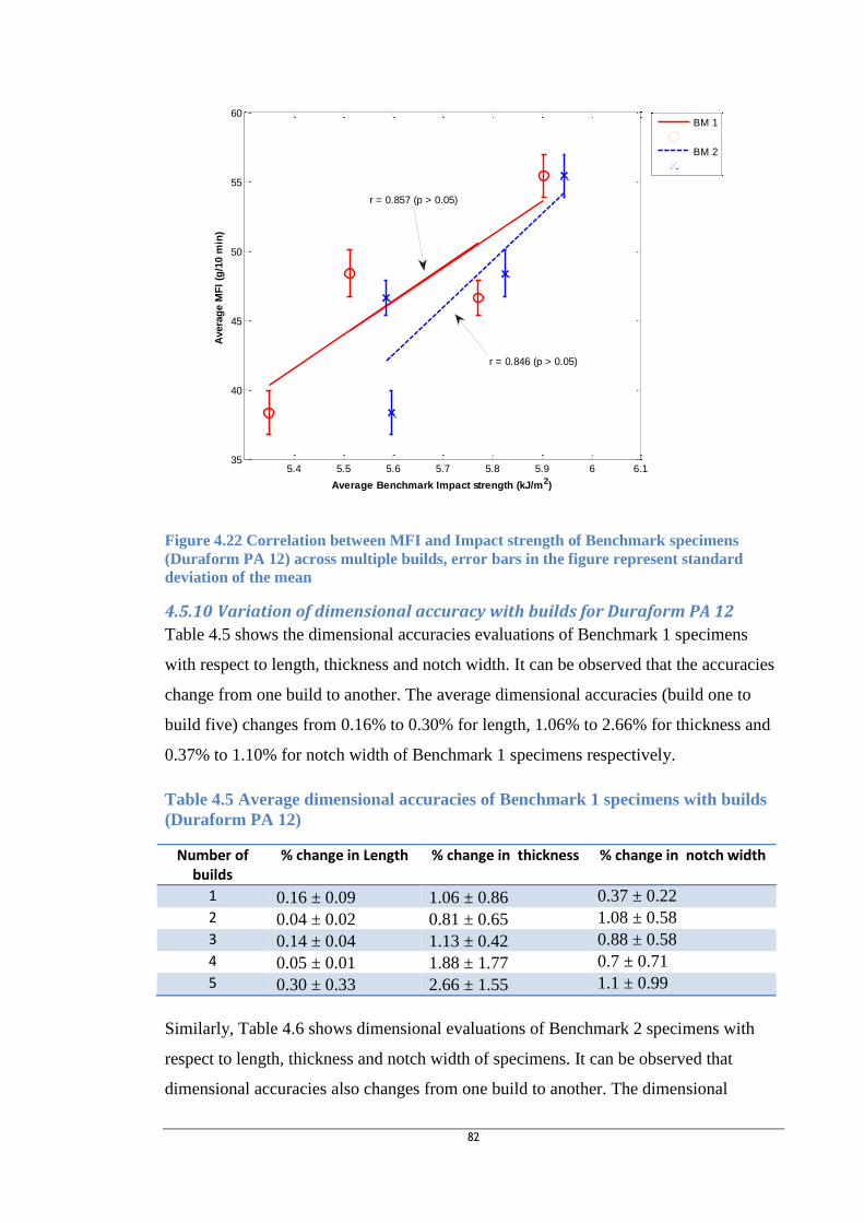
82

Figure 4.22 Correlation between MFI and Impact strength of Benchmark specimens

(Duraform PA 12) across multiple builds, error bars in the figure represent standard


4.5.10 Variation of dimensional accuracy with builds for Duraform PA 12

Table 4.5 shows the dimensional accuracies evaluations of Benchmark 1 specimens

with respect to length, thickness and notch width. It can be observed that the accuracies

change from one build to another. The average dimensional accuracies (build one to

build five) changes from 0.16% to 0.30% for length, 1.06% to 2.66% for thickness and

0.37% to 1.10% for notch width of Benchmark 1 specimens respectively.

Table 4.5 Average dimensional accuracies of Benchmark 1 specimens with builds

(Duraform PA 12)

Number of builds

% change in Length % change in thickness % change in notch width

1 0.16 ± 0.09 1.06 ± 0.86 0.37 ± 0.22

2 0.04 ± 0.02 0.81 ± 0.65 1.08 ± 0.58

3 0.14 ± 0.04 1.13 ± 0.42 0.88 ± 0.58

4 0.05 ± 0.01 1.88 ± 1.77 0.7 ± 0.71

5 0.30 ± 0.33 2.66 ± 1.55 1.1 ± 0.99

Similarly, Table 4.6 shows dimensional evaluations of Benchmark 2 specimens with

respect to length, thickness and notch width of specimens. It can be observed that

dimensional accuracies also changes from one build to another. The dimensional

5.4 5.5 5.6 5.7 5.8 5.9 6 6.135

40

45

50

55

60

Average Benchmark Impact strength (kJ/m2)

Avera

ge M

FI

(g/1

0 m

in)

BM 1

BM 2

r = 0.857 (p > 0.05)

r = 0.846 (p > 0.05)

83

accuracies (build 1 to build 5) changes from 0.14% to 0.43% for length, 0.95% to 2.50%

for thickness and 0.72% to 2% for notch width of Benchmark 2 specimens respectively.

Table 4.6 Average dimensional accuracy of Benchmark 2 specimens with builds

(Duraform PA 12)

Build number % change in Length % change in thickness % change in notch width

1 0.14 ± 0.05 0.95 ± 0.33 0.72 ± 0.24

2 0.12 ± 0.02 1.25 ± 0.71 0.40 ± 0.32

3 0.07 ± 0.02 1.05 ± 0.94 1.48 ± 0.63

4 0.10 ± 0.11 2.38 ± 0.18 1.30 ± 0.99

5 0.43 ± 0.29 2.50 ± 0.71 2.00 ± 1.41

4.5.11 Summary of Nylon 12 Results

From Figure 4.10, Figure 4.12 and Figure 4.13 it was observed that specimen density is

a better predictor of ISO flexural modulus than benchmark flexural modulus.

Benchmark impact strength correlates well with ISO impact strength (see Figure 4.15).

It can also be observed from Figure 4.20 and Figure 4.21 that density correlates well

with modulus over multiple builds, as does MFI. Similarly, impact strength and MFI

correlate less well (Figure 4.22), while dimensional accuracies can also be observed to

vary with builds with the last build having the least accuracy.

4.6 Nylon 11 Results and Analysis

4.6.1 Benchmark Validation against ISO Tests in Virgin Powder Build (Innov

PA 1350 ETX)

Figure 4.23 shows the flexural modulus of ISO and benchmark specimens in the same

build 2 with their respective orientations. X-oriented benchmark specimens only were

made in that build.

84

Figure 4.23 Variation of ISO and Benchmark flexural modulus with orientation (Innov PA

1350 ETx) within a single build

4.6.2 ISO flexural modulus versus benchmark flexural modulus (Innov PA

1350 ETx)

Figure 4.24 shows the correlation between flexural modulus of ISO specimens and

benchmark specimens in the same build 2. The correlation coefficients and the p-values

for each benchmark type are also shown.

Figure 4.24 Correlation between ISO and benchmark flexural modulus (Innov PA 1350)

0.00

200.00

400.00

600.00

800.00

1000.00

1200.00

1400.00

1600.00

1800.00

2000.00

ISO- X ISO-Y ISO-Z BM 1-X BM 2-X

Fle

xura

l mo

du

lus

(MP

a)

Specimen types

19001850180017501700

1650

1625

1600

1575

1550

Benchmark flexural modulus (MPa)

ISO

fle

xu

ral m

od

ulu

s (

MP

a)

BM 1

BM 2

Variable

orientation: X

specimen

r = 0.9

60 (p

< 0.0

5)

r = 0.

955 (

p< 0.

05)

85

Figure 4.25 shows the variation of flexural modulus of ISO and benchmark specimens’

densities in the same build 2 with respective orientations.

Figure 4.25 Variation of flexural modulus specimen’s densities with orientations (Nylon 11)

within a single build

Figure 4.26 shows the correlation between flexural modulus of ISO specimens in the

same build 2 and the densities of the flexural modulus specimens.

Figure 4.26 Correlation between ISO flexural modulus and density (Innov PA 1350ETx)

0.96

0.97

0.98

0.99

1

1.01

1.02

1.03

1.04


De

nsi

ty o

f fl

exu

ral m

od

ulu

s sp

eci

me

ns

(g/c

m^3

)

Specimen types

1.0351.0301.0251.0201.0151.0101.005

1650

1600

1550

1500

1450

Density of flexural modulus test specimens (g/cm^3)

ISO

Fle

xu

ral M

od

ulu

s (

MP

a)

X

Y

Z

Orientations

r = 0.9

45 (p

< 0.0

1)

86

Figure 4.27 shows the correlation between benchmark modulus and density of

benchmark specimen in the same build 2 as that of ISO specimens. The BM 1 results

are clearly skewed by a single low density.

Figure 4.27 Correlation between benchmark modulus and density of benchmark

specimens (Innov PA 1350)

4.6.3 ISO Impact strength versus benchmark Impact strength for Innov PA

1350 ETX material

Figure 4.28 shows the variation of impact strength of ISO and benchmark specimens in

the same build 2 with respective orientations.

Figure 4.28 Variations of Impact strength of ISO and benchmark specimens with

orientation (Innov PA 1350 ETx)

1.0151.0101.0051.0000.9950.9900.985

1900

1850

1800

1750

1700

Density of benchmark flexural modulus specimen (g/cm^3)

Be

nch

ma

rk m

od

ulu

s (

MP

a)

BM 1

BM 2

Variable

orientation: X

Specimen

0

1

2

3

4

5

6

7

8

9


Imp

act

stre

ngt

h (

kJ/m

^2)

Specimen types

87

Correlation between impact strength of ISO and benchmark specimens in the same

build 2 is shown in Figure 4.29. It also shows the correlation coefficients and p-values

for each benchmark type.

Figure 4.29 Correlation between ISO and benchmark impact strengths (Innov PA 1350)

4.6.4 Variation of benchmark impact strength with locations in the build

chamber (Innov PA 1350 ETX material)

In order to find out the effect of location of benchmark in four corners of the build

chamber on properties of fabricated part and sampling method to adopt (number of

benchmark specimens that may be needed). Thirty six (36) benchmark specimens

(impact only) were made in a pack of three, oriented in the Z- direction (see Figure 4.30).

The specimens are held together by a beam of 1mm to ensure that they are actually

located about the same region in the build chamber and for ease of identifying the part

at the end of part fabrication process (traceability). The specimens were then placed at

the four corners of the build chamber and label as shown in Figure 4.30 with each labels

corresponding to the location of the specimens in the build chamber (see Figure 4.30).

The labels are defined as follows:

LC1 = first left hand corner

LC2= Second left hand corner

RC1 = First right hand corner

RC2= Second right hand corner

8.07.57.06.56.05.55.0

7.25

7.00

6.75

6.50

6.25

6.00

5.75

5.50

Benchmark impact strength (kJ/m^2)

ISO

Im

pa

ct

str

en

gth

(kJ/

m^

2)

BM 1

BM 2

Variable

r = 0

.953

(p<

0.0

5)

r = 0

.956

(p<

0.0

5)

Orientation: X

Specimen

88

Figure 4.30 (a) Benchmark specimen with orientation (b) Build chamber set up

The procedure for impact test is as explained in Section 3.4.

Figure 4.31 shows within and between variations in impact strengths of benchmark

specimens made at different date and location in the build chamber at 95% confidence

interval of mean. The results suggest RC2 produces more variable results but beyond

this there are no statistically significant differences between locations.

Figure 4.31 Variation of impact strengths with locations and builds (Innov PA 1350 ETx),

the figure shows 95% confidence interval for the mean

Location

Date Made

RC2

RC1

LC2

LC1

13/01/

2014

25/1

1/20

13

11/1

1/20

13

13/01/

2014

25/11/

2013

11/1

1/20

13

13/01/20

14

25/11/

2013

11/1

1/20

13

13/0

1/20

14

25/11/

2013

11/1

1/20

13

12

10

8

6

4

2

0

BM

Im

pa

ct

str

en

gth

(kJ/

m^

2)

95% CI for the Mean

89

4.6.5 Input Powder Property Variation over Multiple Builds (Innov PA 1350

ETX powders)

Powder properties of Innov PA 1350 ETX were also evaluated from one build to

another and the MFI variations with repeated exposure to thermal history are presented

in Figure 4.32.

MFI of refresh, cake and overflow powders

Figure 4.32 shows the variation of MFI with build for refreshed powders while, Bld in

the figure represent build. The refreshed rate of the powders in each build is given as

follows:

1 = virgin powder

2 = 71% (cake + overflow) (build 1), 29% virgin

3 = 71 % (cake+ overflow) (build 2), 29% virgin

4 = 71 % (cake+ overflow) (build 3), 29% virgin etc.

Figure 4.32 Variation of MFI with builds for Innov PA 1350 ETx refreshed powders, the

graphical summary shows the means at 95% confidence interval

The increase in MFI of build 6 refreshed powder as shown in the above MFI figure

instead of reduction was thought to be due to the use of a greater quantity of virgin

powders in refreshing the old powders in that build as compared to the previous builds.

Thereafter, equal quantities of virgin powders were used in refreshing old powders in

MFI (Bld- 13)

MFI (Bld- 12)

MFI (Bld-

11)

MFI (Bld- 10)

MFI (Bld-

9)

MFI (Bld- 8)

MFI (Bld-

7)

MFI (Bld- 6)

MFI (Bld-

5)

MFI (Bld-

4)

MFI (B

ld- 3

MFI (Bld-

2)

MFI (Virgin)

50

40

30

20

10

0

Powder type

MFI

(g

/1

0 m

in)

95% CI for the Mean

90

the subsequent builds and regular pattern of gradual reduction in MFI with builds can

thus be observed.

Similarly, Figure 4.33 shows the variation of MFI with build for cake and overflow

powders.

Figure 4.33 Variation of MFI with builds for Innov PA 1350 ETx cake and overflow

powders, the graphical summary shows the means at 95% confidence interval

4.6.6 Mechanical Property variation over Multiple Builds (Innov PA 1350

ETx)

4.6.7 Variation of flexural modulus and impact strengths of benchmark

Figure 4.34 shows the variations of Benchmark 1 and Benchmark 2 impact strengths

with number of builds. There is an initial increase in impact strength which levels out,

following a clear drop in properties after build 9.

Powder type

Builds

OverflowCake

13121110987654321312111098765432

40

30

20

10

0

MFI

(g

/1

0 m

in)

95% CI for the Mean

91

Figure 4.34 Variation of impact strengths with builds for Innov PA 1350 ETx powder, the

figure shows the lower and upper quartiles, and means of the data sets.

The relationship between flexural modulus and density of benchmark modulus test

specimens with builds for benchmark 1 specimens is as shown in Figure 4.35 and for

benchmark 2 specimens is as shown in Figure 4.36.

Figure 4.35 Variation of flexural modulus with density and build for Innov PA 1350 ETx

(Benchmark 1), error bars in the figure represent standard deviation of the mean

Builds

Impact strength B.2 -kJ/m^2Impact strength B.1 -kJ/m^2

131211109876432131211109876432

10

9

8

7

6

5

4

3

Imp

act

str

en

gth

(kJ/

m^

2)


0.93

0.94

0.95

0.96

0.97

0.98

0.99

1

1.01

1.02

0

500

1000

1500

2000

0 2 4 6 8 10 12 14

De

nsi

ty (

g/cm

^3)

Fle

xura

l mo

du

lus

(MP

a)

Number of build

Flexural modulus (MPa) - BM 1 Densities of BM 1 (g/cm^3)

92

Figure 4.36 Variation of flexural modulus with density and builds for Innov PA 1350 ETx

powder (Benchmark 2), error bars in the figure represent standard deviation of the mean

The results suggest that once density falls below 0.98 g/cm3, mechanical properties will

be poor.

4.6.8 Variation of ISO tensile strength with builds (Innov PA 1350 ETX

material)

Figure 4.37 shows the variation of tensile strength of ISO designed specimens in build 2

and 11 and of the same orientation like that of benchmark impact specimens. Tensile

strength was observed to fall with build like that of benchmark impact strength.

Figure 4.37 Variation of tensile strength of specimens with builds (Innov PA 1350ETx),

lower and upper quartiles, and means of the data sets are shown in the figure

0.92

0.94

0.96

0.98

1

1.02

1.04

1.06

0

500

1000

1500

2000

2500

0 2 4 6 8 10 12 14

De

nsi

ty (

g/cm

^3)

Fle

xura

l mo

du

lus

(MP

a)

number of build

Flexural modulus (MPa) - BM 2 Densities of BM 2 (g/cm^3)

112

52

51

50

49

48

47

46

Build number

Te

nsile

str

en

gh

t (M

Pa

)

93

4.6.9 Modulus, Impact strength and density correlations (Innov PA 1350 ETX)

over multiple builds

Figure 4.38 shows the correlations between average flexural modulus and average

densities of benchmark specimens made in multiple builds. Figure 4.39 also shows the

correlation between average impact strengths and average densities of Benchmark

impact strength specimens from one build to another. Where BM 1 and BM 2 in the

figure represent benchmark 1 and benchmark 2 specimens respectively. Error bars

showing the spread of the data is also shown on the figure in addition to respective

correlation coefficients and p-values.

Figure 4.38 Correlation between Flexural modulus and density of Benchmark specimens

(Innov PA 1350 ETx powders) across multiple builds, error bars in the figure represent

standard deviation of the mean

0.94 0.95 0.96 0.97 0.98 0.99 1 1.01 1.02 1.031200

1400

1600

1800

2000

2200

2400


Avera

ge B

en

ch

mark

fle

xu

ral

mo

du

lus (

MP

a)

BM 1

BM 2

r = 0.970 (p< 0.01)

r = 0.957 (p< 0.01)

94

Figure 4.39 Correlation between impact strength and density of Benchmark specimens for

Innov PA 1350 ETx powder across multiple builds, error bars in the figure represent

standard deviation of the mean

Density can be observed to be a good indicator of modulus over multiple builds, but is

not the case for impact strength.

4.6.10 MFI and density correlation for Innov PA 1350 ETX material

Figure 4.40 shows the correlation between averages of refreshed powders MFI from one

build to another and the average densities of benchmark flexural modulus specimens

made from those powders.

0.94 0.95 0.96 0.97 0.98 0.99 1 1.01 1.023

4

5

6

7

8

9

10

Average density of Benchmark Impact strength (g/cm3)

Avera

ge B

en

ch

mark

Im

pact

str

en

gth

(kJ/m

2)

BM 1

BM 2

r = 0.666 (p< 0.05)

r = 0.774 (p< 0.05)

95

Figure 4.40 Correlation between MFI (Innov PA 1350 ETx) and densities of benchmark across

multiple builds, error bars in the figure represent standard deviation of the mean

4.6.11 MFI and impact strength correlation for Innov PA 1350 ETX material

Figure 4.41 shows the correlation between averages of refreshed powders MFI and the

average impact strengths of Benchmark 1 and Benchmark 2 specimens from one build

to another. The correlation coefficients with the respective p- values are also shown in

the figure.

0.94 0.95 0.96 0.97 0.98 0.99 1 1.01 1.0228

29

30

31

32

33

34

35

36

37


Avera

ge M

FI

(g/1

0 m

in)

of

Nylo

n 1

1 p

ow

der

BM 1

BM 2

r = 0.823 (p< 0.01)

r = 0.800 (p< 0.05)

96

Figure 4.41 Correlation between MFI and benchmark Impact strength (Innov PA 1350 ETx)

across multiple builds, error bars in the figure represent standard deviation of the mean

4.6.12 MFI and accuracy correlation for Innov PA 1350 ETX material

Table 4.7 shows the dimensional accuracies evaluations of Benchmark 1 and 2

specimens with respect to length, thickness and notch width. It can be observed that the

accuracies vary with builds; but there is a clear deterioration in accuracy for later builds.

Table 4.7 Dimensional accuracy of benchmark specimen with builds (INNOV PA 1350 ETX)


Number of

builds

% Δ Length % Δ thickness % Δ notch width % Δ

Length

%Δ

thickness

% Δ

notch

width

2 0.21 ± 0.05 0.47 ± 0.22 0.20 ± 0.01 0.18±0.03 0.50±0.01 0.33±0.23

3 0.22 ± 0.11 0.52 ± 0.36 0.33 ± 0.42 0.26±0.08 0.50±0.43 0.47±0.12

4 0.24 ± 0.13 0.63 ± 0.01 0.40 ± 0.35 0.28±0.09 0.92±0.38 0.60±0.20

6 0.28 ± 0.04 0.63 ± 0.31 0.73 ± 0.31 0.31±0.07 1.0±0.25 0.60±0.57

7 0.31 ± 0.04 0.63 ± 0.31 0.80 ± 0.20 0.31±0.08 1.0±0.43 0.67±0.31

8 0.31 ± 0.07 0.73 ± 0.48 1.33 ± 0.83 0.42±0.07 1.17±0.52 0.67±0.31

9 0.37 ± 0.16 1.15 ± 0.65 1.53 ± 1.14 0.43±0.04 1.83±1.15 1.20±0.69

10 0.44 ± 0.01 1.67 ± 1 1.93 ± 1.79 0.43±0.05 2.0±0.25 1.27±0.31

11 0.46 ± 0.06 1.88 ± 1.36 1.96 ± 0.1 0.49±0.03 2.67±1.26 1.40±1.04

12 0.51 ± 0.05 3.33 ± 1 2.07 ± 0.58 0.51±0.08 2.75±1.39 1.40±1.56

13 2.76 ± 0.03 4.27 ±0 .72 2.33 ± 0.31 2.82±0.01 5.17±0.29 1.60±1.98

Minimum 0.21% 0.47% 0.20% 0.18% 0.50% 0.33%

Maximum 2.76% 4.27% 2.33% 2.82% 5.17% 1.60%

3 4 5 6 7 8 928

29

30

31

32

33

34

35

36

37

Average Benchmark Impact strength (kJ/m2)

Avera

ge M

FI

(g/1

0 m

in)

of

Nylo

n 1

1 p

ow

der

BM 1

BM 2

r = 0.763 (p< 0.05)

r = 0.900 (p< 0.01)

97

Figure 4.42 shows correlations between average refreshed powders (Innov PA 1350

ETx) MFI and average dimensional accuracies of benchmark 1 and 2 specimens. It also

shows the coefficients of correlation and p- values for respective benchmark type.

Figure 4.42 Correlation between MFI (Innov PA 1350 ETx) and dimensional

accuracy across multiple builds, error bars in the figure represent standard deviation

of the mean

4.6.13 Variation of surface roughness of Benchmark specimens with build

(Innov PA 1350 ETx)

Table 4.8 shows the variation of surface roughness of benchmark impact specimens

with builds and measurement directions; but there is a clear deterioration in surface

roughness for later builds.

Table 4.8 Variations of surface roughness with builds

Build Ra(µm)_Horizontal Ra(µm)_Vertical

#2 7.53 ± 1.24 6.63 ± 1.11

#3 7.13 ± 1.18 8.07 ± 1.03

#4 7.50 ± 2.09 6.60 ± 0.98

#6 9.63 ± 0.78 8.97 ± 2.50

#7 6.67± 1.0 6.90 ± 1.44

#8 7.53± 0.75 8.13 ± 1.67

#9 8.03 ± 0.25 7.83 ± 0.96

#10 6.4 ± 1.37 5.37 ± 0.47

#11 8.13 ± 0.70 7.90 ± 0.36

0 1 2 3 4 5 627

28

29

30

31

32

33

34

35

36

37

Average Benchmark dimensional accuracy (%)

Avera

ge M

FI

(g/1

0 m

in)

of

Nylo

n 1

1

BM 1

BM 2

r = - 0.864 (p< 0.01)

r = - 0.905 (p< 0.01)

98

Build Ra(µm)_Horizontal Ra(µm)_Vertical

#12 10.13 ± 1.07 8.30 ± 1.57

#13 11.57 ± 2.11 11.73 ± 1.97

Minimum 6.4 5.37

Maximum 11.57 11.73

4.6.14 Summary of Nylon 11 Results

Similarly to Nylon 12, the density of Nylon 11 specimens was also observed to be a

better predictor of ISO flexural modulus than benchmark flexural modulus. Benchmark

impact strength also correlates well with ISO impact strength. Density was also

observed to be a good predictor of modulus over multiple builds, not so good for impact

strengths. Good correlations were observed between average MFI and average

dimensional accuracy and density of flexural modulus specimens over multiple builds,

but not so good for average MFI and average benchmark impact strengths across builds.

Surface roughness of benchmark impact specimens were also observed to deteriorate for

later builds. Insignificant difference between impact strength of benchmark specimens

place in three of four corners of build chamber or part bed was also observed.

99

Chapter 5 QUALITY ASSESSMENT FOR FUSED FILAMENT

FABRICATION

5.1 Introduction This chapter presents quality system mapping for FFF process, the evaluation of

possible test types for qualifying a build in FFF processes and also the development of a

low-cost benchmark for use in low-cost FFF machines.

5.2 Quality System Mapping

5.2.1 Detailed Description of FFF process

The process of building a part in an FFF machine (see Figure 2.4) begins with customer

specification which is then followed by the design of the part and generation of a CAD

model of the part. The CAD model is processed into desired file format using CAD

software and then ‘sliced’ into 2D layers, before being sent to the machine for part

building process.

The FFF machine consists of an extruder head with heated nozzle for depositing plastic

filaments of diameter between 1.75 and 3 mm, some machines have a nozzle while

others have multiple nozzles (normally one for depositing part material and the other for

support material). The tool path of the extruder head is based on computer numerical

control system which enables material to be deposited in a precise pattern on the

platform and also controls movement of the platform.

The process involves the movement of filaments from the filament reels through a

system of rollers into the extruder head where it is heated to semi – liquid (molten state)

and then deposited on the movable platform. The deposited material is called a “road”

which then cools and is solidified (dissipating heat by conduction and forced

convection). Commonly, the first thing to be made will be a raft (a grid of material that

provides support for printed part and help print to stick to the build platform or

baseplate) and the first layer of the model will then be deposited on the raft as shown in

Figure 5.1. On completion of deposition of a layer the movable platform will move

downward (Z – direction) to a distance corresponding to the height of the layer, and

another layer will then be deposited or stacked on the previous layer. This process

continues until the part is fully built.

100

Figure 5.1 FFF part with raft and build platform

Figure 5.2 shows a flow chart depicting the stages of preparing and executing build, on

a polymer FFF machine. The input to FFF machine is build material in a form of

filament. On completing of the layering process the output are the fabricated parts or

products which are then removed from the build chamber before undergoing post-

processing processes such as removal of support structures, painting and coating in

order to improve the aesthetic quality of the parts before delivery to respective customer.

10

1

Design product

CAD model

Slicing or

sectioning of

model into layers

Warm up stage

Pre-heating

Build stage

layering & cooling

Layering process

Remove

fabricated part

from build

chamber

Product

Removal of support

structures from product

Post processing/

finishing e.g.

coating, painting

etc.

Product storage

and delivery to

customer

Filaments storage

New material (filament)

OutputInput

Product/part

Pre-processing1.1 1.2 1.3 1.4

1.5

1.6

1.71.8

1.9

Figure 5.2 Process mapping for FFF process

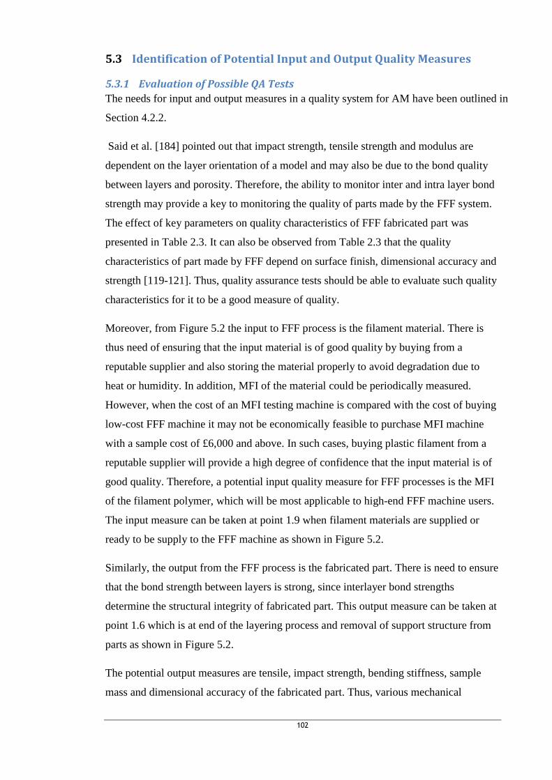
102

5.3 Identification of Potential Input and Output Quality Measures

5.3.1 Evaluation of Possible QA Tests

The needs for input and output measures in a quality system for AM have been outlined in

Section 4.2.2.

Said et al. [184] pointed out that impact strength, tensile strength and modulus are

dependent on the layer orientation of a model and may also be due to the bond quality

between layers and porosity. Therefore, the ability to monitor inter and intra layer bond

strength may provide a key to monitoring the quality of parts made by the FFF system.

The effect of key parameters on quality characteristics of FFF fabricated part was

presented in Table 2.3. It can also be observed from Table 2.3 that the quality

characteristics of part made by FFF depend on surface finish, dimensional accuracy and

strength [119-121]. Thus, quality assurance tests should be able to evaluate such quality

characteristics for it to be a good measure of quality.

Moreover, from Figure 5.2 the input to FFF process is the filament material. There is

thus need of ensuring that the input material is of good quality by buying from a

reputable supplier and also storing the material properly to avoid degradation due to

heat or humidity. In addition, MFI of the material could be periodically measured.

However, when the cost of an MFI testing machine is compared with the cost of buying

low-cost FFF machine it may not be economically feasible to purchase MFI machine

with a sample cost of £6,000 and above. In such cases, buying plastic filament from a

reputable supplier will provide a high degree of confidence that the input material is of

good quality. Therefore, a potential input quality measure for FFF processes is the MFI

of the filament polymer, which will be most applicable to high-end FFF machine users.

The input measure can be taken at point 1.9 when filament materials are supplied or

ready to be supply to the FFF machine as shown in Figure 5.2.

Similarly, the output from the FFF process is the fabricated part. There is need to ensure

that the bond strength between layers is strong, since interlayer bond strengths

determine the structural integrity of fabricated part. This output measure can be taken at

point 1.6 which is at end of the layering process and removal of support structure from

parts as shown in Figure 5.2.

The potential output measures are tensile, impact strength, bending stiffness, sample

mass and dimensional accuracy of the fabricated part. Thus, various mechanical

103

properties of tensile, impact (notched and un-notched) and flexural were evaluated in

order to select the tests that most effectively indicate part quality.

5.4 Proposed Quality System for FFF process The proposed quality system for FFF process incorporates various quality tests

discussed in Section 5.3.1. The flow chart for the tentative quality system is shown in

Figure 5.3. It consists of inspection and measurement after every build, filament

management and control, product check and statistical process control sections. Also

elements (1.2-1.5) in FFF process mapping in Figure 5.2 is represented by element 2.0

in the quality system (see Figure 5.3) in order to simplify the chart for clarity.

In the quality system, input material that is intended for used in a FFF machine should

be properly labelled for traceability and stored in a temperature control room to prevent

degradation due to environmental conditions. In addition:

a) Test parts should be added to every build.

b) On completion of building process and removal of raft and support structures,

parts should be examined to see if they are made successfully or not.

c) Parts should be checked visually for distortion and surface finish qualitatively.

d) Measure the thickness, width after notch, length and mass of the quality

assurance test samples.

e) Determine the strengths, bending stiffness and dimensional accuracy of the QA

test samples.

f) The results from the various QA tests should be stored in a database and

analysed for quality trend using various statistical tools such as comparison of

mean, descriptive statistics and SPC for long term product quality assurance and

process stability monitoring from one build to another.

10

4

Measure

1. Dimension

2. Mass

Test samples

(1) Impact

(2) Flexural

(3) Tensile

Determine

1. Impact strength

2. Flexural strength and

modulus

3. Tensile strength and

modulus

3. Sample mass

4. Accuracy

Database

Inspect for

distortion &

surface finish


made successfully


Post- measurement


FFF

process

Fabricated

part

Visual

inspection of

part

Satisfactory?Yes

Rebuild/

remake

No

Finalized description &

deliver product to

customer

New materials

Apply label to ensure filament

traceability & store in temperature

control room

Filament management & control

Design product

CAD model &

Test part CAD

model

Plot control

chart: Ẋ-R


of variation?

Is the process average

and spread acceptable?

Process

improvement

needed





Yes

YesNo

Product check

No

Customer

specifications

1.1 2.0

1.6

2.1

2.2

2.3

2.4

2.5

2.6

2.7

2.8

3

3.1

3.2

3.3

3.4

3.53.6

2.9

1.9

1.91

Figure 5.3 Tentative Quality System for FFF process

105

5.5 FFF Part production

5.5.1 Hardware

A 3D Touch printer (Figure 5.4a) from Bits from Bytes was used within this work, and

Axon software was used for setting the process parameters. The part design was firstly

created in Autodesk Inventor 2012 and then converted to STL file format before being

imported into the Axon software for setting of processing parameters and conversion of

the STL file to a BFB print file that defines the tool path for printing of the part. The

machine uses heated extruder head (see Figure 5.4b) for deposing extruded filament

called “road” through the nozzle layer by layer onto build platform until the part is fully

built as noted in Section 5.2.1.

Figure 5.4 (a) 3D Touch FFF machine (b) extruder head depositing material

5.5.2 Software

Two versions of Axon software were used for setting FFF machine process parameter in

this work. Axon 2 was initially the current software for use with 3D Touch FFF

machines before the introduction of Axon 3 software. Axon 2 software has more

process parameters that can be varied which are: layer thicknesses, speed of deposition,

fill styles and fill density unlike Axon 3 software where only layer thickness process

parameter can be varied. Axon 2 was therefore, used at the beginning of this work and

also for most of this work. The process parameters that can be varied in Axon 2

106

software are shown in Figure 5.5. The description of the aforementioned process

parameters will be provided in section. 5.5.3.

Figure 5.5 Axon software screen for assigning processing parameters

5.5.3 Build parameters and styles

As the literature has suggested that mechanical properties and dimensional accuracy are

affected by layer thickness, orientation and speed of deposition they are thus considered

in this experiment in addition to fill density each at two levels as shown in Table 5.1.

They are described as:

Layer thickness: The thickness of deposited filament layer.

Orientation: The angular positioning of parts in the build chamber in reference to

X, Y, and Z axes where XY plane is parallel to the build table, and there Z – axis

is perpendicular to the table (as shown in Figure 5.4a).

Fill density/pattern: Most FFF parts are not fully dense. The building of a part

begins with deposition of molten filament called road and collection of roads

form the layer. The deposited road is used for defining the perimeter of the part

107

to form a closed boundary which will later be filled using different fill patterns.

The density of this process is called the fill density (see Figure 5.6) and the fill

style is called the fill pattern. Four fill patterns have been used in this work:

linear (L), lattice (LT), hexagonal (H) and cylindrical (C) (see Figure 5.7).

Print speed: Is the linear speed of deposition of the nozzle to a print part. In the

BFB machine a “speed multiplier” is used for increasing the speed of deposition.

The speed multipliers of 1X and 1.3X are approximately 16 mm/s and 21.33

mm/s linear speed of deposition respectively.

Figure 5.6 Different fill density for the same layer [185]

Linear fill (L)

Lattice fill (LT)

Hexagonal fill (H)

Cylindrical fill (C)

Figure 5.7 Fill patterns with descriptions for parts made using Axon 2 software

However, there are no options for changing the linear speed of a nozzle, fill patterns and

fill density to print a part in Axon 3 software unlike in Axon 2 software. But, the

available fill patterns within a sample or part when Axon 3 software is used for setting

the processing parameters are as shown in Figure 5.8.

108

(a)

(b)

(c)

(d)

Figure 5.8 Micrograph with raster orientations in a part (a) Internal section (b) 0o,

(c) 45o, and (d) 90o angles rasters for a part made using Axon 3 software

Thus, the layering pattern in a part when Axon 3.0 is used in setting the process

parameters are 0o, 45o, 90o followed by alternating layering sections of 0o and 90o until

the part is fully made.

Moreover, the internal patterns for specimens made using either Axon 2 or Axon 3

software are determined or calculated by the software themselves rather than pattern or

property optimisation by the user. In the case of Axon 2 software the user only need to

select one of the fill patterns and then other parameters while in case of Axon 3 software

only one internal pattern is available and is automatically generated by the software

without input from the user.

5.5.4 Experimental plan for FFF specimens

overall experimental approach for specimens made using Axon 2

software

The experiment is divided into three phases. The first phase is concerned with

mechanical property characterization, dimensional accuracy determination and the

search for test types that will be most sensitive to change in process parameters using

109

only one fill style (linear) with specimens oriented in X Y and Z- directions. On

selection of most sensitive orientation based on the result obtained from experiment one

and time taken to produce the part, phases two and three will then involve the

application of different fill patterns to various test types as mentioned in section 5.3 to

assess the consistency of test results across all fill patterns. Two different parameter

settings were used in the experiments, and these are defined in Table 5.1.

Table 5.1 Experimental plan: Specimen design settings

Parameter set A B

Layer thickness (mm) 0.25 0.5

Speed multiplier 1X 1.3 X

Fill density (%) 20 100

Experimental plan two involved the use of all the fill patterns of linear, lattice,

hexagonal and cylindrical to Z-oriented impact, tensile and flexural specimens while

experimental plan three involved only the X- oriented flexural specimens.

The hypotheses of these experiments are:

I. Mechanical properties of specimens made using a process parameter set may not

differ from that made using another process parameter set.

II. Variance in mechanical properties within one specimens parameter set may be

similar to that within another specimens parameter set.

The specimens were made using PLA material sourced from Bits from Bytes and built

on 3D –Touch printer. The processing factors are as shown in Table 5.1.

Test specimens made using Axon 2 software

Flexural and tensile test specimens were made according to ISO standard dimensions.

Izod notch and un– notched impact test specimens were also made according to ISO

standard dimensions. All the test specimen types were then oriented in X, Y and Z

directions to study the effect of the orientations on mechanical properties as shown in

Sections 3.3 to 3.4. The specimen’s geometries and procedures for the respective

standard tests are as presented in Chapter 3.

Table 5.2 shows the phase one experimental plan with total number of specimens used.

Three specimens were made for evaluation of respective flexural, tensile and impact

properties for each parameter set and orientation.

110

Table 5.2 Experimental phase one and number of specimens with respective

orientations

Type of test Number of samples

Orientations: X, Y & Z Parameter set A Parameter set B Total

Tensile 9 9 18

Flexural 9 9 18

Notched Izod impact 9 9 18

Unnotched Izod impact 9 9 18

Total 72

Similarly, Table 5.3 shows the phase two and three experimental plan and the total

number of Z and X – oriented specimens that were used for the evaluation of flexural,

tensile and impact properties of PLA material with their respective fill patterns.

Table 5.3 Experimental phase two and three: number of specimens with respective

orientations

Experiments Phase two Phase three Orientations Fill styles Orient. Z Fill styles Orient. X

L LT H C Parameter set

Total L LT H C Parameter set

Total

A B A B

Tensile ● ● ● ● 12 12 24

Flexural ● ● ● ● 12 12 24 ● ● ● ● 12 12 24 Notched Izod

impact ● ● ● ● 12 12 24

Unnotched

Izod impact ● ● ● ● 12 12 24

Total 96 24

overall experimental approach for specimens made using Axon 3

software

The specimens were also made from PLA material and built on 3D Touch printer just

like the specimens made using Axon 2 software.

Full factorial DOE was used to evaluate the significance of studied process parameter

on the flexural properties and impact strengths of the fabricated parts. The processing

factors and their respective levels that were used in these experiments are as shown in

Table 5.4 and the design matrix that was generated by the use of Minitab 16.0 for the

general full factorial design in coded unit is shown in Table 5.5. The experiment plan

consists of 12 runs, two blocks, two replicates and was randomized.

111

Two specimens were made for each experimental run, with the mean flexural properties

and impact strength values of each run taken as the representative value for that run.

And each run corresponds to the various factor levels combination that will produce the

responses for flexural properties and impact strength that were examined in this study.

The total number of specimens involved in this analysis is forty eight. A brief overview

of DOE methodology has been provided in Section 2.10.3.

Table 5.4 General Linear Model: Flexural properties, impact strengths versus Blocks,

Layer thickness, orientations

Factor Levels Values Remark

Blocks 2 1, 2 Day 1 and day 2

Layer thickness (mm) 2 1, 2 0.25, 0.5

Orientation 3 1, 2, 3 X,Y, Z

Table 5.5 Full factorial experimental design matrix

Run

Order

Blocks Layer

thickness

Orientation

1 1 2 1

2 1 2 3

3 1 1 1

4 1 2 2

5 1 1 3

6 1 1 2

7 2 1 1

8 2 1 2

9 2 2 2

10 2 2 3

11 2 2 1

12 2 1 3

Material sample preparation and determination of MFI of PLA filament

Some quantity of PLA filaments from two production batches supplied by Bits from

Bytes were cut into small sizes as shown in Figure 5.9 using pliers. Parts made by

deposing melted filaments using FFF machine were also cut into small sizes. The cut

samples from each batch of filament were measured using 10 mL cylinder. Measured

quantities were then weighed in a precision balance (KERN ABT 220-5 DM) with

resolution of 0.01 mg/0.1 mg to obtain the mass before MFI tests. MFI of the weighed

samples (5-7) g from each batch of filament were determined using HD-338 melt flow

index machine (Haida Int. Equipment, China) at 190oC and 2.16 kg load according to

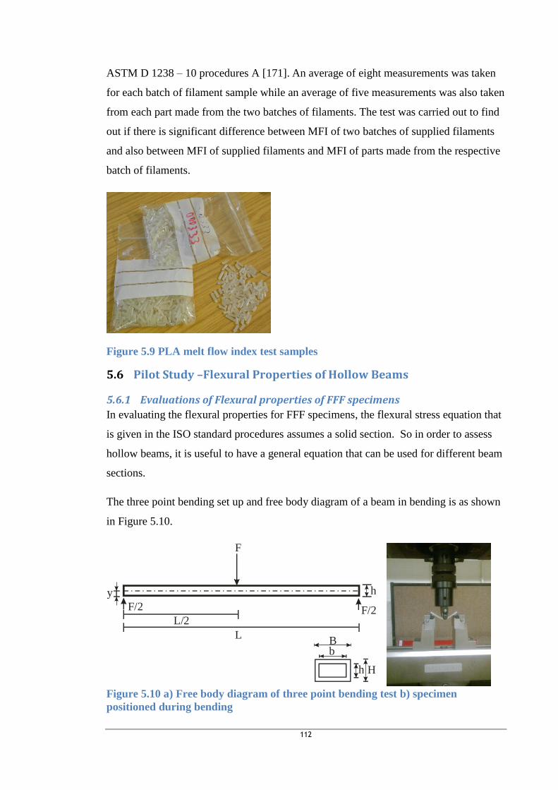
112

ASTM D 1238 – 10 procedures A [171]. An average of eight measurements was taken

for each batch of filament sample while an average of five measurements was also taken

from each part made from the two batches of filaments. The test was carried out to find

out if there is significant difference between MFI of two batches of supplied filaments

and also between MFI of supplied filaments and MFI of parts made from the respective

batch of filaments.

Figure 5.9 PLA melt flow index test samples

5.6 Pilot Study –Flexural Properties of Hollow Beams

5.6.1 Evaluations of Flexural properties of FFF specimens

In evaluating the flexural properties for FFF specimens, the flexural stress equation that

is given in the ISO standard procedures assumes a solid section. So in order to assess

hollow beams, it is useful to have a general equation that can be used for different beam

sections.

The three point bending set up and free body diagram of a beam in bending is as shown

in Figure 5.10.

F

L

h

L/2

h H

bB

F/2 F/2

y

Figure 5.10 a) Free body diagram of three point bending test b) specimen

positioned during bending

113

From the free body diagram in Figure 5.10a, F is the applied force at centre of beam, L

is the span; b is the inner breadth and h is the inner height, B is the outer breadth, H is

the outer height of a hollow beam.

Also the stresses arising from bending are given by:

𝜎

𝑦=

𝑀

𝐼

24

Where, 𝜎 is the tensile or compressive stress, 𝑀 is the bending moment, 𝑦 is the

distance from section centroid to outer fibre and 𝐼 is the moment of inertia of cross

section.

Here,

𝑦𝑀𝑎𝑥 = ± ℎ2⁄ 25

And at the midpoint

𝑀 = 𝐹𝐿4⁄ 26

Substituting equations (25) and (26) into 24 and rearranging gives equation (27)

𝜎𝑀𝑎𝑥 =𝐹𝐿ℎ

8𝐼

27

Therefore, equation (27) now becomes the general equation for calculating flexural

stress in bending.

Figure 5.11 shows a typical fracture surface of a hollow cylindrical fill specimen with

measured dimensions.

Figure 5.11 Fracture surface micrograph of cylindrical parameter A flexural

specimen with dimensions (Z- axis)

For a hollow rectangular beam as shown in (Figure 5.10a), the second moment of area

for the beam (𝐼ℎ) to be substituted into equation (27) is given as:

D1 : 4 mm

114

𝐼ℎ =(𝐵𝐻3 − 𝑏ℎ3)

12

28

The flexural modulus 𝐸𝑓 is calculated using equation (29)

𝐸𝑓 =(𝜎𝑓2

− 𝜎𝑓1)

(𝜀𝑓2− 𝜀𝑓1

)

29

𝑊ℎ𝑒𝑟𝑒, 𝜎𝑓1 is the flexural stress at strain 𝜀𝑓1

and 𝜎𝑓2 is the flexural stress at strain 𝜀𝑓2

,

𝜀𝑓1and 𝜀𝑓2

are defined as 0.0005 and 0.0025 in BS EN ISO 178:2010.

5.6.2 Evaluation of second moment of area of non- fully dense FFF specimen

Determination of dimensions of bending specimens various sections

It was observed that the building process in the studied FFF machine can be divided into

three major sections. That is, the lower section (the first layer before the fill patterns are

being used), the middle sections (were the fill patterns are being used) and the upper

section with the same features as the lower section. This is especially noticeable when

less than 100% fill density is used to fabricate the part as shown in Figure 5.7.

Therefore, in order to determine the dimensions of various sections for the purpose of

evaluating second moment of area of non-fully dense bending specimens; 0%, 20% and

100% fill densities were used to fabricate specimens (see Figure 5.12). Firstly, ten lower

sections of the parts were made by stopping the extruded filament deposition at the end

of first layer/region deposition and at the onset of deposition of the second layer. The

internal dimensions were taken from ten specimens that were fabricated by using 0% fill

density whose layer deposition was also stopped before the completion of the part

building process. Thereafter external dimensions were taken from fully built specimens.

Furthermore, ten fully built specimens were made with fill densities of 0%, 20% and

100% each and with fill patterns of linear, lattice, hexagonal and cylindrical for each of

the fill specimen types.

Figure 5.12 Flexural specimens (a) first layer (b) 0% fill (c) fully build 100% fill

115

All the fabricated specimens dimensions (length, width and thickness) were measured

using Mitutoyo Digital Calliper and the mass of fully built specimens were measured

using weighing balance (KERN PFB 200-3).

The measured dimensions were then used to evaluate second moment of area for the

non-fully dense specimens as presented in the subsequent sections. The total number of

specimens used in this analysis was one hundred and forty (140).

5.6.3 Geometrical modelling and evaluation of second moment of area

Figure 5.13 Sectional view through the beam section

Consider the beam section in Figure 5.13 were b is the outer width of the beam, 𝑏𝑐 is

the inner width, h is the outer thickness, ℎ𝑐 is the inner thickness and t is the thickness

of each section1and 3. If we assume that the beam is isotropic and homogeneous, all

sections are firmly bonded together and that all cross sections remain plane and

perpendicular to the longitudinal axis of the beam.

Standard beam theory tells us that the equivalent second moment of area Ieq, about the

Z-axis can be found by summing the second moments of area of areas 1-5 about the Z-

axis, so

𝐼𝑒𝑞 = 𝐼1 + 𝐼2 + 𝐼3 + 𝐼4 + 𝐼5

30

In this case 𝐼2 = 𝐼4, 𝑎𝑛𝑑 𝐼1 = 𝐼3, 𝑠𝑜

𝐼𝑒𝑞 = 2𝐼1 + 2𝐼2 + 𝐼5 31

116

Area 2 and 5 have their centriods on the Z axis, but area 1 does not , and so it is

calculated as

𝐼1 =𝑏𝑡3

12+ (𝑏𝑡) (

ℎ𝑐 + 𝑡

2)

2

32

From eq (31)

𝐼𝑒𝑞 − 𝐼5 = 2(𝐼1 + 𝐼2) 33

Simiplification of eq (33) and rearranging of variables gives eq (34)

1 −2(𝐼1 + 𝐼2)

𝐼𝑒𝑞=

𝐼5

𝐼𝑒𝑞

34

Where, 2(𝐼1 + 𝐼2) is the moment of inertia of sections 1 to 4 (outer beam sections) and

𝐼5 is the moment of inertia of the inner section about the Z-axis.

The contribution of inner section moment of inertia to equivalent moment of inertia is

given as 𝐼5

𝐼𝑒𝑞 while the contribution of outer sections to equivalent moment of inertia is

2(𝐼1+𝐼2)

𝐼𝑒𝑞.

For fully dense beam we can compare the second moment of area of the outer sections

and inner section in order to find out the contribution of inner sections to overall 𝐼 for

fully dense beam.

If 𝐼5= 0 then the section (5) is hollow

But if,

(𝐼5

𝐼𝑒𝑞) > 2% 𝑜𝑟

𝑑𝑚

𝐷𝑀≥ 0.5 then 𝐼5 may not be negligible for non-fully dense beam

Where, 𝑑𝑀 is the average mass of inner section of specimens and 𝐷𝑀 is the average

mass of inner section of 100% fill specimens.

The second moment of area for non- fully dense beam of different fill patterns may be

approximated by:

Effective second moment of area (𝐼)𝑒𝑓𝑓 = 2(𝐼1 + 𝐼2) + (𝑑𝑚

𝐷𝑀) 𝐼5

35

And, for a fully dense sections 𝑑𝑚

𝐷𝑀= 1,

117

The mass of internal sections for 20% and 100% fill densities specimens and their mass ratio

were computed by using equations 36 to 38.

𝑑𝑀 = 𝑀20% − 𝑀0% 36

𝐷𝑀 = 𝑀100% − 𝑀0% 37

𝑀𝑎𝑠𝑠 𝑟𝑎𝑡𝑖𝑜 (𝑀𝑟) = (𝑑𝑚

𝐷𝑀)

38

Where, 𝑀0% is the average mass of 0% fill specimens, 𝑀20%is the average mass of 20%

fill specimens, 𝑀100% is the average mass of 100% fill specimens.

When mutually independent quantities are being added, subtracted, multiplied or

divided uncertainties or errors for the calculated values can be determined from the

measured values [186, 187].

Therefore, variation or error in average mass of internal section of 20% fill specimens is

calculated as:

∆𝑑𝑚 = √(∆𝑀20%)2 + (∆𝑀0%)2 39

Where, ∆𝑀20% and ∆𝑀0% are associated standard error (is a measure of random error in

a set of data) of mean 𝑀20% and 𝑀0% respectively.

Similarly, Variation or error in average mass of internal section of 100% fill specimens

is calculated as:

∆𝐷𝑀 = √(∆𝑀100%)2 + (∆𝑀0%)2 40

Where, ∆𝑀100% and ∆𝑀0% are associated standard error of mean 𝑀100% and 𝑀0%

Standard error of mean (𝜎𝑚)=𝜎

√𝑛 41

Where σ is the standard deviation of the 𝑥𝑖′𝑠 individual sample mass measurement and

n (n is 10 in this experiment) is the number of𝑥𝑖′𝑠.

From equations (36) and (39):

𝑑𝑀= (𝑀20% − 𝑀0%) ± ∆𝑑𝑚 42

Also from equations (37) and (40),

𝐷𝑀 = (𝑀100% − 𝑀0%) ± ∆𝐷𝑀 43

Similarly, uncertainty or error in calculated mass ratio (∆𝑀𝑟) is calculated as:

118

∆𝑀𝑟 = 𝑀𝑟 × √(∆𝑑𝑚

𝑑𝑚)

2

+ (∆𝐷𝑀

𝐷𝑀)

2

44

∆𝑑𝑚 and ∆𝐷𝑀 are associated standard error of mean 𝑑𝑀 and 𝐷𝑀.

From equations (38) and (44), mass ratio is given by:

(𝑀𝑟) = (𝑑𝑚

𝐷𝑀) ± ∆𝑀𝑟

45

The presented modelling equations in this section were used for evaluating the second

moment of area of flexural specimens made with different fill styles.

5.6.4 Second moment of area modelling results

Table 5.6 shows the dimensions of 100% fill specimens. The parameters in the table are

as shown in Figure 5.13.

Table 5.6 Dimensions of X-oriented flexural specimens made with 100% fill density

S/N Width (mm) Thickness (mm)

b bc t h

1 10.33 6.85 1.82 4.56

2 10.28 6.1 1.83 4.61

3 10.29 6.85 1.8 4.49

4 10.28 6.85 1.78 4.62

5 10.31 6.82 1.78 4.57

6 10.14 6.8 1.68 4.66

7 10.16 6.84 1.69 4.66

8 10.12 6.85 1.66 4.67

9 10.15 6.82 1.69 4.58

10 10.16 6.79 1.67 4.65

The contributions of inner sections of beam moment of inertia and outer sections of

beam to total moment of inertia of the sections were evaluated as explained in Section

5.6.3 for X- oriented flexural specimens made using 100% fill density. The results are

shown in Table 5.7.

119

Table 5.7 Moment of inertia ratio of the inner and outer sections to total section of

fully dense beam X-oriented specimens

sample 𝑰𝟓

𝑰𝒆𝒒

𝟐(𝑰𝟏 + 𝑰𝟐)

𝑰𝒆𝒒

1 0.032 0.968

2 0.028 0.972

3 0.022 0.978

4 0.027 0.973

5 0.030 0.970

6 0.034 0.966

7 0.022 0.978

8 0.029 0.971

9 0.028 0.972

10 0.026 0.974

mean 3% 97%

The fill patterns in X-oriented specimens are as shown in Figure 5.7. However these

types of fill patterns are not formed in 100% fill density specimens and Y and Z-

oriented specimens (Figure 5.46 and Figure 5.27). This may be due to availability of

small space between deposited closed loop perimeters which is not sufficient for the

deposition of the patterns.

Table 5.8 shows the average, minimum and maximum sample mass of X-oriented

flexural specimens of 20% and 100% fill density with their fill patterns.

Table 5.8 Mass of X-oriented flexural specimens with fill patterns fill densities

Mass of specimens (g)

Fill pattern Fill density (%) Ave. Min. Max.

C 20 3.51 3.51 3.53

C 100 4.24 4.21 4.27

H 20 3.60 3.58 3.62

H 100 4.23 4.22 4.23

L 20 3.59 3.57 3.61

L 100 4.25 4.24 4.26

LT 20 3.60 3.72 3.81

LT 100 4.17 4.14 4.20

Mass of 0% fill specimen (g)

Ave 3.12

Max 3.26

Min 2.97

120

The mass ratio for the flexural specimens were computed using Eq (38) and the error

bars for the mass ratio were calculated using Eq (44). Figure 5.14 shows the variation of

mass ratio with fill patterns for X-oriented flexural specimens. Error or variation in the

calculated mass ratio can be observed to be negligible.

Figure 5.14 Variations of X-oriented flexural specimen mass ratios with fill

patterns, error bars are standard error

Since the mass ratio of specimens made by using different fill patterns is low as shown

in Figure 5.14 and the contribution of the inner section moment of inertia to the total

moment of inertia of the beam (𝐼5

𝐼𝑒𝑞) for fully dense (100% fill density) specimen is 3%

while the contribution of outer section to total moment of inertia is 97% (see Table 5.7).

This suggest that the contribution of the 20% fill specimen inner section to the total

moment of inertia is negligible. Thus, the 20% filled specimens with their respective

patterns (Figure 5.7) that were used in this bending experiment will be treated as hollow

beams for the purpose of evaluating the moment of inertia of the beams.

5.7 Influence of Build Parameters on Accuracy Figure 5.15 shows the percentage deviation in length, width and thickness of eighteen

flexural specimens, with three specimens for each parameter set and orientation of

specimens.

It can be observed that the accuracies vary with orientations. The absolute mean

percentage change in length, width and thickness for parameter set A specimens are

0.52%, 3.51%, 4.84% and for parameter set B specimens are 0.16%, 0.9%, and 0.81%

0

0.05

0.1

0.15

0.2

0.25

0.3

0.35

0.4

0.45

0.5

C H L LT

Mas

s ra

tio

(d

m/D

m)

Fill pattens

121

respectively.

Figure 5.15 Dimensional accuracies for parameter settings and orientations, the

graph show the mean, median, lower limit, upper limit, first and third quartile

Top surface

Bottom surface

Figure 5.16 Surface profile (a) top surface (b) bottom surface of Y-oriented

parameter A specimens

X- and Y-oriented specimens were also observed to have the highest inaccuracy in

thickness which was due to machine software error in reproducing the actual thickness

for parameter set A specimens (low layer thickness and low fill density), which have led

to addition of higher number of layers for X-oriented specimens. As there are 17

deposited layers instead of 16 layers for X-oriented parameter A (layer thickness of 0.25

mm) specimens and 8 deposited layers for parameter B (layer thickness of 0.5 mm)

Parameter set

Orientation

% Δ in thickness% Δ in width% Δ in length

BABABA

ZYXZYXZYXZYXZYXZYX

9.00%

8.00%

7.00%

6.00%

5.00%

4.00%

3.00%

2.00%

1.00%

0.00%

% D

ev

iati

on

in

dim

en

sio

ns

122

specimens when the layers were counted under the optical microscope. In addition,

extruder tip also exert limited pressure (which depends on the distance between the

extruder tip and the Z-height of the build platform) during deposition of material on the

machine movable platform which can cause slight shrinkage in the direction of build.

This pressure slightly affects the width for Y-oriented specimens and length for Z-

oriented specimens, since the down facing surfaces of the width and length for that

respective orientation of specimens are along the direction of build as shown in Figure

3.4 (b). The shrinkage in width for Y-oriented specimens as shown in Figure 5.16 may

have also lead to increment in the complementary direction of thickness for Y-oriented

specimens. As the top surface profile for Y-oriented specimens (see Figure 5.16 a) can

be observed to be relatively plane while the bottom profile that is contact with the build

platform can be observed to slightly flatten out due to the pressure exerted by the

extruder tip as shown in Figure 5.16(b). The aforementioned observed effects seems to

influenced more dimensional accuracy of specimens made with parameter set A with

lower layer thickness due to higher numbers of layers required to make the parts as

compared to parameter B specimens with thicker layers, but overall there is no much

difference in dimensional accuracy.

5.8 Influence of Build Parameters on Modulus, Strain at maximum

stress and sample mass

5.8.1 Variations of Modulus with parameter sets and orientations

Figure 5.17 shows variations of flexural modulus and tensile modulus with orientations

and parameter sets for eighteen flexural specimens and eighteen tensile specimens, with

three specimens for each parameter set and orientation of specimens.

123

Parameter sets

Orientation

Tensile specimensFlexural specimens

BABA

ZYXZYXZYXZYX

3500

3250

3000

2750

2500

2250

2000

Fle

xu

ral m

od

ulu

s (

MP

a)

Te

nsile

mo

du

lus (

MP

a)

Figure 5.17 Variation of flexural and tensile modulus with parameter sets and

orientations, the graph shows the mean, median, lower limit, upper limit, first and

third quartile

Flexural and tensile modulus of X- and Y-oriented parameter set B specimens is higher

than that of parameter set A while the converse is true for Z-oriented specimens flexural

and tensile modulus with parameter sets. There is also more variance in tensile modulus

across parameter sets and orientations of specimens than flexural modulus.

Table 5.9 shows the variation of flexural strain at maximum stress with X-, Y-, and Z-

orientations of specimens and parameter sets A and B. The descriptive statistics of

means and standard deviations of strain at maximum stress are also shown in the table.

Z-oriented specimens have the lowest flexural strain maximum stress across parameter

sets.

Table 5.9 Variation of flexural strain at maximum stress with parameter sets and

orientations

Specimen parameter sets A B

Orientation X Y Z X Y Z

Strain at maximum stress

(%)

4.40 ±

0.07

4.85 ±

0.06

2.01 ±

0.04

4.05 ±

0.11

4.22 ±

0.05

2.31 ±

0.37

124

Table 5.10 shows variations of tensile maximum strain at break with X-, Y-, and Z-

orientations of specimens and parameter sets A and B. Z-oriented specimens have the

lowest tensile maximum strain at break across parameter sets.

Table 5.10 Variation of tensile maximum strain at break with parameter sets and

orientations

Specimen

parameter

sets

A B

Orientation X Y Z X Y Z

Maximum

strain at

break (%)

2.87 ± 0.26 1.69 ±

0.17

0.96 ± 0.26 3.26 ± 1.28 2.16 ±

0.3

1.85 ±

0.4

Figure 5.18 shows variations of flexural sample weight with orientations and specimen

parameter sets.

Figure 5.18 Flexural samples weight types with orientations and parameter sets,

the graph shows the mean, median, lower limit, upper limit, first and third quartile

Flexural sample weight for X-oriented parameter set B specimens is higher than that of

parameter set A specimens. One possible reason is that, on deposition of the perimeter

of the part to form a close boundary which will later be fill with selected fill pattern

during part fabrication there is more internal space to be raster fill with the selected high

fill density for that orientation of specimens, that may explained the reason for

Orientation

Parameter sets

ZYX

BABABA

0.0450

0.0425

0.0400

0.0375

0.0350

Fexu

ral sa

mp

le w

eig

ht

(N)

125

parameter set B specimens having higher weight that parameter set A specimens.

However, Y- and Z- oriented parameter set A specimens have more weights than that of

parameter set B specimens. This is because on deposition of the perimeter of the part to

form a close boundary for a layer during layering process of a part, there is limited

internal space for raster filling to complete a layer building process for parameter B

specimens as shown in Figure 5.20. Therefore for parameter set A specimens (see

Figure 5.19) with higher number of layers in a part due to the use of low layer thickness

in fabricating the specimen will have higher weight than parameter set B specimens

made with high layer thickness for both Y- and Z-oriented specimens.

Figure 5.19 Micrograph showing the internal structure of Y - oriented specimen

produced using parameter set A

Figure 5.20 Micrograph showing the internal structure of Y - oriented specimen

produced using parameter set B

Figure 5.21 shows variation of tensile sample weights with orientations and parameter

sets. Tensile sample weight for X-oriented parameter set B specimens is higher than that

of parameter set A specimens but the opposite is true for variation of sample weight for

Y- and Z-oriented specimens with parameter sets. The same aforementioned reason

given for variation of sample mass of flexural modulus with orientation and parameter

set is also applicable to variation of sample mass of tensile modulus with parameter set

and orientation of specimens.

Deposited roads Internal

material

filling

Deposited roads

Internal

material

filling

Space for material filling

Space for material filling

126

Figure 5.21 Tensile samples weight with parameter sets and orientations, the figure

shows the mean, median, first and third quartile

DOE results for flexural properties and impact strength of Axon 3

processed specimens

Table 5.11 shows the resulted response data of flexural properties and impact strengths

for each experimental runs for specimen processed using Axon 3 software. The factorial

analysis is in Appendix C-4.

Table 5.11 Full factorial experimental design with tests results from experimental runs

Run

Order

Blocks Layer

thickness

Orientation Flexural

strength

(MPa)

Flexural

modulus

(MPa)

Strain at

maximum stress

(%)

Impact

strength

(kJ/m2)

1 1 2 1 61.44 1828.98 4.19 5.89

2 1 2 3 30.30 1891.31 1.91 2.90

3 1 1 1 57.09 1794.62 3.85 4.22

4 1 2 2 69.63 2007.39 3.95 4.61

5 1 1 3 20.34 1574.46 1.25 2.80

6 1 1 2 67.48 2261.03 3.28 3.39

7 2 1 1 56.96 1884.90 3.55 4.21

8 2 1 2 67.04 2268.04 3.57 3.52

9 2 2 2 70.70 1988.50 3.67 5.09

10 2 2 3 29.26 1877.70 2.69 2.87

11 2 2 1 58.76 1735.42 4.53 5.77

12 2 1 3 18.86 1563.10 1.16 2.77

Orientation

Parameter sets

ZYX

BABABA

0.135

0.130

0.125

0.120

0.115

0.110

0.105

0.100

0.095

Te

nsile

we

igh

t (N

)

127

5.8.2 Flexural modulus, strain at maximum stress and sample mass of

specimens processed using Axon 3 software

Figure 5.22 shows the variations of flexural modulus and sample mass with orientations

and layer thickness for specimens processed using Axon 3 software. Flexural modulus

and sample mass of flexural modulus specimens are observed to vary with orientation

and layer thickness; with Y-oriented specimens having the highest modulus.

Figure 5.22 Variation of (a) flexural modulus (b) sample mass with orientations

and layer thickness, the figure shows the mean, median, lower limit, upper limit,

first and third quartile

Table 5.12 shows the variation of flexural strain at maximum stress with X-, Y-, and Z-

orientations of specimens and layer thickness, for Axon 3 processed specimens. The

descriptive statistics of means, minimum and maximum strain at maximum stress are

also shown in the table. Z-oriented specimens have the lowest flexural strain at

maximum stress across layer thickness type.

Table 5.12 Variations of flexural strain at maximum stress with layer thickness

and orientations

Strain at maximum stress (%)

Layer thickness (mm) Orientations Mean Minimum Maximum

0.25 X 3.70 3.55 3.85

0.25 Y 3.43 3.28 3.57

Lay er thickness

O rientation

0.5 mm0.25 mm

ZYXZYX

2250

2000

1750

1500

Fle

xu

ra

l m

od

ulu

s (

MP

a)

Lay er thickness

O rientation

0.5 mm0.25 mm

ZYXZYX

3.5

3.0

2.5

Sa

mp

lel

ma

ss (

g)

(a)

(b)

128

Strain at maximum stress (%)

Layer thickness (mm) Orientations Mean Minimum Maximum

0.25 Z 1.20 1.16 1.25

0.5 X 4.36 4.19 4.53

0.5 Y 3.81 3.67 3.95

0.5 Z 2.30 1.91 2.69

5.8.3 Variations of Modulus with parameter sets and fill patterns

Figure 5.23 shows the variations of flexural modulus with fill patterns and parameter set

A and B for X- and Z-oriented flexural modulus specimens.

Figure 5.23 Variation of flexural modulus for X- and Z –oriented specimens with

fill styles, the figure shows the mean, median, lower limit, upper limit, first and

third quartile

Figure 5.24 shows the variation of tensile modulus with fill patterns and parameter set

A and B for Z- oriented tensile modulus specimens.

Fill pattern

Parameter set

Flexural modulus- ZFlexural modulus- X

LTLHCLTLHC

BABABABABABABABA

3000

2800

2600

2400

2200

2000

1800

Fle

xu

ral m

od

ulu

s (

MP

a)

129

Figure 5.24 Variation of tensile modulus for Z –oriented specimens with fill styles

and parameter sets, the figure shows the mean, median, lower limit, upper limit,

first and third quartile

Flexural modulus of X-oriented parameter set B specimens is generally higher than that

of parameter set A, while flexural modulus and tensile modulus of Z-oriented parameter

set A specimens is generally higher than that of parameter set B across fill styles. Also

variance in modulus of X-oriented specimens is lower than that of Z-oriented specimens.

Figure 5.25 shows variation of flexural sample weights with fill styles and parameter

sets, for X- and Z-oriented specimens. Figure 5.26 shows the variation of tensile sample

weights with fill styles and parameter sets A and B.

Flexural sample weight for X-oriented parameter set B specimens is higher than that of

parameter set A specimens across fill syles which may in part expalin the modulus

results. While flexural and tensile sample weights for paramter set A specimens are

higher than that of parameter set B across fill syles.

Fill patterns

Parameter sets

LTLHC

BABABABA

3400

3300

3200

3100

3000

2900

2800

2700

2600

2500

Te

nsile

mo

du

lus (

MP

a)

130

Figure 5.25 Weight of X- and Z – oriented specimens with fill styles and parameter

sets, the figure shows the mean, median, lower limit, upper limit, first and third

quartile

Figure 5.26 Tensile sample weights with parameter sets and fill patterns for Z-oriented

specimens, the figure shows the mean, median, lower limit, upper limit, first and

third quartile

Specimen design

Fill pattern

Flexural sample_ZFlexural sample_X

BABA

LTLHCLTLHCLTLHCLTLHC

0.043

0.042

0.041

0.040

0.039

0.038

0.037

0.036

0.035

0.034

Fle

xu

ral sa

mp

le w

eig

ht

(N)

Parameter sets

Fill patterns

BA

LTLHCLTLHC

0.130

0.125

0.120

0.115

0.110

0.105

0.100

Te

nsile

sa

mp

le w

eig

ht

(N)

131

Parameter set A cylindrical fill specimens can also be observed from the figure to have

the lowest sample mass for both flexural and tensile specimens. This because on

deposition of the perimeter of the part to form a close boundary, which will later be fill

with selected patterns to complete a layer during layering process of a part. There are

are likely limited internal space (1 mm) to create cylindrical fill pattern expecially for

Z-oriented specimens unlike the X-oriented specimens (see Figure 5.7). Therefore,

deposited perimeter of a layer was not filled after the deposition of the outer contour or

perimeter to complete a layer for cylindrical filled parameter set A specimens. They

were thus hollow as shown in Figure 5.27. Although other fill patterns were also not

created in other parameter A specimens but they were raster fill as shown in that figure.

However, all the parameter B specimens were observed to be dense as shown in Figure

5.27 and hence the specimens have similar sample mass across fill patterns. The

aforementioned provides a possible reason for disparity in sample mass for flexural and

tensile specimens with parameter set and fill patterns.

Figure 5.27 shows fracture surfaces of Z – oriented flexural specimens with parameter

sets and fill patterns of lattice, hexagonal and cylindrical.

Parameter set A specimen Parameter set B specimen

linear

linear

Lattice Lattice

132

Parameter set A specimen Parameter set B specimen

Hexagonal Hexagonal

Cylindrical Cylindrical

Figure 5.27 surface micrographs for Z- oreiented flexural samples with their

respective fill patterns and specimen parameter sets

5.9 Influence of Build Parameters on Strength

5.9.1 Variations of strengths with parameter sets and orientations

Figure 5.28 and Figure 5.29 show variations of notched and un-notched impact

strengths and UTS with X-, Y-, and Z-orientations of specimens, one fill style and

parameter sets A and B. Z-oriented specimens have the lowest UTS, and impact

strengths (notched and un-notched) across X-, Y- and Z-orientation of specimens and

parameter sets.

D1 : 4 mm

133

Figure 5.28 Variations of Impact strengths with parameter sets and orientations of

specimens, the figure shows the mean, median, first and third quartiles

Figure 5.29 Variations of UTS with parameter sets and orientations of specimens, the

figure shows the mean, median, first and third quartiles

Parameter set

Orientation

Unnotched Impact specimensNotched Impact specimens

BABA

ZYXZYXZYXZYX

25

20

15

10

5

0

Imp

act

str

en

gth

(kJ/

m^

2)

Parameter set

Orientation

BA

ZYXZYX

55

50

45

40

35

30

25

20

UTS

(M

Pa

)

134

Figure 5.30 shows the variations of flexural strengths with X-, Y-, and Z-orientations of

specimens and parameter sets A and B. Z -oriented specimens have the lowest flexural

strength across X-, Y- and Z-orientation of specimens and parameter sets.

Figure 5.30 Variations of Flexural strength with parameter sets and orientations of


Similar variation in sample mass of flexural and tensile specimens with parameter set

and orientation was also observed in sample mass of impact specimens. Figure 5.31

shows the variations of notched and un-notched impact specimen sample weights with

X, Y and Z – orientations of specimens and parameter sets A and B. The same reason

given for variation in flexural and tensile sample mass with parameter set in section

5.8.1 is also applicable to sample mass of impact specimens.

Orientation

Parameter sets

ZYX

BABABA

80

70

60

50

40

Fle

xu

ral str

en

gth

(M

Pa

)

135

Figure 5.31 Variations of notch and un-notched impact specimen weights with

parameter sets, the figure shows the mean, median, first and third quartiles

5.9.2 Flexural strengths and impact strengths of specimens process using

Axon 3 software

Figure 5.32 shows the variations of flexural strength with layer thickness and X-, Y-

and Z-orientations for test samples processed using Axon 3 software. Z -oriented

specimens have the lowest flexural strength across X-, Y- and Z-orienteation of

specimens and layer thickeness.

Orientation

Parameter set

un-notched impact specimensnotched impact specimens

ZYXZYX

BABABABABABA

0.0450

0.0425

0.0400

0.0375

0.0350

Imp

act

sa

mp

le w

eig

ht

(N)

136

Figure 5.32 Variation of flexural strengths with layer thickness and orientation of

specimens, the figure show the mean, median, first and third quartiles

Figure 5.33 shows the variations of notched impact strength with layer thickness and X-,

Y- and Z-orientations for test samples processed using Axon 3 software. Z -oriented

specimens have the lowest impact strength like that of flexural strength across X-, Y-

and Z-orientation of specimens and layer thickeness.

Figure 5.34 shows the variations of impact sample weight with layer thickness and X-,

Y- and Z-orientations for test samples processed using Axon 3 software. Impact sample

weight varies with orientation and layer thickness, with X-oriented specimens having

the lowest sample weight.

Layer thickness

Orientation

0.5 mm0.25 mm

ZYXZYX

70

60

50

40

30

20

Fle

xu

ral str

en

gth

(M

Pa

)

137

Figure 5.33 Variation of impact strength with layer thickness and orientation of


Figure 5.34 Variation of impact sample weight with layer thickness and orientation

of specimens, the figure show the mean, median, first and third quartiles

Layer thickness

Orientation

0.5 mm0.25 mm

ZYXZYX

6.0

5.5

5.0

4.5

4.0

3.5

3.0

Imp

act

str

en

gth

(kJ/

m^

2)

Layer thickness

Orientation

0.5 mm0.25 mm

ZYXZYX

0.0375

0.0350

0.0325

0.0300

0.0275

0.0250

Imp

act

sa

mp

le w

eig

ht

(N)

138

5.9.3 Variations of strengths with parameter sets and fill patterns

Figure 5.35 shows the variations of flexural strengths of X- and Z-oriented flexural

specimens with parameter sets. Where, L – Linear fill pattern, LT – lattice fill pattern, H –

hexagonal fill pattern, C – cylindrical fill pattern in the respective plots and tables in this section.

Z-oriented specimens have the lowest flexural strength across fill styles and parameter sets.

Figure 5.35 Variation of flexural strengths with parameter sets and fills patterns,

the figure show the mean, median, first and third quartiles

Figure 5.36 and Figure 5.37 show the variation of UTS, notched and un-notched impact

strengths of Z-oriented specimens with parameter sets and fill patterns.

Fill pattern

Parameter sets

Flexural specimens-ZFlexural specimens-X

LTLHCLTLHC

BABABABABABABABA

70

60

50

40

30

Fle

xu

ral str

en

gth

(M

Pa

)

139

Figure 5.36 Variations of impact strengths with parameter sets and fill pattern (Z-orient.),

the figure show the mean, median, first and third quartiles

Figure 5.37 Variations of UTS with parameter sets and fill pattern (Z-orient.), the figure

show the mean, median, first and third quartiles

Fill pattern

Parameter set

Unnot. Impact specimensNotched Impact specimens

LTLHCLTLHC

BABABABABABABABA

12

10

8

6

4

2

Imp

act

str

en

gth

(kJ/

m^

2)

Fill pattern

Parameter set

LTLHC

BABABABA

36

34

32

30

28

26

24

22

UTS

(M

Pa

)

140

Figure 5.38 shows variation of sample weights with fill styles and parameter sets for

both notched and un-notched impact specimens. Impact sample weights for notched and

un-notched specimens vary across fill patterns and parameter sets. Cylindrical fill

impact specimens have the lowest sample weight across fill patterns like the case of

flexural and tensile specimens sample mass. The same reason given for the variation of

sample mass for flexure and tensile specimens in section 5.8.3 also suffice here.

Figure 5.38 Impact samples (Z- orient.) weight with fill patterns and parameter

sets, the figure show the mean, median, first and third quartiles

Table 5.13 shows the variation of tensile maximum strain at break with parameter sets

and fill patterns for Z-oriented specimens. Parameter set B specimens has the highest

tensile maximum strain at break compared to parameter set A specimens.

Table 5.13 Tensile maximum strains at break for Z-oriented specimens with fill

styles and parameter sets

Specimen

parameter

sets

A B

Fill styles L LT H C L LT H C

Max. strain

at break (%)

0.98

± 0.1

0.94 ±

0.1

0.98 ±

0.1

1.18 ±

0.03

1.5 ±

0.1

1.45 ±

0.1

1.20 ±

0.1

1.44 ±

0.17

Parameter sets

Fill patterns

Un-notch impact sampleNotch impact sample

BABA

LTLHCLTLHCLTLHCLTLHC

0.044

0.043

0.042

0.041

0.040

0.039

0.038

0.037

0.036

0.035

Imp

act

sa

mp

le w

eig

ht

(N)

141

Table 5.14 shows variation of flexural strain at maximum stress with fill styles and

parameter sets for X- and Z-oriented specimens. The descriptive statistics of means and

standard deviations of strain at maximum stress are also shown in the table. Z-oriented

specimens have the lowest strain at maximum stress across fill styles and parameter sets.

Table 5.14 Flexural strains at maximum stress of X- and Z – oriented specimens

with fill styles and parameter sets

Specimen

parameter

sets

A B

Fill styles L LT H C L LT H C

Orientation X

Strain at

maximum

stress (%)

4.24 ±

0.01

4.31 ±

0.13

4.35 ±

0.12

4.14 ±

0.06

4.22 ±

0.07

4.30 ±

0.08

4.34 ±

0.10

4.37 ±

0.17

Orientation Z

Strain at

maximum

stress (%)

1.97 ±

0.04

1.93 ±

0.1

1.89 ±

0.02

1.76 ±

0.05

2.22 ±

0.21

1.75 ±

0.38

1.85 ±

0.04

2.32 ±

0.12

5.9.4 Correlation between Impact strength and UTS, Flexural strength and

UTS

Correlations were carried out between UTS and impact strengths and also between

flexural strength and UTS.

Figure 5.39 shows the correlation of UTS with notched and un-notched impact

strengths for X, Y and Z orientation of specimens. Correlation between UTS and

notched impact strengths is reduced by the variation in notched impact strength for Z-

oriented parameter A specimens. Dark symbols represent notched impact strength and

green symbols represent un-notched impact strengths.

Figure 5.40 shows correlation between UTS and flexural strength for X, Y and Z

oriented specimens with parameter sets.

Figure 5.41 shows the correlation between UTS and notched impact strength of Z-

oriented specimens made with fill styles and parameter sets.

142

2520151050

55

50

45

40

35

30

25

20

Impact strength (kJ/m^2)

UTS

(M

Pa

)

Notched Impact strength

Unnot. Impact strength

Variable

B X

B Y

B Z

A X

A Y

A Z

B X

B Y

B Z

A X

A Y

A Z

Variable sets

Parameter

Orientation

r = 0

.829 (

p<

0.0

1)

r= 0

.923

(p<

0.0

1)

Figure 5.39 Correlation between UTS and impact strength for parameter sets A

and B (X, Y & Z orientations) samples

Figure 5.40 Correlation between flexural strength and tensile strength with

parameter sets A and B specimen (X, Y & Z orient.)

5550454035302520

90

80

70

60

50

40

UTS (MPa)

Fle

xu

ral str

en

gth

(M

Pa

)

A X

A Y

A Z

B X

B Y

B Z

sets

Parameter

Orientation

r = 0.8

77 (p

< 0.0

1)

143

Figure 5.41 Correlation between UTS and notched impact strength and build

parameters (Z- orient.)

5.10 MFI of two batch of PLA filament

In order to investigate if there is a significant difference between filaments from two

batches, and also to determine if there is a change in flow property between supplied

filament and deposited filament, MFI test was carried out.

Figure 5.42 shows the MFI of two batches of tested PLA filaments and parts made from

them at 95% confidence interval of mean of the samples. While EF in the figure

represents extruded filaments (test samples obtained by cutting of fabricated part into

small pieces) and RF stands for raw filament that have not been used for fabricating of

part (as supplied filament taken from filament reels). There is a clear significant

difference between MFI of extruded filament used in fabricating part and the supplied

filaments but there is no significant difference between MFI of the two batches of

supplied filaments.

4.54.03.53.02.5

36

34

32

30

28

26

24

22

Impact strength (kJ/m^2)

UTS

(M

Pa

)

C A

C B

H A

H B

L A

L B

LT A

LT B

Fill pattern sets

Parameter

r = 0

.840 (

p< 0

.01)

144

Figure 5.42 MFI of two batches of PLA filament and parts made from them

5.11 Surface morphology

In order to examine the influence of surface conditions on the mechanical properties of

tested parts, microscopic examination of surface profiles was carried out. Figure 5.43

shows the surface profiles of flexural samples with their respective orientations and

parameter sets.

Batch

Sample type

21

RFEFRFEF

40

30

20

10

0

MFI

(g

/1

0 m

in)

95% CI for the Mean

145

Parameter set A specimens Parameter set B specimens

X- oriented specimens

Y- oriented specimens

Z- oriented specimens

Figure 5.43 Surface micrographs of flexural samples with respective orientations

In order to examine the influence of fill densities and raster orientations on fracture of

tested samples, fracture surface micrographs were carried taken. These fracture surface

micrographs are shown in Figure 5.44 to Figure 5.47. Figure 5.44 shows the fracture

surface of notched impact specimens with their respective orientations and parameter sets.

146


X X

Y Y

Z Z

Figure 5.44 Notched impact strength fracture surfaces for X, Y and Z orientations

Figure 5.45 shows the fracture surface of un-notched impact specimens with their

respective orientations and parameter sets.

147


X X

Y Y

Z Z

Figure 5.45 Un-notched impact strength fracture surfaces for X, Y and Z

orientations

Figure 5.46 shows the fracture surface of X, Y and Z – oriented flexural specimens with

their respective specimen’s parameter sets A and B.

148


X X

Y Y

Z Z

Figure 5.46 Flexural sample fracture surfaces for X, Y and Z orientations

149

Figure 5.47 shows the replicated fracture surface of Y – oriented impact specimens.

Failure of the material can be observed to occur by delamination, rupturing of filaments

and crack propagation through the material.

Figure 5.47 Fracture surface of impact specimen (Nikon SMZ 1500 optical

microscope)

5.12 Summary of FFF PLA properties tests results Flexural and tensile properties and impact strengths (notched and un-notched) varies

with parameter sets and orientations. Relationships were observed between modulus and

sample mass of the tensile and flexural specimens across parameter sets and fill styles.

Z-oriented specimens have the lowest modulus, strengths and strain at maximum stress

for both Axon 2 and Axon 3 processed specimens. There was consistency in variation

patterns of tensile and flexural modulus, flexural strength, UTS, notched impact

strengths across fill styles and parameter sets, while variation pattern of un-notched

impact strengths across fill styles and parameter sets was not consistent. Taken together

strengths are more consistent than modulus. Modulus varies a lot for reasons such as

build style and results sample mass. Modulus might not be a good way to get reliable

data on machine performance.

Positive correlations exist between UTS and impact strengths across parameter sets and

orientations of specimens. Positive correlation was found between UTS and flexural

strengths across parameter sets and orientation of specimens. From the micrograph of

the FFF fabricated part fracture surface, failure can be observed to occur by rupturing of

deposited filament and interlayer separations.

Fracture of fibres or rasters Layer separation

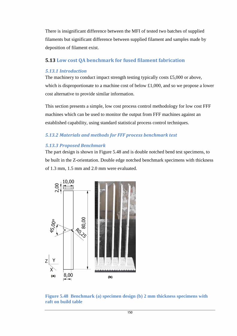
150

There is insignificant difference between the MFI of tested two batches of supplied

filaments but significant difference between supplied filament and samples made by

deposition of filament exist.

5.13 Low cost QA benchmark for fused filament fabrication

5.13.1 Introduction

The machinery to conduct impact strength testing typically costs £5,000 or above,

which is disproportionate to a machine cost of below £1,000, and so we propose a lower

cost alternative to provide similar information.

This section presents a simple, low cost process control methodology for low cost FFF

machines which can be used to monitor the output from FFF machines against an

established capability, using standard statistical process control techniques.

5.13.2 Materials and methods for FFF process benchmark test

5.13.3 Proposed Benchmark

The part design is shown in Figure 5.48 and is double notched bend test specimens, to

be built in the Z-orientation. Double edge notched benchmark specimens with thickness

of 1.3 mm, 1.5 mm and 2.0 mm were evaluated.

Figure 5.48 Benchmark (a) specimen design (b) 2 mm thickness specimens with

raft on build table

151

Figure 5.49 shows the test arrangement. The beam support base and clips can be made

using a low cost printer, and the other parts can be readily acquired from a hardware

store. The test arrangement in effect uses a simple bend test set up to assess inter-layer

bond strength.

Figure 5.49 FFF Design jig (a) Assembly with parts (b) with specimens loaded

The jig design and test arrangement are as shown in Figure 5.49. The jig was made

from clear PLA material (Bits from Bytes) and fabricated on BFB 3D Touch printer

with the exception of the support base plate, two mild steel hollow supports, two M10

bolts and wingnuts. The support base plate is fabricated from mild steel of 10 mm

thickness with a 56 x 38 mm hole in our case, which can be made smaller for the

passage of light string that is used for hanging the applied load. The base plate also has

two M10 threaded holes for clamping the beam support to the base plate.

5.13.4 Experimental plan

The overall aim of the test programme was to validate the low cost benchmark against

standard tests. Impact, tensile and flexural specimens were designed for manufacture

based on ISO tests specimen specifications and built on a BFB 3D Touch printer.

Benchmark specimens were also designed for manufactured and tested on both standard

machine (Tinius Olsen universal material testing machine) and fabricated jig. All the

specimens were fabricated using clear PLA material source from Bits from Bytes.

152

5.13.5 Manufacture

The build parameters for determination of single edge notched, Z-oriented benchmark

specimen types with the least bending load to failure and variance are shown in Table

5.15. The benchmark specimen geometry is patterned after ISO designed impact

specimens.

Table 5.15 Processing parameters for selection of specimens with minimum

thickness

Parameter sets Layer thickness (mm) Fill density (%) Speed multiplier

0.5 100% 1.3X

Table 5.16 shows processing parameters for Z- oriented ISO designed Impact, flexural,

tensile specimens and double notched benchmark specimens with a notch radius of

0.25 mm on each side of the width and of length 80 mm, width 10 mm and thickness of

1.3 mm, 1.5 mm and 2 mm. The specimen geometry and test procedure for ISO

designed specimens are as presented in Chapter 3.

Table 5.16 Specimens parameter sets

Parameter sets F1 F2 G1 G2

Layer thickness (mm) 0.5 0.5 0.25 0.25

Fill density (%) 20 100 20 100

Speed multiplier 1X 1.3X 1X 1.3X

5.13.6 Bending test using design test jig

The experimental set-up was as shown in Figure 5.49. The specimen is simply

supported on two rollers of radius 5 mm at 64 mm centres. A light string (Berkley

TRILENE®) of diameter 0.33 mm and a weight carrier/hanger were hung centrally on

the beam specimen so that they hang vertically thereby loading the beam centrally.

Weights are then carefully added to the carrier. Firstly a weight of 200g was added to

the carrier followed by addition of further weights initially at incremental rate of 100g,

50g and then 10g until the specimens fracture in order to obtain the maximum load to

failure and hence the interlayer bond strength between the interface. Flexural strengths

were computed using equation (46) for three-point bending of a rectangular beam.

153

Figure 5.50 Free body diagram of three-point bending of Benchmark specimens

From flexural formula, benchmark flexural strength is given as:

𝜎𝑓𝑏=

3𝐹𝐿

2𝑏𝑤ℎ𝑤2

46

Where, F is the applied load at centre of beam, L is the span; 𝑏𝑤 is the remaining width

under notch of the test specimens and ℎ𝑤 is the specimen thickness; l is the length of

specimen and 𝜎𝑓𝑏 is benchmark flexural strength.

5.13.7 Test specimens

Two hundred and ninety one (291) specimens all oriented in Z – directions were

involved in these experiments. Firstly, five single edge notched benchmark specimens

with notch radius of 0.25 mm (see Figure 5.51a) were used for determination of

maximum bending load to failure. These is then followed by the fabrication of thirty

single edge notched benchmark specimens (5 for each thickness of 2, 2.5, 3, 4, 6, and 10)

mm with notch radius of 2 mm (see Figure 5.51b), and were used for determination of

feasible minimum section thickness with the lowest maximum bending load to failure

using parameter sets in Table 5.15. Thereafter, ninety six ISO designed impact, flexural

and tensile specimens, with eight specimens for each parameter set as shown in Table

5.16 were also fabricated. One hundred and sixty double edge notched benchmark

specimens were also made using each parameter sets in Table 5.16. With sixty of the

benchmark specimens made with thickness of 2 mm and sixty were also made with

thickness of 1.5 mm while the remaining forty benchmark specimens were made with

thickness of 1.3 mm. Twenty of each benchmark specimens designs were tested (3-

154

point bend test) using standard machine (Tinius Olsen universal material testing

machine) while forty each were tested using the test jig.

Figure 5.51 Single edge notched benchmark specimens with notch radius (a) 0.25 mm (b) 2

mm

5.14 Results and analysis for FFF QA benchmark

5.14.1 Maximum load to failure of benchmark sample with notch radius of 0.25

mm

Table 5.17 shows the maximum bending load to failure of Z- oriented single edge

notched benchmark samples of notched radius 0.25 mm and specimen’s dimensions of

(10 x 10 x 80) mm which were tested using three point bend test on a standard machine

(Tinius Olsen).

Table 5.17 Benchmark sample maximum bending load to failure

Sample Maximum load (N)

1 260.8

2 291.2

3 266

4 258

5 252.8

mean 265.76

155

5.14.2 Maximum load to failure of single edge notched specimens with notch

radius of 2 mm and of different thickness

A load of 265 N (see Table 5.17) is high for intended low cost test jig. In order to

reduce the amount of load that will be required to fracture the benchmark specimens

(see Figure 5.51a). The notch radius was increased to 2 mm as shown in Figure 5.51b. A

variety of thickness was then evaluated from 2 mm to 10 mm. The result obtained after

test on standard machine is as shown in Table 5.18.

Table 5.18 shows the variation of maximum bending load to failure with section

thickness of specimens with the same notch radius (2 mm) and dimensions of 10 x 80

mm for the width and length and of different section thickness as shown in Table 5.18.

Table 5.18 Maximum bending loads (N) versus Sample thickness (mm)

Sample thickness

(mm)

Sample mass (g) Maximum bending load

(N)

Ave. Min. Max. Ave. Min. Max.

2 1.86 1.83 1.91 13.04 12.50 14.00

2.5 2.37 2.35 2.38 21.87 20.00 24.85

3 2.51 2.48 2.53 28.14 24.35 31.00

4 3.62 3.59 3.66 53.88 49.85 57.53

6 5.53 5.44 5.59 129.01 103.38 138.90

10 9.28 9.21 9.36 217.90 204.75 233.75

It can be observed from the results that benchmark sample with thickness of 2 mm

have the lowest maximum bending load to failure and variability (assessed by min-max

range). Benchmark specimen with thickness of 2 mm was then adopted for further

analysis.

5.14.3 Correlation between load, thickness and mass of single edge notched

specimens

Figure 5.52 shows the correlation between the maximum bending load to failure,

sample thickness and mass of specimens of the same notch radius (2 mm), width (10

mm) and length (80 mm) but different thickness. The processing parameters are as

shown in Table 5.15.

156

Figure 5.52 Correlation between maximum load, sample mass and thickness of

single edge notched specimens

In order to ensure that there is no stress concentration on only single edge of the

specimen (to ensure uniform stress distribution on both sides of width). The benchmark

specimen was thus double edged notched with notch radius of 0.25 mm as shown in

Figure 5.48. The processing parameters for the specimens are as shown in Table 5.16.

The following sections will present test results for ISO flexural, tensile and impact

properties with that of double notched benchmark specimens. Interesting maximum

bending load correlates with both sample mass and section thickness.

5.14.4 ISO flexural, tensile and Impact strengths and benchmark flexural

strength

The variations of Z-oriented tensile strength, impact strength and flexural strength of

ISO designed specimens and that of benchmark specimens flexural strengths (tested

with the test jig) with parameter set in Table 5.16 are presented in Table 5.19. Three

benchmark specimens test results are also presented in that table both having the same

geometry but only differs in section thickness. One of the benchmark was made with

thickness of 2 mm while the others were made with thickness of 1.5 mm and 1.3 mm.

10987654321

250

200

150

100

50

0

Sample thickness (mm)

Ma

xim

um

be

nd

ing

lo

ad

(N

)

Sample thickness (mm)

Sample mass (g)

Variable

Sample mass (g)

r= 0.990

(p< 0.01)r

= 0.99

1 (p< 0

.01)

157

Table 5.19 Variations of mechanical properties with parameter set

Parameter set

Mechanical property F1 F2 G1 G2

ISO UTS (MPa)

Ave. 19.71 23.47 24.80 31.10

Min. 19.38 21.76 24.50 30.35

Max. 20.25 24.19 25.30 32.19

ISO Flexural strength (MPa)

Ave. 25.75 42.91 47.62 57.59

Min. 18.34 40.33 45.27 54.60

Max. 28.51 45.27 49.66 61.43

ISO Impact strength (kJ/m2)

Ave. 4.34 4.58 4.66 5.20

Min. 4.23 4.51 4.63 4.80

Max. 4.50 4.62 4.76 5.48

Benchmark test (2 mm)

Flexural strength (MPa)

Ave. 18.59 21.11 38.36 40.40

Min. 17.29 20.66 37.26 38.98

Max. 19.78 21.60 38.95 41.13

Benchmark test (1.5 mm)


Ave. 12.40 13.40 25.71 27.58

Min. 9.18 11.31 24.84 25.94

Max. 13.87 16.10 26.23 30.18

Benchmark test (1.3 mm)


Ave. 12.34 13.91 14.20 20.84

Min. 10.81 13.15 13.40 20.05

Max. 14.33 14.78 14.80 21.68

ANOVA was used to compare the significance of variation of Z-oriented flexural,

tensile and impact strengths of ISO designed specimen results presented in Table 5.19

with parameter set. The results of the comparisons are as presented in Table 5.20 to

Table 5.22. Specimens made with parameter set G2 have the highest strengths across

test types.

Table 5.20 ANOVA: Flexural strength versus parameter sets

Source of Variation SS df MS F P-value F crit

Between Groups 2641.03 3 880.34 93.67 0.00 3.24

Within Groups 150.38 16 9.40

Total 2791.41 19

158

Table 5.21 ANOVA: Tensile strength versus parameter sets


Between Groups 336.51 3 112.17 198.88 0.00 3.24


Total 345.53 19

Table 5.22 ANOVA: Impact strengths versus parameter sets


Between Groups 1.99 3 0.66 32.82 0.00 3.24


Total 2.32 19

df, degree of freedom; SS, sums of squares; MS, mean squares; F, F-statistics; P, p-Value

5.14.5 Correlation analysis of ISO test results and that of benchmark test

results

Figure 5.53 shows the correlation between ISO flexural strength, impact strength and

UTS with flexural strength of benchmark specimens of 2 mm tested by using test jig

and their respective correlation coefficients and p-values. The figure also shows the

correlation between flexural strengths of benchmark specimens tested by using standard

machine (Tinius Olsen) and fabricated test jig. TO in the figure represent Tinius Olsen

universal testing machine.

159

Figure 5.53(a) correlation between flexural strength of benchmark specimens (2 mm)

tested by standard machine and test jig and correlation between ISO (b) Impact strength

(c) UTS (d) Flexural strength with Benchmark flexural strength

Similarly, when benchmark specimens were made with the same process parameters as

that of 2 mm thickness but with thickness of 1.5 mm, the results obtained are presented

in Table 5.19 and Figure 5.54.

Figure 5.54 shows the correlation between ISO flexural strengths, impact strengths and

UTS with flexural strengths of benchmark specimens of 1.5 mm thickness tested by jig



machine (Tinius Olsen) and fabricated test jig.

Figure 5.55 shows the correlation between ISO flexural strengths, impact strengths and

UTS with flexural strengths of benchmark specimens of 1.3 mm thickness tested by jig



machine (Tinius Olsen) and fabricated test jig.

4035302520

40

30

20

Benchmark flexural strength (MPa) Jig Be

nch

ma

rk

fle

x.

str

en

gth

(M

Pa

) T

O

4035302520

5.4

5.1

4.8

4.5

4.2

Benchmark flexural strength (MPa)Jig

IS

O I

mp

act

str

en

gth

(k

J/m

^2

)4035302520

32

28

24

20

Benchmark flexural strength (MPa) Jig

IS

O U

TS

(M

Pa

)

4035302520

60

50

40

30

20

Benchmark flexural strength (MPa) Jig IS

O F

lex

ura

l str

en

gth

(M

Pa

)

r = 0.

960 (p

< 0.01

)

(d)

(b)

r = 0.805 (p

< 0.01)

r = 0.83

3 (p<

0.01)r =

0.848 (

p< 0.01

)

(c)

(a)G

F

G

F

G

F

G

F

160

Figure 5.54 (a) Correlation between flexural strength of benchmark specimens (1.5 mm)


(c) UTS (d) Flexural strength with benchmark flexural strength

Figure 5.55(a) Correlation between flexural strength of benchmark specimens (1. 3mm)


(c) UTS (d) Flexural strength with benchmark flexural strength

3025201510

25

20

15

10

Benchmark flexural strength (MPa) JigBe

nch

ma

rk

fle

x.

str

en

gth

(M

Pa

)_

TO

3025201510

5.4

5.1

4.8

4.5

4.2

Benchmark Flexural Strength (MPa) Jig

IS

O I

mp

act

str

en

gth

(k

J/m

^2

)3025201510

32

28

24

20

Benchmark Flexural strength (MPa) Jig

IS

O U

TS

(M

Pa

)

3025201510

60

50

40

30

20

Benchmark flexural strength (MPa) JigIS

O F

lex

ura

l str

en

gth

(M

Pa

)

r = 9

83 (p

< 0.01)

r = 0.881

(p< 0.01)

r = 0.

913 (p

< 0.01

)

r = 0.904 (p

< 0.01)

(a) (b)

(c) (d)

20.017.515.012.510.0

20.0

17.5

15.0

12.5

10.0

Benchmark flexural strength (MPa) JIG Be

nch

ma

rk

Fle

x.

Str

en

gth

(M

Pa

) T

O

20.017.515.012.510.0

5.4

5.1

4.8

4.5

4.2

Benchmark flexural strength (MPa) JIG

IS

O I

mp

act

str

en

gth

(k

J/m

^2

)

20.017.515.012.510.0

32

28

24

20


IS

O U

TS

(M

Pa

)

20.017.515.012.510.0

60

50

40

30

20


IS

O f

lex

ura

l str

en

gth

(M

Pa

)

r =0 .90

2 (p<

0.01

)

r = 0

.957 (p

< 0.0

1)

r = 0.

971 (

p< 0.

01)

r = 0.

870 (p<

0.01)

G2G2

G2 G2

(a) (b)

(c) (d)

161

Table 5.23 and Table 5.25 show ANOVA tables for investigating the significant of

variation of flexural strengths of benchmark specimens of 1.5 mm, 2 mm and 1.3 mm

thickness tested by the use of standard machine and fabricated test rig.

Table 5.23 ANOVA: Benchmark flexural strengths versus parameter set and

machine type (1.5 mm specimens)

ANOVA 1.5 mm Source of

Variation SS df MS F P-value F crit

Machine type 1.16 1 1.16 0.59 0.45 4.15

Parameter set 803.15 3 267.72 136.38 0.00 2.90

Interaction 111.27 3 37.09 18.89 0.00 2.90

Error 62.82 32 1.96

Total 978.39 39

Table 5.24 ANOVA: Benchmark flexural strengths versus parameter set and

machine type (2 mm specimens)


Machine type 6.40 1 6.40 2.28 0.14 4.15

Parameter set 3765.87 3 1255.29 447.19 0.00 2.90

Interaction 14.34 3 4.78 1.70 0.19 2.90

Error 89.83 32 2.81

Total 3876.44 39

Table 5.25 Benchmark flexural strengths versus parameter set and machine type

(1.3 mm specimens)


Machine 2.39 1 2.39 2.09 0.16 4.15

Parameter set 398.40 3 132.80 116.13 0.00 2.90

Interaction 9.18 3 3.06 2.68 0.06 2.90

Error 36.59 32 1.14

Total 446.57 39

The micrograph of fracture surface of benchmark specimens made with 2 mm thickness

and respective process parameter sets are shown in Figure 5.56.

162

Figure 5.56 Fracture surfaces of benchmark specimens made with parameter sets

(a) F1 (b) F2 (c) G1 (d) G2

5.14.6 Summary of low cost benchmark test results

UTS, flexural strengths and impact strengths are all sensitive to variation in process

parameters that influenced the structural strength of FFF fabricated parts. Correlations

exist between flexural strengths of benchmark specimens tested on test jig and standard

machine and also between flexural strengths of benchmark specimens tested on test jig

and ISO designed specimens. Statistical non-significant variation due to use of standard

machine and fabricated test jig were observed while significant variation due to

parameter sets exist.

163

Chapter 6 DISCUSSION

6.1 Summary of Key SLS Results

The summary of key test results and analysis of tested SLS nylon 11 and nylon 12

include:

Specimen density is a better predictor of ISO flexural modulus than benchmark

flexural modulus.

Benchmark impact strength correlates well with ISO impact strength.

Density of benchmark specimens also correlates well with modulus over

multiple builds, as does MFI.

Good correlation was observed between average MFI and average dimensional

accuracy of benchmark specimens over multiple builds.

The surface roughness of specimens was observed to deteriorate for later builds.

6.2 SLS Mechanical properties

6.2.1 Tensile properties of laser sintered part

Figure 6.1 to Figure 6.3 show the variation of tensile properties with orientations of test

parts fabricated from SLS nylon 11 and nylon 12 powders. The results shown in those

figures are from this research and from manufacturers’ material properties datasheets

for Duraform PA 12 [188] and EOS PA2200 PA 12 [189], INNOV PA 1350_ETx (PA

11) [190] and from research work of Ajoku et al. [90] (using specimens made from

nylon 12) and from Lauren et al [191] using specimens made from nylon PA 11( with

the brand name of PA D80-ST). Where, DF PA 12 in the figure represents Duraform

PA 12 (nylon 12) from 3D systems. For the EOS PA2200 PA12 and Innov PA 11

materials the test orientation was not declared.

164

INNO

V PA

11 da

tash

eet -

Z

INNO

V PA

11 da

tash

eet -

XY

INNO

V PA

11 - Z

INNO

V PA

11- Y

INNO

V PA

11 - X

EOS PA

220

0 datas

heet

Ajok

u_ PA

12 -

Z

Ajok

u_PA

12 - Y

Ajok

u_PA

12 - X

DF PA

datash

eet -

Z

DF PA da

tash

eet -

Y

DF PA

datash

eet -

X

DF PA 12

_Z

DF PA 12

_Y

DF PA

12 _X

50

40

30

20

10

0

UTS

(M

Pa

)

This research This research

Polymer type

Figure 6.1 Variation of UTS with build directions for nylon 11 and nylon 12 polymer, the graph shows the mean, median, lower and upper limit, first and third quartile

INNO

V PA

11 da

tash

eet [

186]

Lauren

_PA

11 -

X [1

88]

INNO

V PA

11 - Z

INNO

V PA

11-

Y

INNO

V PA

11- X

EOS PA

220

0 da

tash

eet [

185]

Ajok

u_ PA 12

- Z [1

87]

Ajok

u_PA

12 -

Y [187

]

Ajok

u_ PA

12 -

X [1

87]

DF PA

datash

eet -

Z [184

]

DF PA

datash

eet -

Y [1

84]

DF PA

datash

eet -

X [184

]

DF PA 12

_Z

DF PA 12

_Y

DF PA

12_X

2250

2000

1750

1500

1250

1000Te

nsile

mo

du

lus (

MP

a)


Polymer type

Figure 6.2 Variation of tensile modulus with build direction for nylon 11 and nylon 12 polymer, the graph shows the mean, median, lower and upper limit, first and third quartile

165

INNO

V PA

11 da

tash

eet_Z [186

]

INNO

V PA

11 da

tash

eet_XY

[186

]

Laur

en_ PA

11 -X

[188

]

Inno

v PA

11 _Z

Inno

v PA

11_

Y

Inno

v PA

11_

X

EOS PA

220

0 da

tash

eet [

185]

Ajok

u_PA

12 -Z [1

87]

Ajok

u_ PA 12

- Y [1

87]

Ajok

u_PA

12 -X

[187

]

DF PA da

tash

eet _

Z [1

84]

DF PA da

tash

eet _

Y [1

84]

DF PA da

tash

eet_ X

[184

]

DF PA

12_Z

DF PA

12_Y

DF PA 12

_ X

50

40

30

20

10

0

Elo

ng

ati

on

at

bre

ak (

%)


Polymer type

Figure 6.3 Variation of elongation at break with build direction for nylon 11 and nylon 12 polymer, the graph shows the mean, median, lower and upper limit, first and third quartile

Typical tensile stress - strain curves for nylon 11 and nylon 12 test parts with their build

orientations are as shown in Figure 6.4 and Figure 6.5 respectfully. It can be observed

from those figures that nylon 11 is more ductile than nylon 12.

Figure 6.4 Tensile stress vs. strain from experimental results for PA 11

0

10

20

30

40

50

60

0.00% 5.00% 10.00% 15.00% 20.00% 25.00% 30.00% 35.00% 40.00% 45.00%

Ten

sile

str

ess

(MP

a)

Strain (%)

X Z Y

166

Figure 6.5 Tensile stress vs. strain from experimental results for PA 12

Also from Figure 6.1 to Figure 6.3 the PA 12 results for modulus and strength were

lower than those reported by others, but PA 11 results matched reported results. The

observed difference in PA 12 results might have being due to the relatively low density

of PA 12 specimens as shown in Figure 4.11 as a result of non-optimum process

conditions or parameters. When these specimens were made the machine was newly

purchased and expertise was still being developed. However, when the PA 11

specimens were made more experience in the use of the machine had been gained.

The results from nylon PA 11 tend to suggest that if parts are made from polymers

using an “optimum” SLS process parameters or conditions and good quality input

material it is possible to have isotropic strengths and modulus but with ductility still

anisotropic. These observed isotropy in tensile strength and anisotropy in ductility

agrees with Bourell [192].

Variations of tensile properties of tested nylon 12 (Duraform PA 12) specimens with

orientations are significant (p< 0.01). The observed variation pattern of tensile

properties with orientations is consistent to that observed by others.

Also from Figure 6.1 to Figure 6.3 the experimental results are not exactly the same in

absolute terms with manufacturers provided material properties, and also between test

values obtained by various researchers. These findings are also consistent with

observations in literature where mechanical properties of SLS made part were observed

to vary between different machines [59, 93] and even for the same machine in different

0

5

10

15

20

25

30

35

40

0.0% 2.0% 4.0% 6.0% 8.0% 10.0% 12.0%

Ten

sile

str

ess

(MP

a)

Strain (%)

X Y Z

167

builds [59]. These variation in mechanical properties may be due to differences in

exposure process parameters of the systems used (such as laser power energy density,

laser part scanning strategy, part bed temperature, position of the parts in build chamber

or part bed, powder material flow properties or quality of the input materials among

others as noted in the literature review), but one thing that is very common to most of

the tensile test results is the anisotropy properties of SLS manufactured part. The

reasons for anisotropy in mechanical properties of SLS parts have been presented in

section 2.6.3.

6.2.2 Flexural properties of laser sintered part

Figure 6.6 and Figure 6.7 show the variation of flexural properties with orientations of

test parts fabricated from SLS nylon 11 and nylon 12 powders. The results shown in

those figures are from this research and from manufacturers’ material properties

datasheets for Duraform PA 12 [188] and EOS PA2200 PA 12 [189], INNOV PA

1350_ETx (PA 11) [190] and from research work of Ajoku et al. [90] (using specimens

made from nylon 12), Munguia et al. [193] (using specimens made from EOS PA2200

PA 12) and from Koo et al. [194] using specimens made from nylon PA

11( RILSAN® PA11). The orientation of the Rilsan PA 11 and Innov PA 11 test

specimens was not stated.

Koo_

Rilsa

n PA

11 [1

91]

INNO

V PA

11 - Z

INNO

V PA

11 - Y

INNO

V PA

11 - X

Mun

guia_E

OS PA 22

00-Z

[19

0]

Mun

guia_E

OS PA 22

00-Y [19

0]

Mun

guia_E

OS

PA 220

0 -X

[19

0]

Ajok

u_ PA

12 -Z

[18

7]

Ajok

u_ PA

12 -

Y [18

7]

Ajok

u_ PA

12 -X [1

87]

DF PA

12 datas

heet-Z [18

4]

DF PA 12

datas

heet-Y [18

4]

DF PA

12 datas

heet -X

[184

]

DF PA

12_Z

DF PA 12

_Y

DF PA 12

_X

80

70

60

50

40

30

20

Fle

xu

ral str

en

gth

(M

Pa

)


Polymer type

Figure 6.6 Variation of flexural strength with build direction for SLS nylon 11 and nylon 12 polymer, the graph shows the mean, median, lower and upper limit, first and third quartile

168

INNO

V PA

11 da

tash

eet [

186]

INNO

V PA

11- Z

INNO

V PA

11 - Y

INNO

V PA

11 - X

EOS PA

220

0 da

tash

eet_X

[185

]

Mun

guia_E

OS PA

220

0 _Z

[19

0]

Mun

guia_E

OS PA

220

0 _Y

[19

0]

Mun

guia_E

OS

PA 220

0_X [1

90]

Ajok

u_ PA

12_Z

[18

7]

Ajok

u_PA

12 -Y [18

7]

Ajok

u_ PA 12

-X [1

87]

DF PA

12 datas

heet -Z

[18

4]

DF PA 12

datas

heet -Y

[18

4]

DF PA

12 datas

heet -X

[184

]

DF PA 12

_Z

DF PA 12

_Y

DF PA 12

_X

1800

1600

1400

1200

1000Fle

xu

ral m

od

ulu

s (

MP

a)


Polymer type

Figure 6.7 Variation of flexural modulus with build direction for SLS nylon 11 and nylon 12 polymer, the graph shows the mean, median, lower and upper limit, first and third quartile

Typical flexural stress - strain curves for nylon 11 and nylon 12 test parts with their

build orientations are as shown in Figure 6.8 and Figure 6.9 respectfully.

Figure 6.8 Flexural stress vs. strain from experimental results for PA 11

0

10

20

30

40

50

60

70

0.00% 2.00% 4.00% 6.00% 8.00% 10.00% 12.00% 14.00% 16.00%

Flex

ura

l str

ess

(MP

a)

strain (%)

stress(MPa) -X stress(MPa) -Y stress(MPa) -Z

169

Figure 6.9 Flexural stress vs. strain from experimental results for PA 12

Also from Figure 6.6 and Figure 6.7 PA 12 results were observed to be lower and more

anisotropic than the manufacturer’s data, while PA 11 results are comparable to

manufacturer’s data. The variation of flexural modulus and strength of tested Duraform

PA 12 (nylon 12) with orientation are significant (p< 0.01).The low test results of PA 12

specimens is due to low density of the specimens (see Figure 4.12) as explained

previously for tensile property results. The Nylon PA 11 results also suggest that this

material is isotropic as in the case of tensile properties.

6.2.3 Impact strength of laser sintered part

Figure 6.10 shows the variation of impact strength with orientations of test parts

fabricated from SLS nylon 11 and nylon 12. The results shown in that figure are from

this research and from manufacturers’ material properties datasheets for EOS PA2200

PA 12 [189] and from material data sheet downloaded from service bureau website [195]

for Rilsan PA 11 (nylon 11). However, the orientation of the specimens used in

determining the impact strength for the data sheet results was not stated.

From Figure 6.10 it can be observed that PA 12 is anisotropic and is in line with

manufactural data while PA 11 is isotropic, but variable and is below the manufacturer

data.

0

10

20

30

40

50

60

70

80

90

0.00% 2.00% 4.00% 6.00% 8.00% 10.00%

Flex

ura

l str

ess

(MP

a)

Strain (%)

stress(MPa) -X stress(MPa) -Y stress(MPa) -Z

170

Rilsa

n PA

11 da

tash

eet [

193]

INNO

V PA

11_

Z

INNO

V PA

11_

Y

INNO

V PA

11_

X

EOS PA

220

0 da

tash

eet [

185]

DF PA

12-Z

DF PA

12-Y

DF PA 12

-X

9

8

7

6

5

4Imp

act

str

en

gth

(kJ/

m^

2)


Polymer type

Figure 6.10 Variation of Impact strengths with build direction for SLS nylon 11 and nylon 12 polymers, the graph shows the mean, median, lower and upper limit, first and third quartile

6.2.4 Implication of SLS Mechanical property results for this work

As noted earlier the tensile and flexural properties of tested PA 12 specimens in this

research (the specimens had low density as shown Figure 4.11) were observed to be

lower than those reported by others, while PA 11 test results in this research (the

specimens had high density as shown in Figure 4.25) matched those reported by others.

However, impact strengths results for PA 12 is consistent to that of manufacturer, while

impact strength of PA 11 is still isotropy as observed for tensile and flexural strength for

that material. These findings tend to suggest that tensile and flexural properties of SLS

made parts are more density dependent unlike impact strength.

Possible reasons for that observation is that the presence of porosity in SLS fabricated

parts will increase the rate of propagation of cracks during loading conditions; as pores

will serve as stress concentrators which will leads to non-uniform distribution of strain

[196-198]. Pores will also reduce the effective load bearing area of the material. The

resultant effect of this is reduction in the net strength of the material (by reducing the

ability of material to resist crack propagation through their sections) and hence lower

strengths and moduli. However, surface conditions under high strain rate as in the case

of impact loading will affect the ability of the material to resist crack initiation through

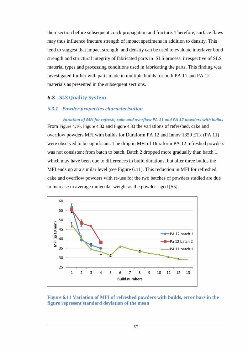
171

their section before subsequent crack propagation and fracture. Therefore, surface flaws

may thus influence fracture strength of impact specimens in addition to density. This

tend to suggest that impact strength and density can be used to evaluate interlayer bond

strength and structural integrity of fabricated parts in SLS process, irrespective of SLS

material types and processing conditions used in fabricating the parts. This finding was

investigated further with parts made in multiple builds for both PA 11 and PA 12

materials as presented in the subsequent sections.

6.3 SLS Quality System

6.3.1 Powder properties characterisation

Variation of MFI for refresh, cake and overflow PA 11 and PA 12 powders with builds

From Figure 4.16, Figure 4.32 and Figure 4.33 the variations of refreshed, cake and

overflow powders MFI with builds for Duraform PA 12 and Innov 1350 ETx (PA 11)

were observed to be significant. The drop in MFI of Duraform PA 12 refreshed powders

was not consistent from batch to batch. Batch 2 dropped more gradually than batch 1,

which may have been due to differences in build durations, but after three builds the

MFI ends up at a similar level (see Figure 6.11). This reduction in MFI for refreshed,

cake and overflow powders with re-use for the two batches of powders studied are due

to increase in average molecular weight as the powder aged [55].

Figure 6.11 Variation of MFI of refreshed powders with builds, error bars in the

figure represent standard deviation of the mean

25

30

35

40

45

50

55

60

1 2 3 4 5 6 7 8 9 10 11 12 13

MFI

(g/

10

min

)

Build numbers

PA 12 batch 1

Pa 12 batch 2

PA 11 batch 1

172

In addition, the increase in MFI of PA 11 in build 6 instead of drop was thought to be

due to the use of a greater quantity of virgin powder in refreshing the old powder in that

build as compared to the previous builds. Thereafter, a consistent decreased in MFI with

builds was observed. Also from Figure 4.16 and Figure 4.33, the cake powders for both

PA 11 and PA 12 were observed to have lowest MFI after a build. This is because they

had more thermal exposure and therefore degrade faster and more than the overflow

powders. Furthermore, from Figure 4.32 there is more significant drop in MFI from the

virgin powder used in build one to the first recycled powder used build two, thereafter

the deterioration is less rapid which agrees with the finding of Pham et al. [55] for nylon

12 (PA2200) though only virgin and refreshed powders were studied in their case.

Similarly, viscosities for the respective powders increased from one build to another as

shown in Figure 6.12. The increase in average molecular weight which leads to

decreased melt flow rates also caused the increase in viscosity with builds. This is

because of increasing resistance to molecular motion or flows due to increase in average

molecular size and molecular distribution, as powders are re-used. The drop in viscosity

in build 6 instead of increase was due to the same reasons as mentioned for MFI.

Figure 6.12 Variation of viscosity with builds for Innov PA 1350 ETx refreshed powders

Viscos

ity (Bld- 13)

Viscos

ity (Bld-

12)

Visc

osity

(Bld- 11)

Viscos

ity (Bld- 10)

Viscos

ity (Bld-

9)

Visc

osity

(Bld- 8)

Viscos

ity (Bld-

7)

Visc

osity

(Bld-

6)

Visc

osity

(Bld-5)

Viscos

ity (Bld-

4)

Viscos

ity (B

ld- 3

Viscos

ity (Bld- 2)

Viscos

ity (Virgin)

350

300

250

200

150

100

50

0

Powder type

Vis

co

sit

y (

Pa

.s)

95% CI for the Mean

173

Figure 6.13 Relationship between MFI, MVR and viscosity of recycled powders for Innov

PA 1350 ETx powder, error bars in the figure represent standard deviation of the mean

Furthermore, from Figure 6.13 correlations exist between average MFI and average

viscosity of refreshed nylon 11 powders tested before every build. The coefficient of

determinations (r2) of the fitted model between MFI and viscosity is 91.3% (p< 0.01).

Thus, it will not be necessary to measure both MFI and viscosity of SLS powders with

builds.

6.3.2 Benchmark validation for SLS specimens

Correlations between ISO and benchmark flexural modulus and density

for Duraform PA 12 (Nylon 12) and Innov PA 1350 ETx (PA 11) in single

build

From Figure 4.10 positive correlation exist between the flexural modulus of Benchmark

1 and that of ISO specimens (r = 0.841, p< 0.01), and also between flexural modulus of

Benchmark 2 and that of ISO specimens (r = 0.843, p< 0.01) made from PA 12 in single

build. But if the single outlier which is due to high modulus values of one of ISO and

benchmark 1 Y-oriented specimens as shown in Figure 4.9 is removed from the

correlation analysis between benchmark 1 and ISO specimens the correlation is even

higher (r = 0.945, p< 0.01). Correlation between ISO designed specimens test results

and BM 2 results was also reduced by the variation in ISO test results and in BM 2-Y.

220 240 260 280 300 320 34025

30

35

40

45

50

Average viscosity (pa.s)

Avera

ge M

FI

(g/1

0 m

in)

r2 = 91.3%

174

Similarly, from Figure 4.24 very strong positive correlations exist between flexural

modulus of ISO designed specimens and that of Benchmark 1 (r = 0.955, p< 0.05) and

also between flexural modulus of ISO designed specimens and that of Benchmark 2

specimens (r = 0.960, p< 0.05) made from PA 11 in single build like in the case of PA

12.

In addition, from Figure 4.12 and Figure 4.26 strong positive correlation also exist

between ISO specimens flexural modulus and density of the flexural modulus

specimens made in single build for PA 12 ( r = 0.974, p< 0.01) and PA 11 (r = 0.945, p<

0.01) materials which suggest that flexural modulus increases with density. Similar

relationships also exist between benchmark modulus and density of benchmark test

specimens made in the same build as that of ISO specimens for both PA 12 (see Figure

4.13) and PA 11 (see Figure 4.27). However, the BM 1 results of PA 11 are clearly

skewed by a low density (0.986 g/cm3) of one BM 1 specimen as compared to other

densities of benchmark specimens with a minimum density of 1.01 g/cm3 as shown in

Figure 4.25. The low density of that specimen may be due to location in the build

chamber. As thermal inconsistencies in the build chamber have been observed by

various researcher to be one of the problem facing SLS users [33, 74].

The results of this investigation show that density of flexural modulus specimen is a

better predictor of ISO flexural modulus than benchmark flexural modulus for both

nylon 11 and nylon 12 material studied. The data also suggests that density as a

predictor of ISO flexural modulus is less susceptible to small variation than modulus.

Correlations between ISO and benchmark Impact strengths for

Duraform PA 12 (Nylon 12) and Innov PA 1350 ETx (PA 11) in single

build

From Figure 4.15 positive correlations exist between impact strengths of Benchmark 1

and that of ISO designed specimens (r = 0.875, p< 0.01) and also between impact

strengths of Benchmark 2 and that ISO designed specimens (r = 0.955, p< 0.01) made in

single build for PA 12 (Figure 4.15) material. Similar positive correlations exist

between impact strengths of Benchmark 1 and that of ISO designed specimens (r =

0.953, p< 0.05) and also between impact strengths of Benchmark 2 and that of ISO

designed specimens (r = 0.956, p< 0.05) made in single build for PA 11 (see Figure 4.29)

material.

175

Taken together, these results suggest that measurements of densities are the simplest

way to infer modulus. Also, since correlations were observed between ISO and

benchmark impact strengths made in the same build. The benchmark tests are thus

validated against that of ISO impact test for both Innov PA 1350 ETx and Duraform PA

12 material in this study.

6.3.3 Correlations between densities and flexural modulus of benchmark

specimen made in multiple builds (PA 11 and PA 12)

Densities and flexural modulus of specimens made from Duraform PA 12 (Nylon 12)

were observed to vary with builds as shown in Figure 4.18. Positive correlations were

thus observed between average densities and average flexural modulus of benchmark 1

specimens and also between average modulus and average density of benchmark 2

specimens as shown in Figure 4.20. Similarly, very strong positive correlations (see

Figure 4.38) exist between average benchmark flexural modulus and average density of

benchmark flexural modulus specimens made from Innov Pa 1350 ETx (Nylon 11)

material in multiple builds like in the case of specimens made from Duraform PA 12.

This implies that modulus increases with density across multiple builds for both PA 11

and PA 12 materials. This increment in modulus with density will have been due to

more effective sintering. This is because increased densification during sintering is

achieved by material flow and pores reduction, as increased in viscosity (low MFI)

lowers the sintering rate [199-202]. This reduction in sintering rate increases the

probability of pores being formed between layers and hence lower modulus for low

density benchmark specimens.

The implication of these findings is that, since in section 6.3.2 very strong positive

correlation exists between flexural moduli and densities of respective ISO designed and

benchmark flexural modulus specimens made in the same single build. Similarly, in this

section very strong positive correlations were also found to exist between benchmark

flexural modulus and densities of benchmark flexural modulus specimens made in

multiple builds, for nylon 11 and nylon 12 materials. Thus, there is no longer a need to

keep measuring benchmark flexural modulus in the proposed quality system, since

density measurement will suffice.

176

6.3.4 Impact strength of benchmark specimens made in multiple builds (PA

11 and PA 12)

From Figure 4.34 impact strengths of benchmark specimens made from Innov PA 1350

ETx (Nylon 11) were observed to drop from build 9 to the last build after the initial

relative increased in impact strength with builds for both types of benchmark specimens.

Also from Figure 4.19 impact strengths of Duraform PA 12 made specimens were

observed to vary with builds and densities with the exception of build five for the

benchmark sample. This variation of impact strength with builds is due to density of the

specimens, average molecular weight and surface conditions of the specimens (see

Table 4.8). As average molecular weights (is inversely related to MFI) have been

known to influence the strength of polymer [203]. Molecular weights have also be

found to be responsible for increased in elongation at break in earlier builds for laser

sintered part [59, 93]. Therefore, this increment in ductility means that more plastic

work will be required before deformation will be sufficient to fracture the impact

specimens. This may provide the reason for initial increased in impact strengths of

benchmark specimens in addition to increase in densities with builds before the drop in

impact strengths and increased in surface roughness for latter builds. However, there is

optimum range of molecular weight for laser sintering polymers as pointed out by

Goodridge et al.[33] and Kruth et al.[204] beyond which the material properties will

deteriorate, which will explained the reason behind the decreased in impact strength in

latter builds.

In addition, higher density will leads into superior strength due to reduction in

porosities that can serve as points of stress concentration [205] in parts. However,

correlations (Figure 4.39) between average impact strengths of benchmark specimens

and average densities of benchmark impact specimens made in multiple builds were not

so good as compared to correlation between average modulus and average density of

benchmark flexural specimens made in multiple builds which may be due to surface

flaws for both Benchmark 1 and 2 specimens. This then suggest that impact strength

measurement is still needed as a QA test for investigating interlayer bond strengths

which determine the structural integrity of SLS manufactured parts.

Furthermore, non-significant variation in impact strength (p > 0.05) due to benchmark

types for both nylon 12 and nylon 11 materials were also observed as shown in

appendix C-2. This result suggests that either of the Benchmark 1 and Benchmark 2 test

177

specimen can be used as a quality assurance test part. However, the benchmark 2 test

part was adopted because it is smaller in size. It will therefore require less material and

time to make.

6.3.5 Correlations between MFI and density of Benchmark specimens made in

multiple builds (PA 11 and PA 12)

Very strong positive correlations exist between average MFI and average density of

Benchmark 1 specimens made in multiple builds and also between average MF1 and

average density of benchmark 2 specimens made in multiple builds for both Duraform

PA 12 (see Figure 4.21) and Innov PA 1350 ETx (see Figure 4.40) specimens. This

suggests that densities increases with increase in MFI which may be due to sufficient

fluidity that is necessary for effective sintering.

However, correlation between MFI and density is more consistent across powder

material types (Nylon 11 and Nylon 12) and is also higher than between MFI and

impact strengths which tend to suggest that impact strength can likewise be influence by

other factors such as flaws in the test part which may be microscopic in nature (voids or

pores distribution) in addition to insufficient interlayer bond strengths and quality of

input material. There is thus a need to keep on measuring impact strength and MFI in

the proposed quality assurance system for SLS.

6.3.6 Fracture surface morphology of SLS made benchmark part

Fracture surface micrograph of impact specimens made from Innov PA 1350 ETx

(nylon 11) is as shown in Figure 6.14. Cracks can be observed to be propagating

through the section of the material. And failure can also be observed to occur by layer

separation. Impact strength can therefore be used to evaluate interlayer bond strengths

which are key determinant of structural integrity of fabricated parts in SLS. This is

because if the interlayer bond strengths are strong they will be able to offer more

resistance to propagation of cracks through their sections. And hence the fabricated part

will have high fracture strength.

178

Figure 6.14 Impact specimen fracture surface (Innov PA 1350 ETx)

Similarly, SEM fracture surfaces of Duraform PA 12 benchmark impact specimen made

at the second build and benchmark bending specimen made at the sixth build and that

fractured during test are presented in Figure 6.15. Cross checking of the fracture

surfaces presented in Figure 6.15 may give the possible reasons for the mechanical

behaviour of the fracture bending specimen of the benchmark sample.

Crack propagations

179

(a) fracture surface of impact specimen

(b) fracture surface of bending specimen

(c) magnification of marked section in (b)

(d) magnification of (c) Figure 6.15 SEM micrographs of fractured surface of Benchmark sample

(a) fracture surface of impact specimen of benchmark 1 made in build two (b)

fracture surface of bending specimen of benchmark 1 made in build six (c) is

the magnifications of the rectangular marked sections of the microstructure in (b)

and (d) is the higher magnification of the microstructure in (c)

Comparing Figure 6.15 (a) to (d) the long horizontal void in (a) is the area where

materials had chipped off during test and the powder particles seems to be more fused

180

and packed together with some smaller voids that are not widely spread even with the

high magnification levels than that of (b). Examination of (b) shows the powder

particles loosely bonded and some of the particles are recognizable with growth of

necking between them even at a lower magnification level compared to (a). This may be

the reason for the low density (0.715g/cm3) and fracturing of the specimen on

application of load of 100 g. Consideration of (c) and (d) in Figure 6.15 shows the

fracture surface of the bending specimen been magnified to show the inner morphology

of the grain. Thread –like structures or filaments forming boundaries with network of

voids between them can be observed. This shows poor interconnections between grains

and can serve as areas of stress concentration with resultant reduction in fracture

strength of the material. In addition, formation of continuous phase had been found to

be favourable to density and strength of parts in SLS because it tends to reduce porosity

and defect in material structures [58].

6.3.7 Comparison between MFI, dimensional accuracies and surface

roughness of benchmark specimens made in multiple builds

For Duraform PA 12 material as the powder MFI varies with builds so does the

dimensional accuracies of the length, thickness and notch width (see Figure 4.16, Table

4.5 and Table 4.6). Similarly, for Innov PA 1350 ETx (Nylon 11) material as the

powder MFI (see Figure 4.32) changes with builds so are the dimensional accuracies of

the length, thickness and notch width changes (see Table 4.7). Negative correlations

were also observed between average MFI and average dimensional accuracy of

Benchmark 1 (r = - 0.905, p< 0.01) and Benchmark 2 (r = - 0.864, p< 0.01) specimens

made in multiple builds as shown in Figure 4.42. This suggests that dimensional

inaccuracy increases with decrease in MFI.

The surface roughness of benchmark impact strengths specimens made in multiple

builds were also observed to vary for both horizontal and vertical direction of

measurement as shown in Figure 3.9. There is also a clear deterioration in surface

roughness for later builds. The observed minimum roughness is 5.37µm and maximum

roughness is 11.73µm (see Table 4.8).

The observed relationship between MFI and shrinkage in benchmark specimens made

in multiple builds for both nylon 11 and nylon 12 materials in this research agrees with

that of Pham et al. [55] for the average shrinkage of part made from PA2200 (Nylon 12).

181

Moreover, inaccuracy in dimensions of fabricated parts can also occur due to drifting of

machine calibration in SLS system. These results thus suggest that dimensional

accuracy of benchmark specimens can also be used as a key indicator of material

degradation and machine calibration. Therefore, the combination of the use of QA

benchmark specimens and MFI tests will make it easier to differentiate between drifting

in accuracy due to machine calibration and material degradation.

6.3.8 Selection of sampling method for data collection in benchmark test

From Figure 4.31 when the impact strengths are compared with each other with respect

to locations there is generally less variation in mean of the impact strengths with

locations at 95% confidence interval of the means. However, specimens placed at

locations RC2 shows more variations in impact strength beyond this there are no

statistically significant difference between locations. This variation may have been due

to variation in powder bed temperatures at RC2 location of specimens. Therefore, the

build location RC2 that shows more variation than the other build locations might be the

least well temperature controlled - but the mean doesn't change that much. The

observation was also confirmed by industrial partner to this research. We are told that

they have experienced the worse warpage in that corner (RC2). The implication of this

finding is that the benchmark parts have demonstrated the ability to capture the effect of

process variation on fabricated part. Based on the observed pattern of variation in

impact strengths with locations in this machine, build chamber location RC2 of SLS

machine is therefore recommended for location of benchmark specimens from one build

to another. That build location was selected in order to find potentially flawed parts. As

the specimens placed in that location show higher within sample variation in impact

strength. Benchmark could also be placed about the same region where the main part is

placed for fabrication so that they can have similar thermal history. There should be

consistency in placing the benchmark test part in a location from one build to another.

On the basis of these results two or three sampling approach (two or three impact

strength specimen) per build is recommended for used in quality control chart for

monitoring of process variation and control in order to assure the quality of part made

by the machine from one build to another.

182

6.3.9 SPC analysis for flexural modulus, impact strength and dimensional

accuracy for benchmark (Innov PA 1350 ETx) The data has been used to develop some sample SPC charts shown in Figure 6.16 to

Figure 6.21. The procedure for determining the upper control limit (UCL) and lower

control limit (LCL) for respective plots are given in sections 2.9.4 to 2.9.6.

In the control chart for benchmark 1 impact strengths (see Figure 6.16) there is no

evidence that the process spread is out of control but a trend is observed with process

average. From the process average control chart, impact strengths of sample data points

of builds 4, 6, 7 and 9 were out of the UCL but there is no cause for concern here

because in terms of mechanical properties the higher the better. However, impact

strength data points of builds 11 to 13 are out of LCL and this could be used to indicate

that the powder had deteriorated beyond a reliable quality level.

Figure 6.16 Mean and range chart for impact strength of benchmark 1 (Innov PA 1350ETx)

Similar patterns that were observed in control chart for impact strengths of benchmark

one specimens were also observed for that of control chart for benchmark 2 specimens,

as build 12 and 13 are also out of LCL (see Figure 6.17).

131211109876432

9.0

7.5

6.0

4.5

3.0

Build numbers

Im

pa

ct

str

en

gth

me

an

(k

J/m

^2

)

__X=6.820

UC L=7.732

LC L=5.909

131211109876432

2.0

1.5

1.0

0.5

0.0

Build numbers

Im

pa

ct

str

en

gth

ra

ng

e (

kJ/m

^2

)

_R=0.891

UC L=2.293

LC L=0

1

1

1

1

1

11

183

Figure 6.17 Mean and range chart for impact strength of benchmark 2 (Innov PA 1350ETx)

Similarly, the chart for control of process spread with respect to modulus for benchmark

1 specimens is also in control as shown in Figure 6.18 like in the case of benchmark

impact strengths. This implies that modulus variability within the build is in control or

stable. However, flexural modulus sample data points of builds 3, 4, 6 and 8 in the chart

for the control of process average were above UCL. As previously explained there is no

cause for great concern with these data points. Build 2 benchmark flexural modulus is

also observed to be outside the LCL, this is because of low density of those flexural

modulus specimens as shown in Figure 4.35. The plot also shows that flexural modulus

data points of build 12 and 13 are out of LCL, thus there is need for action to be taken at

this stage to correct the problem.

131211109876432

9.0

7.5

6.0

4.5

3.0

Build numbers

Im

pa

ct

str

en

gth

me

an

(k

J/m

^2

)

__X=6.714

UC L=7.778

LC L=5.651

131211109876432

3

2

1

0

Build numbers

Im

pa

ct

str

en

gth

ra

ng

e (

kJ/m

^2

)

_R=1.040

UC L=2.677

LC L=0

1

1

1

1

1

11

184


Figure 6.19 Mean and range chart for flexural modulus of benchmark 2 (Innov PA 1350

ETx)

In the same vein, the process spread for flexural modulus of Benchmark 2 specimens is

also in control as shown in Figure 6.19. Flexural modulus sample data point of build 10

131211109876432

1800

1650

1500

1350

1200

Build numbers

Fle

xu

ra

l m

od

ulu

s m

ea

n (

MP

a)

__X=1566.9

UC L=1702.2

LC L=1431.5

131211109876432

300

200

100

0

Build numbers

Fle

x.

mo

du

lus r

an

ge

(M

Pa

)

_R=132.3

UC L=340.5

LC L=0

1

1

111

1

1

131211109876432

2200

2000

1800

1600

1400

Build numbers

Fle

xu

ra

l m

od

ulu

s m

ea

n (

MP

a)

__X=1752.9

UC L=1879.4

LC L=1626.5

131211109876432

300

200

100

0

Build numbers

Fle

x.

mo

du

lus r

an

ge

(M

Pa

)

_R=123.6

UC L=318.1

LC L=0

1

1

1

185

was found to be out of UCL, which was due to density of those specimens as was

previously explained in section 6.3.3. Flexural modulus data points of builds 12 and 13

were also found to be out of the LCL just like that of control chart for benchmark one

specimens.

Furthermore, the SPC charts for dimensional accuracy are shown in Figure 6.20 and

Figure 6.21. It can be observed from the plots that the mean dimensional accuracy

levels out until upward trend for later builds.

131211109876432

4.00%

3.00%

2.00%

1.00%

0.00%

Build numbers

Dim

en

sio

na

l a

ccu

ra

cy

Me

an

(%

)

__X=1.44%

UC L=2.66%

LC L=0.23%

131211109876432

3.00%

2.00%

1.00%

0.00%

Build numbers

Dim

en

sio

na

l a

ccu

ra

cy

Ra

ng

e (

%)

_R=1.19%

UC L=3.06%

LC L=0.00%

1

1


From Figure 6.20 charts for the control of process spread for Benchmark 1 and

Benchmark 2 (see Figure 6.21) dimensional accuracy is in control like in the case of

flexural modulus and impact strength. This implies that the variability of dimensional

accuracy within build is in control or stable. However, the Benchmark 1 dimensional

accuracy sample data points of builds 12 and 13 are outside the UCL. As noted earlier

there is need for corrective action to be taken at this stage to reverse the upward trend.

Similarly, Benchmark 2 dimensional accuracy data point of build 13 is also outside the

UCL like in the case of control chart for Benchmark 1 specimen’s data point.

186

131211109876432

4.80%

3.60%

2.40%

1.20%

0.00%

Build numbers

Dim

en

sio

na

l a

ccu

ra

cy

Me

an

(%

)

__X=1.77%

UC L=3.05%

LC L=0.49%

131211109876432

3.00%

2.00%

1.00%

0.00%

Build numbers

Dim

en

sio

na

l a

ccu

ra

cy

Ra

ng

e (

%)

_R=1.25%

UC L=3.22%

LC L=0.00%

1


Since the applied control charts have demonstrated the ability to determine when

significant variation occurred in quality of SLS manufactured part, and if there is

stability in the process. It can therefore be used to monitor the process stability and

identify cause (s) of variation with the aim of rectifying them. This will enable

preventive and proactive actions to be taken to control the process (s) that can affect the

quality of part. If properly implemented in SLS process, repeatability can be achieved.

6.3.10 SLS quality measure threshold values

From Figure 4.36 there is significant reduction in benchmark modulus for nylon 11

specimens after build 11, and the trend of falling in modulus values also continues with

percentage decrease of 17% between benchmark modulus at builds 11 and 12. Similarly,

there was an increased in surface roughness in both directions of measurement as shown

in Figure 6.22 from build 11 to build 12 with percentage increase of 25% and 5% when

measurements were carried out along the horizontal and vertical directions of the

specimen respectively (see Figure 3.9).

187

Figure 6.22 Variation of MFI and surface roughness with builds (Innov PA 1350 ETx),

error bars in the figure represent standard deviation of the mean

This results therefore suggests that refreshed powder MFI value of build 11 could be

taken as the threshold or reference value for Innov PA 1350 ETx powder (Nylon 11)

reuse or blend, since beyond that value (30 ± 0.31) g/10 min there was significant drop

in modulus with significant increase in surface roughness. Moreover, beyond build 11

the process will not be in control as shown by the control charts for benchmark modulus

in Figure 6.18 (BM 1) and Figure 6.19 (BM 2). The implication of this finding is that,

refreshed powder material should always be tested to ensure that they are not out of the

recommended MFI range as explained above to prevent producing part with bad surface

finish and mechanical properties. However, it was observed in Section 6.3.2 that

flexural modulus correlate very well across multiple builds with densities for both nylon

11and 12 materials. Density can therefore be used in qualifying a build in the place of

flexural modulus. The threshold density value for used in process monitoring could also

be taken from density of flexural specimens at build 11 (see Figure 4.36) which is (0.98

± 0.01) g/cm3 for the same reasons as aforementioned.

Furthermore, the threshold value for impact strengths for the material can also be taken

as (5.97 ± 0.69) kJ/m2 as shown on the control chart in Figure 6.17. This also

corresponds to impact strength of benchmark specimens made at build 11. The reason

for that choice is that after that value there are steady fall in impact strengths below the

lower control limits of the control charts for both benchmark 1 and 2 specimens as

shown in Figure 6.16 and Figure 6.17 respectively. The percentage change in impact

0

2

4

6

8

10

12

14

0

5

10

15

20

25

30

35

40

45

#2 #3 #4 #6 #7 #8 #9 #10 #11 #12 #13

Surf

ace

ro

ugh

ne

ss (

µm

)

Me

lt f

low

ind

ex,

MFI

(g/

10

min

)

Build numbers

MFI (g/10 min) Ra(µm)_Horizontal Ra(µm)_Vertical

188

strength from build 11 to build 12 for benchmark 1 specimens is 25% and for

benchmark 2 specimens is 28%. There was also an increased in surface roughness as

aforementioned. The process will therefore be out of control if the threads hold value is

below that recommended threshold value as shown in Figure 6.17.

Similarly, the threshold value for the dimensional accuracy for the material can be taken

as (2.67± 1.26) % which corresponds to the dimensional accuracy of specimens at build

11. This is due to the fact that beyond that value the process will be out of control and

there is greater possibility for dimensional inaccuracy to be rising at a greater rate as

shown the control chart plots (see Figure 6.20 and Figure 6.21 ).

Therefore, the threshold values for input and output measures for part fabrication in

SLS process are thus recommended in these studies based on analysis of experimental

results. The threshold values are to be used for short term process monitoring while the

UCL and LCL in the SPC charts are for long term process monitoring.

6.4 Elements of a quality system for SLS process Based on analysis of experimental results for both Duraform PA 12 (Nylon 12) and

Innov PA 1350 ETx (Nylon 11), the element of quality system for polymer based SLS

system is made up of the following: Qualification of input material using MFI (for both

virgin and refresh powders), qualification of the process through the use of quality

assurance test part (Impact strength, density and dimensional accuracy determinations)

and qualification of the product (virtual inspection of product for distortion monitoring

from one build to another). Therefore, the combination of benchmark part properties

characterization with builds (process qualification) and qualification of the input

material will enable the SLS process to be benchmarked for manufacturing of parts.

6.4.1 Quality assurance test part

Two quality assurance test parts (see Figure 6.23) should be added to each build, placed

about the same region in a build volume. This is to mitigate the effect of variation of

part quality due to part location in the build volume or powder bed. As it has been

shown by various researchers that part properties varies based on location in the build

volume. However, since RC2 build location has being identified for placing benchmark

specimens in this study (see section 6.3.8), the benchmark parts could therefore be

placed in that the location from one build to another. This should then be used in

checking the system process stability and product quality to ensure repeatability of parts.

189

The quality assurance tests to be carried out are as shown by process box 2.66 in the

quality system flow chart for SLS process (see Figure 6.24).

Figure 6.23 Benchmark parts all dimensions are in mm

19

0

Measure

1. Dimensions

2. Mass

Benchmark

part after

every build

Determine

1. Impact strength

2. Density

3. Accuracy

Database

Plot control

chart: Ẋ-R


of variation?

No

Process

improvement

needed

Yes





Yes NoIs the Process

Average and Spread

acceptable?

Inspect for

distortion &

surface finish


made successfully


Post- measurement


SL

process

Fabricated

part

Visual

inspection of

part

Satisfactory?Yes

Rebuild/

remake

No

Finalized

product

description

Measure MFI

of powder

Is it within the

specified range?

Allocate tag/ label to

ensure powder traceability

& store in temperature

control room

Discard

powder

Yes

No

Post

processing

e.g. coating

Powder management and control

Design product

CAD model &

Test part CAD

model

Product

storage &

delivery to

customer

Product check

2.12.6

4.1

2.61

2.62

2.63

2.642.65

2.66

4.3

2.7

2.71

2.72

2.73

2.74

2.75

2.76

2.77

2.78 4.24.4

1.0

1.1

1.2

2.79

2.8

Virgin powder

Used powders

Refreshed powders

2.9

Customer

specifications

Figure 6.24 Quality system for polymer based SLS process

191

6.4.2 Procedures for using various elements of the SLS quality system

The developed quality system shown in Figure 6.24 is currently being adopted by the

industrial partner to this research (Peacock Medical Group, Newcastle) in their SLS

manufacturing process for parts such as insoles and orthotics. The procedures for using

the quality system are presented below:

1. Measure MFI of virgin and recycled powders to ensure that they are not outside

the specified range as determined from this research.

2. The characterised powders in (1) should then be labelled to ensure the traceability

of parts with quality of powders used in making them.

3. Store the powders from (2) in sealed containers and keep them at room

temperature and away from heat and humidity sources.

4. Two benchmark impact specimens designed as produced by this research should

be added to every build and placed about the same region in the part bed from

one build to another. And on completion of the building process the parts should

be examine for distortion and surface finish.

5. Measure the mass and dimensions (length, width, thickness) of the benchmark

specimens in (4) using digital venial calliper of a resolution of 0.01mm while the

sample mass should also be measured using a digital weighing balance with

division size of 0.001g and accuracy +/- 0.1%.

6. The measured sample mass and dimensions in (5) should then be used to compute

the mass density of the benchmark specimens.

7. Determine the impact strengths of the benchmark specimens using digital impact

tester while the dimensional accuracies should also computed from the measured

dimensions in (5)

8. Store the results in (1, 6, and 7) in a database for future analysis to determine data

trend or process performance with multiple builds.

9. The recommended threshold values of impact strength, density and dimensional

accuracy in this research should be used for short term production run

monitoring and control but for long term purpose the test results should be used

to plot control charts of mean and range. If no special cause of variation is

observed in the used control charts then the process should be left alone without

making any changes to the process and parts production can thus continue. The

exception is the usual routine machine maintenance and cleaning of machine and

its component such as laser lens, laser window and infra-red heat sensor among

192

others. But, if special cause of variation is identified the cause of the variation

should be investigated and corrective action taken to prevent recurrence

10. All the aforementioned procedures should be repeated for every production

cycles

The final description of manufactured part (see 2.78 in Figure 6.24) should also be

carried out on completion of QA tests and finishing process. These should include:

customer requirement specification, designed product CAD model files, type of

finishing processes used, surface quality (qualitatively) and quality of the input material

used. The aforementioned constitutes the internal description to be used for

documenting the details of the product and processes used for producing it for future

reference by the company or manufacturer before the product is then delivered to the

customer. The aforementioned product description should form quality documentation

set for that product.

6.5 Summary of Key FFF Results The following were observed in the analysis of the experimental results of tested FFF

PLA parts:

Flexural and tensile properties and impact strengths of both notched and un-

notched specimens vary with parameter sets and orientation.

Relationship was observed between flexural modulus and sample mass of

flexural modulus specimens.

Consistency in variation pattern of tensile and flexural modulus, flexural

strength, UTS, notched impact strength across fill styles was observed while that

of un-notched impact strength was not consistent. Overall, strengths are more

consistent across parameter sets and fill styles that modulus.

The micrograph of impact specimens fracture surface shows that, failure occurs

by rupturing of the deposited filament and interlayer separations.

Non-significant variation in MFI of two batches of filament tested was observed.

Benchmark test results were similar when the test was conducted on low-cost

test jig and when it was conducted on standard machine.

Correlation was observed between benchmark flexural strength and Impact

strength, UTS and flexural strength of ISO designed specimens.

193

6.6 FFF Mechanical properties

6.6.1 Importance of sample mass for FFF part mechanical properties

The use of fill patterns (see Figure 5.7) for filling of internal contour of parts in FFF

process will lead to differences in raster orientation between parts. This will

consequently influence the distribution of voids in parts made with different fill patterns;

especially when low fill density is used in filling the part. The weight of the specimens

will also differ with build orientations which are due to the number of layers, fill

patterns and the fill density used in making the part as explained in section 5.8.1. And

even with the same fill density but different fill patterns the sample weight still differs

which is again more significant in the low fill density specimen as explained in section

5.8.3 and as shown in Figure 5.25. Moreover, the presence of voids between raster due

to fill patterns and fill density used in fabricating the parts will also cause weak

interlayer bonding and reduction in load carrying capacity of the fabricated part, which

may in part, explained the mechanical properties results. Therefore, by monitoring the

sample weight of FFF parts with builds it may be possible to inferred the quality of the

part.

6.6.2 Tensile properties of FFF made part

Figure 6.25 to Figure 6.27 show the variation of tensile properties of injection moulded

(IM) PLA parts from literature [206-211] [216] and from FFF PLA made parts test

results obtained from this research.

Figure 6.25 UTS of injection moulded PLA and FFF made PLA parts with build direction

for the part, error bars in the figure represent the standard deviation of the mean

0

10

20

30

40

50

60

70

80

X Y Z [206] [207] [208] [209] [210] [211] [216]

UTS

(M

pa)

FFF and injection moulded PLA parts

This research Injection moulded PLA*

194

Figure 6.26 Tensile modulus of injection moulded PLA and FFF made PLA parts with

build direction for the part, error bars in the figure represent the standard deviation of

the mean

Figure 6.27 Elongation at break injection moulded PLA and FFF made PLA parts

with build direction for the part, error bars in the figure represent the standard


* Properties of PLA material varies with grades [210]

The variation of tensile properties of FFF made parts with build orientations is

significant (p< 0.01). It can also be observed from the figures that the highest tensile

strength and tensile modulus came from those builds on Y axis, while the Z –oriented

specimens have the lowest strength and elongation at break. This results agrees with the

finding of other studies for FFF ABS material [188, 212] and FFF polyetherimide

0

500

1000

1500

2000

2500

3000

3500

4000

4500

X Y Z [206] [207] [208] [209] [210] [211] [216]

Ten

sile

mo

du

lus

(MP

a)


0

2

4

6

8

10

12

X Y Z [206] [207] [208] [209]

Elo

nga

tio

n a

t b

reak

(%

)

FFF and Injection moulded PLA parts

This research Injection moulded PLA


195

(ULTEM 9085) material [213], thus confirming the anisotropy in tensile properties of

FFF made parts.

Typical tensile stress - strain curves for PLA test parts with their build orientations are


Figure 6.28 Tensile stress vs. strain from experimental results for PLA

The high value of tensile strength for Y-oriented specimens as compared to other

orientation of specimen is due to the fact that most of the fibres or rasters are oriented

along the direction of tensile loading compared to the specimen volume as shown in

Figure 6.29 (b).

P

P

P

P

P

P

(a) (b) (c)

Figure 6.29 Schematic diagram of fabrication strategy (a) X (b) Y (c) Z

orientations

0

10

20

30

40

50

60

0.00% 0.50% 1.00% 1.50% 2.00% 2.50%

Ten

sile

str

ess

(MP

a)

Strain (%)

X Y Z

196

The strength of the material will hence depend more on the fibre strength than interlayer

bond strength. They can therefore withstand higher load before fracture than X- and Z-

oriented specimens. The low strength of Z – oriented specimens is due to inability of

interlayer bond to withstand tensile loading as a result of layer by layer fabrication

method in AM as compared to X-, Y- orientations of specimens. This is because during

tensile test of Z – oriented specimens, load is applied perpendicular to the build

direction (see Figure 6.29 (c)), which implies that bond between layers will bears most

of the load (load thus affects the bonded layers cross wisely).

Furthermore, strength and elastic modulus of PLA FFF made parts compared averagely

well with the UTS and elastic modulus of injection moulded PLA test parts as shown in

Figure 6.25 and Figure 6.26, but the elongation at break is lower than that of injection

moulded part (see Figure 6.27). This might have been due to the presence of voids

between deposited raster (see Figure 5.46) which reduces effective load carrying cross

section of the material and low layer-layer bond strengths which will leads to quick

fracture of the test part.

6.6.3 Flexural properties of FFF made part

Figure 6.30 and Figure 6.31 show the variation of flexural strength and modulus of

injection moulded (IM) PLA parts from literature [214-217] and from FFF PLA made

parts test results obtained from this research.

Figure 6.30 Flexural strength of injection moulded PLA and FFF made PLA parts



0

20

40

60

80

100

120

X Y Z [214] [215] [216]

Fle

xura

l str

en

gth

(M

Pa)

FFF and Injection moulded PLA parts

Injection moulded PLA This research

197

Figure 6.31 Flexural modulus of injection moulded PLA and FFF made PLA parts




Typical flexural stress - strain curves for PLA test parts with their build orientations are


Figure 6.32 Flexural stress vs. strain from experimental results for PLA

The variation of flexural strength and modulus of FFF made parts with build

orientations is significant (p< 0.01). Also from Figure 6.30 and Figure 6.31, Z-oriented

specimens also have the highest spread in strength and modulus which may have been

due to defects in the interlayer bonds [212]. These results are consistent with those of

0

1000

2000

3000

4000

5000

6000

X Y Z [217] [215] [216]

Fle

xura

l mo

du

lus

(MP

a)


0

10

20

30

40

50

60

70

80

90

0.00% 1.00% 2.00% 3.00% 4.00% 5.00% 6.00%

Flex

ura

l str

ess

(MP

a)

Flexural strain (%)

X Y Z


198

other findings for ABS FFF made parts [103, 184] and suggest that there is anisotropy

in bending for PLA FFF made parts.

Figure 6.33 Schematic diagram of loading during bending test for (a) Z- (b) Y (c) X-oriented

specimens

The high strength and modulus of Y-oriented samples is due to the orientation of

specimens (see Figure 3.4) and rasters of the part as shown in Figure 6.33 (b) and by the

surface micrograph in Figure 5.43. This finding is in agreement to that of Sood et al.

[103] for FFF ABS fabricated parts.

However, for the flexural test specimens oriented in Z-axis, the applied flexural load is

perpendicular to the layer-layer bonding which occurred between extruded filament

layers as shown in Figure 6.33 (a). This explains why the flexural strength for Z-oriented

specimens is lower than that of X- and Y-oriented test specimens. These observations

tend to suggests that interlayer bond strength may be best evaluated by orienting the test

specimens in Z- directions like in the case of aforementioned tensile test. These weak

interlayer bond strengths in the build direction are the weakest and most critical link in

FFF parts [108].

Moreover, flexural strength of PLA made FFF parts performed very well like the

injection moulded PLA parts as shown in Figure 6.30.

6.6.4 Impact strength of FFF made part

Figure 6.34 shows the variation of impact strengths of injection moulded (IM) PLA

results from literature [218-221] and from FFF PLA made parts test results obtained

from this research. The variation of impact strength of FFF made parts with build

orientations is significant (p< 0.01). Also from Figure 6.34, Y-oriented specimens have

the highest impact strength while Z axis oriented specimens have the lowest notched

199

impact strength, as in the case of tensile and flexural strength. This results is consistent

with that of Es-said et al. [184] for ABS material, thus confirming the anisotropy in

impact strength of FFF made parts.

The same aforementioned reasons given for the variation of tensile strength with

orientations of specimens is also applicable here.

Figure 6.34 Impact strength of injection moulded PLA and FFF made PLA parts




The low impact strengths for Z – oriented specimens implies that the interlayer bond

strengths between layers are weak in that orientation of specimens which also

corresponds to the lowest maximum strain at break for tensile specimens as shown in

Figure 6.27. This result also tends to suggest that Z-orientation of specimens is a good

specimen orientation for investigating interlayer bond strengths and hence structural

integrity of FFF made part.

Moreover, FFF PLA parts exhibit similar impact strength to that of injection moulded

PLA parts as shown in Figure 6.34.

6.7 Quality System for “Industrial”/high end FFF machine This section will discuss the results of various tests carried out in order to identify the

test type for qualifying a build in FFF machine and then present a quality system for

FFF process based on the analysis of experimental results.

0

1

2

3

4

5

6

7

8

9

10

X Y Z [218] [219] [220] [221]

Imp

act

stre

ngt

h (

kJ/m

^2)



200

6.7.1 Variation of dimensional accuracy with build parameters

Different orientations of specimens showed unequal deviations in length, width and

thickness from the nominal dimensions as shown in Figure 5.15. The achievable

dimensional accuracies range from 0% to 9.0 %.

The variation in dimensional accuracy may be caused by shrinkage as the extruded

filaments contract as they cool from extrusion temperature to glass transition

temperature during solidification process. The increment in dimension along the

direction of build agrees with Sood et al. [102] and Liao and Chiu [222] findings and

was suggested to be due to machine software error in reproducing the actual thickness .

This was confirmed in this study as there is higher numbers of layers especially for X-

oriented specimens along the direction of build as explained in section 5.7

The implication of this finding is that since, process parameters were observed to affect

the dimensional accuracy of fabricated part. There is thus need to monitor the

dimensional accuracy of the parts fabricated from FFF machine from one build to

another.

6.7.2 Variation of strength and modulus with build parameter sets Tensile, flexural and impact specimens made with high fill density have the highest strength and

modulus across parameter sets and orientations of specimens. This is because of the presence

of more deposited materials or raster in the internal contour of the layers for that

specimen types (see Figure 5.46 and Figure 5.45). This will thus enhance the resistance

to failure, as the resultant reduction in porosity with increased in fill density will leads

to subsequent distribution of stress over wider area. This will thus reduce the net stress

acting in the material and hence higher specimen’s strength and modulus unlike the

parameter set specimens made with low fill density. Furthermore, the dense internal

contour of the layers will acts as stopper of crack and absorber of fracture energy wave,

because more work will be required to fracture the contour of the part and internal

material filling, thereby making crack propagation harder [223]. This will therefore,

leads to higher fracture strength for parameter sets specimens made with higher fill

density. This finding is supported by the failure pattern of the test specimens, as the

observed fracture mechanism is layers separation and fracturing of fibres or rasters as

shown in Figure 5.27 and Figure 5.44 to Figure 5.47.The reduction in strength and

modulus for lower dense specimens in this research agrees with that of Ang et al. [118]

for compressive yield strength and modulus of ABS FFF fabricated part. Therefore,

201

fracture will tend to occur in FFF fabricated part by delamination as a result of

weakening and subsequent fracturing of interlayer bonds and rasters or fibres under

loading conditions.

6.7.3 Comparison between MFI of two batch of PLA filament

In order to compare the flow behaviour of two batches of supplied PLA filaments. To

determine if they are of the same quality, MFI test was carried out. MFI test was also

carried out to study the flow behaviour of parts made from the aforementioned filaments.

From Figure 5.42, it can be observed that there is no statistical significant difference

between two batches of supplied PLA material. This finding suggests that if FFF

filament is purchased from a reputable supplier and also stored properly (to prevent

degradation due to environmental conditions like humidity and heat source) there may

not be need of measuring MFI of supplied FFF filament. This is particularly very

important for low cost FFF machine users as the cost of melt flow indexer machine is

disproportionate to the cost of low cow FFF machine.

However, there is a significant difference between MFI of the parts made from

deposition of extruded filaments (EF) using FFF machine and from tested as supplied

filament (RF) as shown in the aforementioned figure. It can be observed that the MFI of

the tested part made from deposition of EF is lowered than that from tested as supplied

filaments (RF). The percentage difference between EF and RF for batch 1 material is 18%

while for batch 2 materials is 19%. The difference in MFI may have been due to thermal

degradation as a result of exposure of the material to heat cycles (one heat cycle during

deposition of material in FFF machine and the other heat cycle during test of the

material in extrusion plastometer) with resultant increased in molecular weight and

hence decrease in melt flow rate. As MFIs have being reported to be inversely related to

the average molecular weight [224]. This finding agrees with that of Boldizar and

Moller [225], as melt volume rate (MVR) were observed to reduce with repeatedly

extruded ABS material.

6.7.4 Correlations between Impact strength, flexural strength and UTS

Strong positive correlations exist between UTS and notched impact strengths (r = 0.829,

p< 0.01) and also between UTS and un-notched impact strength (r = 0.923, p< 0.01) as

shown in Figure 5.39. Also, from Figure 5.40 strong positive correlation was found

between UTS and flexural strength (r = 0.877, p< 0.01).

202

Similarly, strong positive correlation (r = 0.840, p< 0.01) was observed between UTS

and notched impact strength across fill styles as shown in Figure 5.41 like in the case of

aforementioned specimens made with a fill style.

Overall the results suggest that FFF made parts with high UTS will also have high

impact strengths and flexural strength and vice versa irrespective of the orientations of

specimens. Taken together, positive correlations exist between strengths of PLA tested

parts.

Selection of specimen type for evaluation of part quality

6.7.5 Selecting specimen type for modulus evaluation

In other to select the test type for evaluating the stiffness of parts, tensile and flexural

tests were carried out for X-, Y- and Z-oriented specimens. The following observation

could be made on the flexural and tensile modulus test results:

The studied tensile and flexural modulus tests are sensitive to variation in

processing parameters and orientation as shown in Figure 5.17. The variations of

flexural modulus with specimen parameter sets and orientations are also

significant (p< 0.01). Similarly, significant variation of tensile modulus with

orientation (p< 0.05) exists.

It takes shorter time to make flexural specimens than tensile specimens because

of the volume of the specimens.

Also the cost of equipment to run tensile test is also high while flexural test can

be carry out with a low cost machine.

None of the different tests evaluated offered better insight into the behaviour

than the other, so flexural test was selected for investigation the bending

stiffness of parts made in FFF machine based on build time.

Moreover, because interlayer bond strength carry load directly in Z-orientation

of specimens unlike other build directions. Z-orientation of specimens was thus

adopted for evaluating interlayer bond strengths that determines the structural

integrity of fabricated parts.

6.7.6 Selecting specimen type for strength evaluation

Similarly, in order to select the test type for evaluating structural strength of FFF part,

tensile, flexural, notched and un-notched impact tests were carried out. Initially, tensile,

203

flexural and notched and un-notched impact specimens with their respective X, Y and Z

orientations were made.

The following observations could be made on the flexural strength, tensile strength,

notched and un-notched impact test results:

All the test types were found to be sensitive to variations in specimen parameter

sets and orientations. As the variation of notch impact strengths, un-notch

impact strength, UTS and flexural strength with specimen parameter sets and

orientations are significant (p< 0.05).

It takes more time to make tensile specimens as compared to flexural and impact

specimens. Impact testing machines are also low cost and can be used within the

same room that the part is being fabricated without taking up significant office

space.

It takes shorter time to run impact test than flexural test because of the test

simplicity.

Impact test is also a good test of interlayer bond strengths that determines the

structural integrity of fabricated part. As it can be observed from fracture surface

micrograph of impact specimens (see Figure 5.47), where failure was found to

occurred by interlayer separation and fracturing of rasters. However, variance in

notched impact strengths is also much lower than un-notched impact strengths

(see Figure 5.36). And there is a greater consistency in notch impact strength

results that un-notched impact strength. Though the reason for non-consistencies

in impact strength of un-notched specimens is not very clear, it may have been

due to less scatter in the notch impact test results as compared to un-notched

impact test. The reduction in scatter of notched impact strength is due to

reduction in the effect of random flaws as a result of notching of the specimens

as observed by Ward and Sweeney [226]. Thus notched impact strength is a

better quality indicator than un-notched impact strength.

Notched Z-oriented impact specimen was also selected for evaluating interlayer

bond strength as compared to other orientations of specimens for the same

reason as explained for bending stiffness specimens.

204

Notched impact specimen is therefore adopted for investigating fracture strength

of parts from one build to another in FFF machine based on aforementioned

reasons.

6.7.7 Threshold value for strength

From Figure 6.35 impact strength of the notched ISO designed Z-oriented specimens

made with parameter set F1, F2, G1 and G2 could be used to assess strengths for high-

end FFF machine. This is because variance in impact strengths, within the parameter

sets specimens at 95% Bonferroni confidence intervals for standard deviations of impact

strengths (p > 0.05) is similar. Thus there is no sufficient evidence that the variance in

impact strengths within the parameters sets specimens differs from each other. These

observations are in agreement with the hypothesis of this experiment, thereby validating

that hypothesis (see section 5.5.4).

G2

G1

F2

F1

1.61.41.21.00.80.60.40.20.0

Pa

ram

ete

r se

ts

95% Bonferroni Confidence Intervals for StDevs

Test Statistic 1.76

P-Value 0.623

Bartlett's Test

Test for Equal Variances for Impact strength (kJ/m^2)

Figure 6.35 Test of equality of variances for impact strength with specimen

parameter sets

However, only specimens made with one parameter set is required for qualifying a build

in FFF process to reduce cost of the experiment. Therefore, impact specimens made

with process parameter set G2 (which is also the process parameter set for specimen

with the highest strength) were adopted as a test part for evaluating strength of FFF

205

fabricated part. The minimum mean impact strength (4.80 kJ/m2) for the parameter set

G2 specimens was also taken as the threshold for qualifying a build (see Table 5.19).

The choice of this value is based on the fact that, if the specimen is sufficiently dense

without distortion of part or of good quality the impact strength should not be less than

that aforementioned minimum value. This is especially very important if the parts are

meant for functional use. Moreover, low layer thickness will be the most preferred

process parameter (G - parameter) for use in fabricating part in FFF machine by most

users because the fabricated part will have better surface quality than when high layer

thickness is used as the process parameter (F-parameter). Therefore, if the process is

stable and the machine is in good working condition the minimum impact strength of

FFF PLA made specimens should not be less that aforementioned threshold value.

6.7.8 Threshold value for bending stiffness/mass

Similarly, from Figure 6.36 either of the ISO designed Z-oriented flexural specimens

made with parameter sets F1, F2, G1 and G2 can be used for evaluating bending

stiffness of a part in FFF process. This is because variance in modulus, within the

parameter sets specimens at 95% Bonferroni confidence intervals for standard

deviations is similar (p > 0.05). Thus, the null hypothesis of the variances being equal

cannot be rejected. That is, this data does not provide sufficient statistical evidence that

variance within flexural modulus of specimens made with parameter sets differ.

Table 6.1 Flexural modulus and sample mass with parameter sets for Z-oriented

specimens

Flexural modulus (GPa) Flexural modulus sample mass (g)

Parameter set Ave. Min. Max. Ave. Min. Max.

F1 1.22 1.15 1.31 3.44 3.37 3.47

F2 1.87 1.75 2.02 3.75 3.73 3.78

G1 2.25 2.07 2.36 4.30 4.21 4.36

G2 2.45 2.36 2.53 4.40 4.37 4.43

javascript:BSSCPopup('../../Shared_GLOSSARY/hypothesis_test_def.htm');

206

G2

G1

F2

F1

0.60.50.40.30.20.10.0

pa

ram

ete

r se

ts


Test Statistic 2.59

P-Value 0.459

Bartlett's Test

Test for Equal Variances for Flexural modulus (GPa)

Figure 6.36 Test of equality of variance for flexural modulus with specimen

parameter sets

Figure 6.37 Correlation between flexural modulus and flexural modulus sample

mass of Z-oriented ISO specimens

However, only specimens made with one parameter set is required to reduce the cost of

experiment like in the case of aforementioned impact strengths. Therefore, specimen

made with process parameter set G2 (which is also the process parameter set for

specimen with the highest modulus) is thus recommended for qualifying bending

4.504.254.003.753.50

2600

2400

2200

2000

1800

1600

1400

1200

1000

Flexural sample mass (g)

Fle

xu

ral m

od

ulu

s (

MP

a)

F1

F2

G1

G2

sets

Parameter

r = 0

.961 (

p< 0

.01)

207

stiffness of parts. Furthermore, the recommended threshold value that could be used for

qualifying bending stiffness of a part made from FFF PLA material is 2.36 GPa (see

Table 6.1). That chosen threshold value corresponds to minimum mean flexural

modulus of ISO designed flexural specimen made with process parameter set G2. That

threshold value was chosen because; currently it is not possible in FFF process to

specify more than one layer thickness per build for fabricating parts. The users will

therefore most likely preferred to use low layer thickness and high fill density

(parameter set G2) to fabricate functional part, because such a part will have better

surface finish and high bending stiffness or modulus than when other parameter sets are

used as shown in this studies. However, because very strong positive correlation (see

Figure 6.37) was observed between flexural modulus and sample mass of flexural

modulus specimens. It may no longer be necessary to measure modulus, sample mass

could then be measured.

Therefore, the thread hold value for the sample mass is 4.37 g (see Table 6.1), which is

the minimum sample mass of aforementioned recommended flexural specimens for

qualifying bending stiffness of FFF made part (specimens made with process parameter

G2). However, in order to reduce the number of required specimens for qualifying a

build, sample mass of recommended notched impact specimens (specimens for

qualifying strength of parts) made with process parameter set G2 can also be used in the

place of sample mass of flexural specimens made with process parameter set G2.

Therefore, a need for fabricating flexural specimens in order to determine its mass no

longer exist, since mass of impact specimens can suffice. Consequently, the minimum

sample mass (4.18g) of impact specimens made with parameter set G2 (see Table 6.2)

can thus be used as threshold value for sample mass based on the same reasons given

for sample mass of flexural modulus specimens.

Table 6.2 Mass of Z-oriented impact specimens with parameter set

Impact sample mass (g)

Parameter set Ave. Min. Max.

G2 4.24 4.18 4.35

6.7.9 Element of a quality system for FFF process

Based on analysis of experimental results for FFF process, elements of the proposed

quality system for FFF system are made up of the following: Qualification of input

208

material using MFI (for new filament), Qualification of the process through the use of

quality assurance test part (Impact strength and sample mass of the impact specimens)

and qualification of the product (virtual inspection of product for distortion monitoring

from one build to another). Other element is filament management and control.

Therefore, the combination of impact strengths and sample mass determinations with

builds (process qualification) and qualification of the input material will enable the FFF

process to be benchmarked for manufacturing of parts.

6.7.10 Quality Assurance test part for FFF process

Two impact strength specimens should be added to each build in FFF machine in

addition to intended functional parts. The quality assurance tests to be carried out are as

shown by process box 2.5 in the quality system flow chart for FFF process (see Figure

6.38). The test results should then be used to qualify a build in FFF machine.

The procedure for using the various elements of the FFF quality system will be

explained further in the subsequent Section 6.7.11.

20

9

Measure

1. Dimension

2. Mass of impact

specimen

Impact test parts

after every build

Determine

1. Impact strength

2. Dimensional accuracy

Database

Inspect for

distortion &

surface finish


made successfully


Post- measurement


FFF

process

Fabricated

part

Visual

inspection of

part

Satisfactory?Yes

Rebuild/

remake

No


deliver product to

customer

Measure MFI

of Filament



control room


Design product

CAD model &

Test part CAD

model

Plot control

chart: Ẋ-R


of variation?



Process

improvement

needed





Yes

YesNo

Product check

No

Customer

specifications

1.1 2.0

1.6

2.1

2.2

2.3

2.4

2.5 2.6

2.7

2.8

3

3.1

3.2

3.3

3.4

3.53.6

2.9

1.9

1.91

Is it within the

expected range?

Reject the

filament

Yes

No

New filament

1.92

1.93

Figure 6.38 Quality System for FFF process (high end machine)

210

6.7.11 Procedure for using various elements of FFF Quality System for high end

machine

From Figure 6.38 the MFI test (see 1.9) which is most applicable to high-end FFF

machine users as noted earlier should be carried out for new supplied filament material

before being used. In addition, the following should be carried out:

1) Add impact specimens to every build (see 2.1) in addition to functional parts.

2) On completion of the building process the impact test parts should be examine if

the notch are made successfully and for distortion (see 2.4).

3) Measure the thickness, width after notch and length of impact specimens (see

2.5).

4) Determine sample mass of impact specimens, dimensional accuracy, impact

strength (see 2.6).

5) The obtained results in (4) should be stored in a database or spread sheet for

future analysis of quality trend.

6) Use the stored data in (5) to analyse for quality trend using statistical tools like

comparison of mean and SPC for long term product monitoring and control

(before process instability starts affecting the quality of parts) like in the case of

SLS process as explained in section 6.4.2. The threshold values for impact

strength and impact sample mass (see sections 6.7.7 and 6.7.7) could be used

either alone or in combination with the use of control charts in monitoring the

process stability. At the end of part fabrication process and testing of quality

assurance test parts, the obtained test results should not be less than the

recommended threshold values. Thus, if the process is stable and the machine is

in good working condition the minimum impact strength and sample mass of

impact specimens should not be less the recommended threshold values.

If the procedures in the quality system are well implemented, repeatability in properties

will become a possibility which will encourage more people or companies to adopt the

technology in their manufacturing processes.

6.8 Quality System for low cost FFF machine

6.8.1 Selection of low cost FFF benchmark design type

Z-orientation of specimen was also selected for evaluation of interlayer bond strength

for a low cost FFF benchmark test part.

211

Moreover, it was previously established in this study that impact strength is a good test

of structural integrity of FFF made part in a high-end machine (see section 6.7.6). There

is also need to have a low cost test method that can be used by low cost/low-end FFF

machine users, since the cost of low cost FFF machine is quite low compared to the cost

of impact tester. Benchmark specimen was therefore designed and pattern after the

impact test specimen design. Firstly, Z- oriented specimens with dimensions (10 x 10 x

80) mm and with a single edge notched radius of 0.25 mm were tested and the observed

maximum load to failure was 265.8 N (see Table 5.17 ) which was too high for practical

purpose of using low cost design machine. In order to reduce the amount of load that

will be needed to fracture the specimens, the notch radius was increase to 2 mm and the

samples were made with thickness that ranges from 2 – 10 mm and then tested by

bending (3-point bend test) on the standard machine (Tinuis Olsen machine). It can be

observed from Table 5.18 that specimens with thickness of 2 mm had the lowest

maximum load to failure (13.04 N). Thus, 2 mm thickness specimen was selected for

further evaluations. However, to prevent stress concentration on single edge of the

benchmark specimens during bend test, so that there is uniform stress distribution at

both edges of the benchmark specimens it was thus double edge notched with a radius

of 0.25 mm as shown in Figure 5.48. The maximum load to fracture the new design was

observed to ranges from (8.23 – 14.44) N and is dependent on the processing

parameters. The double edge notched benchmark specimen designed was thus adopted

for further analysis and for evaluating interlayer bond strength and hence structural

integrity of FFF fabricated parts.

6.8.2 Validation of benchmark Jig test results

In order to validate the benchmark test result that was conducted on low cost test jig.

Benchmark tests were carried out on both standard machine (Tinuis Olsen machine) and

fabricated test jig. Benchmark flexural strengths obtained when the standard machine

was used to carry out, benchmark specimen (2 mm thickness) test was correlated with

that obtained when the test jig was used to carry out the test. A very strong positive

correlation (r = 0.960, p< 0.01) was observed between the two benchmark flexural

strengths (see Figure 5.53a). Similarly, when benchmark specimens were made with

thickness of 1.5 mm and 1.3 mm and then tested on both standard machine and

fabricated test jig. Very strong positive correlations also exist between benchmark

flexural strengths obtained when the tests were carried out on both standard machine

212

and fabricated test jig. The correlation coefficients are 0.983 (p< 0.01) and 0.902 (p<

0.01) as shown in Figure 5.54(a) and Figure 5.55 a respectively. Thus correlation exists

between benchmark tests that were carried out on both fabricated test jig and standard

machine.

Furthermore, non-significant variations (p > 0.05) in flexural strengths of benchmark

specimens of thickness 1.3 mm, 1.5 mm and 2 mm due to use of standard machine and

fabricated test jig for carrying out benchmark tests were also observed, but significant

variations (p< 0.05) due to parameter sets exist (see Table 5.23 and Table 5.25). The

implication of this finding is that fabricated test jig can be used to evaluate the flexural

strengths of the benchmark specimens. Benchmarks test on fabricated jig is thus

validated against standard machine test.

6.8.3 Correlation between ISO specimen flexural strength, UTS, Impact

strength with benchmark flexural strengths

Flexural strengths of double edge notched benchmark specimens made with thickness of

1.3 mm, 1.5 mm and 2 mm were respectively correlated with flexural, tensile and

impact strengths of ISO designed specimens to find out if correlations exist between

the them and to find the benchmark type that will correlate better.

From Figure 5.53 to Figure 5.55, very strong positive correlations exist between flexural

strength, impact strength and UTS of ISO designed specimens tested on standard

machine (Tinius Olsen) with that of flexural strengths of benchmark specimens of

thickness 2 mm, 1.5 mm and 1.3 mm respectively tested on the fabricated jig.

However, benchmark specimen with thickness of 1.3 mm was adopted for used as a low

cost quality assurance test part in FFF process. This is because correlations between

flexural strengths of the benchmark specimens of thickness 1.3 mm with strengths of

ISO sample tests are higher than that of benchmark specimens with thickness of 1.5 mm

and 2 mm respectively. The reduction in effect of random flaws as the thickness of

benchmark sample reduces may have been the reason for benchmark flexural strength of

thickness 1.3 correlating better with strengths of ISO designed specimens.

In addition, less time will be required to make the test parts as compared to benchmark

specimens with 1.5 mm and 2 mm thickness as shown in Table 6.3. This will therefore,

save cost of running the test in terms of fabrication time and material usage.

213

Table 6.3 Build durations for FFF benchmark specimens

Parameter set F1 F2 G1 G2

Build time (min)

Benchmark (1.3 mm) 26 21 48 39

Benchmark (1.5mm) 26 22 71 60

Benchmark (2 mm) 38 32 88 77

6.8.4 Threshold value for FFF benchmark strength

From Figure 6.39 any of the Z –oriented benchmark specimens made with parameter

sets F1, F2, G1 and G2 could be used to assess strengths for low-cost FFF machine.

This is because variance in benchmark flexural strengths, within the parameter sets

specimens at 95% Bonferroni confidence intervals for standard deviations of the

strengths (p > 0.05) is similar. Thus there is no sufficient evidence that the variance in

benchmark flexural strengths within the parameters sets specimens differs from each

other like in the case of impact and flexural modulus of ISO designed specimens.

G2

G1

F2

F1

6543210

pa

ram

ete

r se

ts


Test Statistic 3.57

P-Value 0.312

Bartlett's Test

Test for Equal Variances for benchmark flexural strength (MPa)

Figure 6.39 Test of equality of variances for benchmark flexural strength with specimen

parameter sets

However, as noted earlier for impact strength and bending stiffness for high end FFF

machine only specimens made with one parameter set is required to reduce the cost of

214

experiment. Benchmark specimens made with process parameter set G2 (which is the

process parameter set for specimen with the highest benchmark flexural strength) is

therefore recommended for qualifying a build in low cost FFF machine.

Also, the threshold value that could be used for qualifying strength of parts made from

low cost FFF machine and from FFF PLA material is 20.05 MPa (see Table 5.19). That

chosen threshold value corresponds to minimum mean benchmark flexural strength of

specimens made with process parameter set of G2. The reason for choosing that value is

that if the specimen is sufficiently dense without distortion of part or of good quality

benchmark flexural strength should not be less than that aforementioned minimum

value. Other reasons is as explained for threshold values for strength and bending

stiffness of parts made in high end or “industrial” FFF machine as presented in sections

6.7.7 and 6.7.7 respectively.

21

5

Measure

1. Dimension

2. Maximum load to

failure of benchmark

Benchmark,

test parts after

every build

Determine

1. Dimensional accuracy

2. Benchmark flexural

strength

Database

Inspect for

distortion &

surface finish


made successfully


Post- measurement


FFF

process

Fabricated

part

Visual

inspection of

part

Satisfactory?Yes

Rebuild/

remake

No


deliver product to

customer



control room


Design product

CAD model &

Test part CAD

model

Plot control

chart: Ẋ-R


of variation?



Process

improvement

needed





Yes

YesNo

Product check

No

Customer

specifications

1.1 2.0

1.6

2.1

2.2

2.3

2.4

2.5 2.6

2.7

2.8

3

3.1

3.2

3.3

3.4

3.53.6

2.9

1.9

New filament

Figure 6.40 Quality System for FFF low cost machine

216

6.8.5 Procedure for using various elements of FFF Quality System for low cost

machine

From Figure 6.40 the following procedures should be carried out in the quality system

for low cost FFF machine:

1) Add two benchmark specimens to every build (see 2.1) in addition to functional

parts.

2) On completion of the building process the benchmark test parts should be

examine if the notch are made successfully and for distortion (see 2.4).

3) Measure the thickness, width after notch and length of benchmark specimens

(see 2.5).

4) Measure the maximum load to failure of the benchmark specimens.

5) Determine the dimensional accuracy and benchmark flexural strength (see 2.6).

6) The obtained results in (5) should be stored in a database or spread sheet for

future analysis of quality trend.

7) Use the stored data in (6) to analyse for quality trend using statistical tools like

comparison of mean and SPC for long term product monitoring and control like

in the case of high end FFF machine as explained in section 6.7.11. The

threshold value for benchmark flexural strength (see sections 6.8.4) could be

used either alone or in combination with the use of control charts in monitoring

the process stability. At the end of part fabrication process and testing of

benchmark test parts, the obtained test results should not be less than the

recommended threshold value. Thus, if the process is stable and the machine is

in good working condition the minimum benchmark flexural strength should not

be less the recommended threshold value.

217

Chapter 7 Conclusion and recommendations for Future work

7.1 Conclusion

For both SLS and industrial FFF machines impact testing of notched test

specimens built in the z orientation is considered to be the most effective way of

monitoring part strength.

For domestic FFF machines a low cost benchmark part built in z orientation has

been validated as an effective way to monitor part strength, without the need for

expensive testing apparatus.

Density was found to be a better predictor of ISO flexural modulus than

benchmark flexural modulus of specimens for SLS nylon 11 and nylon 12

materials studied. Hence, density was thus adopted for used in the proposed

quality system in the place of benchmark flexural modulus.

For FFF process, very strong positive correlation exist between flexural modulus

and sample mass of flexural modulus specimens. Sample mass was thus

recommended to be used in place of flexural modulus in assessing bending

stiffness of FFF fabricated part.

Relationship between input material quality for nylon 11 and nylon 12 SLS

materials, dimensional accuracy and surface roughness of parts made in multiple

builds were also observed. MFI test was thus recommended for qualifying input

material before being used in a build.

Non-significant difference between MFI of tested as supplied PLA filaments

from two production batches were observed. Thus there is no need to measure

MFI of as supplied FFF material for every batch of filaments reel if it was

purchased from a reputable supplier or seller.

SPC was found to be a useful tool in tracking the changes in properties of SLS

manufactured part, it was thus recommended for used in process stability

monitoring and control ensure repeatability in properties and to assure the

quality of fabricated part.

7.2 Novelty Research achievements are summarized as follows:

218

Powder life studies of SLS powders were undertaken. But unlike the previous

studies, it was not limited to only Nylon 12 virgin and refreshed powders but

also included Nylon 11 virgin, cake and overflow powders.

Benchmark parts were designed for manufacture to track changes in key

parameters from one build to another, and tests on this validated against ISO

standards. A benchmark part was proposed for used in SLS process of AM for a

long term process monitoring and control to ensure repeatability of properties.

Mechanical properties characterization of notched and un-notched impact

strengths, flexural and tensile properties of biodegradable FFF Polylactic (PLA)

polymer were also presented for the first time. Most of the previous studies were

on ABS and polycarbonate FFF materials, thus there is little knowledge on

mechanical properties of PLA FFF material.

A novel low-cost test jig and benchmark parts were also designed for

manufactured, tested and validated against ISO tests. It was then proposed for

used in qualifying a build in FFF machines.

Threshold values were recommended for input and output measures in the

developed quality assurance systems for SLS and FFF.

Statistical process control methodology was proposed for use in process

monitoring and control in AM for the first time after it was successfully applied

to production of insoles and orthotics in collaboration with industrial partner to

this research (Peacock Medical group, Newcastle).

Finally, Quality systems were proposed and presented in these studies for use in

SLS and FFF process of AM. The main elements of the Quality system can be

described with acronyms “3Qs”- qualification of the input material, qualification

of the process and qualification of the product.

7.3 Recommendation for future work

Investigating combine effect of part density, powder molecular weight,

crystallinity and powder bed temperature on dimensional accuracy, compressive

properties and endurance limit (fatigue life) of Nylon 11 SLS made part.

Although studies have been done on the effect of density on tensile properties of

Nylon 11 SLS made parts but none have been done on the combine effect of the

aforementioned factors on the compressive and fatigue life of Nylon 11 SLS

made part. The study of the combine effect may help to understand how those

219

factors jointly influence the quality of a functional fabricated product. Since

effect of molecular weight on tensile properties, crystallinity on precision of

part made from Nylon 12 SLS material have been studied as shown in the

literature [52, 59, 93]. Some studies have also been done on the fatigue

behaviour of laser sintered part [78, 227]. The study of fatigue and compressive

behaviour of SLS Nylon 11 material will also add to the knowledge based of

properties of available SLS material.

Investigating using full factorial design of experiment the best process

parameters such as fill density, layer thickness and speed of deposition of

material that will improve the surface quality of part made using low-cost FFF

machine.

Determination of QA tests threshold values for other FFF material apart from

the PLA that was used in this research. The methodology that was used for FFF

machine in this study is applicable to other FFF machines but raw data for a

specific machine will need to be determine.

Investigating the relationship between FFF deposition temperatures for PLA

made part and mechanical properties, dimensional accuracy, crystallinity and

surface finish. The results of the investigation might be useful in producing parts

with optimum mechanical properties and surface quality.

Number of defective parts per unit or build (if there is any) can also be stored in

a database for future analysis of the performance of the respective quality

systems. The obtained data can then be used to plot control chart for attributes

(U-chart), in order to find out if there is sign of special cause of variation. The

results of this analysis will thus serves as a feedback for measuring quality

system performance over long term production cycles. This can then be used for

the determination of the need to improve or modify the proposed respective

quality systems.

Extending the approach outlined in this thesis to other additive manufacture

processes.

220

REFERENCESReferences

1. Reeves, P. Additive Manufacturing–A supply chain wide response to economic uncertainty and environmental sustainability. in International Conference on Industrial Tools and Material Processing Technologies. 2009. Ljubljana,Slovenia.

2. Yan, X. and P. Gu, A review of rapid prototyping technologies and systems. Computer-Aided Design, 1996. 28(4): p. 307-318.

3. Wohlers, T. Past, present, and future of rapid prototyping. in First International Conference on Advanced Research in Virtual and Rapid Prototyping 2003. Portugal.

4. Jacobs, P.F., Rapid prototyping and manufacturing: Fundamentals of stereolithography. McGraw – Hill, New York, 1996.

5. Bocking, C., et al., Electrochemical routes for engineering tool production. GEC Journal of Technology, 1997. 14(2): p. 66-74.

6. Hague, R., I. Campbell, and P. Dickens, Implications on design of rapid manufacturing. Proceedings of the Institution of Mechanical Engineers, Part C: Journal of Mechanical Engineering Science, 2003. 217(1): p. 25.

7. Anon, The solid future of rapid prototyping, in The Economist Technology Quarterly. 2001, Economist Group: USA. p. 47 - 49.

8. Levy, G.N., R. Schindel, and J.P. Kruth, Rapid manufacturing and rapid tooling with layer manufacturing (LM) technologies, state of the art and future perspectives. CIRP Annals - Manufacturing Technology, 2003. 52(2): p. 589-609.

9. Hopkinson, N., R.J.M. Hague, and P.M. Dickens, Rapid manufacturing: an industrial revolution for a digital age. 2006: Wiley Online Library.

10. Wohlers, T., Wohlers Report 2009 Rapid Prototyping, Tooling & Manufacturing State of the industry, Wohlers Associates. Inc., Fort Collins, Colorado, USA, 2009.

11. Vandenbroucke, B. and J.P. Kruth, Selective laser melting of biocompatible metals for rapid manufacturing of medical parts. Rapid Prototyping Journal, 2007. 13(4): p. 196-203.

12. Caloud, H., M. Pietrafitta, and M. Masters. in SLS Users Group Conference on Use of SLS Technology in Direct Manufacture of Hearing Aids. 2002. San Francisco, USA.

13. Anon, Selective laser sintered parts used directly in spacecraft production. Rapid Prototyping Report, 1999. 9(11).

14. Hopkinson, N. and P. Dickens, Rapid prototyping for direct manufacture. Rapid Prototyping Journal, 2001. 7(4): p. 197-202.

15. De Crescenzio, F., et al., Design and manufacturing of ear prosthesis by means of rapid prototyping technology. Proceedings of the Institution of Mechanical Engineers, Part H: Journal of Engineering in Medicine, 2011. 225(3): p. 296-302.

16. Heckmann, S.M., et al., Overdenture attachment selection and the loading of implant and denture-bearing area. Part 1: In vivo verification of stereolithographic model. Clinical Oral Implants Research, 2001. 12(6): p. 617-623.

17. Winder, J. and R. Bibb, Medical Rapid Prototyping Technologies: State of the Art and Current Limitations for Application in Oral and Maxillofacial Surgery. Journal of Oral and Maxillofacial Surgery, 2005. 63(7): p. 1006-1015.

18. Waterman, N.A. and P. Dickens, Rapid product development in the USA, Europe and Japan. World Class Design to Manufacture, 1994. 1(3): p. 27-36.

19. Gunasekaran, A., An integrated product development-quality management system for manufacturing. The TQM Magazine, 1998. 10(2): p. 115-123.

20. Dimitrov, D., et al., Investigating the achievable accuracy of three dimensional printing. Rapid Prototyping Journal, 2006. 12(1): p. 42-52.

21. Gunasekaran, A., Agile manufacturing: enablers and an implementation framework. International Journal of Production Research, 1998. 36(5): p. 1223-1247.

221

22. Kruth, J.P., et al. Advances in selective laser sintering. in 1st Int.Conf. on Advanced Research in Virtual and RapidPrototyping (VRAP2003),. 2003. Leiria,.

23. Kai, C.C., Three-dimensional rapid prototyping technologies and key development areas. Computing & Control Engineering Journal, 1994. 5(4): p. 200-206.

24. Metelnick, J., How today’s model/prototype shop helps designers use rapid prototyping to full advantage. Society of Manufacturing Engineers Technical Paper, 1991.

25. Chua, C.K. and L. Kah Fai, Rapid Prototyping: Principles & Applications in Manufacturing. 1997: Wiley.

26. Santos, E.C., et al., Rapid manufacturing of metal components by laser forming. International Journal of Machine Tools and Manufacture, 2006. 46(12-13): p. 1459-1468.

27. Campbell, R.I., et al., The potential for the bespoke industrial designer. The Design Journal, 2003. 6(3): p. 24-34.

28. Jacobsen, D.M., et al., Fifth national conference on rapid design, prototyping, and manufacturing : 28 May 2004, Centre for Rapid Design and Manufacture, Buckinghamshire Chilterns University College, UK, Lancaster Product Development Unit, Lancaster University, UK. 2004, Bury St Edmunds: Professional Engineering Publishing. ix, 101.

29. Karapatis, N.P., J.P.S. Van Griethuysen, and R. Glardon, Direct rapid tooling: a review of current research. Rapid Prototyping Journal, 1998. 4(2): p. 77-89.

30. Boothroyd, G., Product design for manufacture and assembly. Computer-Aided Design, 1994. 26(7): p. 505-520.

31. Mansour, S. and R. Hague, Impact of rapid manufacturing on design for manufacture for injection moulding. Proceedings of the Institution of Mechanical Engineers, Part B: Journal of Engineering Manufacture, 2003. 217(4): p. 453.

32. Hague, R., S. Mansour, and N. Saleh, Material and design considerations for rapid manufacturing. International Journal of Production Research, 2004. 42(22): p. 4691-4708.

33. Goodridge, R.D., C.J. Tuck, and R.J.M. Hague, Laser sintering of polyamides and other polymers. Progress in Materials Science, 2012. 57(2): p. 229-267.

34. Jamieson, R. and H. Hacker, Direct slicing of CAD models for rapid prototyping. Rapid Prototyping Journal, 1995. 1(2): p. 4-12.

35. DIN - German Institute for Standardization, Additive Manufacturing - (Rapid Prototyping) - Fundamentals,terms and definitions, quality parameters, supply agreements, in ISO/TS/ P 215. 2010: Berlin - Germany. p. 34.

36. Gibson, I., Rapid Prototyping for Medical Applications, in Advanced Manufacturing Technology for Medical Applications. 2006, John Wiley & Sons, Ltd. p. 1-14.

37. Pham, D.T. and R.S. Gault, A comparison of rapid prototyping technologies. International Journal of Machine Tools and Manufacture, 1998. 38(10–11): p. 1257-1287.

38. Objet Geometries Ltd. PolyJet 3D Printing Technology Process. 2012; Available from: http://www.objet.com/PRODUCTS/PolyJet_Technology/.

39. IEE Manufacturing Engineer, Rapid Prototyping:'The Breakthrough Will Come'. 2004: IEE Publishing,UK. p.7.

40. Objet Geometries Ltd. Inkjet Technology. 2012; Available from: http://www.objet.com/RESOURCES/Rapid_Prototyping/Rapid_Prototyping_technologies_and_methods/.

41. Ahn, S.H., et al., Anisotropic material properties of fused deposition modeling ABS. Rapid Prototyping Journal, 2002. 8(4): p. 248-257.

42. Rosochowski, A. and A. Matuszak, Rapid tooling - the state of art. Journal of Materials Processing Technology, 2000. 106: p. 191 - 198.

http://www.objet.com/PRODUCTS/PolyJet_Technology/

http://www.objet.com/RESOURCES/Rapid_Prototyping/Rapid_Prototyping_technologies_and_methods/

http://www.objet.com/RESOURCES/Rapid_Prototyping/Rapid_Prototyping_technologies_and_methods/

222

43. Pham, D.T. and S.S. Dimov, Rapid manufacturing : the technologies and applications of rapid prototyping and rapid tooling. 2001, London: Springer. xii, 214.

44. Hiemenz, J., 3D PRINTING WITH FDM: How it Works. 2012, Stratasys, Inc. USA. p. 1-5. 45. Bourell, D.L., et al., Selective laser sintering of metals and ceramics. International

Journal of Powder Metallurgy, 1992. 28(4): p. 369-381. 46. Kruth, J.P., et al., Basic powder metallurgical aspects in selective metal powder

sintering. CIRP Annals-Manufacturing Technology, 1996. 45(1): p. 183-186. 47. Van der Schueren, B. and J.P. Kruth, Powder deposition in selective metal powder

sintering. Rapid Prototyping Journal, 1995. 1(3): p. 23-31. 48. Kruth, J.P., M.C. Leu, and T. Nakagawa, Progress in Additive Manufacturing and Rapid

Prototyping. CIRP Annals - Manufacturing Technology, 1998. 47(2): p. 525-540. 49. Kumar, S., Selective laser sintering: A qualitative and objective approach. JOM Journal

of the Minerals, Metals and Materials Society, 2003. 55(10): p. 43-47. 50. Dolenc, A., An overview of rapid prototyping technologies in manufacturing. 1994,

Otaniemi: Helsinki University of Technology. 51. Kruth, J.P., et al., Lasers and materials in selective laser sintering. Assembly

Automation, 2003. 23(4): p. 357-371. 52. Shi, Y., et al., Effect of the properties of the polymer materials on the quality of

selective laser sintering parts. Proceedings of the Institution of Mechanical Engineers, Part L: Journal of Materials Design and Applications, 2004. 218(3): p. 247.

53. Goodridge, R.D., K.W. Dalgarno, and D.J. Wood, Indirect selective laser sintering of an apatite-mullite glass-ceramic for potential use in bone replacement applications. Proceedings of the Institution of Mechanical Engineers, Part H: Journal of Engineering in Medicine, 2006. 220(1): p. 57-68.

54. Klocke, F., T. Celiker, and Y.A. Song, Rapid metal tooling. Rapid Prototyping Journal, 1995. 1(3): p. 32-42.

55. Pham, D.T., K.D. Dotchev, and W.A.Y. Yusoff, Deterioration of polyamide powder properties in the laser sintering process. Proceedings of the Institution of Mechanical Engineers, Part C: Journal of Mechanical Engineering Science, 2008. 222(11): p. 2163-2176.

56. 3D Systems. ZPrinter® 850. 2012; Available from: http://www.zcorp.com/en/Products/3D-Printers/ZPrinter-850/spage.aspx.

57. Z Corporation. How 3D Printing works. [cited 2011; Available from: www.zcorp.com. 58. Beal, V.E., et al., Statistical evaluation of laser energy density effect on mechanical

properties of polyamide parts manufactured by selective laser sintering. Journal of Applied Polymer Science, 2009. 113(5): p. 2910-2919.

59. Gornet, T.J., et al. Characterization of selective laser sintering materials to determine process stability. in Solid Freeform Fabrication Symposium, . August,2002. University of Texas in Austin, USA.

60. Callister, W.D. and D.G. Rethwisch, Fundamentals of materials science and engineering : an integrated approach. 3rd ed. 2008, Singapore: John Wiley & Sons. xxiii, 882 p.

61. Choren, J., et al. SLS powder life study. in Solid Freeform Fabrication Symposium. 2001. University of Texas at Austin.

62. Shenoy, A.V. and D.R. Saini, Melt flow index: More than just a quality control rheological parameter. Part I. Advances in Polymer Technology, 1986. 6(1): p. 1-58.

63. Moeskops, E., et al. Creep behaviour of polyamide in selective laser sintering. in Solid Freeform Fabrication Symposium. 2004. University of Texas in Austin, Texas, USA.

64. Majewski, C., H. Zarringhalam, and N. Hopkinson, Effect of the degree of particle melt on mechanical properties in selective laser-sintered Nylon-12 parts. Proceedings of the

http://www.zcorp.com/en/Products/3D-Printers/ZPrinter-850/spage.aspx

http://www.zcorp.com/

223

Institution of Mechanical Engineers, Part B: Journal of Engineering Manufacture, 2008. 222(9): p. 1055-1064.

65. Schmid, M. and G. Levy, Quality Management and Estimation of Quality Costs for Additive Manufacturing with SLS. 2011.

66. Berumen, S., et al., Quality control of laser- and powder bed-based Additive Manufacturing (AM) technologies. Physics Procedia, 2010. 5, Part B(0): p. 617-622.

67. Krauss, H., C. Eschey, and M.F. Zaeh. Thermography for Monitoring the Selective Laser Melting Process. in Solid Freeform Fabrication Symposium. 2012. Austin, Texas.

68. Craeghs, T., et al. Online quality control of selective laser melting. in Solid Freeform Fabrication: Proceedings. 2011. Austin, Texas.

69. Dasgupta, S., W.B. Hammond, and W.A. Goddard, Crystal structures and properties of nylon polymers from theory. Journal of the American Chemical Society, 1996. 118(49): p. 12291-12301.

70. Zhang, Q., et al., Influence of annealing on structure of Nylon 11. Macromolecules, 2000. 33(16): p. 5999-6005.

71. Meyers M. A and Krishan C.K, Mechanical Behavior of Materials. 2nd ed. 2008, Leiden: Cambridge University Press. 882.

72. Williams, J.D. and C.R. Deckard, Advances in modeling the effects of selected parameters on the SLS process Rapid Prototyping Journal, 1998. 4(2): p. 90-100.

73. Bourell, D.L., M.C. Leu, and D.W. Rosen. Roadmap for Additive Manufacturing Identifying the Future of Freeform Processing. in The University of Texas at Austin, USA. 2009.

74. Tontowi, A.E. and T.H.C. Childs, Density prediction of crystalline polymer sintered parts at various powder bed temperatures. Rapid Prototyping Journal, 2001. 7(3): p. 180-184.

75. Caulfield, B., P.E. McHugh, and S. Lohfeld, Dependence of mechanical properties of polyamide components on build parameters in the SLS process. Journal of Materials Processing Technology, 2007. 182(1-3): p. 477-488.

76. Ho, H.C.H., I. Gibson, and W.L. Cheung, Effects of energy density on morphology and properties of selective laser sintered polycarbonate. Journal of Materials Processing Technology, 1999. 89: p. 204-210.

77. Ho, H.C.H., W.L. Cheung, and I. Gibson, Morphology and properties of selective laser sintered bisphenol a polycarbonate. Industrial and Engineering Chemistry Research, 2003. 42(9): p. 1850-1862.

78. Van Hooreweder, B., et al., Microstructural characterization of SLS-PA12 specimens under dynamic tension/compression excitation. Polymer Testing, 2010. 29(3): p. 319-326.

79. Hollett, A. and O. Way, Thermal Analysis of the Selective Laser Sintering Process. Milwaukee School of Engineering REU, 2005: p. 1 - 8.

80. Choi, S.H. and S. Samavedam, Modelling and optimisation of rapid prototyping. Computers in Industry, 2002. 47(1): p. 39-53.

81. Hope, R.L., R.N. Roth, and P.A. Jacobs, Adaptive slicing with sloping layer surfaces. Rapid Prototyping Journal, 1997. 3(3): p. 89-98.

82. Zarringhalam, H. and N. Hopkinson. Post-Processing of Duraform Parts for Rapid Manufacture. in Proceedings of the 14th SFF Symposium, . August, 2003. Austin, Texas, USA.

83. Paul, R. and S. Anand, Optimal part orientation in Rapid Manufacturing process for achieving geometric tolerances. Journal of Manufacturing Systems, 2011. 30(4): p. 214-222.

84. Hitt, D.J., B. Haworth, and N. Hopkinson, Fracture mechanics approach to compare laser sintered parts and Injection mouldings of Nylon -12. Proc. IMechE Part B: J. Engineering Manufacture, 2011. 225.

224

85. Vyroubalová, M., Fracture surface analysis of selective laser sintered polyamide. Journal of the Association of Czech chemical society, 2011. 105(16): p. 589 - 590.

86. Senthilkumaran, K., P.M. Pandey, and P.V.M. Rao, Influence of building strategies on the accuracy of parts in selective laser sintering. Materials and Design, 2009. 30(8): p. 2946-2954.

87. Wang, X., Calibration of shrinkage and beam offset in SLS process. Rapid Prototyping Journal, 1999. 5(3): p. 129-133.

88. Manetsberger, K., J. Shen, and J. Muellers. Compensation of non-linear shrinkage of polymer materials in selective laser sintering. in Proceedings of Solid Free Form Symposium,. 2001. University of Texas, Austin, TX.

89. Senthilkumaran, K., P.M. Pandey, and P.V.M. Rao, Statitical Modelling and Minimization of Form Error in SLS Prototyping. Rapid Prototyping Journal, 2011. 18(1): p. 4-4.

90. Ajoku, U., et al., Investigating mechanical anisotropy and end-of-vector effect in laser-sintered nylon parts. Proceedings of the Institution of Mechanical Engineers, Part B: Journal of Engineering Manufacture, 2006. 220(7): p. 1077-1086.

91. Gibson, I. and D. Shi, Material properties and fabrication parameters in selective laser sintering process. Rapid Prototyping Journal, 1997. 3(4): p. 129-136.

92. Cooke, W., et al., Anisotropy, homogeneity and ageing in an SLS polymer. Rapid Prototyping Journal, 2011. 17(4): p. 269-279.

93. Zarringhalam, H., et al., Effects of processing on microstructure and properties of SLS Nylon 12. Materials Science and Engineering: A, 2006. 435: p. 172-180.

94. Jain, P., P. Pandey, and P. Rao, Effect of delay time on part strength in selective laser sintering. The International Journal of Advanced Manufacturing Technology, 2009. 43(1): p. 117-126.

95. Ajoku, U., N. Hopkinson, and M. Caine, Experimental measurement and finite element modelling of the compressive properties of laser sintered Nylon-12. Materials Science and Engineering: A, 2006. 428(1-2): p. 211-216.

96. Zhang, Y., et al., Characterization and dynamic mechanical analysis of selective laser sintered hydroxyapatite-filled polymeric composites. Journal of Biomedical Materials Research - Part A, 2008. 86(3): p. 607-616.

97. Bugeda, G., M. Cervera, and G. Lombera, Numerical prediction of temperature and density distributions in selective laser sintering processes. Rapid Prototyping Journal, 1999. 5(1): p. 21-26.

98. Thrimurthulu, K., P.M. Pandey, and N. Venkata Reddy, Optimum part deposition orientation in fused deposition modeling. International Journal of Machine Tools and Manufacture, 2004. 44(6): p. 585-594.

99. Alexander, P., S. Allen, and D. Dutta, Part orientation and build cost determination in layered manufacturing. CAD Computer Aided Design, 1998. 30(5): p. 343-356.

100. Silverman, T.J., et al., Comparison of Material Properties and Microstructure of Specimens Built Using the 3D Systems Vanguard HS and Vanguard HiQ+ HS SLS Systems. SME Technical Paper TP07PUB58, Society of Manufacturing Engineers Dearborn, Mich.,, 2007.

101. Raghunath, N. and P.M. Pandey, Improving accuracy through shrinkage modelling by using Taguchi method in selective laser sintering. International Journal of Machine Tools and Manufacture, 2007. 47(6): p. 985-995.

102. Sood, A.K., R.K. Ohdar, and S.S. Mahapatra, Improving dimensional accuracy of Fused Deposition Modelling processed part using grey Taguchi method. Materials & Design, 2009. 30(10): p. 4243-4252.

225

103. Sood, A.K., R.K. Ohdar, and S.S. Mahapatra, Parametric appraisal of mechanical property of fused deposition modelling processed parts. Materials & Design, 2010. 31(1): p. 287-295.

104. Anitha, R., S. Arunachalam, and P. Radhakrishnan, Critical parameters influencing the quality of prototypes in fused deposition modelling. Journal of Materials Processing Technology, 2001. 118(1–3): p. 385-388.

105. Pandey, P.M., N.V. Reddy, and S.G. Dhande, Real time adaptive slicing for fused deposition modelling. International Journal of Machine Tools and Manufacture, 2003. 43(1): p. 61-71.

106. Pennington, R.C., N.L. Hoekstra, and J.L. Newcomer, Significant factors in the dimensional accuracy of fused deposition modelling. Proceedings of the Institution of Mechanical Engineers, Part E: Journal of Process Mechanical Engineering, 2005. 219(1): p. 89-92.

107. Lee, B.H., J. Abdullah, and Z.A. Khan, Optimization of rapid prototyping parameters for production of flexible ABS object. Journal of Materials Processing Technology, 2005. 169(1): p. 54-61.

108. Sun, Q., et al., Effect of processing conditions on the bonding quality of FDM polymer filaments. Rapid Prototyping Journal, 2008. 14(2): p. 72-80.

109. Qiu, D. and N.A. Langrana, Void eliminating toolpath for extrusion-based multi-material layered manufacturing. Rapid Prototyping Journal, 2002. 8(1): p. 38-45.

110. Qiu, D., et al., Intelligent toolpath for extrusion-based LM process. Rapid Prototyping Journal, 2001. 7(1): p. 18-24.

111. Equbal, A., et al., Prediction and analysis of sliding wear performance of fused deposition modelling-processed ABS plastic parts. Proceedings of the Institution of Mechanical Engineers, Part J: Journal of Engineering Tribology, 2010. 224(12): p. 1261-1271.

112. Pandey, P.M., N. Venkata Reddy, and S.G. Dhande, Improvement of surface finish by staircase machining in fused deposition modeling. Journal of Materials Processing Technology, 2003. 132(1–3): p. 323-331.

113. Vasudevarao, B., et al. Sensitivity of RP surface finish to process parameter variation. in Solid Freeform Fabrication Proceedings. 2000.

114. Agarwala, M.K., et al., Structural quality of parts processed by fused deposition. Rapid Prototyping Journal, 1996. 2(4): p. 4-19.

115. Chang, D.Y. and B.H. Huang, Studies on profile error and extruding aperture for the RP parts using the fused deposition modeling process. International Journal of Advanced Manufacturing Technology, 2011. 53(9-12): p. 1027-1037.

116. Masood, S.H., K. Mau, and W.Q. Song. Tensile Properties of Processed FDM Polycarbonate Material. in Materials Science Forum. 2010. Trans Tech Publ., Switzerland.

117. Zhang, Y. and Y.K. Chou, Three-dimensional finite element analysis simulations of the fused deposition modelling process. Proceedings of the Institution of Mechanical Engineers, Part B: Journal of Engineering Manufacture, 2006. 220(10): p. 1663-1671.

118. Ang, K.C., et al., Investigation of the mechanical properties and porosity relationships in fused deposition modelling-fabricated porous structures. Rapid Prototyping Journal, 2006. 12(2): p. 100-105.

119. Chua, C.K., K.F. Leong, and C.S. Lim, Rapid prototyping: principles and applications. 2010, Singapore: World Scientific Pub Co Inc.

120. Choi, J.Y., et al., Analysis of errors in medical rapid prototyping models. International Journal of Oral and Maxillofacial Surgery, 2002. 31(1): p. 23-32.

121. Berry, E., et al., Preliminary experience with medical applications of rapid prototyping by selective laser sintering. Med. Eng. Phys. 1997. 19: p. 90-96.

226

122. BS EN ISO 8402, Quality management and quality assurance —Vocabulary. 1995, BSI Standards Publication, International Organization for Standardization.: Switzerland.

123. Yeung, A.C.L., L.Y. Chan, and T.S. Lee, An empirical taxonomy for quality management systems: a study of the Hong Kong electronics industry. Journal of Operations Management, 2003. 21(1): p. 45-62.

124. Juran, J.M. and F.M. Gryna, Quality Planning and Analysis. 3rd ed. 1995, New York: McGraw-Hill.

125. BS EN ISO 9000, Quality management systems — Fundamentals and vocabulary. 2005, BSI Standards Publication, International Organization for Standardization.: London.

126. Oakland, J.S., Total quality management : the route to improving performance. 2nd ed. 1993, Oxford ; Boston: Butterworth-Heinemann. x, 463.

127. Paradis, G.W., F. Small, and Information Mapping Inc. Team ISO, Demystifying ISO 9000. 1996, Reading, Mass.: Addison-Wesley Pub. xi, 153.

128. Rose, K., Project quality management why, what and how. 2005, Fort Lauderdale, Florida: J. Ross Pub.

129. Deming, W.E., Out of the Crisis. 2000, Cambridge, MA: The MIT Press. 130. Garvin, D.A., Managing quality: The strategic and competitive edge. 1988, New York:

Free Press. 131. Sousa, R. and C.A. Voss, Quality management re-visited: a reflective review and agenda

for future research. Journal of Operations Management, 2002. 20(1): p. 91-109. 132. Flynn, B.B., R.G. Schroeder, and S. Sakakibara, The impact of quality management

practices on performance and competitive advantage. Decision Sciences, 1995. 26(5): p. 659-691.

133. Flynn, B.B., R.G. Schroeder, and S. Sakakibara, A framework for quality management research and an associated measurement instrument. Journal of Operations Management, 1994. 11(4): p. 339-366.

134. Shewhart, W.A., The Application of Statistics as an Aid in Maintaining Quality of a Manufactured Product. Journal of the American Statistical Association, 1925. 20(152): p. 546-548.

135. Chandra, M.J., Statistical quality control. 2010: CRC Press. 136. Reid, R.D. and N.R. Sanders, Operations management : an integrated approach. 4th ed.

2010, Hoboken, N.J.: Wiley. xxviii, 631 p. 137. Hanna, S.M. Application of Statistical Process Control (SPC) in the manufacturing of

medical accelerators. in Particle Accelerator Conference, 2003. PAC 2003. Proceedings of the. 2003. IEEE.

138. Wadsworth, H.M., Handbook of statistical methods for engineers and scientists. Vol. 14. 1990: McGraw-Hill New York etc.

139. Raheja, D.G. and M. Allocco, Assurance technologies principles and practices: a product, process, and system safety perspective. 2006: Wiley. com.

140. Heizer, J.H. and B. Render, Operations management. Vol. 1. 2008: Pearson Education India.

141. Amsden, R.T., H.E. Butler, and D.M. Amsden, SPC simplified: Practical steps to quality. 1998: Productivity Press.

142. Cook, G.E., et al., Statistical process control application to weld process. Industry Applications, IEEE Transactions on, 1997. 33(2): p. 454-463.

143. MacGregor, J.F. and T. Kourti, Statistical process control of multivariate processes. Control Engineering Practice, 1995. 3(3): p. 403-414.

144. Wetherill, G.B. and D.W. Brown, Statistical process control : theory and practice. 1st ed. 1991, London ; New York: Chapman and Hall. xiv, 400.

145. Gygi, C., B. Williams, and T. Gustafson, Six Sigma Workbook For Dummies. 2006, Hoboken: John Wiley & Sons Inc. 314.

227

146. Siegmann, A., et al., Effect of powder particle morphology on the sintering behaviour of polymers. Journal of Materials Science, 1986. 21(4): p. 1180-1186.

147. Dotchev, K. and W. Yusoff, Recycling of polyamide 12 based powders in the laser sintering process. Rapid Prototyping Journal, 2009. 15(3): p. 192-203.

148. Newton, J., The High-Speed Impact Strength of Polymers. Applied Polymer Symposia, 1971. 17: p. 73-116.

149. Kruth, J.P., et al., Benchmarking of different SLS/SLM processes as rapid manufacturing techniques. Rapid Prototyping 2005. 10(2): p. 123–135.

150. Caulcutt, R., Achieving quality improvement: a practical guide. 1995: Chapman & Hall. 151. Crosby, P.B., Quality is free: The art of making quality certain. Vol. 94. 1979: McGraw-

Hill New York. 152. Ippolito R., Iuliano L., and d. Filippi. A new user part for performance evaluation of

rapid prototyping systems. in Proceedings of Third European Conference on Rapid Prototyping and Manufacturing. July 1994. University of Nottingham.

153. Kim, G.D. and Y.T. Oh, A benchmark study on rapid prototyping processes and machines: Quantitative comparisons of mechanical properties, accuracy, roughness, speed, and material cost. Proceedings of the Institution of Mechanical Engineers, Part B: Journal of Engineering Manufacture, 2008. 222(2): p. 201-215.

154. Childs, T.H.C. and N.P. Juster, Linear and Geometric Accuracies from Layer Manufacturing. CIRP Annals - Manufacturing Technology, 1994. 43(1): p. 163-166.

155. Bakar, N., M. Alkahari, and H. Boejang, Analysis on fused deposition modelling performance. Journal of Zhejiang University - Science A, 2010. 11(12): p. 972-977.

156. Jayaram, D.K., et al., Benchmarking of rapid prototyping systems-Beginning to set standards, in Proceedings of the Solid Freeform Fabrication Symposium. 1994: Austin. p. 146–153.

157. Mahesh, M., et al., Benchmarking for comparative evaluation of RP systems and processes. Rapid Prototyping Journal, 2004. 10(2): p. 123-135.

158. Ippolito, R., L. Iuliano, and A. Gatto, Benchmarking of Rapid Prototyping Techniques in Terms of Dimensional Accuracy and Surface Finish. CIRP Annals - Manufacturing Technology, 1995. 44(1): p. 157-160.

159. Aubin, R.F. A world wide assessment of rapid prototyping technologies. in Solid Freeform Fabrication Proceedings. 1994. United Technologies Research Center.

160. Fahad, M. and N. Hopkinson, A new benchmarking part for evaluating the accuracy and repeatability of Additive Manufacturing (AM) processes, in 2nd International Conference on Mechanical, Production and Automobile Engineering (ICMPAE' 2012). 2012: Singapore.

161. Shellabear M, "Benchmarking study of accuracy and surface quality in RP models" RAPTEC, Task 4.2, Report. 1999.

162. Lart G. Comparison of rapid prototyping systems. in Proceedings of First European Conference on Rapid Prototyping. July, 1992. University of Nottingham.

163. Sercombe, T.B. and N. Hopkinson, Process Shrinkage and Accuracy during Indirect Laser Sintering of Aluminium. Advanced Engineering Materials, 2006. 8(4): p. 260-264.

164. Seepersad, C.C., et al. A DESIGNER'S GUIDE FOR DIMENSIONING AND TOLERANCING SLS PARTS. in Solid freeform symposium. 2012. Texas at Austin,USA.

165. Walpole, R.E., Introduction to statistics. 3rd ed. 1982, New York; London: Macmillan ; Collier Macmillan. xv, 521.

166. Moore, D.S., G.P. McCabe, and B.A. Craig, Introduction to the practice of statistics. 6th , extended version / ed. 2009, New York: W.H. Freeman. 1 v. (various pagings).

167. Ryan, B.F., B.L. Joiner, and J.D. Cryer, Minitab handbook : updated for release 14. 5th ed. 2005, Belmont, CA: Thomson/Brooks/Cole. xv, 505.

228

168. Moore, D.S., G.P. McCabe, and B.A. Craig, Introduction to the practice of statistics. 6th , extended version / ed. 2009, New York: W.H. Freeman.

169. Lin, T. and B. Chananda, Quality Improvement of an Injection-Molded Product Using Design of Experiments: A Case Study. Quality Engineering, 2003. 16(1): p. 99-104.

170. Montgomery Douglas, C., Design and analysis of experiments. 6th ed ed. 2005, Chichester: John Wiley & Sons. xv, 643.

171. ASTM D1238-10, Standard Test Method for Melt Flow Rates of Thermoplastics by Extrusion. 2010, ASTM International, 100 Barr Harbour Drive,Pennnsylvania, USA. p. 15.

172. BS EN ISO 178:2010, Plastics - Determination of flexural properties(ISO 178:2010). European Standards, International Organization for Standardization: Switzerland.

173. BS EN ISO 527-1:1996, Plastics - Determination of tensile properties. European Standards, International Organization for Standardization: Switzerland.

174. ASTM D256-10, Standard Test Methods for Determining the Izod Pendulum Impact Resistance of Plastics. 2010, ASTM International: 100 Barr Harbour Drive Pennsylvania, USA. p. 18.

175. BS EN ISO 180:2001, Plastics - Determination of Izod impact strength. 2001, European Standards, International Organization for Standardization: Switzerland. p. 16.

176. Flegler, S.L., J.W. Heckman Jr, and K.L. Klomparens, Scanning and transmission electron microscopy: an introduction. Oxford University Press(UK), 1993, 1993: p. 225.

177. Engineering & Forensic Technology Limited. CopyRite Replication medium product data sheet. 2012 [cited 2012 11th September]; Available from: http://www.engft.com/.

178. BSI 6741: Part 1 : 1987, Surface roughness terms. 1987, BSI Standards Publication, London.

179. Boyd, R.H. and P.J. Phillips, The science of polymer molecules. Cambridge solid state science series. 1996: Cambridge University Press.

180. Haynes, R., The Mechanical Behavior of Sintered Metals. 1981, London: Freund Publishing House. 101.

181. German, R.M., Powder metallurgy & particulate materials processing. 2005: Metal powder industries federation Princeton, NJ.

182. ASTM D790-10, Standard Test Methods for Flexural Properties of Unreinforced and Reinforced Plastics and Electrical Insulating Materials. 2010, ASTM International: 100 Barr Harbour Drive Pennsylvania, USA. p. 11.

183. BS EN ISO 178:2010, Plastics - Determination of flexural properties(ISO 178:2010). 2010, European Standards, International Organization for Standardization: Switzerland.

184. Es-Said, O.S., et al., Effect of layer orientation on mechanical properties of rapid prototyped samples. Materials and Manufacturing Processes, 2000. 15(1): p. 107-122.

185. Bits from Bytes, BFB Axon 2 manual. 2012: USA. 186. Taylor, J.R., An introduction to error analysis : the study of uncertainties in physical

measurements. 2nd ed. 1997, Sausalito, Calif.: University Science Books. xvii, 327 p. 187. Hughes, I.G. and T. Hase, Measurements and their Uncertainties. 2010: Oxford Univ.

Press. 188. 3D Systems, Benchmark Comparison of 3D Systems' Duraform Polyamide Material to

Stratasys' FDM ABS Material and Injection Molded ABS, in Manufacturer Supplied Materials Data sheet. 2011.

189. EOS GmbH- Electro Optical Systems. Material database. [cited 2014 04/08]; Available from: http://eos.materialdatacenter.com/eo/en.

190. EXCELTEC. INNOV' PA 1350_ETx for Systems of Rapid Prototyping, Material Data Sheet. 2014 [cited 2014 04/08]; Available from: http://www.exceltec.eu/data/document/innov_pa_1350_etx.pdf.

http://www.engft.com/

http://eos.materialdatacenter.com/eo/en

http://www.exceltec.eu/data/document/innov_pa_1350_etx.pdf

229

191. Slattery, L.A., et al. THE INFLUENCE OF POST-SLS-BUILD ANNEALING ON NYLON 11 MATERIAL PROPERTIES. in Solid freeform fabrication symposium. 2012. Austin, Texas, USA.

192. Bourell, D.L., Materials for 3D Printing, in Inside 3D Printing Conference and Expo. 2013: San Jose, California, USA.

193. Munguia, J., S. Akande, and K.W. Dalgarno, Compliant flexural behaviour in laser sintered nylon structures: Experimental test and Finite Element Analysis – correlation. Materials & Design, 2014. 54(0): p. 652-659.

194. Koo, J.H., et al. Innovative selective laser sintering rapid manufacturing using nanotechnology. in Proc. SFF Symp., Austin, Texas. 2005.

195. Northwest Rapid Manufacturing. Nylon 11 Material Data. 2014 [cited 2014 09/08]; Available from: http://www.nwrapidmfg.com/sls-technical-questions/sls-material.html.

196. Inglis, C., Stresses in a plate due to the presence of cracks and sharp corners. SPIE MILESTONE SERIES MS, 1997. 137: p. 3-17.

197. Alam, P., A mixtures’ model for porous particle–polymer composites. Mechanics Research Communications, 2010. 37(4): p. 389-393.

198. Tsukrov, I. and M. Kachanov, Stress concentrations and microfracturing patterns in a brittle-elastic solid with interacting pores of diverse shapes. International journal of solids and structures, 1997. 34(22): p. 2887-2904.

199. Mackenzie, J.K. and R. Shuttleworth, A phenomenological theory of sintering. Proceedings of the Physical Society. Section B, 1949. 62(12): p. 833.

200. Muller, J.-D., K. Lamnawar, and A. Maazouz, Relationship between rheological and surface properties for the sintering process of polymers. Journal of Materials Science, 2012. 47(1): p. 121-131.

201. Sun, M., et al. A model for partial viscous sintering. in Solid freeform fabrication symposium. 1991. The University of Austin, Texas.

202. Kontopoulou, M. and J. Vlachopoulos, Bubble dissolution in molten polymers and its role in rotational molding. Polymer Engineering & Science, 1999. 39(7): p. 1189-1198.

203. Cai, J., et al., Effects of molecular weight on poly(ω-pentadecalactone) mechanical and thermal properties. Polymer, 2010. 51(5): p. 1088-1099.

204. Kruth, J.P., et al., Consolidation phenomena in laser and powder-bed based layered manufacturing. CIRP Annals-Manufacturing Technology, 2007. 56(2): p. 730-759.

205. Stephen, A.O., K.W. Dalgarno, and J. Munguia, Development of a quality system for polymer based-selective laser sintering process in Proceedings of Solid Free Form Symposium. 2013: University of Texas in Austin, Texas, USA. p. 66-75.

206. Li, H. and M.A. Huneault, Effect of nucleation and plasticization on the crystallization of poly(lactic acid). Polymer, 2007. 48(23): p. 6855-6866.

207. Graupner, N., A.S. Herrmann, and J. Müssig, Natural and man-made cellulose fibre-reinforced poly(lactic acid) (PLA) composites: An overview about mechanical characteristics and application areas. Composites Part A: Applied Science and Manufacturing, 2009. 40(6–7): p. 810-821.

208. Oksman, K., M. Skrifvars, and J.F. Selin, Natural fibres as reinforcement in polylactic acid (PLA) composites. Composites Science and Technology, 2003. 63(9): p. 1317-1324.

209. Bledzki, A.K., A. Jaszkiewicz, and D. Scherzer, Mechanical properties of PLA composites with man-made cellulose and abaca fibres. Composites Part A: Applied Science and Manufacturing, 2009. 40(4): p. 404-412.

210. Martin, O. and L. Avérous, Poly(lactic acid): plasticization and properties of biodegradable multiphase systems. Polymer, 2001. 42(14): p. 6209-6219.

211. Huneault, M.A. and H. Li, Morphology and properties of compatibilized polylactide/thermoplastic starch blends. Polymer, 2007. 48(1): p. 270-280.

http://www.nwrapidmfg.com/sls-technical-questions/sls-material.html

230

212. Bellini, A. and S. Güçeri, Mechanical characterization of parts fabricated using fused deposition modeling. Rapid Prototyping Journal, 2003. 9(4): p. 252-264.

213. Bagsik, A., V. Schoeppner, and E. Klemp. FDM Part Quality Manufactured with Ultem* 9085. in 14th International Scientific Conference on Polymeric Materials, September. 2010.

214. Ochi, S., Mechanical properties of kenaf fibers and kenaf/PLA composites. Mechanics of Materials, 2008. 40(4–5): p. 446-452.

215. Ray, S.S., et al., New Polylactide/Layered Silicate Nanocomposite: Nanoscale Control Over Multiple Properties. Macromolecular Rapid Communications, 2002. 23(16): p. 943-947.

216. Huda, M.S., et al., Chopped glass and recycled newspaper as reinforcement fibers in injection molded poly(lactic acid) (PLA) composites: A comparative study. Composites Science and Technology, 2006. 66(11–12): p. 1813-1824.

217. Clarizio, S.C. and R.A. Tatara, Tensile Strength, Elongation, Hardness, and Tensile and Flexural Moduli of PLA Filled with Glycerol-Plasticized DDGS. Journal of Polymers and the Environment, 2012. 20(3): p. 638-646.

218. Jiang, L., M.P. Wolcott, and J. Zhang, Study of Biodegradable Polylactide/Poly(butylene adipate-co-terephthalate) Blends. Biomacromolecules, 2005. 7(1): p. 199-207.

219. Semba, T., et al., The effect of crosslinking on the mechanical properties of polylactic acid/polycaprolactone blends. Journal of Applied Polymer Science, 2006. 101(3): p. 1816-1825.

220. Yu, T., Y. Li, and J. Ren, Preparation and properties of short natural fiber reinforced poly(lactic acid) composites. Transactions of Nonferrous Metals Society of China, 2009. 19, Supplement 3(0): p. s651-s655.

221. Serizawa, S., K. Inoue, and M. Iji, Kenaf-fiber-reinforced poly(lactic acid) used for electronic products. Journal of Applied Polymer Science, 2006. 100(1): p. 618-624.

222. Liao, Y.S. and Y.Y. Chiu, A New Slicing Procedure for Rapid Prototyping Systems. The International Journal of Advanced Manufacturing Technology, 2001. 18(8): p. 579-585.

223. Andrews, E.H., Fracture in polymers. 1968, Edinburgh, London,: Oliver & Boyd. xiii, 204. 224. Mehat, N.M. and S. Kamaruddin, Optimization of mechanical properties of recycled

plastic products via optimal processing parameters using the Taguchi method. Journal of Materials Processing Technology, 2011. 211(12): p. 1989-1994.

225. Boldizar, A. and K. Möller, Degradation of ABS during repeated processing and accelerated ageing. Polymer degradation and stability, 2003. 81(2): p. 359-366.

226. Ward, I.M. and J. Sweeney, Mechanical properties of solid polymers. 2012: John Wiley & Sons.

227. Blattmeier, M., et al., Influence of surface characteristics on fatigue behaviour of laser sintered plastics. Rapid Prototyping Journal, 2012. 18(2): p. 161-171.

231

APPENDICES

Appendix A Layout drawing for SLS Jig

A-1 Jig assembly

A-2 Bottom block of jig

A-3 Bottom block of jig parts drawing

A-4 Horizontal bracket and dial gauge support

A-5 Aluminium Clamp plate

237

Appendix B Layout drawing for FFF Jig

B-1 FFF jig Assembly

B-2 Support base and clip

B-3 Steel base plate and support

241

Appendix C ANOVA table for comparison of Mechanical properties

C-1 Variation of tensile properties of ISO specimens with orientations In order to find out the significant of variation of tensile and flexural properties of

Duraform PA 12 (Nylon 12) with orientation of specimens, ANOVA was carried out as

shown in Table 7.1 to Table 7.4. The variation of tensile modulus, UTS and elongation

at break were observed to be significant (p< 0.01).

Table 7.1 Variation of tensile modulus with orientations

Source DF SS MS F P

Orientations 2 985236 492618 26.5 0.00

Error 12 223096 18591

Total 14 1208332

Table 7.2 Variation of UTS with orientations

Source DF SS MS F P

Orientations 2 1887.04 943.52 103.56 0.00

Error 12 109.33 9.11

Total 14 1996.37

Table 7.3 Variation of elongation at break with orientations

Source DF SS MS F P

Orientations 2 149.54 74.77 45.95 0.00

Error 12 19.53 1.63

Total 14 169.07

Table 7.4 Variation of flexural strength and modulus with orientations

Flexural strength Flexural modulus

Source DF SS MS F P SS MS F P

Orientations 2 5090 2545 68.63 0.00 618625 309313 31.11 0.00

Error 12 445 37.1 119296 9941

Total 14 5535 737921

C-2 Variation of impact strength with builds and benchmark type for

SLS material Table 7.5 and Table 7.6 show the variation of impact strength with builds and

benchmark types. Impact strengths are observed to varied significantly with builds but

insignificant variation due to benchmark type are also observed.

242

Table 7.5 ANOVA: Impact strength versus Builds, Benchmark type (Nylon 12)

Source of

Variation SS df MS F

P-

value

Benchmark

type 0.16 1 0.16 0.46 0.50

Builds 8.20 4 2.05 5.94 0.00

Interaction 0.30 4 0.07 0.22 0.93

Error 6.90 20 0.35

Total 15.55 29

Table 7.6 ANOVA: Impact strengths versus builds and benchmark types (Nylon 11)

Source DF SS MS F P

Builds 10 174.34 17.43 54.54 0.00

Benchmark type 1 0.19 0.19 0.58 0.45

Interaction 10 5.55 0.56 1.73 0.10

Error 44 14.07 0.32

Total 65 194.13

DF- degree of freedom, SS- sequential sums of squares, MS- mean squares F, F-statistics; P, p-Value.

C-3 Variation of mechanical properties with parameter sets for PLA

material (ANOVA)

In order to compare the significant of variation of flexural modulus and tensile modulus

with parameter sets A and B and X-, Y-, and Z-orientations of specimens ANOVA was

used. The results of the analysis are presented in Table 7.7. Variation of flexural

modulus with parameter set is significant while insignificant variation of tensile

modulus with parameter set exist, though variation due to orientations of specimens

exist.

Table 7.7 Modulus versus specimen design and orientations (X, Y, Z)

Flexural modulus Tensile modulus


Parameter sets 1 168407 168407 28.69 0.00 7891 7891 0.16 0.693

Orientation 2 671541 335770 57.19 0.00 1441747 720873 14.93 0.001

Interaction 2 571835 285918 48.7 0.00 928626 464313 9.62 0.003

Error 12 70448 5871 579216 48268

Total 17 1482232 2957481

Similarly, to compare the significant of variation of UTS and notched impact strengths

with parameter sets and X-, Y- and Z-orientation of specimens ANOVA was used. The

243

results of the analysis are presented in Table 7.8. The variation of notched impact

strength and UTS with parameter sets and orientations are significant.

Table 7.8 ANOVA: Impact strength, UTS versus parameter sets, orientations (X, Y & Z)

Notched Impact strength UTS


Parameter

sets

1 1.73 1.73 20.29 0.00 321.92 321.92 119.45 0.00

Orientation 2 18.76 9.38 110.06 0.00 1023.06 511.53 189.8 0.00

Interaction 2 0.74 0.37 4.36 0.04 9.61 4.80 1.78 0.21

Error 12 1.02 0.09 32.34 2.70

Total 17 22.26 1386.93

The variation of flexural strength and un-notched impact strengths with parameter sets

(A and B) and X-, Y- and Z-orientation of specimens are shown in Table 7.9 and Table

7.10.

Table 7.9 ANOVA: Flexural strength versus specimens parameter sets, orientation

Source DF SS MS F P

Parameter sets 1 31.47 31.47 10.51 0.01

Orientation 2 2826.31 1413.15 471.97 0.00

Interaction 2 287.54 143.77 48.02 0.00

Error 12 35.93 2.99

Total 17 3181.24

Table 7.10 ANOVA: Un-notched Impact strength versus specimen parameter sets,

Orientation (X, Y and Z)

Source DF SS MS F P

Parameter sets 1 36.773 36.773 16.5 0.00

Orientation 2 516.612 258.306 115.9 0.000

Interaction 2 15.04 7.52 3.37 0.069

Error 12 26.744 2.229

Total 17 595.168

Variations of flexural strength and un-notched impact strengths with parameter sets and

orientations are statistically significant.

244

C-4 DOE analysis for flexural properties of specimens made using Axon

3 for setting process parameter In order to compare the significant of variation of flexural modulus and strain at

maximum stress with block, orientation and layer thickness, ANOVA was used. The

results of the analysis are presented in Table 7.11 and Table 7.12.

Table 7.11 ANOVA table for Flexural modulus (MPa)

Source DF Seq SS Adj SS Adj MS F P

Blocks 1 134 134 134 0.08 0.792

Layer thickness 1 24 24 24 0.01 0.911

Orientation 2 364507 364507 182254 105.01 0.000

Layer thickness*Orientation 2 174043 174043 87021 50.14 0.000

Error 5 8678 8678 1736

Total 11 547386

Table 7.12 ANOVA table for Strain at maximum stress (%)


Blocks 1 4.6E-06 4.6E-06 4.6E-06 0.53 0.5

Layer thickness 1 0.000152 0.000152 0.000152 17.37 0.009

Orientation 2 0.001179 0.001179 0.000589 67.19 0.000

Layer

thickness*Orientation 2 2.59E-05 2.59E-05 0.000013 1.48 0.313

Error 5 4.39E-05 4.39E-05 8.8E-06

Total 11 0.001406

DF- degree of freedom, Seq SS- sequential sums of squares, Adj SS- adjusted sums of squares.

In order to compare the significant of variation of flexural strengths and impact

strengths with block, orientation and layer thickness, ANOVA was used. The results of

the analysis are presented in Table 7.13 and Table 7.14.

Table 7.13 ANOVA table for Flexural strength (MPa)


Blocks 1 1.83 1.83 1.83 2.26 0.193

Layer thickness 1 87.14 87.14 87.14 107.59 0.000

Orientation 2 4251.41 4251.41 2125.71 2624.41 0.000

Layer

thickness*Orientation

2 34.49 34.49 17.24 21.29 0.004

Error 5 4.05 4.05 0.81

Total 11 4378.92

245

Table 7.14 ANOVA table for Impact strength (kJ/m2)


Blocks 1 0.0142 0.0142 0.0142 0.59 0.476

Layer thickness 1 3.2455 3.2455 3.2455 135.34 0.000

Orientation 2 9.6976 9.6976 4.8488 202.2 0.000

Layer

thickness*Orientation 2 1.3455 1.3455 0.6728 28.06 0.002

Error 5 0.1199 0.1199 0.024

Total 11 14.4228

Taken together this results suggests that variation in strain at maximum stress, flexural

strength and impact strength due to layer thickness and orientation exist while

insignificant variation due to block (difference due to the fact that experiments were

conducted in two days) also exists.

Moreover, Axon 2 processed samples are generally denser than Axon 3 processed

samples which is due to the filling pattern as shown in Figure 5.7 for Axon 2 and Figure

5.8 for Axon 3 processed specimens. This could also be the reason for higher

mechanical properties for Axon 2 processed specimens as compared to Axon 3

processed specimens. The reduction in mechanical properties as a result of the use of

Axon 3 software in setting process parameters thus suggests that it is better to produce

part using Axon 2 software for setting the process parameters than to use Axon 3

software.

Table 7.15 Percentage difference between flexural properties of Axon 2 and Axon 3

processed specimens

Orientations

% Difference X Y Z

Average Flexural modulus 15% 16% 37%

Average Stain at maximum stress 12% 16% 21%

Average Flexural sample mass 26% 21% 16%

Average Flexural strength 11% 17% 69%

Impact strength 4% 20% 4%

Appendix D Publications

Stephen, A.O., K.W. Dalgarno, and J. Munguia. Quality assurance and process

monitoring of fused deposition modelling made parts in 6th International

Conference on Advanced Research in Virtual and Rapid Prototyping 2013. Leiria,

Portugal: Taylor & Francis.

A.O. Stephen, Kenny Dalgarno, Javier Munguia. Development of a Quality System

for Polymer Based-Selective Laser Sintering Process. In: proceedings of 24th

International solid freeform fabrication symposium (SFF 2013), Austin, Texas,

USA; 2013

Development of Quality System for Additive Manufacturing

Documents

Transcript of Development of Quality System for Additive Manufacturing