Design and Optimization for Additive Manufacturing of ...
98
Design and Optimization for Additive Manufacturing of Steering Head and Handlebar Bracket for Ducati Multistrada 1260 S June 2020 Master's thesis Master's thesis Adrian Golten Eikevik 2020 Adrian Golten Eikevik NTNU Norwegian University of Science and Technology Faculty of Engineering Department of Mechanical and Industrial Engineering
-
Upload
khangminh22 -
Category
Documents
-
view
0 -
download
0
Transcript of Design and Optimization for Additive Manufacturing of ...
Design andOptimization for AdditiveManufacturing of Steering Headand Handlebar Bracketfor Ducati Multistrada 1260 S
June 2020
Mas
ter's
thes
is
Master's thesis
Adrian Golten Eikevik
2020Adrian Golten Eikevik
NTNU
Nor
weg
ian
Univ
ersi
ty o
fSc
ienc
e an
d Te
chno
logy
Facu
lty o
f Eng
inee
ring
Depa
rtm
ent o
f Mec
hani
cal a
nd In
dust
rial E
ngin
eerin
g

Design andOptimization for Additive Manufacturingof Steering Head and Handlebar Bracketfor Ducati Multistrada 1260 SAdrian Golten Eikevik
Mechanical EngineeringSubmission date: June 2020Supervisor: Filippo BertoCo-supervisor: Terje Rølvåg
Norwegian University of Science and TechnologyDepartment of Mechanical and Industrial Engineering

v
Abstract
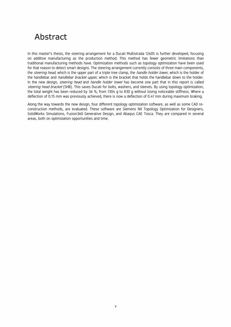
In this master's thesis, the steering arrangement for a Ducati Multistrada 1260S is further developed, focusing
on additive manufacturing as the production method. This method has fewer geometric limitations than
traditional manufacturing methods have. Optimization methods such as topology optimization have been used
for that reason to detect smart designs. The steering arrangement currently consists of three main components,
the steering head, which is the upper part of a triple tree clamp, the handle holder lower, which is the holder of
the handlebar and handlebar bracket upper, which is the bracket that holds the handlebar down to the holder.
In the new design, steering head and handle holder lower has become one part that in this report is called
steering head bracket (SHB). This saves Ducati for bolts, washers, and sleeves. By using topology optimization,
the total weight has been reduced by 36 %, from 1304 g to 830 g without losing noticeable stiffness. Where a
deflection of 0.15 mm was previously achieved, there is now a deflection of 0.41 mm during maximum braking.
Along the way towards the new design, four different topology optimization software, as well as some CAD re-
construction methods, are evaluated. These software are Siemens NX Topology Optimization for Designers,
SolidWorks Simulations, Fusion360 Generative Design, and Abaqus CAE Tosca. They are compared in several
areas, both on optimization opportunities and time.

vi
Sammendrag
I denne masteroppgaven videreutvikles styrekronen på en Ducati Multistrada 1260S, med fokus på additiv
tilvirkning som produksjonsmetode. Denne metoden har langt mindre geometriske begrensninger som
tradisjonelle tilvikningsmetoder har. Optimaliseringsmetoder som topologi optimalisering er av den grunn blitt
anvendt for å oppdage smarte design. Styrekronen består i dag av tre hovedkomponenter, steering head som
er den øvre delen av en trippel tre klemme, handle holder lower som er holderen til styret og handlebar bracket upper som er braketten som holder styret nedtil holderen. I det nye designet er steering head og handle holder lower blitt til èn del som i denne rapporten blir kalt steering head bracket (SHB). Dette sparer Ducati for bolter,
skiver og hylser. Ved hjelp av topologi optimalisering har total vekten blitt redusert med 36%, fra 1304 g til 830
g uten for stor betydning på stivheten. Der man tidligere oppnådde en utbøyning på 0,15 mm har man nå en
utbøyning på 0,41 mm under maksimal nedbremsning.
På veien mot det nye designet evalueres også fire forskjellige topologi optimaliseringsprogrammvarer samt noen
metoder for rekonstruksjon av CAD. Disse programvarene er Siemens NX Topology Optimization for Designers,
SolidWorks Simulations, Fusion360 Generative Design og Abaqus CAE Tosca. De blir sammenlignet på flere
områder, både på optimaliseringsmuligheter og tidsbruk.
.

vii
Preface
This master’s thesis is written at Norwegian University of Science and Technology (NTNU) in the spring of 2020
as the answer to the subject TMM4960 Produktutvikling og materialer, masteroppgave. The project is given by
the Department of Mechanical and Industrial Engineering with Professor Filippo Berto as supervisor and Professor
Terje Rølvåg as co-supervisor.
The topic of the thesis is design and optimization for additive manufacturing parts for Ducati Multistrada 1260 S.
I would like to thank Prof. Berto and Prof. Rølvåg for knowledgeable guidance. I would also like to thank Ducati
for providing us with this interesting and challenging task. Last but not least, I would like to thank Kjetil Ødegård
and Per Kristian Garnes for professional conversations regarding topology optimization and FEA in NX Nastran.

viii

ix
Table of Contents List of Figures .............................................................................................................................................................. x
List of Tables ............................................................................................................................................................. xii
Abbreviations ............................................................................................................................................................ xiii
1 Introduction ........................................................................................................................................................... 14
1.1 Background and Objectives ........................................................................................................................ 14
1.2 Steering arrangement ................................................................................................................................. 15
2 Theory .................................................................................................................................................................... 16
2.1 Structural Optimization ............................................................................................................................... 16
2.2 Topology Optimization ................................................................................................................................ 17
2.3 Generative Design ....................................................................................................................................... 18
2.4 Additive manufacturing .............................................................................................................................. 18
2.5 Fatigue ......................................................................................................................................................... 26
3 Methods and Procedure ....................................................................................................................................... 27
3.1 Steering Head Bracket (SHB) and Handlebar Bracket Upper (HBU) ........................................................ 27
3.2 Evaluation of Tools and Methods for Topology Optimization .................................................................. 27
3.3 Re-construction of CAD .............................................................................................................................. 32
3.4 Load Scenario .............................................................................................................................................. 36
3.5 Fatigue ......................................................................................................................................................... 38
4 Results ................................................................................................................................................................... 39
4.1 Topology Optimization with different tools and methods ....................................................................... 39
4.2 FEM Verification ......................................................................................................................................... 43
4.3 Manufacturing Process ............................................................................................................................... 50
4.4 Final Design ................................................................................................................................................. 51
5 Discussion and Conclusion .................................................................................................................................. 54
5.1 Tools and Methods ..................................................................................................................................... 54
5.2 Steering Head and Handlebar Bracket Upper ........................................................................................... 55
5.3 Conclusion ................................................................................................................................................... 56
References ..................................................................................................................................................................... 58
Appendix ........................................................................................................................................................................ 61
x
List of Figures Figure 1.1 - Ducati Multistrada 1260 S 2019 (Ducati, 2019) ........................................................................................ 14 Figure 1.2 – Explode view of steering arrangement for Multistrada (Ducati, 2020b). ............................................. 15 Figure 2.1 - Two-dimensional topology optimization. The box is to be filled to 50% by material. In the upper
picture, we see the load case and boundary condition at the start. The result is shown in the second picture. 17 Figure 2.2 - Schematics of an LBM machine (left), and the three process steps iterated during the build
(right)(Herzog et al., 2016). .......................................................................................................................................... 19 Figure 2.3 - Schematics of an EBM machine, 1: electron gun, 2: lens system, 3: deflection lens, 4: powder
cassettes with feedstock, 5: rake, 6: building component, 7: build table (Herzog et al., 2016). ............................ 19 Figure 2.4 - Schematics of an LMD set-up (Herzog et al., 2016) .............................................................................. 20 Figure 2.5 - Common defects in the selective laser sintering process (Malekipour and El-Mounayri, 2018) ....... 21 Figure 2.6 - Cost comparison of different AM materials ............................................................................................ 23 Figure 2.7 - (a) Concave radii. Titanium: (b) overhang 9 mm, (d) overhang 15 mm. Aluminum: (c) overhang of 9
mm, (e) overhang of 15 mm. ....................................................................................................................................... 24 Figure 2.8 - (a) Convex radii and (b) overhang of 15 mm. Overhang of 9 mm: (c) titanium and (d) aluminum. 24 Figure 2.9 - Measured roughness of the full-circle at different positions, by Q. Han, H.G. Shwe Soe et.al 2018. 25 Figure 2.10 - Flowchart of optimization of orientation and support by F.Calignano. .............................................. 26 Figure 3.1 - Optimization process for NX TOD............................................................................................................. 27 Figure 3.2 - Optimization process for SW.................................................................................................................... 28 Figure 3.3 - Optimization process for Generative Design .......................................................................................... 29 Figure 3.4 - Optimization process for Abaqus Tosca ................................................................................................. 29 Figure 3.5 - Re-construction procedure of CAD in NX. From STL to modeling stage in Realize shape application
to meshed FEM-model. ................................................................................................................................................. 33 Figure 3.6 - Re-construction procedure of CAD in SolidWorks. From STL to modeling stage in Mesh modeling
application to meshed FEM-model. ............................................................................................................................ 34 Figure 3.7 - Re-construction procedure of CAD with Abaqus optimized result in NX. From unsmoothed ODB-file
in Abaqus to STL in NX to meshed FEM-model. ......................................................................................................... 35 Figure 3.8 - Re-construction procedure of CAD with Abaqus optimized result in SolidWorks. From point cloud
(XYZ-file) in MeshLab to graphics body in SolidWorks to meshed FEM-model. ...................................................... 36 Figure 3.9 - Lateral displacement. Picture from Motorcycle Handling and Chassis Design (Foale, 2006) ............ 37 Figure 3.10 - Illustration to show which direction the loads point. Blue are bump loads, red are deceleration
load, and green are acceleration. ................................................................................................................................ 38 Figure 4.1 - Set-up that is used in the TO ................................................................................................................... 39 Figure 4.2 - Design space and result of optimization in NX TOD ............................................................................. 40 Figure 4.3 - Design space and result of optimization in SW simulations ................................................................. 41 Figure 4.4 - Design space and result of optimization in Fusion360 ......................................................................... 41 Figure 4.5 - Design space and result of optimization in ABAQUS Tosca ................................................................. 42 Figure 4.6 - Key points in a diamond diagram to compare software tools ............................................................ 43 Figure 4.7 - FEA-1 set-up ............................................................................................................................................ 44 Figure 4.8 - FEA-1 maximum stress ........................................................................................................................... 45 Figure 4.9 - FEA-1 average maximum stress............................................................................................................. 45 Figure 4.10 - FEA-1 displacement. Visually exaggerated by 10 %. ........................................................................... 45 Figure 4.11 - FEA-2 set-up .......................................................................................................................................... 46 Figure 4.12 - FEA-2 maximum stress (handlebar is hided) ...................................................................................... 46 Figure 4.13 - FEA-2 average stress in the HBU (handlebar is hided) ...................................................................... 47 Figure 4.14 - FEA-2 average stress in SHB (handlebar is hided) ............................................................................. 47 Figure 4.15 - FEA-2 displacement. Visually exaggerated by 0.5 % ......................................................................... 47 Figure 4.16 - FEA-3 average stress ............................................................................................................................ 48 Figure 4.17 - FEA-3 displacement. Visually exaggerated 10 % ................................................................................ 48 Figure 4.18 - FEA-4 set-up .......................................................................................................................................... 49 Figure 4.19 - FEA-4 average stress ............................................................................................................................ 49 Figure 4.20 - FEA-4 displacement. Visually exaggerated 10 %. ................................................................................ 50 Figure 4.21 - Illustration of SHB in EOSINT M280 with support ................................................................................. 51 Figure 4.22 - Original design. ...................................................................................................................................... 52 Figure 4.23 - New design seen from the front. .......................................................................................................... 52
xi
Figure 4.24 - New design seen from the side. ........................................................................................................... 52 Figure 4.25 - SHB and HBU seen from behind. .......................................................................................................... 53 Figure 4.26 - SHB and HBU seen from the front. ....................................................................................................... 53 Figure 0.1 - Staircase effect .......................................................................................................................................... 62 Figure 0.2 - Close up picture of balling ....................................................................................................................... 62 Figure 0.3 – Defects, delamination and lack of fusion in AM (Milewski, 2017) ........................................................ 63 Figure 0.4 - Motorcycle under braking, from Motorcycle dynamics ........................................................................ 64 Figure 0.5 - Front-wheel vertical acceleration............................................................................................................ 65 Figure 0.6 - Triple tree simulation ............................................................................................................................... 67 Figure 0.7 - Acceleration limited by wheelie, from motorcycle dynamics. .............................................................. 68 Figure 0.8 - Steering torque for a motorcycle in a turn ............................................................................................ 70 Figure 0.9 - NX TOD result and convergence diagram. ............................................................................................. 71 Figure 0.10 - Result NX TOD. The transition between the suspension clamp and struts are exposed. Hints of
stresses in the transition between the headstock connection ring and struts. ....................................................... 72 Figure 0.11 - Result NX TOD. Maximum displacement in the suspension clamps. .................................................. 72 Figure 0.12 – NX TOD. Solid properties check of the re-constructed CAD. .............................................................. 72 Figure 0.13 - NX TOD re-constructed model with 167 MPa legend limit .................................................................. 73 Figure 0.14 - NX TOD re-constructed model maximum stress. ................................................................................. 73 Figure 0.15 - NX TOD re-constructed model convergence check medium mesh. .................................................. 74 Figure 0.16 - NX TOD re-constructed model convergence check fine mesh. ......................................................... 74 Figure 0.17 - NX TOD re-constructed model average stress. ................................................................................... 74 Figure 0.18 - NX TOD re-constructed model maximum displacement...................................................................... 75 Figure 0.19 - Fusion360 TO result ............................................................................................................................... 75 Figure 0.20 - Fusion360 Stress indication .................................................................................................................. 76 Figure 0.21 - Fusion360. Solid properties check for the exported CAD. ................................................................... 76 Figure 0.22 - Fusion360 Stress on the exported CAD. .............................................................................................. 76 Figure 0.23 - Fusion 360 close up of stress ............................................................................................................... 77 Figure 0.24 - Fusion360 average stress ..................................................................................................................... 77 Figure 0.25 - Fusion360 maximum displacement. ..................................................................................................... 78 Figure 0.26 - Result from SW. Material missing between critical regions. ............................................................... 78 Figure 0.27 - Convergence diagram from Abaqus results ......................................................................................... 79 Figure 0.28 - Abaqus maximum stress re-constructed model. ................................................................................ 79 Figure 0.29 - Abaqus close up maximum stress re-constructed model. ................................................................. 80 Figure 0.30 - Abaqus maximum displacement re-constructed model. .................................................................... 80 Figure 0.31 - Solid properties check of re-constructed model from Abaqus ........................................................... 80 Figure 0.32 - S-N curve for AlSi10Mg printed with EOSINT M-280. .......................................................................... 83 Figure 0.33 - S-N curve in log-log plot ...................................................................................................................... 84 Figure 0.34 - A presumed stress history per 10 km. ................................................................................................. 85 Figure 0.35 - OEM FEA-1 set-up .................................................................................................................................. 86 Figure 0.36 - Result OEM FEA-1 ................................................................................................................................... 87 Figure 0.37 - Displacement OEM FEA-1. Visually exaggerated 10 %......................................................................... 87 Figure 0.38 - Result OEM FEA-3 .................................................................................................................................. 88 Figure 0.39 - Displacement OEM FEA-3. Visually exaggerated 10 %. ....................................................................... 88 Figure 0.40 - Result OEM FEA-4 .................................................................................................................................. 89 Figure 0.41 - Displacement OEM FEA-4. Visually exaggerated 10 %. ....................................................................... 89
xii
List of Tables Table 1 - Summary of pros and cons for AM (Bandyopadhyay and Bose, 2015). .................................................... 18 Table 2 - Common AM alloys and application (Milewski, 2017) ................................................................................ 21 Table 3 - Comparing LBM, LMD, and EBM from Michael Schmidt’s articles (Schmidt et al., 2017). ....................... 22 Table 4 - Cost comparison of AM material for 403 cm3 (AMPOWER, 2019)............................................................. 22 Table 5 - Design constraints available in NX TOD ...................................................................................................... 27 Table 6 - Manufacturing constraints available in SW ................................................................................................. 28 Table 7 - Manufacturing constraints available in Fusion360 ..................................................................................... 29 Table 8 - Geometric restriction available in Abaqus Tosca ....................................................................................... 30 Table 9 - Comparing the different topology optimization software .......................................................................... 30 Table 10 - Loads utilized in TO, FEM verifications and fatigue calculations ............................................................. 37 Table 11 - Material properties for AlSi10Mg ................................................................................................................. 39 Table 12 - Material properties for AlSi10Mg in Fusion360 ......................................................................................... 39 Table 13 - Description of different Finite Element Analysis ...................................................................................... 43 Table 14 - Weight comparing OEM and new design ................................................................................................... 51 Table 15 - Values that are crucial for maximum deceleration and acceleration ...................................................... 65 Table 16 - Values for the tensile load calculation ....................................................................................................... 69 Table 17 - Load caused by accelerations and decelerations from 10 to 100 % ....................................................... 82 Table 18 - Stresses in the transition corner between the headstock ring and the struts during acceleration and
deceleration. Positive stress for tension and negative stress for compression. ..................................................... 82 Table 19 - Values from S-N curve ................................................................................................................................ 83 Table 20 – Summary table of required values for Palmgren-Miner rule .................................................................. 85
xiii
Abbreviations AM Additive Manufacturing CAE Computer-Aided Engineering CAD Computer-Aided Design EBM Electron Beam Melting FEA Finite Element Analysis FEM Finite Element Method HBU Handlebar Bracket Upper HHL Handle Holder Lower LMD Laser Metal Deposition LMD NTNU Norwegian University of Science and Technology NX TOD NX Topology Optimization for Designers OEM Original Equipment Manufacturer RBE2 Rigid Body Element 2 SHB Steering Head Bracket STL Stereolithography SW SolidWorks TO Topology Optimization UTS Ultimate Tensile Strength
14
In this master’s thesis, a new innovative and optimized solution for the Ducati Multistrada steering arrangement
has been explored. Different tools and methods for optimizing and re-construction of the model have been
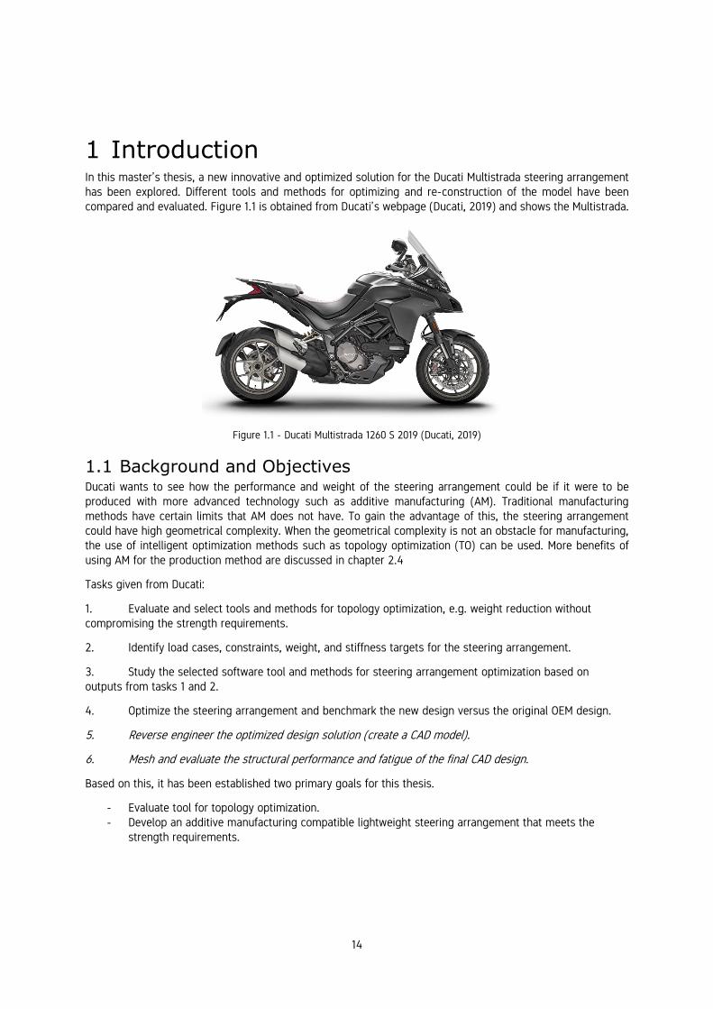
compared and evaluated. Figure 1.1 is obtained from Ducati’s webpage (Ducati, 2019) and shows the Multistrada.
Figure 1.1 - Ducati Multistrada 1260 S 2019 (Ducati, 2019)
1.1 Background and Objectives Ducati wants to see how the performance and weight of the steering arrangement could be if it were to be
produced with more advanced technology such as additive manufacturing (AM). Traditional manufacturing
methods have certain limits that AM does not have. To gain the advantage of this, the steering arrangement
could have high geometrical complexity. When the geometrical complexity is not an obstacle for manufacturing,
the use of intelligent optimization methods such as topology optimization (TO) can be used. More benefits of
using AM for the production method are discussed in chapter 2.4
Tasks given from Ducati:
1. Evaluate and select tools and methods for topology optimization, e.g. weight reduction without
compromising the strength requirements.
2. Identify load cases, constraints, weight, and stiffness targets for the steering arrangement.
3. Study the selected software tool and methods for steering arrangement optimization based on
outputs from tasks 1 and 2.
4. Optimize the steering arrangement and benchmark the new design versus the original OEM design.
5. Reverse engineer the optimized design solution (create a CAD model).
6. Mesh and evaluate the structural performance and fatigue of the final CAD design.
Based on this, it has been established two primary goals for this thesis.
- Evaluate tool for topology optimization.
- Develop an additive manufacturing compatible lightweight steering arrangement that meets the
strength requirements.
1 Introduction
15
1.2 Steering arrangement The Multistrada uses a triple tree steering arrangement with upside-down telescopic forks. The forks consist of
hydraulic shock absorbers with internal coil spring to give the optimal steering and driving qualifications
(Bhanage et al., 2015). With an upside-down fork, the inner fork tube (stanchion) is connected to the front wheel
axle, and the outer fork tube (slider) is connected to the triple tree clamps. The outer fork tube is just referred
to as suspension fork in this thesis.
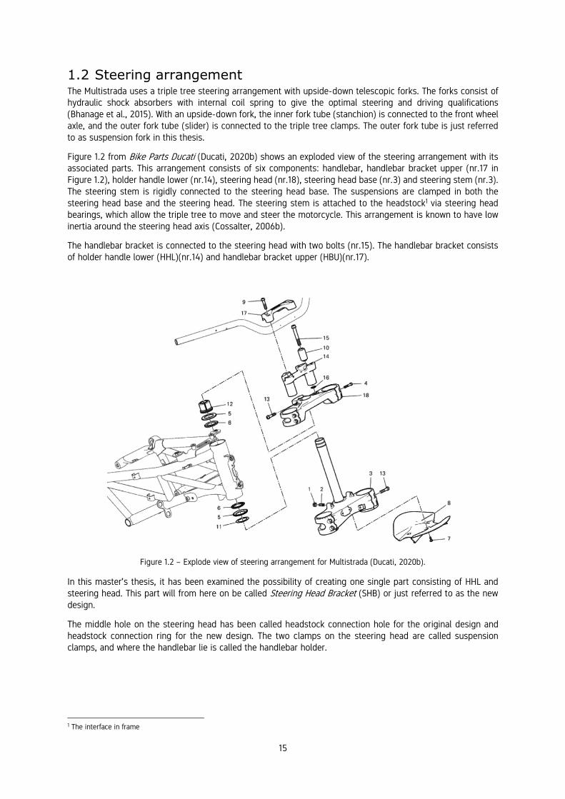
Figure 1.2 from Bike Parts Ducati (Ducati, 2020b) shows an exploded view of the steering arrangement with its
associated parts. This arrangement consists of six components: handlebar, handlebar bracket upper (nr.17 in
Figure 1.2), holder handle lower (nr.14), steering head (nr.18), steering head base (nr.3) and steering stem (nr.3).
The steering stem is rigidly connected to the steering head base. The suspensions are clamped in both the
steering head base and the steering head. The steering stem is attached to the headstock1 via steering head
bearings, which allow the triple tree to move and steer the motorcycle. This arrangement is known to have low
inertia around the steering head axis (Cossalter, 2006b).
The handlebar bracket is connected to the steering head with two bolts (nr.15). The handlebar bracket consists
of holder handle lower (HHL)(nr.14) and handlebar bracket upper (HBU)(nr.17).
Figure 1.2 – Explode view of steering arrangement for Multistrada (Ducati, 2020b).
In this master's thesis, it has been examined the possibility of creating one single part consisting of HHL and
steering head. This part will from here on be called Steering Head Bracket (SHB) or just referred to as the new
design.
The middle hole on the steering head has been called headstock connection hole for the original design and
headstock connection ring for the new design. The two clamps on the steering head are called suspension
clamps, and where the handlebar lie is called the handlebar holder.
1 The interface in frame
16
To better understand the work done in this master thesis, it is essential to have some knowledge about the
methods and technology used to design and produce the SHB. Some underlying theory of structural optimization,
generative design, AM, and fatigue is therefore presented in this chapter. The subsection structural optimization
and some parts of additive manufacturing are obtained from the pre-study done autumn 2019.
2.1 Structural Optimization Structural optimization can be split into three different optimization methods, sizing, shape, and topology
optimization, depending on the geometric feature. All these methods are mathematical methods to find the
optimal solutions, either thickness, form, or connectivity of nodes (13).
Christensen, Klarbring and Gladwell describe structural optimization as a function f(x,y) as shown in equation eq.
(1) (Christensen et al., 2008).
Objective function (f): This is the function that classifies designs. Function f returns a number that tells how good
the design is. It often measures displacement in a certain direction, weight, stress, or even cost of production.
Design variable (x): x is the variable that describes the design. When it represents a geometry, it could be the
thickness of a sheet, area of a bar, or even interpolation of shape. It could also be a choice of material. This
variable can be changed during optimization.
State variable (y): y is the variable that represents the response of the structure. This response could be
displacement, stress, strain, or force.
A general structural optimization takes this form:
𝑆𝑂 =
𝑚𝑖𝑛𝑖𝑚𝑖𝑧𝑒 𝑓 (𝑥, 𝑦) 𝑤𝑖𝑡ℎ 𝑟𝑒𝑠𝑝𝑒𝑐𝑡 𝑡𝑜 𝑥 𝑎𝑛𝑑 𝑦
𝑠𝑢𝑏𝑗𝑒𝑐𝑡 𝑡𝑜
𝑏𝑒ℎ𝑎𝑣𝑖𝑜𝑟𝑎𝑙 𝑐𝑜𝑛𝑠𝑡𝑟𝑎𝑖𝑛𝑡𝑠 𝑜𝑛 𝑦𝑑𝑒𝑠𝑖𝑔𝑛 𝑐𝑜𝑛𝑠𝑡𝑟𝑎𝑖𝑛𝑡𝑠 𝑜𝑛 𝑥𝑒𝑞𝑢𝑖𝑙𝑖𝑏𝑟𝑖𝑢𝑚 𝑐𝑜𝑛𝑠𝑡𝑟𝑎𝑖𝑛𝑡.
(1)
In eq. (1) there are three types of constraints. Behavioral constraints on the state variable y, which is a function
g(y) that represents, e.g., displacement in a particular direction. Often these constraints are written g(y) ≤ 0. This
state function can also be represented by a displacement vector g(u(x)).
Design constraints on the design variable x. Behavioral constraints and design constraints can be combined.
Equilibrium constraints in discrete linear problem looks like
𝐾(𝑥)𝑢 = 𝐹(𝑥) (2)
where K(x) is the stiffness matrix of the structure. The displacement vector is u. And the force vector is F(x).
If we isolate u on left-hand side equation (2) can be rewritten to
𝑢 = 𝑢(𝑥) = 𝐾(𝑥)−1𝐹(𝑥) (3)
This results in the removal of the equilibrium constraint from eq. (1) and we have a so-called nested formulation
as in eq.(4).
2 Theory

17
𝑆𝑂𝑛𝑓 = 𝑚𝑖𝑛𝑖𝑚𝑖𝑧𝑒 𝑓 (𝑥, 𝑢(𝑥)) 𝑤𝑖𝑡ℎ 𝑟𝑒𝑠𝑝𝑒𝑐𝑡 𝑡𝑜 𝑥 𝑎𝑛𝑑 𝑢(𝑥)
𝑠𝑢𝑏𝑗𝑒𝑐𝑡 𝑡𝑜 𝑔(𝑥, 𝑢(𝑥)) ≤ 0 (4)
Multiple criteria or multi objectives are when a problem has several objective functions. This can be formulated
like
𝑚𝑖𝑛𝑖𝑚𝑖𝑧𝑒 𝑓1(𝑥, 𝑦), 𝑓2(𝑥, 𝑦), . . . , 𝑓𝑛(𝑥, 𝑦) (5)
n is the number of objective functions. The constraints are the same as in eq. (1).
The objective can be to minimize the strain energy (U), also called compliance. The strain energy is given by
equation
𝑈 = 1
2𝑉𝜎𝜀 (6)
where V is the volume of the object, σ is the stress, and ε is the strain.
When using minimize strain energy as an objective function, it also maximizes the structural stiffness.
Combination of strain energy as the objective function and volume or weight fraction as the constraint is
common.
2.2 Topology Optimization Topology optimization finds the optimal layout of a solid structure, with determinations of features such as
shape, number, and location of holes. Such optimal Lay-out could be minimum weight/volume or maximum
stiffness. The only known parameters are the applied load, boundary condition, the original volume, and the
design restriction you may have. An example is given in Figure 2.1.
Figure 2.1 - Two-dimensional topology optimization. The box is to be filled to 50% by material. In the upper picture, we see the load case and boundary condition at the start. The result is shown in the second picture.
To topology optimize, we start with a part like the box in Figure 2.1, this part contains a design space and a non-
design space. It is from the design space material is being removed until a final shape is reached during
optimization. It is not favorable to apply loads and support directly on a design space, as this often leads to
incorrect results. Non-design space is the area of the model that is not favorable to remove material from.
Typical non-design space could be constrained areas and load areas.
18
2.3 Generative Design Generative design uses a powerful artificial algorithm to generate thousands of designs in a short amount of
time. Every design iterations structure is tested, and the generative design is learning from each step. It applies
changes in all steps, and then it part by part reaches the optimal solution (Matthew, 2017).
2.4 Additive manufacturing In contrast to machining (subtractive manufacturing), and forging (formative manufacturing), AM is a technology
where 3D designs can be produced directly from a CAD file without any part-specific tools or dies. The CAD
model is being divided into thin slices of cross-section profiles. These cross-sections are being traced and filled
or partly filled by a laser beam, electron beam, extrusion nozzle, or jetting nozzle. This is done by adding layers
in the X-Y plane, and then multiple layers are built on top of these layers generating the third dimension
(Bandyopadhyay and Bose, 2015).
At the start of AM, most of these technologies made only polymeric objects only suitable for rapid prototyping
and visualization of the model. Later it becomes possible to 3D print ceramics and metals parts that had much
greater strength, and this resulted in end-usable parts directly from the printer (Bandyopadhyay and Bose, 2015).
AM allows you to produce optimized products with geometries that were too expensive or impossible to produce
with traditional manufacturing methods. It is possible to redesign several components and make them into one
single part. This reduces complexity and the final assembly time. AM makes it easier to create optimum strength-
to-weight ratio while minimizing material volume. It reduces material waste in production, which leads to a
reduction in cost and energy (Huang et al., 2016). With the design freedom AM gives you, it is possible to achieve
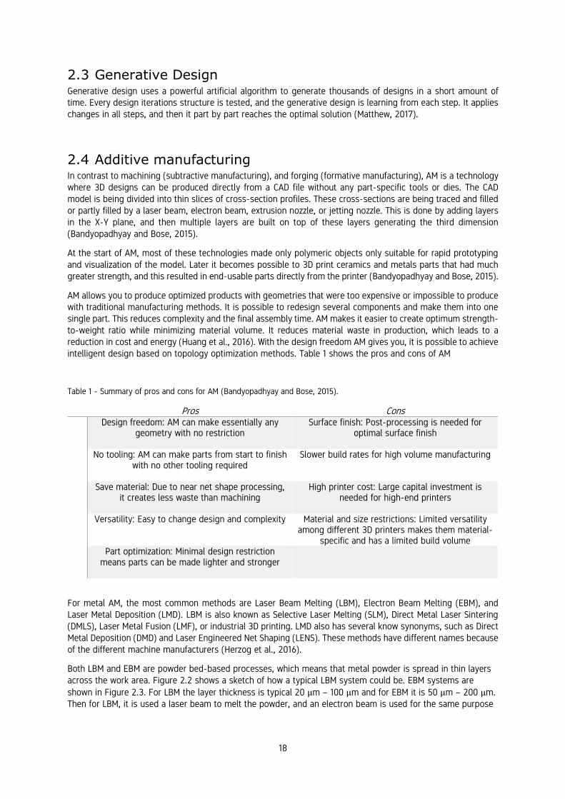
intelligent design based on topology optimization methods. Table 1 shows the pros and cons of AM
Table 1 - Summary of pros and cons for AM (Bandyopadhyay and Bose, 2015).
Pros Cons Design freedom: AM can make essentially any
geometry with no restriction Surface finish: Post-processing is needed for
optimal surface finish
No tooling: AM can make parts from start to finish with no other tooling required
Slower build rates for high volume manufacturing
Save material: Due to near net shape processing, it creates less waste than machining
High printer cost: Large capital investment is needed for high-end printers
Versatility: Easy to change design and complexity Material and size restrictions: Limited versatility among different 3D printers makes them material-
specific and has a limited build volume Part optimization: Minimal design restriction
means parts can be made lighter and stronger
For metal AM, the most common methods are Laser Beam Melting (LBM), Electron Beam Melting (EBM), and
Laser Metal Deposition (LMD). LBM is also known as Selective Laser Melting (SLM), Direct Metal Laser Sintering
(DMLS), Laser Metal Fusion (LMF), or industrial 3D printing. LMD also has several know synonyms, such as Direct
Metal Deposition (DMD) and Laser Engineered Net Shaping (LENS). These methods have different names because
of the different machine manufacturers (Herzog et al., 2016).
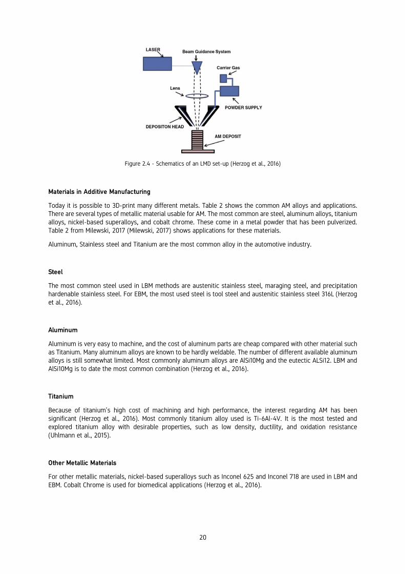
Both LBM and EBM are powder bed-based processes, which means that metal powder is spread in thin layers
across the work area. Figure 2.2 shows a sketch of how a typical LBM system could be. EBM systems are
shown in Figure 2.3. For LBM the layer thickness is typical 20 μm – 100 μm and for EBM it is 50 μm – 200 μm.
Then for LBM, it is used a laser beam to melt the powder, and an electron beam is used for the same purpose
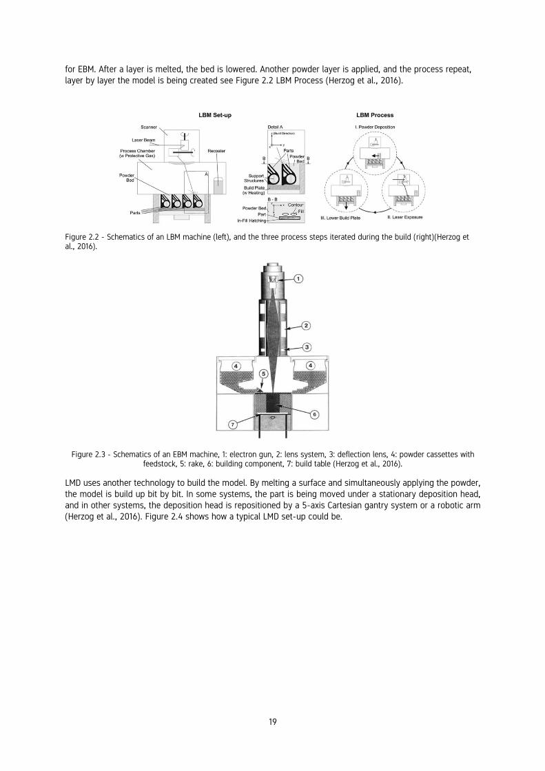
19
for EBM. After a layer is melted, the bed is lowered. Another powder layer is applied, and the process repeat,
layer by layer the model is being created see Figure 2.2 LBM Process (Herzog et al., 2016).
Figure 2.2 - Schematics of an LBM machine (left), and the three process steps iterated during the build (right)(Herzog et al., 2016).
Figure 2.3 - Schematics of an EBM machine, 1: electron gun, 2: lens system, 3: deflection lens, 4: powder cassettes with feedstock, 5: rake, 6: building component, 7: build table (Herzog et al., 2016).
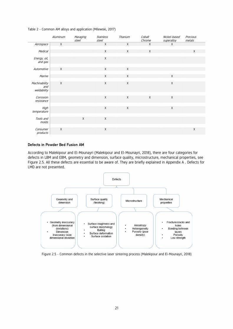
LMD uses another technology to build the model. By melting a surface and simultaneously applying the powder,
the model is build up bit by bit. In some systems, the part is being moved under a stationary deposition head,
and in other systems, the deposition head is repositioned by a 5-axis Cartesian gantry system or a robotic arm
(Herzog et al., 2016). Figure 2.4 shows how a typical LMD set-up could be.
20
Figure 2.4 - Schematics of an LMD set-up (Herzog et al., 2016)
Materials in Additive Manufacturing
Today it is possible to 3D-print many different metals. Table 2 shows the common AM alloys and applications.
There are several types of metallic material usable for AM. The most common are steel, aluminum alloys, titanium
alloys, nickel-based superalloys, and cobalt chrome. These come in a metal powder that has been pulverized.
Table 2 from Milewski, 2017 (Milewski, 2017) shows applications for these materials.
Aluminum, Stainless steel and Titanium are the most common alloy in the automotive industry.
Steel
The most common steel used in LBM methods are austenitic stainless steel, maraging steel, and precipitation
hardenable stainless steel. For EBM, the most used steel is tool steel and austenitic stainless steel 316L (Herzog
et al., 2016).
Aluminum
Aluminum is very easy to machine, and the cost of aluminum parts are cheap compared with other material such
as Titanium. Many aluminum alloys are known to be hardly weldable. The number of different available aluminum
alloys is still somewhat limited. Most commonly aluminum alloys are AlSi10Mg and the eutectic ALSi12. LBM and
AlSi10Mg is to date the most common combination (Herzog et al., 2016).
Titanium
Because of titanium’s high cost of machining and high performance, the interest regarding AM has been
significant (Herzog et al., 2016). Most commonly titanium alloy used is Ti-6Al-4V. It is the most tested and
explored titanium alloy with desirable properties, such as low density, ductility, and oxidation resistance
(Uhlmann et al., 2015).
Other Metallic Materials
For other metallic materials, nickel-based superalloys such as Inconel 625 and Inconel 718 are used in LBM and
EBM. Cobalt Chrome is used for biomedical applications (Herzog et al., 2016).
21
Table 2 - Common AM alloys and application (Milewski, 2017)
Aluminum Maraging steel
Stainless steel
Titanium Cobalt Chrome
Nickel-based superalloy
Precious metals
Aerospace X X X X X
Medical X X X X
Energy, oil, and gas
X
Automotive X X X
Marine X X X
Machinability
and weldability
X X X X
Corrosion resistance
X X X X
High
temperature X X X
Tools and
molds X X
Consumer products
X X X
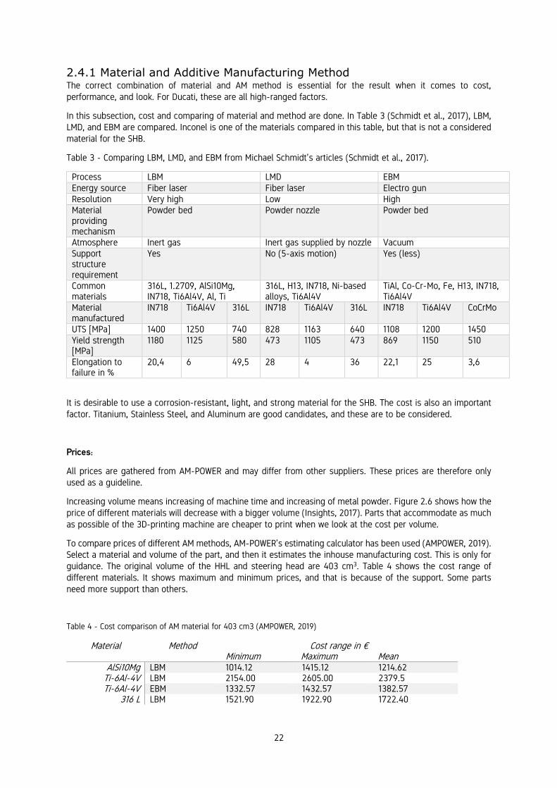
Defects in Powder Bed Fusion AM
According to Malekipour and El-Mounayri (Malekipour and El-Mounayri, 2018), there are four categories for
defects in LBM and EBM, geometry and dimension, surface quality, microstructure, mechanical properties, see
Figure 2.5. All these defects are essential to be aware of. They are briefly explained in Appendix A . Defects for
LMD are not presented.
Figure 2.5 - Common defects in the selective laser sintering process (Malekipour and El-Mounayri, 2018)
22
2.4.1 Material and Additive Manufacturing Method The correct combination of material and AM method is essential for the result when it comes to cost,
performance, and look. For Ducati, these are all high-ranged factors.
In this subsection, cost and comparing of material and method are done. In Table 3 (Schmidt et al., 2017), LBM,
LMD, and EBM are compared. Inconel is one of the materials compared in this table, but that is not a considered
material for the SHB.
Table 3 - Comparing LBM, LMD, and EBM from Michael Schmidt’s articles (Schmidt et al., 2017).
Process LBM LMD EBM Energy source Fiber laser Fiber laser Electro gun Resolution Very high Low High Material providing mechanism
Powder bed Powder nozzle Powder bed
Atmosphere Inert gas Inert gas supplied by nozzle Vacuum Support structure requirement
Yes No (5-axis motion) Yes (less)
Common materials
316L, 1.2709, AlSi10Mg, IN718, Ti6Al4V, Al, Ti
316L, H13, IN718, Ni-based alloys, Ti6Al4V
TiAl, Co-Cr-Mo, Fe, H13, IN718, Ti6Al4V
Material manufactured
IN718 Ti6Al4V 316L IN718 Ti6Al4V 316L IN718 Ti6Al4V CoCrMo
UTS [MPa] 1400 1250 740 828 1163 640 1108 1200 1450 Yield strength [MPa]
1180 1125 580 473 1105 473 869 1150 510
Elongation to failure in %
20,4 6 49,5 28 4 36 22,1 25 3,6
It is desirable to use a corrosion-resistant, light, and strong material for the SHB. The cost is also an important
factor. Titanium, Stainless Steel, and Aluminum are good candidates, and these are to be considered.
Prices:
All prices are gathered from AM-POWER and may differ from other suppliers. These prices are therefore only
used as a guideline.
Increasing volume means increasing of machine time and increasing of metal powder. Figure 2.6 shows how the
price of different materials will decrease with a bigger volume (Insights, 2017). Parts that accommodate as much
as possible of the 3D-printing machine are cheaper to print when we look at the cost per volume.
To compare prices of different AM methods, AM-POWER’s estimating calculator has been used (AMPOWER, 2019).
Select a material and volume of the part, and then it estimates the inhouse manufacturing cost. This is only for
guidance. The original volume of the HHL and steering head are 403 cm3. Table 4 shows the cost range of
different materials. It shows maximum and minimum prices, and that is because of the support. Some parts
need more support than others.
Table 4 - Cost comparison of AM material for 403 cm3 (AMPOWER, 2019)
Material Method Cost range in € Minimum Maximum Mean
AlSi10Mg LBM 1014.12 1415.12 1214.62 Ti-6Al-4V LBM 2154.00 2605.00 2379.5 Ti-6Al-4V EBM 1332.57 1432.57 1382.57
316 L LBM 1521.90 1922.90 1722.40
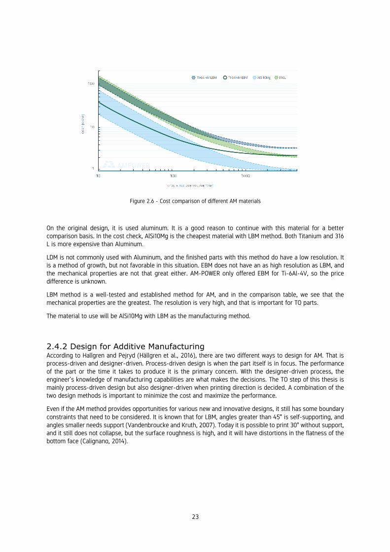
23
Figure 2.6 - Cost comparison of different AM materials
On the original design, it is used aluminum. It is a good reason to continue with this material for a better
comparison basis. In the cost check, AlSi10Mg is the cheapest material with LBM method. Both Titanium and 316
L is more expensive than Aluminum.
LDM is not commonly used with Aluminum, and the finished parts with this method do have a low resolution. It
is a method of growth, but not favorable in this situation. EBM does not have an as high resolution as LBM, and
the mechanical properties are not that great either. AM-POWER only offered EBM for Ti-6Al-4V, so the price
difference is unknown.
LBM method is a well-tested and established method for AM, and in the comparison table, we see that the
mechanical properties are the greatest. The resolution is very high, and that is important for TO parts.
The material to use will be AlSi10Mg with LBM as the manufacturing method.
2.4.2 Design for Additive Manufacturing According to Hallgren and Pejryd (Hällgren et al., 2016), there are two different ways to design for AM. That is
process-driven and designer-driven. Process-driven design is when the part itself is in focus. The performance
of the part or the time it takes to produce it is the primary concern. With the designer-driven process, the
engineer’s knowledge of manufacturing capabilities are what makes the decisions. The TO step of this thesis is
mainly process-driven design but also designer-driven when printing direction is decided. A combination of the
two design methods is important to minimize the cost and maximize the performance.
Even if the AM method provides opportunities for various new and innovative designs, it still has some boundary
constraints that need to be considered. It is known that for LBM, angles greater than 45° is self-supporting, and
angles smaller needs support (Vandenbroucke and Kruth, 2007). Today it is possible to print 30° without support,
and it still does not collapse, but the surface roughness is high, and it will have distortions in the flatness of the
bottom face (Calignano, 2014).
24
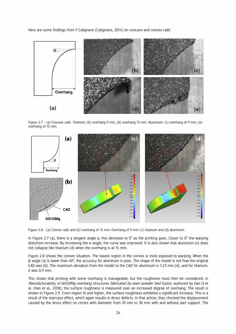
Here are some findings from F.Calignano (Calignano, 2014) on concave and convex radii:
Figure 2.7 - (a) Concave radii. Titanium: (b) overhang 9 mm, (d) overhang 15 mm. Aluminum: (c) overhang of 9 mm, (e) overhang of 15 mm.
Figure 2.8 - (a) Convex radii and (b) overhang of 15 mm. Overhang of 9 mm: (c) titanium and (d) aluminum.
In Figure 2.7 (a), there is a tangent angle α, this decrease to 0° as the printing goes. Closer to 0° the warping
distortion increase. By increasing the α-angle, the curve was improved. It is also shown that aluminum (e) does
not collapse like titanium (d) when the overhang is at 15 mm.
Figure 2.8 shows the convex situation. The lowest region in the convex is most exposed to warping. When the
β-angle (a) is lower than 40°, the accuracy for aluminum is poor. The shape of the model is not how the original
CAD was (b). The maximum deviation from the model to the CAD for aluminum is 1.23 mm (d), and for titanium,
it was 0.9 mm.
This shows that printing with some overhang is manageable, but the roughness must then be considered. In Manufacturability of AlSi10Mg overhang structures fabricated by laser powder bed fusion, authored by Han Q et
al. (Han et al., 2018), the surface roughness is measured over an increased degree of overhang. The result is
shown in Figure 2.9. From region III and higher, the surface roughness exhibited a significant increase. This is a
result of the staircase effect, which again results in dross defects. In that article, they checked the displacement
caused by the dross effect on circles with diameter from 10 mm to 30 mm with and without part support. The
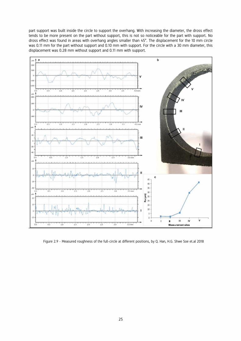
25
part support was built inside the circle to support the overhang. With increasing the diameter, the dross effect
tends to be more present on the part without support, this is not so noticeable for the part with support. No
dross effect was found in areas with overhang angles smaller than 45°. The displacement for the 10 mm circle
was 0.11 mm for the part without support and 0.10 mm with support. For the circle with a 30 mm diameter, this
displacement was 0.28 mm without support and 0.11 mm with support.
Figure 2.9 - Measured roughness of the full-circle at different positions, by Q. Han, H.G. Shwe Soe et.al 2018
26
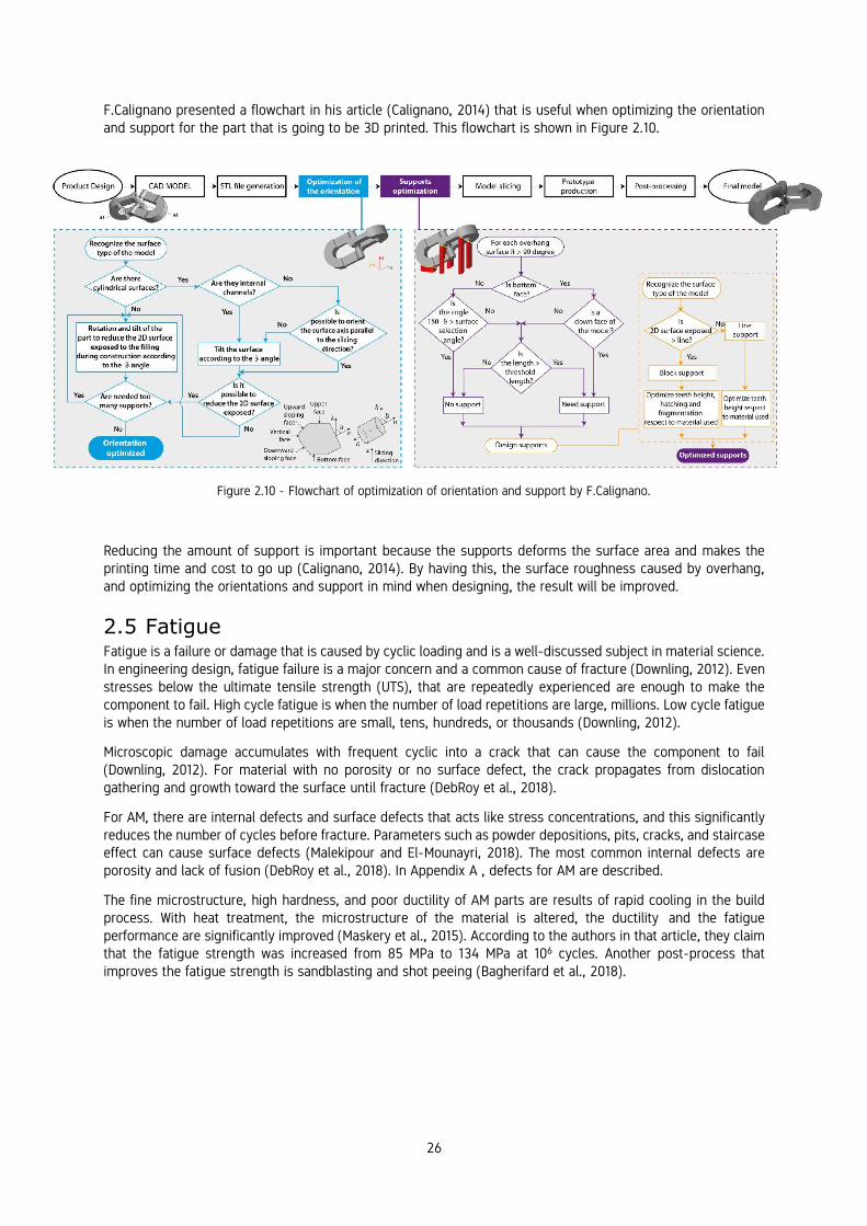
F.Calignano presented a flowchart in his article (Calignano, 2014) that is useful when optimizing the orientation
and support for the part that is going to be 3D printed. This flowchart is shown in Figure 2.10.
Reducing the amount of support is important because the supports deforms the surface area and makes the
printing time and cost to go up (Calignano, 2014). By having this, the surface roughness caused by overhang,
and optimizing the orientations and support in mind when designing, the result will be improved.
2.5 Fatigue Fatigue is a failure or damage that is caused by cyclic loading and is a well-discussed subject in material science.
In engineering design, fatigue failure is a major concern and a common cause of fracture (Downling, 2012). Even
stresses below the ultimate tensile strength (UTS), that are repeatedly experienced are enough to make the
component to fail. High cycle fatigue is when the number of load repetitions are large, millions. Low cycle fatigue
is when the number of load repetitions are small, tens, hundreds, or thousands (Downling, 2012).
Microscopic damage accumulates with frequent cyclic into a crack that can cause the component to fail
(Downling, 2012). For material with no porosity or no surface defect, the crack propagates from dislocation
gathering and growth toward the surface until fracture (DebRoy et al., 2018).
For AM, there are internal defects and surface defects that acts like stress concentrations, and this significantly
reduces the number of cycles before fracture. Parameters such as powder depositions, pits, cracks, and staircase
effect can cause surface defects (Malekipour and El-Mounayri, 2018). The most common internal defects are
porosity and lack of fusion (DebRoy et al., 2018). In Appendix A , defects for AM are described.
The fine microstructure, high hardness, and poor ductility of AM parts are results of rapid cooling in the build
process. With heat treatment, the microstructure of the material is altered, the ductility and the fatigue
performance are significantly improved (Maskery et al., 2015). According to the authors in that article, they claim
that the fatigue strength was increased from 85 MPa to 134 MPa at 106 cycles. Another post-process that
improves the fatigue strength is sandblasting and shot peeing (Bagherifard et al., 2018).
Figure 2.10 - Flowchart of optimization of orientation and support by F.Calignano.
27
In this chapter, the different TO tools are described, evaluated, and compared. The load scenarios that SHB and
HBU are exposed to are defined and the fatigue calculation process is described.
3.1 Steering Head Bracket (SHB) and Handlebar Bracket Upper
(HBU) The SHB is as described earlier, the part that consists of the steering head and HHL. This part is to be 3D-printed
in AlSi10Mg in an EOSINT M-280 machine. HBU will be machined in Aluminum 6061-T6. In Appendix F, the material
datasheet for both AlSi10Mg associated with EOSINT M-280 and Aluminum 6061-T6 can be found.
3.2 Evaluation of Tools and Methods for Topology Optimization In this subsection, some of the TO tools available at NTNU will be briefly described and evaluated. These tools
are NX Topology Optimization for Designers (NX TOD), SolidWorks simulation (SW), Fusion360 Generative Design,
and Abaqus Tosca Structure.
3.2.1 Siemens NX In NX, there are two solvers for TO, NX Topology Optimization for Designers (NX TOD), and NX Nastran
Optimization SOL200. The last one is not evaluated in this thesis. NX TOD is not as complicated and advanced as
the Nastran solver SOL200.
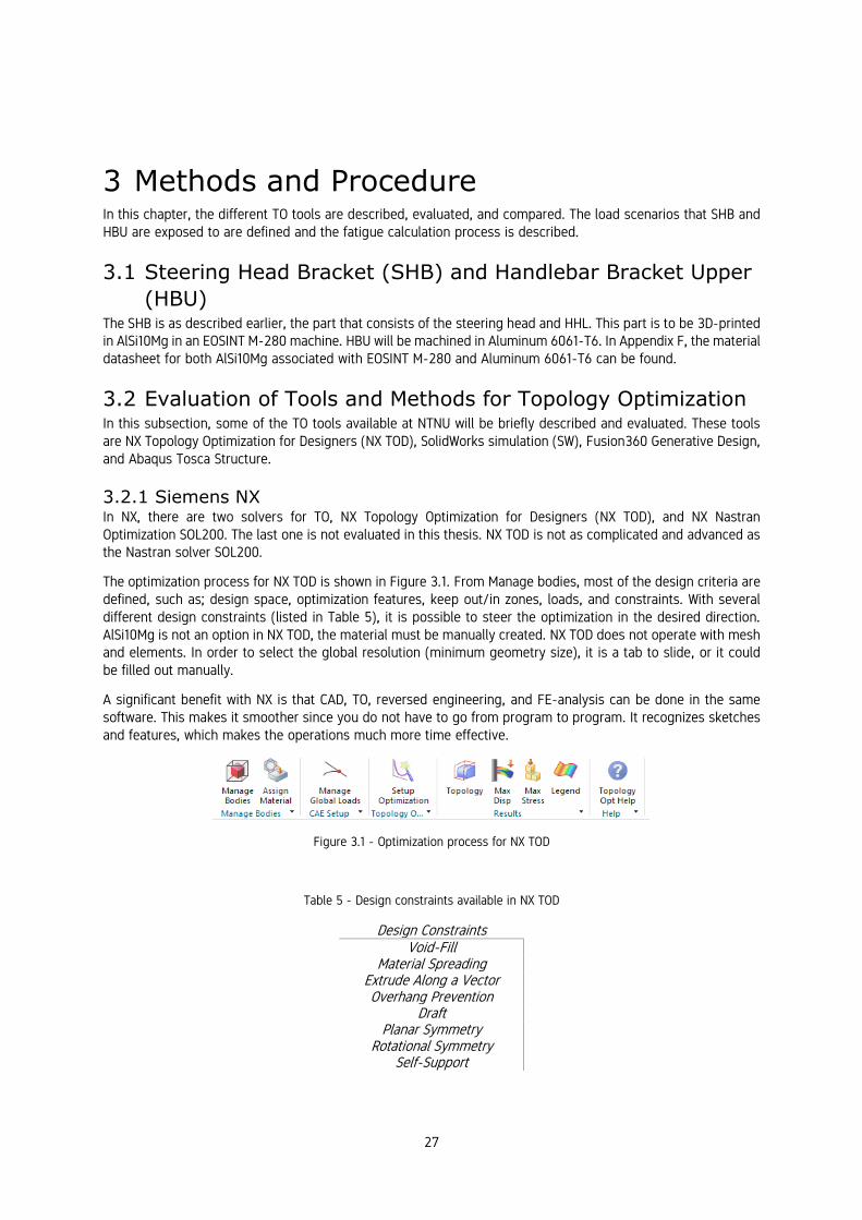
The optimization process for NX TOD is shown in Figure 3.1. From Manage bodies, most of the design criteria are
defined, such as; design space, optimization features, keep out/in zones, loads, and constraints. With several
different design constraints (listed in Table 5), it is possible to steer the optimization in the desired direction.
AlSi10Mg is not an option in NX TOD, the material must be manually created. NX TOD does not operate with mesh
and elements. In order to select the global resolution (minimum geometry size), it is a tab to slide, or it could
be filled out manually.
A significant benefit with NX is that CAD, TO, reversed engineering, and FE-analysis can be done in the same
software. This makes it smoother since you do not have to go from program to program. It recognizes sketches
and features, which makes the operations much more time effective.
Figure 3.1 - Optimization process for NX TOD
Table 5 - Design constraints available in NX TOD
Design Constraints Void-Fill
Material Spreading Extrude Along a Vector Overhang Prevention
Draft Planar Symmetry
Rotational Symmetry Self-Support
3 Methods and Procedure
28
3.2.2 SolidWorks SolidWorks Simulation add-in offers several solvers, including Topology Study. Figure 3.2 shows the optimization
process for SW. It is straightforwardly and easy to set-up the optimization. Choose material from SW material
library or create a material with desired specifications. AlSi10Mg is not an option, but a comparable material has
been created and used. Remote loads are possible to use, which makes it easy to set up moments. Hex mesh
is not possible, but tetrahedron four and ten are options. SW is caching during the optimization and this allows
it to fill up free space on the computer. Therefore, it is crucial to have much free space before starting the
optimization. Some manufacturing constraints are possible and are helpful when you want to steer the
optimization in a more desired direction. These are listed in Table 6.
Before generating the STL-file, the part needs to be smoothed. Mesh modeling is an accurate CAD re-construction
tool, especially when the STL-file is generated in SW, as the modeling commands recognize curves, lines, and
surfaces.
In the same way as NX, it is possible to do all operations in SW. The results from the TO is not that trustworthy
(this is more discussed in Appendix C ) and are challenging to get right. The CAE-environment is not as advanced
and opportunity-rich as NX Nastran.
Figure 3.2 - Optimization process for SW
Table 6 - Manufacturing constraints available in SW
Manufacturing constraints Thickness Constraint
De-mold Direction Planar symmetry
Preserved regions
3.2.3 Fusion360 In Fusion360, it is Generative Design that is used to obtain a solution for an optimized design. Generative design
gives affordable (free for students) access to powerful cloud computing, which empowers it to be very fast and
generate several outcomes in one run (Matthew, 2017). Several manufacturing methods/constraints (listed in
Table 7) are available, and all can be run at the same time. This makes the part optimized for a specific
manufacturing method. When such optimization is finished, it is possible to use a comparison tool that shows
all different features and makes it easy to compare the different solutions from each manufacturing method.
Figure 3.3 shows the optimization process from start to stop. It is an option to start with an explanatory guide.
Loads and constraints opportunities are few and simple and this makes it difficult to set up a real and correct
situation. However, generative design is a simple and straightforwardly tool to use. Before running the
optimization, a checklist tells if all necessary setups are set, and it is possible to preview the result. It is not
possible to choose mesh elements. Only options are coarse or fine resolution, and no indication how coarse or
how fine. AlSi10Mg is an option in the material library, but it does not have anisotropic material properties such
as AM material usually have.

29
Fusion360 generates several outcomes from one optimization depending on what manufacturing constraints and
material that is selected. With only AM constraints and one material selected, it gives us four different outcomes,
dependent on the printing direction, X, Y, and Z. The last one is unrestricted, meaning no AM rule applies.
Fusion360 estimates manufacturing cost.
Figure 3.3 - Optimization process for Generative Design
Table 7 - Manufacturing constraints available in Fusion360
Manufacturing Constraints Additive Manufacturing
Tree and Five-Axis Milling Two-Axis Cutting
Die Casting
3.2.4 Abaqus Tosca structure is a plug-in to Abaqus CAE 2017 and is used for TO. Abaqus Tosca is a much more advanced
optimization tool than the others that are discussed in this chapter. Figure 3.4 shows the dropdown menu that
must be worked through to set up an optimization. This is more time consuming than all the other TO tools
explained earlier. The CAD environment in Abaqus is outdated and inadequate. It is therefore to recommend
doing CAD in another software and import the STEP-file to Abaqus. There is no material library, so the material
must be manually filled in. All sorts of mesh are possible to use. A ton of options for the load and constraint
setup. Many options in all parts of the optimization set-up, this is more explained in the next chapter. To steer
the optimization in the desired direction, the geometric restriction in Table 8 are options. When the optimization
is finished, smoothening must be done before extracting the STL-file.
Figure 3.4 - Optimization process for Abaqus Tosca
30
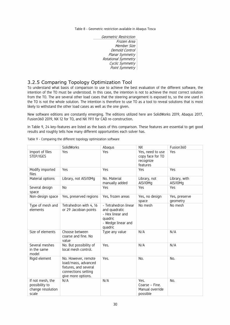
Table 8 - Geometric restriction available in Abaqus Tosca
Geometric Restriction Frozen Area
Member Size Demold Control
Planar Symmetry Rotational Symmetry
Cyclic Symmetry Point Symmetry
3.2.5 Comparing Topology Optimization Tool To understand what basis of comparison to use to achieve the best evaluation of the different software, the
intention of the TO must be understood. In this case, the intention is not to achieve the most correct solution
from the TO. The are several other load cases that the steering arrangement is exposed to, so the one used in
the TO is not the whole solution. The intention is therefore to use TO as a tool to reveal solutions that is most
likely to withstand the other load cases as well as the one given.
New software editions are constantly emerging. The editions utilized here are SolidWorks 2019, Abaqus 2017,
Fusion360 2019, NX 12 for TO, and NX 1911 for CAD re-construction.
In Table 9, 24 key-features are listed as the basis of this comparison. These features are essential to get good
results and roughly tells how many different opportunities each solver has.
Table 9 - Comparing the different topology optimization software
SolidWorks Abaqus NX Fusion360 Import of files STEP/IGES
Yes Yes Yes, need to use copy face for TO recognize features
Yes
Modify imported files
Yes Yes Yes Yes
Material options Library, not AlSi10Mg No. Material manually added
Library, not AlSi10Mg
Library, with AlSi10Mg
Several design space
No Yes Yes Yes
Non-design space Yes, preserved regions Yes, frozen areas Yes, no design space
Yes, preserve geometry
Type of mesh and elements
Tetrahedron with 4, 16 or 29 Jacobian points
- Tetrahedron linear and quadratic - Hex linear and quadric - Wedge linear and quadric
No mesh No mesh
Size of elements Choose between coarse and fine. No value
Type any value N/A N/A
Several meshes in the same model
No. But possibility of local mesh control.
Yes. N/A N/A
Rigid element No. However, remote load/mass, advanced fixtures, and several connections setting give more options.
Yes. No. No.
If not mesh, the possibility to change resolution scale
N/A N/A Yes. Coarse – Fine. Manual override possible
No.
31
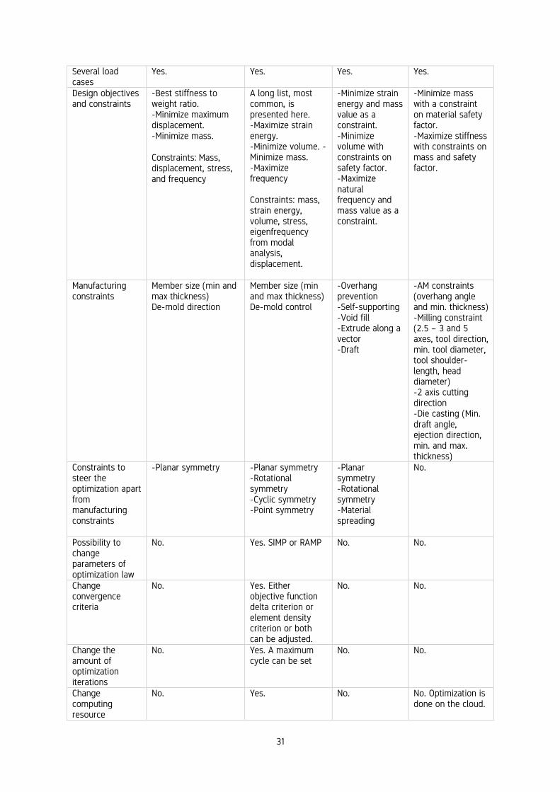
Several load cases
Yes. Yes. Yes. Yes.
Design objectives and constraints
-Best stiffness to weight ratio. -Minimize maximum displacement. -Minimize mass. Constraints: Mass, displacement, stress, and frequency
A long list, most common, is presented here. -Maximize strain energy. -Minimize volume. -Minimize mass. -Maximize frequency Constraints: mass, strain energy, volume, stress, eigenfrequency from modal analysis, displacement.
-Minimize strain energy and mass value as a constraint. -Minimize volume with constraints on safety factor. -Maximize natural frequency and mass value as a constraint.
-Minimize mass with a constraint on material safety factor. -Maximize stiffness with constraints on mass and safety factor.
Manufacturing constraints
Member size (min and max thickness) De-mold direction
Member size (min and max thickness) De-mold control
-Overhang prevention -Self-supporting -Void fill -Extrude along a vector -Draft
-AM constraints (overhang angle and min. thickness) -Milling constraint (2.5 – 3 and 5 axes, tool direction, min. tool diameter, tool shoulder-length, head diameter) -2 axis cutting direction -Die casting (Min. draft angle, ejection direction, min. and max. thickness)
Constraints to steer the optimization apart from manufacturing constraints
-Planar symmetry -Planar symmetry -Rotational symmetry -Cyclic symmetry -Point symmetry
-Planar symmetry -Rotational symmetry -Material spreading
No.
Possibility to change parameters of optimization law
No. Yes. SIMP or RAMP No. No.
Change convergence criteria
No. Yes. Either objective function delta criterion or element density criterion or both can be adjusted.
No. No.
Change the amount of optimization iterations
No. Yes. A maximum cycle can be set
No. No.
Change computing resource
No. Yes. No. No. Optimization is done on the cloud.
32
Graph or report from optimization
Yes. Yes. Yes. No.
Preview of result No. No. No. Yes. Not accurate Result from each cycle
No. However, able to adjust material mass and mesh smoothing.
Yes. No. Yes.
Max stress and displacement on the result
No. Only from the entire model. Not reliable.
Yes. Roughly estimate.
Yes. Roughly estimate.
Only values in the report. No location for displacement. Poor indication for stress, shows only high or low.
Export to solid No. No. No. Yes. Guided optimization
No. But a simple task list is available.
No. Yes. Yes.
3.3 Re-construction of CAD The result file from the TO is an STL-file which can be directly printed, but it is a problematic file type to do
further work on. The TO results in this thesis needs to be further investigated in the form of FE-analysis, and
therefore a CAD must be modeled. Today there is no gold standard on how to create a CAD from an STL-file, and
this can sometimes be the most time-consuming bit of the TO process.
Mainly different options for re-construction of CAD
1. Modeling upon the STL by eye.
2. Steel geometry from STL. Use that for extrude, hole, loft, etc.
3. Software recognizes surfaces.
Options in NX for re-construct CAD
• Realize shape 1, 2 & 3.
• Reversed engineering and use of convergent technology 1, 2 & 3.
Options in SolidWorks for re-construct CAD
• Mesh Prep Wizard in ScanTo3D (SW professional add-in) 1, 2 & 3.
• Mesh Modelling 2 & 3.
• Geomagic for SolidWorks (separately purchased add-in).
Options in Fusin360
• T-spline plane wrapped around mesh 1 & 3.
Methods used in this master thesis are NX realize shape, mesh modeling in SW, and mesh prep wizard in SW.
The last one was done from an optimization completed in Abaqus in the project thesis, autumn 2019.
33
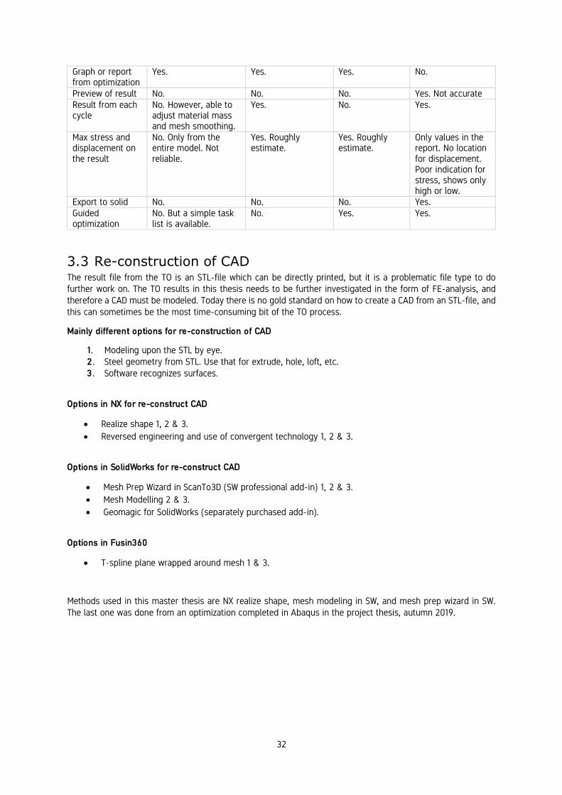
CAD re-construction in NX realize shape
1. Import STL and change transparency.
2. Extrude the cylindrical zones in modeling application.
3. Use section tube command to fill the inside of the STL-surface with solid.
4. Adjust the cage, so it fits.
5. Unite subdivision body and solid body.
6. Add fillets and chamfer and a small adjustment in the modeling application.
The process is illustrated in Figure 3.5.
Note: Section tube command is only available in NX 1872 series and newer.
Figure 3.5 - Re-construction procedure of CAD in NX. From STL to modeling stage in Realize shape application to meshed FEM-model.
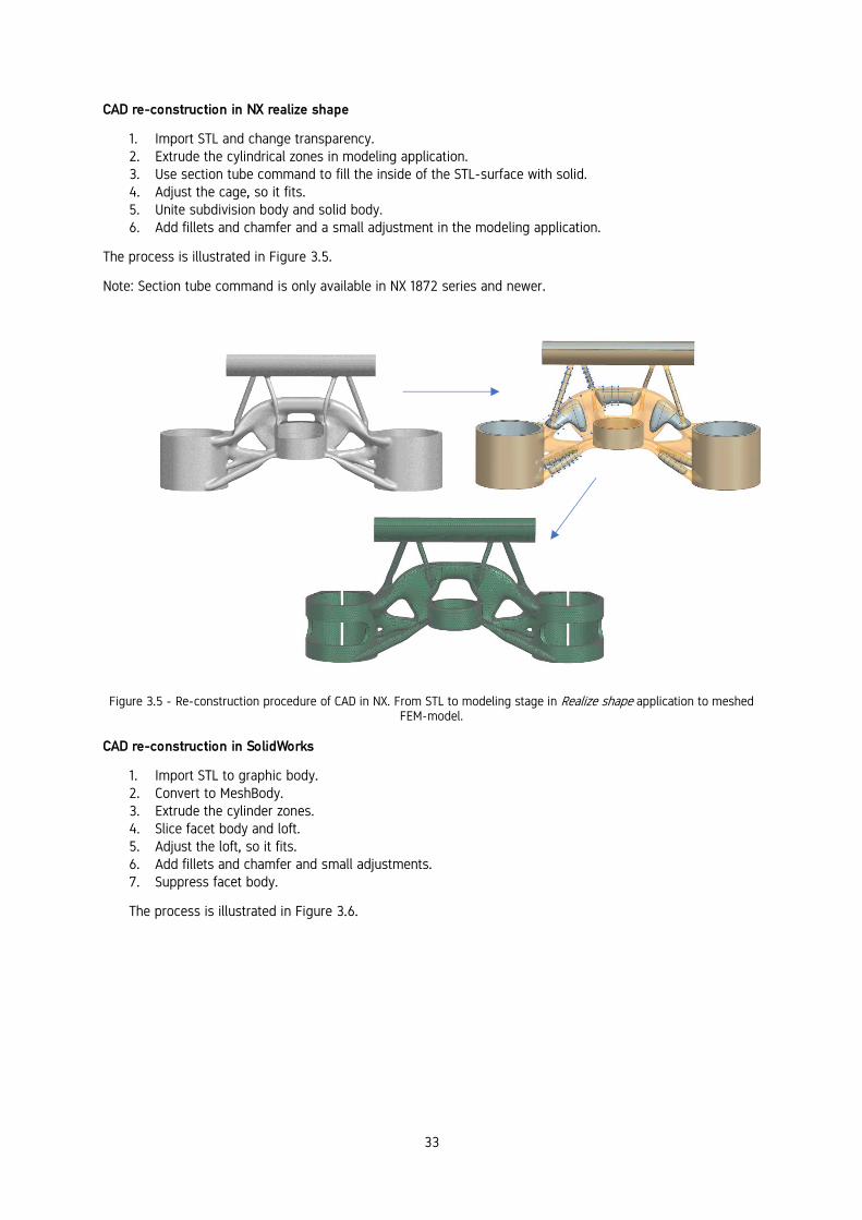
CAD re-construction in SolidWorks
1. Import STL to graphic body.
2. Convert to MeshBody.
3. Extrude the cylinder zones.
4. Slice facet body and loft.
5. Adjust the loft, so it fits.
6. Add fillets and chamfer and small adjustments.
7. Suppress facet body.
The process is illustrated in Figure 3.6.

34
Figure 3.6 - Re-construction procedure of CAD in SolidWorks. From STL to modeling stage in Mesh modeling application to meshed FEM-model.
CAD re-construction in Fusion360
One massive benefit in Fusion360 is that after a TO it is just one click, and then you have a solid model.
1. Export solid
The solid will have strange faces and curves, and it can be difficult to adjust such a part.
In Abaqus, there are no good options for the re-construction. Therefore the actual re-construction with Abaqus
result is done in separate CAD-software, NX, and SW.
CAD re-construction in NX with Abaqus result
1. Smooth and extract STL from Abaqus and import this to NX
2. Mirror feature
3. Extrude the cylindrical zones in modeling application.
4. Start symmetric modeling and use section tube command to fill the inside of the STL-surface with
solid.
5. Adjust the cage, so it fits.
6. Unite subdivision body and solid body
7. Add fillets and chamfer and small adjustments in the modeling application.
The process is illustrated in Figure 3.7.

35
Figure 3.7 - Re-construction procedure of CAD with Abaqus optimized result in NX. From unsmoothed ODB-file in Abaqus to STL in NX to meshed FEM-model.
CAD re-construction in SW with Abaqus results
This was done in the project thesis and has not been done in the master thesis. Figure 3.8 shows HBU after
optimizing (nr 17 in Figure 1.2). The mesh file from Abaqus needs to be smoothed in order to create a good solid.
This is done in a separate software called MeshLab. In this software, a point cloud is created, and that makes
the modeling easier.
1. Import to Meshlab
2. Create point cloud and smooth the mesh
3. Import point cloud to SolidWorks
4. MeshPrep Wizard in ScanTo3D add-in was used to create surfaces
5. Thicken surfaces
The process is illustrated in Figure 3.8.
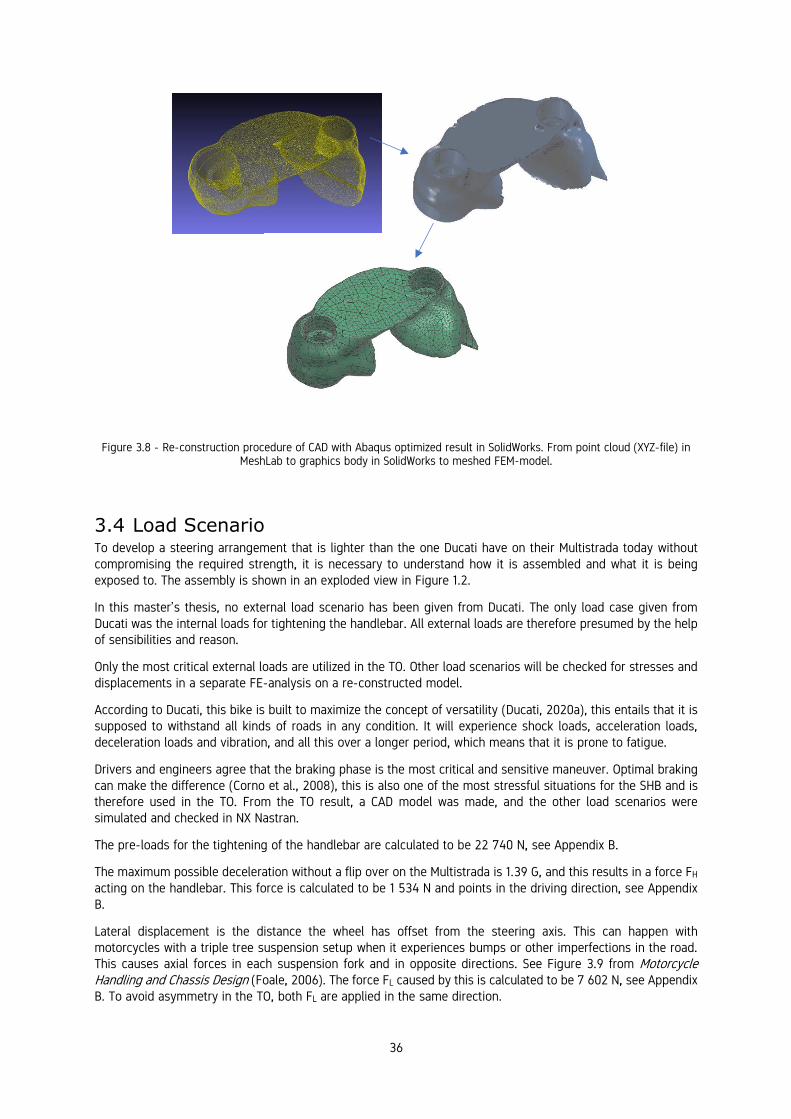
36
Figure 3.8 - Re-construction procedure of CAD with Abaqus optimized result in SolidWorks. From point cloud (XYZ-file) in MeshLab to graphics body in SolidWorks to meshed FEM-model.
3.4 Load Scenario To develop a steering arrangement that is lighter than the one Ducati have on their Multistrada today without
compromising the required strength, it is necessary to understand how it is assembled and what it is being
exposed to. The assembly is shown in an exploded view in Figure 1.2.
In this master’s thesis, no external load scenario has been given from Ducati. The only load case given from
Ducati was the internal loads for tightening the handlebar. All external loads are therefore presumed by the help
of sensibilities and reason.
Only the most critical external loads are utilized in the TO. Other load scenarios will be checked for stresses and
displacements in a separate FE-analysis on a re-constructed model.
According to Ducati, this bike is built to maximize the concept of versatility (Ducati, 2020a), this entails that it is
supposed to withstand all kinds of roads in any condition. It will experience shock loads, acceleration loads,
deceleration loads and vibration, and all this over a longer period, which means that it is prone to fatigue.
Drivers and engineers agree that the braking phase is the most critical and sensitive maneuver. Optimal braking
can make the difference (Corno et al., 2008), this is also one of the most stressful situations for the SHB and is
therefore used in the TO. From the TO result, a CAD model was made, and the other load scenarios were
simulated and checked in NX Nastran.
The pre-loads for the tightening of the handlebar are calculated to be 22 740 N, see Appendix B.
The maximum possible deceleration without a flip over on the Multistrada is 1.39 G, and this results in a force FH
acting on the handlebar. This force is calculated to be 1 534 N and points in the driving direction, see Appendix
B.
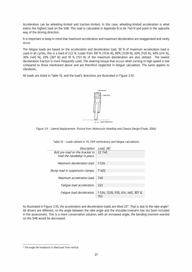
Lateral displacement is the distance the wheel has offset from the steering axis. This can happen with
motorcycles with a triple tree suspension setup when it experiences bumps or other imperfections in the road.
This causes axial forces in each suspension fork and in opposite directions. See Figure 3.9 from Motorcycle Handling and Chassis Design (Foale, 2006). The force FL caused by this is calculated to be 7 602 N, see Appendix
B. To avoid asymmetry in the TO, both FL are applied in the same direction.
37
Acceleration can be wheeling-limited and traction-limited. In this case, wheeling-limited acceleration is what
exerts the highest load on the SHB. This load is calculated in Appendix B to be 740 N and point in the opposite
way of the driving direction.
It is important to keep in mind that maximum acceleration and maximum deceleration are exaggerated and rarely
occur.
The fatigue loads are based on the acceleration and deceleration load. 30 % of maximum acceleration load is
used in all cycles, this is a load of 222 N. Loads from 100 % (1534 N), 80% (1228 N), 60% (920 N), 40% (614 N),
30% (460 N), 20% (307 N) and 10 % (153 N) of the maximum deceleration are also utilized. The lowest
deceleration fraction is more frequently used. The steering torque that occurs when turning in high speed is low
compared to those mentioned above and are therefore neglected in fatigue calculation. The same applies to
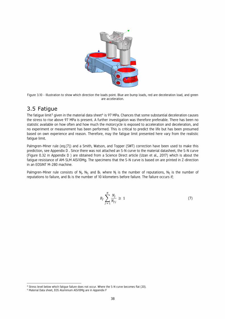
vibrations.
All loads are listed in Table 10, and the load's directions are illustrated in Figure 3.10.
Figure 3.9 - Lateral displacement. Picture from Motorcycle Handling and Chassis Design (Foale, 2006)
Table 10 - Loads utilized in TO, FEM verifications and fatigue calculations
Description Load, [N] Bolt pre-load on the bracket to
hold the handlebar in place. 22 740
Maximum deceleration load. 1 534
Bump load in suspension clamps. 7 602
Maximum acceleration load. 740
Fatigue load acceleration. 222
Fatigue load deceleration. 1 534, 1228, 920, 614, 460, 307 &
153
As illustrated in Figure 3.10, the acceleration and deceleration loads are tilted 25°. That is due to the rake angle2.
All drivers are different, so the angle between the rake angle and the shoulder/overarm has not been included
in the assessment. This is a more conservative solution, with an increased angle, the bending moment exerted
on the SHB would be decreased.
2 The angle the headstock is tilted back from vertical
38
Figure 3.10 - Illustration to show which direction the loads point. Blue are bump loads, red are deceleration load, and green are acceleration.
3.5 Fatigue The fatigue limit3 given in the material data sheet4 is 97 MPa. Chances that some substantial deceleration causes
the stress to rise above 97 MPa is present. A further investigation was therefore preferable. There has been no
statistic available on how often and how much the motorcycle is exposed to acceleration and deceleration, and
no experiment or measurement has been performed. This is critical to predict the life but has been presumed
based on own experience and reason. Therefore, may the fatigue limit presented here vary from the realistic
fatigue limit.
Palmgren-Miner rule (eq.(7)) and a Smith, Watson, and Topper (SWT) correction have been used to make this
prediction, see Appendix D . Since there was not attached an S-N curve to the material datasheet, the S-N curve
(Figure 0.32 in Appendix D ) are obtained from a Science Direct article (Uzan et al., 2017) which is about the
fatigue resistance of AM-SLM AlSi10Mg. The specimens that the S-N curve is based on are printed in Z-direction
in an EOSINT M-280 machine.
Palmgren-Miner rule consists of Nj, Nfj, and Bf, where Nj is the number of reputations, Nfj is the number of
reputations to failure, and Bf is the number of 10 kilometers before failure. The failure occurs if;
𝐵𝑓 ∑𝑁𝑗
𝑁𝑓𝑗
≥ 1
𝑁
𝑗 = 1
(7)
3 Stress level below which fatigue failure does not occur. Where the S-N curve becomes flat (20). 4 Material Data sheet, EOS Aluminium AlSi10Mg are in Appendix F
39
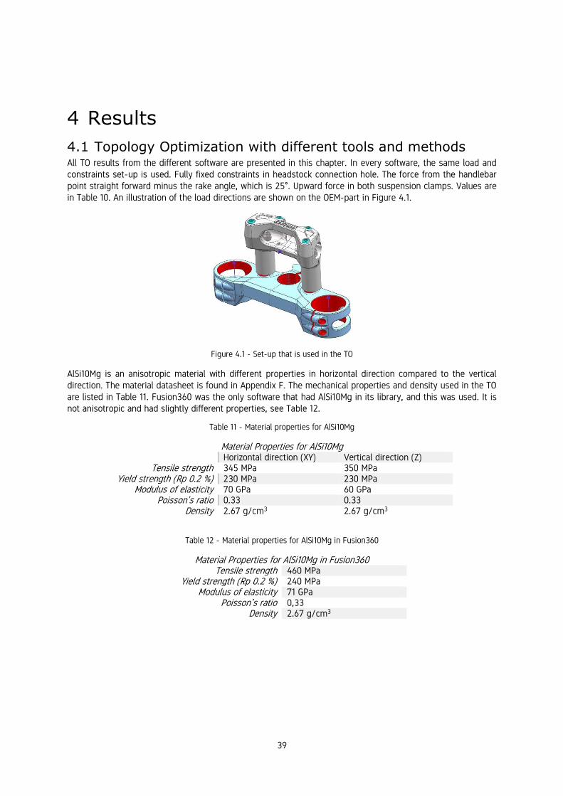
4.1 Topology Optimization with different tools and methods All TO results from the different software are presented in this chapter. In every software, the same load and
constraints set-up is used. Fully fixed constraints in headstock connection hole. The force from the handlebar
point straight forward minus the rake angle, which is 25°. Upward force in both suspension clamps. Values are
in Table 10. An illustration of the load directions are shown on the OEM-part in Figure 4.1.
Figure 4.1 - Set-up that is used in the TO
AlSi10Mg is an anisotropic material with different properties in horizontal direction compared to the vertical
direction. The material datasheet is found in Appendix F. The mechanical properties and density used in the TO
are listed in Table 11. Fusion360 was the only software that had AlSi10Mg in its library, and this was used. It is
not anisotropic and had slightly different properties, see Table 12.
Table 11 - Material properties for AlSi10Mg
Material Properties for AlSi10Mg Horizontal direction (XY) Vertical direction (Z)
Tensile strength 345 MPa 350 MPa Yield strength (Rp 0.2 %) 230 MPa 230 MPa
Modulus of elasticity 70 GPa 60 GPa Poisson’s ratio 0.33 0.33
Density 2.67 g/cm3 2.67 g/cm3
Table 12 - Material properties for AlSi10Mg in Fusion360
Material Properties for AlSi10Mg in Fusion360 Tensile strength 460 MPa
Yield strength (Rp 0.2 %) 240 MPa Modulus of elasticity 71 GPa
Poisson’s ratio 0,33 Density 2.67 g/cm3
4 Results

40
4.1.1 Siemens NX TOD From Table 5, all design constraints available in NX TOD are listed. In this set-up, Planar Symmetry, Void-Fill, and Overhang Prevention were selected. The objective was to minimize the strain energy subject to mass target,
and the optimization constraint was a mass target of 0.5 kg. The global resolution was set to 6 mm. The
optimization took 7 308 s, which is approximately 2 hours. In Figure 4.2, the design space and the result are
shown. The pink transparent body is set to design space, and the gray extruded box inside it are non-design
space. Surfaces in the handlebar holder, suspension clamp, and headstock connection hole are set to keep out, and offset thickness to 4 mm, this is to keep these regions out of the optimization.
From the optimization result, the maximum stress is allegedly 167 MPa in the transition between the struts and
suspension clamps and in the transition between the headstock connection ring and the struts. The maximum
displacement is 0.77 mm in the suspension clamps. In Appendix C , these values are compared to the re-
constructed CAD, maximum stress was 166 MPa, and maximum displacement was 0.47 mm. The final weight
was 0.546 kg.
Figure 4.2 - Design space and result of optimization in NX TOD
4.1.2 SolidWorks In Figure 4.3, the design space and the result are shown. The same design space and keep out regions as in NX
TOD was used. The best stiffness to weight ratio and a mass constraint on 0.5 kg was selected. Linear tetrahedron
element was used in the mesh, and the mesh global size was set to 3 mm with a tolerance of 0.2 mm. From
Table 6, planar symmetry and thickness constraints are used. The minimum thickness is set to 3 mm. After the
optimization, an isovalue slider5 can be adjusted, and a smoothening operation can be done. Figure 0.26 in
Appendix C shows how the default result looks like. Critical material between the handlebar holder and the fixed
constraints are missing. Therefore, the isovalue slider had to be adjusted to gain material in this region. That
results in a much heavier part. The optimized part in Figure 4.3 is approximately 0.7 kg. SW tends to keep
material in areas that are not contributing to the stiffness or strength of the part. It was not made a solid out of
this result due to high mass.
5 Slider to add or remove material from optimized model. Default position closely matches the mass constraints.
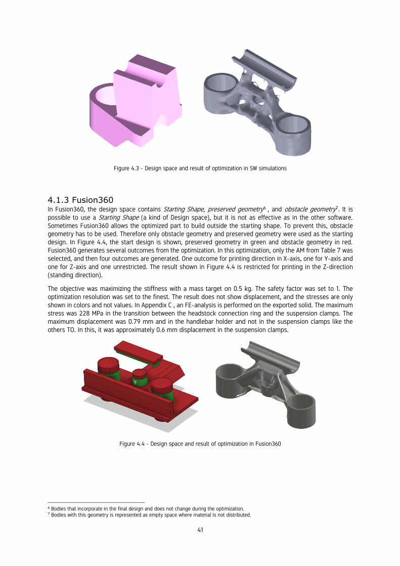
41
Figure 4.3 - Design space and result of optimization in SW simulations
4.1.3 Fusion360 In Fusion360, the design space contains Starting Shape, preserved geometry6 , and obstacle geometry7. It is
possible to use a Starting Shape (a kind of Design space), but it is not as effective as in the other software.
Sometimes Fusion360 allows the optimized part to build outside the starting shape. To prevent this, obstacle
geometry has to be used. Therefore only obstacle geometry and preserved geometry were used as the starting
design. In Figure 4.4, the start design is shown, preserved geometry in green and obstacle geometry in red.
Fusion360 generates several outcomes from the optimization. In this optimization, only the AM from Table 7 was
selected, and then four outcomes are generated. One outcome for printing direction in X-axis, one for Y-axis and
one for Z-axis and one unrestricted. The result shown in Figure 4.4 is restricted for printing in the Z-direction
(standing direction).
The objective was maximizing the stiffness with a mass target on 0.5 kg. The safety factor was set to 1. The
optimization resolution was set to the finest. The result does not show displacement, and the stresses are only
shown in colors and not values. In Appendix C , an FE-analysis is performed on the exported solid. The maximum
stress was 228 MPa in the transition between the headstock connection ring and the suspension clamps. The
maximum displacement was 0.79 mm and in the handlebar holder and not in the suspension clamps like the
others TO. In this, it was approximately 0.6 mm displacement in the suspension clamps.
Figure 4.4 - Design space and result of optimization in Fusion360
6 Bodies that incorporate in the final design and does not change during the optimization. 7 Bodies with this geometry is represented as empty space where material is not distributed.
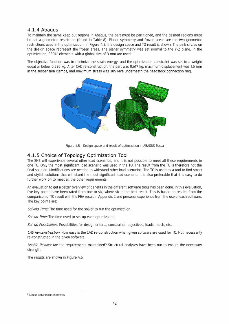
42
4.1.4 Abaqus To maintain the same keep out regions in Abaqus, the part must be partitioned, and the desired regions must
be set a geometric restriction (found in Table 8). Planar symmetry and frozen areas are the two geometric
restrictions used in the optimization. In Figure 4.5, the design space and TO result is shown. The pink circles on
the design space represent the frozen areas. The planar symmetry was set normal to the Y-Z plane. In the
optimization, C3D48 elements with a global size of 3 mm are used.
The objective function was to minimize the strain energy, and the optimization constraint was set to a weight
equal or below 0.520 kg. After CAD re-construction, the part was 0.617 kg, maximum displacement was 1.5 mm
in the suspension clamps, and maximum stress was 385 MPa underneath the headstock connection ring.
Figure 4.5 - Design space and result of optimization in ABAQUS Tosca
4.1.5 Choice of Topology Optimization Tool The SHB will experience several other load scenarios, and it is not possible to meet all these requirements in
one TO. Only the most significant load scenario was used in the TO. The result from the TO is therefore not the
final solution. Modifications are needed to withstand other load scenarios. The TO is used as a tool to find smart
and stylish solutions that withstand the most significant load scenario. It is also preferable that it is easy to do
further work on to meet all the other requirements.
An evaluation to get a better overview of benefits in the different software tools has been done. In this evaluation,
five key points have been rated from one to six, where six is the best result. This is based on results from the
comparison of TO result with the FEA result in Appendix C and personal experience from the use of each software.
The key points are:
Solving Time: The time used for the solver to run the optimization.
Set-up Time: The time used to set up each optimization.
Set-up Possibilities: Possibilities for design criteria, constraints, objectives, loads, mesh, etc.
CAD Re-construction: How easy is the CAD re-construction when given software are used for TO. Not necessarily
re-constructed in the given software.
Usable Results: Are the requirements maintained? Structural analyzes have been run to ensure the necessary
strength.
The results are shown in Figure 4.6.
8 Linear tetrahedron elements
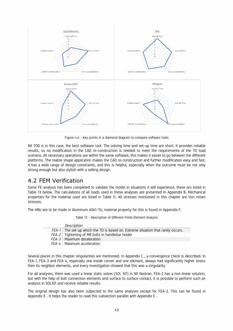
43
Figure 4.6 - Key points in a diamond diagram to compare software tools
NX TOD is in this case, the best software tool. The solving time and set-up time are short. It provides reliable
results, so no modification in the CAD re-construction is needed to meet the requirements of the TO load
scenario. All necessary operations are within the same software, this makes it easier to go between the different
platforms. The realize shape application makes the CAD re-construction and further modification easy and fast.
It has a wide range of design constraints, and this is helpful, especially when the outcome must be not only
strong enough but also stylish with a selling design.
4.2 FEM Verification Some FE-analysis has been completed to validate the model in situations it will experience, these are listed in
Table 13 below. The calculations of all loads used in these analyses are presented in Appendix B. Mechanical
properties for the material used are listed in Table 11. All stresses mentioned in this chapter are Von mises
stresses.
The HBU are to be made in Aluminum 6061-T6, material property for this is found in Appendix F.
Table 13 - Description of different Finite Element Analysis
Description FEA-1 The set-up which the TO is based on. Extreme situation that rarely occurs. FEA-2 Tightening of M8 bolts in handlebar holder FEA-3 Maximum deceleration FEA-4 Maximum acceleration
Several places in this chapter singularities are mentioned. In Appendix C , a convergence check is described. In
FEA-1, FEA-3 and FEA-4, especially one inside corner and one element, always had significantly higher stress
then its neighbor elements, and every investigation showed that this was a singularity.
For all analyses, there was used a linear static solver (SOL 101) in NX Nastran. FEA-2 has a non-linear solution,
but with the help of bolt connection elements and surface to surface contact, it is possible to perform such an
analysis in SOL101 and receive reliable results.
The original design has also been subjected to the same analyses except for FEA-2. This can be found in
Appendix E . It helps the reader to read this subsection parallel with Appendix E .
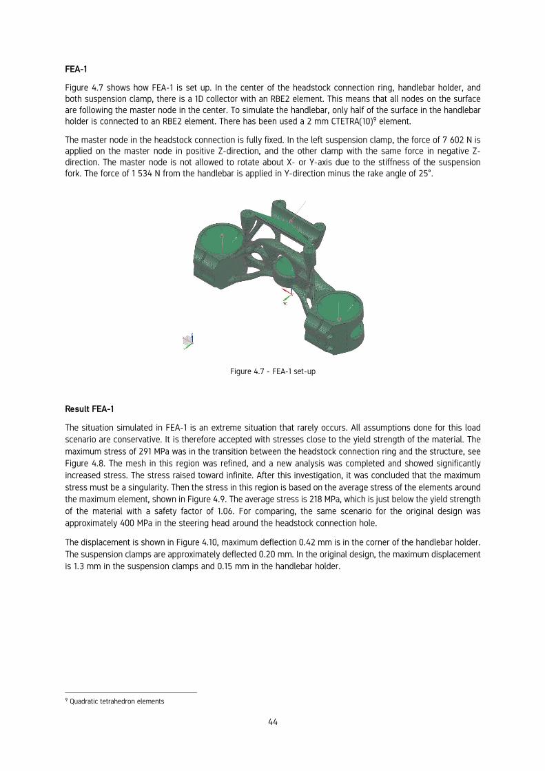
44
FEA-1
Figure 4.7 shows how FEA-1 is set up. In the center of the headstock connection ring, handlebar holder, and
both suspension clamp, there is a 1D collector with an RBE2 element. This means that all nodes on the surface
are following the master node in the center. To simulate the handlebar, only half of the surface in the handlebar
holder is connected to an RBE2 element. There has been used a 2 mm CTETRA(10)9 element.
The master node in the headstock connection is fully fixed. In the left suspension clamp, the force of 7 602 N is
applied on the master node in positive Z-direction, and the other clamp with the same force in negative Z-
direction. The master node is not allowed to rotate about X- or Y-axis due to the stiffness of the suspension
fork. The force of 1 534 N from the handlebar is applied in Y-direction minus the rake angle of 25°.
Figure 4.7 - FEA-1 set-up
Result FEA-1
The situation simulated in FEA-1 is an extreme situation that rarely occurs. All assumptions done for this load
scenario are conservative. It is therefore accepted with stresses close to the yield strength of the material. The
maximum stress of 291 MPa was in the transition between the headstock connection ring and the structure, see
Figure 4.8. The mesh in this region was refined, and a new analysis was completed and showed significantly
increased stress. The stress raised toward infinite. After this investigation, it was concluded that the maximum
stress must be a singularity. Then the stress in this region is based on the average stress of the elements around
the maximum element, shown in Figure 4.9. The average stress is 218 MPa, which is just below the yield strength
of the material with a safety factor of 1.06. For comparing, the same scenario for the original design was
approximately 400 MPa in the steering head around the headstock connection hole.
The displacement is shown in Figure 4.10, maximum deflection 0.42 mm is in the corner of the handlebar holder.
The suspension clamps are approximately deflected 0.20 mm. In the original design, the maximum displacement
is 1.3 mm in the suspension clamps and 0.15 mm in the handlebar holder.
9 Quadratic tetrahedron elements
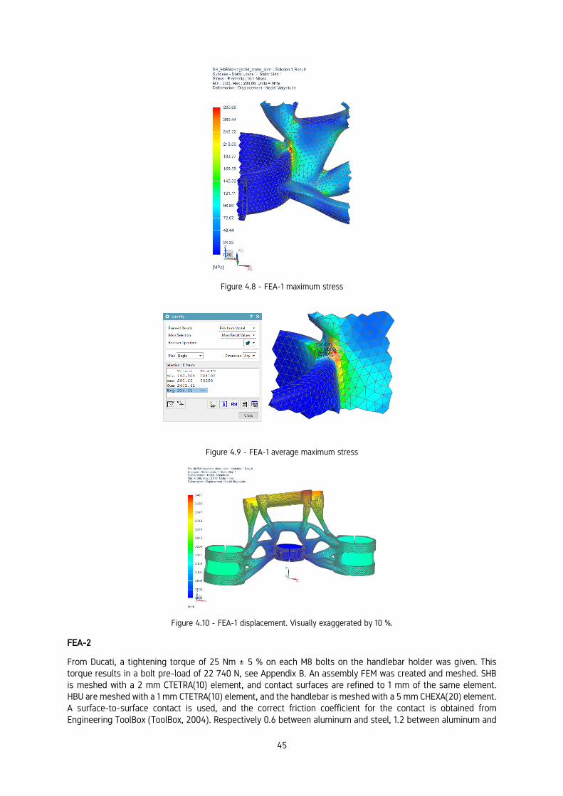
45
Figure 4.8 - FEA-1 maximum stress
Figure 4.9 - FEA-1 average maximum stress
Figure 4.10 - FEA-1 displacement. Visually exaggerated by 10 %.
FEA-2
From Ducati, a tightening torque of 25 Nm ± 5 % on each M8 bolts on the handlebar holder was given. This
torque results in a bolt pre-load of 22 740 N, see Appendix B. An assembly FEM was created and meshed. SHB
is meshed with a 2 mm CTETRA(10) element, and contact surfaces are refined to 1 mm of the same element.
HBU are meshed with a 1 mm CTETRA(10) element, and the handlebar is meshed with a 5 mm CHEXA(20) element.
A surface-to-surface contact is used, and the correct friction coefficient for the contact is obtained from
Engineering ToolBox (ToolBox, 2004). Respectively 0.6 between aluminum and steel, 1.2 between aluminum and
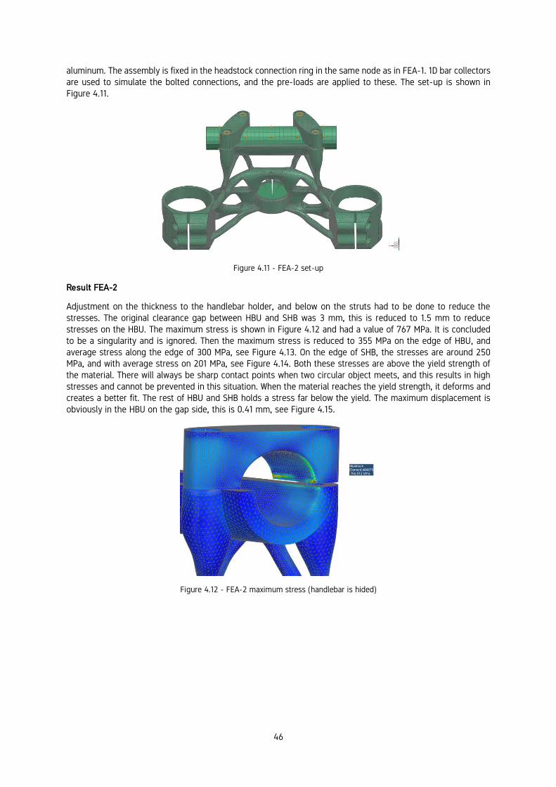
46
aluminum. The assembly is fixed in the headstock connection ring in the same node as in FEA-1. 1D bar collectors
are used to simulate the bolted connections, and the pre-loads are applied to these. The set-up is shown in
Figure 4.11.
Figure 4.11 - FEA-2 set-up
Result FEA-2
Adjustment on the thickness to the handlebar holder, and below on the struts had to be done to reduce the
stresses. The original clearance gap between HBU and SHB was 3 mm, this is reduced to 1.5 mm to reduce
stresses on the HBU. The maximum stress is shown in Figure 4.12 and had a value of 767 MPa. It is concluded
to be a singularity and is ignored. Then the maximum stress is reduced to 355 MPa on the edge of HBU, and
average stress along the edge of 300 MPa, see Figure 4.13. On the edge of SHB, the stresses are around 250
MPa, and with average stress on 201 MPa, see Figure 4.14. Both these stresses are above the yield strength of
the material. There will always be sharp contact points when two circular object meets, and this results in high
stresses and cannot be prevented in this situation. When the material reaches the yield strength, it deforms and
creates a better fit. The rest of HBU and SHB holds a stress far below the yield. The maximum displacement is
obviously in the HBU on the gap side, this is 0.41 mm, see Figure 4.15.
Figure 4.12 - FEA-2 maximum stress (handlebar is hided)
47
Figure 4.13 - FEA-2 average stress in the HBU (handlebar is hided)
Figure 4.14 - FEA-2 average stress in SHB (handlebar is hided)
Figure 4.15 - FEA-2 displacement. Visually exaggerated by 0.5 %
48
FEA-3
CTETRA(10) elements with 2 mm size were used in this analysis. Maximum deceleration load of 1 534 N in y-
direction minus the rake angle of 25°. Without the bump loads in the suspension clamps, the set-up is identical
as in FEA-1.
FEA-3 Result
There was a singularity in the same corner as in FEA-1. By ignoring this, the maximum stress is reduced to
approximately 178 MPa, see Figure 4.16. That is a safety factor of 1.29 to the yield strength of the material. In
the original design, the stress was 70 MPa in the connection between HHL and the steering head. The maximum
displacement is in the handlebar holder and is 0.41 mm, and in the suspension clamp, it is 0.20 mm, see Figure
4.17. For the original design, this displacement is 0.15 mm on the edge of HHL.
Figure 4.16 - FEA-3 average stress
Figure 4.17 - FEA-3 displacement. Visually exaggerated 10 %
FEA-4
CTETRA(10) elements with 2 mm size were used in this analysis.
For maximum acceleration, the force points in negative Y-direction plus the rake angle of 25°. It is applied to
the master node of an RBE2 element linked to one half of the handlebar holder surface to simulate the handlebar.
49
From Appendix B, the force magnitude is set to 740 N. SHB is fully fixed in the master node of the RBE2 element
in the headstock connection ring. Figure 4.18 shows the set-up.
Figure 4.18 - FEA-4 set-up
FEA-4 Result
Singularity in the same corner as in FEA-1. By ignoring this, the maximum stress is reduced from 274 MPa to
approximately 155 MPa, see Figure 4.19. That is a safety factor of 1.48 to the yield strength of the material. In
the original design, the maximum stress was 34 MPa in the connection between HHL and the steering head. The
maximum displacement is 0.19 mm in the handlebar holder, and the displacement in the suspension clamps is
0.08 mm, see Figure 4.20. For the original design, the maximum displacement was 0.07 mm in the handlebar
holder.
Figure 4.19 - FEA-4 average stress
50
Figure 4.20 - FEA-4 displacement. Visually exaggerated 10 %.
4.3 Manufacturing Process During the process of modeling and optimizing the SHB, AM has been kept in mind. Meaning that overhangs are
minimized, self-supporting angles have been used as far as its possible. The model contains no voids to prevent
that un-melted powder from the printer is trapped. The findings from the articles (Vandenbroucke and Kruth,
2007, Calignano, 2014, Han et al., 2018) in chapter 2.4.2 Design for Additive Manufacturing are the basis for the
design.
SHB is fatigue calculated based on the “after stress relief, machined and polished” S-N curve from (Uzan et al.,
2017). Therefore it is necessary to add some extra material in critical areas when 3D-printing so that after post-
processing,10 there is enough material. These areas are primarily in the clamps, the handlebar holder, headstock
connection ring, and in the high stressed region in the transition between the struts and the headstock
connection ring.
It will be printed without the bolt holes, these will be drilled out afterward.
The flowchart in Figure 2.10 has been followed to get the best supports. AutoDesk Netfabb has been used to
build and calculate the necessary amount of support, see Figure 4.21. The volume of the SHB is 275.98 cm3, and
the support volume is 19.78 cm3. The printing time is estimated to take 66 hours and 25 minutes.
The HBU are designed with the intention that it shall be milled.
10 Grinding, sandblasting and polishing.
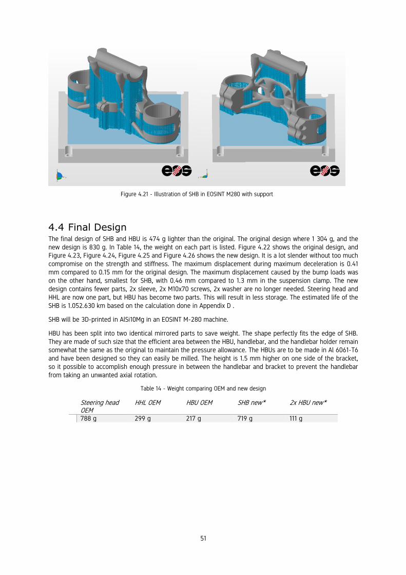
51
4.4 Final Design The final design of SHB and HBU is 474 g lighter than the original. The original design where 1 304 g, and the
new design is 830 g. In Table 14, the weight on each part is listed. Figure 4.22 shows the original design, and
Figure 4.23, Figure 4.24, Figure 4.25 and Figure 4.26 shows the new design. It is a lot slender without too much
compromise on the strength and stiffness. The maximum displacement during maximum deceleration is 0.41
mm compared to 0.15 mm for the original design. The maximum displacement caused by the bump loads was
on the other hand, smallest for SHB, with 0.46 mm compared to 1.3 mm in the suspension clamp. The new
design contains fewer parts, 2x sleeve, 2x M10x70 screws, 2x washer are no longer needed. Steering head and
HHL are now one part, but HBU has become two parts. This will result in less storage. The estimated life of the
SHB is 1.052.630 km based on the calculation done in Appendix D .
SHB will be 3D-printed in AlSi10Mg in an EOSINT M-280 machine.
HBU has been split into two identical mirrored parts to save weight. The shape perfectly fits the edge of SHB.
They are made of such size that the efficient area between the HBU, handlebar, and the handlebar holder remain
somewhat the same as the original to maintain the pressure allowance. The HBUs are to be made in Al 6061-T6
and have been designed so they can easily be milled. The height is 1.5 mm higher on one side of the bracket,
so it possible to accomplish enough pressure in between the handlebar and bracket to prevent the handlebar
from taking an unwanted axial rotation.
Table 14 - Weight comparing OEM and new design
Steering head OEM
HHL OEM HBU OEM SHB new* 2x HBU new*
788 g 299 g 217 g 719 g 111 g
Figure 4.21 - Illustration of SHB in EOSINT M280 with support
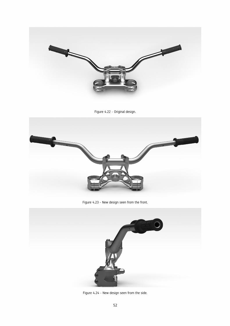
52
Figure 4.22 - Original design.
Figure 4.23 - New design seen from the front.
Figure 4.24 - New design seen from the side.

53
Figure 4.25 - SHB and HBU seen from behind.
Figure 4.26 - SHB and HBU seen from the front.
54
Ducati wanted to get a better overview of the possibilities to produces the steering arrangement with AM. A huge
benefit with AM is that organic and unconventional forms can be produced. With the help of TO, it is possible to
find the optimal material distribution to minimize the mass and maintain the stiffness. In this master’s thesis, it
is presented a solution that reduces the mass by 36 % without a notable decrease in stiffness.
5.1 Tools and Methods There are pros and cons for all the software tested, and some were better than others in this situation. If it would
have turned out different with another part and another load scenario can be discussed. SW had problem meeting
the requirements, it failed to place material in regions that are critical to maintaining the structural stiffness in
part. In Figure 3.6, a different load scenario and design space were used in SW, and then the outcome seemed
reasonable. That part was not further investigated because it turned out that the load scenario was wrong. In
Fusion360 Generative Design, all outcomes were made in such a matter that it did not allow support structure
upon the model. Then the whole model got floating transitions that made the design look strange. Displacement
and stresses in the TO result were higher than the displacement and stresses in the re-constructed model
analysis. AlSi10Mg properties in Fusion360 were different from the properties used in the others TO tools. This
is an essential factor that makes it problematic to compare this software with the others. Abaqus TO result
showed far lower stress then what the re-constructed model showed. It was also heavier than what the TO result
estimated. Drastic modifications and adjustments must have been made to make the re-constructed model
compatible with the load scenario. NX Topology Optimization for Designers is maybe what is sounds like, and
optimization tool for designers, and not engineers? When it comes to realistic set-up for the case, the options
are few, that applies as well for Fusion360 and SW. However, when it comes to options that steer the optimization
toward a desired design, there are a lot of selections possible, compared to Fusion360 and SW. Even so, the
stress and displacement values estimated in the TO result were close to the stress and displacement found in
the re-constructed analysis. These TO tools are only compared in this one case. A different outcome in another
TO-analysis cannot be guaranteed. Table 9 shows 24 fundamental factors that may help in the selection of a TO
tool.
The CAD re-construction was utilized in both SW and NX. In SW, two different methods were tested, mesh prep
wizard and mesh modeling. Within mesh prep wizard, there are two different methods to use, automatic creation
and guided creation. Automatic creation creates surfaces on the STL face, and these must manually be adjusted,
so it fits. For higher precision, more surfaces need to be created. Then there is guided creation, were STL surfaces
are painted in color, and that is the new face. The face must be in such order that it can be wrapped, or simple
geometry can be used. Afterward, the additional surfaces must be trimmed. Guided creation works best for
simple geometry, and automatic creation is better for more complex geometry. In NX, realize shape was used.
Here the STL is “filled” with a subdivision body that is uncomplicated to adjust and model with. The time used
re-construct in NX was a lot less than in SW. Just to learn the methods in SW was time-consuming and
demanding. In NX, the process was intuitive and effortless. On the other hand, the re-constructed model in NX
was not that accurate as in SW. It exists other more advanced methods/add-ons that are maybe faster and more
accurate, but they are not free.
5 Discussion and Conclusion

55
5.2 Steering Head and Handlebar Bracket Upper A part like SHB that experience several different load scenarios at different times is rather difficult to fully optimize
for all the scenarios. It was only optimized for one of them. Although many changes to the TO were necessary
to meet all requirements, it gives a good first draft that could be further developed. Without the TO and AM, it
would have been challenging to find the design and develop SHB with these properties. It can be discussed
rather if the load scenario utilized in the TO is the best one or not. Does it represent a realistic situation that
needs to be considered? Is it too conservative? If so, the total mass could have been further reduced. Stress in
the original part is too high when it is exposed to the extreme situation of FEA-1, the displacement is also
enormous, see Appendix E . This may indicate that the bases for the TO is too strict and probably the load
presumptions were too high, especially the bump load.
FEM verification load scenarios were presumed the worst case. Is it too conservative that SHB should hold the
total weight of a person during acceleration? And that the bump occurs during maximum deceleration. Testing
and measuring the different load scenarios would have been desirable.
More time preparing the re-constructed model for FE-analysis probably should have been done. Adding fillets
and reduce the amount of sharp inner corner would probably have saved us from many of the singularities.
The only basis that underpinned the choice of load history utilized in the fatigue calculations was my own experiences and reason. The estimated life of SHB is thus necessarily not correct. To get a better approximation it should have been measured with strain gauge while driving. Then it would have been interesting to implement a digital twin and monitor the situation. From this it could be scaled up, and a much more precise fatigue prediction in FEDEM11 could have been utilized. The stiffness of SHB during deceleration has been slightly reduced, the effect of this is not known. However, the deflection caused by bump is reduced on the new design. Is it noticeable when driving at all? By doing real testing with the SHB on a Multistrada, the drivability could have been compared. As mentioned before, the SHB is fatigue calculated based on the “after stress relief, machined and polished” S-N curve (Figure 0.32) from (Uzan et al., 2017). Therefore it is necessary to add some extra material in critical areas when 3D-printing so that after post-processing, there is enough material. This has not been included in the final design but is an important factor to consider. Screws directly in aluminum threads often cause problems where the bolt cuts the treads. It should therefore be used HELICOILS12, which improves thread strength for aluminum (Springer India New, 2014). This means that the drilled hole needs to meet dimension requirements for HELICOIL holes for M8 bolts.
The prices calculated in chapter 2.4.1 are only used as a guideline and are probably way off from what prices
Ducati could have arranged if it were to be made ten thousand parts. Yet AM is an expensive manufacturing
method, and prices vs. needs must be considered.
It has been made many assumptions in this thesis, and all of them have been on the “safe side”. This may result
in an over-dimensioned SHB, yet the weight was reduced by 36 %. With experiments and measurements on a
Multistrada, the load scenarios could have been more accurate, the center of gravity would have been correct,
and the load history for the fatigue calculations would have been a lot more precise. Then outcome from this
thesis would have been different, most likely an even lighter SHB. All these values are known for Ducati, and
with the process and method from this thesis, they can achieve a more accurate, lighter and optimized design.
11 A nonlinear finite element program 12 Thread reinforcement for low-strength material

56
5.3 Conclusion Four different TO tools capable of optimizing the steering arrangement for a motorcycle have been evaluated
and compared in this thesis. By utilizing the same load scenario on closely the same design space, all four TO
tools came up with different solutions. Not all TO tools showed that the result they presented was credible. When
the TO result was compared to FE-analysis done on re-constructed models, it showed that NX came out on top.
NX showed that the TO result was close to the result that the FE-analysis showed, and this proves that the TO
results from NX are reliable. Chapter 3.2 and 4.1, Table 9, and Appendix C answer to the evaluation of TO tools.
Two different reversed engineering tools were evaluated. NX realize shape was both faster and easier to use.
The necessary modification after the verification analysis was effortless and quick to perform compared to SW.
However, it was not as accurate as SW, but it was fast, and by iterations the accuracy was enhanced. Chapter
3.3 answer to this evaluation.
The SHB shows that it is achievable to make lighter and strong enough components with a fatigue limit of at
least 1 million km for the motorcycle industries with the help of AM and TO. Even AlSi10Mg with such low
mechanical properties can be utilized in critical components.
Through chapters 3 and 4, Appendix B, Appendix C Appendix D Appendix E , all objectives from chapter 1.1 are
satisfied.
Further work:
To be able to print this steering arrangement, more investigation in the LBM method is necessary. Scanning
speed, scanning pattern, laser power, the support size. At least consult with a manufacturer. Find out how much
more material is needed in the critical areas to be able to machine, grind, and polish the surface smooth and
not compromising the strength of the component. If the desired dimensions lay at least on the lower tolerance
band in Figure 0.1 (Appendix A ), the post-processing only removes the sharp edges. This counts for regions
with higher stresses.
To achieve 100 % correct result, it is recommended to do testing and measuring on a driving Multistrada and
collect data to estimate maximum loads and load history for fatigue prediction. The fatigue prediction can be
made in FEDEM.
Including the steering head base would have been interesting, then a lot more weight could have been reduced.

57
58
AMPOWER. 2019. Estimate your AM part cost in a first screening phase [Online].
AMPOWER. Available: am-power.de/calculator/ [Accessed 01.12 2019].
BAGHERIFARD, S., BERETTA, N., MONTI, S., RICCIO, M., BANDINI, M. & GUAGLIANO, M.
2018. On the fatigue strength enhancement of additive manufactured AlSi10Mg
parts by mechanical and thermal post-processing. Materials & Design, 145, 28-41.
BANDYOPADHYAY, A. & BOSE, S. 2015. Additive Manufacturing, Hoboken, Taylor and
Francis.
BHANAGE, A., KRISHNAN, P. & SUNDGE, R. 2015. Static and Fatigue Simulation of
Telescopic Fork Suspension System Used For Motorcycle. International Journal of
Applied Engineering Research, 10, 477.
CALIGNANO, F. 2014. Design optimization of supports for overhanging structures in
aluminum and titanium alloys by selective laser melting. Materials & Design, 64,
203-213.
CHRISTENSEN, P. W., KLARBRING, A. & GLADWELL, G. M. L. 2008. An Introduction to
Structural Optimization, Dordrecht, Dordrecht: Springer Netherlands.
CORNO, M., SAVARESI, S. M., TANELLI, M. & FABBRI, L. 2008. On optimal motorcycle
braking. Control Engineering Practice, 16, 644-657.
COSSALTER, V. 2006a. Motorcycle Dynamics Vittore Cossalter.
COSSALTER, V. 2006b. Motorcycle Dynamics Ch. 5.2.1, Vittore Cossalter.
DAHLVIG, G. & CHRISTENSEN, S. 1984. Konstruksjonselementer, [Oslo],
Yrkesopplæring.
DEBROY, T., WEI, H. L., ZUBACK, J. S., MUKHERJEE, T., ELMER, J. W., MILEWSKI, J. O.,
BEESE, A. M., WILSON-HEID, A., DE, A. & ZHANG, W. 2018. Additive
manufacturing of metallic components – Process, structure and properties.
Progress in Materials Science, 92, 112-224.
DOWNLING, N. E. 2012. Mechanical Behavior of Materials - Engineering Methods for
Deformation, Fracture and Fatigue, Pearson.
DUCATI. 2019. Multistrada 1260 S [Online]. Ducati. Available:
https://www.ducati.com/ww/en/bikes/multistrada/multistrada-1260 [Accessed
12.09 2019].
DUCATI. 2020a. Multistrada [Online]. Ducati. Available:
https://www.ducati.com/gb/en/bikes/multistrada/multistrada-1260 [Accessed 24.
April 2020].
DUCATI, B. P. 2020b. Bike Parts Ducati [Online]. Available: https://www.bike-parts-
ducati.com/ducati-
motorcycle/Multistrada/2019/Multistrada_1260_S_ABS/Multistrada-1260-S-
ABS/FRONT-FORK-STEM--TRIPLE-CLAMPS/394/2318/0/394 [Accessed 05.27
2020].
FOALE, T. 2006. Motorcycle Handling and Chassis Design - The art and science.
HAN, Q., GU, H., SOE, S., SETCHI, R., LACAN, F. & HILL, J. 2018. Manufacturability of
AlSi10Mg overhang structures fabricated by laser powder bed fusion. Materials &
Design, 160, 1080-1095.
HARTVIGSEN, H. 1994. Verkstedhåndboka: mekaniske fag, [Oslo], Yrkesopplæring i
samarbeid med Norges standardiseringsforbund.
HERZOG, D., SEYDA, V., WYCISK, E. & EMMELMANN, C. 2016. Additive manufacturing of
metals. Acta Materialia, 117, 371-392.
HUANG, R., RIDDLE, M., GRAZIANO, D., WARREN, J., DAS, S., NIMBALKAR, S., CRESKO,
J. & MASANET, E. 2016. Energy and emissions saving potential of additive
References
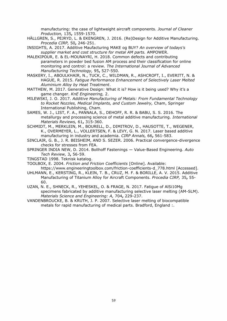
59
manufacturing: the case of lightweight aircraft components. Journal of Cleaner
Production, 135, 1559-1570.
HÄLLGREN, S., PEJRYD, L. & EKENGREN, J. 2016. (Re)Design for Additive Manufacturing.
Procedia CIRP, 50, 246-251.
INSIGHTS, A. 2017. Additive Maufacturing MAKE og BUY? An overview of todays's
supplier market and cost structure for metal AM parts. AMPOWER.
MALEKIPOUR, E. & EL-MOUNAYRI, H. 2018. Common defects and contributing
parameters in powder bed fusion AM process and their classification for online
monitoring and control: a review. The International Journal of Advanced
Manufacturing Technology, 95, 527-550.
MASKERY, I., ABOULKHAIR, N., TUCK, C., WILDMAN, R., ASHCROFT, I., EVERITT, N. &
HAGUE, R. 2015. Fatigue Performance Enhancement of Selectively Laser Melted
Aluminium Alloy by Heat Treatment.
MATTHEW, M. 2017. Generative Design: What it is? How is it being used? Why it’s a
game changer. KnE Engineering, 2.
MILEWSKI, J. O. 2017. Additive Manufacturing of Metals: From Fundamental Technology
to Rocket Nozzles, Medical Implants, and Custom Jewelry, Cham, Springer
International Publishing, Cham.
SAMES, W. J., LIST, F. A., PANNALA, S., DEHOFF, R. R. & BABU, S. S. 2016. The
metallurgy and processing science of metal additive manufacturing. International
Materials Reviews, 61, 315-360.
SCHMIDT, M., MERKLEIN, M., BOURELL, D., DIMITROV, D., HAUSOTTE, T., WEGENER,
K., OVERMEYER, L., VOLLERTSEN, F. & LEVY, G. N. 2017. Laser based additive
manufacturing in industry and academia. CIRP Annals, 66, 561-583.
SINCLAIR, G. B., J. R. BEISHEIM, AND S. SEZER. 2006. Practical convergence-divergence
checks for stresses from FEA.
SPRINGER INDIA NEW, D. 2014. Bollhoff Fastenings — Value-Based Engineering. Auto
Tech Review, 3, 56-59.
TINGSTAD 1998. Teknisk katalog.
TOOLBOX, E. 2004. Friction and Friction Coefficients [Online]. Available:
https://www.engineeringtoolbox.com/friction-coefficients-d_778.html [Accessed].
UHLMANN, E., KERSTING, R., KLEIN, T. B., CRUZ, M. F. & BORILLE, A. V. 2015. Additive
Manufacturing of Titanium Alloy for Aircraft Components. Procedia CIRP, 35, 55-
60.
UZAN, N. E., SHNECK, R., YEHESKEL, O. & FRAGE, N. 2017. Fatigue of AlSi10Mg
specimens fabricated by additive manufacturing selective laser melting (AM-SLM).
Materials Science and Engineering: A, 704, 229-237.
VANDENBROUCKE, B. & KRUTH, J. P. 2007. Selective laser melting of biocompatible
metals for rapid manufacturing of medical parts. Bradford, England :.

60

61
Appendix A : Common defects for LBM and EBM
Appendix B : Load scenarios for TO and FE-analysis
Appendix C : Result from TO compared with FE- analysis
Appendix D : Life prediction
Appendix E : FE-analysis on OEM part
Appendix F : Material Datasheet for AlSi10Mg and Al 6061-T6
Appendix
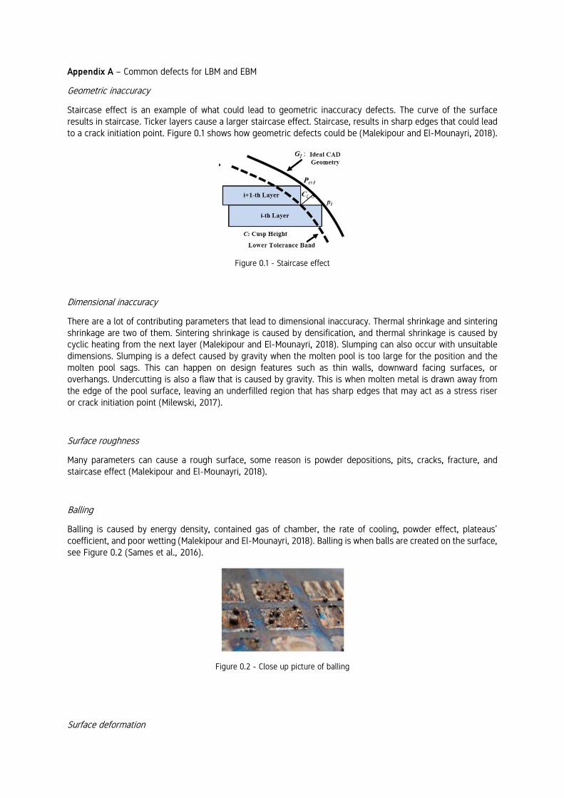
Appendix A – Common defects for LBM and EBM
Geometric inaccuracy
Staircase effect is an example of what could lead to geometric inaccuracy defects. The curve of the surface
results in staircase. Ticker layers cause a larger staircase effect. Staircase, results in sharp edges that could lead
to a crack initiation point. Figure 0.1 shows how geometric defects could be (Malekipour and El-Mounayri, 2018).
Figure 0.1 - Staircase effect
Dimensional inaccuracy
There are a lot of contributing parameters that lead to dimensional inaccuracy. Thermal shrinkage and sintering
shrinkage are two of them. Sintering shrinkage is caused by densification, and thermal shrinkage is caused by
cyclic heating from the next layer (Malekipour and El-Mounayri, 2018). Slumping can also occur with unsuitable
dimensions. Slumping is a defect caused by gravity when the molten pool is too large for the position and the
molten pool sags. This can happen on design features such as thin walls, downward facing surfaces, or
overhangs. Undercutting is also a flaw that is caused by gravity. This is when molten metal is drawn away from
the edge of the pool surface, leaving an underfilled region that has sharp edges that may act as a stress riser
or crack initiation point (Milewski, 2017).
Surface roughness
Many parameters can cause a rough surface, some reason is powder depositions, pits, cracks, fracture, and
staircase effect (Malekipour and El-Mounayri, 2018).
Balling
Balling is caused by energy density, contained gas of chamber, the rate of cooling, powder effect, plateaus’
coefficient, and poor wetting (Malekipour and El-Mounayri, 2018). Balling is when balls are created on the surface,
see Figure 0.2 (Sames et al., 2016).
Figure 0.2 - Close up picture of balling
Surface deformation

Distortion and warping are types of surface deformation caused by heat. Warping means that the form is bending,
and the result is deformed. Distortion are other types of changes, not necessarily on the form (Malekipour and
El-Mounayri, 2018).
Surface oxidation
Surface oxidation is caused by contaminated powder or printing chamber. The use of gasses such as Argon, is
used to prevent this (Malekipour and El-Mounayri, 2018).
Anisotropy and Heterogeneity
The mechanical properties of 3D printed parts are not necessarily isotropic. The tracing direction and layer
orientation affect the strength, elongation, and other mechanical properties. Moreover, this can cause defects.
The powder quality is vital for the density homogeneity (Malekipour and El-Mounayri, 2018).
Porosity (poor density)
Porosity or poor density is when not all the desired powder is melted, and it causes cavity. It can also happen
when gases such as hydrogen are being entrapped underneath the molten pool and cause a pocket with no
material. Several things cause porosity, laser power, scan speed, spot size, scan strategy, entrapped gas, and
powder size are some of them (Malekipour and El-Mounayri, 2018).
Fracture/cracks and holes
These are defects that lead to weaker mechanical properties. Caused by the design or other defects (Malekipour
and El-Mounayri, 2018).
Bonding between layers
Delamination and lack of fusion are common defects where the deposit does not fully melt into the former layers;
these are shown in Figure 0.3 (Milewski, 2017). The layer thickness is one of the reasons that this could happen.
Smaller layers will increase the re-melted substrate between the layers, which results in higher bonding
(Malekipour and El-Mounayri, 2018).
Low strength
Several defects affect the strengthening of the 3D print. Some are the powder specification, trace pattern, and
gas flow. The powder specification is directly connected to the grain size, which again is connected to the
hardness of the material.
Figure 0.3 – Defects, delamination and lack of fusion in AM (Milewski, 2017)

Appendix B – Load Scenarios for TO and FE-analysis
In this appendix, all loads are described. External load from maximum braking and lateral displacement in the
steering arrangement are the main forces and are used in the TO. Other load scenarios described in this appendix
are used in FEM-analysis and fatigue prediction.
External Load from Braking and Lateral Displacement
From Motorcycle Dynamics by Vittore Cossalter, we have eq.(8): “The maximum deceleration, expressed in g’s, is proportional to the longitudinal distance from the center of the gravity to the contact point of the front wheel and is inversely proportional to the height of the center of the gravity”(Cossalter, 2006a).
𝑚𝑎𝑥
𝑔≤ −
(𝑝 − 𝑏)
ℎ (8)
It is also necessary to take aerodynamic resistance force FD into account, to have a more conservative solution.
FD is given by eq. (9), and the equilibrium equation of the horizontal forces is given by eq. (10) where F is the
total braking force.
𝐹𝐷 =1
2𝜌𝐴𝐶𝐷𝑉2
(9)
𝑚 = −𝐹 − 𝐹𝐷 (10)
Then the maximum deceleration depends on both the mass and the velocity.
𝑚𝑎𝑥
𝑔≤ −
(𝑝 − 𝑏)
ℎ−
12
𝜌𝐴𝐶𝐷𝑉2
𝑚𝑔 (11)
Figure 0.4 - Motorcycle under braking, from Motorcycle dynamics
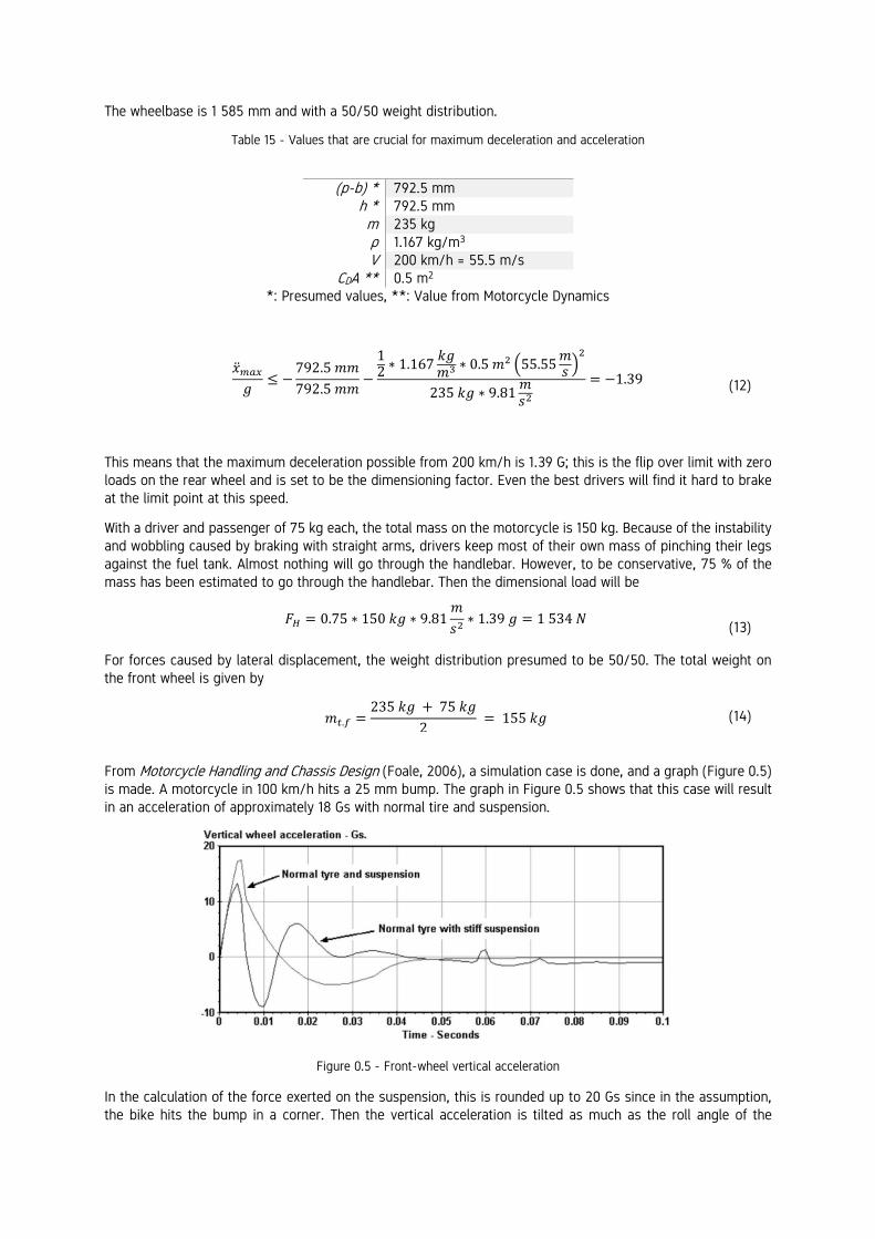
The wheelbase is 1 585 mm and with a 50/50 weight distribution.
Table 15 - Values that are crucial for maximum deceleration and acceleration
(p-b) * 792.5 mm
h * 792.5 mm
m 235 kg
ρ 1.167 kg/m3
V 200 km/h = 55.5 m/s
CDA ** 0.5 m2
*: Presumed values, **: Value from Motorcycle Dynamics
𝑚𝑎𝑥
𝑔≤ −
792.5 𝑚𝑚
792.5 𝑚𝑚−
12
∗ 1.167𝑘𝑔𝑚3 ∗ 0.5 𝑚2 (55.55
𝑚𝑠
)2
235 𝑘𝑔 ∗ 9.81𝑚𝑠2
= −1.39
(12)
This means that the maximum deceleration possible from 200 km/h is 1.39 G; this is the flip over limit with zero
loads on the rear wheel and is set to be the dimensioning factor. Even the best drivers will find it hard to brake
at the limit point at this speed.
With a driver and passenger of 75 kg each, the total mass on the motorcycle is 150 kg. Because of the instability
and wobbling caused by braking with straight arms, drivers keep most of their own mass of pinching their legs
against the fuel tank. Almost nothing will go through the handlebar. However, to be conservative, 75 % of the
mass has been estimated to go through the handlebar. Then the dimensional load will be
𝐹𝐻 = 0.75 ∗ 150 𝑘𝑔 ∗ 9.81
𝑚
𝑠2∗ 1.39 𝑔 = 1 534 𝑁
(13)
For forces caused by lateral displacement, the weight distribution presumed to be 50/50. The total weight on
the front wheel is given by
𝑚𝑡.𝑓 =235 𝑘𝑔 + 75 𝑘𝑔
2 = 155 𝑘𝑔 (14)
From Motorcycle Handling and Chassis Design (Foale, 2006), a simulation case is done, and a graph (Figure 0.5)
is made. A motorcycle in 100 km/h hits a 25 mm bump. The graph in Figure 0.5 shows that this case will result
in an acceleration of approximately 18 Gs with normal tire and suspension.
Figure 0.5 - Front-wheel vertical acceleration
In the calculation of the force exerted on the suspension, this is rounded up to 20 Gs since in the assumption,
the bike hits the bump in a corner. Then the vertical acceleration is tilted as much as the roll angle of the
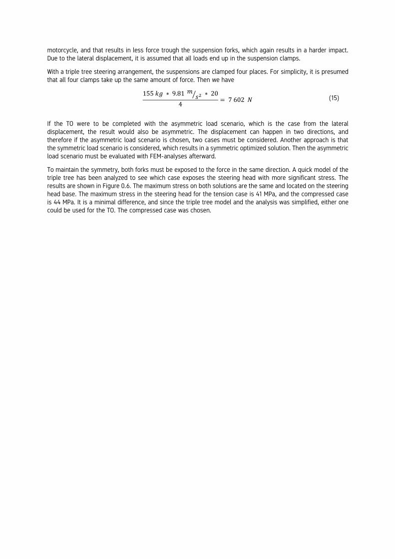
motorcycle, and that results in less force trough the suspension forks, which again results in a harder impact.
Due to the lateral displacement, it is assumed that all loads end up in the suspension clamps.
With a triple tree steering arrangement, the suspensions are clamped four places. For simplicity, it is presumed
that all four clamps take up the same amount of force. Then we have
155 𝑘𝑔 ∗ 9.81 𝑚
𝑠2⁄ ∗ 20
4= 7 602 𝑁 (15)
If the TO were to be completed with the asymmetric load scenario, which is the case from the lateral
displacement, the result would also be asymmetric. The displacement can happen in two directions, and
therefore if the asymmetric load scenario is chosen, two cases must be considered. Another approach is that
the symmetric load scenario is considered, which results in a symmetric optimized solution. Then the asymmetric
load scenario must be evaluated with FEM-analyses afterward.
To maintain the symmetry, both forks must be exposed to the force in the same direction. A quick model of the
triple tree has been analyzed to see which case exposes the steering head with more significant stress. The
results are shown in Figure 0.6. The maximum stress on both solutions are the same and located on the steering
head base. The maximum stress in the steering head for the tension case is 41 MPa, and the compressed case
is 44 MPa. It is a minimal difference, and since the triple tree model and the analysis was simplified, either one
could be used for the TO. The compressed case was chosen.

Figure 0.6 - Triple tree simulation
External Load from Acceleration
Wheeling-limited acceleration is achieved when the load on the front wheel Nf is equal to zero. See eq.(16) and
Figure 0.7.
𝑁𝑓 = 𝑔 ∗ 𝑚 ∗ 𝑏
𝑝 − 𝑆 ∗
ℎ
𝑝 = 0 (16)
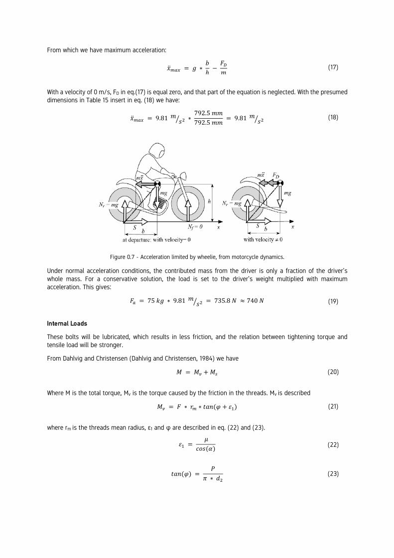
From which we have maximum acceleration:
𝑚𝑎𝑥 = 𝑔 ∗ 𝑏
ℎ −
𝐹𝐷
𝑚 (17)
With a velocity of 0 m/s, FD in eq.(17) is equal zero, and that part of the equation is neglected. With the presumed
dimensions in Table 15 insert in eq. (18) we have:
𝑚𝑎𝑥 = 9.81 𝑚𝑠2⁄ ∗
792.5 𝑚𝑚
792.5 𝑚𝑚 = 9.81 𝑚
𝑠2⁄ (18)
Figure 0.7 - Acceleration limited by wheelie, from motorcycle dynamics.
Under normal acceleration conditions, the contributed mass from the driver is only a fraction of the driver’s
whole mass. For a conservative solution, the load is set to the driver’s weight multiplied with maximum
acceleration. This gives:
𝐹𝑎 = 75 𝑘𝑔 ∗ 9.81 𝑚𝑠2⁄ = 735.8 𝑁 ≈ 740 𝑁 (19)
Internal Loads
These bolts will be lubricated, which results in less friction, and the relation between tightening torque and
tensile load will be stronger.
From Dahlvig and Christensen (Dahlvig and Christensen, 1984) we have
𝑀 = 𝑀𝑣 + 𝑀𝑠 (20)
Where M is the total torque, Mv is the torque caused by the friction in the threads. Mv is described
𝑀𝑣 = 𝐹 ∗ 𝑟𝑚 ∗ 𝑡𝑎𝑛(𝜑 + 𝜀1) (21)
where rm is the threads mean radius, ε1 and φ are described in eq. (22) and (23).
𝜀1 = 𝜇
𝑐𝑜𝑠(𝛼) (22)
𝑡𝑎𝑛(𝜑) = 𝑃
𝜋 ∗ 𝑑2
(23)
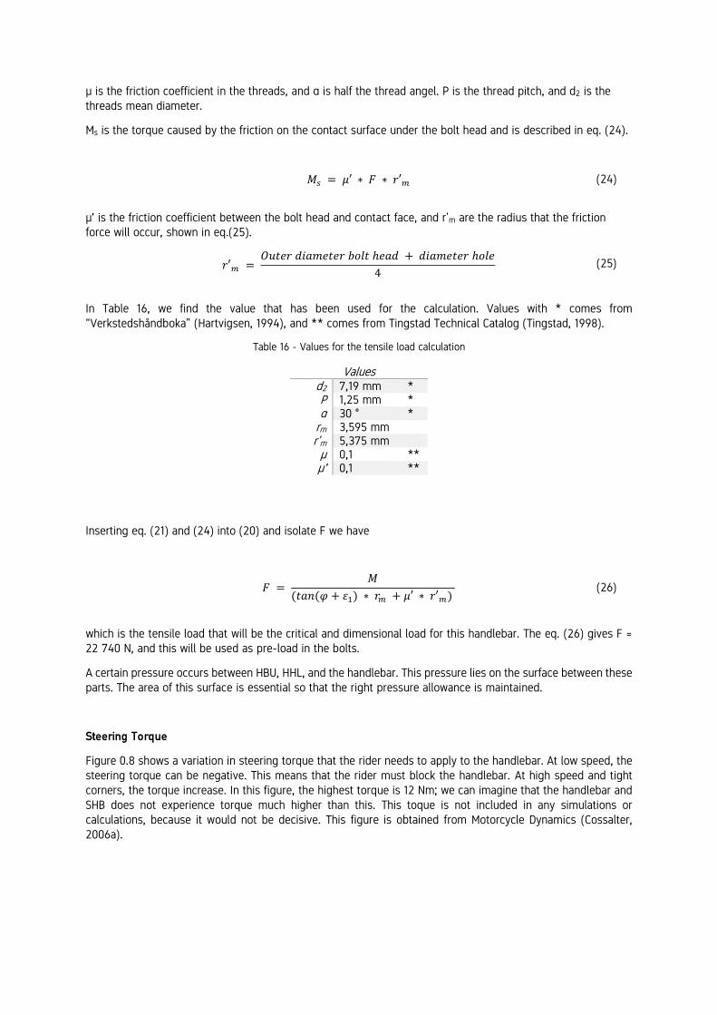
μ is the friction coefficient in the threads, and α is half the thread angel. P is the thread pitch, and d2 is the
threads mean diameter.
Ms is the torque caused by the friction on the contact surface under the bolt head and is described in eq. (24).
𝑀𝑠 = 𝜇′ ∗ 𝐹 ∗ 𝑟′𝑚 (24)
μ' is the friction coefficient between the bolt head and contact face, and r’m are the radius that the friction
force will occur, shown in eq.(25).
𝑟′𝑚 = 𝑂𝑢𝑡𝑒𝑟 𝑑𝑖𝑎𝑚𝑒𝑡𝑒𝑟 𝑏𝑜𝑙𝑡 ℎ𝑒𝑎𝑑 + 𝑑𝑖𝑎𝑚𝑒𝑡𝑒𝑟 ℎ𝑜𝑙𝑒
4 (25)
In Table 16, we find the value that has been used for the calculation. Values with * comes from
“Verkstedshåndboka” (Hartvigsen, 1994), and ** comes from Tingstad Technical Catalog (Tingstad, 1998).
Table 16 - Values for the tensile load calculation
Values d2 7,19 mm * P 1,25 mm * α 30 ° *
rm 3,595 mm r’m 5,375 mm
μ 0,1 ** μ' 0,1 **
Inserting eq. (21) and (24) into (20) and isolate F we have
𝐹 = 𝑀
(𝑡𝑎𝑛(𝜑 + 𝜀1) ∗ 𝑟𝑚 + 𝜇′ ∗ 𝑟′𝑚) (26)
which is the tensile load that will be the critical and dimensional load for this handlebar. The eq. (26) gives F =
22 740 N, and this will be used as pre-load in the bolts.
A certain pressure occurs between HBU, HHL, and the handlebar. This pressure lies on the surface between these
parts. The area of this surface is essential so that the right pressure allowance is maintained.
Steering Torque
Figure 0.8 shows a variation in steering torque that the rider needs to apply to the handlebar. At low speed, the
steering torque can be negative. This means that the rider must block the handlebar. At high speed and tight
corners, the torque increase. In this figure, the highest torque is 12 Nm; we can imagine that the handlebar and
SHB does not experience torque much higher than this. This toque is not included in any simulations or
calculations, because it would not be decisive. This figure is obtained from Motorcycle Dynamics (Cossalter,
2006a).
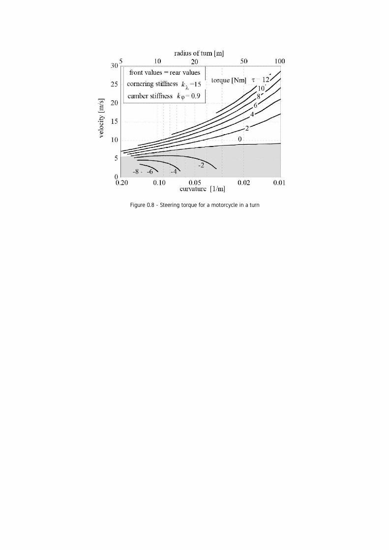
Figure 0.8 - Steering torque for a motorcycle in a turn
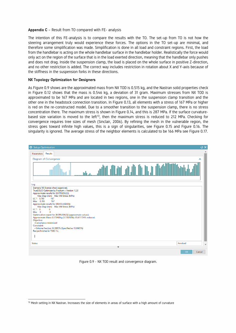
Appendix C – Result from TO compared with FE- analysis
The intention of this FE-analysis is to compare the results with the TO. The set-up from TO is not how the
steering arrangement truly would experience these forces. The options in the TO set-up are minimal, and
therefore some simplification was made. Simplification is done in all load and constraint regions. First, the load
from the handlebar is acting on the whole handlebar surface in the handlebar holder. Realistically the force would
only act on the region of the surface that is in the load exerted direction, meaning that the handlebar only pushes
and does not drag. Inside the suspension clamp, the load is placed on the whole surface in positive Z-direction,
and no other restriction is added. The correct way includes restriction in rotation about X and Y-axis because of
the stiffness in the suspension forks in these directions.
NX Topology Optimization for Designers
As Figure 0.9 shows are the approximated mass from NX TOD is 0.515 kg, and the Nastran solid properties check
in Figure 0.12 shows that the mass is 0.546 kg, a deviation of 31 gram. Maximum stresses from NX TOD is
approximated to be 167 MPa and are located in two regions, one in the suspension clamp transition and the
other one in the headstock connection transition. In Figure 0.13, all elements with a stress of 167 MPa or higher
is red on the re-constructed model. Due to a smoother transition to the suspension clamp, there is no stress
concentration there. The maximum stress is shown in Figure 0.14, and this is 287 MPa. If the surface curvature-
based size variation is moved to the left13, then the maximum stress is reduced to 212 MPa. Checking for
convergence requires tree sizes of mesh (Sinclair, 2006). By refining the mesh in the vulnerable region, the
stress goes toward infinite high values, this is a sign of singularities, see Figure 0.15 and Figure 0.16. The
singularity is ignored. The average stress of the neighbor elements is calculated to be 166 MPa see Figure 0.17.
Figure 0.9 - NX TOD result and convergence diagram.
13 Mesh setting in NX Nastran. Increases the size of elements in areas of surface with a high amount of curvature
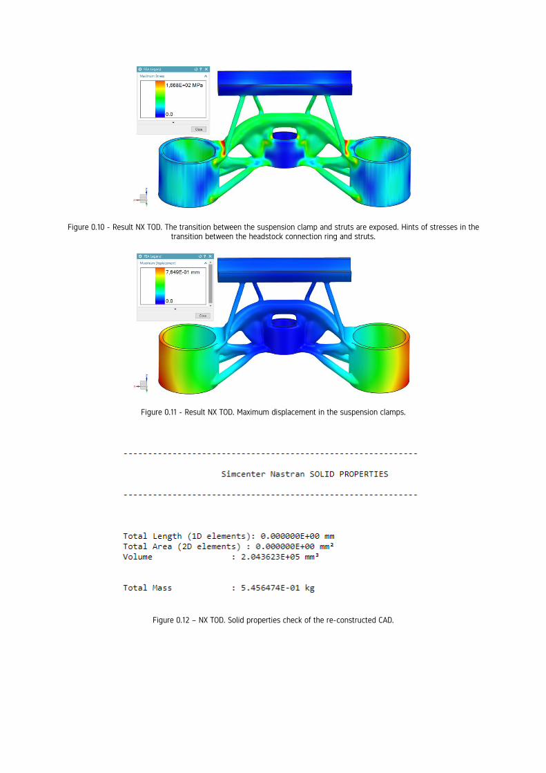
Figure 0.10 - Result NX TOD. The transition between the suspension clamp and struts are exposed. Hints of stresses in the transition between the headstock connection ring and struts.
Figure 0.11 - Result NX TOD. Maximum displacement in the suspension clamps.
Figure 0.12 – NX TOD. Solid properties check of the re-constructed CAD.
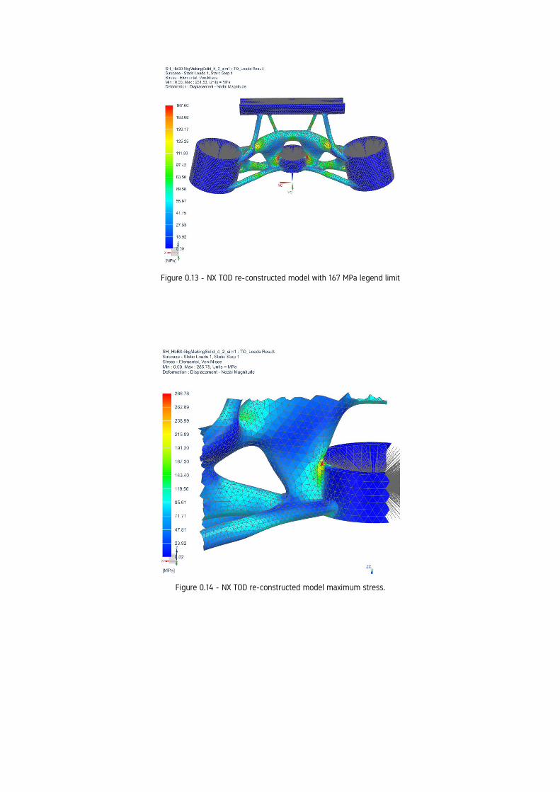
Figure 0.13 - NX TOD re-constructed model with 167 MPa legend limit
Figure 0.14 - NX TOD re-constructed model maximum stress.
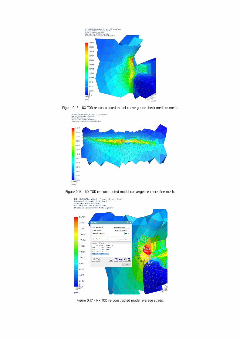
Figure 0.15 - NX TOD re-constructed model convergence check medium mesh.
Figure 0.16 - NX TOD re-constructed model convergence check fine mesh.
Figure 0.17 - NX TOD re-constructed model average stress.
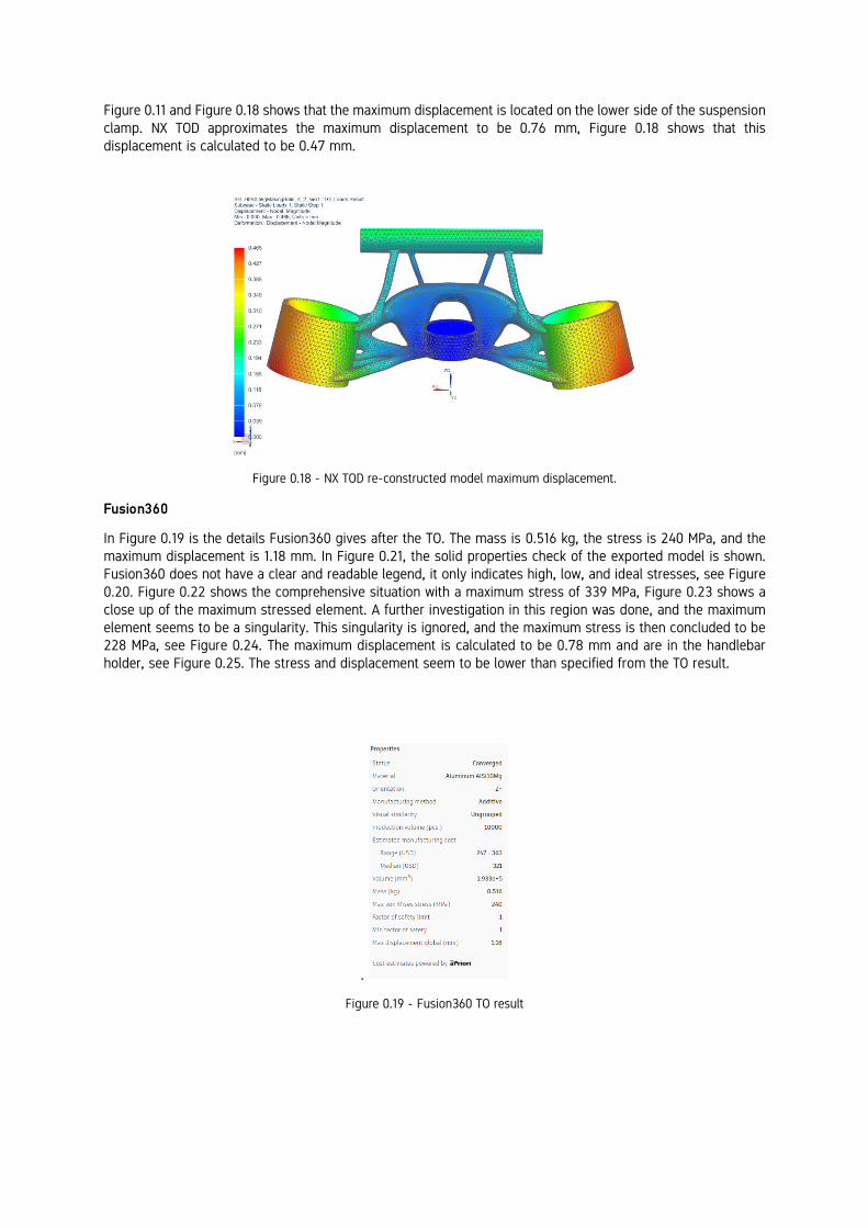
Figure 0.11 and Figure 0.18 shows that the maximum displacement is located on the lower side of the suspension
clamp. NX TOD approximates the maximum displacement to be 0.76 mm, Figure 0.18 shows that this
displacement is calculated to be 0.47 mm.
Figure 0.18 - NX TOD re-constructed model maximum displacement.
Fusion360
In Figure 0.19 is the details Fusion360 gives after the TO. The mass is 0.516 kg, the stress is 240 MPa, and the
maximum displacement is 1.18 mm. In Figure 0.21, the solid properties check of the exported model is shown.
Fusion360 does not have a clear and readable legend, it only indicates high, low, and ideal stresses, see Figure
0.20. Figure 0.22 shows the comprehensive situation with a maximum stress of 339 MPa, Figure 0.23 shows a
close up of the maximum stressed element. A further investigation in this region was done, and the maximum
element seems to be a singularity. This singularity is ignored, and the maximum stress is then concluded to be
228 MPa, see Figure 0.24. The maximum displacement is calculated to be 0.78 mm and are in the handlebar
holder, see Figure 0.25. The stress and displacement seem to be lower than specified from the TO result.
.
Figure 0.19 - Fusion360 TO result
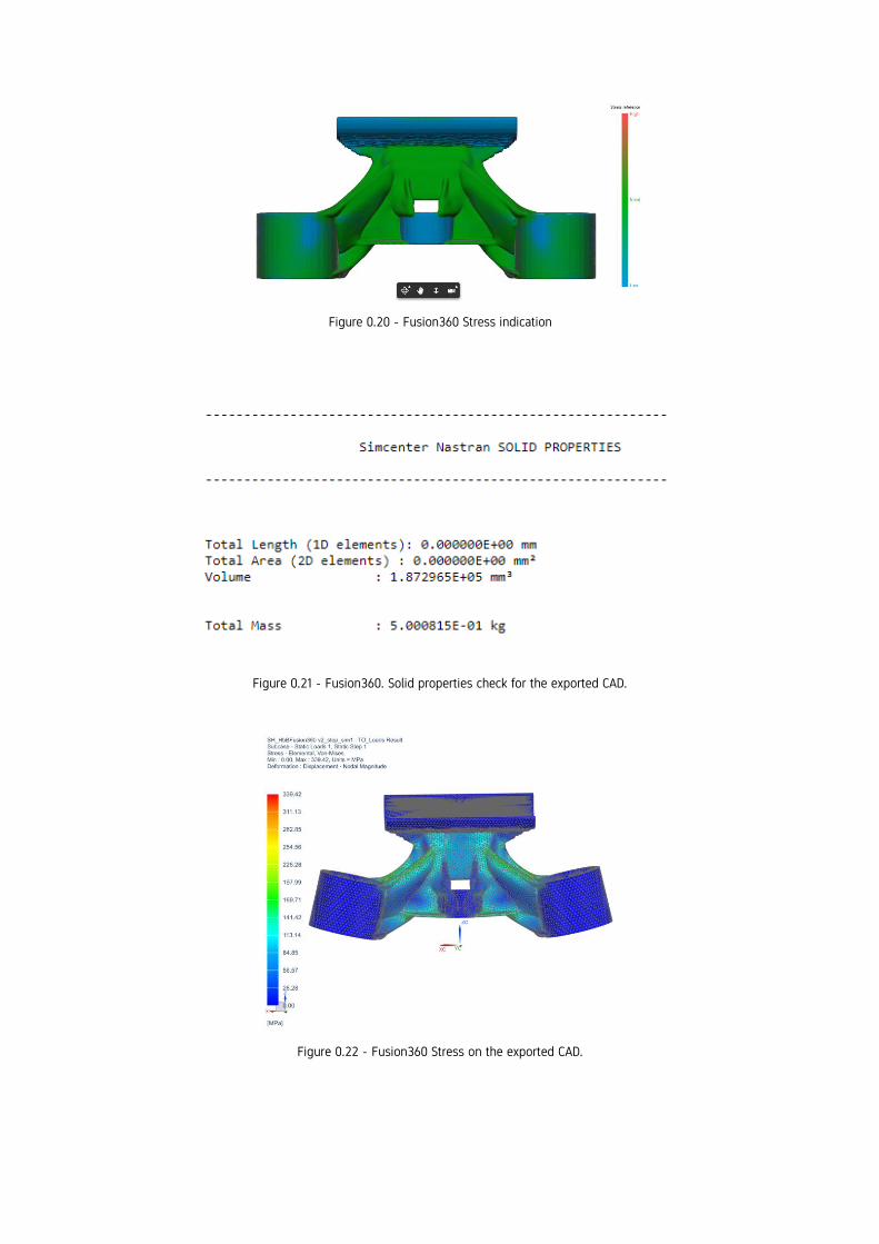
Figure 0.20 - Fusion360 Stress indication
Figure 0.21 - Fusion360. Solid properties check for the exported CAD.
Figure 0.22 - Fusion360 Stress on the exported CAD.
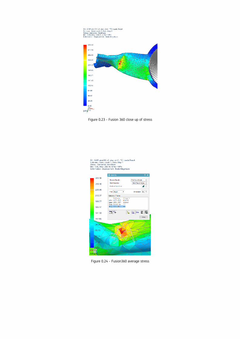
Figure 0.23 - Fusion 360 close up of stress
Figure 0.24 - Fusion360 average stress
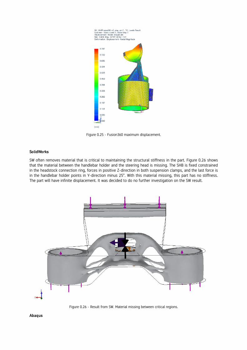
Figure 0.25 - Fusion360 maximum displacement.
SolidWorks
SW often removes material that is critical to maintaining the structural stiffness in the part. Figure 0.26 shows
that the material between the handlebar holder and the steering head is missing. The SHB is fixed constrained
in the headstock connection ring, forces in positive Z-direction in both suspension clamps, and the last force is
in the handlebar holder points in Y-direction minus 25°. With this material missing, this part has no stiffness.
The part will have infinite displacement. It was decided to do no further investigation on the SW result.
Figure 0.26 - Result from SW. Material missing between critical regions.
Abaqus
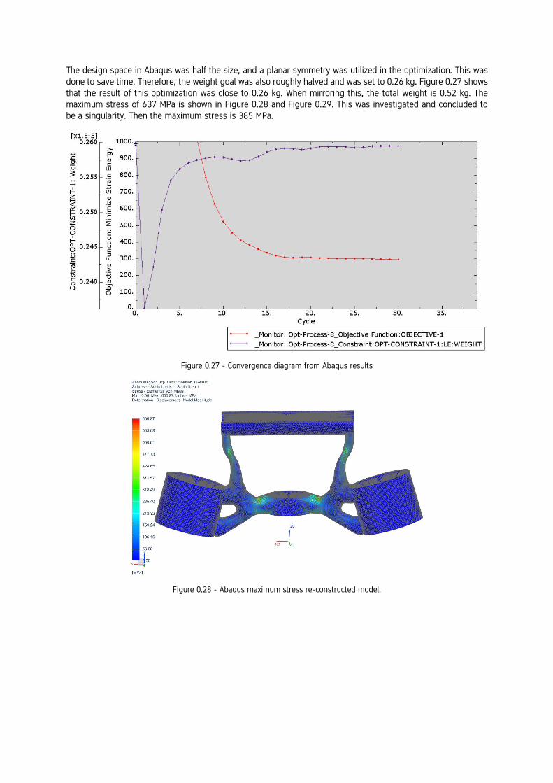
The design space in Abaqus was half the size, and a planar symmetry was utilized in the optimization. This was
done to save time. Therefore, the weight goal was also roughly halved and was set to 0.26 kg. Figure 0.27 shows
that the result of this optimization was close to 0.26 kg. When mirroring this, the total weight is 0.52 kg. The
maximum stress of 637 MPa is shown in Figure 0.28 and Figure 0.29. This was investigated and concluded to
be a singularity. Then the maximum stress is 385 MPa.
Figure 0.27 - Convergence diagram from Abaqus results
Figure 0.28 - Abaqus maximum stress re-constructed model.
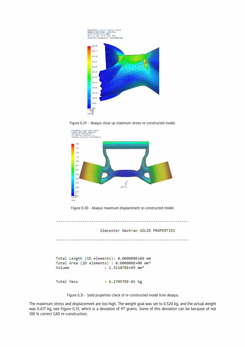
Figure 0.29 - Abaqus close up maximum stress re-constructed model.
Figure 0.30 - Abaqus maximum displacement re-constructed model.
Figure 0.31 - Solid properties check of re-constructed model from Abaqus
The maximum stress and displacement are too high. The weight goal was set to 0.520 kg, and the actual weight
was 0.617 kg, see Figure 0.31, which is a deviation of 97 grams. Some of this deviation can be because of not
100 % correct CAD re-construction.

Short Summary
NX TOD gives reliable results from the TO. There is some small deviation in the maximum displacement. The
deviation in weight is 31 grams. This difference can be a result of not 100 % correct re-build of the STL.
Fusion360 TO result does not indicate where the maximum displacement is located. It is rather difficult to see
where the maximum stress is located as well. The maximum stress from the re-constructed model is close to
the yield strength of the material. The weight deviation from TO result to NX solid properties check is 16 grams.
This can be a result of the split and mirror operation of the exported solid.
SolidWorks was not investigated due to poor TO results.
For Abaqus, the stress was above the yield strength of the material.
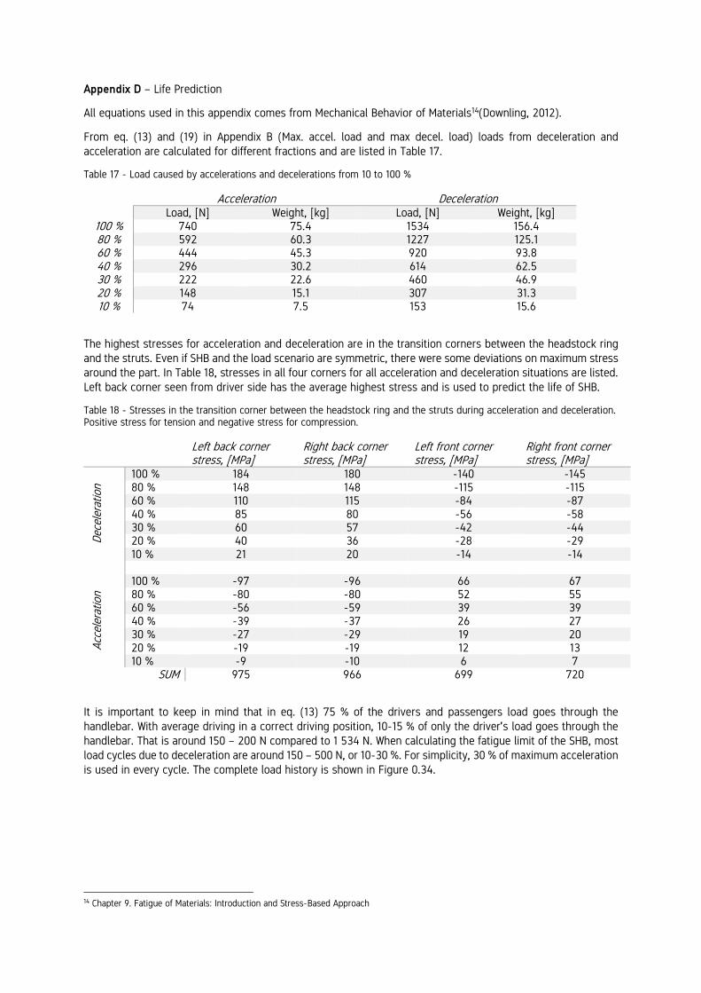
Appendix D – Life Prediction
All equations used in this appendix comes from Mechanical Behavior of Materials14(Downling, 2012).
From eq. (13) and (19) in Appendix B (Max. accel. load and max decel. load) loads from deceleration and
acceleration are calculated for different fractions and are listed in Table 17.
Table 17 - Load caused by accelerations and decelerations from 10 to 100 %
Acceleration Deceleration Load, [N] Weight, [kg] Load, [N] Weight, [kg]
100 % 740 75.4 1534 156.4 80 % 592 60.3 1227 125.1 60 % 444 45.3 920 93.8 40 % 296 30.2 614 62.5 30 % 222 22.6 460 46.9 20 % 148 15.1 307 31.3 10 % 74 7.5 153 15.6
The highest stresses for acceleration and deceleration are in the transition corners between the headstock ring
and the struts. Even if SHB and the load scenario are symmetric, there were some deviations on maximum stress
around the part. In Table 18, stresses in all four corners for all acceleration and deceleration situations are listed.
Left back corner seen from driver side has the average highest stress and is used to predict the life of SHB.
Table 18 - Stresses in the transition corner between the headstock ring and the struts during acceleration and deceleration. Positive stress for tension and negative stress for compression.
Left back corner stress, [MPa]
Right back corner stress, [MPa]
Left front corner stress, [MPa]
Right front corner stress, [MPa]
Dec
eler
atio
n
100 % 184 180 -140 -145 80 % 148 148 -115 -115 60 % 110 115 -84 -87 40 % 85 80 -56 -58 30 % 60 57 -42 -44 20 % 40 36 -28 -29 10 % 21 20 -14 -14
Acc
eler
atio
n
100 % -97 -96 66 67 80 % -80 -80 52 55 60 % -56 -59 39 39 40 % -39 -37 26 27 30 % -27 -29 19 20 20 % -19 -19 12 13 10 % -9 -10 6 7
SUM 975 966 699 720
It is important to keep in mind that in eq. (13) 75 % of the drivers and passengers load goes through the
handlebar. With average driving in a correct driving position, 10-15 % of only the driver's load goes through the
handlebar. That is around 150 – 200 N compared to 1 534 N. When calculating the fatigue limit of the SHB, most
load cycles due to deceleration are around 150 – 500 N, or 10-30 %. For simplicity, 30 % of maximum acceleration
is used in every cycle. The complete load history is shown in Figure 0.34.
14 Chapter 9. Fatigue of Materials: Introduction and Stress-Based Approach
Figure 0.32 - S-N curve for AlSi10Mg printed with EOSINT M-280.
S-N curve is obtained from a Science Direct article (Uzan et al., 2017). A Moor rotating beam machine was used
which means that the σm = 0, this gives:
𝜎𝑚𝑎𝑥 = 𝜎𝑚 + 𝜎𝑎 ⇒ 𝜎𝑚𝑎𝑥 = 𝜎𝑎 (27)
In Table 19, values from the diamond (orange) S-N curve in Figure 0.32 are listed, and in Figure 0.32, these are
plotted on a log-log scale. The four first point seems to lay in a straight line and the most conservative one.
Point 1 and 4 represents this line well and are used to calculate constant A and B from eq.(28).
Table 19 - Values from S-N curve
σa – [MPa] Nf - Cycles 1 250 2500 2 194 7000 3 150 25000 4 100 175000 5 80 3000000

Figure 0.33 - S-N curve in log-log plot
𝜎1 = 𝐴𝑁1
𝐵 , 𝜎2 = 𝐴𝑁2𝐵
(28)
By dividing the second equation on the first and take logarithms of both sides, then solving for B, we have
eq.(29).
𝐵 = 𝑙𝑜𝑔𝜎1 − 𝑙𝑜𝑔𝜎2
𝑙𝑜𝑔𝑁1 − 𝑙𝑜𝑔𝑁2 =
𝑙𝑜𝑔(250) − 𝑙𝑜𝑔(100)
𝑙𝑜𝑔(2500) − 𝑙𝑜𝑔(175000) = −0.2157 (29)
Now A is solved from eq.(28)
𝐴 = 𝜎1
𝑁1𝐵 =
250 𝑀𝑃𝑎
2500−0.2157 = 1351.7 𝑀𝑃𝑎 (30)
B is equal to b, and then from eq.(31) we have eq.(32)
𝜎𝑎 = 𝜎′𝑓 (2𝑁𝑓)𝑏 (31)
𝐴 = 2𝑏𝜎′𝑓 ⇒ 𝜎′𝑓 = 𝐴
2𝑏 =
1351.7 𝑀𝑃𝑎
2−0.2157 = 1569.7 𝑀𝑃𝑎 (32)
Smith, Watson, and Topper (SWT) equation is a good fit for aluminum alloys (Downling, 2012), and by solving
that for Nf, and substitute σmax with σm + σa we have
10
100
1000
1000 10000 100000 1000000 10000000
σa
-M
Pa
Nf - Cycles
S-N curve in Log -Log plot
𝑁𝑓 = 1
2(
𝜎𝑚 + 𝜎𝑎
𝜎′𝑓√
1 − 𝑅
2)
1𝑏
(33)
Figure 0.34 - A presumed stress history per 10 km.
Use Table 20 as an overview of the stresses and cycles.
Table 20 – Summary table of required values for Palmgren-Miner rule
j Nj σmin σmax σa σm Nfj Nj / Nfj
100 % 0,002 -27 184 105,5 78,5 10.355 1,9E-07
80 % 0,01 -27 148 87,5 60,5 28.413 3,5E-07
60 % 0,1 -27 110 68,5 41,5 112.450 8,9E-07
40 % 2 -27 85 56 29 371.601 5,4E-06
30 % 4 -27 60 43,5 16,5 1.867.945 2,1E-06
20 % 6 -27 40 33,5 6,5 12.238.699 4,9E-07
10 % 10 -27 21 24 -3 242.714.619 4,1E-08
Σ = 9,5E-06
By solving the repetitions to failure from eq.(7)(Palmgren-Miner rule) we have
𝐵𝑓 =
1
∑ (𝑁𝑗
𝑁𝑓𝑗)
= 1
9,5𝐸 − 06= 105.263
(34)
This limit is for 10 km, which means that the fatigue limit for SHB is 1.052.630 km.
-40
-20
0
20
40
60
80
100
σ ,
Stre
ss M
Pa
Time
Deceleration and Acceleration in Stress per 10 km

Appendix E - FE-analysis on OEM part
The same load scenarios as in FEM verification (chapter 4.2) on the SHB are used on OEM parts, except FEA-2.
Note: The global coordinate system does not follow the part, it follows the motorcycle. This means that the
coordinate system is rotated the rake angle of 25° about the Y-axis. That means that X-direction points in the
driving direction.
The material used in both parts is Al 6061-T6.
OEM FEA-1 - Maximum deceleration and bumps
CTETRA(10) elements with a size of 2 mm have been used on the steering head and HHL. In each suspension
clamp, an RBE2 element is placed, the surface follows the master node. Such an element is also placed in the
center of the handlebar holder and in the center of the headstock connection hole. For simplicity, there has not
been established a bolted connection between these parts. Between the two parts, four RBE2 elements have
been utilized (Yellow in Figure 0.35). Two on each connection point. Two RBE2 elements for HHL and two for
the steering head. Between one HHL RBE2 element and one steering head RBE2 element, it has been
established a third element. This simulates that there is no gap between these two parts. The gap will then be
infinite stiff. Realistically the stiffness would have been the same as the in pipe, but this approach is close
enough.
In Figure 0.35, the set-up of the OEM FEA-1 is illustrated. The load of 1 534 N on the HHL caused by maximum
deceleration points in X-direction. In the left suspension clamp, the bump load of 7 602 N points in the
positive Z-direction and the same load points in negative Z-directing for the right one. The RBE2 element in
the headstock connection hole is fully fixed. The RBE2 elements in the suspension clamps are restricted to
rotate about the X and Y -axis due to the stiffness in the suspension fork would not allow it.
Figure 0.35 - OEM FEA-1 set-up
Result OEM FEA-1
Maximum stress is 603 MPa in one single element in an inside corner. The neighbor elements have an average
stress of around 400 MPa. The maximum displacement was 1.3 mm in the suspension clamp. The stress result
is shown in Figure 0.36 and displacement in Figure 0.37.
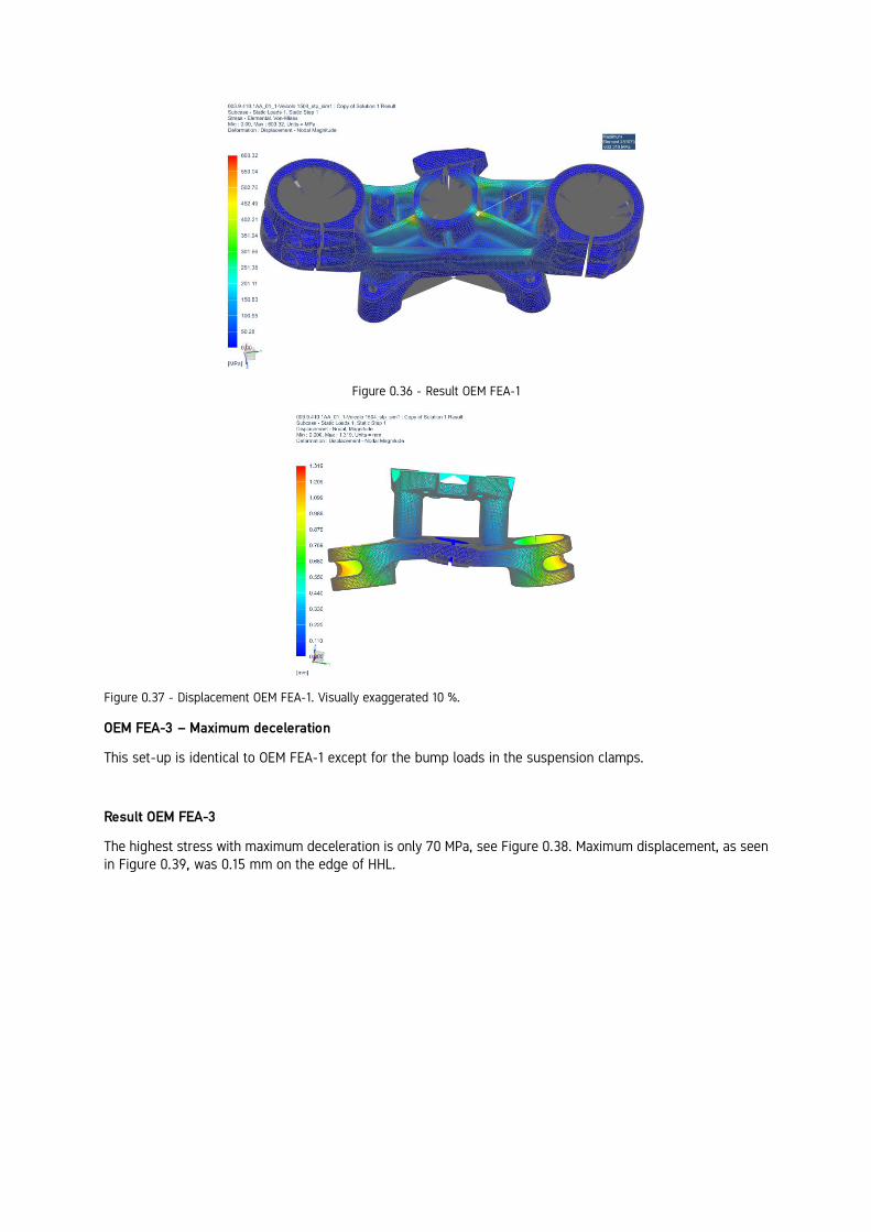
Figure 0.36 - Result OEM FEA-1
Figure 0.37 - Displacement OEM FEA-1. Visually exaggerated 10 %.
OEM FEA-3 – Maximum deceleration
This set-up is identical to OEM FEA-1 except for the bump loads in the suspension clamps.
Result OEM FEA-3
The highest stress with maximum deceleration is only 70 MPa, see Figure 0.38. Maximum displacement, as seen
in Figure 0.39, was 0.15 mm on the edge of HHL.
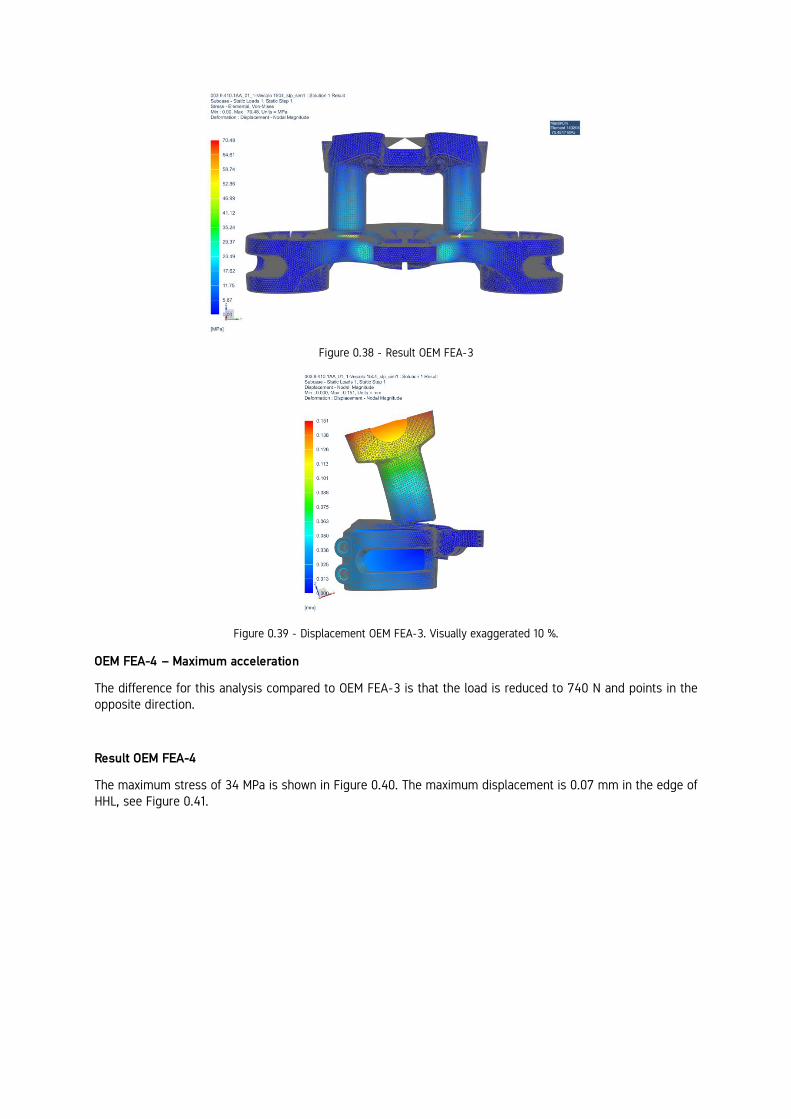
Figure 0.38 - Result OEM FEA-3
Figure 0.39 - Displacement OEM FEA-3. Visually exaggerated 10 %.
OEM FEA-4 – Maximum acceleration
The difference for this analysis compared to OEM FEA-3 is that the load is reduced to 740 N and points in the
opposite direction.
Result OEM FEA-4
The maximum stress of 34 MPa is shown in Figure 0.40. The maximum displacement is 0.07 mm in the edge of
HHL, see Figure 0.41.
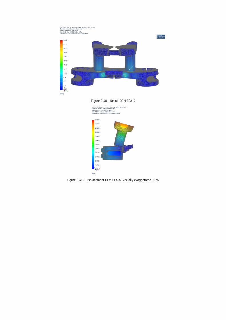
Figure 0.40 - Result OEM FEA-4
Figure 0.41 - Displacement OEM FEA-4. Visually exaggerated 10 %.

Appendix F - Material Datasheet for AlSi10Mg and Al 6061-T6
Material data sheet
EOS GmbH - Electro Optical Systems
Robert-Stirling-Ring 1 D-82152 Krailling / München
Telephone: +49 (0)89 / 893 36-0 Aluminium AlSi10Mg Telefax: +49 (0)89 / 893 36-285 AD, WEIL / 05.2014 1 / 5 Internet: www.eos.info
EOS Aluminium AlSi10Mg
EOS Aluminium AlSi10Mg is an aluminium alloy in fine powder form which has been specially optimised for processing on EOSINT M systems
This document provides information and data for parts built using EOS Aluminium AlSi10Mg powder (EOS art.-no. 9011-0024) on the following system specifications:
- EOSINT M 280 with PSW 3.6 and Original EOS Parameterset AlSi10Mg_Speed 1.0
- EOS M 290 400Watt with EOSPRINT 1.0 and Original EOS Parameterset AlSi10Mg_Speed 1.0
Description
AlSi10Mg is a typical casting alloy with good casting properties and is typically used for cast parts with thin walls and complex geometry. It offers good strength, hardness and dynamic properties and is therefore also used for parts subject to high loads. Parts in EOS Aluminium AlSi10Mg are ideal for applications which require a combination of good thermal properties and low weight. They can be machined, spark-eroded, welded, micro shot-peened, polished and coated if required.
Conventionally cast components in this type of aluminium alloy are often heat treated to im-prove the mechanical properties, for example using the T6 cycle of solution annealing, quenching and age hardening. The laser-sintering process is characterized by extremely rapid melting and re-solidification . This produces a metallurgy and corresponding mechanical proper-ties in the as-built condition which is similar to T6 heat-treated cast parts. Therefore such hardening heat treatments are not recommended for laser-sintered parts, but rather a stress re-lieving cycle of 2 hours at 300 °C (572 °F). Due to the layerwise building method, the parts have a certain anisotropy, which can be reduced or removed by appropriate heat treatment - see Technical Data for examples.
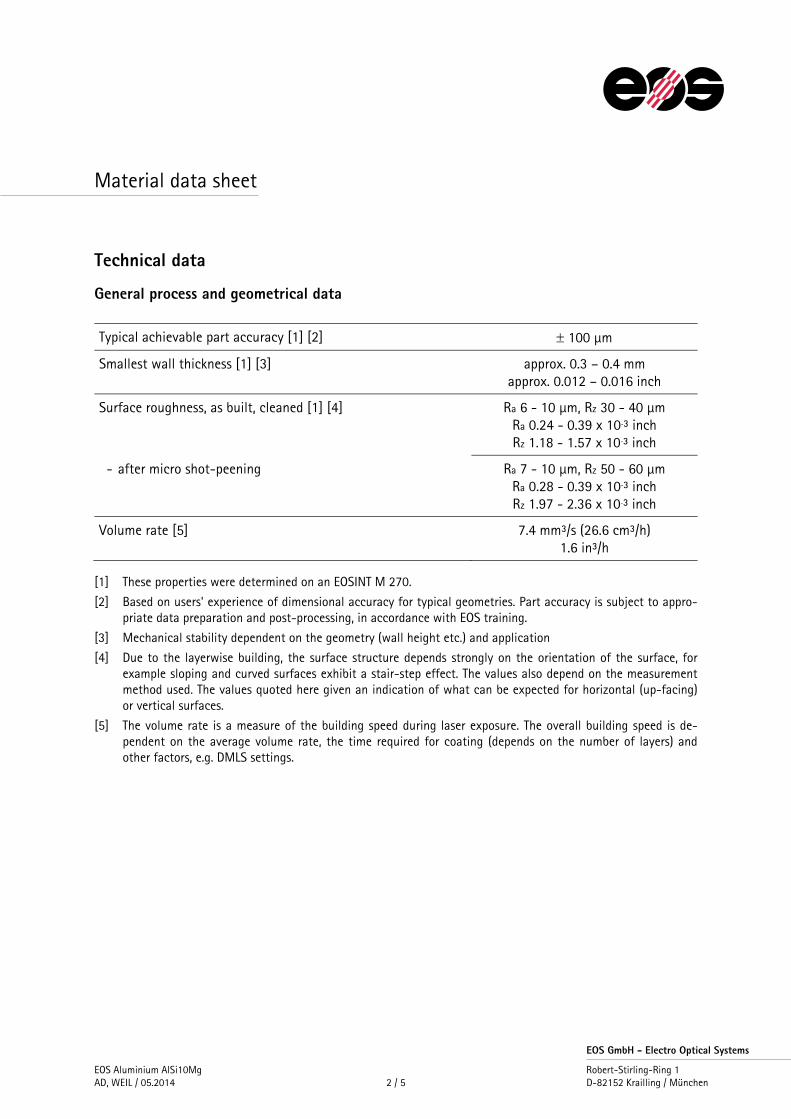
Material data sheet
EOS GmbH - Electro Optical Systems
EOS Aluminium AlSi10Mg Robert-Stirling-Ring 1 AD, WEIL / 05.2014 2 / 5 D-82152 Krailling / München
Technical data
General process and geometrical data
Typical achievable part accuracy [1] [2] 100 µm
Smallest wall thickness [1] [3] approx. 0.3 – 0.4 mm approx. 0.012 – 0.016 inch
Surface roughness, as built, cleaned [1] [4] Ra 6 - 10 µm, Rz 30 - 40 µm Ra 0.24 - 0.39 x 10-³ inch Rz 1.18 - 1.57 x 10-³ inch
- after micro shot-peening Ra 7 - 10 µm, Rz 50 - 60 µm Ra 0.28 - 0.39 x 10-³ inch Rz 1.97 - 2.36 x 10-³ inch
Volume rate [5] 7.4 mm³/s (26.6 cm³/h) 1.6 in³/h
[1] These properties were determined on an EOSINT M 270.
[2] Based on users' experience of dimensional accuracy for typical geometries. Part accuracy is subject to appro-priate data preparation and post-processing, in accordance with EOS training.
[3] Mechanical stability dependent on the geometry (wall height etc.) and application
[4] Due to the layerwise building, the surface structure depends strongly on the orientation of the surface, for example sloping and curved surfaces exhibit a stair-step effect. The values also depend on the measurement method used. The values quoted here given an indication of what can be expected for horizontal (up-facing) or vertical surfaces.
[5] The volume rate is a measure of the building speed during laser exposure. The overall building speed is de-pendent on the average volume rate, the time required for coating (depends on the number of layers) and other factors, e.g. DMLS settings.

Material data sheet
EOS GmbH - Electro Optical Systems
EOS Aluminium AlSi10Mg Robert-Stirling-Ring 1 AD, WEIL / 05.2014 3 / 5 D-82152 Krailling / München
Physical and chemical properties of the parts
Material composition
Al (balance) Si (9.0 - 11.0 wt-%)
Fe ( 0.55 wt-%) Cu ( 0.05 wt-%) Mn ( 0.45 wt-%)
Mg (0.2 - 0.45 wt-%) Ni ( 0.05 wt-%) Zn ( 0.10 wt-%) Pb ( 0.05 wt-%) Sn (. 0.05 wt-%) Ti ( 0.15 wt-%)
Relative density approx. 99.85 %
Density 2.67 g/cm³ 0.096 lb/in³

Material data sheet
EOS GmbH - Electro Optical Systems
EOS Aluminium AlSi10Mg Robert-Stirling-Ring 1 AD, WEIL / 05.2014 4 / 5 D-82152 Krailling / München
Mechanical properties of the parts
As built Heat treated [9]
Tensile strength [6]
- in horizontal direction (XY) 460 20 MPa 66.7 2.9 ksi
345 10 MPA 50.0 1.5 ksi
- in vertical direction (Z) 460 20 MPa 66.7 2.9 ksi
350 10 MPa 50.8 1.5 ksi
Yield strength (Rp 0.2 %) [6]
- in horizontal direction (XY) 270 10 MPa 39.2 1.5 ksi
230 15 MPa 33.4 2.2 ksi
- in vertical direction (Z) 240 10 MPa 34.8 1.5 ksi
230 15 MPa 33.4 2.2 ksi
Modulus of elasticity
- in horizontal direction (XY) 75 10 GPa 10.9 0.7 Msi
70 10 GPa 10.2 0.7 Msi
- in vertical direction (Z) 70 10 GPa 10.2 0.7 Msi
60 10 GPa 8.7 0.7 Msi
Elongation at break [6]
- in horizontal direction (XY) (9 2) % 12 2%
- in vertical direction (Z) (6 2) % 11 2%
Hardness [7] approx.119 5 HBW
Fatigue strength [1] [8]
- in vertical direction (Z) approx. 97 7 MPa approx. 14.1 1.0 ksi
[6] Mechanical strength tested as per ISO 6892-1:2009 (B) annex D, proportional specimens, specimen diameter
5 mm, original gauge length 25 mm (1 inch).
[7] Hardness test in accordance with Brinell (HBW 2.5/62.5) as per DIN EN ISO 6506-1. Note that measured hard-ness can vary significantly depending on how the specimen has been prepared.
[8] Fatigue test with test frequency of 50 Hz, R = -1, measurement stopped on reaching 5 million cycles without fracture.
[9] Stress relieve: anneal for 2 h at 300 °C (572 °F).
[10] These properties were determined on an EOSINT M 280-400W. Test parts from following machine type EOS M 290-400W correspond with these data.
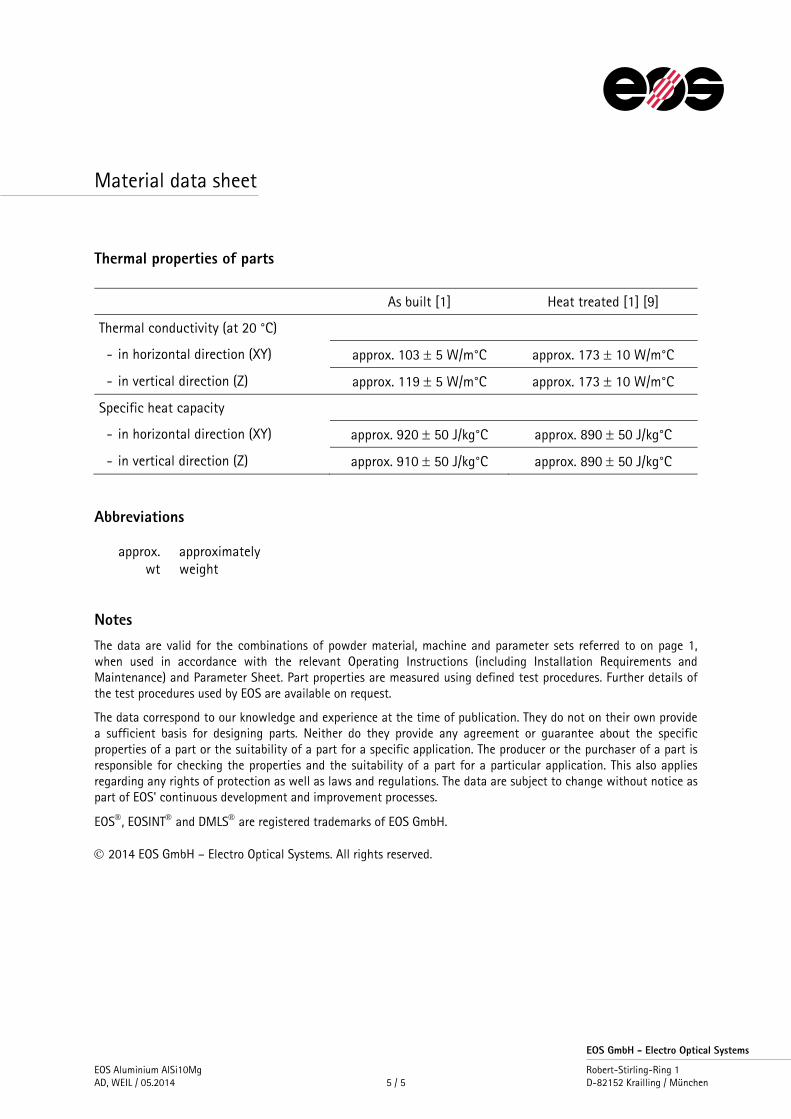
Material data sheet
EOS GmbH - Electro Optical Systems
EOS Aluminium AlSi10Mg Robert-Stirling-Ring 1 AD, WEIL / 05.2014 5 / 5 D-82152 Krailling / München
Thermal properties of parts
As built [1] Heat treated [1] [9]
Thermal conductivity (at 20 °C)
- in horizontal direction (XY) approx. 103 5 W/m°C approx. 173 10 W/m°C
- in vertical direction (Z) approx. 119 5 W/m°C approx. 173 10 W/m°C
Specific heat capacity
- in horizontal direction (XY) approx. 920 50 J/kg°C approx. 890 50 J/kg°C
- in vertical direction (Z) approx. 910 50 J/kg°C approx. 890 50 J/kg°C
Abbreviations
approx. approximately wt weight
Notes
The data are valid for the combinations of powder material, machine and parameter sets referred to on page 1, when used in accordance with the relevant Operating Instructions (including Installation Requirements and Maintenance) and Parameter Sheet. Part properties are measured using defined test procedures. Further details of the test procedures used by EOS are available on request.
The data correspond to our knowledge and experience at the time of publication. They do not on their own provide a sufficient basis for designing parts. Neither do they provide any agreement or guarantee about the specific properties of a part or the suitability of a part for a specific application. The producer or the purchaser of a part is responsible for checking the properties and the suitability of a part for a particular application. This also applies regarding any rights of protection as well as laws and regulations. The data are subject to change without notice as part of EOS' continuous development and improvement processes.
EOS, EOSINT and DMLS are registered trademarks of EOS GmbH.
2014 EOS GmbH – Electro Optical Systems. All rights reserved.
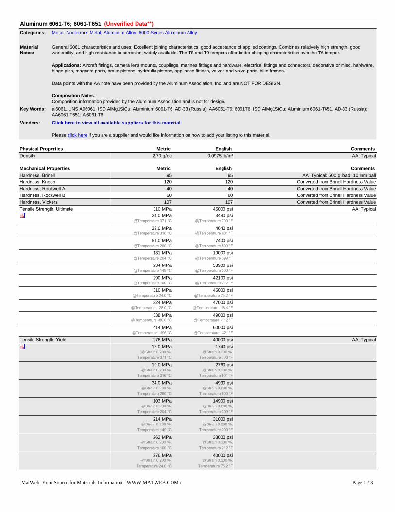
Aluminum 6061-T6; 6061-T651 (Unverified Data**)
Categories: Metal; Nonferrous Metal; Aluminum Alloy; 6000 Series Aluminum Alloy
Material Notes:
General 6061 characteristics and uses: Excellent joining characteristics, good acceptance of applied coatings. Combines relatively high strength, good workability, and high resistance to corrosion; widely available. The T8 and T9 tempers offer better chipping characteristics over the T6 temper.
Applications: Aircraft fittings, camera lens mounts, couplings, marines fittings and hardware, electrical fittings and connectors, decorative or misc. hardware, hinge pins, magneto parts, brake pistons, hydraulic pistons, appliance fittings, valves and valve parts; bike frames.
Data points with the AA note have been provided by the Aluminum Association, Inc. and are NOT FOR DESIGN.
Composition Notes: Composition information provided by the Aluminum Association and is not for design.
Key Words: al6061, UNS A96061; ISO AlMg1SiCu; Aluminium 6061-T6, AD-33 (Russia); AA6061-T6; 6061T6, ISO AlMg1SiCu; Aluminium 6061-T651, AD-33 (Russia); AA6061-T651; Al6061-T6
Vendors: Click here to view all available suppliers for this material.
Please click here if you are a supplier and would like information on how to add your listing to this material.
Physical Properties Metric English Comments
Density 2.70 g/cc 0.0975 lb/in³ AA; Typical
Mechanical Properties Metric English Comments
Hardness, Brinell 95 95 AA; Typical; 500 g load; 10 mm ball
Hardness, Knoop 120 120 Converted from Brinell Hardness Value
Hardness, Rockwell A 40 40 Converted from Brinell Hardness Value
Hardness, Rockwell B 60 60 Converted from Brinell Hardness Value
Hardness, Vickers 107 107 Converted from Brinell Hardness Value
Tensile Strength, Ultimate 310 MPa 45000 psi AA; Typical
24.0 MPa@Temperature 371 °C
3480 psi@Temperature 700 °F
32.0 MPa@Temperature 316 °C
4640 psi@Temperature 601 °F
51.0 MPa@Temperature 260 °C
7400 psi@Temperature 500 °F
131 MPa@Temperature 204 °C
19000 psi@Temperature 399 °F
234 MPa@Temperature 149 °C
33900 psi@Temperature 300 °F
290 MPa@Temperature 100 °C
42100 psi@Temperature 212 °F
310 MPa@Temperature 24.0 °C
45000 psi@Temperature 75.2 °F
324 MPa@Temperature -28.0 °C
47000 psi@Temperature -18.4 °F
338 MPa@Temperature -80.0 °C
49000 psi@Temperature -112 °F
414 MPa@Temperature -196 °C
60000 psi@Temperature -321 °F
Tensile Strength, Yield 276 MPa 40000 psi AA; Typical
12.0 MPa@Strain 0.200 %,
Temperature 371 °C
1740 psi@Strain 0.200 %,
Temperature 700 °F
19.0 MPa@Strain 0.200 %,
Temperature 316 °C
2760 psi@Strain 0.200 %,
Temperature 601 °F
34.0 MPa@Strain 0.200 %,
Temperature 260 °C
4930 psi@Strain 0.200 %,
Temperature 500 °F
103 MPa@Strain 0.200 %,
Temperature 204 °C
14900 psi@Strain 0.200 %,
Temperature 399 °F
214 MPa@Strain 0.200 %,
Temperature 149 °C
31000 psi@Strain 0.200 %,
Temperature 300 °F
262 MPa@Strain 0.200 %,
Temperature 100 °C
38000 psi@Strain 0.200 %,
Temperature 212 °F
276 MPa@Strain 0.200 %,
Temperature 24.0 °C
40000 psi@Strain 0.200 %,
Temperature 75.2 °F
MatWeb, Your Source for Materials Information - WWW.MATWEB.COM / Page 1 / 3
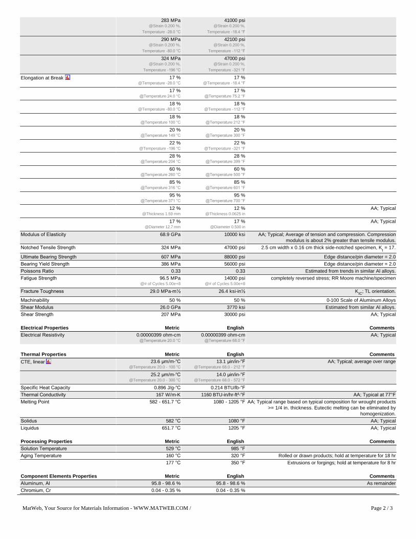
283 MPa@Strain 0.200 %,
Temperature -28.0 °C
41000 psi@Strain 0.200 %,
Temperature -18.4 °F
290 MPa@Strain 0.200 %,
Temperature -80.0 °C
42100 psi@Strain 0.200 %,
Temperature -112 °F
324 MPa@Strain 0.200 %,
Temperature -196 °C
47000 psi@Strain 0.200 %,
Temperature -321 °F
Elongation at Break 17 %@Temperature -28.0 °C
17 %@Temperature -18.4 °F
17 %@Temperature 24.0 °C
17 %@Temperature 75.2 °F
18 %@Temperature -80.0 °C
18 %@Temperature -112 °F
18 %@Temperature 100 °C
18 %@Temperature 212 °F
20 %@Temperature 149 °C
20 %@Temperature 300 °F
22 %@Temperature -196 °C
22 %@Temperature -321 °F
28 %@Temperature 204 °C
28 %@Temperature 399 °F
60 %@Temperature 260 °C
60 %@Temperature 500 °F
85 %@Temperature 316 °C
85 %@Temperature 601 °F
95 %@Temperature 371 °C
95 %@Temperature 700 °F
12 %@Thickness 1.59 mm
12 %@Thickness 0.0625 in
AA; Typical
17 %@Diameter 12.7 mm
17 %@Diameter 0.500 in
AA; Typical
Modulus of Elasticity 68.9 GPa 10000 ksi AA; Typical; Average of tension and compression. Compressionmodulus is about 2% greater than tensile modulus.
Notched Tensile Strength 324 MPa 47000 psi 2.5 cm width x 0.16 cm thick side-notched specimen, Kt = 17.
Ultimate Bearing Strength 607 MPa 88000 psi Edge distance/pin diameter = 2.0
Bearing Yield Strength 386 MPa 56000 psi Edge distance/pin diameter = 2.0
Poissons Ratio 0.33 0.33 Estimated from trends in similar Al alloys.
Fatigue Strength 96.5 MPa@# of Cycles 5.00e+8
14000 psi@# of Cycles 5.00e+8
completely reversed stress; RR Moore machine/specimen
Fracture Toughness 29.0 MPa-m½ 26.4 ksi-in½ KIC
; TL orientation.
Machinability 50 % 50 % 0-100 Scale of Aluminum Alloys
Shear Modulus 26.0 GPa 3770 ksi Estimated from similar Al alloys.
Shear Strength 207 MPa 30000 psi AA; Typical
Electrical Properties Metric English Comments
Electrical Resistivity 0.00000399 ohm-cm@Temperature 20.0 °C
0.00000399 ohm-cm@Temperature 68.0 °F
AA; Typical
Thermal Properties Metric English Comments
CTE, linear 23.6 µm/m-°C@Temperature 20.0 - 100 °C
13.1 µin/in-°F@Temperature 68.0 - 212 °F
AA; Typical; average over range
25.2 µm/m-°C@Temperature 20.0 - 300 °C
14.0 µin/in-°F@Temperature 68.0 - 572 °F
Specific Heat Capacity 0.896 J/g-°C 0.214 BTU/lb-°F
Thermal Conductivity 167 W/m-K 1160 BTU-in/hr-ft²-°F AA; Typical at 77°F
Melting Point 582 - 651.7 °C 1080 - 1205 °F AA; Typical range based on typical composition for wrought products>= 1/4 in. thickness. Eutectic melting can be eliminated by
homogenization.
Solidus 582 °C 1080 °F AA; Typical
Liquidus 651.7 °C 1205 °F AA; Typical
Processing Properties Metric English Comments
Solution Temperature 529 °C 985 °F
Aging Temperature 160 °C 320 °F Rolled or drawn products; hold at temperature for 18 hr
177 °C 350 °F Extrusions or forgings; hold at temperature for 8 hr
Component Elements Properties Metric English Comments
Aluminum, Al 95.8 - 98.6 % 95.8 - 98.6 % As remainder
Chromium, Cr 0.04 - 0.35 % 0.04 - 0.35 %
MatWeb, Your Source for Materials Information - WWW.MATWEB.COM / Page 2 / 3

References for this datasheet.
**
This data sheet is not an active part of MatWeb and the information on it should not be considered reliable.
Inactive data sheets have usually been replaced with newer information on the same material. If this is the case, you can find the active data sheet by using any of our search tools, including the Quick Search
box in the upper part of this page.
If you are unable to locate an active data sheet for this material, then this material is likely discontinued, although various other reasons may be behind its removal. In any event, do not rely on the information on
this page to be accurate or maintained.
You may have reached this data sheet through an outdated bookmark or link. Please update your bookmark accordingly. We apologize if you have accessed this page through MatWeb’s usual search tools.
Some of the values displayed above may have been converted from their original units and/or rounded in order to display the information in a consistent format. Users requiring more precise data for scientific or
engineering calculations can click on the property value to see the original value as well as raw conversions to equivalent units. We advise that you only use the original value or one of its raw conversions in your
calculations to minimize rounding error. We also ask that you refer to MatWeb's terms of use regarding this information. Click here to view all the property values for this datasheet as they were originally entered into
MatWeb.
Copper, Cu 0.15 - 0.40 % 0.15 - 0.40 %
Iron, Fe <= 0.70 % <= 0.70 %
Magnesium, Mg 0.80 - 1.2 % 0.80 - 1.2 %
Manganese, Mn <= 0.15 % <= 0.15 %
Other, each <= 0.05 % <= 0.05 %
Other, total <= 0.15 % <= 0.15 %
Silicon, Si 0.40 - 0.80 % 0.40 - 0.80 %
Titanium, Ti <= 0.15 % <= 0.15 %
Zinc, Zn <= 0.25 % <= 0.25 %
MatWeb, Your Source for Materials Information - WWW.MATWEB.COM / Page 3 / 3