Florida State University Libraries

Electronic Theses, Treatises and Dissertations The Graduate School

2014

An Additive Manufacturing Acrylic for Usein the 32 Tesla All Superconducting MagnetZachary Johnson

Follow this and additional works at the FSU Digital Library. For more information, please contact lib-ir@fsu.edu

FLORIDA STATE UNIVERSITY

THE GRADUATE SCHOOL

AN ADDITIVE MANUFACTURING ACRYLIC FOR USE IN THE 32 TESLA ALL

SUPERCONDUCTING MAGNET

By

ZACHARY JOHNSON

A Thesis submitted to the Program in Materials Science and Engineering

in partial fulfillment of the requirements for the degree of

Master of Science

Degree Awarded: Fall Semester, 2014

ii

Zachary Johnson defended this Thesis on November 14, 2014.

The members of the supervisory committee were:

Eric Hellstrom

Professor Directing Thesis

Zhiyong Richard Liang

Committee Member

William S. Oates

Committee Member

The Graduate School has verified and approved the above-named committee members, and

certifies that the thesis has been approved in accordance with university requirements.

iii

Dedication:

This work is dedicated to my parents who instilled in me a lighthearted approach to excellence

and a desire for knowledge.

And to my wife and my son;

Without whom I would be without a why.

iv

ACKNOWLEDGMENTS

I would like to first acknowledge my wife whose seemingly unlimited patience and

perseverance made this possible.

I would like to thank those in MS&T for allowing me the time and consideration and

funding to work on this project. I would like to thank Dr. Ir. H.W. Weijers and Mr. Tomas

Painter for allowing me to use their individual S-Rad accounts to purchase materials. Dr. Weijers

also assisted me multiple times with consultations, and developing a test plan, and analysis

methods. I would like to thank Mr. W. D. Markiewicz, Distinguished University Scholar for his

input on the scope of research required for use in the 32T coil. I would like to thank Mr. R.P.

Walsh for his patience and assistance in doing all things in the materials testing lab. Also, I

would like to thank Mr. D. McRae for his instruction on cryogenic handling, testing, and the

extensometer calibration.

I would like to thank those at HPMI for their time, equipment usage, and patience while

working on my thesis. I would like to thank Dr. Zhiyong Richard Liang for his guidance in

setting up the appropriate testing parameters, and encouragement to publish my findings. I would

like to thank Mr. Jerry Horne and Mr. Aniket Ingrole for their instruction in how to operate the

Objet 30 and its necessary hardware and software. I would like to thank Ms. Judy Gardner a

minimum of fifty individual occurrences of assistance, with everything from tuition waiver

formalities, to unlocking the door.

I would like to thank Dr. Eric Hellstrom for being my mentor. He has led me from having

a curiosity about superconductivity to a career, a degree, and a lifelong fascination and passion in

the truth behind what makes the world work: Materials.

v

TABLE OF CONTENTS

List of Tables ................................................................................................................................ vii

List of Figures .............................................................................................................................. viii

Abstract .......................................................................................................................................... xi

Chapter One Introduction ............................................................................................................... 1

1.1 Environment .......................................................................................................................... 3

1.1.1 High Magnetic Field ...................................................................................................... 4

1.1.2 Cryogenics ..................................................................................................................... 4

1.2 Additive Manufacturing ........................................................................................................ 6

Chapter Two Methodology ............................................................................................................. 8

2.1 Sample Design ...................................................................................................................... 8

2.2 Sample Processing ................................................................................................................ 9

2.2.1 Objet 30 – The Additive Manufacturing Machine ......................................................... 9

2.2.2 RGD 430 – The Material ............................................................................................. 11

2.2.3 Sample Cleaning and Preparation ................................................................................ 14

2.3 Sample Testing.................................................................................................................... 16

2.3.1 Test Equipment ............................................................................................................ 16

2.3.2 Equipment Calibration ................................................................................................. 17

2.3.3 Test Procedure ............................................................................................................. 18

2.4 Data Analysis ...................................................................................................................... 19

Chapter Three Geometric Tolerancing ......................................................................................... 21

3.1 Method of Measurement ..................................................................................................... 22

3.2 Geometric Statistics ............................................................................................................ 23

3.2.1 Profile Statistics ........................................................................................................... 23

3.2.2 Thickness Statistics ...................................................................................................... 28

vi

Chapter Four Mechanical Statistics .............................................................................................. 38

4.1 Young’s Modulus................................................................................................................ 38

4.2 Stress ................................................................................................................................... 43

4.2.1 Engineering Stress ....................................................................................................... 44

4.2.2 Material Stress ............................................................................................................. 46

4.3 Strain at Failure ................................................................................................................... 48

4.4 Fracture ............................................................................................................................... 49

4.5 Shock Loading .................................................................................................................... 51

4.6 Coefficient of Thermal Expansion ...................................................................................... 52

Chapter Five Application to the Heater Lead cover ..................................................................... 54

Chapter Six Conclusions ............................................................................................................... 58

6.1 Review ................................................................................................................................ 58

6.2 Discussion ........................................................................................................................... 58

6.3 Open Characterizations ....................................................................................................... 59

Appendix A ................................................................................................................................... 61

Resin Identification in Cryogenic Tests ........................................................................................ 61

References ..................................................................................................................................... 62

Biographical Sketch ...................................................................................................................... 64

vii

LIST OF TABLES

Table 1: Details of geometric measurement tools ......................................................................... 23

Table 2: Linear elastic moduli for commonly used cryogenic materials ...................................... 39

viii

LIST OF FIGURES

Figure 1: Screenshot of part called "Short Heater Lead Cover" ..................................................... 2

Figure 2: Tensile strength vs. Young's modulus for cyanate esters and polyester [5] ................... 5

Figure 3: Original double reduced area sample design for polymer measurements. Dimensions

are in mm. Thickness dimensions are not given. ............................................................................ 8

Figure 4: Custom design of the 25.4 μm thick short double-reduced tensile sample ..................... 9

Figure 5: Stratasys Systems Inc. datasheet for room temperature properties of RGD 430 [6] ..... 11

Figure 6: Stratasys Systems Inc. component list from the MSDS datasheet for RGD 430 [7] ... 12

Figure 7: Isobornyl acrylate [8] ................................................................................................... 12

Figure 8: Monomer version of isobornyl acrylate ........................................................................ 13

Figure 9: Printed sample during cleaning. This shows the thickness of the material and the

support matieral. a) shows the partially removed material, and b) shows all of the support

material removed .......................................................................................................................... 14

Figure 10: Detail of a cleaned tensile sample ............................................................................... 15

Figure 11: Detail of three prepared tensile samples with striations going along width and

length............................................................................................................................................. 15

Figure 12: Alignment tool with bolt style clamps and tensile sample in place ............................ 16

Figure 13: 5.08mm thick tensile sample width distribution ......................................................... 25

ix

Figure 14: 5mm width measurement distribution ......................................................................... 26

Figure 15: 50mm length distribution ............................................................................................ 27

Figure 16: 5mm thickness distribution ......................................................................................... 29

Figure 17: Surface plot of sample thickness and position ............................................................ 29

Figure 18: Detail of a) striations across width, and of b) a rare anomaly ..................................... 30

Figure 19: Detail of a) random variation in the thickness, and b) striations along the length of the

sample ........................................................................................................................................... 31

Figure 20: Tensile sample thickness offset of mean from nominal Shows no correlation to

thickness itself ............................................................................................................................... 32

Figure 21:Distribution or spread of offset of mean from nominal................................................ 34

Figure 22: Positioning of tensile sample measurements showing top, middle, bottom

measurements along the width, and position numbers along the length of the specimen area.

Shown at the right are the striation directions .............................................................................. 34

Figure 23: Average thickness across width for the worst thickness variation sample.................. 35

Figure 24: Positional thickness of sample 39 ............................................................................... 36

Figure 25: Distribution of deviation from nominal engineering thickness ................................... 37

Figure 26: Temperature dependence of the modulus, E, of Polymers. A) Examples of idealized

behaviors exhibited by an aorphous thermoplastic B) a semi crystalline thermoplastic, C) a

thermoset polymer. [9] .................................................................................................................. 40

x

Figure 27: Young’s modulus for RGD 430 at 77K....................................................................... 41

Figure 28: Distribution of modulus from all samples available ................................................... 43

Figure 29: Nominal engineering stress at failure for RGD 430 at 77K ........................................ 45

Figure 30: Distribution of calculated material stress at failure The most accurate data is in dark

blue, with the striations across the width Minimum Material Strength ........................................ 48

Figure 31: Distribution of strain at failure for RGD 430 at 77K .................................................. 49

Figure 32: Brittle fracture of a sample with straitions perpendicular to the length ...................... 50

Figure 33: Brittle fracture of a sample with striations parallel to the length ................................ 51

Figure 34: Thermal expansion of copper and RGD 430 from 4.2K to 295K ............................... 53

Figure 35: Prototype Coil known as 20/70. Figure shows detail of a) superconducting coil with

all hardware, b) cross sectional area of coil with heater lead on the right hand side, c) the heater

lead itself, and d) the heater lead profile with axial positions (in mm) from the midplane of the

coil................................................................................................................................................. 54

Figure 36: Worst case of radial magnetic field at the position of the heater lead covers ............. 55

Figure 37: Load distribution applied to the conductor.................................................................. 56

xi

ABSTRACT

The National High Magnetic Field Laboratory is building a world record all superconducting

magnet known as the “32T”. It requires many thousands of parts, but in particular one part called

the “heater lead cover” is unusually expensive to manufacture. These parts have been so far

made out of a glass filled epoxy known as G-10, and conventionally machined. The proposal in

this paper is to change the material and manufacturing method to additive manufacturing using

the material called “RGD 430”. If the expensive to machine material is replaced with the

automatically printed material, the total cost for the project will be reduced from $21,000 to

$455, a 98% cost savings.

To replace the original material, however, the updated material must be able to perform

adequately in the designed situation. In order be an acceptable replacement, RGD 430 must

survive some minor amount of strain, in a cryogenic environment. It is shown to survive a

sufficient amount of strain

The final tolerance for dimensions along the width and length of printed parts is more

precise than ± 0.10mm. The final tolerance for the dimensions in the thickness of printed parts is

more precise than ±0.25mm. This corresponds to the required maximum tolerance on the heater

lead covers of ± 0.10 mm

Before utilizing the material, there should be a few additional tests run on it to ensure it

will work in-situ at 4.2K. Those tests are outside the scope of this thesis. It should be noted that

the material tested is only one of a great many additive manufacturing materials that are

available commercially and at low cost. Any future funded work should take advantage of the

readily available products from industry. This thesis serves as a proof of viability for using

additively manufactured materials in a cryogenic environment.

1

CHAPTER ONE

INTRODUCTION

The intention of the document presented here is to show the viability of additively

manufactured –commonly referred to as 3-D or “printed”—materials, as engineering materials

for 4.2K and high magnetic field applications. To fully characterize a material for all possible

conditions in this environment is beyond the scope of a thesis. It is in this light, therefore, that

the necessary characterization of the acrylic RGD 430 described in chapter 2 to replace the

epoxy and glass composite engineering material garolite G-10/FR4 (known as G-10) in the

“heater lead cover” is completed here. This characterization encompasses the material’s

molecular composition, its manufacturing method, the macroscopic structure and the options

therein, the mechanical properties at room temperature and 77K and the effects of these

characteristics on the application of the given part.

Much attention has been given recently to developing high temperature superconducting

(hereafter called HTS) magnets. Though the discovery of HTS materials was in the 1980’s, a

practical commercial supply has only recently become available [1]. Currently the most

promising commercial HTS material is a rare-earth metal based cuprate superconductor known

generically as ReBCO. Due to the extreme requirement of ~1-3% angle orientation between

grain boundaries in the ReBCO conductor [2] (nearly macroscopic single-crystal texture), these

suppliers are only able to deliver flat conductor in the form of tapes. Magnet designers are used

to building coils with round wire, or cables. These flat tapes introduce design convolutions,

which are not present with round wire designs. Complications in conductor pitch change causes a

need for magnets to be wound in the pancake technique [3]. Specifically this technique means

that the leads for the protection heaters will not exit axially, as is typical, but radially where there

2

is minimal area for materials support. This requires the items on the outer radius of the coils to

be very thin. This can be seen in figure 1. The thinnest portion of the heater lead is 1.19mm.

These heaters leads will rarely if ever be stressed. This is due to the fact that the heaters will only

fire if the coil needs to be protected. There are no forces acting upon the heater leads unless the

heaters are utilized. However, when the heater leads are used, the conductor will be burdened

with some Lorentz forces, which will be sufficiently mechanically supported internally. However

there will be some motion. This motion must be absorbed by the heater lead covers.

In the 32T all superconducting magnet, the heater lead covers have been made from G-

10 in all the prototypes. This part must be radially thin, and longer than the coil (around 400

mm). Shown in figure 1 is a screenshot of a reduced length version of this part, with a span of

only ~120 mm. The cost of this small version using G-10 and standard machining techniques is

$420 per part, even when ordered in quantities. The estimated quoted cost for the full-size part

which is ~400 mm long is at least $1,500. There will be at fourteen such parts on the finished

coil. The cost for mechanical parts is $21,000. Finding a way to reduce cost drove the intent

behind this research.

Figure 1: Screenshot of part called "Short Heater Lead Cover"

3

1.1 Environment

The Magnet Science and Technology (MS&T) division at the NHMFL is currently in the

process of developing a high magnetic field all superconducting magnet known as the 32T. This

magnet will include many hundreds of engineering drawings, with many thousands of individual

parts, all of which are made from a pallet of about a half a dozen materials. These materials

include the following:

The superconductor itself (ReBCO), which is a very complex composite,

constituting the bulk of the magnet’s volume, and cost of the magnet; a purchased

material

316L stainless steel which is used for most of the structural elements

C10100 copper (or 101 copper), which is known as oxygen free high conductivity

copper, or OFHC copper

G-10, which is a high-performance glass filled epoxy

85N, which is a glass-filled polyimide film that is a high performance dielectric

Trace amounts of the following:

o 63/37 lead tin solder

o Alumina powder as a thin dielectric coating on some of the stainless steel

o Teflon FEP (fluorinated ethylene propylene) as a thin thermoplastic adhesive

between polyimide layers

Most of these materials have undergone decades of characterization and proof testing in

coils predating even the NHMFL. These materials are the generally accepted ones for use in

superconducting magnets. The addition of a new material to the tool belt of the magnet designer

4

is a rare occurrence. This is often done out of necessity. In this thesis, however, the target is the

introduction of a new material to reduce development time and cost.

This additively manufactured acrylic is intended to replace a part made out of G-10 that

is very expensive to manufacture.

1.1.1 High Magnetic Field

This material will be subjected to a very high magnetic field on the order 21T In a

cryogenically-cooled solenoid. These high magnetic fields can alter electronic band properties,

the electronic orbitals, the conduction properties, the dielectric strengths, and various other

materials characteristics. For polymers however, there is very little effect. There is some

evidence for the magnetic torque on polymers from the magnetic field increasing crystallinity

during processing [4], but at cryogenic temperatures there is not enough diffusion for this torque

to have any effect.

The field will not affect the heater lead covers directly. It will induce some force in the

heater lead conductor that is in contact with the heater lead covers. This force causes a strain in

the conductor, which will be translated through to the heater lead covers. The heater lead covers

will therefore only be indirectly affected by the magnetic field.

1.1.2 Cryogenics

Cryogenic conditions that will be incurred by this sample material are liquid nitrogen

(77K), liquid helium (4K), and occasional moderate vacuum at these temperatures. There should

be minimal effects due to the liquid itself, as helium is a noble gas and nitrogen is quite inert.

Reduction in temperature for polymers typically changes many of their mechanical

characteristics. A summary of several polymers is given by Reed and Walsh in the paper

5

Tensile Properties of Resins at Low Temperature [5]. Figure 2 shows the elastic modulus and

tensile strength for cyanoesters and polyester, which is the most similar of these to the RRGD

430 material tested here. The data are shown for the temperatures from 295K,to 77K and 4K.

Figure 2: Tensile strength vs. Young's modulus for cyanate esters and polyester [5]

G is a Down Chemical developed cyanate ester I is a Rhone-Poulenc developed cyanate ester P is an Owens Corning developed polyester

Q is an ICL developed cyanate ester The exact definitions for G, I, P and Q are given in Appendix A

6

This graph shows a strong grouping of modulus to temperature, and sometimes of strength to

temperature. From these data and the work in ref. [5] my working assumption was the material

would experience brittle failure at 77K and 4K. Tests at 77K confirmed this assumption. Tests

have not been done at 4K due to budget restrictions but RGD 430 is also expected to be brittle at

4K.

1.2 Additive Manufacturing

Additive manufacturing is generally known as rapid prototyping, or 3-D printing. In the

past almost all final stage manufacturing was subtractive. Steel foundries supplied billets or

plates or round stock, that was parted off and otherwise manipulated by subtracting material until

a final retail or commercial product was created. Additive manufacturing changed this.

Additive manufacturing began in the 1980s. The first techniques included fused

deposition molding, and most importantly photopolymer stereolithography. The process of

Stereo lithography classically is the method of taking a bath of polymer, and then applying an

ultraviolet light to it in a computer aided pattern based off of a CAD file. The UV light will

excite the electrons in the polymers, and allow them to activate and grow together, or

polymerize. The bath of liquid is then filled up slightly higher so that a following layer can be

built upon the first layer. This process is repeated until a finished part is removed from the

polymer bath.

There is another method called plaster printing (PP) which is a powdered plaster that is

applied as a very thin layer, and then inkjet style print heads come along in a raster pattern, and

apply a binder. The raster pattern is one where areas are sprayed by very closely spaced rows,

and each pass moves the printer head up one column. After a layer is complete, another flat

layer, encompassing the entirety of the 3-D printer bed is applied.

7

There are many other methods, including some that utilize coppers, steels and even

refractory metals like niobium [6]. One can use lasers, electron beams, furnace or selective heat

sintering, to bring materials above their glass transition temperature, or close to their melting

point, so that they can be easily molded or shaped from grains, or wires, or extrusions into the

final desired shape.

The additive manufacturing process described in this thesis is a hybrid between

stereolithography, and the raster style printer method. This method is described in more detail in

chapter two.

8

CHAPTER TWO

METHODOLOGY

2.1 Sample Design

The design of the samples was developed with assistance from Robert Walsh at the

National High Magnetic Field Laboratory. The original cryogenic polymer tensile specimen

design was developed at the National Institute for Standards and Technology. It is shown in

figure 3 from a paper entitled “Tensile Properties of Resins at Low Temperatures” [4].

Figure 3: Original double reduced area sample design for polymer measurements. Dimensions are in mm. Thickness dimensions are not given.

9

This design utilizes two area reductions for the purpose of ensuring a standard specimen cross

sectional area and test section length. This design was modified for use in a small cryostat. In the

original design in figure 3 proved to be too long for the small cryostat. So in order to reduce the

length of the specimen the portions of the design that are flat have been eliminated.

2.2 Sample Processing

2.2.1 Objet 30 – The Additive Manufacturing Machine

The Objet 30 is an additive manufacturing machine (a 3-D printer), located in and

belonging to the High Performance Materials Institute (HPMI) at Florida State University. It was

originally purchased from Objet, but that company has since been bought out by Stratasys

Systems. Stratasys Systems currently offers an Objet 30 Pro, which according to telephone

discussions with the company, is merely a software upgrade to the original Objet 30. The

machine can utilize eight different photopolymer materials.

The Objet 30 utilizes an altered stereolithography method. Instead of using the traditional

polymer bath, and then UV curing the polymers in layers, the machine uses inkjet like printer

Figure 4: Custom design of the 25.4 μm thick short double-reduced tensile sample

10

heads to apply a thin layer 16μm thick, and then immediately applies ultraviolet light to cure the

polymer in place. The objet has the advantage over many 3-D printers, in that it utilizes a

secondary material. This “support” material is used to allow for parts to be produced with

overhangs, and holes that require support, so they do not collapse during printing. The heater

lead covers in figure 1 have several details that require overhangs to be of good quality.

The Objet 30 can build objects up to a maximum dimension of 294mm x 192mm

x148.6mm. It has a listed accuracy of ± 0.1mm, which is tested and described in detail in chapter

three [6]. The accuracy of the dimensions through the thickness depends on following the

appropriate procedures for manufacturing.

The first step of printing any samples is to clean the printing heads themselves. These

print heads as discussed in chapters three and four, are critical to creating repeatable parts. The

print heads are cleaned with a lint free cloth, and a spray bottle of isopropyl alcohol, until there is

no more discoloration upon wiping. The print head also has a hot roller for leveling surfaces; it

must be cleaned in the same manner.

The second step of printing is the purging of the material fill lines, heads, heaters and all

other flow sections. The Objet 30 does this automatically by selecting “Reinitiate Wizard”. This

also warms the heads up for use. The heads and material must be around 78⁰C to print properly.

This takes approximately 15 minutes.

While the previous step is being automatically completed, the next step can

simultaneously take place. The organization of the items to be printed must occur. It accepts

“.stl” files, which are a readily available form of CAD file that all popular CAD software

programs can output. The software program can manipulate these drawings in a number of ways,

including scaling, rotating, translating, creating specific surface finishes etc. The main purpose is

11

to serve as an intermediary between a single design, and the platform or “Tray” that these parts

are printed on. After laying out the tray for printing, one simply hit’s “Build Tray”, and another

automatic wizard controls the process from there.

The Objet 30 is a multi-material additive manufacturing machine. It is capable of printing

both a strong polymer, and a very weak wax-like polymer to act as a support material. This

support material makes the Objet 30 capable of making parts with holes, or overhangs, or any

other complicated geometry that the NHMFL might encounter.

2.2.2 RGD 430 – The Material

RGD 430 is a thermoplastic acrylic that is UV cured that is used in the Objet series of

printers from Stratasys Systems Inc. It was chosen because it has the lowest Young’s modulus of

the materials available for the Objet 30, and thus the assumption is that it will be able to absorb

more strain at cryogenic temperatures.

Figure 5: Stratasys Systems Inc. datasheet for room temperature properties of RGD 430 [6]

12

Stratasys did not convey the more precise details on the manufacturing of this polymer.

Thus things like the viscosity of the preset fluid, the void characteristics, kinetics and

suppression, the final molecular weight were not available. In fact, only the information that

isobornyl acrylate forms less than 40 percent of the weight of the monomer precursor is given

anywhere in the literature. Shown below is an excerpt from the MSDS showing that the majority

of the material is proprietary:

Isobornyl acrylate is shown below as a schematic:

Figure 6: Stratasys Systems Inc. component list from the MSDS datasheet for RGD 430 [7]

Figure 7: Isobornyl acrylate [8]

13

It contains the isomer isoborneol, in the acrylic monomer, replacing the vinyl hydrogen. Giving

something akin to the following schematic:

Figure 8 shows a monomer of isobornyl acrylate. The monomer is a vinyl. This means it

is effectively an ethylene molecule with one of the hydrogens replaced with some other

functional group. This functional group is borneol and is shown in figure 8 as the large

connected network of spheres. The black represent carbon, the red represents oxygen and the

white are the hydrogens. To polymerize this the double bond between the carbons It can be seen

that there will be good hydrogen bonding between the finished polymers, as the borneol has a

more rigid three dimensional structure than the classic thermoplastic polyethylene, which has

only a 1 dimensional structure.

Figure 8: Monomer version of isobornyl acrylate

14

2.2.3 Sample Cleaning and Preparation

After the samples are printed as described above, the samples must be removed and

prepared for testing. The samples are initially scraped off of the surface of the tray with a putty

knife and then set aside. The tray itself is cleaned with further scraping, and a liberal application

of isopropyl alcohol and standard lint-free Kim wipes.

After the samples were taken from HPMI to NHMFL, they were mechanically scraped

with a soft plastic scraper to remove the support material. As described in chapter four, some of

the samples were cleaned with isopropyl alcohol, which turned out to be a very bad way to clean

the samples. It reduced the strength of the material by almost 50%. The appropriate method is to

simply mechanically remove the excess support material with a soft piece of plastic. Shown in

figure 9 is an example of a 0.25mm thick sample, with the support material (a), partially

removed and (b) completely removed. This cleaning does cost some man hours, but the expense

has not be included in the cost comparisons discussed. The author believes the time is negligible,

and on the order of 5 minutes per part.

Figure 9: Printed sample during cleaning. This shows the thickness of the material and the support matieral. a) shows the partially removed material, and b) shows all of the support

material removed

15

After cleaning, the samples were measured with calipers, flat anvil micrometers, and ball

micrometers as described in chapter three. An example of a cleaned and prepped sample

clamping area is given below in figure 10. There are clear striations and random thickness

defects shown. These occurred during the printing process.

Figure 11 shows examples of both striations along the width (a and c) and along the length (b)

.

Figure 10: Detail of a cleaned tensile sample

Figure 11: Detail of three prepared tensile samples with striations going along width and length

16

2.3 Sample Testing

The tensile samples were tested using an MTS (Mechanical Test Systems Corporation)

Criterion 42, a liquid nitrogen test cryostat, a custom made extensometer; bolt style grips and an

alignment tool. The alignment is critical to minimize the torque encountered by the samples.

The coefficient of thermal expansion was measured using an MTS dilatometer. The

system was originally created for testing sample expansion in a controlled furnace, but has been

retrofitted to do cryogenic applications. The samples are cooled to 4K in liquid helium, and then

allowed to gradually warm up to room temperature.

2.3.1 Test Equipment

The alignment tool—shown in figure 12 below—was used to make sure that the stress

passes through the cross section of the material, and not at some unknown angle, which would

put an unknown torque on the sample. The samples were placed by aligning the sample edges

with lines on the baseplate.

Figure 12: Alignment tool with bolt style clamps and tensile sample in place

17

The samples were then placed in the MTS Criterion 42. A custom-made test cryostat was

created. All available cryostats were too small to allow for individual’s hands to reach in and

apply the extensometer. So the cryostat was made from an available polystyrene container.

The extensometer used was a custom-built aluminum-framed sensor. It is the lightest

weight extensometer available in the NHMFL materials characterization laboratory for cryogenic

use. The choice of this extensometer was so that the additional weight and torque of the

extensometer would not cause errors in the readings. This specific extensometer was called the

“Shepic” named for the watch craftsman who built it for the NHMFL. It has no official

calibrations, so calibrations must be performed in-situ. It is a basic clip-on style device, with a

sensor arm connected to a four wire linear output strain gauge. The strain gauge uses a full

Wheatstone bridge configuration.

The dilatometer is a Unitherm Model 1101 Dilatometer system with a retrofitted cryostat.

The cryostat and all cryogenic portions were designed by the MS&T Materials Testing and

Characterization group.

2.3.2 Equipment Calibration

The MTS Criterion 42 has internal verifications for its load cell, which were utilized at

the start of every test day. The custom made extensometer required some in-situ calibration. The

extensometer was placed on a very large handle-style dial caliper, with G-10 extensions passing

down into the liquid nitrogen, where the extensometer was set with the initial length of exactly

one inch. This one inch length is the minimum head distance of the extensometer. The dial

caliper was then rotated until it reached the maximum expected extension of 0.254 mm (which

would give 10% strain). The reading on the MTS Criterion 42 software package were then

iteratively changed until they read exactly 0.254 mm extension when rotated, and then 0.00 when

18

rotated back to zero. The proportional Vin to Vout setting was recorded and set as -0.0022 (unit

less V/V).

The dilatometer uses the timed difference between the heights of two Invar bars. The

invar bars are in contact with the sample, and a known copper sample as a standard, to account

for any thermal gradients that might occur. The measured ends of the Invar bars are at room

temperature. Invar is notable for having an extremely low coefficient of thermal expansion, so its

length change due to the temperature difference from room temperature to the sample

temperature is negligible. The samples are at first bathed in liquid helium until they reach

thermal equilibrium at 4.2K. Then the temperature is allowed to naturally increase through heat

transfer through the cryostat walls, floor and invar bars themselves. This creates a moderately

slow temperature increase, which is recorded along with the height difference between the invar

bars. The nominal temperature ramp rate is less than 1K/minute. However, because it is an

uncontrolled system, the maximum can approach 3K/minute. The calibration is done

continuously using the copper standard to give an appropriate calibration.

2.3.3 Test Procedure

A total of 48 individual samples were made to be tested for this project. The first ten were

tested at room temperature. They had results similar to the stated results, but there was error due

to a lack of a procedure. At the end of the room temperature testing a procedure was developed.

It was perfected by sample 35.

Samples were printed and prepared as explained in section 2.2. These samples were then

measured using the methods described in section 3.1. These samples were then individually

placed on the alignment tool shown in figure 12, and bolted into the bolt style clamps. The edges

of the sample were aligned visually using parallel lines on the surface of the alignment tool.

19

The sample was placed into the cryostat and connected with pins through the clamp. The

load cell measurement on the MTS machine was set to only read the load due to the weight of

the lower clamp (approximately 7 N). The clamps were set in the approximate center of the pin

length. When the extensometer was used, this was the time it was placed. The extensometer

measurement arm was compressed into the minimal position so that Lo would be exactly 1.00”.

Some of the samples were tested without compression of the extensometer. The MTS machine’s

top arm was lowered to eliminate the possibility of increasing the load due to thermal contraction

when cryogens were added.

Liquid nitrogen was then added according to NHMFL safety procedures. After the

clamps stopped boiling nitrogen, a time of 60 seconds was waited to ensure thermal equilibrium

in the sample. Then the test was initiated and computer controlled.

The MTS machine moved the clamps at a speed of 0.5 mm/minute. This was a single

cycle strain to failure, where the sample is pulled on until it completely fails. Data for the

extensometer, load cell, and total extension were continuously recorded, and saved for later

analysis. The samples fractured. The cryostat was drained into an awaiting dewar. The clamps

were heated with a heat gun, until the ice melted. The samples were taken out and cataloged for

later analysis. The procedure was started over with placement in the bolt style clamps and a new

sample.

2.4 Data Analysis

Data analysis was done mainly using Microsoft Excel. There were additional calculations

done by hand. The statistical analysis histograms were created using a Microsoft add-in known

as “Data Analysis: Histogram”.

20

The magnetic field solver used is an internal macro-based Excel document known as

“Soleno” developed at the NHMFL. It solves the difficult hyperbolic functions for magnetic field

to an accuracy of at least 4 significant digits.

Error bars throughout the document indicate either standard deviation or sample

maxima/minima of measurements. The measurement error was considered too small be relevant,

as measurement error is much smaller than random variation. Standard deviations were on the

order of 0.5-15%, whereas measurement errors of the calipers and micrometers were on the order

of 0.1%-0.5%.

21

CHAPTER THREE

GEOMETRIC TOLERANCING

In the engineering division of the Magnet Science and Technology department,

engineering drawings conform to a strict set of standards. There are secondary and occasionally

tertiary checks on these drawings to make sure they are correct before leaving the lab for

manufacture. One of the most critical parts of these is the geometric tolerance. These are the

physical size and dimension requirements that a machinist or manufacturer must adhere to. The

three standard tolerances on a linear length, width or thickness vary from the loose ± 1 mm, to

the typical ± 0.25 mm, to the precise ± 0.10 mm. Any tolerance that needs to be more precise

than ± 0.10 mm requires a special callout per dimension. Anything more relaxed than ± 1 mm is

put in parenthesis () to emphasize that the dimension is more of a recommendation. There are

other more rare callouts such as straightness, thread fit, concentricity, and others. These have not

been examined in detail in this research due to their rarity. The straightness in the sample area of

the tensile specimens was measured, and found to have a straightness tolerance maximum of

0.010 mm over a 25.4 mm length ( 0.00040” over a 1” length), which is a very good tolerance.

All the samples printed for testing were measured for geometric tolerances. In general

these samples conformed to the desired dimension. The desired dimensions are described here as

a “nominal engineering” dimensions, and this should be defined as the dimension that was

drafted into the CAD software. Parts with these nominal engineering dimensions were produced

in the profile of the printer, which is the printer’s xy plane. This is layer width and length of the

sample. However the thickness of each piece seemed to be slightly variable. This variation was a

skewed thickness distribution where the thickness was generally averaged just above the nominal

engineering thickness but then skewed thicker. This could be intentionally setup by the

22

manufacturer for the purpose of ensuring that all thicknesses are at least the nominal engineering

thickness if not greater, so that if there were strength requirements they would be met.

3.1 Method of Measurement

All measurements were taken by hand. There were 42 tensile samples and 6 thermal

contraction samples. The widths of the tensile samples were measured in five places with the

calipers described below in table 1. The width of the caliper heads are approximately 3.5mm.

Since the sample section is 25.4mm long, the five measurements did not entirely encapsulate

every position along the length of the sample. It was noticed that there were visible thickness

variations along the samples either along the length of the specimen, or across the width of the

specimen. This was the reason for measuring both the peaks of the thickness with flat anvil

micrometers and the details of the thickness with ball micrometers. These micrometers are

described below.

Thickness measurements with the flat anvil were taken at the same five locations as the width

measurements. As the width of the flat anvil is 6.35mm, this should have taken into account all

areas of the profile with some overlap.

Thickness measurements with the ball micrometer (ball mic) were taken at the same five

locations as with the width and flat anvil micrometer. There were additional measurements at the

bottom, middle and top of the sample, along with width. The ball micrometer has some radius

approximately 6.35 mm. As this micrometer approximates the measurement of the thickness

from point to point, it should—and does—give some smaller measurement than the flat anvil.

Also, the ball micrometers are more likely to cause elastic deformation in the samples due to the

small surface contact area, which will lead to some further reduction in the measured thickness.

23

This effect has been ignored due to the unknown force exerted by the ratcheting mechanism of

the ball mic, and the indeterminate surface contact area between the ball and the sample.

Manufacturer Model Number Instrument Name

Measurement Range

Minimum discretization

Factory Calibration

Mitutoyo 500-196-30 Standard Digital Caliper Caliper 0-6 inches

.0005 inches (0.01 mm) Yes

Mitutoyo 293-831-30 Ratchet Stop Flat Anvil Micrometers

Flat Anvil 0-1 inch

0.00005 inches (0.001 mm) No

Mitutoyo 293-831-30 Ratchet Stop Ball Micrometer

Ball mic 0-1 inch

0.00005 inches (0.001 mm) No

3.2 Geometric Statistics

3.2.1 Profile Statistics

It was found that the profile dimensions were generally within the desired precision

tolerance of ± 0.1 mm. Figure 13 shows the 5.08mm thick tensile sample’s width distribution.

The vertical line on the left is the desired nominal engineering width of 5.08 mm. The line on the

right is the average of all the width measurements. This sufficiently approximates a unimodal

Gaussian distribution, and as such it has a standard deviation of 0.030 mm. The average deviates

from the nominal a total of + 0.031. Thus for a 99.7% confidence in the width, a good model

would be:

Table 1: Details of geometric measurement tools

24

(1)

(2)

This would give a minimum of 5.02mm and a maximum of 5.2mm for a nominal engineering

width of 5.08mm. This 5.2mm is out of tolerance for a precision tolerance as described above,

but if this positive offset of the average is taken into account, it will be within tolerance. Thus if

an engineer desired a 5.08mm wide piece on average, the should be programed as 5.05, so that

the resultant part will measure 5.08 ± 0.090mm with a 99.7% confidence that all dimensions will

be within tolerance.

However, if the desired outcome is stress related, then adhering to the nominal

engineering dimension will be desired. It would seem that the Object manufacturers knew of this

statistical variance, and programmed the machine to give a positive offset, so that all minimums

would approximate the desired dimension. Therefore it should be an engineering practice that

dimensions that are stress originated should be designed exactly, and those that have a strong

geometric requirement where stress is not critical, should be designed with the above modeled

offset.

Equation 1: 99.7% confident model for the dimensional tolerance

Equation 2: Empirical model for dimensions in the x-y plane

25

The samples made for the tests of the coefficient of thermal expansion are rectangles with

dimensions 5x5x50 mm. They followed the same pattern as the tensile sample width

measurements above. There are fewer measurements so the sample standard deviation is higher.

This measurement seems also to be a bit skewed positive, but again there are few sample

numbers (30 total measurements). This has a standard deviation of 0.035 mm. The average

deviates from the nominal to + 0.025mm. Thus for a 99.7% confidence in the width a good

model would be:

Figure 13: 5.08mm thick tensile sample width distribution

26

(3)

This would give a minimum for a nominal engineering width of 5mm of 4.92mm, and a

maximum of 5.13mm. This 5.13mm is out of tolerance for a precision tolerance as described

before, but again, it can be well modeled and should be taken into account for any critical design.

Samples measurements with unusually large thicknesses were checked to ensure that all of the

support material had been removed, so that these are the actual material thicknesses.

Equation 3: Less confident model of dimensions in the x-y plane due to fewer sample measurements

Figure 14: 5mm width measurement distribution

27

The coefficient of thermal expansion samples also had length measurements taken. There

were only a total of 6 of these measurements possible, but they still conform to the previous two

in-plane models.

The average is exactly 0.030 mm above the nominal. The standard deviation is 0.0179

mm. This difference from the previous models in equations two and three is most definitely due

to there being so few samples taken.

Figure 15: 50mm length distribution

28

3.2.2 Thickness Statistics

The statistical variation of the geometric tolerancing through the thickness of these

samples was also modeled, but had much stronger variance than the profile statistics shown in

the above section. This dimension correlates to the z plane in the printer. To begin with, the

simpler example of the thickness of the coefficient of thermal expansion samples is plotted

below in figure 16. The average has increased and the deviation is obviously wider. However

this does not fit a standard Gaussian curve, as it looks bi-modal. One could argue that there are

only 30 samples, and thus a Gaussian fit is sufficient as long as statistical confidence is not

discussed. Thus a back of the envelope model for this system would be

(4)

This is derived from the standard deviation being 0.056mm and the difference between the

nominal and mean is + 0.070mm. However, this scatter is not due to random variation. This

scatter is position dependent in some places along the profile plane of the printer. This is shown

below in figure 17 where in the measurements of the CTE sample thicknesses where there was a

clear pattern of samples 4, 5 and 6 being thicker than the average thickness. This was preceded

by a smooth transition where sample 3 had an intermediate thickness between the lower and

upper numbered samples. This smooth transition bodes well for any engineering strengths

associated with these larger thickness variations. This also shows up later in the tensile sample

measurements. It is very repeatable, and could be modeled if desired.

Equation 4: Empirical Model of Dimensions in the z Plane

29

Figure 16: 5mm thickness distribution

Figure 17: Surface plot of sample thickness and position

30

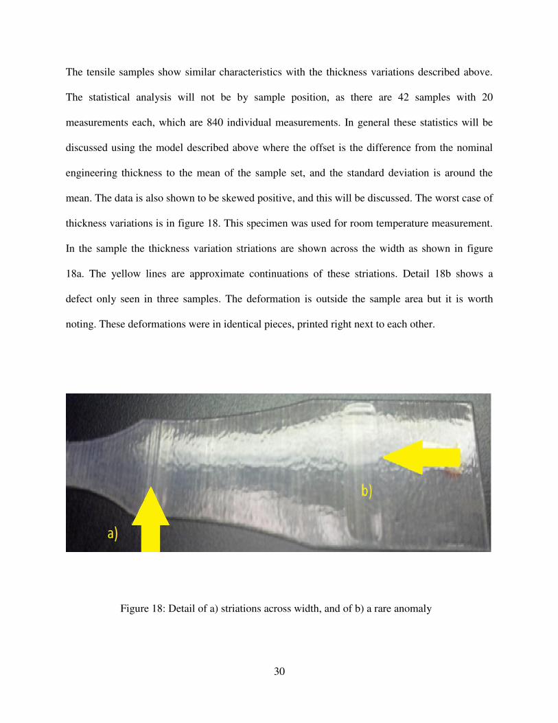
The tensile samples show similar characteristics with the thickness variations described above.

The statistical analysis will not be by sample position, as there are 42 samples with 20

measurements each, which are 840 individual measurements. In general these statistics will be

discussed using the model described above where the offset is the difference from the nominal

engineering thickness to the mean of the sample set, and the standard deviation is around the

mean. The data is also shown to be skewed positive, and this will be discussed. The worst case of

thickness variations is in figure 18. This specimen was used for room temperature measurement.

In the sample the thickness variation striations are shown across the width as shown in figure

18a. The yellow lines are approximate continuations of these striations. Detail 18b shows a

defect only seen in three samples. The deformation is outside the sample area but it is worth

noting. These deformations were in identical pieces, printed right next to each other.

Figure 18: Detail of a) striations across width, and of b) a rare anomaly

31

These samples also exhibited some variation in the thickness, which is not only measureable, but

visible. Figure 19 shows the striations along the length of the sample and figure 19a shows the

noise, or random thickness variation.

Figure 19: Detail of a) random variation in the thickness, and b) striations along the length of the sample

32

This variation, most visible to the left of detail a in figure 19, does not dominate the thickness

variations, as will be shown in upcoming sections.

As was described before when the model was built for predicting the actual thickness for a

nominal engineering thickness, there is some offset of the average from the nominal.

Figure 20: Tensile sample thickness offset of mean from nominal Shows no correlation to thickness itself

33

This offset average for all of the sample thicknesses from the nominal is shown in figure 21.

These are given in terms of the nominal engineering thickness, which shows that that there is no

variance dependence on the thickness itself. However there is a clear dependence on the

thickness with sample number as shown below in figure 21. Clearly the samples from 10-23 have

large variation compared to the rest of the samples. The only correlation that is known from the

lab notes taken during manufacture was that these samples were made first, and that the printer

heads were not cleaned as described in chapter two. The assumption is that the heads were

inappropriately cleaned, and thus lead to large variations in the thickness of the material. It can

clearly be seen that the thickness normalizes after sample #23, which is when the author began

cleaning the heads himself. After that variation dropped significantly. This issue propagates

throughout the rest of the testing and analysis. The stress in particular was affected by this wild

variation, as is shown in chapter four. Thus it is recommended that thorough cleaning of the

heads be done before every printing session.

It can also be seen that the striations travel in straight lines along in the y axis of the

printer surface. This is visible in every sample made, as small striations that were recorded as

either along, or across the width of the sample. These striations were thickness variations, and

were recorded with the ball micrometer to give sufficient detail for analysis. These were assumed

to cause some stress dependence.

The thickness variations have been analyzed below for sample number 39. Figure 23 shows the

thickness variation of sample 39, which was the worst for all samples. The bottom of the sample

was arbitrarily chosen as one of the edges along the one inch length of specimen section. The

middle is the center of the specimen section, and the top is the opposite edge from the bottom

edge. The variation was continuously increasing from the bottom to the top, but it was always

34

worst on the top portion of the sample. This is shown in figure 22.This is the positioning of the

tensile sample measurements throughout the thesis.

Figure 21:Distribution or spread of offset of mean from nominal

Figure 22: Positioning of tensile sample measurements showing top, middle, bottom measurements along the width, and position numbers along the length of the specimen area.

Shown at the right are the striation directions

35

Sample number 39 had the worst width variation. It varied from a minimum of 1.25mm to a

maximum of 1.43 mm, giving a 14% variation. Figure 24 shows a three dimensional surface

graph of that thickness. The axis labeled position across length corresponds to the y axis of the

printer, or the length of the specimen. The axis labeled position across width corresponds to the x

axis of the printer or the width of the specimen. The thickness is the z axis of the printer.

These variations should be eliminated. After discussions with the manufacturer, appropriate

cleaning should eliminate this error.

Figure 23: Average thickness across width for the worst thickness variation sample

36

In the more than 600 individual measurements made, maximum deviation from the

nominal measurement was thicker than the nominal engineering thickness by 0.245 mm

(0.0096”). This is still within the limits of the standard or “typical” tolerance. Figure 25 shows

the distribution of individual thickness measurements deviation from the nominal engineering

thickness. The ball micrometer measurements are centered on the histogram bin of -0.01 to 0 mm

offset, and are fairly strongly skewed positive. However out of all the 600 measurements taken

41 were over the precision tolerance mentioned above and zero were below the precision

tolerance. Therefore it can be stated that there is a greater than 93.2% probability that a printed

Figure 24: Positional thickness of sample 39

37

thickness will be within the precision tolerance and that probability is P > 93.2%. Thus multiple

confidence empirical models could be given to the designer for the thickness measurements.

(5)

(6)

Equation 5: 93.2% confident empirical model for tolerance of thickness

Equation 6: > 99% confident empirical model for tolerance of thickness

Figure 25: Distribution of deviation from nominal engineering thickness

38

CHAPTER FOUR

MECHANICAL STATISTICS

A designer must understand and apply mechanical stresses and materials properties to keep the

design from failing. The main mechanical material constraints in machine design are the strength

and elastic modulus of the material chosen. Anything where the stresses applied are negligible is

described as a kinematic situation. A situation in which the stresses involved are not negligible is

described as a “machine design”. The design of the heater lead covers described in chapter five

requires that for the entirety of their lifecycle these parts will undergo a maximum strain only

once, which is due to the heaters being fired. After that the coil is disassembled and rebuilt. Thus

mechanical fatigue cycling is not a concern. As mentioned in chapter two, a single-cycle strain

to-failure-method was used. Brittle failure was seen at cryogenic temperatures. Ultimate tensile

strength was calculated using a number of methods. These methods were numerous due to the

spread in cross sectional area as described in chapter three.

4.1 Young’s Modulus

Young’s modulus is the measure of stiffness of a material. For a given linear stress, the

modulus is the change in length of some portion with a constant cross sectional area.

(7)

Equation 7: Generic equation relating stress, strain, and Young's modulus

39

Where σ is the stress due to a load normal to some cross sectional area divided by that area, ε is

the change in some sample length divided by the original length, and E is the Young’s modulus.

The higher the value of E the stiffer the material is. See table 2 for engineering moduli for some

common materials used at cryogenic temperatures.

Material

Modulus at room temperature ~ 300 K (GPa)

Modulus at 77K (Liquid nitrogen) (GPa)

Modulus at 4K (Liquid helium) (GPa)

Stainless Steel 316L 193 193 193

Copper 17.3 20 22

Garolite G-10/FR4 18-20 19-32 [10]

RGD 430 3-5 9-12

Judging from Table 2 the modulus of the RGD 430 seems to be similar to for the Copper

and G-10, as long as the materials are in a cryogenic environment. From the ASM Engineered

Materials Handbook on Engineering Plastics [4], it is known that the modulus of polymer based

materials varies with temperature. As the temperature drops below the glass transition

temperature, the modulus increases many fold. See figure 26 for details:

Table 2: Linear elastic moduli for commonly used cryogenic materials

40

This chart suggests that for polymers at cryogenic temperatures the modulus should approach

Log(E (Pa)) ~ 9.7 and thus E ~ 10 GPa. However, for Garolite G-10 this fails to be true. The

value of the modulus is above 10 GPa for G-10 due to the ionic bond strength of the S-2 glass in

the composite. As shown below, this relation for E ~ 10 GPa seems to be valid for RGD430 at

77K.

Figure 26: Temperature dependence of the modulus, E, of Polymers. A) Examples of idealized behaviors exhibited by an aorphous thermoplastic B) a semi crystalline thermoplastic, C) a

thermoset polymer. [9]

41

The decision to choose RGD 430 was based on figure 26 above. The RGD 430 had the

lowest glass transition temperature and the lowest modulus for all available materials that could

be used on the Objet 30. This meant that it would possibly remain ductile until a lower

temperature. If the modulus stays low the stress caused by the controlled strain in the heater

leads will remain low, which will ideally not cause fracture until a higher strain is incurred.

Figure 27 shows the spread of the data for Young’s modulus at 77K for all samples of RGD430

where strain was measured. E is given as a function of nominal engineering thickness to show

that there is no apparent correlation to thickness.

Figure 27: Young’s modulus for RGD 430 at 77K

42

Shown in figure 28 is the distribution of moduli at 77K. This shows a spread of the measured

moduli of between 9-12 GPa. For design purposes the average is given as 10.2 GPa. It is the

opinion of the author that there is some error in these moduli. Due to the strain being measured

by an extensometer, the initial length is intended to be exactly one inch. The extensometer was

calibrated as described in chapter 2, and it is believed that this calibration is correct. However,

when placing the extensometer in place it can be applied with an initial length different than that

which is intended. If put in the exact position of Lo = 1.00” then it is mechanically set at it’s zero

point. This is the calibrated zero point.. In this way it cannot be reduced to L <1.00”. However,

due to the initial design—see chapter 2 for details—the extensometer must require very little

force to move some extension, otherwise it would affect the measurement of the material it was

trying to characterize. Therefore it takes very little effort to extend the Lo to greater than 1.00”.

So in this way some of these measurements have an Lo > 1.00”. This means then that some of the

moduli have a lesser value than what is true. Thus the author states that the modulus should be

reported as 10-11 GPa at 77K.

This modulus is half of what G-10 is the same temperature. However this does not

disqualify RGD430 as an engineering material. If applied to the application of heater lead cover

as described in chapter five, then it may simply need a larger cross sectional area. Since the

heater lead cover will experience strain dependent motion (meaning that the motion of the

conductor underneath will not be changed much by the presence of the heater lead cover itself),

then the smaller modulus is an advantage, as that will reduce the stress accrued within the cover.

43

4.2 Stress

The failure strength of a material is the most critical mechanical aspect of any machine

design. A confident characterization should encompass: isotropy, processing characteristics,

processing history, ambient conditions and any additional conditions that might change the

strength characteristics of a material.

Figure 28: Distribution of modulus from all samples available

44

4.2.1 Engineering Stress

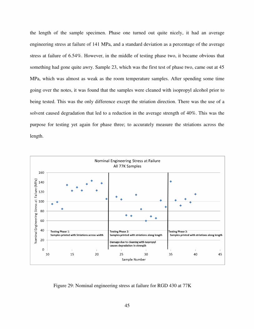
The mechanical strength test data is best broken down into the three phases of testing as

can be seen in figure 29. These phases correspond to the following:

Phase 1: Initial phase where the samples were tested with the striations across the width

(see figure 22 for reference).

Phase 2: Samples were tested with striations along the length, but had very low strength

values. This is due to cleaning with isopropyl alcohol.

Phase 3: Samples were reprinted from phase 2, and cleaned only mechanically to

give more accurate results.

The simplest stress calculation is that of the nominal engineering stress, which is the load

at divided by the nominal engineering thickness and width. The engineering stress at failure is

the load at failure divided by the initial area. For stating a conservative value the nominal area is

given as the product of the minimum of both the thickness and width as measured Thus:

(8)

In phase one the samples were printed with the intention of testing in two phases. The

first with the striations across the width, and then print some samples with the striations along

Equation 8: Engineering stress at failure A function of load at failure and the nominal engineering area

45

the length of the sample specimen. Phase one turned out quite nicely, it had an average

engineering stress at failure of 141 MPa, and a standard deviation as a percentage of the average

stress at failure of 6.54%. However, in the middle of testing phase two, it became obvious that

something had gone quite awry. Sample 23, which was the first test of phase two, came out at 45

MPa, which was almost as weak as the room temperature samples. After spending some time

going over the notes, it was found that the samples were cleaned with isopropyl alcohol prior to

being tested. This was the only difference except the striation direction. There was the use of a

solvent caused degradation that led to a reduction in the average strength of 40%. This was the

purpose for testing yet again for phase three; to accurately measure the striations across the

length.

Figure 29: Nominal engineering stress at failure for RGD 430 at 77K

46

Phase three was a retest of phase two, but with only mechanical cleaning of the samples.

This showed a minor reduction in average strength, down to 122 MPa, but as will be shown in

the coming sections, this is to be expected. Only data from phase one and phase three are used

for stress characteristics. This gives an average stress at failure of 116 MPa, and a standard

deviation of 18.7 MPa.

4.2.2 Material Stress

The more accurate method for measuring the material stress is to modify the calculation

method above to give a different stress output. The cross sectional area as described in detail

throughout chapter three varies. The variations in the width of the sample are negligible;

however the thickness of the sample can vary from the nominal by a maximum measured

difference of 0.245 mm (0.0096”). Thus to get an accurate characterization of the material

strength an accurate model for failure must be developed.

For those samples where the striations occurred across the width of the sample space, the

cross sectional area is not constant. It varies along the length of the sample space. This variation

will lead to failure in a very specific position, where the minimum thickness is observed. Thus

the material stress at failure for phase one samples should be described as :

(9)

Equation 9: Material stress at failure for RGD430 at 77K printed across the width

47

In the other case of the thickness variations occurring along the length of the sample

space as shown in figure 22, the more accurate description would be of an average thickness.

This is true due to the fact that the cross sectional area is generally constant throughout the

length of the sample. As shown in see figure 17 describing sample 39 in chapter three. Thus for

an accurate model of the material stress where the striations occur along the length of the sample,

the equation should read:

(10)

This model is not as accurate as the stress in equation 9, since the load applied will not be

symmetric, and will induce some unknown torque on the material, which will give a higher local

strain and thus higher load and thus much higher stress through the thinner portion of the

material. This gives a stress distribution shown in figure 30 in light grey.

This reduction in failure stress shown in Figure 30 for the striations perpendicular to the

length of the sample, leads to the conclusion that the samples with the striations along the width

give the more conservative data for calculation of the strength of the material in cryogenic

Equation 10: Material stress at failure for RGD 430 at 77K printed across the width

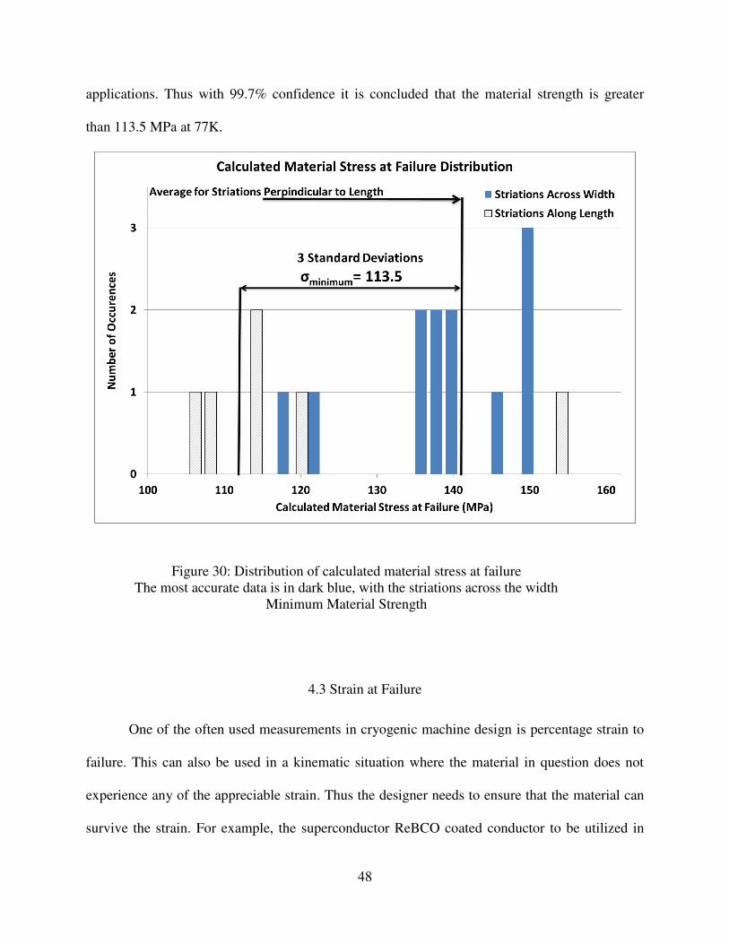
48

applications. Thus with 99.7% confidence it is concluded that the material strength is greater

than 113.5 MPa at 77K.

4.3 Strain at Failure

One of the often used measurements in cryogenic machine design is percentage strain to

failure. This can also be used in a kinematic situation where the material in question does not

experience any of the appreciable strain. Thus the designer needs to ensure that the material can

survive the strain. For example, the superconductor ReBCO coated conductor to be utilized in

Figure 30: Distribution of calculated material stress at failure The most accurate data is in dark blue, with the striations across the width

Minimum Material Strength

49

the 32T project has a well-known irreversible strain (or strain at failure) of around 0.6%. At 77K

the strain at failure of the RGD430 was measured and is described by the distribution in figure

31. This spread gives a 99.7% confidence that the strain at failure will be greater than 0.92%.

Compared to the superconductor it is in contact with, the strain at failure is sufficiently large for

most coil applications made with ReBCO coated conductor.

4.4 Fracture

The fracture mechanism is very relevant to the design consideration. The fracture mode

for each sample was cataloged and recorded, unless the fractured specimen broke into many

pieces that fell into the liquid nitrogen bath. There were two kinds of fracture, typical tensile

Figure 31: Distribution of strain at failure for RGD 430 at 77K

50

brittle fracture, and brittle fracture due to torque. The typical brittle fracture was always seen in

the samples with the striations perpendicular to the length. This is illustrated below in figure 32.

The fracture begins at one edge and propagates through the reduced area, then takes a 45 degree

angle—which is typical of brittle fractures—and continues down another valley between

striations that has a reduced area.

The fracture due to torque was always seen in samples with the parallel to the length of

the sample. These fractures are characterized by a common break along one edge, and then as

above the fracture continues down a valley between striations. This time it travels down a certain

direction down some length, and then grows in the other direction. This spreads the failure area

out and causes the pattern seen below in figure 33. There is a missing area where the failure area

spread out.

Figure 32: Brittle fracture of a sample with straitions perpendicular to the length

51

4.5 Shock Loading

The thermal shock resistance of RGD 430 was tested. In the literature many polymers

cannot survive the thermal expansion and contraction within themselves, and shatter due to

temperature gradients. This was tested by submerging samples into liquid nitrogen, and then air

warming. The samples survived multiple cycles. The samples were then submerged in liquid

nitrogen for several minutes, and then immediately immersed in water. They survived multiple

cycles. Then the samples underwent cryogenic impact studies, where they were submerged in

liquid nitrogen for several minutes and then propelled forcefully against a marble table top

immediately after exiting the cryogenic bath. The samples survived several cycles, with no

failure. Finally the samples were allowed to stay in the nitrogen bath for several minutes, upon

which they were quickly evacuated to an insulating surface of G-10 and robustly impacted with

increasing force by a hammer. They survived two impacts. The third shattered the sample. The

author believes that this is sufficient testing to show that thermal gradients, and impact loading

are not issues with this material for this particular application as a heater lead cover. It would be

a good idea to do fracture toughness tests in the future to determine a value for KIc.

Figure 33: Brittle fracture of a sample with striations parallel to the length

52

4.6 Coefficient of Thermal Expansion

One of the critical aspects of cryogenic design is the fact that materials will decrease in

spatial dimensions as the temperature decreases. This reduction in size per Kelvin change in

temperature is described as the coefficient of thermal expansion (CTE). The common units for

the CTE are K-1, however for most cryogenic materials this reduction in size is reported for a

change in length of a sample in terms of percentages. This percentage difference is for the total

change from 295K to 4K. This percentage for copper is on the order of 0.3% [7]. For the ReBCO

superconductor in the coil, it is measured as 0.315% reduction from 295K to 4K [8]. For the G-

10 that the RGD430 is intended to replace, the CTE from 295 to 4K is anisotropic. G-10 has

woven glass fibers in different directions, and they cause changes in the thermal expansion and

contraction. The percentage reduction from 295 to 4K is 0.25% in the warp direction, and 0.7%

in the normal direction [14]. As shown in figure 34 this thermal expansion is well characterized

for RGD430 and nearly 4 times larger than for copper or the superconductor:

This shows that there is a 1.8% increase in linear size from ambient to operating

conditions for RGD430. This is significantly larger than the copper or the conductor, but since it

is known about, it can be taken into account in the design. Depending on the geometry of the

situation it can be mathematically modeled, or compensated for in the “scale” of the component.

53

Figure 34: Thermal expansion of copper and RGD 430 from 4.2K to 295K

54

CHAPTER FIVE

APPLICATION TO THE HEATER LEAD COVER

The heater lead cover itself will undergo a strain controlled situation. That is the strength

of the heater lead cover should not affect how far the conductor under it will travel mechanically.

The values that determine the travel of the conductor is the radial magnetic field

magnitude and direction, the heater current magnitude and direction, and the effective modulus

Figure 35: Prototype Coil known as 20/70. Figure shows detail of a) superconducting coil with all hardware, b) cross sectional area of coil

with heater lead on the right hand side, c) the heater lead itself, and d) the heater lead profile with axial positions (in mm) from the midplane of the coil

55

of the conductor. The radial magnetic field is shown along the length of the conductor below in

figure 36:

This model was developed with the use of the program called Soleno. The worst case scenario is

when the maximum current is going through the heater lead with the longest length. Which from

the coil design makes the scenario 20 A in the heater lead, with a 312 mm long piece of

conductor. The force exerted on the conductor is given by:

(11)

Figure 36: Worst case of radial magnetic field at the position of the heater lead covers

Equation 11: Lorentz force

56

Where B is the radial field in figure 36, I is the maximum current of 20 A. These are field and

current values are vectors that are perfectly perpendicular, thus the cross product will be

orthogonal to both of them, and equal in magnitude to the scalar product of the two. This is

shown in terms of force per length as follows in figure 35:

To find the strain and see if the heater lead with RGD430 will survive, the deflection

must be calculated. The deflection is a function of the forces and moments through the body of

the conductor. The sum of forces and moments with both ends soldered in position to steel or

copper leads gives maximum resultant distributed load on the conductor of 0.00462 N/mm. If

this were a worst case scenario then: the effective force was for some reason would be 0.00462

N/mm throughout the half length of the conductor, from the top flange to the mid plane, then this

would give a total load of 0.7N. Therefore the maximum deflection encountered from equation

12 would be around 0.1577mm:

Figure 37: Load distribution applied to the conductor

57

Where delta is the deflection, q is the constant load (0.00462 N/mm), L is the length of the

applied load (half the total length 312mm/2 = 166mm) , E is the modulus of the conductor (E =

165 GPa [9]) and I is the moment of inertia through the thickness (1.755 mm4).

This deflection could easily be absorbed by the 3-D Printed RGD 430 at cryogenic

temperatures, as long as the width of the pieces was over 17mm, or 0.67”. The current design

calls for pieces to be made that are 12.7mm wide; this adjustment could be made quickly and

easily.

Equation 12: Calculation of deflection of superconducting heater leads in a worst case scenario Equation for a beam simply supported on both ends with constant load [15]

58

CHAPTER SIX

CONCLUSIONS

6.1 Review

The following characteristics were found for RGD430 at 77K:

Brittle Failure

Yield strengths ≥ 100MPa

Elastic Modulus ≥ 10GPa

Strain at failure ≥ 0.92%

Due to printing process:

o Repeatable thickness variations

o Geometric tolerances of ±0.10mm in the xy plane and +0.25/-0.10mm in

the z direction of the printer

6.2 Discussion

The majority of the characterization needed to apply this material as the heater lead

covers in 32T has been completed here. There is some additional work that could be done in the

future. That is discussed in the following section.

RGD 430 fell within the expected bounds of thermoplastics as described in the literature

for cryogenic applications [11]. Its modulus and strength increase with decreasing temperature.

The only concerns seen throughout this testing sequence was the strength reduction due

to the use of isopropyl. To mitigate this wax support material can be removed manually, and no

solvent is needed. As discussed in the following section, this should be looked into further.

59

6.3 Open Characterizations

There are several areas that should be studied before RGD430 is used in any cryogenic

system for extended lifecycles. The characterization at 4K must be done. It was not done in this

study due to budget constraints. The modulus is expected to increase, but the strength is

potentially going to decrease going from 77K to 4K [5]. See figure 2 to show that the failure

strength is reduced from 77K to 4K for many polymers. This may be detrimental to the strain at

failure, which is critical to apply RGD430 for use in the heater lead covers.

This material is somewhat porous, and may absorb water during thermal cycling to room

temperature. The expansion of water upon freezing could compromise the strength of the

material. It may not have been the isopropyl as described in chapter four that caused the damage,

but the water itself. The material listed can absorb up to 2% water in a short period of time. That

water may freeze and cause damage to the RGD430 material. This should be examined.

As described above, the fracture toughness would also be a critical test to run, as this

material always has brittle failure at cryogenic temperatures.

There will be as much as a 200 V differential between the conductor inside the heater

leads and the material outside of the heater leads. Therefore dielectric breakdown in vacuum—

also known as Paschen testing—should be performed.

There are other characterizations that would be very helpful if performed. The outgassing

of this material, as it is somewhat porous, would be a good thing to know, as the 32T will

undergo some vacuum pumping before helium cool downs.

If one were interested in utilizing this material inside of the coil winding pack itself, then

many other tests should be done, including resistivity, thin layer dielectric breakdown, thermal

conductivity as a function of temperature and specific heat as a function of temperature.

60

There are dozens of other 3-D printed materials that are available that should be

considered. In this thesis a single material has been chosen, purchased and tested. It was shown

to be a viable candidate for low strain, or rapid prototyping applications in cryogenic

environments. For the Objet 30 alone, there are 7 other similar materials that could be used.

There are additively manufactured steels, and ceramics, copper alloys, aluminum alloys and

many more materials available from commercial vendors with equally outstanding tolerances

and lead times.

It would in fact, not be outside of the scope of the MS&T department to develop 3-D

printed materials specifically for the cryogenic high field environment. A few ideas for potential

research candidates would be:

Non-magnetic austenite stabilized stainless steels

Highly cold worked and highly twinned copper for pulsed and resistive magnets

Printed polyimides as super-insulators, with extremely high dielectric breakdown

voltages

Klegecel foam substitutes as baffles for lowering thermal heat loss to cryogenic

baths

61

APPENDIX A

RESIN IDENTIFICATION IN CRYOGENIC TESTS

[5]

62

REFERENCES

[1] V. Y. Selvamanickam, "Recent Progrss in Second-Generation HTS Conductor Scale-Up at SuperPower," IEEE Transactions on Applied Superconductivity, pp. 3231-3234, 2007.

[2]

D. Verebelyi, "Low angle grain boundary transport in YBa 2 Cu 3 O 7 coated conductors," Applied Physics Letters, vol. 76, no. 13, p. 1755, January 2000.

[3] W. Markiewicz, "Design of a Superconducting 32 T Magnet With ReBCO High Field Coils," IEEE TRANSACTIONS ON APPLIED SUPERCONDUCTIVITY, vol. 22, no. 3, p. 4300704, June 2012.

[4] T. Kumura, "Study on the Effect of Magnetic Fields on Polymeric Materials and Its Applications," Polymer Journal, pp. 823-843, 2003.

[5] R. W. R. Reed, "Tensile Properties of Resins at Low Temperatures," Advances in Cryogenic

Engineering, pp. 1129-1136, 1994.

[6] E. Martinez, "Microstructures of Niobium Components Fabricated by Electron Beam Melting," Metallography, microstructure, and analysis, pp. 183-189, 11 06 2013.

[7] Stratasys, "Objet 30 Pro Spec Sheet," 2014. [Online]. Available: http://www.stratasys.com/~/media/Main/Secure/System_Spec_Sheets-SS/PolyJet/objet30%20pro%20brochure_letter%20stratasys%20low%20res.pdf.

[8] Stratasys, "Objet-MaterialBrochures-PolyJetMaterialsDataSheet-05-14," May 2014. [Online]. Available: http://www.stratasys.com/~/media/Main/Secure/Material%20Specs%20MS/PolyJet-Material-Specs/PolyJet_Materials_Data_Sheet.pdf. [Accessed 2014].

[9] Stratasys, "DOC-06143US_B1," 19 September 2011. [Online]. Available: http://www.stratasys.com/~/media/Main/Secure/MSDS/Polypropylene-like%20Materials/DOC-06143-Objet-DurusWhite-RGD430-US.PDF. [Accessed 2014].

[10] Sigma-Aldrich, "Isobornyl acrylate," 2014. [Online]. Available: http://www.sigmaaldrich.com/catalog/product/aldrich/524759?lang=en&region=US. [Accessed 2014].

63

[11] Y. Shindo, "Theoretical and Experimental Evaluation of Double-Notch Shear Strength of G-10CR Glass-Cloth/Epoxy Laminates at Cryogenic Temperatures," Journal of Enginering

Materials Technology, pp. 121-128, 01 07 1999.

[12] A. I. H. Committee, Engineered Materials Handbook Volume 2: Engineering Plastics, Metals Park, OH, 1988.

[13] R. R. R. Walsh, "Thermal Expansion Measurements of Resins (4K-300K)," Advances in

Cryogenic Engineering, vol. 40, pp. 1145-1151, 1994.

[14] R. M. D. Walsh, YBCO, Tallahassee, Fl: NHMFL-MS&T, 2014, p. Sheet "YBCO".

[15] D. Mann, "LNG Materials and Fluids," National Bureau of Standards, Cryogenic Division, 1977.

[16] R. Hibbler, Statics and Mechanics of Materials, Upper Saddle River, new Jersey: Pearson Prentice Hall, 1993.

[17] R. Walsh, 77K Stress Strain Curves and Data for Paper, Tallahassee, Fl: NHMFL-MS&T, 2011.

[18] W. D. Callister, Materials Science and Engineering an Introduction Sixth Edition, New York, New York: John Wiley & Sons, Inc., 2003.

[19] S.-Y. Fu, "Cryogenic Properties of Polymer Materials," in Polymers at Cryogenic

Temperatures, Beijing, China, Springer-Verlag Berlin Heidelberg, 2013, pp. 9-39.

64

BIOGRAPHICAL SKETCH

Zachary Johnson is a Research Engineer in the 32T project in the department of Magnet Science

and Technology at the National High Magnetic Field Laboratory. He has Bachelor’s degrees in

both Business Management and Mechanical Engineering. His graduate research is done in

addition to his engineering work at the NHMFL. All of this is done in addition to his being a

father and a husband.