Journal of Behavioral Decision Making

J. Behav. Dec. Making, 17: 395–408 (2004)

Published online in Wiley InterScience

(www.interscience.wiley.com) DOI: 10.1002/bdm.482

How Does Preference Reversal Appear andDisappear? Effects of the Evaluation Mode

CHRISTOPHE SCHMELTZER1*, JEAN-PAUL CAVERNI1

and MASSIMO WARGLIEN2

1Cognitive Psychology Laboratory, Aix-Marseille I University and CNRS, Marseille,France2Department ofBusiness, Economics andManagement, Ca’FoscariUniversity,Venice, Italy

ABSTRACT

Preference reversal is a systematic change in the preference order between optionswhen different response methods are used (e.g., choice vs. judgment). The presentstudy focuses on procedures used to elicit preferences according to an evaluabilityhypothesis. Two experiments compared joint vs. separate evaluations and explicit vs.non-explicit joint evaluations. Subjects had to express preferences between high-variance gambles (HVGs) and low-variance gambles (LVGs) either by choosing onegamble to play in a lottery or by assigning gambles minimum selling prices. We showthat HVGs are preferred in both choice and pricing conditions when gambles areevaluated separately, and LVGs are preferred in both choice and selling conditionswhen gambles are evaluated in pairs: i.e., when the evaluation mode is heldconstant, classic preference reversal disappears. These results support the evaluabilityhypothesis, and suggest that preferences depend on whether subjects are allowed tocompare the options they are asked to choose from or judge, independently of thenature of the scale (i.e., attractiveness vs. minimum selling price) they are requiredto adopt. Copyright # 2004 John Wiley & Sons, Ltd.

key words preference reversal; evaluability hypothesis; anchoring and adjustment;

evaluation mode

INTRODUCTION

In this paper we explore the hypothesis that preference reversal (PR) in lotteries is driven by the evaluation

mode, i.e., the way pairs of gambles are to be evaluated, whether jointly or separately, independently of the

worth scale—i.e., the nature of the scale—under consideration (e.g., attractiveness or minimum selling

Copyright # 2004 John Wiley & Sons, Ltd.

* Correspondence to: Christophe Schmeltzer, Universite d’Aix-Marseille I, Laboratoire de Psychologie Cognitive, Case 66, 3 PlaceVictor Hugo, F-13331 Marseille Cedex 3, France. E-mail: christophe.schmeltzer@up.univ-mrs.fr

price). We suggest that the relative difficulty in taking into account the variance of lottery outcomes in sepa-

rate evaluation (SE) is largely responsible for the presence or absence of PR. The role of worth scales usually

associated with the choice/judgment distinction may thus have been overemphasized, due to confusion

between evaluation mode and worth scale in most classic experiments on PR.

The PR phenomenon has been attracting interest for more than thirty years, i.e., since the pioneering work

by Lichtenstein and Slovic (1971). It can be broadly defined as a change in the preference order between

options when different procedures are used to elicit such preferences. The best-known example involves lot-

tery gambles in choice vs. judgment procedures: subjects are presented with two different gambles of equal

(or nearly equal) expected value. When choosing which of the two gambles is more attractive, subjects

usually prefer low-variance gambles (LVGs)—called ‘‘P-bet’’ in the PR literature—with high probability

of low winnings (e.g., 28/36 chances of winning $10). When evaluating the minimum selling price of each

gamble, however, the same subjects prefer high-variance gambles (HVGs)—called ‘‘$-bet’’ in the PR litera-

ture—with low probability of high winnings (e.g., 3/36 chances of winning $100). We will refer to this base-

line phenomenon as ‘‘classic’’ PR.

Having resisted many experimental trials (cf. Lichtenstein & Slovic, 1971; Grether & Plott, 1979;

Pommerehne, Schneider, & Zweifel, 1982; Reilly, 1982),1 over time, the PR phenomenon has demonstrated

its robustness (usually from 40% to 50% of responses show classic PR), and has been replicated in a growing

set of decision tasks. This has not come without paying the price of increasing complexity: multiple factors

generating PR have emerged, together with different theoretical explanations trying to account for the phe-

nomenon. For extensive reviews, see Slovic and Lichtenstein (1983), Tversky, Slovic, and Kahneman

(1990), and Camerer (1995).

If PR can be caused by many different factors, interactions between them may matter. These interactions

have not been sufficiently investigated (Caverni, 1996). In this sense the most important exception is the

work of Goldstein and Einhorn (1987), which proposed distinguishing two dimensions of the procedures

involved in classic decision-making tasks: the ‘‘response method’’ (‘‘ . . .what subjects have been asked to

do, i.e., choose or judge’’, p. 237) and the ‘‘worth scale’’ (‘‘ . . . the scale the subjects have been asked to do it

with, i.e., attractiveness or minimum selling price’’, p. 237). This distinction led them to define different

types of PR according to different combinations of the response method and the worth scale.

Goldstein and Einhorn’s distinction has recently been further developed by Hsee et al. (1999) to clarify the

role of the response method. Hsee et al. suggest that a basic source of differentiation between response meth-

ods is due to the degree of comparativeness of the evaluation process induced by the decision procedure.

Joint evaluation (JE) occurs when the options are presented simultaneously, and they are easily compared;

separate evaluation (SE) corresponds to opposite situations in which options are presented and evaluated one

after the other. Hsee et al. show that a shift from JE to SE mode is sufficient to induce PR, with the worth

scale constant. They explain the effect by resorting to the notion of evaluability: some attributes are easier to

evaluate in isolation, while others will be fully apprehended and appreciated only by comparing the options.

Easily evaluable attributes are likely to play a prominent role in SE, while attributes with weaker evaluability

will enter the evaluation process only in JE.

While Hsee et al. carefully restrict their explanation to the case in which the worth scale is held constant, it

is tempting to extend their argument and suggest that in many cases the effect might persist over different

worth scales (as in the case of classic PR). In particular, we expect that, independently of the worth scale

under consideration, when lotteries are presented one by one, the variance of single lotteries is comparatively

harder to evaluate than in JE conditions. Thus, variance should affect subjects’ decision making only in the

JE mode, when a direct comparison of the variance in lotteries can be made. In the classic PR experimental

1By using a procedure involving simultaneous tasks, (i.e., choosing and pricing at the same time), which forced subjects to debias theirjudgements and make explicit their discrepancies, Ordonez et al. (1995) observed that the phenomenon was significantly reduced. In thispaper, we will refer only to the classic conditions (sequential tasks).

396 Journal of Behavioral Decision Making

Copyright # 2004 John Wiley & Sons, Ltd. Journal of Behavioral Decision Making, 17, 395–408 (2004)

paradigm, subjects choose after the joint presentation of a pair of lotteries, while they evaluate separately the

minimum selling price of each lottery. PR might therefore be caused by differences in the relative importance

accorded to variance in different conditions. We suggest that when the evaluation mode is constant, classic

PR should be considerably weakened or even disappear.

Care must be taken in selecting an object for choice simple enough for a stringent formulation of our

hypothesis. A lottery gamble is the most classic object in the PR literature. Gambles are quite complex infor-

mational objects: they contain information on probabilities and outcomes, and both are needed to compute

(even approximately) expected values and variance. This might make gambles ill-suited to a study testing the

evaluability hypothesis: too many factors might affect individual evaluation processes. Ganzach (1996),

however, has recently introduced simpler gambles with equiprobable outcomes and nearly equal expected

values (for the sake of simplicity, we will refer to such gambles as eq-gambles, for equiprobable outcomes

and equal expected values). Ganzach showed that the PR phenomenon also holds with eq-gambles (31% of

classic PR): although most subjects choose LVGs in which all outcomes are moderate (e.g., win one, and

only one, of these five outcomes: $28, $44, $52, $56 or $72), they put a higher price on HVGs, with higher as

well as lower outcomes (e.g., win one, and only one, of these five outcomes: $10, $18, $54, $80 or $90).

These gambles considerably reduce cognitive difficulties connected to probabilities, leaving all variance

to be determined by the values of different outcomes and making the calculation of expected values a rela-

tively simple arithmetic task. We thus decided to use these kinds of gambles in our experiments.

Applied to eq-gambles, our hypothesis can be stated as follows: since the role of probability is eliminated

by the use of equiprobable outcomes, the main sources of differentiation between eq-gambles are the value

of each outcome, the most salient outcomes, and the variance (or other risk-related parameters) of outcomes

in each gamble. We expect, therefore, that in SE, variance would be the less-evaluable attribute of an eq-

gamble; in this case, salient values should play a key role in the evaluation process. Earlier experiments

suggest that an anchoring and adjustment process should occur for the highest monetary outcomes of each

gamble (cf. Slovic & Lichtenstein, 1968; Lichtenstein & Slovic, 1971; Schkade & Johnson, 1989; Ganzach,

1996). Consequently, HVGs that have the highest monetary outcomes should be preferred in SE. In JE, how-

ever, it should be fairly easy to compare the variance of gambles. Risk considerations should play a larger

role in the evaluation process, and risk-averse behavior (i.e., LVG preference) should be expected to prevail,

at least provided that gambles are defined in the domain of gains (Kahneman & Tversky, 1979).

We also expect the worth scale to have less effect on evaluability: whether the worth scale is attractiveness

or minimum selling price, variance should be the hardest attribute to evaluate, and the JE/SE distinction

should dominate over worth-scale differences. Consequently, we predict that while PR will appear whenever

JE and SE are compared, more consistent preferences should be revealed when the evaluation mode is held

constant, even if different worth scales are compared. Moreover, according to our hypothesis, different kinds

of consistency should emerge when different worth scales are compared in constant JE or SE conditions. In

SE, subjects should consistently tend to prefer HVGs, since variance is hard to evaluate; in JE, variance is

more likely to be taken into account, and consistent preferences for LVGs are expected to be the modal

response.

Lastly, we also try to investigate process data that could test our proposals. The evaluability hypothesis

emphasizes the relative difficulty in evaluating information about different attributes as a source of PR. This

should be reflected in the processes by which subjects search and compare information on gambles. A self-

paced display time paradigm (SDTP) enables us to follow these processes. Subjects are presented with slots

of covered information on a computer screen and asked to uncover the screen by passing the mouse on the

slots or by pressing keys. It is thus possible to record how much time subjects spend looking at each stimulus,

and what sequence of information slots they go through (cf. Caverni, 1987; Schkade & Johnson, 1989;

Payne, Bettman, & Johnson, 1992). If their preference for HVGs depends on an anchoring and adjustment

process, subjects should focus more on the highest outcomes, while those consistently preferring LVGs

should distribute their time more evenly among the outcomes.

C. Schmeltzer et al. Preference Reversal 397

Copyright # 2004 John Wiley & Sons, Ltd. Journal of Behavioral Decision Making, 17, 395–408 (2004)

EXPERIMENT 1: JOINT EVALUATION VERSUS SEPARATE EVALUATION WITH

ATTRACTIVENESS AND MINIMUM SELLING PRICE WORTH SCALES

The aim of Experiment 1 was to check if: (1) the PR phenomenon still occurs with eq-gambles when making

use of the classic elicitation procedures (control group); (2) classic PR is reduced when the same evaluation

mode is used for both attractiveness and minimum selling price worth scales (JE and SE groups); and (3)

both anchoring and evaluability have an effect on the allocation of attention (control, JE, and SE groups).

In each group, every subject evaluated the stimuli under both attractiveness and minimum selling price

conditions. Within each group, half of the subjects dealt with the attractiveness condition first, while the

other half dealt with the minimum selling price condition first.

Method

Participants

Ninety-six psychology undergraduate students participated: 32 in each group. In the control and JE groups,

20 subjects were from the University of Quebec in Montreal and 12 from Aix-Marseille I University; in the

SE group all subjects were from Aix-Marseille I University.

Stimuli

The stimuli were 16 eq-gambles. Each gamble involved four possible outcomes ranging from the lowest to

the highest. The outcomes were either in French francs (FF) or in Canadian dollars ($C) according to the

subjects’ nationality: the lowest outcome was FF3 ($C1), the highest was FF368 ($C109). The lottery con-

sisted of selecting only one of the four possible outcomes for each gamble. Thus, for each gamble, subjects

were sure to win one of the four outcomes, and the probability of winning one of each of these outcomes was

0.25.

For example, if the first outcome was selected, subjects could only win FF7 with a gamble involving the

outcomes FF7, FF31, FF56, or FF106 (HVG), while they could win FF34 with a gamble involving the out-

comes FF34, FF46, FF53, or FF67 (LVG). If the fourth outcome was selected, subjects could win FF106 with

the HVG, while they could only win FF67 with the LVG.

Each pair of these gambles included an LVG and an HVG with equal expected values (FF50 ($C15) or

FF150 ($C45)). The range of each HVG was always three-times larger than the range of the LVG, and the

number of outcomes dominating the corresponding outcomes in the other gamble of the same pair was

manipulated: for one pair, the LVG had three outcomes higher than the HVG; for a second pair, the LVG

had three outcomes lower than the HVG; and for two others, the LVG and HVG had an equal number of

dominating outcomes (cf. Table 1).

Material

The experiment was run on a PC, and the SDTP was carried out by a Cþþ program with sequential infor-

mation processing. Gambles were presented randomly and masked. In order to look at the outcome of each

gamble, subjects had to press the appropriate colored keys on the keyboard, each key corresponding to only

one outcome. Each outcome remained visible as long as the subjects pressed the corresponding key. It was

impossible to look at two outcomes at the same time, but subjects could look at them individually as many

times and for as long as they wanted. Another key was pressed to make the response. When subjects made an

outcome visible on the screen, the program recorded which outcome it was and the time spent on it. This

material allowed us to study the visualization times for each outcome and the visualization times for each

gamble.

398 Journal of Behavioral Decision Making

Copyright # 2004 John Wiley & Sons, Ltd. Journal of Behavioral Decision Making, 17, 395–408 (2004)

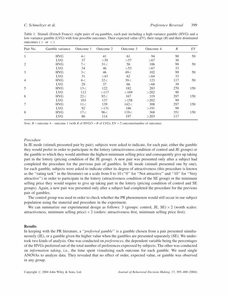
Procedure

In JE mode (stimuli presented pair by pair), subjects were asked to indicate, for each pair, either the gamble

they would prefer in order to participate in the lottery (attractiveness condition of control and JE groups) or

the gamble to which they would attribute the highest minimum selling price and consequently give up taking

part in the lottery (pricing condition of the JE group). A new pair was presented only after a subject had

completed the procedure for the previous pair of gambles. In SE mode (stimuli presented one by one),

for each gamble, subjects were asked to indicate either its degree of attractiveness (this procedure is known

as the ‘‘rating task’’ in the literature) on a scale from 0 to 10 (‘‘0’’ for ‘‘Not attractive’’ and ‘‘10’’ for ‘‘Very

attractive’’) in order to participate in the lottery (attractiveness condition of the SE group) or the minimum

selling price they would require to give up taking part in the lottery (pricing condition of control and SE

groups). Again, a new pair was presented only after a subject had completed the procedure for the previous

pair of gambles.

The control group was used in order to check whether the PR phenomenon would still occur in our subject

population using the material and procedure in the experiment.

We can summarize our experimental design as follows: 3 (groups: control, JE, SE)� 2 (worth scales:

attractiveness, minimum selling price)� 2 (orders: attractiveness first, minimum selling price first).

Results

In keeping with the PR literature, a ‘‘preferred gamble’’ is a gamble chosen from a pair presented simulta-

neously (JE), or a gamble given the higher value when the gambles are presented separately (SE). We under-

took two kinds of analysis. One was conducted on preferences, the dependent variable being the percentages

of the HVGs preferred out of the total number of preferences expressed by subjects. The other was conducted

on information taking, i.e., the time spent visualizing each outcome for each gamble. We used single

ANOVAs to analyze data. They revealed that no effect of order, expected value, or gamble was observed

in any group.

Table 1. Stimuli (French Francs): eight pairs of eq-gambles, each pair including a high-variance gamble (HVG) and alow-variance gamble (LVG) with four possible outcomes. Their expected value (EV), their range (R) and their dominatedoutcomes (> or < )

Pair No. Gamble variance Outcome 1 Outcome 2 Outcome 3 Outcome 4 R EV

1 HVG 4< 41 61 94 90 50LVG 37 >39 >57 >67 30

2 HVG 7< 31< 56 106 99 50LVG 34 46 >53 >67 33

3 HVG 3< 46 49< 102 99 50LVG 31 >43 62 >64 33

4 HVG 6< 32< 39< 123 117 50LVG 29 37 66 >68 39

5 HVG 13< 122 182 283 270 150LVG 112 >117 >169 >202 90

6 HVG 22< 92< 167 319 297 150LVG 103 137 >158 >202 99

7 HVG 11< 139 142< 308 297 150LVG 92 >131 186 >191 99

8 HVG 17< 96< 119< 368 351 150LVG 86 114 197 >203 117

Note: R¼ outcome 4 – outcome 1 (with R of HVG/3¼R of LVG); EV¼� outcome/number of outcomes.

C. Schmeltzer et al. Preference Reversal 399

Copyright # 2004 John Wiley & Sons, Ltd. Journal of Behavioral Decision Making, 17, 395–408 (2004)

Preferences

Table 2 summarizes the results. In the control group, the PR phenomenon was neatly reproduced. In the

attractiveness condition, the LVGs were preferred, while in the pricing condition, preferences were reversed:

the percentages (64 vs. 34) of HVGs preferred were significantly different (F(1, 31)¼ 21.52, p< 0.0001)2

between the two worth scales. The JE and SE groups, on the other hand, show that consistent patterns of

response can be obtained when the response method is held constant by the evaluation mode: there were

no significant differences between the rates of HVGs preferred in the JE group (F(1, 31)¼ 2.79, p< 0.1)

and those in the SE group (F(1, 31)¼ 0.07, p< 0.79). Moreover, the percentages of HVGs preferred (36

vs. 63 and 46 vs. 62) were significantly different in the JE and SE groups (F(1, 62)¼ 16.43, p< 0.0001,

in the attractiveness condition and F(1, 62)¼ 4.10, p< 0.04 in the pricing condition), independently of

the worth scale. Lastly, these results reveal an evaluation-mode effect (F(1, 188)¼ 28.32, p< 0.0001) but

not a worth-scale effect (F(1, 188)¼ 1.53, p< 0.3).

Between-subject comparisons of our different groups show the remarkable overall robustness of each

experimental outcome. The comparison between control and JE groups shows that while there were no sig-

nificant differences between the percentages of HVGs preferred (36 vs. 34) in the JE/attractiveness combi-

nations, the percentage (64) in the control/minimum selling price combination was significantly different

from the percentage (46) in the JE/minimum selling price combination (F(1, 62)¼ 5.49, p< 0.02). The com-

parison between control and SE groups shows a complementary pattern: while there were no significant dif-

ferences between the percentages (64 vs. 62) of HVGs preferred in the SE/minimum selling price

combinations, the percentage (34) in the JE/attractiveness combination was significantly different from

the percentage (63) given in the SE/attractiveness combination (F(1, 62)¼ 20.71, p< 0.00001).

2All F-tests were performed at an alpha level of 0.01.

Table 2. Percentages of high-variance gambles (HVGs) preferred (gray), of preference reversal (bold), and of the modalresponse (*), for each group and each worth scale (attractiveness vs. minimum selling price) in Experiment 1

Control groupMinimum selling price

HVG LVG

Attractiveness HVG 23 11 34LVG 41* 25 66

64 36 100

Joint evaluation groupMinimum selling price

HVG LVGAttractiveness HVG 21 15 36

LVG 25 39* 6446 54 100

Separate evaluation groupMinimum selling price

HVG LVGAttractiveness HVG 40* 23 63

LVG 22 15 3762 38 100

400 Journal of Behavioral Decision Making

Copyright # 2004 John Wiley & Sons, Ltd. Journal of Behavioral Decision Making, 17, 395–408 (2004)

Further insight can be gained by comparing the rate of classic PR responses in the three groups: the

percentages of this inconsistency were significantly lower (25) in the JE group (F(1, 62)¼ 5.82, p< 0.02)

and (22) in the SE group (F(1, 62)¼ 9.19, p< 0.004), than in the control group (41), while there was no

difference (F(1, 62)¼ 0.40, p< 0.6) between those in the JE and SE groups. Moreover, while the modal

pattern of response in the control group was a classic PR response, in the JE and SE groups the modal

pattern of response was a consistent response. This demonstrates that the PR phenomenon effectively

disappeared.3

Information taking

Process observations provided by the use of the SDTP offer insight into the actual patterns of attention

related to subjects’ responses. Former process analyses of PR (Schkade & Johnson, 1989) have shown that

different average response times correspond to different worth scales. The minimum selling price condition

shows systematically higher response times than the attractiveness condition (choice or rating). We obtained

similar findings in our experiment. In all three groups (cf. Table 3) the minimum selling price condition

involved visualization times for each gamble (i.e., the sum of visualization times of the four possible out-

comes for each, gamble) approximately 50% higher than with the attractiveness condition:

F(1, 454)¼ 28.88, p< 0.0001 for the control group, F(1, 508)¼ 22.53, p< 0.00001 for the JE group, and

F(1, 358)¼ 32.35, p< 0.00001 for the SE group.

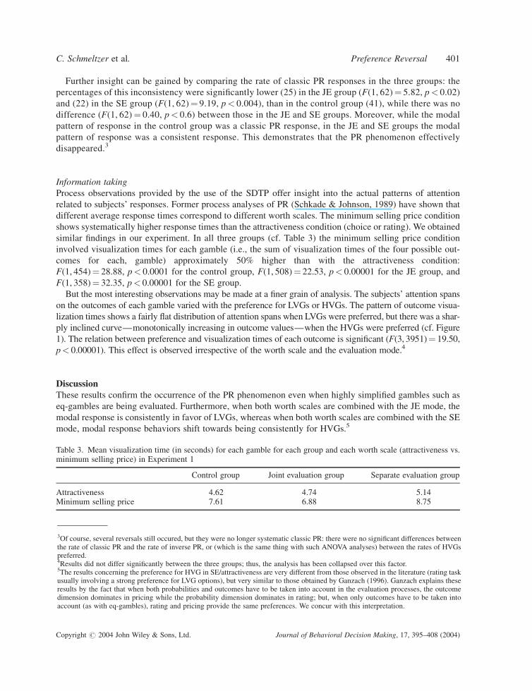
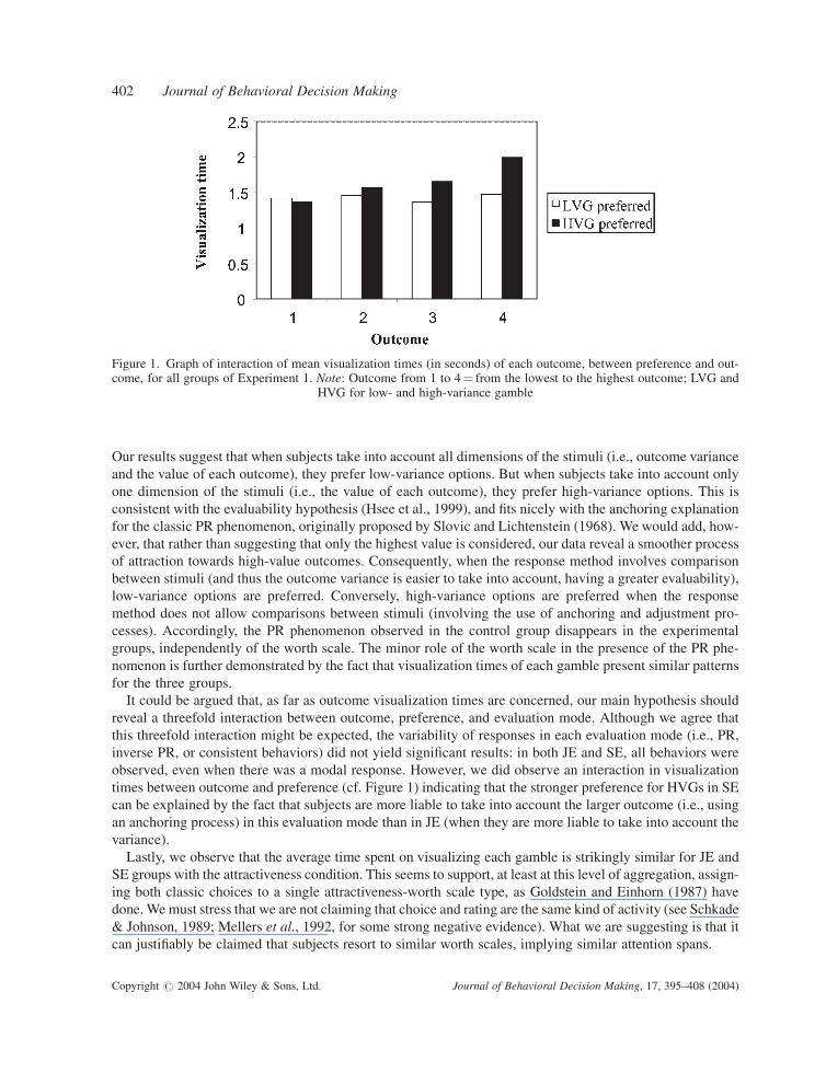
But the most interesting observations may be made at a finer grain of analysis. The subjects’ attention spans

on the outcomes of each gamble varied with the preference for LVGs or HVGs. The pattern of outcome visua-

lization times shows a fairly flat distribution of attention spans when LVGs were preferred, but there was a shar-

ply inclined curve—monotonically increasing in outcome values—when the HVGs were preferred (cf. Figure

1). The relation between preference and visualization times of each outcome is significant (F(3, 3951)¼ 19.50,

p< 0.00001). This effect is observed irrespective of the worth scale and the evaluation mode.4

Discussion

These results confirm the occurrence of the PR phenomenon even when highly simplified gambles such as

eq-gambles are being evaluated. Furthermore, when both worth scales are combined with the JE mode, the

modal response is consistently in favor of LVGs, whereas when both worth scales are combined with the SE

mode, modal response behaviors shift towards being consistently for HVGs.5

3Of course, several reversals still occured, but they were no longer systematic classic PR: there were no significant differences betweenthe rate of classic PR and the rate of inverse PR, or (which is the same thing with such ANOVA analyses) between the rates of HVGspreferred.4Results did not differ significantly between the three groups; thus, the analysis has been collapsed over this factor.5The results concerning the preference for HVG in SE/attractiveness are very different from those observed in the literature (rating taskusually involving a strong preference for LVG options), but very similar to those obtained by Ganzach (1996). Ganzach explains theseresults by the fact that when both probabilities and outcomes have to be taken into account in the evaluation processes, the outcomedimension dominates in pricing while the probability dimension dominates in rating; but, when only outcomes have to be taken intoaccount (as with eq-gambles), rating and pricing provide the same preferences. We concur with this interpretation.

Table 3. Mean visualization time (in seconds) for each gamble for each group and each worth scale (attractiveness vs.minimum selling price) in Experiment 1

Control group Joint evaluation group Separate evaluation group

Attractiveness 4.62 4.74 5.14Minimum selling price 7.61 6.88 8.75

C. Schmeltzer et al. Preference Reversal 401

Copyright # 2004 John Wiley & Sons, Ltd. Journal of Behavioral Decision Making, 17, 395–408 (2004)

Our results suggest that when subjects take into account all dimensions of the stimuli (i.e., outcome variance

and the value of each outcome), they prefer low-variance options. But when subjects take into account only

one dimension of the stimuli (i.e., the value of each outcome), they prefer high-variance options. This is

consistent with the evaluability hypothesis (Hsee et al., 1999), and fits nicely with the anchoring explanation

for the classic PR phenomenon, originally proposed by Slovic and Lichtenstein (1968). We would add, how-

ever, that rather than suggesting that only the highest value is considered, our data reveal a smoother process

of attraction towards high-value outcomes. Consequently, when the response method involves comparison

between stimuli (and thus the outcome variance is easier to take into account, having a greater evaluability),

low-variance options are preferred. Conversely, high-variance options are preferred when the response

method does not allow comparisons between stimuli (involving the use of anchoring and adjustment pro-

cesses). Accordingly, the PR phenomenon observed in the control group disappears in the experimental

groups, independently of the worth scale. The minor role of the worth scale in the presence of the PR phe-

nomenon is further demonstrated by the fact that visualization times of each gamble present similar patterns

for the three groups.

It could be argued that, as far as outcome visualization times are concerned, our main hypothesis should

reveal a threefold interaction between outcome, preference, and evaluation mode. Although we agree that

this threefold interaction might be expected, the variability of responses in each evaluation mode (i.e., PR,

inverse PR, or consistent behaviors) did not yield significant results: in both JE and SE, all behaviors were

observed, even when there was a modal response. However, we did observe an interaction in visualization

times between outcome and preference (cf. Figure 1) indicating that the stronger preference for HVGs in SE

can be explained by the fact that subjects are more liable to take into account the larger outcome (i.e., using

an anchoring process) in this evaluation mode than in JE (when they are more liable to take into account the

variance).

Lastly, we observe that the average time spent on visualizing each gamble is strikingly similar for JE and

SE groups with the attractiveness condition. This seems to support, at least at this level of aggregation, assign-

ing both classic choices to a single attractiveness-worth scale type, as Goldstein and Einhorn (1987) have

done. We must stress that we are not claiming that choice and rating are the same kind of activity (see Schkade

& Johnson, 1989; Mellers et al., 1992, for some strong negative evidence). What we are suggesting is that it

can justifiably be claimed that subjects resort to similar worth scales, implying similar attention spans.

Figure 1. Graph of interaction of mean visualization times (in seconds) of each outcome, between preference and out-come, for all groups of Experiment 1. Note: Outcome from 1 to 4¼ from the lowest to the highest outcome; LVG and

HVG for low- and high-variance gamble

402 Journal of Behavioral Decision Making

Copyright # 2004 John Wiley & Sons, Ltd. Journal of Behavioral Decision Making, 17, 395–408 (2004)

EXPERIMENT 2: EXPLICIT COMPARISON VERSUS NON-EXPLICIT COMPARISON

IN JOINT EVALUATION

Our second experiment was designed to provide an answer to a possible objection to Experiment 1, while

refining the evaluability hypothesis. A possible weakness in the design of Experiment 1 concerns the eva-

luation of the minimum selling price in the JE group. In this condition, subjects were asked to indicate the

gamble for which they would ask the highest minimum selling price for each pair of gambles. It might be

objected that this kind of task does not necessarily require that subjects actually estimate the minimum

selling prices of both gambles—they might just answer by indicating one gamble without using a numer-

ical scale. In that case the task would be much closer to the attractiveness condition than to the pricing

condition. The consistent behavior observed in the JE group might thus reflect a design fault. We

thus designed a variation on the original JE group in which subjects, besides evaluating attractiveness

as in Experiment 1, would have to indicate the gamble for which they would ask the highest minimum

selling price in each pair of gambles. Moreover, they were also asked to indicate the minimum selling

price for each gamble. Our hypothesis was, of course, that the behavior in this case would be very similar

to that observed in the JE group in Experiment 1. We labeled this group the ‘‘JE-explicit comparison

group.’’

At the same time, we wished to refine our understanding of the evaluability hypothesis. In particular,

we were interested in assessing how much the evaluability effect is due to an evaluation mode effect

(JE vs. SE) or to the comparative nature of the task. We thus presented two tasks to a second group

of subjects, maintaining the JE mode. The first included the attractiveness condition of Experiment 1,

while in the second task, subjects were asked to indicate the minimum selling price for each gamble

(numerical scale only) in each pair of gambles, without having to make any explicit comparison

between gambles. We labeled this group the ‘‘JE-non-explicit comparison group.’’ Our hypothesis was

that in the absence of an explicitly comparative task, the effects of the JE mode would be significantly

weakened.

Method

The stimuli (only in FF) and the material were the same as in Experiment 1. Each subject evaluated the sti-

muli in both attractiveness and minimum selling price conditions.

Participants

Sixty (28 in the JE-explicit comparison group and 32 in the JE-non-explicit comparison group) psychology

undergraduate students at Aix-Marseille I University participated. Within each group, half of the subjects

dealt with the attractiveness condition first, while the other half dealt with the minimum selling price condition

first.

Procedure

The attractiveness condition in the JE-explicit and JE-non-explicit comparison groups was the same as in the

control and JE groups in Experiment 1. In the pricing condition of the JE-explicit comparison group (stimuli

presented pair by pair), for each pair, subjects were asked to indicate the gamble to which they would attri-

bute the highest minimum selling price to give up taking part in the lottery and the minimum selling price for

each gamble. In the pricing condition of the JE-non-explicit comparison group (stimuli presented pair by

pair), for each gamble, subjects were asked to indicate only the minimum selling price that they would

require to give up taking part in the lottery.

C. Schmeltzer et al. Preference Reversal 403

Copyright # 2004 John Wiley & Sons, Ltd. Journal of Behavioral Decision Making, 17, 395–408 (2004)

ResultsPreferences

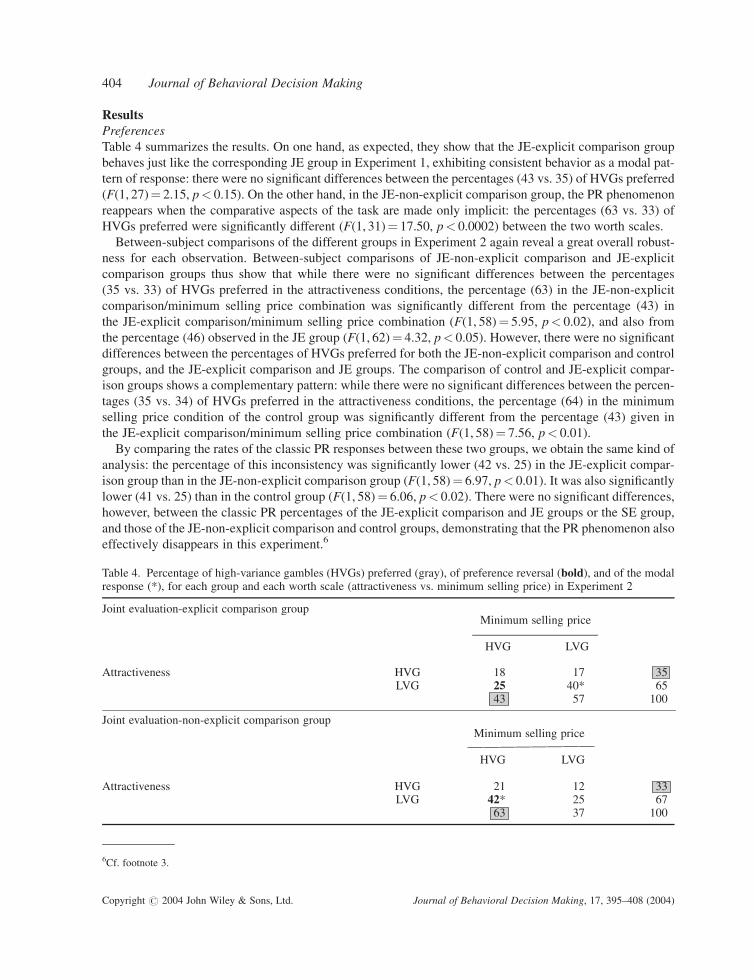
Table 4 summarizes the results. On one hand, as expected, they show that the JE-explicit comparison group

behaves just like the corresponding JE group in Experiment 1, exhibiting consistent behavior as a modal pat-

tern of response: there were no significant differences between the percentages (43 vs. 35) of HVGs preferred

(F(1, 27)¼ 2.15, p< 0.15). On the other hand, in the JE-non-explicit comparison group, the PR phenomenon

reappears when the comparative aspects of the task are made only implicit: the percentages (63 vs. 33) of

HVGs preferred were significantly different (F(1, 31)¼ 17.50, p< 0.0002) between the two worth scales.

Between-subject comparisons of the different groups in Experiment 2 again reveal a great overall robust-

ness for each observation. Between-subject comparisons of JE-non-explicit comparison and JE-explicit

comparison groups thus show that while there were no significant differences between the percentages

(35 vs. 33) of HVGs preferred in the attractiveness conditions, the percentage (63) in the JE-non-explicit

comparison/minimum selling price combination was significantly different from the percentage (43) in

the JE-explicit comparison/minimum selling price combination (F(1, 58)¼ 5.95, p< 0.02), and also from

the percentage (46) observed in the JE group (F(1, 62)¼ 4.32, p< 0.05). However, there were no significant

differences between the percentages of HVGs preferred for both the JE-non-explicit comparison and control

groups, and the JE-explicit comparison and JE groups. The comparison of control and JE-explicit compar-

ison groups shows a complementary pattern: while there were no significant differences between the percen-

tages (35 vs. 34) of HVGs preferred in the attractiveness conditions, the percentage (64) in the minimum

selling price condition of the control group was significantly different from the percentage (43) given in

the JE-explicit comparison/minimum selling price combination (F(1, 58)¼ 7.56, p< 0.01).

By comparing the rates of the classic PR responses between these two groups, we obtain the same kind of

analysis: the percentage of this inconsistency was significantly lower (42 vs. 25) in the JE-explicit compar-

ison group than in the JE-non-explicit comparison group (F(1, 58)¼ 6.97, p< 0.01). It was also significantly

lower (41 vs. 25) than in the control group (F(1, 58)¼ 6.06, p< 0.02). There were no significant differences,

however, between the classic PR percentages of the JE-explicit comparison and JE groups or the SE group,

and those of the JE-non-explicit comparison and control groups, demonstrating that the PR phenomenon also

effectively disappears in this experiment.6

Table 4. Percentage of high-variance gambles (HVGs) preferred (gray), of preference reversal (bold), and of the modalresponse (*), for each group and each worth scale (attractiveness vs. minimum selling price) in Experiment 2

Joint evaluation-explicit comparison groupMinimum selling price

HVG LVG

Attractiveness HVG 18 17 35LVG 25 40* 65

43 57 100

Joint evaluation-non-explicit comparison groupMinimum selling price

HVG LVG

Attractiveness HVG 21 12 33LVG 42* 25 67

63 37 100

6Cf. footnote 3.

404 Journal of Behavioral Decision Making

Copyright # 2004 John Wiley & Sons, Ltd. Journal of Behavioral Decision Making, 17, 395–408 (2004)

Information taking

As regards information, we find the same effects as in Experiment 1. First, concerning the global visualiza-

tion times: in the two groups (F(1, 448)¼ 78.89, p< 0.00001, for the JE-explicit comparison group and

F(1, 442)¼ 77.53, p< 0.00001, for the JE-non-explicit comparison group), the minimum selling price con-

dition significantly involved visualization times approximately 50% higher than the attractiveness condition

(cf. Table 5).

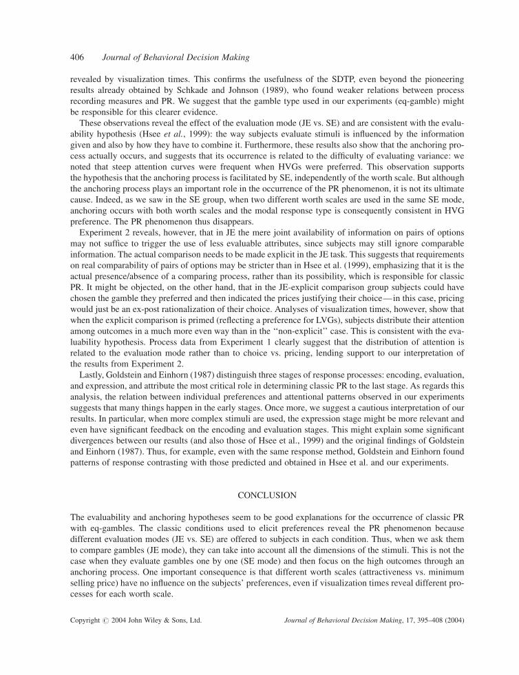
Second, concerning the time spent on each outcome: when subjects preferred LVGs, each outcome was

visualized with a similar attention span, while we observed an increasing focalization on the highest values

when subjects preferred HVGs (cf. Figure 2: the interaction between the preference and the outcomes visua-

lization time was significant (F(3, 2625)¼ 16.36, p< 0.00001).

GENERAL DISCUSSION

By showing both the presence of PR and its disappearance, our results support the hypothesis that the shift in

the evaluation mode can be the major cause of this phenomenon, even across different worth scales, thus also

suggesting that the worth scales only play a minor role. Furthermore, the results show that, when influenced

by response method, different individual preferences also have an impact on the distribution of attention, as

Table 5. Mean visualization time (in seconds) for each gamble for each group and each worth scale (attractiveness vs.minimum selling price) in Experiment 2

Joint evaluation-explicit comparison group Joint evaluation-non-explicit comparison group

Attractiveness 4.83 5.01Minimum selling price 10.21 11.76

Figure 2. Graph of interaction of mean visualization times (in seconds) for each outcome, between preference and out-come, for all groups of Experiment 2. Note: Outcome from 1 to 4¼ from the lowest to the highest outcome; LVG and

HVG for low- and high-variance gamble

C. Schmeltzer et al. Preference Reversal 405

Copyright # 2004 John Wiley & Sons, Ltd. Journal of Behavioral Decision Making, 17, 395–408 (2004)

revealed by visualization times. This confirms the usefulness of the SDTP, even beyond the pioneering

results already obtained by Schkade and Johnson (1989), who found weaker relations between process

recording measures and PR. We suggest that the gamble type used in our experiments (eq-gamble) might

be responsible for this clearer evidence.

These observations reveal the effect of the evaluation mode (JE vs. SE) and are consistent with the evalu-

ability hypothesis (Hsee et al., 1999): the way subjects evaluate stimuli is influenced by the information

given and also by how they have to combine it. Furthermore, these results also show that the anchoring pro-

cess actually occurs, and suggests that its occurrence is related to the difficulty of evaluating variance: we

noted that steep attention curves were frequent when HVGs were preferred. This observation supports

the hypothesis that the anchoring process is facilitated by SE, independently of the worth scale. But although

the anchoring process plays an important role in the occurrence of the PR phenomenon, it is not its ultimate

cause. Indeed, as we saw in the SE group, when two different worth scales are used in the same SE mode,

anchoring occurs with both worth scales and the modal response type is consequently consistent in HVG

preference. The PR phenomenon thus disappears.

Experiment 2 reveals, however, that in JE the mere joint availability of information on pairs of options

may not suffice to trigger the use of less evaluable attributes, since subjects may still ignore comparable

information. The actual comparison needs to be made explicit in the JE task. This suggests that requirements

on real comparability of pairs of options may be stricter than in Hsee et al. (1999), emphasizing that it is the

actual presence/absence of a comparing process, rather than its possibility, which is responsible for classic

PR. It might be objected, on the other hand, that in the JE-explicit comparison group subjects could have

chosen the gamble they preferred and then indicated the prices justifying their choice—in this case, pricing

would just be an ex-post rationalization of their choice. Analyses of visualization times, however, show that

when the explicit comparison is primed (reflecting a preference for LVGs), subjects distribute their attention

among outcomes in a much more even way than in the ‘‘non-explicit’’ case. This is consistent with the eva-

luability hypothesis. Process data from Experiment 1 clearly suggest that the distribution of attention is

related to the evaluation mode rather than to choice vs. pricing, lending support to our interpretation of

the results from Experiment 2.

Lastly, Goldstein and Einhorn (1987) distinguish three stages of response processes: encoding, evaluation,

and expression, and attribute the most critical role in determining classic PR to the last stage. As regards this

analysis, the relation between individual preferences and attentional patterns observed in our experiments

suggests that many things happen in the early stages. Once more, we suggest a cautious interpretation of our

results. In particular, when more complex stimuli are used, the expression stage might be more relevant and

even have significant feedback on the encoding and evaluation stages. This might explain some significant

divergences between our results (and also those of Hsee et al., 1999) and the original findings of Goldstein

and Einhorn (1987). Thus, for example, even with the same response method, Goldstein and Einhorn found

patterns of response contrasting with those predicted and obtained in Hsee et al. and our experiments.

CONCLUSION

The evaluability and anchoring hypotheses seem to be good explanations for the occurrence of classic PR

with eq-gambles. The classic conditions used to elicit preferences reveal the PR phenomenon because

different evaluation modes (JE vs. SE) are offered to subjects in each condition. Thus, when we ask them

to compare gambles (JE mode), they can take into account all the dimensions of the stimuli. This is not the

case when they evaluate gambles one by one (SE mode) and then focus on the high outcomes through an

anchoring process. One important consequence is that different worth scales (attractiveness vs. minimum

selling price) have no influence on the subjects’ preferences, even if visualization times reveal different pro-

cesses for each worth scale.

406 Journal of Behavioral Decision Making

Copyright # 2004 John Wiley & Sons, Ltd. Journal of Behavioral Decision Making, 17, 395–408 (2004)

A final consideration on our findings leads us to extend a doubt already implicit in the notion of evalu-

ability: i.e., does the classic PR phenomenon genuinely occur with the construction of individual prefer-

ences, or does it reflect (at least in many cases) the use of different information in the response

processing? The latter hypothesis is reinforced by the fact that the PR phenomenon tends to become less

frequent with appropriate manipulations of the evaluation mode. If this is the case, the PR phenomenon

may turn out to be an epiphenomenon of underlying information processing rather than a true phenomenon

of cognitive inconsistency.

ACKNOWLEDGMENTS

We thank Nicolas Lipari for his Cþþ program conception, and David Kerr, Olivier Cremieux, and Heloıse

Joly for their very helpful reading.

REFERENCES

Camerer, C. (1995). Individual decision making. In J. H. Kagel, & A. E. Roth (Eds.), The handbook of experimentaleconomics (pp. 340–375). Princeton: Princeton University Press.

Caverni, J.-P. (1987). Self-paced display time for process-tracing in assessment of acquired knowledge. EuropeanBulletin of Cognitive Psychology, 7, 633–651.

Caverni, J.-P. (1996). How to better understand the processes underlying the so-called ‘‘preference reversalphenomenon’’ if there is any reversal phenomenon? Journal of Behavioral Decision Making, 9, 111.

Ganzach, Y. (1996). Preference reversals in equal-probability gambles: a case for anchoring and adjustment. Journal ofBehavioral Decision Making, 9, 95–109.

Goldstein, W. M., & Einhorn, H. J. (1987). Expression theory and the preference reversal phenomena. PsychologicalReview, 94, 236–254.

Grether, D. M., & Plott, C. R. (1979). Economic theory and the preference reversal phenomenon. American EconomicReview, 69, 623–638.

Hsee, C. K., Loewenstein, G. F., Blount, S., & Bazerman, M. H. (1999). Preference reversals between joint and separateevaluations of options: a review and theoretical analysis. Psychological Bulletin, 125, 576–590.

Kahneman, D., & Tversky, A. (1979). Prospect theory: an analysis of decision under risk. Econometrica, 47, 263–291.Lichtenstein, S., & Slovic, P. (1971). Reversal of preference between bids and choices in gambling decisions. Journal of

Experimental Psychology, 89, 46–55.Mellers, B. A., Chang, S.-J., Birnbaum, M. H., & Ordonez, L. D. (1992). Preferences, prices and ratings in risky decision

making. Journal of Experimental Psychology: Human Perception and Performance, 18, 347–361.Ordonez, L. D., Mellers, B. A., Chang, S.-J., & Roberts, J. (1995). Are preference reversals reduced when made explicit?

Journal of Behavioral Decision Making, 8, 265–277.Payne, J. W., Bettman, J. R., & Johnson, E. J. (1992). Behavioral decision research: a constructive processing

perspective. Annual Review of Psychology, 43, 87–131.Pommerehne, W., Schneider, F., & Zweifel, P. (1982). Economic theory of choice and the preference reversal

phenomenon: a reexamination. American Economic Review, 72, 569–574.Reilly, R. J. (1982). Preference reversal: further evidence and some suggested modifications in experimental design.

American Economic Review, 72, 576–584.Schkade, D. A., & Johnson, E. J. (1989). Cognitive processes in preference reversals. Organizational Behavior and

Human Decision Processes, 44, 203–231.Slovic, P., & Lichtenstein, S. (1968). Relative importance of probabilities and payoffs in risk taking. Journal of

Experimental Psychology Monographs, 78, 165–182.Slovic, P., & Lichtenstein, S. (1983). Preference reversals: a broader perspective. American Economic Review, 73,

596–605.Tversky, A., Slovic, P., & Kahneman, D. (1990). The causes of preference reversal. American Economic Review, 80,

204–217.

C. Schmeltzer et al. Preference Reversal 407

Copyright # 2004 John Wiley & Sons, Ltd. Journal of Behavioral Decision Making, 17, 395–408 (2004)

Authors’ biographies:Christophe Schmeltzer has a PhD in psychology from the Aix-Marseille I University. His research interests are primar-ily in the area of judgment, decision making, and reasoning, with a special interest in judgment bias.

Jean-Paul Caverni is a professor in cognitive/experimental psychology. He is the head of a research team on the study ofthe inferential processes in reasoning and decision making. He is currently working on hypothetico-deductive and prob-abilistic reasoning.

Massimo Warglien is a professor of information and decision making at the Ca’ Foscari University of Venice, and aresearch director at the Cognitive Science Lab of Rovereto. Current research interests: neural networks and learning ingames, economics of language; short-term memory capacity and decision-making under risk.

Authors’ addresses:Christophe Schmeltzer and Jean-Paul Caverni, Universite d’Aix-Marseille I, Laboratoire de Psychologie Cognitive,Case 66, 3 Place Victor Hugo, F-13331 Marseille Cedex 3, France.

Massimo Warglien, Universita Ca’ Foscari di Venezia, Dipartimento di Economia e Direzione Aziendale, Dorsoduro1075, 30123 Venezia, Italia.

408 Journal of Behavioral Decision Making

Copyright # 2004 John Wiley & Sons, Ltd. Journal of Behavioral Decision Making, 17, 395–408 (2004)