HAL Id: hal-00793911https://hal.archives-ouvertes.fr/hal-00793911

Submitted on 24 Feb 2013

HAL is a multi-disciplinary open accessarchive for the deposit and dissemination of sci-entific research documents, whether they are pub-lished or not. The documents may come fromteaching and research institutions in France orabroad, or from public or private research centers.

L’archive ouverte pluridisciplinaire HAL, estdestinée au dépôt et à la diffusion de documentsscientifiques de niveau recherche, publiés ou non,émanant des établissements d’enseignement et derecherche français ou étrangers, des laboratoirespublics ou privés.

Far field model for time reversal and application toselective focusing on small dielectric inhomogeneities

Corinna Burkard, Aurelia Minut, Karim Ramdani

To cite this version:Corinna Burkard, Aurelia Minut, Karim Ramdani. Far field model for time reversal and application toselective focusing on small dielectric inhomogeneities. Inverse Problems and Imaging , AIMS AmericanInstitute of Mathematical Sciences, 2013, 7 (2), pp.445-470. �hal-00793911�

Far field model for time reversal and application to selectivefocusing on small dielectric inhomogeneities

Corinna BURKARD∗ † ‡ Aurelia MINUT§ Karim RAMDANI∗†‡

Abstract

Based on the time-harmonic far field model for small dielectric inclusions in 3D, westudy the so-called DORT method (DORT is the French acronym for “Diagonalizationof the Time Reversal Operator”). The main observation is to relate the eigenfunctionsof the time-reversal operator to the location of small scattering inclusions. For nonpenetrable sound-soft acoustic scatterers, this observation has been rigorously provedfor 2 and 3 dimensions by Hazard and Ramdani in [20] for small scatterers. In thiswork, we consider the case of small dielectric inclusions with far field measurements.The main difference with the acoustic case is related to the magnetic permeability andthe related polarization tensors. We show that in the regime kd→∞ (k denotes herethe wavenumber and d the minimal distance between the scatterers), each inhomo-geneity gives rise to -at most- 4 distinct eigenvalues (one due to the electric contrastand three to the magnetic one) while each corresponding eigenfunction generates an in-cident wave focusing selectively on one of the scatterers. The method has connectionsto the MUSIC algorithm known in Signal Processing and the Factorization Method ofKirsch.

KeywordsTime-reversal, scattering, small inhomogeneities, far field operator, wave focusing.Mathematics Subject ClassificationPrimary: 74J20, 35P25; Secondary: 78M35, 35P15, 35B40

1 Introduction

Time reversal techniques have demonstrated in the last decade their efficiency for manyapplications. In particular, focusing waves using time reversal mirrors (TRM) has beensuccessfully used in medicine, submarine communications and non destructive testing (seefor instance Fink et al. [17], Fink and Prada [18] or Fink [16] and references therein).In this work, we are interested in the so-called DORT method which is an experimentaltechnique used to focus waves selectively on small and well resolved scatterers (i.e. when∗Universite de Lorraine, Institut Elie Cartan de Lorraine, UMR 7502, Vandoeuvre-les-Nancy, F-54506,

France†CNRS, Institut Elie Cartan de Lorraine, UMR 7502, Vandoeuvre-les-Nancy, F-54506, France‡Inria, CORIDA, Villers-les-Nancy, F-54600, France§United States Naval Academy, Mathematics Department, 572C Holloway Road, Annapolis, MD 21402-

5002, USA

1

multiple scattering can be neglected). The case of extended (penetrable or non penetrable)obstacles is only skimmed here (see Section 3). More about inverse problems for extendedscatterers can be found for instance in Arens et al. [5], Borcea et al. [7] and Hou etal. [21] in the time-harmonic case and Chen et al. [9] in the time domain. For the caseof small but not necessarily distant scatterers (case where multiple scattering must betaken into account) see Devaney et al. [14]. The DORT method is in some sense relatedto (but different from) the MUSIC algorithm (see for instance Cheney [10], Kirsch [26]or Ammari et al. [2]) where the eigenelements of the the so-called multi-static responsematrix is used to construct an indicator function of the positions of the scatterers. Let usalso point out that the DORT and the MUSIC algorithm can be seen as limit cases of theLinear Sampling Method [12, 11] and Kirsch’s Factorization method [23, 24, 25] for smallobstacles.

Let us turn now to the description of the DORT method. Consider a homogeneousacoustic medium containing small and distant scatterers. One can generate experimen-tally the matrix corresponding to one cycle “Emission-Reception-Time Reversal”, wherethe coefficient (i, j) of this matrix, is the time reversed acoustic field measured by thetransducer i of the TRM when transducer j emits an impulse wave. The time reversalmatrix T is then defined as the matrix corresponding to two successive cycles like the oneabove. It turns out the eigenelements of the time-reversal matrix carry important infor-mation on the propagation medium and on the scatterers contained in it. More precisely,according to the DORT method: 1. the number of nonzero eigenvalues of T is directlyrelated to the number of scatterers contained in the medium, the largest eigenvalue beingassociated with the strongest scatterer, 2. each eigenvector generates an incident wavethat selectively focuses on each scatterer.

From the mathematical point of view, this assertion has been studied in the time-harmonic case, where time reversal amounts to phase conjugation. A mathematical jus-tification of this result has been given in Hazard and Ramdani [20] for the 3D acousticscattering problem by small non penetrable scatterers using a far field model. In thismodel, the TRM was supposed to be continuous and located at infinity. For other modelsof TRM, we refer the reader to Ben Amar et al. [6] and Fannjiang [15]. Then, it hasbeen extended in Pincon and Ramdani [29] to the case of a 2D closed acoustic waveguideand in Antoine et al. [4] to the case of perfectly conducting electromagnetic scatterers.The case of electromagnetic time reversal has also been considered from a different pointof view (more physically or numerically oriented) and with different assumptions on theTRM (near field measurements, discrete TRM) in many other references [8, 22, 28, 33].In this work, we are interested in the case of 3D acoustic scattering by small dielectric(penetrable) inhomogeneities. Using a far field model for time reversal, we prove that forkd → ∞ (k denotes here the wavenumber and d the minimal distance between the scat-terers), each inhomogeneity gives rise to 4 eigenvalues (one corresponding to the dielectriccontrast and three to the magnetic one). Furthermore, each corresponding eigenfunctiongenerates an incident wave focusing selectively on one of the scatterers.

The paper is organized as follows : the mathematical setting of the problem usedthroughout the paper is described in Section 2. In Section 3, we give some focusingproperties of the eigenfunctions of the time reversal operator in the case of extended inho-mogeneities. The last three sections of the paper, constituting the core of the paper, aredevoted to the case of small inhomogeneities. A mathematical justification of the DORTmethod is given in Sections 4 and 5, respectively in the the cases of closed and open (or

2

finite aperture) TRM. For the latter, an additional symmetry assumption (see 5.7) on theopen TRM is needed. Finally, we conclude the paper by presenting in Section 6 somenumerical simulations to illustrate our theoretical results.

2 The mathematical model

We consider a three-dimensional homogeneous electromagnetic medium described by adielectric permittivity ε0 > 0 and a magnetic permeability µ0 > 0. The time dependenceis supposed to be of the form e−iωt and will therefore be implicit. We assume that a localinhomogeneity is embedded in the above medium. In particular, let ε, µ ∈ L∞(R3) bestrictly positive functions describing the dielectric permittivity and the magnetic perme-ability of the perturbed medium. We set B = Supp (ε−ε0)∪Supp (µ−µ0) and we assumethat B is a possibly multiply connected, smooth and bounded domain, i.e. B ⊂ {|x| < a}for some a > 0. The outgoing unit normal to B is denoted ν.

We consider the scattering problem of an incident plane wave uαI (x) = eikα·x of directionα ∈ S2, with wave number k = ω

√ε0µ0 by the local inhomogeneity B. The total field

uα ∈ H1`oc(R3) satisfies

div( 1µ(x)∇u

α(x))

+ ω2ε(x)uα(x) = 0 in R3. (2.1)

In order to ensure existence and uniqueness of the solution of 2.1, it has to be completedby Sommerfeld’s radiation condition for the scattered field vα = uα − uαI ,

∂vα

∂|x|− ikvα(x) = O

( 1|x|2

), |x| → ∞.

Denoting by A(α,β) the scattering amplitude, the far field asymptotics of vα in thedirection β ∈ S2 reads

vα(β|x|) = eik|x|

|x|A(α,β) +O

( 1|x|2

),

Proposition 1. The scattering amplitude is given by the formula

A(α,β) = 14π

∫∂B

{vα

∂u−βI∂ν

− u−βI∂vα

∂ν

}ds. (2.2)

Moreover, it satisfies the reciprocity relation

A(β,α) = A(−α,−β), ∀ α,β ∈ S2. (2.3)

The proof of this result follows easily by adapting the one given in Colton and Kress[13, Theorem 8.8] for the case where µ is constant (TE case).

The far field operator F ∈ L(L2(S2)) is defined as the integral operator with kernelA(·, ·):

Ff(β) =∫S2A(α,β) f(α) dα.

3

By linearity of the scattering problem, note that Ff is nothing but the far field obtainedafter illumination of the inhomogeneity B by the incident Herglotz wave associated toa density f ∈ L2(S2): uI(x) =

∫S2 uαI (x)f(α) dα =

∫S2 eikα·xf(α) dα. As the kernel

A(·, ·) belongs to L2(S2 × S2) (in fact A(·, ·) is an infinitely differentiable function), theoperator F ∈ L(L2(S2)) is clearly compact. Moreover, since ε and µ are supposed to takereal values, it is also a normal operator (this follows from a straightforward adaptation ofthe proof given in [13] for the TE case). Finally, the reciprocity relation 2.3 implies thefollowing result.

Proposition 2. The adjoint F ∗ ∈ L(L2(S2)) of F is the integral operator with ker-nel A∗(α,β) = A(−α,−β), so that: F ∗f = RFRf , where R is the symmetry operatorRf(α) = f(−α).

The time reversal operator is defined as the operator corresponding to two successivecycles “Emission–Reception–Time Reversal”. Recalling that reversing time amounts to aconjugation of the acoustic field when the time dependence is of the form e−iωt, we seethat Tf = RFRFf . The presence of the symmetry operator R in this formula indicatesthat a measured field in a given direction β is re-emitted in the opposite direction −β.Combined to Proposition 2, the last formula yields the following result.

Theorem 3. The time reversal operator T is the self-adjoint, compact and positive semidef-inite operator given by the relation T = F ∗F = FF ∗.

3 Global focusing

Theorem 3 implies that the far field operator F and the time reversal operator T havethe same eigenfunctions (see Zaanen [35, p.442]). Furthermore, the nonzero eigenvaluesof T are exactly the positive numbers |λ1|2 ≥ |λ2|2 ≥ ... > 0, where the complex numbers(λp)p≥1 are the nonzero eigenvalues of the normal compact operator F .

Proposition 4. Let λp 6= 0 be an eigenvalue of F and fp ∈ L2(S2) an eigenfunction of Fassociated to λp. Then, the incident Herglotz wave

uI,p(x) =∫S2uαI (x) fp(α) dα, (3.1)

associated to fp is given by

uI,p(x) = − 1λp

∫∂B

{kj′0(k‖x− y‖)

(νy ·

x− y‖x− y‖

)vp(y)

+j0(k‖x− y‖) ∂vp∂νy

(y)}

dsy.(3.2)

where vp(x) =∫S2vα(x) fp(α) dα the diffracted field corresponding to the incident wave

uI,p and j0(ξ) = sin(ξ)/ξ is the spherical Bessel function of order 0.

4

Proof. Since we have by assumption fp(β) = λ−1p Ffp(β) = λ−1

p

∫S2 A(α,β) fp(α) dα,

expression 2.2 of A(α,β) implies that

fp(β) = 14πλp

∫∂B

{∂u−βI∂νy

(y)vp(y)− u−βI (y) ∂vp∂νy

(y)}

dsy.

The incident field generated by the eigenfunction fp is given by

uI,p(x) = 14πλp

∫∂B

(∫S2

∂u−βI∂νy

(y)eikβ·x dβ)vp(y) dsy

− 14πλp

∫∂B

(∫S2eikβ·(x−y) dβ

)∂vp∂νy

(y) dsy,

Using the identity (see Abramowitz and Stegun [1, p.155])

14π

∫S2eikβ·(x−y) dβ = sin(k‖x− y‖)

k‖x− y‖= j0(k‖x− y‖), (3.3)

and noting that ∂u−βI

∂νy(y) = νy · ∇u−βI (y), we obtain

14π

∫S2νy · ∇u−βI (y) eikβ·x dβ = 1

4πνy · ∇y∫S2eikβ·(x−y) dβ = νy · ∇y

(j0(k‖x− y‖)

).

Equation 3.2 follows then from ∇y(j0(k‖x− y‖)

)= −k x− y

‖x− y‖j′0(k‖x− y‖).

Remark 5. Equation 3.2 shows in particular that the incident field associated to an eigen-function fp of F (and thus of T ) focuses on the inhomogeneity, as uI,p(x) decreases likethe inverse of the distance from x to the inhomogeneity.

4 Selective focusing for closed time reversal mirrors

From now on, we are interested in the case of several small inclusions, and more especiallyin the relation between the eigenfunctions of the time-reversal operator and the location ofthe (asymptotically small) scatterers. We suppose that the inhomogeneity is constitutedof a collection of M homogeneous small imperfections of typical size δ centered at thepoints sp ∈ R3 : Bδ = ∪Mp=1(sp + δBp). Here, the “reference” inhomogeneities Bp ⊂ R3,p = 1, . . . ,M are smooth and bounded domains containing the origin. Moreover, weassume that there exist positive constants (εp, µp), p = 1, . . . ,M , such that{

εδ(x) = ε0, µδ(x) = µ0, ∀ x ∈ R3 \ Bδ,εδ(x) = εp, µδ(x) = µp, ∀ x ∈ (sp + δBp).

We also introduce the minimal distance between the inhomogeneities

d := min1≤p<q≤M

|sp − sq| (4.1)

5

Define respectively by uδ,α and vδ,α the total and scattered fields associated to the scat-tering problem of the incident plane wave uαI (x) of direction α by the small imperfectionsBδ: div

( 1µδ∇uδ,α

)+ ω2εδuδ,α = 0 in R3,

vδ,α := uδ,α − uαI is outgoing.(4.2)

Finally, let Aδ(·, ·), F δ and T δ be respectively the scattering amplitude, the far fieldoperator and the time-reversal operator associated to the above scattering problem. Wefirst state a result due to Ammari et al. which gives an explicit representation of theasymptotic behavior of the scattering amplitude (formula (23) of [3]) .

Theorem 6. (Ammari et al. [3, Theorem 2]) For all p ∈ {1, . . . ,M}, we set

µp(x) ={µ0, for x ∈ R3 \ Bp,µp, for x ∈ Bp.

We also introduce the following quantities measuring the electric and magnetic contrasts

κεp := εpε0− 1, κµp := µp

µ0− 1. (4.3)

Furthermore, let Φp,j, for all 1 ≤ j ≤ 3, be the unique solution ofdiv (µp(x)∇Φp,j(x)) = 0 in R3,

lim|x|→∞

Φp,j(x)− xj = 0.

Let Mp = (Mpi,j)1≤i,j≤3 be the polarization tensor associated to the inhomogeneity Bp given

by

Mpi,j =

(µ0µp

)∫Bp

∂Φp,j

∂xidx, ∀1 ≤ i, j ≤ 3.

Then, as δ → 0, the scattering amplitude Aδ(·, ·) admits the asymptotics

Aδ(α,β) = −(k2

4π

)δ3A0(α,β) + o(δ3), (4.4)

where

A0(α,β) =M∑p=1

eik(α−β)·sp[κµp (β ·Mpα)− κεp|Bp|

],

with |Bp| being the volume of the inclusion Bp.

The asymptotics 4.4 holds uniformly for all α,β ∈ S2 provided δ = o(d) and δ = o(λ),where d is defined by (4.1) and λ = 2π/k denotes the wavelength.

Remark 7. Formula (23) of [3] contains a little typo (a minus sign is missing in frontof the leading term of the asymptotics) and we have corrected this in (4.4). However, thistypo has no influence at all on our analysis, as we only work on the leading term A0(·, ·)of the scattering amplitude which is defined up to a multiplicative constant.

6

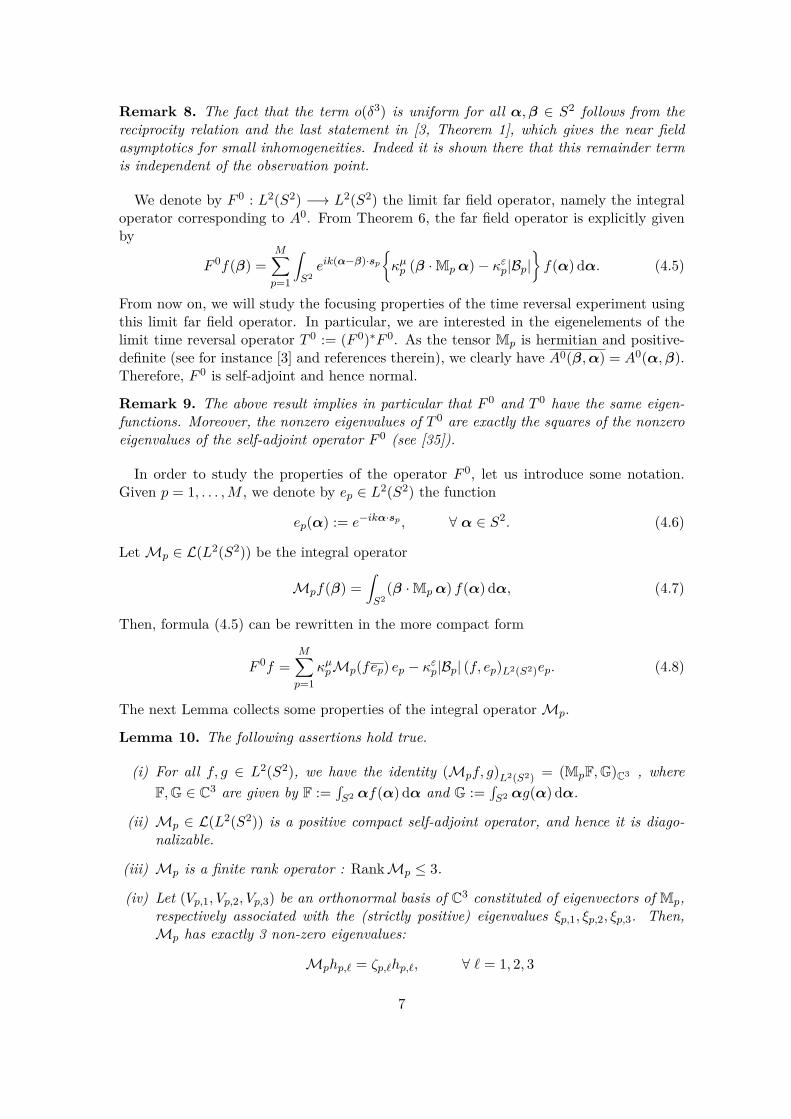
Remark 8. The fact that the term o(δ3) is uniform for all α,β ∈ S2 follows from thereciprocity relation and the last statement in [3, Theorem 1], which gives the near fieldasymptotics for small inhomogeneities. Indeed it is shown there that this remainder termis independent of the observation point.

We denote by F 0 : L2(S2) −→ L2(S2) the limit far field operator, namely the integraloperator corresponding to A0. From Theorem 6, the far field operator is explicitly givenby

F 0f(β) =M∑p=1

∫S2eik(α−β)·sp

{κµp (β ·Mpα)− κεp|Bp|

}f(α) dα. (4.5)

From now on, we will study the focusing properties of the time reversal experiment usingthis limit far field operator. In particular, we are interested in the eigenelements of thelimit time reversal operator T 0 := (F 0)∗F 0. As the tensor Mp is hermitian and positive-definite (see for instance [3] and references therein), we clearly have A0(β,α) = A0(α,β).Therefore, F 0 is self-adjoint and hence normal.

Remark 9. The above result implies in particular that F 0 and T 0 have the same eigen-functions. Moreover, the nonzero eigenvalues of T 0 are exactly the squares of the nonzeroeigenvalues of the self-adjoint operator F 0 (see [35]).

In order to study the properties of the operator F 0, let us introduce some notation.Given p = 1, . . . ,M , we denote by ep ∈ L2(S2) the function

ep(α) := e−ikα·sp , ∀ α ∈ S2. (4.6)

Let Mp ∈ L(L2(S2)) be the integral operator

Mpf(β) =∫S2

(β ·Mpα) f(α) dα, (4.7)

Then, formula (4.5) can be rewritten in the more compact form

F 0f =M∑p=1

κµpMp(fep) ep − κεp|Bp| (f, ep)L2(S2)ep. (4.8)

The next Lemma collects some properties of the integral operator Mp.

Lemma 10. The following assertions hold true.

(i) For all f, g ∈ L2(S2), we have the identity (Mpf, g)L2(S2) = (MpF,G)C3 , whereF,G ∈ C3 are given by F :=

∫S2 αf(α) dα and G :=

∫S2 αg(α) dα.

(ii) Mp ∈ L(L2(S2)) is a positive compact self-adjoint operator, and hence it is diago-nalizable.

(iii) Mp is a finite rank operator : RankMp ≤ 3.

(iv) Let (Vp,1, Vp,2, Vp,3) be an orthonormal basis of C3 constituted of eigenvectors of Mp,respectively associated with the (strictly positive) eigenvalues ξp,1, ξp,2, ξp,3. Then,Mp has exactly 3 non-zero eigenvalues:

Mphp,` = ζp,`hp,`, ∀ ` = 1, 2, 3

7

where the eigenvalues ζp,` and eigenfunctions hp,` are given by

ζp,` = 4π3 ξp,` hp,`(α) = α · Vp,`.

Proof. (i) Straightforward consequence of the definition of Mp.

(ii) The self-adjointness and positivity of Mp follows immediately from (i), since thepolarization tensor Mp = (Mp

i,j)1≤i,j≤3 is a hermitian positive matrix. The compactnessof the integral operator Mp is also clear, as it has a analytic kernel.

(iii) From expression 4.7, one clearly has RanMp ⊂ β · RanMp and the result followsthen from Mp being of rank 3.

(iv) Let us first note that∫S2 ααT dα = 4π

3 I for the identity I ∈ R3×3, which one easilyverifies by using symmetry arguments or by direct calculation via spherical coordinates.Using that the vectors Vp,` are eigenvectors of Mp, we then find that

Mphp,`(β) = β ·(Mp

∫S2α(α · Vp,`) dα

)= β ·

(Mp

[∫S2ααT dα

]Vp,`

)= ζp,`hp,`.

4.1 Eigenvalues and eigenfunctions of the limit far field operator

In this section we focus on the regime kd→∞, i.e. when the inhomogeneities are distantenough. Under this assumption, we derive an explicit formula for what we call “approxi-mate” eigenelements of the limit far field operator F 0 (and thus of the limit time reversaloperator T 0). Before stating this result, we first recall a classical result for oscillatoryintegrals that will be very useful for our analysis. This result, which can be found in[31, p. 348], is restated here in a slightly different form that is more convenient for ourpurposes.

Theorem 11. Let S be a smooth hypersurface in RN whose Gaussian curvature (i.e. theproduct of the principal curvatures) is nonzero everywhere and let ψ ∈ C∞0 (RN ) such thatSupp (ψ) intersects S in a compact subset of S. Then, as |ξ| → +∞, we have∫

Sψ(α)eiα·ξ dα = O(|ξ|(1−N)/2).

Theorem 12. Let κεp and κµp be the contrasts defined by 4.3. For all p = 1, . . . ,M andall ` = 1, 2, 3, we introduce the following functions of L2(S2)

ep(α) = e−ikα·sp , gp,`(α) = hp,`(α)ep(α),

where hp,` ∈ L2(S2) is an eigenfunction (with eigenvalue ζp,`) of the compact self-adjointintegral operator Mp ∈ L(L2(S2)) (see statement (iv) in Lemma 10). We also set

λεp = −4πκεp|Bp|, λµp,` = κµpζp,` (4.9)

Then, we have the following two results.

8

(i) As kd→∞, the functions ep satisfy

F 0ep = λεpep +O((kd)−1

). (4.10)

(ii) As kd→∞, the functions gp,` satisfy

F 0gp,` = λµp,`gp,` +O((kd)−1

). (4.11)

Proof. (i) We compute F 0ep for a fixed 1 ≤ p ≤M . Thanks to 4.8, we have

(F 0ep)(β) =M∑q=1

Ipq(β)eq(β)

in which Ipq(β) = κµqMq(ep eq)(β) − κεq|Bq|(ep, eq)L2(S2). According to 3.3, we note thatfor q 6= p, we have (ep, eq)L2(S2) = O

((kd)−1). On the other hand, Theorem 11 shows

that for q 6= p, the integral Mq(ep eq)(β) =∫S2 (β ·Mq α) eikα·(sq−sp) dα behaves like

O((kd)−1). Consequently, for all q 6= p, we have Ipq(β) = O

((kd)−1) uniformly for all

β ∈ S2. Concerning the diagonal term (q = p), we remark that for all β ∈ S2 (1 is theconstant function equal to 1)

Mp(epep)(β) =Mp(1)(β) =∫S2

(β ·Mpα) dα = β ·Mp

∫S2α dα = 0. (4.12)

Therefore, Ipp(β) = −4πκεp|Bp| = λεp and hence F 0ep = λεpep + O((kd)−1) , from which

one easily gets 4.10.(ii) Let 1 ≤ p ≤ M and 1 ≤ ` ≤ 3 be fixed. Using once again 4.8, we get that

(F 0gp,`)(β) =∑Mq=1 Ipq(β)eq(β) where we have set now

Ipq(β) = κµqMq

(hp,` ep eq

)(β)− κεq|Bq|(hp,`ep, eq)L2(S2).

For q 6= p the two terms (hp,`ep, eq)L2(S2) and Mq

(hp,`ep eq

)(β) are oscillatory integrals

of the form given in Theorem 11. Therefore, Ipq(β) = O((kd)−1) for q 6= p. On the other

hand, for q = p, we see by Lemma 10, (iv), that

Ipp(β) =κµpMphp,`(β)− κεp|Bp|(hp,`ep, ep)L2(S2)

=κµpζp,`hp,`(β)− κεp|Bp|(hp,`, 1)L2(S2).

By (4.12) we observe that 1 is in the null space ofMp. SinceMp is self-adjoint, this yields(hp,`,1)L2(S2) = 1

ζp,`(Mphp,`,1)L2(S2) = 1

ζp,`(hp,`,Mp1)L2(S2) = 0, and, thus, Ipp(β) =

κµpζp,`hp,`(β) which concludes the proof.

Remark 13. We note that the approximate eigenfunctions of F 0 are the far fields cor-responding to monopole or dipole sources located at the centers of the small inhomo-geneities. More precisely, let G(x,y) = eik|x−y|

4π|x−y| denote the outgoing Green’s functionof the Helmholtz operator in R3. Then, ep(β) = e−ikβ·sp is nothing but the far field inthe direction β ∈ S2 of the point source G(·, sp) located at sp. Similarly, the functiongp,`(β) = hp,`(β) ep(β) = (β · Vp,`) e−ikβ·sp represents the far field in the direction β ∈ S2

of the dipole source 1ik∇G(·, sp) · Vp,` of direction Vp,` located at sp.

9

4.2 Justification of the DORT Method

We recall that the DORT method consists of the observation that eigenfunctions of thetime-reversal operator possess selectively focusing properties. In the following section, weprovide a precise signification of this property. We start with a straightforward conse-quence of Theorem 12 (see Remark 9), which provides the approximate eigenelements ofthe limit time reversal operator in the regime of uncoupled scatterers (kd→∞).

Corollary 14. Under the notation of Theorem 12, we have the following estimates askd→∞

T 0ep = (λεp)2ep +O((kd)−1

), T 0gp,` = (λµp,`)

2gp,` +O((kd)−1

).

The next result shows that the above 4M approximate eigenfunctions ep and gp,` forp = 1, . . . ,M and ` = 1, 2, 3 span a subspace of dimension 4M .

Proposition 15. Under the notation of Theorem 12, the functions ep and gp,` for p =1, . . . ,M and ` = 1, 2, 3 are linearly independent.

Proof. Suppose that there exists complex coefficients (ap)p=1,...,M and (bp,`)j=1,2,3p=1,...,M such

thatM∑p=1

ap ep(β) +M∑p=1

3∑`=1

ik bp,` gp,`(β) = 0, ∀ β ∈ S2.

According to Remark 13, the above relation amounts to saying that the function u(x) :=∑Mp=1 apG(x, sp) +

∑Mp=1

∑3`=1 bp,`∇G(x, sp) · Vp,` has a vanishing far field. By Rellich’s

lemma, u must vanish everywhere, so thatM∑p=1

apG(x, sp) +M∑p=1

3∑`=1

bp,`∇G(x, sp) · Vp,` = 0, ∀ x /∈ {s1, . . . , sM}. (4.13)

Fix q ∈ {1, . . . ,M} and choose x = sq + ρx, for x ∈ S2 and 0 ≤ ρ ≤ ρ∗ small enough.Multiplying 4.13 by ρ2 and taking the limit as ρ → 0, we note that the only non van-ishing contribution comes from the most singular term. More precisely, the dipole termcorresponding to p = q gives lim

ρ→0ρ2∇G(sq + ρx, sq) · Vq,` = 1

4π (x · Vq,`). Therefore,

x ·(∑3

`=1 bq,`Vq,`)

= 0. Since x ∈ S2 is arbitrary and since the vector columns Vq,1, Vq,2and Vq,3 are linearly independent, the above relation yields b1q = b2q = b3q = 0 for allq ∈ {1, . . . ,M}. Finally, 4.13 reduces then to

∑Mp=1 apG(x, sp) = 0 for all x /∈ {s1, . . . , sM}

from which one can easily get that a1 = · · · = aM = 0.

Summing up, we have proved that in the regime of small and distant inhomogeneities(δ � λp � d), the limit time reversal operator T 0 admits 4M eigenvalues : (λεp)2, (λµp,`)2

for p = 1, . . . ,M , ` = 1, 2, 3. In order to complete our justification of the DORT method,we need to show that the corresponding (approximate) eigenfunctions ep and gp,` generateincident waves focusing selectively on the inhomogeneities. Given p in {1, . . . ,M}, let usfirst consider the incident Herglotz wave associated with a density ep (TE eigenfunctions).Then, from (3.3), uI,p(x) = O

(|x− sp|−1). Regarding the TM eigenfunctions, the incident

Herglotz wave associated with gp,` = hp,` ep is uI,p,`(x) =∫S2 eikα·(x−sp)hp,`(α) dα, which

behaves like O((kd)−1) from Theorem 11.

10

Remark 16. Clearly, similar selective focusing results hold for the two dimensional prob-lem. More precisely, by using once again Theorem 11 with N = 2, one can show that eachinhomogeneity gives rise to 3 eigenvalues, one associated with the dielectric permittivitycontrast and 2 with the magnetic permeability contrast. This is also confirmed by ournumerical investigations, which are detailed in Section 6.

Remark 17. In the particular case of spherical inclusions, the polarization tensors become(see for example [3]) : Mp = 8π|Bp| µp

µp+µ0I. One can then easily check that the TM eigen-

values λµp,` of the far field operator are given by relations 4.9, with ζp,` = 32π2|Bp| µpµp+µ0

.

5 Selective focusing for open time reversal mirrors

In this section, we investigate the case of an open TRM, i.e. the case where the TRMdoes not completely surround the inhomogeneities. For the sake of brevity, we will onlystress the main differences with the case of a closed TRM. Let S ( S2 denote the set ofemission directions covered by the open TRM (and thus −S represents the set of receptiondirections). We assume that the emission (resp. reception) directions of the open TRM aredescribed by a smooth cutoff function χ+ ∈ C∞0 (S2) (resp. χ− ∈ C∞0 (S2)) with Suppχ+ ⊂S (resp. Suppχ− ⊂ −S). The smoothness assumption on χ± is purely technical and isused to derive more easily the asymptotic behavior of the oscillating integrals. However,our results still hold in the more realistic case where χ± are characteristic functions of±S (see Remark 23). Then, we define the far field operator corresponding to an openTRM by F = P−FP

∗+ ∈ L(L2(S), L2(−S)), where P± : L2(S2) → L2(±S) denote the

restriction operators P±f = (χ±f)|±S and P ∗± : L2(±S) → L2(S2), whose adjoints arethe extension operators by zero from ±S to S2. Then, following the arguments detailedin [20, Sect. 5], one easily gets that for open TRM, the time reversal operator is onceagain of the form T = F ∗F ∈ L(L2(S)), and is nothing but the integral operator withkernel t(α,β) =

∫−S A(α,γ)A(β,γ) dγ. Moreover, T defines a compact positive and self-

adjoint operator. Nevertheless, unlike the full far field operator F , the “finite aperture”far field operator F is not anymore normal and the eigenfunctions of F and T are notnecessary the same. Regarding the case of small inhomogeneities, the limit time reversaloperator denoted T 0 ∈ L(L2(S)) is then the integral operator with kernel t 0(α,β) =∫−S A

0(α,γ)A0(β,γ) dγ where A0 is the limit scattering amplitude is given by 4.4. Then,given f ∈ L2(S), the time reversal operator can be represented by

T 0f(β) =M∑q=1

{ M∑p=1

∫S

(∫−S

[κµp (γ ·Mpα)− κεp|Bp|

][κµq (γ ·Mqβ)− κεq|Bq|

]ep(γ) eq(γ) dγ

)ep(α) f(α) dα

}eq(β).

(5.1)

Concerning the selective focusing properties, the main difference with the case of a closedTRM is that, unlike in 4.12, 1 is not anymore in the kernel of the integral operatorMp (or more exactly to its counterpart for finite aperture TRM). Indeed, the integral∫S

(β ·Mpα) dα does not necessarily vanish for an arbitrary subset S ( S2.

In the sequel, we consider successively the three cases : the purely TE case (i.e. κµp = 0for all p = 1, . . . ,M), the purely TM case (i.e. κεp = 0 for all p = 1, . . . ,M) and finally

11

the mixed TE/TM case. For the latter case, we prove that the DORT method still worksprovided the TRM satisfies a symmetry condition (see 5.7).

We start with the case of vanishing magnetic contrast. One can prove the followingresult using the same arguments as those developed in [20, Sect. 5.2].

Theorem 18. Let us assume that κµp = 0 for all p = 1, . . . ,M (TE polarization). Then,as kd → ∞, the functions ep(α) := (P+ep)(α) = e−ikα·sp, α ∈ S, are approximateeigenfunctions of T 0, in the sense that T 0ep = (λεp)2 ep +O

((kd)−1), with λεp = κεp|Bp| |S|.

Proof. In the case of vanishing contrast κµp = 0 for all p = 1, ...,M , equation (5.1) reducesto

T 0f =M∑

p,q=1

M∑q=1

κεpκεq|Bp||Bq| (ep, eq)L2(−S)(f , ep)L2(S)eq.

Since χ− is assumed to be a smooth function, we can still apply Theorem 11 and get thatfor q 6= p,

(ep, eq)L2(−S) = O((kd)−1

), (5.2)

which leads to T 0em = (κεm)2|Bm|2 |S|2 em +O((kd)−1).

In the case of purely TM polarization, i.e. when κεp = 0 for all of the inhomogeneities,we proceed similarly to the case of the closed time reversal mirror. That is, we shall seethat the eigenfunctions of T 0 can be approximated using eigenfunctions of the integraloperator Mp ∈ L(L2(S)) with kernel

mp(α,β) :=∫−S

(γ ·Mpα)(γ ·Mpβ) dγ. (5.3)

The next Lemma, given without proof, summarizes some simple properties of the integraloperator Mp.

Lemma 19. The following assertions hold true.

(i) Mp ∈ L(L2(S2)) is a positive self-adjoint compact operator and hence it is diago-nalizable.

(ii) Mp is a finite rank operator : RankMp ≤ 3. In particular, Mp admits at most 3non zero eigenvalues ζp,`, ` = 1, 2, 3.

Theorem 20. Let κεp = 0 for all p = 1, ...,M and let hp,` ∈ L2(S) be an eigenfunctionof the compact self-adjoint integral operator Mp with kernel (5.3), associated with aneigenvalue ζp,` 6= 0 for ` = 1, 2, 3. Then, as kd→∞, the function

gp,`(α) = hp,`(α)ep(α), ∀ α ∈ S (5.4)

is an approximate eigenfunction of T 0, in the sense that

T 0gp,` = (λµp,`)2 gp,` +O

((kd)−1

),

with λµp,` = κµp ζp,`.

12

Proof. From (5.1) and for κεp = 0 for all p = 1, . . . ,M , we have

T 0f(β) =M∑

p,q=1κµqκ

µp

∫Sα ·

[∫−S

Mpγ (γ ·Mqβ) ep(γ) eq(γ) dγ]ep(α)f(α) dα eq(β).

For q 6= p the inner integral behaves like O((kd)−1) by Theorem 11. Thus, the time

reversal operator can be represented by

T 0f =M∑p=1

(κµp )2Mp

(f ep

)ep +O

((kd)−1

), (5.5)

Noting that, for m 6= p,

Mp

(hm,`em ep

)(β) = O

((kd)−1

), (5.6)

the statement follows immediately from the representation (5.5) of T 0 and the circum-stance that hp is an eigenfunction of the integral operator Mp.

In the case of mixed TE/TM polarization (i.e. when both contrasts are present), thefollowing statement shows that for particular shapes of S, we can still obtain expressionsof approximate eigenfunctions of the limit time reversal operator.

Theorem 21. Let S be chosen such that∫Sα dα = 0. (5.7)

Then, as kd→∞, the functions ep and gp,`, p = 1, ...,M , respectively defined in Theorem18 and Theorem 20, constitute approximate eigenfunctions of T 0 with an error bound ofsize O

((kd)−1).

Proof. For the functions e`, ` = 1, ...,M , the statement is a result of the representation(5.1), the assumption that the integral

∫Sα dα vanishes and Theorem 11. In particular,

we have

T 0e`(β) =(κε`)2|B`|2 |S| e`(β) +M∑p=1

(κµp )2Mp

(e` ep

)(β) ep(β) +O

((kd)−1

)

−M∑

p,q=1κµpκ

εq|Bq|

∫S

(∫−S

(γ ·Mpα) ep(γ) eq(γ) dγ)ep(α) e`(α) dα eq(β)

−M∑

p,q=1κµqκ

εp|Bp|

∫S

(∫−S

(γ ·Mqβ) ep(γ) eq(γ) dγ)ep(α) e`(α) dα eq(β).

Using for p 6= q Theorem 11, we find that∫−Sγ ep(γ) eq(γ) dγ = O

((kd)−1

), (5.8)

Hence, for kd→∞, the two double sums simplify respectively into

−M∑p=1

κµpκεp|Bp|

∫Sα ·Mp

(∫−Sγ dγ

)ep(α) e`(α) dα ep(β) +O

((kd)−1

),

13

and

−M∑p=1

κµpκεp|Bp|

∫Sβ ·Mp

(∫−Sγ dγ

)ep(α)e`(α) dα ep(β) +O

((kd)−1

).

Thus, we have

T 0e`(β) =(κε`)2|B`|2 |S| e`(β) +M∑p=1

(κµp )2Mp

(e` ep

)(β) ep(β)

−M∑p=1

κµpκεp|Bp|

∫S

(α+ β) ·Mp

(∫−Sγ dγ

)ep(α) e`(α) dα ep(β)

+O((kd)−1

)By 5.7, we obtain

T 0e`(β) = (κε`)2|B`|2 |S| e`(β) +M∑p=1

(κµp )2Mp

(e` ep

)(β) ep(β) +O

((kd)−1

).

But from Theorem 11

Mp

(e` ep

)(β) =

{O((kd)−1) , p 6= `,

Mp (P+1) (β), p = `,

Moreover, from assumption 5.7, P+1 is in the null space of the integral operator Mp.Hence, T 0e`(β) = (κε`)2|B`|2 |S| e`(β) +O

((kd)−1).

Let m ∈ 1, ...,M be fixed. For the functions gm,` defined in (5.4), according to therepresentation (5.1) we obtain

T 0gm,`(β)

=M∑p=1

(κµp )2Mp

(gm,` ep

)(β) ep(β) + (κεp)2|Bp|2 |S| (gm,`, ep)L2(S) ep(β)

−M∑p=1

M∑q=1

κµpκεq|Bq|

∫S

(∫−S

(γ ·Mpα)ep(γ) eq(γ) dγ)ep(α) gm,`(α) dα eq(β)

−M∑p=1

M∑q=1

κµqκεp|Bp|

∫S

(∫−S

(γ ·Mqβ) ep(γ) eq(γ) dγ)ep(α) gm,`(α) dα eq(β)

+O((kd)−1

)Since P+1 ∈ KerMp,

(hm,`, P+1

)L2(S)

= 1ζm,`

(hm,`,MmP+1

)L2(S)

= 0, we get like abovethat

(gm,`, ep)L2(S) = (hm,`em, ep)L2(S) ={O((kd)−1) , m 6= p,

0, m = p,

and hence T 0gm,` = (κµm)2ζm,`gm,` +O((kd)−1).

14

In order to justify the DORT method for the case of open and symmetric mirrors, itremains to show that the functions ep and gp,` generate incident waves focusing selectivelyon the inhomogeneities. Given a fixed p in {1, . . . ,M}, let us first consider the incidentHerglotz wave associated with a density ep (TE eigenfunctions). From (5.2) we immediatelysee that uI,p decreases like |x − sp|−1. Regarding the TM eigenfunctions, the incidentHerglotz wave associated with gp,` = hp,` ep is an oscillatory integral given by uI,p,`(x) =∫Shp,`(α)eikα·(x−sp) dα = O

((k|x− sp|)−1).

Remark 22. Condition (5.7) is satisfied whenever S is symmetric i.e. S = −S. Itsmain advantage lies in the fact that it allows us to decouple between the TE and TMapproximate eigenfunctions ep and gp,`. Nevertheless, numerical experiments indicate thatselective focusing still holds for open TRM even when 5.7 is not satisfied (see Section 6).Unfortunately, we have not been able to prove this result.

Remark 23. We have assumed the open TRM to be described by a smooth cutoff function,so that we can apply directly Theorem 11. Of course, it would be more relevant for practicalapplications to assume the TRM to be defined via the characteristic function 1|±S. In thiscase, one has to derive high frequency asymptotics (i.e. for k → +∞) of integrals of theform

∫Sψ(α)eikα·s dα. Describing the TRM by spherical coordinates S = {α = (θ, ϕ) ∈

Jθ × Jϕ}, the above integral reduces to two dimensional oscillatory integrals of the form∫Jθ

∫Jϕ

Ψ(θ, ϕ)eikΦs(θ,ϕ) dθdϕ. Using a two dimensional version of the stationary phasetheorem [34, Chap. VIII], one can show that the above integrals decay as k → ∞, witha rate of decay of 1/k (as in the case of a smooth TRM). This is due to the fact thatthe possible (interior) critical points of Φs are non degenerate as it can be checked fromlengthy but not difficult calculations.

6 Numerical tests

We consider the case of spherical two-dimensional inclusions, i.e. ∂Bp = sp + apS2, p =

1, ...,M , where ap denotes the radius of the disk Bp. We use an integral equation approachto solve the scattering problem (4.2). Taking advantage of the particular form of the inho-mogeneities, we use a spectral approach (also known as multipole expansion or Mie seriesmethod) to solve the system of integral equations (instead of a using a boundary elementmethod). Each boundary unknown density is then decomposed on the local Fourier basisassociated to each inhomogeneity. Using the projection of the integral operators in theseFourier basis, it is possible to obtain an explicit expression for the integral kernels, formore details see for instance [27, 32]. This leads to solving a linear system whose diagonalblocks represent single scattering, while the off-diagonal blocks take into account multiplescattering phenomena. The above method can be adapted to tackle the three-dimensionalcase, the unknown density being then approximated via an infinite sum of spherical har-monics. Of course, this leads to much larger systems to solve (more details on the case ofnon penetrable scatterers can be found for instance in [19]).

We illustrate the DORT method for several different setups. The implementation wasrealized under MATLAB. Throughout this section we assume that µ0 = ε0 = 1 (which isequivalent to considering ε and µ as being not the absolute but the relative permittivityand permeability) and ω = 2π, leading to a wavelength λ = 1. The radius of the spheres

15

is given by ap = 0.002 for all p = 1, ...,M . The emission and reception directions are ob-tained by discretizing uniformly the unit circle (0, 2π) using 200 points. These directionswill be fixed and in the case of an open TRM, we will restrict ourselves to those emissionand reception directions which are in the interior of the given set S resp. −S. We beginwith an example of one single inclusion. Then, we proceed by an example with two in-clusions, by considering successively a symmetric and a non symmetric configuration (i.e.two inclusions different magnetic and dielectric contrast). More realistic setups (with anopen TRM and noise) are presented in Examples 3a and 3b.

Example 1. One inclusion. We first consider the case of one single inclusion, andwe show in Table 1 the four largest eigenvalues of the time-reversal operator for differentvalues of the dielectric and magnetic contrasts. In particular, we observe that for eachsetup, there are three significant eigenvalues, two of them being equal. These eigenvaluescorrespond to the TM polarization (magnetic contrast) while the third one is related to theTE polarization (dielectric contrast). This fact is in agreement with the DORT methodin dimension two (see Remark 16).

µ1 ε1 λ1 λ2 λ3 λ4

4 2 0.0049019 0.0017636 0.0017636 6.8683e-135 1.5 0.0021772 0.0021772 0.0012253 8.4791e-13

Table 1: Single inclusion at position s1 = (0, 5). We present the different eigenvalues ofthe time-reversal operator (rescaled by a factor 1/|B1| = 1/(πa2

1)).

Figure 1 shows the absolute values of the DORT Herglotz waves for the case µ1 = 4 andε1 = 2. We see that the Herglotz wave function associated to these eigenvalues representsa dipole situated at the (unknown) location of the inclusion. Also, the first Herglotz waveassociated to the largest eigenvalue is a monopole, which confirms our theoretical results.In Figure 2 we present similar results for the case µ1 = 5 and ε1 = 1.5. Here, the firsttwo eigenvalues are equal, see Table 1, and hence, they are most likely associated to themagnetic contrast. Indeed, as we can see in Figure 2, the first two Herglotz waves aredipoles whereas the third is a monopole situated at the unknown location of the inclusion.

Example 2a. Two non symmetric inclusions. We consider a second inclusion atposition (10, 22) with the same size as inclusion B1 and with ε2 = 3 and µ2 = 15. InFigure 3 one can see that the first six eigenvalues (ordered by their magnitude) of thetime-reversal mirror are significantly larger than the subsequent eigenvalues. Moreover,the second and third as well as the fourth and fifth eigenvalues are equal. This indicatesthat the Herglotz waves associated to the 2nd and third eigenvalue are dipoles focusing onone inclusion and that the Herglotz waves generated from the 4th and 5th eigenfunctionsshould focus on the other inclusion. Indeed, as can be seen in Figure 4, this is the case.Also, the first and six Herglotz waves are monopoles each focusing on one of the twoinclusions which is what one expects from the theoretical results.

Example 2b. Two symmetric inclusions. Let us again consider the two inclusionsB1 and B2 at (0, 5) and (10, 22) but with the same magnetic and dielectric contrast givenby ε1 = ε2 = 3 and µ1 = µ2 = 5. In Figure 5 the obtained eigenvalues are shown.

16

(a) (b)

(c)

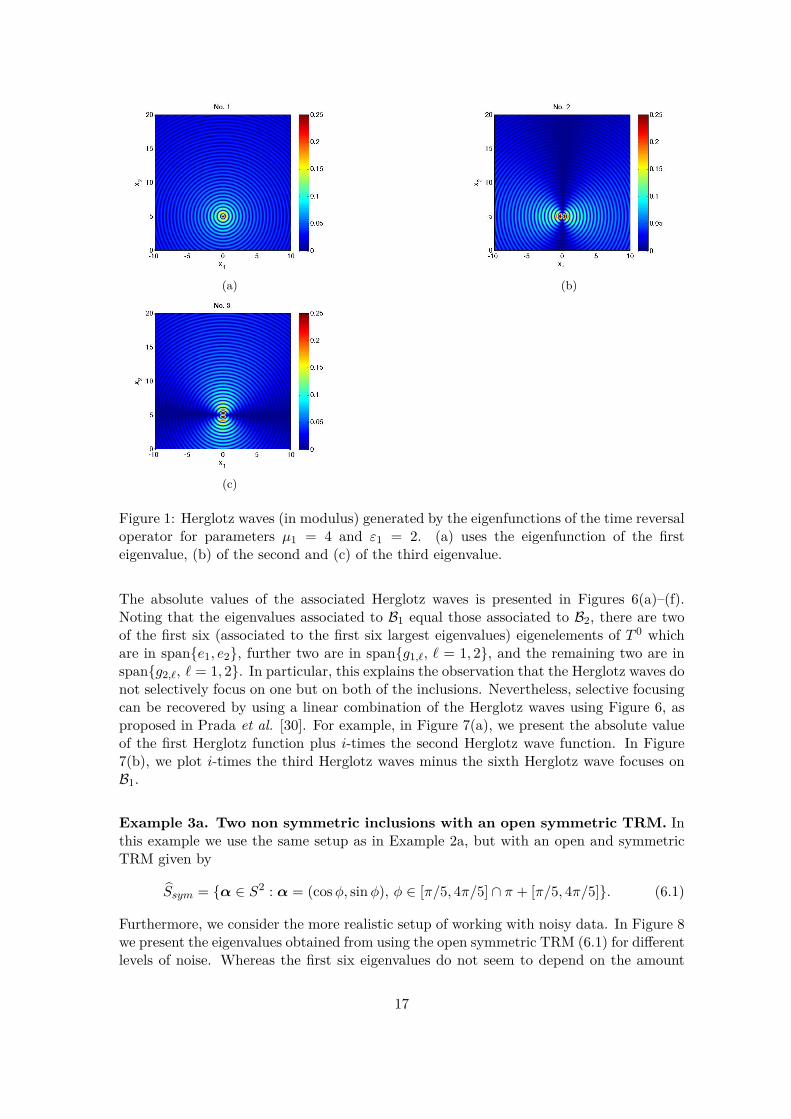
Figure 1: Herglotz waves (in modulus) generated by the eigenfunctions of the time reversaloperator for parameters µ1 = 4 and ε1 = 2. (a) uses the eigenfunction of the firsteigenvalue, (b) of the second and (c) of the third eigenvalue.

The absolute values of the associated Herglotz waves is presented in Figures 6(a)–(f).Noting that the eigenvalues associated to B1 equal those associated to B2, there are twoof the first six (associated to the first six largest eigenvalues) eigenelements of T 0 whichare in span{e1, e2}, further two are in span{g1,`, ` = 1, 2}, and the remaining two are inspan{g2,`, ` = 1, 2}. In particular, this explains the observation that the Herglotz waves donot selectively focus on one but on both of the inclusions. Nevertheless, selective focusingcan be recovered by using a linear combination of the Herglotz waves using Figure 6, asproposed in Prada et al. [30]. For example, in Figure 7(a), we present the absolute valueof the first Herglotz function plus i-times the second Herglotz wave function. In Figure7(b), we plot i-times the third Herglotz waves minus the sixth Herglotz wave focuses onB1.

Example 3a. Two non symmetric inclusions with an open symmetric TRM. Inthis example we use the same setup as in Example 2a, but with an open and symmetricTRM given by

Ssym = {α ∈ S2 : α = (cosφ, sinφ), φ ∈ [π/5, 4π/5] ∩ π + [π/5, 4π/5]}. (6.1)

Furthermore, we consider the more realistic setup of working with noisy data. In Figure 8we present the eigenvalues obtained from using the open symmetric TRM (6.1) for differentlevels of noise. Whereas the first six eigenvalues do not seem to depend on the amount

17

(a) (b)

(c)

Figure 2: Same as Figure 1, but with a strong magnetic contrast.

Figure 3: Eigenvalues of the time-reversal operator obtained for the setup of Example 2a.

18

(a) (b)

(c) (d)

(e) (f)

Figure 4: Two inclusions with different magnetic and dielectric contrast (Example 2a).

19

Figure 5: Eigenvalues of the time-reversal operator obtained for the setup of Example 2b.

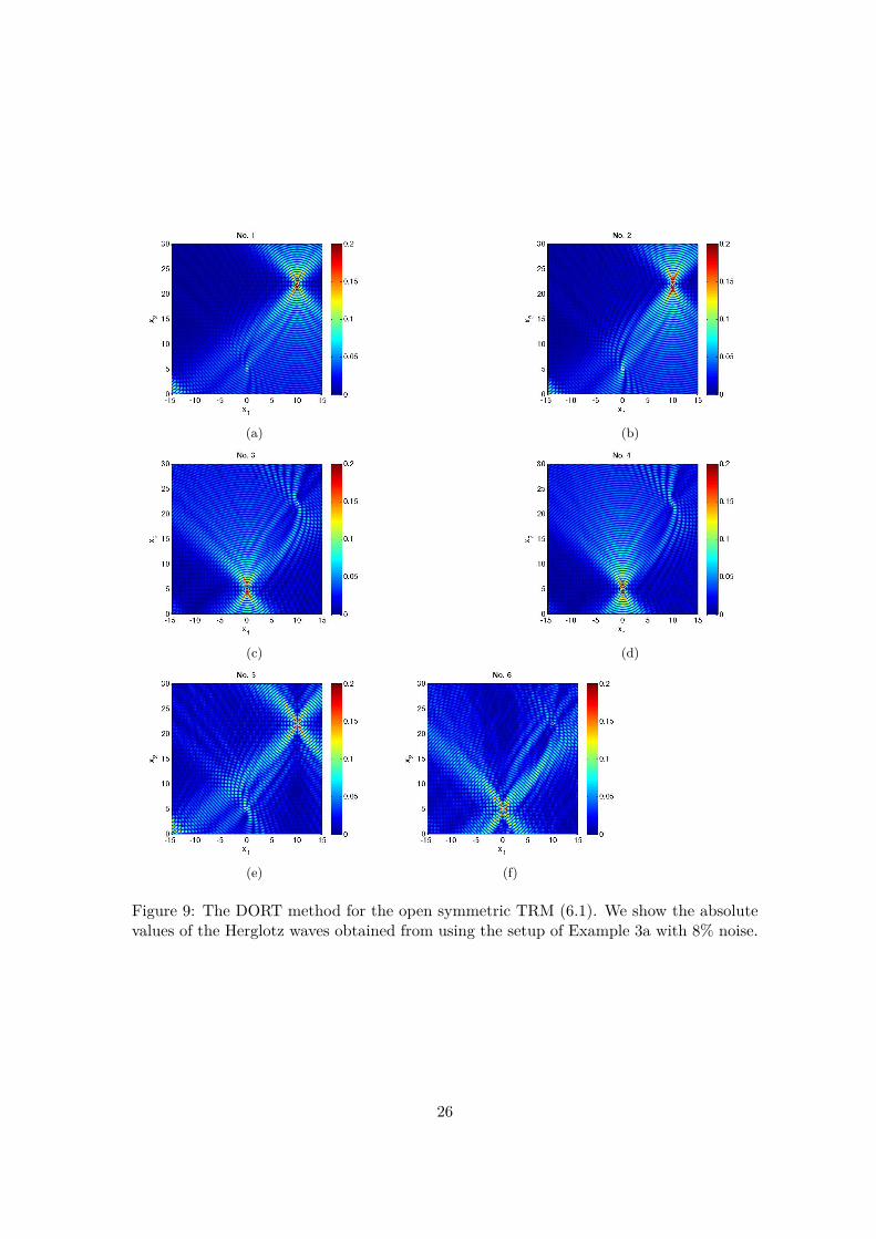
of noise, the subsequent eigenvalues are significantly larger when working with noise. InFigure 9 the absolute values of the associated Herglotz waves are shown for a noise of 8%.Although the first six eigenvalues are not anymore significant larger than the subsequenteigenvalues, the associated Herglotz waves still focus selectively. This is even true in thecase of 20% of noise, compare Figure 10.

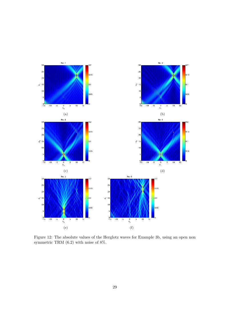
Example 3b. Two non symmetric inclusions with an open and non symmetricTRM. In this last example we study the case of a non symmetric open TRM given by

Snon−sym = {α ∈ S2 : α = (cosφ, sinφ), φ ∈ [π/5, 4π/5]}. (6.2)

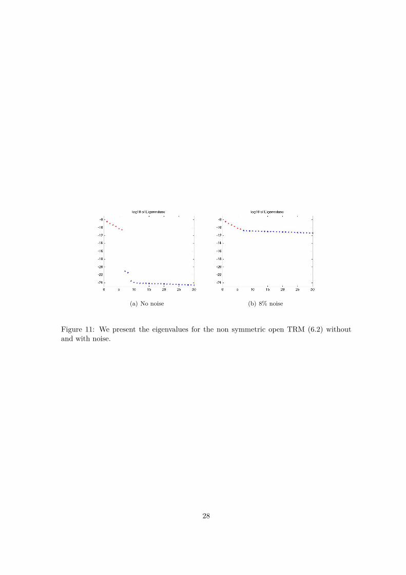
We recall that the open but non symmetric TRM did not allow a direct decoupling ofthe TE- and TM-eigenfunctions, see Remark 22. Nevertheless, it is straightforard to seethat all eigenfunctions are linear combinations of monopoles and dipoles with centres sp,p = 1, ...,M up to an error of order O((kd)−1). In this numerical example, we use thesame setup as in Example 2a (i.e. the same position, size and contrasts of the inclusions).Our numerical experiment indicates that the DORT method still works. We present theeigenvalues in Figure 11 without and with noise. Using noisy data (8% noise added tothe far field data) we obtain the Herglotz waves presented in Figure 12, which do stillselectively focus on the inclusions.

7 Conclusion

In this work, we presented a rigorous mathematical justification of the DORT methodin the context of penetrable small inhomogeneities. The mathematical model used toachieve this analysis is a far field model for time reversal in the frequency domain. Themain result states that each scatterer gives rise to N + 1 significant eigenvalues (N beingthe dimension), provided the scatterers are small and distant enough. This result wasproved for closed mirrors, but also for symmetric finite aperture mirrors. In the two-dimensional case, the theoretical results were further confirmed by numerical simulations.The case of non symmetric open mirrors requires further analysis and it not addressed inthis paper.

20

Acknowledgments

The authors want to thank Bertrand Thierry for his contribution to the MATLAB coderealizing the DORT method for penetrable spheres. They also thank Marc Bonnet (POemsgroup, CNRS/Inria/Ensta) for his careful reading of this work and for pointing out to usa little sign mistake in the far field asymptotics. Support for this work was provided bythe FRAE (http://www.fnrae.org/), research project IPPON.

References

[1] M. Abramowitz and I. A. Stegun, Handbook of mathematical functions withformulas, graphs, and mathematical tables, vol. 55 of National Bureau of StandardsApplied Mathematics Series, U.S. Government Printing Office, Washington, D.C.,1964.

[2] H. Ammari, E. Iakovleva, D. Lesselier, and G. Perrusson, Music-type elec-tromagnetic imaging of a collection of small three-dimensional inclusions, SIAM J.Sci. Comput., 29 (2007), pp. 674–709 (electronic).

[3] H. Ammari, E. Iakovleva, and S. Moskow, Recovery of small inhomogeneitiesfrom the scattering amplitude at a fixed frequency, SIAM J. Math. Anal., 34 (2003),pp. 882–900.

[4] X. Antoine, B. Pincon, K. Ramdani, and B. Thierry, Far field modeling ofelectromagnetic time reversal and application to selective focusing on small scatterers,SIAM J. Appl. Math., 69 (2008), pp. 830–844.

[5] T. Arens, A. Lechleiter, and D. R. Luke, Music for extended scatterers as aninstance of the factorization method, SIAM J. Appl. Math., 70 (2009), pp. 1283–1304.

[6] C. Ben Amar, N. Gmati, C. Hazard, and K. Ramdani, Numerical simulationof acoustic time reversal mirrors, SIAM J. Appl. Math., 67 (2007), pp. 777–791.

[7] L. Borcea, G. Papanicolaou, and F. G. Vasquez, Edge illumination and imag-ing of extended reflectors, SIAM J. Imaging Sciences, 1 (2008), pp. 75–114.

[8] D. H. Chambers and J. G. Berryman, Target characterization using decompo-sition of the time-reversal operator: electromagnetic scattering from small ellipsoids,Inverse Problems, 22 (2006), pp. 2145–2163.

[9] Q. Chen, H. Haddar, A. Lechleiter, and P. Monk, A sampling method forinverse scattering in the time domain, Inverse Problems, 26 (2010), p. 085001.

[10] M. Cheney, The linear sampling method and the MUSIC algorithm, Inverse Prob-lems, 17 (2001), pp. 591–595.

[11] D. Colton, H. Haddar, and M. Piana, The linear sampling method in inverseelectromagnetic scattering theory, Inverse Problems, 19 (2003), pp. S105–S137.

[12] D. Colton and A. Kirsch, A simple method for solving inverse scattering problemsin the resonance region, Inverse Problems, 12 (1996), pp. 383–393.

21

[13] D. Colton and R. Kress, Inverse acoustic and electromagnetic scattering theory,vol. 93 of Applied Mathematical Sciences, Springer-Verlag, Berlin, second ed., 1998.

[14] A. Devaney, E. Marengo, and F. Gruber, Time-reversal-based imaging andinverse scattering of multiply scattering point targets, J. Acoust. Soc. Amer., 118(2005), pp. 3129–3138.

[15] A. Fannjiang, On time reversal mirrors, Inverse Problems, 25 (2009), p. 095010.

[16] M. Fink, Imaging of Complex Media with Acoustic and Seismic Waves, vol. 84 of Top-ics in Applied Physics, Springer, 2002, ch. Acoustic Time-Reversal Mirrors, pp. 17–43.

[17] M. Fink, D. Cassereau, A. Derode, C. Prada, P. Roux, M. Tanter, J.-L. Thomas, and F. Wu, Time-reversed acoustics, Rep. Prog. Phys., 63 (2000),pp. 1933–1995.

[18] M. Fink and C. Prada, Acoustic time-reversal mirrors, Inverse Problems, 17(2001), pp. 1761–1773.

[19] N. A. Gumerov and R. Duraiswami, Multiple scattering from n spheres usingmultipole reexpansion, J. Acoust. Soc. Amer, 112 (2002), pp. 2688–2701.

[20] C. Hazard and K. Ramdani, Selective acoustic focusing using time-harmonic re-versal mirrors, SIAM J. Appl. Math., 64 (2004), pp. 1057–1076.

[21] S. Hou, K. Solna, and H. Zhao, Imaging of location and geometry for extendedtargets using the response matrix, J. Comput. Phys., 199 (2004), pp. 317–338.

[22] E. Iakovleva and D. Lesselier, Multistatic response matrix of spherical scatterersand the back-propagation of singular fields, IEEE Trans. Antenna. Prop., 56 (2008),pp. 825 – 833.

[23] A. Kirsch, Characterization of the shape of a scattering obstacle using the spectraldata of the far field operator, Inverse Problems, 14 (1998), pp. 1489–1512.

[24] , Factorization of the far-field operator for the inhomogeneous medium case andan application in inverse scattering theory, Inverse Problems, 15 (1999), pp. 413–429.

[25] , New characterizations of solutions in inverse scattering theory, Appl. Anal., 76(2000), pp. 319–350.

[26] , The MUSIC algorithm and the factorization method in inverse scattering theoryfor inhomogeneous media, Inverse Problems, 18 (2002), pp. 1025–1040.

[27] R. Kress, Minimizing the condition number of boundary integral operators in acousticand electromagnetic scattering, Quart. J. Mech. Appl. Math., 38 (1985), pp. 323–341.

[28] G. Micolau, Etude theorique et numerique de la methode de la Decomposition del’operateur de Retournement Temporel (D.O.R.T.) en diffraction electromagnetique,PhD thesis, Universite d’Aix-Marseille, June 2001.

[29] B. Pincon and K. Ramdani, Selective focusing on small scatterers in acousticwaveguides using time reversal mirrors, Inverse Problems, 23 (2007), pp. 1–25.

22

[30] C. Prada, S. Manneville, D. Spoliansky, and M. Fink, Decomposition of thetime reversal operator: detection and selective focusing on two scatterers, J. Acoust.Soc. Am., 9 (1996), pp. 2067–2076.

[31] E. Stein, Harmonic analysis: real-variable methods, orthogonality, and oscilla-tory integrals, vol. 43 of Princeton Mathematical Series, Princeton University Press,Princeton, NJ, 1993.

[32] B. Thierry, Analyse et Simulations Numeriques du Retournement Temporel et dela Diffraction Multiple, PhD thesis, Nancy Universite, September 2011.

[33] H. Tortel, G. Micolau, and M. Saillard, Decomposition of the time rever-sal operator for electromagnetic scattering, J. Electromagn. Waves Appl., 13 (1999),pp. 687–719.

[34] R. Wong, Asymptotic approximations of integrals, vol. 34 of Classics in AppliedMathematics, Society for Industrial and Applied Mathematics (SIAM), Philadelphia,PA, 2001.

[35] A. Zaanen, Linear analysis. Measure and integral, Banach and Hilbert space, linearintegral equations, Interscience Publishers Inc., New York, 1953.

23

(a) (b)

(c) (d)

(e) (f)

Figure 6: Two inclusions with identical magnetic and dielectric contrast (Example 2b).The Herglotz waves do selectively focus on both inclusions.

24

(a) (b)

Figure 7: (a) linear combination of the first and second Herglotz waves, (b) linear combi-nation of third and sixth Herglotz wave function of Example 2b.

(a) No added noise (b) 4% noise

(c) 8% noise (d) 20% noise

Figure 8: We present the eigenvalues of Example 3a (using the open symmetric TRM(6.1) for different levels of noise. In (d) we observe that the first six eigenvalues are notanymore significant larger than the subsequent eigenvalues.

25

(a) (b)

(c) (d)

(e) (f)

Figure 9: The DORT method for the open symmetric TRM (6.1). We show the absolutevalues of the Herglotz waves obtained from using the setup of Example 3a with 8% noise.

26

(a) (b)

(c) (d)

(e) (f)

Figure 10: The DORT method for the open symmetric TRM (6.1). We show the absolutevalues of the Herglotz waves obtained from using the setup of Example 3a with 20% noise.

27

(a) No noise (b) 8% noise

Figure 11: We present the eigenvalues for the non symmetric open TRM (6.2) withoutand with noise.

28

(a) (b)

(c) (d)

(e) (f)

Figure 12: The absolute values of the Herglotz waves for Example 3b, using an open nonsymmetric TRM (6.2) with noise of 8%.

29