
How can we know if EU cohesion policy is successful? Integrating micro and macro approaches to the...
91
How can we know if EU cohesion policy is successful? Integrating micro and macro approaches to the evaluation of Structural Funds John Bradley*** Timo Mitze* Edgar Morgenroth** Gerhard Untiedt* March, 2006 – Nr. 1
Transcript of How can we know if EU cohesion policy is successful? Integrating micro and macro approaches to the...

How can we know if EU cohesion policy is successful? Integrating micro and macro approaches to the evaluation of Structural Funds John Bradley*** Timo Mitze* Edgar Morgenroth** Gerhard Untiedt*
March, 2006 – Nr. 1
Herausgeber / Editor: GEFRA – Gesellschaft für Finanz- und Regionaanalysen Anschrift: Ludgeristr. 56, 48143 Münster (Westfalen)
Germany
Telefon: +251-2639310 FAX: +251-2639319 E-mail: [email protected] Internet: www.gefra-muenster.de
Authors: *
Dr. Gerhard Untiedt Timo Mitze
GEFRA – Gesellschaft für Finanz- und Regionalanalysen Ludgeristr. 56, D-48143 Münster, GERMANY Tel: (+49-251) 263 9311, Fax: (+49-251) 263 9319 e-mail: [email protected] [email protected]
**
Dr. Edgar Morgenroth
ESRI – Economic and Social Research Institute, Dublin Burlington Road 4, Dublin 4, IRELAND Tel: (+353-1) 667-1525, Fax: (+353-1) 263 9319, e-mail: [email protected]
***
Dr. John Bradley (formerly Research Professor, ESRI – Economic and Social Research Institute, Dublin) 14 Bloomfield Avenue, Portobello, Dublin 8, IRELAND Home: (353-1) 454 5138 Mobile: (353-86) 829 8799 e-mail: [email protected]
TABLE OF CONTENTS
List of Tables.......................................................................................................................... III
List of Figures ....................................................................................................................... IV
Non-Technical Summary....................................................................................................... V
1 Introduction ..........................................................................................................................1
2 Public policy analysis for national development planning ............................................5
2.1 The Policymaking Problem......................................................................................5 2.2 The elements of the policy analysis process...........................................................7 2.3 Basic evaluation concepts for NDP-type programs.................................................9
3 National Development Plans and Structural Funds......................................................11
4 Micro policy evaluation: multi-criteria decision analysis.............................................15
4.1 General Structure of MCDA models for complex decision making .......................15 4.2 Welfare economics as theoretical input for criteria derivation in policy analysis ..23 4.2.1 Public goods ..........................................................................................................25 4.2.2 Corrective Pricing ..................................................................................................25 4.2.3 Targeted interventions...........................................................................................26 4.2.4 Redistribution.........................................................................................................27
5 The MCDA approach and EU Structural Funds evaluation ..........................................28
5.1 Operational structure of the model for Structural Funds evaluation......................28 5.2 Economic classification of the different measures ................................................30 5.3 Quantification of criteria values .............................................................................30 5.4 Weighting of criteria...............................................................................................32 5.5 Scoring, aggregation and ranking of alternatives..................................................33 5.6 Conclusions on the micro evaluation of the Structural Funds...............................38
6 Public policy analysis: designing a suitable macromodel...........................................39
6.1 The role of macro-models .....................................................................................39 6.2 A macromodel for policy impact analysis ..............................................................41 6.3 Calibrating macromodel behavioural equations ....................................................45 6.4 Concluding remarks...............................................................................................47
7 Using a macro model to evaluate Structural Fund Impacts.........................................48
7.1 Policy externalities.................................................................................................49 7.2 Linking the Externality Mechanisms into the HERMIN Model...............................50 7.2.1 Output Externalities ...............................................................................................50 7.2.2 Factor Productivity Externalities ............................................................................52 7.3 Evaluating SF policy impacts ................................................................................53 7.4 Simulating the macro impacts of SF 2000-2006 on Saxony-Anhalt......................55 7.4.1 Methodology and assumptions..............................................................................55 7.4.2 HERMIN model simulations of SF impacts ...........................................................58
8 An integrated modelling approach to policy evaluation ..............................................62
8.1 Introductory remarks..............................................................................................62 8.2 Macro NDP evaluation: sensitivity analysis...........................................................64 8.3 Using “scoring” to guide sensitivity analysis..........................................................67 8.4 Integrating the two components for analysis in Saxony-Anhalt ............................70
9 Conclusions .......................................................................................................................77
References.............................................................................................................................79
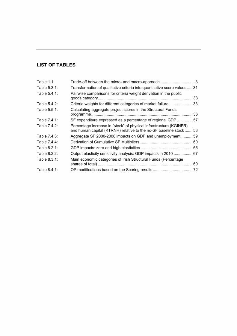
LIST OF TABLES Table 1.1: Trade-off between the micro- and macro-approach ............................... 3 Table 5.3.1: Transformation of qualitative criteria into quantitative score values ..... 31 Table 5.4.1: Pairwise comparisons for criteria weight derivation in the public
goods category...................................................................................... 33 Table 5.4.2: Criteria weights for different categories of market failure ..................... 33 Table 5.5.1: Calculating aggregate project scores in the Structural Funds
programme............................................................................................ 36 Table 7.4.1: SF expenditure expressed as a percentage of regional GDP .............. 57 Table 7.4.2: Percentage increase in “stock” of physical infrastructure (KGINFR)
and human capital (KTRNR) relative to the no-SF baseline stock ....... 58 Table 7.4.3: Aggregate SF 2000-2006 impacts on GDP and unemployment .......... 59 Table 7.4.4: Derivation of Cumulative SF Multipliers................................................ 60 Table 8.2.1: GDP impacts: zero and high elasticities ............................................... 66 Table 8.2.2: Output elasticity sensitivity analysis: GDP impacts in 2010 ................. 67 Table 8.3.1: Main economic categories of Irish Structural Funds (Percentage
shares of total) ...................................................................................... 69 Table 8.4.1: OP modifications based on the Scoring results .................................... 72

LIST OF FIGURES Figure 2.2.1: Endogenous and exogenous Elements in the policy analysis
approach ................................................................................................. 8 Figure 3.1: Integrated Micro- and macro approach (IMM) for EU Structural
Funds (SF) analysis .............................................................................. 14 Figure 4.1.1: Implications of alternative aggregation rules ........................................ 20 Figure 4.1.2: General structure of the MCDA model for public policy analysis.......... 22 Figure 5.1.1: Steps in a policy analysis study ............................................................ 29 Figure 6.2.1: A HERMIN modelling schema .............................................................. 43 Figure 6.2.2: Schematic Outline of the HERMIN Modelling Approach ...................... 44 Figure 7.3.1: Physical infrastructure: average elasticities and confidence intervals.. 55 Figure 8.3.1: Porter’s stages of competitive development (Porter, 1990).................. 68
NON-TECHNICAL SUMMARY
Since the late 1980s the reformed and expanded EU cohesion policy and the Structural Funds have presented policy makers at the European and national level with new possibili-ties but also faced them with major design and impact evaluation problems. This paper arose out of our experience in evaluating the impacts of EU Structural Fund programmes in a wide range of European countries and regions. One fundamental observation is that the design, implementation and evaluation stages of these kinds of large-scale public investment pro-grammes are often carried out in a rather informal and ad-hoc way and can become domi-nated by practical, day-to-day management and implementation concerns. One casualty can be the exclusion of any attempt at a systematic approach to formulating the underlying policy decision problem using a consistent and transparent policy design and evaluation frame-work. In the absence of such a framework, it is difficult to assess adequately the possibility of absorption problems related to funding transfers, effectiveness and efficiency of the policies given specific targets, and the likely micro and macro impacts of the investment interventions in the short- and long-run.
In this paper we describe an integrated approach for assessing the general economic effec-tiveness, efficiency and impact of public policy actions for large investment programs of the kind implemented over the past fifteen years in EU-aided Structural Fund programmes. Far from being rigid, our modelling philosophy includes both formal tools designed to assess all relevant effects, as well as informal (intuitive) elements to allow for flexible policy design and evaluation. When setting up an integrated micro-macro (IMM) model we are trying to over-come two major shortcomings in actual policy design and analysis: Firstly, to bridge the gap between the scientific requirements of model-based decision making and evaluation and the practical requirement for flexible and easy to use decision support tools that are well suited for day-to-day application. Secondly, to address the observed discrepancy in policy analysis between programme monitoring and evaluation realized at a highly aggregate level using quantitative macromodels (the so called “top down” approach) and the highly disaggregated approach to project evaluation, marked as micro- or “bottom up”-approaches.
The gulf between micro and macro policy analysis deserves special attention: It commonly arises because it is never possible in practise to derive the aggregate impact of any large-scale public investment programme from simply adding together all the individual micro im-pacts of its constituent projects. A major reason for this is the presence of complex substitu-tion and externality effects in the overall programme, and their likely absence from micro (or project-specific) analysis. On the other hand, the aggregative top-down approach is de-signed to explore overall macro effects, but cannot make detailed judgements about the efficiency of individual projects embedded within the overall investment programme. How-ever, by combining these two, usually isolated, evaluation approaches, our aim is to show how to avoid the loss of important information in the process of evaluation and thus maxi-mize effectiveness, efficiency and desirable policy impacts.
The elements of our integrated IMM model can be summarized as follows. As the first build-ing bloc of the system, we use a bottom-up approach using a multi-criteria decision analysis (MCDA) model to judge the effectiveness and efficiency of a policy initiative. The economic foundations of the model are based on welfare economics. The model is a transparent and flexible tool which allows for the inclusion of subjective and multiple judgements in decision-making and evaluation process. As the second building bloc, we implement the HERMIN macroeconomic modelling framework, which has been extensively used for Structural Fund

analysis. HERMIN models are up-to-date fully specified, multi-equation model with the ad-vantage of capturing even the indirect impacts of the Structural Funds (i.e., substitution and externality-effects) that are generally not assessed using a micro-orientated bottom-up ap-proach. It has Keynesian small-open-economy theoretical foundations, but also incorporates neo-classical side effects and - crucially for the Structural Fund analysis - it incorporates mechanisms which are based on the endogenous growth literature that capture the long-run impact of Structural Fund investments.
Finally, the interlocking of the micro- and macro-approach in the last step allows us to link the impact of changes induced at the micro level with the relevant macro aggregates (output and employment) in the economic-policy debate. This novel approach therefore is able to evaluate both the efficiency within a general programme, as well as to show how a micro optimisation in terms of modifications within the programme structure may translate into im-proved aggregate macro effects. The method thus significantly improves the evaluation process as a guideline for the decision-making in the public sector.
We illustrate our approach throughout all steps using the mid-term evaluation of the EU Structural Funds in the Objective 1 German region of Saxony-Anhalt for the period 2000-2006, but the approach can easily be applied to other countries and/or regions. The advan-tage of this example is that both the micro and macro analysis have been carried out and used recently in impact evaluation and policy improvement and we show that a careful analysis of the Structural Fund programmes may give rise to substantial welfare gains.
1 INTRODUCTION
This paper arose out of our experience in evaluating the impacts of EU Structural Fund pro-grammes in a wide range of European countries and regions. The design, implementation and evaluation stages of these kinds of large-scale public investment programmes are often carried out in a rather informal and ad-hoc way and can become dominated by practical, day-to-day management and implement concerns. One casualty can be the exclusion of any attempt at a systematic approach to formulating the underlying policy decision problem using a consistent and transparent policy design and evaluation framework. In the absence of such a framework, it is difficult to assess adequately the possibility of absorption problems related to funding transfers, effectiveness and efficiency of the policies, and the likely micro and macro impacts of the investment interventions. 1 In light of the potential problems created by ad-hoc decision making, it is important to make use of simple but clear and comprehensive formal models designed to maximize the systematic use of all relevant information within the overall policy making process.2
The use of an explicit, systematic and consistent framework in policy making is also sup-ported by research and applied work in the field of economics and management science. Here, scholars emphasize that although many decisions are made intuitively in everyday life in the absence of any deep analysis, intuition alone is not sufficient to generate an optimal solution outcome in complex, large-scale, medium-term decision making set-ups such as the case for most public sector investment decision problems.3 Instead, the use of explicit mod-els makes policy design and evaluation much more rational, and assists in the search for optimal policies. 4
1 The essential differences between the analyses of micro and macro effects lie in the extent to
which the rest of the economy is viewed as unchanged while a specific policy intervention is evaluated. For a detailed discussion of this aspect see e.g. Hallet and Untiedt (2001).
2 Krugman (1997) eloquently points out this claim by arguing: „After all, a model – even a crude, small, somewhat silly model – often offers a far more sophisticated, insightful framework for dis-cussion than scores of judicious, fact-laden, but model-free pontifications.”
3 With respect to management science this field of research has become known as „strategic deci-sion making“ or “strategic planning”. The basic assumption of this approach to management be-haviour is that systematic and careful analysis yields choices that are superior to those coming from intuitive processes. An application of the strategic planning approach to the public sector is given by Mercer (1991).
4 However, in a recent field of literature based on advances in cognitive science and artificial intelli-gence the importance of the intuitive element in decision making has been rediscovered based on Mintzberg’s (1994) criticism of a “pure” strategic planning based on rationality principles. Using fieldwork based on manager surveys Khatari and Alvin (2000) come to the synthesis that both ra-tional and intuitive processes need to be taken into account for a new theory of strategic decision

Introduction 2
In an effort to trace back the persistent discrepancy between the ”rational model postulate” in (academic) policy analysis and the more or less model-free decision making/evaluation that takes place in practice, Lootsma (1999) argues that many decision makers typically dislike what they perceive as rigid and formalized methods for decision support, since they fear that such methods do not leave sufficient space for judgement, intuition and creativity. Moreover, decision support models tend to be complex and difficult to understand, often resulting in their neglect by policy practitioners. In this line of argumentation Medda and Nijkamp (2003) observe a general tendency of decision makers – especially in the public domain – to neglect straightforward model based optimisation behaviour and instead to favour simpler, model free modes of planning based on satisfying or compromise principles or an even lower level of ambition.
In this paper we describe an integrated approach for assessing the general economic effec-tiveness, efficiency and impact of public policy actions for large investment programs of the kind implemented over the past fifteen years in EU-aided Structural Fund programmes. Far from being rigid, our modelling philosophy includes both formal tools designed to assess all relevant effects, as well as informal (intuitive) elements to allow for flexible policy design and evaluation. When setting up the model we are trying to overcome two major shortcomings in actual policy design and analysis:
1. Our first aim is to bridge the gap between the scientific requirements of model-based decision making/evaluation and the practical requirement for flexible and easy to use decision support tools that are well suited for day-to-day application. As Salminen and Lahdelma (2001) point out, understanding how humans process information is clearly important when constructing various decision support models. The decision makers are more likely to accept the method and the results if they are able to understand the deci-sion model and find the method in some sense “natural” or “intuitive”. Therefore, our proposed approach tries to be consistent with economic theory, transparent and repro-ducible, and at the same time allows flexible and creative decision making.
2. Our second aim is to address the observed discrepancy in policy analysis between programme monitoring and evaluation realized at a highly aggregate level with the help of quantitative macromodels (the so called “top down” approach) and the highly disag-gregated approach to project evaluation using micro- or “bottom up”-approaches. Our goal is to work towards an integration of the top-down macro methodology and the bot-tom-up micro methodology.
The above mentioned apparent gulf between micro and macro policy analysis deserves some special attention: It commonly arises because it is never possible in practise to derive the aggregate impact of any large-scale public investment programme from simply adding together all the individual micro impacts of its constituent projects. A major reason for this is the presence of complex substitution and externality effects in the overall programme, and their likely absence from micro (or project-specific) analysis. On the other hand, the aggrega-tive top-down approach is designed to explore overall macro effects, but cannot make de-tailed judgements about the efficiency of individual projects embedded within the overall
making. For the later modelling construction we will build on both elements of this strategic deci-sion making synthesis.
Introduction
3
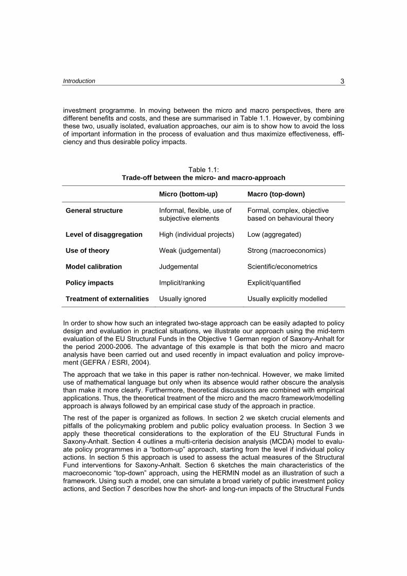
investment programme. In moving between the micro and macro perspectives, there are different benefits and costs, and these are summarised in Table 1.1. However, by combining these two, usually isolated, evaluation approaches, our aim is to show how to avoid the loss of important information in the process of evaluation and thus maximize effectiveness, effi-ciency and thus desirable policy impacts.
Table 1.1: Trade-off between the micro- and macro-approach
Micro (bottom-up) Macro (top-down)
General structure Informal, flexible, use of subjective elements
Formal, complex, objective based on behavioural theory
Level of disaggregation High (individual projects) Low (aggregated)
Use of theory Weak (judgemental) Strong (macroeconomics)
Model calibration Judgemental Scientific/econometrics
Policy impacts Implicit/ranking Explicit/quantified
Treatment of externalities Usually ignored Usually explicitly modelled
In order to show how such an integrated two-stage approach can be easily adapted to policy design and evaluation in practical situations, we illustrate our approach using the mid-term evaluation of the EU Structural Funds in the Objective 1 German region of Saxony-Anhalt for the period 2000-2006. The advantage of this example is that both the micro and macro analysis have been carried out and used recently in impact evaluation and policy improve-ment (GEFRA / ESRI, 2004).
The approach that we take in this paper is rather non-technical. However, we make limited use of mathematical language but only when its absence would rather obscure the analysis than make it more clearly. Furthermore, theoretical discussions are combined with empirical applications. Thus, the theoretical treatment of the micro and the macro framework/modelling approach is always followed by an empirical case study of the approach in practice.
The rest of the paper is organized as follows. In section 2 we sketch crucial elements and pitfalls of the policymaking problem and public policy evaluation process. In Section 3 we apply these theoretical considerations to the exploration of the EU Structural Funds in Saxony-Anhalt. Section 4 outlines a multi-criteria decision analysis (MCDA) model to evalu-ate policy programmes in a “bottom-up” approach, starting from the level if individual policy actions. In section 5 this approach is used to assess the actual measures of the Structural Fund interventions for Saxony-Anhalt. Section 6 sketches the main characteristics of the macroeconomic “top-down” approach, using the HERMIN model as an illustration of such a framework. Using such a model, one can simulate a broad variety of public investment policy actions, and Section 7 describes how the short- and long-run impacts of the Structural Funds

Introduction 4
were evaluated using the HERMIN macromodel for the economy of Saxony-Anhalt. Section 8 explores how the micro- and the macro-approaches can be combined in an overall evalua-tion of Structural Fund impacts. In Section 9 we draw some general conclusions on how to use our approach when designing, implementing and evaluating policy actions within the wider EU National Development Plans (NDPs) that form the context for co-financing of public investments by means of Structural Funds.
2 PUBLIC POLICY ANALYSIS FOR NATIONAL
DEVELOPMENT PLANNING Public policy analysis is a field of interdisciplinary research that seeks to use a rational and systematic approach in order to evaluate the consequences of different policy actions. Its domain of application embraces all the various stages of policy making: namely, design, implementation, monitoring, evaluation and control. Its general purpose in an ex-ante context is to assist policy designers by clarifying the problem, outlining alternative solutions and dis-playing possible tradeoffs among their consequences. In a mid-term or ex-post perspective its task is to review and monitor progress in implementing policy decisions, as well as to evaluate policy outcomes and provide guidance towards seeking better policies.
In the following section the different stages in the policy analysis process are systematically discussed, starting with the “policy making problem”. We then identify crucial conditions for problem solving tools and sketch the institutional framework of policy making. We conclude with a discussion of evaluation approaches classified according to the key concepts of ap-propriateness, effectiveness and efficiency.
2.1 THE POLICYMAKING PROBLEM The general need for drawing on research and professional expertise for policy analysis is grounded in the so-called “policy making problem”. Following Nijkamp (2000), decision mak-ing in a complex economy is fraught with many difficulties: Policy-makers have to decide about alternatives in a situation where the future outcome is uncertain. They are working in a context where relevant information is lacking, and are forced to use imprecise and incom-plete data about the present and the future. They face numerous and diverse policy alterna-tives, with the possibility of complex trade-offs between them. And in addition to using quan-titative criteria, they also need to incorporate qualitative criteria into the decision-making process, a process that is never straightforward. Finally, decision making in the public do-main is usually not a one-shot activity, but part of a continuing choice process (see Medda and Nijkamp, 2003). Hence, choice possibilities, relevant criteria and urgencies evolve over time and give rise to feedback relationships that need to be taken into account.
In spite of such difficulties, policymakers nevertheless have to develop and implement poli-cies that have the best chance of contributing to raising the standard of living of their target audience. Stated formally, this can be best described as the maximisation of a target (or criterion) function consisting of multiple goals, subject to a set of different restrictions (or constraints). From an economic perspective this maximisation approach implies that all fore-seeable costs and benefits of a policy initiative have to be assessed. Further, in a broader perspective, social, cultural, environmental and safety aspects would also have to be con-sidered (Nijkamp, 2000). In response to these requirements, public policy analysis system-atically combines interdisciplinary research elements, drawing extensively on input from
Public Policy Analysis for National Development Planning 6
management science and system engineering, welfare economics, political and administra-tive science as well as empirical social science (Ulrich, 2002).
Since its goal is to assist in arriving at rational decisions based on all information available, policy analysis should benefit from the use of scientific tools. As Walker (2000) suggests, crucial ingredients of such a scientific approach to policy modelling should include certain key criteria, such as that the analysis be open and explicit, objective, empirically based and moreover try to be consistent with existing knowledge. In addition, the results of analysis need to be verifiable and reproducible. Based on these criteria, the most familiar and up-to-date public policy analysis tools in practical application include decision and sensitivity analysis, cost-benefit analysis, as well as evaluation research for economic, environmental and social impact assessment.
Models are an essential element of policy design and analysis. Since they are usually con-structed by academic specialists, the modelling tools that support policy makers have to take account of the need to facilitate communication between the model builders and the model users. The more straightforward the model, the easier it will be to understand its internal logic and the better the chance that the policy maker will use it consistently and appropri-ately.5 Models need to be “parsimonious” in their structure: simplified representations of the world of policy reality, but not so oversimplified as to be inaccurate or misleading. They must be complete on important issues, incorporating all relevant aspects of the underlying prob-lem into the model structure. They must be “robust”, producing results that are plausible and reliable. They must be “transparent”, with results that are checkable and the transformation from input to output data must be transparent. They must be “versatile”, flexible enough to allow for the implementation of new data and the individual requirements of users. In addition to being “positive” descriptions of reality, they must also have some “normative” characteris-tics, and be able partially to include intuitive and subjective judgements.6 Finally, they need to be set up in computer form for high speed data processing, and permit users fast access to input and output data.
5 For this line of argumentation compare Little’s well known work about the ‘decision calculus’ (Little,
1970) and the extensive Operations Research literature that has been published since then.
6 The last aspect is of certain importance in applied decision-making, since typically some kind of subjectivity is included in any form of decision-making. Since the policy analysis model presented here explicitly allows for the inclusion of subjective judgments to processing of this information within the model remains transparent, verifiable and incontestable in policy debates.
Public Policy Analysis for National Development Planning 7
2.2 THE ELEMENTS OF THE POLICY ANALYSIS PROCESS Having defined the “policymaking problem” and described the desirable characteristics of scientific problem solving tools, we can now proceed one step further: Here, the model builder assisting the decision maker by constructing a suitable model with the above de-scribed characteristics has to keep in mind that policy analysis is performed at different lev-els, with different objectives, and that no unique tool exists that is suitable for all problems (Walker, 2000). Therefore, before we can proceed with the construction of decision support models, we first have to map out the general institutional set-up of the policy making frame-work and to identify the specific needs for modelling tools and expertise. As Medda and Ni-jkamp (2003) point out, the institutional context of decision-making is of critical importance for a successful implementation of a policy action.
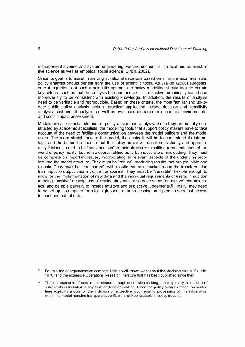
In Figure 2.2.1 we sketch the setup of the general policymaking framework, displaying the crucial elements which have to be taken into account when a policy-maker formulates (eco-nomic) policy programmes which will be implemented in the market system to guide the market outcome towards the politically desired outcome. This diagram separates the policy making process into “endogenous” and “exogenous” elements. The endogenous element is built around the attempt to intervene in the system of markets and to change any undesirable market outcome according to an objective function. The construction of this objective func-tion is influenced by the goals, objectives and preferences of the stakeholders (citizens). The citizen-policymaker relationship is typically of a principal-agent kind, with the stakeholders defining the target function and the agents (here policymakers) acting in their interests when implementing the policies. However, the target function may also be influenced by the poli-cymakers’ own goals and objectives in the actual process of policy making.7 The outcome of the subsequent endogenous policy making process is a policy programme that is imple-mented in the system of markets.
7 This problem to which Niskanen (1971) first called attention is a typical principal-agent problem.
The principal-agent problem is simply the familiar problem of how one person gets another to do what he or she wants. For a detailed discussion see the extensive public choice literature, based on Niskanen’s seminal work. An intuitive introduction is given by Stiglitz (2000).
Public Policy Analysis for National Development Planning 8
Figure 2.2.1: Endogenous and exogenous Elements in the policy analysis approach
Source: Adaptation of Walker (2000).
Figure 2.2.1 shows not only the implemented policy actions but also external forces (outside of the control of the policymaker) acting on the market system and changing the market out-come. Both policy actions and external forces can involve a great deal of uncertainty. Some external forces - such as technological shocks, preference shifts etc. - are uncertain, and their effects on markets are also uncertain. To complete the policy making process induced by principals and agents, the actual market outcome has to be compared to the desired one. Whenever targeted and actual market outcomes are in line, there is no need to alter the im-plemented policy actions. Otherwise the policy actions need to be revised. To summarise, the policy making process engaged in by stakeholders and policymakers therefore contains ex-ante design, monitoring and ex-post review elements that generate feedback to the en-dogenous element of the policy-making process of Figure 2.2.1.
In the above set-up, policy decisions are also classified as exogenous and therefore outside the control of the policy maker. This may seem strange, but is indeed the case for large pol-icy programmes such as National Development Plans (NDPs) and their associated Structural Funds. These are large-scale investment programmes: public investment in physical infra-structure, human resources and direct aid to private firms. They have a medium-term per-spective, with time horizons of up to seven years. Their design requires extensive efforts and careful ex-ante planning since, once those programmes are applied to the market system, they run more or less independently from the policy making process and only need adminis-
Exogenous Process
Endogenous Policymaking Process
FeedbackExternal Forces
Policy makers
Stake-holders
Goals, object-
System of markets
Market outcome
Target-function: Goals,
objectives, preferences
Policies
Public Policy Analysis for National Development Planning 9
trative interventions. Consequently, they are more appropriately located conceptually outside the endogenous process in Figure 2.2.1.
National Development Plans typically have multiple objectives and consequently, trade-offs often exist between some of their competing goals. Therefore the policy making process (that is, the optimisation of the objective function) becomes extremely complex. In response to these difficulties, both stakeholders as well as policy-makers typically rely on a range of modelling tools when deriving goals and targets as well as designing policies and evaluating the likely individual project and overall programme impacts (as suggested in section 2.1). To address the principal-agent relationship, both policy-makers and stakeholders need instru-ments to justify and evaluate the chosen set of actions by systematically describing what has happened and to pass a judgement on the policy in question. Such models need to identify the causal relationships between policy instruments and policy impacts, estimate the true net impact of the policy by isolating it from other accompanying influences, and provide a basis for judgement on the isolated net impact.
2.3 BASIC EVALUATION CONCEPTS FOR NDP-TYPE PROGRAMS In measuring the causal relationships between policy instruments and policy impacts, three important economic criteria for evaluating a policy have evolved: 1.) appropriateness, 2.) micro and macro effectiveness, and 3.) efficiency.8 Appropriateness can be defined as: “suitable or proper in the circumstances”. It is a fairly minimalist criterion. Policies are at least required to be appropriate, in the sense of being broadly suitable for the identified purposes. According welfare economics, those policies are inappropriate which do not attempt to cor-rect market failures and instead bias the optimal functioning of the economy.
The term “effective” can be defined as: “successful in producing a desired or intended re-sult”. Thus, an effective policy always needs to be appropriate, but an appropriate pro-gramme may not necessarily be effective. The assessment of effectiveness is based on the extent to which expected effects have been obtained and desired objectives have been achieved. Effectiveness is usually evaluated by relating an output (i.e., an impact indicator) to a quantified objective. Thereby it is useful to distinguish two approaches to the analysis of effectiveness. The first uses a micro economic (or bottom up) approach, building on welfare economics. The second uses a macromodel to assess the overall (or top-down) impacts (and is often called “impact analysis”).
Finally, the term “efficient” can be defined as: “achieving maximum outputs with minimum wasted effort or expense”. Considerations of efficiency only arise in cases where policy measures are already both appropriate and effective. In analogy with effectiveness, the issue of efficiency has a macro and a micro side. In the case of macro efficiency, one needs to investigate whether the same macro impacts could be obtained by less public spending or whether greater macro impacts could be obtained for the same aggregate level of public ex-penditure, but with a different allocation of resources as between different policy instruments.
8 For a detailed discussion of these concepts see Bradley et al., 2005. Next to these concepts ac-
cording to an evaluation framework elaborated by the OECD (1997), also the aspect of “legiti-macy” of public action plays an key role in public policy analysis. We will integrate this aspect in case study in section 5.

Public Policy Analysis for National Development Planning 10
Efficiency at the microeconomic level is usually measured by assessing the costs and bene-fits of different alternatives (via cost-effectiveness, cost-benefit or multi-criteria analysis).
When large-scale public investment programmes (such as National Development Plans) are designed and evaluated, different modelling tools are needed to assess the micro and macro policy impacts. These modelling tools typically range from cost-benefit analysis of individual projects at the one extreme to an evaluation of aggregate programme impacts on the entire national economy at the other. However, before we turn to consideration of policy evaluation tools, we first describe the main characteristics of EU-inspired National Development Plans and their associated Structural Funds, the thematic subject of our analysis.
3 NATIONAL DEVELOPMENT PLANS AND
STRUCTURAL FUNDS
The EU Structural Fund interventions are designed to play a crucial role in improving social and economic cohesion in the European Union through regional policy. During the actual 2000 – 2006 funding period, the European Commission allocated €213 billion to transfers for regional policy, accounting for about one third of the entire EC budget. Structural Funds are focused on regions with a low per capita income, and regions with a level of GDP per capita below 75 per cent of the EU average are specially singled out for development aid. Very often such regions are characterised by a number of interacting economic problems, such as a low level of investments, a higher than average unemployment rate, a lack of services for businesses and individuals and poor quality basic infrastructure. These regions are desig-nated “Objective 1”. They make up a significant part of the total EU (22 percent of the popu-lation), and receive about 70 percent of total funding.9
The Structural Fund programmes for Objective 1 regions typically comprise a broad set of guiding principles, objectives and policy instruments. For historical reasons most of the EU spending is channelled through four different designated funds: the European Regional De-velopment Fund (ERDF); the European Social Fund (ESF); the Financial Instruments of Fisheries Guidance (FIFG); and the European Agriculture Guidance and Guarantee Fund (EAGGF). The ERDF finances infrastructure, job-creating investments, local development projects and aid for small firms, while the ESF mainly focuses on helping unemployed and disadvantaged people to get back to work, mainly by financing training measures and sys-tems of recruitment aid. The FIFG helps to adapt and modernize the fishing industry, while the EAGGF finances rural development measures and aid for farmers (mainly in less-favoured regions). In principle, all Objective 1 regions are supported by all funds and the main target of this support is to speed up growth and convergence.
Within Germany, the five East German states (or Bundesländer) are classified as Objective 1 regions and receive Structural Fund payments (i.e., Brandenburg, Mecklenburg-Western Pomerania, Saxony, Saxony-Anhalt and Thuringia). In the funding period 2000 – 2006 the EC-payments to East Germany amount to €20.7 billion, co-financed with national and private expenditures of approximately €50.3 billion. In the rest of the paper we take Saxony-Anhalt as an example for policy analysis within the EU Structural Funds cohesion policy. During the period 2000 to 2006 Saxony-Anhalt will receive approximately €3.5 billion of EU Structural Funds. When national and private co-financing are added to the EU element, the overall amount of the Structural Funds is about €8 billion.
Saxony-Anhalt is a political and economic macro-region of Germany (NUTS 1 level) with a population of approximately 2.5 million in 2003. On its difficult way towards becoming an economically powerful region within the EU, it faces a variety of profound and longstanding 9 For a complete description of the EU cohesion policy see
http://europa.eu.int/comm/regional_policy/index_en.htm.
National Development Plans and Structural Funds 12
challenges. It is important to keep in mind that the German unification in 1990 led to a radical change (in terms of institutional and structural reforms) in the economic system for all the former East German states. This change resulted in a sudden breakdown in production and trade, followed by a rapid restructuring process. Both processes are still taking place, and are strongly represented in the empirical data.
Generally speaking, the transformation and cohesion process in Saxony-Anhalt towards the West-German and EU-15 average can be divided into two sub-periods. After some important progress in the renewal and expansion of its basic economic structures and resources, eco-nomic performance (mainly based on growth in production) was strong in the first half of the 1990s. However, this strong growth and convergence process has drastically slowed down in the second half of the last decade. The induced structural break in the empirical pattern may indicate either that the transformation of the regional economic structure has temporary slowed down before convergence has been fully realized, or that Saxony-Anhalt has con-verged to a different steady state path below the West-German and EU-15 average.
Without going into too much detail, the economic situation in Saxony-Anhalt shows a some-what conflicting picture. On the one hand, there are some optimistic developments, such as the positive trend in labour productivity and unit labour costs for the industrial sector, which functions as an important regional export base. On the other hand, there are still substantial structural problems: an oversized building and construction sector; a large and long-standing deficit in the regional current accounts; and a huge public debt that restricts the freedom of action of public policy. Other important factors determining regional competitiveness are also lagging behind: e.g., R&D intensity, patent activity, the level and growth of human capital etc. The EU Structural Funds are designed to support the region in addressing these problems.
In Saxony-Anhalt the Structural Funds are implemented through a series of so-called Opera-tional Programmes (OP), which are sub-plans that embrace a variety of different targeted policy priorities. In accordance with the Community Support Framework (CSF) for East-Germany, investment measures in Saxony-Anhalt during the years 2000 to 2006 are grouped into five main priorities:
(i) Fostering competitiveness, especially for small and medium sized enterprises (SME)
(ii) Physical infrastructure
(iii) Environmental protection and improvement
(iv) Fostering employment potential in an equitable way
(v) Rural development
Whereas the first three priorities are mainly financed by the ERDF, job market interventions (under priority four) are covered by the ESF, and rural development and agriculture by the EAGGF. Below the level of priorities, the Structural Funds in Saxony-Anhalt can be sub-divided into many different individual measures, of which there are about 200.
However, instead of the politically defined priorities and the great variety of individual meas-ures and projects, it is also useful to consider the Structural Funds grouped according to three broad economically meaningful categories: 1.) physical infrastructure, 2.) human re-sources, and 3.) direct investment aid to the private productive sectors (i.e., manufacturing,
National Development Plans and Structural Funds 13
market services and agriculture). The use of these economic categories is a necessary step towards performing any aggregate (or macroeconomic) impact evaluation of Structural Funds.
Whereas the macro (or top-down) assessment of Structural Fund impacts uses the above three-way “economic” aggregation of the expenditures, the micro approach starts from the evaluation of each single project or measure (e.g. a specific road construction project; a spe-cific training scheme; a specific investment incentive). However, in this micro (or bottom-up) approach not all indirect effects (externalities etc.) can be captured, so that an assessment of the overall impact on aggregate goals (employment, output growth, etc.) is difficult. On the other hand, the top-down macroeconometric approach is not able to explore the contribution of single measures or projects in contributing to the overall effect. Therefore, an evaluation of the appropriateness, effectiveness and efficiency on the level of measures or projects within the overall Structural Fund programme is not possible at a macro level. In response to the specific shortcomings at each individual evaluation level (micro “bottom-up” and macro “top-down”), we will apply both approaches in a complementary fashion in order to reach an evaluation outcome that allows a kind of micro-foundation to macro policy analysis.
As the following sections will show, our goal is to design an integrated approach to evalua-tion that combines micro and macro-elements, as illustrated schematically in Figure 3.1 alongside the different levels of the structural funds goals and instruments (from broad cate-gories to single measures). The figure shows that the isolated modelling tools can only evaluate policy impacts at specific programme levels (broad categories for the macro ap-proach; measure/project level for the micro tool). However, externality effects also work be-tween the different levels and influence both the aggregate and the individual outcome (see grey area). Only an integration of micro- and macro-elements (IMM) therefore allows for a complete accounting for all programme effects.
In setting up the IMM approach we start with a presentation of the bottom-up micro ap-proach, which we will build around Multi-Criteria Decision Analysis (MCDA) model in the next section.
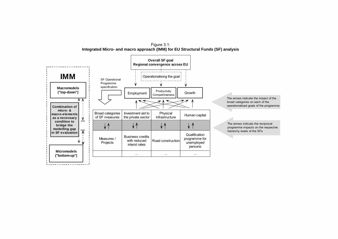
Figure 3.1: Integrated Micro- and macro approach (IMM) for EU Structural Funds (SF) analysis
Overall SF goalRegional convergence across EU
Employment ProductivityCompetitiveness Growth
SF OperationalProgrammespecification
Broad categoriesof SF measures
Investment aid tothe private sector
Physicalinfrastructure Human capital
Measures /Projects
Business creditswith reducedinterst rates
Road construction
Qualificationprogramme for
unemployedpersons
... ... ...
Operationalising the goalIMMMacromodels("top-down")
Combination ofmicro- &
macro-elementsas a necessary
condition tobridge the
modelling gapin SF evaluation
Micromodels("bottom-up")
The arrows indicate the reciprocalprogramme impacts on the respectivehierarchy levels of the SFs
The arrows indicate the impact of thebroad categories on each of theoperationalised goals of the programme

4 MICRO POLICY EVALUATION: MULTI-CRITERIA
DECISION ANALYSIS
4.1 GENERAL STRUCTURE OF MCDA MODELS FOR COMPLEX DECISION MAKING
As described in section 2, decision-making is a process of choosing among alternative courses of action in order to attain specified goals and objectives. For such a task it is useful to have a scientific model whose structure is transparent, empirically based and consistent with prior knowledge. Nijkamp (2000) reviews applied decision making models, and con-cludes that, according to the above stated criteria, the best-known example of evaluation methods in economic terms is the traditional cost-benefit analysis (CBA) technique. How-ever, the most severe problem with CBA techniques is that they are primary applicable and appropriate in situations where the policy decision being examined is a well demarcated and a priori precisely defined project which does not generate many unpriced externalities. If, however, the decision concerns a more general policy programme (of which the details and even sometimes the major features are unknown), then the translation of its impacts into precisely measurable and quantitative consequences and subsequently into monetary fig-ures is often rather problematic. In reality many policy programs are characterized by impre-cise, uncertain, fuzzy or sometimes only qualitative information: In such cases, one has to resort to multi criteria decision analysis (MCDA).
MCDA research experienced an explosive growth in the last decades and the current meth-ods applied vary widely in their scope of action and their ability to support decision making. A recent survey of the evolution of MCDA techniques is given by Roy (2005). The MCDA model presented in this section is best described as an application of Multiple Attribute Utility Theory (MAUT), which is a subfield of MCDA research and mainly used for ranking/selecting different alternatives.10 As Mateu (2002) points out, MAUT models are based on the idea that any decision-maker attempts unconsciously to maximize some function that aggregates utility with respect to different criteria. Following Brams (2005), a typical multi-criteria prob-lem can therefore be stated as
(1) max U = U{c1(a),...,c2(a),...,cm(a) | a ∈ A},
10 In the MCDA field in general a variety of evaluation objectives exist such as: (1.) Choice problems:
selection of the “best” alternative; (2.) Ranking problems: complete ranking of alternatives; (3.) Se-lection problems: selection of the subset of “good alternatives”; (4.) Sorting problems: classification of the alternatives; that is splitting of the alternatives into several classes. In choice problems the aim is to find the best alternative, ranking problems measure the goodness of all alternatives, which is typically presented as a ranking from the best to the worst and finally sorting problems classifies alternatives to predefined sets of classes.

Micro Policy Evaluation 16
where U is a (global) utility function, A is a set of possible alternatives {a1, a2,…,an} and a set of evaluation criteria {c1(⋅), c2(⋅),…cm(⋅)}. The desire of the decision maker is to identify an alternative “a” optimising equation (1). A criterion “c” can be defined as a tool constructed for evaluating and comparing potential alternatives according to a well-defined point of view (Roy, 2005). The evaluation then must take into account all the pertinent effects or attributes linked to this point of view with respect to each alternative “a”. This is expressed by c(a) and denotes the performance of alternative “a” according to the criterion “c”. It is necessary to define explicitly a set Xc of all the possible outcomes to which this criterion can lead. To allow comparisons, it should be possible to define a complete order on Xc, which is called the scale of Xc. Elements x ∈ Xc are called “degrees” or “scores” of the scale. Each degree can be characterised by a number or by a verbal statement, etc. For the comparison of two alter-natives according to criterion “c”, we have to compare the two scores used for evaluating their respective performance. Here it is important to analyse the concrete meaning in terms of preferences covered by such degrees. This leads to a classification of various types of scales as follows (see Roy, 2005):
1. Purely ordinal scale: Here the gap between two scores does not have a clear meaning in terms of difference preferences. An ordinal scale can have the form of a verbal or a numerical scale.
2. Quantitative scale: These are numerical scales whose degrees are defined by referring to a clear, concretely defined quantity in a way that, on the one hand, gives meaning to the absence of quantity (that is a score of 0), and on the other hand to the existence of a unit allowing us to interpret each degree as the addition of a given number of such units. Those scales are also called cardinal or ratio scales.
3. Other types: In the MCDA field there are also other forms of intermediate scales be-tween the above-mentioned ordinal and quantitative forms.
As already shown in (1), in most cases MCDA models are built on “n” criteria with n > 1. They constitute a family F of criteria, with F = {c1(⋅), c2(⋅),…cm(⋅)}. In order to be sure that F is able to play its role in the decision analysis process correctly, it is necessary to fulfil the fol-lowing conditions (Roy, 2005, page 10 – 11):
(i) the intention of each criterion is sufficiently intelligible for each of the stakeholders;
(ii) each criterion is perceived to be a relevant instrument for comparing potential actions along the scale which is associated with it, without prejudging their relative importance when this varies from one stakeholder to another;
(iii) the “n” criteria considered all together satisfy some logical requirements (exhaustive-ness, cohesiveness and non redundancy) which ensure coherence of the family.
Formulating the above evaluation set up in matrix terms, we have to consider a finite number of alternatives (policy actions) ai, with i = 1,…, n, under a family of performance criteria cj, with j = 1,…, m. This situation can be best represented with the help of a decision-matrix M, written as follows:
Micro Policy Evaluation 17
)(...)()( 21 ⋅⋅⋅ mccc
(2)
⎥⎥⎥⎥⎥
⎦
⎤
⎢⎢⎢⎢⎢
⎣
⎡
=
nmn
m
n xx
xxxx
a
aa
M
1
21
11211
2
1
......
...
...,
The matrix entry (or score) xij is a combination of the value of the vector of criteria [c1,…,cm] and the vector of alternatives [a1,…,an]. The matrix entries xij are the basic input values to conduct a multicriteria evaluation for alternatives ranking.
Typically, not all criteria are regarded as equally important, and the introduction of criteria weights help to solve this problem. As Roberts and Goodwin (2002) argue, since the elicita-tion of weights may be difficult, several methods have been proposed for reducing the bur-den of the process. Many of these methods involve asking the decision maker or evaluator questions about the relative importance of the criteria and using the responses to identify weights that approximate the decision maker’s ‘true’ weights. One possible way of deriving different weights according to this approach is the use of so-called “pairwise comparisons”. Their main feature is a step-by-step comparison of the set of alternatives, building up some binary relations and then exploiting in an appropriate way these relations in order to obtain final policy recommendations.11 In empirical applications one way to proceed with the pair-wise comparisons is to use the so-called “half-matrix” method, as described in Strebel (1975). In our approach the construction of pairwise comparisons is used to identify all crite-ria of interest and derive a ranking of criteria in absolute values in term of criteria weights. In this sense our approach resembles other similar approaches, such as the Analytical Hierar-chy Process (AHP).12
The respective criteria weights are labelled as gj, with j = 1,…, m. We typically normalize the criteria weights to sum to unity. The symbol nij below measures the score assigned to project ai under criterion cj and criterion weight gj.
11 Pairwise comparisons evolve from “outranking” methods as a second fruitful sub-field in the MCDA
research next to MAUT techniques (prominent models are ELECTRE, PROMETHEE, etc.). The idea of outranking methods is that information about the relative importance of different criteria weights can be of ordinal rather than cardinal level, especially in the social sciences. Outranking methods are then used to aggregate the available information in order to obtain a comprehensive comparison of alternatives. See Martel and Matarazzo (2005) for an introductionary overview.
12 For details see section 5. For the specification of weights for criteria, the AHP, developed by Saaty (1980, 2005), uses either eigenvector calculation or an approximation of the eigenvector by loga-rithmic least square methods.

Micro Policy Evaluation 18
(3)
11 12 1
21
1
......
*...
m
n nm
x x xx
M
x x
⎡ ⎤⎢ ⎥⎢ ⎥=⎢ ⎥⎢ ⎥⎢ ⎥⎣ ⎦
* [ ]mggg ...21 =
⎥⎥⎥⎥⎥
⎦
⎤
⎢⎢⎢⎢⎢
⎣
⎡
nmn
m
nn
nnnn
1
21
11211
......
...
In order to represent the overall performance of the projects ai under all (weighted) criteria simultaneously, we finally have to calculate the respective aggregate score fi of each alterna-tive ai with respect to all criteria. Consequently, we need some rule of aggregation of the scores. According to Roy (2005), this logic should take into account of the possible types of dependence which we might want to bring into play concerning criteria and the conditions under which we accept or reject compensation between “good” and “bad” performance.
In the MCDA literature there is a variety of different aggregation techniques that satisfy the above conditions. In the following analysis we restrict those techniques to the following three different forms:
(i) Derivation of a minimum value for each criterion
(ii) Additive aggregation rule
(iii) Multiplicative aggregation rule
The first alternative is an aggregation rule that exclusively focuses on the single score of the alternative for each criterion and does not allow for any compensation among high and low scores with respect to fi. The objective of this approach is to define a rule base that rejects those alternatives which do not reach a pre-defined minimum value for each criterion. The aggregate score fi of alternative ai can be calculated as
Micro Policy Evaluation 19
(4) fi =
where the minimum values with respect to each criterion (xijmin) are set exogenously by the
decision maker/evaluator. In the logic of (4), all alternatives with fi = 0 are rejected, and all alternatives with fi = 1 are accepted. The derivation of criteria weights is irrelevant in this setup.
The majority of applied work in MAUT deals with the case when the utility function is of addi-tive form.13 This approach makes use of the so-called arithmetic-mean aggregation, which can be derived as an additive aggregation of form:
(5) fi = ∑=
m
jijj xg
1 = ∑
=
m
jijn
1, with j = 1,…,m.14
Alternatively, it is also possible to score the projects according to a multiplicative aggregation rule as follows:15
(6) fi = ∏=
m
jjij gx
1
)exp(* , with j = 1,…,m.
Since the minimum value approach does not allow any compensation between the criteria, the results are substantially different from (5) and (6). Being more closely related, the sole difference between the additive and multiplicative aggregation rule is based on the degree of compensation between high and low values of the alternative with respect to the derived criteria. In the additive aggregation, space for compensation between low and high values for
13 Fishburn (1965) has worked out necessary and sufficient conditions for a utility function to be addi-
tive. For an overview different utility function in MAUT see Dyer (2005).
14 In an alternative specification of (4) it is also possible to add a constant term in the formula. The constant term then can take the function of a standardisation parameter to compare different alter-natives.
15 Next to the additive and multiplicative aggregation rule, it is also possible to evaluate the alterna-tives with respect to the weighted criteria by using fixed minimum values as a decision rule base. Here, each alternative is evaluated independently for each criterion and is only accepted if the minimum value is achieved in every case. In other words, no compensation is possible for low and high criteria values as it is the case in the additive and (partly in the) multiplicative aggregation rule.
0 if xi1 < xi1min ∩ xi2 < xi2
min ∩ xim < ximmin
1 otherwise,

Micro Policy Evaluation 20
different criteria is high, while it is rather limited in the case of the multiplicative rule.16 There-fore, the choice of the aggregation rule might influence the outcome of the decision-making process. Unfortunately, guidance for applied decision making is rarely available in the litera-ture. For example, Andritzky (1976) argues that the additive aggregation rule is well suited for problems where a solution is typically achieved by a balanced, compromise-orientated decision-making process. In the case of only few alternatives, on the other hand, the multi-plicative rule may be best suited to evaluate the score of each alternative very carefully. It is also possible to apply different aggregation rules to the decision problem in order to build up intuition about the sensitivity of the results. The implications of the different aggregation rules with respect to the evaluation of alternatives are demonstrated in Figure 4.1.1.
Figure 4.1.1: Implications of alternative aggregation rules
Source: Eser et al. (2000).
Figure 4.1.1 shows that different aggregation rules may lead to different outcomes, although the respective scores (xij) and weights (gj) are kept constant. The figure shows four alterna-tives which have to be evaluated according to two criteria. In addition, three different aggre-gation rules are illustrated, and alternatives are accepted according to the different aggrega-tion rules if their combination of scores lies to the right, above the respective line. For exam-ple, alternative 3 is accepted by all approaches. However, alternatives 1 (rejected by the additive rule), 2 (rejected by the additive and minimum value rule) and 4 (rejected by the multiplicative and minimum value rule) do not pass all aggregation procedures. Therefore, when building a MCDA model we need to account carefully for the possibility of (any) com-
16 See Eser et al. (2000) for further details.
1
ABC
Aggregation rule:
Score of ai with respect to c2
Score of ai with respect to c1
2
3
4
Micro Policy Evaluation 21
pensation among low and high scores for respective criteria when calculating the aggregate score fi of each alternative i. The fi’s are then finally used to set up the final ranking.
So far we have derived a model structure that is driven by a mathematical presentation of the evaluation matrix and thus might appear to be purely objective. However, the solution of a multi-criteria problem also depends on the preferences of the decision maker and thus includes subjective (or alternatively, normative) elements. Though MCDA models are moti-vated by a strong desire for objectivity, Roy (2005) points out that even in such a setup it is important to be sensitive to the existence of some fundamental limitations on objectivity. Possible causes of subjectivity in MCDA models are manifold and can arise because of im-precise or ill-defined data (as sketched in section 2); a fuzzy borderline in decision making between what is feasible and what not; or lack of precision in the decision-maker’s prefer-ences. Between the actors in the endogenous policy making framework (see Figure 2.2.1) lie hazy zones of uncertainty, half held beliefs, or indeed conflicts and contradictions. Roy (2005) argues that such sources of ambiguity or arbitrariness concerning preferences which have to be modelled are even more present when the well-defined decision maker is a ‘mythical’ person, or when decision aiding is provided in a multi-criteria context.
The model constructed in this paper has several transmission channels, where the prefer-ence structure of the decision maker influences the model outcome. Examples could include the selection and weighting of criteria, the scoring of the evaluation matrix and finally the choice of the aggregation rule. However, although elements of subjectivity inherently exist in applied decision making, one major merit of the MCDA model is that the introduction and influence of subjective data are made transparent and comprehensible at every step of the model construction. The influence of subjective elements through the decision-maker’s pref-erence structure is sketched in Figure 4.1.2, which also summarizes the general structure of the MCDA model for public policy analysis used throughout this paper.

Micro Policy Evaluation 22
Figure 4.1.2: General structure of the MCDA model for public policy analysis
Set of Alternatives
A = [a1, a2, ..., an]
Value System
Family of criteria
F = [c1, c2, ..., cm]
Preference Structure
PF1 PF2 PF3 PF4
Criteriac1 c2 ... cm
Alternatives
a1 x11 x12 ... x1m
a2 .
... .
an xn1 xn2 .... xnm
g1 g2 .... gm
Criteriac1 c2 ... cm
Alternatives
a1 n11 n12 ... n1m
a2 .
... .
an nn1 nn2 .... nnm
Aggregation / evaluation
Ranking of alternatives
Alternatives Aggregate Score
a1
a2
...
an
f1
f2
...
fn
Legend: The preference functions (PF) show the transmission channels ofsubjective value judgment;PFi is the subjective preferenceaccording to
PF1 = Criteria selection
PF2 = Scoring of alternatives
PF3 = Criteria weighting
PF4 = Aggregation method
Source: Adapted from Strebel (1975).

Micro Policy Evaluation 23
4.2 WELFARE ECONOMICS AS THEORETICAL INPUT FOR CRITERIA DERI-VATION IN POLICY ANALYSIS
The reader may have noticed that the MCDA model setup described above is free of eco-nomic theory and can be used as a base for any evaluation process in the context of multiple criteria. Since we want to apply the MCDA model to policy analysis in the context of large-scale public investment programmes, we need a theoretical foundation as a further input to the model. Therefore, in order to proceed with the model construction, we will select the relevant general principles of welfare economics as a (neo-classical) rationale for public pol-icy and as our theoretical foundation in the MCDA model. The rationale of welfare economics is now briefly sketched.
Welfare economics makes propositions about allocative efficiency in an economy and the income distribution consequences associated with it.17 It attempts to maximize the level of social welfare by examining the economic activities of the individuals that comprise society. Welfare economics is therefore concerned with the welfare of individuals, as opposed to groups, communities, or societies, because it assumes that the individual is the basic unit of analysis. It also assumes that individuals are the best judges of their own welfare; that peo-ple will prefer greater welfare to less welfare; and that welfare can be adequately measured either in monetary units or as a relative preference. Based on the fundamental theorems of welfare economics it can be shown as an important result of the analysis, that perfect com-petition in markets results in economic efficiency.18
As Stiglitz (2000) points out, the design and evaluation of public programs often entail bal-ancing their consequences for economic efficiency and for the distribution of income. Hono-han et al. (1997) suggest that it is useful to break down further the analysis of economic wel-fare into efficiency and distributional aspects. Hence, an optimal outcome can be defined as one in which an economy is functioning efficiently and with an appropriate distribution of resources between individuals. The economy is functioning efficiently if it is producing as much as possible with the resources available, and investing enough to generate sustained growth of capacity subject to respecting the needs of current consumption and environ-mental protection. In contrast to the analysis of efficiency, the analysis of income distribution is much more normative and the ability of economists to make adequate statements about social welfare functions and an optimal distribution are heavily debated.
There is unanimous agreement on the need for policy intervention when the efficiency of markets is limited. The efficiency of market allocation can be restricted for different reasons and those situations are typically labelled “market failures”. One prominent type of market failure is the existence of a public good, i.e., one for which it is not possible or convenient to charge all of the beneficiaries. That is, making it available for one effectively makes it avail-able for many. Private producers will tend to undersupply such goods or services relative to the social optimum. As a result, it is appropriate for the government to act to ensure that such goods are made available.
17 For an overview of the principles of welfare economics see for example Boadway and Bruce
(1985) as well as Stiglitz (2000).
18 For details see Stiglitz (2000), page 60ff.
Micro Policy Evaluation 24
However, a public good is just one of the many types of externalities which may exist. Exter-nalities matter when the consequences of individuals’ actions alter the possibilities available to others. Policy interventions that try to adjust for these distortions or sources of market failure will inevitably be imperfect. A policy therefore has to be evaluated to see whether it makes the best possible correction towards efficient functioning without inducing undue ad-verse side-effects. This suggests that a useful way of approaching the evaluation of particu-lar policy measures is to identify the distortion to which it is principally addressed, and to assess its performance chiefly as a correction for that distortion.
The view that public policy should be seen as directed towards correcting distortions is a powerful approach for analysing the appropriateness and effectiveness of public expenditure and investment policy. This implies that any public expenditure that is not directed towards easing a distortion is undesirable, because of the deadweight costs of taxation. Conse-quently, Honohan et al. (1997) argue that each spending programme has to pass a rigorous test, namely: does it reduce distortions enough to justify the additional taxation involved? By eliminating an unnecessary publicly financed measure, the government is ultimately enabled to reallocate funds in such a way as to reduce the overall need for taxation. Thus, a formal project evaluation of the Structural Funds needs to be able to quantify the social cost of the main distortions and the social costs of additional public funds. The impact of the programme deadweight must also be quantified.19
Generally speaking, welfare economics always indicates a rationale for public spending, whenever market distortions or market failures exist. In order to derive criteria to assess the usefulness of policy actions in the light of market failures, those distortions can be classified according to Honohan et al. (1997) in into four separate categories: public goods, corrective pricing, targeted interventions and redistribution.20 The later captures all those measures which are not connected to efficiency considerations.
The point of distinguishing between these categories of distortion is that we now can focus on category-specific criteria and can therefore achieve a more detailed analysis when as-sessing the performance of projects and the desirability of assigning more or less funding to them. That is, for each category of market failure we need to derive a list of criteria which can be used in the MCDA model to score the alternatives of public policy programmes. In order to make any evaluation as straightforward as possible, we build up a checklist that includes critical questions with respect to the principle goals of welfare economics in combi-nation with the basic evaluation concepts discussed in section 3. Such a checklist facilitates an evaluation of alternatives for each category of market failure. Moreover, since we aim to evaluate measures that are contained within overall programmes of Structural Funds, we try to standardize the checklist as much as possible to facilitate inter-category comparison.
19 Deadweight is essentially the phenomenon that arises when a desired change in relative prices
affects average as well as marginal relative prices. If a project or subsidy does not change behav-iour at all, then not only does it redistribute income arbitrarily, thereby damaging economic welfare and undermining the legitimacy of public spending, but it also reduces economic efficiency be-cause the social cost of public funds is increased. Holtzmann and Herve (1998) provide a detailed theoretical exploration of these issues.
20 The above used classification of market failures is not mutually exclusive. Alternatively, Stiglitz (2000) classifies markets failures as: 1.) Imperfect competition, 2.) Public goods, 3.) Externalities. 4.) Incomplete markets, 5.) Imperfect information, 6.) Unemployment and other macroeconomic disturbances,
Micro Policy Evaluation 25
4.2.1 PUBLIC GOODS The basis for public sector involvement in the provision of services or facilities that have public good characteristics arises from the difficulty or impossibility of charging the users of the facilities directly for the benefit which they receive. As pointed out in Honohan et al. (1997), public good measures are typically of three types: information, infrastructure and cultural. “Information type” public goods involve a number of different activities such as re-search, marketing and evaluation/technical assistance. “Infrastructure” covers spending on roads, environmental services, and basic education. “Cultural spending” is an example of a merit good. The checklist of this category of market failure will include the following ques-tions as evaluation criteria:21
Evaluation criteria Scope of criteria
1. Is the target area important with respect to the policy goals? Appropriateness 2. Is this measure contributing to the target; is it excluding other
measures that might be more effective? Effectiveness
3. Is delivery at least cost; could delivery be more competitive? Efficiency 4. Is this necessarily a public good or might it be privately pro-
vided without subsidy? Is there displacement of private pro-viders?
Legitimacy
5. Are there deadweight effects? Distortion 6. Are there (environmental) side-effects? Distortion
4.2.2 CORRECTIVE PRICING Corrective subsidies are schemes that are chiefly designed to alter relative prices facing private firms and individuals in order to correct for some externality. The so-called corrective subsidies are largely passive grant schemes, where the administration of the scheme is con-fined to ensuring that it is reaching the target group and delivering the intended change in relative prices, thereby minimising deadweight. The most pervasive examples of a need for corrective pricing arise in relation to certain infrastructure projects. In many cases, costs of using the infrastructure do not reflect the full costs to society. As argued in Honohan et al. (1997), alternatively there may be cases where the cost to the private sector of investing takes no account of wider societal benefits from the investment. This category of interven-tions opens up possibilities for innovative forms of public and private sector partnerships. The crucial point is that there needs to be a “truer” pricing of infrastructural usage. The checklist of this category includes the following questions:
21 The scope of the criteria refer to the concepts discussed by Bradley et al. (2005), OECD (1997).

Micro Policy Evaluation 26
Evaluation criteria Scope of criteria
1. Is the target area important with respect to the policy goals?
Appropriateness
2. Is the adjustment to relative prices correct (given the ex-ternality being corrected for, and including the effect of deadweight)?
Effectiveness
3. Is the externality itself policy-induced, suggesting the pos-sibility of a more direct correction?
Legitimacy
4. Is the budgetary provision in line with current projections of demand?
Efficiency
5. Are there deadweight effects? Distortion 6. Are there side effects? Distortion
4.2.3 TARGETED INTERVENTIONS Expenditure in this category is warranted principally where private agents lack information, or are too risk averse to undertake (potentially) profitable activities. For example, they may lack the information necessary to break successfully into a new market. If such information is provided (either directly or indirectly) through government support, they may, as a result, be able to overcome the problem and subsequently such supports can, and should be, phased out. Key areas of investment, identified as predominantly targeted interventions, are training, and support for marketing in industry and services. As Monahan et al. (1997) argue the key difference between the second and third category is that the second is open-ended in terms of financial commitments, whereas the third includes only a particular quantum of interven-tion. The latter involve a much more active administration, greater selectivity and consider-able value-added in the form of training or advice. The checklist of this category includes the following questions:
Evaluation criteria Scope of criteria
1. Is the target area important with respect to the policy goals? Appropriateness 2. Is there a genuine information gap, or specific externality? Legitimacy 3. Is behaviour changing as intended? Effectiveness 4. Are the value-added services being delivered in a cost-effective
manner; to the extent possible, are the value-added services be-ing competitively provided. Is there displacement?
Efficiency
5. How great is deadweight? Distortion 6. Are there environmental or incentive side-effects? Distortion

Micro Policy Evaluation 27
4.2.4 REDISTRIBUTION Although redistribution is best tackled through the tax and social welfare system, there are areas of expenditure that are predominantly redistributive in character (e.g., expenditure on agriculture, social housing etc.). Within the field of economics, the ability to guide redistribu-tion based on economic principles is heavily debated.22 The checklist of this category in-cludes the following questions:23
Evaluation criteria Scope of criteria
1. Is the target area important with respect to the policy goals? Appropriateness 2. Does this measure redistribute an appropriate amount to the
member of the target group? Effectiveness
3. Are there training and experience side-effects? Distortion 4. Are there further side effects (environmental)? Distortion 5. What is the deadweight (including funds spent exceeding
redistribution)? Distortion
Having derived the criteria checklist based on the principles of welfare economics, we finally have an MCDA tool that is able to design, monitor and evaluate the measures contained within Structural Fund-type public investment programs. This is what we have done so far: In the first part of the section we built up the basic framework to process data transparently and comprehensibly to support decision making in a micro (bottom-up) approach. The model was completed by the derivation of a checklist of criteria based on the concept of market failure in welfare economics. In the next section the model is applied to the evaluation of EU Structural Funds in Saxony-Anhalt.
22 A necessary condition is the existence of a social preference function which cannot be derived
empirically.
23 The Evaluation categories „efficiency“ and „legitimacy“ cannot be applied in this context.
5 THE MCDA APPROACH AND EU STRUCTURAL
FUNDS EVALUATION
5.1 OPERATIONAL STRUCTURE OF THE MODEL FOR STRUCTURAL FUNDS EVALUATION
As we already sketched in section 3, the EU Structural Fund programmes of public invest-ment expenditure are complex instruments of EU cohesion policy. For Saxony-Anhalt, the actual Structural Fund instruments used during the period 2000 – 2006 are embedded within a complex programme made up of a broad variety of different categories and interventions (measures). As a first step, we need to structure the relevant elements in the decision proc-ess. As Satyr and Vargas (2001) suggest, a rather simple form to structure such a decision problem is to construct a hierarchy consisting of three levels: first, the goal of the decision at the top level, followed by a second level consisting of the criteria by which the alternatives, located at the third level, will be evaluated.
In section 4 we derived such a hierarchy. In this section we try to look a bit closer at the ele-ments of such a hierarchy in the context of the EU Structural funds: First, the goal is the overall non-quantitative policy objective. As argued in section 3 (see Figure 3.1), in the case of the EU Structural Funds programme, a qualitative goal can be stated in terms of “faster growth in regions that are lagging behind the EU average”, or “achieve convergence in terms of welfare across European regions”. Policy actions are then intended to help meeting the goals, which are defined in the Operational Programme (OP) for Saxony-Anhalt.24 In the evaluation process we finally can use the checklist derived in section 4.2 to measure the degree to which policy actions assist the attainment of the goal.
We will evaluate the OP in Saxony-Anhalt at a point in time that is about half way through its seven-year duration, i.e., in terms of a mid-term review. But the model can also be easily adapted to handle ex-ante and ex-post analysis (see Monahan et al., 1997, and GEFRA / ESRI, 2004). Hence, the applied MCDA model consists of five separate steps:
(i) Definition of a (multiple) system of goals,
(ii) Derivation of useful criteria,
(iii) Derivation of weights for the criteria,
(iv) Calculation of the aggregate score of the project
(v) Ranking of measures as a decision-support output for the decision maker.
24 See the „Operationelles Programm für Sachsen-Anhalt 2000 – 2006“ (Programme document) as
well as the „Ergänzungen zur Programmplanung“ (supplement), November 2000.
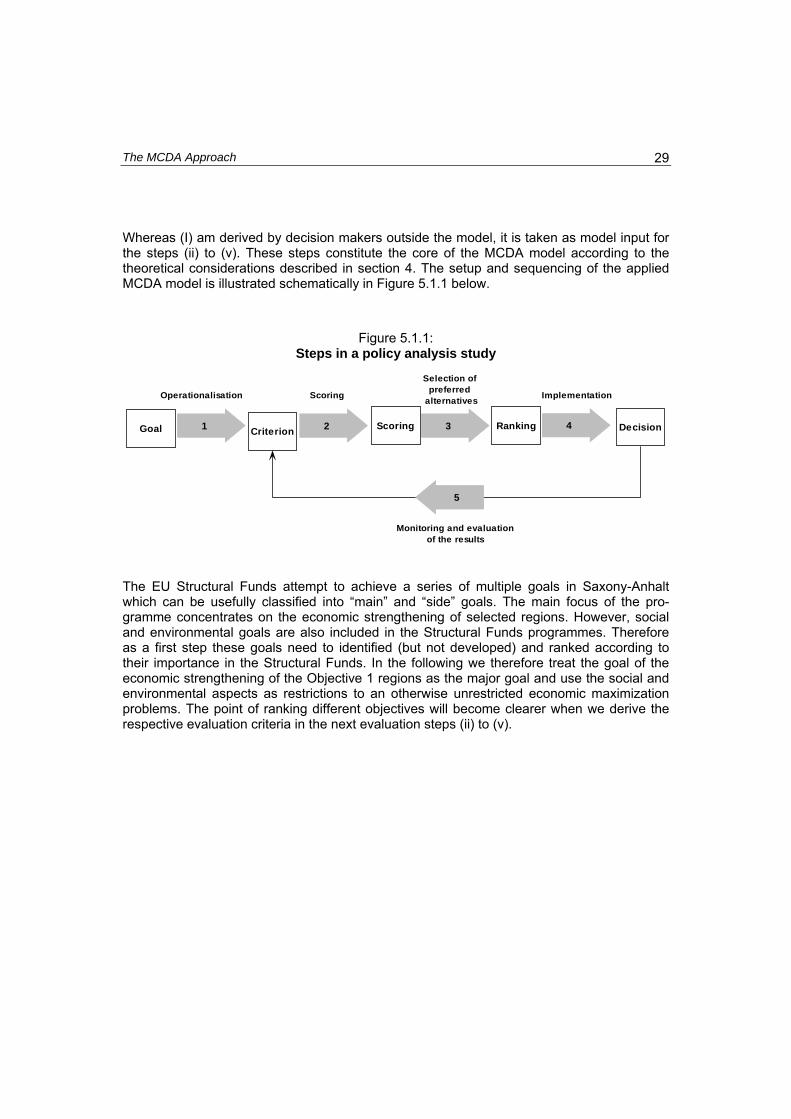
The MCDA Approach 29
Whereas (I) am derived by decision makers outside the model, it is taken as model input for the steps (ii) to (v). These steps constitute the core of the MCDA model according to the theoretical considerations described in section 4. The setup and sequencing of the applied MCDA model is illustrated schematically in Figure 5.1.1 below.
Figure 5.1.1: Steps in a policy analysis study
Goal 1 Criterion 2 Scoring 3 Ranking 4 Decision
5
Operationalisation Scoring
Selection ofpreferred
alternatives Implementation
Monitoring and evaluationof the results
The EU Structural Funds attempt to achieve a series of multiple goals in Saxony-Anhalt which can be usefully classified into “main” and “side” goals. The main focus of the pro-gramme concentrates on the economic strengthening of selected regions. However, social and environmental goals are also included in the Structural Funds programmes. Therefore as a first step these goals need to identified (but not developed) and ranked according to their importance in the Structural Funds. In the following we therefore treat the goal of the economic strengthening of the Objective 1 regions as the major goal and use the social and environmental aspects as restrictions to an otherwise unrestricted economic maximization problems. The point of ranking different objectives will become clearer when we derive the respective evaluation criteria in the next evaluation steps (ii) to (v).
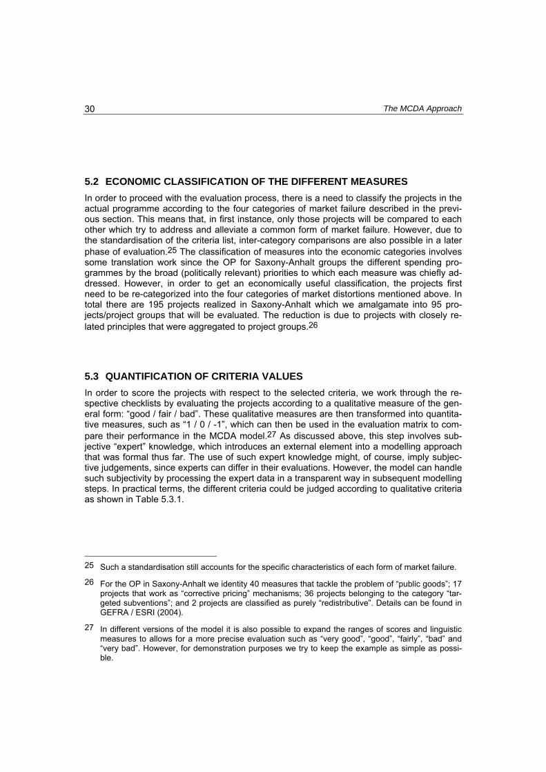
The MCDA Approach 30
5.2 ECONOMIC CLASSIFICATION OF THE DIFFERENT MEASURES In order to proceed with the evaluation process, there is a need to classify the projects in the actual programme according to the four categories of market failure described in the previ-ous section. This means that, in first instance, only those projects will be compared to each other which try to address and alleviate a common form of market failure. However, due to the standardisation of the criteria list, inter-category comparisons are also possible in a later phase of evaluation.25 The classification of measures into the economic categories involves some translation work since the OP for Saxony-Anhalt groups the different spending pro-grammes by the broad (politically relevant) priorities to which each measure was chiefly ad-dressed. However, in order to get an economically useful classification, the projects first need to be re-categorized into the four categories of market distortions mentioned above. In total there are 195 projects realized in Saxony-Anhalt which we amalgamate into 95 pro-jects/project groups that will be evaluated. The reduction is due to projects with closely re-lated principles that were aggregated to project groups.26
5.3 QUANTIFICATION OF CRITERIA VALUES In order to score the projects with respect to the selected criteria, we work through the re-spective checklists by evaluating the projects according to a qualitative measure of the gen-eral form: “good / fair / bad”. These qualitative measures are then transformed into quantita-tive measures, such as “1 / 0 / -1”, which can then be used in the evaluation matrix to com-pare their performance in the MCDA model.27 As discussed above, this step involves sub-jective “expert” knowledge, which introduces an external element into a modelling approach that was formal thus far. The use of such expert knowledge might, of course, imply subjec-tive judgements, since experts can differ in their evaluations. However, the model can handle such subjectivity by processing the expert data in a transparent way in subsequent modelling steps. In practical terms, the different criteria could be judged according to qualitative criteria as shown in Table 5.3.1.
25 Such a standardisation still accounts for the specific characteristics of each form of market failure.
26 For the OP in Saxony-Anhalt we identity 40 measures that tackle the problem of “public goods”; 17 projects that work as “corrective pricing” mechanisms; 36 projects belonging to the category “tar-geted subventions”; and 2 projects are classified as purely “redistributive”. Details can be found in GEFRA / ESRI (2004).
27 In different versions of the model it is also possible to expand the ranges of scores and linguistic measures to allows for a more precise evaluation such as “very good”, “good”, “fairly”, “bad” and “very bad”. However, for demonstration purposes we try to keep the example as simple as possi-ble.

The MCDA Approach 31
Table 5.3.1: Transformation of qualitative criteria into quantitative score values
+1 0 -1
Public Goods Importance28 very medium low Contribution much fair poor Cost of delivery good not great bad Requirement of public funding yes maybe no Deadweight effects no some a lot Environmental side-effects favourable none adverse Corrective pricing Importance very medium low Correction of relative prices just right not enough too generous Policy-induced externality no maybe yes Budget insufficient adequate excessive Deadweight effects no some a lot Side-effects favourable none adverse Targeted Interventions Importance very medium low Genuine distortion yes maybe no Behaviour as intended yes don’t know no Cost of delivery good not great bad Deadweight little some much Side-effects favourable none adverse Redistribution Importance very medium low Targeting, amount well adequate arbitrary Training etc., side effects favourable none adverse (Environmental) side effects favourable none adverse Deadweight little some much
28 Here we only use catchwords to represent the critical questions outlined above. That is, in the
analysing process the expert needs to evaluate project j according to the question: “Is the target area important?” Possible answers are “very”, “medium” or “low”. If the expert thinks project j to be very important with respect to the target area, then the project gets the score “1” or “0” and “-1” re-spectively.
The MCDA Approach 32
5.4 WEIGHTING OF CRITERIA Having scored each project according to the appropriate criteria checklists, we further need to determine whether each criterion is equally important with respect to the stated goals of the Structural Funds or whether we need to introduce a set of criteria weights. In this paper we focus mainly on the economic impacts of the Structural Funds programmes, thereby tak-ing environmental and social aspects into consideration as secondary goals. Thus, with re-spect to these secondary criteria - such as the question for “environmental side effects” – we give them less weight than we give to the economically important criteria, such as the ques-tion concerning the verification of a public good or the achieved correction of the relative prices with respect to different measures.
In judging the relative importance of criteria weights, we use a pairwise-comparison test simi-lar to the one used in the AHP literature (see for example Saaty and Vargas, 2001) and the Fuller method (see Jablonský, 2001).29 In all we try to keep the weight derivation as simple as possible in order to increase the acceptance and “natural” intuition for the model as out-lined in the introduction. The pairwise comparison approach also uses the “expert knowl-edge” of the programme evaluators in order to rank the criteria according to their qualitative importance. The advantage of such a procedure is that the implicit judgements of the experts can explicitly be modelled. Thus, although this modelling step is subjective in nature, it re-tains transparency and is comprehensible to external participants in the evaluation process.
The comparisons are processed as follows. First, each criterion is compared with all other criteria in a pairwise comparison test, based on a half-matrix. The ordinal ranking of the crite-ria follows from the relative preference of each criterion against each other.30 However, the method also generates information to get an approximation of a cardinal ranking of the crite-ria. In order to do so, we derive criteria weights (gj) using a simple scale method that derives the relative importance of each criterion as
(7) gj = ⎝⎛
⎠⎞number of priorities of criterion cj over all other criteria
total number of comparions .
The sum of the individual criteria weights add up to unity.
In table 5.4.1 the setup of the pairwise comparison test is illustrated for the criterion weight-ing in the public goods category. Starting with criterion c1 “appropriateness” in the first row of the half-matrix (grey area), this criterion is compared to all other criteria listed in the respec-tive columns (1 to 6). Thereby, the criterion index that is favoured in a comparion of “row” and “column” criterion is shown in the respective matrix cell. If two criteria are judged as equally important we indicate this indifference by a question-mark. The number of criteria priorities calculated from these pairwise comparisons by adding the number of criteria indi-ces in the half-matrix is then used to derive the ordinal and cardinal ranking.
29 The AHP based on the standard Saaty scale (based on 9 intensities) uses either an eigenvector
calculation or a logarithmic least square method (approximation of the eigenvector) to calculate the criteria weights. The consistency of the comparison matrix is also checked (Saaty, 2005). The Fuller method is based on pairwise comparisons of the criteria with the following possibilities – one of the criteria is more important or both the criteria are equally important.
30 Details can be found in GEFRA, ESRI (2004).

The MCDA Approach 33
Table 5.4.1: Pairwise comparisons for criteria weight derivation in the public goods category
Criterion
c1 c2 c3 c4 c5 c6 Number of Priorities Criterion cj
Ordinal Ranking
Criteria weights (gj)
1 ? 1 1 1 1 5 Appropriatenes (c1) 1 0,25
2 2 2 2 2 5 Effectiveness (c2) 1 0,25
3 4 3 3 3 Efficiency (c3) 3 0,15
4 4 4 4 Legitimacy (c4) 2 0,20
5 ? 1 Deadweight (c5) 4 0,05
6 1 Side-effects (c6) 4 0,05
Total number of comparisons: Σ = 20
Along the same line as criteria weights in the public goods category have been derived, we also calculate respective weights for the other categories. The resulting criteria weights are shown in table 5.4.2.
Table 5.4.2: Criteria weights for different categories of market failure
Weight gj of Criterion j with j = 1 to 6
Public Goods
Corrective Pricing
Targeted Subventions Redistribution
g1 0,25 0,3 0,4 0,4
g2 0,25 0,25 0,2 0,4
g3 0,15 0,1 0,2 0,05
g4 0,20 0,25 0,1 0,05
g5 0,05 0,05 0,05 0,1
g6 0,05 0,05 0,05 ---
Σ 1 1 1 1
5.5 SCORING, AGGREGATION AND RANKING OF ALTERNATIVES The next step in the MCDA model computation is to aggregate the scores and weights to get a final “aggregate” score for the respective measure. As outlined above, there are different

The MCDA Approach 34
aggregation rules that can be used for this task. Since we are initially interested in the aver-age performance of each project with respect to the Structural Fund goals (operationalised through the criteria), we use an additive aggregation according to formula (5).31 By defini-tion, the final project scores lie in an interval [1;-1]. To demonstrate how the “scoring” works, Table 5.5.1 shows the calculation of the project score for selected projects in the programme designated as “strengthening competitiveness” in the Structural Funds (ERDF).32 The right hand side (grey area) of Table 5.5.1 represents the unweighted evaluation matrix from sec-tion 4.
The table shows that most of the projects implemented with the aim of strengthening the competitiveness of the private sector are either classified as corrective pricing (Type II) or as targeted subventions (Type III). Having already classified the projects into their respective categories, scored the project according to expert knowledge and derived the criterion weights, the final calculation of the aggregate project scores is quite straightforward. Here, we apply the additive aggregation rule: For example for measure 1.11.1 (“GA Business Economy, Productive Investment”), the aggregate project score is calculated as follows, with the single elements of the sum symbolising one row of the weighted evaluation matrix:
fGA_1.11.1 = 1*0,3+1*0,25+1*0,1+0*0,25+0*0,05+0*0,05 = 0,65
In order to derive benchmark values to assess the relative performance of the projects within each category, we can use different approaches. For example, Honohan et al. (1997) use a fixed numerical benchmark of 0.5 (“cut-off value”) for each category. All projects that have a value of 0.5 or more are labelled as efficient projects accordingly to this cut-off value, and should continue to be implemented in their original form in the programme or should even be expanded. On the other hand, projects with scores below 0.5 are classified as critical or un-satisfactory and are candidates for possible programme modifications.
Another possibility for classifying the projects is to calculate the average aggregate score within each category. According to this approach, projects with a score that is above the calculated average are candidates for a possible expansion (i.e., promising candidates). Projects with aggregated scores that are below the average are defined as “critical”, and should be further examined (e.g. according to monetary indicators), with a view to a reduc-tion or elimination. A disadvantage is that the derivation of a benchmark value for both alter-natives remains somewhat ad-hoc.
In the case of Saxony-Anhalt, we use the arithmetic mean method to classify the projects. In the Public Good category the average score is calculated as 0.39; Corrective Pricing is 0.43; Targeted Subvention is 0.46. Since those numbers differ only slightly from the 0.5 cut-off benchmark used by Honohan et al. (1997), our method is less restrictive than the 0.5 benchmark, to a slight extent. In the category distribution we only evaluate two projects, which both yield a project-value below zero. Both are marked as candidates for elimination.
31 However, in order to assess the sensitivity of the results we also use a multiplicative aggregation
rule. One has to note that for the multiplicative aggregation instead of using a “1/0/-1” scale we have to adopt a “3/2/1” scale.
32 A complete scoring of all 95 measures in the OP is given in GEFRA, ESRI (2004).

The MCDA Approach 35
Reviewing the overall performance of the Structural Fund programme in Saxonia-Anhalt for the period 2000-2006, the majority of projects were found to contribute positively to the pol-icy goals. However, about 30 projects were found to be unsatisfactory and should be further examined in the decision-making process.33 Those projects, indicated by a question mark in Table 5.5.1, mainly concern agricultural support (8.03% of the total Structural Funds), infra-structure (5.55%), and labour market programmes (5.44%). In total, around 20 percent of the Structural Funds intervention budget was classified as unsatisfactory, i.e. that it may not deliver its targeted goal. After this initial evaluation, the projects that were identified as unsat-isfactory were evaluated by the policy makers of Saxonia-Anhalt in terms of budgetary re-strictions, and this led to a significant modification in the operational programme for the sec-ond half of the funding period 2004-2006.
33 These results are robust also for the case when a multiplicative aggregation rule is applied.

Table 5.5.1: Calculating aggregate project scores in the Structural Funds programme
Level Priorities / measures Type of inter-vention, resp. market failure
Aggregate score of the
Poject
Score for criterion
1.) 2.) 3.) 4.) 5.) 6.) 1.... Strengthening the competitiveness of
the business economy, especially SME1
1.11... Support of productive Investments 1.11.1.. GA business economy (common task), produc-
tive Investments II 0,65 1 1 1 0 0 0
1.11.2.. GA business economy (common task), R&D funding
II 0,45 1 0 1 0 0 1
1.11.3.. GA business economy (common task), SME funding
II 0,65 1 1 1 0 0 0
1.11.4.. GA Gewerbliche Wirtschaft (common task) Funding of establishments for improvements in the economic structure
II No scoring applied: Measure without effective financial value
for the SF programme 1.21... Innovation support, Product- und Process
improvement
1.21.1.. Support of innovation assistents III 0,65 1 0 1 0 1 0 1.21.2.. Support of safeguard and realisation of Trade
mark rights III 0,90 1 1 1 0 1 1
1.21.3.. Support of design development III -0,55 ? -1 -1 1 -1 -1 0
1.21.4.. Support of state-of-the-art investigations III 0,25 ? 1 -1 1 -1 -1 0
1.21.5.. Support for technology-, innovation- u. firm establishment centers
III 0,85 1 1 1 0 0 1
1.21.6.. Innovation support for SME – GA (common task)
III 0,70 1 0 1 0 1 1
1.21.7.. Innovation support for SME III 0,70 1 0 1 0 1 1

Table (continued): Calculating aggregate project scores in the Structural Funds programme
1.21.8.. Project support agriculture III 0,30 ? 0 0 1 0 1 1
1.22... Information and communication technolo-gies
1.22.1.. Special programme "building up / strengthening the information society“"
I - No scoring applied (see measure 1.11.4)
1.22.2.. Pilot projects „information society“ I -0,25 ? 0 0 0 -1 -1 0
1.23... Environmental technologies
1.23.1.. Project support environmental technique III 0,45 ? 0 1 1 0 -1 1
1.23.2.. Support of pilot techniques and prototypes – Energy programme
III - No scoring applied (see measure 1.11.4)
… … … … …
2… Physical Infrastructure 2.11… GA Infrastructure, business economy I 0,95 1 1 1 1 1 0 2.12… GA Infrastructure, tourism I 0,40 1 0 1 0 1 0 2.21… R&D Infrastructure 2.21.1 Construction and Expansion of industry and
telematics centres
2.21.1.1 Construction and Expansion of industry and telematics centres, Infrastructure
I 0,40 1 0 1 0 0 0
2.21.1.2 Support of research, technology orientated development, information society – equipment
I 0,65 1 1 1 0 0 0
… … … … …
The MCDA Approach 38
5.6 CONCLUSIONS ON THE MICRO EVALUATION OF THE STRUCTURAL FUNDS
The proposed MCDA approach to evaluate policy programmes starting from the level of “measures” is a policy analysis tool that is transparent and is easy to apply. One of the main advantages of the model is that it allows both for flexible and intuitive decision making and at the same time provides a model-based evaluation process augmented by a microeconomic foundation to systemize public sector decision making in the presence of multiple goals and criteria. If all participants in the decision making process know the structure of the fairly sim-ple MCDA model, it is much easier to review the proposed decisions and make changes on subsequent model steps. The model therefore may be an important communication tool dur-ing the various rounds of decision making in policy evaluation.
However, it is necessary to stress that some caveats also apply. First, one should never forget that although the model has a kind of mathematical representation, and therefore ap-pears to incorporate a high degree of objectivity, the model also contains subjective ele-ments at various steps in the computation. Therefore, the model assists in the search for a better policy mix, but cannot guarantee that the derived mix is a global optimum. The main merit of the model is systematically to structure and process the available information so that the decision process loses the “black box” characteristics normally inherent in fuzzy decision making. By combining formal MCDA elements and economic theory, the model gives strong guidance in policy debate.
A second caveat concerns the individual setup of the model. Here the model builder needs to find a solution for the trade off between model precision and intelligible application. That is, the more complex the MCDA structure, the less transparent will be the results. On the other hand a minimum of theoretical input is needed to guarantee rational results. In an ap-plied context this trade-off can be specified according to the preferences of the decision maker.
6 PUBLIC POLICY ANALYSIS: DESIGNING
A SUITABLE MACROMODEL
At the start of this paper we drew attention to the two types of “model” that tend to be used for the analysis of public policies (see Table 1.1). In the previous two sections we described a micro-based model, which gave an articulated description of a policy process, systema-tised that process, and used normative rules to evaluate policy impacts. In this section and the following one we turn to the case where the model, in addition to the providing system-atic description function, is also based on a behavioural macro theory. Such a model serves to integrate the analysis, and performs a positive (as distinct from a normative) role. There can be many types of policy model of this type, but in what follows we confine our remarks to the use of macroeconometric models.34 Furthermore, within the class of all possible kinds of macroeconometric model, we focus on one that is designed for the specific purpose of ana-lysing the impacts of Structural Fund policy interventions.
6.1 THE ROLE OF MACRO-MODELS The reform and expansion of EU regional investment programmes (or Structural Funds, henceforth, SF) in the late 1980s presented the European Commission as well as domestic policy makers and analysts with major challenges. Although the SF investment expenditures were very large, this in itself was not a problem for policy design or analysis.35 Indeed, evaluating the macroeconomic impact of public expenditure initiatives had been an active area of work since quantitative macromodels were first developed in the 1930s (Tinbergen, 1939).36 What was special about the SFs was their declared goal to implement policies whose explicit aim was to transform and modernise the underlying structure of the benefici-ary economies in order to prepare them for greater exposure to international competitive forces within the Single Market and EMU. Thus, SF policies moved far beyond a conven-tional demand-side stabilization role, being aimed rather at the promotion of structural change, accelerated medium-term growth and real cohesion through mainly supply-side mechanisms.
34 Other macro-type models include input-output (Beutel, 1993); computable general equilibrium
models (Bourguignon, et al, 1992); and growth models (Gaspar and Pereira, 1991).
35 Typically, SF expenditures range from about 1 percent of GDP annually in the case of Spain to over 3 per cent in the case of Greece. The macro consequences are clearly important.
36 Tinbergen’s early contribution to the literature on the design and evaluation of supply-side policies still reads remarkably well after more than 40 years (Tinbergen, 1958).
Public Policy Analysis 40
The new breed of macroeconomic models of the late 1980s had addressed the theoretical deficiencies of conventional Keynesian econometric models that had precipitated the decline of modelling activity from the mid-1970s (Klein, 1983; Helliwell et al, 1985). However, policy makers and policy analysts were still faced with the dilemma of having to use conventional economic models, calibrated using historical time-series data, to address the consequences of future structural changes. The Lucas critique was potentially a serious threat to such model-based policy impact evaluations (Lucas, 1976).37 In particular, the relationship be-tween public investment policies and private sector supply-side responses - matters that were at the heart of the SFs - were not very well understood or articulated from a modelling point of view.
The revival of the study of growth theory in the mid-1980s provided some guidelines to the complex issues involved in designing policies to boost a country’s growth rate, either perma-nently or temporally, but was more suggestive of possible mechanisms than of actual magni-tudes (Barro and Sala-i-Martin, 1995; Jones, 1998). Furthermore, the available empirical growth studies tended to be predominantly aggregate and cross-country rather than disag-gregated and country-specific.38 Yet another complication facing the designers and analysts of SFs was that the first four main beneficiary countries - Greece, Ireland, Portugal and Spain - were on the geographical periphery of the EU, thus introducing spatial issues into their development processes. With advances in the treatment of imperfect competition, the field of economic geography (or the study of the location of economic activity) had also re-vived during the 1980s (Krugman, 1995; Fujita, Krugman and Venables, 1999). But the in-sights of the new research were confined to small theoretical models and seldom penetrated through to the type of large-scale empirical models that are typically required for realistic policy analysis.
The Keynesian demand-driven view of the world that dominated macro modelling prior to the mid-1970s was exposed as being entirely inadequate when the economies of the OECD were hit by the supply-side shocks of the crisis-wracked 1970s (Blinder, 1979). From the mid-1970s onwards, attention came to be focused on issues of cost competitiveness as an important in-gredient in output determination, at least in highly open economies. More generally, the impor-tance of the manner in which expectation formation was handled by modellers could no longer be ignored, and the reformulation of empirical macro models took place against the back-ground of a radical renewal of macroeconomic theory in general (Blanchard and Fischer, 1990).
37 The Lucas critique suggests that in the presence of large-scale public policy shocks, the underlying
structure of the economy will change and that the use of macromodels calibrated with pre-shock data is invalid. However, if one incorporates explicit sub-models of the structural changes that are associated with the policy shock, such as Structural Funds, then the validity of the Lucas critique is weakened.
38 Fischer (1991) suggested that identifying the determinants of investment, and the other factors contributing to growth, would probably require a switch away from simple cross-country regressi-ons to time series studies of individual countries.
Public Policy Analysis 41
6.2 A MACROMODEL FOR POLICY IMPACT ANALYSIS The HERMIN model framework was developed in Ireland the late 1980s to evaluate the macro impacts of SFs, and drew on many aspects of the above revision and renewal of macro economic modelling.39 HERMIN was initially designed to take account of the very limited data availability in the poorer, less-developed EU member states and regions on the Western and Southern periphery (i.e., Ireland, Northern Ireland, Portugal, Spain, the Italian Mezzogiorno, and Greece).40 A consequence of the lack of detailed macro-sectoral data and of sufficiently long time-series that had no structural breaks was that the HERMIN modelling framework needed to be based on a fairly simple theoretical framework that permitted inter-country and inter-region comparisons and that facilitated the selection of key behavioural parameters in situations where sophisticated econometric analysis was impossible.
The HERMIN model was designed in order to analyse medium-term policy impacts involving large-scale public investments in physical infrastructure and in human resources. Such analysis requires certain basic structural features in a model:
(i) It must be disaggregated into an adequate number of crucial sectors to permit the ex-amination of key sectoral shifts in the economy over the years of policy-influenced de-velopment.
(ii) It must specify the mechanisms through which a “lagging” economy is connected to the external world. The external (or world) economy is a very important direct and indirect factor influencing the economic growth and convergence of all lagging economies, through trade of goods and services, inflation transmission, population migration and in-ward foreign direct investment.
(iii) It must recognise that a possible conflict may exist between the actual situation in the country, as captured in a HERMIN model calibrated with historical data, and the desired situation towards which the lagging economy is evolving. This point applies in particular to the post-Communist countries that make up the new EU member states.
These basic structural requirements have implications for the more detailed features of the model. For example, one needs to focus carefully on the degree of economic openness, exposure to world trade, and response to external and internal shocks. The relative sizes and features of the traded and non-traded sectors and their development, production tech-nology and structural change become crucial mechanisms in the change process. The mechanisms of wage and price determination determine competitiveness relative to more developed economies, together with the functioning and flexibility of labour markets and the possible role of international and inter-regional labour migration. Finally, development possi-bilities can be constrained through fiscal and other imbalances, which emphasises the role of the public sector and the possible consequences of public debt accumulation, as well as the interactions between the public and private sector trade-offs in public policies.
39 Its origins lay in the complex multi-sectoral HERMES model that was developed by the European
Commission from the early 1980s (d’Alcantara and Italianer, 1982).
40 After German unification, the former East Germany was added to the list of “lagging” EU regions.
Public Policy Analysis 42
To satisfy these requirements, the basic HERMIN framework was designed initially with four sectors: manufacturing (a mainly traded sector), market services (a mainly non-traded sec-tor), agriculture and government (or non-market) services. Although agriculture also has important traded elements, its underlying characteristics demand special treatment.41 Simi-larly, the government (or non-market) sector is non-traded, but is best formulated in a way that recognises that it is mainly driven by policy instruments that are available – to some extent, at least – to policy makers.42
The structure of the HERMIN model framework can be best thought as being composed of three main blocks: a supply block, an absorption block and an income distribution block. Obviously, the model functions as integrated systems of equations, with interrelationships between all their sub-components.43 However, for expositional purposes we describe the HERMIN modelling framework in terms of the above three sub-components, which are schematically illustrated in Figure 6.2.1 and Figure 6.2.2.
41 For example, Agriculture is never the “engine” of convergence in a European context. Rather, it
facilitates rapid development in other sectors, through increases in productivity and a labour re-lease mechanism.
42 Elements of public policy are endogenous, but one can handle these in terms of policy feed-back rules rather than behaviourally.
43 It is not our purpose to present a detailed technical description of the structure of a HERMIN model. Rather, we only wish to present some general features, and mention some key behavioural mechanisms. The interested reader is referred to Bradley, Petrakos and Traistaru (eds.), 2004.
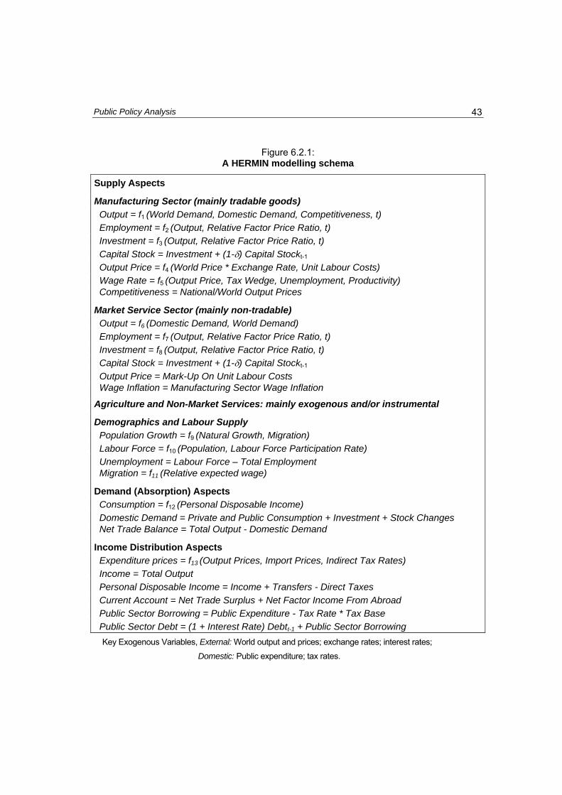
Public Policy Analysis 43
Figure 6.2.1: A HERMIN modelling schema
Supply Aspects
Manufacturing Sector (mainly tradable goods) Output = f1 (World Demand, Domestic Demand, Competitiveness, t) Employment = f2 (Output, Relative Factor Price Ratio, t) Investment = f3 (Output, Relative Factor Price Ratio, t) Capital Stock = Investment + (1-δ) Capital Stockt-1 Output Price = f4 (World Price * Exchange Rate, Unit Labour Costs) Wage Rate = f5 (Output Price, Tax Wedge, Unemployment, Productivity) Competitiveness = National/World Output Prices
Market Service Sector (mainly non-tradable) Output = f6 (Domestic Demand, World Demand) Employment = f7 (Output, Relative Factor Price Ratio, t) Investment = f8 (Output, Relative Factor Price Ratio, t) Capital Stock = Investment + (1-δ) Capital Stockt-1 Output Price = Mark-Up On Unit Labour Costs Wage Inflation = Manufacturing Sector Wage Inflation
Agriculture and Non-Market Services: mainly exogenous and/or instrumental
Demographics and Labour Supply Population Growth = f9 (Natural Growth, Migration) Labour Force = f10 (Population, Labour Force Participation Rate) Unemployment = Labour Force – Total Employment Migration = f11 (Relative expected wage)
Demand (Absorption) Aspects Consumption = f12 (Personal Disposable Income) Domestic Demand = Private and Public Consumption + Investment + Stock Changes Net Trade Balance = Total Output - Domestic Demand
Income Distribution Aspects Expenditure prices = f13 (Output Prices, Import Prices, Indirect Tax Rates) Income = Total Output Personal Disposable Income = Income + Transfers - Direct Taxes Current Account = Net Trade Surplus + Net Factor Income From Abroad Public Sector Borrowing = Public Expenditure - Tax Rate * Tax Base Public Sector Debt = (1 + Interest Rate) Debtt-1 + Public Sector Borrowing
Key Exogenous Variables, External: World output and prices; exchange rates; interest rates;
Domestic: Public expenditure; tax rates.

Figure 6.2.2: Schematic Outline of the HERMIN Modelling Approach
HERMIN
[1] NationalaccountingFramework
[3] Expenditure
[5] Model asintegrated system
[4] Income
[6] Behavioural andidentity equations
Manufacturing (T)
Agriculture (A)
Non-market services (G)
Market services (N)Utilites
Other market services
Output (GDP)
Expenditure (GDE)
Income (GDI)
Private consumption
Public consumption
Investment
Stock changes
Exports
Imports
General Government
Health
Education
Agriculture
Forestry
Fishing
GDP
productivity
PSBR
Output = Expenditure usedto determine net trade balance
(NTS = GDP - GDA)where GDA = C + G + I + DS
Output = Incomeused to determinecorporate profits
(IYC = GDP - YWI)
Revenue
Expenditure
Borrowing requirement
Debt accumulation
Corporate sector
Household sector
Behaviouralequationsinfluencedby theory
Identities adding up,definitional & closure
Public sector
Private sector
Consumption function
Wage bargaining
Factor demands
[2] Output
Building (BC)

Public Policy Analysis 45
Conventional Keynesian mechanisms are at the core of a HERMIN model. Expenditure and income distribution sub-components generate the standard income-expenditure mecha-nisms. But the model also has neoclassical features. Thus, output in manufacturing is not simply driven by demand. It can also be potentially influenced by price and cost competitive-ness, where firms seek out minimum cost locations for production (Bradley and Fitz Gerald, 1988). In addition, factor demands in manufacturing and market services are derived using a production function constraint, where the capital/labour ratio is sensitive to relative factor prices. The incorporation of a structural Phillips curve mechanism in the wage bargaining mechanism introduces further relative price effects.
From Figure 6.2.2 we see that the model, like the national accounts upon which it is based, uses three complementary ways of measuring GDP: the output, expenditure and income basis. On the output basis, HERMIN disaggregates GDP into four sectors: manufacturing (OT), market services (ON), agriculture (OA) and the public (or non-market) sector (OG). On the expenditure side, HERMIN disaggregates the GDP into the conventional five compo-nents: private consumption (CONS), public consumption (G), investment (I), stock changes (DS), and the net trade balance (NTS).44 Finally, national income is determined on the out-put side (via the output-income identity), and is disaggregated into private and public sector elements.
Since all elements of output are modelled, the output-expenditure identity is used to deter-mine the net trade surplus/deficit residually. The output-income identity is used to determine corporate profits residually. Finally, the equations in the model can be classified as behav-ioural or identity. In the case of the former, economic theory and calibration to the data are used to define the relationships. In the case of identities, these follow from the logic of the national accounts, but have important consequences for the behaviour of the model as well.
A typical four-sector HERMIN model contains a total of about 250 equations, many of which are included to increase the model’s transparency and facilitate simulation and policy analy-sis exercises. The essential core of the model consists of a smaller number of equations, of which less than twenty are behavioural in a strictly economic sense (i.e., empirical versions derived from underlying theoretical specifications, containing parameters that must be as-signed data-dependent numerical values). The set of behavioural equations is embedded amongst a larger set of identities, which are of vital importance to the performance and properties of the model, but do not contain numerical parameters that need to be calibrated. Together, the behavioural equations and the identities form an integrated system, and can-not be considered in isolation from each other.
6.3 CALIBRATING MACROMODEL BEHAVIOURAL EQUATIONS In the case of the EU cohesion economies, the nature of structural change suggests that the data sample should be restricted to the post-1980 or post-1985 period. In the case of the CEE transition economies, data constraints (at the time of writing, May 2005) enable us to
44 The traded/non-traded disaggregation implies that only a net trade surplus is logically consistent.
Separate equations for exports and imports could be appended to the model, but would function merely as conveniently calculated “memo” items that were not an essential part of the model’s be-havioral logic.
Public Policy Analysis 46
work only with about ten annual data observations for the period 1994-2003 at most, since the data prior to 1994 are incomplete and not very reliable.45 The small number of observa-tions available prevents us from undertaking the sophisticated econometric estimation and hypothesis testing techniques commonly used to calibrate macro models. Consequently, three different approaches to model calibration (or estimation) are used in the literature of modelling the transition economies of the CEE region:
(i) Extending the data sample over different economic regimes
There is a temptation to make use of data from the pre-transition era.46 The advantage is that this provides more annual observations and facilitates econometric hypothesis testing and estimation. The disadvantage is that the extended data sample covers three very differ-ent economic regimes: the era of communist economic planning; the years immediately fol-lowing the collapse of the communist centralised economic system; and the era of rapid re-covery and growth that followed the post-communist collapse. An additional hurdle to the application of this approach is that out of the ten CEE candidate countries, six are new states established (or re-established) after 1990 (these are the three Baltic states, the Czech and Slovak republics, and Slovenia). For these new entities no reliable data could have been collected for the pre-transition period.
(ii) The Panel data approach This is the approach used within the models of the economies of Central and Eastern Europe that are contained in the NIGEM model of the world economy developed by the Lon-don-based NIESR (Barrell and Holland, 2002). A series of CEE economic data bases are assembled for the post Communist era, a generalised model is posited that is appropriate to each of the constituent economies, and cross-economy constraints are imposed. For exam-ple, a common marginal propensity to consume might be imposed on all models. This has the advantage of increasing the degrees of freedom and obtaining more precise parameter estimates. A disadvantage of this approach is that the cross-economy restrictions are difficult to test, and may be inappropriate.
(iv) Simple curve-fitting to post 1994 data This is the approach that is used for all the HERMIN models of Central and Eastern Europe. The limitation of about eight to ten annual observations excludes econometrics, in the sense of hypothesis testing. By keeping the behavioural equations very simple and ignoring lags, the number of behavioural parameters is kept to a minimum. Using ordinary least squares, a form of “curve-fitting” is used, where the derived parameters are examined and related to a range of estimates from other EU models, where longer data sets are available. In its ex-treme form, this reduces to the way in which computable general equilibrium (CGE) models are calibrated, by imposing all important parameters, and using one year’s data to force con-gruence between the model and the data. Advantages include the tight theoretical control
45 The same data restrictions apply to the Saxony-Anhalt model, which will be used in Sections 7 and 8.
46 For the Polish W8-2000 model, data for the period 1960-1998 are used (Welfe et al, 2002).
Public Policy Analysis 47
imposed on the model, the use of the most recent and consequently, most relevant data sample, and the use of judgement to ensure the relevance of the parameters. Disadvantages are numerous, including a complete lack of formal hypothesis testing.
6.4 CONCLUDING REMARKS The focus of the HERMIN model is on the process of convergence of the lagging EU economies, both “old” and “new” member states, as the latter states complete the process of integration and convergence that is likely to take place after their initial mainly institutional transition is complete. Since the data for the CEE economies are very limited, they relate to the earlier transition process rather than to the post-transition structure that we wish to de-velop. Consequently, although one can make some use of the available data in order to cali-brate CEE HERMIN models, one can also look at other EU economies of broadly compara-ble size and structure to obtain guidance in the quantification of key post-transition market mechanisms such as the development of cost competitiveness, the nature of wage bargain-ing, the likely evolution of technological progress, and the underlying nature of production technology.
Two separate issues are involved here. First, the standard macroeconomic interrelationships that characterise the EU economies may already exist in some of the more advanced CEE economies such as the Czech Republic, Slovenia and Hungary (i.e., sensitivity to interna-tional cost-competition and wage determination mechanisms that are becoming consistent with the need to maintain a cost-competitive position in the global economy), but we may simply have too few data observations to isolate the magnitudes of the relevant elasticities and parameters. Second, it may be the case that these interrelationships are not yet fully developed, but will accelerate after the CEE economies move to full membership of the EU in 2004.
The question then must be posed: is it premature to develop macroeconomic models for CEE economies where data limitations place severe restrictions on our ability to pin down likely parameter values, and where, furthermore, the underlying model structures may be undergoing massive evolution and change? If such empirical model frameworks are not con-structed, then it may prove difficult to explore and study the development choices that will undoubtedly face the CEE economies as their decision makers attempt to design policies and structures that will ensure convergence to average EU standards of living. However, if such models are constructed, then their experimental and speculative nature must be kept in mind and model simulations must be regarded as explorative consistency checks rather than firm forecasts (Barry, et al, 2003).
7 USING A MACRO MODEL TO EVALUATE
STRUCTURAL FUND IMPACTS
In this section we describe how macroeconomic model-based techniques can be used to carry out systematic ex-ante, mid-term and ex-post impact evaluations of EU Structural Funds. However, before we can set up the model for case study of Saxony-Anhalt, this in-volves adapting the macromodel framework (such as HERMIN, as described in the previous section) to take account of the re-structuring effects of the EU programmes, and how the role of the Structural Funds can be separated from other external and domestic influences.
A useful and logical way of aggregating the Structural Fund investment projects, measures and their constituent Operational Programmes (OPs) is to consider the three categories al-ready sketched in section 3:
(i) Investment expenditures on physical infrastructure;
(ii) Investment expenditures on human resources;
(iii) Expenditures on direct production/investment aid to the private sector.
For each of these economic categories of public and private expenditure, there are three possible sources of funding:
a. EU transfers in the form of subventions to the domestic public authorities;
b. Domestic public sector co-financing;
c. Domestic private sector co-financing.
Structural Fund actions influence the economies through a mixture of supply and demand effects. Short term demand (or Keynesian) effects arise as a consequence of increases in the expenditure and income policy instruments associated with SF policy initiatives. Through “multiplier” effects there will be some further knock-on increases in all the components of domestic expenditure (e.g., total investment, private consumption, the net trade balance, etc.) and the components of domestic output and income. These demand effects are of tran-sitory importance and are not the raison d’être of Structural Funds, but merely a side-effect. Rather, the SF interventions are intended to influence the long-run supply potential of the economy.
Using a Macro Model to Evaluate Structural Fund Impacts 49
These so-called “supply-side” effects arise through policies designed to:
1) Increase investment in order to improve physical infrastructure as an input to private sector productive activity;
2) Increase human capital, through investment in training and education, as an input to private sector productive activity;
3) Channel public financial assistance to the private sector to stimulate investment and productive efficiency, thus increasing factor productivity and reducing sectoral costs of production and of capital.
SF interventions are designed in order to improve the regional aggregate stock of public infrastructure and human capital, as well as the private capital stock. Providing more and better infrastructure, increasing the quality of the labour force, or providing investment aid to firms, are the mechanisms through which the SFs improves the output, productivity and cost competitiveness of the economy. The longer-run effects of these policies are to create condi-tions where private firms enjoy the use of additional (and/or higher quality) productive fac-tors, sometimes at no cost to themselves. Alternatively, they may help to make the current private sector inputs that firms are already using available to them at a lower cost, or the general conditions under which firms operate are improved as a consequence. In all these ways, positive externalities may arise out of the SF interventions.
7.1 POLICY EXTERNALITIES Recent advances in growth theory have addressed the role of spill-overs or externalities which arise from public investments, for example in infrastructure or in human capital. Fur-thermore this literature has investigated how technical progress can be affected directly through investment in research and development (R&D). Here too externalities arise when innovations in one firm are adopted elsewhere, i.e., when such innovations have public good qualities.
Two main types of beneficial externalities are likely to enhance the demand-side (or neo-Keynesian) impacts of well designed infrastructure, training and aid policy initiatives. The first type of externality is likely to be associated with the role of improved physical infrastructure and of training in boosting output directly. This works through mechanisms such as attracting productive activities through foreign direct investment, and enhancing the ability of indige-nous industries to compete in the international market place. We call this an ‘output external-ity’ since it is well known that the range of products manufactured in developing countries changes during the process of development, and becomes more complex and technologi-cally advanced.
The second type of externality arises through the increased total or embodied factor produc-tivity likely to be associated with improved infrastructure or a higher level of human capital associated with training and education. We call this a ‘factor productivity externality’. Of course, a side effect of increased factor productivity is that, in the highly restrictive context of fixed output, labour is shed and unemployment rises. The prospect of such “jobless growth”

Using a Macro Model to Evaluate Structural Fund Impacts 50
is particularly serious in economies where the recorded rate of unemployment as well as the rate of hidden unemployment is already high. Thus, the factor productivity externality is a two edged process: industry and market services become more productive and competitive, but labour demand is weakened if output growth remains weak. On the plus side, however, fac-tor productivity is driven up, real incomes rise, and these effects cause knock-on multiplier and other benefits throughout the economy. Thus, the role of the output externality is more unambiguously beneficial than the factor productivity externality: the higher it is, the faster the period of transitional growth to a higher income plateau.
The elasticities, particularly in relation to infrastructure, can be selected from a review of the extensive international research literature in this area (for full details, see Bradley, Morgen-roth and Untiedt, 2002).47 The international literature suggests that the values for the elastic-ity of output with respect to increases in infrastructure are likely to be in the region between 5 and 40 per cent, with small regions and countries characterised by values nearer the lower end of the scale (5 to 20 per cent).48 With respect to human capital, elasticities in the same range also appear reasonable.
How enduring are the beneficial externality elasticities likely to be? The infrastructure deficit in the Objective 1 countries and in the CEE countries is quite large, and is unlikely to match up to the level pertaining in the more developed EU countries until well after the year 2010. Given this, and the fact that there are substantial returns to the elimination of bottlenecks which will take some time to accomplish, it may be quite reasonable to assume that the cho-sen externality elasticities will capture the benefits properly over the time period for which the simulations are carried out. For the same reasons it is unlikely that diminishing returns will set in for the immediate future.
7.2 LINKING THE EXTERNALITY MECHANISMS INTO THE HERMIN MODEL
7.2.1 OUTPUT EXTERNALITIES The output externalities can be viewed as operating directly through the multinational and indigenous firm location and growth process that is so important in the case of the EU pe-riphery and, more recently, in the CEE countries. This draws directly from the extensive lit-erature surveyed in Bradley, Morgenroth and Untiedt (2002). The treatment of the manufac-turing sector in HERMIN builds on a supply side approach in which the share of the world's output being allocated to, or generated within, a peripheral country or region is determined by measures of domestic and international cost competitiveness (Bradley and Fitz Gerald, 1988).
47 Since research does not always exist for the lagging Objective 1 and CEE countries, we are forced
to utilize those for analogous or more advanced economies. However, sensitivity analysis can be carried out over a plausible range of values of the externality elasticities.
48 The implications of these externality elasticities will become clearer below when we set out the actual functional relationships that are incorporated into the HERMIN models.
Using a Macro Model to Evaluate Structural Fund Impacts 51
However, this neglects the fact that many industries will require more than simply an appro-priate level of, say, labour costs before they locate in, or grow spontaneously in, the EU pe-riphery. Without an available labour force that is qualified to work in these industries, or with-out appropriate minimum levels of physical infrastructure, many firms simply may not be able even to consider the periphery as a location for production. Thus, a more realistic framework is one which posits a two stage process in which basic infrastructural and labour force quality dictates the number of industries which could conceivably locate in the periphery, while competitiveness decides how many of the industries which could locate in the periphery ac-tually do locate there.
One simple way of describing this process is to link the growth of infrastructure and the in-creases in human capital to a modified version of the HERMIN behavioural equation that is used to determine manufacturing sector output (OT). We posit a hybrid supply-demand equation of the form:
(8) log(OT ) = a1 + a2 log(OW ) + a3 log(ULCT /POT )
+ a4 log(FDOT ) + a5 log(POT /PWORLD) + a6t
where OW represents external (or world) demand, and FDOT represents the influence of domestic absorption. The two remaining terms represent real unit labour costs (ULCT/POT) and price competitiveness (POT/PWORLD). To take account of output externalities associ-ated with infrastructure and human capital, the following two terms are added to the above equation:
(9) η1 log(KGINFt /KGINF0 )+η2 log(NTRAINt /NTRAIN 0)
where output in the manufacturing sector (OT) is now directly influenced by any increase in the stock of infrastructure and human capital (KGINF and NTRAIN, respectively) over and above a baseline value for these stocks (KGINF0 and NTRAIN0, respectively).49 We are forced to ignore any interactions and complementarities that may exist between physical infrastructure and human capital, since so little is yet known about this aspect of the SFs.50
Such a modification attempts to capture the notion that a peripheral region or country can now attract a greater share of mobile investment than it otherwise could in the absence of improved infrastructure and human capital. Another, demand side, way of interpreting this externality could be to assume that the SF may improve the quality of goods produced do-
49 Thus, if the stock of infrastructure increases by 1 per cent relative to the baseline stock, output in
manufacturing (OT) is boosted by η1 per cent. If the stock of human capital increases by 1 per cent relative to the baseline stock, output in manufacturing (OT) is boosted by η2 per cent
50 The possible interaction between physical infrastructure and human capital is potentially of great importance, and is at the centre of the optimality of the SF design. It is an area where more re-search is urgently needed.

Using a Macro Model to Evaluate Structural Fund Impacts 52
mestically and thus improve the demand for goods produced by firms already located in the country, whether foreign or indigenous.
7.2.2 FACTOR PRODUCTIVITY EXTERNALITIES A factor productivity externality can be associated with improved supply conditions in the economy brought about as a result of investment in human capital and public infrastructure. These can be incorporated into HERMIN by endogenising the “scale” parameter in the CES production function, ‘A’, which is now modelled as a function of the stock of public and hu-man capital. Increases in the value of ‘A’ imply that for a given amount of inputs a higher level of output is produced. We can illustrate this schematically in terms of the simple pro-duction function
(10) Q = A * f (L, I )
where A is the scale parameter, which can be considered to represent the state of technol-ogy, and L and I are the labour and investment inputs, respectively. Public infrastructural investment will increase the efficiency of the market services sector by cutting down on the costs of producing transport and other communication services, and by opening up greater opportunities for domestic competition to take place in the provision of non-traded goods. Such cost reductions will have a favourable supply-side effect on the internationally exposed manufacturing sector.
The infrastructure factor productivity externality can be incorporated into the production process in manufacturing and market services as follows:
(11) At = A0 (KGINFt /KGINF0)η
where A0 is the original (i.e., pre-SF) estimated value of the scale parameter and η is an unknown externality elasticity that can be assigned different numerical values in the empiri-cal model. The variable KGINF is the stock of public infrastructure, computed as an accumu-lation of real infrastructure investments (using the perpetual inventory method with a speci-fied depreciation rate). The baseline stock of infrastructure, KGINF0, is taken as the stock that would have been there in the absence of any SF infrastructural investments made dur-ing the period under consideration.
Similarly, the SF Social Fund programmes on education and training can be considered to promote the efficiency of the workforce in both manufacturing and services sectors and can give rise to a human capital externality. Incorporation of externality effects associated with the accumulation of human capital is not as straightforward as in the infrastructure case, since there is no readily available measure of the stock of human capital equivalent to the stock of infrastructure. However, one can estimate a measure of the extra number of train-ees funded by the SF schemes (see Bradley, Kangur and Lubenets, 2004 for details). Hence, as a first approximation, one can use the inputs into training as a measure of the

Using a Macro Model to Evaluate Structural Fund Impacts 53
unknown outputs, although if the training courses are badly designed and poorly executed, the relationship between training and increased human capital will be tenuous.51
Suppose we assume that, prior to the implementation of the SF, the number of labour force participants trained to a specified level, NTRAIN0, is known. If the ESF element of the SF is used to train an additional number of people, giving a total of NTRAINt trained labour force participants in year t, then the scale parameter in the production function can be modified as follows:
(12) At = A0 (NTRAIN t /NTRAIN 0)η ,
where A0 is the original estimated value of the scale parameter. In the empirical model, this externality is incorporated into the treatment of both the manufacturing and service sectors.
7.3 EVALUATING SF POLICY IMPACTS The real dilemma facing policy analysts when, in the absence of any micro evaluations such as were described in sections 4 and 5, they try to use macro models to evaluate the ex-ante impacts of yet-to-be-implemented Structural Fund programmes is that they cannot know either how appropriate the design of the SF might be in addressing a country’s future devel-opment challenges, nor can they anticipate how effectively the SF investment programmes will eventually be implemented. At best, they can arrive at an informed qualitative judgement on the appropriateness of the SF, drawing on any micro analyses of the kind described in sections 4 and 5 previously. Further guidance and information can also be drawn from eco-nomic theory, detailed quantitative knowledge of the economy being analysed, and examin-ing the impacts of any previous SF-like investment programmes.
But policy analysts cannot, in the complete absence of micro research, easily pre-judge the issue of effectiveness of implementation in any ex ante evaluation. Some countries seem to be better at SF implementation than others. The insistence by the Commission that strict monitoring checks be observed helps towards more effective implementation, but cannot guarantee it. But it is always possible to carry out a sensitivity analysis on what is a kind of SF “effectiveness” parameter in the model.
When a road is built, the construction costs flow through the economy and stimulate invest-ment expenditures and incomes. This generates Keynesian multipliers whose magnitude will vary from model to model, depending on internal structural features. Models of big econo-mies tend to have larger Keynesian multipliers: other things being equal, big economies are likely to produce domestically more of the goods that they demand than do smaller econo-mies like Ireland, Estonia, or in the case of a region, Saxony Anhalt. But when the road con-struction is complete, then all these income-expenditure effects rapidly vanish, and GDP
51 The macro output effects of a poorly designed training scheme, whose implementation was meas-
ured in terms of inputs, would show up in the form of very low externality elasticities. In other words, the macro benefits would be merely the short-run Keynesian income-expenditure ones.
Using a Macro Model to Evaluate Structural Fund Impacts 54
reverts to the underlying “no-SF” baseline. Much the same thing happens as investments are made in education, training and wider human resources.
Whereas the implementation investment expenditures are a flow (the expenditure of x euro per year), their cumulative impact is to cause a rise in stocks. For example, the stock of high quality roads will increase, assuming that the road-building money was not completely wasted on useless projects. If these high quality roads link up to each other, and serve to link the main urban areas of a country, one might say that the stock of “effective” roads is even higher. Much the same applies to raising the “stock” of human capital, measured as the ac-cumulated training and skill level of the national work force.52
It is these increases in the stock of physical infrastructure and the stock of human capital that can generate spill-over (or externality) benefits to the rest of the economy, mainly in terms of increased output and higher productivity. What policy analysts need to know is by how much does output and productivity increase if the stock increases by 1 per cent? In fact, four pa-rameters are needed: α1 , α2 , β1 , β2 where:
1 % increase in the stock of infrastructure raises output by α1 %
1 % increase in the stock of infrastructure raises productivity by α2 %
1 % increase in the stock of human capital raises output by β1 %
1 % increase in the stock of human capital raises productivity by β2 %
These are parameters that have been the subject of very extensive international empirical research (see Bradley, Morgenroth and Untiedt, 2002 for details). Based on an exhaustive review of this literature, one can bracket the upper and lower bounds and define the average values, and this is illustrated in the case of physical infrastructure in Figure 7.3.1 below. In all cases a lower bound of zero appears reasonable. The range of elasticities which we explore in our sensitivity analysis (output elasticities of 0.0, 0.2 and 0.4 and productivity elasticities of , 0.0, 0.1 and 0.2) are within the range of those found in the literature. We take up this point in the following section.
52 The modelling of these two stock accumulation processes in the HERMIN models is described in
detail in Bradley, Kangur and Lubenets (2004).
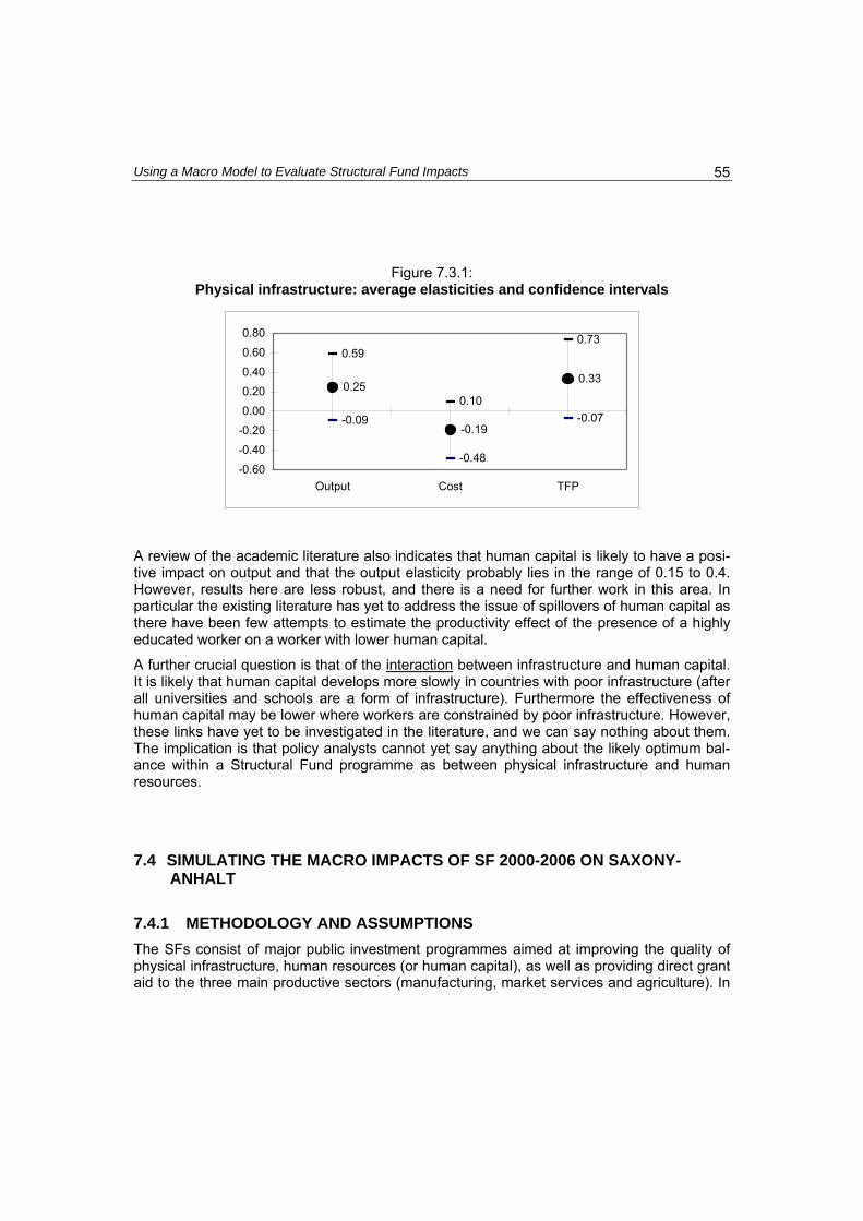
Using a Macro Model to Evaluate Structural Fund Impacts 55
Figure 7.3.1: Physical infrastructure: average elasticities and confidence intervals
-0.09
-0.48
-0.07
0.25
-0.19
0.33
0.59
0.10
0.73
-0.60
-0.40
-0.20
0.00
0.20
0.40
0.60
0.80
Output Cost TFP
A review of the academic literature also indicates that human capital is likely to have a posi-tive impact on output and that the output elasticity probably lies in the range of 0.15 to 0.4. However, results here are less robust, and there is a need for further work in this area. In particular the existing literature has yet to address the issue of spillovers of human capital as there have been few attempts to estimate the productivity effect of the presence of a highly educated worker on a worker with lower human capital.
A further crucial question is that of the interaction between infrastructure and human capital. It is likely that human capital develops more slowly in countries with poor infrastructure (after all universities and schools are a form of infrastructure). Furthermore the effectiveness of human capital may be lower where workers are constrained by poor infrastructure. However, these links have yet to be investigated in the literature, and we can say nothing about them. The implication is that policy analysts cannot yet say anything about the likely optimum bal-ance within a Structural Fund programme as between physical infrastructure and human resources.
7.4 SIMULATING THE MACRO IMPACTS OF SF 2000-2006 ON SAXONY-ANHALT
7.4.1 METHODOLOGY AND ASSUMPTIONS The SFs consist of major public investment programmes aimed at improving the quality of physical infrastructure, human resources (or human capital), as well as providing direct grant aid to the three main productive sectors (manufacturing, market services and agriculture). In
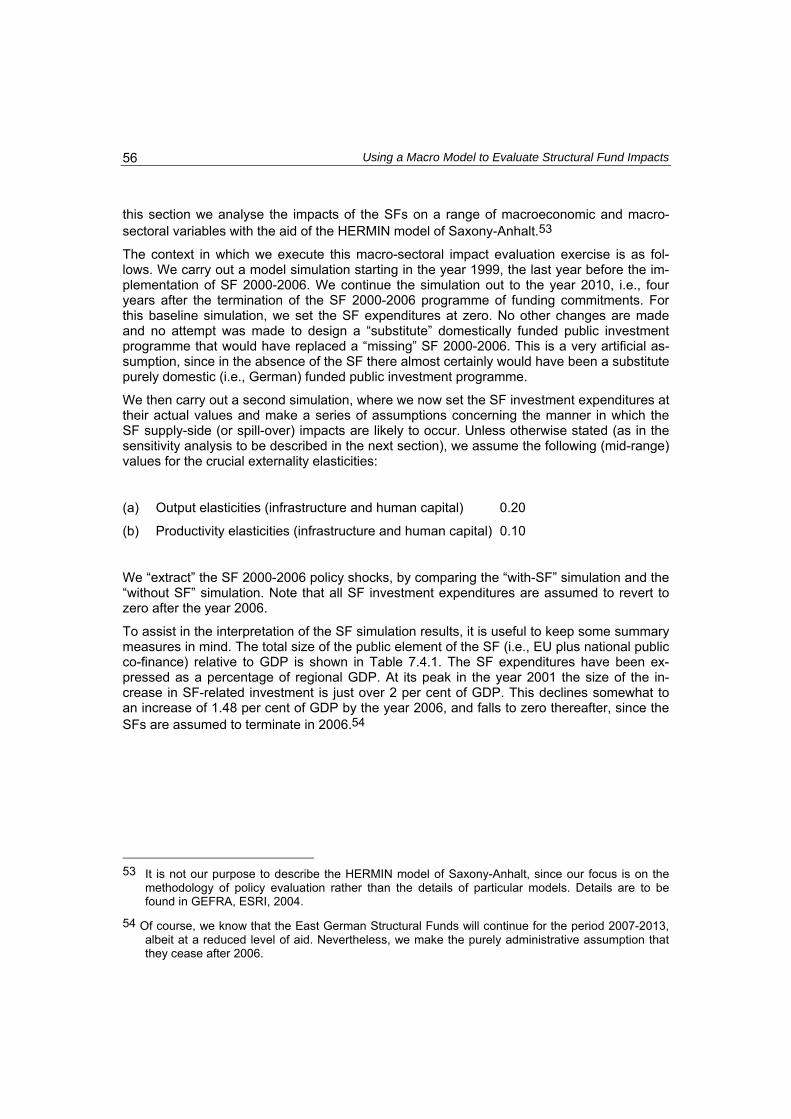
Using a Macro Model to Evaluate Structural Fund Impacts 56
this section we analyse the impacts of the SFs on a range of macroeconomic and macro-sectoral variables with the aid of the HERMIN model of Saxony-Anhalt.53
The context in which we execute this macro-sectoral impact evaluation exercise is as fol-lows. We carry out a model simulation starting in the year 1999, the last year before the im-plementation of SF 2000-2006. We continue the simulation out to the year 2010, i.e., four years after the termination of the SF 2000-2006 programme of funding commitments. For this baseline simulation, we set the SF expenditures at zero. No other changes are made and no attempt was made to design a “substitute” domestically funded public investment programme that would have replaced a “missing” SF 2000-2006. This is a very artificial as-sumption, since in the absence of the SF there almost certainly would have been a substitute purely domestic (i.e., German) funded public investment programme.
We then carry out a second simulation, where we now set the SF investment expenditures at their actual values and make a series of assumptions concerning the manner in which the SF supply-side (or spill-over) impacts are likely to occur. Unless otherwise stated (as in the sensitivity analysis to be described in the next section), we assume the following (mid-range) values for the crucial externality elasticities:
(a) Output elasticities (infrastructure and human capital) 0.20
(b) Productivity elasticities (infrastructure and human capital) 0.10
We “extract” the SF 2000-2006 policy shocks, by comparing the “with-SF” simulation and the “without SF” simulation. Note that all SF investment expenditures are assumed to revert to zero after the year 2006.
To assist in the interpretation of the SF simulation results, it is useful to keep some summary measures in mind. The total size of the public element of the SF (i.e., EU plus national public co-finance) relative to GDP is shown in Table 7.4.1. The SF expenditures have been ex-pressed as a percentage of regional GDP. At its peak in the year 2001 the size of the in-crease in SF-related investment is just over 2 per cent of GDP. This declines somewhat to an increase of 1.48 per cent of GDP by the year 2006, and falls to zero thereafter, since the SFs are assumed to terminate in 2006.54
53 It is not our purpose to describe the HERMIN model of Saxony-Anhalt, since our focus is on the
methodology of policy evaluation rather than the details of particular models. Details are to be found in GEFRA, ESRI, 2004.
54 Of course, we know that the East German Structural Funds will continue for the period 2007-2013, albeit at a reduced level of aid. Nevertheless, we make the purely administrative assumption that they cease after 2006.
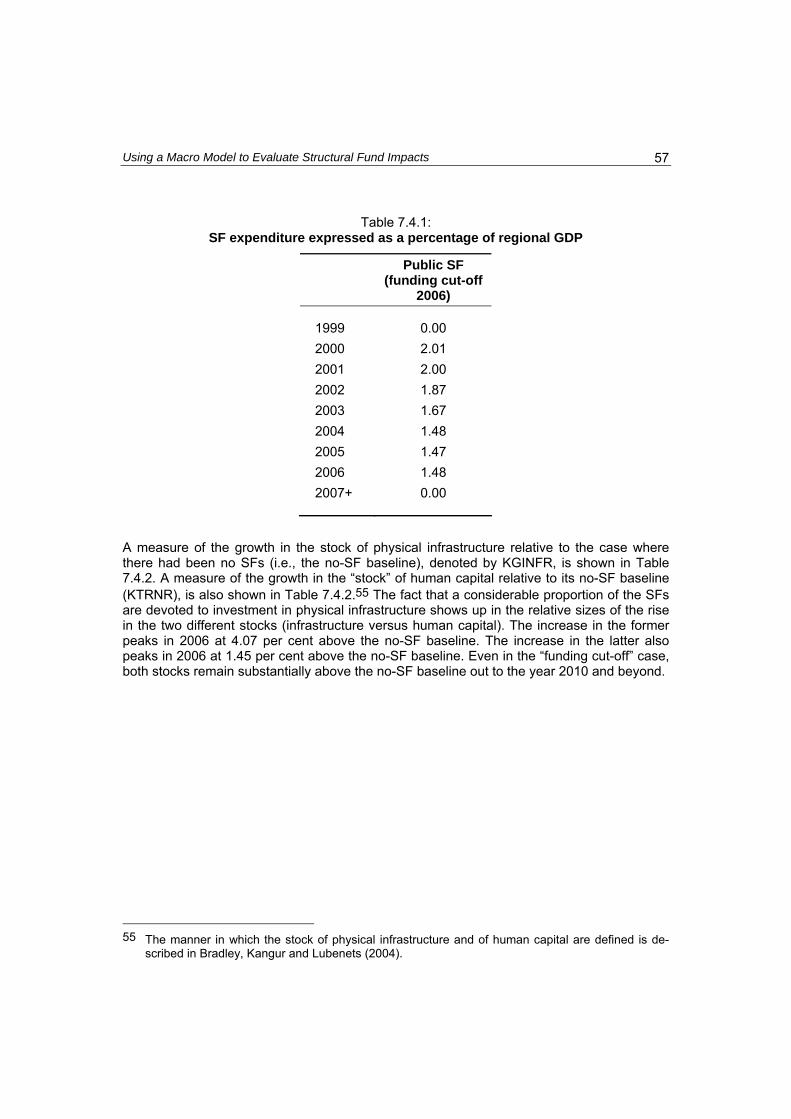
Using a Macro Model to Evaluate Structural Fund Impacts 57
Table 7.4.1: SF expenditure expressed as a percentage of regional GDP
Public SF (funding cut-off
2006)
1999 0.00 2000 2.01 2001 2.00 2002 1.87 2003 1.67 2004 1.48 2005 1.47 2006 1.48 2007+ 0.00
A measure of the growth in the stock of physical infrastructure relative to the case where there had been no SFs (i.e., the no-SF baseline), denoted by KGINFR, is shown in Table 7.4.2. A measure of the growth in the “stock” of human capital relative to its no-SF baseline (KTRNR), is also shown in Table 7.4.2.55 The fact that a considerable proportion of the SFs are devoted to investment in physical infrastructure shows up in the relative sizes of the rise in the two different stocks (infrastructure versus human capital). The increase in the former peaks in 2006 at 4.07 per cent above the no-SF baseline. The increase in the latter also peaks in 2006 at 1.45 per cent above the no-SF baseline. Even in the “funding cut-off” case, both stocks remain substantially above the no-SF baseline out to the year 2010 and beyond.
55 The manner in which the stock of physical infrastructure and of human capital are defined is de-
scribed in Bradley, Kangur and Lubenets (2004).
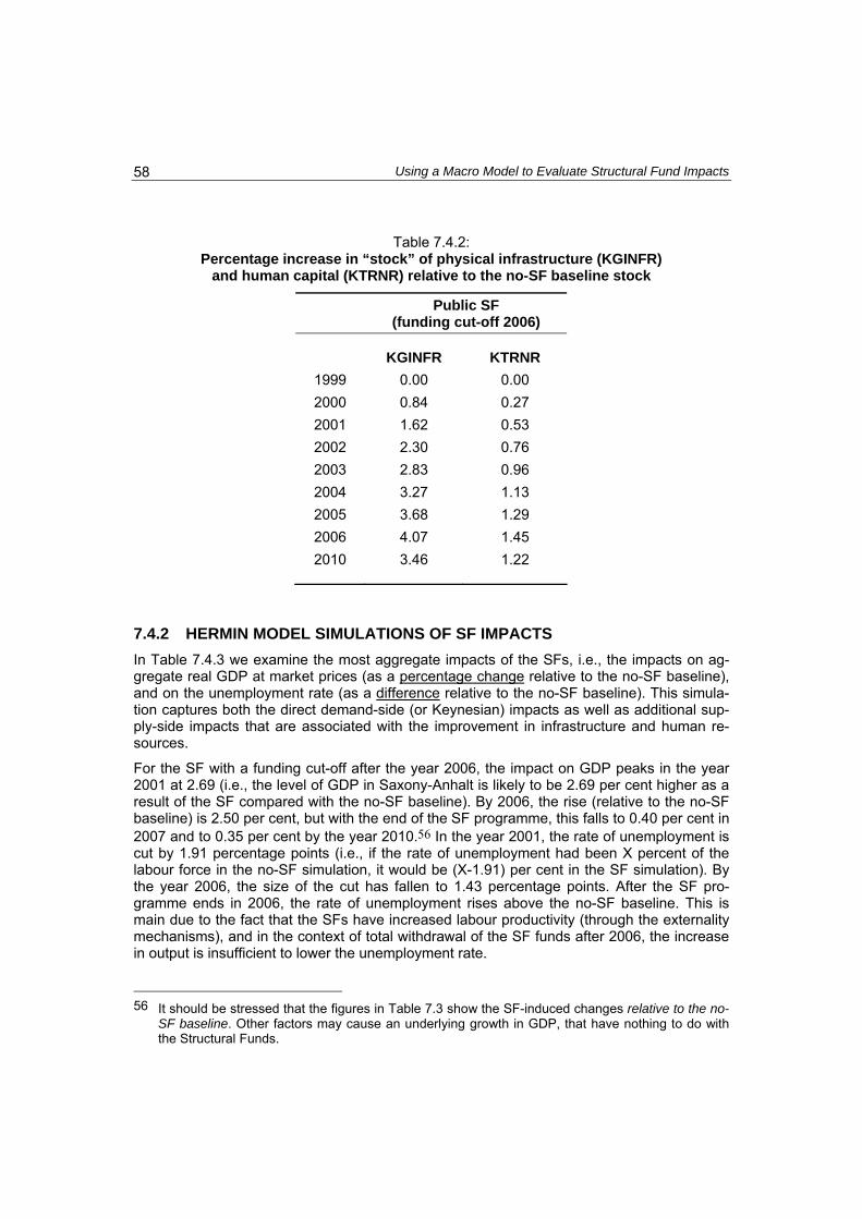
Using a Macro Model to Evaluate Structural Fund Impacts 58
Table 7.4.2: Percentage increase in “stock” of physical infrastructure (KGINFR)
and human capital (KTRNR) relative to the no-SF baseline stock
Public SF (funding cut-off 2006)
KGINFR KTRNR 1999 0.00 0.00 2000 0.84 0.27 2001 1.62 0.53 2002 2.30 0.76 2003 2.83 0.96 2004 3.27 1.13 2005 3.68 1.29 2006 4.07 1.45 2010 3.46 1.22
7.4.2 HERMIN MODEL SIMULATIONS OF SF IMPACTS In Table 7.4.3 we examine the most aggregate impacts of the SFs, i.e., the impacts on ag-gregate real GDP at market prices (as a percentage change relative to the no-SF baseline), and on the unemployment rate (as a difference relative to the no-SF baseline). This simula-tion captures both the direct demand-side (or Keynesian) impacts as well as additional sup-ply-side impacts that are associated with the improvement in infrastructure and human re-sources.
For the SF with a funding cut-off after the year 2006, the impact on GDP peaks in the year 2001 at 2.69 (i.e., the level of GDP in Saxony-Anhalt is likely to be 2.69 per cent higher as a result of the SF compared with the no-SF baseline). By 2006, the rise (relative to the no-SF baseline) is 2.50 per cent, but with the end of the SF programme, this falls to 0.40 per cent in 2007 and to 0.35 per cent by the year 2010.56 In the year 2001, the rate of unemployment is cut by 1.91 percentage points (i.e., if the rate of unemployment had been X percent of the labour force in the no-SF simulation, it would be (X-1.91) per cent in the SF simulation). By the year 2006, the size of the cut has fallen to 1.43 percentage points. After the SF pro-gramme ends in 2006, the rate of unemployment rises above the no-SF baseline. This is main due to the fact that the SFs have increased labour productivity (through the externality mechanisms), and in the context of total withdrawal of the SF funds after 2006, the increase in output is insufficient to lower the unemployment rate.
56 It should be stressed that the figures in Table 7.3 show the SF-induced changes relative to the no-
SF baseline. Other factors may cause an underlying growth in GDP, that have nothing to do with the Structural Funds.

Using a Macro Model to Evaluate Structural Fund Impacts 59
Table 7.4.3: Aggregate SF 2000-2006 impacts on GDP and unemployment
Public SF (funding cut-off after 2006)
GDP UR 1999 0.00 0.00 2000 2.37 -1.85 2001 2.69 -1.91 2002 2.60 -1.77 2003 2.46 -1.58 2004 2.34 -1.40 2005 2.39 -1.39 2006 2.50 -1.43 2007 0.40 0.27 2010 0.35 0.19
GDP: Percentage change from no-SF baseline
UR: Change from no-SF baseline
It should be remembered that the only policy alteration that we introduce into the model is the 2000-2006 SF investment programme. In reality, other changes will accompany the SFs, e.g., the continued restructuring of the Saxony-Anhalt economy and its further opening to increased trade within the German and the wider EU Single Market. So, the above results need to be interpreted carefully as representing only one element of the impact of a wide range of EU policy impacts on the economy.57
It would be possible to investigate the impacts of the SF on a wide range of other economic variables, e.g., sectoral GDP, employment, investment, productivity, prices and wages, as well as the usual expenditure aggregates such as household consumption and the regional public sector financial deficits and the balance of regional trade. But since our purpose is to describe the macro impact evaluation methodology rather than the detail, we refer the reader to GEFRA / ESRI (2004) for a full description of the evaluation results.
A better summary measure of the likely return from Structural Fund investment expenditures is given by the “cumulative” multiplier, which normalises the impact measure (i.e., makes it independent of the actual magnitude of the SF expenditure injection) and attempts to capture the continued (if modest) semi-permanent increase in the level of GDP that should persist after the policy is terminated in the year 2006. Its definition is as follows: 57 See ESRI (1997) for an account of the combined analysis of SF and Single Market impacts for
Greece, Ireland, Portugal and Spain.
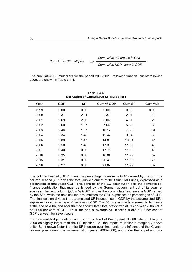
Using a Macro Model to Evaluate Structural Fund Impacts 60
Cumulative %increase in GDP Cumulative SF multiplier ⇒
Cumulative NDP share in GDP
The cumulative SF multipliers for the period 2000-2020, following financial cut off following 2006, are shown in Table 7.4.4.
Table 7.4.4: Derivation of Cumulative SF Multipliers
Year GDP SF Cum % GDP Cum SF CumMult
1999 0.00 0.00 0.00 0.00 0.00 2000 2.37 2.01 2.37 2.01 1.18 2001 2.69 2.00 5.06 4.01 1.26 2002 2.60 1.87 7.66 5.88 1.30 2003 2.46 1.67 10.12 7.56 1.34 2004 2.34 1.48 12.47 9.04 1.38 2005 2.39 1.47 14.86 10.51 1.41 2006 2.50 1.48 17.36 11.99 1.45 2007 0.40 0.00 17.75 11.99 1.48 2010 0.35 0.00 18.84 11.99 1.57 2015 0.31 0.00 20.46 11.99 1.71 2020 0.27 0.00 21.87 11.99 1.82
The column headed „GDP“ gives the percentage increase in GDP caused by the SF. The column headed „SF“ gives the total public element of the Structural Funds, expressed as a percentage of that years GDP. This consists of the EC contribution plus the domestic co-finance contribution that must be funded by the German government out of its own re-sources. The next column („Cum % GDP“) shows the accumulated increase in GDP caused by the SFs, while the next column accumulates the SFs, expressed as percentages of GDP. The final column divides the accumulated SF-induced rise in GDP by the accumulated SFs, expressed as a percentage of the level of GDP. The SF programme is assumed to terminate at the end of 2006, and after that the accumulated total stays fixed at its end-year 2006 value of 11.99 per cent of GDP. Thus, the annual average SF injection is about 1.7 per cent of GDP per year, for seven years.
The accumulated percentage increase in the level of Saxony-Anhalt GDP starts off in year 2000 as slightly larger than the SF injection, i.e., the impact multiplier is marginally above unity. But it grows faster than the SF injection over time, under the influence of the Keynes-ian multiplier (during the implementation years, 2000-2006), and under the output and pro-
Using a Macro Model to Evaluate Structural Fund Impacts 61
ductivity-enhancing influence of the rising stock of infrastructure and human capital. This latter effect endures after the implementation phase is over, i.e., after the year 2006.
From an initial value of just above unity in 2000, the cumulative multiplier increases steadily over time, reaching a value of 1.82 by the year 2020. In interpreting this number, two caveats need to be borne in mind. First, we have assumed values for the “spillover” parameters that are in the mid-range of values found in the international literature. Higher values would give higher multipliers; and lower values, lower multipliers. We return to this point in Section 8. Second, the depreciation rates that we have assumed for the stock of physical infrastructure and human capital (2.5% and 5%, respectively) are probably on the low side. If these were higher, then the cumulated multiplier would level off a few years after the 2006 termination date, and start to decline.
It should be emphasised that in the above simulation we have assumed values of the crucial “externality” elasticities in the mid-range of those found in the international literature. We do not take any ex-ante view on the efficiency and effectiveness of the specific SF programme for Saxony-Anhalt, other than that it is likely to be designed and implemented in a way that reflects average performance of such public investment programmes that have been exam-ined in the international literature. In other words, the returns to the public investment expen-ditures are at the level of the average of international studies.
It must also be stressed that our macro analysis reported here is not “bottom up”, in the sense of working from very detailed Structural Fund measures, up to Operational Pro-grammes, and finally up to the aggregate effects. In fact, only three pieces of SF data are used that can influence the size of the impacts on the cumulative multipliers: the distribution of EU funds between investments in infrastructure, human capital and direct investment aid to the productive sectors.58 The actual size of Structural Fund injection is filtered out by the normalization involved in the calculation of the cumulative multiplier. In reality, everything will depend on the actual mix of projects in the NDP, as well as the organizational ability to utilize and implement CSF efficiently and effectively. So, our model-based macro results are merely broad ball-park estimates. The real challenge is to reconcile the bottom-up micro analysis with the top-down analysis. Until this is achieved, one should approach macro impact analy-sis with extreme caution. In the next section we will describe how the insights from the micro (or bottom-up) evaluations can be used to improve the macro (or top-down) analysis.
58 It will be noted that the size of the cumulative multipliers are independent of the actual magnitude
of the SF funding injection. But of course the impacts on GDP and unemployment (as illustrated in Table 7.3) vary with the actual magnitude of the expenditure.
8 AN INTEGRATED MODELLING APPROACH
TO POLICY EVALUATION
8.1 INTRODUCTORY REMARKS In the analysis so far we have set up the micro and macro evaluation concepts separately. In this section we attempt to combine the two components into an integrated micro-macro model (IMM) in order to exploit the benefits that are expected to arise from the combined use of both approaches. The combination of micro and macro elements within a unified model-ling framework has long attracted considerable research interests in the field of economics. Previous efforts to construct a comprehensive micro-macro model are based on diverse strands of research (see e.g. Voßkamp, 1996). The construction of micro-macro models has been motivated by the need for high compatibility between the micro- and macroeconomic approaches and may be seen as a factual (and practical) necessity. In a different sub-field of research, modelling efforts mainly rest upon the attempt to derive micro foundations of mac-roeconomics explicitly based on the principles of behavioural theory. Though the later ap-proach has attracted major research efforts over the last three decades, it has a general short-coming since the construction of a generally accepted micro foundation of macro mod-els is either impossible (in the case of general equilibrium theory with heterogeneous agents) or substantially criticised (in the case of representative agent models, e.g. Kirman, 1992). It is therefore important to make clear that our approach does not aim to shed further light on the purely academic debate about the behavioural micro foundation of macro models. In-stead we use the term micro-macro model to guide empirical problem-solving on different evaluation levels, where linkages and feedback effects are of special importance. In this sense we use the arguments of a high-compatibility of micro and macro tools, as well as the factual and empirical need in NDP-type policy programme evaluation for a micro-macro model as motivation for further modelling efforts.
The crucial point at this modelling stage is to find an appropriate way to link the elementary building blocks of both approaches. In doing so, we can make use of recent contributions to economic modelling, which have identified different concepts of model linkages that depend on the chosen degree of complexity for the established interaction (see e.g. Baeckgaard, 1995). An important aspect in these circumstances is the treatment of feedback effects. With respect to our IMM concept, the feedback effects can generally go in two directions: a.) from micro to macro and b.) from macro to micro. Moreover, one-way or two-way interaction is possible, as well as sequential (lagged) and simultaneous feedback. Hence, we have to choose among different methods, which are classified not only with regard to the direction but also the extent of interaction.

An Integrated Modelling Approach to Policy Evaluation 63
In this multidimensional set-up, prominent approaches comprise:59
1.) the top-down approach: This approach is a one-way adjustment of the micro outcome to match an externally specified macro scenario.
2.) the bottom up or limited feedback approach: The method involves the macro and micro models running separately, but also includes an adjustment of the macro model in line with the output from the micro model.
3.) recursive linkages: The approach runs a micro and macro model in parallel with two-way lagged interactions over relatively short periods of simulation.
4.) the iterative or simultaneous approach: This method is an extension of 3.) and consid-ers the outcome of the micro and macro models solved simultaneously within each pe-riod.
When moving from 1.) to 4.) we observe an inherent interaction-complexity trade-off. That is, while interaction and feedback effects are rather small in 1.), they gradually increase up and are likely to be highest in 4.). However, the degree of model parsimony (identified above as an important characteristics in the light of public policy analysis) declines. In the following we will make use of the limited feedback approach (2.) in the construction of our IMM. The ap-proach allows for an interaction in form of a sequential combination of micro and macro components to assess the crucial impacts in Structural Funds evaluation, but nevertheless keeps the degree of model complexity low enough to be implemented in an empirically orien-tated policy analysis setup.
One advantage of the chosen “limited feedback” approach is that we can run the micro and macro models unconstrained and therefore make use of the specific strengths of the individ-ual approaches with respect to the different evaluation levels (broad categories versus indi-vidual measures) of the Structural funds. On the other hand, by allowing for an interaction of the two, we also account for the inherent shortcomings of the single approaches as already set out in Table 1.1 previously. In other words, while the micro approach focuses on the spe-cial characteristics of each individual project and usually ignores economy-wide externalities, the macro approach deals with economy-wide externalities, but can say little about the effi-ciency and effectiveness of the underlying projects. Ideally, the macro externality parameters should be derived from micro-based work. In practice, very little of such micro empirical evaluations are ever available for use within macro evaluations. We saw in Section 7 that externality elasticities have to be drawn from international quantitative studies, not all of which are likely to be relevant to (say) an NDP being implemented in a new EU member state, or a region of a state, in Central and Eastern Europe.
The situation is even more serious when one attempts to carry out ex-ante macro evalua-tions of NDPs that have been designed and costed, but not yet implemented. The usual ap-proach is to carry out a sensitivity analysis with respect to the crucial externality elasticities, but to leave unsolved the decision concerning which set of elasticities is relevant in any spe-
59 See Baeckgaard (1995) for details with respect to microsimulation and macroeconomic projection
models.

An Integrated Modelling Approach to Policy Evaluation 64
cific situation. From a macro modelling viewpoint, this seems to be an elegant solution to an intractable problem. But from a policy design and evaluation viewpoint, it is obviously less satisfactory.
What we need is for the “scoring” and the macro evaluations to be carried out sequentially, and for the results of the scoring exercise to be fed back to the macro evaluation, improving the selection of externality elasticities. For example, if the “scoring” approach suggests that an NDP has been poorly designed, this would point to selecting low values of the externality elasticities, and vice versa.
In the remainder of this section we first illustrate how a macro sensitivity analysis can be carried out, and we illustrate it using the Saxony-Anhalt case previously used in Section 7. We then suggest that the “scoring” approach can be used to guide the choice of elasticities in the sensitivity analysis towards the most appropriate ones for a specific NDP. We con-clude with a proposal for a more integrated type of policy evaluation that combines the best features of both micro and macro evaluation techniques.
8.2 MACRO NDP EVALUATION: SENSITIVITY ANALYSIS Using macro models for the evaluation of policy impacts of large-scale public investment projects is a complex area of research, and draws heavily on modern macro theory, new growth theory, and new economic geography. Not all macro models are suitable for such policy analysis. But in what follows we stand aside from the vigorous debates on the relative merits of individual macro models, and assume that the model being used is a realistic rep-resentation of the economy that commands broad consensus.
In Section 7 we described an adaptation to a particular macro model (the so-called HERMIN model), where long-term NDP impacts were included via externality effects caused by an improved stock of physical infrastructure and human capital. There were two kinds of exter-nality, each associated with two different types of structural intervention: improved physical infrastructure and improved human resources: a direct impact on output and an effect on factor productivity. Hence, the values of four parameters largely determine the magnitude of the long-term impacts of EU Structural Funds: two of which relate improvements in the stock of infrastructure and of human capital directly to output; two others which relate these im-provements to factor productivity.
If zero values are selected for these four elasticities, then we are left with the mainly Keynes-ian (or demand-side) impacts. After the implementation stage is complete (the road built; the training course(s) held), then the economy essentially reverts to its pre-NDP baseline level. An extreme case of this would be if roads were built in areas where they are never used; or training courses were given that were unrelated to any possible demand for such skills. Keynes’s example of the government financing the digging and refilling of useless holes in the ground comes to mind. In total this would mean that the entire NDP had been designed in such a way that there is no longer lasting impact on the supply side of the supported economy.
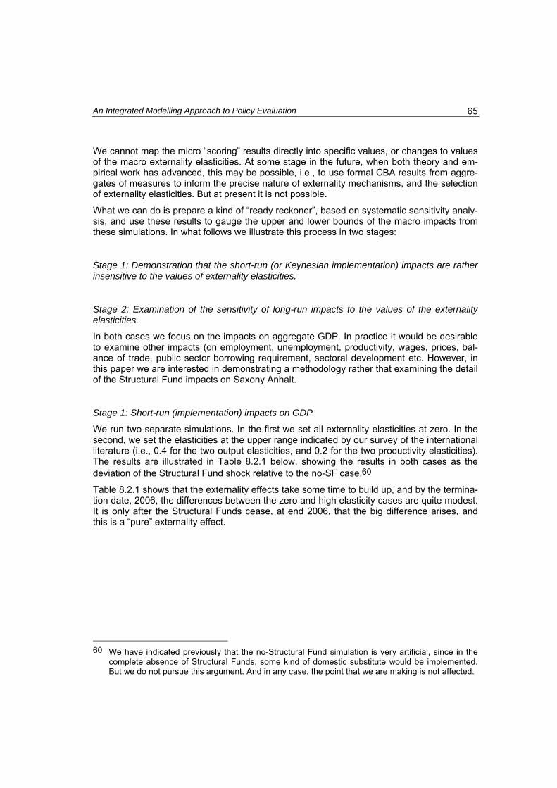
An Integrated Modelling Approach to Policy Evaluation 65
We cannot map the micro “scoring” results directly into specific values, or changes to values of the macro externality elasticities. At some stage in the future, when both theory and em-pirical work has advanced, this may be possible, i.e., to use formal CBA results from aggre-gates of measures to inform the precise nature of externality mechanisms, and the selection of externality elasticities. But at present it is not possible.
What we can do is prepare a kind of “ready reckoner”, based on systematic sensitivity analy-sis, and use these results to gauge the upper and lower bounds of the macro impacts from these simulations. In what follows we illustrate this process in two stages:
Stage 1: Demonstration that the short-run (or Keynesian implementation) impacts are rather insensitive to the values of externality elasticities.
Stage 2: Examination of the sensitivity of long-run impacts to the values of the externality elasticities.
In both cases we focus on the impacts on aggregate GDP. In practice it would be desirable to examine other impacts (on employment, unemployment, productivity, wages, prices, bal-ance of trade, public sector borrowing requirement, sectoral development etc. However, in this paper we are interested in demonstrating a methodology rather that examining the detail of the Structural Fund impacts on Saxony Anhalt.
Stage 1: Short-run (implementation) impacts on GDP
We run two separate simulations. In the first we set all externality elasticities at zero. In the second, we set the elasticities at the upper range indicated by our survey of the international literature (i.e., 0.4 for the two output elasticities, and 0.2 for the two productivity elasticities). The results are illustrated in Table 8.2.1 below, showing the results in both cases as the deviation of the Structural Fund shock relative to the no-SF case.60
Table 8.2.1 shows that the externality effects take some time to build up, and by the termina-tion date, 2006, the differences between the zero and high elasticity cases are quite modest. It is only after the Structural Funds cease, at end 2006, that the big difference arises, and this is a “pure” externality effect.
60 We have indicated previously that the no-Structural Fund simulation is very artificial, since in the
complete absence of Structural Funds, some kind of domestic substitute would be implemented. But we do not pursue this argument. And in any case, the point that we are making is not affected.

An Integrated Modelling Approach to Policy Evaluation 66
Table 8.2.1: GDP impacts: zero and high elasticities
Date GDPE-zero GDPE-high
1999 0.000 0.000 2000 2.357 2.386 2001 2.634 2.745 2002 2.484 2.718 2003 2.271 2.657 2004 2.063 2.626 2005 2.079 2.707 2006 2.145 2.853 2007 0.064 0.735 2008 0.047 0.700 2009 0.047 0.682 2010 0.045 0.663 2015 0.037 0.578 2020 0.030 0.505
Stage 2: Sensitivity of long run impacts on GDP
We illustrate the kind of “ready reckoner” that can be constructed by varying the two output elasticities, while keeping the productivity elasticities constant at zero. The impacts on GDP are illustrated in Table 8.2.2, where, once again, the results are shown as the deviation of the Structural Fund shock relative to the no-SF case.
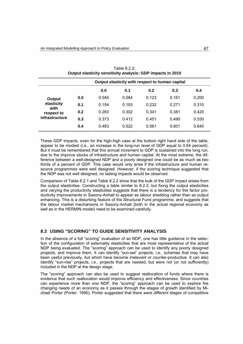
An Integrated Modelling Approach to Policy Evaluation 67
Table 8.2.2: Output elasticity sensitivity analysis: GDP impacts in 2010
Output elasticity with respect to human capital
0.0 0.1 0.2 0.3 0.4
0.0 0.045 0.084 0.123 0.161 0.200
0.1 0.154 0.193 0.232 0.271 0.310
0.2 0.263 0.302 0.341 0.381 0.420
0.3 0.373 0.412 0.451 0.490 0.530
Output elasticity
with respect to
infrastructure
0.4 0.483 0.522 0.561 0.601 0.640
These GDP impacts, even for the high-high case at the bottom right hand side of the table, appear to be modest (i.e., an increase in the long-run level of GDP equal to 0.64 percent). But it must be remembered that this annual increment to GDP is sustained into the long run, due to the improve stocks of infrastructure and human capital. At the most extreme, the dif-ference between a well-designed NDP and a poorly designed one could be as much as two thirds of a percent of GDP. This case would only arise if the infrastructure and human re-source programmes were well designed. However, if the scoring technique suggested that the NDP was not well designed, no lasting impacts would be observed.
Comparison of Table 8.2.1 and Table 8.2.2 show that the bulk of the GDP impact arises from the output elasticities. Constructing a table similar to 8.2.2, but fixing the output elasticities and varying the productivity elasticities suggests that there is a tendency for the factor pro-ductivity improvements in Saxony-Anhalt to appear as labour shedding rather than as output enhancing. This is a disturbing feature of the Structural Fund programme, and suggests that the labour market mechanisms in Saxony-Anhalt (both in the actual regional economy as well as in the HERMIN model) need to be examined carefully.
8.3 USING “SCORING” TO GUIDE SENSITIVITY ANALYSIS In the absence of a full “scoring” evaluation of an NDP, one has little guidance in the selec-tion of the configuration of externality elasticities that are most representative of the actual NDP being evaluated. The “scoring” approach can be used to identify any poorly designed projects, and improve them. It can identify “sun-set” projects, i.e., schemes that may have been useful previously, but which have become irrelevant or counter-productive. It can also identify “sun-rise” projects, i.e., projects that are needed, but were not (or not sufficiently) included in the NDP at the design stage.
The “scoring” approach can also be used to suggest reallocation of funds where there is evidence that such reallocation would improve efficiency and effectiveness. Since countries can experience more than one NDP, the “scoring” approach can be used to explore the changing needs of an economy as it passes through the stages of growth identified by Mi-chael Porter (Porter, 1990). Porter suggested that there were different stages of competitive
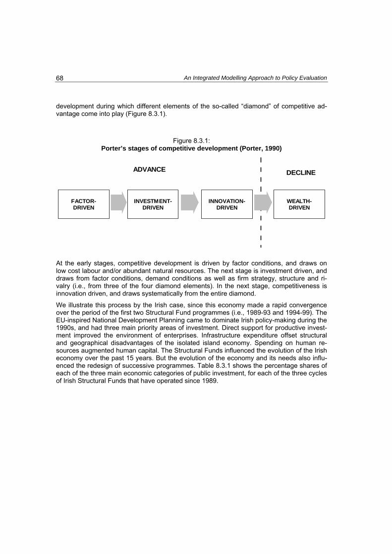
An Integrated Modelling Approach to Policy Evaluation 68
development during which different elements of the so-called “diamond” of competitive ad-vantage come into play (Figure 8.3.1).
Figure 8.3.1: Porter’s stages of competitive development (Porter, 1990)
FACTOR-DRIVEN
INVESTMENT-DRIVEN
INNOVATION-DRIVEN
WEALTH-DRIVEN
ADVANCE DECLINE
At the early stages, competitive development is driven by factor conditions, and draws on low cost labour and/or abundant natural resources. The next stage is investment driven, and draws from factor conditions, demand conditions as well as firm strategy, structure and ri-valry (i.e., from three of the four diamond elements). In the next stage, competitiveness is innovation driven, and draws systematically from the entire diamond.
We illustrate this process by the Irish case, since this economy made a rapid convergence over the period of the first two Structural Fund programmes (i.e., 1989-93 and 1994-99). The EU-inspired National Development Planning came to dominate Irish policy-making during the 1990s, and had three main priority areas of investment. Direct support for productive invest-ment improved the environment of enterprises. Infrastructure expenditure offset structural and geographical disadvantages of the isolated island economy. Spending on human re-sources augmented human capital. The Structural Funds influenced the evolution of the Irish economy over the past 15 years. But the evolution of the economy and its needs also influ-enced the redesign of successive programmes. Table 8.3.1 shows the percentage shares of each of the three main economic categories of public investment, for each of the three cycles of Irish Structural Funds that have operated since 1989.
An Integrated Modelling Approach to Policy Evaluation 69
Table 8.3.1: Main economic categories of Irish Structural Funds
(Percentage shares of total)
Economic Category CSF 1989-93
CSF 1994-99
CSF 2000-06
Aid to productive sector 56.0 47.0 16.0
Human resources 25.0 32.0 36.0
Physical infrastructure 19.0 21.0 48.0
The first NDP focused heavily on direct aid to the productive sectors, with a strong emphasis on human resources, and a substantial programme of investment in physical infrastructure. It was designed at a time when the economy had not fully emerged from the deep crisis of the 1980s, and the direct aid sub-programmes appeared to offer the fastest and best immediate return, while the other sub-programmes built up and offered the promise of longer term re-turns. By the time of the second NDP programme, the increased emphasis on human re-sources (up from 25 to 32 per cent) reflected concerns about the continuing high level of unemployment, and had a strong “equity” element that complemented the “efficiency” ele-ment. The third NDP programme was designed at a time when the convergent success of the Irish economy was apparent. By the late 1990s Ireland had moved to what was effec-tively full employment, and major infrastructural deficits had been exposed by the rapid growth in the volume of traffic on the congested road systems both in the major cities, and connecting these cities. In order to address these bottlenecks, there was a major shift to infrastructure investment, the share going to human resources also increased, with a focus on upgrading skills, and there was a major reduction in direct aid to the now booming pro-ductive sectors.
In contrast to the SF expenditures in Ireland, for the actual funding between 2000 and 2006 period in Saxony-Anhalt the major share of expenditures was devoted to support the invest-ment activity of the private productive sector (51%), followed by physical infrastructure (36%) and human resources (13%). The mix of categories is therefore quite different to that in Ire-land today. This heterogeneity in programme priorities shows that Saxony-Anhalt is likely to stand at a different point of competitive development according to Figure 8.3.1. Whereas Ireland has already proceeded from the investment to the innovation driven stage in competi-tive development, Saxony-Anhalt still remains at an investment driven stage of development. The high shares of SF funding devoted to physical infrastructure and especially human re-sources in Ireland and of direct private sector support in Saxony-Anhalt hint at the different evolutionary positions of the two regions: Whereas Ireland used a specific categorical mix with a special weight to the productive sector in order to overcome the economic crisis in the 80s and now orientates towards an innovation driven regional economy, Saxony-Anhalt for 2000-2006 still gives priority to productive sector support in order overcome the persisting

An Integrated Modelling Approach to Policy Evaluation 70
gap in capital stock per capita compared to the German average in the aftermath of the po-litical transformation process.61
The comparison of the Irish and Saxony-Anhalt case has shown that different programme structures are effective for different economic circumstances. It is therefore always neces-sary to check firstly, whether the proposed measures within the categories are effectively and efficiently designed and secondly, whether the mix of categories is optimal for the actual economic circumstances. Both aspects give a strong indication of the adequacy of the re-spective operational programme. As was argued above, the “scoring” approach can be used to explore the changing needs of an economy as it passes through the stages of growth. This suggests reallocation of funds where there is evidence that such reallocation would improve efficiency and effectiveness. The efficiency and effectiveness then also enhances the likely impacts and externalities that the programme might induce at the macro level.
8.4 INTEGRATING THE TWO COMPONENTS FOR ANALYSIS IN SAXONY-ANHALT
In order to use all the above information in an optimal way for the evaluation process, we therefore need to apply both models sequentially with the micro model taking precedence in order to link micro output (see above) and macro input as envisaged by the limited feedback approach. This two-step setup can be described as follows. The MCDA scoring model is used to optimize the SF programme fit in a first step, and in a second step we can show with the help of the HERMIN model what macro effects may arise in terms of the micro optimisa-tion. This second step is a crucial measurement of the success of the programme modifica-tions induced by the MCDA model.
In the above section we have already shown that the size of the elasticities for the two identi-fied externalities (output and factor productivity) has important implications for the (long-run) effects of the Structural Funds. The externalities only arise if the programme/measure is effectively and efficiently specified and therefore gives rise to positive spill-over externalities. For example, a measure in Saxony-Anhalt that focuses on the rural road and lane construc-tion will likely generate lower positive externalities with respect to public infrastructure com-pared to measures designed to bridge important gaps in the highway or road network. With respect to human resources, training schemes for jobs with a low demand will generate smaller externalities than training schemes targeted specifically at sectors where there is an under supply of qualified workers.
The micro-evaluation of the Structural Funds for the sub-period 2000-2003 in Saxony-Anhalt using the MCDA-model showed that the programme was in some parts inefficiently speci-fied. We have identified some measures that yielded poor scores and which are not ex-pected to support the intended goals of the Structural Funds. As a result of the scoring, based on ex-ante information, the SF interventions were substantially changed in the second
61 In contrast to Ireland the financial categories for Saxony-Anhalt do not entirely represent the actual
political funding within these categories since in Saxony-Anhalt many policy initiatives are run out-side the EU Structural funds. These account especially for human resource funding.
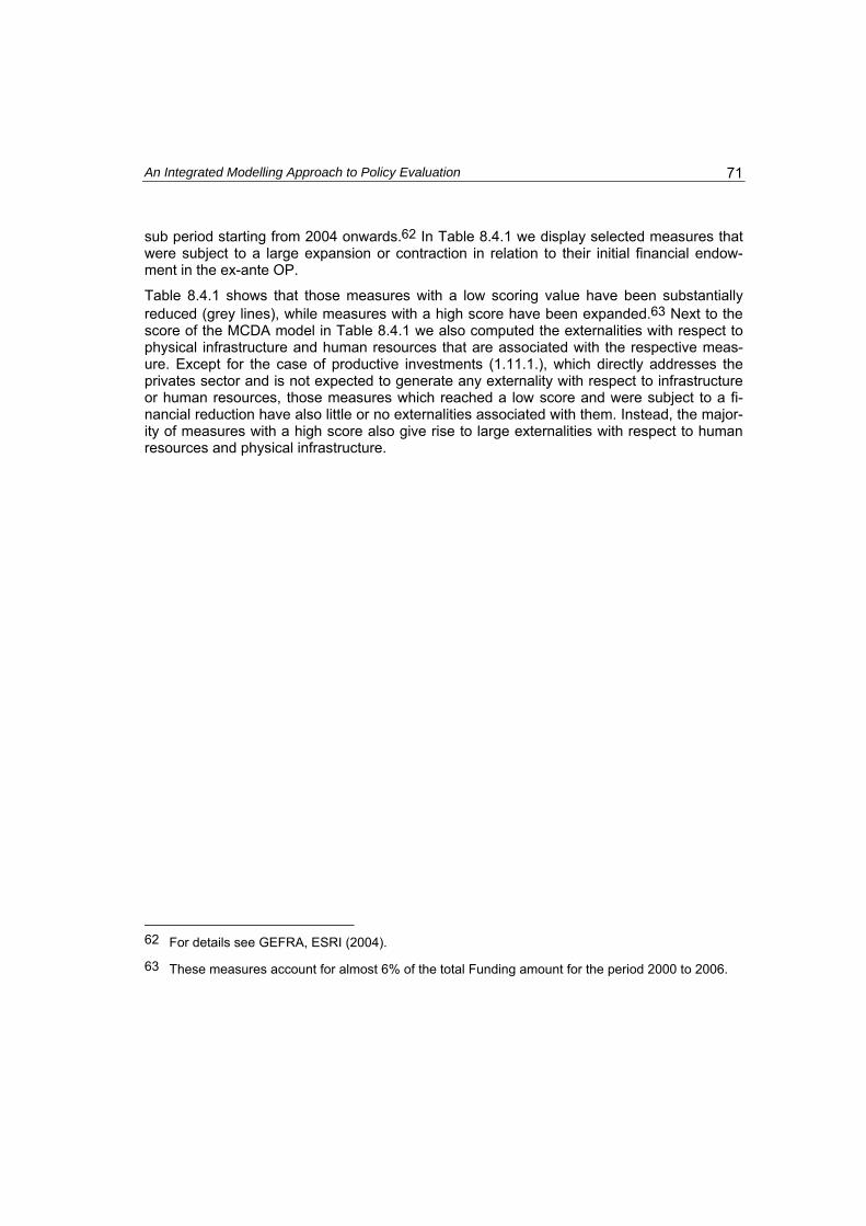
An Integrated Modelling Approach to Policy Evaluation 71
sub period starting from 2004 onwards.62 In Table 8.4.1 we display selected measures that were subject to a large expansion or contraction in relation to their initial financial endow-ment in the ex-ante OP.
Table 8.4.1 shows that those measures with a low scoring value have been substantially reduced (grey lines), while measures with a high score have been expanded.63 Next to the score of the MCDA model in Table 8.4.1 we also computed the externalities with respect to physical infrastructure and human resources that are associated with the respective meas-ure. Except for the case of productive investments (1.11.1.), which directly addresses the privates sector and is not expected to generate any externality with respect to infrastructure or human resources, those measures which reached a low score and were subject to a fi-nancial reduction have also little or no externalities associated with them. Instead, the major-ity of measures with a high score also give rise to large externalities with respect to human resources and physical infrastructure.
62 For details see GEFRA, ESRI (2004).
63 These measures account for almost 6% of the total Funding amount for the period 2000 to 2006.

Table 8.4.1: OP modifications based on the Scoring results
Year64 Level Measure Respective Fund
EU (in Mio. €,
in %)
Co-Financing (in Mio. €,
in %)
Private (in Mio. €,
in %)
Score MCDA model
Externalities with respect to Human
Resources & Infrastructure
2000-2006 1.11.1. Productive Investments
(common task, GA) EFRD 59,63 59,63 221,47 0,65 no direct externality – Productive sector
21,18% 21,18% 21,18%
2000-2006 1.11.2. R&D funding (common
task, GA) EFRD 15,75 15,75 31,50 0,45 high - Human Re-sources
21,18% 21,18% 21,18%
2000-2006 1.22.1.
Special programme "building up / strength-ening the information society“
EFRD -4,89 -1,64 -6,52 n.a. ? minor - Human Resources
-46,33% 32,76% -41,97%
2000-2006 1.22.2. Pilot projects „informati-
on society“ EFRD -2,16 -0,72 -2,88 -0,25 ? minor - Human Resources
-20,47% -14,41% -18,52%
2000-2006 1.31.5. Technology transfer
consulting EFRD -3,57 -1,87 -1,81 0,35 ? no externality –
internalised by en-terprises
-100,00% -100,00% -100,00%
64 The modifications for the measures based on the MCDA results are implemented for 2004 onwards. Between 2000 and 2003 the financial
payments were rather unchanged.
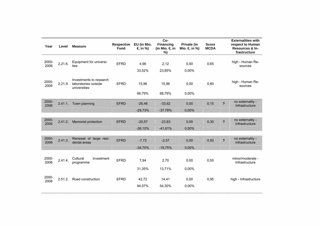
Year Level Measure Respective Fund
EU (in Mio. €, in %)
Co-Financing
(in Mio. €, in %)
Private (in Mio. €, in %)
Score MCDA
Externalities with respect to Human Resources & In-
frastructure
2000-2006 2.21.6. Equipment for universi-
ties EFRD 4,96 2,12 0,00 0,65 high - Human Re-sources
33,52% 23,85% 0,00%
2000-2006 2.21.9.
Investments to research laboratories outside universities
EFRD 15,96 15,96 0,00 0,60 high - Human Re-sources
68,79% 68,79% 0,00%
2000-2006 2.41.1. Town planning EFRD -26,46 -33,62 0,00 0,15 ? no externality -
Infrastructure -29,73% -37,78% 0,00%
2000-2006 2.41.2. Memorial protection EFRD -20,57 -23,83 0,00 0,30 ? no externality -
Infrastructure -36,10% -41,81% 0,00%
2000-2006 2.41.3. Renewal of large resi-
dental areas EFRD -7,72 -2,57 0,00 0,00 ? no externality - Infrastructure
-34,70% -19,75% 0,00%
2000-2006 2.41.4. Cultural investment
programme EFRD 7,94 2,70 0,00 0,50 minor/moderate - Infrastructure
31,35% 13,71% 0,00%
2000-2006 2.51.2. Road construction EFRD 42,72 14,41 0,00 0,95 high - Infrastructure
94,07% 54,30% 0,00%
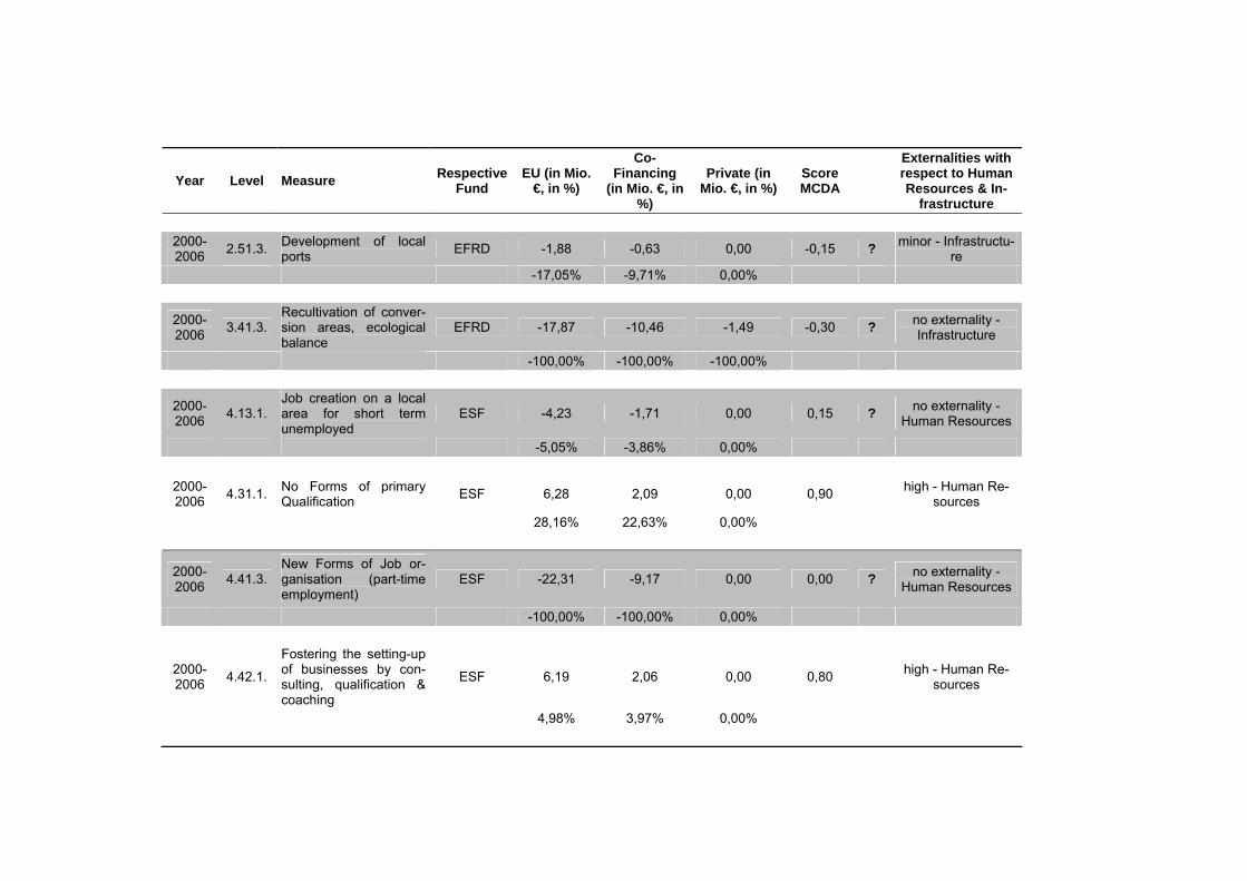
Year Level Measure Respective Fund
EU (in Mio. €, in %)
Co-Financing
(in Mio. €, in %)
Private (in Mio. €, in %)
Score MCDA
Externalities with respect to Human Resources & In-
frastructure
2000-2006 2.51.3. Development of local
ports EFRD -1,88 -0,63 0,00 -0,15 ? minor - Infrastructu-re
-17,05% -9,71% 0,00%
2000-2006 3.41.3.
Recultivation of conver-sion areas, ecological balance
EFRD -17,87 -10,46 -1,49 -0,30 ? no externality - Infrastructure
-100,00% -100,00% -100,00%
2000-2006 4.13.1.
Job creation on a local area for short term unemployed
ESF -4,23 -1,71 0,00 0,15 ? no externality - Human Resources
-5,05% -3,86% 0,00%
2000-2006 4.31.1. No Forms of primary
Qualification ESF 6,28 2,09 0,00 0,90 high - Human Re-sources
28,16% 22,63% 0,00%
2000-2006 4.41.3.
New Forms of Job or-ganisation (part-time employment)
ESF -22,31 -9,17 0,00 0,00 ? no externality - Human Resources
-100,00% -100,00% 0,00%
2000-2006 4.42.1.
Fostering the setting-up of businesses by con-sulting, qualification & coaching
ESF 6,19 2,06 0,00 0,80 high - Human Re-sources
4,98% 3,97% 0,00%
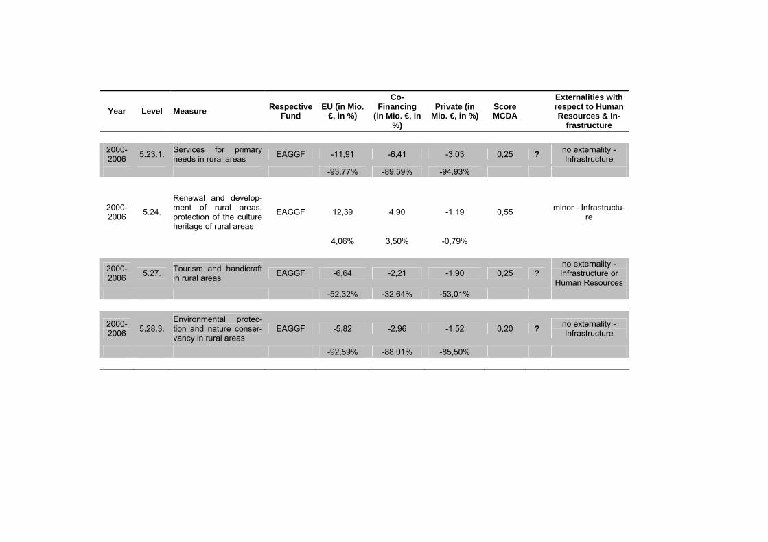
Year Level Measure Respective Fund
EU (in Mio. €, in %)
Co-Financing
(in Mio. €, in %)
Private (in Mio. €, in %)
Score MCDA
Externalities with respect to Human Resources & In-
frastructure
2000-2006 5.23.1. Services for primary
needs in rural areas EAGGF -11,91 -6,41 -3,03 0,25 ? no externality - Infrastructure
-93,77% -89,59% -94,93%
2000-2006 5.24.
Renewal and develop-ment of rural areas, protection of the culture heritage of rural areas
EAGGF 12,39 4,90 -1,19 0,55 minor - Infrastructu-re
4,06% 3,50% -0,79%
2000-2006 5.27. Tourism and handicraft
in rural areas EAGGF -6,64 -2,21 -1,90 0,25 ? no externality - Infrastructure or
Human Resources -52,32% -32,64% -53,01%
2000-2006 5.28.3.
Environmental protec-tion and nature conser-vancy in rural areas
EAGGF -5,82 -2,96 -1,52 0,20 ? no externality - Infrastructure
-92,59% -88,01% -85,50%

An Integrated Policy Approach to Policy Evaluation 76
We now have to take the micro output to the macro model. In sum, the change in the OP structure by the means of micro optimisation might lead to two changes in the macro input (compared to ex-ante data without scoring):
A change in the underlying aggregate financial time series that translate into a shift of the underlying stocks for human capital and physical infrastructure,
A change in the elasticity parameters of the two externalities.
In the following we restrict ourselves to changes in the elasticities.65 Since we observe inef-ficiencies in the ex-ante specification of the projects in the Structural Funds programme, as Table 8.4.1 shows, it is reasonable to suggest that the elasticities for the two externalities increase after the re-specification of the programme. But how does this change the impact of the interventions? Since the financial volume of the interventions does not change, there is at most an insignificant change on the Keynesian demand side effects. During the time the SF programme operates the demand side effects dominate, and there will be no difference between both SF programme set-ups. At the end of the intervention period the demand side effects rapidly fade away and the long-run supply side effects emerge. That is, moving back to Table 8.2.2, a micro optimisation of a SF programme causes a shift from the top left hand corner to the bottom right hand corner. If the optimisation shows that there is no further room for improvements, then we have strong arguments to choose high values for the elasticities, selecting values from the bottom right-hand corner.
However, our examination of the SF programme for Saxony-Anhalt showed inefficiencies in several but not all measures. This suggests elasticities from the upper left-hand corner. For example, if both output elasticities were around 0.1, due to a suboptimal programme design, then the level effect on GDP would be 0.2 percent in 2010 and onwards, and the longstand-ing supply-side effect would be rather small. An optimisation of the measures could result in an increase of the externality elasticities to 0.3. In that case GDP would be 0.5 percent higher, compared to the baseline line. The difference between a suboptimal and an opti-mised SF programme would then show a permanent level effect in GDP of around 0.3 per-cent. The long-run effect would increase substantial. Since we do not know the exact rela-tionship between optimising measures and elasticities the projection of the likely impact re-mains imprecise. Obviously, everything else equal, an optimisation of the measures boosts long-run impact.
65 An analysis of the relation of stock changes and micro optimisation is left for further research.
9 CONCLUSIONS
Contributions to the debate on the effectiveness of EU Structural Fund policy usually focus on the micro, i.e. the policy measure level or the overall macro level, i.e. its impact on overall growth and employment. These different types of investigations are largely separated and no connecting link exists between them. Moreover, these works are usually carried on by differ-ent groups of analysts, which tend not to communicate with each other in a way that would encourage the emergence of an integrated approach to policy evaluation.
In this paper we have outlined two complementary modelling tools to assess the economic impacts of large-scale public policy programmes at both the micro and macro levels. More-over, in addition to their isolated application and as an innovation to the evaluation practice in the field of public policy analysis, both models have been interlinked, resulting in an inte-grated modelling system which is able to partially close the “gap” between highly aggregated and disaggregated evaluation procedures. The advances of the approach have been shown with respect to the actual funding period of the Structural Funds in the German objective 1 macro-region of Saxony-Anhalt. We have shown that a careful analysis and subsequent revision of the Structural Fund programme structure may give rise to substantial welfare gains. Whereas statements concerning welfare improvements based on the level of single measures previously could not be projected to the macro level (due to various externality or spillover effects), with the help of the integrated micro-macro modelling approach (IMM) we can now put forward reasonable suggestions about the macro impacts of an micro optimisa-tion of the Structural Funds programme. This may help policy makers, who typically design and monitor policy programmes starting from the micro level.
The crucial elements of the IMM approach can be best summarized as follows. As a first building bloc of the system, we take a bottom-up approach using an MCDA-model to judge the effectiveness and efficiency of a policy initiative. The economic foundations of the model are based on welfare economics. The model is a transparent and flexible tool which allows for the inclusion of subjective and multiple judgements in the decision-making and evaluation process. As has been shown, the model is able to handle complex problem setups such as the operational programmes of the actual funding period in the macro-region of Saxonia-Anhalt. The resulting model output led to a substantial modification in the micro structure of the programme, thereby improving the micro effectiveness and efficiency.
As the second building bloc, the HERMIN macroeconometric modelling framework, which has been extensively used for Structural Fund analysis, was introduced and applied to the case of Saxony-Anhalt. As shown above, the use of such a fully specified, multi-equation model has the advantage of capturing even the indirect impacts of the Structural Funds (i.e., substitution and externality-effects) that are generally not assessed using a micro-orientated bottom-up approach. The model is in line with the recent generation of structural macromod-els. It has Keynesian small-open-economy theoretical foundations, but also incorporates neo-classical side effects and - crucially for the Structural Fund analysis - it incorporates mechanisms which are based on the endogenous growth literature that capture the long-run impact of Structural Fund investments. With the help of the HERMIN model, the short and
Conclusions 78
long run impacts of broad Structural Fund intervention categories (infrastructure, human capital, private investment aid) could be investigated and the macro effects on output and employment estimated.
Finally, the combination of micro- and macro-approach in a last step allows us to link the impact of changes induced at the micro level with the relevant macro aggregates (output and employment) in the economic-policy debate. This novel approach therefore is able to evalu-ate both the efficiency within a general programme, as well as to show how micro optimisa-tion in terms of modifications within the programme structure may translate into improved aggregate macro effects. As shown in the case of the Structural Fund evaluation in Saxony-Anhalt, this may lead to substantial long-run beneficial effects on output and employment. The method thus significantly improves the evaluation process as a guideline for the deci-sion-making in the public sector.
Nevertheless, we need to keep into mind that some caveats may apply when we work with this modelling approach. On the one hand, these concern the possible critique of economet-ricians with respect to the chosen estimation technique in the HERMIN approach (simple OLS estimations due to the short within-sample range), the imposition of parameter values (rather than estimates, especially in the case of the chosen externality elasticities) and on the other hand the unavoidably subjective nature in parts of the micro MCDA approach. However, turning the argument the other way around, a further advantage of this approach is that those caveats - which are inherently present in almost all empirical evaluation processes with only limited access to input data - are explicitly taken into consideration. As outlined above, in the case of the derivation of the Structural Fund externality elasticities, sensitivity analysis may serve as a rough guidance to yield more robust results. With respect to the subjective judgements in the MCDA scoring model, the model is explicitly constructed to process these subjectivities transparently. Thus, by explicitly accounting for these weak-nesses, the model is well equipped to guide applied policy making problems even when the underlying data is imperfect. Future research especially calls for a further integration of the two approaches.
REFERENCES
Andritzky, K. (1976): „Der Einsatz von Scoring Modellen für die Produktbewertung“, in: Die Unternehmung, page 21-37.
Baekgaard, H. (1995): “Integrating Micro and Macro Models: Mutual Benefits, Conference Paper CP1995_10, National Centre for Social and Economic Modelling (NATSEM), Uni-versity of Canberra.
Baldwin, R. and C. Wyplosz (2004): “The Economics Of European Integration”, London et al.
Barrell, R. and D. Holland, 2002: “The NIGEM approach to modelling EU accession”, paper presented at Macromodels 2002, Cedzyna, Poland, December 4-7.
Barro, R. and X. Sala-i-Martin (1995): “Economic Growth”, New York, McGraw Hill.
Barry, F., J. Bradley, M. Kejak and D. Vavra (2003): “The Czech economic transition: explor-ing options using a macrosectoral model”, The Economics of Transition, 11(3), pp. 539-67.
Beutel, J. (1993): “The Economic Impacts of the Community Support Frameworks for the Objective 1 Regions 1989-93”, Report prepared for DG XVI, Brussels: Commission of the European Communities, April.
Blanchard, O. (1997): The Economics of Post-Communist Transition; Oxford.
Blanchard, O. and S. Fischer (1990): Lectures in Macroeconomics, Cambridge, Massachu-setts: The MIT Press.
Blinder, A. 1979. Economic Policy and the Great Stagflation, New York: Academic Press.
Boadway, Robin; Bruce, Neil (1985): “Welfare economics”, Oxford.
Bourguignon F., Lolos S., Suwa-Eisermann A., and Zonzilos N. G. (1992). ‘Evaluating the Community Support Framework with an Extended Computable General Equilibrium Model: The Case of Greece (1988-1995)’, paper presented at the Annual Conference of the European Economics Association, Trinity College Dublin.
Bradley J., J. Fitz Gerald (1988). ‘Industrial Output and Factor Input Determination in an Econometric Model of a Small Open Economy’, European Economic Review, 32, pp. 1227-1241.
Bradley, J., A. Kangur and N. Lubenets (2004). “Macro impact evaluation of National Devel-opment Plans: Ireland and Estonia”, in J. Bradley, G. Petrakos and I. Traistaru (eds.), In-tegration, Growth and Cohesion in an Enlarged European Union, New York: Springer
Bradley, J., E. Morgenroth and G. Untiedt (2002). Analysis of the macroeconomic impact of the CSF on the economy of East Germany, ifo dresden studien 30, Dresden: ifo Institut.
Bradley, J., Herce, J.A., Modesto, L. (1995a): “Modelling in the EU Periphery. The Hermin Project”, Economic Modelling 12, special issue, page 219-220.
Bradley, J., Herce, J.A., Modesto, L. (1995b): “The macroeconomic effects of the CSF 1994-99 in the EU periphery. An analysis based on the HERMIN model”, Economic Modelling 12, special issue, page 323-334.
References 80
Bradley, J., J. Gács, A. Kangur and N. Lubenets (2004). “HERMIN: A macro model frame-work for the study of cohesion and transition”, in J. Bradley, G. Petrakos and I. Traistaru (eds.), Integration, Growth and Cohesion in an Enlarged European Union, New York: Springer.
Bradley, J., J. Gács, E. Morgenroth and G. Untiedt (2004). A Study of the Macro-economic Impact of the Reform of EU Cohesion Policy, Report submitted to the European Com-mission, Directorate-General for Regional Policy, Brussels (http://europa.eu.int/-comm/regional_policy/sources/docgener/studies/pdf/3cr/macro_impact.pdf).
Bradley, J., Modesto, L., Sosvilla-Rivero, S. (1995): “HERMIN: A macroeconometric model-ling framework for the EU periphery”, Economic Modelling, Vol. 12, page 221-247.
Bradley, J., Morgenroth, E., Untiedt, G. (2001): Analysis of the Macroeconomic Impact of the CSF on the Economy of East Germany, ifo dresden studien 30.
Bradley, John; Morgenroth, Edgar; Untiedt, Gerhard (2003): “Macro-Regional Evaluation of the Structural Funds using the HERMIN Modelling Framework”, in: Italian Journal of Re-gional Science, page 5 – 28.
Bradley, John; Zaleski, Janusz (2002): “Modelling EU accession and Structural Fund impacts using the new Polish HERMIN model”, paper presented at the conference Macromodels 2002 and Modelling Economies in Transition 2002, Cedzyna, Poland, December 2002.
Bradley, J.; Zaleski, J.; Zuber, P. (2005): “The role of ex-ante evaluation in CEE National De-velopment Planning: A case study based on Polish administrative experience”, in J. Bradley, G. Petrakos and I. Traistaru (eds.), Integration, Growth and Cohesion in an Enlarged European Union, New York: Springer.
Brams, J.-P.; Mareschal, B. (2005): „PROMETHEE Methods“, in: Figueira, J.; Greco, S.; Ehr-gott, M. (Eds.): “Multi Criteria Decision Analysis. State of the Art Surveys.”, New York.
D’Alcantara, G. and A. Italianer (1982). A European project for a multinational macrosectoral model, Document MS 11, DG XII, Brussels: Commission of the European Communities
Department of Transport, Local Government and the Regions (DTRL) (o.A.): “DTLR multi-criteria analysis manual”, www.dft.gov.uk.
Dyer, J. (2005): „MAUT – Multiattribute Utility Theory“, in: Figueira, J.; Greco, S.; Ehrgott, M. (Eds.): “Multi Criteria Decision Analysis. State of the Art Surveys.”, New York.
Eser, T., Sauerborn, K. Tischer, M.. (2000): „The Interactive Project Selection Procedure (IPSP) – from arbitrariness via technocracy to process orientation”, TAURUS-Diskussionspapier Nr. 6, TAURUS Institute, University of Trier.
ESRI (1999): „National Investment Priorities for the Period 2000-2006“, Policy research se-ries, Paper No. 33.
ESRI (2002). An examination of the ex-post macroeconomic impacts of CSF 1994-99 on Objective 1 countries and regions: Greece, Ireland, Portugal, Spain, East Germany and Northern Ireland, Report prepared for the European Commission, DG Regional Policy, The Economic and Social Research Institute, December.
Fair, Ray (2004): “Estimating how the Macroeconomy Works”, forthcoming.
References 81
Figueira, J.; Mousseau, V.; Roy, B. (2005) : «ELECTRE Methods », in: Figueira, J.; Greco, S.; Ehrgott, M. (Eds.): “Multi Criteria Decision Analysis. State of the Art Surveys.”, New York.
Fischer, S. (1991). “Growth, Macroeconomics and Development”, in Blanchard, O.J. and Fischer, S. (eds.), The NBER Macroeconomics Annual 1991, Cambridge: The MIT Press. pp. 329-64.
Fishburn, P.C. (1965): “Independence in utility with whole product sets”, in: Operations Re-search, 13, page 205 – 217.
Fujita, M., P. Krugman and A. Venables (1999). The Spatial Economy: Cities, Regions, and International Trade, Massachusetts: The MIT Press.
Funck, Bernhard; Pizzati, Lodovico (2003): „European Integration, Regional Policy and Growth“, Washington, D.C.
Gaspar V., and Pereira A. (1991). ‘The Impact of Financial Integration and Unilateral Public Transfers on Investment and Economic Growth’, Working Paper, Department of Eco-nomics, University of California, San Diego.
GEFRA, ESRI (2004): “Analyse der gesamtwirtschaftlichen Wirkungen der Europäischen Strukturfonds in Sachsen-Anhalt 2000 – 2006”, Gutachten im Auftrag der Staatskanzlei Sachsen-Anhalt.
Hallet, Martin; Untiedt, Gerhard (2001): “The potential and limitations of macroeconomic modelling for the evaluation of EU Structural Funds illustrated by the HERMIN model for East Germany”, in: Informationen zur Raumentwicklung, Heft 6/7, page 451 – 463.
Helliwell, J., P. Sturm, P. Jarrett and Salou, J. (1985) “Aggregate Supply in INTERLINK: Model specification and Empirical Results”, Working Paper No. 26, Department of Eco-nomics and Statistics, OECD, Paris.
Holtzmann, R. and Herve,Y (1998): Fiscal Transfers and Economic Convergence in the EU: An Analysis of Absorption Problems and an Evaluation of the Literature, NOMOS Ver-lagsgesellschaft: Baden-Baden.
Honohan et al. (1997): „EU Structural Funds in Ireland. A Mid-Term Evaluation of the CSF 1994-99“, Policy research series, Paper No. 31.
Jablonský, J. (2001): “Multicriteria evaluation of alternatives in spreadsheets”, Proceedings of the SOR'01 Conference, Preddvor 2001, Slovenia, http://nb.vse.cz/~jablon/.
Jacobs, Jan; Kuper, Gerard; Sterken, Elmar (2003): “Macro Models as Workhorses”, in: J.J. Graafland and A. Ros (Eds.): “Economic Assessment of Election Programs: Does it Make Sense?”, Kluwer Academic Publishers, Dordrecht.
Jones, C. (1998) Introduction to Economic Growth, New York: W.W. Norton.
Khatari, N.; Alvin, H. (2000): “The role of intuition in strategic decision making”, in: Human Relations, Vol. 53, No., page 57 – 86.
Kirman, A. (1992): “Whom or what does the representative individual represent?”, in: Journal of Economic Perspectives”, No. 6, pp. 117 – 136.
Klein, L. (1983). The Economics of Supply and Demand, London: Basil Blackwell.
References 82
Krugman, P. (1995). Development, Geography, and Economic Theory, Cambridge: The MIT Press.
Krugman, P. (1997): „Comment on Frankel et al. ‘Continental Trading blocs: Are they natural or supernatural’“, in: Frankel, J. (Ed.): The regionalisation of the world economy, Chi-cago.
Little, J.D.C. (1970): “Models and Managers: The Concept of a Decision Calculus”, in: Man-agement Science, Vol. 16, No. 8, page 466 – 485.
Lootsma, Freerk (1999): “Distributed Multi-Criteria Decision Making and the Role of the Par-ticipants in the Process”, paper presented at the IIASA/DAS workshop on “Decision Sup-port in the Public Sector”, Delft.
Lucas, R. (1976) “Economic policy evaluation: a critique”, Supplement to Journal of Mone-tary Economics, 1, pp.19-46, April
Mateu, Aida V. (2002): ”ClusDM: A Multiple Criteria Decision Making Method for Heteroge-neous Data Sets”, Doctoral Thesis Universitat Politècnica De Catalunya.
Martel, J.-M.; Matarazzo, B. (2005): “Other Outranking Approaches”, in: Figueira, J.; Greco, S.; Ehrgott, M. (Eds.): “Multi Criteria Decision Analysis. State of the Art Surveys.”, New York.
Medda, F.; Nijkamp, P. (2003): “A Combinatorial Methodology for Complex Transport Policy Analysis”, in: Integrated Assessment, Vol. 4, No. 3, pp. 214-222(9).
Mercer, J.L. (1991): “Strategic Planning for Public Managers”, New York et al.
Mintzberg, H. (1994): “The rise and fall of strategic planning”, New York.
Nijkamp, Peter (2000): ”Advances in Comparative Assessment Research in the Space-Economy”, in: Reggiani, A. (Ed.): “Spatial Econometric Science”, Berlin, page 127 – 147.
Niskanen, W.A. (1971): “Bureaucracy and Representive Government”, Chicago.
OECD (1997): “Politics and the Reform of Governments: Ministerial Symposium on the fu-ture of Public Services”, www.oecd.org.
Pagan, Adrian (2003): “An Examination of Some Tools for Macro-Econometric Model Build-ing”, METU Lecture, ERC Conference VII, Ankara, September 2003.
Roberts, R.; Goodwin, P. (2002): “Weight Approximations in Multi-attribute Decision Models”, in: Journal of Multi-Criteria Decision Analysis, 11, page 291 – 303.
Rodseth, Asbjorn (2000): „Open economy macroeconomics“, Cambridge.
Roy, B. (2005): “Paradigms and Challenges”, in: Figueira, J.; Greco, S.; Ehrgott, M. (Eds.): “Multi Criteria Decision Analysis. State of the Art Surveys.”, New York.
Saaty, Thomas (1980): “The Analytic Hierarchy Process”, New York.
Saaty, Thomas; Vargas, Luis (2001): “Models, Methods, Concepts & Applications of the Ana-lytic Hierarchy Process”.
Saaty, Thomas (2005): “The Analytical Hierarchy and Analytic Network Porcesses for the Measurement of intangibile Criteria and for Decision-Making”, in: Figueira, J.; Greco, S.; Ehrgott, M. (Eds.): “Multi Criteria Decision Analysis. State of the Art Surveys.”, New York.
References 83
Salminen, P.; Lahdelma, R. (2001): “The strength of weaker MCDA methods”, in: EURO Working Group Multicriteria Decision Aiding (EWG-MCDA) Newsletter Series 3, No. 4, Fall 2001.
Sinaesi, B.; Van Reenen, J. (2002). The Returns to Education: A Review of the Empirical Macro-Economic Literature, Working Paper WP 02/05, Institute of Fiscal Studies (IFS), London.
Solow, Robert (1983): “Cowles and the Tradition of Macroeconomics”, paper presented at the conference at Yale University on June 3–4, 1983 to commemorate the Cowles re-search group’s fiftieth anniversary.
Stiglitz, J. (2000): “Economics of the Public Sector”, 3rd edition, New York et al.
Strebel, H. (1975): “Forschungsplanung mit Scoring-Modellen”, Baden-Baden.
Tinbergen, J. (1939): Statistical Testing of Business Cycles Theories, Vols. I and II, Geneva: League of Nations.
Tinbergen, J. (1958). The Design of Development, Baltimore: The Johns Hopkins Press.
Ulrich, W. (2002): “Public Policy Analysis”, in: Daellenbach, H.G.; Flood, R.L. (Eds.): “The Informed Student Guide to Management Science”, London, page 213 – 215.
Voßkamp, R. (1996): “Innovationen, Heterogenität und Struktur in Mikro-Makro-Modellen. Von der Kritik an den bekannten Ansätzen zu einem neuen Modell“, Berlin.
Walker, Warren (2000): “Policy Analysis: A Systematic Approach to Supporting Policymaking in the Public Sector”, in: Journal of Multi-Criteria Decision Analysis, No. 9, p. 11 - 27.
Welfe, W., A. Welfe, W. Florczak and L. Sabanty, (2002):. The W8-2000 medium-term mac-roeconometric model of the Polish economy, paper presented at the International Con-ference MACROMODELS 2002, Cedzyna, Poland, December 4-7.