Linear and nonlinear optical properties of some organoxenon derivatives
Upload
khangminh22Category
view
0download
0
COMPUTER METHODS IN APPLIED MECHANICS AND ENGINEERING 43 (1984) 251-276 NORTH-HOLLAND
HOURGLASS CONTROL IN LINEAR AND NONLINEAR PROBLEMS*
Ted BELYTSCHKO and Jame Shau-Jen ONG Department of Civil and Mechanical/Nuclear Engineering, Northwestern University, Evanston,
IL 60201, U.S.A.
Wing Kam LIU Department of Mechanical/Nuclear Engineering, Northwestern University, Evanston, IL 60201, U.S.A.
James M. KENNEDY
Reactor Analysis and Safety Division, Argonne National Laboratory, Argonne, IL 60439, U.S.A.
Received 13 September 1983 Revised manuscript received 27 December 1983
Mesh stabilization techniques for controlling the hourglass modes in under-integrated hexahedral and quadrilateral elements are described. It is shown that the orthogonal hourglass techniques
previously developed can be obtained from simple requirements that insure the consistency of the finite element equations in the sense that the gradients of linear fields are evaluated correctly. It is also shown that this leads to an hourglass control that satisfies the patch test. The nature of the parameters which relate the generalized stresses and strains for controlling hourglass modes is examined by means of a mixed variational principle and some guidelines for their selection are discussed. Finally, effective means of implementing these hourglass procedure in computer codes are described. Applications to both the Laplace equation and the equations of solid mechanics in 2 and 3 dimensions are considered.
1. Introduction
Many explicit time integration codes employ quadrilateral elements in two dimensions and hexahedral elements in three dimensions with one-point quadrature [l-3]. Finite difference methods based on the contour integral technique [4] employ similar equations [5]. One-point quadrature provides tremendous benefits in nonlinear algorithms because the number of evaluations of the semidiscretized gradient operator, commonly known as the B matrix, and the constitutive equations, is reduced substantially. For example, in two dimensions, full- quadrature generally requires 4 integration points, while in three dimensions, it requires 8 quadrature points. Recent studies suggest that the rate of convergence of the one-point quadrature element is comparable to that of the fully integrated elements. Furthermore, the fully integrated continuum elements tend to lock if the behavior of the material becomes
*This paper is a revised version of a paper under the same title which appeared in: S. Atluri and N. Perrone, eds., Recent Developments in Computer Methods for Nonlinear Solid and Structural Mechanics (ASME, Houston, TX, 1983). The research was supported by the Air Force Office of Scientific Research under Contract F49620-82- KOO13.
00457825/84/$3.00 @ 1984, Elsevier Science Publishers B.V. (North-Holland)
252 T. Belytschko et al.. Hourg1as.r control
incompressible. For these reasons, and in view of the large additional cost, there appears to be littie benefit in using full integration. While reduced-selective integration can overcome the difficulties associated with incompressible materials, it is just as costly as fulf quadrature.
The major drawback of one-point quadrature in these elements is a mesh instability often known as hourglassing. These were first recognized in the finite difference literature (61. They are a special case of the phenomenon known in finite elements as kinematic modes or spurious zero-energy modes; see for example f7]. In static solutions they lead to singularity of the assembled stiffness matrix for certain boundary conditions. Numerous techniques have been devefoped for the control of the hourglass modes in the four node quadrilateral and the corresponding two-dimensional finite difference equations used in Lagrangian finite differences codes. One of the earliest of these is the technique developed by Maenchen and Sack [6] who added artificial viscosity to inhibit opposing rotations of the sides of the quadrilateral zone. A finite element version of the Maenchen and Sack antihourglass viscosity has been developed by Belyts~hko and Kennedy [S]. Alternative methods have been developed in [4,9-111.
It has Iately been recognized that the development of an effective hourglass control requires that the resistance be more generaf than a simple viscosity, and that care must be taken in developing the form of the hourglass generalized strains and stresses so that they are not activated in rigid body motion [lo]. The requirement that the generalized hourglass strains and stresses vanish under rigid body motions can be considered an orthogonality condition, for it implies that the hourglass operator is orthogonal to rigid body motion. A simple, explicit form of this operator for both the 4-node quadrilateral and the &rode hexahedron has been given in [ll], where the hourglass operator was developed by subtracting the effect of the bilinear portion of the velocity field.
However, the development in [ 111 was not completely correct, although the hourglass operator developed in [ll] does meet the correct conditions; see [12]. In this paper, the hourglass projection is obtained in an alternative manner by using the consistency require- ments required for convergence and enforcing the condition that the rank deficiency of the discrete forms be completely eliminated.
A byproduct of this work is the recognition that any hourglass control which does not satisfy the consistency conditions does not meet the patch test [13]. Afthough the necessity and sufficiency of the patch test for convergence is not clearly established, it is widely accepted that elements that do not meet the patch test will have convergence difficulties. Thus, an hourglass control which fails to meet the patch test is not desirable, and it is shown in this paper that the hourglass controls of [1] and [6] do not meet the patch test.
For the sake of clarity, the Laplace (diffusion) equation will be treated first. It has the same characteristics as the two- and three-dimensional equations of solid mechanics, yet enables the salient features and characteristics of hourglass modes and their control to be clearly demonstrated. In the next section, the finite element formulation is given for the two- dimensional diffusion equation and the hourglass control is developed. Hourglass control parameters are then identified by a mixed variational principle for nonlinear problems. The control is then developed for three dimensions. Finally, it is shown that this procedure meets the patch test, whereas others do not.
In Section 3, the method is extended to solid mechanics. Hourglass parameters are again identified by a mixed variational principle. In this section, the implementation is described with operation counts. Modifications required for large displacement problems are described.
T. Belytschko et al., Hourglass control 253
Some results obtained by this procedure are given in Section 4 for both linear and nonlinear problems.
2. Hourglass control for Lapiace equations
2.1. Governing equations and finite element formulation
Throughout this paper, standard indicial notation will be used, so repeated subscripts imply summation over the range of that subscript. Lower case subscripts refer to Cartesian
coordinates and have a range equal to the dimension of the problem, while upper case subscripts correspond to the nodes of the element and have a range equal to the number of nodes in the element. Subscripts which follow a comma denote spatial derivatives.
Consider the Laplace equation over the domain R with boundary r,
(YU,ii + S = 0 in R, (1)
where u is the dependent variable, (Y the diffusivity, and s the dimensionless source term. Equation (1) is obtained from the following:
Conservation law: -9i.i + S = 0 ,
Gradient equation: gi = U.i,
Constitutive law: qi = -(Yij(U)gj .
(24
(2’3
(24
In addition, the definition of the problem requires a combination of essential and natural boundary conditions:
Ui= UT on r,,
qini=qE on r,,
r,ur,=r, r, n r, = 0 ,
(24
(2e)
Gf )
where asterisks denote variables which are prescribed on the boundary. As is well known, see for example [14-151, the finite element discretization of (1) can be written as
ILu+fext=o, (34
where K is assembled from the element stiffnesses K’, and pxt are the external fluxes arising from s and any prescribed boundary flux. The element stiffness is given by
K;, = I aN,,iNJ,i d V 2
a
where 0, is the element domain and N, are the shape functions which give the independent
254 T. Belytschko et al., Hourglass control
variable in the element by
(44
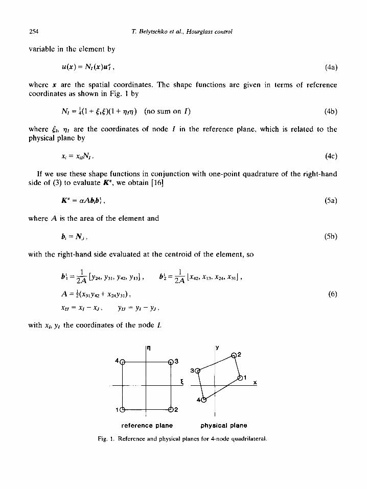
where x are the spatial coordinates. The shape functions are given in terms of reference coordinates as shown in Fig. 1 by
NI = $(l + tlt)(l + ~77) (no sum on I) (4b)
where &, rlr are the coordinates of node I in the reference plane, which is related to the physical plane by
Xi = Xi,NI . (4c)
If we use these shape functions in conjunction with one-point quadrature of the right-hand side of (3) to evaluate K”, we obtain [16]
where A is the area of the element and
with the right-hand side evaluated at the centroid of the element, so
b: = & [)&I, y31, y42, )‘,,I ,
1 b: = 2A [x42, x13, x24, x31] ,
A = i(x3ly42 + %4y31),
XIJ = XI - XJ , YIJ = y, - YJ ,
with x1, yI the coordinates of the node I.
rl Y 2
4c a3
3
F. 1 lj-: X
4
18-_-------+I2
(6)
reference plane physical plane
Fig. 1. Reference and physical planes for 4-node quadrilateral.
T. Belytschko et al., Hourglass control 255
Note that the matrix B, given by
is the discrete counterpart of the gradient operator, for the gradient in the finite element approximation is given by
g = ;I; = Bu" . i I We also define the flux matrix
(W
(7c)
so the counterpart of (2~) for isotropic materials is
q = -aIg. (74
The following additional column vectors are useful:
s’= [l, l,l, l] )
h’ = [l, -1, 1, -11 )
x: = x’ = [Xl, x2, x3, &I ,
x: = Y’ = [Yl, Y2, Y3, Y41 ,
where x and y are the nodal coordinates. It can be easily verified from (6) and (8) that
b:xj = 8,) (9)
where Sij is the Kronecker delta.
REMARK 2.1. Equation (9) is an important necessary requirement for the rows of the gradient matrix B. It is the counterpart of the consistency conditions in finite difference equations; the gradient of a linear field is evaluated properly only if it is satisfied.
Additional conditions which can easily be verified from (6) and (8) are
b:s = 0,
b:h = 0,
s’h = 0 .

256 T. Belytschko et al., Hourglass control
Fig. 2. Basis vectors for the 4-node quadrilateral.
For any nondegenerate quadrilateral, bi, s and h are linearly independent and span the four-dimensional vector space R4. The basis vectors are shown in Fig. 2.
2.2. Hourglass modes and control in two dimensions
The orthogonality properties, (lo), allow us to quickly examine the pathology which results from one-point quadrature. If we let the nodal values of U’ for an element be given by s, then
g=Bu’=Bs=O, (11)
where the last step in the above follows from (5a) and (lOa). This result is expected and in fact necessary since it indicates that for a constant field u, the gradient vanishes. The one- dimensional space spanned by the vector s will be called the proper null-space of B.
If we let ZC = h, (5a) and (lob) again show that g = 0. This result is quite expected since the field associated with these nodal values is obviously not constant. The contradictory nature of this result can be appreciated further by noting that for a square element, with all nodes at +l

T. Belytschko et al., Hourglass control 257
and - 1, ~8 = h corresponds to u(x, y) = xy, yet (7) and (lob) show that the discrete gradient of this field vanishes. The one-dimensional space spanned by h will be called the improper null-space of B. The mode h and the three other base vectors are shown in Fig. 2.
In the finite element literature of solid mechanics, modes such as h are called spurious singular modes, or zero-energy modes. The latter term reflects the fact that these modes, while not rigid body modes, are not accompanied by any work on the element.
Mathematically, the above shows that the null-space, or kernel, of the discrete gradient operator B does not coincide with the kernel of the continuous gradient. Since the dimension of K is 4 and the kernel of the discrete and continuous gradient operators will coincide only if B (and ire) are matrices of rank 3.
This suggests that the pathology of this element may be eliminated by defining
s” = yw, (12)
so that the B matrix becomes
B* = {h, bzr rl’ (13)
with y chosen so that the rank of B* is 3. The discrete gradient operator of (7a) performs properly on linear fields, which can be seen
by letting zC = x or ZC = y and using (9). To maintain this desirable property, y should not have any effect on linear fields. Therefore y will be chosen so that:
(i) for any nodal values associated with linear fields, g = 0; this assures the formal consistency of the resulting discrete equations with the differential equation;
(ii) if ue is in the improper null-space, $j f 0, or in other words, y must span the complement of the proper null-space so that the rank of I(’ is 3.
To obtain y, we expand it in terms of the base vectors of R4 as follows:
y = albl + uzb2 + u3s + a,h .
For an arbitrary linear field, the nodal values are given by
ue = CIX + czy + c3s.
Substituting (14) and (15) into (12) and using (9) and (lo), yields
cl(al + a& + a.&‘~) + ~(a;? + a&y + a&‘y) + ~(4~3) = 0 .
Since the above must vanish for arbitrary ci, it follows that
a3=0, a, = -abh’x, u2 = -a,h’y .
(14)
(15)
(16)
(17)
(18)
Using the above in (14) gives
y = aa[h - @‘x)b, - (h’y)bz] ,
258 T. Belytschko et al., Hourglass control
where a4 is an arbitrary constant. Let a4 = l/A, which gives
y = + [h - (h’x)b, - (h’y)b,] * (1%
This y differs in magnitude from that given in [l l] but is otherwise identical. The choice of a4 is of course completely arbitrary.
The generalized gradient jj is associated with a generalized flux 4; the two are related by
where the factor E remains to be determined. The nodal fluxes are then given (note that the sign of the internal sources differs from f in (3) because it is an internal nodal flux) by
= -A(biqi + rtj) 3
Using (71, (13) and (20) and (21), yields the following form for the element matrix:
K” = aAbibj + &Ayy’ 3
(21)
(22)
so that when & = E”a, (22) becomes
K” = aA(bib: + Eyy’). (234
The parameter E is normalized [16] so that E = 1 gives the exact conductance matrix for a rectangular element
The above form was motivated by the decision to make the amplitude of the second term in (23a) proportional to the maximum eigenvalue of the element. An alternative normalization is proposed in Section 2.3.
REMARK 2.2. The second term in (23a) has been calied the stabilization matrix in ft7-181 because it eliminates the rank deficiency of K” as evaluated by one point quadrature.
REMARK 2.3. When E = 0, K” is of rank 2 because it can easily be shown by using (10) and (22) that K”h = K”s = 0.
REPARK 2.4, When E >O, the element matrix is of rank 3.
2.3. Identification of hourglass control parameter
An important question in the application of the hourglass control procedure is the selection
T. Belytschko et al., Hourglass control 259
of the parameter 6 which relates the generalized gradient and flux, g and 4. For this purpose, a Hu-Washizu type variational principle is used. This approach is motivated by the equivalence principles [19-201 which show that for any element obtained by reduced in- tegration of a single field variational principle, an equivalent element can be constructed from a mixed variational principle. Wempner [21] has previously constructed rectangular elements by this approach.
We consider an anisotropic nonlinear constitutive law
qi = -CXijgj 3 (Yij = (Yij(U) ,
and it is assumed that (Y is constant in each element. The weak form associated with the mixed variational principle takes the form
I n [Ggi(ffijgj
The Euler-Lagrange ditions (2e); u must written in the form
(25)
equations for (25) are (2a), (2b) and (24) with natural boundary con- be C’, while qi and gi must be C-l. The C? interpolant for u can be
(264
WW
This form is complete and satisfies the continuity requirements. The nodal values of u are then given by
ue = u()s + UlX + ufl + a& . (27)
Premultiplying (27) by b: and using (9) and (10) gives
Similarly,
Ui = b:Ue.
premultiplying (27) by h’ and using (28a) gives
~3 = a [hfue - (h’xi)b:u”] = ytue.
(284
(2fW
REMARK 2.5. The function R([, 71) has the following property:
j- A
R.,dA = 1 R,,dA = 0. (29) A
The following approximations are used for g and q:
(30)
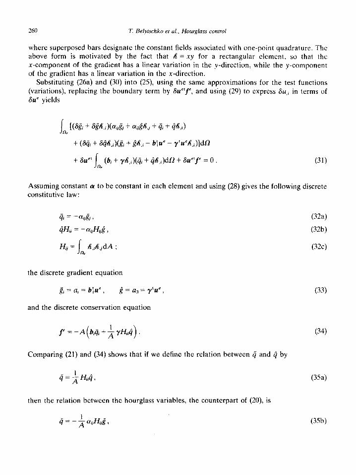
260 T. Belytsc~k~ et al., Hourglass control
where superposed bars designate the constant fields associated with one-point quadrature. The above form is motivated by the fact that R = xy for a rectangular element, so that the x-component of the gradient has a linear variation in the y-direction, while the y-component of the gradient has a linear variation in the x-direction.
Substituting (26a) and (30) into (25) using the same approximations for the test functions (variations), replacing the boundary term by Wtfe, and using (29) to express Su,i in terms of Su’ yields
Assuming constant constitutive law:
(Y to be constant in each element and using (28) gives the following discrete
(32a)
(32b)
> (32~)
the discrete gradient equation
& r= ai = Q’, g = a3 = yw )
and the discrete conservation equation
f’ = -A(biqi + a rH&) a
Comparing (21) and (34) shows that if we define the relation between + and kj by
ij = f Hjiij ,
then the relation between the hourglass variables, the counterpart of (20) is
(33)
(34)
(354
Wb)
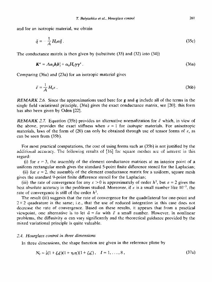
T. Belytschko et al., Hourglass contrd 261
and for an isotropic material, we obtain
(35c)
The conductance matrix is then given by (substitute (33) and (32) into (34))
Comparing (36a) and (23a) for an isotropic material gives
E = ’ Hiie . A (36b)
~~~A~~ 2.6. Since the approximations used here for g and q include all of the terms in the single field variational principle, (36a) gives the exact conductance matrix, see 1201; this form has also been given by Oden [22].
REMARK 2.7. Equation (35b) provides an alternative normalization for r’ which, in view of the above, provides the exact stiffness when f: = 1 for isotropic materials. For anisotropic materials, laws of the form of (20) can only be obtained through use of tensor forms of F, as can be seen from (35b).
For most practical computations, the cost of using forms such as (35b) is not justified by the additional accuracy. The following results of [16] for square meshes are of interest in this regard:
(i) for E = 3, the assembly of the element conductance matrices at an interior point of a uniform rectangular mesh gives the standard S-point finite difference stencil for the Laplacian;
(ii) for 1 = 2, the assembly of the element conductance matrix for a uniform, square mesh gives the standard 9-point finite difference stencil for the Laplacian;
(iii) the rate of convergence for any E >O is approximately of order h2, but F = 2 gives the best absolute accuracy in the problems studied. Moreover, if E is a small number like lo-*, the rate of convergence is still of the order h*.
The result (iii) suggests that the rate of convergence for the quadrilateral for one-point and 2 x 2 quadrature is the same; i.e., that the use of reduced integration in this case does not decrease the rate of convergence. Based on these results, it appears that from a practical viewpoint, one alternative is to let & = r”a with E” a small number. However, in nonlinear problems, the diffusivity cy can vary significantly and the theoretical guidance provided by the mixed variational principle is quite valuable.
2.4. Hourglass control in three dimensions
In three dimensions, the shape function are given in the reference plane by
(374
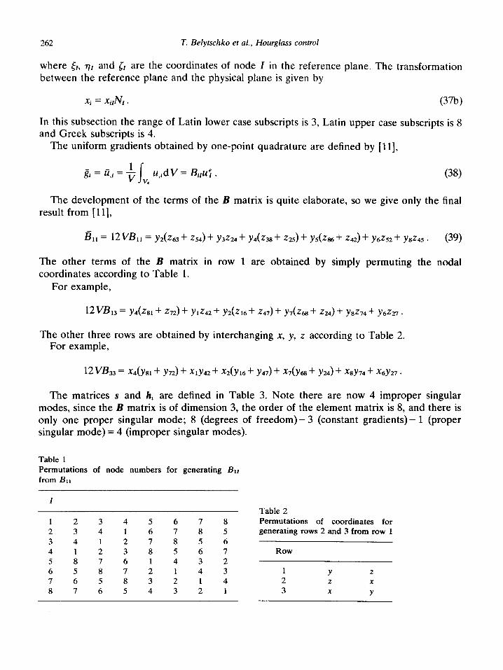
262 T. Belytschko et al., Hourglass control
where &, nr and 5, are the coordinates of node I in the reference plane. The transformation between the reference plane and the physical plane is given by
Xi = Xi,Nr . WV
In this subsection the range of Latin lower case subscripts is 3, Latin upper case subscripts is 8 and Greek subscripts is 4.
The uniform gradients obtained by one-point quadrature are defined by [ll],
u,id V = Bi,u; .
The development of the terms of the B matrix is quite elaborate, so we give only the final result from [ll],
& = 12 V&I = y2(263 + 254) + ysG4 + y4(23s + 225) + y&6 + 242) + y6252 + y8245 . (39)
The other terms of the B matrix in row 1 are obtained by simply permuting the nodal coordinates according to Table 1.
For example,
12 V&3 = y4(%1 + 272) + ylz42 + y2(z16 + 247) + y7(%8 + 224) + ySz74 + y6z27 .
The other three rows are obtained by interchanging X, y, z according to Table 2. For example,
12vB33 = x4(yt31+ y72) + xly42 + x2(y16 + y47) + x7&8 + b) + x8Y74 + x6Y27 *
The matrices s and hi are defined in Table 3. Note there are now 4 improper singular modes, since the B matrix is of dimension 3, the order of the element matrix is 8, and there is only one proper singular mode; 8 (degrees of freedom) - 3 (constant gradients) - 1 (proper singular mode) = 4 (improper singular modes).
Table 1 Permutations of node numbers for generating BII from BII
I
1 2 3 4 5 6 7 8 2 3 4 1 6 7 8 5 3 4 1 2 7 8 5 6 4 1 2 3 8 5 6 7 5 8 7 6 1 4 3 2 6 5 8 7 2 1 4 3 7 6 5 8 3 2 1 4 8 7 6 5 4 3 2 1
Table 2 Permutations of coordinates for generating rows 2 and 3 from row 1
Row
1 Y L 2 z X
3 X Y

T. Belytschko et al., Hourglass control 263
Table 3 The ki and s vectors for the hexahedron
Vector I 1 2 3 4 5 6 7 8
SI +1 +1 +1 +1 +1 +1 +1 +1 h 1, +1 +1 -1 -1 -1 -1 +1 +1 h 2, +1 -1 -1 +1 -1 +1 +1 -1 h 31 +1 -1 +1 -1 +1 -1 +1 -1 hu -1 +1 -1 +1 +1 -1 +1 -1
The volume is given by
u = $ i Bi,Xi, (no sum on i) (40) I=1
where B is defined in (39) and the sum is explicitly indicated since the repeated subscript i is not summed.
The rows of the B matrix are defined to be the vectors bi, so
b: B= b: . I I b;
It can be shown (albeit with considerable algebra) that
b:Xj = Sij 3
b:s = 0,
s’h, = 0 )
W-4
W-4
(4lc)
where Xj are the vectors of nodal coordinates analogous to (SC) and (8d). If the gradient and flux matrices are defined by
then g = Bu' .
(42)
(4%
The following results follow from (40)-(43): (i) the gradient of a linear field u = cj.Xj + co is given by cj, so the B matrix satisfies the
consistency requirement; (ii) if ue = s, g = 0 and s is defined to be the proper null-space of B. It can be shown that if uc = h, for (Y = 1 to 3, g = 0, but not for (Y = 4. However, the
dimension of the improper null space is 4. Fortunately, in the control procedure, it is not
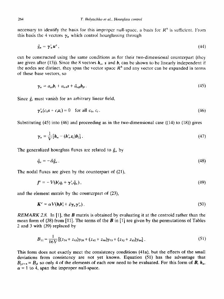
264 T. Belytschko et al., Hourglass control
necessary to identify the basis for this improper null-space. a basis for RX is sufficient. From this basis the 4 vectors ‘yO which control hourglassing through
sa = YLU’, (44)
can be constructed using the same conditions as for their two-dimensional counterpart (they are given after (13)). Since the 8 vectors h,, s and bi can be shown to be linearly independent if the nodes are distinct, they span the vector space R8 and any vector can be expanded in terms of these base vectors, so
ya = auibi + U,~S + Sash, . (45)
Since ji must vanish for an arbitrary linear field,
yb,(CoS + C&i) = 0 for all Co, Ci . (46)
Substituting (45) into (46) and proceeding as in the two-dimensional case ((14) to (18)) gives
ye = $ [ha - (h',xj)hj] . (47)
The generalized hourglass fluxes are related to & by
(48)
The nodal fluxes are given by the counterpart of (21)
f’ = - V(b:qi+ YLda), (49)
and the element matrix by the counterpart of (23),
K’ = CVV(bib: + Eyayh). (W
REMARK 2.8. In [l], the B matrix is obtained by evaluating it at the centroid rather than the mean form of (38) from [ll]. The terms of the B in [l] are given by the permutations of Tables 2 and 3 with (39) replaced by
Bll = j&7 [(%4 + %3)y28 + (242 + 28&53 + (z52 + z83)y64] . (51)
This form does not exactly meet the consistency conditions (41a), but the effects of the small deviations from consistency are not yet known. Equation (51) has the advantage that
Bj,r+4 = Bjl so only 4 of the elements of each row need to be evaluated. For this form of B, h,, a = 1 to 4, span the improper null-space.
T. Belytschko et al., Hourglass control
2.5. Hourglass control and the patch test
265
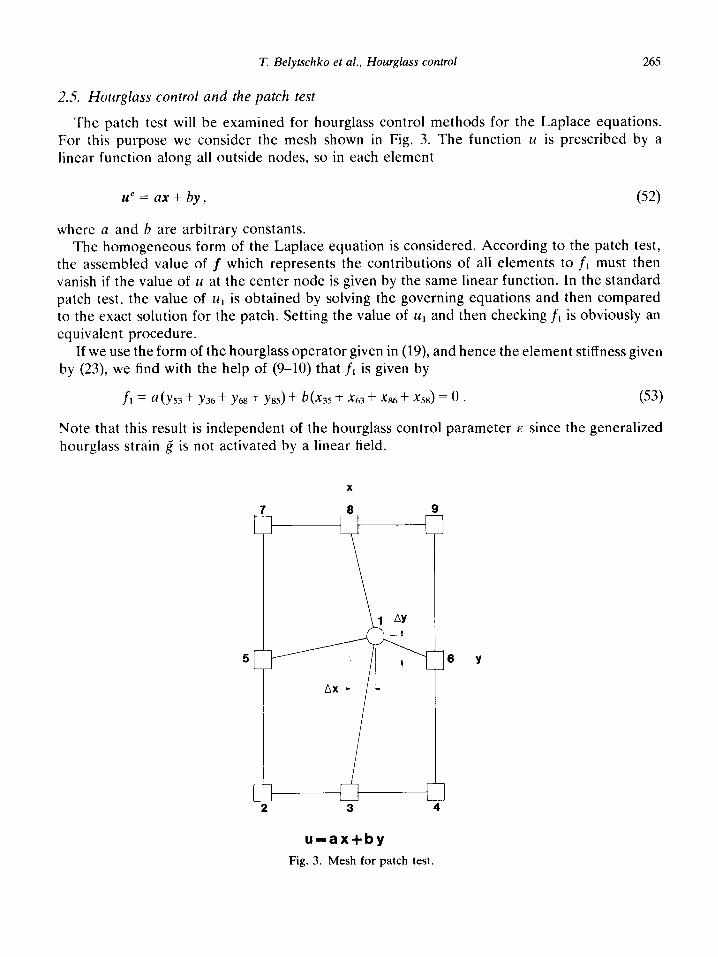
The patch test will be examined for hourglass control methods for the Laplace equations. For this purpose we consider the mesh shown in Fig. 3. The function u is prescribed by a linear function along all outside nodes, so in each element
&=ax+by,
where a and b are arbitrary constants.
(52)
The homogeneous form of the Laplace equation is considered. According to the patch test, the assembled value of f which represents the contributions of all elements to fl must then vanish if the value of u at the center node is given by the same linear function. In the standard patch test, the value of U, is obtained by solving the governing equations and then compared to the exact solution for the patch. Setting the value of uI and then checking f, is obviously an equivalent procedure.
If we use the form of the hourglass operator given in (19) and hence the element stiffness given by (23) we find with the help of (9-10) that fr is given by
fl=a(~53+y36+~68+~s5)+b(~35+x63+~86+x58)=0. (53)
Note that this result is independent of the hourglass control parameter I since the generalized hourglass strain 2 is not activated by a linear field.
u-ax+by Fig. 3. Mesh for patch test.
266 T. Belytschko et al., Hourglass control
In the hourglass control of [l],
SO y=h,
K’ = aA(bib: + Ehh’) e
Repeating the same procedure, we find f, contains the same term as (52) plus an additional term which does not vanish and is given by
fl= 4.s(a Ax + b Ay), m
where, as can be seen from Fig. 3, Ax and Ay are the displacement of the node 1 from the center of the domain. Thus, for rectangular elements, where Ax = by # 0, this hourglass procedure meets the patch test, but for irregularly shaped elements, it fails the patch test.
This result is not surprising once the characteristics which are required for an hourglass control to satisfy the patch test are examined. Since the one-point quadrature of the element stiffness gives a matrix which satisfies the patch test, the stabilization matrix and hence the hourglass projection operator should not be affected by linear fields, i.e., all linear (and constant) fields must be in the kernel of y. These conditions then make the form of y which meets the patch test uniquely that given by (19), and any other form will not meet the patch test. This applies to the hourglass operators of [I, 6,8].
3. Solid mechanics
3.1. Hourglass control for continuum element in two dimensions
In solid mechanics, the components of the displacement field are approximated in a finite element analogously to (4) by
Ui (X) = N, (X)Ui, . (56)
The deformation of the material is characterized by velocity strains
iij = $(Ui,j + Z&i) 3 (57)
where superposed dots designate time derivatives. The discrete operator B for a quadrilateral with one-point quadrature is given by
(58)
(59) so
i=BB’,
T. Belytschko et al., Hourglass control
where Et = [G, &y, 2&X,] 9
267
Using the orthogonality properties of (lo), it follows immediately consists of the following vectors
Y h 0 --x 0 1 h ’
where each column of the above constitutes a separate vector & so that B& vanishes. The first two vectors are obviously rigid body translations and the third is a rigid body
(60)
that the null space of B
(62)
rotation. The fourth and fifth are spurious singular modes associated with displacement fields for which the strains should not vanish. Hence we define the space spanned by the first three vectors of (62) to be the proper null-space of B; the remaining two columns constitute the improper null-space, which is of dimension 2.
Therefore, to control the hourglass modes, we introduce 2 additional generalized strains, qi, which when combined with B, span the complement of the proper null-space. The resulting matrix and formula for generalized strains is given by
b: 0 0 b:
B* = b: b: ,
I I
(634 Yt 0 0 Yt
di = y’& ; (63’4
and using the same arguments as those in the previous section that led to (14~(18) it follows that y for the solid mechanics problem is also given by (19). Although the character of the null-space (kernel) of the operator B is now somewhat different, the requirements that the additional strains do not affect linear fields automatically leads to a form in which rigid body rotations are included in the kernel. It can be shown that the rows of BY are linearly independent for a nondegenerate geometry, so B* is of rank 5 and spans the complement of the proper null-space.
The Cauchy stresses are denoted by u and are arranged in a column matrix
ut = [a,, a,, &J 7 (64)
and the generalized hourglass stresses are denoted by 0,. The internal nodal forces are given
bY
= A(bjaij + Y’Qi). (65)

268 T. Belytsc~ko et al., Hour~iass control
For a hypoelastic material, the stress-strain law can be written as
where the triangle denotes a frame-invariant rate. It is also necessary to develop a constitutive law for the generalized hourglass stresses and strains
The frame-invariant rates for Q can be deduced from (63, which shows that it behaves like a vector. Hence,
where QP = Qi - WijQj , W9
Wij = $( Z&j - lij,;l) . (69)
In two dimensions, (68) becomes
Q:= 6x- W,Q,, Q;= C&f WuQx.
REMARK 3.1. Equation (67) is given in rate form because arbitrary linear velocity fields, so no hourglass resistance is
(70)
in rate form 4; vanishes for developed regardless of the
magnitude of the rigid body motion and this procedure is applicable to ge~~etricuzfy nonlinear ~ra~~e~s. If (67) is not in rate form, it is not applicable to large displacement problems because qi does not vanish for large rigid body rotations.
3.2. Generalized hourglass stress-strain law
In this section, some mechanical insight into the appropriate values of the material parameters for the hourglass generalized stresses and strains is provided by using the Hu-Washizu principle as in Section 2.3. The weak form associated with the Hu-Washizu principle is
I [&C(C - aV) + &‘(E - Vu) + SVu’a]dfi - Su:f, = 0, n
where
(714
(7Ic)
T. Belytschko et al., Hourglass control 269
In the continuum element, in contrast to the Laplace element, several alternatives are available in choosing the stress and strain fields. We choose the following:
(72)
where 4 is given in (26b) and satisfies (29). Alternatively, the generalized hourglass stresses and strains could have been added to the shear terms. Applying (71a) to the above fields yields
(73)
and (66) for the uniform strain and stress components, and (63) and (65); Hij is given by (32~).
3.3. Hourglass control in three di~ensiuns
In three dimensions, the velocity
l2i.j = Bj,liil f
gradient is given by
(74)
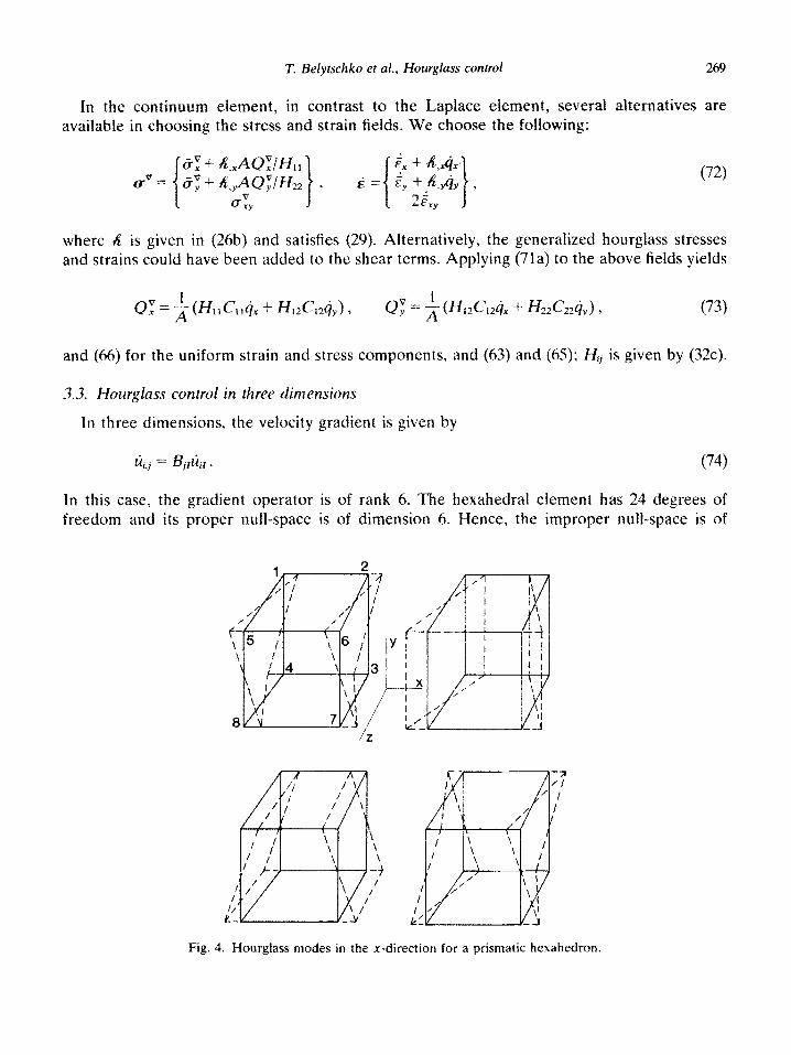
In this case, the gradient operator is of rank 6. The hexahedral element has 24 degrees of freedom and its proper null-space is of dimension 6. Hence, the improper null-space is of
Fig. 4. Hourglass modes in the x-direction for a prismatic hexahedron.
270 T. Belytschko et al., Hourglass control
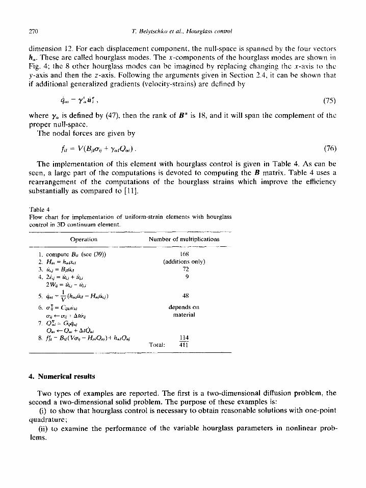
dimension 12. For each displacement component, the null-space is spanned by the four vectors h,. These are called hourglass modes. The x-components of the hourglass modes are shown in Fig. 4; the 8 other hourglass modes can be imagined by replacing changing the x-axis to the y-axis and then the z-axis. Following the arguments given in Section 2.4, it can be shown that if additional generalized gradients (velocity-strains) are defined by
Cjai = y’,ZiF 7 (75)
where ye is defined by (47) then the rank of B” is 18, and it will span the complement of the proper null-space.
The nodal forces are given by
.L = v(BjPij + IyaA?*i) - (76)
The implementation of this element with hourglass control is given in Table 4. As can be seen, a large part of the computations is devoted to computing the B matrix. Table 4 uses a rearrangement of the computations of the hourglass strains which improve the efficiency substantially as compared to [II].
Table 4 Flow chart for implementation of uniform-strain elements with hourglass control in 3D continuum element.
Operation Number of multiplications
1. 2. 3. 4.
5.
6.
7.
8.
compute Bu (see (3%) J%i = h,rxir tit,j = B,,tiir 26jj = lii,j + tij,i 2 Wij = Z&j - tij.i
& = $ (h,& - Hmj&.j)
Uz = Cij&& ci, + mij + A t&j QE, = Gij& Q,i + Q,i + A t&i ff; = Bu( VCr, - &Qaj) + h*Duj
16X (additions only)
72 9
48
depends on material
114 Total: E-l
4. Numerical results
Two types of examples are reported. The first is a two-dimensional diffusion problem, the second a two-dimensional solid problem. The purpose of these examples is:
(i) to show that hourglass control is necessary to obtain reasonable solutions with one-point quadrature;
(ii) to examine the performance of the variable hourglass parameters in nonlinear prob- lems.

T. Belytschko et al., Hourglass control 271
EXAMPLE 4.1. The domain is circular. Four-fold symmetry was used, with the mesh shown in Fig. 5. The parameters are: radius = 5.0; (Y = 0.04, u(x, 0) = 0.1. The outer boundary is
insulated. A point source with the time history shown in Fig. 5 is applied at the center node. The solution was obtained by explicit time integration. Fig. 6 shows a plot of the results with
I = 0, which corresponds to one-point quadrature with no stabilization. As can be seen, the result exhibits severe oscillations due to the rank-deficiency of the element.
The solution was then obtained for a nonlinear problem where
c+) = cXo(1+ o.01u’~4) ) (Yg = 0.04.
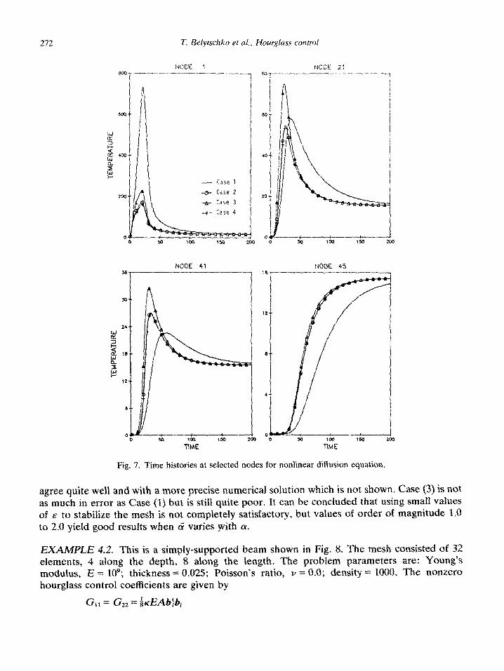
Four cases were considered:
(1) a;; = &CY(), & = 1.0, (2) & = Fff, & = 1.0, (3) & = ECI, & = 0.1, (4) & = &(Y, & = 2.0,
where E’ is given in terms of E by (23b). Selected results are shown in Fig. 7. As can be seen,
Case (I), which fails to account for the change in (Y, is substantially in error. Cases (2) and (4)
Fig. 5. Mesh and time history of heat source s(t) for Example 4.1.
x x
Fig. 6. Solution for Example 4.1 using one-point quadrature without stabilization.
272
NODE 41
NODE 21 ~_~---_----------_ T
-___--_
12
a
+
0 0
Fig. 7. Time histories at selected nodes for nonlinear diffusion equation.
agree quite well and with a more precise numerical solution which is not shown. Case (3) is not as much in error as Case (I) but is still quite poor. It can be concIuded that using small values of E to stabilize the mesh is not completely satisfactory, but values of order of magnitude 1.0 to 2.0 yield good results when ru” varies )yith L~I.
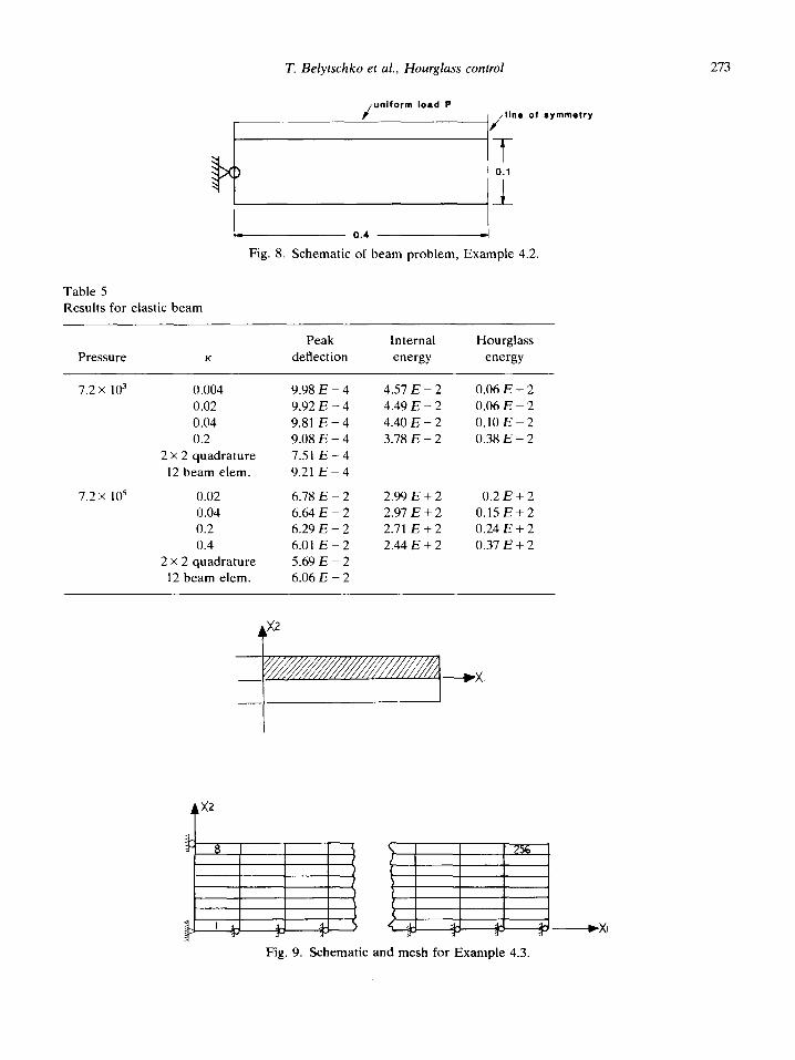
EXAMPLE 4.2. This is a simply-supported beam shown in Fig. 8. The mesh consisted of 32 elements, 4 along the depth, 8 along the length. The problem parameters are: Young’s modulus, E = 109; thickness = 0.025; Poisson’s ratio, v = 0.0; density = 1000. The nonzero hourglass control coefficients are given by
T. Belytschko et al., Hourglass control 273
/ uniform load P
line of symmetry
0.4 -1
Fig. 8. Schematic of beam problem, Example 4.2
Table 5 Results for elastic beam
Pressure K
Peak deflection
Internal
energy
Hourglass energy
7.2 x 10³ 0.004
0.02
0.04
0.2 2 x 2 quadrature
12 beam elem.
7.2 x 10’ 0.02 0.04 0.2 0.4
2 x 2 quadrature 12 beam elem.
9.98 E - 4 4.57 E - 2 9.92 E - 4 4.49 E - 2 9.81 E - 4 4.40 E - 2 9.08 E - 4 3.78 E - 2 7.51 E - 4 9.21 E - 4
6.78 E - 2 2.99 E + 2 6.64E-2 2.97 E f 2 6.29 E - 2 2.71 E + 2 6.01 E - 2 2.44E+2 5.69 E - 2 6.06 E - 2
0.06 E - 2 0.06 E - 2
0.10 E - 2
0.38 E - 2
0.2 E + 2 O.l5E+2 0.24 E + 2 0.37 E + 2
Fig. 9. Schematic and mesh for Example 4.3.

274 T. Beiytschku et al., Hourglass control
2700
K--.
m _J - c7 2250
L
0
4 1800
0 900 L
1.800 2 700 3 coo-
cl (IKCH) (xl o-‘>
LEGEhD _~
frf- SELECT RED
+F E=l 0
-A- E==O.l
t- E-O 01
-X+ BEAM EC!:.
4 500 5 400
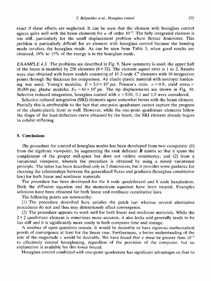
Fig. IO. Tip displacements for Example 4.3 for various values of E, selective reduced integration element and beam element.
{K is ~quivaI~nt to that in [ll] for Y = 0). A uniform pressure which is a step function in time was applied over the span of the beam.
Results are given in Table 5 for a small and a large load, which result in geometrically linear and nonlinear response, respectively. Results for each load are also given for a fully integrated (2 X 2 quadrature) element and a string of cubic beam elements; the latter may be considered
T. Belytschko et al., Hourglass control 275
exact if shear effects are neglected. It can be seen that the element with hourglass control agrees quite well with the beam elements for K of order 10m2. The fully integrated element is too stiff, particularly for the small displacement problem where flexure dominates. This problem is particularly difficult for an element with hourglass control because the bending mode involves the hourglass mode. As can be seen from Table 5, when good results are obtained, 10% to 15% of the energy is in the hourglass mode.
~XA~~~~ 4.3. The problems are described in Fig. 9. Skew symmetry is used; the upper half of the beam is modeled by 256 elements (8 x 32). The element aspect ratio is 1 to 2. Results were also obtained with beam models consisting of 10 2-node C’ elements with 10 integration points through the thickness for comparison. An elastic-plastic material with isotropic harden- ing was used: Young’s modulus, iE = 3.0 x lo7 psi; Poisson’s ratio, v = 0.0; yield stress = 30,000 psi; plastic modulus ET = 65 x lo5 psi. The tip displacements are shown in Fig. 10. Selective reduced integration, hourglass control with E: = 0.01, 0.1 and 1.0 were considered.
Selective reduced integration (SRI) elements agree somewhat better with the beam element. Partially this is attributable to the fact that one-point quadrature cannot capture the progress of the elastic-plastic front as well. However, while the one-point quadrature elements follow the shape of the load-deflection curve obtained by the beam, the SRI element already begins to exhibit stiffening.
5. Conclusions
The procedure for control of hourglass modes has been developed from two viewpoints: (1) from the algebraic viewpoint, by augmenting the rank deficient B matrix so that it spans the complement of the proper null-space but does not violate consistency; and (2) from a variational viewpoint, wherein the procedure is obtained by using a mixed variational principle. The latter has been described only in 2 dimensions, but it provides some guidance for choosing the relationships between the generalized fluxes and gradients (hourglass constitutive law) for both linear and nonlinear materials.
The procedure has been developed for the 4 node quadrilateral and 8 node hexahedron. Both the diffusion equation and the momentum equation have been treated. Examples solutions have been obtained for both linear and nonlinear constitutive laws.
The following points are noteworthy: (1) The procedure described here satisfies the patch test whereas several alternative
procedures do not and thus may deleteriously affect convergence. (2) The procedure appears to work well for both linear and nonlinear materials. While the
2 x 2 quadrature element is sometimes more accurate, it also locks and generally tends to be too stiff and it is significantly more costly in both computer time and storage.
A number of open questions remain. It would be desirable to have rigorous mathematical proofs of convergence at least for the linear case. Furthermore, a better understanding of the role of the magnitude E would be desirable. We have found that E must be greater than 10e2 to effectively control hourglassing, regardless of the precision of the computer, but no explanation is available for this lower bound.
Hourglass control combined with one-point quadrature has significant advantages so that its
276 T. Belytschko et al., Hourglass control
use in computer codes for large scale calculations is irresistable [l-3]. The procedures described
satisfy consistency and so apparently maintain the rate of convergence of the fully integrated element. These attributes provide an important justi~cation, in addition to the usually cited advantages in efficiency, for their use.
References
[l] G.L. Goudreau and J.O. Hallquist, Recent developments in large scale finite eIements ~grangian hydroc~e technology, Rept. UCRL-86460, Lawrence Livermore Laboratory, 1981, Nos. 1-3, 1982, Vol. 33.
[2] T. Belytschko and R.R. Robinson, SAMSON2: A nonlinear two-dimensional structure/media interaction computer code, Rept. AFWL-TR-81-109, Kirtland AFB, NM, 1981.
[3] R.F. Kulak, A finite element formulation for fluid-structure interaction in three-dimensional space, J. Pressure Vessel Tech. 103 (1981) 183-190.
141 M.L. Wilkins, R.E. Blum, E. Cronshagen and P. Grantham, A method for computer simulation of problems in solids mechanics and gas dynamics in three dimensions and time, Rept. UCRL-51574, Revision 1, Lawrence Livermore Laboratory, 1975.
[5] T. Belytschko, J.M. Kennedy and D.F. Schoeberle, On finite element and difference formulations of fluid structure problems, Proc. Conf. Computer Methods in Nuclear Engineering, Charleston, SC, 4 (1975) 39-51.
[b] G. Maenchen and S. Sack, The TENSOR code, in: B. Alder et al., eds., Methods in Computational Physics, Vol. 3 (Academic Press, New York, 1964) 181-210.
[7] B. Irons and S. Ahmad, Techniques of Finite Elements (Ellis Horwood, Chichester, 1980). [8] T. Belytschko and J.M. Kennedy, Computer models for subassembly simulation, Nuclear Engrg. Design
49 (1978) 17-38.
[9] S.W. Key, A finite element procedure for the large deformation dynamics response of axisymmetric solids, Comput. Meths. Appl. Mech. Engrg. 4 (1974) 195-218.
[lo] D. Kosloff and G.A. Frazier, Treatment of hourglass patterns in low order finite element codes, Internat. J. Numer. Anal. Meths. Geomech. 2 (1978) 57-72.
[ 1 t] D.P. Flanagan and T. Belytschko, A uniform strain hexahedron and quadrilateral with orthogonal hourglass control, Internat. J. Numer. Meths. Engrg. 17 (1981) 679-706.
[ 121 T. Belytschko, Correction of article by D.P. Flanagan and T. Belytschko, Internat. J. Numer. Meths. Engrg. 19 (1983) 467-468.
[13] G. Strang, Variational crimes in the finite element method, Internat. J. Numer. Meths. Engrg. 19 (1983) 689-710.
1141 O.C. Zienkiewicz, The Finite Element Method (McGraw-Hill, New York, 3rd ed., 1977). [t5] E.B. Becker, G.F. Carey and J.T. Oden, Finite Elements, An Introduction (Prentice-Hall, Englewood Cliffs,
NJ, 1981).
[ 161 W.K. Liu and T. Belytschko, Efficient linear and nonlinear heat conduction with a quadrilateral element, to be published in Internat. J. Numer. Meths. Engrg.
[ 171 T. Belytschko, C.S. Tsay and W.K. Liu, A stabilization matrix for the bilinear Mindlin plate element, Comput. Meths. Appl. Mech. Engrg. 29 (1981) 313-327.
[i8] T. Belytschko and C.S. Tsay, A stabilization procedure for the quadrilateral plate element with one-point quadrature, Internat. J. Numer. Meths. Engrg. 19 (1983) 405-419.
[ 191 D.S. Malkus and T.J.R. Hughes, Mixed finite element methods-reduced and selective integration techniques: a unification of concepts, Comput. Meths. Appl. Mech. Engrg. 15 (1978) 63-82.
[20] J.T. Oden and J.N. Reddy, Some observations on properties of mixed finite element approximations, Internat. J. Numer. Meths. Engrg. 3 (1973) 2.X-272.
[21f G. Wempner, D. Talaslides and C.M. Hwang, A simple and efficient approximation of shells via finite quadrilateral elements, J. Appl. Mech. 49 (1982) 115-120.
[22] J.T. Oden, Stability and convergence of underintegrated finite element approximations, Proc. Workshop on Nonlinear Structural Analysis, NASA Lewis Research Center, 1983.
Copyright © 2022 FDOKUMEN


![[Is Seasonal Adjustment a Linear or Nonlinear Data-Filtering Process?]: Comment](https://static.fdokumen.com/doc/165x107/6325a53b85efe380f306cf62/is-seasonal-adjustment-a-linear-or-nonlinear-data-filtering-process-comment.jpg)