On the application of preconditioning operatorsfor nonlinear elliptic problems

by O. Axelsson1, I. Farago2, J. Karatson3

Abstract

This paper first gives a brief summary of the framework of preconditioningoperators for discretized nonlinear elliptic problems, which means that the pro-posed preconditioning matrices are the discretizations of suitable linear ellipticoperators. Then a typical application of the preconditioning operator idea ispresented using a diagonal coefficient operator, which is a generalization of anearlier paper by the authors. The obtained estimates of the resulting conditionnumbers are mesh independent, which is important feature of the preconditioningoperator approach.

1 Introduction

In this paper we study the preconditioned iterative solution of nonlinear elliptic prob-lems

− div f(x,∇u) = g(x) in Ω

u|∂Ω = 0(1)

on a bounded domain Ω ⊂ RN with suitable ellipticity conditions. Such problemsarise in many applications in physics and other fields, for instance in elasto-plasticity,magnetic potential equations and subsonic flow problems [7, 15, 16]. In these problemsthe nonlinearity f often has the form

f(x, η) = a(|η|)η (2)

with some positive real C1 function, i.e. the corresponding operator is

T (u) = − div (a(|∇u|)∇u) .

The most frequently used numerical methods for nonlinear elliptic problems relyon some discretized form of the problem, whose solution is obtained by an iterativemethod. As for linear problems, preconditioning is a crucial element of the constructionof the iterative method. The choice of preconditioners is often supported by Hilbertspace background, which helps both the construction of methods and the study ofconvergence. Important examples of this are the equivalent operator approach [9] forlinear equations and the Sobolev gradient technique [17, 18] for nonlinear problems.

1Department of Mathematics, University of Nijmegen, 6525ED Nijmegen, The Netherlands;axelsson@sci.kun.nl

2Department of Applied Analysis, ELTE University, H-1518 Pf. 120, Budapest, Hungary;faragois@cs.elte.hu, supported by the Hungarian Research Fund OTKA under grant no. T031807;

3Department of Applied Analysis, ELTE University, H-1518 Pf. 120, Budapest, Hungary;karatson@cs.elte.hu, supported by the Hungarian Research Fund OTKA under grant no. F034840and T031807.

1

The authors’ related results (see e.g. [4, 6, 10]) rely similarly on a Hilbert spaceframework, and give the idea of preconditioning operators.

In this paper we first give a brief summary on the idea of preconditioning operatorsfor discretized nonlinear elliptic problems. This means that the proposed precondi-tioning matrices are the discretizations of suitable linear elliptic operators. In otherwords, the preconditioner is the projection of a preconditioning operator from theSobolev space into the same discretization subspace as was used for the original non-linear problem. Accordingly, the iterative sequence for the discretized problem is thesimilar projection of a theoretical iteration, defined in the Sobolev space, into the dis-cretization subspace. This means that the preconditioning operator is chosen for theboundary value problem itself on the continuous level, before discretization is executed.In this way the properties of the original problem can be exploited more directly thanwith usual preconditioners defined for the discretized system.

Second, we present a typical application of the preconditioning operator idea, inwhich the derivative operator is preconditioned using a diagonal approximation of itscoefficient. This is a generalization of [4]. The construction of the related precondition-ers and estimates of the resulting condition number are given. The latter depends onlyon the coefficients, showing that the condition numbers for the discretized problemsare mesh independent, which is an important feature of the preconditioning operatorapproach.

2 The general idea of preconditioning operators

The idea of preconditioning operators can be summarized in the following way, consid-ering one-step iterations and allowing the preconditioners to vary stepwise.

Let us consider a nonlinear boundary value problem

F (u) = b . (3)

The standard way of numerical solution consists of ’discretization plus iteration’. Thatis, one first discretizes the problem in some subspace Vh and obtains a nonlinear alge-braic system Fh(uh) = bh. Then one looks for positive definite matrices A(n)

h (n ∈ N)

and one defines the iterative sequence u(n)h n∈N in Vh with these matrices as (variable)

preconditioners, as shown by Figure 1.

The idea of preconditioning operators means that one first defines suitable linearelliptic differential operators B(n) and a sequence u(n)n∈N with these operators as pre-conditioners in the corresponding Sobolev space, then one proposes the preconditioningmatrices

A(n)h = B

(n)h (4)

for the iteration in Vh, which means that the preconditioning matrices are obtainedusing the same discretization for the operators B(n) as was used to obtain the systemFh(uh) = bh from problem (3). (This way of derivation is indicated in the notation

B(n)h .) The above process is shown schematically in Figure 2.

2

Fh(uh) = bh u(n+1)h = u

(n)h − (A(n)

h )−1(Fh(u(n)h )− bh)

F (u) = b

-?

Figure 1: discretization plus iteration

u(n+1) = u(n) − (B(n))−1(F (u(n))− b)

u(n+1)h = u

(n)h − (B

(n)h )−1(Fh(u

(n)h )− bh)

F (u) = b -

?

Figure 2: iteration plus discretization: the preconditioning operator idea

As a matter of fact, both approaches yield the same type of sequence running in Vh,and the difference lies in the special choice of preconditioners in the second case. Onthe other hand, although in Figure 2 the discretization parameter h is fixed, its idearemains just the same if h is redefined in each step n, i.e. in the setting of a multilevelor projection-iteration method [5, 8].

We note that, clearly, the preconditioning operator approach does not include im-portant preconditioning methods which rely on different matrix techniques.

3 Preconditioning operators for nonlinear elliptic

problems

We consider problem (1):

− div f(x,∇u) = g(x) in Ω

u|∂Ω = 0(5)

under the following assumptions:

Assumptions 1.

3

(i) The function f : Ω ×RN → RN is measurable and bounded w.r.t. the variable

x ∈ Ω and C1 w.r.t. the variable η ∈ RN , further, its Jacobians ∂f(x,η)∂η

aresymmetric and their eigenvalues λ satisfy

0 < µ1 ≤ λ ≤ µ2 < ∞ (6)

with constants µ1 and µ2 independent of (x, η).

(ii) g ∈ L2(Ω).

Let Vh ⊂ H10 (Ω) be a finite element subspace of the real Sobolev space H1

0 (Ω) withthe inner product

〈u, v〉 :=∫

Ω∇u · ∇v. (7)

Let F : Vh → Vh denote the operator defined by

〈F (u), v〉 =∫

Ωf(x,∇u) · ∇v (v ∈ Vh) (8)

and b ∈ Vh the element defined by

〈b, v〉 =∫

Ωgv. (v ∈ Vh) (9)

Then the FEM discretization of problem (5) is written as

〈F (u), v〉 = 〈b, v〉 (v ∈ Vh). (10)

Owing to the uniform ellipticity, problem (5) as well as the discretized problems (10)have a unique weak solution, and the latter tend to the former as h → 0. Denote byu∗ ∈ Vh the solution of (10). (For simplicity, no index h is given to u∗.)

The operator F is Gateaux differentiable (see e.g. [16]), and its derivative is givenby

〈F ′(u)v, z〉 =∫

Ω

∂f

∂η(x,∇u)∇v · ∇z (u, v, z ∈ Vh).

3.1 Simple and variable preconditioning

Before turning to the exact formulation of construction and convergence, we brieflysummarize the studied iterative methods in this subsection. The aim of this is twofold:first, we demonstrate that the sequences in Vh for the discretized problems arise directlyas the projections of the similar sequences in H1

0 (Ω). Second, we can arrive fromsimple iterations to Newton-like methods in three steps which gradually improve theconvergence, and this shows that the concept of preconditioning is able to provide ageneral framework to discuss simple iterations and Newton-like methods.

Let us sketch how this way of discussion proceeds. Here V may stand either forH1

0 (Ω) or for Vh.

First, simple iterations can be accelerated by using a fixed linear preconditioningoperator B based on spectral equivalence:

m〈Bv, v〉 ≤ 〈F ′(u)v, v〉 ≤ M〈Bv, v〉 (u, v ∈ V ) (11)

4

(with some constants M ≥ m > 0), which means that

cond(B−1F ′(u)

)≤ M

m(u ∈ V ).

This yields that the preconditioned sequence

un+1 = un − 2

M + mB−1(F (un)− b) (n ∈ N) (12)

converges with ratio

q =M −m

M + m.

If the spectral interval [m, M ] in (11) is too wide (i.e. M−mM+m

is too large), then onecan use variable preconditioners Bn based on spectral equivalence in the distinct steps:

mn〈Bnv, v〉 ≤ 〈F ′(un)v, v〉 ≤ Mn〈Bnv, v〉 (n ∈ N, v ∈ V ) (13)

(with some constants Mn ≥ mn > 0 satisfying 0 < m ≤ mn ≤ Mn ≤ M), which meansthat

cond(B−1

n F ′(un))≤ Mn

mn

(n ∈ N).

In this case the preconditioned sequence

un+1 = un − 2

Mn + mn

B−1n (F (un)− b) (n ∈ N) (14)

converges with ratio estimated by

q = lim supMn −mn

Mn + mn

.

(If the latter is 0 then superlinear convergence is achieved.) On the one hand thisvariable preconditioning generalizes the preconditioned simple iteration (12). On theother hand, condition (13) means that the sequence (14) defines a quasi-Newton methodin which Bn is an approximate derivative operator. Accordingly, the sequence (14) canonly converge globally provided that a suitable damping is also used.

Finally, if one chooses Bn = F ′(un) in (13) with the corresponding spectral boundsmn = Mn = 1, then one arrives at Newton’s method as an extreme case of (14).This shows that (14) can be regarded as a general form of one-step iterations. Wenote that (in contrary to the previous cases) the operators Bn = F ′(un) are not reallyconsidered as preconditioners since they cannot be chosen to yield suitably simpleauxiliary linear equations, as was expected of B and Bn in (12) and (14). Hence,one generally uses some inner iteration for the auxiliary linear problems and appliespreconditioning therein.

3.2 Construction and convergence of the iterations

The construction of the iterations (12) and (14) involves the solution of auxiliary lin-ear elliptic problems, for which one can rely on a highly developed background ofefficient solvers (see the references in Subsection 3.3). Regarding convergence, the pre-conditioned discretized problems have mesh independent condition numbers since theirconvergence properties are asymptotically determined by the theoretical sequence inthe Sobolev space.

5

3.2.1 Simple iterations

Let G ∈ L∞(Ω,RN×N) be a symmetric matrix-valued function for which there existconstants M ≥ m > 0 such that

m〈G(x)ξ, ξ〉 ≤ 〈∂f(x, η)

∂ηξ, ξ〉 ≤ M〈G(x)ξ, ξ〉 ((x, η) ∈ Ω×RN , ξ ∈ RN). (15)

We introduce the self-adjoint positive linear operator

〈Bz, v〉 =∫

ΩG(x)∇z · ∇v (z, v ∈ V ). (16)

Then (15) implies

m〈Bv, v〉 ≤ 〈F ′(u)v, v〉 ≤ M〈Bv, v〉 (u, v ∈ V ). (17)

Theorem 1 For any u0 ∈ V , the sequence

un+1 = un − 2

M + mB−1(F (un)− b) (n ∈ N)

converges linearly to u∗ according to the estimate

‖un − u∗‖B ≤ 1

mp1/2‖F (u0)− b‖

(M −m

M + m

)n

(n ∈ N), (18)

where p > 0 is the lower bound of the operator B.

The proof essentially follows from the well-known special case when B = I and(17) is nothing but the ellipticity of the operator F ′(u) (see e.g. [12]). Namely, B−1Finherits the properties of F in the energy space VB of the operator B (i.e. with respectto the inner product 〈u, v〉B = 〈Bu, v〉).

3.2.2 Variable preconditioning

In order to improve the bounds that arise in (15) and (17), we stepwise introducesymmetric matrix-valued functions Gn ∈ L∞(Ω,RN×N) for which

mn〈Gn(x)ξ, ξ〉 ≤ 〈∂f

∂η(x,∇un(x))ξ, ξ〉 ≤ Mn〈Gn(x)ξ, ξ〉 (19)

with suitable constants Mn ≥ mn > 0 independent of x ∈ Ω, ξ ∈ RN . The correspond-ing positive linear operator is

〈Bnz, v〉 =∫

ΩGn(x)∇z · ∇v (z, v ∈ V ), (20)

which now satisfies

mn〈Bnv, v〉 ≤ 〈F ′(un)v, v〉 ≤ Mn〈Bnv, v〉 (v ∈ V ).

6

The construction of the iteration uses the norms

‖v‖n = 〈F ′(un)−1v, v〉1/2 (n ∈ N), ‖v‖∗ = 〈F ′(u∗)−1v, v〉1/2. (21)

Assumptions 2. Let the items (i)-(ii) of Assumptions 1 hold and let the Jacobians∂f(x,η)

∂ηbe Lipschitz continuous w.r.t. η.

Since Vh is finite-dimensional, the operator F ′ inherits the Lipschitz continuity of∂f/∂η. Let L denote the Lipschitz constant of F ′.

Theorem 2 [14]. For arbitrary u0 ∈ Vh let (un) be the sequence defined by

un+1 = un − 2τn

Mn + mn

B−1n (F (un)− b) (n ∈ N), (22)

where the following conditions hold:

(iii) Mn ≥ mn > 0, further, using notation ω(un) = Lµ−21 ‖F (un) − b‖, there exist

constants K > 1 and ε > 0 such that Mn/mn ≤ 1 + 2/(ε + Kω(un));

(iv) the damping parameters τn are defined by

τn = min1, 1−Qn

2ρn

, (23)

where Qn = Mn−mn

Mn+mn(1 + ω(un)) (and by the assumption in (iii) Qn < 1), further,

ρn = 2LM2nµ

−3/21 (Mn +mn)−2‖F (un)−b‖n(1+ω(un))1/2, ω(un) is as in condition

(iii) and ‖ . ‖n is defined in (21). (This value of τn ensures optimal contractivityin the n-th step in the ‖ . ‖∗-norm.)

Then there holds‖un − u∗‖ ≤ µ−1

1 ‖F (un)− b‖ → 0,

namely,

lim sup‖F (un+1)− b‖∗‖F (un)− b‖∗ ≤ lim sup

Mn −mn

Mn + mn

< 1 . (24)

Moreover, if in addition we assume Mn/mn ≤ 1+ c1‖F (un)− b‖γ (n ∈ N) with someconstants c1 > 0 and 0 < γ ≤ 1, then

‖F (un+1)− b‖∗ ≤ d1‖F (un)− b‖1+γ∗ (n ∈ N) (25)

with some constant d1 > 0.

Owing to the equivalence of the norms ‖ . ‖ and ‖ . ‖∗, the orders of convergencecorresponding to the estimate (25) can be formulated with the original norm:

Corollary 1 (Rate of convergence in the original norm.) Let

Mn/mn ≤ 1 + c1‖F (un − b)‖γ

with some constants c1 > 0, 0 < γ ≤ 1. Then there holds

‖F (un+1)− b‖ ≤ d1‖F (un)− b‖1+γ (n ∈ N),

and consequently

‖un − u∗‖ ≤ µ−11 ‖F (un)− b‖ ≤ const. · ρ(1+γ)n

with some constant 0 < ρ < 1.

7

3.2.3 Inner-outer iterations

Similarly to the previous paragraph, we impose the following

Assumptions 3: let the items (i)-(ii) of Assumptions 1 hold and let the Jacobians∂f(x,η)

∂ηbe Lipschitz continuous w.r.t. η. Let L denote the Lipschitz constant of F ′.

The iterative sequence (un) ⊂ Vh is constructed by the following inner-outer itera-tion. Let u0 ∈ Vh be arbitrary.

(a) The outer iteration defines the sequence

un+1 = un + τnpn (n ∈ N), (26)

where pn ∈ Vh is the numerical solution of the auxiliary linear problem

〈F ′(un)pn, v〉 = −〈F (un)− b, v〉 (v ∈ Vh) (27)

or∫

Ω

∂f

∂η(x,∇un)∇pn · ∇v = −

∫

Ω

(f(x,∇un) · ∇v − gv

)(v ∈ Vh),

further,

δn > 0 is some prescribed constant satisfying 0 < δn ≤ δ0 < 1,

τn = min 1, (1−δn)(1+δn)

µ1

L‖pn‖ ∈ (0, 1] .(28)

(b) To determine pn in (27), the inner iteration defines a sequence

(p(k)n ) ⊂ Vh (k ∈ N)

using a preconditioned conjugate gradient method. Namely, we choose constantsMn ≥ mn > 0 and a symmetric matrix-valued function Gn ∈ L∞(Ω,RN×N),satisfying σ(G(x)) ⊂ [µ1, µ2] (x ∈ Ω) with µ1, µ2 from (6), such that there holds(19), and let Bn : Vh → Vh be the corresponding linear operator defined by (20).

Then we consider the preconditioned form of (27):

B−1n F ′(un)pn = −B−1

n (F (un)− b), (29)

and construct the sequence (p(k)n )k∈N by the standard conjugate gradient method

for the equation (29) (see e.g. [2]). For convenience we let p(0)n = 0.

Finally, pn := p(kn)n ∈ Vh is defined with the smallest index kn for which there

holds the relative error estimate

‖F ′(un)p(kn)n + (F (un)− b)‖B−1

n≤ %n‖F (un)− b‖B−1

n(30)

with %n = (µ1/µ2)1/2 δn and δn > 0 defined in (28).

8

Theorem 3 Let Assumptions 3 be satisfied. Then the following convergence resultshold:

(1) There holds

cond(B−1

n F ′(un))≤ Mn

mn

(31)

and, accordingly, the inner iteration satisfies

‖F ′(un)p(k)n + (F (un)− b)‖B−1

n≤

(√Mn −√mn√Mn +

√mn

)k

‖F (un)− b‖B−1n

(k ∈ N).

Therefore, the number of inner iterations for the nth outer step is at most kn ∈ Ndetermined by the inequality

(√Mn −√mn√Mn +

√mn

)kn

≤ %n (32)

(where %n = (µ1/µ2)1/2 δn).

(2) The outer iteration (un) satisfies

‖un − u∗‖ ≤ µ−11 ‖F (un)− b‖,

which converges to 0 monotonically with speed depending on the sequence (δn) upto locally quadratic order. Namely, if δn ≡ δ0 < 1, then the convergence is linear.Further, if

δn ≤ const. · ‖F (un)− b‖γ

with some constant 0 < γ ≤ 1, then the convergence is locally of order 1 + γ:

‖F (un+1)− b‖ ≤ c1‖F (un)− b‖1+γ (n ≥ n0)

with some index n0 ∈ N and constant c1 > 0, yielding also the convergenceestimate of weak order 1 + γ

‖F (un)− b‖ ≤ d1 q(1+γ)n

(n ∈ N)

with suitable constants 0 < q < 1, d1 > 0.

The construction of the iteration and the proof of parts (1) and (2) of the theoremare based on [2] and [1], respectively.

Remark 1 The estimate (30) in the algorithm can be checked as follows: denotingthe residuals corresponding to (29) by

r(k)n := B−1

n F ′(un)p(k)n + B−1

n (F (un)− b) (k = 0, 1, ..., kn), (33)

(30) is equivalent to the computable estimate

‖r(kn)n ‖Bn ≤ %n‖r(0)

n ‖Bn . (34)

9

3.3 Advantages of the preconditioning operator idea

The advantages of the preconditioning operator idea appear in both areas that areinvolved in the requirements of good preconditioners, i.e. easy construction and solv-ability, and convenient conditioning estimates. Namely:

• Defining the auxiliary systems as discretizations of suitable linear elliptic opera-tors, one can rely on a highly developed background for their solution. Efficientstandard solvers including fast direct methods are summarized e.g. in [3, 13, 19].

• In addition, the construction of a Sobolev space preconditioner is straightforwardfrom the underlying preconditioning operator, and is achieved without studyingthe actual form of the discretized system. In this way the properties of theoriginal problem can be exploited more directly than with usual preconditionersdefined for the discretized system. For instance, this way can help to handlecertain difficulties such as discontinuous coefficients or sharp gradients. (See e.g.[4, 17].)

• The preconditioned discretized problems have mesh independent condition num-bers, since their convergence properties are asymptotically determined by thetheoretical sequence in the Sobolev space. Hence, the conditioning propertiesexploit the fact that the preconditioning operators are chosen for the boundaryvalue problem itself on the continuous level. Moreover, one can obtain a prioribounds for the condition numbers by carrying out analytic estimates, withoutusing the discretized systems. (See e.g. [4].)

4 Diagonal coefficient preconditioners

In this section we discuss preconditioning operators with diagonal (i.e. scalar-valued)coefficients. The motivation for this kind of preconditioner is that the Jacobian of thecoefficient is typically not diagonal, hence, F ′(un) is an elliptic operator with a generalstructure.

We study the scalar nonlinearity (2)

f(x, η) = a(|η|)ηwith some real C1 function a : R+ → R+ satisfying the ellipticity condition

0 < µ1 ≤ a(r) ≤ a(r) + a′(r)r ≤ µ2 (r ≥ 0), (35)

and consider the operator

T (u) = − div (a(|∇u|)∇u) ,

which then satisfies Assumption 1.

The suggested preconditioner will depend on the step n, i.e. it will be describedin the setting of Theorems 2 and 3. (We note that the resulting iteration is obviouslysimpler than the exact Newton iteration if the proposed operator is used in the quasi-Newton setting of Theorem 2. If it is used in an inner iteration in the setting of Theorem3, then the overall cost of the iteration is determined by the actual coefficient.)

10

4.1 The preconditioning operator

The preconditioning operator is defined as follows. Let

c(r) := a(r) + a′(r)r (r ≥ 0).

We choose a real function d : R+ → R+ such that

a(r) ≤ d(r) ≤ c(r) (r ≥ 0), (36)

and let〈Bnz, v〉 =

∫

Ωd(|∇un|)∇z · ∇v (z, v ∈ H1

0 (Ω)). (37)

This preconditioning operator corresponds to the diagonal coefficient matrix

Gn(x) ≡ d(|∇un(x)|) · I,

where I is the identity matrix. This preconditioner uses a simplified operator comparedto F ′(un), since the Jacobian of f(x, η) = a(|η|)η w.r.t. η is not diagonal:

∂f

∂η(x,∇un) = a(|∇un|) I +

a′(|∇un|)|∇un| (∇un · ∇ut

n),

where (∇un · ∇utn) is the diadic product matrix of ∇un, hence, F ′(un) is an elliptic

operator with a general structure.

The diagonal factor will also appear in the discretized form (38) below.

4.2 Construction of the preconditioning matrix

The corresponding preconditioning matrix w.r.t. a basis v1, ..., vk of Vh is given by

((Bn)h)i,j=

∫

Ωd(|∇un|)∇vi · ∇vj (i, j = 1, ..., k).

That is, the auxiliary equations are the discretizations of linear elliptic problems of thetype

find z ∈ Vh :∫

Ωd(|∇un|)∇z · ∇v =

∫

Ωrv (v ∈ Vh).

By virtue of [7], the matrix (Bn)h has the product form

(Bn)h = ZWnZ t , (38)

where the matrices Z and Z t correspond to the discretization of −div and ∇, respec-tively, i.e. they are independent of n and, hence, need not be updated. Since theoperator Bn has the scalar-valued coefficient dn, the weight matrix Wn is diagonal.

The solution of the linear algebraic systems containing the preconditioner (Bn)h

relies on efficient elliptic solvers, see e.g. Subsection 3.3.

11

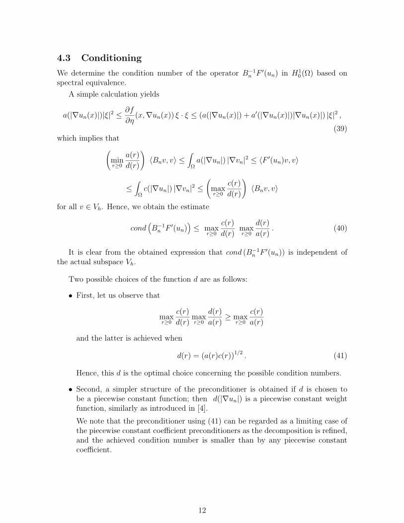
4.3 Conditioning

We determine the condition number of the operator B−1n F ′(un) in H1

0 (Ω) based onspectral equivalence.

A simple calculation yields

a(|∇un(x)|)|ξ|2 ≤ ∂f

∂η(x,∇un(x)) ξ · ξ ≤ (a(|∇un(x)|) + a′(|∇un(x)|)|∇un(x)|) |ξ|2 ,

(39)which implies that

(minr≥0

a(r)

d(r)

)〈Bnv, v〉 ≤

∫

Ωa(|∇un|) |∇vn|2 ≤ 〈F ′(un)v, v〉

≤∫

Ωc(|∇un|) |∇vn|2 ≤

(maxr≥0

c(r)

d(r)

)〈Bnv, v〉

for all v ∈ Vh. Hence, we obtain the estimate

cond(B−1

n F ′(un))≤ max

r≥0

c(r)

d(r)maxr≥0

d(r)

a(r). (40)

It is clear from the obtained expression that cond (B−1n F ′(un)) is independent of

the actual subspace Vh.

Two possible choices of the function d are as follows:

• First, let us observe that

maxr≥0

c(r)

d(r)maxr≥0

d(r)

a(r)≥ max

r≥0

c(r)

a(r)

and the latter is achieved when

d(r) = (a(r)c(r))1/2 . (41)

Hence, this d is the optimal choice concerning the possible condition numbers.

• Second, a simpler structure of the preconditioner is obtained if d is chosen tobe a piecewise constant function; then d(|∇un|) is a piecewise constant weightfunction, similarly as introduced in [4].

We note that the preconditioner using (41) can be regarded as a limiting case ofthe piecewise constant coefficient preconditioners as the decomposition is refined,and the achieved condition number is smaller than by any piecewise constantcoefficient.

12

References

[1] Axelsson, O., On global convergence of iterative methods, in: Iterative solutionof nonlinear systems of equations, pp. 1-19, Lecture Notes in Math. 953, Springer,1982.

[2] Axelsson, O., Iterative Solution Methods, Cambridge Univ. Press, 1994.

[3] Axelsson, O., Barker, V.A., Finite Element Solution of Boundary ValueProblems, Academic Press, 1984.

[4] Axelsson, O., Farago I., Karatson J., Sobolev space preconditioning forNewton’s method using domain decomposition, Numer. Lin. Alg. Appl., 9 (2002),585-598.

[5] Axelsson, O., Kaporin, I., Minimum residual adaptive multilevel finite ele-ment procedure for the solution of nonlinear stationary problems, SIAM J. Nu-mer. Anal. 35 (1998), no. 3, 1213–1229 (electronic).

[6] Axelsson, O., Karatson J., Double Sobolev gradient preconditioning forelliptic problems, Report 0016, Dept. Math., University of Nijmegen, April 2000.

[7] Axelsson, O., Maubach, J., On the updating and assembly of the Hes-sian matrix in finite element methods, Comput. Methods Appl. Mech. Engrg.,71 (1988), pp. 41-67.

[8] Blaheta, R., Multilevel Newton methods for nonlinear problems with applica-tions to elasticity, Copernicus 940820, Technical report.

[9] Faber, V., Manteuffel, T., Parter, S.V., On the theory of equivalentoperators and application to the numerical solution of uniformly elliptic partialdifferential equations, Adv. in Appl. Math., 11 (1990), 109-163.

[10] Farago, I., Karatson, J., The gradient–finite element method for ellipticproblems, Comp. Math. Appl. 42 (2001), 1043-1053.

[11] Farago, I., Karatson, J., Numerical solution of nonlinear elliptic problemsvia preconditioning operators . Theory and applications. NOVA Science Publish-ers, New York, 2002.

[12] Gajewski, H., Groger, K., Zacharias, K., Nichtlineare Operatorgleichun-gen und Operatordifferentialgleichungen, Akademie-Verlag, Berlin, 1974.

[13] Hackbusch, W., Elliptic differential equations. Theory and numerical treat-ment, Springer Series in Computational Mathematics 18, Springer, Berlin, 1992.

[14] Karatson J., Farago I., Variable preconditioning via inexact Newton meth-ods for nonlinear problems in Hilbert space, Publ. Appl. Anal., ELTE University(Budapest), 2001/2. (Submitted)

13

[15] Krizek, M., Neittaanmaki, P., Mathematical and numerical modelling inelectrical engineering: theory and applications, Kluwer Academic Publishers,1996.

[16] Mikhlin, S.G., The Numerical Performance of Variational Methods, Walters-Noordhoff, 1971.

[17] Neuberger, J. W., Sobolev gradients and differential equations, Lecture Notesin Math., No. 1670, Springer, 1997.

[18] Richardson, W.B. JR, Sobolev Gradient Preconditioning for PDE Applica-tions, in: Iterative Methods in Scientific Computation IV. (Kincaid, D.R., Elster,A.C., eds.), pp. 223-234, IMACS, New Jersey, 1999.

[19] Rossi, T., Toivanen, J., A parallel fast direct solver for block tridiagonalsystems with separable matrices of arbitrary dimension, SIAM J. Sci. Comput.20 (1999), no. 5, 1778–1796 (electronic).

14