This content has been downloaded from IOPscience. Please scroll down to see the full text.

Download details:

IP Address: 198.244.61.252

This content was downloaded on 15/10/2013 at 23:12

Please note that terms and conditions apply.

Linear and nonlinear rogue wave statistics in the presence of random currents

View the table of contents for this issue, or go to the journal homepage for more

2011 Nonlinearity 24 R67

(http://iopscience.iop.org/0951-7715/24/11/R01)

Home Search Collections Journals About Contact us My IOPscience

IOP PUBLISHING NONLINEARITY

Nonlinearity 24 (2011) R67–R87 doi:10.1088/0951-7715/24/11/R01

INVITED ARTICLE

Linear and nonlinear rogue wave statistics in thepresence of random currents∗

L H Ying1, Z Zhuang2, E J Heller3 and L Kaplan1

1 Department of Physics and Engineering Physics, Tulane University, New Orleans,LA 70118, USA2 School of Electrical and Computer Engineering, Cornell University, Ithaca, NY 14853, USA3 Department of Physics and Department of Chemistry and Chemical Biology, HarvardUniversity, Cambridge, MA 02138, USA

Received 25 May 2011, in final form 22 August 2011Published 4 October 2011Online at stacks.iop.org/Non/24/R67

Recommended by J P Keating

AbstractWe review recent progress in modelling the probability distribution of waveheights in the deep ocean as a function of a small number of parametersdescribing the local sea state. Both linear and nonlinear mechanisms ofrogue wave formation are considered. First, we show that when the averagewave steepness is small and nonlinear wave effects are subleading, the waveheight distribution is well explained by a single ‘freak index’ parameter, whichdescribes the strength of (linear) wave scattering by random currents relativeto the angular spread of the incoming random sea. When the average steepnessis large, the wave height distribution takes a very similar functional form, butthe key variables determining the probability distribution are the steepness, andthe angular and frequency spread of the incoming waves. Finally, even greaterprobability of extreme wave formation is predicted when linear and nonlineareffects are acting together.

Mathematics Subject Classification: 76B15, 35Q55, 37N10

PACS numbers: 92.10.Hm, 47.20.Ky, 47.35.Bb, 02.60.Cb

(Some figures in this article are in colour only in the electronic version)

1. Introduction

Tales of freak waves by lucky survivors used to be taken with a large grain of salt. Were thesailors making excuses for bad seamanship? The first such wave to be measured directly wasthe famous New Year’s wave in 1995 [1]. With modern cameras and video, not to mention

∗ This invited article is one of a series published throughout 2011 in Nonlinearity on the topic of Rogue Waves.

0951-7715/11/110067+21$33.00 © 2011 IOP Publishing Ltd & London Mathematical Society Printed in the UK & the USA R67

R68 Invited Article

satellites [2, 3], it is no longer controversial that freak or rogue extreme waves do exist on theworld’s great oceans [4–6].

Any realistic seaway (an irregular, moderate to rough sea) is comprised of a superpositionof waves differing in wavelength and direction, with random relative phases. Supposingthat the dispersion in wavelengths is not too large, and assuming uniform sampling, Longuet-Higgins [7] exploited the central limit theorem to derive a large number of statistical propertiesof such random wave superpositions, including of course wave height distributions. Fromthis viewpoint, extreme waves are the result of unlucky coherent addition of plane wavescorresponding to the tail of the Gaussian distribution (see equation (9)). As explained below,wave heights greater than about 4 σ in the tail of the Gaussian are classified as extreme. Theproblem has become how to explain why the observed number of rogue wave events is greaterthan the number 4 σ out in the Longuet-Higgins theory.

For the following discussion, it is important to understand why a 20 m wave in a sea wherethe significant wave height (SWH, defined as the average height of the highest one third of thewaves) is 18 m is far less onerous than a 20 m wave where the SWH is 8 m. An establishedseaway of uniform energy density (uniform if averaged over an area large compared withthe typical wavelength) is ‘accommodated’ over time and distance, through nonlinear energytransfer mechanisms. Seaways of higher energy density develop correspondingly longer waveperiods and wavelengths, even with no further wind forcing, keeping wave steepness undercontrol as a result.

This accommodation process is one of the ways nonlinear processes are implicitly lurkingbehind ‘linear’ theories, in that the input into the linear theories, i.e. the SWH, the period,dispersion in direction, and dispersion in wavelength are all the result of prior nonlinearprocesses. A 20 m wave in a sea of SWH 8 m is necessarily very steep, possibly breaking,with a deep narrow trough preceding it. The tendency for steep waves to break is an oftendevastating blow just as the ship is sailing over an unusually deep trough before meeting thecrest.

Observational evidence has shown that the linear Longuet-Higgins theory is toosimplistic [4]. Recent advances in technology have allowed multiple wave tank experimentsand field observations to be conducted, confirming the need for a more realistic theory to explainthe results [8, 9]. An obvious correction is to incorporate nonlinear wave evolution at everystage, rather than split the process into an implicit nonlinear preparation of the seaway followedby linear propagation. Clearly the exact evolution is always nonlinear to some extent, but thekey is to introduce nonlinearities at the right moment and in an insightful and computable way.Realistic fully nonlinear computations wave by wave over large areas are very challenging,though initial attempts have been made to simulate the ocean surface using the full Eulerequation both on large scales [10] and over smaller areas [11, 12].

Surprisingly, investigation of nonlinear effects is actually not the next logical step neededto improve upon the Longuet-Higgins model. Indeed the full linear statistical theory had notbeen given, for the reason that uniform sampling assumed by Longuet-Higgins is not justified.A nonuniform sampling theory, which does not assume that the energy density is uniformlydistributed over all space, is possible and is still ‘linear’. Moreover, the parameters governinga nonuniform sampling are knowable. Inspired by the work of White and Fornberg [13], thepresent authors showed that current eddies commonly present in the oceans are sufficient tocause the time-averaged wave intensity to be spatially nonuniform, and to exhibit ‘hot spots’and ‘cold spots’ some tens to hundreds of kilometres down flow from the eddies. We emphasizethat in terms of wave evolution, the refraction leading to the patchy energy density is purelylinear evolution. The key ideas are (1) that waves suddenly entering a high-energy patch arenot accommodated to it and grow steep and dangerous, and (2) the process is still probabilistic

Invited Article R69

and the central limit theorem still applies, with the appropriate sampling over a nonuniformdistribution. The high-energy patches will skew the tails of the wave height distribution,perhaps by orders of magnitude. This was the main point in [14].

There is no denying the importance of nonlinear effects in wave evolution, and a full theoryshould certainly include them. On the other hand a nonlinear theory that fails to account forpatchy energy density is missing an important, even crucial effect. The linear theory needs tobe supplemented by nonlinear effects, however, since the accommodation of the waves to thepresence of patchy energy density needs to be considered. It is our goal here to review progressalong these lines and point the way to a more complete theory. We first review the linear theorywith nonuniform sampling and then discuss newer simulations using the nonlinear Schrodingerequation (NLSE). Finally, we show that even larger rogue wave formation probabilities arepredicted when linear and nonlinear formation mechanisms are acting in concert.

Rogue wave modelling would benefit greatly from a comprehensive, accurate, andunbiased global record of extreme wave events, supplemented by data on local oceanconditions, including current strength, SWH, steepness, and the angular and spectral spreadof the sea state. Such a record, not available at present, would allow for direct statisticaltests of linear and nonlinear theories of rogue wave formation. Anecdotal evidence doessuggest that rogue waves may be especially prevalent in regions of strong current, includingthe Gulf Stream, the Kuroshio Current, and especially the Agulhas Current off the coast ofSouth Africa. Consequently, the Agulhas Current in particular has attracted much attention inrogue wave research [5, 15]. However, anecdotal evidence from ships and even oil platformmeasurements cannot provide a systematic, unbiased, and statistically valid record that wouldsupport a correlation between possibly relevant variables and rogue wave formation probability.Instead, satellite-based synthetic aperture radar (SAR) [2, 3] is currently the only method thatshows potential for monitoring the ocean globally with single-wave resolution, but validatingthe surface elevations obtained by SAR is a challenge. The SAR imaging mechanism isnonlinear, and may yield a distorted image of the ocean wave field; the nonlinearity is ofcourse of particular concern for extreme events [16]. Recently, an empirical approach hasbeen proposed that may accurately obtain parameters such as the SWH from SAR data [17],but the application of this approach to measuring individual waves is still controversial.

2. Linear wave model in the presence of currents

2.1. Ray density statistics

To understand the physics of linear rogue wave formation in the presence of currents, it is veryhelpful to begin with a ray, or eikonal, approximation for wave evolution in the ocean [13, 14],

d�kdt

= −∂ω(�r, �k)

∂�r ; d�rdt

= ∂ω(�r, �k)

∂ �k , (1)

where �r is the ray position, �k is the wave vector and ω is the frequency. For surface gravitywaves in deep water, the dispersion relation is

ω(�r, �k) =√

g|�k| + �k · �U(�r), (2)

where �U(�r) is the current velocity, assumed for simplicity to be time-independent, andg = 9.81 m s−1 is the acceleration due to gravity. The validity of the ray approximationdepends firstly on the condition |�k|ξ � 1, where ξ is the length scale on which the currentfield �U(�r) is varying, physically corresponding to the typical eddy size. This condition is wellsatisfied in nature, since wave numbers of interest in the deep ocean are normally of order

R70 Invited Article

Figure 1. A ray density map I (x, y) is calculated for rays moving through a 640 km by 640 kmrandom eddy field, with rms eddy current urms = 0.5 m s−1 and eddy correlation length ξ = 20 km.Here bright regions represent high density. The rays are initially distributed uniformly along theleft edge of each panel, with angular spread �θ around the +x (rightward) direction, and withfrequency ω = 2π/(10 s), corresponding to velocity v = 7.81 m s−1 in the absence of currents.The left and right panels illustrate �θ = 10◦ and �θ = 20◦, respectively.

k ∼ 2π/(100 m), while the typical eddy size may be ξ ∼ 5 km or larger. Secondly, scatteringof the waves by currents is assumed to be weak, i.e. the second term in equation (2) should besmall compared with the free term. This again is well justified since eddy current speeds | �U |are normally less than 0.5 m s−1, whereas the wave speed v = ∂ω/∂k ≈ √

g/4k is greater than5 m s−1. In section 2.3, we will explicitly compare the ray predictions with results obtainedby exact integration of the corresponding wave equation.

In the numerical simulations shown in figure 1, we follow White and Fornberg [13] inconsidering a random incompressible current field in two dimensions, with zero mean currentvelocity, generated as

Ux(�r) = −∂ψ(�r)/∂y; Uy(�r) = ∂ψ(�r)/∂x (3)

from the scalar stream function ψ(�r). The stream function itself is Gaussian distributed withGaussian decay of spatial correlations:

ψ(�r) = 0; ψ(�r) ψ(�r ′) ∼ e−(�r−�r ′)2/2ξ 2, (4)

and the overall current strength is described by u2rms = | �U(�r)|2. The specific choice of a

Gaussian distribution for the stream function is made for convenience only. The detailedstructure of the individual eddies on the scale ξ has no effect on the final rogue wave statisticsas long as the current is weak (urms v), since each ray must travel a distance � ξ beforebeing appreciably scattered. Each panel in figure 1 represents a 640 km by 640 km randomeddy field, with rms eddy current urms = 0.5 m s−1 and eddy correlation length ξ = 20 km.

The initial swell, entering from the left in each panel, is characterized by a single frequencyω = 2π/(10 s) (and thus a single-wave number k = ω2/g = 0.04 m−1 and a single-wavespeed v = √

g/4k = 7.81 m s−1). As discussed in [14], within the context of a linear model,a nonzero frequency spread affects rogue wave formation only at second order in the spread�ω, and may be neglected for all practical purposes. In contrast, the angular spread ofthe incoming sea is very important in determining rogue wave statistics. In this figure, weconsider an initially Gaussian angular distribution p(θ) ∼ e−θ2/2(�θ)2

, where θ is the wavevector direction relative to the mean direction of wave propagation. Here all rays begin at the

Invited Article R71

Figure 2. A cusp singularity, followed by two branches of fold singularities, is formed as initiallyparallel rays pass through a focusing region. The two branches appear because the focal distancevaries with the distance of approach from the centre, as in a ‘bad’ lens with strong sphericalaberration. After averaging over incident directions, the singularities will be softened but notwashed away completely, (reproduced with permission [14]).

left edge of each panel, uniformly distributed in the y direction, and the mean direction of wavepropagation is rightward. The left and right panels illustrate the behaviour for two differentvalues of the initial angular spread �θ .

In both panels we observe bright streaks or branches, corresponding to regions of largerthan average ray density I (x, y), and thus larger than average wave intensity. The branchesmay be understood by considering briefly the limiting (unphysical) case of a unidirectionalinitial sea state (�θ = 0), corresponding to a single incoming plane wave. In the ray picture,and in the coordinates of figure 1, the initial conditions are in this limit characterized bya one-dimensional phase-space manifold (x, y, kx, ky) = (0, y, k, 0), where k is the fixedwave number, and y varies over all space. As this incoming plane wave travels through therandom current field, it undergoes small-angle scattering, with scattering angle ∼ urms/v

after travelling one correlation length ξ in the forward direction. Eventually, singularitiesappear that are characterized in the surface of section map [y(0), ky(0)] → [y(x), ky(x)] byδy(x)/δy(0) = 0, i.e. by local focusing of the manifold of initial conditions at a point (x, y).

The currents leading to such a focusing singularity may be thought of as forming a ‘badlens.’ Whereas a lens without aberration focuses all parallel incoming rays to one point, a badlens only focuses at each point an infinitesimal neighbourhood of nearby rays, so that differentneighbourhoods get focused at different places as the phase-space manifold evolves forwardin x, resulting in lines, or branches, of singularities. The typical pattern is an isolated cuspsingularity, δ2x(y)/δx(0)2 = 0, followed by two branches of fold singularities, as shown infigure 2.

A simple scaling argument [13, 18, 19] shows that the first singularities occur after amedian distance y = L ∼ ξ(urms/v)−2/3 � ξ along the direction of travel, when the typicalray excursion in the transverse x direction becomes of order ξ . Thus, each ray passes throughmany uncorrelated eddies before a singularity occurs, and a statistical description is welljustified. For realistic parameters, L ∼ 100 km or more is typical. The cusp singularitiesformed in this way are separated by a typical distance ξ in the transverse direction, and thusthe rms deflection angle by the time these singularities appear scales as

δθ ∼ ξ/L ∼ (urms/v)2/3. (5)

R72 Invited Article

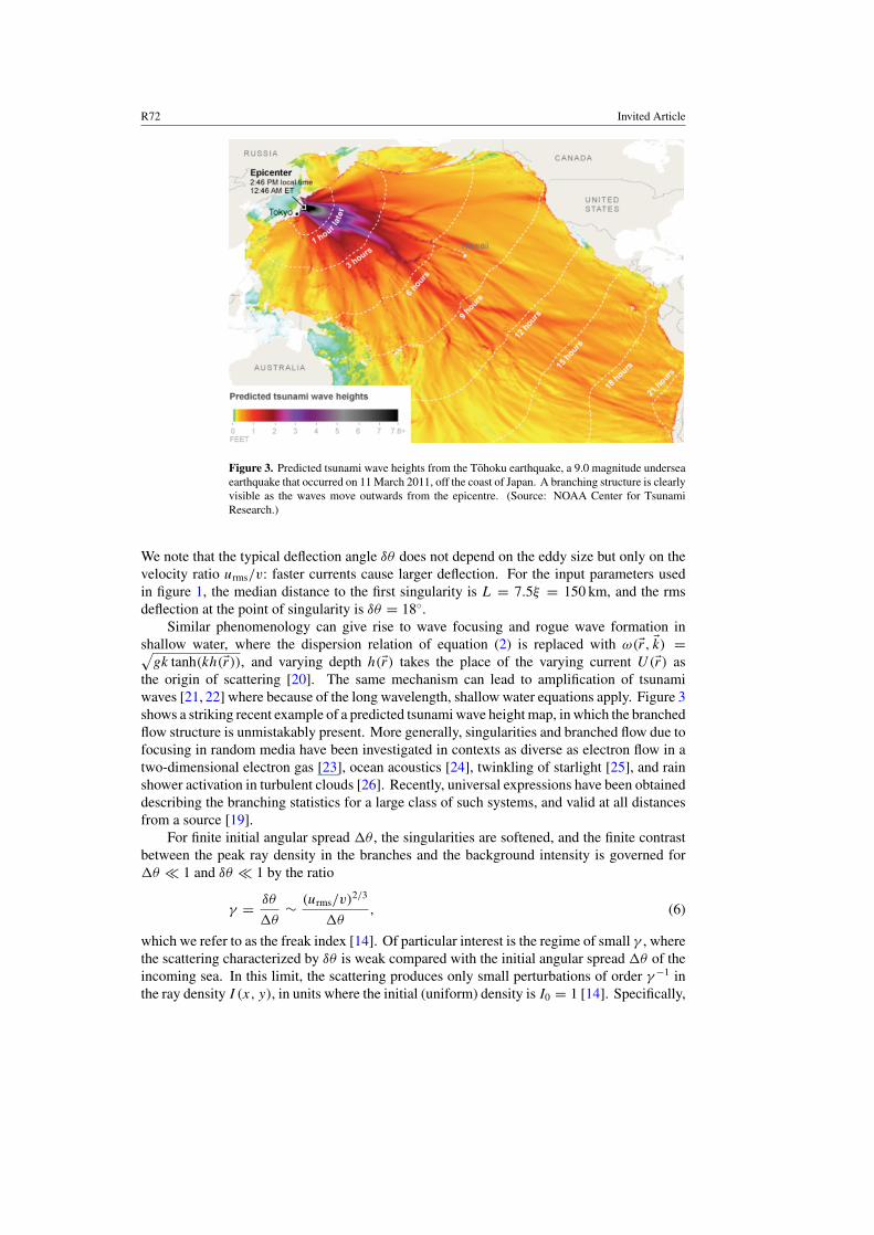
Figure 3. Predicted tsunami wave heights from the Tohoku earthquake, a 9.0 magnitude underseaearthquake that occurred on 11 March 2011, off the coast of Japan. A branching structure is clearlyvisible as the waves move outwards from the epicentre. (Source: NOAA Center for TsunamiResearch.)

We note that the typical deflection angle δθ does not depend on the eddy size but only on thevelocity ratio urms/v: faster currents cause larger deflection. For the input parameters usedin figure 1, the median distance to the first singularity is L = 7.5ξ = 150 km, and the rmsdeflection at the point of singularity is δθ = 18◦.

Similar phenomenology can give rise to wave focusing and rogue wave formation inshallow water, where the dispersion relation of equation (2) is replaced with ω(�r, �k) =√

gk tanh(kh(�r)), and varying depth h(�r) takes the place of the varying current U(�r) asthe origin of scattering [20]. The same mechanism can lead to amplification of tsunamiwaves [21, 22] where because of the long wavelength, shallow water equations apply. Figure 3shows a striking recent example of a predicted tsunami wave height map, in which the branchedflow structure is unmistakably present. More generally, singularities and branched flow due tofocusing in random media have been investigated in contexts as diverse as electron flow in atwo-dimensional electron gas [23], ocean acoustics [24], twinkling of starlight [25], and rainshower activation in turbulent clouds [26]. Recently, universal expressions have been obtaineddescribing the branching statistics for a large class of such systems, and valid at all distancesfrom a source [19].

For finite initial angular spread �θ , the singularities are softened, and the finite contrastbetween the peak ray density in the branches and the background intensity is governed for�θ 1 and δθ 1 by the ratio

γ = δθ

�θ∼ (urms/v)2/3

�θ, (6)

which we refer to as the freak index [14]. Of particular interest is the regime of small γ , wherethe scattering characterized by δθ is weak compared with the initial angular spread �θ of theincoming sea. In this limit, the scattering produces only small perturbations of order γ −1 inthe ray density I (x, y), in units where the initial (uniform) density is I0 = 1 [14]. Specifically,

Invited Article R73

0

0.5

1

1.5

2

2.5

0 0.5 1 1.5 2 2.5 3

Pro

babi

lity

dist

ribut

ion

g(I

)

Ray intensity I

γ = 0.72γ = 1.20γ = 3.60

Figure 4. The ray density distribution, for an initial sea state of uniform density scattered by arandom eddy current field, is shown for several values of the freak index γ . The input parametersare chosen as in figure 1, with initial angular spread �θ = 25◦, 15◦ and 5◦ corresponding to freakindex γ = 0.72, 1.20 and 3.60, respectively. The mean intensity is normalized to unity in eachcase. The dashed curves are fits to the χ2 distribution of equation (7).

as seen in figure 4, the distribution of ray intensities in this regime may be well described bya χ2 distribution [27],

g(I) = χ2N(I) =

(N

2

) N2 I

N2 −1

�(

N2

)e−NI/2, (7)

where the number of degrees of freedom N scales with the freak index as γ −2. Theproportionality constant may be obtained numerically by a fit to the data:

N = α

γ 2= 45

γ 2. (8)

In the limit γ → 0 associated with zero current, we have N → ∞, and we recover as expectedthe uniform ray density distribution g(I) = δ(I − 1).

2.2. Implications for wave statistics

In the Longuet-Higgins random seas model [7], the sea surface elevation above the averageelevation is given by Re ζ(x, y, t), where ζ is a random superposition of many plane waveswith differing directions and frequencies. By the central limit theorem, ζ is distributed as acomplex Gaussian random variable with standard deviation σ . Furthermore, for a narrow-banded spectrum (δω ω) the wave crest height H is equal to the wave function amplitude|ζ |, and the probability of encountering a wave crest of height H or larger is

PRayleigh(H) = e−H 2/2σ 2. (9)

Due to an exact symmetry between crests and troughs in a linear wave model, a crest heightof H corresponds to a wave height (crest to trough) of 2H . Conventionally, a rogue waveis defined as 2H � 2.2 SWH, where the SWH is the average of the largest one third ofwave heights in a time series, or approximately SWH ≈ 4.0σ . Thus the condition for a

R74 Invited Article

rogue wave is H � 4.4σ , and the random seas model predicts such waves to occur withprobability PRayleigh(4.4σ) = 6.3 × 10−5. Similarly, extreme rogue waves may be defined bythe condition 2H � 3 SWH or H � 6.0σ , and these are predicted to occur with probabilityPRayleigh(6.0σ) = 1.5 × 10−8 within the random seas model. As discussed in section 1, therandom seas model significantly underestimates the occurrence probability of extreme waves,when compared with observational data.

What are the implications of scattering by currents, as discussed in section 2.1, on thewave height statistics? Within the regime of validity of the ray approximation, we have at anyspatial point (x, y) correspondence between the ray density I (x, y) and the wave intensityH 2 = |ζ(x, y, t)|2, averaged over time. Thus, in contrast with the original Longuet-Higginsmodel, the time-averaged wave intensity is not uniform over all space but instead exhibits‘hot spots’ and ‘cold spots’ associated with focusing and defocusing in the corresponding rayequations. At each point in space (assuming of course that the currents are stationary), thecentral limit theorem and thus the Rayleigh distribution still apply, and we have

P(x,y)(H) = e−H 2/2σ 2I (x,y), (10)

where I (x, y) is the local ray density, normalized so that the spatial average is unity, and σ 2

is the variance of the surface elevation in the incoming sea state, before scattering by currents.This is the situation a ship experiences at a given position.

Now averaging over space, or over an ensemble of random eddy fields with a given rmscurrent speed, we obtain a total cumulative height distribution

Ptotal(H) =∫ ∞

0dI g(I ) e−H 2/2σ 2I . (11)

In equation (11), the full cumulative distribution of wave heights for a given sea state hasbeen expressed as a convolution of two factors: (i) the local density distribution g(I), whichcan be extracted from the ray dynamics, and (ii) the universal Longuet-Higgins distribution ofwave heights for a given local density. Similar decompositions of chaotic wave functionstatistics into non-universal and universal components have found broad applicability inquantum chaos, including for example in the theory of scars [28, 29]. In the context ofrogue waves, a similar approach was adopted by Regev et al to study wave statistics in aone-dimensional inhomogeneous sea, where the inhomogeneity arises from the interaction ofan initially homogeneous sea with a (deterministic) long swell [30].

Using the previously obtained ray density distribution in the presence of currents,equation (7), we obtain the K-distribution [31]

Ptotal(H) = 2

(√NH/2σ

) N2

�(N/2)KN/2

(√NHσ

), (12)

where Kn(y) is a modified Bessel function.Defining the dimensionless variable x = 2H/SWH ≈ 2H/(4σ), so that a rogue wave is

given by x = 2.2 and an extreme rogue wave by x = 3.0, we find the probability of a waveheight exceeding x SWHs:

Ptotal(x) = 2

(√Nx

) N2

�(N/2)KN/2

(2√

Nx)

, (13)

to be compared with the random seas prediction

PRayleigh(x) = e−2x2(14)

Invited Article R75

Table 1. The N parameter of equation (13), and the associated enhancement in the probabilityof rogue wave formation (wave height 2H = 2.2 SWH) as well as the enhancement of theprobability of extreme rogue wave formation (wave height 2H = 3.0 SWH) are calculated forseveral values of the incoming angular spread �θ using equations (6), (8) and (13). HereE(x) = Ptotal(x)/PRayleigh(x). In all cases we fix the rms current speed urms = 0.5 m s−1 andmean wave speed v = 7.8 m s−1, so δθ = 18◦.

�θ γ N E(2.2) E(3.0)

5 3.6 3.46 57 16 80010 1.8 13.9 10.4 57015 1.2 31.2 4.3 7620 0.90 55.4 2.7 2225 0.72 86.6 2.0 9.830 0.60 125 1.7 5.7

in the same dimensionless units. We recall that N in equation (12) or (13) is a function of thefreak index γ , as given by equation (8).

To examine the predicted enhancement in the probability of rogue wave formation, ascompared with random seas model (9), we may consider two limiting cases. Keeping the waveheight of interest fixed, and taking the limit γ → 0, i.e. N → ∞, we obtain the perturbativeresult

Pperturb(x) =[

1 +4

N(x4 − x2)

]PRayleigh(x) (15)

=[

1 +4γ 2

b(x4 − x2)

]PRayleigh(x), (16)

valid for x4 N , or equivalently x2γ 1. Thus, in the limit of small freak index, thedistribution reduces, as expected, to the prediction of the random seas model. Analogousperturbative corrections appear for quantum wave function intensity distributions in thepresence of weak disorder or weak scarring by periodic orbits [32, 33].

Much more dramatic enhancement is observed if we consider the tail of the intensitydistribution (x → ∞) for a given set of sea conditions (fixed γ or N ). Then for x � N3/2, orequivalently xγ 3 � 1, we obtain the asymptotic form

Pasymptotic(x) = √π

(√Nx

) N−12

�(N/2)e−2x

√N

= √π

(√Nx

) N−12

�(N/2)e2x(x−√

N)PRayleigh(x), (17)

i.e., the probability enhancement over the random seas model is manifestly super-exponentialin the wave height x.

Predicted enhancements in the probability of rogue wave and extreme rogue waveformation, based on equations (13) and (14), are shown in table 1. We note in particularthat enhancements of an order of magnitude or more are predicted in the extreme tail, even formoderate values of the input parameters, corresponding to γ ∼ 0.72–1.2 or N ∼ 30–85.

2.3. Numerical results for linear wave equation

The theoretical predictions of equation (13) are based on several approximations, includingthe assumption of local Rayleigh statistics. To see whether the approximations we have made

R76 Invited Article

are valid, we compare the theoretical predictions with direct numerical integration of thecurrent-modified linear Schrodinger equation, which is obtained from the third-order current-modified nonlinear Schrodinger (CNLS) equation [34] by setting the nonlinear term to zero.CNLS governs the modulations of weakly nonlinear water waves around a mean frequency andmean wave vector, incorporating the effect of currents, and is presented in full in section 3.1.In dimensionless variables, the linear equation for the wave envelope describing the wavemodulations is expressed as [34]

iAT − 1

8AXX +

1

4AYY − k0UxA = 0. (18)

Here A(X, Y, T ) is the wave envelope, defined by separating out the carrier wave propagatingwith mean wave vector �k = k0x,

ζ(X, Y, T ) = k0A(X, Y, T )eik0x−i√

gk0t

= k0A(X, Y, T )eiX−iT/2, (19)

and

(X, Y, T ) = (k0x − 12

√gkt, k0y,

√gk0t) (20)

are dimensionless space and time coordinates. We also note that equation (18) may be obtaineddirectly from the dispersion relation (2), by expanding ω and �k around ω0 and k0x, respectively.

The calculations are performed on a rectangular field measuring 40 km along the meandirection of propagation and 20 km in the transverse direction, with typical eddy size ξ =800 m. (We note that a very small value for the eddy size is chosen to maximize the statisticscollected; this is also a ‘worst case’ scenario for the theory, as the ray approximation is expectedto work ever better as the ratio of eddy size to the wavelength increases.) Equation (18) isintegrated numerically using a split-operator Fourier transform method [35], on a 1024 by 512grid. The incoming wave is a random superposition of a large number of monochromatic waveswith directions uniformly distributed around the mean direction θ = 0 with standard deviation�θ . Without loss of generality, the incoming wave number is fixed at k0 = 2π/(156 m),corresponding to a frequency ω0 = √

gk0 = 2π/(10 s) and a group velocity v = 7.81 m s−1.Each run simulates wave evolution for 5 × 105 s or 5 × 104 wave periods, sufficient for thewave height statistics to converge.

The results for �θ = 5.7◦, corresponding to a very large freak index γ = 3.15, are shownin figure 5. The results are compared both with the theoretical prediction of equation (13) (hereN = 6.8) and with the baseline Rayleigh distribution of equation (14). This is an extremescenario, in which the occurrence probability of extreme rogue waves (3 times the SWH) isenhanced by more than three orders of magnitude. Even better agreement with the theoreticalmodel of equation (13) obtains for more moderate values of γ , corresponding to larger N .

In figure 6 we repeat the numerical simulation for four different values of the incomingangular spread �θ and four different values of the rms current speed urms. In each case, thenumerically obtained wave height distribution is fit to a K-distribution (equation (12)), and theresulting value of N (which fully describes the strength of deviations from Longuet-Higginsstatistics) is plotted as a function of the freak index γ . Excellent agreement is observed withthe power-law prediction of equation (8) all the way up to γ ≈ 2 (corresponding to N ≈ 10),even though the analytic prediction was obtained in a small-γ approximation. The regimein which the analytic formula (8) works well includes most conditions likely to be found innature (e.g. all but the first row of table 1). Referring again to table 1, we observe that thetheory accurately describes enhancements of up to three orders of magnitude in the formationprobability of extreme rogue waves. Modest deviations from the analytic formula are observednumerically at very large values of γ (corresponding to even larger enhancements).

Invited Article R77

10-8

10-7

10-6

10-5

10-4

10-3

10-2

10-1

100

0 0.5 1 1.5 2 2.5 3 3.5

Cum

ulat

ive

Pro

babi

lity

Wave Height / SWH

Numerical DataK Distribution

Rayleigh

Figure 5. The probability of exceeding wave height 2H , in units of the SWH, is shown for anincoming wave speed v = 7.8 m s−1, incoming angular spread �θ = 5.7◦, and rms current speedurms = 0.5 m s−1. The solid curve shows the results of a numerical simulation performed ona 20 km by 40 km field, with typical eddy size ξ = 800 m, while the dashed curve representsequation (13) with N = 6.8. The Rayleigh (random seas) prediction of equation (14) is shown forcomparison.

5

10

20

50

100

0.5 1 1.5 2 2.5 3

Deg

rees

of f

reed

om N

Freak index γ

urms = 0.2 m/surms = 0.3 m/surms = 0.4 m/surms = 0.5 m/s

Figure 6. The wave height distribution for a random incoming sea scattered by random currents isobtained numerically for four values of the rms current speed urms and four values of the incomingangular spread �θ . In each case, a fit to the K-distribution (equation (12)) yields the number-of-degrees-of-freedom parameter N , (describing deviations from Rayleigh statistics), which is plottedas a function of the freak index γ (defined in equation (6)). As in the previous figures, the wavespeed is fixed at v = 7.81 m s−1. The solid line is the theoretical prediction of equation (8).

2.4. Experimental demonstration of linear rogue wave formation

Direct experimental verification in the ocean of the statistical predictions made analyticallyin section 2.2 and confirmed numerically in section 2.3 is obviously highly desirable.

R78 Invited Article

Figure 7. The left panel shows the distribution of the experimentally measured time-averagedmicrowave intensity s, found for 780 positions in the random wave field, which is compared withthe χ2 distribution of equation (7), with N = 32. The inset shows the same data on a logarithmicscale. The right panel displaying a time series of the wave intensity at a single point shows a ‘roguewave’ event. The inset shows a snapshot of the wave intensity field near this point at the momentof the extreme event.

Unfortunately no observational data set exists at this time that would allow the tail of thewave height distribution to be studied as a function of the freak index γ , i.e. as a functionof the rms current speed urms and of the angular spread �θ . Recently, however, experimentsin open quasi-two-dimensional microwave cavities with disorder [27] have found a strongenhancement in the occurrence probability of high-amplitude waves, which may be interpretedas ‘rogue waves’ in this analogue system. In the microwave system, randomly placed brasscones play the role of random ocean currents, and a movable source antenna enables incomingwaves to arrive from different directions. A movable drain antenna acts a weak probe, andallows for a spatial mapping of the wave fields within the scattering arrangement. A greatadvantage of the microwave system is that the electromagnetic wave equation is linear, so thatthe observed enhancement in the tail of the wave height distribution may serve in principle asa direct experimental test of the theory developed in the previous sections.

In the left panel of figure 7, the time-averaged wave intensity s is found for differentpositions of the probe, and the probability distribution g(s) is shown. Most of the distributionis well described by the χ2 distribution of equation (7). We note that in the absence ofdisorder, the time-averaged intensity would be position-independent and g(s) would reduceto δ(s − 1) (N → ∞ in equation (7)). The inset in the left panel shows additional rareevents in the far tail that are not described by the χ2 distribution [27]. The right panel infigure 7 shows time series data of the wave intensity at a single point, including an extremeevent observed in the experiment, and the inset shows a snapshot of the wave intensity in theregion at the moment corresponding to this extreme event. The event presented here has waveheight 2H = 5.3 SWH, and events of this magnitude of greater are observed with probability1.3 × 10−9 in the experiment, which is an enhancement of 15 orders of magnitude comparedwith the Rayleigh distribution.

These results confirm that linear scattering is a sufficient mechanism for a largeenhancement in the tail of the wave height distribution, even when nonlinearity is entirelyabsent from the physical system being studied.

3. Nonlinear wave model

We have already seen (e.g. in table 1) that under physically realistic sea conditions, linear wavedynamics, with nonlinearity only in the corresponding ray equations, are sufficient to enhance

Invited Article R79

the incidence of extreme rogue waves by several orders of magnitude. At the same time, thetrue equations for ocean wave evolution are certainly nonlinear, and furthermore the nonlinearterms, which scale as powers of the wave height, manifestly become ever more important in thetail of the wave height distribution. Thus, a fully quantitative theory of rogue wave statisticsmust necessarily include nonlinear effects, which we address in the following.

3.1. Nonlinear Schrodinger equation

The original NLSE for surface gravity waves in deep water was derived by Zakharov usinga spectral method [36], and is valid to third order in the steepness ε = k0H , where H is themean wave height. Subsequently, the NLSE was extended to fourth order in ε by Dysthe [37]and then to higher order in the bandwidth �ω/ω by Trulsen and Dysthe [38]. The Trulsen–Dysthe equations include frequency downshifting [39], the experimentally observed reductionin average frequency over time [40]; however, the physics of frequency downshifting may notyet be fully understood [41].

In our simulations we implement the current-modified O(ε4) NLSE, as derived by Stockerand Peregrine in dimensionless form [34]:

iBT − 1

8(BXX − 2BYY ) − 1

2B|B|2 − B�cX

= i

16(BXXX − 6BYYX) + �XB +

i

4B(BB∗

X − 6B∗BX)

+ i( 12�cXT − �cZ)B − i(�cXBX + �cY BY ), (21)

where the linear and third-order terms are collected on the left-hand side of equation (21).Here �, �c and B represent the mean flow, surface current and oscillatory parts, respectively,of the velocity potential φ:

φ =√

g

k30

[� + �c +

1

2

(Bek0z+iθ + B2e2(k0z+iθ) + c.c.

)], (22)

where the second-harmonic term B2 is a function of B and its derivatives, (X, Y, T ) aredimensionless space and time coordinates defined previously in equation (20), and θ =k0x − √

gk0t = X − T/2 is the phase. The surface elevation, which is the quantity ofinterest for our purposes, is similarly expanded as

ζ = k0−1

[ζ + ζc +

1

2

(Aiθ + A2e2iθ + A3e3iθ + c.c.

)], (23)

where the expansion coefficients may be obtained from the velocity potential as

A = iB +1

2k0Bx +

i

8k20

(Bxx − 2Byy) +i

8B|B|2

A2 = − 1

2B2 +

i

k0BBx (24)

A3 = − 3i

8B3.

Here both B and A are proportional to the wave height at leading order, and are thus linearin the steepness ε. By scaling the average height of the incoming waves, which to leadingorder is proportional to A and B, we can control the value of the steepness ε. Also, the wavevector spread around k0x, and thus the derivatives ∂/∂X and ∂/∂Y are taken to be O(ε), andfinally the surface current �c is assumed to be O(ε2). Given these assumptions, it is easy tocheck that all terms on the right-hand side of equation (21) are formally O(ε4).

R80 Invited Article

In the simulation, we work with a time-independent two-dimensional current (�cX, �cY ),with a mean value of zero, so several terms on the right-hand side of equation (21) involving�X, and the time and Z derivatives of �c, do not contribute. Finally, we note that if weconsider only the left-hand side of equation (21) and drop the cubic term, we recover the linearSchrodinger equation with current considered earlier in equation (18).

As before, the incoming wave is a random superposition of a large number ofmonochromatic waves with different frequencies and propagating directions. Thus the initialwave can be written as a linear summation of a large number of plane waves,

ζ(�r, t) =M∑i=1

Aiei �ki ·�r−iω( �ki )t , (25)

where �ki is the random wave vector for each monochromatic wave. In our setup, the wavevector can be expressed as

�k = (k0 + k′) · (cos θ ′x + sin θ ′y), (26)

where k′ is a random variation in wave number normally distributed around 0 with width �k,and θ ′ is the angle relative to the x direction, which is uniformly distributed with standarddeviation �θ .

In the following examples, equation (21) is integrated numerically with the current set tozero, in order to investigate systematically and quantitatively the effect of nonlinear focusing. Innature, the interplay between linear and nonlinear mechanisms is also of considerable interest,and may give rise to even stronger enhancement in the probability of rogue wave occurrencethan either effect individually, as demonstrated in section 4 (see also [42, 43]).

3.2. Height distribution

As in the linear case, the split-operator Fourier transform method is used to integrateequation (21) numerically. The rectangular field measuring 20 km along the mean directionof propagation and 10 km in the transverse direction is discretized using a 1024 by 512 grid.The incoming state is a random superposition of plane waves with wave numbers normallydistributed around k0 with standard deviation �k, and directions uniformly distributed aroundthe mean direction θ = 0 with standard deviation �θ . Without loss of generality we fixthe mean incoming wave number at k0 = 2π/(156 m), as in section 2. The steepness k0H isadjusted by varying the mean height H of the incoming sea. Each run simulates wave evolutionfor 4 × 106 s or 4 × 105 wave periods.

Typical results are represented by solid curves in figure 8, where we fix �k/k0 = 0.1 and�θ = 2.6◦ (as we will see below, the values of �θ required to see very strong effects fromnonlinear focusing are typically smaller than those needed to observe significant deviationsfrom Rayleigh by linear scattering). The cumulative probability distribution of the wave height2H , in units of the significant wave height SWH, is shown for four nonzero values of the wavesteepness ε. As expected, the Rayleigh probability distribution of equation (14) is recoveredin the limit ε → 0, and ever stronger enhancement in the tail is observed as the steepness of theincoming sea increases. The occurrence probability of extreme rogue waves, 2H/SWH = 3.0,is enhanced by one to three orders of magnitude for the parameters shown.

To understand the functional form of the distributions in figure 8, we again make use ofthe local Rayleigh approximation discussed in section 2.2. Here the wave height distributionis given locally in space and time by a Rayleigh distribution around the local mean height(corresponding to a locally random superposition of plane waves), while the local mean heightitself varies slowly on the scale of the mean wavelength and mean period. This approximation is

Invited Article R81

0 1 2 3 410−7

10−5

0.001

0.1

Wave Height SWH

Cum

ulat

ive

Prob

abili

ty

e =0.042

e =0.026

e =0.019

e =0

Figure 8. The distribution of wave heights, in units of the SWH, is calculated for three nonzerovalues of the steepness ε (upper three solid curves), and compared with the random seas modelof equation (14) (lowest solid curve). In each case, the dashed or dotted curve is a best fit to theK-distribution of equation (13). Here we fix the angular spread �θ = 2.6◦ and wave numberspread �k/k0 = 0.1 of the incoming sea.

well justified, since the envelope A(X, Y, T ) in equation (23) is slowly varying for �k/k0 1and �θ 1, while the higher harmonics A2(X, Y, T ) and A3(X, Y, T ) are suppressed byfactors of ε and ε2, respectively. Taking the local mean intensity to be χ2 distributed, andconvolving the χ2 distribution of the mean intensity with the Rayleigh distribution around themean intensity, we obtain as in the linear case a K-distribution (13) for the total distributionof wave heights.

In figure 8, each data set is fit to the K-distribution of equation (13), arising from thelocal Rayleigh approximation. We see that the fits, indicated by dashed and dotted lines,perform adequately for probabilities down to 10−6, where statistical noise begins to dominate.In particular, we clearly observe the crossover between the Gaussian behaviour (14) at smallto moderate heights and the asymptotic exponential behaviour (17) at large heights. However,systematic deviations do exist, which are especially visible at larger values of ε, correspondingto smaller values of the N (degrees of freedom) parameter. These systematic deviationsare in large part due to the fact that the true wave height distribution for any given set ofinput parameters exhibits spatial dependence, evolving from the original Rayleigh distributionimposed by incoming boundary conditions to the broader K-distribution, and then graduallyback to a Rayleigh distribution as the wave energy is transferred to longer wavelengths andthe steepness decreases [42]. An example of this spatial dependence appears in figure 11.Thus, a more accurate model for the total wave height distribution consists of a sum ofseveral K-distributions, or equivalently the tail of the full distribution may be modelled bya K-distribution multiplied by a prefactor C < 1, as discussed in [43]. Nevertheless, asseen in figure 8, equation (13) correctly describes wave height probabilities at the ±20%level of accuracy, allows for an extremely simple one-parameter characterization of the waveheight distribution, and facilitates easy comparison between the effects of linear and nonlinearfocusing.

3.3. Scaling with input parameters

Given the single-parameter approximation of equation (13), it is sufficient to explore thedependence of the parameter N on the input variables describing the incoming sea, specifically

R82 Invited Article

1.0 5.02.0 3.01.5 7.0

10

100

50

20

30

15

70

N

fit k ko 0.15

k ko 0.20

k ko 0.15

k ko 0.1

k ko 0.08

0.10 0.200.15

10

50

20

30

15

70

k ko

N

fit 2.6º

1.0º

2.6º

3.6º

5.2º

Figure 9. The best-fit N value (equation (13)) describing the wave height probability distributionis shown as a function of the initial angular spread �θ and initial wave number spread �k/k0 ofthe incoming sea. The steepness is fixed at ε = 0.032. The left panel shows the scaling of N with�θ , with the line showing the best-fit scaling N ∼ (�θ)1.04 for �k/k0 = 0.15. The right panelshows the scaling of N with �k/k0, with the line showing the best-fit scaling N ∼ (�k/k0)

1.15

for �θ = 2.6◦.

the initial angular spread �θ , the initial wave number spread �k/k0, and the initial steepness ε.In the two panels of figure 9, we fix the steepness at ε = 0.032 and show the scaling of N with�θ and δk/k0, respectively. Given that the Benjamin–Feir instability for a monochromaticwave in one dimension [44] is at the root of the nonlinear instability in the general case, it isnot surprising that stronger deviations from the Rayleigh model, as indicated by smaller valuesof N , occur as �θ or �k is reduced, consistent with earlier results [45–48]. Specifically,we find

N ∼ (�θ)a(

�k

k0

)b

(27)

where a, b ≈ 1.We note that the scaling of N with incoming angular spread �θ for nonlinear focusing,

N ∼ �θ , is only half as strong as the scaling N ∼ (�θ)2 arising from linear wave scatteringby currents, as implied by equations (6) and (8). Thus, smaller angular spreads �θ are neededfor the nonlinear focusing mechanism to be effective, as compared with linear focusing bycurrents. This is easily seen by comparing the range of �θ in figure 9 with the correspondingrange in table 1 for the linear mechanism. On the other hand, figure 9 and equation (27)both imply that the nonlinear mechanism exhibits significant sensitivity to the spectral width�k/k0, consistent with previous findings [6, 40, 49–52]. This is to be contrasted with the linearmechanism of rogue wave formation, which is insensitive to the spectral width at leading orderin �k/k0 [14].

Finally, in figure 10, we fix the steepness �k/k0 = 0.1, as in figure 8, and examine thescaling of the N value with the steepness ε, for several values of the initial angular spread �θ .As ε grows, N decreases, indicating greater deviations from the Rayleigh distribution. Again,we observe good power-law scaling with the steepness in the range of parameters consideredhere. We have

N ∼ εc (28)

where c ≈ −3. At larger values of the steepness (not shown), saturation occurs.Table 2, calculated analogously to table 1 in the previous section, aids in extracting the

implications of figures 9 and 10 by indicating the quantitative relationship between the N valueand the enhancement in rogue wave and extreme rogue wave occurrence probabilities. We

Invited Article R83

0.0500.020 0.0300.015 0.0701

2

5

10

20

50

100

Steepness

N fit 3.6º5.2º3.6º2.6º1.0º

Angle

Figure 10. The best-fit N value (equation (13)) describing the wave height probability distributionis shown as a function of the steepness ε for several values of the initial angular spread �θ . Theinitial wave number spread is fixed at �k/k0 = 0.1, as in figure 8. The line shows the best-fitscaling N ∼ ε−2.9 for �θ = 2.6◦.

Table 2. The enhancement in the probability of rogue wave formation (wave height 2H =2.2 SWH) as well as the enhancement of the probability of extreme rogue wave formation (waveheight 2H = 3.0 SWH) are calculated for several values of the N parameter, as in table 1.

N E(2.2) E(3.0)

2 1.1 × 102 5.2 × 104

5 37 7.3 × 103

10 16 1.3 × 103

20 6.8 2.2 × 102

50 2.9 27100 1.8 7.8

note that even at N values between 50 and 100, corresponding to the upper range of values infigures 9 and 10, the occurrence of extreme rogue waves is enhanced by an order of magnitude.Exponentially larger enhancement is predicted for parameters associated with smaller valuesof N .

4. Combined effect of nonlinear and linear focusing

Finally, we discuss the possibility of even greater enhancement in the rogue wave formationprobability when linear and nonlinear mechanisms are acting together [42, 43]. In this context,it is important to consider again the spatial scales associated with rogue wave developmentin the two mechanisms. We recall that when an incoming random sea is linearly scatteredby strong currents, the first singularities in the ray dynamics occur after a distance scaleL ∼ ξ(urms/v)−2/3, as discussed in section 2.1. These first singularities are the ones associatedwith the highest probability of rogue wave formation, as subsequent random scatteringexponentially stretches the phase-space manifold and leads to ever smaller density associatedwith each second- and higher-order singularity [14, 18]. At distances �L, the pattern of hotand cold spots becomes less and less prominent, the ray density again becomes nearly uniform(see figure 1), and the wave height distribution asymptotically approaches again the Rayleigh

R84 Invited Article

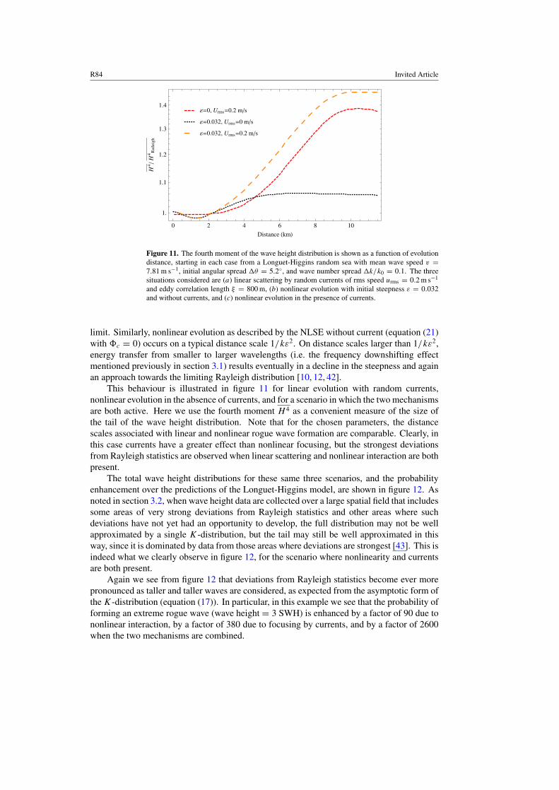
Figure 11. The fourth moment of the wave height distribution is shown as a function of evolutiondistance, starting in each case from a Longuet-Higgins random sea with mean wave speed v =7.81 m s−1, initial angular spread �θ = 5.2◦, and wave number spread �k/k0 = 0.1. The threesituations considered are (a) linear scattering by random currents of rms speed urms = 0.2 m s−1

and eddy correlation length ξ = 800 m, (b) nonlinear evolution with initial steepness ε = 0.032and without currents, and (c) nonlinear evolution in the presence of currents.

limit. Similarly, nonlinear evolution as described by the NLSE without current (equation (21)with �c = 0) occurs on a typical distance scale 1/kε2. On distance scales larger than 1/kε2,energy transfer from smaller to larger wavelengths (i.e. the frequency downshifting effectmentioned previously in section 3.1) results eventually in a decline in the steepness and againan approach towards the limiting Rayleigh distribution [10, 12, 42].

This behaviour is illustrated in figure 11 for linear evolution with random currents,nonlinear evolution in the absence of currents, and for a scenario in which the two mechanismsare both active. Here we use the fourth moment H 4 as a convenient measure of the size ofthe tail of the wave height distribution. Note that for the chosen parameters, the distancescales associated with linear and nonlinear rogue wave formation are comparable. Clearly, inthis case currents have a greater effect than nonlinear focusing, but the strongest deviationsfrom Rayleigh statistics are observed when linear scattering and nonlinear interaction are bothpresent.

The total wave height distributions for these same three scenarios, and the probabilityenhancement over the predictions of the Longuet-Higgins model, are shown in figure 12. Asnoted in section 3.2, when wave height data are collected over a large spatial field that includessome areas of very strong deviations from Rayleigh statistics and other areas where suchdeviations have not yet had an opportunity to develop, the full distribution may not be wellapproximated by a single K-distribution, but the tail may still be well approximated in thisway, since it is dominated by data from those areas where deviations are strongest [43]. This isindeed what we clearly observe in figure 12, for the scenario where nonlinearity and currentsare both present.

Again we see from figure 12 that deviations from Rayleigh statistics become ever morepronounced as taller and taller waves are considered, as expected from the asymptotic form ofthe K-distribution (equation (17)). In particular, in this example we see that the probability offorming an extreme rogue wave (wave height = 3 SWH) is enhanced by a factor of 90 due tononlinear interaction, by a factor of 380 due to focusing by currents, and by a factor of 2600when the two mechanisms are combined.

Invited Article R85

0 1 2 3 410−7

10−5

0.001

0.1

Wave Height SWH

Cum

ulat

ive

Prob

abili

ty

e =0.032, Urms=0.2 m/s

e =0.032, Urms=0 m/s

e =0, Urms=0.2 m/s

e =0, Urms=0 m/s

0.0 0.5 1.0 1.5 2.0 2.5 3.0 3.51

100

104

106

Wave Height SWH

Enh

ance

men

tin

Prob

abili

ty

ε=0.032, Urms=0.2 m/s

ε=0.032, Urms=0 m/s

ε=0, Urms=0.2 m/s

Figure 12. Left panel: the cumulative distribution of wave heights, in units of the SWH, is obtainedfor the same three scenarios as are considered in figure 11. In each case, the solid curve is a fitto a K-distribution with (a) N = 16 for linear scattering by currents, (b) N = 29 for nonlinearevolution, and (c) N = 5.1 when linear and nonlinear focusing are acting in concert. The Rayleighdistribution (N = ∞) is shown for reference. Right panel: in each of the three scenarios, theprobability enhancement factor Ptotal(H)/PRayleigh(H) is obtained from the data.

5. Conclusions and outlook

It will take some time to sort out the mechanisms of rogue wave formation with completecertainty. All potentially important factors and mechanisms ought to be included in thediscourse, which we hope will someday lead to agreement about the several formationmechanisms and their interactions. More importantly, predictive tools leading to safernavigation should eventually emerge. One of the seemingly important factors, which mightbe called ‘statistical focusing’, is highlighted here. In terms of wave propagation, statisticalfocusing is a linear effect (although it is nonlinear dynamics at the level of ray tracing). Itleads to large enhancements in the frequency of rogue wave formation under reasonable seastate assumptions.

Statistical focusing combines the effects of deterministic wave refraction by currenteddies with Longuet-Higgins statistical ideas under realistic conditions. The key notionis that the focusing effects of eddies, which would be very dramatic on an (unrealistic)monochromatic and unidirectional sea, are not altogether washed out when realistic frequencyand directional dispersion are included. Essentially, deterministic caustics present in theunrealistic idealization are smoothed into hot spots, which are then treated statistically withinLonguet-Higgins theory. The hot spots dominate the statistics in the tail of the wave heightdistribution. This amounts to a nonuniform sampling version of Longuet-Higgins theory, witha solid basis for the nonuniform energy density distributions used.

Since nonlinear effects are also important, we have examined them alone within thepopular fourth-order nonlinear Schrodinger equation (NLSE) approximation for nonlinearwave evolution under realistic seaway conditions. Finally, we have investigated the combinedeffect of nonlinear wave evolution and statistical focusing. We find that strongest deviationsfrom Rayleigh statistics are observed when linear scattering (statistical focusing) and nonlinearinteraction (NLSE) are both present. However, for the parameters chosen here at least, thelinear scattering due to eddies was more important than the nonlinear effects, which requirelarge steepness or a very narrow range of propagation directions to become significant.

We have presented a measure closely related to the probability of rogue wave formation,the freak index γ . This could conceivably become the basis for a probabilistic forecast ofrogue wave formation, in the spirit of rainfall forecasts.

R86 Invited Article

There are at least three clear directions for future development of the work presentedhere. First, both the computer simulations and the theory must be developed further to explorefully and systematically the combined effects of nonlinear and linear focusing. This will alsoinvolve investigating in depth the underlying mechanism through which the formation of hotand cold spots is aided by nonlinear focusing. Secondly, a better understanding is needed ofthe stability of the hot spot patterns under slow changes in the current field or in the spectrumor directionality of the incoming sea. The strength of what might be called scintillation ortwinkling [25] in analogy with the case of light travelling through the atmosphere will haveimportant consequences for the predictive power of the model. Thirdly, and most importantly,there is a clear need to compare the model simulations with observations and experiments.Although comprehensive global data are not available at this point, it may be possible tocompare the results with local observations where data are more readily available, e.g. in theNorth Sea.

Whatever the final word is on rogue wave formation (or final words, because there maybe more than one mechanism), it must involve a reallocation of energy from a larger area to asmaller one. Waves cannot propagate and increase in height at no expense to their neighbours:the energy has to come from somewhere, and the effect must be to reduce the wave energysomewhere else. The focusing mechanism is clear in this respect: hot spots form and coldspots do too, according to a ray tracing analysis, maintaining energy balance [53].

Acknowledgments

This work was supported in part by the US NSF under Grant PHY-0545390.

References

[1] Trulsen K and Dysthe K B 1997 Proc. 21st Symp. on Naval Hydrodynamics (Trondheim, Norway) (Washington,DC: National Academy Press) p 550

[2] Dankert H, Horstmann J, Lehner S and Rosenthal W 2003 IEEE Trans. Geosci. Remote Sens. 41 1437[3] Schulz-Stellenfleth J and Lehner S 2004 IEEE Trans. Geosci. Remote Sens. 42 1149[4] Dysthe K B, Krogstad H E and Muller P 2008 Annu. Rev. Fluid Mech. 40 287[5] Mallory J K 1974 Int. Hydrog. Rev. 51 89[6] Kharif C and Pelinovsky E 2003 Eur. J. Mech. 22 603[7] Longuet-Higgins M S 1957 Phil. Trans. R. Soc. Lond. A 249 321[8] Forristall G Z 2000 J. Phys. Oceanogr. 30 1931[9] Onorato M, Osborne A R, Serio M, Cavaleri L, Brandini C and Stansberg C T 2004 Phys. Rev. E 70 067302

[10] Tanaka M 2001 J. Fluid. Mech. 444 199[11] Gibson R S and Taylor P H 2005 Appl. Ocean Res. 27 142[12] Gibson R S and Swan C 2007 Proc. R. Soc. A 463 21[13] White B S and Fornberg B 1998 J. Fluid. Mech. 355 113[14] Heller E J, Kaplan L and Dahlen A 2008 J. Geophys. Res. 113 C09023[15] Peregrine D H 1976 Adv. Appl. Mech. 16 9

Lavrenov I 1998 Natural Hazards 17 117Irvine D E and Tilley D G 1988 J. Geophys. Res. 93 15389Grundlingh M L 1994 AVISO Altimeter Newslett. 3

[16] Jannsen P and Alpers W 2006 Proc. SEASAR Workshop (Frascati, Italy) (23–26 January 2006) ESA SP-613[17] Schulz-Stellenfleth J, Konig T and Lehner S 2007 J. Geophys. Res. 112 C03019[18] Kaplan L 2002 Phys. Rev. Lett. 89 184103[19] Metzger J J, Fleischmann R and Geisel T 2010 Phys. Rev. Lett. 105 020601[20] Tucker M J and Pitt E G 2001 Waves in Ocean Engineering (Ocean Engineering Book Series vol 5) (Amsterdam:

Elsevier) p 521[21] Berry M V 2005 New J. Phys. 7 129

Berry M V 2007 Proc. R. Soc. A 463 3055

Invited Article R87

[22] Dobrokhotov S Y, Sekerzh-Zenkovich S Y, Tirozzi B and Tudorovskii T Y 2006 Dokl. Math. 74 592[23] Topinka M A, LeRoy B J, Westervelt R M, Shaw S E J, Fleischmann R, Heller E J, Maranowski K D and

Gossard A C 2001 Nature 410 183Jura M P, Topinka M A, Urban L, Yazdani A, Shtrikman H, Pfeiffer L N, West K W and Goldhaber-Gordon D

2007 Nature Phys. 3 841[24] Wolfson M and Tomsovic S 2001 J. Acoust. Soc. Am. 109 2693[25] Berry M V 1977 J. Phys. A: Math. Gen. 10 2061[26] Wilkinson M, Mehlig B and Bezuglyy V 2006 Phys. Rev. Lett. 97 048501[27] Hohmann R, Kuhl U, Stockmann H-J, Kaplan L and Heller E J 2010 Phys. Rev. Lett. 104 093901[28] Kaplan L 1999 Nonlinearity 12 R1

Smith A M and Kaplan L 2009 Phys. Rev. E 80 035205(R)[29] Backer A and Schubert R 2002 J. Phys. A: Math. Gen. 35 527[30] Regev A, Agnon Y, Stiassnie M and Gramstad O 2008 Phys. Fluids 20 112102[31] Jakeman E and Pusey P N 1978 Phys. Rev. Lett. 40 546[32] Mirlin A 2000 Phys. Rep. 326 259[33] Damborsky K and Kaplan L 2005 Phys. Rev. E 72 066204[34] Stocker J R and Peregrine D H 1999 J. Fluid Mech. 399 335[35] Weidman J A C and Herbst B M 1986 SIAM J. Numer. Anal. 23 485[36] Zakharov V E 1968 J. Appl. Mech. Tech. Phys. 2 190[37] Dysthe K B 1979 Proc. R. Soc. A 369 105[38] Trulsen K and Dysthe K B 1996 Wave Motion 24 281[39] Trulsen K and Dysthe K B 1997 J. Fluid Mech. 352 359[40] Lake B M, Yuen H C, Rungaldier H and Ferguson W E 1977 J. Fluid Mech. 83 49[41] Segur H, Henderson D, Carter J D, Hammack J, Li C, Pheiff D and Socha K 2005 J. Fluid Mech. 539 229[42] Janssen T T and Herbers T H C 2009 J. Phys. Oceanogr. 39 1948[43] Ying L H and Kaplan L 2011 Systematic study of rogue wave probability distributions in a fourth-order nonlinear

Schrodinger equation (in preparation)[44] Benjamin T B and Feir J E 1967 J. Fluid Mech. 27 417[45] Onorato M, Osborne A R and Serio M 2002 Phys. Fluids 14 L25[46] Dysthe K B 2001 Proc. Rogue Waves 2000 (Brest, France) (Brest, France: Ifremer) p 255[47] Socquet-Juglard H, Dysthe K B, Trulsen K, Krogstad H E and Liu J 2005 J. Fluid Mech. 542 195[48] Gramstad O and Trulsen K 2007 J. Fluid Mech. 582 463[49] Clamond D and Grue J 2002 C. R. Mec. 330 575[50] Henderson K L, Peregrine D H and Dold J W 1999 Wave Motion 29 341[51] Tanaka M 1990 Wave Motion 12 559[52] Zakharov V E, Dyachenko A I and Prokofiev A O 2006 Eur. J. Mech. B 25 667[53] Bretherton F P and Garrett C J R 1968 Proc. R. Soc. A 302 529