Nonlinear Model Reduction for CFD Problems Using Local Reduced Order Bases

Nonlinear Model Reduction for CFD Problems Using

Local Reduced Order Bases

Kyle Washabaugh∗, David Amsallem†, Matthew Zahr‡, and Charbel Farhat§

Stanford University, Stanford, CA, 94305-3035, USA

A model reduction framework based on the concept of local reduced-order bases is

presented. The offline phase of the method builds the local reduced-order bases using an

unsupervised learning algorithm. In the online phase of the method, the choice of the

local basis is based on the current state of the system. Inexpensive rank-one updates to

the local bases are performed during the online phase for increased accuracy. Applications

to nonlinear CFD simulations show that the method is effective in producing small and

accurate reduced order models.

I. Introduction

Although computational fluid dynamics (CFD) models are typically high-dimensional, the trajectoriesof these models are often confined to low-dimensional affine subspaces. For this reason, CFD models are anideal candidate for Model Order Reduction (MOR) methods.

In most MOR methods, the dimension of the system is reduced by projecting the equations of thehigh-dimensional model (HDM) onto the low-dimensional subspace spanned by its trajectories. Using thisapproach, it is possible to greatly reduce the number of degrees of freedom in the model while retaining theaccuracy of the original HDM.1–6

Typically, this low-order projection subspace is represented by a reduced-order basis (ROB), and the stateof the HDM is formed as a linear combination of these basis vectors. The resulting reduced-order model(ROM) can produce accurate responses within the projection subspace; however, a fundamental trade-off isthat the ROM will never be able to explore portions of the state-space outside this subspace. This meansthat the performance of the ROM is ultimately decided by the quality of the ROB.

When a single ROB is used to reduce the dimension of an HDM, it must capture the dynamics of theHDM along the entire trajectory of interest. This can result in a very large ROB, and thus an inefficientreduced order model – an issue that is especially troublesome for design applications, where the ROB needsto capture the dynamics of the HDM at multiple design points.

The MOR method introduced in [7] alleviates this problem through the use of multiple local ROBs. Inthis approach, a local ROB is selected at each time step of the ROM simulation based on the current stateof the system. Ideally, each local ROB captures only the local dynamics at a given point of the state-space,resulting in small and accurate models. Such a concept is particularly well-suited for the proper orthogonaldecomposition (POD) method in which the ROB is built from snapshots of the system taken at variouslocations of the state-space.

This local ROB approach takes advantage of the fact that the state-space of a nonlinear dynamicalsystem can often be partitioned into distinct characteristic regimes. In the context of CFD simulations,these state-space partitions could distinguish, for example, between solutions that are dominated by laminarvs. turbulent flow, subsonic vs. supersonic flow, or transient vs. limit-cycle behavior. As the state of the

∗Graduate Student, Department of Aeronautics and Astronautics, William F. Durand Building, Room 028, Stanford Uni-versity, Stanford, CA 94305-3035; AIAA Member

†Engineering Research Associate, Department of Aeronautics and Astronautics, William F. Durand Building, Room 028A,Stanford University, Stanford, CA 94305-3035; AIAA Member

‡Graduate Student, Institute of Computational and Mathematical Engineering, William F. Durand Building, Room 028,Stanford University, Stanford, CA 94305-3035

§Vivian Church Hoff Professor of Aircraft Structures, Department of Aeronautics and Astronautics, William F. DurandBuilding, Room 257, Stanford University, Stanford, CA 94305-3035; AIAA Fellow

1 of 16

American Institute of Aeronautics and Astronautics

system transitions from one regime to another during a ROM simulation, an appropriate local ROB can bechosen that best captures the physics of the current system, and omits information that is not immediatelyrelevant.

In this work, the local ROB method originally presented in [7] is extended to a three-dimensional CFDproblem, and the details of constructing accurate local ROBs are discussed at length. To this effect, this paperis organized as follows: The underlying principles of the local ROB method are presented in Section II, thedetails of the offline and online portions of the method are discussed in Sections III and IV, and applicationsto two nonlinear CFD systems are presented in Section V.

II. Model Reduction Based on Local Reduced-Order Bases

Consider a set of nonlinear Ordinary Differential Equations (ODEs) arising, for instance, from the dis-cretization in space of a space-time Partial Differential Equation (PDE):

dw(t)dt

= f(w(t), t,µ)w(0) =w0,

(1)

where t ≥ 0 denotes time, w(t) ∈ Rn denotes the fluid state vector of dimension n, µ ∈ Rd denotes a vector ofparameters defining the operating point of the system of interest, and f ∶ Rn ×R×Rd → R

n is the nonlinearflux function containing the semi-discrete counterparts of the convective and diffusive fluxes.

When Eq. (1) is solved by an implicit time-integrator, the state w(i) at time t(i),0 ≤ i ≤ Nt, can becomputed as the solution to a system of discrete nonlinear equations, which are represented here as anonlinear residual

r(i)(w(i),µ) = 0. (2)

When an iterative procedure such as the Newton-Raphson method is used to solve this nonlinear system,w(i,l) denotes the computed solution at the l-th iteration of the i-th time step, t(i).

The main assumption made in reduced-order modeling is that the state solution w belongs to an affinesubspace of Rn, the dimension k of that subspace being typically orders of magnitude smaller than n. Whena single ROB V ∈ Rn×k is used to reduce the system, this one ROB must capture all of the relevant physicsof the HDM (2). For a complex system this can result in a very large basis, and thus a slow ROM.

As suggested in [7], this shortcoming of global ROBs can be overcome by selecting an appropriate local

ROB at each time step of the ROM simulation. Since each local ROB needs only to capture a subset of thephysics exhibited by the HDM, this allows the use of smaller ROBs for a given accuracy.

At a given time iteration i, it is therefore proposed to search for a solution w(i) under the form

w(i) =w(i−1) +V(w(i−1))∆w(i)

k(w(i−1))(3)

whereV(w(i−1)) ∈ Rn×k(w(i−1)) denotes a local ROB that is chosen based on the state w(i−1), and ∆w(i)

k(w(i−1))

denotes the vector of unknowns that contains the increments of the generalized coordinates in the basisV(w(i−1)). The notation k(w(i−1)) emphasizes that each local basis may have a different size.

In practice, a set of NV local reduced-order bases is pre-computed and each basis V(w(i−1)) is chosenwithin this set. In the remainder of this paper, {Ij}NV

j=1 denotes the set of indices i ∈ {1,⋯,Nt} such that

V(w(i−1)) =Vj and k(w(i−1)) = kj . Using this notation, if i ∈ Ij , Eq. (3) can be rewritten as

w(i) =w(i−1) +Vj∆w(i)kj

. (4)

Substituting Eq. (4) into the nonlinear system Eq. (2) results in the following system of n nonlinear

equations in terms of kj variables ∆w(i)kj

,

r(i)(w(i−1) +Vj∆w(i)kj

,µ) = 0. (5)

2 of 16


Once an appropriate local ROB has been chosen, the above system of nonlinear equations can be solvedin a least squares sense by considering the following problem,

min∆w

(i)

kj∈Rkj

∥r(i)(w(i−1) +Vj∆w(i)kj

,µ)∥2. (6)

The next two sections of this paper are concerned with the details of solving Eq. (6); Section III discussesthe offline construction of the local ROBs, {Vj}NV

j=1 , and Section IV discusses the online solution to Eq. (6)

using an iterative Gauss-Newton procedure.6, 8

III. Offline Phase: Construction of the Local ROB Database

In practice, the set of reduced bases {Vj}NV

j=1 is built using a POD algorithm based on the method

of snapshots.9 These snapshots {ys}Nsnaps

s=1 are typically based on pre-computed states {ws}Nsnaps

s=1 of theHDM (2), where Nsnaps ≤Nt.

The proposed method for constructing a database of local ROBs consists of three steps. First, the states

{ws}Nsnaps

s=1 are clustered into NV subsets using an unsupervised learning algorithm, such as the k-meansalgorithm. Second, the clusters are made to overlap with one another by sharing a small number of states

between neighboring clusters. Third, the snapshots {ys}Nsnaps

s=1 are formed from the state clusters and theindividual local ROBs are computed. These three steps are detailed below.

A. Clustering of Pre-Computed Solutions

In this work, the k-means algorithm is used to partition the pre-computed states {ws}Nsnaps

s=1 ⊂ {w(i)}Nt

i=0 intoNV clusters.7 This choice of algorithm is shown to work well for the applications in Section V; however, anyother clustering algorithm could be substituted here with only minor changes to the method.

More important than the choice of algorithm is the choice of distance metric used to compare states. Thechoice of distance metric is fundamental to the local ROM method, and affects both the offline and onlineresults. In this work, the distance metric used for both the partitioning of the pre-computed states as wellas the online choice of ROB is chosen as

d (wi,wj) = ∥wi −wj∥2. (7)

REMARK: This definition of distance has been shown to work well for a simple one dimensional fluidproblem and a fluid-structure-electric interaction problem;7 however, it may not be the best choice for allproblems. For systems that exhibit strongly periodic behavior, it may be more appropriate to choose adistance metric that relies on the frequency content of the states, or possibly an output quantity of interest,such as lift or drag for aeronautical applications.

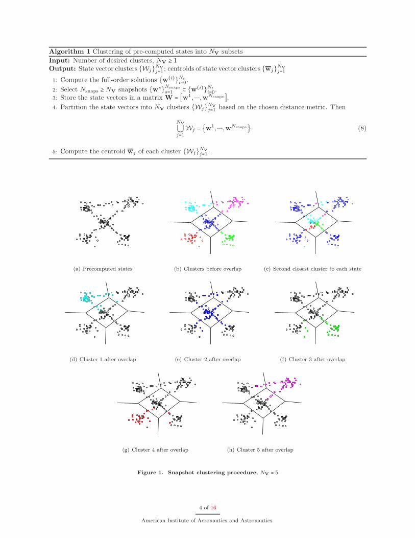
The process of clustering the pre-computed states is summarized in Algorithm 1. To illustrate thealgorithm, a set of states as well the corresponding clusters and state-space partitioning are depicted inFig. 1 (a)-(b).

B. Overlap of Snapshot Clusters

As suggested in [7], cluster overlap can be introduced by adding near-by states to each cluster. This ensuresthat there are no “gaps” between clusters, reducing the error when the state trajectory transitions from onecluster to another. In this paper, a new method is proposed for introducing overlap.

The proposed method is a two-step approach: the connectivity of the clusters is first established, and aspecified number of snapshots are then shared between neighboring clusters. In this section, it is assumedthat the clusters have been generated with a k-means algorithm; substituting a different clustering algorithmwould require slight modifications to the approach presented below.

Here, two clusters are said to be connected if their respective centroids are the two closest to any of

the pre-computed states {ws}Nsnaps

s=1 . With this definition, the cluster connectivity can be established byiterating through the pre-computed states, identifying the two closest cluster centroids to each, and markingthe corresponding pair of clusters as neighbors. This corresponds to lines 1 to 3 in Algorithm 2, and isdepicted in Fig. 1 (c), where states are colored according to the second nearest cluster center.

3 of 16


Algorithm 1 Clustering of pre-computed states into NV subsets

Input: Number of desired clusters, NV ≥ 1Output: State vector clusters {Wj}NV

j=1 ; centroids of state vector clusters {wj}NV

j=1

1: Compute the full-order solutions {w(i)}Nt

i=0.

2: Select Nsnaps ≥ NV snapshots {ws}Nsnaps

s=1 ⊂ {w(i)}Nt

i=0.3: Store the state vectors in a matrix W = [w1,⋯,wNsnaps].4: Partition the state vectors into NV clusters {Wj}NV

j=1 based on the chosen distance metric. Then

NV⋃j=1

Wj = {w1,⋯,wNsnaps} (8)

5: Compute the centroid wj of each cluster {Wj}NV

j=1 .

(a) Precomputed states (b) Clusters before overlap (c) Second closest cluster to each state

(d) Cluster 1 after overlap (e) Cluster 2 after overlap (f) Cluster 3 after overlap

(g) Cluster 4 after overlap (h) Cluster 5 after overlap

Figure 1. Snapshot clustering procedure, NV = 5

4 of 16


The advantage of this method is that any two clusters with states near their common boundary are likelyto be identified as neighbors. Consequently, if the trajectory of the training simulation crosses a clusterboundary, it is likely that the two clusters sharing this boundary will be identified as neighbors. In practice,this method is somewhat conservative; two clusters that are near one another in state space but unrelatedin the training trajectory are not always identified as neighbors. This proves to be a desirable feature whenattempting to reproduce the training trajectory with the ROM, but it may be necessary to share states fromall adjacent clusters for parametric applications.

After the cluster connectivity has been established, the overlap algorithm then iterates through theclusters and identifies which states should be added from each neighboring cluster. In this work, each clusteris enlarged by a set percentage (typically r = 10%) by adding an equal number of states from each of itsneighbors. The algorithm shares the states that are nearest to the boundary between the cluster and itsneighbor. This step corresponds to lines 4 to 13 in Algorithm 2 and its result is depicted in Fig. 1 (d)-(h).

Note that the cluster centers are not updated when overlap is introduced. The cluster centers define thepartitioning of the state-space, and the intent of adding overlap is to improve the performance of the localROBs near the boundaries of each cluster, not to alter the partitioning of the state-space.

Algorithm 2 Introduce overlap into state clusters

Input: State clusters {Wj}NV

j=1 ; state cluster centroids {wj}NV

j=1 ; threshold r

Output: Overlapping state clusters {Wj}NV

j=1

1: for s = 1,⋯,Nsnaps do

2: Identify the two nearest clusters centroids to state ws and mark these clusters as neighbors3: end for

4: for j = 1,⋯,NV do

5: Let Nsnaps,j denote the number of states in cluster j, and Nneighbors,j the number of its neighboringclusters

6: Wj =Wj

7: Calculate the number Nadd,j of states to add from each neighbor of Wj as Nadd,j = ceil ( Nsnaps,j×r

Nneighbors,j)

8: for i = 1,⋯,NV do

9: if i is a neighbor to j then10: Find the Nadd,j states nearest to their common boundary and add these to Wj

11: end if

12: end for

13: end for

C. Local ROB Construction

After forming the overlapping state clusters {wj}NV

j=1 , the set of reduced bases {Vj}NV

j=1 is built using a POD

algorithm based on the method of snapshots.9 These snapshots Yj = {ysj}Nsnaps,j

s=1 are typically formed by

subtracting reference states {wref,j}NV

j=1 from the raw states Wj = {wsj}Nsnaps,j

s=1 . The offline procedure forconstructing a database of local ROBs by POD is summarized in Algorithm 3.

In practice, the choice of the reference states {wref,j}NV

j=1 has an impact on the performance of the resultingROBs. In the following discussion, it is argued that a particular choice of reference condition is the mostappropriate for local ROBs.

To gain insight into this matter of snapshot reference conditions for offline ROB construction, considerthe subsequent online ROM simulation using the pre-computed local ROBs. At any time iteration i beforethe ROM switches from the first local ROB V1 to the second local ROB V2, w

(i) can be expressed in termsof the initial solution, w(0), as follows

w(i) =w(0) +V1

i∑p=1

∆w(p)k1

. (10)

5 of 16


Algorithm 3 Construction of a set of local reduced bases

Input: Number NV ≥ 1 of pre-computed bases, corresponding sets of state clusters {Wj}NV

j=1 , reference states

{wref,j}NV

j=1

Output: Local POD bases {Vj}NV

j=1 , corresponding singular values and right vectors {Σj}NV

j=1 and

{Zj}NV

j=1

1: for j = 1,⋯,NV do

2: Subtract the reference state wref,j from the states Wj = {wsj}Nsnaps,j

s=1 to form the snapshots Yj ={ys

j}Nsnaps,j

s=1 .3: Store the snapshots Yj in a matrix Yj .4: Compute a singular value decomposition

Yj =UΣZT . (9)

5: Choose a dimension kj ≤ Nsnaps,j for the j-th reduced basis6: Truncate the first kj left components to obtain the reduced-order basis Vj = U(∶,1 ∶ kj), singular

values Σj =Σ(1 ∶ kj ,1 ∶ kj), and right singular vectors Zj = Z(∶,1 ∶ kj), such that Yj ≈VjΣjZTj .

7: end for

For the purposes of this discussion, it is helpful to slightly rearrange Eq. (10) as

w(i) −w(0) =V1

i∑p=1

∆w(p)k1

. (11)

Examining Eq. (11), the quantities w(i) −w(0) are constrained to lie in the subspace spanned by V1. Itfollows that, for this ROM to be accurate, V1 must be a good approximation of the subspace spanned by thecorresponding iterates of the HDM. If the basis V1 is formed using Algorithm 3 without truncation, that iskj =Nsnaps,j , then there are several choices of snapshot reference condition that could be appropriate; how-ever, when truncation is present, it is postulated that V1 will best approximate this subspace if constructedfrom snapshots of the type ys

1 = ws1 −w(0). In practice, it has been observed10, 11 that, for global ROMs,

this choice does indeed lead to more accurate reduced models than the common choice ys1 =ws

1 or the choiceys1 =ws

1 −ws−11 presented in [6].

Consider now a later time step i from this same online local ROM simulation after the second localROB V2 has been selected. Here, m denotes the iteration at which this second local ROB was first selected.At this time step, the counterpart to Eq. (10) is then

w(i) =w(0) +V1 ∑1≤p≤m−1

∆w(p)k1+V2 ∑

m≤p≤i

∆w(p)k2

. (12)

Since w(m−1) =w(0) +V1 ∑1≤p≤m−1

∆w(p)k1

, the counterpart of Eq. (11) is then

w(i) −w(m−1) =V2 ∑m≤p≤i

∆w(p)k2

. (13)

Appealing to the same logic as before, it appears that the second local ROB V2 should be constructed fromsnapshots of the type ys

2 =ws2 −w(m−1).

Generalizing this observation, it is expected that a given local ROB Vj will perform well online ifconstructed from snapshots of the type ys

j = wsj −wswitch,j, where wswitch,j denotes the state of the system

when the ROM switches to basis Vj . Unfortunately, this reference condition wswitch,j is not known at thetime of the ROB construction, and additionally, if a basis is used more than once by the simulation it wouldneed to be referenced with two different states.

The novel approach proposed in this paper is to first construct a database of local ROBs offline usingsome reference states {wref,j}NV

j=1 , and to then perform inexpensive rank-one updates to the local ROBs onlinewhen wswitch,j is known. In this paper, the initial condition of the online simulation is used as the referencestate wref,j for all clusters j = 1,⋯,NV, ensuring that the first local ROB does not need to be updated

6 of 16


online; however, for parametric applications it could prove beneficial to use the centroids of the clusters asthe reference state, since the cluster centers should be closer to wswitch,j than the initial condition. Thisrepresents a topic for future investigation.

After constructing the local ROB database using Algorithm 3 with reference snapshots {wref,j}NV

j=1 ,

range(Vj) ⊂ span({wsj −wref,j}Nsnaps,j

s=1 ) = range (Yj) , (14)

where the columns of Yj contain the snapshots wsj − wref,j. During the online ROM simulation, when a

new basis Vj is selected, a local ROB update is then performed using the state wswitch,j . The goal of the

proposed approach is to compute a modified local ROB Vj such that

range(Vj) ⊂ span({wsj −wswitch,j}Nsnaps,j

s=1 ) = range(Yj) , (15)

where the columns of Yj contain the snapshots wsj − wswitch,j . Yj and Yj are therefore related by the

identityYj =Yj + (wref,j −wswitch,j)1T , (16)

where T denotes the transpose operator and 1 is a vector of ones which has the dimension of the number ofsnapshots in Yj . Hence, Yj is a rank-one update matrix to Yj . Since the basis Vj is constructed by a POD

that involves a Singular Value Decomposition (SVD) of the matrix Yj , the fast algorithm for updating an

SVD developed in [12] is used for a fast update of the local ROB Vj . This is described in Algorithm 4.

Algorithm 4 Online Update to Local ROB Vj , j ∈ {1,⋯,NV}Input: Original SVD Yj ≈ VjΣjZ

Tj , Vj ∈ Rn×kj , Σj ∈ Rkj×kj , Qj = ZT

j 1 ∈ Rkj , qj = ∥1 − ZjQj∥2, originalreference state wref,j , online state wswitch,j

Output: Updated local ROB Vj

1: Compute a =wref,j −wswitch,j ∈ Rn

2: Compute m =VTj a ∈ Rkj

3: p = a −Vjm ∈ Rn

4: Ra = ∣∣p∣∣25: p = p/Ra

6: K = [Σj 0

0 0] + [m

Ra

] [Qj

qj]T

∈ R(kj+1)×(kj+1)

7: Compute the SVD of K =C S DT , where C,S,D ∈ R(kj+1)×(kj+1)

8: Compute Vj = [Vj p]C ∈ Rn×(kj+1)

9: Let Vj = Vj(∶,1 ∶ kj)REMARK 1: Algorithm 4 performs an exact SVD update on a low rank approximation to the snapshot

matrix Yj . As a result, the modified basis Vj is an approximation to the exact basis that would have been

computed using the true snapshot matrix Yj . The error introduced due to this approximation is studied forthe one-dimensional Burgers’ equation in Section V.A.

REMARK 2: One of the main benefits of using local ROBs is that the bases can be of varying sizes;however, picking each of these sizes by hand quickly becomes impractical as the number of bases grows. Inthis work, the local ROBs sizes are chosen based on the decay of the singular values, and are constrained tofall between an upper and lower bound. For the applications in this paper, this method yielded appropriatelysized local ROBs without requiring significant assistance.

IV. Online Phase: Simulation of the Reduced-Order Model Using Local Bases

After constructing the local ROBs {Vj}NV

j=1 offline, these bases are used to solve a sequence of minimizationproblems of the form (6) during the online ROM simulation. At every time step, the appropriate ROB isdetermined by computing the distance of the current state to the cluster centers and selecting the local ROBthat corresponds to the closest cluster center.

The approach proposed here is identical to the approach of [7], except that every time a new ROB isselected it is updated online using Algorithm 4. This procedure is summarized in Algorithm 5.

7 of 16


Algorithm 5 Solution of Eq. (6) by the Gauss-Newton procedure

Input: Previous solution w(i−1), set of local ROBs {Vj}NV

j=1 , previous ROB V

Outputs: Solution w(i)

1: Choose a local model j based on the distances between the cluster centroids and the current state, w(i−1)

2: If the ROB j differs from the one used at the previous iteration i − 1, update the ROB Vj using

Algorithm 4 and obtain the modified ROB V = Vj , otherwise use the modified ROB V used at theprevious iteration

3: Let w(i,0) =w(i−1) and ∆w(i,0)kj= 0

4: for l = 0,⋯, (until convergence) do5: Compute r(i,l) = r(i)(w(i,l),µ).6: Evaluate J(i,l) = ∂r(i)

∂w(w(i,l),µ)

7: Compute W(i,l)j = J(i,l)V

8: Compute the thin QR decomposition W(i,l)j =Q(i,l)R(i,l)

9: Solve R(i,l)p(i,l) = −Q(i,l)T r(i,l)10: Compute a step α(i,l) by a line-search procedure (or use the Newton step and set α(i,l) = 1)11: Update ∆w

(i,l+1)kj

=∆w(i,l)kj+ α(i,l)p(i,l)

12: Update w(i,l+1) =w(i,I) + V∆w(i,l+1)kj

13: end for

14: Let w(i) =w(i,l)

REMARK 1: Since the distances from the current state to each of the cluster centers are computed atevery time step, it is important that these distance calculations be computationally efficient. It is shownin [7] that, using the distance metric defined in Eq. (7), it is possible to compute distances with a complexitythat does not depend on the dimension n of the large-scale underlying model. Similarly, in the proposedapproach with updated local ROBs, it can be shown that the same low complexity can be achieved.

REMARK 2: In Eq. (6), the number of unknowns has been reduced through the introduction of a localROB for the state. In spite of this, the computational cost associated with solving this system of equationsvia Algorithm 5 is still comparable to the cost of solving the high-fidelity model as it requires the evaluationof the full-order residual and Jacobian r(i)(w(i,l),µ) and J(i)(w(i,l),µ) at each Newton iteration. It hasbeen shown in [7] that the computational cost of Algorithm 5 can be greatly reduced using hyper-reduction,that is, by introducing an additional level of approximation. The local ROB update procedure outlined inAlgorithm 4 in Section III.C requires full state vectors and therefore has a complexity that scales with thedimension n of the underlying HDM. As a result, it cannot be extended to the online phase of the localhyper-reduction as is. Future work will focus on adapting this approach to hyper-reduction.

V. Applications

A. One dimensional Burgers’ Equation

1. High-Dimensional Model

The first system of interest originates from the inviscid Burgers’ equation

∂W

∂t+W ∂W

∂x= g(x, t), x ∈ [0,1], 0 ≤ t,

W (x,0) = 1, W (0, t) =√5,

(17)

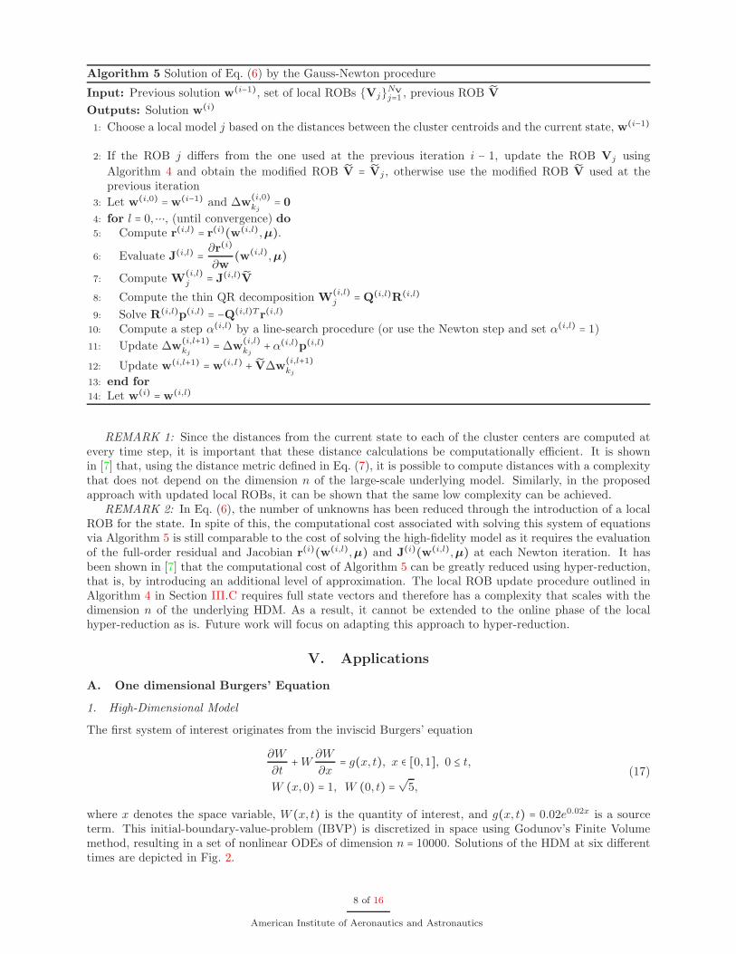
where x denotes the space variable, W (x, t) is the quantity of interest, and g(x, t) = 0.02e0.02x is a sourceterm. This initial-boundary-value-problem (IBVP) is discretized in space using Godunov’s Finite Volumemethod, resulting in a set of nonlinear ODEs of dimension n = 10000. Solutions of the HDM at six differenttimes are depicted in Fig. 2.

8 of 16


0 10 20 30 40 50 60 70 80 90 1001

1.5

2

2.5

3

3.5

4

4.5

x

w

t = 2.5

t = 10

t = 20

t = 30

t = 40

t = 50

Figure 2. HDM solution of the inviscid Burgers’ equation

2. Clustering Results

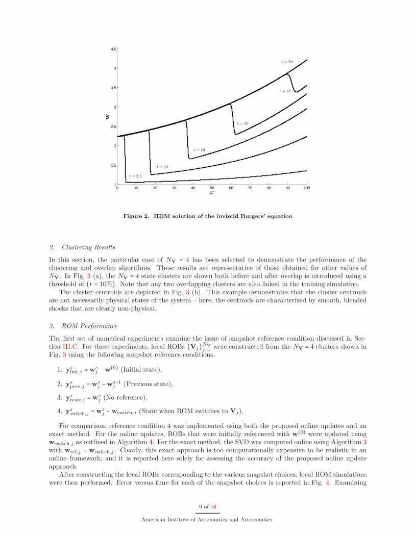
In this section, the particular case of NV = 4 has been selected to demonstrate the performance of theclustering and overlap algorithms. These results are representative of those obtained for other values ofNV. In Fig. 3 (a), the NV = 4 state clusters are shown both before and after overlap is introduced using athreshold of (r = 10%). Note that any two overlapping clusters are also linked in the training simulation.

The cluster centroids are depicted in Fig. 3 (b). This example demonstrates that the cluster centroidsare not necessarily physical states of the system – here, the centroids are characterized by smooth, blendedshocks that are clearly non-physical.

3. ROM Performance

The first set of numerical experiments examine the issue of snapshot reference condition discussed in Sec-tion III.C. For these experiments, local ROBs {Vj}NV

j=1 were constructed from the NV = 4 clusters shown inFig. 3 using the following snapshot reference conditions,

1. ysinit,j =ws

j −w(0) (Initial state),

2. ysprev,j =ws

j −ws−1j (Previous state),

3. ysnone,j =ws

j (No reference),

4. ysswitch,j =ws

j −wswitch,j (State when ROM switches to Vj).

For comparison, reference condition 4 was implemented using both the proposed online updates and anexact method. For the online updates, ROBs that were initially referenced with w(0) were updated usingwswitch,j as outlined in Algorithm 4. For the exact method, the SVD was computed online using Algorithm 3with wref,j = wswitch,j . Clearly, this exact approach is too computationally expensive to be realistic in anonline framework, and it is reported here solely for assessing the accuracy of the proposed online updateapproach.

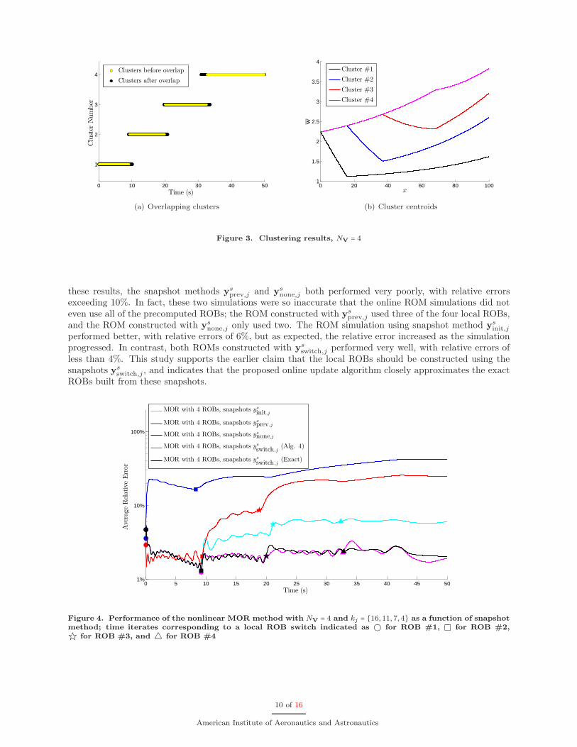
After constructing the local ROBs corresponding to the various snapshot choices, local ROM simulationswere then performed. Error versus time for each of the snapshot choices is reported in Fig. 4. Examining

9 of 16


0 10 20 30 40 50

1

2

3

4

Time (s)

Clu

ster

Num

ber

Clusters before overlap

Clusters after overlap

(a) Overlapping clusters

0 20 40 60 80 1001

1.5

2

2.5

3

3.5

4

x

w

Cluster #1

Cluster #2

Cluster #3

Cluster #4

(b) Cluster centroids

Figure 3. Clustering results, NV = 4

these results, the snapshot methods ysprev,j and ys

none,j both performed very poorly, with relative errorsexceeding 10%. In fact, these two simulations were so inaccurate that the online ROM simulations did noteven use all of the precomputed ROBs; the ROM constructed with ys

prev,j used three of the four local ROBs,and the ROM constructed with ys

none,j only used two. The ROM simulation using snapshot method ysinit,j

performed better, with relative errors of 6%, but as expected, the relative error increased as the simulationprogressed. In contrast, both ROMs constructed with ys

switch,j performed very well, with relative errors ofless than 4%. This study supports the earlier claim that the local ROBs should be constructed using thesnapshots ys

switch,j , and indicates that the proposed online update algorithm closely approximates the exactROBs built from these snapshots.

0 5 10 15 20 25 30 35 40 45 501%

10%

100%

Time (s)

Ave

rage

Relat

ive

Err

or

MOR with 4 ROBs, snapshots ys

init,j

MOR with 4 ROBs, snapshots ysprev,j

MOR with 4 ROBs, snapshots ysnone,j


switch ,j(Alg. 4)


switch ,j(Exact)

Figure 4. Performance of the nonlinear MOR method with NV = 4 and kj = {16,11,7,4} as a function of snapshotmethod; time iterates corresponding to a local ROB switch indicated as ◯ for ROB #1, ◻ for ROB #2,☆ for ROB #3, and △ for ROB #4

10 of 16


In Fig. 5, solutions computed with ysswitch,j (Online Updates) and ys

init,j are presented for comparison.These two ROM simulations use the same local ROBs; the only difference being that the ys

switch,j simulationperforms online updates to the local ROBs using Algorithm 4. Examining the results in Fig. 5, the simulationwith the online updates is able to achieve better accuracy than the simulation without updates – especiallyat the end of the simulation.

0 10 20 30 40 50 60 70 80 90 1000.5

1

1.5

2

2.5

3

3.5

4

4.5

x

w

HDM


init,j


switch ,j(Alg. 4)

Figure 5. Performance of the local ROMs with kj = {20,14,10,4} and NV = 4 for snapshot methods ysinit,j

and

ysswitch,j

(Algorithm 4)

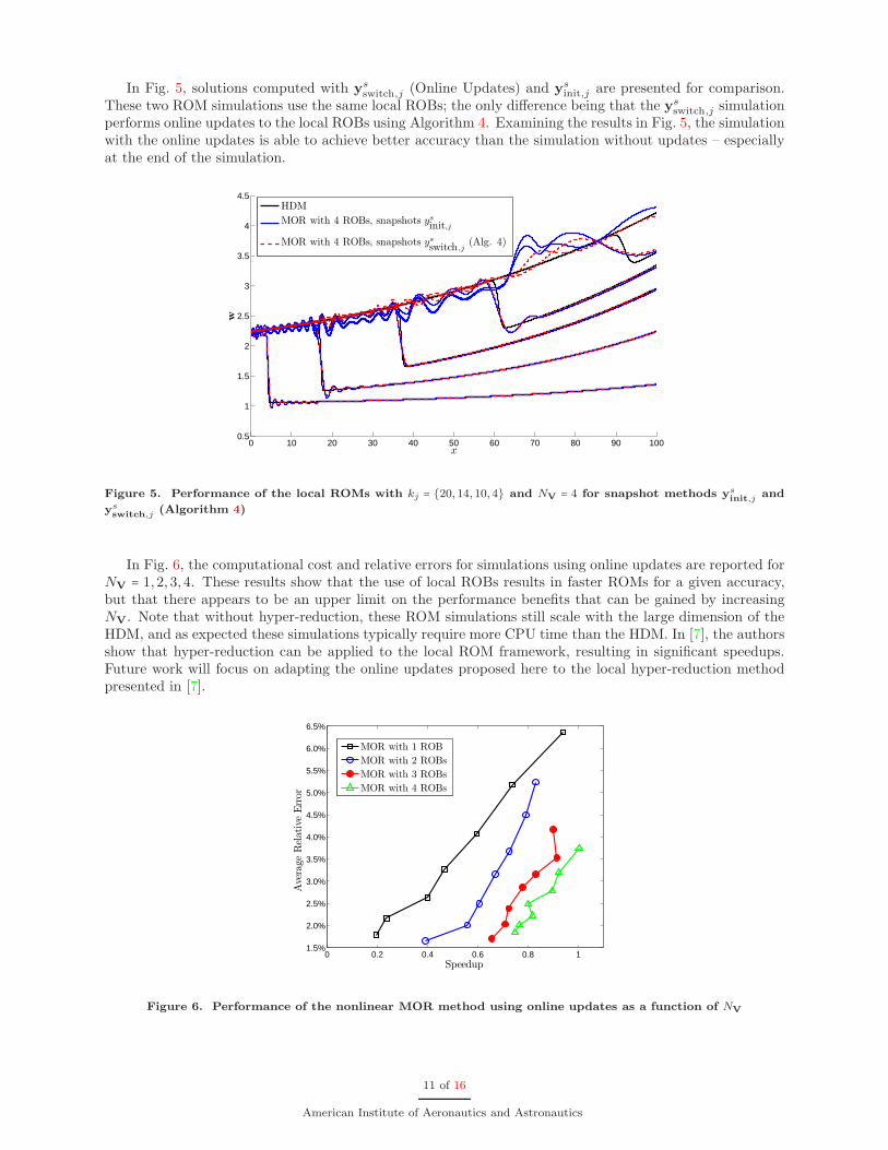
In Fig. 6, the computational cost and relative errors for simulations using online updates are reported forNV = 1,2,3,4. These results show that the use of local ROBs results in faster ROMs for a given accuracy,but that there appears to be an upper limit on the performance benefits that can be gained by increasingNV. Note that without hyper-reduction, these ROM simulations still scale with the large dimension of theHDM, and as expected these simulations typically require more CPU time than the HDM. In [7], the authorsshow that hyper-reduction can be applied to the local ROM framework, resulting in significant speedups.Future work will focus on adapting the online updates proposed here to the local hyper-reduction methodpresented in [7].

0 0.2 0.4 0.6 0.8 11.5%

2.0%

2.5%

3.0%

3.5%

4.0%

4.5%

5.0%

5.5%

6.0%

6.5%

Speedup

Ave

rage

Relat

ive

Err

or

MOR with 1 ROB

MOR with 2 ROBs

MOR with 3 ROBs

MOR with 4 ROBs

Figure 6. Performance of the nonlinear MOR method using online updates as a function of NV

11 of 16


B. Acceleration Study of a Transport Aircraft

1. High-Dimensional Model

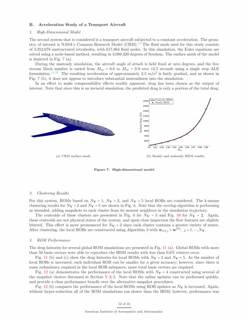
The second system that is considered is a transport aircraft subjected to a constant acceleration. The geom-etry of interest is NASA’s Common Research Model (CRM).13 The fluid mesh used for this study consistsof 3,252,078 unstructured tetrahedra, with 617,864 fluid nodes. In this simulation, the Euler equations aresolved using a node-based method, resulting in 3,089,320 degrees of freedom. The surface mesh of the modelis depicted in Fig. 7 (a).

During the unsteady simulation, the aircraft angle of attack is held fixed at zero degrees, and the freestream Mach number is varied from M∞ = 0.8 to M∞ = 0.9 over 12.5 seconds using a single step ALEformulation.14, 15 The resulting acceleration of approximately 2.5 m/s2 is fairly gradual, and as shown inFig. 7 (b), it does not appear to introduce substantial unsteadiness into the simulation.

In an effort to make compressibility effects readily apparent, drag has been chosen as the output ofinterest. Note that since this is an inviscid simulation, the predicted drag is only a portion of the total drag.

(a) CRM surface mesh

0.8 0.81 0.82 0.83 0.84 0.85 0.86 0.87 0.88 0.89

6000

7000

8000

9000

10000

11000

12000

13000

14000

M∞

Invi

scid

Dra

g(lbf)

Unsteady HDMSteady HDM

(b) Steady and unsteady HDM results

Figure 7. High-dimensional model

2. Clustering Results

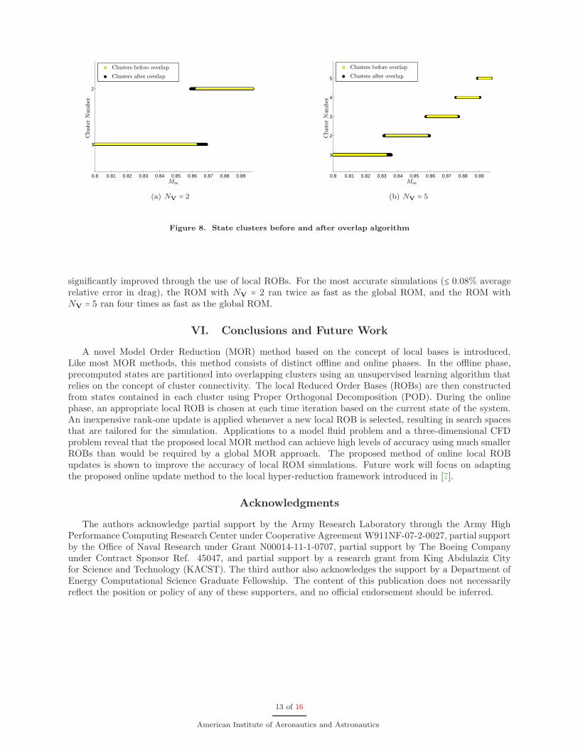
For this system, ROMs based on NV = 1, NV = 2, and NV = 5 local ROBs are considered. The k-meansclustering results for NV = 2 and NV = 5 are shown in Fig. 8. Note that the overlap algorithm is performingas intended, adding snapshots to each cluster from its nearest neighbors in the simulation trajectory.

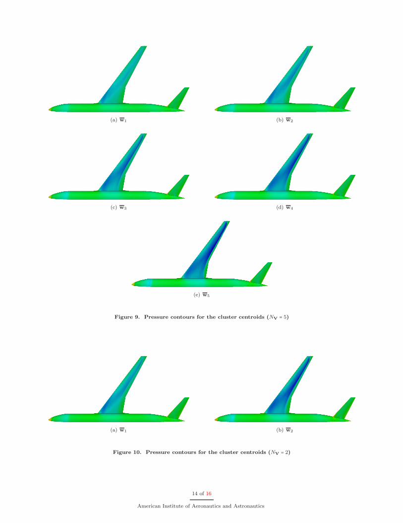
The centroids of these clusters are presented in Fig. 9 for NV = 5 and Fig. 10 for NV = 2. Again,these centroids are not physical states of the system, and upon close inspection the flow features are slightlyblurred. This effect is more pronounced for NV = 2 since each cluster contains a greater variety of states.After clustering, the local ROBs are constructed using Algorithm 3 with wref,j =w(0), j = 1,⋯,NV.

3. ROM Performance

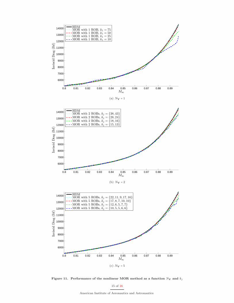
The drag histories for several global ROM simulations are presented in Fig. 11 (a). Global ROMs with morethan 50 basis vectors were able to reproduce the HDM results with less than 0.6% relative error.

Fig. 11 (b) and (c) show the drag histories for local ROMs with NV = 2 and NV = 5. As the number oflocal ROBs is increased, each individual ROB can be smaller for a given accuracy; however, since there issome redundancy required in the local ROB subspaces, more total basis vectors are required.

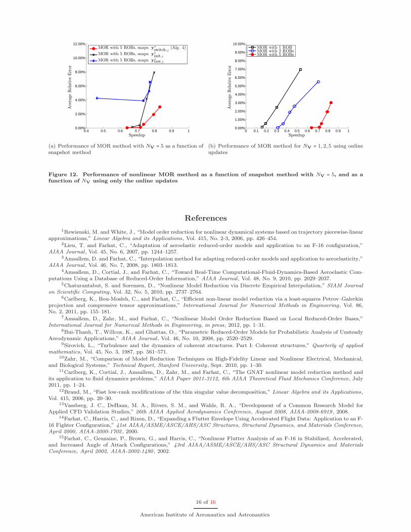
Fig. 12 (a) demonstrates the performance of the local ROMs with NV = 4 constructed using several ofthe snapshot choices discussed in Section V.A.3. Note that the online updates can be performed quickly,and provide a clear performance benefit over the alternative snapshot procedures.

Fig. 12 (b) compares the performance of the local ROMs using ROB updates as NV is increased. Again,without hyper-reduction all of the ROM simulations ran slower than the HDM; however, performance was

12 of 16


0.8 0.81 0.82 0.83 0.84 0.85 0.86 0.87 0.88 0.89

1

2

M∞

Clu

ster

Num

ber



(a) NV = 2

0.8 0.81 0.82 0.83 0.84 0.85 0.86 0.87 0.88 0.89

1

2

3

4

5

M∞

Clu

ster

Num

ber



(b) NV = 5

Figure 8. State clusters before and after overlap algorithm

significantly improved through the use of local ROBs. For the most accurate simulations (≤ 0.08% averagerelative error in drag), the ROM with NV = 2 ran twice as fast as the global ROM, and the ROM withNV = 5 ran four times as fast as the global ROM.

VI. Conclusions and Future Work

A novel Model Order Reduction (MOR) method based on the concept of local bases is introduced.Like most MOR methods, this method consists of distinct offline and online phases. In the offline phase,precomputed states are partitioned into overlapping clusters using an unsupervised learning algorithm thatrelies on the concept of cluster connectivity. The local Reduced Order Bases (ROBs) are then constructedfrom states contained in each cluster using Proper Orthogonal Decomposition (POD). During the onlinephase, an appropriate local ROB is chosen at each time iteration based on the current state of the system.An inexpensive rank-one update is applied whenever a new local ROB is selected, resulting in search spacesthat are tailored for the simulation. Applications to a model fluid problem and a three-dimensional CFDproblem reveal that the proposed local MOR method can achieve high levels of accuracy using much smallerROBs than would be required by a global MOR approach. The proposed method of online local ROBupdates is shown to improve the accuracy of local ROM simulations. Future work will focus on adaptingthe proposed online update method to the local hyper-reduction framework introduced in [7].

Acknowledgments

The authors acknowledge partial support by the Army Research Laboratory through the Army HighPerformance Computing Research Center under Cooperative Agreement W911NF-07-2-0027, partial supportby the Office of Naval Research under Grant N00014-11-1-0707, partial support by The Boeing Companyunder Contract Sponsor Ref. 45047, and partial support by a research grant from King Abdulaziz Cityfor Science and Technology (KACST). The third author also acknowledges the support by a Department ofEnergy Computational Science Graduate Fellowship. The content of this publication does not necessarilyreflect the position or policy of any of these supporters, and no official endorsement should be inferred.

13 of 16


(a) w1 (b) w2

(c) w3 (d) w4

(e) w5

Figure 9. Pressure contours for the cluster centroids (NV = 5)

(a) w1 (b) w2

Figure 10. Pressure contours for the cluster centroids (NV = 2)

14 of 16


0.8 0.81 0.82 0.83 0.84 0.85 0.86 0.87 0.88 0.89

6000

7000

8000

9000

10000

11000

12000

13000

14000

M∞

Invi

scid

Dra

g(lbf)

HDMMOR with 1 ROB, k1 = 75MOR with 1 ROB, k1 = 50MOR with 1 ROB, k1 = 25MOR with 1 ROB, k1 = 10

(a) NV = 1

0.8 0.81 0.82 0.83 0.84 0.85 0.86 0.87 0.88 0.89

6000

7000

8000

9000

10000

11000

12000

13000

14000

M∞

Invi

scid

Dra

g(lbf)

HDMMOR with 2 ROBs, kj = {38, 43}MOR with 2 ROBs, kj = {28, 24}MOR with 2 ROBs, kj = {18, 16}MOR with 2 ROBs, kj = {15, 13}

(b) NV = 2

0.8 0.81 0.82 0.83 0.84 0.85 0.86 0.87 0.88 0.89

6000

7000

8000

9000

10000

11000

12000

13000

14000

M∞

Invi

scid

Dra

g(lbf)

HDMMOR with 5 ROBs, kj = {22, 11, 9, 17, 16}MOR with 5 ROBs, kj = {17, 8, 7, 10, 10}MOR with 5 ROBs, kj = {12, 6, 5, 7, 7}MOR with 5 ROBs, kj = {10, 5, 5, 6, 6}

(c) NV = 5

Figure 11. Performance of the nonlinear MOR method as a function NV and kj

15 of 16


0.4 0.5 0.6 0.7 0.8 0.9 10.00%

2.00%

4.00%

6.00%

8.00%

10.00%

12.00%

Speedup

Ave

rage

Relat

ive

Err

or

MOR with 5 ROBs, snaps. ys

switch ,j(Alg. 4)

MOR with 5 ROBs, snaps. ys

init,j

MOR with 5 ROBs, snaps. ysraw,j

(a) Performance of MOR method with NV = 5 as a function ofsnapshot method

0 0.1 0.2 0.3 0.4 0.5 0.6 0.7 0.8 0.9 10.00%

1.00%

2.00%

3.00%

4.00%

5.00%

6.00%

7.00%

8.00%

9.00%

10.00%

Speedup

Ave

rage

Relat

ive

Err

or

MOR with 1 ROBMOR with 2 ROBsMOR with 5 ROBs

(b) Performance of MOR method for NV = 1,2,5 using onlineupdates

Figure 12. Performance of nonlinear MOR method as a function of snapshot method with NV = 5, and as afunction of NV using only the online updates

References

1Rewienski, M. and White, J., “Model order reduction for nonlinear dynamical systems based on trajectory piecewise-linearapproximations,” Linear Algebra and its Applications, Vol. 415, No. 2-3, 2006, pp. 426–454.

2Lieu, T. and Farhat, C., “Adaptation of aeroelastic reduced-order models and application to an F-16 configuration,”AIAA Journal , Vol. 45, No. 6, 2007, pp. 1244–1257.

3Amsallem, D. and Farhat, C., “Interpolation method for adapting reduced-order models and application to aeroelasticity,”AIAA Journal , Vol. 46, No. 7, 2008, pp. 1803–1813.

4Amsallem, D., Cortial, J., and Farhat, C., “Toward Real-Time Computational-Fluid-Dynamics-Based Aeroelastic Com-putations Using a Database of Reduced-Order Information,” AIAA Journal , Vol. 48, No. 9, 2010, pp. 2029–2037.

5Chaturantabut, S. and Sorensen, D., “Nonlinear Model Reduction via Discrete Empirical Interpolation,” SIAM Journalon Scientific Computing , Vol. 32, No. 5, 2010, pp. 2737–2764.

6Carlberg, K., Bou-Mosleh, C., and Farhat, C., “Efficient non-linear model reduction via a least-squares Petrov–Galerkinprojection and compressive tensor approximations,” International Journal for Numerical Methods in Engineering , Vol. 86,No. 2, 2011, pp. 155–181.

7Amsallem, D., Zahr, M., and Farhat, C., “Nonlinear Model Order Reduction Based on Local Reduced-Order Bases,”International Journal for Numerical Methods in Engineering, in press, 2012, pp. 1–31.

8Bui-Thanh, T., Willcox, K., and Ghattas, O., “Parametric Reduced-Order Models for Probabilistic Analysis of UnsteadyAerodynamic Applications,” AIAA Journal , Vol. 46, No. 10, 2008, pp. 2520–2529.

9Sirovich, L., “Turbulence and the dynamics of coherent structures. Part I: Coherent structures,” Quarterly of appliedmathematics, Vol. 45, No. 3, 1987, pp. 561–571.

10Zahr, M., “Comparison of Model Reduction Techniques on High-Fidelity Linear and Nonlinear Electrical, Mechanical,and Biological Systems,” Technical Report, Stanford University , Sept. 2010, pp. 1–30.

11Carlberg, K., Cortial, J., Amsallem, D., Zahr, M., and Farhat, C., “The GNAT nonlinear model reduction method andits application to fluid dynamics problems,” AIAA Paper 2011-3112, 6th AIAA Theoretical Fluid Mechanics Conference, July2011, pp. 1–24.

12Brand, M., “Fast low-rank modifications of the thin singular value decomposition,” Linear Algebra and its Applications,Vol. 415, 2006, pp. 20–30.

13Vassberg, J. C., DeHaan, M. A., Rivers, S. M., and Wahls, R. A., “Development of a Common Research Model forApplied CFD Validation Studies,” 26th AIAA Applied Aerodynamics Conference, August 2008, AIAA-2008-6919 , 2008.

14Farhat, C., Harris, C., and Rixen, D., “Expanding a Flutter Envelope Using Accelerated Flight Data: Application to an F-16 Fighter Configuration,” 41st AIAA/ASME/ASCE/AHS/ASC Structures, Structural Dynamics, and Materials Conference,April 2000, AIAA-2000-1702 , 2000.

15Farhat, C., Geuzaine, P., Brown, G., and Harris, C., “Nonlinear Flutter Analysis of an F-16 in Stabilized, Accelerated,and Increased Angle of Attack Configurations,” 43rd AIAA/ASME/ASCE/AHS/ASC Structural Dynamics and MaterialsConference, April 2002, AIAA-2002-1490 , 2002.

16 of 16


Nonlinear Model Reduction for CFD Problems Using Local Reduced Order Bases

Documents

Transcript of Nonlinear Model Reduction for CFD Problems Using Local Reduced Order Bases