Reduced NO formation models for CFD simulations of MILD1

combustion2

Chiara Gallettia,∗, Marco Ferrarottia, Alessandro Parenteb,∗, Leonardo Tognottia3

aDipartimento di Ingegneria Civile e Industriale - Universita di Pisa4

bService d Aero-Thermo-Mecanique, Universite Libre de Bruxelles, Bruxelles, Belgium5

Abstract6

Two reduced kinetic models, incorporating thermal, N2O, NNH as well as HNO/NO2 in-

termediate routes, are proposed for the quick evaluation of NO emissions from MILD com-

bustion of H2-enriched fuels through post-processing of Computational Fluid Dynamics

simulations. The models were derived from a Rate Of Production Analysis carried out with

two different detailed kinetic schemes. The models were tested using data from the Ade-

laide Jet in Hot Coflow burner fed with CH4/H2 mixture and operated with three different

O2 contents. Very satisfactory predictions of in-flame NO measurements were achieved for

the three cases, indicating a good applicability of the models across a wide range of MILD

combustion conditions. Significant impact of the NNH intermediate path was observed.

Keywords: flameless combustion; NNH; Computational Fluid Dynamics;7

turbulence-chemistry interaction; hydrogen8

1. Introduction9

MILD (Moderate or Intense Low-Oxygen Combustion) combustion, also known as flame-10

less combustion is able to provide high combustion efficiency with low NOx and soot emis-11

sions [1]. The technology needs the reactants to be preheated above their self-ignition12

temperature and enough inert combustion products to be entrained in the reaction region,13

in order to dilute both reactants and flame. The system is characterized by a more uniform14

temperature field than in traditional non-premixed combustion, and by the absence of high15

temperature peaks, thus suppressing NO formation through the thermal mechanism. The16

technology shows common features with High Temperature Air Combustion (HiTAC) due17

to the common practice of preheating the oxidizer. MILD combustion is very stable and18

noiseless, so it is potentially suited for gas turbine applications. Recently it has also been19

∗Corresponding authors. Dr. Chiara Galletti, email:chiara.galletti@ing.unipi.it. Dr. Alessandro Parente,email: Alessandro.Parente@ulb.ac.bePreprint submitted to International Journal of Hydrogen Energy November 20, 2014

suggested for oxy-fuel combustion, a technology able to provide a step-wise reduction of20

greenhouse gases emissions through the CO2 capture and storage (CCS). However what21

makes such technology very attractive is the large fuel flexibility, being suited for low-BTU22

fuels [2], industrial wastes [3], biogas [4] [5] as well as in presence of hydrogen.23

H2-enriched fuels have received attention as they may be obtained from the gasifica-24

tion of solid fuels, including biomasses; moreover H2-enriched mixtures represent some-25

times byproducts of industrial processes [3]. However, hydrogen shows some specific prop-26

erties (high laminar flame speed, high adiabatic flame temperature and heating value, large27

flammability range, high reactivity and short delay time) which make conventional burners28

unsuited: diffusive burners produce too large NOx emissions because of the very high tem-29

peratures, whereas premixed flames burners could suffer of stability problems and flashback30

phenomena. As a matter of fact, the use of MILD combustion technology appears particu-31

larly beneficial for controlling NOx formation, providing a manner to limit the reactivity of32

hydrogen-based fuels [6] [7] [8] [9] [10].33

The design of novel combustion technologies has taken advantages of recent progresses34

in Computational Fluid Dynamics (CFD) tools, offering considerable time and cost savings35

with respect to experimental campaigns as well as the possibility to be applied directly to36

the scale of interest. Turbulent combustion modelling of practical systems involves often37

heavy computational grids to describe burners, gas turbines, furnace/boilers, etc., so that38

Favre-averaged Navier-Stokes (FANS) equations are usually formulated to make the calcu-39

lations affordable even with parallel computing. In this framework, different sub-models40

(e.g. turbulence model, combustion model/kinetic scheme) are needed for closure; such41

models have been derived for conventional combustion and need to be validated/revised for42

novel technologies. Hence, many efforts have been done in recent years to improve CFD43

predictivity for MILD combustion systems by validating/revising the different sub-models.44

Logically, this issue requires high fidelity and comprehensive experimental data to val-45

idate the numerical models. The Adelaide Jet in Hot Coflow (JHC) burner [11] [12] [13]46

[14] and the Delft Jet in Hot Coflow (DJHC) burner [15] [16] [17] have been developed on47

purpose to emulate MILD combustion conditions by feeding diluted and hot streams, and48

constitute a strong asset for the validation of numerical models as they have been equipped49

with advanced diagnostics to measure mean and fluctuating variables (e.g. chemical species,50

temperature, velocities). As a matter of fact, they have been objective of numerous mod-51

2

elling works, especially aimed at validating the turbulence/chemistry interaction treatment52

and kinetic schemes (e.g. [18] [19] [20] [21] [22] [23] [24] [25] [26]), as well as the use of more53

complex modelling approaches based on Large Eddy Simulations (e.g.[27] [28] [29]).54

Recently a novel methodology to evaluate the chemical time-scale in case of complex55

kinetic schemes was proposed and applied to JHC experimental data, indicating that the56

Damkohler number, which is given by the mixing to chemical time-scale ratio, approaches57

unity, i.e. Da = τm/τc ≈ 1 [30]. This implies a strong coupling between mixing and chem-58

ical kinetics resulting in a very challenging problem. Indeed, many investigators observed59

satisfactory performance of the Eddy Dissipation Concept (EDC) [31] [32] to treat the tur-60

bulence/chemistry interaction in MILD combustion conditions, especially for its capability61

to incorporate efficiently detailed kinetic schemes [18] [26] [24] [20] [23]; however modifica-62

tions of the EDC model have been suggested to improve prediction for both JHC [22] and63

DJHC [25] flames.64

Actually, little attention has been paid to the modelling of NOx emission, even though65

they constitute a main concern when addressing novel combustion technologies and espe-66

cially MILD combustion.67

From the modelling perspective, the description of NO formation in MILD combustion,68

requires the incorporation of additional mechanisms, beside the ones typically adopted for69

conventional combustion systems, i.e. thermal and prompt. The low-temperature operation70

of MILD combustion systems inhibits NOx formation via the thermal-NO mechanism with71

respect to conventional combustion [33] [34] and increases the importance of alternative72

formation routes, such as the Fenimores prompt NO [35] and/or N2O intermediate mecha-73

nisms. Prompt NO are formed by the reaction of atmospheric nitrogen with hydrocarbon74

radicals with the consecutive oxidation of the intermediate species to NO. This mechanism75

becomes significant in particular combustion environments, such as in low-temperature,76

fuel rich conditions and short residence time. Malte and Pratt [36] proposed the first NO77

formation mechanism via the intermediate specie N2O. This mechanism, under favorable78

conditions such as elevated pressure, temperature below 1800 K and oxygen-rich conditions,79

can contribute as much as 90% of the total NO. Therefore this makes it particularly impor-80

tant in gas turbines and compression-ignition engines. Nicolle and Dagaut [37] investigated81

numerically MILD combustion of CH4 in perfecly stirred and plug flow reactors, i.e. PSRs82

and PFRs) and showed that the N2O pathway is fundamental in the post-ignition period .83

3

In presence of hydrogen, the NNH intermediate route [38] could be also important.84

Galletti et al. [6] evaluated NO emissions in a lab-scale burner operating in MILD combus-85

tion conditions and fed with CH4/H2 mixture and compared them to flue gas measurements,86

finding that the NNH intermediate and N2O were the main formation routes. The same con-87

clusion was drawn by Parente et al. [39] who evaluated NO emissions from a self-recuperative88

industrial burner fed with CH4/H2 mixture with different H2 content. Although results were89

satisfactory, the use of only flue gas measurements prevented from an accurate validation of90

the NO formation models, which were based on simple reaction schemes from literature.91

The JHC measurements [11] again may provide a strong asset for the validation and devel-92

opment of NO formation models to be used for MILD combustion systems, because of the93

availability of in-flame NO experimental data. Kim et al. [19] employed the Conditional Mo-94

ment Closure (CMC) method, by using a laminar flamelet model together with a presumed95

β-PDF for single mixture fraction to model the JHC. They evaluated NO emissions through96

thermal and prompt mechanisms but found some discrepancies, which they attributed to97

the poor performance of the overall model in predicting the mixing. Frassoldati et al. [23]98

applied a detailed Kinetic Post Processor to CFD simulations of CH4/H2 flames in the JHC,99

in order to compute NOx emissions. They observed a satisfactory overall agreement with100

experimental measurements, even though there were discrepancies between measured and101

predicted NO profiles downstream (i.e. at axial distances of 120 mm) which they attributed102

to the overestimation of the temperature field of ≈ 100 K, as well as near the flame axis.103

Importantly, they observed that in the near burner region, NO is formed through mainly104

NNH and N2O mechanisms, whereas the prompt NO formation takes place further away.105

The present paper aims at validating some simple existing NO formation schemes to106

be used for the practical simulations of MILD combustion systems as well as at developing107

new schemes suited for MILD conditions, also in presence of hydrogen. Attention is paid108

to computationally-affordable models as the idea is to use them for quick post-processing109

calculations of CFD results to be employed for the design of practical systems.110

The JHC burner fed with CH4/H2 mixture [11] is used as reference case. The first step111

is a good prediction of the thermochemical field in order to limit errors in NO calculations112

related to non-accurate temperature and species field. Hence, new comprehensive models113

for NOx formation in MILD combustion conditions are developed on the basis of Rate Of114

Production Analysis performed in a perfectly stirred reactor with detailed kinetics schemes.115

4

The performance of these model in predicting NOx emissions is compared to existing simple116

models as well as to the comprehensive model proposed by Loffler et al. [40].117

Gao et al. [41] carried out simulations of the JHC to investigate the mechanisms of NO118

formation in MILD combustion. NO production was accounted by including NO formation119

routes in the kinetic mechanism, i.e. GRI2.11, handled by the Eddy Dissipation Concept120

for turbulence/chemistry interactions. Such a modelling choice may be justified for MILD121

conditions, given the reduced importance of the thermal formation route, and the relevance122

of non conventional pathways, i.e. NNH, with characteristic formation times inherently123

coupled to the gas-phase chemistry. However, numerical results showed discrepancies with124

respect to experiments, likely to be attributed to the overestimation of the temperature field125

due to the non-optimal choice of the EDC constants (see discussion above).126

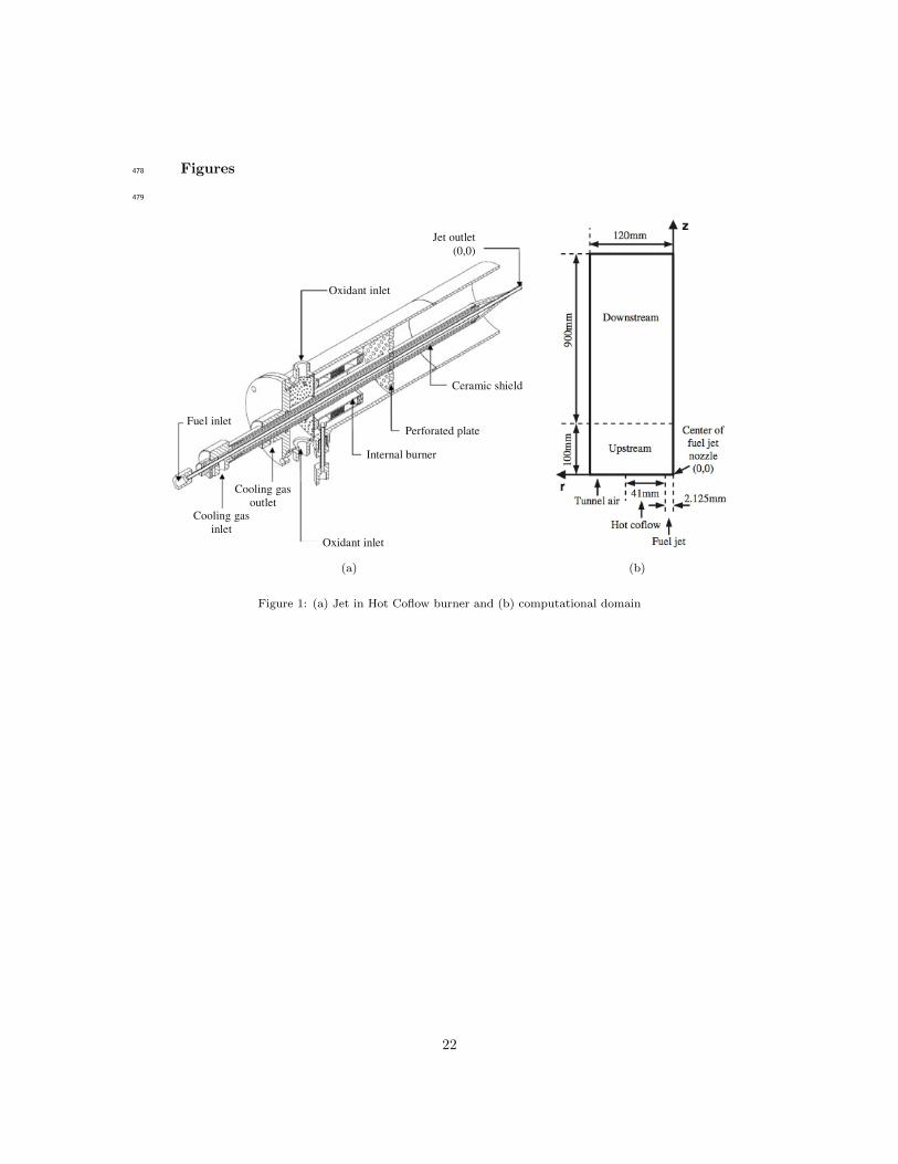
2. Test case127

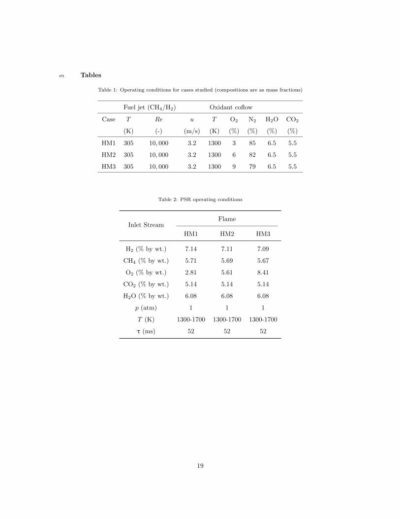
The Adelaide Jet in Hot Coflow burner modelled in this work has been experimentally128

studied by Dally et al. [11] and it is shown for sake of clarity in Figure 1a. It consists129

of a fuel jet nozzle, which has an inner diameter of 4.25 mm and a wall thickness of 0.2130

mm, located at the centre of a perforated disc in an annulus, with inner diameter of 82 mm131

and wall thickness of 2.8 mm, which provides nearly uniform composition of hot oxidizer132

coflow to the reaction zone. The entire burner was placed inside a wind tunnel introducing133

room temperature air at the same velocity as the hot coflow. Table 1 shows the operating134

conditions of three inlet streams for the different case studies. The notations, HM1, HM2135

and HM3, refer to the flames with oxygen mass fraction of 3%, 6%, and 9%, respectively,136

in the hot coflow stream. The jet Reynolds number was around 10,000 for all flames.137

The available data consist of the mean and root mean square (rms) of temperature and138

concentration of major (CH4, H2, H2O, CO2, N2 and O2) and minor species (NO, CO and139

OH). More details can be found in Dally et al.[11].140

3. Numerical model141

The numerical model of the burner is mainly based on previous works [26] [22], so only142

a brief description will be given here. The geometry of the JHC flames allowed to use143

a 2D axisymmetric domain, constructed starting from the burner exit (Figure 1b). The144

5

computational grid was structured with 73x340 (24 k), cells and is shown in Aminian et145

al. [26]. Steady-state FANS equations were solved with a finite volume scheme using the146

commercial CFD code ANSYS FLUENT R©. The κ− ε model using all standard constants,147

except for Cε1, which was set to 1.6 instead of 1.44 to compensate for the round-jet/plane-jet148

anomaly [42], was employed. Information on the performance of more turbulence models149

can be found in Aminian et al. [22]. The KEE-58 oxidation mechanism (17 species and 58150

reversible reactions) [43] was used to treat CH4/H2 oxidation, as it was found to provide151

satisfactory results for MILD combustion modeling [22] [39]. The interaction between turbu-152

lence and chemistry was handled through the EDC model [32]; however, in order to improve153

predictions, the fine structure residence time constant, which equals to Cτ = 0.4083, was154

set to Cτ = 1.5 [26] and [25]. The impact of such modification on predictions is discussed in155

Aminian et al.[22]. The discrete ordinate (DO) method together with the Weighted-Sum-156

of-Gray-Gases (WSGG) model with coefficients taken from Smith et al. [44] was employed157

to solve the radiative transfer equation (RTE) in 16 different directions across the computa-158

tional domain. A zero-shear stress wall was adopted at the side boundary, instead of a more159

realistic pressure inlet/outlet conditions, in order to facilitate calculations. However, as the160

tunnel air was considered wide enough, this boundary condition does not affect the flame161

structure [26]. NO entering with the coflow was considered, setting the boundary condition162

from experimental data profile of NO mass fraction taken close to the entrance, i.e. at axial163

coordinate z = 4 mm, [11]. Subsequently, other simulations were carried out imposing164

the experimental data profile at z = 4 mm of temperature and main species for the fuel165

jet and coflow, instead of the fixed values reported in Table 1. Uniform velocities were set166

for the unmixed fuel jet and coflow oxidizer and are reported in Table 1. The turbulence167

levels of all three inlet streams was adapted to better capture the development of the mixing168

layers[45] [23][26].169

3.1. NO formation models170

As mentioned in the introduction, the low mean and fluctuating temperatures of MILD171

combustion significantly modifies the NOx formation processwith respect to conventional172

combustion. Therefore, NO calculations were carried out by considering the N2O interme-173

diate and NNH routes in addition to the thermal and prompt formation mechanisms. Four174

different models were used, which are:175

6

1. model A - global schemes for thermal, prompt, N2O and NNH formation routes;176

2. model B - global scheme for prompt formation and comprehensive model from Loffler177

et al. [40];178

3. model C1 - global scheme for prompt formation and comprehensive model derived for179

JHC conditions on the basis of POLIMI kinetic scheme [46];180

4. model C2 - global scheme for prompt formation and comprehensive model derived for181

JHC conditions on the basis of Glarborg kinetic scheme [47].182

Model A considers global mechanisms for thermal, prompt, N2O and NNH formation routes.183

The thermal NO formation was evaluated from the Zeldovich mechanism as :184

d[NO]thermaldt

= kthermal[O][N2] (1)

The prompt NO formation is evaluated through a single-step global reaction mechanism185

suggested for methane [48]:186

d[NO]promptdt

= kprompt[O2]a[N2][F ] (2)

where F denotes the fuel. kprompt depends on the fuel and the oxygen reaction order a on187

oxygen mole fraction in flame [48]. The NO formation through intermediate specie N2O188

was determined according to Malte and Pratt [36] [49] as:189

d[NO]N2O

dt= 2(kN2O,f2[N2O][O]− kN2O,r2[NO]2) (3)

where190

[N2O] =2kN2O,f1[N2][O][M ] + kN2O,r2[NO]2

kN2O,r1[M ] + kN2O,f2[O](4)

The NNH route was not available in the code; therefore, it was implemented by means of a191

bespoke C subroutine following the global scheme proposed by Konnov [50].192

d[NO]NNHdt

= 2kNNH [N2][O]XH (5)

where kNNH = 2.3 10−15 exp−3600/T cm3 mol−1 s−1 and XH is the mole fraction of H193

atoms. All reaction rates are integrated over PDF of temperature to take into account the194

effect of turbulent fluctuations on formation rates.195

Model B was taken from Loffler et al. [40]. The model was derived for CH4/air flame in196

one-dimensional plug flow reactor (PFR) operating at ambient pressure and T = 1873 K197

7

and is based on 21 reversible reactions and on the quasi-steady state assumption for N, N2O,198

NNH and NH. The model includes thermal NO formation, N2O and NNH route; hence, the199

prompt NO route evaluated according to (2) is added to the model.200

Model C1 and model C2 were derived in the present work for the JHC conditions starting201

from the kinetic schemes of POLIMI [46] and Glarborg [47], respectively. The models are202

described in the following section.203

4. Development of C1 and C2 schemes for NO calculation204

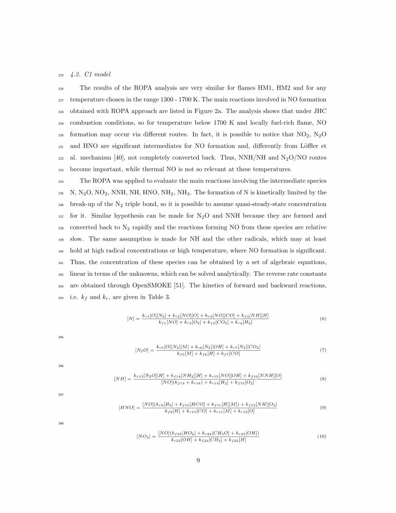
Two new reduced NO formation models are developed for the specific conditions of the205

Jet in Hot Coflow (JHC) burner, fed with a CH4/H2 mixture. Both models combine thermal206

NO formation, N2O/NO and NNH route. Prompt NO formation is neglected because it may207

be estimated very simply in a commercial CFD package.208

4.1. OpenSmoke model209

The first step to create a new comprehensive model is the evaluation of the main reactions210

leading to NO formation under MILD combustion conditions during the oxidation of the211

mixture. To do that, the open-source software OpenSMOKE [51] was used, since it is a212

collection of numerical tools for the kinetic analysis of reacting systems (ideal reactors,213

i.e. Plug Flow Reactors, batch, Perfectly Stirred Reactors, shock-tube; laminar flames, i.e.214

counter-flow diffusion flames, premixed flat flames, steady-state flamelets) with complex215

kinetic mechanisms. The oxidation of the fuel mixture has been investigated in a one-216

dimensional Perfectly Stirred Reactor (PSR) using two different detailed kinetic schemes:217

• POLIMI mechanism [52] (109 species and 1882 reactions).218

• Glarborg mechanism [47] (66 species and 449 reactions)219

The reaction conditions are listed in Table 2. The residence time τ, was estimated from the220

JHC CFD calculations as the time needed to reach the downstream location at z = 120 mm221

from the burner. For each run, temperature T and pressure p have been fixed inside PSR,222

so OpenSMOKE can linearize Arrhenius equations and carry out a sensitivity analysis of223

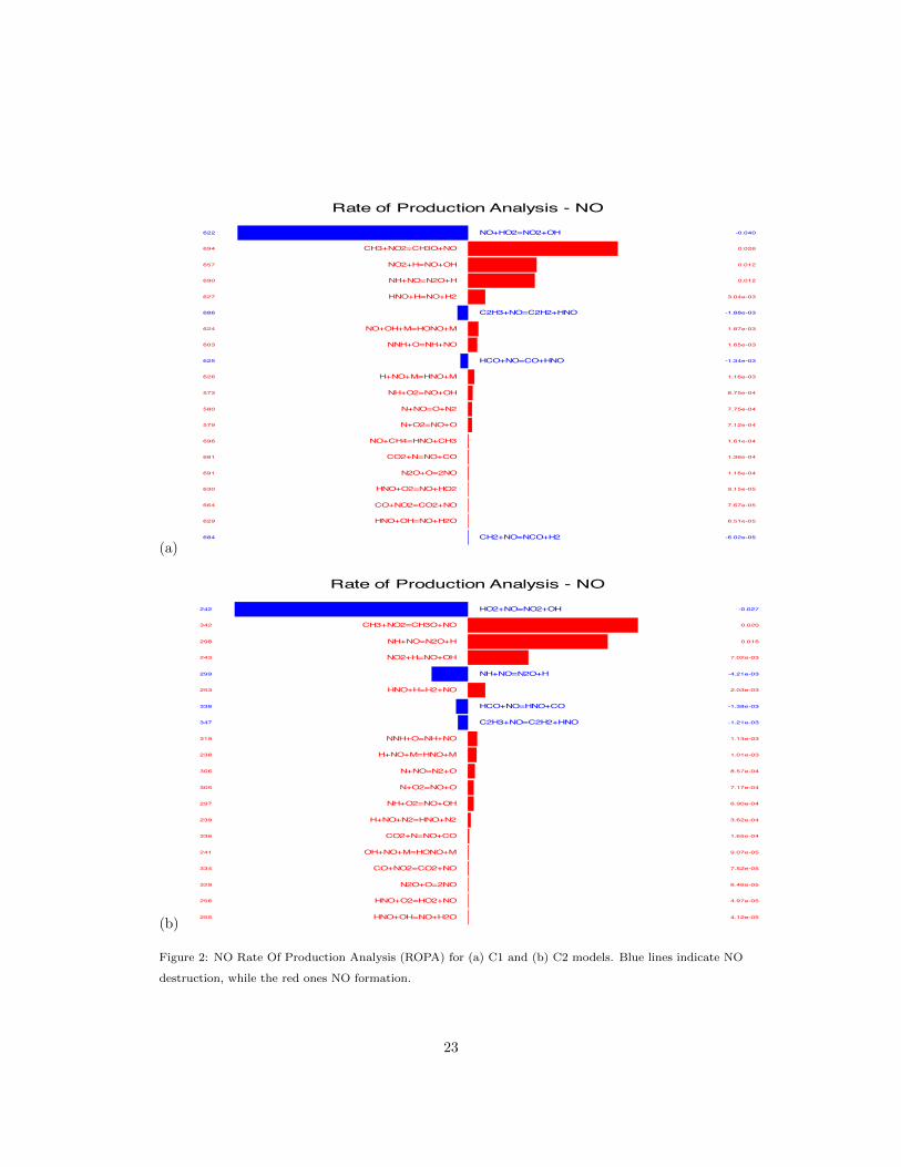
the main reactions taking place in the reactor (Rate Of Production Analysis, ROPA).224

8

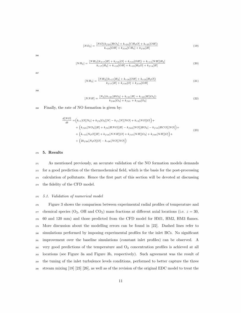
4.2. C1 model225

The results of the ROPA analysis are very similar for flames HM1, HM2 and for any226

temperature chosen in the range 1300 - 1700 K. The main reactions involved in NO formation227

obtained with ROPA approach are listed in Figure 2a. The analysis shows that under JHC228

combustion conditions, so for temperature below 1700 K and locally fuel-rich flame, NO229

formation may occur via different routes. In fact, it is possible to notice that NO2, N2O230

and HNO are significant intermediates for NO formation and, differently from Loffler et231

al. mechanism [40], not completely converted back. Thus, NNH/NH and N2O/NO routes232

become important, while thermal NO is not so relevant at these temperatures.233

The ROPA was applied to evaluate the main reactions involving the intermediate species234

N, N2O, NO2, NNH, NH, HNO, NH2, NH3. The formation of N is kinetically limited by the235

break-up of the N2 triple bond, so it is possible to assume quasi-steady-state concentration236

for it. Similar hypothesis can be made for N2O and NNH because they are formed and237

converted back to N2 rapidly and the reactions forming NO from these species are relative238

slow. The same assumption is made for NH and the other radicals, which may at least239

hold at high radical concentrations or high temperature, where NO formation is significant.240

Thus, the concentration of these species can be obtained by a set of algebraic equations,241

linear in terms of the unknowns, which can be solved analytically. The reverse rate constants242

are obtained through OpenSMOKE [51]. The kinetics of forward and backward reactions,243

i.e. kf and kr, are given in Table 3.244

[N ] =kr1[O][N2] + kr2[NO][O] + kr3[NO][CO] + kf4[NH][H]

kf1[NO] + kr2[O2] + kf3[CO2] + kr4[H2](6)

245

[N2O] =kr5[O][N2][M ] + kr6[N2][OH] + kr7[N2][CO2]

kf5[M ] + kf6[H] + kf7[CO](7)

246

[NH] =kr13[N2O][H] + kf14[NH2][H] + kr15[NO][OH] + kf16[NNH][O]

[NO](kf13 + kr16) + kr14[H2] + kf15[O2](8)

247

[HNO] =[NO](kr9[H2] + kf10[HCO] + kf11[H][M ]) + kf12[NH][O2]

kf9[H] + kr10[CO] + kr11[M ] + kr12[O](9)

248

[NO2] =[NO](kf23[HO2] + kr24[CH3O] + kr25[OH])

kr23[OH] + kf24[CH3] + kf25[H](10)

9

249

[NH2] =[NH3](kf17[H] + kf30[CH3] + kf19[OH]) + kr14[NH][H2]

kr17[H2] + kr30[CH4] + kr19[H2O] + kf14[H](11)

250

[NH3] =[NH2](kr17[H2] + kr30[CH4] + kr19[H2O])

kf17[H] + kf30[CH3] + kf19[OH](12)

251

[NNH] =[N2](kr20[HO2] + kr21[H] + kr22[H][O2])

kf20[O2] + kf21 + kf22[O2](13)

The concentrations of O2, N2, H2, H2O, O, H, OH, HO2, CH3, CH4, CO, CO2, HCO, CH2O252

are obtained from the gas-phase oxidation mechanism. Finally, the rate of NO formation is253

given by:254

d[NO]

dt=(kr1[O][N2] + kf2[O2][N ] − kf1[N ][NO] + kr2[NO][O]

)+

+(kf25[NO2][H] + kf24[CH3][NO2] − kf23[NO][HO2]

)+

+(kr13[N2O][H] + kf16[NNH][O] + kf15[NH][O2] + kf30[NH][O]

)+

+(2kf26[N2O][O] − kr26[NO][NO]

)(14)

4.3. C2 model255

The development of the C2 model from the Glarborg mechanism is based on the same256

procedure explained in the previous subsection. Results from ROPA are shown in Figure257

2b. The main reactions involved in NO formation, are quite similar to those identified in the258

previous model. The kinetic parameters of the resulting mechanism are provided in Table259

4. ROPA was applied for the intermediate species, so that the following algebraic equations260

were obtained.261

[N ] =kr1[O][N2] + kr2[NO][O] + kr3[NO][CO] + kf4[NH][H]

kf1[NO] + kr2[O2] + kf3[CO2] + kr4[H2](15)

262

[N2O] =kr5[O][N2][M ] + kr6[N2][OH] + kr7[N2][CO2] + kr8[N2][HO2]

kf5[M ] + kf6[H] + kf7[CO] + kf8[OH](16)

263

[NH] =kr13[N2O][H] + kf14[NH2][H] + kr15[NO][OH] + kf16[NNH][O] + kr12[HNO][O]

[NO](kf13 + kr16) + kr14[H2] + [O2](kf15 + kf12)(17)

264

[HNO] =[NO](kr9[H2] + kf10[HCO] + kf11[H][M ]) + kf12[NH][O2]

kf9[H] + kr10[CO] + kr11[M ] + kr12[O](18)

265

10

[NO2] =[NO](kf23[HO2] + kr24[CH3O] + kr25[OH])

kr23[OH] + kf24[CH3] + kf25[H](19)

266

[NH2] =[NH3](kf17[H] + kf18[O] + kf19[OH]) + kr14[NH][H2]

kr17[H2] + kr18[OH] + kr19[H2O] + kf14[H](20)

267

[NH3] =[NH2](kr17[H2] + kr18[OH] + kr19[H2O])

kf17[H] + kf18[O] + kf19[OH](21)

268

[NNH] =[N2](kr20[HO2] + kr21[H] + kr22[H][O2])

kf20[O2] + kf21 + kf22[O2](22)

Finally, the rate of NO formation is given by:269

d[NO]

dt=(kr1[O][N2] + kf2[O2][N ] − kf1[N ][NO] + kr2[NO][O]

)+

+(kf25[NO2][H] + kf9[HNO][H] − kf23[NO][HO2] − kf10[HCO][NO]

)+

+(kr13[N2O][H] + kf16[NNH][O] + kf15[NH][O2] + kf30[NH][O]

)+

+(2kf26[N2O][O] − kr26[NO][NO]

)(23)

5. Results270

As mentioned previously, an accurate validation of the NO formation models demands271

for a good prediction of the thermochemical field, which is the basis for the post-processing272

calculation of pollutants. Hence the first part of this section will be devoted at discussing273

the fidelity of the CFD model.274

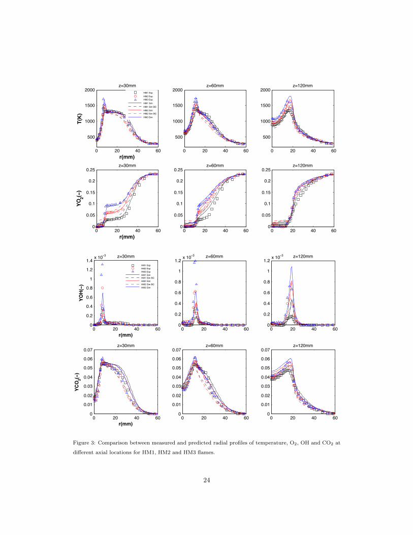
5.1. Validation of numerical model275

Figure 3 shows the comparison between experimental radial profiles of temperature and276

chemical species (O2, OH and CO2) mass fractions at different axial locations (i.e. z = 30,277

60 and 120 mm) and those predicted from the CFD model for HM1, HM2, HM3 flames.278

More discussion about the modelling errors can be found in [22]. Dashed lines refer to279

simulations performed by imposing experimental profiles for the inlet BCs. No significant280

improvement over the baseline simulations (constant inlet profiles) can be observed. A281

very good predictions of the temperature and O2 concentration profiles is achieved at all282

locations (see Figure 3a and Figure 3b, respectively). Such agreement was the result of283

the tuning of the inlet turbulence levels conditions, performed to better capture the three284

stream mixing [18] [23] [26], as well as of the revision of the original EDC model to treat the285

11

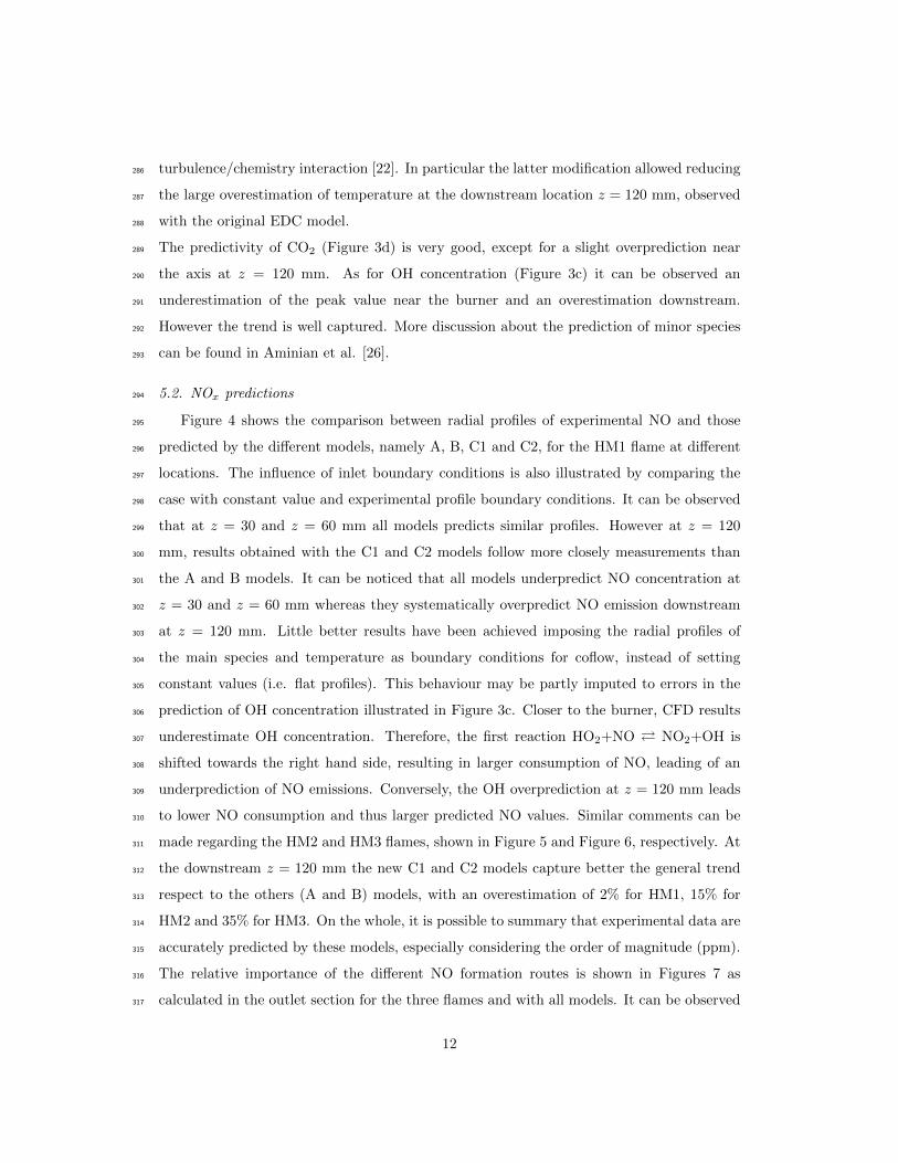
turbulence/chemistry interaction [22]. In particular the latter modification allowed reducing286

the large overestimation of temperature at the downstream location z = 120 mm, observed287

with the original EDC model.288

The predictivity of CO2 (Figure 3d) is very good, except for a slight overprediction near289

the axis at z = 120 mm. As for OH concentration (Figure 3c) it can be observed an290

underestimation of the peak value near the burner and an overestimation downstream.291

However the trend is well captured. More discussion about the prediction of minor species292

can be found in Aminian et al. [26].293

5.2. NOx predictions294

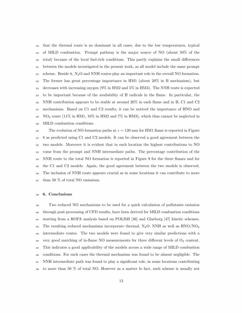
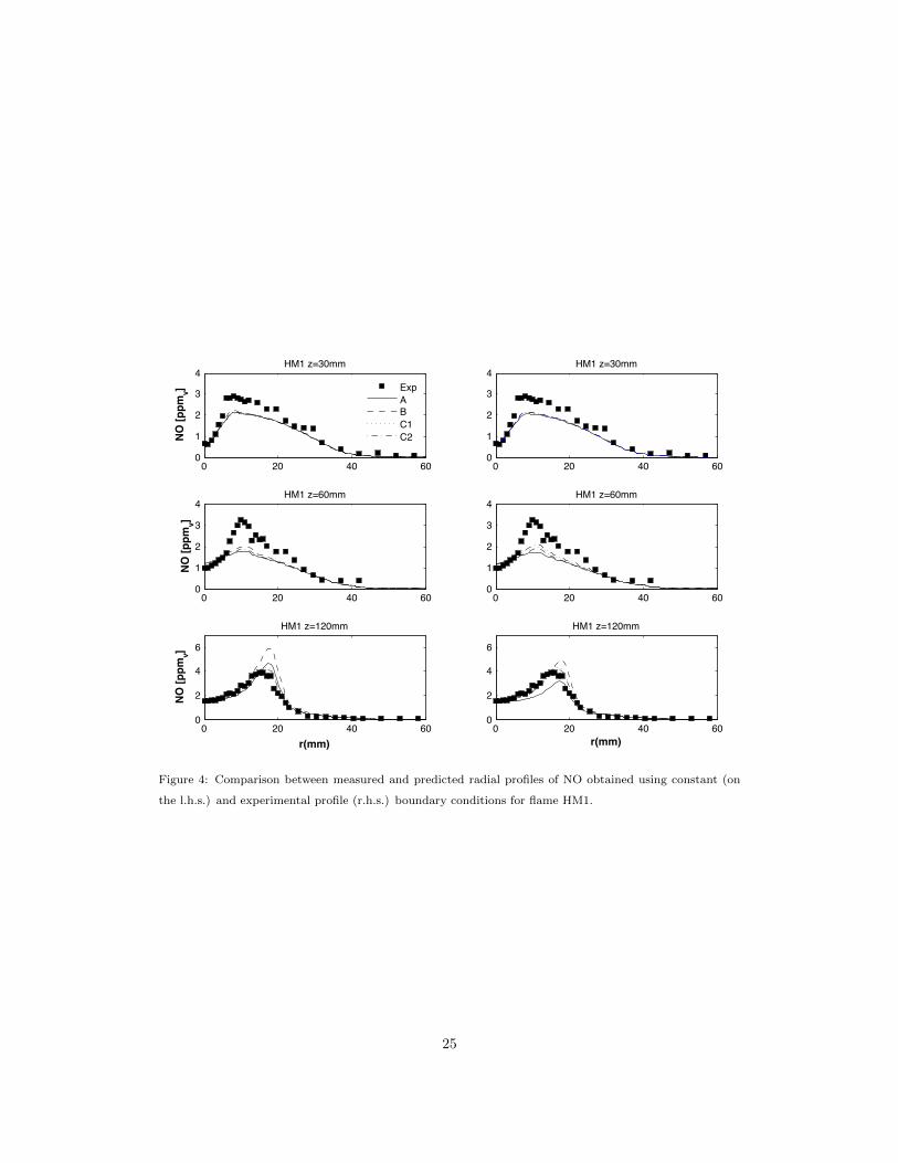
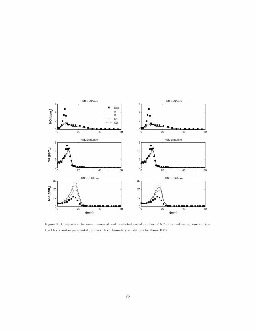
Figure 4 shows the comparison between radial profiles of experimental NO and those295

predicted by the different models, namely A, B, C1 and C2, for the HM1 flame at different296

locations. The influence of inlet boundary conditions is also illustrated by comparing the297

case with constant value and experimental profile boundary conditions. It can be observed298

that at z = 30 and z = 60 mm all models predicts similar profiles. However at z = 120299

mm, results obtained with the C1 and C2 models follow more closely measurements than300

the A and B models. It can be noticed that all models underpredict NO concentration at301

z = 30 and z = 60 mm whereas they systematically overpredict NO emission downstream302

at z = 120 mm. Little better results have been achieved imposing the radial profiles of303

the main species and temperature as boundary conditions for coflow, instead of setting304

constant values (i.e. flat profiles). This behaviour may be partly imputed to errors in the305

prediction of OH concentration illustrated in Figure 3c. Closer to the burner, CFD results306

underestimate OH concentration. Therefore, the first reaction HO2+NO � NO2+OH is307

shifted towards the right hand side, resulting in larger consumption of NO, leading of an308

underprediction of NO emissions. Conversely, the OH overprediction at z = 120 mm leads309

to lower NO consumption and thus larger predicted NO values. Similar comments can be310

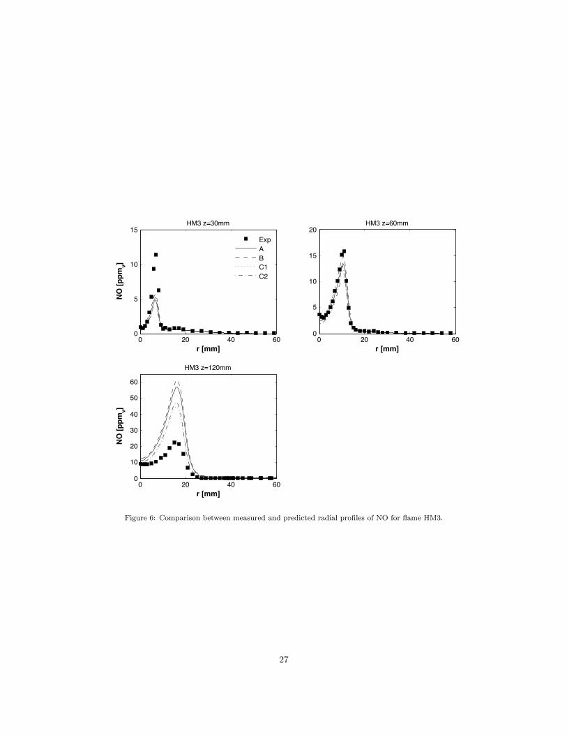
made regarding the HM2 and HM3 flames, shown in Figure 5 and Figure 6, respectively. At311

the downstream z = 120 mm the new C1 and C2 models capture better the general trend312

respect to the others (A and B) models, with an overestimation of 2% for HM1, 15% for313

HM2 and 35% for HM3. On the whole, it is possible to summary that experimental data are314

accurately predicted by these models, especially considering the order of magnitude (ppm).315

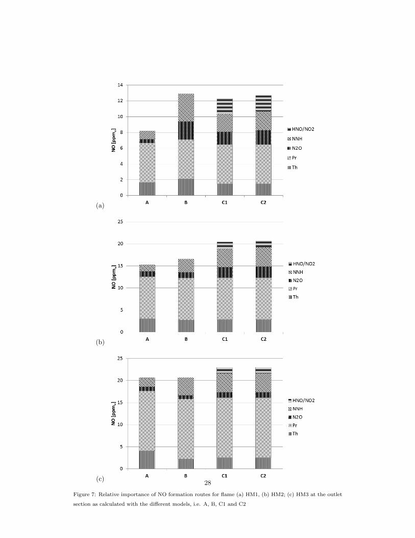
The relative importance of the different NO formation routes is shown in Figures 7 as316

calculated in the outlet section for the three flames and with all models. It can be observed317

12

that the thermal route is no dominant in all cases, due to the low temperatures, typical318

of MILD combustion. Prompt pathway is the major source of NO (about 50% of the319

total) because of the local fuel-rich conditions. This partly explains the small differences320

between the models investigated in the present work, as all model include the same prompt321

scheme. Beside it, N2O and NNH routes play an important role in the overall NO formation.322

The former has great percentage importance in HM1 (about 20% in B mechanism), but323

decreases with increasing oxygen (9% in HM2 and 5% in HM3). The NNH route is expected324

to be important because of the availability of H radicals in the flame. In particular, the325

NNH contribution appears to be stable at around 20% in each flame and in B, C1 and C2326

mechanisms. Based on C1 and C2 results, it can be noticed the importance of HNO and327

NO2 route (11% in HM1, 10% in HM2 and 7% in HM3), which thus cannot be neglected in328

MILD combustion conditions.329

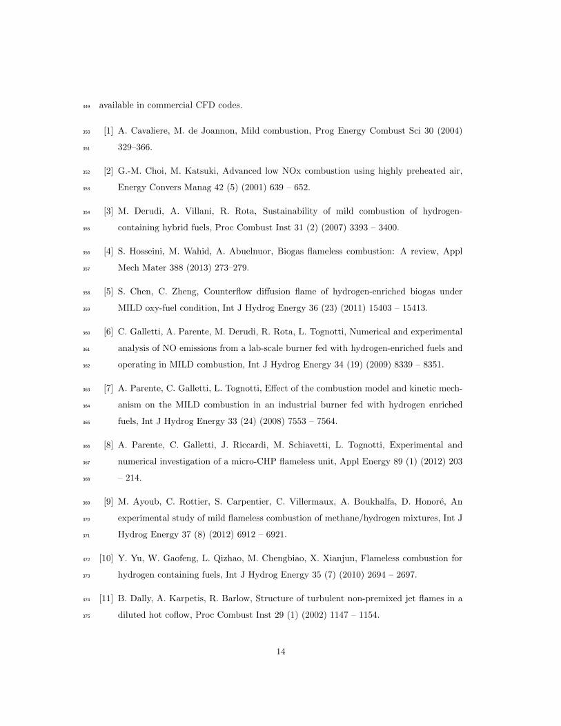
The evolution of NO formation paths at z = 120 mm for HM1 flame is reported in Figure330

8 as predicted using C1 and C2 models. It can be observed a good agreement between the331

two models. Moreover it is evident that in such location the highest contributions to NO332

come from the prompt and NNH intermediate paths. The percentage contribution of the333

NNH route to the total NO formation is reported in Figure 9 for the three flames and for334

the C1 and C2 models. Again, the good agreement between the two models is observed.335

The inclusion of NNH route appears crucial as in some locations it can contribute to more336

than 50 % of total NO emissions.337

6. Conclusions338

Two reduced NO mechanisms to be used for a quick calculation of pollutants emission339

through post-processing of CFD results, have been derived for MILD combustion conditions340

starting from a ROPA analysis based on POLIMI [46] and Glarborg [47] kinetic schemes.341

The resulting reduced mechanisms incorporate thermal, N2O, NNH as well as HNO/NO2342

intermediate routes. The two models were found to give very similar predictions with a343

very good matching of in-flame NO measurements for three different levels of O2 content.344

This indicates a good applicability of the models across a wide range of MILD combustion345

conditions. For such cases the thermal mechanism was found to be almost negligible. The346

NNH intermediate path was found to play a significant role, in some locations contributing347

to more than 50 % of total NO. However as a matter fo fact, such scheme is usually not348

13

available in commercial CFD codes.349

[1] A. Cavaliere, M. de Joannon, Mild combustion, Prog Energy Combust Sci 30 (2004)350

329–366.351

[2] G.-M. Choi, M. Katsuki, Advanced low NOx combustion using highly preheated air,352

Energy Convers Manag 42 (5) (2001) 639 – 652.353

[3] M. Derudi, A. Villani, R. Rota, Sustainability of mild combustion of hydrogen-354

containing hybrid fuels, Proc Combust Inst 31 (2) (2007) 3393 – 3400.355

[4] S. Hosseini, M. Wahid, A. Abuelnuor, Biogas flameless combustion: A review, Appl356

Mech Mater 388 (2013) 273–279.357

[5] S. Chen, C. Zheng, Counterflow diffusion flame of hydrogen-enriched biogas under358

MILD oxy-fuel condition, Int J Hydrog Energy 36 (23) (2011) 15403 – 15413.359

[6] C. Galletti, A. Parente, M. Derudi, R. Rota, L. Tognotti, Numerical and experimental360

analysis of NO emissions from a lab-scale burner fed with hydrogen-enriched fuels and361

operating in MILD combustion, Int J Hydrog Energy 34 (19) (2009) 8339 – 8351.362

[7] A. Parente, C. Galletti, L. Tognotti, Effect of the combustion model and kinetic mech-363

anism on the MILD combustion in an industrial burner fed with hydrogen enriched364

fuels, Int J Hydrog Energy 33 (24) (2008) 7553 – 7564.365

[8] A. Parente, C. Galletti, J. Riccardi, M. Schiavetti, L. Tognotti, Experimental and366

numerical investigation of a micro-CHP flameless unit, Appl Energy 89 (1) (2012) 203367

– 214.368

[9] M. Ayoub, C. Rottier, S. Carpentier, C. Villermaux, A. Boukhalfa, D. Honore, An369

experimental study of mild flameless combustion of methane/hydrogen mixtures, Int J370

Hydrog Energy 37 (8) (2012) 6912 – 6921.371

[10] Y. Yu, W. Gaofeng, L. Qizhao, M. Chengbiao, X. Xianjun, Flameless combustion for372

hydrogen containing fuels, Int J Hydrog Energy 35 (7) (2010) 2694 – 2697.373

[11] B. Dally, A. Karpetis, R. Barlow, Structure of turbulent non-premixed jet flames in a374

diluted hot coflow, Proc Combust Inst 29 (1) (2002) 1147 – 1154.375

14

[12] B. Dally, E. Riesmeier, N. Peters, Effect of fuel mixture on moderate and intense low376

oxygen dilution combustion, Combust Flame 137 (4) (2004) 418 – 431.377

[13] P. R. Medwell, P. A. Kalt, B. B. Dally, Simultaneous imaging of OH, formaldehyde,378

and temperature of turbulent nonpremixed jet flames in a heated and diluted coflow,379

Combust Flame 148 (1–2) (2007) 48 – 61.380

[14] P. R. Medwell, B. B. Dally, Effect of fuel composition on jet flames in a heated and381

diluted oxidant stream, Combust Flame 159 (10) (2012) 3138 – 3145.382

[15] E. Oldenhof, M. Tummers, E. van Veen, D. Roekaerts, Ignition kernel formation and383

lift-off behaviour of jet-in-hot-coflow flames, Combust Flame 157 (6) (2010) 1167 –384

1178.385

[16] E. Oldenhof, M. Tummers, E. van Veen, D. Roekaerts, Role of entrainment in the386

stabilisation of jet-in-hot-coflow flames, Combust Flame 158 (8) (2011) 1553 – 1563.387

[17] E. Oldenhof, M. J. Tummers, E. H. van Veen, D. J. Roekaerts, Transient response of388

the delft jet-in-hot coflow flames, Combust Flame 159 (2) (2012) 697 – 706.389

[18] F. Christo, B. Dally, Modeling turbulent reacting jets issuing into a hot and diluted390

coflow, Combust Flame 142 (1–2) (2005) 117 – 129.391

[19] S. H. Kim, K. Y. Huh, B. Dally, Conditional moment closure modeling of turbulent392

nonpremixed combustion in diluted hot coflow, Proc Combust Inst 30 (1) (2005) 751 –393

757.394

[20] A. Mardani, S. Tabejamaat, S. Hassanpour, Numerical study of CO and CO2 formation395

in CH4/H2 blended flame under MILD condition, Combust Flame 160 (9) (2013) 1636396

– 1649.397

[21] A. Mardani, S. Tabejamaat, Effect of hydrogen on hydrogenmethane turbulent non-398

premixed flame under {MILD} condition, Int J Hydrog Energy 35 (20) (2010) 11324 –399

11331.400

[22] J. Aminian, C. Galletti, S. Shahhosseini, L. Tognotti, Numerical investigation of a401

mild combustion burner: Analysis of mixing field, chemical kinetics and turbulence-402

chemistry interaction, Flow, Turbulence and Combustion 88 (4) (2012) 597–623.403

15

[23] A. Frassoldati, P. Sharma, A. Cuoci, T. Faravelli, E. Ranzi, Kinetic and fluid dynamics404

modeling of methane/hydrogen jet flames in diluted coflow, Appl Therm Eng 30 (4)405

(2010) 376 – 383.406

[24] F. Wang, J. Mi, P. Li, C. Zheng, Diffusion flame of a CH4/H2 jet in hot low-oxygen407

coflow, Int J Hydrog Energy 36 (15) (2011) 9267 – 9277.408

[25] A. De, E. Oldenhof, P. Sathiah, D. Roekaerts, Numerical simulation of delft-jet-in-409

hot-coflow (DJHC) flames using the eddy dissipation concept model for turbulence-410

chemistry interaction, Flow, Turbulence and Combustion 87 (4) (2011) 537–567.411

[26] J. Aminian, C. Galletti, S. Shahhosseini, L. Tognotti, Key modeling issues in prediction412

of minor species in diluted-preheated combustion conditions, Appl Therm Eng 31 (16)413

(2011) 3287 – 3300.414

[27] M. Ihme, Y. C. See, LES flamelet modeling of a three-stream MILD combustor: Anal-415

ysis of flame sensitivity to scalar inflow conditions, Proc Combust Inst 33 (1) (2011)416

1309 – 1317.417

[28] R. M. Kulkarni, W. Polifke, LES of delft-jet-in-hot-coflow (DJHC) with tabulated chem-418

istry and stochastic fields combustion model, Fuel Processing Technology 107 (0) (2013)419

138 – 146.420

[29] Y. Afarin, S. Tabejamaat, Effect of hydrogen on h2/ch4 flame structure of mild com-421

bustion using the {LES} method, Int J Hydrog Energy 38 (8) (2013) 3447 – 3458.422

[30] B. J. Isaac, A. Parente, C. Galletti, J. N. Thornock, P. J. Smith, L. Tognotti, A novel423

methodology for chemical time scale evaluation with detailed chemical reaction kinetics,424

Energy Fuels 27 (2013) 2255 – 2265.425

[31] B. F. Magnussen, On the structure of turbulence and a generalized eddy dissipation426

concept for chemical reaction in turbulent flow, in: 19th AIAA Aerospace Science427

Meeting, 1981.428

[32] B. F. Magnussen, The eddy dissipation concept, a bridge between science and technol-429

ogy, in: Eccomas Thematic Conf on Computat Combust, 2005.430

16

[33] G. Szego, B. Dally, G. Nathan, Scaling of NOx emissions from a laboratory-scale mild431

combustion furnace, Combust Flame 154 (1–2) (2008) 281 – 295.432

[34] P. Li, F. Wang, J. Mi, B. Dally, Z. Mei, J. Zhang, A. Parente, Mechanisms of NO433

formation in MILD combustion of CH4/H2 fuel blends, Int J Hydrog Energy 39 (33)434

(2014) 19187 – 19203.435

[35] C. Fenimore, Formation of nitric oxide in premixed hydrocarbon flames, Proc Combust436

Inst 13 (1) (1971) 373 – 380.437

[36] P. Malte, D. Pratt, Measurement of atomic oxygen and nitrogen oxides in jet-stirred438

combustion, Proc Combust Inst 15 (1) (1975) 1061 – 1070.439

[37] A. Nicolle, P. Dagaut, Occurrence of no-reburning in MILD combustion evidenced via440

chemical kinetic modeling, Fuel 85 (1718) (2006) 2469 – 2478.441

[38] J. W. Bozzelli, A. M. Dean, O + NNH: A possible new route for nox formation in442

flames, Int J Chem Kinet 27 (11) (1995) 1097–1109.443

[39] A. Parente, C. Galletti, L. Tognotti, A simplified approach for predicting NO formation444

in MILD combustion of CH4-H2 mixtures, Proc Combust Inst 33 (2) (2011) 3343 – 3350.445

[40] G. Loffler, R. Sieber, M. Harasek, H. Hofbauer, R. Hauss, J. Landauf, NOx formation446

in natural gas combustion-a new simplified reaction scheme for CFD calculations, Fuel447

85 (4) (2006) 513 – 523.448

[41] X. Gao, F. Duan, S. C. Lim, M. S. Yip, NOx formation in hydrogen-methane turbulent449

diffusion flame under the moderate or intense low-oxygen dilution conditions, Energy450

59 (0) (2013) 559 – 569.451

[42] A. P. Morse, Axisymmetric turbulent shear flows with and without swirl, Ph.D. thesis,452

London University (1977).453

[43] R. Bilger, S. Starner, R. Kee, On reduced mechanisms for methane-air combustion in454

nonpremixed flames, Combust Flame 80 (1990) 135–149.455

[44] T. Smith, Z. Shen, J. N. Friedman, Evaluation of coefficients for the weighted sum of456

gray gases model, J Heat Transf 104 (4) (1982) 602 – 608.457

17

[45] F. C. Christo, B. B. Dally, Modelling turbulent reacting jets issuing into a hot and458

diluted coflow, Combust Flame 142 (2005) 117–129.459

[46] E. Ranzi, A. Sogaro, P. Gaffuri, G. Pennati, T. Faravelli, Wide range modeling study460

of methane oxidation, Combust Sci Technol 96 (4-6) (1994) 279–325.461

[47] P. Glarborg, M. U. Alzueta, K. Dam-Johansen, J. A. Miller, Kinetic modeling of hy-462

drocarbon/nitric oxide interactions in a flow reactor, Combust Flame 115 (1–2) (1998)463

1 – 27.464

[48] G. D. Soete, Overall reaction rates of NO and N2 formation from fuel nitrogen, Proc465

Combust Inst 15 (1) (1975) 1093 – 1102.466

[49] Ansys 13, Fluent User’s Guide.467

[50] A. Konnov, G. Colson, J. D. Ruyck, The new route forming NO via NNH, Combust468

Flame 121 (3) (2000) 548 – 550.469

[51] A. Cuoci, A. Frassoldati, T. Faravelli, E. Ranzi, OpenSMOKE: Numerical modeling of470

reacting systems with detailed kinetic mechanisms, XXXIV Meeting of Italian Section471

of Comb Inst.472

[52] A. Cuoci, A. Frassoldati, T. Faravelli, E. Ranzi, Formation of soot and nitrogen oxides473

in unsteady counterflow diffusion flames, Combust Flame 156 (10) (2009) 2010 – 2022.474

18

Tables475

Table 1: Operating conditions for cases studied (compositions are as mass fractions)

Fuel jet (CH4/H2) Oxidant coflow

Case T Re u T O2 N2 H2O CO2

(K) (-) (m/s) (K) (%) (%) (%) (%)

HM1 305 10, 000 3.2 1300 3 85 6.5 5.5

HM2 305 10, 000 3.2 1300 6 82 6.5 5.5

HM3 305 10, 000 3.2 1300 9 79 6.5 5.5

Table 2: PSR operating conditions

Inlet StreamFlame

HM1 HM2 HM3

H2 (% by wt.) 7.14 7.11 7.09

CH4 (% by wt.) 5.71 5.69 5.67

O2 (% by wt.) 2.81 5.61 8.41

CO2 (% by wt.) 5.14 5.14 5.14

H2O (% by wt.) 6.08 6.08 6.08

p (atm) 1 1 1

T (K) 1300-1700 1300-1700 1300-1700

τ (ms) 52 52 52

19

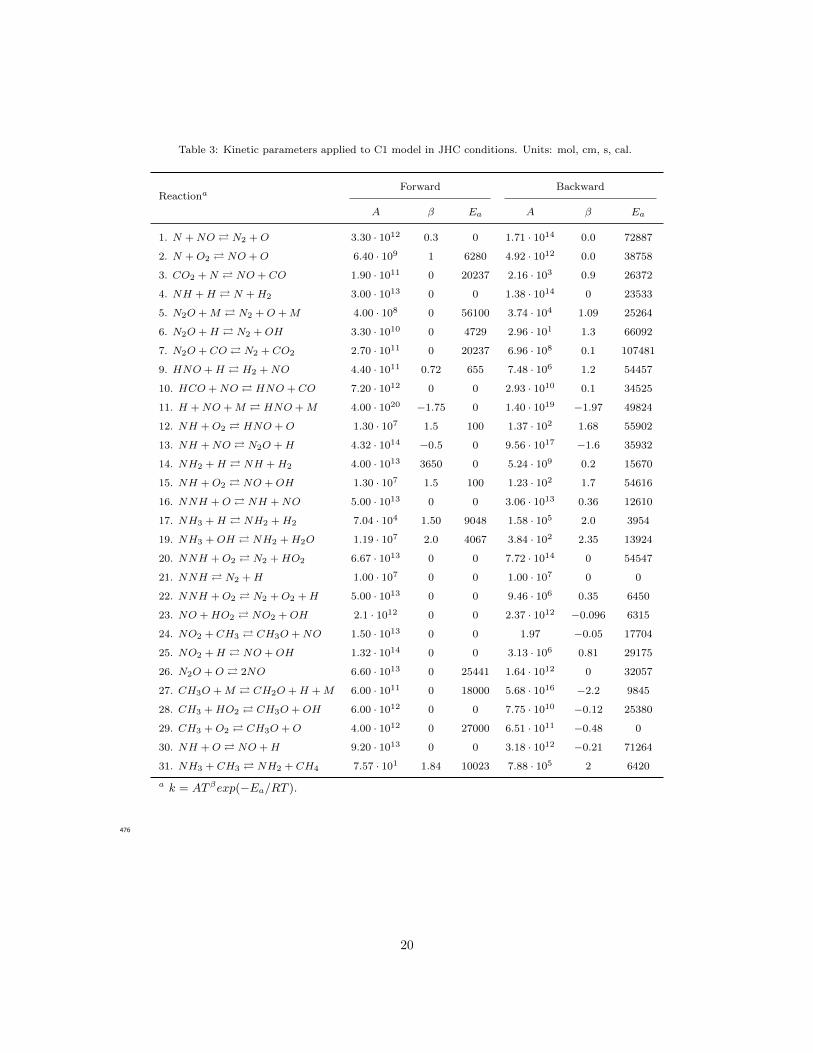
Table 3: Kinetic parameters applied to C1 model in JHC conditions. Units: mol, cm, s, cal.

ReactionaForward Backward

A β Ea A β Ea

1. N +NO � N2 +O 3.30 · 1012 0.3 0 1.71 · 1014 0.0 72887

2. N +O2 � NO +O 6.40 · 109 1 6280 4.92 · 1012 0.0 38758

3. CO2 +N � NO + CO 1.90 · 1011 0 20237 2.16 · 103 0.9 26372

4. NH +H � N +H2 3.00 · 1013 0 0 1.38 · 1014 0 23533

5. N2O +M � N2 +O +M 4.00 · 108 0 56100 3.74 · 104 1.09 25264

6. N2O +H � N2 +OH 3.30 · 1010 0 4729 2.96 · 101 1.3 66092

7. N2O + CO � N2 + CO2 2.70 · 1011 0 20237 6.96 · 108 0.1 107481

9. HNO +H � H2 +NO 4.40 · 1011 0.72 655 7.48 · 106 1.2 54457

10. HCO +NO � HNO + CO 7.20 · 1012 0 0 2.93 · 1010 0.1 34525

11. H +NO +M � HNO +M 4.00 · 1020 −1.75 0 1.40 · 1019 −1.97 49824

12. NH +O2 � HNO +O 1.30 · 107 1.5 100 1.37 · 102 1.68 55902

13. NH +NO � N2O +H 4.32 · 1014 −0.5 0 9.56 · 1017 −1.6 35932

14. NH2 +H � NH +H2 4.00 · 1013 3650 0 5.24 · 109 0.2 15670

15. NH +O2 � NO +OH 1.30 · 107 1.5 100 1.23 · 102 1.7 54616

16. NNH +O � NH +NO 5.00 · 1013 0 0 3.06 · 1013 0.36 12610

17. NH3 +H � NH2 +H2 7.04 · 104 1.50 9048 1.58 · 105 2.0 3954

19. NH3 +OH � NH2 +H2O 1.19 · 107 2.0 4067 3.84 · 102 2.35 13924

20. NNH +O2 � N2 +HO2 6.67 · 1013 0 0 7.72 · 1014 0 54547

21. NNH � N2 +H 1.00 · 107 0 0 1.00 · 107 0 0

22. NNH +O2 � N2 +O2 +H 5.00 · 1013 0 0 9.46 · 106 0.35 6450

23. NO +HO2 � NO2 +OH 2.1 · 1012 0 0 2.37 · 1012 −0.096 6315

24. NO2 + CH3 � CH3O +NO 1.50 · 1013 0 0 1.97 −0.05 17704

25. NO2 +H � NO +OH 1.32 · 1014 0 0 3.13 · 106 0.81 29175

26. N2O +O � 2NO 6.60 · 1013 0 25441 1.64 · 1012 0 32057

27. CH3O +M � CH2O +H +M 6.00 · 1011 0 18000 5.68 · 1016 −2.2 9845

28. CH3 +HO2 � CH3O +OH 6.00 · 1012 0 0 7.75 · 1010 −0.12 25380

29. CH3 +O2 � CH3O +O 4.00 · 1012 0 27000 6.51 · 1011 −0.48 0

30. NH +O � NO +H 9.20 · 1013 0 0 3.18 · 1012 −0.21 71264

31. NH3 + CH3 � NH2 + CH4 7.57 · 101 1.84 10023 7.88 · 105 2 6420

a k = AT βexp(−Ea/RT ).

476

20

Table 4: Kinetic parameters applied to C2 model in JHC conditions. Units: mol, cm, s, cal

ReactionaForward Backward

A β Ea A β Ea

1. N +NO � N2 +O 3.30 · 1012 0.3 0 1.71 · 1014 0.0 72887

2. N +O2 � NO +O 6.40 · 109 1 6280 4.92 · 1012 0.0 38758

3. CO2 +N � NO + CO 1.90 · 1011 0 20237 2.16 · 103 0.9 26372

4. NH +H � N +H2 3.00 · 1013 0 0 1.38 · 1014 0.0 23533

5. N2O +M � N2 +O +M 4.00 · 1014 0 56100 1.067 · 103 1.09 15780

6. N2O +H � N2 +OH 3.30 · 1010 0 4729 2.96 · 101 1.3 66092

7. N2O + CO � N2 + CO2 3.20 · 1011 0 20237 8.25 · 108 0.1 107481

8. N2O +OH � N2 +HO2 2.37 · 1010 −0.09 6316 2.10 · 1012 0.0 0

9. HNO +H � H2 +NO 8.50 · 1011 0.5 655 7.66 · 106 1.2 54457

10. HCO +NO � HNO + CO 7.20 · 1012 0 0 2.93 · 1010 0.1 34525

11. H +NO +M � HNO +M 4.00 · 1020 −1.75 0 1.40 · 1019 −1.9 49824

12. NH +O2 � HNO +O 1.30 · 106 1.5 100 1.37 · 102 1.7 55902

13. NH +NO � N2O +H 2.90 · 1014 −0.4 0 6.42 · 1017 −1.5 35932

14. NH2 +H � NH +H2 4.00 · 1013 0 3650 5.24 · 109 0.2 15670

15. NH +O2 � NO +OH 1.30 · 107 1.5 100 1.23 · 102 1.7 54616

16. NNH +O � NH +NO 5.00 · 1013 0 0 3.06 · 1013 0.0 12610

17. NH3 +H � NH2 +H2 6.40 · 105 2.4 10171 1.43 2.9 5077

18. NH3 +O � NH2 +OH 9.40 · 106 1.9 6460 1.18 · 101 2.4 0

19. NH3 +OH � NH2 +H2O 2.00 · 106 2.1 566 5.75 · 101 2.4 10827

20. NNH +O2 � N2 +HO2 5.00 · 1013 0 0 7.72 · 1014 0 54547

21. NNH � N2 +H 1.00 · 107 0 0 1.00 · 107 0 0

22. NNH +O2 � N2 +O2 +H 5.00 · 1013 0 0 9.46 · 106 0.35 6450

23. NO +HO2 � NO2 +OH 2.20 · 1012 0 0 2.37 · 1012 −0.01 6315

24. NO2 + CH3 � CH3O +NO 1.40 · 1013 0 0 1.97 −0.05 17704

25. NO2 +H � NO +OH 4.00 · 1013 0 0 2.22 · 106 0.81 28410

26. N2O +O � 2NO 6.60 · 1013 0 25441 1.64 · 1012 0 32057

27. CH3O +M � CH2O +H +M 6.00 · 1011 0 18000 5.68 · 1016 −2.2 9845

28. CH3 +HO2 � CH3O +OH 6.00 · 1012 0 0 7.75 · 1010 −0.12 25380

29. CH3 +O2 � CH3O +O 4.00 · 1012 0 27000 6.51 · 1011 −0.48 0

30. NH +O � NO +H 9.20 · 1013 0 0 5.47 · 1014 0 67482

a k = AT βexp(−Ea/RT ).

477

21

Figures478

479

Flow Turbulence Combust

the combustion process. After a preliminary theoretical investigation of the EDCmodel and its sensitivity to the two model constants, the authors showed that theprediction of DJHC flames could be improved by changing these constants withrespect to the classical EDC.

In the present paper, the structure of JHC burner experimentally studied by Dallyet al. [25] is investigated using the steady state Reynolds-Averaged Navier-Stokesapproach coupled with the Eddy Dissipation Concept for the turbulence-chemistryinteraction treatment. An analysis of the EDC model to improve its predictions forMILD combustion conditions is presented in the last section.

2 Test Case

The jet-in-hot coflow burner modeled in this work has been experimentally studiedby Dally et al. [25] and is shown in Fig. 1. It consists of a fuel jet nozzle, which hasan inner diameter of 4.25 mm and a wall thickness of 0.2 mm, located at the centerof a perforated disc in an annulus, with inner diameter of 82 mm and wall thicknessof 2.8 mm, which provides nearly uniform composition of hot oxidizer coflow to thereaction zone. The entire burner was sited inside a wind tunnel introducing roomtemperature air at the same velocity as the hot coflow. Table 1 shows the operatingconditions of three inlet streams for the different case studies. The notations, HM1,HM2 and HM3, refer to the flames with oxygen mass fraction of 3%, 6%, and 9%,respectively, in the hot coflow stream. The jet Reynolds number was around 10000for all flames. The available data consist of the mean and root mean square (rms) oftemperature and concentration of major (CH4, H2, H2O, CO2, N2 and O2) and minorspecies (NO, CO and OH).

2.125mm41mm

120mm z

r

900m

m

100m

m

Upstream

Downstream

Center of fuel jet nozzle (0,0)

Tunnel air

Hot coflow

Fuel jet (b)

Jet outlet (0,0)

Oxidant inlet

Ceramic shield

Perforated plate

Internal burner

Oxidant inlet

Cooling gas inlet

Cooling gas outlet

Fuel inlet

(a)

Fig. 1 (a) Schematic of the jet-in-hot coflow burner [25] and (b) computational domain withboundary conditions

(a) (b)

Figure 1: (a) Jet in Hot Coflow burner and (b) computational domain

22

(a)

Rate of Production Analysis - NO

622 -0.040NO+HO2=NO2+OH

694 0.026CH3+NO2=CH3O+NO

657 0.012NO2+H=NO+OH

690 0.012NH+NO=N2O+H

627 3.04e-03HNO+H=NO+H2

686 -1.88e-03C2H3+NO=C2H2+HNO

624 1.87e-03NO+OH+M=HONO+M

603 1.65e-03NNH+O=NH+NO

625 -1.34e-03HCO+NO=CO+HNO

626 1.16e-03H+NO+M=HNO+M

573 8.75e-04NH+O2=NO+OH

580 7.75e-04N+NO=O+N2

579 7.12e-04N+O2=NO+O

696 1.61e-04NO+CH4=HNO+CH3

681 1.36e-04CO2+N=NO+CO

691 1.16e-04N2O+O=2NO

630 9.15e-05HNO+O2=NO+HO2

664 7.67e-05CO+NO2=CO2+NO

629 6.51e-05HNO+OH=NO+H2O

684 -6.02e-05CH2+NO=NCO+H2

(b)

Rate of Production Analysis - NO

242 -0.027HO2+NO=NO2+OH

342 0.020CH3+NO2=CH3O+NO

298 0.016NH+NO=N2O+H

243 7.02e-03NO2+H=NO+OH

299 -4.21e-03NH+NO=N2O+H

253 2.03e-03HNO+H=H2+NO

338 -1.38e-03HCO+NO=HNO+CO

347 -1.21e-03C2H3+NO=C2H2+HNO

319 1.13e-03NNH+O=NH+NO

238 1.01e-03H+NO+M=HNO+M

306 8.57e-04N+NO=N2+O

305 7.17e-04N+O2=NO+O

297 6.90e-04NH+O2=NO+OH

239 3.62e-04H+NO+N2=HNO+N2

336 1.65e-04CO2+N=NO+CO

241 9.07e-05OH+NO+M=HONO+M

334 7.52e-05CO+NO2=CO2+NO

329 6.46e-05N2O+O=2NO

256 4.97e-05HNO+O2=HO2+NO

255 4.12e-05HNO+OH=NO+H2O

Figure 2: NO Rate Of Production Analysis (ROPA) for (a) C1 and (b) C2 models. Blue lines indicate NO

destruction, while the red ones NO formation.

23

0 20 40 60

500

1000

1500

2000

r(mm)

T(K)

z=30mm

HM1 ExpHM2 ExpHM3 ExpHM1 SimHM1 Sim BCHM2 SimHM2 Sim BCHM3 Sim

0 20 40 60

500

1000

1500

2000z=60mm

0 20 40 60

500

1000

1500

2000z=120mm

0 20 40 600

0.05

0.1

0.15

0.2

0.25

r(mm)

YO2(−)

z=30mm

0 20 40 600

0.05

0.1

0.15

0.2

0.25z=60mm

0 20 40 600

0.05

0.1

0.15

0.2

0.25z=120mm

0 20 40 600

0.2

0.4

0.6

0.8

1

1.2

1.4x 10−3

r(mm)

YOH(−)

z=30mm

HM1 ExpHM2 ExpHM3 ExpHM1 SimHM1 Sim BCHM2 SimHM2 Sim BCHM3 Sim

0 20 40 600

0.2

0.4

0.6

0.8

1

1.2x 10−3 z=60mm

0 20 40 600

0.2

0.4

0.6

0.8

1

1.2x 10−3 z=120mm

0 20 40 600

0.01

0.02

0.03

0.04

0.05

0.06

0.07

r(mm)

YCO2(−)

z=30mm

0 20 40 600

0.01

0.02

0.03

0.04

0.05

0.06

0.07z=60mm

0 20 40 600

0.01

0.02

0.03

0.04

0.05

0.06

0.07z=120mm

Figure 3: Comparison between measured and predicted radial profiles of temperature, O2, OH and CO2 at

different axial locations for HM1, HM2 and HM3 flames.

24

0 20 40 600

1

2

3

4

NO

[ppm

v]

HM1 z=30mm

ExpABC1C2

0 20 40 600

1

2

3

4HM1 z=30mm

0 20 40 600

1

2

3

4

NO

[ppm

v]

HM1 z=60mm

0 20 40 600

1

2

3

4HM1 z=60mm

0 20 40 600

2

4

6

r(mm)

NO

[ppm

v]

HM1 z=120mm

0 20 40 600

2

4

6

r(mm)

HM1 z=120mm

Figure 4: Comparison between measured and predicted radial profiles of NO obtained using constant (on

the l.h.s.) and experimental profile (r.h.s.) boundary conditions for flame HM1.

25

0 20 40 600

2

4

6

NO

[ppm

v]

HM2 z=30mm

0 20 40 600

2

4

6HM2 z=30mm

0 20 40 600

5

10

15

NO

[ppm

v]

HM2 z=60mm

0 20 40 600

5

10

15HM2 z=60mm

0 20 40 600

10

20

30

r(mm)

NO

[ppm

v]

HM2 z=120mm

0 20 40 600

10

20

30

r(mm)

HM2 z=120mm

ExpABC1C2

Figure 5: Comparison between measured and predicted radial profiles of NO obtained using constant (on

the l.h.s.) and experimental profile (r.h.s.) boundary conditions for flame HM2.

26

0 20 40 600

5

10

15

r [mm]

NO

[ppm

v]

HM3 z=30mm

ExpABC1C2

0 20 40 600

5

10

15

20

r [mm]

HM3 z=60mm

0 20 40 600

10

20

30

40

50

60

r [mm]

NO

[ppm

v]

HM3 z=120mm

Figure 6: Comparison between measured and predicted radial profiles of NO for flame HM3.

27

(a)

(b)

(c)

Figure 7: Relative importance of NO formation routes for flame (a) HM1, (b) HM2; (c) HM3 at the outlet

section as calculated with the different models, i.e. A, B, C1 and C2

28

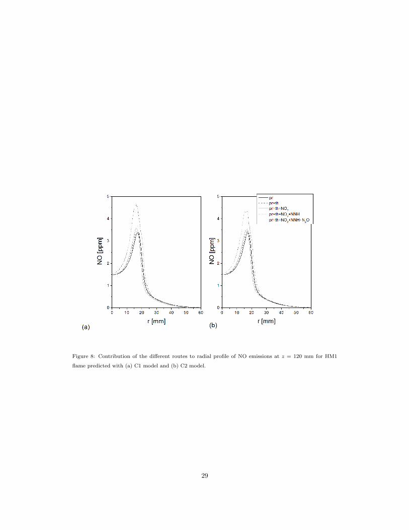
Figure 8: Contribution of the different routes to radial profile of NO emissions at z = 120 mm for HM1

flame predicted with (a) C1 model and (b) C2 model.

29

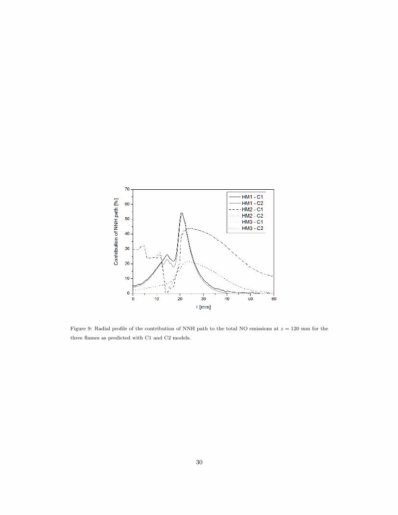
Figure 9: Radial profile of the contribution of NNH path to the total NO emissions at z = 120 mm for the

three flames as predicted with C1 and C2 models.

30