CFD simulation of H2 S Scavenger injection

CFD simulation of H2S Scavenger

injection

PECT 10 - Master’s Thesis

Aalborg University, Campus Esbjerg

Niels Bohrs Vej 8

6700 Esbjerg

May 30, 2019

Title page

Subject : H2S Scavenger

Project title : CFD simulation of H2S Scavenger injection

Project group : PECT10-5-F19.

Semester : 10th semester.

ECTS : 30

Supervisor : Matthias Mandø

Faculty : Aalborg University, Campus Esbjerg.

Author

Emil Tornel Jørgensen

AbstractWhen treating the sour gas, excessive use of scav-

enger is often seen because of the use of a quill

as an injection. The purpose of this study is an

investigation of the survival of the scavenger in

the pipeline by nozzle injection. The scavenger

requires a sufficient time to react with the gas

and is therefore relevant due to particle survival.

The primary part of this study is a CFD simula-

tion of the H2S injection with a nozzle. Different

injection direction is investigated to check the ef-

fectiveness of that. Furthermore, a change in the

pipe design is investigated to see whether this has

an influence on the particle survival.

The simulations showed that the large particles

was not able to be carried from the flow, and

therefore falls to the bottom of the pipe. While

the small particles survives and got sufficient

time to react with the H2S.

Reading Guide

To distinguish between figures, equations, and citations, [] is used for referring to

citations and numbers used for referring to figures and equations.

I

Preface

In table 1 constants used throughout the study, is listed. The table contains spec-

ifications from the gas phase and the injection product, as well as specifications of

the geometries.

Table 1: Table of the used constants

Density of the continuous phase ρc 11.8

[kg

m3

]Density of the particles ρp 1200

[kg

m3

]Viscosity of the continuous phase µc 1.249 · 10−5

[kg

ms

]Viscosity of the particles µp 6.34 · 10−3

[kg

ms

]Velocity of the continuous phase u 10

[ms

], 20

[ms

], 40

[ms

]Velocity of the discrete phase v 1.234

[ms

]Diameter of the pipe D 10 cm

Length of the pipe L 1000 cm

Particle diameter dp Particle distribution

II

Contents

1 Background of H2S Scavenger Injection 1

1.1 Analysis . . . . . . . . . . . . . . . . . . . . . . . . . . . . . . . . . . 2

2 Previous Work 6

2.1 Project Definition . . . . . . . . . . . . . . . . . . . . . . . . . . . . . 7

3 CFD Simulation 8

3.1 Computational Fluid Dynamics . . . . . . . . . . . . . . . . . . . . . 8

3.2 Governing Equations . . . . . . . . . . . . . . . . . . . . . . . . . . . 8

3.3 Meshing . . . . . . . . . . . . . . . . . . . . . . . . . . . . . . . . . . 11

3.4 Mesh Study . . . . . . . . . . . . . . . . . . . . . . . . . . . . . . . . 13

3.5 Simulation . . . . . . . . . . . . . . . . . . . . . . . . . . . . . . . . . 17

3.6 Results . . . . . . . . . . . . . . . . . . . . . . . . . . . . . . . . . . . 26

4 Discussion 35

5 Conclusion 37

6 Appendix 40

6.1 Time Ratio . . . . . . . . . . . . . . . . . . . . . . . . . . . . . . . . 40

6.2 Particle Loading . . . . . . . . . . . . . . . . . . . . . . . . . . . . . . 42

6.3 Stokes Number . . . . . . . . . . . . . . . . . . . . . . . . . . . . . . 43

6.4 Particle Forces . . . . . . . . . . . . . . . . . . . . . . . . . . . . . . 46

III

Chapter 1

Background of H2S Scavenger In-

jection

Crude oil is a naturally occurring process from organic material. Through the oil

formation, the organic material release gases which can contain toxic gases such as

hydrogen sulfide (H2S). H2S is a colorless gas with the characteristic odor of rotten

eggs and is extremely dangerous for humans and corrosive to metals. Therefore,

treatment of this gas is necessary before transferring it ashore. Usually, a quill is

used for the injection of the scavenger. Figure 1.1 is an illustration of the quill in

the pipeline. The quill works thus, it pours the chemical into the gas stream.

Figure 1.1: Illustration of a quill installation [1]

Excessive use of chemicals is often seen, and the efficiency of the process is very

poor. Stoichiometry calculations could estimate the right amount of scavenger, but

usually, 2-5 times more scavenger is used [2].

1

PECT10-5-E18

1.1 Analysis

This chapter is an analytical study of the injection system and the parameters behind

it. The study contains an explanation of the injection system, the hydrogen sulfide

gas and the risks behind it, and the different scavenger which can be used in the

treatment process.

1.1.1 Direct Injection System

On the offshore field, space and weight are a limiter for installation of scavenger

systems. Therefore, direct injection systems, as illustrated in figure 1.2, are the

most commonly used at offshore applications. The scavenger is sprayed directly

into the gas stream. Direct injection is excellent where there is sufficient time to

react with the H2S. Suppliers recommend a minimum of reaction time on 15-20

seconds [3].

Figure 1.2: Illustration of a typical direct injection system [1]

The typical system consists of an injection pump, injection directly into the pipeline,

a given length of the pipe (For the reaction between scavenger and H2s) and a

scrubber. The injection pump is pumping the chemical into the pipeline. The direct

injection is through a quill, injection mixer, or nozzle atomizer. It is assumed that a

nozzle atomizer will deliver a better survival of the particle and is therefore used in

this study. A gas-liquid separator uses gravity to separate the mixture. The spent

or excess scavenger agent falls to the bottom, and the treated gas rises to the top.

2

PECT10-5-E18

Figure 1.3 is a illustration of the injection types.

Figure 1.3: (a) Injection quill, (b) Injection mixer, (c) Atomizing nozzle [1]

The injection mixer is also known as an inline mixer. An injection mixer is used to

mix two or more fluids. The injection mixer is illustrated in figure 1.4, and is very

useful to make a homogeneous mass.

Figure 1.4: Illustration of an injection mixer inside [4]

Hydrogen sulfide (H2S) is a gas found in the drilling and production of crude oil.

H2S is a gas which is naturally released in the microbial breakdown of organic ma-

terial. As previously mentioned, it is extremely toxic for humans, even at small

concentrations. People smell it at low concentrations, as table 1.1 illustrates, only

50% of humans detect H2S at a concentration on 0.0047 ppm, and at high concen-

tration, people lose their ability to smell it. H2S is flammable and highly corrosive

to steel, which is crucial for pipes and valves [5].

3

PECT10-5-E18

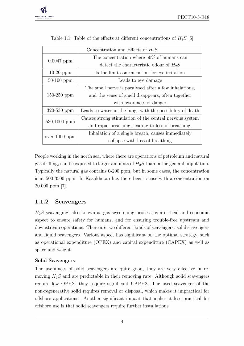
Table 1.1: Table of the effects at different concentrations of H2S [6]

Concentration and Effects of H2S

0.0047 ppmThe concentration where 50% of humans can

detect the characteristic odour of H2S

10-20 ppm Is the limit concentration for eye irritation

50-100 ppm Leads to eye damage

150-250 ppm

The smell nerve is paralysed after a few inhalations,

and the sense of smell disappears, often together

with awareness of danger

320-530 ppm Leads to water in the lungs with the possibility of death

530-1000 ppmCauses strong stimulation of the central nervous system

and rapid breathing, leading to loss of breathing.

over 1000 ppmInhalation of a single breath, causes immediately

collapse with loss of breathing

People working in the north sea, where there are operations of petroleum and natural

gas drilling, can be exposed to larger amounts of H2S than in the general population.

Typically the natural gas contains 0-200 ppm, but in some cases, the concentration

is at 500-3500 ppm. In Kazakhstan has there been a case with a concentration on

20.000 ppm [7].

1.1.2 Scavengers

H2S scavenging, also known as gas sweetening process, is a critical and economic

aspect to ensure safety for humans, and for ensuring trouble-free upstream and

downstream operations. There are two different kinds of scavengers: solid scavengers

and liquid scavengers. Various aspect has significant on the optimal strategy, such

as operational expenditure (OPEX) and capital expenditure (CAPEX) as well as

space and weight.

Solid Scavengers

The usefulness of solid scavengers are quite good, they are very effective in re-

moving H2S and are predictable in their removing rate. Although solid scavengers

require low OPEX, they require significant CAPEX. The used scavenger of the

non-regenerative solid requires removal or disposal, which makes it impractical for

offshore applications. Another significant impact that makes it less practical for

offshore use is that solid scavengers require further installations.

4

PECT10-5-E18

Liquid Scavengers

Liquid scavengers are useful for offshore applications, where space and weight are

a significant parameter, they require less weight and space than solid scavengers.

But liquid scavengers are generally less efficient, and OPEX is significantly higher.

An important feature, which makes it ideal for offshore applications is that liquid

scavengers offer more option for retrofitting an existing facility. Liquid scavengers fall

into two categories: Regenerative- and Non-Regenerative Scavengers, as illustrated

in table 1.2.

Table 1.2: Table of the Regenerative- and Non-Regenerative Scavengers [3]

Regenerative Scavengers Non-Regenerative Scavengers

Amine Wash Aldehydes

Reduction Oxidation Triazine

Sodium Nitrate

Triazine is the most commonly used in the offshore industry and is the one used in

this project. The by-product of the reaction is soluble in the oil or water phase, but

unreacted triazine is highly toxic for aquatic life, therefore, over-treatment of the

gas should be minimized [8].

5

Chapter 2

Previous Work

Based on the background of the H2S scavenger injection, the previous study is inves-

tigated. Examination of the optimum design is made: The Gas Technology Institute

(GTI) has made a study of multi-pipe direct injection [9]. While other studies have

focused on different injection methods and design rules [1]. In the optimum design

work, pipe dimensions, the location of a mixer and design principles are important

parameters.

The performance of injection systems is challenging to predict because the diam-

eter and the length of the pipe have an influence on the reaction. Study of the

optimum dose rate by mathematically modeling and simulation validation is made

[10]. Furthermore, a study of the optimum injection dose concluded that the pipe

diameter, pipe length, gas flow rate, pressure, and temperature had an influence in

the injection dose rate [11][12].

There are two different kind of scavengers: Regenerative- and non-Regenerative

scavengers. The efficiency of commercial scavengers is investigated and showed

different efficiencies in the ability to capture H2S in the gas [13]. Another thing

that is investigated in the scavenger section is the ratio between the scavenger and

the gas [14].

.

The previous study of H2S scavenger provides access to the project definition.

6

PECT10-5-E18

2.1 Project Definition

Based on the literature study and the analysis study, the project definition can be

stated. The amount of scavenger injection is not defined, and usually, the injection

dose rate is determined by experimental lab tests and field trials. Typical efficiency

is approximately 40% removal of H2S, but injection location and product selection

must be carefully considered to be effective [3]. The previous work showed that the

pipe diameter, pipe length, gas flow rate, pressure, and temperature had an influ-

ence on the efficiency on the scavenging process. Therefore, the reaction between

H2S and scavenger is a relevant topic.

No study showed the optimum direction of the injection in the pipe, therefore, the

direction of the injection could have an impact on the efficiency when removing H2S.

As mentioned previously a quill is usually used for the injection, the quill pours the

scavenger into the gas stream. Based on the low efficiency of the removal, the quill

is assumed as poor. Therefore, this project will be stated on nozzle atomizing of the

H2S injection, which is assumed to be better for the process, and will be answering

the following:

What is the impact of the nozzle on the particle survival?

What is the optimum injection direction of the nozzle?

What is the optimum particle size for the system?

What is the impact on particle survival, by a change in the design of geometry?

To answer these questions, a theoretical study of the scavenger is made, along with

a CFD simulation to examinees the physical problem with computational power.

7

Chapter 3

CFD Simulation

This chapter will contain an explanation of the simulation in this project. First,

the governing equation behind the simulation is investigated and listed. Then the

meshing section is reviewed to investigate the quality of the created mesh. Further-

more, particle-fluid interaction is explained to review the flow. At the end of this

chapter, a simulation explained with the set-up, simulations, and results.

3.1 Computational Fluid Dynamics

Computational Fluid Dynamic (CFD) is an analyzing tool for engineering problems

in fluid mechanics. CFD is structured around a numerical algorithm and is the ideal

tool for solving fluid flow problems. [15]

Many different software’s are available according to mathematical models, numerical

methods, computational equipment, and post-treatment. For this project, cubit

software is used for the pre-processing, and Ansys Fluent is used for the simulation

and post-treatment.

3.2 Governing Equations

For solving the fluid flow, Ansys Fluent solve a set of equation. For the continuous

flow, the continuity- and momentum equation is solved. For the prediction of the

particle motion, a set ordinary differential equations are solved. This section will

include an explanation of the underlying equations.

3.2.1 Conservation Of Mass

For the continuous phase, the conservation of mass in a closed system is described

by the continuity equation. Since the continuous phase is an incompressible flow

the continuity equation is stated as:

∂ui∂xi

= 0 (3.1)

Where:

• u = The velocity of the continuous phase

8

PECT10-5-E18

3.2.2 Reynolds-Averaged Navier-Stokes

The RANS equation is solved in the simulation, and are the time-averaged equations

for the fluid flow. The RANS are often used in turbulence flow, to account for the

fluctuating quantities. RANS equation is stated in equation 3.2:

∂uiuj∂xj

= −∂P∂xi

+∂

∂xjµt

(∂ui∂xj

+∂uj∂xi

)+ gi + Sp (3.2)

Where

• ρ = The density of the continuous phase

• P = The average pressure

• µt = The turbulent viscosity

3.2.3 Turbulence Model

To account for the turbulent flow, the standard k-ε is used and is based on model

transport equation. The (k) accounts for the kinetic energy while the (ε) accounts

for the dissipation rate.

The k-equation:

∂

∂t(k) +

∂

∂xj(kuj) = µT

(∂ui∂xj

+∂uj∂xi

)∂ui∂xj

+∂

∂xj

(µ+

µTσk

∂k

∂xj

)− ε (3.3)

While the ε equation is as following:

∂ε

∂t+∂ujε

∂xj=

∂

∂xj

(µ+

µTσε

∂ε

∂xj

)+ Cε1

ε

kµt

(∂ui∂xj

+∂uj∂xi

)∂ui∂xj− Cε2

ε

kε (3.4)

The turbulent viscosity is expressed as:

µt = Cµρk2

ε(3.5)

Where Cε1, Cε2 and Cµ are constant. σk and σε are the turbulent Prandtl numbers

for k and ε:

• σk = 1.0

• σε = 1.3

• Cε1 = 1,44

• Cε2 = 1,92

• Cµ = 0.09

9

PECT10-5-E18

3.2.4 Particle Motion

The particle motion is determined by a set of ordinary differential equations (ODE’s).

The trajectory of the particle is predicted by integrating the force balance on the

particle. The particle force balance is stated as:

d~updt

=~u− ~upτr

+~g(ρp − ρ)

ρp(3.6)

Where:

• ~u− ~upτr

= The drag force per unit particle mass

τr is the particle relaxation time and is expressed as:

τr =ρpd

2p

18µ

24

CdRe(3.7)

Where:

• ~u = Fluid phase velocity

• ~up = Particle velocity

• µ = Viscosity of the fluid

• ρ = Fluid density

• ρp = Particle density

• dp = Particle diameter

• Cd = Drag coefficient

The drag coefficient is calculated by:

CD = 24/Re (3.8)

The Reynolds number is presented by:

Re =ρdp| ~up − u|

µ(3.9)

10

PECT10-5-E18

3.3 Meshing

This section will explain the geometries and the meshing part of them. Furthermore,

a study of the mesh is investigated later on.

3.3.1 Geometry

For this study, two geometries are used, to see if one of them will affect the ef-

fectiveness of the scavenging. The two geometries are illustrated in figure 3.1 and

3.2.

Figure 3.1: Illustration of the straight pipe geometry

Figure 3.2: Illustration of the geometry with an U-bend

Figure 3.1 is a straight pipe, and figure 3.2 is a pipe with a u-bend, to see if this

will affect the process positive or negative.

3.3.2 Mesh

To create the mesh, the Cubit software is used. Cubit software is a simple tool

for creating two- and three-dimensional finite element meshes. It is based around a

solid-modeler pre-processor, to create meshes of the volumes and surfaces for finite

element analysis [16].

The mesh created on both of the geometries is a full hex mesh. The meshes are

created by pave mesh and sweep algorithm. The pave is created on the end surface

as illustrated in figure 3.3

11

PECT10-5-E18

Figure 3.3: Illustration of the pave mesh

Pave mesh is used to mesh arbitrary three-dimensional surfaces and is an unstruc-

tured quadrilateral mesh. The sweep algorithm is used to produce an hex-mesh for

the desired geometry. The algorithm is characterized by source and target surfaces.

In this case, the source surfaces is meshed with the pave mesh, and then hex-mesh

is extruded between the source and the target along a single-logical axis. The mesh

near the wall is not refined because the focus is only on particle survival in this case.

12

PECT10-5-E18

3.4 Mesh Study

As previously mentioned, the mesh is studied, to check the quality. First of all, the

right amount of cells need to be found. This is done in the grid independence study.

Furthermore, the quality is defined by skewness and the aspect ratio of the cells. A

good mesh is crucial for the accuracy and stability of the simulation.

3.4.1 Grid independence study

Grid independence study is important to see the right amount of cells to the mesh.

Many cells are time-dependent and require a lot of computing power, which is why

the smallest, but the right amount of cells is needed.

The study is made by simulating a simple flow and then see the change in pressure

between the different amount of cells.

0

20

40

60

80

100

120

140

0 35000 70000 105000 140000 175000 210000

Pres

sure

(Pa)

Number of cells

Grid independence

Serie1

Figure 3.4: Graph of the grid independence study

Seven mesh resolutions were made: 3000 cells, 5350 cells, 9600 cells, 14000 cells,

34700 cells, 85000 cells, and 183.750 cells. By these results, the mesh with 9600

cells is the optimum mesh resolution due to computational power and still provide

accurate results. Therefore the mesh with 9600 cells is used for further investigation.

13

PECT10-5-E18

3.4.2 Skewness

The skewness of the cells is a significant parameter for the simulation to converge.

It is defined as, how close the cell is to an ideal cell, and if the skewness is to high

the simulation will diverge instead of converging. The skewness is defined as:

Skewness = max

[θmax − 90

90,90− θmin

90

](3.10)

Where:

• θmin = The smallest angle in the cell

• θmax = The largest angle in the cell

The values of the skewness are divided into different value to explain cell quality,

and are listed in table 3.1:

Quality Range

Perfect 0.00

Excellent 0.00-0.25

Good 0.25-0.50

Fair 0.50-0.75

Poor 0.75-0.90

Very poor 0.90-1.00

Degenerate 1.00

Table 3.1: Quality range of skew cells

If some of the cells are in the range of ’degenerate’ or ’very poor’ the simulation

can have troubles with converging. Therefore, a new mesh may be necessary. The

perfect mesh is having as many cells close to perfect.

14

PECT10-5-E18

Figure 3.1 is the investigation of the skewness in the mesh in the straight pipe.

Figure 3.5: Skewness investigation of the straight pipe

As the figure illustrates the range of the cells are between 0.00495-0.365 and the

mesh is of good quality and is seen as acceptable.

Figure 3.6 is the investigation of the skewness in the mesh of the U-pipe, and as the

figure illustrates the mesh is also in the acceptable range.

Figure 3.6: Skewness investigation of the U-pipe

The skewness of the meshes is acceptable and is not an issue for the simulation.

15

PECT10-5-E18

3.4.3 Aspect Ratio

Another thing to investigate is the aspect ratio, which is defined as the ratio between

the longest and the shortest side in the cell. The aspect ratio indicates the perfection

of the mesh and the perfect ratio between cells is 1. Figure 3.7 is the aspect ratio of

the straight pipe, and is seen as acceptable.

Figure 3.7: Aspect ratio investigation of the straight pipe

Figure 3.8 shows a bigger aspect ratio of the geometry with the U-bend. The ratios

of the cells at the bend is a bit higher but is used for further study.

Figure 3.8: Aspect ratio investigation of the U-pipe

16

PECT10-5-E18

3.5 Simulation

3.5.1 Particle-Fluid Interaction

Dilute or Dense flow

This section is to check whether the motion of the particles is controlled by the

continuous phase or not. A dilute flow is where the particle motion is controlled

by the fluid forces. Dense flow is where the motion of the particles is controlled by

collisions. Whether the dispersed flow is dilute or dense, is determined by the ratio

of the momentum response time to the time between collisions.

TVTC

< 1 (3.11)TVTC

> 1 (3.12)

Equation 3.11 represent the dilute flow, where equation 3.12 represent the dense

flow. TV is the momentum response time. TC is the average time between particle-

particle collisions. Further explanation of the time ratio is in the appendix 6.1.

The dilute-dense plot shows the variation in the particle diameter with respect to

the loading, which represents the dilute-dense regions:

Figure 3.9: Dilute-Dense region plot [17]

The loading is expressed as the ratio between the mass flow rate of the dispersed

phase and the mass flow rate of the continuous phase:

17

PECT10-5-E18

Z =Md

Mc

=0.003kg/s

0.927kg/s= 0.00324 (3.13)

The calculation of the loading is in appendix 6.2.

The mean diameter of the particles is estimated as 38µm from figure 3.13, and the

loading is calculated as 0.00324. Therefore, by looking at the graph, this study is

in the dilute region.

Phase coupling

In multiphase flows, phase coupling is an important topic. In this case, the flow

can either be, one-way coupled or two-way coupled. One-way coupling is if the

movement of the particles is affected by the continuous phase, but the continuous

phase is not affected by the particles. On the other hand, the two-way coupling is

when the effect mutual between the flows. Figure 3.10 and 3.11, is an illustration

of one-way coupling and two-way coupling.

Figure 3.10: Illustration of one-way

coupling Multiphase-flows [17]

Figure 3.11: Illustration of two-way

coupling Multiphase-flows[17]

Td and Tc is the temperature of the discrete phase and continuous phase. ud and uc

is the velocity of the discrete phase and continuous phase. Since this case operating

in a dilute flow, it is assumed that this is one-way coupled.

Stokes Number

Stokes number is an important dimensionless parameter, describing the ability of the

particles to follow the flow. Stokes number is defined by the ratio of the characteristic

time of a particle and the characteristic time of the flow:

St =τVτF

(3.14)

18

PECT10-5-E18

Calculation of the Stokes number is placed in appendix 6.3. If St<<1 the particles

response time is small and the particles are able to follow the surrounding flow. If

St>>1 the fluid flow will affect the particle only a bit [17]. From the calculation

is can be seen that particles around 1000 µm, have a Stokes number about 1, and

therefore, these particles can have difficulties of being carried of the continuous

phase.

Particle Forces

This case is operating at steady state, and the particles are spherical. Since this case

is gas-particle flow with small density ratio, at steady state condition, some forces

can be neglected. Forces that need to be taken into consideration is the steady-

state drag, lift force, and the gravitational force. Calculations of the forces are in

appendix [?]

Steady-State drag force

The steady-state drag force acting on the particle, when there is no acceleration in

the relative velocity between the particle and the continuous phase. The drag force

is presented in equation 3.15:

FD = 1/2ρCDA(u− v)|u− v| (3.15)

Where CD is the drag coefficient, and A is the area of the particle.

Gravitational force

The gravitational force is a natural phenomenon and for the particle is presented

by:

Fg = mpg (3.16)

The mass of the particle is calculated by the density and the volume of the particle:

mp = ρp4

3πr3 (3.17)

19

PECT10-5-E18

Saffman Lift Force

The saffman lift force accounts for the pressure distribution on the particle due to

particle rotation [17]. The pressure distribution is caused by a difference in velocity

under and above the particle, as illustrated in figure 3.12.

Figure 3.12: Illustration of the lift force effect [17]

The Saffman equation is stated as:

FL = 1.61µpdp|u− v|√ReG (3.18)

The shear Reynolds number (ReG) is based on the shear velocity and is calculated

by:

ReG =ρVsheardp

µp(3.19)

The shear velocity is the ratio of the shear stress at the pipe wall and the fluid

density, squared [18]

Vshear =

√(ρp − ρc)gdp

6ρc(3.20)

3.5.2 Rosin-Rammler Distribution

In sprays, different sizes of droplets are caused. Some are small, and some are big

and is describes by a size range where the particle sizes are within. The particle

distribution is typically described by a histogram, where a frequency shows each

particle size in the dataset.

Rosin-Rammler is often used in spray flows to represent the droplet size distribution.

Rosin-rammler is expressed by:

Q = 1− exp(−DX

)q(3.21)

Where:

20

PECT10-5-E18

• Q = the fraction of the total volume contained in droplets of diameter less

than D.

• D = diameter

X and q are constants which describing the drop size distribution in sprays. q is the

spread parameter of the droplet size. Typical the value of q is between 1,5-4, and

the higher the value is, the more uniform is the spray.

X can be determined from the mass median diameter and q:

X =DmM

0, 6931/q(3.22)

Particle Distribution

Rosin-rammler (RR) distribution is used in the simulation to simulate the range of

different particle diameters. It was not possible to obtain specification about parti-

cle distribution on a nozzle from the nozzle manufacturers. Therefore, other cases

with atomizing nozzles have been used for the investigation.

A study of spray cooling had information about particle distribution for a nozzle.

Therefore, the specifications for that nozzle is used in the first case of simulations

[19].

When setting up the RR distribution, properties for the particles sizes for the in-

jection is necessary. These parameters are the minimum, maximum, and mean

diameters of the particles, which can be read on figure 3.13. Another important pa-

rameter is the spread parameter, the spread parameter can be read from the slope

of a RR-plot.

Therefore, a RR-plot needs to be created to get the spread parameter. This is done

from the particle distribution. The particle distribution of the study is illustrated

in figure 3.13

21

PECT10-5-E18

Figure 3.13: Particle distribution spray cooling nozzle [19]

From the plot it is possible to retrieve information to make the rosin-rammler plot

of the particle distribution:

y = 8050,7x-1,394

R² = 0,9841

0,1

1

10

100

1000

1 10 100 1000

CUM

ULA

TIVE

MAS

S FR

ACTI

ON

PARTICLE DIAMETER

Figure 3.14: Rosin-rammler plot of the particle distribution

The slope of the graph is the spread parameter (1.394) of the particle distribution

of the spray cooling study. This spread parameter is used in the simulations for this

study.

22

PECT10-5-E18

3.5.3 Discrete Phase Model

The discrete phase model (DPM) is used for the particle trajectory. The model

is based on Euler Lagrange approach, and the continuous phase is solved by the

Navier-stokes equations, as described earlier. While the dispersed phase is solved

by tracking a certain amount of particles, through the continuous flow field.

Turbulent Dispersion

Due to the turbulence in the continuous phase, Ansys fluent account for this by using

stochastic tracking. The stochastic tracking is also known as random walk, because

of the inclusion of the effect from the instantaneous turbulent velocity fluctuations

on the particle trajectories. The trajectory equation is listed as:

u = u+ u′ (3.23)

Stochastic tracking is based on the mean fluid phase velocity (u). By integrating the

trajectory equations for each individual particle, Ansys Fluent predicts the turbulent

dispersion.

3.5.4 Simulations

Through the study, a set of simulations will be necessary. This study will contain

simulation of the two geometries at three different velocities, and with two different

injection forms. Therefore, some considerations are made to minimize the number

of simulations.

First a set of simulations is done for the straight pipe, and is listed in table 3.2:

Table 3.2: Table of the injection form simulations

Injection form simulations

With the flow Against the flow

10 m/s 10 m/s

20 m/s 20 m/s

40 m/s 40 m/s

The first set of simulations are of the two different injection forms, which is injection

with the flow, and injection against the flow. As illustrated in figure 3.15 and 3.16.

23

PECT10-5-E18

Figure 3.15: Injection with the flow

Figure 3.16: Injection against the flow

Results from the injection form is presented in section 3.6. The results showed that

there was not a significant difference in the injection with or against the flow direc-

tion. Therefore, the injection for further simulations is with the flow.

As showed in figure 3.1 and 3.2, two different geometries is investigated. The two

different geometries are studied at different flow velocities. Table 3.3 is a table of

the performed simulations.

Table 3.3: Table of the pipe geometries simulations

Pipe geometries simulations

Straight Pipe U-form Pipe

10 m/s 10 m/s

20 m/s 20 m/s

40 m/s 40 m/s

24

PECT10-5-E18

3.5.5 Used Parameters

To give an overview of the settings and properties used in the simulation, some

tables of the important parameters in the simulation are listed.

Table 3.4 is a table of the parameters used to the simulation.

Table 3.4: Table of the used parameters for the simulation

Simulation setup

Turbulence model k-ε, Standard wall function

Solution method Simple

Discretization scheme First and Second order

Solver Incompressible, steady-state

Discrete Phase Interaction With Continuous Phase

Solid cone Injection

Turbulent Dispersion Discrete Random Walk Model

Table 3.5 is a table of the properties to set up the injection in the DPM model.

Table 3.5: Table of the injection properties

Injection properties

Velocity 1.243 m/s

Cone angle 70◦

Nozzle orifice 0.16 cm

Flow rate 0.003 kg/s

Min. Diameter 0.002 cm

Max. Diameter 0.15 cm

Mean Diameter 0.0042

Spread Parameter 1.394

Number of Diameters 20

The properties for the nozzle are from the study of the spray cooling, as mentioned

previously.

25

PECT10-5-E18

3.6 Results

In this section, the results of the simulation will be presented and explained. The

section is divided into subsections to make manageable. First, the results for the in-

jection direction is presented, then the results from the U-pipe geometry is presented.

In figure 3.17, planes where the particles are sampled, are illustrated. The results

are sampled right after the injection and then at the outlet, to see which size of

particle that survives.

Figure 3.17: Illustration of the sample planes on the geometry

26

PECT10-5-E18

3.6.1 Results - Injection form

The results from the injection form are the first set of results to be represented. The

injection form is to see if the direction of the injection has an impact on the survival

of the particles. The results are from the injection forms illustrated in figure 3.15

and 3.16.

The particle distribution for the injection is the same for every injection. In figure

3.18 the particle distribution for the simulations is illustrated.

Figure 3.18

Different velocities are used for the simulation. Therefore, the results are divided

into subsection for differentiation. Histograms presented to the left are of injection

with the flow direction, and histograms to the right are of injection opposite the

flow direction.

27

PECT10-5-E18

Velocity - 10 m/s

The particle distribution of the simulation with a continuous phase velocity at 10

m/s is illustrated in figure 3.19 and 3.20.

Figure 3.19: Histogram of the particles

at the injection


at the outlet

Figure 3.19 and 3.20 illustrates the particles that survived. From the injection with

the direction particle up to 70 µm survives, where with the injection in the opposite

direction particles up to 140 µm survives.

Velocity - 20 m/s




at the injection


at the outlet

With the injection of 20 m/s, the particle distribution of the two injection form

is quite similar. At the injection with the continuous phase, a bit bigger particles

survive.

28

PECT10-5-E18

Velocity - 40 m/s




at the injection


at the outlet

From the injection at 40 m/s, there is not a significant difference in the particle

distributions.

By looking at the histograms of the particle distribution, it shows that there was not

a significant difference in the injection with the flow or opposite the flow. Therefore,

the injection form with the flow is used for further simulations.

29

PECT10-5-E18

Particle trajectory

Particle trajectories at each velocity are represented in figure 3.25, 3.26 and 3.27.

The figure gives a good view of the particle diameters down through the pipe and

the survival of the big particles.

Figu

re3.25:

Illustration

ofth

eparticle

trajectory

at10

m/s

Figu

re3.26:

Illustration

ofth

eparticle

trajectory

at20

m/s

Figu

re3.27:

Illustration

ofth

eparticle

trajectory

at40

m/s

The trajectories are of 2000 particles, and the higher velocity, the more particles

survive. The biggest particles are with the color red, and by looking at the figures,

it is clear that at a higher velocity, the biggest particles survive longer (market with

a red circle).

30

PECT10-5-E18

3.6.2 Results - U-pipe

Another thing stated in the project definition is to see the impact on the particle

survival by a change in the geometry. Here the results from the U-pipe is presented.

10 m/s

Figure 3.28 is the particles that survive through the geometry.

Figure 3.28: Particle distribution for the u-pipe at 10 m/s

Many of the particles have been trapped through the pipe, but 8 particles survived.

And the particles are with a diameter of 20 µm and 10 µm.

20 m/s

Figure 3.29 is the particles that survive with an increase in the gas phase velocity.


Only 6 particles survived, and these particles have a diameter of 10 µm.

31

PECT10-5-E18

40 m/s

The last histogram is with a gas phase velocity of 40 m/s


Again a small number of particles survived, in this case only 2 survived.

32

PECT10-5-E18

Particle Trajectory

Particle trajectories from the U-pipe is illustrated in figure 3.28, 3.29 and 3.30. The

trajectories gives a vision of where the particles are trapped.

Figu

re3.31:

Illustration

ofth

eparticle

trajectory

at10

m/s

Figu

re3.32:

Illustration

ofth

eparticle

trajectory

at20

m/s

Figu

re3.33:

Illustration

ofth

eparticle

trajectory

at40

m/s

33

PECT10-5-E18

3.6.3 Residual plot

Trough the simulations the residual plot is used to check for convergence. A residual

plot is illustrated in figure 3.34. The residual plot shows the error in the system,

and when the error does not change any more, the simulation is seen as converged.

Figure 3.34: Illustration of a residual plot

34

Chapter 4

Discussion

There is excessive use of scavenger because the quill is used as injection form. The

quill pours the scavenger into the pipeline, and therefore it is presumed that the

particles are too big and the majority falls to the bottom and is useless.

The purpose of this project was primarily to investigate the H2S injection by a

nozzle. It is assumed that a nozzle is better than the quill, because of the smaller

particles which are able to be carried of the continuous phase. The scavenger re-

quires 15-20 seconds to react with the H2S. Therefore the survival of the particles

is essential of good efficiency in H2S removal.

The project did not turn out as planned. The purpose was to investigate different

nozzles with different particle distributions. But the nozzle manufacturers would not

give specific information about the nozzles, and therefore the particle distribution

should be found in another way. A previous study of spray cooling was found, and

the specifications of their nozzle were used for this injection. Since the specifications

of the nozzles are very difficult to achieve, only one nozzle was investigated in this

project.

A lot of previous work on the H2S scavenger injection has been made, these studies

are reviewed to make sure that this study differs from their investigations. The

previous studies had a focus on the optimum design of the injection, the optimum

dose rate, and different scavengers. To differentiate from these, this project focused

on the survival of the particles due to the nozzle injection and geometry design.

Another thing that is investigated is the injection direction.

One of the topics for this project was a CFD simulation of the injection. The

pre-processing part did not cause any significant problems. The meshing part and

quality part went straight forward. But the grid independence study showed that

a significantly smaller amount of cells was enough for the simulation, and therefore

the mesh resolution had to be changed.

The simulation in Fluent was a bit more challenging to set up. The primary part

of the simulation was the DPM model, which required a lot of adjustment. First of

all, the type of injection had to be chosen, and all the different injection types had

35

PECT10-5-E18

various adjustments. But after trial and error with the different types, the solid cone

injection was the ideal one for this simulation. The particles distribution had to be

set up in the DPM model, and this was done by the rosin-rammler distribution. But

there were some troubles with the particle distribution when simulating. It turned

out that the spread between the smallest and the biggest particle was too big, and

Fluent could not handle this. Therefore, adjustments in the particle distribution

had to be done to get some usable results.

The project definition stated several questions, one of them was the injection direc-

tion. The injection in the opposite direction than the continuous flow showed that

at low flow velocity, more particles survived, but at high flow velocity, the injection

with the flow was a bit better. Taken into consideration that the scavenger would

be trapped on the nozzle, the injection in the opposite direction is not the optimum

injection form. Therefore, the injection with the continuous flow direction is used

for the other simulations. Generally, the two injection direction was similar in the

particle distribution at the outlet.

Another thing stated was the design in the geometry. Two designs of pipes were

created: A straight pipe and a pipe with a u-bend. The straight pipe showed that a

significant amount of particles survived through the pipe. While the u-bend design

showed that only a few particles survived and all other particles was trapped on the

walls. Most particles survived at low flow velocity, therefore when at a change in

the pipe system, the flow velocity should be lowered.

Assumed that the quill pours a system with large particles, and many of these falls

to the bottom, the small particles would be more ideal for H2S scavenger injection.

The results from the nozzle showed that the big particles were trapped at the walls,

while the smaller particles survived to the outlet, and had sufficient time to react

with the H2S.

Further study of this project would be, to test a nozzle with a smaller particles

distribution, to get an ideal nozzle with a lot of survived particles. Furthermore, a

reaction between the scavenger and the H2S is ideal to set up in fluent and then see

the reaction time, between the scavenger and the H2S, for the ideal nozzle.

36

Chapter 5

Conclusion

The purpose of this project was to investigate the survival of the particles by a

nozzle atomizing injection. The simulations of the nozzle went very well and gave

some useful results. The results showed that the large particles (>100µm) falls to

the bottom of the pipe, while the small particles (<100µm) survives through the

pipe. Therefore, a nozzle with a small particle distribution could be the optimum

injection for the scavenging process.

Furthermore, it was investigated whether a change in the geometry design affected

the survival of the particles. The results from the u-pipe showed that only a sig-

nificantly small amount of particles survived, and the rest was trapped at the walls

at the bend. Therefore, when changing the pipe direction, a decrease in the flow

velocity would be optimum.

37

Bibliography

[1] M.G. Lioliou, C.B. Jenssen, K. Øvsthus, A-M. Bruras, and Ø.L. Aasen. Design

principles for h2s scavenger injection systems. Oilfield Chemistry Symposium,

March 2018.

[2] Anders Andreasen. Personal cummunication. Date: 29-01-2019 - Rambøll.

[3] GateKeeper. H2s scavenging: Using triazine. GateKeeper homepage.

https://www.gateinc.com/gatekeeper/gat2004-gkp-2014-05.

[4] Kofle. Static inline mixer. Koflo homepage. https://www.koflo.com/static-

mixers.html.

[5] United states department of labor. Health hazards. Osha homepage.

https://www.osha.gov/SLTC/hydrogensulfide/hazards.html.

[6] Health and Safety executive. Managing hydrogen sulfide detection offshore.

[7] Erik Jorgensen. Personal cummunication. ConocoPhilips.

[8] GateKeeper. H2s scavenging: Using triazine. GateKeeper homepage.

https://www.gateinc.com/gatekeeper/gat2004-gkp-2014-04.

[9] Trimeric. Design of direct injection h2s scavenging systems. Trimeric

homepage. http://www.trimeric.com/assets/design-of-direct-injection-h2s-

scavenging-systems.pdf.

[10] T.M. Elshiekh, S.A. Khalil, A.M. Alsabagh, and H.A. Elmawgoudu. Simulation

for estimation of hydrogen sulfide scavenger injection dose rate for treatment

of crude oil. Eqyptian Journal of Petroleum, December 2015.

[11] T.M. Elshiekh, S.A. Khalil, A.M. Alsabagh, and H.A. Elmawgoud. Optimum

injection dose rate of hydrogen sulfide scavenger for treatment of petroleum

crude oil. Eqyptian Journal of Petroleum, March 2016.

[12] T.M. Elshiekh, S.A. Khalil, A.M. Alsabagh, H.A. Elmawgoudu, and M. Tawfik.

Modeling of hydrogen sulfide removal from ptroleum production facilities using

h2s scavenger. Eqyptian Journal of Petroleum, June 2015.

[13] Natalia A. Portela, Samantha R.C. Silva, Luciana F.R. de Jesus, Guilherme P.

Dalmaschio, Cristina M.S. Sad, Eustaquio V.R. Castro, Milton K. Morigaki,

38

PECT10-5-E18

Eloi A. Silva Filho, and Paulo R. Filgueiras. Spectroscopic evaluation of com-

mercial h2s scavengers. Fuel, 2018.

[14] Nadia G. Kandile, Taha M.A. Razek, Ahmed M. Al-Sabagh, and

Maamoun M.T. Khattab. Synthesis and evaluation of some amine com-

pounds having surface active properties as h2s scavenger. Egyptian Journal

of Petroleum, 2014.

[15] H. K Versteeg and W. Malalasekera. Computational fluid dynamics. Pearson,

second edition, 2007.

[16] Sandia National Laboratories. Cubit software. Cubit sandia homepage.

https://cubit.sandia.gov/.

[17] C. Crowe, M. Sommerfeld, and Y. Tsuji. Multiphase flows with droplets and

particles. CRC Press, 1998.

[18] K. C Wilson, G. R Addie, A. Sellgren, and R. Clift. Slurry Transport Using

Centrifugal Pumps. Springer, third edition, 2006.

[19] X. Liu, R. Xue, Y. Ruan, L. Chen, X. Zhang, and Y. Hou. Effect of injection

pressure difference on droplet size distribution and spray cone angle in spray

cooling of liquid nitrogen. Cryogenics, February 2017.

39

Chapter 6

Appendix

6.1 Time Ratio

Momentum response time

The momentum response time is defined as, the time a particle required to respond

to a change in velocity. The momentum response time equation:

TV =ρdD

2

18µ(6.1)

Where:

• ρd = Density of dispersed phase

• D = Diameter of the particle

• µ = Is the viscosity of the ....

Particle collision time

The average time between particle-particle collisions is defined from the collision

frequency:

fc = nπD2vr (6.2)

Where:

• n = Number density of particles

• vr = Particle velocity

The time between collisions equals:

TC =1

fc=

1

nπD2vr(6.3)

Time Ratio

Then the time ratio can be expressed as:

TVTC

=nπρdD

4vr18µ

(6.4)

40

PECT10-5-E18

Since the bulk density ρd is equal to, the number of density and the mass of an

individual particle. Equation 6.4 can be written as [17]:

TVTC

=ρdDvr

3µ(6.5)

41

Particle Loading

≔ρc 11.8 ――kg

m3

≔u 10 ―ms

≔ρd 1200 ――kg

m3

＝Z ―――Mflow.d

Mflow.c

≔Apipe =⋅―π4

((10 cm))2

78.54 cm2

≔Vflow =⋅Apipe u 0.079 ――m

3

s

≔Mflow.c =⋅ρc Vflow 0.927 ―kgs

≔Mflow.d 0.003 ―kgs

From the injection properties

≔Z =―――Mflow.d

Mflow.c

0.00324

PECT10-5-E18

6.2 Particle Loading

42

Stokes number - 10 m/s:

≔ρp 1200 ――kg

m3

≔ρc 11.8 ――kg

m3

≔μp 0.00634 ――kg⋅m s

≔dp

20 μm40 μm100 μm200 μm500 μm1000 μm1500 μm2000 μm

⎡⎢⎢⎢⎢⎢⎢⎢⎣

⎤⎥⎥⎥⎥⎥⎥⎥⎦

≔τV =―――――⋅⎛⎝ −ρp ρc⎞⎠ dp

2

⋅18 μp

⋅4.165 10−6

⋅1.666 10−5

⋅1.041 10−4

⋅4.165 10−4

0.0030.010.0230.042

⎡⎢⎢⎢⎢⎢⎢⎢⎢⎣

⎤⎥⎥⎥⎥⎥⎥⎥⎥⎦

s ≔d 10 cm Diameter of the pipe

≔u 10 ―ms

Gas stream velocity

≔τF =―du

0.01 s

≔St =―τVτF

⋅4.165 10−4

0.0020.010.0420.261.0412.3434.165

⎡⎢⎢⎢⎢⎢⎢⎢⎣

⎤⎥⎥⎥⎥⎥⎥⎥⎦


⎡⎢⎢⎢⎢⎢⎢⎢⎣

⎤⎥⎥⎥⎥⎥⎥⎥⎦

PECT10-5-E18

6.3 Stokes Number

43

Stokes number 20 m/s:

≔ρp 1200 ――kg

m3

≔ρc 11.8 ――kg

m3

≔μp 0.00634 ――kg⋅m s

≔dp


⎡⎢⎢⎢⎢⎢⎢⎢⎣

⎤⎥⎥⎥⎥⎥⎥⎥⎦

≔τV =―――――⋅⎛⎝ −ρp ρc⎞⎠ dp

2

⋅18 μp

⋅4.165 10−6

⋅1.666 10−5

⋅1.041 10−4

⋅4.165 10−4

0.0030.010.0230.042

⎡⎢⎢⎢⎢⎢⎢⎢⎢⎣

⎤⎥⎥⎥⎥⎥⎥⎥⎥⎦


≔u 20 ―ms

Gas stream velocity

≔τF =―du

0.005 s

≔St =―τVτF

⋅8.329 10−4

0.0030.0210.0830.5212.0824.6858.329

⎡⎢⎢⎢⎢⎢⎢⎢⎣

⎤⎥⎥⎥⎥⎥⎥⎥⎦


⎡⎢⎢⎢⎢⎢⎢⎢⎣

⎤⎥⎥⎥⎥⎥⎥⎥⎦

PECT10-5-E18

44

Stokes number 40 m/s:

≔ρp 1200 ――kg

m3

≔ρc 11.8 ――kg

m3

≔μp 0.00634 ――kg⋅m s

≔dp


⎡⎢⎢⎢⎢⎢⎢⎢⎣

⎤⎥⎥⎥⎥⎥⎥⎥⎦

≔τV =―――――⋅⎛⎝ −ρp ρc⎞⎠ dp

2

⋅18 μp

⋅4.165 10−6

⋅1.666 10−5

⋅1.041 10−4

⋅4.165 10−4

0.0030.010.0230.042

⎡⎢⎢⎢⎢⎢⎢⎢⎢⎣

⎤⎥⎥⎥⎥⎥⎥⎥⎥⎦


≔u 40 ―ms

Gas stream velocity

≔τF =―du

0.003 s

≔St =―τVτF

0.0020.0070.0420.1671.0414.1659.371

16.659

⎡⎢⎢⎢⎢⎢⎢⎢⎣

⎤⎥⎥⎥⎥⎥⎥⎥⎦


⎡⎢⎢⎢⎢⎢⎢⎢⎣

⎤⎥⎥⎥⎥⎥⎥⎥⎦

PECT10-5-E18

45

Particle Forces

≔u 10 ―ms

≔v 1.234 ―ms

≔ρc 11.8 ――kg

m3

≔ρp 1200 ――kg

m3

≔A =⋅―π4

42 μm2 ⎛⎝ ⋅3.299 10

−11⎞⎠ m2

≔dp 42 μm ≔μp 0.00634 ――kg⋅m s_____________________________________________________________________________

Forces - 10 m/s

Drag

≔Re =―――⋅⋅ρc u dp

μp

0.782

≔CD =――24Re

30.702

≔FD =⋅⋅⋅⋅⋅―12

ρc CD A (( −u v)) || −u v|| ⎛⎝ ⋅4.592 10−7⎞⎠ N

Gravitational Force

≔mp =⋅ρp⎛⎜⎝

⋅⋅―43

π⎛⎜⎝―dp2

⎞⎟⎠

3 ⎞⎟⎠

⎛⎝ ⋅4.655 10−8⎞⎠ gm

≔Fg =⋅mp g ⎛⎝ ⋅4.565 10−10⎞⎠ N

Liftforce

≔Vshear =‾‾‾‾‾‾‾‾‾‾‾‾―――――

⋅⋅⎛⎝ −ρp ρc⎞⎠ g dp⋅6 ρc

0.083 ―ms

≔ReG =―――――⋅⋅ρp Vshear dp

μp

0.661

≔Flift =⋅⋅⋅⋅1.61 μp dp || −u v|| ‾‾‾‾ReG ⎛⎝ ⋅3.055 10−6⎞⎠ N

PECT10-5-E18

6.4 Particle Forces

46

Forces - 20 m/s ≔u 20 ―ms

Drag


μp

1.563

≔CD =――24Re

15.351

≔FD =⋅⋅⋅⋅⋅―12

ρc CD A (( −u v)) || −u v|| ⎛⎝ ⋅1.052 10−6⎞⎠ N

Gravitational Force

≔mp =⋅⋅⋅ρp ―43

π⎛⎜⎝―dp2

⎞⎟⎠

3

⎛⎝ ⋅4.655 10−8⎞⎠ gm

≔Fg =⋅mp g ⎛⎝ ⋅4.565 10−10⎞⎠ N

Liftforce

≔Vshear =‾‾‾‾‾‾‾‾‾‾‾‾―――――

⋅⋅⎛⎝ −ρp ρc⎞⎠ g dp⋅6 ρc

0.083 ―ms


μp

0.661


PECT10-5-E18

47

Forces - 40 m/s ≔u 40 ―ms

Drag


μp

3.127

≔CD =――24Re

7.676

≔FD =⋅⋅⋅⋅⋅―12

ρc CD A (( −u v)) || −u v|| ⎛⎝ ⋅2.245 10−6⎞⎠ N

Gravitational Force

≔mp =⋅⋅⋅ρp ―43

π⎛⎜⎝―dp2

⎞⎟⎠

3

⎛⎝ ⋅4.655 10−8⎞⎠ gm

≔Fg =⋅mp g ⎛⎝ ⋅4.565 10−10⎞⎠ N

Liftforce

≔Vshear =‾‾‾‾‾‾‾‾‾‾‾‾―――――

⋅⋅⎛⎝ −ρp ρc⎞⎠ g dp⋅6 ρc

0.083 ―ms


μp

0.661


PECT10-5-E18

48

CFD simulation of H2 S Scavenger injection

Documents

Transcript of CFD simulation of H2 S Scavenger injection