HOMOGENIZATION OF DIFFUSION-DEFORMATION IN DUAL-POROUSMEDIUM WITH DISCONTINUITY INTERFACES∗

GEORGES GRISO† AND EDUARD ROHAN‡

Abstract. Models of homogenized fluid-saturated dual-porous media with weak, or strong discontinuity inter-faces (resembling fissures) are derived using the periodic unfolding method. Stress discontinuities at the interfacesare admitted, requesting further restrictions on the applied external forces. The limit models, obtained by a rig-orous asymptotic analysis, reflect some non-local effects inherited from the microstructural interactions. In viewof obtaining the a priori estimates, standard approaches based on smooth extensions, well fitted for perforated orhigh-contrast media, cannot be adopted for fissured domains. Therefore, a new approach is developed which enablesto control the norm of some “off-diagonal” terms which in the model equations are generated by the interfaces andare not involved in the energy-related expressions.

Key words. porous media, dual porosity, periodic homogenization, high contrast media, discontinuity inter-faces, diffusion-deformation.

AMS subject classifications. 35B27, 35Q74, 76S05, 74Q05, 74Q15

1 Introduction Modeling of porous solids penetrated by fluids is still a challenging issuein continuum mechanics, due to important applications in geology and mining, in civil and envi-ronmental engineering, or in tissue biomechanics and material engineering. Nowadays, also newtechnologies related to the transport of liquids in porous deforming structures are inspired bycomplex processes in biological tissues characterized by presence of coupled physical fields.

Here we focus on the mechanical aspects of a coupled fluid diffusion and solid deformation,which could serve as a basis for further extension to “multiphysical problems”. Biot [6] formulatedthe basic theory of deformation of a porous isotropic elastic solid subjected to a small strain andsaturated by a Newtonian fluid. Later on, this theory was extended to anisotropic elastic fluid-saturated media where all the constituents can be compressible. The detailed description of theporoelastic theory can be found, for example, in the book [14].

The model treated in this paper describes the diffusion and deformation coupled in time atthree different scales using the concept of the so-called dual porosity [3, 4]. In the context ofasymptotic analysis with respect to the scale of heterogeneities, the dual porosity is representedby a scale-dependent permeability [3, 8]. The homogenization of diffusion in such a type of mediawas discussed broadly in the literature, see e.g. [30, 15, 21], however without considering thedeformation. The coupled diffusion and deformation was treated by the asymptotic expansionmethod of homogenization e.g. in [25, 26] and for the dual porosity distributed in the form ofinclusions accounted for by the authors in [16] ; therein the limit behaviour was analyzed usingthe periodic unfolding method proposed in [10]. A similar problem with connected dual porositywas reported in [29, 28] and [27] in the context of tissue modeling, where the macroscopic andmicroscopic problems with the fading memory effects were described in detail. Another treatmentof flows in double-porous media is based on genuine treatment of interactions between the Darcyflow in a porous material, representing the dual porosity, and the Stokes flow in channels, cf.[23, 22].

In this paper we extend the model of [29] by including pressure discontinuity interfaces (resem-bling fissures) in a periodic microstructure, where non-standard interface conditions are prescribed.This option is important and interesting from two points of view: firstly, it is a model of non-local interactions in the considered type of medium (see Remark 1 below), secondly it requiresa special non-standard procedure for obtaining uniform a priori estimates. Indeed, standard ap-proaches based on smooth extensions, well applicable for perforated [9, 2], or high-contrast media

∗The research was supported by the projects of the Czech Scientific Foundation under the contractsGACR P101/12/2315 and GACR 13-00863S .†Universite Pierre et Marie Curie, Laboratoire Jacques-Louis Lions, 4, Place Jussieu, 75252 Paris, France

(griso@ann.jussieu.fr)‡ European Centre of Excellence, NTIS New Technologies for Information Society, Faculty of Applied Sciences,

University of West Bohemia in Pilsen, Univerzitnı 8, 30614 Plzen, Czech Republic (rohan@kme.zcu.cz)

1

2 G. GRISO AND E. ROHAN

(cf. [1, 8, 31]) cannot be used in our situation where the discontinuity interfaces induce similareffects to those obtained in fissured domains. That is why we develop a new approach enabling tocontrol the norm of some terms representing the fluid-structure interactions at the interfaces. Themajor difficulty here is related to the fact that these terms are “off-diagonal” and are not involvedin the energy-related expressions. Both these aspects make the problem attractive, since one canthink that our approach can be adapted to other applications characterized by the same kind oftransmission conditions.

The model we study here is motivated by its possible applications in bone tissue biomechanics,namely to describe the influence of the mechanical loading at the macroscopic scale on the fluidredistribution in the hierarchically porous structure with fractured interfaces , see [20]. Thecortical bone is constituted by osteons, see Fig. 2.3 (left), cylindrical units (diameter of ≈ 100µm)containing conducting channels (the Haversian channels) and the tissue matrix which is perforatedby very thin channels (diameter of ≈ 0.1 − 1µm) forming the canalicular system of pores. Thishierarchical structure is repeated almost periodically. Moreover, each osteon unit is bounded bya cement surface with a reduced permeability supposed to give rise to pressure discontinuities.

The paper is organized as follows. In Section 2 we introduce the Biot-type model of theheterogeneous medium. Because of possible pressure discontinuities, in Section 2.2 we proposea generalized mass conservation equation in the neighborhood of the discontinuity interface Γ.We explain why this treatment is consistent with the interface transmission conditions admittingdiscontinuities of the total stress and preserving the symmetry of the system constituted by theequilibrium of forces and by the mass conservation. In Section 2.3 we introduce a microstructuredecomposition, followed in Section 2.5 by a brief recall of the periodic unfolding method.

In Section 2.6 we distinguish two cases of the discontinuity interfaces. They are characterizedby a scale-dependent permeability κε ≈ ε, where ε is the standard scale parameter, and by the“interface Biot coefficients” αΓ,ε. We treat two cases of the “discontinuity effect”, depending onhypotheses on the magnitude of the interface Biot coefficients. In Section 3 we treat the “weaklydiscontinuous case”, αΓ,ε

ij ≈ ε. Under standard model-independent hypotheses on the loadingvolume forces, a priori estimates (uniform in ε) are obtained in the classical way.

Section 4 is devoted to the “strongly discontinuous case”, αΓ,εij ≈ 1. Now, obtaining ε-uniform

a priori estimates is a more delicate task. Moreover, a nonvanishing solution can be obtainedonly for special forms of the volume forces, one of them is represented in the form of interfacedistributions on the discontinuity interfaces. The convergence result yields vanishing macroscopicdisplacement field.

For both the cases, keeping the same scheme of development, in Sections 3 and 4, we followin detail the whole homogenization procedure including a priori estimates, convergence resultsand description of the scale-decoupled problems for the homogenized media. As the problem isevolutionary, i.e. time-dependent, the scale-decoupling step is more complicated than for sta-tionary problems. Therefore, we present the homogenized models merely in the form involvingthe Laplace-transformed time variables; the application of the inverse Laplace transformation isomitted here, since it would make the paper excessively long. This step can be found in [29], cf.[28], where an analogical model is treated.

Notation We shall use the indicial notation for tensors like σij and employ the Einstein sum-mation convention for repeated indices. Also boldface italics (like u = (ui)) refers to vectorialvariables. By ∂yi we abbreviate ∂

∂yi, alternatively we use ∇y = (∂yi ) to deal with the gradient vec-

tors; by default, by ∇ (or ∂i) we mean the gradient (or its component) with respect to x. Lebesgueand Sobolev spaces are refered by using standard notation (e.g. L2(Ω), H1(Ω) = W 1,2(Ω)), forvector-valued spaces we use the boldface letters like L2(Ω), H1(Ω). The space of functions withcompact support is denoted C∞0 (Ω). The symbol λ is the variable of Laplace-transformed func-tions which are denoted by ∗, like A∗ or ∗v. Other notation is introduced subsequently in the text.Throughout the paper we adopt much of general notations employed in [10].

2 Problem formulation We shall define the set of equations and variables which describethe diffusion and deformation processes in a porous medium. We rely on the Biot model [7, 14]representing the solid-fluid interactions at a “mesoscopic scale” (rather than “microscopic” one)

HOMOGENIZATION OF DIFFUSION-DEFORMATION 3

where the pure solid and pure fluid parts cannot be separated. Thus, the heterogeneities of themedium are given in terms of spatial variations of the material coefficients of the Biot model. Inwhat follows by the microscopic scale we mean the scale where these coefficient variations aredistinguishable.

2.1 Porous continuum The Biot theory of the fluid saturated elastic medium is valid for

the linearized material behavior. The stress is decomposed into the effective part σeffij , and the

part generated by the pressure of the interstitial fluid, p. Thus the total stress σij is given by

σij = σeffij − αijp, σeff

ij = Dijkleij(u), eij(u) =1

2(∂jui + ∂iuj), (2.1)

where αij is the Biot tensor, Dijkl is the tensor of elastic coefficients and u = (ui) is the displace-ment vector field associated to the porous solid skeleton. The relative motion of the fluid withrespect to the skeleton is described by the filtration (or discharge) velocity w = (wi), proportionalto the pressure gradient by virtue of the Darcy law, wi = −Kij∂jp, where Kij is the permeabilitytensor. In our model of heterogeneous materials, we consider the system of double porosities,see e.g. [3, 21]. Recently in [16] we considered the incompressible Biot medium with the dualporosity distributed in the form of inclusions. Here we treat the compressible Biot model, whereboth the primary and the dual porosities form connected domains, cf. [29, 28], whereby somesemi-permeable interfaces are embedded in the dual porosity. We remark that homogenizationof the parallel flows, cf. [30], in defermable double-porous medium with two primary mutuallydisconnected porosities was reported in [27].

We do not take into account any inertia effect in the medium, thus the momentum equationreduces to the balance of forces. According to the Biot theory, the local mass conservation relatesthe skeleton compression, αijeij(u), the fluid discharge, divw and the fluid accumulation due tocompressibility of both the skeleton and the fluid, as represented by term p/µ, where 1/µ is theBiot bulk compressibility modulus. The model involves force equilibrium and mass conservationequations,

∂jσij(u , p) = fi, αijeij(u) + divw +1

µp = 0, (2.2)

where f = (fi) is the field of volume forces. Substituting (2.1) into (2.2)1 and using the Darcylaw to express w in (2.2)2, we obtain the reduced system involving just two fields

−∂jDijklekl(u) + ∂j(αijp) = fi

αijeij(u)− ∂iKij∂jp+1

µp = 0 .

(2.3)

We consider an anisotropic material with the following standard symmetries: Dijkl = Dklij =Djikl, αij = αji and Kij = Kji.

2.2 Generalized formulation for surface discontinuities We shall treat a problemcharacterized by pressure discontinuities on the interfaces. In this section we consider the discon-tinuities distributed on surface Γ ⊂ Ω, where Ω ⊂ R3 is the open bounded domain, occupied bythe porous medium.

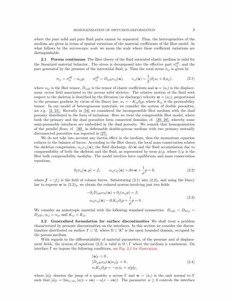
With regards to the differentiability of material parameters, of the pressure and of displace-ment fields, the system of equations (2.2) is valid in Ω \ Γ where the medium is continuous. Oninterface Γ we impose the following conditions, see Fig. 2.1 for illustration,

[u ]Γ = 0 ,

[Dijklekl(u)nj ]Γ = 0 ,

niKij∂jp = −wini = κ[p]Γ,

(2.4)

where [a]Γ denotes the jump of a quantity a across Γ and n = (ni) is the unit normal to Γsuch that [a]Γ = lims→0+

(a(x + sn) − a(x − sn)). The parameter κ ≥ 0 controls the interface

4 G. GRISO AND E. ROHAN

p+

p−

p+

p−

scale << ε

Γ

periodic microstructure

zoom 1

zoom 2

Γ

Γ

Fig. 2.1. Hierarchical structure of the porous medium with the discontinuity interface – two zooms illustrated.An example of sub-microscopic arrangement (the 2nd zoom) of the porous interface Γ (the grey/blue belt). Thepistons, being driven by external forces, may keep the pressure discontinuity |p+ − p−| > 0, whereas the effectivestress (related to the solid phase) is continuous. See Appendix for more details.

permeability, i.e. the filtration velocity w . Conditions analogous to (2.4)3 were considered in theheat conduction problems, cf. [5, 24].

There are two extreme cases, κ → +∞ and κ → 0. The first one yields the perfect pressurebonding and thereby also the bulk stress continuity, [njσij ]Γ = 0 due to (2.4)2 and (2.1)1, i.e.there is no interface effect. In the second case (κ → 0), the interface is completely impermeable,i.e. niKij∂jp = 0 in the sense of traces on both sides of Γ.

Remark 1. Stress discontinuity on the interface. We postulated the continuity of theeffective stress, [σeff

ij ]Γnj = 0 on Γ. This certainly holds at a porous interface when no fluid ispresent (thereby p ≡ 0). If the pores are saturated by the fluid, condition (2.4)2 admits pressurediscontinuities, i.e. [αijp]Γnj 6= 0, so that the overall (bulk) stress (2.1)1 has a jump on Γ. Althoughit does not conform physically to standard continua, there are situations which admit the stressdiscontinuity. Obviously the balance of momentum must hold, however, the stress discontinuitycan compensate additional (external) forces concentrated locally on the interface; for a given fdistributed on Γ the local equilibrium yields

nj [σij ]Γ = fi on Γ .

Then condition [σeffij ]Γnj = 0 only means that f = (fi) acts exclusively on the fluid phase at Γ, thus,

inducing the pressure discontinuity. The external forces can be produced by other physical fields(electromagnetic), or they can represent a mechanical interaction between the medium and other“self-supporting” structure. In the latter example, forces f express long-distance interactions.We discus more details in the Appendix, where an example of a two-phase porous ultra-structureconstituting the interface Γ is described.

Since we shall pursue the limit analysis with respect to the microstructural scale, ε, we recallthat the surface of Γε increases with ε → 0, so that forces f ε must be scaled with respect to ε.We shall treat two general cases of heterogeneities in coefficients αij , as specified in Section 2.6,which for ε→ 0 leads to different limit models and to different additional constraints relating theacting force and the microstructure scale.

We need to develop a special form of the mass conservation which takes into account a possiblepressure discontinuity on the interfaces Γ. In order to obtain a consistent weak formulation ofthe diffusion-deformation problem, the pressure discontinuities must be well-approximated in theformulation of the mass conservation. Therefore, we consider an integral formulation of thisphysical law, where the sources and the fluxes are weighted by discontinuous functions.

2.2.1 Preliminaries Let Γ be a Lipschitz surface in R3 and ω ⊂ R3 be an open bounded“control domain” such that Γω = Γ ∩ ω is nonempty and divides ω in two subdomains, ω =ω+ ∪ ω− ∪ Γω. Set

Γ+ = x′ = x+ tn(x) | x ∈ Γ, t→ 0+,Γ− = x′ = x− tn(x) | x ∈ Γ, t→ 0+.

HOMOGENIZATION OF DIFFUSION-DEFORMATION 5

Now, introduce a test function q ∈ L2(ω) by using the characteristic functions of ω±,

q(x) = q+χω+(x) + q−χω−(x) where χω±(x) =

1 for x ∈ ω±0 for x ∈ R3 \ ω±,

, (2.5)

where q+ and q− are real constants. Due to this construction, we can introduce the generalizedderivative (gradient) of q: for any ϕ ∈ C∞0 (ω)∫

ω

∇ϕ q =∑

k=+,−

∫ωk

∇(qkϕ) =

∫Γ+

q+ϕn+ dS +

∫Γ−

q−ϕn− dS

= −∫

Γω

ϕ[q]Γn = −∫ω

ϕδΓ[q]Γn ,

and

∫ω

ϕδΓ =

∫Γω

ϕdS ,

(2.6)

where δΓ is the Dirac distribution of Γ and n is the unit normal of Γ, such that n+ = −n = −n−.Thus, the generalized gradient of q is

∇q = δΓ[q]Γ n on Γ in the sense of distributions. (2.7)

2.2.2 Local mass conservation for discontinuous pressure fields Let J be the timerate of the fluid volume drained from an infinitesimal volume of the porous medium; later on weidentify J = divw . The mass conservation for the compressible porous medium can be written inthe form ∫

ω

q

(1

µp+ J

)+

∫∂ω

q αij ui nj dS = 0 .

If all integrands (except q) are continuous and αij are constant in ω, the standard differential form

can be obtained, i.e. p/µ + J + αijeij(u) = 0, when taking q+ = q−. We consider in the sequelmore general situations, allowing for discontinuous pressures. Moreover, the Biot coefficients on Γωmay be discontinuous in the case of piecewise constant coefficients: αij(x) = αkij in ωk, (k = +,−),although we shall refrain from such an option later on.

By the Green formula we get formally

0 =

∫ω

q (1

µp+ J ) +

∫ω

q αij∂j ui +

∫ω

ui ∂j(q αij)

=

∫ω

q

(1

µp+ J + αijeij(u)

)+

∫ω

ui ∂j(q αij) ,

where the last integral can be rewritten using (2.7) to get

0 =

∫ω

q

(1

µp+ J + αijeij(u)

)+

∫ω

ui njδΓ[q αij ]Γ

=∑

k=+,−

∫ωk

qk(

1

µp+ J + αijeij(u)

)+

∫Γω

ui[qαij ]Γnj dS .(2.8)

Further, recalling the definitions of Γ+ and Γ−, from(2.8) we derive the following form of thegeneralized mass conservation which is dual to the pressure discontinuities at Γ:

1

µp+ J + αijeij(u) + ui nj (δΓ+αij |Γ+ − δΓ−αij |Γ−) = 0 . (2.9)

Assuming αij |Γ+ = αij |Γ− = αΓij , (2.9) can be rewritten as

1

µp+ J + αijeij(u) + uinj α

Γij (δΓ+ − δΓ−) = 0 . (2.10)

6 G. GRISO AND E. ROHAN

2.2.3 Weak formulation of mass conservation for discontinuous pressure fieldsRecalling that Ω is the domain occupied by our heterogeneous material, for any q given by (2.5),equation (2.9) yields ∫

Ω

q

(1

µp+ J + αijeij(u)

)+

∫Ω

uinj [qαij ]Γ δΓ = 0 , (2.11)

where the last integral can be rewritten in terms of a surface integral by virtue of (2.6)2.We can now develop the term involving local source/sink of fluid, J = divw . Recalling the

impermeability of the outer surface, i.e. n · w = 0 on ∂Ω, for any q defined by (2.5) with ∇qdefined by (2.7), it follows that∫

Ω

qJ =

∫Ω

q∇ ·w = −∫

Ω\Γw · ∇q −

∫Ω

w · n [q]Γ δΓ

= −∫

Ω\Γw · ∇q −

∫Γ

w · n [q]Γ dS =

∫Ω\Γ

Kij∂jp ∂iq +

∫Γ

κ [p]Γ [q]Γ dS ,

(2.12)

where we used the Darcy law and condition (2.4)3 in order to replace w . Thus, from (2.11)-(2.12)it follows that the mass conservation can be written in the form∫

Ω

q

(1

µp+ αijeij(u)

)+

∫Ω\Γ

Kij∂jp ∂iq

+

∫Γ

κ [p]Γ [q]Γ dS +

∫Γ

[qαij ]Γ uinj dS = 0 ∀q .(2.13)

2.2.4 Balance of forces with pressure discontinuities A consequence of the continuity

of the effective stress σeffij = Dijklekl(u) and of the discontinuity of the pressure as defined in (2.17),

the overall stress σij = σeffij − αijp is discontinuous, see Remark 1 below. Therefore, the standard

differential form (2.2)1 of the balance of forces holds in Ω\Γ. Taking a continuous test displacementfield v ∈ H1

0(Ω), we can integrate by parts in Ω \ Γ to get

−∫

Ω\Γvi∂jσij =

∫Ω

f · v ,∫Ω\Γ

σijeij(v) +

∫Γ

vi [σij ]Γ nj dS =

∫Ω

f · v ,∫Ω\Γ

(Dijklekl(u)− αijp) eij(v)−∫

Γ

vi [αijp]Γ nj dS =

∫Ω

f · v ,

(2.14)

where the volume integral over Ω \ Γ can be replaced by an integral over Ω, since all integrandsare “sufficiently smooth” in Ω.

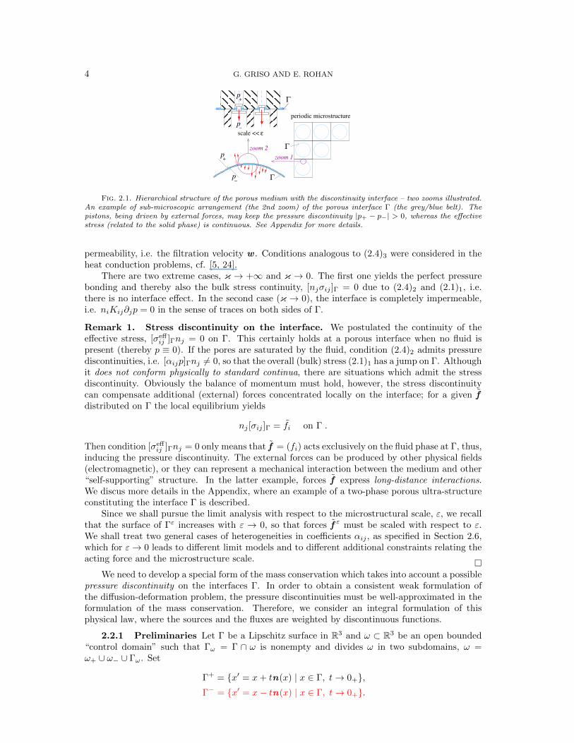
Fig. 2.2. An example of a periodic microstructure generated by a representative cell Y . A two-dimensionalsection of a 3D structure is displayed. Both the matrix part Ym and the channels Yc generate the connecteddomains Ωε

m and Ωεm. The discontinuity interface Γε

m is illustrated by thick lines, it may also form a connectedhypersurface in Ω.

HOMOGENIZATION OF DIFFUSION-DEFORMATION 7

2.3 A periodic microstructure with two compartments The heterogeneous porousmedium consists of two distinct parts with different magnitudes of the respective hydraulic per-meabilities. We consider an open bounded domain Ω ⊂ R3, which is decomposed into two partsΩm (matrix) and Ωc (channels), so that

Ω = Ωm ∪ Ωc ∪ Γmc, with Ωm ∩ Ωc = ∅ .

The microstructure is generated by periodic unit cubes Y =]0, 1[3; this choice of the cell Y ismade for the sake of simplicity (one can consider general parallelotops as periodicity cells via sometechnicalities). Let Yc and Ym be connected, disjoint subdomains of Y with Lipschitz boundaries,so that ∂Yc has common measurable sets with all faces of Y and

Ym = Y \ Yc, ∂mYc = ∂cYm = Yc ∩ Ym,∂cYc = Yc ∩ ∂Y, ∂mYm = Ym ∩ ∂Y,Y = Ym ∪ Yc ∪ ∂mYc, with Ym ∩ Yc = ∅,∂Y = ∂cYc ∪ ∂mYm , ∂Yc = ∂cYc ∪ ∂mYc .

Denote by ε > 0 the scale parameter defining the size of microstructures. The channel Yc issuch that εYc generates a connected ε−periodic domain Ωεc; let us introduce

(Rn)c = Interior( ⋃ζ∈Z3

(ζ + Yc)),

then the open set Ωεc is defined by

Ωεc = ε(Rn)c ∩ Ω .

The “matrix” Ωεm is then obtained by removing the “channel network” from the whole domain:Ωεm = Ω\Ωc

ε. We assume that Ωεm is connected.

Further, we introduce the interface ΓYm embedded in the matrix part, ΓYm ⊂ Ym. As discussedin Section 2.2, pressure discontinuities may be expected on ΓYm. An example of the surface locationis illustrated in Figure 2.3. Due to the interface ΓYm, the matrix compartment generated by εYmis periodically subdivided into the subdomains Ωεm,k, k ∈ Jεm, separated by the interface Γεm sothat

Γεm = Ωεm \⋃k∈Jε

m

Ωεm,k , Ωεm,k ∩ Ωεm,l = ∅ for k 6= l , Ωεm = Interior( ⋃k∈Jε

m

Ωm,kε).

(2.15)

Note that the diameter of each Ωεm,k is proportional to ε. Obviously, if Ω ⊂ R3, then |Γεm| ≈ ε2.In order to define an extension operator (from the channels to the matrix, or briefly an “off-

channels” extension), we introduce the domain containing the “entire” periods εY :

Ωε = interior⋃ζ∈Ξε

Y εζ , Y εζ = ε(Y + ζ)

where Ξε = ζ ∈ Z3 | ε(Y + ζ) ⊂ Ω .(2.16)

2.4 Weak formulation of the problem Having developed a suitable weak forms of boththe balance of forces and mass conservation laws, respectively (2.13) and (2.14), we are readyto define the diffusion-deformation problem with interface pressure discontinuities in the periodicheterogeneous structure. We consider the following boundary and initial conditions:

uε(t, ·) = u0(t, ·) on ∂Ω, for t ∈]0, T [ ,

niKεij∂jp

ε(t, ·) = 0 on ∂Ω, for t ∈]0, T [ ,

uε(0, ·) = 0 in Ω,

pε(0, ·) = 0 in Ω.

8 G. GRISO AND E. ROHAN

Obviously, we assume the consistency constraint u0(0, x) = 0 for x ∈ ∂Ω. Moreover, in Section 4,we impose the homogeneous Dirichlet condition u0 ≡ 0.

Since the pressure field can be discontinuous on Γε, we need the following space of discontin-uous functions:

H1(Ωεm \ Γεm) = q ∈ L2(Ωεm) : ∇q ∈ L2(Ωεm \ Γεm) ,H1(Ω \ Γεm) = q ∈ L2(Ω) : ∇q ∈ L2(Ω \ Γεm) .

(2.17)

As in [16], we integrate (2.13) in time and introduce the integrated pressure

P ε(t, x) =

∫ t

0

pε(t, x) dt . (2.18)

Clearly, P ε(0) = 0.Our aim is to study the asymptotic behavior as ε → 0, of the following problem: Find

uε ∈ H1(0, T ; H10(Ω)) + u0 and P ε ∈ H1

0 (0, T ;H1(Ω \ Γεm)) such that for a.e. t ∈]0, T [

∫Ω

Dεijklekl(u

ε)eij(v)−∫Ω

dP ε

d tαεijeij(v)−

∫Γεm

αΓ,εij vin

εj

[dP ε

d t

]Γεm

dS

=

∫Ω

f · v , ∀v ∈ H10(Ω),∫

Ω

q αεijeij(uε) +

∫Γεm

αΓ,εij u

εinεj [q]Γε

mdS +

∫Ω\Γε

m

Kεij∂jP

ε ∂jq +

∫Ω

1

µεdP ε

d tq

+

∫Γεm

κε [P ε]Γεm

[q]ΓεmdS = 0, ∀q ∈ H1(Ω \ Γεm).

(2.19)

The material coefficients Dεijkl, α

εij , α

Γ,εij , Kε

ij and κε are oscillating and ε-periodic, as specifiedin Section 2.6. We claim that there exists a unique solution of (2.19). For the proof, we refer to[16], Section 3, where a similar model was treated.

2.5 The periodic unfolding method In this paper we apply the unfolding method ofhomogenization, cf. [10, 11], to derive the homogenized model. For the reader’s conveniencewe recall the notion of the periodic unfolding method and of the periodic unfolding operator, inparticular. We shall use the convergence results in the unfolded domain Ω×Y which can be foundin [10].

For all z ∈ R3, let [z] be the unique integer such that z− [z] ∈ Y . We may write z = [z] + zfor all z ∈ R3, so that for all ε > 0, we get the unique decomposition

x = ε([xε

]+xε

)∀x ∈ R3 .

Based on this decomposition, the periodic unfolding operator Tε : L2(Ω;R) → L2(Ω × Y ;R) isdefined as follows: for any function v ∈ L1(Ω;R), extended to L1(R3;R) by zero outside Ω, i.e.v = 0 in R3 \ Ω,

Tε(v)(x, y) =

v(ε[xε

]+ εy

), x ∈ Ωε, y ∈ Y ,

0 otherwise .

The following integration formula holds:∫Ωε

v dx =1

|Y |

∫Ω×Y

Tε(v) dy dx ∀v ∈ L1(Ω) .

Analogously, when integrating on a surface Γε generated by a surface ΓY ⊂ Y (see (2.15)), theformula reads ∫

Γε

v dS =1

ε|Y |

∫Ω×ΓY

Tε(v) dSy dx, ∀v ∈ L1(Ω).

HOMOGENIZATION OF DIFFUSION-DEFORMATION 9

These formulae will be used in the sequel to evaluate integrals over Ω, which typically is approvedupon satisfying so-called unfolding criterion for integrals. For more details and convergence results,we refer the reader to [10], for error estimates see [17, 18, 19].

In what follows we use the following abbreviations (for any Ya ⊂ Y )

1

|Y |

∫Ya

= ∼∫Ya

, and also1

|Y |

∫Ω×Ya

= ∼∫

Ω×Ya

.

2.6 Oscillating material coefficients The porous medium distributed in Ω is featured bymaterial heterogeneities characterized at the length scale ε, thereby the coefficients in equations(2.3) are highly oscillating. We treat strongly heterogeneous permeability coefficients, where theheterogeneity is related to the domain decomposition into the “matrix” part and the “channel”part.

The setting of the problem is based on (2.13) and (2.14) where the material parameters aredefined piecewise with respect to the domain decomposition introduced above. In general, for anymaterial parameter cε = cε(x) identified with Dε

ijkl, αεij or µε, we assume the following:

cε ∈ L∞(Ω) , Tε(cε(x))→ c(x, y) a.e. in Ω× Y, (2.20)

where c(x, y) is identified respectively, as Dijkl, αij or µ. For the permeability coefficients Kεij ∈

L∞(Ω), instead of (2.20), we assume that

Tε(χεcK

εij(x)

)→ χc(y)Kc

ij(x, y) a.e. in Ω× Y,

1

ε2Tε(χεmK

εij(x)

)→ χm(y)Km

ij (x, y) a.e. in Ω× Y,

where χεd(x) = χd

(xε

)is the characteristic function of domain Ωεd, d = c, m. Thus we assume

that the permeability coefficients depend strongly on the scale parameter. In particular, due tothe ε2-scaling of the permeability in Ωεm, the matrix part presents a dual porosity. All the othermaterial coefficients in their unfolded form can also be refered to by superscripts c, m in thedomains Yc and Ym, respectively. Hence, by (2.20),

c(x, y) = χc(y)cc(x, y) + χm(y)cm(x, y) ,

so that Ddijkl, α

dij and µd have a meaning.

Further, we assume the existence of positive constants cD, CD, cK , CK , cµ, Cµ, independent ofε and such that for a.e. x ∈ Ω,

cD|ξ|2 ≤ Dεijkl(x)ξklξij , |Dε

ijkl(x)| ≤ CD for any (symmetric) ξ ∈M2,

cµ ≤ 1/µε(x) ≤ Cµ ,for a.e. x ∈ Ωεm, ∀ζ ∈ R2, |Kε

ij(x)| ≤ ε2CK , ε2cK |ζ|2 ≤ Kεij(x)ζiζj ,

for a.e. x ∈ Ωεc, ∀ζ ∈ R2, |Kεij(x)| ≤ CK , cK |ζ|2 ≤ Kε

ij(x)ζiζj .

(2.21)

Because of the pressure discontinuities on Γεm we need to specify the definitions of κε and αεijon Γεm. To do so, we assume that (2.10) holds with αΓ,ε

ij as the interface Biot coefficients.

Below we shall employ the boundary unfolding opreator T bε () which is introduced as Tε()operating on interface Γεm, i.e. for any v ∈ L1(Γεm;R), T bε (v(x)) = v

(ε[xε

]+ εy

)whenever

x ∈ Γεm ∩ Ωε, so that y ∈ ΓY , and T bε (v(x)) = 0 otherwise.The interface permeability κε ∈ L∞(Γεm). We assume that

T bε (κε(x)) = εκ(xε, y) , where cκ ≤ κ ≤ Cκ , (2.22)

for some given cκ , Cκ > 0, where xε = ε[x/ε] is the lattice restriction of x (using the unfoldingoperation) and y ∈ ΓYm. The scaling employed in (2.22) retains non-vanishing pressure jump inthe limit at the microscopic scale; let us note that a similar scaling effect is comprised in the studyreported in [5], although therein the medium is not strongly heterogeneous.

10 G. GRISO AND E. ROHAN

Biot coefficients αεij ∈ L∞(Γεm) on the interface. As we shall see, the limit model dependsstrongly on the uniform estimates of αεij with respect to ε. We consider the following two particularsituations:

weakly discontinuous data (WD) T bε(αΓ,εij

)= εαΓ

ij(xε, y) , (2.23)

strongly discontinuous data (SD) T bε(αΓ,εij

)= αΓ

ij(xε, y) , (2.24)

where xε = ε[x/ε] and y ∈ ΓYm. In the first case T bε αΓ,εij → 0 a.e. in Ω× ΓYm. Anyway, in Ω \ Γεm

we suppose that Tε(αεij)→ αij(x, y) a.e. in Ω× (Y \ ΓYm).

3 Homogenization of the model with WD data Throughout this section we assumewe are given standard “moderate” forces f ε, i.e., such that

‖f ε‖L2(0,T ;L2(Ω)) ≤ C . (3.1)

The plan of this section is as follows. In Section 3.1 we give a priori estimates which allowus to pass to the limit in Section 3.2. The procedure of the scale-decoupling for the “Laplace-transformed in time” limit equations is explained in Section 3.3.

3.1 A priori estimates Let us recall some basic inequalities that will be used also in thecase of strongly discontinuous data (2.24).

The Young inequality: ∀(a, b) ∈ R2, ∀ν ∈ R∗+, ab ≤ a2

2ν+νb2

2,

The Korn inequality: ∀v ∈ H10(Ω), ‖∇v‖2L2(Ω) ≤ C1

∑i,j

‖eij(v)‖2L2(Ω).(3.2)

Using appropriate test functions, we can eliminate in (2.19) the “mixed terms”, so that onlyquadratic forms appear in the resulting identity,∫

Ω

Dεijklekl(u

ε)eij(uε)−

∫Ω

dP ε

d tαεijeij(u

ε)−∫

Γεm

αΓ,εij u

εinεj

[dP ε

d t

]Γεm

dS =

∫Ω

f · uε ,

∫Ω

dP ε

d tαεijeij(u

ε) +

∫Γεm

αΓ,εij u

εinεj

[dP ε

d t

]Γεm

dS +

∫Ω\Γε

m

Kεij∂jP

ε ∂jdP ε

d t

+

∫Ω

1

µεdP ε

d t

dP ε

d t+

∫Γεm

κε [P ε]Γεm

[dP ε

d t

]Γεm

dS = 0.

(3.3)

Upon summation we obtain∫Ω

Dεijklekl(u

ε)eij(uε) +

1

2

d

d t

∫Ω\Γε

m

Kεij∂jP

ε ∂jPε

+

∫Ω

1

µε

∣∣∣∣dP εd t

∣∣∣∣2 +1

2

d

d t

∫Γεm

κε [P ε]2ΓεmdS =

∫Ω

f · uε.(3.4)

Then we integrate in time t ∈ [0, t], t ≤ T , recalling P ε(0) = 0, see (2.18), and use the lowerboundedness of all the material coefficients, see (2.21) and (2.22); this yields

cD

∫ t

0

∫Ω

∑i,j

|eij(uε)|2 dt+ cµ

∫ t

0

∫Ω

∣∣∣∣dP εd t

∣∣∣∣2 dt+ cK

∫Ωε

c

|∇P ε(t)|2 + cKε2

∫Ωε

m\Γεm

|∇P ε(t)|2 + cκε

∫Γεm

[P ε(t)]2Γεm≤∫ t

0

∫Ω

f ε · uε dt .

(3.5)

HOMOGENIZATION OF DIFFUSION-DEFORMATION 11

Due to the definition of the volume forces and using (3.1), we have∫ t

0

∫Ω

f ε · uε dt ≤ 1

2ν‖f ε‖2L2(0,T ;L2(Ω)) +

νC1

2‖∇uε‖2L2(0,T ;L2(Ω)) , for a.a. t ≤ T , (3.6)

where we used the Poincare inequality and (3.2)1, ν > 0 being an arbitrary constant. Then,using the Korn inequality (3.2)2 to deal with |eij(uε)|2, combining (3.6) with (3.5), and choosingν appropriately, the following estimates are obtained:

‖uε‖L2(0,T ;H1(Ω)) ≤ C, ‖∇P ε‖L∞(0,T ;L2(Ωεc)) ≤ C,

‖∇P ε‖L∞(0,T ;L2(Ωεm\Γε

m)) ≤C

ε,

∥∥∥dP ε

d t

∥∥∥L2(0,T ;L2(Ω))

≤ C,

‖[P ε]Γεm‖L∞(0,T ;L2(Γε

m)) ≤C√ε.

(3.7)

From (3.7)4 we deduce immediately that ‖P ε‖H1(0,T ;L2(Ω)) ≤ C, which follows due to P ε(0) = 0,see (2.18).

3.2 Limit problems In this section we give the limit representation of the model (2.19)with assumption (2.23). First, however, we obtain some results which are applicable in both thestrongly and weakly discontinuous cases. It is worth to emphasize that we do not use extensionoperators which otherwise have been used commonly when dealing with problems in perforateddomains – instead we employ the convergence theorems developed recently in [12].

We shall need the space of discontinuous unfolded functions. Let ΓYm ⊂ Y be the representativediscontinuity interface, i.e. Γεm =

⋃ζ∈Ξε εΓYm + εζ, see (2.16), and set

H#c0(Y,ΓYm) = q ∈ H1#(Y \ ΓYm)| q = 0 in Yc . (3.8)

Below we rely on the following two Theorems which were introduced as Theorem 3.1 andTheorem 3.12 in [12]. Here we adapted these results according to our situation with a changednotation. We recall the decomposition (2.15) and the space H1(Ωεm \ Γεm).

Theorem 3.1. Let (wε)ε be a sequence belonging to H1(Ωεm \ Γεm) and satisfy

‖wε‖L2(Ωεm) + ε‖∇wε‖L2(Ωε

m\Γεm) ≤ C .

Then there exists some w ∈ L2(Ω;H1#(Ym \ ΓYm)), such that, up to a subsequence,

Tε(wε) w weakly in L2(Ω;H1(Ym)) ,

εTε(∇wε) ∇yw weakly in L2(Ω× Ym \ ΓYm) .

Theorem 3.2. Suppose that wε ∈ H1(Ωεc) satisfies ‖wε‖H1(Ωεc) ≤ C. Then there exists

w ∈ H1(Ω) and w ∈ L2(Ω;H1#(Yc)), such that, up to a subsequence,

Tε(wε) w weakly in L2(Ω;H1(Yc)) ,

Tε(∇wε) ∇w +∇yw weakly in L2(Ω× Yc) .

Lemma 3.3. Due to estimates (3.7), the following limit fields exist:

u ∈ L2(0, T ; H10(Ω)), u1 ∈ L2(0, T ; H1

#(Y )),

P ∈ H1(0, T ;L2(Ω)) ∩ L∞(0, T ;H1(Ω)), P 1 ∈ L∞(0, T ;L2(Ω;H1#(Yc))),

Pm ∈ H1(0, T ;L2(Ω× Ym)) ∩ L∞(0, T ;L2(Ω;H#c0(Y,ΓYm))),

(3.9)

such that the following convergences hold, up to subsequences:

uε u weakly in L2(0, T ; H10(Ω)),

Tε(uε) u weakly in L2(0, T ; L2(Ω× Y )),

Tε(∇uε) ∇xu +∇yu1 weakly in L2(0, T ; L2(Ω× Y )),

(3.10)

12 G. GRISO AND E. ROHAN

and

Tε(P ε) P weakly in H1(0, T ;L2(Ω× Yc)),Tε(∇P ε) ∇xP +∇yP 1 weakly ∗ in L∞(0, T ;L2(Ω× Yc)),

Tε(P ε) Pm weakly in H1(0, T ;L2(Ω× Ym)),

εTε(∇P ε) ∇yPm weakly ∗ in L∞(0, T ;L2(Ω× Ym \ ΓYm))

Tε([P ε]Γε

m

)[Pm

]ΓYm

weakly ∗ in L∞(0, T ;L2(Ω;L2(ΓYm)).

(3.11)

Proof. The proof is the direct consequence of estimates (3.7) and Theorems 3.1 and 3.2,whereby some standard convegence results from [10] are applied.

Yet we need to establish a relationship between the limit pressure in Ω × Yc and in Ω × Ym,cf. [30].

Lemma 3.4. The limit fields P and Pm satisfy the following condition:

Pm(·, y) = P for a.a. y ∈ ∂Yc ∩ ∂Ym and a.e. in ]0, T [× Ω . (3.12)

Proof. Let us consider ϕ ∈ C∞0 (Ω) and ψ ∈ [H1#(Y )]3. If ε is small enough, due to the

convergence result (3.11) we obtain the limit∫Ω\Γε

m

ε∇P ε(x) · ϕ(x)ψ(x/ε) =

∫Ω

∼∫Ym\ΓY

m

εTε(∇P ε)(x, y)Tε(ϕ)(x, y) ·ψ(y)

→∫

Ω

∼∫Ym\ΓY

m

∇yPm · ϕψ .

(3.13)

Above the left hand side integral can be rewritten on integrating by parts:

−∫

Ω\Γεm

εP ε(x) (∇ϕ(x) ·ψ(x, x/ε) + ϕ(x)∇ ·ψ(x/ε)) +

∫Γεm

[P ε(x)]Γεmεϕ(x)n(x/ε) ·ψ(x, x/ε) dSx

=−∫

Ω

∼∫Y \ΓY

m

Tε(P ε) (Tε(ε∇xϕ) ·ψ + Tε(ϕ)∇y ·ψ) +

∫Ω

1

ε∼∫

ΓYm

Tε([P ε]Γε

m

)εTε(ϕ)n ·ψ dSy .

Then we can pass to the limit and integrate by parts again:

→−∫

Ω

∼∫Yc

P (x)ϕ(x)∇y ·ψ(y)−∫

Ω

∼∫Ym\ΓY

m

Pm(x, y)ϕ(x)∇y ·ψ(y)

+

∫Ω

∼∫

ΓYm

[Pm(x, y)

]ΓYm

ϕ(x)n(y) ·ψ(y) dSy

=

∫Ω

ϕ ∼∫Ym\ΓY

m

∇yPm ·ψ +

∫Ω

Pϕ ∼∫∂Yc

n ·ψ dSy +

∫Ω

ϕ ∼∫∂Ym

Pmn ·ψ dSy ,

(3.14)

where the last two boundary integrals vanish on ∂Y due to the Y-periodicity of the integrands,so that the only nonvanishing parts are evaluated on ∂Ym ∩ ∂Yc. Condition (3.12) now follows bycomparing both the limit expressions at (3.13) and (3.14), since ψ and ϕ can be chosen arbitrarily.

We may now introduce the bubble function by setting P = Pm−P whereby P ∈ H1(0, T ;L2(Ω×Ym)) ∩ L∞(0, T ;L2(Ω;H#c0(Y,ΓYm))) as the consequence of Lemma 3.4. Thus, since P (x, ·) = 0

on the channel-matrix interface ∂Ym∩∂Yc, P can be extended continuously by zero to all Ω. Thenconvergences (3.11) yield

Tε(P ε) P + P weakly in H1(0, T ;L2(Ω× Y )),

εTε(∇P ε) ∇yP weakly ∗ in L∞(0, T ;L2(Ω× Ym \ ΓYm)),

Tε([P ε]Γε

m

)[P]

ΓYm

weakly ∗ in L∞(0, T ;L2(Ω;L2(ΓYm)).

(3.15)

HOMOGENIZATION OF DIFFUSION-DEFORMATION 13

The limit fields satisfy the limit homogenized problem.Theorem 3.5. Let (uε, P ε) be solution of problem (2.19) where αε on Γεm is given by (2.23).

Then, the limit fields (3.9) with convergences (3.10)-(3.11) are such that (u, P ) and (u1, P 1, P )satisfy the coupled unfolded problem (in the sense of time distributions):

∼∫

Ω×YDijkl[e

xkl(u) + eykl(u

1)] [exij(v0) + eyij(v

1)]

− ∼∫

Ω×Yαij [e

xij(v

0) + eyij(v1)]

(dP

d t+ χm

d P

d t

)

−∫

Ω

v0i ∼∫

ΓYm

njαΓij

[d

d tP

]ΓYm

dSy =

∫Ω

f · v0,

(3.16)

and

∼∫

Ω×Yc

Kcij(∂

xj P + ∂yj P

1) (∂xj q0 + ∂yj q

1)+ ∼∫

Ω×Ym

Kmij ∂jP ∂iq

0

+

∫Ω

∼∫

ΓYm

njαΓijui

[q0]ΓYmdSy+ ∼

∫Ω×Y

αij [exij(u) + eyij(u

1)] [q0 + χmq0]

+

∫Ω

∼∫

ΓYm

κ[P]

ΓYm

[q0]ΓYmdSy+ ∼

∫Ω×Yc

1

µcdP

d tq0

+ ∼∫

Ω×Ym

1

µm

(dP

d t+

d P

d t

)(q0 + q0) = 0 ,

(3.17)

for all v0 ∈ V0 = H10(Ω), q0 ∈ H1(Ω), v1 ∈ L2(Ω; H1

#(Y )), q1 ∈ L2(Ω;H1#(Y )) and q0 ∈

L2(Ω;H#c0(Y,ΓYm)).

Remark 2. The “two-scale” problem (3.16)-(3.17) retains the symmetry of (2.19). The existenceand uniqueness of weak solutions defined in Ω × Y can be proved using similar technique, as forthe original problem (2.19), see [16], Section 3, however, extended for the two-scale functions andappropriate spaces employed in (3.16)-(3.17).

Proof. of Theorem 3.5. We shall derive limit expressions for all unfolded integrals involved in(2.19). For this we need to introduce suitable test functions vε and qε. Due to (3.10)-(3.11), thefollowing test displacements are considered:

vε(x) = v(x) + εv1(x/εY )θ(x) , v ∈ H10(Ω), v1 ∈ H1

#(Y )/R, θ ∈ C∞0 (Ω).

Further, we introduce the pressure test functions qε of the following form

qε(x) = q0(x) + εq1(y)ϑ(x) + q(y)ϑ(x) , where q = 0 in Yc, (3.18)

Passing to the limit in the interface integrals from (2.19), we get∫Γεm

njαεijv

εi [

d

d tP ε]Γε

mdS

=

∫Ω

1

ε|Y |

(vi

∫ΓYm

njεαΓij

[d

d tT bε(P ε)]

ΓYm

dSy + ε2θ

∫ΓYm

njαΓijv

1i

[d

d tT bε(P ε)]

ΓYm

dSy

)

→∫

Ω

vi ∼∫

ΓYm

njαΓij

[d

d tP

]ΓYm

dSy ,

(3.19)

and ∫Γεm

njαεiju

εi [q(x/ε)]Γε

mϑ dS =

∫Ω

1

|Y |

∫ΓYm

njαΓijT bε (uεi ) [q]ΓY

mT bε(ϑ)dSy

→∫

Ω

ϑui ∼∫

ΓYm

njαΓij [q]ΓY

mdSy .

(3.20)

14 G. GRISO AND E. ROHAN

For the other integrals in (2.19), we have the following limits (recalling that αεij is not proportionalto ε in Ω \ Γεm):

∫Ω

Dεijklekl(u

ε)eij(vε)→

∫Ω

∼∫Y

Dijkl(exkl(u) + eykl(u

1)) (exij(v) + eyij(v1)θ),∫

Ω

αεijeij(vε)

d

d tP ε →

∫Ω

∼∫Y

αij(exij(v) + eyij(v

1)θ)d

d t

(P (x) + χmP

),∫

Ω

f ε · vε →∫

Ω

f · v ,

(3.21)

where f ε f weakly in L2(0, T ; L2(Ω)), and

∫Ω

Kεij∂jP

ε∂iqε →

∫Ω

∼∫Yc

Kcij(∂

xj P + ∂yj P

1) (∂xj q0 + ϑ∂yj q

1) +

∫Ω

ϑ ∼∫Ym

Kmij ∂jP ∂iq,∫

Ω

αεijeij(uε)qε →

∫Ω

∼∫Y

αij(exij(u) + eyij(u

1))(q0 + χmqϑ),∫Ω

κε[P ε]Γεm

[qε]Γεm→∫

Ω

∼∫

ΓYm

κ[P]

ΓYm

[q]ΓYmdSy.

(3.22)

The limit expressions in (3.20)-(3.22) are valid (by density arguments) for any test functions ofthe form

vε(x) = v0(x) + εv1(x, y) , v ∈ H10(Ω), v ∈ L2(Ω; H1

#(Y )) ,

qε = q0(x) + εq1(x, y) + χm(y)q0(x, y),

q0 ∈ H1(Ω), q1 ∈ L2(Ω;H1#(Y )), q0 ∈ L2(Ω;H#c0(Y,ΓYm)).

(3.23)

So, instead of v1θ, we can take v1 ∈ L2(Ω; H1#(Y )); instead of q1ϑ, q1 ∈ L2(Ω;H1

#(Y )) and

instead of ϑq we take q0 ∈ L2(Ω;H#c0(Y,ΓYm)). It is now possible to write down the limit form of(2.19). The two-scale problem is obtained from (3.19)-(3.22), making use of the generalized testfunctions (3.23), and taking q1 = 0 in (3.22).

3.3 Scale decoupling and the homogenized constitutive laws In (3.16) and (3.17) wecan take suitable combinations of vanishing and non-vanishing parts of the test functions definedin (3.23), so that the “local” and the “global” problems can be identified.

The local problem describes the diffusion-deformation driven by ex(u), u and P . For allv1 ∈ H1

#(Y ) and q ∈ H#c0(Y,ΓYm), one has

∼∫Y

Dijkl[exkl(u) + eykl(u

1)] eyij(v1)− ∼

∫Y

αijeyij(v

1)dP

d t− ∼∫Ym

αmij eyij(v

1)d P

d t= 0 ,

∼∫Ym

αmij [exij(u) + eyij(u1)] q + ui ∼

∫ΓYm

njαΓij [q]ΓY

mdSy+ ∼

∫Ym

Kmij ∂

yj P ∂

yi q

+ ∼∫

ΓYm

κ[P]

ΓYm

[q]ΓYmdSy+ ∼

∫Ym

1

µm

(dP

d t+

d P

d t

)q = 0 .

(3.24)

HOMOGENIZATION OF DIFFUSION-DEFORMATION 15

The global problem is the diffusion-deformation problem described in terms of ex(u) and P ,

involving the local perturbations P ,u1, P 1. For all v0 ∈ V0 = H10(Ω) and q0 ∈ H1(Ω),

∼∫

Ω×YDijkl[e

xkl(u) + eykl(u

1)] exij(v0)− ∼

∫Ω×Y

αijexij(v

0)

(dP

d t+ χm

d P

d t

)

−∫

Ω

v0i ∼∫

ΓYm

njαΓij

[d

d tP

]ΓYm

dSy =

∫Ω

f · v0 ,∫Ω

Cij∂xj P ∂xi q0+ ∼∫

Ω×Yαij [e

xij(u) + eyij(u

1)] q0+ ∼∫

Ω×Yc

1

µcdP

d tq0

+ ∼∫

Ω×Ym

1

µm

(dP

d t+

d P 0

d t

)q0 = 0.

(3.25)

Homogenized permeability. By selecting q0 ≡ 0 and q ≡ 0, due to (3.22) the limit equation(3.17) reduces to

∼∫Yc

Kcij(∂

xj P + ∂yj P

1) ∂yj q1 = 0 , ∀q1 ∈ L2(Ω;H1

#(Y )) a.e. in Ω. (3.26)

Due to the linearity, we can define corrector basis functions ηk such that P 1(t, x, y) = ηk(y)∂xkP (t, x).Therefore, (3.26) is equivalent to the following problem (set in channels Yc):

Find ηk ∈ H1#(Y )/R (k = 1, 2, 3) such that

∼∫Yc

Kcij∂

yj (ηk + yk) ∂yi ψ = 0 ∀ψ ∈ H1

#(Y ) .(3.27)

It is now easy to replace in (3.17) the only integral involving P 1 using the homogenized permeabilityCij defined as follows:∫

Ω

Cij∂xj P∂xi q0 :=∼∫

Ω×Yc

Kcij [∂xj P + ∂yj P

1] ∂xi q0 =∼∫Yc

Kcil∂

yl (ηj + yj) ∂

xj P ∂

xi q

0 .

We can identify Cij as follows:

Cij =∼∫Yc

Kcil∂

yl (ηj + yj) =∼

∫Yc

Kckl∂

yl (ηj + yj) ∂

ykyi =∼

∫Yc

Kckl∂

yl (ηj + yj) ∂

yk(ηi + yi). (3.28)

The last symmetric expression is a simple consequence of identity (3.27) evaluated for ψ = ηi,where other indices have been changed appropriately.

Let us point out that the effective medium permeability Cij (relevant to the macroscopic scale)depends exclusively on the geometry and permeability of the primary porosity in the channelsrepresented by Yc.

3.3.1 Auxiliary local problems and corrector basis functions Throughout this sec-tion and in Section 4.3 bellow, we use the following notation:

aY (u , v) =∼∫Y

Dijkleykl(u) eyij(v), bY (ϕ, v) =∼

∫Y

ϕ αijeyij(v) ,

bYm (ϕ, v) =∼∫Ym

ϕαmij eyij(v) ,

cYm,Γm (ϕ, ψ) =∼∫Ym\ΓY

m

Kmij ∂

yj ϕ∂

yi ψ+ ∼

∫ΓYm

κ[ϕ]ΓYm

[ψ]ΓYmdSy ,

dYm (ϕ, ψ) =∼∫Ym

1

µmϕψ, γΓ,k(ϕ) =∼

∫ΓYm

njαΓkj [ϕ]ΓY

mdSy .

(3.29)

16 G. GRISO AND E. ROHAN

In order to decouple the microscopic and macroscopic evolutionary problems, we can apply theusual method of the scale separation based on the Laplace transformation v(t)→ Lv(λ), whereλ is the variable in the Laplace domain. For brevity we denote all functions depending on λ asfollows: Lv(λ) = ∗v. In the transformed space we define a suitable multiplicative decompositionto arrive at autonomous local problems arising from (3.24) allowing to compute the local correctorfunctions and, consequently to compute also the homogenized coefficients. We use zero initialconditions, namely u(0, ·) = 0, whereas P (0, ·) ≡ 0 by definition. By the Laplace transformation,the local problem becomes

aY(∗u1, v

)− bYm

(λ ∗P , v

)= −aY

(Πij , v

)eij( ∗u) + λbY (1, v) ∗P ,

bYm

(∗u1, φ

)+ cYm,Γm

(∗P0, φ

)+ λdYm

(∗P , φ

)= −bYm

(φ, Π)∗

eij( ∗u)− dYm(1, φ)λ∗P − γΓ,k(φ)

∗uk.

Due to the linearity, we define the multiplicative decomposition by introducing the correctorfunctions in the L-transformed time domain, in the form

∗u 1(λ, x, y) = λ ∗ω

rs(λ, y) exrs( ∗u )(λ, x) + λ ∗ωP (λ, y)∗P (λ, x) + λ ∗ω

k(λ, y)∗uk(λ, x) ,

∗P0(λ, x, y) = λ ∗π

rs(λ, y) exrs( ∗u )(λ, x) + λ ∗πP (λ, y)∗P (λ, x) + λ ∗π

k(λ, y)∗uk(λ, x) .

The functions ∗ωrs, ∗ω

P , ∗ωk and ∗π

rs, ∗πP , ∗π

k satisfy the following local auxiliary problems.Strain corrector problem: Find ( ∗ω

rs, ∗πrs) ∈ H1

#(Y )×H#c0(Y,ΓYm) such thataY(∗ωrs, v

)− λbYm

(∗πrs, v

)= − 1

λaY (Πrs, v) , ∀v ∈ H1

#(Y ) ,

bYm

(ψ, ∗ω

rs)

+ cYm,Γm

(∗πrs, ψ

)+ λdYm

(∗πrs, ψ

)= − 1

λbYm

(Πrs, ψ) ,

∀ψ ∈ H#c0(Y,ΓYm),

(3.30)

where Πrs = (Πrsi ) = (ysδir).

Pressure corrector problem: Find ( ∗ωrs, ∗π

rs) ∈ H1#(Y )×H#c0(Y,ΓYm) such that

aY(∗ωP , v

)− λbYm

(∗πP , v

)= bY (1, v) ∀v ∈ H1

#(Y ) ,

bYm

(ψ, ∗ω

P)

+ cYm,Γm

(∗πP , ψ

)+ λdYm

(∗πP , ψ

)= −dYm

(1, ψ)

∀ψ ∈ H#c0(Y,ΓYm).

(3.31)

Displacement corrector problem: Find ( ∗ωk, ∗π

k) ∈ H1#(Y )×H#c0(Y,ΓYm) such that

aY(∗ωk, v

)− λbYm

(∗πk, v

)= 0 ∀v ∈ H1

#(Y ),

bYm

(ψ, ∗ω

k)

+ cYm,Γm

(∗πk, ψ

)+ λdYm

(∗πk, ψ

)= − 1

λγΓ,k(ψ),

∀ψ ∈ H#c0(Y,ΓYm).

(3.32)

3.3.2 Homogenized coefficients and the macroscopic problem We now study themain homogenization result for weakly discontinuous data, namely (2.23). Application of theLaplace transformation to (3.25) yields

∼∫

Ω×Yexij(v

0) Dijkl[eykl(Π

rs) + λeykl( ∗ωrs)] exrs( ∗u)

+ ∼∫

Ω×Yexij(v

0) Dijkleykl( ∗ω

P )λ∗P+ ∼∫

Ω×Yexij(v

0) Dijkleykl( ∗ω

n)λ∗un

− ∼∫

Ω×Yexij(v

0)αijλ

(∗P + χmλ ∗π

rsexrs( ∗u) + χmλ ∗πP∗P + χmλ ∗π

n

∗un

)−∫Ω

v0i ∼∫

ΓYm

njαΓijλ

2

([∗πrs]ΓYmexrs( ∗u) +

[∗πP]ΓYm∗P +

[∗πn]ΓYm ∗un

)dSy =

∫Ω∗f · v0,

(3.33)

HOMOGENIZATION OF DIFFUSION-DEFORMATION 17

and

∼∫

Ω×Yq0αkl

([eykl(Π

rs) + λeykl( ∗ωrs)] exrs( ∗u) + λeykl( ∗ω

P )∗P + λeykl( ∗ωn)∗un

)+

∫Ω

Cij∂j ∗P∂iq0+ ∼

∫Ω×Y

q0

µλ∗P+ ∼

∫Ω×Ym

q0

µm

(λ2∗πijexij( ∗u) + λ2

∗πP∗P + λ2

∗πk

∗uk

)= 0.

(3.34)

In these equations we can identify the homogenized coefficients, as explained bellow.Homogenized viscoelasticity. This tensor is obtained by collecting in (3.34) all the terms which

contain λexij( ∗u),

A∗ijkl(λ) = λ[aY

(1

λΠkl + ∗ω

kl,1

λΠij

)− bYm

(∗πkl, Πij

) ]= λ

[aY

(1

λΠkl + ∗ω

kl,1

λΠij + ∗ω

ij

)+λcYm,Γm

(∗πkl, ∗π

ij)+λ2dYm

(∗πkl, ∗π

ij) ],

where the symmetric expression is a consequence of (3.30).The homogenized Biot modulus. This tensor is obtained by collecting in (3.33) all the termscontaining λ∗P ,

M∗(λ) =∼∫Y

1

µ+ λ ∼

∫Ym

1

µm ∗πP+ ∼∫Y

αijeyij( ∗ω

P ) =∼∫Y

1

µ+ λdYm

(∗πP , 1

)+ bYm

(1, ∗ω

P). (3.35)

The homogenized Biot coefficients. They can be obtained independently from both equations(3.33)-(3.34). On collecting in (3.33) all the terms involving λ∗P , one obtains

α∗ij(λ) =∼∫Y

αij − aY(∗ωP , Πij

)− λbYm

(∗πP , Πij

). (3.36)

By collecting in (3.34) all the terms involving λexij( ∗u)), one gets

β∗ij(λ) =1

λ∼∫Y

αij + bY(1, ∗ω

ij)

+ λdYm

(∗πij , 1

). (3.37)

It is easily seen that the following result holds true:Lemma 3.6. The homogenized Biot coefficients defined in (3.36) and (3.37) satisfy

α∗ij(λ) = λβ∗ij(λ) . (3.38)

Proof. Relation (3.38) can be obtained using the microscopic local problems, (3.30) and (3.31),where we use special forms of test functions. First (3.30)2 yields

1

λbYm

(∗πP , Πij

)= −bYm

(∗πP , ∗ω

ij)− λdYm

(∗πij , ∗π

P)− cYm,Γm

(∗πij , ∗π

P).

Then the first and the last terms can be expressed using (3.31)1 and (3.31)2, respectively, so that

1

λbYm

(∗πP , Πij

)=

1

λbY(1, ∗ω

ij)− 1

λaY(∗ωP , ∗ω

ij)− λdYm

(∗πij , ∗π

P)

+ bYm

(∗πij , ∗ω

P)

+ dYm

(1 + λ ∗π

P , ∗πij)

=1

λbY(1, ∗ω

ij)− 1

λaY(∗ωP , ∗ω

ij)

+ bYm

(∗πij , ∗ω

P)

+ dYm

(1, ∗π

ij).

(3.39)

Now (3.30)1 yields

1

λaY(∗ωP , Πij

)= −aY

(∗ωij , ∗ω

P)

+ λbYm

(∗πP , ∗ω

P), (3.40)

18 G. GRISO AND E. ROHAN

so that on substituting (3.39) and (3.40) in (3.36),

α∗ij(λ) = λaY(∗ωij , ∗ω

P)− λ2bYm

(∗πP , ∗ω

P)

+ λbY(1, ∗ω

ij)− λaY

(∗ωP , ∗ω

ij)

+ λ2bYm

(∗πij , ∗ω

P)

+ λ2dYm

(1, ∗π

ij)

+ ∼∫Y

αij

= λbY(1, ∗ω

ij)

+ λ2dYm

(1, ∗π

ij)

+ ∼∫Y

αij = λβ∗ij(λ) .

Coefficients due to the interface terms on “micro” and “macro”. We introduce coefficientsgIII∗kij , gII∗ij , gI∗k and hIII∗kij , hI∗k to express the following integrals appearing in (3.33), (3.34):∫

Ω

vi ∼∫

ΓYm

njαΓijλ

2[∗πrs]ΓYmexrs( ∗u) =

∫Ω

vigIII∗irs (λ)λexrs( ∗u),∫

Ω

vi ∼∫

ΓYm

njαΓijλ

2[∗πn]ΓYm ∗un =

∫Ω

vigII∗in (λ)λ

∗un,∫

Ω

vi ∼∫

ΓYm

njαΓijλ

2[∗πP]ΓYm∗P =

∫Ω

vigI∗i (λ)λ∗P ,

∼∫

Ω×Yexij(v) Dijkle

ykl( ∗ω

k)λ∗uk− ∼

∫Ω×Ym

exij(v)αmijλ2∗πk

∗uk =

∫Ω

exij(v)hIII∗kij (λ)λ∗uk

and

∼∫

Ω×Yqαijλe

yij( ∗ω

k)∗uk+ ∼

∫Ω×Ym

q

µmλ2∗πk

∗uk =

∫Ω

qhI∗k (λ)λuk,

where

gIII∗kij (λ) = λγΓ,k( ∗πij), gII∗kj (λ) = λγΓ,k( ∗π

j), gI∗k (λ) = λγΓ,k( ∗πP ),

hIII∗kij (λ) = aY(∗ωk, Πij

)− λbYm

(∗πk, Πij

),

hI∗k (λ) = bY(1, ∗ω

k)

+ λdYm

(∗πk, 1

).

(3.41)

For the well-posedness of the macroscopic problem, its symmetry is important. It is a conse-quence of the symmetries of the coefficients (3.41) stated bellow.

Lemma 3.7. The following relationships hold:

gII∗kj = gII∗jk , gI∗k = λhI∗k , hIII∗kij = −gIII∗kij , gIII∗kij = gIII∗kji . (3.42)

Proof. The first symmetry follows easily from (3.32) which leads to

γΓ,k( ∗πj) = dYm

(λ ∗π

k, λ ∗πj)

+ λcYm,Γm

(∗πk, ∗π

j)

+ aY(∗ωk, ∗ω

j)

= γΓ,j( ∗πk).

To show the second symmetry, we use (3.31) and rewrite both the terms involved in definition(3.41)5; the first one combined with (3.32)2 and (3.32)1, yields

bY(1, ∗ω

k)

= aY(∗ωk, ∗ω

P)− λbYm

(∗πP , ∗ω

k)

= λbYm

(∗πk, ∗ω

P)

+ γΓ,k( ∗πP ) + λcYm,Γm

(∗πk, ∗π

P)

+ λ2dYm

(∗πk, ∗π

P).

Then, combining the second term in (3.41)5 with (3.31)2, gives

λdYm

(∗πk, 1

)= −λ2dYm

(∗πP , ∗π

k)− λcYm,Γm

(∗πP , ∗π

k)− λbYm

(∗πk, ∗ω

P),

so that

hI∗k (λ) = bY(1, ∗ω

k)

+ λdYm

(∗πk, 1

)=

1

λγΓ,k(λ ∗π

P ) =1

λgI∗k (λ) .

HOMOGENIZATION OF DIFFUSION-DEFORMATION 19

For the third relationship in (3.42), using (3.30) and due to (3.32), we have

hIII∗kij = aY(∗ωk, Πij

)− λbYm

(∗πk, Πij

)= λ2cYm,Γm

(∗πij , ∗π

k)

+ λ3dYm

(∗πij , ∗π

k)

+ λ2bYm

(∗πk, ∗ω

ij)

− λaY(∗ωk, ∗ω

ij)

+ λ2bYm

(∗πij , ∗ω

k)

= −λγΓ,k( ∗πij) = −gIII∗kij .

Obviously gIII∗kij = gIII∗kji , due to the symmetry πij = πji.The main result of this section is the macroscopic problem, obtained from (3.33)-(3.34) by

replacing the integrals over Y , Ym and ΓYm by expressions involving the associated homogenizedcoefficients (the symmetries (3.38) and (3.42) playing an essential role).

The macroscopic homogeneized problem. Given λ ∈ R+, find ∗u in H10(Ω)+

∗u0 and ∗P in H1(Ω)

such that

∫Ω

A∗ijkl(λ)exkl(λ ∗u) exij(v)−∫

Ω

β∗ij(λ)exij(v)λ2∗P −

∫Ω

gI∗k (λ)λ∗Pvk −∫

Ω

gII∗ik (λ)λ∗uk vi

−∫

Ω

vkgIII∗kji e

xij(λ ∗u)−

∫Ω

exij(v)gIII∗kji λ ∗uk =

∫Ω∗f · v ,∫

Ω

Cij∂j ∗P∂iq +

∫Ω

β∗ij(λ)exij(λ ∗u)q +

∫Ω

M∗(λ)λ∗Pq +

∫Ω

λ−1gI∗k (λ)∗ukq = 0,

(3.43)

for all v ∈ H10(Ω) and q ∈ H1(Ω).

Proposition 3.8. There exists λ0 > 0 such that for every λ ∈ Λ0 ≡]0, λ0],(i) M∗(λ) > 0,(ii) problem (3.43) is coercive.

Proof. (i) Using appropriate test functions in (3.31), we obtain

bY(1, ∗ω

P)− λdYm

(1, ∗π

P)

= aY(∗ωP , ∗ω

P)

+ λcYm,Γm

(∗πP , ∗π

P)

+ λ2dYm

(∗πP , ∗π

P)≥ 0 .

Hence problem (3.31) is coercive, so that for any λ > 0 its solution is unique and bounded. Thus,there exists λ0 > 0 such that

dYm (1, 1)− 2λ0|dYm

(1, ∗π

P (λ0))| > 0 .

This implies that M∗(λ) > 0 for λ ∈ Λ0. Indeed, (3.35)2 now yields

M∗(λ) =∼∫Yc

1

µc+ dYm

(1, 1) + λdYm

(1, ∗π

P)

+ bY(1, ∗ω

P)

=∼∫Yc

1

µc+ dYm

(1, 1) + 2λdYm

(1, ∗π

P)

+ bY(1, ∗ω

P)− λdYm

(1, ∗π

P)> 0.

(ii) Upon substituting in (3.43) v := ∗u − ∗u0 and q := ∗P and summing the two identities,

the proof is based on the following symmetries, gII∗kl = gII∗lk , A∗ijkl = A∗klij and Cij = Cji, and onpositive definiteness of Cji, on the positivity of M∗(λ), as shown above, and positive definitenessof

AA =

(A∗ijkl −gIII∗sij

−gIII∗rkl −gII∗rs

).

To see it, we rewrite gII∗rs and gIII∗sij using the corrector problems, as follows:

gII∗kl = λaY(∗ωk, ∗ω

l)

+ λ2[cYm,Γm

(∗πk, ∗π

l)

+ dYm

(∗πk, ∗π

l) ]

,

gIII∗kij = λaY(λ−1Πij + ∗ω

ij , ∗ωk)

+ λ2[cYm,Γm

(∗πij , ∗π

k)

+ dYm

(∗πij , ∗π

k) ]

.

20 G. GRISO AND E. ROHAN

Further, let us introduce W ( ∗u) := ( ∗ωij + λ−1Πij)eij( ∗u) + ∗ω

k∗uk and Q( ∗u) := ∗π

ijeij( ∗u) + ∗πk∗uk.

Now we can see that the positive definiteness of AA results from the ellipticity of aY (·, ·), dYm(·, ·)

and cYm,Γm(·, ·). Indeed, there are m′,m > 0 such that for any ∗u and a.e. x ∈ Ω,

[e( ∗u),u ]TAA[e( ∗u),u ] = λaY (W , W ) + λ2[cYm,Γm (Q, Q) + dYm (Q, Q)

]≥ m′(‖eyij(W )‖2L2(Y ) + ‖∇y(Q)‖2L2(Y ))

≥ m(|exij( ∗u)|2 + | ∗u |2) .

To see the second inequality, due to the uniqueness of solutions to (3.30) and (3.32), for nonvan-ishing exij( ∗u) or ∗u , W and Q cannot be identically zero.

Remark 3. The macroscopic problem (3.43) can rewritten in a form involving the standardpressure. On multiplying (3.43)2 by λ and recalling (2.18) (i.e.

∗p = λ∗P ), the macroscopic L-

transformed problem reads as follows: given λ ∈ C, find ∗u ∈ H10(Ω) and

∗p ∈ H1(Ω) such that

∫Ω

[λA∗ijkl(λ)]exkl( ∗u) exij(v)−∫

Ω

α∗ij(λ)exij(v)∗p−

∫Ω

gI∗k (λ)∗pvk −

∫Ω

gII∗ik (λ)λ∗uk vi

−∫

Ω

vkgIII∗kji e

xij(λ ∗u)−

∫Ω

exij(v)gIII∗kji λ ∗uk =

∫Ω∗f · v ,∫

Ω

Cij∂j∗p∂iq +

∫Ω

α∗ij(λ)exij(λ ∗u)q +

∫Ω

M∗(λ)λ∗pq +

∫Ω

gI∗k (λ)λ∗ukq = 0,

for all v ∈ H10(Ω) and q ∈ H1(Ω).

4 Homogenization of the model with strongly discontinuous (SD) data In thissection we consider coefficients αεij defined according to (2.24). We show, see Remark 4, thatin this case the standard form of the volume forces treated in the weakly discontinuous case isnot relevant and leads to a vanishing solution. Correspondingly to the jump of the pressure andthereby also in the total stress on Γεm, the local equilibrium can be preserved, if the forces arescaled w.r.t. the heterogeneities. The following forms of the scale-dependent forces f ε = (fεi ) willbe considered:

Case AF – progressively increasing magnitude of imposed forces as ε→ 0

‖f ε‖L2(0,T ;H1(Ω)) ≤C

ε, f ε(t, x) =

1

εf (t, x), ‖f ‖L2(0,T ;H1(Ω)) ≤ C. (4.1)

Case BF – forces containing the Dirac distribution δΓεm

(x) on Γεm and such that

f ε(t, x) = f (t, x) + δΓεm

(x)f ε(t, x) , f ∈ L2(0, T ; L2(Ω)),

Tε(f ε)→ f strongly in L2((0, T )× Ω; L2(ΓYm)),

f ∈ L2((0, T )× Ω; L2(ΓYm)), ‖f ‖L2((0,T )×Ω;L2(ΓYm)) ≤ C ,∫

ΓYm

f (t, x, y) dSy = F (t, x) , ‖F‖L2((0,T );H1(Ω)) ≤ C.

(4.2)

Case CF – forces acting on Γεm with “zero average”, satisfying (4.2) and such that

F (t, x) ≡ 0 for a.a. x ∈ Ω , t ∈]0, T [. (4.3)

Case DF – progressively increasing gradients of imposed forces with ε→ 0

‖f ε‖L2(0,T ;H1(Ω)) ≤C

ε, ‖f ε‖L2(0,T ;L2(Ω)) ≤ C ,

Tε(f ε)→ f strongly in L2((0, T )× Ω; L2(Y )).

(4.4)

HOMOGENIZATION OF DIFFUSION-DEFORMATION 21

4.1 A priori estimates We now give a priori estimates for all the cases of external forces(4.1)–(4.4). The strong discontinuity affects the “off-diagonal” interface integrals which, by makinguse of the standard treatment (3.3)-(3.5), disappear from the principal inequality. The crucial roleis played by Proposition 4.1 which allows to involve the interface integral forms in the estimates.The results obtained in this section are summarized in Proposition 4.2.

Proposition 4.1. Let (uε, P ε) be solution to (2.19), where αε is defined according to (2.24).Then there exists a constant CQ such that

‖MεY (uε)‖H−1(Ω) ≤εCQ

(‖∇uε‖L2(Ω) + ‖dP ε

d t‖L2(Ω) + ε‖∇P ε‖L2(Ωε

m) +√ε‖[P ε]Γε

m‖L2(Γε

m)

).

(4.5)

Proof. There exists Q ∈W 1,∞(Y \ ΓYm) such that

Q(y) = 0 for y ∈ Y c, and ∼∫

ΓYm

αΓijnj

[Q]

ΓYm

= 1. (4.6)

Assertion (4.5) follows from (2.19)2 written for the test function qε(x) = Q(x/ε)θ(x) withθ ∈ H1

0 (Ω). Using the decomposition Tε(uε) = (Tε(uε) −MεY (uε)) +Mε

Y (uε) in the interfaceintegral (2.19)2, yields∣∣∣ ∫

Ω

MεY (uεi )

θ

ε|Y |

∫ΓYm

njαΓij

[Q]

ΓYm

dSy

∣∣∣≤∣∣∣ ∫

Ω

θ

ε|Y |

∫ΓYm

njαΓij(T bε (uεi )−Mε

Y (uεi ))[Q]

ΓYm

dSy

∣∣∣+∣∣∣ ∫

Ω

qε αεijeij(uε)∣∣∣+∣∣∣ ∫

Ω\Γεm

Kεij∂jP

ε ∂jqε∣∣∣

+∣∣∣ ∫

Ω

1

µεdP ε

d tqε∣∣∣+∣∣∣ ∫

Γεm

κε [P ε]Γεm

[qε]

Γεm

dS∣∣∣.

(4.7)

We now estimate all the right-hand side integrals in this inequality. Due to the Poincare–Wirtingerinequality and since ∇y(Tε(uε)−Mε

Y (uε)) = ∇yTε(uε) = εTε(∇xuε),

‖T bε (uε)−MεY (uε)‖L2(Ω;H1(Y )) ≤ εC‖∇uε‖L2(Ω). (4.8)

Then, by using the trace theorem to estimate[Q]

ΓYm

and (T bε (uε)−MεY (uε)) on ΓYm, we obtain

∣∣∣ ∫Ω

θ

ε|Y |

∫ΓYm

njαΓij(T bε (uεi )−Mε

Y (uεi ))[Q]

ΓYm

dSy

∣∣∣≤ C‖∇uε‖L2(Ω)‖θ‖L2(Ω)‖Q‖W 1,∞(Ym).

(4.9)

Since

∇(θ(x)Q(x/ε)) = Q(y)∇xθ(x) + θ(x)ε−1∇yQ(y), for y =xε

where Q(y) = 0 outside Ωεm, as follows due to (4.6)1, we get∣∣∣ ∫

Ω\Γεm

Kεij∂jP

ε ∂jqε∣∣∣ ≤ εC‖∇P ε‖L2(Ωε

m)‖Q‖W 1,∞(Ym)‖θ‖H10 (Ω) , (4.10)

where we used the fact that Kεij ≈ ε2 in Ωεm. In order to estimate the last integral in (4.7), we

employ the standard inequality

ε‖θ‖2L2(Γεm) ≤ C‖θ‖

2L2(Ωε

m) + C ε2‖∇θ‖2L2(Ωεm),

22 G. GRISO AND E. ROHAN

thus, we get∫Γεm

ε([qε]Γεm

)2dS =

∫Γεm

ε(θ(x)[Q(x/ε)]Γεm

)2dS ≤ C‖Q‖2W 1,∞(Ym)

∫Γεm

ε|θ(x)|2

≤ C‖Q‖2W 1,∞(Ym)

(‖θ‖2L2(Ωε

m) + ε2‖∇θ‖2L2(Ωεm)

)≤ C ′‖Q‖2W 1,∞(Ym)‖∇θ‖

2L2(Ωε

m) .

Recalling (2.22), i.e. κε ≈ ε, this inequality yields the estimate∫Γεm

κε[P ε]Γεm

[qε]ΓεmdS ≤

√εC ′

Q‖[P ε]Γε

m‖L2(Γε

m)‖∇θ‖L2(Ωεm) , (4.11)

where C ′Q

depends on ‖Q‖W 1,∞(Ym).

The estimates of the other integrals in the right-hand side of (4.7) are straightforward. Finally,using (4.9),(4.10) and (4.11) we obtain∣∣∣ ∫

Ω

MεY (uεi )

θ

ε|Y |

∫ΓYm

njαΓij

[Q]

ΓYm

dSy

∣∣∣≤ CQ‖θ‖H1

0 (Ω)

(‖∇uε‖L2(Ω) + ‖dP ε

d t‖L2(Ω) + ε‖∇P ε‖L2(Ωε

m) +√ε‖[P ε]Γε

m‖L2(Γε

m)

),

(4.12)

from where we deduce boundedness of MεY (uε) in the dual space H−1(Ω). Indeed, (4.6)3 used

in (4.7), hence in (4.12), yields assertion (4.5). Below we shall consider the load Cases AF toBF defined in (4.1)-(4.4). In Cases AF and DF, we will make use of the following preliminaryestimate obtained for f ε is in L2(0, T ; H1(Ω)),∫

Ω

f ε · uε =

∫Ω

f ε · MεY (uε) +

∫Ω

f ε · (uε −MεY (uε))

≤ ‖f ε‖H10(Ω)‖Mε

Y (uε)‖H−1(Ω) + εC‖f ε‖L2(Ω)‖∇uε‖L2(Ω) ,

(4.13)

for a.e. t ∈]0, T [. We employed (4.8) to derive (4.13).

4.1.1 Case AF Due to Proposition 4.1, recalling (4.1), we substitute (4.5) into (4.13) andintegrate in time to get∫ T

0

∫Ω

f ε · uε dt ≤ εC‖f ε‖L2(0,T ;H1(Ω))

(‖∇uε‖L2(0,T ;L2(Ω)) +

∥∥∥dP ε

d t

∥∥∥L2(0,T ;L2(Ω))

)+ εC‖f ε‖L2(0,T ;H1(Ω))

(ε‖∇P ε‖L2(0,T ;L2(Ωε

m)) +√ε‖[P ε]Γε

m‖L2(0,T ;L2(Γε

m))

)≤ C

2νε2‖f ε‖2L2(0,T ;H1(Ω)) +

νC1

2

(‖∇uε‖2L2(0,T ;L2(Ω)) +

∥∥∥dP ε

d t

∥∥∥2

L2(0,T ;L2(Ω))

)+νC1

2

(ε2‖∇P ε‖2L2(0,T ;L2(Ωε

m)) + ε‖[P ε]Γεm‖2L2(0,T ;L2(Γε

m))

).

(4.14)

Then the estimates of (uε, P ε) can be obtained from (4.14) with the force defined in (4.1). Forthis, we proceed formally as in the weakly discontinuous case, using the Korn inequality to dealwith |eij(uε)|2 and combining (4.14) with (3.5), with a ν chosen appropriately. This leads toestimates (3.7).

In addition, due to (4.5), we obtain another important estimate, namely

‖MεY (uε)‖L2(0,T ;H−1(Ω)) ≤εC . (4.15)

HOMOGENIZATION OF DIFFUSION-DEFORMATION 23

4.1.2 Case BF In this case we cannot use directly (4.13). However, the following analogousinequality can be obtained by virtue of definition (4.2),∫

Ω

f ε · uε =

∫Ω

f · uε +

∫Γεm

f ε · uε

≤ ‖f ‖L2(Ω)‖uε‖L2(Ω)

+1

ε‖F‖H1(Ω)‖Mε

Y (uε)‖H−1(Ω) +1

ε‖f ‖L2(Ω×ΓY

m)‖Tε(uε)−MεY (uε)‖L2(Ω×ΓY

m)

≤ Cf(

1

ε‖Mε

Y (uε)‖H−1(Ω) + ‖∇uε‖L2(Ω)

),

(4.16)

where we used the Poincare and the Poincare–Wirtinger inequalities, and (4.8).We now proceed as in (4.14). By (4.5) one obtains∫ T

0

∫Ω

f ε · uε dt ≤√TCf

(‖∇uε‖L2(0,T ;L2(Ω)) +

∥∥∥dP ε

d t

∥∥∥L2(0,T ;L2(Ω))

)+√TCf

(ε‖∇P ε‖L2(0,T ;L2(Ωε

m)) +√ε‖[P ε]Γε

m‖L2(0,T ;L2(Γε

m))

)≤TC2

f

2ν+νC1

2

(‖∇uε‖2L2(0,T ;L2(Ω)) + ‖dP ε

d t‖2L2(0,T ;L2(Ω))

)+νC1

2

(ε2‖∇P ε‖2L2(0,T ;L2(Ωε

m)) + ε‖[P ε]Γεm‖2L2(0,T ;L2(Γε

m))

).

Thus, we get estimates (3.7) and (4.15), as in the Case AF.

4.1.3 Case CF Since (4.3) holds, (4.16) becomes simply∫Ω

f ε · uε ≤ ‖f ‖L2(Ω)‖uε‖L2(Ω) +1

ε‖f ‖L2(Ω×ΓY

m)‖uε −MεY (uε)‖L2(Ω×ΓY

m)

≤ Cf‖∇uε‖L2(Ω) .

Hence, ∫ T

0

∫Ω

f ε · uε dt ≤TC2

f

2ν+νC1

2‖∇uε‖2L2(0,T ;L2(Ω)) ,

which again yields estimates (3.7) and (4.15).

4.1.4 Case DF Invoking directly (4.13), (4.14) is satisfied and, consequently, estimates(3.7) and (4.15) as well.

4.1.5 Main result on the a priori estimates Here we summarize the results obtainedfor all the cases of volume forces considered above.

Proposition 4.2. Let (uε, P ε) be solution to (2.19), where αε is defined by (2.24). Then,for all volume forces specified attaining one of the form (4.1)–(4.4), estimates (3.7) hold and

‖MεY (uε)‖H−1(Ω) ≤ εC . (4.17)

Moreover, if ‖fε‖L2(0,T ;H1(Ω)) ≤ Cf (e.g. if in Case AF, in (3.1)2 fε = f), then in estimates (3.7)the generic constant C is proportional to ε, i.e. Oε(C) = ε.

4.2 Convergence result and limit problems We shall obtain the limit representationof model (2.19) for the strongly discontinuous case. For this we follow the procedure explained

in Section 3.2, namely we use the pressure extension P ε and its consequences from the proof ofLemma 3.3. We shall also need the space of discontinuous unfolded functions given in (3.8).

Lemma 4.3. Due to estimates (3.7), there exist the limit fields u1 ∈ L2(]0, T [×Ω; H1#(Y )), u ∈

L2(0, T ; H−1(Ω)), P ∈ L∞(0, T ;L2(Ω)), P 1 ∈ L∞(0, T ;L2(Ω;H1#(Yc))), and P ∈ L∞(0, T ;L2(Ω;H#c0(Y,ΓYm)))

such that

24 G. GRISO AND E. ROHAN

(i) (3.9)3,4,5 is satisfied and convergences (3.11) of P ε hold,(ii) (3.9)1,2 is satisfied and the displacement uε converges (in the sense of subsequences),as follows:

uε 0 weakly in L2(0, T ; H10(Ω)) ,

1

ε(Tε(uε)−Mε

Y (uε)) u1(t, x, y) weakly in L2(0, T ; L2(Ω× Y )),

Tε(∇uε) ∇yu1(t, x, y) weakly in L2(0, T ; L2(Ω× Y )),

1

εMε

Y (uε) u weakly in L2(0, T ; H−1(Ω)) ,

(4.18)

where −∫Yu1(t, x, y) dy = 0.

Remark 4. When standard form of the loading forces is considered, all the limit fields consideredabove vanish a priory ( consequence of the last assertion in Proposition 4.2).

Proof. of Lemma 4.3. Due to estimates (3.7), convergences (3.11) hold also for the case ofstrongly discontinuous data. Therefore, the point (i) of the lemma follows when using the samearguments as those from the proof of Lemma 3.3. As a simple consequence of Proposition 4.2,(4.17) yields (4.18)5. Moreover, since ‖uε(t, ·)‖L2(Ω) ≤ C, the macroscopic displacements mustvanish, i.e.

MεY (uε) 0 weakly in L2(0, T ; L2(Ω)) . (4.19)

The remainder of assertion (i) is the standard result of the periodic unfolding, cf. [10].The main result of this section is summarized in Theorem 4.4 bellow, where all Cases AF–DF

are considered. To state it, we need to introduce the linear form G(x) : H1(Y ) → R defined fora.e. x ∈ Ω, as follows:

Case AF: G(v)(x) = f (x)· ∼∫Y

v(y) ,

Cases BF and CF: G(v)(x) =∼∫

ΓYm

f (x, y) · v(y) dSy ,

Case DF: G(v) ≡ 0 .

Theorem 4.4. Let (uε, P ε) be solution of problem (2.19) where αΓ,ε on Γεm is given by (2.24).Then there exist the limit fields defined in (3.9), such that convergences (3.10)-(3.11) hold and the

limit fields (u, P ) and (u1, P , P 1) satisfy for a.e. x ∈ Ω the following two identities (in the senseof time distributions):

⟨v,(gi+ ∼

∫ΓYm

αΓijnj

[d

d tP

]ΓYm

dSy

)⟩〈H−1(Ω),H1(Ω)〉

+ ∼∫Y

Dijkleykl(u

1) eyij(v1)

− ∼∫Y

αijeyij(v

1)dP

d t− ∼∫Ym

αmij eyij(v

1)d P

d t− ∼∫

ΓYm

njαΓij v

1i

[d

d tP

]ΓYm

dSy = G(v1) ,

(4.20)

for all v1 ∈ L2(Ω; H1#(Y )), v ∈ H−1(Ω), and

∼∫

Ω×Yc

Kcij(∂

xj P + ∂yj P

1) (∂xj q0 + ∂yj q

1)+ ∼∫

Ω×Ym

Kmij ∂

yj P ∂

yi q

0+ ∼∫

ΓYm

κ[P]

ΓYm

[q0]ΓYmdSy

+ ∼∫

Ω×Y(q0 + χmq

0)αijeyij(u

1) +

∫Ω

∼∫

ΓYm

njαΓiju

1i

[q0]ΓYmdSy

+⟨u, ∼∫

ΓYm

αΓijnj

[q0]ΓYmdSy

⟩〈H−1(Ω),H1(Ω)〉

+ ∼∫

Ω×Y

1

µ

(dP

d t+ χm

d P

d t

)(q0 + χmq

0) = 0 ,

(4.21)

HOMOGENIZATION OF DIFFUSION-DEFORMATION 25

for all q0 ∈ H1(Ω), q1 ∈ L2(Ω;H1#(y)) and q0 ∈ L2(Ω;H#c0(Y,ΓYm)). In (4.20), the force g is

defined in Cases AF and BF, by f and F respectively, while in Cases CF and DF, g ≡ 0.

Proof. We start by deriving the limits of all bilinear forms in the left-hand side of problem(2.19). Then, for each particular case of loading forces (4.1)–(4.4), we examine the right-hand sideintegral in (2.19)1.

Due to (4.18) and (4.19), for θ ∈ C∞0 (Ω), the following test displacements can be used in(2.19)1:

vε(x) = εv(x) + εv1(x/εY )θ(x), v ∈ H10(Ω) , v1 ∈ H1

#(Y ),

∫Y

v1 = 0. (4.22)

The pressure test functions qε are chosen according to (3.18).

First, we pass to the limit in the interface integrals to get∫Γεm

njαεijv

εi [

d

d tP ε]Γε

mdS

=

∫Ω

1

ε|Y |

(εvi

∫ΓYm

njαΓij

[d

d tT bε(P ε)]

ΓYm

dSy + εθ

∫ΓYm

njαΓijv

1i

[d

d tT bε(P ε)]

ΓYm

dSy

)

→∫

Ω

vi ∼∫

ΓYm

njαΓij

[d

d tP

]ΓYm

dSy +

∫Ω

θ ∼∫

ΓYm

njαΓijv

1i

[d

d tP

]ΓYm

dSy .

(4.23)

and∫Γεm

njαεiju

εi [q(x/ε)]Γε

mϑ dS =

∫Ω

ϑMεY (uεi )

ε|Y |

∫ΓYm

njαΓij [q]ΓY

mdSy

+

∫Ω

ϑ

|Y |

∫ΓYm

njαΓij

(T bε (uεi )−MεY (uεi ))

ε[q]ΓY

mdSy

→∫

Ω

ϑ

(ui ∼∫

ΓYm

njαΓij [q]ΓY

mdSy+ ∼

∫ΓYm

njαΓiju

1i [q]ΓY

mdSy

).

(4.24)

Due to Lemma 4.3, one has the following convergences:∫Ω

Dεijklekl(u

ε)ekl(vε)→

∫Ω

∼∫Y

Dijkleykl(u

1)eykl(v1)θ ,∫

Ω

αεijeij(vε)

d

d tP ε →

∫Ω

θ ∼∫Y

αijeyij(v

1)d

d t

(P (x) + P

),

(4.25)

and also∫Ω

Kεij∂jP

ε∂iqε →

∫Ω

∼∫Yc

Kcij(∂

xj P + ∂yj P

1) (∂xj q0 + ϑ∂yj q

1) +

∫Ω

ϑ ∼∫Ym

Kmij ∂jP ∂iq ,∫

Ω

αεijeij(uε)qε →

∫Ω

q0 ∼∫Y

αijeyij(u

1) +

∫Ω

ϑ ∼∫Ym

qαmij eyij(u

1) ,∫Ω

κε[P ε]Γεm

[qε]Γεm→∫

Ω

∼∫

ΓYm

κ[P]

ΓYm

[q]ΓYmdSy .

(4.26)

It remains to compute the limits in the external force integral.

* Case AF, see (4.1), ∫Ω

f ε · vε →∫

Ω

f · v +

∫Ω

f θ· ∼∫Y

v1 , (4.27)

26 G. GRISO AND E. ROHAN

* Case BF, see (4.2), ∫Ω

f ε · vε →∫

Ω

v · F +

∫Ω

θ ∼∫

ΓYm

f · v1 , (4.28)

* Case CF, see (4.3), ∫Ω

f ε · vε →∫

Ω

θ ∼∫

ΓYm

f · v1 , (4.29)

* Case DF, see (4.4), ∫Ω

f ε · vε → 0 . (4.30)

The limit expressions (4.23)-(4.30) substituted in (2.19) now yield (4.20) and (4.21).

4.3 Scale decoupling and homogenized constitutive laws In this section we presentthe final result on the strongly discontinuous case (2.24). The homogenized model describes acomplex Darcy flow with embedded microstructural effects of the diffusion-deformation.

4.3.1 Global and local problems We proceed as in the “weakly” discontinuous case.Choosing different combinations of vanishing and non-vanishing test functions, we derive from(4.20) and (4.21) the local and global problems.

1. The global problem: the limit fields P and (u1, P ) satisfy, for all q ∈ H1(Ω),∫Ω

Cij∂xj P ∂xi q0 +

∫Ω

q0 ∼∫Y

αijeyij(u

1) +

∫Ω

q0 ∼∫Y

1

µ

(d

d tP + χm

d

d tP

)= 0, (4.31)

where Cij are defined as in (3.27) and (3.28). Equation (4.31) is obtained from (4.21) bythe following choice of the test functions: q0 6≡ 0, whereas q1 ≡ 0 and p0 ≡ 0. Since themacroscopic part of the test displacement field vanishes, there is no global balance-of-forcesin the standard sense, see Remark 1.

2. The local problems: the limit fields (u1, P ) and (u(·, x), P (·, x)) satisfy for a.e. x ∈ Ω,

∼∫Y

Dijkleykl(u

1) eyij(v1)− ∼

∫Y

αijeyij(v

1)dP

d t− ∼∫Ym

αmij eyij(v

1)d P

d t

− ∼∫

ΓYm

njαΓijv

1i

[d

d tP

]ΓYm

dSy = G(v1),

∼∫Ym

Kmij ∂

yj P ∂

yi q+ ∼

∫ΓYm

κ[P]

ΓYm

[q]ΓYmdSy+ ∼

∫Ym

αmij eyij(u

1) q

+ ∼∫

ΓYm

njαΓiju

1i [q]ΓY

mdSy + ui ∼

∫ΓYm

αΓijnj [q]ΓY

mdSy

+ ∼∫Ym

1

µm

(dP

d t+

d P

d t

)q = 0,

(4.32)

for all v1 ∈ H1#(Y ) and q ∈ H#c0(Y,ΓYm). The identities follow from (4.20) and (4.21)

with q0, q1, v ≡ 0.3. The force-equilibrium constraint is obtained from (4.20), with v 6= 0 and v1 ≡ 0

gi+ ∼∫

ΓYm

αΓijnj

[d

d tP

]ΓYm

dSy = 0 , a.e. in Ω, (4.33)

where the force g corresponds to the cases AF and BF, see Theorem 4.4.

HOMOGENIZATION OF DIFFUSION-DEFORMATION 27

The global problem describes the diffusion flow with embedded effects of the fluid–structuremicroscopic interaction. Let us point out that the form of (4.31) is independent of the particu-lar definition of forces. The local problem involving the interface integrals, describes the coupleddiffusion-deformation processes relevant to the microscopic scale and involves the external forcesaccording to the specific definition of G(·). Equation (4.33) presents an interface pressure con-straint ; according to (4.22), the macroscopic part of the test displacement field vanishes, so thatthere is no global balance-of-forces in the standard sense, see Remark 1.

4.3.2 Laplace transformation and local correctors We consider here only the CaseBF, the other cases can be treated in a similar manner. Moreover, we shall consider a special formof the force f introduced in (4.2), in order to allow for the scale decoupling. Let us assume that

at the microscale represented by Y , the “reference” interface forces fi(y)1i are given at ΓYm (1i isthe unit vector in the i-th direction). We introduce the tensor Φkl(t, x) satisfying

fk(t, x, y) = Φkl(t, x)fl(y) , Φkl ∈ L2((0, T )× Ω) , f ∈ L2(ΓYm) . (4.34)

With the notation introduced in (3.29), we set

bYm,Γm(ϕ, v) = bYm

(ϕ, v) + ∼∫

ΓYm

αΓijnjvi[ϕ]ΓY

mdSy,

gΓYm

(ψ, φ) =∼∫

ΓYm

ψφdSy.

Now the local problem (4.32) can be written as follows (for a.e. x ∈ Ω):

aY(u1, v

)− bYm,Γm

(d

d tP , v

)= bY (1, v)

d

d tP (t, x) + Φlk(t, x) gΓY

m(fk, vl),

γΓm,i(ψ) ui + bYm,Γm

(ψ, u1

)+ cYm,Γm

(P , ψ

)+ dYm

(d

d tP , ψ

)= −dYm

(1, ψ)d

d tP (t, x) ,

(4.35)

for all v ∈ H1#(Y ) and ψ ∈ H#c0(Y,ΓYm). Moreover, the constraint (4.33) must be satisfied, i.e.

γΓm,i

(d

d tP

)= −Φik(t, x)gΓY

m(fk, 1). (4.36)

Once u and P are given, it is possible to solve problem (4.35)-(4.36) to obtain (u ,u1, P ). As aconsequence, we conclude that u(t, ·) ∈ L2(Ω).

We proceed by decomposing the microscopic response using the multiplicative split into thelocal auxiliary response (corrector basis functions) and the macroscopic response. For this, inanalogy with the treatment in Section 3.3, we apply the Laplace transformation to (4.35)-(4.36),hence

aY(∗u1, v

)− bYm,Γm

(λ ∗P , v

)= bY (1, v)λ∗P + λ

∗ΦklgΓY

m(fk, vl),

γΓm,i(ψ)∗ui + bYm,Γm

(ψ, ∗u

1)

+ cYm,Γm

(∗P , ψ

)+ dYm

(λ ∗P , ψ

)= −dYm (1, ψ)λ∗P ,

γΓm,i(λ ∗P ) = −∗

ΦikgΓYm

(fk, 1).

(4.37)

Introducing the multiplicative decomposition, by the linearity of our problem we can define L-transformed corrector functions ( ∗ω

P , ∗πP ,

∗ζP ) and ( ∗ω

kl, ∗πkl,

∗ζkl) such that

∗u1 = λ ∗ω

P∗P + λ ∗ω

kl

∗Φkl,

∗P = λ ∗πP∗P + λ ∗π

kl

∗Φkl,

∗u = λ∗ζP ∗P + λ

∗ζkl

∗Φkl.

(4.38)

28 G. GRISO AND E. ROHAN

Substituting (4.38) in (4.37), one can formulate the following auxiliary problems where λ is theparameter:

1. Find ( ∗ωP , ∗π

P ,∗ζP ) ∈ H1

#(Y )×H#c0(Y,ΓYm)× R3 such that

aY(∗ωP , v

)− bYm,Γm

(λ ∗π

P , v)

= bY (1, v) ,

γΓm,i(ψ)∗ζP + bYm,Γm

(ψ, ∗ω

P)

+ cYm,Γm

(∗πP , ψ

)+ dYm

(λ ∗π

P , ψ)

= −dYm(1, ψ) ,

γΓm,i( ∗πP ) = 0 , i = 1, 2, 3,

for all v ∈ H1#(Y ) and ψ ∈ H#c0(Y,ΓYm).

2. Find ( ∗ωkl, ∗π

kl,∗ζkl) ∈ H1

#(Y )×H#c0(Y,ΓYm)× R3 such that

aY(∗ωkl, v

)− bYm,Γm

(λ ∗π

kl, v)

=1

λgΓY

m(fk, vl),

γΓm,i(ψ)∗ζkl + bYm,Γm

(ψ, ∗ω

kl)

+ cYm,Γm

(∗πkl, ψ

)+ dYm

(λ ∗π

kl, ψ)

= 0,

γΓm,i( ∗πkl) =

1

λgΓY

m(fk, δil) , i = 1, 2, 3,

(4.39)

for all v ∈ H1#(Y ) and ψ ∈ H#c0(Y,ΓYm).

4.3.3 The macroscopic problem We now apply the L-transformation to the global prob-

lem (4.31). On substituting there the decomposed form of ∗u1 and ∗P , we get∫

Ω

Cij∂j ∗P ∂iq +

∫Ω

q ∼∫Y

αijλ(eyij( ∗ω

P )∗P + eyij( ∗ωkl)

∗Φkl

)+

∫Ω

q ∼∫Y

1

µλ∗P +

∫Ω

q ∼∫Ym

1

µmλ2(∗πP∗P + ∗π

kl

∗Φkl

)= 0 .

(4.40)

It is now possible to collect all the terms involving ∗P and integrations in Y ; this leads to thehomogenized coefficient associated physically to the term 1/µε of the original model,

M∗(λ) =∼∫Y

1

µ+ ∼∫Y

αijeyij( ∗ω

P )+ ∼∫Ym

1

µmλ ∗π

P . (4.41)

Proceeding analogously for∗

Φkl leads to the following homogenized tensorial coefficient:

F∗kl(λ) =∼∫Y

αijeyij( ∗ω

kl)+ ∼∫Ym

1

µmλ ∗π

kl , (4.42)

which is associated with the applied forces distributed on ΓYm. On substituting now (4.41) and(4.42) in (4.40), one obtains the homogenized macroscopic problem.

The homogenized macroscopic problem. Given∗

Φkl ∈ L2(Ω),see (4.34), compute ∗P ∈ H1(Ω)

such that ∫Ω

Cij∂j ∗P ∂iq +

∫Ω

qM∗(λ)λ∗P +

∫Ω

qF∗kl(λ)λ∗

Φkl = 0 , ∀q ∈ H1(Ω). (4.43)

Coercivness of (4.43) is conditioned by the positivity of M∗(λ); this is subject, as stated inProposition 3.8, to the inequality M∗(λ) > 0 for λ positive but small enough.

Remark 5. Note that corrector basis functions ωkl and πkl are not symmetric in kl (in contrastwith the strain-associated correctors in Section 3.3), since the right-hand side terms in (4.39) arenot symmetric with respect to kl, in general. Moreover, ωkl and πkl are related to the “stress-like”quantity Φkl introduced in (4.34) which is not subject to any symmetry.

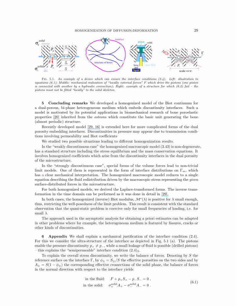
HOMOGENIZATION OF DIFFUSION-DEFORMATION 29

p+

p−

S+

S−

+σ

−σ

solid

F

S

solid

structure of hoses

interface

andpore fluid

solidpiston

hose

liquid

p+

p−

scale << ε

ΓNO

!

Fig. 5.1. An example of a device which can ensure the interface conditions (2.4). Left: illustration toequations (6.1); Middle: mechanical realization of “ locally external forces” F which drive the pistons (one pistonis connected with another by a hydraulic connection); Right: example of a structure for which (6.2) fail – thepistons must not be fitted “locally” to the solid skeleton.

5 Concluding remarks We developed a homogenized model of the Biot continuum fora dual-porous, bi-phase heterogeneous medium which embeds discontinuity interfaces. Such amodel is motivated by its potential applications in biomechanical research of bone poroelasticproperties [20] inherited from the osteons which constitute the basic unit generating the bone(almost periodic) structure.

Recently developed model [29, 16] is extended here for more complicated forms of the dualporosity embedding interfaces. Discontinuities in pressure may appear due to transmission condi-tions involving permeability and Biot coefficients

We studied two possible situations leading to different homogenization results.

In the “weakly discontinuous case” the homogenized macroscopic model (3.43) is non-degenerate,has a standard structure including the stress equilibrium and the mass conservation equations. Itinvolves homogenized coefficients which arise from the discontinuity interfaces in the dual porosityof the microstructure.

In the “strongly discontinuous case”, special forms of the volume forces lead to non-triviallimit models. One of them is represented in the form of interface distributions on Γm, whichhas a clear mechanical interpretation. The homogenized macroscopic model reduces to a singleequation describing the fluid redistribution driven by the macroscopic stress representing the givensurface-distributed forces in the microstructure.

For both homogenized models, we derived the Laplace-transformed forms. The inverse trans-formation in the time domain can be performed as it was done in detail in [29].

In both cases, the homogenized (inverse) Biot modulus,M∗(λ) is positive for λ small enough,thus, restricting the well-posedness of the limit problem. This result is consistent with the standardobservation that the quasi-static problem is coercive only for small frequencies of loading, i.e. forsmall λ.

The approach used in the asymptotic analysis for obtaining a priori estimates can be adaptedin other problems where for example, the heterogeneous medium is featured by fissures, cracks orother kinds of discontinuities.

6 Appendix We shall explain a mechanical justification of the interface condition (2.4).For this we consider the ultra-structure of the interface as depicted in Fig. 5.1 (a). The pistonsenable the pressure discontinuity p+ 6= p−, while a small leakage of fluid is possible (drilled pistons)– this explains the “semipermeable” interface condition (2.4)3.

To explain the overall stress discontinuity, we write the balance of forces. Denoting by S thereference surface on the interface Γ, by φ± = S±/S the effective porosities on the two sides and byA± = S(1− φ±) the corresponding effective crossections of the solid phase, the balance of forcesin the normal direction with respect to the interface yields

in the fluid: F + p+S+ − p−S− = 0 ,

in the solid: σsolid+ A+ − σsolid

− A− = 0 .(6.1)

30 G. GRISO AND E. ROHAN

From there the discontinuity of the total stress is obvious: let us introduce

σeff± := (1− φ±)σsolid

± , and σ± := σeff± − φ±p± , (6.2)

then (6.1) yields

σeff+ − σeff

− = 0 , and σ+ − σ− = φ−p− − φ+p+ = F/S . (6.3)

Hence [σ]Γ 6= 0 if [φp]Γ 6= 0, but the continuity of the effective stress is ensured, [σeff ]Γ = 0.This simple example illustrates that conditions (2.4) are realistic. The “external” forces, here

referred to by F , can have different meanings – they can substitute:• effects of other physical fields (e.g. electric field acting on the pistons),• effects of long-distance interaction — the forces represent the interaction between the

pistons and a separated self-supporting mechanical structure, as depicted in Fig. 5.1 (b),which can be designed as a hydraulic system, or a similar system of bowdens connectingcouples of pistons,

• inertia effects — in our study we consider a quasistatic events, however, for the dynam-ical model the same interface conditions are relevant, where the inertia of the pistons isassociated with the force F , as long as each piston “vibrates” only near the interface.

The pistons cannot be bonded locally to the solid skeleton, like in Fig. 5.1 (b), otherwise theassumed long-distance interaction would fail — in such a case the “standard” continuity of thetotal stress would hold, i.e. [σ]Γ = 0, while [σeff ]Γ 6= 0, in general.

REFERENCES

[1] Allaire G., Homogenization and two-scale convergence, SIAM J. Math. Anal. 23 (1992), 1482–1518.[2] Allaire, G., Prolongement de la pression et homogeneisation des equations de Stokes dans un milieu poreux

connexe , C. R. Acad. Sci. Paris 309 (1989), 717–722.[3] Arbogast T., Douglas J. and Hornung U., Derivation of the double porosity model of single phase flow via

homogenization theory, SIAM J. Math. Anal., 21 (1990), 823-836.[4] Auriault J.-L. and Boutin, C., Deformable porous media with double porosity. Quasi statics. i. Coupling effects,

Transp. Porous Media 7, 1 (1992), 63–82.[5] Auriault, J. L. and Ene, H. I., Macroscopic modelling of heat transfer in composites with interfacial thermal

barrier. Int. J. Heat Mass Transf., 37 (1994) 28852892.[6] Biot M. A., General theory of three-dimensional consolidation, J. Appl. Phys., 12 (1941), 155–164.[7] Biot M. A., Theory of elasticity and consolidation for a porous anisotropic solid, J. Appl. Phys., 26, 2 (1955),

182–185.[8] Briane M., Homogenization of the Stokes equations with high-contrast viscosity, J. Math. Pures Appl. 82 (2003)

843–876.[9] Cioranescu D. and Saint-Jean Paulin J., Homogenization in open sets with holes, J. Mathematical Analysis

and Applications, 71 (1979), 590–607.[10] Cioranescu, D., Damlamian, A., Griso, G., The periodic unfolding method in homogenization, SIAM J. of

Math. Anal. Vol. 40, 4 (2008), 1585–1620.[11] Cioranescu D., Damlamian A., Griso G. and Onofrei D., The periodic unfolding method for perforated domains

and Neumann sieve models, J. Math. Pures Appl., 89 (2008), 248–277.[12] Cioranescu D., Damlamian A., Donato P., Griso G. and Zaki R., The periodic unfolding method in domains

with holes. SIAM J. Math. Anal., 44 (2012), 718–760.[13] Cioranescu D. and Donato, P., An Introduction to Homogenization. Oxford Lecture Series in Mathematics ans

its Applications 17, Oxford University Press, 1999.[14] Coussy O., Poromechanics. John Wiley & Sons, 2004.[15] Ene H. and Polisevski D., Model of diffusion in partially fissured media, Z. Angew. Math. Phys., 53 (2002),

1052–1039.[16] Griso G. and Rohan E., On the homogenization of a diffusion-deformation problem in strongly heterogeneous

media, Ricerche di Mat., 56 (2007), 161–188.[17] Griso G., Error estimates and unfolding for periodic homogenization, Asymptotic Analysis, 40, 3-4 (2004),

269–286.[18] Griso G., Interior error estimates for periodic homogenization, C. R. Acad. Sci. Paris, Ser. I 340 (2005),

251–254.[19] Griso G., Interior error estimates for periodic homogenization, Analysis and Applications, 4 (2006), 61–79.[20] Nguyen V-H., Lemaire T. and Naili S., Poroelastic behaviour of cortical bone under harmonic axial loading:

a finite element study at the osteonal scale, Medical Engineering & Physics, 32 (2010), 384-90.[21] Hornung U., Homogenization and Porous Media. Springer-Verlag, Berlin 1997.

HOMOGENIZATION OF DIFFUSION-DEFORMATION 31

[22] Hornung, U., Jager, W., Mikelic, A., Reactive Transport through an Array of Cells with Semi-PermeableMembranes. Mathematical Modelling and Numerical Analysis 28 (1994) 59-94.

[23] Jager, W., Mikelic, A., Modeling effective interface laws for transport phenomena between an unconfined fluidand a porous medium using homogenization, Transport in Porous Media 78 (2009), 489–508.

[24] Lipton, R., Heat conduction in fine scale mixtures with interfacial contact resistance, SIAM J. Appl. Math.,58 (1998), 55-72.

[25] Murad A. M., Guerreiro J. N. and Loula A. F. D., Micromechanical computational modelling of secondaryconsolidation and hereditary creep in soils, Comput. Methods Appl. Mech. Engrg. 190 (2001), 1985–2016.

[26] Burridge R and Keller J.B., Biot’s poroelasticity equations by homogenization, in Macroscopic Properties ofDisordered Media , Lecture Notes in Physics, 154 (1982), 51–57.

[27] Rohan, E. and Cimrman, R., Two-Scale Modeling of Tissue Perfusion Problem Using Homogenization of DualPorous Media, Int. Jour. Multiscale Comput. Engrg., 8 (2010), 81–102.

[28] Rohan, E. and Cimrman, R, Multiscale FE simulation of diffusion-deformation processes in homogenizeddual-porous media. Accepted in Math. Comp. and Simul., 82 (2012), 1744–1772.

[29] Rohan E., Naili S., Cimrman R. and Lemaire T., Multiscale modelling of a fluid saturated medium with dualporosity: relevance to the compact bone. J. Mech. Phys. Solids, 60 (2012), 857–881.

[30] Showalter R.E. and Visarraga D.B. Double-diffusion models from a highly heterogeneous medium, Jour. ofMath. Anal. and Appl., 295 (2004), 191–210.

[31] Smyshlyaev, V. P., Propagation and localization of elastic waves in highly anisotropic periodic composites viatwo-scale homogenization Mechanics of Materials, 41 (2009), 434–447.