University of Central Florida University of Central Florida

STARS STARS

Electronic Theses and Dissertations

2017

Heat Transfer, Friction, and Turbulent Analysis on Single Ribbed-Heat Transfer, Friction, and Turbulent Analysis on Single Ribbed-

Wall Square Channel Wall Square Channel

Christopher Vergos University of Central Florida

Part of the Mechanical Engineering Commons

Find similar works at: https://stars.library.ucf.edu/etd

University of Central Florida Libraries http://library.ucf.edu

This Masters Thesis (Open Access) is brought to you for free and open access by STARS. It has been accepted for

inclusion in Electronic Theses and Dissertations by an authorized administrator of STARS. For more information,

please contact STARS@ucf.edu.

STARS Citation STARS Citation Vergos, Christopher, "Heat Transfer, Friction, and Turbulent Analysis on Single Ribbed-Wall Square Channel" (2017). Electronic Theses and Dissertations. 5936. https://stars.library.ucf.edu/etd/5936

HEAT TRANSFER, FRICTION, AND TURBULENT ANALYSIS ON SINGLE RIBBED-

WALL SQUARE CHANNEL

by

CHRISTOPHER E. VERGOS

B.S. University of Central Florida, 2014

A thesis submitted in partial fulfillment of the requirements

for the degree of Master of Science in Mechanical Engineering

in the Department of Mechanical and Aerospace Engineering

in the College of Engineering and Computer Sciences

at the University of Central Florida

Orlando, Florida

Summer Term

2017

ii

ABSTRACT

An experimental investigation of heat transfer and friction behavior for a fully developed flow in

a non-rotating square channel was conducted under a wide range of Reynolds numbers from 6,000

to 180,000. The rig used in this study was a single ribbed wall variant of Ahmed et al.’s [ 1 ] rig

from which results of this rig were compared. Ahmed et al.’s rig was a replica of Han et al.’s square

channel [ 2 ] used to validate their work, and expand the Reynolds number range for both heat

transfer and friction data. The test section was 22 hydraulic diameters (Dh) long, and made of four

aluminum plates. One rib roughened bottom wall, and three smooth walls bounded the flow. Glued

brass ribs oriented at 45° to the flow direction, with a ratio of rib height to channel hydraulic

diameter (e/Dh) and a ratio of pitch to rib height (p/e) of 0.063 and 10, respectively, lined the

bottom wall. A 20Dh long acrylic channel with a continuation of the test section’s interior was

attached at the inlet of the test section to confirm the fully developed flow. Heat transfer tests were

conducted in a Reynolds number range of 20,000 to 150,000. During these tests, the four walls

were held under isothermal conditions. Wall-averaged, and module-averaged Nusselt values were

calculated from the log-mean temperature differences between the plate surface temperature and

calculated, by energy balance, fluid bulk temperature. Streamwise Nusselt values become constant

at an x/Dh of 8 within the tested Reynolds number range. Wall averaged Nusselt values were

determined after x/Dh=8, and scaled by the Dittus-Boelter correlation, Nuo, for smooth ducts to

yield a Nusselt augmentation value (Nu/Nuo). Non-heated friction tests were conducted from a

Reynolds number range of 6,000 to 180,000. Pressure drop along the channel was recorded, and

channel-averaged Darcy-Weisbach friction factor was calculated within the range of Reynolds

number tested. Scaling the friction factor by the smooth-wall Blasius correlation, fo, gave the

iii

friction augmentation (f/fo). The thermal performance, a modified ratio of the Nusselt and friction

augmentation used by Han et al. [ 2 ], was then calculated to evaluate the bottom-line performance

of the rig. It was found that the Nusselt augmentation approached a constant value of 1.4 after a

Reynolds number of 60,000 while friction augmentation continued to increase in a linear fashion

past that point. This caused the overall thermal performance to decline as Reynolds number

increased up to a certain point. Further studies were conducted in an all acrylic, non-heated variant

of the rig to study the fluid flow in the streamwise direction on, and between two ribs in the fully

developed region of the channel. Single-wire hot-wire anemometry characterized velocity

magnitude profiles with great detail, as well as turbulence intensity for Reynolds numbers ranging

from 5,000 to 50,000. As the Reynolds number increased the reattachment point between two ribs

remained about stationary while the turbulence intensity receded to the trailing surface of the

upstream rib, and dissipated as it traveled. At low Reynolds numbers, between 5,000 and 10,000,

the velocity and turbulence intensity streamwise profiles seemed to form two distinct flow regions,

indicating that the flow over the upstream rib never completely attached between the two ribs.

Integral length-scales were also derived from the autocorrelation function using the most turbulent

signal acquired at each Reynolds number. It was found that there is a linear trend between

Reynolds number and the integral length-scale at the most turbulent points in the flow. For

example, at Re=50,000 the most the length scale found just past the first rib was on the order of

two times the height of the rib. Rivir et al. [ 30 ] found in a similar case that at Re = 45,000, it was

1.5 times the rib height. Several factors could influence the value of this integral length-scale, but

the fact that their scale is on the order of what was obtained in this case gives some level of

confidence in the value.

iv

ACKNOWLEDGEMENTS

A very special thanks to:

My family for all their love and support, Dr. Kapat for giving me an exciting and rare opportunity

to learn about the fundamentals and applications of turbomachinery through the CATER Lab and

graduate courses, my coworkers and project manager for all the help, support, and memorable

experiences at the lab, and finally Siemens Energy for making my project possible to further the

studies of internal duct cooling.

v

TABLE OF CONTENTS

LIST OF FIGURES ................................................................................................. vii

LIST OF TABLES ................................................................................................... ix

LIST OF ACRONYMS/ABBREVIATIONS ............................................................ x

CHAPTER 1: INTRODUCTION .............................................................................. 1

CHAPTER 2: RIG SETUP ......................................................................................... 4

2.1 Rig Design – Heat Transfer and Friction Analysis ............................................................. 4

2.2 Rig Design – Turbulence Analysis ................................................................................... 10

CHAPTER 3: TESTING ..........................................................................................14

3.1 Heat Transfer Analysis ..................................................................................................... 14

3.1.1 Flow Leakage Testing .............................................................................................. 15

3.1.2 Heat Leakage Testing .............................................................................................. 15

3.1.3 Heat Transfer Testing .............................................................................................. 16

3.2 Friction Analysis ............................................................................................................... 22

3.2.1 Friction Factor Testing ............................................................................................. 23

3.3 Hot-Wire Analysis ............................................................................................................ 25

3.3.1 Understanding the Bridge ........................................................................................ 26

3.3.2 Sensor Heat Transfer Theory ................................................................................... 27

3.3.3 Limitations ............................................................................................................... 30

3.3.4 Temperature Corrections ......................................................................................... 33

3.3.5 Filtering .................................................................................................................... 34

vi

3.3.6 Sample Convergence ............................................................................................... 34

3.3.7 Calibration................................................................................................................ 37

3.3.8 Uncertainty Considerations ...................................................................................... 38

CHAPTER 4: RESULTS AND DISCUSSION .......................................................39

4.1 Heat Transfer Analysis Results ......................................................................................... 39

4.2 Friction Factor Analysis Results ....................................................................................... 42

4.3 Thermal Performance Analysis Results ............................................................................ 44

4.4 Heat Transfer and Friction Experimental Uncertainty Results ......................................... 45

4.5 Hot-wire Analysis Results ................................................................................................ 46

CHAPTER 5: FINDINGS ........................................................................................55

APPENDIX A: UNCERTAINTIES OF MASS FLOWRATE ................................58

APPENDIX B: SYSTEMATIC UNCERTAINTIES OF NUSSELT NUMBER ....60

APPENDIX C: SYSTEMATIC UNCERTAINTIES OF FRICTION FACTOR .....63

APPENDIX D: SYSTEMATIC UNCERTAINTIES OF TURBULENCE .............65

APPENDIX E: MATLAB CODE FOR TURBULENCE ANALYSIS ...................67

Converting Voltage Files to Velocity Files: ........................................................................... 68

Velocity, Turbulence Intensity, Spectral, and Length Scale Analysis: ................................... 69

Sample Convergence Testing: ................................................................................................ 91

King’s Law Analysis: ............................................................................................................. 92

REFERENCES .........................................................................................................94

vii

LIST OF FIGURES

Figure 1 Heat Transfer/ Friction Rig Assembly ............................................................................. 4

Figure 2 Cross-section of metal test section. .................................................................................. 5

Figure 3 Electrical Schematic of Heat Transfer Test Section ......................................................... 7

Figure 4 Schematic of Heat Transfer Testing Setup ....................................................................... 8

Figure 5 Schematic of Friction Testing Setup ................................................................................ 9

Figure 6 Overall Rig Design ......................................................................................................... 10

Figure 7 Test Section Rig Design ................................................................................................. 11

Figure 8 Hot-wire Equipment Setup for Turbulence Analysis ..................................................... 11

Figure 9 Optimized Mesh Spacing – Side-View Section ............................................................. 12

Figure 10 Heat Leakage Test Section Setup (heaters shown exposed) ........................................ 16

Figure 11 Calculated Bulk Fluid and Measured Wall Temperature at Re=70,000 ...................... 18

Figure 12 Calculated Bulk LMTD at Re=70,000 ......................................................................... 19

Figure 13 Calculated Modular Heat Transfer Coefficient at Re=70,000...................................... 19

Figure 14 Calculated Modular-Averaged Nusselt Number at Re = 70,000 .................................. 21

Figure 15 Pressure Drop Across Non-Heated Rig at Re = 70,000 ............................................... 25

Figure 16 Anatomy of a CTA Wheatstone Bridge Amplifier Loop ............................................. 26

Figure 17 Energy Balance of a Hot-Wire Sensor ......................................................................... 28

Figure 18 Sensor Temperature Profile – Error Zones ................................................................... 29

viii

Figure 19 First-order Response to Temperature Step Change ...................................................... 31

Figure 20 Square-Wave Response to DANTEC Sensor ............................................................... 32

Figure 21 Convergence of the Sample Mean ................................................................................ 36

Figure 22 Convergence of the Sample Standard Deviation .......................................................... 36

Figure 23 Modular Nusselt Number distribution, Re = 70,000 .................................................... 39

Figure 24 Wall-Averaged Nusselt number at various Re ranging from 25,000 to 125,000 ......... 40

Figure 25 Channel-Averaged Nusselt Augmentation for Re ranging from 25,000 to 125,000 .... 41

Figure 26 Fanning Friction Factor for Both Single-Wall and Two-Wall Cases ........................... 43

Figure 27 Friction Augmentation for Both Single-Wall and Two-Wall Cases ............................ 43

Figure 28 Thermal Performance for Both Single, and Two-Wall Cases ...................................... 45

Figure 29 Sample Contour Plot .................................................................................................... 46

Figure 30 Re = 50,000 TI Repeatability Test ............................................................................... 47

Figure 31 Local Velocity Normalized by the Channel Bulk Velocity .......................................... 48

Figure 32 Uncertainty of Normalized Velocity ............................................................................ 49

Figure 33 RMS Velocity Fluctuations Normalized by Local Velocity (TI) ................................. 50

Figure 34 Uncertainty in Turbulence Intensity ............................................................................. 51

Figure 35 Autocorrelation Taken at Most Turbulent Point in Re =50,000 ................................... 53

Figure 36 Velocity and Fluctuation Plots at Re = 50,000 ............................................................. 56

ix

LIST OF TABLES

Table 1: Streamwise Hot-Wire Locations..................................................................................... 13

Table 2 Hot-wire Data Validation in Heat Transfer Testing ........................................................ 52

Table 3 Location of Most Turbulent Points at Various Re ........................................................... 53

Table 4 Integral Time and Length-Scales at Various Re .............................................................. 54

x

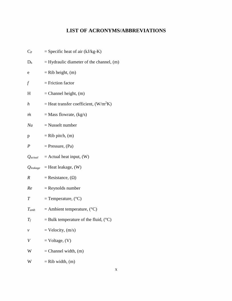
LIST OF ACRONYMS/ABBREVIATIONS

CP = Specific heat of air (kJ/kg-K)

Dh = Hydraulic diameter of the channel, (m)

e = Rib height, (m)

f = Friction factor

H = Channel height, (m)

h = Heat transfer coefficient, (W/m2K)

= Mass flowrate, (kg/s)

Nu = Nusselt number

p = Rib pitch, (m)

P = Pressure, (Pa)

Qactual = Actual heat input, (W)

Qleakage = Heat leakage, (W)

R = Resistance, (Ω)

Re = Reynolds number

T = Temperature, (°C)

Tamb = Ambient temperature, (°C)

Tf = Bulk temperature of the fluid, (°C)

v = Velocity, (m/s)

V = Voltage, (V)

W = Channel width, (m)

W = Rib width, (m)

xi

X = Streamwise direction, (m)

Greek

Δ = Difference between two parameters

= Thermal performance

= Dynamic viscosity (kg/m-s)

air = Air density (kg/m3)

Subscripts

0 = Smooth channels

W = Wall

1

CHAPTER 1: INTRODUCTION

To achieve higher power output and greater thermal efficiency, advanced gas turbines run at higher

inlet temperature (~1600°C), exceeding the metallic airfoils’ material melting temperature within

the turbine. The airfoils at the greatest risk to failure due to thermal stresses and/or melting is the

first stage of vanes and blades. In modern advanced gas turbines, both thermal barrier coating

(TBC) and a variety of blade cooling techniques, including pin fins, crossovers, and impingement

jet inserts, and advanced trailing edges ensure the airfoil’s survival during its expected life cycle,

and the successful operation of the engine. In one of such cooling technique, compressor air, bled

out from one of its final stages before combustion, serpentines in multi-pass flow channels within

the hollow airfoil which is known as Internal Duct Cooling (IDC). Turbulators, often incorporated

in these passages, interrupt viscous sublayer formation, and promote mixing of the hotter fluid

near the metallic surface with the colder fluid at the core, enhancing the heat transfer.

Unfortunately, turbulators are also responsible for high pressure losses due to friction beyond

typical surface roughness. To optimize the cooling performance of internal cooling channels,

maximizing the amount of heat removed while simultaneously minimizing the pressure loss is

critical. For the past fifty years, researchers have been improving the Heat Transfer Coefficient (h)

values (both local and overall) and friction factor in a plethora of turbulated internal cooling

passage variations to further improve the cooling of the IDC airfoil passages.

Several parameters, including rib pitch, height, and angle, dictate whether an arrangement of rib

turbulators will perform better than others. They are expressed as non-dimensional ratios such as

p/e (pitch to height ratio), e/h (blockage ratio) to characterize the various channels studied. Aspect

2

ratio of the channel, number of ribbed walls in cooling channels, and rib arrangement (in line,

staggered, v- and w- pattern) are all non-rib specific features also explored in this field of study.

Han et al. [ 3 ][ 4 ] conducted many studies on these aspects of the rib turbulators. Rib angles

between 45° and 60° show better thermal performance than transverse ribs (90°) during their tests,

and a p/e of 10 was best for rectangular two-ribbed wall channels [ 5 ][ 6 ]. Park et al. [ 7 ]

concluded that narrower aspect ratio channels yielded results favorable to that of larger aspect ratio

channels, and that thermal performance is highly dependent on what aspect ratio the channel is

and what angle the ribs are oriented in. In one such test, the narrow channel (AR=1/2 or 1/4)

showed higher thermal performance with 45°/60° ribs, while, the wider channel (AR=4 or 2)

performs better with 30°/45° ribs. Taslim and Lengkong [ 8 ] [ 9 ] found that transverse ribs show

better thermal performance than 45° ribs for high blockage ratio (e/Dh=0.25) ribs in a square

channel, and that rounded-corner ribs show reduction in both heat transfer and friction factor.

Taslim et al. [ 10 ] even investigated the effect of the number of ribbed walls, and discovered a

full set of turbulated walls has a lot of potential for increasing the heat transfer performance. Berger

and Hau [ 11 ], Bailey and Bunker [ 12 ], and Wang et al. [ 13 ] also conducted studies on several

aspects of rib turbulators. Various rib configurations were also considered, such as continuous and

broken V shaped, W shaped and wedges [ 14 ][ 15 ][ 16 ], etc. Even different measurement

techniques were used to study IDC. Rau et al. [ 17 ] used Laser-Doppler Velocimetry (LDV) as

well as thermochromic liquid crystal (TLC) to investigate the detailed heat transfer and

aerodynamic behavior of a square channel with transverse ribs (blockage ratio equal to 0.1). With

these methods, flow near the ribs was discovered to be very complex and three-dimensional, and

that the average heat transfer data typically resolved in IDC tests may not entirely capture the true

3

thermal performance, due to inaccurate assumptions made for local heat transfer on the wall

surface near the ribs.

Because of all these dependencies, and parametrization, no two researchers have rigorously studied

a single set of rib parameters, especially at high Reynolds numbers. Most experiments found in

literature focus on Re lower than 70,000. Rallabandi et al. [ 18 ] investigated the heat and pressure

drop correlations for a square channel with 45° ribs by varying rib height to channel hydraulic

diameter ratio e/Dh in the range between 0.1 and 0.18. Correlations proposed by Han et al. [ 6 ][

19 ], where 0.048<e/Dh<0.078, 10<p/e<20, and Re<70,000, were modified to expand Reynolds

numbers in the range of 30,000-400,000. This set the stage to investigate the effect of heat and

pressure drop in the higher Reynolds numbers. Very few studies, however, were conducted on

single ribbed-wall channels throughout the history of IDC research. Chandra et al. [ 20 ][ 21 ]

found that although adding more ribbed walls increases average heat transfer with increasing Re,

friction factor increases far more. Thus, the overall thermal performance of the channel suffers.

This thesis intends to shed light on the heat transfer and friction behavior of a fully developed

turbulent flow in a square channel with 45° ribs and e/Dh=0.0625, with a single wall of ribbed

turbulators. Except for the single ribbed wall, this set of rib parameters match Ahmed et al.’s

research [ 1 ], which was conducted to validate the findings of Han et al.’s NASA Contractor

Report in 1984 [ 2 ], in a wide range of Re from 6,000 to 180,000. In addition to heat transfer and

friction, constant-temperature hot-wire anemometry will offer information on the turbulence

behavior of the fluid under a moderate range of Re from 5,000 to 50,000.

4

CHAPTER 2: RIG SETUP

2.1 Rig Design – Heat Transfer and Friction Analysis

The experiment divided into three test setups: heat transfer, friction, and turbulence analysis. The

heat transfer rig was an isothermal heated square channel (AR=1). Square ribs, featuring a pitch to

height ratio (p/e) of 10 and height to channel diameter (blockage) ratio (e/Dh) of 0.0625 with an

angle-of-attack of 45 degrees against the flow, lined the bottom wall of the channel only. The total

length of the rig measured 48Dh with a ribbed unheated acrylic inlet of 20Dh to achieve

hydrodynamically-developed flow upon entering the 22Dh heated aluminum test section with

glued brass ribs to continue of the rib geometry from the inlet. The flow then exited through a 6Dh

unheated acrylic smooth square duct to diminish any back-pressure effects from a dump diffuser

box further downstream. Eight equally-spaced 1/16in dia. static-pressure tap holes were drilled

into each aluminum wall from end to end, except the bottom to extract pressure drop data for

friction analysis. In addition to the pressure taps in the test section, pressure taps line the left and

right walls of the inlet section with a third of the test section spacing. Refer to Figure 1 below.

Figure 1 Heat Transfer/ Friction Rig Assembly

5

Between each pressure tap hole, two silicone rubber etched-foil heaters, bonded to the backs of

each aluminum plate with double-sided polyimide tape from Kapton Tape®, totaled fourteen per

wall. Beneath the center of each of the fourteen heaters per wall, two T-type thermocouples were

cemented in small potting holes 1mm below the flow surface inside the channel. The cement used

to secure these thermocouples was OMEGABOND® OB-600 high-temperature cement. All 112

test section thermocouples, with six more for test section inlet and outlet air temperature

measurements, were routed to an array of six computer-controlled FLUKE 2640 NetDAQs to

record, and check all rig temperatures simultaneously to support near-isothermal conditions,

min/max rig temperature difference < 0.8°C, at any Reynolds number. 1mm thick strip cork

insulated each heated aluminum wall from each other with their corner, and 0.5in-thick casing of

Rohacell® foam core board (thermal conductivity ~ 0.03W/m-K) insulated the walls from the

environment. Beyond the foam insulation, 0.5in-thick acrylic outer walls were bolted together to

hold the structure of the glued metal interior. See Figure 2.

Figure 2 Cross-section of metal test section.

6

Designing the rig for isothermal wall temperatures, the heaters had to give various thermal loads

to the rig in the streamwise direction along each wall. The ribbed wall needed the highest amount

of heating to keep a target temperature because of the added cooling turbulent mixing caused by

the ribs. The top smooth wall needed the least amount of cooling because it will see a greatly

dampened effect from the turbulent mixing occurring on the bottom ribbed wall. The side walls

needed a heat flux somewhere in between the bottom ribbed wall, and the top smooth wall

requirements because near the ribs, the side walls will be cooled more effectively from the

turbulent mixing pickup than near the smooth top wall. Between the two side walls, both needed

about the same amount of heat flux. However, the left wall, where the ribs are directing toward at

45°, needed a small amount of added flux because the ribs cause a steering of the flow toward it,

creating a level of impingement. Secondary vortices caused by the ribs add another, more local,

cooling of the left wall through mixing in the recirculation regions upstream and downstream of

the rib [ 22 ].

Knowing this, the electrical input to the test section had to be divided into three electrically heated

zones: the top wall, bottom ribbed wall, and left-right (paired) walls. It was then further divided

into nine streamwise sections per wall, which will be called modules, hereafter. A single rheostat

controlled each module on each wall, totaling 36 rheostats. The first four modules on each wall

were single-heater modules because control of the heat input was crucial in this entrance region.

As the ambient air entered the test section from the inlet, the plates needed a large amount of heat

flux at the entrance to maintain isothermal conditions throughout the channel. The large power

demand from the heaters quickly died out as the plates heated the air to a higher bulk temperature

compared to ambient downstream of the entrance. After the first four modules on each wall, the

remaining five modules per wall used two heaters. Total control over each heater was not necessary

7

in the middle of the rig because the air temperature in the channel is high enough to have negligible

effect on the heat transfer coefficient. However, the final module on each wall needed slightly

more power than the earlier inner modules. Unlike the earlier modules, the final module does not

have a heated exit downstream of it. It has the non-heated smooth acrylic outlet section. This

induces a thermal back-pressure effect, which required the final module to work harder to maintain

temperature than the ones prior. This final module, named the thermal exit module, was not

included in the trends of the heat transfer analysis. Fifteen variacs (two controlling the first four

modules, one for the next four modules, and one for the final module) power the rig’s three heated

zones (Figure 3).

Figure 3 Electrical Schematic of Heat Transfer Test Section

A FLUKE 2638A Hydra DAQ acquired voltage information from the 36 total modules. A single

VB110 Spencer® Vortex blower provided the flow through the rig under suction, and mass

flowrate was measured from in-house, sonic nozzle calibrated Preso® venturi flowmeters just

upstream of the blowers (Figure 4).

8

Figure 4 Schematic of Heat Transfer Testing Setup

Two OMEGA HHP240 – 5psi range handheld differential manometers measured both the venturi

upstream pressure, and the venturi pressure differential simultaneously. An external barometer

measured atmospheric pressure. A single calibrated T-type thermocouple measured the Venturi

inlet temperatures. A gate value in the blower piping adjusted the flow coming from the rig to

acquire Reynolds numbers ranging from 6000 to 180,000. A relief valve controlled the rig exhaust

temperature so the PVC does not sag due to increasing temperatures.

The friction test setup was the same setup as the heat transfer testing, however, during the friction

testing, no heaters in the test section were active. It was an ambient temperature test (Figure 5).

9

Figure 5 Schematic of Friction Testing Setup

The pressure taps along the test section and inlet section at known distances apart from each other

were routed to a computer-controlled Single Scanivalve System (SSS48C Mk4) pressure scanner

via vinyl tubing. The Scanivalve, and the pressure information from its transducer were controlled

and recorded via LabView on the computer. Pressures inside the rig were close to that of smooth

wall rigs given that this rig only has a single ribbed wall. Therefore, a 20inH2O range transducer

sufficed rather than a usually equipped 5-psi range transducer. Utilizing the smallest range possible

for a test allows for the acquisition of data with higher accuracy. Since no voltage needed to be

recorded from the heaters, and no steady state temperature of the rig needed to be reached, the

friction tests were much faster than heat transfer tests. This allowed more friction tests to be

conducted, and more confidence in the shape of the correlation curve between friction factor and

Reynolds number during post-processing.

10

2.2 Rig Design – Turbulence Analysis

The metal test section was removed after completing the heat transfer and friction analyses, and a

20Dh acrylic turbulence test section was inserted between the ribbed inlet and smooth exit, Figure

6. The top wall of the turbulence test section was modified to be broken into three puzzle-piece

components: a 15.6Dh entrance plate, a 1.56Dh interrogation plate, and a 2.84Dh exit plate. The

interrogation plate was machined to allow a rectangular piece with a centered hole to slide freely

inside. Because the rig was under suction from the Vortex blowers, the rectangular slide piece was

sucked to the interior surface of the interrogation piece, creating a seal. This allowed a single wire

hot-wire probe to be inserted through the rectangular piece’s hole and traverse freely in the

streamwise direction without flow leakage through a traditional traverse slot. A traverse slot on

the bottom of the interrogation piece allowed the single wire hot-wire probe to measure velocity

magnitudes, and turbulence intensities between and on top of two ribs, rib 57 and 58, out of a total

of 63 ribs, Figure 7.

Figure 6 Overall Rig Design

11

Figure 7 Test Section Rig Design

The hot-wire system comprised of a USB-controlled DANTEC Dynamics StreamLine Pro

Constant Temperature Anemometer (CTA) with a 55P11 single-sensor miniature wire probe, a

TSITM 1127 manual flow nozzle calibrator, a VELMEX XSlideTM stepper-motor 2-D traverse

assembly with NI motion controls, and an NI PXI-e Chassis for the computer to communicate with

the motion controls through NI MAX software. To make sure that none of the above-mentioned

instruments interferes with the CTA, the CTA was plugged in to its own electrical outlet, and that

the BNC cable for the probe was away from any EMF emitter in the immediate area. See Figure 8

for further details.

Figure 8 Hot-wire Equipment Setup for Turbulence Analysis

12

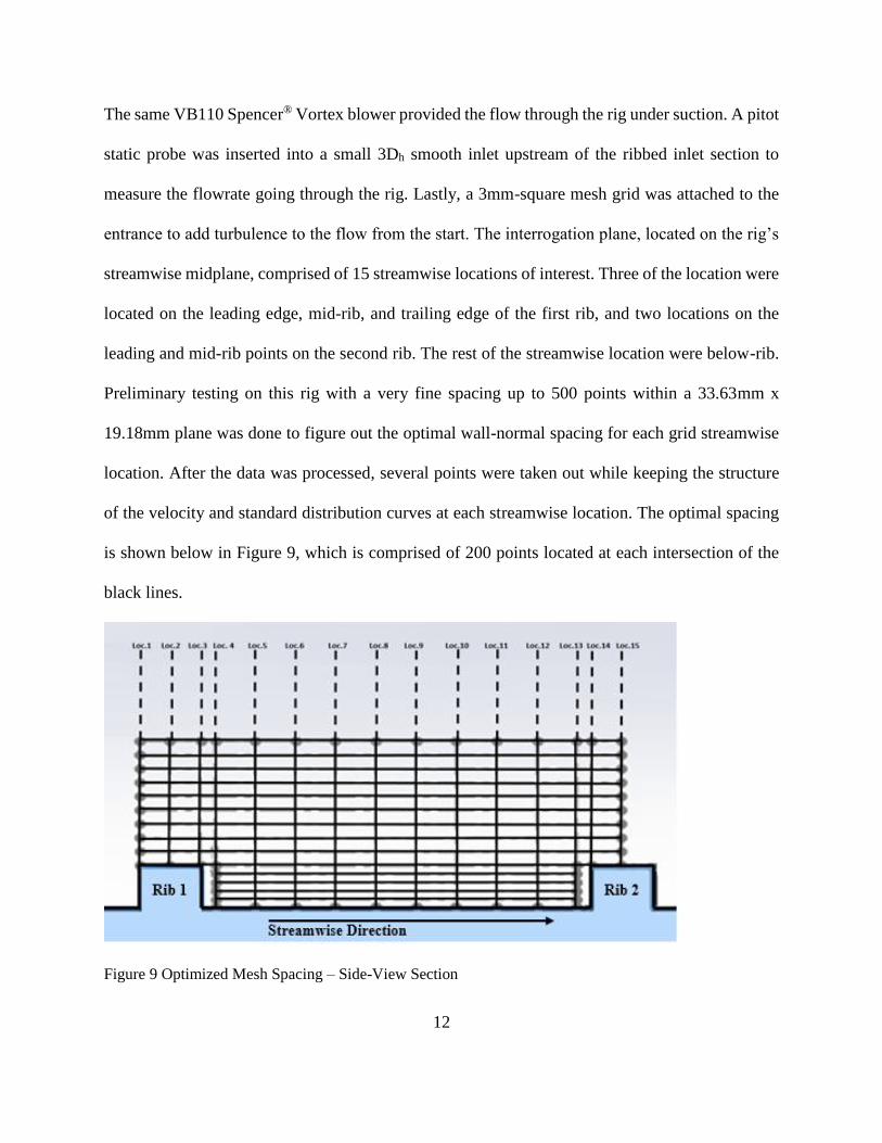
The same VB110 Spencer® Vortex blower provided the flow through the rig under suction. A pitot

static probe was inserted into a small 3Dh smooth inlet upstream of the ribbed inlet section to

measure the flowrate going through the rig. Lastly, a 3mm-square mesh grid was attached to the

entrance to add turbulence to the flow from the start. The interrogation plane, located on the rig’s

streamwise midplane, comprised of 15 streamwise locations of interest. Three of the location were

located on the leading edge, mid-rib, and trailing edge of the first rib, and two locations on the

leading and mid-rib points on the second rib. The rest of the streamwise location were below-rib.

Preliminary testing on this rig with a very fine spacing up to 500 points within a 33.63mm x

19.18mm plane was done to figure out the optimal wall-normal spacing for each grid streamwise

location. After the data was processed, several points were taken out while keeping the structure

of the velocity and standard distribution curves at each streamwise location. The optimal spacing

is shown below in Figure 9, which is comprised of 200 points located at each intersection of the

black lines.

Figure 9 Optimized Mesh Spacing – Side-View Section

13

The wire does not go all the way down to the surface, but hovers about 0.15mm above at all

streamwise locations. Sensor wire positions should always face perpendicular with the flow

direction, so velocities could not be measured flush against the rib walls (Rib 1 trailing wall, and

Rib 2 leading wall) because the ribs faced 45° to the wire. To make sure the wire does not hit the

ribs and break, ‘buffer’ regions were calculated to accommodate the 45° angle between the wire

and the ribs. These buffer regions, measuring 1mm streamwise, were positioned between locations

3 and 4, and 13 and 14. To verify that the flow was fully developed, locations 1-2, and 14-15 were

critical because location 1 and 14 should have the same velocity and turbulence intensity profiles,

as well as location 2 and 15. The grid spacing in region named the valley, between the ribs near

the wall’s surface, was finer than the gird spacing outside, above the ribs. Studies suggest that the

flow behavior within this valley region contains rapidly changing velocities and turbulent

intensities due to the wall’s no-slip conditions, the recirculation zones in front of and behind the

ribs, and the flow reattachment point at the wall. The vertical, y-direction, grid spacing in the valley

was 0.63mm, while the grid spacing outside this region was 1.06mm.

Table 1 below show the distances of each streamwise location with a starting point at the first rib’s

leading edge (location 1). Additional information of the location’s distance with respect to the

length of the entire rig is also given in non-dimensional distance (x/Dh).

Table 1: Streamwise Hot-Wire Locations

Streamwise Location 1 2 3 4 5 6 7 8

Dist. from rib 1-edge (mm) 0.00 2.16 4.32 5.32 8.12 10.91 13.70 16.50

Dist. From rig start (x/Dh) 35.00 35.04 35.09 35.10 35.16 35.21 35.27 35.32

Streamwise Location 9 10 11 12 13 14 15

Dist. from rib 1-edge (mm) 19.29 22.09 24.88 27.67 30.47 31.47 33.63

Dist. From rig start (x/Dh) 35.38 35.43 35.49 35.54 35.60 35.62 35.66

14

CHAPTER 3: TESTING

3.1 Heat Transfer Analysis

The purpose of conducting this test was to find when the flow inside a heated channel will become

fully thermally developed, and how the wall-averaged Nusselt number changes as a function of

Reynolds Number. Due to the mixing mechanic of turbulent flows, heat transfer is enhanced

beyond the threshold of laminar flow heat transfer. Studies using rib-turbulated channels found a

higher thermal performance than that of studies conducting with smooth channels. This showed a

promising future in blade cooling research for more efficient gas turbines engines. With greater

thermal performance of internal cooling, engines can burn hotter, less combustion cooling, and

creep closer toward the harnessing true potential of natural gas.

This section marks the first of three in the chapter dedicated to the testing conducted in this

research. Here the heat transfer testing approach will be explained from preparatory flow and heat

leakage testing to the actual heat transfer analysis, in which an energy balance fluids temperature

marching scheme will be introduced, as well as the use of LMTD for constant temperature walls.

From there, an elaboration on how both modular-averaged, and wall-average heat transfer

coefficient and Nusselt values can be calculated from the LMTD. An augmentation of the Nusselt

results will also be presented using smooth-pipe the Dittus-Boelter correlation for turbulent flow

as a reference to prove the enhancement this rib geometry delivers to the channel cooling

effectiveness.

15

3.1.1 Flow Leakage Testing

Before running a heat transfer test, it was important to make sure that the rig was completely

sealed. Any cool air from the environment leaking into the heated rig under suction would cause

temperatures to fall, and require an, otherwise unnecessary, increase in power to maintain the target

plate temperature. The resulting heat transfer coefficient in the affected area would be predicted

higher than what it really should be. To make sure the rig was leak-proof, incense was lit with a

match to produce smoke. The incense stick was taken along the rig, and if the leak was present,

the smoke will get sucked into the rig, instead of going up into the air. If a leak was discovered,

silicone caulking was used to cover up the leak and let dry. Downstream of the rig, the piping to

the blower was also checked for leaks. Any leaks downstream of the rig would cause an inaccurate,

overprediction in the rig mass flowrate due to an additional source of air to the blower other than

the rig. Checks were also made downstream of the venturi, but made no difference to the mass

flow calculation because the calculation was made at the venturi, not downstream of it. The only

change it would cause was the highest Reynolds number achievable in the rig since the blower has

a maximum pressure drop of 200inH2O. To make the rig leaks as noticeable as possible, the highest

Reynolds number the blower allowed was put through the rig.

3.1.2 Heat Leakage Testing

Despite there being a 0.5in layer of Rohacell® and another 0.5in thick layer of acrylic, nothing is

a perfect insulator, and heat loss to the surrounding must be accounted for to obtain accurate heat

transfer data. Prior to testing, the inlet and exit of the test section was blocked off so that no air

flow can go in or out (Figure 10).

16

Figure 10 Heat Leakage Test Section Setup (heaters shown exposed)

The aim of the test was to create a 3-point linear curve-fit correlating the rig-surrounding

temperature difference, and the required energy input from the silicone heater pads. If the rig was

truly adiabatic, the energy input needed to maintain a steady rig temperature would be zero.

Therefore, the nonzero energy input will be equivalent to the heat loss from the rig. These heat

losses were recorded at rig temperatures of 50°C, 60°C, and 70°C along with the ambient

temperature, and the difference between rig and ambient temperature was correlated with the

required heat input. Heater resistances were also measured to account for the temperature

dependence of electrical resistance, and were also correlated to the rig temperature with a linear

curve-fit. Because only three points were taken to define the linear trend, these curves usually had

high uncertainty. This was considered acceptable base on the fact that the magnitude of the heat

loss compared to the overall heat flux due to convective cooling is very low, typically around 4-

5%.

3.1.3 Heat Transfer Testing

A bulk fluid temperature marching scheme base on energy balance, and the log-mean temperature

difference, LMTD, are used to determine the temperature difference between the isothermal plate

and the air at each module. A pair of thermocouple are placed midway through the acrylic inlet of

the rig to measure the inlet air bulk temperature. Since the air velocities are within the

17

incompressible regime (Ma<0.3), the total temperature the thermocouples are reading will match

the bulk air temperature, and the effect of kinetic energy transfer to thermal energy at the

thermocouple bead’s stagnation point will be negligible.

When the first four modules from each wall reaches a steady state temperature, the power input to

the heaters are added up, and the heat leakage, calculated by the plate-ambient temperature

difference, is subtracted from that power input to give the conducting heat input through the

aluminum plates at those four first modules. Knowing the heat capacity of the air is about constant

(~1.006kJ/kg-K) and the mass flowrate from the venturi flowmeter, the fluid bulk temperature can

be determined by the equation:

𝑇𝑎𝑖𝑟𝑏𝑢𝑙𝑘,𝑓 = 𝑇𝑎𝑖𝑟𝑏𝑢𝑙𝑘,𝑖 +𝑄𝑎𝑐𝑡

𝑐𝑝 ( 3.1 )

where 𝑇𝑎𝑖𝑟𝑏𝑢𝑙𝑘,𝑖 is the averaged bulk fluid temperature entering the module, 𝑄𝑎𝑐𝑡 is the actual heat

input to the aluminum plates after subtracting heat leakage, and 𝑇𝑎𝑖𝑟𝑏𝑢𝑙𝑘,𝑓 is the bulk fluid

temperature exiting the heated module. The next modular bulk fluid temperature would use the

calculated first modular bulk fluid temperature, and reiterate the process with the next averaged

wall temperature and heat input, creating a marching scheme. This reiteration of fluid bulk

temperatures marches all the way to the last module where thermocouples are inserted just

downstream through an acrylic flange to directly measure the test section exit temperature. Ideally,

the calculated final module bulk temperature should match exact with the measured exit

temperature.

18

Figure 11 Calculated Bulk Fluid and Measured Wall Temperature at Re=70,000

The logarithmic mean temperature difference, 𝐿𝑀𝑇𝐷𝑥, method was used to average the difference

between the calculated fluid temperatures and constant wall temperature at each module:

𝐿𝑀𝑇𝐷𝑥 =(𝑇𝑤,𝑥−𝑇𝑓,𝑖,𝑥)−(𝑇𝑤,𝑥−𝑇𝑓,𝑜,𝑥)

𝑙𝑛(𝑇𝑤,𝑥−𝑇𝑓,𝑖,𝑥

𝑇𝑤,𝑥−𝑇𝑓,𝑜,𝑥)

=𝑇𝑓,𝑜,𝑥−𝑇𝑓,𝑖,𝑥

𝑙𝑛(𝑇𝑤,𝑥−𝑇𝑓,𝑖,𝑥

𝑇𝑤,𝑥−𝑇𝑓,𝑜,𝑥)

( 3.2 )

where 𝑇𝑤,𝑥, 𝑇𝑓,𝑖,𝑥, and 𝑇𝑓,𝑜,𝑥 are the wall temperature, income bulk fluid temperature and outgoing

fluid temperature, respectively, of a module at location x (Figure 12).

19

Figure 12 Calculated Bulk LMTD at Re=70,000

The LMTD was then factored into a module based Newton cooling equation to calculate the

module’s heat transfer coefficient, ℎ𝑥.

ℎ𝑥 =𝑄𝑥

𝐴𝑥(𝐿𝑀𝑇𝐷𝑥) ( 3.3 )

Figure 13 Calculated Modular Heat Transfer Coefficient at Re=70,000

20

Since each wall was of a single aluminum plate, lateral conduction had to be calculated to

understand how it affects the energy balance. The lateral conduction in the aluminum plates was

determined by taking the average recorded temperature from neighboring modules on a wall, and

calculate the conduction heat transfer driven by the temperature gradient these two averaged

temperatures create between the two modules.

𝑄𝑙𝑎𝑡.𝑐𝑜𝑛𝑑. = −𝐴𝑐𝑠𝑘𝐴𝑙(𝑇𝑎𝑣𝑔)𝑇𝑚1−𝑇𝑚2

1.5𝐷ℎ ( 3.4 )

where 𝐴𝑐𝑠 is the cross section of the aluminum plate, 𝑘𝐴𝑙 is the thermal conductivity of the

aluminum as a function of the average temperature between the two modules, and 𝑇𝑚1 and 𝑇𝑚2

are the average temperatures of module 1 and 2, respectively. The distance between the two

temperature measurements was 1.5𝐷ℎ in this experiment. The lateral conduction through the

aluminum plates was found negligible, less than 1%, between each module because the

temperature difference between each module was very small in the isothermal wall testing.

The module-averaged Nusselt number, the ratio of convective heat transfer to conductive heat

transfer, was calculated from the heat transfer coefficient at each wall module, the hydraulic

diameter of the channel as the length scale, and the temperature dependent thermal conductivity

of the air. Module-averaged Nusselt numbers for each wall were determined for this experiment.

𝑁𝑢𝐷ℎ=

ℎ𝑥𝐷ℎ

𝑘𝑎𝑖𝑟(𝑇) ( 3.5 )

21

Figure 14 Calculated Modular-Averaged Nusselt Number at Re = 70,000

In internal flows, when a constant temperature surface is the heat source and the air is the cooling

medium, the heat transfer due to convection is greatest at the entrance of the channel because of

the high temperature gradient between the air and the hot surface. As the flow moves down the

channel, it retains the heat it picked up from the walls due to its low specific heat capacity,

increasing its temperature. If the surface stays a constant temperature and the air is picking up less

and less energy from the walls as the temperature difference between the wall and air gets smaller

and smaller. Consequently, the heat input to the plates from the heaters are forced to be smaller

and smaller as well for constant wall temperature cases. As the temperature difference decreases,

and the heat input decrease, there comes a point where the two drops become proportional, and

thus the ratio of the two, the heat transfer coefficient, becomes constant. It is at this point where

22

the flow becomes fully thermally developed. Since Nusselt number is proportional to the heat

transfer coefficient, it also follows the same behavior.

If the fully thermally developed Nusselt number is only considered, the wall-averaged Nusselt

number can be calculated. Mentioned previously, this Nusselt number will not change after the

point of full development. If the channel was very long, the average Nusselt number across a wall

would average to this value because the developing region would be comparatively small and

would not have much effect on the mean. If Prandtl number, the ratio of momentum diffusivity to

thermal diffusivity, is considered constant for air, the wall-averaged Nusselt number will only be

a function of Reynolds number. An augmentation of the wall-averaged Nusselt number at each

wall module can be expressed by the ratio of the rig’s Nusselt number over the Nusselt number

obtained through Dittus-Boelter’s smooth-wall correlation.

𝑁𝑢𝑜 = 0.023𝑅𝑒0.8𝑃𝑟0.4 (𝐷𝑖𝑡𝑡𝑢𝑠 − 𝐵𝑒𝑜𝑙𝑡𝑒𝑟) ( 3.6 )

𝑁𝑢

𝑁𝑢0=

ℎ𝑥(𝑅𝑒)𝐷ℎ𝑘𝑎𝑖𝑟

0.023𝑅𝑒0.8𝑃𝑟0.4 ( 3.7 )

The Dittus-Boelter correlation is only valid for Reynolds numbers > 10,000, 0.6 < Pr > 160, and

L/Dh > 10. The lowest Reynolds number studied in this experiment was 20,000, Pr ~ 0.7, and L//Dh

~ 23. Under these rig conditions, the Dittus-Boelter correlation was valid.

3.2 Friction Analysis

The purpose for this test is to figure out what friction cost results from reaching a certain Reynolds

number in the channel. In real applications, this friction the ribs create is associated with the

23

pressure cost required to cool the first couple of stages in the turbine section in a gas turbine engine.

The pressure originates from a bleed valve near the final stages of the compressor section. Any

airflow removed from the compressor exit will be wasted work potential. However, for the turbine

airfoils’ survival at the combustor exit, this cost of compressor work potential output is necessary.

Without this mode of internal cooling, the airfoils would surely melt in a short amount of time,

destroying the engine. Given that the friction is proportional to compressor work potential loss, it

would be right to seek the least amount of friction possible that would be the least detriment to the

engine’s overall performance. Therefore, an optimization is in order. In the earlier chapter, the heat

transfer capabilities of the ribs were discovered. This enhanced heat transfer is largely attributed

to the turbulent mixing of the ribs. Unfortunately, the turbulent mixing heightens the frictional

losses. Smooth ducts have much less friction, but also much less heat transfer than ribbed-wall

channels.

In this chapter, the approach on how, and which friction factor definition used will be explained.

Assumptions will be elaborated, and a brief reference back to the rig design will supplement the

approach. As in the previous chapter, an augmentation value referenced to a perfectly smooth pipe

wall, the Blasius correlation, will emphasize the friction impact a single ribbed-wall channel will

cause.

3.2.1 Friction Factor Testing

The friction factor of the rig was calculated by using the Fanning equation, which is a quarter of

the Darcy-Weisbach friction. A total pressure drop was not measured for the friction factor, but

rather the static pressure drop along the rig through several pressure taps. Using the mass flow rate

24

equation, and understanding that mass flow rate through the rig will be constant, a negligible

change in density means a negligible change in velocity in a constant cross section duct. For an

incompressible flow at low Mach number along a streamline, the change in dynamic pressure

should be negligible. Thus, by Bernoulli’s equation, the change in total pressure drop should be

directly proportional to the change in rig static pressure. Although negligible as just described, the

average velocity was considered for the friction factor calculation by the slight change in density

that occurred in the channel through turbulent dissipation heating. With the spacing of the pressure

taps known, a pressure drop slope can be calculated

𝑓𝐹𝑎𝑛𝑛𝑖𝑛𝑔 =1

4𝑓𝐷𝑎𝑟𝑐𝑦 =

1

4

𝜕𝑃

𝜕𝑥𝐷ℎ

1

2 𝜌𝑎𝑣𝑔 𝑢𝑎𝑣𝑔

2=

𝜕𝑃

𝜕𝑥𝐷ℎ

2 𝜌𝑎𝑣𝑔 𝑢𝑎𝑣𝑔2 ( 3.8 )

where 𝜌𝑎𝑣𝑔 is the average density, 𝜕𝑃 𝜕𝑥⁄ is the pressure drop slope, and 𝑢𝑎𝑣𝑔 is the average

velocity determined by the mass flowrate and the average density.

A rough indication that the flow is fully developed through the acrylic inlet can be observed

through the straightness of the pressure drop curves measured by the Scanivalve. If the flow is

fully developed the velocity profiles should remain constant. The same goes for the drop in static

pressure.

25

Figure 15 Pressure Drop Across Non-Heated Rig at Re = 70,000

Like the Nusselt number augmentation, a friction factor augmentation was also formed by the

ratio of the rig’s friction factor to the smooth-wall Blasius friction factor correlation

𝑓𝑜 =0.0791

𝑅𝑒0.25 (𝐵𝑙𝑎𝑠𝑖𝑢𝑠) ( 3.9 )

which is valid for 2100 < Re < 100,000.

3.3 Hot-Wire Analysis

The purpose of this study was to determine how the flow of air changes over a specific rib geometry

at a low Reynolds number range. It was of particular interest to investigate how the separation and

reattachment points move, and evolve, as Reynolds number changes from low to moderate values.

Because the sensor is only a single wire, the direction of the velocity cannot be determined, only

the magnitude. Calculations of Reynold’s shear stress, and turbulent kinetic energy (TKE) cannot

26

be accurately measured. Only time-averaged velocity profiles, and turbulence intensities will be

presented in this study.

3.3.1 Understanding the Bridge

Mechanically, a constant temperature hot-wire anemometer is a Wheatstone bridge where the

bridge error, the voltage difference between the left and right ‘arms’ of the bridge top is fed to a

shaping servo amplifier’s non-inverting (+) pin and inverting (-) pin as a differential input. There

are two types of bridge sets available in the DANTEC StreamLine Pro CTA: a 1:20 bridge, and a

1:1 bridge. The set resistors located on the bridge top are each 20ohms in the 1:1 arrangement.

However, the set resistor located on the right arm is adjustable to 20x20Ω (400Ω) in the 1:20

arrangement (Figure 16).

Figure 16 Anatomy of a CTA Wheatstone Bridge Amplifier Loop

27

For this experiment, the 1:20 bridge was selected (1) because the 1:1 setting is only used for very

high frequency responses ~1MHz, and (2) the 1:1 settings requires an external overheat resistor

put into the sensor’s BNC cable to compensate the bridge impedance, which was not included in

the CTA package. As the sensor resistance rises, the voltage input to the non-inverting (+) pin of

the amplifier becomes less than the voltage input to the inverting (-) pin of the amplifier since the

resistance of the voltage divider circuit of the right arm is fixed by the high precision decade

resistor. The inverse response occurs if the sensor resistance drops. This is how the feedback loop

of the amplifier works to bring the error voltage back to zero, where the voltage drop across each

of the two set resistors in the 1:20 bridge become equal.

3.3.2 Sensor Heat Transfer Theory

The sensor itself operates under the simple principle of a heated infinitely long pin-fin from two

sides cooled by convective air, Figure 17. The objective of the anemometer is to keep the sensor

at a constant resistance by controlling the current through the servo amplifier so that the sensor

temperature, and therefore resistance, remains constant under varying convective flow velocities.

28

Figure 17 Energy Balance of a Hot-Wire Sensor

The equation below describes the energy balance that occurs in a control volume around the sensor

with convective flow.

𝑘𝑠𝐴𝑠𝜕2𝑇𝑠

𝜕𝑥2 + 𝐼2𝑑𝑅𝑠 − 𝜋𝐷ℎ(𝑇𝑠 − 𝑇∞)𝑑𝑥 − 𝜋𝐷𝜎𝜀(𝑇𝑠4 − 𝑇∞

4)𝑑𝑥 = 𝜌𝑠𝑐𝑠𝐴𝑠𝜕𝑇𝑠

𝜕𝑡𝑑𝑥 ( 3.10 )

Because the sensor operates under this heat transfer principle, there are regions near the prongs of

the sensor where the temperature is colder than its operating temperature. The aspect ratio (2ls/ds),

where ls is the sensor length and ds is the diameter of the sensor, needs to be very large to minimize

this heat loss (Figure 18).

29

Figure 18 Sensor Temperature Profile – Error Zones

The DANTEC 55P11 Single-sensor Miniature Wire Probe has a sensor length of 1.25mm, and a

sensor diameter of 5μm. This yields an aspect ratio of 500. Champagne et al [ 27 ] recommends an

aspect ratio greater than 200 to make the heat loss error negligible.

In the region of the wire where the difference in temperature of the sensor becomes infinitesimally

small, the effective length, the heat conduction terms of the above energy balance become

negligible. Assuming the measurements are taken during a time where the sensor stabilizes, at or

below the cut-off frequency, temporal dependencies can be considered negligible. Lastly, if

radiation is neglected, the energy balance then becomes:

𝐼2𝑅𝑠 = 𝜋𝐷𝐿𝑒𝑓𝑓ℎ(𝑇𝑠 − 𝑇∞) = 𝜋𝐷𝐿𝑒𝑓𝑓 (𝑁𝑢𝑘

𝐷) (𝑇𝑠 − 𝑇∞) ( 3.11 )

It can be shown that Nusselt number, the ratio of convective heat transfer vs conductive, is a

dependent on many non-dimensional parameters: Reynolds number, Prandtl number, Knudsen

number, several geometric factors, etc. However, in 1914, L.V. King discovered a fundamental

30

relation between the heat transfer from an infinite cylinder and Reynold’s number with his thermal

dispersion mass flowmeter, which he later named “hot-wire anemometer”. This relationship,

shown below, was published as King’s Law.

𝑁𝑢 = 𝐴1 + 𝐵1𝑅𝑒𝑛 = 𝐴2 + 𝐵2𝑈𝑛 ( 3.12 )

Therefore, the expression for the reduced energy balance equation can be equated with King’s law

with the minor adjustment to the energy balance equation by adding a length scale (sensor length),

and fluid thermal conductivity.

𝐼2𝑅𝑠 = 𝜋𝐷𝐿𝑒𝑓𝑓 (𝑁𝑢𝑘

𝐷) (𝑇𝑠 − 𝑇∞) = (𝐴 + 𝐵𝑈𝑛)(𝑇𝑠 − 𝑇∞) = 𝐸2 ( 3.13 )

3.3.3 Limitations

Before the servo-amplifier electronics, hot-wire studies relied on the thermal response, purely on

the sensor itself.

(𝑚𝑐

ℎ𝐴)

𝑑𝑇

𝑑𝑡+ 𝑇 = 𝑇∞ → 𝑇(𝑡) = 𝑇∞ (1 − 𝑒−𝑡/(

𝑚𝑐

ℎ𝐴)) =

𝑇(𝑡)−𝑇∞

𝑇0−𝑇∞= 𝑒−𝑡/(

𝑚𝑐

ℎ𝐴) ( 3.14 )

This first-order response only resolved frequencies in several hundred hertz, where the time

constant is 𝑚𝑐

ℎ𝐴, Figure 19.

31

Figure 19 First-order Response to Temperature Step Change

When more advance anemometers were built in the 70’s, the frequency resolution increased by

three orders of magnitude to several hundred kilohertz thanks to the servo amplifier loop.

Hot-wires have been designed to give very accurate flow data up to several hundred meters per

second, but there is a lower velocity limit at which the convective flow over the sensor is overcome

by flow created by the heated sensor itself through natural convection. The sensor is typically

heated to about 240°C, and when convective flow is so low, natural convection takes over, and the

flow velocity cannot be accurately resolved. DANTEC has estimated the influence of natural

convection holds for their probes up until a velocity of 0.20m/s. They also specify a maximum

velocity of 500m/s for wire structural reasons.

Another limitation comes from the steady-state assumption made earlier in the energy balance

equation (3.10). This limitation is the cut-off frequency, the smallest time-scale the sensor can

observe. The DANTEC StreamLine Pro CTA is equipped with a square-wave generator that is

used to test its overall system response limitations. The CTA sends a square-wave signal through

the sensor while exposed to an expected maximum flow velocity. The signal throws the sensor off

32

balance, and the time it takes for the servo-amplifier loop to balance out the error in the bridge

gives the CTA’s overall response time lag, Figure 20.

Figure 20 Square-Wave Response to DANTEC Sensor

This response lag can then be converted to a frequency by the equation below for turbulent flows

DANTEC provides based on the work of Freymuth et al. [ 29 ]. The ∆𝑡 is determined by the time

it takes for the bridge to recover from 97% of its peak voltage disturbance “height” from the

square-wave generated within the anemometer.

𝑓𝑐𝑢𝑡−𝑜𝑓𝑓 =1

1.3∆𝑡 ( 3.15 )

33

3.3.4 Temperature Corrections

Because the sensor must maintain a constant temperature to work, there are several environmental

factors that can make the measurement less accurate. Changes in local temperature can impact the

accuracy of the sensor. DANTEC warns that each unaccounted 1°C change in temperature can

induce a 2% error in the velocity measurement. StreamLine Pro has a few options to help avoid

this issue. The first option is to maintain a fixed decade resistance and overheat ratio, a non-

dimensional measure the increase in temperature with sensor resistance, but correct the voltage

output with a modification of an equation proposed by Brunn et al. [ 28 ], shown below,

𝐸𝑠,𝑟𝑒𝑓 = 𝐸𝑠 [𝑇𝑠−𝑇𝑟𝑒𝑓

𝑇𝑠−𝑇𝑎𝑚𝑏]

1/2(1±𝑚)

( 3.16 )

where m is a thermal loading factor (typically 0.2 for air on wire sensors with an overheat ratio of

0.8). Es is the measured voltage, Ts is the temperature of the sensor, Tref is the temperature of the

fluid at the time the measurement was taken, and Tamb is the ambient temperature that was recorded

just prior to calibrating, or testing. For this process, a reference temperature must be taken before

each measurement with the use of a temperature probe near the wire. Since turbulence temperature

fluctuations were not an objective in this experiment, primarily because this is experiment is purely

aerodynamic, and has no noticeable thermal gradients, a probe would not be needed direct by the

sensor to disrupt the flow. However, a temperature probe was not available for the experiment, so

corrections by other means had to be taken.

The second option, the option that does not require a reference temperature adjustment is the

automatic overheat adjust operation. In this scenario, the overheat ratio is fixed, and the decade

34

resistance is adjusted to maintain the overheat resistance at a constant value. Therefore, there was

need to retake a reference temperature.

3.3.5 Filtering

After obtaining the raw analog signal, the CTA puts the signal through conditioning. While taking

measurements with the CTA, the Butterworth lowpass filter StreamLine Pro possesses should be

set to the cut-off frequency as closely as possible. The cut-off frequency will be treated as the

Nyquist frequency, the highest resolvable frequency in a signal. Through the StreamWare

software, the user can define the square-wave frequency, and is required to adjusted the amplifier

gain and filter settings up until the point where the response starts to ‘ring,’ indicating that the

bridge has become unstable and cannot recover. The highest flow velocity expected in this

experiment was 100m/s, and after tuning the amplifier, the square-wave test yielded a 126kHz

frequency limit. The lowpass filter was thus set to 130kHz. The Nyquist equation states that the

sampling frequency should by at least twice that of the highest resolvable frequency in a signal, so

the sampling frequency was set to 262kHz for hot-wire measurements in this experiment.

3.3.6 Sample Convergence

In order ensure that a stochastic signal will yield a constant mean and standard deviation, the

duration of the sampling must be determined. Sample convergence analysis tracks the mean and

standard deviation of a signal in time from t=0 to t=T (the duration of the signal). How it works is

that for every sample collected, it will be ‘added’ into the cumulated mean and standard deviation.

Convergence is reach when the ‘addition’ of the next point fails to change the overall mean and

35

standard deviation. Since the standard deviation is a higher order equation than the mean, it will

take longer than the mean to converge. Shown below are partial expansions of the sequences for

mean and standard deviation convergence.

Mean Convergence Sequence:

𝜇1 = 𝑥0, 𝜇2 = 𝑥0+𝑥1

2, 𝜇3 =

𝑥0+𝑥1+𝑥2

3, 𝜇4 =

𝑥0+𝑥1+𝑥2+𝑥3

4, ⋯ ( 3.17 )

Standard Deviation Convergence Sequence:

𝜎1 = 0, 𝜎2 = √1

2∑ (𝑥𝑖 − 𝜇1)22

𝑖=1 , 𝜎3 = √1

3∑ (𝑥𝑖 − 𝜇2)23

𝑖=1 , 𝜎4 = √1

4∑ (𝑥𝑖 − 𝜇3)24

𝑖=1 , ⋯

( 3.18 )

The convergence test was conducted in the most turbulent region found at the highest Reynolds

number tested, 50,000. The most turbulent region was found to be a few locations downstream of

the first rib where the shear layer coming from the rib due to flow separation interacts with the

recirculation zone just behind the rib’s trailing edge. This location was chosen because it is where

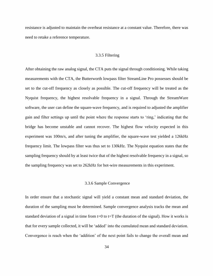
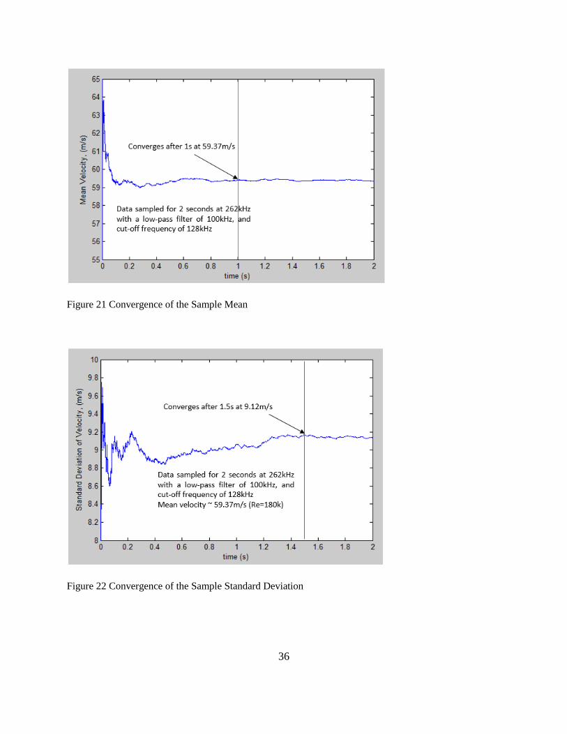
the signal will be least willing to converge due to its high turbulence. The convergence of the mean

for the above sampling frequency was about 1 second worth of signal (Figure 21), and the standard

deviation of the signal converged after about 1.5 seconds (Figure 22).

36

Figure 21 Convergence of the Sample Mean

Figure 22 Convergence of the Sample Standard Deviation

37

To ensure the signal will converge for any Reynolds number, the chosen sampling duration was 4

seconds, a little more than twice the convergence time of the standard deviation. This gave a

sample count of just over a million data points.

3.3.7 Calibration

A TSITM 1127 manual velocity calibrator’s three nozzle sets were used to calibrate the sensor for

various velocity ranges. Contrary to common hot-wire calibration practices, a 4th-order polynomial

curve fit was used to correlate the voltage the anemometer was outputting and the velocity of the

air from the nozzle set. Since the 16-bit A/D board’s voltage input range of 10V, -5 to +5 volts,

the calibration voltage output was offset and amplified to -5 to +5 volts, or however close to the

A/D converter’s limit the CTA would allow without overshooting. When converting the analog

signal to a digital signal, increasing the usage of the A/D board’s range will maximize the number

of ‘bins’ the analog voltage can be placed in during the digitization process. 20 equally-spaced

points are taken within the voltage range the CTA’s amplifier gain will allow for a given

calibration.

To ensure the sensor is accurate while taking measurements, a calibration of the sensor was done

before, and after each test to account for any voltage drift caused by contaminate accumulation on

the sensor during testing, and internal errors that might occur when the CTA is switched between

Standby and Operate mode.

Prior to introducing flow to the sensor, and voltage offset and amplification, an initial (0m/s)

voltage measurement is taken for later use when creating King’s Law curve fits.

38

The velocity of the flow at the nozzle exit was calculated by using high-order polynomial

correlations TSI provides with their calibrator units that link the nozzle set’s venturi pressure

differential to nozzle exit velocity. With the velocity known at each point as well as the sensor’s

voltage, fitting a correlation between the two was possible.

3.3.8 Uncertainty Considerations

DANTEC provides a list of velocity uncertainty equations used to calculate errors from a multitude

of physical phenomena including local temperature variation effects, ambient pressure

fluctuations, and density changes due to temperature and pressure. These errors as well as

systematic errors such as sensor yaw angle and curve-fit biases were considered during the analysis

and for all Reynolds number case, most of the errors amounted to about 5-6% of the velocity

measurement. DANTEC gave a rough estimate of 3% on the total uncertainty of the velocity

measurement. Given that their estimate was based on the use of their automated calibrator and that

the curve-fit error was responsible for most of the uncertainty, 5% with the use of a manual

calibrator is reasonable. The equations for these uncertainties are listed in the Appendix D.

39

CHAPTER 4: RESULTS AND DISCUSSION

4.1 Heat Transfer Analysis Results

The heat transfer experiments were tested at seven Reynolds numbers ranging from 25,000 to

125,000. The module-averaged Nusselt distribution (Figure 23) showed that the highest heat

transfer coefficient occurs at the entrance of the test section due to thermal development as the

flow just begins to be heated. At the entrance, the largest temperature gradient between the plate

and fluid temperature exists.

Figure 23 Modular Nusselt Number distribution, Re = 70,000

Tests conducted by Ahmed et al.[ 1 ] for the two ribbed-wall case conclude that the heat transfer

coefficient became constant after around eight hydraulic diameters in all Re cases. Figure 23 shows

that the same holds true for the single ribbed wall case. x/Dh begins at zero at the test section

40

entrance in this figure. Since the bulk air temperature increases along the test section, local Re

decreases along the streamwise direction.

For the remainder of this paper, averaged wall-based Nu values, calculated by fully turbulent heat

transfer coefficients will be discussed. These Nusselt values will be plotted against test section

averaged Re calculated by averaged test section bulk temperature properties, and mass flowrate

derived average flow velocity. The averaged wall-based Nu was decomposed into three curves:

averaged smooth top walls, averaged smooth left and right walls, and averaged ribbed bottom wall

for each Re, and can be seen in Figure 24. It is seen that the bottom ribbed wall had the most

effective heat transfer, and that the top smooth wall had the least effectiveness. The smooth side

walls had a higher Nu than the top walls due to turbulence which is generated by the bottom ribbed

wall, weakening toward the top wall.

Figure 24 Wall-Averaged Nusselt number at various Re ranging from 25,000 to 125,000

41

In Ahmed et al.’s two ribbed wall study [ 1 ], the top and bottom ribbed walls had nearly identical

Nu values since boundary conditions in the channel were about the same, and thus could be

appropriately averaged together to get an averaged rough wall Nu for both walls. Figure 25

presents the channel-averaged heat transfer augmentation (Nu/Nu0) at various Re for both one

ribbed wall and two ribbed wall cases.

Figure 25 Channel-Averaged Nusselt Augmentation for Re ranging from 25,000 to 125,000

The channel-averaged Nusselt numbers were normalized with a smooth channel Nu0 value, based

on Dittus Boelter correlations for smooth circular tubes, just as Han et al. [ 3 ] [ 5 ] [ 6 ], and

Ahmed et al. [ 1 ] had done, to properly compare results. It should be noted that the Dittus Boelter

equation is valid for 0.6 < Pr < 160, L/D > 10, and ReD > 10,000 for turbulent flows. All tests in

this experiment were conducted within this range.

𝑁𝑢0𝐷ℎ= 0.023𝑅𝑒𝐷ℎ

0.8𝑃𝑟0.4 (𝐷𝑖𝑡𝑡𝑢𝑠 𝐵𝑜𝑒𝑙𝑡𝑒𝑟) ( 4.19 )

42

The results show a nearly constant augmentation of around 1.4 for all Re after 90,000 for the one-

wall case. The two-wall case revealed an augmentation of about 1.3 to 1.5 times higher than the

one wall case as it settles at around 1.9 for Re greater than 50,000 [ 1 ]. This was to be expected

since the two-wall case had much more turbulent mixing than the single-wall channel.

4.2 Friction Factor Analysis Results

To guarantee the accuracy of the friction testing, an extensive investigation was conducted with

several data points at repeated Reynolds numbers. The friction calculation is affected by channel

geometry, flow rate measurements, pressure measurements. Error in any of these measurements

can lead to erroneous friction results. Because of this, all error sources in these measurements were

checked rigorously. Flow rate measurement was confirmed by checking venturi calibrations and

recalibrating when needed. Flow leakage tests through the inlet, test section, and downstream

plumbing were all checked with incense. Venturi upstream pressure and pressure drop were

compared with flow data taken from the heat transfer tests with valid energy balances. Tests were

repeated two or three times for each Reynolds number, and plotted to ensure that these

measurements matched every time. Any geometric inconsistencies in the alignment of the acrylic

inlet and test section were checked, and realigned if needed prior to testing.

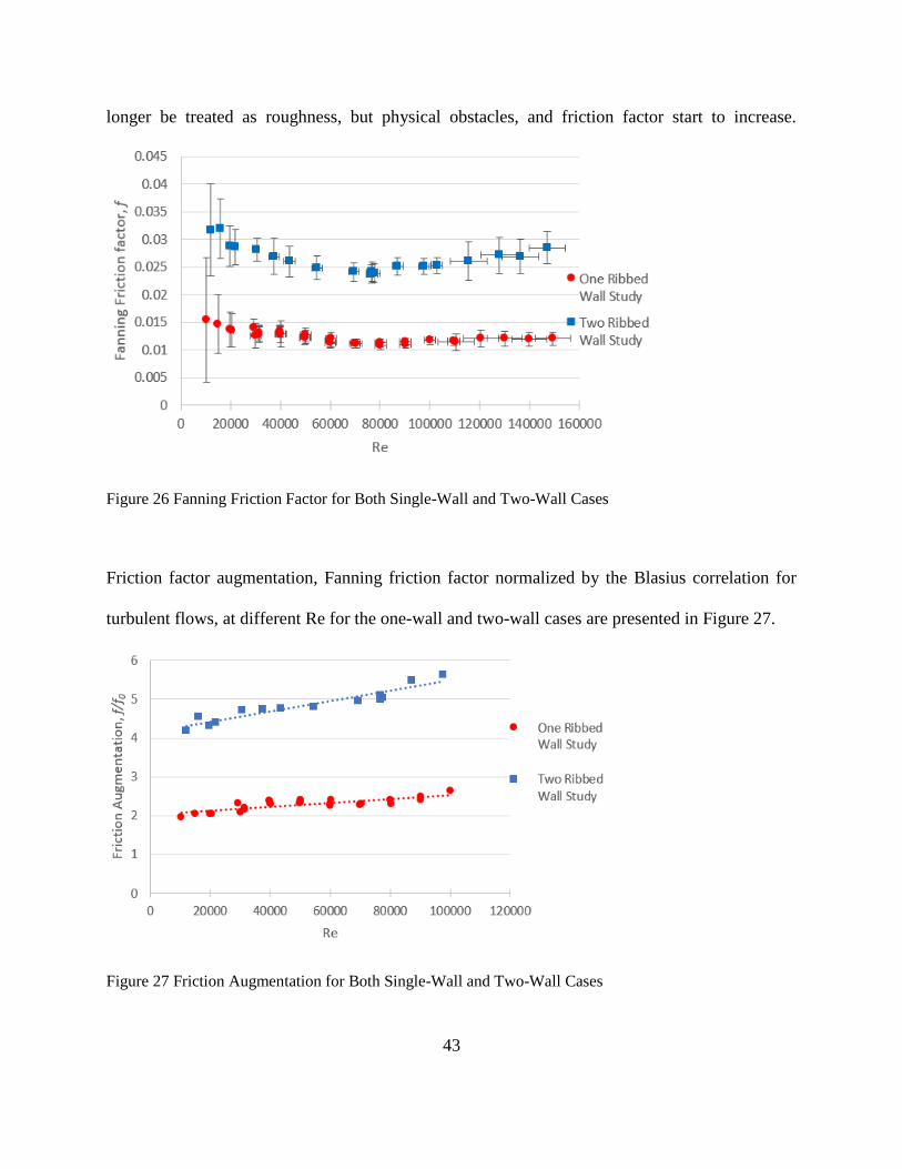
From the friction results, one can observe that the friction factors for both the one-wall and Ahmed

et al.’s [ 1 ] two-wall cases are relatively high at Reynolds numbers below 22,000. Above Re =

120,000, friction factor holds constant at 0.012 for the single-wall case. Ahmed et al.’s [ 1 ] two

ribbed-wall study described an effect where high e+ values at higher Re show that ribs can no

43

longer be treated as roughness, but physical obstacles, and friction factor start to increase.

Figure 26 Fanning Friction Factor for Both Single-Wall and Two-Wall Cases

Friction factor augmentation, Fanning friction factor normalized by the Blasius correlation for

turbulent flows, at different Re for the one-wall and two-wall cases are presented in Figure 27.

Figure 27 Friction Augmentation for Both Single-Wall and Two-Wall Cases

44

These curves exhibit an approximately linear relationship with Reynolds Number. The two ribbed-

wall study showed about a 2.2 times higher friction augmentation than the one-wall case. The

Blasius correlation is only valid between Reynolds numbers of 5,000 to 100,000, so although the

friction factor is calculated up to Re = 125,000, the Augmentation is only valid when the Blasius

correlation is valid. Once again, the Blasius correlation is used in this study because both Han et

al. [ 3 ] [ 5 ] [ 6 ], and Ahmed et al. [ 1 ] determined their augmentations with this correlation.

4.3 Thermal Performance Analysis Results

Heat transfer tests have been conducted for seven Re in the range of 25,000 to 125,000 for the one-

wall case. The pressure drop/friction experiments were conducted at a wider range. A linear curve

fit, generated from the friction augmentation against Re, allowed the prediction of a friction

augmentation at the same Re used during heat transfer testing. This made possible the calculation

of the thermal performance. Han et al. [ 22 ] used an equation to define thermal efficiency:

𝜂 =𝑁𝑢

𝑁𝑢𝑜⁄

(𝑓

𝑓𝑜⁄ )

1/3 ( 4.20 )

Ahmed et. al [ 1 ] incorporated the same equation in their validation case of Han’s square channel.

To make one-to-one comparisons between these results, the same equation was used in this case.

Due to lower friction augmentation, the thermal efficiency was higher at low Reynolds numbers.

With the increasing Re, however, the friction augmentation took a toll on the Nusselt

augmentation.

45

Thermal performance decreased until about Re = 70,000, where it holds constant around unity for

the single ribbed-wall case, Figure 28. Within the Reynolds number range studied, the two-wall

case continually decreases.

Figure 28 Thermal Performance for Both Single, and Two-Wall Cases

4.4 Heat Transfer and Friction Experimental Uncertainty Results

Uncertainties in the experimental results have been quantified by the methods described by Kline

and McClintock [ 25 ] and Moffat [ 26 ]. Refer to Appendix A-D for further detail on the

uncertainty analysis. The uncertainty for Reynolds number was estimated to be less than 6% in all

cases, Noting that the mass flow rate measurement contributes the most to this uncertainty. The

highest uncertainty estimated for Nu was less than 5%. Uncertainties in values such as voltages,

resistances, temperatures, and flow rate measurements were the main contributors to Nu

uncertainty. Pressure and flow rate measurements contributed to the uncertainty estimation in the

46

friction factor which was estimated to be less than 12% for Re > 20,000. The mass flow rate

uncertainty took over in friction factor uncertainty for Re < 20,000. The uncertainty in friction

factor jumped to 21%-73% for 10,000 < Re < 20,000 due to the minute pressure drop across the

rig at this Reynolds number range. Pressure drop uncertainty became comparable to the physical

measurement.

4.5 Hot-wire Analysis Results

Single-wire hot-wire anemometry was used to characterize velocity magnitude profiles in great

detail, as well as turbulence intensity for Reynolds numbers ranging from 5,000 to 50,000. It was

seen that as Reynolds number increased, the reattachment point between two ribs remained

relatively stationary while the turbulence intensity receded to the trailing surface of the upstream

rib, and dissipated as it traveled. At low Reynolds numbers between 5,000 and 10,000 the velocity

and turbulence intensity streamwise profiles seemed to form two distinct flow regions, indicating

that the flow over the upstream rib never completely attached between the two ribs.

The following figures will be presented in this fashion:

Figure 29 Sample Contour Plot

47

Figure 29 depicts a normalized velocity contour plot taken at Reynolds number of 50000. The

black rectangles seen in the figure represent the physical, to scale, ribs in a midspan cross section

of the flow. The white spaces represent the areas the sensor midpoint could not get to because the

sensor had to be faced perpendicularly to the flow direction. Unfortunately, this meant that the

sensor could not be mounted flush with the ribs, and had to have a 45° angle between them. The

thickness of the white spaces aft and forward of the upstream and downstream rib, respectively,

indicates the distance between the sensor midpoint and rib edge as they have a 45° misalignment.

The contour plots are mapped to each of the intersections in Figure 9. The scale to the right of the

contour plots indicates what numeric values are assigned to each color in the plot. To observe the

evolution of the flow, the scales are kept the same between all tested Reynolds numbers and

measurement type.

To make sure the hot-wire measurement was stable and repeatable, a repeatability test was

conducted at Re = 50000. Shown below is a contour of turbulence intensity and its associated

uncertainty percentage for this Reynolds number.

Figure 30 Re = 50,000 TI Repeatability Test

48

In Figure 30, the two top plots are nearly identical, indicating that the testing is repeatable.

However, the uncertainty plots beneath are quite different in magnitude. This was due to the

systematic uncertainty of the velocity calibration curve fit error. Further details on the uncertainty

is shown in Appendix D.

Figure 31 Local Velocity Normalized by the Channel Bulk Velocity

In Figure 31, it is seen that the scaled velocity increased dramatically in the free stream, above the

rib until Re = 30,000, where the freestream velocities between Re = 30,000 and 50,000 appear to

be about the same. Another observation can be made near the wall at x/Dh ~0.48 to 0.55. This is

where the reattachment point was located in the Reynolds number range tested. Although not clear

if the flow is reattaching at Re = 5,000 at x/Dh = 0.55, it can be seen in the other Reynolds numbers

tested. The reattachment point location seems to have a weak, but existent, correlation with flow

increase. As Re increase, the reattachment point slow moves back toward the aft of the upstream

49

rib. Further Reynolds number data need to be obtained to determine if the position stops after Re

= 50,000 because it does not appear to change between this flow rate, and that of Re = 30,000.

Figure 32 Uncertainty of Normalized Velocity

Figure 32 shows that, except for the repeated case of Re = 50,000, the uncertainty of the normalized

velocity peaks about 6.5% near the bottom aft corner if the upstream rib where the flow velocity

is very small and difficult to resolve.

50

Figure 33 RMS Velocity Fluctuations Normalized by Local Velocity (TI)

Figure 33 depicts the turbulence intensity of the flow at the tested Reynolds numbers. It was

observed that as Reynolds number increased, the peak in intensity dramatically moves upstream

toward the aft of upstream rib, and maintained peak intensity within the Reynolds numbers tested.

Unfortunately, after Re = 30,000, the peak in turbulence intensity was not located on the bottom

wall surface. This shows that potential turbulent mixing is being “wasted” just above the

recirculation zone, as it is not interacting much with the bottom wall surface.

51

Figure 34 Uncertainty in Turbulence Intensity

Turbulence data was taken at ambient temperature flow conditions, but heat transfer data was

obviously taken at heated flow conditions. A check to make sure that the turbulence data is still

applicable for the heat transfer environment can be accomplished using Richardson number (Ri),

the ratio of buoyant, natural convective forces over forced convection. In heated flow, the effect

of density changes due to local air thermal gradients on the forced convection from the channel’s

driving pressure drop is scrutinized. A general rule of thumb for Richardson number is as follows:

if Ri < 0.1, then natural convective forces are dominated by forced convection, and if Ri > 10, then

natural convection dominates the forced convection. An Ri in between these limits implies that

neither of these forces can be ignored in the overall flow behavior of the fluid.

𝑅𝑖 =𝑔𝛽(𝑇ℎ𝑜𝑡−𝑇𝑟𝑒𝑓)𝐿

𝑉2

𝑅𝑖 < 0.1 (𝑛𝑎𝑡𝑢𝑟𝑎𝑙 𝑐𝑜𝑛𝑣𝑒𝑐𝑡𝑖𝑜𝑛 𝑖𝑠 𝑖𝑔𝑛𝑜𝑟𝑒𝑑)𝑅𝑖 > 10 (𝑓𝑜𝑟𝑐𝑒𝑑 𝑐𝑜𝑛𝑣𝑒𝑐𝑡𝑖𝑜𝑛 𝑖𝑠 𝑖𝑔𝑛𝑜𝑟𝑒𝑑)0.1 < 𝑅𝑖 < 10 (𝑛𝑖𝑒𝑡ℎ𝑒𝑟 𝑐𝑎𝑛 𝑏𝑒 𝑖𝑔𝑛𝑜𝑟𝑒𝑑)

( 4.21 )

52

Since local fluid temperature variations could not be calculated in the heat transfer experiments

extreme values of temperature difference and local velocity will be used to estimate an upper and

lower bound of this number to determine if density change would play a role in the turbulence

calculations during a heat transfer run. Because the plate temperature is assumed to be isothermal

at the target temperature of 70°C, the following table will show various scenarios of temperature

differences, and velocities while holding the plate temperature constant. The length-scale of the

Richardson number will be that of the hydraulic diameter of the channel, Dh = 0.0508m, and g will

be the gravitational constant, 9.81m/s2.

Table 2 Hot-wire Data Validation in Heat Transfer Testing

High ΔT, high V Low ΔT, high V High ΔT, low V Low ΔT, low V

Tplate (K) 343.15 343.15 343.15 343.15

Tfluid (K) 298.15 323.15 298.15 323.15

β, (1/K) 3.40E-03 3.10E-03 3.40E-03 3.10E-03

V (m/s) 100 100 1 1

Ri 7.62472E-06 3.08976E-06 0.076247244 0.030897576

In Table 2, even with a very high predictable temperature difference and a low velocity of 1 m/s,

which has been observed within the recirculation regions in low Re, Richardson number remains

below 0.1. This means that the flow should not be influenced by thermal effects even under the

worst conceivable circumstance of column three in the above table.

Integral length-scale calculations were also made within the Reynolds number range of 5,000 to

50,000. At each Reynolds number, the most turbulent, highest standard deviation in velocity, point

was located using a search algorithm in MATLAB. Below in Table 3, is a summary of these

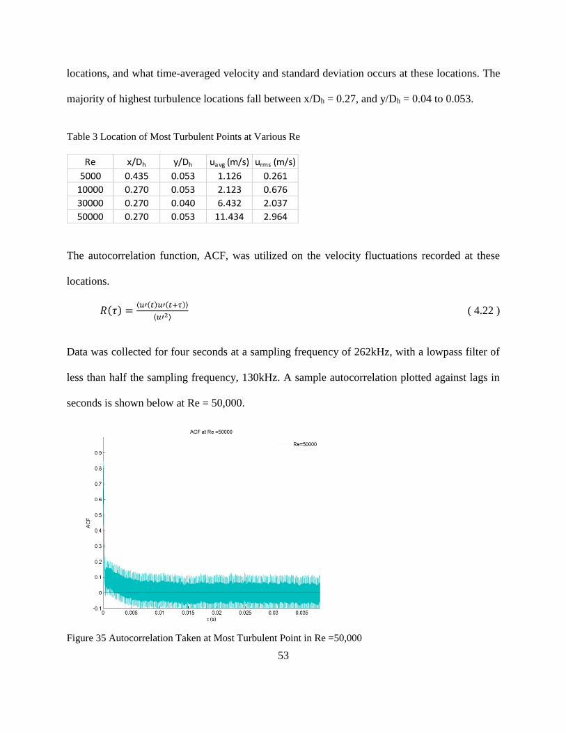
53

locations, and what time-averaged velocity and standard deviation occurs at these locations. The

majority of highest turbulence locations fall between x/Dh = 0.27, and y/Dh = 0.04 to 0.053.

Table 3 Location of Most Turbulent Points at Various Re

Re x/Dh y/Dh uavg (m/s) urms (m/s)

5000 0.435 0.053 1.126 0.261

10000 0.270 0.053 2.123 0.676

30000 0.270 0.040 6.432 2.037

50000 0.270 0.053 11.434 2.964

The autocorrelation function, ACF, was utilized on the velocity fluctuations recorded at these

locations.

𝑅(𝜏) =⟨𝑢′(𝑡)𝑢′(𝑡+𝜏)⟩

⟨𝑢′2⟩ ( 4.22 )

Data was collected for four seconds at a sampling frequency of 262kHz, with a lowpass filter of

less than half the sampling frequency, 130kHz. A sample autocorrelation plotted against lags in

seconds is shown below at Re = 50,000.

Figure 35 Autocorrelation Taken at Most Turbulent Point in Re =50,000

54

The integral length-scale was calculated using the ACF and the Taylor Frozen Hypothesis. The

area under the curve of ACF yields the eddy integral time-scale,

𝑇 = ∫ 𝑟(𝜏)∞

0𝑑𝜏 ( 4.23 )

and the Taylor Frozen Hypothesis (which states that the local disturbances in a turbulent eddy as

it passes a sensor are considered negligible, and the eddy velocity can be estimated as the local

convective velocity) gives the eddy velocity. These terms can be multiplied together to get an eddy

integral length scale. Below, in Table 4, integral time, and length-scales at each Reynolds number

are tabulated.

Table 4 Integral Time and Length-Scales at Various Re

T (s) Λ (mm) Λ/e

5000 0.00390 4.151 1.307

10000 0.00094 2.427 0.764

30000 0.00040 3.371 1.062

50000 0.00048 6.588 2.075

Table 4 shows that Λ/e, the ratio of integral length-scale to rib height has a generally increasing

trend as a function of Reynolds number. At a Reynolds number of 45,000, Rivir et al. [ 30 ]

calculated an integral length-scale of 1.5 times the rib height of a two-wall transverse rib case just

downstream of the rib (very close to where this case’s point was taken).

55

CHAPTER 5: FINDINGS

In curiosity of how a replication, and extension of Han et al.’s [ 2 ] work with 45° ribs with a p/e

of 10, and e/Dh of 0.0625 conducted by Ahmed et al. [ 1 ] would compare to a slight modification

to Ahmed et al.’s original channel (converting a two-ribbed wall channel to single-ribbed wall

channel), heat transfer, friction, and turbulence testing were carried out. Under nearly the same

Reynolds number range of Ahmed et al.’s case, the single ribbed-wall case yielded ~1.4 times less

channel-averaged heat transfer capability than the two-wall case, but also half the friction than the

two ribbed-wall case. Overall, the channel thermal performance as a function of Reynolds number

between the two cases were about the same, the two ribbed-wall case having slightly better

performance in the mid-range Reynolds numbers. Chandra et al. [ 20 ] concluded that overall

performance declines as more ribbed walls are added, but this case and the two ribbed-wall case

comparatively suggest that there are nearly no differences in thermal performance.

On a wall-based scale, the heat transfer of the two ribbed-wall case had nearly identical Nusselt

curves for the top and bottom, and left and right walls, consecutively. This being explained by the

channel’s symmetric boundary conditions on the inner walls. The single ribbed-wall case,

however, had asymmetric boundary conditions on the inner walls since only one wall (bottom) had

ribs. The bottom ribbed-wall, by no surprise, yielded the highest heat transfer of the four walls in

the single ribbed-wall case, the top smooth wall had the least, and the left and right walls having

some heat transfer in between the top and bottom walls.

This lead to the idea of testing fully developed turbulence intensity within the channel, because

there was a turbulent mixing gradient between the top and bottom walls as the heat transfer results

hinted. The turbulent testing results shown that the mixing intensity, at least midspan of the

56

channel, did not have that much of a noticeable TI gradient, as conjectured. Turbulence intensity

invoked by the ribs, nearly diminished only 10% of the channel height above the bottom wall

surface. Velocity contours indicated that, although no directional information can be determined

from a single wire hot-wire sensor, the location of a reattachment point of the flow after deflecting

off an upstream rib can be roughly identified. As Reynolds number increase, the reattachment

point appears hold position, but the velocities around the reattachment point increase, “filling in”

the space between the ribs with faster and faster flow. The TI starts about midstream between two

ribs, and retracts toward the upstream rib as Reynolds number increases. It was seen that the

highest TI zones at each Reynolds number was not located on, or near the flow surface, where heat

transfer would take place. This is unfortunate, to “waste” the mixing potential, but by modifying

the IDC parameters, the high TI zone might be brought down closer to the surface to increase

mixing heat transfer.

To ensure that the flow is under fully turbulent conditions, both the velocity of the flow at Re =

50,000 and the standard deviation of the fluctuations were compared at the upstream rib center and

the downstream rib center.

Figure 36 Velocity and Fluctuation Plots at Re = 50,000

57

Figure 36 shows that at the same geographic locations in the rig, the center points of two ribs, the

velocity and fluctuation profiles nearly match and are well within uncertainty of the velocity

measurement. The flow is indeed fully turbulent at between the two ribs tested in the turbulence

analysis.

Integral length-scale calculations predict an increasing trend between the Reynolds number, and

length-scale located at the most turbulent point in the flow at each Re. Because there isn’t a lot of

length-scale as a function of Reynolds number data existing in literature for IDC, it is difficult to

assert that the results obtained in this study are accurate. However, Rivir et al.’s [ 30 ] results show

that at about the same location tested with respect to the ribs they used, the integral length-scale

was approximately 1.5 times the rib height at a Reynolds number of 45,000. In this case the length-

scale at Re = 50,000 was twice the height. Several factors mentioned in the beginning of this thesis

could influence the value of this integral length-scale, such as rib pitch, number of ribbed walls,

rib angle (in his case transverse, 90deg). The fact that their scale is on the order of what was

obtained in this case gives some level of confidence in the value.

Heat transfer testing was obviously conducted under hot wall condition, but the turbulent testing

was done all at ambient temperature. If one were to try to compare, or extend the turbulence data

to the heat transfer testing, could it be done? The Richard number, the ratio of natural vs. forced

convection suggest that under the Reynolds numbers test, temperature gradients off the walls

should not affect the flow with adverse air density gradients. The flow is too fast for natural

convection to make any contribution to the flow mixing, or direction.

58

APPENDIX A:

UNCERTAINTIES OF MASS FLOWRATE

59

𝑃𝑢𝑝𝑠𝑡𝑟𝑒𝑎𝑚 = 𝑃𝑠𝑡𝑎𝑡𝑖𝑐 +𝑃𝑎𝑡𝑚

(𝑈𝑃_𝑢𝑝𝑠𝑡𝑟𝑒𝑎𝑚)𝑃_𝑠𝑡𝑎𝑡𝑖𝑐

=𝜕𝑃_𝑢𝑝𝑠𝑡𝑟𝑒𝑎𝑚

𝜕𝑃_𝑠𝑡𝑎𝑡𝑖𝑐∙ 𝑈𝑃𝑠𝑡𝑎𝑡𝑖𝑐

= 𝑈𝑃𝑠𝑡𝑎𝑡𝑖𝑐

(𝑈𝑃_𝑢𝑝𝑠𝑡𝑟𝑒𝑎𝑚)𝑃_𝑎𝑡𝑚

=𝜕𝑃_𝑢𝑝𝑠𝑡𝑟𝑒𝑎𝑚

𝜕𝑃_𝑎𝑡𝑚∙ 𝑈𝑃𝑎𝑡𝑚

= 𝑈𝑃𝑎𝑡𝑚

𝑈𝑃_𝑢𝑝𝑠𝑡𝑟𝑒𝑎𝑚 = 𝑅𝑆𝑆 [(𝑈𝑃_𝑢𝑝𝑠𝑡𝑟𝑒𝑎𝑚)𝑃_𝑠𝑡𝑎𝑡𝑖𝑐

, (𝑈𝑃_𝑢𝑝𝑠𝑡𝑟𝑒𝑎𝑚)𝑃_𝑎𝑡𝑚

]

𝑇(𝐾) =5

9(𝑇() − 32) + 273.15

(𝑈𝑇(𝐾))𝑇()

=𝜕𝑇(𝐾)

𝜕𝑇()∙ 𝑈𝑇() =

5

9∙ 𝑈𝑇()

𝜌𝑓𝑙𝑢𝑖𝑑 =𝑃_𝑢𝑝𝑠𝑡𝑟𝑒𝑎𝑚

𝑅 𝑇𝑓𝑙𝑢𝑖𝑑

(𝑈𝜌𝑓𝑙𝑢𝑖𝑑)

𝑃_𝑢𝑝𝑠𝑡𝑟𝑒𝑎𝑚=

𝜕𝜌𝑓𝑙𝑢𝑖𝑑

𝜕𝑃_𝑢𝑝𝑠𝑡𝑟𝑒𝑎𝑚∙ 𝑈𝑃𝑢𝑝𝑠𝑡𝑟𝑒𝑎𝑚

=𝑈𝑃𝑢𝑝𝑠𝑡𝑟𝑒𝑎𝑚

𝑅 𝑇𝑓𝑙𝑢𝑖𝑑

(𝑈𝜌𝑓𝑙𝑢𝑖𝑑)

𝑇𝑓𝑙𝑢𝑖𝑑

=𝜕𝜌𝑓𝑙𝑢𝑖𝑑

𝜕𝑇𝑓𝑙𝑢𝑖𝑑∙ 𝑈𝑇𝑓𝑙𝑢𝑖𝑑

=𝑃_𝑢𝑝𝑠𝑡𝑟𝑒𝑎𝑚

𝑅𝑇𝑓𝑙𝑢𝑖𝑑2 ∙ 𝑈𝑇𝑓𝑙𝑢𝑖𝑑, 𝐾

𝑈𝜌𝑓𝑙𝑢𝑖𝑑= 𝑅𝑆𝑆 [(𝑈𝜌𝑓𝑙𝑢𝑖𝑑

)𝑃_𝑢𝑝𝑠𝑡𝑟𝑒𝑎𝑚

, (𝑈𝜌𝑓𝑙𝑢𝑖𝑑)

𝑇𝑓𝑙𝑢𝑖𝑑

]

= 𝜌𝑓𝑙𝑢𝑖𝑑 𝑄

(𝑈)𝜌 =𝜕

𝜕𝜌∙ 𝑈𝜌 = 𝑄 ∙ 𝑈𝜌

(𝑈)𝑄 =𝜕

𝜕𝑄∙ 𝑈𝑄 = 𝜌 ∙ 𝑈𝑄

𝑈 = 𝑅𝑆𝑆[(𝑈)𝜌 , (𝑈)𝑄]

60

APPENDIX B:

SYSTEMATIC UNCERTAINTIES OF NUSSELT NUMBER

61

𝑄𝑖𝑛𝑝𝑢𝑡 =𝑉2

𝑅

𝑈(𝑄𝑖𝑛𝑝𝑢𝑡)𝑉

=2𝑉

𝑅

𝑈(𝑄𝑖𝑛𝑝𝑢𝑡)𝑅

= (𝑉

𝑅)

2

𝑄𝑎𝑐𝑡 = 𝑄𝑖𝑛𝑝𝑢𝑡 − 𝑄𝑙𝑒𝑎𝑘𝑎𝑔𝑒

𝑈(𝑄𝑎𝑐𝑡)𝑄𝑖𝑛𝑝𝑢𝑡= 𝑈(𝑄𝑖𝑛𝑝𝑢𝑡)

𝑈(𝑄𝑎𝑐𝑡)𝑄𝑙𝑒𝑎𝑘𝑎𝑔𝑒= 𝑈(𝑄𝑙𝑒𝑎𝑘𝑎𝑔𝑒)

𝑇𝑓𝑙𝑢𝑖𝑑,𝑓 =𝑄𝑎𝑐𝑡

𝑐𝑝+ 𝑇𝑓𝑙𝑢𝑖𝑑,𝑖

𝑈(𝑇𝑓𝑙𝑢𝑖𝑑,𝑓)𝑄𝑎𝑐𝑡

=𝑈(𝑄𝑎𝑐𝑡)

𝑐𝑝

𝑈(𝑇𝑓𝑙𝑢𝑖𝑑,𝑓)

=𝑈()𝑄𝑎𝑐𝑡

2𝑐𝑝

𝑈(𝑇𝑓𝑙𝑢𝑖𝑑,𝑓)𝑇𝑓𝑙𝑢𝑖𝑑,𝑖

= 𝑈(𝑇𝑓𝑙𝑢𝑖𝑑,𝑖)

∆𝑇𝑖𝑛,𝑥 = 𝑇𝑤𝑎𝑙𝑙,𝑥 − 𝑇𝑓𝑙𝑢𝑖𝑑,𝑖_𝑥

𝑈(∆𝑇𝑖𝑛,𝑥)𝑇𝑤𝑎𝑙𝑙,𝑥

= 𝑈(𝑇𝑤𝑎𝑙𝑙,𝑥)

𝑈(∆𝑇𝑖𝑛,𝑥)𝑇𝑓𝑙𝑢𝑖𝑑,𝑖_𝑥

= 𝑈(𝑇𝑓𝑙𝑢𝑖𝑑,𝑖_𝑥)

∆𝑇𝑜𝑢𝑡,𝑥 = 𝑇𝑤𝑎𝑙𝑙,𝑥 − 𝑇𝑓𝑙𝑢𝑖𝑑,𝑓_𝑥

𝑈(∆𝑇𝑜𝑢𝑡,𝑥)𝑇𝑤𝑎𝑙𝑙,𝑥

= 𝑈(𝑇𝑤𝑎𝑙𝑙,𝑥)

𝑈(∆𝑇𝑜𝑢𝑡,𝑥)𝑇𝑓𝑙𝑢𝑖𝑑,𝑓_𝑥

= 𝑈(𝑇𝑓𝑙𝑢𝑖𝑑,𝑓_𝑥)

𝐿𝑀𝑇𝐷𝑥 =∆𝑇𝑖𝑛,𝑥 − ∆𝑇𝑜𝑢𝑡,𝑥

𝑙𝑛 (∆𝑇𝑖𝑛,𝑥

∆𝑇𝑜𝑢𝑡,𝑥)

62

𝑈(𝐿𝑀𝑇𝐷𝑥)∆𝑇𝑖𝑛,𝑥= 𝑈(∆𝑇𝑖𝑛,𝑥)

∆𝑇𝑖𝑛,𝑥𝑙𝑛(∆𝑇𝑖𝑛,𝑥

∆𝑇𝑜𝑢𝑡,𝑥)+∆𝑇𝑜𝑢𝑡,𝑥−∆𝑇𝑖𝑛,𝑥

∆𝑇𝑖𝑛,𝑥𝑙𝑛(∆𝑇𝑖𝑛,𝑥

∆𝑇𝑜𝑢𝑡,𝑥)

2

𝑈(𝐿𝑀𝑇𝐷𝑥)∆𝑇𝑜𝑢𝑡,𝑥= 𝑈(∆𝑇𝑜𝑢𝑡,𝑥)

∆𝑇𝑜𝑢𝑡,𝑥𝑙𝑛(∆𝑇𝑖𝑛,𝑥

∆𝑇𝑜𝑢𝑡,𝑥)+∆𝑇𝑖𝑛,𝑥−∆𝑇𝑜𝑢𝑡,𝑥

∆𝑇𝑜𝑢𝑡,𝑥𝑙𝑛(∆𝑇𝑖𝑛,𝑥

∆𝑇𝑜𝑢𝑡,𝑥)

2

ℎ𝑥 =𝑄𝑎𝑐𝑡𝐴

𝑇𝑤𝑎𝑙𝑙𝑥− 𝑇𝑓𝑙𝑢𝑖𝑑,𝑓𝑥

𝑈(ℎ𝑥)𝑄𝑎𝑐𝑡

=𝑈(𝑄𝑎𝑐𝑡)𝐴

𝑇𝑤𝑎𝑙𝑙𝑥−𝑇𝑓𝑙𝑢𝑖𝑑,𝑓𝑥

𝑈(ℎ𝑥)𝑇𝑤𝑎𝑙𝑙𝑥

=𝑈(𝑇𝑤𝑎𝑙𝑙𝑥)𝑄𝑎𝑐𝑡𝐴

(𝑇𝑤𝑎𝑙𝑙𝑥−𝑇𝑓𝑙𝑢𝑖𝑑,𝑓𝑥)2

𝑈(ℎ𝑥)𝑇𝑓𝑙𝑢𝑖𝑑,𝑓𝑥

=𝑈(𝑇𝑓𝑙𝑢𝑖𝑑,𝑓𝑥)𝑄𝑎𝑐𝑡𝐴

(𝑇𝑤𝑎𝑙𝑙𝑥−𝑇𝑓𝑙𝑢𝑖𝑑,𝑓𝑥)2

𝑁𝑢𝐷,𝑥 =ℎ𝑥𝐷ℎ

𝑘

𝑈(𝑁𝑢𝐷,𝑥) =𝑈(ℎ𝑥)𝐷ℎ

𝑘

63

APPENDIX C:

SYSTEMATIC UNCERTAINTIES OF FRICTION FACTOR

64

𝑃𝑖𝑛,𝑎𝑏𝑠 = 𝑃𝑖𝑛,𝑔 + 𝑃𝑎𝑡𝑚

𝑈(𝑃𝑖𝑛) = 𝑅𝑆𝑆 [𝑈(𝑃𝑖𝑛)𝑃𝑖𝑛,𝑔, 𝑈(𝑃𝑖𝑛)𝑃𝑎𝑡𝑚

]

𝑃𝑜𝑢𝑡,𝑎𝑏𝑠 = 𝑃𝑜𝑢𝑡,𝑔 + 𝑃𝑎𝑡𝑚

𝑈(𝑃𝑜𝑢𝑡) = 𝑅𝑆𝑆 [𝑈(𝑃𝑜𝑢𝑡)𝑃𝑜𝑢𝑡,𝑔, 𝑈(𝑃𝑜𝑢𝑡)𝑃𝑎𝑡𝑚

]

𝑃𝑎𝑣𝑔,𝑎𝑏𝑠 =𝑃𝑖𝑛,𝑎𝑡𝑚 + 𝑃𝑜𝑢𝑡,𝑎𝑡𝑚

2

𝑈(𝑃𝑎𝑣𝑔,𝑎𝑏𝑠) = 𝑅𝑆𝑆 [1

2𝑈(𝑃𝑎𝑣𝑔,𝑎𝑏𝑠)

𝑃𝑖𝑛,𝑎𝑡𝑚,

1

2𝑈(𝑃𝑎𝑣𝑔,𝑎𝑏𝑠)

𝑃𝑜𝑢𝑡,𝑎𝑡𝑚]

𝜌𝑎𝑣𝑔 =𝑃𝑎𝑣𝑔,𝑎𝑏𝑠

𝑅𝑎𝑖𝑟𝑇𝑎𝑚𝑏

𝑈(𝜌𝑎𝑣𝑔)𝑃𝑎𝑣𝑔,𝑎𝑏𝑠

=𝑈(𝑃𝑎𝑣𝑔,𝑎𝑏𝑠)

𝑅𝑎𝑖𝑟𝑇𝑎𝑚𝑏

𝑈(𝜌𝑎𝑣𝑔)𝑇𝑎𝑚𝑏

= 𝑈(𝑇𝑎𝑚𝑏)𝑃𝑎𝑣𝑔,𝑎𝑏𝑠

𝑅𝑎𝑖𝑟𝑇𝑎𝑚𝑏2

𝑢𝑎𝑣𝑔 =

𝜌𝑎𝑣𝑔𝐴

𝑈(𝑢𝑎𝑣𝑔)

=𝑈()

𝜌𝑎𝑣𝑔𝐴

𝑈(𝑢𝑎𝑣𝑔)𝜌𝑎𝑣𝑔

= 𝑈(𝜌𝑎𝑣𝑔)

𝜌𝑎𝑣𝑔2𝐴

𝑓𝐹𝑎𝑛𝑛𝑖𝑛𝑔,𝑎𝑣𝑔 =

𝑑𝑃𝑑𝑥

𝐷ℎ

2𝜌𝑎𝑣𝑔𝑢𝑎𝑣𝑔2

𝑈(𝑓𝐹𝑎𝑛𝑛𝑖𝑛𝑔,𝑎𝑣𝑔)𝜌𝑎𝑣𝑔

= 𝑈(𝜌𝑎𝑣𝑔)𝑑𝑃

𝑑𝑥𝐷ℎ

2𝜌𝑎𝑣𝑔2𝑢𝑎𝑣𝑔

2

𝑈(𝑓𝐹𝑎𝑛𝑛𝑖𝑛𝑔,𝑎𝑣𝑔)𝑈𝑎𝑣𝑔

= 𝑈(𝑢𝑎𝑣𝑔)𝑑𝑃

𝑑𝑥𝐷ℎ

𝜌𝑎𝑣𝑔𝑢𝑎𝑣𝑔3

65

APPENDIX D:

SYSTEMATIC UNCERTAINTIES OF TURBULENCE

66

67

APPENDIX E:

MATLAB CODE FOR TURBULENCE ANALYSIS

68

Converting Voltage Files to Velocity Files:

b=input('New hotwire Calibration? (y/n) ','s');

if b=='y'

%Open calibration M-file, and retrieve velocity coeffs

disp('Select calibration correlation MATLAB file');

[filename, pathname]=uigetfile('*.m','File Selector');

run(strcat(pathname,filename));

%Steps:

%Load calibration M-file

%Select calibration text file

%Enter recorded calibration ambient pressure [mbar]

clc;

clearvars htwcal v b

else

end

disp('Locate Hotwire Voltage Data Folder');

directory=uigetdir;

cd(directory)

files=dir(directory);

fileindex=find(~[files.isdir]);

filelist=cell(length(fileindex),1);

for i=1:length(fileindex)

filelisti=files(fileindex(i)).name;

end

clearvars i

clc

VEL=zeros(length(getfield(importdata(filelist1,'\t',23),'data')),1);

disp('Locate Hotwire Velocity Data Folder');

directory2=uigetdir;

for i=1:length(fileindex)

B=getfield(importdata(strcat(directory,'\',filelisti),'\t',23),'data');

Bin=B(:,2);

VEL=calibcoeff(1,1).*Bin.^4+... % VEL = matrix of (data points,y-locations,x-locations)

calibcoeff(1,2).*Bin.^3+... % Using Calibrator Venturi Nozzle

calibcoeff(1,3).*Bin.^2+...

calibcoeff(1,4).*Bin+...

calibcoeff(1,5);

fileID=fopen(strcat(directory2,'\',strrep(filelisti,'.lvm','.txt')),'w');

fprintf(fileID,'%10.6f\r\n',VEL);

Bin(:)=0;

VEL(:)=0;

clc

disp(strcat('progress: ',num2str(i),'/',num2str(length(fileindex))))

69

end

clearvars i

Published with MATLAB® R2014a

Velocity, Turbulence Intensity, Spectral, and Length Scale Analysis:

% Hotwire Analysis for Ribbed Channels (2D Region)

% streamwise traversing was done backwards (upstream direction)

Defining Zonal Layout in Topographic 2-D Region

disp('Locate main hotwire folder')

maindir=uigetdir;

cd(maindir)

disp('Locate Relevant Velocity Data File for Sample Size Determination')

sizedir=uigetdir;

cd(sizedir)

NS=size(load('z1x1y1.txt'),1); %Number of samples collected

cd(maindir)

x_matr = [1,2;1,10;1,3]; % x-locations per section

xmax=sum(x_matr(:,2));

y_matr = [6,10;6,9;6,10]; % y-locations per section

ymax=max(sum(y_matr,2));

z_matr = [0,1;2,3;0,4]; % zones (zones with solids should be valued "0")

sects=size(z_matr,1);

zero_pts=6; % number of y-points that will be within a solid per zone)

q1=input('Adding another test? (y/n) ','s');

if q1=='y'

ZBin=zeros(NS,ymax,max(z_matr(:)));

XBin=zeros(NS,ymax);

VEL=zeros(NS,ymax,xmax);

clc

disp('Navigate to section:')

disp('Velocity Binning')

else

clc

disp('Navigate to section:')

disp('Mesh Gridding & Re/Bulk Velocity Test Matrix Setup')

70

clearvars x_matr ymax zmax

end

Velocity Binning

cd(sizedir)

pos=0;

for i=1:sects % i = 1 to number of streamwise sections - (1 to 3 for IDC)

% Scanning each x-location

m=x_matr(i,:); % m-vector is defined as the (i)th row of x_matr

for x=min(m(m>0),[],2): max(m)

% max/min non-zero values in m - (number of x-pts in (z)th zone)

% Creating Zone matrices per x-location

n=z_matr(i,:); % n-array is defined as the (i)th row of z_matr

for z=min(n(n>0),[],2): max(n)

% max/min non-zero values in n - (zone numbers per section)

% Filling in z(th) Zone matrix

p=y_matr(i,:);

% p-array is defined as the (i)th row of y_matr

% - (number of y-pts in (z)th zone)

for y=1:p(find(n==z)) %#ok<FNDSB>

disp('streamwise position')

disp(pos+1)

disp('streamwise location')

disp(x)

disp('zone')

disp(z)

disp('vertical location')

disp(y)

ZBin(:,y,z)=load(strcat('z',num2str(z),'x',num2str(x),...

'y',num2str(y),'.txt'));

clc

end

end

col=1;

for j=min(n(n>0),[],2): max(n)

for k=1:sum(ZBin(1,:,j)~=0)

XBin(:,col)=ZBin(:,k,j);

col=col+1;

end

end

pos=pos+1;

VEL(:,:,pos)=circshift(XBin,sum(XBin(1,:)==0),2);

XBin=zeros(NS,ymax);

end

71

end

clc

cd(maindir)

clearvars i j k x y z col m n p pos sizedir XBin ZBin

disp('Navigate to section:')

disp('Gridded Velocities/STDEVs')

Gridded Velocities/STDEVs

clc

avgvel=zeros(1,ymax,xmax); % Average velocities initial matrix building

for i=1:xmax

for j=1:ymax

avgvel(1,j,i)=mean(VEL(:,j,i));

end

end

avgvel=reshape(avgvel,ymax,xmax);

avgvel=fliplr(avgvel);

avgvel(1:zero_pts,1:max(x_matr(3,:)))=NaN;

avgvel(1:zero_pts,sum(x_matr(2:3,2))+1:sum(x_matr(2:3,2))+x_matr(1,2))=NaN;

avgvel(1,:)=[];

stdev=zeros(1,ymax,xmax); % Standard deviations initial matrix building

for i=1:xmax

for j=1:ymax

stdev(1,j,i)=std(VEL(:,j,i));

end

end

stdev=reshape(stdev,ymax,xmax);

stdev=fliplr(stdev);

stdev(1:zero_pts,1:max(x_matr(3,:)))=NaN;

stdev(1:zero_pts,sum(x_matr(2:3,2))+1:sum(x_matr(2:3,2))+x_matr(1,2))=NaN;

stdev(1,:)=[];

clearvars i j

% Saving avgvel and stdev matrices to defined directory

q2=input('What Reynolds Number did you test? ');

save(strcat(maindir,'\avgvel\',num2str(q2),'_avgvel.mat'),'avgvel');

save(strcat(maindir,'\stdev\',num2str(q2),'_stdev.mat'),'stdev');

clearvars q2

clc

disp('Navigate to section:')

disp('Mesh Gridding & Re/Bulk Velocity Test Matrix Setup')

disp('You will need:')

disp('Tested Reynolds number';'Bulk velocity at that Reynolds number')

Mesh Gridding & Re/Bulk Velocity Test Matrix Setup

72

clc

% Load x, and y arrays (x=[1:N], y=[N:1])

load(strcat(maindir,'\parameters\probecoord'));

x_Dh=x./0.0508;

y_Dh=y./0.0508;

[X,Y]=meshgrid(x_Dh,y_Dh);

% Test Velocities

% Load bulk velocity array, and Reynolds number array w/ new entries [N:1]

q3=input('First hot-wire test? (y/n) ','s');

if q3=='y'

Re=input('Input Reynolds number tested -> ');

velb=input('Input bulk (mass flow) velocity tested -> ');

elseif q1=='y'

load(strcat(maindir,'\parameters\flowparam'));

m=length(Re);

a=input('Input Reynolds Number -> ');

b=input('Input bulk (mass flow) velocity -> ');

if a>max(Re) % new entries added from the right

Re(m+1)=a;

velb(m+1)=b;

clearvars a b

elseif a<min(Re) % new entries added from the left

Re(m+1)=0;

Re=circshift(Re,1,2);

Re(1)=a;

clearvars a

velb(m+1)=0;

velb=circshift(velb,1,2);

velb(1)=b;

clearvars b

else % new entries added in between existing entries

for i=1:m

if and(Re(i)<a,Re(i+1)>a);

Re=[Re(1:i) a Re(i+1:end)];

velb=[velb(1:i) b velb(i+1:end)];

end

end

clearvars a b i

end

else

load(strcat(maindir,'\parameters\flowparam'));

end

clearvars q3

m=find(Re==max(Re));

save(strcat(maindir,'\parameters\flowparam.mat'),'Re','velb');

clc

qunc=input('Uncertainty Calculations for your plots? (y/n) ','s');

if qunc=='y'

73

cd(maindir)

run('Kings_law.m')

run('Calibration_Uncertainty.m')

q4='n';

disp('Navigate to section:')

disp('Obstacle Image Preparation')

else

q4=input('Just plotting integral length scale and spectra? (y/n) ','s');

disp('Navigate to section:')

disp('Obstacle Image Preparation')

end

Obstacle Image Preparation

clc

r1=input('Number of streamwise locations on first streamwise rib (3)-> ');

r2=input('Number of streamwise locations on second streamwise rib (2)-> ');

probe1xo=min(x_Dh); % Probe boundary image cut (/Dh)

probe1yo=min(y_Dh); %

probe1w=x_Dh(r1+1)-min(x_Dh); %

probe1h=y_Dh(zero_pts); %

probe2xo=x_Dh(length(x_Dh)-r2); %

probe2yo=probe1yo; %

probe2w=max(x_Dh)-x_Dh(length(x_Dh)-r2); %

probe2h=probe1h; %

load(strcat(maindir,'\parameters\rib_spec.mat'))

delay=0.75; % Set time delay (seconds) for animated GIF images

disp('Navigate to section:')

disp('MAX/MIN Scaling Control')

MAX/MIN Scaling Control

clc

AVGL=zeros(length(y),length(x),m);

NONAVGL=zeros(length(y),length(x),m);

STDV=zeros(length(y),length(x),m);

NONSTDV=zeros(length(y),length(x),m);

TI=zeros(length(y),length(x),m);

NONVELUNCRTPRCNT=zeros(length(y),length(x),m);

TIUNCRTPRCNT=zeros(length(y),length(x),m);

for i=1:m

load(strcat(maindir,'\avgvel\',num2str(Re(i)),'_avgvel.mat'));

load(strcat(maindir,'\stdev\',num2str(Re(i)),'_stdev.mat'));

74

AVGL(:,:,i)=avgvel;

STDV(:,:,i)=stdev;

if q4=='n'

NONAVGL(:,:,i)=avgvel./velb(i);

NONSTDV(:,:,i)=stdev./velb(i);

TI(:,:,i)=stdev./avgvel;

if qunc=='y'

% load(strcat(maindir,'\hotwire calibrations\UVELB.mat'))

NONVELUNCRTPRCNT(:,:,i)=100.*sqrt((mean(...

UPRCNT.(strcat('Re',num2str(Re(i))))(:,6))./velb(i)).^2+...

(1./velb(i).^2.*UVELB(i).*avgvel).^2)./NONAVGL(:,:,i);

TIUNCRTPRCNT(:,:,i)=100.*mean(UPRCNT.(strcat('Re',num2str(Re(i))))...

(:,6))./avgvel.^2.*stdev./TI(:,:,i);

end

else

end

end

clearvars i

if q4=='n'

nonavgl_max=max(NONAVGL(:));

nonavgl_min=min(NONAVGL(:));

ti_max=max(TI(:)); %------------------ user control!!

ti_min=min(TI(:));

stdev_max=max(STDV(:)); %------------------ user control!!

stdev_min=min(STDV(:));

nonstdv_max=max(NONSTDV(:)); %------------------ user control!!

nonstdv_min=min(NONSTDV(:));

nonveluncrtprcnt_min=min(NONVELUNCRTPRCNT(:));

nonveluncrtprcnt_max=max(NONVELUNCRTPRCNT(:));

tiuncrtprcnt_min=min(TIUNCRTPRCNT(:));

tiuncrtprcnt_max=max(TIUNCRTPRCNT(:));

contlyr=15; %------------- user control!! (number of contour layers)

disp('Navigate to section:')

disp('Interpolated Suface Plots (Non-D Velocity, TI, STDEV, Non-D STDEV)')

else

disp('Navigate to section:')

disp('Locating Most Turbulent Grid Points on Rib for All Re Cases')

end

% clearvars q4

Locating Most Turbulent Grid Points for All Re Cases in Rib Valley

stdevloc=zeros(m,2);

VelFluctBin=zeros(NS,m);

cd autocorrelations

b=struct2cell(dir('*autocorr*'));

c=sort(str2double(strrep(b(1,:),'_autocorr.mat','')));

cd(maindir)

75

clearvars b

valoc=input('Number of points taken in rib valley (5) -> ');

r1=input('Number of streamwise locations on first streamwise rib (3)-> ');

r2=input('Number of streamwise locations on second streamwise rib (2)-> ');

% Locating relevant velocity data files (in Zone 2 -rib valley)

for a=1:m

clc

if any(c==Re(a))

VelFluctBin(:,a)=0;

disp(strcat(sprintf('%.0f%%',100*(a/m)),' - VelFluctBin complete'))

else

STDV_sub=STDV(:,:,a);

% [y's from bottom surface, downstream x's]

[i,j]=ind2sub(size(STDV_sub(1:valoc,(r1+1):(length(x_Dh)-r2))),...

find(STDV_sub(1:valoc,(r1+1):(length(x_Dh)-r2))==...

max(max(STDV_sub(1:valoc,(r1+1):(length(x_Dh)-r2))))));

stdevloc(a,:)=[i,j];

filename=strcat(maindir,'\hotwire tests\',strcat(num2str(Re(a)),...

' Raw\Velocities\z2x',num2str(stdevloc(a,2)),'y',num2str(stdevloc(a,1)),...

'.txt'));

% d(a,1)=filename; % to check which files are being pulled

B=load(filename);

VelFluctBin(:,a)=B(1:NS,1);

clearvars B filename STDV_sub

disp(strcat(sprintf('%.0f%%',100*(a/m)),' - VelFluctBin complete'))

end

end

clearvars a i j

for i=1:m

clc

if std(VelFluctBin(:,i))==0

disp(strcat(sprintf('%.0f%%',100*(i/m)),' - U-file complete (already done)'))

else

U=VelFluctBin(:,i);

U_bar=mean(VelFluctBin(:,i));

u=U-U_bar;

save(strcat(maindir,'\autocorrelations\turb velocity fluct\',...

num2str(Re(i)),'_U.mat'),'U');

save(strcat(maindir,'\autocorrelations\turb velocity fluct\',...

num2str(Re(i)),'_U_bar.mat'),'U_bar');

save(strcat(maindir,'\autocorrelations\turb velocity fluct\',...

num2str(Re(i)),'_u_fluct.mat'),'u');

clearvars U

disp(strcat(sprintf('%.0f%%',100*(i/m)),' - U-file complete'))

end

end

clc

clearvars VelFluctBin vel U_bar u U i

76

disp('Navigate to section:')

disp('Length Scales - Autocorrelation')

Length Scales - Autocorrelation

% Autocorrelation Parameter Setup

f_s=262000; % sampling frequenzy (Hz)

f_s_new=262000;

fr=f_s/f_s_new;

dt = 1/f_s_new; % time step (s)

maxlag=10000; % autocorrelation lags

lags=0:maxlag;

tau=lags.*dt;

clearvars f_s

%Autocorrelation

cor=zeros(m,maxlag+1);

lgnd=cell(1,m);

% % Autocorrelation function; u = U - <U>

%

% rho(tau)= <u(t)*u(t+tau)>

% ---------------

% <u^2(t)>

for i=1:m

if any(c==Re(i))

disp(strcat(sprintf('%.0f%%',100*(i/m)),' - autocorr-file complete'))

else

disp(strcat(sprintf('%.0f%%',100*(i/m)),' - autocorr-file complete'))

lgndi=strcat('Re = ',num2str(Re(i)));

load(strcat(maindir,'\autocorrelations\turb velocity fluct\',...

num2str(Re(i)),'_u_fluct.mat'));

u_new=u(1:fr:NS);

% sumacorr=zeros(maxlag,1);

% for k=0:maxlag

% u_new_tau=circshift(u_new,[-k,0]);

% prod=u_new.*u_new_tau;

% sumacorr(k+1)=sum(prod(1:(length(prod)-k)));

% end

% acorr=1/(length(u_new)-1).*sumacorr./var(u_new);

rho=xcorr(u_new,maxlag)./((length(u_new)-1).*var(u_new));

save(strcat(maindir,'\autocorrelations\',num2str(Re(i)),'_autocorr.mat'),...

'rho');

cor(i,:)=rho(maxlag+1:2*maxlag+1);

clearvars u U

clc

end

end

77

figure

hold on

atcr=plot(tau,cor);

lclr=get(atcr,'color');

lnclr=lclr1,1;

legend(lgnd);

legend('boxoff');

plot([0 max(tau)],[0 0],'Color','k')

xlim([0 max(tau)])

xlabel('\tau (s)');

ylim([-0.1 1])

ylabel('ACF');

title('ACF for all Re');

hold off

saveas(gcf,strcat(maindir,'\figures\acf'),'png');

set(gcf,'visible','off');

for i=1:m

figure

hold on

plot(tau,cor(i,:),'Color',lnclri);

plot([0 max(tau)],[0 0],'Color','k')

xlim([0 max(tau)])

xlabel('\tau (s)');

ylim([-0.1 1])

ylabel('ACF');

lgnd(i)=strcat('Re=',num2str(Re(i)));

legend(strcat('Re=',num2str(Re(i))));

legend('boxoff');

title(strcat('ACF at Re = ',num2str(Re(i))));

hold off

saveas(gcf,strcat(maindir,'\figures\',num2str(Re(i)),'_acf'),'png');

set(gcf,'visible','off');

end

% clearvars lclr i j u

% Taylor Microscales

cd autocorrelations

lag_tylr=3;

max_tylr_tau=lag_tylr.*dt;

tau_tylr=0:dt:dt*(lag_tylr-1);

tylr_tscale=zeros(1,m);

tylr_autocorr_fit=zeros(m:3);

for i=1:m

load(strcat(maindir,'\autocorrelations\turb velocity fluct\',...

num2str(Re(i)),'_U_bar.mat'));

ubar(i)=U_bar; %#ok<SAGROW>

end

figure

78

for i=1:m

tylr_autocorr_fit(i,:)=polyfit(tau(1:lag_tylr),cor(i,1:lag_tylr),2);

rts=roots(tylr_autocorr_fit(i,:));

tylr_tscale(i)=rts(rts>0);

hold on

atcr=plot(tau,cor);

tau_tylr_parab=linspace(0,tylr_tscale(i),lag_tylr);

tylr_para=tylr_autocorr_fit(i,1).*tau_tylr_parab.^2+...

tylr_autocorr_fit(i,2).*tau_tylr_parab+...

tylr_autocorr_fit(i,3);

para=plot(tau_tylr_parab,tylr_para,'Color',lnclri,'LineStyle','--');

clc

end

tylr_lscale=tylr_tscale.*ubar; % Taylor Frozen Field Hypothesis

save(strcat(maindir,'\autocorrelations\Taylor scales\tylr_tscale.mat'),...

'tylr_tscale');

save(strcat(maindir,'\autocorrelations\Taylor scales\tylr_lscale.mat'),...

'tylr_lscale');

legend(lgnd);

legend('boxoff');

str='ACF - solid';'Taylor - dashed';

dim=[0.4 0.6 0.3 0.3];

annotation('textbox',dim,'String',str,'FitBoxToText','on','FontSize',9);

title('ACF for all Tested Re - Taylor Parabolas');

xlabel('\tau (s)');

ylabel('ACF');

ylim([0,1])

xlim([0,2*max(tylr_tscale)])

hold off

saveas(gcf,strcat(maindir,'\figures\acf_taylor_tscales'),'png');

set(gcf,'visible','off');

cd(maindir)

% Integral Scales - Trapezoidal Integral Approximation

cd autocorrelations

int_tscale=zeros(1,m);

int_lscale=zeros(1,m);

for i=1:m

int_tscale(i)=trapz(tau,cor(i,:));

int_lscale(i)=int_tscale(i)*ubar(i);

save(strcat(maindir,'\autocorrelations\integral scales\int_tscale.mat'),...

'int_tscale');

save(strcat(maindir,'\autocorrelations\integral scales\int_lscale.mat'),...

'int_lscale');

end

cd(maindir)

clearvars i

79

Energy Spectrum - Autocovariance to Fourier Transform

% Autocovariance

cov=zeros(m,maxlag+1);

for i=1:m

% if any(c==Re(i))

% disp(strcat(sprintf('%.0f%%',100*(i/m)),' - autocorr-file complete'))

% else

tic

disp(i)

lgndi=strcat('Re = ',num2str(Re(i)));

load(strcat(maindir,'\autocorrelations\turb velocity fluct\',num2str(Re(i)),...

'_u_fluct.mat'));

R=xcov(u,maxlag)./(NS-1);

save(strcat(maindir,'\autocorrelations\',num2str(Re(i)),'_autocov.mat'),'R');

disp(strcat(sprintf('%.0f%%',100*(i/m)),' - autocov-file complete'))

cov(i,:)=R(maxlag+1:2*maxlag+1);

toc

clearvars U

clc

% end

end

Fourier Transform

E2=zeros(1,maxlag+1);

E=zeros(1,maxlag/2+1);

for i=1:m

E2(i,:)=abs(fft(cov(i,:))/maxlag); %Two-sided spectrum

E(i,:)=2.*E2(i,1:maxlag/2+1); %Two-sided -> Single-sided spectrum

f=1/dt*(0:(maxlag/2))/maxlag;

hold on

figure

loglog(f,E(i,:));

title('Energy Spectra for all Tested Re');

legend(num2str(Re(i)));

legend('boxoff');

xlabel('Frequency');

ylabel('Energy');

hold off

save(strcat(maindir,'\autocorrelations\',num2str(Re(i)),'_energy.mat'),'E');

saveas(gcf,strcat(maindir,'\figures\energy_spectra_Re=',num2str(Re(i))),'png');

set(gcf,'visible','off');

end

figure

loglog(f,E);

title('Energy Spectra for all Tested Re');

legend(lgnd);

80

legend('boxoff');

xlabel('Frequency');

ylabel('Energy');

saveas(gcf,strcat(maindir,'\figures\energy_spectra'),'png');

Interpolated Surface Plots (Non-D Velocity, TI, STDEV, Non-D STDEV)

aspect=max(x)/max(y);

filename=strcat(maindir,'\gifs\surf_vel.gif');

for i=1:m % Non-Dimensional Average Velocity "u_avg/u_bulk"

figure('Name','NonDim Velocity - SurfPlot','NumberTitle','off')

hold on

surfc(X,Y,AVGL(:,:,i)./velb(i),'FaceColor','interp');

title(strcat('Re= ',num2str(Re(i)),' (u_avg/u_b)'));

xlabel('x/D_h');

ylabel('y/D_h');

view(0,90);

rectangle('position',[rib1xo,rib1yo,rib1w,rib1h],'Facecolor',[0,0,0],...

'EdgeColor','k');

rectangle('position',[rib2xo,rib2yo,rib2w,rib2h],'Facecolor',[0,0,0],...

'EdgeColor','k');

axis('tight');

pbaspect([aspect 1 1])

grid('on');

colorbar;

caxis([nonavgl_min nonavgl_max]);

pause(1/2);

[A,map] = rgb2ind(frame2im(getframe(gcf)),256);

if i == 1

imwrite(A,map,filename,'gif','LoopCount',Inf,'DelayTime',delay);

else

imwrite(A,map,filename,'gif','WriteMode','append','DelayTime',delay);

end

saveas(gcf,strcat(maindir,'\figures\surf_vel\',num2str(Re(i)),'_surf_vel'),...

'png');

set(gcf,'visible','off');

end

filename=strcat(maindir,'\gifs\surf_uvel.gif');

for i=1:m % Non-Dimensional Average Velocity Uncertainty "%U(u_avg/u_bulk)"

figure('Name','NonDim Velocity %Uncertainty - SurfPlot','NumberTitle','off')

hold on

rectangle('position',[rib1xo,rib1yo,rib1w,rib1h],'Facecolor',[0,0,0],...

'EdgeColor','k');

rectangle('position',[rib2xo,rib2yo,rib2w,rib2h],'Facecolor',[0,0,0],...

'EdgeColor','k');

surfc(X,Y,NONVELUNCRTPRCNT(:,:,i),'FaceColor','interp');

title(strcat('Re= ',num2str(Re(i)),' (%U(u_avg/u_b))'));

xlabel('x/D_h');

81

ylabel('y/D_h');

view(0,90);

axis('tight');

pbaspect([aspect 1 1])

grid('on');

colorbar;

caxis([nonveluncrtprcnt_min nonveluncrtprcnt_max]);

pause(1/2);

[A,map] = rgb2ind(frame2im(getframe(gcf)),256);

if i == 1

imwrite(A,map,filename,'gif','LoopCount',Inf,'DelayTime',delay);

else

imwrite(A,map,filename,'gif','WriteMode','append','DelayTime',delay);

end

saveas(gcf,strcat(maindir,'\figures\surf_uvel\',num2str(Re(i)),'_surf_uvel'),...

'png');

set(gcf,'visible','off');

end

filename=strcat(maindir,'\gifs\surf_ti.gif');

for i=1:m % Turbulence Intensities "u_rms/u_avg"

figure('Name','TI - SurfPlot','NumberTitle','off')

hold on

surfc(X,Y,STDV(:,:,i)./AVGL(:,:,i),'FaceColor','interp');

title(strcat('Re= ',num2str(Re(i)),' (TI)'));

xlabel('x/D_h');

ylabel('y/D_h');

view(0,90);

rectangle('position',[rib1xo,rib1yo,rib1w,rib1h],'Facecolor',[0,0,0],...

'EdgeColor','k');

rectangle('position',[rib2xo,rib2yo,rib2w,rib2h],'Facecolor',[0,0,0],...

'EdgeColor','k');

axis('tight');

pbaspect([aspect 1 1])

grid on;

colorbar;

caxis([ti_min ti_max]);

pause(1/2);

[A,map] = rgb2ind(frame2im(getframe(gcf)),256);

if i == 1

imwrite(A,map,filename,'gif','LoopCount',Inf,'DelayTime',delay);

else

imwrite(A,map,filename,'gif','WriteMode','append','DelayTime',delay);

end

saveas(gcf,strcat(maindir,'\figures\surf_ti\',num2str(Re(i)),'_surf_ti'),...

'png');

set(gcf,'visible','off');

end

filename=strcat(maindir,'\gifs\surf_uti.gif');

for i=1:m % Turbulence Intensity Uncertainties "%U(u_rms/u_avg)"

figure('Name','TI Uncertainty - SurfPlot','NumberTitle','off')

82

hold on

surfc(X,Y,TIUNCRTPRCNT(:,:,i),'FaceColor','interp');

title(strcat('Re= ',num2str(Re(i)),' (%U(TI))'));

xlabel('x/D_h');

ylabel('y/D_h');

view(0,90);

rectangle('position',[rib1xo,rib1yo,rib1w,rib1h],'Facecolor',[0,0,0],...

'EdgeColor','k');

rectangle('position',[rib2xo,rib2yo,rib2w,rib2h],'Facecolor',[0,0,0],...

'EdgeColor','k');

axis('tight');

pbaspect([aspect 1 1])

grid on;

colorbar;

caxis([tiuncrtprcnt_min tiuncrtprcnt_max]);

pause(1/2);

[A,map] = rgb2ind(frame2im(getframe(gcf)),256);

if i == 1

imwrite(A,map,filename,'gif','LoopCount',Inf,'DelayTime',delay);

else

imwrite(A,map,filename,'gif','WriteMode','append','DelayTime',delay);

end

saveas(gcf,strcat(maindir,'\figures\surf_uti\',num2str(Re(i)),'_surf_uti'),...

'png');

set(gcf,'visible','off');

end

filename=strcat(maindir,'\gifs\surf_stdev.gif');

for i=1:m % Standard Deviation "u_rms"

figure('Name','Stdev - SurfPlot','NumberTitle','off')

hold on

surfc(X,Y,STDV(:,:,i),'FaceColor','interp');

title(strcat('Re= ',num2str(Re(i)),' (u_rms)'));

xlabel('x/D_h');

ylabel('y/D_h');

view(0,90);

rectangle('position',[rib1xo,rib1yo,rib1w,rib1h],'Facecolor',[0,0,0],...

'EdgeColor','k');

rectangle('position',[rib2xo,rib2yo,rib2w,rib2h],'Facecolor',[0,0,0],...

'EdgeColor','k');

axis('tight');

pbaspect([aspect 1 1])

grid on;

colorbar;

caxis([stdev_min stdev_max]);

pause(1/2);

[A,map] = rgb2ind(frame2im(getframe(gcf)),256);

if i == 1

imwrite(A,map,filename,'gif','LoopCount',Inf,'DelayTime',delay);

else

imwrite(A,map,filename,'gif','WriteMode','append','DelayTime',delay);

end

83

saveas(gcf,strcat(maindir,'\figures\surf_stdev\',num2str(Re(i)),'_surf_stdev'),...

'png');

set(gcf,'visible','off');

end

filename=strcat(maindir,'\gifs\surf_stdev_ub.gif');

for i=1:m % Standard Deviation / Bulk Velocity "u_rms/u_bulk"

figure('Name','NonDim Stdev - SurfPlot','NumberTitle','off')

hold on

surfc(X,Y,STDV(:,:,i)./velb(i),'FaceColor','interp');

title(strcat('Re= ',num2str(Re(i)),' (u_rms/u_b)'));

xlabel('x/D_h');

ylabel('y/D_h');

view(0,90);

rectangle('position',[rib1xo,rib1yo,rib1w,rib1h],'Facecolor',[0,0,0],...

'EdgeColor','k');

rectangle('position',[rib2xo,rib2yo,rib2w,rib2h],'Facecolor',[0,0,0],...

'EdgeColor','k');

axis('tight');

pbaspect([aspect 1 1])

grid on;

colorbar;

caxis([nonstdv_min nonstdv_max]);

pause(1/2);

[A,map] = rgb2ind(frame2im(getframe(gcf)),256);

if i == 1

imwrite(A,map,filename,'gif','LoopCount',Inf,'DelayTime',delay);

else

imwrite(A,map,filename,'gif','WriteMode','append','DelayTime',delay);

end

saveas(gcf,strcat(maindir,'\figures\surf_stdev_ub\',num2str(Re(i)),...

'_surf_stdev_ub'),'png');

set(gcf,'visible','off');

end

clc

disp('Navigate to section:')

disp('Contour Plots (Non-D Velocity, TI, STDEV, Non-D STDEV)')

Contour Plots (Non-D Velocity, TI, STDEV, Non-D STDEV)

clc

filename=strcat(maindir,'\gifs\cont_vel.gif');

for i=1:m % Non-Dimensional Average Velocity "u_avg/u_bulk"

figure('Name','NonDim Velocity - ContPlot','NumberTitle','off')

contourf(X,Y,AVGL(:,:,i)./velb(i),contlyr);

title(strcat('Re= ',num2str(Re(i)),' (u_avg/u_b)'));

xlabel('x/D_h');

ylabel('y/D_h');

caxis([nonavgl_min nonavgl_max]);

axis('tight');

84

pbaspect([aspect 1 1])

colorbar;

rectangle('position',[probe1xo,probe1yo,probe1w,probe1h],'Facecolor',...

[1,1,1],'EdgeColor','w');

rectangle('position',[rib1xo,rib1yo,rib1w,rib1h],'Facecolor',[0,0,0],...

'EdgeColor','k');

rectangle('position',[probe2xo,probe2yo,probe2w,probe2h],'Facecolor',...

[1,1,1],'EdgeColor','w');

rectangle('position',[rib2xo,rib2yo,rib2w,rib2h],'Facecolor',[0,0,0],...

'EdgeColor','k');

[A,map] = rgb2ind(frame2im(getframe(gcf)),256);

if i == 1

imwrite(A,map,filename,'gif','LoopCount',Inf,'DelayTime',delay);

else

imwrite(A,map,filename,'gif','WriteMode','append','DelayTime',delay);

end

saveas(gcf,strcat(maindir,'\figures\cont_vel\',num2str(Re(i)),'_cont_vel'),...

'png');

set(gcf,'visible','off');

end

filename=strcat(maindir,'\gifs\cont_uvel.gif');

for i=1:m % Non-Dimensional Average Velocity Uncertainty "%U(u_avg/u_bulk)"

figure('Name','NonDim Velocity Uncertainty - ContPlot','NumberTitle','off')

contourf(X,Y,NONVELUNCRTPRCNT(:,:,i),contlyr);

title(strcat('Re= ',num2str(Re(i)),' (%U(u_avg/u_b))'));

xlabel('x/D_h');

ylabel('y/D_h');

caxis([nonveluncrtprcnt_min nonveluncrtprcnt_max]);

axis('tight');

pbaspect([aspect 1 1])

colorbar;

rectangle('position',[probe1xo,probe1yo,probe1w,probe1h],'Facecolor',...

[1,1,1],'EdgeColor','w');

rectangle('position',[rib1xo,rib1yo,rib1w,rib1h],'Facecolor',[0,0,0],...

'EdgeColor','k');

rectangle('position',[probe2xo,probe2yo,probe2w,probe2h],'Facecolor',...

[1,1,1],'EdgeColor','w');

rectangle('position',[rib2xo,rib2yo,rib2w,rib2h],'Facecolor',[0,0,0],...

'EdgeColor','k');

[A,map] = rgb2ind(frame2im(getframe(gcf)),256);

if i == 1

imwrite(A,map,filename,'gif','LoopCount',Inf,'DelayTime',delay);

else

imwrite(A,map,filename,'gif','WriteMode','append','DelayTime',delay);

end

saveas(gcf,strcat(maindir,'\figures\cont_uvel\',num2str(Re(i)),'_cont_uvel'),...

'png');

set(gcf,'visible','off');

end

filename=strcat(maindir,'\gifs\cont_ti.gif');

85

for i=1:m % Turbulence Intensities "u_rms/u_avg"

figure('Name','TI - ContPlot','NumberTitle','off')

contourf(X,Y,TI(:,:,i),contlyr);

title(strcat('Re= ',num2str(Re(i)),' (TI_b)'));

xlabel('x/D_h');

ylabel('y/D_h');

caxis([ti_min ti_max]);

axis('tight');

pbaspect([aspect 1 1])

colorbar;

rectangle('position',[probe1xo,probe1yo,probe1w,probe1h],'Facecolor',[1,1,1],...

'EdgeColor','w');

rectangle('position',[rib1xo,rib1yo,rib1w,rib1h],'Facecolor',[0,0,0],...

'EdgeColor','k');

rectangle('position',[probe2xo,probe2yo,probe2w,probe2h],'Facecolor',...

[1,1,1],'EdgeColor','w');

rectangle('position',[rib2xo,rib2yo,rib2w,rib2h],'Facecolor',[0,0,0],...

'EdgeColor','k');

[A,map] = rgb2ind(frame2im(getframe(gcf)),256);

if i == 1

imwrite(A,map,filename,'gif','LoopCount',Inf,'DelayTime',delay);

else

imwrite(A,map,filename,'gif','WriteMode','append','DelayTime',delay);

end

saveas(gcf,strcat(maindir,'\figures\cont_ti\',num2str(Re(i)),'_cont_ti'),...

'png');

set(gcf,'visible','off');

end

filename=strcat(maindir,'\gifs\cont_uti.gif');

for i=1:m % Turbulence Intensity Uncertainties "%U(u_rms/u_avg)"

figure('Name','TI Uncertainties - ContPlot','NumberTitle','off')

contourf(X,Y,TIUNCRTPRCNT(:,:,i),contlyr);

title(strcat('Re= ',num2str(Re(i)),' (TI_b)'));

xlabel('x/D_h');

ylabel('y/D_h');

caxis([tiuncrtprcnt_min tiuncrtprcnt_max]);

axis('tight');

pbaspect([aspect 1 1])

colorbar;

rectangle('position',[probe1xo,probe1yo,probe1w,probe1h],'Facecolor',[1,1,1],...

'EdgeColor','w');

rectangle('position',[rib1xo,rib1yo,rib1w,rib1h],'Facecolor',[0,0,0],...

'EdgeColor','k');

rectangle('position',[probe2xo,probe2yo,probe2w,probe2h],'Facecolor',...

[1,1,1],'EdgeColor','w');

rectangle('position',[rib2xo,rib2yo,rib2w,rib2h],'Facecolor',[0,0,0],...

'EdgeColor','k');

[A,map] = rgb2ind(frame2im(getframe(gcf)),256);

if i == 1

imwrite(A,map,filename,'gif','LoopCount',Inf,'DelayTime',delay);

else

86

imwrite(A,map,filename,'gif','WriteMode','append','DelayTime',delay);

end

saveas(gcf,strcat(maindir,'\figures\cont_uti\',num2str(Re(i)),'_cont_uti'),...

'png');

set(gcf,'visible','off');

end

filename=strcat(maindir,'\gifs\cont_stdev.gif');

for i=1:m % Standard Deviation "u_rms"

figure('Name','Stdev - ContPlot','NumberTitle','off')

load(strcat(maindir,'\stdev\',num2str(Re(i)),'_stdev.mat'));

contourf(X,Y,STDV(:,:,i),contlyr);

title(strcat('Re= ',num2str(Re(i)),' (u_rms)'));

xlabel('x/D_h');

ylabel('y/D_h');

caxis([stdev_min stdev_max]);

axis('tight');

pbaspect([aspect 1 1])

colorbar;

rectangle('position',[probe1xo,probe1yo,probe1w,probe1h],'Facecolor',...

[1,1,1],'EdgeColor','w');

rectangle('position',[rib1xo,rib1yo,rib1w,rib1h],'Facecolor',[0,0,0],...

'EdgeColor','k');

rectangle('position',[probe2xo,probe2yo,probe2w,probe2h],'Facecolor',...

[1,1,1],'EdgeColor','w');

rectangle('position',[rib2xo,rib2yo,rib2w,rib2h],'Facecolor',[0,0,0],...

'EdgeColor','k');

[A,map] = rgb2ind(frame2im(getframe(gcf)),256);

if i == 1

imwrite(A,map,filename,'gif','LoopCount',Inf,'DelayTime',delay);

else

imwrite(A,map,filename,'gif','WriteMode','append','DelayTime',delay);

end

saveas(gcf,strcat(maindir,'\figures\cont_stdev\',num2str(Re(i)),...

'_cont_stdev'),'png');

set(gcf,'visible','off');

end

filename=strcat(maindir,'\gifs\cont_stdev_ub.gif');

for i=1:m % Standard Deviation "u_rms /u_bulk"

figure('Name','NonDim Stdev - ContPlot','NumberTitle','off')

load(strcat(maindir,'\stdev\',num2str(Re(i)),'_stdev.mat'));

contourf(X,Y,STDV(:,:,i)./velb(i),contlyr);

title(strcat('Re= ',num2str(Re(i)),' (u_rms/u_b)'));

xlabel('x/D_h');

ylabel('y/D_h');

caxis([nonstdv_min nonstdv_max]);

axis('tight');

pbaspect([aspect 1 1])

colorbar;

rectangle('position',[probe1xo,probe1yo,probe1w,probe1h],'Facecolor',...

[1,1,1],'EdgeColor','w');

87

rectangle('position',[rib1xo,rib1yo,rib1w,rib1h],'Facecolor',[0,0,0],...

'EdgeColor','k');

rectangle('position',[probe2xo,probe2yo,probe2w,probe2h],'Facecolor',...

[1,1,1],'EdgeColor','w');

rectangle('position',[rib2xo,rib2yo,rib2w,rib2h],'Facecolor',[0,0,0],...

'EdgeColor','k');

[A,map] = rgb2ind(frame2im(getframe(gcf)),256);

if i == 1

imwrite(A,map,filename,'gif','LoopCount',Inf,'DelayTime',delay);

else

imwrite(A,map,filename,'gif','WriteMode','append','DelayTime',delay);

end

saveas(gcf,strcat(maindir,'\figures\cont_stdev_ub\',num2str(Re(i)),...

'_cont_stdev_ub'),'png');

set(gcf,'visible','off');

end

% clearvars -except avgvel n Re stdev velb X x x_Dh y Y y_Dh zero_pts xmax ymax

disp('Navigate to section:')

disp('Scatter Plots (Non-D Velocity, TI, STDEV, Non-D STDEV)')

Scatter Plots (Non-D Velocity, TI, STDEV, Non-D STDEV)

clc

% U/Ub "Velocity Scaled Plot"

for i=1:m

a=AVGL(:,:,i)./velb(i);

figure('Name','NonDim Velocity - ScatPlot','NumberTitle','off')

hold on

for j=1:xmax

subplot(2,ceil(xmax/2),j)

hold on

plot(a(:,j),y_Dh,'.','MarkerSize',6,'Color','k')

set(gca,'FontSize',6)

xlabel('u/u_b')

ylabel('y/Dh')

ylim([0 ceil(max(y_Dh*10))/10])

xlim([0 ceil(10*nonavgl_max)/10])

text(0.3,ceil(max(y_Dh*10))/10,strcat('Loc.',num2str(j)),'FontSize',8)

hold off

end

if mod(j/2,2)==0

b=subplot(2,ceil(xmax/2),ceil(m/2));

else

b=subplot(2,ceil(xmax/2),ceil((m+1)/2));

title(b,strcat('Re= ',num2str(Re(i)),' (u/u_b)'),'FontSize',10);

saveas(gcf,strcat(maindir,'\figures\scat_vel\',num2str(Re(i)),'_scat_vel'),...

'png');

set(gcf,'visible','off');

end

88

end

hold off

clearvars a b i j

% %U(U/Ub) "Non-dimensional Velocity Uncertainty Plot"

for i=1:m

a=NONVELUNCRTPRCNT(:,:,i);

figure('Name','NonDim Velocity Uncertainty- ScatPlot','NumberTitle','off')

hold on

for j=1:xmax

subplot(2,ceil(xmax/2),j)

hold on

plot(a(:,j),y_Dh,'.','MarkerSize',6,'Color','k')

set(gca,'FontSize',6)

xlabel('%U(u/u_b)')

ylabel('y/Dh')

ylim([0 ceil(max(y_Dh*10))/10])

xlim([0 ceil(10*nonveluncrtprcnt_max)/10])

text(0.3,ceil(max(y_Dh*10))/10,strcat('Loc.',num2str(j)),'FontSize',8)

hold off

end

if mod(j/2,2)==0

b=subplot(2,ceil(xmax/2),ceil(m/2));

else

b=subplot(2,ceil(xmax/2),ceil((m+1)/2));

title(b,strcat('Re= ',num2str(Re(i)),' (%U(u/u_b))'),'FontSize',10);

saveas(gcf,strcat(maindir,'\figures\scat_uvel\',num2str(Re(i)),'_scat_uvel'),...

'png');

set(gcf,'visible','off');

end

end

hold off

clearvars a b i j

% U_RMS /Ub "Tubulence Intensity, TI, Scaled by Bulk Velocity" Plot

for i=1:m

a=STDV(:,:,i)./AVGL(:,:,i);

figure('Name','TI - ScatPlot','NumberTitle','off')

hold on

for j=1:xmax

subplot(2,ceil(xmax/2),j)

hold on

plot(a(:,j),y_Dh,'.','MarkerSize',6,'Color','k')

set(gca,'FontSize',6)

xlabel('TI')

ylabel('y/Dh')

ylim([0 ceil(max(y_Dh*10))/10])

xlim([0 ceil(10*ti_max)/10])

text(0.3,ceil(max(y_Dh*10))/10,strcat('Loc.',num2str(j)),'FontSize',8)

hold off

end

if mod(j/2,2)==0

89

b=subplot(2,ceil(xmax/2),ceil(m/2));

else

b=subplot(2,ceil(xmax/2),ceil((m+1)/2));

title(b,strcat('Re= ',num2str(Re(i)),' (TI)'),'FontSize',10);

saveas(gcf,strcat(maindir,'\figures\scat_ti\',num2str(Re(i)),'_scat_ti'),...

'png');

set(gcf,'visible','off');

end

end

hold off

clearvars a b i j

% %U(TI) "Tubulence Intensity Uncertainty" Plot

for i=1:m

a=TIUNCRTPRCNT(:,:,i);

figure('Name','%U(TI) - ScatPlot','NumberTitle','off')

hold on

for j=1:xmax

subplot(2,ceil(xmax/2),j)

hold on

plot(a(:,j),y_Dh,'.','MarkerSize',6,'Color','k')

set(gca,'FontSize',6)

xlabel('%U(TI)')

ylabel('y/Dh')

ylim([0 ceil(max(y_Dh*10))/10])

xlim([0 ceil(10*tiuncrtprcnt_max)/10])

text(0.3,ceil(max(y_Dh*10))/10,strcat('Loc.',num2str(j)),'FontSize',8)

hold off

end

if mod(j/2,2)==0

b=subplot(2,ceil(xmax/2),ceil(m/2));

else

b=subplot(2,ceil(xmax/2),ceil((m+1)/2));

title(b,strcat('Re= ',num2str(Re(i)),' %U(TI)'),'FontSize',10);

saveas(gcf,strcat(maindir,'\figures\scat_uti\',num2str(Re(i)),'_scat_uti'),...

'png');

set(gcf,'visible','off');

end

end

hold off

clearvars a b i j

% Standard Deviation "u_rms"

for i=1:m

a=STDV(:,:,i);

figure('Name','u_rms - ScatPlot','NumberTitle','off')

hold on

for j=1:xmax

subplot(2,ceil(xmax/2),j)

hold on

plot(a(:,j),y_Dh,'.','MarkerSize',6,'Color','k')

set(gca,'FontSize',6)

90

xlabel('u_rms','FontSize',7)

ylabel('y/Dh')

ylim([0 ceil(max(y_Dh*10))/10])

xlim([0 ceil(10*stdev_max)/10])

text(0.3,ceil(max(y_Dh*10))/10,strcat('Loc.',num2str(j)),'FontSize',8)

hold off

end

if mod(j/2,2)==0

b=subplot(2,ceil(xmax/2),ceil(m/2));

else

b=subplot(2,ceil(xmax/2),ceil((m+1)/2));

title(b,strcat('Re= ',num2str(Re(i)),' (u_rms)'),'FontSize',10);

saveas(gcf,strcat(maindir,'\figures\scat_stdev\',num2str(Re(i)),...

'_scat_stdev'),'png');

set(gcf,'visible','off');

end

end

hold off

clearvars a b i j

% Non-dimensional Standard Deviation "u_rms/u_bulk"

for i=1:m

a=STDV(:,:,i)/velb(i);

figure('Name','NonDim Stdev - ScatPlot','NumberTitle','off')

hold on

for j=1:xmax

subplot(2,ceil(xmax/2),j)

hold on

plot(a(:,j),y_Dh,'.','MarkerSize',6,'Color','k')

set(gca,'FontSize',6)

xlabel('u_rms/u_b','FontSize',7)

ylabel('y/Dh')

ylim([0 ceil(max(y_Dh*10))/10])

xlim([0 ceil(10*nonstdv_max)/10])

text(0.3,ceil(max(y_Dh*10))/10,strcat('Loc.',num2str(j)),'FontSize',8)

hold off

end

if mod(j/2,2)==0

b=subplot(2,ceil(xmax/2),ceil(m/2));

else

b=subplot(2,ceil(xmax/2),ceil((m+1)/2));

title(b,strcat('Re= ',num2str(Re(i)),' (u_rms/u_b)'),'FontSize',10);

saveas(gcf,strcat(maindir,'\figures\scat_stdev_ub\',num2str(Re(i)),...

'_scat_stdev_ub'),'png');

set(gcf,'visible','off');

end

end

hold off

clearvars a b i j

Published with MATLAB® R2014a

91

Sample Convergence Testing:

disp('Locate Sample Convergence Velocity Data Folder');

directory=uigetdir;

cd(directory)

files=dir(directory);

fileindex=find(~[files.isdir]);

filelist=cell(length(fileindex),1);

for i=1:length(fileindex)

filelisti=files(fileindex(i)).name;

end

clearvars i

clc

% Structuring Velocity Data

abclist=('a':'z').';

for i=1:length(filelist)

s.(char(abclist(i)))=load(filelisti);

end

Sample Mean Convergence

% load sample from cell

for i=1:length(filelist)

N=length(s.(char(abclist(i))));

mu.(char(abclist(i)))=zeros(N,1);

mu.(char(abclist(i)))(1)=s.(char(abclist(i)))(1);

for j=2:N

mu.(char(abclist(i)))(j)=((j-1)*mu.(char(abclist(i)))(j-1)+s.(char(abclist(i)))(j))/(j);

end

end

Sample Standard Deviation Convergence

% load sample from cell

% N=length(sample)

% for i=1:N(of each test)

% diff=zeros(i,1)

% diff=sample(1:i)-mu(i)

% sumsq=sum(diff.^2)

%stdev(i)=sqrt(1/(i-1)*sumsq)

% we have mean

for i=1:length(filelist)

N=length(s.(char(abclist(i))));

for j=1:N

92

x=s.(char(abclist(i)))(1:j);

diff=x-mu.(char(abclist(i)))(j);

sqrdiff=diff.^2;

ss=sum(sqrdiff);

stdv.(char(abclist(i)))(j,1)=sqrt((1/(j-1)*ss));

end

end

tic

for i=1:l

for j=1:N % takes about 3.5 hours per test

m(j,i)=mean(U(1:j,i)); % requires about an hour and ten minutes for 1000000 samples

s(j,i)=std(U(1:j,i)); % takes about two hours for 1000000 samples

end

end

toc

clearvars i

% save(strcat(maindir,'\hotwire convergence test\Re=15000_Convergence_Results.mat'),'s','U','m');

m_fluct=zeros(N,3);

s_fluct=zeros(N,3);

mbar=mean(m);

sbar=mean(s);

for i=1:3

for j=1:N

m_fluct(j,i)=m(j,i)-m(N,i);

s_fluct(j,i)=s(j,i)-s(N,i);

end

end

Published with MATLAB® R2014a

King’s Law Analysis:

% King's Law

disp('Locate Hotwire Calibration Folder');

directory=uigetdir;

cd(directory)

files=dir('*txt*');

filelist=files.name';

clc

Kinglaw=zeros(4,length(filelist));

for i=1:length(filelist)

93

disp(filelisti)

Re=input('What Reynolds number was this calibration for? ');

A=input('Wire voltage at 0m/s ');

G=input('Calibration wire gain ');

Offset=input('Calibration wire offset ');

Bin=load(filelisti);

load(strcat('Calib_',strrep(filelisti,'_Calib.txt',''),'.mat'),...

'calibcoeff','nv')

volt=Bin(:,2);

% Calibration velocities

King.(strcat('Re',num2str(Re)))=nv;

% Calibration unamplified voltages squared (E^2)

King.(strcat('Re',num2str(Re)))(:,2)=(volt./G+Offset).^2;

% Natural log of calibration velocities

King.(strcat('Re',num2str(Re)))(:,3)=...

log(King.(strcat('Re',num2str(Re)))(:,1));

% Natural log of calibration unamplified voltages

King.(strcat('Re',num2str(Re)))(:,4)=...

log(King.(strcat('Re',num2str(Re)))(:,2)-A);

coeff=polyfit(King.(strcat('Re',num2str(Re)))(3:end,3),...

King.(strcat('Re',num2str(Re)))(3:end,4),1);

B=exp(coeff(2));

Kinglaw(1,i)=Re;

Kinglaw(2:4,i)=[A;B;coeff(1)];

clc

end

save('kings_law','King','Kinglaw')

Published with MATLAB® R2014a

94

REFERENCES

[ 1 ] L. Ahmed, C. Vergos, P. K. Tran, W. Wang, and J. S. Kapat. "Investigation of Pressure

Drop and Heat Transfer Behavior of a Square Channel with 45° Angle Ribs at Wide

Range of Reynolds Numbers", 51st AIAA/SAE/ASEE Joint Propulsion Conference,

2015.

[ 2 ] Han, J.C., Park, J.S., and Lei, C.K., 1985, “Heat Transfer Enhancement in Channels with

Turbulence Promoters,” ASME Journal of Engineering for Gas Turbines and Power, 107,

pp. 628-635.

[ 3 ] J. C. Han and H. C. Chen, "Turbine Blade Internal Cooling Passages with Rib Turbulators,"

Journal of Propulsion Power, vol. 22, no. 2, pp. 226-248, 2006.

[ 4 ] J. C. Han, S. Ou, J. Park and C. K. Lei, "Augmented Heat Transfer in Rectangular Channels

of Narrow Aspect Ratios with Rib Turbulators," Int. J. Heat Mass Transfer, vol. 32, pp.

1619-1630, 1989.

[ 5 ] H. J. C., L. R. Glicksman and W. M. Rohsenow, "An Investigation of Heat Transfer and

Friction for Rib-Roughened Surfaces," Int. J. Heat Mass Transfer, vol. 21, pp. 1143-

1156, 1978.

[ 6 ] Han, J. C., 1984, “Heat Transfer and Friction in Channels with Two Opposite Rib-

Roughened Walls,” ASME J. Heat Transfer, 106, pp. 774-781.

95

[ 7 ] J. S. Park, J. C. Han, Y. Huang, S. Ou and R. J. Boyle, "Heat Transfer Performance

Comparisons of Five Different Rectangular Channels with Parallel Angled Ribs," Int. J.

Heat Mass Transfer, vol. 35, no. 11, pp. 2891-2903, 1992.

[ 8 ] M. E. Taslim and G. Korotky, "Low-Aspect-Ratio Rib Heat Transfer Coefficient

Measurements in a Sqaure Channel," Journal of Turbomachinary, vol. 120, pp. 831-838,

1998.

[ 9 ] M. Taslim and A. Lengkong, "45 deg Round-Corner Rib Heat Transfer Coefficient

Measurements in a Square Channel," Journal of Turbomachinary, vol. 121, pp. 272-279,

1999.

[ 10 ] M. E. Taslim and C. M. Wadsworth, "An Experimental Investigation of the Rib Surface-

Averaged Heat Transfer Coefficient in a Rib-Roughened Sqaure Passage," Journal of

Turbomachinary, vol. 119, pp. 381-389, 1997.

[ 11 ] F. P. Berger and K. Hau, "Local Mass/ Heat Transfer Distribution on Surfaces Roughened

with Small Sqaure Ribs.," International J. Heat and Mass Transfer, vol. 22, pp. 1645-

1656, 1979.

[ 12 ] J. Bailey and R. Bunker, "Heat Transfer and Friction in Channels with Very High

Blockage 45° Staggered Turbulators.," in ASME, 2003.

[ 13 ] P. T. I. T. K. T. K. W. C. Z. Wang, "Heat Transfer Measurements to a Gas Turbine

Cooling Passage With Inclined Ribs," Journal of Turbomachinary, vol. 120, pp. 63-69,

1998.

96

[ 14 ] M. L. Valentino, L. Tran, M. Ricklick and J. S. Kapat, "Comparison of heat transfer and

friction augmentation for symmetric and non-symmetric wedge turbulators on two

opposite walls," in 47th ASME Joint Propulsion Conference &Exhibit, San Diego,

California, 2011.

[ 15 ] N. Alkhamis, A. P. Rallabandi and J. C. Han, "Heat transfer and pressure drop correlations

for square channels with v-shaped ribs at high reynolds numbers," ASME Journal of Heat

Transfer, vol. 133, no. 11, 2011.

[ 16 ] L.M.Wright, W. LungFu and J. Han, "Thermal performance of angled, V-shaped, and W-

shaped rib turbulators in rotating rectangular cooling channels (AR=4:1)," Journal of

Turbomachinary, vol. 126, pp. 604-614, 2004.

[ 17 ] M. Q. M. A. G. Rau, "The Effect of Periodic Ribs on the Local Aerodynamic and Heat

Transfer Performance of a Straight Cooling Channel," Journal of Turbomachinary, vol.

120, pp. 368-374, 1998.

[ 18 ] A. P. Rallabandi, H. Yang and J. C. Han, "Heat Transfer and Pressure Drop Correlations

for Square Channels with 45 Deg at High Reynolds Numbers.," Journal of Heat Transfer,

vol. 131, 2009.

[ 19 ] J. C. Han, "Heat Transfer and Friction Charactersitics in Rectangular Channel with Rib

Turbulators.," ASME J. Heat transfer, vol. 110, pp. 321-328, 1988.

97

[ 20 ] P.R. Chandra, M.E. Niland, J.C. Han, Turbulent Flow Heat Transfer and Friction in a

Rectangular Channel with Varying Numbers of Ribbed Walls, ASME Journal of

Turbomachinery 119 (1997) 374-380

[ 21 ] P.R. Chandra, C.R. Alexander, J.C. Han, Heat Transfer and Friction Behaviors in

Rectangular Channels with Varying Number of Ribbed Walls, International Journal of

Heat and Mass Transfer 46 (2003) 481-495

[ 22 ] Han, J.C., 2004. Recent studies in turbine blade cooling. Int. J. Rotat. Mach., 10: 443-457

[ 23 ] A. P. Rallabandi, N. Alkhamis and J.-C. Han, "Heat Transfer and Pressure Drop

Measurements for a Square Channel with 45 deg Round-Edged Ribs at High Reynolds

Numbers," Journal of Turbomachinery, vol. 133, July 2011.

[ 24 ] R. L. Webb, "Heat Transfer and Pressure Drop in Blade Cooling Channels with

Turbulence Promoters," International Journal of Heat and Mass Transfer, vol. 24, no. 4,

pp. 715-726, 1981.

[ 25 ] S. J. Kline and F. A. McClintock, "Describing Uncertainties in Single Sample

Experiments.," Mechanical Engineering, pp. 3-8, January,1953.

[ 26 ] R. Moffat, "Uncertianty Analysis in the Planning of an Experiment," Journal of Fluids

Engineering., vol. 107, no. 2, pp. 173-181, 1985.

[ 27 ] Champagne, F.H., Sleicher, C.A. and Wehrmann, O.H. Turbulence Measurements with

Inclined Hot Wires, Part 1: Heat Transfer Experiments with Inclined Hot Wires, J. Fluid

Mech., 28, 1967, 153-175.

98

[ 28 ] Brunn H. H. 1995 Hot-Wire Anemometry: Principles and Signal Analysis (Oxford: Oxford

University Press.

[ 29 ] Freymuth P 1977 Frequency response and electronic testing for constant temperature hot-

wire anemometers J. Phys. E: Sci. Instrum. 10 705–10

[ 30 ] Richard B. Rivir, Mingking K. Chyu, and Paul K. Maciejewski, “Turbulence and Scale

Measurements in a Square Channel with Transverse Square Ribs,” International Journal of

Rotating Machinery, vol. 2, no. 3, pp. 209-218, 1996.