Encouraging Results of International Friction Measurement ...

HAL Id: hal-02065905https://hal.archives-ouvertes.fr/hal-02065905

Submitted on 13 Mar 2019

HAL is a multi-disciplinary open accessarchive for the deposit and dissemination of sci-entific research documents, whether they are pub-lished or not. The documents may come fromteaching and research institutions in France orabroad, or from public or private research centers.

L’archive ouverte pluridisciplinaire HAL, estdestinée au dépôt et à la diffusion de documentsscientifiques de niveau recherche, publiés ou non,émanant des établissements d’enseignement et derecherche français ou étrangers, des laboratoirespublics ou privés.

Encouraging Results of International FrictionMeasurement Harmonization through Quality Assurance

and CalibrationVéronique Cerezo, Zoltan Rado, Malal Kane

To cite this version:Véronique Cerezo, Zoltan Rado, Malal Kane. Encouraging Results of International Friction Measure-ment Harmonization through Quality Assurance and Calibration. 98th Annual Meeting Transporta-tion Research Board, Jan 2019, WASHINGTON, United States. �hal-02065905�

https://hal.archives-ouvertes.fr/hal-02065905

https://hal.archives-ouvertes.fr

ENCOURAGING RESULTS OF INTERNATIONAL FRICTION MEASUREMENT 1

HARMONIZATION THROUGH QUALITY ASSURANCE AND CALIBRATION 2

3

4

5

Veronique Cerezo, Corresponding Author 6

IFSTTAR, AME-EASE 7

Allée des Ponts et Chaussées, CS5004, 44340 Bouguenais, France 8

Tel: (+33)2 40 84 59 37 Email: [email protected] 9

10

Zoltan Rado 11

Aviation Safety Technologies LTD. 12

222 S. Riverside Plaza, 28th Floor, Chicago IL 60606, USA 13

Tel: +1 312 332 1900, Email: [email protected] 14

15

Malal Kane 16

IFSTTAR, AME-EASE 17

Allée des Ponts et Chaussées, CS5004, 44340 Bouguenais, France 18

Tel: (+33)2 40 84 58 39 Email: [email protected] 19

20

21

22

23

24

25

Word count: 4339 words text + 8 tables x 250 words (each) = 6339 words 26

27

28

29

30

31

32

Submission Date: 31/07/2018; revision: 31/10/2018 33

34

35

36

37

38

39

40

41

Cerezo, Rado, Kane 2

ABSTRACT 1

The friction measurement devices being used today in accordance with various international 2

standards for the assessment of surface conditions on highways and runways are numerous. 3

Although among the different equipment designs there are only a few substantially different 4

measurement principles, they all have a significant number of design and operational differences. 5

The difficulty of correlation and harmonization between the friction measurement systems due to 6

these design variations has led to operator and regulatory governmental concerns regarding the 7

viability of high-quality harmonized measurements collected by the large array of devices. 8

9

This paper presents the work performed and the results obtained in the 1st European Pavement 10

Friction Workshop to overcome the differences of designs and technical specifications of device 11

subcomponents using unified standardization practice and uniform requirement/compliance 12

checks and quality assessment of devices. The work also evaluated, analyzed and validated the 13

European and US developed methodologies and technical solutions for standardization and the 14

practical procedures for calibration and quality assessment to ensure reliable, quality data from all 15

devices in a common scale. 16

17

Keywords: friction, harmonization, macrotexture, round robin tests 18

19


INTRODUCTION 1

The variety and number of friction measurement devices in use all around the world for the 2

assessment of pavement surface characteristics is quite large. These devices are using different 3

principles of measurement and can highly differ regarding their design or operating conditions. 4

Regarding the range of variation of these operating conditions (load, slip ratio, pressure, etc.), it is 5

very difficult to obtain a robust correlation between the measured friction coefficients. The scale 6

correction requested to use more advanced modelisation. 7

In the past twenty years, some research projects tried to tackle this issue (Hermes, PIARC 8

International Experiment (1), Tyrosafe, Rosanne). These projects highlighted the need of quality 9

controlled, reliable and accurate calibration/checking process of the devices prior to round robin 10

tests and proposed several methodologies for harmonization processes. Additionaly, a skid 11

resistance index (SRI) was proposed to harmonize friction coefficient measurements at the 12

European scale. Despite the progress, work remains to confirm the robustness and the effectiveness 13

of the common scale. 14

Therefore, IFSTTAR (France) organized the 1st annual European Pavement Friction 15

Workshop hosted at the IFSTTAR facility in Nantes, France. The program included improved 16

checking processes, new unified component level calibration processes of the participating devices 17

and a well-controlled comparison trial on the IFSTTAR test surfaces. The results were analysed 18

both according to the harmonization method developed in the framework of FP7 European 19

Research project ROSANNE (2013-2016) and according the method used in the United States 20

(International Friction Index “two steps approach”). The first methodology uses an average friction 21

value from all measurement devices as the reference of the common scale whereas the US method 22

uses a two-step approach utilizing a laboratory scale reference surface and a pair of unique 23

laboratory and field useable devices to establish time stable universal check standards for friction 24

harmonization. 25

This paper describes the first European Pavement Friction Workshop and the application 26

of the two harmonization processes. After describing the common scale and its calibration, the 27

results obtained by the two approaches are discussed. 28

29

EXPERIMENTS 30

31

Devices 32

The 1st European Pavement Friction Workshop incorporated high-speed friction measuring 33

devices (both at low and high speeds) and stationary friction measuring devices. 34

35

Longitudinal Friction measuring devices 36

Ten devices measuring Longitudinal Friction Coefficient (LFC) attended the trials. These devices 37

operated on the principle of a vertically loaded wheel rotating at a lower speed than the forward 38

vehicle speed. The slip ratio of the devices ranged from 10 to 25%. The static vertical load ranged 39

from 105 to 180 kg. Three different smooth tires were used depending on the device: PIARC (2), 40

ASTM E1551-16 (3) and ASTM E1844-96 (4). The theoretical water film thickness was 0.5 or 1 41

mm depending the device. 42

43

Side force friction measuring devices 44

Five devices measuring Sideway-Force Friction Coefficiet (SFC) attended the trials. These devices 45

operated on the principle of a sideway-force generated by a free rotating wheel, which is set at an 46

angle with respect to the driving direction. All the five SFC devices had the same measurement 47


wheel angle of 20°, which generated a slip ratio of 34%. The static vertical load was 200 kg and 1

water film thickness spread on the surface was 0.5 mm. 2

3

Stationary measurement devices 4

Five Dynamic Friction Tester (DFT) stationary measurement devices attended the trials. The DFT 5

device is composed of a measuring unit and a control unit. The measuring unit operates a motor 6

driven horizontal disc. Three rubber sliders are attached to the disc and a watering system allow 7

maintaining a constant waterflow during the measurement process. Once the set speed of the 8

rotating disc is reached, the electric motor is switched off and the disc with the measurement pads 9

is lowered into contact with the surface with a constant vertical load. The speed of the pads 10

decreases to a full stop due to the generated friction. Friction values at different speeds (mostly 40 11

and 60 km/h) are extracted from the recorded braking curve. For the tests, all the devices were 12

equipped with new rubber pads from the same batch provided by the machine supplier. Tests were 13

conducted according to ASTM standard E1911-09ae1 (5). 14

15

Macrotexture measurements 16

Macro-texture measurements were performed with the Circular Track-texture Meter (CTM) 17

according to the ASTM E2157-15 (6) standard and the ISO EN 13473-1 (7) standard for Mean 18

Profile Depth (MPD) calculation. The CTM device uses a laser sensor attached to a rotating arm, 19

measuring texture profile along a circle of 142 mm radius. The obtained profile is composed of 20

1024 data points spaced at 0.87 mm intervals, meaning a total profile length of 892 mm (8). CTM 21

measures profile in the exact same circular track where DFT measures friction. 22

23

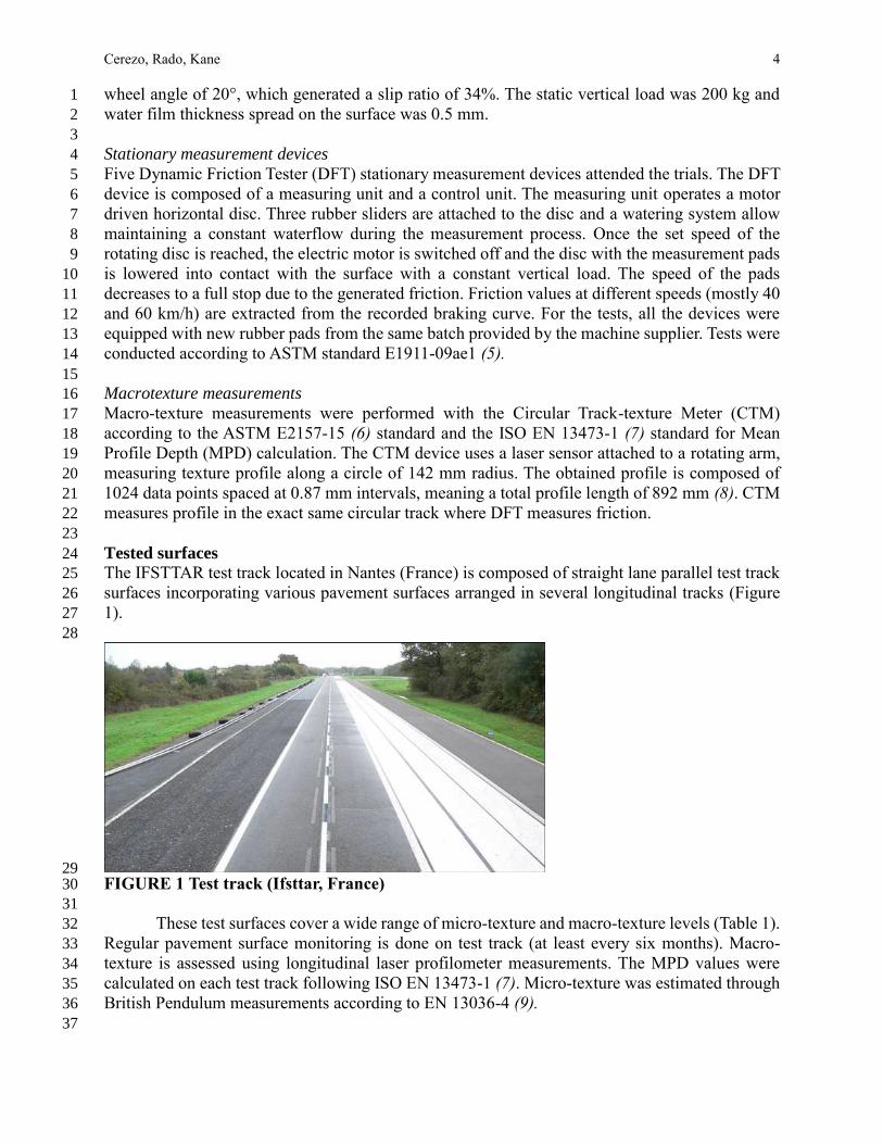
Tested surfaces 24

The IFSTTAR test track located in Nantes (France) is composed of straight lane parallel test track 25

surfaces incorporating various pavement surfaces arranged in several longitudinal tracks (Figure 26

1). 27

28

29 FIGURE 1 Test track (Ifsttar, France) 30

31

These test surfaces cover a wide range of micro-texture and macro-texture levels (Table 1). 32

Regular pavement surface monitoring is done on test track (at least every six months). Macro-33

texture is assessed using longitudinal laser profilometer measurements. The MPD values were 34

calculated on each test track following ISO EN 13473-1 (7). Micro-texture was estimated through 35

British Pendulum measurements according to EN 13036-4 (9). 36

37


TABLE 1 Pavement surfaces characteristics on test tracks 1

2

Surface Pavement mix Grains

size

MPD

(mm) DFT20

A Porous asphalt concrete 0/6 2.90 0.29 C1 Asphalt concrete 0/10 0.35 0.61

E1 Semi – coarse asphalt

concrete 0/10 0.66 0.34

E3 Stone Mastic Asphalt 0/10 1.19 0.40 L2 Sand asphalt 0/4 0.50 0.38 M2 Very thin asphalt concrete 0/6 1.10 0.30 G0 Asphalt concrete - 0.83 0.34

G1 Painted surface (low

microtexture) - 0.60 0.25

G2 Painted surface with glass

balls - 0.59 0.26

G22 Painted surface with glass

balls - 0.67 0.35

3

Test program 4

5

Tests were performed during one week and were divided into two phases (10). In the first phase, a 6

calibration exercise was conducted to ensure that devices are working properly. In a second phase, 7

the round robin tests were performed by all the participating devices. Each device provided five 8

valid measurements on ten different pavement surfaces at three speeds (40, 60 and 80 km/h). A 9

measurement was considered as valid when it was realized in the 0.50 m centre strip of the test 10

lane. An orange mark at the beginning of each test track indicated the valid measurement strip. 11

Within each test track white points every 20m indicated the valid measurement strip. In parallel, 12

continuous macrotexture measurements were performed with laser profilometers in order to 13

provide MPD (Mean Profile Depth) values on the same test tracks according to ISO EN 13473-1. 14

15

16

17

FIGURE 2 Marks on the test sections 18

19

Then, static friction measurements were performed with Dynamic Friction Tester on the 20

same test tracks. For each test surface, measurement points were defined every twenty meters. For 21

each location, two measurements were obtained and average values were calculated to characterize 22


each test section. Three test speeds were used for the analysis: 20, 40 and 60 km/h. Static 1

macrotexture values with CTM were also collected on the same locations as the DFT 2

measurements. 3

4

Thus, a database containing 2250 average friction values for high-speed devices, 1230 DFT 5

values and 41 macro-texture values obtained with CTM was built for the analysis. 6

7

CALIBRATION EXERCICE 8

Checking process was conducted only on dynamic friction measuring devices. The DFT devices 9

were directly calibrated by the manufacturer at the beginning of the friction workshop to ensure 10

they were working properly. 11

12

Checking process of dynamic devices focused on those main parameters, that can have an 13

influence on friction measurements: 14

Tire (pressure, cleanness, wear, Shore hardness), 15

Measuring system (static vertical load, wheel angle), 16

Speed, 17

Water flow (nominal magnitude, film thickness distribution under the tire). 18

Participants were also requested to have a calibration certificate of the force sensor and to 19

use a new or honed tire, without visible defects. 20

21

Tires checking 22

Five different tires were used during the trials depending on the device: ASTM 1551, Piarc smooth, 23

Trelleborg T49, Avon and SKM. Checking were based on European, American, national 24

specifications or existing standards. 25

26

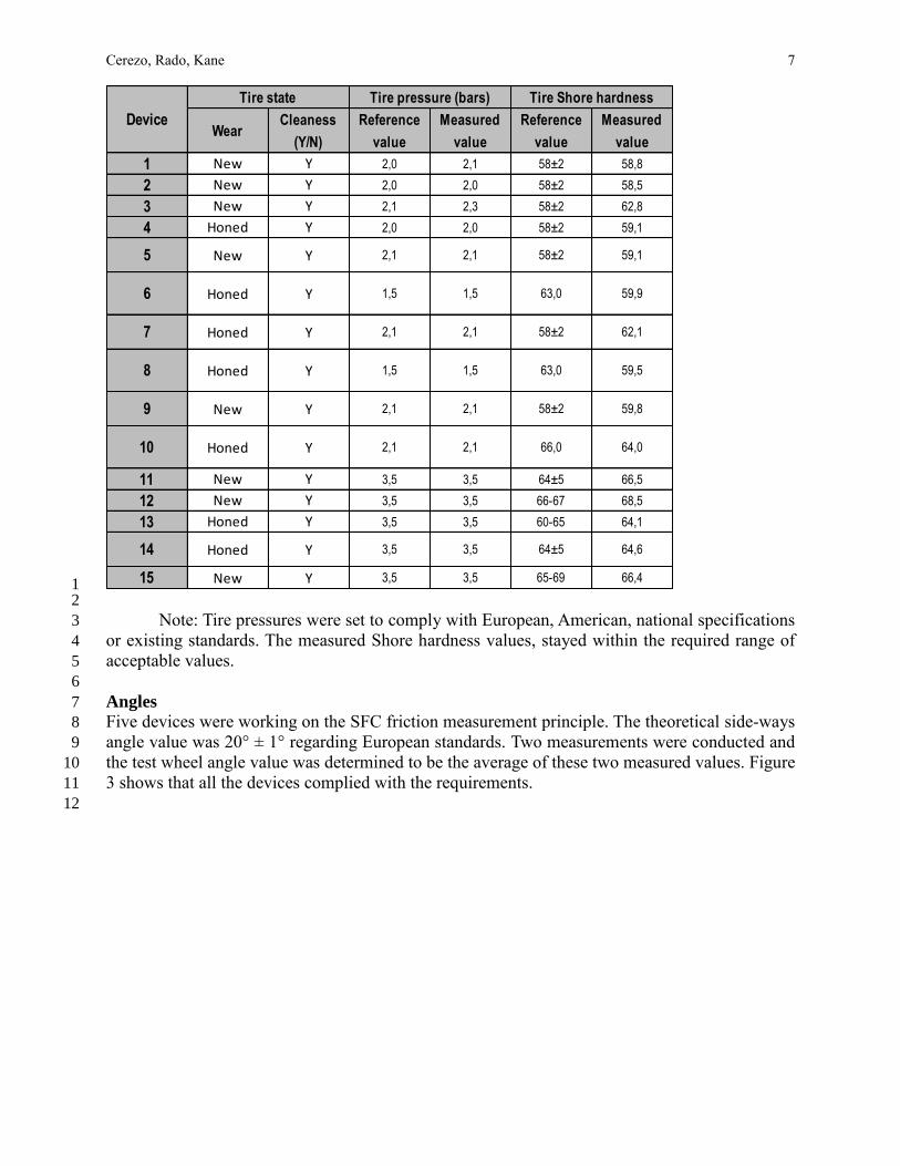
TABLE 2 Checking results for the tires 27

28


1 2

Note: Tire pressures were set to comply with European, American, national specifications 3

or existing standards. The measured Shore hardness values, stayed within the required range of 4

acceptable values. 5

6

Angles 7

Five devices were working on the SFC friction measurement principle. The theoretical side-ways 8

angle value was 20° ± 1° regarding European standards. Two measurements were conducted and 9

the test wheel angle value was determined to be the average of these two measured values. Figure 10

3 shows that all the devices complied with the requirements. 11

12

WearCleaness

(Y/N)

Reference

value

Measured

value

Reference

value

Measured

value

1 New Y 2,0 2,1 58±2 58,8

2 New Y 2,0 2,0 58±2 58,5

3 New Y 2,1 2,3 58±2 62,8

4 Honed Y 2,0 2,0 58±2 59,1

5 New Y 2,1 2,1 58±2 59,1

6 Honed Y 1,5 1,5 63,0 59,9

7 Honed Y 2,1 2,1 58±2 62,1

8 Honed Y 1,5 1,5 63,0 59,5

9 New Y 2,1 2,1 58±2 59,8

10 Honed Y 2,1 2,1 66,0 64,0

11 New Y 3,5 3,5 64±5 66,5

12 New Y 3,5 3,5 66-67 68,5

13 Honed Y 3,5 3,5 60-65 64,1

14 Honed Y 3,5 3,5 64±5 64,6

15 New Y 3,5 3,5 65-69 66,4

Tire pressure (bars) Tire Shore hardnessTire state

Device


1 FIGURE 3 Measured wheel angle 2

3

Speed 4

The measurement speed of each device was checked by a calibrated radar. The radar was set up on 5

the side of the test track. Devices drove at constant speed on straight line along the test track and 6

the radar recorded value was compared to the on-board speed measured on the friction devices. 7

The speeds 40, 60 and 80 km/h were tested. The results shall be within ± 5% of the reference speed. 8

Figure 4 presents the results obtained for the fifteen vehicles. Only, one value at 60 km/h was 9

outside the resquested range. Further analysis showed that this lower speed value can be explained 10

by a small braking manoeuver during the checking process. 11

12

13 FIGURE 4 Measured speeds 14

15

16

17,5

18

18,5

19

19,5

20

20,5

21

21,5

22

Angle 1 Angle 2 Angle 3 Angle 4 Angle 5

An

gle

(°)

0

10

20

30

40

50

60

70

80

90

100

0 10 20 30 40 50 60 70 80 90 100

Spee

d (

km/h

)

Sref (km/h)

Sref +5%

Sref - 5%


Vertical load 1

The static vertical load was checked by using a calibrated weigh pad, readable and accurate to 0.5 2

kg. The test vehicle was positioned on a level surface such that the test wheel could be lowered, 3

when required, on to the weigh pad. The weigh pad was constructed to ensure that a device’s 4

measurement wheel when lowered to the weigh padpositioned at it’s normal measurement place. 5

During the calibration the measured and reference load values were used to ensure compliance to 6

the standards EN TS 15901-1 to 15 (11) (12) (13) (14) or existing national procedures. Two 7

measurements were performed and the static load was determined to be the average of the two 8

measured values. Table 3 shows that static load values complied with European, American or 9

national specifications or existing standards. 10

11

TABLE 3 Checking results for the vertical load 12

13

14 15

16

Water film thickness 17

Water film thickness was checked using a special aluminium tray composed of small channels. 18

The platform was embedded in the pavement such that the top of the platform was level with the 19

pavement surface. The vehicles drove over the platform at 40, 60 and 80 km/h in normal 20

measurement mode. The amount of water spread in the channels of the platform was measured 21

using digital high-resolution pictures taken after the vehicles have passed. A special purpose 22

software allowed a semi-automatic analysis of each photo. Two criteria were analysed: a) the 23

homogeneity and width of the water distribution in the tubes; b) the average nominal water film 24

thickness under the tire. 25

26

27

DeviceReference

value (kg)

Measured

value (kg)

Difference

(%)

1 148,0 146,5 1%

2 135,0 128,3 5%

3 135,0 128,8 5%

4 100,0 96,8 3%

5 90,0 87,8 3%

6120

[110-130]123,0 -3%

7 180,0 178,5 1%

8 120,0 133,8 -11%

9 185,0 183,5 1%

10 106,8 107,5 -1%

11 200,0 - -

12 200,0 199,0 1%

13 200,0 209,3 -5%

14 200,0 200,0 0%

15 200,0 201,0 -1%


FIGURE 5 Grid (a) and method used to analyze pictures (b) 1

2

Table 4 presents the results of the water film thickness checking. The total width of water 3

dispersal under the tire was generally sufficient, but when only the width of the homogeneous area 4

was considereded results were different. In half of the cases, the water-film thickness under the 5

tire was not uniform and not provided the required niminal water depth. 6

Even though the average water-film thickness for most of the devices was close to the 7

required, under the tire in the homogeneous area for the majority of devices, it was significantly 8

smaller. This fact can be explained by the calibration process employed for numerous devices, 9

which is based on the weighing the amount of water delivered during a given time. 10

Only the average water-film thickness measurement was considered to accept devices 11

(distribution and below tire water-film thicknesses were not included), due to the fact that 12

standards and specifications generally consider an average water-film thickness value in their 13

requirements. All the devices were compliant with these specifications. 14

Three devices (2 side-forces devices and 1 longitudinal friction device) were not able to 15

perform this check due to the shape of their water delivery system. However, these devices 16

contained electronic closed-loop controlled water delivery systems to ensure a regular and correct 17

water flow. 18

Homogeneous area

Total area for calculus


TABLE 4 Checking results for the water film thickness 1

2

Average

water film

thickness

(mm)

Standard

deviation

(mm)

Number of

tubes filled in

Average

water film

thickness

(mm)

Stabdard

deviation

(mm)

Number of

tubes filled in

40 61 5 1,0 1,04 0,23 5 1,16 0,10 4 N Y 16% 4%

60 61 5 1,0 0,95 0,34 6 1,20 0,06 4 N Y 20% -5%

80 61 5 1,0 1,04 0,33 6 1,29 0,08 4 N Y 29% 4%

40 61 5 1,0 1,11 0,55 6 1,45 0,34 4 N Y 45% 11%

60 61 5 1,0 1,14 0,31 6 1,27 0,24 5 Y Y 27% 14%

80 61 5 1,0 1,28 0,47 8 1,65 0,10 5 Y Y 65% 28%

40 61 5 0,5 0,42 0,21 5 0,50 0,03 2 N Y -1% -16%

60 61 5 0,5 0,36 0,11 4 0,43 0,05 3 N N -14% -28%

80 61 5 0,5 0,26 0,10 4 0,24 0,02 2 N N -53% -48%

40 61 5 1,0 0,37 0,13 6 0,46 0,08 4 N Y -54% -64%

60 61 5 1,0 0,28 0,09 8 0,36 0,07 5 Y Y -64% -72%

80 61 5 1,0 0,35 0,13 8 0,45 0,12 5 Y Y -55% -65%

40 61 5 1,0 0,97 0,06 5 0,97 0,06 5 Y Y -3% -3%

60 61 5 1,0 0,90 0,25 6 1,05 0,08 5 Y Y 5% -10%

80 61 5 1,0 0,59 0,12 6 0,67 0,04 5 Y Y -33% -41%

40 100 8 1,0 1,01 0,38 8 1,26 0,10 6 N Y 26% 1%

60 100 8 1,0 0,97 0,34 8 1,19 0,11 6 N Y 19% -3%

80 100 8 1,0 1,01 0,21 7 1,15 0,06 5 N N 15% 1%

40 61 5 1,0 0,83 0,58 7 1,51 0,05 3 N Y 51% -17%

60 61 5 1,0 0,64 0,32 7 1,01 0,11 3 N Y 1% -36%

80 61 5 1,0 0,68 0,35 7 0,80 0,09 3 N Y -20% -32%

40 100 8 1,0 0,94 0,53 10 1,38 0,10 6 N Y 38% -7%

60 100 8 1,0 0,77 0,35 9 1,08 0,05 5 N Y 8% -23%

80 100 8 1,0 0,74 0,37 9 1,07 0,07 5 N Y 7% -26%

40 61 5 0,5 0,57 0,30 8 0,87 0,11 6 Y Y 73% 14%

60 61 5 0,5 0,33 0,15 6 0,53 0,18 2 N Y 5% -34%

80 61 5 0,5 0,26 0,13 8 0,39 0,06 4 N Y -22% -48%

40 76 6 0,5 0,25 0,15 9 0,57 0,07 2 N Y 13% -50%

60 76 6 0,5 0,33 0,22 10 0,56 0,11 5 N Y 11% -33%

80 76 6 0,5 0,29 0,16 9 0,53 0,04 3 N Y 7% -42%

40 76 6 0,5 0,42 0,33 10 0,83 0,27 4 N Y 67% -17%

60 76 6 0,5 0,39 0,21 15 0,62 0,16 7 Y Y 23% -23%

80 76 6 0,5 0,28 0,18 15 0,51 0,19 6 Y Y 1% -45%

40 76 6 0,5 0,38 0,22 6 0,60 0,15 3 N Y 20% -24%

60 76 6 0,5 0,30 0,17 8 0,48 0,11 4 N Y -5% -40%

80 76 6 0,5 0,36 0,21 7 0,55 0,14 4 N Y 10% -27%

All tubesHomogeneous

wetting width

sufficient (Y/N)

Speed

(km/h)

1

2

4

5

6

13

15

Tire Width

(mm)

Theoretical

number of

tubes under

the tire

Theoretical

water film

thickness

(mm)

Homogeneous area Wetting

width

sufficient

(Y/N)

DWD (%)

(homogeneous

area)

DWD (%)

(total)

11

Device

7

8

9

10


METHODOLOGY FOR ROUND ROBIN TESTS ANALYSIS 1

Two different harmonization methodologies were examined using the friction workshop’s database. 2

The first one was based on the Skid Resistance Index (CEN/TS 13036-2) (15) which was improved 3

during FP7 EU ROSANNE project funded between 2013 and 2016 (16) (17) (18). The second one 4

according to the methodology developed in the US used a two-step method utilizing a laboratory 5

scale reference surface and a pair of unique laboratory and field useable devices (DFT and CTM) 6

to establish time stable check standards for friction harmonization (19). 7

8

Common scale principle (SRI) 9

The concept is to transform measured friction values provided by an individual device under its 10

particular test conditions (speed, load, tire) to equivalent friction values under reference conditions. 11

This transformation is based on the following formula defining the SRI (Skid Resistance Index): 12

13

𝑆𝑅𝐼 = 𝐵 ∙ 𝐹 ∙ 𝑒𝑆−𝑆𝑅𝑒𝑓

𝑆0 14

(1) 15

16

𝑆0 = 𝑎 ∙ 𝑀𝑃𝐷𝑏 (2) 17

18

Where SRI is the skid resistance value reported against the common scale 19

a, b, and B are device-specific calibration parameters to be determined 20

F is the measured skid resistance value 21

S is the vehicle operating speed (in km/h) 22

SRef is the reference speed at which SRI values are reported (in km/h) 23

S0 represents speed gradient of skid resistance values related to the surface texture 24

MPD is the Mean Profile Depth (in mm) 25

26

To determine the device-specific calibration factors (a, b and B), the value of the common 27

scale for each test surface must be fixed. Based on former research work, the reference value is set 28

to be the average value of friction coefficients measured on a given surface by a group of devices 29

operating on the same measuring principle (i.e. 10 devices for longitudinal friction and 5 devices 30

for sideways-force friction). Data scattering for each group on each surface was checked with 31

statistical tests to detect outliers, outliers were excluded from the calculation of the reference 32

values (20) (21). When the reference value is defined, parameters a, b and B are adjusted with least 33

squares method. 34

35

Check-standard IFI “two-steps approach” 36

The process embodies the use of a pair of macro-texture and friction measurement equipment that 37

can be used both in the laboratory and on field and have good reproducibility and high precision. 38

It also uses a set of small highly reproducible manufactured standard surfaces for dynamic 39

laboratory calibration. Thus, the calibration and harmonization of any high-speed continuous 40

friction measurement equipment or locked wheel tester can be accomplished. 41

42

The implementation of check-standard IFI method requires the following steps: 43

Calibration of DFT and CTM according to manufacturer’s specifications: static 44

calibration of each individual part of the devices and dynamical tests on two 45


laboratory reference surfaces manufactured from special aluminium alloy and highly 1

wear resistant ceramic (Figure 6). 2

Use the calibrated DFT and CTM devices on the test sections to establish the “check 3

standard” friction and macro-texture values for each of the test surfaces. 4

The F60 and Sp values of each surface were thus calculated using: 5

𝐹60 = 0.081 + .732 ∗ 𝐷𝐹𝑇20 ∗ 𝑒(20−60)

𝑆𝑝 (3) 6

7

𝑆𝑝 = 14.2 + 89.7 ∗ 𝑀𝑃𝐷 (4) 8

9

Where DFT20 is the skid resistance measured at 20 km/h with DFT 10

MPD is the Mean Profile Depth (in mm) 11

12

13

FIGURE 6 Small-scale laboratory standard friction surfaces 14

15

16

RESULTS 17

Application of common scale (SRI) 18

The database was split into two sub-bases, one for longitudinal friction devices and the other for 19

transversal friction devices. Each sub-database was analyzed by using 60 km/h as a reference speed. 20

The set of parameters (a, b, B) was calculated for each operating device. 21

22

Figures 7 and 8 present examples of results for both types of devices with raw data and 23

calibrated data when the SRI approach is used. The SRI approach effectively reduces the 24

distribution range of friction values. The same trend was observed for all the speeds and both 25

groups of devices. 26

27


1

2 FIGURE 7 Raw data measured at 60 km/h and SRI correction (Ref. speed = 60 km/h) for 3

longitudinal friction measuring devices (22) 4

5

6

0,00

0,10

0,20

0,30

0,40

0,50

0,60

0,70

0,80

0,90

1,00

1,10

1,20

Porous Asphalt Asphalt concrete

0/10

New Semi-coarse

Asphalt Concrete

Stone Mastic

Asphalt

Asphalt Concrete Painted Asphalt

Concrete (no

inclusion)

Painted Asphalt

Concrete (low-

volume glass

beads)

Painted Asphalt

Concrete (lhigh-

volume glass

beads)

Sand Asphalt

Concrete

Very Thin Asphalt

Concrete

Ori

gin

al d

ata

-6

0km

/h

0,00

0,10

0,20

0,30

0,40

0,50

0,60

0,70

0,80

0,90

1,00

1,10

1,20


0/10

New Semi-coarse

Asphalt Concrete

Stone Mastic

Asphalt


Concrete (no

inclusion)

Painted Asphalt

Concrete (low-

volume glass

beads)

Painted Asphalt

Concrete (lhigh-

volume glass

beads)

Sand Asphalt

Concrete

Very Thin Asphalt

Concrete

Full

SR

I co

rre

ctio

n (u

sin

g 6

0km

/h a

s re

fere

nce

ve

hic

le s

pe

ed

) -6

0km

/h

0,00

0,10

0,20

0,30

0,40

0,50

0,60

0,70

0,80

0,90

1,00

1,10

1,20


0/10

New Semi-coarse

Asphalt Concrete

Stone Mastic

Asphalt


Concrete (no

inclusion)

Painted Asphalt

Concrete (low-

volume glass

beads)

Painted Asphalt

Concrete (lhigh-

volume glass

beads)

Sand Asphalt

Concrete

Very Thin Asphalt

Concrete

Ori

gin

al d

ata

-4

0km

/h


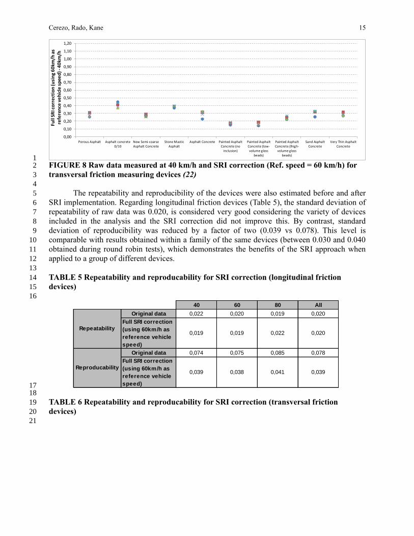
1 FIGURE 8 Raw data measured at 40 km/h and SRI correction (Ref. speed = 60 km/h) for 2

transversal friction measuring devices (22) 3

4

The repeatability and reproducibility of the devices were also estimated before and after 5

SRI implementation. Regarding longitudinal friction devices (Table 5), the standard deviation of 6

repeatability of raw data was 0.020, is considered very good considering the variety of devices 7

included in the analysis and the SRI correction did not improve this. By contrast, standard 8

deviation of reproducibility was reduced by a factor of two (0.039 vs 0.078). This level is 9

comparable with results obtained within a family of the same devices (between 0.030 and 0.040 10

obtained during round robin tests), which demonstrates the benefits of the SRI approach when 11

applied to a group of different devices. 12

13

TABLE 5 Repeatability and reproducability for SRI correction (longitudinal friction 14

devices) 15

16

17 18

TABLE 6 Repeatability and reproducability for SRI correction (transversal friction 19

devices) 20

21

0,00

0,10

0,20

0,30

0,40

0,50

0,60

0,70

0,80

0,90

1,00

1,10

1,20


0/10

New Semi-coarse

Asphalt Concrete

Stone Mastic

Asphalt


Concrete (no

inclusion)

Painted Asphalt

Concrete (low-

volume glass

beads)

Painted Asphalt

Concrete (lhigh-

volume glass

beads)

Sand Asphalt

Concrete

Very Thin Asphalt

Concrete

Full

SR

I co

rre

ctio

n (u

sin

g 6

0km

/h a

s re

fere

nce

ve

hic

le s

pee

d) -

40

km/h

40 60 80 All

Original data 0,022 0,020 0,019 0,020

Full SRI correction

(using 60km/h as

reference vehicle

speed)

0,019 0,019 0,022 0,020

Original data 0,074 0,075 0,085 0,078

Full SRI correction

(using 60km/h as

reference vehicle

speed)

0,039 0,038 0,041 0,039

Repeatability

Reproducability


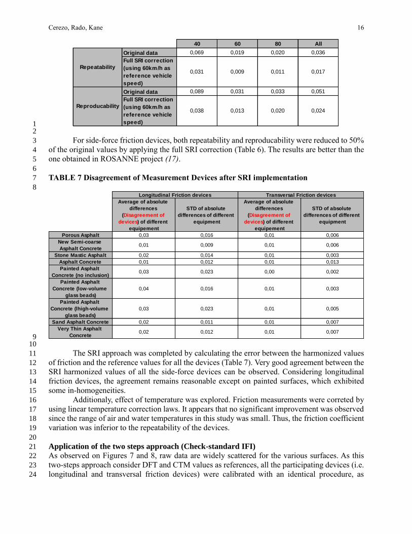
1 2

For side-force friction devices, both repeatability and reproducability were reduced to 50% 3

of the original values by applying the full SRI correction (Table 6). The results are better than the 4

one obtained in ROSANNE project (17). 5

6

TABLE 7 Disagreement of Measurement Devices after SRI implementation 7

8

9 10

The SRI approach was completed by calculating the error between the harmonized values 11

of friction and the reference values for all the devices (Table 7). Very good agreement between the 12

SRI harmonized values of all the side-force devices can be observed. Considering longitudinal 13

friction devices, the agreement remains reasonable except on painted surfaces, which exhibited 14

some in-homogeneities. 15

Additionaly, effect of temperature was explored. Friction measurements were correted by 16

using linear temperature correction laws. It appears that no significant improvement was observed 17

since the range of air and water temperatures in this study was small. Thus, the friction coefficient 18

variation was inferior to the repeatability of the devices. 19

20

Application of the two steps approach (Check-standard IFI) 21

As observed on Figures 7 and 8, raw data are widely scattered for the various surfaces. As this 22

two-steps approach consider DFT and CTM values as references, all the participating devices (i.e. 23

longitudinal and transversal friction devices) were calibrated with an identical procedure, as 24

40 60 80 All

Original data 0,069 0,019 0,020 0,036

Full SRI correction

(using 60km/h as

reference vehicle

speed)

0,031 0,009 0,011 0,017

Original data 0,089 0,031 0,033 0,051

Full SRI correction

(using 60km/h as

reference vehicle

speed)

0,038 0,013 0,020 0,024

Repeatability

Reproducability

Average of absolute

differences

(Disagreement of

devices) of different

equipement

STD of absolute

differences of different

equipment

Average of absolute

differences

(Disagreement of

devices) of different

equipement

STD of absolute


equipment

Porous Asphalt 0,03 0,016 0,01 0,006

New Semi-coarse

Asphalt Concrete0,01 0,009 0,01 0,006

Stone Mastic Asphalt 0,02 0,014 0,01 0,003

Asphalt Concrete 0,01 0,012 0,01 0,013

Painted Asphalt

Concrete (no inclusion)0,03 0,023 0,00 0,002

Painted Asphalt

Concrete (low-volume

glass beads)

0,04 0,016 0,01 0,003

Painted Asphalt

Concrete (lhigh-volume

glass beads)

0,03 0,023 0,01 0,005

Sand Asphalt Concrete 0,02 0,011 0,01 0,007

Very Thin Asphalt

Concrete0,02 0,012 0,01 0,007

Longitudinal Friction devices Transversal Friction devices


described in the section “Methodology”. Figure 9 presents results obtained for all the devices after 1

harmonization process. The data scatter among different measurement equipment was reduced and 2

the agreement between the different devices and the established check standard had been moved 3

to a very good agreement with the line of equality. 4

5

6 FIGURE 9 Harmonized Friction Measurement of All Devices by IFI approach 7

8

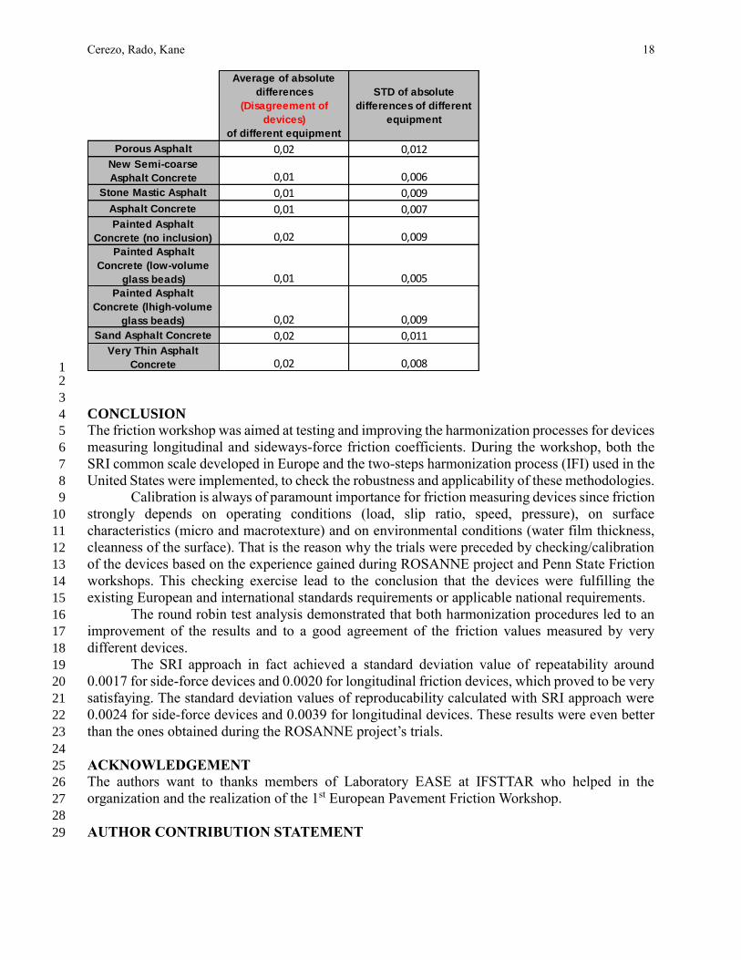
This approach was completed by calculating the error between the harmonized values of 9

friction and the reference for all the devices (Table 8). Good agreement between harmonized 10

friction values on the various test sections is observed. Moreover, the results are comparable to the 11

ones obtained with the “common scale (SRI)” approach. 12

13

TABLE 8 Disagreement of Measurement Devices after IFI implementation 14

15

0,00

0,05

0,10

0,15

0,20

0,25

0,30

0,35

0,40

0,45

0,50

0,00 0,10 0,20 0,30 0,40 0,50

Pre

dic

ted

IFI

Established IFI


1 2

3

CONCLUSION 4

The friction workshop was aimed at testing and improving the harmonization processes for devices 5

measuring longitudinal and sideways-force friction coefficients. During the workshop, both the 6

SRI common scale developed in Europe and the two-steps harmonization process (IFI) used in the 7

United States were implemented, to check the robustness and applicability of these methodologies. 8

Calibration is always of paramount importance for friction measuring devices since friction 9

strongly depends on operating conditions (load, slip ratio, speed, pressure), on surface 10

characteristics (micro and macrotexture) and on environmental conditions (water film thickness, 11

cleanness of the surface). That is the reason why the trials were preceded by checking/calibration 12

of the devices based on the experience gained during ROSANNE project and Penn State Friction 13

workshops. This checking exercise lead to the conclusion that the devices were fulfilling the 14

existing European and international standards requirements or applicable national requirements. 15

The round robin test analysis demonstrated that both harmonization procedures led to an 16

improvement of the results and to a good agreement of the friction values measured by very 17

different devices. 18

The SRI approach in fact achieved a standard deviation value of repeatability around 19

0.0017 for side-force devices and 0.0020 for longitudinal friction devices, which proved to be very 20

satisfaying. The standard deviation values of reproducability calculated with SRI approach were 21

0.0024 for side-force devices and 0.0039 for longitudinal devices. These results were even better 22

than the ones obtained during the ROSANNE project’s trials. 23

24

ACKNOWLEDGEMENT 25

The authors want to thanks members of Laboratory EASE at IFSTTAR who helped in the 26

organization and the realization of the 1st European Pavement Friction Workshop. 27

28

AUTHOR CONTRIBUTION STATEMENT 29

Average of absolute

differences

(Disagreement of

devices)

of different equipment

STD of absolute


equipment

Porous Asphalt 0,02 0,012New Semi-coarse

Asphalt Concrete 0,01 0,006

Stone Mastic Asphalt 0,01 0,009

Asphalt Concrete 0,01 0,007Painted Asphalt

Concrete (no inclusion) 0,02 0,009Painted Asphalt

Concrete (low-volume

glass beads) 0,01 0,005Painted Asphalt

Concrete (lhigh-volume

glass beads) 0,02 0,009

Sand Asphalt Concrete 0,02 0,011Very Thin Asphalt

Concrete 0,02 0,008


The authors confirm contribution to the paper as follows: study conception and design: V. Cerezo, 1

Z. Rado, M. Kane; data collection: V. Cerezo, Z. Rado; analysis and interpretation of results: V. 2

Cerezo, Z. Rado; draft manuscript preparation: V. Cerezo, Z. Rado, M. Kane. All authors reviewed 3

the results and approved the final version of the manuscript. 4

5

REFERENCES 6

1. Wambold, J. C., C. E. Antle, J. J. Henry, and Z. Rado. (1995) International PIARC 7

Experiment to Compare and Harmonize Texture and Skid Resistance 8

Measurements. Final report submitted to the Permanent International Association 9

of Road Congresses (PIARC), State College, Pa. 10

2. PIARC (2004), Specification for a standard test tyre for friction coefficient 11

measurement of a pavement surface: SmooTh TeS TyRe, Technical Committee 1 12

Surfaces characteristics, 13 pages. 13

3. ASTM E1551-16 (2016), Standard Specification for a Size 4.00-8 Smooth Tread 14

Friction Test Tire, ASTM International, West Conshohocken, PA, 2016, 15

www.astm.org. 16

4. ASTM E1844-96 (1996), Standard Specification for A Size 10 x 4-5 Smooth-Tread 17

Friction Test Tire, ASTM International, West Conshohocken, PA, 1996, 18

www.astm.org. 19

5. ASTM E1911-09ae1 (2009), Standard Test Method for Measuring Paved Surface 20

Frictional Properties Using the Dynamic Friction Tester, ASTM International, West 21

Conshohocken, PA, 2009, www.astm.org. 22

6. ASTM E2157-15 (2015), Standard Test Method for Measuring Pavement Macro-23

texture Properties Using the Circular Track Meter, ASTM International, West 24

Conshohocken, PA, 2015, www.astm.org. 25

7. ISO 13473-1 (2005), Characterisation of pavement texture by use of surface profiles 26

-–Part 1: Determination of Mean Profile Depth, January. 27

8. Hanson D. and B. Prowel, B (2004), Evaluation of Circular Track Meter for 28

measuring surface texture of Pavements, NCAT Report 04-05, 26 pages, 29

September. 30

9. CEN (2011), DD CEN/TS 13036-4: Road and airfield surface characteristics – test 31

methods. Part 4: Method for measurement of slip/skid resistance of a surface: The 32

pendulum test. 33

10. Cerezo V. and Dauvergne, S. (2017), 1st European Pavement Friction Workshop - 34

experimental program, 1st European Pavement Friction Workshop, 31 pages, May. 35

11. CEN (2009), CEN TS 15901-4: Road and airfield surface characteristics — Part 4: 36

Procedure for determining the skid resistance of a pavement surface using a device 37

with longitudinal controlled slip (LFCT): Tatra Runway Tester (TRT). 38

12. CEN (2009), CEN/TS 15901-6: Road and airfield surface characteristics — Part 6: 39

Procedure for determining the skid resistance of a pavement surface by 40

measurement of the sideway force coefficient (SFCS): SCRIM ®. 41

13. CEN (2009), CEN/TS 15901-8: Road and airfield surface characteristics — Part 8: 42

Procedure for determining the skid resistance of a pavement surface by 43

measurement of the sideway force coefficient (SFCD): SKM. 44

14. CEN (2013), CEN/TS 15901-15: Road and airfield surface characteristics — Part 45

15: Procedure for determining the skid resistance of a pavement surface using a 46

device with longitudinal controlled slip (LFCI): The IMAG. 47


15. CEN (2010), DD CEN/TS 13036-2: Road and airfield surface characteristics – test 1

methods. Part 2: Assessment of the skid resistance of a road pavement surface by 2

the use of dynamic measuring systems. 3

16. Greene M J, Viner H, Cerezo v, Kokot D and Schmidt B (2014), Deliverable D1.1: 4

Definition of boundaries and requirements for the common scale for harmonisation 5

of skid resistance measurements, Collaborative Project FP7- ROlling resistance, 6

Skid resistance, ANd Noise Emission measurement standards for road surfaces 7

(ROSANNE), 79 pages, May. 8

17. Greene M., Viner H., Cerezo V., Brittain S. (2016), Deliverable 1.3: Analysis of 9

data from the second round of tests and further development of the common scale, 10

Collaborative Project FP7- ROlling resistance, Skid resistance, ANd Noise 11

Emission measurement standards for road surfaces (ROSANNE), 89 pages, 12

November. 13

18. Greene, M. Viner, H. Cerezo, V. Schmidt, B. Scharnigg, K. (2015), Deliverable 14

D1.2: Analysis of data from the first round of tests and initial development of the 15

common scale, Collaborative Project FP7- ROlling resistance, Skid resistance, ANd 16

Noise Emission measurement standards for road surfaces (ROSANNE), 63 pages, 17

May. 18

19. ASTM E1960-07 (2015), Standard Practice for Calculating International Friction 19

Index of a Pavement Surface, ASTM International, West Conshohocken, PA, 2015, 20

www.astm.org. 21

20. ISO 5725-1 (1994), Application of statistics: accuracy (trueness and precision) of 22

measurements methods and results – part 1: General principles and definition, 23

December. 24

21. ISO 5725-5 (1998), Application of statistics: accuracy (trueness and precision) of 25

measurements methods and results – part 5: Alternative methods for the 26

determination of the precision of a standard measurement method, October. 27

22. Cerezo V. and Rado, Z. (2017), 1st European Pavement Friction Workshop – round 28

robin tests analysis, 1st European Pavement Friction Workshop, 59 pages, 29

December. 30

31

Encouraging Results of International Friction Measurement ...

Documents

Transcript of Encouraging Results of International Friction Measurement ...