Continuous Friction Measurement Equipment (CFME) for ... - ShareOK

Oklahoma Department of Transportation 200 NE 21st Street, Oklahoma City, OK 73105 -3204

FINAL REPORT ~ FHWA-OK-20-02

CONTINUOUS FRICTION MEASUREMENT EQUIPMENT (CFME) FOR HIGHWAY SAFETY MANAGEMENT IN OKLAHOMA Joshua Q. Li, Ph.D., P.E. Kelvin C. P. Wang, Ph.D., P.E Wenying Yu Wenyao Liu School of Civil and Environmental Engineering College of Engineering, Architecture and Technology Oklahoma State University Stillwater, Oklahoma

January 2020

[email protected] Transportation Excellence through Research and Implementation

Office of Research & Implementation

i

The Oklahoma Department of Transportation (ODOT) ensures that no person or groups of persons shall, on the grounds of race, color, sex, religion, national origin, age, disability, retaliation or genetic information, be excluded from participation in, be denied the benefits of, or be otherwise subjected to discrimination under any and all programs, services, or activities administered by ODOT, its recipients, sub-recipients, and contractors. To request an accommodation please contact the ADA Coordinator at 405-521-4140 or the Oklahoma Relay Service at 1-800-722-0353. If you have any ADA or Title VI questions email [email protected].

mailto:[email protected]

ii

The contents of this report reflect the views of the author(s) who is responsible for the facts and the accuracy of the data presented herein. The contents do not necessarily reflect the views of the Oklahoma Department of Transportation or the Federal Highway Administration. This report does not constitute a standard, specification, or regulation. While trade names may be used in this report, it is not intended as an endorsement of any machine, contractor, process, or product.

iii

CONTINUOUS FRICTION MEASUREMENT

EQUIPMENT (CFME) FOR HIGHWAY SAFETY MANAGEMENT IN OKLAHOMA

FINAL REPORT ~ FHWA-OK-20-02 ODOT SP&R ITEM NUMBER 2306

Submitted to: Office of Research and Implementation

Oklahoma Department of Transportation

Submitted by: Joshua Q. Li, Ph.D. P.E. Kelvin Wang, Ph.D., P.E

Wenying Yu Wenyao Liu

Oklahoma State University

March 2020

iv

TECHNICAL REPORT DOCUMENTATION PAGE

Form DOT F 1700.7 (08/72)

1. REPORT NO.FHWA-OK-20-02

2. GOVERNMENTACCESSION NO.

3. RECIPIENT’S CATALOG NO.

4. TITLE AND SUBTITLEContinuous Friction Measurement Equipment (CFME) for Highway Safety Management in Oklahoma

5. REPORT DATEJan 2020 6. PERFORMING ORGANIZATION CODE

7. AUTHOR(S)Joshua Q. Li, Ph.D., P.E. and Kelvin Wang, Ph.D., P.E.

8. PERFORMING ORGANIZATIONREPORT

9. PERFORMING ORGANIZATION NAME AND ADDRESSOklahoma State University, Stillwater Oklahoma 74078

10. WORK UNIT NO.

11. CONTRACT OR GRANT NO.ODOT SPR Item Number 2306

12. SPONSORING AGENCY NAME AND ADDRESSOklahoma Department of Transportation Office of Research and Implementation 200 N.E. 21st Street, Room G18 Oklahoma City, OK 73105

13. TYPE OF REPORT AND PERIODCOVEREDFinal Report Oct 2017 – Dec 2019 14. SPONSORING AGENCY CODE

15. SUPPLEMENTARY NOTESN/A 16. ABSTRACTAn important part of the pavement friction management (PFM) process is the selection of the most appropriate friction measuring equipment. In this project, the capabilities of the Grip Tester, a type of continuous friction measurement (CFME) device, and its ability to provide information to support PFM programs were evaluated based on comprehensive field data collection. Various statistical and comparisons analyses were performed, suggesting that CFME can acquire repeatable and reproducible friction profiles. The friction measurements from the Grip Tester and the locked-wheel skid trailer were tested to be statistically correlated. In addition, several potential implementations of CFME data were discussed for PFM and highway safety applications.

17. KEY WORDSSkid Resistance, Continuous Friction Measurement Equipment (CFME), Grip Tester, Pavement Friction Management (PFM)

18. DISTRIBUTION STATEMENTNo restrictions. This publication is available from the Office of Research and Implementation, Oklahoma DOT.

19. SECURITY CLASSIF. (OF THISREPORT)Unclassified

20. SECURITY CLASSIF. (OFTHIS PAGE)Unclassified

21. NO. OFPAGES137

22. PRICE N/A

v

SI* (MODERN METRIC) CONVERSION FACTORS APPROXIMATE CONVERSIONS TO SI UNITS

SYMBOL WHEN YOU KNOW MULTIPLY BY TO FIND SYMBOL LENGTH

in inches 25.4 millimeters mm ft feet 0.305 meters m yd yards 0.914 meters m mi miles 1.61 kilometers km

AREA in2

square inches 645.2 square millimeters mm2

ft2 square feet 0.093 square meters m2

yd2 square yard 0.836 square meters m2

ac acres 0.405 hectares ha mi2 square miles 2.59 square kilometers km2

fl oz gal ft3

yd3

VOLUME fluid ounces 29.57 milliliters gallons 3.785 liters cubic feet 0.028 cubic meters cubic yards 0.765 cubic meters

NOTE: volumes greater than 1000 L shall be shown in m3

mL L m3

m3

MASS oz ounces 28.35 grams g lb pounds 0.454 kilograms kg T short tons (2000 lb) 0.907 megagrams (or "metric ton") Mg (or "t")

oF

TEMPERATURE (exact degrees) Fahrenheit 5 (F-32)/9 Celsius

or (F-32)/1.8

oC

ILLUMINATION fc foot-candles 10.76 lux lx fl foot-Lamberts 3.426 candela/m2

cd/m2

FORCE and PRESSURE or STRESS lbf poundforce 4.45 newtons N lbf/in2

poundforce per square inch 6.89 kilopascals kPa

APPROXIMATE CONVERSIONS FROM SI UNITS SYMBOL WHEN YOU KNOW MULTIPLY BY TO FIND SYMBOL

LENGTH mm millimeters 0.039 inches in m meters 3.28 feet ft m meters 1.09 yards yd km kilometers 0.621 miles mi

AREA mm2

square millimeters 0.0016 square inches in2

m2 square meters 10.764 square feet ft2

m2 square meters 1.195 square yards yd2

ha hectares 2.47 acres ac km2

square kilometers 0.386 square miles mi2

VOLUME mL milliliters 0.034 fluid ounces fl oz L liters 0.264 gallons gal m3 cubic meters 35.314 cubic feet ft3

m3 cubic meters 1.307 cubic yards yd3

MASS g grams 0.035 ounces oz kg kilograms 2.202 pounds lb Mg (or "t") megagrams (or "metric ton") 1.103 short tons (2000 lb) T

TEMPERATURE (exact degrees) oC Celsius 1.8C+32 Fahrenheit oF

ILLUMINATION lx lux 0.0929 foot-candles fc cd/m2

candela/m2 0.2919 foot-Lamberts fl

FORCE and PRESSURE or STRESS N newtons 0.225 poundforce lbf kPa kilopascals 0.145 poundforce per square inc h lbf/in2

*SI is the symbol for the International System of Units. Appropriate rounding should be made to comply with Section 4 of ASTM E380. (Revised March 2003)

vi

Table of Contents

Table of Contents ............................................................................................... vi

List of Figures ............................................................................................... ix

List of Tables ............................................................................................... xi

CHAPTER 1 INTRODUCTION ............................................................................ 1

1.1 Background ..................................................................................... 1

1.2 Project Objective ............................................................................. 4

1.3 Project Tasks .................................................................................. 4

1.4 Report Outline ................................................................................. 6

CHAPTER 2 LITERATURE REVIEW .................................................................. 8

2.1 Pavement Friction Characteristics .................................................. 8

2.2 Pavement Friction Measurement and Influencing Factors ............ 12

2.2.1 Testing Equipment .................................................................... 12

2.2.2 Influencing Factors .................................................................... 16

2.3 Pavement Friction and Highway Safety ........................................ 23

2.3.1 Safety Performance Function .................................................... 24

CHAPTER 3 FIELD TESTING SITES AND DATA COLLECTION ..................... 26

3.1 Field Testing Sites ........................................................................ 26

3.2 Field Data Collection ..................................................................... 32

vii

CHAPTER 4 EVALUATION OF GRIP TESTER MEASUREMENTS ................. 37

4.1 Descriptive Statistics of CFME Measurements ............................. 37

4.1.1 Friction by Treatment Type ....................................................... 38

4.1.2 Friction by Testing Speed .......................................................... 40

4.1.3 Friction by Water Film Thickness .............................................. 41

4.1.4 Friction on Bridge Desks ........................................................... 42

4.2 Comparison Analysis with Locked-Wheel Measurements ............ 44

4.2.1 Data Collection .......................................................................... 44

4.2.2 Data Compilation ....................................................................... 46

4.2.3 Data Comparisons ..................................................................... 49

4.2.4 Model Development .................................................................. 51

4.3 Repeatability Analysis ................................................................... 57

4.4 Operational Characteristics of Grip Tester .................................... 63

CHAPTER 5 CRASH RATE PREDICTION MODELS USING CFME DATA ...... 67

5.1 Proposed Framework .................................................................... 67

5.2 Case Study ................................................................................... 72

5.3 Summary ...................................................................................... 76

CHAPTER 6 PRILIMINARY APPLICATIONS OF CFME DATA ........................ 77

6.1 Dynamic Segmentation of CFME Data ......................................... 77

6.1.1 Introduction ............................................................................... 77

viii

6.1.2 Change Point Detection Methods .............................................. 79

6.1.3 Segmentation Results ............................................................... 81

6.1.4 Results Evaluation ..................................................................... 85

6.2 CFME Software Interface .............................................................. 88

6.2.1 Data Import and Visualization.................................................... 89

6.2.2 Profile Synchronization and Repeatability Analysis ................... 89

6.2.3 Homogeneous Segments .......................................................... 90

6.3 CFME for Pavement Friction Management (PFM) ........................ 93

6.3.1 The AASHTO Guideline ............................................................ 93

6.3.2 Use of Friction Data for PFM ..................................................... 96

CHAPTER 7 CONCLUSIONS AND RECOMMENDATIONS ........................... 105

7.1 Conclusions ................................................................................ 105

7.2 Recommendations ...................................................................... 110

REFERENCES ............................................................................................ 115

ix

List of Figures

Figure 2-1 Forces on a Rotating Wheel (Hall et al., 2009) ......................................... 9

Figure 2-2 Texture Three Zone Concept of a Wet Surface (Moore, 1966) ............... 10

Figure 2-3 Friction vs. Tire Slip (Hall et al, 2009) ..................................................... 11

Figure 2-4 Friction Variation during a Rainfall Event (Wilson, 2006) ........................ 21

Figure 3-1 Locations of Field Testing Sites on GoogleMap ..................................... 32

Figure 3-2 Data Collection Devices.......................................................................... 34

Figure 4-1 Friction vs. Treatments ........................................................................... 39

Figure 4-2 Treatment Ages of Testing Sites ............................................................ 39

Figure 4.3 AADT of Testing Sites ............................................................................. 40

Figure 4-4 Friction vs. Vehicle Speeds .................................................................... 41

Figure 4-5 Friction vs. Water Film Thickness ........................................................... 42

Figure 4-6 Friction on Bridge Decks (Northbound I-35) ........................................... 43

Figure 4-7 Friction on Bridge Decks (Southbound I-35) ........................................... 43

Figure 4-8 Grip Numbers on Google Maps .............................................................. 45

Figure 4-9 Sliding Window of the Hampel Filter ...................................................... 47

Figure 4-10 Grip Number (GN) Before and After Outlier Removal ........................... 48

Figure 4-11 Comparison of SN and GN (I-35 NB).................................................... 50

Figure 4-12 Linear Correlation Results (a) All Samples, (b) AC, (c) PC Samples .... 51

Figure 4-13 Residual and Q-Q Plots ........................................................................ 57

Figure 4-14 Grip Tester Friction Measurements ...................................................... 60

Figure 4-15 Cross-correlation Methodology ............................................................. 61

Figure 6-1 Comparisons of Results based on Different Segmentation Criterion ...... 82

x

Figure 6-2 Number of Change Points vs Penalty Value in the PELT Method .......... 84

Figure 6-3 PELT and Binary Segmentation Results: 10 vs. 28 Segments ............... 85

Figure 6-4 Frequency Distribution of Raw Friction Data .......................................... 86

Figure 6-5 Q-Q Plot of Overall Residual Check: 28 Segments. ............................... 88

Figure 6-6 CFME Data Import and Visualization ...................................................... 89

Figure 6-7 CFME Profile Repeatability Analysis ...................................................... 90

Figure 6-8 Homogeneous Section Using CDA (AASHTO, 1993) ............................. 92

Figure 6-9 CDA based CFME Homogeneous Sections ........................................... 93

Figure 6-10 Setting of Investigatory and Intervention Levels (Hall et al. 2009) ...... 102

xi

List of Tables

Table 2-1 Pavement Friction Test Equipment (Henry, 2000) ................................... 14

Table 2-2 Factors Affecting Available Pavement Friction (AASHTO 2008) .............. 16

Table 2-3 Common Mix Types and Texturing Techniques ....................................... 17

Table 3-1 Testing Sites for ODOT Project SP&R2306 ............................................. 29

Table 3-2 Bridge Decks on I-35-NB ......................................................................... 31

Table 4-1 Location Reference and Reporting Interval .............................................. 46

Table 4-2 Backward Stepwise Final Model Results: All Sections ............................ 55

Table 4-3 Backward Stepwise Final Model Results: Asphalt Sections..................... 55

Table 4-4 Backward Stepwise Final Model Results: Concrete Sections .................. 56

Table 4-5 Evaluation of Repeatability: Mean and Standard Deviations (STD) ......... 59

Table 4-6 Maximum Cross-correlation Value for Evaluation Repeatability .............. 62

Table 4-7 Multiple Regression Model ....................................................................... 65

Table 5-1 Friction Coefficient and Crash Rate (Wallman and Astrom, 2001) ........... 68

Table 5-2 Enhanced SPF Model Results for the Case Study .................................. 74

Table 6-1 Comparisons of Percentage of “Good” Segments ................................... 87

Table 6-2 Illinois SPF Peer Groups .......................................................................... 97

1

CHAPTER 1 INTRODUCTION

1.1 Background

Pavement skid resistance plays a significant role in road safety as the friction

between tire and pavement surface is a critical contributing factor in reducing

potential crashes and improve roadway safety. Therefore, it is important that

Departments of Transportation (DOTs) monitor the friction performance of their

pavement networks in a systematic manner and establish Pavement Friction

Management (PFM) programs. The Federal Highway Administration (FHWA)

Technical Advisory T 5040.38, 2010 recommends that “to provide roadway data that

will establish the relative severity of locations identified for highway safety

improvement projects, a state highway agency should implement a program to

manage pavement friction on its public roads.” The aim of this program is to

minimize friction-related vehicle crashes by ensuring that pavements provide

adequate friction properties throughout their lives. A proactive friction management

program can help identify areas that have elevated friction-related crash rates,

investigate road segments with friction deficiencies, and prioritize use of resources

to reduce friction-related vehicle crashes in a cost-effective manner (AASHTO 2008,

Flintsch 2009).

An important part of the friction management process is the selection of the

most appropriate friction measuring equipment. There are many devices used

around the world to measure friction, which can be classified into four groups:

2

locked-wheel, fixed slip, side force and variable slip. Locked-wheel (LW) skid trailers

simulate the typical vehicular response to sudden braking before the widespread

implementation of anti-lock braking systems (ABSs). The side force friction

measurement devices simulate the ability of a vehicle to maintain control during

vehicular maneuver. Fixed slip and variable slip devices are designed to measure

the friction around the critical slip of an ABS. The locked-wheel skid tester (AASHTO

T 242) is the predominant high-speed device used on U.S. roads. This device

requires a tow vehicle and a locked wheel skid trailer, equipped with either standard

smooth tires (ASTM E-524) and ribbed tires (ASTM E-521). Friction measurements

are obtained by locking the testing tire on a wetted pavement surface while traveling

at a specified speed (40mph in standard). The smooth tire is more sensitive to

pavement macro-texture, while the ribbed tire is more sensitive to micro-texture

change in the pavement.

Although this technology has been useful for several decades, the locked-

wheel device based on the 1950s technology have major limitations: (1) it

completely locks the wheel during testing, which does not accurately represent the

braking conditions experienced in modern vehicles equipped with ABS; (2) it only

provides a single average reading of friction over long distances (typically 1056 ft),

which could result in inaccurate or loss of testing at intersections, ramps, sharp

curves etc. where the friction demands are high; (3) it consumes approximately 2

gallons of water per mile and requires expensive testing tires, which hinders the

wide application of friction measurements at the network level. As a result, agencies

around the world have started using Continuous Friction Measurement Equipment

3

(CFME). CFMEs have the advantage of operating under conditions similar to

modern vehicles equipped with ABS. These devices can measure friction

continuously around the critical slip ratio of a vehicle braking with ABS at highway

speed across the entire stretch of a road. CFMEs also use less water, possibly

providing a more practical alternative for both project and network level friction

management.

The Grip Tester (GT), one type of CFME, has been used extensively in the

UK and Germany. It continuously measures the longitudinal friction along the wheel

path and operates at a fixed slip ratio at highway speeds using users defined water

film thickness. The friction measurements are recorded at an interval of 3-ft (0.9 m)

by default or another value set by the users (Findlay Irvine Ltd 2017). Because

CFME devices are developed based on the modern ABS technology, the friction

measurements from CFME may not correspond precisely with historical data

collected with locked-wheel trailers. In addition, although CFME provides information

with greater details about spatial variability of pavement friction, processing large

amount of data may be cumbersome and time consuming at this time due to the lack

of available practical software for roadway applications. Therefore, research is

needed to understand the various factors that affect the CFME measurements, to

evaluate the capabilities of CFME devices and its ability to support PFM programs in

Oklahoma.

4

1.2 Project Objective

The main objective of this study is to evaluate the capabilities of the Grip

Tester, one type of CFME device, and its ability to provide information to support

PFM programs. Specifically, the research aims to address the following sub-

objectives:

• Design an experiment using various types of pavement surfaces in

Oklahoma to investigate the effect of various operational factors on CFME

friction measurements,

• Compare CFME measurements from the Grip Tester with data from the

ODOT locked-wheel trailer,

• Investigate the repeatability of CFME measurements,

• Investigate the potential implementation of CFME Grip Tester data sets for

pavement friction management and highway safety applications in

Oklahoma.

1.3 Project Tasks

The aforementioned project objectives were achieved through the following

project tasks, each outlined in one chapter in this report:

• Literature Review. This task included a comprehensive literature review in

order to develop an in-depth understanding of various aspects related to

this project.

5

• Experimental Design. Working closely with ODOT, asphalt and concrete

testing sections with various surface characteristics (texture and materials)

were selected in Oklahoma as the testing bed for the implementation of

Grip Tester. Various operation characteristics of a Grip Tester were

integrated into the field data collection to evaluate the CFME friction

measurements.

• Field Data Collection. Several state-of-the-art instruments were used (1) to

collect pavement surface and macro-texture data at highway speed, and

(2) to measure pavement surface skid resistance using the Grip Tester

under various operational conditions.

• Evaluation of Grip Tester. Statistical testing was conducted to determine

whether the Grip Tester and locked wheel friction measurements were

significantly different. The repeatability of multiple friction measurements

from the Grip Tester was evaluated. Also the effect of various operational

factors on CFME friction measurements was investigated.

• Implementation of CFME Data. There were several potential

implementations of CFME data sets for pavement friction management

and highway safety applications. Combining the CFME and pavement

condition data sets collected from this project with the Oklahoma safety

database, updated Safety Performance Function (SPF) was developed to

improve the prediction accuracy of expected average crash frequency.

With detailed CFME data, pavement network could be better segmented

into homogenous sections for road maintenance scheduling and

6

management. Several algorithms were tested for this purpose. In addition,

in order to ease the use of CFME data, a CFME data analysis software

interface was developed, which is able to upload and visualize CFME

measurements, and perform statistical and comparison analyses for data

reporting. Finally, how CFME data and the findings from this study can be

used to assist the pavement friction management was discussed.

• Final Reporting. This task was the submission of the final report

documenting each of the tasks conducted as part of this study and the

lessons learned.

1.4 Report Outline

Accordingly, the annual report is organized as below:

• Chapter 1 provides the background and objectives of the project.

• Chapter 2 documents the comprehensive literature review of related

aspects for the project.

• Chapter 3 introduces the field experimental design, the list of field testing

sites, field data collection devices and their operation conditions.

• Chapter 4 provides the data analysis for the evaluation of Grip Tester, and

the influences of operation testing factors on friction CFME

measurements.

• Chapter 5 and Chapter 6 presents the potential implementation of CFME

for pavement friction management and highway safety analysis. The

7

features and functions of the developed data analysis software interface

are also introduced.

• Chapter 7 summarizes the key findings and future work of this project.

8

CHAPTER 2 LITERATURE REVIEW

An extensive literature review was completed to develop an in-depth

understanding of various aspects related to this project. Several important related

topics were summarized in this Chapter, including the pavement friction

measurement and surface characteristics, testing equipment, existing safety

prediction models and the relationships between friction and highway safety, and

pavement friction management.

2.1 Pavement Friction Characteristics

Pavement friction is the force resisting the relative motion between the vehicle

tire and pavement surface, and it is a critical factor influencing the crash ratios on

both wet and dry conditions for roads (Hall et al., 2009; Najafi et al., 2015). The

resistive force, illustrated in Figure 2-1, is the result of the interaction between the

tire and the pavement (Flintsch et. al, 2012). It is dominated by the texture of the

pavement surface, with different texture components making different contributions.

9

Figure 2-1 Forces on a Rotating Wheel (Hall et al., 2009)

Pavement micro- and macro-texture are the main pavement surface

characteristics that affect tire-pavement friction. Micro-texture is generally provided

by the relative roughness of the aggregate particles in asphalt pavements and by the

fine aggregate in concrete surfaces. Macro-texture is generally provided by proper

aggregate gradation in asphalt pavement and by a supplemental treatment such as

tinning, broom, diamond grinding or grooving in concrete surfaces. The reduction in

friction with increasing testing speed would be lower for the pavements with higher

macro-texture since they have more channels for the water to escape while pressed

between the tire and the pavement (Henry, 2000). Kanafi et al. (2015) monitored

variations of pavement texture and observed that macro-texture decreased and

micro-texture increased during summer time. Early rapid reduction followed by an

increase and subsequent gradual decline of macro-texture change of asphalt

concrete samples was observed in lab using close range photogrammetry (Millar et

10

al. 2009). Wavelet analysis was applied to interpret macro-texture collected by

Circular Texture Meter (CTM) to determine the wavelength ranges and energy

content that affect the macro-texture properties of asphalt pavements (Zelelew et al.

2013; Zelelew et al. 2014).

To better visualize the role of texture with the contact region of a tire on a wet

pavement, the Three Zone Concept, first suggested by Gough and later extended by

Moore, is shown in Figure 2-2 (Moore, 1966). In zone 1, water is squeezed out by

the macro-texture of the pavement surface, whereas in zone 2, the micro-texture

dominates. In zone 3, the tire gains dry contact with the pavement’s surface. It is in

this last zone, that the forces of adhesion and hysteresis come into play. Adhesion

and hysteresis are the two main components of tire pavement friction. Adhesion is

due to the molecular bonding between the tire and the pavement surface while

hysteresis is the result of energy loss due to tire deformation. Both hysteresis and

adhesion are related to surface characteristics and tire properties (Hall et al. 2009).

Figure 2-2 Texture Three Zone Concept of a Wet Surface (Moore, 1966)

11

As drivers maneuver their vehicles (i.e. braking, accelerating, or changing

their vehicle’s direction of travel), tire-pavement friction is produced at the tire-

pavement contact patch. In the situation where a driver applies the brakes, the

relative difference between the peripheral speed of the tire and the velocity of the

vehicle result in tire slipping over the pavement surface. Literature commonly refers

to this slippage as (longitudinal) slip speed, S, which is the relative difference

between the directional velocity of a vehicle, V, and the average peripheral velocity

of the tire, Vp, during constant braking or free rolling. Figure 2-3 illustrates the

process of slip speed as a result of applied braking which is also expressed as the

percentage of slip calculated by taking the ratio of S over V, multiplied by 100 (Hall,

2009).

Figure 2-3 Friction vs. Tire Slip (Hall et al, 2009)

12

Flintsch et al. (2012) illustrated in “The Little Book of Tire Pavement Friction”

that on a dry road surface, there is often little difference between peak and sliding

friction and relatively little effect of speed. However, on a wet road, peak friction is

often lower than that in dry conditions, the sliding friction is typically lower than peak

friction, and both usually (but not always) decrease with increasing speed. The

differences between wet and dry, peak and sliding friction, depend not only on

vehicle speed and tire properties (including tread depth and pattern), but also to a

large extent on the characteristics of the road surface, particularly its state of micro-

texture, the form and magnitude of the macro-texture, and the amount of water and

other contaminants on the pavement. It is important to point out that when friction

measurements occur on the left side of the peak, these will be mostly influenced by

the characteristics of the tire, whereas those measurements made on the right side

of the peak, will be influenced by those properties of the surface (macro-texture).

2.2 Pavement Friction Measurement and Influencing Factors

This section discusses the four common pavement friction measurement

devices and the influencing factors of pavement friction measurements.

2.2.1 Testing Equipment

In the context of roadway safety management, there are several methods for

pavement friction measurements, the majority of which obtain measurements by

moving a tire or slider over a wetted pavement surface (Do and Roe, 2008). The

methods can be grouped into two categories: high-speed equipment, and low-speed

13

or stationary equipment (Hall et al., 2009). The slow-moving and static test methods,

also referred to as laboratory methods, can be used in the field or in a lab. Two

devices that are typical for industrial and research use are the Dynamic Friction

Tester (DFT) and the British Pendulum Tester (BPT). For network-level

management, an optimal method for measuring skid resistance could be the use of

high-speed equipment. The high-speed equipment is often subcategorized into four

groups: locked-wheel (longitudinal friction force), sideway-force (sideway “lateral”

friction factor), and variable-slip (Hall et al., 2009), fixed-slip (longitudinal friction

force). Table 2-1 summaries the characteristics of these four groups of friction test

equipment. The last three devices can be characterized as continuous friction

measurement equipment (CFME) because they collect friction measurements

continuously. More agencies around the world have started using CFME instruments

for highway friction management. CFMEs have the advantage that they continuously

measure the friction across the entire stretch of a road, providing greater detail about

spatial variability of the tire pavement frictional properties (Flintsch et al. 2012), using

either sideway-force or fixed-slip device.

14

Table 2-1 Pavement Friction Test Equipment (Henry, 2000)

Test Method

Associated Standard Description Equipment Measurement

Index Application Cost

Locked Wheel ASTM E 274

This device is installed on a trailer which is towed behind the measuring vehicle at a speed of 40 mi/hr (64 km/hr). Water may be applied in front of the test tire, a braking system is forced to lock the tire, and the resistive drag force is measured and averaged for 1 sec after the test wheel is fully locked.

Measuring vehicle and locked-wheel skid trailer, equipped with either a ribbed tire (ASTM E 501) or a smooth tire (ASTM E 524). ASTM E 274 recommends the ribbed tire.

The measured resistive drag force and the wheel load applied to the road are used to compute the coefficient of friction, µ. Friction is reported as FN.

Field testing (straight segments) and curves up to a side acceleration of 0.3 Gs.

Equipment: $100,000 to $200,000 Test Rate: Highway speeds Other: Not continuous collection.

Side Force ASTM E 670

Side-force friction measuring devices estimate the road surface friction at an angle to the direction of motion (usually perpendicular).

British Mu-Meter (measures the side force developed by two yawed wheels). British Sideway Force Coefficient Routine Investigation Machine (SCRIM) (has a wheel yaw angle of 20°).

The side force perpendicular to the plane of rotation is measured and used to compute the sideways force coefficient, SFC.

Field testing (straight and curved sections).

Equipment: $50,000 and up Test Rate: Highway speeds.

Fixed Slip

Under ASTM ballot

Fixed-slip devices perform tests typically between 10 and 20 percent slip speed.

Roadway and runway friction testers (RFTs) Airport Surface friction Tester (ASFT) Saab friction Tester (SFT) Grip Tester.


Field testing (straight segments).

Equipment: $35,000 to $150,000 Test Rate: Highway speeds.

15

Test Method

Associated Standard Description Equipment Measurement

Index Application Cost

Variable Slip ASTM E 1859

Variable-slip devices measure friction as a function of slip between the wheel and the highway surface. They provide information about the frictional characteristics of the tire and highway surfaces, such as the initial increasing portion of the friction slip curve is dependent upon the tire properties, whereas the portion after the peak is dependent upon the road surface characteristics.

French IMAG Norwegian Norsemeter RUNAR, ROAR, and SALTAR systems. ASTM E 1551 specifies the test tire suitable for use in variable-slip devices (ASTM 1998f).


Field testing (straight segments).

Equipment: $40,000 to $500,000 Test Rate: Highway speeds

16

2.2.2 Influencing Factors

According to NCHRP (2009), the factors that influence pavement friction

forces can be grouped into four categories: pavement surface characteristics,

vehicle operational parameters, tire properties, and environmental factors. Table 2-2

lists the various factors comprising each category, in which the more critical factors

are shown in bold. Particularly, friction is affected primarily by micro-texture and

macro-texture. At low speeds, micro-texture dominates the wet and dry friction level.

At higher speeds, the presence of high macro-texture facilitates the drainage of

water so that the adhesive component of friction afforded by micro-texture is re-

established by being above the water. Pavement material properties influence both

micro- and macro-texture, and also affect the long-term durability of texture under

accumulated traffic and environmental loadings.

Table 2-2 Factors Affecting Available Pavement Friction (AASHTO 2008)

Pavement Surface Characteristics

Vehicle Operating Parameters Tire Properties Environment

Micro-texture Macro-texture Mega-texture Material properties Temperature

Slip speed • Vehicle speed • Braking action

Driving maneuver • Turning • Overtaking

Foot Print Tread design and condition Rubber composition and hardness Inflation pressure Load Temperature

Climate • Wind • Temperature • Water • Snow and ice

Contaminants • Anti-skid material • Dirt, mud, debris

Previous research has also indicated that pavement surfaces of a given type,

vary tremendously in skid resistant properties. Several different surface mix types

and finishing/texturing techniques are available to use in constructing new

17

pavements and overlays, or for restoring friction on existing pavements, as shown in

Table 2-3 with typical macro-texture levels.

Table 2-3 Common Mix Types and Texturing Techniques

Application Mix / Texture Type Typical Macro-Texture Depth New AC or AC Overlay Dense Fine-Graded HMA 0.015 to 0.025 in New AC or AC Overlay Dense Coarse-Graded HMA 0.025 to 0.05 in New AC or AC Overlay Gap-Graded HMA or

Stone Matrix Asphalt exceeds 0.04 in

New AC or AC Overlay Open-Graded Friction Course (OGFC)

0.06 to 0.14 in

Friction Restoration(AC) Chip Seal exceeds 0.04 in Friction Restoration(AC) Slurry Seal 0.01 to 0.025 in Friction Restoration(AC) Micro-Surfacing 0.02 to 0.04 in Friction Restoration(AC) HMA Overlay

Friction Restoration(AC) Ultra-Thin Polymer-Modified Asphalt (e.g., NovaChip)

exceeds 0.04 in

Friction Restoration(AC) Epoxied Synthetic Treatment (e.g., HFST)

exceeds 0.06 in

Retexturing (AC) Micro-Milling exceeds 0.04 in New PCC Or Overlay Broom Drag 0.008 to 0.016 in New PCC Or Overlay Artificial Turf Drag (longitudinal) 0.008 to 0.016 in New PCC Or Overlay Burlap Drag (longitudinal) 0.008 to 0.016 in New PCC Or Overlay Longitudinal Tine 0.015 to 0.04 in New PCC Or Overlay Transverse Tine 0.015 to 0.04 in New PCC Or Overlay Diamond Grinding (longitudinal) 0.03 to 0.05 in New PCC Or Overlay Porous PCC exceeds 0.04 in New PCC Or Overlay Exposed Aggregate PCC exceeds 0.035 in Friction Restoration HMA Overlay Retexturing (PCC) Diamond Grinding (longitudinal) 0.03 to 0.05 in Retexturing (PCC) Longitudinal Diamond Grooving 0.035 to 0.055 in Retexturing (PCC) Transverse Diamond Grooving 0.035 to 0.055 in Retexturing (PCC) Shot Abrading 0.025 to 0.05 in

Specifically, several important factors that can influence the available

pavement friction are discussed as below, including pavement texture, types of

surfacing, water film thickness, slip speed, temperature, and road geometry

(AASHTO, 2008 and Austroads, 2009).

18

Pavement Texture

Pavement micro- and macro-texture are the main pavement surface

characteristics that affect tire pavement friction. Micro-texture (fine scale texture of

less than 0.5 mm depth) is the dominant factor in determining wet skid resistance at

low to moderate speeds. At high speeds, micro-texture is still important but the

macro-texture (coarse texture in the range of 0.5 mm to 15.0 mm) becomes

dominant, as it provides rapid drainage routes between the tire and road surface

(Vicroads, 2015).

Najafi (2010) also pointed out that the reduction in friction with increasing

testing speed would be lower for the pavements with higher macro-texture since

they have more channels for the water to escape while pressed between the tire and

the pavement. Macro-texture data can be used to predict the changes of friction with

speed (Najafi et al., 2011).

Currently there is no widely accepted specification on pavement texture within

the U.S., while some countries have such a requirement to maintain proper

performance. UK required a mean texture depth (MTD) of 1.5 mm (0.06’’) for new

AC pavements (Henry, 2000), while a minimum 0.65 mm (0.026’’) sand patch MTD

or 1.0 mm (0.04’’) laser-based MTD for transversely textured new PCC surfaces was

required to meet the skid resistance requirement (Ahammed and Tighe, 2010).

France recommended the desired glass beads MTD ≥ 0.40 mm (0.016’’) to ≥ 0.70

mm (0.028’’) for urban and suburban roads, ≥ 0.60 mm (0.024’’) to ≥ 0.80 mm

(0.031’’) MTD for rural (interurban) roads, depending on speed, longitudinal slope,

curve radius, and number of lanes per direction (Dupont and Bauduin, 2005). China

19

specified texture depth to be greater than 0.55 mm (0.022’’) for AC interstate

pavements, and from 0.77 mm (0.030’’) to 1.1 mm (0.043’’) for interstate PCC

pavements. Larson et al. (2004) recommended a minimum macrotexture for Ohio,

whose thresholds are the same as the French specification for intervention at

network level, but a 1.0 mm (0.04’’) as an investigatory (desirable) value for network

and project levels. Minnesota required an MTD greater than 0.8 mm (0.031’’) on new

PCC surfaces (Henry, 2000). Roe et al. (1991, and 1998) applied high-speed texture

meter to assess texture depth and found that accident risk started to increase when

texture depth was less than 0.7 mm (0.028’’).

Types of Surfacing

Several studies have been conducted to investigate pavement friction with

different types of pavement surfacing. Gardiner (2001) measured friction on sites

with Superpave and Marshall Mix designs, and found that friction related more to the

nominal maximum size of aggregate rather than mix design practices. Li et al. (2007)

evaluated the influence of the aggregates characteristics on pavement friction

performance considering different mixture designs, and concluded pavements with

coarse aggregate generated more consistent friction performance than regular

mixes. Asi (2007) tested friction for different pavement mixes and observed that

harder aggregate induced higher friction value while vice versa for asphalt content.

Kumar and Wilson (2010) demonstrated more than 24% improvement in skid

resistance performance when Grade 6 was used compared to Grade 4 for two

geologically similar sourced aggregate chips. Prapaitrakul et al. (2005) investigated

20

the skid resistance effectiveness of fog seal, while Li et al. (2012) evaluated the

long-term friction performance of chip seal, fog-chip, rejuvenating seal, micro-

surfacing, ultrathin bonded wearing course (UBWC), and thin overlay. Wang (2013)

applied boxplot and Fisher’s Least Significance Difference test to rank the

effectiveness of preservation treatments on friction. Li et al. (2016) studied the

effectiveness of high friction surface treatment (HFST) in improving pavement

friction.

Water Film Thickness

NCHRP (2009) points out that water, can act as a lubricant, significantly

reducing the friction between tire and pavement. The effect of water film thickness

on friction is minimal at low speeds (<20 mph or 32 km/h) and quite pronounced at

higher speeds (>40mph or 64 km/h). In fact, a water film thickness of 0.002 inches

reduces the tire pavement friction by 20 to 30 percent of the dry surface friction

(Merritt et al., 2015).

Figure 2-4 presents an idealized representation of the loss of friction with time

during a rain event from a dry surface to wet and then dry again. In dry conditions,

clean surfaced roads have high friction because the vehicle tires can keep in good

contact with the road surface. When a road surface transitions from dry to being

slightly wet, there is a sharp reduction in the coefficient of friction due to the

presence of the water film, which acts as a lubricant between the tire and road

surface (Wilson, 2006). Harwood et al. (1987) reported that even 0.025 mm depth of

water on the pavement can reduce the tire–pavement friction by as much as 75% on

21

surfaces having poor skid resistance characteristics. Thin films of water have also

been shown to be sufficient to produce hydroplaning. The micro drainage routes

provided by the surface texture roughness (macro-texture) together with the tire

tread help to eliminate the bulk of the water. However, the penetration of the

remaining water film can only be achieved if there are sufficient fine-scale sharp

edges (micro-texture) on which high pressures can build up as the tire passes.

These high pressures are needed to break through the water film to establish dry

contact between road and tire (Rogers & Gargett, 1991).

Figure 2-4 Friction Variation during a Rainfall Event (Wilson, 2006)

Slip Speed

Slip speed contains vehicle speed and braking action (NCHRP, 2009). In dry

conditions the level of surface friction is considered to be constant with increasing

vehicle speed. However, in wet conditions, the level of surface friction reduces

22

rapidly with increasing vehicle speed (Vicroads, 2015). The coefficient of friction

between a tire and the pavement is increasing rapidly to a peak value usually at 10

to 20 percent slip. The friction then decreases to a value known as the coefficient of

sliding friction that occurs at full sliding.

Standards for locked-wheel friction measurements (SN, skid number) are set

at 40 mph (Flintsch et al., 2012). For Grip Tester, a speed modification factor (0.007/

mph) found in a previous study was used to convert the results to the 40 mph

standard (Flintsch et al., 2010). Because on open roadways, it is very difficult to

maintain a constant speed as required by friction specifications, normally 40 mph.

Temperature

As both tire rubber and bituminous materials are viscoelastic materials, these

materials are sensitive to change in temperature and will subsequently affect

pavement friction. Many studies have been performed in the past several decades

with key findings summarized below (Jayawickrama 1981, Oliver 1989, Henry 2000,

Grosch, 2005):

• pavement surface temperature plays a significant role in influencing the

tire temperature and hence the skid resistance,

• temperature change has more effect on the frictional properties of the tire,

leading to an indirect effect on friction as measured by testers,

• measured coefficient of friction tends to decrease with increasing air

temperature,

23

• water temperature has negligible effect on measured coefficients of

friction.

• tire slip condition has a major influence on temperature development in a

tire and a resulting effect on friction.

Road Geometry

VicRoads (2015) pointed out that the highest rates of loss to surface friction

are found at sites where the highest vehicle stresses are imparted onto the surface

aggregates, such as at tight curves and the approaches to intersections. At these

sites, polishing of the surface aggregate occurs. It is also recognized that crossfall

and superelevation have an effect on the propensity of water ponding on a road

surface.

2.3 Pavement Friction and Highway Safety

Highway safety is a critical transportation issue in the United States. The DOT

has had a long-standing goal of reducing the fatality rate by a certain amount over a

certain time period; the most recent goal being a reduction from 1.5 fatalities per 100

million vehicle miles travelled (VMT) in 2003 to 1.0 fatality per 100 million VMT in

2008 (Ostensen 2005). There are a number of factors that contribute to the high

number of traffic crashes and the resulting fatalities and injuries. The factors fall

under three broad categories: Human (driver and/or passenger behavior); Vehicle

(design and condition); Roadway environment (design and condition). Merritt et al.

(2015) pointed out that one factor that is fairly well understood is the link between

24

pavement friction and safety, or more specifically, the probability of wet-weather

skidding crashes. The probability of wet-skidding crashes is reduced when friction

between a vehicle tire and pavement is high. The FHWA and National

Transportation Safety Board (NTSB) (2016) indicate that up to 70 percent of wet-

pavement crashes can be prevented or minimized (in terms of damage) by improved

pavement friction (FHWA, 2016).

As documented in the AASHTO Guide for Pavement Friction (2008), although

a basic relationship exists between pavement friction and wet-crash rates, no

specific threshold values have been established for pavement friction that make a

pavement more or less safe. Pavement friction demand, which is specific to the

characteristics of a particular roadway, must be considered when establishing any

sort of threshold. Pavement friction demand is dictated by site conditions (such as

longitudinal grade, superelevation, radius of curvature, terrain, climatic conditions),

traffic characteristics (volume and mix of vehicle types), and driver behavior

(prevailing speed, response to conditions, etc.). These conditions are continually

changing over time and are different for every roadway, making it difficult to

establish a “one size fits all” friction threshold (Merritt et al., 2015).

2.3.1 Safety Performance Function

Safety performance functions (SPFs) are essentially mathematical equations

used to predict the average number of crashes per year at a location as a function of

traffic volume (AADT), and in some cases site characteristics, such as lane width

25

and shoulder width (Srinivasan, Carter, and Karin Bauer, 2013). The HSM identifies

three types of SPF applications:

• Network screening to identify locations with promise, which are locations

that may benefit the most from a safety treatment.

• Determination of safety impacts of design changes: When SPFs are used

in project-level decision making, they are used for estimating the average

expected crash frequency for existing conditions, alternatives to existing

conditions, or proposed new roadways.

• Determination of safety effects of engineering treatments (before/after).

These are usually implemented in combination with Empirical Bayes (EB)

methods to address potential bias due to regression to the mean.

In mathematical form, an SPF can be represented in the following manner:

(Eq. 2.1)

Where Np is the predicted number of crashes during a particular time as a

function of traffic volume (AADT), and other site characteristics, X1, X2, X3, X4, and

so on (f is a mathematical function that relates the predicted number of crashes with

AADT and other site characteristics). The relevant site characteristics may also be

different depending on the type of road and whether it is a roadway segment,

intersection, or ramp (Srinivasan, Carter, and Karin Bauer, 2013).

26

CHAPTER 3 FIELD TESTING SITES AND DATA COLLECTION

This Chapter discusses the experimental design of field testing sites and the

corresponding data collection devices for this project. Specifically, built on the

extensive literature review and technical guidance from ODOT, the field testing sites

was finalized as the test beds to evaluate the capabilities of the Grip Tester.

Subsequently, pavement surface characteristics, including surface friction and

texture properties were acquired form the filed sites using several state-of-the-art

instruments.

3.1 Field Testing Sites

Based on the comprehensive literature review presented in Chapter 2, the

most influential factors to pavement friction were considered in the experimental

design of the field testing sites. In particular, several influencing factors, including

pavement surface conditions, friction testing speeds, roadway geometry, traffic

volume, preventive treatment type, and treatment age, were included in the selection

of the testing sites. In addition, the research team worked closely with ODOT

engineers to finalize these sites.

Currently, various pavement preventive treatments have been applied in

Oklahoma to retrieve surface characteristics including pavement skid resistance.

Pavement micro- and macro-texture are the main pavement surface characteristics

that affect tire pavement friction. Therefore, different pavement preventive

27

treatments with various texture properties should be considered in the experimental

design. Nine commonly used treatment types in Oklahoma were investigated in this

project, including chip seal, ultra-thin bonded wearing course (UTBWC), resurfacing

(asphalt), micro-surfacing, warm mix asphalt (WMA) thin overlay, resurfacing

(concrete), next generation concrete surface (NGCS), longitudinal grooving, and

high friction surfacing treatment (HFST). In addition, for the ODOT SP&R 2275

project, forty-five field sites with various surface treatments and aggregate sources

were monitored, and the data and findings from this project were utilized in this study

to leverage existing/current resources and data sets.

Besides, ODOT maintains an annual skid resistance testing program to

gather locked-wheel friction data on Oklahoma interstates and US-69. Since one of

the goals of this project is to explore the relationship between Grip Tester and

locked-wheel tester measurements. It is important to work closely with ODOT to

include the annual testing of those highways and take full advantage of the abundant

data resources from the statewide data collected program.

In addition, pavement friction is a major factor for highway safety. Sites with

high crash rates should maintain high skid demand. In order to manage and improve

safety performance of the pavement network in Oklahoma, it is necessary to

understand how various testing factors could impact pavement surface friction on

those high friction demand sites. Crash data from the past ten years was obtained

from the ODOT Safe-T database, and subsequently the roadway segments with high

observed crashes, particular those within the ODOT skid testing program (interstates

and US-69), were identified as the potential field testing locations for this project.

28

For practical purposes, the accessibility of the testing sites should also be

considered. For each site, multiple friction measurements were acquired at various

testing conditions such as different water film thicknesses and testing speeds.

Whether the testing vehicle can be easily turned around is important for the need of

multiple data collection.

Considering the aforementioned factors, the field testing sites was selected

as shown in Table 3-1, which had been approved by ODOT and were severed as

the testing bed for this project. It should be noted that the LTPP SPS-10 WMA site

on State Highway 66 selected in this project contains six sections with different

WMA mixtures.

In addition to the sites listed in Table 3-1, ODOT Bridge Division showed

interests in the skid resistance performance of bridge deck surfaces. ODOT Bridge

engineer, Mr. Peters Walt suggested including bridge decks on north bound of

Interstate 35 into the monitoring process. After exploring the 2017 Oklahoma

National Bridge Inventory (NBI) data, ten bridge decks with six different surface

treatment types were identified for testing as shown in Table 3-2. The selected

pavement and bridge testing sites are displayed in GoogleMap® in Figure 3-1.

29

Table 3-1 Testing Sites for ODOT Project SP&R 2306

Treatment Type Highway Completion Date

# of Lanes

Age③ (yrs)

AADT Start Latitude

Start Longitude

End Latitude

End Longitude

Chip Seal SH-11 Aug 2017 2 2.1 1,572 36.811312 -98.074823 36.811395 -98.019699

Chip Seal US-81 Late 2016 4 2.8 7,025 35.883830 -97.932807 35.89863 -97.932984

UTBWC I-35 ① 10/31/2015 4 4.0 117,263 35.320032 -97.489843 35.333824 -97.489964

UTBWC US-69 ① 4/10/2015 4 4.3 15,938 34.630777 -95.956830 34.618544 -95.966249

UTBWC US-177 5/6/2016 4 3.4 6,400 36.601094 -97.075970 36.615428 -97.075769

Resurface (HMA) I-40 ① 8/27/2013 4 6.1 39,652 35.384105 -97.142144 35.384043 -97.124881

Resurface (HMA) US-69 ① 10/23/2016 4 3.0 19,600 34.878994 -95.795848 34.874646 -95.800424

Resurface (HMA) SH-51 9/5/2014 2 5.1 3,967 36.116240 -96.872502 36.116223 -96.855061

Resurface (HMA) US-64 ② 9/1/2017 4 2.1 6,400 36.289580 -97.326090 36.289663 -97.308270

Micro-surfacing Lakeview Rd ② 3/11/2015 4 4.5 5,443 36.145126 -97.070381 36.144978 -97.087410

WMA Overlay SH-66( LTPP) 6/11/2015 4 4.3 5,767 35.507971 -97.792731 35.507987 -97.824039

Resurface(Concrete) I-35 (Exit 170-174) NA 4 NA 24, 000 36.055158 -97.345019 36.111081 -97.345006

Resurface(Concrete) SH-33 6/1/2015 4 4.3 10,592 35.880167 -97.412350 35.878079 -97.395522

NGCS US-77 ?/?/2009 4 9.4 22,523 35.265704 -97.477576 35.274498 -97.481400

Long Grooving I-40 ① NA 6 NA 46,130 35.490895 -97.768640 35.482942 -97.753825

HFST I-40 ① -1 10/3/2015 4 4.1 55,200 35.435075 -97.392165 35.434341 -97.398857

HFST I-40 ①② -2 10/3/2015 6 3.1 62,248 35.434340 -97.405709 35.436512 -97.411423

HFST SH-20 ②-1 8/29/2015 2 4.1 3,200 36.310404 -95.132119 36.311426 -95.128759

HFST SH-20 ② -2 12/22/2013 2 5.8 3,200 36.323257 -95.121682 36.325060 -95.120359

Note: ① ODOT skid resistance program sites; ②ODOT SP&R 2275 sites; ③ age in years till Oct 2019.

31

Table 3-2 Bridge Decks on I-35-NB

# Latitude Longitude Length (ft) Year Reconstructed Surface Type

1 35°52'40.56''N 97°23'39.59''W 49.4 1989 5 - Epoxy overlay

2 35°59'04.92''N 97°21'10.91''W 244.8 1980 4 - Low slump concrete

3 35°59'26.89''N 97°21'07.00''W 415.8 / 1 - Monolithic concrete

4 36°00'13.47''N 97°20'58.69''W 64 1988 1 - Monolithic concrete



7 36°17'06.60''N 97°19'39.18''W 40.5 2013 0 - None

8 36°20'56.88''N 97°19'36.33''W 103.9 1975 6 - Bituminous

9 36°28'31.91''N 97°19'36.65''W 100.6 1975 3 - Latex concrete or similar additive

10 36°40'30.84''N 97°20'44.35''W 178 1984 4 - Low slump concrete

Note: All deck structure is concrete cast-in-place.

32

Figure 3-1 Locations of Field Testing Sites on GoogleMap

3.2 Field Data Collection

For each testing site, multiple runs of friction data collection were conducted

using the Grip Tester at various testing speeds, water film thicknesses, and ambient

temperatures. The data collected at these sites were further used to assess the

repeatability of CFME friction measurements, and to compare the measurements

from locked-wheel friction trailer and Grip Tester. The collected field data were also

used for the development of crash rate prediction models.

According to the ASTM “Standard Test Method for Skid Resistance of Paved

Surfaces Using a Full-Scale Tire” (ASTM E274 / E274M - 15), the standard

operational conditions of locked-wheel friction measurement are 40 mph in terms of

33

testing speed and 0.25 mm of water film thickness. For safety considerations, ODOT

collects locked-wheel friction data at 50 mph for its annual skid resistance testing

program on the Oklahoma interstates and US-69 truck corridor. Therefore, Grip

Tester friction measurements were made at both 40 mph and 50 mph of testing

speeds, so that the comparisons with ODOT locked-wheel testing data are possible.

Two additional testing: 30 mph on minor arterials and 60mph on major arterials,

were also performed to understand the influence of testing speed on friction

measurements. For water film thickness, three scenarios including 0.25 mm

(standard), 0.5 mm and 1.00 mm, were applied during the testing of each location to

simulate various levels of rain intensity.

Besides friction measurements, pavement surface texture data were acquired

using the PaveVision3D data vehicle equipped with the AMES® high speed profiler

at highway speed with full-lane coverage. An overview of each instrument and its

role in this project is given below.

Grip Tester

Grip Tester has been used in recent years by FHWA on many demonstration

projects in the United States. It is designed to continuously measure the longitudinal

friction along the wheel path operating around the critical slip of an anti-braking

system (ABS). The device has the capability to test at highway speeds (50 mph) as

well as low speeds (20 mph) using a constant water film thickness. The collected

data are recorded in 3-ft (0.9 m) interval by default and can be adjusted by the user.

34

This method follows the ASTM E274 - 11 "Standard Test Method for Skid

Resistance of Paved Surfaces Using a Full-Scale Tire".

Figure 3-2 Data Collection Devices

Locked-Wheel Friction Tester

Locked-wheel friction tester (AASHTO T 242) is the predominant friction

measurement device used in the United States. This device requires a tow vehicle

35

and a locked-wheel skid trailer, equipped with either a standard ribbed tire (AASHTO

M 261) or a standard smooth tire (AASHTO M 286). Friction measurements are

obtained by locking the test tire (ribbed or smooth) on a wetted pavement surface

while traveling at a specified standard speed of 40 mph (AASHTO T 242). The

smooth tire is more sensitive to pavement macro-texture, while the ribbed tire is

more sensitive to micro-texture of pavement surfaces.

PaveVision3D Data Vehicle

The PaveVision3D data vehicle is used to collect 1mm 3D surface data with

full-lane coverage for pavement distresses, transverse and longitudinal profiles, and

texture data at highway speed of up to 60 mph. In particular, pavement geometric

data (including horizontal curve, longitudinal grade, and cross slope) are

continuously acquired with an Inertial Measurement Unit (IMU) equipped in

PaveVision3D. The collected 1 mm data sets can be utilized to analyze the impacts

of pavement conditions and surface characteristics on CFME friction measurements,

while the geometric data form IMU can be used to develop crash rate prediction

models along with the CFME data for pavement friction management in Oklahoma.

AMES® High Speed Profiler

The Model 8300 Survey Pro High Speed Profiler is designed to collect macro

surface texture data along with standard profile data at highway speeds. Multiple

texture indices such as Mean Profile Depth (MPD) can be calculated from the testing

data. This High Speed Profiler meets or exceeds the ASTM E950 Class 1 profiler

36

specifications, AASHTO PP 51-02 and Texas test method TEX 1001-S. Texture data

were used to investigate the impacts of texture on pavement friction and to develop

the relationship between friction and texture.

37

CHAPTER 4 EVALUATION OF GRIP TESTER MEASUREMENTS

Pavement friction and surface characteristics data used in this Chapter were

collected in August and November 2018 on 22 selected field testing sites. For each

site, pavement friction was measured using the Grip Tester under nine operating

conditions at three different vehicle speeds (40, 50, 60 mph for major arterials; 30,

40, 50 mph for minor arterials) and three different water film thicknesses (0.25, 0.50,

1.00 mm). The 1 mm 3D pavement surface and macro-texture data were collected

using the PaveVision3D data vehicle at posted highway speed under dry surface

condition since these characteristics are measured via non-contact methodology and

do not vary with changing testing conditions. In this Chapter, the CFME testing

results under various conditions were summarized with descriptive statistics.

Further, the performance of CFME was evaluated from three aspects: (1) the

correlation with Locked-wheel measurements, (2) the repeatability of CFME data,

and (3) the influence of operational characteristics on CFME measurements.

4.1 Descriptive Statistics of CFME Measurements

The descriptive testing results summarized in this section include (1) Friction

by treatment type; (2) Friction by testing speed; (3) Friction by water film thickness,

and (4) Friction of the 10 bridge desks on I-35.

38

4.1.1 Friction by Treatment Type

Figure 4-1 presents the average friction number by treatment type measured

at the standard testing conditions (40 mph of testing speed and 0.25 mm of water

film thickness). The treatment types herein include Chip Seal (ChipS), Ultra-Thin

Bounded Wearing Course (UTBWC), Asphalt Resurface (HMA), Micro-surfacing

(MicroS), Concrete Resurface (PC), Longitudinal Groove (LGroove), Transverse

Groove (TGroove), Next Generation Diamond Grinding (NGDG), High Friction

Surface Treatment (HFST), and Warm Mix Asphalt (WMA). As shown in Figure 4-1,

the two HFST sites on I-40 show the best friction performance, followed by the

transverse grooving site on US-77. The other testing sites, with various surface

types, are observed to have comparable friction performance ranging from 0.35 to

0.62. Meanwhile, since friction number could be highly related to treatment age and

traffic exposure, Figure 4-2 and Figure 4-3 also provide the treatment age for each

site and its traffic information in terms of Annual Average Daily Traffic (AADT).

Missing data are shown as blank columns in the figure.

39

Figure 4-1 Friction vs. Treatments

Figure 4-2 Treatment Ages of Testing Sites

40

Figure 4.3 AADT of Testing Sites

4.1.2 Friction by Testing Speed

To investigate the effects of testing speeds on pavement friction, the

comparison of friction numbers at different testing speeds under the “base” water

film thickness (0.25 mm) is shown in Figure 4-4. For most sites, with increasing

testing speeds, the friction numbers show decreasing trend, which is consistent with

previous research work. However, the effects of varying testing speed differ for

different treatment types. Some sites demonstrate pronounced reduction in friction

performance with increasing speeds, such as chip seal, UTBWC, HMA and some

WMA sites, while others are not as significant. Particularly, HFST as the example, it

seems that their friction performance does not depend on testing speeds.

41

Figure 4-4 Friction vs. Vehicle Speeds

4.1.3 Friction by Water Film Thickness

Similarly, friction numbers were measured at three different water film

thicknesses but compared at the standard testing speed (40 mph), as shown in

Figure 4-5. It is shown that friction numbers decrease when larger water film

thickness is applied. For some sites, the friction values are significantly reduced

when the water film thickness is increased from 0.25 mm to 0.5 mm. On the other

hand, HFST sites for example, the impact of water film thickness for some sites does

not demonstrate such significant influences.

42

Figure 4-5 Friction vs. Water Film Thickness

4.1.4 Friction on Bridge Desks

The friction values of the 10 bridges on I-35, both the South and North bound,

are presented in Figure 4-6 and Figure 4-7 from 2011 to 2018. It should be noted

that the friction data, with the range from 0 to 100, were measured from the ODOT

locked-wheel testing trailer.

43

Figure 4-6 Friction on Bridge Decks (Northbound I-35)

Figure 4-7 Friction on Bridge Decks (Southbound I-35)

44

4.2 Comparison Analysis with Locked-Wheel Measurements

The Oklahoma Department of Transportation (ODOT), like most of the states

in the United States, uses locked-wheel skid tester (LWST) fitted with a ribbed tire

(ASTM E274) as the predominant method for pavement skid resistance

measurements. This method is believed to behave well in detecting micro-texture

properties of pavement surfaces (McCarthy et al. 2018). Besides, the measurement

of an LWST is periodic and discrete, which is the average fiction value measured in

a fully locked state over a specific period (ASTM E501). In recent years, continuous

friction measurement equipment (CFME) has been widely used for the measurement

of pavement friction. Grip Tester is one of the CFME device that measure pavement

friction at an interval up to 1 meter or 3 ft. In this section, the correlation of friction

measurements from LWST and Grip Tester are evaluated.

4.2.1 Data Collection

Grip Numbers (GN) were collected using the OSU Grip Tester on 4 ODOT

control sections (35-42-30, 35-60-29, 35-52-33 and 35-36-25 respectively), with a

total of 85 miles on Interstate-35 (I-35). The testing speed was 40mph, the

measurement water film depth was 0.25 mm, and the GN was reported at 1-m

intervals. A Global Positioning System (GPS) was integrated in the Grip Tester to

record the latitude and longitude at 10Hz frequency. The collected GNs were

mapped as slim column on Google Maps®, as shown in Figure 4-8. The column in

blue, green, yellow and red represents GN numbers collected from section. During

45

the measurement, the water tank of the Grip Tester was filled twice, and thus the

friction measurements were disrupted, as showed by the two blanks in the figure.

Figure 4-8 Grip Numbers on Google Maps

Meanwhile, the Skid Number (SN) on the same sections were also measured

by the ODOT LWST. The testing interval was approximately 0.5 mile. The LWST

data collection always started at the beginning of each control section, and tested

every 0.5 miles thereafter. Each data point corresponded to a particular mile post of

the control section.

In addition, the ODOT Pavement Management System (PMS) data for those

sections were also acquired, which were saved at an interval of 0.01 miles. The

PMS data included various data sets, such as traffic flow, roadway geometry,

pavement roughness, surface macrotexture, and pavement distresses. The PMS

data were referenced by the mile post of the control section and also the GPS

coordinates.

46

4.2.2 Data Compilation

The data collection interval and their geographical reference information were

summarized in Table 4-1. The GN are collected at an interval of 1 meter (3 feet) with

GPS coordinates recorded, while the SN collected by LWST was at the interval of

0.5 mile with recorded mile post for each control section. The intervals of the PMS

data were 0.01 mile with both GPS coordinate and mile post. Therefore, the three

data sets were linked per the mile post, or GPS coordinates. In total 188 data pairs

with SN, GN and corresponding PMS data were obtained.

Table 4-1 Location Reference and Reporting Interval

Data Item Data Interval Mile post GPS coordinates

SN 0.5 mile ×

PMS 0.01 mile × ×

GN 3 feet ×

The friction data were considered as random variables whose dispersion is

attributed to random errors or noise of measurement and heterogeneities on the

surface. The random errors, statically named as outliers, were identified and

removed using the Hampel based filtering. The Hampel filter is a sliding window

implementation of the Hampel identifier to calculate the outlier sensitive z-score. To

provide robust estimation of µ and σ in the contaminated data, the Hampel process

uses the median and Median Absolute Deviation (MAD) as the outlier resistant

parameters. Assuming a sliding window containing the prior w values of grip

numbers GNiw = {GNi−w, ..., GNi}, the median and the scale (MAD) of GNiw is

computed as follows.

47

(Eq. 4-1)

(Eq. 4-2)

Figure 4-9 Sliding Window of the Hampel Filter

After replacing the mean µ by the median φw, and the standard deviation σ by

Sw, the z-score is used to test if the new value Ei+1 is abnormal, where k is a

threshold value (k = 1.96 in this study).

(Eq. 4-3)

As illustrated in Figure 4-9, the first step of Hamper filter is to get the median,

φw of a sliding window (Eq. 4-1) that is composed of a point and its N surrounding

samples, N/2 per side. Then the MAD of the window can be estimated by Eq. 4-2. If

a sample differs from the median by a threshold value, it is identified as an outlier, as

shown in Figure 4-10(b). The detected outliers are replaced by φw, the median of the

sliding window. A denoised pavement friction profiler is finally obtained and ready for

further analysis, as shown in Figure 4-10(c). This process is completed in R

programming.

48

It is generally agreed that any denoising process could sacrifice some details

of the data sets. The data sets shown in Figure 4-10 were several miles long

collected on I-35 with several bridge decks. The data sets were carefully examined

and it was found that most majority if not all of the spikes in the data occurred near

joints (at transitions from regular roadway to bridge or vice versa, and joints on the

decks). This is logic because the friction trailer maybe bounced up to some degree

and the contact between the testing tire and roadway surface was partially lost. In

addition, the data interval of the Grip Tester is a meter. A significant difference of

friction between consecutive data points is highly problematic. Therefore, it is

concluded that this denoising method is valid and necessary.

Figure 4-10 Grip Number (GN) Before and After Outlier Removal

49

4.2.3 Data Comparisons

The SNs from LWST and GNs from Grip Tester were compared in Figure 3.

The GN, which was saved at the range of 0 to 1, were multiplied by 100 so that they

fell into the same data range of SN. In general, the GNs are larger than the SNs for

the same roadway sections. This is justifiable since the Grip Tester operates at the

critical slip while the locked wheel trailer operates at 100% full sliding conditions. Per

the friction-slip curve as shown in Figure 4-10, the friction number measured at the

critical slip is greater than that at the fully-locked.

The pavement type of each section was also labeled in the figure. There are

three types of pavements: asphalt concrete (AC), jointed concrete pavement (JCP)

and continuously reinforced concrete pavements (CRCP). As shown in Figure 4-11,

the SN, obtained with LWST, is not as sensitive as the GN to the change of

pavement types. Since the LWST used ribbed tires during testing, its measurements

are more sensitive to the surface micro-texture performance (McCarthy et al. 2018),

while the friction on JCP and CRCP are primarily provided by their macro-texture

components resulting from surface grooving. As a result, the Grip Tester recorded

much higher friction numbers on concrete pavements.

Per Figure 4-11, pavement surface type seems to be a significant factor to

correlate SN and GN. Figure 4-12 plots the simple linear regression results of SN

and GN: (a) for all the data samples, (b) and (c) for asphalt and Portland pavements

separately. The coefficient of determination, R2 indicates the strength of the model,

50

ranging from 0 to 1 where 1 supports the absolute exact linear regression. Overall all

the three linear models are not robust with the highest R2 value being 0.3185. The

trend for asphalt pavements seem to be more consistent than that for the rigid

surfaces.

Figure 4-11 Comparison of SN and GN (I-35 NB)

51

Figure 4-12 Linear Correlation Results (a) All Samples, (b) AC, (c) PC Samples

4.2.4 Model Development

Multi-variant regression was applied to develop the correlation between SN

and GN. The dependent variable was the grip number (GN) from the Grip Tester

measurements. The potential influencing factors included the skid number (SN) from

the LWST, roadway surface characteristics (surface macrotexture in terms of mean

profile depth – MPD; pavement roughness index – IRI; and the ODOT specific

performance indices), roadway geometry (degree of curvature, longitudinal grade,

cross fall), type of terrain (rural and urban), and pavement type (asphalt and

concrete). The degree of curvature data in the PMS database for the parallel testing

section on I-35 were mostly zeros, and thus it was removed.

52

ODOT’s primary performance measure for pavement condition is Pavement

Quality Index (PQI). Each pavement type has several summary condition indices as

well as an overall PQI that can be calculated based on aggregated subsection

pavement distress data. The PQI score, on a scale of 0 to 100, is the weighted

average of various PQI component that reflects the primary distresses found in each

pavement type in Oklahoma.

• For asphalt concrete pavements, such components in PQI include ride,

rut, functional, and structural indices.

• For JPCP pavements, the components in PQI include ride index,

faulting/joint measures, and slab index.

• For CRCP pavements, it only includes ride and structural indices.

Correlation analysis was conducted among the various pavement surface

characteristics to remove the parameters who exhibited strong correlations and

remove their potential multicollinearity for regressional model development.

Correlation coefficient of 0 means that there is no correlation, -1 denotes a perfect

negative correlation, while +1 suggests a perfect positive correlation between the

two variables. A correlation greater than 0.8 is generally described as strong,

whereas a correlation less than 0.5 is generally described as weak (MathBits, 2019).

Three sets of correlation analyses and models were developed herein: one

for all the data samples (both asphalt and concrete pavements), another for asphalt

pavement data only, and the last for JPCP pavement data only. The correlation

analyses revealed that PQI and ride index had strong correlations with IRI for both

53

asphalt and concrete pavements. Therefore, IRI was kept in the model development

while PQI and ride index removed. As a result, the following pavement condition

indices were maintained as the influencing variables in the three sets of statistical

models.

• For all data samples: IRI;

• For asphalt samples: IRI, rut index, and structural index;

• For concrete samples: IRI, faulting index, and slab index.

In addition, although the automated watering system for the grip tester was

set to generate 0.25 mm water film thickness and the testing vehicle was under

cruise control at the speed of 40 mph, the water flow recorded in the testing data

sets showed noticeable variations. Therefore, the water flow rate (in liters per

minute) was also included as one of the independent variables.

Variable selection is a process to determine a set of independent variables for

the final regression model from a pool of candidate variables. On one hand, the

subset of the independent variables needs to be as complete and realistic as

possible. On the other hand, the independent variables included should be as few as

possible to eliminate irrelevant variables, which will decrease the precision of the

model as well as increase the complexity of data collection. To balance the

goodness-of-fit and model simplicity, the backward stepwise method was

implemented for the model development. It is a stepwise regression approach which

begins with a full (saturated) model and at each step gradually eliminates the least

significant variables from the regression model for a reduced model that best

54

explains the data. The multivariate method with backward regression was conducted

in R programming. The Akaike information criterion (AIC), an estimator of out-of-

sample prediction error and thereby relative quality of statistical models for a given

set of data, was used as the parameter for model evaluation.

Accordingly, three sets of regressional models were developed: one based on

data from all pavement types, one for asphalt sections and the third for concrete

pavement sections. The statistical results are shown in Table 4-2 to Table 4-4. The

p-value for each factor tests the null hypothesis that the coefficient is equal to zero

(no effect). A low p-value (< 0.05) indicates that the null hypothesis can be rejected.

In other words, a predictor that has a low p-value is likely to be a meaningful addition

to the model because changes in the predictor's value are related to changes in the

response variable. The skid number from LWST is a significant factor to correlate

with grip number for all the models. Meanwhile, there are several other factors that

have showed statistical significance to the grip tester measurements. The R squared

value of the first model reaches 0.77, and the p-value is significantly smaller than

0.05, indicating the correlation between the model and dependent variable is

statistically significant. However, the R squared values for the separated models for

asphalt and concrete pavements are much lower (0.35 and 0.39 respectively), while

the p-values remain very small, indicating the models are statistically significant but

the scatter around the regression line increases. In case of a low R-squared value

but the independent variables are statistically significant, important conclusions can

still be drawn about the relationships between the variables. Statistically significant

55

coefficients continue to represent the mean change in the dependent variable given

a one-unit shift in the independent variable.

Table 4-2 Backward Stepwise Final Model Results: All Sections

Category Variable Estimate Std. Error t value P-value Sig. Level

Constant Intercept 26.52 4.81 5.52 0.00 ***

GT Water Flow -0.54 0.15 -3.53 0.00 ***

LWST Skid Number 0.53 0.11 4.68 0.00 ***

Surface Condition IRI -0.03 0.01 -2.05 0.04 *

Roadway Geometry Cross Fall -1.42 0.69 -2.07 0.04 *

Roadway Geometry Longitudinal

Grade -1.13 0.64 -1.77 0.08 .

Others Surface Type 6.80 0.39 17.63 < 2e-16 ***

Notes: (1) Significance codes: 0 - ‘***’, 0.001 - ‘**’, 0.01 - ‘*’, 0.05 - ‘.’, 0.1 - ‘ ’;

(2) Residuals: Min (-18.70), 1Q (-3.68), Median (0.33), 3Q (3.44), Max (18.13);

(3) Multiple R-squared: 0.7816, Adjusted R-squared: 0.7742;

(4) F-statistic: 105.6 on 6 and 177 DF, p-value: <2.2e-16

Table 4-3 Backward Stepwise Final Model Results: Asphalt Sections

Variable Symbol Estimate Std. Error t value P-value Sig. Level

Constant (Intercept) 6.50 4.77 1.36 0.18

LWST Skid Number 0.78 0.13 6.03 0.00 ***

Surface Condition Functional Index 0.06 0.02 2.52 0.01 *

Others Terrain Type 0.58 0.28 2.06 0.04 *




(4) F-statistic: 18.02 on 3 and 101 DF, p-value: <1.932e-09

56

Table 4-4 Backward Stepwise Final Model Results: Concrete Sections

Category Variable Estimate Std. Error t value P-value Sig. Level

Constant Intercept 60.71 7.82 7.77 0.00 ***

GT Water Flow -1.02 0.26 -4.01 0.00 ***

LWST Skid Number 0.40 0.17 2.33 0.02 *

Surface Condition IRI -0.11 0.04 -2.92 0.00 **

Surface Condition Macrotexture 6.22 3.31 1.88 0.06 .

Surface Condition Average Faulting 152.35 57.67 2.64 0.01 *

Others Terrain Type -1.36 0.86 -1.59 0.12




(4) F-statistic: 7.529 on 6 and 72 DF, p-value: <2.768e-06.

One important item in the model output is the residuals. Residuals are

essentially the difference between the actual observed response values and the

response values that the model predicted. A residual plot is a graph that shows the

residuals on the vertical axis and the independent variable on the horizontal axis. If

the points in a residual plot are randomly dispersed around the horizontal axis, a

linear regression model is appropriate for the data; otherwise, a non-linear model is

more appropriate. In addition, the norm Q-Q plot, or quantile-quantile plot, is a

graphical tool to help assess if a set of data plausibly came from normal distribution.

The residual and Q-Q plots for the first model (with all data samples) are shown in

Figure 4-13. It can be seen that the model residual presents a symmetrical

distribution across these points on the mean value zero, and the norm Q-Q plot

suggests it follows the normal distribution and thus linear regression model is

statistically valid. On the other hand, on the residual plot, it is observed that the

57

residuals scatter with a wide range. This is also echoed in the model summary

statistics as shown in Table 4-2. The Residuals section of the model output breaks it

down into 5 summary quantile points. The median residual is 0.33, the first and third

quartiles are -3.68 and 3.44. In other words, 50% of the grip number predictions

have less than 4.0 of difference (out of 100 scale), implying the model is a good fit.

However, the maximum and minimum of residuals is -18.70 and 18.31, indicating

that some of the predictions will have significant variations and thus the variability

present in the field friction measurement data. Further research is therefore highly

needed to reduce such variability for friction measurements and enhance the

reliability of friction testing instruments.

Figure 4-13 Residual and Q-Q Plots

4.3 Repeatability Analysis

58

The repeatability, also known as precision, of any measuring device is a

primary concern of equipment users. It is desired that continuous friction

measurements are not altered from repeating runs taken with the same equipment

under unchanged conditions. If the system is repeatable, the measurement error can

be mapped and compensated for. If the measurements differ greatly, one can argue

that the findings derived from the measurements are inaccurate. However,

continuous friction measurements may differ to a certain degree from multiple runs

due to the potential vehicle wandering during driving and the measurement

variations from various sensor components of the Grip Tester.

Friction measurements can be affected by several factors, such as pavement

surface type, testing speed, water film thickness, tire characteristics, and ambient

temperature et al (AASHTO, 2008). To investigate the repeatability of Grip Tester

measurements, both concrete and asphalt pavement testing sites with various

pavement preventive treatments were included, as described in Chapter 3. For each

site, multiple repeating runs were performed by the OSU Grip Tester under the same

operational conditions (0.25 mm of water film thickness and 40 mph of testing

speed). Five testing sites were tested over the course of two field trips, three of

which were tested in November 2018: Lakeview Road in Stillwater (flexible

pavement with Micro-surfacing), SH-33 in Perkins (concrete pavement with

longitudinal grooving), and US-77 North Bound in Norman (concrete pavement with

five types of preventive treatments including shotblasting). The other two testing

sites were tested in March 2019: I-40 in Oklahoma City (high friction surface with

lead in and lead out asphalt pavements) and US-177 in Ponca City (ultra-thin

59

bounded wearing course (UTBWC) asphalt pavements). The impact of temperature

is neglected since the testing was generally completed within an hour. Example

friction measurement of each site is displayed in Figure 4-14.

Various methodologies are available for repeatability testing. Traditionally,

repeatability is often reported in terms of standard deviation, which measures the

variation of measurements taken by a single device under the same conditions.

Table 4-5 summarizes the average friction numbers and their standard deviations on

each site. The average differences (the maximum minus minimum friction) and

standard deviation of the five measurements are 0.039 and 0.051 respectively,

indicating the Grip Tester can measure surface friction in a consistent manner.

Table 4-5 Evaluation of Repeatability: Mean and Standard Deviations (STD)

Site Type Run 1 Run 2 Run 3 Run 4 Run 5 Diff. STD Lakeview Rd Micro-surface 0.468 0.470 0.479 0.500 0.474 0.032 0.0107

SH-33 Long. Groove 0.604 0.612 0.625 0.615 0.630 0.026 0.0004

US-77 NB Shotblasting 0.628 0.586 0.602 0.565 / 0.063 0.0012

I-40 HFST 0.591 0.619 0.652 0.645 0.653 0.062 0.0125

US-177 UTBWC 0.595 0.596 0.592 0.604 0.602 0.012 0.0006

Average 0.039 0.0051

60

Figure 4-14 Grip Tester Friction Measurements

61

In addition, cross-correlation is a more rigorous statistical approach to

identifying the similarity among repeating measurements, which has been applied

successfully in many disciplines, including pavement engineering in the areas of

pavement longitudinal profiles (Karamihas, 2004) and friction profiles (Najafi et al.,

2017), for repeatability and accuracy testing. The output of this methodology yields a

single value, the cross-correlation coefficient, whose range is -1.0 to 1.0, whereby

1.0 indicates a perfect positive correlation, and -1.0 indicates a perfect negative

correlation.

(a) 0 Lag (b) 22 Lags

Figure 4-15 Cross-correlation Methodology

Cross-correlation may also be employed to determine the lag one waveform

should be shifted to obtain the best match with another waveform for optimal

synchronization. The two friction profiles measured on Lakeview Road in Stillwater

62

are shown in Figure 4-15(a): the first run (black line) and the second run (dotted red

line). The two profiles were shifted in waveform by various number of lags using the

cross-correlation method so that the highest cross-correlation coefficient is achieved.

The calculation process was performed by the R programming language. For this

case study, the maximum cross-correlation coefficient is 0.833 after the second run

(dotted red line) is shifted to the left by 22 lags, as exhibited in Figure 4-15(b).

Table 4-6 Maximum Cross-correlation Value for Evaluation Repeatability

Site # of Run Run 1 Run 2 Run 3 Run 4 Run 5 Lakeview Rd. Run 1 1.000 0.833 0.592 0.573 0.714

Lakeview Rd. Run 2 / 1.000 0.676 0.569 0.725

Lakeview Rd. Run 3 / / 1.000 0.582 0.794

Lakeview Rd. Run 4 / / / 1.000 0.644

Lakeview Rd. Run 5 / / / / 1.000

SH-33 Run 1 1.000 0.916 0.912 0.939 0.925

SH-33 Run 2 / 1.000 0.863 0.878 0.881

SH-33 Run 3 / / 1.000 0.902 0.878

SH-33 Run 4 / / / 1.000 0.887

SH-33 Run 5 / / / / 1.000

US-77 Run 1 1.000 0.534 0.633 0.484 /

US-77 Run 2 / 1.000 0.782 0.735 /

US-77 Run 3 / / 1.000 0.621 /

US-77 Run 4 / / / 1.000 /

I-40 Run 1 1.000 0.955 0.926 0.943 0.943

I-40 Run 2 / 1.000 0.954 0.959 0.950

I-40 Run 3 / / 1.000 0.941 0.950

I-40 Run 4 / / / 1.000 0.950

I-40 Run 5 / / / / 1.000

US-177 Run 1 1.000 0.817 0.828 0.662 0.838

US-177 Run 2 / 1.000 0.873 0.637 0.855

63

Site # of Run Run 1 Run 2 Run 3 Run 4 Run 5 US-177 Run 3 / / 1.000 0.688 0.871

US-177 Run 4 / / / 1.000 0.647

US-177 Run 5 / / / / 1.000

Cross-correlation analysis was subsequently applied to the possible

combinations of the multiple runs, whose results for the five testing sites are shown

in Table 4-6. The highest repeatability is obtained on the HFST site, while there is

relatively weaker repeatability on the shotblasting site. The range of the friction on

the shotblasting site is small and thus the friction profile is uniform in shape without

distinct changes and profile features (Figure 4.13). As a result, the synchronization

process based on cross-correlation is not as robust. For the HFST site, since there

is a significant increase of friction from the non-HFST to HFST surface, the

synchronization of the friction measurements is more accurate and easier to

implement. Additionally, the wandering of the testing vehicle during measurements

could reduce the correlation among different runs. Overall, the repeatability analysis

results suggest that the Grip Tester based CFME measurements have sufficient

repeatability.

4.4 Operational Characteristics of Grip Tester

Understanding the influences of various factors on CFME measurements

could have many benefits for state agencies to effectively implement CFME for

pavement friction management. The objective of this section is to assess the

impacts of various operational factors on CFME friction measurements so that

64

friction measured at different testing conditions can be adjustable to achieve

universal comparability of tire/pavement friction measurements.

The experimental design in this study includes twenty-two pavement sections

with ten different treatment types and nine testing conditions. The ambient

temperature during the testing ranges from 56°F to 110°F.

• Ten types of preventive maintenance treatments: chip seal, ultra-thin

bounded wearing course (UTBWC), asphalt resurface, warm mix asphalt,

micro-surface, high friction surface treatment (HFST), concrete surface

without grooving, concrete surface with longitudinal grooving, next

generation concrete surface (NGCS), and shotblasting.

• Nine combinations of friction testing conditions: three water film

thicknesses (WFT) (0.25, 0.50, 1.00mm) combined with three different

testing speeds (40, 50, 60 mph for major arterials, while 30, 40, 50 mph

for minor arterials).

Pavement friction data was collected by the Grip Tester, while the

corresponding pavement macro-texture (in terms of MPD) and roughness (in terms

of IRI) data were acquired by the AMES 8300 Survey Pro High Speed Profiler.

To access the impact of friction measurements due to the change of

operational characteristics (testing speed, WFT, ambient temperature), the base

scenario was selected as the standard testing conditions of Grip Tester, i.e. 50 mph,

0.25 mm (WFT) and 700F. Multivariate regression analysis was performed to

quantify the change of friction measurements under various operational testing

65

characteristics. Pavement surface texture (in terms of MPD) and roughness (in

terms of IRI) levels were also included in the model development as the independent

variables to characterize the testing site conditions. The regression model was

developed following the backward stepwise analysis. This process starts with the

inclusion of all independent variables in the model, and then gradually removes the

least significant variable step by step until the highest model of fit is achieved. IRI

was found insignificant to the friction measurement and thus was removed in the

model. The statistical result is summarized in Table 4-7.

The adjusted R-squared of the model is 0.68, indicating that the model has

satisfactory statistical performance. Ambient temperature, testing speed, and water

film thickness show negative effects on the friction measurements. In other words,

friction measurements tend to decrease with the increasing of these operational

characteristics. The average MPD has a positive effect on friction measurements.

Such findings are consistent with those in several previous studies (Hall et al., 2009;

Vicroads, 2018). Utilizing the multivariate regression model in Table 4-7, state

agencies can adjust/correct the friction collected at different testing conditions to the

baseline condition and be comparable for further decision making.

Table 4-7 Multiple Regression Model

Coefficients Estimate Std. Error t value Pr(>|t|) Significance Level

(Intercept) -0.09151 1.28E-02 -7.16E+00 2.30E-11 ***

Average MPD 2.67801 2.52E-01 1.06E+01 < 2e-16 ***

ΔTemperature -0.00089 2.36E-04 -3.79E+00 2.06E-04 ***

ΔSpeed -0.00381 4.08E-04 -9.35E+00 < 2e-16 ***

66

Coefficients Estimate Std. Error t value Pr(>|t|) Significance Level

ΔWFT -0.12472 1.08E-02 -1.15E+01 < 2e-16 ***

Note: (1) Signif. codes: 0 ‘***’ 0.001 ‘**’ 0.01 ‘*’ 0.05 ‘.’ 0.1 ‘ ’ 1; (2) Multiple R-squared: 0.6861,

Adjusted R-squared: 0.6788; (3) F-statistic: 93.45 on 4 and 171 DF, p-value: < 2.2e-16

67

CHAPTER 5 CRASH RATE PREDICTION MODELS USING CFME DATA

One of the goals in the FHWA Strategic Plan (2018) is improving roadway

safety through a data-driven approach to reducing transportation-related fatalities

and serious injuries across the transportation system. In this chapter, a framework is

proposed to integrate the roadway characteristics data collected by the Grip Tester

(for pavement friction) and 1 mm 3D laser imaging technology (for roadway surface

conditions) into the development of crash rate prediction model. A case study is

subsequently provided to implement the framework utilizing various sources of data

sets.

5.1 Proposed Framework

The AASHTO Highway Safety Manual (HSM, 2010) provides an approach

that utilizes regression equations, the Safety Performance Functions (SPFs), to

predict the crash frequency for a specific site type. Factors contributing to roadway

crashes are generally classified into three categories (HSM, 2010):

• Human behavior,

• Vehicle performance,

• Roadway condition and characteristics.

68

At the era of autonomous driving and connected vehicles, the role of roadway

on crashes is becoming even more important. Factors in the roadway category

include surface conditions (skid resistance, IRI, texture, etc.) and roadway geometry

(curves, grade, shoulders, etc.). Miller and Zoloshnja (2009) found that inadequate

roadway condition was a contributing factor, 52.7 percent of the nearly 42,000

American deaths from motor vehicle crashes each year and 38 percent of the non-

fatal injuries, resulting in more than $217 billion of economy loss each year. Many

studies have consistently shown a link between crashes and roadway

characteristics. The National Transportation Safety Board and FHWA concluded that

about 70 percent of wet pavement crashes could be prevented or minimized by

improved pavement surface friction (FHWA, 2016). Wallman and Astrom (2001)

developed relationship between pavement friction and roadway crash rate, revealing

that higher friction can significantly reduce the crash rate (Table 5-1).

Table 5-1 Friction Coefficient and Crash Rate (Wallman and Astrom, 2001)

Frictional Coefficient

Crash Rate (injuries per million vehicle km)

<0.15 0.80

0.15-0.24 0.55

0.25-0.34 0.25

0.35-0.44 0.20

Although roadway condition is widely recognized as one important category of

contributing factors to roadway crash, it is not yet fully considered in the current

SPFs. The SPFs for highway segments in the AASHTO HSM are functions of the

69

annual average daily traffic (AADT) and the segment length, which are both crash

exposure indicators (HSM, 2010). Highway agencies are encouraged to develop

state-specific SPFs for different roadway facilities and crash types (Merritt, et al.,

2015). For example, in Virginia SPF was developed to include skid resistance and

the radius of curvature for interstate and primary highway systems (de León Izeppi,

et al., 2016).

Jurisdiction-specific SPFs are likely to enhance the reliability of safety

predictive method (HSM, 2010; Lu et al., 2012). Built on extensive literature review

results (HSM, 2010; Srinivasan, Carter, and Karin Bauer, 2013; de León Izeppi, et

al., 2016; Merritt, et al., 2015), the following step-by-step framework is proposed for

the development of enhanced SPFs with roadway characteristics integrated.

Step 1 - Identify facility type

Depending on whether the SPF is being estimated for project-level analysis or

network screening, state agencies can decide which facility types they are most

interested in. The most frequent analysis types include highway segments and

intersections.

Step 2 – Determine the data needs and compile necessary data

The selection of explanatory (independent) variables is an important step in

the development of SPFs. The list of explanatory variables may depend on the

proposed application of the SPF. Such data sets may include but not limited to:

section length, traffic volume, crash history, surface characteristics (pavement

70

friction, surface texture, IRI, rutting, cracking), roadway geometry (roadway

curvature, longitudinal grade, number of lanes, presence of shoulder and/or

median).

Step 3 - Determine functional form

Given the discrete non-negative data nature of traffic crashes, count data

modeling techniques are typically used to predict crash frequencies. Common

techniques include Poisson Generalized Linear Models (GLMs) and Negative

Binomial GLMs. The SPFs in Part C of the AASHTO HSM are negative binomial

regression models with a log-linear relationship between crash frequency and site

characteristics. Agencies can determine their state-specific functional forms based

on the characteristics of available data.

Step 4 - Develop the SPF

A common approach for identifying significant variables is a stepwise

regression approach, which could be based on either a forward selection or a

backward elimination procedure. Examples of model comparison criteria include t-

statistic, chi-square statistic, Akaike’s information criterion (AIC), and Bayesian

Information Criterion (BIC). The model development can be readily implemented in

many statistical software tools as long as the model is a generalized linear model

(GLM), such as commercially available software packages SAS, STATA, and

GENSTAT. Other software such as R, an open source programming language, and

the widely available Microsoft Excel spreadsheet can be used as well.

71

Step 5 - Conduct model diagnostics

Many statistics can be used for model diagnostics, such as checking the sign

of the parameters’ coefficients, examining residuals via residual plots and cumulative

residual plots (i.e., CURE plots), and identifying potential outliers using Cook’s D or

other methods, and examining the goodness-of-fit measures.

Step 6 - Re-estimate the SPF model

Based on the results from Step 5, the SPF may have to be re-estimated using

a different statistical model or functional form. The SPF may also need to be re-

estimated after removing outliers that were identified in the diagnostics step.

Step 7 – Crash estimation

The statistically reliability of average crash estimation can be improved by

combining observed crash frequency and estimates of the average crash frequency,

using the Empirical Bayes predictive method (EB Method) to compensate for the

potential bias resulting from regression-to-the-mean (RTM). The RTM is the

tendency of crash fluctuations where a comparatively high crash frequency is

followed by a low crash frequency (Hauer, 1996). Failure to account for the RTM

bias may result in an over- or under- estimation of long-term crash frequency. The

Empirical Bayes (EB) method is commonly known to address two problems of safety

estimation: it increases the precision of estimates beyond what is possible when one

is limited to the use of two-three years of history accidents, and it corrects for the

72

RTM bias. The EB method uses a weighted adjustment factor, w, which is a function

of the SPF’s over-dispersion parameter, k, in the negative binomial distribution:

(Eq. 5-1)

Therefore, the expected average crash frequency for the analyzed period is:

(Eq. 5-2)

5.2 Case Study

A case study is provided in this section to demonstrate the development of

enhanced SPF using CFME friction and 1 mm pavement condition data sets

collected from this project and two additional projects conducted by the research

team: the ODOT project titled “Development of Aggregate Characteristics-Based

Preventive Maintenance Treatments for Optimized Skid Resistance of Pavements”

(Li et al., 2018), and the FHWA project titled “3D Laser Imaging based Real Time

Pavement Surface Evaluation for High Friction Surfacing Treatments (HFST)”. The

team has used the CFME Grip Tester as the data collection instrument, and

conducted multiple years of field monitoring for dozens of testing sites which have

different preventive treatment types and installation ages, various climate and traffic

conditions, and roadway geometry characteristics. It should be noted that the data

herein for this case study is only used for demonstration purpose due to the limited

number of testing sites and the duration of the monitoring cycle (less than 2 years).

73

The crash data in Oklahoma for this case study was obtained from the SAFE-

T database managed by ODOT, while additional crash data were acquired directly

from state agencies through email communications. The traffic volume in terms of

AADT was obtained manually from the AADT Maps managed by each DOT. The

friction data was collected using the Grip Tester owned by the OSU research team

(Figure 3-2 (a)). The pavement surface texture and roadway geometry data were

obtained at highway speed with full-lane coverage using the 1 mm laser imaging

data vehicle equipped with the AMES high speed profiler (Figure 3-2 (c) and (d)).

Mean profile depth (MPD), International roughness index (IRI), number of lanes, and

presence or absence of shoulder and median.

After data acquisition, the enhanced SPF model can be developed following

the framework proposed previously in this chapter.

Step 1 - Identify Facility Type.

The data herein was collected on highway segments. Each testing site

included in this project defined one highway segment.

Step 2 - Determine the Data Needs and Compile Necessary Data.

The acquired data was attached to each highway segment, including the

AADT data, surface characteristics (surface friction, MPD, IRI), and roadway

geometry (# of lanes, presence or absence of shoulder and/or median). The crash

data in five years, obtained from the SAFE-T database, divided by the length of the

74

segment length, in terms of crash rate in five years per mile, was used as the

dependent variable for the SPF model.

Step 3 - Determine Functional Form.

A negative binomial regression model with a log-linear relationship between

crash rate and traffic volume was adopted in this study, the same functional form as

that for the HSM SPF model shown in Equation 5.3.

Step 4 - Develop the SPF.

The statistical analysis and model development were performed in R

programming. Backward regression analysis was used to select the most significant

variables for crash rate prediction model. This process started with the full model

including all the identified variables (in Step 2) and removed the least significant

variable at each step until the remaining variables were statistically significant. The

final model results are shown in Table 5-2. It can be seen that the predicted number

of crashes per mile in 5 years is most significant to AADT, followed by pavement

friction at 99.999% significance level.

(Eq. 5.3)

Table 5-2 Enhanced SPF Model Results for the Case Study

75

Coefficients Estimate Std. Error z value Pr(>|z|) Significance Level

(Intercept) 0.5095 1.3305 0.383 0.7018

AADT 0.4953 0.1175 4.214 2.51E-05 ***

Friction -2.3916 0.883 -2.708 0.00676 **

Note: (1) Signif. codes: 0 ‘***’ 0.001 ‘**’ 0.01 ‘*’ 0.05 ‘.’ 0.1 ‘ ’ 1; (2) Dispersion parameter for Negative

Binomial: 0.485; (3) AIC: 660.98

Step 5 - Conduct Model Diagnostics.

As shown in Table 5-2, the crash per mile in five years is expected to

increase with the increase of traffic volume or the decrease of surface friction

coefficient, which is consistent with engineering judgement and the findings in

previous studies. The model has the dispersion parameter of 0.485, indicating that

the crash data is over-dispersed and thus the negative binomial model is suitable for

this case study. For a real-world engineering practice, additional diagnostics can be

conducted based on the various needs from the agency.

Step 6 - Re-estimate the SPF.

The SPF may be re-estimate based on the feedback in Step 5, however, this

step is eliminated in this case study. Furthermore, with the enhanced SPF, the

statistical reliability of the crash estimation can be further improved by the Empirical

Bayes method to compensate for the potential bias resulting from RTM. Per Eq. 5.1,

the weighted adjustment factor, w, can be integrated to estimate the expected

average crash rate in Eq. 5.2.

76

5.3 Summary

Besides traffic volume and segment length that are considered in the HSM

SPF model, the statistical results of the case study have shown that pavement

friction is also critical to crash rate prediction.

The case study provided in this Chapter is only for demonstrate purpose,

which has two main limitations. First, in order to increase the size of the samples for

model development, the testing sites were selected from different States that may

not be appropriate for developing state-specific SPF. Second, the data size for the

model development used in this Chapter is limited in terms of the number of sites

and the number of influencing variables. In total seventy-six samples were included

in the data set and seven independent variables for the SPF model development.

Besides, all the segments considered in this study were chosen on tangent sections

on level terrain. Longitudinal grade and curvature of highway segments, which could

have significant influence on highway safety, were not included in the model

development.

77

CHAPTER 6 PRILIMINARY APPLICATIONS OF CFME DATA

In this Chapter, several potential implementations of CFME data sets were

illustrated for pavement friction management and highway safety applications. With

detailed CFME data, pavement network could be better segmented into

homogenous sections for road maintenance scheduling and management. Several

algorithms were tested for this purpose. In addition, in order to ease the using of

CFME data, a CFME data analysis software interface was developed, which is able

to upload and visualize CFME measurements, and perform statistical and

comparison analyses for data reporting. Finally, how CFME data and the findings

from this study can be used to assist the pavement friction management was

discussed.

6.1 Dynamic Segmentation of CFME Data

6.1.1 Introduction

Pavement network should be divided into roadway segments at different

levels for the convenience of management and maintenance. Traditional Pavement

Management System (PMS) define sections with a fixed length (such as 0.1 mile) or

variable length. Fixed-length segments must be short enough to accurately

represent uniform pavement performance, which could result in data redundancy if

the condition does not change much among multiple segments. Variable length

78

segments address this issue but can be cumbersome and requires the breakage of

an integrated road section. One typical variable method is the Cumulative Difference

Approach (CDA) recommended by AASHTO (1993). Though powerful and simple for

continuous and constant response values, CDA was pointed out to be highly

sensitive to what the exact part of the data series is used for the analysis (Thomas,

2003). The Oklahoma Department of Transportation (ODOT) defines pavement

subsections based on more than a dozen of criteria primarily related to traffic

characteristics, roadway geometry, construction activities, and political jurisdiction.

Recent advancement of testing technologies has made the collection of

detailed pavement data at a much smaller interval or resolution possible. With large

amount of data sets, dynamic segmentation (DS) was believed to be a better

solution to this problem. Researchers have applied different segmentation methods,

such as the binary segmentation (Scott and Knott, 1974), the neighborhood

segmentation algorithm (Auger and Lawrence, 1989), and Pruned Exact Linear Time

(PELT) method (Li et al., 2015) for dynamic segmentation under different

circumstances. Kenneth [6] developed a framework for the evaluation of dynamic

segmentation based on a mile-point linear data model.

The objective of this implementation is to investigate and evaluate different

dynamic segmentation methods based on pavement performance data (surface

friction data herein). Three dynamic segmentation methods: binary, neighborhood

and PELT methods were applied. The results were compared with the ODOT

subsections and their efficiency was evaluated according to the computation time

79

and the robustness per the residual check for individual segment and the overall

roadway.

The CFME data used in this case study was collected on northbound of I-35.

The details on CFME data collection and the data pre-processing can be referred to

Section 4.2.

6.1.2 Change Point Detection Methods

The problem of segmentation can be led back to the detection of change

points that divide measures into homogenous segments along the measured data

series (Cafiso and Graziano, 2012). A change point is the point where the statistical

properties of a sequence change. The property can be mean, variance, slope, or

their combination. For example, suppose a series of data y1:n=(y1,…,yn) has change

points in order at positions ꞇ1:m=(ꞇ1,…,ꞇm), where ꞇ0=0 and ꞇm+1=n. As a result, the

series of data were split into m+1 segment, and each segment yꞇk:ꞇk+1, 0≤k≤m, has

different statistical properties as compared with their adjacent segments. Arguably,

the most common approach to identify the locations of change points is to minimize:

(Eq. 6-1)

Where C is a cost function for a segment and βf(m) is a penalty to guard

against over-fitting.

In this study, three multiple change point algorithms were applied to minimize

such objective: binary segmentation (Edwards and Cavalli-Sforza, 1965), segment

80

neighborhood algorithm (Auger and Lawrence, 1989), and the more recent PELT

method (Killick et al., 2012). Binary segmentation repeats the procedure of applying

a single change point segmentation to the existed data segments in previous round

and splitting in current round if a change point is identified. The data series are split

further if new change points are identified in either of the new data sets. As any

change point locations are conditional on change points identified previously, binary

segmentation is considered an approximate algorithm but computationally fast as it

only considers a subset of the 2n-1 possible solutions (Killick and Eckley, 2014). The

computational complexity of the algorithm is O(nlogn) but this speed can come at the

expense of accuracy of the resulting change points (Killick et al., 2012).

The segment neighborhood algorithm was proposed by Auger and Lawrence

(1989) and further explored in Bai and Perron (1998). The algorithm minimizes the

expression given by Eq. 6-1 exactly using a dynamic programming technique to

obtain the optimal segmentation for m+1 change points reusing the information that

was calculated for 𝑚𝑚 change points. This reduces the computational complexity from

O(2n) for a naive search to O(Qn2) where Q is the maximum number of change

points to identify. Whilst this algorithm is exact, the computational complexity is

considerably higher than that of binary segmentation.

The binary segmentation and segment neighborhood algorithms would

appear to indicate a trade-off between speed and accuracy. The PELT algorithm

proposed by Killick is similar to the segment neighborhood algorithm in which it

provides an exact segmentation (Killick et al., 2012). However, due to the

construction of the PELT algorithm, it can be shown to be more computationally

81

efficient, due to its use of dynamic programming and pruning, which can result in an

O(n) search algorithm. Indeed, the main assumption that controls the computational

time is that the number of change points increases linearly as the size of data set.

6.1.3 Segmentation Results

Influence of Segmentation Criteria

Segmentation results could be influenced by different criteria considered in

Equation 6-1. As shown in Fig. 4-8, the 29.6-mile section consists of three pavement

surface types: Joint Concrete pavement (JCP), Asphalt Concrete (AC) and

Continuous Reinforced Concrete Pavement (CRCP), and ten bridge decks (BR)

(shown in Figure 6-1 with short vertical lines). Currently, the entire testing section

was divided into 28 ODOT subsections. The breaking rules for the roadway sub-

control sections include any traffic, functional, geometry, geographical or jurisdiction

changes of the roadway, such as changing of highway function class, junction of

highways, terrain area type, surface width or type, shoulder width or type, political

regions (municipal limits, urban area, county or state line), or maintenance

responsibility (maintenance division) etc. For example, as shown in Figure 6-1, the

ODOT subsections always break at junctions where pavement surface type

changes. However, the difference between the ODOT subsections and the dynamic

segmentation results, whether based on mean, variance or both, suggests that the

specific subsection sectioning practice used in this case study does not take

pavement friction herein into consideration. It is acknowledged that ODOT makes

82

dynamic segmentation based on pavement performance (such as roughness,

rutting, and cracking etc.) in-house if demanded by individual projects.

The dynamic segmentation results based on mean, variance or both, could

also detect the change of different surface types. The segmentation results based on

the change of variance seems to be insensitive to pavement surface change within a

short distance, since variance reflects the level of pavement performance uniformity.

In this case study, the segmentation based on variance only generate the least

number (16 in total) of homogeneous sections, followed by the ODOT subsections

(28), the mean and variance method (46), and lastly the mean only method (48

sections).

Figure 6-1 Comparisons of Results based on Different Segmentation Criterion

Influence of Segmentation Methods

The challenge of dynamic segmentation is the tradeoff between the

convenience of engineering practice (which prefer a reasonable number of

segments) and the deviations of characteristics within each segment (which could

lead to a large number of segments). In other words, a proper segmentation method

83

should balance the number of segments and the uniformity in each segment. For the

binary segmentation method, the number of segments can be directly determined

since its procedure splits new segments based on the results from previous iteration.

When the total number of segments or change points are reached, the procedure

stops, and the segmentation result is obtained.

As for the PELT method, the minimum length of the segment controls the

number of change points and the penalty value defined in Eq. 6-1. The minimum

length is set to 0.01-mile, the smallest decision-making unit used in ODOT. The

relationship between the penalty value and the number of change points are

presented in Figure 6-2. As the penalty value increases, the number of change

points decreases rapidly in the beginning and then stabilizes. The point of maximum

curvature change is used as the optimal balanced number of segments. In this case,

the balanced number of change points is 10 and the penalty value of approximately

60.

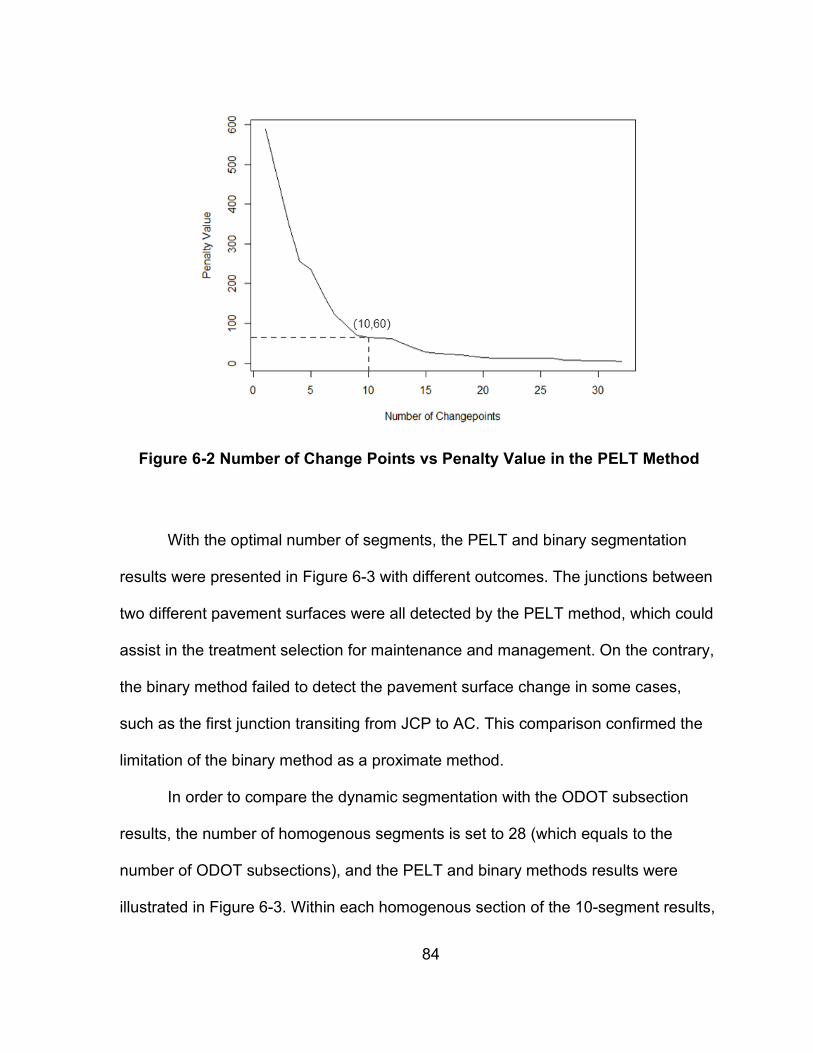
84

Figure 6-2 Number of Change Points vs Penalty Value in the PELT Method

With the optimal number of segments, the PELT and binary segmentation

results were presented in Figure 6-3 with different outcomes. The junctions between

two different pavement surfaces were all detected by the PELT method, which could

assist in the treatment selection for maintenance and management. On the contrary,

the binary method failed to detect the pavement surface change in some cases,

such as the first junction transiting from JCP to AC. This comparison confirmed the

limitation of the binary method as a proximate method.

In order to compare the dynamic segmentation with the ODOT subsection

results, the number of homogenous segments is set to 28 (which equals to the

number of ODOT subsections), and the PELT and binary methods results were

illustrated in Figure 6-3. Within each homogenous section of the 10-segment results,

85

multiple sections were further divided in the 28-segment results. The beginning and

ending locations of these segments match well between the two methods. However,

even with the same total number of segments, the PELT and binary methods gain

different segmentation results, as compared to the ODOT subsection method.

Therefore, the uniformity of each segment needs to be evaluated for comparisons of

these methods.

Figure 6-3 PELT and Binary Segmentation Results: 10 vs. 28 Segments

6.1.4 Results Evaluation

An ideal segmentation should consist of the minimum number of segments,

and the data within each segment should be normally distributed. To evaluate the

uniformity of the segmentation results, residual plots were provided before and after

the segmentation. The frequency distribution of the raw friction data was presented

in Figure 6-4. The raw GN data presents an obvious bi-modal distribution. The

Shapiro-Wilk normality test was carried out with the W value of 0.91086, p-value of

1.31e-09. A higher W value closer to one supports the sample being from a normally

distributed population only if the p-value is higher than 0.05. However, in this case,

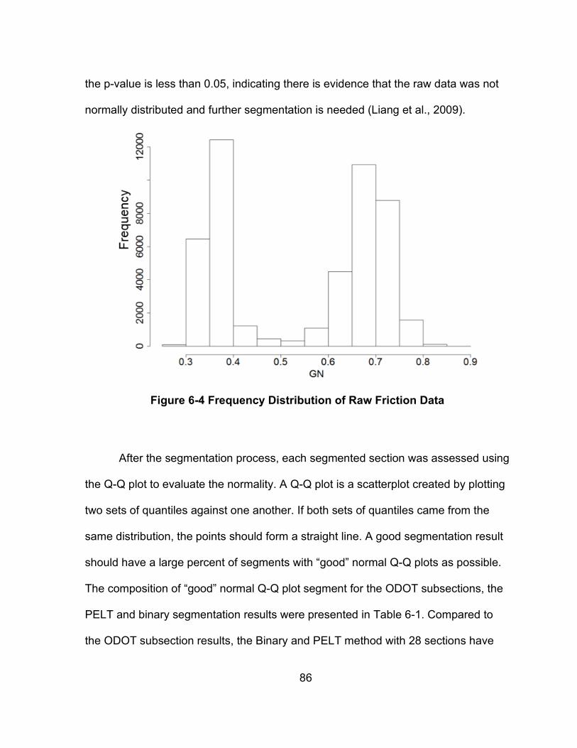
86

the p-value is less than 0.05, indicating there is evidence that the raw data was not

normally distributed and further segmentation is needed (Liang et al., 2009).

Figure 6-4 Frequency Distribution of Raw Friction Data

After the segmentation process, each segmented section was assessed using

the Q-Q plot to evaluate the normality. A Q-Q plot is a scatterplot created by plotting

two sets of quantiles against one another. If both sets of quantiles came from the

same distribution, the points should form a straight line. A good segmentation result

should have a large percent of segments with “good” normal Q-Q plots as possible.

The composition of “good” normal Q-Q plot segment for the ODOT subsections, the

PELT and binary segmentation results were presented in Table 6-1. Compared to

the ODOT subsection results, the Binary and PELT method with 28 sections have

87

higher percentage of “good” segments, 57.14% and 67.90% respectively as

compared to the ODOT method 28.60%. In addition, as the number of segments

increases from 10 to 28, the percentage of “good” segments increased for both the

binary and PELT methods, and the PELT being the best performer.

Table 6-1 Comparisons of Percentage of “Good” Segments

Segmentation ODOT 28 Subsection Binary

10 segments Binary

28 segments PELT

10 segments PELT

28 segments

Percentage 28.60% 30.00% 57.14% 40.00% 67.90%

An alternative comparison of the three segmentation results is to check the

total residuals of the model fit, illustrated by the normal Q-Q plots shown in Figure 6-

5. The closer the points are to the approximation line; the smaller the total residuals

were gained. The PELT method has a smaller residual than the Binary method and

the ODOT subsection method has the largest residual, indicating that the PELT

segmentation method generates the most uniform segments, which is consistent

with its higher percentage of “good” segments shown in Table 6-1.

88

Figure 6-5 Q-Q Plot of Overall Residual Check: 28 Segments.

6.2 CFME Software Interface

It became evident that, although CFME friction profiles provide more

information than what presently is being obtained by most locked wheel testers, its

processing becomes sophisticated. It is thus important to develop a software

interface to allow the users to view and perform basic analysis on CFME pavement

friction profiles. The developed software interface has three major capabilities.

89

6.2.1 Data Import and Visualization

Firstly, the software interface is able to import CFME measurements and

allows users to conduct direct comparisons of CFME friction measurements from

multiple testing runs under different operating conditions (at various testing speeds

and water film depths) in the same chart.

Figure 6-6 CFME Data Import and Visualization

6.2.2 Profile Synchronization and Repeatability Analysis

In order to make direct comparisons between different runs of the same road

segment, the software allows friction profiles to be shifted distance wise for

synchronization and making friction profile comparisons for repeatability. Basic

statistics, mean and standard deviation, are provided. In addition, cross-correlation

is employed to determine the lag one waveform should be shifted to obtain the best

90

match with another waveform for optimal synchronization among multiple testing

runs. It is also applied for repeatability and accuracy testing. The cross-correlation

coefficient ranges from -1.0 to 1.0, whereby 1.0 indicates a perfect positive

correlation, and -1.0 indicates a perfect negative correlation, as shown in Figure 6-7.

For the example in the figure, the results suggest that the Grip Tester based CFME

measurements have sufficient repeatability.

Figure 6-7 CFME Profile Repeatability Analysis

6.2.3 Homogeneous Segments

Lastly, the software is able to create uniform segmentations with statistically

similar CFME friction properties. Segmenting pavement network into homogenous

sections is important for decision makers to properly evaluate road maintenance

scheduling and management work required as evidenced by the individual condition

of each segment. In the software, two types of segmentation approaches are

included: fixed-length segments and dynamic segmentation. Although the Pruned

91

Exact Linear Time (PELT) method has been demonstrated with slightly better

performance in identifying homogenous segments, this method is excluded from the

software for practical applications due to its complexity of computation requirements.

The fixed-length static method breaks highway routes into every 0.01 miles,

which is the default reporting interval for the ODOT pavement management systems

(PMS). The results can be directly imported into Excel spreadsheet for further

analysis (as shown in Figure 6-6).

In addition, the cumulative difference approach (CDA), advocated by the

AASHTO Guide (AASHTO, 1993) which compares the sequence of actual

cumulative sums in a measurement series with the sums resulted from the adding

averages, is also implemented in the software for identification of homogenous

segments. In the CDA, the term Zx is defined as the difference in the cumulative

area values at a given distance (x) between the actual response and the average

response (AASHTO, 1993). Mathematically,

(Eq. 6-2)

(Eq. 6-3)

where, xi is the distance along the road section up to ith response

measurement; n is the nth pavement response measurement; nt is the total number

of pavement response measurements taken in the project; ri is the pavement

response value of the ith measurement; Lp is the total project length.

92

The Zx values are plotted versus distance along the road length and the

points where the slope of the Zx curve changes its algebraic sign are taken as the

border line between the consecutive homogeneous sections (AASHTO, 1993).

These points have been described as change-points. A sample plot of the pavement

response values as read from in the AASHTO’s Guide (1993) and the resulting Zx

values, are plotted in Figure 6-8. The change points, thus identified, are shown by

vertical lines intersecting the Zx curve.

Figure 6-8 Homogeneous Section Using CDA (AASHTO, 1993)

An example screenshot of the CDA approach is provided in Figure 6-9. It

successfully identifies the sections with different friction levels. CDA, though a quick

and straight-forward method for identification of homogeneous sections, has certain

limitations. CDA does not have any control over the number of homogeneous

93

sections a designer intends to choose. There may not be any restriction on

maximum length of a homogenous section, but from practical considerations, there

must be a provision for specifying minimum length of a homogeneous section.

Because, frequent changes in specification along the road stretch may cause

inconvenience from the construction point of view. Choice of minimum section length

cannot be incorporated in CDA.

Figure 6-9 CDA based CFME Homogeneous Sections

6.3 CFME for Pavement Friction Management (PFM)

6.3.1 The AASHTO Guideline

The Technical Advisory 5040.38 Pavement Friction Management (FHWA,

2010) provides guidance to highway agencies towards developing or improving

pavement friction management programs (PFMPs) to ensure pavement surfaces are

designed, constructed, and maintained to provide adequate and durable friction

properties that reduce friction-related crashes in a cost-effective manner (FHWA,

2017). The 2008 AASHTO Guide for Pavement Friction defines PFM as a

systematic approach to measuring and monitoring the friction qualities and wet crash

rates of roadways, identifying those pavement surfaces and roadway situations that

94

are or will immediately be in need of remedial treatment, and planning and budgeting

for treatments and reconstruction work that will ensure appropriate friction

characteristics (AASHTO 2008). The AASHTO Guide provides an overall approach

for managing pavement friction and a rigorous process for implementation (AASHTO

2008). This approach calls for routine friction testing of the roadway network and the

subsequent analysis of friction and crash data to identify locations with potentially

inadequate levels of friction/texture, comprising of the following components.

• Step 1 Network Definition - subdivide the highway network into distinct

pavement sections and group the sections according to levels of friction

need

o Define pavement sections;

o Establish friction demand categories.

• Step 2 Network-Level Data Collection - Gather all the necessary

information

o Establish field testing protocols (methods, equipment, frequency,

conditions, etc.) for measuring pavement friction and texture;

o Collect friction and texture data and determine overall friction of each

section;

o Collect crash data.

• Step 3 Network-Level Data Analysis - Analyze friction and/or crash data

to assess overall network condition and identify friction deficiencies

95

o Establish investigatory and intervention levels for friction, which are

defined as the levels that prompt the need for a detailed site

investigation or the application of a friction restoration treatment;

o Identify pavement sections requiring detailed site investigation or

intervention.

• Step 4 Detailed Site Investigation - Evaluate and test deficient

pavement sections to determine causes and remedies

o Evaluate non-friction-related items, such as alignment, the layout of

lanes, intersections, and traffic control devices, the presence, amount,

and severity of pavement distresses, and longitudinal and transverse

pavement profiles;

o Assess current pavement friction characteristics, both in terms of

micro-texture and macro-texture;

o Identify deficiencies that must be addressed by restoration;

o Identify uniform sections for restoration design over the project length.

• Step 5 Selection and Prioritization of Short- and Long-Term

Restoration Treatments - Plan and schedule friction restoration activities

as an integral part of the overall pavement management process

o Identify candidate restoration techniques best suitable for correcting

existing pavement deficiencies;

o Compare costs and benefits of the different restoration alternatives

over a defined analysis period;

96

o Consider monetary and non-monetary factors and select one

pavement rehabilitation strategy.

6.3.2 Use of Friction Data for PFM

Following the AASHTO Guideline (AASHTO, 2008), friction data from CFME

or other skid trailers (such as locked-wheel tester at ODOT) can be used in several

components of a pavement friction management program.

Step 1 Network Pavement Sections Definition

According to the NCHRP Project 01-43 (Hall et al. 2009), the friction demand

levels should be estimated by evaluating three broad categories of influencing

factors: highway alignment, highway features/environment, and highway traffic

characteristics. At ODOT, control section has been widely implemented as the

primary key for GIS and roadway asset management. Control section numbers

contain the county number, a continuous route number, and the control number. A

control section generally starts or ends at state/county line, a major

intersection/highway junction, etc. by different roadway functional classes (interstate,

freeway, principal arterial, minor arterial, major collector). In addition, one control

section is further divided into multiple sections based on data owners’ needs.

Therefore, the currently used ODOT subsections of a control section meet the

criteria as recommended in NCHRP Project 01-43, and can be used as the basic

network pavement sections. The location of a pavement section can be identified

97

from various information such as route number, direction, county name, control

section number, milepost, and GPS coordinates. Since control sections and

subsections are used in the ODOT Pavement Management System (PMS), the

recommended definition of pavement sections for PFM programs can be easily

integrated into existing ODOT programs. However, the current field friction database

at ODOT are slightly different in terms of data items from year to year. All data

includes county name, route number, control section number, but some data are

saved per reference milepost while others also have GPS coordinates. Subsections

of a control section are not provided for all the data sets from 2010.

In addition, the control sections at ODOT are defined mainly for roadway

segments. However, roadway segments and intersections, two major facility types in

the AASHTO Highway Safety Manual (AASHTO, 2010), could require different

friction demand levels. For this reason, the Illinois DOT (IDOT) defines roadway

segments or intersection into peer groups based on fundamental roadway data

elements in their roadway safety analysis. Therefore, the IDOT approaches should

be referenced for the defining of roadway sections but also intersections.

Table 6-2 Illinois SPF Peer Groups

Segments Intersections 1 – Rural two-lane highways 1 – Rural minor-road STOP control

2 – Rural multilane undivided highways 2 – Rural all-way STOP control

3 – Rural multilane divided highways 3 – Rural signalized

4 - Rural freeways – four lanes 4 – Rural undetermined

5 - Rural freeways – six plus lanes 5 – Urban minor-road STOP control

6 – Urban two-lane arterials 6 – Urban all-way STOP control

7 - Urban multilane undivided arterials 7 – Urban signalized

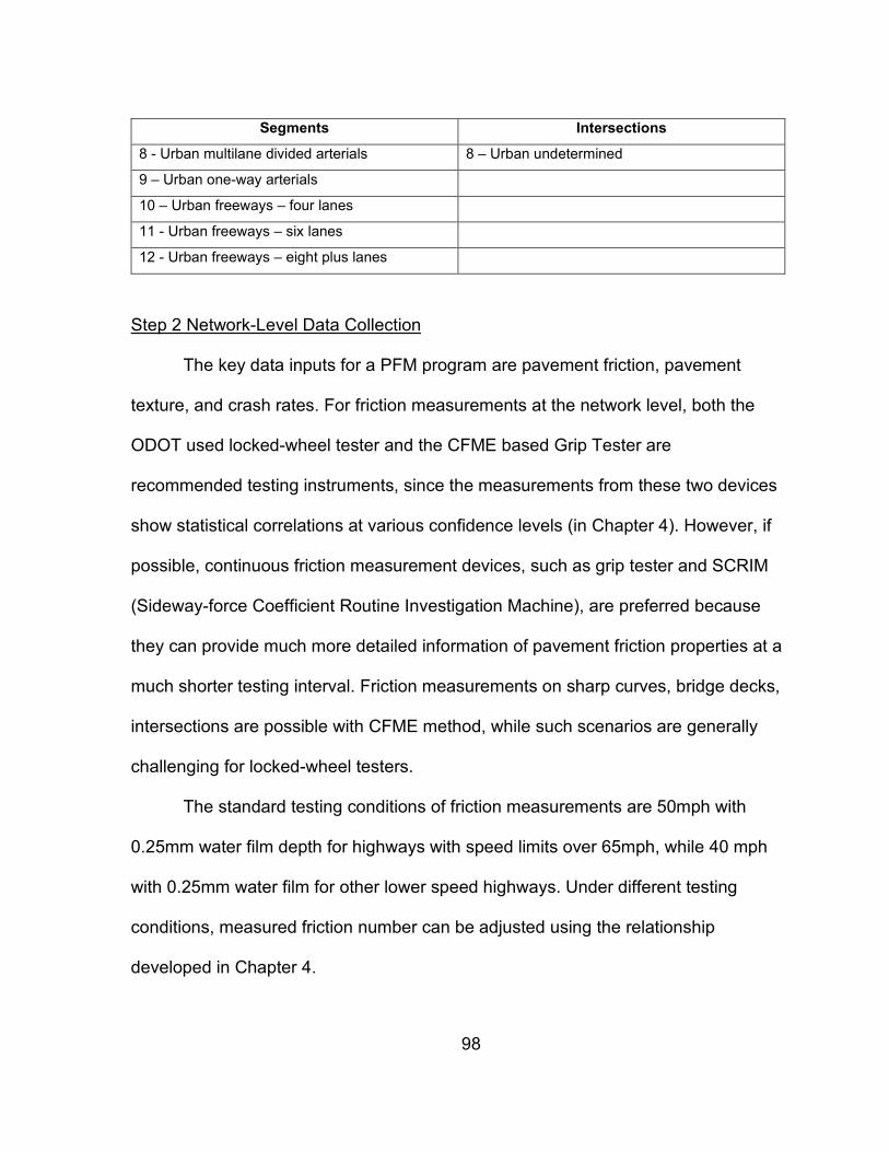
98

Segments Intersections 8 - Urban multilane divided arterials 8 – Urban undetermined

9 – Urban one-way arterials

10 – Urban freeways – four lanes

11 - Urban freeways – six lanes

12 - Urban freeways – eight plus lanes

Step 2 Network-Level Data Collection

The key data inputs for a PFM program are pavement friction, pavement

texture, and crash rates. For friction measurements at the network level, both the

ODOT used locked-wheel tester and the CFME based Grip Tester are

recommended testing instruments, since the measurements from these two devices

show statistical correlations at various confidence levels (in Chapter 4). However, if

possible, continuous friction measurement devices, such as grip tester and SCRIM

(Sideway-force Coefficient Routine Investigation Machine), are preferred because

they can provide much more detailed information of pavement friction properties at a

much shorter testing interval. Friction measurements on sharp curves, bridge decks,

intersections are possible with CFME method, while such scenarios are generally

challenging for locked-wheel testers.

The standard testing conditions of friction measurements are 50mph with

0.25mm water film depth for highways with speed limits over 65mph, while 40 mph

with 0.25mm water film for other lower speed highways. Under different testing

conditions, measured friction number can be adjusted using the relationship

developed in Chapter 4.

99

For pavement texture data collection at ODOT, they are collected

simultaneously using a laser-based high-speed profiler with the statewide automated

collection of pavement condition data. The data are saved at every 0.01 miles, same

as other PMS data sets, in terms of mean profile depth (MPD). The current data

collection practices on texture are considered as adequate for PFM purposes. It is

widely recognized that pavement surface texture is important for pavement friction

and roadway safety. MPD has been the primary index used to characterize macro-

texture. However, MPD is a two-dimensional (2D) height indicator calculated from a

single profile, which is insufficient to represent surface texture especially for friction

analysis. Many studies have found that MPD failed to capture the differences and

variations in friction performance. As a result, new texture parameters have been

tested and developed to relate pavement texture with friction performance at both

the macro- and micro-level. In order to be able to better characterize pavement

texture performance, it is therefore recommended that ODOT should store the raw

texture profiles so that such analysis is feasible.

Regarding the data collection frequency for friction and texture, it is desirable

to test all network pavement sections annually because of the year-to-year variation

in pavement friction. However, due to the limitation of available resources, a cost-

effective approach should be conducted to identify the pavement sections with

priority in terms of friction and texture. The first level of priority should be tested

annually, of which the roadway segments have high friction demand and high risk of

crashes. The second level of priority can be tested once every few years, such as a

2-year to 3-year based program, half or one-third of the network is tested each year.

100

While the third level of priority can be selected based on statistical sampling, of

which the pavement sections have low friction demand and low risk of crashes.

Crash data is an important data component for a successful PFM program.

ODOT currently manages a computer-based crash database called Statewide

Analysis for Engineering & Technology (SAFE-T), to save all highway crashes in the

state since 1998. The crash data and related information can be gathered from

SAFE-T database, including the severity, type, location of each crash, and

corresponding pavement condition (wet or dry) etc. In addition, a comprehensive

data check process is also conducted before the crash data are imported into the

Safe-T database. It is thus believed the quality of crash data is satisfactory. From

those aspects, the rich crash data are sufficient for the need of developing PFM.

Step 3 Network-Level Data Analysis

The collected network-level data should be assessed to identify roadway

segments with potential safety risk. Firstly, pavement network should be segmented

into homogeneous sections, using the change point methodologies discussed in

Chapter 5, or approaches that are used or desired at ODOT. Subsequently, the

adequacy of friction of these segments can be assessed and compared with the

investigatory and intervention friction demand levels. Pavement sections with

measured friction below investigatory level are subjected to detailed site

investigation to determine the need for warning or remedial actions, such as

performing more frequency testing and analysis or applying short-term restoration

101

treatment. Once the site friction reaches the intervention level, remedial actions are

needed.

It should be noted that the establishment of investigatory and intervention

friction levels is out of the scope of this project and should be carried out for each

friction demand category. The friction thresholds can be determined using one of

three methods presented in the NCHRP Project 01-43 project (Hall et al. 2009)

based on the data availability. The first method (Figure 6-10a) sets investigatory

level as the friction value where there is a significant increase in friction loss. The

intervention level is set as a certain percentage below the investigatory level. The

second method (Figure 6-10b) examines both historical friction and wet-to-dry crash

data trends. The investigatory level is set corresponding to a large change in friction

loss rate while the intervention level is set where there is a significant increase in

crashes. The third method (Figure 6-10c) is the most detailed approach, which uses

the distribution of friction data versus the crash rates that correspond with the friction

for the category of roadway for which the levels are being set.

102

Figure 6-10 Setting of Investigatory and Intervention Levels (Hall et al. 2009)

103

Step 4 Detailed Site Investigation

The goal of detailed site investigation for highway sections is to determine the

specific causes and evaluate non-friction-related items. The detailed site

investigation could involve visual, video, or laser based roadway condition data

survey, micro- and macro-texture data evaluation.

The first step is to check the roadway features that may be compounding the

friction problems, such as the layout of the lanes, traffic control devices, roadway

geometry characteristics, and the extent and severity of pavement distresses (e.g.

cracking, rutting, patches, potholes, etc.). The second step involves the testing of

pavement surface texture. The collection of macro-texture data is becoming mature

with the use of high speed laser profilers. While the micro-texture can be evaluated

using Dynamic Friction Tester (DFT) on representative sections. In addition, other

relevant information, including traffic volume and the truck percentages, pavement

surface type and materials, signs of polishing aggregates should be collected if

possible.

Step 5 Selection and Prioritization of Friction Restoration Treatments

The final step is to plan and schedule friction restoration activities best suited

to correct existing pavement deficiencies and compare costs and benefits of the

different restoration alternatives over a defined analysis period. The prioritization of

the highway sections can be identified based on pavement friction, other condition

data, and site crash features. In analyzing pavement friction data, the minimum

104

desirable outcome is to ensure that the most “deficient” sites are detected and given

reasonable priority. Two possible actions could be considered:

• Continue to monitor the site: Such a decision typically would be reached

where (a) current crash rates are sufficiently low and an increase is not

expected to significantly impact safety and (b) the pavement surface does

not require maintenance because of other factors.

• Select for remedial action to improve pavement friction (e.g., resurface,

retexture): This usually would apply where an increase in crash rate might

occur if friction remains the same or continues to decrease, and such an

increase would significantly impact safety. Preventive maintenance is a

cost-effectiveness option to restore pavement performance and extend

service life. It is critical to determine the optimal timing of the appropriate

treatment.

105

CHAPTER 7 CONCLUSIONS AND RECOMMENDATIONS

7.1 Conclusions

Pavement skid resistance plays a significant role in road safety. The

application of new technologies can be used to determine the low friction areas or

vulnerable accident sites at both the project and network levels. An important part of

the friction management process is the selection of the most appropriate friction

measuring equipment. Continuous friction devices are one of the newest systems

currently used in European countries that have recently been introduced to the

United States. In this project, the capabilities of the Grip Tester, a type of continuous

friction measurement (CFME) device, and its ability to provide information to support

PFM programs were evaluated based on a comprehensive field data collection and

statistical analysis.

An extensive literature review was conducted to develop an in-depth

understanding of various aspects related to friction measurements. The most

influential factors to pavement friction were summarized and considered in the field

data collection experimental design. In addition, crash data during the past ten years

was obtained, and the roadway segments with high observed crashes, particular

those within the ODOT skid testing program (interstates and US-69), were also

identified as the potential field testing locations. After close consultation with ODOT,

twenty-two testing sites were included in this project with nine commonly used

treatment types in Oklahoma: chip seal, ultra-thin bonded wearing course (UTBWC),

106

resurfacing (asphalt), micro-surfacing, warm mix asphalt (WMA) thin overlay,

resurfacing (concrete), next generation concrete surface (NGCS), longitudinal

grooving, and high friction surfacing treatment (HFST).

For each testing site, nine runs of friction data collection were conducted

using the Grip Tester at three testing speeds (40mph, 50mph, 60mph for interstates

and major arterials; 30mph, 40mph, 50mph for minor arterials), three water film

thicknesses (0.25mm, 0.50mm, 1.0mm). Pavement surface condition and texture

data were also acquired for each site. In addition, approximate 90-mile of friction

data collection were conducted in parallel on northbound of mainline I-35 using the

Grip Tester and the ODOT locked-wheel friction trailer. The data collected at these

sites along with Oklahoma crash data were further used to assess the operation

characteristics and repeatability of CFME friction measurements, to compare the

measurements from locked-wheel friction trailer and Grip Tester, and to develop

enhanced crash rate prediction models.

Various statistical and comparisons analyses were performed. First, the

CFME testing results under various conditions were summarized with descriptive

statistics. Further, the performance of CFME was evaluated from three aspects: (1)

the correlation with Locked-wheel measurements, (2) the repeatability of CFME

data, and (3) the influence of operational characteristics on CFME measurements.

The key findings are summarized below:

• The HFST sites show the best friction performance, followed by the

transverse grooving site on US-77. The other testing sites, with various

surface types, are observed to have comparable friction performance

107

• For most sites, with increasing testing speeds, the friction numbers show

decreasing trend. However, the effects of varying testing speed differ for

different treatment types. Some sites demonstrate pronounced reduction

in friction performance with increasing speeds, such as chip seal,

UTBWC, HMA and some WMA sites, while others are not as significant.

HFST as the example, it seems that their friction performance does not

depend on testing speeds.

• Friction numbers decrease when larger water film thickness is applied. For

some sites, the friction values are significantly reduced when the water

film thickness is increased from 0.25mm to 0.5mm. On the other hand,

HFST sites for example, the impact of water film thickness for some sites

does not demonstrate such significant influences.

• Comparing to the friction measurements from LWST, Grip Numbers from

the Grip Tester measured on the same sites are consistently larger, and

are more sensitive to pavement surface types. Multi-variant regression

analysis was applied to develop the correlation between SN and GN. The

skid number from LWST is statistically significant when correlating to the

grip number, while there are several other factors that have showed

statistical significance to the Grip Tester measurements. Even though the

correlation models between the two measurements are statistically

significant, the R-squared value is not strong due to the high variabilities

presented in the field friction measurements using contact-based method

for both LWST and grip tester.

108

• Various methodologies were implemented for repeatability testing. The

average differences (the maximum minus minimum friction) and standard

deviation of the repeating measurements are 0.039 and 0.051

respectively, indicating the Grip Tester can measure surface friction in a

consistent manner. The correlation based repeatability analysis results

suggest that the Grip Tester based CFME measurements have sufficient

repeatability. On average, the cross-correlation coefficient is 94.71% for

the HFST testing sites, and 63.15% for the shotblasting site. The cross-

correlation analysis method is more robust for friction profiles with more

distinct changes and pronounced features.

• To access the impact of friction measurements due to the change of

operational characteristics (testing speed, WFT, ambient temperature),

regression model was developed following the backward stepwise

analysis. The adjusted R-squared of the model is 0.68, indicating that the

model has satisfactory statistical performance. Ambient temperature,

testing speed, and water film thickness show negative effects on the

friction measurements, while the average MPD has a positive effect on

friction measurements. State agencies can utilize the multivariate

regression model to adjust/correct the friction collected at different testing

conditions to the baseline condition and be comparable for further decision

making.

109

The continuous friction data provides much more detailed skid resistance

information, and can have several potential implementations for pavement friction

management and highway safety applications.

• Combining the CFME friction and pavement condition data sets collected

from this project with the Oklahoma safety database, a framework was

proposed to integrate the roadway characteristics into the development of

crash rate prediction model. A case study was subsequently provided to

implement the framework for the development of enhanced safety

performance function (SPF) using CFME friction data. The statistical

significant factors for crash includes AADT, segment length, and

pavement surface friction. The number of crashes per mile in five years

was expected to increase with the increase of traffic volume or the

decrease of surface friction coefficient. The model indicated that the crash

data was over-dispersed and thus the negative binomial model was

suitable for this case study.

• With detailed CFME data, pavement network could be better segmented

into homogenous sections for road maintenance scheduling and

management. Surface friction data were collected in Oklahoma using a

Grip Tester and used for the case study. Three dynamic segmentation

methods: binary, neighborhood and PELT methods were implemented.

The segmentation results were compared with the subsection-based

method currently used in the pavement management system (PMS) at

110

ODOT, and their efficiency and robustness were evaluated for each

individual segment and the overall roadway.

• In order to ease the using of CFME data, a CFME data analysis software

interface was developed, which is able to upload and visualize CFME

measurements, and perform basic statistical and comparison analyses for

data reporting.

In addition, the AASHTO Guide for Pavement Friction provides an overall

approach for managing pavement friction, which calls for routine friction testing of

the roadway network and the subsequent analysis of friction and crash data to

identify potentially inadequate locations. How CFME data and the findings from this

study can be used to assist the pavement friction management was discussed.

7.2 Recommendations

The use of slip-wheel CFMEs devices has gained popularity in Europe and

recently started using in U.S. for roadway applications. These devices can measure

friction continuously and provide more spatial details than locked-wheel devices.

This project presents the research effort to explore the use of CFME, Grip Tester

herein, as a tool for pavement friction management and roadway safety practices.

The direct comparison results suggest that CFME can provide repeatable and

reproducible friction profiles, and the measurements from Grip Tester and locked-

wheel skid trailer are statistically correlated. However, such relationships are not

very strong in some cases and impacted by several other factors. It should be noted

111

that the data used in this report as case studies is only for demonstration purpose

due to the limited number of testing sites and the duration of the monitoring cycle

(less than 2 years). Therefore, it is recommended that ODOT should consider

adopting CFME for their skid resistance program. Through a wide range of

measurements and analysis, an in-depth understanding of the testing methodology

could be achieved to (1) quantify the effect of operational factors, and (2) establish

standard testing condition and approaches.

Besides, several other challenges and opportunities remain for the wide

implementation of CFME for friction management and roadway safety practices. The

Grip Tester has been proved by several studies to be an accurate and economical

way to measure skid resistance on roads. Meanwhile, it is also found that the

variations of measurements could be high on segments with bad surface conditions

(such as high IRI, faulted roads) while traveling at highway speed. This is probably

due to the low weight of the trailer. During the field testing, the team depended on

vehicular cruise control capability and was able to maintain a stable testing speed

(generally within 1 mph range). However, the water flow data recorded by the Grip

Tester software could vary significantly in some occasions, which could result in

variations of friction measurements.

Grip Tester is one of the CFME devices on the market. Others in use include

Side-Force Coefficient Routine Investigation Machine (SCRIM), Mu-Meters, Airport

Surface Friction Testers (ASFT), Dynatest Pavement Friction Tester (DPFT), etc. In

particular, SCRIM has been implemented in the very recent years with support from

Federal Highway Administration (FHWA) and many state agencies through a

112

transportation pooled fund study. Although both the Grip Tester and the SCRIM

continuously measure wet pavement friction, they use different test tires, different

tire orientation, and different slip ratios (and slip speeds). In addition to measuring

friction, the SCRIM generally also measures macrotexture (MPD, in mm),

longitudinal grade (%), cross-slope (%), and horizontal curvature (1/m). As a result,

different CFME devices should be investigated and evaluated for ODOT’s

consideration regarding its capabilities, advantages, disadvantages, and costs etc.

for potential future adoptions.

Furthermore, no matter which friction testing instruments are used, the

existing methodologies are all contact based, which require dragging a tire/rubber

pad across a road/specimen to measure roadway skid resistance. Such technology

could result in inconsistent friction measurements depending on many operational

factors, such as the viscoelastic properties of testing tires under various

temperatures, testing speed, and surface conditions with various water film depth,

and the wandering of testing vehicle. In addition, it requires in-vehicle water tank in

order to wet testing surface and consumes testing rubber pads or tires which could

wear quickly due to the physical contact with pavement surfaces. Therefore, it is

long desired to develop non-contact methods, such as surface texture collection, to

supplement and/or replace the existing contacting pavement friction measurements

with less inconsistency and variations. With the fast development of non-contact 3-

Dimensioal (3D) measurement technologies and the improvement in the computing

and processing power of computers, it is becoming feasible and desirable to

113

describe road surface texture in both macro- and micro-scale under 3D at high

resolution for pavement skid resistance characterization.

It is also found that the existing contact-based friction measurement methods

(such as the LWST with a ribbed tire) can be insensitive to macrotexture under

specific circumstances. It thus should be recommended that CFME friction testing be

complemented by macro-texture measurement, in order to which could facilitate the

definitions of investigatory friction and macro-texture levels to support the state’s

pavement friction management program. This will allow areas with potentially

deficient macro-texture to be identified and investigated at the project level and

corrected, if necessary, before the occurrence of wet-weather crashes.

In recent years, the scope of the ODOT Skid Studies Program has been

downsized to annual testing of US-69, all the Interstate Highways, as well as the

Strategic Highway Research Program (SHRP) sites. In order to develop a

comprehensive pavement friction program, a wider range of friction measurements

is desired for common pavement types, overlays, and surface treatments on various

highways with different traffic levels and environmental zones in the state.

Subsequently, more advanced analysis could be conducted for enhanced roadway

safety management, such as:

• The incorporation of CFME friction measurements into safety performance

functions (SPF) to improve the assessment of overall network condition

and identify friction deficiencies that might cause crashes,

114

• Developing preservation policies that improve the safety of the roadway

network and decrease the number of skidding-related crashes through

engineered safety improvements.

Finally, there is also a serious need to predict friction and macro-texture

properties during mix design, when the mix can be adjusted to meet frictional

demand at the project location. The detailed information used to develop mix-

specific performance equations can then be used to predict (and accurately monitor)

the substantial benefits that can be expected from skid-resistant surface mixes and

surface treatments, which will be further related to highway safety in terms of the

reduction of traffic crashes.

115

REFERENCES

AASHTO (1993), Guide for design of pavement structures, American Association of

State Highway and Transportation Officials, Washington, DC.

AASTHO. (2013a). Quantifying cracks in asphalt pavement surfaces from collected

images utilizing automated methods. AASHTO Designation PP67-10.

Washington, D.C.

AASTHO. (2013b). Standard practice for determining pavement deformation

parameters and cross slope from collected transverse profiles. AASHTO

Designation: PP69-10. American Association of State Highway and

Transportation Officials. Washington, D.C.

Adelle W. (2006). Quantitative Characterisation of Surface Finishes on Stainless

Steel Sheet using 3D Surface Topography Analysis. Doctoral thesis,

University of Huddersfield.

Arhin, S.A., Noel, E.C., and Ribbiso, A. (2015). Acceptable International Roughness

Index Thresholds based on Present Serviceability Rating. Journal of Civil

Engineering Research, 5(4), pp. 90-96, doi:10.5923/j.jce.20150504.03.

116

ASTM Designation D6433-18. (2018). Standard Practice for Roads and Parking Lots

Pavement Condition Index Surveys. ASTM International. West

Conshohocken, PA, DOI: 10.1520/ D6433-18.

ASTM Standard E1845-15. (2015). Standard Practice for Calculating Pavement

Macrotexture Mean Profile Depth. ASTM International. West Conshohocken,

PA, DOI: 10.1520/E1845-15.

ASTM Standard E1911-09a. (2009). Standard Test Method for Measuring Paved

Surface Frictional Properties Using the Dynamic Friction Tester. ASTM

International, West Conshohocken, PA, DOI: 10.1520/E1911-09AE01.

ASTM Standard E2157-15. (2015). Standard Test Method for Measuring Pavement

Macrotexture Properties Using the Circular Track Meter. ASTM International,

West Conshohocken, PA, DOI: 10.1520/E2157-15.

ASTM Standard E274/E274M-115. (2015). Standard Test Method for Skid

Resistance of Paved Surfaces Using a Full-Scale Tire. ASTM International,

West Conshohocken, PA, DOI: 10.1520/E0274_E0274M-15.

ASTM Standard E303-93. (2013). Standard Test Method for Measuring Surface

Friction Properties Using the British Pendulum Tester. ASTM International,

West Conshohocken, PA, DOI: 10.1520/E0303-93R13.

117

ASTM Standard E950-98. (1998). Measuring Test Method for Measuring the

Longitudinal Profile of Traveled Surfaces with an Accelerometer Established

Inertial Profiling Reference. ASTM International, West Conshohocken, PA.

ASTM Standard E965-15. (2015). Standard Test Method for Measuring Pavement

Macrotexture Using a Volumetric Technique. ASTM International, West

Conshohocken, PA, DOI: 10.1520/E0965-15.

Auger I.E., C.E. Lawrence (1989). Algorithms for the optimal identification of

segment neighborhoods. Bulletin of mathematical biology 51(1), pp 39-54.

Bai J.S., P. Perron (1998). Estimating and testing linear models with multiple

structural changes. Econometrica 66(1), pp 47-78.

Bitelli G. et al. (2012). Laser Scanning on Road Pavements: A New Approach for

Characterizing Surface Texture. Sensors, Vol. 12, pp. 9110-9128, DOI:

10.3390/s120709110.

Bonaquist, R. (2011). Mix Design Practices for Warm Mix Asphalt. NCHRP Report

691, Transportation Research Board, National Research Council,

Washington, D.C.

Bower N. et al. (2012). Evaluation of the Performance of Warm Mix Asphalt in

Washington State. Washington DOT. Olympia, WA.

118

Button J.W., Estakhri C. and Wimsatt A., (2007). A Synthesis of Warm-Mix Asphalt.

Publication FHWA/TX-07/0-5597-1. FHWA and Texas Department of

Transportation.

Cafiso S., A. Di Graziano (2012). Definition of Homogenous Sections in Road

Pavement Measurements, Procedia - Social and Behavioral Sciences 53, pp

1069-1079.

Cerezo, V., Do, M., Prevost, D., and Bouteldja, M. (2014). Friction/Water Depth

Relationship-In Situ Observations and Its Integration in Tire/Road Friction

Models. Journal of Engineering Tribology, 228(11), pp. 1285-1297.

Copeland, A. et al. (2010). Field Evaluation of High Reclaimed Asphalt

Pavement/Warm Mix Asphalt Project in Florida: A Case Study. Transportation

Research Board Annual Meeting CD-ROM, Transportation Research Board of

the National Academies, Washington, D.C.

Dave, E.V., Hanson, C.E., Helmer, B., Dailey, J., and Hoplin, C.M. (2015).

Laboratory Performance Test for Asphalt Concrete. Publication MN/RC 2015-

24, Minnesota Department of Transportation, St. Paul, Minnesota.

D'Angelo J. et al. (2008). Warm-Mix Asphalt: European Practice. Publication FHWA-

PL-08-007. Washington D.C., Federal Highway Administration Office of

International Programs.

119

Deltombe, R., Kubiak, K.J., Bigerelle, M. (2011). How to Select the Most Relevant

3D Roughness Parameters of a Surface Scanning, Vol. 36, No. 1, pp. 150-

160, DOI: 10.1002/sca.21113.

Diefenderfer, S. and A. Hearon. (2008). Laboratory Evaluation of a Warm Asphalt

Technology for Use in Virginia. Publication VTRC 09-R11, Virginia

Transportation Research Council, Charlottesville, VA.

Do, M. et al. (2007). Pavement Polishing-Development of a Dedicated Laboratory

Test and its Correlation with Road Results. Wear, Vol. 263, pp. 36-42.

Do, M., Cerezo, V., Beautru, Y., and Kane, M. (2014) Influence of Thin Water Film

on Skid Resistance. Journal of Traffic and Transportation Engineering, 2(1),

pp. 36-44.

Dueker K.J., R. Vrana (1992). Dynamic segmentation revisited: a milepoint linear

data model. Journal of the Urban and Regional Information Systems

Association 4(2), pp 94-105.

Dunford A.M. et al. (2012). Three-Dimensional Characterization of Surface Texture

for Road Stones Undergoing Simulated Traffic Wear. Wear, Vol. 292-293, pp.

188-196.

Edwards A.W., L.L. Cavalli-Sforza (1965). A method for cluster analysis, Biometrics,

pp 362-375.

120

Ergun, M., Iyinam, S., and Iyinam, A. (2005). Prediction of Road Surface Friction

Coefficient Using Only Macro- and Microtexture Measurements. Journal of

Transportation Engineering, Vol. 131, No. 4, pp. 311-319.

Federal Highway Administration (FHWA). (2016). “Pavement Friction.” U.S.

Department of Transportation, FHWA, Washington, D.C.

<https://safety.fhwa.dot.gov/roadway_dept/pavement_friction/> (Accessed on

April 1, 2019)

Flintsch G.W. et al. (2012). The Little Book of Tire Pavement Friction. Pavement

Surface Properties Consortium.

Hall J.W. et al. (2009). NCHRP Web Document 108: Guide for Pavement Friction.

Transportation Research Board, National Research Council, Washington,

D.C.

Henry, J.J. (2000). NCHRP Synthesis 291: Evaluation of Pavement Friction

Characteristics. TRB, National Research Council, Washington, D.C.

Hartikainen L., Petry F. and Westermann S. (2014). Frequency-wise Correlation of

the Power Spectral Density of Asphalt Surface Roughness and Tire Wet

Friction. Wear, Vol. 317, pp. 111-119.

Hurley, G. C. et al. (2006) "Evaluation of potential processes for use in Warm Mix

Asphalt." Journal of the Association of Asphalt Paving Technologists,

Savannah, GA, United States, 41-90.

121

Izeppi E., Flintsch G. and McGhee K. (2010). Field Performance of High Friction

Surfaces. Publication FHWA/VTRC 10-CR6. FHWA, U.S. Department of

Transportation.

Kanafi M.M. et al. (2015). Macro- and Micro-Texture Evolution of Road Pavements

and Correlation with Friction. International Journal of Pavement Engineering,

Vol. 16, No. 2, pp. 168-179, DOI: 10.1080/10298436.2014.937715.

Kane M., Rado Z. and Timmons A. (2015). Exploring the Texture-Friction

Relationship: from Texture Empirical Decomposition to Pavement Friction.

International Journal of Pavement Engineering, Vol. 16, No. 10, pp.919-918,

DOI:10.1080/10298436.2014.972956.

Killick R., P. Fearnhead, I.A. Eckley (2012). Optimal detection of changepoints with a

linear computational cost. Journal of the American Statistical Association

107(500), pp 1590-1598.

Killick R., I. Eckley, changepoint (2014). An R package for changepoint analysis.

Journal of statistical software 58(3), pp 1-19.

Kvasnak, A., J. Moore, A. Taylor, and B. Prowell. (2010). Evaluation of Warm Mix

Asphalt Field Demonstration: Nashville, Tennessee. NCAT Report 10-01,

National Center for Asphalt Technology. Auburn, AL.

Leach R. (2012). Characterisation of Areal Surface Texture. Springer-Verlag Berlin

Heidelberg, DOI: 10.1007/978-3-642-36458-7.

122

Li L., Wang K.C.P., and Li Q.J. (2016). Geometric Texture Indicators for Safety on

AC Pavements with 1 mm 3D Laser Texture Data. International Journal of

Pavement Research and Technology, Vol. 9, pp. 49-62.

Li Q., K. Wang, G. Yang (2015). PELT based dynamic segmentation for network

level pavement evaluation with 1 mm 3D data. 6th International Conference on

Bituminous Mixtures and Pavements, Thessaloniki, Greece.

Li S. et al. (2016). Pavement Surface Microtexture: Testing, Characterization and

Frictional Interpretation.

Liang J., M.-L. Tang, P.S. Chan (2009). A generalized Shapiro–Wilk W statistic for

testing high-dimensional normality. Computational statistics & data analysis

53(11), pp 3883-3891.

Liu Q. and Shalaby A. (2015). Relating Concrete Pavement Noise and Friction to

Three-Dimensional Texture Parameters. International Journal of Pavement

Engineering, DOI: 10.1080/10298436.2015.1095897.

Michigan Metrology. (2014). Michigan Metrology Surface Texture Parameters

Glossary. Michigan Metrology, LLC, MI.

Mohammad, L., Hassan, M., Vallabhu, B., and Kabir, M. (2015). Louisiana’s

Experience with WMA Technologies: Mechanistic, Environmental, and

Economic Analysis. Journal of Materials in Civil Engineering, 27(6):

04014185.

123

Nataadmadja A.D. et al. (2012). Quantifying Aggregate Microtexture with Respect to

Wear-Case of New Zealand Aggregates. Wear, Vol. 332-333, pp. 907-917.

National Asphalt Pavement Association (NAPA). (2002). Designing and Constructing

SMA Mixtures—State-of-the-Practice. Quality Improvement Series 122,

NAPA, Lanham, Maryland.

Prowell, B. D., G. C. Hurley, and E. Crews. (2007). Field Performance of Warm Mix

Asphalt at the NCAT Test Track. Transportation Research Board Annual

Meeting CD-ROM, Transportation Research Board of the National

Academies, Washington, D.C.

West, R., et al. (2014). Field Performance of Warm Mix Asphalt Technologies.

NCHRP REPORT 779. Transportation Research Board of the National

Academies, Washington, D.C.

Salem O., Y. Liu, A. Mehaoua (2013). A lightweight anomaly detection framework for

medical wireless sensor networks. IEEE Wireless Communications and

Networking Conference (WCNC), IEEE, pp. 4358-4363.

Sargand, S., Nazzal, M.D., AI-Rawashdeh, A., and Powers, D. (2012). Field

Evaluation of Warm-Mix Asphalt Technologies. Journal of Materials in Civil

Engineering, 24(11), pp. 1343-1349. DOI: 10.1061/(ASCE)MT.1943-

5533.0000434.

124

Scott A.J., M. Knott (1974). A cluster analysis method for grouping means in the

analysis of variance. Biometrics, pp 507-512.

Serigos P.A. (2013). The Contribution of Micro- and Macro-Texture to the Skid

Resistance of Pavements.

http://www.ectri.org/YRS13/Documents/Presentations/Session5b-

6a/YRS13_Session5b-6a_Serigos_TRB.pdf. Accessed 12 May, 2016.

Thomas F. (2003). Statistical approach to road segmentation, J Transp Eng 129(3),

pp 300-308.

Ueckermann et al. (2015). A Contribution to Non-contact Skid Resistance

Measurement. International Journal of Pavement Engineering, Vol. 16, No. 7,

pp. 646-659, DOI:10.1080/10298436.2014.943216.

Villani M.M. et al. (2014). Application of Fractal Analysis for Measuring the Effects of

Rubber Polishing on the Friction of Asphalt Concrete Mixtures. Wear, Vol.

320, pp. 179-188.

Wang, K.C.P. et al. (2015). Network Level Pavement Evaluation with 1 mm 3D

Survey System. Journal of Transportation Engineering (English Edition), 2(6),

pp. 391–398.

West, R. et al. (2011). Field Performance of Warm Mix Asphalt Technologies.

NCHRP Report 779, Transportation Research Board, National Research

Council, Washington, D.C.

125

Wielinski, J., A. Hand, and D. M. Rausch. (2009). Laboratory and Field Evaluations

of Foamed Warm Mix Asphalt Projects. Transportation Research Record, No.

2126, Transportation Research Board, National Research Council,

Washington, D.C., pp. 125-131.

Williams, Brett A., Audrey Copeland, and T. Carter Ross (2018). Asphalt Pavement

Industry Survey on Recycled Materials and Warm-Mix Asphalt Usage: 2017.

Information Series 138 (8th edition). National Asphalt Pavement Association.

Lanham MD.

Yang, G. et al. (2018). Wavelet based macrotexture analysis for pavement friction

prediction. KSCE Journal of Civil Engineering, 22(1), 117–124.

https://doi.org/10.1007/s12205-017-1165-x.

Zelelew H.M. et al. (2014). Wavelet-based Characterisation of Asphalt Pavement

Surface Macro-texture. Road Materials and Pavement Design, Vol. 15, No. 3,

pp. 622-641, DOI:10.1080/14680629.2014.908137.

Zhang, A. et al. (2017). Automated Pixel-Level Pavement Crack Detection on 3D

Asphalt Surfaces Using a Deep-Learning Network. Computer-Aided Civil and

Infrastructure Engineering, 32, pp. 805–819.

Zhang, A. et al. (2018). Pavement Lane Marking Detection Using Matched Filter.

Measurement, 130, pp. 105-117.

Continuous Friction Measurement Equipment (CFME) for ... - ShareOK

Documents

Transcript of Continuous Friction Measurement Equipment (CFME) for ... - ShareOK