TURBULENT FLOW COOLING OF MULTIPLE PLANAR HEAT SOURCES ARRANGED IN TANDEM , Proceedings of the 22nd...

Proceedings of the 22nd National and 11th InternationalISHMT-ASME Heat and Mass Transfer Conference

December 28-31, 2013, IIT Kharagpur, India

HMTC1300672

TURBULENT FLOW COOLING OF MULTIPLE PLANAR HEAT SOURCESARRANGED IN TANDEM

G. VenugopalRajiv Gandhi Institute of Technology

Kottayam, Kerala, 686501India

[email protected]

M.R.Rajkumar∗College of Engineering,Trivandrum

Trivandrum, Kerala, 695014India

[email protected]

Arun.MCollege of Engineering,Trivandrum


[email protected]

Nithin J.TCollege of Engineering,Trivandrum


[email protected]

Cino M.JCollege of Engineering,Trivandrum


[email protected]

ABSTRACTThis paper reports the combined experimental and numer-

ical study of turbulent cooling of four planar heat generatingelements arranged in tandem, placed horizontally and symmetri-cally. The dependence of Reynolds number and heat input on theflow and heat transfer characteristics of the heat generating ele-ments is analyzed and discussed. Experiments are performed byplacing the heat generating elements in the test section of a lowspeed subsonic wind tunnel. The surface temperature of the heatsources is measured from the color images generated by Liquidcrystal thermography. The mathematical model governing theproblem is numerically solved in a three dimensional computa-tional domain using a commercial computational fluid dynamicspackage ANYSYS FLUENT 14.0. Numerical simulations and ex-periments have been carried out for Reynolds number = 2.4 ×105, volumetric heat input q′′′ = 3.9 × 105 and fixed spacingbetween the heat source, s = 10mm. The comparison of experi-mental and numerical results shows good agreement.

∗Address all correspondence to this author.

NOMENCLATUREb span wise length of heat source (m)U velocity (m/s)s spacing between the heat sources (m)L total length of heat sources in the flow direction including the

spacing between them (m)Q heat input (W)l length of individual heat source (m)t thickness of individual heat source (m)u, v, w velocity in the x, y, z directions (m/s)T temperature (K)p pressure (Pa)n normalρ density of the fluid kg/m3

µ kinematic viscosity (Kg/m.s)∞ free streamatm atmosphere0 stagnationq′′′

volumetric heat generation, (W/m3)Re Reynolds numberHS heat sourceLCT Liquid crystal thermography

1

INTRODUCTIONThe heat sources arranged in tandem appears in several ther-

mal application systems such as heat exchangers, thermal man-agement of electronic devices, solar heat collectors and so on.Flow characteristics of downstream heat sources are significantlyinfluenced by the upstream heat sources, and consequently af-fecting the heat transfer characteristics too. A review of literaturereveals that earlier investigations on heat sources arranged in tan-dem were restricted to classical geometries such as round, ellipti-cal and square cylinders whose walls are subjected to isothermalor isoflux boundary conditions.

Experimental and numerical investigation has been con-ducted by Young and Vafai [1] to study the forced convectionheat transfer of individual and array of multiple two dimensionalobstacles. They studied the effect of changes in channel height,input heater power and airflow rate upon the surface temperatureof the individual as well as the array of obstacles in the channel.The experimental mean Nusselt number for multiple and indi-vidual heat sources in the array were found to agree well withnumerical results. The mean heat transfer from individual andarray of heat sources within the channel was correlated with air-flow Reynolds number. Sultan [2] experimentally studied forcedconvection heat transfer from multiple protruding heat sources ina small aspect ratio horizontal channel provided with perforatedholes in the base of the channel with passive cooling. They anal-ysed the effect of air entering through the holes with differentopen area ratio, provided at the base of the channel on the heattransfer characterstics of the heat sources. The study revealedthat an heat transfer enhancement of 33.3% was observed for anopen area ratio of 0.0589. Bharti et al. [3] numerically studied,steady forced convection heat transfer from heated circular cylin-der in a cross flow regime. They analyzed dependence of theaverage Nusselt number on Reynolds number and Prandtl num-ber. Da Silva et al. [4] investigated numerically the arrangementsof discrete heat sources on a wall, cooled by forced convection.The study revealed that for better heat transfer the heat sourcesshould be arranged nonuniformly. Experiments were performedby Mousa M. Mohamed [5] to study the air cooling characteris-tics of heat sink with various square modules placed in a channel.The study reported that the air velocity has a significant effect onthe average heat transfer coefficient rather than the base temper-ature of the modules array. Based on the experimental data aver-age Nusselt number were correlated by using module to channelheight ratio. Wang et al. [6] experimentally studied the forcedconvection from a NACA-63421 airfoil using a wind tunnel. Acorrelation for Nusselt number was developed based on the con-vection coefficient obtained for different air flow temperatures.

The present work uses a powerful experimental techniqueLCT for measuring surface temperature distribution of the heatsources with subsequent determination of surface heat transfercoefficient. Various aspects of liquid crystal thermography havebeen addressed in literature [7, 8]

From the above literature survey, it can be seen that many ofthe previous investigators have performed experimental as wellas numerical investigations on forced convection from single aswell as multiple heat generating elements. However none of theinvestigators have studied heat transfer from multiple planar heatsources arranged in tandem. Tandem arrangement of planar heatsources finds application in the placement of integrated circuitchips in electronic application devices.The aim of this work isto explore the heat transfer characterstics of multiple planar heatsources by using experimental technique LCT and to analyse theflow field with the help of numerical simulations.

EXPERIMENTAL SETUPThe experimental facility comprises a flow circuit, test sec-

tion, traversing mechanism, liquid crystal sheets and an im-age processing system. Experiments have been performed inthe open loop low speed subsonic wind tunnel in which air isdrawn into the test section through a honeycomb section. anti-turbulence screens and a 3:1 contraction cone. The speed of theblower is controlled by a speed controller. The test section overwhich measurements have been carried out is 2000mm long withcross section 500mm × 500mm. The free stream turbulence atthe entrance of the test section was measured using single wirehot wire anemometer and was found to be in the range 0.2%-0.3% for the velocity considered in the present work. At thetest section four heat sources each having dimension of 40 mm× 240 mm × 8 mm, placed horizontally and arranged in tan-dem. Each heat source is an assembly of two aluminum plates(40 mm × 240 mm × 3 mm) with a flat electric heater sand-wiched between them. The heater-plate assembly is carefullyfabricated to avoid protrusions. The ends of the heat sources restin grooves (40 mm 8 mm) built on perspex glass (8mm thick-ness), flush with heat sources. The heat sources together withthe perspex glass are inserted in to the slots provided on woodenframes fixed to the side walls of the test section of the wind tun-nel. Four T-type (32AWG) thermocouples, two on each half ofthe heaterplate assembly, are used for the measurement of tem-perature at different locations of each heat source. All the ther-mocouples are fixed to the measurement points using a highlyconducting thermo bond.The whole assembly consisting of heatsources, perspex glass and wooden frame is placed inside the testsection of a low speed subsonic wind tunnel. The ambient tem-perature is measured by a separate T-type thermocouple placedoutside the test section. A polishing operation, namely buffing, isperformed on the surfaces of the heat sources so as to reduce sur-face emissivity and thereby making the radiation loss negligible.All thermocouples are connected to PC based data acquisitionsystem. The power input to the electric heaters of all the heatgenerating elements is supplied from four regulated DC powersource each having a rating of 30-600V and 0-1.5A.The velocityat the inlet of test section is varied by using variable speed drive

2

FIGURE 1. SCHEMATIC DIAGRAM OF THE FLOW ARRANGE-MENT AND INSTRUMENTATION.

FIGURE 2. PHOTOGRAPH OF THE EXPERIMENTAL SETUP.

provided in the wind tunnel and is measured using pitot statictube, connected to a projection manometer. The schematic andphotographic view of the experimental arrangement is shown inFig. 1 and 2, respectively.

The temperature variation over the surfaces of the heatsources has been measured by liquid crystal thermogra-phy(LCT). The heated surface is coated with thermochromic liq-uid crystal sheets (Hallcrest R30C20W), whose activation of redcolor begins at 330C the bandwidth being 200C. The image ac-quisition used in the present investigation consists of 3.28MPcamcorder (Canon Legria HF R306) and The image is proceesedwith the help of image processing tool in Matlab. For calibra-tion of liquid crystal sheet, the color image of the area aroundthe thermocouple placed on the heat sources is recorded and thecorresponding HSI values are calculated using Matlab. For therange of temperatures studied, hue was found to have a mono-tonic variation with temperature. A calibration curve relating

FIGURE 3. CALIBRATION CURVE RELATING HUE AND TEM-PERATURE FOR LCT FOR HS1 IN THE PRESENT EXPERIMENT.

hue to temperature for HS1 is shown in Fig. 3. Similar curvesare obtained for other heat sources but not shown here for brevity.Non-linear regression analysis [9] was performed to obtain cor-relation for temperature as a function of hue for the HS1. Thecorrelation coefficient of the above non linear fit is 0.99 with astd error of±0.35

The important parameters considered in the study are:

Re =ρ∞U∞L

µ(1)

Volumetric heat input, q′′′

=Qlbt

(2)

NUMERICAL ANALYSISThe numerical analysis of the problem has been per-

formed using commercial computational fluid dynamics pack-age ANYSYS FLUENT 14.0 [10]. The physical geometry isthree dimensional consisting of fluid zone inside the test sectionand solid zones representing the four heat sources and perspexglass. The fluid medium (air) is assumed to be incompressiblewith constant thermo physical properties. The flow is assumedto be steady and turbulent. The governing equations of flow andheat transfer can be seen in [11].

Boundary conditionsNo slip for velocity components and zero normal pressure

gradients are the boundary conditions used on all solid walls. Atthe inlet of the test section, the velocity inlet boundary condition

3

TABLE 1. Summary of grid sensitivity study (Re = 2.4×105 ,Q=30W, S=10mm)

Number of Measured surface Numerically predicted

cells temperature rise of the temperature rise of the

heat sources (K) heat sources (K)

HS1 HS2 HS3 HS4 HS1 HS2 HS3 HS4

162536 17.40 19.91 22.34.3 24.51

296112 13.91 14.21 17.51.7 19.41

526500 9.21 10.11 13.06 16.06 11.30 12.51 15.61 17.23

889080 11.0 12.81 15.4 17.50

is specified whereas pressure outlet condition is given at exit.Mathematically, the boundary conditions can be described asfollows Inletu = U∞, v=0, w=0, T = T∞

∂ p∂n = 0

On adiabatic walls (top, bottom and side wallsu = 0, ∂ p

∂n = 0 ∂T∂n = 0

On heated wall (surfaces of heat sources)u = 0, ∂ p

∂n = 0

OutletPressure p = patm, T = T∞

Computational domain and gridA 3D computational domain has been created for numer-

ical solutions. The computational domain is discretized usingstructured non- uniform hexahedral cells. Fine grids have beenemployed over all the solid-fluid interfaces to resolve accuratelythe gradient of field variables. A grid sensitivity study has beenconducted to arrive at an optimum grid for the numerical simula-tions. A summary of the results of grid sensitivity study is shownin Table 1. Clearly, result are insensitive to grid beyond theone with 526500 cells consisting of 1608025 faces and 554808nodes. The final computational domain and the grid used areshown in Fig. 4. Numerical simulations have been carried outfor the heat input of 30W and velocity of 19.7m/s. The heat in-put applied for numerical simulations is modelled as a volumetricheat generation term (q′′′).

Numerical solution procedureIn the present computation the segregated steady state solver

option available in the FLUENT solver has been used for solv-ing the governing partial differential equations of fluid flow andheat transfer. A second order upwind scheme is used to interpo-

FIGURE 4. COMPUTATIONAL DOMAIN ALONG WITH GRIDUSED FOR NUMERICAL SIMULATIONS.

late the unknown cell interface values required for modeling theconvection terms. The coupling between velocity and pressureis resolved by selecting the SIMPLE (Semi-implicit method forpressure linked equations) [12] algorithm. Experiments are per-formed for velocities 19.7m/s heat input 30W, corresponds to Re= 2.4 × 105 and to model this flow in Fluent k-ω SST modelis employed. Numerical simulations are performed for Re = 4.9× 105 corresponding to heat input of 30W. Non linearity of theequations requires the solution to be progressed in a controlledmanner with the use of relaxation factors. The under relaxationfactors used in the present study are 0.3 for pressure, 0.7 for mo-mentum and 0.8 for turbulent Kinetiec energy and 0.8 for spe-cific dessipation rate . Convergence of the solution is checked byexamining the residues of discretized conservation equations ofmass, momentum and energy. The iteration is terminated onlywhen the maximum of all the residues reaches less than 1×10−5

for continuity momentum and energy and 1×10−3 for k and ω toassure conservation of quantities.

RESULTS AND DISCUSSIONSExperimental results

The variation of local heat transfer coefficient along the sur-face of each heat source (along the flow direction) at the X-Yplane of the mid span of heat sources calculated using LCT isdepicted in Fig.5. The figure reveals that at the leading edge ofHS1 the heat transfer coefficient is high. The high heat transfercoefficient at the leading edge of HS1 is due to the sudden decel-eration of the fluid, there by experiencing maximum temperaturedifference. This is due to the fact due to the high velocity of theincoming fluid the flow separates from the leading edge of HS1and stagnation zone will be created in the region near the lead-ing edge of HS1. Further downstream of HS1 the heat transfer

4

FIGURE 5. VARIATION OF LOCAL HEAT TRANSFER COEFFI-CIENT USING LCT.

coefficient continues to decreases and reaches a minimum, andthen continues to increase due to the reattachment of flow to thesurface of HS1. Furthermore at the trailing edge of HS1 there isa slight increase in local heat transfer coefficient due to the local-ized increase of velocity resulting from a backward facing step.At the leading edge of HS2 there is an increase in local heat trans-fer coefficient but the magnitude of this rise is less compared tothat rise that is seen at the leading edge of HS1. This is becausethe fluid leaving HS1 will be at higher temperature and velocityand due to the small spacing between the heat sources thereforethe fluid will be striking the leading of HS2 at a higher temper-ature. Further downstream of HS2 due to the turbulent nature ofthe flow the heat transfer coefficient remains more or less con-stant. The magnitude of the local heat transfer coefficient, overHS3 and HS4 is less and remains nearly constant from the lead-ing edge to trailing edge due to higher temperature and velocityof fluid leaving HS2. It is worth to mention here that that valuesof local heat transfer coefficient for HS3 and HS4 almost samedue to the small variation of temperature along the flow directionover the surfaces of HS3 and HS4, as seen in Fig. 5 However theaverage temperature of the downstream heat sources continues torise due to the interaction between the heat sources.

Numerical resultsThe appropriateness of the numerical methodology em-

ployed for solving the problem is verified by comparing the nu-merical results with experiments. The comparison between the

FIGURE 6. CONTOURS OF VELOCITY VECTOR OVER THESURFACE OF HS1 (Re = 2.4 × 105, q′′′ = 3.9 × 105.)

FIGURE 7. CONTOURS OF VELOCITY VECTOR OVER THESURFACES OF HS2, HS3 and HS4(Re = 2.4 × 105, q′′′ = 3.9 × 105) .

results of numerical and experimental investigations is presentedin Table 1. It can be seen that the numerical results slightly over-predicts experimental results and this deviation is due to losseswhich are inherent to any experimental setup. The heat transfercharacteristics of individual heat sources shows marked differ-ences as can seen from the experimental results depicted in Fig.5. The reason for this is essentially due to the change in flowstructure. The change in flow structure can be explained with theaid of velocity vectors depicted in Figs. 6 and 7. At the leadingedge of HS1, the flow gets suddenly decelerated and a stagnationzone is created as seen in Fig 6. The presence of recirculationzone and the turbulent nature of flow over the surfaces of heatsources is further evident from the velocity profiles over the sur-faces of the heat sources, see Fig. 8. However due to low spac-ing between heat sources the fluid mass within the gap betweenthe heat sources enact as a stagnant fluid zone (Fig. 7)which inturn appears as a region of high temperature. The resulting hightemperature region behaves as a heat source exchanging, ther-mal energy to the adjacent heat generating elements, and causestemperature to increase.

5

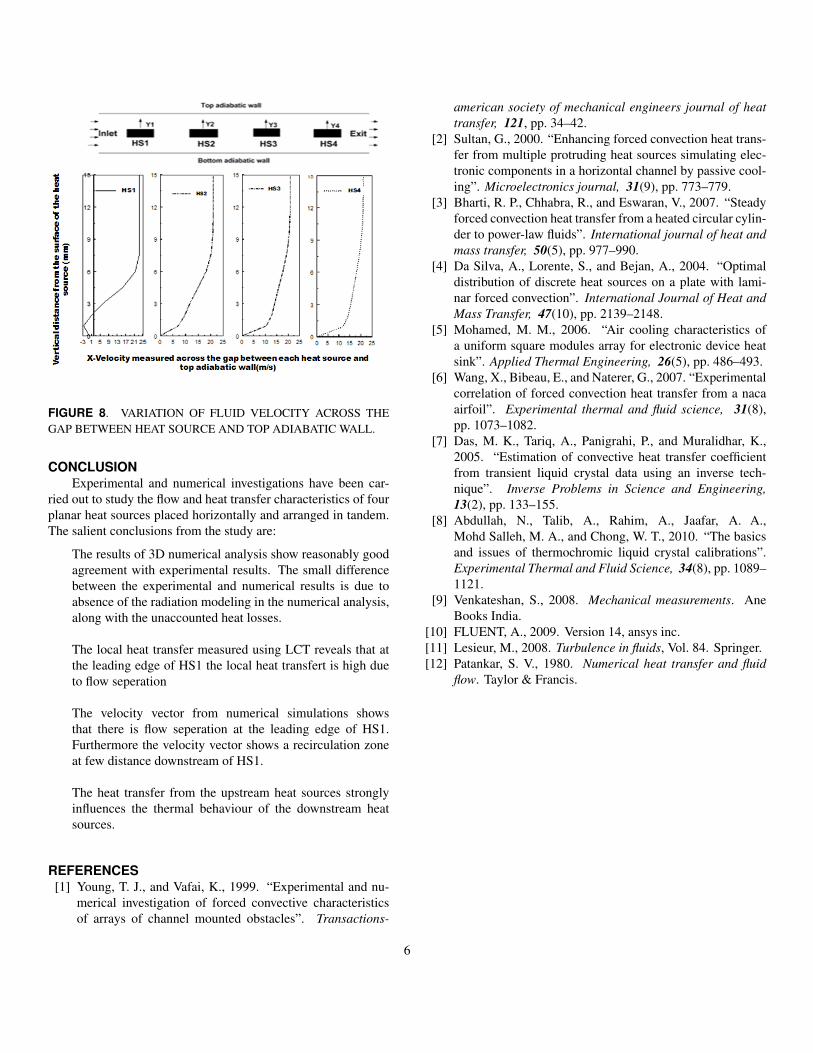
FIGURE 8. VARIATION OF FLUID VELOCITY ACROSS THEGAP BETWEEN HEAT SOURCE AND TOP ADIABATIC WALL.

CONCLUSIONExperimental and numerical investigations have been car-

ried out to study the flow and heat transfer characteristics of fourplanar heat sources placed horizontally and arranged in tandem.The salient conclusions from the study are:

The results of 3D numerical analysis show reasonably goodagreement with experimental results. The small differencebetween the experimental and numerical results is due toabsence of the radiation modeling in the numerical analysis,along with the unaccounted heat losses.

The local heat transfer measured using LCT reveals that atthe leading edge of HS1 the local heat transfert is high dueto flow seperation

The velocity vector from numerical simulations showsthat there is flow seperation at the leading edge of HS1.Furthermore the velocity vector shows a recirculation zoneat few distance downstream of HS1.

The heat transfer from the upstream heat sources stronglyinfluences the thermal behaviour of the downstream heatsources.

REFERENCES[1] Young, T. J., and Vafai, K., 1999. “Experimental and nu-

merical investigation of forced convective characteristicsof arrays of channel mounted obstacles”. Transactions-

american society of mechanical engineers journal of heattransfer, 121, pp. 34–42.

[2] Sultan, G., 2000. “Enhancing forced convection heat trans-fer from multiple protruding heat sources simulating elec-tronic components in a horizontal channel by passive cool-ing”. Microelectronics journal, 31(9), pp. 773–779.

[3] Bharti, R. P., Chhabra, R., and Eswaran, V., 2007. “Steadyforced convection heat transfer from a heated circular cylin-der to power-law fluids”. International journal of heat andmass transfer, 50(5), pp. 977–990.

[4] Da Silva, A., Lorente, S., and Bejan, A., 2004. “Optimaldistribution of discrete heat sources on a plate with lami-nar forced convection”. International Journal of Heat andMass Transfer, 47(10), pp. 2139–2148.

[5] Mohamed, M. M., 2006. “Air cooling characteristics ofa uniform square modules array for electronic device heatsink”. Applied Thermal Engineering, 26(5), pp. 486–493.

[6] Wang, X., Bibeau, E., and Naterer, G., 2007. “Experimentalcorrelation of forced convection heat transfer from a nacaairfoil”. Experimental thermal and fluid science, 31(8),pp. 1073–1082.

[7] Das, M. K., Tariq, A., Panigrahi, P., and Muralidhar, K.,2005. “Estimation of convective heat transfer coefficientfrom transient liquid crystal data using an inverse tech-nique”. Inverse Problems in Science and Engineering,13(2), pp. 133–155.

[8] Abdullah, N., Talib, A., Rahim, A., Jaafar, A. A.,Mohd Salleh, M. A., and Chong, W. T., 2010. “The basicsand issues of thermochromic liquid crystal calibrations”.Experimental Thermal and Fluid Science, 34(8), pp. 1089–1121.

[9] Venkateshan, S., 2008. Mechanical measurements. AneBooks India.

[10] FLUENT, A., 2009. Version 14, ansys inc.[11] Lesieur, M., 2008. Turbulence in fluids, Vol. 84. Springer.[12] Patankar, S. V., 1980. Numerical heat transfer and fluid

flow. Taylor & Francis.

6

TURBULENT FLOW COOLING OF MULTIPLE PLANAR HEAT SOURCES ARRANGED IN TANDEM , Proceedings of the 22nd...

Documents

Transcript of TURBULENT FLOW COOLING OF MULTIPLE PLANAR HEAT SOURCES ARRANGED IN TANDEM , Proceedings of the 22nd...