An empirical approach for estimating macro-turbulent heat transport conditional upon the time mean...

2070 VOLUME 56J O U R N A L O F T H E A T M O S P H E R I C S C I E N C E S

q 1999 American Meteorological Society

An Empirical Approach for Estimating Macroturbulent Heat TransportConditional upon the Mean State

UTE LUKSCH AND HANS VON STORCH

Meteorologisches Institut der Universitat Hamburg, Hamburg, Germany

(Manuscript received 14 January 1998, in final form 17 August 1998)

ABSTRACT

A stochastic specification for monthly mean wintertime eddy heat transport conditional upon the monthlymean circulation is proposed. The approach is based on an analog technique. The nearest neighbor for themonthly mean streamfunction (at 850 and 300 hPa) is searched for in a library composed of monthly data of a1268-yr control simulation with a coupled ocean–atmosphere model. To reduce the degrees of freedom a limitedarea (the North Atlantic sector) is used for the analog specification. The monthly means of northward transienteddy flux of temperature (at 750 hPa) are simulated as a function of these analogues.

The stochastic model is applied to 300 years of a paleosimulation (last interglacial maximum around 125 kyrBP). The level of variability of the eddy heat flux is reproduced by the analog estimator, as well as the linkbetween monthly mean circulation and synoptic-scale variability. The changed boundary conditions (solar ra-diation and CO2 level) cause the Eemian variability to be significantly reduced compared to the control simulation.Although analogues are not a very good predictor of heat fluxes for individual months, they turn out to beexcellent predictors of the distribution (or at least the variance) of heat fluxes in an anomalous climate.

1. Introduction

The analog technique has a long history in weatherforecasting; the idea is to analyze the present state andto find in a library of past cases that one that resemblesmost closely the present state. This closest case is theanalogue, and the properties of this analogue are thenassigned to the present state. In the case of day-to-dayor seasonal forecasting, this property is the trajectoryemanating from the analogue in the next few days orin the upcoming season (Barnett and Preisendorfer1978; Drosdowsky 1994; just to mention a few). Theanalog technique for weather forecasting purposes hasbeen widely discredited. For instance, Petterssen (1957)summarized the state of the art: ‘‘While types and an-alogues . . . have been found useful as background in-formation . . . , forecasts with acceptable tolerance donot appear to be obtainable on the basis of analoguesalone.’’ Theoretical studies have shown that the librarymust be enormously large to guarantee a reasonable skillfor forecast on the daily timescale (i.e., returning a tra-jectory reasonably close to the actual trajectory; Lorenz1969; van den Dool 1994).

In spite of this general failure of the analog method

Corresponding author address: Dr. Ute Luksch, MeteorologischesInstitut der Universitat Hamburg, Bundesstrasse 55, D-20146 Ham-burg, Germany.E-mail: [email protected]

for predictive purposes, the analog technique has beenused for a number of useful purposes recently. Fraedrich(1986) and Fraedrich and Leslie (1991) studied the fore-cast problem in a phase space setup. They examined thedivergence of trajectories emanating from a state andits analogue and estimated the dimension of the attractor.In a recent study, Fraedrich and Ruckert (1998) deter-mined a metric leading to optimal forecasts. This metricdescribes a subspace of the full phase space, and Frae-drich argues that this subspace is an approximation ofthe attractor of the weather system. Another applicationdeals with the specification problem in downscaling(Zorita et al. 1995). In this case, the property of theanalogue is a variable insufficiently represented in cli-mate modeling, such as precipitation. The analogue isdetermined in terms of a variable well simulated by aclimate model, for instance, a large-scale pressure map.

In the present study, we deal with the specificationproblem of determining complex variables with the helpof known distributions. Such problems occur when tur-bulent fluxes are to be parameterized in reduced modelsor atmospheric feedbacks are to specified as a functionof sea surface temperature as in Barnett et al. (1993;Tropics) and Xu et al. (1998; North Pacific). We dealexemplarily with the specification of midlatitude mac-roturbulent meridional heat flux by means of the time-mean circulation. More specifically, we ask for a randomfunction relating the monthly mean streamfunction Cand the monthly mean of poleward eddy heat transport

1 JULY 1999 2071L U K S C H A N D V O N S T O R C H

in the Northern Hemisphere y9T9 . That is, we adopt theview that the transport is not determined by the meanstate but only conditioned by it. In probabilistic terms,the random vector X, a vector of scalar random variablesthat are the result of the same experiments, (here, month-ly mean of poleward eddy heat transport in the NorthAtlantic sector) is conditioned upon the mean state (cf.von Storch 1997). This may formally be written as

X ; P(C), (1)

where P represents a probability distribution that de-pends in some way on the variable C.

Earlier, linear regression analyses have been madelinking the mean state and the (conditional) mean trans-port (Lau 1988). In our terminology, such a regressionestablishes a linear deterministic link,

E(X) 5 SC, (2)

with the expectation operator E and some suitable matrixS. In the present analysis, the probabilistic approach[(1)] is adopted and executed by means of an analogapproach. A similar concept is used by Da Costa andVautard (1997). They used 25 years of observed datato close their low-order model for diagnosing weatherregimes with the analog technique.

By using the analog method, several advantages aregained. First, automatically a probabilistic specificationis obtained, and second, there is no need for explicitlyspecifying the conditional probability distribution P,which is an unsolved problem, nor the deterministiclinkage S. The application of the analog method requiresa large library of cases, and we are in the lucky situationof being among the first having access to large sets ofpairs of fields C and y9T9 , which have been simulatedin ultralong (thousands of years) simulations with quasi-realistic coupled ocean–atmosphere models (e.g., Man-abe and Stouffer 1994; von Storch et al. 1997). Thus,we do not claim to be more insightful than earlier sci-entists but only that we luckily have access to powerfultools that were unavailable just a few years earlier.

Equation (1) offers an intriguing perspective. It maybe used as a parameterization of macroturbulence in anatmospheric model operating with time-mean fields asstate variables, without calculating the detailed synopticactivity. Such a model automatically would be a sto-chastic climate model (Hasselmann 1976), being ableto generate long-term variations as a response to short-term random fluctuations. Simple closure relations forthe horizontal eddy fluxes cannot be derived from eddyflux equations (Opsteegh and van den Dool 1979). Anempirical approach by analogues makes sense if thevariability of monthly or seasonal mean patterns is notcompletely caused by day-to-day weather fluctuations.The path in the phase space is realistic but not applicableto the development of the real atmosphere (Opsteeghand van den Dool 1979). Therefore, we cannot expectvery high pattern correlation coefficients as a measurefor the difference between original and estimated fields.

But we can expect that the connection between low-frequency and bandpass-filtered variability measured,for example, by the canonical correlation analysis(CCA) is maintained by the analog system. The ap-proach is tested with an independent dataset where thevariability is changed in comparison with the library.This test is stronger than splitting the control run in twohalves or taking the target month out.

The paper is organized as follows. The analog modeland the data basis (library and an independent test set)are described in sections 2 and 3. Measures of skill arebriefly introduced in section 4. Afterward, the stochasticmodel is tested with data from a GCM simulation ofthe last interglacial period, using a library of a multi-century simulation of the present state (section 5). Atthe end the results are summarized and an outlook isoffered.

2. The analog specification

The analog specification is done in the phase spacespanned by EOFs; that is, the originally gridded dataare expanded into a series of EOFs:

Nc

C CC 5 a e . (3)O i ii51

In this expansion, the EOFs are normalized, \ \ 5 1,Cei

so that the variance of is maximum, that of isc Ca a1 2

second largest, and so on. To find better analogues theanalog specification area is restricted the North Atlanticsector, which is defined as the domain lying between208 and 708N latitude and 1108W and 408E longitude.Here NC is the number of grid points in this limitedarea, which may be an overestimation of the theoreticaldegree of freedom. All data are anomalies; the long-term mean of the control run is subtracted.

Given any circulation pattern, say C0, its analogueis its nearest neighbor in terms of some distance in thephase space. In general, the distance between any twofields C1 and C2 will be of the form

Nc

C C 21 2d (C , C ) 5 g [a (4)2 a ]Og 1 2 i i ii51

with suitably chosen weights gi. In our application, wetake into account only the first nC EOFs, so that g i 50 for i . nC. All other weights are set to 1. Note thatthe expected difference ( 2 )2 5 2 var( ) be-C C C1 2a a ai i i

tween two randomly selected fields C1 and C2 is de-creasing with increasing index i, so that the contribu-tions of the low-indexed EOFs are more important thanthose of high-indexed EOFs.

With this definition, the analogue C* of C0 satisfies

d (C , C ) 5 min d (C , C), (5)g 0 g 0*C∈L

where L is the library, that is, the collection of all cir-culation fields available. After this analogue of C


(monthly mean streamfunction at 300 and 850 hPa) isdetermined, a dynamically consistent macroturbulentheat transport y9T9 (monthly mean values at 750 hPa)may be determined as the heat transport observed (orsimulated) together with C*, that is,

5 v9 .v9T9 T9* (6)

The estimated flux is the monthly mean anomaly fromthe long-term mean of the control run for the neighbor‘‘∗’’. The full field y9 is used without truncation toT9*preserve variance. The estimator [(6)] depends on thechoice of the ‘‘key’’ variable C and the available libraryof cases, and on the parameters nC and the weights gi.

For the following, we need to define some technicalnomenclature. The field, for which a consistent prop-erty—in this case the monthly mean streamfunction C—is sought, is called the key field, while the y9T9 field iscalled the property field. The consistent property fieldassigned to the key field is the estimated property field.

In the basic setup, the complete key fields C neednot to be stored in the library but only the first nC EOFcoefficients. Since nC K NC the amount of requiredstorage is significantly reduced, and also the computa-tional efforts for finding the minimum [(5)] are consid-erably eased. In a similar manner, the required disk spacefor the property field library may be reduced signifi-cantly (for details, see the appendix).

Note that no feature of the property field enters theanalog determination. Indeed, when an analogue isfound for some key field, then any property attached tothe analogue may be seen as an estimate of that propertyof the original key variable. This means, in practicalterms, that when we deal with climate model data, weobtain not only an estimate of the meridional heat trans-port but also of all other properties simulated by theclimate model, be it the angular momentum, regionalsoil moisture, or intramonthly extreme values. However,when the metric used to determine the analogue is op-timized for returning best fits of the property field, asin case of Fraedrich and Ruckert (1998), an analoguesuitable for y9T9 is no longer automatically also suitablefor, say, soil moisture.

3. Ultralong ocean–atmosphere GCM simulations

For the success of our study the availability of a largelibrary of dynamically consistent cases is mandatory.We use two such ultralong simulations, namely, a 1268-yr simulation of the present climate (‘‘control run’’; vonStorch et al. 1997) and a 500-yr simulation of the lastinterglacial about 125 kyr BP (‘‘Eemian run’’; Montoyaet al. 1998). Boundary conditions of the Eemian ex-periment differ from those of the control run in twoways: CO2 is reduced (control run, 330 ppmv; Eemianrun, 267 ppmv) and the orbit parameters are changed.During Eem (approximately 125 kyr BP) the obliquityand eccentricity was increased and the perihelion oc-curred in Northern Hemisphere summer (rather than

winter, as today) causing an amplification (reduction)of the seasonal cycle of insolation in the Northern(Southern) Hemisphere. The proposed 6-m sea level risefor the Eemian results in negligible changes in the T21land–sea grid. From the control run the library is de-rived, and the data from the Eemian run are used forthe determination of the skill of the estimator (see sec-tion 4).

In the remainder of this section, we describe the setupof the two simulations, demonstrate the ability of thecontrol run to generate a quasi-realistic link betweenmean states and the meridional heat transport, and de-scribe the modifications in the meridional heat transportsimulated in the Eemian run. In section 5 we will showthat our analog estimator is able not only to reproducethe link between mean states and the heat transport butalso the modification of the heat transport variability inthe Eemian run.

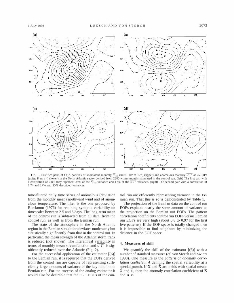
Both long-term simulations are done with the coupledocean–atmosphere Hamburg climate model (ECHAM1/LSG; Cubasch et al. 1992), which is driven by a pre-scribed annual cycle of solar radiation and a fixed con-centration of atmospheric carbon dioxide. The oceanand the atmosphere interact freely in this model, anddynamically inactive flux correction is adopted for pre-venting the model from ‘‘running away.’’ The resolutionof the GCM is around 5.68 in the longitudinal and me-ridional directions both in the atmosphere and in theocean. In spite of this rather coarse resolution the NorthAtlantic storm track is simulated reasonably well interms of its pattern, but its strength is underestimatedcompared to observations. Also, the link betweenmonthly mean states and the monthly midtroposphericheat transports are simulated reasonably well (see Fig.1; cf. Lau 1988).

The 1268-yr control run (von Storch et al. 1997) isintegrated with the present-day annual solar radiationcycle and an atmospheric CO2 concentration of 330ppm; the Eemian run (Montoya et al. 1998) was initiatedwith the state of the control run in the year 600, whenthe control run has long reached a statistical equilibriumstate in terms of atmospheric variables, and then inte-grated with a CO2 concentration of 267 ppm and ra-diation reconstructed for the time about 125 000 yearsbefore present (the ‘‘Eem’’).

In the present study only the winter months Decem-ber, January, and February are used. During the firstcenturies, the model simulations drift toward their sta-tistical equilibria. Therefore, only the 2880 cases fromthe winter months of the years 309–1268 were placedinto the library of cases. Similarly, the test with theEemian simulation was limited to the 900 winter monthsof the last 300 years of that run.

We use three variables in an area covering the NorthAtlantic in this study: the monthly mean meridional heattransport y9T9 at 750 hPa due to synoptic disturbances,and the monthly mean streamfunction at 300 and 850hPa. The meridional heat transport is calculated from


FIG. 1. First two pairs of CCA patterns of anomalous monthly C850 (units: 106 m2 s21) (upper) and anomalous monthly y9T 9 at 750 hPa(units: K m s21) (lower) in the North Atlantic sector derived from 2880 winter months simulated in the control run. (left) The first pair witha correlation of 0.85; they represent 29% of the C850 variance and 17% of the y9T 9 variance. (right) The second pair with a correlation of0.74 and 17% and 15% described variances.

time-filtered daily time series of anomalous (deviationfrom the monthly mean) northward wind and of anom-alous temperature. The filter is the one proposed byBlackmon (1976) for retaining synoptic variability ontimescales between 2.5 and 6 days. The long-term meanof the control run is subtracted from all data, from thecontrol run, as well as from the Eemian run.

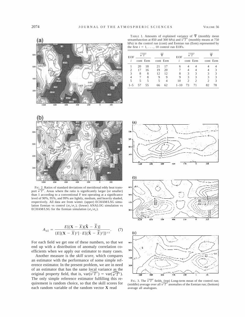
The state of the atmosphere in the North Atlanticregion in the Eemian simulation deviates moderately butstatistically significantly from that in the control run. Inparticular, the mean strength of the Atlantic storm trackis reduced (not shown). The interannual variability interms of monthly mean streamfunction and y9T9 is sig-nificantly reduced over the Atlantic (Fig. 2).

For the successful application of the estimator [(6)]to the Eemian run, it is required that the EOFs derivedfrom the control run are capable of representing suffi-ciently large amounts of variance of the key field in theEemian run. For the success of the analog estimator itwould also be desirable that the y9T9 EOFs of the con-

trol run are efficiently representing variance in the Ee-mian run. That this is so is demonstrated by Table 1.

The projection of the Eemian data on the control runEOFs explains nearly the same amount of variance asthe projection on the Eemian run EOFs. The patterncorrelation coefficients control run EOFs versus Eemianrun EOFs are very high (about 0.8 to 0.97 for the firstfive patterns). If the EOF space is totally changed thenit is impossible to find neighbors by minimizing thedistance in the EOF space.

4. Measures of skill

We quantify the skill of the estimator [(6)] with anumber of standard measures (cf. von Storch and Zwiers1998). One measure is the pattern or anomaly corre-lation coefficient A defining the spatial variability at aspecial month. If X and X are fields with spatial meansX and , then the anomaly correlation coefficient of XXand X is


FIG. 2. Ratios of standard deviations of meridional eddy heat trans-port y9T 9 . Areas where the ratio is significantly larger (or smaller)than 1 according to a conventional F test operating at a significancelevel of 90%, 95%, and 99% are lightly, medium, and heavily shaded,respectively. All data are from winter. (upper) ECHAM/LSG simu-lation Eemian vs control (sE/sC); (lower) ANALOG simulation vsECHAM/LSG for the Eemian simulation (sA/sE).

TABLE 1. Amounts of explained variance of C (monthly meanstreamfunction at 850 and 300 hPa) and y9T 9 (monthly means at 750hPa) in the control run (cont) and Eemian run (Eem) represented bythe first i 5 1, . . . , 10 control run EOFs.

EOFi

y9T 9

cont Eem

C

cont EemEOF

i

y9T 9

cont Eem

C

cont Eem

12345

2017

875

1816

885

211912

95

172012

94

6789

10

44332

44332

44332

43333

1–5 57 55 66 62 1–10 73 71 82 78

FIG. 3. The y9T 9 fields. (top) Long-term mean of the control run;(middle) average over all y9T 9 anomalies of the Eemian run; (bottom)average all analogues.

ˆ ˆE [(X 2 X )(X 2 X )]A 5 . (7)ˆXX

2 2 1/2ˆ ˆ{E [(X 2 X ) ] · E [(X 2 X ) ]}

For each field we get one of these numbers, so that weend up with a distribution of anomaly correlation co-efficients when we apply our estimator to many cases.

Another measure is the skill score, which comparesan estimator with the performance of some simple ref-erence estimator. In the present problem, we are in needof an estimator that has the same local variance as theoriginal property field, that is, var(y9T9) 5 var( ).y T9 9The only simple reference estimator fulfilling this re-quirement is random choice, so that the skill scores foreach random variable of the random vector X read


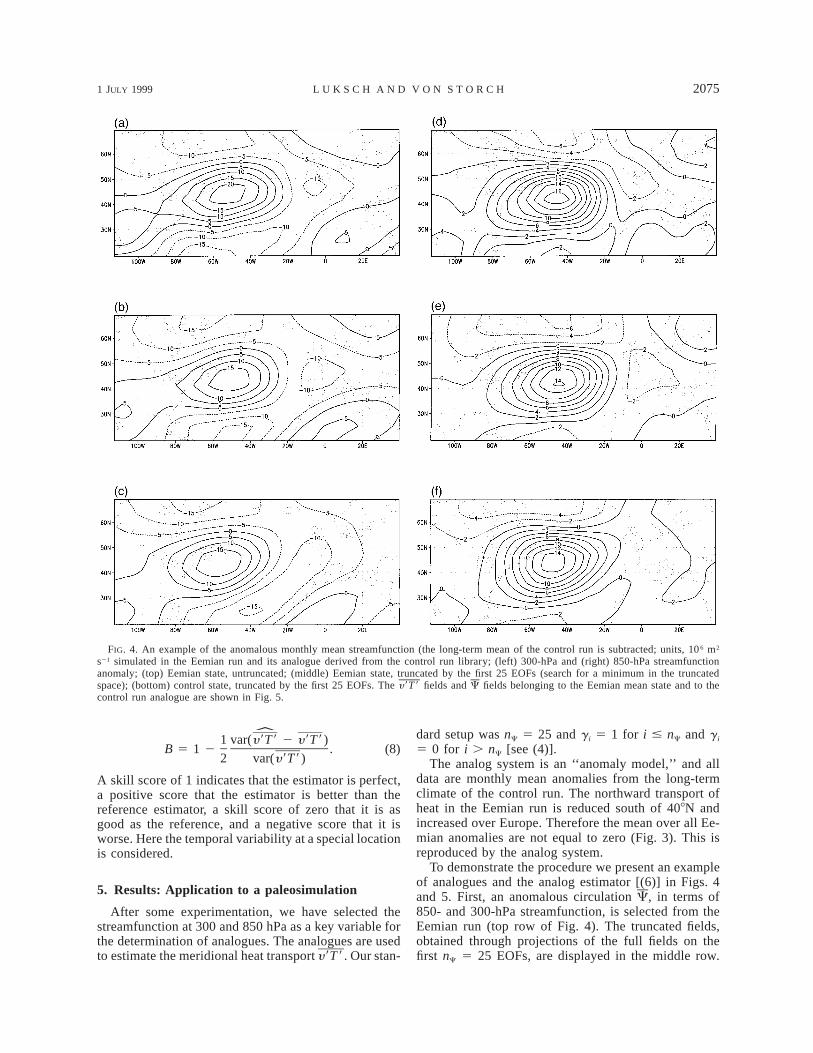
FIG. 4. An example of the anomalous monthly mean streamfunction (the long-term mean of the control run is subtracted; units, 10 6 m2

s21 simulated in the Eemian run and its analogue derived from the control run library; (left) 300-hPa and (right) 850-hPa streamfunctionanomaly; (top) Eemian state, untruncated; (middle) Eemian state, truncated by the first 25 EOFs (search for a minimum in the truncatedspace); (bottom) control state, truncated by the first 25 EOFs. The y9T 9 fields and C fields belonging to the Eemian mean state and to thecontrol run analogue are shown in Fig. 5.

1 var(y9T9 2 y9T9)B 5 1 2 . (8)

2 var(y9T9)

A skill score of 1 indicates that the estimator is perfect,a positive score that the estimator is better than thereference estimator, a skill score of zero that it is asgood as the reference, and a negative score that it isworse. Here the temporal variability at a special locationis considered.

5. Results: Application to a paleosimulation

After some experimentation, we have selected thestreamfunction at 300 and 850 hPa as a key variable forthe determination of analogues. The analogues are usedto estimate the meridional heat transport y9T9 . Our stan-

dard setup was nC 5 25 and g i 5 1 for i # nC and gi

5 0 for i . nC [see (4)].The analog system is an ‘‘anomaly model,’’ and all

data are monthly mean anomalies from the long-termclimate of the control run. The northward transport ofheat in the Eemian run is reduced south of 408N andincreased over Europe. Therefore the mean over all Ee-mian anomalies are not equal to zero (Fig. 3). This isreproduced by the analog system.

To demonstrate the procedure we present an exampleof analogues and the analog estimator [(6)] in Figs. 4and 5. First, an anomalous circulation C, in terms of850- and 300-hPa streamfunction, is selected from theEemian run (top row of Fig. 4). The truncated fields,obtained through projections of the full fields on thefirst nC 5 25 EOFs, are displayed in the middle row.


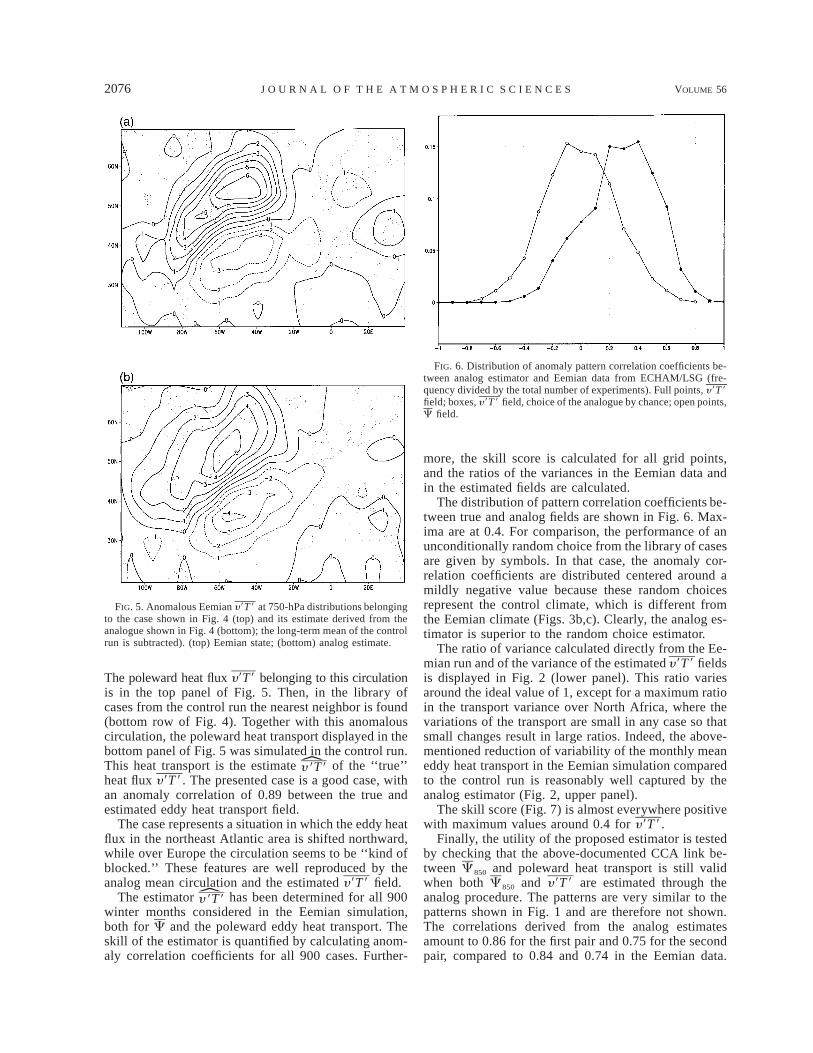
FIG. 5. Anomalous Eemian y9T 9 at 750-hPa distributions belongingto the case shown in Fig. 4 (top) and its estimate derived from theanalogue shown in Fig. 4 (bottom); the long-term mean of the controlrun is subtracted). (top) Eemian state; (bottom) analog estimate.

FIG. 6. Distribution of anomaly pattern correlation coefficients be-tween analog estimator and Eemian data from ECHAM/LSG (fre-quency divided by the total number of experiments). Full points, y9T 9field; boxes, y9T 9 field, choice of the analogue by chance; open points,C field.

The poleward heat flux y9T9 belonging to this circulationis in the top panel of Fig. 5. Then, in the library ofcases from the control run the nearest neighbor is found(bottom row of Fig. 4). Together with this anomalouscirculation, the poleward heat transport displayed in thebottom panel of Fig. 5 was simulated in the control run.This heat transport is the estimate of the ‘‘true’’y T9 9heat flux y9T9 . The presented case is a good case, withan anomaly correlation of 0.89 between the true andestimated eddy heat transport field.

The case represents a situation in which the eddy heatflux in the northeast Atlantic area is shifted northward,while over Europe the circulation seems to be ‘‘kind ofblocked.’’ These features are well reproduced by theanalog mean circulation and the estimated y9T9 field.

The estimator has been determined for all 900y T9 9winter months considered in the Eemian simulation,both for C and the poleward eddy heat transport. Theskill of the estimator is quantified by calculating anom-aly correlation coefficients for all 900 cases. Further-

more, the skill score is calculated for all grid points,and the ratios of the variances in the Eemian data andin the estimated fields are calculated.

The distribution of pattern correlation coefficients be-tween true and analog fields are shown in Fig. 6. Max-ima are at 0.4. For comparison, the performance of anunconditionally random choice from the library of casesare given by symbols. In that case, the anomaly cor-relation coefficients are distributed centered around amildly negative value because these random choicesrepresent the control climate, which is different fromthe Eemian climate (Figs. 3b,c). Clearly, the analog es-timator is superior to the random choice estimator.

The ratio of variance calculated directly from the Ee-mian run and of the variance of the estimated y9T9 fieldsis displayed in Fig. 2 (lower panel). This ratio variesaround the ideal value of 1, except for a maximum ratioin the transport variance over North Africa, where thevariations of the transport are small in any case so thatsmall changes result in large ratios. Indeed, the above-mentioned reduction of variability of the monthly meaneddy heat transport in the Eemian simulation comparedto the control run is reasonably well captured by theanalog estimator (Fig. 2, upper panel).

The skill score (Fig. 7) is almost everywhere positivewith maximum values around 0.4 for y9T9 .

Finally, the utility of the proposed estimator is testedby checking that the above-documented CCA link be-tween C850 and poleward heat transport is still validwhen both C850 and y9T9 are estimated through theanalog procedure. The patterns are very similar to thepatterns shown in Fig. 1 and are therefore not shown.The correlations derived from the analog estimatesamount to 0.86 for the first pair and 0.75 for the secondpair, compared to 0.84 and 0.74 in the Eemian data.


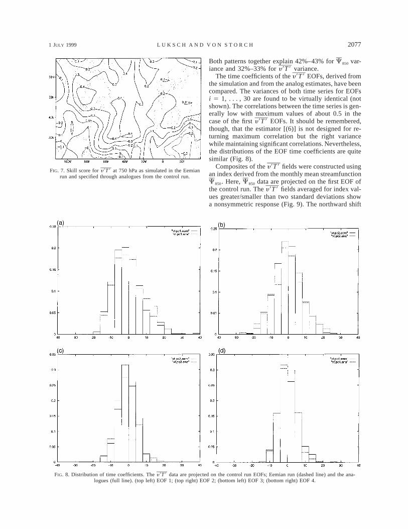
FIG. 7. Skill score for y9T 9 at 750 hPa as simulated in the Eemianrun and specified through analogues from the control run.

FIG. 8. Distribution of time coefficients. The y9T 9 data are projected on the control run EOFs; Eemian run (dashed line) and the ana-logues (full line). (top left) EOF 1; (top right) EOF 2; (bottom left) EOF 3; (bottom right) EOF 4.

Both patterns together explain 42%–43% for C850 var-iance and 32%–33% for y9T9 variance.

The time coefficients of the y9T9 EOFs, derived fromthe simulation and from the analog estimates, have beencompared. The variances of both time series for EOFsi 5 1, . . . , 30 are found to be virtually identical (notshown). The correlations between the time series is gen-erally low with maximum values of about 0.5 in thecase of the first y9T9 EOFs. It should be remembered,though, that the estimator [(6)] is not designed for re-turning maximum correlation but the right variancewhile maintaining significant correlations. Nevertheless,the distributions of the EOF time coefficients are quitesimilar (Fig. 8).

Composites of the y9T9 fields were constructed usingan index derived from the monthly mean streamfunctionC850. Here, C850 data are projected on the first EOF ofthe control run. The y9T9 fields averaged for index val-ues greater/smaller than two standard deviations showa nonsymmetric response (Fig. 9). The northward shift


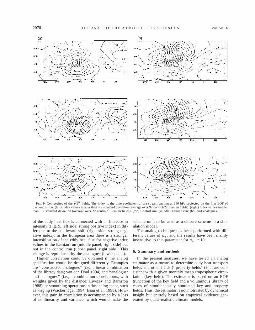
FIG. 9. Composites of the y9T 9 fields. The index is the time coefficient of the streamfunction at 850 hPa projected on the first EOF ofthe control run. (left) index values greater than 12 standard deviation (average over 92 control/22 Eemian fields). (right) Index values smallerthan 22 standard deviation (average over 22 control/8 Eemian fields). (top) Control run; (middle) Eemian run; (bottom) analogues.

of the eddy heat flux is connected with an increase inintensity (Fig. 9, left side: strong positive index) in dif-ference to the southward shift (right side: strong neg-ative index). In the European area there is a strongerintensification of the eddy heat flux for negative indexvalues in the Eemian run (middle panel, right side) butnot in the control run (upper panel, right side). Thischange is reproduced by the analogues (lower panel).

Higher correlation could be obtained if the analogspecification would be designed differently. Examplesare ‘‘constructed analogues’’ (i.e., a linear combinationof the library data; van den Dool 1994) and ‘‘analogue/anti-analogues’’ (i.e., a combination of neighbors, withweights given by the distance; Livezey and Barnston1988), or smoothing operations in the analog space, suchas kriging (Wackernagel 1994; Biau et al. 1999). How-ever, this gain in correlation is accompanied by a lossof nonlinearity and variance, which would make the

scheme unfit to be used as a closure scheme in a sim-ulation model.

The analog technique has been performed with dif-ferent values of nC, and the results have been mainlyinsensitive to this parameter for nC $ 10.

6. Summary and outlook

In the present analyses, we have tested an analogestimator as a means to determine eddy heat transportfields and other fields (‘‘property fields’’) that are con-sistent with a given monthly mean tropospheric circu-lation (key field). The estimator is based on an EOFtruncation of the key field and a voluminous library ofcases of simultaneously simulated key and propertyfields. Thus, the estimator is not motivated by dynamicalinsight but entirely based on empirical evidence gen-erated by quasi-realistic climate models.


The proposed scheme has been tested with indepen-dent data from a climate model simulation of the lastinterglacial (Eem, approximately 125 kyr BP). The sim-ulated decrease of eddy activity as well as the link be-tween the mean circulation and the eddy activity sim-ulated in this climate model integration are reproducedby the estimator. In particular it demonstrates that evenwhen analogues are not particularly adept at predictingeddy heat fluxes associated with individual monthlymean states, they can be remarkably accurate predictorsof the distribution of monthly mean eddy flux fields thatoccur in anomalous climates.

It is suggested to use this estimator as an empiricalmeans for closing the macroturbulent problem in sim-plified atmospheric and ocean large-scale modeling.Simple closure relations for the horizontal eddy fluxescannot be derived from eddy flux equations (Opsteeghand van den Dool 1979). An empirical approach byanalogues makes sense if the variability of monthly orseasonal mean patterns is not completely caused by day-to-day weather fluctuations. The path in the phase spaceis realistic but not applicable to the development of thereal atmosphere (Opsteegh and van den Dool 1979).Therefore, we cannot expect very high pattern corre-lation coefficients as a measure for the difference be-tween original and estimated fields. But we can expectthat the connection between low- and high-frequencyvariability measured, for example, by the CCA is main-tained by the analog system. For these first tests of themethod we used an independent dataset where the var-iability is changed in comparison with the library. Thisis a stronger test than cutting the control run in twohalves or taking the target month out. A test with a localregression model (not shown here) gives nearly the samedistribution of pattern correlation coefficients as in Fig.6 but the the CCA patterns are totally changed and thecorrelation coefficients are much too high. The analogapproach will fail if the EOF space is totally changedin the library and the test set. In this case it is impossibleto find neighbors by minimizing the distance in the EOFspace.

Acknowledgments. The present analysis was done inthe framework of the project MILLENNIA funded bythe Climate and Environment Programme of the Eu-ropean Commission. We thank Jin-Song von Storch,Marisa Montoya, Eduardo Zorita, and Viatcheslav Khar-in for their support. Computational assistance was of-fered by Matthias Dorn. Finally, we thank the reviewersfor their valuable comments.

APPENDIX

A Computationally Efficient Way of GeneratingConsistent Property Fields

If the number of grid points NyT of the property fieldy9T9 is large, it may be computationally inefficient to

store all complete fields in the library. In that case, itmay be advantageous to expand the property field intoan EOF series,

NyT

yT yTv9T9 5 a e , (A1)O i ii51

and to keep only the first nyT EOF coefficients, with nyT

K NyT. Then the estimated property field is composedof nyT EOF ‘‘analog’’ coefficients and NyT 2 nyT 2 1randomly drawn coefficients:

Nm yT

yT yT yT *5 a e 1 h e , (A2)O Ov9T9 i i i i0i51 i5m11

where is the ith EOF coefficient of the propertyyT*ai

field associated with C*, and hi is randomly drawny9T9*from a normal distribution with mean zero and a vari-ance equal to that of the ith EOF coefficient.

The first sum on the right side of (A2) is the analogpart, and the second sum is the noise part. This splittingis motivated by the observation that only the most im-portant EOFs contribute skillfully to the estimate. How-ever, a truncation of the property field to the first nyT

EOFs would return an estimated property field with anunderestimated spatial variance. Therefore, the coeffi-cients of the remaining EOFs are drawn at random.

For this procedure, it is needed that the first nyT EOFcoefficients of the property field y9T9 are kept in thelibrary, and the variances of the remaining NyT 2 nyT

2 1 EOF coefficients.

REFERENCES

Barnett, T. P., and R. W. Preisendorfer, 1978: Multifield analog pre-diction of short-term climate fluctuations using a climate statevector. J. Atmos. Sci, 35, 1771–1787., M. Latif, N. Graham, M. Flugel, S. Pazan, and W. White, 1993:ENSO and ENSO-related predictability. Part I: Prediction ofequatorial Pacific sea surface temperature with hybrid coupledocean–atmosphere model. J. Climate, 6, 1545–1566.

Biau, G., E. Zorita, H. von Storch, and H. Wackernagel, 1999: Es-timation of precipitation by kriging in the EOF space of the sealevel pressure field. J. Climate, 12, 1070–1085.

Blackmon, M. L., 1976: A climatological spectral study of the 500mb geopotential height of the Northern Hemisphere. J. Atmos.Sci., 33, 1607–1623.

Cubasch, U., K. Hasselmann, H. Hock, E. Maier-Reimer, U. Miko-lajewicz, B. D. Santer, and R. Sausen, 1992: Time-dependentgreenhouse warming computations with a coupled ocean–at-mosphere model. Climate Dyn., 8, 55–69.

da Costa, E., and R. Vautard, 1997: A qualitatively realistic low-ordermodel of the extratropical low-frequency variability built fromlong records of potential vorticity. J. Atmos. Sci., 54, 1064–1984.

Drosdowksy, W., 1994: Analog (nonlinear) forecasts of the SouthernOscillation index time series. Wea. Forecasting, 9, 78–84.

Fraedrich, K., 1986: Estimating the dimension of weather and climateattractors. J. Atmos. Sci., 43, 331–344., and L. Leslie, 1991: Predictability studies of the Antarcticatmosphere. Aust. Meteor. Mag., 39, 1–9., and B. Ruckert, 1998: Metric adaption for analog forecasting.Physica A, 254, 379–393.

Hasselmann, K., 1976: Stochastic climate models. Part I. Theory.Tellus, 28, 473–485.


Lau, N.-C., 1988: Variability of the observed midlatitude storm tracksin relation to low-frequency changes in the circulation patterns.J. Atmos. Sci., 45, 2718–2743.

Livezey, R. E., and A. G. Barnston, 1988: An operational multifieldanalog/antianalog prediction system for United States seasonaltemperatures. Part I: System design and winter experiments. J.Geophys. Res., 93 (D9), 10 953–10 974.

Lorenz, E. N., 1969: Atmospheric predictability as revealed by nat-urally occurring analogues. J. Atmos. Sci., 26, 636–646.

Manabe, S., and R. J. Stouffer, 1994: Multiple-century response ofa coupled ocean–atmosphere model to an increase of atmosphericcarbon dioxide. J. Climate, 7, 5–23.

Montoya, M., T. J. Crowley, and H. von Storch, 1998: Temperaturesat the last interglacial simulated by a coupled ocean–atmosphereclimate model. Paleooceanogr., 13, 170–177.

Opsteegh, J. D., and H. M. van den Dool, 1979: A diagnostic studyof the time mean atmosphere over nortwestern Europe duringwinter. J. Atmos. Sci., 36, 1862–1879.

Petterssen, S., 1957: Weather observations, analysis and forecasting.Meteor. Monogr., No. 3, Amer. Meteor. Soc., 114–151.

van den Dool, H. M., 1994: Searching for analogues, how long mustwe wait? Tellus, 46A, 314–324.

von Storch, H., 1997: Conditional statistical models: A discourseabout the local scale in climate modelling. Monte Carlo Simu-lations in Oceanography, Proc. ’Aha Huliko’a Hawaiian WinterWorkshop, Manoa, HI, University of Hawaii, 58–59., and F. W. Zwiers, 1998: Statistical Analysis in Climate Re-search. Cambridge University Press, 528 pp.

von Storch, J.-S., V. Kharin, U. Cubasch, G. C. Hegerl, D. Schriever,H. von Storch, and E. Zorita, 1997: A description of a 1260-year control integration with the coupled ECHAM1/LSG generalcirculation model. J. Climate, 10, 1526–1544.

Wackernagel, H., 1994: Cokriging versus kriging in regionalized mul-tivariate data analysis. Geoderma, 62, 83–92.

Xu, W., T. P. Barnett, and M. Latif, 1998: Decadal variability in theNorth Pacific as simulated by a hybrid coupled model. J. Climate,11, 297–312.

Zorita, E., J. P. Hughes, D. P. Lettenmaier, and H. von Storch, 1995:Stochastic characterization of regional circulation patterns forclimate model diagnosis and estimation of local precipitation. J.Climate, 8, 1023–1042.

An empirical approach for estimating macro-turbulent heat transport conditional upon the time mean...

Documents

Transcript of An empirical approach for estimating macro-turbulent heat transport conditional upon the time mean...