Habitat Characteristics Predicting Distribution and Abundance Patterns of Scallops in...

Habitat Characteristics Predicting Distribution andAbundance Patterns of Scallops in D’EntrecasteauxChannel, TasmaniaTania Mendo1*, Jeremy M. Lyle1, Natalie A. Moltschaniwskyj2, Sean R. Tracey1, Jayson M. Semmens1

1 Institute for Marine and Antarctic Studies, University of Tasmania, Hobart, Tasmania, Australia, 2 School of Environmental and Life Sciences, University of Newcastle,

Ourimbah, New South Wales, Australia

Abstract

Habitat characteristics greatly influence the patterns of distribution and abundance in scallops, providing structure for thesettlement of spat and influencing predation risk and rates of survival. Establishing scallop-habitat relationships is relevantto understanding the ecological processes that regulate scallop populations and to managing critical habitats. Thisinformation is particularly relevant for the D’Entrecasteaux Channel, south-eastern Tasmania (147.335 W, 43.220 S), a regionthat has supported significant but highly variable scallop production over many years, including protracted periods of stockcollapse. Three species of scallops are present in the region; the commercial scallop Pecten fumatus, the queen scallopEquichlamys bifrons, and the doughboy scallop Mimachlamys asperrima. We used dive surveys and Generalized AdditiveModelling to examine the relationship between the distribution and abundance patterns of each species and associatedhabitat characteristics. The aggregated distribution of each species could be predicted as a function of sediment type andspecies-specific habitat structural components. While P. fumatus was strongly associated with finer sediments and E. bifronswith coarse grain sediments, M. asperrima had a less selective association, possibly related to its ability to attach on a widerange of substrates. Other habitat characteristics explaining P. fumatus abundance were depth, Asterias amurensisabundance, shell and macroalgae cover. Equichlamys bifrons was strongly associated with macroalgae and seagrass cover,whereas M. asperrima abundance was greatly explained by sponge cover. The models define a set of relationships fromwhich plausible hypotheses can be developed. We propose that these relationships are mediated by predation pressure aswell as the specific behavioural characteristics of each species. The findings also highlight the specific habitat characteristicsthat are relevant for spatial management and habitat restoration plans.

Citation: Mendo T, Lyle JM, Moltschaniwskyj NA, Tracey SR, Semmens JM (2014) Habitat Characteristics Predicting Distribution and Abundance Patterns ofScallops in D’Entrecasteaux Channel, Tasmania. PLoS ONE 9(1): e85895. doi:10.1371/journal.pone.0085895

Editor: Christopher J. Fulton, The Australian National University, Australia

Received September 26, 2013; Accepted December 9, 2013; Published January 13, 2014

Copyright: � 2014 Mendo et al. This is an open-access article distributed under the terms of the Creative Commons Attribution License, which permitsunrestricted use, distribution, and reproduction in any medium, provided the original author and source are credited.

Funding: This project was funded by the Fishwise Community Grants Scheme administered by the Department of Primary Industries, Parks, Water andEnvironment, Australia. The first author was supported by an Endeavour International Postgraduate Research Scholarship (EIPRS). The funders had no role in studydesign, data collection and analysis, decision to publish, or preparation of the manuscript.

Competing Interests: The authors have declared that no competing interests exist.

* E-mail: [email protected]

Introduction

The distribution and abundance of scallops are influenced by

habitat characteristics such as depth, substrate type, currents,

turbidity, and salinity (see review by [1]). At a finer spatial scale

structural components of habitat, such as presence of polychaete

tubes [2], hydroids [3]), sponges [4], macroalgae [5] and or shells

[6], provide settlement substrates for settled scallop larvae or ‘spat’.

Attachment by spat on structures can reduce predation rates [7],

enhance growth - as an elevated position in the water column

provides access to better quality food [8], and avoids smothering

by soft sediments [9].

The value of habitat structure in reducing risk of predation

continues into the juvenile and adult phase. Habitat characteristics

greatly influence predation by affecting predation efficiency and

predator-prey encounter rates [10,11]. Predator encounters are

reduced for juvenile bay scallops Argopecten irradians by attaching to

the upper canopy of the eelgrass Zostera marina [7]. Complex

habitats with greater numbers of horse mussels, sponges and

ascidians provide refuge for Pecten novaezelandiae from predation by

sea stars and gastropods [12]. Beyond directly reducing scallop

visibility to predators, structure may impact movement and

foraging behaviours of predators, as is the case with the queen

scallop Equichlamys bifrons which suffer less predation mortality in

seagrass beds than on bare sand because starfish have reduced

mobility within the seagrass [13].

Despite the apparent importance of specific habitat character-

istics in influencing scallop distribution and abundance patterns,

quantitative studies on scallop-habitat relationships are rare.

Identifying the habitat characteristics to which scallops are

associated is relevant in managing, conserving, and even restoring

these habitats. This type of information is particularly necessary

for the D’Entrecasteaux Channel, south-eastern Tasmania, where

three species of scallops co-occur; the commercial scallop Pecten

fumatus, queen scallop Equichlamys bifrons, and doughboy scallop

Mimachlamys asperrima. The D’Entrecasteaux Channel supported a

significant commercial dredge fishery for scallops from the early

1920s to late 1960s, with catches peaking 4500 tonnes of meat in

the mid 1960s and declining rapidly thereafter [14]. Significant

depletions of scallop populations have occurred throughout the

PLOS ONE | www.plosone.org 1 January 2014 | Volume 9 | Issue 1 | e85895

history of the fishery, resulting in area closures to allow for stock

recovery. In 1990 the D’Entrecasteaux Channel was declared a

recreational-only scallop fishery [15] but the fishery was closed

shortly afterwards due to the lack of scallops. By the mid-2000s

there was evidence of stock rebuilding, following more than a

decade of fishery closure, that led to the area being reopened as a

dive-only fishery in 2005, with a reduced daily bag limit of 40

scallops per person. Despite this ostensibly ‘conservative’ approach

to management, the abundance of commercial scallops declined

by approximately 80% between 2006 and 2010, due in part to the

effects of fishing coupled with natural mortality and poor

recruitment during this period [16].

The three co-occurring scallop species exhibited distinct and

temporally consistent distribution patterns within the area during

the 2000s [16], suggesting that species-specific habitat require-

ments may have an influence on their distribution. The abundance

of scallops, however, has varied significantly from year to year,

with variable and episodic recruitment experienced by each of the

species. Pecten fumatus is found mainly on a range of soft sediment

substrates including silt-sand and coarse sand [17,18]. Pecten

fumatus spat bysally attach to filamentous substrate such as

macroalgae until approximately 6–10 mm in shell length when

they release the byssus and then recess in the substrate [19].

Equichlamys bifrons, do not recess [20] and are often found in

association with the seagrass Heterozostera tasmanica [13,18].

Mimachlamys asperrima, bysally attach throughout their lifetime to

a wide range of substrates such as bryozoans, seaweeds, sponges,

oysters, mussels, old scallop shells, timber and rock [21].

An understanding of the relationships between habitat charac-

teristics and the distribution and abundance patterns of each of

these three species of scallops will provide insight into the

ecological processes that regulate these populations. Being a

relatively shallow and sheltered system, the D’Entrecasteaux

Channel provided a unique opportunity to study the patterns of

distribution by direct observation. In this study we have used dive

surveys to examine the relationship between the distribution and

abundance patterns of each species and associated habitat

characteristics, including structural components, sediment type,

predator abundance and depth. We hypothesize that specific

habitat features influence the patterns of distribution of each

species in different ways and discuss how these relationships are

possibly mediated by predation pressure and the behavioural

characteristics of each species.

Materials and Methods

Study AreaThe D’Entrecasteaux Channel (147.33590 W and 43.22028 S),

separates Bruny Island from the Tasmanian mainland. It was

divided into four sections based on topography and bathymetry: a

narrow northern section with an average depth of 20 m (Area 1 in

Fig. 1), an extensive shallow mid-section with an average depth of

15 m (Area 2), a narrow central area with stronger currents than

the other Areas and an average depth of 14 m (Area 3) and a

southern region with an average depth of 40 m which opens to the

Southern Ocean (Area 4) [18,22]. D’Entrecasteaux Channel

(Channel) system is micro-tidal, with a spring tide ranging up to

1 m [22]. The study was conducted under the Authority of the

Department of Primary Industries, Parks, Water and Environment

(DPIPWE) permit No. 10028.

Distribution PatternsScallop distribution and abundance in the Channel were

quantified using dive surveys of 59 sites defined in [16]. The

survey sites were restricted to depths ,20 m and to soft sediments.

Briefly, at each site, a 100 m transect was laid in a haphazard

direction from the boat and two divers then searched and collected

all scallops 1 m either side of the transect line covering an area of

200 m2. The species and shell length (largest distance parallel to

the hinge) was recorded for each scallop collected. However, given

the potential for very small scallops to be underrepresented due to

collection bias based on size, analyses have been limited to include

only individuals .30 mm. The numbers of two potential scallop

predators, the native eleven-arm sea star Coscinasterias muricata and

the invasive northern Pacific sea star Asterias amurensis, was also

recorded for each transect.

Patterns of scallop abundance were analyzed by comparing

them to a Poisson (random) distribution, which assumes that the

expected number of organisms is the same in all sampling areas

and is equal to the mean [23]. Agreement between observed and

expected values was evaluated using a chi-square test of goodness

of fit at the 5% level of significance, the null hypothesis being that

the distribution did not differ significantly from a Poisson

distribution [24]. To evaluate if the distribution was aggregated,

the standardised Morisita’s Index of dispersion (I) was used

because it is independent of population density and sample size

[25]. This index ranges from 21 to +1, with zero indicating a

random distribution pattern and negative values indicating a

uniform distribution and positive values an aggregated distribution

pattern [26]. Values .20.5 and ,0.5 are significant at the 5%

level.

Habitat Structural Components, Sediment Type andDepthThe main habitat structural components of the surveyed sites

were macroalgae species (including seagrass), sponges, and shell

debris. To generate semi-quantitative estimates of coverage, these

structural components were ranked using a three-point scale of

relative abundance. Sponges were ranked as being absent when

none were recorded within the transect area, low when 1–10

sponges were counted and medium when more than 10 were

present. Macroalgae and shell cover were estimated visually and

when the component was not observed within the transect area it

was ranked as absent, low when the coverage was judged to be less

than about 10% and medium when the coverage was .10%.

None of these components, however, had coverage levels in excess

of 50%.

A sediment core, taken to a depth of approximately 2 cm, was

collected by divers at each site for grain size assessment. Samples

were dispersed using calgon (0.5% [mass:volume] sodium

hexametaphosphate) [27] and then oven dried (60uC, 48 hours),

weighed and shaken through a series of eight sieves ranging from

63 mm to 8 mm. The sediment in each sieved fraction was

weighed to the nearest 0.1 gram and the cumulative percentage by

weight of the eight fractions was calculated and the mean plotted

against a phi (F) scale where:

W~log2d

where d is particle diameter in millimeters. Mean grain size (dm)

was estimated using phi values corresponding to the 16th, 50th and

84th percentiles of the cumulative proportion of weight using the

formula:

dm~W16zW50zW84

3½28�

Habitat Predicting Scallop Abundance


where larger dm values correspond to finer grain sizes [29]. Mean

grain size was classified according to the Wentworth scale [29]

which combines numerical intervals of grain size with rational

definitions (pebble, sand, mud, etc) [30]. Water depth was

measured at each site using dive computers within 0.1 m

precision.

Relationship between Abundance Patterns andExplanatory VariablesTo visualize the spatial distribution of scallops, sea stars, mean

grain size and depth, a triangle-based cubic interpolation

algorithm was applied to fit an interpolated surface to the average

value recorded for each site using Matlab [31]. Coastlines for maps

were extracted from [32].

Scatterplots indicated than none of the continuous explana-

tory variables (mean grain size, depth, A. amurensis and C.

muricata counts) were correlated. Scallop abundance was

modelled as a function of explanatory variables using Gener-

alized Additive Models (GAMs) [33]. Generalized Additive

Models provide a flexible framework to model the relationship

between abundance and environmental variables and have been

applied to several marine organisms [34–36]. Generalized

Additive Models were fitted using the mgcv package from the

statistic software R [37,38]. Explanatory variables were selected

if significant (p,0.05). As the data were overdispersed a quasi-

Poisson distribution was used [39]. Due to the tendency of

GAMs to overfit the basis dimension parameter k was set to a

maximum of 8 to correct for over fitting without compromising

the model [38]. Categorical variables were analysed as ordered

variables using orthogonal polynomial contrasts to examine

trends and determine whether response variables changed

linearly or nonlinearly as a function of habitat structural

component cover [40].

Model selection was based on Generalized Cross Validation

(GCV) [38], percentage deviance explained and visual exami-

nation of residuals. Spatial autocorrelation in the models’

residuals was investigated through Variogram analysis using

the geoR package v 1.6-22 in R [41]. One of the model

assumptions is there is no spatial autocorrelation. Violation of

this assumption was tested by comparing a variogram of the

deviance residuals with Monte Carlo envelope empirical

variograms computed from 300 independent random permuta-

tions of the residuals [42]. There was no evidence of significant

spatial autocorrelation on the residuals of any model as the

semi-variance was within the boundaries of the Monte Carlo

envelopes in the variograms.

Results

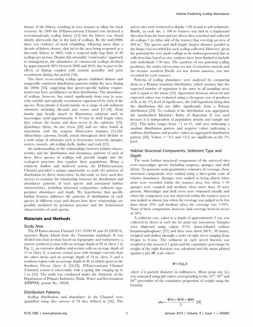
Distribution PatternsPecten fumatus were most dense in the eastern section of Area 2,

with a maximum of 85 scallops per 100 m2 but were very scarce in

Areas 1, 3 and 4 (Fig. 2). Equichlamys bifrons were most dense in

Area 3 with as many as 33 scallops per 100 m2, scarce in Areas 1,

2 and were absent in Area 4. Mimachlamys asperrima were found in

the highest densities in Areas 2 and 3, with a maximum of 73

scallops per 100 m2, but were absent in Area 4. All three species

had aggregated, non random distribution according to the

Standarised Morisita’s Index (Table 1).

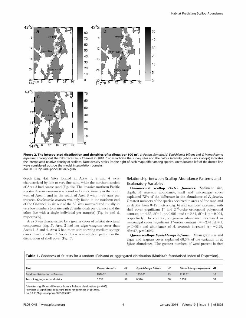
The size frequencies of the three species of scallops consisted of

multimodal distributions and were dominated by large (adult)

scallops (Fig. 3).

Habitat ElementsThe 59 sites ranged from 5.6–18.9 m in depth. The deepest

survey sites were located in Area 1, with an average depth of 13.2

meters, while the Area 2 sites were shallowest, averaging 9 m

Figure 1. Map of the D’Entrecasteaux Channel. Numbers represent the Areas referred to throughout the manuscript.doi:10.1371/journal.pone.0085895.g001



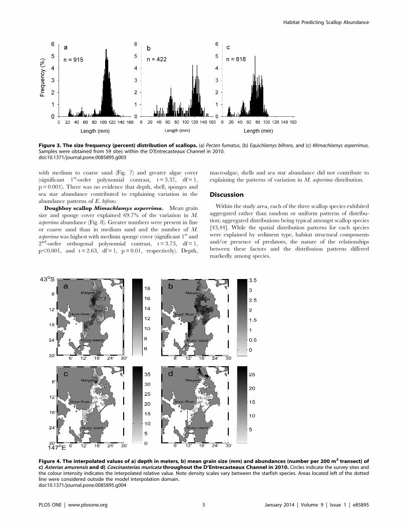
depth (Fig. 4a). Sites located in Areas 1, 2 and 4 were

characterized by fine to very fine sand, while the northern section

of Area 3 had coarse sand (Fig. 4b). The invasive northern Pacific

sea star Asterias amurensis was found in 12 sites, mainly in the north

west of Area 1 and in the south of Area 3 with 1–39 stars per

transect. Coscinasterias muricata was only found in the northern end

of the Channel, in six out of the 59 sites surveyed and usually in

very low numbers (one site with 28 individuals per transect and the

other five with a single individual per transect) (Fig. 4c and d,

respectively).

Area 3 was characterized by a greater cover of habitat structural

components (Fig. 5). Area 2 had less algae/seagrass cover than

Areas 1, 3 and 4. Area 3 had more sites showing medium sponge

cover than the other 3 Areas. There was no clear pattern in the

distribution of shell cover (Fig. 5).

Relationship between Scallop Abundance Patterns andExplanatory Variables

Commercial scallop Pecten fumatus. Sediment size,

depth, A. amurensis abundance, shell and macroalgae cover

explained 72% of the difference in the abundance of P. fumatus.

Greatest numbers of the species occurred in areas of fine sand and

in depths from 8–12 meters (Fig. 6) and numbers increased with

shell cover (significant 1st and 2nd-order orthogonal polynomial

contrast, t = 4.65, df = 1, p,0.001, and t = 2.31, df = 1, p = 0.024,

respectively). In contrast, P. fumatus abundance decreased as

macroalgal cover (significant 1st-order contrast t =22.41, df = 1,

p,0.001) and abundance of A. amurensis increased (t =22.29,

df = 57, p = 0.026).

Queen scallops Equichlamys bifrons. Mean grain size and

algae and seagrass cover explained 68.3% of the variation in E.

bifrons abundance. The greatest numbers of were present in sites

Figure 2. The interpolated distribution and densities of scallops per 100 m2. a) Pecten. fumatus, b) Equichlamys bifrons and c) Mimachlamysasperrima throughout the D’Entrecasteaux Channel in 2010. Circles indicate the survey sites and the colour intensity (white = no scallops) indicatesthe interpolated relative density of scallops. Note density scales (to the right of each map) differ among species. Areas located left of the dotted linewere considered outside the model interpolation domain.doi:10.1371/journal.pone.0085895.g002

Table 1. Goodness of fit tests for a random (Poisson) or aggregated distribution (Morisita’s Standarised Index of Dispersion).

Test Pecten fumatus df Equichlamys bifrons df Mimachlamys asperrima df

Random distribution – Poisson 2976.5* 18 1350.6* 13 2131.3* 16

Test of aggregation – Morisita 0.555‘ 58 0.546‘ 58 0.558‘ 58

*denotes significant difference from a Poisson distribution (p,0.05).‘denotes a significant departure from randomness at p,0.05.doi:10.1371/journal.pone.0085895.t001



with medium to coarse sand (Fig. 7) and greater algae cover

(significant 1st-order polynomial contrast, t = 3.37, df = 1,

p = 0.001). There was no evidence that depth, shell, sponges and

sea star abundance contributed to explaining variation in the

abundance patterns of E. bifrons.

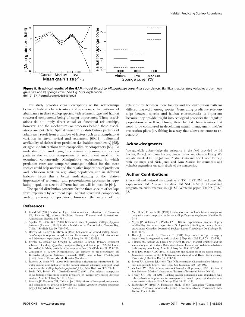
Doughboy scallop Mimachlamys asperrima. Mean grain

size and sponge cover explained 69.7% of the variation in M.

asperrima abundance (Fig. 8). Greater numbers were present in fine

or coarse sand than in medium sand and the number of M.

asperrima was highest with medium sponge cover (significant 1st and

2nd-order orthogonal polynomial contrast, t = 3.73, df = 1,

p,0.001, and t = 2.63, df = 1, p= 0.01, respectively). Depth,

macroalgae, shells and sea star abundance did not contribute to

explaining the patterns of variation in M. asperrima distribution.

Discussion

Within the study area, each of the three scallop species exhibited

aggregated rather than random or uniform patterns of distribu-

tion; aggregated distributions being typical amongst scallop species

[43,44]. While the spatial distribution patterns for each species

were explained by sediment type, habitat structural components

and/or presence of predators, the nature of the relationships

between these factors and the distribution patterns differed

markedly among species.

Figure 3. The size frequency (percent) distribution of scallops. (a) Pecten fumatus, (b) Equichlamys bifrons, and (c) Mimachlamys asperrimus.Samples were obtained from 59 sites within the D’Entrecasteaux Channel in 2010.doi:10.1371/journal.pone.0085895.g003

Figure 4. The interpolated values of a) depth in meters, b) mean grain size (mm) and abundances (number per 200 m2 transect) ofc) Asterias amurensis and d) Coscinasterias muricata throughout the D’Entrecasteaux Channel in 2010. Circles indicate the survey sites andthe colour intensity indicates the interpolated relative value. Note density scales vary between the starfish species. Areas located left of the dottedline were considered outside the model interpolation domain.doi:10.1371/journal.pone.0085895.g004



Across all species sediment type significantly explained scallop

abundance. Pecten fumatus was more strongly associated with finer

sediments, E. bifrons with coarse grain sediments, whereas M.

asperrima had a less selective association with sediment type,

possibly because this species is able to use byssal attachment on a

wide range of substrates [45]. Habitat preferences are assumed to

be adaptive, which means that associations between species and

their habitats reflect enhanced survival and reproductive success in

these particular habitats [46]. Differential abundance of bivalves

based on sediment characteristics suggests differing refuge

properties related to physical properties of the sediment or

changes in predator-prey relationships [47,48].

Prevalence of P. fumatus in fine sediments suggests that

abundances may depend, in part upon increased survival in those

sediments. The semi-burying or recessing behaviour of the

juveniles and adults, in which the upper valve is level with or

just below the surface of the sediment [1] is favoured in finer

sediments compared to coarser sediments and provides protection

from visual and non-visual predators, reduces fouling on the shell,

and can anchor the individual in areas of strong currents [1].

Moreover, this behaviour does not interfere with active predator

escape responses such as swimming [49].

While P. fumatus distribution was negatively associated with

macroalgal/seagrass cover, E. bifrons had a positive relationship

with macroalgae/seagrass cover that may be related to its use of

this structural component as a refuge from predation. Predation

rates in E. bifrons by sea stars have been shown to be lower in

seagrass beds compared to bare sand and this is linked to the

reduced mobility of sea stars within seagrass compared with over

bare sand [13]. The positive relationship between M. asperrima and

sponge abundances may be linked to the epizoic association

between M. asperrima and sponges, including the red sponge

(Crellidae family), the yellowish sponge (Myxillidae family), and

the purple honeycomb sponge (Equinochlathria sp.) [50]. This

association has the benefit that adhesion of the sea star

Coscinasterias muricata tube feet on the scallop shell is reduced on

sponges, effectively protecting the scallops from predation [50,51].

To some extent the relationships between scallop abundance

patterns and specific habitat characteristics can, therefore, be

explained in terms of the benefits that these relationships afford in

reducing predation pressure for each species.

The abundance of Coscinateris muricata did not explain distribu-

tion and abundance patterns of scallops. On the other hand,

greater abundances of P. fumatus occurred where the invasive sea

star Asterias amurensis was in relatively low numbers or absent. This

sea star was first recorded in Tasmanian waters in 1986 [52] and

its expansion within the Channel raised concerns about their

potential impact on the endemic scallop populations. Outbreaks of

this species had detrimental impacts on the shellfish industry in

Japan [53] and losses of P. fumatus spat over a settlement season

due to A. amurensis predation may be as much as 50% in Tasmania

(S. Crawford pers. comm. in [54]). The negative relationship

between the invasive A. amurensis and the scallop P. fumatus, but not

the other two species of scallops may be due to habitat-mediated

changes in predation risk [55]. Vulnerability to predation can vary

in a species-specific manner within habitat types even among

species that are morphologically and phylogenetically similar [56].

For instance, the probabilities of encountering scallops and

predation success rates for a related predator, Asterias vulgaris,

were influenced by particle size [57]. In the present study, the

nature of the relationship between A. amurensis and P. fumatus

abundance is unclear and we cannot rule out preferential habitat

use by A. amurensis or interactions with other sources of prey, such

as the distribution of other epi-benthic bivalves [58], as

explanatory factors for the sea star abundance.

This study has demonstrated that macroalgae and seagrass, shell

and sponge cover have important roles in determining adult

scallop distributions. However, it is uncertain when these

distribution patterns are established, whether at settlement and/

or as a result of post-settlement processes. Scallop spat have

distinct habitat requirements due to their need to attach to

structural elements. Therefore, the habitat characteristics associ-

ated with settlement might be very different to those observed for

the adults as observed by Howarth et al [59] for Pecten maximus and

Aequipecten opercularis. Information is needed about habitat specific-

ity during the attached and unattached stage concurrently to

identify if habitat associations vary ontogenetically and therefore, if

different habitats need to be included in management plans.

Figure 5. Distribution of main structural components in the D’Entrecasteaux Channel. a) sponges; b) shells and c) algae. Circle coloursindicate percent cover, with absent (white), low (gray) and medium (black) cover.doi:10.1371/journal.pone.0085895.g005



Figure 6. Graphical results of the GAM model fitted to Pecten fumatus abundance. Only significant variables are shown: a) mean grain size,b) depth, c) Asterias amurensis abundance, d) shell and e) algae/seagrass cover. The y-axis shows the relationship between the variable and scallopabundance, with effective degrees in freedom shown in brackets. Dashed lines represent 95% confidence intervals and whiskers on the x-axis indicatedata presence.doi:10.1371/journal.pone.0085895.g006

Figure 7. Graphical results of the GAM model fitted to Equichlamys bifrons abundance. Significant explanatory variables are a) mean grainsize and b) algae/seagrass cover. See Fig. 6 for explanation.doi:10.1371/journal.pone.0085895.g007



This study provides clear descriptions of the relationships

between habitat characteristics and species-specific patterns of

abundance in three scallop species; with sediment type and habitat

structural components being of major importance. These associ-

ations do not imply direct causal or functional relationships,

however, and the mechanisms or processes behind these associ-

ations are not clear. Spatial variation in distribution patterns of

adults may result from a number of factors such as among-habitat

variation in larval arrival and settlement [60,61], differential

availability of shelter from predation (i.e. habitat complexity) [62],

or agonistic interactions with conspecifics or competitors [63]. To

understand the underlying mechanisms explaining distribution

patterns the various components of recruitment need to be

examined concurrently. Manipulative experiments in which

predation rates are compared amongst habitats for the three

species could help understand the relative importance of predation

and behaviour traits in regulating population size in different

habitats. From this a better understanding of the relative

importance of settlement and post-settlement processes in regu-

lating population size in different habitats will be possible [64].

The spatial distribution patterns for the three species of scallops

were explained by sediment type, habitat structural components

and/or presence of predators, however, the nature of the

relationships between these factors and the distribution patterns

differed markedly among species. Generating predictive relation-

ships between species and habitat characteristics is important

because they provide insight into ecological processes that regulate

populations as well as defining those habitat characteristics that

need to be considered in developing spatial management and/or

restoration plans (i.e. fishing in a way that allows structure to re-

establish).

Acknowledgments

We gratefully acknowledge the assistance in the field provided by Ed

Forbes, Dane Jones, Luisa Forbes, Simon Talbot and Graeme Ewing. We

are also thankful to Rob Johnson, Andre Couto and Eric Olivier for help

with the maps and Nick Jones and Lara Marcus for comments and

valuable suggestions on early drafts of the manuscript.

Author Contributions

Conceived and designed the experiments: TM JL ST NM. Performed the

experiments: TM. Analyzed the data: TM NM JL ST JS. Contributed

reagents/materials/analysis tools: JL ST. Wrote the paper: TM NM JL ST

JS.

References

1. Brand AR (2006) Scallop ecology: Distributions and behaviour. In: Shumway

SE, Parsons GJ, editors. Scallops: Biology, Ecology and Aquaculture.

Amsterdam: Elsevier. 651–713.

2. Aguilar M, Stotz WB (2000) Settlement sites of juvenile scallops Argopecten

purpuratus (Lamarck, 1819) in the subtidal zone at Puerto Aldea, Tongoy Bay,

Chile. J Shellfish Res 19: 749–755.

3. Harvey M, Bourget E, Miron G (1993) Settlement of iceland scallop Chlamys

islandica spat in response to hydroids and filamentous red algae: field observation

and laboratory experiments. Mar Ecol Prog Ser 99: 283–292.

4. Bremec C, Escolar M, Schejter L, Genzano G (2008) Primary settlement

substrate of scallop, Zygochlamys patagonica (King and Broderip, 1832) (Mollusca:

Pectinidae) in fishing grounds in the Argentine Sea. J Shellfish Res 27: 273–280.

5. Cantillanez M (2000) Reproduction, vie larvaire et pre-recrutement du

Pectinidae Argopecten purpuratus (Lamarck, 1819) dans la baie d’Antofagasta

(Chili). France: Universidad de Bretana Occidental.

6. Pacheco A, Stotz WB (2006) Will providing a filamentous substratum in the

water column and shell litter on the bottom increase settlement and post-larval

survival of the scallop Argopecten purpuratus? J Exp Mar Biol Ecol 333: 27–39.

7. Pohle DG, Bricelj VM, Garcia-Esquivel Z (1991) The eelgrass canopy: an

above-bottom refuge from benthic predators for juvenile bay scallops Argopecten

irradians. Mar Ecol Prog Ser 74: 47–59.

8. Eckman JE, Peterson CH, Cahalan JA (1989) Effects of flow speed, turbulence,

and orientation on growth of juvenile bay scallops Argopecten irradians concentricus

(Say). J Exp Mar Biol Ecol 132: 123–140.

9. Merrill AS, Edwards RL (1976) Observations on molluscs from a navigation

buoy with special emphasis on the sea scallop Placopecten magellanicus. Nautilus 90:

54–61.

10. Myers JP, Williams SL, Pitelka FA (1980) An experimental analysis of prey

availbability for sanderlings (Aves, Scolopacidae) feeding on sandy beach

crustaceans. Canadian Journal of Zoology-Revue Canadienne De Zoologie 58:

1564–1574.

11. Heck J, Kenneth L, Thoman T (1981) Experiments on predator-prey

interactions in vegetated aquatic habitats. J Exp Mar Biol Ecol 53: 125–134.

12. Talman SG, Norkko A, Thrush SF, Hewitt JE (2004) Habitat structure and the

survival of juvenile scallops Pecten novaezelandiae: Comparing predation in habitats

with varying complexity. Mar Ecol Prog Ser 269: 197–207.

13. Wolf BM, White RWG (1997) Movements and habitat use of the queen scallop,

Equichlamys bifrons, in the D’Entrecasteaux channel and Huon River estuary,

Tasmania. J Shellfish Res 16: 533–539.

14. Perrin RA, Croome RL (1988) The D’Entrecasteaux Channel scallop fishery: its

past and possible future. Proc Royal SocTasmania 122: 179–197.

15. Zacharin W (1991) D’Entrecasteaux Channel scallop survey, 1990. Division of

Sea Fisheries, Marine Laboratories, Tasmania.Technical Report No. 42.

16. Tracey SR, Lyle JM (2011) Linking scallop distribution and abundance with

fisher behaviour: implication for management to avoid repeated stock collapse in

a recreational fishery. Fish Manage Ecol 18: 221–232.

17. Fairbridge W (1953) A Population Study of the Tasmanian ‘‘Commercial’’

Scallop, Notovola meridionalis (Tate) (Lamellibranchiata, Pectinidae). Mar

Freshw Res 4: 1–40.

Figure 8. Graphical results of the GAM model fitted to Mimachlamys asperrima abundance. Significant explanatory variables are a) meangrain size and b) sponge cover. See Fig. 6 for explanation.doi:10.1371/journal.pone.0085895.g008



18. Olsen A (1955) Underwater Studies on the Tasmanian Commercial Scallop,

Notovola meridionalis (Tate) (Lamellibranchiata: Pectinidae). Mar Freshw Res6: 392–409.

19. Hortle M, Cropp D (1987) Settlement of the commercial scallop, Pecten fumatus

(Reeve) 1855 on artifical collectors in eastern Tasmania. Aquaculture 66: 79–95.20. Minchin D (2003) Introductions: some biological and ecological characteristics

of scallops. Aquat Living Resour 16: 521–532.21. Zacharin W (1994) Reproduction and recruitment in the doughboy scallop,

Chlamys asperrimus, in the D’Entrecasteaux Channel, Tasmania. Mem Queensl

Mus 36: 299–306.22. Herzfeld M, Andrewartha J, Sakov P (2010) Modelling the physical

oceanography of the D’Entrecasteaux Channel and the Huon Estuary, south-eastern Tasmania. Mar Freshw Res 61: 568–586.

23. Krebs C (1994) Ecology. The experimental analysis of distribution andabundance: Harper Collins College Publishers. 801 p.

24. Elliot JM (1971) Statistical analysis of smaples of benthic invertebrates:

Freshwater Biological Association. Scientific Publication No25.25. Myers JH (1978) Selecting a Measure of Dispersion. Environ Entomol 7: 619–

621.26. Krebs CJ (1999) Ecological Methodology; ed. n, editor: Addison-Wesley

Educational Publishers, Inc.

27. Gatehouse JSI (1971) Sedimentary analysis. In: Carver ERE, editor. Proceduresin Sedimentology and Petrology. New York: Wiley Interscience.

28. Folk R (1968) Petrology of Sedimentary Rocks. Austin, Texas: Hemphill’s.29. Wentworth CK (1922) A Scale of Grade and Class Terms for Clastic Sediments.

J Geol 30: 377–392.30. Eleftheriou A, McIntyre A (2008) Methods for the Study of Marine Benthos:

Wiley. 494 p.

31. MATLAB (2006) Matlab version 7.2.0.232. Natick, Massachusetts: TheMathWorks Inc.

32. NOAA (2013) National Geophysical Data Center. A Global Self-consistent,Hierarchical, High-resolution Geography Database. NOAA website Available:.

http://www.ngdc.noaa.gov/mgg/shorelines/shorelines.html. Accessed 2013

Jan 3.33. Hastie TJ, Tibshirani RJ (1990) Generalized Additive models. United States of

America: Chapman and Hall/CRC. 335p.34. Swartzman G, Silverman E, Williamson N (1995) Relating trends in walleye

pollock (Theraga chalcogramma) abundance in the Bering Sea to environmentalfactors. Can J Fish Aquat Sci 52: 369–380.

35. Hedger R, McKenzie E, Heath M, Wright P, Scott B, et al. (2004) Analysis of

the spatial distributions of mature cod (Gadus morhua) and haddock (Melano-

grammus aeglefinus) abundance in the North Sea (1980–1999) using generalised

additive models. Fish Res 70: 17–25.36. Dalla Rosa L, Ford JKB, Trites AW (2012) Distribution and relative abundance

of humpback whales in relation to environmental variables in coastal British

Columbia and adjacent waters. Cont Shelf Res 36: 89–104.37. R Development Core Team (2010) R Foundation for R: A language and

environment for statistical computing, reference index version 2.12.1. StatisticalComputing.Vienna, Austria. Available: http://www.R-project.org Accessed

2013 Jan 3.38. Wood S (2006) Generalized Additive Models: An introduction with R; Press

CaHC, editor. Boca Raton, Florida.

39. Zuur A, Ieno E, Walker N, Saveliev A, Smith G (2009) Mixed effects models andextensions in ecology with R. New York: Springer Science+ Business Media. 574

p.40. Crawley M (2007) The R Book. England: John Wiley and Sons. 942 p.

41. Ribeiro PJD, P.J. (2001) geoR: A package for geostatistical analysis. R News 1:

15–18.42. Diggle PJR, P.J. (2007) Model-based Geostatistics. New York: Springer-Verlag.

43. Langton RW, Robinson WE (1990) Faunal associations on scallop grounds inthe western Gulf of Maine. J Exp Mar Biol Ecol 144: 157–171.

44. Stokesbury KDE, Himmelman JH (1993) Spatial distribution of the giant scallop

Placopecten magellanicus in unharvested beds in the Baie des Chaleurs, Quebec.Mar Ecol Prog Ser 96: 159–168.

45. Zacharin W (1995) Growth, reproduction and recruitment of the Doughboy

scallop, Mimachlamys asperrimus (Lamarck) in the D’Entrecasteaux Channel,

Tasmania, Australia. Tasmania: University of Tasmania. 103 p.

46. Martin TE (1998) Are microhabitat preferences of coexisting species underselection and adaptive? Ecology 79: 656–670.

47. Lipcius RN, Hines AH (1986) Variable functional responses of a marine

predator in dissimilar homogeneous microhabitats. Ecology 67: 1361–1371.

48. Eggleston DB, Lipcius RN, Hines AH (1992) Density-dependent predation by

blue crabs upon infaunal clam species with contrasting distribution andabundance patterns. Mar Ecol Prog Ser 85: 55–68.

49. Minchin D (1992) Biological observations on young scallops, Pecten maximus.

J Mar Biol Assoc UK 72: 807–819.

50. Pitcher CR, Butler AJ (1987) Predation by asteroids, escape response, and

morphometrics of scallops with epizoic sponges. J Exp Mar Biol Ecol 112: 233–249.

51. Chernoff H (1987) Factors affecting mortality of the scallop Chlamys asperrima

(Lamarck) and its epizooic sponges in South Australian waters. J Exp Mar Biol

Ecol 109: 155–171.

52. Byrne M, Morrice MG, Wolf B (1997) Introduction of the northern Pacificasteroid Asterias amurensis to Tasmania: Reproduction and current distribution.

Mar Biol 127: 673–685.

53. Hatanaka M, Kosaka M (1958) Biological studies on the population of the

starfish Asterias amurensis, in Sendai Bay. Tohoku J Agr Res 9: 159–178.

54. Hutson KS, Ross DJ, Day RW, Ahern JJ (2005) Australian scallops do notrecognise the introduced predatory seastar Asterias amurensis. Mar Ecol Prog Ser

298: 305–309.

55. Andruskiw M, Fryxell JM, Thompson ID, Baker JA (2008) Habitat-mediated

variation in predation risk by the American marten. Ecology 89: 2273–2280.

56. Seitz RD, Lipcius RN, Hines AH, Eggleston DB (2001) Density-dependentpredation, habitat variation, and the persistence of marine bivalve prey. Ecology

82: 2435–2451.

57. Wong MC, Barbeau MA (2003) Effects of substrate on interactions between

juvenile sea scallops (Placopecten magellanicus Gmelin) and predatory sea stars(Asterias vulgaris Verrill) and rock crabs (Cancer irroratus Say). J Exp Mar Biol

Ecol 287: 155–178.

58. Ling SD, Johnson CR, Mundy CN, Morris A, Ross DJ (2012) Hotspots of exoticfree-spawning sex: man-made environment facilitates success of an invasive

seastar. J Appl Ecol 49: 733–741.

59. Howarth LM, Wood HL, Turner AP, Beukers-Stewart BD (2011) Complex

habitat boosts scallop recruitment in a fully protected marine reserve. Mar Biol158: 1767–1780.

60. Minchinton TE (1997) Life on the edge: Conspecific attraction and recruitment

of populations to disturbed habitats. Oecologia 111: 45–52.

61. Moksnes PO (2002) The relative importance of habitat-specific settlement,

predation and juvenile dispersal for distribution and abundance of youngjuvenile shore crabs Carcinus maenas L. J Exp Mar Biol Ecol 271: 41–73.

62. Tupper M, Boutilier RG (1995) Effects of habitat on settlement, growth and

postsettlement survival of Atlantic cod (Gadus morhua). Can J Fish Aquat Sci 52:

1834–1841.

63. Sweatman HPA (1985) The influence of adults of some coral reef fishes on larvalrecruitment. Ecol Monogr 55: 469–485.

64. Eggleston DB, Armstrong DA (1995) Pre- And Post-Settlement Determinants of

Estuarine Dungeness Crab Recruitment. Ecol Monogr 65: 193–216.



Habitat Characteristics Predicting Distribution and Abundance Patterns of Scallops in...

Documents

Transcript of Habitat Characteristics Predicting Distribution and Abundance Patterns of Scallops in...