Groundwater Monitoring Network Optimization with Redundancy Reduction

k:

rithms whenstationstionsel, as

Groundwater Monitoring Network Optimizationwith Redundancy Reduction

L. M. Nunes1; M. C. Cunha2; and L. Ribeiro3

Abstract: Three optimization models are proposed to select the best subset of stations from a large groundwater monitoring networ~1!one that maximizes spatial accuracy;~2! one that minimizes temporal redundancy; and~3! a model that both maximizes spatial accuracyand minimizes temporal redundancy. The proposed optimization models are solved with simulated annealing, along with an algoparametrization using statistical entropy. A synthetic case-study with 32 stations is used to compare results of the proposed modela subset of 17 stations are to be chosen. The first model tends to distribute the stations evenly in space; the second model clustersin areas of higher temporal variability; and results of the third model provide a compromise between the first two, i.e., spatial distributhat are less regular in space, but also less clustered. The inclusion of both temporal and spatial information in the optimization modembodied in the third model, contributes to selection of the most relevant stations.

DOI: 10.1061/~ASCE!0733-9496~2004!130:1~33!

CE Database subject headings: Monitoring; Optimization models; Ground-water management.

sn

se-

ennk

e

ahd

cica

d

a-enby

fe-

-

edd

d

c-

lp

f

--

ona

oai

ga

monitoib

apt/1

Introduction

Monitoring network dimension reduction is a need foreseenEurope and other developed countries because of the alreadystantial financial effort put into maintaining the present enviromental monitoring network. This amounts to many thousandstations in the European Union~EU! space and the need to dvelop specific networks imposed by EU norms@see Nixon et al.~1996! for a discussion on this theme#. Rational allocation offinancial resources means eliminating redundant stations fromisting networks and placing new ones in unsampled locatiowhere necessary. Which stations from already existing nationetworks should be included in each of the specific EU networThis is a question that needs not only expert judgment@as pro-posed by Nixon~1996!#, but also optimization tools like thospresented herein.

The optimization of environmental monitoring networks issubject that has been studied for many years. Much effortbeen put into the development of statistical methodologies tosign new sampling campaigns and monitoring networks~e.g.,Harmancioglu and Alspaslan 1992; Thompson 1992; Harmanglu et al. 1999!. Further developments considering the physi

1Environmental Engineer, Assistant, Faculty of Marine and Envirmental Sciences, Univ. of Algarve, Campus de Gambelas, 8000 FPortugal. E-mail: [email protected]

2Civil Engineer, Assistant Professor, Civil Engineer Dept., Univ.Coimbra, Pinhal de Marrocos, 3030 Coimbra, Portugal. [email protected]

3Mining Engineer, Assistant Professor, Instituto Superior Te´cnico,Lisbon Technical Univ., Av. Rovisco Pais, 1096 Lisboa Codex, PortuE-mail: [email protected]

Note. Discussion open until June 1, 2004. Separate discussionsbe submitted for individual papers. To extend the closing date bymonth, a written request must be filed with the ASCE Managing EdThe manuscript for this paper was submitted for review and posspublication on March 20, 2002; approved on October 1, 2002. This pis part of theJournal of Water Resources Planning and Managemen,Vol. 130, No. 1, January 1, 2004. ©ASCE, ISSN 0733-9496/2004

ri-33–43/$18.00.

JOURNAL OF WATER RESOURCES PLA

Downloaded 04 Nov 2008 to 129.116.232.152. Redistribution subject t

inub--of

x-s,al

s?

ase-

o-l

reality and its variability, particularly with groundwater stochasticsimulation and modeling, were examined by Massmann anFreeze~1987a,b!, Wagner and Gorelick~1989!, and Ahlfeld andPinder~1988! in the context of geostatistical simulation and mod-eling. These works concentrated either on the optimization ofnew network or on expansion of an existing one. Network optimization when there is the need to reduce its dimension has bemuch less studied. Some of the rare exceptions are the worksKnopman and Voss~1989!, Meyer et al. ~1994!, Reed et al.~2000!, and Grabow et al.~1993!.

Monitoring networks for areal mean rainfall events was thesubject of early works by Rodrı´guez-Iturbe and Mejı´a ~1974a,b!,where they considered the spatial and temporal variability omean rainfall. The variance of mean rainfall was calculated as thproduct of point process variance, a reduction factor due to sampling in time ~dependent only on the correlation in time andlength of the time series!, and a reduction factor due to samplingin space~dependent on the spatial correlation structure, the sampling geometry, and the number of stations!. The writers studiedrandom and stratified random sampling schemes, and obtainabacus for different correlation functions, number of stations, anarea of the region. Lenton and Rodrı´guez-Iturbe~1974! furtherconsidered the density and location of the stations. Bras anRodrıguez-Iturbe~1975! compared sampling schemes for differ-ent point variances, covariance functions, and covariance funtions parameter. Bras and Rodrı´guez-Iturbe~1976! included in thesame formalism the cost associated with each station to hechoose the best set~i.e., number and position! of stations with lesscost and less mean rainfall variance. Delhomme~1978! appliedthe geostatistical fictitious point method~usually used to assessthe quality of covariance models when estimating with kriging! todetermine the optimal location of rain gauges. If the number ostations is large, then the dimension of the combinatorial problemmay be exhaustively intractable. Pardo-Igu´zquiza ~1998! solvedthis problem with a metaheuristic approach~simulated annealing!.Rouhani~1985! also used variance reduction techniques to determine the number and position of groundwater monitoring stations, and also analyzed the robustness and resilience of the va

-ro,

fl:

l.

uste

r.leer

-

NNING AND MANAGEMENT © ASCE / JANUARY/FEBRUARY 2004 / 33

o ASCE license or copyright; see http://pubs.asce.org/copyright/

e-

oag

i-

rho

ad

aa

t-s

ean

sracr

ite-h

t

tde

o

bh

e

eb-

r tothe

ti-e-

eenoni-sivenal-pe-theu-

andIn

inedtap

oneshesemse

rawsedta-rageg-ni-,

be., ofova-ere-

ible

ssesnri-8nd

bles

tdersn-

is a

reas

points by

ance reduction analysis. Rouhani and Hall~1988! proposed theincorporation of risk, defined as the weighted sum of the expectvalue and the estimation variance, in order to correct the ‘‘blindness’’ of the estimation variance to extreme values. The methalso considers temporal changes in the hydrologic variables. Loiciga ~1989! also proposed a variance reduction method usintime-dependent spatial models~based on space-time means andcovariances!, with good results. This writer used the mixed-integer programming model of Hsu and Yeh~1989!, originallydeveloped for optimum design for parameter identification. Maxmum periodicity was allowed in this study, but did not includetrade-off analysis between sampling periodicity and furtheincreasing the number of stations. Later developments in tsolution of time-dependent models were proposed by PardIguzquiza ~1998!, with the inclusion of the climatological vari-ogram ~Bastin et al. 1984; Lebel et al. 1987!. More extensivereviews on this topic may be found in Loaiciga et al.~1992!,Dixon and Chiswell~1996!, and Harmancioglu et al.~1999!.

Variance reduction techniques use the variance of the estimtion error (sE

2) as an indicator of the accuracy of the estimatevalues. In geostatistics, the mathematical definition ofsE

2 meansthat its value does not depend on the actual values of the mesured variables, but on the relative spatial distribution of the mesuring locations. Therefore, one may usesE

2 as an indicator ofwhich spatial distribution is best for a sampling network by tesing all the combinations between available sampling locationand selecting the combination that minimizessE

2.Temporal redundancy is considered to be a function of th

similarity between time series. By adopting this approach, sttions that show larger differences between them over time asimultaneously have thebestspatial distribution are retained. Inprinciple, this would generate a network of monitoring stationsmaller than the original, but which best reproduces the tempoand spatial behavior of the state variable. Temporal redundanreduction had already been proposed by Amorocho and Espildo~1973!, Caselton and Husain~1980!, Harmancioglu and Yevjevich~1987!, Husain~1989!, and Harmancioglu and Alspaslan~1992!.Harmancioglu et al.~1999! reviewed its applications in the con-text of information theory. Despite the elegance of this method,is limited by the need to assume a probability distribution for thvariables, which may be unknown or difficult to determine. Moreover the method is particularly well adapted to variables witequal probability distributions~usually normal or lognormal!.

Space-time models have already been applied by, e.g., Baset al. ~1984!, Lebel et al.~1987!, Buxton and Pate~1994!, Dimi-trakopoulos and Luo~1994!, and Pardo-Igu´zquiza~1998!. Theseapproaches require complex variogram fitting and are intendedreproduce the primary space-time nested variances. ParIguzquiza~1998! also used simulated annealing to solve the samproblem with good results in a network augmentation problem.

Considered herein is the problem of reducing the dimensionan existing network of groundwater monitoring~GMN! stationsfrom P to p, p,P. Both the spatial covariance and availabletime series of a state variable are used. The problem is solvedreplacing one station at a time and evaluating the effect on tcost function. Simulated annealing~SA! is used to approximatethe solution. It should also be emphasized that the algorithmusually referenced as SA are in reality simulated quenching bcause the temperature schedule used is exponential insteadlogarithmic @see Ingber~1993! for a discussion of this#. Fastercooling schedules are necessary to circumvent the slow convgence rate of SA, and have been proven to give good results,without guaranteeing discovery of the global optimum. The expo

34 / JOURNAL OF WATER RESOURCES PLANNING AND MANAGEMENT

Downloaded 04 Nov 2008 to 129.116.232.152. Redistribution subject to

d

d-

e-

-

--

-d

lya

in

oo-

f

ye

s-of

r-ut

nential schedule is used herein and is referred to as SA in ordemaintain the current nomenclature. Three different models foroptimization model are proposed and tested:~1! one consideringonly spatial information in the form of accuracy of spatial esmates;~2! one that considers only temporal information, by rducing redundancy in the time series; and~3! a model that in-cludes both space and time information.

Space and Time Models for Network OptimizationSome groundwater monitoring programs have, in the past, bimplemented on the basis of spatial and temporal intensive mtoring programs. These have been shown to require extenmanipulation or expensive and sensitive hardware. Cost ratioization and the need to orient monitoring programs to other scific objectives have made it necessary to reduce the size ofexisting monitoring networks. The new size and spatial distribtion must, however, be sufficient to ensure that both spatialtemporal variabilities are correctly included in the new design.many instances some of the monitoring stations must be retain the future design. This is the case for wells used to producewater, stations that detect specific contamination sources, orwhose position is considered strategic for any other reason. Trestrictions are easily implemented in the optimization algorithif known a priori. A direct comparison method between all timseries is used in this study that considers all the availabledata. A new definition for data temporal redundancy is propoand used to obtain better spatial distribution of monitoring stions. Temporal redundancy and a measure of spatial covequality ~i.e, variance of the error of estimation obtained by kriing, sE

2) are combined in a single model and subjected to mimization. Simulated annealing~SA! is used to find the solutionwith entropy used to help parameterize the SA algorithm.

Estimation Variance

Field data within the geostatistical formalism is considered tothe result of random processes of regionalized variables, i.erandom variables with space coordinates, with some spatial criance. Regionalized variables are continuous in space and thfore not completely random, but at the same time it is not possto model them by a deterministic function~or spatial process!.They therefore lie between deterministic and stochastic proce~Matheron 1970!, thus incorporating the notion of uncertainty ithe conception of inference models or in the simulation of vaables~Matheron 1970; David 1977; Journel and Huigbrejts 197!.A thorough review of the use of geostatistics for mapping asampling design appears in Task~1990a,b!.

The values of a state variablez(x) at the sampled points in thefield can be considered as realizations of a set of random variaZ(x) in a field G. A set of random variablesZ(xi) defined in afield G is a random functionZ(x). Some restrictions with respecto stationarity are needed. The most common theory consithat the distribution function is invariant by translation and intrisic stationarity. If increments are made at steph, then the resultingexpression is the variogram:

g~h!51

2E$@Z~x1h!2Z~x!#2% (1)

It is a necessary and sufficient condition that the variogramnegative definite function.

If an estimate of the mean value of a state variable in an aA from values at locationsxa , Z(xa), inside or outside the area iV, then a linear estimation ofV can be obtained fromp data

© ASCE / JANUARY/FEBRUARY 2004

ASCE license or copyright; see http://pubs.asce.org/copyright/

T

r

a

g

r

O

e

ta-

V5(i 51

p

k i•Z~xi ! (2)

which is unbiased if the sum of the weightsk is one. This is acommon requirement in several methods, and also in kriging.kriging system is~Journel and Huijbregts 1978!

(i 51

n

k i•g~h!1m5g~hiA!

(i 51

n

k i51

(3)

where m5Lagrange parameter; andg(hiA)5average variogrambetween the pointi and the areaA when one extreme of the vectoh is fixed in xi and the other extreme describes the areaA inde-pendently. The estimation variance is expressed by~Journel andHuijbregts 1978!

sE25(

i 51

n

k i•g~hiA!2g~hAA!1m (4)

with g(hAA) being the average variogram insideA. The estima-tion variance is a measure of the estimation accuracy ofV. Be-causesE

2 only depends on the geometric configuration of the dpoints, and, once a variogram model is defined, it is possiblechange data locations and calculate the estimation variance aThe spatial arrangement of points that minimizessE

2 has the low-est estimation error and therefore best reflects the spatial cortion introduced in the variogram model. By minimizingsE

2 thestations that can best be predicted by the remaining stationsexcluded. The estimation variance is incorporated in themodel in a reduced form:

sE2~n!5

sE2~n!

max~sE2 !

(5)

wheren5iteration number. In order to have a value that vari

a

et

e


Downloaded 04 Nov 2008 to 129.116.232.152. Redistribution subject

he

tatoain.

ela-

areF

s

between fixed boundaries,@0,1#, sE2 is divided at each iteration by

the maximum estimation variance found so far. The estimationvariance is calculated at each iteration~combination of stations!usingp(5p) stations.

Temporal Redundancy

Time series are considered to be synchronous, either because daare collected at the same time, or because the necessary interpolations are made to synchronize data. Time events can thereforebe handled as realizations of random functions,Yi(m), i51,...,LFIXED1LEXP; m51,...,D, ~with LFIXED being the numberof fixed stations, i.e., those that are to be included in all solutions;LEXP the dimension of the subset of stations to be included in thenew design, andD the dimension of the time series vectors!. Forthe sake of simplicity, time indices are used only when needed;mathematical operations with time are made over all times.Yi(m)PXPx, with X being the current solution,x the set ofpossible solutions, andi 51,...,p. The sum of the differences be-tween time series,S, is used to evaluate temporal redundancy:large values ofS indicate that series are significantly different,while smaller values indicate the opposite. The sumS is an ap-proximation to the sum of the integrals between time series, or tothe sum of the areas defined between any two time functions. Inorder to calculate temporal redundancy, time series should havean equal mean value, with redundancy depending only on thetime series variances and temporal fluctuations. Hence, a newvariable is defined,Yi

0(m)5Yi(m)2Yi , with Yi being the meantemporal value of the state variable in stationi. The summation ofthe difference between series is made for all time periods, withthe possibility of shifting one time series in relation to the othersby the time valueD so that the sum is the lowest, i.e., whensumming the difference between seriesYi

0(m) and seriesYk

0(m) kÞ i , only the minimum summed values are used. Mini-mum temporal redundancy means maximumS:

S~n!5maxH (i 51

k5 i 11

LFIXED1LEXP21

minH (m51D2dYi

0~m!2Yk0~m1d!

D2d, 0<d<1DJ J (6)

dd

sn

max„S(n)… is incorporated in the objective function model inreduced form: max@S(n)# is kept between fixed bounds,@0,1#, bydividing it by the largest max(S) found so far:

S~n!5S~n!

max~S!(7)

n5iteration number.This approach is believed to outperform statistical metho

because~1! extreme values with low frequency tend to be maskby most statistical methods,~2! seasonality and trends are difficulto handle and preprocessing is usually required to filter thefeatures,~3! statistical methods that handle seasonal phenomwell ~i.e., either in correlation or frequency domains! are ill-suitedto handling trends, and~4! nonparametric methods well suited to

N

to

s

ea

handling complex data~e.g., factorial analysis! require humanintervention and are therefore not appropriate for automatic pro-cedures.

Resulting Model

Consider the following optimization model:

mind•sE2~n!1h@2S~n!# (8)

whered and h5weighting factors that allow the spatial compo-nent to be weighted differently from the temporal component inthe objective function.

Three different optimization models are compared by~1! set-ting h equal to zero and therefore including only the spatial com-ponent in the objective function,~2! settingd equal to zero andtherefore including only the time component, and~3! setting both

NING AND MANAGEMENT © ASCE / JANUARY/FEBRUARY 2004 / 35


e

eaii

r

xnn

a

-

.ctinwy

h

lll

a

e

e

em-ature,m is-

haveem-

thed

ch-

ceaseptan-f theer a

the

dy-ra-mic

to

heas-so-

ter-

d and h equal to one and thereby building a space-time modwith equal weighting. Different weightings may be used to compensate for different statistical reliability. The problem is singleobjective as it depends only on the selected set of stations.

Solving the Optimization Problem

Iterative Improvement

The problem of reducing a monitoring network of dimensionP toa network of smaller dimensionp requires testing all possiblecombinations ofp in P. The number of possible combinations isgiven by P!/@p!•~P2p!!#. If the dimension of the network islarge, the number of combinations may be high. The propossolution to the combinatorial problem involves replacing one sttion at a time, evaluating the result, retaining the station ifreduces the objective function, or if the result fulfills a probablistic criterion @the Metropolis criterion~Metropolis et al. 1953!#,and rejecting the station otherwise. The iterative process ofplacing the stations and analyzing the fulfillment of the Metropolis criterion is known as simulated annealing. The algorithm eamines at each iteration the cost of a given set of statio~solution!, and it may happen that a station that is rejected in oiteration, with a particular combination of stations, is acceptelater if the combination is different~different solution!. It is guar-anteed that most of the solution space is searched. SA is onethe threshold algorithms included in the class of local searchgorithms. The other two, as defined by Aarts and Korst~1990!,are iterative improvement, where only objective functionreducing neighbors are accepted, and threshold accepting, whsome deterministic nonincreasing threshold sequence is usedthe latter method, neighbor solutions with larger objective funtion values are accepted, but to a limited extent, becausethreshold value is fixed and always decreasing, with a very rigcontrol on the size of the cost difference. Simulated annealiuses a more flexible control on the values of the threshold, alloing transitions out of a local minimum. SA was first introduced bKirkpatrick et al. ~1983! as an algorithm to solve well-knowncombinatorial optimization problems, and one that reduces trisk of falling into local minima~or metastable solutions! com-mon to iterative improvement methods. This is a consequenceSA accepting only solutions that lower the objective functionThese authors proposed the use of the Metropolis~Metropoliset al. 1953! procedure from statistical mechanics, which generaizes iterative improvement by incorporating controlled uphisteps~to worse solutions!. The procedure states the following:Consider one small random change in the system at a certtemperature; the change in the objective function isDOF; ifDOF<0, then the change in the system is accepted and the nconfiguration is used as the starting point in the next step;DOF.0 then the probability that the change is accepted is detmined by P(DOF)5exp(2DOF/kbT); a random number uni-formly distributed in the interval~0,1! is taken and compared withthe former probability; if this number is lower thanP(DOF) thenthe change is accepted. The control parameterskbT are replacedby the parametert ~also called temperature! to avoid using theBoltzmann constant,kb , which would have no meaning in thepresent context.

The SA algorithm operates in the following way:~1! The sys-tem is meltedat a high temperature~initial temperature,t1); ~2!the temperature is decreased gradually until the systemfreezes~i.e., no further objective function change occurs!; and~3! at eachiteration the Metropolis procedure is applied. The following de

36 / JOURNAL OF WATER RESOURCES PLANNING AND MANAGEMEN


l--

d-

t-

e---sed

ofl-

ereIn

-hedg-

e

of.

-

in

wifr-

-

scribes how to establish the initial temperature, the rate of tperature decrease, the number of iterations at each temperand the stopping criteria to halt the process when the systefrozen. The generic SA algorithm~Fig. 1! incorporates a neighborhood functionN( ), a heuristichN , a random functionP( ), theiterations counterc, and the current temperaturet:c←0; t←t0 .Choose a feasible solutionXPx, Xbest←X; do while c,cMAX ,or t.tmin .

In order to accelerate the process, several improvementsbeen proposed for limiting the number of iterations at each tperature. The dimension of the Markov chain~in a Markov chainthe probability of the outcome of a given trial depends only onoutcome of the previous trial, as occurs in SA! has been proposeto be a function of the dimension of the problem~Kirkpatricket al. 1983!. Temperature is maintained until 100P solutions~it-erations!, or 10P successful solutions have been tested, whiever comes first, whereP is the number of variables~stations! ina problem. These authors propose that the annealing processif, after three consecutive temperatures, the number of acceces is not achieved. The annealing can also be stopped iaverage value of the objective function does not change aftpreestablished number of temperature decreases (RSTOP). Alongwith these dynamic criteria, a static one may be used to haltprocess when a minimum temperature,tmin , is attained. Theformer guarantees that the annealing will stop if none of thenamic criteria are fulfilled, even before the total number of itetions is attained. In the algorithm used herein, both the dynaand the static criteria are implemented.

Cunha and Sousa~1999! proposed the following expressioncalculate the initial temperature,t1 :

t152b•OF0

ln a(9)

where OF05cost of the initial configuration;a5elasticity of ac-ceptance; andb5amount of dispersion around the cost of tinitial solution. A prior model run determines the latter. The elticity of acceptance represents the probability of accepting alution worse than the initial one. The initial temperature demined by Eq.~9! is such that there is a probabilitya of accepting

Fig. 1. Simulated annealing algorithm;Randomis a random realnumber taken from a uniform distribution in~0,1!

T © ASCE / JANUARY/FEBRUARY 2004


p-

uret

rete

er

hysy bpysy

pytur

-ve,al

retro

sse

ua

umth

thmthee bbeethatfinoo

allovar

e-

s,y dorvecti

e

o

b--g

k

e-a

solutions that areb% worse than the initial solution. This aproach is similar to the one proposed by Cunha and Sousa~1999!,but here the amount of worsening is established. Temperatusually decreased with a constant rate~cooling factor! a such thaafter s temperature decreases, the temperature ists5t1a

s. Thetwo stopping criteria—tmin and number of temperatudecreases—are complementary because it is easy to calculaminimum temperature attained ift1 and a are known. Criteriontmin may be useful if one wants to stop the annealing aftcertain temperature is reached.

Analysis of the Convergence

Due to the similarity between simulated annealing and the pcal equivalent, a measure of disorder similar to entropy maused to assess the evolution of the annealing process. Entroclassical statistical mechanics definition of a thermodynamictem used to evaluate the state of disorder. Marginal entrogiven by~if the Boltzmann constant is set equal to one and nalogarithms are used!

H~ t !52(l Px

pl~ t !ln pl~ t ! (10)

wherepl(t)5probability that the system is in statel at temperature t; andx5solution space. The summation is carried out othe states allowed by the system. As temperatures declinenumber of states found that improve the best so far shoulddecrease, which is equivalent to the system reaching a moganized structure, or that entropy is decreasing. Marginal enshould decrease monotonically to lnuxu if equilibrium is attainedat each temperature~Aarts and Korst 1990!. If the best solution iunique, then marginal entropy converges to zero. It can bethat the value ofH(t) is maximum when all states have eqprobability of occurrence, and thatHmax(t)5ln(IMAX). I MAX is thedimension of the Markov chain at each temperature~e.g., 100P or10P!.

Relative entropy is defined as

H~ t !

Hmax~ t !5

H~ t !

ln~ I MAX !(11)

Relative entropy should decrease monotonically from a sill~'1!as temperature decreases, attaining at the limit and the optimvalue close to zero. Hence, at sufficiently low temperaturesprobability of finding better states tends to zero. If the algoriis operating well, and if the tuning parameters are correct,this should happen. This was used as a criterion to select thset of annealing parameters. Entropy therefore seems toappropriate indicator of how well the search is made, and whit is converging to viable solutions. Although it does not indicwhether the solution found is a global one, it can help togood parameters for the simulated annealing algorithm. A gconvergence schedule must fulfill the following criteria:~1! Thetime spent at high temperatures must be long enough torunning through many of the candidate solutions, i.e., theables must oscillate for the first high temperatures, with theception ofH/Hmax, which must be close to one;~2! as temperature decreases,S must converge to its maximum,sE

2, and theobjective function must converge to their minima, andH/Hmax

must converge to lnuxu; and~3! for sufficiently low temperatureno oscillation is expected. These criteria have been elegantlscribed in the theory of simulated annealing by Aarts and K~1990!, and correspond to two well-defined regions in the congence curve: Region 1 and Region 2. In Region 1 the obje


Downloaded 04 Nov 2008 to 129.116.232.152. Redistribution subject t

is

the

a

i-e

is as-isal

rthesoor-py

enl

ae

nestaner

edd

wi-x-

e-str-ve

function values are distributed uniformly~modeled with a normaldensity curve! and the structure of the combinatorial problemplays a minor role; in Region 2, close to the minimum, the struc-ture of the combinatorial problem determines the solution density~as modeled with other density curves!. Similar conclusions arealso drawn from the entropy curves: at high temperatures thesystem is disordered and the entropy is maximum, as compatiblwith a normal density curve; at low temperatures entropy is mini-mum and should be modeled with densities that minimize entropy~e.g., exponential!. Entropy analysis should help in the selectionof a good set of SA parameters if the criteria mentioned previ-ously are fulfilled, although it does not indicate the values di-rectly.

Application Example

To test the three models, a grid of 32 GMN stations randomlydistributed in a square grid of eight by eight spatial units wascreated~Fig. 5!. Monitoring stations numbers 1 and 2 representwells for water supply, and are therefore to be included in all thesolutions. Hypothetical time series for all stations are calculatedusing common mathematical functions, both purely deterministicand with normally distributed errors. The functions were selectedbased on empirical judgment and experience, and attempt tmimic the behavior of water quality variables. Some of the result-ing variables are nonhomocedastic~i.e., variance is dependent onthe magnitude of the value!, thus reflecting a feature common tovariables such as redox potential and electrical conductivity whenthe scale of measure has to be changed between consecutive oservations. With the method proposed here, no statistical assumption on the data is made, which accelerates the preprocessinstage. The time series equations are presented in Table 1.

It is now intended to choose the 15 monitoring stations thatshould be added to Stations 1 and 2 in order to obtain a networwith lower exploration costs~considered dependent on the num-ber of stations! that best preserves the temporal features of thedata. This is the network that eliminates stations which add lessinformation and has agood spatial distribution, given a spatialcovariance model. It is assumed that the costs of sampling armuch lower than those of the chemical analysis and that the number of stations was set such that they can all be sampled in

Table 1. Time Series Equations

Seriesnumber Equation:x5

1 cos~time!10.54Dtime2 0.12 time3 sin~time!

4 cos~Dtime1time!

5 cos~2 Dtime1time!

6 log~time!2log~Dtime!

7 exp@2time/~end time2start time!#8 19 cos~0.3 time13 Dtime!

10 atan~time!

11 atan~time11.5Dtime!

12–22 Repeat Eqs.~1!–~11!120% normally distributed erroraround mean

23–32 Repeat Eqs.~1!–~10!140% normally distributed erroraround mean


o ASCE license or copyright; see http://pubs.asce.org/copyright/

o

nc-

theorem

uf-oreo bateons

m-eech

t

s o

pyto

pt-tartan

sta

d bns

etionaluct or-en

nd

f aoon

aemwa

ighd

rstet

.s

na-

o

s-eb-

o

ero

single day. Therefore the cost of sampling is dependent onlytransport costs. In this caseP is equal to 30 andp is equal to 15,and the problem amounts to finding the minimum objective fution value within a solution space of more than 1.553108 pos-sible combinations.

Results and Discussion

It should be noticed now that the example state variable ofcase study is generic in that it represents the general behavinatural parameters such as water levels, concentration of a chcal element, and temperature. Therefore the values ofS and sE

2

are given inunit ~un! andsquare unit~un2!, respectively; objec-tive function andH/Hmax are dimensionless.

In order to guarantee stationarity of the Markov chains, a sficient length of time must be spent at each temperature. Mover, the amount of time spent at high temperatures must alslarge enough to allow running through many of the candidsolutions, to avoid being trapped in local minima. The questito be answered are these:~1! How high should the initial tem-perature be;~2! how many iterations are to be made at each teperature; and~3! how fast should the temperature fall. If thsearch is to take a feasible amount of time, some other aspmust also be considered:~1! The number of iterations at eactemperature has to be the lowest possible;~2! the number of tem-perature reductions should be optimized; and~3! the search musstop if acrystallizedsystem is attained.

Relative entropy may be used to complement the analysithe change in the objective function,sE

2, and S as temperaturechanges. What should be examined is the value oft1 for whichthe objective function is minimized, and such that relative entrois kept at high values for the first few iterations, decreasingzero after that. This would indicate that the probability of acceing a new solution decreases as temperature decreases, swith a value near 1, where most of the solutions are acceptedthe probability of accepting worse solutions decreases as crylization is attained.

The time spent by the search at high temperatures shoullarge enough to avoid being trapped in local optimal solutiobut small enough to minimize running time. Eq.~9! allows thetime spent at the higher temperatures to be tuned, and alsoables the amount of dispersion around the objective funcvalue of the initial solution to be set. Both parameters were evated in prior batch runs, as described subsequently. The effeadding temporal information to the optimization of the monitoing network is studied by comparing the resultant network whusing only spatial information, only temporal information, ausing both.

By construction, the objective function may decrease imaximum of S or sE

2 is found in any iteration. This is due tdivision by the maximum value whereby the objective functiattains relatively small differences in equal solutions~since dif-ferent maxima are used!, but random jumps out of local minimare also allowed. These jumps are less frequent for lower tperatures, because a larger part of the solution spacesearched. Even if they occur, the probability of missing the neboring minimum decreases witht because most of the allowetransitions become more strictly descending.

An experimental spherical isotropic variogram for the fitime period was fitted with the following parameters: nugg8.131023un2; sill58.131022un2; range52.428 m. A specificcomputer program was developed~OPTIVAR! and run on Pen-



n

ofi-

-e

ts

f

ingdl-

e,

n-

-f

-s

-

tium III ~Intel 800 MHz! computers. Some prior batch runs usingEq. ~9! were undertaken to obtain the proper initial temperatureThe results indicated an initial temperature of 1.424, and this waused in all subsequent runs. Convergence was evaluated by alyzing the evolution in the variablesS, sE

2, objective function,processing time, andH/Hmax, with temperature.

Network Optimization with Only Spatial Information

Both sE2 and objective function decreased from high values t

their minima@Figs. 2~a and b!#. At high temperatures the objec-tive function andsE

2 show high variability, indicating that worsesolutions are still being accepted, but this variability decreasewith temperature. No variability was detected at low temperatures, indicating that no further improvements were possible. Thsystem was unable to jump to worse solutions because the proability of drawing a random number that fulfills the Metropoliscriterion is low, as discussed previously. Marginal entropy alsfulfills the criteria for convergence with a long sill for high tem-peratures. It decreases for lower temperatures, converging to zas the best solution is found@Fig. 2~c!#. The minimum objective

Fig. 2. Minimizing only sE2: ~a! sE

2 (un2); ~b! OF; ~c! H/Hmax



Table 2. Solutions: Minimizing OnlysE2, Maximizing OnlyS, and MinimizingsE

2 and MaximizingS ~OF: Objective Function!

Solution name Solution setFrequency

~%!

sE2

~un2!S

~un! OF

Only spatial informationSolution A1 $1,2,3,4,6,8,9,12,14,17,18,19,26,28,29,31,32% 55.6 4.24431022 — 0.3294

Solution A2 $1,2,3,4,9,12,13,14,17,18,19,26,28,29,30,31,32% 44.4 4.24431022 — 0.3294

Only temporal informationSolution B $1,2,3,19,20,21,22,23,24,25,26,27,28,29,30,31,32% 100 — 438.2 6.9631028

Both spatial and temporal informationSolution C1 $1,2,3,12,16,17,19,20,21,22,25,27,28,29,30,31,32% 87.5 8.0731022 335.7 0.557

Solution C2 $1,2,3,8,18,19,20,21,22,23,26,27,28,29,30,31,32% 12.5 8.0931022 335.8 0.596

a

onrethe5

sonc

r-he

nby

tioatata

ait

ee-es

function value is attained at 0.3294, corresponding to asE2

of 4.24431022 square units. The average processing time w993 s.

When only spatial information is used, the objective functiis only dependent onsE

2 and the sampling stations must therefobe distributed in space, thereby minimizing the variance ofestimation error. Table 2 shows the two sets that result forruns, along with the frequency of occurrence of the resultinglution sets. The two solution sets have equal final objective fution values, and are therefore equallygood. Both solutions areshown in Fig. 3. The minimum objective function value is diffeent from the minimumsE

2 because the cost is obtained after tdivision of sE

2 by its maximum value@Eq. ~10!#.Considering only the spatial component, the stations are u

formly distributed in space. Similar results were obtainedSacks and Schiller~1988! and Pardo-Igu´zquiza~1998! for spatialmodels~without sampling costs in the case of the latter!. The twosolution sets~A1 and A2! have similar spatial distribution andcorrespond to geometric configurations with the same estimavariance. Had an anisotropic variogram been used, the spdistribution would be different. One interesting feature of the dused in this case study is that variogram models are similar intime periods. In cases where the variogram models vary wtime, care is needed when identifying the period~s! when the spa-tial variability is best reproduced, and this/these is/are not necsarily when it is higher. High spatial variabilities may occur bcause of particular events, like extraordinary pumping regimand thus do not reflect the natural state of the system.

Fig. 3. Minimizing only sE2: optimal solution ~Solution A1 in

squares and Solution A2 in filled circles!

JOURNAL OF WATER RESOURCES PLAN


s

0--

i-

nial

llh

s-

,

The frequency of occurrence of the two solutions is similar~55.6 and 44.4%, for A1 and A2, respectively!. The differencebetween the two solutions are stations 6, 8, 13, and 30~in bold inTable 2!. The problem is therefore nonunique and some othercriterion has to be used in choosing one over the other, such astravel costs and sampling costs.

Fig. 4. Maximizing only S: ~a! S ~un!; ~b! OF; ~c! H/Hmax

NING AND MANAGEMENT © ASCE / JANUARY/FEBRUARY 2004 / 39


n

tiv

to

tedst

c-ve

nd.5-

ewache bith

ons

heguor

-m-

ret

r,

as

Network Optimization with Only Temporal Information

When only temporal information is used, the objective functiodepends solely on the value ofS. The objective function shouldconverge to zero because the spatial component of the objecfunction model was set constant and equal to zero; asS is ob-tained by the division by the maximumS value found so far, thetemporal component of the objective function should convergezero. The objective function value obtained was 6.9631028

~Table 2!. The discrepancy between this value and that expec~zero! may be justified by numerical oscillations and truncationduring data storage and handling. The solution was attained aS5438.24. It is clear from Figs. 4~a and b! that bothS and objec-tive function converge to a maximum and a minimum, respetively. Relative entropy also shows a good convergence curfulfilling the convergence criteria stated in Section 3@Fig. 4~c!#.The resulting solution is shown in Table 2 as Solution Set B, ais represented in Fig. 5. The average processing time was 886

If only temporal information is used then the spatial distribution of the stations is dictated by local variability of the timseries and by their mutual redundancy. The spatial coveragemore clustered than when using only spatial information, whimay be explained by the need to choose stations that are closbut which have significantly different time series, as happens wstations 19 to 32~with high random fluctuations around themean!. In practical problems this result may be a consequencehaving stations near faults, pumping areas, contaminatiosources, or any other source of strong local variability.

Space-Time Network Optimization

If both spatial and temporal information is considered, then tspatial distribution of stations is expected to be between the relar coverage proposed by the estimation variance and the mclustered distribution proposed byS. Again, the convergencecurves fulfill the convergence criteria@Figs. 6~a and b!#. Theminimum objective function value was attained at 0.557 forsE

2

58.0731022 squared units andS5335.7. As expected, the solution for the complete model is between those for the single coponents:sE

2 is now higher andS is now lower. Objective functionvalue is now 40% higher than it would be if the components weindependent~summing the objective function values for the firstwo models: objective function50.399!, and the resulting solution

Fig. 5. Maximizing only S: optimal solution~Solution B shown infilled circles!


Downloaded 04 Nov 2008 to 129.116.232.152. Redistribution subject to A

e

,

s.

s

y

f

-esets~C1 and C2, see Table 2! are different from Solution Sets Aand B, and could not be obtained by any simple combination ofthe latter. The frequency of the two solution sets is very different~87.5 and 12.5%, for C1 and C2, respectively! and does not cor-respond to equally good solutions—the costs are different. Ratheit indicates that a worse solution, very near to the best, was foundone in every eight runs. Unlike the results of the first model, thebest solution in this case is known, and no other criterion isneeded to choose between them. The average processing time w1,012 s.

Fig. 6. Minimizing sE2 and maximizingS: ~a! sE

2 (un2); ~b! S ~un!;~c! OF; ~d! H/Hmax


SCE license or copyright; see http://pubs.asce.org/copyright/

ofeptts

tTrkse

ittyle

su

netho

f tdatin

dtlecsb

ismatc

n-

lhy-e

f-t-ao

fi

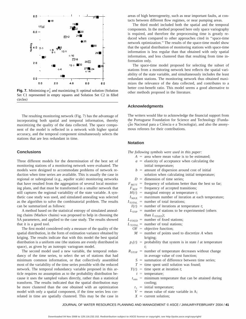
The resulting monitoring network~Fig. 7! has the advantageincorporating both spatial and temporal information, thermaximizing the quality of the data collected. The space comnent of the model is reflected in a network with higher spaaccuracy, and the temporal component simultaneously selecstations that are less redundant in time.

Conclusions

Three different models for the determination of the best semonitoring stations of a monitoring network were evaluated.models were designed to accommodate problems of netwoduction when time series are available. This is usually the caregional or subregional~e.g., aquifer scale! monitoring networksthat have resulted from the aggregation of several local moning plans, and that must be transformed in a smaller networkstill captures the regional variability of the state variable. A sthetic case study was used, and simulated annealing was seas the algorithm to solve the combinatorial problem. The recan be summarized as follows:

A method based on the statistical entropy of simulated aning chains~Markov chains! was proposed to help in choosingSA parameters, and applied to the case study. The results shthat it is a good tool.

The first model considered only a measure of the quality ospatial distribution, in the form of estimation variance obtainekriging. The results indicate that with this model the best spdistribution is a uniform one~the stations are evenly distributedspace!, as given by an isotropic variogram model.

The second model used a new variable, the temporal redancy of the time series, to select the set of stations thaminimum common information, or that collectively assembmost of the variability of the time series possible with the redunetwork. The temporal redundancy variable proposed in thiticle requires no assumption as to the probability distributioncause it uses the sampled values directly, rather than a stattransform. The results indicated that the spatial distributionbe more clustered than the one obtained with an optimizmodel with only a spatial component, if the time series less

Fig. 7. Minimizing sE2 and maximizingS: optimal solution~Solution

Set C1 represented in empty squares and Solution Set C2 incircles!

related in time are spatially clustered. This may be the case


Downloaded 04 Nov 2008 to 129.116.232.152. Redistribution subject

byo-

ialthe

ofhere-in

or-hatn-ctedlts

al-ewed

hebyial

un-haddedar-e-ticalayionor-

in

areas of high heterogeneity, such as near important faults, at cotacts between different flow regimes, or near pumping areas.

The third model included both the spatial and the temporacomponents. In the method proposed here only space variograpis required, and therefore the preprocessing time is greatly reduced when compared to other approaches cited in ‘‘space-timnetwork optimization.’’ The results of the space-time model showthat the spatial distribution of monitoring stations with space-timeinformation is less regular than that obtained with only spatialinformation, and less clustered than that resulting from time in-formation only.

The space-time model proposed for selecting the subset ostations from a monitoring network best reflects the spatial variability of the state variable, and simultaneously includes the leasredundant stations. The monitoring network thus obtained maximizes the relevance of the data collected, and contributes tobetter cost-benefit ratio. This model seems a good alternative tother methods proposed in the literature.

Acknowledgments

The writers would like to acknowledge the financial support fromthe Portuguese Foundation for Science and Technology~Funda-cao Nacional para a Cieˆncia e a Tecnologia!, and also the anony-mous referees for their contributions.

Notation

The following symbols were used in this paper:A 5 area where mean value is to be estimated;a 5 elasticity of acceptance when calculating the

initial temperature;b 5 amount of dispersion around cost of initial

solution when calculating initial temperature;D 5 dimension of time series;

FBETT 5 frequency of solutions better than the best so far;FREP 5 frequency of accepted transitions;H(t) 5 marginal entropy at temperaturet;I MAX 5 maximum number of iteration at each temperature;

I TOTAL 5 number of total iterations;I (t) 5 number of iterations at temperaturet;

LEXP 5 number of stations to be experimented~othersthanLFIXED);

LFIXED 5 number of fixed stations;LTOTAL 5 number of total stations;

OF 5 objective function;M 5 number of points used to discretizeA when

kriging;pl(t) 5 probability that system is in statel at temperature

t;RSTOP 5 number of temperature decreases without change

in average value of cost function;S 5 summation of difference between time series;T 5 time spent until solution was found;

T(t) 5 time spent at iterationt;t 5 temperature;

tmin 5 minimum temperature that can be attained duringcooling;

t1 5 initial temperature;V 5 mean value of state variable in A;X 5 current solution;

lled


to ASCE license or copyright; see http://pubs.asce.org/copyright/

e

o

.

-

-

xa 5 value of state variable at locationa ~known!;Z(X) 5 state random variable;z(x) 5 value of state random variable;

a 5 temperature decrease factor;D 5 time shift;G 5 field where random state variable is defined;

g(h) 5 variogram;x 5 solution space;

k i 5 weights in estimation function;m 5 Lagrange parameter;P 5 Cartesian coordinate of set of stations in original

design;p 5 Cartesian coordinate of subset of stations to be

included in new design; andsE

2 5 estimation variance.

References

Aarts, E., and Korst, J.~1990!. Simulated Annealing and Boltzmann Ma-chines, Wiley, New York.

Ahlfeld, D. P., and Pinder, G. F.~1988!. A Ground Water MonitoringNetwork Design Algorithm, Dept. of Civil Engineering and Opera-tions Research, Princeton University, Princeton, N.J.

Amorocho, J., and Espildora, B.~1973!. ‘‘Entropy in the assessment ofuncertainty of hydrologic systems and models.’’Water Resour. Res.,9~6!, 1511–1522.

Bastin, G., Lorent, B., Duque, C., and Gevers, M.~1984!. ‘‘Optimal es-timation of the average rainfall and optimal selection of rain-gauglocations.’’Water Resour. Res.,20~4!, 463–470.

Bras, R. L., and Rodrı´guez-Iturbe, I.~1976!. ‘‘Network design for theestimation of areal mean of rainfall events.’’Water Resour. Res.,12~6!, 1185–1195.

Bras, R. L., and Rodriguez-Iturbe, I.~1975!. Rainfall-Runoff as SpatialStochastic Processes: Data Collection and Synthesis, Ralph M. Par-sons Laboratory for Water Resources and Hydrodynamics, Dept.Civil Engineering, Massachusetts Institute of Technology, CambridgeMass.

Buxton, B. E., and Pate, A. D.~1994!. ‘‘Joint temporal-spatial modelingof concentrations of hazardous pollutants in urban air.’’Proc., Geo-statistics for the Next Century, R. Dimitrakopoulos, ed., Kluwer Aca-demic, Dordrecht, The Netherlands, 75–87.

Caselton, W. F., and Husain, T.~1980!. ‘‘Hydrologic networks: Informa-tion transmission.’’J. Water Resour. Plan. Manage. Div., Am. Soc.Civ. Eng.,106~2!, 503–520.

Cunha, M. C., and Sousa, J.~1999!. ‘‘Water distribution network designoptimization: Simulated annealing approach.’’J. Water Resour. Plan.Manage. Div., Am. Soc. Civ. Eng.,125~4!, 215–221.

David, M. ~1977!. Geostatistical Ore Reserve Estimation, Elsevier, Am-sterdam.

Delhomme, J. P.~1978!. ‘‘Kriging in the hydrosciences.’’Adv. WaterResour.,1~5!, 251–266.

Dimitrakopoulos, R., and Luo, X.~1994!. ‘‘Spatiotemporal modelling:Covariances and ordinary kriging systems.’’Proc., Geostatistics forthe Next Century, R. Dimitrakopoulos, ed., Kluwer Academic, Dor-drecht, The Netherlands, 88–93.

Dixon, W., and Chiswell, B.~1996!. ‘‘Review of aquatic monitoring pro-gram design.’’Water Resour.,30~9!, 1935–1948.

Grabow, G. L., Mote, C. R., Sanders, W. L., Smoot, J. L., and Yoder, DC. ~1993!. ‘‘Groundwater monitoring network using minimum welldensity.’’ Water Sci. Technol.,28~3–5!, 327–335.

Harmancioglu, N., and Alspaslan, N.~1992!. ‘‘Water quality monitoringnetwork design: A problem of multi-objective decision making.’’Water Resour. Bull.,28~2!, 179–192.

Harmancioglu, N., and Yevjevich, V.~1987!. ‘‘Transfer of hydrologicinformation among river points.’’J. Hydrol.,91, 103–118.

Harmancioglu, N. B., Fistikoglu, O., Ozkul, S. D., Singh, V. P., andAlspaslan, M. N.~1999!. Water Quality Monitoring Network Design,



f,

Kluwer Academic, Dordrecht, The Netherlands.Hsu, N. S., and Yeh, W.~1989!. ‘‘Optimum experimental design for pa-

rameter identification in groundwater hydrology.’’Water Resour. Res.,25~5!, 1025–1040.

Husain, T. ~1989!. ‘‘Hydrologic uncertainty measure and network de-sign.’’ Water Resour. Bull.,25~3!, 527–534.

Ingber, L. ~1993!. ‘‘Simulated annealing: Practice versus theory.’’J.Mathl. Comput. Modelling,18~11!, 29–57.

Journel, A., and Huijbregts, Ch.~1978!. Mining Geostatistics, AcademicPress, New York.

Kirkpatrick, S., Gellat, C. D., Jr., and Vecchi, M. P.~1983!. ‘‘Optimiza-tion by simulated annealing.’’Science,220, 671–680.

Knopman, D. S., and Voss, C. I.~1989!. ‘‘Multiobjective sampling designfor parameter estimation and model discrimination in groundwatersolute transport.’’Water Resour. Res.,25~10!, 2245–2258.

Lebel, T., Bastin, G., Obled, C., and Creutin, J. D.~1987!. ‘‘On theaccuracy of areal rainfall estimation: A case study.’’Water Resour.Res.,23~11!, 2123–2134.

Lenton, R. L., and Rodrı´guez-Iturbe, I.~1974!. On the Collection, theAnalysis, and the Synthesis of Spatial Rainfall Data, Ralph M. Par-sons Laboratory for Water Resources and Hydrodynamics, Dept. ofCivil Engineering, Massachusetts Institute of Technology, Cambridge,Mass.

Loaiciga, H. A.~1989!. ‘‘An optimization approach for groundwater qual-ity monitoring network design.’’Water Resour. Res.,25~8!, 1771–1782.

Loaiciga, H. A., Charbeneau, R. J., Everett, L. G., Fogg, G. E., Hobbs, B.F., and Rouhani, S.~1992!. ‘‘Review of ground-water quality moni-toring network design.’’J. Hydraul. Eng.,118~1!, 11–37.

Massmann, J., and Freeze, R. A.~1987a!. ‘‘Groundwater contaminationfrom waste management sites: The interaction between risk-based engineering design and regulatory policy, 1. Methodology.’’Water Re-sour. Res.,23~2!, 351–367.

Massmann, J., and Freeze, R. A.~1987b!. ‘‘Groundwater contaminationfrom waste management sites: The interaction between risk-based engineering design and regulatory policy, 2. Results.’’Water Resour.Res.,23~2!, 368–380.

Matheron, G.~1970!. ‘‘La theorie des variables re´gionalizees, et ses ap-plications.’’ Les Cahiers du Centre de Morphologie Mathe´matique deFontainbleau, Fascicule 5.

Metropolis, N., Rosenbluth, A. W., Rosenbluth, M. N., Teller, A. H., andTeller, E. ~1953!. ‘‘Equation of state calculations by fast computingmachines.’’J. Chem. Phys.,21, 1087–1092.

Meyer, P. D., Valocchi, A. J., and Eheart, J. W.~1994!. ‘‘Monitoringnetwork design to provide initial detection of groundwater contami-nation.’’ Water Resour. Res.,30~9!, 2647–2659.

Nixon, S. C.~1996!. ‘‘European freshwater monitoring network design.’’Topic Rep. No. 10/1996, European Environment Agency, Copenhagen.

Nixon, S. C., Rees, Y. J., Gendebien, A., and Ashley, S. J.~1996!. ‘‘Re-quirements for water monitoring.’’Topic Rep. No. 1/1996, EuropeanEnvironment Agency, Copenhagen.

Pardo-Igu´zquiza, E.~1998!. ‘‘Optimal selection of number and locationof rainfall gauges for areal rainfall estimation using geostatistics andsimulated annealing.’’J. Hydrol.,210, 206–220.

Reed, P., Minsker, B., and Valocchi, A. J.~2000!. ‘‘Cost-effective long-term groundwater monitoring design using a genetic algorithm andglobal mass interpolation.’’Water Resour. Res.,36~12!, 3731–3741.

Rodrıguez-Iturbe, I., and Mejı´a, J. M. ~1974a!. ‘‘The design of rainfallnetworks in time and space.’’Water Resour. Res.,10~4!, 713–728.

Rodrıguez-Iturbe, I., and Mejı´a, J. M.~1974b!. ‘‘On the transformation ofpoint rainfall to areal rainfall.’’Water Resour. Res.,10~4!, 729–736.

Rouhani, S.~1985!. ‘‘Variance reduction analysis.’’Water Resour. Res.,21~6!, 837–846.

Rouhani, S., and Hall, T.~1988!. ‘‘Geostatistical schemes for groundwa-ter sampling.’’J. Hydrol.,103, 85–102.

Sacks, J., and Schiller, S.~1988!. ‘‘Spatial designs.’’Spatial Designs in



thei--

the

Statistical Decision Theory and Related Topics IV, S. S. Gupta and J.O. Berger, eds., Springer, New York, 385–399.

Task Committee on Geostatistical Techniques in Geohydrology ofGround Water Hydrology/Committee of the ASCE Hydraulics, Divsion.~1990a!. ‘‘Review of geostatistics in geohydrology: I. Basic concepts.’’J. Hydraul. Eng.,116~5!, 612–632.

Task Committee on Geostatistical Techniques in Geohydrology of

JOURNAL OF WATER RESOURCES PLANN

Downloaded 04 Nov 2008 to 129.116.232.152. Redistribution subject to A

Ground Water Hydrology/Committee of the ASCE Hydraulics, Divi-sion. ~1990b!. ‘‘Review of geostatistics in geohydrology: II. Applica-tions.’’ J. Hydraul. Eng.,116~5!, 633–658.

Thompson, S. K.~1992!. Sampling, Wiley, New York.Wagner, B. J., and Gorelick, S. M.~1989!. ‘‘Reliable aquifer remediation

in the presence of spatially variable hydraulic conductivity: From datato design.’’Water Resour. Res.,25~10!, 2211–2225.

ING AND MANAGEMENT © ASCE / JANUARY/FEBRUARY 2004 / 43

SCE license or copyright; see http://pubs.asce.org/copyright/

Groundwater Monitoring Network Optimization with Redundancy Reduction

Documents

Transcript of Groundwater Monitoring Network Optimization with Redundancy Reduction