arX

iv:0

805.

2094

v2 [

hep-

ph]

9 J

ul 2

008

Gluino production in some supersymmetricmodels at the LHC

C. Brenner Mariotto and M. C. RodriguezUniversidade Federal do Rio Grande - FURG

Departamento de FısicaAv. Italia, km 8, Campus Carreiros

96201-900, Rio Grande, RSBrazil

Abstract

In this article we review the mechanisms in several supersymmetricmodels for producing gluinos at the LHC and its potential for discov-ering them. We focus on the MSSM and its left-right extensions. Westudy in detail the strong sector of both models. Moreover, we obtainthe total cross section and differential distributions. We also make ananalysis of their uncertainties, such as the gluino and squark masses,which are related to the soft SUSY breaking parameters.

PACS numbers: 12.60.-i ;12.60.Jv; 13.85.Lg; 13.85.Qk; 14.80.Ly.

1 Introduction

Although the Standard Model (SM) [1], based on the gauge symmetry SU(3)c⊗SU(2)L ⊗ U(1)Y describes the observed properties of charged leptons andquarks it is not the ultimate theory. However, the necessity to go beyondit, from the experimental point of view, comes at the moment only fromneutrino data. If neutrinos are massive then new physics beyond the SM isneeded.

Supersymmetry (SUSY) or symmetry between bosons (particles with in-teger spin) and fermions (particles with half-integer spin) has been introducedin theoretical papers nearly 30 years ago [2]. Since that time there appearedthousands of papers. The reason for this remarkable activity is the uniquemathematical nature of supersymmetric theories, possible solution of vari-ous problems of the SM within its supersymmetric extentions as well as theopening perspective of unification of all interactions in the framework of asingle theory [3, 4, 5].

1

However supersymmetry seemed, in the early days, clearly inappropriatefor a description of our physical world1, for obvious and less obvious reasons,which often tend to be somewhat forgotten, now that we got so accustomed todeal with Supersymmetric extensions of the Standard Model. We recall theobstacles which seemed, long ago, to prevent supersymmetry from possiblybeing a fundamental symmetry of Nature2 [6].

We know that bosons and fermions should have equal masses in a su-persymmetric theory. However, it even seemed initially that supersymmetrycould not be spontaneously broken at all which would imply that bosons andfermions be systematically degenerated in mass, unless of course supersymmetry-breaking terms are explicitly introduced “by hand”. As a result, this lead tothe question:

• Is spontaneous supersymmetry breaking possible at all ?

Until today, the spontaneous supersymmetry breaking remains, in gen-eral, rather difficult to obtain. Of course just accepting the possibilityof explicit supersymmetry breaking without worrying too much aboutthe origin of supersymmetry breaking terms, as is frequently done now,makes things much easier – but also at the price of introducing a largenumber of arbitrary parameters, coefficients of these supersymmetrybreaking terms. These terms essentially serve as a parametrizationof our ignorance about the true mechanism of supersymmetry break-ing chosen by Nature to make superpartners heavy. In any case suchterms must have their origin in a spontaneous supersymmetry breakingmechanism.

However, much before getting to the Supersymmetric Standard Model,and irrespective of the question of supersymmetry breaking, the crucialquestion, if supersymmetry is to be relevant in particle physics, is:

• Which bosons and fermions could be related ?

But there seems to be no answer since known bosons and fermions donot appear to have much in common – except, maybe, for the photonand the neutrino.

1The most physicists considered supersymmetry as irrelevant for “real physics”.2We are grateful to P. Fayet that called our attention, and sent to us all these interesting

information about the “early” day of the Supersymmetric extensions of the StandardModel, as well as sent us all the original articles.

2

May be supersymmetry could act at the level of composite objects, e.g.as relating baryons with mesons ? Or should it act at a fundamentallevel, i.e. at the level of quarks and gluons ? (But quarks are colortriplets, and electrically charged, while gluons transform as an SU(3)color octet, and are electrically neutral !)

In a more general way the number of (known) degrees of freedom issignificantly larger for the fermions (now 90, for three families of quarksand leptons) than for the bosons (27 for the gluons, the photon andthe W± and Z gauge bosons, ignoring for the moment the spin-2graviton, and the still-undiscovered Higgs boson). And these fermionsand bosons have very different gauge symmetry properties ! This leadsto the question:

• How could one define (conserved) baryon and lepton numbers, in asupersymmetric theory ?

Of course nowadays we are so used to deal with spin-0 squarks andsleptons, carrying baryon and lepton numbers almost by definition, thatwe can hardly imagine this could once have appeared as a problem.

Supersymmetry today is the main candidate for a unified theory beyondthe SM. Search for various manifestations of supersymmetry in Nature isone of the main tasks of numerous experiments at colliders. Unfortunately,the result is negative so far. There are no direct indications on existence ofsupersymmetry in particle physics, however there are a number of theoreticaland phenomenological issues that the SM fails to address adequately [7]:

• Unification with gravity; The point is that SUSY algebra being a gen-eralization of Poincare algebra [5, 8, 9]

{Qα, Qα} = 2σmα,αPm. (1)

Therefore, an anticommutator of two SUSY transformations is a lo-cal coordinate translation. And a theory which is invariant under thegeneral coordinate transformation is General Relativity. Thus, makingSUSY local, one obtains General Relativity, or a theory of gravity, orsupergravity [10].

• Unification of Gauge Couplings; According to hypothesis of Grand Uni-fication Theory (GUT) all gauge couplings change with energy. All

3

known interactions are the branches of a single interaction associatedwith a simple gauge group which includes the group of the SM. Toreach this goal one has to examine how the coupling change with en-ergy. Considerating the evolution of the inverse couplings, one can seethat in the SM unification of the gauge couplings is impossible. In thesupersymmetric case the slopes of Renormalization Group Equationcurves are changed and the results show that in supersymmetric modelone can achieve perfect unification [11].

• Hierarchy problem; The supersymmetry automatically cancels all quadraticcorrections in all orders of perturbation theory due to the contributionsof superpartners of the ordinary particles. The contributions of the bo-son loops are cancelled by those of fermions due to additional factor(−1) coming from Fermi statistic. This cancellation is true up to theSUSY breaking scale, MSUSY , since

∑

bosons

m2 −∑

fermions

m2 = M2SUSY , (2)

which should not be very large (≤ 1 TeV) to make the fine-tuningnatural. Therefore, it provides a solution to the hierarchy problem byprotecting the eletroweak scale from large radiative corrections [12].However, the origin of the hierarchy is the other part of the problem.We show below how SUSY can explain this part as well.

• Electroweak symmetry breaking (EWSB); The “running” of the Higgsmasses leads to the phenomenon known as radiative electroweak sym-metry breaking. Indeed, the mass parameters from the Higgs potentialm2

1 and m22 (or one of them) decrease while running from the GUT scale

to the scale MZ may even change the sign. As a result for some valueof the momentum Q2 the potential may acquire a nontrivial minimum.This triggers spontaneous breaking of SU(2) symmetry. The vacuumexpectations of the Higgs fields acquire nonzero values and providemasses to fermions and gauge bosons, and additional masses to theirsuperpartners [13]. Thus the breaking of the electroweak symmetry isnot introduced by brute force as in the SM, but appears naturally fromthe radiative corrections.

SUSY has also made several correct predictions [7]:

4

• Supersymmetry predicted in the early 1980s that the top quark wouldbe heavy [14], because this was a necessary condition for the validityof the electroweak symmetry breaking explanation.

• Supersymmetric grand unified theories with a high fundamental scaleaccurately predicted the present experimental value of sin2 θW beforeit was measured [15].

• Supersymmetry requires a light Higgs boson to exist [16], consistentwith current precision measurements, which suggest Mh < 200 GeV[17].

Together these successes provide powerful indirect evidence that low energySUSY is indeed part of correct description of nature.

Certainly the most popular extension of the SM is its supersymmetriccounterpart called Minimal Supersymmetric Standard Model (MSSM) [3,18, 19].

The first attempt to construct a phenomenological model was done in[20], where the author tried to relate known particles together (in particu-lar, the photon with a “neutrino”, and the W±’s with charged “leptons”,also related with charged Higgs bosons H±), in a SU(2) ⊗ U(1) electroweaktheory involving two doublet Higgs superfields now known as H1 and H2

3.The limitations of this approach quickly led to reinterpret the fermions ofthis model (which all have 1 unit of a conserved additive R quantum num-ber carried by the supersymmetry generator) as belonging to a new classof particles. The “neutrino” ought to be considered as a really new parti-cle, a “photonic neutrino”, a name transformed in 1977 into photino; thefermionic partners of the colored gluons (quite distinct from the quarks) thenbecoming the gluinos, and so on. More generally this led one to postulatethe existence of new R-odd “superpartners” for all particles and considerthem seriously, despite their rather non-conventional properties: e.g. newbosons carrying “fermion” number, now known as sleptons and squarks, orMajorana fermions transforming as an SU(3) color octet, which are pre-cisely the gluinos, etc.. In addition the electroweak breaking must be in-duced by a pair of electroweak Higgs doublets, not just a single one as inthe SM, which requires the existence of charged Higgs bosons, and of several

3Then called S = H1 left-handed and T = Hc

2right-handed [6].

5

neutral ones [3, 18]. We also want to stress that on reference [3] were intro-duced squarks and gluinos (color octet of Majorana fermions, which couple tosquark/quark pairs within what is now known as Supersymmetric QuantumChromodynamics (sQCD)), that is the main subject of this article.

The still-hypothetical superpartners may be distinguished by a new quan-tum number called R -parity, first defined in terms of the previous R quan-tum number as Rp = (−1)R, i.e. +1 for the ordinary particles and −1 fortheir superpartners. It is associated with a Z2 remnant of the previous R-symmetry acting continuously on gauge, lepton, quark and Higgs superfieldsas in [3], which must be abandoned as a continuous symmetry to allowmasses for the gravitino [18] and gluinos [21]. The conservation (or non-conservation) of R-parity is therefore closely related with the conservation(or non-conservation) of baryon and lepton numbers, B and L, as illus-trated by the well-known formula reexpressing R-parity in terms of baryonand lepton numbers, as (−1) 2S (−1) 3B+L [22]. This may also be writtenas (−1)2S (−1) 3 (B−L) , showing that this discrete symmetry may still beconserved even if baryon and lepton numbers are separately violated, as longas their difference ( B − L ) remains conserved, at least modulo 2.

The finding of the basic building blocks of the Supersymmetric StandardModel, whether “minimal” or not, allowed for the experimental searches for“supersymmetric particles”, which started with the first searches for gluinosand photinos, selectrons and smuons, in the years 1978-1980, and have beengoing on continuously since. These searches often use the “missing energy”signature corresponding to energy-momentum carried away by unobservedneutralinos [3, 22, 23]. A conserved R-parity also ensures the stability ofthe “lightest supersymmetric particle”, a good candidate to constitute thenon-baryonic Dark Matter that seems to be present in the Universe.

Massive neutrinos can also be naturally accommodated in R-parity vio-lating supersymmetric theories, in which neutrinos can mix with neutralinosso that they acquire small masses [24, 25]. However, the phenomenologicalbounds on B and/or L violation [25, 26] can be satisfied by imposing B asa symmetry and allowing the lepton number violating couplings to be largeenough to generate Majorana neutrino masses.

However, the minimalistic extension of the MSSM is to introduce a gaugesinglet superfield N , this model is called “Next Minimal SupersymmetricStandard Model” (NMSSM) [8, 27].

It is mainly motivated by its potential to eliminate the µ problem of the

6

MSSM [28], where the origin of the the µ parameter in the superpotential

WMSSM = µH1H2 (3)

is not understood. For phenomenological reasons it has to be of the orderof the electroweak scale, while the “natural” mass scale would be of theorder of the GUT or Planck scale. This problem is evaded in the NMSSMwhere the µ term in the superpotential is dynamically generated through thesuperpotential

WNMSSM = λH1H2N − 1

3kN3 + WMSSM (4)

The scalar component of N is the Higgs singlet with vacuum expectationvalue x. Therefore, this problem is evaded in the NMSSM where the µterm in the superpotential is dynamically generated through µ = λx with adimensionless coupling λ.

One of the simplest extensions of the SM that allows to naturally ex-plain the smallness of the neutrino masses (without excessively tiny Yukawacouplings) consists in incorporating right-handed Majorana neutrinos, andimposing a see-saw mechanism 4 [30, 31] for the neutrino mass genera-tion [28, 32], it is the “Minimal Supersymmetric Standard Model with threeright handed neutrinos” (MSSM3RHN) [9].

The introduction of three families of the right-handed neutrinos N i (wherei is flavor indice) brings two new ingredients to the standard model; one isa new scale of the Majorana masses for the right-handed neutrinos, andthe other a new matrix for Yukawa coupling constants of these new particles.Thus, we have two independent Yukawa matrices in the lepton sector as in thequark sector. Therefore, this model can accommodate a see-saw mechanism,and at the same time stabilise the hierarchy between the scale of new physicsand the electroweak (EW) scale [33].

Other very popular ones are Left-Right symmetric theories (LRM) [34].The main motivations for this model are that it gives an explanation forthe parity violation of weak interactions, provides a mechanism (see-saw) forgenerating neutrino masses, and has B−L as a gauge symmetry. The modelhas many predictions one can directly test at a TeV-scale linear collider [35].

The interesting and important features [36] of this kind of models are:

4For the see-saw mechanism the first paper is [29]

7

1. It incorporates Left-Right (LR) symmetry [34] (on top of the quark-lepton symmetry mentioned above), which leads naturally to the spon-taneous breaking of parity and charge conjugation [34, 37].

2. It incorporates a see-saw mechanism for small neutrino masses [30, 31].

3. It predicts the existence of magnetic monopoles [38].

4. It leads to rare processes such as KL → µe through the lepto-quarkgauge bosons (with however a negligible rate for MPS ≥ 10GeV ) [34].

5. In the case of single-step breaking, predicts the scale of quark-lepton(and Left-Right) unification [39].

6. It allows naturally for ∆B = 2 process of n − n oscillations (withhowever a negligible rate unless there are light diquarks in the TeVmass region)[40].

7. Last but not least, it allows for implementation of the leptogenesisscenario, as suggested by the see-saw mechanism [41].

On the technical side, the left-right symmetric model has a problem sim-ilar to that in the SM: the masses of the fundamental Higgs scalars divergequadratically. As in the SM, the Supersymmetric Left-Right model (SU-SYLR) can be used to stabilize the scalar masses and cure this hierarchyproblem.

On the literature there are two different SUSYLR models. They differ intheir SU(2)R breaking fields: one uses SU(2)R triplets [42] (SUSYLRT) andthe other SU(2)R doublets [43] (SUSYLRD).

Another, maybe more important raison d’etre for SUSYLR is the factthat they lead naturally to R-parity conservation [44]. Namely, Left-Rightmodels contain a B−L gauge symmetry, which allows for this possibility [45].All that is needed is that one uses a version of the theory that incorporatesa see-saw mechanism [30, 31] at the renormalizable level.

As we said before, the supersymmetric particles have not yet been de-tected in the present machines such as HERA and Tevatron. By anotherhand there are many interesting supersymmetric models in the literature aswe shown above. Therefore, if SUSY is detected in the Large Hadron Col-lider (LHC), one of the next steps will be to discriminate among the different

8

SM extensions, scenarios and also to find the mass spectrum of the differentparticles (which can be obtained theoretically in different scenarios).

To discriminate among the several possibilities, it is important to makepredictions for different observables and confront these predictions with theforthcoming experimental data. One important process which could be mea-sured at the LHC is the gluino production.

The R-symmetry transformations act chirally on gluinos, so that anunbroken R-invariance would require them to remain massless, even after aspontaneous breaking of the supersymmetry ! In the early days it was verydifficult to obtain large masses for gluinos, since: i) no direct gluino massterm was present in the Lagrangian density; and ii) no such term may begenerated spontaneously, at the tree approximation, since gluino couplingsinvolve colored spin-0 fields.

On this case, gluino remain massless, and we would then expect the ex-istence of relatively light “R-hadrons” [22, 23] made of quarks, antiquarksand gluinos, which have not been observed. We know today that gluinos,if they do exist, should be rather heavy, requiring a significant breaking ofthe continuous R-invariance, in addition to the necessary breaking of thesupersymmetry.

A third reason for abandoning the continuous R-symmetry could nowbe the non-observation at LEP of a charged wino – also called chargino –lighter than the W±, that would exist in the case of a continuous U(1)R-invariance [3, 20]. The just-discovered τ− particle could tentatively beconsidered, in 1976, as a possible light wino/chargino candidate, before get-ting clearly identified as a sequential heavy lepton.

The gluino masses result directly from supergravity, through m3/2,which leads one to abandon continuous R for R-parity as already observedin 1977 [18]. Another way does not use SUGRA but generates mgluino radia-tively, using messengers quarks sensitive to the source of SUSY-breaking [46],on this case the gluino masses are generated by radiative corrections involv-ing a new sector of quarks sensitive to the source of supersymmetry breaking,that would now be called “messenger quarks” 5.

Today, the gluinos are expected to be one of the most massive sparticleswhich constitute the Minimal Supersymmetric Standard Model (MSSM), and

5Remember that the see-saw mechanism [29] did not attract attention at the time,however the article [46] on gluino masses discusses a see-saw mechanism for gluinos.

9

therefore their production is only feasible at a very energetic machine such asthe LHC. Being the fermion partners of the gluons, their role and interactionsare directly related with the properties of the supersymmetric QCD (sQCD).

The aim of this paper is twofold. The first one is to study the strong sectorof some supersymmetric models and to show explicit that the Feynmann rulesfor the gluino production are the same in all supersymmetric extensions of theStandard Model here considered. After that, as the second aim of this article,we show predictions for the gluino production on these models at the LHC,for various SPS benchmark points. The outline of the paper is the following.In sections 2 and 3, we obtain the relevant Feynman rules of the strongsector from the MSSM and SUSYLR models, respectivelly. Moreover, wesee that the Feynman rules are indeed the same in these models. In section4 we consider the different scenarious for the relevant SUSY parameters,which lead to different gluinos and squark masses. In section 5 we considergluino production in the studied models and present the relevant expressions,which are used to obtain the numerical results in section 6. Conclusions aresummarized in section 7.

2 Minimal Supersymmetric Standard Model

(MSSM).

In the MSSM [3, 18, 19], the gauge group is SU(3)C ⊗SU(2)L ⊗U(1)Y . Theparticle content of this model consists in associate to every known quark andlepton a new scalar superpartner to form a chiral supermultiplet. Similarly,we group a gauge fermion (gaugino) with each of the gauge bosons of thestandard model to form a vector multiplet. In the scalar sector, we need tointroduce two Higgs scalars and also their supersymmetric partners knownas Higgsinos (Our notation 6 is given at [47]). We also need to impose a newglobal U(1) invariance usually called R-invariance, to get interactions thatconserve both lepton and baryon number (invariance). On this section wewill derive the Feynman rules of the strong sector of this model.

6The particle content and the Lagrangian of this model.

10

2.1 Interaction from LGauge

We can rewrite LGauge, see [8, 9], in the following way

LGauge = Lcin + Lgaugino + LgaugeD . (5)

where

Lcin = LSU(3)cin + LSU(2)

cin + LU(1)cin ,

Lgaugino = LSU(3)gaugino + LSU(2)

gaugino + LU(1)gaugino,

LgaugeD = LSU(3)

D + LSU(2)D + LU(1)

D , (6)

the first part is given by:

LSU(3)cin = −1

4Ga

mnGamn, (7)

withGa

mn = ∂mgan − ∂nga

m − gsfabcgb

mgcn, (8)

gs is the strong coupling constant and fabc are totally antisymmetric structureconstant of the SU(3) group . The second term can be rewriten as

LSU(3)gaugino = −ıλa

C σmDmλaC , (9)

whereDmλa

C = ∂mλaC − gsf

abcλaCgc

m. (10)

The last term is given by

LSU(3)D =

1

2Da

CDaC . (11)

2.1.1 Gluon Self Interaction

These interactions are derived from Eqs.(7,8) which are the same as the usualQCD. Therefore, on this case, we get the same Feynman rules as those fromthe QCD.

11

2.1.2 Gluino–Gluino–Gluon Interaction

This interaction is got from Eqs.(9, 10) combining both equations to obtain

Lgaugino = Lcin + Lggg, (12)

where

Lcin = ı(∂mλaC)σmλa

C ,

Lggg = ıgsfabcλa

C σmλbCgc

m, (13)

the first term gives the cinetic term to gluino, while the last one provides thegluino-gluino-gluon interaction.

Considerating the four-component Majorana spinor for the gluino, givenby

Ψ(ga) =

(

−ıλaC(x)

ıλaC(x)

)

., (14)

we can rewrite Lggg in the following way

Lggg =ı

2gsf

bacΨ(ga)γmΨ(gb)gcm. (15)

Owing to the Majorana nature of the gluino one must multiply by 2 to obtainthe Feynman rule (or add the graph with g ↔ ¯g)!

The equation above induce the following Feynman rule, for the verticegluino-gluino-gluon, given at Fig.(1) and it is the same result as presented

ga

gb

gcm

−gsfbacγm

Figure 1: Feynman rule for the vertice Gluino-Gluino-Gluon at the MSSM.

at [8, 9, 19, 48].

12

2.2 Interaction from LQuarks

The interaction of the strong sector are obtained from the following La-grangians

Lqqg = gsQσmT aQgam + gsucσmT aucgam + gsdcσmT adcgam

Lqqg = ıgs

( ¯QT a∂mQ − QT a∂m¯Q)

gam + ıgs

(

ucT a∂muc − ucT a∂muc)

gam

+ ıgs

(

dcT a∂mdc − dcT a∂mdc

)

gam,

Lqqg = −ı√

2gs

(

QT aQλaC − ¯QT aQλa

C

)

− ı√

2gs

(

ucT aucλaC − ucT aucλa

C

)

− ı√

2gs

(

dcT adcλaC − dcT adcλa

C

)

,

Lqqgg = −g2s¯QT aT bQga

mgbm − g2s u

cT aT bucgamgbm − g2

s dcT aT bdcga

mgbm. (16)

Where T ars are the color triplet generators, then one must use

T ars = −T ∗a

rs = −T asr, (17)

for the color anti-triplet generators.

2.2.1 Quark–Quark–Gluon Interaction

This interaction comes from the first Lagrangian given at Eq.(16), and canbe rewritten as

Lqqg = gs(urσmT a

rsus + drσmT a

rsds + ucrσ

mT arsu

cs + dc

rσmT a

rsdcs)g

am, (18)

u and d are color triplets while uc and dc are color anti-triplets. We mustrecall that r and s are color indices. Using Eq.(17) we can rewrite Eq.(18)as

Lqqg = gs(urσmT a

rsus + drσmT a

rsds + ucrσ

mT arsu

cs + dc

rσmT a

rsdcs)g

am. (19)

Now, if we take into account the four-component Dirac spinor of the quarks(q = u, d), given by

Ψ(q) =

(

qL(x)qc

L(x)

)

, (20)

13

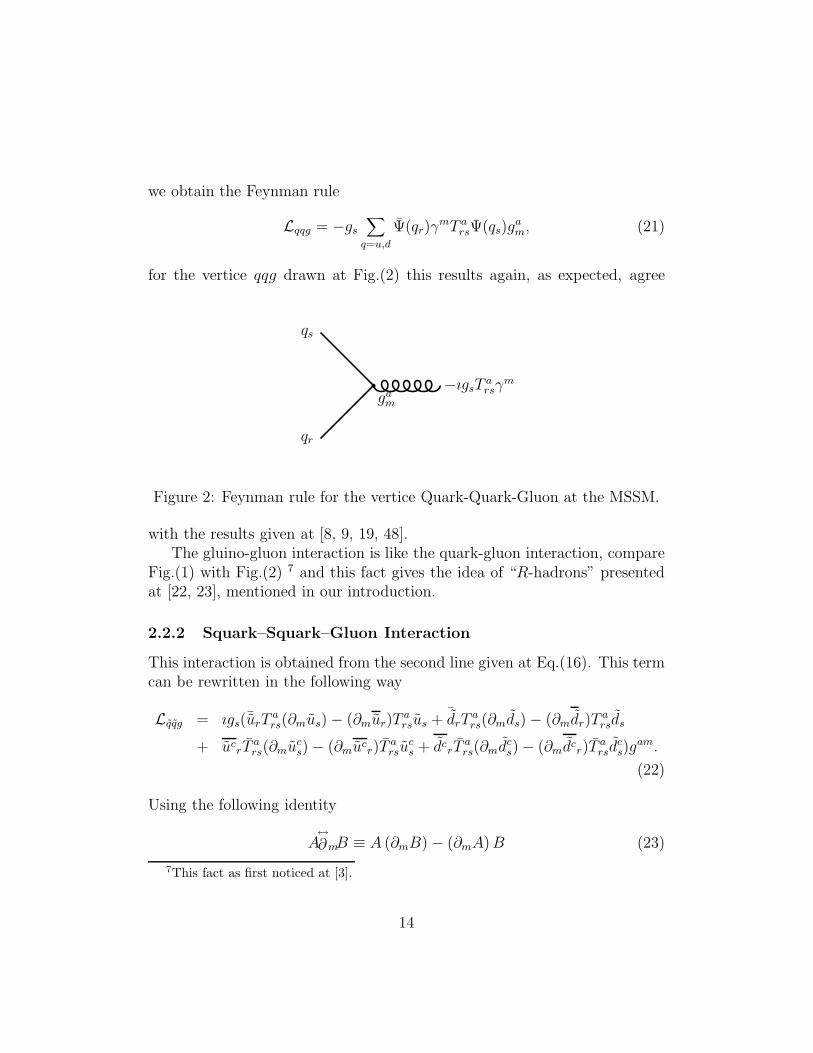
we obtain the Feynman rule

Lqqg = −gs

∑

q=u,d

Ψ(qr)γmT a

rsΨ(qs)gam, (21)

for the vertice qqg drawn at Fig.(2) this results again, as expected, agree

qr

qs

gam

−ıgsTarsγ

m

Figure 2: Feynman rule for the vertice Quark-Quark-Gluon at the MSSM.

with the results given at [8, 9, 19, 48].The gluino-gluon interaction is like the quark-gluon interaction, compare

Fig.(1) with Fig.(2) 7 and this fact gives the idea of “R-hadrons” presentedat [22, 23], mentioned in our introduction.

2.2.2 Squark–Squark–Gluon Interaction

This interaction is obtained from the second line given at Eq.(16). This termcan be rewritten in the following way

Lqqg = ıgs(¯urTars(∂mus) − (∂mur)T

arsus + ¯drT

ars(∂mds) − (∂mdr)T

arsds

+ ucrT

ars(∂muc

s) − (∂mucr)T

arsu

cs + dc

rTars(∂mdc

s) − (∂mdcr)T

arsd

cs)g

am.

(22)

Using the following identity

A↔∂mB ≡ A (∂mB) − (∂mA) B (23)

7This fact as first noticed at [3].

14

we can rewrite our Lagrangian in the following simple way

Lqqg = ıgs

∑

q=u,d

(q∗LrTars

↔∂mqLs − q∗RrT

ars

↔∂mqRs)g

am . (24)

Note the relative minus sign between the terms with qL and qR: This is dueto the facts that qR are colour anti–triplets and the anti–colour generatorgiven at Eq.(17). Here, we use a similar notation as given at [19], it meansthat q∗ creates the scalar quark q, while q destroys the scalar quark q.

Including the generalization to six flavors, we can write

Lqqg = ıgs

∑

q=u,d

6∑

p=1

(q∗LprTars

↔∂mqLps − q∗RprT

ars

↔∂mqRps)g

am (25)

The corresponding Feynman rule we obtain from

q∗j↔∂

mqi = ı (ki + kj)

m (26)

where ki and kj are the four–momenta of qi and qj in direction of the chargeflow. This relations give us the following Feynman rules given at Fig.(3)and we conclude that this results, as expected, agree with the references

qr

qs

gam

−ıgsTars(ki + kj)

m

Figure 3: Feynman rule for the vertice Squark-Squark-Gluon at the MSSM.

[8, 9, 19, 48].

2.2.3 Squark-Squark-Gluon-Gluon Interaction

This interaction comes from the last line given at Eq.(16), which can bewritten as

Lqqgg = −g2s(¯urT

arsT

bstut +

¯drT

arsT

bstdt + uc

rTarsT

bstu

ct + dc

rTarsT

bstd

ct)g

amgbm.

15

(27)

By using the following formula valid for SU(3) generators

T arsT

bst =

1

6δabδrt +

1

2(dabc + ıfabc)T c

rt, (28)

it allows us to rewrite our Lagrangian in the following way8

Lqqgg = −g2s

6

∑

q=u,d

q∗r qrgamgam − g2

s(dabc + ıfabc)

∑

q=u,d

q∗rTcrtqtg

amgbm, (29)

however fabcgamgbm = 0 because fabc is totally antisymmetric structure con-

stant of the group SU(3) while gamgbm is symmetric ones. The Feynman rule

is drawn at Fig.(4) and it is in agreement with [8, 9, 19, 48] .

qr

qtga

m

gbn

−ıg2s

(

δabδrt

3+ dabcT c

rt

)

gmn

Figure 4: Feynman rule to Squark-Squark-Gluon-Gluon vertice at MSSM.

2.2.4 Gluino-Quark-Squark Interaction

This interaction is described by the third line at Eq.(16), writing this termas

Lqqg = −√

2ıgs(urTarsusλa

C − urTarsusλ

aC + drT

arsdsλa

C − drTarsdsλ

aC

+ ucrT

arsu

csλ

aC − uc

rTarsu

csλ

aC + dc

rTarsd

csλ

aC − dc

rTarsd

csλ

aC). (30)

8Including the generalization to six flavors, see Eq.(25).

16

Using the Eqs.(20,14) and the usual chiral projectors

L =1

2(1 + γ5) , R =

1

2(1 − γ5) , (31)

we can rewrite our Lagrangian in the following way

Lqqg = −√

2gs

∑

q=u,d

(Ψ(ga)LΨ(qr)Tarsq

∗sL + Ψ(qr)RT a

rsΨ(ga)qsL − Ψ(qr)LT arsΨ(ga)qsL

− Ψ(ga)RΨ(qr)Tarsq

∗sR). (32)

this equation give us the following Feynman rule, given at Fig.(5), and again

ga

qr

qs

−ı√

2gs(LT ars − RT a

rs)

Figure 5: Feynman rule for the vertice Gluino-Quark-Squarks at the MSSM.

it is in concordance with [8, 9, 19, 48].Before considerating the left-right models, we want to say that the color

sector of the interesting models NMSSM and MSSM3RHN are the same asin the MSSM model, therefore the results presented above are still hold onthese models.

3 Supersymmetric Left-Right Model (SUSYLR)

The supersymmetric extension of left-right models is based on the gaugegroup SU(3)C ⊗ SU(2)L ⊗ SU(2)R ⊗U(1)B−L. On the literature, as we saidat introduction, there are two different SUSYLR models. They differ in theirSU(2)R breaking fields: one uses SU(2)R triplets [42] (SUSYLRT) and theother SU(2)R doublets [43] (SUSYLRD). Some details of both models are

17

described at [47]. SUSYLR models have the additional appealing character-istics of having automatic R-parity conservation.

In this article, we are interested in studying only the strong sector. Asthis sector is the same in both models, SUSYLRT and SUSYLRD, the resultswe are presenting in this section hold in both models.

3.1 Interaction from LGauge

We can rewrite LGauge, as done in the MSSM case, in the following way

LGauge = Lcin + Lgaugino + LgaugeD . (33)

where

Lcin = LSU(3)cin + LSU(2)L

cin + LSU(2)R

cin + LU(1)cin ,

Lgaugino = LSU(3)gaugino + LSU(2)L

gaugino + LSU(2)R

gaugino + LU(1)gaugino,

LgaugeD = LSU(3)

D + LSU(2)L

D + LSU(2)R

D + LU(1)D , (34)

the first part is given by:

LSU(3)cin = −1

4Ga

mnGamn, (35)

with Gamn is given by Eq.(8)

LSU(3)gaugino = −ıλa

C σmDmλaC , (36)

while DCn λa

C is defined at Eq.(10). The last term is given by

LSU(3)D =

1

2Da

CDaC . (37)

The Eqs.(35,36) are equal from the Lagrangian of the MSSM, given atEqs.(7,9). Therefore the Feynman rules are the same as in the MSSM case.The Feynman rule of the interaction Gluino-Gluino-Gluon is given at Eq.(15).

18

3.2 Interaction from LQuarks

In terms of the doublets the Lagrangian of the strong sector can be rewrittenas

Lqqg = gsQσmT aQgam + gsQcσmT aQcgam

Lqqg = ıgs

( ¯QT a∂mQ − QT a∂m¯Q)

gam + ıgs

( ¯QcT a∂mQc − QcT a∂m

¯Qc)

gam,

Lqqg = −ı√

2gs

(

QT aQ¯ga − ¯QT aQga

)

− ı√

2gs

(

QcT aQc¯ga − ¯Q

cT aQcga

)

,

Lqqgg = g2s¯QT aT bQga

mgbm − g2s¯Q

cT aT bQcga

mgbm.

(38)

3.2.1 Quark–Quark–Gluon Interaction

This interaction is given by the first line given at Eq.(38). Using the doubletswe can write our Lagrangian in the following way

Lqqg = gs(urσmT a

rsus + drσmT a

rsds + ucrσ

mT arsu

cs + dc

rσmT a

rsdcs)g

am, (39)

which is the same as of the MSSM, see Eq.(18), therefore the Feynman ruleis again given by Eq.(21).

3.2.2 Squark–Squark–Gluon Interaction

This interaction comes from the second line at Eq.(38), and can be rewrittenas

Lqqg = ıgs(¯urTars(∂mus) − (∂mur)T

arsus +

¯drT

ars(∂mds) − (∂mdr)T

arsds

+ ucrT

ars(∂muc

s) − (∂mucr)T

arsu

cs + dc

rTars(∂mdc

s) − (∂mdcr)T

arsd

cs)g

am,

(40)

which is the same of the MSSM, see Eq.(22), and the Feynman rule is givenby Eqs.(25,26), as expected.

3.2.3 Squark-Squark-Gluon-Gluon Interaction

This interaction is given by the last line of Eq.(38), and it is given by

Lqqgg = −g2s(¯urT

arsT

bstut + ¯drT

arsT

bstdt + uc

rTarsT

bstu

ct + dc

rTarsT

bstd

ct)g

amgbm,

(41)

19

which is the same as Eq.(27), and the Feynman rule is given at Eq.(29).

3.2.4 Gluino-Quark-Squark Interaction

This interaction is given by the third line of Eq.(38), and can be rewrittenas

Lqqg = −√

2ıgs(urTarsusλa

C − urTarsusλ

aC + drT

arsdsλa

C − drTarsdsλ

aC

+ ucrT

arsu

csλ

aC − uc

rTarsu

csλ

aC + dc

rTarsd

csλ

aC − dc

rTarsd

csλ

aC), (42)

which is given by Eq.(30), and the Feynman rule is given by Eq.(32).As a conclusion of sections 2 and 3, we have shown that the Feynman

rules of the strong sector are the same in the following MSSM, NMSSM,MSSM3RHN and SUSYLR models.

4 Parameters

The “Snowmass Points and Slopes” (SPS) [49] are a set of benchmark pointsand parameter lines in the MSSM parameter space corresponding to differentscenarios in the search for supersymmetry at present and future experiments(See [50] for a very nice review). The aim of this convention is reconstructingthe fundamental supersymmetric theory, and its breaking mechanism, fromthe experimental data.

The different scenarious correspond to three different kinds of models.The points SPS 1-6 are Minimal Supergravity (mSUGRA) model, SPS 7-8 are gauge-mediated symmetry breaking (GMSB) model, and SPS 9 areanomaly-mediated symmetry breaking (mAMSB) model ([49, 50, 51]), seeappendix A.

Each set of parameters leads to different masses of the gluinos and squarks,wich are the only relevant parameters in our study, and we shown their valuesin Tab.(1). In this paper, all these ten possibilities will be considered in ourpredictions for gluino production.

5 Gluino Production

Gluino and squark production at hadron colliders occurs dominantly viastrong interactions. Thus, their production rate may be expected to be con-

20

Scenario mg (GeV ) mq (GeV )

SPS1a 595.2 539.9

SPS1b 916.1 836.2

SPS2 784.4 1533.6

SPS3 914.3 818.3

SPS4 721.0 732.2

SPS5 710.3 643.9

SPS6 708.5 641.3

SPS7 926.0 861.3

SPS8 820.5 1081.6

SPS9 1275.2 1219.2

Table 1: The values of the masses of gluinos and squarks in the SPS scenarios.

siderably larger than for sparticles with just electroweak interactions whoseproduction was widely studied in the literature [8, 9]. As shown above, theFeynman rules of the strong sector are the same in the followings MSSM,NMSSM, MSSM3RHN and SUSYLR models. Therefore the diagrams thatcontribute to the gluino production are the same in these models. In thissense, regarding the supersymmetric extensions of SM we consider here, theanalysis we are going to do is model independent.

In the present paper we study the gluino production in pp collisions. Wewill study the following reactions

pp −→ gg, gq + X , (43)

where X is anything, in the proton–proton collisions at the LHC.In order to make a consistent comparison and for sake of simplicity, we

restrict ourselves to leading-order (LO) accuracy, where the partonic cross-sections for the production of squarks and gluinos in hadron collisions werecalculated at the Born level already quite some time ago [52]. The corre-sponding NLO calculation has already been done for the MSSM case [53],and the impact of the higher order terms is mainly on the normalization of

21

q

q

g

g

k1

k2

p1

p2

q

q

g

g

k1

k2

p1

p2

q

q

g

g

k1

k2

p1

p2

(a)g

g

g

g

k1

k2

p1

p2

g

g

g

g

k1

k2

p1

p2

g

g

g

g

k1

k2

p1

p2

(b)

Figure 6: Feynman diagrams for gluino pair production: (a) quark-antiquarkinitial states, (b) gluon-gluon initial states.

q

g

q

g

k1

k2

p1

p2

q

g

q

g

k1

k2

p1

p2

q

g

q

g

k1

k2

p1

p2

Figure 7: Feynman diagrams for squark–gluino production.

the cross section, which could be taken in to account here by introducing aK factor in the results here obtained [53].

The LO QCD subprocesses for single gluino production are gluon-gluonand quark-antiquark anihilation (gg → gg and qq → gg) (shown in Fig. 6),and the Compton process qg → gq (shown in Fig. 7). For double gluino pro-duction only the anihilation processes contribute. These two kinds of eventscould be separated, in principle, by analysing the different decay channelsfor gluinos and squarks [8, 9].

Incoming quarks (including incoming b quarks) are assumed to be mass-less, such that we have nf = 5 light flavours. We only consider final state

22

squarks corresponding to the light quark flavours. All squark masses aretaken equal to mq

9. We do not consider in detail top squark productionwhere these assumptions do not hold and which require a more dedicatedtreatment [54].

The invariant cross section for single gluino production can be written as[52]

Edσ

d3p=∑

ijd

∫ 1

xmin

dxaf(a)i (xa, µ)f

(b)j (xb, µ)

xaxb

xa − x⊥(

ζ+cos θ2 sin θ

)

dσ

dt(ij → gd),(44)

where fi,j are the parton distributions of the incoming protons and dσdt

is theLO partonic cross section [52] for the subprocesses involved. The identifiedgluino is produced at center-of-mass angle θ and transverse momentum pT ,and x⊥ = 2pT√

s. The Mandelstam variables of the partonic reactions ij →

gg, gq are then

s = xaxbs,

t = m2g − xax⊥s

(

ζ − cos θ

2 sin θ

)

,

u = m2g − xbx⊥s

(

ζ + cos θ

2 sin θ

)

. (45)

Here

xb =2υ + xax⊥s

(

ζ−cos θsin θ

)

2xas − x⊥s(

ζ+cos θsin θ

) ,

xmin =2υ + x⊥s

(

ζ+cos θsin θ

)

2s − x⊥s(

ζ−cos θsin θ

) ,

ζ =

(

1 +4m2

g sin2 θ

x2⊥s

)1/2

,

υ = m2d − m2

g, (46)

where mg and md are the masses of the final-state partons produced. Thecenter-of-mass angle θ and the differential cross section above can be easilly

9L-squarks and R-squarks are therefore mass-degenerate and experimentallyindistinguishable.

23

written in terms of the pseudorapidity variable η = − ln tan(θ/2), which isone of the experimental observables10. The total cross section for the gluinoproduction can be obtained from above upon integration. The correspondingpartonic total cross sections for the subprocesses considered are well knownand can be found at [52, 53].

6 Numerical Results

Here in this section we present our numerical results and plots about thegluino production at the LHC. Since the pp CM energy

√s =14 TeV is several

times larger than the expected gluino and squark masses, these particlesmight be produced and detected at the LHC.

In Fig.8 we present the LO QCD total cross section for gluino productionat the LHC as a function of the gluino masses. We use the CTEQ6L [55],parton densities, with two assumptions on the squark masses and choices ofthe hard scale (curves). The sensitivity with the hard scale is also presentedin the case mq = mg. We also, want to stress that the behaviour of ourcurves are similar to ones presented at Chapter 12 on reference [9], wherethey use the CTEQ5L parton distribution on their calculation.

The search for gluinos and squarks (as well as other searches for SUSYparticles) and the possibility of detecting them will depend on their realmasses. We also show (points) in Fig.8 the numerical results for the LOgluino total cross section in all SPS scenarios, fixing the gluino and squarkmasses, taken from Tab.(1).

The results show a strong dependence on the masses of gluinos andsquarks. In the model curves, we get a larger cross section in the degen-erated mass case, which agrees with [9]. Most of the SPS points are close tothe first curve, which can be easily understood by looking at Table 1.

To discriminate among the different scenarious, it is relevant to lookinto more detailed observables such as differential distributions. In Fig.9we present the transverse momentum distributions for single gluino produc-tion at LHC energies. The results show a huge diference in the magnitudefor different scenarios - SPS1a (mSUGRA) gives the bigger values, SPS9(AMSB) the smallest one. The predictions for the points SPS5 and SPS6

10Remember that since gluinos are heavy, their rapidity and pseudorapidity are notequal.

24

500 1000 1500 2000m

gl (GeV)

100

101

102

103

104

105

106

σ (f

b)

msq

=mgl

, µ=mgl

msq

=2mgl

,µ=(m1+m

2)/2

SPS points, µ=mgl

msq

=mgl

, µ=2mgl

msq

=mgl

, µ=0.5 mgl

Figure 8: The total LO cross section for gluino production at the LHC asa function of the gluino masses. Parton densities: CTEQ6L, with two as-sumptions on the squark masses and choices of the hard scale (curves). Thesensitivity with the hard scale is also presented in the case mq = mg. Thepoints are the numerical results for the SPS points as explained in the text.

(both mSUGRA) are indistinguishable, since the gluinos and squarks massesare almost the same in these two mSUGRA scenarios, so gluino productionis not a good process to discriminate between them. Regarding the magni-tude of the cross section of gluino production, this process could be usefullto discriminate among basically four kinds of SPS scenarios, namelly:(i) SPS 1a;(ii) SPS 5, SPS 6, and SPS 4 (in fact, this point is a bit lower than the othertwo);(iii) SPS 1b, SPS 2, SPS 3, SPS 7, SPS 8;(iv) SPS 9.

Looking into the details of the predictions, namely the behavior of thecross section, can give us further information to discriminate among the (iii)-

25

0 200 400 600 800 1000p

T (GeV)

10-1

100

101

102

d2 σ/dp

Tdη

(fb

/GeV

)

SPS 1aSPS 6SPS 5SPS 4SPS 2SPS 8SPS 3SPS 1bSPS 7SPS 9

Figure 9: The LO pT distributions for single gluino production at the LHC(|η| < 2.5) for the different SPS points [49, 50]. We use CTEQ6L partondensities, and µ2 = m2

g + p2T as a hard scale.

scenarios. The pT dependency in these scenarios is not the same for most ofthese points (except SPS 1b and SPS 3, which are almost equal). The SPS2 (mSUGRA) model prediction has clearly a steeper falloff at high very highpT , and the reason for that is the much higher squark mass in this scenario.At moderate pT of about 200 GeV, the SPS 7 (GMSB) curve has the lowestnormalization, that is because the gluino mass is higher in this scenario.However, because the squark mass is much lower than in SPS 2, the falloff athigher pT is less steep and in this region the curve tend to other (iii)-points.So, the gluino and squark masses are more important in different regionsand there is an interplay between them wich produces different behaviors in

26

0 200 400 600 800 1000p

T (GeV)

10-2

10-1

100

101

d2 σ/dp

Tdη

(fb

/GeV

)

SPS 1aSPS 6SPS 5SPS 4SPS 2SPS 8SPS 3SPS 1bSPS 7SPS 9

Figure 10: The LO pT distributions for double gluino production at the LHC(|η| < 2.5) for the different SPS points [49, 50]. We use CTEQ6L partondensities, and µ2 = m2

g + p2T as a hard scale.

different scenarios.The gluino mass is important in all subprocesses, but the squark mass

only contributes to the qq anihilation and the Compton-like process qg → gq,because of the t-channel squark exchange in both subprocesses and, of course,the squark production in the latter one. Comparing these two processes, theCompton process is dominant. Therefore, the different behaviors of the crosssecion are mainly due to the Compton-like contribution.

A complementary analysis can be done by considering double gluino pro-duction, which is easy to obtain from the calculation above, by picking onlythe anihilation processes (Fig. 6). The results for double gluino productionare shown in Fig. 10. Similarly to the previous case, the results show huge

27

diferences in the magnitude of the cross section for different scenarios - SPS1agives the bigger values, SPS9 the smallest one. Also, we find very close valuesfor SPS1b, SPS3 (mSUGRA) and SPS7 (GMSB), which makes it difficult todiscriminate between these mSUGRA and GMSB models. The same occursfor SPS5 and SPS6 (both mSUGRA). However, differently from the singlegluino case, the pT dependencies are similar in all scenarios. Another differ-ence is the magnitude of curves for the points SPS 2 and SPS 8, wich can beclearly separated from the other (iii)-points described above. From all this,we conclude that both processes, single and double gluino production, arecomplementary and usefull to make different discriminations among the SPSscenarios.

7 Conclusions

In this paper we have studied the color sector in some extensions of theSM, namely MSSM and SUSYLR, and some others. We have derived theFeynman rules for the strong sector, and have showed explicitly that theyare the same in all these models. This happens because the strong sector isthe same in all SUSY extensions considered.

There are several scenarios for SUSY breaking, within the SPS conven-tion, which imply in different values for the masses of the supersymmetricparticles. To find the correct SUSY breaking mechanism one has to considerdifferent observables which could be measured when SUSY particles startsto be detected. In this article, we analyse gluino production at the LHC.

Gluinos are color octet fermions and play a major role to understandingsQCD. Because of their large mass as predicted in several scenarios, up tonow the LHC is the only possible machine where they could be found.

Because the Feynman rules for the strong sector are the same in all SMextensions considered, the gluino production cross section are indeed equal inthese models. Our results are in this sense model independent, or conversely,gluino production is not a good process to discriminate among those SUSYextensions of SM.

Besides, our results depend on the gluino and squark masses and no otherSUSY parameters. Since the masses of gluinos come only from the soft terms,measuring their masses can test the soft SUSY breaking approximations.We have considered all the SPS scenarios and showed the corresponding

28

differences on the magnitude of the production cross sections. From this itis easy to distinguish mAMSB from the other scenarios. However, it is notso easy to distinguish mSUGRA from GMSB depending on the real valuesof masses of gluinos and squarks. Gluino production cannot distinguish thetwo scenarios SPS1b and SPS7, provided the gluino and squark masses arealmost similar in these two cases (the same occurs for SPS 5 and SPS 6). Forthe other scenarios, such discrimination can be done, especially if we considerboth single and double gluino production as complementary processes.

Gluino production is not a good process to discriminate among the Su-persymmetric Models, but can be helpfull is determining the correct SUSYbreaking scenario and to understanding supersymmetric quantum chromo-dynamics.

Acknowledgments

This work was partially financed by the Brazilian funding agency CNPq,CBM under contract number 472850/2006-7, and MCR under contract num-ber 309564/2006-9. We would like to thank V. P. Goncalves for useful discus-sion. We are gratefull to Pierre Fayet for many useful discussions and also forproviding us with very useful material about the early days of phenomenologyof Supersymmetric QCD.

A Tables of SPS Convention

On this appendix we present the parameters of the SPS convention, whichare given at Table 2.

References

[1] S. L. Glashow, Nucl. Phys.22, 579 (1961); S. Weinberg, Phys. Rev.

Lett.19, 1264 (1967); A. Salam in Elementary Particle Theory: Rela-

tivistic Groups and Analyticity, Nobel Symposium N8 (Alquivist andWilksells, Stockolm, 1968); S. L. Glashow, J.Iliopoulos and L.Maini,Phys. Rev.D 2, 1285 (1970).

29

SPS Point

mSUGRA: m0 m1/2 A0 tanβ1a 100 250 -100 101b 200 400 0 302 1450 300 0 103 90 400 0 104 400 300 0 505 150 300 -1000 5

mSUGRA-like: m0 m1/2 A0 tanβ M1 M2 = M3

6 150 300 0 10 480 300

GMSB: Λ/103 Mmes/103 Nmes tanβ7 40 80 3 158 100 200 1 15

AMSB: m0 maux/103 tanβ9 450 60 10

Table 2: The parameters for the Snowmass Points and Slopes (SPS). On thistable all the scenarios consider signµ = + taken from [50].

[2] Y. A. Golfand and E. P. Likhtman, JETP Letters 13, 452 (1971); D. V.Volkov and V. P. Akulov, JETP Letters 16, 621 (1972); J. Wess and B.Zumino, Phys. Lett. B49, 52 (1974).

[3] P. Fayet, Phys. Lett. B64 159 (1976); B69 489 (1977).

[4] M. F. Sohnius, Phys. Rep. 128, 41 (1985); H. P. Nilles, Phys. Rep. 110,1(1984); A. B. Lahanas and D. V. Nanopoulos, Phys. Rep. 145, 1 (1987);S. J. Gates, M. Grisaru, M. Rocek and W. Siegel, Superspace or OneThousand and One Lessons in Supersymmetry (Benjamin & Cummings,1983);P.West, Introduction to supersymmetry and supergravity, 2nd edition,World Scientific Publishing Co. Pte. Ltd., Singapore, (1990);S.Weinberg, The quantum theory of fields. Vol. 3. Supersymmetry 1stedition, Cambridge University Press, United Kindom, (2000).

30

[5] J. Wess and J. Bagger, Supersymmetry and Supergravity 2nd edition,Princeton University Press, Princeton NJ, (1992).

[6] P. Fayet, Nucl. Phys. Proc. Suppl. 101, 81 (2001).

[7] D. J. H. Chung, L. L. Everett, G. L. Kane, S. F. King, J. D. Lykkenand L. T. Wang, Phys.Rept.407, 1 (2005).

[8] M. Dress, R. M. Godbole and P. Royr, Theory and Phenomenology ofSparticles 1st edition, World Scientific Publishing Co. Pte. Ltd., Singa-pore, (2004).

[9] H. E. Baer and X. Tata, Weak Scale Supersymmetry 1st edition, Cam-bridge University Press, United Kindom, (2006).

[10] P. Nath and R. Arnowitt, Phys. Lett. B56, 177 (1975); D. Z. Freedman,P. van Nieuwenhuizen and S. Ferrara, Phys. Rev. D13, 3214 (1976);S. Deser and B. Zumino, Phys. Lett. B62, 335 (1976); see also ”Su-persymmetry”, S.Ferrara, ed. (North Holland/World Scientific, Amster-dam/Singapore, 1987).

[11] U. Amaldi, W. de Boer, H. Furstenau, Phys. Lett. B260, 447 (1991).

[12] K. Inoue, A. Komatsu and S. Takeshita, Prog. Theor. Phys. 68, 927(1982); Prog. Theor. Phys. 70, 330 (1983).

[13] V. Barger, M. S. Berger and P. Ohmann, Phys. Rev. D47, 1093 (1993);W. de Boer, R. Ehret and D. Kazakov, Z. Phys. C67, 647 (1995); W.de Boer et al., Z. Phys. C71, 415 (1996).

[14] L. E. Ibanez and G. G. Ross, Phys. Lett. B131, 335 (1983); B. Pendletonand G. G. Ross, Phys. Lett. B98, 291 (1981).

[15] S. Dimopoulos, S. Raby and F. Wilczek, Phys. Rev. D24, 1681(1981); S. Dimopoulos and H. Georgi, Nucl. Phys. B193, 150 (1981);L. E. Ibanez and G. G. Ross, Phys. Lett. B105, 439 (1981); M. B. Ein-horn and D. R. T. Jones, Nucl. Phys. B196, 475 (1982).

[16] G. L. Kane, C. F. Kolda and J. D. Wells, Phys. Rev. Lett. 70, 2686(1993); J. R. Espinosa and M. Quiros, Phys. Lett. B302, 51 (1993).

31

[17] LEP Electroweak Working Group, LEPEWWG/2001-01.

[18] P. Fayet, Phys. Lett. B70, 461 (1977).

[19] H. E. Haber and G. L. Kane, Phys. Rep.117, 75 (1985).

[20] P. Fayet, Nucl. Phys. B90, 104 (1975).

[21] P. Fayet, in New Frontiers in High-Energy Physics, Proc. Orbis Scien-tiae, Coral Gables (Florida, USA), 1978, eds. A. Perlmutter and L.F.Scott (Plenum, N.Y., 1978) p. 413.

[22] G.R. Farrar and P. Fayet, Phys. Lett. B76, 575 (1978).

[23] G.R. Farrar and P. Fayet, Phys. Lett. B79, 442 (1978); Phys. Lett. B89,191 (1980).

[24] L. Hall and M. Suzuki, Nucl. Phys., B231, 419,(1984); H.P. Nilles andN. Polonsky, Nucl. Phys. B499, 33 (1997); T. Banks, Y. Grossman, E.Nardi and Y. Nir, Phys. Rev. D52, 5319 (1995); F.M. Borzumati, Y.Grossman, E. Nardi and Y. Nir, Phys.Lett. B384, 123 (1996); E.Nardi,Phys. Rev. D55, 5772 (1997); Y. Grossman and H. E. Haber, Phys. Rev.Lett. 78, 3438 (1997); Phys.Rev. D59, 093008; hep-ph/9906310.

[25] H. Dreiner, hep-ph/9707435; G. Bhattacharyya, Nucl. Phys. Proc.

Suppl. 52A, 83 (1997); hep-ph/9709395; B. Allanach, A. Dedes andH. Dreiner, Phys. Rev. D60, 075014 (1999).

[26] R. Barbier et al., Phys. Rept. 420, 1 (2005). G. Moreau, [arXiv:hep-ph/0012156].

[27] P. Fayet, Nucl. Phys. B90, 104 (1975).

[28] J.E. Kim and H.P. Nilles, Phys. Lett. B 138, 150 (1984).

[29] P. Minkowski, Phys.Lett.B67, 421 (1977).

[30] M. Gell-Mann, P. Ramond and R. Slansky, in Supergravity, editedby P. van Niewenhuizen and D. Freedman, North Holland, Amster-dam,1979.

32

[31] R. N. Mohapatra and G. Senjanovic, Phys. Rev. Lett. 44, 912 (1980).

[32] S. F. King, hep-ph/9806440; S. Davidson and S. F. King, Phys.

Lett. B445, 191 (1998); S. Antusch, E. Arganda, M. J. Herrero andA. M. Teixeira, Nucl. Phys. Proc.Suppl. 169, 155 (2007).

[33] A. M. Teixeira, S. Antusch, E. Arganda and M. J. Herrero, In the Pro-ceedings of 5th Flavor Physics and CP Violation Conference (FPCP2007), Bled, Slovenia, 12-16 May 2007, pp 029 [arXiv:0708.2617 [hep-ph]].

[34] J.C. Pati and A. Salam, Phys. Rev. D10, 275 (1974); R.N. Mohapatraand J.C. Pati, ibid D11, 566; 2558 (1975); G. Senjanovic and R.N.Mohapatra, ibid D12, 1502 (1975).

[35] K. Huitu, J. Maalampi, P. N. Pandita, K. Puolamaki, M. Raidal andN. Romanenko, arXiv:hep-ph/9912405.

[36] A. Melfo and G. Senjanovic, Phys.Rev.D68, 035013 (2003).

[37] G. Senjanovic, Nucl. Phys. B153, 334 (1979).

[38] A. M. Polyakov, JETP Lett. 20, 194 (1974) [Pisma Zh. Eksp. Teor. Fiz.20 (1974) 430]; G. ’t Hooft, Nucl. Phys. B79, 276 (1974); A. Sen, Phys.

Lett. B153, 55 (1985).

[39] J. C. Pati, A. Salam and U. Sarkar, Phys. Lett. BB133, 330 (1983) .

[40] R. N. Mohapatra and R. E. Marshak, Phys. Rev. Lett. 44, 1316 (1980)[Erratum-ibid. 44, 1643 (1980)]; Z. Chacko and R. N. Mohapatra, Phys.

Rev. D59, 055004 (1999).

[41] M. Fukugita and T. Yanagida, Phys. Lett. B174, 45 (1986).

[42] K. Huitu, J. Maalampi and M. Raidal, Nucl. Phys.B420, 449 (1994);C.S.Aulakh,A.Melfo and G.Senjanovic, Phys.Rev.D57,4174 (1998); G.Barenboim and N. Rius, Phys. Rev.D58, 065010, (1998); N. Setzer andS. Spinner, Phys. Rev. D71, 115010 (2005).

[43] K. S. Babu.B. Dutta and R.N. Mohapatra, Phys.Rev. D65, 016005,(2002).

33

[44] C. S. Aulakh, A. Melfo and Goran Senjanovic , Phys.Rev.D57, 4174(1998).

[45] R. N. Mohapatra, Phys. Rev. D34 3457 (1986); A. Font, L. E. Ibanezand F. Quevedo, Phys. Lett. B228 79 (1989); L. Ibanez and G. Ross,Phys. Lett. B260 291 (1991); S. P. Martin, Phys. Rev. D 46 2769(1992).

[46] P. Fayet, Phys. Lett. B78, 417 (1978).

[47] C.M. Maekawa and M. C. Rodriguez, JHEP 04, 031 (2006).

[48] S. Kraml, hep-ph/9903257; J. Rosiek, Phys. Rev. D41, 3464 (1990);

[49] B.C. Allanach et al, Eur.Phys.J.C25, 113 (2002).

[50] Nabil Ghodbane, Hans-Ulrich Martyn, hep-ph/0201233.

[51] http://spa.desy.de/spa/

[52] S. Dawson, E. Eichten and C. Quigg, Phys. Rev. D31, 1581 (1985).

[53] W. Beenakker, R. Hopker, M. Spira and P.M. Zerwas, Nucl. Phys.B492,51 (1997).

[54] W. Beenakker, M. Kramer, T. Plehn, M. Spira and P. M. Zerwas, Nucl.

Phys. B515, 3 (1998).

[55] J. Pumplin, D. R. Stump, J. Huston, H. L. Lai, P. Nadolsky andW. K. Tung, JHEP 0207, 012 (2002).

34