arX

iv:h

ep-t

h/02

1117

0v2

17

Dec

200

2

hep-th/0211170RUNHETC-2002-45

Chiral Rings and Anomaliesin Supersymmetric Gauge Theory

Freddy Cachazo,1 Michael R. Douglas,2,3 Nathan Seiberg1 and Edward Witten1

1School of Natural Sciences, Institute for Advanced Study, Princeton NJ 08540 USA

2Department of Physics and Astronomy, Rutgers University, Piscataway, NJ 08855-0849 USA

3I.H.E.S., Le Bois-Marie, Bures-sur-Yvette, 91440 France

Motivated by recent work of Dijkgraaf and Vafa, we study anomalies and the chiral ring

structure in a supersymmetric U(N) gauge theory with an adjoint chiral superfield and

an arbitrary superpotential. A certain generalization of the Konishi anomaly leads to

an equation which is identical to the loop equation of a bosonic matrix model. This

allows us to solve for the expectation values of the chiral operators as functions of a finite

number of “integration constants.” From this, we can derive the Dijkgraaf-Vafa relation

of the effective superpotential to a matrix model. Some of our results are applicable to

more general theories. For example, we determine the classical relations and quantum

deformations of the chiral ring of N = 1 super Yang-Mills theory with SU(N) gauge

group, showing, as one consequence, that all supersymmetric vacua of this theory have a

nonzero chiral condensate.

November 2002

3 Louis Michel Professor

1. Introduction

It is widely hoped that gauge theories with N = 1 supersymmetry will be relevant

for real world physics. Much work has been done on their dynamics. In the early and

mid-1990’s, holomorphy of the effective superpotential and gauge couplings were used,

together with numerous other arguments, to obtain many nonperturbative results about

supersymmetric dynamics. For a review, see e.g. [1]. Many such results were later obtained

by a variety of constructions that depend on embedding the gauge theories in string theory.

These provided systematic derivations of many results for extensive but special classes of

theories.

Recently Dijkgraaf and Vafa [2] have made a striking conjecture, according to which

the exact superpotential and gauge couplings for a wide class of N = 1 gauge theories

can be obtained by doing perturbative computations in a closely related matrix model, in

which the superpotential of the gauge theory is interpreted as an ordinary potential. Even

more strikingly, these results are obtained entirely from the planar diagrams of this matrix

model, even though no large N limit is taken in the gauge theory. This conjecture was

motivated by the earlier work [3-7] and a perturbative argument was given in [8].

A prototypical example for their results, which we will focus on, is the case of a

U(N) gauge theory with N = 1 supersymmetry and a chiral superfield Φ in the adjoint

representation of U(N). The superpotential is taken to be

W (Φ) =

n∑

k=0

gkk + 1

Tr Φk+1 (1.1)

for some n.1 If W ′(z) = gn∏ni=1(z − ai), then by taking Φ to have eigenvalues ai, with

multiplicities Ni (which obey∑iNi = N), one breaks U(N) to G =

∏i U(Ni); we denote

the gauge superfields of the U(Ni) gauge group as Wαi. If the roots ai of W ′ are distinct,

as we will assume throughout this paper, then the chiral superfields are all massive and can

be integrated out to get an effective Lagrangian for the low energy gauge theory with gauge

1 This action is unrenormalizable if n > 3, and hence to quantize it requires a cutoff. This is

inessential for us, since the cutoff dependence does not affect the chiral quantities that we will

study. Actually, by introducing additional massive superfields, one could obtain a renormalizable

theory with an arbitrary effective superpotential (1.1). For example, a theory with two adjoint

superfields Φ and Ψ and superpotential W (Φ,Ψ) = Tr (mΨ2 + ΨΦ2) would be equivalent, after

integrating out Ψ, to a theory with Φ only and a Φ4 term in the superpotential.

1

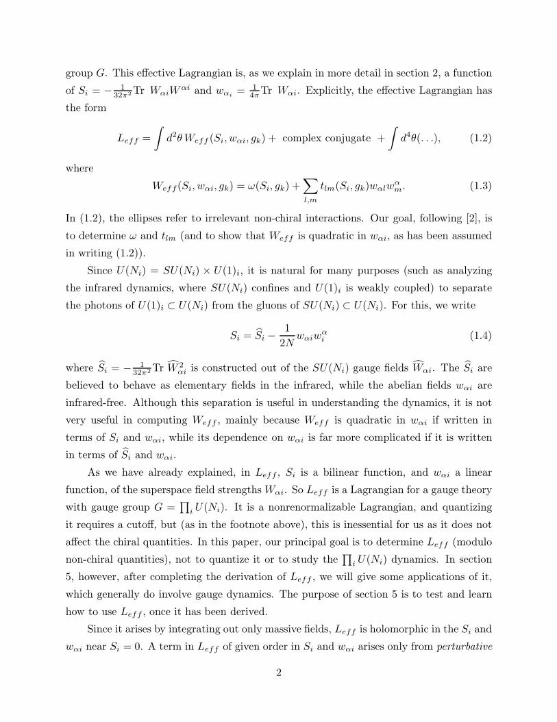
group G. This effective Lagrangian is, as we explain in more detail in section 2, a function

of Si = − 132π2 Tr WαiW

αi and wαi= 1

4πTr Wαi. Explicitly, the effective Lagrangian has

the form

Leff =

∫d2θWeff (Si, wαi, gk) + complex conjugate +

∫d4θ(. . .), (1.2)

where

Weff (Si, wαi, gk) = ω(Si, gk) +∑

l,m

tlm(Si, gk)wαlwαm. (1.3)

In (1.2), the ellipses refer to irrelevant non-chiral interactions. Our goal, following [2], is

to determine ω and tlm (and to show that Weff is quadratic in wαi, as has been assumed

in writing (1.2)).

Since U(Ni) = SU(Ni) × U(1)i, it is natural for many purposes (such as analyzing

the infrared dynamics, where SU(Ni) confines and U(1)i is weakly coupled) to separate

the photons of U(1)i ⊂ U(Ni) from the gluons of SU(Ni) ⊂ U(Ni). For this, we write

Si = Si −1

2Nwαiw

αi (1.4)

where Si = − 132π2 Tr W 2

αi is constructed out of the SU(Ni) gauge fields Wαi. The Si are

believed to behave as elementary fields in the infrared, while the abelian fields wαi are

infrared-free. Although this separation is useful in understanding the dynamics, it is not

very useful in computing Weff , mainly because Weff is quadratic in wαi if written in

terms of Si and wαi, while its dependence on wαi is far more complicated if it is written

in terms of Si and wαi.

As we have already explained, in Leff , Si is a bilinear function, and wαi a linear

function, of the superspace field strengths Wαi. So Leff is a Lagrangian for a gauge theory

with gauge group G =∏i U(Ni). It is a nonrenormalizable Lagrangian, and quantizing

it requires a cutoff, but (as in the footnote above), this is inessential for us as it does not

affect the chiral quantities. In this paper, our principal goal is to determine Leff (modulo

non-chiral quantities), not to quantize it or to study the∏i U(Ni) dynamics. In section

5, however, after completing the derivation of Leff , we will give some applications of it,

which generally do involve gauge dynamics. The purpose of section 5 is to test and learn

how to use Leff , once it has been derived.

Since it arises by integrating out only massive fields, Leff is holomorphic in the Si and

wαi near Si = 0. A term in Leff of given order in Si and wαi arises only from perturbative

2

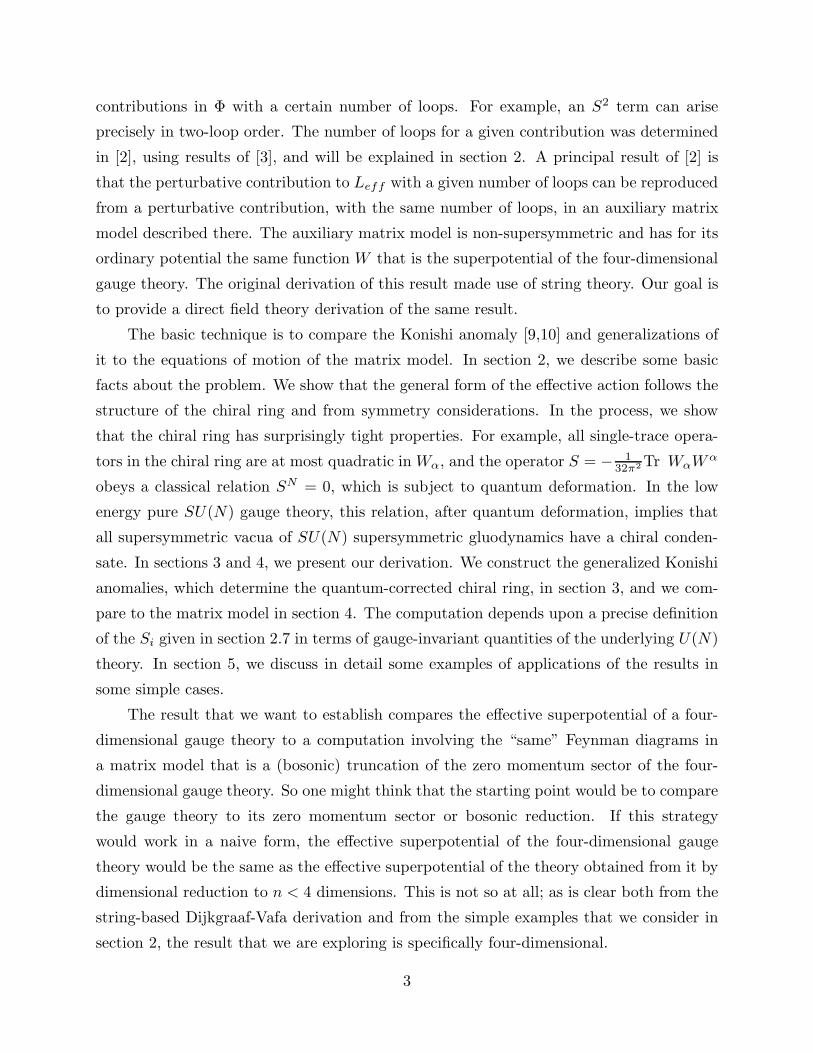
contributions in Φ with a certain number of loops. For example, an S2 term can arise

precisely in two-loop order. The number of loops for a given contribution was determined

in [2], using results of [3], and will be explained in section 2. A principal result of [2] is

that the perturbative contribution to Leff with a given number of loops can be reproduced

from a perturbative contribution, with the same number of loops, in an auxiliary matrix

model described there. The auxiliary matrix model is non-supersymmetric and has for its

ordinary potential the same function W that is the superpotential of the four-dimensional

gauge theory. The original derivation of this result made use of string theory. Our goal is

to provide a direct field theory derivation of the same result.

The basic technique is to compare the Konishi anomaly [9,10] and generalizations of

it to the equations of motion of the matrix model. In section 2, we describe some basic

facts about the problem. We show that the general form of the effective action follows the

structure of the chiral ring and from symmetry considerations. In the process, we show

that the chiral ring has surprisingly tight properties. For example, all single-trace opera-

tors in the chiral ring are at most quadratic in Wα, and the operator S = − 132π2 Tr WαW

α

obeys a classical relation SN = 0, which is subject to quantum deformation. In the low

energy pure SU(N) gauge theory, this relation, after quantum deformation, implies that

all supersymmetric vacua of SU(N) supersymmetric gluodynamics have a chiral conden-

sate. In sections 3 and 4, we present our derivation. We construct the generalized Konishi

anomalies, which determine the quantum-corrected chiral ring, in section 3, and we com-

pare to the matrix model in section 4. The computation depends upon a precise definition

of the Si given in section 2.7 in terms of gauge-invariant quantities of the underlying U(N)

theory. In section 5, we discuss in detail some examples of applications of the results in

some simple cases.

The result that we want to establish compares the effective superpotential of a four-

dimensional gauge theory to a computation involving the “same” Feynman diagrams in

a matrix model that is a (bosonic) truncation of the zero momentum sector of the four-

dimensional gauge theory. So one might think that the starting point would be to compare

the gauge theory to its zero momentum sector or bosonic reduction. If this strategy

would work in a naive form, the effective superpotential of the four-dimensional gauge

theory would be the same as the effective superpotential of the theory obtained from it by

dimensional reduction to n < 4 dimensions. This is not so at all; as is clear both from the

string-based Dijkgraaf-Vafa derivation and from the simple examples that we consider in

section 2, the result that we are exploring is specifically four-dimensional.

3

Comparison With Gauge Dynamics

Though gauge dynamics is not the main goal of the present paper, it may help the

reader if we summarize some of the conjectured and expected facts about the dynamics

of the low energy effective gauge theory with gauge group G =∏i U(Ni) that arises if we

try to quantize Leff :

(1) It is believed to have a mass gap and confinement, and as a result an effective descrip-

tion in terms of G-singlet fields.

(2) For understanding the chiral vacuum states and the value of the superpotential in

them, the important singlet fields are believed to be the chiral superfields Si = Si +1

2Niwαiw

αi) defined in (1.4).

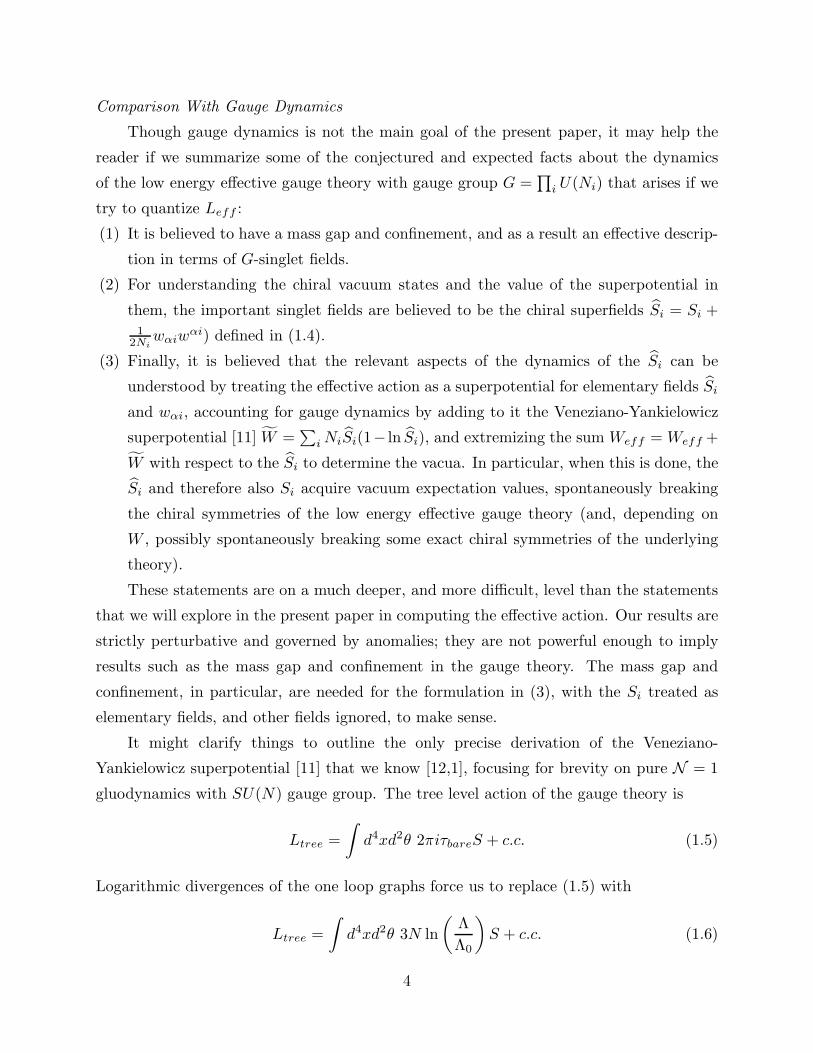
(3) Finally, it is believed that the relevant aspects of the dynamics of the Si can be

understood by treating the effective action as a superpotential for elementary fields Si

and wαi, accounting for gauge dynamics by adding to it the Veneziano-Yankielowicz

superpotential [11] W =∑iNiSi(1− ln Si), and extremizing the sum Weff = Weff +

W with respect to the Si to determine the vacua. In particular, when this is done, the

Si and therefore also Si acquire vacuum expectation values, spontaneously breaking

the chiral symmetries of the low energy effective gauge theory (and, depending on

W , possibly spontaneously breaking some exact chiral symmetries of the underlying

theory).

These statements are on a much deeper, and more difficult, level than the statements

that we will explore in the present paper in computing the effective action. Our results are

strictly perturbative and governed by anomalies; they are not powerful enough to imply

results such as the mass gap and confinement in the gauge theory. The mass gap and

confinement, in particular, are needed for the formulation in (3), with the Si treated as

elementary fields, and other fields ignored, to make sense.

It might clarify things to outline the only precise derivation of the Veneziano-

Yankielowicz superpotential [11] that we know [12,1], focusing for brevity on pure N = 1

gluodynamics with SU(N) gauge group. The tree level action of the gauge theory is

Ltree =

∫d4xd2θ 2πiτbareS + c.c. (1.5)

Logarithmic divergences of the one loop graphs force us to replace (1.5) with

Ltree =

∫d4xd2θ 3N ln

(Λ

Λ0

)S + c.c. (1.6)

4

where Λ0 is an ultraviolet cutoff and Λ is a finite scale which describes the theory. We

can think of (1.6) as a microscopic action which describes the physics at the scale Λ0.

The long distance physics does not change when Λ0 varies with fixed Λ. The factor of

3N comes from the coefficient of the one-loop beta function. Consider performing the

complete path integral of the theory over the gauge fields. Nonperturbatively, a massive

vacuum is generated, with a superpotential

Weff (Λ) = NΛ3. (1.7)

Since the well-defined instanton factor is Λ3N , we prefer to write this as

Weff (Λ) = N(Λ3N

) 1N . (1.8)

This superpotential controls the tension of BPS domain walls. The N th root is related to

chiral symmetry breaking. The N branches correspond to the N vacua associated with

chiral symmetry breaking.

Now looking back at (1.6), we see that 3N lnΛ couples linearly to S and thus behaves

as a “source” for S. The superpotential Weff (Λ) is defined directly by the gauge theory

path integral. If we want to compute an effective superpotential for S, the general recipe

is to introduce S as a c-number field linearly coupled to the source ln Λ, and perform a

Legendre transform of Weff (Λ). A simple way to do that is to introduce an auxiliary field

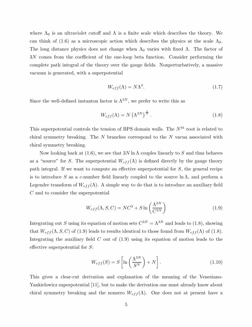
C and to consider the superpotential

Weff (Λ, S, C) = NC3 + S ln

(Λ3N

C3N

)(1.9)

Integrating out S using its equation of motion sets C3N = Λ3N and leads to (1.8), showing

that Weff (Λ, S, C) of (1.9) leads to results identical to those found from Weff (Λ) of (1.8).

Integrating the auxiliary field C out of (1.9) using its equation of motion leads to the

effective superpotential for S:

Weff (S) = S

[ln

(Λ3N

SN

)+N

]. (1.10)

This gives a clear-cut derivation and explanation of the meaning of the Veneziano-

Yankielowicz superpotential [11], but to make the derivation one must already know about

chiral symmetry breaking and the nonzero Weff (Λ). One does not at present have a

5

derivation in which one first computes the superpotential, proves that S can be treated as

an elementary field, and then uses the superpotential to prove chiral symmetry breaking.

In this paper, we concentrate first on generating the function Weff (Si), understood

(as we have explained above in detail) as an effective Lagrangian for the low energy gauge

fields. We do not (until section 5) analyze the gauge dynamics, give or assume expectation

values for the Si, treat the Si or Si as elementary fields, or extremize Weff (Si) (or any

superpotential containing it as a contribution) with respect to the Si. These are not needed

to derive the function Weff (Si). We stress that Si cannot be introduced by a Legendre

transform, as we did above for S =∑

i Si, because they do not couple to independent

sources.

We thus do not claim to have an a priori argument that the gauge dynamics is governed

by an effective Lagrangian for elementary fields Si. However, we will argue in section 4

that, if it is described by such a Lagrangian, its effective superpotential must be the sum

of Weff (Si) with a second contribution W =∑iNiSi(1 − lnSi), which (in the sense that

was just described) is believed to summarize the effects of the low energy gauge dynamics.

(In some cases it describes the effects of instantons of the underlying U(N) theory, as we

explain in section 5.)

Finally, we note that Dijkgraaf and Vafa showed that this additional “gauge” part of

the superpotential can be extracted from the measure of the matrix model. Regrettably,

in this paper we cast little new light on this fascinating result.

2. Preliminary Results

In this section, we will obtain a few important preliminary results, and give elementary

arguments for why, as claimed by Dijkgraaf and Vafa, only planar diagrams contribute to

the chiral effective action.

2.1. The Chiral Ring

Chiral operators are simply operators (such as Tr Φk or S) that are annihilated by the

supersymmetries Qα of one chirality. The product of two chiral operators is also chiral.

Chiral operators are usually considered modulo operators of the form {Qα, . . .}. The

equivalence classes can be multiplied, and form a ring called the chiral ring. A superfield

whose lowest component is a chiral operator is called a chiral superfield.

6

Chiral operators are independent of position x, up toQα-commutators. If {Qα,O(x)} =

0, then∂

∂xµO(x) = [Pµ,O(x)] = {Q

α, [Qα,O(x)]}. (2.1)

This implies [13] that the expectation value of a product of chiral operators is independent

of each of their positions:

∂

∂xαα1

⟨OI1(x1)O

I2(x2) . . .⟩

=⟨{Q

α, [Qα,OI1(x1)]}O

I2(x2) . . .⟩

= −∑

k>1

⟨[Qα,OI1(x1)

]. . .[Qα,OIk(xk)

]. . .⟩

= 0.

(2.2)

Thus we can write 〈∏I O

I(x)〉 = 〈∏I O

I〉 without specifying the positions x.

Using this invariance, we can take a correlation function of chiral operators at distinct

points, and separate the points by an arbitrarily large distance. Cluster decomposition

then implies that the correlation function factorizes [13]:

〈OI1(x1)OI2(x2) . . .O

In(xn)〉 = 〈OI1〉〈OI2〉 . . . 〈OIn〉. (2.3)

There are no contact terms in the expectation value of a product of chiral fields,

because as we have just seen a correlation function such as 〈OI1(x1)OI2(x2) . . .〉 is entirely

independent of the positions xi and so in particular does not have delta functions. A

correlation function of chiral operators together with the upper component of a chiral

superfield (for example 〈Tr Φk ·∫d2θTr Φm〉) can have contact terms.

In the theory considered here, with an adjoint superfield Φ, we can form gauge-

invariant chiral superfields Tr Φk for positive integer k. These are all non-trivial chiral

fields. The gauge field strength Wα is likewise chiral, and though it is not gauge-invariant,

it can be used to form gauge-invariant chiral superfields such as Tr ΦkWα, Tr ΦkWαΦlWβ ,

etc. (Similar chiral fields involving Wα were important in the duality of SO(N) theories

[14,15].) Setting k = l = 0, we get, in particular, chiral superfields constructed from vector

multiplets only.

There is, however, a very simple fact that drastically simplifies the classification of

chiral operators. If O is any adjoint-valued chiral superfield, we have

[Qα, DααO

}= [Wα, O} , (2.4)

7

(Dαα = DDxαα is the bosonic covariant derivative) using the Jacobi identity and definition

of Wα plus the assumption that O (anti)commutes with Qα. Taking O = Φ, we see that in

operators such as Tr ΦkWαΦmWβ , Wα commutes with Φ modulo {Qα, . . .}, so it suffices

to consider only operators Tr ΦnWαWβ .

Moreover, taking O = Wβ in the same identity, we learn that

{Qα, [Dαα,Wβ]} = {Wα,Wβ}, (2.5)

so in the chiral ring we can make the substitution WαWβ → −WβWα. So in any string

of W ’s, say Wα1. . .Wαs

, we can assume antisymmetry in α1, . . . , αs. As the αi only take

two values, we can assume s ≤ 2. So a complete list of independent single-trace chiral

operators is Tr Φk, Tr ΦkWα, and Tr ΦkWαWα. This list of operators has already been

studied by [16,17].

2.2. Relations in The Chiral Ring

We have seen that the generators of the chiral ring are of the form Tr Φk, Tr WαΦk,

Tr WαWαΦk. These operators are not completely independent and are subject to relations.

The first kind of relation stems from the fact that Φ is an N ×N matrix. Therefore,

Tr Φk with k > N can be expressed as a polynomial in ul = Tr Φl with l ≤ N

Tr Φk = Pk(u1, ..., uN) (2.6)

In Appendix A, we show that the classical relations (2.6) are modified by instantons for

k ≥ 2N . This is similar to familiar modifications due to instantons of classical relations

in the two dimensional CPN model [18] and in certain four dimensional N = 1 gauge

theories [19]. The general story is that to every classical relation corresponds a quantum

relation, but the quantum relations may be different.

A second kind of relations follows from the tree level superpotential W (Φ). As is

familiar in Wess-Zumino models, the equation of motion of Φ

∂ΦW (Φ) = DαDαΦ (2.7)

shows that in the chiral ring ∂ΦW (Φ)c.r. = 0 (the subscript c.r. denotes the fact that this

equation is true only in the chiral ring). In a gauge theory, we want to consider gauge-

invariant chiral operators; classically, for any k, Tr Φk∂ΦW (Φ) vanishes in the chiral ring.

8

This is a nontrivial relation among the generators. In section 3, we will discuss in detail

how this classical relation is modified by the Konishi anomaly [9,10] and its generalizations.

We now turn to discuss interesting relations which are satisfied by the operator S =

− 132π2 Tr W 2

α. We first discuss the pure gauge N = 1 theory with gauge group SU(N).

We will comment about other gauge groups (such as U(N)) below.

The operator S is subtle because it is a bosonic operator which is constructed out of

fermionic operators. Since the gauge group has N2 − 1 generators, the Lorentz index α in

Wα take two different values, and S is bilinear in Wα, it follows from Fermi statistics that

(SN2

)p = 0, (2.8)

so in particular S is nilpotent. We added the subscript p to denote that this relation is valid

in perturbation theory. Soon we will argue that this relation receives quantum corrections.

It is important that (2.8) is true for any S which is constructed out of fermionic Wα. The

latter does not have to satisfy the equations of motion.

If we are interested in the chiral ring, we can derive a more powerful result. We will

show that

(SN )p = {Qα, Xα} (2.9)

for some X α, and therefore in the chiral ring

(SN )p,c.r. = 0 (2.10)

For SU(2), we can show (2.9) using the identity

Tr ABCD =1

2(Tr ABTr CD + Tr DATr BC − Tr ACTr BD) (2.11)

for any SU(2) generators A,B,C,D. Hence, allowing for Fermi statistics (which imply

Tr W1W1 = Tr W2W2 = 0), we have

Tr W1W1W2W2 = (Tr W1W2)2. (2.12)

The left hand side is non-chiral, as we have seen above, and the right hand side is a multiple

of S2, so we have established (2.10) for SU(2). In appendix B we extend this proof to

SU(N) with any N , and we also show that SN−1 6= 0 in the chiral ring.

If the relation SN = {Qα, Xα} were an exact quantum statement, it would follow

that in any supersymmetric vacuum, 〈SN 〉 = 0, and hence by factorization and cluster

9

decomposition, also 〈S〉 = 0. What kind of quantum corrections are possible in the ring

relation SN = 0? In perturbation theory, because of R-symmetry and dimensional analysis,

there are no possible quantum corrections to this relation. Nonperturbatively, the instanton

factor Λ3N has the same chiral properties as SN , so it is conceivable that instantons could

modify the chiral ring relation to SN = constant · Λ3N . In fact [13], instantons lead to an

expectation value 〈SN 〉 = Λ3N , and therefore, they do indeed modify the classical operator

relation to

SN = Λ3N + {Qα, Xα} (2.13)

where in the chiral ring we can set the last term to zero. Equation (2.13) is an exact

operator relation in the theory. It is true in all correlation functions with all operators.

Also, since it is an operator equation, it is satisfied in all the vacua of the theory. The

relation SN2

= 0, which we recall is an exact relation, not just a statement in the chiral

ring, must also receive instanton corrections so as to be compatible with (2.13). To be

consistent with the existence of a supersymmetric vacuum in which 〈SN 〉 = Λ3N , as well

as with the classical limit in which SN2

= 0, the corrected equation must be of the form

(SN −Λ3N )P (SN ,Λ3N) = 0, where P is a homogeneous polynomial of degree N − 1 with

a non-zero coefficient of (SN )N−1. We do not know the precise form of P .

To illustrate the power of the chiral ring relation SN = Λ3N , let us note that it implies

that 〈S〉N = 〈SN 〉 = Λ3N in all supersymmetric vacua of the theory. Indeed, the chiral

ring relation SN = Λ3N is an exact operator relation, independent of the particular state

considered. Thus, contrary to some conjectures, there does not exist a supersymmetric

vacuum of the SU(N) supersymmetric gauge theory with 〈S〉 = 0.

This situation is very similar to the analogous situation in the the two dimensional

supersymmetric CPN−1 model as well as its generalization to Grassmannians (see section

3.2 of [18]). In the CPN−1 model, a twisted chiral superfield, often called σ, obeys a

classical relation σN = 0; this is deformed by instantons to a quantum relation σN = e−I ,

where I is the instanton action. (In the non-linear CPN−1 model, σ is bilinear in fermions

and associated with the generator of H2(CPN−1); the classical relation σN = 0 then

follows from Fermi statistics, as the fermions only have 2N − 2 components, and so is

analogous to the classical relation SN2

= 0 considered above.)

Role Of These Relations In Different Approaches

It is common that an operator relation which is “always true” in one formulation of a

theory, being a kinematical relation that holds off-shell, follows from the equation of motion

10

in a second formulation. In that second formulation, the given relation is not true off-shell.

A familiar example is the Bianchi identity in two dual descriptions of free electrodynamics.

The Bianchi identity is always true in the electric description of the theory, but it appears

as an equation of motion in the magnetic description.

This analogy leads to a simple interpretation of the Veneziano-Yankielowicz superpo-

tential S(N + ln(Λ3N/SN )). It is valid in a description (difficult to establish rigorously)

in which S is an unconstrained bosonic field. In that description, we should not use the

classical equation SN = {Qα, Xα} or its quantum deformation SN = Λ3N + {Qα, X

α}

to simplify the Lagrangian; such an equation should arise from the equation of motion.

Indeed, the equation for the stationary points of this superpotential is SN = Λ3N (or zero

in perturbation theory) which is the relation in the chiral ring (2.13).

From here through section 4 of the paper, we will determine an effective action for

the supersymmetric gauge theory with adjoint superfield Φ, understood as an action for

low energy gauge fields that enter via Si. Each term∏i S

ki

i that we generate has a clear

meaning for large enough Ni. However, for fixed Ni and large enough ki could we not

simplify this Lagrangian, using for example the U(Ni) relation SN2i +1 = 0? An attempt to

do this would run into potentially complicated instanton corrections, because actually the

Si fields in the interactions∏i S

Ni

i are smeared slightly by the propagators of the massive

Φ fields; in attempting to simplify this to a local Lagrangian (where one could use Fermi

statistics to set SN2i +1 = 0), one would run into corrections from small instantons, so

the attempt to simplify the Lagrangian could not be separated from an analysis of gauge

dynamics. Alternatively, in section 5, we use a more powerful (but less rigorous) approach

in which it is assumed that the Si can be treated as independent classical fields. From this

point of view, the ring relations for the Si (which are written below in terms of Si and

wαi) are not valid off-shell and should arise from the equations of motion.

Behavior For Other Groups

What happens for other groups? Consider an N = 1 theory with a simple gauge group

G and no chiral multiplets. The theory has a global discrete chiral symmetry ZZ2h(G) with

h(G) the dual Coxeter number of G (h = N for SU(N)). Numerous arguments suggest

that the ZZ2h discrete symmetry of the system is spontaneously broken to ZZ2, and that the

theory has h vacua in which 〈Sh〉 = c(G)Λ3h with a nonzero constant c(G). We conjecture

11

that at the classical level, S obeys a relation Sh = {Qα, Xα}, and that instantons deform

this relation to an exact operator statement

Sh = c(G)Λ3h + {Qα, Xα} (2.14)

for some X α. As for SU(N), this statement would imply that chiral symmetry breaking

occurs in all supersymmetric vacua. It would be interesting to understand how the chiral

ring relation Sh = 0 arises at the classical level, and in particular how h(G) enters.

Before ending this discussion, we will make a few comments about the U(N) gauge

theory, as opposed to SU(N). As we explained in the introduction, here it makes sense to

define (1.4) S = S− 12Nwαw

α where S is the SU(N) part of S, and the second term is the

contribution of the gauge fields of the U(1) part wα = 14π

Tr Wα. The quantum relation is

SN = Λ3N + {Qα, Xα}. Since there are only two wα and they are fermionic, S obeys

SN = −1

2SN−1wαw

α + Λ3N + {Qα, Xα} = −

1

2SN−1wαw

α + Λ3N + {Qα, Xα} (2.15)

In vacua where U(N) is broken to∏i U(Ni), each with its own Si = Si−

12Ni

wiαwαi these

operators satisfy complicated relations. They follow from the equation of motion of the

effective superpotential ω(Si). What happens for Ni = 1? In this case, one might expect

Si = 0. This is the correct answer classically but it can be modified quantum mechanically

to Si = constant. We will see that in more detail in section 5, where we study the case

with all Ni = 1. In this case instantons lead to Si 6= 0. In order to describe this case in

the effective theory, one must include an independent field Si even for a U(1) factor.

2.3. First Look at Perturbation Theory – Unbroken Gauge Group

Now we begin our study of the theory with the adjoint chiral superfield Φ. For

simplicity, we will begin with the case of unbroken gauge symmetry. So we expand around

Φ = a, where a is a (c-number) critical point of the function W that appears in the

superpotential

W (Φ) =n∑

k=0

gkk + 1

Tr Φk+1. (2.16)

The mass parameter of the Φ field in expanding around this vacuum is m = W ′′(a). We

may as well assume that a = 0, so g0 = 0 and g1 = m.

12

X

a. b.

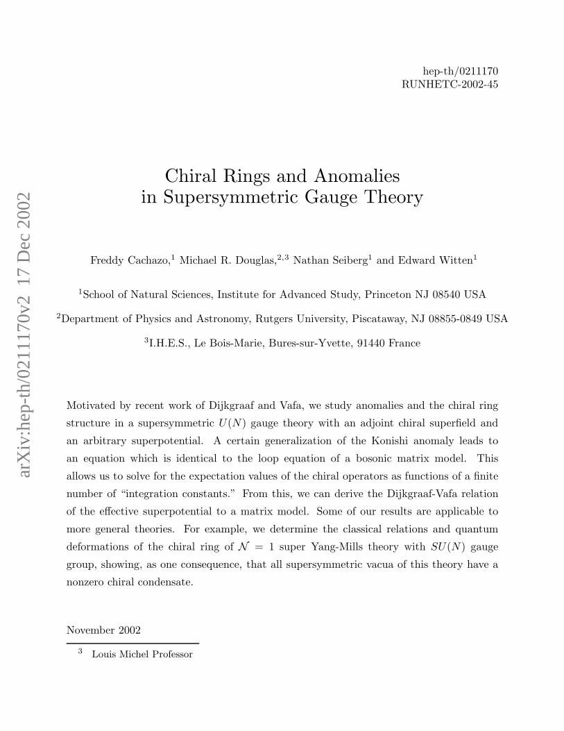
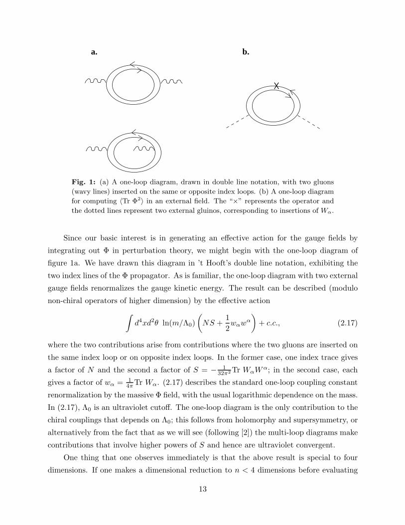
Fig. 1: (a) A one-loop diagram, drawn in double line notation, with two gluons

(wavy lines) inserted on the same or opposite index loops. (b) A one-loop diagram

for computing 〈Tr Φ2〉 in an external field. The “×” represents the operator and

the dotted lines represent two external gluinos, corresponding to insertions of Wα.

Since our basic interest is in generating an effective action for the gauge fields by

integrating out Φ in perturbation theory, we might begin with the one-loop diagram of

figure 1a. We have drawn this diagram in ’t Hooft’s double line notation, exhibiting the

two index lines of the Φ propagator. As is familiar, the one-loop diagram with two external

gauge fields renormalizes the gauge kinetic energy. The result can be described (modulo

non-chiral operators of higher dimension) by the effective action

∫d4xd2θ ln(m/Λ0)

(NS +

1

2wαw

α

)+ c.c., (2.17)

where the two contributions arise from contributions where the two gluons are inserted on

the same index loop or on opposite index loops. In the former case, one index trace gives

a factor of N and the second a factor of S = − 132π2 Tr WαW

α; in the second case, each

gives a factor of wα = 14π

Tr Wα. (2.17) describes the standard one-loop coupling constant

renormalization by the massive Φ field, with the usual logarithmic dependence on the mass.

In (2.17), Λ0 is an ultraviolet cutoff. The one-loop diagram is the only contribution to the

chiral couplings that depends on Λ0; this follows from holomorphy and supersymmetry, or

alternatively from the fact that as we will see (following [2]) the multi-loop diagrams make

contributions that involve higher powers of S and hence are ultraviolet convergent.

One thing that one observes immediately is that the above result is special to four

dimensions. If one makes a dimensional reduction to n < 4 dimensions before evaluating

13

the Feynman diagram, dimensional analysis will forbid a contribution as in (2.17), and a

different result will ensue, depending on the dimension. Moreover, the m dependence in

(2.16) is controlled in a familiar way by the chiral anomaly under phase rotations of the Φ

field; this is a hint that also the higher order terms can be determined by using anomalies,

as we will do in this paper.

One can phrase even the one loop results in a way in which the cutoff does not appear,

by instead computing a first derivative of the effective superpotential with respect to the

couplings. On general grounds, these first derivatives are the expectation values of the

gauge invariant chiral operators. We will need this result in section 4, so we will explain it

in detail. A variation of the couplings gk → gk+δgk will produce an effective superpotential

Weff (Si, wαi, gk + δgk) given by⟨

exp

(−

∫d4xd2θ

∑

k

δgkk + 1

Tr Φk+1 − c.c.

)⟩

Φ

, (2.18)

where the bracket 〈 〉Φ refers to the result of a path integral over the massive fields, in

the presence of a (long wavelength) background gauge field characterized by variables Si

and wαi. By holomorphy and supersymmetry, this result remains valid if the coupling

constants gk + δgk in (2.16) and (2.18) are promoted to chiral superfields [20]. Now, take

the variational derivative of (2.18) with respect to the upper component of δgk. This

eliminates the d2θ integral, and produces

∂Weff

∂gk=

⟨Tr

Φk+1

k + 1

⟩

Φ

. (2.19)

Thus, if we can get an expectation value as a function of the couplings, we can integrate

it to get Weff , up to a constant of integration independent of the couplings.

To illustrate, let us compute the right hand side of (2.19) in the one-loop approxima-

tion for k = 1. The diagram that we need to evaluate is shown in figure 1b. There are two

boson propagators and one fermion propagator. The integral that we must evaluate is∫

d4k

(2π)4

(1

k2 +mm

)2m

k2 +mm=

1

32π2m. (2.20)

This multiplies NS or wαwα depending on whether the two external gluinos are inserted

on equal or opposite index loops, so in the one-loop approximation, we get

∂Weff

∂g1=NS + 1

2wαwα

m. (2.21)

(Recall that g1 = m.)

This illustrates the process of integrating out the massive Φ fields to get a chiral

function of the background gauge fields. To go farther, however, we want more general

arguments.

14

2.4. A More Detailed Look at the Effective Action – Unbroken Gauge Group

Next we will consider the multi-loop corrections. Let us first see what we can learn

just from symmetries and dimensional analysis. The one adjoint theory has two continuous

symmetries, a standard U(1)R symmetry and a symmetry U(1)Φ under which the entire

superfield Φ undergoes

Φ → eiαΦ. (2.22)

We also introduce a linear combination of these, U(1)θ, which is convenient in certain

arguments.

If we allow the couplings to transform non-trivially, these are also symmetries of the

theory with a superpotential. The dimensions ∆ and charges Q of the chiral fields and

couplings are∆ QΦ QR Qθ

Φ 1 1 2/3 0Wα 3/2 0 1 1gl 2 − l −(l + 1) 2

3(2 − l) 2

Λ2N 2N 2N 4N/3 0

(2.23)

(Although we will not use it here, we also included the gauge theory scale Λ for later

reference.) Since all of these are chiral superfields, their dimensions satisfy the relation

∆ = 3QR/2.

All of these symmetries are anomalous at one loop. The U(1)Φ anomaly was first

discussed by Konishi [9,10] and (as we discuss in more detail in section 3) says that the

one-loop contribution toWeff (S) is shifted under (2.22) by a multiple of S; this can be used

to recover the result already given in (2.17). On the other hand, higher loop computations

are finite and the transformation (2.22) leaves these invariant (again, we discuss this point

in detail in section 3). It follows that the effective action must depend on the gk’s only

through the ratios gk/g(k+1)/21 . Equivalently, we can write

∑

k

(k + 1)gk∂

∂gkWeff = 0, (2.24)

except at one loop.

Now let us consider dimensional analysis (by the relation ∆ = 3QR/2, R symmetry

leads to the same constraint). The effective superpotential Weff has dimension 3. So,

15

taking into account the result in the last paragraph, Weff must depend on the gk’s and

Wα in the form2

Weff = W 2αF

(gkW

k−1α

g(k+1)/21

). (2.25)

Here we are being rather schematic, just to indicate the overall power of Wα. So, for

example, W 2α may correspond to either S or wαw

α. Instead of (2.25), we could write

(∑

k

(2 − k)gk∂

∂gk+

3

2Wα

∂

∂Wα

)Weff = 3Weff . (2.26)

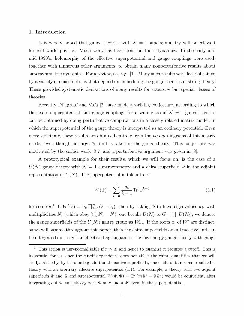
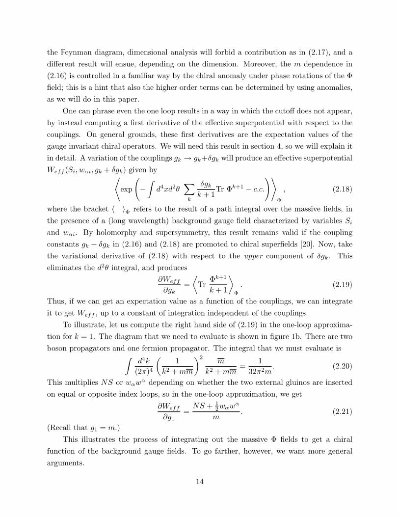
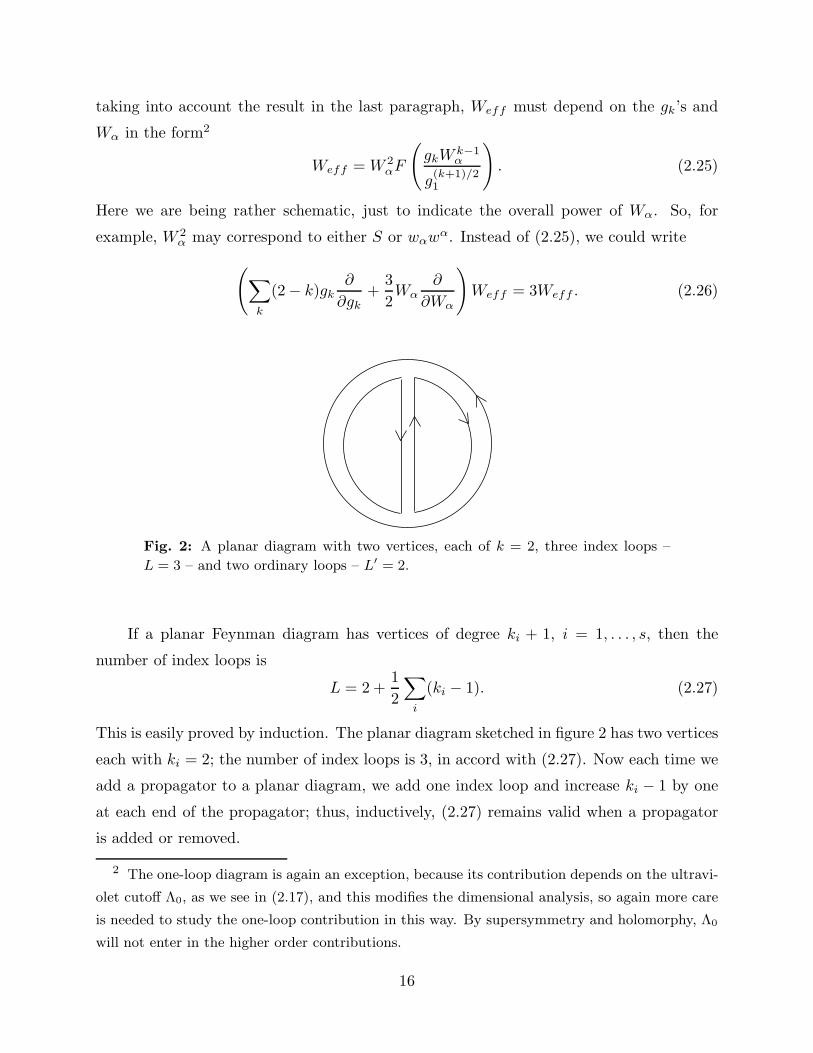
Fig. 2: A planar diagram with two vertices, each of k = 2, three index loops –

L = 3 – and two ordinary loops – L′ = 2.

If a planar Feynman diagram has vertices of degree ki + 1, i = 1, . . . , s, then the

number of index loops is

L = 2 +1

2

∑

i

(ki − 1). (2.27)

This is easily proved by induction. The planar diagram sketched in figure 2 has two vertices

each with ki = 2; the number of index loops is 3, in accord with (2.27). Now each time we

add a propagator to a planar diagram, we add one index loop and increase ki − 1 by one

at each end of the propagator; thus, inductively, (2.27) remains valid when a propagator

is added or removed.

2 The one-loop diagram is again an exception, because its contribution depends on the ultravi-

olet cutoff Λ0, as we see in (2.17), and this modifies the dimensional analysis, so again more care

is needed to study the one-loop contribution in this way. By supersymmetry and holomorphy, Λ0

will not enter in the higher order contributions.

16

By taking a linear combination of (2.24) and (2.26), we get(∑

k

(1 − k)gk∂

∂gk+Wα

∂

∂Wα

)Weff = 2Weff . (2.28)

(2.27) lets us replace∑k(1 − k)gk∂/∂gk by 4 − 2L. It follows therefore that the power

of Wα in a contribution coming from a planar Feynman diagram with L index loops is

2L− 2. Such a contribution might be a multiple of SL−1, or of SL−2wαwα. We get SL−1

if L− 1 index loops each have two insertions of external gauge bosons and one has none,

or SL−2wαwα if L− 2 index loops each have two gauge insertions and two loops have one

gauge insertion each.

The generalization of (2.27) for a diagram that is not planar but has genus g (that is,

the Riemann surface made by filling in every index loop with a disc has genus g) is

L = 2 − 2g +1

2

∑

i

(ki − 1). (2.29)

This statement reflects ’t Hooft’s observation that increasing the genus by one removes

two index loops and so multiplies an amplitude by 1/N2. So a diagram of genus g has a

power of Wα equal to 2L+ 4g − 2.

At first sight, it appears that additional invariants such as Tr WαWαWβW

β will

arise if there are more then two gauge insertions on the same index loop. But as we have

seen, such operators are non-chiral and so can be neglected for the purposes of this paper.

Also, the bilinear expression Tr WαWβ vanishes by Fermi statistics unless the indices α

and β are contracted to a Lorentz singlet. Therefore the effective superpotential can be

expressed in terms of S = − 132π2 Tr WαW

α and wα = 14πTr Wα only.

Since each index loop in a Feynman diagram can only contribute a factor of S, wα,

or N , depending on whether the number of gauge insertions on the loop is two, one, or

zero, it now follows, as first argued by Dijkgraaf and Vafa, that only planar diagrams

can contribute to the effective chiral interaction for the gauge fields. Indeed, according to

(2.29), in the case of a non-planar diagram, at least one index loop would have to give a

trace of a product of more than two Wα’s, but these are trivial as elements of the chiral

ring.

Furthermore, the interactions generated by planar diagrams are highly constrained.

The only way to obey (2.29) without generating a trace with more than two W ’s is to

have one index loop with no W and the others with two each, or two index loops with one

W and again the others with two each. The possible interactions generated by a planar

diagram with L index loops are hence SL−1 and SL−2wαwα.

This reproduces the results of [8] and the previous papers cited in the introduction.

17

2.5. The Case Of Broken Gauge Symmetry

Now let us briefly consider how to extend these arguments for the case of sponta-

neously broken gauge symmetry. Here we assume that U(N) is spontaneously broken to∏ni=1 U(Ni). We integrate out all massive fields, including the massive gauge bosons and

their superpartners, to obtain an effective action for the massless superfields of the unbro-

ken gauge group. The effective action depends now on the assortment of gauge-invariant

operators Si = − 132π2 Tr WαiW

αi and wαi = 14πTr Wαi that appeared in the introduction.

Their definitions will be considered more critically in section 2.7, but for now we can be

casual.

Unlike the simpler case of unbroken gauge symmetry, here we need to integrate out

massive gauge fields. Their propagator involves the complexified gauge coupling τbare or

ln Λ. But the perturbative answers must be independent of its real part, which is the theta

angle, and therefore τbare cannot appear in holomorphic quantities (except for the trivial

classical term). This means that the number of massive gauge field propagators must be

equal to the number of vertices of three gauge fields.

The considerations of symmetries and dimensional analysis that led to (2.25) are still

valid.3 However, the Wα’s that appear in (2.25) can now be of different kinds; they can

be of the type Wαi for any 1 ≤ i ≤ n. They thus can assemble themselves into different

invariants such as Si and wαi, but for the moment we will not be specific about this.

A key difference when the gauge symmetry is spontaneously broken is that the depen-

dence on the gk can be much more complicated. The gk do not merely enter as factors at

interaction vertices. The reason is that perturbation theory is constructed by expanding

around a critical point of W (Φ) in which the matrix Φ has eigenvalues ai (the zeroes of W ′)

with multiplicities Ni. The ai depend on the gk, as do the masses of various components of

Φ; and after shifting Φ to the critical point about we intend to expand, a Feynman vertex

of order r is no longer merely proportional to gr−1 but receives contributions from gs with

s > r− 1. Because of all this, we need a better way to determine the relation between the

number of loops and the S-dependence.

3 The one-loop diagram still provides an exception to (2.25) because it depends logarithmically

on the cutoff Λ0; it can be studied specially and gives, in the usual way, a linear combination of

the Si and of wαiwαj . This is of the general form that the discussion below would suggest, though

this discussion will be formulated in a way that does not quite apply at one-loop order.

18

Let L′ be the number of ordinary loops in a Feynman diagram, as opposed to L, the

number of index loops. Thus, in the diagram of figure 2, L′ = 2 and L = 3. For planar

diagrams, L′ = L− 1, and in general,

L′ = L− 1 + 2g. (2.30)

In order to enumerate the loops we modify the tree level Lagrangian as follows. We replace

the superpotential W with W/h, we replace the kinetic term Tr Φ†eV Φ with ZhTr Φ†eV Φ,

and we replace the gauge kinetic term τbareW2α with 1

hτbareW

2α. Here Z is a real vector

superfield, τ is a chiral superfield and h is taken to be a real number. The contribution

WL′

eff to Weff from diagrams with L′ loops is then proportional to hL′−1, so

h∂

∂hWL′

eff = (L′ − 1)WL′

eff . (2.31)

Since Z is a real superfield, it cannot appear in the effective superpotential. We have

already remarked that the perturbative superpotential is independent of τbare (except the

trivial tree dependence). Therefore, simply by calculus, since W/h depends only on ratios

gk/h, we have

h∂

∂hWL′

eff = −∑

k

gk∂

∂gkWL′

eff (2.32)

so ∑

k

gk∂

∂gkWL′

eff = −(L′ − 1)WL′

eff . (2.33)

Using (2.30), the contribution WL,geff with L index loops and genus g hence obeys

h∂

∂hWL,geff = −(L− 2 + 2g)WL,g

eff . (2.34)

By combining (2.34) with (2.24) and (2.26), we learn that

∑

α,i

Wαi∂

∂WαiWL,geff = (2L− 2 + 4g)WL,g

eff , (2.35)

so a diagram with a given L and g makes contributions to the superpotential that is of

order 2L−2+4g in the Wαi’s. This is the same result as in the case of unbroken symmetry;

we have merely given a more general derivation using (2.34) instead of (2.29). It follows

from (2.35) that for g > 0, the overall power of Wαi is greater than 2L, so at least one

19

index loop contains more than two gauge insertions and gives a trace of more than two

powers of Wαi for some i.

Generalizing the discussion of the unbroken group, each index loop in a Feynman

diagram labeled by one of the unbroken gauge groups U(Ni) can only contribute a factor

of Si, wαi, or Ni, depending on whether the number of gauge insertions on the loop is two,

one, or zero. It again follows that only planar diagrams can contribute to the effective

chiral interaction for the gauge fields. As in the unbroken case, we learn that the possible

interactions generated by a planar diagram with L index loops are SL−1 and SL−2wαwα,

where here each factor of S or wα can be any of the Si or wαi, depending on how the index

loops in the diagram are labeled. In particular, the chiral effective action is quadratic in

the wαi.

2.6. General Form Of The Effective Action

Making use of the last statement to constrain the dependence on the w’s, the general

form of the chiral effective action for the low energy gauge fields is thus

∫d4x d2θ Weff (Sk, wαk) (2.36)

with

Weff (Sk, wαk) = ω(Sk) +n∑

i,j=1

tij(Sk)wαiwαj . (2.37)

We now make a simple observation that drastically constrains the form of the effective

action. Since all fields in the underlying U(N) gauge theory under discussion here are in

the adjoint representation, the U(1) factor of U(N) is free. It is described completely by

the simple W 2α classical action.

In particular, there is an exact symmetry of shifting Wα by an anticommuting c-

number (times the identity N × N matrix). In the low energy theory with gauge

group∏i U(Ni), this symmetry simply shifts each Wαi. So the transformation of

Si = − 132π2 Tr WαiW

αi and wαi = 1

4πTr Wαi under Wα →Wα − 4πψα is

δSi = −ψαwαi

δwαi= −Niψα.

(2.38)

20

It is not difficult to work out by hand the conditions imposed by the invariance (2.38)

on the effective action (2.37). However, it is more illuminating to combine the operators

Si and wαi in a superfield Si which will also play a very useful role in the sequel:

Si = −1

2Tr

(1

4πWαi

− ψα

)(1

4πWαi − ψα

)= Si + ψαw

αi − ψ1ψ2Ni. (2.39)

In this description, the symmetry is simply generated by ∂/∂ψα. Invariance under this

transformation implies that the effective action is

Weff =

∫d2ψFp (2.40)

for some function Fp. Fp is not uniquely determined by (2.40), since, for example, we

could add to Fp any function of the SU(Ni) fields Si of (1.4). However, the form of (2.36)

implies that we can take Fp to be a function only of the Si , and Fp is then uniquely

determined if we also require

Fp(Si = 0) = 0. (2.41)

The subscript p in the definition of Fp denotes the fact that∫d2ψFp reproduces the chiral

interactions induced by integrating out the massive fields (without the nonperturbative

contribution from low energy gauge dynamics). On doing the ψ integrals, we learn that

Weff = ω(Sk) + tijwαiwαj =

∫d2ψFp(Sk) =

∑

i

Ni∂Fp(Sk)

∂Si+

1

2

∑

ij

∂2Fp(Sk)

∂Si∂Sjwαiw

αj .

(2.42)

This is the general structure claimed by Dijkgraaf and Vafa, with Fp still to be determined.

By expanding (2.42) in powers of wαi (and recalling the expansion (1.4)), we derive

their gauge coupling matrix

τij =∂2Fp(Sk)

∂Si∂Sj− δij

1

Ni

∑

l

Nl∂2Fp(Sk)

∂Si∂Sl. (2.43)

It is easy to see that ∑

j

τijNj = 0 (2.44)

which signals the decoupling of the overall U(1). Note that it decouples without using the

equations of motion. While the overall U(1) decouples from the perturbative corrections,

it of course participates in the classical kinetic energy of the theory, which in the present

variables is τ∑i Si, with τ the bare coupling parameter.

21

In many string and brane constructions, as mentioned in [2], nonrenormalizable inter-

actions are added to the underlying U(N) gauge theory in such a way that the symmetry

generated by ∂/∂ψ actually becomes a second, spontaneously broken supersymmetry. This

fact is certainly of great interest, but will not be exploited in the present paper. We only

note that as the scale of that symmetry breaking is taken to infinity, the Goldstone fermion

multiplet which is the U(1) gauge multiplet becomes free. In this limit the broken gen-

erators of the N = 2 supersymmetry are contracted. By that we mean that while the

anticommutator of two unbroken supersymmetry generators is a translation generator,

two broken supersymmetry generators anticommute. Indeed, our fermionic generators

∂/∂ψ anticommute with the analogous anti-chiral symmetries ∂/∂ψ† that shift Wα by a

constant.

Despite this relation to spontaneously broken N = 2 supersymmetry in certain con-

structions, the symmetry (2.38) is present even in theories which have no obvious N = 2

analog. For example, it would be present in any N = 1 quiver gauge theory (i.e. with

U(N) gauge groups and bifundamental and adjoint matter), including chiral theories.

2.7. U(N)-Invariant Description Of Effective Operators Of the Low Energy Theory

As preparation for the next section, we now wish to give a more accurate description

of the effective operators Si and wαi, i = 1, . . . , n of the low energy theory in terms of

U(N)-invariant operators of the underlying U(N) theory. We assume as always that the

superpotential W has n distinct critical points ai, i = 1, . . . , n.

Roughly speaking, we can do this by taking the Si to be linear combinations of

Tr ΦkWαWα (as we have seen, the precise ordering of factors does not matter), for

k = 0, . . . , n−1. Similarly, one would take the wαi to be linear combinations of Tr ΦkWα.

However, to be precise, we need to take linear combinations of these operators to project

out, for example, the Si associated with a given critical point ai. Proceeding in this way,

one would get rather complicated formulas which might appear to be subject to quantum

corrections.

There is a more illuminating approach which also will be extremely helpful in the next

section. We let Ci be a small contour surrounding the critical point ai in the counterclock-

wise direction, and not enclosing any other critical points. And we define

Si = −1

2πi

∮

Ci

dz1

32π2Tr WαW

α 1

z − Φ

wαi=

1

2πi

∮

Ci

dz1

4πTr Wα

1

z − Φ.

(2.45)

22

It is easy to see, first of all, that in the semiclassical limit, the definitions in (2.45) give

what we want. In the classical limit, to evaluate the integral, we set Φ to its vacuum

value. In the vacuum, Φ is a diagonal matrix with diagonal entries λ1, λ2, . . . , λN (which

are equal to the ai with multiplicity Ni). If M is any matrix and Mxy, x, y = 1, . . . , N are

the matrix elements of M in this basis, then

Tr M1

z − Φ=∑

x

Mxx

z − λx, (2.46)

so

1

2πi

∮

Ci

dzTr M1

z − Φ=∑

x

1

2πi

∮

Ci

dzMxx

z − λx=∑

λx∈Ci

Mxx = Tr MPi. (2.47)

Here λx ∈ Ci means that λx is inside the contour Ci, and Pi is the projector onto

eigenspaces of Φ corresponding to eigenvalues that are inside this contour. In the clas-

sical limit, Pi is just the projector onto the subspace in which Φ = ai. Hence the above

definitions amount in the classical limit to

Si = −1

32π2Tr WαW

αPi, wαi =1

4πTr WαPi. (2.48)

This agrees with what we want.

The formula (2.47) is still valid in perturbation theory around the classical limit,

except that the projection matrix Pi might undergo perturbative quantum fluctuations.

One might expect that in perturbation theory, Pi in (2.48) could be expressed as its classical

value plus loop corrections that would themselves be functions of the vector multiplets of

the low energy theory. In this case, the objects Si and wαi as defined in (2.45) would not

be precisely the usual functions of the massless vector multiplets of the low energy theory.

We will now argue, however, that there are no such corrections. First we complete Si and

wαi into the natural superfield

Si = −1

2πi

∮dz

1

2Tr (

1

4πWα − ψα)(

1

4πWα − ψα)

1

z − Φ. (2.49)

So

Si = Si + ψαwαi − ψ1ψ2N ′

i , (2.50)

where

N ′i =

1

2πi

∮

Ci

dzTr1

z − Φ. (2.51)

23

A priori, it might seem that N ′i is another chiral superfield, but actually, in pertur-

bation theory N ′i is just the constant Ni. In fact, using (2.47), N ′

i = Tr Pi. Although the

projection matrix Pi can fluctuate in perturbation theory, the dimension of the space onto

which it projects cannot fluctuate, since perturbation theory only moves eigenvalues by a

bounded amount.4 Thus this dimension N ′i is the constant Ni, the dimension of the space

on which Φ = ai. Because of this relation, we henceforth drop the prime and refer to N ′i

simply as Ni.

Now we can show that in (2.48), the Pi can be simply replaced by their classical

values, so that Si and wαi are the usual functions of the low energy U(Ni) gauge fields.

The components of the superfield Si transform nontrivially under the symmetry (2.38), but

the top component of this superfield is a c-number. Therefore, the bottom component Si is

only a quadratic function of the gauge fields Wαi of the low energy theory. If fluctuations

in Pi caused Si to be a non-quadratic function of the low energy Wαi, then ∂2Si/∂ψ2

would be non-constant. Thus, what is defined in (2.45) is precisely the object that one

would want to define as Si in the low energy U(Ni) gauge theory. Likewise, the “middle”

component wαi of this superfield is linear in the low energy gauge fields, so it is precisely

the superspace field strength of the ith U(1) in the low energy gauge theory, that is, of the

center of U(Ni).

In particular, since the Si and wαi have no quantum corrections, they are functions

only of the low energy gauge fields and not of the gk. In section 4, we will want to

differentiate with respect to the gk at “fixed gauge field background”; this can be done

simply by keeping Si and wαi fixed.

We can describe this intuitively by saying that modulo {Qα, }, the fluctuations in Pi

are pure gauge fluctuations, roughly since there are no invariant data associated with the

choice of an Ni-dimensional subspace in U(N).

The meaningfulness of the couplings tij in (1.2) depends on having correctly nor-

malized the field strengths wαi; in the absence of a preferred normalization, by making

arbitrary field redefinitions one could always set tij = δij . Since the low energy gauge

theory contains particles charged under U(1)n (the W bosons of broken gauge symmetry),

the preferred normalization is the one in which these particles have integer charge in each

U(1) factor. Again, this is clearly true of (2.45) in the semiclassical limit, and in the form

(2.48) is clearly true in general.

4 This is trivial in perturbation theory. Moreover, the reduction to planar diagrams means

that perturbation theory is summable, so the rank of Pi also cannot fluctuate nonperturbatively.

24

These properties are not preserved under general superfield redefinitions fj(Si). By

analogy with conventional N = 2 supersymmetry, in which one speaks of the preferred

N = 2 superfields for which U(1)n charge quantization is manifest as defining “special

coordinates,” we can also use the term special coordinates for the variables Si we have

discussed here.

3. The Generalized Konishi Anomaly

The Konishi anomaly is an anomaly for the (superfield) current5

J = Tr Φead V Φ, (3.1)

which generates the infinitesimal rescaling of the chiral field,

δΦ = ǫΦ. (3.2)

It can be computed by any of the standard techniques: point splitting, Pauli-Villars reg-

ularization (since our model is non-chiral), anomalous variation of the functional measure

(at one loop) or simply by computing Feynman diagrams [10,21]. The result is a super-

field generalization of the familiar U(1)× SU(N)2 mixed chiral anomaly for the fermionic

component of Φ; in the theory with zero superpotential,6

D2J =

1

32π2tradj (ad Wα)(ad Wα) (3.3)

where the trace is taken in the adjoint representation.

Evaluating this trace and adding the classical variation present in the theory with

superpotential, we obtain

D2J = Tr Φ

∂W (Φ)

∂Φ+

N

16π2Tr WαW

α −1

16π2Tr WαTr Wα. (3.4)

5 Here ad V signifies the adjoint representation, i.e. (ad V Φ)ij = V i

kΦkj − Φi

kV kj .

6 In a general supersymmetric theory, we have to express such an identity in terms of commu-

tators with Qα In the present theory, we use the existence of a superspace formalism and write the

identity in terms of Dα. Note that when a superspace formalism exists, Qα and Dα are conjugate

(by exp(θθ∂/∂x), so the chiral ring defined in terms of operators annihilated by Qα is isomorphic

to that defined using Dα.

25

One way to see why this combination of traces appears here is to check that the diagonal

U(1) subgroup of the gauge group decouples.

We now take the expectation value of this equation. Since the divergence D2J is a

Qα-commutator, it must have zero expectation value in a supersymmetric vacuum. Fur-

thermore, we can use (2.3) and 〈Tr Wα〉 = 0 to see that the last term is zero. Thus, we

infer that ⟨Tr Φ

∂W (Φ)

∂Φ

⟩= −2

N

32π2〈Tr WαW

α〉 .

Using (2.19), this can also be formulated in terms of a constraint on Weff . The left hand

side reproduces (2.24), so we find that

∑

k≥0

(k + 1)gk∂

∂gkWeff = 2NS (3.5)

where (in the notations of section 2)

S =∑

i

Si = −1

32π2〈Tr WαW

α〉.

This has the solution (2.17), and the general solution is (2.17) plus a solution of the

homogeneous equation (2.24).

In general, this anomaly receives higher loop contributions, which are renormalization

scheme dependent and somewhat complicated. However, one can see without detailed

computation that these contributions can all be written as non-chiral local functionals.

To see this, we consider possible chiral operator corrections to (3.4), and enforce

symmetry under the U(1)Φ ×U(1)θ of (2.23). An anomaly must have charges (0, 2) under

U(1)Φ × U(1)θ. Furthermore the correction must vanish for gk = 0, so inverse powers of

the couplings cannot appear. Referring to (2.23), we see that the only expressions with the

right charges are W 2α and gkΦ

k+1, with no additional dependence on couplings. These are

the terms already evaluated in (3.4), and thus no further corrections are possible.7 This

7 The situation in the full gauge theory is less clear. Including nonperturbative effects, one

might generate corrections such as g2Nl+k−1Λ2NlTr Φk. Such terms would not affect the pertur-

bative analysis of Weff in section 4, but would affect the study of gauge dynamics in section

5. In particular, this simple form of the Ward identities depends on making the proper defini-

tion of the operators Tr Φk for k ≥ N , which has interesting aspects discussed in section 5 and

Appendix A. We suspect, but will not prove here, that such nonperturbative corrections can be

excluded (after properly defining the operators) by considering the algebra of chiral transforma-

tions δΦ =∑

nǫnΦn+1 (as is well known in matrix theory, this algebra is a partial Virasoro

algebra), showing that it can undergo no quantum corrections, and using this algebra to constrain

the anomalies, along the lines of the Wess-Zumino consistency condition for anomalies.

26

implies that, for purposes of computing the chiral ring and effective superpotential, the

result (3.4) is exact.8

Thus we have an exact constraint on the functional Weff . Readers familiar with

matrix models will notice the close similarity between (3.5) and the L0 Virasoro constraint

of the one bosonic matrix model (this was also pointed out in [22]). Indeed, the similarity

is not a coincidence as the matrix model L0 constraint has a very parallel origin: it is a

Ward identity for the matrix variation δM = ǫM . In the matrix model, one derives further

useful constraints (which we recall in section 4.2) from the variation δM = ǫMn+1.

This similarity suggests that we try to get more constraints on the functional

Weff (gn, Si) by considering possible anomalies for the currents

Jn = Tr Φead V Φn+1, (3.6)

which generate the variations

δΦ = ǫnΦn+1. (3.7)

The hope would be that these would provide an infinite system of equations analogous to

(3.5), which could determine the infinite series of expectation values 〈Tr Φn〉.

It is easy to find the generalization of the classical term in (3.4), by applying the

variations (3.7) to the action. This produces

D2Jn = Tr Φn+1 ∂W (Φ)

∂Φ+ anomaly +D(. . .). (3.8)

Following the same procedure which led to (3.5), we obtain∑

k≥0

(k + n+ 1)gk∂

∂gk+nWeff = anomaly terms. (3.9)

These are independent constraints on Weff , motivating us to continue and compute the

anomaly terms. However, before doing this, we should recognize that we did not yet

consider the most general variation in the chiral ring. This would have been

δΦ = f(Φ,Wα) (3.10)

for a general holomorphic function f(Φ,Wα). It is no harder to compute the anomaly for

the corresponding current

Jf = Tr Φead V f(Φ,Wα), (3.11)

so let us do that.

8 We can also reach this conclusion by quite a different argument. Pauli-Villars regularization

of the Φ kinetic energy improves the convergence of all diagrams containing Φ fields with more

than one loop, without modifying chiral quantities. So anomalies obtained by integrating out Φ

must arise only at one-loop order.

27

3.1. Computation of the generalized anomaly

We want to compute

D2〈Jf 〉 = D

2〈Tr Φead V f(Φ,Wα)〉. (3.12)

Let us first do this at zeroth order in the couplings gk (except that we assume a mass term);

we will then argue that holomorphy precludes corrections depending on these couplings.

At zero coupling, the one loop contributions to (3.12) come from graphs involving Φ

and a single Φ in f(Φ,Wα). In any one of these graphs, the other appearances of Φ and

Wα in f are simply spectators. In other words, given

Aij,kl ≡ D2〈Φije

ad V Φkl〉,

the generalized anomaly at one loop is

D2〈Tr Φead V f(Φ,Wα)〉 =

∑

ijkl

Aij,kl∂f(Φ,Wα)ji

∂Φkl. (3.13)

The index structure on the right hand side should be clear on considering the following

example,

∂

∂Φkl

(Φm+1

)ji

=m∑

s=0

(Φs)jk(Φm−s)li.

In general, the expression (3.13) might need to be covariantized using eV and e−V . How-

ever, we are only interested in the chiral part of the anomaly, for which this is not necessary.

In fact, the computation of Aij,kl is the same as the computation of (3.3), with the

only difference being that we do not take the trace. Thus

Aij,kl =1

32π2[(WαW

α)ilδjk + (WαWα)jkδil − 2(Wα)il(W

α)jk]

≡1

32π2[Wα, [W

α, elk]]ij

where elk is the basis matrix with the single non-zero entry (elk)ij = δilδjk.

Substituting this in (3.13) and adding the classical variation, we obtain the final result

D2Jf = Tr f(Φ,Wα)

∂W (Φ)

∂Φ+

1

32π2

∑

i,j

[Wα,

[Wα,

∂f

∂Φij

]]

ji

. (3.14)

Finally, we argue that this result cannot receive perturbative (or nonperturbative)

corrections in the coupling. The argument starts off in the same way as for the standard

28

Konishi anomaly, using U(1)Φ ×U(1)θ symmetry to conclude that the only allowed terms

are those involving the same powers of the fields and the couplings as already appear

in (3.14). The same sort of analysis that we used in section 2 to show that particular

interactions only arise from diagrams with a particular number of loops (for example,

S2 only arises from two-loop diagrams) then shows that the terms proportional or not

proportional to W 2α in (3.14) can only arise from one-loop or tree level diagrams. But the

tree level contribution is classical, and we have already evaluated the one-loop contribution

to arrive at (3.14).

Taking expectation values, we obtain the Ward identities

⟨Tr f(Φ,Wα)

∂W

∂Φ

⟩= −

1

32π2

⟨∑

i,j

([Wα,

[Wα,

∂f(Φ,Wα)

∂Φij

]])

ij

⟩. (3.15)

Functional measure description

In the next section, we will use these Ward identities to solve for Weff . They have

a close formal similarity with those of the one matrix model, and a good way to see

the reason for this is to rederive them using the technique of anomalous variation of the

functional measure. This technique can be criticized on the grounds that it is not obvious

how to extend it beyond one loop, and this is why we instead gave the more conventional

perturbative argument for (3.14). Now that we have the result in hand, we make a brief

interlude to explain it from this point of view.

A simple way to derive classical Ward identities such as (3.8) is to perform the variation

under the functional integral: we write

∫[DΦ]Tr

(f(Φ)

∂

∂Φ

)exp

(−

∫d2θW (Φ) − c.c.

)

= −

∫d2θ

⟨Tr f(Φ)

∂W

∂Φ

⟩.

(3.16)

In the classical theory, this would vanish by the equations of motion. However, in the

quantum theory, the functional measure might not be invariant under such a variation.

Formally, we might try to evaluate this term by integrating by parts under the functional

integral (3.16). This would produce the anomalous Ward identity

⟨Tr f(Φ)

∂W

∂Φ

⟩=

⟨∑

i,j

∂f(Φ)ij∂Φij

⟩. (3.17)

29

Such a term might be present in bosonic field theory, and is clearly present in zero dimen-

sional field theory (i.e. the bosonic one matrix integral), as integration by parts is obviously

valid. In fact it is simply the Jacobian for an infinitesimal transformation δΦ = f ,

log J = tr log

(1 +

δf(Φ)

δΦ

), (3.18)

which expresses the change in functional measure from Φ to Φ + δΦ. Thus the Ward

identities (3.17), which can serve as a starting point for solving the matrix model (and

which we will discuss further in section 4.2), in fact express this “anomalous” or “quantum”

variation of the measure.

One can make the same computation in supersymmetric theory, by computing the

product of Jacobians for the individual component fields. As is well-known (this is used,

for example, in the discussion of the Nicolai map [23]), the result is J = 1, by cancellations

between the Jacobians of the bosonic and fermionic components. Consistent with this, the

anomalous term in (3.17) is not present in (3.15).

However, to properly compute the variation of the functional measure in field theory,

one must regulate the trace appearing in (3.18). This is how the Konishi anomaly was

computed in [10]. It is straightforward to generalize their computation by taking

log J = ǫ Str e−tLδf(Φ,Wα)

δΦ

= ǫ

(Trφ e

−t(Dµ)2 δf(Φ,Wα)

δΦ− Trψ e

−t /D2 δf(Φ,Wα)

δΦ+ TrF e−t(Dµ)2 δf(Φ,Wα)

δΦ

),

(3.19)

where L = D2e−2VD2e2V is an appropriate superspace wave operator, to obtain precisely

the result (3.15).

More general quiver theories

Without going into details, let us mention that all of the arguments we just gave

generalize straightforwardly to a general gauge theory with a product of classical gauge

groups, bifundamental and adjoint matter. An important point here is that the identities

(2.4) and (2.5), which freed us from the need to specify the operator ordering of Wα

insertions, now free us from the need to specify which gauge group each Wα lives in (in

any given ordering of Φa and Wα’s, this is fixed by gauge invariance). One still needs to

keep track of the ordering of the various chiral multiplets, call them Φa.

30

One can then use a general holomorphic variation

δΦa = fa(Φ,Wα)

in the arguments following (3.10), to derive Ward identities very similar to (3.15). These are

analogs of standard Ward identities known for multi-matrix models [24] which generalize

the “factorized loop equations” of large N Yang-Mills theory [25].

4. Solution of The Adjoint Theory

We now have the ingredients we need to find Weff (S, g). Readers familiar with matrix

models will recognize that much of the formalism used in the following discussion was

directly borrowed from that theory. However, we do not assume familiarity with matrix

models, nor do we rely on any assumed relation between the problems in making the

following arguments.

We also stress that the arguments in this section generally do not assume the reduction

to planar diagrams which we argued for in section 2, but will lead to an independent

derivation of this claim. Indeed, the arguments of section 3 and this section do not use

any diagrammatic expansion and are completely non-perturbative.

We are still considering the one adjoint theory with superpotential (1.1). We assemble

all of its chiral operators into a generating function,

R(z, ψ) = −1

2Tr

(1

4πWα − ψα

)21

z − Φ. (4.1)

We simply regard this as a function whose expansion in powers of 1/z and ψ generates the

chiral ring. Its components in the ψ expansion are

R(z, ψ) = R(z) + ψαwα(z) − ψ1ψ2T (z) (4.2)

with

T (z) =∑

k≥0

z−1−kTr Φk = Tr1

z − Φ;

wα(z) =1

4πTr Wα

1

z − Φ;

R(z) = −1

32π2Tr WαW

α 1

z − Φ.

(4.3)

31

We will also use the same symbols to denote the vacuum expectation values of these

operators; the meaning should be clear from the context. Finally, we write

R(z, ψ)ij = −1

2

((1

4πWα − ψα

)21

z − Φ

)

ij

(4.4)

to denote the corresponding matrix expressions (before taking the trace).

Note that the expansion in powers of ψ runs “backwards” compared to a typical super-

space formalism: the lowest component is R(z), the gaugino condensate, while operators

constructed only from powers of Φ are upper components. Because of this, it will turn out

that R(z) is the basic quantity from which the behavior of the others can be inferred.

Basic loop equations for gauge theory

Let us start by deriving Ward identities for the lowest component R(z) in (4.2), i.e.

with ψ = 0. By then taking non-zero ψ, we will obtain the Ward identities following from

the most general possible variation which is a function of chiral operators.

So, we start with

δΦij = fij(Φ,Wα) = −1

32π2

(WαW

α

z − Φ

)

ij

. (4.5)

Substituting into (3.15), one finds the Ward identity

⟨−

1

32π2

∑

i,j

[Wα,

[Wα,

∂

∂Φij

WαWα

z − Φ

]]

ij

⟩=

⟨Tr

(W ′(Φ)WαW

α

z − Φ

)⟩. (4.6)

We next note the identity

∑

i,j

[χ1,

[χ2,

∂

∂Φij

χ1χ2

z − Φ

]]

ij

=

(Tr

χ1χ2

z − Φ

)2

(4.7)

which is valid if χ21 = χ2

2 = 0 and the chiral operators Φ and χα commute, as can be

verified by elementary algebra.

Applying this identity with χα = Wα, we find

〈R(z) R(z)〉 = 〈Tr (W ′(Φ)R(z))〉 .

We now come to the key point. Expectation values of products of gauge invariant

chiral operators factorize, as expressed in (2.3). This allows us to rewrite (4.6) as

〈R(z)〉2 = 〈Tr (W ′(Φ)R(z))〉 .

32

Thus, both sides have been expressed purely in terms of the vacuum expectation values

〈Tr WαWαΦk〉, allowing us to write a closed equation for R(z).

This point can be made more explicit by rewriting the right hand side in the following

way. We start by noting the identity

TrW ′(Φ)WαW

α

z − Φ= Tr

(W ′(Φ) −W ′(z) +W ′(z))WαWα

z − Φ

= W ′(z)TrWαW

α

z − Φ+

1

4f(z)

(4.8)

with

f(z) = 4 Tr(W ′(Φ) −W ′(z))WαW

α

z − Φ.

(The factor of 4 is introduced for later convenience.) The function f(z) is analytic and,

for polynomial W , is a polynomial in z of degree n − 1 = degW ′ − 1, simply because

W ′(Φ) −W ′(z) vanishes at z − Φ = 0. In terms of this function, we can write

R(z)2 = W ′(z)R(z) +1

4f(z) (4.9)

This statement holds as a statement in the chiral ring, and (therefore) also holds if the

operators R(z) and f(z) are replaced by their values in a supersymmetric vacuum.

Another way to understand this result is to note that

TrW ′(Φ)WαW

α

z − Φ∼ O(1/z)

for large z, while f(z) as defined above is polynomial. Thus we can write

−1

32π2Tr

W ′(Φ)WαWα

z − Φ= [W ′(z)R(z)]−

where the notation [F (z)]− means to drop the non-negative powers in a Laurent expansion

in z, i.e.

[zk]− =

{zk for k < 00 for k ≥ 0

.

Using this notation, we can write the Ward identity as

R(z)2 = [W ′(z)R(z)]−. (4.10)

In other words, the role of f(z) in (4.9) is just to cancel the polynomial part of the right

hand side.

33

Readers familiar with matrix models will recognize (4.9) and (4.10) as the standard

loop equations for the one bosonic matrix model. If the resolvent of the matrix field M is

defined by

RM (z) =gm

N

⟨Tr

1

z −M

⟩, (4.11)

then it obeys precisely the above Ward identities, as we recall more fully in section 4.2.

Thus, we will soon be in a position to prove a precise relation between gauge theory

expectation values 〈. . .〉g.t. and matrix model expectation values 〈. . .〉m.m.,

−1

32π2

⟨Tr

WαWα

z − Φ

⟩

g.t.

=gm

N

⟨Tr

1

z −M

⟩

m.m.

.

Let us continue, however, without assuming any a priori relationship, and complete

the computation of Weff purely in terms of gauge theory.

General loop equations for gauge theory

The general system of Ward identities is no harder to derive. We apply the general

variation (3.10) with

δΦij = fij(Φ,Wα) = R(z, ψ)ij . (4.12)

Substituting into (3.15), one finds the Ward identity

⟨1

4(4π)2

∑

i,j

[Wα,

[Wα,

∂

∂Φij

( 14πWα − ψα)2

z − Φ

]]

ij

⟩= 〈Tr (W ′(Φ)R(z, ψ))〉 . (4.13)

Now, one can substitute ad ( 14πWα−ψα) for ad 1

4πWα in this expression, as ad 1 = 0.

One can then apply (4.7) with χα = 14πWα − ψα, and gauge theory factorization (2.3),

exactly as before, to find

R(z, ψ)2 = Tr (W ′(Φ)R(z, ψ)).

Note that the variable ψ does not appear explicitly in this result. This expresses the

decoupling of the diagonal U(1), and thus was clear a priori. Again, this statement holds

as a statement about the chiral ring, or as a statement about expectation values.

Finally, we can apply the same identity (4.8), now using a degree n − 1 polynomial

f(z, ψ), to obtain

R(z, ψ)2 = W ′(z)R(z, ψ) +1

4f(z, ψ). (4.14)

34

This equation contains (4.9) and higher components which will allow us to determine the

expectation values of the other operators in the chiral ring. Expanding (4.14) in powers of

ψ, and writing

f(z, ψ) = f(z) + ψαρα(z) − ψ1ψ2c(z), (4.15)

we obtain the component equations

R2(z) = W ′(z)R(z) +1

4f(z),

2R(z)wα(z) = W ′(z)wα(z) +1

4ρα(z),

2R(z)T (z) + wα(z)wα(z) = W ′(z)T (z) +1

4c(z).

(4.16)

This system of equations is the complete set of independent Ward identities which

can be derived using the generalized Konishi anomaly.9 It can be used in various ways.

For example, by expanding in powers of 1/z, one can derive a system of recursion relations

determining all vevs in terms of those with k ≤ n. One can also expand R in powers

of the couplings, to derive Schwinger-Dyson equations which recursively build up planar

diagrams from subdiagrams.

4.1. General solution and derivation of F

Since the equation (4.14) is quadratic in R, it is trivial to write its general solution:

2R(z, ψ) = W ′(z) −√W ′(z)2 + f(z, ψ). (4.17)

The sign of the square root is determined by the asymptotics R(z, ψ) ∼ 1/z at large z.

The result determines all expectation values of chiral operators in terms of the 2n

bosonic and 2n fermionic coefficients of f(z, ψ). Furthermore, to obtain Weff , we need

merely integrate one of these expectation values with respect to its coupling. Thus we are

close to having the solution, if we can interpret these parameters.

The meaning of the solution is perhaps easier to understand by considering the com-

ponent expansion (4.16). The ψ0 term is a quadratic equation for R(z), whose solution is

determined by the n coefficients fi in the expansion

f(z) =n−1∑

i=0

fizi.

9 There are further equations which can be derived by considering correlation functions of

(3.11) with other chiral operators, but these are equivalent to derivatives of (4.14) with respect

to the couplings.

35

R(z) is not a single-valued function of z, but rather is single valued on a Riemann surface

branched over the z plane; call this Σ. Since W ′(z)2 + f(z) is a polynomial of order 2n, Σ

is a Riemann surface of genus n− 1.

The functions wα(z) and T (z) are then derived from R(z) by solving linear equations

involving the higher ψ components in f(z, ψ). In particular, the gauge theory expectation

values⟨Tr Φn+1

⟩

are encoded in the expansion of the component T (z) that is quadratic in ψ, and depend

on all of the parameters in f .

As we discussed in section 2, there is a related set of 2n+ 2n parameters, the compo-

nents of Si defined in (2.49),

Si = Si + ψαwαi − ψ1ψ2Ni

=1

2πi

∮

Ci

dzR(z, ψ).(4.18)

These are different from the coefficients in the expansion of f(z, ψ), but the two sets of

parameters are simply related. Substituting (4.17) in (4.18) and considering the ψα = 0

component, we get

Si = −1

4πi

∮

Ci

dz√W ′(z)2 + f(z). (4.19)

(The polynomial W ′(z), being non-singular, does not contribute to the contour integral.)

We expanded f(z) as f(z) =∑i fiz

i. Differentiating with respect to the coefficients fi,

one finds∂Si∂fj

= −1

8πi

∮

Ci

dzzj√

W ′(z)2 + f(z). (4.20)

The integrands in (4.20) for 0 ≤ j ≤ n − 2 provide a complete set of n − 1 holomorphic

one-forms on the genus g = n − 1 Riemann surface Σ, while the n cycles Ci provide a

(once redundant) basis of A cycles on Σ. Thus, by taking an (n− 1) × (n− 1) submatrix

of (4.20), we have a period matrix, which for a generic surface Σ this matrix will have

non-vanishing determinant.

Finally, by examining the O(1/z) term of R(z), the remaining variable fn−1 can

be identified with S =∑i Si, the ψ0 component of an integral (4.18) around a contour

surrounding all the cuts. More precisely, one finds

R(z) ∼S

z= −

1

zfn−1

n!

4(∂n+1W/∂zn+1)= −

1

z

fn−1

4gn.

36

Combining this relation with (4.20), one finds that the coordinate transformation Si →

S′i(Sj) is generically non-singular. Thus, in general either set of parameters, Si or fj , could

be used to parameterize the family of surfaces Σ which appear in the solutions of (4.14).

As we discussed in section 2, the natural fields which specify a gauge field background

in a Φ-independent way are the Si. Thus we can regard the solution (4.17) as a function

of the couplings gk, but at fixed Si, as giving us the complete set of expectation values

of chiral operators in the background specified by Si. We could then obtain the effective

superpotential Weff by integrating any of these expectation values with respect to its

coupling (using (2.19)), up to a coupling-independent constant of integration.

Rather than derive Weff directly, we can get the complete effective action by first

deriving the function Fp of section 2. As we discussed there, the ψ shift symmetry tells us

that

Weff =

∫d2ψ Fp(Si, gk)

for some function Fp(Si, gk). Using (2.19), we have that

−1

2(k + 1)

∫d2ψ

⟨Tr (

1

4πWα − ψα)2Φk+1

⟩

Φ

=1

k + 1

⟨Tr Φk+1

⟩Φ

=

∫d2ψ

∂Fp(Si, gj)

∂gk.

(4.21)

This equation does not provide enough information to determine ∂Fp/∂gk, since there are

functions (depending only on the Si introduced in (1.4), for example) that are annihilated

by∫d2ψ. However, all we are planning to do with Fp, or its derivative ∂Fp/∂gk, is to

act with∫d2ψd2θ to compute the effective action, or its derivative with respect to gk.

As we discussed in introducing (2.40), Fp is uniquely determined if we require it to be a

function only of the Si, and to vanish at Si = 0. In that case, ∂Fp/∂gk will have the same

properties. The unique Fp that has those properties and obeys (4.21) also satisfies

∂Fp∂gk

= −1

2(k + 1)

⟨Tr (

1

4πWα − ψα)2Φk+1

⟩

Φ

(4.22)

By integrating over ψ, (4.22) clearly implies (4.21). (4.22) implies the auxiliary conditions

on Fp, since from section 2, we know that the right hand side of (4.22) is a function only

of Si and vanishes at Si = 0. That (4.21) plus the auxiliary conditions on Fp imply (4.22)

should be clear: no nonconstant function of the Si is annihilated by∫d2ψ, so adding such

a function to the right hand side of (4.22) would spoil (4.21).

37

Finally, we can complete our argument. The right hand side of (4.22) is determined

as a function of Si by (4.17). By integrating with respect to the gk, Fp is determined

from (4.22) up to a function independent of the gk. By scaling the gk, or equivalently

scaling the superpotential W → W/h with h small, we can reduce the evaluation of Fp

to a one-loop contribution, which can be computed explicitly. So finally we have shown

that the anomalies plus explicit evaluation of a one-loop contribution suffice to determine

Weff .

In summary, using gauge theory arguments, we have derived a procedure which deter-

mines Fp up to a gk-independent, but possibly Si-dependent, contribution. The subsequent

gauge theory functional integral can also produce such terms, so if we are discussing the

solution of the full gauge theory, the problem of determining this contribution is not really

separable from the problem of gauge dynamics.

4.2. Comparison with the Bosonic Matrix Model

Our arguments so far did not assume any relationship between gauge theory and

matrix models, and did not assume that the gauge theory reduced to summing planar

diagrams. Indeed, given the non-perturbative validity of (3.14), the arguments are valid

non-perturbatively.

Nevertheless, the final result is most simply described by the relation to the matrix

model. We very briefly review the matrix model to explain this point. For a more com-

prehensive review, see [26].

The bosonic one matrix model is simply the integral over an N × N hermitian matrix

M , with action (N/gm)trW (M). (N is different from N of the gauge theory, and will be

taken to infinity, while N is held fixed.) To make the action dimensionless, we introduced

a dimensionful parameter gm with dimension 3 (like W (Φ)). W in general could be any

smooth function with reasonable properties, but for present purposes, it is the same func-

tion that serves as the superpotential W (Φ) of the four-dimensional gauge theory. The

free energy Fm.m. of the matrix theory is defined by

exp

(−N2

g2m

Fm.m.

)=

∫dN

2

M exp

(−N

gmtr W (M)

). (4.23)

This model admits an ’t Hooft large N limit, which is reached by taking N → ∞ at

fixed W (M) and gm. As is well known, in this limit, the perturbative expansion of the free

38

energy Fm.m. reduces to planar diagrams. One also has many nonperturbative techniques

for computing the exact free energy Fm.m., as first explained in [27].

One of the many ways to see this is to derive loop equations, which are Ward identities

derived by considering the variations

δM = ǫMn+1

or equivalently by using the identity

0 =

∫dN

2

M Tr

(∂

∂MMn

)exp

(−N

gmtr W (M)

). (4.24)

These Ward identities are most simply formulated in terms of the matrix model resolvent.

For this, one takes a generating function of the identities (4.24), and writes

0 =

∫dN

2

M Tr

(∂

∂M

1

z −M

)exp

(−N

gmtr W (M)

). (4.25)

Evaluating this expression, one learns that

(gm

N

)2⟨(

Tr1

z −M

)2⟩

=gm

N

⟨Tr

W ′(M)

z −M

⟩. (4.26)

If now we define the matrix model resolvent,

Rm(z) =gm

N

⟨Tr

1

z −M

⟩, (4.27)

then from (4.26), exactly as in section 3, we deduce that

⟨Rm(z)2

⟩= 〈W ′(z)Rm(z)〉 +

1

4fm(z), (4.28)

where fm(z) is a polynomial of degree n− 1. Equivalently, we deduce that

⟨Rm(z)2

⟩= 〈 [W ′(z)Rm(z)]− 〉 . (4.29)

If now we take N → ∞, then correlation functions factor in the matrix model,

⟨Rm(z)2

⟩= 〈Rm(z)〉2 . (4.30)

39

In the gauge theory, the analogous factorization was justified using the properties of chiral

operators, without a large N limit. This lets us rewrite (4.28) in the form

Rm(z)2 = W ′(z)Rm(z) +1

4fm(z), (4.31)

where now the expectation value of Rm(z) is understood. Here we recognize an equation

(the first equation in (4.16)) that we have seen in analyzing the gauge theory.

In the matrix model, as explained by Dijkgraaf and Vafa, the choice of fm corresponds

to the choice of how to distribute N eigenvalues of the matrixM among the n critical points

of W . Since the gauge theory object R(z) obeys the same equation as the matrix model

resolvent Rm(z), they will be equal if f = fm, or equivalently if the fields Si of the gauge

theory equal the analogous objects in the matrix model. In other words, they are equal if

Si =1

2πi

∮

Ci

Rm(z)dz =1

2πi

∮

Ci

gm

N

⟨Tr

1

z −M

⟩=gmNi

N, (4.32)

where Ni is the number of eigenvalues of M near the ith critical point. Dijkgraaf and Vafa

express this relation as Si = gsNi, where gs = gm/N . In the gauge theory, R(z) depends

on complex variables Si, which cannot be varied independently if we want them to be of

the form Si = gmNi/N . Nevertheless, the holomorphic function R(z) is determined by its

values for Si that are of this form, and in this sense the matrix model determines R(z).

The derivative of the matrix model free energy with respect to the couplings is

∂Fm.m.∂gk

=

⟨Tr Mk+1

k + 1

⟩, (4.33)

as one learns by directly differentiating the definition (4.23). So Rm(z) is the generating

function for ∂Fm.m./∂gk, just as the gauge theory object R(z) is the generating function

for ∂F/∂gk at ψ = 0. So for gauge theory and matrix model parameters related by (4.32),

we have

Fm.m.(Si, gk) = Fp(Si, gk)|ψ=0 + H(Si), (4.34)

where H(Si) is independent of gk. This is the relation between the two models as formu-

lated by Dijkgraaf and Vafa, who further claim that the left-hand side (or the right hand

side including H) is the full gauge theory effective superpotential, including the effects of

gauge dynamics, in a description in which the Si can be treated as elementary fields.

Despite the similarities in the gauge theory and matrix model derivations, there are

certainly some differences. As we have already noted, the crucial factorization of correlation

40

functions is justified in the gauge theory using the properties of chiral operators, and in

the matrix model using a large N limit. Another difference is that in the gauge theory,

the variables are naturally complex, but the parameters and eigenvalues of M naturally

take real values. Furthermore, Ni and some other natural gauge theory quantities have no

direct matrix model analogs.

Now that we have derived the relation to the matrix model, we are free to use this

where it simplifies the arguments, to get concrete expressions for F(S, g), and so forth, as

we will do in section 5.

The deepest point where the matrix model produces a stronger result than our gauge

theory considerations so far is in predicting the coupling-independent factor in F(S, g). It

is easy to compute this, in the matrix model, by taking special values for the couplings.

For example, for the case of unbroken gauge symmetry, if we take the superpotential

W = mΦ2/2, we have, following Dijkgraaf and Vafa,

exp

(−N2Fm.m.(S,m)

g2m

)=

∫dN

2

M

µN2exp

(−Nm

2gmTr M2

)

=

(2πgm

Nmµ2

)N2/2

where the constant µ with dimensions of mass was introduced in order to keep the measure

dimensionless. From (4.32), S = gm so

Fm.m.(S,m) =1

2S2 log

(mµ2N

2πS

).

Using (4.34) and inserting this in (2.42), the m dependence agrees with (2.17), which is

the simplest check of the general claim. More impressively, this determines the integration

constant as well. Identifying Nµ2/2π with the gauge theory cutoff as e3/2Λ20 (we absorbed

the 1/ΛN0 from (2.17) here) and again using (2.42), we find precisely (1.10).

4.3. Determining the Full Effective Superpotential

There are at least two ways one can interpret the final result. One, which we have

emphasized in the introduction as being conceptually more straightforward, is to consider

it as an effective Lagrangian to be used in the low energy gauge dynamics. Our arguments

seem adequate for proving the result with this conservative interpretation.

41

A more ambitious interpretation of the final result is to regard it as an ingredient in

a complete “effective superpotential,” obtained by integrating out both matter and gauge

fields in a description in which the Si are treated as elementary fields. Despite our caveats

in the introduction, one can certainly make a very simple suggestion for how to determine

this. It is that the Ward identities and derivation we just discussed apply to the full

gauge theory functional integral.10 After all, these identities did not explicitly depend

on the mysterious quantities Si and wi; rather those quantities emerged as undetermined

parameters in the solution.

If we accept this idea, then the remaining ambiguity in the full effective superpotential

is a coupling-independent function of the variables Si denoted H(Si) in (4.34). Since it is

coupling independent, we can compute it in any convenient limit. In particular, we can

consider the limit W ≫ Λ3i in which the gauge coupling is negligible at the scale of gauge

symmetry breaking. In this limit, the gauge dynamics reduces to that of∏i U(Ni) super

Yang-Mills theory. And we know the contribution of this gauge theory to the effective

superpotential – it is the sum of Veneziano-Yankielowicz superpotentials (1.10) for each

factorH(Si) =

∑

i

NiH(Si)

∂H(Si)

∂Si= Si(1 − lnSi)

(4.35)

Thus, we might conclude that the complete effective superpotential has the constant

of integration fixed

Weff (Si, gk) = 2πiτ∑

i

Si +∑

i

Ni∂F(Si, gk)

∂Si+

1

2

∑

ij

∂2F(Si, gk)

∂Si∂Sjwαiw

αj . (4.36)

Furthermore, since the shift (2.38) is a symmetry of the full gauge theory, the full effective

action must take the form (2.42) with

F(Si) = Fm.m.(Si), (4.37)

with even the coupling independent Si dependence reproduced, as conjectured by Dijkgraaf

and Vafa. We believe this conjecture is correct and the observations we just made are

certainly suggestive.

10 As discussed in section 3, the nonrenormalization arguments so far leave room for Λ-

dependent corrections. We suggested there that this might not be the case.

42

We point out that since H is written as a sum of terms each depending only on a

single Si = Si−1

2Nwαiwαi , its contribution to the effective superpotential depends only on

the SU(Ni) field Si.

There are (at least) two more points one would want to understand to feel that one

indeed had a complete proof of the conjecture. One is to explain why the final step in

finding the physical solution of the gauge theory is to minimize this effective superpotential.

Now on general grounds, if one can convince oneself that the variables Si and wiα are fields

in an effective Lagrangian, this would clearly be a correct procedure. Now their origin was

the parameters determining a particular solution of the Ward identities (4.14), and one

might argue that, since one can imagine configurations in which this choice varies in space

and time, the parameters must be fields.

It would be more satisfying to have a better microscopic understanding of the param-

eters to justify this argument. This brings us back to the other point mentioned in the

introduction – we have no a priori argument that the solution should be representable as

an effective Lagrangian depending on such fields at all, and we know of very similar gauge

theory problems in which this is not the case.

So the best we can say with these arguments is that assuming that the solution of

the gauge theory takes the general form (1.2), we have demonstrated that the fields and

effective Lagrangian are as in (4.36).

Relation to special geometry

In section 2 we noted that the fields Si, which as we discussed can be regarded as

coordinates on the space of gauge backgrounds, satisfy many the defining properties of

the “special coordinates” which appear in N = 2 supersymmetry (e.g. see [28] for a

discussion). In particular they include gauge field strengths (the wαi) normalized so that

the charge quantization condition is independent of Si.

Another observation of [6] (stemming from previous work on geometric engineering of

these models) is that the matrix model free energy Fm.m.(S, g), and thus the gauge theory

quantity F (S, g), can be regarded as an N = 2 prepotential. Furthermore, the relations

of special geometry can be seen to follow from matrix model relations.

In particular, the matrix model/loop equation definition (4.32) of the quantities Si, as

periods of non-intersecting cycles Ci of the Riemann surface Σ. Special geometry includes

43

a conjugate relation for the periods of a set of non-intersecting conjugate cycles Bj whose

intersection form satisfies 〈Ci, Bj〉 = δij . This relation is

∂F

∂Si=

∮

Bi

R(z)dz. (4.38)

In the matrix model, one can interpret this formula as the energy required to move an

eigenvalue from the i’th cut to infinity. This striking interpretation suggests that the

matrix model eigenvalues are more than just a convenient technical device. Although the

special geometry relations can be proven in many other ways We do not know a direct

gauge theory argument for this relation.

We end this section by commenting on the situation when some of the Ni vanish.

In this case the corresponding Si do not exist. This means that the Riemann surface

degenerates and the cycles associated with these Ni are pinched. In section 5 we will

discuss a simple example in which the Riemann surface degenerates to a sphere.

5. Examples

We now grant that supersymmetric vacua of the one adjoint theory are critical points

of the effective superpotential (4.36), and study this solution explicitly. We consider two

particular cases in which we have other information to compare with. In the first case the

U(N) gauge group is maximally Higgsed and the low energy gauge group is U(1)N . In the

second case the U(N) gauge group is maximally confining and the low energy gauge group

is U(1). Of particular interest is to see how effects usually computed using instantons can

emerge from the procedure of minimizing this effective superpotential.

5.1. Maximally Higgsed vacua

In this subsection we consider the maximally Higgsed vacua in which the U(N) gauge

symmetry is broken to U(1)N . As shown in [5], these vacua are obtained when the tree

level superpotential is of degree N + 1; i.e. n = N . The vacuum with 〈Φ〉 with eigenvalues

φi is obtained when

W ′(z) = gN∏

i

(z − φi) (5.1)

Since there is no strong dynamics in the IR, we expect all nonperturbative phenomena

to be calculable using instantons. These are instantons in the broken part of the group and

since they cannot grow in the IR they lead to finite and therefore meaningful contributions

44

to the functional integral. As the parameters in the superpotential are varied the low

energy degrees of freedom are the photons of U(1)N and at some special points there are

also massless monopoles (there can also be Argyres-Douglas points [29,30]). It is important

that for all values of the parameters the number of photons remains N and there is no

confinement. Therefore, there is never any strong IR dynamics.

Let us consider the expectation value of tk = − 132π2 Tr W 2

αΦk. Since the light degrees

of freedom are the N photons and at special points also some massless monopoles, there

is no strong dynamics and no IR divergences. Therefore, there cannot be any singularities

as a function of the parameters in the superpotential gk, and they can be treated in

perturbation theory. Therefore the contribution of s instantons is of the form

∑

r1,r2...rn

ar1,r2...rnΛ2Nsgr00 g

r11 . . . grn

n (5.2)

with coefficients ar1,r2...rn, which are independent of the various coupling constants. Fur-

ther constraints follow from the U(1)Φ×U(1)θ symmetry of (2.23) and holomorphy. The tk

have U(1)Φ ×U(1)θ charges (k, 2). This leads to the selection rules 2Ns−∑

l rl(l+1) = k

and∑l 2rl = 2. The only solution for k ≤ N − 1 is s = 1, l = N , k = N − 1. Therefore,

〈tk〉 =

{0 0 ≤ k ≤ N − 2c(N)gNΛ2N k = N − 1

(5.3)

and 〈tN−1〉 is given exactly by the contribution of one instanton, and it is first order in

gN . The coefficient c(N) can be computed explicitly, but we will not do it here. Note that

in particular, 〈S〉 = 〈t0〉 = 0.

Let us compare these conclusions with the matrix model. To find the matrix model

curve from the N = 2 curve, which is y2 = PN (x)2 − 4Λ2N , we are supposed to factor the

right hand side as PN (x)2 − 4Λ2N = Q(x)2((W ′(x))2 + f)), where the double roots are

contained in Q(x)2. In the present case, as the unbroken group has rank N , there are no

double roots, so Q = 1/gN , W ′ = gNPN , and f = −4g2nΛ

2N . So for 0 ≤ k ≤ N − 1, we

find

〈tk〉 = −1

4πi

∮

Czky(z)dz =

g2NΛ2N

2πi

∮

C

zk

W ′(z)dz

=

{0 0 ≤ k ≤ N − 2gNΛ2N k = N − 1

(5.4)

which agrees with the expression of 〈tk〉 found in (5.3) for the constant c(N) = 1. In

deriving (5.4), we made the expansion y =√

(W ′)2 − 4Λ2N = W ′ − 2Λ2N/W ′ + . . .; in

this expansion, only the term Λ2N/W ′ contributes to the integral.

45

We mentioned in section 2.2 that also for Ni = 1 we should still use Si = Si−12wαiw

αi

with a scalar field Si . Classically Si = 0 but quantum mechanically it can be nonzero.

Using contour integrals we see that 〈Si〉 = 〈Si〉 are given by a power series in Λ2N ; i.e. they

are given by an instanton sum. This is a satisfying result because in this case there is no

strong IR dynamics and we do not expect “gluino condensation in the unbroken SU(1).”

Instead the nonzero 〈Si〉 arise from nonperturbative high energy effects; i.e. instantons.

In appendix A we further study these vacua of maximally broken gauge symmetry and

use our Ward identities to determine the instanton corrections to 〈Tr Φk〉 in the N = 2

theory. These can be interpreted as a nonperturbative deformation of the N = 2 chiral

ring.

5.2. Unbroken gauge group

In this subsection we consider the special vacua in which the U(N) gauge group is

unbroken, and at very low energy only the photon of U(1) ⊂ U(N) is massless. These

vacua were also discussed recently in [31,32].

Strong gauge coupling analysis

Following [4] we start our discussion by neglecting the tree level superpotential

W =n+1∑

p=0

gpp+ 1

Tr Φp+1 (5.5)

Now the theory has N = 2 supersymmetry. The vacua we are interested in originate from

points in the N = 2 moduli space with N − 1 massless monopoles. Turning on the tree

level superpotential (5.5) leads to the condensation of these monopoles and leaves only a

single massless photon. At these points in the moduli space the hyper-elliptic curve which

determines the low energy dynamics factorizes as [33]

y2 = PN (z)2 − 4Λ2N =((z − z0)

2 − 4Λ2)H2N−1(z − z0); PN (z) = det(z − Φ) (5.6)

The constant z0 is present because unlike [33], we consider the gauge group U(N) rather

than SU(N) and therefore the matrix Φ is not traceless. This factorization problem is

solved by Chebyshev polynomials and determines the locations of these points in the

moduli space of the N = 2 theory at points where the eigenvalues of Φ are

φj = z0 + φj = z0 + 2Λ cosπ(j − 1

2)

N; j = 1, ..., N (5.7)

46

or related to it by Λ → e2πi/2NΛ (this leads to N such points). Here Φ is a traceless matrix

in the adjoint representation of SU(N). Naively the expectation value 〈Tr Φk〉 is given by

the sum

N∑

i=1

(2Λ cos

π(i− 12 )

N

)k=

NΛk

0 k odd(kk2

)k even, 0 ≤ k < 2N

(kk2

)− 2

(k

k2 +N

)k even, 2N ≤ k < 4N

(kk2

)− 2

(k

k2 +N

)+ 2

(k

k2 + 2N

)k even, 4N ≤ k < 6N

(5.8)

However, in appendix A we argue that 〈Tr Φk〉 is corrected by instantons and is not given

by the sum (5.8). Instead

〈Tr Φk〉 =1

2πi

∮

C

zkP ′N (z)√

PN (z)2 − 4Λ2Ndz (5.9)

with PN of (5.6), which leads to

〈Tr Φk〉 =

{0 k odd

NΛk(kk2

)k even (5.10)

for all k.

Using (5.10) we find an effective superpotential for z0

Weff (z0) = 〈W 〉 = N

[n+1

2 ]∑

l=0

Λ2l

(l!)2W (2l)(z0) (5.11)

The field S can be integrated in by performing a Legendre transform with respect to

2N log Λ. One way to do that is, as in (1.9) by considering

Weff (z0, C, S) = N

[n+1

2 ]∑

l=0

C2l

(l!)2W (2l)(z0) + 2NS log

Λ

C(5.12)

Integrating S and C out of Weff (z0, C, S) we recover Weff (z0) of (5.11). Alternatively, we

can integrate out C to find Weff (z0, S). It is obtained from Weff (z0, C, S) by substituting

C which solves

0 =C

2N∂CWeff (z0, C, S) =

[n+1

2 ]∑

l=0

lC2l

(l!)2W (2l)(z0) − S (5.13)

47

This equation can be interpreted as the Konishi anomaly (3.4) for the rotation of the field

Φ by a phase. We can also integrate out z0 to find Weff (S) by solving its equation of

motion

∂z0Weff (z0, C, S) = N

[n2 ]∑

l=0

C2l

(l!)2W (2l+1)(z0) = 0 (5.14)

and substituting its solution in Weff (z0, C, S).

It is interesting that the complexity of Weff (S) as opposed to the simplicity of

Weff (z0) arises because S was integrated in and z0 was integrated out.

Weak gauge coupling analysis

We now study this vacuum in the limit of weak gauge coupling. This is the approach

we used throughout most of this paper. Rather than first neglecting the tree level super-

potential (5.5) and adding it later, we first neglect the gauge interactions. In the vacuum

we are interested in we expand around Φ which is proportional to the unit matrix, Φ = z0.

The traceless components of Φ acquire a mass m(Φ) = W ′′(z0), and can be integrated out.

We choose not to integrate out Tr Φ = Nz0, even though its mass is also W ′′(z0). The

remaining light degrees of freedom are the U(N) gauge fields. Their tree level effective

Lagrangian is−iτ

16πTr W 2

α = 2πiτS

τ =θ

2π+ i

4π

g2YM

(5.15)

At one loop order 2πiτ is replaced with

N log Λ(z0)3 = N log

(Λ2W ′′(z0)

)(5.16)

which is derived by the threshold matching with the masses of the massive particles.

Consider the effective Lagrangian at energies above Λ(z0) but below W ′′(z0), which

is obtained by integrating out the adjoint massive fields Φ. The leading order F-terms are

NW (z0) + 3NS log Λ(z0) + higher order terms (5.17)

with Λ(z0) of (5.16). The higher order terms include higher powers of WαWα. The

discussion of section 2 shows that the F terms are only functions of S; i.e. there are no

terms with a trace of more than two Wα, or terms with different contractions of the Lorentz

indices. Furthermore, terms of order Sk arise only from diagrams with k loops.

48

Integrating z0 out of (5.17) leads to more higher order terms in S. They correspond to

diagrams in the high energy theory which are not 1PI with respect to z0. Note that these

terms satisfy the nonrenormalization theorem of section 2 and generate Sk by diagrams

with k loops.

As in the rest of the paper we integrate out the strong SU(N) dynamics by adding

to (5.17) the Veneziano-Yankielowicz term S(1 − logS). We find the full effective super-

potential of z0 and S

Weff (z0, S) = N

[W (z0) + S

[log

(Λ2W ′′(z0)

S

)+ 1

]+ higher order terms

](5.18)

We can compare this expression with the strong gauge coupling analysis we did earlier

in this subsection. If we neglect the higher order terms in (5.18) and integrate out S, we

find1

NWeff (z0) = W (z0) + Λ2W ′′(z0) + O(Λ4) (5.19)

which agrees with (5.11). We can interpret it as follows. The first term is due to the tree

level superpotential. The second term Λ2W ′′(z0) = Λ(z0)3 is due to gluino condensation

in the low energy unbroken group. Higher order terms in (5.11) can then be interpreted

as powers of gluino condensation.

It follows from (5.11) that if the tree level superpotential is cubic, there are no higher

order corrections in (5.19), and therefore there are no higher order corrections in (5.18).

This means that in this case (5.18) is given exactly by the one loop approximation. If we

integrate z0 out of (5.18) to find an effective Lagrangian for S, the term Sk arises from

diagrams with k loops, which are connected by z0 lines and are not 1PI. We conclude that

in this case of a cubic superpotential with a maximally confining group only a very small

subset of the k loop diagrams contribute to the term Sk.

Matrix model computations

In this special case the analysis of the matrix model simplifies considerably. As men-

tioned at the end of section 4, when some of theNi vanish the Riemann surface degenerates.

In our case of only one nonzero Ni it degenerates to a sphere. Only one of the n cuts of

the curve

y2 = W ′(z)2 + f(z) (5.20)

49

exists and the other n− 1 cuts shrink to zero size; i.e. f splits only one of the double zeros

of W ′(z)2 and shifts the others. Therefore, equation (5.20) must factorize as

y2 = W ′(z)2 + f(z) =((z − z0)

2 − 4C2)Q(z)2 (5.21)

with Q a polynomial of degree n − 1. z0 and C will soon be identified with the objects

denoted by the same symbols above. It is easy to find the polynomial Q as

Q(z) =

[W ′(z)√

(z − z0)2 − 4C2

]

+

(5.22)

We first solve

W ′(z)2 =((z − z0)

2 − 4C2)Q(z)2 (5.23)

for Q(z) and expand it around z0

Q(z) =W ′(z)√

(z − z0)2 − 4C2=

n∑

k=0

∞∑

l=0

C2l

k!

(2ll

)W (k+1)(z0)(z − z0)

k−2l−1 (5.24)

where we used 1√1−4x

=∑∞l=0

(2ll

)xl. Q in (5.21) should be a polynomial and therefore

Q(z) =

n∑

k=1

[k−1

2 ]∑

l=0

C2l

k!

(2ll

)W (k+1)(z0)(z − z0)

k−2l−1 (5.25)

Substituting this Q in (5.21) it is easy to see (using (5.24)) that it is satisfied with f

a polynomial of degree n. The order zn term in equation (5.21) is cancelled when the

coefficient of (z − z0)−1 in Q vanishes. Therefore, equation (5.21) can be satisfied only

when[n2 ]∑

l=0

C2l

(l!)2W (2l+1)(z0) = 0 (5.26)

Furthermore, the coefficient of zn−1 in fn−1 is determined by the coefficient of (z − z0)−2

in Q

fn−1 = −4W (n+1)

n!

[n+1

2 ]∑

l=1

lC2l

(l!)2W (2l)(z0) (5.27)

50

We can now compare our field theory results with this discussion. The relation of z0

and C (5.26) is identical to the equation of motion of z0 (5.14). S is determined in terms

of fn−1 [5]

S = −n!

4W (n+1)fn−1 =

[n+1

2 ]∑

l=1

lC2l

(l!)2W (2l)(z0) (5.28)

which is the same as the equation of motion of C (5.13). This confirms the identification

of z0 and C with the objects denoted by the same symbols above.

As we reviewed at the end of section 4, the effective superpotential is determined by

the period integral (4.38)

−2πiΠ = −

∫ Λ0

z0+2C

ydz (5.29)

In Appendix C we perform this integral and find

−2πiΠ = −

∫ Λ0

z0+2C

ydz

= −W (Λ0) − 2S log

(Λ0

C

)+

[n+1

2 ]∑

k=0

C2k

(k!)2W (2k)(z0) + O(

1

Λ0)

(5.30)

The first term is independent of the fields and can be ignored. The second and third

terms (after renormalizing the bare gauge coupling) are as in (5.12). We conclude that as

Λ → ∞ we recover the superpotential (5.12) with C(z0) determined by (5.26) and z0(S)

determined by (5.28).

Using the explicit expression for y it is straightforward to compute

〈tm〉 = −1

32π2

⟨Tr W 2

αΦm⟩

= −1

4πi

∮

Czmydz = −

1

4πi

∮

Czm√

(z − z0)2 − 4C2Q(z)dz

=n∑

k=1

k odd

[m2 ]∑

r=0

2m!

(2r + k + 1)(r!)2((k−1

2)!)2

(m− 2r)!zm−2r0 W (k+1)(z0)C

2r+k+1

+n∑

k=1

k even

[m−1

2 ]∑

r=0

2m!

(2r + k + 2)(k2 )!(k−22 )!r!(r+ 1)!(m− 2r − 1)!

zm−2r−10 W (k+1)(z0)C

2r+k+2

(5.31)

51

Using this expression for 〈tm〉 and the expectation values

〈Tr Φk〉 = N

[ k2 ]∑

p=0

k!

(k − 2p)!p!2C2pzk−2p

0

〈Tr Φm+1W ′(Φ)〉 = Nm+1∑

k=0

n∑

l=0

k+l even

1

l!

(k + l

(k + l)/2

)(m+ 1k

)zm+1−k0 W (l+1)(z0)C

k+l

(5.32)

it is straightforward to explicitly check the generalized anomaly identity

〈Tr Φm+1W ′(Φ)〉 = 2

m∑

l=0

〈Tr Φm−l〉〈tl〉 (5.33)

or equivalently⟨

TrW ′(Φ)

z − Φ

⟩= 2

⟨Tr

1

z − Φ

⟩⟨−

1

32π2Tr

W 2α

z − Φ

⟩. (5.34)

Instead of checking (5.33) or (5.34) explicitly, we can proceed as follows. We use the

matrix model loop equation

(−

1

4πi

∮

C

y(z)

z − xdz

)2

= −1

4πi

∮

C

W ′(z)y(z)

z − xdz (5.35)

where C is a large circle at infinity and our identification

−1

32π2

⟨Tr

W 2α

z − Φ

⟩= −

1

4πi

∮

C

y(x)

z − xdx (5.36)

to show that the values obtained in the field theory analysis for 〈Tr Φk〉 (5.32) or⟨Tr 1

z−Φ

⟩

satisfy (5.34).

Equations (5.32) can be written as11

〈Tr Φk〉 =N

2πi

∮

C

zk√(z − z0)2 − 4C2

dz

〈Tr ΦkW ′(Φ)〉 =N

2πi

∮

C

zkW ′(z)√(z − z0)2 − 4C2

dz

(5.37)

11 From differentiating (5.6), HN−1 divides PNP ′

N . However, (5.6) shows that PN and HN−1

cannot have the same root and therefore, P ′

N has a factor of HN−1. Since they are polynomials of

the same degree, they are proportional to each other. The proportionality factor can be determined

by matching the highest power in the polynomial, and therefore P ′

N = NHN−1. Finally, the

equations in appendix A show that we needP ′

N√P 2

N−4Λ2N

= N√(z−z0)2−4C2

.

52

or equivalently

⟨Tr

1

z − Φ

⟩=

N

2πi

∮

C

1

(z − x)√

(x− z0)2 − 4C2dx

⟨Tr

W ′(Φ)

z − Φ

⟩=

N

2πi

∮

C

W ′(x)

(z − x)√

(x− z0)2 − 4C2dx

(5.38)

In appendix C we show that for the y of (5.21),

∂y

∂S= −

2√(z − z0)2 − 4C2

. (5.39)

and therefore (5.37) can be written as

⟨Tr

1

z − Φ

⟩= −

N

πi

∂

∂S

∮

C

y(x)

z − xdx

⟨Tr

W ′(Φ)

z − Φ

⟩= −

N

πi

∂

∂S

∮

C

W ′(x)y(x)

z − xdx

(5.40)

The derivative of (5.35) with respect to S is

2

(1

4πi

∂

∂S

∮

C

y(z)

z − xdz

)1

4πi

∮

C

y(z)

z − xdz = −

1

4πi

∂

∂S

∮

C

W ′(z)y(z)

z − xdz (5.41)

Now equations (5.36)(5.40) leads to the desired result (5.34).

6. Conclusions

Following the ideas of Dijkgraaf and Vafa, and specifically their observation that

the superpotential in N = 1 gauge theory arises entirely from the planar diagrams of an

associated bosonic matrix model, we were able to derive a complete solution for the general

N = 1 gauge theory with a single adjoint chiral multiplet, confirming their conjectured

solution.

Besides confirming their results, we have provided an explanation for the conjecture,

which allowed us to make a nonperturbative proof, and see clearly how far it should gener-

alize. The reduction to planar diagrams is analogous to the explanation of the reduction of

perturbation theory to planar diagrams in the ’t Hooft large N limit, but it is essentially

different. In particular it happens for finite N .

We can identify four essential ingredients in this proof: the use of the complete chiral

ring, the generalized Konishi anomaly, factorization for vacuum expectation values of chiral

53

operators, and the correct gauge-invariant identification of the gaugino condensates. Let

us discuss these points in turn.

First of all, we made essential use of the complete chiral ring in the gauge theory,

which we showed in the single adjoint theory consists of Tr ΦnW kα for all n and all k ≤ 2.

This explicit description of the chiral ring shows up in some previous work (for example

on the AdS/CFT correspondence [34]) but was not systematically exploited in solving the

theories.

One reason for this is that in U(N) gauge theory at any finite N , one expects that

all of the operators with k > N can be written in terms of a finite O(N) subset of them,

using operator relations which are simple deformations of those in the classical theory.

We illustrated this point and its power by using it to show that in pure super Yang-Mills

theory, every vacuum has a non-zero gaugino condensate. One might think that knowing

these finite N relations would be essential in solving the theory, but in the end we were

able to do it using only a subset of relations which survive the large N limit.

The description of the chiral ring is simplified by making use of a nonlinearly realized

N = 2 supersymmetry, which is simply the shift of the gaugino for the decoupled diagonal

U(1) subgroup of the gauge group. This symmetry leads to many parallels between the

subsequent discussion and the discussion of gauge theory with N = 2 supersymmetry. On

first sight, these parallels might have led one to think that the Dijkgraaf-Vafa conjectures

would only apply to theories (such as our example) with an explicitly broken N = 2

supersymmetry. However, this particular nonlinearly realized N = 2 is present in any

gauge theory with a decoupled U(1). Indeed, our proof of the conjecture applies to a very

large class of N = 1 gauge theories, including chiral theories.

Our second ingredient was a generalization of the Konishi anomaly, an anomaly in the

symmetry δΦ = ǫΦ, to the general reparameterization of the chiral ring δΦ = f(Φ,Wα).

The analogous algebra of reparameterizations of a bosonic matrix integral leads to the

Virasoro constraints and is thus central both to many methods for its solution and to its

connection to topological string theory. In gauge theory, these considerations lead to a

N = 2 super-Virasoro algebra of constraints12.

12 Making this point explicit requires introducing couplings for all of the chiral operators. We

did not need this for the rest of our arguments, and in fact giving finite values to these couplings

is problematic because then the kinetic term of the scalar fields is not positive definite, but it is

a nice formal way to understand the constraints.

54

Perhaps the simplest consequence of the generalized Konishi anomaly is a closed set

of equations for expectation values of the “generalized gaugino condensate,” the operator

Tr W 2α/(z − Φ). This leads to the identification of this operator with the matrix model

resolvent.

Our third ingredient was the factorization of gauge-invariant expectation values for

chiral operators. This is perhaps the most striking point where the discussion for the

matrix model and the gauge theory, while formally parallel, in fact rest on rather different

physics.

Let us explain this point. In both cases, the key observation is factorization of corre-

lation functions of gauge-invariant operators. This allows rewriting the Schwinger-Dyson

equations, which generally relate n-point functions to n + 1-point functions, as a closed

system of equations for the one-point functions. The resulting equations can be expanded

in the couplings and seen to generate planar perturbation theory. However, if their deriva-

tion is valid nonperturbatively, then so are the equations. In this case, one wants a more

conceptual description of the simplification which does not rely on planarity of Feynman

diagrams for its formulation.

In the large N limit, the deeper reason for factorization is the existence of a “master

field,” a single field configuration which dominates the functional integral in this limit. It

can be determined by solving a corrected “equation of motion,” derived from an effective

action which is the sum of the classical action with a “quantum entropy” term which is the

logarithm of the volume of the gauge orbit of a configuration. Both terms scale as O(N2)

and thus one can think of the master field as a saddle point dominating the functional

integral. This description is nonperturbative and can be used to exhibit many phenomena

(such as certain large N transitions) which have no diagrammatic interpretation.

In supersymmetric gauge theory, the deeper reason for factorization is the position

independence of chiral operators combined with cluster decomposition. There is no obvious

sense in which a single field configuration dominates the functional integral. Instead, the

correlation function of chiral operators is given by a single state, the vacuum, in all possible

channels. Yet the formal conclusions are the same, a system of factorized Ward identities

which determine all expectation values of chiral operators.

Finally, the last ingredient in the proof was to identify the undetermined parameters

in the general solution of the Ward identities, expressed in a correct set of coordinates,

as fields in an effective Lagrangian. This is one of the points at which previous attempts

55

to understand generalizations of the Veneziano-Yankielowicz effective Lagrangian ran into

difficulties, so let us also explain this point further.

It was long realized that in simple limits (e.g. when the underlying gauge symmetry

is broken to a product of nonabelian subgroups at very high energy and thus very weak

couping), the physics of the theory under discussion would be well described by a sum

of a Veneziano-Yankielowicz effective superpotential in each unbroken subgroup, each de-

pending on a gaugino condensate for its subgroup. The problem with making sense of this

observation more generally is that there is no obvious way to make this definition gauge

invariant, as quantum fluctuations do not preserve the simple picture of subgroups sitting

in the complete gauge group in a fixed way. Because of this, it is not a priori obvious that

these variables have any meaning in the strong coupling regime.

The only gauge invariant way to pick out subgroups of the overall gauge group is to

use the expectation values of the matter fields to do it. So, one can try to write an operator

such as “Tr W 2αδ(Φ − ai)” to pick out the gaugino condensate associated to the vacuum

W ′(ai) = 0. However, this definition would also appear to behave in a very complicated

way under adding quantum fluctuations.

The resolution of this problem is rather striking. Because of holomorphy, one can

replace the δ(Φ− ai) of the previous definition with a contour integral∮dz/(z−Φ) where

the contour surrounds the classical vacuum ai. Note that this object involves all powers

of Φ. This is manifestly independent of infinitesimal quantum fluctuations of Φ and thus

provides a good definition to all orders in perturbation theory. However it is not a priori

obvious that it provides a good nonperturbative definition.

Of course, in the explicit solution, these poles turn into cuts at finite coupling, so

by enlarging the contours to surround the cuts one does obtain a good nonperturbative

definition. However this point could not have been taken for granted but actually rests

on the previous discovery that computations in the chiral ring reduce to planar diagrams.

Let us explain this point.

An important general feature of the sum over planar diagrams is that, while the total

number of diagrams at a given order V in the couplings g (and thus weighed by gV )

grows as V !, the number of planar diagrams only grows exponentially in V . Furthermore,

since we are integrating out massive fields and obtaining cutoff-independent results each

diagram makes a finite contribution. This means that, in contrast to the typical behavior

of perturbation theory, the perturbative expansion for the effective matter superpotential

has a finite radius of convergence.

56

This makes it sensible to claim that this expansion converges to the exact result. Holo-

morphy precludes nonperturbative corrections because they have an essential singularity

at the origin. Therefore the expansion must converge to the exact result.

Thus, perturbation theory is much more powerful than one might have expected,

because of the reduction to planar diagrams combined with holomorphy. Indeed, the

most striking aspect of the Dijkgraaf-Vafa conjecture is the possibility to derive effective

actions which from other points of view involve infinite sums over instanton corrections,

without any need to explicitly discuss instantons. On the other hand, even if one can derive

correct results by summing perturbation theory, it is very useful to have a nondiagrammatic

framework and derivation to properly justify and understand the results.

There are a number of fairly clear questions coming out of this work which we believe

could be answered in the near future. A particularly important question is to better

understand the chiral ring and the relations which hold at finite N . We discussed the

exact quantum relations in some cases; having a simple and general description would

significantly clarify the theory.

Our arguments generalize straightforwardly to arbitrary U(N) quiver theories, with

the inhomogeneous N = 2 supersymmetry, loop equations, and so forth, including the

general conjectured relation between these theories and the corresponding multi-matrix

models. Although the list of matrix models we know how to solve exactly is rather limited

and will probably stay that way, one can of course get perturbative results. There is also a

general mathematical framework called free probability theory [35] which allows discussing

these models nonperturbatively and may eventually be useful in this context.

It will be interesting to generalize these arguments to the other classical gauge groups.

Since we do not rely on large N , it may be that even exceptional groups can be treated.

Although we feel we have provided a more precise connection between supersymmet-

ric gauge theory and matrix models than given in previous work, we have by no means

understood all of the connections or even all of the aspects of Dijkgraaf and Vafa’s work,

from the point of view of gauge theory. We mentioned two particularly striking points in

section 4; the fact that the matrix model naturally reproduces the complete effective su-

perpotential coming from gauge theory, and the deeper aspects of the connection to N = 2

supersymmetry and special geometry. We believe the first point will obtain a purely gauge

theoretic explanation, perhaps by considering additional anomalies.

Regarding the second point, given the way in which the solution for the adjoint theory

is expressed using periods and a Riemann surface, one can make a simple proof of the

57

relation to special geometry (expressed for example in (4.38)), but in itself this is not a

very physical argument. A more physical argument for this relation in this example uses

the relation to N = 2 super Yang-Mills and holomorphy. If this were the only correct

argument, the relation might not be expected to hold in more general N = 1 theories.

On the other hand, clearly many more N = 1 theories, including chiral theories, can be

obtained by wrapping branes in Calabi-Yau compactification of string theory, a situation

in which one might think special geometry would appear, so it could be that there are

more general arguments.

Perhaps the largest question of which this question is a small part is to what extent this

structure can be generalized to describe all of the N = 1 supersymmetric compactifications

of string theory. Although the present rate of progress may be grounds for optimism, clearly

we have much farther to go.

Acknowledgements

This work was supported in part by DOE grant #DE-FG02-96ER40959 to Rutgers,

and DOE grant #DE-FG02-90ER40542 and NSF grant #NSF-PHY-0070928 to IAS.

Appendix A. Comments on the Chiral Ring of Pure Gauge N = 2 Theories

Following [5] in this appendix we learn about the N = 2 theory by first perturbing it

by a superpotential and then turning off the perturbation.

Let us recall some well known facts about the classical chiral ring of N = 2 theories.

The Coulomb branch of the U(N) gauge theory with N = 2 supersymmetry can be

parametrized by the eigenvalues φi of the N × N matrix Φcl (modulo permutations).

Equivalently, in terms of the quantum field Φ we can take

〈uk〉 = 〈Tr Φk〉 = Tr Φkcl =

N∑

i=1

φki ; k = 1, ..., N. (A.1)

as good coordinates on the Coulomb branch.

Classically it is clear that uk generate the chiral ring of this theory. To see that, recall

that Φcl is an N ×N matrix and therefore for l > N we can express the classical elements

of the ring Tr Φlcl as polynomials in the classical generators Tr Φkcl with k = 1, ..., N

Tr Φlcl = Pl(Tr Φcl,Tr Φ2cl, ...,Tr ΦNcl ) (A.2)

58

These relations can be nicely summarized by introducing the characteristic polynomial of

Φcl, PN (z,Φcl) = det (z−Φcl), which can be expressed as an explicit polynomial in Tr Φkcl,

k ≤ N . In order not to clutter the equations, we will suppress the second argument Φcl in

PN . Then,

Tr1

z − Φcl=P ′N (z)

PN (z). (A.3)

The desired relations can be found by expanding (A.3) in powers of 1/z or equivalently

Tr Φlcl =1

2πi

∮

CzlTr

1

z − Φcldz =

∮

CzlP ′N (z)

PN (z)dz (A.4)

where C is a large contour around z = ∞.

We expect the relations (A.2) to be modified by instantons. In order to determine

these modifications we follow [5] and deform the N = 2 theory to N = 1 by adding a

superpotential of degree N + 1, i.e. n = N . We take W ′(x) = gNPN (x) with PN (x) =

det(x − Φcl). As in section 5.1, we expand around the vacuum where the U(N) group is

broken to U(1)N . This vacuum is uniquely characterized by 〈uk〉 expressed in terms of Φcl

as in (A.1).

We can solve the theory, as in section 4, using the Ward identities (4.16) (with wα set

to zero as we will be considering expectation values)

R(z)2 = gNPN (z)R(z) +1

4f(z)

2T (z)R(z) = gNPN (z)T (z) +1

4c(z).

(A.5)

The solution of these equations is

R(z) =1

2

(gNPN (z) −

√g2NP

2N (z) + f(z)

)

T (z) = −c(z)

4√g2NP

2N (z) + f(z)

.

(A.6)

The polynomial c(z) depends only on 〈Tr Φk〉 =∑

i φki for k = 1, ..., N − 1

c(z) = 4

⟨Tr

W ′(Φ) −W ′(z)

z − Φ

⟩= −4W ′′(z) = −4gNP

′N (z) (A.7)

In a vacuum with unbroken U(1)N and W ′ = gNPN , f(z) = −4g2NΛ2N , as we explained

in deriving (5.4). Therefore, the quantum modified version of (A.3) is

T (z) =

⟨Tr

1

z − Φ

⟩=

P ′N (z)√

P 2N (z) − 4Λ2N

. (A.8)

59

Notice that the gN dependence drops out of the equation and therefore we can take it to

zero. We conclude that (A.8) is satisfied in the pure N = 2 theory.

Using (A.8) we can write,

〈Tr Φl〉 =1

2πi

∮

C

zlP ′N (z)√

P 2N (z) − 4Λ2N

dz =

[ 2Nl ]∑

m=0

(2mm

)Λ2Nm 1

2πi

∮

C

zlP ′N (z)

PN (z)2m+1dz

(A.9)

The m = 0 term is the classical formula (A.4), and the other terms are generated by

m instantons. This equation was conjectured in [36] and has been used and explored in

[37,38].

Once we establish this expectation value we can derive the modifications of the rela-

tions in the chiral ring. We replace (A.2) with

Tr Φl = Ql(Tr Φ,Tr Φ2, ...,Tr ΦN ,Λ2N ) (A.10)

Let us compute the expectation value of this equation

〈Tr Φl〉 = Ql(〈Tr Φ〉, 〈Tr Φ2〉, ..., 〈Tr ΦN 〉,Λ2N ) = Ql(Tr Φcl,Tr Φ2cl, ...,Tr ΦNcl ,Λ

2N )

(A.11)

Comparing with (A.9) we find the polynomials Ql. The important point is that once

we establish that the ring is modified as in (A.10), we can use this equation not only in

expectation values of the one point function but also in all correlation functions.

Before closing this appendix, we comment on the N = 1 chiral operators Tr WαΦk

and Tr WαWαΦk. They are related by the N = 2 algebra to the chiral operators Tr Φk.

Hence, although they are N = 1 chiral, they are not chiral with respect to the N = 2

symmetry. Therefore, they play no role in the chiral ring of N = 2 theories.

Appendix B. The Classical Chiral Ring in SU(N) with N = 1

In this appendix, filling in some details from section 2.2, we establish the classical ring

relation SN = 0 for SU(N) gluodynamics, and we show that SN−1 6= 0.

We start with the following identity, which holds for any N ×N matrix M :

detM =1

N !(Tr M)N + . . . . (B.1)

60

Here the ellipses are a sum of products of traces of M , with each term in the sum being

proportional to at least one factor of Tr Mk with some k > 1. (To prove this relation, note

that if λ1, . . . , λN are the eigenvalues of M , then detM = λ1λ2 · · ·λN , while (Tr M)N =

N !λ1λ2 · · ·λN + . . ., the ellipses being a sum of terms proportional to some λkj with k > 1.

Those latter terms contribute the terms represented by ellipses in (B.1).) Now, set M =

W1W2. The ellipses in (B.1) are non-chiral terms, and (Tr M)N is a multiple of SN , so if

we can show that detM is non-chiral, it follows that SN vanishes in the chiral ring. To

show that detM is non-chiral, we write first

detM = (−1)N(N−1)/2ǫi1i2...iN ǫk1k2...kNW i1

j1Wi2j2 . . .W

iNjN W

j1k1W

j2k2 . . . W

jNkN,

(B.2)

where to minimize the number of indices, we write W and W for W1 and W2. We will

focus on the factor

ǫi1i2...iNWi1j1W

i2j2 . . .W

iNjN . (B.3)

This is symmetric in j1, . . . , jN , so we may as well set those indices to a common value,

say N , replacing (B.3) with

ǫi1i2...iNWi1NW

i2N . . .W

iNN . (B.4)

We will show that (B.4) is a multiple of the non-chiral quantity

ǫi1i2...iN−1NWi1NW

i2N . . .W

iN−2N

{Qα, [D1,α,W

iN−1N ]}

= ǫi1i2...iN−1NWi1NW

i2N . . .W

iN−2N{W,W}iN−1

N

= ǫi1i2...iN−1NWi1NW

i1N . . .W

iN−2NW

iN−1xW

xN

(B.5)

where D1,α is the bosonic covariant derivative D/Dxαα with α = 1. Our goal is now

to show that this quantity is a non-zero multiple of the quantity in (B.4). If we set

x = N , we do get such a multiple. If we set x to be one of i1, . . . , iN−2, we get an

expression that vanishes by Fermi statistics. And finally, if we set x = iN−1, we get

W iN−1iN−1

= Tr W = 0, since W takes values in the Lie algebra of SU(N). A more

precise way to express this argument is to use Fermi statistics to write

W i1NW

i2N · · ·W

iN−2

N W xN =

1

(N − 1)!ǫi1...iN−2xyǫm1m2...mN−1yW

m1NW

m2N . . .W

mN−1N .

(B.6)

61

Inserting this in (B.5), one then expresses ǫi1i2...iN−1N ǫi1...iN−2xy as a multiple of δxiN−1

δyN−

δyiN−1δxN . The first term then gives a multiple of Tr W = 0, and the second gives the desired

multiple of (B.4).

To complete the picture, we should also prove that SN−1 6= 0 in the chiral ring; in

other words, we should prove that for any X α,

SN−1 6= {Qα, Xα}. (B.7)

Any expression of the form {Qα, Xα} that can be written as a polynomial in Wα is pro-

portional to an anticommutator {Wα,Wβ}, since the action of Qα on a bosonic covariant

derivative generates {Wα, · · ·}, and acting on anything else there is no way to generate

an expression involving only Wα. (Conversely, we have seen that any polynomial in W

proportional to {Wα,Wβ} is of the form {Qα, Xα}.) If, therefore, we can find a gauge

field configuration in which {Wα,Wβ} = 0 for all α, β, and in which SN−1 6= 0, this will

establish that SN−1 6= {Qα, Xα} for any X α. We simply take an abelian background con-

nection for which Wα is diagonal, Wα = diag(ψ1α, ψ

2α, . . . , ψ

Nα ); here ψiα are anticommuting

c-numbers obeying ∑

i

ψiα = 0, (B.8)

but otherwise unconstrained. So S = − 132π2

∑Ni=1 ψ

iαψ

α i, from which it follows that for

this configuration SN−1 6= 0, though (B.8) implies that this configuration has SN = 0.

Appendix C. Computing the Period Integral

The purpose of this appendix is to compute the period integral in the case of a

maximally confining gauge group. We need to calculate

−2πiΠ(z0,Λ0) = −

∫ Λ0

z0+2C

ydz

y2 =W ′(z)2 + f(z) =((z − z0)

2 − 4C2)Q(z)2

(C.1)

with C a solution of[n2 ]∑

l=0

C2l

(l!)2W (2l+1)(z0) = 0 (C.2)

and Q given by (5.25).

62

We are interested in the limit of Π(z0,Λ0) as Λ0 → ∞. The asymptotic behavior of y

is

y = W ′(z) +1

2

fn−1n!

W (n+1)

1

z+ O(

1

z2) (C.3)

with

fn−1 = −4W (n+1)

n!S = −4

W (n+1)

n!

[n+1

2 ]∑

l=1

lC2l

(l!)2W (2l)(z0). (C.4)

Therefore by integrating (C.3),

−2πiΠ(z0,Λ0) = −W (Λ0) + 2S log Λ0 + F (z0) + O

(1

Λ0

). (C.5)

We should determine the Λ0 independent function F (z0).

Let us differentiate (C.5) with respect to S. In doing that we should remember that

z0 is a function of S through the relation (C.4).

2t(S) = −2πi∂

∂SΠ(z0,Λ0) = 2 log Λ0 +

∂

∂SF (z0) + O

(1

Λ0

)(C.6)

Although we will not need it in the derivation, we comment that this t(S) is the coupling

denoted by t(S) in (1.3).

We can also compute 2t(S) = −2πi ∂∂SΠ(z0,Λ0) from the integral expression,

2t(S) = −2πi∂

∂SΠ(z0,Λ0) = −

∫ Λ0

z0+2C

∂

∂Sydz (C.7)

where the term from the derivative acting on the lower bound of the integral is zero since

y(z0 + 2C) = 0 as can be seen in (C.1).

Let us determine the meromorphic function ∂∂Sy(z) by its behavior at its singular

points.

∂y

∂S→

− 2z for z → ∞c1√

z−z0+2Cfor z → z0 − 2C

c2√z−z0−2C

for z → z0 + 2C.

with ci two non zero constants. The unique meromorphic function with this behavior is,

∂y

∂S= −

2√(z − z0)2 − 4C2

The integral (C.7) is elementary and is given by,

2t(S) = 2 log

(Λ0 − z0 +

√(Λ0 − z0)2 − 4C2

2C

)= 2 log

Λ0

C+ O

(1

Λ0

)

63

Comparing this result with (C.6) we get,

∂

∂SF (z0) = −2 logC(z0) (C.8)

It is not difficult to check using (C.2) that

F (z0) = −2S logC(z0) +

[n+1

2 ]∑

k=0

C2k

(k!)2W (2k)(z0) (C.9)

satisfies (C.8).

Combining the results into (C.5), we get our final answer,

I(z0,Λ0) = −W (Λ0) + 2S logΛ0

C+

[n+1

2 ]∑

k=0

C2k

(k!)2W (2k)(z0) + O

(1

Λ0

).

64

References

[1] K. A. Intriligator and N. Seiberg, “Lectures on supersymmetric gauge theories and

electric-magnetic duality,” Nucl. Phys. Proc. Suppl. 45BC, 1 (1996) [arXiv:hep-

th/9509066].

[2] R. Dijkgraaf and C. Vafa, “A perturbative window into non-perturbative physics,”

arXiv:hep-th/0208048.

[3] M. Bershadsky, S. Cecotti, H. Ooguri and C. Vafa, “Kodaira-Spencer theory of gravity

and exact results for quantum string amplitudes,” Commun. Math. Phys. 165, 311

(1994) [arXiv:hep-th/9309140].

[4] F. Cachazo, K. A. Intriligator and C. Vafa, “A large N duality via a geometric tran-

sition,” Nucl. Phys. B 603, 3 (2001) [arXiv:hep-th/0103067].

[5] F. Cachazo and C. Vafa, “N = 1 and N = 2 geometry from fluxes,” arXiv:hep-

th/0206017.

[6] R. Dijkgraaf and C. Vafa, “Matrix models, topological strings, and supersymmetric

gauge theories,” arXiv:hep-th/0206255.

[7] R. Dijkgraaf and C. Vafa, “On geometry and matrix models,” arXiv:hep-th/0207106.

[8] R. Dijkgraaf, M. T. Grisaru, C. S. Lam, C. Vafa and D. Zanon, “Perturbative Com-

putation of Glueball Superpotentials,” arXiv:hep-th/0211017.

[9] K. Konishi, “Anomalous Supersymmetry Transformation Of Some Composite Oper-

ators In Sqcd,” Phys. Lett. B 135, 439 (1984).

[10] K. i. Konishi and K. i. Shizuya, “Functional Integral Approach To Chiral Anomalies

In Supersymmetric Gauge Theories,” Nuovo Cim. A 90, 111 (1985).

[11] G. Veneziano and S. Yankielowicz, “An Effective Lagrangian For The Pure N=1 Su-

persymmetric Yang-Mills Theory,” Phys. Lett. B 113, 231 (1982).

[12] K. A. Intriligator, R. G. Leigh and N. Seiberg, “Exact superpotentials in four-

dimensions,” Phys. Rev. D 50, 1092 (1994) [arXiv:hep-th/9403198].

[13] V. A. Novikov, M. A. Shifman, A. I. Vainshtein and V. I. Zakharov, “Instanton Effects

In Supersymmetric Theories,” Nucl. Phys. B 229, 407 (1983).

[14] N. Seiberg, “Electric - magnetic duality in supersymmetric nonAbelian gauge theo-

ries,” Nucl. Phys. B 435, 129 (1995) [arXiv:hep-th/9411149].

[15] K. A. Intriligator and N. Seiberg, “Duality, monopoles, dyons, confinement and oblique

confinement in supersymmetric SO(N(c)) gauge theories,” Nucl. Phys. B 444, 125

(1995) [arXiv:hep-th/9503179].

[16] O. Aharony, unpublished.

[17] A. Ceresole, G. Dall’Agata, R. D’Auria and S. Ferrara, “Spectrum of type IIB super-

gravity on AdS(5) x T(11): Predictions on N = 1 SCFT’s,” Phys. Rev. D 61, 066001

(2000) [arXiv:hep-th/9905226].

65

[18] E. Witten, “The Verlinde Algebra And The Cohomology Of The Grassmannian,”

arXiv:hep-th/9312104, and in Quantum Fields And Strings: A Course For Mathe-

maticians, ed. P. Deligne et. al. (American Mathematical Society, 1999), vol. 2, pp.

1338-9.

[19] N. Seiberg, “Exact results on the space of vacua of four-dimensional SUSY gauge

theories,” Phys. Rev. D 49, 6857 (1994) [arXiv:hep-th/9402044].

[20] N. Seiberg, “Naturalness versus supersymmetric nonrenormalization theorems,” Phys.

Lett. B 318, 469 (1993) [arXiv:hep-ph/9309335].

[21] S. J. Gates, M. T. Grisaru, M. Rocek and W. Siegel, “Superspace, Or One Thou-

sand And One Lessons In Supersymmetry,” Front. Phys. 58, 1 (1983) [arXiv:hep-

th/0108200].

[22] A. Gorsky, “Konishi anomaly and N = 1 effective superpotentials from matrix models,”

arXiv:hep-th/0210281.

[23] H. Nicolai, “On A New Characterization Of Scalar Supersymmetric Theories,” Phys.

Lett. B 89, 341 (1980).

[24] M. Staudacher, “Combinatorial solution of the two matrix model,” Phys. Lett. B 305,

332 (1993) [arXiv:hep-th/9301038].

[25] A. A. Migdal, “Loop Equations And 1/N Expansion,” Phys. Rept. 102, 199 (1983).

[26] P. Ginsparg and G. W. Moore, “Lectures On 2-D Gravity And 2-D String Theory,”

arXiv:hep-th/9304011.

[27] E. Brezin, C. Itzykson, G. Parisi and J. B. Zuber, “Planar Diagrams,” Commun.

Math. Phys. 59, 35 (1978).

[28] N. Seiberg and E. Witten, “Electric - magnetic duality, monopole condensation, and

confinement in N=2 supersymmetric Yang-Mills theory,” Nucl. Phys. B 426, 19 (1994)

[Erratum-ibid. B 430, 485 (1994)] [arXiv:hep-th/9407087].

[29] P. C. Argyres and M. R. Douglas, “New phenomena in SU(3) supersymmetric gauge

theory,” Nucl. Phys. B 448, 93 (1995) [arXiv:hep-th/9505062].

[30] P. C. Argyres, M. Ronen Plesser, N. Seiberg and E. Witten, “New N=2 Superconfor-

mal Field Theories in Four Dimensions,” Nucl. Phys. B 461, 71 (1996) [arXiv:hep-

th/9511154].

[31] F. Ferrari, “On exact superpotentials in confining vacua,” arXiv:hep-th/0210135.

[32] H. Fuji and Y. Ookouchi, “Comments on effective superpotentials via matrix models,”

arXiv:hep-th/0210148.

[33] M. R. Douglas and S. H. Shenker, “Dynamics of SU(N) supersymmetric gauge theory,”

Nucl. Phys. B 447, 271 (1995) [arXiv:hep-th/9503163].

[34] O. Aharony, S. S. Gubser, J. M. Maldacena, H. Ooguri and Y. Oz, “Large N field the-

ories, string theory and gravity,” Phys. Rept. 323, 183 (2000) arXiv:hep-th/9905111.

[35] Free Probability Theory, ed. D. Voiculescu, pp. 21–40, AMS, 1997.

66

[36] R. Dijkgraaf, S. Gukov, V. A. Kazakov and C. Vafa, “Perturbative analysis of gauged

matrix models,” arXiv:hep-th/0210238.

[37] R. Gopakumar, “N = 1 Theories and a Geometric Master Field,” arXiv:hep-

th/0211100.

[38] S.G. Naculich, H.J. Schnitzer and N. Wyllard, “The N = 2 U(N) gauge theory

prepotential and periods from a perturbative matrix model calculation,” arXiv:hep-

th/0211123.

67