Geological mapping using remote sensing data: A comparison of fivemachine learning algorithms, their response to variations in the spatialdistribution of training data and the use of explicitspatial information$

Matthew J. Cracknell n, Anya M. ReadingUniversity of Tasmania, CODES – ARC Centre of Excellence in Ore Deposits and School of Earth Sciences, Private Bag 126, Hobart, Tasmania 7001, Australia

a r t i c l e i n f o

Article history:Received 20 December 2012Received in revised form15 October 2013Accepted 17 October 2013Available online 26 October 2013

Keywords:Geological mappingRemote sensingMachine learningSupervised classificationSpatial clusteringSpatial information

a b s t r a c t

Machine learning algorithms (MLAs) are a powerful group of data-driven inference tools that offer anautomated means of recognizing patterns in high-dimensional data. Hence, there is much scope for theapplication of MLAs to the rapidly increasing volumes of remotely sensed geophysical data for geologicalmapping problems. We carry out a rigorous comparison of five MLAs: Naive Bayes, k-Nearest Neighbors,Random Forests, Support Vector Machines, and Artificial Neural Networks, in the context of a supervisedlithology classification task using widely available and spatially constrained remotely sensed geophysicaldata. We make a further comparison of MLAs based on their sensitivity to variations in the degree of spatialclustering of training data, and their response to the inclusion of explicit spatial information (spatialcoordinates). Our work identifies Random Forests as a good first choice algorithm for the supervisedclassification of lithology using remotely sensed geophysical data. RandomForests is straightforward to train,computationally efficient, highly stable with respect to variations in classification model parameter values,andasaccurate as, or substantiallymore accurate than theotherMLAs trialed. The resultsofour study indicatethat as training data becomes increasingly dispersed across the region under investigation, MLA predictiveaccuracy improves dramatically. The use of explicit spatial information generates accurate lithologypredictions but should be used in conjunction with geophysical data in order to generate geologicallyplausible predictions. MLAs, such as Random Forests, are valuable tools for generating reliable first-passpredictions for practical geological mapping applications that combine widely available geophysical data.

& 2013 The Authors. Published by Elsevier Ltd. All rights reserved.

1. Introduction

Machine learning algorithms (MLAs) use an automatic inductiveapproach to recognize patterns indata. Once learned, pattern relation-ships are applied to other similar data in order to generate predictionsfor data-driven classification and regression problems. MLAs havebeen shown to perform well in situations involving the prediction ofcategories from spatially dispersed training data and are especiallyuseful where the process under investigation is complex and/orrepresented by a high-dimensional input space (Kanevski et al.,2009). In this study we compare MLAs, applied to the task ofsupervised lithology classification, i.e. geological mapping, using

airborne geophysics and multispectral satellite data. The algorithmsthat we evaluate represent the five general learning strategiesemployed byMLAs: Naive Bayes (NB) – statistical learning algorithms,k-NearestNeighbors (kNN)– instance-based learners, RandomForests(RF) – logic-based learners, Support Vector Machines (SVM), andArtificial Neural Networks (ANN) – Perceptrons (Kotsiantis, 2007).

The basic premise of supervised classification is that it requirestrainingdata containing labeled samples representingwhat is knownabout the inference target (Kotsiantis, 2007; Ripley,1996;Witten andFrank, 2005). MLA architecture and the statistical distributions ofobserved data guides the training of classification models, which isusually carried out by minimizing a loss (error) function (Kuncheva,2004; Marsland, 2009). Trained classification models are thenapplied to similar input variables to predict classes present withinthe training data (Hastie et al., 2009; Witten and Frank, 2005).

The majority of published research focusing on the use of MLAsfor the supervised classification of remote sensing data has been forthe prediction of land cover or vegetation classes (e.g., Foody andMathur, 2004; Ham et al., 2005; Huang et al., 2002; Pal, 2005; Song

Contents lists available at ScienceDirect

journal homepage: www.elsevier.com/locate/cageo

Computers & Geosciences

0098-3004/$ - see front matter & 2013 The Authors. Published by Elsevier Ltd. All rights reserved.http://dx.doi.org/10.1016/j.cageo.2013.10.008

☆This is an open-access article distributed under the terms of the CreativeCommons Attribution License, which permits unrestricted use, distribution, andreproduction in any medium, provided the original author and source are credited.

n Corresponding author. Tel.: þ61 3 6226 2472; fax: þ61 3 6226 7662.E-mail addresses: M.J.Cracknell@utas.edu.au (M.J. Cracknell),

anya.reading@utas.edu.au (A.M. Reading).

Computers & Geosciences 63 (2014) 22–33

et al., 2012; Waske and Braun, 2009). These studies use multi orhyperspectral spectral reflectance imagery as inputs and trainingdata is sourced from manually interpreted classes. MLAs such as RF,SVM and ANN are commonly compared in terms of their predictiveaccuracies to more traditional methods of classifying remote sen-sing data such as the Maximum Likelihood Classifier (MLC). Ingeneral, RF and SVM outperform ANN and MLC, especially whenfaced with a limited number of training samples and a largenumber of inputs and/or classes. Previous investigations into theuse of MLAs for supervised classification of lithology (e.g.,Leverington, 2010; Leverington and Moon, 2012; Oommen et al.,2008; Waske et al., 2009; Yu et al., 2012) focus on comparing MLAs,such as RF and/or SVM, with more traditional classifiers.

Common to all remote sensing image classification studies is theuse of geographical referenced input data containing co-locatedpixels specified by coordinates linked to a spatial reference frame.Despite this, inputs used in the majority of studies cited do notinclude reference to the spatial domain. This is equivalent tocarrying out the classification task in geographic space wheresamples are only compared numerically (Gahegan, 2000). To datefew investigations have evaluated the performance of MLAs inconjunction with the input of spatial coordinates. Kovacevic et al.(2009), for example, investigated the performance of SVM usingLandsat ETMþ multispectral bands and spatial coordinates, con-cluding that, given training data of suitable quality, there wassufficient information in the spatial coordinates alone to makereliable predictions. However, when applying trained classificationmodel to regions outside the spatial domain of the training data theinformation in Landsat ETMþ bands became increasingly important.

Our supervised lithology classification example evaluates MLAperformance in the economically important Broken Hill area ofwestern New South Wales, a region of Paleoproterozoic metase-dimentary, metavolcanic and intrusive rocks with a complexdeformation history. In this study, we use airborne geophysicsand Landsat ETMþ imagery to classify lithology. Airborne geo-physics, unlike satellite spectral reflectance imaging, it is notaffected by cloud and/or vegetation cover and represents thecharacteristics of surface and near surface geological materials(Carneiro et al., 2012). Landsat ETMþ data are freely available andhave extensive coverage at medium resolutions over large regionsof the globe (Leverington and Moon, 2012). Although hyperspec-tral data has been shown to generate excellent results in sparselyvegetated regions due to high spectral and spatial resolutions(Waske et al., 2009) this data is limited in its coverage and abilityto penetrate dense vegetation for the characterization of geologi-cal materials (Leverington and Moon, 2012).

We explore and compare the response of MLAs to variations inthe spatial distributions and spatial information content of trainingdata, and their ability to predict lithologies in spatially disjointregions. We facilitate this comparison by conducting three separateexperiments: (1) assessing the sensitivity of MLA performanceusing different training datasets on test samples not located withintraining regions; (2) random sampling of multiple training datasetswith contrasting spatial distributions; and (3) using three differentcombinations of input variables, X and Y spatial coordinates (XYOnly), geophysical data (i.e. airborne geophysics and Landsat ETMþimagery; no XY), and combining geophysical data and spatialcoordinates (all data). These experiments are combined to providea robust understanding of the capabilities of MLAs when faced withtraining data collected by geologists in challenging field samplingsituations using widely available remotely sensed input data.

1.1. Machine learning for supervised classification

Classification can be defined as mapping from one domain (i.e.input data) to another (target classes) via a discrimination function

y¼ f(x). Inputs are represented as d vectors of the form ⟨x1, x2, …,xd⟩ and y is a finite set of c class labels {y1, y2, …, yc}. Giveninstances of x and y, supervised machine learning attempts toinduce or train a classification model f', which is an approximationof the discrimination function, ŷ¼ f'(x), and maps input data totarget classes (Gahegan, 2000; Hastie et al., 2009; Kovacevic et al.,2009). In practice, as we only have class labels for a limited set ofdata, Τ, it is necessary to divide available data into separate groupsfor training and evaluating MLAs. Training data, Τa, are used tooptimize and train classification models via methods such ascross-validation. Test data, Τb, contains an independent set ofsamples not previously seen by the classifier and is used to providean unbiased estimate of classifier performance (Hastie et al., 2009;Witten and Frank, 2005).

The task of MLA supervised classification can be divided intothree general stages, (1) data pre-processing, (2) classificationmodel training, and (3) prediction evaluation. Data pre-processing aims to compile, correct, transform or subset availabledata into a representative set of inputs. Pre-processing is moti-vated by the need to prepare data so that it contains informationrelevant to the intended application (Guyon, 2008; Hastie et al.,2009).

MLAs require the selection of one or more algorithm specificparameters that are adjusted to optimize their performance giventhe available data and intended application (Guyon, 2009). Withonly Τa available for training and estimating performance, the useof techniques such as k-fold cross-validation is required. Trainedclassification model performance is usually estimated by summingor averaging over the results of k folds. Parameters that generatethe best performing classifier, given the conditions imposed, areused to train a MLA using all of the samples in Τa (Guyon, 2009;Hastie et al., 2009).

An unbiased evaluation of the ability of MLAs to classify samplesnot used during training, i.e. to generalize, is achieved using Τb

(Hastie et al., 2009; Witten and Frank, 2005). Classifier performancemetrics such as overall accuracy and kappa (Lu and Weng, 2007) areeasily interpretable and commonly used measures of MLA perfor-mance for remote sensing applications (Congalton and Green, 1998).

1.2. Machine learning algorithm theory

1.2.1. Naive BayesNaive Bayes (NB) is a well known statistical learning algorithm

recommended as a base level classifier for comparison with otheralgorithms (Guyon, 2009; Henery, 1994). NB estimates class-conditional probabilities by “naively” assuming that for a givenclass the inputs are independent of each other. This assumptionyields a discrimination function indicated by the products of thejoint probabilities that the classes are true given the inputs. NBreduces the problem of discriminating classes to finding classconditional marginal densities, which represent the probabilitythat a given sample is one of the possible target classes (Molinaet al., 1994). NB performs well against other alternatives unless thedata contains correlated inputs (Hastie et al., 2009; Witten andFrank, 2005).

1.2.2. k-Nearest NeighborsThe k-Nearest Neighbors (kNN) algorithm (Cover and Hart,

1967; Fix and Hodges, 1951) is an instance-based learner that doesnot train a classification model until provided with samples toclassify (Kotsiantis, 2007). During classification, individual testsamples are compared locally to k neighboring training samplesin variable space. Neighbors are commonly identified using aEuclidian distance metric. Predictions are based on a majority votecast by neighboring samples (Henery, 1994; Kotsiantis, 2007;

M.J. Cracknell, A.M. Reading / Computers & Geosciences 63 (2014) 22–33 23

Witten and Frank, 2005). As high k can lead to over fitting andmodel instability, appropriate values must be selected for a givenapplication (Hastie et al., 2009).

1.2.3. Random ForestsRandom Forests (RF), developed by Breiman (2001), is an

ensemble classification scheme that utilizes a majority vote topredict classes based on the partition of data from multipledecision trees. RF grows multiple trees by randomly subsetting apredefined number of variables to split at each node of thedecision trees and by bagging. Bagging generates training datafor each tree by sampling with replacement a number of samplesequal to the number of samples in the source dataset (Breiman,1996). RF implements the Gini Index to determine a “best split”threshold of input values for given classes. The Gini Index returns ameasure of class heterogeneity within child nodes as comparedto the parent node (Breiman et al., 1984; Waske et al., 2009).RF requires the selection ofmtrywhich sets the number of possiblevariables that can be randomly selected for splitting at each nodeof the trees in the forest.

1.2.4. Support Vector MachinesSupport Vector Machines (SVM), formally described by Vapnik

(1998), has the ability to define non-linear decision boundaries inhigh-dimensional variable space by solving a quadratic optimiza-tion problem (Hsu et al., 2010; Karatzoglou et al., 2006). Basic SVMtheory states that for a non-linearly separable dataset containingpoints from two classes there are an infinite number of hyper-planes that divide classes. The selection of a hyperplane thatoptimally separates two classes (i.e. the decision boundary) iscarried out using only a subset of training samples known assupport vectors. The maximal margin M (distance) between thesupport vectors is taken to represent the optimal decision bound-ary. In non-separable linear cases, SVM finds M while incorporat-ing a cost parameter C, which defines a penalty for misclassifyingsupport vectors. High values of C generate complex decisionboundaries in order to misclassify as few support vectors as

possible (Karatzoglou et al., 2006). For problems where classesare not linearly separable, SVM uses an implicit transformation ofinput variables using a kernel function. Kernel functions allowSVM to separate non-linearly separable support vectors using alinear hyperplane (Yu et al., 2012). Selection of an appropriatekernel function and kernel width, s, are required to optimizeperformance for most applications (Hsu et al., 2010). SVM can beextended to multi-class problems by constructing c(c-1)/2 binaryclassification models, the so called one-against-one method, thatgenerate predictions based on a majority vote (Hsu and Lin, 2002;Melgani and Bruzzone, 2004).

1.2.5. Artificial Neural NetworksArtificial Neural Networks (ANN) have been widely used in

science and engineering problems. They attempt to model theability of biological nervous systems to recognize patterns andobjects. ANN basic architecture consists of networks of primitivefunctions capable of receiving multiple weighted inputs that areevaluated in terms of their success at discriminating the classes inΤa. Different types of primitive functions and network configura-tions result in varying models (Hastie et al., 2009; Rojas, 1996).During training network connection weights are adjusted if theseparation of inputs and predefined classes incurs an error.Convergence proceeds until the reduction in error between itera-tions reaches a decay threshold (Kotsiantis, 2007; Rojas, 1996).We use feed-forward networks with a single hidden layer ofnodes, a so called Multi-Layer Perceptron (MLP) (Venables andRipley, 2002), and select one of two possible parameters: size, thenumber nodes in the hidden layer.

1.3. Geology and tectonic setting

This study covers an area of �160 km2 located near BrokenHill, far western New South Wales, Australia (Fig. 1). The geologyof the Broken Hill Domain (BHD) (Webster, 2004) features an inlierof the Paleoproterozoic Willyama Supergroup (WSG) (Willis et al.,1983). WSG contains a suite of metamorphosed sedimentary,

Fig. 1. Reference geological map (after Buckley et al., 2002) and associated class proportions for the 13 lithological classes present within the Broken Hill study area, modifiedfrom Cracknell and Reading (2013). (For interpretation of the references to color in this figure legend, the reader is referred to the web version of this article.)

M.J. Cracknell, A.M. Reading / Computers & Geosciences 63 (2014) 22–3324

volcanic and intrusive rocks, deposited between 1710 and170473 Ma (Page et al., 2005a; Page et al., 2005b). WSG featurescomplex lithology distributions resulting from a long history offolding, shearing, faulting and metamorphism (Stevens, 1986;Webster, 2004). BHD is of significant economic importance as itis the location of the largest and richest known Broken Hill Typestratiform and stratabound Pb–Zn–Ag deposit in the world(Webster, 2004; Willis et al., 1983).

Within the study area defined for this experiment are 13lithology classes that form a chronological sequence youngingfrom west to east. In general, WSG basal units are dominated byquartzo-feldspathic composite gneisses (i.e., Thorndale CompositeGneiss and Thackaringa Group), and are overlain by dominantlypsammitic and pelitic metasedimentary rocks (i.e., AllendaleMetasediments, Purnamoota Subgroup and Sundown Group).Table 1 provides a detailed summary of lithology classes presentwithin the study area.

BHD deformation history can be summarized into four events(Stevens, 1986; Webster, 2004). The first two events of the OlarianOrogeny (1600–1590 Ma; Page et al., 2005a; Page et al., 2005b) areassociated with amphibolite–granulite facies metamorphism andnorth-northeast to south–southwest trending regional fabric.A third event is characterized by localized planar or curviplanarzones of Retrograde Schist. These zones fulfill the role of faults inthe BHD and display well developed and intense schistosity,

strongly deformed metasediment bedding, and generally displacethe units they intersect (Stevens, 1986). The fourth deformationevent, associated with the Delamerian Orogeny (458–520 Ma)(Webster, 2004), is interpreted from gentle dome and basinstructures.

2. Data

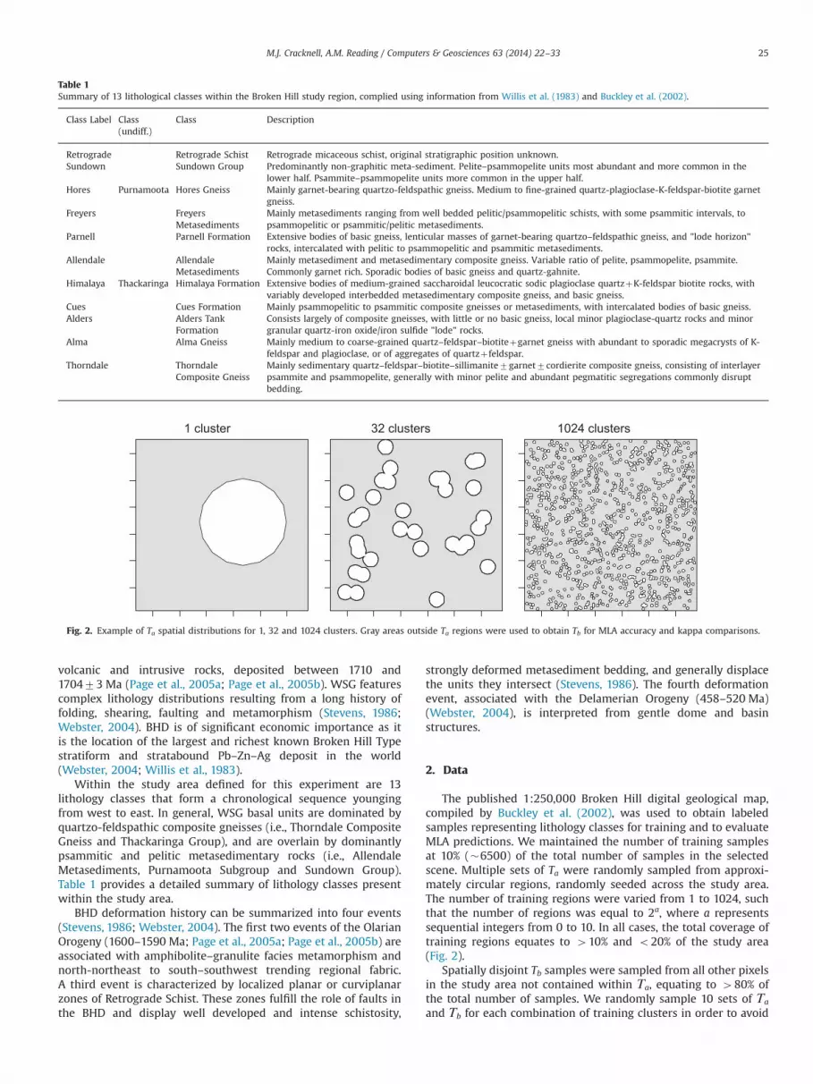
The published 1:250,000 Broken Hill digital geological map,compiled by Buckley et al. (2002), was used to obtain labeledsamples representing lithology classes for training and to evaluateMLA predictions. We maintained the number of training samplesat 10% (�6500) of the total number of samples in the selectedscene. Multiple sets of Ta were randomly sampled from approxi-mately circular regions, randomly seeded across the study area.The number of training regions were varied from 1 to 1024, suchthat the number of regions was equal to 2a, where a representssequential integers from 0 to 10. In all cases, the total coverage oftraining regions equates to 410% and o20% of the study area(Fig. 2).

Spatially disjoint Tb samples were sampled from all other pixelsin the study area not contained within Τa, equating to 480% ofthe total number of samples. We randomly sample 10 sets of Τa

and Τb for each combination of training clusters in order to avoid

Table 1Summary of 13 lithological classes within the Broken Hill study region, complied using information from Willis et al. (1983) and Buckley et al. (2002).

Class Label Class(undiff.)

Class Description

Retrograde Retrograde Schist Retrograde micaceous schist, original stratigraphic position unknown.Sundown Sundown Group Predominantly non-graphitic meta-sediment. Pelite–psammopelite units most abundant and more common in the

lower half. Psammite–psammopelite units more common in the upper half.Hores Purnamoota Hores Gneiss Mainly garnet-bearing quartzo-feldspathic gneiss. Medium to fine-grained quartz-plagioclase-K-feldspar-biotite garnet

gneiss.Freyers Freyers

MetasedimentsMainly metasediments ranging from well bedded pelitic/psammopelitic schists, with some psammitic intervals, topsammopelitic or psammitic/pelitic metasediments.

Parnell Parnell Formation Extensive bodies of basic gneiss, lenticular masses of garnet-bearing quartzo–feldspathic gneiss, and "lode horizon"rocks, intercalated with pelitic to psammopelitic and psammitic metasediments.

Allendale AllendaleMetasediments

Mainly metasediment and metasedimentary composite gneiss. Variable ratio of pelite, psammopelite, psammite.Commonly garnet rich. Sporadic bodies of basic gneiss and quartz-gahnite.

Himalaya Thackaringa Himalaya Formation Extensive bodies of medium-grained saccharoidal leucocratic sodic plagioclase quartzþK-feldspar biotite rocks, withvariably developed interbedded metasedimentary composite gneiss, and basic gneiss.

Cues Cues Formation Mainly psammopelitic to psammitic composite gneisses or metasediments, with intercalated bodies of basic gneiss.Alders Alders Tank

FormationConsists largely of composite gneisses, with little or no basic gneiss, local minor plagioclase-quartz rocks and minorgranular quartz-iron oxide/iron sulfide "lode" rocks.

Alma Alma Gneiss Mainly medium to coarse-grained quartz–feldspar–biotiteþgarnet gneiss with abundant to sporadic megacrysts of K-feldspar and plagioclase, or of aggregates of quartzþ feldspar.

Thorndale ThorndaleComposite Gneiss

Mainly sedimentary quartz–feldspar–biotite–sillimanite7garnet7cordierite composite gneiss, consisting of interlayerpsammite and psammopelite, generally with minor pelite and abundant pegmatitic segregations commonly disruptbedding.

1 cluster 32 clusters 1024 clusters

Fig. 2. Example of Ta spatial distributions for 1, 32 and 1024 clusters. Gray areas outside Ta regions were used to obtain Tb for MLA accuracy and kappa comparisons.

M.J. Cracknell, A.M. Reading / Computers & Geosciences 63 (2014) 22–33 25

any bias associated with individual groups of Τa or Τb. Due to thenatural variability of lithological class distributions, Ta sampledfrom low numbers of training regions often did not containrepresentatives for all 13 lithological classes. This leads to biasedaccuracy assessments due to the incorporation of samples thatcannot be accurately classified. Therefore, those classes not repre-sented in Τa were eliminated from their corresponding Τb whenevaluating MLA predictions.

Airborne geophysical data used in this study contained a DigitalElevation Model (DEM ASL), Total Magnetic Intensity TMI (nT), andfour Gamma-Ray Spectrometry (GRS) channels comprising Potas-sium (K%), Thorium (Th ppm), Uranium (U ppm), and Total Countchannels. The Landsat 7 ETMþ data contained 8 bands suppliedwith Level 1 processing applied. Landsat 7 ETMþ band 8, whichcovers the spectral bandwidths of bands 2, 3, and 4 (Williams,2009) was not included.

3. Methods

3.1. Pre-processing

Geophysical data were transformed to a common projectedcoordinate system WGS84 UTM zone 54S, using bilinear interpola-tion. All inputs were resampled to a common extent (12.8�12.8 km) and cell resolution (50 m�50 m), resulting in imagedimensions of 256�256 pixels (65,536 samples). To enhance theirrelevance to the task of lithology discrimination, projected data wereprocessed in a variety of ways specific to the geophysical propertythey represent. An account of pre-processing steps implemented togenerate input data is provided in Supplementary InformationSection 1 (S1 – Data). Spatial coordinates (Easting (m) and Northing(m)), obtained from the location of grid cell centers were includedresulting in a total of 27 variables available for input. Processed inputdata were standardized to zero mean and unit variance. Highlycorrelated data, with mean Pearson's correlation coefficients 40.8associated with a large proportion of other data, were eliminated

resulting in a total of 17 inputs available for MLA training andprediction. Relative normalized variable importance was calculatedby generating Receiver Operating Curves (ROC) (Provost and Fawcett,1997) for all pair-wise class combinations and obtaining the areaunder the curve for each pair. The maximum area under the curveacross all pair-wise comparisons was used to defined the importanceof variables with respect to individual classes (Kuhn et al., 2012).

3.2. Classification model training

Table 2 indicates the MLA parameter values assessed in thisstudy. Optimal parameters were selected based on maximummean accuracies resulting from 10-fold cross-validation. MLAclassification models were trained using selected parameters onthe entire set of samples in Τa prior to prediction evaluation.Information on the R packages and functions used to train MLAclassification models and details regarding associated parametersare provided in Supplementary information Section (S2 – MLASoftware and Parameters).

3.3. Prediction evaluation

Overall accuracy and Cohen's kappa statistic (Cohen, 1960) arecommonly used to evaluate classifier performance (Lu and Weng,2007). Overall accuracy treats predictions as either correct orincorrect and is defined as the number of correctly classified testsamples divided by the total number of test samples. The kappastatistic is a measure of the similarity between predictions andobservations while correcting for agreement that occurs by chance(Congalton and Green, 1998). We do not use the area under ROC toevaluate MLA predictions because multiclass ROC becomesincreasing intractable with a large number of classes (i.e. 48)(Landgrebe and Paclik, 2010). We visualize the spatial distributionof prediction error and assess their geological validity by plottingMLA predictions in the spatial domain and by comparing thelocations of misclassified samples.

4. Results

In this section we present the results of our comparison of thefive MLAs trialed in this study. Initially, we assess the effect ofchanges in the spatial distribution of training data on the relativeimportance of input variables and MLA parameter selection. This isfollowed by a comparison of MLA test statistics in light ofvariations in the spatial distribution of training data and theinclusion of explicit spatial information.

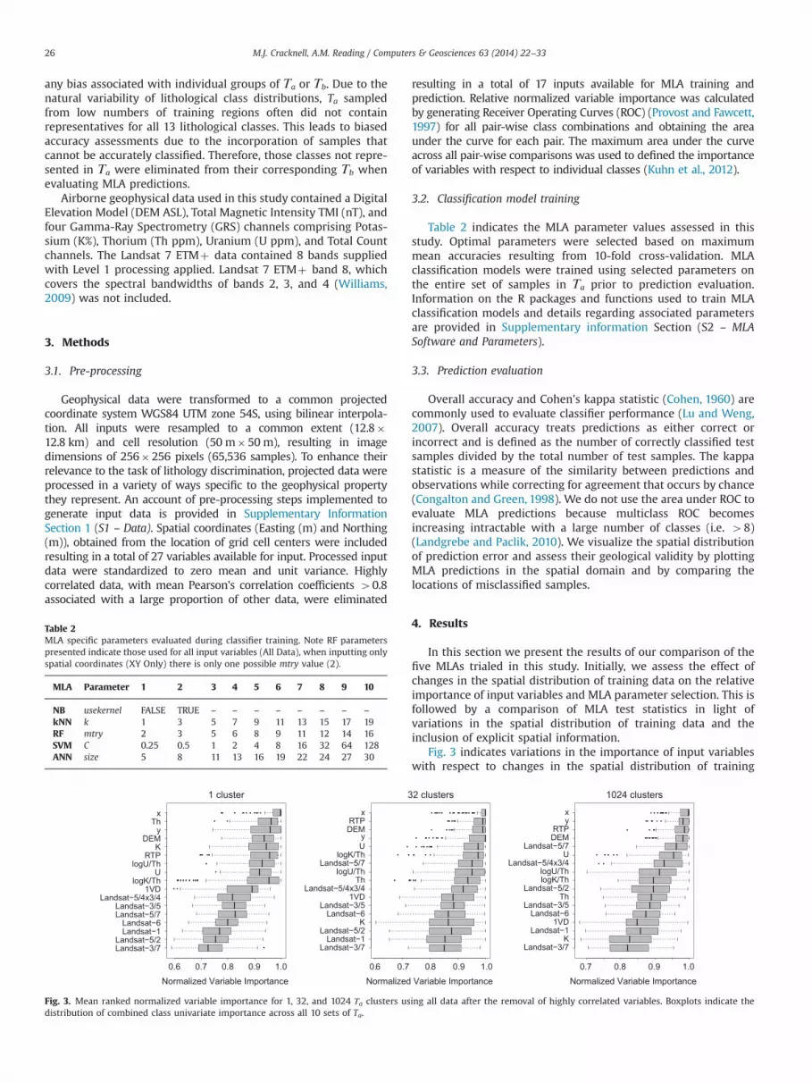
Fig. 3 indicates variations in the importance of input variableswith respect to changes in the spatial distribution of training

Table 2MLA specific parameters evaluated during classifier training. Note RF parameterspresented indicate those used for all input variables (All Data), when inputting onlyspatial coordinates (XY Only) there is only one possible mtry value (2).

MLA Parameter 1 2 3 4 5 6 7 8 9 10

NB usekernel FALSE TRUE – – – – – – – –

kNN k 1 3 5 7 9 11 13 15 17 19RF mtry 2 3 5 6 8 9 11 12 14 16SVM C 0.25 0.5 1 2 4 8 16 32 64 128ANN size 5 8 11 13 16 19 22 24 27 30

Landsat−3/7Landsat−5/2

Landsat−1Landsat−6

Landsat−5/7Landsat−3/5

Landsat−5/4x3/41VD

logK/ThU

logU/ThRTP

KDEM

yTh

x

1.00.6 0.7 0.8 0.9 1.0

Landsat−3/7Landsat−1

Landsat−5/2K

Landsat−6Landsat−3/5

1VDLandsat−5/4x3/4

ThlogU/Th

Landsat−5/7logK/Th

Uy

DEMRTP

x

0.6 0.7 0.8 0.9

Landsat−3/7K

Landsat−11VD

Landsat−6Landsat−3/5

ThLandsat−5/2

logK/ThlogU/Th

Landsat−5/4x3/4U

Landsat−5/7DEMRTP

yx

0.7 0.8 0.9 1.0

Normalized Variable Importance Normalized Variable Importance Normalized Variable Importance

1 cluster 32 clusters 1024 clusters

Fig. 3. Mean ranked normalized variable importance for 1, 32, and 1024 Τa clusters using all data after the removal of highly correlated variables. Boxplots indicate thedistribution of combined class univariate importance across all 10 sets of Ta.

M.J. Cracknell, A.M. Reading / Computers & Geosciences 63 (2014) 22–3326

samples. A large range of importance suggests that the usefulnessof a particular input at discriminating individual classes is highlyvariable. Top ranked variables with relatively narrow distributionsinclude X and Y spatial coordinates, DEM and Reduced to Pole(RTP) magnetics. Less important inputs represent GRS channelsand ratios with Landsat ETMþ band 5 variables. Lowest rankedvariables are 1st Vertical Derivative (1VD) of RTP TMI, and theremaining Landsat ETMþ bands. As the number of trainingregions increases, GRS variables decrease in importance whileratios with Landsat ETMþ 5 increase in importance. The Xcoordinate is consistently the most important variable, reflectingthe presence of approximately north–south trending geologicalstructures.

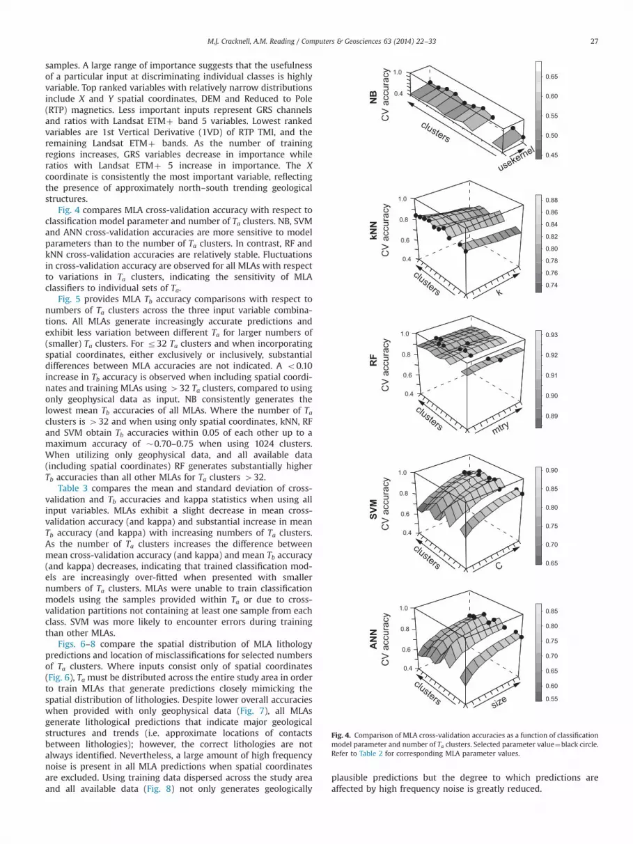
Fig. 4 compares MLA cross-validation accuracy with respect toclassification model parameter and number of Ta clusters. NB, SVMand ANN cross-validation accuracies are more sensitive to modelparameters than to the number of Ta clusters. In contrast, RF andkNN cross-validation accuracies are relatively stable. Fluctuationsin cross-validation accuracy are observed for all MLAs with respectto variations in Ta clusters, indicating the sensitivity of MLAclassifiers to individual sets of Ta.

Fig. 5 provides MLA Tb accuracy comparisons with respect tonumbers of Ta clusters across the three input variable combina-tions. All MLAs generate increasingly accurate predictions andexhibit less variation between different Ta for larger numbers of(smaller) Ta clusters. For r32 Ta clusters and when incorporatingspatial coordinates, either exclusively or inclusively, substantialdifferences between MLA accuracies are not indicated. A o0.10increase in Tb accuracy is observed when including spatial coordi-nates and training MLAs using 432 Ta clusters, compared to usingonly geophysical data as input. NB consistently generates thelowest mean Tb accuracies of all MLAs. Where the number of Taclusters is 432 and when using only spatial coordinates, kNN, RFand SVM obtain Tb accuracies within 0.05 of each other up to amaximum accuracy of �0.70–0.75 when using 1024 clusters.When utilizing only geophysical data, and all available data(including spatial coordinates) RF generates substantially higherTb accuracies than all other MLAs for Ta clusters 432.

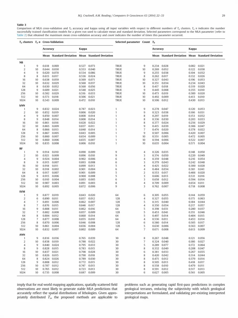
Table 3 compares the mean and standard deviation of cross-validation and Tb accuracies and kappa statistics when using allinput variables. MLAs exhibit a slight decrease in mean cross-validation accuracy (and kappa) and substantial increase in meanTb accuracy (and kappa) with increasing numbers of Ta clusters.As the number of Ta clusters increases the difference betweenmean cross-validation accuracy (and kappa) and mean Tb accuracy(and kappa) decreases, indicating that trained classification mod-els are increasingly over-fitted when presented with smallernumbers of Ta clusters. MLAs were unable to train classificationmodels using the samples provided within Ta or due to cross-validation partitions not containing at least one sample from eachclass. SVM was more likely to encounter errors during trainingthan other MLAs.

Figs. 6–8 compare the spatial distribution of MLA lithologypredictions and location of misclassifications for selected numbersof Ta clusters. Where inputs consist only of spatial coordinates(Fig. 6), Ta must be distributed across the entire study area in orderto train MLAs that generate predictions closely mimicking thespatial distribution of lithologies. Despite lower overall accuracieswhen provided with only geophysical data (Fig. 7), all MLAsgenerate lithological predictions that indicate major geologicalstructures and trends (i.e. approximate locations of contactsbetween lithologies); however, the correct lithologies are notalways identified. Nevertheless, a large amount of high frequencynoise is present in all MLA predictions when spatial coordinatesare excluded. Using training data dispersed across the study areaand all available data (Fig. 8) not only generates geologically

plausible predictions but the degree to which predictions areaffected by high frequency noise is greatly reduced.

0.45

0.50

0.55

0.60

0.65

NB

0.89

0.90

0.91

0.92

0.93

0.74

0.76

0.78

0.80

0.82

0.84

0.86

0.88

0.65

0.70

0.75

0.80

0.85

0.90

0.55

0.60

0.65

0.70

0.75

0.80

0.85

clusters k

1.0

0.8

0.6

0.4

CV

acc

urac

y

clustersmtry

1.0

0.8

0.6

0.4C

V a

ccur

acy

clusters C

1.0

0.8

0.6

0.4

CV

acc

urac

y

clusterssize

1.0

0.8

0.6

0.4

CV

acc

urac

y

clusters

usekernel

1.0

CV

acc

urac

y

0.4

kNN

RF

SVM

ANN

Fig. 4. Comparison of MLA cross-validation accuracies as a function of classificationmodel parameter and number of Ta clusters. Selected parameter value¼black circle.Refer to Table 2 for corresponding MLA parameter values.

M.J. Cracknell, A.M. Reading / Computers & Geosciences 63 (2014) 22–33 27

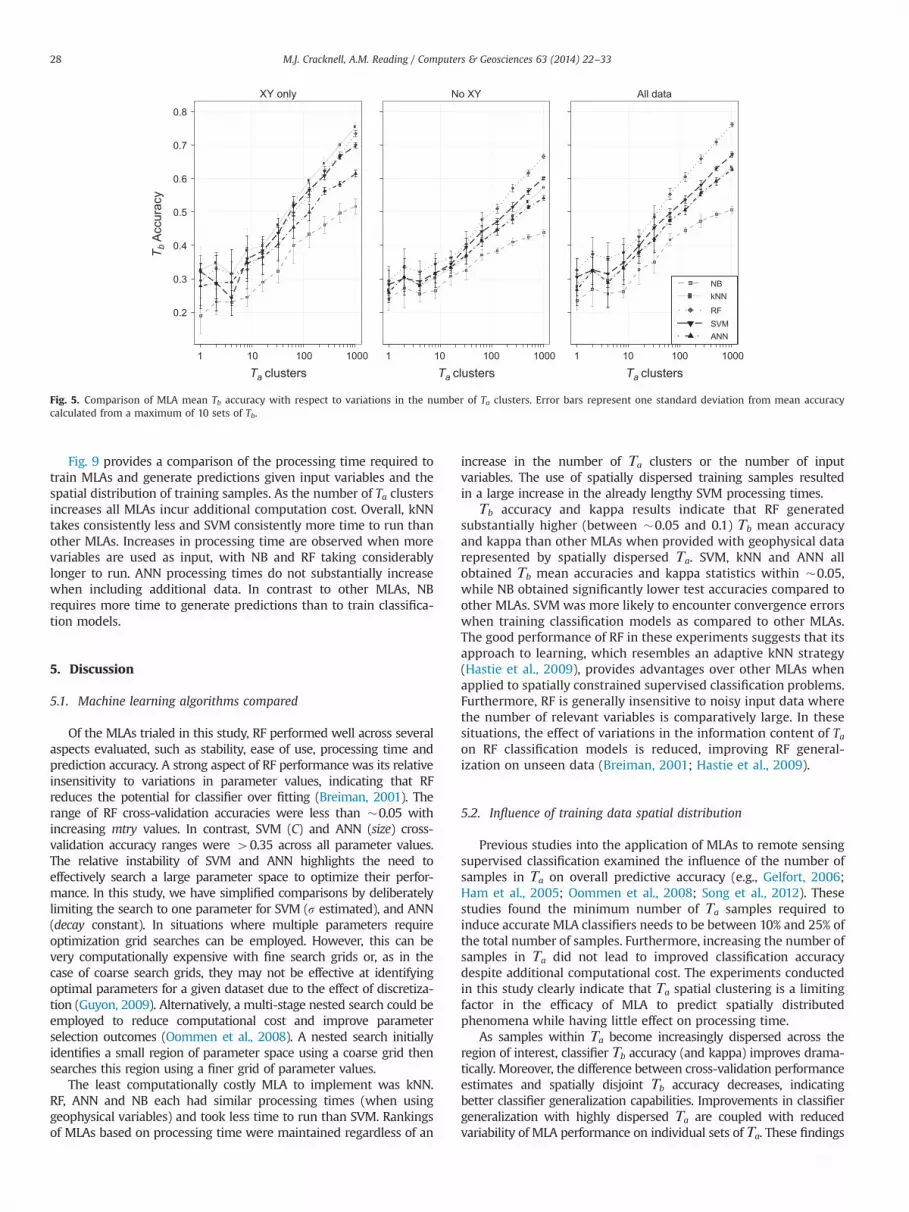
Fig. 9 provides a comparison of the processing time required totrain MLAs and generate predictions given input variables and thespatial distribution of training samples. As the number of Ta clustersincreases all MLAs incur additional computation cost. Overall, kNNtakes consistently less and SVM consistently more time to run thanother MLAs. Increases in processing time are observed when morevariables are used as input, with NB and RF taking considerablylonger to run. ANN processing times do not substantially increasewhen including additional data. In contrast to other MLAs, NBrequires more time to generate predictions than to train classifica-tion models.

5. Discussion

5.1. Machine learning algorithms compared

Of the MLAs trialed in this study, RF performed well across severalaspects evaluated, such as stability, ease of use, processing time andprediction accuracy. A strong aspect of RF performance was its relativeinsensitivity to variations in parameter values, indicating that RFreduces the potential for classifier over fitting (Breiman, 2001). Therange of RF cross-validation accuracies were less than �0.05 withincreasing mtry values. In contrast, SVM (C) and ANN (size) cross-validation accuracy ranges were 40.35 across all parameter values.The relative instability of SVM and ANN highlights the need toeffectively search a large parameter space to optimize their perfor-mance. In this study, we have simplified comparisons by deliberatelylimiting the search to one parameter for SVM (s estimated), and ANN(decay constant). In situations where multiple parameters requireoptimization grid searches can be employed. However, this can bevery computationally expensive with fine search grids or, as in thecase of coarse search grids, they may not be effective at identifyingoptimal parameters for a given dataset due to the effect of discretiza-tion (Guyon, 2009). Alternatively, a multi-stage nested search could beemployed to reduce computational cost and improve parameterselection outcomes (Oommen et al., 2008). A nested search initiallyidentifies a small region of parameter space using a coarse grid thensearches this region using a finer grid of parameter values.

The least computationally costly MLA to implement was kNN.RF, ANN and NB each had similar processing times (when usinggeophysical variables) and took less time to run than SVM. Rankingsof MLAs based on processing time were maintained regardless of an

increase in the number of Τa clusters or the number of inputvariables. The use of spatially dispersed training samples resultedin a large increase in the already lengthy SVM processing times.

Τb accuracy and kappa results indicate that RF generatedsubstantially higher (between �0.05 and 0.1) Τb mean accuracyand kappa than other MLAs when provided with geophysical datarepresented by spatially dispersed Τa. SVM, kNN and ANN allobtained Τb mean accuracies and kappa statistics within �0.05,while NB obtained significantly lower test accuracies compared toother MLAs. SVM was more likely to encounter convergence errorswhen training classification models as compared to other MLAs.The good performance of RF in these experiments suggests that itsapproach to learning, which resembles an adaptive kNN strategy(Hastie et al., 2009), provides advantages over other MLAs whenapplied to spatially constrained supervised classification problems.Furthermore, RF is generally insensitive to noisy input data wherethe number of relevant variables is comparatively large. In thesesituations, the effect of variations in the information content of Taon RF classification models is reduced, improving RF general-ization on unseen data (Breiman, 2001; Hastie et al., 2009).

5.2. Influence of training data spatial distribution

Previous studies into the application of MLAs to remote sensingsupervised classification examined the influence of the number ofsamples in Τa on overall predictive accuracy (e.g., Gelfort, 2006;Ham et al., 2005; Oommen et al., 2008; Song et al., 2012). Thesestudies found the minimum number of Τa samples required toinduce accurate MLA classifiers needs to be between 10% and 25% ofthe total number of samples. Furthermore, increasing the number ofsamples in Τa did not lead to improved classification accuracydespite additional computational cost. The experiments conductedin this study clearly indicate that Τa spatial clustering is a limitingfactor in the efficacy of MLA to predict spatially distributedphenomena while having little effect on processing time.

As samples within Τa become increasingly dispersed across theregion of interest, classifier Τb accuracy (and kappa) improves drama-tically. Moreover, the difference between cross-validation performanceestimates and spatially disjoint Τb accuracy decreases, indicatingbetter classifier generalization capabilities. Improvements in classifiergeneralization with highly dispersed Τa are coupled with reducedvariability of MLA performance on individual sets of Τa. These findings

0.2

0.3

0.4

0.5

0.6

0.7

0.8

1 10 100 1000 1 10 100 1000 1 10 100 1000

kNNNB

RF

ANNSVM

Ta clusters Ta clusters Ta clusters

T b A

ccur

acy

All dataNo XYXY only

Fig. 5. Comparison of MLA mean Tb accuracy with respect to variations in the number of Ta clusters. Error bars represent one standard deviation from mean accuracycalculated from a maximum of 10 sets of Tb.

M.J. Cracknell, A.M. Reading / Computers & Geosciences 63 (2014) 22–3328

imply that for real worldmapping applications, spatially scattered fieldobservations are most likely to generate stable MLA predictions thataccurately reflect the spatial distributions of lithologies. Given appro-priately distributed Τa, the proposed methods are applicable to

problems such as generating rapid first-pass predictions in complexgeological terranes, reducing the subjectivity with which geologicalinterpretations are formulated, and validating pre-existing interpretedgeological maps.

Table 3Comparison of MLA cross-validation and Tb accuracy and kappa using all input variables with respect to different numbers of Ta clusters. Ta n indicates the numbersuccessfully trained classification models for a given run used to calculate mean and standard deviation. Selected parameters correspond to the MLA parameter (refer toTable 2) that obtained the maximum mean cross-validation accuracy and count indicates the number of times this parameter occurred.

Ta clusters Ta n Cross-Validation Selected parameter Count Tb

Accuracy Kappa Accuracy Kappa

Mean Standard Deviation Mean Standard Deviation Mean Standard Deviation Mean Standard Deviation

NB1 9 0.618 0.069 0.527 0.073 TRUE 9 0.234 0.028 0.082 0.0212 10 0.644 0.030 0.553 0.040 TRUE 10 0.269 0.052 0.122 0.0384 9 0.620 0.070 0.534 0.086 TRUE 9 0.255 0.038 0.104 0.0328 8 0.615 0.017 0.536 0.024 TRUE 8 0.262 0.017 0.132 0.026

16 10 0.638 0.059 0.569 0.071 TRUE 10 0.327 0.043 0.196 0.05332 10 0.632 0.029 0.568 0.037 TRUE 10 0.351 0.034 0.234 0.04364 8 0.630 0.052 0.568 0.056 TRUE 8 0.417 0.018 0.319 0.020

128 9 0.609 0.021 0.548 0.025 TRUE 9 0.445 0.008 0.355 0.010256 10 0.582 0.029 0.516 0.033 TRUE 10 0.473 0.019 0.389 0.020512 10 0.573 0.018 0.506 0.021 TRUE 10 0.492 0.009 0.413 0.010

1024 10 0.543 0.009 0.472 0.010 TRUE 10 0.506 0.012 0.430 0.013

kNN1 9 0.832 0.024 0.787 0.023 1 9 0.278 0.047 0.120 0.0532 10 0.852 0.019 0.806 0.020 1 9 0.323 0.038 0.166 0.0314 9 0.850 0.007 0.808 0.014 1 8 0.297 0.019 0.153 0.0328 9 0.848 0.014 0.808 0.014 1 8 0.336 0.030 0.203 0.033

16 10 0.861 0.016 0.828 0.022 1 8 0.377 0.024 0.256 0.02932 10 0.865 0.009 0.837 0.011 1 9 0.415 0.039 0.306 0.04764 8 0.866 0.013 0.840 0.014 1 7 0.474 0.020 0.378 0.022

128 9 0.867 0.005 0.843 0.005 1 9 0.507 0.006 0.420 0.007256 10 0.860 0.007 0.834 0.009 1 10 0.551 0.005 0.472 0.005512 10 0.860 0.006 0.835 0.007 1 10 0.594 0.006 0.522 0.007

1024 10 0.835 0.008 0.806 0.010 1 10 0.635 0.004 0.571 0.004

RF1 9 0.914 0.010 0.890 0.009 9 4 0.326 0.035 0.148 0.0502 10 0.921 0.009 0.896 0.010 9 3 0.374 0.050 0.220 0.0494 9 0.924 0.004 0.902 0.006 6 4 0.359 0.048 0.216 0.0548 9 0.915 0.007 0.893 0.008 6 3 0.379 0.043 0.242 0.048

16 10 0.918 0.011 0.899 0.013 5 4 0.425 0.022 0.300 0.02832 10 0.918 0.002 0.901 0.004 6 4 0.484 0.034 0.381 0.04164 8 0.917 0.007 0.901 0.009 5 2 0.553 0.017 0.466 0.020

128 9 0.915 0.006 0.900 0.008 5 3 0.606 0.013 0.531 0.016256 10 0.910 0.004 0.893 0.005 6 3 0.658 0.012 0.594 0.014512 10 0.907 0.003 0.891 0.003 8 4 0.709 0.009 0.654 0.011

1024 10 0.892 0.005 0.872 0.006 9 3 0.762 0.007 0.718 0.008

SVM1 9 0.877 0.019 0.843 0.020 64 6 0.305 0.055 0.144 0.0592 6 0.890 0.011 0.857 0.012 128 4 0.327 0.055 0.175 0.0634 7 0.891 0.006 0.862 0.007 128 5 0.315 0.040 0.184 0.0448 7 0.876 0.015 0.846 0.017 128 4 0.350 0.054 0.217 0.057

16 9 0.888 0.011 0.862 0.016 64 5 0.398 0.031 0.280 0.03732 7 0.882 0.008 0.857 0.009 128 5 0.453 0.041 0.351 0.04664 8 0.884 0.012 0.860 0.014 64 5 0.497 0.014 0.404 0.015

128 7 0.877 0.008 0.855 0.010 64 4 0.536 0.011 0.453 0.014256 8 0.870 0.006 0.846 0.008 128 6 0.580 0.014 0.505 0.017512 10 0.861 0.004 0.836 0.004 128 5 0.630 0.006 0.563 0.007

1024 10 0.832 0.007 0.802 0.009 64 7 0.671 0.008 0.613 0.009

ANN1 9 0.816 0.036 0.765 0.039 30 8 0.267 0.048 0.121 0.0562 10 0.838 0.019 0.788 0.022 30 7 0.324 0.040 0.180 0.0274 9 0.840 0.024 0.795 0.033 30 5 0.289 0.077 0.172 0.0648 9 0.828 0.015 0.783 0.015 30 8 0.332 0.049 0.208 0.047

16 10 0.837 0.021 0.798 0.028 30 6 0.381 0.033 0.267 0.03532 10 0.826 0.015 0.790 0.018 30 8 0.420 0.042 0.314 0.04464 8 0.824 0.026 0.789 0.030 30 8 0.475 0.012 0.379 0.014

128 9 0.808 0.012 0.772 0.015 30 8 0.505 0.013 0.418 0.017256 10 0.787 0.012 0.747 0.015 30 8 0.558 0.010 0.479 0.011512 10 0.765 0.012 0.723 0.013 30 8 0.591 0.012 0.517 0.013

1024 10 0.735 0.008 0.687 0.009 30 6 0.627 0.005 0.561 0.005

M.J. Cracknell, A.M. Reading / Computers & Geosciences 63 (2014) 22–33 29

Fig. 6. Visualization of the spatial distribution of MLA lithology class predictions (refer to Fig. 1 for reference map and key to class labels), and misclassified samples (blackpixels) for 1, 32 and 1024 Ta clusters (red circles) using X and Y spatial coordinates (XY Only) as inputs. (For interpretation of the references to color in this figure legend, thereader is referred to the web version of this article.)

Fig. 7. Visualization of the spatial distribution of MLA lithology class predictions (refer to Fig. 1 for reference map and key to class labels), and misclassified samples (blackpixels) for 1, 32 and 1024 Ta clusters (red circles) using geophysical data (No XY) as inputs. (For interpretation of the references to color in this figure legend, the reader isreferred to the web version of this article.)

M.J. Cracknell, A.M. Reading / Computers & Geosciences 63 (2014) 22–3330

5.3. Using spatially constrained data

Spatial dependencies (spatial autocorrelation), i.e. closer obser-vations are more related than those farther apart, are commonly

encountered within spatial data (Anselin, 1995; Getis, 2010; Lloyd,2011). When incorporating spatial coordinates as input data fortraining and prediction, MLAs are provided with explicit informa-tion linking location and lithology classes. Spatial values, coupled

Fig. 8. Visualization of the spatial distribution of MLA lithology class predictions (refer to Fig. 1 for reference map and key to class labels), and misclassified samples (blackpixels) for 1, 32 and 1024 Ta clusters (red circles) using spatial coordinates and geophysical data (all data) as inputs. (For interpretation of the references to color in this figurelegend, the reader is referred to the web version of this article.)

ANNSVMRFkNNNB

ANNSVMRFkNNNB

ANNSVMRFkNNNB

0 5 10 15 20 25 30 0 5 10 15 20 25 30 0 5 10 15 20 25 30

trainingtesting

1024 clusters32 clusters1 clusters

minutesminutes minutes

XY

Onl

yN

o X

YA

ll D

ata

Fig. 9. Comparison of MLA training (using 10-fold cross-validation) and prediction processing times (minutes). Bars represent the mean time taken to train a MLAclassification model and generate predictions for a maximum of 10 sets of Ta and Tb. All processes were executed using a DELL Desktop PC 64-bit Intel Dual Core CPU @3.00 GHz and 8 GB of RAM. Cross-validation folds and Tb predictions (divided into groups of 10,000) were run independently using Message Passing Interface parallelprocessing on 2 cores.

M.J. Cracknell, A.M. Reading / Computers & Geosciences 63 (2014) 22–33 31

with randomly distributed Τa samples over the entire study area,resulted in a best-case scenario in terms of MLA test accuracy.However, geologically plausible predictions were only achievedusing input variables containing information that reflected thephysical properties of the lithologies under investigation. Thisobservation suggests that standard measures of classifier perfor-mance, such as accuracy and kappa, do not necessarily provide anindication of the validity of MLA classifications in the spatialdomain. Therefore, the use of spatial coordinates should beapproached with caution. If, for instance, training data werecollected only from field observations, these data are likely to bespatially clustered due outcrop exposure, accessibility, and timeconstraints. Using only spatial coordinates with highly spatiallyclustered Τa samples generates classifiers that incorrectly learn afinite range of coordinate values for a particular class and wereunable to generalize well to spatially disjoint regions (Gahegan,2000).

An alternative to the use of spatial coordinates as a means ofproviding MLAs with spatial context would be to incorporate somemeasure of local spatial relationships during pre-processing usingneighborhood models (Gahegan, 2000). In its simplest form,neighborhood models generate new variables by deriving statis-tical measures of the values of proximal observations such asmean or standard deviation. In this way neighborhood modelsrepresent local spatial similarity or dissimilarity (Lloyd, 2011).An alternative to pre-processing inputs to include information onthe spatial context of observations is to code some notion ofspatial dependency into the MLA itself. Li et al. (2012) developedand tested a SVM algorithm that directly utilized spatial informa-tion to improve classifier accuracy. Their SVM variant takesanalyzed hold-out test sample results obtained in geographicalspace, and using a local neighborhood identifies the supportvectors that are likely to be misclassified. The SVM hyperplaneboundary is then adjusted to include these support vectors. Thisprocess proceeds iteratively until the change in prediction accu-racy reaches some minimum threshold.

6. Conclusions

We compared five machine learning algorithms (MLAs) interms their performance with respect to a supervised lithologyclassification problem in a complex metamorphosed geologicalterrane. These MLAs, Naive Bayes, k-Nearest Neighbors, RandomForests, Support Vector Machines and Artificial Neural Networks,represent the five general machine learning strategies for auto-mated data-driven inference. MLA comparisons included theirsensitivity to variations in spatial distribution of training data,and response to the inclusion of explicit spatial information.

We conclude that Random Forests is a good first choice MLA formulticlass inference using widely available high-dimensional multi-source remotely sensed geophysical variables. Random Forestsclassification models are, in this case, easy to train, stable across arange of model parameter values, computationally efficient, andwhen faced with spatially dispersed training data, substantiallymore accurate than other MLAs. These traits, coupled with theinsensitively of Random Forests to noise and over fitting, indicatethat it is well suited to remote sensing lithological classificationapplications.

As the spatial distribution of training data becomes moredispersed across the region under investigation, MLA predictiveaccuracy (and kappa) increases. In addition, the sensitivity of MLAcategorical predictions to different training datasets decreases. Theinclusion of explicit spatial information (i.e. spatial coordinates)proved to generate highly accurate MLA predictions when trainingdata was dispersed across the study area. Despite resulting in

lower test accuracy (and kappa), the use of geophysical dataprovided MLAs with information that characterized geologicalstructural trends. Therefore, combining spatial and geophysicaldata is beneficial, especially in situations where training data ismoderately spatially clustered. Our results illustrate the use ofmachine learning techniques to address data-driven spatial infer-ence problems and will generalize readily to other geoscienceapplications.

Acknowledgments

We thank Malcolm Sambridge and Ron Berry for their con-structive comments and discussion which significantly improvedthe draft manuscript. Airborne geophysics data were sourced fromGeoscience Australia and Landsat ETMþ data from the UnitedStates Geological Survey. This research was conducted at theAustralian Research Council Centre of Excellence in Ore Deposits(CODES) under Project no. P3A3A. M. Cracknell was supportedthrough a University of Tasmania Elite Research Ph.D. Scholarship.We thank the editor and Milos Kovacevic for their constructivecomments that have strengthened the scientific content andclarity of presentation.

Appendix A. Supplementary material

Supplementary data associated with this article can be found inthe online version at http://dx.doi.org/10.1016/j.cageo.2013.10.008.

References

Anselin, L., 1995. Local indicators of spatial association – LISA. Geogr. Anal. 27,93–115.

Breiman, L., 1996. Bagging predictors. Machine Learn. 24, 123–140.Breiman, L., 2001. Random forests. Mach. Learn. 45, 5–32.Breiman, L., Friedman, J.H., Olshen, R.A., Stone, C.J., 1984. Classification and

Regression Trees. Wadsworths & Brooks/Cole Advanced Books & Software,Pacific Grove, USA p. 358.

Buckley, P.M., Moriarty, T., Needham, J. (compilers), 2002. Broken Hill GeoscienceDatabase, 2nd ed. Geological Survey of New SouthWales , Sydney.

Carneiro, C.C., Fraser, S.J., Croacutesta, A.P., Silva, A.M., Barros, C.E.M., 2012.Semiautomated geologic mapping using self-organizing maps and airbornegeophysics in the Brazilian Amazon. Geophysics 77, K17–K24.

Cohen, J., 1960. A coefficient of agreement for nominal scales. Educ. Psychol. Meas.20, 37–46.

Congalton, R.G., Green, K., 1998. Assessing the Accuracy of Remotely Sensed Data:Principles and Practices, first edn. Lewis Publications, Boca Raton p. 137.

Cover, T., Hart, P., 1967. Nearest neighbor pattern classification. IEEE Trans. Inf.Theory 13, 21–27.

Cracknell, M.J., Reading, A.M., 2013. The upside of uncertainty: identification oflithology contact zones from airborne geophysics and satellite data usingRandom Forests and Support Vector Machines. Geophysics 78, WB113–WB126.

Fix, E., Hodges, J.L., 1951. Discriminatory analysis. Nonparametric discrimination;Consistency properties. U.S. Air Force, School of Aviation Medicine, RandolphField, Texas.

Foody, G.M., Mathur, A., 2004. A relative evaluation of multiclass image classifica-tion by support vector machines. IEEE Trans. Geosci. Remote Sens. 42,1335–1343.

Gahegan, M., 2000. On the application of inductive machine learning tools togeographical analysis. Geogr. Anal. 32, 113–139.

Gelfort, R., 2006. On Classification of Logging Data, Department of Energy andEconomics. Clausthal University of Technology, Germany, p. 131.

Getis, A., 2010. Spatial autocorrelation. In: Fisher, M.M., Getis, A. (Eds.), Handbookof Applied Spatial Analysis: Software, Tools, Methods and Applications.Springer-Verlag, Berlin, pp. 255–278.

Guyon, I., 2008. Practical feature selection: from correlation to causality. In:Fogelman-Soulié, F., Perrotta, D., Piskorski, J., Steinberger, R. (Eds.), MiningMassive Data Sets for Security – Advances in Data Mining, Search, SocialNetworks and Text Mining, and their Applications to Security. IOS Press,Amsterdam, pp. 27–43.

Guyon, I., 2009. A practical guide to model selection. In: Marie, J. (Ed.), Proceedingsof the Machine Learning Summer School. Canberra, Australia, January 26 -February 6, Springer Text in Statistics, Springer p.37.

M.J. Cracknell, A.M. Reading / Computers & Geosciences 63 (2014) 22–3332

Ham, J., Yangchi, C., Crawford, M.M., Ghosh, J., 2005. Investigation of the randomforest framework for classification of hyperspectral data. IEEE Trans. Geosci.Remote Sens. 43, 492–501.

Hastie, T., Tibshirani, R., Friedman, J.H., 2009. The elements of statistical learning:data mining, Inference and Prediction, 2nd edn. Springer, New York, USA p. 533.

Henery, R.J., 1994. Classification. In: Michie, D., Spiegelhalter, D.J., Taylor, C.C. (Eds.),Machine Learning, Neural and Statistical Classification. Ellis Horwood,New York, pp. 6–16.

Hsu, C.-W., Lin, C.-J., 2002. A comparison of methods for multiclass support vectormachines. IEEE Trans. Neural Netw. 13, 415–425.

Hsu, C.-W., Chang, C.-C., Lin, C.-J., 2010. A Practical Guide to Support VectorClassificationDepartment of Computer Science, National Taiwan University,Taipei, Taiwan16.

Huang, C., Davis, L.S., Townshend, J.R.G., 2002. An assessment of support vectormachines for land cover classification. Int. J. Remote Sens. 23, 725–749.

Kanevski, M., Pozdnoukhov, A., Timonin, V., 2009. Machine learning for spatialenvironmental data: theory, Applications and Software. CRC Press, Boca Raton,USA (368 pp.).

Karatzoglou, A., Meyer, D., Hornik, K., 2006. Support vector machines in R. J. Stat.Softw. 15, 28.

Kotsiantis, S.B., 2007. Supervised machine learning: a review of classificationtechniques. Informatica 31, 249–268.

Kovacevic, M., Bajat, B., Trivic, B., Pavlovic, R., 2009. Geological units classification ofmultispectral images by using Support Vector Machines. In: Proceedings of theInternational Conference on Intelligent Networking and Collaborative Systems,IEEE, pp. 267–272.

Kuhn, M., Wing, J., Weston, S., Williams, A., Keefer, C., Engelhardt, A., 2012. caret:Classifcation and Regression Training, R Package Version 5.15-023.

Kuncheva, L., 2004. Combining Pattern Classifiers: Methods and Algorithms.John Wiley & Sons p. 376.

Landgrebe, T.C.W., Paclik, P., 2010. The ROC skeleton for multiclass ROC estimation.Pattern Recogn. Lett. 31, 949–958.

Leverington, D.W., 2010. Discrimination of sedimentary lithologies using Hyperionand Landsat Thematic Mapper data: a case study at Melville Island, CanadianHigh Arctic. Int. J. Remote Sens. 31, 233–260.

Leverington, D.W., Moon, W.M., 2012. Landsat-TM-based discrimination of litholo-gical units associated with the Purtuniq Ophiolite, Quebec, Canada. RemoteSens. 4, 1208–1231.

Li, C.-H., Kuo, B.-C., Lin, C.-T., Huang, C.-S., 2012. A spatial-contextual Support VectorMachine for remotely sensed image classification. IEEE Trans. Geosci. RemoteSens. 50, 784–799.

Lloyd, C.D., 2011. Local Models for Spatial Analysis, 2nd edn. CRC Press, Taylor &Francis Group, Boco Raton, USA p. 336.

Lu, D., Weng, Q., 2007. A survey of image classification methods and techniques forimproving classification performance. Int. J. Remote Sens. 28, 823–870.

Marsland, S., 2009. Machine Learning: An Algorithmic Perspective. Chapman &Hall/CRC (406 pp.).

Melgani, F., Bruzzone, L., 2004. Classification of hyperspectral remote sensingimages with support vector machines. IEEE Trans. Geosci. Remote Sens. 42,1778–1790.

Molina, R., P´erez de la Blanca, N., Taylor, C.C., 1994. Modern statistical techniques.In: Michie, D., Spiegelhalter, D.J., Taylor, C.C. (Eds.), Machine Learning. Neuraland Statistical Classification. Ellis Horwood, New York, pp. 29–49.

Oommen, T., Misra, D., Twarakavi, N.K.C., Prakash, A., Sahoo, B., Bandopadhyay, S.,2008. An objective analysis of support vector machine based classification forremote sensing. Math. Geosci. 40, 409–424.

Page, R.W., Conor, C.H.H., Stevens, B.P.J., Gibson, G.M., Preiss, W.V., Southgate, P.N.,2005a. Correlation of Olary and Broken Hill Domains, Curnamona Province:possible relationship to Mount Isa and other North Australian Pb–Zn–Ag-bearing successions. Econ. Geol. 100, 663–676.

Page, R.W., Stevens, B.P.J., Gibson, G.M., 2005b. Geochronology of the sequencehosting the Broken Hill Pb–Zn–Ag orebody, Australia. Econ. Geol. 100, 633–661.

Pal, M., 2005. Random forest classifier for remote sensing classification. Int. J.Remote Sens. 26, 217–222.

Provost, F., Fawcett, T., 1997. Analysis and visualization of classifier performance:Comparison under imprecise class and cost distributions, Proceedings of theThird International Conference on Knowledge Discovery and Data Mining (KDD97). American Association for Artificial Intelligence, Huntington Beach, CA, pp.43–48.

Ripley, B.D., 1996. Pattern Recognition and Neural Networks. Cambridge UniversityPress, Cambridge, UK p. 403.

Rojas, R., 1996. Neural Netwoks: A Systematic Introduction. Springer-Verlag, Berlinp. 502.

Song, X., Duan, Z., Jiang, X., 2012. Comparison of artificial neural networks andsupport vector machine classifiers for land cover classification in NorthernChina using a SPOT-5 HRG image. Int. J. Remote Sens. 33, 3301–3320.

Stevens, B.P.J., 1986. Post-depositional history of the Willyama Supergroup in theBroken Hill Block, NSW. Aust. J. Earth Sci. 33, 73–98.

Vapnik, V.N., 1998. Statistical Learning Theory. John Wiley & Sons, Inc., New York,USA p. 736.

Venables, W.N., Ripley, B.D., 2002. Modern Applied Statistics with S, 4th edn.Springer, New York, USA (495 pp.).

Waske, B., Braun, M., 2009. Classifier ensembles for land cover mapping usingmultitemporal SAR imagery. ISPRS J. Photogramm. Remote Sens. 64, 450–457.

Waske, B., Benediktsson, J.A., Árnason, K., Sveinsson, J.R., 2009. Mapping ofhyperspectral AVIRIS data using machine-learning algorithms. Can. J. RemoteSens. 35, 106–116.

Webster, A.E., 2004. The Structural Evolution of the Broken Hill Pb–Zn–Ag deposit,New South Wales, Australia, ARC Centre for Excellence in Ore DepositResearchUniversity of Tasmania, Hobart p. 430.

Williams, D., 2009. Landsat 7 Science Data User's Handbook. National Aeronauticsand Space Administration, Greenbelt, Maryland p. 186.

Willis, I.L., Brown, R.E., Stroud, W.J., Stevens, B.P.J., 1983. The early proterozoicWillyama supergroup: stratigraphic subdivision and interpretation of high tolow‐grade metamorphic rocks in the Broken Hill Block, New South Wales. J.Geol. Soc. Aust. 30, 195–224.

Witten, I.H., Frank, E., 2005. Data Mining: Practical Machine Learning Tools andTechniques, 2nd edn. Elsevier/Morgan Kaufman, San Fransisco, USA p. 525.

Yu, L., Porwal, A., Holden, E.J., Dentith, M.C., 2012. Towards automatic lithologicalclassification from remote sensing data using support vector machines.Comput. Geosci. 45, 229–239.

M.J. Cracknell, A.M. Reading / Computers & Geosciences 63 (2014) 22–33 33