This article was downloaded by: [Nanjing University]On: 25 September 2013, At: 18:40Publisher: Taylor & FrancisInforma Ltd Registered in England and Wales Registered Number: 1072954 Registeredoffice: Mortimer House, 37-41 Mortimer Street, London W1T 3JH, UK

International Journal of RemoteSensingPublication details, including instructions for authors andsubscription information:http://www.tandfonline.com/loi/tres20

Modelling the diurnal variations ofurban heat islands with multi-sourcesatellite dataJi Zhoua, Yunhao Chenb, Xu Zhanga & Wenfeng Zhanbc

a School of Resources and Environment, University of ElectronicScience and Technology of China, Chengdu, 611731, PR, Chinab College of Resources Science & Technology, Beijing NormalUniversity, Beijing, 100875, PR, Chinac Jiangsu Provincial Key Laboratory of Geographic InformationScience and Technology, International Institute for Earth SystemScience, Nanjing University, Nanjing, 210093, PR, ChinaPublished online: 25 Aug 2013.

To cite this article: Ji Zhou, Yunhao Chen, Xu Zhang & Wenfeng Zhan (2013) Modelling the diurnalvariations of urban heat islands with multi-source satellite data, International Journal of RemoteSensing, 34:21, 7568-7588, DOI: 10.1080/01431161.2013.821576

To link to this article: http://dx.doi.org/10.1080/01431161.2013.821576

PLEASE SCROLL DOWN FOR ARTICLE

Taylor & Francis makes every effort to ensure the accuracy of all the information (the“Content”) contained in the publications on our platform. However, Taylor & Francis,our agents, and our licensors make no representations or warranties whatsoever as tothe accuracy, completeness, or suitability for any purpose of the Content. Any opinionsand views expressed in this publication are the opinions and views of the authors,and are not the views of or endorsed by Taylor & Francis. The accuracy of the Contentshould not be relied upon and should be independently verified with primary sourcesof information. Taylor and Francis shall not be liable for any losses, actions, claims,proceedings, demands, costs, expenses, damages, and other liabilities whatsoever orhowsoever caused arising directly or indirectly in connection with, in relation to or arisingout of the use of the Content.

This article may be used for research, teaching, and private study purposes. Anysubstantial or systematic reproduction, redistribution, reselling, loan, sub-licensing,systematic supply, or distribution in any form to anyone is expressly forbidden. Terms &

Conditions of access and use can be found at http://www.tandfonline.com/page/terms-and-conditions

Dow

nloa

ded

by [

Nan

jing

Uni

vers

ity]

at 1

8:40

25

Sept

embe

r 20

13

International Journal of Remote Sensing, 2013Vol. 34, No. 21, 7568–7588, http://dx.doi.org/10.1080/01431161.2013.821576

Modelling the diurnal variations of urban heat islands withmulti-source satellite data

Ji Zhoua, Yunhao Chenb*, Xu Zhanga, and Wenfeng Zhanb,c

aSchool of Resources and Environment, University of Electronic Science and Technology of China,Chengdu 611731, PR China; bCollege of Resources Science & Technology, Beijing NormalUniversity, Beijing 100875, PR China; cJiangsu Provincial Key Laboratory of Geographic

Information Science and Technology, International Institute for Earth System Science, NanjingUniversity, Nanjing 210093, PR China

(Received 12 April 2012; accepted 31 March 2013)

Examination of the diurnal variations in surface urban heat islands (UHIs) has been hin-dered by incompatible spatial and temporal resolutions of satellite data. In this study, adiurnal temperature cycle genetic algorithm (DTC-GA) approach was used to generatethe hourly 1 km land-surface temperature (LST) by integrating multi-source satellitedata. Diurnal variations of the UHI in ‘ideal’ weather conditions in the city of Beijingwere examined. Results show that the DTC-GA approach was applicable for generatingthe hourly 1 km LSTs. In the summer diurnal cycle, the city experienced a weak UHIeffect in the early morning and a significant UHI effect from morning to night. In thediurnal cycles of the other seasons, the city showed transitions between a significant UHIeffect and weak UHI or urban heat sink effects. In all diurnal cycles, daytime UHIs var-ied significantly but night-time UHIs were stable. Heating/cooling rates, surface energybalance, and local land use and land cover contributed to the diurnal variations in UHI.Partial analysis shows that diurnal temperature range had the most significant influ-ence on UHI, while strong negative correlations were found between UHI signatureand urban and rural differences in the normalized difference vegetation index, albedo,and normalized difference water index. Different contributions of surface characteris-tics suggest that various strategies should be used to mitigate the UHI effect in differentseasons.

1. Introduction

Urban environments play important roles in the terrestrial ecosystem on the Earth’s sur-faces. The rapid urbanization of many cities has caused land-use and land-cover changeswhich have been recognized as one of the most important anthropogenic influences on cli-mate (Kalnay and Cai 2003). One of the most well-known effects induced by urbanizationis the ‘urban heat island’ (UHI) effect, which describes the phenomenon that temperaturesin urban areas are higher than those in nearby rural ones. The UHI has become a preva-lent climatic effect in cities all over the world, even in cities with populations of less than10,000 (Karl, Diaz, and Kukla 1988). The UHI phenomenon triggers strong adverse envi-ronment effects. One example is that of heat waves, induced by the UHI phenomenon insummer in Beijing, China, detrimentally affecting human health through their contributionto heat-related illness and urban air quality (Qi, Yang, and Wang 2007).

*Corresponding author. Email: cyh@bnu.edu.cn

© 2013 Taylor & Francis

Dow

nloa

ded

by [

Nan

jing

Uni

vers

ity]

at 1

8:40

25

Sept

embe

r 20

13

International Journal of Remote Sensing 7569

The advent of thermal remote sensors on board satellites has enabled estimationsof land-surface temperature (LST) over large areas. In recent decades, scientists haveused LSTs retrieved from remotely sensed thermal images to model surface UHI effects.The most commonly used satellite images for surface UHI analysis can be divided intotwo categories. The first category is images with medium spatial resolution (e.g. thoseacquired by Landsat Thematic Mapper (TM)/Enhanced TM Plus (ETM+) and TerraAdvanced Spaceborne Thermal Emission and Reflection Radiometer (ASTER)). Theseimages provide details for LST patterns at spatial resolutions of around 100 m and theyare appropriate for examining the spatial structures of surface UHIs. With such images,UHI has been proved to correlate with surface characteristics such as land use and landcover, landscape patterns, vegetation abundance, and impervious surfaces (e.g. Chen et al.2006; 2007). The second category of satellite images includes the National Oceanicand Atmospheric Administration Advanced Very High Resolution Radiometer (NOAAAVHRR) and Terra/Aqua Moderate Resolution Imaging Spectroradiometer (MODIS) data,which have spatial resolutions of about 1000 m. These images have been used to charac-terize intra-annual variations of UHI because of their relatively higher temporal resolutions(Hung et al. 2006; Pongracz, Bartholy, and Dezso 2006; Wang et al. 2007; Zhou et al. 2008;2011).

In addition to seasonal and monthly variations, UHI has obvious diurnal characteris-tics which have been demonstrated by observation of both air temperatures and numericalsimulations (Basara et al. 2008; Johnson 1985; Zhan et al. 2012). The diurnal variation ofUHI is an important issue due to its relation to air pollution and atmospheric circulation atlocal scales. Scientists have made efforts to model diurnal UHI variation based on remote-sensing images with high temporal resolutions acquired by polar orbiting satellites (e.g.Dousset and Gourmelon 2003). Unfortunately, advances in the research of diurnal UHIvariations have been hampered because the observations provided by polar orbiting satel-lites for a specific city per day are extremely limited, and these instantaneous observationsare not sufficient for monitoring the diurnal dynamics of UHI. An optional solution to thislimitation could come from the hourly or half-hourly thermal observations of geostation-ary satellites. However, the coarse spatial resolutions of such satellite data greatly impedetheir application to UHI studies. In fact, the incompatible spatial resolution and temporalresolution (or visitation time) of remote-sensing data make it difficult to analyse the effectsof UHI at appropriate spatial and temporal scales (Sobrino et al. 2012). Although somesharpening algorithms have been proposed to enhance the spatial resolutions of satellitethermal images, thus meeting the requirement for analysing diurnal variations in UHI (e.g.Zakšek and Oštir 2012), the sharpening technique remains a great challenge (Zhan et al.2011, 2013).

The main objectives of this study are to investigate the possibility of generating hourly1 km LSTs with multi-source satellite data and to apply these in modelling of diurnalUHI variations. Data sets provided by MODIS instruments and a Chinese geostation-ary satellite – FengYun-2C (FY-2C) – are combined. By selecting the city of Beijingand its rural environs as the study area, the specific objectives are (1) to infer hourly1 km LSTs by integrating observations of FY-2C and MODIS based on a diurnal tem-perature cycle genetic algorithm (DTC-GA) approach; (2) to apply estimated LSTs tocharacterize hourly UHI variations in four diurnal cycles for four different seasons;and (3) to investigate the relationships between diurnal UHI characteristics and relatedfactors.

Dow

nloa

ded

by [

Nan

jing

Uni

vers

ity]

at 1

8:40

25

Sept

embe

r 20

13

7570 J. Zhou et al.

2. Study area and data sets

2.1. Study area

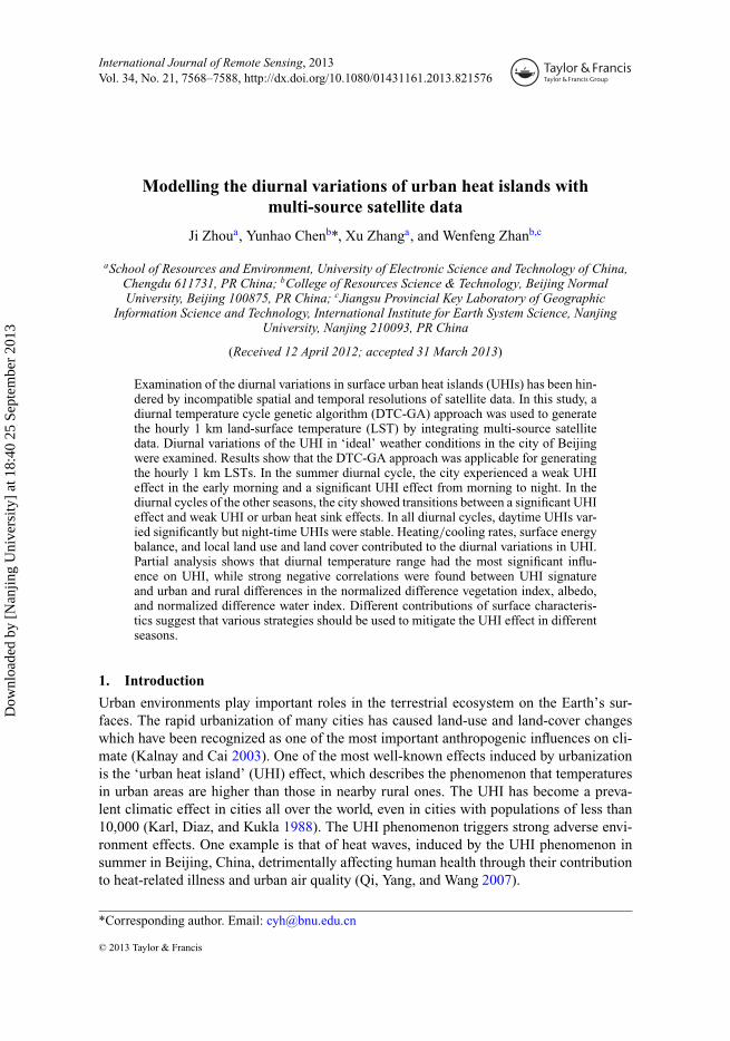
The city of Beijing, China, was selected as the study area (Figure 1). The city is in Beijingmunicipality, which is located in the northern part of China between 39◦ 26′ N–41◦ 03′ Nand 115◦ 25′ E–117◦ 30′ E. Beijing municipality is in a warm temperate zone, with annualaverage air temperature of about 10.0–12.0 ◦C. Beijing has distinct seasons in climate, witha hot and humid summer but a cold and dry winter. The relative humidity is about 72–74%in the summer, during which approximately 75% of annual average precipitation occurs,while the humidity in winter is 44–47% (Cheng et al. 2004). As the capital and the secondlargest city of China, Beijing municipality has 18.953 million inhabitants (i.e. 15.38 millionpermanent and 3.573 million non-permanent residents, with 63.25% of the total populationliving in the core and extended districts) (Yu 2005). More and more people continue toswarm into this mega city, mirroring the rapid urbanization occurring throughout China.In recent decades, the city of Beijing has suffered from severe UHI effects due to rapidurbanization and its physical setting (Zhou et al. 2011).

There are mountains to the west, north, and northeast of the city, while the rural areaslocated to the east, southeast, and south are basically flat. Commercial and business areas

Figure 1. Map of the study area. (a) Location of Beijing municipality in North China, and theframe with skew lines is the region at 112◦ E–120◦ E and 38◦ N–42◦ N. (b) Elevation of Beijingmunicipality. (c) Land-cover types of Beijing municipality and urban extent of Beijing City derivedfrom MCD12Q1 products: 0, water; 1, evergreen needle-leaf forest; 3, deciduous needle-leaf forest;4, deciduous broadleaf forest; 5, mixed forest; 6, closed shrubland; 7, open shrubland; 8, woodysavannah; 9, savannah; 10, grassland; 11, permanent wetland; 12, cropland; 13, urban/built-up; 14,cropland/natural vegetation mosaic; and 16, barren lands. The black polylines in (b) and (c) denotethe boundaries of regions of elevation not greater than 100 m.

Dow

nloa

ded

by [

Nan

jing

Uni

vers

ity]

at 1

8:40

25

Sept

embe

r 20

13

International Journal of Remote Sensing 7571

are concentrated in the central part of the study area, which is characterized by high-risebuildings. Low-rise houses covered by lower-albedo tiles are also dispersed throughout thecity, but most of these are concentrated in the core districts. The extremely dense residentialareas lie in the southern parts of the city and northern suburban regions. Many industrialareas are located in the western and southern areas. In addition, cropland dominates therural areas at similar altitudes to the city. As per Zhou, Hu, and Weng (2010), these ruralareas are covered by abundant crops in the summer, but turn to bare soil or are sparselyvegetated in winter (e.g. winter wheat).

2.2. Data sets

The FY-2C satellite, which is located in a geostationary orbit above the Equator at 105◦ Eand acquires one full disc image covering the Earth’s surface in the region of 60◦ N–60◦ Sand 45◦ E–165◦ E per hour, carries the Stretched Visible and Infrared Spin Scan Radiometer(S-VISSR). The S-VISSR has a visible channel (0.55–0.90 μm) and four thermal channels(3.5–12.5 μm). The specifications of the thermal channels of S-VISSR are listed in Table 1,which shows that these thermal channels have a good ability to monitor the thermal char-acteristics of the Earth’s surface. The S-VISSR data sets used here were acquired from theNational Satellite Meteorological Centre, China Meteorological Administration, via thefollowing website: http://satellite.cma.gov.cn/portalsite/default.aspx.

MODIS instruments are carried on the Terra and Aqua satellites. In general, MODISprovides up to four observations per region per day. The Terra overpass times are around10:30 and 22:30 local solar time, while the Aqua overpass times are around 13:30 and01:30 local solar time. Four categories of MODIS land data products (all in version 5) areused in this study: the daily LST/emissivity product (MOD11A1 and MYD11A1); theyearly land cover (MCD12Q1); the 16 day vegetation indices (MOD13A2); and the 8 dayland-surface reflectance (MOD09A1).

To investigate diurnal UHI variations, strict standards were followed according to theweather observations at Beijing Meteorological Observatory (116◦ 28′ E, 39◦ 48′ N) whenselecting remotely sensed images, because LST is sensitive to meteorological conditions.The following standards should be met for an entire diurnal cycle: (1) the weather is clearand (2) the wind speed is low. In addition, two further steps were conducted to check theremotely sensed data sets. First, both daytime and night-time MODISLST images extractedfrom the MOD11A1 and MYD11A1 products were inspected to ensure that urban andnearby rural areas were not influenced by clouds. Second, the hourly S-VISSR images werevisually inspected. Ultimately, in 2005, four diurnal cycles were selected: 29–30 March,18–19 August, 8–9 October, and 23–24 December. The meteorological conditions on thefirst days of the four diurnal cycles are shown in Table 2. According to Table 2, the fourselected diurnal cycles were almost ‘ideal’ weather conditions for examining the UHI

Table 1. Specifications of FY-2C S-VISSR thermal channels.

ChannelWavelength

(μm)Spatial resolution

(km)Dynamic range

(K)

Noiseequivalent deltatemperature (K)

Quantificationlevel (bit)

IR1 10.3−11.3 5 180−330 0.2−0.4 10IR2 11.5−12.5 5 180−330 0.2−0.4 10IR3 6.3−7.6 5 190−300 0.3−0.5 10IR4 3.5−4.0 5 180−340 0.5−0.6 10

Dow

nloa

ded

by [

Nan

jing

Uni

vers

ity]

at 1

8:40

25

Sept

embe

r 20

13

7572 J. Zhou et al.

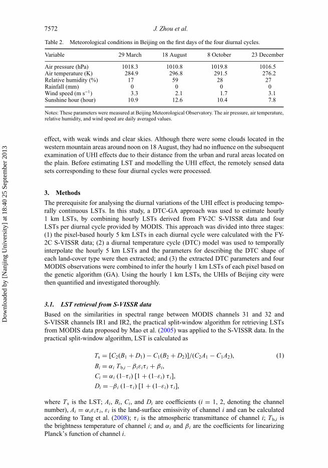
Table 2. Meteorological conditions in Beijing on the first days of the four diurnal cycles.

Variable 29 March 18 August 8 October 23 December

Air pressure (hPa) 1018.3 1010.8 1019.8 1016.5Air temperature (K) 284.9 296.8 291.5 276.2Relative humidity (%) 17 59 28 27Rainfall (mm) 0 0 0 0Wind speed (m s−1) 3.3 2.1 1.7 3.1Sunshine hour (hour) 10.9 12.6 10.4 7.8

Notes: These parameters were measured at Beijing Meteorological Observatory. The air pressure, air temperature,relative humidity, and wind speed are daily averaged values.

effect, with weak winds and clear skies. Although there were some clouds located in thewestern mountain areas around noon on 18 August, they had no influence on the subsequentexamination of UHI effects due to their distance from the urban and rural areas located onthe plain. Before estimating LST and modelling the UHI effect, the remotely sensed datasets corresponding to these four diurnal cycles were processed.

3. Methods

The prerequisite for analysing the diurnal variations of the UHI effect is producing tempo-rally continuous LSTs. In this study, a DTC-GA approach was used to estimate hourly1 km LSTs, by combining hourly LSTs derived from FY-2C S-VISSR data and fourLSTs per diurnal cycle provided by MODIS. This approach was divided into three stages:(1) the pixel-based hourly 5 km LSTs in each diurnal cycle were calculated with the FY-2C S-VISSR data; (2) a diurnal temperature cycle (DTC) model was used to temporallyinterpolate the hourly 5 km LSTs and the parameters for describing the DTC shape ofeach land-cover type were then extracted; and (3) the extracted DTC parameters and fourMODIS observations were combined to infer the hourly 1 km LSTs of each pixel based onthe genetic algorithm (GA). Using the hourly 1 km LSTs, the UHIs of Beijing city werethen quantified and investigated thoroughly.

3.1. LST retrieval from S-VISSR data

Based on the similarities in spectral range between MODIS channels 31 and 32 andS-VISSR channels IR1 and IR2, the practical split-window algorithm for retrieving LSTsfrom MODIS data proposed by Mao et al. (2005) was applied to the S-VISSR data. In thepractical split-window algorithm, LST is calculated as

Ts = [C2(B1 + D1) − C1(B2 + D2)]/(C2A1 − C1A2), (1)

Bi = αi Tb,i – β iεiτ i + β i,

Ci = αi (1–τ i) [1 + (1–εi) τ i],

Di = –β i (1–τ i) [1 + (1–εi) τ i],

where T s is the LST; Ai, Bi, Ci, and Di are coefficients (i = 1, 2, denoting the channelnumber), Ai = αiεiτ i, εi is the land-surface emissivity of channel i and can be calculatedaccording to Tang et al. (2008); τ i is the atmospheric transmittance of channel i; Tb,i isthe brightness temperature of channel i; and αi and β i are the coefficients for linearizingPlanck’s function of channel i.

Dow

nloa

ded

by [

Nan

jing

Uni

vers

ity]

at 1

8:40

25

Sept

embe

r 20

13

International Journal of Remote Sensing 7573

The coefficients in the practical split-window algorithm should be revised accordingto the spectral response functions of S-VISSR channels IR1 and IR2 when applying thepractical split-window algorithm to FY-2C data. In addition, the models for calculatingthe land-surface emissivities and atmospheric transmittances in the practical split-windowalgorithm rely on the spectral response functions of the thermal channels. Therefore, theforms and coefficients of these models needed revision.

First, αi and β i were revised. In the temperature range of 260.0K to 320.0K, the spectralradiances of IR1 and IR2 were calculated according to Planck’s functions. Significant linearrelationships were found between spectral radiances and temperatures:

Ri(T , λi) = αiT + βi, (2)

where T is the brightness temperature or LST in kelvin; Ri is the spectral radiance ofchannel i corresponding to T in W (m2 sr μm)−1; and λi is the effective wavelength ofchannel i in μm. The regression coefficients and accuracies for Equation (2) are shownin Table 3. The correlations were significant at the 0.001 probability level. The statisticalresults imply that linear regressions are reasonable simplifications of Planck’s functions forIR1 and IR2.

Second, models for estimating the atmospheric transmittances of channels IR1 andIR2 from the total water vapour content were developed based on atmospheric radiativetransfer simulations with the Thermodynamic Initial Guess Retrieval (TIGR) atmosphericprofiles in version Tigr2000_v1.1 (Chedin et al. 1985; Chevallier et al. 1998). Theatmospheric radiative transfer model – Moderate Resolution Atmospheric Transmission(MODTRAN) 4.0 code was used (Berk et al. 1998). The relationships between total watercontent and atmospheric transmittances for IR1 and IR2 were calculated as

τ1 = −0.1096w + 0.9895, (3)

τ2 = 0.007w2 − 0.1718w + 0.9841, (4)

where w is the total water content in g cm−2, which can be calculated via the methodproposed by Li et al. (2003). The regression coefficients and accuracies for Equations (3)and (4) are shown in Table 4. The correlations were significant at the 0.001 probabilitylevel, suggesting Equations (3) and (4) possess high accuracy.

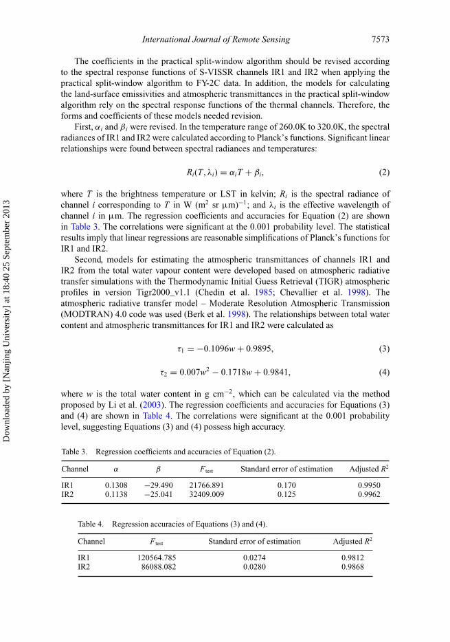
Table 3. Regression coefficients and accuracies of Equation (2).

Channel α β F test Standard error of estimation Adjusted R2

IR1 0.1308 −29.490 21766.891 0.170 0.9950IR2 0.1138 −25.041 32409.009 0.125 0.9962

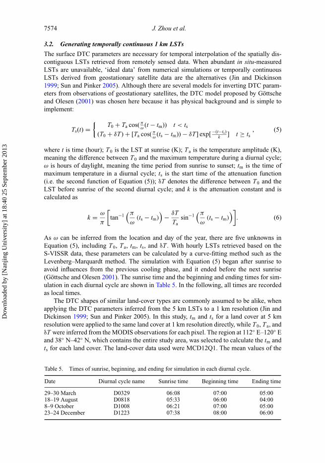
Table 4. Regression accuracies of Equations (3) and (4).

Channel F test Standard error of estimation Adjusted R2

IR1 120564.785 0.0274 0.9812IR2 86088.082 0.0280 0.9868

Dow

nloa

ded

by [

Nan

jing

Uni

vers

ity]

at 1

8:40

25

Sept

embe

r 20

13

7574 J. Zhou et al.

3.2. Generating temporally continuous 1 km LSTs

The surface DTC parameters are necessary for temporal interpolation of the spatially dis-contiguous LSTs retrieved from remotely sensed data. When abundant in situ-measuredLSTs are unavailable, ‘ideal data’ from numerical simulations or temporally continuousLSTs derived from geostationary satellite data are the alternatives (Jin and Dickinson1999; Sun and Pinker 2005). Although there are several models for inverting DTC param-eters from observations of geostationary satellites, the DTC model proposed by Göttscheand Olesen (2001) was chosen here because it has physical background and is simple toimplement:

Ts(t) ={

T0 + Ta cos(πω

(t − tm)) t < ts(T0 + δT) + [Ta cos(π

ω(ts − tm)) − δT] exp[−(t−ts)

k ] t ≥ ts, (5)

where t is time (hour); T0 is the LST at sunrise (K); T a is the temperature amplitude (K),meaning the difference between T0 and the maximum temperature during a diurnal cycle;ω is hours of daylight, meaning the time period from sunrise to sunset; tm is the time ofmaximum temperature in a diurnal cycle; ts is the start time of the attenuation function(i.e. the second function of Equation (5)); δT denotes the difference between T0 and theLST before sunrise of the second diurnal cycle; and k is the attenuation constant and iscalculated as

k = ω

π

[tan−1

(π

ω(ts − tm)

)− δT

Tasin−1

(π

ω(ts − tm)

)]. (6)

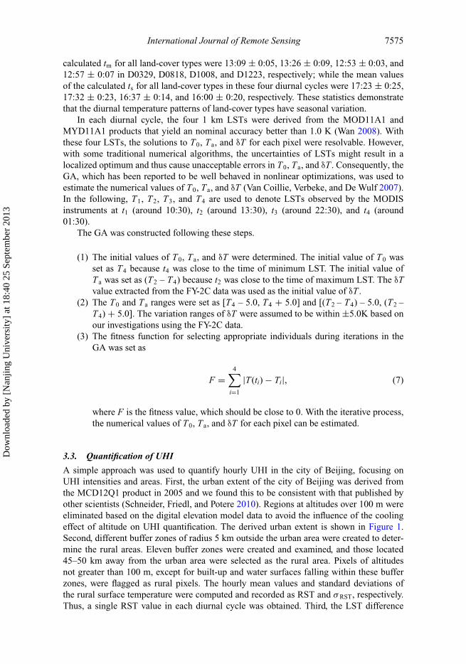
As ω can be inferred from the location and day of the year, there are five unknowns inEquation (5), including T0, T a, tm, ts, and δT . With hourly LSTs retrieved based on theS-VISSR data, these parameters can be calculated by a curve-fitting method such as theLevenberg–Marquardt method. The simulation with Equation (5) began after sunrise toavoid influences from the previous cooling phase, and it ended before the next sunrise(Göttsche and Olesen 2001). The sunrise time and the beginning and ending times for sim-ulation in each diurnal cycle are shown in Table 5. In the following, all times are recordedas local times.

The DTC shapes of similar land-cover types are commonly assumed to be alike, whenapplying the DTC parameters inferred from the 5 km LSTs to a 1 km resolution (Jin andDickinson 1999; Sun and Pinker 2005). In this study, tm and ts for a land cover at 5 kmresolution were applied to the same land cover at 1 km resolution directly, while T0, T a, andδT were inferred from the MODIS observations for each pixel. The region at 112◦ E–120◦ Eand 38◦ N–42◦ N, which contains the entire study area, was selected to calculate the tm andts for each land cover. The land-cover data used were MCD12Q1. The mean values of the

Table 5. Times of sunrise, beginning, and ending for simulation in each diurnal cycle.

Date Diurnal cycle name Sunrise time Beginning time Ending time

29–30 March D0329 06:08 07:00 05:0018–19 August D0818 05:33 06:00 04:008–9 October D1008 06:21 07:00 05:0023–24 December D1223 07:38 08:00 06:00

Dow

nloa

ded

by [

Nan

jing

Uni

vers

ity]

at 1

8:40

25

Sept

embe

r 20

13

International Journal of Remote Sensing 7575

calculated tm for all land-cover types were 13:09 ± 0:05, 13:26 ± 0:09, 12:53 ± 0:03, and12:57 ± 0:07 in D0329, D0818, D1008, and D1223, respectively; while the mean valuesof the calculated ts for all land-cover types in these four diurnal cycles were 17:23 ± 0:25,17:32 ± 0:23, 16:37 ± 0:14, and 16:00 ± 0:20, respectively. These statistics demonstratethat the diurnal temperature patterns of land-cover types have seasonal variation.

In each diurnal cycle, the four 1 km LSTs were derived from the MOD11A1 andMYD11A1 products that yield an nominal accuracy better than 1.0 K (Wan 2008). Withthese four LSTs, the solutions to T0, T a, and δT for each pixel were resolvable. However,with some traditional numerical algorithms, the uncertainties of LSTs might result in alocalized optimum and thus cause unacceptable errors in T0, T a, and δT . Consequently, theGA, which has been reported to be well behaved in nonlinear optimizations, was used toestimate the numerical values of T0, T a, and δT (Van Coillie, Verbeke, and De Wulf 2007).In the following, T1, T2, T3, and T4 are used to denote LSTs observed by the MODISinstruments at t1 (around 10:30), t2 (around 13:30), t3 (around 22:30), and t4 (around01:30).

The GA was constructed following these steps.

(1) The initial values of T0, T a, and δT were determined. The initial value of T0 wasset as T4 because t4 was close to the time of minimum LST. The initial value ofT a was set as (T2 – T4) because t2 was close to the time of maximum LST. The δTvalue extracted from the FY-2C data was used as the initial value of δT .

(2) The T0 and T a ranges were set as [T4 – 5.0, T4 + 5.0] and [(T2 – T4) – 5.0, (T2 –T4) + 5.0]. The variation ranges of δT were assumed to be within ±5.0K based onour investigations using the FY-2C data.

(3) The fitness function for selecting appropriate individuals during iterations in theGA was set as

F =4∑

i=1

|T(ti) − Ti|, (7)

where F is the fitness value, which should be close to 0. With the iterative process,the numerical values of T0, T a, and δT for each pixel can be estimated.

3.3. Quantification of UHI

A simple approach was used to quantify hourly UHI in the city of Beijing, focusing onUHI intensities and areas. First, the urban extent of the city of Beijing was derived fromthe MCD12Q1 product in 2005 and we found this to be consistent with that published byother scientists (Schneider, Friedl, and Potere 2010). Regions at altitudes over 100 m wereeliminated based on the digital elevation model data to avoid the influence of the coolingeffect of altitude on UHI quantification. The derived urban extent is shown in Figure 1.Second, different buffer zones of radius 5 km outside the urban area were created to deter-mine the rural areas. Eleven buffer zones were created and examined, and those located45–50 km away from the urban area were selected as the rural area. Pixels of altitudesnot greater than 100 m, except for built-up and water surfaces falling within these bufferzones, were flagged as rural pixels. The hourly mean values and standard deviations ofthe rural surface temperature were computed and recorded as RST and σ RST, respectively.Thus, a single RST value in each diurnal cycle was obtained. Third, the LST difference

Dow

nloa

ded

by [

Nan

jing

Uni

vers

ity]

at 1

8:40

25

Sept

embe

r 20

13

7576 J. Zhou et al.

between each pixel and RST (i.e. LSTd,) was calculated by subtracting the RST fromthe LST of each pixel in the study area. Then, LSTd values of urban pixels were used toquantify UHIs.

Four indices were computed based on LSTd: (1) UHII1, defined as the mean LSTd of allurban pixels (i.e. mean UHI Intensity (UHII) of the city); (2) UHII2, defined as the meanLSTd of urban pixels, LSTs of which were higher than (RST + σ RST); and (3) urban heatsink intensity (UHSI), defined as the mean LSTd of the urban pixels, LSTs of which werelower than (RST – σ RST); and (4) UHI area, defined as the urban area corresponding toUHII2.

4. Results and discussion

4.1. Evaluation of the hourly 1 km LSTs

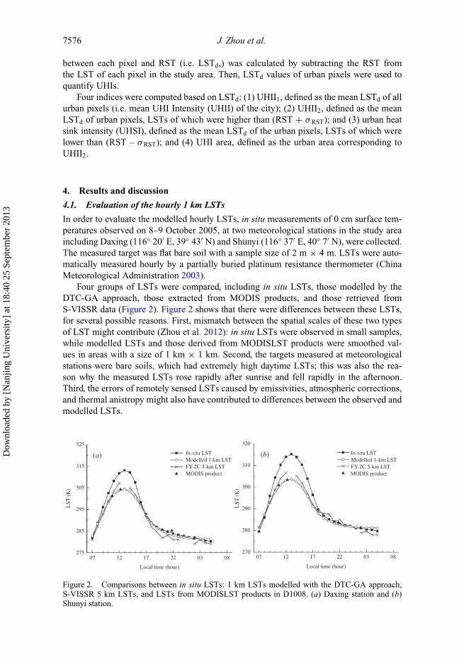
In order to evaluate the modelled hourly LSTs, in situ measurements of 0 cm surface tem-peratures observed on 8–9 October 2005, at two meteorological stations in the study areaincluding Daxing (116◦ 20′ E, 39◦ 43′ N) and Shunyi (116◦ 37′ E, 40◦ 7′ N), were collected.The measured target was flat bare soil with a sample size of 2 m × 4 m. LSTs were auto-matically measured hourly by a partially buried platinum resistance thermometer (ChinaMeteorological Administration 2003).

Four groups of LSTs were compared, including in situ LSTs, those modelled by theDTC-GA approach, those extracted from MODIS products, and those retrieved fromS-VISSR data (Figure 2). Figure 2 shows that there were differences between these LSTs,for several possible reasons. First, mismatch between the spatial scales of these two typesof LST might contribute (Zhou et al. 2012): in situ LSTs were observed in small samples,while modelled LSTs and those derived from MODISLST products were smoothed val-ues in areas with a size of 1 km × 1 km. Second, the targets measured at meteorologicalstations were bare soils, which had extremely high daytime LSTs; this was also the rea-son why the measured LSTs rose rapidly after sunrise and fell rapidly in the afternoon.Third, the errors of remotely sensed LSTs caused by emissivities, atmospheric corrections,and thermal anistropy might also have contributed to differences between the observed andmodelled LSTs.

325 320

310

300

290

280

270

In-situ LSTModelled 1-km LSTFY-2C 5-km LSTMODIS product

In-situ LSTModelled 1-km LSTFY-2C 5-km LSTMODIS product

(a) (b)

315

305

LST

(K

)

LST

(K

)

295

285

275

Local time (hour)

07 12 17 22 03 08

Local time (hour)

07 12 17 22 03 08

Figure 2. Comparisons between in situ LSTs: 1 km LSTs modelled with the DTC-GA approach,S-VISSR 5 km LSTs, and LSTs from MODISLST products in D1008. (a) Daxing station and (b)Shunyi station.

Dow

nloa

ded

by [

Nan

jing

Uni

vers

ity]

at 1

8:40

25

Sept

embe

r 20

13

International Journal of Remote Sensing 7577

Further comparisons between these LSTs revealed some interesting issues. On the onehand, the modelled night-time LSTs are close to the in situ LSTs because LST differencesbetween different land-cover types decreased at night. The mean absolute error (MAE)and root mean square error (RMSE) of the generated hourly night-time LSTs for Daxingstation were 0.5 K and 0.6 K, respectively, while those for Shunyi station were 0.7 K and0.8 K, respectively. These values suggest that the DTC-GA approach has good accuracyfor generating hourly LSTs. The time of both generated and observed maximum LSTs wasaround 13:00 local time, indicating that the DTC-GA approach represented the diurnal LSTvariations objectively. In addition, the hourly LSTs retrieved from the FY-2C S-VISSR hadsimilar diurnal cycles to the modelled 1 km LSTs.

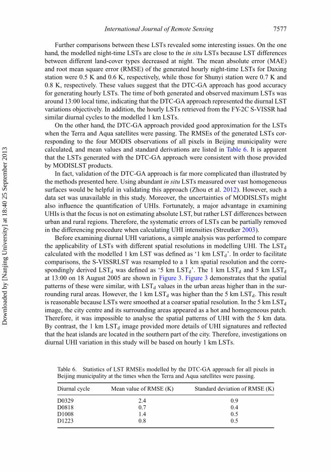
On the other hand, the DTC-GA approach provided good approximation for the LSTswhen the Terra and Aqua satellites were passing. The RMSEs of the generated LSTs cor-responding to the four MODIS observations of all pixels in Beijing municipality werecalculated, and mean values and standard derivations are listed in Table 6. It is apparentthat the LSTs generated with the DTC-GA approach were consistent with those providedby MODISLST products.

In fact, validation of the DTC-GA approach is far more complicated than illustrated bythe methods presented here. Using abundant in situ LSTs measured over vast homogeneoussurfaces would be helpful in validating this approach (Zhou et al. 2012). However, such adata set was unavailable in this study. Moreover, the uncertainties of MODISLSTs mightalso influence the quantification of UHIs. Fortunately, a major advantage in examiningUHIs is that the focus is not on estimating absolute LST, but rather LST differences betweenurban and rural regions. Therefore, the systematic errors of LSTs can be partially removedin the differencing procedure when calculating UHI intensities (Streutker 2003).

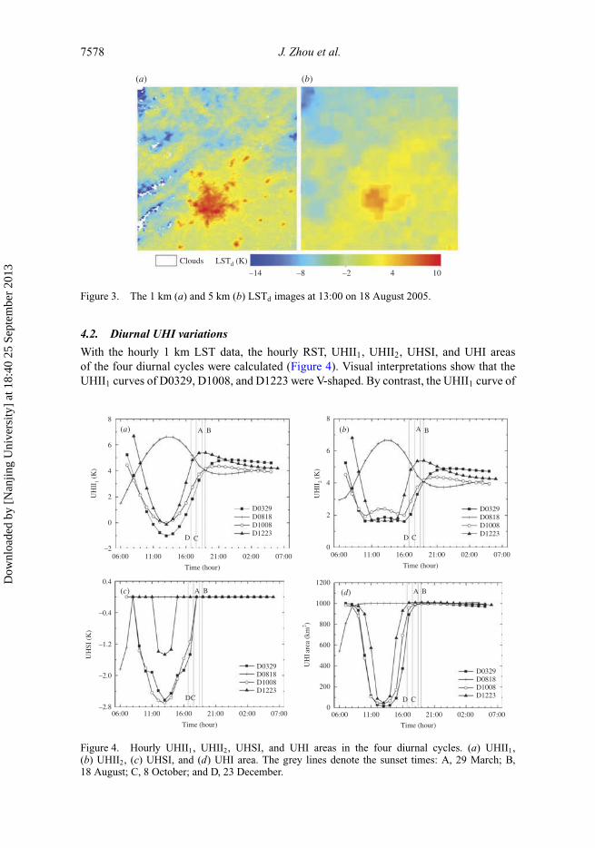
Before examining diurnal UHI variations, a simple analysis was performed to comparethe applicability of LSTs with different spatial resolutions in modelling UHI. The LSTd

calculated with the modelled 1 km LST was defined as ‘1 km LSTd’. In order to facilitatecomparisons, the S-VISSRLST was resampled to a 1 km spatial resolution and the corre-spondingly derived LSTd was defined as ‘5 km LSTd’. The 1 km LSTd and 5 km LSTd

at 13:00 on 18 August 2005 are shown in Figure 3. Figure 3 demonstrates that the spatialpatterns of these were similar, with LSTd values in the urban areas higher than in the sur-rounding rural areas. However, the 1 km LSTd was higher than the 5 km LSTd. This resultis reasonable because LSTs were smoothed at a coarser spatial resolution. In the 5 km LSTd

image, the city centre and its surrounding areas appeared as a hot and homogeneous patch.Therefore, it was impossible to analyse the spatial patterns of UHI with the 5 km data.By contrast, the 1 km LSTd image provided more details of UHI signatures and reflectedthat the heat islands are located in the southern part of the city. Therefore, investigations ondiurnal UHI variation in this study will be based on hourly 1 km LSTs.

Table 6. Statistics of LST RMSEs modelled by the DTC-GA approach for all pixels inBeijing municipality at the times when the Terra and Aqua satellites were passing.

Diurnal cycle Mean value of RMSE (K) Standard deviation of RMSE (K)

D0329 2.4 0.9D0818 0.7 0.4D1008 1.4 0.5D1223 0.8 0.5

Dow

nloa

ded

by [

Nan

jing

Uni

vers

ity]

at 1

8:40

25

Sept

embe

r 20

13

7578 J. Zhou et al.

(a) (b)

Clouds LSTd (K)

–14 –8 –2 4 10

Figure 3. The 1 km (a) and 5 km (b) LSTd images at 13:00 on 18 August 2005.

4.2. Diurnal UHI variations

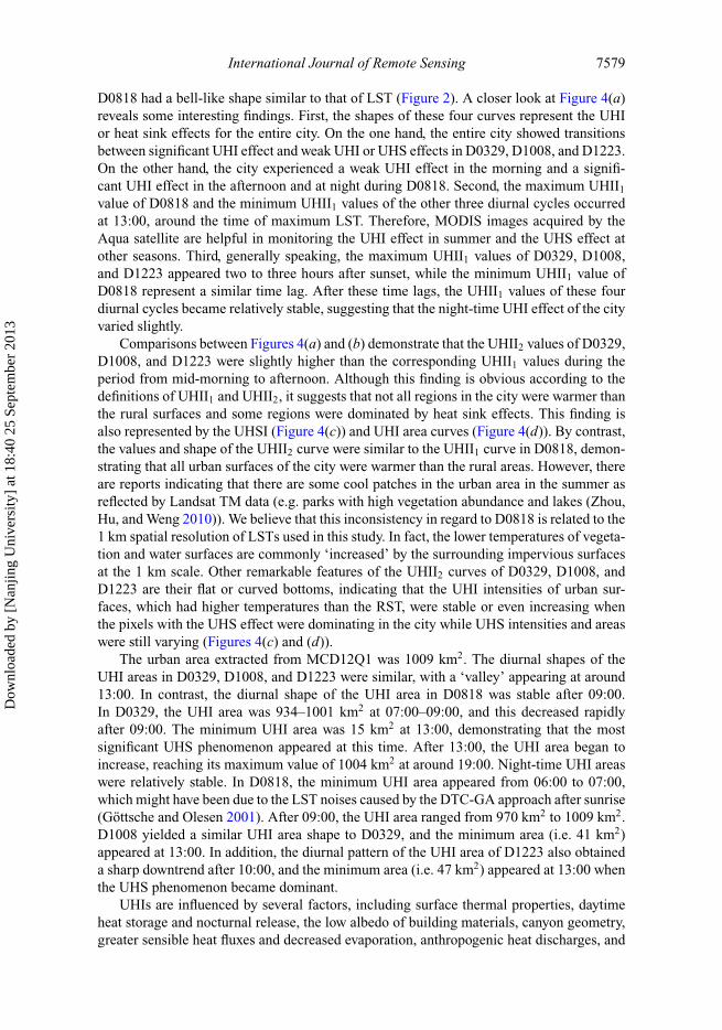
With the hourly 1 km LST data, the hourly RST, UHII1, UHII2, UHSI, and UHI areasof the four diurnal cycles were calculated (Figure 4). Visual interpretations show that theUHII1 curves of D0329, D1008, and D1223 were V-shaped. By contrast, the UHII1 curve of

8

A AB

A B A B

B

D D

Time (hour)

C

DC D C

C

D0329D0818

D1223D1008

D0329D0818

D1223D1008

D0329D0818

D1223D1008

D0329D0818

D1223D1008

(a)

(c) (d)

(b)

6

4

UH

II1

(K)

UH

SI (

K)

UH

II2

(K)

UH

I are

a (k

m2 )

2

–206:00 11:00 16:00 21:00 02:00 07:00

Time (hour)

06:00 11:00 16:00 21:00 02:00 07:00

Time (hour)

06:00 11:00 16:00 21:00 02:00 07:00

Time (hour)

06:00 11:00 16:00 21:00 02:00 07:00

0

–0.4

–1.2

–2.0

–2.8

0.4 1200

1000

800

600

400

200

0

8

6

4

2

0

Figure 4. Hourly UHII1, UHII2, UHSI, and UHI areas in the four diurnal cycles. (a) UHII1,(b) UHII2, (c) UHSI, and (d) UHI area. The grey lines denote the sunset times: A, 29 March; B,18 August; C, 8 October; and D, 23 December.

Dow

nloa

ded

by [

Nan

jing

Uni

vers

ity]

at 1

8:40

25

Sept

embe

r 20

13

International Journal of Remote Sensing 7579

D0818 had a bell-like shape similar to that of LST (Figure 2). A closer look at Figure 4(a)reveals some interesting findings. First, the shapes of these four curves represent the UHIor heat sink effects for the entire city. On the one hand, the entire city showed transitionsbetween significant UHI effect and weak UHI or UHS effects in D0329, D1008, and D1223.On the other hand, the city experienced a weak UHI effect in the morning and a signifi-cant UHI effect in the afternoon and at night during D0818. Second, the maximum UHII1

value of D0818 and the minimum UHII1 values of the other three diurnal cycles occurredat 13:00, around the time of maximum LST. Therefore, MODIS images acquired by theAqua satellite are helpful in monitoring the UHI effect in summer and the UHS effect atother seasons. Third, generally speaking, the maximum UHII1 values of D0329, D1008,and D1223 appeared two to three hours after sunset, while the minimum UHII1 value ofD0818 represent a similar time lag. After these time lags, the UHII1 values of these fourdiurnal cycles became relatively stable, suggesting that the night-time UHI effect of the cityvaried slightly.

Comparisons between Figures 4(a) and (b) demonstrate that the UHII2 values of D0329,D1008, and D1223 were slightly higher than the corresponding UHII1 values during theperiod from mid-morning to afternoon. Although this finding is obvious according to thedefinitions of UHII1 and UHII2, it suggests that not all regions in the city were warmer thanthe rural surfaces and some regions were dominated by heat sink effects. This finding isalso represented by the UHSI (Figure 4(c)) and UHI area curves (Figure 4(d)). By contrast,the values and shape of the UHII2 curve were similar to the UHII1 curve in D0818, demon-strating that all urban surfaces of the city were warmer than the rural areas. However, thereare reports indicating that there are some cool patches in the urban area in the summer asreflected by Landsat TM data (e.g. parks with high vegetation abundance and lakes (Zhou,Hu, and Weng 2010)). We believe that this inconsistency in regard to D0818 is related to the1 km spatial resolution of LSTs used in this study. In fact, the lower temperatures of vegeta-tion and water surfaces are commonly ‘increased’ by the surrounding impervious surfacesat the 1 km scale. Other remarkable features of the UHII2 curves of D0329, D1008, andD1223 are their flat or curved bottoms, indicating that the UHI intensities of urban sur-faces, which had higher temperatures than the RST, were stable or even increasing whenthe pixels with the UHS effect were dominating in the city while UHS intensities and areaswere still varying (Figures 4(c) and (d)).

The urban area extracted from MCD12Q1 was 1009 km2. The diurnal shapes of theUHI areas in D0329, D1008, and D1223 were similar, with a ‘valley’ appearing at around13:00. In contrast, the diurnal shape of the UHI area in D0818 was stable after 09:00.In D0329, the UHI area was 934–1001 km2 at 07:00–09:00, and this decreased rapidlyafter 09:00. The minimum UHI area was 15 km2 at 13:00, demonstrating that the mostsignificant UHS phenomenon appeared at this time. After 13:00, the UHI area began toincrease, reaching its maximum value of 1004 km2 at around 19:00. Night-time UHI areaswere relatively stable. In D0818, the minimum UHI area appeared from 06:00 to 07:00,which might have been due to the LST noises caused by the DTC-GA approach after sunrise(Göttsche and Olesen 2001). After 09:00, the UHI area ranged from 970 km2 to 1009 km2.D1008 yielded a similar UHI area shape to D0329, and the minimum area (i.e. 41 km2)appeared at 13:00. In addition, the diurnal pattern of the UHI area of D1223 also obtaineda sharp downtrend after 10:00, and the minimum area (i.e. 47 km2) appeared at 13:00 whenthe UHS phenomenon became dominant.

UHIs are influenced by several factors, including surface thermal properties, daytimeheat storage and nocturnal release, the low albedo of building materials, canyon geometry,greater sensible heat fluxes and decreased evaporation, anthropogenic heat discharges, and

Dow

nloa

ded

by [

Nan

jing

Uni

vers

ity]

at 1

8:40

25

Sept

embe

r 20

13

7580 J. Zhou et al.

meteorological and climatic conditions (Kato and Yamaguchi 2005; Oke 1978; Zhou et al.2011). Generally speaking, the roles of these factors in UHI can be attributed to their differ-ent influences on urban and rural surface temperatures. According to the DTC model usedin this study (e.g. Equation (5)), daytime LST variations are similar to harmonic, whichhas a bell shape. In fact, similar simulations have been used in many DTC models (e.g.Jin and Dickinson 1999; Sun and Pinker 2005; Zhan et al. 2013). It is easy to infer thatthe difference between urban and rural surface temperatures has a bell shape or invertedbell shape. The shapes presented here appeared in ‘ideal’ weather conditions. When windspeed increases or clouds appear in the urban area, the shapes will become more compli-cated than in the ‘ideal’ condition because the UHI effect is sensitive to weather conditions(Oke 1978; Zakšek and Oštir 2012).

Inter-comparisons of the UHII1 curves demonstrate that D0818 was different from theother three diurnal cycles: there was a daytime UHI effect in the summer diurnal cyclebut daytime UHS effects in the diurnal cycles of the other seasons. In fact, similar find-ings have been reported by Zhang et al. (2005) and Wang et al. (2007) when they wereinvestigating the UHI phenomenon in Beijing with the four observations of MODIS ineach diurnal cycle. In addition, daytime UHI in summer and daytime UHS in winter havealso been reported in our previous research with Landsat TM data (Zhou, Hu, and Weng2010). The difference between D0818 and the other three diurnal cycles can be partiallyexplained by differences in physical characteristics between urban and rural surfaces. Theurban area of Beijing is dominated by impervious surfaces with low evapotranspiration andlow albedo. Artificial constructions store considerable heat due to their huge volumes andcanyon geometry. In summer, the main land-cover type of rural areas is cropland (Figure 1),with a higher evapotranspiration than urban areas. In addition, rural areas have higher ther-mal inertia due to higher vegetation abundance and moisture than urban areas (Wang et al.2007). Therefore, the urban area heated up faster than the rural area after sunrise, and thetemperature difference between these areas reached its peak after one or two hours aftersolar shortwave radiance had reached its peak. On the following afternoon, the tempera-ture difference between urban and rural areas decreased. This is also the reason why theUHII1 curve of D0818 appeared as a bell shape.

The land-cover types of the rural area of Beijing turn to bare soil or sparse vegetationin the spring, autumn, and winter. These land-cover types have two important features –low evapotranspiration and low thermal inertia (Carnahan and Larson 1990; Wang et al.2007) – that cause the heating rate of the rural surface to be similar to or faster than that ofthe urban surface after sunrise. Therefore, UHI intensity decreases in the morning and theminimum UHII1 values appear around 13:00, followed by an increase in the afternoon dueto decreasing solar shortwave radiation.

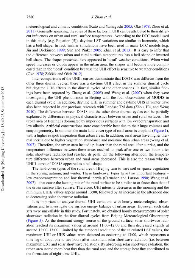
It is important to analyse diurnal UHI variations with hourly meteorological obser-vations and to investigate the surface energy balance of urban areas. However, such datasets were unavailable in this study. Fortunately, we obtained hourly measurements of solarshortwave radiation in the four diurnal cycles from Beijing Meteorological Observatory(Figure 5). As the dominant energy source of the ground surface, solar shortwave radi-ation reached its maximum values at around 11:00–12:00 and then decreased slightly ataround 12:00–13:00. Limited by the temporal resolution of the calculated LST values, themaximum UHI or UHS values were detected as occurring at 13:00, which represents atime lag of about one to two hours after maximum solar shortwave radiation (i.e. betweenmaximum LST and solar shortwave radiation). By absorbing solar shortwave radiation, theurban area stored more heat flux than the rural area and the storage heat flux contributed tothe formation of night-time UHIs.

Dow

nloa

ded

by [

Nan

jing

Uni

vers

ity]

at 1

8:40

25

Sept

embe

r 20

13

International Journal of Remote Sensing 7581

3.5

29 March18 August8 October23 December

3.0

2.5

2.0

1.0

Shor

twav

e ra

diat

ion

(MJm

–2)

1.5

0.5

0.0

03:00 06:00 09:00 12:00

Time (hour)

15:00 18:00 21:00

Figure 5. Hourly integrated solar shortwave radiation measured at Beijing MeteorologicalObservatory during the initial period of the four diurnal cycles.

Anthropogenic heat is another source of surface energy balance in urban areas: itheats the atmosphere directly and increases LSTs through longwave radiation (Kato andYamaguchi 2005). The ratio of the anthropogenic heat flux to total surface net radiationis greater in winter because of weak solar shortwave radiation and an intensive heatingload (Taha 1997; Ichinose, Shimodozono, and Hanaki 1999). In addition, the influenceof anthropogenic heat on daytime UHI is much weaker than at night because anthro-pogenic heat plays a more important role in surface energy balance at night. Tong et al.(2004) conducted a detailed investigation on anthropogenic heat discharge in Beijing, theirresults showing that the total anthropogenic daytime heat over the urban area in 2002 var-ied from 130 to 170 W m−2, with one peak in the morning (at around 09:00 local time)and one in the late afternoon (at around 18:00 local time). As previously noted, peak UHIintensity in the D1223 cycle appeared at 18:00–19:00, at the same time as maximum anthro-pogenic heat discharge. This finding further confirms that anthropogenic heat contributesto night-time UHI.

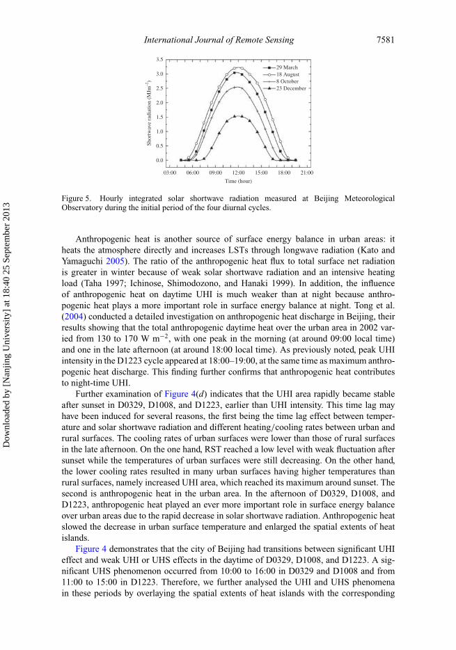
Further examination of Figure 4(d) indicates that the UHI area rapidly became stableafter sunset in D0329, D1008, and D1223, earlier than UHI intensity. This time lag mayhave been induced for several reasons, the first being the time lag effect between temper-ature and solar shortwave radiation and different heating/cooling rates between urban andrural surfaces. The cooling rates of urban surfaces were lower than those of rural surfacesin the late afternoon. On the one hand, RST reached a low level with weak fluctuation aftersunset while the temperatures of urban surfaces were still decreasing. On the other hand,the lower cooling rates resulted in many urban surfaces having higher temperatures thanrural surfaces, namely increased UHI area, which reached its maximum around sunset. Thesecond is anthropogenic heat in the urban area. In the afternoon of D0329, D1008, andD1223, anthropogenic heat played an ever more important role in surface energy balanceover urban areas due to the rapid decrease in solar shortwave radiation. Anthropogenic heatslowed the decrease in urban surface temperature and enlarged the spatial extents of heatislands.

Figure 4 demonstrates that the city of Beijing had transitions between significant UHIeffect and weak UHI or UHS effects in the daytime of D0329, D1008, and D1223. A sig-nificant UHS phenomenon occurred from 10:00 to 16:00 in D0329 and D1008 and from11:00 to 15:00 in D1223. Therefore, we further analysed the UHI and UHS phenomenain these periods by overlaying the spatial extents of heat islands with the corresponding

Dow

nloa

ded

by [

Nan

jing

Uni

vers

ity]

at 1

8:40

25

Sept

embe

r 20

13

7582 J. Zhou et al.

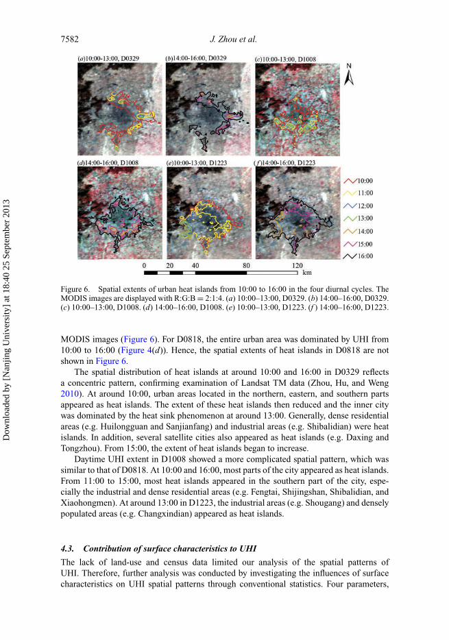
Figure 6. Spatial extents of urban heat islands from 10:00 to 16:00 in the four diurnal cycles. TheMODIS images are displayed with R:G:B = 2:1:4. (a) 10:00–13:00, D0329. (b) 14:00–16:00, D0329.(c) 10:00–13:00, D1008. (d) 14:00–16:00, D1008. (e) 10:00–13:00, D1223. (f ) 14:00–16:00, D1223.

MODIS images (Figure 6). For D0818, the entire urban area was dominated by UHI from10:00 to 16:00 (Figure 4(d)). Hence, the spatial extents of heat islands in D0818 are notshown in Figure 6.

The spatial distribution of heat islands at around 10:00 and 16:00 in D0329 reflectsa concentric pattern, confirming examination of Landsat TM data (Zhou, Hu, and Weng2010). At around 10:00, urban areas located in the northern, eastern, and southern partsappeared as heat islands. The extent of these heat islands then reduced and the inner citywas dominated by the heat sink phenomenon at around 13:00. Generally, dense residentialareas (e.g. Huilongguan and Sanjianfang) and industrial areas (e.g. Shibalidian) were heatislands. In addition, several satellite cities also appeared as heat islands (e.g. Daxing andTongzhou). From 15:00, the extent of heat islands began to increase.

Daytime UHI extent in D1008 showed a more complicated spatial pattern, which wassimilar to that of D0818. At 10:00 and 16:00, most parts of the city appeared as heat islands.From 11:00 to 15:00, most heat islands appeared in the southern part of the city, espe-cially the industrial and dense residential areas (e.g. Fengtai, Shijingshan, Shibalidian, andXiaohongmen). At around 13:00 in D1223, the industrial areas (e.g. Shougang) and denselypopulated areas (e.g. Changxindian) appeared as heat islands.

4.3. Contribution of surface characteristics to UHI

The lack of land-use and census data limited our analysis of the spatial patterns ofUHI. Therefore, further analysis was conducted by investigating the influences of surfacecharacteristics on UHI spatial patterns through conventional statistics. Four parameters,

Dow

nloa

ded

by [

Nan

jing

Uni

vers

ity]

at 1

8:40

25

Sept

embe

r 20

13

International Journal of Remote Sensing 7583

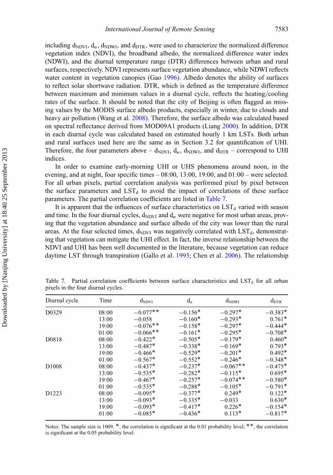
including dNDVI, dα , dNDWI, and dDTR, were used to characterize the normalized differencevegetation index (NDVI), the broadband albedo, the normalized difference water index(NDWI), and the diurnal temperature range (DTR) differences between urban and ruralsurfaces, respectively. NDVI represents surface vegetation abundance, while NDWI reflectswater content in vegetation canopies (Gao 1996). Albedo denotes the ability of surfacesto reflect solar shortwave radiation. DTR, which is defined as the temperature differencebetween maximum and minimum values in a diurnal cycle, reflects the heating/coolingrates of the surface. It should be noted that the city of Beijing is often flagged as miss-ing values by the MODIS surface albedo products, especially in winter, due to clouds andheavy air pollution (Wang et al. 2008). Therefore, the surface albedo was calculated basedon spectral reflectance derived from MOD09A1 products (Liang 2000). In addition, DTRin each diurnal cycle was calculated based on estimated hourly 1 km LSTs. Both urbanand rural surfaces used here are the same as in Section 3.2 for quantification of UHI.Therefore, the four parameters above – dNDVI, dα , dNDWI, and dDTR – correspond to UHIindices.

In order to examine early-morning UHI or UHS phenomena around noon, in theevening, and at night, four specific times – 08:00, 13:00, 19:00, and 01:00 – were selected.For all urban pixels, partial correlation analysis was performed pixel by pixel betweenthe surface parameters and LSTd to avoid the impact of correlations of these surfaceparameters. The partial correlation coefficients are listed in Table 7.

It is apparent that the influences of surface characteristics on LSTd varied with seasonand time. In the four diurnal cycles, dNDVI and dα were negative for most urban areas, prov-ing that the vegetation abundance and surface albedo of the city was lower than the ruralareas. At the four selected times, dNDVI was negatively correlated with LSTd, demonstrat-ing that vegetation can mitigate the UHI effect. In fact, the inverse relationship between theNDVI and UHI has been well documented in the literature, because vegetation can reducedaytime LST through transpiration (Gallo et al. 1993; Chen et al. 2006). The relationship

Table 7. Partial correlation coefficients between surface characteristics and LSTd for all urbanpixels in the four diurnal cycles.

Diurnal cycle Time dNDVI dα dNDWI dDTR

D0329 08:00 −0.077** −0.156* −0.297* −0.383*13:00 −0.058 −0.160* −0.293* 0.761*19:00 −0.076** −0.158* −0.297* −0.444*01:00 −0.066** −0.161* −0.295* −0.708*

D0818 08:00 −0.422* −0.505* −0.179* 0.460*13:00 −0.487* −0.338* −0.169* 0.793*19:00 −0.466* −0.529* −0.201* 0.492*01:00 −0.567* −0.552* −0.246* −0.348*

D1008 08:00 −0.437* −0.237* −0.067** −0.475*13:00 −0.535* −0.282* −0.115* 0.695*19:00 −0.467* −0.257* −0.074** −0.580*01:00 −0.535* −0.288* −0.105* −0.791*

D1223 08:00 −0.095* −0.377* 0.249* 0.122*13:00 −0.093* −0.335* −0.033 0.630*19:00 −0.093* −0.417* 0.226* −0.154*01:00 −0.085* −0.436* 0.113* −0.817*

Notes: The sample size is 1009. *, the correlation is significant at the 0.01 probability level; **, the correlationis significant at the 0.05 probability level.

Dow

nloa

ded

by [

Nan

jing

Uni

vers

ity]

at 1

8:40

25

Sept

embe

r 20

13

7584 J. Zhou et al.

between NDVI and UHI has also been found to be negative at night, possibly caused bythe lower level of heat stored by vegetation in daytime (Tiangco, Lagmay, and Argete2008; Zhou et al. 2011). The weak correlation between dNDVI and LSTd in D0329 andD1223 might have been caused by the low activity of vegetation in spring and winter. Theinverse relationships between dNDVI and LSTd at 13:00 in D1008 and D1223 also demon-strate that urban areas with higher vegetation abundance (e.g. residential areas located inthe inner city and parks) tended to appear as UHS patches (Figure 6). In addition, UHIintensity in urban areas with high vegetation abundances was weaker than in areas withhighly impervious surfaces in D0818.

dα was also negatively correlated with LSTd in all cases. In the four selected diurnalcycles, the spatial distribution of albedo was concentric (i.e. albedo increased from thecentre of the city to the surrounding areas). The inner city had a lower albedo due to thedark rooftops, while the high-rise buildings surrounding the inner city had a higher albedobecause their rooftops are commonly made of concrete, metal, and glass. Negative dα valuescan be attributed to construction materials with low tone and urban canyon geometries.On the one hand, inverse relationships between dα and LSTd demonstrated that the UHIeffect might be mitigated by increasing the albedo of urban areas (Oleson, Bonan, andFeddema 2010). On the other hand, partial correlations at 13:00 in D0329, D1008, andD1223 show that high albedo tended to cause an UHS effect. This finding seems to beinconsistent with the UHI extents represented in Figure 6. In fact, the influence of surfacealbedo on UHI was disturbed by other factors, such as vegetation abundance, moisture, andheating/cooling rates. Thereby, it should be assumed that UHIs in high-albedo areas weremarkedly influenced by other factors (e.g. heating/cooling rates).

dNDWI varied with season: nearly all dNDWI values were negative in D0818, suggestingthe water contents of vegetation canopies are generally lower than that of rural area; mostdNDWI values were positive in D1008, except for densely built-up and industrial areas (e.g.Shibalidian, Fengtai, and Shijingshan); by contrast, dNDWI values over areas with high veg-etation abundance were positive and those over highly impervious areas were negative inD0329 and D1223. The inverse relationship between dNDWI and LSTd suggests that vegeta-tion canopies with high water content can mitigate the UHI effect due to evapotranspiration.In addition, urban areas with high water content were apt to appear as heat sinks. However,LSTd was inversely correlated with dNDWI at 08:00, 19:00, and 01:00. We carefully exam-ined LSTd and dNDWI images and found that areas with both high LSTd and dNDWI appearedin the inner city, which had low surface albedo. Therefore, we speculate that the relationshipbetween LSTd and dNDWI was influenced by other surface characteristics and anthropogenicactivities.

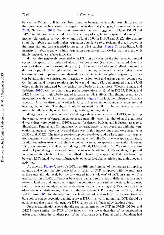
As shown in Figure 7, the city’s DTR was different from that of the rural area. In spring,autumn, and winter, the city behaved as a ‘basin’ of DTR compared with the rural areaat the same altitude level, but the city turned into a ‘plateau’ of DTR in summer. Thetransformation of DTR differences between urban and rural areas in different seasons mayrelate to land use and land cover, vegetation conditions, and surface moisture. In summer,rural surfaces are mainly covered by vegetation (e.g. crops and grass). Evapotranspirationof vegetation contributes significantly to the decrease in DTR during summer (Sun, Pinker,and Kafatos 2006). In other seasons, most land cover of rural surfaces is converted to eitherbare soil or sparse vegetation, giving a lower DTR. It is worth noting that DTR should bepositive and that pixels with negative DTR values were influenced by daytime cloud.

Further examination shows that the spatial patterns of the DTR in D0329, D1008, andD1223 were similar: the DTR of the inner city was lower than that of the surroundingurban areas while the southern part of the urban area (e.g. Fengtai and Shibalidian) had

Dow

nloa

ded

by [

Nan

jing

Uni

vers

ity]

at 1

8:40

25

Sept

embe

r 20

13

International Journal of Remote Sensing 7585

Figure 7. Diurnal temperature ranges (DTRs) in Beijing municipality in the four diurnal cycles. Thegrey line is the boundary of the city. (a) D0329. (b) D0818. (c) D1008. (d) D1223.

a larger DTR than the northern part. This partial correlation demonstrates that DTR isclosely related spatially with UHI or UHS (Table 7). The positive relationship betweendDTR and LSTd suggests that urban areas with high heating/cooling rates (e.g. Shijingshan,Changxindian, and Fengtai) tend to appear as intense heat islands in the daytime whilesuch areas are commonly dominated by weak heat islands at night, exhibiting an inverserelationship between dDTR and LSTd compared to that in the daytime.

Inter-comparisons of the partial correlation coefficients listed in Table 7 indicate thatthe contribution of the surface characteristics to UHI or UHS varies by season. In mostcases, DTR was a more pivotal parameter than the other three while NDVI, albedo, andNDWI contributed variously towards UHI or UHS in the four diurnal cycles. This suggeststhat different strategies should be used to mitigate the UHI effect in different seasons.

5. Conclusions

The remotely sensed data provided by current satellites cannot meet the demands ofanalysing diurnal variations in the UHI effect due to their incompatible spatial and tem-poral resolutions. In this study, the data acquired by both FY-2C S-VISSR and Terra/AquaMODIS instruments were integrated. A DTC-GA approach was developed to infer hourly1 km LSTs. The diurnal UHI variations in the city of Beijing were then investigatedin four typical diurnal cycles in 2005: 29–30 March, 18–19 August, 8–9 October, and23–24 December.

Evaluation using in situ measurements of LSTs at two meteorological stations demon-strated that the DTC-GA approach is applicable and feasible to generate hourly 1 kmLSTs. The consistency between LSTs provided by MODISLST products and those esti-mated via the DTC-GA approach further confirms the accuracy of estimated hourly LSTs.Advantages of the DTC-GA approach over other methods (e.g. combining remotely senseddata and numerical simulations) include its simplicity in use and its extendibility in appli-cations (e.g. drought monitoring, surface energy balance modelling, and hydrologicalanalysis) over large areas.

The UHI effect in the city of Beijing was analysed based on 1 km LSTs in four diurnalcycles, by considering UHI intensity and area and following the physical processes. TheUHS effect was also incorporated. Our results indicate that the city of Beijing showed tran-sitions between significant UHI effects and weak UHI or UHS effects in D0329, D1008,and D1223, while experiencing weak UHI effects in the early morning and significant UHIeffects in the morning, afternoon, and night-time in D0818. The maximum UHII1 valueof D0818 and the minimum UHII1 values of the other three diurnal cycles occurred at

Dow

nloa

ded

by [

Nan

jing

Uni

vers

ity]

at 1

8:40

25

Sept

embe

r 20

13

7586 J. Zhou et al.

13:00, around the time of maximum LST. The maximum UHII1 values of D0329, D1008,and D1223 appeared two to three hours after sunset, while the minimum UHII1 value ofD0818 exhibited a similar time lag. After these time lags, the UHII1 values of these fourdiurnal cycles became relatively stable, suggesting that the night-time UHI effect of thecity varied slightly. Diurnal UHI variations were influenced by many factors includingheating/cooling rates, local land-use and land-cover patterns, solar shortwave radiation,and anthropogenic heat discharges.

Further investigations were conducted by examining the contributions to UHI of sur-face characteristics from the spatial perspective through partial correlation analysis. NDVI,surface albedo, NDWI, and DTR were used to denote surface characteristics. Results showthat the contributions of surface characteristics varied by season and time. The strongestcorrelation existed between UHI signature and DTR, showing that the heating/coolingof surfaces are the main factors influencing UHI formation. Strong negative correlationswere also found between NDVI, albedo, NDWI, and UHI signatures, demonstrating thatincreases in vegetation, water content in vegetation canopies, and albedo effectively depressUHI. However, the influences of NDWI and albedo on UHI were modified by other factors.The different contributions of surface characteristics suggest that different strategies shouldbe utilized to mitigate the UHI effect in different seasons.

AcknowledgementsThis work was supported in part by the National Natural Science Foundation of China undergrants 41101380 and 41071258, by the Chinese State Key Basic Research Project under grant2013CB733406, by the Postdoctoral Science Foundation of China under grant 2011M500145,and by the Fundamental Research Funds for the Central Universities of China under grantZYGX2010J087. We thank Dr Yuanyuan Wang from the National Satellite Meteorological Centre,China Meteorological Administration, and Professor Jinfei Wang from the University of WesternOntario for improving this article. We also wish to thank the anonymous referees for their constructivecriticism and comments.

ReferencesBasara, J. B., P. K. Hall Jr, A. J. Schroeder, B. G. Illston, and K. L. Nemunaitis. 2008. “Diurnal

Cycle of the Oklahoma City Urban Heat Island.” Journal of Geophysical Research 113.doi:10.1029/2008JD010311.

Berk, A., L. S. Bernstein, G. P. Anderson, P. K. Acharya, D. C. Robertson, J. H. Chetwynd, and S. M.Adler-Golden. 1998. “MODTRAN Cloud and Multiple Scattering Upgrades with Application toAVIRIS.” Remote Sensing of Environment 65: 367–375.

Carnahan, W. H., and R. C. Larson. 1990. “An Analysis of an Urban Heat Sink.” Remote Sensing ofEnvironment 33: 65–71.

Chedin, A., N. A. Scott, C. Wahiche, and P. Moulinier. 1985. “The Improved Initialization InversionMethod: A High Resolution Physical Method for Temperature Retrievals from Satellites of theTiros-N Series.” Journal of Applied Meteorology 24: 128–143.

Chen, X. L., H. M. Zhao, P. X. Li, and Z. Y. Yin. 2006. “Remote Sensing Image-Based Analysis ofthe Relationship Between Urban Heat Island and Land Use/Cover Changes.” Remote Sensing ofEnvironment 104: 133–146.

Chen, Y., D. Z. Sui, T. Fung, and W. Dou. 2007. “Fractal Analysis of the Structure and Dynamics of aSatellite-Detected Urban Heat Island.” International Journal of Remote Sensing 28: 2359–2366.

Cheng, C., N. Wu, S. Guo, S. Li, and D. Liu. 2004. “A Study on the Interaction Between Urban HeatIsland and Vegetation Theory, Methodology, and Case Study.” [In Chinese.] Research of Soil andWater Conservation 11: 172–174.

Chevallier, F., F. Chéruy, N. A. Scott, and A. Chédin. 1998. “A Neural Network Approach for a Fastand Accurate Computation of a Longwave Radiative Budget.” Journal of Applied Meteorology37: 1385–1397.

Dow

nloa

ded

by [

Nan

jing

Uni

vers

ity]

at 1

8:40

25

Sept

embe

r 20

13

International Journal of Remote Sensing 7587

China Meteorological Administration. 2003. Ground Meteorological Observation Criterion [InChinese.]. Beijing: China Meteorological Press.

Dousset, B., and F. Gourmelon. 2003. “Satellite Multi-Sensor Data Analysis of Urban SurfaceTemperatures and Landcover.” ISPRS Journal of Photogrammetry and Remote Sensing 58:43–54.

Gallo, K., A. McNab, T. Karl, J. Brown, J. Hood, and J. Tarpley. 1993. “The Use of NOAA AVHRRData for Assessment of the Urban Heat Island Effect.” Journal of Applied Meteorology 32: 899–908.

Gao, B. 1996. “NDWI – A Normalized Difference Water Index for Remote Sensing of VegetationLiquid Water from Space.” Remote Sensing of Environment 58: 257–266.

Göttsche, F. M., and F. S. Olesen. 2001. “Modelling of Diurnal Cycles of Brightness TemperatureExtracted from METEOSAT Data.” Remote Sensing of Environment 76: 337–348.

Hung, T., D. Uchihama, S. Ochi, and Y. Yasuoka. 2006. “Assessment with Satellite Data of the UrbanHeat Island Effect in Asian Mega Cities.” International Journal of Applied Earth Observationand Geoinformation 8: 34–48.

Ichinose, T., K. Shimodozono, and K. Hanaki. 1999. “Impact of Anthropogenic Heat on UrbanClimate in Tokyo.” Atmospheric Environment 33: 3897–3909.

Jin, M., and R. E. Dickinson. 1999. “Interpolation of Surface Radiative Temperature Measured fromPolar Orbiting Satellites to a Diurnal Cycle 1. without Clouds.” Journal of Geophysical Research104: 2105–2116.

Johnson, D. B. 1985. “Urban Modification of Diurnal Temperature Cycles in Birmingham, U.K.”International Journal of Climatology 5: 221–225.

Kalnay, E., and M. Cai. 2003. “Impact of Urbanization and Land-Use Change on Climate.” Nature423: 528–531.

Karl, T. R., H. F. Diaz, and G. Kukla. 1988. “Urbanization: Its Detection and Effect in the UnitedStates Climate Record.” Journal of Climate 1: 1099–1123.

Kato, S., and Y. Yamaguchi. 2005. “Analysis of Urban Heat-Island Effect Using Aster and Etm+Data: Separation of Anthropogenic Heat Discharge and Natural Heat Radiation from SensibleHeat Flux.” Remote Sensing of Environment 99: 44–54.

Li, Z. L., L. Jia, Z. B. Su, Z. M. Wan, and R. H. Zhang. 2003. “A New Approach for RetrievingPrecipitable Water from Atsr2 Split-Window Channel Data Over Land Area.” InternationalJournal of Remote Sensing 24: 5095–5117.

Liang, S. L. 2000. “Narrowband to Broadband Conversions of Land Surface Albedo I: Algorithm.”Remote Sensing of Environment 76: 213–238.

Mao, K., Z. Qin, J. Shi, and P. Gong. 2005. “A Practical Split-Window Algorithm for RetrievingLand-Surface Temperature from MODIS Data.” International Journal of Remote Sensing 26:3181–3204.

Oke, T. R.1978. Boundary Layer Climates. New York: Cambridge University Press.Oleson, K. W., G. B. Bonan, and J. Feddema. 2010. “Effects of White Roofs on Urban Temperature

in a Global Climate Model.” Geophysical Research Letters 37. doi:10.1029/2009GL042194.Pongracz, R., J. Bartholy, and Z. Dezso. 2006. “Remotely Sensed Thermal Information Applied to

Urban Climate Analysis.” Advances in Space Research 37: 2191–2196.Qi, J., L. Yang, and W. Wang. 2007. “Environmental Degradation and Health Risks in Beijing, China.”

Archives of Environmental & Occupational Health 62: 33–37.Schneider, A., M. A. Friedl, and D. Potere. 2010. “Mapping Global Urban Areas Using Modis 500-M

Data: New Methods and Datasets Based on ‘Urban Ecoregions’.” Remote Sensing of Environment114: 1733–1746.

Sobrino, J. A., R. Oltra-Carrió, G. Sòria, R. Bianchi, and M. Paganini. 2012. “Impact of SpatialResolution and Satellite Overpass Time on Evaluation of the Surface Urban Heat Island Effects.”Remote Sensing of Environment 117: 50–56.

Streutker, D. R. 2003. “Satellite-Measured Growth of the Urban Heat Island of Houston, Texas.”Remote Sensing of Environment 85: 282–289.

Sun, D., and R. T. Pinker. 2005. “Implementation of Goes-Based Land Surface Temperature DiurnalCycle to AVHRR.” International Journal of Remote Sensing 26: 3975–3984.

Sun, D., R. T. Pinker, and M. Kafatos. 2006. “Diurnal Temperature Range over the United States: ASatellite View.” Geophysical Research Letters 33. doi:10.1029/2005GL024780.

Taha, H. 1997. “Urban Climate and Heat Islands: Albedo, Evapotranspiration, and AnthropogenicHeat.” Energy and Buildings 25: 99–103.

Dow

nloa

ded

by [

Nan

jing

Uni

vers

ity]

at 1

8:40

25

Sept

embe

r 20

13

7588 J. Zhou et al.

Tang, B. H., Y. Y. Bi, Z. L. Li, and J. Xia. 2008. “Generalized Split-Window Algorithm for Estimateof Land Surface Temperature from Chinese Geostationary Fengyun Meteorological Satellite(Fy-2C) Data.” Sensors 8: 933–951.

Tiangco, M., A. M. F. Lagmay, and J. Argete. 2008. “ASTER-Based Study of the Night-Time UrbanHeat Island Effect in Metro Manila.” International Journal of Remote Sensing 29: 2799–2818.

Tong, H., H. Z. Liu, J. G. Sang, and F. Hu. 2004. “The Impact of Urban Anthropogenic Heat onBeijing Heat Environment.” [In Chinese.] Climatic and Environmental Research 9: 409–421.

Van Coillie, F. M. B., L. P. C. Verbeke, and R. R. De Wulf. 2007. “Feature Selection by GeneticAlgorithms in Object-Based Classification of Ikonos Imagery for Forest Mapping in Flanders,Belgium.” Remote Sensing of Environment 110: 476–487.

Wan, Z. 2008. “New Refinements and Validation of the Modis Land-Surface Temperature/EmissivityProducts.” Remote Sensing of Environment 112: 59–74.

Wang, K. C., J. K. Wang, P. C. Wang, and H. B. Chen. 2008. “The Accuracy of Modis Albedo overBeijing Urban Area and Its Algorithm Improvement.” Chinese Journal of Atmospheric Sciences32: 67–84.

Wang, K. C., J. K. Wang, P. C. Wang, M. Sparrow, J. Yang, and H. B. Chen. 2007. “Influencesof Urbanization on Surface Characteristics as Derived from the Moderate-Resolution ImagingSpectroradiometer: A Case Study for the Beijing Metropolitan Area.” Journal of GeophysicalResearch 112. doi:10.1029/2006JD007997.

Yu, X. 2005. Beijing Statistical Yearbook. [In Chinese.] Beijing: Chinese Statistics Press.Zakšek, K., and K. Oštir. 2012. “Downscaling Land Surface Temperature for Urban Heat Island

Diurnal Cycle Analysis.” Remote sensing of environment 117: 114–124.Zhan, W., Y. Chen, J. Voogt, J. Zhou, J. Wang, W. Liu, and W. Ma. 2012. “Interpolating Diurnal

Surface Temperatures of an Urban Facet Using Sporadic Thermal Observations.” Building andEnvironment 57: 239–252.

Zhan, W., Y. Chen, J. Zhou, J. Li, and W. Liu. 2011. “Sharpening Thermal Imageries: A GeneralizedTheoretical Framework from an Assimilation Perspective.” IEEE Transactions on Geoscienceand Remote Sensing 49: 773–789.

Zhan, W., Y. Chen, J. Zhou, J. Wang, W. Liu, J. Voogt, X. Zhu, J. Quan, and J. Li. 2013.“Disaggregation of Remotely Sensed Land Surface Temperature: Literature Survey, Taxonomy,Issues, and Caveats.” Remote Sensing of Environment 131: 119–139.

Zhang, J. H., Y. Y. Hou, G. C. Li, H. Yan, L. M. Yang, and F. M. Yao. 2005. “The Diurnal and SeasonalCharacteristics of Urban Heat Island Variation in Beijing City and Surrounding Areas and ImpactFactors Based on Remote Sensing Satellite Data.” Science China Earth Sciences 48: 220–229.

Zhou, J., Y. Chen, J. Wang, and W. Zhan. 2011. “Maximum Nighttime Urban Heat Island (Uhi)Intensity Simulation by Integrating Remotely Sensed Data and Meteorological Observations.”IEEE Journal of Selected Topics in Applied Earth Observations and Remote Sensing 4: 138–146.

Zhou, J., Y. H. Chen, J. Li, Q. H. Weng, and W. B. Yi. 2008. “A Volume Model for Urban Heat IslandBased on Remote Sensing Imagery and its Application: A Case Study in Beijing.” [In Chinese.]Journal of Remote Sensing 12: 734–742.

Zhou, J., D. Hu, and Q. Weng. 2010. “Analysis of Surface Radiation Budget During the Summerand Winter in the Metropolitan Area of Beijing, China.” Journal of Applied Remote Sensing 4.doi:10.1117/1.3374329.

Zhou, J., J. Li, L. Zhang, D. Hu, and W. Zhan. 2012. “Intercomparison of Methods for EstimatingLand Surface Temperature from A Landsat-5 Tm Image in an Arid Region with Low WaterVapour in the Atmosphere.” International Journal of Remote Sensing 33: 2582–2602.

Dow

nloa

ded

by [

Nan

jing

Uni

vers

ity]

at 1

8:40

25

Sept

embe

r 20

13