Geographic, seasonal, and diurnal surface behavior of harbor porpoises

MARINE MAMMAL SCIENCE, **(*): ***–*** (*** 2012)© 2012 by the Society for Marine MammalogyDOI: 10.1111/j.1748-7692.2012.00597.x

Geographic, seasonal, and diurnal surface behavior ofharbor porpoises

JONAS TEILMANN,1 Department of Bioscience, Aarhus University, DK-4000, Roskilde,

Denmark; CASPER T. CHRISTIANSEN, Department of Biology, Queens University,

Kingston, Ontario K7L 3N6, Canada; SANNE KJELLERUP, National Institute of Aquatic

Resources, DTU Aqua, Section for Ocean Ecology and Climate, Technical University of

Denmark, Kavalergarden 6, DK-2920, Charlottenlund, Denmark and Greenland Climate

Research Centre, Box 570, 3900, Nuuk, Greenland; RUNE DIETZ, Department of

Bioscience, Aarhus University, DK-4000, Roskilde, Denmark; GOSTA NACHMAN,Section of Ecology and Evolution, Department of Biology, University of Copenhagen,

Universitetsparken 15, DK-2100, Copenhagen Ø, Denmark.

Abstract

During ship surveys harbor porpoises are only visible when breaking the seasurface to breathe, while during aerial surveys they may be seen down to 2 mbelow the surface. The fractions of time spent at these two depths can be usedfor correcting visual surveys to actual population estimates, which are essentialinformation on the status and management of the species. Thirty-fivefree-ranging harbor porpoises (Phocoena phocoena) were tracked in the regionbetween the Baltic and the North Sea for 25–349 d using Argos satellitetransmitters. No differences were found in surface behavior between geographi-cal areas or the size of the animals. Slight differences were found between thetwo sexes and time of day. Surface time peaked in April, where 6% was spentwith the transmitter above surface and 61.5% between 0 and 2 m depth,while the minimum values occurred in February (3.4% and 42.5%, respec-tively). The analyses reveal that individual variation among porpoises is themost important factor in explaining variation in surface rates. However, thelarge number of animals documented in the present study covering a widerange of age and sex groups justifies the use of the seasonal average surfacetimes for correcting abundance surveys.

Key words: Phocoena phocoena, diving behavior, surface time, satellite telemetry,ship surveys, aerial surveys, correction factor, diurnal surface pattern, geographi-cal differences, line transect surveys.

Absolute abundance of cetaceans is almost always estimated from ship oraerial line transect surveys (e.g., Hammond et al. 2002, Scheidat et al. 2008).

1Corresponding author (e-mail: [email protected]).

1

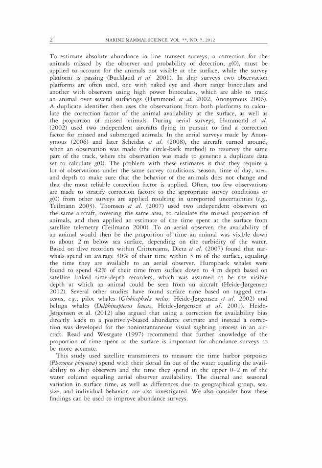
To estimate absolute abundance in line transect surveys, a correction for theanimals missed by the observer and probability of detection, g(0), must beapplied to account for the animals not visible at the surface, while the surveyplatform is passing (Buckland et al. 2001). In ship surveys two observationplatforms are often used, one with naked eye and short range binoculars andanother with observers using high power binoculars, which are able to trackan animal over several surfacings (Hammond et al. 2002, Anonymous 2006).A duplicate identifier then uses the observations from both platforms to calcu-late the correction factor of the animal availability at the surface, as well asthe proportion of missed animals. During aerial surveys, Hammond et al.(2002) used two independent aircrafts flying in pursuit to find a correctionfactor for missed and submerged animals. In the aerial surveys made by Anon-ymous (2006) and later Scheidat et al. (2008), the aircraft turned around,when an observation was made (the circle-back method) to resurvey the samepart of the track, where the observation was made to generate a duplicate dataset to calculate g(0). The problem with these estimates is that they require alot of observations under the same survey conditions, season, time of day, area,and depth to make sure that the behavior of the animals does not change andthat the most reliable correction factor is applied. Often, too few observationsare made to stratify correction factors to the appropriate survey conditions org(0) from other surveys are applied resulting in unreported uncertainties (e.g.,Teilmann 2003). Thomsen et al. (2007) used two independent observers onthe same aircraft, covering the same area, to calculate the missed proportion ofanimals, and then applied an estimate of the time spent at the surface fromsatellite telemetry (Teilmann 2000). To an aerial observer, the availability ofan animal would then be the proportion of time an animal was visible downto about 2 m below sea surface, depending on the turbidity of the water.Based on dive recorders within Crittercams, Dietz et al. (2007) found that nar-whals spend on average 30% of their time within 3 m of the surface, equalingthe time they are available to an aerial observer. Humpback whales werefound to spend 42% of their time from surface down to 4 m depth based onsatellite linked time-depth recorders, which was assumed to be the visibledepth at which an animal could be seen from an aircraft (Heide-Jørgensen2012). Several other studies have found surface time based on tagged ceta-ceans, e.g., pilot whales (Globicephala melas, Heide-Jørgensen et al. 2002) andbeluga whales (Delphinapterus leucas, Heide-Jørgensen et al. 2001). Heide-Jørgensen et al. (2012) also argued that using a correction for availability biasdirectly leads to a positively-biased abundance estimate and instead a correc-tion was developed for the noninstantaneous visual sighting process in an air-craft. Read and Westgate (1997) recommend that further knowledge of theproportion of time spent at the surface is important for abundance surveys tobe more accurate.This study used satellite transmitters to measure the time harbor porpoises

(Phocoena phocoena) spend with their dorsal fin out of the water equaling the avail-ability to ship observers and the time they spend in the upper 0–2 m of thewater column equaling aerial observer availability. The diurnal and seasonalvariation in surface time, as well as differences due to geographical group, sex,size, and individual behavior, are also investigated. We also consider how thesefindings can be used to improve abundance surveys.

2 MARINE MAMMAL SCIENCE, VOL. **, NO. *, 2012

Materials and Methods

Study Animals and Areas

This study was carried out in the seas around Denmark, from 14 April 1997to 9 April 2004 and includes 35 harbor porpoises, 15 (4 adults, 11 juveniles)females and 20 (4 adults, 16 juveniles) males (Table 1). Twenty-two of thesewere tagged in the Kattegat, Belt Seas, or the western Baltic Sea while theremaining 13 were tagged around Skagen at the border between Kattegat andSkagerrak (see Fig. 1 in Sveegaard et al. 2011). The study area was divided intotwo areas, (1) Kattegat/Belt Seas/Western Baltic (K/B/W) and (2) Skagerrak/North Sea (S/N) due to limited movements between areas and genetic differenti-ation (Fig. 1; Wiemann et al. 2010, Sveegaard et al. 2011). The main part of theKattegat, Belt Seas, and Western Baltic is between 10 and 40 m deep, whereasthe Skagerrak and North Sea include deeper waters, in particular, the NorwegianTrench, which runs along the Norwegian/Danish border and represents a suddendrop in depth from 100 to 700 m.

Transmitter Types

Three different types of satellite transmitters were used, of which two of thetransmitter types appear in two different tag versions. The transmittersdeployed were SDR-T10, SDR-T16 (both Wildlife Computers, Redmond,WA), Kiwi 101 (Sirtrack, Havelock North, New Zealand), ST-10 and ST-18(both Telonics, Mesa, AZ) (Table 1). The shapes of the transmitters are differ-ent, leading to small differences in water resistance, unlikely affecting theresults of the study. The weights of the transmitters ranged between 105 and240 g in air and all weighed less than 25 g in water. The two Kiwi 101transmitters reported the percentage of time where the dorsal fin was out ofthe water during the past 24 h. Data provided by these transmitters were usedto calculate the time spent at 0 m depth, i.e., with the transmitter above thesurface (TAS). The 11 ST-10 and ST-18 transmitters had saltwater switches,which recorded the number of seconds where the transmitter was out of thewater between transmissions, thus also providing data on TAS. The SDR trans-mitters were able to measure dive depths from 0 to 250 m with one meterresolution and an accuracy of ±1% of the measured depth. All of the 22 SDR-transmitters provided data on time spent at 0–2 m depths. Twelve of thesetransmitters also measured the amount of time where the transmitter was outof the water, and data from these were also used in the TAS data group. Datafrom the SDR-transmitters were by default gathered into four 6 h periods perday using local Danish time, CET (Period 0: 2100–0300, Period 1: 0300–0900, Period 2: 0900–1500, Period 3: 1500–2100).

Mounting of Transmitters

All animals were tagged after being incidentally trapped in a pound net.Pound nets have small mesh (2 9 2 cm) and pose no threat to the porpoises asthey can swim freely in the trap measuring 10–30 m in diameter and 3–7 m indepth. The porpoises were equipped with a transmitter according to the proce-dure described in Teilmann et al. (2007). Effects of tagging, handling, and tissue

TEILMANN ET AL.: SURFACE BEHAVIOR OF HARBOR PORPOISES 3

Table1.

Listof

tagged

harbor

porpoiseswithlocation

oftaggingor

site

(S/N

=Skagerrak/N

orth

Sea,

K/B/W

=Kattegat/BeltSeas/W

es-

tern

Baltic)

aswellas

sex,

weight,andrelative

agegroup(based

onlength).Thetrackingperiodsareshow

nas

dates

andnumber

ofdays.The

timespentwithtransm

itterabovesurfaceor

0–2

misin

percentof

totalrecordingtime(m

ean±SD

).

IDno.

Locationof

tagging

(S/N

orK/B/W

)Sex

Age

group

Standard

length

(cm)

Body

weight

(kg)

Tracking

period

Daysof

contact

Transm

itter

type

Tim

ewith

transm

itter

above

surface(%

)

Tim

espent

at0–2

m(%

)

199706171

K/B/W

(BaringVig)

FJuvenile

110

26

14April–9

May

1997

26

SDR-T10

-68.5

±3.96

199706170

K/B/W

(Korsør)

FAdult

164

62

16April–23

MAy1997

38

SDR-T10

-46.4

±3.64

199806420

K/B/W

(BaringVig)

MJuvenile

116

32

19May–1

4July

1998

57

SDR-T10

-43.2

±2.23

199906172

K/B/W

(Korsør)

FAdult

138

45

30March–16

July

1999

109

SDR-T10

-62.8

±2.47

199906421

K/B/W

(Korsør)

FJuvenile

127

37

13April–20

July

1999

99

SDR-T10

-42.8

±2.80

199906422

K/B/W

(BaringVig

MJuvenile

120

31

13April—

2August1999

112

SDR-T10

-60.3

±2.95

199906174

K/B/W

(Langø)

FJuvenile

112

31

25April–17

August1999

115

SDR-T10

-56.4

±2.76

199906173

K/B/W

(Langø)

FAdult

144

65

25April–17

August1999

115

SDR-T10

-49.6

±1.64

199906171

K/B/W

(BaringVig)

FJuvenile

116

30

26April–4

August1999

101

SDR-T10

-60.6

±2.43

199906170

K/B/W

(Abeldshoved)

MJuvenile

118

37

27April–3

September

1999

130

SDR-T10

-73.3

±2.33

199906420

K/B/W

(Æbelø)

MJuvenile

107

18

28July

1999–7

April2000

255

ST-18

4.19±0.22

-

(Continued)


199904108

K/B/W

(Illum

Ø)

MJuvenile

117

25

14October–7

Novem

ber

1999

25

SDR-T16

4.58±0.64

51.3

±11.44

199904540

K/B/W

(Ketem

inde

FJuvenile

109

-2Novem

ber

1999–3

September

2000

306

SDR-T16

3.01±0.32

53.±3.25

200004178

K/B/W

(Kerteminde)

FJuvenile

98

25

26March–1

3August2000

140

SDR-T16

3.13±0.44

57.7

±6.08

200006171

S/N (Skagen)

MJuvenile

134

37

8August2000–6

June2001

303

SDR-T16

5.11±0.36

49.0

±1.89

200006172

S/N (Skagen)

MJuvenile

123

31

23/8

2000-10/1

2001

140

SDR-T16

4.61±0.64

43.1

±3.40

200002919

K/B/W

(Hesnæs)

MJuvenile

121

36

1September

2000–6

January2001

128

ST-18

3.93±0.23

-

200004542

K/B/W

(Kerteminde)

FJuvenile

116

28

8Novem

ber

2000–4

September

2001

301

SDR-T16

3.46±0.22

61.3

±4.14

200103758

S/N (Skagen)

MJuvenile

130

38

22May–1

9June2001

29

ST-18

4.05±0.54

-

200106170

S/N (Skagen)

MJuvenile

109

23

22May

2001–28

Decem

ber

2001

221

SDR-T16

5.53±0.77

41.3

±2.95

200110340

S/N (Skagen)

FJuvenile

119

29

12June–2

August2001

52

SDR-T16

4.18±0.69

49.4

±10.30

200110338

S/N (Skagen)

MJuvenile

114

-2August2001–1

6July

2002

349

SDR-T16

5.61±2.18

44.6

±4.01

200103772

S/N (Skagen)

MAdult

139

-15August

2001–8

January2002

147

ST-18

3.21±0.16

-

200115538

S/N (Skagen)

MJuvenile

134

32

20August–1

0October

2001

52

ST-18

3.13±0.78

-

200102854

S/N (Skagen)

FJuvenile

136

39

20August

2001–26

March

2002

219

ST-18

2.89±0.08

-

200224296

K/B/W

(Korsør)

FAdult

170

58

5April–25

Novem

ber

2002

235

Kiwi101

5.14±0.29

-

(Continued)


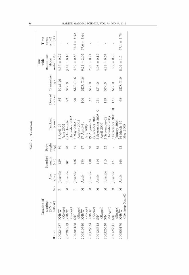
Table1.

(Continued)

IDno.

Locationof

tagging

(S/N

orK/B/W

)Sex

Age

group

Standard

length

(cm)

Body

weight

(kg)

Tracking

period

Daysof

contact

Transm

itter

type

Tim

ewith

transm

itter

above

surface(%

)

Tim

espent

at0–2

m(%

)

200224287

K/B/W

(Korsør)

FJuvenile

129

39

5April–26

June2002

84

Kiwi101

3.56±0.22

-

200202919

K/B/W

(Korsør)

MJuvenile

101

20

6October–26

Decem

ber

2002

82

ST-10

3.47±0.16

-

200204188

S/N (Skagen)

FJuvenile

126

33

7May

2002–2

August2002

90

SDR-T16

4.39±0.56

63.4

±5.52

200310340

K/B/W

(Korsør)

MAdult

153

47

17April–31

July

2003

106

SDR-T16

9.21±2.05

67.6

±3.64

200326634

K/B/W

(Korsør)

MJuvenile

130

30

19August–2

4September

2003

37

ST-10

2.95±0.21

-

200326642

S/N (Skagen)

MAdult

134

38

2September

2003–9

April2004

221

ST-10

3.08±0.12

-

200326630

S/N (Skagen)

MJuvenile

113

32

2September–2

9Decem

ber

2003

119

ST-10

4.22±0.67

-

200326641

S/N (Skagen)

MJuvenile

121

-2September

2003 –10

January2004

131

ST-10

3.9

±0.22

-

200306170

K/B/W

(FjellerupStrand)

MAdult

143

42

14March–1

5May

2003

63

SDR-T10

8.02±1.7

67.1

±5.73


healing are described by Geertsen et al. (2004), Eskesen et al. (2009), and Sonneet al. (2012).

Maps

The maps were made in ArcGis and the tracks were based on Argos satellitelocations received from the 35 harbor porpoises. Data for the mappingunderwent filtering as described in detail by Sveegaard et al. (2011).

Data Analysis

The data collected in this study were divided into two depth categories; TAS(transmitter above surface) and 0–2 m (<2 m below the surface, i.e., includingTAS). Some of the tags provide data for both categories (Table 1). This

Figure 1. Tracks based on Argos satellite locations of the harbor porpoises tracked inSkagerrak/North Sea (S/N) (red lines, n = 13) and in the Kattegat/Belt Seas/WesternBaltic (K/B/W) (blue lines, n = 22).


partitioning of data is based on the use of boats and aircrafts in abundance sur-veys. Data in the TAS group reflect the actual proportion of time the dorsal finis above the water surface and therefore visible from horizontal observations, i.e.,from ship or land. The water clarity may change between areas and seasons dueto algae blooms, but aircraft observations made during summer in the study areaindicate that porpoises can be seen down to a depth of approximately 2 m(Heide-Jørgensen et al. 1993, Teilmann et al. 2007). The data also representedtwo geographical groups, which have been documented to be genetically differ-ent (Wiemann et al. 2010) and exploit different habitats (Sveegaard et al. 2011).The two groups were therefore treated separately in some of the analyses.The experimental unit in the statistical analyses is each of the tagged harbor

porpoises. This implies that the maximum sample size is 35, but due to missingvalues the actual sample size in most analyses is smaller. Although each individ-ual contributes with many observations, these are pseudo-replicates nested withinindividuals. Each individual is characterized by an ID value, which links theindividual to a specific geographical group (site) and to a specific sex.We analyzed the data by means of a five-way ANOVA (Quinn and Keough

2002) using PROC GLM in SAS (SAS Institute, Cary, NC). The dependentvariable (y) is defined as the proportion of time an animal spends at the surfaceor in the depth range between 0 and 2 m summed over each 24 h period (alltag types), in the analysis where Period is included each observation is a 6 hperiod but since only some transmitters collected data at a 6 h time scale thesample size is reduced (only SDR tags). The independent (explanatory) variablesavailable for each observation of y are Site with two levels (Kattegat/Belt Seas/Western Baltic and Skagerrak/North Sea), Sex with two levels (males, females),Month with 12 levels (January through December), and Period with four levels(Period 0 through Period 3) and the ID of the individual. ID has as many levelsas individuals in the sample and is treated as a random factor nested within Siteand Sex, whereas the other independent variables are fixed factors. Though timewithin a year or within a day could be regarded as a continuous variable, time isentered into the model as discrete (classification) variables (Month and Period) tocircumvent the problem that these variables are cyclic and quantification of timetherefore is ambiguous (e.g., the time between 1 February and 1 December canbe either 2 or 10 mo).As ANOVAs require variance homogeneity and normally distributed residuals,

we subjected the dependent variable (y), which is a proportion between 0 and 1,to a transformation in order to meet these conditions. Because y is derived as aratio between two continuous variables (time spent in a given stratum dividedby total time), y will not be binomially distributed, so in this case the arcsinetransformation, i.e., y� ¼ sin�1 ffiffi

yp

, seems most appropriate (Sokal and Rohlf1995, Quinn and Keough 2002).Finally, as a further complicating circumstance the design is unbalanced, both

with respect to number of animals allocated to the various groups and to numberof observations per animal. This means that the statistical tests yield approxi-mate P-values. The general linear model (GLM) includes the main effects of allthe factors as additive terms. The mean square (MS) used as denominator in thevarious F-tests depends on the factor tested. Thus, tests for effects of Site and Sexuse the MS for variation among porpoises corrected for the unbalanced design,while tests for effects of Month and Period use MS(error). P-values less than 0.05are considered significant.


Three GLM analyses were carried out: Analysis 1 is based on the full model,i.e., a five-way ANOVA with Site, Sex, Month, Period, and ID as the factors. Dueto many missing values for the variable Period (only collected by the SDR-trans-mitters throughout the day) in the TAS group, the number of porpoises in thisanalysis was reduced to 12 individuals. In Analysis 2, Period was omitted fromthe model to increase sample size. In Analysis 3, based on the full model, weused Tukey’s Studentized Range Test to identify which months and periods aresignificantly different from each other.During surveys, information on the ID of an observed individual or on its sex

will not be available, whereas both the location and time of an observation areknown. As a way to adjust for the proportion of individuals not being observedduring a survey, we may therefore use Site, Month, and Period as predictor vari-ables in a model to estimate the percent of time an observed individual is mostlikely to spend in a given depth. The parameters associated with the three fixedfactors are estimated by means of a mixed effect ANOVA (Quinn and Keough2002) with variation among individual porpoises treated as a random effect.PROC MIXED (SAS Institute) was used for this analysis. All the above variablesare included in the model as main factors even though previous analysis mayhave shown that they are not all significant, thereby maximizing the fit of themodel to data.Linear regression was used to test for trends in size of animals and their

geographical origin.

Results

Effect of Individual, Sex and Site

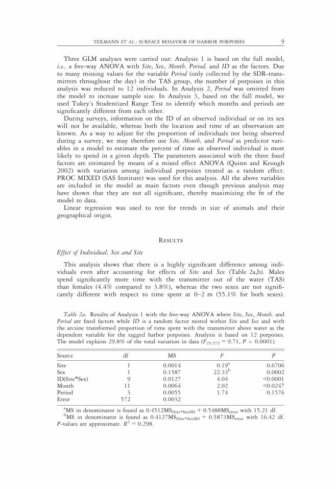
This analysis shows that there is a highly significant difference among indi-viduals even after accounting for effects of Site and Sex (Table 2a,b). Malesspend significantly more time with the transmitter out of the water (TAS)than females (4.4% compared to 3.8%), whereas the two sexes are not signifi-cantly different with respect to time spent at 0–2 m (55.1% for both sexes).

Table 2a. Results of Analysis 1 with the five-way ANOVA where Site, Sex, Month, andPeriod are fixed factors while ID is a random factor nested within Site and Sex and withthe arcsine transformed proportion of time spent with the transmitter above water as thedependent variable for the tagged harbor porpoises. Analysis is based on 12 porpoises.The model explains 29.8% of the total variation in data (F25,572 = 9.71, P < 0.0001).

Source df MS F P

Site 1 0.0014 0.19a 0.6706Sex 1 0.1587 22.33b 0.0002ID(Site*Sex) 9 0.0127 4.04 <0.0001Month 11 0.0064 2.02 <0.0247Period 3 0.0055 1.74 0.1576Error 572 0.0032

aMS in denominator is found as 0.4512MS(Site*Sex)ID + 0.5488MSerror with 15.21 df.bMS in denominator is found as 0.4127MS(Site*Sex)ID + 0.5873MSerror with 16.42 df.

P-values are approximate. R2 = 0.298.


The range for the females was 2.9%–5.1% and 42.8%–68.5% for TAS and0–2 m, respectively, while males ranged between 3.0%–9.2% and 41.3%–73.3% for TAS and 0–2 m, respectively (Table 1). Effect of Site is nonsignifi-cant for both surface range categories (3.9% and 47.5% for TAS and 0–2 m,respectively, for the Skagerrak/North Sea animals, and 4.5% and 57.7% for theKattegat/Belt Seas/Western Baltic animals). Although sample size was increasedin analysis 2 the results are consistent with those found in analysis 1(Table 3a, b).

Effect of Month and Time of Day

This analysis shows that time spent near the surface was highest during springand summer. The maximum value, for both TAS and 0–2 m occurred in April(6.0% and 61.5%, respectively), and was significantly higher than during Novem-ber–December for TAS and from August through March for 0–2 m (P < 0.05,Table 4, Fig. 2). The minimum time for TAS and 0–2 m occurred in February,September, and November (3.4%) and February (42.5%), respectively.

Table 2b. Same as Table 2a except that depth is 0–2 m. Analysis is based on 22 por-poises. The model explains 40.3% of the total variation in data (F35,1386 = 26.7,P < 0.0001)

Source df MS F P

Site 1 0.3818 1.90a 0.1825Sex 1 0.0763 0.34b 0.5655ID(Site*Sex) 19 0.5270 29.54 <0.0001Month 11 0.1398 7.84 <0.0001Period 3 0.1843 10.33 <0.0001Error 1,386 0.0178



Table 3a. Results of Analysis 2 with the four-way ANOVA (Period omitted) with Site,Sex and Month as fixed factors and ID as a random factor nested within Site and Sex, andwith the arcsine transformed proportion of time spent with the transmitter above wateras the dependent variable for the tagged harbor porpoises. Analysis is based on 25 por-poises. The model explains 34.9% of the total variation in data (F35,1896 = 29.0,P < 0.0001)

Source df MS F P

Site 1 0.0131 0.76a 0.3920Sex 1 0.0995 6.73b 0.0155ID(Site*Sex) 22 0.0391 24.30 <0.0001Month 11 0.0163 10.14 <0.0001Error 1,896 0.0016




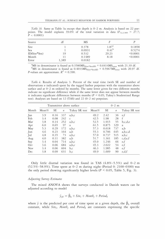
Only little diurnal variation was found in TAS (4.8%–5.5%) and 0–2 m(52.5%–58.9%). Time spent at 0–2 m during night (Period 0: 2100–0300) wasthe only period showing significantly higher levels (P < 0.05, Table 5, Fig. 3).

Adjusting Survey Estimates

The mixed ANOVA shows that surveys conducted in Danish waters can beadjusted according to model

yijk ¼ b0 þ Sitei þMonthj þ Periodk

where y is the predicted per cent of time spent at a given depth, the b0 overallconstant, while Sitei, Monthj and Periodk are constants expressing the specific

Table 3b. Same as Table 3a except that depth is 0–2 m. Analysis is based on 22 por-poises. The model explains 39.0% of the total variation in data (F32,1389 = 27.7;P < 0.0001)

Source df MS F P

Site 1 0.378 1.87a 0.1858Sex 1 0.0931 0.41b 0.5274ID(Site*Sex) 19 0.532 29.23 <0.0001Month 11 0.1489 8.18 <0.0001Error 1,389 0.0182



Table 4. Results of Analysis 3. Percent of the total time (with SE and number ofobservations n indicated) spent by the tagged harbor porpoises with the transmitter abovesurface and at 0–2 m ordered by months. The same letter given for two different monthsindicate no significant difference while if the same letter does not appear between monthsit indicates significant differences between months (P < 0.05; Tukey’s Studentized Rangetest). Analyses are based on 12 (TAS) and 22 (0–2 m) porpoises.

Month

Transmitter above surface 0–2 m

Mean% SE n Tukey SR test Mean% SE n Tukey SR test

Jan 3.9 0.16 337 a,b,c 49.2 2.42 36 e,fFeb 3.4 0.08 242 c 42.5 1.98 28 fMar 3.8 0.14 252 a,b,c 52.5 1.915 55 b,c,d,eApr 6.0 0.65 97 a 61.5 0.875 329 aMay 5.3 0.29 172 a,b,c 57.3 0.618 737 a,bJun 4.6 0.23 164 a,b 55.3 0.706 645 a,b,c,dJul 4.8 0.35 73 a,b,c 57.0 0.737 515 a,b,cAug 4.0 0.11 382 a,b 51.7 1.361 185 c,d,e,fSep 3.4 0.04 714 a,b,c 45.0 1.246 66 e,fOct 3.6 0.06 684 a,b,c 45.3 2.022 54 e,fNov 3.4 0.06 604 b,c 46.3 1.985 48 e,fDec 3.8 0.09 631 b,c 49.9 1.609 90 e,d,f


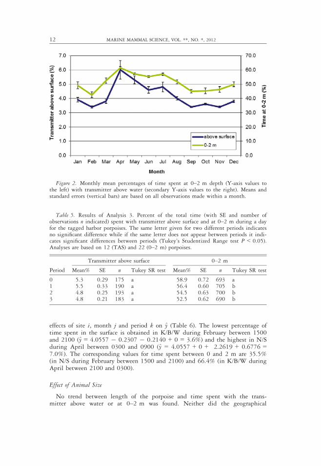
effects of site i, month j and period k on y (Table 6). The lowest percentage oftime spent in the surface is obtained in K/B/W during February between 1500and 2100 (y = 4.0557 � 0.2307 � 0.2140 + 0 = 3.6%) and the highest in N/Sduring April between 0300 and 0900 (y = 4.0557 + 0 + 2.2619 + 0.6776 =7.0%). The corresponding values for time spent between 0 and 2 m are 35.5%(in N/S during February between 1500 and 2100) and 66.4% (in K/B/W duringApril between 2100 and 0300).

Effect of Animal Size

No trend between length of the porpoise and time spent with the trans-mitter above water or at 0–2 m was found. Neither did the geographical

Figure 2. Monthly mean percentages of time spent at 0–2 m depth (Y-axis values tothe left) with transmitter above water (secondary Y-axis values to the right). Means andstandard errors (vertical bars) are based on all observations made within a month.

Table 5. Results of Analysis 3. Percent of the total time (with SE and number ofobservations n indicated) spent with transmitter above surface and at 0–2 m during a dayfor the tagged harbor porpoises. The same letter given for two different periods indicatesno significant difference while if the same letter does not appear between periods it indi-cates significant differences between periods (Tukey’s Studentized Range test P < 0.05).Analyses are based on 12 (TAS) and 22 (0–2 m) porpoises.

Period

Transmitter above surface 0–2 m

Mean% SE n Tukey SR test Mean% SE n Tukey SR test

0 5.3 0.29 175 a 58.9 0.72 693 a1 5.5 0.33 190 a 56.4 0.60 705 b2 4.8 0.25 193 a 54.5 0.63 700 b3 4.8 0.21 183 a 52.5 0.62 690 b


location of the porpoise show any differences (Fig. 4). The mean TAS for allindividuals was 4.3% and for 0–2 m 55.1%.

Figure 3. Mean percentages of time spent during the day with transmitter above thesurface and at 0–2 m depth. Means and standard errors (vertical bars) are based on allobservations made within a time interval.

Table 6. Predicted percent of time spent by a harbor porpoise in the surface and in0–2 m for a given combination of Site, Month and Period. The parameter values wereestimated by means of a mixed model with Site, Month and Period as fixed effects andindividual porpoises as a random effect. The predicted value for a given site, month andperiod is found as. yijk ¼ b0 þ Sitei þMonthj þ Periodk

Factor Parameter

% of time

Surface 0–2 m

b0 Constant 4.0557 42.7348Sitei Kattegat/Belt Seas/Western Baltic �0.2307 5.1175

Skagerrak/North Sea 0 0Monthj January 0.7010 �0.8734

February �0.2140 �7.2000March 1.2350 1.6923April 2.2619 12.3983May 1.4295 7.9387June 0.9784 6.2461July 0.7358 6.4751August 1.1013 0.3945September 0 0October �0.07018 �0.4588November �0.1380 �0.2917December 0.09229 3.2207

Periodk 2100–0300 0.6419 6.19370300–0900 0.6776 3.91950900–1500 0.1417 1.94661500–2100 0 0


Discussion

Satellite transmitters offer great potential for the study of ecology, behavior,and conservation of small cetaceans. Increased knowledge on these subjects isimportant to better monitor and manage harbor porpoise populations. Especiallyabundance surveys are sensitive to the diving behavior of porpoises, since theanimals are only visible from a ship when they break the surface, whereas theycan be seen down to a depth of approximately 2 m from an aircraft. Surveys ofcetaceans always result in large confidence intervals (e.g., Gilles et al. 2009) dueto uncertainty in estimating the different components in abundance analysis,such as the fraction of submerged animals. More accurate estimates of abundancewill be useful for better understanding natural fluctuations in abundance, todiscover population declines, and to evaluate the status of the species. Variationin the amount of time these animals spend in or near the surface is thereforeimportant for optimizing the statistical models used to estimate abundance.

Diurnal Variation

Our results did not show any diurnal variation in the TAS group. Otani et al.(1998) also found that there was no significant difference in the time of TASbetween day and night. However, our study revealed that at 0–2 m depth theporpoises spent significantly more time at night (2100–0300) than during therest of the day. This finding might be caused by a diurnal movement of preylike herring (Clupea harengus) and sprat (Sprattus sprattus) closer to the surfaceduring night (Cardinale et al. 2003).

Annual Variation

The less time spent at the surface during fall and winter could be explainedby the lower sea temperature causing an extra need for nourishment to build up

Figure 4. Time spent with transmitter above surface and at 0–2 m for each animal inrelation to their length. The two geographic areas Kattegat/Belt Seas/Western Baltic(K/B/W) and Skagerrak/North Sea (S/N) are shown separately. Trendlines for the twodepth categories are shown for all animals.


and maintain the thickness of the isolating blubber layer. In spring and summerwhen the sea temperature rises, the porpoises do not need to spend excess timeforaging, so rather than maintaining a thick blubber layer it is necessary toreduce the blubber layer to avoid overheating, as also seen in captive porpoises(Lockyer et al. 2003). Also, mating and breeding take place from April throughAugust and may affect surface behavior (Lockyer and Kinze 2003).

Location

Read and Westgate (1997) showed that the proportion of time the dorsalfin was above sea surface ranged from 3% to 7% (n = 6 harbor porpoises).Our comparable mean values for Skagerrak/North Sea and Kattegat/Belt Seas/Western Baltic are within this interval being on average 3.9% and 4.5%,respectively. This reflects the actual time the porpoises will be visible from asurvey vessel.Westgate et al. (1995) found that seven harbor porpoises in the Gulf of

Maine spent 33%–60% of their time at 0–2 m. In comparison, our studyshows that porpoises in Skagerrak/North Sea and Kattegat/Belt Seas/WesternBaltic spent 47.5% and 57.7% in the 0–2 m interval, respectively. The timeat 0–2 m represents the time that porpoises are visible from aerial surveysunder normal conditions.

Conclusion

The fact that individual variation among porpoises (ID) is the factor thatexplains most of the variation in data emphasizes that diving behavior ofharbor porpoises has a considerable individual component. Hence, it takesmany animals covering a wide range of age and sex classes over a long periodto generalize on surface and diving behavior of this species. However, sincethis study includes the largest number of harbor porpoises analyzed over theentire year and a wider range of age and sex classes than any other publishedstudy, and as our results are similar to previous studies from other areas, itleads us to conclude that our study is likely to reflect the general surfacebehavior of harbor porpoises. It implies that the results can be used to adjustvisual abundance surveys within the geographic areas studied. Thus, the studyindicates that survey data should be corrected for time submerged as well asfor seasonal effects. The correction factors for boat surveys calculated fromsurface activities and correction factors for aerial surveys (surface between 0and 2 m depth are substantial. Hence surface activity peaked in April, duringwhich animals would be visible above surface for 6% of the time and 61.5%between 0 and 2 m depth leading to correction factors (CF) of 16.7 and 1.6fold respectively. The minimum values of the time spent at the surface andbetween 0 and 2 m depth occurred in February with 3.4% (CF: 29.4) and42.5% (CF: 2.4), respectively. Because harbor porpoises spend up to 3.4%more time with the transmitter above surface and up to 31% more time nearthe surface (0–2 m) during the spring months than during the wintermonths, the seasonal component is important. By ignoring the seasonal phe-nomenon, population sizes are at risk of being overestimated during springand summer and underestimated during fall and winter.


Acknowledgments

We wish to thank the pound net fishermen and the people who volunteered to joinduring field work for their invaluable contribution to the satellite tagging project. Wealso thank Signe Sveegaard for making the maps and Kelly Macleod and Martin Lacznyfor comments to an earlier draft of this paper. During 1997–2002 porpoises weretagged as part of a joint project between the Danish National Institute of AquaticResources (DTU Aqua), Fjord&Bælt, National Environmental Research Institute (NERI)and University of Southern Denmark, Odense. The remaining porpoises were tagged aspart of cooperation between NERI and University of Kiel, Research and TechnologyCentre (FTZ) during 2003–2007. The study was carried out with permission fromDanish Forest and Nature Agency (SN 343/SN-0008) and the Animal Welfare Division(Ministry of Justice, 1995-101-62). The Danish Forest and Nature Agency (DanishMinistry of Environment), DTU Aqua (Danish Technical University), University ofKiel (Germany), Fjord&Bælt (Kerteminde, Denmark), University of Southern Denmark(Odense), and National Environmental Research Institute (Aarhus University) fundedthe study.

Literature Cited

Anonymous, 2006. Small Cetaceans in the European Atlantic and North Sea (SCANS-II).Final report to the European Commission under project LIFE04NAT/GB/000245.University of St. Andrews, St. Andrews, U.K. Available at http://biology.st-and.ac.uk/scans2/inner-finalReport.html.

Buckland, S. T., D. R. Anderson, K. P. Burnham, J. L. Laake, D. L. Borchers and L.Thomas. 2001. Introduction to distance sampling. Oxford University Press, Oxford,U.K.

Cardinale, M., M. Casini, F. Arrhenius and N. Hakansson. 2003. Diel spatialdistribution and feeding activity of herring (Clupea harengus) and sprat (Sprattussprattus) in the Baltic Sea. Aquatic Living Resources 16:283–292.

Dietz, R., A. D. Shapiro, M. Bakhtiari, et al. 2007. Upside-down swimming behavior offree-ranging narwhals. BMC Ecology 7:14 doi:10.1186/1472-6785-7-14.

Eskesen, I. G., J. Teilmann, M. B. Geertsen, et al. 2009. Stress level in wild harbourporpoises (Phocoena phocoena) during satellite tagging measured by respiration, heartrate and corstisol. Journal of the Marine Biological Association of the UnitedKingdom 89:885–892.

Geertsen, B. M., J. Teilmann, R. A. Kastelein, H. N. J. Vlemmix and L. A. Miller.2004. Behaviour and physiological effects of transmitter attachments on a captiveharbour porpoise (Phocoena phocoena). Journal of Cetacean Research and Management6:139–146.

Gilles, A., M. Scheidat and U. Siebert. 2009. Seasonal distribution of harbor porpoisesand possible interference of offshore wind farms in the German North Sea. MarineEcology Progress Series 383:295–307.

Hammond, P. S., P. Berggren, H. Benke, et al. 2002. Abundance of harbor porpoisesand other cetaceans in the North Sea and adjacent waters. Journal of AppliedEcology 39:361–376.

Heide-Jørgensen, M. P., J. Teilmann, H. Benke and J. Wulf. 1993. Abundance anddistribution of harbor porpoises, Phocoena phocoena, in selected areas of thewestern Baltic and the North Sea. Helgolander Meeresuntersuchungen 47:335–346.

Heide-Jørgensen, M. P., N. Hammeken, R. Dietz, J. Orr and P. Richard. 2001.Surfacing times and dive rates for narwhals (Monodon monoceros) and belugas(Delphinapterus leucas). Arctic 54:284–298.


Heide-Jørgensen, M. P., D. Bloch, E. Stefansson, B. Mikkelsen, L. H. Ofstad andR. Dietz. 2002. Diving behaviour of long-finned pilot whales Globicephala melasaround the Faroe Islands. Wildlife Biology 8:307–313.

Heide-Jørgensen, M. P., K. L. Laidre, R. G. Hansen, et al. 2012. Rate of increase andcurrent abundance of humpback whales in West Greenland. Journal of CetaceanResearch and Management 12:1–14.

Lockyer, C., and C. Kinze. 2003. Status, ecology and life history of harbor porpoise(Phocoena phocoena), in Danish waters. NAMMCO Scientific Publications 5:143–175.

Lockyer, C., G. Desportes, K. Hansen, S. Labberte and U. Siebert. 2003. Monitoringgrowth and energy utilisation of harbor porpoise (Phocoena phocoena) in human care.NAMMCO Scientific Publications 5:107–102.

Otani, S., Y. Naito, A. Kawamura, M. Kawasaki, S. Nishiwaki and A. Kato. 1998.Diving behavior and performance of harbor porpoises, Phocoena phocoena, in FunkaBay, Hakkaido, Japan. Marine Mammal Science 14:209–220.

Quinn, G. P., and M. J. Keough. 2002. Experimental design and data analysis forbiologists. Cambridge University Press, Cambridge, U.K.

Read, A. J., and A. J. Westgate. 1997. Monitoring the movements of harbor porpoises(Phocoena phocoena) with satellite telemetry. Marine Biology 130:315–322.

Sonne, C., P. S. Leifsson, J. Teilmann and R. Dietz. 2012. Tissue healing in two harborporpoises (Phocoena phocoena) following long-term satellite transmitter attachment.Marine Mammal Science 28:E316–E324.

Scheidat, M., A. Gilles, K.-H. Kock and U. Siebert. 2008. Harbor porpoise Phocoenaphocoena abundance in the southwestern Baltic Sea. Endangered Species Research5:215–223.

Sokal, R. R., and F. J. Rohlf. 1995. Biometry. 3rd edition. W. H. Freeman andCompany, New York, NY.

Sveegaard, S., J. Teilmann, J. Tougaard, R. Dietz, K. N. Mouritsen, G. Desportes andU. Siebert. 2011. High density areas for harbor porpoises (Phocoena phocoena)identified by satellite tracking. Marine Mammal Science 27:230–246.

Teilmann, J. 2000. The behavior and sensory abilities of harbor porpoises (Phocoenaphocoena) in relation to bycatch in Danish gillnet fishery. Ph.D. thesis, University ofSouthern Denmark, Odense, Denmark. 219 pp.

Teilmann, J. 2003. Influence of seastate on abundance estimates of harbor porpoises(Phocoena phocoena). Journal of Cetacean Research and Management 5:85–92.

Teilmann, J., F. Larsen and G. Desportes. 2007. Time allocation and diving behavior ofharbor porpoises (Phocoena phocoena) in Danish waters. Journal of Cetacean Researchand Management 9:35–44.

Thomsen, F., M. Laczny and W. Piper. 2007. The harbor porpoise (Phocoena phocoena) inthe central German Bight: Phenology, abundance and distribution in 2002–2004.Helgolander Marrine Research 61:283–289.

Westgate, A. J., A. J. Read, P. Berggren, H. N. Koopman and D. E. Gaskin. 1995.Diving behavior of harbor porpoises (Phocoena phocoena) in the Bay of Fundy.Canadian Journal of Fisheries and Aquatic Science 52:1064–1073.

Wiemann, A., L. W. Andersen, P. Berggren, et al. 2010. Mitochondrial ControlRegion and microsatellite analyses on harbor porpoise (Phocoena phocoena) unravelpopulation differentiation in the Baltic Sea and adjacent waters. ConservationGenetics 11:195–211.

Received: 31 August 2011Accepted: 8 May 2012


Geographic, seasonal, and diurnal surface behavior of harbor porpoises

Documents

Transcript of Geographic, seasonal, and diurnal surface behavior of harbor porpoises