From echolocation clicks to animal density—Acoustic samplingof harbor porpoises with static dataloggers

Line A. Kyhna)

Department of Bioscience, Aarhus University, Frederiksborgvej 399, DK-4000 Roskilde, Denmark

Jakob TougaardDepartment of Bioscience, Aarhus University, DK-4000 Roskilde, Denmark

Len ThomasCentre for Research into Ecological and Environmental Modeling, University of St. Andrews, St Andrews,KY16 9LZ, Scotland

Linda Rosager DuveDepartment of Animal Science, Aarhus University, DK-8830 Tjele, Denmark

Joanna StenbackNyckelvagen 18, 554 72 Jonkoping, Sweden

Mats AmundinKolmarden Djurpark, SE-618 92, Kolmarden, Sweden

Genevieve DesportesGDnatur, DK-5300 Kerteminde, Denmark

Jonas TeilmannDepartment of Bioscience, Aarhus University, DK-4000 Roskilde, Denmark

(Received 24 March 2011; revised 5 October 2011; accepted 19 October 2011)

Monitoring abundance and population trends of small odontocetes is notoriously difficult and labor

intensive. There is a need to develop alternative methods to the traditional visual line transect

surveys, especially for low density areas. Here, the prospect of obtaining robust density estimates

for porpoises by passive acoustic monitoring (PAM) is demonstrated by combining rigorous appli-

cation of methods adapted from distance sampling to PAM. Acoustic dataloggers (T-PODs) were

deployed in an area where harbor porpoises concurrently were tracked visually. Probability of

detection was estimated in a mark–recapture approach, where a visual sighting constituted a “mark”

and a simultaneous acoustic detection a “recapture.” As a distance could be assigned to each visual

observation, a detection function was estimated. Effective detection radius of T-PODs ranged from

22 to 104 m depending on T-POD type, T-POD sensitivity, train classification settings, and

snapshot duration. The T-POD density estimates corresponded to the visual densities derived

concurrently for the same period. With more dataloggers, located according to a systematic design,

density estimates would be obtainable for a larger area. This provides a method suitable for

monitoring in areas with densities too low for visual surveys to be practically feasible, e.g., the

endangered harbor porpoise population in the Baltic. VC 2012 Acoustical Society of America.

[DOI: 10.1121/1.3662070]

PACS number(s): 43.80.Ev [WWA] Pages: 550–560

I. INTRODUCTION

A central element in the conservation and management

of any organism is an ability to evaluate the effectiveness of

measures taken to protect the species. The most direct over-

all measure of effectiveness is to monitor population size

and trends, by conducting regular surveys or other continu-

ous monitoring. To quantify changes in population sizes it is

not recommended using indirect measures of abundance,

e.g., indexes such as vocal activity (Anderson, 2001, 2003).

Indirect measures can only provide information on trends in

population developments and not the actual change in num-

bers of animals. Survey techniques, which can provide abso-

lute numbers, either as the total number (“abundance”) of

animals within a designated area or as densities of animals

per unit area, are to be favored. However, providing absolute

density and abundance is not a straightforward task and is

usually very costly, especially when applied to cetaceans.

Harbor porpoises (Phocoena phocoena, L 1758) are

small cetaceans with inconspicuous behavior making them

difficult to observe and count at sea. During the last decade,

passive acoustic monitoring (PAM) has therefore been used

increasingly to account for the presence or absence of harbor

a)Author to whom correspondence should be addressed. Electronic mail:

lky@dmu.dk

550 J. Acoust. Soc. Am. 131 (1), January 2012 0001-4966/2012/131(1)/550/11/$30.00 VC 2012 Acoustical Society of America

Au

tho

r's

com

plim

enta

ry c

op

y

porpoises, e.g., in connection with construction of offshore

wind farms (Carstensen et al., 2006; Tougaard et al., 2009;

Scheidat et al., 2011) and spatial distribution and migration

(Verfuss et al., 2007). PAM exploits the fact that odonto-

cetes echolocate regularly. Porpoises (family Phocoenidae)

are particularly well suited for such acoustic monitoring due

to their unique sonar signals, which are extremely stereo-

typic and have features that separate them from most other

sounds in the ocean. They are of short duration (approxi-

mately 100 ls), with peak frequency around 130 kHz and

no energy below 100 kHz (Møhl and Andersen, 1973;

Villadsgaard et al., 2007). No other species of cetacean that

occurs regularly in the eastern North Atlantic produces

sounds with similar characteristics. Furthermore, porpoises

apparently produce sound almost continually, with silent

gaps rarely exceeding 1 min (Akamatsu et al., 2007).

Detecting sounds from porpoises by a PAM device in a

fixed position does not in itself provide information on abso-

lute density of animals because the surveyed area is not auto-

matically known. As with visual observations, acoustic

detections also will decrease as the distance from the obser-

vation point increases and more and more animals remain

undetected. In addition, not all animals are necessarily

detected even at zero distance, e.g., when a porpoise passes a

passive acoustic detector without echolocating. The first step

toward an animal density estimate is thus to derive the detec-

tion function, g(r), describing the probability of detection as

a function of distance, r, to the datalogger (Buckland et al.,2001; Marquez et al., 2009). Given that g(r) can be esti-

mated, it is possible to compensate for the animals that

remain undetected by estimating an effective area of detec-

tion (Buckland et al., 2001) and thus convert the relative

index of abundance to an absolute density.

Estimating g(r) for an acoustic datalogger may be

achieved by adapting the standard point transect sampling

methodology commonly used to estimate density of forest

birds (Buckland et al., 2001; Buckland, 2006). In point tran-

sect sampling, a set of randomly located points within the

study area is visited by an observer, and at each point the

number of detected birds is recorded, as well as the distance

to each bird from the point. Long counting periods at each

point tend to result in positively biased density estimates due

to animal movement: Animals that were not present at the

beginning of the count can move into the vicinity of the

point and be detected. To combat this, a “snapshot” moment

is defined, i.e., a notional instant at the midpoint of a count

lasting a few minutes, and only birds who’s position at that

instant is known are counted (see Buckland, 2006 for a more

detailed justification of this, together with an empirical test

of the efficacy of the snapshot approach). The distribution of

observed distances is used to estimate the detection function.

This approach requires the assumption that all animals at

zero distance are detected, and also that accurate distances to

detections are obtained, and hence is not feasible for many

PAM surveys. We therefore used an alternative approach to

obtain the detection function: We tracked harbor porpoises

visually while they were in the vicinity of the acoustic data-

loggers, which enabled us to estimate their location at a set

of successive snapshot moments (in practice, short intervals).

The resulting data were used to estimate the probability of

detection given the known distances of animals from the

dataloggers. This is similar to estimation of detection proba-

bility in a mark–recapture framework, where the visual ob-

servation constitutes the mark and the acoustic detection a

recapture.

In the following we present a feasibility test of applica-

tion of point transect distance sampling snapshot methodol-

ogy and detection modeling to PAM of harbor porpoises,

based on observations taken from a single fixed observation

point overlooking an experimental site. Success of the feasi-

bility test lies in obtaining robust density estimates considered

realistic for the experimental site during the experiments.

II. MATERIALS AND METHODS

Observations were made at Fyns Hoved, northern Great

Belt, Denmark (55�370900N 10�3502600E) in May 2003 and in

August 2007. The area was chosen due to its high abundance

of porpoises and the presence of a cliff offering a good over-

view of the experimental area. The seabed in the area is

sandy-muddy with small and large boulders gently sloping

down to about 15 m. The experimental area was marked

with buoys in an effort to keep boats out of the area during

observations.

A. Theodolite observations

Visual observations, using a team of at least three

observers, were made from a 22 m high cliff top overlooking

the experimental area. When a harbor porpoise was sighted,

one person tracked it with a digital theodolite (Geodimeter

468), which was connected to a computer with the tracking

software Cyclopes 2004 (University of Newcastle, Aus-

tralia). Each position of a surfacing porpoise was entered

into Cyclopes automatically when the observer pushed a but-

ton on the theodolite after aiming the theodolite sight at the

porpoise or the “footprint” left in the surface. Timing was

essential for the comparison between visual and acoustic

detections and any delay in entering a position of a surfacing

animal was commented on in Cyclopes. Other observation

notes, such as total number of animals visible in the area,

behavior of the focal animal and accompanying calves were

also commented on. Observations were made only at sea

states below three.

B. Acoustic datalogger deployment

The dataloggers used to obtain the acoustic detections

were three versions of the T-POD (Chelonia, U.K.). In 2003,

one version 1 and one version 3 were used. In 2007, eight

version 5 were used. The T-POD is specifically designed to

detect harbor porpoise clicks taking advantage of the narrow

bandwidth of the clicks. The fundamental construction is a

hydrophone connected to an amplifier and two bandpass fil-

ters, a comparator=detector circuit, and a microprocessor

with attached memory to store information on the time of

occurrence of possible porpoise clicks. The T-POD has a cy-

lindrical piezoceramic transducer with an approximately

omnidirectional response, except for a 40� cone of greatly

J. Acoust. Soc. Am., Vol. 131, No. 1, January 2012 Kyhn et al.: From clicks to density 551

Au

tho

r's

com

plim

enta

ry c

op

y

reduced sensitivity in the direction of the housing (i.e.,

downwards during deployment). The sensitivity of the

hydrophone peaks around 160 kHz and equals �207 dB re

1 V=lPa at 130 kHz (Chelonia, U.K.). Clicks are detected

based on a comparison between the output of a target band-

pass filter centered at 130 kHz and a reference filter at 90

kHz. There are slight differences between the different

T-POD versions, but the general mode of operation is the

same. Settings were as follows. Version 1: Target filter

sharpness 5 (arbitrary unit); reference filter sharpness 18 (ar-

bitrary unit); selectivity ratio: 5, threshold 0 (arbitrary unit),

minimum click duration 10 ls. Version 3: Target filter inte-

gration time “short,” reference filter integration time “long”;

selectivity ratio 5; sensitivity 6 (arbitrary unit); minimum

click duration 10 ls. Version 5: as version 3, except mini-

mum click duration 30 ls and sensitivity adjusted individu-

ally, see the following.

T-PODs are known to have individual differences in

sensitivity and hence detection thresholds (Dahne et al.,2006; Kyhn et al., 2008). From the trials in 2003 it was clear

that threshold differences transferred to detection probabil-

ities: Therefore, sensitivity of all T-PODs used in 2007 was

measured in a tank according to Kyhn et al. (2008). Detec-

tion thresholds were then adjusted accordingly by changing

the sensitivity parameter so that detection thresholds fell in

three groups: 115, 121, and 125 dB re 1 lPa peak–peak,

respectively. T-PODs were deployed in three clusters; two

clusters contained three T-PODs that had sensitivities of

115, 121, and 125 dB, respectively, and the last cluster con-

tained two T-PODs with sensitivities of 115 and 121 dB,

respectively.

In 2003 the two T-PODs were deployed approximately

150 m from the coast at a depth of approximately 6 m. The

eight T-PODs used in 2007 were deployed in three clusters

at different distances (up to 180 m) from the observation

point and at 8–10 m of water depth. All T-PODs were

deployed with their hydrophones positioned about 2 m above

the seafloor and pointing upwards.

C. T-POD data analysis

T-POD data were downloaded to a computer by the

associated software (T-POD.EXE, Chelonia Inc., version 5.41

in 2003; version 8.23 in 2007). All data were subsequently

analyzed with version 8.23 of the software (train detection

algorithm 4.1). The software groups detected clicks into

clusters termed “trains” and assigns each train to one of six

different categories: “Click trains with high probability of

arriving from cetaceans (Cet Hi)”; “Click trains with lower

probability of coming from cetaceans (Cet Low)”;

“Cetaceans and trains of doubtful origin (d)”; “Cetaceans

and very doubtful trains (dd)”; and “Trains with features of

boat sonar (Sonar).” The grouping of clicks into trains and

classification of trains is largely undocumented by the manu-

facturer, but is primarily based on analysis of interclick

interval statistics. Detection functions were estimated for

two different datasets: Based on all clicks except sonar clicks

(“All Trains”) and based only on the categories Cet Hi and

Cet Lo (referred to as “Cet All”). The choice of these data

categories is based on the common T-POD usage. The time

of occurrence of each click train was exported from the soft-

ware for further analysis.

D. Estimation of detection function

Visual observations resulted in a number of observed

surfacings for each animal. The track between each pair of

consecutive surfacings was interpolated as a straight line,

assuming a constant swimming speed and direction. The

whole track of each porpoise was then divided into segments

of constant duration. Each segment was then treated as a

snapshot and used as a trial to help estimate detection proba-

bility, as follows. For each segment, we assumed that the

location of the animal was the midpoint of its track during

that time interval. We then determined the distance from this

position to the T-PODs. Segments with distances to the

T-PODs greater than 350 m were excluded, as accurate esti-

mation of location at such ranges was difficult. An assump-

tion of the method is that probability of detection at

distances greater than 350 m is zero. For all remaining seg-

ments, we matched up the time interval of the segment with

the corresponding T-POD data record, and determined

whether there were porpoise detections in that time period.

Each segment represents a trial made at (assumed) known

distance from the T-POD; the trial was successful if there

was an acoustic detection on the T-POD during that time

interval and a failure otherwise (Fig. 1). Another way to

think of it is that each segment is a kind of mark–recapture

experiment: The visual sighting is the equivalent of a mark,

and a positive detection on the T-POD is a recapture, ena-

bling probability of detection at that distance to be estimated

using binary regression (see the following). Because there

was more than one T-POD deployed in each time period,

each segment of track produced more than one trial (one for

each T-POD). For the 2003 dataset each snapshot produced

two observations, one for the version 1 and one for the ver-

sion 3 T-POD, both assigned the same distance x. For the

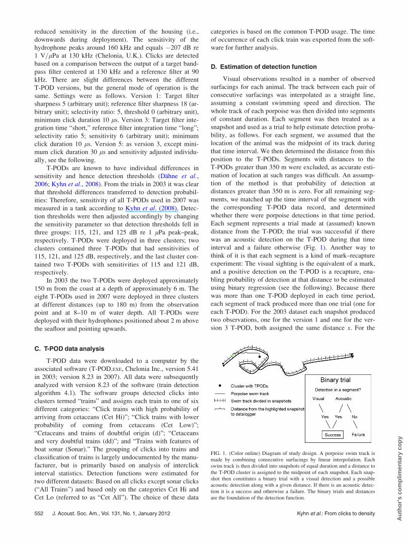
FIG. 1. (Color online) Diagram of study design. A porpoise swim track is

made by combining consecutive surfacings by linear interpolation. Each

swim track is then divided into snapshots of equal duration and a distance to

the T-POD cluster is assigned to the midpoint of each snapshot. Each snap-

shot then constitutes a binary trial with a visual detection and a possible

acoustic detection along with a given distance. If there is an acoustic detec-

tion it is a success and otherwise a failure. The binary trials and distances

are the foundation of the detection function.

552 J. Acoust. Soc. Am., Vol. 131, No. 1, January 2012 Kyhn et al.: From clicks to density

Au

tho

r's

com

plim

enta

ry c

op

y

2007 data each snapshot produced eight observations, one

for each of the T-PODs and assigned one of three different

distances, as the T-PODs were grouped in three clusters.

The choice of time interval to use for the segments is

somewhat arbitrary. A short interval (perhaps 1 min or less)

is preferred because of the assumption that the porpoise is at

the midpoint of its track during this interval, which will be

highly unrealistic for longer intervals. However, intervals

that are too short (perhaps just a few seconds) will contain

very few successful trials and may be hard to model. To test

sensitivity to choice of time interval, we repeated the analy-

sis using intervals of 15, 30, and 60 s.

False detection rate (expressed as percent of total obser-

vation time) was calculated per T-POD for the 2007 data in

order to take account of false detections in the density estima-

tion. A false detection was defined as 1 min without visual

observations of porpoises within the observation period, but

with acoustic detections. Ideally, false detection rates should

be calculated separately for snapshot intervals of 15, 30, and

60 s, but in practice the per-minute false detection rate was

negligible (see Sec. III) so there was no need to do this.

The detection function was modeled using a binary gen-

eralized linear model (GLM) with distance of the segment

midpoint from the T-POD as the explanatory variable,

success=failure as the response, and a logit link function.

Both for 2003 and 2007, data were stratified by T-POD. Trials

are not independent, for two reasons: The same track seg-

ments were used multiple times (once for each T-POD present

in the relevant year), and measurements from sequential time

segments are not necessarily independent. Hence, analytic

variance estimates from the GLM were not valid. Instead, var-

iance and 95% confidence intervals (CIs) were calculated

using a nonparametric bootstrap, treating the porpoise track as

the unit for resampling and with 1 000 bootstrap replicates.

The above-mentioned procedure yields estimates of the

detection function g(x), i.e., probability of detecting a por-

poise given it is at distance x. However, the quantity required

for density estimation (to follow) is the average probability

of detecting a porpoise given it is within distance w of the

detector, denoted P. As is standard in distance sampling

applications, this was estimated from the detection function

by assuming that animal density is uniform over space

within the area surveyed by the detector (the circle of radius

w, where w is the right truncation distance of 350 m), and

then integrating out distance:

P ¼ 2

w2

ðw

x¼0

xgðxÞdx:

An equivalent quantity often computed in the distance sam-

pling literature is the effective detection radius, q, which

again defines the effective detection area. The effective

detection area is the area which would be covered by the

detector if all animals are detected within the effective detec-

tion radius and none are detected outside. To ease interpreta-

tion of results, the effective detection radius was also

computed, using the relationship

q ¼ffiffiffiffiffiffiffiffiffiPw2

p:

The above-presented analysis was repeated six times for

each T-POD: Once for each combination of snapshot dura-

tion (15, 30, and 60 s) and click train category (All Trains

and Cet All). Analyses were performed in the software

R v2.11.1 (R Development Core Team, 2008).

E. Density estimation

Given an estimate of the effective detection radius, each

snapshot can be used to provide an estimate of animal den-

sity, using the following formula:

Dt ¼ntð1� cÞ

Kpq2;

where Dt is estimated density for the tth snapshot (t¼ 1,…,T),

nt is the number of animals detected at the tth snapshot, c is

the proportion of false positive detections, and K is the num-

ber of detectors. Here, we assume that at most only one ani-

mal can be detected in each snapshot, so that nt is either 1

(animal detected) or 0 (no animal detected; see Sec. IV for

more on this assumption). Averaging over all T snapshots

gives

D ¼ nð1� cÞKpq2T

;

where n is the total count of snapshots with detected por-

poises, summed over all snapshots. An alternative way to

express this, using the average detection probability P, is

D ¼ nð1� cÞKpw2PT

:

This formula is identical to that used by Marques et al.(2009), except that in that paper the counts n were of individ-

ual animal vocalizations, not animals, and hence the denomi-

nator required an additional term, r, the vocalization rate. We

also note that the above-presented formulation can be

extended to the case where animals are present in well-

defined groups or clusters—in this case, detection probability

of clusters, Pc, is estimated by setting up trials on the clusters,

with the appropriate distance being the distance to the middle

of the cluster. Then, density can be estimated using

D ¼ ncð1� ccÞsKpw2PcT

; (1)

where nc is the number of clusters detected, cc is the false

positive rate for clusters, and s is the mean cluster size,

estimated for example from visual observations during the

trials.

In the current study, estimates of density were made

separately for each T-POD using the T-POD-specific detec-

tion functions computed in the previous section. Number of

detected porpoises, n, was calculated for the entire experi-

mental period, and thus included periods where no synoptic

visual observations took place. This gave a much larger data-

set, but requires the assumption that the detection probabil-

ities were unrelated to visual observation times.

J. Acoust. Soc. Am., Vol. 131, No. 1, January 2012 Kyhn et al.: From clicks to density 553

Au

tho

r's

com

plim

enta

ry c

op

y

Variance was estimated per T-POD by combining var-

iances of the random components of D, assuming they are

mutually independent, using the delta method (Buckland

et al., 2001; Marques et al., 2009):

varðDÞ ¼ D2 varðnÞn2þ varðPÞ

P2þ varðcÞ

c2

� �:

In standard distance sampling methods, variance in n is

calculated from the between-sample variance in encounters.

In the present study, where estimates of density were made

by T-POD, only one sample (T-POD) was available per esti-

mate, and hence another method had to be used to derive an

estimate of var(n). We followed the suggestion of Buckland

et al. (2001) in assuming that n followed an overdispersed

Poission distribution, with overdispersion factor 2, leading to

varðnÞ ¼ 2n.

Confidence intervals on D were calculated by assuming

the density estimate follows a lognormal distribution (Buck-

land et al., 2001; Marques et al., 2009).

F. Independent visual estimate of density

For the 2007 survey, porpoise density was also esti-

mated from the visual observations within a 100 m radius

around each T-POD cluster. It was assumed that all animals

were observed within this radius, and density was then esti-

mated as

Dv ¼nv

Tv � a;

where nv is the number of 60 s snapshots with interpolated

porpoise observations within 100 m of the T-PODs over Tv

minutes of visual observations, and a is the observation area

(0.031 km2). No attempt was made to estimate a variance on

this quantity.

III. RESULTS

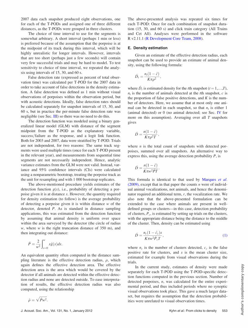
After right truncation at 350 m the dataset consisted of

91 tracks from 2003 and 32 tracks from 2007 (Fig. 2). Each

track consisted of between 2 and 128 sightings. Visual and

acoustic data are summarized in Table I.

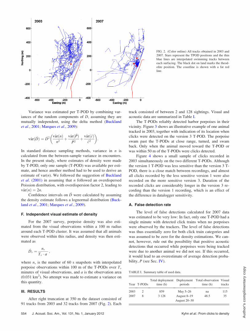
The T-PODs reliably detected harbor porpoises in their

vicinity. Figure 3 shows an illustrative example of one animal

tracked in 2003, together with indication of its location when

clicks were detected on the version 3 T-POD. The porpoise

swam past the T-PODs at close range, turned, and swam

back. Only when the animal moved toward the T-POD or

was within 50 m of the T-PODs were clicks detected.

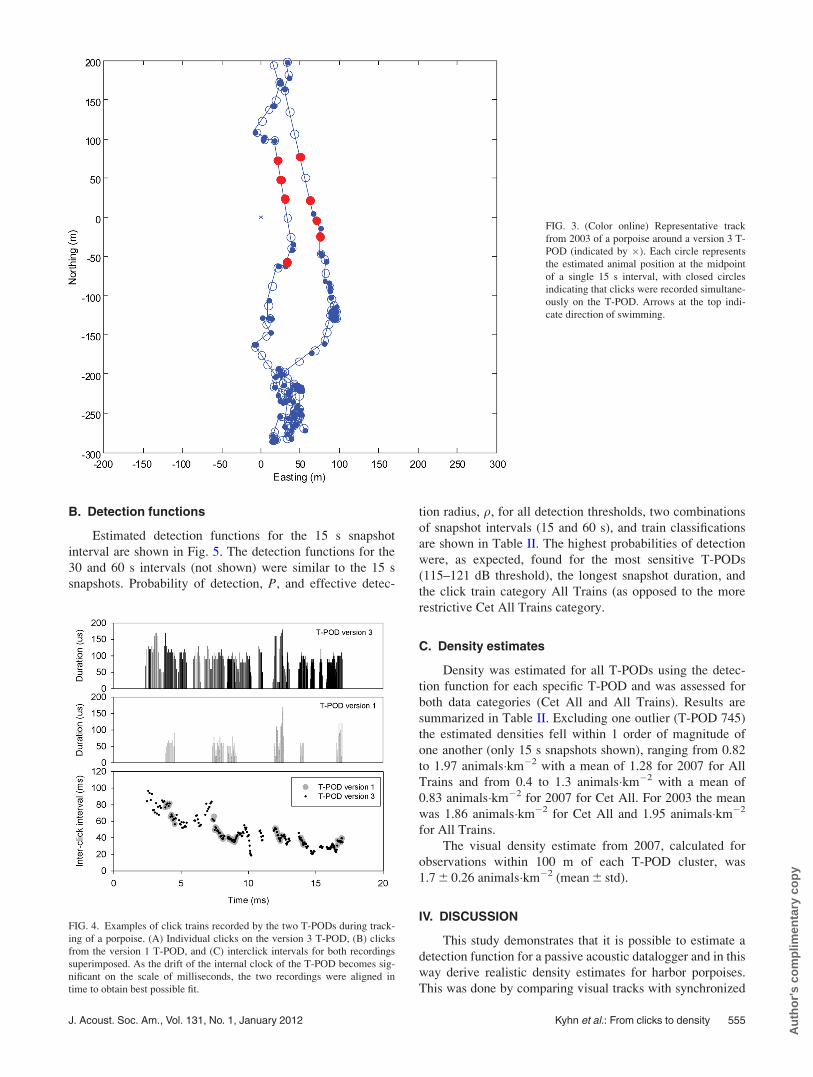
Figure 4 shows a small sample of clicks recorded in

2003 simultaneously on the two different T-PODs. Although

the version 1 T-POD was less sensitive than the version 3 T-

POD, there is a close match between recordings, and almost

all clicks recorded by the less sensitive version 1 were also

recorded on the more sensitive version 3. Duration of the

recorded clicks are considerably longer in the version 3 re-

cording than the version 1 recording, which is an effect of

the difference in datalogger sensitivity.

A. False detection rate

The level of false detections calculated for 2007 data

was estimated to be very low: In fact, only one T-POD had a

single minute with detected click trains when no porpoises

were observed by the trackers. The level of false detections

was thus essentially zero for both click train categories and

was assumed to be zero for the density estimations. We can-

not, however, rule out the possibility that positive acoustic

detections that occurred while porpoises were being tracked

were due to another animal we did not see. If this occurred,

it would lead to an overestimate of average detection proba-

bility, P (see Sec. IV).

FIG. 2. (Color online) All tracks obtained in 2003 and

2007. Stars represent the TPOD positions and the thin

blue lines are interpolated swimming tracks between

each surfacing. The black dot on land marks the theod-

olite position. The coastline is shown with a fat red

line.

TABLE I. Summary table of used data.

Year T-PODs

Total deployment

time (h)

Deployment

periods

Total observation

time (h)

Visual

tracks

2003 2 859 May 5–26 na 115

2007 8 3 128 August 8–19 48.5 35

August 20–30

554 J. Acoust. Soc. Am., Vol. 131, No. 1, January 2012 Kyhn et al.: From clicks to density

Au

tho

r's

com

plim

enta

ry c

op

y

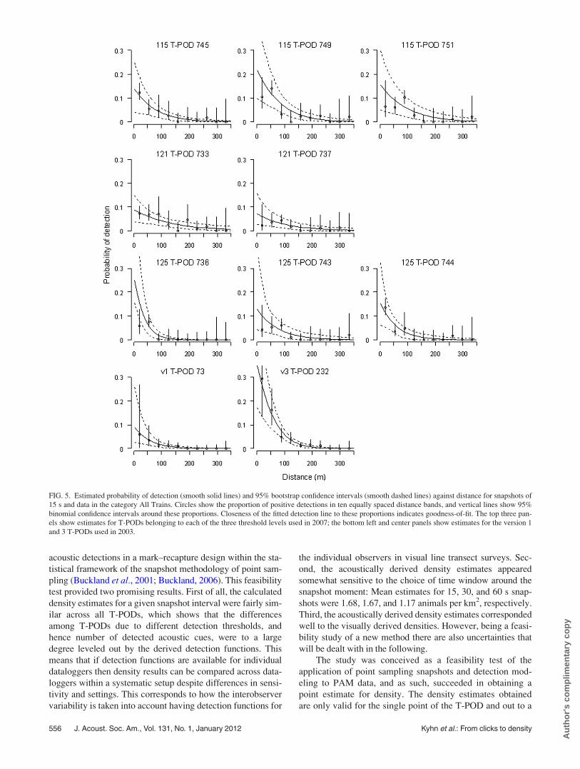
B. Detection functions

Estimated detection functions for the 15 s snapshot

interval are shown in Fig. 5. The detection functions for the

30 and 60 s intervals (not shown) were similar to the 15 s

snapshots. Probability of detection, P, and effective detec-

tion radius, q, for all detection thresholds, two combinations

of snapshot intervals (15 and 60 s), and train classifications

are shown in Table II. The highest probabilities of detection

were, as expected, found for the most sensitive T-PODs

(115–121 dB threshold), the longest snapshot duration, and

the click train category All Trains (as opposed to the more

restrictive Cet All Trains category.

C. Density estimates

Density was estimated for all T-PODs using the detec-

tion function for each specific T-POD and was assessed for

both data categories (Cet All and All Trains). Results are

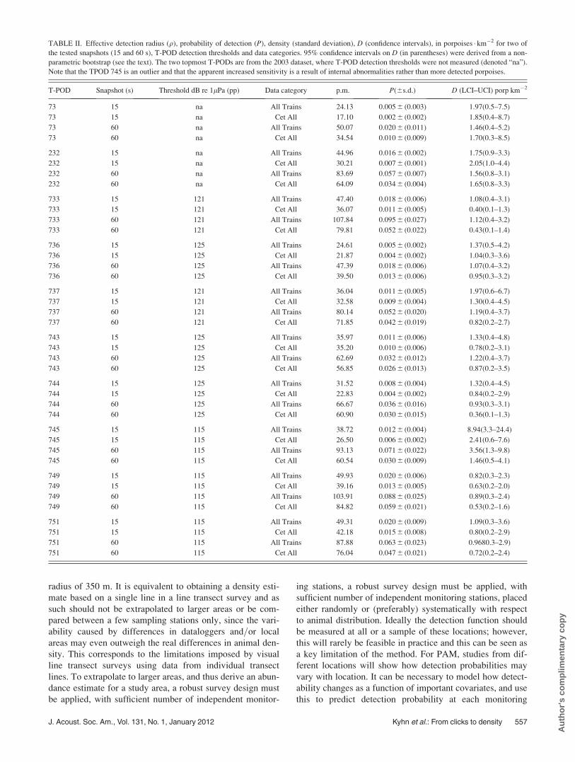
summarized in Table II. Excluding one outlier (T-POD 745)

the estimated densities fell within 1 order of magnitude of

one another (only 15 s snapshots shown), ranging from 0.82

to 1.97 animals�km�2 with a mean of 1.28 for 2007 for All

Trains and from 0.4 to 1.3 animals�km�2 with a mean of

0.83 animals�km�2 for 2007 for Cet All. For 2003 the mean

was 1.86 animals�km�2 for Cet All and 1.95 animals�km�2

for All Trains.

The visual density estimate from 2007, calculated for

observations within 100 m of each T-POD cluster, was

1.7 6 0.26 animals�km�2 (mean 6 std).

IV. DISCUSSION

This study demonstrates that it is possible to estimate a

detection function for a passive acoustic datalogger and in this

way derive realistic density estimates for harbor porpoises.

This was done by comparing visual tracks with synchronized

FIG. 3. (Color online) Representative track

from 2003 of a porpoise around a version 3 T-

POD (indicated by �). Each circle represents

the estimated animal position at the midpoint

of a single 15 s interval, with closed circles

indicating that clicks were recorded simultane-

ously on the T-POD. Arrows at the top indi-

cate direction of swimming.

FIG. 4. Examples of click trains recorded by the two T-PODs during track-

ing of a porpoise. (A) Individual clicks on the version 3 T-POD, (B) clicks

from the version 1 T-POD, and (C) interclick intervals for both recordings

superimposed. As the drift of the internal clock of the T-POD becomes sig-

nificant on the scale of milliseconds, the two recordings were aligned in

time to obtain best possible fit.

J. Acoust. Soc. Am., Vol. 131, No. 1, January 2012 Kyhn et al.: From clicks to density 555

Au

tho

r's

com

plim

enta

ry c

op

y

acoustic detections in a mark–recapture design within the sta-

tistical framework of the snapshot methodology of point sam-

pling (Buckland et al., 2001; Buckland, 2006). This feasibility

test provided two promising results. First of all, the calculated

density estimates for a given snapshot interval were fairly sim-

ilar across all T-PODs, which shows that the differences

among T-PODs due to different detection thresholds, and

hence number of detected acoustic cues, were to a large

degree leveled out by the derived detection functions. This

means that if detection functions are available for individual

dataloggers then density results can be compared across data-

loggers within a systematic setup despite differences in sensi-

tivity and settings. This corresponds to how the interobserver

variability is taken into account having detection functions for

the individual observers in visual line transect surveys. Sec-

ond, the acoustically derived density estimates appeared

somewhat sensitive to the choice of time window around the

snapshot moment: Mean estimates for 15, 30, and 60 s snap-

shots were 1.68, 1.67, and 1.17 animals per km2, respectively.

Third, the acoustically derived density estimates corresponded

well to the visually derived densities. However, being a feasi-

bility study of a new method there are also uncertainties that

will be dealt with in the following.

The study was conceived as a feasibility test of the

application of point sampling snapshots and detection mod-

eling to PAM data, and as such, succeeded in obtaining a

point estimate for density. The density estimates obtained

are only valid for the single point of the T-POD and out to a

FIG. 5. Estimated probability of detection (smooth solid lines) and 95% bootstrap confidence intervals (smooth dashed lines) against distance for snapshots of

15 s and data in the category All Trains. Circles show the proportion of positive detections in ten equally spaced distance bands, and vertical lines show 95%

binomial confidence intervals around these proportions. Closeness of the fitted detection line to these proportions indicates goodness-of-fit. The top three pan-

els show estimates for T-PODs belonging to each of the three threshold levels used in 2007; the bottom left and center panels show estimates for the version 1

and 3 T-PODs used in 2003.

556 J. Acoust. Soc. Am., Vol. 131, No. 1, January 2012 Kyhn et al.: From clicks to density

Au

tho

r's

com

plim

enta

ry c

op

y

radius of 350 m. It is equivalent to obtaining a density esti-

mate based on a single line in a line transect survey and as

such should not be extrapolated to larger areas or be com-

pared between a few sampling stations only, since the vari-

ability caused by differences in dataloggers and=or local

areas may even outweigh the real differences in animal den-

sity. This corresponds to the limitations imposed by visual

line transect surveys using data from individual transect

lines. To extrapolate to larger areas, and thus derive an abun-

dance estimate for a study area, a robust survey design must

be applied, with sufficient number of independent monitor-

ing stations, a robust survey design must be applied, with

sufficient number of independent monitoring stations, placed

either randomly or (preferably) systematically with respect

to animal distribution. Ideally the detection function should

be measured at all or a sample of these locations; however,

this will rarely be feasible in practice and this can be seen as

a key limitation of the method. For PAM, studies from dif-

ferent locations will show how detection probabilities may

vary with location. It can be necessary to model how detect-

ability changes as a function of important covariates, and use

this to predict detection probability at each monitoring

TABLE II. Effective detection radius (q), probability of detection (P), density (standard deviation), D (confidence intervals), in porpoises � km�2 for two of

the tested snapshots (15 and 60 s), T-POD detection thresholds and data categories. 95% confidence intervals on D (in parentheses) were derived from a non-

parametric bootstrap (see the text). The two topmost T-PODs are from the 2003 dataset, where T-POD detection thresholds were not measured (denoted “na”).

Note that the TPOD 745 is an outlier and that the apparent increased sensitivity is a result of internal abnormalities rather than more detected porpoises.

T-POD Snapshot (s) Threshold dB re 1lPa (pp) Data category p.m. P(6s.d.) D (LCI–UCI) porp km�2

73 15 na All Trains 24.13 0.005 6 (0.003) 1.97(0.5–7.5)

73 15 na Cet All 17.10 0.002 6 (0.002) 1.85(0.4–8.7)

73 60 na All Trains 50.07 0.020 6 (0.011) 1.46(0.4–5.2)

73 60 na Cet All 34.54 0.010 6 (0.009) 1.70(0.3–8.5)

232 15 na All Trains 44.96 0.016 6 (0.002) 1.75(0.9–3.3)

232 15 na Cet All 30.21 0.007 6 (0.001) 2.05(1.0–4.4)

232 60 na All Trains 83.69 0.057 6 (0.007) 1.56(0.8–3.1)

232 60 na Cet All 64.09 0.034 6 (0.004) 1.65(0.8–3.3)

733 15 121 All Trains 47.40 0.018 6 (0.006) 1.08(0.4–3.1)

733 15 121 Cet All 36.07 0.011 6 (0.005) 0.40(0.1–1.3)

733 60 121 All Trains 107.84 0.095 6 (0.027) 1.12(0.4–3.2)

733 60 121 Cet All 79.81 0.052 6 (0.022) 0.43(0.1–1.4)

736 15 125 All Trains 24.61 0.005 6 (0.002) 1.37(0.5–4.2)

736 15 125 Cet All 21.87 0.004 6 (0.002) 1.04(0.3–3.6)

736 60 125 All Trains 47.39 0.018 6 (0.006) 1.07(0.4–3.2)

736 60 125 Cet All 39.50 0.013 6 (0.006) 0.95(0.3–3.2)

737 15 121 All Trains 36.04 0.011 6 (0.005) 1.97(0.6–6.7)

737 15 121 Cet All 32.58 0.009 6 (0.004) 1.30(0.4–4.5)

737 60 121 All Trains 80.14 0.052 6 (0.020) 1.19(0.4–3.7)

737 60 121 Cet All 71.85 0.042 6 (0.019) 0.82(0.2–2.7)

743 15 125 All Trains 35.97 0.011 6 (0.006) 1.33(0.4–4.8)

743 15 125 Cet All 35.20 0.010 6 (0.006) 0.78(0.2–3.1)

743 60 125 All Trains 62.69 0.032 6 (0.012) 1.22(0.4–3.7)

743 60 125 Cet All 56.85 0.026 6 (0.013) 0.87(0.2–3.5)

744 15 125 All Trains 31.52 0.008 6 (0.004) 1.32(0.4–4.5)

744 15 125 Cet All 22.83 0.004 6 (0.002) 0.84(0.2–2.9)

744 60 125 All Trains 66.67 0.036 6 (0.016) 0.93(0.3–3.1)

744 60 125 Cet All 60.90 0.030 6 (0.015) 0.36(0.1–1.3)

745 15 115 All Trains 38.72 0.012 6 (0.004) 8.94(3.3–24.4)

745 15 115 Cet All 26.50 0.006 6 (0.002) 2.41(0.6–7.6)

745 60 115 All Trains 93.13 0.071 6 (0.022) 3.56(1.3–9.8)

745 60 115 Cet All 60.54 0.030 6 (0.009) 1.46(0.5–4.1)

749 15 115 All Trains 49.93 0.020 6 (0.006) 0.82(0.3–2.3)

749 15 115 Cet All 39.16 0.013 6 (0.005) 0.63(0.2–2.0)

749 60 115 All Trains 103.91 0.088 6 (0.025) 0.89(0.3–2.4)

749 60 115 Cet All 84.82 0.059 6 (0.021) 0.53(0.2–1.6)

751 15 115 All Trains 49.31 0.020 6 (0.009) 1.09(0.3–3.6)

751 15 115 Cet All 42.18 0.015 6 (0.008) 0.80(0.2–2.9)

751 60 115 All Trains 87.88 0.063 6 (0.023) 0.9680.3–2.9)

751 60 115 Cet All 76.04 0.047 6 (0.021) 0.72(0.2–2.4)

J. Acoust. Soc. Am., Vol. 131, No. 1, January 2012 Kyhn et al.: From clicks to density 557

Au

tho

r's

com

plim

enta

ry c

op

y

location. Future studies on detection probability will also

help us understand how detection probability may be

affected by factors such as animal behavior and group size.

We used the snapshot methodology of point sampling

here. Normally the number of animals detected is counted

within each snapshot when counting, for example, in bird

studies (Buckland, 2006). Here, we used much shorter snap-

shots and categorized each snapshot as either detecting or

not detecting porpoises, by checking if the snapshot con-

tained click trains or not. The reason for choosing this meth-

odology was that from the T-POD data it is not possible to

determine whether two sequential click trains are from the

same or different animals. Such information requires the use

of a hydrophone array to localize vocalizing animals and

may even then not be possible if the animals are close to-

gether. There may have been more than one animal recorded

within some snapshots, but this is considered to have been

uncommon due to (1) the directional radiation characteristics

of harbor porpoise clicks (see the example in Fig. 3) in com-

bination with (2) the loose group structure of harbor por-

poises, which jointly means that the chance that two or more

porpoises point towards the datalogger within the same snap-

shot interval is low, especially for short snapshots. We con-

firmed this by visually inspecting all the click trains in the

T-POD software in search for overlapping click trains with

different click repetition rates—a clear indication that more

than one animal were pointing at the datalogger at the same

time—and found a range of only 0–0.7% overlapping click

trains across all the data. At this study site more than one

porpoise can be seen at a time (mean observed group size

1.6), but they were observed to be moving independently

rather than swimming in coordinated fashion, and could be

more than a hundred meters apart. Detecting multiple ani-

mals in the same snapshot, and treating it as a single acoustic

detection, will cause the density estimate to be biased down-

wards. This will happen less for shorter snapshot intervals,

and is one reason to prefer the density estimate from the 15 s

interval. For other species, most notably dolphin species that

have a different group and vocalization behavior, the snap-

shot approach used here may not be directly applicable, as

the above-mentioned assumptions may not hold. Conse-

quently, this should be tested thoroughly before applying

this method for other species than harbor porpoises.

Another consequence of not being able to distinguish

detections from multiple animals was that there may have

been cases in the detection function trials where a trial was

erroneously scored as a success due to a click from another,

unnoticed animal closer to the T-POD than the one being

tracked. This would lead to an overestimation of the detec-

tion probability and hence an underestimation of density.

However, for the above-mentioned reasons, we judge that

this happened very rarely in our study. In other studies,

where animals move in larger, well-coordinated groups, the

method mentioned earlier of defining trials on groups of ani-

mals and then multiplying the density estimate by an inde-

pendent estimate of mean group size [Eq. (1)] would be

preferred.

As the basis for detection we used click trains as defined

by the T-POD software, rather than individual clicks. Using

click trains resulted in practically no false detections. Using

single porpoise clicks as a cue of detection within a snap-

shot, however, would be problematic because the rate of

false positives can be very high, due to many other sounds

(cavitation noise, shifting sand, echo sounders, etc.) possibly

recorded by the datalogger. Such false positives can be diffi-

cult to separate from porpoise clicks when treated individu-

ally, but can be removed to a large degree by filtering based

on properties of click trains as done in the T-POD software.

We therefore recommend the use of click trains per time unit

instead of individual clicks per time unit.

An assumption in distance sampling theory is that dis-

tances are measured exactly. In the present study, distances

were based on theodolite tracks of porpoises. Theodolites

are very precise at short distances but the multiplicative error

increases with true distance from the theodolite and further-

more is positively biased (i.e., errors on overestimated dis-

tances are larger than errors on underestimated distances).

For this reason we only used distances within 350 m of the

theodolite station and most observations were even closer to

the observation point (as is evident from Fig. 2), so the bias

is considered negligible. However, another uncertainty on

distance estimation arises because we interpolated porpoise

swimming tracks between surfacings assuming straight lines.

This inevitably leads to errors, but these are likely random

and independent of true distance to the theodolite as the

interpolation was performed in the same fashion for all posi-

tions regardless of distance to observers. The effect of this

measurement error is not clear, but is likely a limiting factor

for precision. Further investigation of the effect of measure-

ment errors caused by the use of surface observations is an

important topic for future research. Obtaining true distance

estimates between surfacings would require detailed knowl-

edge on subsurface movement of porpoises, obtainable either

by equipping animals with dataloggers that can accurately

track the animals under water, or acoustically by means of a

sufficiently large hydrophone array. Furthermore, as the sub-

surface behavior of porpoises may likely depend upon site

specific factors such as water depth, prey availability, and

bottom characteristics such data should ideally be obtained

within the actual study site in order for the modeling to

actually reduce measurement error. If more precise animal

tracks could be obtained, then shorter snapshot intervals

would be preferred over longer ones, as the position used in

the midpoint of a short interval better represents the position

than that for a long interval. This is another reason to prefer

the 15 s interval, of the three intervals used here.

In standard distance sampling applications it is assumed

that all animals at zero distance from the transect line or

point are detected [i.e., g(0)¼ 1]. This assumption does not

hold in the present experiment (evident on Fig. 5.), but as the

mark–recapture method used here allows for a direct deter-

mination of g(0), this assumption is not relevant. However, it

is useful to consider why g(0) is relatively low, between 0.1

and 0.3 for T-PODs. Harbor porpoises are known to be silent

for shorter or longer periods of time (Linnenschmidt, 2007),

but the primary reason is probably the directional character-

istics of the echolocation sounds. This means that porpoises

are only able to effectively ensonify a T-POD part of the

558 J. Acoust. Soc. Am., Vol. 131, No. 1, January 2012 Kyhn et al.: From clicks to density

Au

tho

r's

com

plim

enta

ry c

op

y

time with sound levels above the detection threshold of the

T-POD, likely only when looking straight towards the

T-POD. Desportes et al. (2000) described a behavior termed

“bottom grubbing,” also observed at the experimental site, in

which porpoises swim in a near vertical position, close to the

bottom, the head pointing downwards in search of prey. This

behavior can continue for extended periods of time and dur-

ing this behavior clicks from the porpoise will only reach the

T-PODs in an erratic fashion, unlikely to be recognized as

entire click trains. Prey search behavior may thus, in this

study, be part of the explanation for the low g(0) value. For

the same reason the g(0) value may be different in areas with

a different depth or prey composition, as well as it may be

entirely different for other odontocete species foraging and

echolocating in a different fashion.

Further, the estimated detection functions varied between

the different dataloggers, thresholds, and cluster positions,

even though the dataloggers were positioned in the same vi-

cinity quite close together and experienced the same level of

porpoise visits. Here the design of this feasibility study was

likely too ambitious in the sense that it is not possible to sepa-

rate the effect of both cluster position and threshold of the

dataloggers with only one replicate in each cluster position,

i.e., it is clear that there is an effect of cluster, but it also

appears that there is an added effect of the cluster position.

More data would likely level out the observed differences,

and future studies should examine a single threshold, prefera-

bly the lowest at 115 dB re 1 lPa (p-p), in different locations.

Anyhow, most often the major source of uncertainty on the

estimate of density is in fact on the encounter rate variance

and less the precision of the detection function.

The false detection rate, assessed in 2007, was very low

and indicates that the click train algorithm in the T-POD

software is efficient and conservative, and when combined

with the high abundance of porpoises in this study, false

detections could be ignored. In a high density area like the

present, all T-POD click train categories (except boat sonar)

may thus be used if data are divided into timed snapshot

intervals as done here. Even if some trains in fact are false

positives, proportion of false positives will still be low, espe-

cially when using click trains rather than individual clicks as

cues, and false positives are therefore not very important.

The situation, however, is radically different in a low density

area, for instance the Baltic Proper. Because the porpoise

density is very low (Hammond et al., 2002), inclusion of

false positives will weigh much higher in a density assess-

ment and it is therefore extremely important to be as con-

servative as possible and to limit the rate of false positives as

much as possible, if the rate is unknown. In a low density

area only the two highest T-POD click train categories (Cet

All) should therefore be used despite the risk of discarding

true detections, in order to keep the density estimate con-

servative. In this respect, one of the T-PODs was obviously

different than the rest and was regarded as an outlier. This

T-POD (T-POD 745) recorded many thousand more click

trains and likely had some internal abnormalities overruling

the applied sensitivity settings. This was especially visible

for the All Trains category. Dataloggers should therefore be

deployed for field tests to assess such abnormalities before

deployment to obtain density estimates, and the decision on

which of the data categories to use All trains or Cet All

should take such results into account.

Density estimation by a passive acoustic method as pre-

sented here offers a cheaper alternative to visual surveys

since the observer effort and associated costs are greatly

reduced. Additional advantages are that data can be collected

and density estimated year round and under all weather con-

ditions, and that data from dataloggers are unaffected by

human subjectivity and fatigue during observations. The pas-

sive acoustic methodology in combination with point tran-

sect distance sampling thus provides a viable alternative

to visual surveys for density estimation, in particular for

low density areas, where reliable visual estimates may be

unattainable.

We have presented a method to obtain a detection func-

tion for acoustic dataloggers by observing animals visually

around the dataloggers and comparing visual and acoustic

detections in a mark–recapture setup, based on the snapshot

methodology of point transect distance sampling. This

method provides for use of PAM of porpoises to obtain abso-

lute changes in density over time. However, there is a poten-

tial for a slight negative bias overall due to missing some

occasions when multiple animals were detected in the same

snapshot.

ACKNOWLEDGMENTS

The following persons are thanked for a dedicated effort

during data collection: Dania Wiesnewska, Daniel Wenner-

berg, Jakob Hansen Rye, Lisette Buholzer Søgaard, Nikolai

Ilsted Bech, Nina Eriksen, Signe Sveegaard, and Trine Baier

Jepsen. Oluf D. Henriksen is thanked for assistance with

deployment and recovery of T-PODs in 2003. We thank the

landowners at Fyns Hoved for access to the area and the

Danish Forest and Nature agency for permission to conduct

experiments. Magnus Wahlberg, Lee A. Miller, and Peter T.

Madsen are thanked for loan of equipment and access to cali-

bration tank. Thanks to Tiago Marques for contributing to

the analysis framework at an early stage, and to Hanna Nuut-

tila and two anonymous reviewers for their helpful com-

ments on the manuscript. This study was supported by the

Danish Research Council for Strategic Research and the

Danish Ministry of Environment.

Akamatsu, T., Dietz, R., Miller, L. A., Naito, Y., Siebert, U., Teilmann, J.,

Tougaard, J., Wang, D., and Wang, K. (2007). “Comparison of echoloca-

tion behavior between coastal oceanic and riverine porpoises,” Deep-Sea

Res., Part II 54, 290–297.

Anderson, D. R. (2001). “The need to get the basics right in wildlife stud-

ies,” Wildl. Soc. Bull. 29, 1294–1297.

Anderson, D. R. (2003). “Response to Engeman: Index values rarely consti-

tute reliable information,” Wildl. Soc. Bull. 31, 288–291.

Buckland, S. T., Anderson, D. R., Burnham, K. P., Laake, J. L., Borchers,

D. L., Thomas, L., (2001). “Introduction to Distance SamplingEstimatingAbundance of Biological Populations,” (Oxford University Press, New

York) p. 432.

Buckland, S. T. (2006). “Point-Transect surveys for songbirds: Robust meth-

odologies,” Auk 123(2), 345–357.

Carstensen, J., Henriksen, O. D., and Teilmann, J. (2006). “Impacts on har-

bour porpoises from offshore wind farm construction: Acoustic monitoring

J. Acoust. Soc. Am., Vol. 131, No. 1, January 2012 Kyhn et al.: From clicks to density 559

Au

tho

r's

com

plim

enta

ry c

op

y

of echolocation activity using porpoise detectors (T-PODs),” Mar. Ecol.

Prog. Ser. 321, 295–308.

Dahne, M., Verfuss, U. K., Diederichs, A., Meding, A., and Benke, H.

(2006). “TPOD test tank calibration and field calibration,” Proceedingsof the Workshop on Static Acoustic Monitoring of Cetaceans, 20thAnnual Meeting of the European Cetacean Society, Gdynia, ECS News-

letter 46.

Desportes, G., Amundin, M., and Goodson, D., (2000). “Investigate porpoise

foraging behaviour-Task1,” in Lockyer, C., Amundin, M., Desportes, G.,

Goodson, D., and Larsen, F., eds, The tail of EPIC Elimination of harbour

Porpoise Incidental Catch. Final report to the European Commission of

Project No DG XIV 97/00006. p. 249.

Hammond, P. S., Berggren, P., Benke, H., Borchers, D. L., Collet, Al.,

Heide-Jørgensen, M. P., Heimlich, S., Hiby, A. R., Leopold, M. F., and

øien, N., (2002). “Abundance of harbour porpoise and other cetaceans in

the North Sea and adjacent waters,” J. Appl. Ecol. 39, 361–376.

Kyhn, L. A., Tougaard, J., Teilmann, J., Wahlberg, M., Jørgensen, P. B.,

and Bech, N. I. (2008). “Harbour porpoise (Phocoena phocoena) static

acoustic monitoring: Laboratory detection thresholds of T-PODs are

reflected in field sensitivity,” J. Mar. Biol. Assoc. U.K. 88, 1085–1091.

Linnenschmidt, M. (2007). “Acoustical behaviour of free-ranging harbour

porpoises (Phocoena phocoena),” Master thesis, University of SouthernDenmark, MS, University of Southern Denmark, Denmark.

Marques, T. A, Thomas, L. E. N., Ward, J., DiMarzio, N., and Tyack, P.

L. (2009). “Estimating cetacean population density using fixed passive

acoustic sensors: An example with Blainville’s beaked whales,” J.

Acoust. Soc. Am. 125, 1982–1994.

Møhl, B., and Andersen, S. (1973). “Echolocation: high-frequency compo-

nent in the click of the harbour porpoise (Phocoena ph. L.),” J. Acoust.

Soc. Am. 54, 1368–1372.

R Development Core Team (2008). R: A Language and Environment for Statis-tical Computing (R Foundation for Statistical Computing, Vienna, Austria).

Scheidat, M., Tougaard, J., Brasseur, S., Carstensen, J., Petel, T. v. P.,

Teilmann, J., and Reijnders, P. (2011). “Harbour porpoises (Phocoenaphocoena) and wind farms: A case study in the Dutch North Sea,” Envi-

ron. Res. Lett. 6, 025102.

Tougaard, J., Carstensen, J., Teilmann, J., Skov, H., and Rasmussen, P. (2009).

“Pile driving zone of responsiveness extends beyond 20 km for harbour por-

poises (Phocoena phocoena, (L.)),” J. Acoust. Soc. Am. 126, 11–14.

Verfuss, U. K., Honnef, C. G., Meding, A., Dahne, M., Mundry, R., and

Benke, H. (2007). “Geographical and seasonal variation of harbour por-

poise (Phocoena phocoena) presence in the German Baltic Sea revealed

by passive acoustic monitoring,” J. Mar. Biol. Assoc. U.K. 87, 165–176.

Villadsgaard, A., Wahlberg, M., and Tougaard, J. (2007). “Echolocation sig-

nals of free-ranging harbour porpoises, Phocoena phocoena,” J. Exp. Biol.

210, 56–64.

560 J. Acoust. Soc. Am., Vol. 131, No. 1, January 2012 Kyhn et al.: From clicks to density

Au

tho

r's

com

plim

enta

ry c

op

y