Characterizing Geological and Geochemical Properties of ...

i

Characterizing Geological and Geochemical Properties of Selected Gas Shales and Their

Thermal Maturation in the Black Warrior Basin, Alabama

by

Christopher Scott Marlow

A thesis submitted to the Graduate Faculty of

Auburn University

in partial fulfillment of the

requirements for the Degree of

Master of Science

Auburn, Alabama

August 2, 2014

Copyright 2014 by Christopher Marlow

Approved by

Ming-Kuo Lee, Chair, Robert B. Cook Professor, Department of Geology and Geography

Lorraine Wolf, Professor, Department of Geology and Geography

David T. King Jr., Professor, Department of Geology and Geography

Richard Esposito, Principal Research Geologist, Southern Company

ii

Abstract

This study will focus on selected gas shale’s, geological and geochemical

properties in Alabama’s Black Warrior Basin, which contains Cambrian through Mississippian

shales; these gas-shales that may potentially produce up to 800 trillion cubic feet of natural gas.

This study was performed from a multidisciplinary standpoint where several important

aspects of gas-shale production were examined where both industrial and environmental

concerns of gas-shale were addressed. Environmental concerns were restricted to aspects of gas-

shale production that could potentially contaminate groundwater. Considering industry concerns,

special attention was paid to the hydrocarbon development in each of the gas-shales studied. To

do this, several techniques were utilized to (1) characterize the variations in gas-shale

mineralogy’s, (2) quantify the concentration of trace elements (e.g., those with potential impacts

to drinking water), (3) characterize and correlate key organic compounds (i.e., biomarkers)

extracted from shales, (4) model the thermal history and hydrodynamic evolution of the basin,

and (5) understand how new regulations involving hydraulic fracturing may potentially affect the

industrial practices of protecting groundwater supplies.

X-ray diffraction (XRD) and X-ray fluorescence (XRF) techniques were used to

characterize the variations in gas shale mineralogy and quantify the concentration of trace

elements, especially those with potential to impact potable groundwater if mixing of brine fluids

and groundwater occur. The XRD results show that these shales contained varying amounts of

quartz, calcite, and sulfide minerals (e.g., pyrite and arsenopyrite). Elevated concentrations of

iii

certain trace elements such as arsenic (As) and lead (Pb) are found in all but the Cambrian

Conasauga Shale, which is dominated by carbonate minerals (up to 50% by weight). The Neal

(Floyd) Shale has the highest sulfide mineral and As contents. Trace metals tend to concentrate

in fine-grained sulfide minerals, which commonly serve as the major sinks for toxic metals such

as As and Pb under reducing environments. These particular toxic metals are currently regulated

by groundwater regulations in Illinois, Colorado, and Pennsylvania, during gas-shale production.

Similarities in gas fragmentographs of all three biomarkers associated with m/z 191, 217,

and 218 suggest a common source of organic carbon for the Devonian Chattanooga Shale and

Cambrian Conasauga Shale. By contrast, significantly different biomarker signatures of the

Mississippian Neal (Floyd) Shale indicate that organic matter in this younger unit is likely

derived from a different source. Geophysical logs (gamma logs) were used to correlate hydro-

geologic units in the basin. A three dimensional hydro-stratigraphic framework of the Black

Warrior Basin was reconstructed; utilizing this hydro-stratigraphic framework, a two-

dimensional transect across the basin was modeled for thermal and hydrologic evolution. The

modeling results indicate that major over-pressurization within the Black Warrior Basin occurred

during the rapid deposition of the thick Pottsville Formation (Pennsylvanian). It was during

Pennsylvanian that the majority of the Neal (Floyd) and Chattanooga shales reached the oil

window; the gas window in these units was not reached until the erosion of the Upper Pottsville

Formation during Late Pennsylvanian.

iv

Table of Contents

Abstract ......................................................................................................................................... ii

List of Tables .............................................................................................................................. vii

List of Figures ............................................................................................................................ viii

Chapter 1: Introduction ............................................................................................................... 1

Chapter 2: Site Location and Background ................................................................................... 4

Gas-Shale reservoirs ............................................................................................................... 7

Mineralogy ............................................................................................................................... 8

Heavy metals/radio nuclides .................................................................................................... 9

Redox geochemistry................................................................................................................. 9

Permeability/porosity ............................................................................................................. 10

Total organic carbon .............................................................................................................. 12

Petroleum Bio-markers .......................................................................................................... 13

Thermal maturation ................................................................................................................ 13

Chapter 3: Materials and Methods ............................................................................................ 17

Core sample collection ........................................................................................................... 17

X-ray diffraction (XRD) analysis .......................................................................................... 17

X-ray fluorescence (XRF) analysis ........................................................................................ 18

Organic matter extraction and biomarker analysis ................................................................ 21

Geophysical log analysis and basin modeling ....................................................................... 22

v

Chapter 4: Results and Discussion .............................................................................................. 26

Inorganic Geochemistry ......................................................................................................... 26

Aluminum ........................................................................................................................ 30

Arsenic .............................................................................................................................. 32

Lead................................................................................................................................... 35

Mercury ............................................................................................................................. 38

Sulfur................................................................................................................................. 40

Iron .................................................................................................................................... 43

Wellbore, Pit, and Base Line Water Testing..................................................................... 47

Potential USDW Degradation and Economic Impact Due to Gas-Shale Production ....... 48

Subsurface Monitoring and Contaminant Modeling......................................................... 49

Future Impact Due to Colorado, Pennsylvania, and Illinois Base Line Water Testing .... 50

Metal enrichment in the Black Warrior Basin Shale’s .......................................................... 52

Mineralogy ............................................................................................................................. 59

Organic geochemistry ............................................................................................................ 68

Chattanooga Shale, Greene County Alabama ................................................................... 68

Conasauga Formation, St. Claire County Alabama .......................................................... 73

Neal (Floyd) Shale, Pickens County Alabama ................................................................. 78

Petroleum Bio-markers .......................................................................................................... 83

Chattanooga Shale, Greene County Alabama ................................................................... 83

Conasauga Formation, St. Claire County Alabama .......................................................... 88

Neal (Floyd) Shale, Pickens County Alabama ................................................................. 89

Reconstruction of hydro-stratigraphic sections ..................................................................... 94

vi

Basin hydraulic evolution, overpressurization, and thermal maturation ............................. 101

Modeling results.............................................................................................................. 104

Discussion Summary ....................................................................................................... 119

Conclusions ............................................................................................................................... 120

References ............................................................................................................................... 126

Appendix1. Script written for and utilized in Basin2 modeling thermal maturation,

overpressurization, and hydraulic evolution of the Black Warrior Basin ................................. 131

vii

List of Tables

Table 1. TTI values and thermal maturation .............................................................................. 14

Table 2. Depth and location of well permit #s 2191 and 1780 .................................................. 14

Table 3. Location and depth of drill cores ................................................................................. 17

Table 4. XRF settings used in elemental analysis....................................................................... 19

Table 5. ICP-MS standard for elemental analysis ..................................................................... 20

Table 6. Permit #s, well name, and location of down hole geophysical logs ............................. 23

Table 7. Wellbore and baseline water testing requirements ...................................................... 51

Table 8. Containment pit requirements ....................................................................................... 52

Table 9. Illinois water testing requirements for hydraulic fracturing ......................................... 52

Table 10. ANEF values for selected EPA regulated elements .................................................... 55

viii

List of Figures

Figure 1. Black Warrior Basin location and study area ............................................................... 6

Figure 2. Log-linear relationship of porosity and permeability ................................................. 11

Figure 3. TTI index for stratigraphic units present in well permit #s 2191 and 1780 ............... 16

Figure 4. Locations of Black Warrior Basin down-hole geophysical logs ................................ 25

Figure 5. Spectral signature from the Neal (Floyd) Shale in Greene County ....................... 27-29

Figure 6. Aluminum concentrations for each shale ................................................................... 31

Figure 7. Arsenic concentrations for each shale ........................................................................ 34

Figure 8. Lead concentrations for each shale.............................................................................. 37

Figure 9. Mercury concentrations for each shale ........................................................................ 39

Figure 10. Sulfur concentrations for each shale .......................................................................... 42

Figure 11. Iron concentrations for each shale ............................................................................. 45

Figure 12. Arsenic, lead, and sulfur concentrations versus iron concentrations......................... 46

Figure 13. ANEF for the Chattanooga Shale in Greene County................................................. 56

Figure 14. ANEF for the Conasauga Shale in Shelby County .................................................... 56

Figure 15. ANEF for the Conasauga Shale in St. Claire County ................................................ 57

Figure 16. ANEF for the Devonian Shale in Hale County ......................................................... 57

Figure 17. ANEF for the Neal (Floyd) Shale in Greene County ................................................ 58

Figure 18. ANEF for the Neal (Floyd) Shale in Pickens County ............................................... 58

Figure 19. 2θ spectrum for the Chattanooga Shale in Greene County ....................................... 62

ix

Figure 20. 2θ spectrum for the Conasauga Shale in Shelby County........................................... 63

Figure 21. 2θ spectrum for the Conasauga Shale in St. Claire County....................................... 64

Figure 22. 2θ spectrum for the Devonian Shale in Hale County ................................................ 65

Figure 23. 2θ spectrum for the Neal (Floyd) Shale in Pickens County ...................................... 66

Figure 24. 2θ spectrum for the Neal (Floyd) Shale in Greene County ....................................... 67

Figure 25. Hydrocarbon compound identified in the Chattanooga Shale in Greene County ..... 69

Figure 26. Spectral signature of the hydrocarbon compound extracted from the Chattanooga

Shale in Greene County .............................................................................................................. 70

Figure 27. M/Z ratios of extracted organics from the Chattanooga Shale in Greene County .... 71

Figure 28. Gas Chromatograph of extracted organics from the Chattanooga Shale in Greene

County ......................................................................................................................................... 72

Figure 29. Hydrocarbon compound identified in the Conasauga Shale in St. Claire County .... 74

Figure 30. Spectral signature of the hydrocarbon compound extracted from the Conasauga Shale

in St. Claire County..................................................................................................................... 75

Figure 31. M/Z ratios of extracted organics from the Conasauga Shale in St. Claire County ... 76

Figure 32. Gas Chromatograph of extracted organics from the Conasauga Shale in St. Claire

County ......................................................................................................................................... 77

Figure 33. Hydrocarbon compound identified in the Neal (Floyd) Shale in Pickens County .... 79

Figure 34. Spectral signature of the hydrocarbon compound from the Neal (Floyd) Shale in

Pickens County ........................................................................................................................... 80

Figure 35. M/Z ratios of extracted organics from the Neal (Floyd) Shale in Pickens County ... 81

Figure 36. Gas Chromatograph of extracted organics from the Neal (Floyd) Shale in Pickens

County ......................................................................................................................................... 82

Figure 37. Gas Fragmentograph of m/z 191 bio-marker for the Chattanooga Shale in Greene

County and the Conasauga Shale in St. Claire County ............................................................... 85



x



Figure 40. Gas Fragmentograph of m/z 191 bio-marker for the Neal (Floyd) Shale in Pickens

County ......................................................................................................................................... 91


County ......................................................................................................................................... 92


County ......................................................................................................................................... 93

Figure 43. Panel diagram of well permit #s 1800 and 1810 ....................................................... 96

Figure 44. Reconstructed surfaces of the Chattanooga Shale and Neal (Floyd) Shale within the

Black Warrior Basin ............................................................................................................ 97-100

Figure 45. Transect of the Black Warrior Basin modeled in Basin2 ........................................ 102

Figure 46. Present day stratigraphic cross section of the Black Warrior Basin ........................ 103

Figure 47. Black Warrior Basin modeling results at 505 m.y. ................................................. 109





Figure 52. Black Warrior Basin modeling results at 75 m.y. ................................................... 114

Figure 53. Black Warrior Basin modeling results at present day ............................................. 115

Figure 54. Calculated oil window, through time, for the Conasauga Formation, Chattanooga

Shale, and Neal (Floyd) Shale .................................................................................................. 116

Figure 55. Calculated oil percentage generated, through time, for the Conasauga Formation,

Chattanooga Shale, and Neal (Floyd) Shale ............................................................................. 117

Figure 56. Calculated gas window, through time, for the Conasauga Formation, Chattanooga

Shale, and Neal (Floyd) Shale ................................................................................................. 118

1

INTRODUCTION

Unconventional oil and gas exploration and development is in the very early stage in

Alabama and most of this is being currently directed at the state’s Cambrian through

Mississippian shale reservoirs (Pashin et al., 2011). Shale is considered an unconventional

reservoir due to its nature as a reservoir body as well as its very low porosity and permeability

(Miskimins, 2009; Jarvie et al., 2007). For unconventional reservoirs to be economically viable,

secondary fracture systems must be present or induced through hydraulic fracturing (Miskimins,

2009; Jarvie et al., 2007). Hydraulic fracturing technologies and implementation have surpassed

current regulations due to a lack of scientific understanding of fracturing fluids-rock interaction

and the potential release of heavy metals, radionuclides, and organic compounds from metal- and

organic-rich shales (Alley, et. al, 2011; Coveney, 1989; Perkins, 2012).

The potential soci-economic impact of gas-shale production is staggering, according to

the Energy Information Administration (EIA) gas-shale accounted for 14% of gas production in

the United States in 2004 and by 2030 it is projected that gas-shale will account for

approximately 53% of new electricity (Myers, 2012). Further research must progress in the

realm of unconventional reservoirs to understand reservoir viability and potential geologic and

geochemical interactions caused by exploiting this vast hydrocarbon resource.

With this in mind, the largest oil and gas reservoirs within Alabama are located in the

Black Warrior Basin (Figure 1) where 800 trillion cubic feet of natural gas are potentially held in

three gas-shales: the Cambrian Conasauga Shale, the Devonian Chattanooga Shale, and the

2

Mississippian Neal (Floyd) Shale (Pashin et al., 2011). The Neal (Floyd) Shale is the

stratigraphic equivalent of two high-yield unconventional reservoirs, namely the Fayetteville

Shale of the Arkoma Basin and the Barnett Shale of the Fort Worth Basin (Pashin et al., 2011).

When developing gas-shale, one must consider the regulations that are either being

emplaced or may potentially be emplaced. Of major concern are regulations concerning gas-

shale production and potential contamination of groundwater resources and how this is related to

the inorganic/organic geochemistry and mineralogy within shales. One particular element that

Colorado, Pennsylvania, and Illinois require to be tested is arsenic. Arsenic is of special concern

because of its negative health effects (Smith et al., 2012; Soeder and Kappel, 2009).

This research project will focus on characterizing three gas-shale units in the Black

Warrior Basin. Of special interest is the mineralogy of the various reservoir bodies, levels of

heavy metals present, organic compounds in the reservoirs, permeability and porosity,

stratigraphy and spatial distribution of shales, and thermal history and basin hydrodynamics.

The hydrocarbons within gas-shale generally lack analysis beyond the particular types of

organic compounds, the amount of free gas, and total organic carbon present; however,

biomarker fingerprinting the organic carbon of the hydrocarbons has not been conducted in

previous studies. This research will move forward the understanding of source of organic matter

in the various shales by petroleum biomarker analysis.

Mineralogical, geochemical, and hydrological properties of various shales in the Black

Warrior Basin reflect their depositional and thermal history. The geological, geochemical, and

hydrological characteristics of shales could be investigated using mineralogy, bulk geochemistry,

petroleum biomarker, and porosity/permeability analyses. Metal-rich gas shales with potential

environmental implications may be identified by bulk geochemical analysis.

3

Key gas-production shale units with unique hydrogeophysical properties may be revealed

by geophysical logs and hydrologic analysis. Geophysical data could be used in conjunction

with stratigraphy and geochemical data for basin hydrology and thermal modeling.

This study was performed from a multidisciplinary standpoint were several important

aspects of gas-shale production were examined where both industrial and environmental

concerns of gas-shale were addressed. Environmental concerns were restricted to aspects of gas-

shale production that could potentially contaminate groundwater. Considering industry concerns,

special attention was paid to the hydrocarbon development in each of the gas-shales studied. To

do this, several techniques were utilized to (1) characterize the variations in gas-shale

mineralogies, (2) quantify the concentration of trace elements (e.g., those with potential impacts

to drinking water), (3) characterize and correlate key organic compounds (i.e., biomarkers)

extracted from shales, (4) model the thermal history and hydrodynamic evolution of the basin,

and (5) understand how new regulations involving hydraulic fracturing may potentially affect the

industrial practices of protecting groundwater supplies.

This study first explored the fundamental geologic properties and organic geochemistry

of major shale units in Black Warrior Basin. Stratigraphic cross sections were correlated using

geological and geophysical logs and these sections were then used to model the thermal and

hydrodynamic evolution of the basin; basin modeling results shed lights on hydrocarbon

generation and migration, overpressuring by sedimentation processes, as well as overall oil and

gas production potential and timing in the Black Warrior Basin. Future study should focus on

characterizing pore-connectivity of shales; such hydrologic properties control fluid and

hydrocarbon migration and thus are of great interest to energy and environmental industry.

4

BACKGROUND

Geologic Setting

The Black Warrior Basin, evolved from a Late Paleozoic foreland depression, is located

in northeast Mississippi and northwest Alabama (Figure 1). The Black Warrior Basin’s structure

is mainly controlled by two orogenic events and a doming event, the Ouachita Orogeny to the

southwest, the Appalachian Orogeny to the southeast, and the Nashville Dome to the north

(Carroll, et al., 1995). Folding, faulting, and major fracture systems within the Black Warrior

Basin were influenced by tectonic stresses on weakly deformed, sub-horizontal strata that dip

uniformly to the southwest (Thomas, 1988; Pashin and Groshong, 1998; Groshong , et. al. 2010;

Pashin, et al., 2011). Along the margin of the Black Warrior Basin bordering the Appalachian

Mountains are a series of thrust faults, which strike northeast (Pashin, 2008).

The Black Warrior Basin first developed in response to the spreading of the Laurentian

platform, following by subsequent deposition on the Alabama Promontory during Precambrian

through Cambrian Iapentan rifting (Thomas, 1988; Pashin and Groshong, 1998; Groshong et al.,

2010). Dominant faulting type throughout the Black Warrior Basin is expressed through normal

faults, striking northwest, that exhibit vertical displacement up to 1,000 feet and extend laterally

for up to ten miles (Pashin et al., 2011).

During Cambrian, the Conasauga Formation was deposited in a graben due to the Iapetan

rifting event that occurred from Late Precambrian to Early Cambrian. During later thrusting

5

associated with the Appalachian orogeny, thick sections of Conasauga Shale were deposited

(Thomas, 2001; Thomas and Bayona, 2005).

Devonian shale of the Black Warrior Basin are dominated by the Chattanooga Shale,

which was deposited during Middle to Late Devonian. The distribution of Chattanooga Shale is

wide-spread, representing the deposition in an euxinic basin created as a cratonic extension of

the Acadian foreland basin (Pashin et al., 2010). Chattanooga Shale is dominantly produced

along the southeastern margin of the Black Warrior Basin where the basin borders the

Appalachian thrust belt (Pashin, 2008; 2009; Pashin, et. al., 2010; Haynes et al., 2010).

Secondary development of the Black Warrior Basin occurred along the southwestern part

of the Alabama promontory during Mississippian, as a result of the Ouachita Orogeny (Thomas,

1977). However, major sediment loads were not delivered to southwestern section of the Black

Warrior Basin until the beginning of Pennsylvanian (Pashin, 2004).

Deposition of the Neal (Floyd) Shale during Mississippian resulted in a complex that

involves interbedded siliclastic and carbonate rock types. It is suggested that the Neal section of

the shale body was deposited in a continental slope and ocean-floor environment (Cleaves and

Broussard, 1980; Pashin, 1993; 1994).

6

Figure 1. Generalized diagram of the study area of the Black Warrior Basin

(Modified from Pashin, 2008)

7

Gas-Shale Reserviors

The Middle to Upper Cambrian Conasauga Formation ranges in thickness from 1,500 to

3,000 feet; however, due to deformation, thickness may reach 12,000 feet at certain localities

influenced by downwarping of normal faults (Thomas and Bayona, 2005). Shale is dominant in

the lower sections of the formation, whereas limestone and dolostone dominate in the upper

reaches of the formation (Pashin et al., 2011). Oil production has been restricted mainly to shale

and limestone sections (Pashin et al., 2011).

The Middle to Upper Devonian Chattanooga Formation is an organic-rich black shale

unit (Rheams and Neathery, 1988). The Chattanooga is easily identified in gamma ray logs due

to its relatively high radioactivity, associated with fine-grain minerals enriched in radioactive

isotopes. In the southwestern margin of the basin a deposition center is present, representing the

possibly of major plays of oil and gas.

The Neal (Floyd) Shale is equivalent to the highly productive Barnett Shale found in the

Fort Worth Basin and the Fayetteville Shale located in the Arkoma Basin (Pashin et al., 2011).

An important section of lower Floyd is referred the Neal Shale; this section contains abundant

organics and is a probable source of oil and gas (Pashin, 1994; Carroll et al., 1995). Within the

Mississippian stratigraphic section of the Black Warrior Basin, the Neal Shale has the potential

to be the largest gas shale reservoir. The Neal Shale can be delineated from the Chattanooga

Shale by its relatively lower gamma-ray signature in geophysical logs (Pashin et al., 2011).

8

Mineralogy

The mineralogy varies considerably in three main gas-shale units in the Black Warrior

Basin. Within the Conasauga Shale, carbonates dominate the bulk mineralogy with calcite

ranging from 8-49% by weight. Quartz percentages vary from 12-20%, whereas clay minerals

constitute 12-50% of the mineralogy (Pashin et al., 2011). Within the Chattanooga Shale quartz

is the dominant mineral present with a range of 34-54%, whereas clay minerals range from 27-

42% and calcite where present, can be as high as 14%. Within the Neal (Floyd) Shale the bulk

mineralogy primarily consists of clay minerals, while quartz varies from 25 - 47% and calcite

and dolomite, where present, are at negligible percentages (Pashin et al., 2011).

A possible analog for ideal mineralogical make up for unconventional Black Warrior

Basin reservoirs are high yield sections in the Barnett Shale. Maximum production in the Barnett

Shale occurs where the shale is approximately 45% quartz, 27% clay, 8% carbonates, 7%

feldspar, 5% organic matter, 5% pyrite, and 3% siderite (Bowker, 2003; 2002). This composition

allows the reservoir body to behave in a brittle manner when hydraulically fractured. The well-

formed induced fracture networks allow for the connection of pore throats which increases the

permeability and potential recovery of free hydrocarbons (Jarvie, et al., 2007). Where secondary

micro-fractures have occurred naturally the hydraulic fracturing potential has been dramatically

reduced due to secondary infilling of calcite. Not only does a high quartz and carbonate content

increase the overall fracturing potential but also they have a very low gas-sorbing capacity. Thus

larger percentages of quartz and carbonate may allow increased amounts of free gas to be

produced during hydraulic fracturing (Wang and Carr, 2012).

9

Heavy Metals/Radionuclides

The Marcellus Shale in the Appalachian Basin has shown elevated amounts of arsenic,

barium, radionuclides, as well as other heavy metals that may impact local drinking water

(Soeder and Kappel, 2009). Injection of solvents and chemicals into a formation may lead to

increased water-rock interaction and subsequent leaching of hosting shale and release of toxic

elements (e.g., arsenic, vanadium, and uranium) into pore fluids (Soerensen and Cant, 1988;

Dale and Fardy, 1984; Aunela-Tapola et al., 1998). It is thus important to quantify the

concentration of trace elements to order to find more productive and environmentally responsible

ways to explore the gas shale.

Redox Geochemistry

Due to the potential for contamination of groundwater resources by trace elements (e.g.,

arsenic) during the production of gas-shale, it is imperative to understand the correlation between

shale mineralogy, geochemistry, trace metal content, and how the mobility of toxic elements may

be affected by the redox and pH conditions. Both the redox and pH conditions found in the

formation fluids will affect the speciation and mobility of arsenic (Beaulie and Ramirez, 2013;

Smedley and Kinniburgh, 2002). Water-rock interaction involving sorption or de-sorption of

arsenic are highly dependent on the concentration of iron, sulfur, as well as the Eh-pH values

(Kao et al., 2013). This in turn will affect the stability of main mineral phases present (e.g.,

sulfide and oxide solids) which serve as major sinks of trace elements to be sorbed onto, or

incorporated within mineral’s structure (Saunders et al., 2008).

10

It has been proposed that pyrite is the most important mineral for the sorption or co-

precipitation of arsenic (Kao et al., 2013; Mandal et al., 2009; 2012; Saunders et al., 2008; La

Force et al., 2000); Arsenic may also be precipitated in biogenic pyrite by sulfate reducing

bacteria (Saunders et al., 1997). Once arsenic bearing sulfides are formed and stable under

sulfate reducing conditions, the arsenic should remain immobile (Saunders et al., 2008). The

stability of Fe-sulfides generally decreases as pH decreases or Eh increases. The oxidation of Fe-

sulfides will result in the release of iron, sulfuric acid, as well as arsenic from the sulfide

minerals. It has been shown that high concentrations of arsenic are often correlated with those of

dissolved iron in fluids as both are released simultaneously from pyrite (Saunders et al., 2008).

If the redox conditions at which pyrites are stable within a gas-shale are altered, possibly

due to the fracking-induced oxidation, there stands to be a potential release of arsenic and other

elements (e.g., lead) that are found within sulfides. If hydrologic mixing occurs between the

shale formation fluids and potable groundwater sources, the socio-economic and environmental

impact could be significant.

Permeability/Porosity

Shale bodies generally have an extremely low intrinsic permeability; as low as 10-16 darcy

has been recorded for the Marcellus Shale. However, typical permeability values of shales in the

Black Warrior Basin fall into the range of approximately 10-7 darcy (Kwon et al. 2004a; 2004b;

Neuzil, 1986; 1994; Soeder, 1988). Within the three gas-shale reservoirs average permeability

values vary from 1.33 x 10-7 darcy for the Conasauga Formation, to 2.37 ×10-7 darcy for the

Devonian Chattanooga Shale, and to 1.47 ×10-7 darcy for the Neal (Floyd) Shale, all of which are

consistent with their expected low permeability nature (Pashin et al., 2011).

11

Considering porosity values of a major gas-shale, the Barnett Shale has an average

porosity of 6% (Jarvie et al., 2007). Within the Black Warrior Basin the Conasauga Formation

has porosity values that range from 1.4-5.4%. The Devonian Chattanooga shale has porosity

values that range from 1.2-2.5%. The Neal (Floyd) Shale has the highest natural porosity with

values that range from 2.2-7.7% (Pashin et al., 2011).

In general there is a log-linear relationship between porosity and permeability (Figure 2),

however at any given porosity the permeability within clay or a shale body can vary by several

orders of magnitude due to the presence of fractures or fracture networks. There is a general

trend that for every 13% reduction in porosity there is an order of magnitude drop in

permeability (Neuzil, 1994). A major uncertainty when measuring permeability is the scale of

the flow system measured. When measuring values of permeability at small-scales, the main

control will be original depositional arrangement of clay minerals, resulting in relatively small

permeability variance; however, when measuring values over regional geologic provinces,

permeability will be enhanced by the presence of fractures or conduit networks (Neuzil, 1994).

Figure 2. Log-Linear relationship shown

between porosity and permeability.

Numbered fields represent correlation

between porosity and permeability for

various experiments (Modified from

Neuzil, 1994).

12

Fracture networks can allow orders of magnitude differences in permeability in all

directions. Within the Black Warrior Basin, shale bodies have fracture networks consisting of

orthogonal, systematic and cross joints (Pashin et al., 2011). The systematic joints tend to be

much more laterally continuous, whereas the cross joints are more sinuous and terminate when

intersecting systematic joints (Pashin et al., 2011).

The low porosity and permeability nature of unconventional shale reservoirs implies that

they must be hydraulically fractured to produce economically viable resources (Myers, 2012).

During the hydraulic fracturing process millions of liters of fracturing fluids are pumped into the

targeted unit at pressures that can reach 69,000 kPa (PADEP, 2011). The hydraulic fracturing of

the shale creates up to 9.2 million square meters of surface area accessible from a horizontal well

(King, 2010; King et al., 2008). However, it has been noted in the Marcellus Shale that fractures

have propagated as much as 500 m into overlying, non-target formations (Fisher and Warpinski,

2011). These fractures that protrude into overlying layers can work as conduits for advetive and

dispersive transport of heavy metals and radionuclides into aquifer systems. The over-

pressurization that occurs during the hydraulic fracturing process will also facilitate rapid

movement of fluids from target formations to overlying and surrounding formations (Lacombe et

al., 1995).

Total Organic Carbon (TOC)

The presence of organic carbon within an unconventional reservoir tends to increase the

porosity, and furnish the material to be converted into oil and gas through thermal maturation

(Zhang et al., 2012). The fundamental element of oil and gas generation potential lies in the TOC

present within a given reservoir body (Wang and Carr, 2012). In the three gas-shale reservoirs

within the Black Warrior Basin, TOC percentages range from 0.2%-1.8% with an average value

13

of 0.5% for the Conasauga Shale measured in Dawson 34-3-1. The Chattanooga Shale values

range from 2.9%-7.6% with a mean value of 4.8% measured in Lamb 1-3 #1. The Neal (Floyd)

Shale has TOC values that range from 2.3%-4.0% with a mean value of 3.3% measured in Lamb

1-3 #1 (Pashin et al., 2011).

Petroleum Bio-Markers

As crude oil and gas degrade due to microbial interactions and environmental alteration,

particular hydrocarbon compounds, known as biomarkers, will remain stable and largely

unchanged throughout geologic time (Natter et al., 2012). These biomarkers (e.g., terpanes,

hopanes, and steranes) have been used to correlate organic matter in reservoirs to their initial

sources (Wang and Stout, 2007). Stable carbon isotopes can also be used to characterize the

sources of organic matter in reservoir rocks. This process is possible due to the different

pathways that carbon is fixated in plants (Natter et al., 2012) during photosynthesis. Plants that

utilize a photosynthetic pathway are C3 plants; while plants that utilize the Hatch-Slack pathway

are C4 plants. Plants utilizing the C3 pathway typically have significantly lower 13C isotopic

signatures when compared to those of C4 plants (Natter et al., 2012). Thus, when examining the

biomarker and stable carbon isotope signatures of organic matter in the shales, it is possible to

evaluate the possible sources and geochemical evolution of hydrocarbons.

Thermal Maturation

When quantifying thermal maturation of source rocks the most influential factors are time

and temperature (Bethke et al., 1993). In 1971, Lopatin defined the Time-Temperature Index

(TTI) of a potential source rock representing thermal maturities developed over time at different

temperatures (Tk, in Kelvins):

dtTTIt

Tk

)815.37

10(

2 (1)

14

Waples (1980) further assigned a quantitative measure to correlate TTI with oil and gas

generation windows (Table 1).

TTI Thermal Maturation Stage

15 Onset of oil generation

75 Peak oil generation

160 End of oil generation

500-1,000 Deadline for preserving oil

1,500 Deadline for preserving wet gas

> 65,000 Deadline for preserving Dry gas

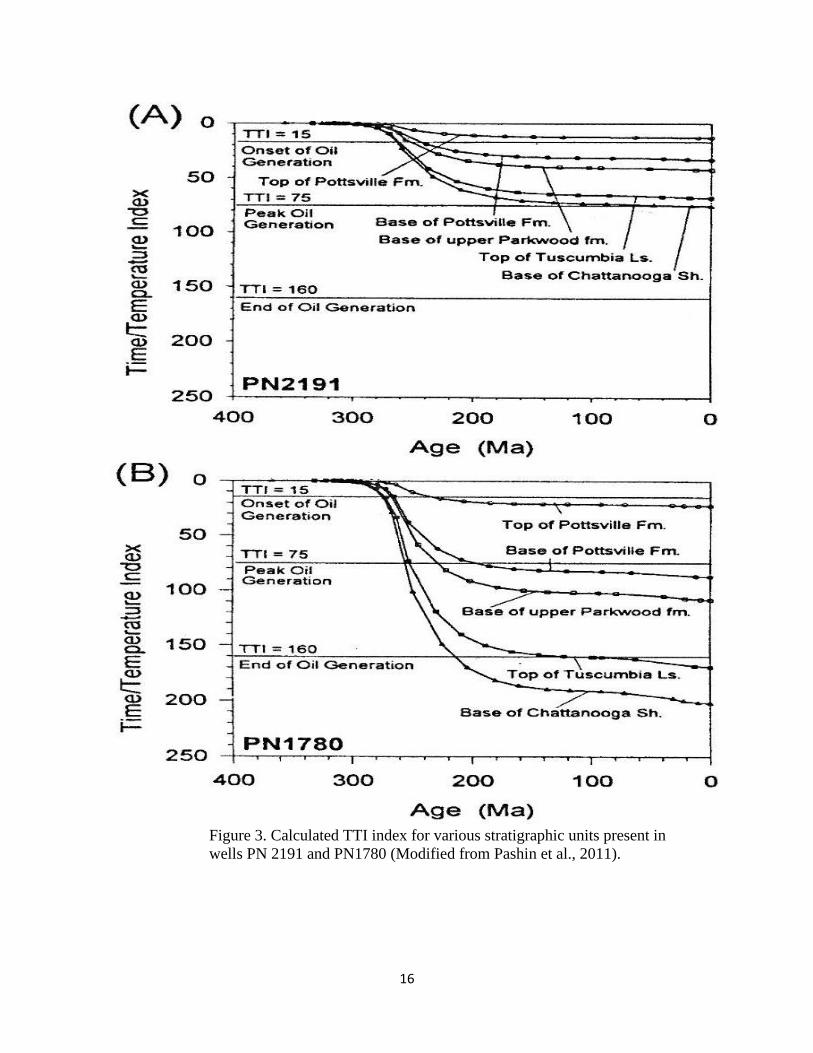
Within the Black Warrior Basin, The TTI values of Chattanooga Shale were calculated in

two wells, PN 2191 and PN 1780 (Table 2). It was found that maturation of kerogen was rapid,

reaching a maximum between 290 m.y. to 200 m.y. ago; correlating to the deepest burial of

Pottsville Formation (Carroll et al., 1995). However, in well PN 2191 the base of Chattanooga

Shale was located above the depth interval of peak oil-generation window, indicating that most

of the shale at this location is thermally immature. The deeper Chattanooga Shale in well PN

1780 (Figure 3) fell into the gas generation window, indicating that the shale was thermally

mature at this location since 200 m.y. ago (Carroll et al.,1995).

Table2. Permit number, depth, and location of wells.

Within the Black Warrior Basin, there is a trend of increasing thermal maturation from

northwest to southeast, as indicated by vitrinite reflectance values (Pashin et al., 2011). Where

Permit number Depth Longitude Latitude County

2191 4688 feet

-88.03758 33.8409 Lamar

1780 7000 feet

-88.04983 33.1115 Pickens

Table 1. TTI values and corresponding thermal

maturation stage.

15

the largest amount of conventional oil has been produced in Lamar and Pickens counties,

vitrinite reflectance increases in a uniform manner with depth, indicating that depth of burial, as

well as variations in the geothermal gradient, have had the greatest influence on thermal

maturation (Pashin et al., 2011). Within the Big Canoe Creek Field, vitrinite reflectance values

for the Conasauga shale ranged from 1.1 to 1.9, indicating that most of the reservoir body

currently falls into the gas production window (Pashin et al., 2011).

16

Figure 3. Calculated TTI index for various stratigraphic units present in

wells PN 2191 and PN1780 (Modified from Pashin et al., 2011).

17

MATERIALS AND METHODS

Core Sample Collection

During November 2012, shale samples were collected from seven oil and gas drill cores

(Table 3) stored in the Core Warehouse of the Alabama Geological Survey. From these seven

drill cores, 36 sub-samples, from varying depths, were processed for various geological,

geochemical, and hydrological analyses. The cores analyzed include 10 samples from the

Conasauga Shale, three samples from Chattanooga Shale, seven samples of the Devonian Shale,

and 16 samples from the Neal (Floyd) Shale.

Formation County Depth (top) Depth (bottom) Permit # Longitude Latitude

Conasauga St. Clair 7540 feet 7577 feet 15720 -86.22214 33.85764

Devonian Hale 10301 feet 10362 feet 3939 -87.70136 32.76762

Neal (Floyd) Greene 7996 feet 8055.1 feet 15075 -87.85457 33.08227

Neal (Floyd) Greene 9013 feet 9073 feet 15668 -87.74112 33.00451

Conasauga Shelby 14, 1698 feet 14,197 feet 3518 -86.52885 33.28967

Chattanooga Greene 8,441 feet 8,446 feet 3800 -87.87437 32.63802

Neal (Floyd) Pickens 6,650 feet 6,568 feet 14289 -88.06002 33.20421

X-Ray Diffraction (XRD) Analysis

About 1-10 grams of shales from each sub-sample were processed for a period of 40

minutes using a mortar and pestle. To avoid cross contamination the mortar and pestle were

scrubbed using soap and water after each sample was prepared. The XRD analysis measured

the bulk weight percentage of silicate, carbonate, sulfide, clay minerals, as well as other minerals

present within each sample. As previously discussed, differences in mineralogy (quartz,

Table 3. Location, depths, and permit #s of drill core samples used in this study.

18

carbonate, sulfide, iron oxide contents) are known to influence trace element contents and make

a great difference in hydraulic fracturing operation.

XRD analysis was conducted using a Bruker D2 Phaser XRD in the Geology and

Geography Department at Auburn University. Samples were run from 2 theta values of 10

degrees to 90 degrees with a 3800 step interval, resulting in a total time of 20 minutes for each

sample analysis. This time step and 2 theta angle allows for the non-clay minerals present within

each sample to be identified with a relative high degree of accuracy while being time efficient.

The mineral composition of the samples was determined by a peak search and match

procedure using DIFFRAC.EVA software. Furthermore, XRD pattern also reveals semi-

quantitative make-up of a material since the areas under the peak reflect the amount of each

phase present in the sample.

X-Ray Fluorescence (XRF) analysis

XRF analysis of shale samples was performed by an Elemental Tracer IV-ED handheld

unit in the Geology and Geography Department at Auburn University. Sample preparation

consists of creating a fresh surface on the same set of samples collected from the Alabama

Geological Survey. For each sample, three different filter, voltage, and amperage setting (Table

4) were used for targets different element groups. Analyses were repeated at three locations on

each sample, near the front, rear, and center of each sample. The elemental compositions of each

sample were averaged from values measured at three locations. Each filter, voltage, and current

setting used allowed for different suite of elements to be analyzed (Table 4).

19

Table 4. Voltage, amperage, filter, and vacuum setting used for each applicable element in XRF

analysis.

Voltage (KeV) Amperage (µA) Filter # Elements Vacuum

15 55 2 Na-Fe Yes

40 18 1 Fe-U No

45 30 3 As, Hg, Pb, etc. No

The XRF technology analyzes the energy emission of characteristic fluorescent X-rays

from a sample that has been excited by bombarding with high-energy (i.e., short-wavelength) X-

rays. The XRF technology can quantify the elemental composition of a material because each

element has unique electronic orbitals of characteristic energy and the intensity of each

characteristic radiation is directly related to the amount of each element in the material. Major

elements and most trace elements (Ba, Cr, Co, Cu, Mo, Nb, Ni, Pb, Rb, Sr, U, Th, V, Y, Zn, Se,

As, etc) of shale samples, in the range of parts per million (ppm), were measured at Auburn

University’s XRF and XRD laboratory. The instrument takes a sample reading from a very

small area (about 3 × 4 mm) with a small distance to the target so that potential heavy metal/trace

element zones can be recognized in high detail. The Elemental Tracer IV-ED has been calibrated

by various international shale standards (i.e., GBW07107, SARM-41, SCO-1, SDO-1, etc.) for

quantitative elemental analysis. For this study a standard was set by an ICP-MS analysis (Table

5) of a representative sample from the Neal (Floyd) Shale, Greene County, so that a quantitative

measurement of elemental concentrations in all samples could be obtained. This ICP-MS

analysis was performed at the commercial laboratory Spectrum Analysis.

20

Table 5. ICP-MS standard for selected elements.

Element Concentration (ppm or weight %)

Aluminum (Al) 0.29 %

Arsenic (As) 20.8 ppm

Lead (Pb) 22.5 ppm

Mercury (Hg) 0.11 ppm

Sulfur (S) 2.26 %

Iron (Fe) 1.94 %

Molybdenum (Mo) 2.4 ppm

Copper (Cu) 143.1 ppm

Zinc (Zn) 96.0 ppm

Silver (Ag) <0.1 ppm

Nickel (Ni) 68.0 ppm

Cobalt (Co) 13.7 ppm

Manganese (Mn) 90.0 ppm

Gold (Au) <0.5 ppm

Thorium (Th) 3.0 ppm

Strontium (Sr) 90.0 ppm

Cadmium (Cd) <0.1 ppm

Antimony (Sb) 2.0 ppm

Bismuth (Bi) 0.4 ppm

Vanadium (V) 29.0 ppm

Calcium (Ca) 1.3 %

Phosphorus (P) 0.04%

Lanthanum (La) 6.0 ppm

Chromium (Cr) 9.0 ppm

Magnesium (Mg) 0.67%

Barium (Ba) 63.0 ppm

Titanium (Ti) 0.002%

Boron (B) 17.0 ppm

Sodium (Na) 0.052%

Potassium (K) 0.21%

Tungsten (W) <0.1ppm

Scandium (Sc) 4.8 ppm

Thallium (Tl) 0.2 ppm

Gallium (Ga) 1.0 ppm

Selenium (Se) 1.8 ppm

Tellurium (Te) 0.4 ppm

21

Organic Matter Extraction and Biomarker Analysis

In order to fingerprint the source of organic matter in shales, organic compounds were

extracted from shales, at Auburn University’s Geology and Geography department, based on the

EPA method 3570 on microscale solvent extraction (USEPA, 2002). In this method, 2.5 grams of

anhydrous sodium sulfate is first added to a pre-cleaned glass extraction tube which has a

polytetrafluoroethylene (PTFE) screw cap. Three grams of crushed shales are measured and

transferred into the tarred extraction tube. 10 mL of dichloromethane (DCM) is then added to the

extraction tube. The tubes need to be agitated vigorously until slurry is free flowing for 10 min at

250 rpm. More sodium sulfate can be added as necessary to produce free-flowing, finely divided

slurry. The organic phase is then transferred to DCM by rotating them for at least 24 hours in an

orbital rotator. The organic phase is centrifuged at 3000 rpm for 10 minutes. Liquid phase

(supernatant) is transferred with a Pasteur pipette to glass vial. The liquid phase is filtered using

glass syringe and syringe filter (0.2 µm PTFE) to another glass vial. The organic phase in solvent

is then dried under a vent hood with nitrogen gas for approximately 30 minutes. One and one-

half mL of Hexane-MTBE 1:1 solution is added to dried organics in glass vial. After 10 minutes,

the extract is transferred to 2 mL amber GC vial. The vials containing the solutions were stored

in the freezer until analysis by the gas chromatograph mass spectroscopy. Sample preparation

was performed at Auburn University’s Civil Engineering department.

Extracted organic compounds were analyzed using an Agilent 5975C gas chromatograph

mass spectrometer (GC-MS) in a full-scan mode at Auburn University. Additionally, selected

22

samples were analyzed for petroleum biomarkers, with specific mass to charge ratios (m/z) of

191, 217, and 218, under much higher sensitivity by GC-MS Selected Ion Mode at ACTLAB.

Data was processed at Auburn University’s Pharmacy school utilizing ChemStation software.

Geophysical Log Analysis and Basin Modeling

Approximately forty down-hole geophysical logs were collected from the Alabama Oil

and Gas Board (Table 6). Down-hole geophysical logs are available in six counties (Figure 4).

Log types consist of gamma-ray, spontaneous potential, conductivity, resistivity, neutron bulk

density, and neutron porosity. Using the software package Neuralog, various logs were converted

from raster files to digital outputs by tracing individual logs from each well. These digital

outputs were then converted to file formats that are suitable for PETRA software for 3-D spatial

analysis and stratigraphy correlation.

Gamma logs were then used to correlate hydro-geologic units, focusing on the Conasauga

Shale, Chattanooga Shale, and the Neal (Floyd) Shale. Correlations were done with the Software

package PETRA. A three dimensional hydro-stratigraphic section of the Black Warrior Basin

was completed using this technique. From this hydro-stratigraphic section, a two dimensional

north-to-south transect across the entire basin was modeled for thermal and hydrologic evolution

using Basin2 modeling software (Bethke et al., 1993). The modeled transect represents a section

of the Black Warrior Basin with abundant down-hole geophysical and geologic data. The basin

modeling is centered on evaluating the thermal maturation and potential development of over-

pressurization due to sediment compaction. Oil-generation and gas-generation windows were

also calculated using the TTI model method described above.

23

Table 6. Permit #s, well names and locations of selected geophysical logs in the Black Warrior

Basin. The second columns numbers correlate to locations of geophysical logs in Figure 4.

Permit # Well Name Lat. Long. County

15241 1 Sumter Farm and Stock, Inc. 04-10 No. 1

32.91152 -88.29867 Sumter

3597 2 Sumter Farm and Stock Co. 33-15 #1 32.92097 -88.29915 Sumter

1160 3 James B. Hill #1 32.821557 -88.210098

Sumter

1040 4 J.J. Hagerman #1 32.98267 -88.30412 Sumter

16220 5 Caldwell 19-15 #1 ST 32.68846 -87.81838 Greene

16221 6 Tate 9-4 #1 32.6412 -87.89489 Greene

15668 7 Lamb 1-3H No. 1 33.00451 -87.74112 Greene

15075 8 Weyehaeuser No. 2-43-4202 33.08227 -87.85457 Greene

14673 9 Bayne Etheridge 36-9 #1 32.66203 -87.8308 Greene

10010 10 Weyerhaeuser 2-3 #1 33.09607 -87.85663 Greene

3800 11 Arco/Amoco Et Al- Ethel M. Koch 10-6 #1

32.63802 -87.87437 Greene

1810 12 James W. Sterling Et Al #17-14 32.96905 -88.01753 Greene

16066 13 Cain 6-6 #1 33.08637 -87.5128 Tuscaloosa

16065 14 JWR 25-14-04 33.26927 -87.32906 Tuscaloosa

16183 15 Westervelt 19-2H #1 33.04468 -87.50938 Tuscaloosa

14971 16 JWR 28-05-02 33.27324 -87.2816 Tuscaloosa

13680 17 Bolton 1-4 #1A 33.51241 -87.43834 Tuscaloosa

13387 18 Alawest 2-3 #1 33.51322 -87.45047 Tuscaloosa

13388 19 Bane 36-14 #1 33.51731 -87.43535 Tuscaloosa

16184 20 Lee 26-12 33.02772 -88.27422 Pickens

14371 21 Parker 3-16 # 1 33.16757 -88.19051 Pickens

14319 22 Eric Smith 18-12 #1 33.31505 -88.0442 Pickens

8599 23 Chicken Swamp Branch Gas 33.4564 -88.07608 Pickens

6922 24 Lizzie Johnson Et Al 15-16 #1 33.49163 -88.19153 Pickens

6809 25 Betty Wilcox 17-12 #1 33.49355 -88.23822 Pickens

5787 26 Melrose Timber Co. Inc. 2-15 #1 33.34732 -88.3636 Pickens

2580 27 Andrew C. Wade 26-1 #1 33.20469 -88.06501 Pickens

1800 28 George M. Collins # 5-11 33.1671 -88.02157 Pickens

1792 29 B.E. Turner #32-10 33.44293 -87.91381 Pickens

1763 30 Francis Bell Exum #7-8 33.24765 -88.13628 Pickens

1634 31 Robinson Et. Al. #1 33.31809 -88.18026 Pickens

1087 32 J.G. Lee #1 33.02773 -88.27526 Pickens

4100 33 Mother 13-15 #1 34.34087 -86.90556 Morgan

2794 34 Skidmore 36-1 #1 34.39113 -86.58231 Morgan

3097 35 Leroy Jones 14-10#1 33.6653 -88.07631 Lamar

24

2527 36 Weyerhaeuser #1 33.69054 -87.98549 Lamar

3939 37 Burke 29-7 No. 1 32.76742 -87.70123 Hale

9515 38 Teco Injection Well #26-8-224A-4400 32.93927 -87.54321 Hale

13389 39 U.S. Steel Corporation 21-13 #1 33.36588 -87.07329 Jefferson

25

Figure 4. Locations of Black Warrior Basin down-hole

geophysical logs. Latitudes, longitudes, permit #s, and

counties available in Table 6.

3

4

1

2

5 6

7 8

9 11

12

10

17, 18, 19

13

15

16 14

24 25 23

27 28 30

32

29 21 22

26

33 34

35 36

37

38

39

26

Results and Discussion

Inorganic Geochemistry

The geochemical analysis done in this study consists of measuring concentration of

selected EPA regulated elements (e.g., arsenic, lead, iron, sulfur, and aluminum) in shales at

varying depths using XRF technology. Special attention was paid to these elements due to new

groundwater regulations concerning these elements when hydraulic fracturing gas-shale (Table

5). Elemental concentrations are measured in either parts per million (ppm) or in weight

percentage (%). Concentrations (C) of trace elements in all samples are calculated from the

standard sample of the Neal (Floyd) shale (Table 5) using the following equation:

dards

sample

MSICPsampleA

ACC

tan

(2)

Here Csample and CICP-MS represent concentrations of a given element in a sample and the Neal

Floyd standard (measured by ICP-MS). Asample and Astandard are the total areas under the XRF

peaks of the same element in a sample and the Neal (Floyd) standard. The energy dispersive

spectrum of the Neal Floyd standard sample is shown in Figure 5a-c. The XRF analysis resulted

in peaks for trace elements for Fe, Mn, As, Pb, Hg, Al, Se, Cu, Zn, Ni, Sr, Ba, Ti, and V, along

with Ca, K, S and silica. Several of these trace elements are regulated by the EPA and are on the

list of primary drinking water standards.

27

Figure 5a. X- ray fluorescent spectral signature from the Neal (Floyd) Shale in Greene County

which targeted elements Na-Fe utilizing settings of 15 Kev, 55µA, filter #2, and a vacuum.

0

50000

100000

150000

200000

250000

300000

0 2 4 6 8 10 12 14 16

Inte

nsi

ty

Kev

Al

Si

SRh

KCa

Ti

VCr

Mn

Fe

28

Figure 5b. X- ray fluorescent spectral signature from the Neal (Floyd) Shale in Greene County

which targeted elements Fe-U utilizing settings of 40 KeV, 18 µA, filter #1, and no vacuum.

0

10000

20000

30000

40000

50000

60000

5 10 15 20 25 30 35

Inte

nsi

ty

Kev

Fe

Ni

Cu

Zn

Ga

Pb

As

Se

Bi

RbY

Zr

Nb

Sr

Rh

Pb

Sn

29

Figure 5c. X- ray fluorescent spectral signature from the Neal (Floyd) Shale in Greene County

which targeted elements As, Pb, Hg, Ba ect., utilizing settings of 45 Kev, 30 µa, and no vacuum.

0

2000

4000

6000

8000

10000

12000

14000

16000

5 10 15 20 25 30 35 40

Inte

nsi

ty

KeV

Fe

Ni

Cu

Zn

Ga

Pb

As

Bi

Se

Rb

Sr

Y

Zr

Nb

Rh

Pd

SnBa

30

Aluminum

Concentrations of Al in all shale samples are significantly lower than the average of

Earth’s crust (about 9.30 % by weight). For the Chattanooga Shale, Greene County, aluminum

concentrations varies from approximately 0.33% to 0.44% (Figure 6a). The Conasauga Shale,

Shelby County, contains the least amount of Al among the all shale units analyzed (Figure 6b).

Concentrations vary from 0.00% to approximately 0.04% by weight. However, the Al

concentration of the Conasauga Shale in St. Claire County varies from 0.12% at a depth of 7557

feet to 0.51% at a depth of 7553 feet (Figure 6c). This is slightly higher than concentrations in

Shelby County (Figure 6b).

A possible explanation for relatively low Al concentration within the Conasauga Shale is

the large amount of calcium carbonates present. This is especially true if carbonate rich section

are either being targeted for analysis or the sample analyzed represents a predominantly

carbonate-rich section of this shale. This interpretation is backed by XRD data (see Conasauga

Shale mineralogy) which shows large amounts of carbonates in this shale.

In the Devonian shale, of Hale County, concentrations of Al range from 0.29% to 0.32%,

at depths of 10,336 and 10,349 feet, respectively (Figure 6d). In the Neal (Floyd) Shale, in

Pickens and Greene County, similar ranges of Al concentrations are found, 0.45% to 0.75% for

Pickens County and 0.20% to 0.92% in Greene County (Figure 6e-f).

31

Figure 6a. Concentration of Al for Chattanooga Figure 6b. Concentration of Al for Conasauga

Shale in well permit # 3800, Greene County. Shale in well permit # 3518, Shelby County.

Figure 6c. Concentration of Al for Conasauga Figure 6d. Concentration of Al for Devonian

Shale in well permit # 15720, St. Claire County. Shale in well permit # 3939, Hale County.

Figure 6e. Concentration of Al for Neal (Floyd) Figure 6f. Concentration of Al for Neal (Floyd)

Shale in well permit # 14289 Pickens County. Shale in well permit # 15668, Greene County.

8,4468,4468,4458,4458,4448,4448,4438,4438,4428,4428,441

0 0.1 0.2 0.3 0.4 0.5D

epth

in F

eet

% Al14,200

14,195

14,190

14,185

14,180

14,175

14,170

14,165

0 0.01 0.02 0.03 0.04

Dep

th in

Fee

t

% Al

7,559

7,558

7,557

7,556

7,555

7,554

7,553

7,552

7,551

7,550

0 0.2 0.4 0.6

Dep

th in

Fee

t

% Al10,360

10,355

10,350

10,345

10,340

10,335

0.28 0.29 0.3 0.31 0.32 0.33 0.34

Dep

th in

Fee

t

% Al

6,570

6,569

6,568

6,567

6,566

6,565

6,564

6,563

6,562

6,561

6,560

0 0.2 0.4 0.6 0.8

Dep

th in

Fee

t

% Al9,400

9,200

9,000

8,800

8,600

8,400

8,200

8,000

7,800

0 0.2 0.4 0.6 0.8 1

Dep

th in

Fee

t

% Al

32

Arsenic

Arsenic concentrations vary from 0.00 to 20.80 ppm (Figure 7 a-e). A few samples have

As concentrations significantly higher than those in granite (about 2 ppm), basalt (about 2 ppm),

and sandstone (about 1 ppm) whereas certain concentrations fall below the detection limits (a

few ppm) of the XRF instrumentation. The average arsenic concentration in shales reported in

literature is roughly 13 ppm (Drever, 1997).

In the Chattanooga Shale, Greene County, the As concentrations range from 13.18 to

14.26 ppm with one sampling point falling below the lower detection limit of the instrumentation

(Figure 7a). Within the Conasauga Shale, Shelby County and St. Claire County, all of the

measured concentrations fall below the detection limit, suggesting that arsenic is very low in

shales dominated by carbonate minerals (Figure 7 b-c).

The Devonian shale, Hale County, has one recorded As concentration above the

minimum detection limit (Figure 7d). This is found at a depth of 10,336.5 feet with a

concentration of 10.60 ppm.

Two shales have relatively high concentrations of As; these are the Neal (Floyd) Shale,

Pickens County, and the Neal (Floyd) Shale, Greene County (Figure 7e-f). In the Neal (Floyd)

Shale, Pickens County, As concentrations are as high as 12.95 ppm (Figure 7e); As

concentrations in the Neal (Floyd) Shale, Greene County, range from 12.38 ppm to 20.80 ppm

(Figure 7f). However, there are several locations within this gas-shale close to As-rich depth

33

intervals do not show detectable As contents. These results indicate a heterogeneous distribution

of arsenic within the shales.

Special attention must be placed on the presence of As within gas shales. As mobility is

highly sensitive to redox geochemical conditions (Lee et al., 2005). Saunders et al (2008)

indicated that As is mobile under Fe-reducing conditions, immobile under sulfate-reducing

conditions. The geochemical environments may become more oxidized through the hydraulic

fracturing process, as a result, arsenic, which is either sorbed or co-precipitated onto pyrite

mineral structure, could potentially be released into the surrounding formation water or brine

fluids by pyrite oxidation. Considering this coupled with the EPA’s minimum contaminant levels

of As in groundwater, 0.010 ppm, there is the potential for large amounts of As to be released

into the brine fluids when oxidizing conditions are induced with the hydraulic fracturing. It is

enough concern that three states, Illinois, Colorado, and Pennsylvania, require baseline and

subsequent testing of the groundwater with As as one of the elements that must be quantified.

34

Figure 7a. Concentration of As for Chattanooga Figure 7b. Concentration of As for Conasauga


Figure 7c. Concentration of As for Conasauga Figure 7d. Concentration of As for Devonian


Figure 7e. Concentration of As for Neal (Floyd) Figure 7f. Concentration of As for Neal (Floyd)


8,446.0

8,445.5

8,445.0

8,444.5

8,444.0

8,443.5

8,443.0

8,442.5

8,442.0

8,441.5

8,441.0

0 5 10 15D

epth

in F

eet

As concentration ppm14,200

14,195

14,190

14,185

14,180

14,175

14,170

14,165

0 1 2 3

Dep

th in

Fee

t

As concentration ppm

7,559

7,558

7,557

7,556

7,555

7,554

7,553

7,552

7,551

7,550

0 2 4 6 8

Dep

th in

Fee

t


10,355

10,350

10,345

10,340

10,335

0 5 10 15D

epth

in F

eet


6,570

6,569

6,568

6,567

6,566

6,565

6,564

6,563

6,562

6,561

6,560

0 5 10 15

Dep

th in

Fee

t


9,200

9,000

8,800

8,600

8,400

8,200

8,000

7,800

0 5 10 15 20 25

Dep

th in

Fee

t


35

Lead

Lead concentration in shales appears to vary with depth and ranges from below detection

limits of the instrumentation (< 10 ppm) to 98.25 ppm (Figure 8 a-e). The average lead

concentration in shales reported in literature is approximately 20.00 ppm (Drever, 1997). The

Chattanooga Shale, Greene County, has a large variance of Pb concentrations that range from

21.52 ppm at 8,445.5 feet to 98.25 ppm at 8441 feet (Figure 8a).

The Conasauga Shale, Shelby County, has lead concentrations that fall below the

detection limit of the equipment (Figure 8b). In contrast, the Conasauga Shale, St. Claire County

has higher Pb concentrations, ranging from 12.66 ppm to 33.26 ppm (Figure 8c). This result

indicates a heterogeneous distribution of lead within the shales. The Conasauga Shale is known

for high amounts of carbonates within the upper sections. Carbonate-rich sections of shales

generally have very low lead content.

The Devonian Shale, Hale County, has a wide range of Pb concentrations.

Concentrations range from 30.57 ppm at a depth of 10,336.5 feet and 12.07 ppm at a depth of

10,349 feet (Figure 8d).

The Neal (Floyd) Shale, Pickens County and Greene County, have varying

concentrations of Pb (Figure 8 e-f). Concentrations vary in the Neal (Floyd) Shale, Pickens

County, from 12.38 ppm at a depth of 6551 feet to 32.69 ppm at a depth of 6563 feet (Figure 8e).

The Neal (Floyd) Shale, Greene County, has similar Pb concentrations to those found in the Neal

(Floyd) Shale, Pickens County (Figure 8e-f). A low value of 13.18 ppm is found at a depth of

8044 feet and a high value of 24.18 ppm is found at a depth of 8035 feet. Two deeper samples at

36

9181.5 feet and 9178 feet however, have relatively low Pb concentrations with respect to shallow

samples.

With the EPA’s maximum concentration of 0.015 ppm for lead allowed in drinking

water, the potential for contamination of Pb in groundwater is quite large; this is based upon the

combination of high lead contents in shales, the potential communication of produced fluids with

USDWs, and surface contamination from mechanical failure.

37

Figure 8a. Concentration of Pb for Chattanooga Figure 8b. Concentration of Pb for Conasauga


Figure 8c. Concentration of Pb for Conasauga Figure 8d. Concentration of Pb for Devonian


Figure 8e. Concentration of Pb for Neal (Floyd) Figure 8f. Concentration of Pb for Neal (Floyd)


8,446.0

8,445.5

8,445.0

8,444.5

8,444.0

8,443.5

8,443.0

8,442.5

8,442.0

8,441.5

8,441.0

0 50 100 150D

epth

in F

eet

Pb concentration ppm14,200

14,195

14,190

14,185

14,180

14,175

14,170

14,165

0 2 4 6 8 10

Dep

th in

Fee

t

Pb concentration ppm

7,559

7,558

7,557

7,556

7,555

7,554

7,553

7,552

7,551

7,550

0 10 20 30 40

Dep

th in

Fee

t


10,355

10,350

10,345

10,340

10,335

0 10 20 30 40

Dep

th in

Fee

t


6,5706,5696,5686,5676,5666,5656,5646,5636,5626,5616,560

0 10 20 30 40

Dep

th in

Fee

t


9,200

9,000

8,800

8,600

8,400

8,200

8,000

7,800

0 10 20 30

Dep

th in

Fee

t


38

Mercury

Mercury concentration in shales appears to vary with depth and ranges from 0.00 to 73.41

ppm (Figure 9 a-b). The average mercury concentration in shales reported in literature is about

0.4 ppm (Drever, 1997). Two shales had concentrations of mercury (Hg) that were above the

detection limit; these were the Devonian Shale in Hale County and the Neal (Floyd) Shale in

Greene County (Figure 9 a-b).

The Devonian Shale within Hale County has substantial concentrations of Hg (Figure

9a). The lowest concentration is found at a depth of 10,357 feet with a concentration of 17.73

ppm while the highest concentration is 58.74 ppm at a depth of 10,349 feet.

In the Neal (Floyd) Shale located in Greene County there are also very high levels of Hg

(Figure 9b). The highest concentration of 73.41 ppm is found at a depth of 8048 feet and the

lowest concentration of 13.5 ppm is found at a depth of 8034 feet (Figure 9b). Large Hg

concentration heterogeneity exists within this shale body.

Current EPA standard dictate that no more than 2 parts per billion (ppb) of Hg can be

present in drinking water. With mercury’s extreme health effects and the potential for large

quantities present in the shales, special attention must be paid when it comes to proper care of

produced fluids as well as cutting from the well bore.

39

Figure 9a. Concentration of Pb for Devonian Figure 9b. Concentration of Pb for Neal (Floyd)

Shale in well permit # 15668, Greene County. Shale in well permit # 15720, St. Claire County.

10,360

10,355

10,350

10,345

10,340

10,335

0 20 40 60 80

Dep

th in

Fee

t

Hg concentration ppm9,400

9,200

9,000

8,800

8,600

8,400

8,200

8,000

7,800

0 20 40 60 80

Dep

th in

Fee

t

Hg concentration ppm

40

Sulfur

Sulfur concentration in shales appears to vary with depth and ranges from 0.00 to 6.82 %

(Figure 10 a-e). The average sulfur concentration in shales reported in literature is about 2.60 %

(Karl and Karl, 1961). The Chattanooga Shale, Greene County, has relatively high

concentrations of sulfur (Figure 10a). The highest concentration of 5.21% occurs at a depth of

8441.5 feet; the lowest concentration of about 2.78% is found at a depth of 8443 feet.

The Conasauga Shale within Shelby County has very low concentrations of sulfur

(<0.40%) (Figure 10b). This is consistent with the low amounts of Fe, and other trace metals

found in this shale body; sulfur tends to have high geochemical affinity with Fe. Moreover, high

amounts of calcium carbonates are present in this shale. The lowest concentration of sulfur in

this shale is about 0.15%, found at a depth of 14,196 feet, while the highest concentration is

0.33%, found at a depth of 14,192 feet. This is consistent with the mineralogy results of this

study as there are insignificant sulfide minerals present (see Conasauga Shale Shelby County

mineralogy section).

Sulfur concentrations in the Conasauga Shale, St. Claire County (Figure 10c), are

significantly higher those in the carbonate-rich shale Conasauga Shale, Shelby County (Figure

10b). The lowest concentration in this shale is about 1.05% at a depth of 7551 feet, while the

highest concentration of 6.82% is found at a depth of 7555 feet. It should be noted that As and

Pb concentrations are also significantly higher in St. Claire County than those in Shelby County.

The concentrations of sulfur in the Devonian Shale, Hale County, ranging from 1.26% to

5.88 %, are significantly higher than those of the Conasauga Shale in Shelby County (Figure

41

10d). As and Pb concentrations are also significantly higher in the Devonian Shale than those in

Conasauga Shale, Shelby County. Concentrations of sulfur in the Neal (Floyd) Shale, Pickens

County, range from 1.94% at a depth of 6,563 feet to 3.24% at a depth of 6,565 feet (Figure 10e).

Concentrations of sulfur in the Neal (Floyd) Shale, Greene County, vary from a maximum of

4.89% to a minimum of 1.40%; these concentrations are found at depths of 8035 feet and 9181.5

feet, respectively (Figure 10f).

It is imperative to quantify the amount of sulfur within each of these shale bodies’ due to

the strong geochemical affinity for trace metals to be sorbed or incorporated into common sulfide

minerals. Sulfide minerals are common in shales typically deposited under highly reducing

environments. Natural occurring metal and metalloid sulfide minerals include pyrite (FeS2, most

common), galena (PbS), sphalerite (ZnS), cinnabar (HgS), as well as the arsenic sulfides realgar

(AsS), orpiment (As2S3), and arsenopyrite (FeAsS). The low solubility of these minerals makes

them effective in removing trace metals (e.g., As and Pb) from formation water.

As stated before these minerals are very redox sensitive and a change of the redox state

from the injection of fracturing fluid into shale could make these minerals unstable, thus

facilitating the release of toxic elements into the brine fluid. This fluid may then be returned as

produced water to the surface where it has the potential to contaminate groundwater through

either mechanical failure in cementation or casing or human failure at the surface.

42

Figure 10a. Concentration of S for Chattanooga Figure 10b. Concentration of S for Conasauga


Figure 10c. Concentration of S for Conasauga Figure 10d. Concentration of S for Devonian


Figure 10e. Concentration of S for Neal (Floyd) Figure 10f. Concentration of S for Neal (Floyd)


8,446.08,445.58,445.08,444.58,444.08,443.58,443.08,442.58,442.08,441.58,441.0

0 2 4 6D

epth

in F

eet

% S14,200

14,195

14,190

14,185

14,180

14,175

14,170

14,165

0 0.1 0.2 0.3 0.4

Dep

th in

Fee

t

% S

7,559

7,558

7,557

7,556

7,555

7,554

7,553

7,552

7,551

7,550

0 2 4 6 8

Dep

th in

Fee

t

% S10,360

10,355

10,350

10,345

10,340

10,335

0 2 4 6 8

Dep

th in

Fee

t

% S

6,5706,5696,5686,5676,5666,5656,5646,5636,5626,5616,560

0 1 2 3 4

Dep

th in

Fee

t

% S9,400

9,200

9,000

8,800

8,600

8,400

8,200

8,000

7,800

0 2 4 6

Dep

th in

Fee

t

% S

43

Iron

Iron concentration in shales appears to vary with depth and ranges from 0 .08% to 4.49%

(Figure 11 a-f). The average Fe concentration in shales reported in literature is 4.72 % (Karl and

Karl, 1961). Fe concentrations in the Chattanooga Shale within Greene County range from

4.49% at a depth of 8441.5 feet to 2.41% at a depth of 8444.5 feet (Figure 11a).

The Conasauga Shale located in Shelby County has considerably lower Fe concentrations

as compared to those in the Greene County (Figure 11b). Iron concentrations range from a low of

0.08% at a depth of 14,181 feet to a high concentration of 0.36% at a depth of 14,192 feet. This

result is consistent with the high amounts of calcium carbonates present in this section of the

Conasauga Shale (see Conasauga Shale Shelby County mineralogy section). The low iron

content corresponds well with low concentrations of metals such as Pb and As which has strong

geochemical affiliation with Fe (Figures 8b and 7b).

The Conasauga Shale in St. Claire County (Figure 11c) also has higher concentrations of

Fe as compared to the Conasauga Shale in Shelby County. In St. Claire County, Fe

concentrations range from 0.67% at a depth of 7557 feet to 2.19% at a depth of 7553 feet.

The Fe concentration in the Devonian shale in Hale County spans a narrow range; a low

of 1.68% is present at a depth of 10,347 feet and a high of 1.86% is present at a depth of 10,349

feet (Figure 11d).

The maximum concentration of Fe within the Neal (Floyd) Shale, located in Pickens

County, is 2.63 % at a depth of 6561 feet (Figure 11e). The lowest concentration of 1.77 % is

found a depth of 6565 feet. Iron concentration in the Neal (Floyd) Shale within Greene County

44

range from a high value of 2.72% at a depth of 8034 feet to a low concentration value of 1.39%

at a depth of 9181.5 feet (Figure 11f).

The concentration of Fe within each of the shale bodies reflect the abundance of iron-

bearing minerals (e.g., Fe sulfides, Fe oxides, Fe carbonate, Fe-rich silicate, etc). The iron-

bearing minerals have strong geochemical affinity to sorb trace metals onto their surfaces or

incorporate these trace metals into their crystalline structure. There is a strong trend for

increasing concentrations of As, Pb, and S with increasing concentrations of Fe (Figure 12 a-c)

with R2 values of 0.29 for S, 0.36 for Pb, and 0.36 for As (Figure 12 a-c).

The transformation of Fe-bearing minerals under changing redox conditions may control

mobility and concentrations of trace metals in groundwater. For example, a large quantity of

trace metals could be introduced into the groundwater as pyrite becomes oxidized. Weathering of

Fe-rich silicate minerals and reduction of Fe oxides also releases Fe and trace metals into

groundwater (Saunders et al., 2008). The metal-rich fluid then has the potential to contaminate

underground drinking water supplies (USDWs) from a multitude of scenarios, such as

cementation failure, well bore failure, or intimate contact of produced fluids with the surface due

to human or mechanical failure. Because of this the regulations involving hydraulic fracturing

gas-shale must be considered.

45

Figure 11a. Concentration of Fe for Chattanooga Figure 11b. Concentration of Fe for Conasauga


Figure 11c. Concentration of Fe for Conasauga Figure 11d. Concentration of Fe for Devonian

Shale in well permit # 15720, St. Claire County. shale in well permit # 3939, Hale County.

Figure 11e. Concentration of Fe for Neal (Floyd) Figure 11f. Concentration of S for Neal (Floyd)


8,446.08,445.58,445.08,444.58,444.08,443.58,443.08,442.58,442.08,441.58,441.0

0 2 4 6D

epth

in F

eet

% Fe14,200

14,195

14,190

14,185

14,180

14,175

14,170

14,165

0 0.1 0.2 0.3 0.4

Dep

th in

Fee

t

% Fe

7,559

7,558

7,557

7,556

7,555

7,554

7,553

7,552

7,551

7,550

0 0.5 1 1.5 2 2.5

Dep

th in

Fee

t

% Fe

10,360

10,355

10,350

10,345

10,340

10,335

1.65 1.7 1.75 1.8 1.85 1.9

Dep

th in

Fee

t

% Fe

6,570

6,568

6,566

6,564

6,562

6,560

0 1 2 3

Dep

th in

Fee

t

% Fe9,4009,2009,0008,8008,6008,4008,2008,0007,800

0 1 2 3

Dep

th in

Fee

t

% Fe

46

Figure 12a. Correlation of As concentrations (ppm) and

Fe concentrations (weight %) for all shales investigated.

Figure 12b. Correlation of Pb concentrations (ppm) and Fe

concentrations (weight %) for all shales investigated.

Figure 12c. Correlation of S concentrations (weight %) and Fe

concentrations (weight %) for all shales investigated.

R² = 0.3602

0

1

2

3

4

5

6

0 5 10 15 20 25 30Fe C

on

cen

trat

ion

wei

ght

%

As Concentration ppm

As vs. Fe

R² = 0.3608

0

1

2

3

4

5

6

0 50 100 150 200Fe C

on

cen

trat

ion

wei

ght

%

Pb Concentration ppm

Pb vs. Fe

R² = 0.2928

0

1

2

3

4

5

6

0 2 4 6 8 10

Fe C

on

cen

trat

ion

wei

ght

%

S Concentration weight %

S vs. Fe

47

Wellbore, Pit, and Base Line Water Testing Regulations

This section reviews relevant environmental regulations on gas-shale hydraulic fracturing

operation. The new hydraulic fracturing technologies used for shale oil and gas production

requires specific protocols or guidelines for environmental protection, which have not been

properly reviewed and formulated. Throughout state and federal regulations, there exists a

related regulations required for wellbore construction (e.g. casing, cementation, mechanical

integrity test, and cement evaluation logs) (Table 7) and pit construction (Table 8).

A major concern involving wellbore integrity occurs during the cementing process; when

fresh cement encounters natural gas from non-producing horizons there is potential for high

pressure gas to cut channels in the cement, allowing for communication of deep reservoirs with

shallow underground source of drinking groundwater or USDWs. As of now, there is not a proof

test that can be done to inspect if channeling has occurred, or inspect the quality of the

cement/rock contact. This is a major concern for the potential contamination of USDWs

(Ingraffea, 2010).

Wellbore construction and pit construction is essentially standard for each state; however,

baseline water testing is not. Only three states, Pennsylvania, Illinois, and Colorado, require this

testing (Table 7).

48

Potential USDW Degradation and Economic Impact Due to Gas-shale Production

When producing shale-gas there are two main areas of potential USDW contamination;

1) communication of hydrocarbons and formation waters from producing and non-producing

formations to USDWs due to improper cementing and casing, and 2) migration of flowback

fluids and produced fluids from the containment pit into USDWs. It has been found that there is

a failure rate of about 6.5% in well casings (Ingraffea, 2010). Failure can be either casing failure

or failure of the cement to isolate USDWs from the migration of fluids or contaminants

(Ingraffea, 2010). This number may seem small, however, when considering the dynamics of

shale-gas production and the amount of wells that must be drilled in order for gas plays to remain

economical this stands as a significant potential for contamination (Ingraffea, 2010; Berman, et

al., 2012)

With current federal and state regulations, only three states (e.g. Pennsylvania, Colorado,

and Illinois) require determinations if the contamination within USDWs is due to the production

of shale-gas or naturally occurring (background or from an unidentified source). Presented in

Table 8 are Illinois state baseline water testing requirements.

As illustrated in Table 9, water sampling in Illinois is quite extensive, and while not a

probable large expense for any one well, the culmination of testing could possibly lead to a

larger overhead expenditure for shale-gas development.

If there is contamination from either the wellbore or the containment pit, the source will

need be determined and the appropriate action will take place. This is because natural occurring

49

contamination would be differentiated from contamination from production. These regulations

allow for a proactive position as opposed to a reactive position.

One testing requirement that Colorado has put into place states that if methane

concentration is found within a well over 1 mg/L, isotope analysis will be conducted on C12 and

C13 ratios, as well as H1 and H2 ratios. Particular ratios of these stable isotopes indicate either a

biogenic or thermogenic formation of the gas. From this it will be possible to determine if the

methane in the groundwater was either produced from natural bacterial activities in groundwater

or natural gas seeping from a producing zone into groundwater (Colorado Oil and Gas

Conservation Commission, 2012).

Subsurface Monitoring and Contaminant Modeling

Recent EPA regulations, 40 CFR 146.6(a) (2) and 40 CFR 144.41, would require the

monitoring and modeling of subsurface flow to determine the likelihood of USDW

contamination from contaminant migration. The process of modeling is extremely complex,

involving extensive literature review as well as collection of raw geological and hydrologic data,

the prediction of contamination scenarios (i.e., fluid migration through a fault, well bore failure),

the actual model (i.e. geomechanical model, transport model) and analysis of the model quality.

Subsurface monitoring would consist of pressure monitoring; where an increase in pressure

could indicate the migration of gas or potential casing failure, both of which could be detrimental

to USDWs (Briskin and Stephen, 2013).

The practice of subsurface contaminant modeling introduces many unknown

complexities and would require extensive work and expenditures on top of the overhead

allocated for production. As of now, EPA’s regulatory arm only extends to those wells that are

hydraulically fractured using diesel fuel, thus negating regulations for companies that

50

hydraulically fracture rocks with water based fluid. However, if future hydraulic fracturing

operations fall under the Clean Water Act (CWA), operations would be required to follow these

preemptive guidelines, potentially causing a dramatic cost increase for “business as usual”

practices.

Future Impact Due to Colorado, Pennsylvania, and Illinois Base-Line Water Testing

Colorado, Pennsylvania, and Illinois have recently passed the most comprehensive

regulations concerning the practice of hydraulic fracturing, namely the requirement of baseline

water testing as well as other requirements not presented in this paper. These new regulations

(i.e., baseline water testing) will potentially set the precedent for standards to be put forth for the

regulation of shale-gas production in the United States.

These new regulations could serve as a double-edged sword, that is, if contamination is

confirmed by the baseline and subsequent testing at a site, it could possibly limit hydraulic

fracturing practices in the United States. However, this testing could also confirm the industry’s

stance on hydraulic fracturing; it is a safe practice and does not commonly impact USDWs. This

could result in encouraging the opening of new shale-gas opportunities in states where

moratoriums have been placed upon hydraulic fracturing (e.g., Marcellus shale in New York

State and municipal bans in parts of Colorado).

New baseline water testing regulations could have an impact on the cost of producing

gas-shale. With well failure rates coupled with the amount of wells that must be drilled, the

potential for contamination due to shale-gas production increases. If all state and federal

regulations come up to par to Illinois, Colorado, and Pennsylvania regulations, additional

accountability will be placed on all potential contamination as a result of producing shale-gas.

51

This coupled with a large public dissent concerning hydraulic fracturing has the potential to

impact the proliferation of unconventional gas production.

The concerns of groundwater contamination have created great uncertainty on future gas-

shale development. This uncertainty stems largely from inadequate knowledge on shales’

mineralogy, fractures, mechanic properties, porosity, permeability, and chemical (trace metal)

composition.

Table 7. Wellbore and baseline water testing requirements for Colorado, Illinois, and

Pennsylvania. (Colorado Oil and Gas Conservation Commission, 2012; Bradley et. al., 2013;

Pennsylvania Department of Environmental Protection, 2012)

Regulating Body

Casing Cementation Mechanical integrity Test

Cement Evaluation Log

Baseline Water Testing

Colorado

Required to protect all USDWs.

Must protect all aquifers and have a minimum compressive strength after 24 and 72 hours.

The production casing must be pressure tested with pressures similar to those expected.

A cement bond log shall be run on all production casing.

Required for new permitted oil and gas well in a ½ mile radius from the well bore.

Illinois

Must isolate all USDWs.

Cement must conform to current industry standards published by the American petroleum institute.

A pressure test demonstrating less than or equal to a 5% pressure drop after 30 minutes

A radial cement bond evaluation log must be run on each well. If cementation is found inadequate, it must be remediated.

Required in a 1,500 feet radius extending out from the well bore.

Pennsylvania

Required to protect all USDWs from fluid migration.

Cementing must secure the casing in the wellbore, isolate the wellbore from fresh groundwater, and contain any pressure from drilling, completion and production.

A pressure test demonstrating less than or equal to a 10% pressure drop after 30 minutes

None required. Required in a 1,000 feet radius from the well bore.

52

Table 8. Containment pit requirements for Colorado, Illinois, and Pennsylvania. (Colorado Oil

and Gas Conservation Commission, 2012; Bradley, J., et. al., 2013; Pennsylvania Department of

Environmental Protection, 2012) Regulating Body Use of Pits Allowed Pit construction requirements

Colorado Yes, however, only in emergency situations.

Must not allow any communication of contaminants and aquifers or USDWs.

Illinois Yes, however only for temporary storage due higher than expected flow back.

The synthetic liner must have a minimum thickness of 24 mils, capacity of at least 110% of maximum volume of anticipated recovered fluid.

Pennsylvania

Yes, however only for temporary containment.

Pits must be constructed with synthetic flexible liner that has a permeability value no greater than 1 x 10-7 cm/sec.

Table 9. Illinois water testing requirements for hydraulically fractured wells (Bradley, et al.,

2013)

Metal Enrichment in Black Warrior Basin Shale’s

The concentrations of selected elements of gas-shales in the Black Warrior Basin were

normalized (Table 10) using the aluminum normalized enrichment factor (ANEF);

𝑀𝑒𝑠𝑎𝑚𝑝𝑙𝑒𝐴𝑙𝑠𝑎𝑚𝑝𝑙𝑒⁄

𝑀𝑒𝑐𝑟𝑢𝑠𝑡𝐴𝑙𝑐𝑟𝑢𝑠𝑡⁄

= ANEF (2)

Here Me represent trace metals in shale samples and Al (aluminum) is the selected reference

metal in Earth’s crust. ANEF determines the enrichment or depletion of an element relative to

the reference aluminum. Since there are no known anthropogenic sources of aluminum to

Water properties and dissolved gasses to be tested pH, total dissolved solids, dissolved methane, dissolved propane, dissolved ethane, alkalinity, and specific conductance.

Anions and Elements to be tested

Chloride, sulfate, arsenic, barium, calcium, chromium, iron, magnesium, selenium, cadmium, lead, manganese, mercury, and silver.

Benzenes to be tested Benzene, toluene, etheylbenzene, and xylene. (BTEX)

Radioactivity to be tested Gross alpha and beta particles.

Responsible testing body Either a licensed engineer (P.E.) or a licensed Geologist (P.G.). Analysis must be conducted at an independent testing laboratory.

Sampling frequency Baseline, 6 months, 18 months, and 30 months.

53

sediments or rocks, any metals with substantial terrigenous inputs would have positive ANEF

anomalies. ANEF may also provide useful insights on reactivity relationship such as the

retention of chalcophile metals in sediments or minerals via bacterial sulfate reduction and

formation of sulfide solids.

The Chattanooga Shale located in Greene County (Figure 13 and Table 10) is highly

enriched in most trace elements but three (Hg, Ba, and Mn). The enrichment factor is greater

than 100 for As, Cu, and S; Pb, Fe, Zn, and Ca also display relatively high ANEF values (>10).

The high ANEF values suggest that this shale represent a significant sink for trace elements.

The Conasauga Shale located in Shelby County (Figure 14 and Table 10), shows

astronomically high enrichment values for several of the elements (e.g., Ca, Cu, and S). This is

most likely the result of targeting a carbonate-rich section of the sample being analyzed; little or

almost no aluminum present in the sample causes these anomalously high ANEF results.

The Conasauga Shale in St. Claire County are enriched in As, Cu, and Pb with ANEF

factors greater 10 (Figure 15 and Table 10). These data match nicely with the enrichment of

sulfur and iron, which is consistent with the hypothesis that iron sulfide minerals such as pyrite

represent major sinks for arsenic as well as lead. When comparing this section of the Conasauga

Shale with the section found in Shelby County, (Figure 14 and Table 10), we can denote that

there is a considerable difference in the enrichment of elements such as Ca, Cu, Fe, S, and Mn.

In the case of calcium, there are five orders of magnitude difference between the two shales;

however, the enrichment factors of arsenic are similar.

54

The Devonian Shale in Hale County (Figure 16 and Table 10), exhibits similar

enrichments of As, Cu, S, Fe, and Pb to those found in the Conasauga Shale. However, there is a

considerable enrichment of Hg present within this shale with ANEF values near 10,000

The Neal (Floyd) Shale in Greene County (Figure 17 and Table 9) shows great

enrichment S, As, Cu, and Hg (ANEF>100). Other trace elements such as Fe, Pb, V, and Zn also

display relatively high ANEF values (>10).

The Neal (Floyd) Shale in Pickens County (Figure 18 and Table 10) has one

element S with an ANEF value greater than 100. Other trace elements such as As, Cu, Pb, Zn,

and V also display relatively high ANEF values (>10).

The highest enrichment factor of As (ANEF> 100) and Pb (ANEF > 65) is found in the

Chattanooga Shale in Greene County. It should be noted that very high enrichment factor of

sulfur is found in all the shales. This result supports the hypothesis that the sulfide minerals are

abundant and represent the primary sinks for the toxic trace metals arsenic, lead, and mercury.

55

Element Chattanooga Shale,

Greene Co

Conasauga Shale,

Shelby Co

Conasauga Shale,

St. Claire Co

Devonian shale,

Hale Co

Neal (Floyd), Pickens

Co

Neal (Floyd), Greene

Co

As 128.1 66.3 59.9 83.9 48.4 93.2

Ba 6.4 0.00 1.4 5.0 1.4 1.8

Ca 22.9 3063209.0 201.8 62.2 8.8 8.1

Cu 129.3 320487.3 154.9 115.5 78.3 113.4

Fe 22.0 5196.3 11.3 14.1 8.7 11.5

S 850.0 539055.4 655.0 1118.7 358.8 457.0

Pb 64.6 30.4 25.6 35.3 16.6 15.2

Mn 4.8 9777.4 8.3 4.3 3.2 3.4

Hg 0.000 0.000 0.000 9821.8 0.000 6173.7

V 2.8 24.7 7.3 18.6 10.3 11.8

Zn 11.6 169.2 18.4 57.0 65.9 0.000

Table 10. Aluminum enrichment factor for selected EPA regulated elements

for the Chattanooga Shale, Conasauga Shale, Devonian Shale, and the Neal

(Floyd) Shale.

56

Figure 13. Aluminum normalized enrichment factor for the Chattanooga Shale, Greene County.

Figure 14. Aluminum normalized enrichment factor for the Conasauga Shale, Shelby County.

1

10

100

1000

As Ba Ca Cu Fe S Pb Mn Hg V Zn

AL

NO

RM

ALI

ZED

EN

RIC

HM

ENT

FAC

TOR

1

10

100

1000

10000

100000

1000000

10000000


AL

NO

RM

ALI

ZED

EN

RIC

HM

ENT

FAC

TOR

57

Figure 15. Aluminum normalized enrichment factor for the Conasauga Shale, St. Claire County.

Figure 16. Aluminum normalized enrichment factor for the Devonian shale, Hale County.

1

10

100

1000


AL

NO

RM

ALI

ZED

EN

RIC

HM

ENT

FAC

TOR

1

10

100

1000

10000


AL

NO

RM

ALI

ZED

EN

RIC

HM

ENT

FAC

TOR

58

Figure 17. Aluminum normalized enrichment factor for the Neal (Floyd) Shale, Greene County.

Figure 18. Aluminum normalized enrichment factor for the Neal (Floyd) Shale, Pickens County.

1

10

100

1000

10000


AL

NO

RM

ALI

ZED

EN

RIC

HM

ENT

FAC

TOR

1

10

100

1000


AL

NO

RM

ALI

ZED

EN

RIC

HM

ENT

FAC

TOR

59

Mineralogy

X-ray diffraction (XRD) analyses of shales were performed on selective sections of three

shale units. Powdered XRD pattern were recorded using Bruker D2 Phaser with Ni-filtered Cu

K radiation at 30 kV and 10 mA. Samples were scanned from 2 of 10 to 900 for 4500 steps

at 0.3 sec per step. Identification of clay minerals, which requires preparation of oriented

sample, was not performed in this study.

Mineralogical components of the Chattanooga Shale, Greene County (Figure 19), consist

mainly of quartz, with accessory sulfide minerals pyrite and marcasite as well as carbonate

minerals (calcite and dolomite). Mineralogical composition correlates well with bulk

geochemistry analysis of shales. The presence of iron sulfides (i.e., pyrite) is consistent with the

abundance of sulfur and iron in this shale (see inorganic geochemistry section) and the positive

geochemical correlation between S with Fe (Figure 12c). Other sulfide minerals enriched in Zn

and Cu were also identified.

Mineralogical make-up of the Conasauga Shale, Shelby County (Figure 20), is dominated

by various carbonates (e.g., magnesium rich calcite, pure calcite, calcium rich dolomite, pure

dolomite) with minor amount of quartz. Sulfide minerals are not identified in the XRD spectrum.

The lack of sulfides is consistent with the results of bulk geochemical analysis in which there are

low Fe, As, Pb, and S (Figure 12a, 12b, 12c) contents in this shale.

Carbonates (e.g., calcite and dolomite) are the main mineralogical constituent in the

Conasauga Shale, St. Claire County (Figure 21). Muscovite and magnetite are present as

accessory minerals. Muscovite is a common phyllosilicate mineral enriched in Al and K. X-ray

60

fluorescence analysis also shows the presence of Al and K in this sample. Sulfide mineral

assemblages are absent in this sample. Magnetite (Fe3O4), a common naturally occurring Fe

oxide, is the primary source of Fe in this sample.

Mineralogy in the Devonian shale, Hale County (Figure 22), is dominated by quartz,

calcite, and dolomite. Fe-rich sulfide (pyrite) and oxide are accessory minerals. Iron sulfides and

iron oxides provide an appropriate mineralogy for trace metal sinks. With increasing iron content

an increase in Pb and S is expected; this is confirmed by linear the correlation between of Fe and

Pb and bulk geochemical data (Figure 12 b-c).

Dominate mineralogy of the Neal (Floyd) Shale consist of quartz; major accessory

minerals include dolomite, calcite, pyrite, and Fe-oxides (Figure 23). Minor silicate minerals

(e.g., albite) were also identified. Iron oxides and iron sulfides would be expected with the Fe-

and S-rich nature of this shale (see inorganic geochemistry section). Bulk geochemistry data

(Figure 12 a-c) indicate that Pb and As may be contained within Fe sulfide minerals.

Mineralogy of the Neal (Floyd) Shale, Greene County (Figure 24) is very similar to the Neal

(Floyd) Shale, Shelby County (Figure 23). Quartz is the dominant mineral and accessory

minerals consist of pyrite, dolomite, and magnetite. Other sulfide minerals enriched in Zn were

also identified. The enrichment of sulfide minerals is consistent with the results of bulk

geochemical analysis exhibiting high Fe, As, S, Pb and Hg contents (Figures 7-11).

To fully understand the potential environmental impact of producing shales that are rich

in sulfides and iron oxides, we must fully characterize the mineral contents and bulk

geochemistry of shale. As shown above, there are high concentrations of toxic elements (e.g., As,

Pb, etc.) held within minerals in these shales. These minerals are inherently sensitive to changes

in redox conditions and pH states. When hydraulic fracturing fluid is introduced into the shale

61

the conditions under which the minerals exhibit stability may be changed. This in turn will

potentially lead to disintegration or break down of the minerals structure, causing the release of

toxic elements into groundwater. There is also the possibility of expedited fluid-minerals

interactions due to the unique makeup of the fracturing fluid, which is not in thermal or chemical

equilibrium with hosting shales.

62

Intensity

2 t

het

a (o

)

Fig

ure

19. 2Ɵ

spec

trum

for

the

Chat

tanooga

Shal

e, G

reen

e C

ounty

.

63

Intensity

2 t

het

a (o

)

Fig

ure

20. 2Ɵ

spec

trum

for

the

Conas

auga

Shal

e, S

hel

by C

ounty

.

64

Intensity

2 t

het

a (o

)

Fig

ure

21. 2Ɵ

spec

trum

for

the

Conas

auga

Shal

e, S

t. C

lair

e C

ounty

.

65

Intensity

2 t

het

a (o

)

Fig

ure

22. 2Ɵ

spec

turm

for

the

Dev

onia

n S

hal

e, H

ale

County

.

66

Intensity

2 t

het

a (o

)

Fig

ure

23

. 2Ɵ

spec

trum

for

the

Nea

l (F

loyd)

Shal

e, P

icken

s C

ounty

.

67

Intensity

2 t

het

a (o

)

Fig

ure

24. 2Ɵ

spec

trum

for

the

Nea

l (F

loyd)

Shal

e, G

reen

e C

ounty

68

Organic Geochemistry

Chattanooga Shale, Greene County

Full scan gas chromatography mass spectroscopy (GC-MS) results indicate the presence

of hentriacontanone (C31H62O) in the Chattanooga Shale, Greene County in well permit #3800

(Figure 25). Hentriacontanone was identified by comparison of idealized (standard) and actual

spectral signatures of extracted organic compounds (Figure 26). The spectral signature shows

that the extracted organics are dominated by compounds with m/z ratios of 71, 85, 194, 211, 239,

255, 267, 281, 295, 309, and 323 (Figure 27). Spectral signatures of both light and heavy

sections of the hydrocarbon match very well, implying the stability of hentriacontanone through

geologic time (Figure 26, 27). Full scan gas chromatograph shows that organic compounds with

very light molecular weight (< 9 minutes) are not presented (Figure 28), indicating this group of

light hydrocarbon has been degraded in the geologic past. The complete gas chromatogram

(Figure 28) shows the occurrence of many high peaks between 9-40 minutes, with highest-

intensity peaks associated with heavier compounds in the 34-36 minute range.

For production and environmental concerns identification of reservoir hydrocarbons is

essential. Gas migration from reservoir rock to overlying groundwater is of major concern. This

study indicates that gas chromatographs of specific organic compounds present in contaminated

groundwater may fingerprint their initial sources in shales. With regulations becoming stricter, in

regards to groundwater contamination from the hydraulic fracturing process, geochemical

correlation and fingerprinting of specific organic compounds (i.e., biomarkers) within shales will

allow for responsibility to be placed if gas migration does occur.

69

Figure 25. Hydrocarbon compounds and structure (top center) with specific m/z ratios identified,

hentriacontanone C31H62O, in the Chattanooga Shale, Greene County, well permit # 3800.

(mainlib) 16-Hentriacontanone

50 110 170 230 290 350 410

0

50

100

57

71

85

96

166

194

239

255

281323 407

O

Rel

ativ

e In

tensi

ty

m/z ratio

70

Figure 26. Standard spectral signature of hentriacontanone (blue) and actual spectral signature of

organics extracted from the Chattanooga Shale, Greene County, well permit # 3800 (red).

Ming_Kuo_gas-shale_Chattanooga Shale_050713_1 937 (35.794) Cm (932:943-946:951x5.000)16-Hentriacontanone

50 70 90 110 130 150 170 190 210 230 250 270 290 310 330 350 370 390 410

0

50

100

50

100 57

58 71

71

85

85

96

96109

113

123

127

137

141

152

156

166

170

180

194

194

211

211

227

239

239

255

255

267

267

281

281

295

295

309

309

323

323

335 347 361 373 386 399

407

m/z ratio

Rel

ativ

e In

tensi

ty

71

Figure 27. Mass to charge ratio (m/z) of organics extracted from the Chattanooga Shale, Greene

County, well permit # 3800.

m/z ratio

Rel

ativ

e In

tensi

ty

239.2366

72

Figure 28. Full Scan gas chromatograph of extracted organics from the Chattanooga Shale,

Greene County, well permit # 3800. The time peaks occur labeled atop of individual peaks.

Time (min)

Rel

ativ

e In

tensi

ty

73

Conasauga Shale, St. Claire County

Full scan GC-MS results for the Conasauga Shale, St. Claire County, well permit #

15720, indicate the presence of the hydrocarbon docosenamide (C22H43NO) (Figure 29).

Docosenamide was identified through comparison of measured hydrocarbon spectral signatures

and standard spectrum in the database library (Figure 30). The spectral signature shows that the

extracted organics are dominated by compounds with mass to charge ratios (m/z) of 59, 72, 126,

320, and 337 (Figure 31). Full scan spectral also show the absence of hydrocarbon compounds

with very light molecular weight (< 9 minutes), indicating this group of light hydrocarbon has

been degraded in the geologic past (Figure 32). Other lighter sections of the hydrocarbon

compounds (between 9 to 15 minutes) are still prevalent in this sample, indicating this group of

hydrocarbon has remained stable since Late Cambrian (Figure 32). The remainder of the

chromatograms shows presence of heavier compounds, as indicated by the occurrence of highest

peaks after 15 minutes.

Degradation of petroleum hydrocarbons by natural microbes is a complex process that

depends on the nature of the hydrologic environments and the composition of the hydrocarbons

present. Preferential degradation of the lighter sections of the hydrocarbon compounds will occur

when microbial interactions occur (Natter et al., 2012). With the lighter sections of hydrocarbon

compounds (between 9 and 15 minutes) still prevalent it implies that little or no microbial

degradation occurred in low-permeability shales.

74


docosenamide C22H43NO, in the Conasauga Shale, St. Claire County, well permit # 15720.

(mainlib) 13-Docosenamide, (Z)-

50 110 170 230 290 350 410

0

50

100

59

72

83

112

126

184240

294

320

337

H2N

O

m/z ratio

Rel

ativ

e In

tensi

ty

75

Figure 30. Standard spectral signature of docosenamide hydrocarbon (blue), and actual spectral

signature of hydrocarbon extracted from the Conasauga Shale, St. Claire County, well permit #

15720 (red).

Ming_Kuo_gas-shale_Conasauga Shale_050713_1 894 (34.361) Cm (894-887x5.000) 13-Docosenamide, (Z)-

50 70 90 110 130 150 170 190 210 230 250 270 290 310 330 350 370 390 410

0

50

100

50

100

55

59

59

72

72

83

86

97

100

112

114 126

126

140

140

154

154 166

168 182

184196

198

208

212

221

226 240

240 254

263 277

277

294

294

309

320

320

337

337

345357 370382 394

m/z ratio

Rel

ativ

e In

tensi

ty

76

Figure 31. Mass to charge ratios of major organics extracted from the Conasauga Shale, St.

Claire County, well permit # 15720.

Rel

ativ

e In

tensi

ty

m/z ratio

77

Figure 32. Full scan gas chromatogram of extracted organics from the Conasauga Shale, St.

Claire County, well permit # 15720. The time peaks occur is labeled on top of individual peaks.

Rel

ativ

e In

tensi

ty

Time (min)

78

Neal (Floyd) Shale, Pickens County

Full scan GC-MS results for the Neal (Floyd) Shale, Pickens County, well permit #

14289, indicate the presence of tetradecandioic acid, bis(trimethylsilyl) ester (C20H42O4Si2)

(Figure 33). Tetradecandioic acid, bis(trimethylsilyl) ester was identified by a comparison of the

spectral signature of the hydrocarbon to an idealized hydrocarbon spectral signature from the

database library (Figure 34). Strongest correlations between the ideal spectral signature and

actual spectral signature are present at m/z ratios of 204 and 387 (Figure 34). The spectral

signature shows that the extracted organics are dominated by compounds with mass a charge

ratio of 368 (Figure 35). Hydrocarbon compounds with very light molecular weight (< 7

minutes) are not presented in the chromatograph, indicating the group of the lightest hydrocarbon

has been degraded in the geologic past (Figure 36). The complete gas chromatogram has a high

percentage of relatively lighter compounds, as indicated by the occurrence of high peaks between

6 and 16 minutes, whereas the remainder of the chromatogram shows multiple high-intensity

peaks representing heavier compounds over the 18-36 minute range (Figure 36).

Degradation of the lightest section of hydrocarbon compounds in Neal (Floyd) Shale

would be the result of microbial interactions. It is these interactions that are responsible for the

non-peak sections of the chromatograph from 0 to 7 minutes (Figure 36). This line of evidence

suggests that microbial degradation had occurred mostly to the lightest organic compounds in the

past.

79


tetradecandioic acid, bis(trimethylsiyl) ester C20H42O4Si2, in the Neal (Floyd) Shale, Pickens


(mainlib) 1,14-Tetradecandioic acid , bis(trimethylsilyl) ester

100 150 200 250 300 350 400

0

50

100

117

147

170

217

241

271

315

343

359

371

387

402

O

OO

O SiSi

m/z ratio

Rel

ativ

e In

tensi

ty

80

Figure 34. Standard spectral signature (blue) of tetradecandioic acid, bis(trimethylsilyl) ester, and

actual spectral signature of organic compounds (red) extracted from the Neal (Floyd) Shale,

Pickens County, well permit # 14289.

Ming_Kuo_gas-shale_Floyd (Neal) Shale_050713_1 795 (31.060) Cm (794:796-802:806x5.000)1,14-Tetradecandioic acid , bis(trimethylsilyl) ester

100 120 140 160 180 200 220 240 260 280 300 320 340 360 380 400

0

50

100

50

100

101

109

115

117 129

133

147

149 163

170

175

181

191 204

204 217

221232

241

245

255

264

271

277

279

289

297

301

313

315

329

333

343

345

359

366

371

376

387

387

402

Rel

ativ

e In

tensi

ty

m/z ratio

81

Figure 35. Mass to charge ratio (m/z) of organics extracted from the Neal (Floyd) Shale, Pickens


m/z ratio

Rel

ativ

e In

tensi

ty

82

Figure 36. GC-MS full scan chromatograph of the Neal (Floyd) Shale, Pickens County, well

permit # 14289.Time peaks occurred labeled atop of individual peaks.

Time (min)

Rel

ativ

e In

tensi

ty

83

Petroleum Biomarkers

Special geochemical biomarkers such as terpanes/hopanes (m/z 191) and steranes (m/z

217 and m/z 218) can be used to trace the source and biotransformation of hydrocarbons in

sedimentary rocks. GC-MS single ion mode (SIM) analysis for m/z ratios of 191, 217, and 218

were conducted on organic compounds extracted from the Neal (Floyd) Shale, Pickens County,

Chattanooga Shale, Greene County, and the Conasauga Shale, St. Claire County. From this,

geochemical correlations of organic carbon sources can be conducted.

Chattanooga Shale, Greene County, Well Permit # 3800

The m/z 191gas fragmentograph for the Chattanooga Shale indicate large peaks occurring

at 4.0, 5.5, 8, 9.1, 9.5, and 11.0 minutes (Figure 37a). The largest abundance of m/z 191 is

located at 4 minutes with a relative intensity over 1000. Abundances in the remaining peaks vary

from 100 to 550 above background. This gas fragmentograph is analogous to the m/z 191 gas

fragmentograph for the Conasauga Shale (Figure 37b). The presence of terpanes/hopanes

compounds after 18 minutes forms a plateau pattern in the gas fragmentograph of the

Chattanooga Shale (Figure 37a). The main peaks in this gas fragementograph, abundances of m/z

191, and the plateau from 18 to 23.5 minutes all match those of the Conasauga Shales (Figure

37b).

Results for the m/z 217 gas fragmentograph show isolated peaks with very low intensity

throughout the entire spectrum (Figure 38a-b). Signatures of m/z ratio 217 throughout the entire

gas fragmentograph are very low with a maximum abundance of three above background values.

The presence of steranes compounds after 19 minutes for the Chattanooga Shale (Figure 38a)

84

forms a plateau pattern in the gas fragmentograph. The main peaks in this gas fragementograph,

abundances of m/z 217, and the plateau from 9 to 10.5 minutes match those of the Conasauga

Shales (Figure 38b).

Results for m/z ratio 218 shows there are limited peaks with significant intensity present

throughout the entire gas fragromentograph (Figure 39a). Abundances are very low, with a

maximum of four above background values. A plateau exists from 9 to 10 minutes and after 19

minutes. Results of this gas fragmentograph are similar to that seen in the Conasauga Shale

(Figure 39b).

85

Figure 37a. Gas fragmentograph of m/z 191 petroleum biomarker from the Chattanooga Shale,

Greene County.

Figure 37b. Gas fragmentograph of m/z 191 petroleum biomarker from the Conasauga Shale, St.

Claire County.

0

200

400

600

800

1000

1200

4 9 14 19 24

Re

lati

veA

abu

nd

ance

Time (min)

0

100

200

300

400

500

600

700

800

900

1000

4 9 14 19 24

Re

lati

ve A

bu

nd

ance

Time (min)

86


Greene County.


Claire County.

46

47

48

49

50

51

52

53

5 7 9 11 13 15 17 19 21 23 25

Re

lati

ve A

bu

nd

ance

Time (min)

46

47

48

49

50

51

52

53

4 9 14 19 24

Re

lati

ve A

bu

nd

ance

Time (min)

87


Greene County.


Claire County

46

47

48

49

50

51

52

53

5 7 9 11 13 15 17 19 21 23 25

Re

lati

ve A

bu

nd

ance

Time (min)

46.5

47

47.5

48

48.5

49

49.5

50

50.5

51

51.5

4 6 8 10 12 14 16 18 20 22 24

Re

lati

ve A

bu

nd

ance

Time (min)

88

Conasauga Shale, St. Claire County, Well Permit # 15720

The gas fragmentograph m/z ratio 191 for the Conasauga Shale, St. Claire County reveals

high intensity spikes at 4.0, 5.5, 8.0, and 9.25 minutes (Figure 37b). The largest m/z 191

abundance is found at 4.0 minutes with relatively intensity of 1000. Other major spikes in the

m/z 191 fragmentograph range from 225 to 325. The presence of other terpanes/hopanes

compounds after 18 minutes forms a plateau pattern in the gas fragmentograph. This gas

fragmentograph matches the gas fragmentograph m/z 191 for the Chattanooga Shale (Figure

37a).

Gas fragmentograph results for m/z ratios of 217 and 218 indicate very low abundances

of sterane biomarkers for the entirety of the spectrum (Figures 38b, 39b). The largest

abundances are only 1-2 above the background values. The largest spike in the fragmentograph

occurs from 9 minutes to 11 minutes. These gas fragmentographs are similar to those of the

Chattanooga Shale (Figures 38, 39), which also show very low abundances of sterane

biomarkers.

Similarities in all three biomarker gas fragmentographs of m/z 191, 217, and 218 (Figure

37 a-b, 38a-b, 39 a-b) suggest that the Chattanooga Shale and Conasauga Shale share the same

source of organic carbon.

89

Neal (Floyd) Shale, Pickens County, Well Permit # 14289

The gas fragmentograph m/z 191 of the Neal (Floyd) Shale (Figure 40) indicates

abundances of terpanes/hopanes biomarkers from 8 to 20 minutes. There is a cyclic

exponentially decaying nature to the abundance of m/z 191 starting at 8 minutes and ending at 20

minutes. Higher intensity of peaks is present between 8 and 12 minutes. The m/z 191 gas

fragmentograph of Neal (Floyd) Shale, showing more distinct, high intensity peaks of different

compounds, varies greatly those from those of the Conasauga Shale and Chattanooga Shale

(Figure 37)

The gas fragmentograph of m/z ratio 217 indicates significant enrichment in sterane

biomarkers from 10 to 14 minutes (Figure 41). High intensity peaks also appear at 8.0, 8.5, and

19.5 minutes. The lighter section of the sterane compounds, less than 8 minutes, are void of

peaks. Gas fragmentograph of m/z 217 in the Neal (Floyd) Shale, show higher abundances of

sterane compounds, which is markedly different from those of the Conasauga Shale and

Chattanooga Shale (Figure 38).

The gas fragmentograph of m/z ratio 218 indicate significant enrichment at 12 minutes

(Figure 42). High intensity peaks also appear at 9.5-10, 11, 12.8, and 14.5 minutes. Lighter

sections of the sterane compounds, less than 8 minutes, are devoid of peaks. The general gas

fragmentograph pattern, showing enrichment of sterane biomarkers, is significantly different

from those of the Conasauga Shale and Chattanooga Shale (Figure 39).

This study shows that petroleum biomarkers of terpanes/hopanes (m/z 191) and steranes

(m/z 217 and m/z 218) can be analyzed using gas chromatography to fingerprint sources of

90

organic matter in shales. Both GC-MS full-scan and single ion analyses provide enhanced

specificity and peak intensity that can separate diagnostic biomarkers. Significant differences in

all three biomarkers exist between the younger Neal (Floyd) Shale and two older Conasauga

Shale and Chattanooga Shale in the Black Warrior Basin. This is an indication that while the

Conasauga Shale and Chattanooga Shale share common sources of organic carbon, those in the

younger Neal (Floyd) Shale are likely derived from a different source (Carroll et al., 1995).

91

Figure 40. Gas fragmentograph of m/z 191petroleum biomarker from the Neal (Floyd) Shale,

Pickens County.

0

1000

2000

3000

4000

5000

6000

4 6 8 10 12 14 16 18 20 22 24

REl

ativ

e A

bu

nd

ance

Time (min)

92

Figure 41. Gas fragmentograph of m/z 217 petroleum biomarker from the Neal (Floyd) Shale,

Pickens County.

0

50

100

150

200

250

300

350

400

450

5 7 9 11 13 15 17 19 21 23 25

Re

lati

ve A

bu

nd

ance

Time (min)

93

Figure 42. Gas fragmentograph of m/z 218 petroleum biomarker from the Neal (Floyd) Shale,

Pickens County.

0

100

200

300

400

500

600

5 7 9 11 13 15 17 19 21 23 25

Re

lati

ve A

bu

nd

ance

Time (min)

94

Reconstruction of Hydro-Stratigraphic Sections

Gamma ray logs collected from 31 of the 39 wells were correlated using PETRA

software (Figure 43, Table 6). Counties in Alabama for this correlation included Lamar, Fayette,

Tuscaloosa, Pickens, Greene, Hale, Sumter, and Jefferson Counties. The panel diagrams

generated by Petra correlate the tops of the Neal (Floyd) Shale and Chattanooga Shale. The

spatial distribution of correlated three-dimensional surfaces is presented in Figure 44. Three-

dimensional surfaces, representing the physical tops of the Neal (Floyd) Shale and Chattanooga

Shale, were created by correlating geophysical gamma logs (Table 6) in conjunction with

previously interpreted well logs, and geologic sections (Figure 44 a-d). These surfaces present

stratigraphic framework and give a visual representation of spatial distribution of shales, from a

head on view of both gas-shales, as they progress into the depositional center of the Black

Warrior Basin (Figure 44 a-d).

The Chattanooga shale is characterized by relatively high gamma ray counts, or higher

radioactivity, as compared to the lower values seen in the overlying Neal (Floyd) Shale. Also,

surfaces of both shales are deepen toward the southeast margin of the basin where it boarders the

Appalachian thrust system. This reconstructed stratigraphy and basin geometry is consistent with

the previous geologic interpretation of the basin (Pashing et al., 2011).

Along the south-eastern margin of the basin a large deposition center is present, as

recognized by a large depression in the surfaces. A minor deposition center is located along the

eastern margin of the basin (Figure 44 a-d).

95

Missing from this surface model is the deeper Conasuaga Formation. There were only a

few wells drilled into the appropriate depth and thus limited geophysical logs are available to

allow stratigraphic reconstruction of the Consasuage Formation within the Black Warrior Basin.

96

Figure 43. Panel diagram of wells with permit number’s 1800 (left), and1810 (right) correlating

the top of the Neal (Floyd) Shale and top of the Chattanooga Shale. Area above the top of the

Neal (Floyd) Shale contains units not correlated in geophysical logs. Blue area corresponds to

the body of the Neal (Floyd) Shale and the Tuscumbia Limestone and Fort Payne Chert

undifferentiated. Colors seen in the wells indicate measured gamma ray intensities of the

individual wells (scale on right of diagram). Horizontal scale 1:10,000.

Well permit #1800 Well permit #1810

Dep

th i

n f

eet

GA

PI

Top of the

Neal (Floyd)

Shale

Top of the

Chattanooga

Shale

97

Fig

ure

44a.

Thre

e-dim

ensi

onal

spat

ial

dis

trib

uti

on o

f th

e in

terp

rete

d t

op o

f th

e C

hat

tanooga

Shal

e in

the

Bla

ck W

arri

or

Bas

in.

Layer

colo

r sc

aled

for

inte

rpola

ted g

amm

a ra

y i

nte

nsi

ties

fo

r th

e C

hat

tanooga

Sh

ale.

Geo

ph

ysi

cal

logs

are

pre

sent

as l

ong c

yli

ndri

cal

tubes

and c

olo

r sc

aled

for

mea

sure

d g

amm

a ra

y i

nte

nsi

ty (

See

App

endix

1 f

or

wel

l lo

g

loca

tions)

. V

erti

cal

exag

ger

atio

n i

s 30. S

hal

e su

rfac

e is

see

n h

ead o

n w

ith N

ort

h g

oin

g i

nto

the

pag

e. D

epth

(Z

axis

) is

in f

eet.

0

1

00,0

00 f

eet.

Hori

zonta

l sc

ale.

GAPI

98

Fig

ure

44b. T

hre

e-dim

ensi

onal

spat

ial

dis

trib

uti

on o

f th

e in

terp

rete

d p

hysi

cal

top o

f th

e C

hat

tanooga

Shal

e

thro

ughout

the

Bla

ck W

arri

or

Bas

in.

Layer

colo

r sc

aled

fo

r in

terp

ola

ted g

amm

a ra

y i

nte

nsi

ties

fo

r th

e C

hat

tan

oo

ga

Shal

e. V

erti

cal

exag

ger

atio

n i

s se

t to

30. S

hal

e su

rfac

e is

see

n h

ead o

n w

ith N

ort

h g

oin

g i

nto

the

pag

e. D

epth

(Z

axis

)

is i

n f

eet

0 100,0

00 f

eet.

Hori

zonta

l sc

ale.

GAPI

99

Fig

ure

44c.

Thre

e-dim

ensi

onal

spat

ial

dis

trib

uti

on o

f th

e in

terp

rete

d p

hysi

cal

top o

f th

e N

eal

(Flo

yd)

Shal

e in

the

Bla

ck W

arri

or

Bas

in.

Lay

er c

olo

r sc

aled

fo

r in

terp

ola

ted g

amm

a ra

y i

nte

nsi

ties

for

the

Nea

l (F

loyd

) S

hal

e.

Geo

ph

ysi

cal

logs

are

pre

sent

as l

ong c

yli

ndri

cal

tubes

and c

olo

r sc

aled

fo

r m

easu

red g

amm

a ra

y i

nte

nsi

ty (

See

Appen

dix

1 f

or

wel

l lo

g l

oca

tions)

. V

erti

cal

exag

ger

atio

n i

s 30. S

hal

e su

rfac

e is

see

n h

ead o

n w

ith N

ort

h g

oin

g i

nto

the

pag

e. D

epth

(Z

axis

) is

in f

eet.

0

100,0

00 f

eet.

Hori

zonta

l sc

ale.

GAPI

100

Fig

ure

44d. T

hre

e-dim

ensi

onal

sp

atia

l dis

trib

uti

on o

f th

e in

terp

rete

d p

hysi

cal

top o

f th

e N

eal

(Flo

yd)

Shal

e th

roughout

the

Bla

ck W

arri

or

Bas

in.

Lay

er c

olo

r sc

aled

fo

r in

terp

ola

ted g

amm

a ra

y i

nte

nsi

ties

for

the

Nea

l (F

loyd

) S

hal

e. V

erti

cal

exag

ger

atio

n i

s se

t to

30. S

hal

e su

rfac

e is

see

n h

ead o

n w

ith N

ort

h g

oin

g i

nto

the

pag

e. D

epth

(Z

axis

) is

in f

eet

0

100,0

00 f

eet.

Hori

zonta

l sc

ale.

GAPI

101

Basin Hydrologic Evolution, Overpressurization, and Thermal Maturation

A numerical model, Basin2 (Bethke et al., 1993), was used to simulate thermal

maturation and fluid migration of the Black Warrior basin in the geologic past. The input file for

simulation is shown in Appendix A. The model calculates the groundwater flow that arises from

sediment compaction, the transfer of heat by conduction and advection, and the maturity of

petroleum source beds through time. The modeling results along a north-to-south transect

(Figure 45) were presented. The basin was modeled with both open and closed boundary

conditions. The closed system assumes that the basin’s margins are bounded by impermeable

basement rocks or faults while the open system allows fluids to move outside of the basin.

Reconstructed present-day stratigraphy is presented in Figure 46. Each stratigraphic unit in the

calculations is composed of varying fractions of three common rock types: sandstone, carbonate,

and shale. The evolution of porosity and permeability of each rock type is calculated using the

correlations provided by Bethke et al., (1993).

102

Figure 45. Transect modeled in the Black Warrior Basin utilizing Basin2 software.

Well 1 is permit # 3097,well is permit # 2527, well 3 is permit # 14319, well 4 is

permit # 14371, well 5 is permit # 5787, well 6 is permit # 1800, well 7 is permit #

10010, well 8 is permit # 3800.

Well 8

Well 2

Well 3

Well 4

Well 5

Well 6

Well 7

Well 1

0 100,000 feet

N

103

Figure 46. Stratigraphic-cross section of the Black Warrior Basin (see transect location in Figure

45), created in Basin2, presenting all formations of interest in the modeling results.

Conasauga Formation

Knox Formation

Ordovician Undifferentiated

Parkwood Formation

Neal (Floyd) Shale

Pottsville Formation

Chattanooga Shale

Eutaw Formation

North South

104

Modeling Results

The modeling results indicate that the first overpressurization episode in the Black

Warrior Basin occurred during the deposition of the Knox Formation (Figure 47 a-b) in which

the Conasauga Formation became overpressurized to approximately 45 atm above hydrostatic

condition, when the sides of the basin were closed to groundwater flow (Figure 47a), and 30 atm

above hydrostatic condition when the sides of the basin were open to groundwater flow (Figure

47b). During this time the Conasauga Formation reached the oil window (as defined by TTI

values ranging from 15-160; Figure 47 a-b). Results are present in both close (Figure 47a) and

open (Figure 47b) boundary conditions. The variation occurs in fluid flow directions predicted

by the model under different boundary conditions, as the open system allows fluid flow to

migrate across of the basin’s margins. Groundwater is driven upward and in the lateral

directions (in case of open flow boundaries) by compaction.

A second, slightly larger overpressurization occurred during the deposition of the

Ordovician undifferentiated unit (Figure 48 a-b). Ovepressurization occurred primarily in the

Conasauga Formation and reached approximately 70 atm above hydrostatic when the sides of the

basin were closed to flow (Figure 48a). When the sides of the basin were open to groundwater

flow, overpressurization reached approximately 70 atm above the hydrostatic (Figure 48b).

Overpressurization was reduced along the margins of the basin as opposed to the closed flow

system in which overpressurization is maintained at slightly higher values through the basin,

specifically along the basin margins (Figure 48a). During this time the Conasauga Formation

reached the oil window (Figure 48 a-b). Flow during this time was driven by compaction.

105

Overpressurization occurred in the Conasauga Formation during the deposition of the

Parkwood Formation (Figure 49 a-b). When the margins of the basin were closed to groundwater

flow overpressurization reached approximately 30 atm, above the hydrostatic, and was centered

under well 7 and well 8 (Figure 49a). When the sides of the basin are open to groundwater flow

overpressurization reached approximately 25 atm above the hydrostatic and was centered under

well 7 (Figure 49b). The Conasauga Formation reached the gas window (TTI = 1000-5000)

during the deposition of the Parkwood Formation (Figure 49 a-b). Fluid flow was driven by

compaction process during this time.

The largest overpressurization of the Black Warrior Basin occurred during the deposition

of the thick Pottsville Formation (Figure 50 a-b). When the sides of the basin are closed to

groundwater flow modeling results indicate overpressurization reached approximately 240 atm

above the hydrostatic. The overpressurization was centered under well 8 near basin’s southern

margin (Figure 50a). When the sides of the basin were open to groundwater flow modeling

results indicate that overpressurization reached approximately 190 atm above the hydrostatic.

Overpressurization shifted north (away from open boundary in the south) and is centered under

well 7 (Figure 50b). The Chattanooga Shale and Neal (Floyd) Shale both reached oil window

during this time (Figure 50 a-b). Modeling results indicate that the Chattanooga Shale was within

the oil window from well 3 to well 5 and the Neal (Floyd) Shale was within the oil window from

well 5 to well 8 (Figure 50 a-b). Fluid flow is driven from compaction in both modeling results.

However, in the closed flow system compaction and overpressure are the highest near basin’s

deposition center with fluid flow being directed upward and laterally (northward) towards well 1

(Figure 50a). In the open flow system the compaction and overpressure center is shift northward

106

due to the open flow boundary present along the southern margin; in this flow regime fluid flow

was directed upward and laterally towards basin’s northern and southern margins (Figure 50b).

During the erosion of the Upper Pottsville Formation the Chattanooga Shale and Neal

(Floyd) Shale reached the gas window, as defined by TTI values ranging from 1000-5000

(Figure 51 a-b). The Chattanooga Shale is thermally mature from well 5 to well 6 while the Neal

(Floyd) Shale is thermally mature from well 7 to well 8. As indicated by both open and closed

flow systems, there was no overpressurization of the basin during this time due to the lack of

active sedimentation and compaction. There was no active groundwater flow during this erosion

period.

During deposition of the Eutaw Formation the Black Warrior Basin experienced its last

overpressurization event (Figure 52 a-b). The magnitude of overpressure (up to 18 atm) is much

smaller with respect to those developed during the deposition of the thicker Pottsville Formation.

Modeling results indicate that an overpressurization of 18 atm above hydrostatic occurred when

the basin margins were closed to groundwater flow (Figure 52a). This overpressurization was

centered along the southern margin of the basin (Figure 52a). When the basin margins were open

to groundwater flow modeling results indicate an overpressurization of 10 atm above the

hydrostatic (Figure 52b). Also, overpressurization has shifted northward under well 7 (Figure

52b). Both the Chattanooga Shale and Neal (Floyd) shale were in the gas window during this

time (Figure 52 a-b). The Chattanooga Shale fell into the gas window from well 4 to well 6 while

the Neal (Floyd) Shale fell into the gas window from well 6 to well 8. The driving hydraulic

force was compaction during this time. However, in the closed system compaction and

overpressure is maximized along the deposition center near the southern margin, which drives

fluid updip northward (Figure 52a). In the open system, compaction and overpressure center

107

shifted north under well 7, fluid is driven updip and laterally towards both northern and southern

margins (Figure 52b).

Overpressure created by sedimentation and compaction in the geologic past has largely

dissipated (Figure 53 a-b) in the present-day. This implies that the overpressure condition

observed in the Big Canoe Creek Field (Pashin, personal communication) is likely created or

maintained by gas generation (Hansom and Lee, 2008) since the Chattanooga Shale and Neal

(Floyd) Shale are currently in the gas window, in locations from well 3 to well 5 and from well 5

to well 7, respectively (Figure 53 a-b). This modeling result is consistent with measured vitrinite

reflectance values for these two shales. Measured vitrinite reflectance values for the Conasauga

shale in the Big Canoe Creek Field ranged from 1.1 to 1.9 (Pashin et al., 2011), indicating that

they have reached thermal maturation for gas generation.

At present, the basin tilts to the south and groundwater flow is driven southward by

gravity and topographic relief. In this gravity-driven flow system, local groundwater flow

system dominates in the shallow basin with recharge areas at local topographic highs and

discharge areas at adjacent topographic low. Recharge is occurring near well one, well three,

well six, and well seven. Discharge is occurring at well 2, well 4, well 5, and well 8 (Figure 53 a-

b). A regional flow system develops in the deeper basin with consistent southward flow

directions. In the closed flow system fluid flow moves down dip and discharge or converges

toward the surface near well 8 along the basin’s southern margin (Figure 53a). However, in the

open flow system all fluid flow is directed towards the southern margin where it discharges out

of the basin instead of towards the surface (Figure 53b).

Figure 54 shows calculated evolution of oil thermal maturity (expressed as TTI) of three

shales near basin’s southern deposition center over geologic time. The Conasauga Formation

108

reached the onset of oil generation at 505 m.y. (TTI = 15), peak oil generation (TTI = 75) at 490

m.y., and reached the end of oil generation (TTI = 160) by 480 my. The Chattanooga Formation


m.y., and reached the end of oil generation (TTI = 160) by 328 m.y. The Neal (Floyd) Formation


m.y., and reached the end of oil generation (TTI = 160) by 325 m.y.

Figure 55 illustrates the calculated fraction of oil generation in each of the shales near

basin’s southern deposition center through geologic time. In the Conasauga Formation 100% of

the possible oil generation occurred at 478 m.y. In the Chattanooga Shale and Neal (Floyd) Shale

had 100% oil generation at 324.8 m.y. These values correlate with calculated TTI values for oil

generation for the Conasauga Formation, Chattanooga Shale, and Neal (Floyd) Shale presented

in Figure 55.

Figure 56 illustrates the calculated evolution of gas maturation (expressed as TTI) of the

three shales near basin’s southern deposition center over geologic time. The Conasauga

Formation reached the onset of gas generation (TTI = 1000) at approximately 470 m.y. and

reached a TTI of 5000 at 410 m.y. The Chattanooga Shale reached the onset of gas generation at

305 my reached a TTI of 5000 at 148 m.y. The Neal (Floyd) Shale reached the onset of gas

generation at 275 my reached a TTI of 5000 at 40 m.y.

109

Figure 47a. Calculated distribution of overpressurization in the Black Warrior Basin during

deposition of the Knox Formation. Refer to Figure 46 for stratigraphy. The Conasauga

Formation reached the oil window, TTI of 15-160, represented by the color mask (blue). The

sides of the basin are closed to groundwater flow. Arrows indicate the direction of fluid flow.

Figure 47b. Calculated distribution of overpressurization in the Black Warrior Basin during

deposition of the Knox Formation. Refer to Figure 46 for stratigraphy. The Conasauga

Formation reached the oil window, TTI of 15-160, represented by the color mask (blue). The

sides of the basin are open to groundwater flow. Arrows indicate the direction of fluid flow.

North South

North South

110


deposition of the Ordovician undifferentiated unit. Refer to Figure 46 for stratigraphy. The

Conasauga Formation reached the oil window, TTI of 15-160, represented by the color mask

(blue). The sides of the basin are closed to groundwater flow. Arrows indicate the direction of

fluid flow.


deposition of the Ordovician undifferentiated unit. Refer to Figure 46 for stratigraphy. The

Conasauga Formation reached the oil window, TTI of 15-160, represented by the color mask

(blue). The sides of the basin are open to groundwater flow. Arrows indicate the direction of

fluid flow.

North South

North South

111


deposition of the Parkwood Formation. Refer to Figure 46 for stratigraphy. The Conasauga

Formation reached the gas window, TTI of 1000-5000, represented by the color mask (blue). The

sides of the basin are closed to groundwater flow. Arrows indicate the direction of fluid flow.


deposition of the Parkwood Formation. Refer to Figure 46 for stratigraphy. The Conasauga

Formation reached the gas window, TTI of 1000-5000, represented by the color mask (blue). The

sides of the basin are open to groundwater flow. Arrows indicate the direction of fluid flow.

North South

North South

112


deposition of the Pottsville Formation. Refer to Figure 46 for stratigraphy. The Neal (Floyd)

Shale and the Chattanooga Shale reached the oil window, TTI of 15-160, represented by the

color mask (blue). The sides of the basin are closed to groundwater flow. Arrows indicate the

direction of fluid flow.


deposition of the Pottsville Formation. Refer to Figure 46 for stratigraphy. The Neal (Floyd)

Shale and the Chattanooga Shale reached the oil window, TTI of 15-160, represented by the

color mask (blue). The sides of the basin are open to groundwater flow. Arrows indicate the

direction of fluid flow.

North South

North South

113

Figure 51a. Predicted Chattanooga Shale and Neal (Floyd) Gas-shale window (blue), TTI 1000-

5000 reached during erosion of the Pottsville Formation. Refer to Figure 46 for stratigraphy.

The sides of the basin are closed to groundwater flow. Arrows indicate the direction of fluid

flow.

Figure 51b. Predicted Chattanooga Shale and Neal (Floyd) Gas-shale window (blue), TTI 1000-

5000 reached during erosion of the Pottsville Formation. Refer to Figure 46 for stratigraphy.

The sides of the basin are open to groundwater flow. Arrows indicate the direction of fluid flow.

North South

North

South

114


deposition of the Eutaw Formation. Refer to Figure 46 for stratigraphy. The Neal (Floyd) Shale

and the Chattanooga Shale reached the gas window, TTI of 1000-5000, represented by the color

mask (blue). The sides of the basin are closed to groundwater flow. Arrows indicate the direction

of fluid flow.


deposition of the Eutaw Formation. Refer to Figure 46 for stratigraphy. The Neal (Floyd) Shale

and the Chattanooga Shale reached the gas window, TTI of 1000-5000, represented by the color

mask (blue). The sides of the basin are open to groundwater flow. Arrows indicate the direction

of fluid flow.

North South

North South

115

Figure 53a. Calculated present-day flow and gas window in the Black Warrior Basin. Refer to

Figure 46 for stratigraphy. The Chattanooga Shale and Neal (Floyd) Shale are in the gas

window, TTI 1000-5000, represented by the color mask (blue). The sides of the basin are closed

to groundwater flow. Arrows indicate the direction of fluid flow.

Figure 53b. Calculated present-day flow and gas window in the Black Warrior Basin. Refer to

Figure 46 for stratigraphy. The Chattanooga Shale and Neal (Floyd) Shale are in the gas

window, TTI 1000-5000, represented by the color mask (blue). The sides of the basin are open to

groundwater flow. Arrows indicate the direction of fluid flow.

North South

North South

116

Figure 54. Calculated oil window thermal maturation through time, for the Conasauga Formation

(1), Chattanooga Shale (2), and Neal (Floyd) Shale (3).

1 2

3

117

Figure 55. Calculated oil generated (%), through time, for the Conasauga Formation (1),

Chattanooga Shale (2), and Neal (Floyd) Shale (3).

1 (2, 3)

118

Figure 56. Calculated thermal maturation of gas generation (TTI> 1000) through time for the

Conasauga Formation (1), Chattanooga Shale (2), and the Neal (Floyd) Shale (3).

1 2 3

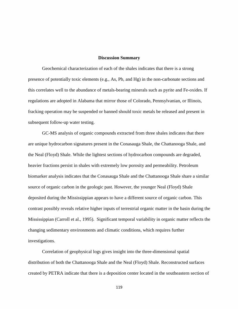
119

Discussion Summary

Geochemical characterization of each of the shales indicates that there is a strong

presence of potentially toxic elements (e.g., As, Pb, and Hg) in the non-carbonate sections and

this correlates well to the abundance of metals-bearing minerals such as pyrite and Fe-oxides. If

regulations are adopted in Alabama that mirror those of Colorado, Pennsylvanian, or Illinois,

fracking operation may be suspended or banned should toxic metals be released and present in

subsequent follow-up water testing.

GC-MS analysis of organic compounds extracted from three shales indicates that there

are unique hydrocarbon signatures present in the Conasauga Shale, the Chattanooga Shale, and

the Neal (Floyd) Shale. While the lightest sections of hydrocarbon compounds are degraded,

heavier fractions persist in shales with extremely low porosity and permeability. Petroleum

biomarker analysis indicates that the Conasauga Shale and the Chattanooga Shale share a similar

source of organic carbon in the geologic past. However, the younger Neal (Floyd) Shale

deposited during the Mississippian appears to have a different source of organic carbon. This

contrast possibly reveals relative higher inputs of terrestrial organic matter in the basin during the

Mississippian (Carroll et al., 1995). Significant temporal variability in organic matter reflects the

changing sedimentary environments and climatic conditions, which requires further

investigations.

Correlation of geophysical logs gives insight into the three-dimensional spatial

distribution of both the Chattanooga Shale and the Neal (Floyd) Shale. Reconstructed surfaces

created by PETRA indicate that there is a deposition center located in the southeastern section of

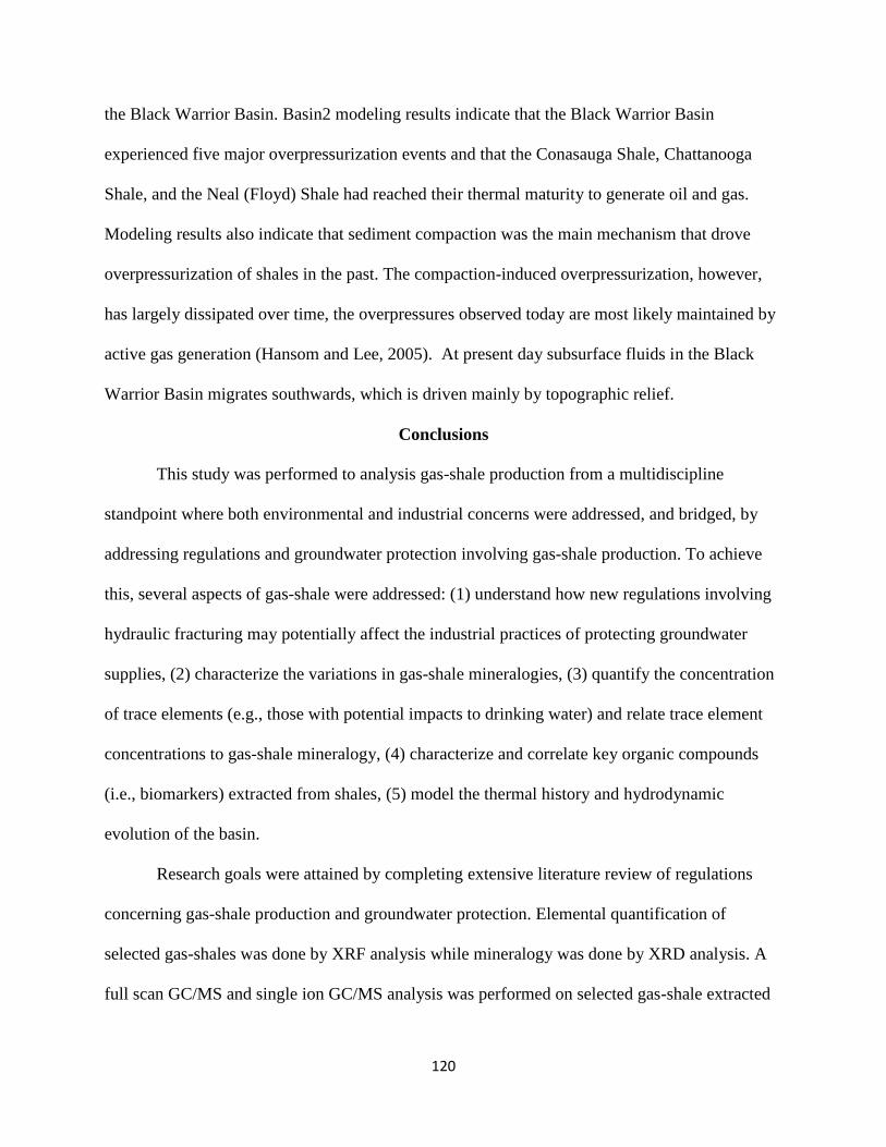
120

the Black Warrior Basin. Basin2 modeling results indicate that the Black Warrior Basin

experienced five major overpressurization events and that the Conasauga Shale, Chattanooga

Shale, and the Neal (Floyd) Shale had reached their thermal maturity to generate oil and gas.

Modeling results also indicate that sediment compaction was the main mechanism that drove

overpressurization of shales in the past. The compaction-induced overpressurization, however,

has largely dissipated over time, the overpressures observed today are most likely maintained by

active gas generation (Hansom and Lee, 2005). At present day subsurface fluids in the Black

Warrior Basin migrates southwards, which is driven mainly by topographic relief.

Conclusions

This study was performed to analysis gas-shale production from a multidiscipline

standpoint where both environmental and industrial concerns were addressed, and bridged, by

addressing regulations and groundwater protection involving gas-shale production. To achieve

this, several aspects of gas-shale were addressed: (1) understand how new regulations involving

hydraulic fracturing may potentially affect the industrial practices of protecting groundwater

supplies, (2) characterize the variations in gas-shale mineralogies, (3) quantify the concentration

of trace elements (e.g., those with potential impacts to drinking water) and relate trace element

concentrations to gas-shale mineralogy, (4) characterize and correlate key organic compounds

(i.e., biomarkers) extracted from shales, (5) model the thermal history and hydrodynamic

evolution of the basin.

Research goals were attained by completing extensive literature review of regulations

concerning gas-shale production and groundwater protection. Elemental quantification of

selected gas-shales was done by XRF analysis while mineralogy was done by XRD analysis. A

full scan GC/MS and single ion GC/MS analysis was performed on selected gas-shale extracted

121

organics providing insight into hydrocarbons present as well as sources of organics. Lastly, the

thermal and hydrodynamic histories of the gas-shales were modeled utilizing Basin2 modeling

software.

Illinois, Pennsylvania, and Colorado, have put forth the most extensive

regulations involving hydraulic fracturing and the protection of USDWs. Each

state requires baseline water testing of chloride, sulfate, arsenic, barium, calcium,

chromium, iron, magnesium, selenium, cadmium, lead, manganese, mercury, and

silver; subsequent follow-up testing is also required at regular time intervals up to

½ mile radius from the wellbore. These regulations will possibly be the standard

adopted by states that have high yield gas-shale production. If these regulations

become standardized throughout the United States it will enable regulatory bodies

to asses a problem and determine the responsible party, if any.

If Alabama gas-shale production increases and similar regulations as those in

Colorado, Pennsylvania, and Illinois are adopted there could be additional

expenditures above business as usual costs due to baseline and follow up water

testing and potential contamination. This is due to the potential release of toxic

trace elements due to the interactions of an oxidizing fluid and hosting geologic

material.

Elemental quantification of the Conasauga Formation, Devonian Shale,

Chattanooga Shale, and Neal (Floyd) Shale resulted in elevated concentrations of

trace elements in each, except in the Conasauga Formation in Shelby County,

which is dominated by carbonate minerals. This would suggest that the

122

Conasauga Formation in Shelby County would pose the least amount of risk of

trace elements contaminating the groundwater.

The Chattanooga Shale in Greene County had the highest lead concentrations

(98.25 ppm) and the Neal (Floyd) Shale in Greene County had the highest arsenic

(20.8 ppm) and mercury (73.42ppm) concentrations. This would suggest that

these two units would have the greatest potential for release of As and Pb if

produced.

Positive correlations exist between iron and arsenic concentrations (R2 = 0.36),

iron and lead concentrations (R2 = 0.36), and sulfur and iron concentrations (R2 =

0.29), implying that the iron- and sulfur-bearing minerals have strong

geochemical affinity to adsorb trace metals onto their surfaces or crystalline

structure. This suggests where ever large amounts of Fe-sulfides are present

elevated concentrations of As and Pb could be expected.

Aluminum enrichment factors of trace elements (i.e., As, Pb, Cu, and Hg) are

very high in all of the shales. The greatest enrichments for arsenic and lead are

found in the Chattanooga Shale in Greene County; the greatest enrichment for

copper is found in the Conasauga Formation in Shelby County; the highest

enrichment factor for mercury is found in the Devonian Shale in Hale County.

Sulfur and Fe enrichment is also very high in each of the shales. This suggests

that S and Fe bearing minerals work as sinks for the toxic trace metals.

The presence of pyrite and iron oxides in each of the shales corresponds with the

abundance of trace elements. The highest concentration of arsenic and lead are

found in shales (i.e., Chattanooga Shale in Greene County and the Neal (Floyd)

123

Shale in Greene County) with the highest sulfide and iron oxide contents. The

Conasauga Formation in Shelby County is dominated by carbonate minerals and

lacks iron sulfide and iron oxide minerals. This corresponds to very low

concentrations of sulfur, iron, as well as concentrations of arsenic and lead.

Analysis of extracted organics from the Conasauga Formation, Chattanooga Shale

in Greene County, and Neal (Floyd) Shale in Pickens County, indicate that

docosenamide hydrocarbon is present in the Conasauga Formation,

Hentraicontanone is present in the Chattanooga Shale, and Tetradecandioic acid,

bis(trimethylsilyl) ester is present in the Neal (Floyd) Shale. This indicates that

hydrocarbons had been generated in the geologic past in each of the shales and

could potentially be production targets.

Full scan GC-MS gas chromatographs indicate that microbial degradation had

occurred mostly to the lightest organic compounds in the geological past.

Biomarker analysis of m/z ratios 191, 217, and 218 indicate that the Conasauga

Formation and the Chattanooga Shale share a similar source of organic carbon

while those in the Neal (Floyd) Shale has a unique source of organic carbon

represent a different source. This is most likely to a significant increase of land

based plants during the Carboniferous.

Biomarkers could be of significant importance if hydrocarbon if fugitive methane

or other fugitive hydrocarbons are reported. This is due to the fingerprinting

capability of biomarkers. It would enable a determination of the origin of that

particular hydrocarbon to be determined by comparing the fugitive hydrocarbon

124

to a potential source. This would enable responsibility to be place, or removed, if

contamination occurs.

Correlations of geophysical gamma ray logs give an insight into the spatial

distribution of these shales as they progress into the Black Warrior Basin. The

major deposition center of the Black Warrior Basin is located at its southern

margin.

Modeling results indicate that the Black Warrior Basin experienced its first

overpressurization event during the deposition of the Knox Formation. During

this time the Conasauga Formation reached the oil window. A second

overpressurization event occurred during the deposition of the Ordovician

Undifferentiated unit. During this time the Conasauga Formation was in the oil

window. A third overpressurization occurred during the deposition of the

Parkwood Formation. During this time the Conasauga Formation fell into the gas

window. The fourth and largest overpressurization event occurred during the

deposition of the thick Pottsville Formation. During this time the Chattanooga

Shale and the Neal (Floyd) Shale fell into the oil window. During the erosion of

the Pottsville Formation the Chattanooga Shale and the Neal (Floyd) Shale fell

into the gas window. A fifth overpressurization event occurred during the

deposition of the Eutaw Formation. During this time the Chattanooga Shale and

the Neal (Floyd) Shale reached the gas window.

The Chattanooga Shale is currently overpressurized. Modeling results indicate

that this is not from sedimentation. This is most likely due to hydrocarbons being

present in the pore spaces of this shale.

125

The Conasauga Formation began oil generation at 505 m.y. (TTI = 15), reached

peak oil generation at 490 m.y. (TTI = 75), and ended oil generation at 480 m.y.

(TTI = 160). At 478 m.y. 100% of possible oil generation in the Conasauga

Formation had occurred. Onset of gas generation (TTI = 1000) occurred at 470

my and reached a TTI of 5000 at 410 m.y. That Chattanooga Shale began oil

generation at 326 m.y. (TTI = 15), reached peak oil generation at 325.5 m.y. (TTI

= 75), and ended oil generation at 325.25 my (TTI = 160). At 324.8 my 100% of

possible oil generation in the Chattanooga Shale had occurred. Onset of gas

generation (TTI = 1000) occurred at 305 m.y. and reached a TTI of 5000 at 148

m.y. The Neal (Floyd) Shale began oil generation at 326 m.y. (TTI = 15), reached

peak oil generation at 325.5 m.y., and ended oil generation at 325 m.y. At 324.8

my 100% of possible oil generation in the Neal (Floyd) Shale had occurred. Onset

of gas generation (TTI = 1000) occurred at 275 m.y. and reached a TTI of 5000 at

40 my.

Thermal maturation modeling data is confirmed with the presence of

hydrocarbons in each of the shales indicating they been thermally mature.

Fluid flow modeled in the geologic past gives insight into the possible migration

pathways of hydrocarbons in the Black Warrior Basin.

Groundwater flow in the Black Warrior was mostly driven by compaction in the

past. At present day the basin tilts to the south and groundwater flow is driven

southward by gravity and topographic relief.

126

References

Alley, B., Beebe, A., Rodgers, J., & Castel, J. (2011) Chemical and physical characterization of

produced waters from conventional and unconventional fossil fuel resources. Chemosphere.,

85, 74-82.

Aunela-Tapola, L., Frandsen, F., & Hasanen, E. (1998) Trace metals emissions from the

Estonian oil shale fired power plant. Fuel Process Technologies., 21, 490-494.

Beaulie, B., & Ramirez, R.E. (2013) Arsenic Remediation Field Study Using a Sulfate Reduction

and Zero-Valent Iron PRB. Groundwater Monitoring and Remediation., 33, 85-94.

Berman, A., & Engelderan, T. (2012). North American Energy Summit, Panel 1. Baker Institute

Energy Forum and PFC Energy. http://www.youtube.com/watch?v=ZKRyq5RubOY

Bethke, C., Lee, M., Quinodoz, H., & Kreiling, W. (1993) Basin Modeling with Basin2: A guide

to using Basin2, B2plot, B2video, and B2view, University of Illinois Hydrogeology program,

1- 225.

Bowker, K.A. (2002) Recent developments of the Barnet Shale play, Fort Worth basin, in B.E.

Law and M. Wilson, eds., Innovative Gas Exploration Concepts Symposium, Rocky

Mountain Association of Geologist and Petroleum Technology Transfer Council, October,

2002, Denver, Colorado, 16.

Bowker, K.A. (2003) Recent development of the Barnett Shale play, Fort Worth Basin, West

Texas Geological Society Bulletin., v 42, 1-11.

Bradley, J., David R. , Naomi J., Mike B., & Williams A (2013). State of Illinois. 98th

General Assembly. Hydraulic Fracturing Regulatory Act. 2013.

Briskin, J., and Stephen Kraemer. (2013) United States. Environmental Protection Agency .

Well Construction/Operation and Subsurface Modeling., Web

Carroll, R. E., Pashin, J. C., & Kugler, R. L. (1995) Burial history and source-rock characteristics

of upper Devonian through Pennsylvanian strata, Black Warrior Basin, Alabama: Alabama

Geological Survey Circular., 187, 1-29.

Cleaves, A.W., & Broussard, M.C. (1980) Chester and Pottsville depositional systems, outcrop

and subsurface, in the Black Warrior basin of Mississippi and Alabama. Gulf Coast

Association of Geological Societies Transactions., 30, 49-60.

Colorado. Colorado Oil and Gas Conservation Commission. (2012)Complete Rules 100-1200

Series.

Coveney, R., & Glascock, M. (1989) A review of the origins of metal-rich Pennsylvanian black

shales, central U.S.A. with an inferred role for basinal brines. Applied Geochemistry., 4,

347-367.

Dale, L., & Fardy, J. (1984) Trace elements partitioning during the retorting of some Australian

oil shales. Environmental Science Technologies., 18, 887-889.

Drever, J. I. (1997) The geochemistry of natural waters surface and groundwater environments

Upper Saddle River, Prentice Hall

Ingraffea. (2010) . Facts on Fracking., Nanticoke, Pennsylvania. Web.

15 Jul 2013. <http://www.youtube.com/watch?v=mSWmXpEkEPg>.

EIA (Energy Information Administration) (2006) U.S. Crude oil, natural gas, and natural gas

http://www.youtube.com/watch?v=ZKRyq5RubOY

127

liquids reserves 2005 annual report., Appendix B, 10,

http://www.eia.doe.gov/oil_gas/natural_gas/data_publications/crude_oil_natural_gas_reserves

/cr.html.

Fisher, K., & Warpinski, N. (2011) Hydraulic fracture-height growth: real data, Paper SPE

145949 presented at the Annual Technical Conference and Exhibition, Denver, Colorado.,

DOI:10.2118/145949-MS.

Groshong, R.H., Jr., Hawkins, W.B.Jr., Pashin, J.C., & Harry, D.L. (2010) Extensional

structures of the Alabama promontory and Black Warrior foreland Basin: Styles and

relationship to the Appalachian fold-thrust belt, in Tollo, R.P., Bartholomew, M.J., Hibbard,

J.P., and Darabinos, P.M., eds., From Rodinia to Pangea: Geological Society of America

Memoir., 206, 579-605.

Hansom, J., & Lee, M.-K.. (2005) Effects of hydrocarbon generation, basal heat flow, and

sediment compaction on overpressure development: A numerical study. Petroleum

Geoscience., 11, 353-360.

Haynes, C.D., Malone, P.G., & Camp, B.S. (2010) Exploration of the shallow Chattanooga

Shale in north central Alabama: Tuscaloosa, Alabama. University of Alabama, college of

Continuing Studies, 2010 International coalbed and Gas-shale Symposium proceedings,

paper., 1015, 1-16.

Jarvie, D.M., Hill, R.J., Ruble, T.E., & Pollastro, R.M. (2007) Unconventional shale-gas

systems: the Mississippian Barnett Shale of north central Texas as one model for thermogenic

shale- gas assessment. AAPG Bulletin., 91, no. 4, 475- 499.

Kao, Y.-H., Wang, S.-W., Maji, S.K., Liu, C.-W., Wang, P.-L., Chang, F.-J., & Liao, C.-M.

(2013) Hydrochemical, Mineralogical and Isotopic Investigation of Arsenic Distribution and

Mobilization in the Guandu Wetland of Taiwan. Journal of Hydrology., 498, 274-286.

Karl, K., & Karl, W, H. (1961) Distribution of elements in some major units of the Earth’s crust.

Geological Society of America Billiton, 72, 175-192.

King, G., 2010, Thirty years of gas shale fracturing: What have we learned? Paper SPE 133456

presented at the SPE Annual Technical Conference and Exhibition, September 19-22, 2010,

Florence, Italy.

King, G., Hale, L., Shuss, J., & Dobkins, T. (2008) Increasing fracture path complexity and

controlling downward fracture growth in the Barnett shale. Paper 119896 presented at the

SPE gas-shale Production Conference, November 16-18, 2008, Fort Worth, Texas.

Kwon, O., Kronenberg, Gangi, A., Johnson, B., &Herbert, B. (2004a) Permeability of illite-

bearing shale: 1. Anisotropy and effects of clay content and loading. Journal of Geophysical

Research .,109, B10205.doi: 10.1029/2004/JB003052.

Kwon, O., Herbert, & Kronenberg, A. (2004b) Permeability of illite-bearing shale: 2. Influence

of fluid chemistry on flow and functionally connected pores. Journal of Geophysical

Research, 109, B10206. DOI: 10.1029/2004B002055.

La Force, M.J., Hansel, C.M., & Fendorf, S. (2000) Arsenic speciation, seasonal transformations,

and co-distribution with iron in a mine waste-influenced palustrine emergent wetland.

Environmental Science Technology., 34, 3937-3943.

Lacombe, S., Sudickey, E., Frape, S., Unger, A. (1995) Influence of leak boreholes on cross-

formational groundwater flow and contaminant transport. Water Resources Research, 31, no

8, 1871-1882.

Lee, M.-K., Saunders, J.A., Wilkin, R.T. & Mohammad, S. (2005) Geochemical modeling of

arsenic speciation and mobilization: Implications for bioremediation, in Advances in Arsenic

http://www.eia.doe.gov/oil_gas/natural_gas/data_publications/crude_oil_natural_gas_reserves/cr.html

http://www.eia.doe.gov/oil_gas/natural_gas/data_publications/crude_oil_natural_gas_reserves/cr.html

128

Research: Integration of Experimental and Observational Studies and Implications for

Mitigation, O’Day et al. (eds.), American Chemical Society Symposium Series., 915,

398-413. Lopatin, V. (1971) Temperature and geologic time as factors in coalification (in Russian),

Akademiia Nauk SSSR Izvestiya Seriy Geologiches-Kaya ., 4, 95-106.

Mandal, S.K., Dey, M., Ganguly, D., Sen, S., & Jana, T.K. (2009) Biogeochemical controls of

arsenic occurrence and mobility in the Indian Sundarban mangrove ecosystem.. Mar.

Pollution Bulletin,. 58, 652-657.

Mandal, S.D., Majumder, N., Chowdhury, C., Ganguly, D., Dey, M., & Jana, T.K.. (2012)

Adsorption kinetic control of As (III andV) mobilization and sequestration by Mangrove

Sediment. Environmental Earth Science., 65, 2027-2036.

Miskimins, J. (2009) The importance of geophysical and petrophysical data intergration for the

hydraulic fracturing of unconventional reservoirs. The Leading Edge, Special Section:

Unconventional Resources and CO2 Monitoring., 844- 849.

Myers T. (2012) Potential Contaminant Pathways from Hydraulically Fractured Shale to

Aquifers. Ground Water., 50, no 6, 872-882.

Natter, M., Keevan, J., Wang, Y.,Keimowitz, A. R., Okeke, B. C., Son, A., & Lee, M. K. (2012)

Level and Degradation of Deep-water Horizon Spilled Oil in Coastal Marsh Sediments and

Pore-Water. Environmental Science Technology., 46, 5744-5755.

Neuzil, C. E. (1994) How permeable are clays and shales. Water Resources Research,. 30, no2,

145-150.

Neuzil, C. (1986) Groundwater flow in low-permeability environments. Water Resources

Research, 22, no 2, 145-150.

Pahin, J.C. (1993) Tectonics, paleoceanography, and paleoclimate of the Kaskaskia sequence in

the Black Warrior basin of Alabama, in Pashin, J.C., ed. New perspectives on the

Mississippian System of Alabama, Alabama Geological Society 30th Annual Field Trip

Guidebook, 1-28.

Pashin, J. C. (1994) Cycles and stacking patterns in Carboniferous rocks of the Black Warrior

foreland Basin. Gulf Coast Association of Geological Societies Transactions., 44, 555-

563.

Pashin, J.C. (2004) Cyclothems of the Black Warrior basin in Alabama: eustatic snapshots of

foreland basin tectonism, in Pashin, J.C., and Gastaldo, R.A., eds., Sequence stratigraphy,

paleclimate, and tectonics of coal-bearing strata, American Association of Petroleum

Geologists Studies in Geology., 51, 199-217.

Pashin, J. C., Kopaska-Merkel, D. C., Arnold, A. C., & McIntyre, M. R. (2011) Geological

foundation for production of natural gas resources from diverse shale formations: Sugarland,

Texas, Research Partnership to Secure Energy for America Final Report 07122.17.01;

Geological Survey of Alabama Open-File Report 1110, 156. Annual Conference and

Exposition, New Orleans, Louisiana.

Pashin, J. C., & Groshong, R.H., Jr. (1998) Structural control of coalbed methane production in

Alabama. International journal of Coal Geology., 38, 89-113.

Pashin, J. C. (2008) Gas shale potential of Alabama, Tuscaloosa, Alabama, University of

Alabama, College of Continuing Studies. 2008 International Coalbed and Gas-shale Symposium

Proceedings., paper 0808, 13.

Pashin, J.C., Gas-shale plays of the sourthern Appalachian thrust belt: Tuscaloosa, Alabama,

University of Alabama, College of Continuing Studies, 2009 International Coalbed and Shale

129

Gas Symposium Proceedings, paper 0907, 14p.

Pashin, J.C., Grace, R.L.B., & Kopaska-Merkel, D.C. (2010) Devonian shale plays in the black

Warrior basin and Appalachian thrust belt of Alabama: Tuscaloosa, Alabama, University of

Alabama, College of Continuing Studies. 2010 International Coalbed and Gas-shale

Symposium Proceedings, paper 1016, 20.

Pennsylvania Department of Environmental Protection (PADEP), 2011, Marcellus Shale,

http://www.dep.state.pa.us/dep/deputate/minres/oilgas/new_forms/marcellus/marcellus.htm

Pennsylvania. Pennsylvania Department of Environmental Protection. (2012) Oil and Gas Title

58.

Perkins, R., Mason, C., & Piper, D. (2012) Mobility of trace elements from the Sunbury Shale,

eastern Kentucky. Mineralogical Magazine, 76, i 6, 2220.

Rheams, K.F., and Neathery, T.L. (1988) Characterization and geochemistry of Devonian oil

shale, north Alabama, northwest Georgia, and south-central Tennessee ( a resource

evaluation). Alabama Geological Survey Bulletin., 128, 214.

Saunders, J.A., Pritchett, M.A., & Cook, R.B. (1997) Geochemistry of biogenic pyrite and

ferromanganese stream coatings: a bacterial connection?. Geomicrobiology, 14, 203-217.

Saunders, J.A., Lee, M.-K., Shamsudduha, M., Dhakal, P., Uddin, A., Chowdury, M.T., &

Ahmed, K.M. (2008) Geochemistry and Mineralogy of Arsenic in (Natural) Anaerobic

Groundwaters. Applied Geochemistry, 23, 3205-3214.

Smedley, P.L., &Kinniburgh, D,G. (2002) A review of the source, behavior and distribution of

arsenic in natural waters. Applied Geochemistry., 17, 517-568.

Smith, A. H., Marshall, G., Liaw, J.,& Ferreccio, C. (2012) Mortality in Young Adults Following

in Utero and Childhood Exposure to Arsenic in Drinking Water. Environmental Health

Perspectives, 120, no 11, 1527 – 1531.

Soeder, D., &Kappel, W., 2009, Water Resources and Natural Gas Production from the

MarcellusShale, USGS fact shee.,t 2009-3032.

Soeder, D. (1988) Porosity and permeability of eastern Devonian gas shale. Society of Petroleum

Engineers Formation Evaluation, Society of Petroleum Engineers, 3, no 2, 116-124. DOI:

10.2118/15213-PA.

Soerensen K., & Cant, N. (1988) The role of catalysis by mineral matter during oil shale

retorting. Fuel., 67, 1344-1348.

Thomas, W. A. (1988) The Black Warrior basin, in Sloss, L.L., ed., Sedimentary cover— North

American Craton. Geological Society of America, The Geology of North America, D-2,

471-492.

Thomas, W. A. (1977) Evolution of Appalachian-Ouachita salient and recesses from reentrants

and promontories in the continental margin. American Journal of Science, 277, 1233-

1278.

Thomas, W. A., and Bayona, G. (2005) The Appalachian thrust belt in Alabama and Georgia:

thrust-belt structure, basement structure, and palinspastic reconstruction. Alabama Geologic

Survey Monograph., 16, 48.

Thomas, W.A. (2001) Mushwad: Ductile duplex in the Appalachian thrust belt in Alabama,

American. Association of Petroleum Geologist Bulletin, 85, 1847-1869.

United States. Environmental Protection Agency. Permitting Guidance for Oil and Gas

Hydraulic Fracturing Activities Using Diesel Fuels –Draft: Underground Injection Control

Program Guidance , <http://cluin.org/live/archive/>.

http://www.dep.state.pa.us/dep/deputate/minres/oilgas/new_forms/marcellus/marcellus.htm

130

U.S. Environmental Protection Agency. (2002)

http://www.epa.gov/osw/hazard/testmethods/pdfs/3570.pdf

Waples, W. (1980) Time and temperature in petroleum formation, application of Lopatin’s

method to petroleum exploration. American Association of Petroleum Geologists Bulletin.,

64, 916-926.

Wang, G., &Carr, T. (2012) Methodology of organic-rich shale lithofacies identification and

prediction: A case study from Marcellus Shale in the Appalachian basin. Computers and

Geosciences, 49, 151-163.

Wang, Z., & Stout, S.A. (2007) Oil Spill Environmental Forensics. Academic Press: New York.

Zhang, T., Ellis, G., Ruppel, S., Milliken, K., & Yang, R. (2012) Effect of organic-matter type

and thermal maturity on methane adsorption in shale-gas systems. Organic Geochemistry.,

47, 120-131.

131

APPENDIX 1. Input file for Basin2 modeling thermal history, overpressurization, and basin

hydrology simulation. Input file describes three basic rock types and their associated hydraulic

properties. Percentages of these particular rock types are then placed at defined thicknesses and

amount at each well location used in the modeled transect. Thermal properties of the basin were

set in this input as well as the boundary conditions of the model. For more detailed instruction of

input parameters see Bethke et al. (1993).

start = -518 m.y.; end = 0 m.y.

nx = 60; dztarg = 800 m

y_LHS = 10 cm; y_RHS = 1 cm

press_increase = 5; temp_increase = 5

initial = steady; compaction = irreversible

tti = $TTI; vitrinite = on; arrhenius = on

tables = TTI

tables = X_oil

rock ss

A_perm = 15.5; B_perm = -5 log_darcy; p_kxkz = 2.5

rock sh

A_perm = 8; B_perm = -8 log_darcy; p_kxkz = 10

rock cn

A_perm = 10; B_perm = -6.5 log_darcy; p_kxkz = 6

rock im

A_perm = 4; B_perm = -9 log_darcy; p_kxkz = 0

end_rock

width = 417485 ft

x_well(ft) 0 29117 105129 157473 198128 217199 289268 417485

left = closed; right = closed

heat_flow = 1.5 HFU;

X_average = geometric, Z_average = harmonic

strat 'Conasuaga Formation'

t_dep = -518 m.y.

column thickness(ft) X(ss) X(sh) X(cn)

w(1:8) 5000 0.0 0.6 0.4

strat 'Knox Group'

t_dep = -505 m.y.


w(1:8) 4000 0.0 0.0 1

strat 'erosion 1'

t_dep = -490 m.y.

column thickness(ft)

w(1:8) -1500

132

strat 'Ordovician undifferentiated'

t_dep = -480 m.y.


w(1) 3500 0.0 0.0 1

w(2) 4000 0.0 0.0 1

w(3) 6000 0.0 0.0 1

w(4) 6000 0.0 0.0 1

w(5) 6000 0.0 0.0 1

w(6) 5500 0.0 0.0 1

w(7) 5500 0.0 0.0 1

w(8) 5500 0.0 0.0 1

strat 'erosion 2'

t_dep = -440 m.y.


w(1:8) -1000

strat 'Silurian undifferentiated'

t_dep = -438 m.y.


w(1:2) 600 0.3 0.2 0.5

w(3:6) 600 0.0 0.0 1

w(7:8) 600 0.0 0.0 1

strat 'erosion 3'

t_dep = -417 m.y.


w(1:8) -200

strat 'Unnamed Devonian carbonate and chert unit'

t_dep = -400 m.y.


w(1) 1000 0.0 0.0 1

w(2) 1050 0.0 0.0 1

w(3) 1075 0.0 0.0 1

w(4) 1075 0.0 0.0 1

w(5) 1500 0.0 0.0 1

w(6) 1500 0.0 0.0 1

w(7) 2000 0.0 0.0 1

w(8) 2200 0.0 0.0 1

strat 'erosion 4'

t_dep = -370 m.y.


w(1:8) -500

strat 'Chattanooga Shale'

t_dep = -365 m.y.


w(1) 40 0.0 1 0.0

w(2) 40 0.0 1 0.0

w(3) 80 0.0 1 0.0

133

w(4) 45 0.0 1 0.0

w(5) 90 0.0 1 0.0

w(6) 90 0.0 1 0.0

w(7) 300 0.0 1 0.0

w(8) 90 0.0 1 0.0

strat 'erosion 5'

t_dep = -360 m.y.


w(1) -30

w(2) -30

w(3) -48

w(4) -30

w(5) -40

w(6) -40

w(7) -100

w(8) -40

strat 'Tuscumbia Limestone and Fort Payne Chert undifferentiated'

t_dep = -354 m.y.


w(1:8) 200 0.0 0.0 1

strat 'Bangor Limestone and Floyd Shale Undifferentiated'

t_dep = -350 m.y.


w(1) 700 0.3 0.5 0.2

w(2) 900 0.2 0.6 0.2

w(3) 1400 0.0 0.8 0.2

w(4) 1600 0.0 0.9 0.1

w(5) 1800 0.0 1 0.0

w(6) 1800 0.0 1 0.0

w(7) 2300 0.0 1 0.0

w(8) 2000 0.0 1 0.0

strat 'Parkwood Formation'

t_dep = -330 m.y.


w(1) 900 0.3 0.4 0.3

w(2) 850 0.3 0.4 0.3

w(3:6) 1000 0.1 0.9 0.0

w(7:8) 1300 0.2 0.8 0.0

strat 'Pottsville Formation'

t_dep = -323 m.y.


w(1) 4000 0.5 0.5 0.0

w(2) 4500 0.4 0.6 0.0

w(3) 5500 0.3 0.7 0.0

w(4) 6500 0.3 0.7 0.0

w(5) 7500 0.2 0.8 0.0

134

w(6) 8500 0.2 0.8 0.0

w(7:8) 9500 0.4 0.6 0.0

strat 'erosion 6'

t_dep = -248 m.y.


w(1:2) -1000

w(3) -1500

w(4:8) -2000

strat 'lower Creataceous undiff'

t_dep = -144 m.y.


w(1:6) 100 1 0 0

w(7:8) 400 0.8 0 0.2

strat 'erosion 7'

t_dep = -120 m.y.


w(1:8) -100

strat 'Coker Formation'

t_dep = -99 m.y.


w(1) 500 0.5 0.5 0

w(2) 650 0.5 0.5 0

w(3) 750 0.6 0.4 0

w(4) 800 0.5 0.5 0

w(5) 900 0.5 0.5 0

w(6) 1000 0.5 0.5 0

w(7) 1100 0.5 0.5 0

w(8) 1200 0.5 0.5 0

strat 'erosion 8'

t_dep = -90 m.y.


w(1:8) -100

strat 'Gordo Formation'

t_dep = -80 m.y.


w(1:2) 300 0.4 0.6 0.0

w(3:8) 500 0.5 0.5 0.0

strat 'erosion 9'

t_dep = -85 m.y.


w(1:8) -100

strat 'Eutaw Formation'

t_dep = -75 m.y.


w(1) 0 0.0 0.0 0.0

w(2) 100 0.5 0.5 0.0

135

w(3) 200 0.5 0.5 0.0

w(4) 300 0.5 0.5 0.0

w(5) 400 0.5 0.5 0.0

w(6) 500 0.5 0.5 0.0

w(7) 600 0.5 0.5 0.0

w(8) 700 0.5 0.5 0.0

strat 'Deposition Hiatus'

t_dep = -65 m.y.


w(1:8) 0

strat 'present day'

t_dep = 0 m.y.

thickness = 0

column water_depth(ft)

w(1) -470

w(2) -369

w(3) -351

w(4) -226

w(5) -242

w(6) -336

w(7) -273

w(8) -175

Characterizing Geological and Geochemical Properties of ...

Documents

Transcript of Characterizing Geological and Geochemical Properties of ...