Genetic-Fuzzy Approach for Modeling ComplexSystems with an Example Application in Masonry Bond

Strength PredictionDylan R. Harp, S.M.ASCE1; Mahmoud Reda Taha, P.Eng., M.ASCE2; and Timothy J. Ross, P.E., F.ASCE3

Abstract: A genetic-fuzzy learning from examples �GFLFE� approach is presented for determining fuzzy rule bases generated frominput/output data sets. The method is less computationally intensive than existing fuzzy rule base learning algorithms as the optimizationvariables are limited to the membership function widths of a single rule, which is equal to the number of input variables to the fuzzy rulebase. This is accomplished by primary width optimization of a fuzzy learning from examples algorithm. The approach is demonstrated bya case study in masonry bond strength prediction. This example is appropriate as theoretical models to predict masonry bond strength arenot available. The GFLFE method is compared to a similar learning method using constrained nonlinear optimization. The writers’ resultsindicate that the use of a genetic optimization strategy as opposed to constrained nonlinear optimization provides significant improvementin the fuzzy rule base as indicated by a reduced fitness �objective� function and reduced root-mean-squared error of an evaluation data set.

DOI: 10.1061/�ASCE�0887-3801�2009�23:3�193�

CE Database subject headings: Fuzzy sets; Bonding; Artificial intelligence; Optimization; Predictions.

Introduction

Civil engineers are often confronted with systems of input/outputdata where the relationships between inputs and output are notwell understood. Often, the physical basis of these relations isunknown or ambiguous. In other cases, the data may be too im-precise, or the complexity might be too large, to extract the rela-tionships in a deterministic way. All too often, the situation is anunknown combination of these factors. In these situations, fuzzyset theory can be used to handle the uncertainty due to modelingambiguity and/or data imprecision. Fuzzy set theory can be usedwhere information in the form of complex relationships betweeninputs and output is extracted into a fuzzy rule base. In order toextract a useful model in the form of a fuzzy rule base from anumerical data set, a method is needed to learn the fuzzy rulebase.

Genetic algorithms have been used to develop fuzzy rule basesas well as to tune existing fuzzy rule bases �Cordón et al. 2004�.The use of genetic algorithms to fully develop a fuzzy rule base,generally called learning, is a challenging task �Ross 2004�.Common approaches for general rule base learning have beenthe Pittsburgh approach �Smith 1980�, the Michigan approach

1Ph.D. Student, Dept. of Civil Engineering, Univ. of New Mexico,MSC01 1070, Albuquerque, NM 87131. E-mail: dharp@unm.edu

2Associate Professor and Regents’ Lecturer, Dept. of Civil Engineer-ing, Univ. of New Mexico, MSC01 1070, Albuquerque, NM 87131.E-mail: mrtaha@unm.edu

3Professor and Regents’ Lecturer, Dept. of Civil Engineering, Univ. ofNew Mexico, MSC01 1070, Albuquerque, NM 87131. E-mail:ross@unm.edu

Note. Discussion open until October 1, 2009. Separate discussionsmust be submitted for individual papers. The manuscript for this paperwas submitted for review and possible publication on October 16, 2007;approved on November 14, 2008. This paper is part of the Journal ofComputing in Civil Engineering, Vol. 23, No. 3, May 1, 2009. ©ASCE,

ISSN 0887-3801/2009/3-193–199/$25.00.

JOURNAL OF CO

Downloaded 11 May 2009 to 64.106.42.43. Redistribution subject to

�Holland and Reitman 1978�, and iterative rule learning �Ven-turini 1993�. The Michigan approach and iterative rule learningmethods encode each rule as a chromosome, whereas in the Pitts-burgh approach, an entire set of rules is encoded in a single chro-mosome �Castro and Camargo 2004�. In this way, the Michiganapproach and iterative rule learning are more computationally ef-ficient, however they have the disadvantage that the individualrules are pitted against each other for survival to the next genera-tion �Castro and Camargo 2004�. In the Pittsburgh approach, apopulation of rule bases compete for survival, thereby allowingthe collective synergism of the rules within a rule base to influ-ence the fitness of a particular rule base �Castro and Camargo2004�. The drawback of the Pittsburgh approach is the computa-tional effort required to handle the complexity of chromosomeevolution.

Tuning an existing fuzzy rule base entails optimizing the mem-bership function parameters of the rule base. But tuning may alsorefer to adjusting the functions used to scale the input and outputvariables �Cordón et al. 2004; Jang et al. 1997�. Although theprocess of tuning an existing rule base is in general less compli-cated than learning a rule base, the optimization can be compli-cated by the number of membership function parameters in therule base. The disadvantage of tuning an existing rule base is thatthe search will be limited to solutions possessing the prespecifiedstructure. Learning algorithms, such as the one presented here, donot have this limitation as the structure is not prespecified, butderived from the training data.

A methodology is presented here that allows the automaticextraction of the relationships between the input and output into afuzzy rule base. The proposed method employs a genetic algo-rithm to optimize a modified learning from example approachafter Passino and Yurkovich 1998 �referred to in general as fuzzylearning from examples �FLFE��. The novelty of the proposedmethod lies in its ability to significantly enhance the learningprocess by solely optimizing the parameters of the first rule de-

veloped by the FLFE algorithm. Existing learning algorithms that

MPUTING IN CIVIL ENGINEERING © ASCE / MAY/JUNE 2009 / 193

ASCE license or copyright; see http://pubs.asce.org/copyright

optimize an entire fuzzy rule base will be computationally moreexpensive.

The membership function widths for the first rule developedby the FLFE approach are differentiated from the subsequentmembership function widths by the terms primary widths andsecondary widths, respectively. This categorization is useful asthe determination of the primary and secondary widths differ dur-ing the development of the fuzzy rule base using FLFE. Theprimary widths must be specified to initiate the FLFE method,whereas the secondary widths are determined by the method itselfto allow overlap of adjacent membership functions �MFs� using aprespecified weighting factor �Ross 2004�. Varying the primarywidths supplied to the FLFE method will alter the resulting rulebase. Primary width optimization exploits this property by deter-mining the most appropriate primary widths for the FLFEmethod.

The initialized rule base can be fine-tuned by adjusting theoutput membership function centers using a recursive least-squares method �Ross 2004�. A more complete fine-tuning of thealgorithm is possible using the gradient method �Ross 2004�,where all membership function centers and widths are tuned. Ge-netic FLFE �GFLFE� couples the computational efficiency of pri-mary width optimization of the FLFE method and recursive least-squares method with a global search strategy able to traverse thecomplicated fitness landscape of this optimization.

To illustrate the proposed methodology, a sample civil engi-neering application is presented. The application extracts a fuzzyrule base to model the flexural bond strength of masonry. Al-though experimental research has indicated correlations betweenseveral input variables and flexural bond strength of masonry, thecomplex interactions of these various input variables are not wellknown �Sugo 2000�. The results of a sensitivity analysis by RedaTaha et al. �2005� are utilized to select the most influential param-eters for modeling flexural bond strength of masonry such asbrick strength, absorption, sorptivity index, cement content, andrelative humidity. This application presents a case where the lackof knowledge about the complex interaction between input andoutput, or modeling ambiguity, can be dealt with by automaticallyextracting the relationships from the data into a fuzzy rule base.

Methods

The following sections describe the rule base structure, discussthe FLFE method used for learning physical phenomenon, presentthe GFLFE approach to primary width optimization, and discussthe constrained nonlinear optimization method.

Rule Base Structure

The knowledge rule base is comprised of a collection of if–thenrules where the rules are in the form of a premise clause and anassociated consequence. This can be considered a Mamdami sys-tem of deductive inference where the fuzzy linguistic terms havebeen replaced with fuzzy values �Ross 2004�. Here, the writersassume Gaussian MFs for the inputs described as

��x� = exp�−1

2� x − c

��2� �1�

where x=input variable; c=center of the membership function;and �=relative width of the membership function �Ross 2004�. Itis important to note that the choice of Gaussian MFs does not

imply the use of probabilistic distributions, but were chosen as

194 / JOURNAL OF COMPUTING IN CIVIL ENGINEERING © ASCE / MAY/J

Downloaded 11 May 2009 to 64.106.42.43. Redistribution subject to

these MFs can be described by a single continuous equation.Delta functions have been used for the output MFs. Other MFtypes can be used for input and output MFs without greatly influ-encing the proposed method. The proposed method implementsthe center-average defuzzification method.

The fuzzy knowledge rule base implements a product t-normfor the premise as

�i�x� = �j=1

n �−1

2exp� xj − cj

i

� ji �2� �2�

where �i�x�=membership value of the input data-tuple x in theith rule, cj

i and � ji =center and width for the jth input of the ith

rule, respectively, and n=number of inputs �Ross 2004�. Alongwith center-average defuzzification, product implication is usedfor the output as

f�x��� =i=1

R bi�i�x�i=1

R �i�x��3�

where �=matrix that contains the rule-base parameters ci, �i, andbi, where bi defines the delta function for the output of the ithrule, and R=number of rules in the rule base. By substituting Eq.�2� into Eq. �3�, the output of the rule base can be explicitlydescribed by the rule-base parameters; c, �, and b, as

f�x��� =

i=1

R

bi�j=1

n �−1

2exp� xj − cj

i

� ji �2�

i=1

R

�j=1

n �−1

2exp� xj − cj

i

� ji �2� �4�

Eq. �4� is the numerical equivalent of a collection of R fuzzy ruleswhich employ Gaussian input �antecedent� MFs and delta func-tion output �consequent� MFs with center average defuzzification.

Automated Fuzzy Learning

Similar to most fuzzy rule-base development methods, a collec-tion of training data-tuples are required. The training data areseparated into initialization and optimization data. The initializa-tion data are processed into a first approximation of the rule baseusing the FLFE method.

The writers start by assigning the values of the inputs for thefirst data-tuple in the initialization data set to the centers of theinput MFs and the associated output value to the delta functiondescribing the output membership function for the first rule. Thisleaves the designation of the input membership function widths tofully describe the first rule. As there is no way to extract thevalues of these widths directly from the data, optimization can beused to appropriately determine these values. This is the basis ofprimary width optimization, and these are the MF widths intro-duced previously as primary widths.

The proposed method then iterates through the remaining data-tuples in the initialization data set, determining that a new rule isnecessary when the following inequality is violated:

� f � �f�x��� − y� �5�

where � f =specified test factor; f�x ���=fuzzy rule base output de-scribed by Eq. �4�; and y=measured output for the current data-tuple. If inequality �5� is violated, a new rule is created byassigning the inputs of the current data-tuple to the centers of theinput MFs and the output of the current data-tuple to the delta

function for the output membership function for the new rule. The

UNE 2009

ASCE license or copyright; see http://pubs.asce.org/copyright

membership function widths for each new rule, introduced as sec-ondary widths previously, are calculated to allow for the overlapof adjacent MFs specified by the weighting factor w as

�s =1

w�c − cmin� �6�

where c=center of the membership function in question, andcmin=nearest existing center to c �Ross 2004�. It is in this way thatthe FLFE method is able to derive all MF parameters, except forthe primary widths, directly from the training data. Once the al-gorithm has iterated through the initialization data set, the initial-ized rule base is passed to a recursive least-squares method inorder to fine-tune the output membership functions �Passino andYurkovich 1998�.

Genetic-Fuzzy Learning from Examples „GFLFE…

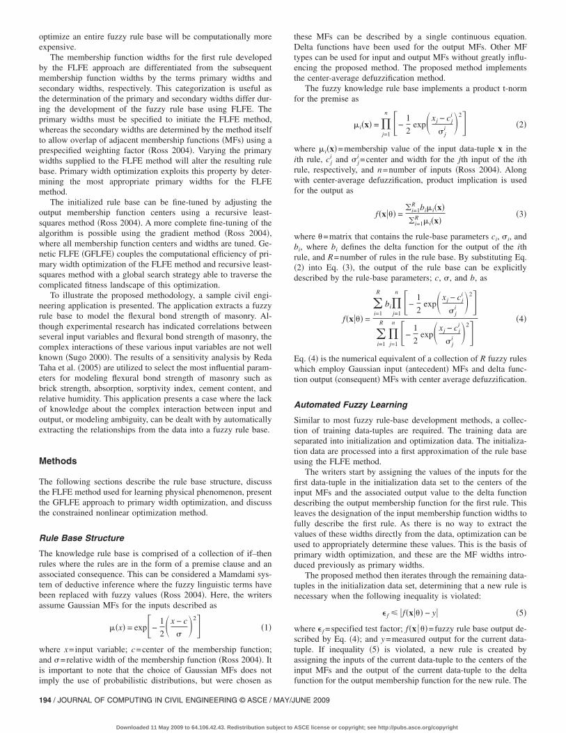
Fig. 1 presents a diagram of the primary width optimizationmethod for fuzzy rule base development described below. Thefitness function �referred to as the objective function in the con-strained nonlinear case� is defined as

min��B

� 1

mk=1

m

�f�xk��� − yk�2�0.5

�7�

where �=vector containing the primary widths constrained by B;m=number of data-tuples in the optimization data set; f�xk ���=fuzzy rule base output for the kth data-tuple xk of the optimiza-tion data set; and yk=kth measured output in the optimization dataset. The use of a designated optimization data set as opposed toreusing the initialization data set ensures that the fuzzy rule baseis not overtrained. Overtraining or overfitting tends to producesystems with limited ability to generalize the phenomenon being

TrainingData

OptimizationData

InitializationData

Fuzzy LearningFrom Examples

Method

Recursive LeastSquaresMethod

Calculateobjectivefunction

Convergence?

No

FuzzyRule BaseYes

Update primarywidths

Fig. 1. Primary width optimization flow diagram

learned �Haykin 1998�. By substituting Eq. �4� into Eq. �7�, the

JOURNAL OF CO

Downloaded 11 May 2009 to 64.106.42.43. Redistribution subject to

primary widths �� j1 , j=1, . . . ,n� can be expressed explicitly in the

fitness function as

min��B 1

mk=1

m ��i=1

R

bi�j=1

n �−1

2exp� xk,j − cj

i

� ji �2�

i=1

R

�j=1

n �−1

2exp� xk,j − cj

i

� ji �2� � − yk�

2

0.5

�8�

where xk,j = jth input of the kth data-tuple of the optimization dataset. It is important to note that primary width optimization is notsimply the minimization of Eq. �8� by varying the primary widths.The optimization also includes the FLFE learning algorithm,which, given different values of primary widths, will alter the restof the rule base further by influencing the selection of rules andaltering the secondary widths �� j

i, j=1, . . . ,n i=2, . . . ,R� and out-put membership function centers �bi , i=1, . . . ,R�, as described inthis paper.

A binary genetic algorithm is used in this research, where apopulation of possible solutions is converted to binary form forimplementation of the genetic algorithm �Haupt and Haupt 2004�.The population of possible solutions corresponds to a collectionof alternative sets of primary widths. The fitness of these solu-tions within the population is determined using the fitness func-tion �Eq. �8��. A stochastic uniform selection method is employed,where parents are laid out along a line where their length is pro-portional to their scaled length based on their fitness. The algo-rithm moves along the line in equal steps, selecting the parent itlands on at each step. Crossover is performed using a randombinary vector, where a value of zero indicates the gene from oneparent is passed to the offspring, whereas a one indicates the gene

Table 1. Mixed Proportions by Volume of the Four Masonry MortarsUsed in the Experimental Program

Mortargroup

Portlandcement

Hydratedlime

Fly ashtype �F� Sand

A 1 0.5 0 4.5

B 1 1 0 6

C 0.8 0.4 0.3 4.5

D 0.8 0.8 0.4 6

0 20 40 60 80 100 120 140 160 180 200 2200

5,000

10,000

15,000

20,000

Population size

Fun

ctio

nev

alua

tions

Fig. 2. Function �learning algorithm� evaluations versus genetic al-gorithm population size. The number of function evaluations neces-sary to reduce the fitness function below 0.13 MPa is determined20 times at each population size from 20 to 200 at increments of 20.The stars connected by a dotted line represent the mean number offunction evaluations, whereas the error bars indicate the standarddeviation about the mean at each population size.

MPUTING IN CIVIL ENGINEERING © ASCE / MAY/JUNE 2009 / 195

ASCE license or copyright; see http://pubs.asce.org/copyright

from the other parent is passed to the offspring. The number ofoffspring derived from crossover at each generation is set to 80%.Mutation is performed by selecting a random number from aGaussian distribution with an initial variance equal to two timesthe length of the range of the variable, specified by the upper andlower bounds. The variance was decreased linearly until itreached zero at the last generation. A single optimal solution,known as an elite, is guaranteed to survive each generation. Thesemethods emulate natural selection and are designed to allow op-timal solutions to evolve �Haupt and Haupt 2004�.

The initial population used in the optimization was createdusing a uniform distribution of values, where the values wererestricted to provide realistic membership function widths andnumerical stability. A parametric study to identify genetic algo-rithm �GA� population size was performed. This parametricanalysis is presented in Fig. 2, where the number of functionevaluations necessary to reduce the fitness function below a des-ignated value is evaluated 20 times for each population size from20 to 200 at increments of 20. By inspecting Fig. 2, it is apparentthat a reduced number of function evaluations and standard de-viation are achieved at a population size of 120, without signifi-cant improvements at larger population sizes. Therefore, apopulation size of 120 was selected for the GA optimization pro-cess. Similar results were obtained from a parametric study ofpopulation size for a bare-soil evaporation case study �not pre-sented here�, however, it is not verified that these results willapply to all case studies.

Primary widths outside of the prescribed range are discour-aged in successive generations by penalizing the fitness function

Table 2. Brick Types and Properties

Groupdesignation

Compressivestrength�MPa�

IRA�kg /m2 /min�a

Totalabsorption

�%�Sorptivity

index

1 43.9 3.67 8.11 2,347

2 38.5 6.55 7.98 5,781

3 59.2 2.40 8.32 1,465

4 72.0 2.28 6.70 1,216aIRA=initial rate of absorption.

Table 3. Bond Strength �MPa� for All Brick and Mortar Types

Mortarmix

Age�days�

1

Wet Dry Wet

A 28 0.59 0.47 0.37

180 1.42 1.16 0.72

360 1.19 0.94 0.72

B 28 0.67 0.86 0.43

180 1.16 0.94 0.89

360 1.2 0.95 1.01

C 28 0.63 0.62 0.42

180 0.88 0.66 0.7

360 0.96 0.75 0.81

D 28 0.48 0.59 0.34

180 0.87 0.65 0.42

360 0.88 0.67 0.53

196 / JOURNAL OF COMPUTING IN CIVIL ENGINEERING © ASCE / MAY/J

Downloaded 11 May 2009 to 64.106.42.43. Redistribution subject to

�Eq. �8��. The number of generations was set to 150 as this ap-peared to enable the optimization process to converge to a stablesolution.

Constrained Nonlinear Optimization

The GFLFE method is compared to a similar learning approachusing constrained nonlinear optimization �CNO� proposed by twoof the writers previously �Harp et al. 2007�. The two methods aresimilar in that both learning methods attempt to develop optimalknowledge rule bases by primary width optimization. This com-parison demonstrates the necessity of using a global optimizationstrategy as indicated by the improved performance of the GFLFEmethod. Primary width optimization by constrained nonlinear op-timization is performed here using sequential quadratic program-ming �SQP�. The SQP method closely mimics the Newtonmethod for constrained optimization. As the calculation of exact

Brick type

3 4

Dry Wet Dry Wet Dry

0.35 0.39 0.46 0.48 0.45

0.6 0.071 0.59 1.06 0.68

0.6 0.71 0.59 0.97 0.67

0.43 0.39 0.34 0.6 0.5

0.49 0.72 0.4 0.97 0.64

0.55 0.78 0.38 0.99 0.69

0.36 0.44 0.33 0.59 0.51

0.39 0.76 0.38 0.78 0.7

0.42 0.78 0.45 0.82 0.68

0.26 0.38 0.32 0.58 0.47

0.38 0.57 0.51 0.86 0.58

0.36 0.61 0.47 0.88 0.58

CNO GA0.10

0.11

0.12

0.13

0.14

0.15

0.16

Fitn

ess

(obj

ectiv

e)fu

nctio

n(M

Pa)

Primary width optimization strategy

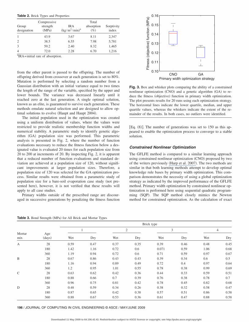
Fig. 3. Box and whisker plots comparing the ability of a constrainednonlinear optimization �CNO� and a genetic algorithm �GA� to re-duce the fitness �objective� function in primary width optimization.The plot presents results for 20 runs using each optimization strategy.The horizontal lines indicate the lower quartile, median, and upperquartile values, whereas the whiskers indicate the extent of the re-mainder of the results. In both cases, no outliers were identified.

2

UNE 2009

ASCE license or copyright; see http://pubs.asce.org/copyright

derivatives is not possible given the nature of the optimization,quasi-Newton methods must be used to approximate their values.A quasi-Newton updating method is used at each major iterationto approximate the Hessian, or second derivatives, of the La-grangian function �L�x ,��� �Nocedal and Wright 1999� defined as

L�x,�� = f�x� − �ici�x� − ¯ − �ncn�x� �9�

where f�x�=objective function; ci= ith constraint placed on theoptimization; �i= ith Lagrange multiplier; and n=number of con-straints. This approximation is used to generate a quadratic pro-gramming subproblem that is used to form a search direction fora line search procedure.

Case Study

The case study involves the evaluation of masonry bond strengthby testing masonry prisms made of four types of mortar and four

Table 4. Optimized Primary Widths

Optimizationstrategy

Cementvolume

Masonryage

�days�

Constrained nonlinear 0.0249 67.15

GFLFE 0.0611 114.6

0.8 0.85 0.9 0.95 10

0.5

1

Portland cement volume

µ(x 1)

0.2 0.3 0.4 0.5 0.6 0.7 0.8 0.9 10

0.5

1

Curing index

µ(x 3)

6.8 7 7.2 7.4 7.6 7.8 8 8.20

0.5

1

Total absorption, %

µ(x 5)

0.2 0.4 0.6 0.80

0.5

1

Bond stren

µ(x)

Fig. 4. Input and outpu

JOURNAL OF CO

Downloaded 11 May 2009 to 64.106.42.43. Redistribution subject to

types of brick units under two curing regimes. The masonryprisms were tested at three ages up to a year creating an ex-perimental database of 96 data tuples. Table 1 presents the mixproportions of four masonry mortars used in the experiments,whereas Table 2 presents the properties of the brick units.Twenty-four, five-high stack bonded prisms were constructedfrom each mortar type and brick unit. Each mix was tested atdry �20% relative humidity �RH�� and moist �100% RH� airingconditions at 20°C. Four prisms were tested from each curingcondition at 28, 180, and 360 days of age. The masonry bondstrength was examined using a bond wrench test apparatus asdesigned by Shrive and Tillemann �1992�. The top half of thebrick is gripped between two neoprene pads in a clamp and atorque wrench is attached to the clamp such that the center-line ofthe torque wrench arm is centered over the brick. The methodcomplies with the requirements of ASTM C1072-94 �1994�.Table 3 presents the bond strength database. Six input parameterswere selected based on a ranking of significance performed by

ngx

Compressivestrength�MPa�

Totalabsorption

�%�Sorptivity

index

0 13.35 0.562 1826

6 13.00 0.582 1678

50 100 150 200 250 300 3500

0.5

1

Masonry age, days

µ(x 2)

40 45 50 55 60 65 700

0.5

1

Compressive strength, MPa

µ(x 4)

1500 2000 2500 3000 3500 4000 4500 5000 55000

0.5

1

Sorptivity index

µ(x 6)

1.2 1.4 1.6a

developed by GFLFE

Curiinde

0.32

0.09

1gth, MP

t MFs

MPUTING IN CIVIL ENGINEERING © ASCE / MAY/JUNE 2009 / 197

ASCE license or copyright; see http://pubs.asce.org/copyright

Reda Taha et al. �2005�. These include: Portland cement volume,masonry age, curing index, compressive strength, total absorp-tion, and sorptivity.

Results and Discussion

A comparison of the performance of constrained nonlinear andgenetic optimization strategies in primary width optimization ispresented. The comparison includes the results of 20 sequentialoptimization runs using each strategy starting from random initialvalues. A training data set of 72 data-tuples is separated into aninitialization data set �48 data-tuples� and an optimization data set�24 data-tuples�. The resulting objective function values �althoughfitness value would be more appropriate for the genetic algorithmcase, objective function value will be used here for both the CNOapproach and GFLFE method, as the fitness and objective func-tions are equivalent here� are presented in box and whisker plotsin Fig. 3, where the horizontal lines indicate the lower quartile,median, and upper quartile of the objective function values andthe whiskers indicate the extent of the remaining values. It isapparent in Fig. 3 that the GFLFE method produces lower objec-tive function values. The GFLFE method runs result in a meanfitness value of 0.121 MPa with a standard deviation of 0.0072,whereas the CNO approach results in a mean of 0.138 with astandard deviation of 0.0073. This indicates a decrease of over12% in the fitness value using the GFLFE method with nearlyequivalent standard deviation. The average run time on a2.80 GHz processor for the GFLFE method is 9.88 min with astandard deviation of 0.86 min, whereas the average for the con-strained nonlinear optimization is 0.40 min with a standard ofdeviation of 0.28 min. Although this indicates that GFLFE runtime was longer than that of the CNO approach, it is important torealize that the CNO approach clearly converged to suboptimalsolutions. The relatively long run time for the GFLFE approach isexpected as the method relies on the evolution of optimal solu-tions, as opposed to a gradient-based search utilized by the CNOapproach. The advantage of the evolutionary approach is the abil-ity to escape local minima providing a strategy for locating glo-bally optimal solutions for complex objective functions.

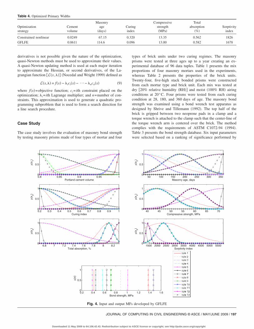
Table 4 presents the optimized primary widths for the run withthe lowest objective function value for both optimization strate-gies. It is apparent that there are significant differences in theoptimized primary widths for the two cases. This is an indicationof the difficulty of primary width optimization, providing supportfor the use of a global search strategy by GA as opposed to a localsearch strategy by CNO. The input and output MFs correspondingto the GFLFE primary widths presented in Table 4 are presentedin Fig. 4. Thirteen rules have been developed during the learningalgorithm resulting in an efficiency quotient �number of trainingdata-tuples/number of rules� of greater than 5.5.

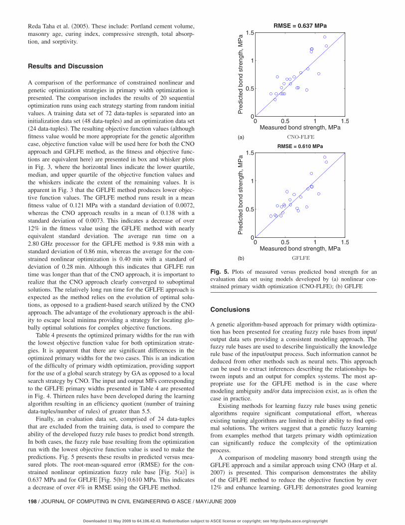
Finally, an evaluation data set, comprised of 24 data-tuplesthat are excluded from the training data, is used to compare theability of the developed fuzzy rule bases to predict bond strength.In both cases, the fuzzy rule base resulting from the optimizationrun with the lowest objective function value is used to make thepredictions. Fig. 5 presents these results in predicted versus mea-sured plots. The root-mean-squared error �RMSE� for the con-strained nonlinear optimization fuzzy rule base �Fig. 5�a�� is0.637 MPa and for GFLFE �Fig. 5�b�� 0.610 MPa. This indicates

a decrease of over 4% in RMSE using the GFLFE method.

198 / JOURNAL OF COMPUTING IN CIVIL ENGINEERING © ASCE / MAY/J

Downloaded 11 May 2009 to 64.106.42.43. Redistribution subject to

Conclusions

A genetic algorithm-based approach for primary width optimiza-tion has been presented for creating fuzzy rule bases from input/output data sets providing a consistent modeling approach. Thefuzzy rule bases are used to describe linguistically the knowledgerule base of the input/output process. Such information cannot bededuced from other methods such as neural nets. This approachcan be used to extract inferences describing the relationships be-tween inputs and an output for complex systems. The most ap-propriate use for the GFLFE method is in the case wheremodeling ambiguity and/or data imprecision exist, as is often thecase in practice.

Existing methods for learning fuzzy rule bases using geneticalgorithms require significant computational effort, whereasexisting tuning algorithms are limited in their ability to find opti-mal solutions. The writers suggest that a genetic fuzzy learningfrom examples method that targets primary width optimizationcan significantly reduce the complexity of the optimizationprocess.

A comparison of modeling masonry bond strength using theGFLFE approach and a similar approach using CNO �Harp et al.2007� is presented. This comparison demonstrates the abilityof the GFLFE method to reduce the objective function by over

0 0.5 1 1.50

0.5

1

1.5

Measured bond strength, MPa

Pre

dict

edbo

ndst

reng

th,M

Pa

RMSE = 0.637 MPa

(a) CNO-FLFE

0 0.5 1 1.50

0.5

1

1.5

Measured bond strength, MPaP

redi

cted

bond

stre

ngth

,MP

a

RMSE = 0.610 MPa

(b) GFLFE

(a)

(b)

Fig. 5. Plots of measured versus predicted bond strength for anevaluation data set using models developed by �a� nonlinear con-strained primary width optimization �CNO-FLFE�; �b� GFLFE

12% and enhance learning. GFLFE demonstrates good learning

UNE 2009

ASCE license or copyright; see http://pubs.asce.org/copyright

efficiency for the case study with an efficiency quotient ofover 5.5. Although the increase in run time for the GFLFEmethod is significant, it is proposed that the additional computa-tional effort is justified in most modeling scenarios given the im-provements in the rule base resulting in increased predictionaccuracy.

Acknowledgments

The first writer was supported by Los Alamos National Labora-tory as a graduate research assistant. The writers greatly appreci-ate this support.

References

ASTM. �1994�. “Standard specifications for standard test method formeasurement of masonry flexural bond strength.” C1072-94, Philadel-phia.

Castro, P. A., and Camargo, H. A. �2004�. “Learning and optimization of

fuzzy rule base by means of self-adaptive genetic algorithm.” Proc.,

IEEE Int. Conf. on Fuzzy Systems, Vol. 2, Budapest, Hungary,1037–1042.

Cordón, O., Gomide, F., Herrera, F., Hoffman, F., and Magdalena, L.�2004�. “Ten years of genetic fuzzy systems: Current framework andnew trends.” Fuzzy Sets Syst., 141�1�, 5–31.

Harp, D., Reda Taha, M., Stormont, J., Farfan, E., and Coonrod, J.�2007�. “An evaporation estimation model using optimized fuzzylearning from example algorithm with an application to the riparian

JOURNAL OF CO

Downloaded 11 May 2009 to 64.106.42.43. Redistribution subject to

zone of the Middle Rio Grande in New Mexico, U.S.A.” Ecol. Mod-ell., 208�2�, 119–128.

Haupt, R., and Haupt, S. �2004�. Practical genetic algorithms, 2nd Ed.,Wiley, Hoboken, N.J.

Haykin, S. �1998�. Neural networks: A comprehensive foundation,Prentice-Hall, Englewood Cliffs, N.J.

Holland, J., and Reitman, J. �1978�. “Cognitive systems based on adap-tive algorithms.” Pattern-directed inference systems, D. A. Watermanand F. Hayes-Roth, eds., Academic, New York.

Jang, J., Sun, C., and Mizutani, E. �1997�. Neuro-fuzzy and soft comput-ing, a computational approach to learning and machine intelligence,Prentice-Hall, Englewood Cliffs, N.J.

Nocedal, J., and Wright, S. �1999�. Numerical optimization, Springer,New York.

Passino, K., and Yurkovich, S. �1998�. Fuzzy control, Addison WesleyLongman, Menlo Park, Calif.

Reda Taha, M., Lucero, J., and Ross, T. �2005�. “Examining the signifi-cance of mortar and brick unit properties on masonry bond strengthusing Bayesian model screening.” Proc., 10th Canadian Masonry

Symp., Vol. 1, Banff, Canada, 112–122.Ross, T. �2004�. Fuzzy logic with engineering applications, 2nd Ed.,

Wiley, West Sussex, U.K.Shrive, N., and Tillemann, D. �1992�. “A simple apparatus and method

for measuring on-site flexural bond strength.” Proc., 6th Canadian

Masonry Sympos., Saskatoon, Canada, 283–294.Smith, S. �1980�. “A learning system based on genetic adaptive systems.”

Ph.D. dissertation, Univ. of Pittsburgh, Pittsburgh.Sugo, H. �2000�. “Strength and microstructural characteristics of brick/

mortar bond.” Ph.D. dissertation, Univ. of Newcastle, New Castle,Australia.

Venturini, G. �1993�. “Sia: A supervised inductive algorithm with geneticsearch for learning attribute based concepts.” European Conf. on Ma-

chine Learning, Vol. 667, P. Brazdil, ed., Vienna, Austria, 280–296.

MPUTING IN CIVIL ENGINEERING © ASCE / MAY/JUNE 2009 / 199

ASCE license or copyright; see http://pubs.asce.org/copyright