Report to the 2015 Hawai'i State Legislature Lead By Example
Upload
khangminh22Category
view
1download
0

Maple by Example
Third Edition

This Page Intentionally Left Blank

Maple by Example
Third Edition
Martha L. Abell and James P. Braselton
Amsterdam Boston Heidelberg London New York OxfordParis San Diego San Francisco Singapore Sydney Tokyo

Senior Acquisition Editor Barbara HollandProject Manager Brandy LillyAssociate Editor Tom SingerMarketing Manager Linda BeattieCover Design Eric DeCiccoComposition CephaCover Printer Phoenix ColorInterior Printer Maple Vail Book Manufacturing Group
Elsevier Academic Press30 Corporate Drive, Suite 400, Burlington, MA 01803, USA525 B Street, Suite 1900, San Diego, California 92101-4495, USA84 Theobald’s Road, London WC1X 8RR, UK
This book is printed on acid-free paper.
Copyright © 2005, Elsevier Inc. All rights reserved.
No part of this publication may be reproduced or transmitted in any form or by anymeans, electronic or mechanical, including photocopy, recording, or any informationstorage and retrieval system, without permission in writing from the publisher.
Permissions may be sought directly from Elsevier’s Science & Technology RightsDepartment in Oxford, UK: phone: (+44) 1865 843830, fax: (+44) 1865 853333, e-mail:[email protected]. You may also complete your request on-line via the Elsevierhomepage (http://elsevier.com), by selecting “Customer Support” and then “ObtainingPermissions.”
Library of Congress Cataloging-in-Publication DataApplication submitted
British Library Cataloguing in Publication DataA catalogue record for this book is available from the British Library
ISBN: 0-12-088526-3
For all information on all Elsevier Academic Press Publicationsvisit our Web site at www.books.elsevier.com
PRINTED IN THE UNITED STATES OF AMERICA05 06 07 08 09 10 9 8 7 6 5 4 3 2 1

Contents
Preface ix
1 Getting Started 1
1.1 Introduction to Maple . . . . . . . . . . . . . . . . . . . . . . . . 1A Note Regarding Different Versions of Maple . . . . . . . . . . . 21.1.1 Getting Started with Maple . . . . . . . . . . . . . . . . . 3Preview . . . . . . . . . . . . . . . . . . . . . . . . . . . . . . . . 7
1.2 Loading Packages . . . . . . . . . . . . . . . . . . . . . . . . . . . 8
1.3 Getting Help from Maple . . . . . . . . . . . . . . . . . . . . . . . 11Maple Help . . . . . . . . . . . . . . . . . . . . . . . . . . . . . . 13The Maple Menu . . . . . . . . . . . . . . . . . . . . . . . . . . . 15
2 Basic Operations on Numbers, Expressions, and Functions 19
2.1 Numerical Calculations and Built-In Functions . . . . . . . . . . . 192.1.1 Numerical Calculations . . . . . . . . . . . . . . . . . . . 192.1.2 Built-In Constants . . . . . . . . . . . . . . . . . . . . . . 222.1.3 Built-In Functions . . . . . . . . . . . . . . . . . . . . . . 23A Word of Caution . . . . . . . . . . . . . . . . . . . . . . . . . . 26
2.2 Expressions and Functions: Elementary Algebra . . . . . . . . . . 272.2.1 Basic Algebraic Operations on Expressions . . . . . . . . . 272.2.2 Naming and Evaluating Expressions . . . . . . . . . . . . 31Two Words of Caution . . . . . . . . . . . . . . . . . . . . . . . . 332.2.3 Defining and Evaluating Functions . . . . . . . . . . . . . 33
2.3 Graphing Functions, Expressions, and Equations . . . . . . . . . . 402.3.1 Functions of a Single Variable . . . . . . . . . . . . . . . . 402.3.2 Parametric and Polar Plots in Two Dimensions . . . . . . 51
v

vi Contents
2.3.3 Three-Dimensional and Contour Plots; GraphingEquations . . . . . . . . . . . . . . . . . . . . . . . . . . . 57
2.3.4 Parametric Curves and Surfaces in Space . . . . . . . . . . 66
2.4 Solving Equations and Inequalities . . . . . . . . . . . . . . . . . 732.4.1 Exact Solutions of Equations . . . . . . . . . . . . . . . . 732.4.2 Solving Inequalities . . . . . . . . . . . . . . . . . . . . . 822.4.3 Approximate Solutions of Equations . . . . . . . . . . . . 84
3 Calculus 91
3.1 Limits . . . . . . . . . . . . . . . . . . . . . . . . . . . . . . . . . 913.1.1 Using Graphs and Tables to Predict Limits . . . . . . . . . 913.1.2 Computing Limits . . . . . . . . . . . . . . . . . . . . . . 933.1.3 One-Sided Limits . . . . . . . . . . . . . . . . . . . . . . . 96
3.2 Differential Calculus . . . . . . . . . . . . . . . . . . . . . . . . . 983.2.1 Definition of the Derivative . . . . . . . . . . . . . . . . . 983.2.2 Calculating Derivatives . . . . . . . . . . . . . . . . . . . 1023.2.3 Implicit Differentiation . . . . . . . . . . . . . . . . . . . 1053.2.4 Tangent Lines . . . . . . . . . . . . . . . . . . . . . . . . 1053.2.5 The First Derivative Test and Second Derivative Test . . . 1163.2.6 Applied Max/Min Problems . . . . . . . . . . . . . . . . 1213.2.7 Antidifferentiation . . . . . . . . . . . . . . . . . . . . . . 131
3.3 Integral Calculus . . . . . . . . . . . . . . . . . . . . . . . . . . . 1343.3.1 Area . . . . . . . . . . . . . . . . . . . . . . . . . . . . . . 1343.3.2 The Definite Integral . . . . . . . . . . . . . . . . . . . . . 1393.3.3 Approximating Definite Integrals . . . . . . . . . . . . . . 1443.3.4 Area . . . . . . . . . . . . . . . . . . . . . . . . . . . . . . 1483.3.5 Arc Length . . . . . . . . . . . . . . . . . . . . . . . . . . 1543.3.6 Solids of Revolution . . . . . . . . . . . . . . . . . . . . . 158
3.4 Series . . . . . . . . . . . . . . . . . . . . . . . . . . . . . . . . . 1643.4.1 Introduction to Sequences and Series . . . . . . . . . . . . 1643.4.2 Convergence Tests . . . . . . . . . . . . . . . . . . . . . . 1703.4.3 Alternating Series . . . . . . . . . . . . . . . . . . . . . . 1743.4.4 Power Series . . . . . . . . . . . . . . . . . . . . . . . . . 1763.4.5 Taylor and Maclaurin Series . . . . . . . . . . . . . . . . . 1793.4.6 Taylor’s Theorem . . . . . . . . . . . . . . . . . . . . . . 1853.4.7 Other Series . . . . . . . . . . . . . . . . . . . . . . . . . 188
3.5 Multi-Variable Calculus . . . . . . . . . . . . . . . . . . . . . . . 1903.5.1 Limits of Functions of Two Variables . . . . . . . . . . . . 1903.5.2 Partial and Directional Derivatives . . . . . . . . . . . . . 1933.5.3 Iterated Integrals . . . . . . . . . . . . . . . . . . . . . . . 212
4 Introduction to Lists and Tables 223
4.1 Lists and List Operations . . . . . . . . . . . . . . . . . . . . . . . 223

Contents vii
4.1.1 Defining Lists . . . . . . . . . . . . . . . . . . . . . . . . . 2234.1.2 Plotting Lists of Points . . . . . . . . . . . . . . . . . . . . 227
4.2 Manipulating Lists: More on op and map . . . . . . . . . . . . . . 2384.2.1 More on Graphing Lists . . . . . . . . . . . . . . . . . . . 247
4.3 Mathematics of Finance . . . . . . . . . . . . . . . . . . . . . . . 2534.3.1 Compound Interest . . . . . . . . . . . . . . . . . . . . . 2544.3.2 Future Value . . . . . . . . . . . . . . . . . . . . . . . . . 2564.3.3 Annuity Due . . . . . . . . . . . . . . . . . . . . . . . . . 2574.3.4 Present Value . . . . . . . . . . . . . . . . . . . . . . . . . 2594.3.5 Deferred Annuities . . . . . . . . . . . . . . . . . . . . . . 2604.3.6 Amortization . . . . . . . . . . . . . . . . . . . . . . . . . 2624.3.7 More on Financial Planning . . . . . . . . . . . . . . . . . 267
4.4 Other Applications . . . . . . . . . . . . . . . . . . . . . . . . . . 2744.4.1 Approximating Lists with Functions . . . . . . . . . . . . 2744.4.2 Introduction to Fourier Series . . . . . . . . . . . . . . . . 2814.4.3 The Mandelbrot Set and Julia Sets . . . . . . . . . . . . . . 294
5 Matrices and Vectors: Topics from Linear Algebra and Vector
Calculus 311
5.1 Nested Lists: Introduction to Matrices, Vectors, andMatrix Operations . . . . . . . . . . . . . . . . . . . . . . . . . . 3125.1.1 Defining Nested Lists, Matrices, and Vectors . . . . . . . . 3125.1.2 Extracting Elements of Matrices . . . . . . . . . . . . . . . 3205.1.3 Basic Computations with Matrices . . . . . . . . . . . . . 3225.1.4 Basic Computations with Vectors . . . . . . . . . . . . . . 328
5.2 Linear Systems of Equations . . . . . . . . . . . . . . . . . . . . . 3365.2.1 Calculating Solutions of Linear Systems of Equations . . . 3365.2.2 Gauss-Jordan Elimination . . . . . . . . . . . . . . . . . . 342
5.3 Selected Topics from Linear Algebra . . . . . . . . . . . . . . . . 3495.3.1 Fundamental Subspaces Associated with Matrices . . . . . 3495.3.2 The Gram-Schmidt Process . . . . . . . . . . . . . . . . . 3525.3.3 Linear Transformations . . . . . . . . . . . . . . . . . . . 3555.3.4 Eigenvalues and Eigenvectors . . . . . . . . . . . . . . . . 3605.3.5 Jordan Canonical Form . . . . . . . . . . . . . . . . . . . 3655.3.6 The QR Method . . . . . . . . . . . . . . . . . . . . . . . 369
5.4 Maxima and Minima Using Linear Programming . . . . . . . . . 3725.4.1 The Standard Form of a Linear Programming Problem . . 3725.4.2 The Dual Problem . . . . . . . . . . . . . . . . . . . . . . 375
5.5 Selected Topics from Vector Calculus . . . . . . . . . . . . . . . . 3845.5.1 Vector-Valued Functions . . . . . . . . . . . . . . . . . . 3845.5.2 Line Integrals . . . . . . . . . . . . . . . . . . . . . . . . . 3975.5.3 Surface Integrals . . . . . . . . . . . . . . . . . . . . . . . 4015.5.4 A Note on Nonorientability . . . . . . . . . . . . . . . . . 406

viii Contents
6 Applications Related to Ordinary and Partial Differential Equations 417
6.1 First-Order Differential Equations . . . . . . . . . . . . . . . . . . 4176.1.1 Separable Equations . . . . . . . . . . . . . . . . . . . . . 4176.1.2 Linear Equations . . . . . . . . . . . . . . . . . . . . . . . 4226.1.3 Nonlinear Equations . . . . . . . . . . . . . . . . . . . . . 4336.1.4 Numerical Methods . . . . . . . . . . . . . . . . . . . . . 437
6.2 Second-Order Linear Equations . . . . . . . . . . . . . . . . . . . 4436.2.1 Basic Theory . . . . . . . . . . . . . . . . . . . . . . . . . 4436.2.2 Constant Coefficients . . . . . . . . . . . . . . . . . . . . 4446.2.3 Undetermined Coefficients . . . . . . . . . . . . . . . . . 4526.2.4 Variation of Parameters . . . . . . . . . . . . . . . . . . . 457
6.3 Higher-Order Linear Equations . . . . . . . . . . . . . . . . . . . 4606.3.1 Basic Theory . . . . . . . . . . . . . . . . . . . . . . . . . 4606.3.2 Constant Coefficients . . . . . . . . . . . . . . . . . . . . 4606.3.3 Undetermined Coefficients . . . . . . . . . . . . . . . . . 4636.3.4 Laplace Transform Methods . . . . . . . . . . . . . . . . . 4736.3.5 Nonlinear Higher-Order Equations . . . . . . . . . . . . . 486
6.4 Systems of Equations . . . . . . . . . . . . . . . . . . . . . . . . . 4876.4.1 Linear Systems . . . . . . . . . . . . . . . . . . . . . . . . 4876.4.2 Nonhomogeneous Linear Systems . . . . . . . . . . . . . 4986.4.3 Nonlinear Systems . . . . . . . . . . . . . . . . . . . . . . 502
6.5 Some Partial Differential Equations . . . . . . . . . . . . . . . . . 5186.5.1 The One-Dimensional Wave Equation . . . . . . . . . . . 5196.5.2 The Two-Dimensional Wave Equation . . . . . . . . . . . 5246.5.3 Other Partial Differential Equations . . . . . . . . . . . . . 534
Bibliography 539
Subject Index 541

Preface
Maple by Example bridges the gap that exists between the very elementary
handbooks available on Maple and those reference books written for the advanced
Maple users. Maple by Example is an appropriate reference for all users of Maple
and, in particular, for beginning users like students, instructors, engineers, business
people, and other professionals first learning to use Maple. Maple by Example intro-
duces the very basic commands and includes typical examples of applications of
these commands. In addition, the text also includes commands useful in areas such
as calculus, linear algebra, business mathematics, ordinary and partial differential
equations, and graphics. In all cases, however, examples follow the introduction
of new commands. Readers from the most elementary to advanced levels will find
that the range of topics covered addresses their needs.
Taking advantage of Version 9 of Maple, Maple by Example, Third Edition, intro-
duces the fundamental concepts of Maple to solve typical problems of interest to
students, instructors, and scientists. Other features to help make Maple by Example,
Third Edition, as easy to use and as useful as possible include the following.
1. Version 9 Compatibility. All examples illustrated in Maple by Example, Third
Edition, were completed using Version 9 of Maple. Although most computations
can continue to be carried out with earlier versions of Maple, like Versions 5–8,
we have taken advantage of the new features in Version 9 as much as possible.
2. Applications. New applications, many of which are documented by refer-
ences, from a variety of fields, especially biology, physics, and engineering,
are included throughout the text.
3. Detailed Table of Contents. The table of contents includes all chapter, section,
and subsection headings. Along with the comprehensive index, we hope that
users will be able to locate information quickly and easily.
ix

x Preface
4. Additional Examples. We have considerably expanded the topics in Chap-
ters 1 through 6. The results should be more useful to instructors, students,
business people, engineers, and other professionals using Maple on a variety of
platforms. In addition, several sections have been added to help make locating
information easier for the user.
5. Comprehensive Index. In the index, mathematical examples and applications
are listed by topic, or name, as well as commands along with frequently used
options: particular mathematical examples as well as examples illustrating how
to use frequently used commands are easy to locate. In addition, commands in
the index are cross-referenced with frequently used options. Functions available
in the various packages are cross-referenced both by package and alphabetically.
6. Included CD. All Maple code that appears in Maple by Example, Third Edition,
is included on the CD packaged with the text.
We began Maple by Example in 1991 and the first edition was published in 1992.
Back then, we were on top of the world using Macintosh IIcx’s with 8 megs of RAM
and 40 meg hard drives. We tried to choose examples that we thought would be
relevant to beginning users – typically in the context of mathematics encountered
in the undergraduate curriculum. Those examples could also be carried out by
Maple in a timely manner on a computer as powerful as a Macintosh IIcx.
Now, we are on top of the world with Power Macintosh G4’s with 768 megs of
RAM and 50 gig hard drives, which will almost certainly be obsolete by the time
you are reading this. The examples presented in Maple by Example continue to be
the ones that we think are most similar to the problems encountered by beginning
users and are presented in the context of someone familiar with mathematics typ-
ically encountered by undergraduates. However, for this third edition of Maple
by Example we have taken the opportunity to expand on several of our favorite
examples because the machines now have the speed and power to explore them in
greater detail.
Other improvements to the third edition include:
1. Throughout the text, we have attempted to eliminate redundant examples and
added several interesting ones. The following changes are especially worth
noting.
(a) In Chapter 2, we have increased the number of parametric and polar plots
in two and three dimensions. For a sample, see Examples 2.3.8, 2.3.9, 2.3.10,
2.3.11, 2.3.17, and 2.3.18.
(b) In Chapter 3, Calculus, we have added examples dealing with parametric
and polar coordinates to every section. Examples 3.2.9, 3.3.9, and 3.3.10 are
new examples worth noting.

Preface xi
(c) Chapter 4, Introduction to Lists and Tables, contains several new examples
illustrating various techniques of how to quickly create plots of bifurcation
diagrams, Julia sets, and the Mandelbrot set. See Examples 4.1.7, 4.2.5, 4.2.7,
4.4.6, 4.4.7, 4.4.8, 4.4.9, 4.4.10, 4.4.11, 4.4.12, and 4.4.13.
(d) Several examples illustrating how to determine graphically if a surface is
nonorientable have been added to Chapter 5, Matrices and Vectors. See
especially Examples 5.5.8 and 5.5.9.
(e) Chapter 6, Differential Equations, has been completely reorganized. More
basic – and more difficult – examples have been added throughout.
2. We have included references that we find particularly interesting in the Bibli-
ography, even if they are not specific Maple-related texts. A comprehensive list
of Maple-related publications can be found at the Maple website.
http://www.maplesoft.com/publications/
Finally, we must express our appreciation to those who assisted in this project.
We would like to express appreciation to our editors, Tom Singer and Barbara
Holland, and our production editor, Brandy Lilly, at Academic Press for providing
a pleasant environment in which to work. In addition, Frances Morgan, our project
manager at Keyword Typesetting Services, deserves thanks for making the produc-
tion process run smoothly. Finally, we thank those close to us, especially Imogene
Abell, Lori Braselton, Ada Braselton, and Mattie Braselton for enduring with us the
pressures of meeting a deadline and for graciously accepting our demanding work
schedules. We certainly could not have completed this task without their care and
understanding.
Martha Abell (email: [email protected])
James Braselton (email: [email protected])
Statesboro, Georgia
June, 2004

This Page Intentionally Left Blank

Getting Started 1
1.1 Introduction to Maple
Maple, first released in 1981 by Waterloo Maple, Inc.,
http://www.maplesoft.com/,
is a system for doing mathematics on a computer. Maple combines symbolic
manipulation, numerical mathematics, outstanding graphics, and a sophisti-
cated programming language. Because of its versatility, Maple has established
itself as the computer algebra system of choice for many computer users includ-
ing commercial and government scientists and engineers, mathematics, science,
and engineering teachers and researchers, and students enrolled in mathematics,
science, and engineering courses. However, due to its special nature and sophis-
tication, beginning users need to be aware of the special syntax required to make
Maple perform in the way intended. You will find that calculations and sequences
of calculations most frequently used by beginning users are discussed in detail
along with many typical examples. In addition, the comprehensive index not only
lists a variety of topics but also cross-references commands with frequently used
options. Maple by Example serves as a valuable tool and reference to the beginning
user of Maple as well as to the more sophisticated user, with specialized needs.
For information, including purchasing information, about Maple contact:
Corporate Headquarters:
Maplesoft
615 Kumpf Drive, Waterloo
Ontario, Canada N2V 1K8
telephone: 519-747-2373
fax: 519-747-5284
1

2 Chapter 1 Getting Started
email: [email protected]
web: http://www.maplesoft.com
Europe:
Maplesoft Europe GmbH
Grienbachstrasse 11
CH-6300 Zug
Switzerland
telephone: +41-(0)41-763.33.11
fax: +41-(0)41-763.33.15
email: [email protected]
A Note Regarding Different Versions of Maple
With the release of Version 9 of Maple, many new functions and features have
been added to Maple. We encourage users of earlier versions of Maple to update
to Version 9 as soon as they can. All examples in Maple by Example, Third Edition,
were completed with Version 9. In most cases, the same results will be obtained if
you are using earlier versions of Maple, although the appearance of your results will
almost certainly differ from that presented here. Occasionally, however, particular
features of Version 9 are used and in those cases, of course, these features are not
available in earlier versions. If you are using an earlier or later version of Maple,
your results may not appear in a form identical to those found in this book: some
commands found in Version 9 are not available in earlier versions of Maple; in
later versions some commands will certainly be changed, new commands added,
and obsolete commands removed.
On-line help for upgrading older versions of Maple and installing new versions
of Maple is available at the Maple website:
http://www.maplesoft.com/.

1.1 Introduction to Maple 3
1.1.1 Getting Started with Maple
We begin by introducing the essentials of Maple. The examples presented are
taken from algebra, trigonometry, and calculus topics that you are familiar with to
assist you in becoming acquainted with the Maple computer algebra system.
We assume that Maple has been correctly installed on the computer you
are using. If you need to install Maple on your computer, please refer to the
documentation that came with the Maple software package.
Start Maple on your computer system. Using Windows or Macintosh mouse or
keyboard commands, activate the Maple program by selecting the Maple icon or
an existing Maple document (or worksheet), and then clicking or double-clicking
on the icon.Maple worksheets are
platform-independent and
can be exchanged by users of
different platforms. Even the
appearance of Maple
worksheets looks the same
across platforms. To
illustrate, we have included
screenshots for both
Windows and Macintosh
versions of Maple throughout
Maple by Example.
If you start Maple by selecting the Maple icon, a blank untitled worksheet is
opened, as illustrated in the following screenshot.
When you start typing, your typing appears to the right of the prompt.

4 Chapter 1 Getting Started
Once Maple has been started, computations can be carried out immediately.
Maple commands are typed to the right of the prompt. End a command by plac-
ing a semicolon at the end and then evaluate the command by pressing Enter.
If you wish to suppress the resulting output, place a colon at the end of theIf you forget to include a
semicolon (or colon) at the
end of a command, Maple will
remind you that you have
forgotten it but try to
evaluate the command
anyway.
command instead of a semicolon. Note that pressing Enter or Return evaluates
commands and pressing Shift-Return yields a new line. Output is displayed below
With some operating
systems, Enter evaluates
commands and Return
yields a new line.
input. We illustrate some of the typical steps involved in working with Maple in
the calculations that follow. In each case, we type the command, end the command
with a semicolon, and press Enter. Maple evaluates the command, displays the
result, and inserts a prompt after the result. For example, typing evalf(Pi,25);
and then pressing the Enter key
> evalf(Pi,25);
3.141592653589793238462643
returns a 25-digit approximation of π .
The next calculation can then be typed and entered in the same manner as the
first. For example, entering
> plot(sin(x),2*cos(2*x),x=0..3*Pi);

1.1 Introduction to Maple 5
2
0
1
-1
-2
x
20 4 6 8
Figure 1-1 A two-dimensional plot
Figure 1-2 A three-dimensional plot
graphs the functions y = sin x and y = 2 cos 2x and on the interval [0, 3π ] shown
in Figure 1-1. Similarly, entering
> plot3d(sin(x+cos(y)),x=0..4*Pi,y=0..4*Pi);
graphs the function z = sin(x + cos y) for 0 ≤ x ≤ 4π and 0 ≤ y ≤ 4π shown in
Figure 1-2.
Similarly,
> solve(xˆ3-2*x+1=0);
1, −1/2 + 1/2√
5, −1/2 − 1/2√
5
solves the equation x3 − 2x + 1 = 0 for x.

6 Chapter 1 Getting Started
You can control how input and output are displayed by following the Maple
menu from Maple to Preferences.
In the following screenshot, we illustrate the appearance of output for each of
the four output options.
Maple sessions are terminated by selecting Quit from the File menu, or by
using a keyboard shortcut, like command-Q, as with other applications. They can
be saved by referring to Save from the File menu.
Maple allows you to save worksheets (as well as combinations of cells) in a
variety of formats, in addition to the standard Maple format.

1.1 Introduction to Maple 7
Remark. Input and text regions in worksheets can be edited. Editing input can
create a worksheet in which the mathematical output does not make sense in the
sequence it appears. It is also possible to simply go into a worksheet and alter input
without doing any recalculation. To insert command prompts, go to the menu and
select Insert followed by Execution Group.
You may then choose to insert an execution group before or after the cursor.
However, this can create misleading worksheets. Hence, common sense and
caution should be used when editing the input regions of worksheets. Recalculating
all commands in the worksheet will clarify any confusion.
Preview
In order for the Maple user to take full advantage of this powerful software,
an understanding of its syntax is imperative. The goal of Maple by Example is to

8 Chapter 1 Getting Started
introduce the reader to the Maple commands and sequences of commands most
frequently used by beginning users. Although all of the rules of Maple syntax
are far too numerous to list here, knowledge of the following five rules equips
the beginner with the necessary tools to start using the Maple program with little
trouble.
Five Basic Rules of Maple Syntax
1. The arguments of all functions (both built-in ones and ones that you define) are
given in parentheses (...). Brackets [...] are used for grouping operations:
vectors, matrices, and lists are given in brackets.
2. A semicolon (;) or colon (:) must be included at the end of each command.
Maple does not display the result when a colon is included at the end of a
command. Never name a user-defined object with the same name as that of a
built-in Maple object.
3. Multiplication is represented by an asterisk, *. Enter 2*x*y to evaluate 2xy
not 2xy.
4. Powers are denoted by a ˆ. Enter (8*xˆ3)ˆ(1/3) to evaluate (8x3)1/3 =81/3(x3)1/3 = 2x instead of 8*xˆ1/3, which returns 8x/3.
5. Maple follows the order of operations exactly. Thus, entering (1+x)ˆ1/x
returns(1+x)1
x while (1+x)ˆ(1/x) returns (1+x)1/x. Similarly, entering xˆ3*x
returns x3 · x = x4 while entering xˆ(3*x) returns x3x.
Remark. If you get no response or an incorrect response, you may have entered
or executed the command incorrectly. In some cases, the amount of memory
allocated to Maple can cause a crash. Like people, Maple is not perfect and
errors can occur.
1.2 Loading Packages
Although Maple contains many built-in functions, some other functions are
contained in packages that must be loaded separately. A tremendous number
of additional commands are available in various packages that are shipped with
each version of Maple. Experienced users can create their own packages; other
packages are available from user groups and Maplesoft, which electronically
distributes Maple-related products. Also see
http://www.mapleapps.com/

1.2 Loading Packages 9
Enter index[packages] at the prompt to see a list of the standard packages.
Information regarding the packages in each category is obtained by clicking
on the package name from the Help Browser’s menu.
Commands that are contained in packages can be entered in their long form
or, after the particular package has been loaded, in their short form. For exam-
ple, the display command, which allows us to show multiple graphics together,
is contained in the plots package. The long form of this command is
plots[display](arguments).
On the other hand, after the plots package has been loaded, you can use the
short form:
display(arguments).
Much work is done by trial and error so our convention throughout Maple by Exam-
ple is to load a package when we need it rather than repeatedly re-enter commands
in their long form.
Packages are loaded by entering the command
with(packagename).

10 Chapter 1 Getting Started
For example, to load the plots and plottools packages,
we enter
> with(plots):
> with(plottools);
[arc, arrow, circle, cone, cuboid, curve, cutin, cutout, cylinder, disk, dodecahedron, ellipse,
ellipticArc, hemisphere, hexahedron, homothety, hyperbola, icosahedron, line, octahedron,
pieslice, point, polygon, project, rectangle, reflect, rotate, scale, semitorus, sphere, stellate,
tetrahedron, torus, transform, translate, vrml]
In this case, the commands contained in the plottools package are displayed
because we have included a semicolon at the end of the command; the commands
contained in the plots package are not displayed because we have included a
colon at the end of the command. After the plottools package has been loaded,
entering
> display(torus(1,0.5,grid=[30,30]),
> scaling=constrained);
generates the graph of a torus shown in Figure 1-3. Note that torus is contained
in the plottools package and display is contained in the plots package.
Next, we generate an icosahedron and a sphere and display the two side-by-side
in Figure 1-4.

1.3 Getting Help from Maple 11
Figure 1-3 A torus created with torus
Figure 1-4 An icosahedron and a sphere
> display(sphere(grid=[30,30]),scaling=constrained);
> display(icosahedron(1,0.5,grid=[30,30]),
> scaling=constrained);
The plottools package contains definitions of familiar three-dimensional
shapes. In addition, it contains tools that allow us to perform transformations
like rotations and translations on three-dimensional graphics.
In Maple by Example, we use the plots, linalg, and LinearAlgebra
packages frequently. We will make occasional use of the DEtools, finance, and
PDEtools packages, as well.
1.3 Getting Help from Maple
Becoming competent with Maple can take a serious investment of time. Hope-
fully, messages that result from syntax errors will be viewed lightheartedly.

12 Chapter 1 Getting Started
Ideally, instead of becoming frustrated, beginning Maple users will find it chal-
lenging and fun to locate the source of errors. Frequently, Maple’s error messages
indicate where the error(s) has (have) occurred. In this process, it is natural that
you will become more proficient with Maple. In addition to Maple’s extensive
help facilities, which are described next, a tremendous amount of information is
available for all Maple users at the Maplesoft website.
http://www.maplesoft.com/
One way to obtain information about commands and functions, including user-
defined functions, is the command?. ?objectgives a basic description and syntax
information of the Maple object object.
EXAMPLE 1.3.1: Use ? to obtain information about the command
plot.
SOLUTION: ?plot uses basic information about the plot function.
�
For packages, Maple’s help facility provides links to package commands. For
example, entering ?plots returns the main help page for the plots package.

1.3 Getting Help from Maple 13
The main page contains links to all commands contained in the package. Thus,
clicking on display gives us Maple’s help page for the display command,
which is contained in the plots package.
Maple Help
Additional help features are accessed from the Maple menu under Help. For
basic information about Maple, go to the menu and select Help. If you are

14 Chapter 1 Getting Started
a beginning Maple user, you might choose to select New Users followed by
Quick Tour
or you might select Using Help or Basic How To

1.3 Getting Help from Maple 15
The Maple Menu
File Edit View
Insert Format Tools
Window Help
Many features of Maple worksheets can be controlled from the Maple menu.
Because worksheets are platform-independent, you can format an entire document
on one platform and then deliver it to an individual using a different platform and
they will see the same worksheet that you do.
Within a worksheet, you can incorporate text, Maple input and output, and
graphics as well as organize your work into sections, subsections, and so on.
Many features of a worksheet can be controlled from the Maple menu.

16 Chapter 1 Getting Started
In the worksheet shown, we have inserted a section, text, Maple input, and
Maple output using the formatting options available from the Maple menu.
Subsections (and sub-subsections) are inserted within a section (or subsection)
by selecting Insert followed by Subsection

1.3 Getting Help from Maple 17
The +/− toggle switch at the top of each group opens and closes the group.
When the group is closed, its contents are not seen. Open the group by pressing on
the + icon.

This Page Intentionally Left Blank

Basic Operations on
Numbers, Expressions,
and Functions2
Chapter 2 introduces the essential commands of Maple. Basic operations on
numbers, expressions, and functions are introduced and discussed.
2.1 Numerical Calculations andBuilt-In Functions
2.1.1 Numerical Calculations
The basic arithmetic operations (addition, subtraction, multiplication, division,
and exponentiation) are performed in the natural way with Maple. Whenever
possible, Maple gives an exact answer and reduces fractions.
1. Maple follows the standard order of operations exactly.
2. “a plus b,” a + b, is entered as a+b;
3. “a minus b,” a − b, is entered as a-b;
4. “a times b,” ab, is entered as a*b;
5. “a divided by b,” a/b, is entered as a/b. Executing the command a/b results in
a fraction reduced to lowest terms; and
6. “a raised to the bth power,” ab, is entered as aˆb.
19

20 Chapter 2 Numbers, Expressions, and Functions
When entering commands, be sure to follow the order of operations exactly
and pay particular attention to nesting symbols (parentheses), multiplication
operators (like * and the noncommutative multiplication operator, &*), and the
exponentiation symbol (ˆ).
EXAMPLE 2.1.1: Calculate (a) 121 + 542; (b) 3231 − 9876; (c) (−23)(76);
(d) (22341)(832748)(387281); (e)467
31; and (f)
12315
35.
SOLUTION: These calculations are carried out in the following
screenshot. In (f), Maple simplifies the quotient because the numera-
tor and denominator have a common factor of 5. In each case, the input
is typed, a semicolon is placed at the end of the command, and then
evaluated by pressing Enter.
�
The term an/m = m√
an =(
m√
a)n
is entered as aˆ(n/m). For n/m = 1/2, the
command sqrt(a) can be used instead. Usually, the result is returned in uneval-
uated form but evalf can be used to obtain numerical approximations to virtually
any degree of accuracy. With evalf(expr,n), Maple yields a numerical approx-
imation of expr to n digits of precision, if possible. At other times, simplify can
be used to produce the expected results.
Remark. If the expression b in ab contains more than one symbol, be sure that the
exponent is included in parentheses. Entering aˆn/m computes an/m = 1man while
entering aˆ(n/m) computes an/m.

2.1 Numerical Calculations and Built-In Functions 21
EXAMPLE 2.1.2: Compute (a)√
27 and (b)3√
82 = 82/3.
SOLUTION: (a) Maple automatically simplifies√
27 = 3√
3.
> sqrt(27);
3√
3
We use evalf to obtain an approximation of√
27. evalf(number) returns a
numerical approximation of
number.> evalf(sqrt(27));
5.196152424
(b) Maple does not automatically simplify 82/3 so we use simplify.
Generally,
simplify(expression)
performs routine simplification on expression.
> 8ˆ(2/3);
82/3
> simplify(8ˆ(2/3));
4�
When computing odd roots of negative numbers, Maple’s results are surprising
to the novice. Namely, Maple returns a complex number. We will see that this
has important consequences when graphing certain functions.
EXAMPLE 2.1.3: Calculate (a)1
3
(
−27
64
)2
and (b)
(
−27
64
)2/3
.
SOLUTION: (a) Because Maple follows the order of operations,
(-27/64)ˆ2/3 first computes (−27/64)2 and then divides the result
by 3.
> (-27/64)ˆ2/3;
243
4096

22 Chapter 2 Numbers, Expressions, and Functions
(b) On the other hand, (-27/64)ˆ(2/3) raises −27/64 to the 2/3
power. Maple does not automatically simplify(
− 2764
)2/3.
> (-27/64)ˆ(2/3);
1
64(−27)2/3 3
√64
However, when we use simplify, Maple returns the principal root of(
− 2764
)2/3.
> simplify((-27/64)ˆ(2/3));
9
64
(
1 + i√
3)2
To obtain the result
(
−27
64
)2/3
=
(
3
√
−27
64
)2
=(
−3
4
)2
=9
16,
which would be expected by most algebra and calculus students, we
use the surd function:
surd(x,n) =
⎧
⎨
⎩
x1/n, x ≥ 0
− (−x)1/n , x < 0.
Then,
> surd((-27/64),3);
−3/4
> surd((-27/64),3)ˆ2;
9
16
returns the result 9/16.
�
2.1.2 Built-In Constants
Maple has built-in definitions of many commonly used constants. In particular,
e ≈ 2.71828 is denoted by exp(1), π ≈ 3.14159 is denoted by Pi, and i =√
−1 is
denoted by I. Usually, Maple performs complex arithmetic automatically.

2.1 Numerical Calculations and Built-In Functions 23
Other built-in constants include ∞, denoted by infinity, Euler’s constant,
γ ≈ 0.577216, denoted by gamma, and Catalan’s constant, approximately 0.915966,
denoted by Catalan.
EXAMPLE 2.1.4: Entering
> evalf(exp(1),50);
2.7182818284590452353602874713526624977572470937000
returns a 50-digit approximation of e. Entering
> evalf(Pi,25);
3.141592653589793238462643
returns a 25-digit approximation of π . Entering
> (3+I)/(4-I);
11
17+
7
17i
performs the division (3 + i)/(4 − i) and writes the result in standard
form.
2.1.3 Built-In Functions
Maple contains numerous mathematical functions.
Functions frequently encountered by beginning users include the exponen-
tial function, exp(x); the natural logarithm, ln(x); the absolute value function,
abs(x); the square root function, sqrt(x); the trigonometric functions sin(x),
cos(x), tan(x), sec(x), csc(x), and cot(x); the inverse trigonometric
functions arcsin(x), arccos(x), arctan(x), arcsec(x), arccsc(x), and
arccot(x); the hyperbolic trigonometric functions sinh(x), cosh(x), and
tanh(x); and their inverses arcsinh(x), arccosh(x), and arctanh(x).
Generally, Maple tries to return an exact value unless otherwise specified with
evalf.
Several examples of the natural logarithm and the exponential functions are
given next. Maple often recognizes the properties associated with these functions
and simplifies expressions accordingly.

24 Chapter 2 Numbers, Expressions, and Functions
EXAMPLE 2.1.5: Entering
> evalf(exp(-5));
0.006737946999
returns an approximation of e−5 = 1/e5. Enteringevalf(number) returns
an approximation of
number.
exp(x) computes ex . Enter
exp(1) to compute
e ≈ 2.718.
ln(x) computes ln x. ln x
and ex are inverse functions
(ln ex = x and eln x = x) and
Maple uses these properties
when simplifying expressions
involving these functions.
> ln(exp(3));
3
computes ln e3 = 3. Entering
> exp(ln(4));
4
computes eln 4 = 4. Entering
> abs(-Pi);
π
computes | − π | = π . Enteringabs(x) returns the
absolute value of x, |x|.> abs((3+2*I)/(2-9*I));
1
85
√1105
computes |(3 + 2i)/(2 − 9i)|. Entering
> sin(Pi/12);
sin(
1/12 π)
returns sin(π/12) because it does not know a formula for the explicit
value of sin(π/12). Although Maple cannot compute the exact value of
tan 1000, entering
> evalf(tan(1000));
1.470324156
returns an approximation of tan 1000. Similarly, entering
> evalf(arcsin(1/3));
0.3398369094

2.1 Numerical Calculations and Built-In Functions 25
returns an approximation of sin−1(1/3) and entering
> (evalf@arccos)(2/3);
0.8410686705
returns an approximation of cos−1(2/3), where we have used the com-
position operator, @ to compose evalf and arccos: (f@g)(x)=f(
g(x))
.
Maple is able to apply many identities that relate the trigonometric and
exponential functions.
1. simplify(expression,trig)applies the circular identities toexpression.
2. combine(expression,trig) applies the product to sum identities to
expression.
3. expand(expression) expands expression; for trigonometric functions it
applies the angle sum and difference identities.
4. convert(expression,form) tries to convert expression to the indi-
cated form. For trigonometric functions, form is typically sincos (converts
to sines and cosines), exp (converts to exponentials), or tan (converts to
tangents).
EXAMPLE 2.1.6: Maple does not automatically apply the identity
sin2 x + cos2 x = 1.
> cos(x)ˆ2+sin(x)ˆ2;
(sin (x))2 + (cos (x))2
To apply the identity, we use simplify. Note that in this case there is
no need to include the trig option.
> simplify(cos(x)ˆ2+sin(x)ˆ2);
1
Use expand to multiply expressions or to rewrite trigonometric func-
tions. In this case, entering
> expand(cos(3*x));
4 (cos (x))3 − 3 cos (x)

26 Chapter 2 Numbers, Expressions, and Functions
writes cos 3x in terms of trigonometric functions with argument x. We
use the combine function to convert products to sums.
> combine(sin(3*x)*cos(4*x));
1/2 sin (7 x) − 1/2 sin (x)
We use simplify to write
> simplify(sin(3*x)*cos(4*x));
(
−1 + 32 (cos (x))6 − 40 (cos (x))4 + 12 (cos (x))2)
sin (x)
in terms of trigonometric functions with argument x. We use convert
with the trig option to convert exponential expressions to trigonomet-
ric expressions.
> convert(1/2*(exp(x)+exp(-x)),trig);
cosh (x)
Similarly, we useconvertwith theexpoption to convert trigonometric
expressions to exponential expressions.
> convert(sin(x),exp);
−1/2 i
(
eix −(
eix)−1
)
Usually, you can use expand to apply elementary identities.
> expand(cos(2*x));
2 (cos (x))2 − 1
A Word of Caution
Remember that there are certain ambiguities in traditional mathematical notation.
For example, the expression sin2(π/6) is usually interpreted to mean “compute
sin(π/6) and square the result.” That is, sin2(π/6) = [sin(π/6)]2. The symbol sin
is not being squared; the number sin(π/6) is squared. With Maple, we must be
especially careful and follow the standard order of operations exactly.

2.2 Expressions and Functions: Elementary Algebra 27
2.2 Expressions and Functions:Elementary Algebra
2.2.1 Basic Algebraic Operations on Expressions
Expressions involving unknowns are entered in the same way as numbers. Maple
performs standard algebraic operations on mathematical expressions. For example,
the commands
1. factor(expression) factors expression;
2. expand(expression) multiplies expression;
3. simplify(expression) performs basic algebraic manipulations on
expression and returns the simplest form it finds.
For basic information about any of these commands (or any other) enter ?command
as we do here for factor.
When entering expressions, be sure to include an asterisk, *, between variables
to denote multiplication.
EXAMPLE 2.2.1: (a) Factor the polynomial 12x2 + 27xy − 84y2. (b)
Expand the expression (x + y)2(3x − y)3. (c) Write the sum2
x2−
x2
2as a single fraction.

28 Chapter 2 Numbers, Expressions, and Functions
SOLUTION: The result obtained with factor indicates that 12x2 +27xy − 84y2 = 3(4x − 7y)(x + 4y). When typing the command, be
sure to include an asterisk, *, between the x and y terms to denote
multiplication. xy represents an expression while x*y denotes x
multiplied by y.
> factor(12*xˆ2+27*x*y-84*yˆ2);
3(
x + 4y) (
4x − 7y)
We use expand to compute the product (x+y)2(3x−y)3 and simplify
to express 2x2 − 2
x2 as a single fraction.
> expand((x+y)ˆ2*(3*x-y)ˆ3);
27x5 + 27x4y − 18x3y2 − 10x2y3 + 7xy4 − y5
> simplify(2/xˆ2-xˆ2/2);
−1/2−4 + x4
x2�
To factor an expression like x2 − 3 = x2 − (√
3)2 = (x −√
3)(x +√
3), use factorfactor(xˆ2-3) returns
x2 − 3. and specify the extension, which in this case is√
3.
> factor(xˆ2-3,sqrt(3));
(x +√
3)(x −√
3)
Similarly, use factor and indicate the extension I to factor expressions like
x2 + 1 = x2 − i2 = (x + i)(x − i).
> factor(xˆ2+1,I);
(x − i)(x + i)
Maple does not automatically simplify√
x2 to the expression x
> simplify(sqrt(xˆ2));
csgn(x)x
because without restrictions on x,√
x2 = |x|. The commands radsimp
(expression) and simplify(expression,symbolic) simplify expres-
sion assuming that all variables are positive.
> simplify(sqrt(xˆ2),symbolic);
x

2.2 Expressions and Functions: Elementary Algebra 29
> radsimp(sqrt(xˆ2));
x
Thus, entering
> simplify(sqrt(aˆ2*bˆ4));
√
a2b4
returns√
a2b4 but entering
> simplify(sqrt(aˆ2*bˆ4),symbolic);
ab2
returns ab2. If x is truly positive (or negative), you can instruct Maple to assume
that x is positive with the assume function. In this case, Maple uses a tilde, ∼, to
indicate that assumptions have been made about the variable.
> assume(x>0):
> sqrt(xˆ2);
x
When multiplying two expressions always include an asterisk, *, between the
expressions being multiplied.
1. cat*dog means “variable cat times variable dog.”
2. But, catdog is interpreted as a variable catdog.
The command convert(expression,parfrac,variable) computes the
partial fraction decomposition of expression in terms of the variable
variable. normal(expression) factors the numerator and denominator of
expression then reducesexpression to lowest terms. For a rational expression,
simplify(expression) does the same.
EXAMPLE 2.2.2: (a) Determine the partial fraction decomposition of1
(x − 3)(x − 1). (b) Simplify
x2 − 1
x2 − 2x + 1.
SOLUTION: convert with the parfrac option is used to see that
1
(x − 3)(x − 1)=
1
2(x − 3)−
1
2(x − 1).

30 Chapter 2 Numbers, Expressions, and Functions
Then, normal is used to find that
x2 − 1
x2 − 2x + 1=
(x − 1)(x + 1)
(x − 1)2=
x + 1
x − 1.
In this calculation, we have assumed that x �= 1.
> convert(1/((x-3)*(x-1)),parfrac,x);
1/2 (x − 3)−1 − 1/2 (x − 1)−1
> normal((xˆ2-1)/(xˆ2-2*x+1));
x + 1
x − 1�
In addition, Maple has several built-in functions for manipulating parts of
fractions:
1. numer(fraction) yields the numerator of a fraction.
2. denom(fraction) yields the denominator of a fraction.
EXAMPLE 2.2.3: Givenx3 + 2x2 − x − 2
x3 + x2 − 4x − 4, (a) factor both the numerator
and denominator; (b) reducex3 + 2x2 − x − 2
x3 + x2 − 4x − 4to lowest terms; and (c)
find the partial fraction decomposition ofx3 + 2x2 − x − 2
x3 + x2 − 4x − 4.
SOLUTION: The numerator ofx3 + 2x2 − x − 2
x3 + x2 − 4x − 4is extracted with
numer. We then use factor to factor the result of executing the numer
command.
> numer((xˆ3+2*xˆ2-x-2)/(xˆ3+xˆ2-4*x-4));
x3 + 2x2 − x − 2
> factor(xˆ3+2*xˆ2-x-2);
(x − 1) (x + 2) (x + 1)
Similarly, we use denom to extract the denominator of the fraction.
Again, factor is used to factor the denominator of the fraction.

2.2 Expressions and Functions: Elementary Algebra 31
> denom((xˆ3+2*xˆ2-x-2)/(xˆ3+xˆ2-4*x-4));
x3 + x2 − 4x − 4
> factor(xˆ3+xˆ2-4*x-4);
(x − 2) (x + 2) (x + 1)
normal is used to reduce the fraction to lowest terms.
> normal((xˆ3+2*xˆ2-x-2)/(xˆ3+xˆ2-4*x-4));
x − 1
x − 2
Finally, convert with the parfrac option is used to find its partial
fraction decomposition.
> convert((xˆ3+2*xˆ2-x-2)/(xˆ3+xˆ2-4*x-4),parfrac,x);
1 + (x − 2)−1
�
2.2.2 Naming and Evaluating Expressions
In Maple, objects can be named. Naming objects is convenient: we can avoid typing
the same mathematical expression repeatedly (as we did in Example 2.2.3) and
named expressions can be referenced throughout a notebook or Maple session.
Every Maple object can be named – expressions, functions, graphics and so on can
be named with Maple. Objects are named by using a colon followed by a single
equals sign (:=).
Expressions are easily evaluated using subs. For example, entering the
command
subs(x=3,xˆ2)
returns the value of the expression x2 if x = 3. Note, however, this does not assign
the symbolx the value 3: enteringx:=3 assigns x the value 3. eval(expression)
evaluates expression immediately. evalf(expression) attempts to numeri-
cally evaluate expression.
EXAMPLE 2.2.4: Evaluatex3 + 2x2 − x − 2
x3 + x2 − 4x − 4if x = 4, x = −3, and x = 2.

32 Chapter 2 Numbers, Expressions, and Functions
SOLUTION: To avoid retypingx3 + 2x2 − x − 2
x3 + x2 − 4x − 4, we define f to be
x3 + 2x2 − x − 2
x3 + x2 − 4x − 4.Of course, you can simply
copy and paste this
expression if you want
neither to name it nor to
retype it.
> f:=(xˆ3+2*xˆ2-x-2)/(xˆ3+xˆ2-4*x-4);
f :=x3 + 2x2 − x − 2
x3 + x2 − 4x − 4
subs is used to evaluate f if x = 4 and then if x = −3.If you include a colon (:)
at the end of the
command, the resulting
output is suppressed.
> subs(x=4,f);
3/2
> subs(x=-3,f);
4/5
The eval command is closely related to the subs command. Entering
> eval(f,x=1/2);
1/3
evaluates f if x = 1/2.
When we try to replace each x in f by −2, we see that the result is
undefined: division by 0 is always undefined.
> eval(f,x=-2);
Error, numeric exception: division by zero
However, when we use simplify to first simplify and then use subs
to evaluate,
> g:=simplify(f);
g :=x − 1
x − 2
> subs(x=-2,g);
3/4
we see that the result is 3/4. The result indicates that
limx→−2x3+2x2−x−2x3+x2−4x−4
= 34 . We confirm this result with limit.

2.2 Expressions and Functions: Elementary Algebra 33
> limit(g,x=-2);
3/4
Generally, use limit(f(x),x=a) to compute limx→a f (x). The
limit function is discussed in more detail in Chapter 3.
�
Two Words of Caution
Be aware that Maple does not remember anything defined in a previous Maple
session. That is, if you define certain symbols during a Maple session, quit the
Maple session, and then continue later, the previous symbols must be redefined
to be used. When you assign a name to an object that is similar to a previously
defined or built-in function, Maple issues an error message.
2.2.3 Defining and Evaluating Functions
It is important to remember that functions, expressions, and graphics can be
named anything that is not the name of a built-in Maple function or command.
Because definitions of functions and names of objects are frequently modified, we
introduce the command clear command: expression:=’expression’ clears
all definitions of expression, if any. You can see if a particular symbol has a
definition by entering ?symbol.
If you wish to clear many symbols, you may find it easier to enter restart,
which clears Maple’s internal memory.
In Maple, an elementary function of a single variable, y = f (x) = expression in x,
is typically defined using the form
f:=x->expression in x
EXAMPLE 2.2.5: Entering
> f:=x->x/(xˆ2+1);
f := x →x
x2 + 1
defines and computes f (x) = x/(
x2 + 1)
. Entering
> f(3);
3/10

34 Chapter 2 Numbers, Expressions, and Functions
computes f (3) = 3/(
32 + 1)
= 3/10. Entering
> f(a);
a
a2 + 1
computes f (a) = a/(
a2 + 1)
. Entering
> f(3+h);
3 + h
(3 + h)2 + 1
computes f (3 + h) = (3 + h)/(
(3 + h)2 + 1)
. Entering
> n1:=simplify((f(3+h)-f(3))/h);
n1 := −1/108 + 3 h
10 + 6 h + h2
computes and simplifiesf (3 + h) − f (3)
hand names the result n1.
Entering
> subs(h=0,n1);
−2
25
evaluates n1 if h = 0. Entering
> n2:=simplify((f(a+h)-f(a))/h);
n2 := −a2 − 1 + ah
(
a2 + 2 ah + h2 + 1) (
a2 + 1)
computes and simplifiesf (a + h) − f (a)
hand names the result n2.
Entering
> subs(h=0,n2);
−a2 − 1
(
a2 + 1)2
evaluates n2 if h = 0.

2.2 Expressions and Functions: Elementary Algebra 35
Often, you will need to evaluate a function for the values in a list,
list = [a1, a2, a3, . . . , an] .
Once f (x) has been defined, map(f,list) returns the list
[
f (a1) , f (a2) , f (a3) , . . . , f (an)]
Also, The seq function will be
discussed in more detail as
needed as well as in Chapters
4 and 5.
1. [seq(f(n),n=n1..n2)] returns the list
[
f (n1) , f (n1 + 1) , f (n1 + 2) , . . . , f (n2)]
2. [seq([n,f(n)],n=n1..n2)] returns the list of ordered pairs
{(
n1, f (n1))
,(
n1 + 1, f (n1 + 1))
,(
n1 + 2, f (n1 + 2))
, . . . ,(
n2, f (n2))}
3. [seq(f(n),n=nvals)] returns the list consisting of f (n) evaluated for each n
in the list nvals.
EXAMPLE 2.2.6: Entering
> h:=‘h’:
> h:=t->(1+t)ˆ(1/t):
> h(1);
2
defines h(t) = (1 + t)1/t and then computes h(1) = 2. Because division
by 0 is always undefined, h(0) is undefined.
> h(0);
Error, (in h) numeric exception: division by zero
However, h(t) is defined for all t > 0. In the following, we use rand
together with seq to generate 6 random numbers “close” to 0 and name
the resulting listt1. Because we are usingrand, your results will almost rand() returns a random
12 digit integer.certainly differ from those here.
> t1:=[seq(evalf(rand()*10ˆ(-n)),n=12..17)];
t1 := [0.4293926737, 0.05254285110, 0.002726006090, 0.0002197600994,
0.00006759829338, 0.000008454735095]

36 Chapter 2 Numbers, Expressions, and Functions
We then use map to compute h(t) for each of the values in the list t1.
> map(h,t1);
[2.297882921, 2.650144108, 2.714585947, 2.717981974,
2.718178163, 2.718355508]
From the result, we suspect that limt→0+ h(t) = e.
Remember to always include arguments of functions in parentheses.
Defining functions as procedures using proc offers more flexibility, espe-
cially for more complicated functions. For a simple function like y = f (x) =formula in terms of the variable x,
f:=proc(x) formula in terms of the variable x
defines y = f (x) as a procedure.
Remark. Remember that pressing Enter or Return evaluates commands while
pressing Shift-Return and Shift-Enter give new lines so that you can continue
typing Maple input.
Including a colon at the end
of a command suppresses the
resulting output.EXAMPLE 2.2.7: Entering
> f:=‘f’:
> f:=proc(n)
> f(n-1)+f(n-2)
> end proc:
> f(0):=1:
> f(1):=1:
defines the recursively defined function defined by f (0) = 1, f (1) = 1,
and f (n) = f (n−1)+ f (n−2). For example, f (2) = f (1)+ f (0) = 1+1 = 2;
f (3) = f (2) + f (1) = 2 + 1 = 3. We use seq to create a list of ordered
pairs (n, f (n)) for n = 0, 1, . . . , 10.
> seq([n,f(n)],n=0..10);
[0,1], [1,1], [2,2], [3,3], [4,5], [5,8], [6,13], [7,21], [8,34], [9,55], [10,89]
In this case, the same result is obtained with
> f:=n->f(n-1)+f(n-2):
> f(0):=1:

2.2 Expressions and Functions: Elementary Algebra 37
> f(1):=1:
> seq([n,f(n)],n=0..10);
[0,1], [1,1], [2,2], [3,3], [4,5], [5,8], [6,13], [7,21], [8,34], [9,55], [10,89]
but proc offers more flexibility, especially when dealing with more
complicated functions.
To define piecewise-defined functions, we usually use proc or piecewise.
A basic piecewise-defined function like f (t) =
{
g(t), t ≤ a
h(t), t > ais defined using
piecewise with
f:=t->piecewise(t<=a,g(t),t>a,h(t))
For more complicated functions, the pattern follows: condition followed by
formula.
Remember that
Shift-Return and
Shift-Enter give a new line;
Return and Enter evaluate
Maple commands.
EXAMPLE 2.2.8: With
> f:=t->piecewise(t >0, sin(1/t), t <=0,-t):
> f(-1);
1
we have defined the piecewise-defined function
f (t) =
⎧
⎪⎨
⎪⎩
sin1
t, t > 0
−t, t ≤ 0
.
We can now evaluate f (t) for any real number t.
> f(1/(10*Pi));
0
> f(0);
0

38 Chapter 2 Numbers, Expressions, and Functions
However, f (a) returns unevaluated because Maple does not know if
a ≤ 0 or if a > 0.
> f(a);
PIECEWISE(
[sin(
a−1)
, 0 < a], [−a, a ≤ 0])
However, if you make specific assumptions about a withassume, Maple
can evaluate. In this case, we instruct Maple to assume that a ≤ 0. Maple
is then able to evaluate f (a).
> assume(a<=0);
> f(a);
−a
Virtually the same results are obtained by defining f as a procedure with
proc.
> f:=proc(t)
> if t>0 then sin(1/t) else -t fi
> end proc:
> f(0);
> f(evalf(1/(10*Pi)));
0
0.000000004102067615
> f(a);
Error, (in f) cannot determine if this expression is
true or false: -a < 0
Recursively defined functions are handled in the same way. The following
example shows how to define a periodic function with proc.
EXAMPLE 2.2.9: EnteringEnd procedures with end or
end proc. End an if
statement with fi. > g:=‘g’:
> g:=proc(x)
> if x>=0 and x<1 then x
> elif x>=1 and x<2 then 1
> elif x>=2 and x<3 then 3-x
> elif x>=3 then g(x-3) fi
> end:

2.2 Expressions and Functions: Elementary Algebra 39
defines the recursively defined function g(x). For 0 ≤ x < 3, g(x) is
defined by
g(x) =
⎧
⎪⎪⎨
⎪⎪⎩
x, 0 ≤ x < 1
1, 1 ≤ x < 2
3 − x, 2 ≤ x < 3
.
In the procedure, elif represents “else-if,” which lets us avoid repeated
nestings of if...fi. For x ≥ 3, g(x) = g(x − 3). We use seq to create a
list of ordered pairs (x, g(x)) for 25 equally spaced values of x between
0 and 6.
> xvals:=seq(6*i/24,i=0..24):
> seq([x,g(x)],x=xvals);
[0, 0], [1/4, 1/4], [1/2, 1/2], [3/4, 3/4], [1, 1], [5/4, 1],
[3/2, 1], [7/4, 1], [2, 1], [9/4, 3/4], [5/2, 1/2],
[11/4, 1/4], [3, 0],[
13
4, 1/4
]
, [7/2, 1/2],[
15
4, 3/4
]
,
[4, 1],[
17
4, 1
]
, [9/2, 1],[
19
4, 1
]
, [5, 1],[
21
4, 3/4
]
, [11/2, 1/2],[
23
4, 1/4
]
, [6, 0]
Be especially careful when plotting piecewise-defined and recursively
defined functions. For the function g(x) defined here, Maple cannot
compute g(x) unless the value of x is known. In the next section, we see
that for the standard plot command,
plot(f(x),x=a..b),
Maple evaluates f (x) first and then the domain, which is impossible for a
function like g(x). In this case, the x-values need to be first and then g(x).
To delay the evaluation of g(x) enclose g(x) in single quotation marks, ’.
Thus,
> plot(‘g(x)’,x=0..12);
gives us the plot of g(x) shown in Figure 2-1.

40 Chapter 2 Numbers, Expressions, and Functions
1
0.8
0.6
0.4
0.2
0
x121086420
Figure 2-1 Plot of a recursively defined function
We will discuss additional ways to define, manipulate, and evaluate functions
as needed. However, Maple’s extensive programming language allows a great deal
of flexibility in defining functions, many of which are beyond the scope of this text.
2.3 Graphing Functions, Expressions, andEquations
One of the best features of Maple is its graphics capabilities. In this section, we
discuss methods of graphing functions, expressions, and equations, and several of
the options available to help graph functions.
2.3.1 Functions of a Single Variable
The command
plot(f(x),x=a..b)
graphs the function y = f (x) on the interval [a, b]. Maple returns detailed
information regarding the plot command with ?plot.

2.3 Graphing Functions, Expressions, and Equations 41
Remember that every Maple object can be assigned a name, including
graphics. display(p1,p2,...pn) displays the graphics p1, p2, ..., pn
together. The display command is contained in the plots package so be
sure to load the plots package before using the display command by enter-
ing with(plots) unless you choose to use the long form of the command,
plots[display](p1,p2,...,pn).
EXAMPLE 2.3.1: Graph y = sin x for −π ≤ x ≤ 2π . y = cos x, and
y = tan x.
SOLUTION: Entering
> plot(sin(x),x=-Pi..2*Pi);
graphs y = sin x for −π ≤ x ≤ 2π . The plot is shown in Figure 2-2.
�
Use delayed evaluation by enclosing the function in single quotation marks, ’,
to plot functions that are defined using proc.
EXAMPLE 2.3.2: Graph s(t) for 0 ≤ t ≤ 5 where s(t) = 1 for 0 ≤ t < 1
and s(t) = 1 + s(t − 1) for t ≥ 1.

42 Chapter 2 Numbers, Expressions, and Functions
x6420−2
1
0.5
0
−0.5
−1
Figure 2-2 y = sin x for −π ≤ x ≤ 2π
6
5
4
3
2
1
t543210
Figure 2-3 s(t) = 1 + s(t − 1), 0 ≤ t ≤ 5
SOLUTION: After defining s(t) with proc,
> s:=proc(t)
> if t>=0 and t<1 then 1
> else 1+s(t-1) fi
> end proc:
we use plot to graph s(t) for 0 ≤ t ≤ 5 in Figure 2-3.
> plot(‘s(t)’,t=0..5,scaling=constrained);

2.3 Graphing Functions, Expressions, and Equations 43
Of course, Figure 2-3 is not completely precise: vertical lines are
never the graphs of functions. In this case, discontinuities occur at
t = 1, 2, 3, 4, and 5. If we were to redraw the figure by hand, we would
erase the vertical line segments, and then for emphasis place open dots
at (1, 1), (2, 2), (3, 3), (4, 4), and (5, 5) and then filled dots at (1, 2), (2, 3),
(3, 4), (4, 5), and (5, 6).
�
Entering ?plot[options] lists all plot options and their default values.
The options most frequently used by beginning users include color, coords,
symbol, thickness, view, linestyle, and scaling, which are illustrated in
the following examples.
EXAMPLE 2.3.3: Graph y = sin x, y = cos x, and y = tan x together
with their inverse functions.
SOLUTION: In p1, p2, and p3, we use plot to graph y = sin−1 x
and y = x, respectively. None of the plots are displayed because we
included a colon at the end of each command. p1, p2, and p3 are dis-
played together with display in Figure 2-4. The plot is shown to scale
because we included the option scaling=constrained; the graph of
y = sin x is in black (because we used the option color=black in p1),
y = sin−1 x is in gray (because we used the option color=gray in p3),

44 Chapter 2 Numbers, Expressions, and Functions
3
2
1
0
−1
−2
−3
x3210-1-2-3
Figure 2-4 y = sin x, y = sin−1 x, and y = x
and y = x is dashed (because we used the option linestyle=DASH
in p2). Generally, including the option view=[a..b,c..d] instructs
Maple that the horizontal axis displayed should correspond to the inter-
val [a, b] and that the vertical axis displayed should correspond to the
interval [c, d].
> p1:=plot(sin(x),x=-Pi..Pi,color=black):
> p2:=plot(x,x=-Pi..Pi,linestyle=DASH,color=black):
> p3:=plot(arcsin(x),x=-1..1,color=gray):
> with(plots):
> display(p1,p2,p3,view=[-Pi..Pi,-Pi..Pi],
scaling=constrained);
The command plot([f1(x),f2(x),...,fn(x)],x=a..b) plots
f1(x), f2(x), . . . , fn(x) together for a ≤ x ≤ b. color and linestyle
options are incorporated with color=[color1,color2,...,
colorn] and linestyle=[style1,style2,...,stylen].
In the following, we use plot to graph y = cos x, y = cos−1 x, and
y = x together. We show the plot in Figure 2-5. The plot is shown to
scale; the graph of y = cos x is in black, y = cos−1 x is in gray, and y = xFor two-dimensional plots,
you can specify the
linestyle to be SOLID,
DOT, DASH, or DASHDOT.
These options are
case-sensitive so be sure to
use all caps if you change
from the default, SOLID.
is in light gray.
> plot([cos(x),arccos(x),x],x=-Pi..Pi,
> color=[COLOR(RGB,0,0,0),COLOR(RGB,.25,.25,.25),
COLOR(RGB,.75,.75,.75)],
> view=[-Pi..Pi,-Pi..Pi],scaling=constrained);

2.3 Graphing Functions, Expressions, and Equations 45
3
2
1
0
-1
-2
-3
x3210-1-2-3
Figure 2-5 y = cos x, y = cos−1 x, and y = x
3
2
1
0
−1
−2
−3
x3210−1−2−3
Figure 2-6 y = tan x, y = tan−1 x, and y = x
We use the same idea to graph y = tan x, y = tan−1 x, and y = x and
incorporate the linestyle option in Figure 2-6.
> plot([tan(x),arctan(x),x],x=-Pi..Pi,
> color=[COLOR(RGB,0,0,0),COLOR(RGB,.25,.25,.25),
COLOR(RGB,.5,.5,.5)],
> view=[-Pi..Pi,-Pi..Pi],linestyle=[SOLID,DASH,DOT],
scaling=constrained);�

46 Chapter 2 Numbers, Expressions, and Functions
The previous example illustrates the graphical relationship between a function
and its inverse.
EXAMPLE 2.3.4 (Inverse Functions): f (x) and g(x) are inverse func-
tions if
f (g(x)) = g(f (x)) = x.
If f (x) and g(x) are inverse functions, their graphs are symmetric about
the line y = x.
The @ symbol is Maple’s composition operator. The command
(f1@f2@f3...@fn)(x)
computes the composition
(
f1 ◦ f2 ◦ · · · fn)
(x) = f1(
f2(
· · ·(
fn(x))))
.
For two functions f (x) and g(x), it is usually easiest to compute the
composition f (g(x)) with f(g(x)) or (f@g)(x).
Show that
f (x) =−1 − 2x
−4 + xand g(x) =
4x − 1
x + 2
are inverse functions.
SOLUTION: After defining f (x) and g(x),f (x) and g(x) are not
returned because a colon is
included at the end of each
command.
> f:=x->(-1-2*x)/(-4+x):
> g:=x->(4*x-1)/(x+2):
we compute and simplify the compositions f (g(x)) and g(f (x)). Because
both results are x, f (x) and g(x) are inverse functions.
> simplify(f(g(x)));
x
> simplify((f@g)(x));
x
> simplify(g(f(x)));
x

2.3 Graphing Functions, Expressions, and Equations 47
10
5
0
-5
-10
x1050-5-10
Figure 2-7 f (x) in black, g(x) in gray, and y = x dashed
> simplify((g@f)(x));
x
To see that the graphs of f (x) and g(x) are symmetric about the line
y = x, we use plot to graph f (x), g(x), and y = x together in Figure 2-7,
illustrating the use of the color and linestyle options.
> plot([f(x),g(x),x],x=-10..10,
> color=[COLOR(RGB,0,0,0),COLOR(RGB,.25,.25,.25),
COLOR(RGB,0,0,0)],
> linestyle=[SOLID,SOLID,DASH],view=[-10..10,-10..10],
> scaling=constrained);
In the plot, observe that the graphs of f (x) and g(x) are symmet-
ric about the line y = x. The plot also illustrates that the domain
and range of a function and its inverse are interchanged: f (x) has
domain (−∞, 4)∪ (4, ∞) and range (−∞, −2)∪ (−2, ∞); g(x) has domain
(−∞, −2) ∪ (−2, ∞) and range (−∞, 4) ∪ (4, ∞).
�
For repeated compositions of a function with itself, use the repeated composi-
tion operator, @@: (f@@n)(x) computes the composition
(
f ◦ f ◦ f ◦ · · · f)
︸ ︷︷ ︸
n times
(x) =(
f(
f(
f · · ·)))
︸ ︷︷ ︸
n times
(x) = f n(x).

48 Chapter 2 Numbers, Expressions, and Functions
EXAMPLE 2.3.5: Graph f (x), f 10(x), f 20(x), f 30(x), f 40(x), and f 50(x) if
f (x) = sin x for 0 ≤ x ≤ 2π .
SOLUTION: After defining f (x) = sin x, we graph f (x) inp1withplot
> with(plots):
> f:=x->sin(x):
> p1:=plot(f(x),x=0..2*Pi,color=black):
and then illustrate the use of the repeated composition operator, @@, by
computing f 5(x).
> (f@@5)(x);
sin (sin (sin (sin (sin (x)))))
Next, we use seq together with @@ to create the list of functions
{
f 10(x), f 20(x), f 30(x), f 40(x), f 50(x)}
.
Because the resulting output is rather long, we include a colon at the
end of the seq command to suppress the resulting output.
> toplot:=[seq((f@@(10*n))(x),n=1..5)]:
In grays, we compute a list of COLOR(RGB,i,i,i) for five equally
spaced values of i between 0.2 and 0.8. We then graph the functions
in toplot on the interval [0, 2π ] with plot. The graphs are shaded
according to grays and named p2.
Finally, we use display to display p1 and p2 together in Figure 2-8.
> grays:=[seq(COLOR(RGB,.2+.6*i/4,.2+.6*i/4,.2+.6*i/4),
i=0..4)]:
1
0.5
0
-0.5
-1
x6543210
Figure 2-8 f (x) in black; the graphs of f 10(x), f 20(x), f 30(x), f 40(x), and f 50(x) are
successively lighter – the graph of f 50(x) is the lightest

2.3 Graphing Functions, Expressions, and Equations 49
> p2:=plot(toplot,x=0..2*Pi,color=grays):
> display(p1,p2,scaling=constrained);
In the plot, we see that repeatedly composing sine with itself has a
flattening effect on y = sin x.
�
Usually, Maple’s plot command selects an appropriate vertical axis for the
displayed graphic. If it does not make a wise choice, use the view option
(Figure 2-9). Including view=[a..b,c..d] in your plot or display command
instructs Maple that the horizontal axis displayed should correspond to the interval
[a, b] and that the vertical axis displayed should correspond to the interval [c, d].Include the option scaling=constrained if you wish your plot to be displayed
to scale.
EXAMPLE 2.3.6: Graph y =√
9 − x2
x2 − 4.
SOLUTION: We use plot to generate the basic graph of y shown in
Figure 2-10(a). The asymptotes result in a plot that we do not expect. Maple’s error messages do
not always mean that you
have made a mistake entering
a command.
> g:=x->sqrt(4-xˆ2)/(xˆ 2-1);
g := x →√
4 − x2
x2 − 1
> plot(g(x),x=-10..10);
Observe that the domain of y is [−3, −2) ∪ (−2, 2) ∪ (2, 3]: the values of
x where the denominator is not equal to zero and where the radicand
−10
400
200
−200
300
100
−100
010
x50−5
10
5
0
−5
−10
x210−1−2
Figure 2-9 Two plots of g(x). In the first, the vertical asymptotes cause a problem for Mapleand it does not select a vertical range that we desire. In the second, we use the view optionto specify the vertical range displayed resulting in a more interesting plot

50 Chapter 2 Numbers, Expressions, and Functions
6
2
8(a) (b)
4
0
x3210-2 -1
6
4
2
0
-2
x3210-1-2
Figure 2-10 (a) and (b) Two plots of y = x1/3(x − 2)2/3(x + 1)4/3
of the numerator is greater than or equal to zero. We determine these
values with solve. The solve command is discussed in more detail in
the next section.
> solve(xˆ2-1=0,x);
1, −1
> solve(4-xˆ2>=0,x);
RealRange (−2, 2)
A better graph of y is obtained by plotting y for −3 ≤ x ≤ 3 and
shown in Figure 2-10(b). We then use the view option to specify that
the displayed horizontal axis corresponds to −2 ≤ x ≤ 2 and that the
displayed vertical axis corresponds to −10 ≤ y ≤ 10.
> plot(g(x),x=-2..2,view=[-2..2,-10..10],color=BLACK);
�
When graphing functions involving odd roots, Maple’s results may be
surprising to the beginner. The key is to use the surd function when defining
the function to be graphed.
EXAMPLE 2.3.7: Graph y = x1/3(x − 2)2/3(x + 1)4/3.

2.3 Graphing Functions, Expressions, and Equations 51
SOLUTION: Entering
> f:=x->xˆ(1/3)*(x-2)ˆ(2/3)*(x+1)ˆ(4/3):
> plot(f(x),x=-2..3,color=black);
does not produce the graph we expect (see Figure 2-10(a)) because many
of us consider y = x1/3(x − 2)2/3(x + 1)4/3 to be a real-valued function
with domain (−∞, ∞).
Generally, Maple does return a real number when computing the
oddroot of a negative number. For example, x3 = −1 has three solutions. solve is discussed in more
detail in the next section.
evalf(number) returns
an approximation of
number.
> s1:=solve(xˆ3+1=0);
s1 := −1, 1/2 + 1/2 i√
3, 1/2 − 1/2 i√
3
> evalf(s1);
−1.0, 0.5000000000 + 0.8660254040 i, 0.5000000000 − 0.8660254040 i
When computing an odd root of a negative number, Maple has many
choices (as illustrated above) and chooses a root with positive imaginary
part – the result is not a real number.
> evalf((-1)ˆ(1/3));
0.5000000001 + 0.8660254037 i
To obtain real values when computing odd roots of negative numbers,
use surd: if x is negative, surd(x,n) returns −(−x)1/n. Thus,
> plot(surd(x,3)*surd((x-2),3)ˆ2*surd((x+1),3)ˆ4,x=-2..3,
> view=[-2..3,-2..6],color=black,numpoints=200,
scaling=constrained);
produces the expected graph (see Figure 2-10(b)).
�
2.3.2 Parametric and Polar Plots in Two Dimensions
To graph the parametric equations x = x(t), y = y(t), a ≤ t ≤ b, use
plot([x(t),y(t),t=a..b])

52 Chapter 2 Numbers, Expressions, and Functions
and to graph the polar function r = r(θ ), α ≤ θ ≤ β, use plot with the
coords=polar option
plot(f(theta),theta=alpha..beta,coords=polar)
or use polarplot
polarplot(r(theta),theta=alpha..beta)
The polarplot function is contained in the plots package, so load this by enter-
ingwith(plots) before using thepolarplot function or enter it in its long form:
plots[polarplot](...).
EXAMPLE 2.3.8 (The Unit Circle): The unit circle is the set of points
(x, y) exactly 1 unit from the origin, (0, 0), and, in rectangular coordi-
nates, has equation x2 + y2 = 1. The unit circle is the classic example of
a relation that is neither a function of x nor a function of y. The top half
of the unit circle is given by y =√
1 − x2 and the bottom half is given
by y = −√
1 − x2.
> plot([sqrt(1-xˆ2),-sqrt(1-xˆ2)],x=-1..1,
view=[-3/2..3/2,-3/2..3/2],
> scaling=constrained,color=black);

2.3 Graphing Functions, Expressions, and Equations 53
0
1.5
1
0.5
0
-0.5
-1
−1.5
x1.510.5−0.5−1−1.5
0
-1
1
0.5
-0.5
10.50-1 -0.5
1.5
1
0.5
0
-0.5
-1
-1.5
1.510.50-0.5-1-1.5
Figure 2-11 Three plots of the unit circle
Each point (x, y) on the unit circle is a function of the angle, t, that
subtends the x-axis, which leads to a parametric representation of the
unit circle,
{
x = cos t
y = sin t, 0 ≤ t ≤ 2π , which we graph with plot.
> plot([cos(t),sin(t),t=0..2*Pi],color=black,
scaling=constrained);
Using the change of variables x = r cos t and y = r sin t to convert
from rectangular to polar coordinates, a polar equation for the unit
circle is r = 1. We use plot together with the coords=polar to
graph r = 1.
> plot(1,t=0..2*Pi,view=[-3/2..3/2,-3/2..3/2],
scaling=constrained,color=black,
> coords=polar);
The three plots are shown side-by-side in Figure 2-11. Of course, they
all look like unit circles.
EXAMPLE 2.3.9: Graph the parametric equations
{
x = t + sin 2t
y = t + sin 3t, −2π ≤ t ≤ 2π .
SOLUTION: After defining x and y, we use plot to graph the
parametric equations in Figure 2-12.
> x:=t->t+sin(2*t):
> y:=t->t+sin(3*t):

54 Chapter 2 Numbers, Expressions, and Functions
6
2
−6
4
06420−4 −2−6
−4
−2
Figure 2-12 (x(t), y(t)), −2π ≤ t ≤ 2π
> plot([x(t),y(t),t=-2*Pi..2*Pi],color=black,
scaling=constrained);
�
In the following example, the equations involve integrals.
Remark. Topics from calculus are discussed in Chapter 3. For now, we state that
int(f(x),x=a..b) attempts to evaluate∫ b
a f (x) dx.
EXAMPLE 2.3.10 (Cornu Spiral): The Cornu spiral (or clothoid) (see
[11] and [17]) has parametric equations
x =∫ t
0sin
(1
2u2
)
du and y =∫ t
0cos
(1
2u2
)
du.
Graph the Cornu spiral.
SOLUTION: We begin by defining x and y. Notice that Maple can
evaluate these integrals, even though the results are in terms of the

2.3 Graphing Functions, Expressions, and Equations 55
FresnelS and FresnelC functions, which are defined in terms of
integrals:
FresnelS(t) =∫ t
0sin
(π
2u2)
du and
FresnelC(t) =∫ t
0cos
(π
2u2)
du.
> x:=t->int(sin(uˆ2/2),u=0..t);
> x(t);
t →√
πFresnelS
(t
√π
)
√πFresnelS
(t
√π
)
> x(1);
FresnelS
(1
√π
)√π
> y:=t->int(cos(uˆ2/2),u=0..t);
> y(t);
t →√
πFresnelC
(t
√π
)
√πFresnelC
(t
√π
)
We use plot to graph the Cornu spiral in Figure 2-13. The option
scaling=constrained instructs Maple to generate the plot to
scale.
> plot([x(t),y(t),t=-10..10],color=black,
scaling=constrained);
�
Observe that the graph of the polar equation r = f (θ), α ≤ θ ≤ β is the same as
the graph of the parametric equations
x = f (θ ) cos θ and y = f (θ ) sin θ , α ≤ θ ≤ β.

56 Chapter 2 Numbers, Expressions, and Functions
1
0
0.5
−0.5
−1
10.5−0.5 0−1
Figure 2-13 The Cornu spiral
EXAMPLE 2.3.11: Graph (a) r = sin(
8θ/7)
, 0 ≤ θ ≤ 14π ; (b) r =θ cos θ , −19π/2 ≤ θ ≤ 19π/2; (c) (“The Butterfly”) r = ecos θ −2 cos 4θ + sin5
(
θ/12)
, 0 ≤ θ ≤ 24π ; and (d) (“The Lituus”) r2 = 1/θ ,
0.1 ≤ θ ≤ 10π .
SOLUTION: For (a) and (b) we use plot together with the
coords=polar option. First define r and then use plot to generate
the graph of the polar curve.
> plot(sin(8*theta/7),theta=0..14*Pi,coords=polar,
color=black,scaling=constrained);
> plot(theta*cos(theta),theta=-19*Pi/2..19*Pi/2,
coords=polar,color=black,scaling=constrained);
For (c) and (d) we use polarplot. Using standard mathematicalYou do not need to reload
the plots package if you
have already loaded it during
your current Maple session.
notation, we know that sin5(θ/12) = (sin(θ/12))5. However, when
defining r with Maple, be sure you use the form sin(θ/12)ˆ5, not
sinˆ5(θ/12), which Maple will not interpret in the way intended.
> with(plots):
> polarplot(exp(cos(theta))-2*cos(4*theta)
+sin(theta/12)ˆ5,theta=0..24*Pi,
> color=black,scaling=constrained);

2.3 Graphing Functions, Expressions, and Equations 57
1
0
0.5
0.5−0.5 10−1
−0.5
−1
15
5
10
0
−10
2010−5
−10−20 0
3
1
-3
2
04
-2
-12-1-2 1 30
1
0.5
0
−0.5
−1
3210−1−2−3
Figure 2-14 Graphs of four polar equations
For (d), we graph r2 = 1/θ by graphing r = 1/√
θ and r = −1/√
θ
together with polarplot.
> polarplot([sqrt(1/theta),-sqrt(1/theta)],
theta=0..10*Pi,
> color=black,view=[-3..3,-1..1],scaling=constrained);
All four graphs are shown in Figure 2-14.
�
2.3.3 Three-Dimensional and Contour Plots; GraphingEquations
An elementary function of two variables, z = f (x, y) = expression in x and y, is
typically defined using the form
f:=(x,y)->expression in x and y

58 Chapter 2 Numbers, Expressions, and Functions
Once a function has been defined, a basic graph is generated with plot3d:
plot3d(f(x,y),x=a..b,y=c..d)
graphs f (x, y) for a ≤ x ≤ b and c ≤ y ≤ d.
For details regarding plot3d and its options enter ?plot3d or
?options[plot3d], as we do here.
Graphs of several level curves of z = f (x, y) are generated with
contourplot(f(x,y),x=a..b,y=c..d).
Note that contourplot is contained in the plots package so be sure to load
the plots package first by entering with(plots) or enter the command in its
long form, plots[contourplot](...).
For details regarding contourplot and its options enter ?contourplot or
?options[contourplot].
EXAMPLE 2.3.12: Let
f (x, y) =x2y
x4 + 4y2.
(a) Calculate f (1, −1). (b) Graph f (x, y) and several contour plots of f (x, y)
on a region containing (0, 0).

2.3 Graphing Functions, Expressions, and Equations 59
-0.4-0.2 y
00.2
0.4
−0.4−0.2
0x0.2
0.4
Figure 2-15 Three-dimensional plot of f (x, y)
SOLUTION: After defining f (x, y), we evaluate f (1, −1) = −1/5.
> f:=(x,y)->xˆ2*y/(xˆ4+4*yˆ2);
(x, y) →x2y
x4 + 4 y2
> f(1,-1);
−1/5
Next, we use plot3d to graph f (x, y) for −1/2 ≤ x ≤ 1/2 and −1/2 ≤y ≤ 1/2 in Figure 2-15. We illustrate the use of the axes and grid
options.
> plot3d(f(x,y),x=-1/2..1/2,y=-1/2..1/2,axes=BOXED,
grid=[50,50]);
Two contour plots are generated with contourplot. The second illus-
trates the use of the grid, color, and scaling options (Figure 2-16).
> with(plots):
> contourplot(f(x,y),x=-1/2..1/2,y=-1/2..1/2,
grid=[50,50]);
> contourplot(f(x,y),x=-1/4..1/4,y=-1/4..1/4,
grid=[60,60],
> color=BLACK,scaling=CONSTRAINED);
�

60 Chapter 2 Numbers, Expressions, and Functions
y
0.2
0.4
0
-0.4
x−0.2
−0.2−0.4 0.20 0.4y
0.1
0.2
0
−0.2
x−0.1
−0.1−0.2 0.10 0.2
Figure 2-16 Two contour plots of f (x, y)
Various perspectives can be adjusted by clicking on the graphic and dragging
the bounding box. Also, once you have selected the graphic, the Plot submenu
becomes available from the Maple menu.
Figure 2-17 shows four different views of the graph of g(x, y) = x sin y + y sin x
for 0 ≤ x ≤ 5π and 0 ≤ y ≤ 5π . In the first, we have slightly rotated the plot. In the
second, we selected Patch and Contour from the Style submenu. In the third we
selected Wireframe from the Style submenu and Normal from the Axes submenu.
In the fourth, we selected Hidden Line from Style and Graylevel from Color. In
subsequent examples, we will see that these options can be included in the plot3d
command as well.
contourplot is especially useful when graphing equations. The graph of the
equation f (x, y) = C, where C is a constant, is the same as the contour plot of
z = f (x, y) corresponding to C. That is, the graph of f (x, y) = C is the same as the
level curve of z = f (x, y) corresponding to z = C.

2.3 Graphing Functions, Expressions, and Equations 61
Figure 2-17 Four different plots of g(x, y) = x sin y +y sin x for 0 ≤ x ≤ 5π and 0 ≤ y ≤ 5π

62 Chapter 2 Numbers, Expressions, and Functions
EXAMPLE 2.3.13: Graph the unit circle, x2 + y2 = 1.
SOLUTION: We first graph z = x2 +y2 for −4 ≤ x ≤ 4 and −4 ≤ y ≤ 4
with plot3d in Figure 2-18.
> plot3d(xˆ2+yˆ2,x=-4..4,y=-4..4,axes=boxed);
The graph of x2 + y2 = 1 is the graph of z = x2 + y2 corresponding to
z = 1. We use contourplot together with the contours option to
graph this equation in Figure 2-19.
> with(plots):
> contourplot(xˆ2+yˆ2,x=-3/2..3/2,y=-3/2..3/2,
contours=[1],color=black);
Multiple graphs can be generated as well. As an illustration, we graph
x2 + y2 = C for C = 1, 4, and 9 in Figure 2-20.
> contourplot(xˆ2+yˆ2,x=-4..4,y=-4..4,
> contours=[1,4,9],color=black,grid=[50,50]);
�
-4
-2y
0
2
4−4
−2
0x
2
4
Figure 2-18 Three-dimensional plot of z = x2 + y2

2.3 Graphing Functions, Expressions, and Equations 63
y
0.5
1
0
−0.5
−1
x1−1 0.5−0.5 0
Figure 2-19 The unit circle, x2 + y2 = 1
y
2
−2
3
1
−3
x30−2 −1
−1
0
1
2−3
Figure 2-20 Graphs of x2 + y2 = 1, x2 + y2 = 4, and x2 + y2 = 9
As an alternative to using contourplot to graph equations, you can also use
the implicitplot function, which is also contained in the plots package.
After loading the plots package by entering with(plots), the command
implicitplot(equation,x=a..b,y=c..d)
graphs the equation, equation for a ≤ x ≤ b and c ≤ y ≤ d.

64 Chapter 2 Numbers, Expressions, and Functions
EXAMPLE 2.3.14: Graph the equation y2 −x4 +2x6 −x8 = 0 for −1.5 ≤x ≤ 1.5.
SOLUTION: After loading the plots package, we define eq to be the
equation y2 − x4 + 2x6 − x8 = 0 and then use implicitplot to graph
eq for −1.5 ≤ x ≤ 1.5 and −1 ≤ y ≤ 1 in Figure 2-21. We illustrate the
use of the grid option (to increase the number of sample points) and
the color option.
> with(plots):
> eq:=yˆ2-xˆ4+2*xˆ6-xˆ8=0:
> implicitplot(eq,x=-1.5..1.5,y=-1..1,
> grid=[90,90],color=black);
�
Equations can be plotted together, as with the plot command, with
implicitplot([eq1,eq2,...,eqn],x=a..b,y=c..d)
Any options included are passed to the plot of the respective equation.
EXAMPLE 2.3.15: Graph the equations x2 + y2 = 1 and 4x2 − y2 = 1
for −1.5 ≤ x ≤ 1.5.
y
0.5
1
x
010
−1
−0.5
−1 −0.5 0.5
Figure 2-21 Plot of y2 − x4 + 2x6 − x8 = 0

2.3 Graphing Functions, Expressions, and Equations 65
y
1
2
−2
x0−0.5
−1
0.50
1−1
Figure 2-22 Plots of x2 + y2 = 1 and 4x2 − y2 = 1
SOLUTION: We use implicitplot to graph the equations together
on the same axes in Figure 2-22. The graph of x2 + y2 = 1 is the unit
circle while the graph of 4x2 − y2 = 1 is a hyperbola. With the included
color option, the circle is in black and the hyperbola is in gray.
> with(plots):
> implicitplot([xˆ2+yˆ2=1,4*xˆ2-yˆ2=1],
x=-1.5..1.5,y=-2..2,
> color=[black,gray], scaling=constrained);
�
Also see Example 2.3.19.
EXAMPLE 2.3.16 (Conic Sections): A conic section is a graph of the
equation
Ax2 + Bxy + Cy2 + Dx + Ey + F = 0.
Except when the conic is degenerate, the conic Ax2 + Bxy + Cy2 + Dx +Ey + F = 0 is a (an)
1. Ellipse or circle if B2 − 4AC < 0;
2. Parabola if B2 − 4AC = 0; or
3. Hyperbola if B2 − 4AC > 0.
Graph the conic section ax2 + bxy + cy2 = 1 for −4 ≤ x ≤ 4 and for
various values of a, b, and c.

66 Chapter 2 Numbers, Expressions, and Functions
y
2
4
x40 2
−2
−40
−4
−2
y
2
4
x 40 2
−2
−40
−4
−2
y
0.5
1
0
-1
-0.5
x0.6-0.2 0.40 0.2-0.4-0.6
Figure 2-23 Plots of three conic sections
SOLUTION: We define the function p. Given a, b, and c, p plots
the equation ax2 + bxy + cy2 = 1 for −4 ≤ x ≤ 4 and −4 ≤y ≤ 4. The plot is displayed in black because we include the option
color=black and is drawn to scale because we include the option
scaling=constrained. We increase the number of points sampled
by Maple with grid=[60,60], which results in smoother plots.
> with(plots):
> p:=(a,b,c)->implicitplot(a*xˆ2+b*x*y+c*yˆ2=1,
x=-4..4,y=-4..4,
> scaling=constrained,color=black,grid=[60,60]):
We then compute p(−1, 1, 2), p(2, −1, 1), and p(2, 1, 1). The results are
shown side-by-side in Figure 2-23.
> p(-1,1,2);
> p(2,1,-1);
> p(2,1,1);
�
2.3.4 Parametric Curves and Surfaces in Space
The command
spacecurve([x(t),y(t),z(t)],t=a..b)
generates the three-dimensional curve
⎧
⎨
⎩
x = x(t)
y = y(t)
z = z(t)
, a ≤ t ≤ b and the command

2.3 Graphing Functions, Expressions, and Equations 67
plot3d([x(u,v),y(u,v),z(u,v)],u=a..b,v=c..d)
plots the surface
⎧
⎪⎪⎨
⎪⎪⎩
x = x(u, v)
y = y(u, v)
z = z(u, v)
, a ≤ u ≤ b, c ≤ v ≤ d.
As with the implicitplot and contourplot commands, spacecurve is
contained in the plots package.
Thus,
> with(plots):
> x:=t->t*cos(2*t):
> y:=t->t*sin(2*t):
> z:=t->t/5:
> spacecurve([x(t),y(t),z(t)],t=0..8*Pi,
> numpoints=240,axes=NORMAL,color=black);
loads the plots package, defines x(t) = t cos 2t, y(t) = t sin 2t, and z(t) = t/5
and then graphs the parametric equations
⎧
⎪⎪⎨
⎪⎪⎩
x = x(t)
y = y(t)
z = z(t)
for 0 ≤ t ≤ 8π . We have
used the numpoints option to increase the number of sample points resulting in
a smoother plot. The axes=NORMAL option instructs Maple to place axes on the
plot, and the color of the graph is in black because of the option color=black
(Figure 2-24).
Entering ?spacecurve returns a description of the spacecurve command
along with a list of options and their current settings.
−20−20
−10−10
00010
10
1
2020
2
3
4
5
Figure 2-24 A curve in space

68 Chapter 2 Numbers, Expressions, and Functions
EXAMPLE 2.3.17 (Umbilic Torus NC): A parametrization of Umbilic
Torus NC is given by r(s, t) = x(s, t)i + y(s, t)j + z(s, t)k, −π ≤ s ≤ π ,
−π ≤ t ≤ π , where
x =[
7 + cos
(1
3s − 2t
)
+ 2 cos
(1
3s + t
)]
sin s
y =[
7 + cos
(1
3s − 2t
)
+ 2 cos
(1
3s + t
)]
cos s
and
z = sin
(1
3s − 2t
)
+ 2 sin
(1
3s + t
)
.
Graph the torus.
SOLUTION: We define x, y, and z.
> x:=(s,t)->(7+cos(1/3*s-2*t)+2*cos(1/3*s+t))*sin(s):
> y:=(s,t)->(7+cos(1/3*s-2*t)+2*cos(1/3*s+t))*cos(s):
> z:=(s,t)->sin(1/3*s-2*t)+2*sin(1/3*s+t):
The torus is then graphed with plot3d in Figure 2-25. We illustrate the
use of the grid, axes, and scaling options.
> plot3d([x(s,t),y(s,t),z(s,t)],s=-Pi..Pi,t=-Pi..Pi,
> grid=[40,40],axes=boxed,scaling=constrained);
�
−3−2−10123
−8−8
−4 −4
0 0
4 4
8 8
Figure 2-25 Umbilic torus

2.3 Graphing Functions, Expressions, and Equations 69
This example is explored in
detail in sections 8.2 and 11.4
of Gray’s Modern Differential
Geometry of Curves and
Surfaces [11], an
indispensable reference for
those who use Maple’s
graphics extensively.
EXAMPLE 2.3.18 (Gray’s Torus Example): A parametrization of an
elliptical torus is given by
x = (a + b cos v) cos u, y = (a + b cos v) sin u, z = c sin v.
For positive integers p and q, the curve with parametrization
x =(
a + b cos qt)
cos pt, y =(
a + b cos qt)
sin pt, z = c sin qt
winds around the elliptical torus and is called a torus knot.
Plot the torus if a = 8, b = 3, and c = 5 and then graph the torus
knots for p = 2 and q = 5, p = 1 and q = 10, and p = 2 and q = 3.
SOLUTION: We begin by defining torus and torusknot. Given
a, b, and c, torus(a,b,c) plots the torus. In the case of
torusknot, we have used proc to define the “indexed function,”
torusknot(a,b,c)(p,q).
> torus:=(a,b,c)->
> plot3d([(a+b*cos(u))*cos(v),(a+b*cos(u))*sin(v),
c*sin(u)],
> u=0..2*Pi,v=0..2*Pi,
> grid=[60,60],scaling=constrained,axes=boxed):
> torusknot:=(a,b,c)->proc(p,q)
> spacecurve(
> [(a+b*cos(q*t))*cos(p*t),(a+b*cos(q*t))*sin(p*t),
> c*sin(q*t)],t=0..3*Pi,numpoints=300,color=black,
> scaling=constrained,axes=boxed)
> end proc:
Next, we use torus and torusknot to generate all four graphs
> torus(8,3,5);
> torusknot(8,3,5)(2,5);
> torusknot(8,3,5)(1,10);
> torusknot(8,3,5)(2,3);
and show the results in Figure 2-26.
�
EXAMPLE 2.3.19 (Quadric Surfaces): The quadric surfaces are the
three-dimensional objects corresponding to the conic sections in two
dimensions. A quadric surface is a graph of Also see Example 2.3.16.
Ax2 + By2 + Cz2 + Dxy + Exz + Fyz + Gx + Hy + Iz + J = 0,

70 Chapter 2 Numbers, Expressions, and Functions
−10−5
05
10
−10−5
−4
0
−20
5
2410
−10
−50
5
10
−10
−5
−4
0
−20
5
2410
−4−2024−10
−10−5−5
0055
1010
−5
0
5
10
−10
−5
−4−2
0
0
5
2410
(a)
(c) (d)
(b)
Figure 2-26 (a) An elliptical torus. (b) This knot is also known as the trefoil knot. (c) Thecurve generated bytorusknot(8,3,5)(1,10) is not a knot. (d) The torus knot with p = 2and q = 3
where A, B, C, D, E, F, G, H, I, and J are constants.
The intersection of a plane and a quadric surface is a conic section.
Three of the basic quadric surfaces, in standard form, and a
parametrization of the surface are listed in Table 2-1.
Graph the ellipsoid with equation 116x2 + 1
4y2 + z2 = 1, the hyper-
boloid of one sheet with equation 116x2 + 1
4y2 − z2 = 1, and the
hyperboloid of two sheets with equation 116x2 − 1
4y2 − z2 = 1.
SOLUTION: A parametrization of the ellipsoid with equation116x2 + 1
4y2 + z2 = 1 is given by
x = 4 cos t cos r, y = 2 cos t sin r,
z = sin t, −π/2 ≤ t ≤ π/2, −π ≤ r ≤ π ,
which is graphed with plot3d and shown in Figure 2-27(a).
> x:=‘x’:y:=‘y’:z:=‘z’:
> x:=(t,r)->4*cos(t)*cos(r):

2.3 Graphing Functions, Expressions, and Equations 71
Table 2-1 Three of the basic quadric surfaces and their parametrizations
Name Parametric Equations
Ellipsoid
x2
a2+
y2
b2+
z2
c2= 1
⎧
⎪⎨
⎪⎩
x = a cos t cos r
y = b cos t sin r
z = c sin t
, −π/2 ≤ t ≤ π/2, −π ≤ r ≤ π
Hyperboloid of One Sheet
x2
a2+
y2
b2−
z2
c2= 1
⎧
⎪⎨
⎪⎩
x = a sec t cos r
y = b sec t sin r
z = c tan t
, −π/2 < t < π/2, −π ≤ r ≤ π
Hyperboloid of Two Sheets
x2
a2−
y2
b2−
z2
c2= 1
⎧
⎪⎨
⎪⎩
x = a sec t
y = b tan t cos r
z = c tan t sin r
, −π/2 < t < π/2 or π/2 < t < 3π/2, −π ≤ r ≤ π
-2-1
01
2-4
-20
24
(a) (b)
-4−2
02
4−8
−40
48
Figure 2-27 (a) Plot of 116
x2 + 14 y2 + z2 = 1. (b) Plot of 1
16x2 + 1
4 y2 − z2 = 1
> y:=(t,r)->2*cos(t)*sin(r):
> z:=(t,r)->sin(t):
> plot3d([x(t,r),y(t,r),z(t,r)],
> t=-Pi/2..Pi/2,r=-Pi..Pi,axes=BOXED);
A parametrization of the hyperboloid of one sheet with equation116x2 + 1
4y2 − z2 = 1 is given by
x = 4 sec t cos r, y = 2 sec t sin r,
z = tan t, −π/2 < t < π/2, −π ≤ r ≤ π .

72 Chapter 2 Numbers, Expressions, and Functions
y0
4
8−10
−5
0x5
10
−8−4
Figure 2-28 Plot of 116
x2 − 14 y2 − z2 = 1 generated with implicitplot3d
Because sec t and tan t are undefined if t = ±π/2, we use plot3d
to graph these parametric equations on a subinterval of [−π/2, π/2],[−π/3, π/3] (Figure 2-27(b)).
> x:=‘x’:y:=‘y’:z:=‘z’:
> x:=(t,r)->4*sec(t)*cos(r):
> y:=(t,r)->2*sec(t)*sin(r):
> z:=(t,r)->tan(t):
> plot3d([x(t,r),y(t,r),z(t,r)],
> t=-Pi/3..Pi/3,r=-Pi..Pi,axes=BOXED);
For (c), we take advantage of the implicitplot3d command, which
is located in the plots package. After the plots package has been
loaded by entering with(plots), the command
implicitplot3d(f(x,y,z),x=a..b,y=c..d,z=u..v)
attempts to graph the level surface of w = f (x, y, z) corresponding to
w = 0.
After loading the plots package, we use implicitplot3d to
graph the equation 116x2 − 1
4y2 − z2 − 1 = 0 in Figure 2-28, illustrating
the use of the axes and grid options.
> with(plots):
> implicitplot3d(xˆ2/16-yˆ2/4-zˆ2=1,
> x=-10..10,y=-8..8,z=-5..5,axes=BOXED,
grid=[20,20,20]);
�

2.4 Solving Equations and Inequalities 73
2.4 Solving Equations and Inequalities
2.4.1 Exact Solutions of Equations
Maple can find exact solutions to many equations and systems of equations, includ-
ing exact solutions to polynomial equations of degree four or less. Equations in
Maple are of the form
left-hand side=right-hand side
The equals sign ‘=’ between the left-hand side and right-hand side specifies
that the object is an equation. For example, to represent the equation 3x + 7 = 4
in Maple, type 3*x+7=4. The command solve(lhs=rhs,x) attempts to solve
the equation lhs = rhs for x. If the only unknown in the equation lhs =rhs is x and Maple does not need to use inverse functions to solve for x, the
command solve(lhs=rhs) solves the equation lhs = rhs for x. Hence, to
solve the equation 3x + 7 = 4, both the commands solve(3*x+7=4) and
solve(3*x+7=4,x) return the same result.
EXAMPLE 2.4.1: Solve the equations 3x + 7 = 4,x2 − 1
x − 1= 0, and x3 +
x2 + x + 1 = 0.

74 Chapter 2 Numbers, Expressions, and Functions
SOLUTION: In each case, we use solve to solve the indicated equa-
tion. Be sure to include the equals sign ‘=’ between the left- and
right-hand sides of each equation. Thus, the result of enteringSolving linear equations is
discussed in more detail in
Chapter 5. > solve(3*x+7=4);
−1
means that the solution of 3x+7 = 4 is x = −1 and the result of entering
> solve((xˆ2-1)/(x-1)=0,x);
−1
means that the solution ofx2 − 1
x − 1= 0 is x = −1. On the other hand,
the equation x3 + x2 + x + 1 = 0 has two imaginary roots. We see that
entering
> solve(xˆ3+xˆ2+x+1=0);
−1, i, −i
yields all three solutions. Thus, the solutions of x3 + x2 + x + 1 = 0 are
x = −1 and x = ±i. Remember that the Maple symbol I represents the
complex number i =√
−1. In general, Maple can find the exact solutions
of any polynomial equation of degree four or less.
�
Observe that the results of a solve command are a list.Lists and tables are discussed
in more detail in Chapter 4. Maple canalso solve equations involvingmore thanone variable foronevariable
in terms of other unknowns.
EXAMPLE 2.4.2: (a) Solve the equation v = πr2/h for h. (b) Solve the
equation a2 + b2 = c2 for a.
SOLUTION: These equations involve more than one unknown so
we must specify the variable for which we are solving in the solve
commands. Thus, entering
> solve(v=Pi*rˆ2/h,h);
π r2
v

2.4 Solving Equations and Inequalities 75
solves the equation v = πr2/h for h. (Be sure to include an asterisk, *,
between π and r.) Similarly, entering
> solve(aˆ2+bˆ2=cˆ2,a);
√
−b2 + c2, −√
−b2 + c2
solves the equation a2 + b2 = c2 for a.
�
If Maple needs to use inverse functions to solve an equation, you must be sure
to specify the variable(s) for which you want Maple to solve.
EXAMPLE 2.4.3: Find a solution of sin2 x − 2 sin x − 3 = 0.
SOLUTION: Whenthecommandsolve(sin(x)ˆ2-2*sin(x)-3=0)
is entered, Maple solves the equation for x.
> solve(sin(x)ˆ2-2*sin(x)-3=0);
arcsin (3) , −1/2 π
However, when we set _EnvAllSolutions:=true, Maple attempts
to solve the equation for all values of x. In this case, the equation has
infinitely many solutions of the form x = 12 (4k − 1)π , k = 0, ±1, ±2, . . .;
sin x = 3 has no solutions.
> _EnvAllSolutions:=true:
> solve(sin(x)ˆ2-2*sin(x)-3=0);
arcsin (3) − 2 arcsin (3) _B1 + 2 π _Z1 + π _B1, −1/2 π + 2 π _Z2
�
The example indicates that it is especially important to be careful when dealing
with equations involving trigonometric functions.
EXAMPLE 2.4.4: Let f (θ ) = sin 2θ + 2 cos θ , 0 ≤ θ ≤ 2π . (a) Solve
f ′(θ ) = 0. (b) Graph f (θ ) and f ′(θ ).

76 Chapter 2 Numbers, Expressions, and Functions
SOLUTION: After defining f (θ ), we use diff to compute f ′(θ ) and
then use solve to solve f ′(θ ) = 0.diff(f(x),x) computes
f ′(x). Topics from calculus
are discussed in more detail
in Chapter 3.
> f:=theta->sin(2*theta)+2*cos(theta):
> df:=diff(f(theta),theta);
df := 2 cos (2 θ) − 2 sin (θ)
> solve(df=0,theta);
−1/2 π , 1/6 π , 5/6 π
Notice that −π/2 is not between 0 and 2π . Moreover, π/6 and 5π/6
are not the only solutions of f ′(θ ) = 0 between 0 and 2π . Proceeding by
hand, we use the identity cos 2θ = 1 − 2 sin2 θ and factor:
2 cos 2θ − 2 sin θ = 0
1 − 2 sin2 θ − sin θ = 0
2 sin2 θ + sin θ − 1 = 0
(2 sin θ − 1)(sin θ + 1) = 0
so sin θ = 1/2 or sin θ = −1. Because we are assuming that 0 ≤ θ ≤ 2π ,
we obtain the solutions θ = π/6, 5π/6, or 3π/2. We perform the same
steps with Maple.subs(x=y,expression)
replaces all occurrences of x
in expression by y. > s1:=expand(df);
s1 := 4 (cos (θ))2 − 2 − 2 sin (θ)
> s2:=subs(cos(theta)ˆ2=1-sin(theta)ˆ2,s1);
s2 := 2 − 4 (sin (θ))2 − 2 sin (θ)
> factor(s2);
−2 (sin (θ) + 1) (2 sin (θ) − 1)
Finally, we graph f (θ ) and f ′(θ ) with plot in Figure 2-29. Note
that the plot is drawn to scale because we include the option
scaling=constrained.
> plot([f(theta),df],theta=0..2*Pi,color=[black,gray],
> scaling=constrained);
�

2.4 Solving Equations and Inequalities 77
2
1
0
-1
-2
-3
-4
theta6543210
Figure 2-29 Graphs of f (θ ) and f ′(θ )
We can also use solve to find the solutions, if any, of various types of systems
of equations. Entering
solve([lhs=rhs1,lhs2=rhs2],{x,y})
solves a system of two equations for x and y while entering
solve([lhs=rhs1,lhs2=rhs2])
attempts to solve the system of equations for all unknowns. In general, solve can
find the solutions to a system of linear equations. In fact, if the systems to be solved
are inconsistent or dependent, Maple ’s output indicates so. Systems of linear equations
are discussed in more detail
in Chapter 5.
EXAMPLE 2.4.5: Solve each system: (a)
{
3x−y=4
x+y=2; (b)
⎧
⎪⎨
⎪⎩
2x−3y+4z=2
3x−2y+z=0
x+y−z=1
;
(c)
⎧
⎪⎨
⎪⎩
2x − 2y − 2z = −2
−x + y + 3z = 0
−3x + 3y − 2z = 1
; and (d)
⎧
⎪⎨
⎪⎩
−2x + 2y − 2z = −2
3x − 2y + 2z = 2
x + 3y − 3z = −3
.

78 Chapter 2 Numbers, Expressions, and Functions
SOLUTION: In each case we use solve to solve the given system. For
(a), the result of entering
> solve(3*x-y=4,x+y=2);
{
y = 1/2, x = 3/2}
means that the solution of
{
3x − y = 4
x + y = 2is (x, y) = (3/2, 1/2).
(b) We can verify that the results returned by Maple are correct. First,
we name the system of equations sys and then use solve to solve the
system of equations naming the result sols.
> sys:=2*x-3*y+4*z=2,3*x-2*y+z=0,x+y-z=1:
> sols:=solve(sys);
sols :={
x =7
10, y = 9/5, z = 3/2
}
We verify the result by substituting the values obtained with solve
back into sys with subs.
> subs(sols,sys);
{1 = 1, 0 = 0, 2 = 2}
means that the solution of
⎧
⎨
⎩
2x − 3y + 4z = 2
3x − 2y + z = 0
x + y − z = 1
is (x, y, z) =
(7/10, 9/5, 3/2).
(c) When we use solve to solve this system, Maple returns noth-
ing, which indicates that the system has no solution; the system is
inconsistent.
> solve(2*x-2*y-2*z=-2,-x+y+3*z=0,
-3*x+3*y-2*z=1,x,y,z);
(d) On the other hand, when we usesolve to solve this system, Maple’s
result indicates that the system has infinitely many solutions. That is, all
ordered triples of the form {(0, z−1, z)|z real} are solutions of the system.
> solve(-2*x+2*y-2*z=-2,3*x-2*y+2*z=2,
x+3*y-3*z=-3);
{
x = 0, y = −1 + z, z = z}
�

2.4 Solving Equations and Inequalities 79
We can often use solve to find solutions of a nonlinear system of equations
as well.
EXAMPLE 2.4.6: Solve the systems (a)
{
4x2 + y2 = 4
x2 + 4y2 = 4and
(b)
⎧
⎨
⎩
1
a2x2 +
1
b2y2 = 1
y = mx(a, b greater than zero) for x and y.
SOLUTION: (a) The graphs of the equations are both ellipses. We use
contourplot to graph each equation, naming the resultscp1 andcp2,
respectively, and then use display to display both graphs together in
Figure 2-30. The solutions of the system correspond to the intersection
points of the two graphs.
> with(plots):
> cp1:=contourplot(4*xˆ2+yˆ2,x=-4..4,y=-4..4,
contours=[4],color=black):
> cp2:=contourplot(xˆ2+4*yˆ2,x=-4..4,y=-4..4,
contours=[4],color=black):
> display(cp1,cp2);
y0
2
1
-2
-1
x−1 20−2 1
Figure 2-30 Graphs of 4x2 + y2 = 4 and x2 + 4y2 = 4

80 Chapter 2 Numbers, Expressions, and Functions
Finally, we use solve to find the solutions of the system.
> sola:=solve(4*xˆ2+yˆ2=4,xˆ2+4*yˆ2=4);
sola :={
y = 2 RootOf(
5 _Z2 − 1, label = _L1)
,
x = 2 RootOf(
5 _Z2 − 1, label = _L1)}
{
x = 2/5√
5, y = 2/5√
5}
,{
x = −2/5√
5, y = −2/5√
5}
For (b), we also use solve to find the solutions of the system. How-
ever, because the unknowns in the equations are a, b, m, x, and y,
we must specify that we want to solve for x and y in the solve
command.
> solb:=solve(xˆ2/aˆ2+yˆ2/bˆ2=1,y=m*x,x,y);
solb :={
y = mRootOf((
b2 + m2a2)
_Z2 − 1, label = _L4)
ba,
x = RootOf((
b2 + m2a2)
_Z2 − 1, label = _L4)
ba}
{
y = m
√(
b2 + m2a2)−1
ba, x =√(
b2 + m2a2)−1
ba
}
,
{
y = −m
√(
b2 + m2a2)−1
ba, x = −√(
b2 + m2a2)−1
ba
}
�
Although Maple can find the exact solution to every polynomial equation of
degree four or less, exact solutions to some equations may not be meaningful. In
those cases, Maple can provide approximations of the exact solutions using either
the evalf command in conjunction with solve or fsolve.
EXAMPLE 2.4.7: Approximate the solutions to the equation 1−x2 = x3.
SOLUTION: This is a polynomial equation with degree less than five
so solve will find the exact solutions of the equation. However, the
solutions are quite complicated so we use evalf to obtain approximate
solutions of it.

2.4 Solving Equations and Inequalities 81
> solb:=solve(1-xˆ2=xˆ3,x);
solb := 1/63√
100 + 12√
69 + 2/31
3√
100 + 12√
69− 1/3,
− 1/123√
100 + 12√
69 − 1/31
3√
100 + 12√
69− 1/3
+ 1/2 i√
3
(
1/63√
100 + 12√
69 − 2/31
3√
100 + 12√
69
)
,
− 1/123√
100 + 12√
69 − 1/31
3√
100 + 12√
69− 1/3
− 1/2 i√
3
(
1/63√
100 + 12√
69 − 2/31
3√
100 + 12√
69
)
> evalf(solb);
0.7548776667, −0.8774388331 + 0.7448617670 i,
− 0.8774388331 − 0.7448617670 i�
To solve an identity, use solve together with identity.
EXAMPLE 2.4.8: Solve (A + B) cos x + (A − B + C) sin x + (A + B − C +D + 1)ex + (A − B + C − D + 2)x = 0.
SOLUTION: In differential equations, we learn that if a linear combi-
nation of linearly independent functions is identically the zero func-
tion, the corresponding coefficients must be 0. Because the set S ={cos x, sin x, ex, x} is linearly independent, the coefficients must all be
0. After defining eqn and declaring it to be an identity in the vari-
able x, we use solve to solve for A, B, C, and D. Note that we use
lower-case letters to avoid any possible ambiguity with built-in Maple
objects.
> eqn:=(a+b)*cos(x)+(a-b+c)*sin(x)+
> (a+b-c+d+1)*exp(x)+(a-b+c-d+2)*x=0;
eqn := (a + b) cos (x) + (a − b + c) sin (x)
+ (a + b − c + d + 1) ex + (a − b + c − d + 2) x = 0

82 Chapter 2 Numbers, Expressions, and Functions
> sols:=solve(identity(eqn,x));
sols :={
d = 2, a = −3/2, c = 3, b = 3/2}
We verify that these values result in an identity by substituting back
into the equation with subs.
> subs(sols,eqn);
0 = 0�
2.4.2 Solving Inequalities
You can also use solve to solve many inequalities. In Maple, the symbols <, <=, >,
>=, and <>, represent “less than,” “less than or equal to,” “greater than,” “greater
than or equal to,” and “not equal to,” respectively.
EXAMPLE 2.4.9: Solve x3 − 2x2 − x + 2 ≥ 0.
SOLUTION: We use solve to solve the inequality. We must be careful
of our interpretation of the result. Looking back at the inequality, we see
that the endpoints must be included. Thus, the solution is −1 ≤ x ≤ 1
and x ≥ 2.
> solve(xˆ3-2*xˆ2-x+2>=0);
RealRange (−1, 1) , RealRange (2, ∞)
We confirm the result by plotting y = x3 − 2x2 − x + 2 with plot in
Figure 2-31.
> plot(xˆ3-2*xˆ2-x+2,x=-2..3);
�
EXAMPLE 2.4.10: Find the domain of f (x) =√
−x4 + 4x3 + 4x2 − 16x
x2 − 2x − 3.
SOLUTION: The domain is the values of x for which −x4 +4x3 +4x2 −16x ≥ 0 and x2 − 2x − 3 �= 0. We solve these two inequalities together
with solve.
> solve(-xˆ4+4*xˆ3+4*xˆ2-16*x>=0,xˆ2-2*x-3<>0,x);
{x < −1, −2 ≤ x} , {−1 < x, x ≤ 0} , {2 ≤ x, x < 3} , {x ≤ 4, 3 < x}

2.4 Solving Equations and Inequalities 83
5
0
−5
−10
x3210−1−2
Figure 2-31 Plot of y = x3 − 2x2 − x + 2
4
2
0
−2
−4
x420-2
Figure 2-32 Plot of y = x3 − 2x2 − x + 2
Thus, the domain of f (x) is
[−2, −1) ∪ (−1, 0] ∪ [2, 3) ∪ (3, 4],
which we confirm by using plot to graph f (x) in Figure 2-32.
> plot(sqrt(-xˆ4+4*xˆ3+4*xˆ2-16*x)/(xˆ2-2*x-3),x=-3..5,
color=black,
> view=[-3..5,-5..5],scaling=constrained);
�

84 Chapter 2 Numbers, Expressions, and Functions
2.4.3 Approximate Solutions of Equations
When solving an equation is either impractical or impossible, Maple provides
fsolve to approximate solutions of equations.
1. fsolve(eqn,x) attempts to find a solution of eqn.
2. fsolve(eqn,x=a..b) attempts to find a solution of eqn contained in the
interval [a, b].
EXAMPLE 2.4.11: Approximate the solutions of x5 + x4 − 4x3 + 2x2 −3x − 7 = 0.
SOLUTION: We use fsolve to approximate the solutions of the
equation. Thus, entering
> fsolve(xˆ5+xˆ4-4*xˆ3+2*xˆ2-3*x-7=0);
−2.744632420, −0.8808584760, 1.796450526
approximates the real solutions of x5 +x4 −4x3 +2x2 −3x−7 = 0 while
including the complex option in the fsolve command
> fsolve(xˆ5+xˆ4-4*xˆ3+2*xˆ2-3*x-7=0,x,complex);

2.4 Solving Equations and Inequalities 85
x210−1−2−3
20
10
0
−10
−20
−30
Figure 2-33 Graph of f (x) = x5 + x4 − 4x3 + 2x2 − 3x − 7
− 2.744632420, −0.8808584760, 0.4145201849 − 1.199959840 i,
0.4145201849 + 1.199959840 i, 1.796450526
approximates all solutions.
fsolve may also be used to approximate each root of the equation
if we supply an initial approximation of the solution that we wish to
approximate. The real solutions of x5 + x4 − 4x3 + 2x2 − 3x − 7 = 0
correspond to the values of x where the graph of f (x) = x5 + x4 −4x3 + 2x2 − 3x − 7 intersects the x-axis. We use plot to graph f (x) in
Figure 2-33.
> f:=x->xˆ5+xˆ4-4*xˆ3+2*xˆ2-3*x-7:
> plot(f(x),x=-3..2,color=black);
We see that the graph intersects the x-axis near x ≈ −2.5, −1, and 1.5.
We use these values as initial approximations of each solution. Thus,
entering
> fsolve(f(x)=0,x=-1..-0.5);
−0.8808584760
approximates the solution near −1 and entering
> fsolve(f(x)=0,x=1.5..2);
1.796450526

86 Chapter 2 Numbers, Expressions, and Functions
y
1
2
x20
0
−2
−1
−2 −1 1
Figure 2-34 Level curves of w = |f (x + iy)|, −2 ≤ x ≤ 2, −2 ≤ y ≤ 2
approximates the solution near 1.5. Note that fsolve may be used
to approximate complex solutions as well. To obtain initial guesses,
observe that the solutions of f (z) = 0, z = x + iy, x, y real, are the level
curves of w = |f (z)| that are points. In Figure 2-34, we usecontourplot
to graph various level curves of w = |f (x+ iy)|, −2 ≤ x ≤ 2, −2 ≤ y ≤ 2.
In the plot, observe that the two complex solutions occur at x ± iy ≈0.5 ± 1.2i.
> f:=z->zˆ5+zˆ4-4*zˆ3+2*zˆ2-3*z-7:
> with(plots):
> contourplot(abs(f(x+I*y)),x=-2..2,y=-2..2,
contours=60,grid=[60,60],axes=normal,
> color=black);
Thus, entering
> fsolve(Re(f(x+I*y))=0,Im(f(x+I*y))=0,
x=0..0.5,y=1.0..1.25);
{
y = 1.199959840, x = 0.4145201850}
approximates the solution near x+ iy ≈ 0.5+1.2i. For polynomials with
real coefficients, complex solutions occur in conjugate pairs so the other
complex solution is approximately 0.41452 − 1.19996i.
�

2.4 Solving Equations and Inequalities 87
EXAMPLE 2.4.12: Find the first three non-negative solutions of x =tan x.
SOLUTION: We attempt to solve x = tan x with solve.
> solve(x=tan(x),x);
RootOf (− tan (_Z) + _Z)
We next graph y = x and y = tan x together in Figure 2-35.
> plot([x,tan(x)],x=0..4*Pi,view=[0..4*Pi,-4*Pi..4*Pi],
> color=[black,gray]);Remember that vertical lines
are never the graphs of
functions. In this case, they
represent the vertical
asymptotes at odd multiples
of π/2.
In the graph, we see that x = 0 is a solution. This is confirmed with
fsolve.
> fsolve(x=tan(x),x);
0.0
The second solution is near 4 while the third solution is near 7. Using
fsolve together with these initial approximations locates the second
two solutions.
> fsolve(x=tan(x),x=4..5);
4.493409458
10
5
0
-5
-10
x121086420
Figure 2-35 y = x and y = tan x

88 Chapter 2 Numbers, Expressions, and Functions
y
2
4
x40 2
−2
−40
−4
−2
Figure 2-36 Graphs of x2 + 4xy + y2 = 4 and 5x2 − 4xy + 2y2 = 8
> fsolve(x=tan(x),x=7..8);
7.725251837�
fsolve can also be used to approximate solutions to systems of equations.
When approximations of solutions of systems of equations are desired, use either
solve and evalf together, when possible, or fsolve.
EXAMPLE 2.4.13: Approximate the solutions to the system of equa-
tions
{
x2 + 4xy + y2 = 4
5x2 − 4xy + 2y2 = 8.
SOLUTION: We begin by usingcontourplot to graph each equation
in Figure 2-36. From the resulting graph, we see that x2 + 4xy + y2 = 4
is a hyperbola, 5x2 − 4xy + 2y2 = 8 is an ellipse, and there are four
solutions to the system of equations.
> with(plots):
> cp1:=contourplot(xˆ2+4*x*y+yˆ2-4,x=-4..4,y=-4..4,
contours=[0],
> grid=[60,60],color=black):
> cp2:=contourplot(5*xˆ2-4*x*y+2*yˆ2-8,

2.4 Solving Equations and Inequalities 89
> x=-4..4,y=-4..4,contours=[0],
> grid=[60,60],color=gray):
> display(cp1,cp2);
From the graph we see that possible solutions are (0, 2) and (0, −2).
In fact, substituting x = 0 and y = −2, and x = 0 and y = 2, into
each equation verifies that these points are both exact solutions of the
equation. The remaining two solutions are approximated with fsolve.
> fsolve(xˆ2+4*x*y+yˆ2=4,5*xˆ2-4*x*y+2*yˆ2=8,
x=1..2,y=0..1);
{
x = 1.392621248, y = 0.3481553119}
> fsolve(xˆ2+4*x*y+yˆ2=4,5*xˆ2-4*x*y+2*yˆ2=8,
x=-1.5..-1,y=-1..0);
{
y = −0.3481553119, x = −1.392621248}
�

This Page Intentionally Left Blank

Calculus 3
Chapter 3 introduces Maple’s built-in calculus commands. The examples used to
illustrate the various commands are similar to examples routinely done in first-year
calculus courses.
3.1 Limits
Remember that pressing
Enter or Return evaluates
commands while pressing
Shift-Return or
Shift-Enter gives new lines
so that you can continue
typing Maple input.
One of the first topics discussed in calculus is that of limits. Maple can be used to
investigate limits graphically and numerically. In addition, the Maple command
limit(f(x),x=a)
attempts to compute the limit of y = f (x) as x approaches a, limx→a f (x), where a
can be a finite number, ∞ (infinity), or−∞ (-infinity).
Remark. To define a function of a single variable, f (x) = expression in x, enter
f:=x->expression in x. To generate a basic plot of y = f (x) for a ≤ x ≤ b,
enter plot(f(x),x=a..b).
3.1.1 Using Graphs and Tables to Predict Limits
EXAMPLE 3.1.1: Use a graph and table of values to investigate
limx→0sin 3x
x.
91

92 Chapter 3 Calculus
3
2
0
2.5
1.5
0.5
1
−0.5
−1 0
x
2−2 31−3
Figure 3-1 Graph of f (x) = sin 3xx on the interval [−π , π ]
SOLUTION: We clear all prior definitions of f , define f (x) = sin 3xx , andf:=‘f’: clears all prior
definitions of f , if any.
Clearing function definitions
before defining new ones
helps eliminate any possible
confusion and/or ambiguities.
then graph y = f (x) on the interval [−π , π ] with plot.
> f:=‘f’:
> f:=x->sin(3*x)/x:
> plot(f(x),x=-Pi..Pi,color=black);
From the graph shown in Figure 3-1, we might, correctly, conclude
that limx→0sin 3x
x = 3. Further evidence that limx→0sin 3x
x = 3 can be
obtained by computing the values of f (x) for values of x “near” 0. In the
following, we use rand to define xvals to be a table of six “random”rand() returns a “random”
12-digit non-negative integer.
Because we are generating
“random” numbers, your
results will differ from those
obtained here.
real numbers. The first number inxvals is between−1 and 1, the second
between −1/10 and 1/10, and so on.
> xvals:=[seq((-1)ˆrand()*rand()*10.ˆ(-12-n),n=0..5)];
xvals :=[−0.3211106933,−0.04742561436,0.007467538305,
−0.0007229741218,−0.00007455800374,mbox,−0.000003100754872]
We then use map to compute the value of f (x) for each x in xvals.map(f,[x1,x2, . . . ,xn])
returns the list
[f (x1), f (x2), . . . , f (xn)]. > fvals:=map(f,xvals);
fvals := [2.557056020, 2.989888890, 2.999749068,
2.999997647, 2.999999974, 3.0]

3.1 Limits 93
From these values, we might again correctly deduce that limx→0sin 3x
x =3. Of course, these results do not prove that limx→0
sin 3xx = 3 but they
are helpful in convincing us that limx→0sin 3x
x = 3.
�
3.1.2 Computing Limits
Some limits involving rational functions can be computed by factoring the
numerator and denominator.
EXAMPLE 3.1.2: Compute limx→−9/22x2 + 25x + 72
72 − 47x − 14x2.
SOLUTION: We define frac1 to be the rational expression2x2 + 25x + 72
72 − 47x − 14x2. We then attempt to compute the value of frac1 if
x = −9/2 by using eval to evaluate frac1 if x = −9/2 but see that it
is undefined.
> frac1:=(2*xˆ2+25*x+72)/(72-47*x-14*xˆ2):
> eval(frac1,x=-9/2);
Error, numeric exception: division by zero
Factoring the numerator and denominator with factor, numer, and
denom, we see that
limx→−9/2
2x2 + 25x + 72
72 − 47x − 14x2= lim
x→−9/2
(x + 8) (2x + 9)
(8 − 7x) (2x + 9)= lim
x→−9/2
x + 8
8 − 7x.
The fraction (x + 8)/(8 − 7x) is named frac2 and the limit is evaluated
by computing the value of frac2 if x = −9/2.
> factor(numer(frac1));
− (x + 8) (2 x + 9)
> factor(denom(frac1));
(2 x + 9) (7 x − 8)

94 Chapter 3 Calculus
> frac2:=simplify(frac1);
frac2 := −x + 8
7 x − 8
> eval(frac2,x=-9/2);
7
79
We conclude that
limx→−9/2
2x2 + 25x + 72
72 − 47x − 14x2=
7
79.
�
We can also use the limit command to evaluate frequently encountered limits:
limit(f(x),x=a)
attempts to compute limx→a f (x). Thus, entering
> limit((2*xˆ2+25*x+72)/(72-47*x-14*xˆ2),x=-9/2);
7
79
computes limx→−9/22x2 + 25x + 72
72 − 47x − 14x2=
7
79.
EXAMPLE 3.1.3: Calculate each limit: (a) limx→−5/33x2 − 7x − 20
21x2 + 14x − 35;
(b) limx→0sin x
x; (c) limx→∞
(
1 +1
x
)x
; (d) limx→0e3x − 1
x;
(e) limx→∞ e−2x√x; and (f) limx→1+
(1
ln x−
1
x − 1
)
.
SOLUTION: In each case, we uselimit to evaluate the indicated limit.
Entering
> limit((3*xˆ2-7*x-20)/(21*xˆ2+14*x-35),x=-5/3);
17
56
computes
limx→−5/3
3x2 − 7x − 20
21x2 + 14x − 35=
17
56;

3.1 Limits 95
and entering
> limit(sin(x)/x,x=0);
1
computes
limx→0
sin x
x= 1.
Maple represents ∞ by infinity. Thus, entering
> limit((1+1/x)ˆx,x=infinity);
e1
computes
limx→∞
(
1 +1
x
)x
= e.
Entering
> limit((exp(3*x)-1)/x,x=0);
3
computes
limx→0
e3x − 1
x= 3.
Entering
> limit(exp(-2*x)*sqrt(x),x=infinity);
0
computes limx→∞ e−2x√x = 0, and entering Because ln x is undefined for
x ≤ 0, a right-hand limit is
mathematically necessary,
even though Maple’s limit
function computes the limit
correctly without the
distinction.
> limit(1/ln(x)-1/(x-1),x=1);
1/2
computes
limx→1+
(1
ln x−
1
x − 1
)
=1
2.
�
We can often use the limit command to compute symbolic limits.

96 Chapter 3 Calculus
EXAMPLE 3.1.4: If $P is compounded n times per year at an annual
interest rate of r, the value of the account, A, after t years is given by
A = P(
1 +r
n
)nt.
The formula for continuously compounded interest is obtained by
taking the limit of this expression as t → ∞.
SOLUTION: The formula for continuously compounded interest,
A = Pert, is obtained using limit.
> limit(p*(1+r/n)ˆ(n*t),n=infinity);
ertp�
3.1.3 One-Sided Limits
In some cases, Maple can compute certain one-sided limits. The command
limit(f(x),x=a,left)
attempts to compute limx→a− f (x) while
limit(f(x),x=a,right)
attempts to compute limx→a+ f (x).
EXAMPLE 3.1.5: Compute (a) limx→0+ |x|/x; (b) limx→0− |x|/x; (c)
limx→0+ 1/x; (d) limx→0− 1/x; (e) limx→0+ e−1/x; and (f) limx→0− e−1/x.
SOLUTION: Even though limx→0 |x|/x does not exist, limx→0+ |x|/x =1 and limx→0− |x|/x = −1, as we see using limit together with the
left and right options, respectively.
> limit(abs(x)/x,x=0);
undefined
> limit(abs(x)/x,x=0,right);
1

3.1 Limits 97
10.50-0.5-1
10
8
6
4
2
0
x
Figure 3-2 Graph of y = e−1/x on the interval [−3/2, 3/2]
> limit(abs(x)/x,x=0,left);
−1
The right and left options are used to calculate the correct values
for (c) and (d), respectively. For (c), we have:
> limit(1/x,x=0);
> limit(1/x,x=0,right);
> limit(1/x,x=0,left);
undefined
∞
−∞
For (e) we see that limx→0 e−1/x does not exist (see Figure 3-2).
> limit(exp(-1/x),x=0);
undefined
Using limit together with the left and right options gives the
correct left and right limits as well.
> limit(exp(-1/x),x=0,right);
0

98 Chapter 3 Calculus
> limit(exp(-1/x),x=0,left);
∞
We confirm these results by graphing y = e−1/x with plot in
Figure 3-2.
> plot(exp(-1/x),x=-3/2..3/2,view=[-1..1,0..10],
color=black);
�
The limit command together with the left and right options is a “fragile”
command and should be used with caution because its results are unpredictable,
especially for the beginner. It is wise to check or confirm results using a different
technique for nearly all problems faced by the beginner.
3.2 Differential Calculus
3.2.1 Definition of the Derivative
Definition 1 (The Derivative): The derivative of y = f (x) is
y′ = f ′(x) =dy
dx= lim
h→0
f (x + h) − f (x)
h, (3.1)
provided the limit exists.
The limit command can be used along with simplify to compute the
derivative of a function using the definition of the derivative.
EXAMPLE 3.2.1: Use the definition of the derivative to compute the
derivative of (a) f (x) = x + 1/x, (b) g(x) = 1/√
x, and (c) h(x) = sin 2x.
SOLUTION: For (a) and (b), we first define f and g, compute the differ-Limit is the inert form of
the limit function:
Limit(f(x),x=a)
returns the symbols
limx→a f (x) while
limit(f(x),x=a)
attempts to calculate
limx→a f (x).
ence quotient,(
f (x + h) − f (x))
/h, simplify the difference quotient with
simplify, and use limit to calculate the derivative.
> f:=x->x+1/x:
> s1:=(f(x+h)-f(x))/h;
s1 :=(
h + (x + h)−1 − x−1)
h−1

3.2 Differential Calculus 99
> s2:=simplify(s1);
s2 :=x2 + xh − 1
(x + h) x
> Limit(s2,h=0)=limit(s2,h=0);
limh→0
x2 + xh − 1
(x + h) x=
x2 − 1
x2
> g:=x->1/sqrt(x):
> s1:=(g(x+h)-g(x))/h;
s1 :=(
1√
x + h−
1√
x
)
h−1
> s2:=simplify(s1);
s2 := −−
√x +
√x + h
√x + h
√xh
> Limit(s2,h=0)=limit(s2,h=0);
limh→0
−−
√x +
√x + h
√x + h
√xh
= −1/2 x−3/2
For (c), we define h and then use expand to simplify the difference
quotient. We use limit to compute the derivative. The result is written
as a single trigonometric function using combinewith the trig option
and shows us that ddx (sin 2x) = 2 cos 2x.
> h:=x->sin(2*x):
> s1:=(h(x+h)-h(x))/h;
s1 :=sin (2 x + 2 h) − sin (2 x)
h
> s2:=expand(s1);
s2 := 4sin (x) cos (x) (cos (h))2
h− 4
sin (x) cos (x)
h
+ 4(cos (x))2 sin (h) cos (h)
h− 2
sin (h) cos (h)
h
> s3:=limit(s2,h=0);
s3 := 4 (cos (x))2 − 2
> s4:=combine(s3,trig);
s4 := 2 cos (2 x)�

100 Chapter 3 Calculus
If the derivative of y = f (x) exists at x = a, a geometric interpretation of
f ′(a) is that f ′(a) is the slope of the line tangent to the graph of y = f (x) at the
point (a, f (a)).
To motivate the definition of the derivative, many calculus texts choose a value
of x, x = a, and then draw the graph of the secant line passing through the points
(a, f (a)) and (a + h, f (a + h)) for “small” values of h to show that as h approaches 0,
the secant line approaches the tangent line. An equation of the secant line passing
through the points (a, f (a)) and (a + h, f (a + h)) is given by
y − f (a) =f (a + h) − f (a)
(a + h) − a(x − a) or y =
f (a + h) − f (a)
h(x − a) + f (a).
EXAMPLE 3.2.2: If f (x) = 9 − 4x2, graph f (x) together with the secant
line containing (1, f (1)) and (1 + h, f (1 + h)) for various values of h.
SOLUTION: We define f (x) = 9 − 4x2 and y(x, h) to be a function
returning the line containing (1, f (1)) and (1 + h, f (1 + h)).
> with(plots):
> f:=x->9-4*xˆ2:
> y:=(x,h)->(f(1+h)-f(1))/h*(x-1)+f(1):
In the following, we use animate to show the graphs of f (x) and y(x, h)
for h = 1, 2, . . . , 9. The resulting animation can be played and controlled
from the Maple menu (Figure 3-3).
> animate(f(x),y(x,1/h),x=-3..3,h=1..10,color=black,
> view=[-3..3,-10..10]);
If instead the command is entered as
> A:=animate(f(x),y(x,1/h),x=-3..3,h=1..10,
color=black,
> view=[-3..3,-10..10]):
> display(A);
the result is displayed as a graphics array (Figure 3-4).
Greater control over the graphics is obtained by using plot directly
as indicated with the following commands.
> hvals:=[seq((2/3)ˆi,i=-1..9)];
hvals :=[
3/2, 1, 2/3, 4/9,8
27,16
81,
32
243,
64
729,
128
2187,
256
6561,
512
19683
]

3.2 Differential Calculus 101
10
5
0
-5
-10
x
3210-1-2-3
Figure 3-3 An animation
.1e20.
-.1e2-.2e2
3.2.1.0.-1.-2.-3.
.4e2
.3e2
.2e2
.1e20.
-.1e2-.2e2
3.2.1.0.-1.-2.-3.
.4e2
.3e2
.2e2
.1e20.
-.1e2-.2e2 3.2.1.0.-1.-2.-3.
.5e2
.4e2
.3e2
.2e2
.1e20.
-.1e2-.2e2 3.2.1.0.-1.-2.-3.
xxxx
xxxx
xxxx
xxxx
.3e2
.2e2
.1e20.
-.1e2-.2e2
3.2.1.0.-1.-2.-3.
.3e2
.2e2
.1e20.
-.1e2-.2e2
3.2.1.0.-1.-2.-3.
.3e2
.2e2
.1e20.
-.1e2-.2e2
3.2.1.0.-1.-2.-3.
.3e2
.2e2
.1e20.
-.1e2-.2e2
3.2.1.0.-1.-2.-3.
.3e2
.2e2
.1e20.
-.1e2-.2e2
3.2.1.0.-1.-2.-3.
.3e2
.2e2
.1e20.
-.1e2-.2e2
3.2.1.0.-1.-2.-3.
.3e2
.2e2
.1e20.
-.1e2-.2e2
3.2.1.0.-1.-2.-3.
.3e2
.2e2
.1e20.
-.1e2-.2e2
3.2.1.0.-1.-2.-3.
.4e2
.3e2
.2e2
.1e20.
-.1e2-.2e2
3.2.1.0.-1.-2.-3.
.4e2
.3e2
.2e2
.1e20.
-.1e2-.2e2
3.2.1.0.-1.-2.-3.
.4e2
.3e2
.2e2
.1e20.
-.1e2-.2e2
3.2.1.0.-1.-2.-3.
.4e2
.3e2
.2e2
.1e20.
-.1e2-.2e2
3.2.1.0.-1.-2.-3.
.4e2
.3e2
.2e2
Figure 3-4 A graphics array

102 Chapter 3 Calculus
> toshow:=[seq(plot([f(x),y(x,h)],x=-3..3,
color=[black,gray],
> view=[-3..3,-10..10]),h=hvals)]:
Entering
> display(toshow);
displays the result as a graphics array while
> display(toshow,insequence=true);
generates an animation.
�
3.2.2 Calculating Derivatives
The functions D and diff are used to differentiate functions. Assuming that
y = f (x) is differentiable,
1. diff(f(x),x) computes and returns f ′(x) = df /dx,
2. D(f)(x) computes and returns f ′(x) = df /dx,
3. diff(f(x),x$n) computes and returns f (n)(x) = dnf /dxn, and
4. (D@@n)(f)(x) computes and returns f (n)(x) = dnf /dxn.
Maple knows the numerous differentiation rules, including the product,
quotient, and chain rules. Thus, entering
> f:=‘f’:g:=‘g’:
> diff(f(x)*g(x),x);
(d
dxf (x)
)
g(x) + f (x)d
dxg(x)
shows us that ddx (f (x)) · g(x) = f ′(x)g(x) + f (x)g′(x); entering
> (simplify@diff)(f(x)/g(x),x);
(d
dxf (x)
)
g(x) − f (x)d
dxg(x)
(
g(x))2

3.2 Differential Calculus 103
shows us that ddx (f (x)/g(x)) = (f ′(x)g(x) − f (x)g′(x))/(g(x))2; and entering
> diff(f(g(x)),x);
D(
f) (
g(x)) d
dxg(x)
shows us that ddx
(
f(
g(x)))
= f ′ (g(x))
g′(x).
EXAMPLE 3.2.3: Compute the first and second derivatives of (a) y =x4 + 4
3x3 − 3x2, (b) f (x) = 4x5 − 52 x4 − 10x3, (c) y =
√
e2x + e−2x, and (d)
y =(
1 + 1/x)x
.
SOLUTION: For (a), we use diff.
> diff(xˆ4+4/3*xˆ3-3*xˆ2,x);
4 x3 + 4 x2 − 6 x
> diff(xˆ4+4/3*xˆ3-3*xˆ2,x$2);
12 x2 + 8 x − 6
For (b), we first define f and then use D to calculate f ′(x) and f ′′(x).
> f:=x->4*xˆ5-5/2*xˆ4-10*xˆ3:
> factor(D(f)(x));
> factor((D@@2)(f)(x));
10 x2 (x + 1) (2 x − 3)
10 x(
8 x2 − 3 x − 6)
For (c), we use simplify together with diff to calculate and simplify
y′ and y′′.
> diff(sqrt(exp(2*x)+exp(-2*x)),x);
> (simplify@diff)(sqrt(exp(2*x)+exp(-2*x)),x$2);
1/22 e2 x − 2 e−2 x
√
e2 x + e−2 x
e4 x + 6 + e−4 x
(
e2 x + e−2 x)3/2
By hand, (d) would require logarithmic differentiation. The second
derivative would be particularly difficult to compute by hand. Maple
quickly computes and simplifies each derivative.

104 Chapter 3 Calculus
> simplify(diff((1+1/x)ˆx,x));
> simplify(diff((1+1/x)ˆx,x$2));
(x + 1
x
)x (
x ln
(x + 1
x
)
+ ln
(x + 1
x
)
− 1
)
(x + 1)−1
(x + 1
x
)x(
x3
(
ln
(x + 1
x
))2
+ 2 x2
(
ln
(x + 1
x
))2
− 2 x2 ln
(x + 1
x
)
+ x
(
ln
(x + 1
x
))2
− 2 x ln
(x + 1
x
)
+ x − 1
)
x−1 (x + 1)−2
�
The command map(f,list) applies the function f to each element of the listmap and operations on lists
are discussed in more detail
in Chapter 4.list. Thus, if you are computing the derivatives of a large number of functions,
you can use map together with diff.
EXAMPLE 3.2.4: Compute the first and second derivatives of sin x,
cos x, tan x, sin−1 x, cos−1 x, and tan−1 x.
SOLUTION: Notice that lists are contained in brackets. Thus, entering
> map(diff,[sin(x),cos(x),tan(x),arcsin(x),arccos(x),
arctan(x)],x);[
cos (x) , − sin (x) , 1 + (tan (x))2 ,1
√
1 − x2, −
1√
1 − x2,(
1 + x2)−1
]
and
> map(diff,[sin(x),cos(x),tan(x),arcsin(x),arccos(x),
arctan(x)],x$2);[
− sin (x) , − cos (x) , 2 tan (x)
(
1 + (tan (x))2)
,x
(
1 − x2)3/2
,
−x
(
1 − x2)3/2
, −2x
(
1 + x2)2
]
computes the first and second derivatives of the three trigonometric
functions and their inverses.
�

3.2 Differential Calculus 105
3.2.3 Implicit Differentiation
If an equation contains two variables, x and y, implicit differentiation can be carried
out by explicitly declaring y to be a function of x, y = y(x), and using diff or by
using the implicitdiff command.
EXAMPLE 3.2.5: Find y′ = dy/dx if (a) cos (exy) = x and (b) ln(
x/y)
+5xy = 3y.
SOLUTION: For (a) we illustrate the use of diff. Notice that we are
careful to specifically indicate that y = y(x). First we differentiate with
respect to x
> s1:=diff(cos(exp(x*y(x)))=x,x);
s1 := − sin(
exy(x))(
y (x) + xd
dxy (x)
)
exy(x) = 1
and then we solve the resulting equation for y′ = dy/dx with
> s2:=solve(s1,diff(y(x),x));
s2 := −sin
(
exy(x))
exy(x)y (x) + 1
sin(
exy(x))
exy(x)x
For (b), we use implicitdiff.
> implicitdiff(ln(x/y)+5*x*y=3*y,y,x);
−y(
1 + 5 xy)
x(
−1 + 5 xy − 3 y)
shows us that if ln(
x/y)
+ 5xy = 3y,
y′ =dy
dx= −
(1 + 5xy)y
(5xy − 3y − 1)x�
3.2.4 Tangent Lines
If f ′(a) exists, we interpret f ′(a) to be the slope of the line tangent to the graph of
y = f (x) at the point (a, f (a)). An equation of the tangent is given by
y − f (a) = f ′(a)(x − a) or y = f ′(a)(x − a) + f (a).

106 Chapter 3 Calculus
EXAMPLE 3.2.6: Find an equation of the line tangent to the graph of
f (x) = sin x1/3 + cos1/3 x at the point with x-coordinate x = 5π/3.
SOLUTION: We first define f (x) and compute f ′(x).
> f:=x->sin(xˆ(1/3))+cos(x)ˆ(1/3):
> D(f)(x);
1/3cos
(3√
x)
x2/3− 1/3
sin (x)
(cos (x))2/3
Then, the slope of the line tangent to the graph of f (x) at the point with
x-coordinate x = 5π/3 is
> D(f)(5*Pi/3);
> evalf(D(f)(5*Pi/3));
1/15cos
(
1/33√
532/3 3√
π
)3√
532/3
π2/3+ 1/6 22/3
√3
0.4400126493
while the y-coordinate of the point is
> f(5*Pi/3);
> evalf(f(5*Pi/3));
sin(
1/33√
532/3 3√
π
)
+ 1/2 22/3
1.780008715
Thus, an equation of the line tangent to the graph of f (x) at the point
with x-coordinate x = 5π/3 is
y −(
13√
2+ sin 3
√
5π/3
)
=
(
cos 3√
5π/33√
33√
25π2+
13√
2√
3
)(
x −5π
3
)
,
as shown in Figure 3-5. To generate the plot, notice that we redefine f
using the surd function because computing f (x) values requires taking
odd roots of negative numbers.surd(x,n) =⎧
⎨
⎩
x1/n, x ≥ 0
− (−x)1/n , x < 0> fsurd:=x->sin(surd(x,3))+surd(cos(x),3):
> plot([fsurd(x),D(f)(5*Pi/3)*(x-5*Pi/3)+f(5*Pi/3)],
x=0..4*Pi,
> color=[black,gray],scaling=constrained);
�

3.2 Differential Calculus 107
x
121086420
5
4
3
2
1
0
Figure 3-5 f (x) = sin x1/3 +cos1/3 x together with its tangent at the point(
5π/3, f(
5π/3))
EXAMPLE 3.2.7: Find an equation of the line tangent to the graph of
f (x) = 9 − 4x2 at the point (1, f (1)).
SOLUTION: After defining f , we see that f (1) = 5 and f ′(1) = −8
> f:=x->9-4*xˆ2:
> f(1);
> D(f)(1);
5
−8
so an equation of the line tangent to y = f (x) at the point (1, 5) is y − 5 =−8(x − 1) or y = −8x + 13. We can visualize the tangent at (1, f (1)) with
showtangent, which is contained in the student package, or plot
(Figure 3-6).
> with(student):
> showtangent(f(x),x=1,color=[gray,black]);
> plot([f(x),D(f)(1)*(x-1)+f(1)],x=-3..3,
color=[black,gray],
> view=[-3..3,-10..10]);
In addition, we can view a sequence of lines tangent to the graph of a
function for a sequence of x values using animate. In the following, we
use animate to generate graphs of y = f (x) and y = f ′(a)(x − a) + f (a)
for 50 equally spaced values of a between −3 and 3 (Figure 3-7).

108 Chapter 3 Calculus
10
5
0
−5
−10
x
3210−1−2−3
Figure 3-6 f (x) together with its tangent at (1, f (1))
10
5
0
-5
-10
x
3210-1-2-3
Figure 3-7 An animation
> animate(f(x),D(f)(a)*(x-a)+f(a),x=-3..3,a=-2..2,
frames=50,
> color=black,view=[-3..3,-10..10]);
On the other hand,
> A:=animate(f(x),D(f)(a)*(x-a)+f(a),x=-3..3,a=-2..2,
frames=9,
> color=black,view=[-3..3,-10..10]):
> display(A);
graphs y = f (x) and y = f ′(a)(x − a) + f (a) for nine equally spaced
values of a between −3 and 3 and displays the result as a graphics array
(Figure 3-8).

3.2 Differential Calculus 109
-.2e2
3.2.1.0.-1.-2.-3.
.3e2
.2e2
.1e20.
-.1e2-.2e2
3.2.1.0.-1.-2.-3.
.5e2
.4e2
.3e2
.2e2
.1e20.
-.1e2-.2e2
3.2.1.0.-1.-2.-3.
.6e2
.4e2
.2e2
0.
-.2e23.2.1.0.-1.-2.-3.
xx
x
x
x
x
xx
x
.6e2
.4e2
.2e2
0.
-.2e2 3.2.1.0.-1.-2.-3.
.5e2
.4e2
.3e2
.2e2
.1e20.
-.1e2-.2e2
3.2.1.0.-1.-2.-3.
.3e2
.2e2
.1e20.
-.1e2-.2e2
3.2.1.0.-1.-2.-3.
.2e2
.1e2
0.
-.1e2
-.2e2
3.2.1.0.-1.-2.-3.
5.0.-5.
-10.-15.-.2e2
3.2.1.0.-1.-2.-3.
.2e2
.1e2
0.
-.1e2
Figure 3-8 f (x) together with various tangents
In the graphs, notice that where the tangent lines have positive slope
(f ′(x) > 0), f (x) is increasing while where the tangent lines have negative
slope (f ′(x) < 0), f (x) is decreasing.
�
Tangent Lines of Implicit Functions
EXAMPLE 3.2.8: Find equations of the tangent line and normal line
to the graph of x2y − y3 = 8 at the point (−3, 1). Find and simplify
y′′ = d2y/dx2.
SOLUTION: We will evaluate y′ = dy/dx if x = −3 and y = 1 to
determine the slope of the tangent line at the point (−3, 1). Note that we

110 Chapter 3 Calculus
cannot (easily) solve x2y −y3 = 8 for y so we use implicit differentiation
to find y′ = dy/dx:By the product and chain
rules, ddx
(x2y) =ddx
(x2)y + x2 ddx
(y) =
2x · y + x2 · dydx
= 2xy + x2y′ .
d
dx
(
x2y − y3)
=d
dx(8)
2xy + x2y − 3y2y′ = 0
y′ =−2xy
x2 − 3y2.
> with(plots):
> eq:=xˆ2*y-yˆ3=8:
> s1:=implicitdiff(eq,y,x);
s1 := −2xy
x2 − 3 y2
We then use eval to find that the slope of the tangent at (−3, 1) is
> s2:=eval(s1,x=-3,y=1);
s2 := 1
The slope of the normal is −1/1 = −1. Equations of the tangent and
normal are given by
y − 1 = 1(x + 3) and y − 1 = −1(x + 3),
respectively (Figure 3-9).
> cp1:=contourplot(xˆ2*y-yˆ3-8,x=-5..5,y=-5..5,
grid=[50,50],
> color=black,contours=[0]):
y
4
2
0
−2
−4
x420-2-4
Figure 3-9 Graphs of x2y−y3 = 8 (in black) and the tangent and normal at (−3, 1) (in gray)

3.2 Differential Calculus 111
> cp2:=plot([(x+3)+1,-(x+3)+1],x=-5..5,
color=[gray,gray]):
> display(cp1,cp2,view=[-5..5,-5..5],
scaling=constrained);
To find y′′ = d2y/dx2, we also use implicitdiff. Both
> implicitdiff(eq,y,x,x);
6y(
x4 + 2 x2y2 − 3 y4)
x6 − 9 x4y2 + 27 x2y4 − 27 y6
and
> implicitdiff(eq,y,x$2);
6y(
x4 + 2 x2y2 − 3 y4)
x6 − 9 x4y2 + 27 x2y4 − 27 y6
find
y′′ =d2y
dx2=
6(
x2y − y3) (
x2 + 3y2)
(
x2 − 3y2)3
.
Because x2y − y3 = 8, the second derivative is further simplified to
y′′ =d2y
dx2=
48(
x2 + 3y2)
(
x2 − 3y2)3
.
�
Parametric Equations and Polar Coordinates
For the parametric equations {x = f (t), y = g(t)}, t ∈ I,
y′ =dy
dx=
dy/dt
dx/dt=
g′(t)
f ′(t)
and
y′′ =d2y
dx2=
d
dx
dy
dx=
d/dt(dy/dx)
dx/dt.
If {x = f (t), y = g(t)} has a tangent line at the point (f (a), g(a)), parametric equations
of the tangent are given by
x = f (a) + tf ′(a) and y = g(a) + tg′(a). (3.2)

112 Chapter 3 Calculus
If f ′(a), g′(a) �= 0, we can eliminate the parameter from (3.2)
x − f (a)
f ′(a)=
y − g(a)
g′(a)
y − g(a) =g′(a)
f ′(a)(x − f (a))
and obtain an equation of the tangent line in point-slope form.
> x:=’x’:y:=’y’:
> l:=solve(x(a)+t*D(x)(a)=X,t);
> r:=solve(y(a)+t*D(y)(a)=Y,t);
l :=−x (a) + X
D (x) (a)
r :=−y (a) + Y
D(
y)
(a)
EXAMPLE 3.2.9 (The Cycloid): The cycloid has parametric equations
x = t − sin t and y = 1 − cos t.
Graph the cycloid together with the line tangent to the graph of the
cycloid at the point (x(a), y(a)) for various values of a between −2π
and 4π .
SOLUTION: After defining x and y we use diff to compute dy/dt and
dx/dt. We then compute dy/dx = (dy/dt)/(dx/dt) and d2y/dx2.
> x:=t->t-sin(t):
> y:=t->1-cos(t):
> dx:=D(x)(t);
> dy:=D(y)(t);
> dydx:=dy/dx;
dx := 1 − cos (t)
dy := sin (t)
dydx :=sin (t)
1 − cos (t)
> dypdt:=simplify(diff(dydx,t));
dypdt := (−1 + cos (t))−1

3.2 Differential Calculus 113
3210
−1 1050-5
Figure 3-10 The cycloid with various tangents
> secondderiv:=simplify(dypdt/dx);
> factor(denom(secondderiv));
secondderiv := −(
1 − 2 cos (t) + (cos (t))2)−1
(−1 + cos (t))2
We then use plot to graph the cycloid for −2π ≤ t ≤ 4π , naming the
resulting graph p1.
> with(plots):
> p1:=plot([x(t),y(t),t=-2*Pi..4*Pi],color=BLACK):
Next, we use seq and plot to graph 40 tangent lines, equation
(3.2), for 40 equally spaced values of a between −2π and 4π and
name the resulting graph p2. Finally, we show p1 and p2 together
with the display function. The resulting plot is shown to scale
because the lengths of the x- and y-axes are equal and we include the
option scaling=CONSTRAINED. In the graphs, notice that on inter-
vals for which dy/dx is defined, dy/dx is a decreasing function and,
consequently, d2y/dx2 < 0 (Figure 3-10).
> avals:=[seq(-2*Pi+6*Pi*i/39,i=0..39)]:
> p2:=plot([seq([x(a)+t*D(x)(a),y(a)+t*D(y)(a),
t=-2..2],a=avals)],
> color=gray):
> display(p1,p2,scaling=CONSTRAINED);
�
EXAMPLE 3.2.10 (Orthogonal Curves): Two lines L1 and L2 with
slopes m1 and m2, respectively, are orthogonal if their slopes are
negative reciprocals: m1 = −1/m2.
Extended to curves, we say that the curves C1 and C2 are orthogonal
at a point of intersection if their respective tangent lines to the curves at
that point are orthogonal.

114 Chapter 3 Calculus
Show that the family of curves with equation x2 + 2xy − y2 = C is
orthogonal to the family of curves with equation y2 + 2xy − x2 = C.
SOLUTION: We begin by defining Eq1 and Eq2 to be the equations
x2 + 2xy − y2 = C and y2 + 2xy − x2 = C, respectively.
> Eq1:=xˆ2+2*x*y-yˆ2=c:
> Eq2:=yˆ2+2*x*y-xˆ2=c:
We then useimplicitdiff to find y′ = dy/dx. Because the derivatives
are negative reciprocals, we conclude that the curves are orthogonal. We
confirm this graphically by graphing several members of each family
with contourplot and showing the results together (Figure 3-11).
> dEq1:=implicitdiff(Eq1,y,x);
> dEq2:=implicitdiff(Eq2,y,x);
dEq1 := −x + y
x − y
dEq2 :=x − y
x + y
> with(plots):
> cp1:=contourplot(xˆ2+2*x*y-yˆ2,x=-5..5,y=-5..5,
color=black):
> cp2:=contourplot(yˆ2+2*x*y-xˆ2,x=-5..5,y=-5..5,
color=gray):
> display(cp1,cp2,scaling=CONSTRAINED);
�
y
2
4
0
−4
x−2
−2−4 20 4
Figure 3-11 x2 + 2xy − y2 = C and y2 + 2xy − x2 = C for various values of C

3.2 Differential Calculus 115
EXAMPLE 3.2.11 (The Mean-Value Theorem for Derivatives):
Theorem 1 (The Mean-Value Theorem). If y = f (x) is continuous on
[a, b] and differentiable on (a, b) then there is at least one value of c between a
and b for which
f ′(c) =f (b) − f (a)
b − aor, equivalently, f (b) − f (a) = f ′(c)(b − a). (3.3)
Find all number(s) c that satisfy the conclusion of the Mean-Value
theorem for f (x) = x2 − 3x on the interval [0, 7/2].
SOLUTION: By the Power rule, f ′(x) = 2x − 3. The slope of the secant
containing (0, f (0)) and (7/2, f (7/2)) is
f (7/2) − f (0)
7/2 − 0=
1
2.
Solving 2x − 3 = 1/2 for x gives us x = 7/4.
> f:=x->xˆ2-3*x:
> solve(D(f)(x)=0);
> solve(D(f)(x)=(f(7/2)-f(0))/(7/2-0));
3/2
7/4
x = 7/4 satisfies the conclusion of the Mean-Value theorem for
f (x) = x2 − 3x on the interval [0, 7/2], as shown in Figure 3-12.
> with(plots):
> p1:=plot(f(x),x=-2..4,color=black):
> p2:=plot(f(x),x=0..7/2,color=black,thickness=5):
> p3:=plot([[0,f(0)],[7/4,f(7/4)]],style=point,
color=black,
> symbol=circle,symbolsize=15):
> p4:=plot([D(f)(7/4)*(x-7/4)+f(7/4),
(f(7/2)-f(0))/(7/2-0)*x],
> x=-2..4,color=black,style=point,symbol=point):
> display([p1,p2,p3,p4],view=[-2..4,-5..5],
scaling=constrained);
�

116 Chapter 3 Calculus
Figure 3-12 Graphs of f (x) = x2 − 3x, the secant containing (0, f (0)) and (7/2, f (7/2)), andthe tangent at (7/4, f (7/4))
3.2.5 The First Derivative Test and SecondDerivative Test
Examples 3.2.12 and 3.2.13 illustrate the following properties of the first and second
derivative.
Theorem 2. Let y = f (x) be continuous on [a, b] and differentiable on (a, b).
1. If f ′(x) = 0 for all x in (a, b), then f (x) is constant on [a, b].2. If f ′(x) > 0 for all x in (a, b), then f (x) is increasing on [a, b].3. If f ′(x) < 0 for all x in (a, b), then f (x) is decreasing on [a, b].
For the second derivative, we have the following theorem.
Theorem 3. Let y = f (x) have a second derivative on (a, b).
1. If f ′′(x) > 0 for all x in (a, b), then the graph of f (x) is concave up on (a, b).
2. If f ′′(x) < 0 for all x in (a, b), then the graph of f (x) is concave down on (a, b).
The critical points correspond to those points on the graph of y = f (x) where
the tangent line is horizontal or vertical; the number x = a is a critical number if
f ′(a) = 0 or f ′(x) does not exist if x = a. The inflection points correspond to those
points on the graph of y = f (x) where the graph of y = f (x) is neither concave up
nor concave down. Theorems 2 and 3 help establish the First Derivative Test and
Second Derivative Test.
Theorem 4 (First Derivative Test). Let x = a be a critical number of a func-
tion y = f (x) continuous on an open interval I containing x = a. If f (x)

3.2 Differential Calculus 117
is differentiable on I, except possibly at x = a, f (a) can be classified as
follows.
1. If f ′(x) changes from positive to negative at x = a, then f (a) is a relative
maximum.
2. If f ′(x) changes from negative to positive at x = a, then f (a) is a relative
minimum.
Theorem 5 (Second Derivative Test). Let x = a be a critical number of a function
y = f (x) and suppose that f ′′(x) exists on an open interval containing x = a.
1. If f ′′(a) < 0, then f (a) is a relative maximum.
2. If f ′′(a) > 0, then f (a) is a relative minimum.
EXAMPLE 3.2.12: Graph f (x) = 3x5 − 5x3.
SOLUTION: We begin by defining f (x) and then computing and
factoring f ′(x) and f ′′(x).
> f:=x->3*xˆ5-5*xˆ3:
> d1:=factor(D(f)(x));
> d2:=factor((D@@2)(f)(x));
d1 := 15 x2 (x − 1) (x + 1)
d2 := 30 x(
2 x2 − 1)
By inspection, we see that the critical numbers are x = 0, 1, and −1
while f ′′(x) = 0 if x = 0, 1/√
2, or −1/√
2. Of course, these values can
also be found with solve as done next in cns and ins, respectively.
> cns:=[solve(d1=0,x)];
> ins:=[solve(d2=0,x)];
cns := [−1, 1, 0, 0]
ins := [0, 1/2√
2, −1/2√
2]
We find the critical and inflection points by using map to compute f (x)
for each value of x in cns and ins, respectively. The result means that
the critical points are (0, 0), (1, −2), and (−1, 2); the inflection points are
(0, 0), (1/√
2, −7√
2/8), and (−1/√
2, 7√
2/8). We also see that f ′′(0) = 0
so Theorem 5 cannot be used to classify f (0).

118 Chapter 3 Calculus
2
1
0
−1
−2
x
210−1−2
Figure 3-13 Graphs of |f ′(x)|/f ′(x) and |f ′′(x)|/f ′′(x)
On the other hand, f ′′(1) = 30 > 0 and f ′′(−1) = −30 < 0 so by
Theorem 5, f (1) = −2 is a relative minimum and f (−1) = 2 is a relative
maximum.
> cps:=map(f,cns);
> ips:=map(f,ins);
> map((D@@2)(f),cns);
cps := [2, −2, 0, 0]
ips := [0, −7
8
√2,
7
8
√2]
[−30, 30, 0, 0]
We can graphically determine the intervals of increase and decrease
by noting that if f ′(x) > 0 (f ′(x) < 0), |f ′(x)|/f ′(x) = 1 (|f ′(x)|/f ′(x) =−1). Similarly, the intervals for which the graph is concave up and
concave down can be determined by noting that if f ′′(x) > 0 (f ′′(x) < 0),
|f ′′(x)|/f ′′(x) = 1 (|f ′′(x)|/f ′′(x) = −1). We useplot to graph |f ′(x)|/f ′(x)
and |f ′′(x)|/f ′′(x) in Figure 3-13.
> plot([abs(d1)/d1,abs(d2)/d2],x=-2..2,
color=[black,gray],view=[-2..2,-2..2]);
From the graph, we see that f ′(x) > 0 for x in (−∞, −1)∪(1, ∞), f ′(x) < 0
for x in (−1, 1), f ′′(x) > 0 for x in (−1/√
2, 0) ∪ (1/√
2, ∞), and f ′′(x) < 0
for x in (−∞, −1/√
2) ∪ (0, 1/√
2). Thus, the graph of f (x) is
• increasing and concave down for x in (−∞, −1),• decreasing and concave down for x in (−1, −1/
√2),
• decreasing and concave up for x in (−1/√
2, 0),

3.2 Differential Calculus 119
210−1−2
4
2
0
−2
−4
x
Figure 3-14 f (x) for −2 ≤ x ≤ 2 and −4 ≤ y ≤ 4
• decreasing and concave down for x in (0, 1√
2),• decreasing and concave up for x in (1/
√2, 1), and
• increasing and concave up for x in (1, ∞).
We also see that f (0) = 0 is neither a relative minimum nor maximum.
To see all points of interest, our domain must contain −1 and 1 while our
range must contain −2 and 2. We choose to graph f (x) for −2 ≤ x ≤ 2;
we choose the range displayed to be −4 ≤ y ≤ 4 (Figure 3-14).
> plot(f(x),x=-2..2,view=[-2..2,-4..4],color=black);
�
Remember to be especially careful when working with functions that involve
odd roots.
EXAMPLE 3.2.13: Graph f (x) = (x − 2)2/3(x + 1)1/3.
SOLUTION: We begin by defining f (x) and then computing and
simplifying f ′(x) and f ′′(x) with D and simplify.
> f:=x->(x-2)ˆ(2/3)*(x+1)ˆ(1/3):
> d1:=simplify(D(f)(x));
> d2:=simplify((D@@2)(f)(x));
d1 :=x
3√
x − 2 (x + 1)2/3
d2 := −21
(x − 2)4/3 (x + 1)5/3

120 Chapter 3 Calculus
x3210-1-2
1
0
−1
−2
Figure 3-15 f (x) for −2 ≤ x ≤ 3
By inspection, we see that the critical numbers are x = 0, 2, and −1.
We cannot use Theorem 5 to classify f (2) and f (−1) because f ′′(x) is
undefined if x = 2 or −1. On the other hand, f ′′(0) < 0 so f (0) = 22/3 is a
relative maximum. By hand, we make a sign chart to see that the graph
of f (x) is
• increasing and concave up on (−∞, −1),• increasing and concave down on (−1, 0),• decreasing and concave down on (0, 2), and• increasing and concave down on (2, ∞).
Hence, f (−1) = 0 is neither a relative minimum nor maximum while
f (2) = 0 is a relative minimum by Theorem 4. To graph f (x), redefine
f (x) using surd and then use plot to graph f (x) for −2 ≤ x ≤ 3 in
Figure 3-15.
> f:=x->surd((x-2)ˆ2,3)*surd(x+1,3):
plot(f(x),x=-2..3,color=black);
�
The previous examples illustrate that if x = a is a critical number of f (x) and f ′(x)
makes a simple change in sign from positive to negative at x = a, then (a, f (a)) is a
relative maximum. If f ′(x) makes a simple change in sign from negative to positive at
x = a, then (a, f (a)) is a relative minimum. Maple is especially useful in investigating
interesting functions for which this may not be the case.

3.2 Differential Calculus 121
0.008
0.006
0.004
0.002
0
x0.10.050−0.05−0.1
−1
x0.10.050−0.05−0.1
1
0.5
0
−0.5
Figure 3-16 f (x) =[
x sin(
1x
)]2and f ′(x) for −0.1 ≤ x ≤ 0.1
EXAMPLE 3.2.14: Consider
f (x) =
⎧
⎨
⎩
x2 sin2
(1
x
)
, x �= 0
0, x = 0.
x = 0 is a critical number because f ′(x) does not exist if x = 0. (0, 0) is
both a relative and absolute minimum but f ′(x) does not make a simple
change in sign at x = 0, as illustrated in Figure 3-16.
> f:=x->xˆ2*sin(1/x)ˆ2:
> factor(D(f)(x));
2 sin(
x−1) (
x sin(
x−1)
− cos(
x−1))
> plot(f(x),x=-0.1..0.1,color=black);
> plot(D(f)(x),x=-0.1..0.1,color=black);
In the figure, notice that the derivative “oscillates” infinitely many times
near x = 0, so the first derivative test cannot be used to classify (0, 0).
3.2.6 Applied Max/Min Problems
Maple can be used to assist in solving maximization/minimization problems
encountered in a differential calculus course.

122 Chapter 3 Calculus
EXAMPLE 3.2.15: A woman is located on one side of a body of water 4
miles wide. Her position is directly across from a point on the other side
of the body of water 16 miles from her house, as shown in the figure.
If she can move across land at a rate of 10 miles per hour and move
over water at a rate of 6 miles per hour, find the least amount of time
for her to reach her house.
SOLUTION: From the figure, we see that the woman will travel from
A to B by land and then from B to D by water. We wish to find the least
time for her to complete the trip.
Let x denote the distance BC, where 0 ≤ x ≤ 16. Then, the dis-
tance AB is given by 16 − x and, by the Pythagorean theorem, the
distance BD is given by√
x2 + 42. Because rate × time = distance,
time = distance/rate. Thus, the time to travel from A to B is 110 (16 − x),
the time to travel from B to D is 16
√
x2 + 16, and the total time to complete
the trip, as a function of x, is
time(x) =1
10(16 − x) +
1
6
√
x2 + 16, 0 ≤ x ≤ 16.
We must minimize the function time. First, we define y = t(x) (to
avoid conflict with the built-in function time) and then verify that

3.2 Differential Calculus 123
3
2.8
2.6
2.4
2.2
2
x1612840
Figure 3-17 Plot of t(x) = 110 (16 − x) + 1
6
√
x2 + 16, 0 ≤ x ≤ 16
y = t(x) has a minimum by graphing y = t(x) on the interval [0, 16] in
Figure 3-17.
> t:=x->(16-x)/10+1/6*sqrt(xˆ2+16):
> plot(t(x),x=0..16,view=[0..16,2..3],color=black);
Next, we compute the derivative of t and find the values of x for which
the derivative is 0 with solve.
> simplify(D(t)(x));
1/30−3
√
x2 + 16 + 5 x√
x2 + 16
> solve(D(t)(x)=0);
3
At this point, we can calculate the minimum time by calculating t(3).
> t(3);
32
15

124 Chapter 3 Calculus
Alternatively, we demonstrate how to find the value of t(x)with subs
and simplify.
> s1:=subs(x=3,t(x));
s1 :=13
10+ 1/6
√25
> simplify(s1);
32
15
Regardless of our evaluation method, we see that the minimum time to
complete the trip is 32/15 hours.
�
One of the more interesting applied max/min problems is the beam problem. We
present two solutions.
EXAMPLE 3.2.16 (The Beam Problem): Find the exact length of the
longest beam that can be carried around a corner from a hallway 2 feet
wide to a hallway that is 3 feet wide (Figure 3-18).
SOLUTION: We assume that the beam has negligible thickness. Our
first approach is algebraic. Using Figure 3-18 and the Pythagorean
2
3
θ
θ
x
y
Figure 3-18 The length of the beam is found using similar triangles

3.2 Differential Calculus 125
theorem, the total length of the beam is
L =√
22 + x2 +√
y2 + 32.
By similar triangles,
y
3=
2
xso y =
6
x
and the length of the beam, L, becomes
L(x) =√
4 + x2 +√
9 +36
x2, 0 < x < ∞.
> l:=x->sqrt(2ˆ2+xˆ2)+sqrt((6/x)ˆ2+3ˆ2);
l := x →√
4 + x2 + 3√
4 x−2 + 1
Observe that the length of the longest beam is obtained by minimizing
L. (Why?) We ignore negative values
because length must be
non-negative.Differentiating gives us
> D(l)(x);
x√
4 + x2− 12 x−3 1
√
4 x−2 + 1
and solving L′(x) = 0 for x results in
> cns:=solve(D(l)(x)=0);
cns := −√
26√
18,√
26√
18
so x = 22/331/3 ≈ 2.29.
> evalf(cns);
−2.289428485, 2.289428485
> l(cns[2]);√
4 + 23√
18 +√
182/3 + 9
> evalf(l(cns[2]));
7.023482380
It follows that the length of the beam is
L(22/331/3) =√
9 + 3 · 22/3 · 31/3 +√
4 + 2 · 21/3 · 32/3
=√
13 + 9 · 22/3 · 31/3 + 6 · 21/3 · 32/3 ≈ 7.02.

126 Chapter 3 Calculus
20
15
10
5
0
x20151050
Figure 3-19 Graph of L(x)
See Figure 3-19.
> plot(l(x),x=0..20,color=black,view=[0..20,0..20],
scaling=constrained);
Our second approach uses right triangle trigonometry. In terms of
θ , the length of the beam is given by
L(θ ) = 3 csc θ + 2 sec θ , 0 < θ < π/2.
Differentiating gives us
L′(θ ) = −3 csc θ cot θ + 2 sec θ tan θ .
To avoid typing the θ symbol, we define L as a function of t.
> l:=t->2*sec(t)+3*csc(t):
> D(l)(t);
2 sec (t) tan (t) − 3 csc (t) cot (t)
We now solve L′(θ ) = 0. First multiply through by sin θ and then by
tan θ .
2 sec θ tan θ = 3 csc θ cot θ
tan2 θ =3
2cot θ
tan3 θ =3
2
tan θ = 3
√
3
2.

3.2 Differential Calculus 127
t1.41.210.80.60.40.20
20
10
0
−10
−20
Figure 3-20 Graph of L(θ ) and L′(θ )
In this case, observe that we cannot compute θ exactly. However, we
do not need to do so. Let 0 < θ < π/2 be the unique solution of
tan θ = 3√
3/2 (Figure 3-20). Using the identity tan2 θ + 1 = sec2 θ , we
find that csc θ =√
1 + 3√
4/9. Similarly, because tan θ = 3√
3/2 and
cot2 θ + 1 = csc2 θ , sec θ = 3√
3/2√
1 + 3√
4/9. Hence, the length of the
beam is
L(θ ) = 23
√
3
2
√
1 + 3
√
4
9+ 3
√
1 + 3
√
4
9≈ 7.02.
> plot([l(t),D(l)(t)],t=0..Pi/2,color=[black,gray],
> view=[0..Pi/2,-20..20]);
�
In the next two examples, the constants do not have specific numerical values.
EXAMPLE 3.2.17: Find the volume of the right circular cone of maxi-
mum volume that can be inscribed in a sphere of radius R.
SOLUTION: Try to avoid three-dimensional figures unless they are
absolutely necessary. For this problem, a cross-section of the situation
is sufficient (Figure 3-21).
The volume, V, of a right circular cone with radius r and height h is
V = 13πr2h. Using the notation in Figure 3-21, the volume is given by
V =1
3πx2(R + y). (3.4)

128 Chapter 3 Calculus
R
R
y
x
Figure 3-21 Cross-section of a right circular cone inscribed in a sphere
However, by the Pythagorean theorem, x2 + y2 = R2 so x2 = R2 − y2
and (3.4) becomes
V =1
3π
(
R2 − y2)
(R + y) =1
3π
(
R3 + R2y − Ry2 − y3)
, (3.5)
> y:=’y’:
> s1:=expand((rˆ2-yˆ2)*(r+y));
s1 := r3 + r2y − y2r − y3
where 0 ≤ y ≤ R. V(y) is continuous on [0, R] so it will have a min-
imum and maximum value on this interval. Moreover, the minimum
and maximum values occur either at the endpoints of the interval or at
the critical numbers on the interior of the interval. Differentiating (3.5)
with respect to y gives usRemember that R is a
constant.
dV
dy=
1
3π
(
R2 − 2Ry − 3y2)
=1
3π (R − 3y)(R + y)
> s2:=diff(s1,y);
s2 := r2 − 2 yr − 3 y2
and we see that dV/dy = 0 if y = 13R or y = −R.
> factor(s2);
> solve(s2=0,y);
(
r + y) (
r − 3 y)
−r, 1/3 r

3.2 Differential Calculus 129
We ignore y = −R because −R is not in the interval [0, R]. Note that
V(0) = V(R) = 0. The maximum volume of the cone is
V
(1
3R
)
=1
3π ·
32
27R3 =
32
81πR2 ≈ 1.24R3.
> s3:=subs(y=r/3,s1);
s3 :=32
27r3
> s3*Pi/3;
32
81r3π
> evalf(s3*Pi/3);
1.241123024 r3
�
EXAMPLE 3.2.18 (The Stayed-Wire Problem): Two poles D feet apart
with heights L1 feet and L2 feet are to be stayed by a wire as shown in
Figure 3-22. Find the minimum amount of wire required to stay the
poles, as illustrated in Figure 3-22.
SOLUTION: Using the notation in Figure 3-22, the length of the wire,
L, is
L(x) =√
L12 + x2 +
√
L22 + (D − x)2, 0 ≤ x ≤ D. (3.6)
L1
xx
L12+x2
(D-x)2+L22
D−x
√−−−−−− √
−−−−−−−−−−
Figure 3-22 When the wire is stayed to minimize the length, the result is two similartriangles

130 Chapter 3 Calculus
In the special case that L1 = L2, the length of the wire to stay the poles is
minimized when the wire is placed halfway between the two poles, at
a distance D/2 from each pole. Thus, we assume that the lengths of the
poles are different; we assume that L1 < L2, as illustrated in Figure 3-22.
We compute L′(x) and then solve L′(x) = 0.
> l:=‘l’:
> l:=x->sqrt(xˆ2+l1ˆ2)+sqrt((d-x)ˆ2+l2ˆ2);
l := x →√
x2 + l12 +√
d2 − 2 dx + x2 + l22
> simplify(D(l)(x));
x√
d2 − 2 dx + x2 + l22 −√
x2 + l12d +√
x2 + l12x√
x2 + l12√
d2 − 2 dx + x2 + l22
> l(0);
√
l12 +√
d2 + l22
> l(d);
√
d2 + l12 +√
l22
> solve(D(l)(x)=0,x);
dl1
l2 + l1,
dl1
−l2 + l1
The result indicates that x = L1D/ (L1 + L2) minimizes L(x). Moreover,
the triangles formed by minimizing L are similar triangles.
> l1/(d*l1/(l1+l2));
l2 + l1
d
> simplify(l2/(d-d*l1/(l1+l2)));
l2 + l1
d
�

3.2 Differential Calculus 131
3.2.7 Antidifferentiation
Antiderivatives
F(x) is an antiderivative of f (x) if F′(x) = f (x). The symbol
∫
f (x) dx
means “find all antiderivatives of f (x).” Because all antiderivatives of a given func-
tion differ by a constant, we usually find an antiderivative, F(x), of f (x) and then
write∫
f (x) dx = F(x) + C,
where C represents an arbitrary constant. The commands
int(f(x),x)
and
integrate(f(x),x)
attempt to find an antiderivative, F(x), of f (x). Maple does not include the “+C”
that we include when writing∫
f (x) dx = F(x) + C. In the same way as diff
can differentiate many functions, int (or integrate) can antidifferentiate many
functions. However, antidifferentiation is a fundamentally difficult procedure so it
is not difficult to find functions f (x) for which the command int(f(x),x) returns
unevaluated.
EXAMPLE 3.2.19: Evaluate each of the following antiderivatives:
(a)∫ 1
x2e1/xdx, (b)
∫
x2 cos x dx, (c)∫
x2√
1 + x2 dx, (d)∫ x2−x+2
x3−x2+x−1dx,
and (e)∫ sinx
xdx.
SOLUTION: Entering
> int(1/xˆ2*exp(1/x),x);
−ex−1
shows us that∫ 1
x2e1/xdx = −e1/x +C. Notice that Maple does not auto-
matically include the arbitrary constant, C. When computing several

132 Chapter 3 Calculus
antiderivatives, you can usemap to applyint to a list of antiderivatives,
which we illustrate to compute (b), (c), and (d).
> map(int,[xˆ2*cos(x),xˆ2*sqrt(1+xˆ2),
(xˆ2-x+2)/(xˆ3-xˆ2+x-1)],x);
[
x2 sin (x) − 2 sin (x) + 2 x cos (x) ,
1/4 x(
1 + x2)3/2
− 1/8 x√
1 + x2 − 1/8 arcsinh (x) ,
ln (x − 1) − arctan (x)]
For (e), we see that there is not a “closed form” antiderivative of∫
sin xx dx
and the result is given in terms of a definite integral, the sine integral
function:
Si(x) =∫ x
0
sin t
tdt.
> int(sin(x)/x,x);
Si (x)
�
u-Substitutions
Usually, the first antidifferentiation technique discussed is the method of u
substitution. Suppose that F(x) is an antiderivative of f (x). Given
∫
f(
g(x))
g′(x) dx,
we let u = g(x) so that du = g′(x) dx. Then,
∫
f(
g(x))
g′(x) dx =∫
f (u) du = F(u) + C = F(
g(x))
+ C,
where F(x) is an antiderivative of f (x). After mastering u-substitutions, the
integration by parts formula,
∫
u dv = uv −∫
v du, (3.7)
is introduced.
EXAMPLE 3.2.20: Evaluate∫
2x√
4x − 1 dx.

3.2 Differential Calculus 133
SOLUTION: We useint to evaluate the antiderivative. Notice that the
result is very complicated.
> int(2ˆx*sqrt(4ˆx-1),x);
1/2ex ln(2)
√(
ex ln(2))2 − 1
ln (2)− 1/2
ln
(
ex ln(2) +√(
ex ln(2))2 − 1
)
ln (2)
Proceeding by hand, we let u = 2x. Then, du = 2x ln 2 dx or,
equivalently, 1ln 2 du = 2x dx
> diff(2ˆx,x);
2x ln (2)
so∫
2x√
4x − 1 dx = 1ln 2
∫ √
u2 − 1 du. We now use int to evaluate∫ √
u2 − 1 du
> s1:=int(sqrt(uˆ2-1),u);
s1 := 1/2 u√
u2 − 1 − 1/2 ln(
u +√
u2 − 1)
and then subs to replace u with 2x.
> s2:=subs(u=2ˆx,s1);
s2 := 1/2 2x√
(2x)2 − 1 − 1/2 ln
(
2x +√
(2x)2 − 1
)
Clearly, proceeding by hand results in a significantly simpler antideriva-
tive than using int directly.
You can also use the changevar command contained in the
student package to perform the change of variables as illustrated with
the following commands.
> with(student):
> s1:=changevar(2ˆx=u,Int(2ˆx*sqrt(4ˆx-1),x));
s1 :=∫ √
4ln(u)ln(2) − 1
(
ln (2))−1
du
> s2:=value(s1);
s2 := 1/2u√
u2 − 1
ln (2)− 1/2
ln(
u +√
u2 − 1)
ln (2)

134 Chapter 3 Calculus
> subs(u=2ˆx,s2);
1/22x√
(2x)2 − 1
ln (2)− 1/2
ln
(
2x +√
(2x)2 − 1
)
ln (2)
�
3.3 Integral Calculus
3.3.1 Area
In integral calculus courses, the definite integral is frequently motivated by inves-
tigating the area under the graph of a positive continuous function on a closed
interval. Let y = f (x) be a non-negative continuous function on an interval [a, b] and
let n be a positive integer. If we divide [a, b] into n subintervals of equal length and
let [xk−1, xk] denote the kth subinterval, the length of each subinterval is (b − a)/n
and xk = a + k b−an . The area bounded by the graphs of y = f (x), x = a, x = b, and
the y-axis can be approximated with the sum
n∑
k=1
f(
xk∗) b − a
n, (3.8)
where xk∗ ∈ [xk−1, xk]. Typically, we take xk
∗ = xk−1 = a + (k − 1) b−an (the left
endpoint of the kth subinterval), xk∗ = xk = a + k b−a
n (the right endpoint of the kth
subinterval), or xk∗ = 1
2
(
xk−1 + xk
)
= a + 12 (2k − 1) b−a
n (the midpoint of the kth
subinterval). For these choices of xk∗, (3.8) becomes
b − a
n
n∑
k=1
f
(
a + (k − 1)b − a
n
)
(3.9)
b − a
n
n∑
k=1
f
(
a + kb − a
n
)
, and (3.10)
b − a
n
n∑
k=1
f
(
a +1
2(2k − 1)
b − a
n
)
, (3.11)
respectively. If y = f (x) is increasing on [a, b], (3.9) is an under-approximation and
(3.10) is an upper approximation: (3.9) corresponds to an approximation of the

3.3 Integral Calculus 135
area using n inscribed rectangles; (3.10) corresponds to an approximation of the
area using n circumscribed rectangles. If y = f (x) is decreasing on [a, b], (3.10) is
an under-approximation and (3.9) is an upper approximation: (3.10) corresponds
to an approximation of the area using n inscribed rectangles; (3.9) corresponds to
an approximation of the area using n circumscribed rectangles.
The functions leftsum(f(x),x=a..b,n), middlesum(f(x),x=a..b,n),
andrightsum(f(x),x=a..b,n), which are contained in thestudentpackage,
compute (3.9), (3.11), and (3.10), respectively, and leftbox(f(x),x=a..b,n),
middlebox(f(x),x=a..b,n), and rightbox(f(x),x=a..b,n), which are
also contained in the student package, generate the corresponding graphs.
EXAMPLE 3.3.1: Let f (x) = 9 − 4x2. Approximate the area bounded
by the graph of y = f (x), x = 0, x = 3/2, and the y-axis using (a) 100
inscribed and (b) 100 circumscribed rectangles. (c) What is the exact
value of the area?
SOLUTION: We begin by defining and graphing y = f (x) in
Figure 3-23.
> f:=x->9-4*xˆ2:
> plot(f(x),x=0..3/2,color=black);
The first derivative, f ′(x) = −8x, is negative on the interval so f (x) is
decreasing on [0, 3/2]. Thus, an approximation of the area using 100

136 Chapter 3 Calculus
6
4
2
0
x
1.41.210.80.60.40.20
8
Figure 3-23 f (x) for 0 ≤ x ≤ 3/2
inscribed rectangles is given by (3.10) while an approximation of the
area using 100 circumscribed rectangles is given by (3.9). These values
are computed using leftsum and rightsum. The use of middlesum
is illustrated as well. Approximations of the sums are obtained with
evalf.evalf(number) returns a
numerical approximation of
number. > with(student):
> l100:=leftsum(f(x),x=0..3/2,100);
> evalf(l100);
> r100:=rightsum(f(x),x=0..3/2,100);
> evalf(r100);
> m100:=middlesum(f(x),x=0..3/2,100);
> evalf(m100);
l100 :=3
200
99∑
i=0
9 −9
10000i2
9.067275000
r100 :=3
200
100∑
i=1
9 −9
10000i2
8.932275000
m100 :=3
200
99∑
i=0
9 − 4
(3
200i +
3
400
)2
9.000112500

3.3 Integral Calculus 137
2.
1.0 .6
2.
2.
.8
8.
1.0
6.
.21.4
6.
2.
6.
0.
4.
1.2
4.
1.4
0.
6.
4.
0.
8.
8.
2.
4.
0.
1.0
8.
4.
8.
0.
2.
.2
6.
8.
4.
2.
0.
6.
8.
4.
2.
0.
1.2.40.1.40.
x
.2 .6 .8.6.40.
8.
6.
x
4.
x
0.
1.2.8.4
1.0 .6 .8 1.0.21.41.2 1.41.0.2 1.2.40.1.40. .2 .6 .8.6.40.1.2.8.4
1.0 .6 .8 1.0.21.41.2 1.41.0.2 1.2.40.1.40. .2 .6 .8.6.40.1.2.8.4
x
x
xx
xx
6.
0.
2.
4.
6.
8.
Figure 3-24 f (x) with 4, 16, and 32 rectangles
Observe that these three values appear to be close to 9. In fact, 9 is
the exact value of the area of the region bounded by y = f (x), x = 0,
x = 3/2, and the y-axis. To help us see why this is true, we useleftbox,
middlebox, and rightbox to visualize the situation using n = 4, 16,
and 32 rectangles in Figure 3-24.
> with(plots):
> A:=array(1..3,1..3):
> A[1,1]:=leftbox(f(x),x=0..3/2,4):
> A[1,2]:=middlebox(f(x),x=0..3/2,4):
> A[1,3]:=rightbox(f(x),x=0..3/2,4):
> A[2,1]:=leftbox(f(x),x=0..3/2,16):
> A[2,2]:=middlebox(f(x),x=0..3/2,16):
> A[2,3]:=rightbox(f(x),x=0..3/2,16):
> A[3,1]:=leftbox(f(x),x=0..3/2,32):
> A[3,2]:=middlebox(f(x),x=0..3/2,32):
> A[3,3]:=rightbox(f(x),x=0..3/2,32):
> display(A);

138 Chapter 3 Calculus
Notice that as n increases, the under-approximations increase while the
upper approximations decrease.
These graphs help convince us that the limit of the sum as n → ∞ of
the areas of the inscribed and circumscribed rectangles is the same. We
compute the exact value of (3.9) with leftsum, evaluate and simplify
the sum with simplify, and compute the limit as n → ∞ with limit.
We see that the limit is 9.
> ls:=leftsum(f(x),x=0..3/2,n);
> ls2:=(simplify@value)(ls);
> limit(ls2,n=infinity);
ls := 3/2n−1∑
i=0
9 − 9i2
n2n−1
ls2 := 9/44 n2 + 3 n − 1
n2
9
Similar calculations are carried out for (3.10) and again we see that the
limit is 9. We conclude that the exact value of the area is 9.
> rs:=rightsum(f(x),x=0..3/2,n);
> rs2:=(simplify@value)(rs);
> limit(rs2,n=infinity);
rs := 3/2n∑
i=1
9 − 9i2
n2n−1
rs2 := 9/44 n2 − 1 − 3 n
n2
9
For illustrative purposes, we confirm this result with middlesum.
> ms:=middlesum(f(x),x=0..3/2,n);
> ms2:=(simplify@value)(ms);
> limit(ms2,n=infinity);
ms := 3/2n−1∑
i=0
9 − 9
(
i + 1/2)2
n2n−1
ms2 :=9
8
8 n2 + 1
n2
9
�

3.3 Integral Calculus 139
3.3.2 The Definite Integral
In integral calculus courses, we formally learn that the definite integral of the
function y = f (x) from x = a to x = b is∫ b
af (x) dx = lim
|P|→0
n∑
k=1
f(
xk∗)�xk, (3.12)
provided that the limit exists. In (3.12), P = {a = x0 < x1 < x2 < . . . < xn = b} is apartition of [a, b], |P| is the norm of P,
|P| = max{xk − xk−1|k = 1, 2, . . . , n},
�xk = xk − xk−1, and xk∗ ∈ [xk−1, xk].
The Fundamental Theorem of Calculus provides the fundamental relationship
between differentiation and integration.
Theorem 6 (The Fundamental Theorem of Calculus). Suppose that y = f (x) is
continuous on [a, b].
1. If F(x) =∫ x
a f (t) dt, then F is an antiderivative of f : F′(x) = f (x).
2. If G is any antiderivative of f , then∫ b
a f (x) dx = G(b) − G(a).
Maple’s int and integrate commands can compute many definite integrals.
The commands
int(f(x),x=a..b)
and
integrate(f(x),x=a..b)
attempt to compute∫ b
a f (x) dx. Because integration is a fundamentally difficult
procedure, it is easy to create integrals for which the exact value cannot be found
explicitly. In those cases, use evalf to obtain an approximation of the integral’s
value.
EXAMPLE 3.3.2: Evaluate (a)∫ 4
1
(
x2 + 1)
/√
x dx; (b)∫√
π/2
0 x cos x2 dx;
(c)∫ π
0 e2x sin2 2x dx; (d)∫ 1
02√π
e−x2dx; and (e)
∫ 0−1
3√
u du.
SOLUTION: We evaluate (a)–(c) directly with int.
> int((xˆ2+1)/sqrt(x),x=1..4);
72
5

140 Chapter 3 Calculus
> int(x*cos(xˆ2),x=0..sqrt(Pi/2));
1/2
> integrate(exp(2*x)*sin(2*x)ˆ2,x=0..Pi);
1/5 e2 π − 1/5
For (d), the result returned is in terms of the error function, erf(x),
which is defined by the integral
erf(x) =2
√π
∫ x
0e−t2
dt.
> int(2/sqrt(Pi)*exp(-xˆ2),x=0..1);
erf (1)
We use evalf to obtain an approximation of the value of the definite
integral.
> evalf(int(2/sqrt(Pi)*exp(-xˆ2),x=0..1));
0.8427007929
(e) Recall that Maple does not return a real number when we compute
odd roots of negative numbers so the following result would be sur-
prising to many students in an introductory calculus course because it
is complex.See Chapter 2, Example 2.1.3.
> int(uˆ(1/3),u=-1..0);
3/43√
−1
Therefore, we use surd when typing the integrand so that Maple
returns the real-valued third root of u.
> int(surd(u,3),u=-1..0);
−3/4
�
Improper integrals are computed using int in the same way as other definite
integrals.

3.3 Integral Calculus 141
EXAMPLE 3.3.3: Evaluate (a)∫ 1
0
ln x√
xdx; (b)
∫∞−∞
2√
πe−x2
dx;
(c)∫∞
1
1
x√
x2 − 1dx; (d)
∫∞0
1
x2 + x4dx; (e)
∫ 42
13√
(x − 3)2dx; and
(f)∫∞−∞
1
x2 + x − 6dx.
SOLUTION: (a) This is an improper integral because the integrand is
discontinuous on the interval [0, 1], but we see that the improper integral
converges to −4.
> int(ln(x)/sqrt(x),x=0..1);
−4
(b) This is an improper integral because the interval of integration is
infinite, but we see that the improper integral converges to 2.
> int(2/sqrt(Pi)*exp(-xˆ2),x=-infinity..infinity);
2
(c) This is an improper integral because the integrand is discontinuous
on the interval of integration and because the interval of integration is
infinite, but we see that the improper integral converges to π/2.
> int(1/(x*sqrt(xˆ2-1)),x=1..infinity);
1/2 π
(d) As with (c), this is an improper integral because the integrand is
discontinuous on the interval of integration and because the interval of
integration is infinite, but we see that the improper integral diverges
to ∞.
> int(1/(xˆ2+xˆ4),x=0..infinity);
∞
(e) Recall that Maple does not return a real number when we compute
odd roots of negative numbers so the following result would be sur-
prising to many students in an introductory calculus course because

142 Chapter 3 Calculus
it contains imaginary numbers. We use surd to carefully define the
integrand so that the returned result is the expected one.
> int(1/(x-3)ˆ(2/3),x=2..4);
−3/2 i√
3 + 3/2
> int((1/(x-3)ˆ2)ˆ(1/3),x=2..4);
∫ 4
2
3√
(x − 3)−2dx
> int(surd(1/(x-3),3)ˆ2,x=2..4);
6
(f) In this case, Maple warns us that the improper integral diverges.
> factor(xˆ2+x-6);
(x + 3) (x − 2)
> int(1/(xˆ2+x-6),x=-infinity..-4);
1/5 ln (2) + 1/5 ln (3)
> int(1/(xˆ2+x-6),x=-4..-3);
∞
> int(1/(xˆ2+x-6),x=-3..0);
−∞
> int(1/(xˆ2+x-6),x=0..2);
−∞
> int(1/(xˆ2+x-6),x=2..3);
∞
> int(1/(xˆ2+x-6),x=3..infinity);
1/5 ln (2) + 1/5 ln (3)
> s1:=int(1/(xˆ2+x-6),x=-infinity..infinity);
s1 := undefined

3.3 Integral Calculus 143
To help us understand why the improper integral diverges, we note that
1
x2 + x − 6=
1
5
(1
x − 2−
1
x + 3
)
and∫
1
x2 + x − 6dx =
∫1
5
(1
x − 2−
1
x + 3
)
dx =1
5ln
(x − 2
x + 3
)
+ C.
> convert(1/(xˆ2+x-6),parfrac,x);
−1/5 (x + 3)−1 + 1/5 (x − 2)−1
> int(1/(xˆ2+x-6),x);
1/5 ln (x − 2) − 1/5 ln (x + 3)
> s1:=int(1/(xˆ2+x-6),x);
s1 := 1/5 ln (x − 2) − 1/5 ln (x + 3)
Hence the integral is improper because the interval of integration is
infinite and because the integrand is discontinuous on the interval of
integration so
∫ ∞
−∞
1
x2 + x − 6dx =
∫ −4
−∞
1
x2 + x − 6dx +
∫ −3
−4
1
x2 + x − 6dx
+∫ 0
−3
1
x2 + x − 6dx +
∫ 2
0
1
x2 + x − 6dx
+∫ 3
2
1
x2 + x − 6dx +
∫ ∞
3
1
x2 + x − 6dx.
(3.13)
We conclude that the improper integral diverges because at least one of
the improper integrals in (3.13) diverges.
�
In some cases, Maple can help illustrate the steps carried out when computing
integrals using standard methods of integration like u-substitutions and integration
by parts.
EXAMPLE 3.3.4: Evaluate (a)∫ e3
e
1
x√
ln xdx and (b)
∫ π/40 x sin 2x dx.

144 Chapter 3 Calculus
SOLUTION: (a) We let u = ln x. Then, du = 1x dx so
∫ e3
e1
x√
ln xdx =
∫ 31
1√udu =
∫ 31 u−1/2du. We use changevar, which is contained in the
student package, to perform this change of variables.The new lower limit of
integration is 1 because if
x = e, u = ln e = 1. The new
upper limit of integration is 3
because if x = e3 ,
u = ln e3 = 3.
Int represents the inert
form of the int command.
That is,
Int(f(x),x=a..b)
returns the symbols∫ ba f (x) dx while
int(f(x),x=a..b)
attempts to evaluate∫ ba f (x) dx.
> with(student):
> s1:=changevar(ln(x)=u,Int(1/(x*sqrt(ln(x))),
x=exp(1)..exp(3)));
s1 :=∫ 3
1
1√
udu
The value of the definite integral is obtained with value.
> value(s1);
2−
√π +
√π
√3
√π
To evaluate (b), we use integration by parts and let u = x ⇒ du = dx
and dv = sin 2x dx ⇒ v = − 12 cos 2x. We carry out the calculation using
intparts, which is also contained in the student package.
> s1:=intparts(Int(x*sin(2*x),x=0..Pi/4),x);
s1 := −∫ 1/4 π
0−1/2 cos (2 x) dx
The results mean that
∫ π/4
0x sin 2x dx = −
1
2x cos 2x
]π/4
0
+1
2
∫ π/4
0cos 2x dx
= 0 +1
2
∫ π/4
0cos 2x dx.
The result is evaluated with value.
> value(s1);
1/4
�
3.3.3 Approximating Definite Integrals
Because integration is a fundamentally difficult procedure, Maple is unable to
compute a “closed form” of the value of many definite integrals. In these cases,

3.3 Integral Calculus 145
numerical integration can be used to obtain an approximation of the definite
integral using evalf together with int or Int.
EXAMPLE 3.3.5: Evaluate∫ 3√π
0 e−x2cos x3 dx.
SOLUTION: In this case, Maple is unable to evaluate the integral
with int.
> i1:=int(exp(-xˆ2)*cos(xˆ3),x=0..Piˆ(1/3));
i1 :=∫ 3√π
0e−x2
cos(
x3)
dx
An approximation is obtained with evalf.
> evalf(i1);
0.7015656956
�
In some cases, you may wish to investigate particular numerical methods that
can be used to approximate integrals. If needed you can use the functionsleftsum,
middlesum, and rightsum that are contained in the student package and were
discussed previously. In addition the student package contains the functions
simpson, which implements Simpson’s rule, and trapezoid, which implements
the trapezoidal rule.,
EXAMPLE 3.3.6: Let f (x) = e−(x−3)2 cos(4(x−3)). (a) Graph y = f (x) on
the interval [1, 5]. Use (b) Simpson’s rule with n = 4, (c) the trapezoidal
rule with n = 4, and (d) the midpoint rule with n = 4 to approximate∫ 5
1 f (x) dx.
SOLUTION: We define f , and then graph y = f (x) on the interval [1, 5]with plot in Figure 3-25.
> with(student):
> f:=x->exp(-(x-3)ˆ2*cos(4*(x-3))):
> plot(f(x),x=1..5,color=black);

146 Chapter 3 Calculus
2
1
1.5
4
x
531 2
0.5
Figure 3-25 f (x) for 1 ≤ x ≤ 5
We use the functions simpson, trapezoid, and middlesum to
approximate∫ 5
1 f (x) dx using n = 4 rectangles. In each case, evalf
is used to evaluate the sum.
> s1:=simpson(f(x),x=1..5,4);
> evalf(s1);
> t1:=trapezoid(f(x),x=1..5,4);
> evalf(t1);
> m1:=middlesum(f(x),x=1..5,4);
> evalf(m1);
s1 := 2/3 e−4 cos(8) + 4/32∑
i=1
e−(2 i−3)2 cos(8 i−12)
+ 2/31∑
i=1
e−(−2+2 i)2 cos(−8+8 i)
6.986497720
t1 := e−4 cos(8) +3∑
i=1
e−(−2+i)2 cos(−8+4 i)
6.634680453

3.3 Integral Calculus 147
m1 :=3∑
i=0
e−(−3/2+i)2
cos(−6+4 i)
2.449844263
We obtain an accurate approximation of the value of the integral using
evalf together with int.
> evalf(int(f(x),x=1..5));
3.761001249
Notice that with n = 4 rectangles, the midpoint rule gives the best
approximation. However, as n increases, Simpson’s rule gives a better
approximation, as we see using n = 50 rectangles.
> s1:=simpson(f(x),x=1..5,50);
> evalf(s1);
> t1:=trapezoid(f(x),x=1..5,50);
> evalf(t1);
> m1:=middlesum(f(x),x=1..5,50);
> evalf(m1);
s1 :=4
75e−4 cos(8) +
8
75
25∑
i=1
e−(
− 5225 + 4
25 i)2
cos(
− 20825 + 16
25 i)
mbox
+4
75
24∑
i=1
e−(
−2+ 425 i
)2cos
(
−8+ 1625 i
)
3.764454020
t1 :=2
25e−4 cos(8) +
2
25
49∑
i=1
e−(
−2+ 225 i
)2cos
(
−8+ 825 i
)
3.791301168
m1 :=2
25
49∑
i=0
e−(
− 4925 + 2
25 i)2
cos(
− 19625 + 8
25 i)
3.746232810
�

148 Chapter 3 Calculus
3.3.4 Area
Suppose that y = f (x) and y = g(x) are continuous on [a, b] and that f (x) ≥ g(x)
for a ≤ x ≤ b. The area of the region bounded by the graphs of y = f (x), y = g(x),
x = a, and x = b is
A =∫ b
a
[
f (x) − g(x)]
dx. (3.14)
EXAMPLE 3.3.7: Find the area between the graphs of y = sin x and
y = cos x on the interval [0, 2π ].
SOLUTION: We graph y = sin x and y = cos x on the interval [0, 2π ]in Figure 3-26. The graph of y = cos x is gray.
> plot([sin(x),cos(x)],x=0..2*Pi,color=[black,gray],
> scaling=CONSTRAINED);
To find the upper and lower limits of integration, we must
solve the equation sin x = cos x for x. In this case, we set
_EnvAllSolutions := true to force Maple to try to find all
solutions to the equation.
> _EnvAllSolutions := true:
> s1:=solve(sin(x)=cos(x),x);
s1 := 1/4 π + π _Z1
Thus, for 0 ≤ x ≤ 2π , sin x = cos x if x = π/4 or x = 5π/4. Hence, the
area of the region between the graphs is given by
A =∫ π/4
0[cos x − sin x] dx +
∫ 5π/4
π/4[sin x − cos x] dx
+∫ 2π
5π/4[cos x − sin x] dx.
(3.15)
1
0
0.5
-0.5
-1 x
653 420 1
Figure 3-26 y = sin x and y = cos x on the interval [0, 2π]

3.3 Integral Calculus 149
Notice that if we take advantage of symmetry we can simplify
(3.15) to
A = 2
∫ 5π/4
π/4[sin x − cos x] dx. (3.16)
We evaluate (3.16) with int to see that the area is 4√
2.
> 2*int(sin(x)-cos(x),x=Pi/4..5*Pi/4);
4√
2
�
In cases when we cannot calculate the points of intersection of two graphs
exactly, we can frequently use fsolve to approximate the points of intersection.
EXAMPLE 3.3.8: Let
p(x) =3
10x5 − 3x4 + 11x3 − 18x2 + 12x + 1
and
q(x) = −4x3 + 28x2 − 56x + 32.
Approximate the area of the region bounded by the graphs of y = p(x)
and y = q(x).
SOLUTION: After defining p and q, we graph them on the interval
[−1, 5] in Figure 3-27.
> p:=‘p’:q:=‘q’:
> p:=3*xˆ5/10-3*xˆ4+11*xˆ3-18*xˆ2+12*x+1:
> q:=-4*xˆ3+28*xˆ2-56*x+32:
> plot([p,q],x=-1..5,-15..20,color=[black,gray]);
The x-coordinates of the three intersection points are the solutions of the
equation p(x) = q(x). Although Maple can solve this equation exactly,
approximate solutions are more useful for the problem and are obtained
with fsolve.
> intpts:=fsolve(p=q,x);
intpts := 0.7720583045, 2.291819211, 3.865127100

150 Chapter 3 Calculus
x
543210−1
20
15
10
5
0
−5
−10
−15
Figure 3-27 p and q on the interval [−1, 5]
Using the roots to the equation p(x) = q(x) and the graph we see that
p(x) ≥ q(x) for 0.772 ≤ x ≤ 2.292 and q(x) ≥ p(x) for 2.292 ≤ x ≤ 3.865.
Hence, an approximation of the area bounded by p and q is given by
the sum∫ 2.292
0.772
[
p(x) − q(x)]
dx +∫ 3.865
2.292
[
q(x) − p(x)]
dx.
These two integrals are computed with evalf and Int.
> intone:=evalf(Int(p-q,x=intpts[1]..intpts[2]));
> inttwo:=evalf(Int(q-p,x=intpts[2]..intpts[3]));
intone := 5.269124281
inttwo := 6.925994162
and added to see that the area is approximately 12.195.
> intone+inttwo;
12.19511844�
Parametric Equations
If the curve, C, defined parametrically by x = x(t), y = y(t), a ≤ t ≤ b is a non-
negative continuous function of x and x(a) < x(b) the area under the graph of CGraphically, y is a function of
x, y = y(x) if the graph of
y = y(x) passes the vertical
line test.
and above the x-axis is∫ x(b)
x(a)y dx =
∫ b
ay(t)x′(t) dt.

3.3 Integral Calculus 151
1
−0.5
0.5
0
−1
10.50−1 −0.5
Figure 3-28 The astroid x = sin3 t, y = cos3 t, 0 ≤ t ≤ 2π
EXAMPLE 3.3.9 (The Astroid): Find the area enclosed by the astroid
x = sin3 t, y = cos3 t, 0 ≤ t ≤ 2π .
SOLUTION: We begin by defining x and y and then graphing the
asteroid with plot in Figure 3-28.
> x:=t->sin(t)ˆ3:
> y:=t->cos(t)ˆ3:
> plot([sin(t)ˆ3,cos(t)ˆ3,t=0..2*Pi],
color=black,scaling=CONSTRAINED);
Observe that x(0) = 0 and x(π/2) = 1 and the graph of the astroid in
the first quadrant is given by x = sin3 t, y = cos3 t, 0 ≤ t ≤ π/2. Hence,
the area of the astroid in the first quadrant is given by
∫ π/2
0y(t)x′(t) dt = 3
∫ π/2
0sin2 t cos4 t dt
and the total area is given by
A = 4
∫ π/2
0y(t)x′(t) dt = 3
∫ π/2
0sin2 t cos4 t dt =
3
8π ≈ 1.178,
which is computed with int and then approximated with evalf.
> area:=4*int(y(t)*D(x)(t),t=0..Pi/2);
area := 3/8 π

152 Chapter 3 Calculus
> evalf(area);
1.178097245�
Polar Coordinates
For problems involving “circular symmetry” it is often easier to work in polar
coordinates. The relationship between (x, y) in rectangular coordinates and (r, θ ) in
polar coordinates is given by
x = r cos θ y = r sin θ
and
r2 = x2 + y2 tan θ =y
x.
If r = f (θ ) is continuous and non-negative for α ≤ θ ≤ β, then the area A of the
region enclosed by the graphs of r = f (θ ), θ = α, and θ = β is
A =1
2
∫ β
α
[
f (θ )]2
dθ =1
2
∫ β
α
r2 dθ .
EXAMPLE 3.3.10 (Lemniscate of Bernoulli): The Lemniscate of Ber-
noulli is given by
(
x2 + y2)2
= a2(
x2 − y2)
,
where a is a constant. (a) Graph the Lemniscate of Bernoulli if a = 2.
(b) Find the area of the region bounded by the Lemniscate of Bernoulli.
SOLUTION: This problem is much easier solved in polar coordinates
so we first convert the equation from rectangular to polar coordinates
with subs and then solve for r with solve.
> lofb:=(xˆ2+yˆ2)ˆ2=aˆ2*(xˆ2-yˆ2):
> topolar:=subs(x=r*cos(theta),y=r*sin(theta),lofb);
topolar :=(
r2 (cos(θ))2+r2 (sin (θ))2)2
=a2(
r2 (cos(θ))2−r2 (sin (θ))2)
> solve(topolar,r);
0, 0,
√
1−2 (sin (θ))2a, −√
1−2 (sin (θ))2a

3.3 Integral Calculus 153
0.6
0.4
−0.6
0.2
−0.2
210−20
−0.4
−1
Figure 3-29 The Lemniscate
> s1:=isolate(topolar,rˆ2);
s1 := r2 =a2(
(cos(θ))2−(sin (θ))2)
2 (cos(θ))2 (sin (θ))2+(sin (θ))4+(cos(θ))4
> s2:=simplify(s1,trig);
s2 := r2 =(
2 (cos(θ))2−1)
a2
> combine(s2,trig);
r2 =cos(2θ)a2
These results indicate that an equation of the Lemniscate in polar coor-
dinates is r2 =a2 cos2θ . The graph of the Lemniscate is then generated
in Figure 3-29 using plot together with the coords=polar option.
> plot(2*sqrt(cos(2*theta)),-2*sqrt(cos(2*theta)),
> theta=0..2*Pi,coords=polar,color=[black,black]);
The portion of the Lemniscate in quadrant 1 is obtained by graphing
r =2cos2θ , 0≤θ ≤π/4 (Figure 3-30).
> plot(2*sqrt(cos(2*theta)),theta=0..Pi/4,
> theta=coords=polar,color=black);
Then, taking advantage of symmetry, the area of the Lemniscate is
given by
A=2·1
2
∫ π/4
−π/4r2 dθ =2
∫ π/4
0r2 dθ =2
∫ π/4
0a2 cos2θ dθ =a2,

154 Chapter 3 Calculus
0.6
0.4
0.2
021.510.50
0.7
0.5
0.3
0.1
Figure 3-30 The portion of the Lemniscate in quadrant 1
which we calculate with int.
> int(2*aˆ2*cos(2*theta),theta=0..Pi/4);
a2
�
3.3.5 Arc Length
Let y = f (x) be a function for which f ′(x) is continuous on an interval [a, b]. Then
the arc length of the graph of y = f (x) from x = a to x = b is given by
L =∫ b
a
√(
dy
dx
)2
+ 1 dx. (3.17)
The resulting definite integrals used for determining arc length are usually difficult
to compute because they involve a radical. In these situations, Maple is helpful with
approximating solutions to these types of problems.
EXAMPLE 3.3.11: Find the length of the graph of
y =x4
8+
1
4x2
from (a) x = 1 to x = 2 and (b) x = −2 to x = −1.

3.3 Integral Calculus 155
SOLUTION: With no restrictions on the value of x,√
x2 = |x|. Notice
that Maple does not automatically algebraically simplify
√(
dydx
)2+ 1
because Maple does not know if x is positive or negative unless we use
assume to instruct Maple to make the desired choice.
> y:=x->xˆ4/8+1/(4*xˆ2):
> simplify(sqrt(D(y)(x)ˆ2+1));
1/2
√(
x6 + 1)2
x6
In fact, for (b), x is negative so
1
2
√(
x6 + 1)2
x6= −
1
2
x6 + 1
x3.
Maple simplifies
1
2
√(
x6 + 1)2
x6=
1
2
x6 + 1
x3
and correctly evaluates the arc length integral (3.17) for (a).
> assume(x>0):
> simplify(sqrt(D(y)(x)ˆ2+1));
1/2
√(
x6 + 1)2
x6
> int(sqrt(D(y)(x)ˆ2+1),x=1..2);
33
16
For (b), we compute the arc length integral (3.17).
> assume(x<0):
> int(sqrt(D(y)(x)ˆ2+1),x=-2..-1);
33
16
As we expect due to symmetry, both values are the same.
�

156 Chapter 3 Calculus
Parametric Equations
If the smooth curve, C, defined parametrically by x = x(t), y = y(t), t ∈ [a, b] isC is smooth if both x′(t)and y′(t) are continuous on
(a, b) and not simultaneously
zero for t ∈ (a, b).
traversed exactly once as t increases from t = a to t = b, the arc length of C is
given by
L =∫ b
a
√(
dx
dt
)2
+(
dy
dt
)2
dt. (3.18)
EXAMPLE 3.3.12: Find the length of the graph of x =√
2t2, y = 2t− 12 t3,
−2 ≤ t ≤ 2.
SOLUTION: For illustrative purposes, we graph x =√
2t2, y = 2t− 12 t3
for −3 ≤ t ≤ 3 (in black) and −2 ≤ t ≤ 2 (in thick black) in Figure 3-31.
> x:=t->tˆ2*sqrt(2):
> y:=t->2*t-1/2*tˆ3:
> with(plots):
> p1:=plot([x(t),y(t),t=-3..3],color=black):
> p2:=plot([x(t),y(t),t=-2..2],color=black,
thickness=4):
> display(p1,p2);
Maple is able to compute the exact value of the arc length (3.18)
although the result is quite complicated and not displayed here for
length considerations.
> factor(D(x)(t)ˆ2+D(y)(t)ˆ2);
1/4(
3 t2 + 4 t + 4) (
3 t2 − 4 t + 4)
6
2
−6
4
0
−4
6−2
12102 840
Figure 3-31 x =√
2t2, y = 2t − 12 t3

3.3 Integral Calculus 157
> i1:=int(2*sqrt(D(x)(t)ˆ2+D(y)(t)ˆ2),t=0..2):
A more meaningful approximation is obtained with evalf or using
Int together with evalf.
> evalf(i1);
13.70985196 − 0.000000002720174721 i
> evalf(Int(2*sqrt(D(x)(t)ˆ2+D(y)(t)ˆ2),t=0..2));
13.70985196
We conclude that the arc length is approximately 13.71.
�
Polar Coordinates
If the smooth polar curve C given by r = f (θ ), α ≤ θ ≤ β is traversed exactly once
as θ increases from α to β, the arc length of C is given by
L =∫ β
α
√(
dr
dθ
)2
+ r2 dθ . (3.19)
EXAMPLE 3.3.13: Find the length of the graph of r = θ , 0 ≤ θ ≤ 10π .
SOLUTION: We begin by defining r and then graphing r with plot
using the coords=polar option in Figure 3-32.
> r:=theta->theta:
> plot(r(theta),theta=0..10*Pi,coords=polar,
color=black,
> scaling=CONSTRAINED);
Using (3.19), the length of the graph of r is given by∫ 10π
0
√
1 + θ2 dθ .
The exact value is computed with int
> ev:=int(sqrt(D(r)(theta)ˆ2+r(theta)ˆ2),
theta=0..10*Pi):
and then approximated with evalf.
> evalf(ev);
495.8005145
We conclude that the length of the graph is approximately 495.8.
�

158 Chapter 3 Calculus
20
0
10
−10
−30
3020100−20 −10
−20
Figure 3-32 r = θ for 0 ≤ θ ≤ 10π
3.3.6 Solids of Revolution
Volume
Let y = f (x) be a non-negative continuous function on [a, b]. The volume of the
solid of revolution obtained by revolving the region bounded by the graphs of
y = f (x), x = a, x = b, and the x-axis about the x-axis is given by
V = π
∫ b
a
[
f (x)]2
dx. (3.20)
If 0 ≤ a < b, the volume of the solid of revolution obtained by revolving the region
bounded by the graphs of y = f (x), x = a, x = b, and the x-axis about the y-axis is
given by
V = 2π
∫ b
ax f (x) dx. (3.21)
EXAMPLE 3.3.14: Let g(x) = x sin2 x. Find the volume of the solid
obtained by revolving the region bounded by the graphs of y = g(x),
x = 0, x = π , and the x-axis about (a) the x-axis and (b) the y-axis.
SOLUTION: After defining g, we graph g on the interval [0, π ] in
Figure 3-33.
> g:=‘g’:
> g:=x->x*sin(x)ˆ2:
> plot(g(x),x=0..Pi,color=black,scaling=CONSTRAINED);

3.3 Integral Calculus 159
1.2
0.8
0.4
0
x
32.521.510 0.5
1.6
Figure 3-33 g(x) for 0 ≤ x ≤ π
The volume of the solid obtained by revolving the region about the x-axis
is given by (3.20), while the volume of the solid obtained by revolving the
region about the y-axis is given by (3.21). These integrals are computed
with int and named xvol and yvol, respectively. evalf is used to
approximate each volume.
> xvol:=int(Pi*g(x)ˆ2,x=0..Pi);
> evalf(xvol);
xvol := 1/8 π4 −15
64π2
9.862947848
> yvol:=int(2*Pi*x*g(x),x=0..Pi);
> evalf(yvol);
yvol := −1/2 π2 + 1/3 π4
27.53489482
We can use plot3d to visualize the resulting solids by parametrically
graphing the equations given by⎧
⎪⎪⎨
⎪⎪⎩
x = r cos t
y = r sin t
z = g(r)
for r between 0 and π and t between −π and π to visualize the graph
of the solid obtained by revolving the region about the y-axis, and by
parametrically graphing the equations given by⎧
⎪⎪⎨
⎪⎪⎩
x = r
y = g(r) cos t
z = g(r) sin t

160 Chapter 3 Calculus
−1.5
−1.5 0−1 0.5
−1
−0.5 1
−0.5
0 1.50.5 2
0
1 2.5
0.5
1.5 3
11.5
Figure 3-34 g(x) revolved about the x-axis
-3-2
-10
12
3
-3-2
-1
0
0
0.4
1
0.81.2
2 1.63
Figure 3-35 g(x) revolved about the y-axis
for r between 0 and π and t between −π and π to visualize the graph of
the solid obtained by revolving the region about the x-axis (Figures 3-34
and 3-35). In this case, we identify the z-axis as the y-axis. Notice that
we are simply using polar coordinates for the x- and y-coordinates, and
the height above the x,y-plane is given by z = g(r) because r is replacing
x in the new coordinate system.
> plot3d([r,g(r)*cos(t),g(r)*sin(t)],
> r=0..Pi,t=0..2*Pi,grid=[30,30],axes=FRAME,
scaling=CONSTRAINED);
> plot3d([r*cos(t),r*sin(t),g(r)],
> r=0..Pi,t=0..2*Pi,grid=[30,30],axes=FRAME,
scaling=CONSTRAINED);
�

3.3 Integral Calculus 161
We now demonstrate a volume problem that requires the method of disks.
EXAMPLE 3.3.15: Let f (x) = e−(x−3) cos[4(x−3)]. Approximate thevolume
of the solid obtained by revolving the region bounded by the graphs of
y = f (x), x = 1, x = 5, and the x-axis about the x-axis.
SOLUTION: Proceeding as in the previous example, we first define
and graph f on the interval [1, 5] in Figure 3-36.
> f:=‘f’:
> f:=x->exp(-(x-3)ˆ2*cos(4*(x-3))):
> plot(f(x),x=1..5,color=black,scaling=CONSTRAINED);
In this case, an approximation is desired so we use evalf together with
Int to approximate the integral V =∫ 5
1 π[
f (x)]2
dx.
> evalf(Int(Pi*f(x)ˆ2,x=1..5));
16.07615213
In the same manner as in the previous example, plot3d can be used
to visualize the resulting solid by graphing the set of equations given
parametrically by
⎧
⎪⎪⎨
⎪⎪⎩
x = r
y = f (r) cos t
z = f (r) sin t
2
1
1.5
4x
531 2
0.5
Figure 3-36 f (x) for 1 ≤ x ≤ 5

162 Chapter 3 Calculus
−2−2 1
−1 2
−1
0 3
0
1 42 5
1
2
Figure 3-37 f (x) revolved about the x-axis
for r between 1 and 5 and t between 0 and 2π . In this case, polar coordi-
nates are used in the y,z-plane with the distance from the x-axis given
by f (x). Because r replaces x in the new coordinate system, f (x) becomes
f (r) in these equations (Figure 3-37).
> plot3d([r,f(r)*cos(t),f(r)*sin(t)],
> r=1..5,t=0..2*Pi,grid=[45,35],axes=FRAME,
scaling=CONSTRAINED);
�
Surface Area
Let y = f (x) be a non-negative function for which f ′(x) is continuous on an interval
[a, b]. Then the surface area of the solid of revolution obtained by revolving the
region bounded by the graphs of y = f (x), x = a, x = b, and the x-axis about the
x-axis is given by
SA = 2π
∫ b
af (x)
√
1 +[
f ′(x)]2
dx. (3.22)
EXAMPLE 3.3.16 (Gabriel’s Horn): Gabriel’s Horn is the solid of
revolution obtained by revolving the area of the region bounded by
y = 1/x and the x-axis for x ≥ 1 about the x-axis. Show that the surface
area of Gabriel’s Horn is infinite but that its volume is finite.

3.3 Integral Calculus 163
10.5
0−0.5
−1
108
642
−1
−0.5
0
0.5
1
Figure 3-38 A portion of Gabriel’s Horn
SOLUTION: After defining f (x) = 1/x, we use plot3d to visualize a
portion of Gabriel’s Horn in Figure 3-38.
> f:=‘f’:
> f:=x->1/x:
> plot3d([r,f(r)*cos(t),f(r)*sin(t)],
> r=1..10,t=0..2*Pi,grid=[40,40],axes=FRAME,
orientation=[-120,64]);
Using (3.22), the surface area of Gabriel’s Horn is given by the improper
integral
SA = 2π
∫ ∞
1
1
x
√
1 +1
x4dx = 2π lim
L→∞
∫ L
1
1
x
√
1 +1
x4dx.
> int(2*Pi*f(x)*sqrt(1+D(f)(x)ˆ2),x=1..infinity);
∞
On the other hand, using (3.20) the volume of Gabriel’s Horn is given
by the improper integral
SA = 2π
∫ ∞
1
1
x2dx = π lim
L→∞
∫ L
1
1
x2dx,
which converges to π .
> int(Pi*f(x)ˆ2,x=1..infinity);
π
�

164 Chapter 3 Calculus
3.4 Series
3.4.1 Introduction to Sequences and Series
Sequences and series are usually discussed in the third quarter or second semester
of introductory calculus courses. Most students find that it is one of the most
difficult topics covered in calculus. A sequence is a function with domain consisting
of the positive integers. The terms of the sequence {an} are a1, a2, a3, . . . . The nth
term is an; the (n+1)th term is an+1. If limn→∞ an = L, we say that {an} converges to
L. If {an} does not converge, {an} diverges. We can sometimes prove that a sequence
converges by applying the following theorem.
Theorem 7. Every bounded monotonic sequence converges.A sequence {an} is
monotonic if {an} is
increasing (an+1 ≥ an for
all n) or decreasing
(an+1 ≤ an for all n).
In particular, Theorem 7 gives us the following special cases.
1. If {an} has positive terms and is eventually decreasing, {an} converges.
2. If {an} has negative terms and is eventually increasing, {an} converges.
After you have defined a sequence, use seq to compute the first few terms of the
sequence.
1. seq(a(n),n=1..m) returns the list [a1, a2, a3, . . . , am].
2. seq(a(n),n=k..m) returns [ak, ak+1, ak+2, . . . , am}
.
EXAMPLE 3.4.1: If an =50n
n!, show that limn→∞ an = 0.
SOLUTION: We remark that the symbol n! in the denominator of an
represents the factorial sequence:
n! = n · (n − 1) · (n − 2) · · · · · 2 · 1.
We begin by defining an and then computing the first few terms of the
sequence with seq.
> a:=n->50ˆn/n!:
> afewterms:=[seq(a(n),n=1..10)];
> evalf(afewterms);
[50.0, 1250.0, 20833.33333, 260416.6667, 2604166.667, 21701388.89,
155009920.6, 968812004.0, 5382288911.0, 26911444550.0]

3.4 Series 165
1.6E17
8E16
1.2E17
15
4E16
0E02520105
Figure 3-39 The first few terms of an
The first few terms increase in magnitude. In fact, this is further con-
firmed by graphing the first few terms of the sequence using plot
together with the style=point option in Figure 3-39. Based on the
graph and the values of the first few terms we might incorrectly conclude
that the sequence diverges.
> toplot1:=[seq([k,a(k)],k=1..25)]:
> plot(toplot1,style=point,color=black);
However, notice that
an+1 =50
n + 1an ⇒
an+1
an=
50
n + 1.
Because 50/(n + 1) < 1 for n > 49, we conclude that the sequence is
decreasing for n > 49. Because it has positive terms, it is bounded below
by 0 so the sequence converges by Theorem 7. Let L = limn→∞ an. Then,
limn→∞
an+1 = limn→∞
50
n + 1an
L = limn→∞
50
n + 1· L
L = 0.

166 Chapter 3 Calculus
2.5E20
1.5E20
2E20
1E20
0E07060200
5E19
30 4010 50
Figure 3-40 The first 75 terms of an
When we graph a larger number of terms, it is clear that the limit is 0
(Figure 3-40). It is a good exercise to show that for any real value of x,
limn→∞xn
n!= 0.
> toplot2:=[seq([k,a(k)],k=1..75)]:
> plot(toplot2,style=point,color=black);
�
An infinite series is a series of the form∞∑
k=1
ak (3.23)
where {an} is a sequence. The nth partial sum of (3.23) is
sn =n∑
k=1
ak = a1 + a2 + · · · + an. (3.24)
Notice that the partial sums of the series (3.23) form a sequence {sn}. Hence, we
say that the infinite series (3.23) converges to L if the sequence of partial sums {sn}converges to L, and write
∞∑
k=1
ak = L.

3.4 Series 167
The infinite series (3.23) diverges if the sequence of partial sums diverges. Given
the infinite series (3.23),
sum(a(k),k=1..n)
calculates the nth partial sum (3.24). In some cases, if the infinite series (3.23)
converges,
sum(a(k),k=1..infinity)
can compute the value of the infinite sum. You should think of the sum function as
a “fragile” command and be certain to examine its results carefully.
EXAMPLE 3.4.2: Determine whether each of the following series con-
verges or diverges. If the series converges, find its sum. (a)∑∞
k=1(−1)k+1;
(b)∑∞
k=2
2
k2 − 1; (c)
∑∞k=0 ark.
SOLUTION: For (a), we compute the nth partial sum (3.24) in sn
with sum.
> sn:=sum((-1)ˆ(k+1),k=1..n);
sn := 1/2 (−1)n+1 + 1/2
Notice that the odd partial sums are 1:
s2n+1 =1
2
(
(−1)2n+1+1 + 1)
=1
2(1 + 1) = 1
while the even partial sums are 0:
s2n =1
2
(
(−1)2n+1 + 1)
=1
2(−1 + 1) = 0.
We confirm that the limit of the partial sums does not exist with limit.
Maple’s result indicates that it cannot determine the limit uniquely.
> limit(sn,n=infinity);
0 . . . 1
However, when we attempt to compute the infinite sum with sum,
Maple is able to determine that the sum diverges.
> sum((-1)ˆ(k+1),k=1..infinity);
undefined
Thus, the series diverges.

168 Chapter 3 Calculus
For (b), we have a telescoping series. Using partial fractions,
∞∑
k=2
2
k2 − 1=
∞∑
k=2
(1
k − 1−
1
k + 1
)
=(
1 −1
3
)
+(
1
2−
1
4
)
+(
1
3−
1
5
)
+ · · · +(
1
n − 2−
1
n
)
+(
1
n − 1−
1
n + 1
)
+ · · ·
we see that the nth partial sum is given by
sn =3
2−
1
n−
1
n + 1
and sn → 3/2 as n → ∞ so the series converges to 3/2:
∞∑
k=2
2
k2 − 1=
3
2.
We perform the same steps with Maple using sum, convert with the
parfrac option, and limit.convert with the
parfrac option computes
the partial fraction
decomposition of a rational
expression.
> sn:=sum(1/(k-1)-1/(k+1),k=2..n);
sn := −1 + 2 n
(n + 1) n+ 3/2
> convert(sn,parfrac,n);
3/2 − (n + 1)−1 − n−1
> limit(sn,n=infinity);
3/2
In this case, you can use sum to find the sum of the infinite series.
> sum(1/(k-1)-1/(k+1),k=2..infinity);
3/2

3.4 Series 169
(c) A series of the form∑∞
k=0 ark is called a geometric series. We compute
the nth partial sum of the geometric series with sum.
> sn:=sum(a*rˆk,k=0..n);
sn :=arn+1
r − 1−
a
r − 1
When using limit to determine the limit of sn as n → ∞, we see
that Maple returns the limit unevaluated because it does not know the
value of r.
> limit(sn,n=infinity);
limn→∞
arn+1
r − 1−
a
r − 1
In fact, the geometric series diverges if |r| ≥ 1 and converges if |r| < 1.
> assume(r<1,r>-1);
> limit(sn,n=infinity);
limn→∞
arn+1
r − 1−
a
r − 1
Observe that if we simply compute the sum with sum, Maple returns
a/(1 − r), which is correct if |r| < 1 but incorrect if |r| ≥ 1.
> r:=’r’:
> sum(a*rˆk,k=0..infinity);
−a
r − 1
However, the result of entering
> sum((-5/3)ˆk,k=0..infinity);
undefined
is correct because the series∑∞
k=0
(
− 53
)kis geometric with |r| = 5/3 ≥ 1
and, consequently, diverges. Similarly,
> sum(9*(1/10)ˆk,k=1..infinity);
1

170 Chapter 3 Calculus
is correct because∑∞
k=1 9(
110
)kis geometric with a = 9/10 and r = 1/10
so the series converges to
a
1 − r=
9/10
1 − 1/10= 1.
�
3.4.2 Convergence Tests
Frequently used convergence tests are stated in the following theorems.
Theorem 8 (The Divergence Test). Let∑∞
k=1 ak be an infinite series. If limk→∞ ak �=0, then
∑∞k=1 ak diverges.
Theorem 9 (The Integral Test). Let∑∞
k=1 ak be an infinite series with positive terms.
If f (x) is a decreasing continuous function for which f (k) = ak for all k, then∑∞
k=1 ak and∫∞
1 f (x) dx either both converge or both diverge.
Theorem 10 (The Ratio Test). Let∑∞
k=1 ak be an infinite series with positive terms and
let ρ = limk→∞ak+1ak
.
1. If ρ < 1,∑∞
k=1 ak converges.
2. If ρ > 1,∑∞
k=1 ak diverges.
3. If ρ = 1, the Ratio Test is inconclusive.
Theorem 11 (The Root Test). Let∑∞
k=1 ak be an infinite series with positive terms and
let ρ = limk→∞ k√
ak.
1. If ρ < 1,∑∞
k=1 ak converges.
2. If ρ > 1,∑∞
k=1 ak diverges.
3. If ρ = 1, the Root Test is inconclusive.
Theorem 12 (The Limit Comparison Test). Let∑∞
k=1 ak and∑∞
k=1 bk be infinite
series with positive terms and let L = limk→∞akbk
. If 0 < L < ∞, then either both
series converge or both series diverge.

3.4 Series 171
EXAMPLE 3.4.3: Determine whether each of the following series con-
verges or diverges: (a)∑∞
k=1
(
1 +1
k
)k
; (b)∑∞
k=1
1
kp ; (c)∑∞
k=1
k
3k;
(d)∑∞
k=1
(k!)2
(2k)!; (e)
∑∞k=1
(k
4k + 1
)k
; and (f)∑∞
k=1
2√
k + 1
(√
k + 1)(2k + 1).
SOLUTION: (a) Using limit, we see that the limit of the terms is e �= 0
so the series diverges by the Divergence Test, Theorem 8.
> limit((1+1/k)ˆk,k=infinity);
e1
It is a very good exercise to show that the limit of the terms of the series
is e by hand. Let L = limk→∞(
1 + 1k
)k. Take the logarithm of each side
of this equation and apply L’Hôpital’s rule:
ln L = limk→∞
ln
(
1 +1
k
)k
ln L = limk→∞
k ln
(
1 +1
k
)
ln L = limk→∞
ln
(
1 +1
k
)
1
k
ln L = limk→∞
1
1 +1
k
· −1
k2
−1
k2
ln L = 1.
Exponentiating yields L = eln L = e1 = e.
(b) A series of the form∑∞
k=11kp is called a p-series. Let f (x) = x−p. Then,
f (x) is continuous and decreasing for x ≥ 1, f (k) = k−p and
∫ ∞
1x−pdx =
{
∞, if p ≤ 1
1/(p − 1), if p > 1

172 Chapter 3 Calculus
so the p-series converges if p > 1 and diverges if p ≤ 1. If p = 1, the
series∑∞
k=11k is called the harmonic series.
> p:=‘p’:
> s1:=int(xˆ(-p),x=1..infinity);
s1 := limx→∞
−x−p+1 − 1
p − 1
> assume(p>1):
> value(s1);
(
p − 1)−1
(c) Let f (x) = x · 3−x. Then, f (k) = k · 3−k and f (x) is decreasing for
x > 1/ ln 3.
> f:=x->x*3ˆ(-x):
> factor(D(f)(x));
−3−x (−1 + x ln(3))
> solve(-1+x*ln(3)=0);
(
ln (3))−1
Using integrate, we see that the improper integral∫∞
1 f (x) dx con-int and integrate can
be used interchangeably. verges.
> ival:=integrate(f(x),x=1..infinity);
> evalf(ival);
ival := 1/3ln (3) + 1(
ln (3))2
0.5795915583
Thus, by the Integral Test, Theorem 9, we conclude that the series con-
verges. Note that when applying the Integral Test, if the improper
integral converges its value is not the value of the sum of the series.
In this case, we see that Maple is able to evaluate the sum with sum and
the series converges to 3/4.
> sum(k*3ˆ(-k),k=1..infinity);
3/4

3.4 Series 173
(d) If ak contains factorials, the Ratio Test, Theorem 10, is a good first
test to try. After defining ak we compute
limk→∞
ak+1
ak= lim
k→∞
[(k + 1)!]2
[2(k + 1)]!(k!)2
(2k)!
= limk→∞
(k + 1)! · (k + 1)!k! · k!
(2k)!(2k + 2)!
= limk→∞
(k + 1)2
(2k + 2)(2k + 1)= lim
k→∞
(k + 1)
2(2k + 1)=
1
4.
Because 1/4 < 1, the series converges by the Ratio Test. We confirm
these results with Maple.
Remark. Use simplify to simplify expressions involving factorials.
> a:=k->(k!)ˆ2/(2*k)!:
> s1:=simplify(a(k+1)/a(k));
s1 := 1/2k + 1
2 k + 1
> limit(s1,k=infinity);
1/4
We illustrate that we can approximate the sum using evalf and sum
as follows.
> evalf(sum(a(k),k=1..infinity));
0.7363998585
(e) Because
limk→∞
k
√(
k
4k + 1
)k
= limk→∞
k
4k + 1=
1
4< 1,
the series converges by the Root Test, Theorem 11.
> a:=k->(k/(4*k+1))ˆk:
> limit(a(k)ˆ(1/k),k=infinity);
1/4

174 Chapter 3 Calculus
As with (d), we can approximate the sum with evalf and sum.
> evalf(sum(a(k),k=1..infinity));
0.2657572097
(f) We use the Limit Comparison Test, Theorem 12, and compare the
series to∑∞
k=1
√k
k√
k=
∑∞k=1
1k , which diverges because it is a p-series
with p = 1. Because
0 < limk→∞
2√
k + 1
(√
k + 1)(2k + 1)
1
k
= 1 < ∞
and the harmonic series diverges, the series diverges by the Limit
Comparison Test.
> a:=k->(2*sqrt(k)+1)/((sqrt(k)+1)*(2*k+1)):
> b:=k->1/k:
> limit(a(k)/b(k),k=infinity);
1
�
3.4.3 Alternating Series
An alternating series is a series of the form
∞∑
k=1
(−1)kak or∞∑
k=1
(−1)k+1ak (3.25)
where {ak} is a sequence with positive terms.
Theorem 13 (Alternating Series Test). If {ak} is decreasing and limk→∞ ak = 0, the
alternating series (3.25) converges.
The alternating series (3.25) converges absolutely if∑∞
k=1 ak converges.
Theorem 14. If the alternating series (3.25) converges absolutely, it converges.
If the alternating series (3.25) converges but does not converge absolutely, we
say that it conditionally converges.

3.4 Series 175
EXAMPLE 3.4.4: Determine whether each of the following series
converges or diverges. If the series converges, determine whether
the convergence is conditional or absolute. (a)∑∞
k=1
(−1)k+1
k;
(b)∑∞
k=1(−1)k+1 (k + 1)!4k(k!)2
; (c)∑∞
k=1(−1)k+1
(
1 +1
k
)k
.
SOLUTION: (a) Because{
1/k}
is decreasing and 1/k → 0 as k → ∞,
the series converges. The series does not converge absolutely because
the harmonic series diverges. Hence,∑∞
k=1(−1)k+1
k , which is called the
alternating harmonic series, converges conditionally. We see that this
series converges to ln 2 with sum.
> a:=k->(-1)ˆ(k+1)/k:
> sum(a(k),k=1..infinity);
ln (2)
(b) We test for absolute convergence first using the Ratio Test. Because
limk→∞
((k + 1) + 1)!4k+1[(k + 1)!]2
(k + 2)!4k(k!)2
= limk→∞
k + 1
4(k + 1)2= 0 < 1,
> a:=k->(k+1)!/(4ˆk*(k!)ˆ2):
> simplify(a(k+1)/a(k));
> limit(a(k+1)/a(k),k=infinity);
1/4k + 2
(k + 1)2
0
the series converges absolutely by the Ratio Test. Absolute convergence
implies convergence so the series converges.
(c) Because limk→∞(
1 + 1k
)k= e, limk→∞(−1)k+1
(
1 + 1k
)kdoes not
exist, so the series diverges by the Divergence Test. We confirm that the
limit of the terms is not zero with limit.

176 Chapter 3 Calculus
> a:=k->(-1)ˆ(k+1)*(1+1/k)ˆk:
> sum(a(k),k=1..infinity);
∞∑
k=1
(−1)k+1(
k−1 + 1)k
> limit(a(k),k=infinity);
−e1 . . . e1
�
3.4.4 Power Series
Let x0 be a number. A power series in x − x0 is a series of the form
∞∑
k=0
ak (x − x0)k . (3.26)
A fundamental problem is determining the values of x, if any, for which the power
series converges.
Theorem 15. For the power series (3.26), exactly one of the following is true.
1. The power series converges absolutely for all values of x. The interval of convergence
is (−∞, ∞).
2. There is a positive number r so that the series converges absolutely if x0 − r < x <
x0+r. The series may or may not converge at x = x0−r and x = x0+r. The interval
of convergence will be one of (x0 − r, x0 + r), [x0 − r, x0 + r), (x0 − r, x0 + r], or
[x0 − r, x0 + r].
3. The series converges only if x = x0. The interval of convergence is {x0}.
EXAMPLE 3.4.5: Determine the interval of convergence for each of the
following power series: (a)∑∞
k=0
(−1)k
(2k + 1)!x2k+1; (b)
∑∞k=0
k!1000k
(x−1)k;
(c)∑∞
k=1
2k
√k
(x − 4)k.

3.4 Series 177
SOLUTION: (a) We test for absolute convergence first using the Ratio
Test. Because
limk→∞
∣∣∣∣∣∣∣∣∣
(−1)k+1
(2(k + 1) + 1)!x2(k+1)+1
(−1)k
(2k + 1)!x2k+1
∣∣∣∣∣∣∣∣∣
= limk→∞
1
2(k + 1)(2k + 3)x2 = 0 < 1
> a:=k->(-1)ˆk/(2*k+1)!*xˆ(2*k+1):
> s1:=simplify(a(k+1)/a(k));
> limit(s1,k=infinity);
s1 := −1/2x2
(k + 1) (2 k + 3)
0
for all values of x, we conclude that the series converges absolutely for
all values of x; the interval of convergence is (−∞, ∞). In fact, we will
see later that this series converges to sin x:
sin x =∞∑
k=0
(−1)k+1
(2k + 1)!x2k+1 = x −
1
3!x3 +
1
5!x5 −
1
7!x7 + · · · ,
which means that the partial sums of the series converge to sin x.
Graphically, we can visualize this by graphing partial sums of the series
together with the graph of y = sin x. Note that the partial sums of a
series are a recursively defined function: sn = sn−1 + an, s0 = a0. We use
this observation to define p to be the nth partial sum of the series.
> p:=(x,n)->sum(a(k),k=0..n);
p := (x, n) →n∑
k=0
a (k)
> p(x,1);
x − 1/6 x3
In Figure 3-41 we graph pn(x) =∑n
k=0(−1)k
(2k+1)!x2k+1 together with
y = sin x for n = 1, 5, and 10. In the graphs, notice that as n increases,
the graphs of pn(x) more closely resemble the graph of y = sin x.
> plot([sin(x),p(x,1),p(x,5),p(x,10)],x=-2*Pi..2*Pi,
> view=[-2*Pi..2*Pi,-Pi..Pi],scaling=CONSTRAINED,
> color=[black,COLOR(RGB,.4,.4,.4),
COLOR(RGB,.6,.6,.6)]);

178 Chapter 3 Calculus
3
2
1
0
-1
-2
-3
x6420-2-4-6
Figure 3-41 y = sin x together with the graphs of p1(x), p5(x), and p10(x)
(b) As in (a), we test for absolute convergence first using the Ratio Test:
limk→∞
∣∣∣∣∣∣∣∣
(k + 1)k!1000k+1
(x − 1)k+1
k!1000k
(x − 1)k
∣∣∣∣∣∣∣∣
=1
1000(k + 1)|x − 1| =
{
0, if x = 1
∞, if x �= 1.
> a:=k->k!/1000ˆk*(x-1)ˆk:
> s1:=simplify(abs(a(k+1)/a(k)));
> limit(s1,k=infinity);
s1 :=1
1000|(k + 1) (x − 1)|
∞
Be careful of your interpretation of the result of the limit command
because Maple does not consider the case x = 1 separately: if x = 1 the
limit is 0. Because 0 < 1 the series converges by the Ratio Test if x = 1.
The series converges only if x = 1; the interval of convergence is {1}.You should observe that if you graph several partial sums for “small”
values of n, you might incorrectly conclude that the series converges.
(c) Use the Ratio Test to check absolute convergence first:
limk→∞
∣∣∣∣∣∣∣∣∣
2k+1
√k + 1
(x − 4)k+1
2k
√k
(x − 4)k
∣∣∣∣∣∣∣∣∣
= limk→∞
2
√
k
k + 1|x − 4| = 2|x − 4|.
By the Ratio Test, the series converges absolutely if 2|x−4| < 1. We solve
this inequality for x with solve to see that 2|x−4| < 1 if 7/2 < x < 9/2.
> a:=k->2ˆk/sqrt(k)*(x-4)ˆk:
> s1:=simplify(abs(a(k+1)/a(k)));
> s2:=limit(s1,k=infinity);

3.4 Series 179
s1 := 2
∣∣∣∣∣
(x − 4)√
k√
k + 1
∣∣∣∣∣
s2 := 2 |x − 4|
> solve(s2<1,x);
RealRange(
Open(
7/2)
, Open(
9/2))
We check x = 7/2 and x = 9/2 separately. If x = 7/2, the series becomes∑∞
k=1(−1)k 1√k, which converges conditionally.
> simplify(subs(x=7/2,a(k)));
(−1)k
√k
On the other hand, if x = 9/2, the series is∑∞
k=11√k, which diverges.
We conclude that the interval of convergence is [7/2, 9/2).
> simplify(subs(x=9/2,a(k)));
1√
k
�
3.4.5 Taylor and Maclaurin Series
Let y = f (x) be a function with derivatives of all orders at x = x0. The Taylor series
for f (x) about x = x0 is
∞∑
k=0
f (k) (x0)
k!(x − x0)
k . (3.27)
The Maclaurin series for f (x) is the Taylor series for f (x) about x = 0. If y = f (x)
has derivatives up to at least order n at x = x0, the nth degree Taylor polynomial
for f (x) about x = x0 is
pn(x) =n∑
k=0
f (k) (x0)
k!(x − x0)
k . (3.28)
The nth degree Maclaurin polynomial for f (x) is the nth degree Taylor polynomial
for f (x) about x = 0. Generally, finding Taylor and Maclaurin series using the
definition is a tedious task at best.

180 Chapter 3 Calculus
EXAMPLE 3.4.6: Find the first few terms of (a) the Maclaurin series and
(b) the Taylor series about x = π/4 for f (x) = tan x.
SOLUTION: (a) After defining f (x) = tan x, we use seq together with
D and simplify to compute f (k)(0)/k! for k = 0, 1, . . . , 8.
> f:=x->tan(x):
> [seq([k,simplify((D@@k)(f)(x)),(D@@k)(f)(0)/k!],
k=0..8)];[
[0, tan (x) , 0],[
1, 1 + (tan (x))2 , 1]
,
[
2, 2 tan (x)
(
1 + (tan (x))2)
, 0]
,
[
3, 2(
1 + (tan (x))2) (
1 + 3 (tan (x))2)
, 1/3]
,
[
4, 8 tan (x)
(
1 + (tan (x))2) (
2 + 3 (tan (x))2)
, 0]
,
[
5, 8(
1 + (tan (x))2) (
15 (tan (x))2 + 15 (tan (x))4 + 2)
, 2/15]
,
[
6, 16 tan (x)
(
1 + (tan (x))2) (
60 (tan (x))2 + 45 (tan (x))4 + 17)
, 0]
,
[
7, 16(
1 + (tan (x))2) (
525 (tan (x))4 + 315 (tan (x))6
+231 (tan (x))2 + 17)
,17
315
]
,
[
8, 128(
1 + (tan (x))2)
tan (x)
(
630 (tan (x))4 + 315 (tan (x))6
+378 (tan (x))2 + 62)
, 0]]
Using the values in the table, we apply the definition to see that the
Maclaurin series is
∞∑
k=0
f (k)(0)
k!xk = x +
1
3x3 +
2
15x5 +
17
315x7 + · · ·
For (b), we repeat (a) using x = π/4 instead of x = 0
> [seq([k,simplify((D@@k)(f)(x)),(D@@k)(f)(Pi/4)/k!],
k=0..8)];

3.4 Series 181
[
[0,tan (x) ,1],[
1,1+(tan (x))2 ,2]
,
[
2,2 tan (x)
(
1+(tan (x))2)
,2]
,
[
3,2(
1+(tan (x))2)(
1+3 (tan (x))2)
,8/3]
,
[
4,8 tan (x)
(
1+(tan (x))2)(
2+3 (tan (x))2)
,10/3]
,
[
5,8(
1+(tan (x))2)(
15 (tan (x))2+15 (tan (x))4+2)
,64
15
]
,
[
6,16 tan (x)
(
1+(tan (x))2)(
60 (tan (x))2+45 (tan (x))4+17)
,244
45
]
,
[
7,16(
1+(tan (x))2)(
525 (tan (x))4+315 (tan (x))6
+231 (tan (x))2+17)
,2176
315
]
,
[
8,128(
1+(tan (x))2)
tan (x)
(
630 (tan (x))4+315 (tan (x))6
+378 (tan (x))2+62)
,554
63
]]
and then apply the definition to see that the Taylor series about x=π/4 is
∞∑
k=0
f (k) (x0)
k!(x−x0)
k =1+2(
x−π
4
)
+2(
x−π
4
)2+
8
3
(
x−π
4
)3
+10
3
(
x−π
4
)4+
64
15
(
x−π
4
)5+
244
45
(
x−π
4
)6+···
From the series, we can see various Taylor and Maclaurin polynomials.
For example, the third Maclaurin polynomial is
p3(x)=x+1
3x3
and the fourth-degree Taylor polynomial about x=π/4 is
p4(x)=1+2(
x−π
4
)
+2(
x−π
4
)2+
8
3
(
x−π
4
)3+
10
3
(
x−π
4
)4.
�

182 Chapter 3 Calculus
The command
series(f(x),x=x0,n)
computes (3.27) to (at least) order n − 1. Because of the O-term in the result that
represents the terms omitted from the power series for f (x) expanded about the
point x = x0, the result of entering a series command is not a function that can
be evaluated if x is a particular number. We remove the remainder (O-) term of
the power series series(f(x),x=x0,n) using the command convertwith the
polynom option. The resulting polynomial can then be evaluated for particular
values of x.
EXAMPLE 3.4.7: Find the first few terms of the Taylor series for f (x)
about x = x0: (a) f (x) = cos x, x = 0; (b) f (x) = 1/x2, x = 1.
SOLUTION: Entering
> series(cos(x),x=0);
series(
1 − 1/2 x2 + 1/24 x4 + O(
x6)
, x, 6)
computes the Maclaurin series to order 6. Entering
> series(cos(x),x=0,14);
series
(
1 − 1/2 x2 + 1/24 x4 −1
720x6 +
1
40320x8 −
1
3628800x10
+1
479001600x12 + O
(
x14)
, x, 14
)
computes the Maclaurin series to order 14. In this case, the Maclaurin
series for cos x converges to cos x for all real x. To see this graphically, we
define the function p. Given n, p(n) returns the Maclaurin polynomial
of degree n for cos x.
> p:=proc(n)
> convert(series(cos(x),x=0,n+1),polynom)
> end:
For example, p8(x) is given by
> p(8);
1 − 1/2 x2 + 1/24 x4 −1
720x6 +
1
40320x8

3.4 Series 183
.8
.6
.4
.20.
−.2−.4−.6−.8
4.2.0.−2.−4.
1.21.0.8.6.4.20.
−.2−.4−.6−.8
4.2.0.−2.−4.
10.
8.
6.
4.
2.
0.
4.2.0.-2.-4.
0.
-2.
-4.
-6.
-8.
-.1e2
4.2.0.-2.-4.
xx
x
x
Figure 3-42 Graphs of y = cos x together with its second, fourth, eighth, and sixteenthMaclaurin polynomials
We then graph cos x together with the Maclaurin polynomial of degree
n = 2, 4, 8, and 16 on the interval [−3π/2, 3π/2] in Figure 3-42. Notice
that as n increases, the graph of the Maclaurin polynomial more closely
resembles the graph of cos x. We would see the same pattern if we
increased the length of the interval and the value of n.
> with(plots):
> A:=array(1..2,1..2):
> A[1,1]:=plot([cos(x),p(2)],x=-3*Pi/2..3*Pi/2,
color=[black,gray]):
> A[1,2]:=plot([cos(x),p(4)],x=-3*Pi/2..3*Pi/2,
color=[black,gray]):
> A[2,1]:=plot([cos(x),p(8)],x=-3*Pi/2..3*Pi/2,
color=[black,gray]):
> A[2,2]:=plot([cos(x),p(16)],x=-3*Pi/2..3*Pi/2,
color=[black,gray]):
> display(A);
(b) After defining f (x) = 1/x2, we compute the first 10 terms of the
Taylor series for f (x) about x = 1 with series.
> f:=x->1/xˆ2:
> p10:=series(f(x),x=1,10);

184 Chapter 3 Calculus
p10 := series(
3 − 2 x + 3 (x − 1)2 − 4 (x − 1)3 + 5 (x − 1)4
− 6 (x − 1)5 + 7 (x − 1)6 − 8 (x − 1)7 + 9 (x − 1)8
− 10 (x − 1)9 + O (x − 1) , x − 1, 10)
In this case, the pattern for the series is relatively easy to see: the Taylor
series for f (x) about x = 1 is
∞∑
k=0
(−1)k(k + 1)(x − 1)k.
This series converges absolutely if
limk→∞
∣∣∣∣∣
(−1)k+1(k + 2)(x − 1)k+1
(−1)k(k + 1)(x − 1)k
∣∣∣∣∣= |x − 1| < 1
or 0 < x < 2. The series diverges if x = 0 and x = 2. In this case, the
series converges to f (x) on the interval (0, 2).
> a:=k->(-1)ˆk*(k+1)*(x-1)ˆk:
> s1:=simplify(abs(a(k+1)/a(k)));
s1 :=∣∣∣∣
(k + 2) (x − 1)
k + 1
∣∣∣∣
> limit(s1,k=infinity);
|x − 1|
> solve(abs(x-1)<1,x);
RealRange(
Open(0), Open(2))
To see this, we graph f (x) together with the Taylor polynomial for f (x)
about x = 1 of degree n for large n. Regardless of the size of n, the
graphs of f (x) and the Taylor polynomial closely resemble each other
on the interval (0, 2) – but not at the endpoints or outside the interval
(Figure 3-43).
> f:=x->1/xˆ2:
> p:=proc(n)
> convert(series(f(x),x=1,n+1),polynom)
> end:
> plot([f(x),p(16)],x=0..2,color=[black,gray],
view=[0..2,-5..45]);
�

3.4 Series 185
x21.510.50
40
30
20
10
0
Figure 3-43 Graph of f (x) together with the sixteenth-degree Taylor polynomial aboutx = 1
3.4.6 Taylor’s Theorem
Taylor’s theorem states the relationship between f (x) and the Taylor series for f (x)
about x = x0.
Theorem 16 (Taylor’s Theorem). Let y = f (x) have (at least) n + 1 derivatives on an
interval I containing x = x0. Then, for every number x ∈ I, there is a number z between x
and x0 so that
f (x) = pn(x) + Rn(x),
where pn(x) is given by (3.28) and
Rn(x) =f (n+1)(z)
(n + 1)!(x − x0)
n+1 . (3.29)
EXAMPLE 3.4.8: Use Taylor’s theorem to show that
sin x =∞∑
k=0
(−1)k
(2k + 1)!x2k+1.

186 Chapter 3 Calculus
SOLUTION: Let f (x) = sin x. Then, for each value of x, there is
a number z between 0 and x so that sin x = pn(x) + Rn(x) where
pn(x) =∑n
k=0f (k)(0)
k! xk and Rn(x) = f (n+1)(z)(n+1)! xn+1. Regardless of the value
of n, f (n+1)(z) is one of sin z, − sin z, cos z, or − cos z, which are all
bounded by 1. Then,
∣∣sin x − pn(x)
∣∣ =
∣∣∣∣∣
f (n+1)(z)
(n + 1)!xn+1
∣∣∣∣∣
∣∣sin x − pn(x)
∣∣ ≤
1
(n + 1)!|x|n+1
and xn
n! → 0 as n → ∞ for all real values of x.
You should remember that the number z in Rn(x) is guaranteed to
exist by Taylor’s theorem. However, from a practical point of view, you
would rarely (if ever) need to compute the z value for a particular x
value.
For illustrative purposes, we show the difficulties. Suppose we wish
to approximate sin(
π/180)
using the Maclaurin polynomial of degree
4, p4(x) = x − 16x3, for sin x. The fourth remainder isThe Maclaurin polynomial of
degree 4 for sin x is∑4
k=0f (k)(0)
k! x4 =0 + x + 0 · x2 + −1
3! x3 + 0 · x4 . R4(x) =1
120cos z x5.
> f:=x->sin(x):
> r5:=(D@@5)(f)(z)/5!*xˆ5;
r5 :=1
120cos (z) x5
If x = π/180 there is a number z between 0 and π/180 so that
∣∣∣R4
( π
180
)∣∣∣ =
1
120cos z
( π
180
)5
≤1
120
( π
180
)5≈ 0.135 × 10⁻¹⁰,
which shows us that the maximum the error can be is 1120
(π
180
)5 ≈ 0.135×10⁻¹⁰.
> maxerror:=evalf(1/120*(Pi/180)ˆ5);
maxerror := 1.349601624 × 10⁻¹¹

3.4 Series 187
Abstractly, the exact error can be computed. By Taylor’s theorem, z
satisfies
f( π
180
)
= p4
( π
180
)
+ R4
( π
180
)
sinπ
180=
1
180π −
1
34992000π3 +
1
22674816000000π5 cos z
0 =1
180π −
1
34992000π3 +
1
22674816000000π5 cos z − sin
π
180.
We graph the right-hand side of this equation with plot in Figure 3-44.
The exact value of z is the z-coordinate of the point where the graph
intersects the z-axis.
> p4:=convert(series(f(x),x=0,5),polynom);
p4 := x − 1/6 x3
> exval:=sin(Pi/180);
> p4b:=subs(x=Pi/180,p4);
> r5b:=subs(x=Pi/180,r5);
exval := sin
(1
180π
)
p4b :=1
180π −
1
34992000π3
0E0
−5E-16
−1E-15
−1.5E-15
z0.0160.0120.0080.0040
Figure 3-44 Finding z

188 Chapter 3 Calculus
r5b :=1
22674816000000cos (z) π5
> toplot:=r5b+p4b-exval:
> plot(toplot,z=0..Pi/180,color=black);
We can use fsolve to approximate z, if we increase the number of
digits carried in floating point calculations with Digits.
> Digits:=20:
> exz:=fsolve(toplot=0,z,0..0.01,fulldigits);
exz := 0.0038086149165541606417
Alternatively, we can compute the exact value of z with solve
> cz:=solve(toplot,z);
cz := arccos
⎛
⎜⎜⎝
648000
−194400 π + π3 + 34992000 sin
(1
180π
)
π5
⎞
⎟⎟⎠
and then approximate the result with evalf.
> czn:=evalf(cz);
czn := 0.0038086261175999712083
�
3.4.7 Other Series
In calculus, we learn that the power series f (x) =∑∞
k=0 ak (x − x0)k is differentiable
and integrable on its interval of convergence. However, for series that are not power
series this result is not generally true. For example, in more advanced courses, we
learn that the function
f (x) =∞∑
k=0
1
2ksin
(
3kx)
is continuous for all values of x but nowhere differentiable. We can use Maple to
help us see why this function is not differentiable. Let
fn(x) =n∑
k=0
1
2ksin
(
3kx)
.

3.4 Series 189
Notice that fn(x) is defined recursively by f0(x) = sin x and fn(x) = fn−1(x) +12n sin (3nx). We use Maple to recursively define fn(x).
> f:=‘f’:
> f:=proc(n) option remember;
> f(n-1)+sin(3ˆn*x)/2ˆn end:
> f(0):=sin(x):
We define fn(x) using the form with proc using the remember option so that
Maple “remembers” the values it computes. Thus, to compute f(5), Maple uses
the previously computed values, namely f(4).
Next, we use seq to generate f3(x), f6(x), f9(x), and f12(x).
> ints:=seq(3*i,i=1..4);
> seq(f(n),n=ints);
sin (x) + 1/2 sin (3 x) + 1/4 sin (9 x) + 1/8 sin (27 x) ,
sin (x) + 1/2 sin (3 x) + 1/4 sin (9 x) + 1/8 sin (27 x) + 1/16 sin (81 x)
+ 1/32 sin (243 x) +1
64sin (729 x) ,
sin (x) + 1/2 sin (3 x) + 1/4 sin (9 x) + 1/8 sin (27 x) + 1/16 sin (81 x)
+ 1/32 sin (243 x) +1
64sin (729 x) +
1
128sin (2187 x) +
1
256sin
(
6561 x)
+1
512sin
(
19683 x)
,
sin (x) + 1/2 sin (3 x) + 1/4 sin (9 x) + 1/8 sin (27 x) + 1/16 sin (81 x)
+ 1/32 sin (243 x) +1
64sin (729 x) +
1
128sin (2187 x) +
1
256sin
(
6561 x)
+1
512sin
(
19683 x)
+1
1024sin (59049 x) +
1
2048sin (177147 x)
+1
4096sin (531441 x)
We now graph each of these functions and show the results as a graphics array
with display in Figure 3-45.
> with(plots):
> A:=array(1..2,1..2):
> A[1,1]:=plot(f(3),x=0..3*Pi,color=black):
> A[1,2]:=plot(f(6),x=0..3*Pi,color=black):
> A[2,1]:=plot(f(9),x=0..3*Pi,color=black):

190 Chapter 3 Calculus
1.0
.5
0.
-.5
-1.
8.6.4.2.0.
1.0
.5
0.
-.5
-1.
8.6.4.2.0.
1.0
.5
0.
-.5
−1.
8.6.4.2.0.
1.0
.5
0.
-.5
-1.
8.6.4.2.0.
xx
xx
Figure 3-45 Approximating a function that is continuous everywhere but nowheredifferentiable
> A[2,2]:=plot(f(12),x=0..3*Pi,color=black):
> display(A);
From these graphs, we see that for large values of n, the graph of fn(x), although
actually smooth, appears “jagged” and thus we might suspect that f (x) =limn→∞ fn(x) =
∑∞k=0
12k sin
(
3kx)
is indeed continuous everywhere but nowhere
differentiable.
3.5 Multi-Variable Calculus
Maple is useful in investigating functions involving more than one variable. In par-
ticular, the graphical analysis of functions that depend on two (or more) variables
is enhanced with the help of Maple’s graphics capabilities.
3.5.1 Limits of Functions of Two Variables
Maple’s graphics and numerical capabilities are helpful in investigating limits of
functions of two variables.

3.5 Multi-Variable Calculus 191
EXAMPLE 3.5.1: Show that the limit lim(x,y)→(0,0)
x2 − y2
x2 + y2does not
exist.
SOLUTION: We begin by defining f (x, y) =x2 − y2
x2 + y2. Next, we use
plot3d to graph z = f (x, y) for −1/2 ≤ x ≤ 1/2 and −1/2 ≤ y ≤ 1/2.
contourplot is used to graph several level curves on the same rect-
angle (Figure 3-46). (To define a function of two variables, f (x, y) =expression in x and y, enter f:=(x,y)->expression in x and y.
plot3d(f(x,y),x=a..b,y=c..d) generates a basic graph of
z = f (x, y) for a ≤ x ≤ b and c ≤ y ≤ d. contourplot(f(x,y),
x=a..b,y=c..d) generates a basic plot of the level curves for
z = f (x, y).)
> with(plots):
> f:=(x,y)->(xˆ2-yˆ2)/(xˆ2+yˆ2):
> plot3d(f(x,y),x=-.5..0.5,y=-.5..0.5,axes=BOXED,
color=gray,
> grid=[40,40],orientation=[-45,30]);
> contourplot(f(x,y),x=-.5..0.5,y=-.5..0.5,
axes=FRAME,color=black,
> grid=[40,40],scaling=CONSTRAINED);
0.40.2
y
0−0.2
−0.4
−0.4-0.2
0x 0.2
0.4
y
0.2
0.4
0
-0.4
x
-0.2
−0.2−0.4 0.20 0.4
(a) (b)
Figure 3-46 (a) Three-dimensional and (b) contour plots of f (x, y)

192 Chapter 3 Calculus
From the graph of the level curves, we suspect that the limit does not
exist because we see that near (0, 0), z = f (x, y) attains many differ-
ent values. We obtain further evidence that the limit does not exist
by computing the value of z = f (x, y) for various points chosen ran-
domly near (0, 0). We use seq and rand to generate 13 ordered triples(
x, y, f (x, y))
for x and y “close to” 0. Because rand is included in the cal-
culation, your results will almost certainly be different from those here.
The first column corresponds to the x-coordinate, the second column to
the y-coordinate, and the third column to the value of z = f (x, y).
> r:=‘r’:
> r:=proc(n)
> local a,b;
> a:=evalf(rand()*12ˆ(-12-n));
> b:=evalf(rand()*12ˆ(-12-n));
> [a,b,f(a,b)]
> end:
> seq(r(n),n=0..12);
[0.04793796027, 0.03601470117, 0.2784310478],
[0.003211728002, 0.004432581881, −0.3114705452],
[0.0004349643177, 0.0005816209138, −0.2826454490],
[0.000002081013642, 0.00004692497627, −0.9960742878],
[0.000003268561734, 0.000004032685324, −0.2070454032],
[0.0000001171056756, 0.0000001397610813, −0.1750364920],
[0.00000002994288814, 0.000000001471250566, 0.9951830886],
[0.0000000002767953294, 0.000000003006444334, −0.9831897010],
[0.0000000002120426056, 0.0000000001183556144, 0.5249101775],
[1.399912437 × 10⁻¹¹, 2.001135850 × 10⁻¹¹, −0.3428382246],
[1.722731318 × 10⁻¹², 2.653442115 × 10⁻¹³, 0.9536519637],
[2.348632968 × 10⁻¹⁴, 6.481655897 × 10⁻¹⁴, −0.7678806689],
[6.609425775 × 10⁻¹⁵, 3.429074467 × 10⁻¹⁵, 0.5758332410]
From the third column, we see that z = f (x, y) does not appear to
approach any particular value for points chosen randomly near (0, 0).

3.5 Multi-Variable Calculus 193
In fact, along the line y = mx we see that We choose lines of the form
y = mx because near (0, 0)
the level curves of z = f (x, y)
look like lines of the form
y = mx.
f (x, y) = f (x, mx) =1 − m2
1 + m2.
Hence as(
x, y)
→ (0, 0) along y = mx, f (x, y) = f (x, mx) → 1−m2
1+m2 . Thus,
f (x, y) does not have a limit as(
x, y)
→ (0, 0) because the value depends
on the choice of m.
> v1:=simplify(f(x,m*x));
> subs(m=0,v1);
> subs(m=1,v1);
> subs(m=1/2,v1);
v1 := −−1 + m2
1 + m2
1
0
3/5
�
In some cases, you can establish that a limit does not exist by converting to
polar coordinates. For example, in polar coordinates, f (x, y) = x2−y2
x2+y2 becomes
f (r cos θ , r sin θ ) = 2 cos2 θ − 1
> simplify(f(r*cos(theta),r*sin(theta)));
2 (cos (θ))2 − 1
and
lim(x,y)→(0,0)
f (x, y) = limr→0
f (r cos θ , r sin θ) = limr→0
2 cos2 θ − 1 = 2 cos2 θ − 1 = cos 2θ
depends on θ .
3.5.2 Partial and Directional Derivatives
Partial derivatives of functions of two or more variables are computed with Maple
using diff or D. For z = f (x, y),
1. diff(f(x,y),x) computes∂f∂x = fx(x, y),
2. diff(f(x,y),y) computes∂f∂y = fy(x, y),

194 Chapter 3 Calculus
3. diff(f(x,y),x$n) computes∂nf∂xn ,
4. diff(f(x,y),x,y) computes∂2f∂x∂y = fyx(x, y), and
5. diff(f(x,y),x$n,y$m) computes∂n+mf∂nx∂my .
You can also use D to compute partial derivatives. For example, D[1](f)(x,y)
computes∂f∂x = fx(x, y) and D[2](f)(x,y) computes
∂f∂y = fy(x, y). The
calculations are carried out similarly for functions of more than two variables.
EXAMPLE 3.5.2: Calculate fx(x, y), fy(x, y), fxy(x, y), fyx(x, y), fxx(x, y),
and fyy(x, y) if f (x, y) = sin√
x2 + y2 + 1.
SOLUTION: After defining f (x, y) = sin√
x2 + y2 + 1,
> f:=(x,y)->sin(sqrt(xˆ2+yˆ2+1)):
we illustrate the use of D and diff to compute the partial derivatives.
Entering
> diff(f(x,y),x);
> D[1](f)(x,y);
cos
(√
x2 + y2 + 1
)
x
√
x2 + y2 + 1
cos
(√
x2 + y2 + 1
)
x
√
x2 + y2 + 1
computes fx(x, y). Entering
> diff(f(x,y),y);
> D[2](f)(x,y);
cos
(√
x2 + y2 + 1
)
y
√
x2 + y2 + 1

3.5 Multi-Variable Calculus 195
cos
(√
x2 + y2 + 1
)
y
√
x2 + y2 + 1
computes fy(x, y). Entering
> simplify(diff(f(x,y),x,y));
> simplify(D[1,2](f)(x,y));
−
(
sin
(√
x2 + y2 + 1
)√
x2 + y2 + 1 + cos
(√
x2 + y2 + 1
))
yx
(
x2 + y2 + 1)3/2
−
(
sin
(√
x2 + y2 + 1
)√
x2 + y2 + 1 + cos
(√
x2 + y2 + 1
))
yx
(
x2 + y2 + 1)3/2
computes fyx(x, y). Entering
> simplify(diff(f(x,y),y,x));
> simplify(D[2,1](f)(x,y));
−
(
sin
(√
x2 + y2 + 1
)√
x2 + y2 + 1 + cos
(√
x2 + y2 + 1
))
yx
(
x2 + y2 + 1)3/2
−
(
sin
(√
x2 + y2 + 1
)√
x2 + y2 + 1 + cos
(√
x2 + y2 + 1
))
yx
(
x2 + y2 + 1)3/2
computes fxy(x, y). Remember that under appropriate assumptions,
fxy(x, y) = fyx(x, y). Entering
> simplify(diff(f(x,y),x$2));
> simplify(D[1$2](f)(x,y));
−sin
(√
x2+y2+1
)
x2√
x2+y2+1−cos
(√
x2+y2+1
)
−cos
(√
x2+y2+1
)
y2
(
x2+y2+1)3/2
−sin
(√
x2+y2+1
)
x2√
x2+y2+1−cos
(√
x2+y2+1
)
−cos
(√
x2+y2+1
)
y2
(
x2+y2+1)3/2
computes fxx(x, y). Entering
> simplify(diff(f(x,y),y$2));
> simplify(D[2$2](f)(x,y));

196 Chapter 3 Calculus
cos
(√
x2+y2+1
)
x2−sin
(√
x2+y2+1
)
y2√
x2+y2+1+cos
(√
x2+y2+1
)
(
x2+y2+1)3/2
cos
(√
x2+y2+1
)
x2−sin
(√
x2+y2+1
)
y2√
x2+y2+1+cos
(√
x2+y2+1
)
(
x2+y2+1)3/2
computes fyy(x, y).
�
The directional derivative of z = f (x, y) in the direction of the unit vector
u = cos θ i + sin θ j isThe vectors i and j are
defined by i = 〈1, 0〉 and
j = 〈0, 1〉.Duf (x, y) = fx(x, y) cos θ + fy(x, y) sin θ ,
provided that fx(x, y) and fy(x, y) both exist.
If fx(x, y) and fy(x, y) both exist, the gradient of f (x, y) is the vector-valued
functionCalculus of vector-valued
functions is discussed in
more detail in Chapter 5. ▽f (x, y) = fx(x, y)i + fy(x, y)j =⟨
fx(x, y), fy(x, y)⟩
.
Notice that if u = 〈cos θ , sin θ〉,
Duf (x, y) = ▽f (x, y) · 〈cos θ , sin θ〉 .
Use the grad command, which is contained in the linalg package,
grad(f(x,y),[x,y])
to compute ▽f (x, y).
EXAMPLE 3.5.3: Let f (x, y) = 6x2y − 3x4 − 2y3. (a) Find Duf (x, y) in the
direction of v = 〈3, 4〉. (b) Compute
D〈3/5,4/5〉f(
1
3
√
9 + 3√
3, 1
)
.
(c) Find an equation of the line tangent to the graph of 6x2y−3x4−2y3 = 0
at the point(
13
√
9 + 3√
3, 1)
.

3.5 Multi-Variable Calculus 197
SOLUTION: After defining f (x, y) = 6x2y − 3x4 − 2y3, we graph z =f (x, y) with plot3d in Figure 3-47, illustrating the grid, gridstyle,
and axes options.
> f:=(x,y)->6*xˆ2*y-3*xˆ4-2*yˆ3:
> plot3d(f(x,y),x=-2..2,y=-2..3,
view=[-2..2,-2..3,-2..2],grid=[35,35],
> gridstyle=triangular,axes=BOXED);
(a) A unit vector, u, in the same direction as v is norm(v,frobenius)
computes the Euclidean
norm of the vector v. norm
is contained in the linalg
package.v =
⟨
3√
32 + 42,
4√
32 + 42
⟩
=⟨3
5,4
5
⟩
.
> with(linalg):
> v:=[3,4]:
> u:=v/norm(v,frobenius);
u := [3/5, 4/5]
Then, Duf (x, y) =⟨
fx(x, y), fy(x, y)⟩
· u, calculated in du.
> du:=dotprod([D[1](f)(x,y),D[2](f)(x,y)],u);
du :=36
5yx −
36
5x3 +
24
5x2 −
24
5y2
−2-1
y01
23−2
−1
0x
1
2
Figure 3-47 f (x, y) = 6x2y − 3x4 − 2y3 for −2 ≤ x ≤ 2 and −2 ≤ y ≤ 3

198 Chapter 3 Calculus
(b) D〈3/4,4/5〉f(
13
√
9 + 3√
3, 1)
is calculated by evaluating du if x =13
√
9 + 3√
3 and y = 1.
> du1:=simplify(subs(x=1/3*sqrt(9+3*sqrt(3)),y=1,du));
> evalf(du1);
du1 := −4/5
√
9 + 3√
3√
3 + 8/5√
3
−2.449505301
(c) The gradient is evaluated if x = 13
√
9 + 3√
3 and y = 1.
> gradf:=grad(f(x,y),[x,y]);
> nvec:=simplify(subs(x=1/3*sqrt(9+3*sqrt(3)),y=1,
eval(gradf)));
gradf := vector(
[12 yx − 12 x3, 6 x2 − 6 y2])
[
−4/3
√
9 + 3√
3√
3, 2√
3
]
:= vector
([
−4/3
√
9 + 3√
3√
3, 2√
3
])
Generally, ▽f (x, y) is perpendicular to the level curves of z = f (x, y), so
nvec=▽f
(1
3
√
9+3√
3,1
)
=⟨
fx
(1
3
√
9+3√
3,1
)
, fy
(1
3
√
9+3√
3,1
)⟩
is perpendicular to f (x, y) = 0 at the point(
13
√
9 + 3√
3, 1)
. Thus, anAn equation of the line L
containing(
x0, y0)
and
perpendicular to n =⟨
a, b⟩
is
a(
x − x0)
+ b(
y − y0)
= 0.
equation of the line tangent to the graph of f (x, y) = 0 at the point(
13
√
9 + 3√
3, 1)
is
fx
(1
3
√
9+3√
3,1
)(
x−1
3
√
9+3√
3
)
+fy
(1
3
√
9+3√
3,1
)(
y−1)
=0,
which we solve for y with solve. We confirm this result by graphing
f (x, y) = 0 using contourplot with the contours=[0] option in
conf and then graphing the tangent line in tanplot. tanplot and
conf are shown together with display in Figure 3-48.
> with(plots):
> conf:=contourplot(f(x,y),x=-2..2,y=-2..3,
contours=[0],

3.5 Multi-Variable Calculus 199
y
3
2
1
0
−1
−2
x
210−1−2
Figure 3-48 Level curves of f (x, y)
> color=black,grid=[40,40],scaling=CONSTRAINED)
> tanline:=solve(nvec[1]*(x-1/3*sqrt(9+3*sqrt(3)))
+nvec[2]*(y-1)=0,y);
tanline := 1/9
(
2
√
9 + 3√
3√
3x − 3√
3 − 6
)√3
> tanplot:=plot(tanline,x=-2..2,color=black,
view=[-2..2,-2..3]):
> display([conf,tanplot],scaling=CONSTRAINED);
�
EXAMPLE 3.5.4: Let
f (x,y)= (y−1)2e−(x+1)2−y2−
10
3
(
−x5+1
5y−y3
)
e−x2−y2−
1
9e−x2−(y+1)2 .
Calculate ▽f (x, y) and then graph ▽f (x, y) together with several level
curves of f (x, y).
SOLUTION: We begin by defining and graphing z = f (x, y) with
plot3d in Figure 3-49.
> f:=(x,y)->(y-1)ˆ2*exp(-(x+1)ˆ2-yˆ2)
-10/3*(-xˆ5+1/5*y-yˆ3)*
> exp(-xˆ2-yˆ2)-1/9*exp(-xˆ2-(y+1)ˆ2):

200 Chapter 3 Calculus
32
1
−2
x 0
−1
−1
0
−2
1
−3
2 1
20 -1 -2 -3y
Figure 3-49 f (x, y) for −3 ≤ x ≤ 3 and −3 ≤ y ≤ 2
Remember that with most
operating systems, Enter
and Return evaluate a Maple
command; shift-Enter and
shift-Return give a new line.
> with(plots):
> plot3d(f(x,y),x=-3..3,y=-3..2,orientation=[-165,45],
axes=boxed,
> scaling=CONSTRAINED,grid=[30,30]);
> conf:=contourplot(f(x,y),x=-3..3,y=-3..3,
grid=[50,50],color=black,
> scaling=CONSTRAINED,contours=25):
In the three-dimensional plot, notice that z appears to have six rela-
tive extrema: three relative maxima and three relative minima. We also
graph several level curves of f (x, y) with contourplot and name the
resulting graphicconf. The graphic is not displayed because we include
a colon at the end of the contourplot command.
Next we calculate fx(x, y) and fy(x, y) using simplify anddiff. The
gradient is the vector-valued function⟨
fx(x, y), fy(x, y)⟩
, computed with
the grad function that is contained in the linalg package.
> fx:=simplify(diff(f(x,y),x));
> fy:=simplify(diff(f(x,y),y));
fx := − 2 e−x2−2 x−1−y2y2x − 2 e−x2−2 x−1−y2
y2 + 4 e−x2−2 x−1−y2yx
+ 4 e−x2−2 x−1−y2y − 2 e−x2−2 x−1−y2
x − 2 e−x2−2 x−1−y2
+50
3x4e−x2−y2
−20
3x6e−x2−y2
+ 4/3 xe−x2−y2y
−20
3xe−x2−y2
y3 + 2/9 xe−x2−y2−2 y−1

3.5 Multi-Variable Calculus 201
fy := − 2 e−x2−2 x−1−y2− 2 e−x2−2 x−1−y2
y3 + 4 e−x2−2 x−1−y2y2
− 2/3 e−x2−y2+
34
3e−x2−y2
y2 −20
3ye−x2−y2
x5 −20
3y4e−x2−y2
+ 2/9 e−x2−y2−2 y−1y + 2/9 e−x2−y2−2 y−1
> with(linalg):
> grad(f(x,y),[x,y]);
vector
([(
y − 1)2
(−2 x − 2) e−(x+1)2−y2+
50
3x4e−x2−y2
+20
3
(
−x5 + 1/5 y − y3)
xe−x2−y2+ 2/9 xe−x2−(y+1)
2
,
2(
y − 1)
e−(x+1)2−y2− 2
(
y − 1)2
ye−(x+1)2−y2
− 10/3(
1/5 − 3 y2)
e−x2−y2+
20
3
(
−x5 + 1/5 y − y3)
ye−x2−y2
− 1/9(
−2 y − 2)
e−x2−(y+1)2])
To graph the gradient, we use gradplot, which is contained in the Use gradplot in the same
way that you use
contourplot.plots package. We use gradplot to graph the gradient, naming the
resulting graphic gradf. gradf and conf are displayed together using
display.
> gradf:=gradplot(f(x,y),x=-3..3,y=-3..3,
grid=[40,40],arrows=THICK,
> color=black,scaling=CONSTRAINED):
> display(conf,gradf);
In the result (Figure 3-50), notice that the gradient is perpendicular to
the level curves; the gradient is pointing in the direction of maximal
increase of z = f (x, y).
�
Classifying Critical Points
Let z = f (x, y) be a real-valued function of two variables with continuous second-
order partial derivatives. A critical point of z = f (x, y) is a point(
x0, y0
)
in the
interior of the domain of z = f (x, y) for which
fx(
x0, y0
)
= 0 and fy(
x0, y0
)
= 0.
Critical points are classified by the Second Derivatives (or Partials) Test.

202 Chapter 3 Calculus
y
−2
-1
3
−3
2
−3 0 1
1
20
-1-2
x
3
Figure 3-50 Contour plot of f (x, y) along with several gradient vectors
Theorem 17 (Second Derivatives Test). Let(
x0, y0
)
be a critical point of a function
z = f (x, y) of two variables and let
d = fxx(
x0, y0
)
fyy(
x0, y0
)
−[
fxy(
x0, y0
)]2. (3.30)
1. If d > 0 and fxx(
x0, y0
)
> 0, then z = f (x, y) has a relative (or local) minimum
at(
x0, y0
)
.
2. If d > 0 and fxx(
x0, y0
)
< 0, then z = f (x, y) has a relative (or local) maximum
at(
x0, y0
)
.
3. If d < 0, then z = f (x, y) has a saddle point at(
x0, y0
)
.
4. If d = 0, no conclusion can be drawn and(
x0, y0
)
is called a degenerate critical
point.
EXAMPLE 3.5.5: Find the relative maximum, relative minimum, and
saddle points of f (x, y) = −2x2 + x4 + 3y − y3.
SOLUTION: After defining f (x, y), the critical points are found with
solve and named critpts.
> f:=(x,y)->-2*xˆ2+xˆ4+3*y-yˆ3:
> critpts:=[solve(D[1](f)(x,y)=0,
D[2](f)(x,y)=0,x,y)];
critpts :=[{
x = 0, y = 1}
,{
y = −1, x = 0}
,{
x = 1, y = 1}
,
{
x = 1, y = −1}
,{
x = −1, y = 1}
,{
x = −1, y = −1}]

3.5 Multi-Variable Calculus 203
−3−2−1
1.5
0
1
1
0.5
0
2
x−0.5
−1.5-1-0.5
−100.51
−1.5y1.5
y
1
−1
1.5
0.5
−0.5
0.5−0.5
−1.5
1−1 1.50
x
0−1.5
(a) (b)
Figure 3-51 (a) Three-dimensional and (b) contour plots of f (x, y)
We then define dfxx. Given(
x0, y0
)
, dfxx(
x0, y0
)
returns the ordered
quadruple x0, y0, (3.30) evaluated at(
x0, y0
)
, and fxx(
x0, y0
)
.
> dfxx:=(x,y)->[x,y,D[1$2](f)(x,y)*D[2$2](f)(x,y)-
> D[1,2](f)(x,y)ˆ2,D[1$2](f)(x,y)]:
For example,
> dfxx(0,1);
[0, 1, 24, −4]
shows us that a relative maximum occurs at (0, 1). We then use subs to
substitute the values in each element of critpts into dfxx.
> map(subs,critpts,dfxx(x,y));
[[0, 1, 24, −4], [0, −1, −24, −4], [1, 1, −48, 8],
[1, −1, 48, 8], [−1, 1, −48, 8], [−1, −1, 48, 8]]
From the result, we see that (0, 1) results in a relative maximum, (0, −1)
results in a saddle, (1, 1) results in a saddle, (1, −1) results in a rel-
ative minimum, (−1, 1) results in a saddle, and (−1, −1) results in a
relative minimum. We confirm these results graphically with a three-
dimensional plot generated with plot3d and a contour plot generated
with contourplot in Figure 3-51.
> with(plots):
> plot3d(f(x,y),x=-3/2..3/2,y=-3/2..3/2,axes=FRAMED,

204 Chapter 3 Calculus
> orientation=[162,38],color=gray);
> contourplot(f(x,y),x=-3/2..3/2,y=-3/2..3/2,
contours=25,
> grid=[45,45],color=black,scaling=constrained);
In the contour plot, notice that near relative extrema, the level curves
look like circles while near saddles they look like hyperbolas.
�
If the Second Derivatives Test fails, graphical analysis is especially useful.
EXAMPLE 3.5.6: Find the relative maximum, relative minimum, and
saddle points of f (x, y) = x2 + x2y2 + y4.
SOLUTION: Initially we proceed in the same manner as in the previ-
ous example: we define f (x, y) and compute the critical points. Several
complex solutions are returned, which we ignore.
> f:=(x,y)->xˆ2+xˆ2*yˆ2+yˆ4:
> critpts:=[solve(D[1](f)(x,y)=0,
D[2](f)(x,y)=0,x,y)];
critpts :=[{
x = 0, y = 0}
,{
y = RootOf(
_Z2 + 1, label = _L3)
,
x = RootOf(
_Z2 − 2, label = _L4)}]
> critpts:=evalf(map(allvalues,critpts));
critpts :=[{
x=0.0,y=0.0}
,{
x=1.414213562,y=1.0 i}
,
{
x=−1.414213562,y=1.0 i}
,{
x=1.414213562,y=−1.0 i}
,
{
x=−1.414213562,y=−1.0 i}]
We then compute the value of (3.30) at the real critical point, and the
value of fxx(x, y) at this critical point.
> dfxx:=(x,y)->[x,y,D[1$2](f)(x,y)*D[2$2](f)(x,y)
-D[1,2](f)(x,y)ˆ2,D[1$2](f)(x,y)]:
> map(subs,critpts,dfxx(x,y));

3.5 Multi-Variable Calculus 205
y
-1-0.5
00.5
1 −1−0.5
0x0.5
1
y
0.5
1
x−0.5 0.5
010
-1
−0.5
−1
(a) (b)
Figure 3-52 (a) Three-dimensional and (b) contour plots of f (x, y)
[
[0.0, 0.0, 0.0, 2.0], [1.414213562, 1.0 i, 31.99999998, 0],
[−1.414213562, 1.0 i, 31.99999998, 0],
[1.414213562, −1.0 i, 31.99999998, 0],
[−1.414213562, −1.0 i, 31.99999998, 0]]
The result shows us that the Second Derivatives Test fails at (0, 0).
> ?allvalues
> with(plots):
> plot3d(f(x,y),x=-1..1,y=-1..1,axes=BOXED,
scaling=CONSTRAINED);
> contourplot(f(x,y),x=-1..1,y=-1..1,contours=20,
color=black,grid=[50,50],scaling=CONSTRAINED);
However, the contour plot of f (x, y) near (0, 0) indicates that an extreme
value occurs at (0, 0). The three-dimensional plot shows that (0, 0) is a
relative minimum (Figure 3-52).
�
Tangent Planes
Let z = f (x, y) be a real-valued function of two variables. If both fx(
x0, y0
)
and
fy(
x0, y0
)
exist, then an equation of the tangent plane to the graph of z = f (x, y) at
the point(
x0, y0, f(
x0, y0
))
is given by
fx(
x0, y0
) (
x − x0
)
+ fy(
x0, y0
) (
y − y0
)
−(
z − z0
)
= 0, (3.31)

206 Chapter 3 Calculus
where z0 = f(
x0, y0
)
. Solving for z yields the function (of two variables)
z = fx(
x0, y0
)
(x − x0) + fy(
x0, y0
) (
y − y0
)
+ z0. (3.32)
Symmetric equations of the line perpendicular to the surface z = f (x, y) at the point(
x0, y0, z0
)
are given by
x − x0
fx(
x0, y0
) =y − y0
fy(
x0, y0
) =z − z0
−1(3.33)
and parametric equations are
⎧
⎪⎨
⎪⎩
x = x0 + fx(
x0, y0
)
t
y = y0 + fy(
x0, y0
)
t
z = z0 − t.
(3.34)
The plane tangent to the graph of z = f (x, y) at the point(
x0, y0, f(
x0, y0
))
is the
“best” linear approximation of z = f (x, y) near (x, y) =(
x0, y0
)
in the same way as
the line tangent to the graph of y = f (x) at the point(
x0, f (x0))
is the “best” linear
approximation of y = f (x) near x = x0.
EXAMPLE 3.5.7: Find an equation of the plane tangent and normal line
to the graph of f (x, y) = 4 − 14
(
2x2 + y2)
at the point (1, 2, 5/2).
SOLUTION: We define f (x, y) and compute fx(1, 2) and fy(1, 2).
> f:=(x,y)->4-1/4*(2*xˆ2+yˆ2):
> f(1,2);
> dx:=D[1](f)(1,2);
> dy:=D[2](f)(1,2);
5/2
dx := −1
dy := −1
Using (3.32), an equation of the tangent plane is z = −1(x − 1) − 1(y −2) + f (1, 2). Using (3.34), parametric equations of the normal line are
x = 1 − t, y = 2 − t, z = f (1, 2) − t. We confirm the result graphically by
graphing f (x, y) together with the tangent plane in p1 using plot3d.
We use spacecurve, which is contained in the plots package, to

3.5 Multi-Variable Calculus 207
4
0
3
1
y 2
1
2
0
−1
3
01 2x 4
3
Figure 3-53 Graph of f (x, y) with a tangent plane and normal line
graph the normal line in p2 and then display p1 and p2 together with
display in Figure 3-53.
> with(plots):
> p1:=plot3d(f(x,y),dx*(x-1)+dy*(y-2)+f(1,2),
x=-1..3,y=0..4,
> axes=BOXED,view=[-1..3,0..4,0..4],
orientation=[-70,40]):
> p2:=spacecurve([1+dx*t,2+dy*t,f(1,2)-t],t=-4..4,
color=black):
> display([p1,p2],scaling=CONSTRAINED);
Because z = −1(x−1)−1(y−2)+f (1, 2) is the “best” linear approximation
of f (x, y) near (1, 2), the graphs are very similar near (1, 2) as shown in the
three-dimensional plot. We also expect the level curves of each near (1, 2)
to be similar, which is confirmed with contourplot in Figure 3-54.
> A:=array(1..2):
> A[1]:=contourplot(f(x,y),x=0.75..1.15,y=1.75..2.25,
color=black,
> scaling=CONSTRAINED):
> A[2]:=contourplot(dx*(x-1)+dy*(y-2)+f(1,2),
x=0.75..1.25,y=1.75..2.25,
> color=black,scaling=CONSTRAINED):
> display(A);
�

208 Chapter 3 Calculus
.8
x
y
2.2
x
2.1
2.
2.2
1.1
2.1
1.0
2.
1.2.9
y
1.11.0.8 .9
Figure 3-54 Zooming in near (1, 2)
Lagrange Multipliers
Certain types of optimization problems can be solved using the method of Lagrange
multipliers that is based on the following theorem.
Theorem 18 (Lagrange’s Theorem). Let z = f (x, y) and z = g(x, y) be real-valued
functions with continuous partial derivatives and let z = f (x, y) have an extreme value at
a point(
x0, y0
)
on the smooth constraint curve g(x, y) = 0. If ▽g(
x0, y0
)
�= 0, then there
is a real number λ satisfying
▽f(
x0, y0
)
= λ ▽ g(
x0, y0
)
. (3.35)
Graphically, the points(
x0, y0
)
at which the extreme values occur correspond
to the points where the level curves of z = f (x, y) are tangent to the graph of
g(x, y) = 0.
EXAMPLE 3.5.8: Find the maximum and minimum values of f (x, y) =xy subject to the constraint 1
4x2 + 19y2 = 1.
SOLUTION: For this problem, f (x, y) = xy and g(x, y) = 14x2 + 1
9y2 −1.
Observe that parametric equations for 14x2 + 1
9y2 = 1 are x = 2 cos t, y =3 sin t, 0 ≤ t ≤ 2π . In Figure 3-55, we usespacecurve to parametrically
graph g(x, y) = 0 and f (x, y) for x- and y-values on the curve g(x, y) = 0
by graphing
⎧
⎨
⎩
x = 2 cos t
y = 3 sin t
z = 0
and
⎧
⎨
⎩
x = 2 cos t
y = 3 sin t
z = x · y = 6 cos t sin t
for 0 ≤ t ≤ 2π . Our goal is to find the minimum and maximum values
in Figure 3-55 and the points at which they occur.

3.5 Multi-Variable Calculus 209
−3−3
−2
−2
−1 −2
−1
0 −11
0
02 1
1
3 2
2
3
Figure 3-55 f (x, y) on g(x, y) = 0
> with(student):
> with(linalg):
> f:=(x,y)->x*y:
> g:=(x,y)->xˆ2/4+yˆ2/9-1:
> with(plots):
> s1:=spacecurve([2*cos(t),3*sin(t),0],t=0..2*Pi,
color=black,thickness=3):
> s2:=spacecurve([2*cos(t),3*sin(t),6*cos(t)*sin(t)],
t=0..2*Pi,color=black):
> display(s1,s2,scaling=CONSTRAINED,axes=BOXED);
To implement the method of Lagrange multipliers, we compute fx(x, y),
fy(x, y), gx(x, y), and gy(x, y) with diff.
> fx:=diff(f(x,y),x);
> fy:=diff(f(x,y),y);
> gx:=diff(g(x,y),x);
> gy:=diff(g(x,y),y);
fx := y
fy := x
gx := 1/2 x
gy := 2/9 y
solve is used to solve the system of equations (3.35):
fx(x, y) = λgx(x, y)

210 Chapter 3 Calculus
fy(x, y) = λgy(x, y)
g(x, y) = 0
for x, y, and λ.
> vals:=solve(fx=lambda*gx,fy=lambda*gy,g(x,y)=0,
x,y,lambda);
vals :={
y=3/2RootOf(
_Z2−2)
,λ=3,x=RootOf(
_Z2−2)}
,
{
y=−3/2RootOf(
_Z2−2)
,λ=−3,x=RootOf(
_Z2−2)}
The corresponding values of f (x, y) are found using subs and seq.
> n1:=seq(subs(vals[i],[x,y,f(x,y)]),i=1..2);
n1 :=[
RootOf(
_Z2 − 2)
, 3/2 RootOf(
_Z2 − 2)
,
3/2(
RootOf(
_Z2 − 2))2 ]
,[
RootOf(
_Z2 − 2)
,
− 3/2 RootOf(
_Z2 − 2)
, −3/2(
RootOf(
_Z2 − 2))2 ]
> allvalues(n1[1]);
> evalf(%);
> allvalues(n1[2]);
> evalf(%);
[√2, 3/2
√2, 3
]
,[
−√
2, −3/2√
2, 3]
[1.414213562, 2.121320343, 3.0], [−1.414213562, −2.121320343, 3.0]
[√2, −3/2
√2, −3
]
,[
−√
2, 3/2√
2, −3]
[1.414213562, −2.121320343, −3.0], [−1.414213562, 2.121320343, −3.0]
We conclude that the maximum value f (x, y) subject to the constraint
g(x, y) = 0 is 3 and occurs at(√
2, 32
√2)
and(
−√
2, − 32
√2)
. The min-
imum value is −3 and occurs at(
−√
2, 32
√2)
and(√
2, − 32
√2)
. We
graph several level curves of f (x, y) and the graph of g(x, y) = 0 with
contourplot and show the graphs together with display. The mini-
mum and maximum values of f (x, y) subject to the constraint g(x, y) = 0

3.5 Multi-Variable Calculus 211
y
2
−2
3
1
x−1
01−1−3
−3
2−2 30
Figure 3-56 Level curves of f (x, y) together with g(x, y) = 0
occur at the points where the level curves of f (x, y) are tangent to the
graph of g(x, y) = 0 as illustrated in Figure 3-56.
> with(plots):
> cp1:=contourplot(f(x,y),x=-3..3,y=-3..3,
contours=30,
> color=BLACK):
> cp2:=contourplot(g(x,y),x=-3..3,y=-3..3,
contours=[0],
> color=BLACK,thickness=3):
> display(cp1,cp2,scaling=CONSTRAINED);
You can also use the extrema function to find the maximum and mini-
mum values of a function with appropriate constraints as illustrated in
the following commands.
> extrema(x*y,xˆ2/4+yˆ2/9=1,x,y,’s’);
{−3, 3}
> s;
{{
y = 3/2 RootOf(
_Z2 − 2)
, x = RootOf(
_Z2 − 2)}
,
{
y = −3/2 RootOf(
_Z2 − 2)
, x = RootOf(
_Z2 − 2)}
}

212 Chapter 3 Calculus
> allvalues(s);
{{
x =√
2, y = −3/2√
2}
,{
y = 3/2√
2, x =√
2}}
,
{{
y = −3/2√
2, x = −√
2}
,{
y = 3/2√
2, x = −√
2}}
�
3.5.3 Iterated Integrals
The int and integrate commands, used to compute single integrals, are used
to compute iterated integrals. The command
int(int(f(x,y),x=a..b),y=c..d)
attempts to compute the iterated integral
∫ d
c
∫ b
af (x, y) dx dy. (3.36)
The integrate command works in the exact same way as the int command. If
Maple cannot compute the exact value of the integral, it is returned unevaluated,
in which case numerical results may be more useful. The iterated integral (3.36) is
numerically evaluated with the command evalf. The student package contains
the commands Doubleint and Tripleint that can be used to form double and
triple iterated integrals, respectively. For example, after the student package has
been loaded
Doubleint(f(x,y),x,y)
returns the unevaluated indefinite integral∫∫
f (x, y) dx dy; the command
Doubleint(f(x,y),x=a..b,y=c..d)
returns the unevaluated definite integral∫ d
c
∫ ba f (x, y) dx dy. If the integral can be
evaluated exactly, the exact value is obtained with value; numerical evaluation is
obtained with evalf.
EXAMPLE 3.5.9: Evaluate each integral: (a)∫ 4
2
∫ 21
(
2xy2 + 3x2y)
dx dy;
(b)∫ 2
0
∫ 2y
y2
(
3x2 + y3)
dx dy; (c)∫∞
0
∫∞0 xye−x2−y2
dydx; (d)∫ π
0
∫ π
0 esinxydxdy.

3.5 Multi-Variable Calculus 213
SOLUTION: (a) First we compute∫∫ (
2xy2 + 3x2y)
dx dy with
int. Second, we compute∫ 4
2
∫ 21
(
2xy2 + 3x2y)
dx dy with int and
Doubleint.
> int(int(2*x*yˆ2+3*xˆ2*y,x),y);
> int(int(2*x*yˆ2+3*xˆ2*y,x=1..2),y=2..4);
> a1:=Doubleint(2*x*yˆ2+3*xˆ2*y,x=1..2,y=2..4);
> value(a1);
1/3 x2y3 + 1/2 x3y2
98
a1 :=∫ 4
2
∫ 2
12 xy2 + 3 x2ydx dy
98
(b) We illustrate the same commands as in (a), except we are integrating
over a nonrectangular region.
> int(int(3*xˆ2+yˆ3,x),y);
> int(int(3*xˆ2+yˆ3,x=yˆ2..2*y),y=0..2);
> a1:=Doubleint(3*xˆ2+yˆ3,x=yˆ2..2*y,y=0..2);
> value(a1);
x3y + 1/4 y4x
1664
105
a1 :=∫ 2
0
∫ 2 y
y23 x2 + y3dx dy
1664
105
(c) Improper integrals can be handled in the same way as proper
integrals.
> int(int(x*y*exp(-xˆ2-yˆ2),y),x);
> int(int(x*y*exp(-xˆ2-yˆ2),y=0..infinity),
x=0..infinity);
> a1:=Doubleint(x*y*exp(-xˆ2-yˆ2),y=0..infinity,
x=0..infinity);
> value(a1);
1/4 e−x2−y2
1/4

214 Chapter 3 Calculus
a1 :=∫ ∞
0
∫ ∞
0xye−x2−y2
dy dx
1/4
(d) In this case, Maple cannot evaluate the integral exactly so we use
> a1:=int(int(exp(sin(x*y)),x=0..Pi),y=0..Pi);
a1 :=∫ π
0
∫ π
0esin(xy)dx dy
> evalf(a1);
15.50915577
> evalf(Int(Int(exp(sin(x*y)),x=0..Pi),y=0..Pi));
15.50915577
�
Area, Volume, and Surface Area
Typical applications of iterated integrals include determining the area of a planar
region, the volume of a region in three-dimensional space, or the surface area of a
region in three-dimensional space. The area of the planar region R is given by
A =∫∫
RdA. (3.37)
If z = f (x, y) has continuous partial derivatives on a closed region R, then the
surface area of the portion of the surface that projects onto R is given by
SA =∫∫
R
√(
∂f
∂x
)2
+(
∂f
∂y
)2
+ 1 dA. (3.38)
If f (x, y) ≥ g(x, y) on R, the volume of the region between the graphs of f (x, y) and
g(x, y) is
V =∫∫
R
(
f (x, y) − g(x, y))
dA. (3.39)
EXAMPLE 3.5.10: Find the area of the region R bounded by the graphs
of y = 2x2 and y = 1 + x2.

3.5 Multi-Variable Calculus 215
4
2
3
x
1
01.50.5-1.5 10-1 -0.5
Figure 3-57 y = 2x2 and y = 1 + x2 for −3/2 ≤ x ≤ 3/2
SOLUTION: We begin by graphing y = 2x2 and y = 1 + x2 with plot
in Figure 3-57. The x-coordinates of the intersection points are found
with solve.
> plot([2*xˆ2,1+xˆ2],x=-3/2..3/2,color=[black,gray],
> scaling=CONSTRAINED);
> solve(2*xˆ2=1+xˆ2);
1, −1
Using (3.37) and taking advantage of symmetry, the area of R is given by
A =∫∫
RdA = 2
∫ 1
0
∫ 1+x2
2x2dy dx,
which we compute with int.
> 2*int(int(1,y=2*xˆ2..1+xˆ2),x=0..1);
4/3
We conclude that the area of R is 4/3.
�
If the problem exhibits “circular symmetry,” changing to polar coordinates is
often useful. If R ={
(r, θ) |a ≤ r ≤ b, α ≤ θ ≤ β}
, then
∫∫
Rf (x, y) dA =
∫ β
α
∫ b
af (r cos θ , r sin θ) r dr dθ .

216 Chapter 3 Calculus
EXAMPLE 3.5.11: Find the surface area of the portion of f (x, y) =√
4 − x2 − y2 that lies above the region R ={
(x, y)∣∣x2 + y2 ≤ 1
}
.
SOLUTION: First, observe that the domain of f (x, y) is{
(x, y)
∣∣∣∣−√
4 − y2 ≤ x ≤√
4 − y2, −2 ≤ y ≤ 2
}
={
(r, θ )|0 ≤ r ≤ 2,
0 ≤ θ ≤ 2π}
.
Similarly,
R={
(x,y)
∣∣∣∣−√
1−y2 ≤x≤√
1−y2,−1≤y≤1
}
={
(r,θ )|0≤ r ≤1,
0≤θ ≤2π}
.
With this observation, we use plot3d to graph f (x, y) in p1 and the
portion of the graph of f (x, y) above R in p2 and show the two graphs
together with display. We wish to find the area of the black region in
Figure 3-58.
> with(plots):
> f:=(x,y)->sqrt(4-xˆ2-yˆ2):
> p1:=plot3d(f(x,y),x=-sqrt(4-yˆ2)..sqrt(4-yˆ2),
y=-2..2,
> style=wireframe,color=gray,gridstyle=triangular):
> p2:=plot3d(f(x,y),x=-sqrt(1-yˆ2)..sqrt(1-yˆ2),
y=-1..1,
> color=gray,gridstyle=triangular):
00.511.5
-22-2-1
-10
0y1 x1
2 2
Figure 3-58 The portion of the graph of f (x, y) above R

3.5 Multi-Variable Calculus 217
> display(p1,p2,axes=boxed,scaling=CONSTRAINED,
> orientation=[50,30]);
We compute fx(x, y), fy(x, y) and√[
fx(x, y)]2 +
[
fy(x, y)]2 + 1 with diff
and simplify.
> fx:=diff(f(x,y),x);
> fy:=diff(f(x,y),y);
fx := −x
√
4 − x2 − y2
fy := −y
√
4 − x2 − y2
Then, using (3.38), the surface area is given by
SA =∫∫
R
√(
∂f
∂x
)2
+(
∂f
∂y
)2
+ 1 dA
=∫∫
R
2√
4 − x2 − y2dA
=∫ 1
−1
∫√
1−y2
−√
1−y2
2√
4 − x2 − y2dx dy.
(3.40)
However, notice that in polar coordinates,
R ={
(r, θ ) |0 ≤ r ≤ 1, 0 ≤ θ ≤ 2π}
so in polar coordinates the surface area is given by
SA =∫ 2π
0
∫ 1
0
2√
4 − r2r dr dθ ,
> s1:=simplify(sqrt(1+fxˆ2+fyˆ2));
s1 := 2
√
−(
−4 + x2 + y2)−1
> s2:=simplify(subs(x=r*cos(theta),
y=r*sin(theta),s1));
s2 := 2
√
−(
−4 + r2)−1

218 Chapter 3 Calculus
which is much easier to evaluate than (3.40). We evaluate the iterated
integral with int
> s3:=int(int(s2*r,r=0..1),theta=0..2*Pi);
s3 := −4 π√
3 + 8 π
> evalf(s3);
3.36714885
and conclude that the surface area is(
8 − 4√
3)
π ≈ 3.367.
�
EXAMPLE 3.5.12: Find the volume of the region between the graphs of
z = 4 − x2 − y2 and z = 2 − x.
SOLUTION: We begin by graphing z = 4 − x2 − y2 and z = 2 − x
together with plot3d in Figure 3-59.
> with(plots):
> p1:=plot3d(4-xˆ2-yˆ2,x=-2..2,y=-2..2,
style=WIREFRAME,
> gridstyle=triangular,color=black):
-2-1 y
01
2-2
-10
x12
Figure 3-59 z = 4 − x2 − y2 and z = 2 − x for −2 ≤ x ≤ 2 and −2 ≤ y ≤ 2

3.5 Multi-Variable Calculus 219
y
1
1.5
0.5
0
-0.5x
20 1.5-0.5-1
-1.5
-1
0.5 1
Figure 3-60 Graph of 4 − x2 − y2 = 2 − x
> p2:=plot3d(2-x,x=-2..2,y=-2..2,style=WIREFRAME,
color=gray):
> display(p1,p2,axes=BOXED,view=[-2..2,-2..2,-2..4]);
The region of integration, R, is determined by graphing 4−x2−y2 = 2−x
with implicitplot in Figure 3-60.
> implicitplot(4-xˆ2-yˆ2=2-x,x=-2..2,y=-2..2,
> scaling=CONSTRAINED,color=black);
Completing the square with completesquare shows us that
R =
{
(x, y)
∣∣∣∣∣
(
x −1
2
)2
+ y2 ≤9
4
}
={
(x, y)
∣∣∣∣
1
2−
1
2
√
9 − 4y2 ≤ x ≤1
2+
1
2
√
9 − 4y2, −3
2≤ y ≤
3
2
}
.
> with(student):
> c1:=completesquare(4-xˆ2-yˆ2-(2-x),[x,y]);
c1 := −(
x − 1/2)2 + 9/4 − y2
> solve(c1=0,x);
1/2 + 1/2√
9 − 4 y2, 1/2 − 1/2√
9 − 4 y2

220 Chapter 3 Calculus
Thus, using (3.39), the volume of the solid is given by
V =∫∫
R
[(
4 − x2 − y2)
− (2 − x)
]
dA
=∫ 3
2
− 32
∫ 12 + 1
2
√9−4y2
12 − 1
2
√9−4y2
[(
4 − x2 − y2)
− (2 − x)
]
dx dy,
which we evaluate with int.
> i1:=int(int((4-xˆ2-yˆ2)-(2-x),
> x=1/2-1/2*sqrt(9-4*yˆ2)..1/2+1/2*sqrt(9-4*yˆ2)),
y=-3/2..3/2);
i1 :=81
32π
> evalf(i1);
7.952156405
We conclude that the volume is 8132π ≈ 7.952.
�
Triple Iterated Integrals
Triple iterated integrals are calculated in the same manner as double iterated
integrals.
EXAMPLE 3.5.13: Evaluate
∫ π/4
0
∫ y
0
∫ y+z
0(x + 2z) sin y dx dz dy.
SOLUTION: Entering
> i1:=int(int(int(sin(y)*(x+2*z),x=0..y+z),
z=0..y),y=0..Pi/4);
i1 :=17
8
√2π − 17/2
√2 −
17
768
√2π3 +
17
64
√2π2
calculates the triple integral exactly with int.

3.5 Multi-Variable Calculus 221
An approximation of the exact value is found with evalf.
> evalf(i1);
0.157205682
�
We illustrate how triple integrals can be used to find the volume of a solid when
using spherical coordinates.
EXAMPLE 3.5.14: Find the volume of the torus with equation in
spherical coordinates ρ = sin φ.
SOLUTION: We proceed by graphing the torus using plot3d with
the coords=spherical option in Figure 3-61.
> plot3d(sin(phi),theta=0..2*Pi,phi=0..2*Pi,
> coords=spherical,axes=BOXED,grid=[30,30],
gridstyle=triangular,
> scaling=CONSTRAINED);
In general, the volume of the solid region D is given by
V =∫∫∫
DdV.
-1
-0.5
0
0.5
1
-1
-0.5
-0.4-0.2
0
00.2
0.5
0.41
Figure 3-61 A graph of the torus

222 Chapter 3 Calculus
Thus, the volume of the torus is given by the triple iterated integral
V =∫ 2π
0
∫ π
0
∫ sin φ
0ρ2 sin φ dρ dφ dθ ,
> i1:=int(int(int(rhoˆ2*sin(phi),rho=0..sin(phi)),
> phi=0..Pi),theta=0..2*Pi);
i1 := 1/4 π2
> evalf(i1);
2.467401101
which we evaluate with int. We conclude that the volume of the torus
is 14π2 ≈ 2.467.
�

Introduction to Lists
and Tables 4
Chapter 4 introduces operations on lists and tables. The examples used to illustrate
the various commands in this chapter are taken from calculus, business, dynamical
systems, and engineering applications.
4.1 Lists and List Operations
4.1.1 Defining Lists
A list of n elements is a Maple object of the form
list:=[a1,a2,a3,...,an].
The ith element of the list is extracted from list with list[i].
Elements of a list are separated by commas. Lists are always enclosed in brackets
[...] and each element of a list may be (almost any) Maple object – even other
lists. Because lists are Maple objects, they can be named. For easy reference, we
will usually name lists.
Lists can be defined in a variety of ways: they may be completely typed
in, imported from other programs and text files, or they may be created with Maple distinguishes between
lists (order matters) and sets
(order does not matter).
Lists are contained in
brackets; sets are contained
in braces.
either the seq or array commands. Given a function f (x) and a number n, the
command
1. [seq(f(i),i=1..n)] creates the list [f(1),...,f(n)];
2. [seq(f(i),i=0..n)] creates the list [f(0),...,f(n)]; and
223

224 Chapter 4 Introduction to Lists and Tables
3. [seq(f(i),i=n..m)] creates the list
[f(n),f(n+1),...,f(m)].
The array command will be discussed in Chapter 5.
In particular,
avals:=seq(a+(b-a)/(n-1),i=0..n-1)
returns a sequence of n equally spaced numbers between a and b so
seq(f(x),x=avals)
returns a sequence of f (x) values for n equally spaced values of x between a and b
and
seq([x,f(x)],x=avals)
returns a sequence of points (x, f (x)) for n equally spaced values of x between a
and b.
Once you have defined a list, elements are extracted with brackets ([...])
or op.
1. list[i] and op(i,list) return the ith element of list.
2. list[i..j] andop(i..j,list) return the ith through jth elements oflist.

4.1 Lists and List Operations 225
EXAMPLE 4.1.1: Use Maple to generate the list [1,2,3,4,5,6,7,8,
9,10].
SOLUTION: Generally, a given list can be constructed in sev-
eral ways. Each of the following commands generates the list
[1,2,3,4,5,6,7,8,9,10].
> [1,2,3,4,5,6,7,8,9,10];
[1, 2, 3, 4, 5, 6, 7, 8, 9, 10]
> [seq(i,i=1..10)];
[1, 2, 3, 4, 5, 6, 7, 8, 9, 10]�
EXAMPLE 4.1.2: Use Maple to definelistone to be the list of numbers
[1, 3/2, 2, 5/2, 3, 7/2, 4].

226 Chapter 4 Introduction to Lists and Tables
SOLUTION: In this case, we generate a list and name the result
listone. As in Example 4.1.1, we illustrate that listone can be
created in several ways.
> listone:=[1,3/2,2,5/2,3,7/2,4];
listone := [1, 3/2, 2, 5/2, 3, 7/2, 4]
> listone:=seq(1+i/2,i=0..6);
listone := 1, 3/2, 2, 5/2, 3, 7/2, 4
Once you have defined a list, elements are extracted with op or [...].
Thus,
> listone[4];
5/2
returns the fourth element of listone while
> listone[4..6];
5/2, 3, 7/2
returns the fourth through sixth elements of listone.
�
EXAMPLE 4.1.3: Create a list of the first 25 prime numbers. What is the
fifteenth prime number?
SOLUTION: The command ithprime(n) yields the nth prime
number. We use seq to generate a list of the ordered pairs
[n,ithprime(n)] for n = 1, 2, 3, . . . , 25.
> prime_list:=[seq([i,ithprime(i)],i=1..25)];
prime_list :=[
[1, 2], [2, 3], [3, 5], [4, 7], [5, 11], [6, 13], [7, 17], [8, 19],
[9, 23], [10, 29], [11, 31], [12, 37], [13, 41], [14, 43], [15, 47],
[16, 53], [17, 59], [18, 61], [19, 67], [20, 71], [21, 73], [22, 79],
[23, 83], [24, 89], [25, 97]]
The ith element of a list list is extracted from list with list[i].
From the resulting output, we see that the fifteenth prime number is 47.

4.1 Lists and List Operations 227
> prime_list[15];
[15, 47]�
In addition, we can use seq to generate lists consisting of the same or similar
objects.
EXAMPLE 4.1.4: (a) Generate a list consisting of five copies of the
letter a. (b) Generate a list consisting of 10 random integers between
−10 and 10.
SOLUTION: Entering
> seq(a,i=1..5);
a, a, a, a, a
generates a list consisting of five copies of the letter a. For (b), we use
the command rand to generate the desired list. Because we are using
rand, your results will certainly differ from those obtained here.
> g:=rand(-10..10):
> seq(g(),i=1..10);
5, −10, 1, 1, −3, −10, 5, −4, −8, −1
�
4.1.2 Plotting Lists of Points
Lists are plotted using plot together with the style=point option. If you do
not include the style=point option, successive points are connected with line
segments.
1. plot([[x1,y1],[x2,y2],...,[xn,yn]],style=point) plots the list of
points
[(
x1, y1
)
,(
x2, y2
)
, . . . ,(
xn, yn)]
.
The point symbol in the resulting plot is controlled with the option symbol=w,
where w is one of BOX, CROSS, CIRCLE, POINT, and DIAMOND.

228 Chapter 4 Introduction to Lists and Tables
1
0.5
0
−0.5
−1
10008006004002000
Figure 4-1 Plot of (n, sin n) for n = 1, 2, . . . , 1000
2. plot([y1,y2,..,yn],style=point) plots the list of points
[(
1, y1
)
,(
2, y2
)
, . . . ,(
n, yn)]
.
You can also use the listplot command, which is contained in the plots
package, in the exact same way to plot lists.
EXAMPLE 4.1.5: EnteringWhen a colon is included
at the end of a command,
the resulting output is
suppressed.
> t1:=[seq([n,sin(n)],n=1..1000)]:
> plot(t1,style=point,color=black);
creates a list consisting of (n, sin n) for n = 1, 2, . . . , 1000 and then graphs
the list of points (n, sin n) for n = 1, 2, . . . , 1000 (Figure 4-1).
EXAMPLE 4.1.6 (The Prime Difference Function and the Prime
Number Theorem): In t1, we use ithprime and seq to compute a
list of the first 3000 prime numbers.
> t1:=[seq(ithprime(n),n=1..3000)]:nops(list) returns the
number of elements of
list.
We use nops to verify that t1 has 3000 elements and [..] to see an
abbreviated portion of t1.

4.1 Lists and List Operations 229
Figure 4-2 A plot of the difference, dn, between successive prime numbers
> nops(t1);
3000
> t1[1..5];
> t1[2996..3000];
[2, 3, 5, 7, 11]
[27409, 27427, 27431, 27437, 27449]
In t2, we compute the difference, dn, between the successive prime
numbers in t1. The result is plotted with plot in Figure 4-2. list[i] returns the ith
element of list so
list[i+ 1] − list[i]computes the difference
between the (i + 1)th and ith
elements of list.
> t2:=[seq([i,t1[i+1]-t1[i]],i=1..2999)]:
> t2[1..5];
> t2[2995..2999];
> plot(t2,style=point,symbol=point,color=black);
[
[1, 1], [2, 2], [3, 2], [4, 4], [5, 2]]
[
[2995, 2], [2996, 18], [2997, 4], [2998, 6], [2999, 12]]
Let π (n) denote the number of primes less than n and Li(x) denote the
logarithmic integral:
Li(x) =∫ x
0
1
ln tdt − ln 2.

230 Chapter 4 Introduction to Lists and Tables
After defining Li(x),
> li:=x->int(1/ln(t),t=2..x)-ln(2);
li := x →∫ x
2
(
ln (t))−1
dt − ln (2)
we compute Li(3) and then approximate the result with evalf.
> li(3);
> evalf(li(3));
Ei(1, − ln(2)) − Ei(1, − ln(3)) − ln(2)
0.425277635 + 0.0 i
The Prime Number theorem states that
π (n) ≈ Li(n).
(See [17].) In the following, we use select and nops to define π (n).
select(list,criteria) returns the elements of list for which
criteria is true. Thus, given n, select(isless(n),t1) returns a
list of the elements oft1 less than n; nops(select(isless(n),t1))
returns the number of elements in the list.
> isless:=x->proc(y) evalb(y<x) end proc:
For example,
> smallpi:=n->nops(select(isless(n),t1)):
> smallpi(100);
25
shows us that π (100) = 25. Note that because t1 contains the first 3000
primes, smallpi(n) is valid for 1 ≤ n ≤ N where π (N) = 3000. In t3,
we compute π (n) for n = 1, 2, . . . , 5000
> t3:=[seq([n,smallpi(n)],n=1..5000)]:
> p1:=plot(t3,style=point,symbol=point,color=gray):
and plot the resulting list with plot. In Figure 4-3, we display the plots
of π (n) and Li(x) together.
> with(plots):
> p2:=plot(eval(li(x)),x=2..5000,color=black):
> display(p1,p2);

4.1 Lists and List Operations 231
Figure 4-3 Graphs of Li(x) (in black) and π (n) (in gray)
You can iterate recursively with seq. Thus,
> seq(seq(a[i,2*j],j=1..5),i=1..5);
a1,2, a1,4, a1,6, a1,8, a1,10,
a2,2, a2,4, a2,6, a2,8, a2,10,
a3,2, a3,4, a3,6, a3,8, a3,10,
a4,2, a4,4, a4,6, a4,8, a4,10,
a5,2, a5,4, a5,6, a5,8, a5,10
computes a list of aij values. For example,
> t1:=[seq(seq([sin(x+y),cos(x-y)],x=1..5),y=1..5)];
t1 :=[
[sin(2), 1], [sin(3), cos(1)], [sin(4), cos(2)], [sin(5), cos(3)], [sin(6), cos(4)],
[sin(3), cos(1)], [sin(4), 1], [sin(5), cos(1)], [sin(6), cos(2)], [sin(7), cos(3)],
[sin(4), cos(2)], [sin(5), cos(1)], [sin(6), 1], [sin(7), cos(1)], [sin(8), cos(2)],
[sin(5), cos(3)], [sin(6), cos(2)], [sin(7), cos(1)], [sin(8), 1], [sin(9), cos(1)],
[sin(6), cos(4)], [sin(7), cos(3)], [sin(8), cos(2)], [sin(9), cos(1)], [sin(10), 1]]

232 Chapter 4 Introduction to Lists and Tables
1
(a) (b)
0.50−0.5
1
0.5
0
-0.5
-1
1
0.5
0
−0.5
-1
10.50-0.5-1
Figure 4-4 Plotting lists of ordered pairs (a) and (b)
returns a list of 25 points. The third point is extracted with [...].
> t1[3];
[sin (4) , cos (2)]
The points are plotted in Figure 4-4(a). In t2, we increase the number of points.
> t2:=[seq(seq([sin(x+y),cos(x-y)],x=1..75),y=1..75)]:
These are plotted with plot in Figure 4-4(b). We also illustrate the use of the
style, symbol, and color options in the plot command.
> plot(t1,style=point,color=black);
> plot(t2,style=point,color=black,symbol=diamond);
Remark. Maple is very flexible and most calculations can be carried out in more
than one way. Depending on how you think, some sequences of calculations may
make more sense to you than others, even if they are less efficient than the most
efficient way to perform the desired calculations. Often, the difference in time
required for Maple to perform equivalent – but different – calculations is quite
small. For the beginner, we think it is wisest to work with familiar calculations first
and then efficiency.
EXAMPLE 4.1.7 (Dynamical Systems): A sequence of the form
xn+1 = f (xn) is called a dynamical system. Sometimes, unusual behav-
ior can be observed when working with dynamical systems. For
example, consider the dynamical system with f (x) = x + 2.5x(1 − x)
and x0 = 1.2. Note that we define xn using proc with the remember
option so that Maple remembers the functional values it computes and

4.1 Lists and List Operations 233
Figure 4-5 A 2-cycle
thus avoids recomputing functional values previously computed. This
is particularly advantageous when we compute the value of xn for large
values of n. Observe that xn+1 = f (xn)
can also be computed with
xn+1 = f n (x0)
.> f:=x->x+2.5*x*(1-x):
> x:=proc(n) option remember;
> f(x(n-1))
> end proc:
> x(0):=1.2:
In Figure 4-5, we see that the sequence oscillates between 0.6 and 1.2.
We say that the dynamical system has a 2-cycle because the values of
the sequence oscillate between two numbers.
> tb:=[seq([n,x(n)],n=1..200)]:
> tb[1..5];
[
[1, 0.600], [2, 1.2000000], [3, 0.6000000000],
[4, 1.200000000], [5, 0.6000000000]]
> plot(tb,style=point,symbol=point,color=black);
In Figure 4-6, we see that changing x0 from 1.2 to 1.201 results in a
4-cycle.
> f:=‘f’:
> x:=‘x’:

234 Chapter 4 Introduction to Lists and Tables
Figure 4-6 A 4-cycle
> f:=x->x+2.5*x*(1-x):
> x:=proc(n) option remember;
> f(x(n-1))
> end proc:
> x(0):=1.201:
> tb:=[seq([n,x(n)],n=1..200)]:
> plot(tb,style=point,symbol=point,color=black);
The calculations indicate that the behavior of the system can change
considerably for small changes in x0. With the following, we adjust the
definition of x so that x depends on x0 = c: x(c, 0) = c.
> f:=‘f’:x:=‘x’:
> f:=x->x+2.5*x*(1-x):
> x:=proc(c,n) option remember;
> if n=0 then c else f(x(c,n-1)) end if
> end proc:
In tb, we create a list of ordered pairs of the form{
(c, x(c, n))|n =100, . . . , 150
}
for 100 equally spaced values of c between 0 and 1.5, which
are then graphed with plot in Figure 4-7(a).
> cvals:=seq(1.5/99*i,i=0..99):
> tb:=[seq(seq([c,x(c,n)],c=cvals),n=100..150)]:
> plot(tb,style=point,color=black,symbol=point);

4.1 Lists and List Operations 235
(a) (b)
Figure 4-7 (a) and (b) A bifurcation diagram
Another interesting situation occurs if we fix x0 and let c vary in
f (x) = x + cx(1 − x).
With the following we set x0 = 1.2 and adjust the definition of f so
that f depends on c: f (x) = x + cx(1 − x).
> f:=‘f’:x:=‘x’:
> f:=(c,x)->x+c*x*(1-x):
> x:=proc(c,n) option remember;
> if n=0 then 1.2 else f(c,x(c,n-1)) end if
> end proc:
In tb, we create a list of ordered pairs of the form{
(c, x(c, n))|n =200, . . . , 300
}
for 150 equally spaced values of c between 0 and 3.5, which
is then graphed with plot in Figure 4-7(b).
> x(2,3);
0.84644352
> cvals:=seq(3.5/149*i,i=0..149):
> tb:=[seq(seq([c,x(c,n)],c=cvals),n=200..300)]:
> plot(tb,style=point,color=black,symbol=point);
This plot is called a bifurcation diagram.
As indicated earlier, elements of lists can be numbers, ordered pairs, func-
tions, and even other lists. You can also use Maple to manipulate lists in

236 Chapter 4 Introduction to Lists and Tables
numerous ways. Most importantly, the map function is used to apply a function
to a list:
map(f,[x1,x2,...,xn])
returns the list[
f (x1), f (x2), . . . , f (xn)]
. We will discuss other operations that can
be performed on lists in the following sections.
EXAMPLE 4.1.8 (Hermite Polynomials): The Hermite polynomials,
Hn(x), satisfy the differential equation y′′ − 2xy′ + 2ny = 0 and the
orthogonality relation∫∞−∞ Hn(x)Hm(x)e−x2
dx = δmn2nn!√
π . The Maple
command H(n,x), which is contained in the orthopoly package,
yields the Hermite polynomial Hn(x). (a) Create a table of the first five
Hermite polynomials. (b) Evaluate each Hermite polynomial if x = 1.
(c) Compute the derivative of each Hermite polynomial in the table.
(d) Compute an antiderivative of each Hermite polynomial in the table.
(e) Graph the five Hermite polynomials on the interval [−1, 1]. (f) Verify
that Hn(x) satisfies y′′ − 2xy′ + 2ny = 0 for n = 1, 2, . . . , 5.
SOLUTION: (a) After loading the orthopoly package, we proceed
by using H together with seq to define hermitetable to be the list
consisting of the first five Hermite polynomials.
> with(orthopoly);
[G, H, L, P, T, U]
> hermitetable:=[seq(H(n,x),n=1..5)];
hermitetable :=[
2 x, −2 + 4 x2, 8 x3 − 12 x, 12 + 16 x4 − 48 x2,
32 x5 − 160 x3 + 120 x]
(b) We then use subs to evaluate each member of hermitetable if x
is replaced by 1.
> subs(x=1,hermitetable);
[2, 2, −4, −20, −8]
(c) Both diff(list,x) and map(diff,list,x) differentiate each
element of list with respect to x.
> diff(hermitetable,x);
[
2, 8 x, 24 x2 − 12, 64 x3 − 96 x, 160 x4 − 480 x2 + 120]

4.1 Lists and List Operations 237
> map(diff,hermitetable,x);
[
2, 8 x, 24 x2 − 12, 64 x3 − 96 x, 160 x4 − 480 x2 + 120]
(d) int does not work in the same way as diff: we use map(int,
hermitetable,x) to antidifferentiate each member of
hermitetable with respect to x. Remember that Maple does not
automatically include the “+C” that we include when we anti-
differentiate.
> int(hermitetable,x);
Error, (in int) wrong number (or type) of arguments
> map(int,hermitetable,x);
[
x2,−2x+4/3x3,2x4−6x2,12x+16
5x5−16x3,16/3x6−40x4+60x2
]
(e) To graph the list hermitetable, we use plot to plot each function
in the set hermitetable on the interval [−2, 2] in Figure 4-8. In this
case, we specify that the displayed y-values correspond to the interval
[−20,20]. The plots of the Hermite polynomials are then shaded accord-
ing to grays. The graph of H1(x) is in black and successive plots are
lighter, with the graph of H5(x) being the lightest gray.
> plot(hermitetable,x=-1..1,view=[-1..1,-20..20]);
x10.50-0.5-1
20
10
0
-10
-20
Figure 4-8 Graphs of H1(x) (in black), H2(x), H3(x), H4(x), and H5(x) (in light gray)

238 Chapter 4 Introduction to Lists and Tables
hermitetable[n] returns the nth element of hermitetable, which
corresponds to Hn(x). Thus,
> verifyde:=[seq(simplify(diff(hermitetable[n],x$2)-
> 2*x*diff(hermitetable[n],x)+2*n*hermitetable[n]),
n=1..5)];
verifyde := [0, 0, 0, 0, 0]
computes and simplifies Hn′′ − 2xHn
′ + 2nHn for n = 1, 2, . . . , 5. We use
seq and int to compute∫∞−∞ Hn(x)Hm(x)e−x2
dx for n = 1, 2, . . . , 5 and
m = 1, 2, . . . , 5.
> verifyortho:=[seq([seq(int(hermitetable[n]
*hermitetable[m]*exp(-xˆ2),
> x=-infinity..infinity),n=1..5)],m=1..5)];
verifyortho :=[
[2√
π , 0, 0, 0, 0], [0, 8√
π , 0, 0, 0], [0, 0, 48√
π , 0, 0],
[0, 0, 0, 384√
π , 0], [0, 0, 0, 0, 3840√
π ]]
To view a table in traditional row-and-column form use array.
> array(verifyortho);
⎡
⎢⎢⎢⎢⎢⎣
2√
π 0 0 0 0
0 8√
π 0 0 0
0 0 48√
π 0 0
0 0 0 384√
π 0
0 0 0 0 3840√
π
⎤
⎥⎥⎥⎥⎥⎦
Be careful when using array: array(table) is no longer a list and
cannot be manipulated like a list.
�
4.2 Manipulating Lists: More on op
and map
Often, Maple’s output is given to us as a list that we need to use in subsequent
calculations. Elements of a list are extracted with op ([...]). list[i] returns
the ith element of list; list[i,j] (or list[i][j]) returns the jth element of
the ith element of list, and so on.

4.2 Manipulating Lists: More on op and map 239
EXAMPLE 4.2.1: Let f (x) = 3x4 − 8x3 − 30x2 + 72x. Locate and classify
the critical points of y = f (x).
SOLUTION: We begin by clearing all prior definitions of f and then
defining f . The critical numbers are found by solving the equation
f ′(x) = 0. The resulting list is named critnums.
> f:=‘f’:
> f:=x->3*xˆ4-8*xˆ3-30*xˆ2+72*x:
> critnums:=solve(D(f)(x)=0);
critnums := 1, −2, 3
critnums is a list.
> critnums[1];
1
We locate and classify the points by evaluating f (x) and f ′′(x) for each
of the numbers in critnums. seq(g(x),x=avals) computes g(x) for
each value of x in avals
> seq([x,f(x),D(f)(x),(D@@2)(f)(x)],x=critnums);
[1, 37, 0, −72], [−2, −152, 0, 180], [3, −27, 0, 120]
replaces each x in the list {x, f (x), f ′′(x)} by each of the x-values in
critnums.
By the Second Derivative Test, we conclude that y = f (x) has relative
minima at the points (−2, −152) and (3, −27) while f (x) has a relative
maximum at (1, 37). In fact, because limx→±∞ = ∞, −152 is the absolute
minimum value of f (x). These results are confirmed by the graph of
y = f (x) in Figure 4-9.
> plot(f(x),x=-4..4);
�
map is a very powerful and useful function: map(f,list) creates a list con-
sisting of elements obtained by evaluating f for each element of list, provided
that each member of list is an element of the domain of f.

240 Chapter 4 Introduction to Lists and Tables
0
−100x
420−2−4
500
400
300
200
100
Figure 4-9 Graph of f (x) = 3x4 − 8x3 − 30x2 + 72x
EXAMPLE 4.2.2: Entering
> t1:=[seq(n,n=1..100)];
t1 := [1, 2, 3, 4, 5, 6, 7, 8, 9, 10, 11, 12, 13, 14, 15, 16, 17, 18, 19, 20,
21, 22, 23, 24, 25, 26, 27, 28, 29, 30, 31, 32, 33, 34, 35, 36, 37, 38, 39, 40,
41, 42, 43, 44, 45, 46, 47, 48, 49, 50, 51, 52, 53, 54, 55, 56, 57, 58, 59, 60,
61, 62, 63, 64, 65, 66, 67, 68, 69, 70, 71, 72, 73, 74, 75, 76, 77, 78, 79, 80,
81, 82, 83, 84, 85, 86, 87, 88, 89, 90, 91, 92, 93, 94, 95, 96, 97, 98, 99, 100]
computes a list of the first 100 integers and names the result t1. We then
define f (x) = x2 and use map to square each number in t1.
> f:=x->xˆ2:
> map(f,t1);
[1, 4, 9, 16, 25, 36, 49, 64, 81, 100, 121, 144, 169, 196, 225, 256, 289, 324,
361, 400, 441, 484, 529, 576, 625, 676, 729, 784, 841, 900, 961, 1024, 1089,
1156, 1225, 1296, 1369, 1444, 1521, 1600, 1681, 1764, 1849, 1936, 2025, 2116,
2209, 2304, 2401, 2500, 2601, 2704, 2809, 2916, 3025, 3136, 3249, 3364, 3481,
3600, 3721, 3844, 3969, 4096, 4225, 4356, 4489, 4624, 4761, 4900, 5041, 5184,

4.2 Manipulating Lists: More on op and map 241
5329, 5476, 5625, 5776, 5929, 6084, 6241, 6400, 6561, 6724, 6889, 7056, 7225,
7396, 7569, 7744, 7921, 8100, 8281, 8464, 8649, 8836, 9025, 9216, 9409, 9604,
9801, 10000]
The same result is accomplished by applying the function that squares
its argument to t1.
> map(x->xˆ2,t1);
[1, 4, 9, 16, 25, 36, 49, 64, 81, 100, 121, 144, 169, 196, 225, 256, 289, 324,
361, 400, 441, 484, 529, 576, 625, 676, 729, 784, 841, 900, 961, 1024, 1089,
1156, 1225, 1296, 1369, 1444, 1521, 1600, 1681, 1764, 1849, 1936, 2025, 2116,
2209, 2304, 2401, 2500, 2601, 2704, 2809, 2916, 3025, 3136, 3249, 3364, 3481,
3600, 3721, 3844, 3969, 4096, 4225, 4356, 4489, 4624, 4761, 4900, 5041, 5184,
5329, 5476, 5625, 5776, 5929, 6084, 6241, 6400, 6561, 6724, 6889, 7056, 7225,
7396, 7569, 7744, 7921, 8100, 8281, 8464, 8649, 8836, 9025, 9216, 9409, 9604,
9801, 10000]
On the other hand, entering
> t1:=[seq(seq([a,b],a=1..5),b=1..5)];
t1 :=[
[1, 1], [2, 1], [3, 1], [4, 1], [5, 1], [1, 2], [2, 2], [3, 2], [4, 2], [5, 2],
[1, 3], [2, 3], [3, 3], [4, 3], [5, 3], [1, 4], [2, 4], [3, 4], [4, 4], [5, 4],
[1, 5], [2, 5], [3, 5], [4, 5], [5, 5]]
is a list of 25 ordered pairs. f is a function of one variable. Given an
ordered pair v = (x, y), f (v) returns the ordered triple(
(x, y), x2 + y2)
.
> f:=v->[[v[1],v[2]],v[1]ˆ2+v[2]ˆ2]:
> map(f,t1);
[
[[1, 1], 2], [[2, 1], 5], [[3, 1], 10], [[4, 1], 17], [[5, 1], 26], [[1, 2], 5],
[[2, 2], 8], [[3, 2], 13], [[4, 2], 20], [[5, 2], 29], [[1, 3], 10], [[2, 3], 13],
[[3, 3], 18], [[4, 3], 25], [[5, 3], 34], [[1, 4], 17], [[2, 4], 20], [[3, 4], 25],
[[4, 4], 32], [[5, 4], 41], [[1, 5], 26], [[2, 5], 29], [[3, 5], 34], [[4, 5], 41],
[[5, 5], 50]]

242 Chapter 4 Introduction to Lists and Tables
EXAMPLE 4.2.3: Make a table of the values of the trigonometric
functions y = sin x, y = cos x, and y = tan x for the principal angles.
SOLUTION: We first construct a set of the principal angles, which
is accomplished by defining setone to be the set consisting of nπ/4
for n = 0, 1, . . . , 8 and settwo to be the set consisting of nπ/6 for
n = 0, 1, . . . , 12. The principal angles are obtained by taking the union
of setone and settwo. ‘union‘(setone,settwo) joins the sets
setone and settwo, removes repeated elements.
> setone:={seq(n*Pi/4,n=0..8)};
> settwo:={seq(n*Pi/6,n=0..12)};
> setthree:=‘union‘(setone,settwo);
setone :={
0, π , 5/4 π , 3/2 π , 1/4 π , 1/2 π , 2 π , 3/4 π , 7/4 π}
settwo :={
0, π , 3/2 π , 1/2 π , 2 π , 1/6 π , 1/3 π , 2/3 π , 5/6 π ,
7/6 π , 4/3 π , 5/3 π ,11
6π
}
setthree :={
0, π , 5/4 π , 3/2 π , 1/4 π , 1/2 π , 2 π , 3/4 π , 7/4 π ,
1/6 π , 1/3 π , 2/3 π , 5/6 π , 7/6 π , 4/3 π , 5/3 π ,11
6π
}
> prin_vals:=convert(setthree,list);
prin_vals :=[
0, π , 5/4 π , 3/2 π , 1/4 π , 1/2 π , 2 π , 3/4 π , 7/4 π ,
1/6 π , 1/3 π , 2/3 π , 5/6 π , 7/6 π , 4/3 π , 5/3 π ,11
6π
]
Next, we define f (x) to be the function that returns the ordered quadru-
ple (x, sin x, cos x, tan x) and compute the value of f (x) for each number
in prin_vals with map naming the resulting table prin_vals.
> g:=(x,y)->is(x<y):
> prin_vals:=sort(prin_vals,g);

4.2 Manipulating Lists: More on op and map 243
prin_vals :=[
0, 1/6 π , 1/4 π , 1/3 π , 1/2 π , 2/3 π , 3/4 π , 5/6 π , π ,
7/6 π , 5/4 π , 4/3 π , 3/2 π , 5/3 π , 7/4 π ,11
6π , 2 π
]
Finally, we use map followed by array to display s_and_c in row-
and-column form Remember that the result of
using array is not a list so
cannot be manipulated like a
list.
> f:=x->[x,sin(x),cos(x)]:
> s_and_c:=array(map(f,prin_vals));
⎡
⎢⎢⎢⎢⎢⎢⎢⎢⎢⎢⎢⎢⎢⎢⎢⎢⎢⎢⎢⎢⎢⎢⎢⎢⎢⎢⎢⎢⎢⎢⎢⎢⎢⎢⎢⎢⎢⎢⎢⎢⎢⎢⎢⎢⎢⎢⎢⎣
0 0 1
1/6 π 1/2 1/2√
3
1/4 π 1/2√
2 1/2√
2
1/3 π 1/2√
3 1/2
1/2 π 1 0
2/3 π 1/2√
3 −1/2
3/4 π 1/2√
2 −1/2√
2
5/6 π 1/2 −1/2√
3
π 0 −1
7/6 π −1/2 −1/2√
3
5/4 π −1/2√
2 −1/2√
2
4/3 π −1/2√
3 −1/2
3/2 π −1 0
5/3 π −1/2√
3 1/2
7/4 π −1/2√
2 1/2√
2
116 π −1/2 1/2
√3
2 π 0 1
⎤
⎥⎥⎥⎥⎥⎥⎥⎥⎥⎥⎥⎥⎥⎥⎥⎥⎥⎥⎥⎥⎥⎥⎥⎥⎥⎥⎥⎥⎥⎥⎥⎥⎥⎥⎥⎥⎥⎥⎥⎥⎥⎥⎥⎥⎥⎥⎥⎦
Remark. The result of using array is not a list (or table) and calculations on it
using commands like map cannot be performed. array helps you see results
in a more readable format. To avoid confusion, do not assign the results
of using array any name: adopting this convention avoids any possible object:=name assigns the
object object the name
name.manipulation of array objects.
�

244 Chapter 4 Introduction to Lists and Tables
Lists of functions are graphed with plot:We can use map and seq
with any lists, including lists of
functions and/or other lists. plot(listoffunctions,x=a..b)
graphs the list of functions of x, listoffunctions, for a ≤ x ≤ b.
EXAMPLE 4.2.4 (Bessel Functions): The Bessel functions of the first
kind, Jn(x), are nonsingular solutions of x2y′′ + xy′ +(
x2 − n2)
y = 0.
BesselJ(n,x) returns Jn(x). Graph Jn(x) for n = 0, 1, 2, . . . , 8.
SOLUTION: In t1, we use seq and BesselJ to create a list of Jn(x)
for n = 0, 1, 2, . . . , 8. We then use plot to graph each function in t1,
which are displayed in Figure 4-10.
> t1:=[seq(BesselJ(n,x),n=0..8)]:
> plot(t1,x=0..25);
A different effect is achieved by graphing each function separately. To
do so, in A we plot each function using map and then display each plot
using a for loop in Figure 4-11.
> with(plots):
> A:=map(plot,t1,x=0..25,color=black):
> for i from 1 to 9 do A[i]end do;
�
1
0.8
0.6
0.4
0.2
0
−0.2
−0.4
x2520151050
Figure 4-10 Graphs of Jn(x) for n = 0, 1, 2, . . . , 8

4.2 Manipulating Lists: More on op and map 245
1
0.8
0.6
0.4
0.2
0
-0.2
-0.4
x2520151050
0.6
0.4
0.2
0
−0.2x
2520151050
0.4
0.2
0
−0.2
x2520151050
0.4
0.3
0.2
0.1
0
−0.1
−0.2
−0.3
x 2520151050
0.4
0.3
0.2
0.1
0
−0.1
−0.2
x 2520151050
0.3
0.2
0.1
0
−0.1
−0.2
x2520151050
0.3
0.2
0.1
0
−0.1
−0.2
x 2520151050
0.3
0.2
0.1
0
−0.1
−0.2
x 2520151050
0.3
0.2
0.1
0
−0.1
−0.2
x2520151050
Figure 4-11 In the first row, from left to right, graphs of J0(x), J1(x), and J2(x); in the secondrow, from left to right, graphs of J3(x), J4(x), and J5(x); in the third row, from left to right,graphs of J6(x), J7(x), and J8(x)
EXAMPLE 4.2.5 (Dynamical Systems): Let fc(x) = x2 + c and consider
the dynamical system given by x0 = 0 and xn+1 = fc (xn). Generate a
bifurcation diagram of fc.
Compare the approach used
here with the approach used
in Example 4.1.7.SOLUTION: First, recall that (f@@n)(x) computes the repeated
composition f n(x). Then, in terms of a composition,
xn+1 = fc (xn) = fcn (0) .

246 Chapter 4 Introduction to Lists and Tables
Figure 4-12 Bifurcation diagram of fc
We will compute fcn (0) for various values of c and “large” values of n
so we begin by defining cvals to be a list of 150 equally spaced values
of c between −2.5 and 1.
> cvals:=[seq(-2.5+3.5/149*i,i=0..149)]:
We then define fc(x) = x2 + c. For a given value of c, f(c) is a function
of one variable, x, while the form f:=(c,x)->... results in a function
of two variables.
> f:=c->proc(x) xˆ2+c end proc:
To iterate fc for various values of c, we define h. For a given value of c, h(c)
returns the list of points{(
c, fc100(0)
)
,(
c, fc101(0)
)
, . . . ,(
c, fc200(0)
)}
.
> h:=c->seq([c,(f(c)@@n)(0)],n=100..200):
We then use map to apply h to the list cvals.
> t1:=map(h,cvals):
The resulting set of points is plotted with plot in Figure 4-12.
> plot(t1,style=point,symbol=point,color=black,
view=[-2.5..1,-2..2]);
�

4.2 Manipulating Lists: More on op and map 247
4.2.1 More on Graphing Lists
If you do not include the option style=point when plotting a list of points with
plot, successive points are connected with line segments.
EXAMPLE 4.2.6: Table 4-1 shows the percentage of the United States
labor force that belonged to unions during certain years. Graph the data
represented in the table.
SOLUTION: We begin by entering the data represented in the table as
dataunion:
> dataunion:=[[30,11.6],[35,13.2],[40,26.9],
> [45,35.5],[50,31.5],
> [55,33.2],[60,31.4],[65,28.4],[70,27.3],
> [75,25.5],[80,21.9],
> [85,18.0],[90,16.1]]:
The x-coordinate of each point corresponds to the year, where x is the
number of years past 1900, and the y-coordinate of each point corre-
sponds to the percentage of the United States labor force that belonged
to unions in the given year. We then use plot to graph the set of points
represented in dataunion in p1, p2 (illustrating the style=point
Table 4-1 Union membership as a percentage of the labor force
Year Union Membership as a Percentage of the Labor Force
1930 11.6
1935 13.2
1940 26.9
1945 35.5
1950 31.5
1955 33.2
1960 31.4
1965 28.4
1970 27.3
1975 25.5
1980 21.9
1985 18.0
1990 16.1

248 Chapter 4 Introduction to Lists and Tables
90807060504030
35
30
25
20
15
35
30
25
20
15
908070605030 40
30
20
908070605030 40
35
25
15
Figure 4-13 Union membership as a percentage of the labor force
symbol, and symbolsize option), and finally show the two together.
All three plots are shown side-by-side in Figure 4-13 using display.Remember that display is
contained in the plots
package. > with(plots):
> p1:=plot(dataunion,color=black):
> display(p1);
> p2:=plot(dataunion,style=point,symbol=diamond,
> color=black,symbolsize=20):
> display(p2);
> display(p1,p2);
To achieve even greater control over plots of sets of points, plot each
point separately and then show all the plots together with display.
For example, in t1, we plot each point separately. Successive points
will appear in lighter shades of gray. On the other hand, in t2, we plot
the points together; successive points are connected with thickened gray
line segments.
> t1:=[seq(plot([dataunion[i]],style=point,
symbol=circle,
> symbolsize=30,color=COLOR(RGB,i/13,i/13,i/13)),
i=1..13)]:
> t2:=plot(dataunion,thickness=5,color=gray):
The results are shown together with display in Figure 4-14.
> display(t1,t2);
�
The select function is used to extract elements of a list that satisfy specific
criteria:
select(list,criteria)

4.2 Manipulating Lists: More on op and map 249
35
25
30
20
15
908050 60 704030
Figure 4-14 Union membership as a percentage of the labor force
returns the elements of list for which criteria, a Boolean valued function, is
true. To define Boolean valued functions, use evalb. For example, the function
f:=x->evalb(x<y)
returns true if x < y and false otherwise. Similarly, f:=x->evalb(x=y) returns
true if x = y and false otherwise.

250 Chapter 4 Introduction to Lists and Tables
With the speed of today’s computers and the power of Maple, it is rela-
tively easy now to carry out many calculations that required supercomputers and
sophisticated programming experience just a few years ago.
EXAMPLE 4.2.7 (Julia Sets): Plot Julia sets for f (z) = λ cos z if λ = .66i
and λ = .665i.
SOLUTION: The sets are visualized by plotting the points (a, b) for
which∣∣f n(a + bi)
∣∣ is not large in magnitude so we begin by forming our
complex grid. Using seq, we define complexpts to be a list of 22,500
points of the form a + bi for 150 equally spaced real values of a between
0 and 8 and 150 equally spaced real values of b between −4 and 4 and
then f (z) = .66i cos z.nops(list) returns the
number of elements of
list. > avals:=seq(8.0*i/149,i=0..149):
> bvals:=seq(-4.0+8.0*i/149,i=0..149):
> complexpts:=[seq(seq(a+b*I,a=avals),b=bvals)]:
> nops(complexpts);
22500
> f:=proc(z) option remember;
evalf(0.66*I*cos(z)) end proc:
For a given value of c = a + bi, q(c) returns the ordered triple consist-
ing of the real part of c, the imaginary part of c, and∣∣f 25(c)
∣∣ unless
∣∣f n(c)
∣∣ > 1010 for some n < 25 in which case the ordered triple
(
Re(c), Im(c), 1010)
is returned. We terminate the procedure when∣∣f n(c)
∣∣
is “large” (in this case, greater than 1010) to avoid exceeding numerical
precision.
> q:= proc(c) local i;
> for i from 1 to 24 while evalb(abs((f@@i)(c))<10ˆ10)
> do [Re(c),Im(c),min(abs((f@@(i+1))(c)),10ˆ10)] end do
> end proc:
We then use seq to apply q to complexpts.
> t1:=[seq(q(complexpts[i]),i=1..nops(complexpts))]:
In t2, we use select to select those elements of t1 for which
the third coordinate is smaller than 1010, which corresponds to the

4.2 Manipulating Lists: More on op and map 251
(a) (b)
Figure 4-15 Julia set for 0.66i cos z
ordered triples(
a, b,∣∣f n(a + bi)
∣∣)
for which∣∣f n(a + bi)
∣∣ is not large in
magnitude.
> t2:=select(x->evalb(x[3]<10ˆ10),t1):
> nops(t2);
14916
The first two coordinates of each ordered triple in t2 are then obtained
usingmap int3. This list of points is plotted withplot in Figure 4-15(a).
> t3:=map(x->[x[1],x[2]],t2):
> plot(t3,style=point,symbol=point,color=black);
The inversion of Figure 4-15(a), Figure 4-15(b), is obtained by selecting
those elements of t1 for which the third coordinate is equal to 1010,
which corresponds to the ordered triples(
a, b,∣∣f n(a + bi)
∣∣)
for which∣∣f n(a + bi)
∣∣ is large in magnitude.
> t4:=select(x->evalb(x[3]=10ˆ10),t1):
> t5:=map(x->[x[1],x[2]],t4):
> plot(t5,style=point,symbol=point,color=black);
For λ = 0.665i we use a different grid and a larger number of sample
points (Figure 4-16).
> avals:=seq(-1+2.0*i/149,i=0..149):
> bvals:=seq(1+6.0*i/249,i=0..249):
> complexpts:=[seq(seq(a+b*I,a=avals),b=bvals)]:
> f:=proc(z) option remember;
> evalf(0.665*I*cos(z)) end proc:

252 Chapter 4 Introduction to Lists and Tables
Figure 4-16 Julia set for 0.665i cos z
We increase the number of iterations as well.
> q:= proc(c) local i;
> for i from 1 to 49 while evalb(abs((f@@i)(c))<10ˆ10)
> do [Re(c),Im(c),min(abs((f@@(i+1))(c)),10ˆ10)] end do
> end proc:
> t1:=[seq(q(complexpts[i]),i=1..nops(complexpts))]:
> t2:=select(x->evalb(x[3]<10ˆ10),t1):
In t4, we compute each iteration’s distance from the origin. sort is
used to find the minimum and maximum distance. We use these values
to help us color-code the color of each point in the subsequent plot.
> t4:=sort([seq(t2[i,3],i=1..nops(t2))]):
> sm:=t4[1];
> lg:=t4[nops(t4)];
sm := 0.7985886788
lg := 2.779851981
To see detail, we plot each point separately and display the plots
together with display. In Figure 4-16, the shading of the point (a, b) is
assigned according to the distance of f 50(a + bi) from the origin, calcu-
lated in t4. The color black indicates a distance of zero from the origin;
as the distance increases, the shading of the point becomes lighter.
> lgdisplay1:=seq(plot([[t2[i,1],t2[i,2]]],
> style=point,symbol=point,
> color=COLOR(RGB,(t2[i,3]-sm)/(lg-sm),
(t2[i,3]-sm)/(lg-sm),

4.3 Mathematics of Finance 253
> (t2[i,3]-sm)/(lg-sm))),i=1..nops(t2)):
> lgdisplay2:=seq(plot([[t2[i,1],t2[i,2]]],
> style=point,symbol=point,
> color=COLOR(RGB,1-(t2[i,3]-sm)/(lg-sm),
1-(t2[i,3]-sm)/(lg-sm),
> 1-(t2[i,3]-sm)/(lg-sm))),i=1..nops(t2)):
> with(plots):
> display(lgdisplay1,scaling=constrained);
> display(lgdisplay2,scaling=constrained);
�
4.3 Mathematics of Finance
The use of lists and tables is quite useful in economic applications that deal with
interest rates, annuities, and amortization. Maple is, therefore, of great use in these
types of problems through its ability to show the results of problems in tabular
form. Also, if a change is made to the problem, Maple can easily recompute the
results.
In addition to defining functions yourself, you can also take advantage of the
many finance-related functions defined in the finance package.

254 Chapter 4 Introduction to Lists and Tables
4.3.1 Compound Interest
A common problem in economics is the determination of the amount of interest
earned from an investment. If P dollars are invested for t years at an annual interest
rate of r% compounded m times per year, the compound amount, A(t), at time t is
given by
A(t) = P(
1 +r
m
)mt.
If P dollars are invested for t years at an annual interest rate of r% compounded
continuously, the compound amount, A(t), at time t is given by A(t) = Pemt.
EXAMPLE 4.3.1: Suppose $12,500 is invested at an annual rate of 7%
compounded daily. How much money has accumulated and how much
interest has been earned at the end of each 5-year period for t = 0, 5,
10, 15, 20, 25, 30? How much money has accumulated if interest is
compounded continuously instead of daily?
SOLUTION: We define ac(t) to give the total value of the investment
at the end of t years and Interest(t) to yield the total amount of
interest earned at the end of t years. Then seq and array are used
to produce the table of ordered triples corresponding to the year, total
value of the investment, and total interest earned.
> ac:=‘ac’:interest:=‘interest’:
> ac:=t->12500*(1+.07/365)ˆ(365*t):
> Interest:=t->ac(t)-12500:
> Time:=seq(5*n,n=0..6);
> array([seq([t,ac(t)],t=Time)]);
Time := 0, 5, 10, 15, 20, 25, 30
⎡
⎢⎢⎢⎢⎢⎢⎢⎢⎢⎣
0 12500
5 17737.75488
10 25170.23585
15 35717.07790
20 50683.26182
25 71920.58199
30 102056.7723
⎤
⎥⎥⎥⎥⎥⎥⎥⎥⎥⎦

4.3 Mathematics of Finance 255
Next, we compute the value of the investment if interest is compounded
continuously.
> array([seq([t,ac(t),Interest(t)],t=Time)]);
⎡
⎢⎢⎢⎢⎢⎢⎢⎢⎢⎣
0 12500 0
5 17737.75488 5237.75488
10 25170.23585 12670.23585
15 35717.07790 23217.07790
20 50683.26182 38183.26182
25 71920.58199 59420.58199
30 102056.7723 89556.7723
⎤
⎥⎥⎥⎥⎥⎥⎥⎥⎥⎦
�
The problem can be redefined for arbitrary values of t, P, r, and n as follows.
> ac:=‘ac’:Interest:=‘Interest’:
> results:=‘results’:
> ac:=(t,P,r,n)->P*(1+r/n)ˆ(n*t):
> Interest:=(t,P,r,n)->ac(t,P,r,n)-P:
> results:=proc(Time,P,r,n)
> local k,vals,t;
> vals:=seq(
> Time[1]+k*Time[3],
> k=0..(Time[2]-Time[1])/Time[3]);
> array(
> [seq([t,ac(t,P,r,n),Interest(t,P,r,n)],
> t=vals)])
> end:
Hence, any problem of this type can be worked using these functions.
EXAMPLE 4.3.2: Suppose $10,000 is invested at an interest rate of 12%
compounded daily. Create a table consisting of the total value of the
investment and the interest earned at the end of 0, 5, 10, 15, 20, and 25
years. What is the total value and interest earned on an investment of
$15,000 invested at an interest rate of 15% compounded daily at the end
of 0, 10, 20, and 30 years?

256 Chapter 4 Introduction to Lists and Tables
SOLUTION: In this case, we use the function results defined above.
Here, t0=0, t1=25, m=5, P=10000, r=0.12, and n=365.
> results([0,25,5],10000,.12,365);
⎡
⎢⎢⎣
0 15000.0 0.0
10 67204.64830 52204.64830
20 301097.6502 286097.6502
30 1349010.779 1334010.77
⎤
⎥⎥⎦
If the conditions are changed tot0=0, t1=30, m=10, P=15000, r=0.15,
and n=365, the desired table can be quickly calculated.
> results([0,30,10],15000,.15,365);
⎡
⎢⎢⎣
0 15000.0 0.0
10 67204.64830 52204.64830
20 301097.6502 286097.6502
30 1349010.779 1334010.779
⎤
⎥⎥⎦
�
4.3.2 Future Value
If R dollars are deposited at the end of each period for n periods in an annuity that
earns interest at a rate of j% per period, the future value of the annuity is
Sfuture = R(1 + j)n − 1
j.
EXAMPLE 4.3.3: Define a function future that calculates the future
value of an annuity. Compute the future value of an annuity where
$250 is deposited at the end of each month for 60 months at a rate of 7%
per year. Make a table of the future values of the annuity where $150 is
deposited at the end of each month for 12t months at a rate of 8% per
year for t = 1, 5, 9, 13, . . . , 21, 25.
SOLUTION: After defining future, we use future to calculate that
the future value of an annuity where $250 is deposited at the end of each
month for 60 months at a rate of 7% per year is $17,898.22.
> future:=(r,j,n)->r*(((1+j)ˆn-1)/j):

4.3 Mathematics of Finance 257
> future(250,.07/12,5*12);
17898.22420
For the second problem, we use seq and future to compute the future
values of the annuity where $150 is deposited at the end of each month
for 12t months at a rate of 8% per year for t = 1, 5, 9, 13, . . . , 21, 25. The
first column in the following table corresponds to the time (in years)
and the second column corresponds to the future value of the annuity.
> tocompute:=seq(1+4*i,i=0..(25-1)/4);
tocompute := 1, 5, 9, 13, 17, 21, 25
> array([seq([t,future(150,.08/12,12*t)],
> t=tocompute)]);
⎡
⎢⎢⎢⎢⎢⎢⎢⎢⎢⎣
1 1867.488997
5 11021.52910
9 23614.43196
13 40938.06180
17 64769.59246
21 97553.82186
25 142653.9756
⎤
⎥⎥⎥⎥⎥⎥⎥⎥⎥⎦
�
4.3.3 Annuity Due
If R dollars are deposited at the beginning of each period for n periods with an
interest rate of j% per period, the annuity due is
Sdue = R
[
(1 + j)n+1 − 1
j− 1
]
.
EXAMPLE 4.3.4: Define a function due that computes the annuity due.
Use due to (a) compute the annuity due of $500 deposited at the begin-
ning of each month at an annual rate of 12% compounded monthly for 3
years; and (b) calculate the annuity due of $100k deposited at the begin-
ning of each month at an annual rate of 9% compounded monthly for
10 years for k = 1, 2, 3, . . . , 10.

258 Chapter 4 Introduction to Lists and Tables
SOLUTION: (a) In the same manner as the previous example, we first
define due and then use due to compute the annuity due of $500
deposited at the beginning of each month at an annual rate of 12%
compounded monthly for 3 years.
> due:=(r,j,n)->r*(((1+j)ˆ(n+1)-1)/j)-r:
> due(500,.12/12,3*12);
21753.82355
(b) We then use seq and due to calculate the annuity due of $100k
deposited at the beginning of each month at an annual rate of 9% com-
pounded monthly for 10 years for k = 1, 2, 3, . . . , 10. The first column
corresponds to the amount deposited each month at an annual rate of
9% compounded monthly and the second column corresponds to the
value of the annuity.
> array([seq([100*k,due(100*k,.09/12,10*12)],
> k=1..10)]);
⎡
⎢⎢⎢⎢⎢⎢⎢⎢⎢⎢⎢⎢⎢⎢⎢⎣
100 19496.56341
200 38993.12683
300 58489.69024
400 77986.25365
500 97482.81707
600 116979.3805
700 136475.9439
800 155972.5073
900 175469.0707
1000 194965.6341
⎤
⎥⎥⎥⎥⎥⎥⎥⎥⎥⎥⎥⎥⎥⎥⎥⎦
�
EXAMPLE 4.3.5: Compare the annuity due on a $100k monthly invest-
ment at an annual rate of 8% compounded monthly for t = 5, 10, 15, 20
and k = 1, 2, 3, 4, 5.
SOLUTION: We use seq and due to calculate due[100 k,
0.08/12,t 12], corresponding to the annuity due of $100k deposited
monthly at an annual rate of 8% compounded monthly for t years, for
k = 1, 2, 3, 4, and t = 5, 10, 15, and 20. Notice that the rows correspond

4.3 Mathematics of Finance 259
to the annuity due on a $100, $200, $300, $400, and $500 monthly invest-
ment for 5, 10, 15, and 20 years, respectively. For example, the annuity
due on $300 deposited monthly at an annual rate of 8% compounded
monthly for 15 years is $104,504.
> times:=seq(5*i,i=1..4):
> array([seq([seq(due(100*k,.08/12,t*12),t=times)],
> k=1..5)]);
⎡
⎢⎢⎢⎢⎢⎣
7396.670645 18416.56889 34834.51730 59294.72777
14793.34129 36833.13778 69669.03460 118589.4555
22190.01193 55249.70667 104503.5519 177884.1832
29586.68258 73666.27556 139338.0692 237178.9110
36983.35322 92082.84445 174172.5865 296473.6388
⎤
⎥⎥⎥⎥⎥⎦
�
4.3.4 Present Value
Another type of problem deals with determining the amount of money that must
be invested in order to insure a particular return on the investment over a certain
period of time. The present value, P, of an annuity of n payments of R dollars each
at the end of consecutive interest periods with interest compounded at a rate of j%
per period is
P = R1 − (1 + j)−n
j.
EXAMPLE 4.3.6: Define a function present to compute the present
value of an annuity. (a) Find the amount of money that would have
to be invested at 7 12 % compounded annually to provide an ordinary
annuity income of $45,000 per year for 40 years; and (b) find the amount
of money that would have to be invested at 8% compounded annually
to provide an ordinary annuity income of $20,000 + $5000k per year for
35 years for k = 0, 1, 2, 3, 4, and 5 years.
SOLUTION: In the same manner as in the previous examples, we first
define the function present which calculates the present value of an
annuity. (a) We then usepresent to calculate the amount of money that

260 Chapter 4 Introduction to Lists and Tables
would have to be invested at 7 12 % compounded annually to provide an
ordinary annuity income of $45,000 per year for 40 years.
> r:=‘r’:j:=‘j’:n:=‘n’:
> present:=(r,j,n)->r*((1-(1+j)ˆ(-n))/j):
> present(45000,.075,40);
566748.3899
(b) Also, we use seq to find the amount of money that would have to be
invested at 8% compounded annually to provide an ordinary annuity
income of $20, 000+ $5000k per year for 35 years for k = 0, 1, 2, 3, 4, and
5. In the table, the first column corresponds to the annuity income and
the second column corresponds to the present value of the annuity.
> array([seq(
> [20000+5000*k,present(20000+5000*k,.08,35)],
> k=0..5)]);⎡
⎢⎢⎢⎢⎢⎢⎢⎣
20000 233091.3644
25000 291364.2054
30000 349637.0465
35000 407909.8876
40000 466182.7286
45000 524455.5698
⎤
⎥⎥⎥⎥⎥⎥⎥⎦
�
4.3.5 Deferred Annuities
The present value of a deferred annuity of R dollars per period for n periods
deferred for k periods with an interest rate of j per period is
Pdef = R
[
1 − (1 + j)−(n+k)
j−
1 − (1 + j)−k
j
]
.
EXAMPLE 4.3.7: Define a function def(r,n,k,j) to compute the
value of a deferred annuity where r equals the amount of the deferred
annuity, n equals the number of years in which the annuity is received, k
equals the number of years in which the lump sum investment is made,
and j equals the rate of interest. Use def to compute the lump sum that
would have to be invested for 30 years at a rate of 15% compounded

4.3 Mathematics of Finance 261
annually to provide an ordinary annuity income of $35,000 per year for
35 years. How much money would have to be invested at the ages of
25, 35, 45, 55, and 65 at a rate of 8 12 % compounded annually to provide
an ordinary annuity income of $30,000 per year for 40 years beginning
at age 65?
SOLUTION: As in the previous examples, we first definedef and then
use def to compute the lump sum that would have to be invested for
30 years at a rate of 15% compounded annually to provide an ordi-
nary annuity income of $35,000 per year for 35 years. The function def
computes the present value of a deferred annuity where r equals the
amount of the deferred annuity, n equals the number of years in which
the annuity is received, k equals the number of years in which the lump
sum investment is made, and j equals the rate of interest is defined.
> def:=(r,n,k,j)->
> r*((1-(1+j)ˆ(-(n+k)))/j-(1-(1+j)ˆ(-k))/j):
> def(35000,35,30,.15);
3497.584370
To answer the second question, we note that the number of years the
annuity is deferred is equal to 65 (the age at retirement) minus the age
at which the money is initially invested and then use seq and def to
compute the amount of money that would have to be invested at the ages
of 25, 35, 45, 55, and 65 at a rate of 8 12 % compounded annually to provide
an ordinary annuity income of $30,000 per year for 40 years beginning
at age 65. Note that the first column corresponds to the current age of
the individual, the second column corresponds to the number of years
from retirement, and the third column corresponds to the present value
of the annuity.
> k_vals:=seq(25+10*k,k=0..4):
> array([seq([k,65-k,def(30000,40,65-k,.085)],
> k=k_vals)]);⎡
⎢⎢⎢⎢⎢⎣
25 40 12988.76520
35 30 29367.38340
45 20 66399.16809
55 10 150127.4196
65 0 339435.6102
⎤
⎥⎥⎥⎥⎥⎦
�

262 Chapter 4 Introduction to Lists and Tables
4.3.6 Amortization
A loan is amortized if both the principal and interest are paid by a sequence of
equal periodic payments. A loan of P dollars at interest rate j per period may be
amortized in n equal periodic payments of R dollars made at the end of each period,
where
R =Pj
1 − (1 + j)−n.
The function amort(p,j,n) defined next determines the monthly payment
needed to amortize a loan of p dollars with an interest rate of j compounded
monthly over n months. A second function, totintpaid(p,j,n), calculates the
total amount of interest paid to amortize a loan of p dollars with an interest rate
of j% compounded monthly over n months.
> amort:=(p,j,n)->p*j/(1-(1+j)ˆ(-n)):
> totintpaid:=(p,j,n)->n*amort(p,j,n)-p:
EXAMPLE 4.3.8: What is the monthly payment necessary to amortize a
loan of $75,000 with an interest rate of 9.5% compounded monthly over
20 years?
SOLUTION: The first calculation uses amort to determine the nec-
essary monthly payment to amortize the loan. The second calculation
determines the total amount paid on a loan of $75,000 at a rate of 9.5%
compounded monthly over 20 years while the third shows how much
of this amount was paid towards the interest.
> amort(75000,0.095/12,20*12);
699.0983810
> 240*amort(75000,0.095/12,20*12);
167783.6114
> totintpaid(75000,0.095/12,20*12);
92783.6114
�

4.3 Mathematics of Finance 263
EXAMPLE 4.3.9: What is the monthly payment necessary to amortize
a loan of $80,000 at an annual rate of j% in 20 years for j = 8, 8.5, 9, 9.5,
10, and 10.5?
SOLUTION: We use amort to calculate the necessary monthly pay-
ments. The first column corresponds to the annual interest rate and the
second column corresponds to the monthly payment.
> jvals:=[.08,.085,.09,.095,.10,.105]:
> array([seq([j,amort(80000.,j/12,240)],j=jvals)]);
⎡
⎢⎢⎢⎢⎢⎢⎢⎣
0.08 669.1520417
0.085 694.2585990
0.09 719.7807647
0.095 745.7049399
0.10 772.0173256
0.105 798.7039096
⎤
⎥⎥⎥⎥⎥⎥⎥⎦
�
In many cases, the amount paid towards the principal of the loan and the total
amount that remains to be paid after a certain payment need to be computed. This
is easily accomplished with the functions unpaidbalance and curprinpaid
defined using the function amort(p,j,n) that was previously defined.
> unpaidbalance:=(p,j,n,m)->present(amort(p,j,n),j,n-m):
> unpaidbalance(p,j,n,m);
p(
1 −(
1 + j)−n+m
)
1 −(
1 + j)−n
> curprinpaid:=(p,j,n,m)->p-unpaidbalance(p,j,n,m):
> curprinpaid(p,j,n,m);
p −p(
1 −(
1 + j)−n+m
)
1 −(
1 + j)−n
EXAMPLE 4.3.10: What is the unpaid balance of the principal at the
end of the fifth year of a loan of $60,000 with an annual interest rate of
8% scheduled to be amortized with monthly payments over a period

264 Chapter 4 Introduction to Lists and Tables
of 10 years? What is the total interest paid immediately after the 60th
payment?
SOLUTION: Weuse the functionsunpaidbalanceandcurprinpaid,
defined above, to calculate that of the original $60,000 loan, $24,097.90
has been paid at the end of 5 years; $35,902.10 is still owed on the loan.
> unpaidbalance(60000,0.08/12,120,60);
35902.12153
> curprinpaid(60000,0.08/12,120,60);
24097.87847
�
Maple can also be used to determine the total amount of interest paid on a loan
using the following function
> curintpaid:=(p,j,n,m)->m*amort(p,j,n)-curprinpaid(p,j,n,m):
> curintpaid(p,j,n,m);
mpj
1 −(
1 + j)−n − p +
p(
1 −(
1 + j)−n+m
)
1 −(
1 + j)−n
where curintpaid(p,j,n,m) computes the interest paid on a loan of $p
amortized at a rate of j per period over n periods immediately after the mth
payment.
EXAMPLE 4.3.11: What is the total interest paid on a loan of $60,000
with an interest rate of 8% compounded monthly amortized over a
period of 10 years (120 months) immediately after the 60th payment?
SOLUTION: Using curintpaid, we see that the total interest paid is
$19,580.10.
> curintpaid(60000,0.08/12,120,60);
19580.05407
�

4.3 Mathematics of Finance 265
Using the functions defined above, amortization tables can be created that show
a breakdown of the payments made on a loan.
EXAMPLE 4.3.12: What is the monthly payment necessary to amortize
a loan of $45,000 with an interest rate of 7% compounded monthly over a
period of 15 years (180 months)? What is the total principal and interest
paid after 0, 3, 6, 9, 12, and 15 years?
SOLUTION: We first use amort to calculate the monthly payment
necessary to amortize the loan.
> amort(45000,0.07/12,15*12);
404.4727349
Next, we use seq, curprinpaid, and curintpaid to determine the
interest and principal paid at the end of 0, 3, 6, 9, 12, and 15 years.
> tvals:=seq(3*t,t=0..5):
> array([seq([t,curprinpaid(45000,0.07/12,15*12,12*t),
curintpaid(45000,0.07/12,15*12,12*t)],t=tvals)]);
⎡
⎢⎢⎢⎢⎢⎢⎢⎣
0 0.0 0.0
3 5668.98524 8892.03322
6 12658.42214 16463.61477
9 21275.87760 22407.17777
12 31900.55882 26343.51501
15 45000.0 27805.09228
⎤
⎥⎥⎥⎥⎥⎥⎥⎦
Note that the first column represents the number of years, the second
column represents the principal paid, and the third column represents
the interest paid. Thus, at the end of 12 years, $31,900.60 of the principal
has been paid and $26,343.50 has been paid in interest.
�
Because curintpaid(p,j,n,y) computes the interest paid on a loan of $p
amortized at a rate of j per period over n periods immediately after the yth pay-
ment, and curintpaid(p,j,n,y-12) computes the interest paid on a loan of $p
amortized at a rate of j per period over n periods immediately after the (y − 12)th
payment,
curintpaid(p,j,n,y)-curintpaid(p,j,n,y-12)

266 Chapter 4 Introduction to Lists and Tables
yields the amount of interest paid on a loan of $p amortized at a rate of j per period
over n periods between the (y − 12)th and yth payment. Consequently, the interest
paid and the amount of principal paid over a year can also be computed.
EXAMPLE 4.3.13: Suppose that a loan of $45,000 with interest rate of
7% compounded monthly is amortized over a period of 15 years (180
months)? What is the principal and interest paid during each of the first
5 years of the loan?
SOLUTION: We begin by defining the functionsannualintpaid and
annualprinpaid that calculate the interest and principal paid during
the yth year on a loan of $p amortized at a rate of j per period over n
periods.
> annualintpaid:=(p,j,n,y)->curintpaid(p,j,n,y)-
curintpaid(p,j,n,y-12):
> annualprinpaid:=(p,j,n,y)->curprinpaid(p,j,n,y)-
> curprinpaid(p,j,n,y-12):
We then use these functions along with seq to calculate the principal
and interest paid during the first 5 years of the loan. Note that the first
column represents the number of years the loan has been held, the sec-
ond column represents the interest paid on the loan during the year,
and the third column represents the amount of the principal that has
been paid.
> array([seq([t,annualintpaid(45000,0.07/12,
15*12,12*t),
> annualprinpaid(45000,0.07/12,15*12,12*t)],
t=1..5)]);
⎡
⎢⎢⎢⎢⎢⎣
1 3094.263699 1759.40912
2 2967.075879 1886.59694
3 2830.693642 2022.97918
4 2684.45231 2169.22051
5 2527.63920 2326.03361
⎤
⎥⎥⎥⎥⎥⎦
For example, we see that during the third year of the loan, $2830.69 was
paid in interest and $2022.98 was paid on the principal.
�

4.3 Mathematics of Finance 267
4.3.7 More on Financial Planning
We can use many of the functions defined above to help make decisions about
financial planning.
EXAMPLE 4.3.14: Suppose a retiree has $1,200,000. If she can invest
this sum at 7%, compounded annually, what level payment can she
withdraw annually for a period of 40 years?
SOLUTION: The answer to the question is the same as the monthly
payment necessary to amortize a loan of $1,200,000 at a rate of 7% com-
pounded annually over a period of 40 years. Thus, we use amort to see
that she can withdraw $90,011 annually for 40 years.
> amort(1200000,0.07,40);
90010.96665
�
EXAMPLE 4.3.15: Suppose an investor begins investing at a rate of d
dollars per year at an annual rate of j%. Each year the investor increases
the amount invested by i%. How much has the investor accumulated
after m years?
SOLUTION: The following table illustrates the amount invested each
year and the value of the annual investment after m years.
Rate of Annual Amount
Year Increase Interest Invested Value after m Years
0 j% d (1 + j%)md
1 i% j% (1 + i%)d (1 + i%)(1 + j%)m−1d
2 i% j% (1 + i%)2d (1 + i%)2(1 + j%)m−2d
3 i% j% (1 + i%)3d (1 + i%)3(1 + j%)m−3d
k i% j% (1 + i%)kd (1 + i%)k(1 + j%)m−kd
m i% j% (1 + i%)md (1 + i%)md

268 Chapter 4 Introduction to Lists and Tables
It follows that the total value of the amount invested for the first k years
after m years is given by:
Year Total Investment
0 (1 + j%)md
1 (1 + j%)md + (1 + i%)(1 + j%)m−1d
2 (1 + j%)md + (1 + i%)(1 + j%)m−1d + (1 + i%)2(1 + j%)m−2d
3∑3
n=0(1 + i%)n(1 + j%)m−nd
k∑k
n=0(1 + i%)n(1 + j%)m−nd
m∑m
n=0(1 + i%)n(1 + j%)m−nd
The command sum can be used to find a closed form of the sums∑k
n=0(1 + i%)n(1 + j%)m−nd and∑m
n=0(1 + i%)n(1 + j%)m−nd. We use
sum to find the sum∑k
n=0(1 + i%)n(1 + j%)m−nd and name the result
closedone.
> closedone:=sum((1+i)ˆn*(1+j)ˆ(m-n)*d,n=0..k);
closedone := −(
1+j)m
d
(1+i
1+j
)k+1(
1+j)(
−i+j)−1+
(
1+j)m
d(
1+j)
−i+j
In the same way, sum is used to find a closed form of∑m
n=0(1+ i%)n(1+j%)m−nd, naming the result closedtwo.
> closedtwo:=sum((1+i)ˆn*(1+j)ˆ(m-n)*d,n=0..m);
closedtwo := −(
1+j)m
d
(1+i
1+j
)m+1(
1+j)(
−i+j)−1+
(
1+j)m
d(
1+j)
−i+j
These results are used to define the functions investment(d,i,j,
k,m) and investmenttot(d,i,j,m) that return the value of the
investment after k and m years, respectively.
> investment:=(d,i,j,k,m)->-(1+j)ˆm*d*((1+i)/
> (1+j))ˆ(k+1)*(1+j)/(-i+j)+(1+j)ˆm*d*(1+j)/(-i+j):
> investmenttot:=(d,i,j,m)->-(1+j)ˆm*d*((1+i)/
> (1+j))ˆ(m+1)*(1+j)/(-i+j)+(1+j)ˆm*d*(1+j)/(-i+j):
Finally, investment and investmenttot are used to illustrate var-
ious financial scenarios. In the first example, investment is used to
compute the value after 25 years of investing $6500 the first year and

4.3 Mathematics of Finance 269
then increasing the amount invested 5% per year for 5, 10, 15, 20, and
25 years assuming a 15% rate of interest on the amount invested. In
the second example, investmenttot is used to compute the value
after 25 years of investing $6500 the first year and then increasing the
amount invested 5% per year for 25 years assuming various rates of
interest.
> tvals:=seq(5*t,t=1..5):
> array([seq([t,investment(6500,0.05,0.15,t,25)],
t=tvals)]);
⎡
⎢⎢⎢⎢⎢⎢⎣
5 1035064.556
10 1556077.818
15 1886680.271
20 2096459.926
25 2229572.983
⎤
⎥⎥⎥⎥⎥⎥⎦
> ivals:=seq(0.08+0.02*i,i=0..6):
> array([seq([i,investmenttot(6500,0.05,i,25)],
i=ivals)]);
⎡
⎢⎢⎢⎢⎢⎢⎢⎢⎢⎢⎢⎣
0.08 832147.4477
0.10 1087125.500
0.12 1437837.092
0.14 1921899.153
0.16 2591635.686
0.18 3519665.382
0.20 4806524.115
⎤
⎥⎥⎥⎥⎥⎥⎥⎥⎥⎥⎥⎦
�
Another interesting investment problem is discussed in the following example.
In this case, Maple is useful in solving a recurrence equation that occurs in the
problem. The command
rsolve({equations},a[n])
attempts to solve the recurrence equations equations for the variable a(n) with
no dependence on a(j), j ≤ n − 1.

270 Chapter 4 Introduction to Lists and Tables
EXAMPLE 4.3.16: I am 50 years old and I have $500,000 that I can invest
at a rate of 7% annually. Furthermore, I wish to receive a payment
of $50,000 the first year. Future annual payments should include cost-
of-living adjustments at a rate of 3% annually. Is $500,000 enough to
guarantee this amount of annual income if I live to be 80 years old?
SOLUTION: Instead of directly solving the above problem, let’s solve
a more general problem. Let a denote the amount invested and p the
first-year payment. Let an denote the balance of the principal at the end
of year n. Then, the amount of the nth payment, the interest earned on
the principal, the decrease in principal, and the principal balance at the
end of year n is shown in the table for various values of n. Observe that
if (1+ j)n−1 > (1+ j)an−1, then the procedure terminates and the amount
received in year n is (1 + j)an−1.
Year Amount Interest From Principal Principal Balance
1 p ia p − ia a1 = (1 + i)a − p
2 (1 + j)p ia1 (1 + j)p − ia1 a2 = (1 + i)a1 − (1 + j)p
3 (1 + j)2p ia2 (1 + j)2p − ia2 a3 = (1 + i)a2 − (1 + j)2p
4 (1 + j)3p ia3 (1 + j)3p − ia3 a4 = (1 + i)a3 − (1 + j)3p
n (1 + j)n−1p ian−1 (1 + j)n−1p − ian−1 an = (1 + i)an−1 − (1 + j)n−1p

4.3 Mathematics of Finance 271
The recurrence equation
an = (1 + i)an−1 − (1 + j)n−1p
is solved for an with nodependence on an−1. After clearing severaldefini-
tions of variable names, we usersolve to solve the recurrence equation
given above where the initial balance is represented by amount. Hence,
an is given by the expression found in bigstep.
> eq1:=a(1)=(1+i)*amount-p:
> eq2:=a(n)=(1+i)*a(n-1)-(1+j)ˆ(n-1)*p:
> bigstep:=rsolve(eq1,eq2,a(n));
bigstep := −(
−amount − amount i + p)
(1 + i)n
1 + i
+p(
1 + j)n
−j + i−
p(
1 + j)
(1 + i)n
(1 + i)(
−j + i)
We then define am(n,amount,i,p,j) to be the explicit solution
found in bigstep, which corresponds to the balance of the princi-
pal of a dollars invested under the above conditions at the end of the
nth year.
> am:=(n,amount,i,p,j)->-(-amount-amount*i+p)*
(1+i)ˆn/(1+i)+p*(1+j)ˆn/(-j+i)-
> p*(1+j)*(1+i)ˆn/((1+i)*(-j+i)):
To answer the question, we first define annuitytable in the fol-
lowing. For given a, i, p, j, and m, annuitytable(a,i,p,j,m)
returns an ordered triple corresponding to the year, amount of income
received in that year, and principal balance at the end of the year for
m years.
> annuitytable:=(a,i,p,j,m)->array([seq([k,(1+j)ˆ
(k-1)*p,am(k,a,i,p,j)],k=1..m)]):
Then we compute annuitytable(500000,.07,50000,.03,15).
In this case, we see that the desired level of income is only guaranteed
for 13 years, which corresponds to an age of 67, because the principal
balance is negative after 13 years.
> annuitytable(500000,.07,50000,.03,15);

272 Chapter 4 Introduction to Lists and Tables
⎡
⎢⎢⎢⎢⎢⎢⎢⎢⎢⎢⎢⎢⎢⎢⎢⎢⎢⎢⎢⎢⎢⎢⎢⎢⎣
1 50000.0 485000.02 51500.0 467450.03 53045.0 447126.5004 54636.35000 423789.0055 56275.44050 397178.7946 57963.70370 367017.6067 59702.61485 333006.2258 61493.69325 294822.9669 63338.50405 252122.07110 65238.65920 204531.95611 67195.81895 151653.37512 69211.69355 93057.41813 71288.04435 28283.39214 73426.68565 −43163.45715 75629.48625 −121814.386
⎤
⎥⎥⎥⎥⎥⎥⎥⎥⎥⎥⎥⎥⎥⎥⎥⎥⎥⎥⎥⎥⎥⎥⎥⎥⎦
We can also investigate other problems. For example, a 30-year mort-
gage of $80,000 with an annual interest rate of 8.125% requires monthly
payments of approximately $600 ($7200 annually) to amortize the loan
in 30 years. However, using annuitytable, we see that if the amount
of the payments is increased by 3% each year, the 30-year mortgage
is amortized in 17 years. In the following result, the first column corre-
sponds to the year of the loan, the second column to the annual payment,
and the third column to the principal balance.
> annuitytable(80000,.08125,7200,.03,18);
⎡
⎢⎢⎢⎢⎢⎢⎢⎢⎢⎢⎢⎢⎢⎢⎢⎢⎢⎢⎢⎢⎢⎢⎢⎢⎢⎢⎢⎢⎢⎢⎣
1 7200.0 79300.02 7416.0 78327.12513 7638.4800 77052.72404 7867.634400 75445.62345 8103.663432 73471.91676 8346.773333 71094.73677 8597.176538 68274.00738 8855.091828 64966.17899 9120.744583 61123.936310 9394.366925 56695.889011 9676.197929 51626.232212 9966.483871 45854.379813 10265.47839 39314.569714 10573.44273 31935.435715 10890.64602 23639.543816 11217.36540 14342.891517 11553.88636 3954.364818 11900.50295 −7624.8458
⎤
⎥⎥⎥⎥⎥⎥⎥⎥⎥⎥⎥⎥⎥⎥⎥⎥⎥⎥⎥⎥⎥⎥⎥⎥⎥⎥⎥⎥⎥⎥⎦
�

4.3 Mathematics of Finance 273
Instead of defining our own functions, we could also have taken advantage
of functions contained in the finance package. For example, the command
growingannuity(p,i,j,n) returns the present value of an annuity of n periods
invested at a rate of i per period with initial payment p. The payments increase at
a rate j per period. Thus, entering
> with(finance):
> growingannuity(50000,.07,.03,30);
851421.9086
shows that to receive the desired income, I must invest $851,422. On the other hand,
using fsolve we see that
> fsolve(growingannuity(x,0.07,0.03,30)=500000,x);
29362.64589
if I invest my $500,000 at 7% annually, I can receive an initial payment of $29,363
with subsequent 3% annual increases for 30 years. If, on the other hand, I wish
to receive $50,000 my first year and guarantee annual increases of 3% annually
forever, growingperpetuity, which is also contained in the finance package,
> growingperpetuity(50000,0.07,0.03);
1250000.0
shows us that I must initially invest $1,250,000. On the other hand, my $500,000
investment is enough to guarantee a first-year income of $20,000 with subsequent
annual increases of 3% per year forever.
> fsolve(growingperpetuity(x,0.07,0.03)=500000);
20000.0
We can also investigate certain other problems. For example usingannuity, which
is also contained in thefinancepackage, we see that a 30-year mortgage of $80,000
at 8 18% requires an annual payment of $7190 or approximately $600 per month.
> fsolve(annuity(x,0.08125,30)=80000);
7190.169059
On the other hand, using growingannuity, we see that if the amount of the
payments is increased by 3% each year, the 30-year mortgage is amortized in 17
years!
> fsolve(growingannuity(7200,0.08125,0.03,k)=80000);
17.35372050

274 Chapter 4 Introduction to Lists and Tables
4.4 Other Applications
We now present several other applications that we find interesting and require the
manipulation of lists. The examples also illustrate (and combine) many of the skills
that were demonstrated in the earlier chapters.
4.4.1 Approximating Lists with Functions
Another interesting application of lists is that of curve-fitting.
Given a set of data points, we frequently want to approximate the data with a
particular function. The command
fit[leastsquare[[x,y]],function,unknown parameters]([xcoords],
[ycoords])
fits the list of data points [xcoords],[ycoords] using the function, function,
containing parameters unknown parameters to be determined by the method
of least-squares. The unknown parameters must appear linearly. If function and
unknown parameters are not specified, a linear fit is found. Note that fit is
contained in the stats package so is loaded by entering with(stats) before
being used.
Recall from Sections 4.1 and 4.2, that when we graph lists of points with plot,
the lists are in the form
(
x1, y1
)
,(
x2, y2
)
, . . . ,(
xn, yn)
.
However, when we use fit to find an approximating function, the lists are of the
form
(x1, x2, . . . , xn) ,(
y1, y2, . . . , yn)
,
as indicated above. The following example illustrates how to use seq to
transform a list from the form (x1, x2, . . . , xn) ,(
y1, y2, . . . , yn)
to the form(
x1, y1
)
,(
x2, y2
)
, . . . ,(
xn, yn)
.
EXAMPLE 4.4.1: Define datalist to be the list of numbers con-
sisting of 1.14479, 1.5767, 2.68572, 2.5199, 3.58019, 3.84176, 4.09957,
5.09166, 5.98085, 6.49449, and 6.12113. (a) Find a quadratic approxi-
mation of the points in datalist. (b) Find a fourth-degree polynomial
approximation of the points in datalist.

4.4 Other Applications 275
SOLUTION: (a) After loading the stats package, the approximating
function obtained via the least-squares method withfit is plotted along
with the data points in Figure 4-17. Notice that many of the data points
are not very close to the approximating function.
> with(stats);
[anova, describe, fit, importdata, random, statevalf , statplots, transform]
> datalist:=[[1,1.14479],[2,1.5767],[3,2.68572],
[4,2.5199],[5,3.58019],[6,3.84176],
> [7,4.09957],[8,5.09166],[9,5.98085],
[10,6.49449],[11,6.12113]]:
Next, we transform datalist from a list of the form (x1, x2, . . . , xn),(
y1, y2, . . . , yn)
to the form(
x1, y1
)
,(
x2, y2
)
, . . . ,(
xn, yn)
with seq. nops returns the number of
elements in a list.
> datalist2:=[[seq(datalist[i,1],
i=1..nops(datalist))],
> [seq(datalist[i,2],i=1..nops(datalist))]]:
We then use fit to find the linear least-squares function that approxi-
mates the data.
> y:=‘y’:
> fit1:=fit[leastsquare[[x,y]]](datalist2);
fit1 := y = 0.6432790909 + 0.5463740909 x
4
7
5
1
20
4
2
3
x12106 8
6
Figure 4-17 The graph of a quadratic fit shown with the data points

276 Chapter 4 Introduction to Lists and Tables
Note that the same results would have been obtained with the command
fit[leastsquare[[x,y],y=a*x+b,{a,b}]](datalist2).
We then use assign to name y the result obtained in fit1. The
approximating function obtained via the least-squares method with
fit is plotted along with the data points in Figure 4-17. Notice that
many of the data points are not very close to the approximating
function.
> assign(fit1):
with(plots):
p1:=plot(y,x=0..12):
p2:=plot(datalist,style=POINT):
display(p1,p2);
(b) A better approximation is obtained using a polynomial of higher
degree (4).
> y:=‘y’:
fit2:=fit[leastsquare[[x,y],y=a*xˆ4+b*xˆ3+c*xˆ2+d*x+e,
a,b,c,d,e]](datalist2);
fit2 := y = −0.003109847999 x4 + 0.07092011267 x3 − 0.5322814690 x2
+ 2.027437282 x − 0.5413294697
To check its accuracy, the second approximation is graphed simultane-
ously with the data points in Figure 4-18.
> assign(fit2):
p3:=plot(y,x=0..12):
display(p2,p3);
�
Next, consider a list of data points made up of ordered pairs, where we illustrate
the use of interp: interp(xcoords,ycoords,x) fits the list of data points
data with an n − 1 degree polynomial in the variable x.
EXAMPLE 4.4.2: Table 4-2 shows the average percentage of petroleum
products imported to the United States for certain years. (a) Graph the
points corresponding to the data in the table and connect the consecu-
tive points with line segments. (b) Use interp to find a function that

4.4 Other Applications 277
4
6
4
020
3
1
2
121086
5
Figure 4-18 The graph of a quadratic fit shown with the data points
Table 4-2 Petroleum products imported tothe United States for certain years
Year Percent Year Percent
1973 34.8105 1983 28.3107
1974 35.381 1984 29.9822
1975 35.8167 1985 27.2542
1976 40.6048 1986 33.407
1977 47.0132 1987 35.4875
1978 42.4577 1988 38.1126
1979 43.1319 1989 41.57
1980 37.3182 1990 42.1533
1981 33.6343 1991 39.5108
1982 28.0988
approximates the data in the table. (c) Find a fourth-degree polyno-
mial approximation of the data in the table. (d) Find a trigonometric
approximation of the data in the table.
SOLUTION: (a) We begin by defining dataset to be the set of
ordered pairs represented in the table: the x-coordinate of each
point represents the number of years past 1900 and the y-coordinate

278 Chapter 4 Introduction to Lists and Tables
represents the percentage of petroleum products imported to the
United States.
> dataset:=[[73,35],[74,35],[75,36],[76,41],[77,47],
[78,42],[79,43],[80,37],[81,34],[82,28],[83,28],
[84,30],[85,27],[86,33],[87,35],[88,38],[89,42],
[90,42],[91,40]]:
Next, we transform dataset from a list of the form (x1, x2, . . . , xn),(
y1, y2, . . . , yn)
to the form(
x1, y1
)
,(
x2, y2
)
, . . . ,(
xn, yn)
with seq.
> dataset2:=[[seq(dataset[i,1],i=1..nops(dataset))],
[seq(dataset[i,2],
> i=1..nops(dataset))]]:
(b) Then, interp is used to find a polynomial approximation of the
data in the table.
> y:=‘y’:
> fit1:=interp(dataset2[1],dataset2[2],x);
fit1 := −8901154279393747643198828831
120120x−
2033879577347986346352031757761
2615348736000x5
+337588915678714649774671−3148089018927878046631
32514048000x9
+481141615128786053
7242504192000x12+
7454802587402128323908513695981
326918592000x4
−9064819061626501603716868341323
18162144000x3+
3704451028200883596066032402797
482431950x2
+482912957593598837505727547399
23538138624000x6−
2734215331536842411137507
6386688000x7
+4323270957744829419848171
603542016000x8+
930326130558469580087
877879296000x10
−7540401104389514323
804722688000x11−
41241822239551
110702592000x13+
101442473918507
62768369664000x14
−6083042893
1162377216000x15+
373836119
31384184832000x16
−711649
41845579776000x17 +
73387
6402373705728000x18
We then graph fit1 along with the data in the table for the years cor-
responding to 1973 to 1991 in Figure 4-19. Although the interpolating
polynomial agrees with the data exactly, the interpolating polynomial
oscillates wildly.

4.4 Other Applications 279
y
60
50
40
30
20
10
0
x88848076
Figure 4-19 Even though interpolating polynomials agree with the data exactly, they mayhave extreme oscillations, even for relatively small data sets
> with(plots):
> p1:=plot(dataset,style=POINT,color=BLACK):
> p2:=plot(fit1,x=73..91,y=0..60):
> display(p2,p1);
In fact, it may be difficult to believe that the interpolating polynomial
agrees with the data exactly so we use seq and subs to substitute the
x-coordinates into the polynomial to confirm that it does agree exactly.
> seq(subs(x=t,fit1),t=dataset2[1]);
35, 35, 36, 41, 47, 42, 43, 37, 34, 28, 28, 30, 27, 33, 35, 38, 42, 42, 40
(c) To find a polynomial that approximates the data but does not oscillate
wildly, we use fit. Again, we graph the fit and display the graph
of the fit and the data simultaneously. In this case, the fit does not
identically agree with the data but does not oscillate wildly, as illustrated
in Figure 4-20.
> with(stats):
> y:=‘y’:
> fit2:=fit[leastsquare[[x,y],
y=a*xˆ4+b*xˆ3+c*xˆ2+d*x+e,a,b,c,d,e]](dataset2);

280 Chapter 4 Introduction to Lists and Tables
45
35
40
84x
888076
30
Figure 4-20 Even though the fit does not agree with the data exactly, the oscillations seenin Figure 4-19 do not occur
fit2 := y = −2659
653752x4 +
4002953
2941884x3 −
333893095
1961256x2
+27775296511
2941884x −
122751569
627
> assign(fit2):
> p3:=plot(y,x=73..91):
> display(p1,p3);
(d) In addition to curve-fitting with polynomials, Maple can also fit the
data with trigonometric functions. In this case, we use fit to find an
approximation of the data of the form p = c1 + c2 sin x + c3 sin(
x/2)
+c4 cos x+ c5 cos
(
x/2)
. As in the previous two cases, we graph the fit and
display the graph of the fit and the data simultaneously; the results are
shown in Figure 4-21.See texts like Abell,
Braselton, and Rafter’s
Statistics with Maple [3]
for a more sophisticated
discussion of curve-fitting and
related statistical applications.
> y:=‘y’:
> fit3:=fit[leastsquare[[x,y],y=a+b*sin(x)
+c*sin(x/2)+d*cos(x)+e*cos(x/2),
> a,b,c,d,e]](evalf(dataset2));
fit3 := y=35.36378125+0.1147371447 sin (x)+6.159409180 sin(
1/2x)
−0.8594797306 cos(x)+4.267714121 cos(
1/2x)

4.4 Other Applications 281
45
30
40
35
x84 888076
Figure 4-21 You can use fit to approximate data by a variety of functions
> y:=‘y’:
> fit3:=fit[leastsquare[[x,y],y=a+b*sin(x/4)+
> c*cos(x/4),a,b,c]](evalf(dataset2));
fit3 := y = 37.77201950 − 4.270766858 sin(
1/4 x)
+ 2.216757902 cos(
1/4 x)
> with(plots):
> p1:=plot(dataset,style=POINT,color=BLACK):
> assign(fit3):
> p4:=plot(y,x=73..91):
> display(p1,p4);
�
4.4.2 Introduction to Fourier Series
Many problems in applied mathematics are solved through the use of Fourier
series. Maple assists in the computation of these series in several ways. Suppose
that y = f (x) is defined on −p < x < p. Then the Fourier series for f (x) is
1
2a0 +
∞∑
n=1
(
an cosnπx
p+ bn sin
nπx
p
)
(4.1)

282 Chapter 4 Introduction to Lists and Tables
where
a0 =1
p
∫ p
−pf (x) dx
an =1
p
∫ p
−pf (x) cos
nπx
pdx n = 1, 2 . . .
bn =1
p
∫ p
−pf (x) sin
nπx
pdx n = 1, 2 . . .
(4.2)
The nth term of the Fourier series (4.2) is
an cosnπx
p+ bn sin
nπx
p. (4.3)
The kth partial sum of the Fourier series (4.2) is
1
2a0 +
k∑
n=1
(
an cosnπx
p+ bn sin
nπx
p
)
. (4.4)
It is a well-known theorem that if y = f (x) is a periodic function with period 2p
and f ′(x) is continuous on [−p, p] except at finitely many points, then at each point
x the Fourier series for f (x) converges and
1
2a0 +
∞∑
n=1
(
an cosnπx
p+ bn sin
nπx
p
)
=1
2
(
limz→x+
f (z) + limz→x−
f (z)
)
.
In fact, if the series∑∞
n=1 (|an| + |bn|) converges, then the Fourier series converges
uniformly on (−∞, ∞).
EXAMPLE 4.4.3: Let f (x) =
⎧
⎪⎪⎨
⎪⎪⎩
−x, −1 ≤ x < 0
1, 0 ≤ x < 1
f (x − 2), x ≥ 1
. Compute and
graph the first few partial sums of the Fourier series for f (x).
SOLUTION: We begin by clearing all prior definitions of f . We then
define the piecewise function f (x) and graph f (x) on the interval [−1, 5]in Figure 4-22. Note that elif is used to avoid repeated use of fi and
means “else if.”
> f:=‘f’:
> f:=proc(x) if x>=0 and x<1 then 1

4.4 Other Applications 283
1
0.6
0.8
0.4
0
x5410-1 2
0.2
3
Figure 4-22 Plot of a few periods of f (x)
> elif x<0 and x>=-1 then -x
> elif x>=1 then f(x-2) fi end:
In the plot command, the function f and the variable x are contained
in single quotation marks (’) so that a delayed evaluation takes place.
Of course, since f is defined as a procedure, operator notation may also
be used to graph f .
> plot(‘f(x)’,‘x’=-1..5,numpoints=150);
The Fourier series coefficients are computed with the integral formu-
las in (4.2). Executing the following commands defines a[0] to be an
approximation of the integral a0 = 1p
∫ p−p f (x) dx, a[n] to be an approx-
imation of the integral an = 1p
∫ p−p f (x) cos nπx
p dx, and b[n] to be an
approximation of the integral bn = 1p
∫ p−p f (x) sin nπx
p dx.
> f1:=x->-x:
> f2:=x->1:
> a:=‘a’:
> a:=table():
> a[0]:=evalf(1/2*(int(f1(x),x=-1..0)+
> int(f2(x),x=0..1))):
We use a for loop to determine a1 through a12. As with a0 integration
is performed over the two intervals [−1, 0] and [0, 1]. Notice that the

284 Chapter 4 Introduction to Lists and Tables
variable x is contained in single quotation marks so that the integrals
are not evaluated until given a value of i.
> j:=‘j’:
> for j from 1 to 12 do
> a[j]:=evalf(Int(f1(x)*cos(j*Pi*x),‘x’=-1..0)+
> f2(x)*Int(cos(j*Pi*x),‘x’=0..1)) od:
A similar loop is then used to compute the coefficients b1 through b12.
> b:=‘b’:
> b:=table():
> j:=‘j’:
> for j from 1 to 12 do
> b[j]:=evalf(Int(f1(x)*sin(j*Pi*x),‘x’=-1..0)+
> f2(x)*Int(sin(j*Pi*x),‘x’=0..1)) od:
We now display the coefficients computed above. The elements in the
second column of the array represent the ai’s and the third column
represents the bi’s.
> array([seq([i,a[i],b[i]],i=1..12)]);
⎡
⎢⎢⎢⎢⎢⎢⎢⎢⎢⎢⎢⎢⎢⎢⎢⎢⎢⎢⎢⎢⎣
1 −0.2026423673 0.3183098862
2 −2.053102225 × 10⁻¹⁵ 0.1591549431
3 −0.02251581859 0.1061032954
4 4.683922638 × 10⁻¹⁵ 0.07957747155
5 −0.008105694691 0.06366197726
6 −6.404955766 × 10⁻¹⁵ 0.05305164770
7 −0.004135558516 0.04547284089
8 −3.839413640 × 10⁻¹⁵ 0.03978873577
9 −0.002501757621 0.03536776513
10 −2.235182450 × 10⁻¹⁵ 0.03183098862
11 −0.001674730308 0.02893726238
12 −9.399385301 × 10⁻¹⁶ 0.02652582385
⎤
⎥⎥⎥⎥⎥⎥⎥⎥⎥⎥⎥⎥⎥⎥⎥⎥⎥⎥⎥⎥⎦
After the coefficients are calculated, the nth partial sum of the Fourier
series is obtained with sum. The kth term of the Fourier series,
ak cos (kπx) + bk sin (kπx), is defined in kterm. Hence, the nth partial
sum of the series is given by
a0 +n∑
k=1
[ak cos (kπx) + bk sin (kπx)] = a[0] +n∑
k=1
fs[k,x],

4.4 Other Applications 285
.8
.6
.4
.2
5.0.
xxx
xxx
1.0
.8
.6
.4
.2
5.0.
1.0
.8
.6
.4
.2
5.0.
1.0
.8
.6
.4
.2
5.0.
1.0
.8
.6
.4
.2
5.0.
1.0
.8
.6
.4
.2
5.0.
1.0
Figure 4-23 The first few terms of a Fourier series for a periodic function plotted with thefunction
which is defined in fapprox using sum. We illustrate the use of
fapprox by finding fapprox(2).
> i:=’i’:k:=’k’:
> kterm:=k->a[k]*cos(k*Pi*x)+b[k]*sin(k*Pi*x):
> fapprox:=n->a[0]+sum(kterm(i),i=1..n):
> fapprox(2);
0.7500000000 − 0.2026423673 cos (π x) + 0.3183098862 sin (π x)
− 2.053102225 × 10⁻¹⁵ cos (2 π x) + 0.1591549431 sin (2 π x)
To see how the Fourier series approximates the periodic function, we
plot the function simultaneously with the Fourier approximation for
n = 2 and n = 5. The results are displayed together using animate and
display in Figure 4-23.
> with(plots):
> A:=animate(’f(x)’,fapprox(n),x=-1..5,n=2..12,
> frames=6,color=black,tickmarks=[2,4]):
> display(A);
�

286 Chapter 4 Introduction to Lists and Tables
Application: The One-Dimensional Heat Equation
A typical problem in applied mathematics that involves the use of Fourier series
is that of the one-dimensional heat equation. The boundary value problem that
describes the temperature in a uniform rod with insulated surface is
k∂2u
∂x2=
∂u
∂t, 0 < x < a, t > 0,
u(0, t) = T0, t > 0,
u(a, t) = Ta, t > 0, and
u(x, 0) = f (x), 0 < x < a.
(4.5)
In this case, the rod has “fixed end temperatures” at x = 0 and x = a. f (x) is the
initial temperature distribution. The solution to the problem is
u(x, t) = T0 +1
a(Ta − T0) x
︸ ︷︷ ︸
v(x)
+∞∑
n=1
bn sin (λnx) e−λn2kt, (4.6)
where
λn = nπ/a and bn =2
a
∫ a
0
(
f(
x)
− v(
x))
sinnπx
adx,
and is obtained through separation of variable techniques. The coefficient bn in the
solution (4.6) is the Fourier series coefficient bn of the function f (x) − v(x), where
v(x) is the steady-state temperature.
EXAMPLE 4.4.4: Solve
⎧
⎪⎪⎪⎨
⎪⎪⎪⎩
∂2u
∂x2=
∂u
∂t, 0 < x < 1, t > 0
u(0, t) = 10, u(1, t) = 10, t > 0
u(x, 0) = 10 + 20 sin2 πx
SOLUTION: In this case, a = 1 and k = 1. The fixed end temper-
atures are T0 = Ta = 10, and the initial heat distribution is f (x) =10 + 20 sin2 πx. The steady-state temperature v(x) = 10 and f (x) func-
tions are defined. Also, the steady-state temperature, v(x), and the
eigenvalue are defined. Finally, Int and evalf are used to define a
function that will be used to calculate the coefficients of the solution.
> f:=‘f’:
> f:=x->10+20*sin(Pi*x)ˆ2:

4.4 Other Applications 287
> v:=x->10:
> lambda:=n->n*Pi:
> b:=proc(n) option remember;
> evalf(2*Int((f(x)-v(x))*sin(n*Pi*x),x=0..1))
> end:
> b(1);
16.97652726
Notice that b is defined using the remember option so that Maple
“remembers” the values of b(n) computed and thus avoids recom-
puting previously computed values.
Let Sm = bm sin (λmx) e−λm2t. Then, the desired solution, u(x, t), is
given by
u(x, t) = v(x) +∞∑
m=1
Sm.
Let u(x, t, n) = v(x) +∑n
m=1 Sm. Notice that u(x, t, n) = u(x, t, n − 1) + Sn.
Consequently, approximations of the solution to the heat equation are
obtained recursively taking advantage of Maple’s ability to compute
recursively. The solution is first defined for n = 1 by u(1). Subsequent
partial sums, u(n), are obtained by adding the nth term of the series,
Sn, to u(n-1).
> u:=‘u’:
> u:=proc(n) option remember;
> u(n-1)+b(n)*sin(lambda(n)*x)*
> exp(-lambda(n)ˆ2*t)
> end:
> u(1):=v(x)+b(1)*sin(lambda(1)*x)*
> exp(-lambda(1)ˆ2*t):
> u(2);
10 + 16.97652726 sin (π x) e−π2t − 6.240298228 × 10⁻¹⁶ sin (2 π x) e−4 π2t
> u(8);
10+16.97652726 sin (π x)e−π2t −6.240298228×10⁻¹⁶ sin (2π x)e−4π2t
−3.395305452 sin (3π x)e−9π2t +1.982867836×10⁻¹⁵ sin (4π x)e−16π2t
−0.4850436360 sin (5π x)e−25π2t +2.114252388×10⁻¹⁵ sin(
6π x)
e−36π2t
−0.1616812120 sin (7π x)e−49π2t +2.761834600×10⁻¹⁵ sin (8π x)e−64π2t

288 Chapter 4 Introduction to Lists and Tables
10.2
.1e21.0.
12.
.1e21.0.
.3e2
.2e2
.1e21.0.
xxxx
xxxx
xxxx
10.00000005
.1e21.0.
10.0000002
.1e21.0.
10.000001
.1e21.0.
10.000005
.1e21.0.
10.00005
.1e21.0.
10.0002
.1e21.0.
10.002
.1e21.0.
10.01
.1e21.0.
10.05
.1e21.0.
10.4
Figure 4-24 Temperature distribution in a uniform rod with insulated surface
By defining the solution in this manner a table can be created that
includes the partial sums of the solution. In the following we use
animate to graph the first, fourth, and seventh partial sums of the
solution to the problem (Figure 4-24).
> j:=’j’:
> with(plots):
> A:=animate(subs(t=j,u(8)),x=0..1,j=0..2,frames=12,
tickmarks=[2,2],color=BLACK,view=[0..1,0..30]):
> display(A);
> animate(subs(t=j,u(8)),x=0..1,j=0..2,frames=30,
tickmarks=[2,2],color=BLACK);
�

4.4 Other Applications 289
Fourier series and generalized Fourier series arise in too many applications to
list. Examples using them illustrate Maple’s power to manipulate lists, symbolics,
and graphics.
Application: The Wave Equation on a Circular Plate For a classic approach to the
subject see Graff’s Wave
Motion in Elastic Solids [10].
The vibrations of a circular plate satisfy the equation
D ▽4 w(r, θ , t) + ρh∂2w(r, θ , t)
∂t2= q(r, θ , t), (4.7)
where ▽4w = ▽2 ▽2 w and ▽2 is the Laplacian in polar coordinates, which is
defined by
▽2 =1
r
∂
∂r
(
r∂
∂r
)
+1
r2
∂2
∂θ2=
∂2
∂r2+
1
r
∂
∂r+
1
r2
∂2
∂θ2.
Assuming no forcing so that q(r, θ , t) = 0 and w(r, θ , t) = W (r, θ )e−iωt, (4.7) can be
written as
▽4W (r, θ ) − β4W (r, θ ) = 0, β4 = ω2ρh/D. (4.8)
For a clamped plate, the boundary conditions are W (a, θ ) = ∂W (a, θ )/∂r = 0 and
after much work (see [10]) the normal modes are found to be
Wnm(r, θ ) =[
Jn (βnmr) −Jn (βnma)
In (βnma)In (βnmr)
](
sin nθ
cos nθ
)
. (4.9)
In (4.9), βnm = λnm/a where λnm is the mth solution of
In(x)Jn′(x) − Jn(x)In
′(x) = 0, (4.10)
where Jn(x) is the Bessel function of the first kind of order n and In(x) is the modified See Example 4.2.4.
Bessel function of the first kind of order n, related to Jn(x) by inIn(x) = Jn(ix).
The Maple command BesselI(n,x) returns In(x).
EXAMPLE 4.4.5: Graph the first few normal modes of the clamped
circular plate.
SOLUTION: We must determine the value of λnm for several values of
n and m so we begin by defining eqn(n)(x) to be In(x)Jn′(x)−Jn(x)In
′(x).
The mth solution of (4.10) corresponds to the mth zero of the graph of
eqn(n)(x) so we graph eqn(n)(x) for n = 0, 1, 2, and 3 with plot
and show the results in Figure 4-25.

290 Chapter 4 Introduction to Lists and Tables
x2520151050
10
5
0
−5
−10
x2520151050
10
5
0
-5
-10
x2520151050
10
5
0
−5
−10
x2520151050
10
5
0
−5
−10
Figure 4-25 Plot of In(x)Jn′(x) − Jn(x)In′(x) for n = 0 and 1 in the first row; n = 2 and 3 inthe second row
> eqn:=n->proc(x) BesselI(n,x)*diff(BesselJ(n,x),x)-
> BesselJ(n,x)*diff(BesselI(n,x),x) end proc:
> plot(eqn(0)(x),x=0..25,view=[0..25,-10..10],
color=black);
> plot(eqn(1)(x),x=0..25,view=[0..25,-10..10],
color=black);
> plot(eqn(2)(x),x=0..25,view=[0..25,-10..10],
color=black);
> plot(eqn(3)(x),x=0..25,view=[0..25,-10..10],
color=black);
To determine λnm we use fsolve. Recall that to use fsolve to search
for solutions of equation on an interval (a, b) specify the interval:
fsolve(equation,x,a..b). For example,
> lambda01:=fsolve(eqn(0)(x)=0,x,3.0..3.5);
lambda01 := 3.196220617

4.4 Other Applications 291
approximates λ01, the first solution of (4.10) if n = 0. Thus, We use the graphs in Figure
4-25 to obtain initial
approximations of each
solution.
> lambda0s:=[seq(fsolve(eqn(0)(x)=0,x,ints),
> ints=[3.0..3.2,6.0..6.5,9.0..9.5,
12.25..13,15..16])];
lambda0s := [3.196220617, 6.306437048, 9.439499138,
12.57713064, 15.71643853]approximates the first five solutions of (4.10) if n = 0 and then returns
the specific value of each solution. We use the same steps to approximate
the first five solutions of (4.10) if n = 1, 2, and 3.
> lambda1s:=[seq(fsolve(eqn(1)(x)=0,x,ints),
> ints=[4.0..5,7.0..8.5,10.0..12,14..15,17..18])];
> lambda2s:=[seq(fsolve(eqn(2)(x)=0,x,ints),
> ints=[5.0..6,9.0..10,12.0..13,15..16,18..19])];
> lambda3s:=[seq(fsolve(eqn(3)(x)=0,x,ints),
> ints=[7.0..8,10.0..11,13.0..14,16.5..17.5,20..21])];
lambda1s := [4.610899879, 7.799273801, 10.95806719,
14.10862781, 17.25572701]
lambda2s := [5.905678235, 9.196882600, 12.40222097,
15.57949149, 18.74395810]
lambda3s := [7.143531024, 10.53666987, 13.79506359,
17.00529018, 20.19231303]All four lists are combined together in λs.
> lambdas:=[lambda0s,lambda1s,lambda2s,lambda3s];
lambdas :=[
[3.196220617,6.306437048,9.439499138,12.57713064,15.71643853],
[4.610899879,7.799273801,10.95806719,14.10862781,17.25572701],
[5.905678235,9.196882600,12.40222097,15.57949149,18.74395810],
[7.143531024,10.53666987,13.79506359,17.00529018,20.19231303]]
For n = 0, 1, 2, and 3 and m = 1, 2, 3, 4, and 5, λnm is the mth part of the
(n + 1)st part of λs.
Observe that the value of a does not affect the shape of the graphs of
the normal modes so we use a = 1 and then define βnm.
> a:=1:
> beta:=(n,m)->lambdas[n+1,m]/a:

292 Chapter 4 Introduction to Lists and Tables
> beta(3,4);
17.00529018
ws is defined to be the sine part of (4.9)
> ws:=(n,m)->proc(r,theta)
> (BesselJ(n,beta(n,m)*r)-
> BesselJ(n,beta(n,m)*a)/BesselI(n,beta(n,m)*a)*
BesselI(n,beta(n,m)*r))*
> sin(n*theta)
> end proc:
and wc to be the cosine part.
> wc:=(n,m)->proc(r,theta)
> (BesselJ(n,beta(n,m)*r)-
> BesselJ(n,beta(n,m)*a)/BesselI(n,beta(n,m)*a)*
BesselI(n,beta(n,m)*r))*
> cos(n*theta)
> end proc:
We use plot3d to plot ws and wc. For example,
> plot3d([r*cos(theta),r*sin(theta),
ws(3,4)(r,theta)],r=0..1,
> theta=0..2*Pi,scaling=constrained,
view=[-1..1,-1..1,-0.5..0.5],
> grid=[40,40]);
graphs the sine part of W34(r, θ ) shown in Figure 4-26. We use seq
together with plot3d followed by display to graph the sine part
of Wnm(r, θ ) for n = 0, 1, 2, and 3 and m = 1, 2, 3, and 4 shown in
Figure 4-27.
Figure 4-26 The sine part of W34(r, θ )

4.4 Other Applications 293
Figure 4-27 The sine part of Wnm(r, θ ): n = 0 in row 1, n = 1 in row 2, n = 2 in row 3, andn = 3 in row 4 (m = 1 to 4 from left to right in each row)
> nandmvals:=[seq(seq([n,m],n=0..3),m=1..4)];
nandmvals := [[0, 1], [1, 1], [2, 1], [3, 1], [0, 2], [1, 2], [2, 2], [3, 2],
[0, 3], [1, 3], [2, 3], [3, 3], [0, 4], [1, 4], [2, 4], [3, 4]]
> wsplot:=v->plot3d([r*cos(theta),r*sin(theta),
ws(v[1],v[2])(r,theta)],
> r=0..1,theta=0..2*Pi,scaling=constrained,
> view=[-1..1,-1..1,-0.5..0.5]):
> for i from 1 to nops(nandmvals) do
wsplot(nandmvals[i]) end do;
Identical steps are followed to graph the cosine part shown in
Figure 4-28.
> wcplot:=v->plot3d([r*cos(theta),r*sin(theta),
wc(v[1],v[2])(r,theta)],r=0..1,theta=0..2*Pi,
scaling=constrained,view=[-1..1,-1..1,-0.5..0.5]):
> for i from 1 to nops(nandmvals) do
wcplot(nandmvals[i]) end do;
�

294 Chapter 4 Introduction to Lists and Tables
Figure 4-28 The cosine part of Wnm(r, θ ): n = 0 in row 1, n = 1 in row 2, n = 2 in row 3,and n = 3 in row 4 (m = 1 to 4 from left to right in each row)
4.4.3 The Mandelbrot Set and Julia SetsSee references like Barnsley’s
Fractals Everywhere [4], or
Devaney and Keen’s Chaos
and Fractals [6], for detailed
discussions regarding many of
the topics briefly described in
this section.
In Examples 4.1.7, 4.2.5, and 4.2.7 we illustrated several techniques for plotting
bifurcation diagrams and Julia sets.
Let fc(x) = x2 +c. In Example 4.2.5, we generated the c-values when plotting the
fc(x) = x2 + c is the special
case of p = 2 for
fp,c(x) = xp + c.
Compare the approach here
with the approach used in
Example 4.2.5.
bifurcation diagram of fc. Depending upon how you think, some approaches may
be easier to understand than others. With the exception of very serious calculations,
the differences in the time needed to carry out the computations may be minimal
so we encourage you to follow the approach that you understand. Learn new
techniques as needed.
EXAMPLE 4.4.6 (Dynamical Systems): For example, entering
> f:=‘f’:
> f:=c->proc(x) evalf(xˆ2+c) end proc;
f := c −→ proc(x) evalf (x2c) end proc;
defines fc(x) = x2 + c so
> (f(-1)@@3)(x);
((
x2 − 1.0)2
− 1.0
)2
− 1.0

4.4 Other Applications 295
computes f−13(x) and
> seq((f(1/4)@@n)(0),n=101..200);
0.4906925007, 0.4907791302, 0.4908641546, 0.4909476183, 0.4910295639,
0.4911100326, 0.4911890641, 0.4912666967, 0.4913429673, 0.4914179115,
0.4914915637, 0.4915639572, 0.4916351240, 0.4917050952, 0.4917739006,
0.4918415693, 0.4919081293, 0.4919736077, 0.4920380307, 0.4921014237,
0.4921638112, 0.4922252171, 0.4922856643, 0.4923451753, 0.4924037716,
0.4924614743, 0.4925183037, 0.4925742795, 0.4926294208, 0.4926837462,
0.4927372738, 0.4927900210, 0.4928420048, 0.4928932417, 0.4929437477,
0.4929935384, 0.4930426289, 0.4930910339, 0.4931387677, 0.4931858442,
0.4932322769, 0.4932780790, 0.4933232632, 0.4933678420, 0.4934118275,
0.4934552315, 0.4934980655, 0.4935403407, 0.4935820679, 0.4936232578,
0.4936639206, 0.4937040665, 0.4937437053, 0.4937828465, 0.4938214995,
0.4938596734, 0.4938973770, 0.4939346190, 0.4939714078, 0.4940077517,
0.4940436587, 0.4940791367, 0.4941141933, 0.4941488360, 0.4941830721,
0.4942169088, 0.4942503529, 0.4942834113, 0.4943160907, 0.4943483975,
0.4943803381, 0.4944119187, 0.4944431454, 0.4944740240, 0.4945045604,
0.4945347603, 0.4945646291, 0.4945941724, 0.4946233954, 0.4946523033,
0.4946809012, 0.4947091940, 0.4947371866, 0.4947648838, 0.4947922902,
0.4948194104, 0.4948462489, 0.4948728100, 0.4948990981, 0.4949251173,
0.4949508717, 0.4949763654, 0.4950016023, 0.4950265863, 0.4950513211,
0.4950758105, 0.4951000581, 0.4951240675, 0.4951478422, 0.4951713856
returns a list of f1/4n(0) for n = 101, 102, . . . , 200. Thus,
> cvals:=[seq(-2+9/(4*299)*i,i=0..299)]:
> nops(cvals);
300
> lgtable:=[seq(seq([c,(f(c)@@n)(0)],c=cvals),
n=101..200)]:
> lgtable[1..10];

296 Chapter 4 Introduction to Lists and Tables
Figure 4-29 Another bifurcation diagram for fc
[
[−2,2.0] ,
[
−2383
1196,−1.408377461
]
,
[
−1187
598,1.572643643
]
,
[
−2365
1196,−1.405546006
]
,
[
−589
299,−1.638767890
]
,
[
−2347
1196,1.817025091
]
,
[
−1169
598,0.798494327
]
,
[
−2329
1196,0.120263477
]
,
[
−580
299,1.682973122
]
,
[
−2311
1196,−1.053082612
]]
returns a list of lists of fcn(0) for n = 101, 102, . . . , 200 for 300 equally
spaced values of c between −2 and 1. The list lgtable is plotted with
plot. See Figure 4-29 and compare this result to the result obtained in
Example 4.2.5.
> plot(lgtable,style=point,symbol=point,color=black,
> view=[-2..0.5,-2..2]);
For a given complex number c the Julia set, Jc, of fc(x) = x2 + c is the set of
complex numbers, z = a + bi, a, b real, for which the sequence z, fc(z) = z2 + c,
fc(
fc(z))
=(
z2 + c)2 + c, . . . , fc
n(z), . . . , does not tend to ∞ as n → ∞:We use the notation f n(x) to
represent the composition(
f ◦ f ◦ · · · ◦ f)
︸ ︷︷ ︸
n
(x).Jc =
{
z ∈ C|z, z2 + c(
z2 + c)2
+ c, . . . � ∞}
.

4.4 Other Applications 297
Using a dynamical system, setting z = z0 and computing zn+1 = fc (zn) for large n
can help us determine if z is an element of Jc. In terms of a composition, computing
fcn(z) for large n can help us determine if z is an element of Jc.
EXAMPLE 4.4.7 (Julia Sets): Plot the Julia set of fc(x) = x2 + c if c =−0.122561 + 0.744862i.
You do not need to redefine
fc(x) if you have already
defined it during your
current Maple session.
SOLUTION: After defining fc(x) = x2 + c, we use seq together with
the repeated composition operator @@ to compute ordered triples of the
form(
x, y,∣∣∣ f−0.122561+0.744862i
200(x + iy)∣∣∣
)
for 150 equally spaced values of x between−3/2 and 3/2 and 150 equally
spaced values of y between −3/2 and 3/2.
> f:=c->proc(x) evalf(xˆ2+c) end proc:
> xvals:=[seq(-3./2+3/149*i,i=0..149)]:
> yvals:=[seq(-3./2+3/149*i,i=0..149)]:
> g1:=[seq(seq([x,y,abs((f(-0.122561+0.744862*I)
@@200)(x+I*y))],x=xvals),y=yvals)];
We select those elements of g1 for which the third coordinate is less than
∞ with select, then extract a list of the first two coordinates, (x, y),
from the elements of g2 with map, and plot the resulting list of points
in Figure 4-30 using plot.
> g2:=select(x->evalb(x[3]<Float(infinity)),g1);
> g2b:=map(x->[x[1],x[2]],g2);
> plot(g2b,style=point,color=black,symbol=point);
�
Of course, one can consider functions other than fc(x) = x2 + c as well as
rearrange the order in which we carry out the computations.
EXAMPLE 4.4.8 (Julia Sets): Plot the Julia set for f (z) = .36ez.
SOLUTION: For this example, we begin by forming our complex grid
first in avals and bvals using seq. We will use these results to form a
list of numbers of the form a + bi for 150 equally spaced values of a

298 Chapter 4 Introduction to Lists and Tables
Figure 4-30 Filled Julia set for fc
between 0 and 5 and 150 equally spaced values of b between −2.5
and 2.5.
> avals:=[seq(5./149*i,i=0..149)]:
> bvals:=[seq(-2.5+5/149*i,i=0..149)]:
After defining f (z), we use seq to compute the ordered triple(
a, b,∣∣ f 200(a + bi)
∣∣)
for each a in avals and each b in bvals.
> f:=z->evalf(0.36*exp(z)):
> t1:=[seq(seq([a,b,abs((f@@200)(a+b*I))],
a=avals),b=bvals)]:
We then use select to extract those elements of t1 for which the third
coordinate is less than (complex) ∞ in t2. The first two coordinates
of each point in t2 are obtained in t2b with map. The resulting list of
ordered pairs is plotted with plot and shown in Figure 4-31.
> t2:=select(x->evalb(x[3]<Float(infinity)),t1):
> t2b:=map(x->[x[1],x[2]],t2):
> plot(t2b,style=point,color=black,symbol=point);
�
You have even greater control over your graphics if you use select to extract
points meeting specified criteria and then plot the results in different colors and/or
gray levels.

4.4 Other Applications 299
Figure 4-31 The Julia set of f (z) = .36ez: the black points (a, b) are the points for which
f 200(a + bi) is finite
EXAMPLE 4.4.9 (Julia Sets): Plot the Julia set for fc(z) = z2 − cz if
c = 0.737369 + 0.67549i.
SOLUTION: We proceed as in Example 4.4.7.
> f:=c->proc(x) evalf(xˆ2-c*x) end proc:
> pts:=[seq(seq([-1.2+2.95/199*i,-0.7+2.1/199*j],
i=0..199),j=0..199)]:
> g1:=[seq([v[1],v[2],abs((f(0.737369+0.67549*I)
@@100)(v[1]+v[2]*I))],
> v=pts)]:
> g2:=select(v->evalb(v[3]<Float(infinity)),g1):
> nops(g2);
11213
After selecting thepointswith thirdcoordinate less thanFloat(infinity),
we plot the remaining ones according to their distance from the origin.
The effects of using various shades of gray are show in Figure 4-32.
> g2a:=select(v->evalb(v[3]<0.125),g1):
> g3a:=map(x->[x[1],x[2]],g2a):

300 Chapter 4 Introduction to Lists and Tables
Figure 4-32 The lightest points (a, b) are the ones for which∣∣∣ f0.737369+0.67549i
100(z)∣∣∣ is the
largest
> g2b:=select(v->evalb(v[3]>0.125 and v[3]<0.25),g1):
> g3b:=map(x->[x[1],x[2]],g2b):
> g2c:=select(v->evalb(v[3]>0.25 and v[3]<0.375),g1):
> g3c:=map(x->[x[1],x[2]],g2c):
> g2d:=select(v->evalb(v[3]>0.375 and v[3]<0.5),g1):
> g3d:=map(x->[x[1],x[2]],g2d):
> with(plots):
> p1:=plot(g3a,style=point,symbol=point,
color=COLOR(RGB,0,0,0)):
> p2:=plot(g3b,style=point,symbol=point,
color=COLOR(RGB,.15,.15,.15)):
> p3:=plot(g3c,style=point,symbol=point,
color=COLOR(RGB,.30,.30,.30)):
> p4:=plot(g3d,style=point,symbol=point,
color=COLOR(RGB,.45,.45,.45)):
> display(p1,p2,p3,p4,scaling=constrained);
�
EXAMPLE 4.4.10 (The Ikeda Map): The Ikeda map is defined by
F(x, y) =⟨
γ + β(
x cos τ − y sin τ)
, β(
x sin τ + y cos τ)⟩
, (4.11)
where τ = μ − α/(
1 + x2 + y2)
. If β = .9, μ = .4, and α = 4.0, plot the
basins of attaction for F if γ = .92 and γ = 1.0.

4.4 Other Applications 301
SOLUTION: The basins of attaction for F are the set of points (x, y) for
which∥∥Fn(x, y)
∥∥
� ∞ as n → ∞.
After defining f(γ)([x,y]) to be (4.11) and then β = .9, μ = .4,
and α = 4.0, we use seq to define pts to be the list of 22,500 ordered
pairs (x, y) for 150 equally spaced values of x between −2.3 and 1.3 and
150 equally spaced values of y between −2.8 and .8.
> f:=gamma->proc(v) evalf(
> [gamma+beta*(v[1]*cos(mu-alpha/(1+v[1]ˆ2+v[2]ˆ2))-
> v[2]*sin(mu-alpha/(1+v[1]ˆ2+v[2]ˆ2))),
> beta*(v[1]*sin(mu-alpha/(1+v[1]ˆ2+v[2]ˆ2))+
> v[2]*cos(mu-alpha/(1+v[1]ˆ2+v[2]ˆ2)))]) end proc:
> beta:=0.9:mu:=0.4:alpha:=4.0:
> xvals:=[seq(-2.3+3.6/149*i,i=0..149)]:
> yvals:=[seq(-2.8+3.6/149*i,i=0..149)]:
> pts:=[seq(seq([x,y],x=xvals),y=yvals)]:
> nops(pts);
22500
In l1, we use seq to compute(
x, y, F.9225(x, y)
)
for each (x, y) in pts. In
l2, we convert the norm of the third component of each element of l1.
> l1:=[seq([v[1],v[2],(f(.92)@@25)(v)],v=pts)]:
> g:=v->[v[1],v[2],sqrt(v[3,1]ˆ2+v[3,2]ˆ2)]:
> l2:=map(g,l1):
> maxl2:=max(seq(l2[i,3],i=1..nops(l2)));
maxl2 := 5.829963954
and see that the maximum norm is approximately 5.83 with max.
We then select and plot those points with norm less than 1
> t1:=select(x->evalb(x[3]<1),l2):
> nops(t1);
> t1b:=map(x->[x[1],x[2]],t1):
8505
and those points with norm between 1 and 2
> t2:=select(x->evalb(1 < x[3] and x[3] < 2),l2):
> nops(t2);

302 Chapter 4 Introduction to Lists and Tables
(a) (b)
Figure 4-33 Basins of attaction for F if (a) γ = .92 and (b) γ = 1.0
> t2b:=map(x->[x[1],x[2]],t2):
407
and plot the results. The resulting plots are displayed together in
Figure 4-33(a).
> p1:=plot(t1b,style=point,symbol=point,color=black):
> p2:=plot(t2b,style=point,symbol=point,color=gray):
> with(plots):
> display(p1,p2);
For γ = 1.0, we proceed in the same way (Figure 4-33(b)).
> l1b:=[seq([v[1],v[2],(f(1.0)@@25)(v)],v=pts)]:
> l2b:=map(g,l1b):
> t1b:=select(x->evalb(x[3]<1),l2b):
> t1bb:=map(x->[x[1],x[2]],t1b):
> t2b:=select(x->evalb(1 < x[3] and x[3] < 2),l2b):
> t2bb:=map(x->[x[1],x[2]],t2b):
> p1b:=plot(t1bb,style=point,symbol=point,
color=black):
> p2b:=plot(t2bb,style=point,symbol=point,
color=gray):
> display(p1b,p2b);
�
The Mandelbrot set, M, is the set of complex numbers, z = a + bi, a, b real, for
which the sequence z, fz(
z)
= z2 + z, fz(
fz(
z))
=(
z2 + z)2 + z, . . . , fz
n(z)
, . . . , does

4.4 Other Applications 303
not tend to ∞ as n → ∞:
M ={
z ∈ C|z, z2 + z(
z2 + z)2
+ z, . . . � ∞}
.
Using a dynamical system, setting z = z0 and computing zn+1 = fz0 (zn) for large n
can help us determine if z is an element of M. In terms of a composition, computing
fzn(z) for large n can help us determine if z is an element of M.
EXAMPLE 4.4.11 (Mandelbrot Set): Plot the Mandelbrot set.
SOLUTION: We proceed as in Example 4.4.7 except that instead of
iterating fc(z) for fixed c we iterate fz(z).
> f:=c->proc(x) evalf(xˆ2+c) end proc:
> pts:=[seq(seq([-1.5+5/(2*149)*i,-1.0+2/149*j],
i=0..149),j=0..149)]:
> nops(pts);
22500
> g1:=[seq([v[1],v[2],abs((f(v[1]+v[2]*I)
@@100)(v[1]+v[2]*I))],v=pts)]:
The following gives us the image on the left in Figure 4-34.
> g2:=select(v->evalb(v[3]<Float(infinity)),g1):
> g3:=map(x->[x[1],x[2]],g2):
Figure 4-34 Two different views of the Mandelbrot set: on the left, the black points (a, b)
are the points for which fa+bi100(a + bi) is finite; on the right, the black points (a, b) are the
ones for which fa+bi200(a + bi) is not finite

304 Chapter 4 Introduction to Lists and Tables
> plot(g3,style=point,symbol=point,color=black,
scaling=constrained);
To invert the image, we use the following to obtain the result on the
right in Figure 4-34.
> g2b:=select(v->evalb(v[3]=Float(infinity)),g1):
> nops(g2b);
15512
> g3b:=map(x->[x[1],x[2]],g2b):
> plot(g3b,style=point,symbol=point,color=black,
scaling=constrained);
�
In Example 4.4.11, the Mandelbrot set is obtained (or, more precisely, approxi-
mated) by repeatedly composing fz(z) for a grid of z-values and then deleting those
for which the values exceed machine precision, Float(infinity).
We can generalize by considering exponents other than 2 by letting fp,c = xp +c.
The generalized Mandelbrot set, Mp, is the set of complex numbers, z = a + bi,
a, b real, for which the sequence z, fp,z(z) = zp + z, fp,z(
fp,z(z))
= (zp + z)p + z, . . . ,
fp,zn(z), . . . , does not tend to ∞ as n → ∞:
Mp ={
z ∈ C|z, zp + z(
zp + z)p + z, . . . � ∞
}
.
Using a dynamical system, setting z = z0 and computing zn+1 = fp (zn) for
large n can help us determine if z is an element of Mp. In terms of a composition,
computing fpn(z) for large n can help us determine if z is an element of Mp.
EXAMPLE 4.4.12 (Generalized Mandelbrot Set): After defining
fp,c(x) = xp + c, we use seq, abs, and the repeated composi-
tion operator, @@, to compute a list of ordered triples of the form(
x, y,∣∣∣ fp,x+iy
100(x + iy)∣∣∣
)
for p-values from 1.625 to 2.625 spaced by equal
values of 1/3 and 125 values of x(y) values equally spaced between
−2 and 2, resulting in 15,625 sample points of the form x + iy.
> f:=(p,c)->proc(x) evalf(xˆp+c) end proc:
> pts:=[seq(seq([-2.0+4/124*i,-2.0+4/124*j],
i=0..124),j=0..124)]:
> pvals:=[seq(1.625+i/3,i=0..3)]:

4.4 Other Applications 305
Figure 4-35 The generalized Mandelbrot set for 4 equally spaced values of p between 1.625and 2.625
> nops(pts);
15625
> h:=proc(p,v) local i;
> for i from 1 to 24 while evalb(abs((f(p,v[1]+v[2]
*I)@@i)(v[1]+v[2]*I))<10ˆ10)
> do min(abs((f(p,v[1]+v[2]*I)@@(i+1))(v[1]+v[2]*I)),
10ˆ10) end do
> end proc:
> g1:=[seq([seq([v[1],v[2],h(p,v)],v=pts)],p=pvals)]:
Next, we select those points for which the third coordinate is less than
1010 with seq and select, ordered pairs of the first two coordinates
are obtained in g3. The resulting lists of points are plotted with plot
in Figure 4-35.
> g2:=[seq(select(x->evalb(x[3]<10ˆ10),g1[i]),
i=1..4)]:

306 Chapter 4 Introduction to Lists and Tables
> g3:=[seq(map(x->[x[1],x[2]],g2[i]),i=1..4)]:
> for i from 1 to 4 do plot(g3[i],style=point,
symbol=point,color=black) end do;
Throughout these examples, we have typically computed the iteration f n(z) for
“large” n, like values of n between 25 and 100. To indicate why we have selected
those values of n, we revisit the Mandelbrot set plotted in Example 4.4.11.
EXAMPLE 4.4.13 (Mandelbrot Set): We proceed in essentially the
same way as in the previous examples. After defining fc(x) = x2 + c,
> f:=c->proc(x) evalf(xˆ2+c) end proc:
> pts:=[seq(seq([-1.5+5/(2*149)*i,-1.0+2/149*j],
i=0..149),j=0..149)]:
> nops(pts);
22500
we use seq to create a nested list. For each n = 5, 10, 15, 25, 50, and
100, a nested list is formed for 150 equally spaced values of y between
−1 and 1 and then 150 equally spaced values of x between −1.5 and 1.
At the bottom level of each nested list, the elements are of the form(
x, y,∣∣ fx+iy
n(x + iy)∣∣)
.
> g1:=[seq(
> [seq([v[1],v[2],abs((f(v[1]+v[2]*I)@@k)
(v[1]+v[2]*I))],
> v=pts)],k=[5,10,15,25,50,100])]:
> nops(g1);
6
We then select those points for which the third coordinate,∣∣ f2,x+iy
n(x + iy)∣∣, is less than Float(infinity),
> g2:=[seq(select(v->evalb(v[3]<Float(infinity)),
g1[i]),i=1..6)]:
extract (x, y) from the remaining ordered triples
> g3:=[seq(map(x->[x[1],x[2]],g2[i]),i=1..6)]:
and graph the resulting sets of points using plot in Figure 4-36. As
shown in Figure 4-36, we see that Maple’s numerical precision provides
decent plots are obtained when n = 50 or n = 100.

4.4 Other Applications 307
Figure 4-36 Without shading the points, the effects of iteration are difficult to see until thenumber of iterations is “large”
> for i from 1 to 6
> do plot(g3[i],style=point,symbol=point,color=black,
scaling=constrained) end do;
If instead, we shade each point (x, y) according to∣∣ fx+iy
n(x + iy)∣∣ detail
emerges quickly as shown in Figure 4-37.
> g2a:=[seq(select(v->evalb(v[3]<.125),g1[i]),
i=1..6)]:
> g2b:=[seq(select(v->evalb(v[3]>.125 and v[3]<.25),
g1[i]),i=1..6)]:
> g2c:=[seq(select(v->evalb(v[3]>.25 and v[3]<.375),
g1[i]),i=1..6)]:
> g2d:=[seq(select(v->evalb(v[3]>.375 and v[3]<.5),
g1[i]),i=1..6)]:
> g3a:=[seq(map(x->[x[1],x[2]],g2a[i]),i=1..6)]:
> g3b:=[seq(map(x->[x[1],x[2]],g2b[i]),i=1..6)]:
> g3c:=[seq(map(x->[x[1],x[2]],g2c[i]),i=1..6)]:
> g3d:=[seq(map(x->[x[1],x[2]],g2d[i]),i=1..6)]:
> with(plots):
> p1a:=plot(g3a[1],style=point,symbol=point,
color=COLOR(RGB,0,0,0),
> scaling=constrained):
> p1b:=plot(g3b[1],style=point,symbol=point,
color=COLOR(RGB,.2,.2,.2),
> scaling=constrained):

308 Chapter 4 Introduction to Lists and Tables
Figure 4-37 Using shading, we see that we can use a relatively small number of iterationsto visualize the Mandelbrot set
> p1c:=plot(g3c[1],style=point,symbol=point,
color=COLOR(RGB,.4,.4,.4),
> scaling=constrained):
> p1d:=plot(g3d[1],style=point,symbol=point,
color=COLOR(RGB,.6,.6,.6),
> scaling=constrained):
> display(p1a,p1b,p1c,p1d);
> p2a:=plot(g3a[2],style=point,symbol=point,
color=COLOR(RGB,0,0,0),
> scaling=constrained):
> p2b:=plot(g3b[2],style=point,symbol=point,
color=COLOR(RGB,.2,.2,.2),
> scaling=constrained):
> p2c:=plot(g3c[2],style=point,symbol=point,
color=COLOR(RGB,.4,.4,.4),
> scaling=constrained):
> p2d:=plot(g3d[2],style=point,symbol=point,
color=COLOR(RGB,.6,.6,.6),
> scaling=constrained):
> display(p2a,p2b,p2c,p2d);
> p3a:=plot(g3a[3],style=point,symbol=point,
color=COLOR(RGB,0,0,0),
> scaling=constrained):

4.4 Other Applications 309
> p3b:=plot(g3b[3],style=point,symbol=point,
color=COLOR(RGB,.2,.2,.2),
> scaling=constrained):
> p3c:=plot(g3c[3],style=point,symbol=point,
color=COLOR(RGB,.4,.4,.4),
> scaling=constrained):
> p3d:=plot(g3d[3],style=point,symbol=point,
color=COLOR(RGB,.6,.6,.6),
> scaling=constrained):
> display(p3a,p3b,p3c,p3d);
> p4a:=plot(g3a[4],style=point,symbol=point,
color=COLOR(RGB,0,0,0),
> scaling=constrained):
> p4b:=plot(g3b[4],style=point,symbol=point,
color=COLOR(RGB,.2,.2,.2),
> scaling=constrained):
> p4c:=plot(g3c[4],style=point,symbol=point,
color=COLOR(RGB,.4,.4,.4),
> scaling=constrained):
> p4d:=plot(g3d[4],style=point,symbol=point,
color=COLOR(RGB,.6,.6,.6),
> scaling=constrained):
> display(p4a,p4b,p4c,p4d);
> p5a:=plot(g3a[5],style=point,symbol=point,
color=COLOR(RGB,0,0,0),
> scaling=constrained):
> p5b:=plot(g3b[5],style=point,symbol=point,
color=COLOR(RGB,.2,.2,.2),
> scaling=constrained):
> p5c:=plot(g3c[5],style=point,symbol=point,
color=COLOR(RGB,.4,.4,.4),
> scaling=constrained):
> p5d:=plot(g3d[5],style=point,symbol=point,
color=COLOR(RGB,.6,.6,.6),
> scaling=constrained):
> display(p5a,p5b,p5c,p5d);
> p6a:=plot(g3a[6],style=point,symbol=point,
color=COLOR(RGB,0,0,0),
> scaling=constrained):
> p6b:=plot(g3b[6],style=point,symbol=point,
color=COLOR(RGB,.2,.2,.2),
> scaling=constrained):

310 Chapter 4 Introduction to Lists and Tables
> p6c:=plot(g3c[6],style=point,symbol=point,
color=COLOR(RGB,.4,.4,.4),
> scaling=constrained):
> p6d:=plot(g3d[6],style=point,symbol=point,
color=COLOR(RGB,.6,.6,.6),
> scaling=constrained):
> display(p6a,p6b,p6c,p6d);
Thus, these figures indicate that for examples like the ones illustrated here
similar results could have been accomplished using far smaller values of n than
n = 100 or n = 200. With fast machines, the difference in the time needed to
perform the calculations is minimal; n = 100 and n = 200 appear to be “safe” large
values of n for well-studied examples like these.
Not even10 years agocalculations like these required theuseof a supercomputer
and sophisticated computer programming. Now, they are accessible to virtually
anyone working on a relatively new machine with just a few lines of Maple code.
Quite amazing!

Matrices and Vectors: Topics
from Linear Algebra and
Vector Calculus5
Chapter 5 discusses operations on matrices and vectors, including topics from
linear algebra, linear programming, and vector calculus.
The LinearAlgebra and linalg packages have extensive and sophisticated
capabilities with nested lists, matrices, and vectors. A brief overview of the capa-
bilities of each package are described on the main LinearAgebra and linalg
help windows, which are obtained by entering ?LinearAlgebra and ?linalg,
respectively.
311

312 Chapter 5 Matrices and Vectors
5.1 Nested Lists: Introduction toMatrices, Vectors, and MatrixOperations
5.1.1 Defining Nested Lists, Matrices,and Vectors
In Maple, a matrix is a list of lists where each list represents a row of the matrix or
a data structure of type Matrix. Thus, the m × n matrix
A =
⎛
⎜⎜⎜⎜⎜⎜⎝
a11 a12 a13 · · · a1n
a21 a22 a23 · · · a2n
a31 a32 a33 · · · a3n...
......
...
am1 am2 am3 · · · amn
⎞
⎟⎟⎟⎟⎟⎟⎠
can be entered with
A:=array(1..n,1..m),
if each entry is not assigned a value immediately, or with either
A:=array(1..m,1..m,list_of_rows) or A:=array(list_of_rows),
where list_of_rows is a list of lists in which the ith list in list_of_rows
corresponds to the entries in the ith row of the matrix A, if the entries of A are
assigned a value immediately. In this case, the resulting data structure is essentially
a nested list.
Alternatively,
A:=Matrix(1..m,1..m,list_of_rows) or A:=Matrix(list_of_rows),
results in a data structure of type Matrix.
For the beginner, either method will produce decent results. For the advanced
user, the Matrix data structure offers more flexibility, especially when dealing
with large matrices.
Regardless of the way you choose to define matrices, be consistent throughout
your calculations as the two data types are not interchangeable.
In both situations, use evalm to evaluate expressions involving matrices.

5.1 Introduction to Matrices, Vectors, and Matrix Operations 313
For example, to use Maple to define A to be the matrix A =
(
a11 a12
a21 a22
)
enter
the command
> A:=array([[a[1,1],a[1,2]],[a[2,1],a[2,2]]]);
A :=
[
a1,1 a1,2
a2,1 a2,2
]
> whattype(A);
symbol
The resulting data structure is a nested list.
Entering
> evalm(Aˆ2);
[
a1,12 + a1,2a2,1 a1,1a1,2 + a1,2a2,2
a2,1a1,1 + a2,2a2,1 a1,2a2,1 + a2,22
]
computes A2 and, after the linalg package has been loading,
> with(linalg):
> inverse(A);

314 Chapter 5 Matrices and Vectors
⎡
⎢⎢⎣
a2,2
a1,1a2,2 − a1,2a2,1−
a1,2
a1,1a2,2 − a1,2a2,1
−a2,1
a1,1a2,2 − a1,2a2,1
a1,1
a1,1a2,2 − a1,2a2,1
⎤
⎥⎥⎦
returns the inverse of A, A−1, assuming the inverse of A exists.
Alternatively, you can construct matrices so that the resulting data type is of
type Matrix with Matrix. Thus,
> B:=Matrix(2,2,[[b[1,1],b[1,2]],[b[2,1],b[2,2]]]);
B :=[
b1,1 b1,2
b2,1 b2,2
]
defines B =(
b11 b12
b21 b22
)
, which is a data set of type Matrix.
> whattype(B);
symbol
Use evalm to evaluate computations involving matrices. So,
> evalm(Bˆ2);
[
b1,12 + b1,2b2,1 b1,1b1,2 + b1,2b2,2
b2,1b1,1 + b2,2b2,1 b1,2b2,1 + b2,22
]
computes B2. And, since we have already loaded the linalg package,
> inverse(B);
⎡
⎢⎢⎢⎣
b2,2
b1,1b2,2 − b1,2b2,1−
b1,2
b1,1b2,2 − b1,2b2,1
−b2,1
b1,1b2,2 − b1,2b2,1
b1,1
b1,1b2,2 − b1,2b2,1
⎤
⎥⎥⎥⎦
computes the inverse of B, assuming the inverse of B exists. However, when dealing
with Matrix objects, the LinearAlgebra package is preferred. After loading the
LinearAlgebra package, we see that MatrixInverse finds the inverse of B
(a Matrix object) but not the inverse of A (a nested list).
> with(LinearAlgebra):

5.1 Introduction to Matrices, Vectors, and Matrix Operations 315
> MatrixInverse(B);
⎡
⎢⎢⎢⎣
b2,2
b1,1b2,2 − b1,2b2,1−
b1,2
b1,1b2,2 − b1,2b2,1
−b2,1
b1,1b2,2 − b1,2b2,1
b1,1
b1,1b2,2 − b1,2b2,1
⎤
⎥⎥⎥⎦
> MatrixInverse(A);
Error, (in MatrixInverse) invalid input: MatrixInverse expects
its 1st argument, M, to be of type {Matrix, list} but received A
Objects of type Matrix can also be constructed using the <...> shortcut. Thus,
> B:=<<b[1,1] | b[1,2]>,<b[2,1] | b[2,2]>>;
B :=[
b1,1 b1,2
b2,1 b2,2
]
> MatrixPower(B,2);
[
b1,12 + b1,2b2,1 b1,1b1,2 + b1,2b2,2
b2,1b1,1 + b2,2b2,1 b1,2b2,1 + b2,22
]
returns the same results as those obtained previously.
Arrays and matrices do not need to be square. Thus,
> C:=
> <<c[1,1] | c[1,2] | c[1,3] | c[1,4]>,
<c[2,1]|c[2,2]|c[2,3]|c[2,4]>>:
C :=
[
c1,1 c1,2 c1,3 c1,4
c2,1 c2,2 c2,3 c2,4
]
and
> Matrix(2,4,symbol=c);
[
c1,1 c1,2 c1,3 c1,4
c2,1 c2,2 c2,3 c2,4
]

316 Chapter 5 Matrices and Vectors
both return the 2×4 matrix C =(
c11 c12 c13 c14
c21 c22 c23 c24
)
. Alternatively, usingMatrix
in a slightly different manner, we see that
> C:=Matrix(2,4,c):
C :=
[
c (1, 1) c (1, 2) c (1, 3) c (1, 4)
c (2, 1) c (2, 2) c (2, 3) c (2, 4)
]
returns an equivalent result.
More generally the command
array([seq([seq(f(i,j),j=1..m)],i=1..n)])
yields the nested list (or array) corresponding to the n × m matrix
⎛
⎜⎜⎜⎝
f (1, 1) f (1, 2) · · · f (1, m)
f (2, 1) f (2, 2) · · · f (2, m)...
......
...
f (n, 1) f (n, 2) · · · f (n, m)
⎞
⎟⎟⎟⎠
while the command
Matrix(n,m,f)
returns the n × m matrix
⎛
⎜⎜⎜⎝
f (1, 1) f (1, 2) · · · f (1, m)
f (2, 1) f (2, 2) · · · f (2, m)...
......
...
f (n, 1) f (n, 2) · · · f (n, m)
⎞
⎟⎟⎟⎠
.
EXAMPLE 5.1.1: Define E to be the 3×4 matrix(
cij
)
, where cij, the entry
in the ith row and jth column of E, is the value of cos(
j2 − i2)
sin(
i2 − j2)
.
SOLUTION: Wedefinee(i,j) tobe thevalueof cos(
j2 − i2)
sin(
i2 − j2)
and then use Matrix to compute the 3 × 4 matrix E.
> e:=(i,j)->cos(jˆ2-iˆ2)*sin(iˆ2-jˆ2):
> E:=Matrix(3,4,e);
E :=
⎡
⎢⎢⎣
0 −cos(3)sin (3) −cos(8)sin (8) −cos(15)sin (15)
cos(3)sin (3) 0 −cos(5)sin (5) −cos(12)sin (12)
cos(8)sin (8) cos(5)sin (5) 0 −cos(7)sin (7)
⎤
⎥⎥⎦

5.1 Introduction to Matrices, Vectors, and Matrix Operations 317
Use evalf to approximate each entry.
> evalf(E);
⎡
⎢⎢⎣
0.0 0.1397077491 0.1439516583 0.4940158121
−0.1397077491 0.0 0.2720105555 0.4527891810
−0.1439516583 −0.2720105555 0.0 −0.4953036778
⎤
⎥⎥⎦
On the other hand, using array and seq, we define altE to be an
equivalent array.
> altE:=array([seq([seq(e(i,j),j=1..4)],i=1..3)]);
altE :=
⎡
⎢⎢⎣
0 −cos(3)sin (3) −cos(8)sin (8) −cos(15)sin (15)
cos(3)sin (3) 0 −cos(5)sin (5) −cos(12)sin (12)
cos(8)sin (8) cos(5)sin (5) 0 −cos(7)sin (7)
⎤
⎥⎥⎦
> evalf(eval(altE));
⎡
⎢⎢⎣
0.0 0.1397077491 0.1439516583 0.4940158121
−0.1397077491 0.0 0.2720105555 0.4527891810
−0.1439516583 −0.2720105555 0.0 −0.4953036778
⎤
⎥⎥⎦
�
EXAMPLE 5.1.2: Define the matrix I3 =
⎛
⎝
1 0 0
0 1 0
0 0 1
⎞
⎠.
SOLUTION: The matrix I3 is the 3 × 3 identity matrix. Generally, the
n × n matrix with 1’s on the diagonal and 0’s elsewhere is the n × n
identity matrix. The command IdentityMatrix(n), which is con-
tained in theLinearAlgebrapackage, returns the n×n identity matrix.
Thus,
> with(LinearAlgebra):

318 Chapter 5 Matrices and Vectors
> IdentityMatrix(3);
⎡
⎣
1 0 0
0 1 0
0 0 1
⎤
⎦
returns I3.
�
In Maple, a vector can be viewed as a list of numbers and, thus, entered in the
same manner as lists. For example, to use Maple to define the row vector vectorv
to be(
v1 v2 v3
)
enter
> vvec:=array([v[1],v[2],v[3]]);
vvec := [v1, v2, v3]
Similarly, to define the column vector vectorv to be
⎛
⎝
v1
v2
v3
⎞
⎠ enter
> vvec:=array([[v[1]],[v[2]],[v[3]]]);
vvec :=
⎡
⎣
v1
v2
v3
⎤
⎦
In these two cases, the end result is a list, which can be manipulated with com-
mands contained in the linalg package but not with commands contained in the
LinearAlgebra package.
Alternatively, you can use Vector to create a Maple object of type Vector that
can be manipulated by commands contained in the LinearAlgebra and linalg
packages. By default, Vector returns a column vector. Entering
> vvec:=Vector([v[1],v[2],v[3]]);
vvec :=
⎡
⎣
v1
v2
v3
⎤
⎦
returns an object of type Vector; the result corresponds to the vector
⎛
⎝
v1
v2
v3
⎞
⎠.

5.1 Introduction to Matrices, Vectors, and Matrix Operations 319
For a row vector, specify row in the Vector command:
> vvec:=Vector[row]([v[1],v[2],v[3]]);
vvec :=[
v1 v2 v3
]
EXAMPLE 5.1.3: Define the vector w =
⎛
⎝
−4
−5
2
⎞
⎠, vectorv to be the
vector(
v1 v2 v3 v4
)
andzerovec to be the vector(
0 0 0 0 0)
.
SOLUTION: To define w, we enter
> w:=Vector([-4,-5,-2]);
w :=
⎡
⎣
−4
−5
−2
⎤
⎦
To define vectorv, we use Vector[row].
> vvec:=Vector[row](4,symbol=v);
vvec :=[
v1 v2 v3 v4
]
To define zerovec, we use ZeroVector.
> with(LinearAlgebra):
> zerovec:=ZeroVector(5);
zerovec :=
⎡
⎢⎢⎢⎢⎢⎣
0
0
0
0
0
⎤
⎥⎥⎥⎥⎥⎦
For a row vector, specify row in brackets.
> zerovec:=ZeroVector[row](5):
zerovec :=[
0 0 0 0 0]
�

320 Chapter 5 Matrices and Vectors
5.1.2 Extracting Elements of Matrices
Elements of matrices and vectors are extracted in the same way as they are for
nested lists. Once you have defined the matrix A, A[i,j] returns the element in
the ith row and jth column; A[m..n,p..q] returns the submatrix(
aij
)
, i = m . . . n,
j = p . . . q. To illustrate, we define the 5 × 7 matrix A with Matrix.
> A:=Matrix(5,7,symbol=a);
A :=
⎡
⎢⎢⎢⎢⎢⎢⎣
a1,1 a1,2 a1,3 a1,4 a1,5 a1,6 a1,7
a2,1 a2,2 a2,3 a2,4 a2,5 a2,6 a2,7
a3,1 a3,2 a3,3 a3,4 a3,5 a3,6 a3,7
a4,1 a4,2 a4,3 a4,4 a4,5 a4,6 a4,7
a5,1 a5,2 a5,3 a5,4 a5,5 a5,6 a5,7
⎤
⎥⎥⎥⎥⎥⎥⎦
Entering
> A[3,4];
a3,4
returns a34, the entry in the third row and fourth column of A. On the other hand,
> A[2..5,4..6];
⎡
⎢⎢⎢⎣
a2,4 a2,5 a2,6
a3,4 a3,5 a3,6
a4,4 a4,5 a4,6
a5,4 a5,5 a5,6
⎤
⎥⎥⎥⎦
returns the submatrix(
aij
)
, i = 2, 3, 4, 5, j = 4, 5, 6 of A while
> A[[1,2,3],[4,5,6]];
⎡
⎢⎣
a1,4 a1,5 a1,6
a2,4 a2,5 a2,6
a3,4 a3,5 a3,6
⎤
⎥⎦
returns the submatrix(
aij
)
, i = 1, 2, 3, j = 4, 5, 6 of A.
Rows and columns of a Matrix object can be extracted using the Row and
Column commands contained in the LinearAlgebra package. After loading the
LinearAlgebra package, we use Row and Column
> with(LinearAlgebra):
> Row(A,2);

5.1 Introduction to Matrices, Vectors, and Matrix Operations 321
> Column(A,1);
[
a2,1 a2,2 a2,3 a2,4 a2,5 a2,6 a2,7
]
⎡
⎢⎢⎢⎢⎢⎢⎣
a1,1
a2,1
a3,1
a4,1
a5,1
⎤
⎥⎥⎥⎥⎥⎥⎦
to extract the second row and first column of A. Similarly,
> [Row(A,3..5)];
[[
a3,1 a3,2 a3,3 a3,4 a3,5 a3,6 a3,7
]
,
[
a4,1 a4,2 a4,3 a4,4 a4,5 a4,6 a4,7
]
,
[
a5,1 a5,2 a5,3 a5,4 a5,5 a5,6 a5,7
]]
returns a list of rows 3 to 5 of A while
> [Column(A,[1,3,5])];
⎡
⎢⎢⎢⎢⎢⎢⎣
⎡
⎢⎢⎢⎢⎢⎢⎣
a1,1
a2,1
a3,1
a4,1
a5,1
⎤
⎥⎥⎥⎥⎥⎥⎦
,
⎡
⎢⎢⎢⎢⎢⎢⎣
a1,3
a2,3
a3,3
a4,3
a5,3
⎤
⎥⎥⎥⎥⎥⎥⎦
,
⎡
⎢⎢⎢⎢⎢⎢⎣
a1,5
a2,5
a3,5
a4,5
a5,5
⎤
⎥⎥⎥⎥⎥⎥⎦
⎤
⎥⎥⎥⎥⎥⎥⎦
returns a list consisting of A’s columns 1, 3, and 5.
EXAMPLE 5.1.4: Define mb to be the matrix
⎛
⎝
10 −6 −9
6 −5 −7
−10 9 12
⎞
⎠.
(a) Extract the third row of mb; (b) extract the element in the first row
and third column of mb.
SOLUTION: We begin by defining mb. mb[i,j] yields the (unique)
number in the ith row and jth column of mb.
> mb:=<<10|-6|-9>,<6|-5|-7>,<-10|9|12>>;

322 Chapter 5 Matrices and Vectors
mb :=
⎡
⎣
10 −6 −9
6 −5 −7
−10 9 12
⎤
⎦
> mb[1,3];
−9
After loading the LinearAlgebra package, you can use Row and
Column to extract rows and columns of a matrix. Thus,
> with(LinearAlgebra):
> Row(mb,1);
[
10 −6 −9]
returns the first row of mb and
> Column(mb,2);
⎡
⎣
−6
−5
9
⎤
⎦
returns the second column of mb.
�
5.1.3 Basic Computations with Matrices
Maple performs all of the usual operations on matrices. Matrix addition (A + B),
scalar multiplication (kA), matrix multiplication (when defined) (AB), and
combinations of these operations are all possible. The transpose of A, At, is
obtained by interchanging the rows and columns of A and is computed with the
commandTranspose(A). If A is a square matrix, the determinant of A is obtained
withDeterminant(A). BothTranspose andDeterminant are contained in the
LinearAlgebra package.
If A and B are n × n matrices satisfying AB = BA = I, where I is the n × n
matrix with 1’s on the diagonal and 0’s elsewhere (the n × n identity matrix),
B is called the inverse of A and is denoted by A−1. If the inverse of a matrix
A exists, the inverse is found with MatrixInverse(A). As with Transpose
and Determinant, MatrixInverse is contained in the LinearAlgebra

5.1 Introduction to Matrices, Vectors, and Matrix Operations 323
package. Thus, assuming that
(
a b
c d
)
has an inverse (ad − bc �= 0), the
inverse is
> with(LinearAlgebra):
> MatrixInverse(<<a|b>,<c|d>>);
⎡
⎢⎢⎣
d
ad − bc−
b
ad − bc
−c
ad − bc
a
ad − bc
⎤
⎥⎥⎦
EXAMPLE 5.1.5: Let A =
⎛
⎝
3 −4 5
8 0 −3
5 2 1
⎞
⎠ and B =
⎛
⎝
10 −6 −9
6 −5 −7
−10 9 12
⎞
⎠.
Compute (a) A + B; (b) B − 4A; (c) the inverse of AB; (d) the transpose
of (A − 2B) B; and (e) det A = |A|.
SOLUTION: We enter A (corresponding to A) and B (corresponding to
B) as matrices. We suppress the output by ending each command with
a colon.
> with(LinearAlgebra):
> A:=<<3|-4|5>,<8|0|-3>,<5|2|1>>:
> B:=<<10|-6|-9>,<6|-5|-7>,<-10|9|12>>:
Entering
> A+B;
⎡
⎣
13 −10 −4
14 −5 −10
−5 11 13
⎤
⎦
adds matrix A to B and expresses the result in traditional matrix form.
Entering
> B-4*A;
⎡
⎣
−2 10 −29
−26 −5 5
−30 1 8
⎤
⎦
subtracts 4 times matrix A from B and expresses the result in traditional
matrix form.

324 Chapter 5 Matrices and Vectors
Use evalm together with the noncommutative multiplication
operator, &*, or Multiply, which is contained in the LinearAlgebra
package, to compute matrix products when they are defined.
Thus, both
> evalm(A&*B);
⎡
⎣
−2 10 −29
−26 −5 5
−30 1 8
⎤
⎦
and
> Multiply(A,B);
⎡
⎣
−2 10 −29
−26 −5 5
−30 1 8
⎤
⎦
compute the matrix product AB and
> MatrixInverse(Multiply(A,B));
⎡
⎢⎢⎢⎢⎢⎢⎢⎣
59
380
53
190−
167
380
−223
570−
92
95
979
570
49
114
18
19−
187
114
⎤
⎥⎥⎥⎥⎥⎥⎥⎦
computes the inverse of the matrix product AB. Similarly, entering
> Transpose(Multiply(A-2*B,B));
⎡
⎣
−352 −90 384
269 73 −277
373 98 −389
⎤
⎦
computes the transpose of (A − 2B) B and entering
> Determinant(A);
190
computes the determinant of A.
�

5.1 Introduction to Matrices, Vectors, and Matrix Operations 325
EXAMPLE 5.1.6: Compute AB and BA if A =
⎛
⎝
−1 −5 −5 −4
−3 5 3 −2
−4 4 2 −3
⎞
⎠
and B =
⎛
⎜⎜⎝
1 −2
−4 3
4 −4
−5 −3
⎞
⎟⎟⎠
.
SOLUTION: Because A is a 3 × 4 matrix and B is a 4 × 2 matrix, AB
is defined and is a 3 × 2 matrix. We define A and B with the following Remember that you do
not need to reload the
LinearAlgebra package
if you have already loaded it
during your current Maple
session.
commands.
> with(LinearAlgebra):
> A:=Matrix([[-1,-5,-5,-4],[-3,5,3,-2],[-4,4,2,-3]]):
> B:=Matrix([[1,-2],[-4,3],[4,-4],[-5,-3]]):
We then compute the product using both evalm together with the
noncommutative multiplication operator, &*, and Multiply.
> evalm(A&*B);
⎡
⎣
19 19
−1 15
3 21
⎤
⎦
> Multiply(A,B);
⎡
⎣
19 19
−1 15
3 21
⎤
⎦
However, the matrix product BA is not defined and Maple produces
error messages when we attempt to compute it. (The symbol <> means
“not equal to.”)
> Multiply(B,A);
Error, (in MatrixMatrixMultiply) first matrix column
dimension (2) <> second matrix row dimension (3)
�
You can use either ˆ or MatrixPower, which is contained in the LinearAlgebra
package, to compute powers of matrices.

326 Chapter 5 Matrices and Vectors
EXAMPLE 5.1.7: Compute B3 if B =
⎛
⎜⎜⎝
−2 3 4 0
−2 0 1 3
−1 4 −6 5
4 8 11 −4
⎞
⎟⎟⎠
.
SOLUTION: After defining B, we compute B3. The same result is
obtained by entering MatrixPower(B,3).
> B:=Matrix([[-2,3,4,0],[-2,0,1,3],[-1,4,-6,5],
[4,8,11,-4]]):
> Bˆ3;
⎡
⎢⎢⎣
137 98 479 −231
−121 65 −109 189
−309 120 −871 646
520 263 1381 −738
⎤
⎥⎥⎦
> MatrixPower(B,3);
⎡
⎢⎢⎣
137 98 479 −231
−121 65 −109 189
−309 120 −871 646
520 263 1381 −738
⎤
⎥⎥⎦
�
If |A| �= 0, the inverse of A can be computed using the formula
A−1 =1
|A|Aa, (5.1)
where Aa is the transpose of the cofactor matrix.The cofactor matrix, Ac ,
of A is the matrix obtained
by replacing each element of
A by its cofactor.
If A has an inverse, reducing the matrix (A|I) to reduced row echelon form
results in (I|A−1). This method is often easier to implement than computing (5.1).
EXAMPLE 5.1.8: Calculate A−1 if A =
⎛
⎝
2 −2 1
0 −2 2
−2 −1 −1
⎞
⎠.

5.1 Introduction to Matrices, Vectors, and Matrix Operations 327
SOLUTION: After defining A and I =
⎛
⎝
1 0 0
0 1 0
0 0 1
⎞
⎠, we compute
|A| = 12 with Determinant, so A−1 exists.
> with(LinearAlgebra):
> A:=Matrix([[2,-2,1],[0,-2,2],[-2,-1,-1]]):
> i3:=IdentityMatrix(3):
> Determinant(A);
12
We then form the matrix (A|I)
> ai3:=<A | i3>;
⎡
⎢⎣
2 −2 1 1 0 0
0 −2 2 0 1 0
−2 −1 −1 0 0 1
⎤
⎥⎦
and then useReducedRowEchelonForm to reduce (A|I) to row echelon
form. ReducedRowEchelonForm(A)
reduces A to reduced row
echelon form.
ReducedRowEchelonForm
is contained in the
LinearAlgebra package.
> ReducedRowEchelonForm(ai3);
⎡
⎢⎣
1 0 0 1/3 −1/4 −1/6
0 1 0 −1/3 0 −1/3
0 0 1 −1/3 1/2 −1/3
⎤
⎥⎦
The result indicates that A−1 =
⎛
⎜⎝
1/3 −1/4 −1/6
−1/3 0 −1/3
−1/3 1/2 −1/3
⎞
⎟⎠. We
check this result with MatrixInverse, which is contained in the
LinearAlgebra package.
> MatrixInverse(A);
⎡
⎢⎣
1/3 −1/4 −1/6
−1/3 0 −1/3
−1/3 1/2 −1/3
⎤
⎥⎦
�

328 Chapter 5 Matrices and Vectors
5.1.4 Basic Computations with Vectors
Basic Operations on Vectors
Computations with vectors are performed in the same way as computations with
matrices.
EXAMPLE 5.1.9: Let v =
⎛
⎜⎜⎝
0
5
1
2
⎞
⎟⎟⎠
and w =
⎛
⎜⎜⎝
3
0
4
−2
⎞
⎟⎟⎠
. (a) Calculate v − 2w
and v · w. (b) Find a unit vector with same direction as v and a unit
vector with the same direction as w.
SOLUTION: We begin by defining v and w and then compute v − 2w
and v · w.Remember that you do not
need to reload a package if
you have already loaded it
during your current Maple
session.
> with(LinearAlgebra):
> v:=Vector([0,5,1,2]):
> w:=Vector([3,0,4,-2]):
> v-2*w;
⎡
⎢⎢⎣
−6
5
−7
6
⎤
⎥⎥⎦
> v.w;
0
The norm of the vector v =
⎛
⎜⎜⎜⎝
v1
v2...
vn
⎞
⎟⎟⎟⎠
is
‖v‖ =√
v12 + v2
2 + · · · + vn2 =
√v · v.
If k is a positive scalar, the direction of kv is the same as the direction of v.
Thus, if v is a nonzero vector, the vector1
‖v‖v has the same direction as
v and because
∥∥∥∥
1
‖v‖v
∥∥∥∥
=1
‖v‖‖v‖ = 1,
1
‖v‖v is a unit vector. The com-
mand Norm(v,Frobenius) computes ‖v‖. (Norm is contained in the

5.1 Introduction to Matrices, Vectors, and Matrix Operations 329
LinearAlgebra package.) We then compute1
‖v‖v, calling the result
uv, and1
‖w‖w. The results correspond to unit vectors with the same
direction as v and w, respectively.
> uv:=v/Norm(v,Frobenius);⎡
⎢⎢⎢⎢⎣
0
1/6√
30
1/30√
30
1/15√
30
⎤
⎥⎥⎥⎥⎦
> Norm(uv,Frobenius);
1
> w/Norm(w,Frobenius);
⎡
⎢⎢⎢⎢⎢⎢⎢⎢⎢⎣
3
29
√29
0
4
29
√29
−2
29
√29
⎤
⎥⎥⎥⎥⎥⎥⎥⎥⎥⎦
�
Basic Operations on Vectors in 3-Space Vector calculus is discussed
in Section 5.5.We review the elementary properties of vectors in 3-space. Let
u = 〈u1, u2, u3〉 = u1i + u2j + u3k
and
v = 〈v1, v2, v3〉 = v1i + v2j + v3k
be vectors in space.
In space, the standard unit
vectors are i = 〈1, 0, 0〉,j = 〈0, 1, 0〉, and k = 〈0, 0, 1〉.With the exception of the
cross product, the vector
operations discussed here
are performed in the same
way for vectors in the plane
as they are in space. In the
plane, the standard unit
vectors are i = 〈1, 0〉 and
j = 〈0, 1〉.
1. u and v are equal if and only if their components are equal:
u = v ⇔ u1 = v1, u2 = v2, and u3 = v3.
2. The length (or norm) of u is
‖u‖ =√
u12 + u2
2 + u32.

330 Chapter 5 Matrices and Vectors
3. If c is a scalar (number),
cu = 〈cu1, cu2, cu3〉 .
4. The sum of u and v is defined to be the vector
u + v = 〈u1 + v1, u2 + v2, u3 + v3〉 .
5. If u �= 0, a unit vector with the same direction as u isA unit vector is a vector
with length 1.
1
‖u‖u =
1√
u12 + u2
2 + u32
〈u1, u2, u3〉 .
6. u and v are parallel if there is a scalar c so that u = cv.
7. The dot product of u and v is
u · v = u1v1 + u2v2 + u3v3.
If θ is the angle between u and v,
cos θ =u · v
‖u‖ ‖v‖.
Consequently, u and v are orthogonal if u · v = 0.
8. The cross product of u and v is
u × v =
∣∣∣∣∣∣
i j k
u1 u2 u3
v1 v2 v3
∣∣∣∣∣∣
= (u2v3 − u3v2) i − (u1v3 − u3v1) j + (u1v2 − u2v1) k.
You should verify that u · (u × v) = 0 and v · (u × v) = 0. Hence, u × v is
orthogonal to both u and v.
Topics from linear algebra (including determinants) are discussed in more detail in
the next sections. For now, we illustrate several of the basic operations listed above.
In Maple, many other vector calculations take advantage of functions contained in
the VectorCalculus package. Use Maple’s Help facility to obtain general help
regarding the VectorCalculus package.

5.1 Introduction to Matrices, Vectors, and Matrix Operations 331
EXAMPLE 5.1.10: Let u = 〈3, 4, 1〉 and v = 〈−4, 3, −2〉. Calculate (a)
u · v, (b) u × v, (c) ‖u‖, and (d) ‖v‖. (e) Find the angle between u and v.
(f) Find unit vectors with the same direction as u, v, and u × v.
SOLUTION: We define u = 〈3, 4, 1〉 and v = 〈−4, 3, −2〉 and then illus-
trate the use of DotProduct and CrossProduct, which are contained
in the LinearAlgebra package, to calculate (a)–(d).
Remark. Generally, u.v returns the same result as DotProduct(u,v).
> with(LinearAlgebra):
> u:=Vector([3,4,1]):
> v:=Vector([-4,3,-2]):
> udv:=u.v;
udv := −2
> udv:=DotProduct(u,v);
udv := −2

332 Chapter 5 Matrices and Vectors
> ucv:=CrossProduct(u,v);
⎡
⎣
−11
2
25
⎤
⎦
Both sqrt(v.v) and Norm(v,Frobenius) return the norm of v.
> nv:=sqrt(v.v);
√29
> nv:=Norm(v,Frobenius);
√29
> nv:=Norm(u,Frobenius);
√26
(e) We use the formula θ = cos−1
(u · v
‖u‖ ‖v‖
)
to find the angle θ between
u and v.
> ev:=arccos(u.v/(nu*nv));
π − arccos
(1
377
√26
√29
)
> evalf(ev);
1.643696585
(f) Unit vectors with the same direction as u, v, and u × v are found
next. You can use the formula or Normalize(v,Frobenius) to find
a unit vector with the same direction as v. (Normalize is contained in
the LinearAlgebra package.)
> normv:=v/Norm(v,Frobenius);
⎡
⎢⎢⎢⎢⎢⎢⎣
−4
29
√29
3
29
√29
−2
29
√29
⎤
⎥⎥⎥⎥⎥⎥⎦

5.1 Introduction to Matrices, Vectors, and Matrix Operations 333
> normv:=Normalize(v,Frobenius);
⎡
⎢⎢⎢⎢⎢⎢⎣
−4
29
√29
3
29
√29
−2
29
√29
⎤
⎥⎥⎥⎥⎥⎥⎦
> normu:=Normalize(u,Frobenius);⎡
⎢⎢⎢⎣
3
26
√26
2/13√
26
1/26√
26
⎤
⎥⎥⎥⎦
> nuucrossuv:=Normalize(CrossProduct(normu,normv));
⎡
⎢⎢⎢⎢⎣
−11
252
25
1
⎤
⎥⎥⎥⎥⎦
We can graphically confirm that these three vectors are orthogonal by
graphing all three vectors with the arrow function, which is contained
in the plottools package.

334 Chapter 5 Matrices and Vectors
−0.6−0.4
−0.20
0 0.2
-0.4
0.2 0.40.4
0.6
-0.2
0.60.8
0
0.2
0.4
0.6
0.8
1
Figure 5-1 Orthogonal vectors
We show the vectors in Figure 5-1.
> with(plots):
> with(plottools):
> l1:=arrow(Vector([0,0,0]),normu,.2,.4,.1):
> l2:=arrow(Vector([0,0,0]),normv,.2,.4,.1):
> l3:=arrow(Vector([0,0,0]),
nuucrossuv,.2,.4,.1):
> display(l1,l2,l3);
In the plot, the vectors do appear to be orthogonal as expected.
�
With the exception of the cross product, the calculations described above can
also be performed on vectors in the plane.
EXAMPLE 5.1.11: If u and v are nonzero vectors, the projection of u
onto v is
projvu =u · v
‖v‖2v.
Find projvu if u = 〈−1, 4〉 and v =⟨
2, 6⟩
.

5.1 Introduction to Matrices, Vectors, and Matrix Operations 335
0
6
5
4
3
1
21.5
2
10.50-0.5-1 21.510.50-0.5-1
4
6
5
3
1
0
2
Figure 5-2 Projection of a vector
SOLUTION: We define u = 〈−1, 4〉 and v =⟨
2, 6⟩
and then compute
projvu.
> u:=Vector([-1,4]):
> v:=Vector([2,6]):
> projvu:=(u.v)*v/(v.v);
projvu := Vectorcolumn
([[11
10
]
,
[33
10
]]
,[
“x”, “y”])
Finally, we graph u, v, and projvu together using arrow and display
in Figure 5-2.
> with(plots):
> with(plottools):
> p1:=arrow(Vector([0,0]),u,.1,.2,.1,color=black):
> p2:=arrow(Vector([0,0]),v,.1,.2,.1,color=black):
> p3:=arrow(Vector([0,0]),projvu,.05,.25,.05,
color=gray):
> display(p1,p3,p2,scaling=constrained);
> with(plots):
> with(plottools):
> p1:=arrow(Vector([0,0]),u,.1,.2,.1,color=black):
> p2:=arrow(Vector([0,0]),v,.1,.2,.1,color=black):
> p3:=arrow(Vector([0,0]),projvu,.05,.25,.05,
color=gray):
> p4:=arrow(projvu,u-projvu,.05,.25,.05,color=gray):
> display(p1,p3,p2,p4,scaling=constrained);
In the graph, notice that u = projvu +(
u − projvu)
and the vector
u − projvu is perpendicular to v.
�

336 Chapter 5 Matrices and Vectors
5.2 Linear Systems of Equations
Maple offers several commands for solving systems of linear equations, however,
that do not depend on the computation of the inverse of A. The command
solve({eqn1,eqn2,...,eqnm},{var1,var2,...,varn})
solves an m × n system of linear equations (m equations and n unknown vari-
ables). Note that both the equations as well as the variables are entered as sets.
If one wishes to solve for all variables that appear in a system, the command
solve({eqn1,eqn2,...eqnn}) attempts to solve eqn1, eqn2, ... , eqnn for
all variables that appear in them.
Generally, solve(set_of_equations,set_of_variables) will solve
most linear systems of equations you encounter. In some situations, you may wish
to see detail and construct solutions to a system using particular methods.
The following commands that are contained in the LinearAlgebra package
are especially helpful in solving linear systems of equations.
1. Column(A,i) returns the ith column of A.
2. LinearSolve(A,b) solves the matrix equations Ax = b for x.
3. MatrixInverse(A) finds the inverse of the matrix A, if it exists.
4. ReducedRowEchelonForm(A) reduces A to reduced row echelon form.
5. RowOperation(A,i,k) returns the matrix obtained by multiplying row i of
matrix A by k.
6. RowOperation(A,[j,i],k) returns the matrix obtained by multiplying row
i of matrix A by k and adding the result to row j of matrix A.
In the following examples, we load the LinearAlgebra package first so that
each example can be completed independently of the others. Remember that you
do not need to reload a package if you have already loaded it during your current
Maple session.
5.2.1 Calculating Solutions of Linear Systemsof Equations
To solve the system of linear equations Ax = b, where A is the coefficient matrix,
b is the known vector, and x is the unknown vector, we often proceed as follows:
if A−1 exists, then AA−1x = A−1b so x = A−1b.

5.2 Linear Systems of Equations 337
EXAMPLE 5.2.1: Solve the matrix equation
⎛
⎝
3 0 2
−3 2 2
2 −3 3
⎞
⎠
⎛
⎝
x
y
z
⎞
⎠ =
⎛
⎝
3
−1
4
⎞
⎠.
SOLUTION: The solution is given by
⎛
⎝
x
y
z
⎞
⎠ =
⎛
⎝
3 0 2
−3 2 2
2 −3 3
⎞
⎠
−1 ⎛
⎝
3
−1
4
⎞
⎠.
We proceed by defining A and b and then using MatrixInverse
to calculate MatrixInverse(A).b naming the resulting output
Vector([x,y,z]).
> with(LinearAlgebra):
> A:=Matrix([[3,0,2],[-3,2,2],[2,-3,3]]):
> b:=Vector([3,-1,4]):
> Vector([x,y,z]):=MatrixInverse(A).b;
⎡
⎢⎢⎢⎢⎢⎢⎣
13
23
−7
23
15
23
⎤
⎥⎥⎥⎥⎥⎥⎦
We verify that the result is the desired solution by calculating A &*
Vector([x,y,z]). Because the result of this procedure is
⎛
⎝
3
−1
4
⎞
⎠, we
conclude that the solution to the system is
⎛
⎝
x
y
z
⎞
⎠ =
⎛
⎜⎝
13/23
−7/23
15/23
⎞
⎟⎠.
> evalm(A &* Vector([x,y,z]));
[3, −1, 4]
Instead of using the noncommutative multiplication operator, &*,
we could also have used Multiply, which is contained in the
LinearAlgebra package, to perform the verification.
> Multiply(A, Vector([x,y,z]));
⎡
⎣
3
−1
4
⎤
⎦

338 Chapter 5 Matrices and Vectors
We note that this matrix equation is equivalent to the system of equations
3x + 2z = 3
−3x + 2y + 2z = −1
2x − 3y + 3z = 4
,
which we are able to solve with solve.
> solve(3*x+2*z=3,-3*x+2*y+2*z=-1,2*x-3*y+3*z=4);{
z =15
23, y = −
7
23, x =
13
23
}
�
In addition to using solve to solve a system of linear equations, the command
LinearSolve(A,b)
calculates the solution vector x of the system Ax = b. LinearSolve generally
solves a system more quickly than does solve.

5.2 Linear Systems of Equations 339
EXAMPLE 5.2.2: Solve the system
⎧
⎨
⎩
x − 2y + z = −4
3x + 2y − z = 8
−x + 3y + 5z = 0
for x, y, and z.
SOLUTION: In this case, entering
> with(LinearAlgebra):
> solve(x-2*y+z=-4,3*x+2*y-z=8,-x+3*y+5*z=0);
{
z = −1, y = 2, x = 1}
solves the system for x, y, and z.
Another way to solve systems of equations is based on the matrix
form of the system of equations, Ax = b. This system of equations is
equivalent to the matrix equation
⎛
⎝
1 −2 1
3 2 −1
−1 3 5
⎞
⎠
⎛
⎝
x
y
z
⎞
⎠ =
⎛
⎝
−4
8
0
⎞
⎠ .
The matrix of coefficients for this example is entered as A along with the
vector of right-hand side values b. After defining the vector of variables,
vectorx, the system Ax = b is solved explicitly with the command
LinearSolve.
> A:=Matrix([[1,-2,1],[3,2,-1],[-1,3,5]]):
> b:=Vector([-4,8,0]):
> xvec:=LinearSolve(A,b);
xvec :=
⎡
⎣
1
2
−1
⎤
⎦
We verify the solution by computing Ax.
> A.xvec;
⎡
⎣
−4
8
0
⎤
⎦
�

340 Chapter 5 Matrices and Vectors
EXAMPLE 5.2.3: Solve the system
⎧
⎪⎨
⎪⎩
2x − 4y + z = −1
3x + y − 2z = 3
−5x + y − 2z = 4
. Verify that the
result returned satisfies the system.
SOLUTION: To solve the system using solve, we define eqs and
then use solve to solve the set of equations eqs. The resulting output
is named sols.
> with(LinearAlgebra):
> eqs:=2*x-4*y+z=-1,3*x+y-2*z=3,-5*x+y-2*z=4:
> sols:=solve(eqs);
sols :={
y = −15
56, z = −
51
28, x = −1/8
}
To verify that the result given insols is the desired solution, we replace
each occurrence of x, y, and z in eqs by the values found in sols using
subs. Because the result indicates each of the three equations is satisfied,
we conclude that the values given in sols are the components of the
desired solution.
> subs(sols,eqs);
{−1 = −1, 3 = 3, 4 = 4}
To solve the system using LinearSolve, we note that the system
is equivalent to the matrix equation
⎛
⎝
2 −4 1
3 1 −2
−5 1 −2
⎞
⎠
⎛
⎝
x
y
z
⎞
⎠ =
⎛
⎝
−1
3
4
⎞
⎠,
define A and b, and use LinearSolve to solve this matrix equation.
> A:=Matrix([[2,-4,1],[3,1,-2],[-5,1,-2]]):
> b:=Vector([-1,3,4]):
> solvector:=LinearSolve(A,b);
⎡
⎢⎢⎢⎢⎢⎣
−1/8
−15
56
−51
28
⎤
⎥⎥⎥⎥⎥⎦

5.2 Linear Systems of Equations 341
To verify that the results are correct, we compute A.solvector.
Because the result is
⎛
⎝
−1
3
4
⎞
⎠, we conclude that the solution to the
system is
⎛
⎝
x
y
z
⎞
⎠ =
⎛
⎝
−1/8
−15/36
−51/28
⎞
⎠.
> A.solvector;
⎡
⎣
−1
3
4
⎤
⎦
�
EXAMPLE 5.2.4: Solve the system of equations⎧
⎪⎪⎪⎪⎪⎪⎨
⎪⎪⎪⎪⎪⎪⎩
4x1 + 5x2 − 5x3 − 8x4 − 2x5 = 5
7x1 + 2x2 − 10x3 − x4 − 6x5 = −4
6x1 + 2x2 + 10x3 − 10x4 + 7x5 = −7
−8x1 − x2 − 4x3 + 3x5 = 5
8x1 − 7x2 − 3x3 + 10x4 + 5x5 = 7
.
SOLUTION: We solve the system in two ways. First, we use solve to
solve the system.
> solve(4*x[1]+5*x[2]-5*x[3]-8*x[4]-2*x[5]
=5,7*x[1]+2*x[2]-10*x[3]-x[4]-6*x[5]=-4,
> 6*x[1]+2*x[2]+10*x[3]-10*x[4]+7*x[5]
=-7,-8*x[1]-x[2]-4*x[3]+3*x[5]=5,
> 8*x[1]-7*x[2]-3*x[3]+10*x[4]+5*x[5]=7);
{
x3 = −7457
9939, x1 =
1245
6626, x5 =
49327
9939, x4 =
38523
6626, x2 =
113174
9939
}
We also use LinearSolve after defining A and b. As expected, in each
case the results are the same.
> with(LinearAlgebra):
> A:=Matrix([[4,5,-5,-8,-2],[7,2,-10,-1,-6],
> [6,2,10,-10,7],[-8,-1,-4,0,3],[8,-7,-3,10,5]]):

342 Chapter 5 Matrices and Vectors
> b:=Vector([5,-4,-7,5,7]):
> LinearSolve(A,b);⎡
⎢⎢⎢⎢⎢⎢⎢⎢⎢⎢⎢⎢⎢⎢⎢⎢⎣
1245
6626
113174
9939
−7457
9939
38523
6626
49327
9939
⎤
⎥⎥⎥⎥⎥⎥⎥⎥⎥⎥⎥⎥⎥⎥⎥⎥⎦
�
5.2.2 Gauss-Jordan Elimination
Given the matrix equation Ax = b, where
A =
⎛
⎜⎜⎜⎝
a11 a12 · · · a1n
a21 a22 · · · a2n...
.... . .
...
am1 am2 · · · amn
⎞
⎟⎟⎟⎠
, x =
⎛
⎜⎜⎜⎝
x1
x2...
xn
⎞
⎟⎟⎟⎠
, and b =
⎛
⎜⎜⎜⎝
b1
b2...
bm
⎞
⎟⎟⎟⎠
,
the m × n matrix A is called the coefficient matrix for the matrix equation Ax = b
and the m × (n + 1) matrix⎛
⎜⎜⎜⎝
a11 a12 · · · a1n b1
a21 a22 · · · a2n b2...
.... . .
......
am1 am2 · · · amn bm
⎞
⎟⎟⎟⎠
is called the augmented (or associated) matrix for the matrix equation. We may
enter the augmented matrix associated with a linear system of equations directly:
once you have defined A as a matrix and b as a vector, the augmented matrix is
formed with the command <A | b>.
EXAMPLE 5.2.5: Solve the system
⎧
⎨
⎩
−2x + y − 2x = 4
2x − 4y − 2z = −4
x − 4y − 2z = 3
using Gauss-
Jordan elimination.

5.2 Linear Systems of Equations 343
SOLUTION: The system is equivalent to the matrix equation
⎛
⎝
−2 1 −2
2 −4 −2
1 −4 −2
⎞
⎠
⎛
⎝
x
y
z
⎞
⎠ =
⎛
⎝
4
−4
3
⎞
⎠ .
The augmented matrix associated with this system is
⎛
⎝
−2 1 −2 4
2 −4 −2 −4
1 −4 −2 3
⎞
⎠
which we construct using the command <A | b>. We proceed by
loading the LinearAlgebra package, defining A and b, and then
constructing the augmented matrix which we name augm.
> with(LinearAlgebra):
> A:=Matrix([[-2,1,-2],[2,-4,-2],[1,-4,-2]]):
> b:=Vector([4,-4,3]):
> augm:=<A | b >;
augm :=
⎡
⎣
−2 1 −2 4
2 −4 −2 −4
1 −4 −2 3
⎤
⎦
We calculate the solution by row-reducing augm using the built-in com-
mand ReducedRowEchelonForm. Generally, ReducedRowEchelonForm(A)
reduces A to reduced row echelon form.
> rrefAb:=ReducedRowEchelonForm(augm);
rrefAb :=
⎡
⎣
1 0 0 −7
0 1 0 −4
0 0 1 3
⎤
⎦
From this result, we see that the solution is⎛
⎝
x
y
z
⎞
⎠ =
⎛
⎝
−7
−4
3
⎞
⎠ ,
which we extract from rrefAb with Column.
> solvec:=Column(rrefAb,4);
solvec :=
⎡
⎣
−7
−4
3
⎤
⎦

344 Chapter 5 Matrices and Vectors
We verify the solution by computing A.solvec.
> A.solvec;
⎡
⎣
4
−4
3
⎤
⎦
�
If you wish to implement the reduction of A to reduced row echelon form
yourself, useRowOperation, which is contained in theLinearAlgebrapackage.ColumnOperation
works in the same way
as RowOperation but
performs the corresponding
column operations on a
matrix.
EXAMPLE 5.2.6: Solve
−3x + 2y − 2z = −10
3x − y + 2z = 7
2x − y + z = 6.
SOLUTION: The associated matrix is A =
⎛
⎝
−3 2 −2 −10
3 −1 2 7
2 −1 1 6
⎞
⎠,
defined in A.
> with(LinearAlgebra):
> A:=Matrix([[-3,2,-2,-10],[3,-1,2,7],[2,-1,1,6]]):
We eliminate methodically. First, we multiply row 1 by −1/3 so that
the first entry in the first column is 1.
> A:=RowOperation(A,1,-1/3);
A :=
⎡
⎣
1 −2/3 2/3 10/3
3 −1 2 7
2 −1 1 6
⎤
⎦
We now eliminate below. First, we multiply row 1 by −3 and add it to
row 2 and then we multiply row 1 by −2 and add it to row 3.
> A:=RowOperation(A,[2,1],-3);
A :=
⎡
⎣
1 −2/3 2/3 10/3
0 1 0 −3
2 −1 1 6
⎤
⎦

5.2 Linear Systems of Equations 345
> A:=RowOperation(A,[3,1],-2);
A :=
⎡
⎣
1 −2/3 2/3 10/3
0 1 0 −3
0 1/3 −1/3 −2/3
⎤
⎦
Observe that the first nonzero entry in the second row is 1. We eliminate
below this entry by adding −1/3 times row 2 to row 3.
> A:=RowOperation(A,[3,2],-1/3);
A :=
⎡
⎣
1 −2/3 2/3 10/3
0 1 0 −3
0 0 −1/3 1/3
⎤
⎦
We multiply the third row by −3 so that the first nonzero entry is 1.
> A:=RowOperation(A,3,-3);
A :=
⎡
⎣
1 −2/3 2/3 10/3
0 1 0 −3
0 0 1 −1
⎤
⎦
This matrix is equivalent to the system
x −2
3y +
2
3z =
10
3
y = −3
z = −1,
which shows us that the solution is x = 2, y = −3, z = −1.
Working backwards with BackwardSubstitute confirms this.
> BackwardSubstitute(A);
⎡
⎣
2
−3
−1
⎤
⎦
We confirm the result directly with solve.
> solve(-3*x+2*y-2*z=-10,3*x-y+2*z=7,2*x-y+z=6);
{
z = −1, x = 2, y = −3}
�

346 Chapter 5 Matrices and Vectors
EXAMPLE 5.2.7: Solve
−3x1 + 2x2 + 5x3 = −12
3x1 − x2 − 4x3 = 9
2x1 − x2 − 3x3 = 7.
SOLUTION: The associated matrix is A =
⎛
⎝
−3 2 5 −12
3 −1 −4 9
2 −1 −3 7
⎞
⎠,
which is reduced to row echelon formwithReducedRowEchelonForm.
> with(LinearAlgebra):
> A:=Matrix([[-3,2,5,-12],[3,-1,-4,9],[2,-1,-3,7]]):
> rrefA:=ReducedRowEchelonForm(A);
rrefA :=
⎡
⎣
1 0 −1 2
0 1 1 −3
0 0 0 0
⎤
⎦
The result means that the original system is equivalent to
x1 − x3 = 2
x2 + x3 = −3or
x1 = 2 + x3
x2 = −3 − x3
so x3 is free. That is, for any real number t, a solution to the system is
⎛
⎝
x1
x2
x3
⎞
⎠ =
⎛
⎝
2 + t
−3 − t
t
⎞
⎠ =
⎛
⎝
2
−3
0
⎞
⎠+ t
⎛
⎝
1
−1
1
⎞
⎠ .
The system has infinitely many solutions.
Equivalent results are obtained with solve.
> solve(-3*x[1]+2*x[2]+5*x[3]=-12,3*x[1]-x[2]-4*x[3]
=9,2*x[1]-x[2]-3*x[3]=7);
{x3 = x1 − 2, x2 = −x1 − 1, x1 = x1}
> solve(-3*x[1]+2*x[2]+5*x[3]=-12,3*x[1]-x[2]-4*x[3]
=9,2*x[1]-x[2]-3*x[3]=7,x[1],x[2]);
{x1 = 2 + x3, x2 = −3 − x3}
�

5.2 Linear Systems of Equations 347
EXAMPLE 5.2.8: Solve
−3x1 + 2x2 + 5x3 = −14
3x1 − x2 − 4x3 = 11
2x1 − x2 − 3x3 = 8.
SOLUTION: The associated matrix is A =
⎛
⎝
−3 2 5 −14
3 −1 −4 11
2 −1 −3 8
⎞
⎠,
which is reduced to row echelon formwithReducedRowEchelonForm.
> with(LinearAlgebra):
> A:=Matrix([[-3,2,5,-14],[3,-1,-4,11],[2,-1,-3,8]]):
> ReducedRowEchelonForm(A);
⎡
⎣
1 0 −1 0
0 1 1 0
0 0 0 1
⎤
⎦
The result shows that the original system is equivalent to
x1 − x3 = 0
x2 + x3 = 0
0 = 1.
Of course, 0 is not equal to 1: the last equation is false. The system has
no solutions.
We check the calculation with solve. In this case, Maple returns
nothing, which indicates that solve cannot find any solutions to the
system.
> solve(-3*x[1]+2*x[2]+5*x[3]=-14,
> 3*x[1]-x[2]-4*x[3]=11,2*x[1]-x[2]-3*x[3]=8);
Generally, if Maple returns nothing, the result means either that there is
no solution or that Maple cannot solve the problem. In such a situation,
we must always check using another method.
�

348 Chapter 5 Matrices and Vectors
EXAMPLE 5.2.9: The nullspace of A is the set of solutions to
the system of equations Ax = 0. Find the nullspace of A =⎛
⎜⎜⎜⎜⎜⎝
3 2 1 1 −2
3 3 1 2 −1
2 2 1 1 −1
−1 −1 0 −1 0
5 4 2 2 −3
⎞
⎟⎟⎟⎟⎟⎠
.
SOLUTION: Observe that row-reducing (A|0) is equivalent to row-
reducing A. After defining A, we use ReducedRowEchelonForm to
row 4 reduce A.
> with(LinearAlgebra):
> A:=Matrix([[3,2,1,1,-2],[3,3,1,2,-1],[2,2,1,1,-1],
> [-1,-1,0,-1,0],[5,4,2,2,-3]]):
> ReducedRowEchelonForm(A);⎡
⎢⎢⎢⎢⎢⎣
1 0 0 0 −1
0 1 0 1 1
0 0 1 −1 −1
0 0 0 0 0
0 0 0 0 0
⎤
⎥⎥⎥⎥⎥⎦
The result indicates that the solutions of Ax = 0 are
x =
⎛
⎜⎜⎜⎜⎜⎝
x1
x2
x3
x4
x5
⎞
⎟⎟⎟⎟⎟⎠
=
⎛
⎜⎜⎜⎜⎜⎝
t
−s − t
s + t
s
t
⎞
⎟⎟⎟⎟⎟⎠
= s
⎛
⎜⎜⎜⎜⎜⎝
0
−1
1
1
0
⎞
⎟⎟⎟⎟⎟⎠
+ t
⎛
⎜⎜⎜⎜⎜⎝
1
−1
1
0
1
⎞
⎟⎟⎟⎟⎟⎠
,
where s and t are any real numbers. The dimension of the nullspace, the
nullity, is 2; a basis for the nullspace is⎧
⎪⎪⎪⎪⎪⎨
⎪⎪⎪⎪⎪⎩
⎛
⎜⎜⎜⎜⎜⎝
0
−1
1
1
0
⎞
⎟⎟⎟⎟⎟⎠
,
⎛
⎜⎜⎜⎜⎜⎝
1
−1
1
0
1
⎞
⎟⎟⎟⎟⎟⎠
⎫
⎪⎪⎪⎪⎪⎬
⎪⎪⎪⎪⎪⎭
.
You can use the command NullSpace[A], which is contained in the
LinearAlgebra package, to find a basis of the nullspace of a matrix A
directly.

5.3 Selected Topics from Linear Algebra 349
> NullSpace(A);
⎧
⎪⎪⎪⎪⎪⎨
⎪⎪⎪⎪⎪⎩
⎡
⎢⎢⎢⎢⎢⎣
0
−1
1
1
0
⎤
⎥⎥⎥⎥⎥⎦
,
⎡
⎢⎢⎢⎢⎢⎣
1
−1
1
0
1
⎤
⎥⎥⎥⎥⎥⎦
⎫
⎪⎪⎪⎪⎪⎬
⎪⎪⎪⎪⎪⎭
�
5.3 Selected Topics from LinearAlgebra
5.3.1 Fundamental Subspaces Associatedwith Matrices
Let A =(
aij
)
be an n × m matrix with entry aij in the ith row and jth column. The
row space of A, row(A), is the spanning set of the rows of A; the column space
of A, col(A), is the spanning set of the columns of A. If A is any matrix, then the
dimension of the column space of A is equal to the dimension of the row space of A.
The dimension of the row space (column space) of a matrix A is called the rank
of A. The nullspace of A is the set of solutions to the system of equations Ax = 0.
The nullspace of A is a subspace and its dimension is called the nullity of A. The
rank of A is equal to the number of nonzero rows in the row echelon form of A,
the nullity of A is equal to the number of zero rows in the row echelon form of A.
Thus, if A is a square matrix, the sum of the rank of A and the nullity of A is equal
to the number of rows (columns) of A.
1. NullSpace(A) returns a list of vectors which form a basis for the nullspace (or
kernel) of the matrix A.
2. ColumnSpace(A) returns a list of vectors which form a basis for the column
space of the matrix A.
3. ReducedRowEchelonForm(A) yields the reduced row echelon form of the
matrix A.
NullSpace, ColumnSpace, andReducedRowEchelonForm are contained in the
LinearAlgebra package.

350 Chapter 5 Matrices and Vectors
EXAMPLE 5.3.1: Place the matrix
A =
⎛
⎜⎜⎜⎜⎜⎝
−1 −1 2 0 −1
−2 2 0 0 −2
2 −1 −1 0 1
−1 −1 1 2 2
1 −2 2 −2 0
⎞
⎟⎟⎟⎟⎟⎠
in reduced row echelon form. What is the rank of A? Find a basis for
the nullspace of A.
SOLUTION: We begin by defining the matrix A. Then, ReducedRow-
EchelonForm is used to place A in reduced row echelon form.
> with(LinearAlgebra):
> A:=Matrix([[-1,-1,2,0,-1],[-2,2,0,0,-2],
> [2,-1,-1,0,1],[-1,-1,1,2,2],[1,-2,2,-2,0]]):
> ReducedRowEchelonForm(A);
⎡
⎢⎢⎢⎢⎢⎣
1 0 0 −2 0
0 1 0 −2 0
0 0 1 −2 0
0 0 0 0 1
0 0 0 0 0
⎤
⎥⎥⎥⎥⎥⎦
Because the row-reduced form ofA contains four nonzero rows, the rank
of A is 4 and thus the nullity is 1. We obtain a basis for the nullspace
with NullSpace.
> NullSpace(A);
⎧
⎪⎪⎪⎪⎪⎨
⎪⎪⎪⎪⎪⎩
⎡
⎢⎢⎢⎢⎢⎣
2
2
2
1
0
⎤
⎥⎥⎥⎥⎥⎦
⎫
⎪⎪⎪⎪⎪⎬
⎪⎪⎪⎪⎪⎭
As expected, because the nullity is 1, a basis for the nullspace contains
one vector.
�

5.3 Selected Topics from Linear Algebra 351
EXAMPLE 5.3.2: Find a basis for the column space of
B =
⎛
⎜⎜⎜⎜⎜⎝
1 −2 2 1 −2
1 1 2 −2 −2
1 0 0 2 −1
0 0 0 −2 0
−2 1 0 1 2
⎞
⎟⎟⎟⎟⎟⎠
.
SOLUTION: A basis for the column space of B is the same as a basis
for the row space of the transpose of B. We begin by defining B and then
using Transpose to compute the transpose of B, naming the resulting
output Bt.
> with(LinearAlgebra):
> B:=Matrix([[1,-2,2,1,-2],[1,1,2,-2,-2],[1,0,0,2,-1],
> [0,0,0,-2,0],[-2,1,0,1,2]]):
> Bt:=Transpose(B);
Bt :=
⎡
⎢⎢⎢⎢⎢⎣
1 1 1 0 −2
−2 1 0 0 1
2 2 0 0 0
1 −2 2 −2 1
−2 −2 −1 0 2
⎤
⎥⎥⎥⎥⎥⎦
Next, we use ReducedRowEchelonForm to row reduce Bt and name
the result rrBtt. A basis for the column space consists of the first
four elements of rrBtt. We also use Transpose to show that the
first four elements of rrBtt are the same as the first four columns of the
transpose of rrBtt. Thus, the jth column of a matrix A can be extracted
from A with Row(Transpose(A),j).
> rrBt:=ReducedRowEchelonForm(Bt):
> rrBtt:=Transpose(rrBt);
rrBtt :=
⎡
⎢⎢⎢⎢⎢⎣
1 0 0 0 0
0 1 0 0 0
0 0 1 0 0
0 0 0 1 0
−1/3 1/3 −2 −3 0
⎤
⎥⎥⎥⎥⎥⎦
More easily, a basis for the column space of B is found with
ColumnSpace.

352 Chapter 5 Matrices and Vectors
> ColumnSpace(B);
⎡
⎢⎢⎢⎢⎢⎣
⎡
⎢⎢⎢⎢⎢⎣
1
0
0
0
−1/3
⎤
⎥⎥⎥⎥⎥⎦
,
⎡
⎢⎢⎢⎢⎢⎣
0
1
0
0
1/3
⎤
⎥⎥⎥⎥⎥⎦
,
⎡
⎢⎢⎢⎢⎢⎣
0
0
1
0
−2
⎤
⎥⎥⎥⎥⎥⎦
,
⎡
⎢⎢⎢⎢⎢⎣
0
0
0
1
−3
⎤
⎥⎥⎥⎥⎥⎦
⎤
⎥⎥⎥⎥⎥⎦
�
5.3.2 The Gram-Schmidt Process
A set of vectors {v1, v2, . . . , vn} is orthonormal means that ‖vi‖ = 1 for all
values of i and vi · vj = 0 for i �= j. Given a set of linearly independent vec-
tors S = {v1, v2, . . . , vn}, the set of all linear combinations of the elements of S,
V = span S, is a vector space. Note that if S is an orthonormal set and u ∈ span S,
then u = (u · v1) v1 + (u · v2) v2 +· · ·+ (u · vn) vn. Thus, we may easily express u as
a linear combination of the vectors in S. Consequently, if we are given any vector
space, V, it is frequently convenient to be able to find an orthonormal basis of V.
We may use the Gram-Schmidt process to find an orthonormal basis of the vector
space V = span {v1, v2, . . . , vn}.We summarize the algorithm of the Gram-Schmidt process so that given
a set of n linearly independent vectors S = {v1, v1, . . . , vn}, where V =span {v1, v2, . . . , vn}, we can construct a set of orthonormal vectors {u1, u2, . . . , un}so that V = span {u1, u2, . . . , un}.
1. Let u1 =1
‖v‖v;
2. Compute proj{u1}v2 = (u1 · v2) u1, v2 − proj{u1}v2, and let
u2 =1
∥∥∥v2 − proj{u1}v2
∥∥∥
(
v2 − proj{u1}v2
)
.
Then, span {u1, u2} = span {v1, v2} and
span {u1, u2, v3, . . . , vn} = span {v1, v1, . . . , vn} ;
3. Generally, for 3 ≤ i ≤ n, compute
proj{u1,u2,...,un}vi = (u1 · vi) u1 + (u2 · vi) u2 + · · · +(
ui−1 · vi
)
ui−1,

5.3 Selected Topics from Linear Algebra 353
vi − proj{u1,u2,...,un}vi, and let
ui =1
∥∥∥proj{u1,u2,...,un}vi
∥∥∥
(
proj{u1,u2,...,un}vi
)
.
Then, span {u1, u2, . . . , ui} = span {v1, v2, . . . , vi} and
span{
u1, u2, . . . , ui, vi+1, . . . , vn}
= span {v1, v2, v3, . . . , vn} ;
and
4. Because span {u1, u2, . . . , un} = span {v1, v2, . . . , vn} and {u1, u2, . . . , un} is an
orthonormal set, {u1, u2, . . . , un} is an orthonormal basis of V.
The Gram-Schmidt process is well suited to computer arithmetic. Given a set of
vectors, V, the LinearAlgebra command GramSchmidt returns a set of orthog-
onal vectors with the same span as V; including the normalized=true option
in the GramSchmidt command results in an orthonormal set of vectors with the
same span as V.
EXAMPLE 5.3.3: Use the Gram-Schmidt process to transform the basis
S =
⎧
⎨
⎩
⎛
⎝
−2
−1
−2
⎞
⎠ ,
⎛
⎝
0
−1
2
⎞
⎠ ,
⎛
⎝
1
3
−2
⎞
⎠
⎫
⎬
⎭of R3 into an orthonormal basis.

354 Chapter 5 Matrices and Vectors
SOLUTION: We proceed by definingv1, v2, andv3 to be the vectors in
the basis S and useGramSchmidt({v1,v2,v3}) to find an orthogonal
basis
> with(LinearAlgebra):
> v1:=Vector([-2,-1,-2]):
> v2:=Vector([0,-1,2]):
> v3:=Vector([1,3,-2]):
> GramSchmidt(v1,v2,v3);
⎧
⎨
⎩
⎡
⎣
−2
−1
−2
⎤
⎦ ,
⎡
⎣
−2/3
−4/3
4/3
⎤
⎦ ,
⎡
⎣
−4/9
4/9
2/9
⎤
⎦
⎫
⎬
⎭
and then GramSchmidt({v1,v2,v3},normalized=true) to find
an orthonormal basis.
> GramSchmidt(v1,v2,v3,normalized=true);
⎧
⎨
⎩
⎡
⎣
−2/3
−1/3
−2/3
⎤
⎦ ,
⎡
⎣
−1/3
−2/3
2/3
⎤
⎦ ,
⎡
⎣
−2/3
2/3
1/3
⎤
⎦
⎫
⎬
⎭
�
EXAMPLE 5.3.4: Compute an orthonormal basis for the subspace of R4
spanned by the vectors
⎛
⎜⎜⎝
2
4
4
1
⎞
⎟⎟⎠
,
⎛
⎜⎜⎝
−4
1
−3
2
⎞
⎟⎟⎠
, and
⎛
⎜⎜⎝
1
4
4
−1
⎞
⎟⎟⎠
. Also, verify that the
basis vectors are orthogonal and have norm 1.
SOLUTION: With GramSchmidt, we compute orthogonal and
orthonormal basis vectors. The orthogonality of these vectors is then
verified. The norm of each vector is then found to be 1.
> with(LinearAlgebra):
> oset1:=GramSchmidt([Vector([2,4,4,1]),
> Vector([-4,1,-3,2]),Vector([1,4,4,-1])]);

5.3 Selected Topics from Linear Algebra 355
oset1 :=
⎡
⎢⎢⎢⎢⎢⎢⎢⎢⎢⎢⎢⎣
⎡
⎢⎢⎢⎢⎢⎢⎢⎢⎢⎢⎢⎣
2
4
4
1
⎤
⎥⎥⎥⎥⎥⎥⎥⎥⎥⎥⎥⎦
,
⎡
⎢⎢⎢⎢⎢⎢⎢⎢⎢⎢⎢⎣
−120
37
93
37
−55
37
88
37
⎤
⎥⎥⎥⎥⎥⎥⎥⎥⎥⎥⎥⎦
,
⎡
⎢⎢⎢⎢⎢⎢⎢⎢⎢⎢⎢⎣
−449
457
268
457
156
457
−798
457
⎤
⎥⎥⎥⎥⎥⎥⎥⎥⎥⎥⎥⎦
⎤
⎥⎥⎥⎥⎥⎥⎥⎥⎥⎥⎥⎦
> oset2:=GramSchmidt([Vector([2,4,4,1]),
> Vector([-4,1,-3,2]),Vector([1,4,4,-1])],
normalized=true);
oset2 :=
⎡
⎢⎢⎢⎢⎢⎢⎢⎢⎢⎢⎢⎣
⎡
⎢⎢⎢⎢⎢⎢⎢⎢⎢⎢⎢⎣
2
37
√37
4
37
√37
4
37
√37
1/37√
37
⎤
⎥⎥⎥⎥⎥⎥⎥⎥⎥⎥⎥⎦
,
⎡
⎢⎢⎢⎢⎢⎢⎢⎢⎢⎢⎢⎣
−60
16909
√33818
93
33818
√33818
−55
33818
√33818
44
16909
√33818
⎤
⎥⎥⎥⎥⎥⎥⎥⎥⎥⎥⎥⎦
,
⎡
⎢⎢⎢⎢⎢⎢⎢⎢⎢⎢⎢⎣
−449
934565
√934565
268
934565
√934565
156
934565
√934565
−798
934565
√934565
⎤
⎥⎥⎥⎥⎥⎥⎥⎥⎥⎥⎥⎦
⎤
⎥⎥⎥⎥⎥⎥⎥⎥⎥⎥⎥⎦
The three vectors are extracted withoset2withoset2[1], oset2[2],
and oset2[3].
> map(Norm,oset2,Frobenius);
[1, 1, 1]
> array([seq([seq(oset2[i].oset2[j],i=1..3)],j=1..3)]);
⎡
⎣
1 0 0
0 1 0
0 0 1
⎤
⎦
�
5.3.3 Linear Transformations
A function T : Rn −→ Rm is a linear transformation means that T satisfies the
properties T (u + v) = T (u) + T (v) and T (cu) = cT (u) for all vectors u and v
in Rn and all real numbers c. Let T : Rn −→ Rm be a linear transformation and

356 Chapter 5 Matrices and Vectors
suppose T (e1) = v1, T (e2) = v2, . . . , T (en) = vn where {e1, e2, . . . , en} repre-
sents the standard basis of Rn and v1, v2, . . . , vn are (column) vectors in Rm. The
associated matrix of T is the m × n matrix A =(
v1 v2 · · · vn)
:
if x =
⎛
⎜⎜⎜⎝
x1
x2...
xn
⎞
⎟⎟⎟⎠
, T (x) = T
⎛
⎜⎜⎜⎝
⎛
⎜⎜⎜⎝
x1
x2...
xn
⎞
⎟⎟⎟⎠
⎞
⎟⎟⎟⎠
= Ax =(
v1 v2 · · · vn)
⎛
⎜⎜⎜⎝
x1
x2...
xn
⎞
⎟⎟⎟⎠
Moreover, if A is any m × n matrix, then A is the associated matrix of the
linear transformation defined by T (x) = Ax. In fact, a linear transformation T
is completely determined by its action on any basis.
The kernel of the linear transformation T, ker (T), is the set of all vectors x in Rn
such that T (x) = 0: ker (T) = {x ∈ Rn|T (x) = 0}. The kernel of T is a subspace of Rn.
Because T (x) = Ax for all x in Rn, ker (T) = {x ∈ Rn|T (x) = 0} = {x ∈ Rn|Ax = 0}so the kernel of T is the same as the nullspace of A.
EXAMPLE 5.3.5: Let T : R5 −→ R3 be the linear transformation
defined by T (x) =
⎛
⎝
0 −3 −1 −3 −1
−3 3 −3 −3 −1
2 2 −1 1 2
⎞
⎠ x. (a) Calculate a basis
for the kernel of the linear transformation. (b) Determine which of the
vectors
⎛
⎜⎜⎜⎜⎜⎝
4
2
0
0
−6
⎞
⎟⎟⎟⎟⎟⎠
and
⎛
⎜⎜⎜⎜⎜⎝
1
2
−1
−2
3
⎞
⎟⎟⎟⎟⎟⎠
is in the kernel of T.
SOLUTION: We begin by defining A to be the matrix A =⎛
⎝
0 −3 −1 −3 −1
−3 3 −3 −3 −1
2 2 −1 1 2
⎞
⎠ and then defining t. A basis for the kernel
of T is the same as a basis for the nullspace of A found with NullSpace.
> with(LinearAlgebra):
> A:=Matrix([[0,-3,-1,-3,-1],[-3,3,-3,-3,-1],
[2,2,-1,1,2]]):
> t:=x->A.x:
> na:=NullSpace(A);

5.3 Selected Topics from Linear Algebra 357
na :=
⎧
⎪⎪⎪⎪⎪⎪⎪⎪⎪⎪⎪⎪⎪⎨
⎪⎪⎪⎪⎪⎪⎪⎪⎪⎪⎪⎪⎪⎩
⎡
⎢⎢⎢⎢⎢⎢⎢⎢⎢⎢⎢⎢⎢⎣
−2
3
−1
3
0
0
1
⎤
⎥⎥⎥⎥⎥⎥⎥⎥⎥⎥⎥⎥⎥⎦
,
⎡
⎢⎢⎢⎢⎢⎢⎢⎢⎢⎢⎢⎢⎢⎣
−6
13
−8
13
−15
13
1
0
⎤
⎥⎥⎥⎥⎥⎥⎥⎥⎥⎥⎥⎥⎥⎦
⎫
⎪⎪⎪⎪⎪⎪⎪⎪⎪⎪⎪⎪⎪⎬
⎪⎪⎪⎪⎪⎪⎪⎪⎪⎪⎪⎪⎪⎭
Because
⎛
⎜⎜⎜⎜⎜⎝
4
2
0
0
−6
⎞
⎟⎟⎟⎟⎟⎠
is a linear combination of the vectors that form a basis
for the kernel,
⎛
⎜⎜⎜⎜⎜⎝
4
2
0
0
−6
⎞
⎟⎟⎟⎟⎟⎠
is in the kernel while
⎛
⎜⎜⎜⎜⎜⎝
1
2
−1
−2
3
⎞
⎟⎟⎟⎟⎟⎠
is not. These results
are verified more easily by evaluating t for each vector.
> t(na[1]);⎡
⎣
0
0
0
⎤
⎦
> t(Vector([4,2,0,0,-6]));⎡
⎣
0
0
0
⎤
⎦
Of course, any linear combination of the vectors in na is in the nullspace
of A.
> t(a*na[1]+b*na[2]);⎡
⎣
0
0
0
⎤
⎦
> t(Vector([1,2,-1,-2,3]));⎡
⎣
−2
9
11
⎤
⎦
�

358 Chapter 5 Matrices and Vectors
Application: Rotations
Let x =(
x1
x2
)
be a vector in R2 and θ an angle. Then, there are numbers r and φ
given by r =√
x12 + x2
2 and φ = tan−1(
x2/x1
)
so that x1 = r cos φ and x2 = r sin φ.
When we rotate x =(
x1
x2
)
=(
r cos φ
r sin φ
)
through the angle θ , we obtain the vector
x′ =(
r cos (θ + φ)
r sin (θ + φ)
)
. Using the trigonometric identities sin (θ ± φ) = sin θ cos φ ±
sin φ cos θ and cos (θ ± φ) = cos θ cos φ ∓ sin θ sin φ we rewrite
x′ =(
r cos (θ + φ)
r sin (θ + φ)
)
=(
r cos θ cos φ − r sin θ sin φ
r sin θ cos φ + r sin φ cos θ
)
=(
cos θ − sin θ
sin θ cos θ
)(
r cos φ
r sin φ
)
=(
cos θ − sin θ
sin θ cos θ
)(
x1
x2
)
.
Thus, the vector x′ is obtained from x by computing
(
cos θ − sin θ
sin θ cos θ
)
x. Generally,
if θ represents an angle, the linear transformation T : R2 −→ R2 defined by T (x) =(
cos θ − sin θ
sin θ cos θ
)
x is called the rotation of R2 through the angle θ .
We can use the rotate command that is contained in the plottools package
to rotate two- and three-dimensional graphics objects.

5.3 Selected Topics from Linear Algebra 359
(a) (b)
Figure 5-3 (a) A square. (b) A rotated square
As an illustration ofrotate, we first load theplots andplottoolspackages
> with(plots):
> with(plottools):
and then use rectangle to create a gray square with corners at (−1/2, −1/2) and
(1/2, 1/2). The resulting graphics object, named sq, is displayed with display in
Figure 5-3(a).
> sq:=rectangle([-1/2,-1/2],[1/2,1/2],color=GRAY):
> display(sq,axes=NONE);
Next, we use rotate to rotate the square counter-clockwise π/3 radians. We use
display to see the rotated square in Figure 5-3(b).
> display(rotate(sq, Pi/3),axes=NONE);
We can rotate the square through various angles and either animate the result
or display the result as an array with display together with the option
insequence=true. We begin by defining thetavals to be nine equally spaced
numbers between 0 and π/2. Then, we use seq and display to rotate the square
about each of the angles in thetavals and name the resulting list of graphics
objects toanimate.
> thetavals:=seq(j*Pi/16,j=0..8):
> toanimate:=[seq(display(rotate(sq,theta),axes=NONE),
theta=thetavals)]:
When we use display to display toanimate, all nine graphs are shown together,
as illustrated in Figure 5-4.
> display(toanimate);

360 Chapter 5 Matrices and Vectors
Figure 5-4 Rotated squares displayed together
To display toanimate as an array or as an animation, we use display together
with the option insequence=true. Entering
> p:=display(toanimate,insequence=true):
> display(p);
displays p as an array of graphics in Figure 5-5, while entering
> display(p,insequence=true);
animates the graphics in p.
5.3.4 Eigenvalues and Eigenvectors
Let A be an n × n matrix. λ is an eigenvalue of A if there is a nonzero vector, v,
called an eigenvector, satisfying
Av = λv. (5.2)
We find the eigenvalues of A by solving the characteristic polynomial
|A − λI| = 0 (5.3)

5.3 Selected Topics from Linear Algebra 361
Figure 5-5 Rotated squares shown as an array
for λ. Once we find the eigenvalues, the corresponding eigenvectors are found by
solving
(A − λI) v = 0 (5.4)
for v.
If A is a square matrix,
Eigenvalues(A)
finds the eigenvalues of A and
Eigenvectors(A)
finds the eigenvalues and corresponding eigenvectors of A.
CharacteristicPolynomial(A,lambda)

362 Chapter 5 Matrices and Vectors
finds the characteristic polynomial of A as a function of λ. Eigenvalues,
Eigenvectors, and CharacteristicPolynomial are contained in the
LinearAlgebra package.
EXAMPLE 5.3.6: Find the eigenvalues and corresponding eigen-
vectors for each of the following matrices. (a) A =(
−3 2
2 −3
)
;
(b) A =(
1 −1
1 3
)
; (c) A =
⎛
⎝
0 1 1
1 0 1
1 1 0
⎞
⎠; (d) A =(
−1/4 2
−8 −1/4
)
.
SOLUTION: (a) We begin by finding the eigenvalues. Solving
|A − λI| =∣∣∣∣
−3 − λ 2
2 −3 − λ
∣∣∣∣= λ2 + 6λ + 5 = 0
gives us λ1 = −5 and λ2 = −1.
Observe that the sameresults areobtainedusingCharacteristic-
Polynomial and Eigenvalues.
> with(LinearAlgebra):
> A:=Matrix([[-3,2],[2,-3]]):
> factor(CharacteristicPolynomial(A,lambda));
(λ + 5) (λ + 1)
> e1:=Eigenvalues(A);
e1 :=[
−1
−5
]
We now find the corresponding eigenvectors. Let v1 =(
x1
y1
)
be an
eigenvector corresponding to λ1, then
(A − λ1I) v1 = 0[(
−3 2
2 −3
)
− (−5)
(
1 0
0 1
)](
x1
y1
)
=(
0
0
)
(
2 2
2 2
)(
x1
y1
)
=(
0
0
)
,

5.3 Selected Topics from Linear Algebra 363
which row-reduces to(
1 1
0 0
)(
x1
y1
)
=(
0
0
)
.
That is, x1 + y1 = 0 or x1 = −y1. Hence, for any value of y1 �= 0,
v1 =(
x1
y1
)
=(
−y1
y1
)
= y1
(
−1
1
)
is an eigenvector corresponding to λ1. Of course, this represents
infinitely many vectors. But, they are all linearly dependent. Choos-
ing y1 = 1 yields v1 =(
−1
1
)
. Note that you might have chosen y1 = −1
and obtained v1 =(
1
−1
)
. However, both of our results are “correct”
because these vectors are linearly dependent.
Similarly, letting v2 =(
x2
y2
)
be an eigenvector corresponding to λ2
we solve (A − λ2I) v1 = 0:(
−2 2
2 −2
)(
x2
y2
)
=(
0
0
)
or
(
1 −1
0 0
)(
x2
y2
)
=(
0
0
)
.
Thus, x2 − y2 = 0 or x2 = y2. Hence, for any value of y2 �= 0,
v2 =(
x2
y2
)
=(
y2
y2
)
= y2
(
1
1
)
is an eigenvector corresponding to λ2. Choosing y2 = 1 yields v2 =(
1
1
)
.
We confirm these results using ReducedRowEchelonForm.
> i2:=IdentityMatrix(2):
> ev1:=A-e1[1]*i2;
ev1 :=[
−2 2
2 −2
]
> ReducedRowEchelonForm(ev1);
[
1 −1
0 0
]
> ev2:=A-e1[2]*i2;
ev2 :=[
2 2
2 2
]

364 Chapter 5 Matrices and Vectors
> ReducedRowEchelonForm(ev2);
[
1 1
0 0
]
We obtain the same results using Eigenvectors.
> [Eigenvectors(A)];
[[
−5
−1
]
,
[
−1 1
1 1
]]
(b) In this case, we see that λ = 2 has multiplicity 2. There is only one
linearly independent eigenvector, v =(
−1
1
)
, corresponding to λ.
> A:=Matrix([[1,-1],[1,3]]):
> factor(CharacteristicPolynomial(A,lambda));
(λ − 2)2
> [Eigenvectors(A)];
[[
2
2
]
,
[
−1 0
1 0
]]
(c) The eigenvalue λ1 = 2 has corresponding eigenvector v1 =
⎛
⎝
1
1
1
⎞
⎠.
The eigenvalue λ2,3 = −1 has multiplicity 2. In this case, there are two
linearly independent eigenvectors corresponding to this eigenvalue:
v2 =
⎛
⎝
−1
0
1
⎞
⎠ and v3 =
⎛
⎝
−1
1
0
⎞
⎠.
> A:=Matrix([[0,1,1],[1,0,1],[1,1,0]]):
> factor(CharacteristicPolynomial(A,lambda));
(λ − 2) (λ + 1)2
> [Eigenvectors(A)];
⎡
⎣
⎡
⎣
2
−1
−1
⎤
⎦ ,
⎡
⎣
1 −1 −1
1 1 0
1 0 1
⎤
⎦
⎤
⎦

5.3 Selected Topics from Linear Algebra 365
(d) In this case, the eigenvalues λ1,2 = −1
4± 4i are complex conjugates.
We see that the eigenvectors v1,2 =(
0
2
)
±(
1
0
)
i are complex conjugates
as well.
> A:=Matrix([[-1/4,2],[-8,-1/4]]):
> factor(CharacteristicPolynomial(A,lambda));
λ2 + 1/2 λ +257
16
> factor(CharacteristicPolynomial(A,lambda),I);
−1/16(
−4 λ − 1 + 16 i) (
4 λ + 1 + 16 i)
> [Eigenvectors(A)];
[[
−1/4 + 4 i
−1/4 − 4 i
]
,
[
−1/2 i 1/2 i
1 1
]]
�
5.3.5 Jordan Canonical Form
Let Nk =(
nij
)
=
{
1, j = i + 1
0, otherwiserepresent a k × k matrix with the indicated
elements. The k × k Jordan block matrix is given by B(λ) = λI + Nk where λ
is a constant:
Nk =
⎛
⎜⎜⎜⎜⎜⎜⎜⎝
0 1 0 · · · 0
0 0 1 · · · 0...
......
...
0 0 0 · · · 1
0 0 0 · · · 0
⎞
⎟⎟⎟⎟⎟⎟⎟⎠
and B(λ) = λI + Nk =
⎛
⎜⎜⎜⎜⎜⎜⎜⎝
λ 1 0 · · · 0
0 λ 1 · · · 0...
......
...
0 0 0 · · · 1
0 0 0 · · · λ
⎞
⎟⎟⎟⎟⎟⎟⎟⎠
.

366 Chapter 5 Matrices and Vectors
Hence, B(λ) can be defined as B(λ) =(
bij
)
=
⎧
⎪⎪⎨
⎪⎪⎩
λ, i = j
1, j = i + 1
0, otherwise
. A Jordan matrix has
the form
J =
⎛
⎜⎜⎜⎜⎝
B1(λ) 0 · · · 0
0 B2(λ) · · · 0...
......
0 0 · · · Bn(λ)
⎞
⎟⎟⎟⎟⎠
where the entries Bj(λ), j = 1, 2, . . . , n represent Jordan block matrices.
Suppose that A is an n × n matrix. Then there is an invertible n × n matrix
C such that C−1AC = J where J is a Jordan matrix with the eigenvalues of A as
diagonal elements. The matrix J is called the Jordan canonical form of A. The
LinearAlgebra command
JordanForm(A)
returns the Jordan canonical form, J,
JordanForm(A,output=Q)
returns the matrix C, and
JordanForm(A,output=[J,Q])
returns a list consisting of J and C.
For a given matrix A, the unique monic polynomial q of least degree satisfying
q (A) = 0 is called the minimal polynomial of A. Let p denote the characteris-
tic polynomial of A. Because p (A) = 0, it follows that q divides p. We can use
the Jordan canonical form of a matrix to determine its characteristic and minimal
polynomials. Note that the LinearAlgebra command
MinimalPolynomial(A,lambda)
finds the minimal polynomial of A.
EXAMPLE 5.3.7: Find the Jordan canonical form, JA, of A =
⎛
⎝
2 9 −9
0 8 −6
0 9 −7
⎞
⎠.

5.3 Selected Topics from Linear Algebra 367
SOLUTION: After defining A, we use JordanForm to find the Jordan
canonical form of A and name the resulting output jA.
> with(LinearAlgebra):
> A:=Matrix([[2,9,-9],[0,8,-6],[0,9,-7]]):
> jA:=JordanForm(A);
jA :=
⎡
⎣
−1 0 0
0 2 0
0 0 2
⎤
⎦
> jAQ:=JordanForm(A,output=Q);
jAQ :=
⎡
⎣
−3 3 0
−2 4 1
−3 4 1
⎤
⎦
> jAQ:=[JordanForm(A,output=[J,Q])];
jAQ :=
⎡
⎣
⎡
⎣
−1 0 0
0 2 0
0 0 2
⎤
⎦ ,
⎡
⎣
−3 3 0
−2 4 1
−3 4 1
⎤
⎦
⎤
⎦
The Jordan matrix corresponds to the first element ofjAQ extracted with
jAQ[1]. We also verify that the matrices J = jAQ[1] and C = jAQ[2]satisfy the relationship A = CAC−1.
> evalm(jAQ[2]&*jAQ[1&*MatrixInverse(jAQ[2]));
⎡
⎣
2 9 −9
0 8 −6
0 9 −7
⎤
⎦
From the Jordan matrix, we see that the characteristic polynomial is
(x + 1)(x − 2)2. We also use CharacteristicPolynomial to find
the characteristic polynomial of A and then verify that A satisfies its
characteristic polynomial.
> p:=CharacteristicPolynomial(A,lambda);
p := λ3 − 3 λ2 + 4
> Aˆ3-3*Aˆ2+4*IdentityMatrix(3);
⎡
⎣
0 0 0
0 0 0
0 0 0
⎤
⎦

368 Chapter 5 Matrices and Vectors
From the Jordan form, we see that the minimal polynomial of A is
(x + 1)(x − 2) and confirm with MinimalPolynomial. We define the
minimal polynomial to be q and then verify that A satisfies its minimal
polynomial.
> q:=expand((lambda+1)*(lambda-2));
q := λ2 − λ − 2
> MinimalPolynomial(A,lambda);
λ2 − λ − 2
> Aˆ2-A-2*IdentityMatrix(3);
⎡
⎣
0 0 0
0 0 0
0 0 0
⎤
⎦
As expected, q divides p.
> simplify(p/q);
λ − 2
�
EXAMPLE 5.3.8: If A =
⎛
⎜⎜⎝
3 8 6 −1
−3 2 0 3
3 −3 −1 −3
4 8 6 −2
⎞
⎟⎟⎠
, find the characteristic
and minimal polynomials of A.
SOLUTION: As in the previous example, we first define A and then
use JordanForm to find the Jordan canonical form of A.
> with(LinearAlgebra):
> A:=Matrix([[3,8,6,-1],[-3,2,0,3],[3,-3,-1,-3],
[4,8,6,-2]]):
> jAQ:=[JordanForm(A,output=[J,Q])];
⎡
⎢⎢⎣
⎡
⎢⎢⎣
−1 0 0 0
0 2 1 0
0 0 2 0
0 0 0 −1
⎤
⎥⎥⎦
,
⎡
⎢⎢⎣
0 −2 2 1
−2 0 −1 −3
3 0 1 4
2 −2 2 4
⎤
⎥⎥⎦
⎤
⎥⎥⎦

5.3 Selected Topics from Linear Algebra 369
The Jordan canonical form of A is the first element of jAQ. From this
result, we see that the minimal polynomial of A is (x + 1)(x − 2)2 and
the characteristic polynomial is (x + 1)2(x − 2)2. We confirm this result
with MinimalPolynomial and define q to be the minimal polynomial
of A and then verify that A satisfies q.
> q:=MinimalPolynomial(A,lambda);
λ3 − 3 λ2 + 4
> Aˆ3-3*Aˆ2+4*IdentityMatrix(4);
⎡
⎢⎢⎣
0 0 0 0
0 0 0 0
0 0 0 0
0 0 0 0
⎤
⎥⎥⎦
The characteristic polynomial is obtained next withCharacteristic-
Polynomial and named p. As expected, q divides p, verified with
simplify.
> p:=CharacteristicPolynomial(A,lambda);
λ4 − 2 λ3 − 3 λ2 + 4 λ + 4
> simplify(p/q);
λ + 1
�
5.3.6 The QR Method
The conjugate transpose (or Hermitian adjoint matrix) of the m × n complex
matrix A which is denoted by A∗ is the transpose of the complex conjugate of
A. Symbolically, we have A∗ =(
A)t
. A complex matrix A is unitary if A∗ = A−1.
Given a matrix A, there is a unitary matrix Q and an upper triangular matrix R
such that A = QR. The product matrix QR is called the QR factorization of A. The
LinearAlgebra command
QRDecomposition(A)
determines the QR decomposition of the matrix A and returns the list[Q,R], where
Q is an orthogonal matrix, R is an upper triangular matrix and A = QR.

370 Chapter 5 Matrices and Vectors
EXAMPLE 5.3.9: Find the QR factorization of the matrix
A =
⎛
⎝
4 −1 1
−1 4 1
1 1 4
⎞
⎠.
SOLUTION: We define A and then use QRDecomposition to find the
QR decomposition of A, naming the resulting output qrm.
> with(LinearAlgebra):
> A:=Matrix([[4,-1,1],[-1,4,1],[1,1,4]]):
> qrm:=[QRDecomposition(A)];
qrm :=
⎡
⎢⎢⎢⎢⎢⎣
⎡
⎢⎢⎢⎢⎢⎣
2/3√
2 1/33√
22 −1/11√
11
−1/6√
213
66
√22 −1/11
√11
1/6√
25
66
√22 3/11
√11
⎤
⎥⎥⎥⎥⎥⎦
,
⎡
⎢⎢⎢⎢⎢⎣
3√
2 −7/6√
2 7/6√
2
0 5/6√
2235
66
√22
0 010
11
√11
⎤
⎥⎥⎥⎥⎥⎦
⎤
⎥⎥⎥⎥⎥⎦
We verify that the results returned are the QR decomposition of A.
> evalm(qrm[1]&*qrm[2]);
⎡
⎣
4 −1 1
−1 4 1
1 1 4
⎤
⎦
�
One of the most efficient and most widely used methods for numerically calcu-
lating the eigenvalues of a matrix is the QR method. Given a matrix A, then there
is a Hermitian matrix Q and an upper triangular matrix R such that A = QR. If
we define a sequence of matrices A1 = A, factored as A1 = Q1R1; A2 = R1Q1,
factored as A2 = R2Q2; A3 = R2Q2, factored as A3 = R3Q3; and in general,
Ak = Rk+1Qk+1, k = 1, 2, . . . Then, the sequence {An} converges to a triangular
matrix with the eigenvalues of A along the diagonal or to a nearly triangular matrix
from which the eigenvalues of A can be calculated rather easily.
EXAMPLE 5.3.10: Consider the 3 × 3 matrix A =
⎛
⎝
4 −1 1
−1 4 1
1 1 4
⎞
⎠.
Approximate the eigenvalues of A with the QR method.

5.3 Selected Topics from Linear Algebra 371
SOLUTION: We define the sequence a and qr recursively. We define
a and qr using procwith the remember option so that Maple “remem-
bers” the values of a and qr computed, and thus avoids recomputing
values previously computed. This is of particular advantage when
computing a(n) and qr(n) for large values of n.
> a:=’a’:qr:=’qr’:
> a:=proc(n) option remember;
> evalm(qr(n-1)[2]&*qr(n-1)[1])
> end proc:
> qr:=proc(n) option remember;
> [QRDecomposition(Matrix(a(n)))]
> end proc:
> a(1):=A:
> qr(1):=[QRDecomposition(A)]:
We illustrate a(n) and qr(n) by computing qr(9) and a(10). Note
that computing a(10) requires the computation of qr(9). From the
results, we suspect that the eigenvalues of A are 5 and 2.
> qr(9);
⎡
⎢⎣
⎡
⎢⎣
−0.99999996134530366 −0.0000000892632930532733703 −0.000278045649784791985
0.000000223167013828192205 −0.99999988403599250 −0.000481588985849757377
−0.000278045574553285468 −0.000481589029284698676 0.99999984538132070
⎤
⎥⎦ ,
⎡
⎢⎣
−4.99999955127346496 0.00000156171596893394247 −0.00194631923823934379
0.0 −4.99999864781953196 −0.00337112366200416738
0.0 0.0 2.00000072057584699
⎤
⎥⎦
⎤
⎥⎦
> a(10);
⎡
⎢⎣
4.999999899 −0.0000001780733705 −0.000556091565
−0.0000001785087514 4.999999691 −0.000963178863
−0.0005560913497 −0.0009631784058 2.000000412
⎤
⎥⎦
Next, we compute a(n) for n = 5, 10, and 15. We obtain further
evidence that the eigenvalues of A are 5 and 2.
> array([[a(5)],[a(10)],[a(15)]]);

372 Chapter 5 Matrices and Vectors
⎡
⎢⎢⎢⎢⎢⎢⎢⎢⎢⎢⎢⎢⎢⎢⎢⎢⎢⎢⎣
⎡
⎢⎣
4.999017283 −0.001701002608 0.0542613566
−0.001701003045 4.997055705 0.0939218941
0.05426135638 0.09392189364 2.003927012
⎤
⎥⎦
⎡
⎢⎣
4.999999899 −0.0000001780733705 −0.000556091565
−0.0000001785087514 4.999999691 −0.000963178863
−0.0005560913497 −0.0009631784058 2.000000412
⎤
⎥⎦
⎡
⎢⎣
5.000000002 0.0000000004463944226 0.00000569459130
1.102914355 × 10⁻¹¹ 5.000000001 0.00000986340624
0.000005694375901 0.000009862948399 2.000000001
⎤
⎥⎦
⎤
⎥⎥⎥⎥⎥⎥⎥⎥⎥⎥⎥⎥⎥⎥⎥⎥⎥⎥⎦
We verify that the eigenvalues of A are indeed 5 and 2 with
Eigenvalues.
> Eigenvalues(A):⎡
⎢⎣
5.0 + 0.0 i
1.99999999999999956 + 0.0 i
5.0 + 0.0 i
⎤
⎥⎦
�
5.4 Maxima and Minima Using LinearProgramming
5.4.1 The Standard Form of a LinearProgramming Problem
We call the linear programming problem of the following form the standard form
of the linear programming problem:
Minimize Z = c1x1 + c2x2 + · · · + cnxn︸ ︷︷ ︸
function
, subject to the restrictions
⎧
⎪⎪⎪⎪⎪⎨
⎪⎪⎪⎪⎪⎩
a11x1 + a12x2 + · · · + a1nxn ≥ b1
a21x1 + a22x2 + · · · + a2nxn ≥ b2
...
am1x1 + am2x2 + · · · + amnxn ≥ bm
,
and x1 ≥ 0, x2 ≥ 0, . . . , xn ≥ 0.
(5.5)

5.4 Maxima and Minima Using Linear Programming 373
The Maple command minimize, contained in the simplex package, solves
the standard form of the linear programming problem. Similarly, the command
maximize, also contained in the simplex package, solves the linear program-
ming problem: Maximize Z = c1x1 + c2x2 + · · · + cnxn︸ ︷︷ ︸
function
, subject to the restrictions
⎧
⎪⎪⎪⎪⎪⎨
⎪⎪⎪⎪⎪⎩
a11x1 + a12x2 + · · · + a1nxn ≥ b1
a21x1 + a22x2 + · · · + a2nxn ≥ b2
...
am1x1 + am2x2 + · · · + amnxn ≥ bm
,
and x1 ≥ 0, x2 ≥ 0, . . . , xn ≥ 0.
Enter ?simplex for basic help regarding the simplex package.
As when using commands contained in any other package, be sure to load the
simplex package prior to using the commands minimize and maximize.

374 Chapter 5 Matrices and Vectors
EXAMPLE 5.4.1: Maximize Z (x1, x2, x3) = 4x1 −3x2 +2x3 subject to the
constraints 3x1 − 5x2 + 2x3 ≤ 60, x1 − x2 + 2x3 ≤ 10, x1 + x2 − x3 ≤ 20,
and x1, x2, x3 all non-negative.
SOLUTION: In this case, we begin by clearing all prior definitions of
the variables we will use, if any, and then loading thesimplexpackage.
After loading the simplex package, we define the objective function
Z. In an effort to limit the amount of typing required to complete the
problem, the set of inequalities is assigned the name constraints.
The symbol “<=”, obtained by typing the “<” key and then the “=”
key, represents “less than or equal to” and is used in constraints.
> ’Z’:x1:=’x1’:x2:=’x2’:x3:=’x3’:
> with(simplex):
> Z:=4*x1-3*x2+2*x3:
> constraints:=3*x1-5*x2+x3<=60,
> x1-x2+2*x3<=10,x1+x2-x3<=20:
The solution to the problem in which the non-negativity constraint is not
considered is determined withmaximize and namedsols_one so that
the maximum value of Z can be determined with subs(sols_one,Z).
> sols_one:=maximize(Z,constraints);
sols_one :={
x3 = −5, x1 =35
2, x2 = −5/2
}
> subs(sols_one,Z);
135
2
The non-negative constraints are indicated with NONNEGATIVE in the
maximize command or entered explicitly along with the other con-
straints. We make use of the NONNEGATIVE setting to find the solution
in sols_two. The maximum value of Z in this case is then found to
be 45.
> sols_two:=maximize(Z,constraints,NONNEGATIVE);
sols_two := {x3 = 0, x2 = 5, x1 = 15}

5.4 Maxima and Minima Using Linear Programming 375
> assign(sols_two):
> Z;
45
�
We demonstrate the use of minimize in the following example.
EXAMPLE 5.4.2: Minimize Z(x, y, z) = 4x − 3y + 2z subject to the con-
straints 3x − 5y + z ≤ 60, x − y + 2z ≤ 10, x + y − z ≤ 20, and x, y, and z
all non-negative.
SOLUTION: We begin by loading the simplex package. The point at
which Z has a minimum value is found with minimize and named
vals. The value of Z(x, y, z) at this point is then found to be −90 with
subs, which substitutes the values of x, y, and z that were determined
with minimize into the function Z = Z(x, y, z).
> with(simplex):
> vals:=minimize(4*x-3*y+2*z,3*x-5*y+2*z<=60,
> x-y+2*z<=10,x+y-z<=20,NONNEGATIVE);
vals :={
y = 50, z = 30, x = 0}
> subs(vals,4*x-3*y+2*z);
−90
We conclude that the minimum value is −90 and occurs if x1 = 0,
x2 = 50, and x3 = 30.
�
5.4.2 The Dual Problem
Given the standard form of the linear programming problem in (5.5), the dual prob-
lem is as follows: “Maximize Y =∑m
i=1 biyy subject to the constraints∑m
i=1 aijyi ≤ cij
for j = 1, 2, . . . , n and yi ≥ 0 for i = 1, 2, . . . , m.” Similarly, for the problem:
“Maximize Z =∑n
j=1 cjxj subject to the constraints∑n
j=1 aijxj ≤ bj for i = 1, 2, . . . , m
and xj ≥ 0 for j = 1, 2, . . . , n,” the dual problem is as follows: “Minimize
Y =∑m
i=1 biyi subject to the constraints∑m
i=1 aijyi ≥ cj for j = 1, 2, . . . , n and
yi ≥ 0 for i = 1, 2, . . . , m.”

376 Chapter 5 Matrices and Vectors
The simplex package contains the command dual(func,conlist,var),
which produces the dual of the linear programming problem in standard form
with objective function func and constraints conlist. The dual problem that
results is given in terms of the dual variables var1, var2, . . . , varn.
EXAMPLE 5.4.3: Maximize Z = 6x + 8y subject to the constraints 5x +2y ≤ 20, x + 2y ≤ 10, x ≥ 0, and y ≥ 0. State the dual problem and find
its solution.
SOLUTION: First, we solve the problem in its original form by using
steps similar to those used in the previous example. The point at which
the maximum value of the objective function occurs is determined and
namedmax_sols. This maximum value is 45 which is found withsubs.
> with(simplex):
> Z:=6*x+8*y:
> constraints:=5*x+2*y<=20,x+2*y<=10:
> max_sols:=maximize(Z,constraints,NONNEGATIVE);
max_sols :={
y =15
4, x = 5/2
}
> subs(max_sols,Z);
45
In this case, we can graph the feasibility set determined by the con-
straints with inequal, which is contained in the plots package, as
shown in Figure 5-6.
> with(plots):
> inequal( 5*x+2*y<=20,x+2*y<=10,x>=0,y>=0,
x=-1..10,y=-1..10,
> optionsexcluded=(color=white,thickness=2) );
Because in this problem we have c1 = 6, c2 = 8, b1 = 20, and b2 = 10,
the dual problem is as follows: Minimize Z = 20y1 + 10y2 subject to the
constraints 5y1 + y2 ≥ 6, 2y1 + 2y2 ≥ 8, y1 ≥ 0, and y2 ≥ 0.
Since y is specified in the dual command, the two dual variables
are given by y1 and y2. The resulting problem is assigned the name
dual_problem. Then, the solution of the dual problem is easily found
withminimize. The point at which this minimum value occurs is called

5.4 Maxima and Minima Using Linear Programming 377
1086420
10
8
6
2
0
4
Figure 5-6 The gray region is the feasibility set
min_sols. By extracting the objective function of the dual problem with
dual_problem[1], we are able to substitute the values in min_sols
into this function with subs to see that we obtain the same optimal
value as that found for the original problem.
> dual_problem:=dual(Z,constraints,y);
dual_problem := 20 y1 + 10 y2,{
6 ≤ 5 y1 + y2, 8 ≤ 2 y1 + 2 y2}
> min_sols:=minimize(dual_problem,NONNEGATIVE);
min_sols :={
y1 = 1/2, y2 = 7/2}
> dual_problem[1];
20 y1 + 10 y2
> subs(min_sols,dual_problem[1]);
45
�
Of course, linear programming models can involve numerous variables.
Consider the following: given the standard form linear programming problem
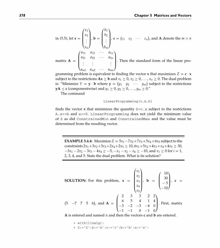
378 Chapter 5 Matrices and Vectors
in (5.5), let x =
⎛
⎜⎜⎜⎝
x1
x2...
xn
⎞
⎟⎟⎟⎠
, b =
⎛
⎜⎜⎜⎝
b1
b2...
bm
⎞
⎟⎟⎟⎠
, c =(
c1 c2 · · · cn)
, and A denote the m × n
matrix A =
⎛
⎜⎜⎜⎝
a11 a12 · · · a1n
a21 a22 · · · a2n...
......
am1 am2 · · · amn
⎞
⎟⎟⎟⎠
. Then the standard form of the linear pro-
gramming problem is equivalent to finding the vector x that maximizes Z = c · x
subject to the restrictions Ax ≥ b and x1 ≥ 0, x2 ≥ 0, . . . , xn ≥ 0. The dual problem
is: “Minimize Y = y · b where y =(
y1 y2 · · · ym)
subject to the restrictions
yA ≤ c (componentwise) and y1 ≥ 0, y2 ≥ 0, . . . , ym ≥ 0.”
The command
LinearProgramming[c,A,b]
finds the vector x that minimizes the quantity Z=c.x subject to the restrictions
A.x>=b and x>=0. LinearProgramming does not yield the minimum value
of Z as did ConstrainedMin and ConstrainedMax and the value must be
determined from the resulting vector.
EXAMPLE 5.4.4: Maximize Z = 5x1−7x2+7x3+5x4+6x5 subject to the
constraints 2x1+3x2+3x3+2x4+2x5 ≥ 10, 6x1+5x2+4x3+x4+4x5 ≥ 30,
−3x1 − 2x2 − 3x3 − 4x4 ≥ −5, −x1 − x2 − x4 ≥ −10, and x1 ≥ 0 for i = 1,
2, 3, 4, and 5. State the dual problem. What is its solution?
SOLUTION: For this problem, x =
⎛
⎜⎜⎜⎜⎜⎝
x1
x2
x3
x4
x5
⎞
⎟⎟⎟⎟⎟⎠
, b =
⎛
⎜⎜⎝
10
30
− 5
−10
⎞
⎟⎟⎠
, c =
(
5 −7 7 5 6)
, and A =
⎛
⎜⎜⎝
2 3 3 2 2
6 5 4 1 4
−3 −2 −3 −4 0
−1 −1 0 −1 0
⎞
⎟⎟⎠
. First, matrix
A is entered and named A and then the vectors c and b are entered.
> with(linalg):
> Z:=’Z’:A:=’A’:c:=’c’:b:=’b’:x:=’x’:

5.4 Maxima and Minima Using Linear Programming 379
> A:=array([[2,3,3,2,2],[6,5,4,1,4],
> [-3,-2,-3,-4,0],[-1,-1,0,-1,0],
> [0$5]]);⎡
⎢⎢⎢⎢⎢⎣
2 3 3 2 2
6 5 4 1 4
−3 −2 −3 −4 0
−1 −1 0 −1 0
0 0 0 0 0
⎤
⎥⎥⎥⎥⎥⎦
> c:=array([[5,-7,7,5,6]]):
> b:=vector([10,30,-5,-10,0]):
> x:=vector(5):
The objective function Z is defined by finding the scalar (dot) product
of the solution vector x and the vector c with multiply, which is found
in the linalg package. This objective function is extracted from the
output list that results with Z[1].
> Z:=multiply(c,x);
Z := vector(
[5 x1 − 7 x2 + 7 x3 + 5 x4 + 6 x5])
> Z[1];
5 x1 − 7 x2 + 7 x3 + 5 x4 + 6 x5
The left-hand sides of the constraints are then defined in prod by
multiplying the coefficient matrix A by the solution vector x. Notice
that the output list is made up of four components that can be extracted
with prod[1], prod[2], prod[3], and prod[4], respectively. In
constraints, the set of constraints for this problem are constructed
by substituting i = 1, 2, 3, 4 into the inequalityprod[i]>=b[i]. Hence,
a constraint is produced for each value of i.
> prod:=multiply(A,x);
[
2 x1 + 3 x2 + 3 x3 + 2 x4 + 2 x5, 6 x1 + 5 x2 + 4 x3 + x4 + 4 x5,
− 3 x1 − 2 x2 − 3 x3 − 4 x4, −x1 − x2 − x4, 0]
> constraints:=seq(prod[i]>=b[i],i=1..4);
constraints :={
10 ≤ 2 x1 + 3 x2 + 3 x3 + 2 x4 + 2 x5,
30 ≤ 6 x1 + 5 x2 + 4 x3 + x4 + 4 x5,
− 5 ≤ −3 x1 − 2 x2 − 3 x3 − 4 x4, −10 ≤ −x1 − x2 − x4
}

380 Chapter 5 Matrices and Vectors
The point at which the minimum value of the objective function
Z[1] subject to the constraints given in constraints is found with
minimize with the NONNEGATIVE setting so that the non-negativty
constraints are considered by the simplex method. Of course, the
simplex package must be loaded before this command is used. The
solution is assigned the name vals. Finally, the components in vals
are assigned to the solution vector x so that the minimum value of the
objective function is determined by taking the scalar product of c and x
which is equivalent to substituting the components of x into the objective
function. The scalar product of 34/5 is found with multiply.
> with(simplex):
> vals:=minimize(Z[1],constraints,NONNEGATIVE);
vals :={
x1 = 0, x3 = 0, x4 = 0, x5 =35
8, x2 = 5/2
}
> assign(vals):
> multiply(c,x);
vector
([35
4
])
Next, we solve the corresponding dual problem. The vector Y is defined
below that has as its components the dual variables y1, y2, y3, y4,
and y5. The objective function of the dual problem is then defined by
multiplying Y by the vector b. Similarly, the left-hand sides of the con-
straints are determined by multiplying the vector Y by the matrix of
coefficients A.
> Y:=array([[y1,y2,y3,y4,y5]]):
> multiply(Y,b);
vector(
[10 y1 + 30 y2 − 5 y3 − 10 y4])
> multiply(Y,A);
⎡
⎢⎢⎢⎢⎣
2 y1 + 6 y2 − 3 y3 − y4
3 y1 + 5 y2 − 2 y3 − y4
3 y1 + 4 y2 − 3 y3, 2 y1 + y2 − 4 y3 − y4
2 y1 + 4 y2
⎤
⎥⎥⎥⎥⎦

5.4 Maxima and Minima Using Linear Programming 381
Hence, we may state the dual problem as:
Minimize Y = 10y1 + 30y2 − 5y3 − 10y4 subject to the constraints⎧
⎪⎪⎪⎪⎪⎪⎪⎨
⎪⎪⎪⎪⎪⎪⎪⎩
2y1 + 6y2 − 3y3 − y4 ≤ 5
3y1 + 5y2 − 2y3 − y4 ≤ −7
3y1 + 4y2 − 3y3 ≤ 7
2y1 + y2 − 4y3 − y4 ≤ 5
2y1 + 4y2 ≤ 6
,
and yi ≥ 0 for i = 1, 2, 3, and 4.
�
Application: A Transportation Problem
A certain company has two factories, F1 and F2, each producing two products,
P1 and P2, that are to be shipped to three distribution centers, D1, D2, and D3.
The following table illustrates the cost associated with shipping each product from
the factory to the distribution center, the minimum number of each product each
distribution center needs, and the maximum output of each factory. How much
of each product should be shipped from each plant to each distribution center to
minimize the total shipping costs?
F1/P1 F1/P2 F2/P1 F2/P2 Minimum
D1/P1 $0.75 $0.80 500
D1/P2 $0.50 $0.40 400
D2/P1 $1.00 $0.90 300
D2/P2 $0.75 $1.20 500
D3/P1 $0.90 $0.85 700
D3/P2 $0.80 $0.95 300
Maximum Output 1000 400 800 900
SOLUTION: Let x1 denote the number of units of P1 shipped from
F1 to D1; x2 the number of units of P2 shipped from F1 to D1; x3 the
number of units of P1 shipped from F1 to D2; x4 the number of units of
P2 shipped from F1 to D2; x5 the number of units of P1 shipped from
F1 to D3; x6 the number of units of P2 shipped from F1 to D3; x7 the
number of units of P1 shipped from F2 to D1; x8 the number of units of
P2 shipped from F2 to D1; x9 the number of units of P1 shipped from
F2 to D2; x10 the number of units of P2 shipped from F2 to D2; x11 the

382 Chapter 5 Matrices and Vectors
number of units of P1 shipped from F2 to D3; and x12 the number of
units of P2 shipped from F2 to D3.
Then, it is necessary to minimize the number
Z = .75x1 + .5x2 + x3 + .75x4 + .9x5 + .8x6 + .8x7
+ .4x8 + .9x9 + 1.2x10 + .85x11 + .95x12
subject to the constraints x1 + x3 + x5 ≤ 1000, x2 + x4 + x6 ≤ 400,
x7 + x9 + x11 ≤ 800, x8 + x10 + x12 ≤ 900, x1 + x7 ≥ 500, x3 + x9 ≥ 500,
x5 + x11 ≥ 700, x2 + x8 ≥ 400, x4 + x10 ≥ 500, x6 + x12 ≥ 300, and xi
non-negative for i = 1, 2, . . . , 12.
In order to solve this linear programming problem, the objective
function that computes the total cost, the 12 variables, and the set of
inequalities must be entered. The coefficients of the objective function
are given in the vector c. We will use several of the commands in the
linalg package; we begin by loading this package. The objective func-
tion is defined by computing the dot product of the vectors x and c
with dotprod. (Recall, that a similar computation was performed with
multiply in a previous example.) The list of constraints are entered
explicitly in constraints.
> with(linalg):
> c:=vector(
> [.75,.5,1,.75,.9,.8,.8,.4,.9,1.2,.85,.95]):
> x:=vector(12):
Warning, the names basis and pivot have been redefined
> Z:=dotprod(x,c);
Z := 0.75 x1 + 0.5 x2 + x3 + 0.75 x4 + 0.9 x5 + 0.8 x6 + 0.8 x7
+ 0.4 x8 + 0.9 x9 + 1.2 x10 + 0.85 x11 + 0.95 x12
> constraints:=x[1]+x[3]+x[5]<=1000,
x[2]+x[4]+x[6]<=400,x[7]+x[9]+x[11]<=800,
x[8]+x[10]+x[12]<=900,x[1]+x[7]>=500,
x[3]+x[9]>=300,x[5]+x[11]>=700,
x[2]+x[8]>=400,x[4]+x[10]>=500,
x[6]+x[12]>=300:
The simplex package is then loaded so that the minimize command
can be used. This is done in min_vals, which determines the variable
values at which the minimum occurs. These values are assigned to the
components of the vector x with assign. Therefore, the total number

5.4 Maxima and Minima Using Linear Programming 383
of units produced of each product at each factory is easily found by
entering
x[1]+x[3]+x[5], x[2]+x[4]+x[6], ..., x[6]+x[12].
Also, the minimum value of the objective function 2115 is determined
by entering Z. From these results, we see that F1 produces 700 units
of P1, F1 produces 400 units of P2, F2 produces 800 units of P1, F2
produces 800 units of P2, and each distribution center receives exactly
the minimum number of each product it requests.
> with(simplex):
min_vals:=minimize(Z,constraints,NONNEGATIVE);
min_vals :={
x1 = 500, x12 = 300, x3 = 0, x2 = 0, x8 = 400, x9 = 300,
x6 = 0, x7 = 0, x10 = 100, x4 = 400, x11 = 500, x5 = 200}
> assign(min_vals):
> Z;
> x[1]+x[3]+x[5];
> x[2]+x[4]+x[6];
> x[7]+x[9]+x[11];
> x[3]+x[9];
> x[5]+x[11];
> x[2]+x[8];
> x[4]+x[10];
> x[6]+x[12];
2115.0
700
400
800
300
700
400
500
300
�

384 Chapter 5 Matrices and Vectors
5.5 Selected Topics from Vector Calculus
Basic operations on two- and
three-dimensional vectors
are discussed in Section 5.1.4.5.5.1 Vector-Valued Functions
We now turn our attention to vector-valued functions. In particular, we consider
vector-valued functions of the following forms.
Plane curves: r(t) = x(t)i + y(t)j (5.6)
Space curves: r(t) = x(t)i + y(t)j + z(t)k (5.7)
Parametric surfaces: r(s, t) = x(s, t)i + y(s, t)j + z(s, t)k (5.8)
Vector fields in the plane: F(x, y) = P(x, y)i + Q(x, y)j (5.9)
Vector fields in space: F(x, y, z) = P(x, y, z)i + Q(x, y, z)j + R(x, y, z)k
(5.10)
For the vector-valued functions (5.6) and (5.7), differentiation and integration
is carried out term-by-term, provided that all the terms are differentiable and
integrable. Suppose that C is a smooth curve defined by r(t), a ≤ t ≤ b.
1. If r′(t) �= 0, the unit tangent vector, T(t), is
T(t) =r′(t)
‖r′(t)‖.
2. If T′(t) �= 0, the principal unit normal vector, N(t), is
N(t) =T′(t)
‖T′(t)‖.
3. The arc length function, s(t), is
s(t) =∫ t
a‖r′(u)‖ du.
In particular, the length of C on the interval [a, b] is∫ b
a ‖r′(t)‖ dt.
4. The curvature, κ , of C isIt is a good exercise to show
that the curvature of a circle
of radius r is 1/r.κ =
‖T′(t)‖‖r′(t)‖
=a(t) · N(t)
‖v(t)‖2=
‖r′(t) × r′′(t)‖‖r′(t)‖3
,
where v(t) = r′(t) and a(t) = r′′(t)
Use the VectorCalculus and LinearAlgebra packages to perform opera-
tions on vector-valued functions.

5.5 Selected Topics from Vector Calculus 385
EXAMPLE 5.5.1 (Folium of Descartes): Consider the Folium of
Descartes,
r(t) =3at
1 + t3i +
3at2
1 + t3j
for t �= −1, if a = 1. (a) Find r′(t), r′′(t), and∫
r(t) dt. (b) Find T(t) and
N(t). (c) Find the curvature, κ . (d) Find the length of the loop of the
Folium.
SOLUTION: (a) After loading the VectorCalculus package and
defining r(t),
> with(VectorCalculus):
> with(LinearAlgebra):
> r:=t->Vector([3*a*t/(1+tˆ3),3*a*tˆ2/(1+tˆ3)]):
> a:=1:
we compute r′(t), r′′(t), and∫
r(t) dt with diff and int. We
name r′(t) dr, r′′(t) dr2, and∫
r(t) dt ir. Observe that when the
VectorCalculus package is loaded, int is redefined, but not
integrate. Thus, int(r(t),t) antidifferentiates each component

386 Chapter 5 Matrices and Vectors
of r(t) but integrate(r(t),t) does not. To use integrate, we
must use map to apply integrate to each component of r(t).
> dr:=simplify(diff(r(t),t));
dr :=
⎡
⎢⎢⎢⎢⎣
−32 t3 − 1(
t3 + 1)2
−3t(
t3 − 2)
(
t3 + 1)2
⎤
⎥⎥⎥⎥⎦
> dr2:=simplify(diff(r(t),t$2));
dr2 :=
⎡
⎢⎢⎢⎢⎣
18t2(
t3 − 2)
(
t3 + 1)3
6t6 − 7 t3 + 1(
t3 + 1)3
⎤
⎥⎥⎥⎥⎦
> ir:=map(integrate,r(t),t);
ir :=
[
− ln (t + 1) + 1/2 ln(
t2 − t + 1)
+√
3 arctan(
1/3 (2 t − 1)√
3)
ln(
t3 + 1)
]
> ir:=int(r(t),t);
ir :=
[
− ln (t + 1) + 1/2 ln(
t2 − t + 1)
+√
3 arctan(
1/3 (2 t − 1)√
3)
ln(
t3 + 1)
]
(b) Maple does not automatically make assumptions regarding the value
of t, so it does not algebraically simplify ‖r′(t)‖ as we might typically do
unless we use radsimp.radsimp(Sqrt(xˆ2))
returns x.
> simplify(sqrt(dr.dr));
3
√√√√
4 t6 − 4 t3 + 1 + t8 − 4 t5 + 4 t2
(
t3 + 1)4
> nr:=radsimp(sqrt(dr.dr));
nr := 3
√
4 t6 − 4 t3 + 1 + t8 − 4 t5 + 4 t2
(
t3 + 1)2
We perform the same steps to compute the unit normal vector, N(t). In
particular, note that dutb = ‖T′(t)‖.

5.5 Selected Topics from Vector Calculus 387
> ut:=1/nr*dr;
⎡
⎢⎢⎢⎢⎣
−32 t3 − 1
nr(
t3 + 1)2
−3t(
t3 − 2)
nr(
t3 + 1)2
⎤
⎥⎥⎥⎥⎦
Alternatively,TangentVector, which is contained in theVectorCalculus
package, computes r′(t)
> simplify(TangentVector(r(t)));
⎡
⎢⎢⎢⎢⎣
−32 t3 − 1(
t3 + 1)2
−3t(
t3 − 2)
(
t3 + 1)2
⎤
⎥⎥⎥⎥⎦
so TangentVector followed by Normalize, which is contained in the
LinearAlgebra package, returns T(t).
> simplify(Normalize(TangentVector(r(t))));
⎡
⎢⎢⎢⎢⎢⎢⎣
−3(
2 t3 − 1)
(
max
(
3
∣∣∣∣∣
2 t3 − 1(
t3 + 1)2
∣∣∣∣∣, 3
∣∣∣∣∣
t(
t3 − 2)
(
t3 + 1)2
∣∣∣∣∣
))−1(
t3 + 1)−2
−3 t(
t3 − 2)
(
max
(
3
∣∣∣∣∣
2 t3 − 1(
t3 + 1)2
∣∣∣∣∣, 3
∣∣∣∣∣
t(
t3 − 2)
(
t3 + 1)2
∣∣∣∣∣
))−1(
t3 + 1)−2
⎤
⎥⎥⎥⎥⎥⎥⎦
We perform the same steps to compute the unit normal vector, N(t).
> dut:=simplify(diff(ut,t));
dut :=
⎡
⎢⎢⎢⎢⎣
18t2(
t3 − 2)
nr(
t3 + 1)3
6t6 − 7 t3 + 1
nr(
t3 + 1)3
⎤
⎥⎥⎥⎥⎦
> duta:=simplify(dut.dut);
duta := 369 t10 − 36 t7 + 36 t4 + t12 − 14 t9 + 51 t6 − 14 t3 + 1
nr2(
t3 + 1)6

388 Chapter 5 Matrices and Vectors
> dutb:=radsimp(sqrt(duta);
dutb := 6
√
9 t10 − 36 t7 + 36 t4 + t12 − 14 t9 + 51 t6 − 14 t3 + 1
nr(
t3 + 1)3
> nt:=simplify(1/dutb*dut);
nt :=
⎡
⎢⎢⎢⎢⎣
3t2(
t3 − 2)
√
9 t10 − 36 t7 + 36 t4 + t12 − 14 t9 + 51 t6 − 14 t3 + 1
t6 − 7 t3 + 1√
9 t10 − 36 t7 + 36 t4 + t12 − 14 t9 + 51 t6 − 14 t3 + 1
⎤
⎥⎥⎥⎥⎦
Alternatively, use PrincipalNormal, which is contained in the
VectorCalculus package,
> radsimp(PrincipalNormal(r(t)));
⎡
⎢⎢⎢⎢⎣
2t(
t9 − 3 t3 − 2)
(
4 t6 − 4 t3 + 1 + t8 − 4 t5 + 4 t2)3/2
−22 t9 + 3 t6 − 1
(
4 t6 − 4 t3 + 1 + t8 − 4 t5 + 4 t2)3/2
⎤
⎥⎥⎥⎥⎦
followed by Normalize.
> radsimp(Normalize(PrincipalNormal(r(t))))
⎡
⎢⎢⎢⎢⎢⎢⎢⎢⎢⎢⎢⎢⎢⎢⎢⎢⎢⎢⎢⎢⎢⎢⎢⎢⎢⎢⎢⎢⎣
2 t(
t9 − 3 t3 − 2)(
4 t6 − 4 t3 + 1 + t8 − 4 t5 + 4 t2)−3/2
×
(
max
(
2
∣∣∣∣∣
2 t9 + 3 t6 − 1(
4 t6 − 4 t3 + 1 + t8 − 4 t5 + 4 t2)3/2
∣∣∣∣∣
,
2
∣∣∣∣∣
t(
t9 − 3 t3 − 2)
(
4 t6 − 4 t3 + 1 + t8 − 4 t5 + 4 t2)3/2
∣∣∣∣∣
))−1
−2(
2 t9 + 3 t6 − 1) (
4 t6 − 4 t3 + 1 + t8 − 4 t5 + 4 t2)−3/2
×
(
max
(
2
∣∣∣∣∣
2 t9 + 3 t6 − 1(
4 t6 − 4 t3 + 1 + t8 − 4 t5 + 4 t2)3/2
∣∣∣∣∣
,
2
∣∣∣∣∣
t(
t9 − 3 t3 − 2)
(
4 t6 − 4 t3 + 1 + t8 − 4 t5 + 4 t2)3/2
∣∣∣∣∣
))−1
⎤
⎥⎥⎥⎥⎥⎥⎥⎥⎥⎥⎥⎥⎥⎥⎥⎥⎥⎥⎥⎥⎥⎥⎥⎥⎥⎥⎥⎥⎦

5.5 Selected Topics from Vector Calculus 389
(c) We use the formula κ =‖T′(t)‖‖r′(t)‖
to determine the curvature in
curvature
> curvature:=simplify(dutb/nr);
curvature := 2/3
(
t3 + 1)4
(
4 t6 − 4 t3 + 1 + t8 − 4 t5 + 4 t2)3/2
and confirm the result with Curvature, which is contained in the
VectorCalculus package.
> radsimp(Curvature(r(t)));
2/3
(
t3 + 1)4
(
4 t6 − 4 t3 + 1 + t8 − 4 t5 + 4 t2)3/2
We graphically illustrate the unit tangent and normal vectors at r(1) =⟨
3/2, 3/2⟩
. First, we compute the unit tangent and normal vectors if t = 1
using subs.
> ut1:=subs(t=1,ut);
ut1 :=
[
−3/4 nr−1
3/4 nr−1
]
> nt1:=subs(t=1,nt)
nt1 :=
⎡
⎢⎣
−3
34
√34
−5
34
√34
⎤
⎥⎦
We then compute the curvature if t = 1 in smallk. The center of the
osculating circle at r(1) is found in x0 and y0. The radius of the osculating
circle is 1/κ ; the position
vector of the center is
r + 1κ N.
> smallk:=subs(t=1,curvature);
smallk := 8/3√
2
> evalf(smallk);
3.771236166

390 Chapter 5 Matrices and Vectors
> evalf(1/smallk);
0.2651650429
Note that RadiusofCurvature, which is contained in the
VectorCalculus package, computes 1/κ .
> radsimp(RadiusOfCurvature(r(t)));
3/2
(
4 t6 − 4 t3 + 1 + t8 − 4 t5 + 4 t2)3/2
(
t3 + 1)4
> subs(t=1,radsimp(RadiusOfCurvature(r(t))));
> evalf(subs(t=1,radsimp(RadiusOfCurvature(r(t)))));
3/16√
2
0.2651650429
> x0:=subs(t=1,r(t)[1]-dr.dr*dr[2]/(dr[1]*dr2[2]
-dr2[1]*dr[2]));
x0 :=21
16
> y0:=subs(t=1,r(t)[2]-dr.dr*dr[2]/(dr[1]*dr2[2]
-dr2[1]*dr[2]));
y0 :=21
16
We now load the plots package and graph r(t) with plot. The unit
tangent and normal vectors at r(1) are graphed with arrow in p3 and
p4. The osculating circle at r(1) is graphed with circle in c1. All fourcircle([x0, y0], r)
is a two-dimensional graphics
object that represents a
circle of radius r centered at
the point (x0, y0). Use
display to display the
graph.
graphs are displayed together with display in Figure 5-7.
> with(plots):
> p1:=plot([r(t)[1],r(t)[2],t=-100..100],
> view=[-2..3,-2..3],color=black):
> p2:=circle([x0,y0],1/smallk):
> p3:=arrow(r(1),ut1):
> p4:=arrow(r(1),nt1):
> display(p1,p2,p3,p4,view=[-2..3,-2..3]);
(d) The loop is formed by graphing r(t) for t ≥ 0. Hence, the length of the
loop is given by the improper integral∫∞
0 ‖r(t)‖ dt, which we compute
with evalf and int.

5.5 Selected Topics from Vector Calculus 391
3
2
1
0
−1
−2
3210−1−2
Figure 5-7 The Folium with an osculating circle
> evalf(int(nr,t=0..infinity));
4.917488722
�
Recall that the gradient of z = f (x, y) is the vector-valued function ▽f (x, y) =⟨
fx(x, y), fy(x, y)⟩
. Similarly, we define the gradient of w = f (x, y, z) to be
▽f (x, y, z) =⟨
fx(x, y, z), fy(x, y, z), fz(x, y, z)⟩
=∂f
∂xi +
∂f
∂yj +
∂f
∂zk. (5.11)
A vector field F is conservative if there is a function f , called a potential func-
tion, satisfying ▽f = F. In the special case that F(x, y) = P(x, y)i + Q(x, y)j, F is
conservative if and only if∂P
∂y=
∂Q
∂x.
The divergence of the vector field F(x, y, z) = P(x, y, z)i + Q(x, y, z)j + R(x, y, z)k
is the scalar field
divF = ▽ · F =∂P
∂x+
∂Q
∂y+
∂R
∂z. (5.12)
Use the command
F:=(x,y,z)->VectorField(<P(x,y,z),Q(x,y,z),R(x,y,z)>,
‘cartesian’[x,y,z])

392 Chapter 5 Matrices and Vectors
to define the Cartesian vector field F(x, y, z) = P(x, y, z)i + Q(x, y, z)j + R(x, y, z)k.
In general, when defining a vector field using VectorField, you must specify the
coordinate system used.
The Divergence command, which is contained in the VectorCalculus
package, can be used to find the divergence of a vector field:
Divergence(F(x,y,z))
computes the divergence of F(x, y, z) = P(x, y, z)i + Q(x, y, z)j + R(x, y, z)k. The
laplacian of the scalar field w = f (x, y, z) is defined to be
div(
▽f)
= ▽ ·(
▽f)
= ▽2f =∂2f
∂x2+
∂2f
∂y2+
∂2f
∂z2= △f . (5.13)
In the same way that Divergence computes the divergence of a vector field,
Laplacian, which is also contained in the VectorCalculus package, computes
the laplacian of a scalar field.

5.5 Selected Topics from Vector Calculus 393
The curl of the vector field F(x, y, z) = P(x, y, z)i + Q(x, y, z)j + R(x, y, z)k is
curlF(x, y, z) = ▽ × F(x, y, z)
=
∣∣∣∣∣∣∣∣∣
i j k
∂
∂x
∂
∂y
∂
∂z
P(x, y, z) Q(x, y, z) R(x, y, z)
∣∣∣∣∣∣∣∣∣
=(
∂R
∂y−
∂Q
∂z
)
i −(
∂R
∂x−
∂P
∂z
)
j +(
∂Q
∂x−
∂P
∂y
)
k.
(5.14)
If F(x, y, z) = P(x, y, z)i + Q(x, y, z)j + R(x, y, z)k, F is conservative if and only if
curlF(x, y, z) = 0, in which case F is said to be irrotational.
EXAMPLE 5.5.2: Determine if
F(x, y) =(
1 − 2x2)
ye−x2−y2i +
(
1 − 2y2)
xe−x2−y2j
is conservative. If F is conservative find a potential function for F.
SOLUTION: We define F(x, y) usingVectorField. Then we usediff
and simplify to see that Py(x, y) = Qx(x, y). Hence, F is conservative.
> with(VectorCalculus):
> with(LinearAlgebra):
> F:=(x,y)->VectorField(<(1-2*xˆ2)*y*exp(-xˆ2-yˆ2),
> (1-2*yˆ2)*x*exp(-xˆ2-yˆ2)>,’cartesian’[x,y]):
> simplify(diff(F(x,y)[1],y));
e−x2−y2(
−2 x2 + 1 + 4 y2x2 − 2 y2)
> simplify(diff(F(x,y)[2],x));
e−x2−y2(
−2 x2 + 1 + 4 y2x2 − 2 y2)
We use int to find f satisfying ▽f = F.
> i1:=simplify(int(F(x,y)[1],x))+g(y);
i1 := yxe−x2−y2+ g
(
y)

394 Chapter 5 Matrices and Vectors
> solve(diff(i1,y)=F(x,y)[2],diff(g(y),y));
0
Therefore, g(y) = C, where C is an arbitrary constant. Letting
C = 0 gives us the potential function. We confirm this result using
ScalarPotential, which is contained in the VectorCalculus
package.
> f:=simplify(ScalarPotential(F(x,y)));
f := yxe−x2−y2
Remember that the vectors F are perpendicular to the level curves of f .
To see this, we normalize F in nF with Normalize.
> nF:=Normalize(F(x,y));
nf :=
⎡
⎢⎢⎢⎢⎢⎢⎣
(
−2 x2 + 1)
ye−x2−y2
max(
e−Re(x2+y2)∣∣(
−2 x2 + 1)
y∣∣ , e−Re(x2+y2)
∣∣(
−2 y2 + 1)
x∣∣
)
(
−2 y2 + 1)
xe−x2−y2
max(
e−Re(x2+y2)∣∣(
−2 x2 + 1)
y∣∣ , e−Re(x2+y2)
∣∣(
−2 y2 + 1)
x∣∣
)
⎤
⎥⎥⎥⎥⎥⎥⎦
We then graph several level curves of f in cp with contourplot and
several vectors of nFwith fieldplot, which is contained in theplots
package, in fp. We show the graphs together with Show in Figure 5-8.
y
1
−1
1.5
0.5
−0.5
0.5−0.5
−1.5
0 1.51−1
x
0−1.5
Figure 5-8 The vectors F are perpendicular to the level curves of f

5.5 Selected Topics from Vector Calculus 395
> with(plots):
> fp:=fieldplot(nF,x=-3/2..3/2,y=-3/2..3/2):
> cp:=contourplot(f,x=-3/2..3/2,y=-3/2..3/2,
color=black,contours=20):
> display(fp,cp);
Note that we can use gradplot, which is contained in the plots pack-
age, to graph several vectors of ▽f . However, the vectors are scaled and
it can be difficult to see that the vectors are perpendicular to the level
curves of f . The advantage of proceeding this way is that by graphing
unit vectors, it is easier to see that the vectors are perpendicular to the
level curves of f in the resulting plot.
�
EXAMPLE 5.5.3: (a) Show that
F(x, y, z) = −10xy2i +(
3z3 − 10x2y)
j + 9yz2k
is irrotational. (b) Find f satisfying ▽f = F. (c) Compute div F and ▽2f .
SOLUTION: (a) After defining F(x, y, z), we use Curl, which is con-
tained in the VectorCalculus package, to see that curl F(x, y, z) = 0.
> with(VectorCalculus):
> F:=(x,y,z)->VectorField(<-10*x*yˆ2,3*zˆ3-10*xˆ2*y,
9*y*zˆ2>,’cartesian’[x,y,z]):
> Curl(F(x,y,z));
⎡
⎣
0
0
0
⎤
⎦
(b) We then use ScalarPotential to find w = f (x, y, z) satisfying
▽f = F.
> lf:=ScalarPotential(F(x,y,z));
lf := −5 y2x2 + 3 z3y
Thus, f (x, y, z) = −5x2y2 + 3yz3. ▽f is orthogonal to the level surfaces
of f . To illustrate this, we use implicitplot3d, which is contained
in the plots package, to graph the level surface of w = f (x, y, z)

396 Chapter 5 Matrices and Vectors
−2
−1
x0
1
2
21
0y
−1−2
−2
−1
0z
1
2
Figure 5-9 ▽f is orthogonal to the level surfaces of f
corresponding to w = 0 for −2 ≤ x ≤ 2, −2 ≤ y ≤ 2, and −2 ≤ z ≤ 2 in
pf. We then use gradplot3d, which is contained in the plots pack-
age, to graph several vectors in the gradient field of f over the same
domain in gradf. The two plots are shown together with display in
Figure 5-9. In the plot, notice that the vectors appear to be perpendicular
to the surface.
> with(plots):
> pf:=implicitplot3d(lf,x=-2..2,y=-2..2,z=-2..2,
grid=[15,15,15]):
> pg:=gradplot3d(lf,x=-2..2,y=-2..2,z=-2..2,
color=black):
> display(pf,pg,axes=boxed);
For (c), we take advantage of Divergence and Laplacian. As
expected, the results are the same.
> Divergence(F(x,y,z));
−10 y2 − 10 x2 + 18 yz
> Laplacian(lf,’cartesian’[x,y,z]);
−10 y2 − 10 x2 + 18 yz
�

5.5 Selected Topics from Vector Calculus 397
5.5.2 Line Integrals
If F is continuous on the smooth curve C with parametrization r(t), a ≤ t ≤ b, the
line integral of F on C is
∫
CF · dr =
∫ b
aF · r′(t) dt. (5.15)
If you can parametrize C, you can use LineInt, which is contained in the
VectorCalculus package, to compute∫
C F · dr.
If F is conservative and C is piecewise smooth, line integrals can be evaluated
using the Fundamental Theorem of Line Integrals.
Theorem 19 (Fundamental Theorem of Line Integrals): If F is conservative and the
curve C defined by r(t), a ≤ t ≤ b is piecewise smooth,∫
CF · dr = f
(
r(b))
− f(
r(a))
(5.16)
where F = ▽f .
EXAMPLE 5.5.4: Find∫
C F · dr where F(x, y) =(
e−y − ye−x)
i +(
e−x − xe−y)
j and C is defined by r(t) = cos t i + ln(
2t/π)
j, π/2 ≤t ≤ 4π .

398 Chapter 5 Matrices and Vectors
SOLUTION: We see that F is conservative with diff and find that
f (x, y) = xe−y + ye−x satisfies ▽f = F with ScalarPotential.
> with(VectorCalculus):
> F:=(x,y)->VectorField(<exp(-y)-y*exp(-x),
exp(-x)-x*exp(-y)>,’cartesian’[x,y]):
> diff(F(x,y)[1],y);
> diff(F(x,y)[2],x);
−e−y − e−x
−e−y − e−x
> lf:=ScalarPotential(F(x,y));
lf := xe−y + ye−x
Hence, using (5.16),∫
CF · dr =
(
xe−y + ye−x)]x=1,y=ln 8x=0,y=0
=3 ln 2
e+
1
8≈ 0.890,
> xr:=t->cos(t):
> yr:=t->ln(2*t/Pi):
> [xr(Pi/2),yr(Pi/2)];
> [xr(4*Pi),yr(4*Pi)];
[0, 0]
[1, 3 ln (2)]
> simplify(subs([x=1,y=ln(8)],lf));
1/8 + 3 ln (2) e−1
> evalf(simplify(subs([x=1,y=ln(8)],lf)));
0.8899837925
which we confirm with LineInt.
> LineInt(F(x,y),Path(<cos(t),ln(2*t/Pi)>,
t=Pi/2..4*Pi));
1/8 + 3 ln (2) e−1
�
If C is a piecewise smooth simple closed curve and P(x, y) and Q(x, y)
have continuous partial derivatives, Green’s theorem relates the line integral∮
C
(
P(x, y) dx + Q(x, y) dy)
to a double integral.

5.5 Selected Topics from Vector Calculus 399
Theorem 20 (Green’s Theorem): Let C be a piecewise smooth simple closed curve in
the plane and R the region bounded by C. If P(x, y) and Q(x, y) have continuous partial
derivatives on R,
∮
C
(
P(x, y) dx + Q(x, y) dy)
=∫∫
R
(∂Q
∂x−
∂P
∂y
)
dA. (5.17)
EXAMPLE 5.5.5: Evaluate We assume that the symbol∮
means to evaluate the
integral in the positive (or
counter-clockwise) direction.
∮
C
(
e−x − sin y)
dx +(
cos x − e−y) dy
where C is the boundary of the region between y = x2 and x = y2.
SOLUTION: After defining P(x, y) = e−x − sin y and Q(x, y) = cos x −e−y, we useplot to determine the region R bounded by C in Figure 5-10.
> with(VectorCalculus):
> p:=(x,y)->exp(-x)-sin(y):
> q:=(x,y)->cos(x)-exp(y):
> plot([xˆ2,sqrt(x)],x=0..1.1,color=[black,gray]);
1.2
1
0.8
0.6
0.4
0.2
0
x10.80.60.40.20
Figure 5-10 y = x2 and y =√
x, 0 ≤ x ≤ 1

400 Chapter 5 Matrices and Vectors
Using (5.17),
∮
C
(
e−x − sin y)
dx +(
cos x − e−y) dy =∫∫
R
(∂Q
∂x−
∂P
∂y
)
dA
=∫∫
R
(
cos y − sin x)
dA
=∫ 1
0
∫ √x
x2
(
cos y − sin x)
dy dx,
> dqdp:=simplify(diff(q(x,y),x)-diff(p(x,y),y));
dqdp := − sin (x) + cos(
y)
which we evaluate with int.
> ev:=int(int(dqdp,y=xˆ2..sqrt(x)),x=0..1);
ev := 4 sin (1) − 1/2√
2√
πFresnelS
(√2
√π
)
− 1/2√
2√
πFresnelC
(√2
√π
)
− 2
> evalf(ev);
0.151091400
Notice that the result is given in terms of the FresnelS and FresnelC
functions, which are defined by
FresnelS(x)=∫ x
0sin
(π
2t2)
dt and FresnelC(x)=∫ x
0cos
(π
2t2)
dt.
A more meaningful approximation is obtained with evalf. We check
with LineInt.
> check:=LineInt(VectorField(<p(x,y),q(x,y)>,
> ’cartesian’[x,y]),Path(<t,sqrt(t)>,t=1..0))+
> LineInt(VectorField(<p(x,y),q(x,y)>,
> ’cartesian’[x,y]),Path(<t,tˆ2>,t=0..1));
check := 4 sin (1) − 1/2√
2√
πFresnelS
(√2
√π
)
− 1/2√
2√
πFresnelC
(√2
√π
)
− 2

5.5 Selected Topics from Vector Calculus 401
> evalf(check);
0.151091400
We conclude that∫ 1
0
∫ √x
x2
(
cos y − sin x)
dy dx ≈ 0.151.
�
5.5.3 Surface Integrals
Let S be the graph of z = f (x, y) (y = h(x, z), x = k(y, z)) and let Rxy (Rxz, Ryz) be the
projection of S onto the xy (xz, yz) plane. Then,∫∫
Sg(x, y, z) dS =
∫∫
Rxy
g(
x, y, f (x, y))√[
fx(x, y)]2 +
[
fy(x, y)]2 + 1 dA (5.18)
=∫∫
Rxz
g(
x, h(x, z), z)√
[hx(x, z)]2 + [hz(x, z)]2 + 1 dA (5.19)
=∫∫
Ryz
g(
k(y, z), y, z)√[
ky(y, z)]2 +
[
kz(y, z)]2 + 1 dA. (5.20)
If S is defined parametrically by
r(s, t) = x(s, t)i + y(s, t)j + z(s, t)k, (s, t) ∈ R
the formula∫∫
Sg(x, y, z) dS =
∫∫
Rg(
r(s, t))
‖rs × rt‖ dA, (5.21)
where
rs =∂x
∂si +
∂y
∂sj +
∂z
∂sk and rt =
∂x
∂ti +
∂y
∂tj +
∂z
∂tk,
is also useful.
Theorem 21 (The Divergence Theorem): Let Q be any domain with the property that
each line through any interior point of the domain cuts the boundary in exactly two points,
and such that the boundary S is a piecewise smooth closed, oriented surface with unit For our purposes, a surface is
oriented if it has two
distinct sides.normal n. If F is a vector field that has continuous partial derivatives on Q, then
∫∫∫
Q▽ · F dV =
∫∫∫
Qdiv F dV =
∫∫
SF · n dS. (5.22)

402 Chapter 5 Matrices and Vectors
In (5.22),∫∫
S F ·n dS is called the outward flux of the vector field F across the surface
S. If S is a portion of the level curve g(x, y) = C for some g, then a unit normal vector
n may be taken to be either
n =▽g
‖ ▽ g‖or n = −
▽g
‖ ▽ g‖.
If S is defined parametrically by
r(s, t) = x(s, t)i + y(s, t)j + z(s, t)k, (s, t) ∈ R,
a unit normal vector to the surface is
n =rs × rt
‖rs × rt‖
and (5.22) becomes
∫∫
SF · n dS =
∫∫
RF · (rs × rt) dA.
EXAMPLE 5.5.6: Find the outward flux of the vector field
F(x, y, z) =(
xz + xyz2)
i +(
xy + x2yz)
j +(
yz + xy2z)
k
through the surface of the cube cut from the first octant by the planes
x = 1, y = 1, and z = 1.
SOLUTION: By the Divergence theorem,
∫∫
cube surfaceF · n dA =
∫∫∫
cube interior▽ · F dV.
Hence, without the Divergence theorem, calculating the outward flux
would require six separate integrals, corresponding to the six faces of
the cube. After defining F, we compute ▽ · F with Divergence.Divergence is contained
in the VectorCalculus
package. You do not need to
reload the
VectorCalculus package
if you have already loaded it
during your current Maple
session.
> with(VectorCalculus):
> F:=(x,y,z)->VectorField(<x*z+x*y*zˆ2,
> x*y+xˆ2*y*z,y*z+x*yˆ2*z>,’cartesian’[x,y,z]):
> divF:=Divergence(F(x,y,z));
divF := z + yz2 + x + x2z + y + xy2

5.5 Selected Topics from Vector Calculus 403
The outward flux is then given by
∫∫∫
cube interior▽ · F dV =
∫ 1
0
∫ 1
0
∫ 1
0▽ · F dz dy dx = 2,
which we compute with int.
> int(int(int(divF,x=0..1),y=0..1),z=0..1);
2
�
Theorem 22 (Stoke’s Theorem): Let S be an oriented surface with finite surface area,
unit normal n, and boundary C. Let F be a continuous vector field defined on S such that
the components of F have continuous partial derivatives at each nonboundary point of S.
Then,∮
CF · dr =
∫∫
Scurl F · n dS. (5.23)
In other words, the surface integral of the normal component of the curl of F
taken over S equals the line integral of the tangential component of the field taken
over C. In particular, if F = P(x, y, z)i + Q(x, y, z)j + R(x, y, z)k, then∫
C
(
P(x, y, z)dx + Q(x, y, z)dy + R(x, y, z)dz)
=∫∫
Scurl F · n dS.
EXAMPLE 5.5.7: Verify Stoke’s theorem for the vector field
F(x, y, z) =(
x2 − y)
i +(
y2 − z)
j +(
x + z2)
k
and S the portion of the paraboloid z = f (x, y) = 9 −(
x2 + y2)
, z > 0.
SOLUTION: After loading theVectorCalculusandLinearAlgebra
packages, we define F and f . The curl of F is computed with Curl in
curlF.
> with(VectorCalculus):
> with(LinearAlgebra):
> F:=(x,y,z)->VectorField(<xˆ2-y,yˆ2-z,x+zˆ2>,
‘cartesian’[x,y,z]):
> f:=(x,y)->9-(xˆ2+yˆ2):

404 Chapter 5 Matrices and Vectors
> curlF:=Curl(F(x,y,z));
curlF :=
⎡
⎣
1
−1
1
⎤
⎦
Next, we define the function h(x, y, z) = z − f (x, y). A normal vector to
the surface is given by ▽h. A unit normal vector, n, is then given by
n =▽h
‖ ▽ h‖, which is computed in un.
> h:=(x,y,z)->z-f(x,y):
> normtosurf:=Gradient(h(x,y,z),’cartesian’[x,y,z]);
normtosurf :=
⎡
⎣
2 x
2 y
1
⎤
⎦
> un:=Normalize(normtosurf);
un :=
⎡
⎢⎢⎢⎢⎢⎢⎣
2x
max(
1, 2 |x| , 2∣∣y∣∣)
2y
max(
1, 2 |x| , 2∣∣y∣∣)
(
max(
1, 2 |x| , 2∣∣y∣∣))−1
⎤
⎥⎥⎥⎥⎥⎥⎦
> un:=simplify(normtosurf/sqrt(normtosurf.normtosurf));
un :=
⎡
⎢⎢⎢⎢⎢⎢⎢⎢⎢⎢⎣
2x
√
1 + 4 x2 + 4 y2
2y
√
1 + 4 x2 + 4 y2
1√
1 + 4 x2 + 4 y2
⎤
⎥⎥⎥⎥⎥⎥⎥⎥⎥⎥⎦
The dot product curl F · n is computed in g.
> g:=simplify(curlF.un);
g :=2 x − 2 y + 1
√
1 + 4 x2 + 4 y2

5.5 Selected Topics from Vector Calculus 405
Using the surface integral evaluation formula (5.18), In this example, R, the
projection of f (x, y) onto the
xy-plane, is the region
bounded by the graph of the
circle x2 + y2 = 9.
∫∫
Scurl F ·ndS=
∫∫
Rg(
x,y, f (x,y))√[
fx(x,y)]2+
[
fy(x,y)]2+1dA
=∫ 3
−3
∫√
9−x2
−√
9−x2g(
x,y, f (x,y))√[
fx(x,y)]2+
[
fy(x,y)]2+1dydx
=9π ,
which we compute with integrate.
> tointegrate:=subs(z=f(x,y),sqrt(diff(f(x,y),x)ˆ2
+diff(f(x,y),y)ˆ2+1)*g);
tointegrate := 2 x − 2 y + 1
> i1:=integrate(integrate(tointegrate,
y=-sqrt(9-xˆ2)..sqrt(9-xˆ2)),x=-3..3);
i1 := 9π
To verify Stoke’s theorem, we must compute the associated line inte-
gral. Notice that the boundary of z = f (x, y) = 9 − (x2 + y2), z = 0,
is the circle x2 + y2 = 9 with parametrization x = 3 cos t, y = 3 sin t,
z = 0, 0 ≤ t ≤ 2π . This parametrization is substituted into F(x, y, z) and
named pvf.
> pvf:=subs([x=3*cos(t),y=3*sin(t),z=0],F(x,y,z));
pvf :=
⎡
⎢⎢⎣
9 (cos (t))2 − 3 sin (t)
9 (sin (t))2
3 cos (t)
⎤
⎥⎥⎦
To evaluate the line integral along the circle, we next define the
parametrization of the circle and calculate dr. The dot product of pvf
and dr represents the integrand of the line integral.
> r:=t->Vector([3*cos(t),3*sin(t),0]):
> dr:=diff(r(t),t);
dr :=
⎡
⎣
−3 sin (t)3 cos (t)
0
⎤
⎦
> tointegrate:=pvf[1]*dr[1]+pvf[2]*dr[2]+pvf[3]*dr[3]:

406 Chapter 5 Matrices and Vectors
As before with x and y, we instruct Maple to assume that t is real,
compute the dot product of pvf and dr and evaluate the line integral
with integrate.
> integrate(tointegrate,t=0..2*Pi);
9π
As expected, the result is 9π .
�
5.5.4 A Note on Nonorientability
Suppose that S is the surface determined bySee “When is a surface not
orientable?” by Braselton,
Abell, and Braselton [5] for a
detailed discussion regarding
the examples in this section.
r(s, t) = x(s, t)i + y(s, t)j + z(s, t)k, (s, t) ∈ R
and let
n =rs × rt
‖rs × rt‖or n = −
rs × rt
‖rs × rt‖, (5.24)
where
rs =∂x
∂si +
∂y
∂sj +
∂z
∂sk and rt =
∂x
∂ti +
∂y
∂tj +
∂z
∂tk,
if ‖rs × rt‖ �= 0. If n is defined, n is orthogonal (or perpendicular) to S. We state
three familiar definitions of orientable.
• S is orientable if S has a unit normal vector field, n, that varies continuously
between any two points(
x0, y0, z0
)
and(
x1, y1, z1
)
on S. (See [7].)• S is orientable if S has a continuous unit normal vector field, n. (See [7]
and [16].)• S is orientable if a unit vector n can be defined at every nonboundary point of
S in such a way that the normal vectors vary continuously over the surface S.
(See [13].)
A path is order preserving if our chosen orientation is preserved as we move along
the path.
Thus, a surface like a torus is orientable.
Also see Example 2.3.18.
EXAMPLE 5.5.8 (The Torus): Using the standard parametrization of
the torus,
x = (a + b cos v) cos u, y = (a + b cos v) sin u, z = c sin v,

5.5 Selected Topics from Vector Calculus 407
Figure 5-11 A torus
we use plot3d to plot the torus if c = 3 and a = 1 in Figure 5-11.
> with(VectorCalculus):
> with(LinearAlgebra):
> r:=’r’:
> c:=3:
> a:=1:
> x:=(s,t)->(c+a*cos(s))*cos(t):
> y:=(s,t)->(c+a*cos(s))*sin(t):
> z:=(s,t)->a*sin(s):
> with(plots):
> threedp1t:=plot3d([x(s,t),y(s,t),z(s,t)],
s=-Pi..Pi,t=-Pi..Pi):
> display(threedp1t,scaling=constrained);
To plot a normal vector field on the torus, we compute∂
∂sr(s, t),
> r:=(s,t)->Vector([x(s,t),y(s,t),z(s,t)]):
> rs:=diff(r(s,t),s);
rs :=
⎡
⎢⎢⎣
− sin (s) cos (t)
− sin (s) sin (t)
cos (s)
⎤
⎥⎥⎦
and∂
∂tr(s, t).
> rt:=diff(r(s,t),t):
rt :=
⎡
⎢⎢⎣
− (3 + cos (s)) sin (t)
(3 + cos (s)) cos (t)
0
⎤
⎥⎥⎦

408 Chapter 5 Matrices and Vectors
−4
−2
0
2
4
−4
−2
−2
0
−10
2
1
42
Figure 5-12 Unit normal vector field on a torus
The cross product∂
∂sr(s, t) ×
∂
∂tr(s, t) is formed in rscrossrt.
> rscrossrt:=CrossProduct(rs,rt);
rscrossrt :=
⎡
⎢⎢⎣
−cos(s)(3+cos(s))cos(t)
−cos(s)(3+cos(s))sin (t)
−sin (s)(cos(t))2 (3+cos(s))−sin (s)(sin (t))2 (3+cos(s))
⎤
⎥⎥⎦
Using (5.24), we define un.
> simplify(sqrt(rscrossrt.rscrossrt));
csgn (3 + cos (s)) (3 + cos (s))
> un:=simplify(-rscrossrt/sqrt(rscrossrt.rscrossrt));
un :=
⎡
⎢⎢⎣
csgn (3 + cos (s)) cos (s) cos (t)
csgn (3 + cos (s)) cos (s) sin (t)
sin (s) csgn (3 + cos (s))
⎤
⎥⎥⎦
To plot the normal vector field on the torus, we take advantage of
the command arrow, which is contained in the plots package (see
Figure 5-12).
> tvals:=evalf(seq(-Pi+2*Pi/29*i,i=0..29)):
> svals:=evalf(seq(-Pi+2*Pi/29*i,i=0..29)):
> vecs:=[seq(seq(arrow(r(s0,t0),
> evalf(subs([s=s0,t=t0],un))),t0=tvals),s0=svals)]:
> display(vecs);

5.5 Selected Topics from Vector Calculus 409
−4
−2
0
2
4
−4
−2
0
2
4
Figure 5-13 The torus is orientable
We use display to see the vector field on the torus together in
Figure 5-13. Regardless of the viewing angle, the figure looks the same;
the torus is orientable.
> pp2:=display(vecs,color=black):
> display(threedp1t,pp2,view=[-5..5,-5..5,-2..2],
> axes=boxed,scaling=constrained);
If a 2-manifold, S, has an order reversing path (or not order preserving path),
S is nonorientable (or not orientable).
Determining whether a given surface S is orientable or not may be a difficult
problem.
EXAMPLE 5.5.9 (The Möbius Strip): The Möbius strip is frequently
cited as an example of a nonorientable surface with boundary: it has
one side and is physically easy to construct by hand by half twisting
and taping (or pasting) together the ends of a piece of paper (for exam-
ple, see [5], [7], [13], and [16]). A parametrization of the Möbius strip is
r(s, t) = x(s, t)i + y(s, t)j + z(s, t)k, −1 ≤ s ≤ 1, −π ≤ t ≤ π , where
x =[
c + s cos
(1
2t
)]
cos t, y =[
c + s cos
(1
2t
)]
sin t, and
z = s sin
(1
2t
)
, (5.25)

410 Chapter 5 Matrices and Vectors
−4
−2
0
2
4
-4
-2
0
2
4
Figure 5-14 Parametric plot of equations (5.25) if c = 3
and we assume that c > 1. In Figure 5-14, we graph the Möbius strip
using c = 3.
> with(VectorCalculus):
> with(plots):
> c:=3:
> x:=(s,t)->(c+s*cos(t/2))*cos(t):
> y:=(s,t)->(c+s*cos(t/2))*sin(t):
> z:=(s,t)->s*sin(t/2):
> r:=(s,t)->Vector([x(s,t),y(s,t),z(s,t)]):
> threedp1:=plot3d([x(s,t),y(s,t),z(s,t)],s=-1..1,
t=-Pi..Pi,
> grid=[30,30],view=[-4..4,-4..4,-1..1],
scaling=constrained,
> axes=boxed):
> display(threedp1);
Although it is relatively easy to see in the plot that the Möbius strip has
only one side, the fact that a unit vector, n, normal to the Möbius strip
at a point P reverses its direction as n moves around the strip to P is not
obvious to the novice.
With Maple, we compute ‖rs × rt‖ and n =rs × rt
‖rs × rt‖.
> rs:=diff(r(s,t),s);
rs :=
⎡
⎢⎢⎣
cos(
1/2 t)
cos (t)
cos(
1/2 t)
sin (t)
sin(
1/2 t)
⎤
⎥⎥⎦

5.5 Selected Topics from Vector Calculus 411
> rt:=diff(r(s,t),t);
rt :=
⎡
⎢⎢⎣
−1/2 s sin(
1/2 t)
cos (t) −(
s cos(
1/2 t)
+ 3)
sin (t)
−1/2 s sin(
1/2 t)
sin (t) +(
s cos(
1/2 t)
+ 3)
cos (t)
1/2 s cos(
1/2 t)
⎤
⎥⎥⎦
> rscrossrt:=simplify(CrossProduct(Vector(rs),Vector(rt)));
rscrossrt :=
⎡
⎢⎢⎣
−(
−3 + 2(
cos(
1/2 t))3
s + 6(
cos(
1/2 t))2 − 2 s cos
(
1/2 t))
sin(
1/2 t)
−3 s(
cos(
1/2 t))2 + 2
(
cos(
1/2 t))4
s + 6(
cos(
1/2 t))3 − 6 cos
(
1/2 t)
+ 1/2 s(
s cos(
1/2 t)
+ 3)
cos(
1/2 t)
⎤
⎥⎥⎦
> simplify(sqrt(rscrossrt.rscrossrt));
1/2
√
4 s2(
cos(
1/2 t))2 + 24 s cos
(
1/2 t)
+ s2 + 36
> un:=simplify(rscrossrt/sqrt(rscrossrt.rscrossrt));
un :=
⎡
⎢⎢⎢⎢⎢⎢⎢⎢⎢⎢⎢⎢⎢⎣
−2
(
−3 + 2(
cos(
1/2 t))3
s + 6(
cos(
1/2 t))2 − 2 s cos
(
1/2 t))
sin(
1/2 t)
√
4 s2(
cos(
1/2 t))2 + 24 s cos
(
1/2 t)
+ s2 + 36
−6 s(
cos(
1/2 t))2 + 4
(
cos(
1/2 t))4
s + 12(
cos(
1/2 t))3 − 12 cos
(
1/2 t)
+ s√
4 s2(
cos(
1/2 t))2 + 24 s cos
(
1/2 t)
+ s2 + 36
2
(
s cos(
1/2 t)
+ 3)
cos(
1/2 t)
√
4 s2(
cos(
1/2 t))2 + 24 s cos
(
1/2 t)
+ s2 + 36
⎤
⎥⎥⎥⎥⎥⎥⎥⎥⎥⎥⎥⎥⎥⎦
Consider the path C given by r(0, t), −π ≤ t ≤ π that begins and ends
at 〈−3, 0, 0〉. On C, n(0, t) is given by
> curvec:=simplify(subs(s=0,un));
curvec :=
⎡
⎢⎢⎣
−(
−1 + 2(
cos(
1/2 t))2
)
sin(
1/2 t)
−2(
sin(
1/2 t))2
cos(
1/2 t)
cos(
1/2 t)
⎤
⎥⎥⎦
At t = −π , n(0, −π ) = 〈1, 0, 0〉, while at t = π , n(0, π ) = 〈−1, 0, 0〉.
> r(0,-Pi);
⎡
⎣
−3
0
0
⎤
⎦

412 Chapter 5 Matrices and Vectors
Figure 5-15 The path is not order preserving
−1−0.50
−4
0.51 −4
−2
−20
02
2
4 4
Figure 5-16 A Möbius strip with an orientation reversing path
> r(0,Pi);
⎡
⎣
−3
0
0
⎤
⎦
As n moves along C from r(0, −π ) to r(0, π ), the orientation of n reverses,
as shown in Figure 5-15.
> tvals:=evalf(seq(-Pi+2*Pi/59*i,i=0..59)):
> vecs:=[seq(arrow(r(0,t0),
evalf(subs([s=0,t=t0],un))),t0=tvals)]:
> pp2:=display(vecs,color=black,scaling=constrained):
> display(pp2);
> display(threedp1,pp2,view=[-4..4,-4..4,-1..1],
> scaling=constrained,axes=boxed);
The orientation reversing path is shown on the Möbius strip in Figure
5-16. C is an orientation reversing path and we can conclude that the
Möbius strip is not orientable.

5.5 Selected Topics from Vector Calculus 413
EXAMPLE 5.5.10 (The Klein Bottle): The Klein bottle is an interesting
surface with neither an inside nor an outside, which indicates to us that
it is not orientable. In Figure 5-17(a) we show the “usual” immersion of
the Klein bottle. Although the Klein bottle does not intersect itself, it
is not possible to visualize it in Euclidean 3-space without it doing so.
Visualizations of 2-manifolds like the Klein bottle’s “usual” rendering
in Euclidean 3-space are called immersions. The “usual” immersion of
the Klein bottle has parametrization r(u, v) = x(u, v)i+y(u, v)j+z(u, v)k,
where
x =
{
6(1 + sin u) cos u + r cos u cos v, 0 ≤ u ≤ π
6(1 + sin u) cos u + r cos u cos(v + π), π ≤ u ≤ 2π,
y =
{
16 sin u + r sin u cos v, 0 ≤ u ≤ π
16 sin u, π ≤ u ≤ 2π,
z = r sin v,
r = r
(
1 −1
2cos u
)
, 0 ≤ u ≤ 2π , 0 ≤ v ≤ 2π .
(5.26)
(See [11] for a non-technical discussion of immersions.)
> x1:=’x1’:x2:=’x2’:
> y1:=’y1’:y2:=’y2’:
> z:=’z’:
> r:=u->4*(1-1/2*cos(u)):
> x1:=(u,v)->6*(1+sin(u))*cos(u)+r(u)*cos(u)*cos(v):
> x2:=(u,v)->6*(1+sin(u))*cos(u)+r(u)*cos(v+Pi):
> y1:=(u,v)->16*sin(u)+r(u)*sin(u)*cos(v):
> y2:=(u,v)->16*sin(u):
> z:=(u,v)->r(u)*sin(v):
> with(plots):
> kb1a:=plot3d([x1(s,t),y1(s,t),z(s,t)],s=0..Pi,
> t=0..2*Pi,grid=[30,30],scaling=constrained):
> kb1b:=plot3d([x2(s,t),y2(s,t),z(s,t)],s=Pi..2*Pi,
> t=0..2*Pi,grid=[30,30],scaling=constrained):
> display(kb1a,kb1b,scaling=constrained);
Warning, the name changecoords has been redefined
Figure 5-17(b) shows the Figure-8 immersion of the Klein bottle. Notice
that it is not easy to see that the Klein bottle has neither an inside nor an
outside in the figure.

414 Chapter 5 Matrices and Vectors
(a) (b)
Figure 5-17 Two different immersions of the Klein bottle: (a) The “usual” immersion;(b) the Figure-8 immersion
> a:=3:
> x:=(u,v)->(a+cos(u/2)*sin(v)
-sin(u/2)*sin(2*v))*cos(u):
> y:=(u,v)->(a+cos(u/2)*sin(v)
-sin(u/2)*sin(2*v))*sin(u):
> z:=(u,v)->sin(u/2)*sin(v)+cos(u/2)*sin(2*v):
> kb2:=plot3d([x(u,v),y(u,v),z(u,v)],u=-Pi..Pi,
> v=-Pi..Pi,grid=[40,40],scaling=constrained):
> display(kb2);
In fact, to many readers it may not be clear whether the Klein bottle is
orientable or nonorientable, especially when we compare the graph to
the graphs of the Möbius strip and torus in the previous examples.
A parametrization of the Figure-8 immersion of the Klein bottle (see
[17]) is r(s, t) = x(s, t)i + y(s, t)j + z(s, t)k, −π ≤ s ≤ π , −π ≤ t ≤ π ,
where
x =[
c + cos
(1
2s
)
sin t − sin
(1
2s
)
sin 2t
]
cos s,
y =[
c + cos
(1
2s
)
sin t − sin
(1
2s
)
sin 2t
]
sin s, (5.27)
and
z = sin
(1
2s
)
sin t + cos
(1
2s
)
sin 2t.
The plot in Figure 5-17(b) uses equation (5.27) if c = 3.
Using (5.24), let
n =rs × rt
‖rs × rt‖.

5.5 Selected Topics from Vector Calculus 415
(a) (b)
Figure 5-18 (a) An orientation reversing path. (b) The Figure-8 immersion of the Kleinbottle with an orientation reversing path
Let C be the path given by
r(t, t) = x(t, t)i + y(t, t)j + z(t, t)k, −π ≤ t ≤ π (5.28)
that begins and ends at r(−π , −π ) = r(π , π ) = 〈−3, 0, 0〉 and where
the components are given by (5.27). The components of r and n are
computed with Maple. The final calculations are quite lengthy so we
suppress the output of the last few by placing a colon (:) at the end of
those commands.
> with(LinearAlgebra):
> with(VectorCalculus):
> r:=(s,t)->Vector([x(s,t),y(s,t),z(s,t)]):
> rs:=diff(r(s,t),s);
rs :=
⎡
⎢⎢⎢⎢⎢⎢⎢⎣
(
−1/2 sin(
1/2 s)
sin (t) − 1/2 cos(
1/2 s)
sin (2 t))
cos (s)−(
3 + cos(
1/2 s)
sin (t) − sin(
1/2 s)
sin (2 t))
sin (s)(
−1/2 sin(
1/2 s)
sin (t) − 1/2 cos(
1/2 s)
sin (2 t))
sin (s)+(
3 + cos(
1/2 s)
sin (t) − sin(
1/2 s)
sin (2 t))
cos (s)
1/2 cos(
1/2 s)
sin (t) − 1/2 sin(
1/2 s)
sin (2 t)
⎤
⎥⎥⎥⎥⎥⎥⎥⎦
> rt:=diff(r(s,t),t);
rt :=
⎡
⎢⎢⎣
(
cos(
1/2 s)
cos (t) − 2 sin(
1/2 s)
cos (2 t))
cos (s)(
cos(
1/2 s)
cos (t) − 2 sin(
1/2 s)
cos (2 t))
sin (s)
sin(
1/2 s)
cos (t) + 2 cos(
1/2 s)
cos (2 t)
⎤
⎥⎥⎦
> rscrossrt:=CrossProduct(rs,rt):
> normcross:=sqrt(rscrossrt.rscrossrt):
> un:=-rscrossrt/normcross:

416 Chapter 5 Matrices and Vectors
At t = −π , n(−π , −π ) =⟨
1√
5, 0,
2√
5
⟩
, while at t = π , n(π , π ) =⟨
−1
√5
, 0, −2
√5
⟩
so as n moves along C from r(−π , −π ) to r(π , π ), the
orientation of n reverses. This orientation reversing path is shown on
the Klein bottle (Figure 5-18b).
> with(plots):
> svals:=seq(-Pi+2*Pi/59*i,i=0..59):
> vecs:=seq(arrow(r(s0,s0),evalf(subs([s=s0,t=s0],
un))),s0=svals):
> display(vecs,scaling=constrained);
> pp2:=display(vecs,color=black):
> display(kb2,pp2,scaling=constrained);

Applications Related to
Ordinary and Partial
Differential Equations6
Chapter 6 discusses Maple’s differential equations commands. The examples used
to illustrate the various commands are similar to examples routinely done in one-
and two-semester differential equations courses.For more detailed
discussions regarding Maple
and differential equations see
references like Abell and
Braselton’s Differential
Equations with Maple [1].6.1 First-Order Differential Equations
6.1.1 Separable Equations
Because they are solved by integrating, separable differential equations are usually
the first introduced in the introductory differential equations course.
Definition 2 (Separable Differential Equation). A differential equation of the form
f (y) dy = g(t) dt (6.1)
is called a first-order separable differential equation.
We solve separable differential equations by integrating.
Remark. The command
dsolve(diff(y(t),t)=f(t,y(t)),y(t))417

418 Chapter 6 Applications Related to Ordinary and Partial Differential Equations
attempts to solve y′ = dy/dt = f (t, y) for y.
EXAMPLE 6.1.1: Solve each of the following equations: (a) y′−y2 sin t =0; (b) y′ = αy
(
1 − 1K y)
, K, α > 0 constant.
SOLUTION: (a) The equation is separable:
1
y2dy = sin t dt
∫1
y2dy =
∫
sin t dt
−1
y= − cos t + C
y =1
cos t + C.
We check our result with dsolve.

6.1 First-Order Differential Equations 419
1
0.8
0.6
0.4
0.2
0
t6543210
Figure 6-1 Several solutions of y′ − y2 sin t = 0
> sola:=dsolve(diff(y(t),t)-y(t)ˆ2*sin(t)=0,y(t));
sola := y (t) = (cos (t) + _C1)−1
The formula for the solution is the right-hand side of y(t) =1
cos t + C,
which we obtain with rhs.
> rhs(sola);
(cos (t) + _C1)−1
We then graph the solution for various values of C with plot in
Figure 6-1.
> toplota:=seq(subs(_C1=i,rhs(sola)),i=2..10);
toplota := (cos (t) + 2)−1 , (cos (t) + 3)−1 , (cos (t) + 4)−1 ,
(cos (t) + 5)−1 ,(
cos (t) + 6)−1
, (cos (t) + 7)−1 ,
(cos (t) + 8)−1 , (cos (t) + 9)−1 , (cos (t) + 10)−1
> plot([toplota],t=0..2*Pi,view=[0..2*Pi,0..1],
color=black);

420 Chapter 6 Applications Related to Ordinary and Partial Differential Equations
(b) After separating variables, we use partial fractions to integrate.
y′ = αy
(
1 −1
Ky
)
1
αy(
1 − 1K y)dy = dt
1
α
(1
y+
1
K − y
)
= dt
1
α
(
ln |y| − ln |K − y|)
= C1 + t
y
K − y= Ceαt
y =CKeαt
Ceαt − 1
We check the calculations with Maple. First, we use convert with
the parfrac option to find the partial fraction decomposition of1
αy(
1 − 1K y) .
> s1:=convert(1/(alpha*y*(1-1/k*y)),parfrac,y);
s1 := y−1 −(
−k + y)−1
Then, we use integrate to check the integration.
> s2:=integrate(s1,y);
s2 := ln(
y)
− ln(
−k + y)
Last, we use solve to solve 1α
(
ln |y| − ln |K − y|)
= C + t for y.
> simplify(solve(s2=c+t,y));
kec+t
−1 + ec+t
We can use dsolve to find a general solution of the equation
> solb:=dsolve(diff(y(t),t)=alpha*y(t)*
(1-1/k*y(t)),y(t));
solb := y (t) =k
1 + e−t_C1 k
as well as to find the solution that satisfies the initial condition y(0) = y0.

6.1 First-Order Differential Equations 421
> solc:=dsolve(diff(y(t),t)=alpha*y(t)*(1-1/k*y(t)),
y(0)=y0,y(t));
solc := y (t) = k
(
1 +e−t
(
k − y0)
y0
)−1
The equation y′ = αy(
1 − 1K y)
is called the Logistic equation (or
Verhulst equation) and is used to model the size of a population
that is not allowed to grow in an unbounded manner. Assuming that
y(0) > 0, then all solutions of the equation have the property that
limt→∞ y(t) = K.
To see this, we set α = K = 1 and use fieldplot, which is con-
tained in theplotspackage, to graph the direction field associated with
the equation in Figure 6-2.
> with(plots):
> pvf:=fieldplot([1,y*(1-y)],t=0..5,y=0..5/2,
scaling=constrained):
> display(pvf);
The property is more easily seen when we graph various solutions along
with the direction field as done next in Figure 6-3.

422 Chapter 6 Applications Related to Ordinary and Partial Differential Equations
y
2
0
2.5
1.5
t5
0.5
1
0 1 42 3
Figure 6-2 A typical direction field for the Logistic equation
y
2.5
2
1.5
1
0.5
0
t543210
Figure 6-3 A typical direction field for the Logistic equation along with several solutions
> k:=1:
> alpha:=1:
> yvals:=seq(i/5,i=1..12):
> toplot:=seq(subs(y=y0,rhs(solc)),y0=yvals):
> sols:=plot([toplot],t=0..5,color=black):
> display(pvf,sols,color=black,view=[0..5,0..5/2],
scaling=constrained);
�
6.1.2 Linear Equations
Definition 3 (First-Order Linear Equation). A differential equation of the form
a1(t)dy
dt+ a0(t)y = f (t), (6.2)
where a1(t) is not identically the zero function, is a first-order linear differential equation.

6.1 First-Order Differential Equations 423
Assuming that a1(t) is not identically the zero function, dividing (6.2) by a1(t)
gives us the standard form of the first-order linear equation:
dy
dt+ p(t)y = q(t). (6.3)
If q(t) is identically the zero function, we say that the equation is homogeneous.
The corresponding homogeneous equation of (6.3) is
dy
dt+ p(t)y = 0. (6.4)
Observe that (6.4) is separable:
dy
dt+ p(t)y = 0
1
ydy = −p(t) dt
ln∣∣y∣∣ = −
∫
p(t) dt + C
y = Ce−∫
p(t) dt.
Notice that any constant multiple of a solution to a linear homogeneous equation
is also a solution. Now suppose that y is any solution of (6.3) and yp is a particular
solution of (6.3). Then, A particular solution is a
specific solution to the
equation that does not
contain any arbitrary
constants.
(
y − yp)′ + p(t)
(
y − yp)
= y′ + p(t)y −(
yp′ + p(t)yp
)
= q(t) − q(t) = 0.
Thus, y − yp is a solution to the corresponding homogeneous equation of (6.3).
Hence,
y − yp = Ce−∫
p(t) dt
y = Ce−∫
p(t) dt + yp
y = yh + yp,
where yh = Ce−∫
p(t) dt. That is, a general solution of (6.3) is
y = yh + yp,
where yp is a particular solution to the nonhomogeneous equation and yh is a gen-
eral solution to the corresponding homogeneous equation. Thus, to solve (6.3),

424 Chapter 6 Applications Related to Ordinary and Partial Differential Equations
we need to first find a general solution to the corresponding homogeneous equa-
tion, yh, which we can accomplish through separation of variables, and then find
a particular solution, yp, to the nonhomogeneous equation.
If yh is a solution to the corresponding homogeneous equation of (6.3) then for
any constant C, Cyh is also a solution to the corresponding homogeneous equation.
Hence, it is impossible to find a particular solution to (6.3) of this form. Instead, we
search for a particular solution of the form yp = u(t)yh, where u(t) is not a constant
function. Assuming that a particular solution, yp, to (6.3) has the form yp = u(t)yh,
differentiating gives us
yp′ = u′yh + uyh
′
and substituting into (6.3) results in
yp′ + p(t)yp = u′yh + uyh
′ + p(t)uyh = q(t).
Because uyh′ + p(t)uyh = u
[
yh′ + p(t)yh
]
= u · 0 = 0, we obtainyh is a solution to the
corresponding homogeneous
equation so yh′ + p(t)yh = 0. u′yh = q(t)
u′ =1
yhq(t)
u′ = e∫
p(t) dtq(t)
u =∫
e∫
p(t) dtq(t) dt
so
yp = u(t) yh = Ce−∫
p(t) dt∫
e∫
p(t) dtq(t) dt.
Because we can include an arbitrary constant of integration when evaluating∫
e∫
p(t) dtq(t) dt, it follows that we can write a general solution of (6.3) as
y = e−∫
p(t) dt∫
e∫
p(t) dtq(t) dt. (6.5)
Alternatively, multiplying (6.3) by the integrating factor μ(t) = e∫
p(t) dt gives
us the same result:
e∫
p(t) dt dy
dt+ p(t)e
∫
p(t) dty = q(t)e∫
p(t) dt
d
dt
(
e∫
p(t) dty)
= q(t)e∫
p(t) dt
e∫
p(t) dty =∫
q(t)e∫
p(t) dtdt
y = e−∫
p(t) dt∫
q(t)e∫
p(t) dtdt.

6.1 First-Order Differential Equations 425
Thus, first-order linear equations can always be solved, although the resulting
integrals may be difficult or impossible to evaluate exactly.
Maple is able to solve the general form of the first-order equation, the initial-
value problem y′ + p(t)y = q(t), y(0) = y0,
> dsolve(diff(y(t),t)+p(t)*y(t)=q(t),y(t));
y (t) =(∫
q (t) e∫
p(t)dtdt + _C1
)
e∫
−p(t)dt
> dsolve(diff(y(t),t)+p(t)*y(t)=q(t),y(0)=y0,y(t));
y (t) =(∫ t
0q (_z1) e
∫ _z10 p(_z1)d_z1d_z1 + y0
)
e∫ t
0 −p(_z1)d_z1
as well as the corresponding homogeneous equation,
> dsolve(diff(y(t),t)+p(t)*y(t)=0,y(t));
y (t) = e∫
−p(t)dt_C1
> dsolve(diff(y(t),t)+p(t)*y(t)=0,y(0)=y0,y(t));
y (t) = e∫ t
0 −p(_z1)d_z1y0
although the results contain unevaluated integrals.
EXAMPLE 6.1.2 (Exponential Growth): Let y = y(t) denote the size of
a population at time t. If y grows at a rate proportional to the amount
present, y satisfies
dy
dt= αy, (6.6)
where α is the growth constant. If y(0) = y0, using (6.5) results in
y = y0eαt. We use dsolve to confirm this result.
> dsolve(diff(y(t),t)=alpha*y(t),y(0)=y0,y(t));
y (t) = y0 et dy/dt = k(
y − ys)
models
Newton’s Law of Cooling: the
rate at which the
temperature, y(t), changes in
a heating/cooling body is
proportional to the
difference between the
temperature of the body and
the constant temperature, ys ,
of the surroundings.
EXAMPLE 6.1.3: Solve each of the following equations: (a) dy/dt =k(
y − ys)
, y(0) = y0, k and ys constant; (b) y′ − 2ty = t; (c) ty′ − y =4t cos 4t − sin 4t.

426 Chapter 6 Applications Related to Ordinary and Partial Differential Equations
SOLUTION: (a) By hand, we rewrite the equation and obtain
dy
dt− ky = −kys.
A general solution of the corresponding homogeneous equation
dy
dt− ky = 0
is yh = ekt. Because k and−kys are constants, we suppose that a particular
solution of the nonhomogeneous equation, yp, has the form yp = A,
where A is a constant.
Assuming that yp = A, we have y′p = 0 and substitution into theThis will turn out to be a
lucky guess. If there is not a
solution of this form, we
would not find one of this
form.
nonhomogeneous equation gives us
dyp
dt− kyp = −kA = −kys so A = ys.
Thus, a general solution is y = yh + yp = Cekt + ys. Applying the initial
condition y(0) = y0 results in y = ys + (y0 − ys)ekt.
We obtain the same result with dsolve. We graph the solution sat-
isfying y(0) = 75 assuming that k = −1/2 and ys = 300 in Figure 6-4.
Notice that y(t) → ys as t → ∞.
> k:=’k’:
> sola:=dsolve(diff(y(t),t)=k*(y(t)-ys),y(0)=y0,y(t));
sola := y (t) = ys + ekt (−ys + y0)
> tp:=subs([k=-1/2,ys=300,y0=75],rhs(sola));
> plot(tp,t=0..10,color=black);
tp := 300 − 225 e−1/2 t
(b) The equation is in standard form and we identify p(t) = −2t. Then,
the integrating factor is μ(t) = e∫
p(t) dt = e−t2. Multiplying the equation
by the integrating factor, μ(t), results in
e−t2(y′ − 2ty) = te−t2
ord
dt
(
ye−t2)
= te−t2.
Integrating gives us
ye−t2= −
1
2e−t2
+ C or y = −1
2+ Cet2
.
We confirm the result with dsolve.

6.1 First-Order Differential Equations 427
250
150
300
200
100
t108620 4
Figure 6-4 The temperature of the body approaches the temperature of its surroundings
> dsolve(diff(y(t),t)-2*t*y(t)=t,y(t));
y (t) = −1/2 + et2_C1
(c) In standard form, the equation is y′ − y/t = (4t cos 4t − sin 4t)/t so
p(t) = −1/t. The integrating factor is μ(t) = e∫
p(t) dt = e− ln t = 1/t and
multiplying the equation by the integrating factor and then integrating
gives us
1
t
dy
dt−
1
t2y =
1
t2(4t cos 4t − sin 4t)
d
dt
(1
ty
)
=1
t2(4t cos 4t − sin 4t)
1
ty =
sin 4t
t+ C
y = sin 4t + Ct,
where we use the integrate function to evaluate∫
1
t2(4t cos 4t − sin 4t) dt =
sin 4t
t+ C.
> integrate((4*t*cos(4*t)-sin(4*t))/tˆ2,t);
sin (4 t)
t

428 Chapter 6 Applications Related to Ordinary and Partial Differential Equations
6
4
2
0
-2
-4
-6
t6420-2-4-6
Figure 6-5 Every solution satisfies y(0) = 0
We confirm this result with dsolve.
> sol:=dsolve(diff(y(t),t)-y(t)/t=
(4*t*cos(4*t)-sin(4*t))/t,y(t));
sol := y (t) = sin (4 t) + t_C1
In the general solution, observe that every solution satisfies y(0) = 0.
That is, the initial-value problem
dy
dt−
1
ty =
1
t2(4t cos 4t − sin 4t), y(0) = 0
has infinitely many solutions. We see this in the plot of several solutions
that is generated with plot in Figure 6-5.
> toplot:=seq(subs(_C1=i,rhs(sol)),i=-5..5):
> plot([toplot],t=-2*Pi..2*Pi,
view=[-2*Pi..2*Pi,-2*Pi..2*Pi],
> color=black,scaling=constrained);
�
Application: Free-Falling Bodies
The motion of objects can be determined through the solution of first-order initial-
value problems. We begin by explaining some of the theory that is needed to set
up the differential equation that models the situation.

6.1 First-Order Differential Equations 429
Newton’s Second Law of Motion: The rate at which the momen-
tum of a body changes with respect to time is equal to the resultant
force acting on the body.
Because the body’s momentum is defined as the product of its mass and velocity,
this statement is modeled as
d
dt(mv) = F,
where m and v represent the body’s mass and velocity, respectively, and F is the
sum of the forces (the resultant force) acting on the body. Because m is constant,
differentiation leads to the well-known equation
mdv
dt= F.
If the body is subjected only to the force due to gravity, then its velocity is
determined by solving the differential equation
mdv
dt= mg or
dv
dt= g,
where g = 32 ft/s2 (English system) and g = 9.8 m/s2 (international system). This
differential equation is applicable only when the resistive force due to the medium
(such as air resistance) is ignored. If this offsetting resistance is considered, we
must discuss all of the forces acting on the object. Mathematically, we write the
equation as
mdv
dt=∑(
forces acting on the object)
where the direction of motion is taken to be the positive direction. Because air
resistance acts against the object as it falls and g acts in the same direction of the
motion, we state the differential equation in the form
mdv
dt= mg + (−FR) or m
dv
dt= mg − FR,
where FR represents this resistive force. Note that down is assumed to be the pos-
itive direction. The resistive force is typically proportional to the body’s velocity,
v, or the square of its velocity, v2. Hence, the differential equation is linear or
nonlinear based on the resistance of the medium taken into account.

430 Chapter 6 Applications Related to Ordinary and Partial Differential Equations
EXAMPLE 6.1.4: An object of mass m = 1 is dropped from a height of
50 feet above the surface of a small pond. While the object is in the air,
the force due to air resistance is v. However, when the object is in the
pond, it is subjected to a buoyancy force equivalent to 6v. Determine
how much time is required for the object to reach a depth of 25 feet in
the pond.
SOLUTION: This problem must be broken into two parts: an initial-
value problem for the object above the pond, and an initial-value
problem for the object below the surface of the pond. The initial-value
problem above the pond’s surface is found to be
{
dv/dt = 32 − v
v(0) = 0.
However, to define the initial-value problem to find the velocity of the
object beneath the pond’s surface, the velocity of the object when it
reaches the surface must be known. Hence, the velocity of the object
above the surface must be determined by solving the initial-value prob-
lem above. The equation dv/dt = 32 − v is separable and solved with
dsolve in d1.
> d1:=dsolve(diff(v(t),t)=32-v(t),v(0)=0,v(t));
d1 := v (t) = 32 − 32 e−t
> op(2,d1);
32 − 32 e−t
> rhs(d1);
32 − 32 e−t
In order to find the velocity when the object hits the pond’s surface we
must know the time at which the distance traveled by the object (or the
displacement of the object) is 50. Thus, we must find the displacement
function, which is done by integrating the velocity function obtaining
s(t) = 32e−t + 32t − 32.
> p1:=dsolve(diff(y(t),t)=op(2,d1),y(0)=0,y(t));
p1 := y (t) = 32 e−t + 32 t − 32

6.1 First-Order Differential Equations 431
3
120
80
021
60
20
40
t
54
100
0
Figure 6-6 The object has traveled 50 feet when t ≈ 2.5
The displacement function is graphed with plot in Figure 6-6. The
value of t at which the object has traveled 50 feet is needed. This time
appears to be approximately 2.5 seconds.
> assign(p1);
> plot(y(t),50,t=0..5);
A more accurate value of the time at which the object hits the surface is
found using fsolve. In this case, we obtain t ≈ 2.47864. The velocity
at this time is then determined by substitution into the velocity func-
tion resulting in v(2.47864) ≈ 29.3166. Note that this value is the initial
velocity of the object when it hits the surface of the pond.
> t1:=fsolve(op(2,p1)=50,t);
t1 := 2.478643063
> v1:=evalf(subs(t=t1,op(2,d1)));
v1 := 29.31657802
Thus, the initial-value problem that determines the velocity of the object
beneath the surface of the pond is given by
{
dv/dt = 32 − 6v
v(0) = 29.3166.

432 Chapter 6 Applications Related to Ordinary and Partial Differential Equations
The solution of this initial-value problem is v(t) = 163 + 23.9833e−t and
integrating to obtain the displacement function (the initial displacement
is 0) we obtain s(t) = 3.99722−3.99722e−6t + 163 t. These steps are carried
out in d2 and p2.
> d2:=dsolve(diff(v(t),t)=32-6*v(t),
> v(0)=v1,v(t));
d2 := v (t) = 16/3 +3597486703
150000000e−6 t
> y:=’y’:
> p2:=dsolve(diff(y(t),t)=op(2,d2),y(0)=0,y(t));
p2 := y (t) = −3597486703
900000000e−6 t + 16/3 t +
3597486703
900000000
This displacement function is then plotted in Figure 6-7 to determine
when the object is 25 feet beneath the surface of the pond. This time
appears to be near 4 seconds.
> assign(p2):
> plot(y(t),25,t=0..5);
A more accurate approximation of the time at which the object is 25 feet
beneath the pond’s surface is obtained with fsolve. In this case, we
3
30
20
021
15
5
10
t
4 5
25
0
Figure 6-7 After approximately 4 seconds, the object is 25 feet below the surface ofthe pond

6.1 First-Order Differential Equations 433
obtain t ≈ 3.93802. Finally, the time required for the object to reach the
pond’s surface is added to the time needed for it to travel 25 feet beneath
the surface to see that approximately 6.41667 seconds are required for
the object to travel from a height of 50 feet above the pond to a depth of
25 feet below the surface.
> t2:=fsolve(op(2,p2)=25,t);
t2 := 3.938023604
> t1+t2;
6.416666667
�
6.1.3 Nonlinear Equations
Maple can solve a variety of nonlinear first-order equations that are typically
encountered in the introductory differential equations course.
Use the odeadvisor function, which is contained in the DEtools package, to
help you classify equations.
EXAMPLE 6.1.5: Solve each of the following equations: (a)(
y cos x +2xey
)
dx +(
sin y + x2ey − 1)
dy = 0; (b)(
y2 + 2xy)
dx − x2dy = 0.
SOLUTION: (a) Notice that (cos x + 2xey) dx+(
sin y + x2ey − 1)
dy = 0
can be written as dy/dx = −(
y cos x + 2xey)
/(
sin y + x2ey − 1)
.
The equation is an example of an exact equation. A theorem tells us
that the equation
M(x, y)dx + N(x, y)dy = 0
is exact if and only if ∂M/∂y = ∂N/∂x.
> M:=(x,y)->cos(x)+2*x*exp(y):
> N:=(x,y)->sin(y)+xˆ2*exp(y)-1:
> diff(M(x,y),y);
2 xey
> diff(N(x,y),x);

434 Chapter 6 Applications Related to Ordinary and Partial Differential Equations
2 xey
We confirm that the equation is exact with odeadvisor.
> with(DEtools):
> eq:=M(x,y(x))+N(x,y(x))*diff(y(x),x)=0:
> odeadvisor(eq);
[_exact]
We solve exact equations by integrating. Let F(x, y) = C satisfy
(cos x + 2xey) dx +(
sin y + x2ey − 1)
dy = 0. Then,
F(x, y) =∫(
cos x + 2xey) dx = sin x + x2ey + g(y),
where g(y) is a function of y.
> f1:=integrate(M(x,y),x);
f1 := sin (x) + x2ey
We next find that g′(y) = sin y−1 so g(y) = − cos y−y. Hence, a general
solution of the equation is
sin x + x2ey − cos y = C.
> f2:=diff(f1,y);
f2 := x2ey
> f3:=solve(f2+c=N(x,y),c);
f3 := sin(
y)
− 1
> integrate(f3,y);
− cos(
y)
− y
We confirm this result with dsolve. Notice that Maple cannot solve for
y explicitly and returns the same implicit solution obtained by us.
> sol:=dsolve(eq,y(x));
sol := sin (x) + x2ey(x) − cos(
y (x))
− y (x) + _C1 = 0
Graphs of several solutions using the values of C generated in cvals
are graphed with contourplot in Figure 6-8.

6.1 First-Order Differential Equations 435
y
12
16
8
080-4 4
x
4
-8
Figure 6-8 Graphs of several solutions of(
cos x + 2xey)
dx +(
sin y + x2ey − 1)
dy = 0
> sol2:=subs([_C1=0,y(x)=y],lhs(sol));
sol2 := sin (x) + x2ey − cos(
y)
− y
> ivals:=seq(6*Pi*i/24,i=0..24):
> cvals:=seq(subs([x=-3*Pi/2,y=i],sol2),i=ivals):
> with(plots):
> contourplot(sol2,x=-3*Pi..3*Pi,y=0..6*Pi,
contours=[cvals],
> scaling=constrained,color=black,grid=[60,60]);
(b) We can write(
y2 + 2xy)
dx − x2dy = 0 as dy/dx =(
y2 + 2xy)
/x2.
A first-order equation is homogeneous if it can be written in the form
dy
dx= F
(y
x
)
.
Homogeneous equations are reduced to separable equations with either
the substitution y = ux or x = vy.
In this case, we have that dy/dx = (y/x)2 + 2(y/x) so the equation is
homogeneous, which we confirm with odeadvisor.
> eq:=(y(x)ˆ2+2*x*y(x))-xˆ2*diff(y(x),x)=0:
> odeadvisor(eq);
[[homogeneous, classA], rational, Bernoulli]

436 Chapter 6 Applications Related to Ordinary and Partial Differential Equations
Let y = ux. Then, dy = u dx + x du. Substituting into(
y2 + 2xy)
dx −x2dy = 0 and separating gives us
(
y2 + 2xy)
dx − x2dy = 0
(
u2x2 + 2ux2)
dx − x2(u dx + x du) = 0
(
u2 + 2u)
dx − (u dx + x du) = 0
(
u2 + u)
dx = −x du
1
u (u + 1)du = −
1
xdx.
Integrating the left- and right-hand sides of this equation with
integrate,
> integrate(1/(u*(u+1)),u);
ln (u) − ln (u + 1)
> integrate(1/x,x);
ln (x)
exponentiating, resubstituting u = y/x, and solving for y gives us
ln |u| − ln |u + 1| = − ln |x| + C
u
u + 1= Cx
y
xy
x+ 1
= Cx
y =Cx2
1 − Cx.
> solve((y/x)/(y/x+1)=c*x,y);
−cx2
−1 + cx
We confirm this result with dsolve and then graph several solutions
with plot in Figure 6-9.

6.1 First-Order Differential Equations 437
4
2
0
-2
-4
x420-2-4
Figure 6-9 Graphs of several solutions of(
y2 + 2xy)
dx − x2dy = 0
> sol:=dsolve(eq,y(x));
sol := y (x) = −x2
x − _C1
> toplot:=seq(subs(_C1=i,rhs(sol)),i=-5..5):
> plot([toplot],x=-5..5,view=[-5..5,-5..5],
scaling=constrained,color=black);
�
6.1.4 Numerical Methods
If numerical results are desired, use dsolve together with the numeric option:
dsolve({diff(y(t),t)=f(t,y(t)),y(t0)=y0},y(t),numeric)
attempts to generate a numerical solution of
{
dy/dt = f (t, y)
y (t0) = y0.
Use odeplot, which is contained in the plots package, to graph the
numerical functions that result from using dsolve together with the numeric
option.

438 Chapter 6 Applications Related to Ordinary and Partial Differential Equations
EXAMPLE 6.1.6: Consider
dy
dt=(
t2 − y2)
sin y, y(0) = −1.
(a) Determine y(1). (b) Graph y(t), −1 ≤ t ≤ 10.
SOLUTION: We first remark that dsolve can neither exactly solve
the differential equation y′ =(
t2 − y2)
sin y nor find the solution that
satisfies y(0) = −1.No output means that Maple
cannot solve the problem or
that the problem has no
solution. Generally, when
Maple returns nothing, you
should try other methods to
determine if the problem has
solutions that Maple cannot
find.
> sol:=dsolve(diff(y(t),t)=(tˆ2-y(t)ˆ2)*
sin(y(t)),y(t));
sol :=
> sol:=dsolve(diff(y(t),t)=(tˆ2-y(t)ˆ2)*sin(y(t)),
y(0)=y0,y(t));
sol :=

6.1 First-Order Differential Equations 439
-1.5
y
-1
-2
-2.5
-3
t108640 2
Figure 6-10 Graph of the solution to y′ =(
t2 − y2)
sin y, y(0) = −1
However, we obtain a numerical solution using dsolve together with
the numeric option.
> sol:=dsolve(diff(y(t),t)=(tˆ2-y(t)ˆ2)*sin(y(t)),
y(0)=-1,y(t),numeric);
sol := proc(xrkf 45) . . . endproc
Entering sol(1) evaluates the numerical solution if t = 1.
> sol(1);
[t = 1.0, y (t) = −0.766019744278580882]
The result means that y(1) ≈ −.766. We use the odeplot command,
which is contained in the plots package, to graph the solution for
0 ≤ t ≤ 10 in Figure 6-10.
> with(plots):
> odeplot(sol,[t,y(t)],t=0..10,color=black);
�

440 Chapter 6 Applications Related to Ordinary and Partial Differential Equations
EXAMPLE 6.1.7 (Logistic Equation with Predation): Incorporating
predation into the logistic equation, y′ = αy
(
1 −1
Ky
)
, results in
dy
dt= αy
(
1 −1
Ky
)
− P(y),
where P(y) is a function of y describing the rate of predation. A typical
choice for P is P(y) = ay2/(b2 + y2) because P(0) = 0 and P is bounded
above: limt→∞ P(y) < ∞.
Remark. Of course, if limt→∞ y(t) = Y, then limt→∞ P(y) = aY2/
(b2 + Y2). Generally, however, limt→∞ P(y) �= a because limt→∞ y(t) ≤K �= ∞, for some K ≥ 0, in the predation situation.
If α = 1, a = 5 and b = 2, graph the direction field associated with the
equation as well as various solutions if (a) K = 19 and (b) K = 20.
SOLUTION: (a) We define eqn(k) to be
dy
dt= y
(
1 −1
Ky
)
−5y2
4 + y2.
> with(plots):
> eqn:=k->diff(y(t),t)=y(t)*(1-1/k*y(t))
-5*y(t)ˆ2/(4+y(t)ˆ2):
We use fieldplot to graph the direction field in Figure 6-11(a) and
then the direction field along with the solutions that satisfy y(0) = .5,
y(0) = .2, and y(0) = 4 in Figure 6-11(b).
> eqn(1);
d
dty (t) = y (t)
(
1 − y (t))
− 5
(
y (t))2
4 +(
y (t))2
> pvf19:=fieldplot([1,y*(1-1/19*y)-5*yˆ2/(4+yˆ2)],
t=0..10,y=0..6,color=black):
> display(pvf19,scaling=constrained);
> n1:=dsolve(eqn(19),y(0)=0.5,y(t),numeric):
> n2:=dsolve(eqn(19),y(0)=2,y(t),numeric):
> n3:=dsolve(eqn(19),y(0)=4,y(t),numeric):

6.1 First-Order Differential Equations 441
y
5
1
6
4
t
(a) (b)
104
2
3
6200 8
5
4
2
3
1
t10
y
6
20 640
8
Figure 6-11 (a) Direction field and (b) direction field with three solutions
> sols:=map(odeplot,[n1,n2,n3],[t,y(t)],t=0..10,
color=black,thickness=5):
> solplot:=display(sols):
> display(pvf19,solplot,scaling=constrained);
In the plot, notice that all nontrivial solutions appear to approach an
equilibrium solution. We determine the equilibrium solution by solving
y′ = 0
> solve(rhs(eqn(19.))=0,y(t));
0.,0.9233508108,9.038324594−0.7858752075I,9.038324594+0.7858752075I
to see that it is y ≈ 0.923.
(b) We carry out similar steps for (b). First, we graph the direction field
with fieldplot in Figure 6-12.
> pvf20:=fieldplot([1,y*(1-1/20*y)-5*yˆ2/(4+yˆ2)],
t=0..10,y=0..20,color=gray):
> display(pvf20);
We then use seq together with dsolve and the numeric option to
numerically find the solution satisfying y(0) = .5i, for i = 1, 2, . . . ,
40 and name the resulting list numsols. The functions contained in
numsols are graphed with odeplot in solplot. Last, we display
the direction field along with the solution graphs in solplot using
display in Figure 6-13.
> ivals:=seq(0.5*i,i=1..40):
> numsols:=[seq(dsolve(eqn(20),y(0)=i,y(t),
numeric),i=ivals)]:
> sols:=map(odeplot,numsols,[t,y(t)],
t=0..10,color=black):

442 Chapter 6 Applications Related to Ordinary and Partial Differential Equations
y
15
20
t
10
1060
5
0 4 82
Figure 6-12 Direction field
y
15
20
t
10
04 82 60 10
5
Figure 6-13 Direction field with several solutions

6.2 Second-Order Linear Equations 443
> solplot:=display(sols):
> display(pvf20,solplot);
Notice that there are three nontrivial equilibrium solutions that are
found by solving y′ = 0.
> solve(rhs(eqn(20.))=0,y(t));
0.0, 0.9267407576, 7.386450268, 11.68680897
In this case, y ≈ .927 and y ≈ 11.687 are stable while y ≈ 7.386 is
unstable.
�
6.2 Second-Order Linear Equations
We now present a concise discussion of second-order linear equations, which are
extensively discussed in the introductory differential equations course.
6.2.1 Basic Theory
The general form of the second-order linear equation is
a2(t)d2y
dt2+ a1(t)
dy
dt+ a0(t)y = f (t), (6.7)
where a2(t) is not identically the zero function.
The standard form of the second-order linear equation (6.7) is
d2y
dt2+ p(t)
dy
dt+ q(t)y = f (t). (6.8)
The corresponding homogeneous equation of (6.8) is
d2y
dt2+ p(t)
dy
dt+ q(t)y = 0. (6.9)
A general solution of (6.9) is y = c1y1 + c2y2 where
1. y1 and y2 are solutions of (6.9), and
2. y1 and y2 are linearly independent.

444 Chapter 6 Applications Related to Ordinary and Partial Differential Equations
If y1 and y2 are solutions of (6.9), then y1 and y2 are linearly independent if and
only if the Wronskian,
W({
y1, y2
})
=∣∣∣∣
y1 y2
y1′ y2
′
∣∣∣∣= y1y2
′ − y1′y2, (6.10)
is not the zero function. If y1 and y2 are linearly independent solutions of (6.9), we
call the set S ={
y1, y2
}
a fundamental set of solutions for (6.9).
We use the wronskian function, which is contained in the linalg package,
to compute the Wronskian determinant and then use det, which is also contained
in the linalg package, to compute the determinant of the result.
Let y be a general solution of (6.8) and yp be a particular solution of (6.8). ItA particular solution,
yp , is a solution that
does not contain any
arbitrary constants.
follows that y − yp is a solution of (6.9) so y − yp = yh where yh is a general solution
of (6.9). Hence, y = yh + yp. That is, to solve the nonhomogeneous equation, we
need a general solution, yh, of the corresponding homogeneous equation and a
particular solution, yp, of the nonhomogeneous equation.
6.2.2 Constant Coefficients
Suppose that the coefficient functions of (6.7) are constants: a2(t) = a, a1(t) = b, and
a0(t) = c and that f (t) is identically the zero function. In this case, (6.7) becomes
ay′′ + by′ + cy = 0. (6.11)
Now suppose that y = ekt, k constant, is a solution of (6.11). Then, y′ = kekt and
y′′ = k2ekt. Substitution into (6.11) then gives us
ay′′ + by′ + cy = ak2ekt + bkekt + cekt
= ekt(
ak2 + bk + c)
= 0.
Because ekt �= 0, the solutions of (6.11) are determined by the solutions of
ak2 + bk + c = 0, (6.12)
called the characteristic equation of (6.11).
Theorem 23. Let k1 and k2 be the solutions of (6.12).
1. If k1 �= k2 are real and distinct, two linearly independent solutions of (6.11) are
y1 = ek1t and y2 = ek2t; a general solution of (6.11) is
y = c1ek1t + c2ek2t.

6.2 Second-Order Linear Equations 445
2. If k1 = k2, two linearly independent solutions of (6.11) are y1 = ek1t and y2 = tek1t;
a general solution of (6.11) is
y = c1ek1t + c2tek1t.
3. If k1,2 = α±βi, β �= 0, two linearly independent solutions of (6.11) are y1 = eαt cos βt
and y2 = eαt sin βt; a general solution of (6.11) is
y = eαt (c1 cos βt + c2 sin βt) .
EXAMPLE 6.2.1: Solve each of the following equations: (a) 6y′′ + y′ −2y = 0; (b) y′′ + 2y′ + y = 0; (c) 16y′′ + 8y′ + 145y = 0.
SOLUTION: (a) The characteristic equation is 6k2 + k − 2 = (3k +2)(2k − 1) = 0 with solutions k = −2/3 and k = 1/2. We check with
either factor or solve.
> factor(6*kˆ2+k-2);
(3 k + 2) (2 k − 1)
> solve(6*kˆ2+k-2=0);
1/2, −2/3
Then, a fundamental set of solutions is{
e−2t/3, et/2}
and a general
solution is
y = c1e−2t/3 + c2et/2.
Of course, we obtain the same result with dsolve.
> dsolve(6*diff(y(t),t$2)+diff(y(t),t)-2*y(t)=0,y(t));
y (t) = _C1 e1/2 t + _C2 e−2/3 t
(b) The characteristic equation is k2 +2k +1 = (k +1)2 = 0 with solution
k = −1, which has multiplicity two, so a fundamental set of solutions is{
e−t, te−t}
and a general solution is
y = c1e−t + c2te−t.

446 Chapter 6 Applications Related to Ordinary and Partial Differential Equations
We check the calculation in the same way as in (a).
> factor(kˆ2+2*k+1);
(k + 1)2
> solve(kˆ2+2*k+1=0);
−1, −1
> dsolve(diff(y(t),t$2)+2*diff(y(t),t)+y(t)=0,y(t));
y (t) = _C1 e−t + _C2 e−tt
(c) The characteristic equation is 16k2 + 8k + 145 = 0 with
solutions k1,2 = − 14 ± 3i so a fundamental set of solutions is
{
e−t/4 cos 3t, e−t/4 sin 3t}
and a general solution is
y = e−t/4 (c1 cos 3t + c2 sin 3t) .
The calculation is verified in the same way as in (a) and (b).
> factor(16*kˆ2+8*k+145,I);
(4 k + 1 − 12 i) (4 k + 1 + 12 i)
> solve(16*kˆ2+8*k+145=0);
−1/4 + 3 i, −1/4 − 3 i
> dsolve(16*diff(y(t),t$2)+8*diff(y(t),t)
+145*y(t)=0,y(t));
y (t) = _C1 e−1/4 t sin (3 t) + _C2 e−1/4 t cos (3 t)
�
EXAMPLE 6.2.2: Solve
64d2y
dt2+ 16
dy
dt+ 1025y = 0, y(0) = 1,
dy
dt(0) = 2.

6.2 Second-Order Linear Equations 447
SOLUTION: A general solution of 64y′′ + 16y′ + 1025y = 0 is
y = e−t/8 (c1 sin 4t + c2 cos 4t).
> gensol:=dsolve(64*diff(y(t),t$2)+16*diff(y(t ),t)
+1025*y(t)=0,y(t));
gensol := y (t) = _C1 e−1/8 t sin (4 t) + _C2 e−1/8 t cos (4 t)
Applying y(0) = 1 shows us that c2 = 1.
> e1:=eval(subs(t=0,rhs(gensol)));
e1 := _C2
Computing y′
> diff(rhs(gensol),t);
− 1/8 _C1 e−1/8 t sin (4 t) + 4 _C1 e−1/8 t cos (4 t)
− 1/8 _C2 e−1/8 t cos (4 t) − 4 _C2 e−1/8 t sin (4 t)
and then y′(0), shows us that 4c1 − 18c2 = 3.
> e2:=eval(subs(t=0,diff(rhs(gensol),t)));
e2 := 4 _C1 − 1/8 _C2
Solving for c1 and c2 with solve shows us that c1 = 25/32 and c2 = 1.
> cvals:=solve(e1=1,e2=3);
cvals :={
_C2 = 1, _C1 =25
32
}
Thus, y = e−t/8(
2532 sin 4t + cos 4t
)
, which we graph with plot in
Figure 6-14.
> sol:=subs(cvals,rhs(gensol));
sol :=25
32e−1/8 t sin (4 t) + e−1/8 t cos (4 t)
> plot(sol,t=0..8*Pi,color=black);
We verify the calculation with dsolve.
> dsolve(64*diff(y(t),t$2)+16*diff(y(t),t)
> +1025*y(t)=0,y(0)=1,D(y)(0)=3,y(t));
y (t) =25
32e−1/8 t sin (4 t) + e−1/8 t cos (4 t)
�

448 Chapter 6 Applications Related to Ordinary and Partial Differential Equations
1
0.5
0
-0.5
-1
t2520151050
Figure 6-14 The solution to the initial-value problem tends to 0 as t → ∞
Application: Harmonic Motion
Suppose that a mass is attached to an elastic spring that is suspended from a rigid
support such as a ceiling. According to Hooke’s law, the spring exerts a restor-
ing force in the upward direction that is proportional to the displacement of the
spring.
Hooke’s Law: F = ks, where k > 0 is the constant of propor-
tionality or spring constant, and s is the displacement of the
spring.
Using Hooke’s Law and assuming that x(t) represents the displacement of the mass
from the equilibrium position at time t, we obtain the initial-value problem
⎧
⎪⎨
⎪⎩
md2x
dt2+ kx = 0
x(0) = α,dx
dt(0) = β
.
Note that the initial conditions give the initial displacement and velocity, respec-
tively. This differential equation disregards all retarding forces acting on the
motion of the mass and a more realistic model which takes these forces into
account is needed. Studies in mechanics reveal that resistive forces due to
damping are proportional to a power of the velocity of the motion. Hence,
FR = c dx/dt or FR = c(
dx/dt)3
, where c > 0, are typically used to represent the

6.2 Second-Order Linear Equations 449
damping force. Then, we have the following initial-value problem assuming that
FR = c dx/dt:⎧
⎪⎪⎨
⎪⎪⎩
md2x
dt2+ c
dx
dt+ kx = 0
x(0) = α,dx
dt(0) = β
.
Problems of this type are characterized by the value of c2 − 4mk as follows:
1. c2 − 4mk > 0. This situation is said to be overdamped because the damping
coefficient c is large in comparison with the spring constant k.
2. c2 − 4mk = 0. This situation is described as critically damped because the
resulting motion is oscillatory with a slight decrease in the damping coefficient c.
3. c2 − 4mk > 0. This situation is called underdamped because the damping
coefficient c is small in comparison with the spring constant k.
EXAMPLE 6.2.3: Classify the following differential equations as over-
damped, underdamped, or critically damped. Also, solve the corre-
sponding initial-value problem using the given initial conditions and
investigate the behavior of the solutions.
(a)d2x
dt2+ 8
dx
dt+ 16x = 0 subject to x(0) = 0 and
dx
dt(0) = 1;
(b)d2x
dt2+ 5
dx
dt+ 4x = 0 subject to x(0) = 1 and
dx
dt(0) = 1; and
(c)d2x
dt2+
dx
dt+ 16x = 0 subject to x(0) = 0 and
dx
dt(0) = 1.
SOLUTION: For (a), we identify m = 1, c = 8, and k = 16 so that
c2−4mk = 0, which means that the differential equation x′′+8x′+16x = 0
is critically damped. After definingDEOne, we solve the equation subject
to the initial conditions and name the resulting output sola. We then
graph the solution shown in Figure 6-15.
> m:=1:c:=8:k:=16:
> cˆ2-4*m*k;
0
> x:=’x’:
> DEOne:=diff(x(t),t$2)+8*diff(x(t),t)+16*x(t)=0:

450 Chapter 6 Applications Related to Ordinary and Partial Differential Equations
0.08
0.04
0.06
0.02
0
t
4320 1
Figure 6-15 Critically damped motion
> sola:=dsolve(DEOne,x(0)=0,D(x)(0)=1,x(t));
sola := x (t) = e−4 tt
> assign(sola):
> plot(x(t),t=0..4);
For (b), we proceed in the same manner. We identify m = 1, c = 5, and
k = 4 so that c2 − 4mk = 9 and the equation x′′ + 5x′ + 4x = 0 is over-
damped. We then define DETwo to be the equation and the solution to
the initial-value problem obtained with dsolve, solb and then graph
x(t) on the interval [0, 4] in Figure 6-16.
> m:=1:c:=5:k:=4:
> cˆ2-4*m*k;
9
> x:=’x’:
> DETwo:=diff(x(t),t$2)+5*diff(x(t),t)+4*x(t)=0:
> solb:=dsolve(DETwo,x(0)=1,D(x)(0)=-1,x(t));
> assign(solb):
> plot(x(t),t=0..6);
solb := x (t) = e−t

6.2 Second-Order Linear Equations 451
1
0.8
0.6
0.4
0.2
0
t
654320 1
Figure 6-16 Overdamped motion
0.2
0.1
-0.1
0.15
0.05
t
51 640
-0.05
02 3
Figure 6-17 Underdamped motion
For (c), we proceed in the same manner as in (a) and (b) to show that
the equation is underdamped because the value of c2 − 4mk is −63
(Figure 6-17).
> m:=1:c:=1:k:=16:
> cˆ2-4*m*k;
> x:=’x’:

452 Chapter 6 Applications Related to Ordinary and Partial Differential Equations
> DEThree:=diff(x(t),t$2)+diff(x(t),t)+16*x(t)=0:
> solc:=dsolve(DEThree,x(0)=0,D(x)(0)=1,x(t));
> assign(solc):
> plot(x(t),t=0..6);
−63
solc := x (t) = 2/21√
7e−1/2 t sin(
3/2√
7t)
�
6.2.3 Undetermined Coefficients
If (6.7) has constant coefficients and f (t) is a product of terms tn, eαt, α constant,
cos βt, and/or sin βt, β constant, undetermined coefficients can often be used to find
a particular solution of (6.7). The key to implementing the method is to judiciously
choose the correct form of yp.
Assume that a general solution, yh, of the corresponding homogeneous equation
has been found and that each term of f (t) has the form
tneαt cos βt or tneαt sin βt.
For each term of f (t), write down the associated set
F ={
tneαt cos βt, tneαt sin βt, tn−1eαt cos βt,
tn−1eαt sin βt, . . . , eαt cos βt, eαt sin βt}
.
If any element of F is a solution to the corresponding homogeneous equation,
multiply each element of F by tm, where m is the smallest positive integer so
that none of the elements of tmF are solutions to the corresponding homogeneous
equation. A particular solution will be a linear combination of the functions in all
the F’s.
EXAMPLE 6.2.4: Solve
4d2y
dt2− y = t − 2 − 5 cos t − e−t/2.

6.2 Second-Order Linear Equations 453
SOLUTION: The corresponding homogeneous equation is 4y′′ −y = 0
with general solution yh = c1e−t/2 + c2et/2.
> dsolve(4*diff(y(t),t$2)-y(t)=0,y(t));
y (t) = _C1 e−1/2 t + _C2 e1/2 t
A fundamental set of solutions for the corresponding homogeneous
equation is S ={
e−t/2, et/2}
. The associated set of functions for t − 2 is
F1 = {1, t}, the associated set of functions for −5 cos t is F2 = {cos t, sin t},and the associated set of functions for −e−t/2 is F3 =
{
e−t/2}
. Note that No element of F1 is
contained in S and
no element of F2 is
contained in S.
e−t/2 is an element of S so we multiply F3 by t resulting in tF3 ={
te−t/2}
.
Then, we search for a particular solution of the form
yp = A + Bt + C cos t + D sin t + Ete−t/2,
where A, B, C, D, and E are constants to be determined.
> yp:=a+b*t+c*cos(t)+d*sin(t)+e*t*exp(-t/2):
Computing y′p and y′′
p
> dyp:=diff(yp,t);
dyp := b − c sin (t) + d cos (t) + ee−1/2 t − 1/2 ete−1/2 t
> d2yp:=diff(yp,t$2);
d2yp := −c cos (t) − d sin (t) − ee−1/2 t + 1/4 ete−1/2 t
and substituting into the nonhomogeneous equation results in
− A − Bt − 5C cos t − 5D sin t − 4Ee−t/2 = t − 2 − 5 cos t − e−t/2. (6.13)
> eqn:=4*diff(yp,t$2)-yp=t-2-5*cos(t)-exp(-t/2);
eqn := −5ccos(t)−5dsin (t)−4ee−1/2 t −a−bt = t−2−5 cos(t)−e−1/2 t
Equation (6.13) is an identity: it is true for all values of t so the corre-
sponding coefficients must be equal. Equating coefficients results in
−A = −2 − B = 1 − 5C = −5 − 5D = 0 − 4E = −1
so A = 2, B = −1, C = 1, D = 0, and E = 1/4.

454 Chapter 6 Applications Related to Ordinary and Partial Differential Equations
> cvals:=solve(-a=-2,-b=1,-5*c=-5,-5*d=0,-4*e=-1);
cvals :={
d = 0, c = 1, a = 2, b = −1, e = 1/4}
Alternatively, use solve together with identity.
> solve(identity(eqn,t),a,b,c,d,e);
{
d = 0, c = 1, a = 2, b = −1, e = 1/4}
yp is then given by yp = 2 − t + cos t + 14 te−t/2
> subs(cvals,yp);
2 − t + cos (t) + 1/4 te−1/2 t
and a general solution is given by
y = yh + yp = c1e−t/2 + ct/2e + 2 − t + cos t +
1
4te−t/2.
Remember that −A−Bt −5C cos t −5D sin t −4Ee−t/2 = t −2−5 cos t −e−t/2 is true for all values of t. Evaluating for five different values of t
gives us five equations that we then solve for A, B, C, D, and E, resulting
in the same solutions as already obtained.
> sys:=seq(subs(t=i,eqn),i=0..4);
sys := −5ccos(0)−5dsin (0)−4ee0−a=−2−5 cos(0)−e0,
−5ccos(1)−5dsin (1)−4ee−1/2−a−b=−1−5 cos(1)−e−1/2,
−5ccos(2)−5dsin (2)−4ee−1−a−2b=−5 cos(2)−e−1,
−5ccos(3)−5dsin (3)−4ee−3/2−a−3b=1−5 cos(3)−e−3/2,
−5ccos(4)−5dsin (4)−4ee−2−a−4b=2−5 cos(4)−e−2
> cvals:=solve(sys,a,b,c,d,e);
cvals :={
a = 2, e = 1/4, d = 0, c = 1, b = −1}
Last, we check our calculations with dsolve and simplify.
> sol2:=dsolve(4*diff(y(t),t$2)-y(t)
=t-2-5*cos(t)-exp(-t/2),y(t));
sol2 := y (t) = e1/2 t_C2 + e−1/2 t_C1
−(
(− cos (t) − 2 + t) e1/2 t − 1/4 t − 1/4)
e−1/2 t

6.2 Second-Order Linear Equations 455
> simplify(sol2);
y (t) = e1/2 t_C2 + e−1/2 t_C1 + cos (t) + 2 − t + 1/4 te−1/2 t + 1/4 e−1/2 t
�
EXAMPLE 6.2.5: Solve y′′ + 4y = cos 2t, y(0) = 0, y′(0) = 0.
SOLUTION: A general solution of the corresponding homogeneous
equation is yh = c1 cos 2t+c2 sin 2t. For this equation, F = {cos 2t, sin 2t}.Because elements of F are solutions to the corresponding homoge-
neous equation, we multiply each element of F by t resulting in
tF = {t cos 2t, t sin 2t}. Therefore, we assume that a particular solution
has the form
yp = At cos 2t + Bt sin 2t,
where A and B are constants to be determined. Proceeding in the same
manner as before, we compute y′p and y′′
p
> yp:=t->a*t*cos(2*t)+b*t*sin(2*t):
> diff(yp(t),t);
a cos (2 t) − 2 at sin (2 t) + b sin (2 t) + 2 bt cos (2 t)
> diff(yp(t),t$2);
−4 a sin (2 t) − 4 at cos (2 t) + 4 b cos (2 t) − 4 bt sin (2 t)
and then substitute into the nonhomogeneous equation
> eqn:=diff(yp(t),t$2)+4*yp(t)=cos(2*t);
eqn := −4 a sin (2 t) + 4 b cos (2 t) = cos (2 t)
Equating coefficients readily yields A = 0 and B = 1/4. Alternatively,
remember that −4A sin 2t + 4B cos 2t = cos 2t is true for all values of t.
Evaluating for two values of t and then solving for A and B
> e1:=subs(t=0,eqn):
> e2:=subs(t=Pi/4,eqn):
> cvals:=solve(e1,e2,a,b);
cvals :={
a = 0, b = 1/4}

456 Chapter 6 Applications Related to Ordinary and Partial Differential Equations
or using solve together with identity
> solve(identity(eqn,t),a,b);
{
a = 0, b = 1/4}
gives the same result. It follows that yp = 14 t sin 2t and y = c1 cos 2t +
c2 sin 2t + 14 t sin 2t.
> subs(cvals,yp(t));
1/4 t sin (2 t)
> y:=t->c1*cos(2*t)+c2*sin(2*t)+1/4*t*sin(2*t):
Applying the initial conditions
> diff(y(t),t);
−2 c1 sin (2 t) + 2 c2 cos (2 t) + 1/4 sin (2 t) + 1/2 t cos (2 t)
> cvals:=solve(y(0)=0,D(y)(0)=0,c1,c2);
cvals := {c1 = 0, c2 = 0}
results in y = 14 t sin 2t, which we graph with plot in Figure 6-18.
> subs(cvals,y(t));
1/4 t sin (2 t)
10
5
0
-5
-10
t50403020100
Figure 6-18 The forcing function causes the solution to become unbounded as t → ∞

6.2 Second-Order Linear Equations 457
> plot(subs(cvals,y(t)),t=0..16*Pi,color=black);
We verify the calculation with dsolve.
> y:=’y’:
> dsolve(diff(y(t),t$2)+4*y(t)=cos(2*t),y(0)=0,
D(y)(0)=0,y(t));
y (t) = 1/4 t sin (2 t)
�
6.2.4 Variation of Parameters
Let S ={
y1, y2
}
be a fundamental set of solutions for (6.9). To solve the nonhomo- A particular solution, yp ,
is a solution that does
not contain any arbitrary
constants.
geneous equation (6.8), we need to find a particular solution, yp, of (6.8). We search
for a particular solution of the form
yp = u1(t)y1(t) + u2(t)y2(t), (6.14)
where u1 and u2 are functions of t. Differentiating (6.14) gives us Observe that it is pointless
to search for solutions of
the form yp = c1y1 + c2y2
where c1 and c2 are
constants because for
every choice of c1 and c2 ,
c1y1 + c2y2 is a solution
to the corresponding
homogeneous equation.
yp′ = u1
′y1 + u1y1′ + u2
′y2 + u2y2′.
Assuming that
y1u1′ + y2u2
′ = 0 (6.15)
results in yp′ = u1y1
′ + u2y2′. Computing the second derivative then yields
yp′′ = u1
′y1′ + u1y1
′′ + u2′y2
′ + u2y2′′.
Substituting yp, yp′, and yp
′′ into (6.8) and using the facts that
u1
(
y1′′ + p y1
′ + q y1
)
= 0 and u2
(
y2′′ + p y2
′ + q y2
)
= 0
(because y1 and y2 are solutions to the corresponding homogeneous equation)
results in
d2yp
dt2+ p(t)
dyp
dt+ q(t)yp = u1
′y1′ + u1y1
′′ + u2′y2
′ + u2y2′′
+ p(t)(
u1y1′ + u2y2
′)+ q(t)(
u1y1 + u2y2
)
= y1′u1
′ + y2′u2
′ = f (t).
(6.16)

458 Chapter 6 Applications Related to Ordinary and Partial Differential Equations
Observe that (6.15) and (6.16) form a system of two linear equations in the
unknowns u1′ and u2
′:
y1u1′ + y2u2
′ = 0
y1′u1
′ + y2′u2
′ = f (t).(6.17)
Applying Cramer’s Rule gives us
u1′ =
∣∣∣∣
0 y2
f (t) y2′
∣∣∣∣
∣∣∣∣
y1 y2
y1′ y2
′
∣∣∣∣
= −y2(t)f (t)
W (S)and u2
′ =
∣∣∣∣
y1 0
y1′ f (t)
∣∣∣∣
∣∣∣∣
y1 y2
y1′ y2
′
∣∣∣∣
=y1(t) f (t)
W (S), (6.18)
where W (S) is the Wronskian, W (S) =∣∣∣∣
y1 y2
y1′ y2
′
∣∣∣∣. After integrating to obtain u1 and
u2, we form yp and then a general solution, y = yh + yp.
If S ={
y1, y2
}
is a fundamental set of solutions for (6.9), the DEtools command
varpar([y1,y2],f(t),t)
solves (6.9) for y.
EXAMPLE 6.2.6: Solve y′′+ 9y = sec 3t, y(0) = 0, y′(0) = 0, 0 ≤ t < π/6.
SOLUTION: The corresponding homogeneous equation is y′′ +9y = 0
with general solution yh = c1 cos 3t + c2 sin 3t. Then, a fundamental
set of solutions is S = {cos 3t, sin 3t} and W (S) = 3, as we see using
wronskian, det, and simplify.
> with(linalg):
> fs:=[cos(3*t),sin(3*t)]:
> wm:=wronskian(fs,t);
wm :=
[
cos (3 t) sin (3 t)
−3 sin (3 t) 3 cos (3 t)
]
> wd:=simplify(det(wm));
wd := 3
We use (6.18) to find u1 = 19 ln cos 3t and u2 = 1
3 t.
> u1:=integrate(-sin(3*t)*sec(3*t)/3,t);
u1 := 1/9 ln (cos (3 t))

6.2 Second-Order Linear Equations 459
0.16
0.12
0.08
0.04
0
t0.50.40.30.20.10
Figure 6-19 The domain of the solution is −π/6 < t < π/6
> u2:=integrate(cos(3*t)*sec(3*t)/3,t);
u2 := 1/3 t
It follows that a particular solution of the nonhomogeneous equation is
yp = 19 cos 3t ln cos 3t + 1
3 t sin 3t and a general solution is y = yh + yp =c1 cos 3t + c2 sin 3t + 1
9 cos 3t ln cos 3t + 13 t sin 3t.
> yp:=u1*cos(3*t)+u2*sin(3*t);
yp := 1/9 ln (cos (3 t)) cos (3 t) + 1/3 t sin (3 t)
Identical results are obtained using dsolve.
> dsolve(diff(y(t),t$2)+9*y(t)=sec(3*t),y(t));
y (t)=sin (3t)_C2+cos(3t)_C1+1/9 ln (cos(3t))cos(3t)+1/3t sin (3t)
Applying the initial conditions gives us c1 = c2 = 0 so we conclude
that the solution to the initial-value problem is y = 19 cos 3t ln cos 3t +
13 t sin 3t.
> sol:=dsolve(diff(y(t),t$2)+9*y(t)=sec(3*t),
y(0)=0,D(y)(0)=0,y(t));
sol := y (t) = 1/9 ln (cos (3 t)) cos (3 t) + 1/3 t sin (3 t)
We graph the solution with plot in Figure 6-19.
> plot(rhs(sol),t=0..Pi/6);
�

460 Chapter 6 Applications Related to Ordinary and Partial Differential Equations
6.3 Higher-Order Linear Equations
6.3.1 Basic Theory
The standard form of the nth-order linear equation is
dny
dtn+ an−1(t)
dn−1y
dtn−1+ · · · + a1(t)
dy
dt+ a0(t)y = f (t). (6.19)
The corresponding homogeneous equation of (6.19) is
dny
dtn+ an−1(t)
dn−1y
dtn−1+ · · · + a1(t)
dy
dt+ a0(t)y = 0. (6.20)
Let y1, y2, . . . , yn be n solutions of (6.20). The set S ={
y1, y2, . . . , yn}
is linearly
independent if and only if the Wronskian,
W (S) =
∣∣∣∣∣∣∣∣∣∣∣∣∣∣∣∣
y1 y2 y3 · · · yn
y1′ y2
′ y3′ · · · yn
′
y1′′ y2
′′ y3′′ · · · yn
′′
y1(3) y2
(3) y3(3) · · · yn
(3)
......
... . . ....
y1(n−1) y2
(n−1) y3(n−1) · · · yn
(n−1)
∣∣∣∣∣∣∣∣∣∣∣∣∣∣∣∣
, (6.21)
is not identically the zero function. S is linearly dependent if S is not linearly
independent.
If y1, y2, . . . , yn are n linearly independent solutions of (6.20), we say that S ={
y1, y2, . . . , yn}
is a fundamental set for (6.20) and a general solution of (6.20) is
y = c1y1 + c2y2 + c3y3 + · · · + cnyn.
A general solution of (6.19) is y = yh + yp where yh is a general solution of the
corresponding homogeneous equation and yp is a particular solution of (6.19).
6.3.2 Constant Coefficients
If
dny
dtn+ an−1
dn−1y
dtn−1+ · · · + a1
dy
dt+ a0y = 0
has real constant coefficients, we assume that y = ekt and find that k satisfies the
characteristic equation
kn + an−1kn−1 + · · · + a1k + a0 = 0. (6.22)

6.3 Higher-Order Linear Equations 461
If a solution k of (6.22) has multiplicity m, m linearly independent solutions
corresponding to k are
ekt, tekt, . . . , tm−1ekt.
If a solution k = α +βi, β �= 0, of (6.22) has multiplicity m, 2m linearly independent
solutions corresponding to k = α + βi (and k = α − βi) are
eαt cos βt, eαt sin βt, teαt cos βt, teαt sin βt, . . . , tm−1eαt cos βt, tm−1eαt sin βt.
EXAMPLE 6.3.1: Solve 12y′′′ − 5y′′ − 6y′ − y = 0.
SOLUTION: The characteristic equation is
12k3 − 5k2 − 6k − 1 = (k − 1) (3k + 1) (4k + 1) = 0
with solutions k1 = −1/3, k2 = −1/4 and k3 = 1. factor(expression)
attempts to factor
expression.> y:=’y’:
> factor(12*kˆ3-5*kˆ2-6*k-1);
(k − 1) (3 k + 1) (4 k + 1)
> solve(12*kˆ3-5*kˆ2-6*k-1=0);
1, −1/3, −1/4
Thus, three linearly independent solutions of the equation are
y1 = e−t/3, y2 = e−t/4, and y3 = et; a general solution is y = c1e−t/3 +c2e−t/4 + c3et. We check with dsolve.
> dsolve(12*diff(y(t),t$3)-5*diff(y(t),t$2)
-6*diff(y(t),t)-y(t)=0,y(t));
y (t) = _C1 et + _C2 e−1/3 t + _C3 e−1/4 t
�
EXAMPLE 6.3.2: Solve y′′′ + 4y′ = 0, y(0) = 0, y′(0) = 1, y′′(0) = −1.
SOLUTION: The characteristic equation is k3 +4k = k(k2 +4) = 0 with
solutions k1 = 0 and k2,3 = ±2i that are found with solve.
Enter ?solve to obtain
basic help regarding the
solve function.

462 Chapter 6 Applications Related to Ordinary and Partial Differential Equations
0.20
-0.2-0.4-0.6-0.8
t
6543210
Figure 6-20 Graph of y = − 14 + 1
2 sin 2t + 14 cos 2t
> solve(kˆ3+4*k=0);
0, 2 i, −2 i
Three linearly independent solutions of the equation are y1 = 1, y2 =cos 2t, and y3 = sin 2t. A general solution is y = c1 + c2 sin 2t + c3 cos 2t.
> gensol:=dsolve(diff(y(t),t$3)+4*diff(y(t),t)=0,y(t));
gensol := y (t) = _C1 + _C2 sin (2 t) + _C3 cos (2 t)
Application of the initial conditions shows us that c1 = −1/4, c2 = 1/2,
and c3 = 1/4 so the solution to the initial-value problem is y = − 14 +
12 sin 2t + 1
4 cos 2t. We verify the computation with dsolve and graph
the result with plot in Figure 6-20.
> e1:=eval(subs(t=0,rhs(gensol)));
e1 := _C1 + _C3
> e2:=eval(subs(t=0,diff(rhs(gensol),t)));
e2 := 2 _C2
> e3:=eval(subs(t=0,diff(rhs(gensol),t$2)));
e3 := −4 _C3
> cvals:=solve(e1=0,e2=1,e3=-1);
cvals :={
_C1 = −1/4, _C3 = 1/4, _C2 = 1/2}
> partsol:=dsolve(diff(y(t),t$3)+4*diff(y(t),t)=0,
> y(0)=0,D(y)(0)=1,(D@@2)(y)(0)=-1,y(t));
partsol := y (t) = −1/4 + 1/2 sin (2 t) + 1/4 cos (2 t)
> plot(rhs(partsol),t=0..2*Pi,scaling=constrained,
color=black);
�

6.3 Higher-Order Linear Equations 463
EXAMPLE 6.3.3: Find a differential equation with general solution y =c1e−2t/3 + c2te−2t/3 + c3t2e−2t/3 + c4 cos t + c5 sin t + c6t cos t + c7t sin t +c8t2 cos t + c9t2 sin t.
SOLUTION: A linear homogeneous differential equation with con-
stant coefficients that has this general solution has fundamental set of
solutions
S ={
e−2t/3, te−2t/3, t2e−2t/3, cos t, sin t, t cos t, t sin t, t2 cos t, t2 sin t}
Hence, in the characteristic equation k = −2/3 has multiplicity 3 while
k = ±i has multiplicity 3. The characteristic equation is
27
(
k +2
3
)3
(k − i)3(k + i)3 = k9 + 2k8 +13
3k7 +
170
27k6 + 7k5
+62
9k4 + 5k3 +
26
9k2 +
4
3k +
8
27,
where we use Maple to compute the multiplication with expand.
> expand(27*(k+2/3)ˆ3*(kˆ2+1)ˆ3);
27k9+117k7 +189k5+135k3+54k8+170k6+186k4+78k2+36k+8
Thus, a differential equation obtained after dividing by 27 with the
indicated general solution is
d9y
dt9+ 2
d8y
dt8+
13
3
d7y
dt7+
170
27
d6y
dt6+ 7
d5y
dt5
+62
9
d4y
dt4+ 5
d3y
dt3+
26
9
d2y
dt2+
4
3
dy
dt+
8
27y = 0.
�
6.3.3 Undetermined Coefficients
For higher-order linear equations with constant coefficients, the method of unde-
termined coefficients is the same as for second-order equations discussed in Section
6.2.3, provided that the forcing function involves appropriate terms.

464 Chapter 6 Applications Related to Ordinary and Partial Differential Equations
EXAMPLE 6.3.4: Solve
d3y
dt3+
2
3
d2y
dt2+
145
9
dy
dt= e−t, y(0) = 1,
dy
dt(0) = 2,
d2y
dt2(0) = −1.
SOLUTION: The corresponding homogeneous equation, y′′′ + 23 y′′ +
1459 y′ = 0, has general solution yh = c1 + (c2 sin 4t + c3 cos 4t) e−t/3
and a fundamental set of solutions for the corresponding homogeneous
equation is S ={
1, e−t/3 cos 4t, e−t/3 sin 4t}
.
> dsolve(diff(y(t),t$3)+2/3*diff(y(t),t$2)
+145/9*diff(y(t),t)=0,y(t));
y (t) = _C1 + _C2 e−1/3 t sin (4 t) + _C3 e−1/3 t cos (4 t)
For e−t, the associated set of functions is F ={
e−t}
. Because no element
of F is an element of S, we assume that yp = Ae−t, where A is a constant to
be determined. After defining yp, we compute the necessary derivatives
> yp:=t->a*exp(-t):
> diff(yp(t),t);
−ae−t
> diff(yp(t),t$2);
ae−t
> diff(yp(t),t$3);
−ae−t
and substitute into the nonhomogeneous equation.
> eqn:=diff(yp(t),t$3)+2/3*diff(yp(t),t$2)
+145/9*diff(yp(t),t)=exp(-t);
eqn := −148
9ae−t = e−t
Equating coefficients and solving for A gives us A = −9/148 so
yp = − 9148 e−t and a general solution is y = yh + yp.
> solve(eqn,a);
−9
148We verify the result with dsolve.

6.3 Higher-Order Linear Equations 465
> gensol:=dsolve(diff(y(t),t$3)+2/3*diff(y(t),t$2)
> +145/9*diff(y(t),t)=exp(-t),y(t));
gensol := y (t) = −36
145_C2 e−1/3 t cos (4 t) −
3
145_C2 e−1/3 t sin (4 t)
−3
145e−1/3 t cos (4 t) _C1
+36
145_C1 e−1/3 t sin (4 t) −
9
148e−t + _C3
To apply the initial conditions, we compute y(0) = 1, y′(0) = 2, and
y′′(0) = −1
> e1:=eval(subs(t=0,rhs(gensol)))=1;
e1 := −36
145_C2 −
9
148−
3
145_C1 + _C3 = 1
> e2:=eval(subs(t=0,diff(rhs(gensol),t)))=2;
e2 :=9
148+ _C1 = 2
> e3:=eval(subs(t=0,diff(rhs(gensol),t$2)))=-1;
e3 := −9
148+ 4 _C2 − 1/3 _C1 = −1
and solve for c1, c2, and c3 with solve.
> cvals:=solve(e1,e2,e3);
cvals :={
_C2 = −65
888, _C1 =
287
148, _C3 =
157
145
}
The solution of the initial-value problem is obtained by substituting
these values into the general solution with subs.
> subs(cvals,rhs(gensol));
−471
21460e−1/3 t cos (4 t) +
20729
42920e−1/3 t sin (4 t) −
9
148e−t +
157
145
We check by using dsolve to solve the initial-value problem and graph
the result with plot in Figure 6-21.
> sol:=dsolve(diff(y(t),t$3)+2/3*diff(y(t),t$2)
> +145/9*diff(y(t),t)=exp(-t),y(0)=-1,D(y)(0)=2,
(D@@2)(y)(0)=-1,y(t));

466 Chapter 6 Applications Related to Ordinary and Partial Differential Equations
-0.6-0.7-0.8-0.9
-1-1.1-1.2
t
6543210
Figure 6-21 The solution of the equation that satisfies y(0) = 1, y′(0) = 2, and y′′(0) = −1
sol := y (t) = −471
21460e−1/3 t cos (4 t)
+20729
42920e−1/3 t sin (4 t) −
9
148e−t −
133
145
> plot(rhs(sol),t=0..2*Pi,color=black,
scaling=constrained);
�
EXAMPLE 6.3.5: Solve
d8y
dt8+
7
2
d7y
dt7+
73
2
d6y
dt6+
229
2
d5y
dt5+
801
2
d4y
dt4
+ 976d3y
dt3+ 1168
d2y
dt2+ 640
dy
dt+ 128y = te−t + sin 4t + t.
SOLUTION: Solving the characteristic equation
> solve(kˆ8+7/2*kˆ7+73/2*kˆ6+229/2*kˆ5
+801/2*kˆ4+976*kˆ3+1168*kˆ2+
> 640*k+128=0);
−1/2, −1, −1, −1, 4 i, −4 i, 4 i, −4 i
shows us that the solutions are k1 = −1/2, k2 = −1 with multiplicity 3,
and k3,4 = ±4i, each with multiplicity 2. A fundamental set of solutions
for the corresponding homogeneous equation is
S ={
e−t/2, e−t, te−t, t2e−t, cos 4t, t cos 4t, sin 4t, t sin 4t}
.
A general solution of the corresponding homogeneous equation is
yh = c1e−t/2 +(
c2 + c3t + c4t2)
e−t + (c5 + c7t) sin 4t + (c6 + c8t) cos 4t.

6.3 Higher-Order Linear Equations 467
> gensol:=dsolve(diff(y(t),t$8)+7/2*diff(y(t),t$7)
> +73/2*diff(y(t),t$6)+229/2*diff(y(t),t$5)
> +801/2*diff(y(t),t$4)+976*diff(y(t),t$3)
> +1168*diff(y(t),t$2)+640*diff(y(t),t)+128*y(t)=0);
gensol := y (t) = e−1/2 t_C1 + _C2 e−t + _C3 e−tt + _C4 e−tt2
+ _C5 sin (4 t) + _C6 cos (4 t) + _C7 sin (4 t) t + _C8 cos (4 t) t
The associated set of functions for te−t is F1 ={
e−t, te−t}
. We multiply
F1 by tn, where n is the smallest non-negative integer so that no element
of tnF1 is an element of S: t3F1 ={
t3e−t, t4e−t}
. The associated set of
functions for sin 4t is F2 = {cos 4t, sin 4t}. We multiply F2 by tn, where
n is the smallest non-negative integer so that no element of tnF2 is an
element of S: t2F2 ={
t2 cos 4t, t2 sin 4t}
. The associated set of functions
for t is F3 = {1, t}. No element of F3 is an element of S.
Thus, we search for a particular solution of the form
yp = A1t3e−t + A2t4e−t + A3t2 cos 4t + A4t2 sin 4t + A5 + A6t,
where the Ai are constants to be determined.
After defining yp, we compute the necessary derivatives
Remark. We have used array and seq twice for typesetting pur-
poses. You can compute the derivatives using array([seq([n,
diff(yp(t),t\$n)], n=1..8)]).
> yp:=t->a[1]*tˆ3*exp(-t)+a[2]*tˆ4*exp(-t)+
> a[3]*tˆ2*cos(4*t)+a[4]*tˆ2*sin(4*t)+a[5]+a[6]*t;
yp := t → a1t3e−t + a2t4e−t + a3t2 cos (4 t) + a4t2 sin (4 t) + a5 + a6t
> array([seq([n,diff(yp(t),t$n)],n=1..4)]);
[
1, 3a1t2e−t − a1t3e−t + 4a2t3e−t − a2t4e−t + 2a3t cos (4t)
− 4a3t2 sin (4t) + 2a4t sin (4t) + 4a4t2 cos (4t) + a6
]
[
2, 6a1te−t − 6a1t2e−t + a1t3e−t + 12a2t2e−t − 8a2t3e−t + a2t4e−t
+ 2a3 cos (4t) − 16a3t sin (4t) − 16a3t2 cos (4t) + 2a4 sin (4t)
+ 16a4t cos (4t) − 16a4t2 sin (4t)]

468 Chapter 6 Applications Related to Ordinary and Partial Differential Equations
[
3, 6a1e−t − 18a1te−t + 9a1t2e−t − a1t3e−t + 24a2te−t − 36a2t2e−t
+ 12a2t3e−t − a2t4e−t − 24a3 sin (4t) − 96a3t cos (4t) + 64a3t2 sin (4t)
+ 24a4 cos (4t) − 96a4t sin (4t) − 64a4t2 cos (4t)]
[
4, 256a3t2 cos (4t) + 256a4t2 sin (4t) − 192a3 cos (4t) + 512a3t sin (4t)
− 192a4 sin (4t) − 512a4t cos (4t) − 24a1e−t + 24a2e−t + a1t3e−t
+ a2t4e−t − 12a1t2e−t − 16a2t3e−t + 36a1te−t + 72a2t2e−t − 96a2te−t]
> array([seq([n,diff(yp(t),t$n)],n=5..8)]);
[
5, −1024 a3t2 sin (4 t) + 1024 a4t2 cos (4 t) + 60 a1e−t + 1280 a3 sin (4 t)
− 1280 a4 cos (4 t) − 120 a2e−t − a1t3e−t − a2t4e−t + 15 a1t2e−t
+ 20 a2t3e−t + 2560 a3t cos (4 t) + 2560 a4t sin (4 t) − 60 a1te−t
− 120 a2t2e−t + 240 a2te−t],
[
6, −4096 a3t2 cos (4 t) − 4096 a4t2 sin (4 t) + 7680 a3 cos (4 t)
− 12288 a3t sin (4 t) + 7680 a4 sin (4 t) + 12288 a4t cos (4 t) − 120 a1e−t
+ 360 a2e−t + a1t3e−t + a2t4e−t − 18 a1t2e−t − 24 a2t3e−t
+ 90 a1te−t + 180 a2t2e−t − 480 a2te−t],
[
7, 16384 a3t2 sin (4 t) − 16384 a4t2 cos (4 t) + 210 a1e−t
− 43008 a3 sin (4 t) + 43008 a4 cos (4 t) − 840 a2e−t − a1t3e−t − a2t4e−t
+ 21 a1t2e−t + 28 a2t3e−t − 57344 a3t cos (4 t) − 57344 a4t sin (4 t)
− 126 a1te−t − 252 a2t2e−t + 840 a2te−t],
[
8, 65536 a3t2 cos (4 t) + 65536 a4t2 sin (4 t) − 229376 a3 cos (4 t)
+ 262144 a3t sin (4 t) − 229376 a4 sin (4 t) − 262144 a4t cos (4 t)
− 336 a1e−t + 1680 a2e−t + a1t3e−t + a2t4e−t − 24 a1t2e−t
− 32 a2t3e−t + 168 a1te−t + 336 a2t2e−t − 1344 a2te−t]]
and substitute into the nonhomogeneous equation, naming the result
eqn. At this point we can either equate coefficients and solve for Ai or

6.3 Higher-Order Linear Equations 469
use the fact that eqn is true for all values of t and solve for the coefficients
using solve together with identity as we do here.
> eqn:=simplify(diff(yp(t),t$8)+7/2*diff(yp(t),t$7)
> +73/2*diff(yp(t),t$6)+229/2*diff(yp(t),t$5)
> +801/2*diff(yp(t),t$4)+976*diff(yp(t),t$3)
> +1168*diff(yp(t),t$2)+640*diff(yp(t),t)
> +128*yp(t)=t*exp(-t)+sin(4*t)+t):
> avals:=solve(identity(eqn,t),a[1],a[2],a[3],
a[4],a[5],a[6]);
avals :={
a1 = −38
14739, a3 = −
107
5109520, a2 = −
1
3468,
a4 = −369
20438080, a6 =
1
128, a5 = −
5
128
}
yp is obtained by substituting the values for Ai into yp and a general
solution is y = yh + yp. dsolve is able to find an exact solution, too,
although dsolve does not obtain the simplified solution we obtained. For length considerations, we
have only displayed a portion
of the result returned by
dsolve.
> gensol:=dsolve(diff(y(t),t$8)+7/2*diff(y(t),t$7)
> +73/2*diff(y(t),t$6)+229/2*diff(y(t),t$5)
> +801/2*diff(y(t),t$4)+976*diff(y(t),t$3)
> +1168*diff(y(t),t$2)+640*diff(y(t),t)
> +128*y(t)=t*exp(-t)+sin(4*t)+t);
gensol := y (t) = −256
4225te−t + _C8e−tt2 + _C6t sin (4t) + _C7te−t
+ _C5t cos (4t) +1866128
20757425t +
107
20438080t cos (4t) sin (8t)
+369
81752320t cos (4t) cos (8t) −
2111
1476651280t (sin (4t))2 e−t
+2081
86861840t2 (sin (4t))2 e−t −
2111
1476651280(cos (4t))2 te−t
+2081
86861840(cos (4t))2 e−tt2 +
369
81752320t sin (4t) sin (8t)
−107
20438080t sin (4t) cos (8t) − · · ·
�
Variation of Parameters
In the same way as with second-order equations, we assume that a
particular solution of the nth-order linear equation (6.19) has the form

470 Chapter 6 Applications Related to Ordinary and Partial Differential Equations
yp = u1(t)y1 + u2(t)y2 + · · · + un(t)yn, where S = {y1, y2, . . . , yn} is a fundamen-
tal set of solutions to the corresponding homogeneous equation (6.20). With the
assumptions
yp′ = y1u1
′ + y2u2′ + · · · + ynun
′ = 0
yp′′ = y1
′u1′ + y2
′u2′ + · · · + yn
′un′ = 0
...
yp(n−1) = y1
(n−2)u1′ + y2
(n−2)u2′ + · · · + yn
(n−2)un′ = 0
(6.23)
we obtain the equation
y1(n−1)u1
′ + y2(n−1)u2
′ + · · · + yn(n−1)un
′ = f (t). (6.24)
Equations (6.23) and (6.24) form a system of n linear equations in the unknowns
u1′, u2
′, . . . , un′. Applying Cramer’s Rule,
ui′ =
Wi(S)
W (S), (6.25)
where W (S) is given by (6.21) and Wi(S) is the determinant of the matrix obtained
by replacing the ith column of
⎛
⎜⎜⎜⎜⎜⎝
y1 y2 . . . yn
y1′ y2
′ . . . yn′
...... . . .
...
y1(n−1) y2
(n−1) . . . yn(n−1)
⎞
⎟⎟⎟⎟⎟⎠
by
⎛
⎜⎜⎜⎜⎜⎝
0
0...
f (t)
⎞
⎟⎟⎟⎟⎟⎠
.
You can use the DEtools varparam function to implement the method of vari-
ation of parameters. After you have loaded the DEtools package and found and
defined a fundamental set of solutions, S = {y1, y2, . . . , yn}, to the corresponding
homogeneous equation, the command
varparam([y1(t),y2(t),...,yn(t)],f(t),t)
solves (6.19).
EXAMPLE 6.3.6: Solve y(3) + 4y′ = sec 2t.

6.3 Higher-Order Linear Equations 471
SOLUTION: A general solution of the corresponding homogeneous
equation is yh = c1 + c2 cos 2t + c3 sin 2t; a fundamental set is S ={1, cos 2t, sin 2t} with Wronskian W (S) = 8. wronskian and det are
contained in the linalg
package.> with(DEtools):
> yh:=dsolve(diff(y(t),t$3)+4*diff(y(t),t)=0,y(t));
yh := y (t) = _C1 + _C2 sin (2 t) + _C3 cos (2 t)
> with(linalg):
> S:=[1,cos(2*t),sin(2*t)]:
> ws:=wronskian(S,t);
⎡
⎢⎣
1 cos (2 t) sin (2 t)
0 −2 sin (2 t) 2 cos (2 t)
0 −4 cos (2 t) −4 sin (2 t)
⎤
⎥⎦
> dws:=simplify(det(ws));
dws := 8
Using variation of parameters to find a particular solution of the non-
homogeneous equation, we let y1 = 1, y2 = cos 2t, and y3 = sin 2t and
assume that a particular solution has the form yp = u1y1 + u2y2 + u3y3.
Using the variation of parameters formula, we obtain
u′1 =
1
8
∣∣∣∣∣∣∣
0 cos2t sin2t
0 −2sin2t 2cos2t
sec2t −4cos2t −4sin2t
∣∣∣∣∣∣∣
=1
4sec 2t so u1 =
1
8ln |sec 2t+tan2t|,
u′2 =
1
8
∣∣∣∣∣∣∣
1 0 sin2t
0 0 2cos2t
0 sec2t −4sin2t
∣∣∣∣∣∣∣
=−1
4so u2 =−
1
4t
and
u′3 =
1
8
∣∣∣∣∣∣∣
1 cos2t 0
0 −2sin2t 0
0 −4cos2t sec2t
∣∣∣∣∣∣∣
=−1
2tan2t so u3 =
1
8ln |cos2t|,
where we use det, which is contained in the linalg package, and
integrate to evaluate the determinants and integrals. In the case of u1,

472 Chapter 6 Applications Related to Ordinary and Partial Differential Equations
the output given by Maple looks different from the result we obtained
by hand but using properties of logarithms (ln(
a/b)
= ln a − ln b)
and trigonometric identities (cos2 x + sin2 x = 1, sin 2x = 2 sin x cos x,
cos2 x − sin2 x = cos 2x, and the reciprocal identities) shows us that
1
8
(
ln | cos t + sin t| − ln | cos t + sin t|)
=1
8ln
∣∣∣∣
cos t + sin t
cos t − sin t
∣∣∣∣
=1
8ln
∣∣∣∣
cos t + sin t
cos t − sin t·
cos t + sin t
cos t + sin t
∣∣∣∣
=1
8ln
∣∣∣∣∣
cos2 t + 2 cos t sin t + sin2 t
cos2 t − sin2 t
∣∣∣∣∣
=1
8ln
∣∣∣∣
1 + sin 2t
cos 2t
∣∣∣∣
=1
8ln
∣∣∣∣
1
cos 2t+
sin 2t
cos 2t
∣∣∣∣
=1
8ln |sec 2t + tan 2t|
so the results obtained by hand and with Maple are the same.
> A:=transpose(array([[0,0,sec(2*t)],
[cos(2*t),-2*sin(2*t),-4*cos(2*t)],
> [sin(2*t),2*cos(2*t),-4*sin(2*t)]]));
⎡
⎢⎣
0 cos (2 t) sin (2 t)
0 −2 sin (2 t) 2 cos (2 t)
sec (2 t) −4 cos (2 t) −4 sin (2 t)
⎤
⎥⎦
> u1p:=simplify(1/8*det(transpose([[0,0,sec(2*t)],
> [cos(2*t),-2*sin(2*t),-4*cos(2*t)],
> [sin(2*t),2*cos(2*t),-4*sin(2*t)]])));
u1p := 1/4 (cos (2 t))−1
> integrate(u1p,t);
1/8 ln (sec (2 t) + tan (2 t))
> u2p:=simplify(1/8*det(transpose([[1,0,0],
[0,0,sec(2*t)],[sin(2*t),2*cos(2*t),
-4*sin(2*t)]])));
u2p := −1/4

6.3 Higher-Order Linear Equations 473
> integrate(u2p,t);
−1/4 t
> u3p:=simplify(1/8*det(transpose([[1,0,0],[cos(2*t),
-2*sin(2*t),-4*cos(2*t)],[0,0,sec(2*t)]])));
u3p := −1/4sin (2 t)
cos (2 t)
> integrate(u3p,t);
1/8 ln (cos (2 t))
Thus, a particular solution of the nonhomogeneous equation is
yp =1
8ln | sec 2t + tan 2t| −
1
4t cos 2t +
1
8ln | cos 2t| sin 2t
and a general solution is y = yh + yp. We verify the calculations using
varparam and note that dsolve returns an equivalent solution.
> varparam([1,cos(2*t),sin(2*t)],sec(2*t),t);
_C1 + _C2 cos (2 t) + _C3 sin (2 t) + 1/8 ln (sec (2 t) + tan (2 t))
− 1/4 t cos (2 t) + 1/8 ln (cos (2 t)) sin (2 t)
> gensol:=simplify(dsolve(diff(y(t),t$3)
+4*diff(y(t),t)=sec(2*t),y(t)));
gensol := y (t) = −1/2 _C2 cos (2 t) + 1/2 _C1 sin (2 t)
+ 1/8 sin (2 t) − 1/4 t cos (2 t) − 1/16 ie2 it ln (cos (2 t))
+ 1/16 ie2 it − 1/4 i arctan(
e2 it)
+ 1/16 ie−2 it ln (cos (2 t))
− 1/16 ie−2 it + _C3
�
6.3.4 Laplace Transform Methods
The method of Laplace transforms can be useful when the forcing function is
piecewise-defined or periodic.
Definition 4 (Laplace Transform and Inverse Laplace Transform). Let y = f (t)
be a function defined on the interval [0, ∞). The Laplace transform of f (t) is the

474 Chapter 6 Applications Related to Ordinary and Partial Differential Equations
function (of s)
F(s) = L{
f (t)}
=∫ ∞
0e−stf (t) dt, (6.26)
provided the improper integral exists. f (t) is the inverse Laplace transform of F(s) means
that L{
f (t)}
= F(s) and we write L−1{
F(s)}
= f (t).
Use the commands laplace and invlaplace, which are contained in
the inttrans package, to compute Laplace transforms and inverse Laplace
transforms.
1. laplace(f(t),t,s) computes L{
f (t)}
= F(s).
2. invlaplace(F(s),s,t) computes L−1{
F(s)}
= f (t).
3. Heaviside(t) returns U(t) =
{
0, t < 0
1, t ≥ 0.
Typically, when we use Laplace transforms to solve a differential equation for
a function y(t), we will compute the Laplace transform of each term of the differ-
ential equation, solve the resulting algebraic equation for the Laplace transform of
y(t), L{
y(t)}
= Y(s), and finally determine y(t) by computing the inverse Laplace
transform of Y(s), L−1{
Y(s)}
= y(t).

6.3 Higher-Order Linear Equations 475
EXAMPLE 6.3.7: Let y = f (t) be defined recursively by f (t) ={
1, 0 ≤ t < 1
−1, 1 ≤ t < 2and f (t) = f (t − 2) if t ≥ 2. Solve y′′ + 4y′ + 20y = f (t).
SOLUTION: We begin by defining and graphing y = f (t) for 0 ≤ t ≤ 5
in Figure 6-22. Note that elif is used to avoid repeated if...fi
statements.
> f:=’f’:y:=’y’:
> f:=proc(t) option remember;
> if t<1 and t>=0 then 1 elif
> t<2 and t>=1 then -1 else
> f(t-2) fi end:
> plot(’f(t)’,’t’=0..6,numpoints=200);
We then define LHS_Eq to be the left-hand side of the equation
y′′ + 4y′ + 20y = f (t),
> with(inttrans):
> LHS_Eq:=diff(y(t),t$2)+4*diff(y(t),t)+20*y(t):
and compute the Laplace transform of LHS_Eq with laplace, naming
the result stepone.
1
0
0.5
6
-0.5
t
53 4
-1
0 1 2
Figure 6-22 Plot of f (t) for 0 ≤ t ≤ 5

476 Chapter 6 Applications Related to Ordinary and Partial Differential Equations
> stepone:=laplace(LHS_Eq,t,s);
stepone := s2laplace(
y (t) , t, s)
− D(y) (0) − sy (0) + 4 slaplace(
y (t) , t, s)
− 4 y (0) + 20 laplace(
y (t) , t, s)
Let lr denote the Laplace transform of the right-hand side of the equa-
tion, f (t). We now solve the equation 20ly+4sly+s2ly−4y(0)−sy(0)−y′(0 = lr for ly and name the resulting output steptwo.
> steptwo:=solve(stepone=lr,laplace(y(t),t,s));
steptwo :=D(
y)
(0) + sy (0) + 4 y (0) + lr
s2 + 4 s + 20
> stepthree:=expand(steptwo);
stepthree :=D(
y)
(0)
s2+4s+20+
sy (0)
s2+4s+20+4
y (0)
s2+4s+20+
lr
s2+4s+20
To find y(t), we must compute the inverse Laplace transform of
L{
y(t)}
; the formula for which is explicitly obtained from steptwo
with op(4,stepthree). First, we rewrite : L{
y(t)}
. Then,
y(t) = L−1
{
L{
y(t)}
s2 + 4s + 20+
4y(0) + sy(0) + y′(0)
s2 + 4s + 20
}
= L−1
{
L{
y(t)}
s2 + 4s + 20
}
+ L−1
{4y(0) + sy(0) + y′(0)
s2 + 4s + 20
}
.
Completing the square yields s2 + 4s + 20 = (s + 2)2 + 16. Because
L−1
{b
(s − a)2 + b2
}
= eat sin bt and L−1
{s − a
(s − a)2 + b2
}
= eat cos bt,
the inverse Laplace transform of
4y(0) + sy(0) + y′(0)
s2 + 4s + 20= y(0)
s + 2
(s + 2)2 + 42+
y′(0) + 2y(0)
4
4
(s + 2)2 + 42
is
y(0)e−2t cos 4t +y′(0) + 2y(0)
4e−2t sin 4t,
which is defined as y1(t). We perform these steps with Maple by first
usinginvlaplace to calculateL−1
{4y(0) + sy(0) + y′(0)
s2 + 4s + 20
}
, naming the
result stepfour.

6.3 Higher-Order Linear Equations 477
> op(4,stepthree);
lr
s2 + 4 s + 20
> stepfour:=stepthree-op(4,stepthree);
stepfour :=D(
y)
(0)
s2 + 4 s + 20+
sy (0)
s2 + 4 s + 20+ 4
y (0)
s2 + 4 s + 20
> y1:=simplify(invlaplace(stepfour,s,t));
y1 := 1/4 e−2 t(
sin (4 t) D(
y)
(0) + 2 sin (4 t) y (0) + 4 y (0) cos (4 t))
> y1:=simplify(convert(y1,trig));
y1 := −1/2 cos (2 t) sin (2 t) sinh (2 t) D(
y)
(0)
− cos (2 t) sin (2 t) y (0) sinh (2 t)
+ 1/2 cos (2 t) sin (2 t) cosh (2 t) D(
y)
(0)
+ cos (2 t) sin (2 t) cosh (2 t) y (0)
− 2 (cos (2 t))2 y (0) sinh (2 t) + 2 (cos (2 t))2 cosh (2 t) y (0)
+ y (0) sinh (2 t) − cosh (2 t) y (0)
> y1:=simplify(convert(y1,expsincos));
y1 := 1/2(
cos (2 t) sin (2 t) D(
y)
(0) + 2 cos (2 t) sin (2 t) y (0)
+ 4 (cos (2 t))2 y (0) − 2 y (0)
)
e−2 t
To compute the inverse Laplace transform ofL{
f (t)}
s2 + 4s + 20, we begin by
computing lr = L{
f (t)}
. Let Ua(t) =
{
1, t ≥ a
0, t < a. Then,
Ua(t) = U(t − a) = Heaviside(t− a).
The periodic function f (t) =
{
1, 0 ≤ t < 1
−1, 1 ≤ t < 2and f (t) = f (t − 2) if t ≥ 2
can be written in terms of step functions as
f (t) = U0(t) − 2 U1(t) + 2 U2(t) − 2 U3(t) + 2 U4(t) − · · ·
= U(t) − 2 U(t − 1) + 2 U(t − 2) − 2 U(t − 3) + 2 U(t − 4) − · · ·
= U(t) + 2∞∑
n=1
(−1)nU(t − n).

478 Chapter 6 Applications Related to Ordinary and Partial Differential Equations
The Laplace transform of Ua(t) = U(t − a) is 1s e−as and the Laplace trans-
form of f (t)Ua(t) = f (t)U(t − a) is e−asF(s), where F(s) is the Laplace
transform of f (t). Then,
lr =1
s−
2
se−s +
2
se−2s −
2
se−3s + · · ·
=1
s
(
1 − 2e−s + 2e−2s − 2e−3s + · · ·)
and
lr
s2 + 4s + 20=
1
s(
s2 + 4s + 20)
(
1 − 2e−s + 2e−2s − 2e−3s + · · ·)
=1
s(
s2 + 4s + 20) + 2
∞∑
n=1
(−1)ne−ns
s(
s2 + 4s + 20) .
Because1
s2 + 4s + 20=
1
4
1
(s + 2)2 + 42, L−1
{
1
s(
s2 + 4s + 20)
}
=
∫ t0
1
4e−2α sin 4α dα, computed and defined to be the function g(t).
> s:=’s’:
> stepfive:=simplify(op(4,stepthree)/(s*lr));
stepfive :=1
(
s2 + 4 s + 20)
s
> g:=convert(simplify(invlaplace(stepfive,s,t)),trig);
g := 1/20 − 1/20(
cosh (2 t) − sinh (2 t))
cos (4 t)
− 1/40(
cosh (2 t) − sinh (2 t))
sin (4 t)
> g:=simplify(convert(g,expsincos));
g := −1/40(
−2 e2 t + 2 cos (4 t) + sin (4 t))
e−2 t
> array([seq([n,2*(-1)ˆn*subs(t=t-n,g)*
> Heaviside(t-n)],n=1..4)]);
⎡
⎢⎢⎢⎢⎣
1 1/20(
−2e2t−2 + 2 cos (4t − 4) + sin (4t − 4)
)
e−2t+2Heaviside (t − 1)
2 −1/20(
−2e2t−4 + 2 cos (4t − 8) + sin (4t − 8)
)
e−2t+4Heaviside (t − 2)
3 1/20(
−2e2t−6 + 2 cos (4t − 12) + sin (4t − 12)
)
e−2t+6Heaviside (t − 3)
4 −1/20(
−2e2t−8 + 2 cos(
4t − 16)
+ sin(
4t − 16))
e−2t+8Heaviside (t − 4)
⎤
⎥⎥⎥⎥⎦

6.3 Higher-Order Linear Equations 479
Then, L−1
{
2(−1)ne−ns
s(
s2 + 4s + 20)
}
= 2(−1)ng(t − n)U(t − n) and the
inverse Laplace transform of
1
s(
s2 + 4s + 20) + 2
∞∑
n=1
(−1)ne−ns
s(
s2 + 4s + 20)
is
y2(t) = g(t) + 2∞∑
n=1
(−1)ng(t − n)U(t − n).
It then follows that
y(t) = y1(t) + y2(t) = y(0)e−2t cos 4t +y′(0) + 2y(0)
4e−2t sin 4t
+ 2∞∑
n=1
(−1)ng(t − n)U(t − n),
where g(t) = 120 − 1
20 e−2t cos 4t − 140 e−2t sin 4t.
To graph the solution for various initial conditions on the interval
[0, 5], we define y2(t) = g(t) + 2∑5
n=1(−1)ng(t − n)U(t − n), sol, and
inits. (Note that we can graph the solution for various initial condi-
tions on the interval [0, m] by defining y2(t) = g(t) + 2∑m
n=1(−1)ng(t −n)U(t − n).)
> y2:=’y2’:
> y2:=g+2*sum(’(-1)ˆn*subs(t=t-n,g)*
> Heaviside(t-n)’,’n’=1..4):
> sol:=y1+y2:
We then create a table of graphs of sol on the interval [0, 5] correspond-
ing to replacing y(0) and y′(0) by the values −1/2, 0, and 1/2 and then
display the resulting graphics array in Figure 6-23.
> init_pos:=[-1/2,0,1/2]:
> init_vel:=[-1/2,1/2,1]:
> to_graph:=seq(seq(subs(y(0)=init_pos[i],
> D(y)(0)=init_vel[j],sol),i=1..3),j=1..3):
> to_show:=seq(plot(to_graph[i],t=0..5,
color=BLACK),i=1..9):
> with(plots):
> graphics_array:=display(to_show,insequence=true):
> display(graphics_array);
�

480 Chapter 6 Applications Related to Ordinary and Partial Differential Equations
.15
.10
.5e-1
0.
-.5e-15.4.3.2.1.0.
.6e-1
.4e-1
.2e-1
0.
-.2e-1
-.4e-1
5.4.3.2.1.0.
.10.
-.1-.2
-.3
-.4-.5
5.4.3.2.1.0.
.5
.4
.3
.2
.1
0.
-.1 5.4.3.2.1.0.
.5
.8e-1
.4
.6e-1
.3
.2
.4e-1
.10.
.2e-1
-.1 5.
0.
4.3.
-.2e-1
2.1.
-.4e-1
0.
-.6e-1
5.4.3.2.1.
.1
0.
0.-.1
-.2-.3-.4
-.5
5.4.3.2.1.0.
.5
.4
.3
.2
t
.1
0.
t
-.1 5.
t
4.3.
t
2.1.
t
0.
t
t
t
t
.1
0.-.1-.2
-.3-.4-.5
5.4.3.2.1.0.
Figure 6-23 Solutions to a differential equation with a piecewise-defined periodic forcingfunction
Application: The Convolution Theorem
Sometimes we are required to determine the inverse Laplace transform of a product
of two functions. Just as in differential and integral calculus when the derivative
and integral of a product of two functions did not produce the product of the
derivatives and integrals, respectively, neither does the inverse Laplace transform
of the product yield the product of the inverse Laplace transforms. The Convolution
Theorem tells us how to compute the inverse Laplace transform of a product of two
functions.
Theorem 24 (The Convolution Theorem). Suppose that f (t) and g(t) are piecewise
continuous on [0, ∞) and both are of exponential order. Further, suppose that the Laplace
transform of f (t) is F(s) and that of g(t) is G(s). Then,
L−1{
F(s)G(s)}
= L−1{
L{(
f ∗ g)
(t)}}
=∫ t
0f (t − ν)g(ν) dν. (6.27)
Note that(
f ∗ g)
(t) =∫ t
0 f (t − ν)g(ν) dν is called the convolution integral.

6.3 Higher-Order Linear Equations 481
EXAMPLE 6.3.8 (L-R-C Circuits): The initial-value problem used to
determine the charge q(t) on the capacitor in an L-R-C circuit is{
L d2Qdt2 + R dQ
dt + 1C Q = f (t)
Q(0) = 0, dQdt (0) = 0
,
where L denotes inductance, dQ/dt = I, I(t) current, R resistance,
C capacitance, and E(t) voltage supply. Because dQ/dt = I, this
differential equation can be represented as
LdI
dt+ RI +
1
C
∫ t
0I(u) du = E(t).
Note also that the initial condition Q(0) = 0 is satisfied because Q(0) =1C
∫ 00 I(u) du = 0. The condition dQ/dt(0) = 0 is replaced by I(0) = 0.
(a) Solve this integrodifferential equation, an equation that involves a
derivative as well as an integral of the unknown function, by using
the Convolution theorem. (b) Consider this example with constant val-
ues L = C = R = 1, and E(t) =
{
sin t, 0 ≤ t < π/2
0, t ≥ π/2. Determine I(t) and
graph the solution.
SOLUTION: We proceed as in the case of a differential equation by
taking the Laplace transform of both sides of the equation. The Convo-
lution theorem, (6.27), is used in determining the Laplace transform of
the integral with
L
{∫ t
0I(u) du
}
= L{
1 ∗ I(t)}
= L {1} L{
I(t)}
=1
sL{
I(t)}
.
Therefore, application of the Laplace transform yields
LsL{
I(t)}
− LI(0) + RL{
I(t)}
+1
C
1
sL{
I(t)}
= L{
E(t)}
.
Because I(0) = 0, we have LsL{
I(t)}
+ RL{
I(t)}
+ 1C
1
sL{
I(t)}
=L{
E(t)}
. Simplifying and solving for L{
I(t)}
results in L{
I(t)}
=CsL
{
E(t)}
LCs2 + RCs + 1.
> with(inttrans):
> laplace(int(i(u),u=0..t),t,s);

482 Chapter 6 Applications Related to Ordinary and Partial Differential Equations
laplace (i (t) , t, s)
s
> step1:=laplace(L*diff(i(t),t)+R*i(t)+1/C*int(i(u),
u=0..t)=E(t),t,s);
step1, := L(
slaplace (i (t) , t, s) − i (0))
+ Rlaplace (i (t) , t, s)
+laplace (i (t) , t, s)
Cs
= laplace (E (t) , t, s)
> step2:=solve(subs(i(0)=0,step1),laplace(i(t),t,s));
step2 :=laplace (E (t) , t, s) Cs
Ls2C + RCs + 1
so that I(t) = L−1
{
CsL{
E(t)}
LCs2 + RCs + 1
}
. For (b), we note that E(t) ={
sin t, 0 ≤ t < π/2
0, t ≥ π/2can be written as E(t) = sin t
(
U(t) − U(t − π/2))
.
We define and plot the forcing function E(t) on the interval [0, π ] in
Figure 6-24.We use lower-case letters to
avoid any possible ambiguity
with built-in Maple functions,
like I.
0.6
0.2
t
32.521.50.50 1
1
0.8
0.4
0
Figure 6-24 Plot of E(t) = sin t(
U(t) − U (t − π/2))

6.3 Higher-Order Linear Equations 483
Next, we compute the Laplace transform of L{
E(t)}
with laplace.
We call this result cape.
> E:=t->sin(t)*Heaviside(Pi/2-t):
> Plot_E:=plot(E(t),t=0..Pi,color=BLACK):
> with(plots):
> display(Plot_E);
> cape:=laplace(E(t),t,s);
cape := −−1 + se−1/2 π s
s2 + 1
The Laplace transform of I(t), called capi, is computed next.
> capi:=simplify(cape/(sˆ2+s+1));
capi := −−1 + se−1/2 π s
(
s2 + 1) (
s2 + s + 1)
> capi_2:=expand(capi);
capi_2 :=1
(
s2 + 1) (
s2 + s + 1) −
se−1/2 π s
(
s2 + 1) (
s2 + s + 1)
We determine I(t) with invlaplace.
> i:=invlaplace(capi,s,t);
i :=(
2/3√
3e−1/2 t+1/4 π sin(
1/4√
3 (−π + 2 t))
+ cos (t))
× Heaviside(
−1/2 π + t)
− cos (t) + e−1/2 t cos(
1/2√
3t)
+ 1/3√
3e−1/2 t sin(
1/2√
3t)
This solution is plotted in and displayed with the forcing function
(in gray) in Figure 6-25. Notice the effect that the forcing function has
on the solution to the differential equation.
> Plot_i:=plot(i,t=0..10):
> display(Plot_i,Plot_E);
In this case, we see that we can use dsolve together with the option
method=laplace to solve the initial-value problem
{
Q′′ + Q′ + q = E(t)
Q(0) = 0, Q′(0) = 0
as well.

484 Chapter 6 Applications Related to Ordinary and Partial Differential Equations
1
0.6
0.8
0.4
0
t
106 84
0.2
0 2
Figure 6-25 I(t) (in black) and E(t) (in gray)
> solb:=dsolve(diff(Q(t),t$2)+diff(Q(t),t)+Q(t)=E(t),
Q(0)=0,D(Q)(0)=0,Q(t),method=laplace);
solb := Q (t) =(
2/3√
3e−1/2 t+1/4 π sin(
1/4√
3 (−π + 2 t))
+ cos (t))
× Heaviside(
−1/2 π + t)
− cos (t) + e−1/2 t cos(
1/2√
3t)
+ 1/3√
3e−1/2 t sin(
1/2√
3t)
�
Application: The Dirac Delta Function
Let δ (t − t0) denote the (generalized) function with the two properties
1. δ (t − t0) = 0 if t �= t0, and
2.∫∞−∞ δ (t − t0) dt = 1,
which is called the Dirac delta function and is quite useful in the definition of
impulse forcing functions that arise in some differential equations. The Laplace
transform of δ (t − t0) is L {δ (t − t0)} = e−st0 . The Maple functionDirac represents
the δ distribution.
EXAMPLE 6.3.9: Solve
{
x′′ + x′ + x = δ(t) + U(t − 2π )
x(0) = 0, x′(0) = 0.

6.3 Higher-Order Linear Equations 485
SOLUTION: We defineEq to be the equation x′′+x′+x = δ(t)+U(t−2π )
and then use laplace to compute the Laplace transform of Eq, nam-
ing the resulting output lap_Eq. The symbol laplace(x(t),t,s)
represents the Laplace transform of x(t). We then apply the initial
conditions x(0) = 0 and x′(0) = 0 to lap_Eq and name the resulting
output sub_conds.
> Eq:=diff(x(t),t$2)+diff(x(t),t)+x(t)=
> Dirac(t)+Heaviside(t-2*Pi);
Eq := dd‘$’(t,2)
x (t) + ddt x (t) + x (t) = Dirac (t) + Heaviside (t − 2 π)
> lap_Eq:=laplace(Eq,t,s);
lap_Eq := s2laplace (x (t) , t, s) − D (x) (0) − sx (0)
+ slaplace (x (t) , t, s) − x (0) + laplace (x (t) , t, s) = 1 +e−2 π s
s
> sub_conds:=subs(x(0)=0,D(x)(0)=0,lap_Eq);
sub_conds := s2laplace (x (t) , t, s) + slaplace (x (t) , t, s) + laplace (x (t) , t, s)
= 1 +e−2 π s
s
Next, we use solve to solve the equation sub_conds for the Laplace
transform of x(t).
> lap_x:=solve(sub_conds,laplace(x(t),t,s));
lap_x :=s + e−2 π s
s(
s2 + s + 1)
To find x(t), we must compute the inverse Laplace transform of the
Laplace transform of L{
x(t)}
obtained in lap_x. We use invlaplace
to compute the inverse Laplace transform of lap_x.
> invlaplace(lap_x,s,t);
2/3√
3e−1/2 t sin(
1/2√
3t)
−
2/3 iHeaviside (t − 2 π)
(
2 i√
3 +(
1 − i√
3)
e−1/2
(
1+i√
3)
(t−2 π) −(
1 + i√
3)
e−1/2
(
1−i√
3)
(t−2 π))√
3
(
1 − i√
3) (
1 + i√
3)

486 Chapter 6 Applications Related to Ordinary and Partial Differential Equations
1
0.6
0.8
0.4
0
t
205 10
0.2
25150
Figure 6-26 Plot of x(t) on the interval [0, 8π ]
We use plot to graph the solution on the interval [0, 8π ] in Figure 6-26.
> plot(rhs(sola),t=0..8*Pi,discont=true,numpoints=500);
Finally, we note that dsolve together with the method=laplace
option is able to solve the initial-value problem directly as well.
> sola:=dsolve(Eq,x(0)=0,D(x)(0)=0,x(t),method=laplace);
sola := x (t) = 2/3√
3e−1/2 t sin(
1/2√
3t)
−
2/3 i Heaviside (t − 2 π)
(
2 i√
3 +(
1 − i√
3)
e−1/2
(
1+i√
3)
(t−2 π) −(
1 + i√
3)
e−1/2
(
1−i√
3)
(t−2 π))√
3
(
1 − i√
3) (
1 + i√
3)
�
6.3.5 Nonlinear Higher-Order Equations
Generally, rigorous results regarding nonlinear equations are very difficult to
obtain. In some cases, analysis is best carried out numerically and/or graphically.
In other situations, rewriting the equation as a system can be of benefit, which is
discussed in the next section (see Examples 6.4.5, 6.4.4, and 6.4.7).

6.4 Systems of Equations 487
6.4 Systems of Equations
6.4.1 Linear Systems
We now consider first-order linear systems of differential equations:
X′ = A(t)X + F(t), (6.28)
where
X(t) =
⎛
⎜⎜⎜⎝
x1(t)
x2(t)...
xn(t)
⎞
⎟⎟⎟⎠
, A(t) =
⎛
⎜⎜⎜⎝
a11(t) a12(t) . . . a1n(t)
a21(t) a22(t) . . . a2n(t)...
... . . ....
an1(t) an2(t) . . . ann(t)
⎞
⎟⎟⎟⎠
, and F(t) =
⎛
⎜⎜⎜⎝
f1(t)
f2(t)...
fn(t)
⎞
⎟⎟⎟⎠
.
Homogeneous Linear Systems
The corresponding homogeneous system of equation (6.28) is
X′ = AX. (6.29)
In the same way as with the previously discussed linear equations, a general solu-
tion of (6.28) is X = Xh + Xp where Xh is a general solution of (6.29) and Xp is a
particular solution of the nonhomogeneous system (6.28). A particular solution to a
system of ordinary
differential equations is a set
of functions that satisfy the
system but do not contain
any arbitrary constants. That
is, a particular solution to a
system is a set of specific
functions, containing no
arbitrary constants, that satisfy
the system.
If �1, �2, . . . , �n are n linearly independent solutions of (6.29), a general
solution of (6.29) is
X = c1�1 + c2�2 + · · · + cn�n =(
�1 �2 · · · �n)
⎛
⎜⎜⎜⎝
c1
c2...
cn
⎞
⎟⎟⎟⎠
= �C,
where
� =(
�1 �2 · · · �n)
and C =
⎛
⎜⎜⎜⎝
c1
c2...
cn
⎞
⎟⎟⎟⎠
.
� is called a fundamental matrix for (6.29). If � is a fundamental matrix for (6.29),
�′ = A� or �′ − A� = 0.
After loading the DEtools package and defining A, the command
matrixDE(A,t)
attempts to find a fundamental matrix for (6.29).

488 Chapter 6 Applications Related to Ordinary and Partial Differential Equations
A(t) constant
Suppose that A(t) = A has constant real entries. Let λ be an eigenvalue of A with
corresponding eigenvector v. Then, veλt is a solution of X′ = AX.
If λ = α + βi, β �= 0, is an eigenvalue of A and has corresponding eigenvector
v = a + bi, two linearly independent solutions of X′ = AX are
eαt (a cos βt − b sin βt)
and eαt (a sin βt + b cos βt)
. (6.30)
EXAMPLE 6.4.1: Solve each of the following systems: (a) X′ =(
−1/2 −1/3
−1/3 −1/2
)
X; (b)
{
x′ = 12 y
y′ = − 18x
; (c)
{
dx/dt = − 14x + 2y
dy/dt = −8x − 14y
.
SOLUTION: (a) With eigenvects, which is contained in the linalg
package, we see that the eigenvalues and eigenvectors of A =(
−1/2 −1/3
−1/3 −1/2
)
are λ1 = −1/6 and λ2 = −5/6 and v1 =(
−1
1
)
and
v2 =(
1
1
)
, respectively.
> with(linalg):
> with(DEtools):
> A:=matrix(2,2,[-1/2,-1/3,-1/3,-1/2]);
A := matrix(
[[−1/2, −1/3], [−1/3, −1/2]])
> eigenvects(A);
[−1/6, 1, {vector ([−1, 1])}], [−5/6, 1, {vector ([1, 1])}]
Then X1 =(
−1
1
)
e−t/6 and X2 =(
1
1
)
e−5t/6 are two lin-
early independent solutions of the system so a general solution
is X =(
−e−t/6 e−5t/6
e−t/6 e−5t/6
)(
c1
c2
)
; a fundamental matrix is � =(
−e−t/6 e−5t/6
e−t/6 e−5t/6
)
, which we confirm using matrixDE.
> matrixDE(A,t);
[
matrix(
[[e−1/6 t, e−5/6 t], [−e−1/6 t, e−5/6 t]])
, vector ([0, 0])]

6.4 Systems of Equations 489
y(t)
1
0.5
0
-0.5
-1
x(t)10.50-0.5-1
Figure 6-27 Direction field for X′ = AX
We use dsolve to find a general solution of the system by entering
> gensol:=dsolve(diff(x(t),t)=-1/2*x(t)-1/3*y(t),
diff(y(t),t)=-1/3*x(t)-1/2*y(t),x(t),y(t));
gensol :={
x(t)=_C1e−5/6t +_C2e−1/6t,y (t)=_C1e−5/6t −_C2e−1/6t}
We graph the direction field with DEplot, which is contained in the
DEtools package, in Figure 6-27.
Remark. After you have loaded the DEplot package,
DEplot([diff(x(t),t)=f(x(t),y(t)),diff(y(t),t)=g(x(t),
y(t))],x=a..b,y=c..d,scene=[x(t),y(t)])
generates a basic direction field for the system {x′ = f (x, y), y′ = g(x, y)}for a ≤ x ≤ b and c ≤ y ≤ d.
> DEplot([diff(x(t),t)=-1/2*x(t)-1/3*y(t),diff(y(t),t)
=-1/3*x(t)-1/2*y(t)],
> [x(t),y(t)],t=-1..1,x=-1..1,y=-1..1,scene=[x(t),
> y(t)],scaling=CONSTRAINED,color=BLACK);
Several solutions are also graphed with DEplot and shown together
with the direction field in Figure 6-28.
> ivals:=seq(-1+.25*i,i=0..8):
> i1:=seq([x(0)=1,y(0)=i],i=ivals):
> i2:=seq([x(0)=i,y(0)=1],i=ivals):
> i3:=seq([x(0)=-1,y(0)=i],i=ivals):
> i4:=seq([x(0)=i,y(0)=-1],i=ivals):

490 Chapter 6 Applications Related to Ordinary and Partial Differential Equations
y(t)
1
0.5
0
-0.5
-1
x(t)10.50-0.5-1
Figure 6-28 Direction field for X′ = AX along with various solution curves
> DEplot([diff(x(t),t)=-1/2*x(t)-1/3*y(t),
> diff(y(t),t)=-1/3*x(t)-1/2*y(t)],[x(t),y(t)],t=0..10,
> [i1,i2,i3,i4],x=-1..1,y=-1..1,scene=[x(t),y(t)],
scaling=CONSTRAINED,
> color=BLACK,linecolor=GRAY,thickness=1);
(b) In matrix form the system is equivalent to the system X′ =(
0 1/2
−1/8 0
)
X. As in (a), we use eigenvects to see that the eigen-
values and eigenvectors of A =(
0 1/2
−1/8 0
)
are λ1,2 = 0 ± 14 i and
v1,2 =(
1
0
)
±(
0
1/2
)
i.
> A:=matrix(2,2,[0,1/2,-1/8,0]);
A := matrix(
[[0, 1/2], [−1/8, 0]])
> eigenvects(A);
[1/4 i, 1,{
vector(
[1, 1/2 i])}
], [−1/4 i, 1,{
vector(
[1, −1/2 i])}
]
Two linearly independent solutions are then X1 =(
1
0
)
cos 14 t
−(
0
1/2
)
sin 14 t =
(
cos 14 t
− 12 sin 1
4 t
)
and X2 =(
1
0
)
sin 14 t +
(
0
1/2
)
cos 14 t
=(
sin 14 t
12 cos 1
4 t
)
and a general solution is X = c1X1 + c2X2

6.4 Systems of Equations 491
=(
cos 14 t sin 1
4 t
− 12 sin 1
4 t 12 cos 1
4 t
)(
c1
c2
)
or x = c1 cos 14 t + c2 sin 1
4 t and y
= −c112 sin 1
4 t + 12 c2 cos 1
4 t.
> matrixDE(A,t);
[matrix(
[[cos(
1/4 t)
, sin(
1/4 t)
], [−1/2 sin(
1/4 t)
,
1/2 cos(
1/4 t)
]])
, vector ([0, 0])]
As before, we use dsolve to find a general solution.
> gensol:=dsolve(diff(x(t),t)=1/2*y(t),diff(y(t),t)
=-1/8*x(t),x(t),y(t));
gensol :={
y (t) = 1/2 _C1 cos(
1/4 t)
− 1/2 _C2 sin(
1/4 t)
, x (t)
= _C1 sin(
1/4 t)
+ _C2 cos(
1/4 t)}
Initial-value problems for systems are solved in the same way as for
other equations. For example, entering
> partsol:=dsolve(diff(x(t),t)=1/2*y(t),diff(y(t),t)
=-1/8*x(t),x(0)=1,y(0)=-1,x(t),y(t));
partsol :={
y (t) = − cos(
1/4 t)
− 1/2 sin(
1/4 t)
, x (t) = −2 sin(
1/4 t)
+ cos(
1/4 t)}
finds the solution that satisfies x(0) = 1 and y(0) = −1.
We graph x(t) and y(t) together as well as parametrically with plot
in Figure 6-29.
> assign(partsol):
> plot([x(t),y(t)],t=0..8*Pi,color=[BLACK,GRAY]);
> plot([x(t),y(t),t=0..8*Pi],color=BLACK,scaling=
CONSTRAINED);
We can also use DEplot to graph the direction field and/or various
solutions as we do next in Figure 6-30.
> x:=’x’:y:=’y’:
> i1:=seq([x(0)=0,y(0)=-1+.25*i],i=0..8):
> DEplot([diff(x(t),t)=1/2*y(t),diff(y(t),t)
=-1/8*x(t)],[x(t),y(t)],
> t=0..8*Pi,[i1],x=-1..1,y=-1..1,scene=[x(t),y(t)],
scaling=CONSTRAINED,
> color=GRAY,linecolor=BLACK,thickness=1,arrows=LARGE);

492 Chapter 6 Applications Related to Ordinary and Partial Differential Equations
2
1
(a) (b)
0
-1
-2
t2520151050
1
0.5
0
-0.5
-1
210-1-2
Figure 6-29 (a) Graph of x(t) and y(t). (b) Parametric plot of x(t) versus y(t)
-1 -0.5y(t)
-1
0 1
-0.5
0
x(t)
1
0.5
0.5
Figure 6-30 Notice that all nontrivial solutions are periodic
(c) In matrix form, the system is equivalent to the system X′ =(
− 14 2
−8 − 14
)
X. The eigenvalues and corresponding eigenvectors of A =(
− 14 2
−8 − 14
)
are found to be λ1,2 = − 14 ± 4i and v1,2 =
(
0
2
)
±(
1
0
)
i with
eigenvects.
> A:=matrix(2,2,[-1/4,2,-8,-1/4]):
> eigenvects(A);
[−1/4 + 4 i, 1, {vector ([1, 2 i])}], [−1/4 − 4 i, 1, {vector ([1, −2 i])}]

6.4 Systems of Equations 493
A general solution is then
X = c1X1 + c2X2
= c1e−t/4
((
1
0
)
cos 4t −(
0
2
)
sin 4t
)
+ c2e−t/4
((
1
0
)
sin 4t +(
0
2
)
cos 4t
)
= e−t/4
[
c1
(
cos 4t
−2 sin 4t
)
+ c2
(
sin 4t
2 cos 4t
)]
= e−t/4
(
cos 4t sin 4t
−2 sin 4t 2 cos 4t
)(
c1
c2
)
or x = e−t/4 (c1 cos 4t + c2 sin 4t) and y = e−t/4 (2c2 cos 4t − 2c1 sin 4t).
> matrixDE(A,t);
[
matrix(
[[e−1/4 t cos(
4 t)
, e−1/4 t sin(
4 t)]
,[
− 2 e−1/4 t sin(
4 t)
, 2 e−1/4 t
cos(
4 t)
]])
, vector(
[0, 0])]
We confirm this result using dsolve.
> dsolve(diff(x(t),t)=-1/4*x(t)+2*y(t),diff(y(t),t)
=-8*x(t)-1/4*y(t),
> x(t),y(t));
{
y (t) = −2 e−1/4 t (−_C1 cos (4 t) + _C2 sin (4 t)) ,
x (t) = e−1/4 t (_C1 sin (4 t) + _C2 cos (4 t))}
We use DEplot to graph the direction field associated with the system
along with various solutions in Figure 6-31.
> ivals:=seq(-1+.25*i,i=0..8):
> i1:=seq([x(0)=1,y(0)=i],i=ivals):
> i2:=seq([x(0)=i,y(0)=1],i=ivals):
> i3:=seq([x(0)=-1,y(0)=i],i=ivals):
> i4:=seq([x(0)=i,y(0)=-1],i=ivals):
> DEplot([diff(x(t),t)=-1/4*x(t)+2*y(t),diff(y(t),t)
=-8*x(t)-1/4*y(t)],
> [x(t),y(t)],t=0..10,[i1,i2,i3,i4],x=-1..1,y=-1..1,
scene=[x(t),y(t)],
> scaling=CONSTRAINED,color=GRAY,linecolor=BLACK,
thickness=1,
> stepsize=.05);

494 Chapter 6 Applications Related to Ordinary and Partial Differential Equations
y(t)
1
0.5
0
-0.5
-1
x(t)10.50-0.5-1
Figure 6-31 Various solutions and direction field associated with the system
Last, we illustrate how to solve an initial-value problem and graph the
resulting solutions by finding the solution that satisfies the initial condi-
tions x(0) = 100 and y(0) = 10 and then graphing the results with plot
in Figure 6-32.
> x:=’x’:y:=’y’:
> partsol:=dsolve(diff(x(t),t)=-1/4*x(t)+2*y(t),
> diff(y(t),t)=-8*x(t)-1/4*y(t),x(0)=100,y(0)=10,x(t),
y(t));
> assign(partsol):
> plot([x(t),y(t)],t=0..20,color=[BLACK,GRAY]);
> plot([x(t),y(t),t=0..20],color=BLACK);
partsol :={
y (t) = −2 e−1/4 t (−5 cos (4 t) + 100 sin (4 t)) , x (t)
= e−1/4 t (5 sin (4 t) + 100 cos (4 t))}
�
Application: The Double Pendulum
The motion of a double pendulum is modeled by the system of differential
equations⎧
⎪⎨
⎪⎩
(m1 + m2) l12 d2θ1
dt2+ m2l1l2
d2θ2
dt2+ (m1 + m2) l1gθ1 = 0
m2l22 d2θ2
dt2+ m2l1l2
d2θ1
dt2+ m2l2gθ2 = 0
using the approximation sin θ ≈ θ for small displacements. θ1 represents the dis-
placement of the upper pendulum and θ2 that of the lower pendulum. Also, m1 and

6.4 Systems of Equations 495
t20151050
150
(a) (b)
100
50
0
-50
-100
-150
150
100
50
0
-50
-100
-150
80400-40-80
Figure 6-32 (a) Graph of x(t) and y(t). (b) Parametric plot of x(t) versus y(t)
m2 represent the mass attached to the upper and lower pendulums, respectively,
while the length of each is given by l1 and l2.
EXAMPLE 6.4.2: Suppose that m1 = 3, m2 = 1, and each pendulum has
length 16. If θ1(0) = 1, θ1′(0) = 0, θ2(0) = −1, and θ2
′(0) = 0, solve the
double pendulum problem using g = 32. Plot the solution.
SOLUTION: In this case, the system to be solved is
⎧
⎪⎪⎨
⎪⎪⎩
4 · 162 d2θ1
dt2+ 162 d2θ2
dt2+ 4 · 16 · 32θ1 = 0
162 d2θ2
dt2+ 162 d2θ1
dt2+ 16 · 32θ2 = 0
,
which we simplify to obtain
⎧
⎪⎪⎨
⎪⎪⎩
4d2θ1
dt2+
d2θ2
dt2+ 8θ1 = 0
d2θ2
dt2+
d2θ1
dt2+ 2θ2 = 0
.
First, we use dsolve to solve the initial value problem.
> Eq1:=4*diff(theta[1](t),t$2)+diff(theta[2](t),t$2)+
> 8*theta[1](t)=0:

496 Chapter 6 Applications Related to Ordinary and Partial Differential Equations
2
(a) (b)
0
1
20t
155
-2
-1
0 10
2
1
0
-2
10.5
-1
-0.5 0-1
Figure 6-33 (a) θ1(t) (in black) and θ2(t) (in gray) as functions of t. (b) Parametric plot ofθ1(t) versus θ2(t)
> Eq2:=diff(theta[1](t),t$2)+diff(theta[2](t),t$2)+
> 2*theta[2](t)=0:
To solve the initial-value problem using traditional methods, we use
the method of Laplace transforms. To do so, we define sys to be theThe Laplace transform of
y = f (t) is F(s)=L{
f (t)}
=∫∞0 e−st f (t) dt.
system of equations and then use dsolve together with the option
method=laplace to compute the Laplace transform of each equation.
> sola:=dsolve(Eq1,Eq2,theta[1](0)=1,D(theta[1])(0)=0,
theta[2](0)=1,
> D(theta[2])(0)=0,theta[1](t),theta[2](t),
method=laplace);
sola :={
θ1 (t) = 1/4 cos (2 t) + 3/4 cos(
2/3√
3t)
, θ2 (t)
= 3/2 cos(
2/3√
3t)
− 1/2 cos (2 t)}
These two functions are graphed together in Figure 6-33(a) and para-
metrically in Figure 6-33(b).
> assign(sola):
> plot([theta[1](t),theta[2](t)],t=0..20,
color=[BLACK,GRAY]);
> plot([theta[1](t),theta[2](t),t=0..20],color=BLACK);
We can illustrate the motion of the pendulum as follows. First, we
define the function pen2.
> pen2:=proc(t0,len1,len2)
> local pt1,pt2,xt0,yt0;

6.4 Systems of Equations 497
> xt0:=evalf(subs(t=t0,theta[1](t)));
> yt0:=evalf(subs(t=t0,theta[2](t)));
> pt1:=[len1*cos(3*Pi/2+xt0),len1*sin(3*Pi/2+xt0)];
> pt2:=[len1*cos(3*Pi/2+xt0)+len2*cos(3*Pi/2+yt0),
> len1*sin(3*Pi/2+xt0)+len2*sin(3*Pi/2+yt0)];
> plot([[0,0],pt1,pt2],xtickmarks=2,ytickmarks=2,
> view=[-32..32,-32..0]);
> end:
Next, we define ivals to be a list of 16 evenly spaced numbers between
0 and 10. seq is then used to applypen2 to the list of numbers inivals.
The resulting set of graphics is displayed as an array using display
with the option insequence=true in Figure 6-34.
> with(plots):
> ivals:=[seq(10*i/15,i=0..15)]:
0.
-.2e2
0.-2.
0.
-.1e2
0.
0.
.1e2
-.2e2
0.
-.1e2
0.-.2e2
0.
0.
-.2e2
-.2e2
0.
-.2e24.
0.
0.
-.2e2
0.-.1e2
0.
0.
-.2e2
-.1e2
-.2e2
2.0.
0.
-2.
-.1e2
0.-.2e2
0.
-.2e2
0.-.1e2
0.
0.
-.2e2
-.2e2
.2e2
4.2.
0.
0.
0.
-.2e2
.2e20.
0.
-.1e2
0.
.2e2
-.1e2
0.
.2e20.
0.
-.1e2
.1e20.
Figure 6-34 The double pendulum for 16 equally spaced values of t between 0 and 10

498 Chapter 6 Applications Related to Ordinary and Partial Differential Equations
> toshow:=[seq(pen2(i,16,16),i=ivals)]:
> nops(toshow);
16
> anarray:=display(toshow,insequence=true):
> display(anarray);
We can also usedisplay to generate an animation. We show one frame
from the animation that results from the following command.
> display(toshow,insequence=true);
0
-20
0
�
6.4.2 Nonhomogeneous Linear Systems
Generally, the method of undetermined coefficients is difficult to implement for
nonhomogeneous linear systems as the choice for the particular solution must be
very carefully made.
Variation of parameters is implemented in much the same way as for first-order
linear equations.
Let Xh be a general solution to the corresponding homogeneous system of (6.28),
X a general solution of (6.28), and Xp a particular solution of (6.28). It then follows
that X −Xp is a solution to the corresponding homogeneous system so X −Xp = Xh
and, consequently, X = Xh + Xp.
A particular solution of (6.28) is found in much the same way as with first-order
linear equations. Let � be a fundamental matrix for the corresponding homoge-
neous system. We assume that a particular solution has the form Xp = �U(t).

6.4 Systems of Equations 499
Differentiating Xp gives us
Xp′ = �′U + �U′.
Substituting into (6.28) results in
�′U + �U′ = A�U + F
�U′ = F
U′ = �−1F
U =∫
�−1F dt,
where we have used the fact that �′U − A�U =(
�′ − A�)
U = 0. It follows that
Xp = �
∫
�−1F dt. (6.31)
A general solution is then
X = Xh + Xp
= �C + �
∫
�−1F dt
= �
(
C +∫
�−1F dt
)
= �
∫
�−1F dt,
where we have incorporated the constant vector C into the indefinite integral∫
�−1F dt.
EXAMPLE 6.4.3: Solve the initial-value problem
X′ =(
1 −1
10 −1
)
X −(
t cos 3t
t sin t + t cos 3t
)
, X(0) =(
1
−1
)
.
Remark. In traditional form, the system is equivalent to
{
x′ = x − y − t cos 3t
y′ = 10x − y − t sin t − t cos 3t, x(0) = 1, y(0) = −1.

500 Chapter 6 Applications Related to Ordinary and Partial Differential Equations
SOLUTION: The corresponding homogeneous system is X′h =
(
1 −1
10 −1
)
Xh. The eigenvalues and corresponding eigenvectors of A =(
1 −1
10 −1
)
are λ1,2 = ± 3i and v1,2 =(
1
10
)
±(
−3
0
)
i, respectively.
> with(linalg):
> with(DEtools):
> A:=matrix(2,2,[1,-1,10,-1]):
> eigenvects(A);
[3 i, 1, {vector ([1, 1 − 3 i])}] , [−3 i, 1, {vector ([1, 1 + 3 i])}]
A fundamental matrix is � =(
sin 3t cos 3t
sin 3t − 3 cos 3t cos 3t + 3 sin 3t
)
> fm:=matrixDE(A,t);
fm := [matrix ([[sin (3 t) , cos (3 t)], [sin (3 t) − 3 cos (3 t) , cos (3 t) ,
+3 sin (3 t)]]) vector ([0, 0])]
> fm[1];
matrix ([[sin (3 t) , cos (3 t)], [sin (3 t) − 3 cos (3 t) , cos (3 t) + 3 sin (3 t)]])
> fminv:=simplify(inverse(fm[1]));
[
1/3 cos (3 t) + sin (3 t) −1/3 cos (3 t)
−1/3 sin (3 t) + cos (3 t) 1/3 sin (3 t)
]
We now compute �−1F(t)
> ft:=matrix(2,1,[-t*cos(3*t),-t*sin(t)-t*cos(3*t)]);
[
−t cos (3 t)
−t sin (t) − t cos (3 t)
]
> step1:=evalm(fminv &* ft);
[
−(1/3 cos(3t)+sin (3t))tcos(3t)−1/3 cos(3t)(−t sin (t)−tcos(3t))
−(−1/3 sin (3t)+cos(3t))tcos(3t)+1/3 sin (3t)(−t sin (t)−tcos(3t))
]
and∫
�−1F(t) dt.
For length considerations, we
display only the final results.
To see each result as it is
generated, replace the colons
with semi-colons. > step2:=map(int,step1,t):

6.4 Systems of Equations 501
A general solution of the nonhomogeneous system is then
�(∫
�−1F(t) dt + C)
.
> simplify(evalm(fm[1] &* step2)):
It is easiest to use matrixDE
> check1:=matrixDE(A,ft,t):
> check1[1];
[
cos (3t) sin (3t)
cos (3t) + 3 sin (3t) sin (3t) − 3 cos (3t)
]
> check1[2];
[
−1
72cos (3t) − 1/32 cos (t) − 1/12 sin (3t) t − 1/4 cos (3t) t2 + 1/8t sin (t) ,
−1
72cos (3t) − 1/32 cos (t) − 1/12 sin (3t) t − 1/4 cos (3t) t2 + 1/8t sin (t) + 1/24 sin (3t)
−5
32sin (t) + 3/4t cos (3t) − 3/4 sin (3t) t2 +
23
8t cos (t) − 4t (cos (t))3
]
or dsolve to solve the initial-value problem directly.
> check2:=dsolve(diff(x(t),t)=x(t)-y(t)-t*cos(3*t),
> diff(y(t),t)=10*x(t)-y(t)-t*sin(t)-t*cos(3*t),x(0)=1,y(0)=-1,
> x(t),y(t));
check2 :={
y (t) = −31
32cos (3 t) +
123
32sin (3 t) −
5
32sin (t) − 1/4 t cos (3 t) − 1/8 t cos (t)
− 3/4 sin (3 t) t2 − 1/12 sin (3 t) t + 1/8 t sin (t) − 1/32 cos (t) − 1/4 cos (3 t) t2,
x (t) = 2/3 sin (3 t) +33
32cos (3 t) − 1/12 sin (3 t) t + 1/8 t sin (t)
− 1/32 cos (t) − 1/4 cos(
3 t)
t2
}
The solutions are graphed with plot in Figure 6-35.
> assign(check2):
> plot([x(t),y(t)],t=0..8*Pi,color=[BLACK,GRAY]);
> plot([x(t),y(t),t=0..8*Pi],color=BLACK,scaling=CONSTRAINED);
�

502 Chapter 6 Applications Related to Ordinary and Partial Differential Equations
400
(a) (b)
0
200
10
–200
t
2550
–400
15 20
400
0
200
–200
10050–150–100–50 0
–400
Figure 6-35 (a) Graph of x(t) (in black) and y(t) (in gray). (b) Parametric plot of x(t)versus y(t)
6.4.3 Nonlinear Systems
Nonlinear systems of differential equations arise in numerous situations. Rigorous
analysis of the behavior of solutions to nonlinear systems is usually very difficult,
if not impossible.
To generate numerical solutions of equations, use dsolve with the numeric
option.

6.4 Systems of Equations 503
Also see Example 6.4.7.
EXAMPLE 6.4.4 (Van-der-Pol’s equation): Van-der-Pol’s equation x′′+μ(
x2 − 1)
x′ + x = 0 can be written as the system
x′ = y
y′ = −x − μ
(
x2 − 1)
y.(6.32)
If μ = 2/3, x(0) = 1, and y(0) = 0, (a) find x(1) and y(1). (b) Graph the
solution that satisfies these initial conditions.
SOLUTION: We use dsolve with the numeric option to solve (6.32)
with μ = 2/3 subject to x(0) = 1 and y(0) = 0. We name the resulting
numerical solution numsol.
> with(plots):
> numsol:=dsolve([diff(x(t),t)=y(t),diff(y(t),t)=-x(t)
-2/3*(x(t)ˆ2-1)*y(t),
> x(0)=1,y(0)=0],[x(t),y(t)],numeric);
Warning, the name changecoords has been redefined
numsol := proc(xrkf 45)...endproc
We evaluate numsol if t = 1 to see that x(1) ≈ .5128 and y(1) ≈ −.9692.
> numsol(1);
[t = 1.0, x (t) = 0.512847902997304538, y (t) = −0.969203620640395002]
odeplot is used to graph x(t) and y(t) together in Figure 6-36(a); a three-
dimensional plot, (t, x(t), y(t)), is shown in Figure 6-36(b); a parametric
plot is shown in Figure 6-36(c); and the limit cycle is shown more clearly
in Figure 6-36(d) by graphing the solution for 20 ≤ t ≤ 30.
> odeplot(numsol,[[t,x(t)],[t,y(t)]],0..15,numpoints
=200);
> odeplot(numsol,[t,x(t),y(t)],0..15,axes=BOXED,
numpoints=200);
> odeplot(numsol,[x(t),y(t)],0..15,numpoints=200);
> odeplot(numsol,[x(t),y(t)],20..30,numpoints=200);
�

504 Chapter 6 Applications Related to Ordinary and Partial Differential Equations
x, y
1
2
0
-2
t12108
-1
60 142 4-2
-1x0
120
24
68t10
1214
y
1
2
0
-2
x21
(c)
(a) (b)
(d)
-2
-1
0-1y
1
2
0
-2
x21-2
-1
0-1
Figure 6-36 (a) x(t) and y(t). (b) A three-dimensional plot. (c) x(t) versus y(t). (d) x(t) versusy(t) for 20 ≤ t ≤ 30
Linearization
Consider the autonomous system of the formAn autonomous system
does not explicitly depend on
the independent variable, t.
That is, if you write the
system omitting all
arguments, the independent
variable (typically t) does not
appear.
x1′ = f1 (x1, x2, . . . , xn)
x2′ = f2 (x1, x2, . . . , xn)
...
xn′ = fn (x1, x2, . . . , xn) .
(6.33)
An equilibrium (or rest) point, E = (x1∗, x2
∗, . . . , xn∗), of (6.33) is a solution of the
system
f1 (x1, x2, . . . , xn) = 0
f2 (x1, x2, . . . , xn) = 0
...
fn (x1, x2, . . . , xn) = 0.
(6.34)

6.4 Systems of Equations 505
The Jacobian of (6.33) is
J (x1, x2, . . . , xn) =
⎛
⎜⎜⎜⎜⎜⎜⎜⎜⎜⎝
∂f1∂x1
∂f1∂x2
. . .∂f1∂xn
∂f2∂x1
∂f2∂x2
. . .∂f2∂xn
...... . . .
...
∂fn∂x1
∂fn∂x2
. . .∂fn∂xn
⎞
⎟⎟⎟⎟⎟⎟⎟⎟⎟⎠
.
Use the jacobian function, which is contained in the linalg package, to
compute the Jacobian matrix for a set of functions.
The rest point, E, is locally stable if and only if all the eigenvalues of J(E) have
negative real part. If E is not locally stable, E is unstable.
EXAMPLE 6.4.5 (Duffing’s Equation): Consider the forced pendu-
lum equation with damping,
x′′ + kx′ + ω sin x = F(t). (6.35)
Recall the Maclaurin series for sin x: sin x = x − 13!x
3 + 15!x
5 − 17!x
7 + · · · .
Using sin x ≈ x, (6.35) reduces to the linear equation x′′+kx′+ωx = F(t).
On the other hand, using the approximation sin x ≈ x − 16x3, we
obtain x′′ + kx′ + ω
(
x − 16x3
)
= F(t). Adjusting the coefficients of x and
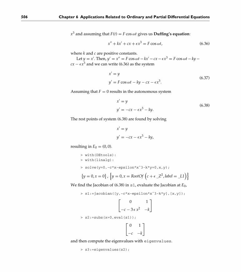
506 Chapter 6 Applications Related to Ordinary and Partial Differential Equations
x3 and assuming that F(t) = F cos ωt gives us Duffing’s equation:
x′′ + kx′ + cx + ǫx3 = F cos ωt, (6.36)
where k and c are positive constants.
Let y = x′. Then, y′ = x′′ = F cos ωt − kx′ − cx − ǫx3 = F cos ωt − ky −cx − ǫx3 and we can write (6.36) as the system
x′ = y
y′ = F cos ωt − ky − cx − ǫx3.(6.37)
Assuming that F = 0 results in the autonomous system
x′ = y
y′ = −cx − ǫx3 − ky.(6.38)
The rest points of system (6.38) are found by solving
x′ = y
y′ = −cx − ǫx3 − ky,
resulting in E0 = (0, 0).
> with(DEtools):
> with(linalg):
> solve(y=0,-c*x-epsilon*xˆ3-k*y=0,x,y);
{
y = 0, x = 0}
,{
y = 0, x = RootOf(
c + ǫ _Z2, label = _L1)}
We find the Jacobian of (6.38) in s1, evaluate the Jacobian at E0,
> s1:=jacobian([y,-c*x-epsilon*xˆ3-k*y],[x,y]);
[
0 1
−c − 3 ǫ x2 −k
]
> s2:=subs(x=0,eval(s1));
[
0 1
−c −k
]
and then compute the eigenvalues with eigenvalues.
> s3:=eigenvalues(s2);

6.4 Systems of Equations 507
s3 := −1/2 k + 1/2√
k2 − 4 c, −1/2 k − 1/2√
k2 − 4 c
Because k and c are positive, k2 − 4c < k2 so the real part of each
eigenvalue is always negative if k2 − 4c �= 0. Thus, E0 is locally stable.
For the autonomous system
x′ = f (x, y)
y′ = g(x, y),(6.39)
Bendixson’s theorem states that if fx(x, y)+gy(x, y) is a continuous func-
tion that is either always positive or always negative in a particular
region R of the plane, then system (6.39) has no limit cycles in R. For
(6.38) we have
d
dx
(
y)
+d
dy
(
−cx − ǫx3 − ky)
= −k,
which is always negative. Hence, (6.38) has no limit cycles and it follows
that E0 is globally, asymptotically stable.
> diff(y,x)+diff(-c*x-epsilon*xˆ3-k*y,y);
−k
We use DEplot to illustrate two situations that occur. In Figure 6-37(a),
we use c = 1, ǫ = 1/2, and k = 3. In this case, E0 is a stable node. On the
other hand, in Figure 6-37(b), we use c = 10, ǫ = 1/2, and k = 3. In this
case, E0 is a stable spiral.
> ivals:=seq(-2.5+.5*i,i=0..10):
> i1:=seq([x(0)=2.5,y(0)=i],i=ivals):
> i2:=seq([x(0)=i,y(0)=2.5],i=ivals):
> i3:=seq([x(0)=-2.5,y(0)=i],i=ivals):
> i4:=seq([x(0)=i,y(0)=-2.5],i=ivals):
> DEplot([diff(x(t),t)=y(t),diff(y(t),t)
=-1*x(t)-1/2*x(t)ˆ3-3*y(t)],
> [x(t),y(t)],t=0..10,[i1,i2,i3,i4],x=-2.5..2.5,
y=-2.5..2.5,
> scene=[x(t),y(t)],scaling=CONSTRAINED,color=GRAY,
linecolor=BLACK,
> thickness=1,stepsize=.05);
> ivals:=seq(-1+.25*i,i=0..8): i1:=seq([x(0)=1,y(0)=i],
i=ivals):
> i2:=seq([x(0)=i,y(0)=1],i=ivals):
> i3:=seq([x(0)=-1,y(0)=i],i=ivals):

508 Chapter 6 Applications Related to Ordinary and Partial Differential Equations
y(t)
2
(a) (b)
1
0
-1
-2
x(t)210-1-2
y(t)
1
0.5
0
-0.5
-1
x(t)10.50-0.5-1
Figure 6-37 (a) The origin is a stable node. (b) The origin is a stable spiral
> i4:=seq([x(0)=i,y(0)=-1],i=ivals):
> DEplot([diff(x(t),t)=y(t),diff(y(t),t)
=-10*x(t)-1/2*x(t)ˆ3-3*y(t)],
> [x(t),y(t)],t=0..10,[i1,i2,i3,i4],x=-1..1,y=-1..1,
> scene=[x(t),y(t)],scaling=CONSTRAINED,color=GRAY,
linecolor=BLACK,
> thickness=1,stepsize=.01);
EXAMPLE 6.4.6 (Predator – Prey): The predator–prey equations take
the form
dx
dt= ax − bxy
dy
dt= dxy − cy
where a, b, c, and d are positive constants. x represents the size of the
prey population at time t while y represents the size of the predator
population at time t. We use solve to calculate the rest points. In this
case, there is one boundary rest point, E0 = (0, 0), and one interior rest
point, E1 = (c/d, a/b).
> with(linalg):
> with(DEtools):
> rps:=solve(a*x-b*x*y=0,d*x*y-c*y=0,x,y);
rps :={
x = 0, y = 0}
,{
x =c
d, y =
a
b
}

6.4 Systems of Equations 509
y(t)
2
1.5
1
0.5
0
x(t)21.510.50
Figure 6-38 Multiple limit cycles about the interior rest point
The Jacobian is then found using jacobian.
> jac:=jacobian([a*x-b*x*y,d*x*y-c*y],[x,y]);
jac := matrix(
[[a − by, −xb], [yd, dx − c]])
E0 is unstable because one eigenvalue of J(E0) is positive. For the lin-
earized system, E1 is a center because the eigenvalues of J(E1) are
complex conjugates.
> eigenvalues(subs(rps[1],eval(jac)));
a, −c
> eigenvalues(subs(rps[2],eval(jac)));
√−ca, −
√−ca
In fact, E1 is a center for the nonlinear system as illustrated in
Figure 6-38, where we have used a = 1, b = 2, c = 2, and d = 1.
Notice that there are multiple limit cycles around E1 = (1/2, 1/2).
> inits:=seq([x(0)=i/20,y(0)=i/20],i=3..10):
> DEplot([diff(x(t),t)=x(t)-2*x(t)*y(t),
> diff(y(t),t)=2*x(t)*y(t)-y(t)],[x(t),y(t)],
t=0..50,[inits],
> x=0..2,y=0..2,scene=[x(t),y(t)],scaling=CONSTRAINED,
color=GRAY,
> linecolor=BLACK,thickness=1,stepsize=.1);
In this model, a stable interior rest state is not possible.

510 Chapter 6 Applications Related to Ordinary and Partial Differential Equations
The complexity of the behavior of solutions to the system increases
based on the assumptions made. Typical assumptions include adding
satiation terms for the predator (y) and/or limiting the growth of the
prey (x). The standard predator – prey equations of Kolmogorov type,
x′ = αx
(
1 −1
Kx
)
−mxy
a + x
y′ = y
(mx
a + x− s
)
,
(6.40)
incorporate both of these assumptions.
We use solve to find the three rest points of system (6.40). Let E0 =(0, 0) and E1 = (k, 0) denote the two boundary rest points, and let E2
represent the interior rest point.
> with(linalg):
> with(DEtools):
> rps:=solve(alpha*x*(1-1/k*x)-m*x*y/(a+x)=0,
y*(m*x/(a+x)-s)=0,x,y);
rps :={
x = 0, y = 0}
,{
y = 0, x = k}
,{
y = −α a (−mk + ks + sa)
k(
m2 − 2 ms + s2) , x = −
sa
−m + s
}
The Jacobian, J, is calculated next in s1 with jacobian.
> s1:=jacobian([alpha*x*(1-1/k*x)-m*x*y/(a+x),
y*(m*x/(a+x)-s)],[x,y]);⎡
⎢⎣
1 − 2 x − y1/10+x + xy
(1/10+x)2 − x
1/10+x
y
((
1/10 + x)−1 − x
(1/10+x)2
)
x1/10+x − s
⎤
⎥⎦
Because J(E0) has a positive eigenvalue, E0 is unstable.
> e0:=subs(rps[1],eval(s1));[
1 0
0 −s
]
> eigenvalues(e0);
α, −s
The stability of E1 is determined by the sign of m − s − am/(a + k).
> e1:=subs(rps[2],eval(s1));

6.4 Systems of Equations 511
[
−1 − 1011
0 1011 − s
]
> eigs1:=eigenvalues(e1);
eigs1 := −α, −−mk + ks + sa
a + k
The eigenvalues of J(E2) are quite complicated.
> e2:=subs(rps[3],eval(s1)):
> eigenvalues(e2);
1/2
s2α a + s2α k − sα mk + α sam +
√√√√√
s4α2a2 + 2 s4α2ak + 2 s3α2a2m + s4α2k2 − 2 s3α2k2m + s2α2m2k2
−2 s2α2m2ka + α2s2a2m2 + 4 mks4α a + 4 mk2s4α − 12 m2k2s3α
−8 m2ks3α a + 12 m3k2s2α + 4 m3ks2α a − 4 m4k2sα
mks − m2k,
1/2
s2α a + s2α k − sα mk + α sam −
√√√√√
s4α2a2 + 2 s4α2ak + 2 s3α2a2m + s4α2k2 − 2 s3α2k2m + s2α2m2k2
−2 s2α2m2ka + α2s2a2m2 + 4 mks4α a + 4 mk2s4α − 12 m2k2s3α
−8 m2ks3α a + 12 m3k2s2α + 4 m3ks2α a − 4 m4k2sα
mks − m2k
Instead of using the eigenvalues to classify E2, we compute the char-
acteristic polynomial of J(E2), p(λ) = c2λ2 + c1λ + c0, and examine the
coefficients. Notice that c2 is always positive.
> cpe2:=charpoly(e2,lambda);
cpe2 := −s3α k+s3α a+s2λα a+s2λα k−2s2αmk−s2α am−sλ2km−sλαmk+sαm2k+sλαma+λ2km2
m(−m+s)k
> c0:=simplify(subs(lambda=0,eval(cpe2)));
c0 := −(−mk + ks + sa) sα
mk
> c1:=simplify(coeff(cpe2,lambda));
c1 := −sα (sa + ks − mk + am)
m (−m + s) k
> c2:=simplify(coeff(cpe2,lambdaˆ2));
c2 := 1
On the other hand, c0 and m− s−am/(a+k) have the same sign because
> simplify(c0/eigs1);

512 Chapter 6 Applications Related to Ordinary and Partial Differential Equations
(−mk + ks + sa) s
mk
is always positive. In particular, if m − s − am/(a + k) < 0, E1 is stable.
Because c0 is negative, by Descartes’ rule of signs, it follows that p(λ)
will have one positive root and hence E2 will be unstable.
On the other hand, if m − s − am/(a + k) > 0 so that E1 is unstable,
E2 may be either stable or unstable. To illustrate these two possibilities
let α = K = m = 1 and a = 1/10. We recalculate.
> alpha:=1:k:=1:m:=1:a:=1/10:
> rps:=solve(alpha*x*(1-1/k*x)-m*x*y/(a+x)=0,
y*(m*x/(a+x)-s)=0,x,y);
rps :={
x = 0, y = 0}
,{
x = 1, y = 0}
,{
x = −1/10s
−1 + s, y = −
1
100
−10 + 11 s
(−1 + s)2
}
> s1:=jacobian([alpha*x*(1-1/k*x)-m*x*y/(a+x),
y*(m*x/(a+x)-s)],[x,y]);
⎡
⎢⎢⎣
1 − 2 x − y1/10+x + xy
(1/10+x)2 − x
1/10+x
y
((
1/10 + x)−1 − x
(1/10+x)2
)
x1/10+x − s
⎤
⎥⎥⎦
> e2:=subs(rps[3],eval(s1)):
> cpe2:=charpoly(e2,lambda);
cpe2 := −1/1010 λ2 − 10 λ2s − 9 λ s + 11 λ s2 + 10 s − 21 s2 + 11 s3
−1 + s
> c0:=simplify(subs(lambda=0,cpe2));
c0 := −1/10 s (−10 + 11 s)
> c1:=simplify(coeff(cpe2,lambda));
c1 := −1/10s (−9 + 11 s)
−1 + s
> c2:=simplify(coeff(cpe2,lambdaˆ2));
c2 := 1
Using solve, we see that
1. c0, c1, and c2 are positive if 9/11 < s < 10/11, and
2. c0 and c2 are positive and c1 is negative if 0 < s < 9/11.

6.4 Systems of Equations 513
> solve(c0>0 and c1>0,s);
{9
11< s, s <
10
11
}
> solve(c0>0 and c1 <0,s);
{
0 < s, s <9
11
}
In the first situation, E2 is stable; in the second, E2 is unstable.
Using s = 19/22, we graph the direction field associated with the
system as well as various solutions in Figure 6-39. In the plot, notice
that all nontrivial solutions approach E2 ≈ (.63, .27); E2 is stable – a
situation that cannot occur with the standard predator–prey equations.
> subs(s=19/22,rps[3]);
{
x =19
30, y =
121
450
}
> ivals:=seq(i/14,i=0..14):
> i1:=seq([x(0)=1,y(0)=i],i=ivals):
> i2:=seq([x(0)=i,y(0)=1],i=ivals):
> DEplot([diff(x(t),t)=alpha*x(t)*(1-1/k*x(t))
-m*x(t)*y(t)/(a+x(t)),
> diff(y(t),t)=y(t)*(m*x(t)/(a+x(t))-19/22)],
> [x(t),y(t)],t=0..25,[i1,i2],x=0..1,y=0..1,
scene=[x(t),y(t)],
> scaling=CONSTRAINED,color=GRAY,linecolor=BLACK,
> thickness=1,stepsize=.075);
On the other hand, using s = 8/11 (so that E2 is unstable) in Figure 6-40
we see that all nontrivial solutions appear to approach a limit cycle.
> DEplot([diff(x(t),t)=alpha*x(t)*(1-1/k*x(t))
-m*x(t)*y(t)/(a+x(t)),
> diff(y(t),t)=y(t)*(m*x(t)/(a+x(t))-8/11)],
> [x(t),y(t)],t=0..50,[i1,i2],x=0..1,y=0..1,
scene=[x(t),y(t)], > scaling=CONSTRAINED,color=GRAY,
linecolor=BLACK,thickness=1,stepsize=.075);
The limit cycle is shown more clearly in Figure 6-41.
> DEplot([diff(x(t),t)=alpha*x(t)*(1-1/k*x(t))
-m*x(t)*y(t)/(a+x(t)),
> diff(y(t),t)=y(t)*(m*x(t)/(a+x(t))-8/11)],
> [x(t),y(t)],t=0..50,[[x(0)=.759,y(0)=.262]],x=0..1,y=0..1,
scene=[x(t),y(t)],

514 Chapter 6 Applications Related to Ordinary and Partial Differential Equations
> scaling=CONSTRAINED,color=GRAY,linecolor=BLACK,
thickness=1,
> arrows=NONE,stepsize=.075);
y(t)
1
0.8
0.6
0.4
0.2
0
x(t)10.80.60.40.20
Figure 6-39 s = 19/22
y(t)
1
0.8
0.6
0.4
0.2
0
x(t)10.80.60.40.20
Figure 6-40 s = 8/11

6.4 Systems of Equations 515
y(t)
1
0.8
0.6
0.4
0.2
0
x(t)
10.80.60.40.20
Figure 6-41 A better view of the limit cycle without the direction field
Also see Example 6.4.4.
EXAMPLE 6.4.7 (Van-der-Pol’s equation): In Example 6.4.4 we saw
that Van-der-Pol’s equation x′′ + μ(
x2 − 1)
x′ + x = 0 is equivalent
to the system
⎧
⎨
⎩
x′ = y
y′ = μ(
1 − x2)
y − x.
Classify the equilibrium points, use dsolve with the numeric option,
to approximate the solutions to this nonlinear system, and plot the phase
plane.
SOLUTION: We find the equilibrium points by solving{
y = 0
μ(
1 − x2)
y − x = 0. From the first equation, we see that y = 0. Then,
substitution of y = 0 into the second equation yields x = 0. There-
fore, the only equilibrium point is (0, 0). The Jacobian matrix for this
system is
J(x, y) =(
0 1
−1 − 2μxy −μ(
x2 − 1)
)
.

516 Chapter 6 Applications Related to Ordinary and Partial Differential Equations
The eigenvalues of J(0, 0) are λ1,2 = 12
(
μ ±√
μ2 − 4)
.
> with(DEtools):
> with(linalg):
> f:=(x,y)->y:
> g:=(x,y)->-x-mu*(xˆ2-1)*y:
> jac:=jacobian([f(x,y),g(x,y)],[x,y]);
[
0 1
−1 − 2 μ xy −μ(
x2 − 1)
]
> eigenvalues(subs([x=0,y=0],jac));
− 1/2 μ x2 + 1/2 μ + 1/2√
μ2x4 − 2 μ2x2 + μ2 − 4 − 8 μ xy,
− 1/2 μ x2 + 1/2 μ − 1/2√
μ2x4 − 2 μ2x2 + μ2 − 4 − 8 μ xy
Alternatively, the sequence of commands
> lin_mat:=array([[0,1],[-1,mu]]):
> with(linalg):
> eigs:=eigenvals(lin_mat);
eigs := 1/2 μ + 1/2
√
μ2 − 4, 1/2 μ − 1/2
√
μ2 − 4
gives us the same result.
Notice that if μ > 2, then both eigenvalues are positive and real.
Hence, we classify (0, 0) as an unstable node. On the other hand, if
0 < μ < 2, then the eigenvalues are a complex conjugate pair with a
positive real part. Hence, (0, 0) is an unstable spiral. (We omit the case
μ = 2 because the eigenvalues are repeated.)
> sys:=mu->[diff(x(t),t)=y(t),diff(y(t),t)
=mu*(1-x(t)ˆ2)*y(t)-x(t)];
sys := μ →[
d
dtx (t) = y (t) ,
d
dty (t) = μ
(
1 − (x (t))2)
y (t) − x (t)
]
We now show several curves in the phase plane that begin at various
points for various values of μ by using seq to generate a list of ordered
pairs that will correspond to the initial conditions in the initial-value
problem.
> inits1:=seq([x(0)=0.1*cos(2*Pi*i/4),
y(0)=0.1*sin(2*Pi/4)],i=0..4);

6.4 Systems of Equations 517
inits1 :={
[x (0) = 0.1, y (0) = 0.1], [x (0) = 0.0, y (0) = 0.1],
[x (0) = −0.1, y (0) = 0.1]}
> inits2:=seq([x(0)=-5,y(0)=-5+10*i/9],i=0..9);
inits2 :=
{[
x (0) = −5, y (0) =35
9
]
, [x (0) = −5, y (0) = 5], [x (0) = −5, y (0) = −5],
[
x (0) = −5, y (0) = −35
9
]
,
[
x (0) = −5, y (0) = −25
9
]
, [x (0) = −5, y (0) = −5/3],
[x (0) = −5, y (0) = −5/9], [x (0) = −5, y (0) = 5/9], [x (0) = −5, y (0) = 5/3],[
x (0) = −5, y (0) =25
9
]}
> inits3:=seq([x(0)=5,y(0)=-5+10*i/9],i=0..9):
> inits4:=seq([x(0)=-5+10*i/9,y(0)=-5],i=0..9):
> inits5:=seq([x(0)=-5+10*i/9,y(0)=5],i=0..9):
> initconds:=‘union’(inits1,inits2,inits3,inits4,inits5):
> nops(initconds);
39
We then use phaseportrait in the same way as we use DEplot to
graph various solutions.
> phaseportrait(sys(1/2),[x(t),y(t)],t=0..20,initconds,
x=-5..5,y=-5..5,
> arrows=NONE,linecolor=BLACK,stepsize=0.05);
> phaseportrait(sys(1),[x(t),y(t)],t=0..20,initconds,
x=-5..5,y=-5..5,
> arrows=NONE,linecolor=BLACK,stepsize=0.05);
> phaseportrait(sys(3/2),[x(t),y(t)],t=0..20,initconds,
x=-5..5,y=-5..5,
> arrows=NONE,linecolor=BLACK,stepsize=0.05);
> phaseportrait(sys(3),[x(t),y(t)],t=0..20,initconds,
x=-5..5,y=-5..5,
> arrows=NONE,linecolor=BLACK,stepsize=0.05);
We show all four graphs together in Figure 6-42. In each figure, we
see that all of the curves approach a curve called a limit cycle. Physically,
the fact that the system has a limit cycle indicates that for all oscillations,

518 Chapter 6 Applications Related to Ordinary and Partial Differential Equations
y
4
2
0
-2
-4
x420-2-4
y
4
2
0
-2
-4
x420-2-4
y
4
2
0
-2
-4
x420-2-4
y
4
2
0
-2
-4
x420-2-4
Figure 6-42 Solutions to the Van-der-Pol equation for various values of μ
the motion eventually becomes periodic, which is represented by a
closed curve in the phase plane.
�
6.5 Some Partial Differential Equations
We now turn our attention to several partial differential equations. Several exam-
ples in this section will take advantage of commands contained in the PDEtools
package. Information regarding the functions contained in the PDEtools package
is obtained with ?PDEtools.

6.5 Some Partial Differential Equations 519
6.5.1 The One-Dimensional Wave Equation
Suppose that we pluck a string (like a guitar or violin string ) of length p and
constant mass density that is fixed at each end. A question that we might ask is:
What is the position of the string at a particular instance of time? We answer this
question by modeling the physical situation with a partial differential equation,
namely the wave equation in one spatial variable:
c2 ∂2u
∂x2=
∂2u
∂t2or c2uxx = utt. (6.41)
In (6.41), c2 = T/ρ, where T is the tension of the string and ρ is the constant mass
of the string per unit length. The solution u(x, t) represents the displacement of the
string from the x-axis at time t. To determine u we must describe the boundary and
initial conditions that model the physical situation. At the ends of the string, the
displacement from the x-axis is fixed at zero, so we use the homogeneous boundary
conditions u(0, t) = u(p, t) = 0 for t > 0. The motion of the string also depends on
the displacement and the velocity at each point of the string at t = 0. If the initial
displacement is given by f (x) and the initial velocity by g(x), we have the initial
conditions u(x, 0) = f (x) and ut(x, 0) = g(x) for 0 ≤ x ≤ p. Therefore, we determine

520 Chapter 6 Applications Related to Ordinary and Partial Differential Equations
the displacement of the string with the initial-boundary-value problem
⎧
⎪⎪⎪⎪⎨
⎪⎪⎪⎪⎩
c2 ∂2u
∂x2=
∂2u
∂t2, 0 < x < p, t > 0
u(0, t) = u(p, t) = 0, t > 0
u(x, 0) = f (x), ut(x, 0) = g(x), 0 < x < p
. (6.42)
This problem is solved through separation of variables by assuming that u(x, t) =X(x)T(t). Substitution into (6.41) yieldsλ is a constant.
c2X′′T = XT ′′ orX′′
X=
T ′′
c2T= −λ
so we obtain the two second-order ordinary differential equations X′′+λX = 0 and
T ′′ + c2λT = 0. At this point, we solve the equation that involves the homogeneous
boundary conditions. The boundary conditions in terms of u(x, t) = X(x)T(t) are
u(0, t) = X(0)T(t) = 0 and u(p, t) = X(p)T(t) = 0, so we have X(0) = 0 and X(p) = 0.
Therefore, we determine X(x) by solving the eigenvalue problem
{
X′′ + λX = 0, 0 < x < p
X(0) = X(p) = 0.
The eigenvalues of this problem are λn =(
nπ/p)2
, n = 1, 2, 3, . . . with corre-
sponding eigenfunctions Xn(x) = sin(
nπx/p)2
, n = 1, 2, 3, . . .. Next, we solve the
equation T ′′ + c2λnT = 0. A general solution is
Tn(t) = an cos(
c√
λnt)
+ bn sin(
c√
λnt)
= an coscnπ t
p+ bn sin
cnπ t
p,
where the coefficients ab and bn must be determined. Putting this information
together, we obtain
un(x, t) =(
an coscnπ t
p+ bn sin
cnπ t
p
)
sinnπx
p,
so by the Principle of Superposition, we have
u(x, t) =∞∑
n=1
(
an coscnπ t
p+ bn sin
cnπ t
p
)
sinnπx
p.
Applying the initial displacement u(x, 0) = f (x) yields
u(x, 0) =∞∑
n=1
an sinnπx
p= f (x),

6.5 Some Partial Differential Equations 521
so an is the Fourier sine series coefficient for f (x), which is given by
an =2
p
∫ p
0f (x) sin
nπx
pdx, n = 1, 2 . . .
In order to determine bn, we must use the initial velocity. Therefore, we compute
∂u
∂t(x, t) =
∞∑
n=1
(
−ancnπ
psin
cnπ t
p+ bn
cnπ
pcos
cnπ t
p
)
sinnπx
p.
Then,
∂u
∂t(x, 0) =
∞∑
n=1
bncnπ
psin
nπx
p= g(x)
so bncnπ
p represents the Fourier sine series coefficient for g(x) which means that
bn =p
cnπ
∫ p
0g(x) sin
nπx
pdx, n = 1, 2 . . .
EXAMPLE 6.5.1: Solve
⎧
⎪⎪⎨
⎪⎪⎩
uxx = utt, 0 < x < 1, t > 0
u(0, t) = u(1, t) = 0, t > 0
u(x, 0) = sin πx, ut(x, 0) = 3x + 1, 0 < x < 1
.
SOLUTION: The initial displacement and velocity functions are
defined first.
> f:=x->sin(Pi*x):
> g:=x->3*x+1:
Next, the functions to determine the coefficients an and bn in the series
approximation of the solution u(x, t) are defined. Here, p = c = 1.
> a[1]:=2*int(f(x)*sin(Pi*x),x=0..1);
a1 := 1
> n:=’n’:
> a[n]:=2*int(f(x)*sin(n*Pi*x),x=0..2);
an := 4sin (nπ) cos (nπ)
π(
−1 + n2)
Because n represents an integer, these results indicate that an = 0 for all
n ≥ 2. In fact, when we instruct Maple to assume that n is an integer
with assume, Maple determines that an = 0.

522 Chapter 6 Applications Related to Ordinary and Partial Differential Equations
> assume(n,integer):
> a[n]:=2*int(f(x)*sin(n*Pi*x),x=0..2);
an := 0
Similarly, assuming that n is an integer, we see that bn =2(
1 + (−4)n+1)
π2n2.
> b[n]:=2/(n*Pi)*int(g(x)*sin(n*Pi*x),x=0..1);
bn := −2−1 + 4 (−1)n
n2π2
The function u defined next computes the nth term in the series
expansion. Thus, uapprox determines the approximation of order k
by summing the first k terms of the expansion, as illustrated with
approx(10).Notice that we define
uapprox(n) so that Maple
“remembers” the terms
uapprox that are
computed. That is, Maple
need not recompute
uapprox(n-1) to
compute uapprox(n)
provided that
uapprox(n-1) has already
been computed.
> u:=n->-2*(4*(-1)ˆn-1)/(nˆ2*Piˆ2)*sin(n*Pi*t)*sin(n*Pi*x):
> uapprox:=proc(n) option remember;
> uapprox(n-1)+u(n);
> end:
> uapprox(0):=cos(Pi*t)*sin(Pi*x):
> uapprox(10);
cos(π t)sin (π x)+10sin (π t)sin (π x)
π2−3/2
sin (2π t)sin (2π x)
π2
+10
9
sin (3π t)sin (3π x)
π2−3/8
sin (4π t)sin (4π x)
π2+2/5
sin (5π t)sin (5π x)
π2
−1/6sin
(
6π t)
sin(
6π x)
π2+
10
49
sin (7π t)sin (7π x)
π2−
3
32
sin (8π t)sin (8π x)
π2
+10
81
sin (9π t)sin (9π x)
π2−
3
50
sin (10π t)sin (10π x)
π2
To illustrate the motion of the string, we graphuapprox(10), the tenth
partial sum of the series, on the interval [0, 1] for 16 equally spaced values
of t between 0 and 2. One frame from the resulting animation is shown
in Figure 6-43.
> with(plots):
> animate(uapprox(10),x=0..1,t=0..2,frames=16);
On the other hand, entering
> anarray:=animate(uapprox(10),x=0..1,t=0..2,frames=16,
color=BLACK):
> display(anarray);

6.5 Some Partial Differential Equations 523
0.5
1
-0.5
0
-1
x10.80.60.40.20
Figure 6-43 The motion of the spring for 16 equally spaced values of t between 0 and 2
1.0.8.6.4.20.
.5
.4
.3
.2
.10.
.5e-10.
-.5e-1-.10-.15-.20-.25-.3
0.-.1-.2-.3-.4-.5-.6-.7
0.-.2-.4-.6-.8-1.
0.-.2-.4-.6-.8-1.
0.-.2-.4-.6-.8-1.
0.-.2-.4-.6-.8-1.
0.-.2-.4-.6-.8
.10.-.1-.2-.3
.5
.4
.3
.2
.10.
1.21.0.8.6.4.20.
1.21.0.8.6.4.20.
1.21.0.8.6.4.20.
1.0.8.6.4.20.
1.0.8.6.4.20.
1.0.8.6.4.20.
1.0.8.6.4.20. 1.0.8.6.4.20.
1.0.8.6.4.20.
1.0.8.6.4.20.
1.0.8.6.4.20.
1.0.8.6.4.20.1.0.8.6.4.20.
1.0.8.6.4.20. 1.0.8.6.4.20. 1.0.8.6.4.20.
1.0.8.6.4.20.
1.0.8.6.4.20. 1.0.8.6.4.20. 1.0.8.6.4.20.
1.0.8.6.4.20.
xx
xx
xxxx
x
x
xx
xxxx
Curve 1
Curve 2
Curve 3
Curve 4
Curve 5
Curve 6
Curve 7
Curve 8
Curve 9
Figure 6-44 The motion of the spring for 16 equally spaced values of t between 0 and 2
graphs uapprox(10), for 16 equally spaced values of t between 0 and
2 with animate and then displays the resulting graphs as the array
shown in Figure 6-44.
pdsolve attempts to solve partial differential equations in the same
way that dsolve attempts to solve ordinary differential equations.

524 Chapter 6 Applications Related to Ordinary and Partial Differential Equations
Using pdsolve, we obtain D’Alembert’s solution.
> pdsolve(pde);
u (x, t) = _F1 (t + x) + _F2 (t − x)
�
6.5.2 The Two-Dimensional Wave Equation
One of the more interesting problems involving two spatial dimensions (x and y) is
the wave equation. The two-dimensional wave equation in a circular region which
is radially symmetric (not dependent on θ ) with boundary and initial conditions is
expressed in polar coordinates as⎧
⎪⎪⎪⎪⎪⎪⎨
⎪⎪⎪⎪⎪⎪⎩
c2
(
∂2u
∂r2+
1
r
∂u
∂r
)
=∂2u
∂t2, 0 < r < ρ, t > 0
u (ρ, t) = 0,∣∣u(0, t)
∣∣ < ∞, t > 0
u(r, 0) = f (r),∂u
∂t(r, 0) = g(r), 0 < r < ρ
.

6.5 Some Partial Differential Equations 525
Notice that the boundary condition u (ρ, t) = 0 indicates that u is fixed at zero
around the boundary; the condition∣∣u(0, t)
∣∣ < ∞ indicates that the solution is
bounded at the center of the circular region. Like the wave equation discussed
previously, this problem is typically solved through separation of variables by
assuming a solution of the form u(r, t) = F(r)G(t). Applying separation of variables
yields the solution
u(r, t) =∞∑
n=1
(An cos cknt + Bn sin cknt) J0 (knr) ,
where λn = cαn/ρ, and the coefficients An and Bn are found through application αn represents the nth zero
of the Bessel function of the
first kind of order zero.of the initial displacement and velocity functions. With
u(r, 0) =∞∑
n=1
AnJ0 (knr) = f (r)
and the orthogonality conditions of the Bessel functions, we find that
An =∫ ρ
0 r f (r)J0 (knr) dr∫ ρ
0 r [J0 (knr)]2 dr=
2
[J1 (αn)]2
∫ ρ
0r f (r)J0 (knr) dr, n = 1, 2, . . .
Similarly, because
∂u
∂t(r, 0) =
∞∑
n=1
(−cknAn sin cknt + cknBn cos cknt) J0 (knr)
we have
ut(r, 0) =∞∑
n=1
cknBnJ0 (knr) = g(r).
Therefore,
Bn =∫ ρ
0 r g(r)J0 (knr) dr
ckn∫ ρ
0 r [J0 (knr)]2 dr=
2
ckn [J1 (αn)]2
∫ ρ
0r g(r)J0 (knr) dr, n = 1, 2, . . .
As a practical matter, in nearly all cases, these formulas are difficult to evaluate.
EXAMPLE 6.5.2: Solve
⎧
⎪⎪⎪⎪⎪⎨
⎪⎪⎪⎪⎪⎩
∂2u
∂r2+
1
r
∂u
∂r=
∂2u
∂t2, 0 < r < 1, t > 0
u(1, t) = 0, |u(0, t)| < ∞, t > 0
u(r, 0) = r(r − 1),∂u
∂t(r, 0) = sin πr, 0 < r < 1
.

526 Chapter 6 Applications Related to Ordinary and Partial Differential Equations
SOLUTION: In this case, ρ = 1, f (r) = r(r − 1), and g(r) = sin πr. To
calculate the coefficients, we will need to have approximations of the
zeros of the Bessel functions, so we re-enter the table of zeros that were
found earlier in Chapter 4. Then, for 1 ≤ n ≤ 8, αn is the nth zero of J0.
> alpha:=array([2.4048, 5.5201, 8.6537, 11.792,
> 14.931, 18.071, 21.212, 24.352]):
> alpha[1];
2.4048
Next, we define the constants ρ and c and the functions f (r) = r(r − 1),
g(r) = sin πr, and kn = αn/ρ.
> c:=1:
> rho:=1:
> f:=r->r*(r-1):
> g:=r->sin(Pi*r):
> k:=n->alpha[n]/rho:
The formulas for the coefficients An and Bn are then defined so that an
approximate solution may be determined. (We use lower-case letters
to avoid any possible ambiguity with built-in Maple functions.) Note
that we use evalf and Int to approximate the coefficients and avoid
the difficulties in integration associated with the presence of the Bessel
function of order zero.
> a:=proc(n) option remember;
> 2/BesselJ(1,alpha[n])ˆ2*evalf(Int(r*f(r)*BesselJ
(0,k(n)*r),r=0..rho))
> end:
> b:=proc(n) option remember;
> 2/(c*k(n)*BesselJ(1,alpha[n])ˆ2)*evalf(Int(r*g(r)
*BesselJ(0,k(n)*r),r=0..rho))
> end:
We now compute the first eight values of An and Bn. Because a and b
are defined using proc with the remember option, Maple remembers
these values for later use.
> array([seq([n,a(n),b(n)],n=1..8)]);

6.5 Some Partial Differential Equations 527
⎡
⎢⎢⎢⎢⎢⎢⎢⎢⎢⎢⎢⎣
1 −0.3235010276 0.5211819702
2 0.2084692034 −0.1457773395
3 0.007640292446 −0.01342290349
4 0.03838004574 −0.008330225220
5 0.005341000922 −0.002504216150
6 0.01503575901 −0.002082788164
7 0.003340078858 −0.0008805687934
8 0.007857367112 −0.0008134612340
⎤
⎥⎥⎥⎥⎥⎥⎥⎥⎥⎥⎥⎦
The nth term of the series solution is defined in u. Then, an approximate
solution is obtained in uapprox by summing the first eight terms of u.
> u:=’u’:n:=’n’:
> u:=(n,r,t)->(a(n)*cos(c*k(n)*t)+b(n)*sin(c*k(n)*t))
*BesselJ(0,k(n)*r):
> uapprox:=sum(’u(n,r,t)’,’n’=1..8);
uapprox :=(
−0.3235010276 cos (2.4048 t) + 0.5211819702 sin (2.4048 t))
BesselJ (0, 2.4048 r)
+(
0.2084692034 cos (5.5201 t) − 0.1457773395 sin (5.5201 t))
BesselJ (0, 5.5201 r)
+(
0.007640292446 cos(
8.6537 t)
− 0.01342290349 sin(
8.6537 t))
BesselJ(
0, 8.6537 r)
+ (0.03838004574 cos (11.792 t) − 0.008330225220 sin (11.792 t)) BesselJ (0, 11.792 r)
+(
0.005341000922 cos (14.931 t) − 0.002504216150 sin (14.931 t))
BesselJ (0, 14.931 r)
+(
0.01503575901 cos (18.071 t) − 0.002082788164 sin (18.071 t))
BesselJ (0, 18.071 r)
+(
0.003340078858 cos (21.212 t) − 0.0008805687934 sin (21.212 t))
BesselJ (0, 21.212 r)
+(
0.007857367112 cos (24.352 t) − 0.0008134612340 sin (24.352 t))
BesselJ (0, 24.352 r)
We graph uapprox for several values of t in Figure 6-45.
> with(plots):
> drumhead:=animate3d([r*cos(theta),r*sin(theta),uapprox],
r=0..1,theta=-Pi..Pi,t=0..1.5,
> frames=9):
> display(drumhead);
In order to actually watch the drumhead move, we can use animate
loop to generate an animation. Be aware, however, that generating many
three-dimensional graphics and then animating the results uses a great
deal of memory and can take considerable time, even on a relatively
powerful computer. We show one frame from the animation that results
from the following animation command in Figure 6-46.
> ?animate3d

528 Chapter 6 Applications Related to Ordinary and Partial Differential Equations
Figure 6-45 The drumhead for nine equally spaced values of t between 0 and 1.5
Figure 6-46 A drumhead
> tvals:=[seq(1.5*i/8,i=0..9)]:
> animate3d([r*cos(theta),r*sin(theta),uapprox],r=0..1,
> theta=-Pi..Pi,t=0..1.5,frames=9);
�
If the displacement of the drumhead is not radially symmetric, the problem that
describes the displacement of a circular membrane in its general case is
⎧
⎪⎪⎪⎪⎪⎪⎪⎪⎨
⎪⎪⎪⎪⎪⎪⎪⎪⎩
c2
(
∂2u
∂r2+
1
r
∂u
∂r+
1
r2
∂2u
∂θ2
)
=∂2u
∂t2, 0 < r < ρ, −π < θ < π , t > 0
u(ρ, θ , t) = 0, |u(0, θ , t)| < ∞, −π ≤ θ ≤ π , t > 0
u(r, π , t) = u(r, −π , t),∂u
∂θ(r, π , t) =
∂u
∂θ(r, −π , t), 0 < r < ρ, t > 0
u(r, θ , 0) = f (r, θ ),∂u
∂t(r, π , 0) = g(r, θ ), 0 < r < ρ, −π < θ < π
. (6.43)

6.5 Some Partial Differential Equations 529
Using separation of variables and assuming that u(r, θ , t) = R(t)H(θ )T(t), we obtain
that a general solution is given by
u(r, θ , t) =∑
n
a0nJ0 (λ0nr) cos (λ0nct) +∑
m,n
amnJm (λmnr) cos (mθ) cos (λmnct)
+∑
m,n
bmnJm (λmnr) sin (mθ) cos (λmnct) +∑
n
A0nJ0 (λ0nr) sin (λ0nct)
+∑
m,n
AmnJm (λmnr) cos (mθ) sin (λmnct)
+∑
m,n
BmnJm (λmnr) sin (mθ) sin (λmnct)
,
where Jm represents the mth Bessel function of the first kind, αmn denotes the nth
zero of the Bessel function y = Jm(x), and λmn = αmn/ρ. The coefficients are given
by the following formulas.
a0n =∫ 2π
0
∫ ρ
0 f (r, θ )J0 (λ0nr) r dr dθ
2π∫ ρ
0 [J0 (λ0nr)]2 r dramn =
∫ 2π
0
∫ ρ
0 f (r, θ )Jm (λmnr) cos (mθ) r dr dθ
π∫ ρ
0 [Jm (λmnr)]2 r dr
bmn =∫ 2π
0
∫ ρ
0 f (r, θ )Jm (λmnr) sin (mθ) r dr dθ
π∫ ρ
0 [Jm (λmnr)]2 r drA0n =
∫ 2π
0
∫ ρ
0 g(r, θ )J0 (λ0nr) r dr dθ
2πλ0ncπ∫ ρ
0 [J0 (λ0nr)]2 r dr
Amn =∫ 2π
0
∫ ρ
0 g(r, θ )Jm (λmnr) cos (mθ) r dr dθ
πλmnc∫ ρ
0 [Jm (λmnr)]2 r drBmn =
∫ 2π
0
∫ ρ
0 g(r, θ )Jm (λmnr) sin (mθ) r dr dθ
πλmnc∫ ρ
0 [Jm (λmnr)]2 r dr
EXAMPLE 6.5.3: Solve
⎧
⎪⎪⎪⎪⎪⎪⎪⎪⎪⎪⎪⎪⎪⎪⎪⎪⎪⎪⎪⎨
⎪⎪⎪⎪⎪⎪⎪⎪⎪⎪⎪⎪⎪⎪⎪⎪⎪⎪⎪⎩
102
(
∂2u
∂r2+
1
r
∂u
∂r+
1
r2
∂2u
∂θ2
)
=∂2u
∂t2, 0 < r < 1,
−π < θ < π , t > 0
u(1, θ , t) = 0, |u(0, θ , t)| < ∞, −π ≤ θ ≤ π , t > 0
u(r, π , t) = u(r, −π , t),∂u
∂θ(r, π , t) =
∂u
∂θ(r, −π , t), . . .
0 < r < 1, t > 0
u(r, θ , 0) = cos(
πr/2)
sin θ ,∂u
∂t(r, π , 0) = (r − 1) cos
(
πθ/2)
, 0 < r < 1,
−π < θ < π
,
SOLUTION: To calculate the coefficients, we will need to have approx-
imations of the zeros of the Bessel functions, so we re-enter the table of

530 Chapter 6 Applications Related to Ordinary and Partial Differential Equations
zeros that were found earlier in Chapter 4. A function alpha is then
defined so that these zeros of the Bessel functions can more easily be
obtained from the list.
> ALPHA:=array([
> [2.4048, 5.5201, 8.6537, 11.792,
> 14.931, 18.071, 21.212, 24.352],
> [3.8317, 7.0156, 10.173, 13.324,
> 16.471, 19.616, 22.760, 25.904],
> [5.1356, 8.4172, 11.620, 14.796,
> 17.960, 21.117, 24.270, 27.421],
> [6.3802, 9.7610, 13.015, 16.223,
> 19.409, 22.583, 25.748, 28.908],
> [7.5883, 11.065, 14.373, 17.616,
> 20.827, 24.019, 27.199, 30.371],
> [8.7715, 12.339, 15.700, 18.980,
> 22.218, 25.430, 28.627, 31.812],
> [9.9361, 13.589, 17.004, 20.321,
> 23.586, 26.820, 30.034, 33.233]]):
> alpha:=table():
> for i from 0 to 6 do
> for j from 1 to 8 do
> alpha[i,j]:=ALPHA[i+1,j] od od:
The appropriate parameter values as well as the initial condition func-
tions are defined as follows. Notice that the functions describing the
initial displacement and velocity are defined as the product of func-
tions. This enables the subsequent calculations to be carried out using
evalf and Int.
> c:=10:
> rho:=1:
> f:=’f’:
> f1:=r->cos(Pi*r/2):
> f2:=theta->sin(theta):
> f:=proc(r,theta) option remember;
> f1(r)*f2(theta)
> end:
> g1:=r->r-1:
> g2:=theta->cos(Pi*theta/2):
> g:=proc(r,theta) option remember;
> g1(r)*g2(theta)
> end:

6.5 Some Partial Differential Equations 531
The coefficients a0n are determined with the function a0.
> a0:=proc(n) option remember;
> evalf(Int(f1(r)*BesselJ(0,alpha[0,n]*r)*r,
r=0..rho)*Int(f2(t),
t=0..2*Pi)/(2*Pi*Int(r*BesselJ(0,alpha[0,n]*r)ˆ2,
r=0..rho)))
> end:
We use seq to calculate the first five values of a0n.
> seq(a0(n),n=1..5):
Because the denominator of each integral formula used to find amn and
bmn is the same, the function bjmnwhich computes this value is defined
next. A table of nine values of this coefficient is then determined.
> bjmn:=proc(m,n) option remember;
> evalf(Int(r*BesselJ(m,alpha[m,n]*r)ˆ2,r=0..rho))
> end:
> seq(seq(bjmn(m,n),m=1..3),n=1..3):
We also note that in evaluating the numerators of amn and bmn we must
compute∫ ρ
0 rf1(r)Jm (αmnr) dr. This integral is defined in fbjmn and the
corresponding values are found for n = 1, 2, 3 and m = 1, 2, 3.
> fbjmn:=proc(m,n) option remember;
> evalf(Int(f1(r)*BesselJ(m,alpha[m,n]*r)*r,r=0..rho))
> end:
> seq(seq(fbjmn(m,n),m=1..3),n=1..3):
The formula to compute amn is then defined and uses the informa-
tion calculated in fbjmn and bjmn. As in the previous calculation, the
coefficient values for n = 1, 2, 3 and m = 1, 2, 3 are determined.
> a:=proc(m,n) option remember;
> evalf(fbjmn(m,n)*Int(f2(t)*cos(m*t),
t=0..2*Pi)/(Pi*bjmn(m,n)))
> end:
> seq(seq(a(m,n),m=1..3),n=1..3):
A similar formula is then defined for the computation of bmn.
> b:=proc(m,n) option remember;
> evalf(fbjmn(m,n)*Int(f2(t)*sin(m*t),
t=0..2*Pi)/(Pi*bjmn(m,n)))

532 Chapter 6 Applications Related to Ordinary and Partial Differential Equations
> end:
> seq(seq(b(m,n),m=1..3),n=1..3):
Note that we define the coefficients using proc with the remember
option so that Maple “remembers” previously computed values, reduc-
ing computation time. The values of A0n are found similar to those of
a0n. After defining the function capa to calculate these coefficients, a
table of values is then found.
> capa0:=proc(n) option remember;
> evalf(Int(g1(r)*BesselJ(0,alpha[0,n]*r)*r,
r=0..rho)*Int(g2(t),t=0..2*Pi)/(2*Pi*c*alpha[0,n]
*Int(r*BesselJ(0,alpha[0,n]*r)ˆ2,r=0..rho)))
> end:
> seq(capa0(n),n=1..6):
The value of the integral of the component of g, g1, which depends on
r and the appropriate Bessel functions, is defined as gbjmn.
> gbjmn:=proc(m,n) option remember;
> evalf(Int(g1(r)*BesselJ(m,alpha[m,n]*r)*r,r=0..rho))
> end:
> seq(seq(gbjmn(m,n),m=1..3),n=1..3):
Then, Amn is found by taking the product of integrals, gbjmndepending
on r and one depending on θ . A table of coefficient values is generated
in this case as well.
> capa:=’capa’:
> capa:=proc(m,n) option remember;
> evalf(gbjmn(m,n)*Int(g2(t)*cos(m*t),t=0..2*Pi)
/(Pi*alpha[m,n]*c*bjmn(m,n)))
> end:
> seq(seq(capa(m,n),m=1..3),n=1..3):
Similarly, the Bmn are determined.
> capb:=proc(m,n) option remember;
> evalf(gbjmn(m,n)*Int(g2(t)*sin(m*t),t=0..2*Pi)
/(Pi*alpha[m,n]*c*bjmn(m,n)))
> end:
> seq(seq(capb(m,n),m=1..3),n=1..3):

6.5 Some Partial Differential Equations 533
Now that the necessary coefficients have been found, we construct an
approximate solution to the wave equation by using our results. In
the following, term1 represents those terms of the expansion involv-
ing a0n, term2 those terms involving amn, term3 those involving bmn,
term4 those involving A0n, term5 those involving Amn, and term6
those involving Bmn.
> term1:=sum(’a0(n)*BesselJ(0,alpha[0,n]*r)
*cos(alpha[0,n]*c*t)’,n=1..5);
> n:=’n’:m:=’m’:
> term2:=sum(’sum(’a(m,n)*BesselJ(m,alpha[m,n]*r)
*cos(m*theta)*cos(alpha[m,n]*c*t)’,
> n=1..3)’,m=1..3):
> n:=’n’:m:=’m’:
> term3:=sum(’sum(’b(m,n)*BesselJ(m,alpha[m,n]*r)
*sin(m*theta)*cos(alpha[m,n]*c*t)’,
> n=1..3)’,m=1..3):
> n:=’n’:
> term4:=sum(’capa0(n)*BesselJ(0,alpha[0,n]*r)
*sin(alpha[0,n]*c*t)’,n=1..5):
> n:=’n’:m:=’m’:
> term5:=sum(’sum(’capa(m,n)*BesselJ(m,alpha[m,n]*r)
*cos(m*theta)*sin(alpha[m,n]
*c*t)’,
> n=1..3)’,m=1..3):
> n:=’n’:m:=’m’:
> term6:=sum(’sum(’capb(m,n)*BesselJ(m,alpha[m,n]*r)
*sin(m*theta)*sin(alpha[m,n]
*c*t)’,
> n=1..3)’,m=1..3):
Therefore, our approximate solution is given as the sum of these terms
as computed in u.
> u:=term3+term4+term5+term6:
A table of nine plots for nine equally spaced values of t from t = 0 to
t = 1 using increments of 1/8 is then generated with animate. This
table of graphs is displayed as a graphics array in Figure 6-47.
> with(plots):

534 Chapter 6 Applications Related to Ordinary and Partial Differential Equations
Figure 6-47 The drumhead for nine equally spaced values of t from t = 0 to t = 1
> somegraphs:=animate3d([r*cos(theta),r*sin(theta),u],
r=0..1,
> theta=-Pi..Pi,t=0..1,frames=9):
> display(somegraphs);
Of course, we can generate many graphs with a Do loop and animate
the result as in the previous example. Be aware, however, that gener-
ating many three-dimensional graphics and then animating the results
uses a great deal of memory and can take considerable time, even on a
relatively powerful computer.
�
6.5.3 Other Partial Differential Equations
A partial differential equation of the form
a(x, y, u)∂u
∂x+ b(x, y, u)
∂u
∂y= c(x, y, u) (6.44)
is called a first-order, quasi-linear partial differential equation. In the case when
c(x, y, u) = 0, (6.44) is homogeneous; if a and b are independent of u, (6.44) is almost
linear; and when c(x, y, u) can be written in the form c(x, y, u) = d(x, y)u + s(x, y),
(6.44) is linear. Quasi-linear partial differential equations can frequently be solved
using the method of characteristics.

6.5 Some Partial Differential Equations 535
EXAMPLE 6.5.4: Use the method of characteristics to solve the initial-
value problem
{
−3xtux + ut = xt
u(x, o) = x.
SOLUTION: Note that pdsolve can find a general solution to the
equation, but not solve the initial-value problem.
> with(PDEtools):
> u:=’u’:x:=’x’:t:=’t’:
> pdsolve(-3*x*t*diff(u(x,t),x)+diff(u(x,t),t)=x*t);
u (x, t) = −1/3 x + _F1(
2/3 ln (x) + t2)
For this problem, the characteristic system is
∂x/∂r = −3xt, x(0, s) = s
∂t/∂r = 1, t(0, s) = 0
∂u/∂r = xt, u(0, s) = s
We begin by using dsolve to solve ∂t/∂r = 1, t(0, s) = 0
> d1:=dsolve(diff(t(r),r)=1,t(0)=0,t(r));
d1 := t (r) = r
and obtain t = r. Thus, ∂x/∂r = −3xr, x(0, s) = s, which we solve next
> d2:=dsolve(diff(x(r),r)=-3*x(r)*r,x(0)=s,x(r));
d2 := x (r) = se−3/2 r2
and obtain x = se−3r2/2. Substituting r = t and x = se−3r2/2 into ∂u/∂r =xt, u(0, s) = s and using dsolve to solve the resulting equation yields
the following result, named d3.
> u:=’u’:
> d3:=dsolve(diff(u(r),r)=exp(-3/2*rˆ2)*s*r,
> u(0)=s,u(r));
d3 := u (r) = −1/3 se−3/2 r2+ 4/3 s
To find u(x, t), we must solve the system of equations{
t = r
x = se−3r2/2

536 Chapter 6 Applications Related to Ordinary and Partial Differential Equations
for r and s. Substituting r = t into x = se−3r2/2 and solving for s yields
s = xe3t2/2.
> vals:=solve(x=exp(-3/2*rˆ2)*s,t=r,r,s);
vals :={
r = t, s =x
e−3/2 t2
}
Thus, the solution is given by replacing the values obtained above in the
solution obtained in d3. We do this below by using assign to assign r
and s the values invals andassign to assign u(r) the value obtained in
d3. We then evaluate u(r) . The resulting output represents the solution
to the initial-value problem.
> assign(vals):
> assign(d3):
> u(r);
−1/3 x + 4/3x
e−3/2 t2
Finally, we verify that this result is the solution to the problem.
> simplify(-3*x*t*diff(u(r),x)+diff(u(r),t));
xt
The initial condition u(x, 0) = x has parametrization
⎧
⎪⎪⎨
⎪⎪⎩
x = s
t = 0
u = s
. We use
PDEplot, which is contained in the PDEtools package, to graph the
solution for 0 ≤ s ≤ 15 in Figure 6-48. With the first command, we graph
-2-1 t
01
024
68 x10
1214
-2-1
t01
02
46
8 x10¹²
14
Figure 6-48 Plot of u(x, t) = 13 x(
4e3t2/2 − 1)

6.5 Some Partial Differential Equations 537
the solution drawing 20 characteristics (the default is 10) and in the
second command, we draw 20 characteristics in addition to including
the option basechar=true so that the base characteristics are also
displayed in the resulting graph.
> u:=’u’:
> s:=’s’:
> PDEplot(-3*x*t*diff(u(x,t),x)+diff(u(x,t),t)
=x*t,[s,0,s],s=0..15,
> numchar=20);
> PDEplot(-3*x*t*diff(u(x,t),x)+diff(u(x,t),t)
=x*t,[s,0,s],s=0..15,
> numchar=20,basechar=true);
�

This Page Intentionally Left Blank

Bibliography
[1] Abell, Martha and Braselton, James, Differential Equations with Maple, Third
Edition, Academic Press, 2004.
[2] Abell, Martha and Braselton, James, Modern Differential Equations, Second
Edition, Harcourt, 2001.
[3] Abell, Martha L., Braselton, James P., and Rafter, John A., Statistics with Maple,
Academic Press, 1999.
[4] Barnsley, Michael, Fractals Everywhere, Second Edition, Morgan Kaufmann,
2000.
[5] Braselton, James P., Abell, Martha L., and Braselton, Lorraine M., “When
is a surface not orientable?”, International Journal of Mathematical Education in
Science and Technology, Volume 33, Number 4, 2002, pp. 529–541.
[6] Devaney, Robert L. and Keen, Linda (eds.), Chaos and Fractals: The Math-
ematics Behind the Computer Graphics, Proceedings of Symposia in Applied
Mathematics, Volume 39, American Mathematical Society, 1989.
[7] Edwards, C. Henry and Penney, David E., Calculus with Analytic Geometry,
Fifth Edition, Prentice Hall, 1998.
[8] Edwards, C. Henry and Penney, David E., Differential Equations and Boundary
Value Problems: Computing and Modeling, Third Edition, Pearson/Prentice Hall,
2004.
[9] Gaylord, Richard J., Kamin, Samuel N., and Wellin, Paul R., Introduction to
Programming with Maple, Second Edition, TELOS/Springer-Verlag, 1996.
539

540 Bibliography
[10] Graff, Karl F., Wave Motion in Elastic Solids, Oxford University Press/Dover,
1975/1991.
[11] Gray, Alfred, Modern Differential Geometry of Curves and Surfaces, Second
Edition, CRC Press, 1997.
[12] Kyreszig, Erwin, Advanced Engineering Mathematics, Seventh Edition, John
Wiley & Sons, 1993.
[13] Larson, Roland E., Hostetler, Robert P., and Edwards, Bruce H., Calculus with
Analytic Geometry, Sixth Edition, Houghton Mifflin, 1998.
[14] Robinson, Clark, Dynamical Systems: Stability, Symbolic Dynamics, and Chaos,
Second Edition, CRC Press, 1999.
[15] Smith, Hal L. and Waltman, P., The Theory of the Chemostat: Dynamics of
Microbial Competition, Cambridge University Press, 1995.
[16] Stewart, James, Calculus: Concepts and Contexts, Second Edition, Brooks/Cole,
2001.
[17] Weisstein, Eric W., CRC Concise Encyclopedia of Mathematics, CRC Press, 1999.
[18] Wolfram, Stephen, A New Kind of Science, Wolfram Media, 2002.
[19] Zwillinger, Daniel, Handbook of Differential Equations, Second Edition, Aca-
demic Press, 1992.

Subject Index
Symbols
&* 20, 324, 337
* 19
+ 19
+/- toggle switch 17
- 19
/ 19
: 32
:= 31, 92, 243
< 82
<...> 315, 343
<= 82
<> 82
> 82
>= 82
? 12, 33
contourplot 58
factor 27
linalg 311
LinearAlgebra 311
options 58
PDEtools 518
plot 12, 41
plot[options] 43
plot3d 58
plots 12
simplex 373
solve 73
spacecurve 67
@ 25, 46
@@ 47, 245, 297
[...] 224, 320ˆ 19, 325~ 29γ 23π 22
A
abs 23, 24, 304algebraic operations 27Alternating series 174Alternating series test 174Amortization 262animate 100, 107, 285, 522animate3d 527, 534Animation 100, 527, 534Annuities
annuity due 257deferred 260future value 256present value 259
annuity 273Antiderivatives 131Antidifferentiation 131Approximating
arc length 154definite integrals 144lists 274periodic function by Fourier
series 285points of intersection
149
Arc length 154approximating 154function 384parametric equations 156polar coordinates 157
arccos 23, 24, 44arccosh 23arccot 23arccsc 23arcsec 23arcsin 23, 24, 44arcsinh 23arctan 23, 45arctanh 23Area 134, 148, 214array 223, 238, 243, 312, 316,
467arrow 333, 335, 408assign 276, 382, 536Associated matrix 342, 356assume 29, 38, 155Astroid 151Asymptotes 49Augmented matrix 342Autonomous systems 504Axes
Normal 60
B
BackwardSubstitute 345Basic How To 14
541

542 SUBJECT INDEX
Basins of attraction 300Beam problem 124Bendixson’s theorem 507Bessel functions 244, 289, 525,
529BesselI 289BesselJ 244, 526, 531Bifurcation diagrams 235Butterfly 56
C
Calculusfundamental theorem of 139
Catalan 23Catalan’s constant 23Chain rule 110changevar 133, 144Characteristic equation 444,
460Characteristic polynomial 360CharacteristicPolynomial
361, 367Characteristics
method of 534Circle 65
osculating 389unit 52
graphing 62circle 390Circuits
L-R-C 481Circular membrane 528Circular plate
normal modes 289wave equation on 289
Clearingdefinitions 33, 92
Clothoid 54Coefficient matrix 342Coefficients
undetermined 452, 463Cofactor matrix 326
transpose of 326Color
Graylevel 60Column 320, 336, 343Column space 349ColumnOperation 344ColumnSpace 349combine
expression,trig 25trig 25, 99
Command clear 33, 92command-Q 6Commands
long form 9short form 9
completesquare 219Composition operator 25
repeated 47, 245, 297Compound amount 254Compound interest 96, 254Computing
limits 93Conic sections 65Conjugate transpose 369Conservative vector field 391,
393Constants
built-in 22Catalan 23exp(1) 22gamma 23I 22, 74infinity 23, 95Pi 22
Contour plots 57contourplot 58, 60, 79, 114,
191, 207, 394, 434color 59contours 62, 198grid 59scaling 59
Convergence tests 170convertexpression,form 25expression, parfrac,
variable 29parfrac 168, 420polynom 182
Convolution integrals 480Convolution theorem 480Cooling
Newton’s law of 425Cornu spiral 54cos 23, 44cosh 23cot 23Cramer’s rule 458, 470Critical number 116Critical points 116, 201
classifying 201degenerate 202
CrossProduct 331, 408csc 23
Curl 393Curl 395, 403Curvature 384Curvature 389Curve-fitting 274
with trigonometricfunctions 280
Curvesplane 384smooth 156space 384
Cycloid 112Cylinder
inscribed in sphere 127
D
D 102, 119, 194[1](f)(x,y) 194[2](f)(x,y) 194(f)(x) 102
(D@@n)(f)(x) 102
Damping 448, 505Deferred annuities 260Defining
functions 33, 57lists 223matrices 312vectors 318
Definite integrals 139approximating 144
Delayed evaluation 41denom 95fraction 30
DEplot 489, 491, 493, 507Derivatives
calculating 102definition 98directional 196first
properties 116first derivative test 116mean-value theorem 115oscillating 121partial 193second
properties 116second derivative test 117,
202det 458, 471Determinant 322, 324, 327Determinants 322DEtools 11

SUBJECT INDEX 543
DEplot 489, 491, 493, 507matrixDE 487, 501odeadvisor 433, 435varpar 458varparam 470, 473
diff 76, 102, 105, 193, 209, 393f(x),x 102f(x),x$n 102f(x,y),x 193f(x,y),x,y 193f(x,y),x$n 194f(x,y),x$n,y$m 194f(x,y),y 193
Difference quotient 98Differential calculus 98Differential equations
first-orderexact 433homogeneous 423, 435linear 422nonlinear 433particular solution 423separable 417standard form 423
heat equation 286higher-order linear
characteristic equation460
constant coefficients 460fundamental set of
solutions 460general solution 460homogeneous 460Laplace transform
method 473linearly dependent
solutions 460linearly independent
solutions 460standard form 460undetermined
coefficients 463variation of parameters
469linear systems 487
fundamental matrix 487general solution 487homogeneous 487Laplace transform
method 496particular solution 487
nonhomogeneous linearsystems 498
fundamental matrix 498particular solution 498variation of parameters
498nonlinear higher-order 486nonlinear systems 502
autonomous 504linearization 504
partialalmost linear 534characteristic system 535first-order quasi-linear
534homogeneous 534linear 534method of characteristics
534one-dimensional wave
519two-dimensional wave
524second-order linear
associated set of functions452
characteristic equation444
constant coefficients 444fundamental set of
solutions 444general form 443general solution 443homogeneous 443linearly independent
solutions 444standard form 443undetermined
coefficients 452variation of parameters
457Differentiation
implicit 105rules 102
Dirac 484Dirac delta function 484Directional derivatives 196display 9, 10, 13, 41, 79, 248,
390insequence 359, 497scaling 113
Divergenceof series
test 170, 171, 175of vector field 391
Divergence 392, 396, 402
Divergence theorem 401Division
by zero 32Do 534Domain
finding 82dotprod 197, 382DotProduct 331Double pendulum 494Doubleint 212Drumhead 527dsolve 417, 420, 426, 430,
445, 454, 459, 461, 469,489, 501, 535
method 483, 496numeric 437, 441, 502, 515
dual 376Dual problem 375Duffing’s equation 505Dynamical systems 232, 245,
2942-cycle 2334-cycle 233
Ee 22, 24Eigenvalue problem 520Eigenvalues 360, 370eigenvalues 506, 509, 361,
372Eigenvectors 360Eigenvectors 361eigenvects 488, 490, 492elif 39, 282, 475Elimination
Gauss-Jordan 342Ellipse 65Ellipsoid 70Elliptical torus 69end 38end proc 38Enter 4, 20_EnvAllSolutions 75, 148Equations 73
graphing 60recurrence 269solving
approximate solutions 84complex solutions 86exact solutions 73linear systems 77, 336nonlinear systems 79, 88
see also Linear systems

544 SUBJECT INDEX
Equilibrium point 504erf 140Error function 140Euler’s constant 23eval 31, 93evalb 249evalf 20, 31, 80, 88, 145, 157,
212expr,n 20int 147, 150, 157, 286, 526number 21, 136sum 173
evalm 312, 314, 324Evaluating
expressions 31functions 33
Exact differential equations433
Execution Group 7exp 23, 24, 25(1) 25
expand 25, 27, 99, 463expression 25, 27
Exponential function 22, 24Exponential growth 425Export As 7Expressions
evaluating 31Extracting
columnsof matrices 320
elementsof matrices 320
rowsof matrices 320
extrema 211
F
factor 27, 30, 95, 445, 461expression 27, 461
Factorial sequences 164fi 38fieldplot 394, 421, 440File
Export As 7Quit 6Save 6
finance 11, 253, 273annuity 273growingannuity 273growingperpetuity 273
Financial planning 267
First derivative test 116
fit 274, 279, 280
Flux
outward 402
Folium of Descartes 385
for 244, 283
Force
damping 448
resistive 429
resultant 429
Fourier series 281
approximating periodicfunction by 285
Fourier sine series 521
Free-falling bodies 428
FresnelC 54, 400
FresnelS 54, 400
fsolve 43, 80, 84, 149, 273,431
complex 84
eqn,x 84
eqn,x,a..b 84, 290
fulldigits 188
Functions
approximating lists with274
arc length 384
Bessel 244, 289, 525, 529
built-in 23
continuous but notdifferentiable 188
defining 33, 57
Dirac delta 484
evaluating 33
implicit
tangent lines of 109
inverse 46
periodic
approximating by Fourierseries 285
piecewise-defined 37
polar 51
potential 391
recursively defined 38
of single variable 33
graphing 40
of two variables 57
limits of 190
vector-valued 196, 384
Fundamental matrix 487, 498
Fundamental set of solutions444, 460
Fundamental theorem ofcalculus 139
Fundamental theorem of lineintegrals 397
Future value 256
G
Gabriel’s horn 162gamma 23Gauss-Jordan elimination 342Geometric series 169grad 196, 200Gradient 196, 391gradplot 201, 395gradplot3d 396Gram-Schmidt process 352GramSchmidt 353normalized 353, 354
Graphics array 100Graphing
approximating intersectionpoints 149
equations 60functions of a single
variable 40lists 227, 247parametric curves and
surfaces in space 66parametric and polar plots
in two dimensions 51three-dimensional and
contour plots 57unit circle 62
Gravity 429Graylevel 60Gray’s torus 69Green’s theorem 398growingannuity 273growingperpetuity 273Growth constant 425
H
H 236Harmonic motion 448
critically damped 449overdamped 449underdamped 449
Harmonic series 172alternating 175
Heat equationone-dimensional 286
Heaviside 474, 478

SUBJECT INDEX 545
Help 13Basic How To 14New Users 14
Quick Tour 14Using Help 14
Help Browser 9Hermite polynomials 236Hermitian adjoint matrix 369Hidden Line 60Homogeneous differential
equations 423, 435, 443,460, 487, 534
corresponding 423Hooke’s law 448Hyperbola 65Hyperboloid
of one sheet 71of two sheets 71
I
I 22, 74i 22icosahedron 11identity 81, 454Identity matrix 317IdentityMatrix 317if 38Ikeda map 300Immersions 413Implicit differentiation 105implicitdiff 105, 111implicitplot 63, 219color 64, 66grid 64, 66scaling 66
implicitplot3d 72, 395axes 72grid 72
Improper integrals 140index
packages 9inequal 376Inequalities
solving 82Infinite series, see Series,
infiniteinfinity 23, 95Inflection points 116Insert
Execution Group 7Subsection 16
int 133, 172, 212, 215, 220,237, 385
f(x),x 131f(x),x=a..b 53, 139, 144see also integrate
Int 144, 286Integral calculus 134Integral test 170, 172Integrals
convolution 480iterated 212
triple 220line 397
fundamental theorem of397
logarithmic 229surface 401
integrate 172, 212, 385, 405,420, 427, 471
see also intIntegrating factor 424Integration by parts 144
formula 132Integrodifferential equations
481Interest
compound 96, 254total paid on loan 264
interp 276Intersection points of graphs
149intparts 144inttrans 474invlaplace 474, 483, 485laplace 474, 483, 485
inverse 313Inverse functions 46invlaplace 474, 483, 485Irrotational vector field 393Iterated integrals 212
triple 220ithprime 228
Jjacobian 505, 509Jacobian matrix 505, 515Jordan block matrix 365Jordan canonical form 366Jordan matrix 366JordanForm 366Julia sets 250, 296
KKernel 356Klein bottle 413
L
L-R-C circuits 481
Lagrange multipliers 208
Lagrange’s theorem 208
laplace 474, 483, 485
Laplace transform 473, 496
inverse 474
of product of twofunctions 480
Laplacian 392
in polar coordinates 289
Laplacian 392, 396
leftbox 135
leftsum 135, 145
Lemniscate of Bernoulli 152
L’Hôpital’s rule 171
limit 32, 98, 138, 167
f(x),x=a 91, 94
f(x),x=a,left 96
f(x),x=a,right 96
left 96, 99
right 96, 99
Limit 98
Limit comparison test 170,174
Limit cycle 517
Limits 91
computing 93
of functions of twovariables 190
graphs and tables to predict91
one-sided 96
linalg 11, 311, 318
det 458, 471
dotprod 197, 382
eigenvalues 506, 509
eigenvects 488, 490, 492
grad 196, 200
inverse 313
jacobian 505, 509
multiply 379
norm 197
wronskian 458, 471
Line integrals 397
fundamental theorem of 397
Linear differential equations
first-order 422
nth-order 460
partial 534
second-order 443
standard form 423, 443, 460

546 SUBJECT INDEX
Linear programming 372dual problem 375standard form of problem
372Linear systems 77, 336Linear transformations 355
kernel 356LinearAlgebra 11, 311, 318BackwardSubstitute
345Characteristic-
Polynomial 361, 367Column 320, 336, 343ColumnOperation 344ColumnSpace 349CrossProduct 331, 408Determinant 322, 324, 327DotProduct 331Eigenvalues 361, 372Eigenvectors 361GramSchmidt 353normalized 353, 354
IdentityMatrix 317JordanForm 366LinearProgramming 378LinearSolve 336, 338MatrixInverse 314, 322,
324, 336MatrixPower 315, 325MinimalPolynomial 366Multiply 324, 337Norm 328, 332Normalize 332, 387, 394NullSpace 348, 349, 356QRDecomposition 369ReducedRowEchelonForm
327, 336, 343, 349Row 320RowOperation 336, 344Transpose 322, 324, 351ZeroVector 319
LinearProgramming 378LinearSolve 336, 338LineInt 397list 35, 223
[i] 224, 238[i..j] 224, 238
list_of_rows 312listplot 228Lists 74, 223
approximating 274defining 223graphing 227, 247
manipulating 238nested 316
Lituus 56ln 23, 24, 95Loans
amortized 262amount paid towards
principal 263total interest paid on 264
Local maximum 202Local minimum 202Logarithmic integral 229Logistic equation 421
with predation 440
M
Maclaurinpolynomial 179series 179
Mandelbrot set 302, 306generalized 304
MapIkeda 300
map 92, 117, 239diff 104f,list 35, 104, 136, 239int 132, 237integrate 386
Maple
Preferences 6Matrices
addition of 323associated 342, 356augmented 342coefficient 342cofactor 326
transpose of 326column space 349conjugate transpose 369defining 312determinant 322eigenvalues 360, 370extracting
columns 320elements 320rows 320
fundamental 487, 498Hermitian adjoint 369identity 317inverse 314, 322, 326Jacobian 505, 515Jordan block 365
Jordan 366
minimal polynomial 366
nullity 348, 349
nullspace 348, 349
products of 324
QR factorization 369
rank 349
reduced row echelon form326, 343
row space 349
transpose 322
unitary 369
upper triangular 369
Matrix 312, 314, 316, 320
matrixDE 487, 501
MatrixInverse 314, 322,324, 336
MatrixPower 315, 325
maximize 373
NONNEGATIVE 374
Maximum
relative 117, 202
Max/min problems 121
beam 124
cylinder inscribed in sphere127
stayed-wire 129
water crossing 122
Mean-value theorem 115
Membrane
circular 528
Menu 15
Method of characteristics 534
Method of disks 161
middlebox 135
middlesum 135, 145
Midpoint rule 145
Minimal polynomial 366
MinimalPolynomial 366
minimize 373, 382
NONNEGATIVE 380
Minimum
relative 117, 202
Möbius strip 409
Momemtum 429
Monotonic sequences 164
Motion
harmonic 448
Newton’s second law of 429
of string 519
Multi-variable calculus 190
multiply 379, 324, 337

SUBJECT INDEX 547
N
Namingobjects 31
Nested lists 316New Users 14
Quick Tour 14Newton’s law of cooling
425Newton’s second law of
motion 429Node
stable 507unstable 516
Nonlinear differentialequations
first-order 433Nonorientable surfaces 409nops 228, 230, 250Norm 139, 328, 329norm 197, 328, 332normal
expression 29Normal 60Normal lines 109Normal vector 384Normalize 332, 387, 394nth-order linear differential
equation 460Nullity 348, 349Nullspace 348, 349NullSpace 348, 349, 356numer 95fraction 30
Numerical calculations 19
O
Objectsnaming 31
odeadvisor 433, 435odeplot 437, 439, 503One-dimensional heat
equation 286op 224, 238
i,list 224i..j,list 224
Order preserving path 406Order reversing path 409Orientable surfaces 406Oriented surfaces 401Orthogonal
curves 113lines 113
Orthonormal vectors 352orthopoly
H 236Osculating circle 389Output
suppressing 32Outward flux 402
P
p-series 171Packages 10Parabola 65Parameters
variation of 457, 469, 498Parametric curves
graphing 66Parametric equations
arc length 156area under graph 150graphing 51of tangent 111
Parametric surfaces 384Partial derivatives 193Partial differential equations
almost linear 534characteristic system 535first-order quasi-linear 534heat equation 286homogeneous 534linear 534method of characteristics
534one-dimensional wave 519two-dimensional wave 524
Partial fraction decomposition29
Partials test 201Patch and Contour 60Path
order preserving 406order reversing 409
PDEplot 536basechar 537
PDEtools 11, 518PDEplot 536basechar 537
pdsolve 523, 535pdsolve 523, 535Pendulum
double 494forced
with damping 505
Periodic functionsapproximating by Fourier
series 285phaseportrait 517Pi 22piecewise 37Plane curves 384Planes
tangent 205plot 12, 39, 107, 274, 283, 419,
501color 43, 232coords 51, 153[f1(x),f2(x),...,fn(x)],
x=a..b 44f(x),x=a..b 40linestyle 44scaling 43, 76style 165, 227, 232, 247symbol 227, 232, 248symbolsize 248view 44, 49viewpoint 49[x(t),y(t),t=a..b] 51
Plot 60plot3d 58, 159, 161, 191, 206,
292, 407axes 59, 68, 197coords 221grid 59, 68, 197gridstyle 197orientation 200scaling 68
plots 11, 12animate3d 527, 534arrow 408circle 390contourplot 58, 60, 79,
114, 191, 207, 394, 434color 59contours 62, 198grid 59scaling 59
display 9, 10, 13, 41, 79,248, 390
insequence 359scaling 113
fieldplot 394, 421, 440gradplot 201, 395gradplot3d 396implicitplot 63, 219color 64, 66grid 64, 66scaling 66

548 SUBJECT INDEX
plots (continued )implicitplot3d 72, 395axes 72grid 72
inequal 376listplot 228odeplot 437, 439, 503polarplot 51, 56spacecurve 67, 206, 208axes 67color 67numpoints 67
plottools 10arrow 333, 335icosahedron 11rectangle 359rotate 358sphere 11torus 10
Polar coordinates 111, 152,193, 215
arc length 157area enclosed by graphs
152related to rectangular
coordinates 152Polar functions 51polarplot 51, 56Polynomials
approximations by 278characteristic 360Hermite 236interpolating 278Maclaurin 179minimal 366Taylor 179
Potential function 391Power rule 115Power series 176, 188
interval of convergence 176Predation 440Predator-prey equations 508
standardof Kolmogorov type 510
Preferences 6Present value 259Prime Difference function 228Prime Number theorem 230Principal angles
values of trigonometricfunctions for 242
PrincipalNormal 388Principle of superposition 520
proc 36remember 189, 232, 371,
526, 532Product rule 110Products
of vectorscross 330dot 330
Projectionof vector 334
Q
QR method 369QRDecomposition 369Quadric surfaces 69Quick Tour 14Quit 6
R
RadiusOfCurvature 390radsimp 386expression 28
rand 35, 92, 227Rank 349Ratio test 170, 173, 175rectangle 359Rectangular coordinates
polar coordinates related to152
Recurrence equations 269ReducedRowEchelonForm
327, 336, 343, 349Relative maximum 117, 202Relative minimum 117, 202Resistive force 429Rest point 504restart 33Resultant force 429Return 4rhs 419rightbox 135rightsum 135, 145Root test 170, 173roots
of negative numbers21, 51
rotate 358Rotations 358Row 320Row space 349RowOperation 336, 344rsolve 269
S
Saddle points 202
Save 6
ScalarPotential 394, 398
sec 23
Secant lines 100
Second derivative test 117,202
Second law of motion
Newton’s 429
select 230, 248, 297
Separable differentialequations 417
seq 35, 164, 180, 210, 223, 231,275, 441, 467, 516, 531
f(i),i=n..m 224
Sequences 164
bounded monotonic 164
converging 164
diverging 164
factorial 164
monotonic 164
terms of 164
series 182, 183
f(x),x=x0,n 182
Series, infinite 166
alternating 174
converging 166
absolutely 174
conditionally 174
diverging 167
Fourier 281
approximating periodicfunction by 285
geometric 169
harmonic 172
alternating 175
Maclaurin 179
p- 171
partial sum 166
power 176, 188
interval of convergence176
Taylor 179
telescoping 168
Sets 223
Julia 250, 296
Mandelbrot 302, 306
generalized 304
Shift-Enter 36
Shift-Return 4
showtangent 107

SUBJECT INDEX 549
simplex 373dual 376maximize 373
NONNEGATIVE 374minimize 373, 382NONNEGATIVE 380
simplify 20, 31, 98, 119, 173,393, 458
expression 21, 27, 29expression,symbolic
27expression,trig 25
(simplify@diff) 102simpson 145Simpson’s rule 145sin 23, 24, 41, 44sin x
series for 185sincos 25Sine integral function 132sinh 23Smooth curve 156Solids of revolution 158
surface area 162volume 158
solve 50, 73, 80, 82, 88, 178,202, 336, 420, 445, 461,485, 508
identity 454, 469lhs=rhs 73[lhs=rhs1,lhs2=rhs2]
77[lhs=rhs1,lhs2=rhs2],
{x,y} 77lhs=rhs,x 73
Solvingequations
approximate solutions 84complex solutions 86exact solutions 73linear systems 77, 336nonlinear systems 79, 88
inequalities 82sort 252Space curves 384spacecurve 67, 206, 208axes 67color 67numpoints 67
sphere 11Spherical coordinates 221Spiral
Cornu 54
stable 507
unstable 516
sqrt 20, 23, 332
stats
fit 274, 279, 280
Stayed-wire problem 129
Steady-state temperature 286
Stokes’ theorem 403
String
motion of 519
student
changevar 133, 144
completesquare 219
Doubleint 212
intparts 144
leftbox 135
leftsum 135, 145
middlebox 135
middlesum 135, 145
rightbox 135
rightsum 135, 145
showtangent 107
simpson 145
trapezoid 145
Tripleint 212
Style
Hidden Line 60
Patch and Contour 60
Wireframe 60
subs 31, 76, 133, 210, 340
Subsection 16
sum 167, 268, 284
Superposition
principle of 520
Suppressing
output 32
surd 22, 50, 106
Surface area 214
of solid of revolution 162
Surface integrals 401
Surfaces
nonorientable 409
orientable 406
oriented 401
parametric 384
in space 66
Syntax
basic rules 8
Systems
dynamical 232, 245, 294
2-cycle 233
4-cycle 233
T
tan 23, 24, 25, 45Tangent lines 100, 105
equation 105point-slope form 112
of implicit functions 109parametric equations 111
Tangent planes 205Tangent vector 384TangentVector 387tanh 23Taylor
polynomial 179series 179
Taylor’s theorem 185Telescoping series 168Temperature
steady-state 286Torus 406
elliptical 69Gray’s 69umbilic 68volume 221
torus 10Torus knot 69Transformations
linear 355kernel 356
Transportation problem 381Transpose 322, 324, 351Transpose of matrix 322trapezoid 145Trapezoidal rule 145Trigonometric functions
curve-fitting with 280Tripleint 212
U
u-substituions 132Umbilic torus NC 68Undetermined coefficients
452, 463Unit circle 52
graphing 62Unitary matrix 369UnitStep 477Using Help 14
V
Valuefuture 256present 259

550 SUBJECT INDEX
value 144, 212Van-der-Pol’s equation 503,
515Variation of parameters 457,
469, 498varpar 458varparam 470, 473Vector 318row 319
Vector fieldsconservative 391, 393curl 393divergence 391irrotational 393outward flux 402in plane 384in space 384
Vector spaces 352Vector-valued functions 196,
384VectorCalculus 330, 384Curl 395, 403Curvature 389
Divergence 392, 396, 402
int 385
Laplacian 392, 396
LineInt 397
PrincipalNormal 388
RadiusOfCurvature 390
ScalarPotential 394,398
TangentVector 387
Vectors
column 318
cross product 330
defining 318
dot product 330
eigenvectors 360
equal 329
length 329
norm 328, 329
orthonormal 352
parallel 330
principal unit normal 384
projection 334
row 318sum 330unit 196, 330
standard 329unit tangent 384
Verhulst equation 421Volume 214
of solid of revolution 158
W
Water crossing problem 122Wave equation
on circular plate 289one-dimensional 519two-dimensional 524
Wireframe 60with 9Wronskian 444, 460wronskian 458, 471
Z
ZeroVector 319
Copyright © 2022 FDOKUMEN