INTRODUCTION TO MAPLE 18 STANDARD WORKSHEET

INTRODUCTION

TO

MAPLE 18

STANDARD WORKSHEET

Written by: Hendrick Delcham and Luis A. Gonzalez/AL/KM

Department of Mathematics, Engineering and Computer Science

LaGuardia Community College, CUNY, 2016

Welcome to Maple

Maple is a comprehensive computer system for advanced mathematics. It includes facilities for interactive

algebra, pre-calculus, calculus, discrete mathematics, graphics, numerical computation and many other

areas of mathematics. With Maple you will be able to do everything you can do with a graphing

calculator and much more. Therefore, Maple will enable you to spend more time understanding the basic

concepts of mathematics, and it will allow you to solve more difficult and realistic problems.

Maple offers two models of operation: Standard and Classic Worksheet. This brief introduction will help

you to get started using Standard Worksheet Maple by teaching you how to get the program running, how

to write plain text and comments, and how to do some basic operations and graphs.

One of the “advantages” of the Standard Worksheet mode (compared to the Classic Worksheet mode) is

that it is more graphical, intuitive, and user-friendly.

INDEX

INTRODUCTION…………………………………………….…………………………………………....1

DOING NUMERICAL COMPUTATIONS WITH MAPLE………………………………………………7

Using the standard keys from a keyboard………………………………………………………….7

Using the palettes from the palette menu…………………………………………………………10

DOING ALGEBRAIC COMPUTATIONS WITH MAPLE……………………………………………...19

Solving formulas………………………………………………………………………………….22

Solving a system of equations…………………………………………………………………….23

Solving equations with absolute value and square roots…………………………………………23

COMMANDS IN PACKAGES…………………………………………………………………………...24

Introductory Maple Lab. #1………………………………………………………………………28

WORKING WITH FUNCTIONS………………………………………………………………………...29

Performing operations with functions…………………………………………………………….30

GRAPHING FUNCTIONS………………………………………………………………………………..32

Introductory Maple Lab. #2………………………………………………………………………39

MORE PRECALCULUS PROBLEMS AND EXAMPLES……………………………………………...40

Working with piecewise functions………………………………………………………………..41

MORE OPERATIONS ON FUNCTIONS: COMPOSITE FUNCTIONS………………………………..44

Finding the Domain and Range of a function from the Plot……………………………………...44

MODELING………………………………………………………………………………………………49

Plotting points in Maple…………………………………………………………………………..49

Linear Fitting……………………………………………………………………………………..50

Exponential Functions……………………………………………………………………………51

The Exponential Function………………………………………………………………………...53

Exponential Curve Fitting………………………………………………………………………...55

Trigonometric Curve Fitting…………………………………………………………...…………58

Logarithms in Maple……………………………………………………………………………...59

Natural Logarithms……………………………………………………………………………….62

Trigonometric Functions………………………………………………………………………….63

Animated Plots of Trigonometric Functions (Sine and Cosine)………………………………….69

APPLICATIONS AND ADDITIONAL EXAMPLES……………………………………………………72

Curve Transformation and Family of Curves…………………………………………………….74

Applications of Quadratic Functions……………………………………………………….….....84

Analyzing a Function………………………………...…………………………………………...95

Modeling………………………………………………………………………………………...102

Introduction to Calculus………………………………………………………………………....119

1

INTRODUCTION

To start Maple in Standard mode click on the red Maple icon:

This will open the Maple window:

To start working just click on the icon “New Worksheet”

2

This action will open the standard graphical interface

Let us discuss some of the important parts of this standard graphical interface

This is the menu bar

Use the mouse to point and click to open the different menus. Take some time to investigate what each

one does. The most important ones are shown below

This is the File menu

From the File Menu you can create a new Maple file, open an existing file, save and print your work.

3

You must bring your own portable drive (i.e. pen drive or flash drive) to the lab in order to save your

work. To save your work you will click on Save from the File Menu above. The Save Menu will pop up.

Form the Save Menu you should select your drive and then type a name for your worksheet in the File

name field. The file extension .mw identifies your file as a Maple worksheet. You should save your work

often so that you will not lose too much of it in case the computer crashes.

This is the Save Menu:

And very important, this is the Help menu:

Maple has an excellent help system. The full text search allows you to type one or more words and you

can use it to check command syntax or even to check if a particular function, feature or command even

exists. Be curious, explore!

This is the toolbar:

This is the context bar (which changes depending on which input mode you are):

The font & style bar is shown below

4

This is the status bar

By default Maple will display its command prompt:

And you will see the blinking cursor just to the right of it. Maple expects you to enter a command.

Anything you type will be displayed in red and it will be interpreted as a Maple command or

mathematics.

When working in the lab, you will usually want to start with a line of text that includes your name, id

course and section, and maybe the lab assignment or project number. If you type this at the command

prompt you will get an error message. You must go into the “text mode” by either clicking the Text Icon

“T” from the tool bar or by pressing and holding the control key and then pressing the letter t from the

keyboard [Ctrl+t].

By pressing the “T” above you enter the text mode…

You can always go back to the “command mode” by clicking the Command Icon [ > from the toolbar, or

by pressing and holding the control key and then pressing the letter m.

5

This is the palette menu which contains the most common mathematical operators, symbols, and

expressions

When working in a project using Maple standard worksheet mode, you should always have the following

palettes active and ready to use: “Expression”, “Calculus”, and “Common Symbols”. To active these

palettes just click on their respective names.

6

It is very important for you to remember the following three things:

1) Every command in Maple must end with a semicolon [;]. The semicolon assures that the

computer will execute your instruction. To execute your instructions you must press the Enter key.

2) Maple is case sensitive. For example, x is not the same as X because Maple distinguishes between

upper case and lower case letters, and it will take them as being two different variables.

3) Always type Maple commands in lower case, unless your instructor tells you otherwise. In such

cases be very careful to type everything exactly as your instructor tells you.

Finally, if you make a mistake, do not continue typing on the next line. Go back, fix it! Maple behaves

like a text editor and you can always go back to fix mistakes or to make changes by moving the mouse

and clicking over the place where you would like to make the change.

You can also use the arrow keys to move the cursor around. Once you make the change, press the Enter

key to re-execute the instruction (if needed). It is not necessary to move the cursor to the end of the line.

Note: With some exceptions, avoid using blank spaces when typing commands or instructions in Maple.

Your instruction cannot be executed properly.

7

DOING NUMERICAL COMPUTATIONS WITH MAPLE

In this section you will learn how to use Maple to do some standard numerical calculations. When solving

problems Maple will give you an exact answer or a numerical approximation.

You can use the standard characters found in a typical computer keyboard, and/or use the “Expression”

palette. We will explore both cases. Here are some examples:

Using the standard keys from a keyboard

Use “ + ” for addition and “ - “ for subtraction

>

>

As mentioned before the [>] input is “live” and it can be modified at any time. Notice that Maple displays

the results in blue, below the input and in the middle of the screen.

Use “ * “ for multiplication and “ / “ for division

>

The example above shows that the key “ * “ from the keyboard was used for multiplication. When

working with real numbers the use of “ * “ is a must to perform a multiplication. We will see later that

when working with algebraic expressions, the use of “ * “ to indicate a multiplication may be omitted.

The example above also shows you how to add comments to your Maple math or command input. After

the end of your command you type the pound sign [ # ] followed by your short comment. Comments are

ignored by Maple when it makes the computation.

Maple can work with fractions without changing to decimal form, and unlike most calculators it will

display the answer as a fraction. In this way Maple will always give you an exact answer.

>

Note that when using the key “ / “ from the keyboard, Maple automatically expresses the division (or

fraction) in the classical stacked form (i.e. 𝑎

𝑏 ).

8

By default Maple leaves the answer in fractional form. If you want a decimal answer, you must give

Maple specific instructions by using the evalf( ) command:

>

Normally Maple displays the answer using up to 10 digits, but you can change that in the following way:

>

>

Sometimes it is useful to be able to use a previously computed result in the next instruction that you want

Maple to execute. This can be done by using the ditto operator [ % ]. Let us do another division:

>

As before, we would like the answer to be displayed as a decimal, with 12 digits. We can enter

>

Use “ ^ “ to enter exponents in Maple, for example:

>

Note that when using the key “ ^ “ from the keyboard, Maple automatically displays the exponentiation

(i.e. the base and the exponent) in the classical superscript form (i.e. 𝑎𝑏).

When 27315 is entered, Maple displays the exact answer (all 37 digits!)

>

9

Since the operator square root (i.e. √ ) is not found on a typical computer keyboard, to find the square

root of a positive real number we have to type “sqrt”

For example, to find the square root of four (√4), we have to enter

>

For the square root of positive real numbers which are not perfect squares (i.e. irrational numbers), Maple

gives you the exact answer in simplified form (it will not give you a decimal approximation like a

standard calculator).

>

If you want the decimal approximation, you need to use the evalf( ) command again

>

For absolute values we need to type “abs” because the absolute value operator (i.e. | | ) is not found in a

typical computer keyboard either.

For example to find the absolute value of – 45 (i.e. |−45| ), we enter

>

Maple has all of the important mathematical constants built in. For example, to enter 𝜋 you need to type

Pi (notice that a capital P is required!)

>

>

So far, we have seen how to use Maple to perform some standard numerical calculations using only the

standard keys from a typical computer keyboard. Now it is time to explore how we can perform the same

numerical operations (and, in general, any mathematical operation) using the palettes mentioned lines

above. In many cases, the use of the palettes eases the input of complicated mathematical expressions.

10

Using the palettes from the palette menu

Let us go over the same examples shown before.

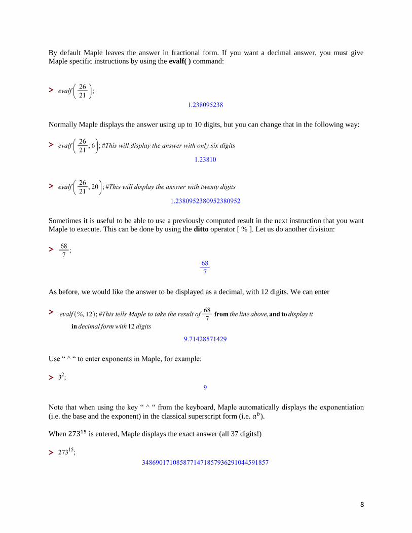
For example, to perform the following addition: 6+4,

Click on the icon “a+b” form the Expression palette (you should have the Expression palette ready to be

used!)

Maple will display the expression “a+b” as a template ready to edit or change in order to be executed

Now, delete the “a” and “b” characters, and enter the respective values (i.e. 6 and 4). Do not forget to

input the semicolon [ ; ]. Hit the Enter key to execute the instruction

>

11

Now, let us perform the following subtraction: 5 – 3

Click on the icon “a-b” form the Expression palette

Maple will show the expression “a-b” as a template ready to modify in order to be executed

Now, delete the “a” and “b” characters as we did previously, and enter the respective values (i.e. 5 and 3).

Again, do not forget to put the semicolon [ ; ]. Hit the Enter key to execute the instruction

>

12

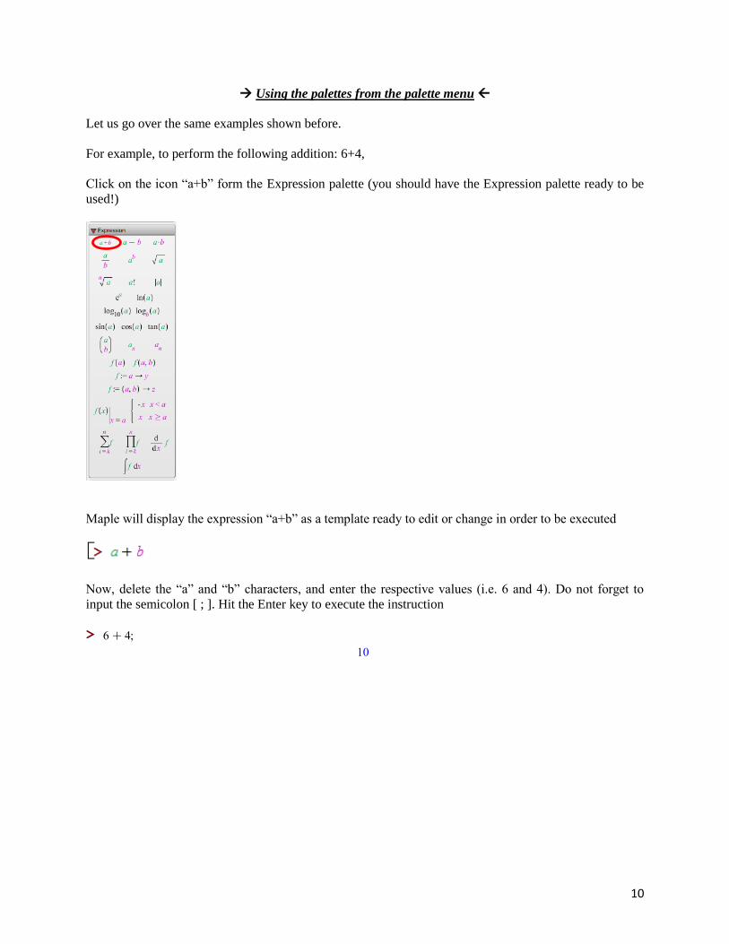
Let us go on with the following multiplication: 6*5

Click on the icon “a.b” form the Expression palette

Maple will prompt the expression “a.b” as a template ready to modify in order to be executed

Now, move the cursor and delete the “a” and “b” characters as shown previously, and enter the respective

values (i.e. 6 and 5). Do not forget to type the semicolon [ ; ]. Press the Enter key to execute the

instruction

>

13

Continuing with the examples, let us see how Maple works with fractions. For this example, we will

perform the following operation: “ 2

3 +

4

7 “

Click on the icon “ 𝑎

𝑏 ” form the Expression palette

Maple will display the expression “ 𝑎

𝑏 ” ready to edit in order to be executed

Move the cursor and delete the “a” and “b” characters as seen before, and enter the first fraction (i.e. 2

3 ).

Then, type the plus sign (i.e. +) and using the same fraction symbol from the palette menu, enter the other

fraction (i.e. 4

7 ). Do not forget to type the semicolon [ ; ]. Press the Enter key to execute the instruction

>

Again, by default the answer is given in fractional form. If you want a decimal answer, you must give

Maple specific instructions by using the evalf( ) command:

>

14

Since Maple displays the answer usually using up to 10 digits, we can customize that in the following

way:

>

>

It is useful to be able to use a previously computed result in the next instruction line that you want Maple

to execute. As seen before this can be done by using the ditto operator [ % ]. Let us perform another

division:

>

If we like the answer to be displayed as a decimal using 12 digits, we can enter

>

15

Following the previous examples, let us see how Maple works with exponents. For this example, we will

perform the following operation: “ 32 “

Click on the icon “𝑎𝑏 ” form the Expression palette

Maple will show the expression “ 𝑎𝑏 ” ready to edit in order to be executed

Move the cursor, change the “a” and “b” characters, and enter the expression (i.e. 32 ). Do not forget to

input the semicolon [ ; ]. Hit the Enter key to execute the instruction

>

Let us explore another example, when 27315 is entered, Maple will show you the exact answer (all 37

digits!)

>

16

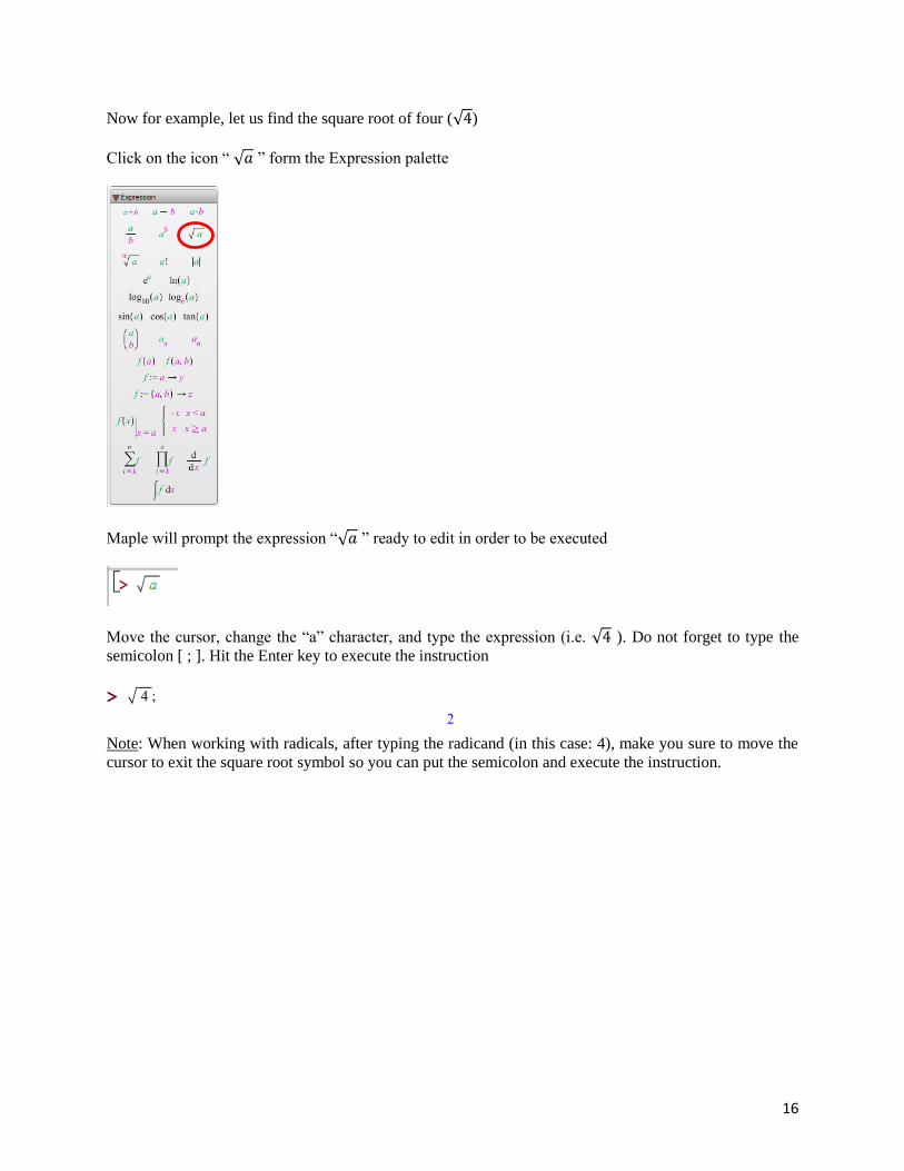
Now for example, let us find the square root of four (√4)

Click on the icon “ √𝑎 ” form the Expression palette

Maple will prompt the expression “√𝑎 ” ready to edit in order to be executed

Move the cursor, change the “a” character, and type the expression (i.e. √4 ). Do not forget to type the

semicolon [ ; ]. Hit the Enter key to execute the instruction

>

Note: When working with radicals, after typing the radicand (in this case: 4), make you sure to move the

cursor to exit the square root symbol so you can put the semicolon and execute the instruction.

17

For the square root of positive real numbers which are not perfect squares (i.e. irrational numbers), Maple

gives you the exact answer in simplified form (it will not give you a decimal approximation like a

standard calculator).

>

If we want the decimal approximation, you need to use the evalf( ) command again

>

Let us see an example with absolute value. To find the absolute value of – 45 (i.e. |−45| )

Click on the icon “ |𝑎| ” form the Expression palette

Maple will display the expression “ |𝑎| ” ready to edit in order to be executed

Move the cursor, change the “a” character (between the absolute value bars), and type the expression (i.e. |−45| ). Do not forget to type the semicolon [ ; ]. Hit the Enter key to execute the instruction

>

18

Maple has in its library all of the important mathematical constants built in.

For example, to enter the constant 𝜋 (Pi), find the respective symbol on the “Common Symbols” palette

and click on it

>

If we want a decimal approximation, we type:

>

At this point, we have shown the use of the input methods for mathematical expressions (i.e. the standard

keyboard and the palette menu). We have gone over the same examples and shown how to type and

perform basic mathematical operations. From now on, the rest of the content will use a combination of

both input methods.

19

DOING ALGEBRAIC COMPUTATIONS WITH MAPLE

In this section you will learn how to use Maple to do some algebra.

All of the arithmetic operators discussed before can be used with variables and algebraic expressions.

Look at the following examples:

To simplify the expression: 2x + 6y + 3x – 8y, we can enter

>

To simplify: 𝑥6 + 2𝑥5 − 3𝑥 + 2 − (−3𝑥6 + 4𝑥 − 8) we can enter

>

To multiply polynomials we must tell Maple to expand the answer, otherwise Maple leaves the problem

in factored form. For example, let us expand the following multiplication: (3𝑥2 − 5𝑥)(4𝑥2 + 7𝑥 + 1)

>

>

We can also square a binomial. For example, to find (𝑥 + 5)2 we enter

>

Again, we must tell Maple to expand the result if we want the binomial expansion of this expression

>

We can raise a polynomial to any power. For example, to find the binomial expansion of (x+y) to the

fourth power that is (𝑥 + 𝑦)4 we enter:

>

20

On the other hand, Maple can factor for us. If we factor the answer we obtained above we should get back

the expression we started with

>

Another factoring example: Factor the polynomial 𝑎4 + 9𝑎3 − 𝑎2 − 9𝑎 completely.

>

We can use the simplify command to simplify rational expressions. For example, to simplify 𝑡2−4

𝑡+2 we can

enter

>

To find the square root of x that is √𝑥 we enter

>

The absolute value expression |𝑥 − 8| is entered

>

We can assign a name to the result of a calculation or to an algebraic expression that we intend to use in

subsequent calculations. To assign a name we can use a colon followed by an equal sign [ := ]. When

making your assignment, do not forget that Maple is case sensitive so try to use lower case letters. Keep

the names short.

In the example below, we are assigning the polynomial 2𝑥2 − 𝑥 − 10 to the letter p.

Please keep in mind that we use assignments to save time typing, and p is just a name given to a location

in the computer’s memory where the algebraic expression is stored. Therefore, p, is not really an

algebraic variable.

>

21

Now that we have assigned the polynomial to the letter p, we can use p instead of the expression to do a

number of things:

>

>

Suppose that we would like to evaluate the polynomial for x=3. We can do this easily by using the subs( )

command:

>

We can also solve the quadratic equation 2𝑥2 − 𝑥 − 10 = 0 for x, by making p=0, and using the solve( )

command:

>

You can also obtain the same result by entering:

>

Notice that there are some differences. First, we did not tell Maple that we wanted to set p=0, but Maple

assumes this by default. Second, the variable x is not inside braces. This changes the way in which the

result is displayed (it does not say x=). You may choose to use the solve command in this way, but as you

can see it is not too clear to someone reading your paper what you are trying to do.

If you wish to assign a different expression to the same letter (or name) you must unassign the letter first

to clear the contents of the memory location. This is done in the following way:

>

The variable p has been unassigned. It no longer equals 2𝑥2 − 𝑥 − 10 = 0. You can check this:

>

22

The variable p is now “free” and we can re-assign it to another expression

>

Let us take a look at other uses of the solve( ) command.

You can solve the expression above for either variable:

>

>

Notice that in the two examples above, p does not appear in the answer. Why? Because you were solving

2x+3y=0. Remember that p is a location in memory and Maple sets the expression it contains equal to

zero by default.

Let us look at other examples. We want to set the expression in p equals to 6 that is 2x+3y=6, and solve it

for y:

>

Solving 2x+3y=6 for x:

>

Solving formulas, for example to solve “A = P.r.t + P” for P you can enter:

>

23

Solving a system of equations:

[𝑥 + 2𝑦 = 4

3𝑥 + 4𝑦 = 6]

In Maple we can enter:

>

Note that we entered the equations between braces and separated by a comma. And the variables (i.e. x

and y) were also entered between braces and separated by a comma.

Solving equations with absolute value and square roots:

For the absolute value equation: |𝑥 + 3| = 12

>

For the square root equation: √𝑥 − 4 = 4

>

24

COMMANDS IN PACKAGES

Maple offers some very useful commands that are found in packages. A package is a group of routines or

built-in functions related to a particular area of mathematics or a set of commands designed to help a

particular audience. For example, the student package was designed with students like you in mind. In

order to access commands contained in a package, you must use the with command first. Every time you

see the command with in this manual, you should know that we are using a package. For example, to use

the commands contained in the student package you must type with(student), as shown below:

>

As seen above, Maple replies with a list of all the commands available in the student package. Let us

investigate some of them.

For example, let us find the slope (say “m”) of the equation of a line given in its standard form: 3x+2y=5

>

Or, for example, let us find the slope of line when given two passing points: (1,2) and (5,6)

>

If we want to find the distance (say “dist”) between two given points, for example: (1,2) and (5,6), we can

enter

>

Or, if for example, we need to find the midpoint of line passing through two given points: (1,2) and (5,6),

we can enter

>

25

Now let us take a look at the geometry package:

>

For example, you are given the equation of a circle: (𝑥 + 4)2 + (𝑦 − 3)2 = 81 and you need to find its

center, its radius, and draw it. To do so we can use:

>

After typing this line, Maple will prompt a small window asking for the names of the horizontal axis and

the vertical axis

All you need to do is to enter: x for the horizontal axis; y for the vertical axis; and click OK in both cases

26

If the previous steps were done correctly, you should see the following output

>

Now, to obtain the details for the circle “c”, we just need to enter:

>

To plot the circle defined above, we can type

>

27

Another example, let us say you are given the coordinates of the center of a circle (say: (-2,1) ) and its

respective radius (say: 6), and you need to find its equation and plot it.

We can type the following line:

>

As shown in the previous example, to get the details of the circle c1, we enter

>

assume that the names of the horizontal and vertical axes are _x

and _y, respectively

To draw the circle c1:

>

Note: There are many packages available, and we will use some of them later on

28

Introductory Maple Lab. #1

Do the following exercises using Maple. Print your results to hand-in to your instructor

1) a) 24 + (4 + 8 ÷ 4 × 2 + 7) ÷ 3

b) Solve for x: 1.5(4 − x) = 1.3(2 − x)

c) If P = 2L + 2W, solve for W

2) Solve the following system of linear equations algebraically:

4x − y = 10

3𝑥 + 5𝑦 = 19

3) a) Factor completely: 6𝑥2 − 3𝑥3

b) Factor completely: 12𝑥2 − 17𝑥 + 6

c) Simplify (Reduce to the lowest terms): 𝑥2−9

𝑥2−2𝑥−15

d) Simplify: 𝑥2−12𝑥+32

𝑥2−6𝑥−16÷

𝑥2−𝑥−12

𝑥2−5𝑥−24

4) a) Solve: 𝑥2 − 2𝑥 − 35 = 0

b) Solve for x: 3

2𝑥−5+

2

2𝑥+3= 0

5) a) Solve: √1 − 2𝑥3

− 2 = 0

b) Solve: √12 − 𝑥 = 𝑥

c) Solve: |2𝑥 − 3| = 5

6) Use the student package to find the slope of the line 2y = 5x – 4

7) Use the student package to find the slope of the line passing through the points (1,5) and (-1,-1)

8) Use the student package to find the distance between the points (1,5) and (-1,-1)

9) Use the student package to find the midpoint between the points (-1,-1) and (5,3)

10) Use the geometry package to find the radius and center of the circle: (𝑥 − 1)2 + (𝑦 + 3)2 = 4

29

WORKING WITH FUNCTIONS

We have seen how to assign expressions to a variable. We can use assignments to represent functions. For

example, we can think of p as being a function of x. However, Maple has a more convenient way of

defining functions. See below:

Textbook Notation Maple Syntax

f(x)

g(x)

h(t)

Note: The right arrow symbol (i.e. →) in Maple can be obtained by performing the following sequence in

the keyboard: - (+) Shift (+) >

For example, let us define a function 𝑓(𝑥) = 2𝑥2 − 𝑥 − 10. Notice that f(x) is the same as p from a

previous example.

>

We can do with f the same things that we did with p in a previous section. For example:

>

Notice that the notation used here resembles closely what we use in mathematics. It is no longer necessary

to use the subs( ) command to evaluate the function when x=3. We just have to tell Maple that we want

f(3)

>

In this way we can easily evaluate the function for any input we want. Look at these following examples:

>

>

>

30

Performing operations with functions

We can also do operations on functions in Maple:

>

>

>

>

>

>

Now let us define another function 𝑔(𝑥) = 3𝑥 − 4

>

We can now do combinations of functions using f(x) and g(x):

>

>

>

>

>

31

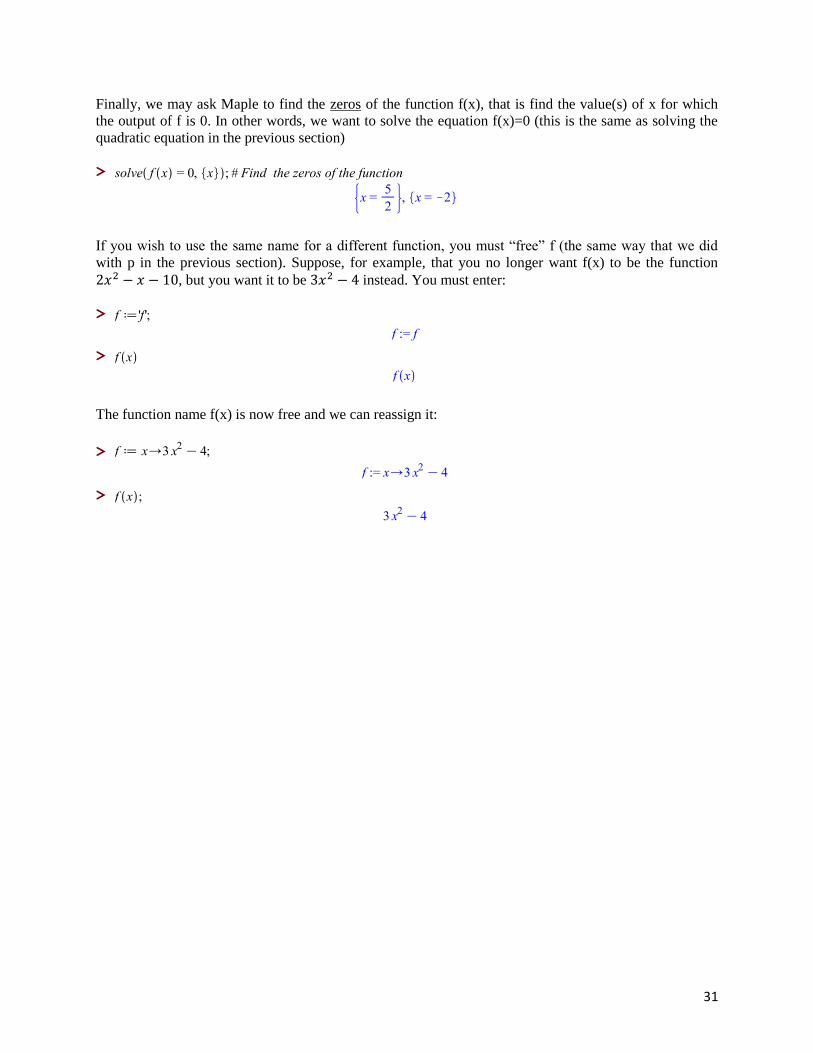
Finally, we may ask Maple to find the zeros of the function f(x), that is find the value(s) of x for which

the output of f is 0. In other words, we want to solve the equation f(x)=0 (this is the same as solving the

quadratic equation in the previous section)

>

If you wish to use the same name for a different function, you must “free” f (the same way that we did

with p in the previous section). Suppose, for example, that you no longer want f(x) to be the function

2𝑥2 − 𝑥 − 10, but you want it to be 3𝑥2 − 4 instead. You must enter:

>

>

The function name f(x) is now free and we can reassign it:

>

>

32

GRAPHING FUNCTIONS

Now let us turn our attention to plotting graphs. We do this in Maple by using the plot( ) command. The

plot( ) command can be used in several ways. Although we can get a graph by entering the expression

directly into the plot( ) command, it is better to do assignment first, and then to use the variable name in

the plot( ) command. For example, we can plot the graph of 2𝑥2 − 𝑥 − 10 by first assigning the

expression to p.

>

Now we use p in the plot( ) command. Notice that p is playing the role of y.

>

Notice the syntax above: p(x). This means in math language: “p of x”. When you are graphing an

equation you have to tell the software which variable is the independent variable. In our case it is “x”.

Notice also that Maple (by default) graphs the equations using x-values between -10 and 10. This range of

values for x would be like the “domain” of the function just for graphing purposes. We can also change

the scale to our convenience.

33

For example, to change the x-scale in Maple the syntax is: x=low_value.. high_value

>

Since the vertical scale was not specified. Maple again chose the appropriate y-scale to show the entire

graph. The following example shows you how to specify the vertical scale as well.

>

34

Let us explore more examples.

>

>

>

>

35

Continuing with the examples, now let us explore how to add some extra features to the graphs.

>

You can add a title to your graph by using the title option in the plot command. Your title must be inside

quotation marks as shown below.

>

Now, suppose we want to plot two or more equations on the same x-y axes.

We must place both expressions inside square brackets and separated by commas: “[expression1,

expression2]”.

You can graph both the cube and absolute value functions together as follows:

>

36

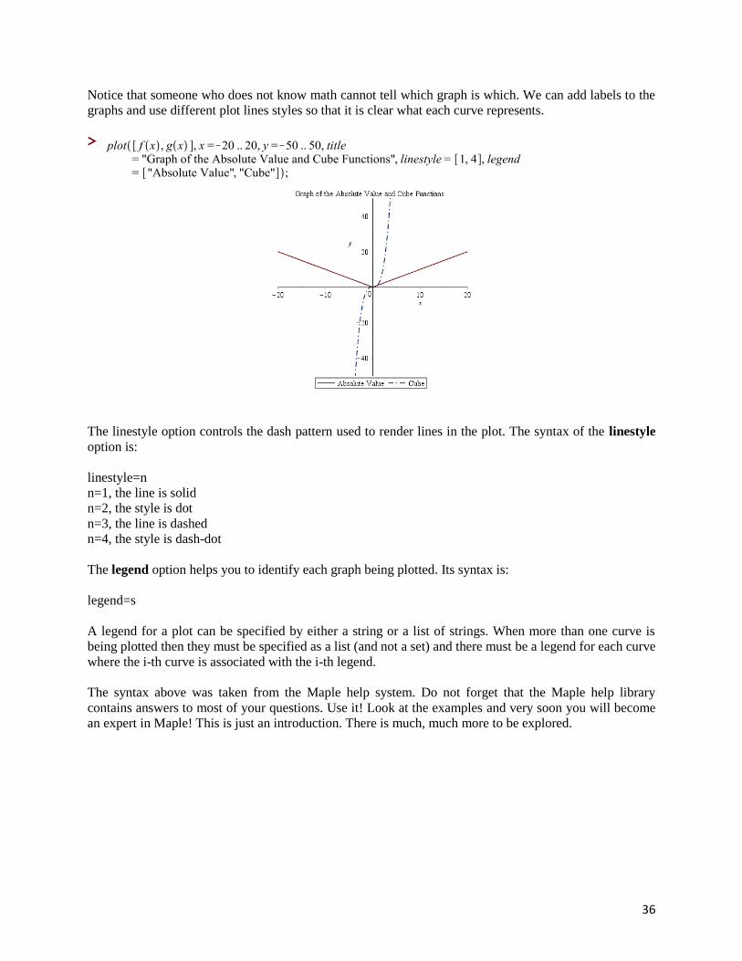
Notice that someone who does not know math cannot tell which graph is which. We can add labels to the

graphs and use different plot lines styles so that it is clear what each curve represents.

>

The linestyle option controls the dash pattern used to render lines in the plot. The syntax of the linestyle

option is:

linestyle=n

n=1, the line is solid

n=2, the style is dot

n=3, the line is dashed

n=4, the style is dash-dot

The legend option helps you to identify each graph being plotted. Its syntax is:

legend=s

A legend for a plot can be specified by either a string or a list of strings. When more than one curve is

being plotted then they must be specified as a list (and not a set) and there must be a legend for each curve

where the i-th curve is associated with the i-th legend.

The syntax above was taken from the Maple help system. Do not forget that the Maple help library

contains answers to most of your questions. Use it! Look at the examples and very soon you will become

an expert in Maple! This is just an introduction. There is much, much more to be explored.

37

The next example shows you how to plot three functions together in the same x-y axes:

>

>

>

Now we can plot these three functions together.

The first example, shows you how to let Maple choose the scaling for you. When doing a lab, you should

use this option first to get an idea of how the graphs look like. Later, you can adjust the scale to suit your

needs. Experiment until you get the best possible graph for your lab assignment.

>

We can adjust the scale of the x-axis only:

>

38

Or we can just adjust both the x-axis and the y-axis if we want to:

>

39

Introductory Maple Lab. #2

1) If g(x) = 𝑥3 + 2𝑥2 − 6, find: g(0), g(-2), g(-1), g(-2) – 1, g(0) + 2

2) Given f(x) = 8 − 2𝑥2, compute:

𝑓(4)−𝑓(2)

4−2 and

𝑓(4)−𝑓(3)

4−3

3) Let h(x) = √3𝑥 − 8

a) Find h(8)

b) Find h(24)

4) Graph p(x) = 5 – 4x using:

a) −2 ≤ x ≤ 2

b) −15 ≤ x ≤ 8

5) Graph:

a) f(x) = √𝑥, 0 ≤ x ≤ 25

b) g(x) = |𝑥|, −20 ≤ x ≤ 20

6) If q(x) = 2𝑥2 − 4𝑥 − 1

a) Graph q(x)

b) Identify the vertex

c) Identify the intercepts

7) Graph the following on the same x-y axes:

j(x) = 2x + 1 and p(x) = 𝑥2 − 5

Can you identify the intersection points of these two functions?

Use an appropriate viewing window

8) Graph the following on the same x-y axes: (Use an appropriate viewing window)

g1(x) = 𝑥2, g2(x) = 𝑥2 + 5, g3(x) = (𝑥 + 5)2

a) Is there a difference between g1(x) and g2(x)? Explain

b) Is there a difference between g1(x) and g3(x)? Explain

c) Is there a difference between g2(x) and g3(x)? Explain

40

MORE PRECALCULUS PROBLEMS AND EXAMPLES

For example, let us solve the following system of equations both algebraically and graphically:

-x + 3y = 10

x + y = 2

>

Now let us do it graphically: first solve each equation for y:

>

>

Then plot g and h as follows using different line styles. The solution is the point of intersection.

>

41

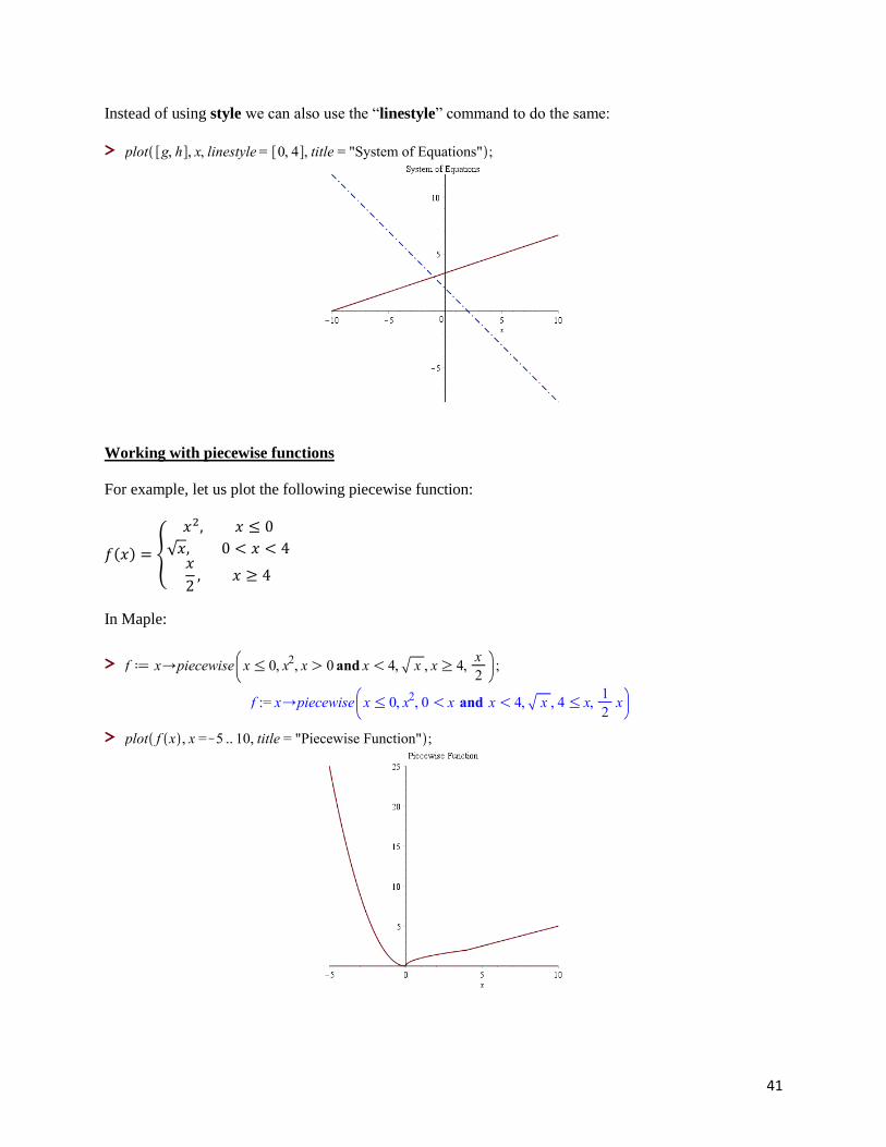
Instead of using style we can also use the “linestyle” command to do the same:

>

Working with piecewise functions

For example, let us plot the following piecewise function:

𝑓(𝑥) = {

𝑥2, 𝑥 ≤ 0

√𝑥, 0 < 𝑥 < 4𝑥

2, 𝑥 ≥ 4

In Maple:

>

>

42

Another way to create the same piecewise function is to use short programming code in Maple:

>

Clearly here, the first syntax is much easier than the second one. However if your major is computer

programming, then it is a good idea to start practicing your programming skills.

>

>

Here is another example of piecewise function:

𝑔(𝑥) = {

−𝑥 + 1, 𝑖𝑓 𝑥 < 12𝑥 + 3, 𝑖𝑓 1 ≤ 𝑥 ≤ 4

𝑥2, 𝑜𝑡ℎ𝑒𝑟𝑤𝑖𝑠𝑒

Notice that this is a discontinuous function

>

43

Let us plot g(x) the usual way:

>

Notice that Maple did not show the discontinuities! To see this function properly you should add:

‘discount=true’:

>

44

MORE OPERATIONS ON FUNCTIONS: COMPOSITE FUNCTIONS

Let us define two functions: f(x) = 2𝑥2 − 9𝑥 − 6, and g(x) = 3𝑥 − 4

>

>

We can use g(x) as the input to f(x)

>

The process above is known as the composition of the functions f and g denoted by “f o g”. This is a very

common way of combining functions, therefore Maple provides a separate way of writing it:

>

>

Finding the Domain and the Range of a Function from the Plot

When plotting equations or functions, students must use the right viewing window. Suppose we want to

find the domain and range for the following function:

>

45

If we use the default scale in Maple we will not be able to find the right answer because the entire graph

will not be displayed.

>

But the same function using a different viewing window yields:

>

Clearly, when you the students, are trying to answer questions from a lab assignment, you must try

different viewing windows in order to provide the best possible answer. Remember that your labs and

projects are worth 20% of your grade.

46

Now take a look at this function: b(x) = 𝑥8

8−

𝑥6

2− 𝑥5 + 5𝑥3

>

>

Without scaling the axes, it would be impossible for a student to answer any question about the domain

and range as well as maximum, minimum, and also the zeros of the function. Now with the scaled axes:

>

47

Here again when dealing with rational functions students must be careful in choosing their viewing

window. For example: m(x) = 5

(𝑥−1)(𝑥2−4)

>

>

Using the default scaling, the students will not be able to find the domain or range of this function as it

appears. Rescaling both x-y axes then we have:

>

48

The same also applies in determining the asymptotes of a function such as:

>

>

As you can see, beside the two vertical asymptotes it would be impossible to discuss anything else about

the above graph. But using the right viewing window we have the following

>

49

MODELING

Plotting points in Maple

Example – Use Maple to plot the following points: (-4,6), (-3,2), (-1,-6), (1,-14), (2,-18)

In Maple each pair must be inside square brackets

>

Plotting the points:

>

Note that you can use the least square fit method in the stats package to find the equation of the line

through the points shown above.

>

Note that the all commands shown above are built-in functions or procedures embedded inside the stats

package.

For this example, we will use the least square fit method to obtain the equation of the line through the

points shown lines above.

>

Note:

The newer versions of Maple let solve problems in different ways using other commands. Thus, a

problem can be solved using commands supported in previous versions as new commands implemented

for newer versions of the software.

50

Linear Fitting

In the following example a set of ordered pairs is given and a linear function that fits the data will be

calculated to illustrate a practical case of modeling.

Example – Given: (X,Y) = {(3,5),(4,8),(5,9),(6,12),(7,15),(8,14)}, we can use the following commands to

do the linear fit (i.e. least square fit)

>

>

>

>

Note:

See page 103 for more examples of linear fitting

51

Exponential Functions

Let us plot the following functions: f(x) = 2𝑥, h(x) = (1

3)𝑥, g(x) = 10(

1

5)𝑥

In Maple:

>

>

>

52

Plotting multiple exponential functions on the same x-y axes:

>

You should be able to identify f1, f9, and g from the graph above

Note that in PreCalculus most of your labs will involve comparing functions. In that case you should

graph these functions on the same x-y coordinates in order to compare the functions.

Also if you are plotting more than two functions on the same x-y axes you need to use “linestyle” instead

of “style”.

When using “linestyle=[0,3,5,7…]” these values modify the style of the graph from solid line to dash, dot,

dot-dash, and so on.

53

The Exponential Function

The exponential function with the natural constant “℮” in Maple must be entered either using “exp( )” or

the respective symbol from the Expression Palette (see below)

To enter “℮” (the base of the exponential function) you must type:

>

Or, use the operator “℮𝑎” from the Expression Palette

>

If you want Maple to compute the exact value for “℮3”, you must enter

>

>

Or

>

>

54

Now let us plot the functions: q(t) = 𝑒𝑡 and m(t) = 15𝑒−0.087𝑡

>

>

>

>

55

Exponential Curve Fitting

Note that some equations which have their parameters appearing nonlinearly can be transformed to linear

ones. For example, y = 𝑎 ∗ 𝑒𝑏∗𝑥 can be transformed into: log 𝑦 = 𝐴 + 𝑏 ∗ 𝑥, where A = log(𝑎)

Let us see the following example

>

>

>

>

>

In the result above, recall that 𝑒(0.01326703173+4.364573113) is the same as the product: 𝑒0.01326703173∗𝑥 ∗𝑒4.364573113

Also notice that 𝑒4.364573113 = 78.61583270. Therefore the formula becomes:

q1 = 78.61583270𝑒0.01326703173∗𝑥

>

Here the zip command will group X and Y into pairs of (x,y) points

The following graph represents the least square fit of the data points

>

56

Exponential Curve Fitting (continuation)

Using the same example shown previously, now let us see a different way to solve this same problem

Let us begin by enabling the packages: Statistics and plots

Defining the values for X and Y

>

>

To find the scatter diagram, we can use the command ScatterPlot

>

57

Finally, to obtain the exponential function that fits the given data, we can use the command

ExponentialFit

>

If we wish to draw the scatter diagram along with the exponential function found previously, we can use

the command plots[display]

>

Note:

See page 102 for more examples of exponential curve fitting

58

Trigonometric Curve Fitting

In the following example, a set of ordered pairs is given and the relation between the variables is not

linear.

Let us explore how a trigonometric function can be interpolated and fit the data.

(x,y) = { (1,10.2) (2,10.7) (3,11.5) (4,12.5) (5,13.3) (6,13.9) (7,14.1) (8,13.6) (9,12.7) (10,11.9) (11,11)

(12,10.4) }

>

>

>

>

The zip command will group X and Y into pairs of (x,y) points

>

The following graph represents the trigonometric fit of the data points

>

Note:

See page 115 for more examples of trigonometric modeling

59

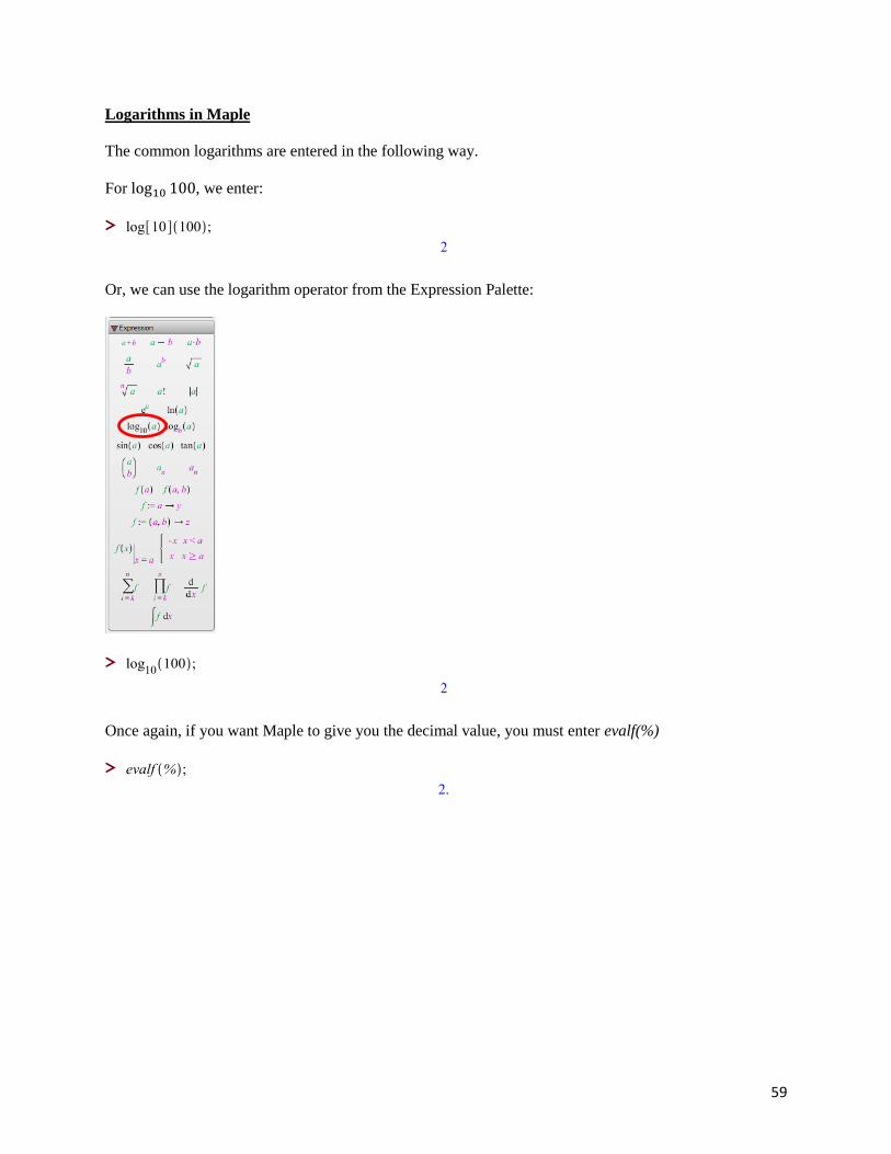
Logarithms in Maple

The common logarithms are entered in the following way.

For log10 100, we enter:

>

Or, we can use the logarithm operator from the Expression Palette:

>

Once again, if you want Maple to give you the decimal value, you must enter evalf(%)

>

60

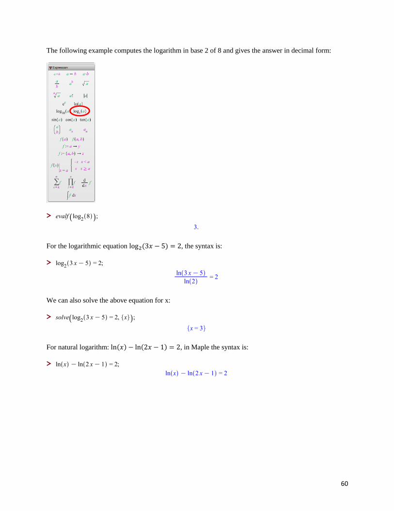
The following example computes the logarithm in base 2 of 8 and gives the answer in decimal form:

>

For the logarithmic equation log2(3𝑥 − 5) = 2, the syntax is:

>

We can also solve the above equation for x:

>

For natural logarithm: ln(𝑥) − ln(2𝑥 − 1) = 2, in Maple the syntax is:

>

61

Next, let us plot some graphs of logarithm functions: r(x) = log(𝑥) and r1(x) = log5(𝑥 + 1)

>

>

>

62

Natural Logarithms

For example, let us graph the following functions: h(x) = ln(x), j(x) = ln(x)+1, and k(x) = ln(x-2)

>

>

>

Graphing all the functions on the same x-y axes

>

63

Trigonometric Functions

In Maple, 𝜋 is entered either as “Pi” or using the symbol located on the “Common Symbols” Palette.

For example:

>

Or,

>

Note: By default, when working with Trigonometric functions, Maple is set to operate with radians. If

you need to work in degrees, you should make the proper conversion beforehand.

64

>

>

For example, let us graph: h(t) = sin(3t)+4

>

>

65

Cosine Function

>

>

Another example, let us graph k(t) = 5*cos(t – 0.875)

>

>

66

We can also have multiple graphs of trigonometric functions on the same x-y axes

>

Another example:

a1(t) = cos(t), a2(t) = cos(t) – 2, a3(t) = cos(t) – 4

>

>

>

>

67

We can use Maple to solve trigonometric equations, for example:

>

Tangent, Cotangent, Secant, and Cosecant Functions

>

>

>

>

68

>

>

>

>

Note that the above functions are very important in our day-to-day living. For example, ordinary

household alternating current, sound from musical instrument, radio transmissions, suspension systems in

automobiles, modeling suspension bridges such as the Verrazano, the Golden Gate, and so on. Practical

applications will be assigned as a lab or final project.

69

Animated Plots of Trigonometric Functions (Sine and Cosine)

All of the following animations use the plots package:

>

To see how the period affects the sine wave, enter the following commands. Right click on the graph and

choose Animation. Then select Play.

>

70

To see how the amplitude affects the sine wave, enter the following commands. Right click on the graph

and choose Animation. Then select Play.

>

71

To see how the midline affects the sine wave, enter the following commands. Right click on the graph and

choose Animation. Then select Play.

>

72

APPLICATIONS

AND

ADDITIONAL EXAMPLES

73

So far we have gone over the basic commands, packages, and use of Maple for a quick get-to-know. In

the following pages we will explore the use of Maple in terms of applications. Recall that Maple is like an

“advanced graphic calculator”.

One of the most common misconceptions that many students have is that Maple is here to “solve” the

math problems. Maple is a powerful tool that when used wisely can make your life easier when dealing

with math problems or projects. Maple does not and will not do the analysis for you. Thus, it is of capital

importance that you must first understand the math concepts and definitions before attempting to type any

instruction on Maple. If you do not have the math knowledge clear in your mind, you may end up even

more confused after using Maple to complete an assignment or lab.

A practical rule of thumb to start working on a math project is to read the problem, to understand the

problem, to use a scratch paper, and to sketch a solution draft of the problem. Then once you have the

“figure” clear, you may proceed to use Maple to make the calculations or graphs you need in order to

solve the problem.

Note: For reference and didactic purposes, some of the examples shown in the following pages have been taken

from the text book:

PreCalculus

Concepts through Functions

A Unit Circle Approach to Trigonometry with Supplement Appendix by Natalia Mosina

Second Custom Edition for LaGuardia Community College

Michael Sullivan – Michael Sullivan III

Pearson

74

Curve Transformations and Family of Curves

A curve transformation might be defined as a chain of successive changes made to a single curve (or

function) in order to obtain a more elaborated or complex curve. Likewise, the plot of these successive

transformations on a same x-y coordinate system is what we may call a family of curves.

Let us explore a couple of examples.

Example 1

Given the function f(x) = 𝑥3, let us perform some changes (transformations) and graph all of them in the

same x-y axis

For example, let us shift the function five units up

This means: f(x) + 5

Or, in other words: 𝑥3 + 5

Let us call this new function f1(x)

Therefore: f1(x) = 𝑥3 + 5

For example, let us shift the function three units down

This means: f(x) – 3

Or, in other words: 𝑥3 – 3


Therefore: f2(x) = 𝑥3 – 3

For example, let us shift the function two units to the right

This means: f(x – 2)

Or, in other words: (𝑥 − 2)3


Therefore: f3(x) = (𝑥 − 2)3

For example, let us shift the function one unit to the left

This means: f(x + 1)

Or, in other words: (𝑥 + 1)3


Therefore: f4(x) = (𝑥 + 1)3

For example, let us multiply the function by four

This means: 4*f(x)

Or, in other words: 4𝑥3 (the function f(x) gets shrunk)


Therefore: f5(x) = 4𝑥3

For example, let us multiply the function by negative one fourth

This means: −1

4*f(x)

Or, in other words: −1

4𝑥3 (the function f(x) gets stretched)


Therefore: f6(x) = −1

4𝑥3

75

After doing all the transformations shown previously, now let us plot both the original function (i.e. f(x))

and each different transformation (one by one at a time)

To do this in Maple, let us just define the base function (i.e. f(x)) and each new function separately.

>

>

>

>

>

76

>

>

>

>

77

>

>

>

>

78

Now let us graph a little more “elaborated” transformation:

For example, let us shift the function two units to the left, multiply the result by three, and move it five

units up

This means: 3*f(x+2)+5

Or, in other words: 3(𝑥 + 2)3 + 5


Therefore: f7(x) = 3(𝑥 + 2)3 + 5

>

>

79

Example 2

Given the function g(x) = sin(x), let us perform some changes (transformations) and graph all of them in

the same x-y axis as we did in the previous example.

But first, let us recall the basics of trigonometric functions.

In general a typical trigonometric function looks like:

𝐴 ∗ sin(𝜔 ∗ 𝑡 + 𝜑) + 𝐷

Now let us identify the key elements of a trigonometric function:

A = Amplitude

𝜔 = Angular Frequency, in radians per second [𝑟𝑎𝑑

𝑠𝑒𝑐]

t = Time, usually in seconds [s], is the argument of the function

𝜑 = Phase, it can be given in degrees or radians

D = A vertical shift, it can be upward or downward

It is also important to remember some key relations or formulas which apply to trigonometric functions:

𝜔 = 2 ∗ 𝜋 ∗ 𝑓

Where:

𝑓 = Frequency, in Hertz [Hz]

𝑓 = 1

𝑇

Where:

T = Period, usually given in seconds [s]

We are now ready to explore some changes that can be made to the function g(x) = sin(x)

For example, let us double the angular frequency of the trigonometric function

This means: g(2x)

Or, in other words: sin(2x)

Let us call this new function g1(x)

Therefore: g1(x) = sin(2x)

For example, let us double the amplitude of the trigonometric function

This means: 2*g(x)

Or, in other words: 2*sin(x)


Therefore: g2(x) = 2*sin(x)

For example, let us reduce the angular frequency of the trigonometric function by half

This means: g(𝑥

2)

Or, in other words: sin(𝑥

2)


Therefore: g3(x) = sin(𝑥

2)

80

For example, let us reduce the amplitude of the trigonometric function by half

This means: 1

2*g(x)

Or, in other words: 1

2*sin(x)


Therefore: g4(x) = 1

2*sin(x)

For example, let us shift the trigonometric function 𝜋

4 radians to the left

This means: g(x + 𝜋

4)

Or, in other words: sin(x + 𝜋

4)


Therefore: g5(x) = sin(x + 𝜋

4)

For example, let us shift the trigonometric function 𝜋

3 radians to the right

This means: g(x - 𝜋

3)

Or, in other words: sin(x - 𝜋

3)


Therefore: g6(x) = sin(x - 𝜋

3)

To do this in Maple, as seen previously, let us just define the base function (i.e. g(x)) and each new

function separately.

>

>

>

81

>

>

>

>

82

>

>

>

>

83

>

>

Now let us graph a more “general” transformation:

For example, let us triple the angular frequency, shift 𝜋 radians to the right, double the amplitude, and

move 4 units up the trigonometric function

This means: 2*f(3x - 𝜋) + 4

Or, in other words: 2*sin(3x – 𝜋) + 4


Therefore: g7(x) = 2*sin(3x – 𝜋) + 4

>

>

84

Applications of Quadratic Functions

Applications of a quadratic function (i.e. parabola) can be found in many fields. For instance, problems

that involve physics, economics, statistics, modeling, and so on. A useful tip when solving text problems

is to understand the text and sketch a draft of the problem. This approach can help you greatly because

you are “translating” a text or plain information into a graph or diagram.

Before getting to the examples, let us revisit the basics of the quadratic function

In general, a quadratic function (i.e. a polynomial of degree 2) may be represented as:

𝑎𝑥2 + 𝑏𝑥 + 𝑐

Where:

“a”, “b”, “c” are the coefficients. All of them are real numbers. Note that “a” must not be zero (i.e. 𝑎 ≠ 0)

The two most common representations of a quadratic equation are:

The Standard Form: 𝑦 = 𝑎𝑥2 + 𝑏𝑥 + 𝑐

The Vertex Form: 𝑦 − 𝑘 = 𝑝(𝑥 − ℎ)2

We can obtain the vertex form of a quadratic equation from its standard form by using the following

relations:

𝑘 = 𝑦(−𝑏

2𝑎)

𝑝 = 𝑎

ℎ = −𝑏

2𝑎

It is also important to remember some useful properties such as:

X – Intercepts, i.e. the solutions of 𝑎𝑥2 + 𝑏𝑥 + 𝑐 = 0

𝑥1 = −𝑏+√𝑏2−4𝑎𝑐

2𝑎

𝑥2 = −𝑏−√𝑏2−4𝑎𝑐

2𝑎

Coordinates of the vertex (h, k), i.e. the highest or lowest point of the graph (as the case may be):

V = ( −𝑏

2𝑎 , 𝑦(−

𝑏

2𝑎) )

85

Now, let us explore some examples.

Example 1

The height h (in feet) of a stone thrown by a catapult is given by the following quadratic equation:

ℎ = −1

16𝑥2 + 2𝑥 + 4

Where x is the horizontal distance (in feet) from where the stone is thrown.

Based on this given information:

a) Draw a sketch the problem

b) Graph the quadratic equation using an adequate scale

c) Find how high the stone was when it left the catapult’s bucket

d) Find how high the stone was when it reached its maximum height

e) Find how far from the catapult the stone hit the ground

Solution:

Part a)

To draw a sketch of the problem, let us just image the situation:

- The catapult has a certain height which needs to be considered

- The movement described by the stone will look like a parabola that opens down

- The stone will hit the ground after some time

Keeping in mind all of these facts, a sketch of problem is shown below:

86

Part b)

To graph the quadratic equation in Maple, we can use the plot command. To find out a proper scale for

the graph, we need to keep in mind that there is no negative horizontal distance, thus the window size for

the x values to plot the equation should begin from 0. Likewise, we need to consider that there is no

negative height, therefore the other value for x to plot the equation should be chosen carefully. If you

need to play with the scale for the x axis, feel free to do it!

>

Part c)

To find how high the stone was when it left the catapult’s bucket, or in other words, how high the stone

was when it was thrown, we just need to observe carefully the graph of the quadratic equation. See below.

As shown above, we can see that the x-y axes are our reference system.

From a physical point of view, the initial height of the stone to be thrown is the height of the catapult’s

bucket. From a mathematical point of view, the initial height of the stone to be thrown is the y-intercept

of the graph of our quadratic equation.

87

To find the y-intercept of our quadratic equation, we just need to plug the value of x=0 in the equation

and calculate the value. In other words, we need to substitute the value of x=0 in the quadratic equation

and find the value.

To begin, let us define in Maple our quadratic function:

>

Then, let us calculate the value of the function when x=0:

>

Therefore, the initial height of the stone to be thrown, i.e. the height of the stone was when it left the

catapult’s bucket is 4 feet.

Part d)

To find how high the stone was when it reached its maximum height, or in other words, the maximum

height the stone reaches after being thrown; we need, again, to observe carefully the graph of the

quadratic equation. See below.

In math language, this means to find the y-coordinate of the vertex of the parabola (i.e. the vertex of our

quadratic equation)

Let us remember that the coordinates of the vertex (h, k) of a parabola is given by the following formula:

V = ( −𝑏

2𝑎 , ℎ (−

𝑏

2𝑎) )

Where:

ℎ = 𝑎𝑥2 + 𝑏𝑥 + 𝑐 is the standard form of a quadratic equation.

88

Now let us identify the coefficients “a” “b” and “c” for our quadratic equation

𝑎𝑥2 + 𝑏𝑥 + 𝑐 ≡ −1

16𝑥2 + 2𝑥 + 4

Therefore:

a = -1/16

b = 2

c = 4

Once we have the values of a, b, and c, now let us proceed to calculate the y-coordinate of the vertex of

our parabola by using:

Y-coordinate = ℎ(−𝑏

2𝑎)

>

Therefore, the maximum height reached by the stone after being thrown is 20 feet.

Part e)

To find how far from the catapult the stone hits the ground, let us observe the graph of the quadratic

equation. See below.

In math language, this means to find the x-intercepts of the parabola (i.e. the x-intercepts of our quadratic

equation)

89

Let us remember that the x–intercepts or the solutions of the equation 𝑎𝑥2 + 𝑏𝑥 + 𝑐 = 0, are given by the

following formulas:

𝑥1 = −𝑏+√𝑏2−4𝑎𝑐

2𝑎

𝑥2 = −𝑏−√𝑏2−4𝑎𝑐

2𝑎

Since we already have the values of the coefficients: “a” “b” and “c”, we might replace those values in the

expressions shown above, make the calculations, and obtain the respective values for 𝑥1and 𝑥2

However, if you are not enough careful with such calculations, you can easily get a wrong value.

Thankfully, in Maple we have the command solve which can be used to solve the equation:

−1

16𝑥2 + 2𝑥 + 4 = 0, and find the x-intercepts of our quadratic equation.

>

>

Our quadratic equation has two x-intercepts:

𝑥1= - 1.888

𝑥2= 33.888

Nevertheless, in problem that involves a quadratic equation, having two roots (or x-intercepts) does not

necessarily mean that we have two correct answers.

As mentioned before, in this problem we need to keep in mind that there is no negative horizontal

distance. This means that a negative x-intercept should not be considered. Therefore, we just use the value

of the other x-intercept (the positive one)

Thus, the ball hit the ground when it was 33.888 feet away from the catapult after being thrown.

90

Example 2

A famous soccer player kicks a ball with an initial velocity of 80 feet per second. The height “y” (in feet)

of the ball is given by the following quadratic equation:

𝑦(𝑥) =−32𝑥2

(802)+ 𝑥

Where: x is the horizontal distance of the ball (in feet) from the starting point.

Based on the information given above, answer the following questions:

a) Draw a sketch the problem

b) Graph the quadratic function using an appropriate scale

c) How far from the starting point is the height of the ball a maximum?

d) What is the maximum height that the ball reaches?

e) How far from the starting point will the ball strike the ground?

Solution:

Part a)

The approach to solve this problem is the same that was shown for the previous problem.

To draw a sketch of the problem, let us read carefully and consider the following:

- The ball is launched from ground, there is no initial height

- The movement described by the ball will also look like a parabola that opens down

- The ball will strike the ground after some time reaching its maximum horizontal distance

Keeping in mind this information, a sketch of problem is shown below:

91

Part b)

To graph this quadratic equation in Maple, we can use the plot command. To find out an appropriate

viewing window, we need to consider that there is no negative horizontal distance, thus the window size

for the x values to plot the equation should begin from 0. Likewise, we need to consider that there is no

negative height, therefore the other value for x to plot the equation should be chosen carefully. Again, feel

free to play with the scale for the x axis.

>

Part c)

To find how far from the starting point the ball reaches its maximum height, we need to look at the graph

of the quadratic equation. See below.

As shown above, we can see that the x-y axes are our reference system.

92

To find the horizontal distance from the starting point where the ball reaches its maximum height we need

to find the x-coordinate of the vertex of the parabola (i.e. the vertex of our quadratic equation)

Let us remember that the x-coordinate of the vertex of a parabola is given by the following formula: −𝑏

2𝑎

Now let us identify the coefficients “a” “b” and “c” for our quadratic equation

𝑎𝑥2 + 𝑏𝑥 + 𝑐 ≡ −32

(80)2 𝑥2 + 𝑥

Therefore:

a = −32

(80)2

b = 1

c = 0

Once we have the values of a, b, and c, now let us proceed to calculate the x-coordinate of the vertex of

our parabola by using:

X-coordinate = −𝑏

2𝑎

>

Therefore, the horizontal distance from the starting point where the ball reaches its maximum height is

100 feet.

Part d)

To find the maximum height that ball reaches after being launched, we need, again, to see carefully the

graph of the quadratic equation. See below.

93

To obtain the maximum height reached by the ball, we need to find the y-coordinate of the vertex of the

parabola (i.e. the vertex of our quadratic equation)

Let us remember that the y-coordinate of the vertex of a parabola is given by the following formula:

𝑦(−𝑏

2𝑎)

Since we already found the coefficients a” “b” and “c” for our quadratic equation in the previous

question, we just proceed to calculate the y-coordinate of the vertex of our parabola:

>

>

Therefore, the maximum height reached by the ball is 50 feet.

Part e)

To find how far from the starting point the ball hits the ground, let us observe the graph of the quadratic

equation. See below.

We need to find the x-intercepts of the parabola (i.e. the x-intercepts of our quadratic equation) in order to

get the point where the ball strikes the ground after being launched.

To do so, in Maple we can use the command solve

>

94

Our quadratic equation has two x-intercepts:

𝑥1= 0

𝑥2= 200

The first solution (𝑥1= 0) tells us the point from where the ball was launched (i.e. the starting point). The

second solution (𝑥2= 200) informs us the point where the ball hits the ground.

Therefore, the ball hit the ground when it was 200 feet away from the starting point.

95

Analyzing a Function

Functions is one of the most important chapters in math. Many PreCalculus and Calculus classes look into

this topic in detail. And consequently, new math concepts come up and often many students struggle to

understand the subject. There is no magic receipt to catch with functions. You are encouraged to devote a

fair deal of time in order to be able to understand and comprehend the concepts involving function

analysis. Let us not forget that Maple is just a tool, and you are the one who thinks and solves the

problems.

Now, let us explore some examples in Maple.

Example 1*

Given the following function: f(x) = −1.2𝑥4 + 0.5𝑥2 − √3𝑥 + 2

a) Graph the function

b) Approximate graphically any absolute extrema

c) Find the zeros of the function

d) Determine the x-interval(s) where f(x) is increasing or decreasing

Solution:

Part a)

To begin, let us define our function f(x) in Maple:

>

Let us plot the function f(x) by using the command plot

>

96

Part b)

Before approximating any absolute extrema of the function, let us remember the following:

An absolute extremum can be an absolute maximum or an absolute minimum of a function on its entire

domain.

The formal way to obtain an absolute or local maximum or minimum of a function is to use the derivative

of the function and solving the equation: 𝑓′(𝑥) = 0. The solutions of this equation are the so called

critical points of a curve. However, for this example, the use of the derivative is slightly out of scope.

With the first plot we just made in the previous question it may not so easy to approximate the absolute

extrema of the function. Thus, in order to obtain a fair approximation, let us make a zoom in of the

previous graph by changing the viewing window.

>

From the above graph, we can say that the function f(x) has one absolute extrema: one absolute maximum

at x = -1 (approximately)

Part c)

The zeros of any function are the x-values where the function is equal to zero. This, graphically, means

the points over the x axis where the sketch of the function crosses the x axis.

To find the zeros of the function, in Maple, let us use the command solve:

>

As we can see, the equation f(x) = 0, has four solutions which means the function h(x) has four zeros;

𝑥1 = 0.913, 𝑥2 = 0.279 + 1.077 × 𝑖, 𝑥3 = −1.471, 𝑥4 = 0.279 − 1.077 × 𝑖

Thus, the function f(x) has two real zeros and two imaginary zeros

97

Part d)

To determine the x-interval(s) where f(x) increases or decreases, we need to use the previous result we

have obtained: the absolute extrema

Let us review:

- One absolute maximum at x = –1 (approx.)

If we place it using a real-number line:

In order to establish in which interval(s) the function is increasing or decreasing, let us use the graph of

the function along with the line shown above.

>

- From −∞ to x = -1, the function increases (it goes upward)

- From x = -1 to +∞, the function decreases (it goes downward)

*Taken from:

Chapter 3, Polynomials and Rational Functions

Page 210, Problem 104

98

Example 2*

Given the following function: R(x) = 3𝑥2−3𝑥

𝑥2+𝑥−12

a) Identify which type of function is

b) Graph the function

c) Find the asymptotes of the function

d) Find the domain of the function

e) Find the range of the function

Solution:

Part a)

To tell which kind of function is, we just need to carefully look at it

The numerator is a polynomial of second degree (i.e. quadratic). The denominator is a polynomial of

second degree as well. Since the function R(x) is given in a fractional form, we can conclude that it is the

case of a rational function.

Part b)

To start with, let us define our function first:

>

Now let us graph our rational function using the command plot:

>

99

Part c)

Before finding any asymptote of the function, let us remember the following:

An asymptote may be defined as a line or curve that approaches a given function closely, but they never

touch each other. The distance between the function and its asymptote(s) approaches zero as they tend to

infinity. In general, there are three types of asymptotes:

- Vertical Asymptotes (They have the form: 𝑥 = ℎ)

- Horizontal Asymptotes (They have the form: 𝑦 = 𝑘)

- Oblique Asymptotes (They have the form: 𝑦 = 𝑚𝑥 + 𝑛)

Strictly speaking an asymptote is the calculation of a limit. Even though the formal study of the limits and

asymptotes of a function is out of scope for this manual, students are highly encouraged to get to know

about these subjects especially during pre-calculus classes.

Fortunately, Maple has a package that allow us to find the asymptotes of a curve. We need to use the

package Student-Calculus1, and use the command Asymptotes.

>

Then, to find the asymptotes of our rational function R(x):

>

From above, we can see that our rational function R(x) has three asymptotes: one that is horizontal, and

two that are vertical.

- Vertical Asymptotes: x = - 4, and x = 3

- Horizontal Asymptotes: y = 3

100

Part d)

Let us remember that the domain of a function may be defined as the set or range of x-values where the

function acts or works. Or, in other words, the domain is the set of x-values where the function makes

sense.

To find the domain of our rational function R(x), we need to keep in mind that its denominator cannot be

equal to zero. This means that we need to find such x-values (if any) which make the denominator equal

to zero. And, therefore, those values will not be part of the domain of the function.

Let us observe that for our rational function R(x) = 3𝑥2−3𝑥

𝑥2+𝑥−12, the denominator is: 𝑥2 + 𝑥 − 12.

To find the values that will not be part of the domain of the function, we need to solve the equation:

𝑥2 + 𝑥 − 12 = 0

>

From above we can see that the solutions of the previous equation are the values that will not belong to

the domain of our rational function. In other words, the forbidden values for x are: - 4 and 3.

Therefore, the domain of our rational function R(x) is: {𝑥 ∈ ℝ | 𝑥 ≠ −4, 𝑥 ≠ 3}, this means: All real numbers except x = - 4, and x = 3

Or if we use the interval notation:

𝑥 ∈ (−∞, −4) 𝑈 (−4, 3) 𝑈 (3, +∞)

Part e)

Let us remember that the range of a function may be defined as the set or range of y-values which

conform the output of the function.

To find the range of a function (in general) may not be straightforward because usually the independent

variable is “x” and the dependent variable is “y”. This means that y is a function of x (i.e. y in terms of x).

For this reason, often it is easier to identify and determine the domain than the range.

A practical rule of thumb to find the range of a function is to look carefully the graph of the function and

to consider the horizontal asymptotes as the forbidden y-values that will not be part of the range.

101

Let us observe one more time the graph of our rational function:

From above, by simple inspection we can say that the range of our rational function is all real numbers

except y = 3 [the horizontal asymptote, see part c)].

Therefore, the range of our rational function is: { 𝑦 ∈ ℝ | 𝑦 ≠ 3 }

Or if we use the interval notation:

𝑦 ∈ (−∞, 3) 𝑈 (3, +∞)

*Taken from:

Chapter 3, Polynomial and Rational Functions

Page 249, Example 4

102

Modeling

Mathematical modeling is one of the most interesting disciplines and can be applied to many other

sciences, for example: physics, biology, meteorology, engineering, statistics, finances, economics, etc.

Several types and classes of modeling can be found in text or reference books. The mathematical models

can range from simple and static to complex and dynamic.

One of the most common applications of math modeling is when we want to create a framework of data

presented as a collection or set of ordered pairs in a table or chart. Then, to look for an equation which

allows us to find a possible relation between two given variables.

The same approach taken to address problems that involve applications of functions applies when solving

modeling problems. This means: To read the problem, to understand what the problem is about, to

identify which math concepts may be involved, to interpret the math model and its results, and finally to

elaborate conclusions based on analysis.

In the following pages we will explore some examples in Maple involving modeling. In particular we will

focus on linear modeling, quadratic modeling (a particular case of polynomial modeling), exponential

modeling, and trigonometric modeling.

103

Example 1 – Linear Modeling

Demand for Jeans*

The marketing manager at Levi Strauss wishes to find a function that relates the demand (d) for men’s

jeans and the price of the jeans (p). The following data were obtained based on a price history of the

jeans:

Price “p”

( $ 𝒑𝒂𝒊𝒓⁄ )

Demand “d”

( 𝑷𝒂𝒊𝒓𝒔 𝒐𝒇 𝑱𝒆𝒂𝒏𝒔 𝒔𝒐𝒍𝒅 𝒑𝒆𝒓 𝒅𝒂𝒚 )

20 60

22 57

23 56

23 53

27 52

29 49

30 44

Answer the following questions using Maple:

a) Does the relation defined by the set of ordered pairs (p,d) represent a function?

b) Draw a scatter diagram of the data

c) Find the line of best fit relating price and quantity demanded

d) Interpret the slope

e) Express the relationship found in part c) using function notation

f) What is the domain of the function? Take into account a real life setting of the problem

g) How many jeans will be demanded if the price is $28 a pair?

h) What should be the price of jeans to sell at least 50 pairs a day?

Solution:

Part a)

Let us consider “p” (the price) as the independent variable (i.e. the input) and “d” (the demand) as the

dependent variable (i.e. the output).

By definition, a function is a set of ordered pairs (or coordinate pairs) where for each origin point exists a

unique destination point. Or, in other words, for each “x” value exists one and only one “y” value.

If we take a look carefully at the given set of values, we can see that the value p = 23 is repeated and has

two different correspondent d values (i.e. d = 56 and d = 53 respectively).

Therefore, we can conclude that the relation defined by the set of ordered pairs (p,d) does not represent a

function.

104

Part b)

Since many modeling problems require the use of statistical calculations heretofore we will use the

package Statistics to enable all of its built-in functions or procedures.

To begin with, let us define our set of ordered pairs (p,d) as an array (or vector) of successive numbers

separately, i.e. one array for “p”, and one array for “d”

>

>

Now, let us use the package Statistics:

To draw our scatter diagram of the data, we can use the command ScatterPlot

>

105

Part c)

The line of best fit is also known as the least-square line. It is one of the simplest math and statistical

models. To find it in Maple, we can use the command LinearFit

>

Part d)

From the previous result, we can see that the slope of the line of best fit is negative (m = - 1.3355).

Having a negative slope in our math model means that as one variable increases the other variable

decreases. If the price for the jeans is expected to go up, then the demand for these jeans is likely to go

down. This case adjusts to the real life because usually when the price of one product or good tends to be

more and more expensive, the respective demand for this product or good tends to be less and less, and

vice versa.

Part e)

As we can see from part c), the result of executing the command LinearFit is that we obtain a function in

terms of “x”. One might wonder why this is happening since the working variables are “p” and “d”. The

answer is that by default Maple associates the input variable (i.e. “p” in this case) as the independent

variable on the horizontal axis (i.e. “x”); and the output variable (i.e. “d” in this case) as the dependent

variable on the vertical axis (i.e. “y”).

The way Maple represents the result of calculating a math model (i.e. “y” as a function of “x”) should not

cause confusion and students ought to be able to identify and relate quickly the variables for a given

problem.

To express our line of best fit as a math function: y(x)

>

Part f)

For math modeling purposes we need to set a “domain” for our function so it could be found and studied

furthermore.

When studying and applying math models to real life examples, part of a good analysis is to distinguish in

which case(s) for a given problem a model can be used and in which case(s) the model should not be

used.

For example, in theory, the domain of the math function we just found is from x = 0 to any positive real

number. However, as x becomes greater than 64.5418 (x-intercept of our function) and according to our

math model we would have a negative demand. This means the price of the jeans would be very

expensive that nobody would be willing to buy those jeans anymore. The latter is not necessarily true

since there can be people with enough money willing to acquire the jeans in matter.

106

On the other hand, the value of x = 0 (i.e. price = $0.00) suggests that the jeans are free of cost, and this is

unrealistic.

To answer this question, and using a real life scenario at the same time, we can venture to say that domain

for our linear function might be: 𝑥 ∈ [15, 60]. This means that the price for the jeans might range from

$15 to $60.

Part g)

To find how many jeans would be demanded when the price is $28, we just need to use our linear

function we obtained previously:

y = - 1.3355x + 86.1973, where “x” is the price of jeans and “y” is the demand of the jeans

Let us plug the value x = 28 and make the calculation:

y = -1.3355(28) + 86.1973

y = - 37.394 + 86.1973

y = 48.8033

From the result above we can infer that when the price of jeans is $28, approximately 48 pairs will be

demanded.

Part h)

To find the suggested price of the jeans if we want to assure a demand of at least 50 pairs a day, we need

to use again our math function.

y = - 1.3355x + 86.1973, where “x” is the price of jeans and “y” is the demand of the jeans

Let us plug the value y = 28 and solve the equation for x

50 = -1.3355x + 86.1973

1.3355x = 86.1973 – 50

1.3355x = 36.1973

x = 27.1039

Therefore, we can infer that if we want to sell at least 50 pairs a day, then we should set a price of $27 at

most.

*Taken from:

Appendix C, Hands-On Laboratory Supplement with Projects. Enhanced Pre-Calculus Learning Experience

Page 23

107

Example 2 – Quadratic Modeling

Advertising*

A small manufacturing firm collected the following data on advertising expenditures, A, (in thousands of

dollars); and total revenue, R, (in thousands of dollars).

Advertising “A” Total Revenue “R”

20 6101

22 6222

25 6350

25 6378

27 6453

28 6423

29 6360

31 6231

a) Use the command ScatterPlot to make a scatter diagram. Comment on the type of relation that may

exist between the two variables

b) Find the quadratic function of the best fit to the data. Express the solution using function notation

c) Predict the total revenue when the optimal level of advertisement is spent. In other words, use your

quadratic model to approximate the maximum total revenue R given the present data (think of what vertex

represents in this case). Use your current knowledge of Maple commands to present your solution

showing all your work

d) Graph the scatter diagram and the best fit parabola together

Solution:

Part a)

To start with, let us define our set of ordered pairs (A,R) as an array of numbers separately, i.e. one array

for “A”, and one array for “R”

>

>


108

To draw our scatter diagram, let us use the command ScatterPlot

>

From the scatter diagram, by simple inspection, we may say that it looks like the relation between the

amount of advertising expenditures “A” and the amount of total revenue obtained “R” follows a

quadratic-function pattern (i.e. parabola). One might argue that a linear model should be used instead.

However a least-square line may not be accurate to represent the relationship between these variables.

From the scatter diagram it can be seen that the revenue reaches a top value and then decreases, this

certainly suggests a second-degree polynomial tendency.

Part b)

To find the function of the best fit to the data in this case: a quadratic function let us use the command

PolynomialFit

>

Note that regarding the arguments of the command PolynomialFit:

* The number 2 means that we are interested in getting a polynomial of second degree (i.e. a parabola). If

we wish to obtain a polynomial of third degree, then we should enter the number 3 instead. In general, we

can calculate a polynomial fit for a given data by specifying the degree of the polynomial within the

arguments of the command PolynomialFit.

* The letters “A” and “R” are the arrays of the numbers previously given

* The variable “x” is the variable (by default) in which Maple shows the result as a typical function of “x”

109

To express the solution as a function notation:

>

Where “x” is the amount of advertising expenditures (A); and “y” is the amount of total revenue (R)

Part c)

If we wish to predict the total revenue “R” when the optimal level of advertising “A” is spent using our

quadratic model, we need first to take a look closely at the scatter diagram

From the scatter diagram, and as mentioned before, we can see that the revenue “R” comes to a top value

and then decreases. Applying this math modeling case to a real life scenario means that taking extreme

measures is not always a good choice.

If the firm spends a few thousands of dollars in advertisement, then the firm will not obtain profitable

revenue. And the opposite applies as well: if the firm spends several thousands of dollars in

advertisement, it is not likely that its revenue will continue skyrocketing.

Nevertheless, making use of our math model we can find an optimal level of advertising spent at which

the firm will obtain its maximum total revenue.

To obtain the optimal level of advertising, we need to find the x-coordinate of the vertex of our quadratic

equation (i.e. parabola)

Let us recall that the x-coordinate of the vertex of a parabola is given by the following formula:

𝑉𝑥 = −𝑏

2𝑎

Where:

𝑦 = 𝑎𝑥2 + 𝑏𝑥 + 𝑐 is the standard form of a quadratic equation.

110

Identifying the coefficients “a” “b” and “c” for our quadratic function

𝑎𝑥2 + 𝑏𝑥 + 𝑐 ≡ −7.7595𝑥2 + 411.8750𝑥 + 942.7210

We obtain:

a = - 7.7595

b = 411.875

c = 942.721

Therefore,

X-coordinate = −𝑏

2𝑎

>

This means that the optimal level of advertisement is approximately: $ 26.54 thousand of dollars

Now, to predict the maximum total revenue for the firm investing $ 26.54 thousand of dollars in

advertisement, we need to use our quadratic function, to plug the value x = 26.54 in and to make the

calculation:

𝑦(26.54) = −7.7595 ∗ (26.54)2 + 411.8750 ∗ (26.54) + 942.7210

𝑦(26.54) = 6408.312

Therefore, the maximum total revenue that the firm can obtain is approximately $ 6408.312 thousands of

dollars when an amount of $ 26.54 thousand of dollars is spent in advertisement.

Part d)

To draw the scatter diagram and the best fit parabola together, let us follow the steps in Maple:

Let us name our scatter diagram as “SP”

>

Let us name the plot of the function y(x) as “PM”. Again note that we need to set a viewing window

for the function y(x). In this case let us take the values from x = 20 to x = 31

>

111

Let us use the command plots so that the scatter diagram and the parabola can be drawn together and,

optionally, edit the graph to present an appropriate title:

>

Note: The objective of this example was to illustrate one of the simplest cases of polynomial modeling

(i.e. quadratic modeling). As the case may be, polynomials of higher degrees can be used to model the

data more accurately. However, to make a depth analysis of a polynomial function and to find its maxima

and minima requires knowledge of basic calculus. Although the formal study of some calculus topics is

out of scope for this manual, the reader is highly encouraged to get familiar with such concepts.

*Taken from:

Appendix C, Hands-On Laboratory Supplemental with Projects. Enhanced Pre-Calculus Learning Experience

Pages 23, 24

112

Example 3 – Exponential Modeling

“Internet Traffic”

An engineering student conducted a field study on how fast the amount of data rate on the Internet (i.e.

Bandwidth) increased during the broadcast of live event via YouTube in a city. The following table shows

the elapsed time (in minutes) during the transmission of the event and the amount of bandwidth (in

Gigabits per second) registered by the student

Minutes “M” Bandwidth “B”

(𝒊𝒏 𝑮𝒊𝒈𝒂𝒃𝒊𝒕𝒔 𝒑𝒆𝒓 𝒔𝒆𝒄𝒐𝒏𝒅)

0 76.1

30 123.2

50 151.7

70 204.9

80 226.5

90 249.6

Based on the previous information, answer the following questions:

a) Find an exponential model for the Internet traffic growth

b) Plot both the data points and the model on the same x-y axis

c) Comment on the model

d) Use the exponential model to predict the bandwidth consumption after two hours

Solution:

Part a)

Let us first define the set of ordered pairs (M,B) as an array of numbers separately.

In Maple:

>

>


113

To find an exponential model for the data given above, we can use the command ExponentialFit

>

About the arguments of the command ExponentialFit:

* By default the base is the number “℮” (i.e. the base of natural logarithms, e = 2.718…)

* The letters “M” and “B” are the arrays of the numbers previously given


If we express the exponential model obtained above using function notation, we have:

>

Part b)

To plot both the scatter diagram and the exponential model, let us follow the steps which have been

shown previously:

Let us name our scatter diagram as “SD”

>

Let us name the plot of the function y(x) as “EM”. To establish a viewing window for the function

y(x) let us use the given values for x ranging from x = 0 to x = 90

>

114

Let us use the command plots so that the scatter diagram and the function y(x) can be sketched

together and edit the picture using an appropriate title:

>

Part c)

From the graph shown above, it can be seen that the exponential model is a fair approximation for the set

of ordered pairs. In other words, the exponential function obtained from the analysis fairly matches and

follows the data points.

When using exponential models there is an important parameter that has to be taken into account: the rate

of change (i.e. how fast the exponential function increases or decreases). In math terms this means the

coefficient of the exponent.

Part d)

To predict the bandwidth consumption after two hours, let us recall that two hours equal 120 minutes and

then plug this value into our exponential function.

Thus the x-value that we need to use is x = 120

𝑦(𝑥) = 78.9519995255586(𝑒0.0131870263651163𝑥)

Where “x” is the time (in minutes); and “y” is the amount of bandwidth utilized

Now, let us plug the value x = 120 and make the calculation:

𝑦(120) = 78.9519995255586(𝑒0.0131870263651163∗120)

𝑦(120) = 384.2460993

From the result above we may predict that after two hours, the used bandwidth was approximately 384.24

Gigabits per second.

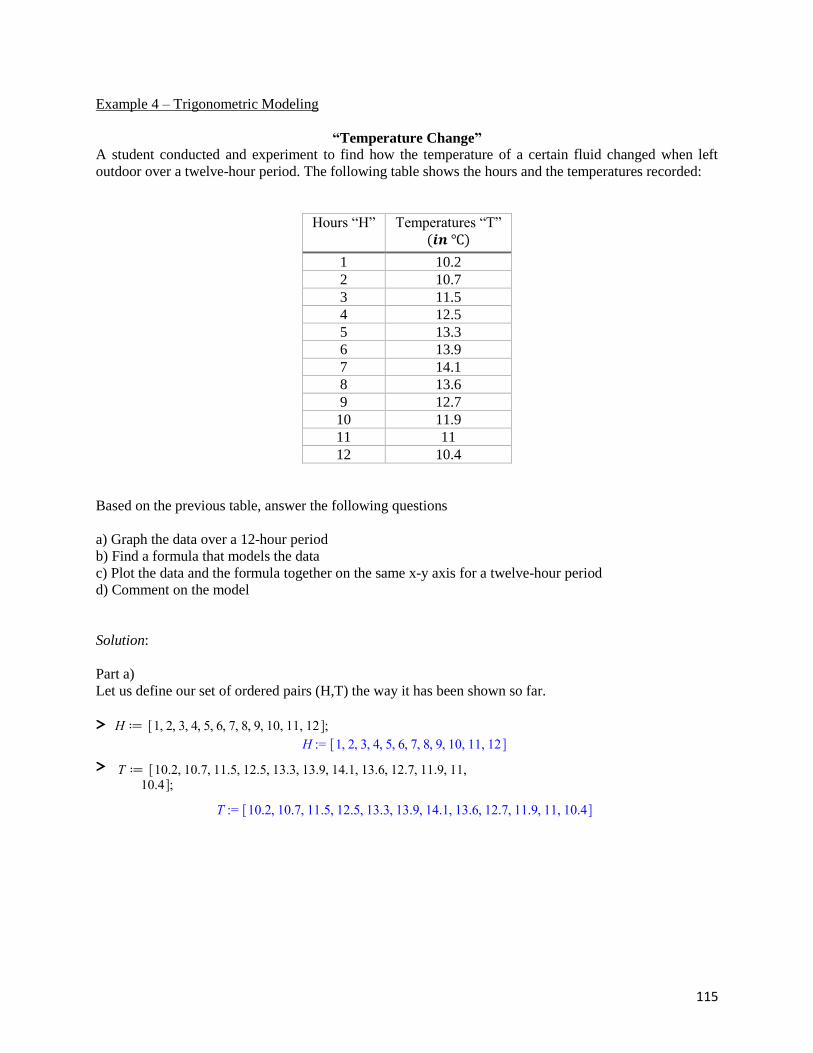
115

Example 4 – Trigonometric Modeling

“Temperature Change”

A student conducted and experiment to find how the temperature of a certain fluid changed when left

outdoor over a twelve-hour period. The following table shows the hours and the temperatures recorded:

Hours “H”

Temperatures “T”

(𝒊𝒏 ℃)

1 10.2

2 10.7

3 11.5

4 12.5

5 13.3

6 13.9

7 14.1

8 13.6

9 12.7

10 11.9

11 11

12 10.4

Based on the previous table, answer the following questions

a) Graph the data over a 12-hour period

b) Find a formula that models the data

c) Plot the data and the formula together on the same x-y axis for a twelve-hour period

d) Comment on the model

Solution:

Part a)

Let us define our set of ordered pairs (H,T) the way it has been shown so far.

>

>

116


To draw the scatter diagram of the data, let us use the command ScatterPlot

>

Part b)

From the previous graph, it looks like the data follows a sinusoidal trend over the time.

To find a formula that models the data (i.e. a trigonometric model), let us use the command NonlinearFit

to obtain the trigonometric fit we need:

>

About the arguments of the command NonlinearFit:

* The first part of the argument, i.e. the expression: “a*sin(b*x + c) + d” is the most general form for a

trigonometric function (in this case: sine).

Let us recall that in general a trigonometric function looks like:

𝐴 ∗ sin(𝜔 ∗ 𝑡 + 𝜑) + 𝐷

Where:

A = Amplitude

𝜔 = Angular Frequency, in radians per second [𝑟𝑎𝑑

𝑠𝑒𝑐]

t = Time, usually in seconds [s], is the argument of the function

117

𝜑 = Phase, it can be given in degrees or radians

D = A vertical shift, it can be upward or downward


Note:

In general, when trying to find a non-linear model for curve fitting in Maple, a good option is to use of the

command NonlinearFit. The advantage of this command lies in the flexibility we have to tell Maple what

kind of fitting we are interested to find. Think of a way to “customize” a math modeling.

If we wish to express the non-linear function we just obtained using the function notation, we type:

>

Part c)

To plot the data and the trigonometric model on the same x-y axis for a twelve-hour period, let us follow

the well-known steps;

Let us name our scatter diagram as “SS”

>

Let us name the plot of the function f(x) as “FF”. The viewing window for the function f(x) will be the

x-values ranging from x = 1 to x = 12

>

118

Let us use the command plots so that both the scatter diagram and the function f(x) can be depicted

together and add an appropriate title for the picture:

>

Part d)

From the graph shown above, it can be said that the trigonometric model is a good approximation for the

data given previously. It seems like the trigonometric function obtained matches and follows the data

points closely.

One of the advantages of the trigonometric model is that it can be applied to problems where repetitions

or repeated periods are involved. This is possible due to the inherent characteristic of the trigonometric

functions.

119

Introduction to Calculus

Calculus is perhaps the most interesting part of modern math education. The study of calculus is

fundamental for students majoring in science and/or engineering. Calculus has a vast use and countless

applications in many fields such as: engineering disciplines, statistics, financial math, physics, and so on.

In the following pages, the reader will get a “sneak peek” of calculus and how Maple can be used to make

some calculations. Once again, students are encouraged to get familiar with the concepts and definitions

before attempting to type any instruction on Maple.

To start using the built-in calculus capabilities that Maple has, let us first enable the package:

Student[Calculus1]

>

And let us have the palette Calculus ready to be used. This palette can be found on the left column.

120

Calculating Limits

Let us go over some examples.

* Example 1.- Calculate the following limit: lim𝑥→0

sin (𝑥)

𝑥

First, let us define the function f(x)

>

To calculate the above limit we can use either the command limit or the operator found in the palette.

Using the command limit:

>

Using the operator in the palette:

>

121

* Example 2.- Calculate the limit: lim𝑥→−2

x+2

𝑥2−4

Define the above function as g(x)

>

Calculate the limit by using the command limit

>

Or using the operator from the palette

>

* Example 3.- Calculate: lim𝑥→0

𝑥 ∗ sin(1

𝑥)

Using the operator from the palette

>

122

Calculating Derivatives of One-Variable Functions

Let us explore some examples.

* Example 1.- Calculate the derivative of 𝑥5, and 𝑦4

To find the derivative we can use either the command diff or the respective operator from the palette

Using the command diff

>

>


>

>

123

However if we use the previous command (diff) but with capital D (i.e. Diff), Maple will show the

formula to calculate the derivative but will not perform the operation. See below:

>

>

* Example 2.- Find the derivative of 8 − 2𝑥2


>


>

Again, if we type the command diff with capital D (i.e. Diff), Maple will give us the formula to find the

derivative but will not find it

>

* Example 3.- Calculate the derivative of 12𝑡2 + 2𝑡 + 102


>


>

124

Calculating Derivatives of Two-Variable Functions

Let us go over some examples.

* Example 1.- Given the two-variable function f(x,y) = 3𝑥3𝑦2 , calculate 𝜕𝑓(𝑥,𝑦)

𝜕𝑥 and

𝜕𝑓(𝑥,𝑦)

𝜕𝑦

First, let us define the function f(x,y) in Maple:

>

To find the derivatives respect to the variables x and y, we can use different options:


>

Therefore, 𝜕𝑓(𝑥,𝑦)

𝜕𝑥= 9𝑥2𝑦2

>

Therefore, 𝜕𝑓(𝑥,𝑦)

𝜕𝑦= 6𝑥3𝑦

Using the operator D

>

Thus, 𝜕𝑓(𝑥,𝑦)

𝜕𝑥= 9𝑥2𝑦2 , note that in this case “1” refers to the variable x

>

Thus, 𝜕𝑓(𝑥,𝑦)

𝜕𝑦= 6𝑥3𝑦 , note that in this case “2” refers to the variable y

125


>

Then, 𝜕𝑓(𝑥,𝑦)

𝜕𝑥= 9𝑥2𝑦2

>

Then, 𝜕𝑓(𝑥,𝑦)

𝜕𝑦= 6𝑥3𝑦

As seen previously, note that if we use the command (diff) but with capital D (i.e. Diff), Maple will

display the formula to calculate the partial derivative but will not perform the operation. See below:

>

>

126

* Example 2.-Find 𝜕𝑔(𝑥,𝑦)

𝜕𝑥 and

𝜕𝑔(𝑥,𝑦)

𝜕𝑦 for the function g(x,y) = 2𝑥3 + 4𝑦5

First, let us define the function g(x,y) in Maple:

>

Using the command diff to find 𝜕𝑔(𝑥,𝑦)

𝜕𝑥, and

𝜕𝑔(𝑥,𝑦)

𝜕𝑦; we have:

>

>

Using the operator D, we have:

>

>

Note that “1” indicates the variable x, and “2” indicates the variable y

Now, using the operator 𝜕

𝜕𝑥𝑓 from the palette

>

>

Again, if we type the command diff with capital D (i.e. Diff), Maple will show us the formula to find the

partial derivative but will not calculate it

>

>

127

* Example 3.- Given the following two-variable function h(x,y) = 𝑥

𝑦+

𝑦

𝑥 calculate its partial derivatives

Defining the function h(x,y) in Maple:

>

Finding 𝜕ℎ(𝑥,𝑦)

𝜕𝑥, and

𝜕ℎ(𝑥,𝑦)

𝜕𝑦:

- With the command diff

>

>

- With the operator D

>

>

- With the operator 𝜕

𝜕𝑥𝑓 from the palette

>

>

128

Calculating Antiderivatives (Indefinite Integrals) of One-Variable Functions

Let us go through some examples.

* Example 1.- Calculate the antiderivative of 21𝑥 + 2

To find the antiderivative we can use either the command int or the respective operator from the palette

Using the command int

>


>

Nevertheless, if we use the previous command (int) but with capital I (i.e. Int), Maple will show the

formula to calculate the antiderivative but will not perform the operation. See below:

>

129

* Example 2.- Find the antiderivative of 3𝑥2


>


>

Again, if we type the command int with capital I (i.e. Int), Maple will show the formula to find the

antiderivative but will not calculate it

>

* Example 3.- Calculate the antiderivative of 2𝑥3 − 𝑥2 − 3


>


>

130

Calculating Definite Integrals of One-Variable Functions

Let us explore some examples.

* Example 1.- Calculate the definite integral of 21𝑥 + 2 between x =1 and x = 5

To find the definite integral we can use either the command int or the respective operator from the palette


>


>

However, if we use the previous command (int) but with capital I (i.e. Int), Maple will give us the

formula to calculate the definite integral but will not perform the operation. See below:

>

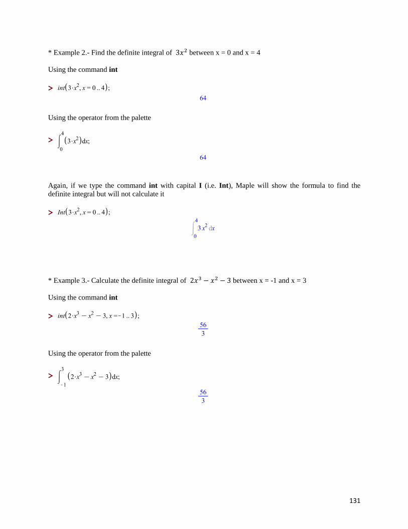
131

* Example 2.- Find the definite integral of 3𝑥2 between x = 0 and x = 4


>


>

Again, if we type the command int with capital I (i.e. Int), Maple will show the formula to find the

definite integral but will not calculate it

>

* Example 3.- Calculate the definite integral of 2𝑥3 − 𝑥2 − 3 between x = -1 and x = 3


>


>

132

Calculating Roots, Critical Points, and Plotting Derivative Functions

Let us see the following examples.

* Example 1.- Given the function f(x) = 𝑥3 + 2𝑥2 − 5𝑥 − 6, calculate its roots (i.e. zeros), critical points

(i.e. 𝑑𝑓(𝑥)

𝑑𝑥= 0), and plot both f(x) and

𝑑𝑓(𝑥)

𝑑𝑥 over the same x-y axis

Let us begin by defining the function f(x) in Maple:

>

To find the roots of the function f(x), we use the command Roots

>

To find the critical points of the function f(x), we use the command CriticalPoints

>

To plot both the function f(x) and its derivative f ’(x), we use the command DerivativePlot

>

133

* Example 2.- Given the function g(x) = 𝑥3 + 𝑥2 − 𝑥 + 2, find its real zeros, critical points, and plot its

derivative

Defining the function g(x) in Maple:

>

To find the real zeros of the function g(x), we use the command fsolve**

>

To find the critical points of the function g(x), we use the command CriticalPoints

>

To plot g(x) and g’(x) together in the same x-y axis, we use the command DerivativePlot

>

Note:

While the command solve give us all the solutions for the equation g(x) = 0, the command fsolve gives us

only the real solutions of the equation g(x) = 0. The function g(x) = 𝑥3 + 𝑥2 − 𝑥 + 2 is a third-degree

polynomial and has three solutions: one solution is real and the other two solutions are complex

conjugate; however since we are only interested in finding the real zeros of the function g(x), the

command fsolve is sufficient.

134

* Example 3.- Given the function h(x) = 2𝑥3 − 𝑥2 − 3, plot its derivative, find its critical points, and a

root for h(x) between 1 and 2.

Defining the function h(x) in Maple:

>

To plot h(x) and h’(x) at the same time:

>

To find the critical points of h(x):

>

To find a root of h(x) that is between x = 1 and x = 2**

>

Note that in this case, we can also specify an interval to find the solutions for x within the command

fsolve. This feature might be very useful when trying to find a specific root or solution of a function.

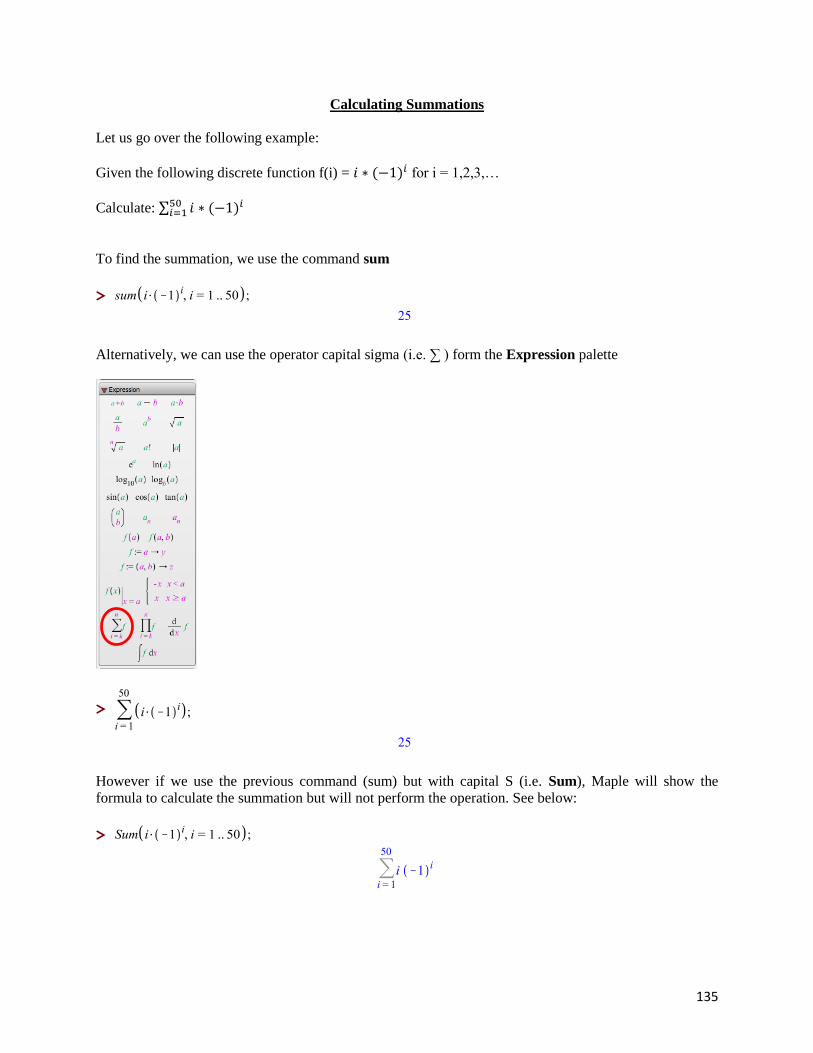
135

Calculating Summations

Let us go over the following example:

Given the following discrete function f(i) = 𝑖 ∗ (−1)𝑖 for i = 1,2,3,…

Calculate: ∑ 𝑖 ∗ (−1)𝑖50𝑖=1

To find the summation, we use the command sum

>

Alternatively, we can use the operator capital sigma (i.e. ∑ ) form the Expression palette

>

However if we use the previous command (sum) but with capital S (i.e. Sum), Maple will show the

formula to calculate the summation but will not perform the operation. See below:

>

INTRODUCTION TO MAPLE 18 STANDARD WORKSHEET

Documents

Transcript of INTRODUCTION TO MAPLE 18 STANDARD WORKSHEET