1.1 Fundamentals of Worksheet: - mkics

1.1 Fundamentals of Worksheet: � Concepts of workbook � A workbook is a collection of one or more spreadsheets, also called worksheets, in

a single file.

� Below is an example of a spreadsheet called "Sheet1" in an Excel workbook file

called "Book1." Our example also has the "Sheet2" and "Sheet3" sheet tabs, which

are also part of the same workbook.

� Each spreadsheet can have many sheets and each sheet can have many individual

cells.

� Each sheet can have a maximum of 65,536 rows and a maximum of 1024 columns,

for a total of over 67 million cells.

� Difference between a workbook, worksheet, and

spreadsheet � When you open Excel (a spreadsheet program), you're opening a workbook.

� A workbook can contain one or more different worksheets that can be accessed

through the tabs at the bottom of the worksheet.

� A spreadsheet and worksheet mean the same thing.

� workbook consist of a number of individual sheets, each containing cells arranged

in rows and columns.

� A particular cell is identified by its column letter and row number.

� These cells hold the individual elements—text, numbers, formulas, and so on—that

make up the data to display and manipulate.

� Adding worksheet � Step to insert new worksheets:

o Click on the Insert menu and select Sheet, or

o Right-click on its tab and select Insert Sheet, or

o Click into an empty space at the end of the line of sheet tabs.

� Each method will open the Insert Sheet dialog box.

� Here you can select whether the new sheet is to go before or after the selected sheet

and how many sheets you want to insert.

� Cell address � A cell is a rectangular box that occurs at the intersection of a vertical column and

a horizontal row in a worksheet.

� Vertical columns are numbered with alphabetic values such as A, B, C.

� Horizontal rows are numbered with numeric values such as 1, 2, 3.

� Each cell has its own set of coordinates or position in the worksheet such as A1, A2,

or M16 and its is a combination of column and row.

� In the example above, we are positioned on cell A1 which is the intersection of

column A and row 1. so the cell address is A1.

� Active cell: � The cell which is selected is known as active cell.

� It referred as a cell pointer or selected cell.

� An active cell is a rectangular box, highlighting the cell in a spreadsheet.

� It helps identify what cell is being worked with and where data will be

entered. (as shown in figure)

� Formula bar : � The formula bar has five components: the name box, the function wizard, the

sum function, the function button and the input line.

1. The name box shows what cell or group of cells that are currently selected.

2. The function wizard button will open another window with the functions available

in OpenOffice Calc.

3. The sum function button adds the sum function into the input line.

4. The function button adds an equal sign to the input line to prepare for the input of

a function expression.

5. Finally, the input line allows you to input data and functions into cells. It also

displays the contents of a cell before the execution of the function.

� Insert cell

� Step to insert cell using the Insert menu:

1. Select the cell where you want the new cell inserted.

2. Select Insert --> Cell.

OR

� Step to insert cell using right-click (context) menu:

1. Select the cell you want the new cell inserted.

2. Right-click the selected cell.

3. Select Insert Cells (figure show below)

� Inserting columns and rows � Step for inserting columns and rows using the Insert menu:

1. Select the column or row where you want the new column or row inserted.

2. Select either Insert --> Columns or Insert--> Rows.

OR

� Step Using the right-click (context) menu:

1. Select the column or rows where you want the new column or row inserted.

2. Right-click the header.

3. Select Insert Rows or Insert Columns.

� Deleting columns and rows � Columns and rows can be deleted individually or in groups.

Step:

1. Select the column or row to be deleted.

2. Right-click on the column or row header.

3. Select Delete Columns or Delete Rows from the pop-up menu.

� Removing data from a cell

� Data can be removed (deleted) from a cell in several ways.

1. Removing data only

� Click in the cell to select it, and then press the Backspace key.

2. Removing data and formatting

� The data and the formatting can be removed from a cell at the same time.

� Press the Delete key (or right-click and choose Delete Contents, or use Edit >

Delete Contents) to open the Delete Contents dialog.

� From this dialog, the different aspects of the cell can be deleted. To delete

everything in a cell (contents and format), check Delete all.

� Click on ok button.

� Format cells � It can either be edited as part of a cell style so that it is automatically applied, or it

can be applied manually to the cell.

� Some manual formatting can be applied using toolbar icons.

� For more control and extra options, select the appropriate cell or cells, right-click on

it, and select Format Cells.

� All of the format options are show in below figure.

• Number

• Font

• Font effects

• Alignment

• Border

• Background

• Cell Protection.

� Formatting numbers

� Several number formats can be applied to cells by using icons on the Formatting

toolbar.

� Select the cell, then click the relevant icon. Some icons may not be visible in a default

setup; click the down-arrow at the end of the Formatting bar and select other icons

to display.

�

� Number format icons. Left to right: currency, percentage, date, exponential, standard,

add decimal place, delete decimal place.

� For more control or to select other number formats, use the Numbers tab of the

Format Cells dialog as shown on above.

� Apply any of the data types in the Category list to the data.

� Control the number of decimal places and leading zeros.

� Enter a custom format code.

� The Language setting controls the local settings for the different formats such as the

date order and the currency marker.

� Formatting the font

� To choose the size of the font, click the arrow next to the Font Size box on the

Formatting toolbar. For other formatting, you can use the Bold, Italic, or Underline

icons.

� To choose a font color, click the arrow next to the Font Color icon to display a color

palette. Click on the required color.

� Choosing font effects

� Overlining and underlining

� You can choose from a variety of overlining and underlining options (solid lines,

dots, short and long dashes, in various combinations) and the color of the line.

� Strikethrough

� The strikethrough options include lines, slashes, and Xs.

� Relief

� The relief options are embossed (raised text), engraved (sunken text), outline, and

shadow.

� Alignment and orientation

� Use the Alignment tab of the Format Cells dialog to set the horizontal and vertical

alignment and rotate the text.

� Formatting the cell borders

� To quickly choose a line style and color for the borders of a cell, click the small

arrows next to the Line Style and Line Color icons on the Formatting toolbar.

� In each case, a palette of choices is displayed. (If the Line Style and Line Color icons

are not displayed in the formatting toolbar, select the down arrow on the right side

of the bar, then Visible Buttons.)

� For more control, including the spacing between the cell borders and the text, use

the Borders tab of the Format Cells dialog. There you can also define a shadow.

� The cell border properties apply to a cell, and can only be changed if you are editing

that cell. For example, if cell C3 has a top border (which would be equivalent visually

to a bottom border on C2), that border can only be removed by selecting C3. It

cannot be removed in C2

� Formatting the cell background

To quickly choose a background color for a cell, click the small arrow next to the

Background Color icon on the Formatting toolbar. A palette of color choices, similar to the

Font Color palette, is displayed.

(To define custom colors, use Tools > Options > OpenOffice.org > Colors. See Setting up

and Customizing Calc for more information.)

You can also use the Background tab of the Format Cells dialog. See Styles and

Templates for details.

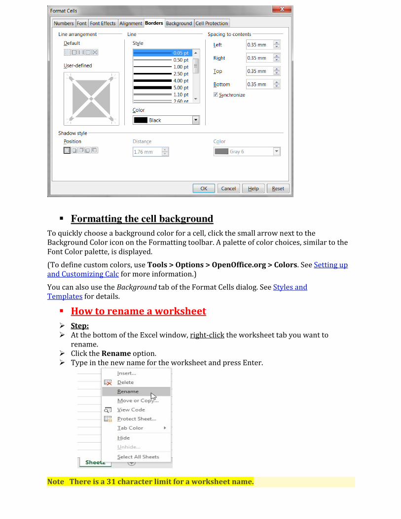
� How to rename a worksheet

� Step:

� At the bottom of the Excel window, right-click the worksheet tab you want to

rename.

� Click the Rename option.

� Type in the new name for the worksheet and press Enter.

Note There is a 31 character limit for a worksheet name.

� How to copy a worksheet

� Step

� At the bottom of the Excel window, right-click the worksheet tab you want to copy.

� Click the Move or Copy option.

�

� In the Move or Copy window, in the Before sheet section, select the worksheet

where you want to place the copied worksheet.

� Check the box for the Create a copy option, then click OK.

A copy of the worksheet is added and placed before the worksheet you selected in step 3

above. For example, if you had two worksheets named "Sheet1" and "Sheet2," and you

selected Sheet2 in step 3, a copy of Sheet2 would be placed before the Sheet1. The result

would look like the example picture below. The worksheet named "Sheet2 (2)" is the copy

of Sheet2.

� Lock cell/ Protection of cell

Cell protection is active for all cells by default. If only certain cells are to be protected, this

setting must be turned off.

Step to exclude cells from the protection:

1. Select the cells to be excluded from protection.

2. Select Format - Cells from the main menu

3. Click on the Cell Protection tab

4. Clear the check mark for the Protected option

5. Click OK

Initially however, the protection is not activated. To activate the protection:

� Select Tools - Protect Document - Sheet to protect the current sheet only

� Select Tools - Protect Document - Document to protect all sheets in the current

document

� Protect Sheets:

• steps for protect a sheet in open office.

• Select Tools --->Protect Document---> Sheet.

• Enter a password.

• Confirm the password.

• Click OK.

� Protect Workbook:

• protect workbook is use to protect all sheets in the current document

• Steps for protect a workbook in open office.

• Select Tools --->Protect Document---> Document.

• Enter a password.

• Confirm the password.

• Click OK.

� Cut, Copy, Paste,Paste Spacial

� You can copy or move text within a document, or between documents, by dragging

or by using menu selections, icons, or keyboard shortcuts.

� You can also copy text from other sources such as Web pages and paste it into a

Writer document.

� To move (cut and paste) selected text using the mouse, drag it to the new location

and release it.

� To copy selected text, hold down the Control key while dragging. The text retains

the formatting it had before dragging.

� After selecting text, you can use the mouse or the keyboard for these operations.

1. Cut: To removes the selected data from the original position

Use menu Edit --> Cut or

The keyboard shortcut CTRL+X or

The Cut icon on the toolbar.

2. Copy: To duplicates the selected content

Use Edit --> Copy or

The keyboard shortcut CTRL+C or

The Copy icon.

3. Paste: frequently used with cut or copy options.

Use Edit --> Paste or

The keyboard shortcut CTRL+V or

The Paste icon.

4. Paste Special: Special types of Paste command for formula use.

Use edit -->Paste Special or

The keyboard shortcut CTRL+ATL+V or

Click the triangle to the right of the Paste icon shown in diagram.

� Paste Special is a special type of paste option.

� The difference between paste and paste special is that the paste command allows

the user to insert the selected data from the clipboard into an application while the

paste special command follows the same functionality similar to paste, but provides

additional options to select how the inserted data should appear on the

application.

� If the user selects Formulas, the data will be pasted in the new location with the

formulas as follows. In the new copy, the totals are calculated, and it has taken the

new cells for calculation. The total 7000 in G9 is the summation of G4 to G7. The

formula is visible in the formula bar.

� Like the Paste special Option allows selecting how the pasted content should display.

� Format Painter

� Highlight the area from which you wish to copy the format from.

� copies the formatting from your selected cell or data range and pastes it onto the

next data range you select.

� Step:-

1. First add formats to a cell

2. Click on the format painter icon in the toolbar shown in given diagram.

3. When the mouse looks like a paint bucket, highlight the cell to which you want to

apply the format.

4. Let the mouse button go and the format will be applied to that section of cells

5. Click on the Format Painter button again to deactivate it.

1.2 Alignment, indent, Number format, percent style, coma style,

increase/decrease decimal

� Alignment :

• Align or alignment is a term used to describe how text is placed on the screen.

• For example, left-aligned text creates a straight line of text on the left side of

the page (like this paragraph).

• Text can be aligned along the edge of a page, cell, div, table, or another visible or

non-visible line.

• For apply alignment in open office calc or spreadsheet file ,

From menu bar select Format option and then select Alignment option.

Menu bar Format Alignment

• This will open sub menu which display various types of

alignment like : left, right, center , justify, top, center, bottom.

The four primary types of alignment are in open office writer include left aligned,

right aligned, cantered, and justified.

1. Left Aligned - It is the default setting. This setting is often referred to as

"left justified," but is technically called "flush left."

Left aligned text begins each line along the left margin of the cell.

This results in a straight margin on the left and a "ragged edge" margin on

the right.

2. Right Aligned - This setting is also called "right justified," but is technically

known as "flush right."

It aligns the beginning of each line of text along the right margin of the cell.

As you type, the text expands to the left of the cursor.

If you type more than one line, the next line will begin along the right

margin.

The result is a straight margin on the right and a "ragged edge" margin on

the left.

Right justification is commonly used to display the company name and

address near the top of a business document.

3. Cantered - As the name implies, cantered text is placed in the centre of

each line.

As you type, the text expands equally to the left and right, leaving the same

margin on both sides.

When you start a new line, the cursor stays in the centre, which is where

the next line begins.

Centred text is often used for document titles and may be appropriate for

headers and footers as well.

4. Justified - Justified text combines left and right aligned text.

When a block of text is justified, each line fills the entire space from left to

right, except for the cell indent and the last line of a cell.

This is accomplished by adjusting the space between words

and characters in each line so that the text fills 100% of the space.

Justified text is commonly used in newspapers and magazines and has

become increasingly popular on the Web as well.

5. Default - Aligns the cell contents to the bottom of the cell.

6. Top - Aligns the contents of the cell to the upper edge of the cell.

7. Bottom - Aligns the contents of the cell to the lower edge of the cell.

• Number format

• Number formats are template strings consisting of format codes defining how

numbers or text appear.

• For example, whether or not to display trailing zeros, group by thousands,

separators, colors, and how many decimals are displayed.

• This does not include any font attributes, except for colors.

• They are found wherever number formats are applied, for example, on

the Numbers tab of the Format – Cells dialog in spreadsheets.

• Number formats are defined on the document level.

• A document displaying formatted values has a collection of number formats, each

with a unique index key within that document.

• Identical formats are not necessarily represented by the same index key in

different documents.

coma style : (Thousands Separator)

• Depending on your language setting, you can use a comma or a period as a

thousand separator.

• You can also use the separator to reduce the size of the number that is

displayed by a multiple of 1000.

• For this, set thousand separator check box marked .

percent style: To display numbers as percentages, add the percent sign (%) to the

number format.

Increase/Decrease decimal : For increase or decrease decimal palces, add

number in OPTION Decimal Places.

1.2.1 Insert picture, insert shapes

� Insert Image : To add any image from file select Picture option From Insert

menu.

M.K. Institute of Computer Studies, Bharuch

F.Y.B.C.A. (SEM – 1 )

105: Data Manipulation and Analysis (DMA)

UNIT-1

� shapes:

• To add any type of shape in open office calc file, select VIEW menu ->

TOOLBAR -> DRAWING option.

It will display drawing tool bar at bottom of window.


F.Y.B.C.A. (SEM – 1 )


UNIT-1

1.2.2 Insert Textbox, Header & Footer, Symbols

� Insert Textbox :

• Text boxes are fields in which the user can enter text. In a form, text boxes

display data or allow for new data input.

• To insert text boxes in spread sheet file: click on VIEW menu -> TOOLBAR -

>Form Control.

• This will open form control dialog box and select Text Box option.


F.Y.B.C.A. (SEM – 1 )


UNIT-1

• After then it will display text box for add text as shown in figure.

� insert Symbols : (means special character)

• A "special character" is one not found on a standard English keyboard.

• For example, © ¾ æ ç ñ ö ø ¢ are all special characters. To insert a special

character:

1. Place the cursor in your document where you want the character to

appear.

2. Click Insert > Special Character to open the Special Characters dialog

box.

3. Select the characters (from any font or mixture of fonts) you wish to

insert, in order; then click OK.

4. The selected characters are shown in the lower left of the dialog box.

As you select each character, it is shown on the lower right, along with

the numerical code for that character.


F.Y.B.C.A. (SEM – 1 )


UNIT-1

• Header & Footer :

• Headers and footers are predefined pieces of text that are printed at the top

or bottom of a sheet outside of the sheet area. They are set the same way.

• Header prints in heading area and footer prints in bottom area.

• Headers and footers are assigned to a page style.

• You can define more than one page style for a spreadsheet and assign

different page styles to different sheets.

• For more about page styles, see Using styles and templates in Calc.

• Setting a header or a footer: To set a header or footer:

1. Select Format > Page.

2. Select the Header (or Footer) tab.


F.Y.B.C.A. (SEM – 1 )


UNIT-1

3. Select the Header on option.

• From here you can also set the margins, the spacing, and height for the

header or footer.

• You can check the AutoFit height box to automatically adjust the height of

the header or footer.

Margin : Changing the size of the left or right margin adjusts how far the

header or footer is from the side of the page.

Spacing : Spacing affects how far above or below the sheet the header or

footer will print. So, if spacing is set to 1.00", then there will be 1 inch

between the header or footer and the sheet.

Height: Height affects how big the header or footer will be.

Header or footer appearance :To change the appearance of the header or

footer, click the More button in the dialog. This opens the

Border/Background dialog.

• From this dialog you can set the background and border style of the header or

footer. See Using styles and templates in Calc for more information.


F.Y.B.C.A. (SEM – 1 )


UNIT-1

• Setting the contents of the header or footer

The header or footer of a Calc spreadsheet has three columns for text. Each

column can have different contents.

To set the contents of the header or footer, click the Edit button in the

header or footer dialog shown above to display the dialog shown below.

Areas: Each area in the header or footer is independent and can have

different information in it.

Header : You can select from several preset choices in the Header drop-down

list, or specify a custom header using the buttons below. (If you are

formatting a footer, the choices are the same.)


F.Y.B.C.A. (SEM – 1 )


UNIT-1 Custom header: Click in the area (Left, Center, Right) that you want to

customize, then use the buttons to add elements or change text attributes.

Opens the Text Attributes dialog.

Inserts the total number of pages.

Inserts the File Name field.

Inserts the Date field.

Inserts the Sheet Name field.

Inserts the Time field.

Inserts the current page number.

1.2.3 Save, save as, save file as csv, spell check, protect sheet and Workbook, Linking

spread sheets.

� What is Save

• Assume the user created a sheet in the desktop and enter some content.

• If he goes to the top of the screen, there is an icon which looks like a disk.

• After pressing that icon, the content is saved to that document.

• When closing the file and reopening it again, the user can view those written

content.

• Another method to Save is by going to the File menu and selecting Save.

• When working, the user can click Save to update the completed work up to that

point.

• Each time the user press Save, it will overwrite the document with the latest

content.

� What is Save As


F.Y.B.C.A. (SEM – 1 )


UNIT-1

• Assume that the user goes to Sheet and add data to file.

• When he presses the save icon, it will open the Save As Dialog box.

• From that, the user can select the location to store the file with file name and file

type.

• Here, the file name is “test1”, and it is a worksheet. Then he can press save

button.

Figure 2: Save As

• If the user wants to save that already created test1 file to some other

location with the same name or a different name, then also he has to

use Save As. Therefore, it helps to create backup files.

� Difference Between Save and Save As

Definition :

Save is a command in the File menu of most applications that stores the data

back to the file and folder it originally came from.

On the other hand, Save As is a command in the File menu of most

applications that allows to store a new file or to store the file in a new

location.


F.Y.B.C.A. (SEM – 1 )


UNIT-1

Main Usage:

Save helps to prevent data loss and to update the lastly preserved file with

the latest content.

Save As helps to store a new file or to store an existing file in a new location

with the same name or with a different name.

Application:

Save applies to a current file. On the other hand, the Save As applies to a new

file.

Number of Steps:

Save is easier as it has only one step but Save As requires some additional

steps.

Storing Method:

Save does not allow saving the file in some other format. But it is different

with Save As. It allows the user to change the file format with the Save As

dialog box.

� Saving as a CSV file

• A CSV is a comma-separated values file, which allows data to be saved in a

tabular format with a .csv extension.

• CSV files can be used with most any spreadsheet program, such as Microsoft

Excel or Google Spreadsheets.

• They differ from other spreadsheet file types because you can only have a single

sheet in a file, they cannot save cell, column, or row.

• Also, you cannot not save formulas in this format.

• To save a spreadsheet as a comma separated value (CSV) file:

1. Choose File > Save As.

2. In the File name box, type a name for the file.

3. In the File type list, select Text CSV and click Save.

You may see the message box shown below. Click Keep Current

Format.


F.Y.B.C.A. (SEM – 1 )


UNIT-1

4. In the Export of text files dialog, select the options you want. Click OK.

� spell check

• Spell check option is used to detect the misspelled word and replace it

with the correct word.

Step 1: Open the spell-checker

• Click on 'Tools' in the menu bar and then 'Spelling and Grammar' from the

drop-down menu, or press Alt + T and then press Alt + S, to open the

'Spelling' window (shown in Fig 1).

• You can also spell-check your document at any time by pressing F7.


F.Y.B.C.A. (SEM – 1 )


UNIT-1

Step 2: Open the thesaurus

• OpenOffice.org Writer also includes a thesaurus, which will provide

synonyms (words with similar meanings) for any given word. To use this

feature, first highlight the word in your text.

• Open the 'Thesaurus' window (shown in Fig 2) by clicking on 'Tools' in the

menu bar and then 'Language' from the drop-down menu, followed by

'Thesaurus'. Alternatively, press Alt + T and then press Alt + L, followed by Alt

+ T.

• You can also open the thesaurus at any time by pressing Ctrl + F7.

• Features Of Spell Check utility

1.Enable Spell check:

Click on the Auto Spellcheck icon from the standard toolbar. If this option is

enabled, it will highlight the spelling errors in a wavy red line.


F.Y.B.C.A. (SEM – 1 )


UNIT-1

2.Suggestions:

To get suggestions for the misspelled words, do the following.

Step 1: Right click on the misspelled word. You will be provided with the list of

suggested words.

Step 2: Select the required suggested word. The misspelled word will be

automatically replaced by the selected word.


F.Y.B.C.A. (SEM – 1 )


UNIT-1 3.Ignore All:

The misspelled word will be ignored by the spell checker.

4.To replace a word:

Replace option is used to replace the misspelled word with the correct word.

Step 1: Select the misspelled words and click on the Spelling icon or right click

and select "Spellcheck..."


F.Y.B.C.A. (SEM – 1 )


UNIT-1 Step 2: In the spell check dialog box, misspelled word will be highlighted

under Not in dictionary text box. Under Suggestions, suggested words will be

listed. Select the correct word and click Change. Now the selected word will be

replaced.

5. To replace all the misspelled word:

Step 1: Select the correct word under Suggestions and click Change All option.


F.Y.B.C.A. (SEM – 1 )


UNIT-1 Step 2: You will get an alert message, click Yes to replace all the words.

The particular word used anywhere in the spreadsheet file will be replaced with

the selected word.


F.Y.B.C.A. (SEM – 1 )


UNIT-1 6.Add a word to Dictionary

If the word is not added in the Standard dictionary, then the word will be

highlighted in the wavy red line. You can add a word to Dictionary using two

options.

Option 1: Right click on the word and select Add -> standard.dic

Option 2: Select the word and click Spelling icon.

Step 3: Spelling: English dialog box appears. click on the downward arrow near

the Add option and select Standard.dic. The word will be added into the standard

dictionary.

For the next time, the word won't be highlighted with the wavy red line as

misspelled word.


F.Y.B.C.A. (SEM – 1 )


UNIT-1

1.2.4 Print, Quick print, Print preview

� Print

• Prints the current document, selection, or the pages that you specify.

• You can also set the print options for the current document.

• Printing from Calc is the same as printing from other OO document

components but some details are different, especially regarding preparation

for printing.

• To access this Option...

1. Choose File - Print

2. Press Ctrl+P option from keyboard.

3. On print standard file bar Click directly.

The Print dialog consists of three main parts: A preview with navigation

buttons, several tab pages with control elements specific to the current

document type, and the Print, Cancel, and Help buttons.

• Using the Print dialog box

For more control over printing, use File > Print to display the Print dialog box.


F.Y.B.C.A. (SEM – 1 )


UNIT-1

On the Print dialog box, you can choose:

• Which printer to use (if more than one are installed on your system)

and the properties of the printer—for example, orientation (portrait or

landscape), which paper tray to use, and what paper size to print on. The

properties available depend on the selected printer; consult the printer's

documentation for details.

• What pages to print, how many copies to print, and in what order to

print them.

o Use dashes to specify page ranges and commas or semicolons to

separate ranges; for example: 1, 5, 11-14, 34-40.

o Selection is the highlighted part of a page or pages.

• What items to print. Click the Options button to display the Printer

Options dialog box.

3. Click OK.

• Quick printing

• Click the Print File Directly icon to send the entire document to the

default printer defined for your computer.

• You can change the action of the Print File Directly icon to send the

document to the printer defined for the document instead of the default

printer for the computer.

• Choose Tools > Options > Load/Save > General and the Load printer settings

with the document option.


F.Y.B.C.A. (SEM – 1 )


UNIT-1

• Previewing pages before printing

• The normal page view in Writer shows you what each page will look like

when printed, but it shows only one page at a time.

• If you are designing a document to be printed double-sided, you may want to

see what facing pages look like. OOo provides a way to do this in Page

Preview.

1. Click File > Page Preview, or click the Page Preview button . The

Writer window changes to display the current page and the following

page, and shows the Page Preview toolbar in place of the Formatting

toolbar.

2. Click the Book Preview icon to display left and right pages in their

correct orientation.

3. To print the document in this page view, click the Print page

view icon to open the Print dialog box. Choose your options and

click OK to print as usual.

4. To choose margins and other options for the printout, click the Print

options page view icon to display the Print Options dialog box.

1.2.5 Split, Hide and freeze panes in worksheet.

• Split option

• Sometimes Calc users need to split (or divide) data in one column into

another.


F.Y.B.C.A. (SEM – 1 )


UNIT-1

• As such, Calc has a Text to Columns option for splitting columns. With that

you can divide the columns.

1. Open a spreadsheet and then select a column, or group of cells in a

column, to split. For example, if there was an address column in the

spreadsheet you could select that to split it down into smaller parts.

2. Click Data > Text to Columns to open the window shown in shot below.

3. Now select the Separated by radio button on that window. Then you

can choose a separator for the column. You can

select Tab, Space, Comma, Merge delimiters or Semicolon separator

check boxes.


F.Y.B.C.A. (SEM – 1 )


UNIT-1 4. They mark the point where your column splits. As shown in figure

below

Now it is splits in different cell. As shown in figure below.


F.Y.B.C.A. (SEM – 1 )


UNIT-1

• Alternatively, you can add custom separators. Click the Other check box

and enter a separator in the text box. For example, you could enter a

hyphen (-) in that text box as the separator.

• You can also split the column with the Fixed width option. Select

the Fixed width radio button and adjust the ruler on the preview

window to a set a width for the column to split at. The column then

splits at the ruler point.

• When you’re done, press the OK button.

• The column will split as you selected it to. For example, in the shot

below the address column has split into three alternative columns.

• So now you can quickly split columns in Calc spreadsheets without any

copying and pasting.

• With the Text to Column option you can reorganize your spreadsheet

tables more effectively.

• Hide and freeze panes


F.Y.B.C.A. (SEM – 1 )


UNIT-1 Hide/Show Rows and Columns

• When elements are hidden, they are neither visible nor printed, but can still

be selected for copying if you select the elements around them.

• For example, if column B is hidden, it is copied when you select columns A

and C. When you need a hidden element again, you can reverse the process,

and show the element.

1. To hide or show rows and columns, use the option in the Format menu

or the right-click and choose from pop-up menu.

2. To hide a row/column, first select the row/column, and then use menu

options,

3. Format → Row → Hide or Format → Column → Hide to hide row

and column respectively.

4. The same can be achieved by choosing “Hide” option from the pop-up

menu when you right-click the selected row/column.

5. To show the hidden row / column, choose Format→ Row → Show

or Format →Column → Show (or)

6. Right-click and choose Show from pop-up menu.

• Freezing rows and columns

• Freezing locks number of rows at the top of a spreadsheet or number of columns

on the left of a spreadsheet or both.

• Frozen columns and rows remain the view during scrolling, whereas other rows

and columns gets scrolled.


F.Y.B.C.A. (SEM – 1 )


UNIT-1

Freezing single rows or columns:

1. Click on the Header for the row below where to the freeze or for the column to

the right of where to freeze.

2. Choose the Window -> Freeze. A dark line appears, indicating where the freeze is

put.

Freezing a row and a column:

1. Click the Cell that is immediately below the row to be frozen and immediately

to the right of the column to be frozen.

2. Choose Window -> Freeze.

3. Two lines appear on the screen, a horizontal line above this cell and a vertical

line to the left of this cell. Now as you scroll around the screen, everything above

and to the left of these lines will remain in view.

Unfreeze:

• To unfreeze rows or columns, choose Window -> Freeze. The check mark in

Freeze will vanish.

1.1 Fundamentals of Worksheet: - mkics

Documents

Transcript of 1.1 Fundamentals of Worksheet: - mkics