Gechtercontetlamottegallandkoukam2012

Draft for Franck GECHTER, Jean-Michel CONTET, Olivier LAMOTTE, Stphane GALLAND, and Abder-rafiaa KOUKAM. “Virtual Intelligent Vehicle Urban Simulator: Application to Vehicle Platoon Evaluation.”In Simulation Modelling Practice and Theory (SIMPAT), vol. 24, pp. 103-114, 2012..2012 c© Elsevier

Virtual Intelligent Vehicle Urban Simulator:Application to Vehicle Platoon Evaluation

Franck GECHTER, Jean-Michel CONTET, Stephane GALLAND, OlivierLAMOTTE, Abderrafiaa KOUKAM

Laboratoire Systemes et Transports,Universite de Technologie de Belfort-Montbeliard, Belfort, France

[email protected], [email protected], [email protected],[email protected], [email protected]

http://www.multiagent.fr

Abstract

Testing algorithms with real cars is a mandatory step in developing new intelli-gent abilities for future transportation devices. However, this step is sometimeshard to accomplish especially due to technical problems,... It is also difficultto reproduce the same scenario several times. Besides, some critical and/orforbidden scenarios cannot be tested in real. Thus, the comparison of severalalgorithms using the same experimental conditions is hard to realize. Consider-ing that, it seems important to use simulation tools to perform scenarios withnear reality conditions. The main problem with these tools is their distance withreal conditions, since they deeply simplify the real world. This paper presentsthe architecture of the simulation/prototyping tool named Virtual IntelligentVehicle Urban Simulator (vivus). The goal of vivus is thus to overcome thegeneral drawbacks of classical solutions by providing the possibility of designinga vehicle virtual prototype with well simulated embedded sensors and physicalproperties. Part experiments made on linear platoon algorithms are exposedin this paper in order to illustrate the similarity between simulated results andthose obtained in reality.

Keywords: Sensors simulation, Physics simulation, Autonomous vehicle,Platoon systems, 3D modelling

1. Introduction

Testing algorithms with real cars is a mandatory step in developing new in-telligent abilities for future transportation devices. However, this step is some-times hard to accomplish especially due to hardware problem, vehicle dispos-ability problem, etc. Moreover, it is also difficult to reproduce the same scenarioseveral times since some experimental parameters are variable and uncontrol-lable such as perception conditions, for instance. Thus, it is hard to compare

Preprint submitted to Elsevier November 15, 2012


several algorithms using the same experimental conditions. Besides, some crit-ical and/or forbidden scenarios (i.e. scenario that implies the collision and/ordestruction of a part of the physical device) are difficult to test in real.

Considering that, it seems important to find a less restrictive way to performscenarios with near reality conditions. That’s why many laboratories are testingtheir algorithms in simulation. The main problem of standard simulation tools istheir distance with real conditions, since they generally simplify vehicle/sensorsphysical models and road topology. Virtual cameras are basically reduced to asimple pinhole model without distortion simulation and vehicle models do nottake into account any dynamical characteristics and tyre-road contact exceptedin specific automotive industry tools.

The participation of the SeT Laboratory to cristal project 1 puts in evi-dence the fact that a new simulation/prototyping tool is required to perform acomparison between several solutions in the context of urban intelligent vehi-cles. For instance, in the context of the cristal project, a comparison betweenlinear platoon solutions has had to be performed. In order to obtain results nearto reality, this tool must be as precise as possible in terms of sensors simulationand vehicle dynamical model.

This paper presents the global architecture of the simulation/prototypingtool named Virtual Intelligent Vehicle Urban Simulator2 (vivus) developed bythe SeT Laboratory. This simulator is aimed at simulating vehicles and sen-sors, taking into account their physical properties and prototyping artificialintelligence algorithms such as platoon solutions [1] and obstacle avoidance de-vices [2]. The goal of vivus is thus to overcome the general drawbacks ofclassical solutions by providing the possibility of designing a vehiclevirtual pro-totype with well simulated embedded sensors. The retained solution has severalinterestssuch as:

• Prototyping artificial intelligence algorithms before the construction ofthe first vehicle prototype. In this case, they can be developed, tested andtuned with a virtual prototype of a real vehicle.

• Testing critical and/or banned use cases, i.e., cases that imply partial ortotal destruction of vehicles, to draw the limits of the retained solutions.

• Testing and comparing several algorithms/solutions for embedded featureswith a low development cost. It can thus help to choose the future embed-ded devices related to retained solutions requirements (processing powerneeds, connectivity, etc.).

• Testing and comparing the sensor solutions before integrating them intothe vehicle.

1Industrial Research Cell for Autonomous Light Weight Transportation Systems. InFrench: “Cellule de Recherche Industrielle en Systemes de Transports Automatises Legers”

2http://www.multiagent.fr/Vivus_Platform

2


• Integrating tests and evaluations results into the vehicle design process.

• Using informed and documented virtual reality to access the attribute andstate values of the vehicle, its components, and the environmental objectsaround.

This tool has been especially used during the cristal project to compare severallinear platoon algorithms to the results obtained with a real vehicle. Parts ofthese experiments are exposed in this paper in order to illustrate the similaritiesbetween the simulation’s and real car’s results.The paper is structured as follows. Next section presents a state of the art of thesimulation applications with a comparison of them according to several criteria.Section 3 gives a description of vivus architecture focusing on physics modeland virtual sensors description. Then Section 4 gives a short presentation of thetarget application, linear platoon evaluation, on which the developed simulatorhas been tested. Section 5 exposes results obtained comparing simulator andreal vehicle experiments. Finally, the paper finishes with a conclusion and ashort description of future work.

2. Simulation tools comparison

Computer simulation and their extension into robot and vehicle simulationsare an emerging topic. The main motivation for using simulation tools is thepotential to validate new technology before its deployment in real devices. Thevalidation aims at assessing the compliance of a system according to the de-sign objectives. Generally, this evaluation is done by submitting the system (ora model that represents it more or less accurately) to a series of tests. Thequality of test cases determines the confidence in the validation results. Whenthe focus is put on a model, the validation is then linked to simulation. Inthe domain of vehicle systems, the simulation must take into account the kine-matic/dynamical models of the vehicle and their connection to the ground (tyreson road) and model-board sensors. The representation model of the real worldin which sensors are taking their measures and where vehicles evolve must beprecise enough from a physics point of view. Various proposals currently exist tosimulate robots and vehicles in virtual environments, to model their dynamicalbehaviors and their sensors. Among the existing simulators, the following canbe mentioned:

• Open source: MissionLab 3, Player/Stage/Gazebo 4, SimRobot 5, USAR-Sim 6, Simbad 7.

3http://www.cc.gatech.edu/ai/robot-lab/research/MissionLab/4http://playerstage.sourceforge.net/5http://www.informatik.uni-bremen.de/simrobot/6http://usarsim.sourceforge.net/7http://simbad.sourceforge.net/

3


• Commercial devote to robots: Webots 8, Microsoft Robotics Studio 9.

• Commercial devote to vehicle: Carsim 10, CarMaker 11, PreScan 12, Pro-SiVIC 13.

As expressed in [3], simulation tools can be classified according to the followingcriteria:

• Physics accuracy: vehicle dynamical model, vehicle kinetic model, roadtopology...

• Sensors accuracy: frequency, data, noise...

• Functional accuracy: intelligent behavior, ...

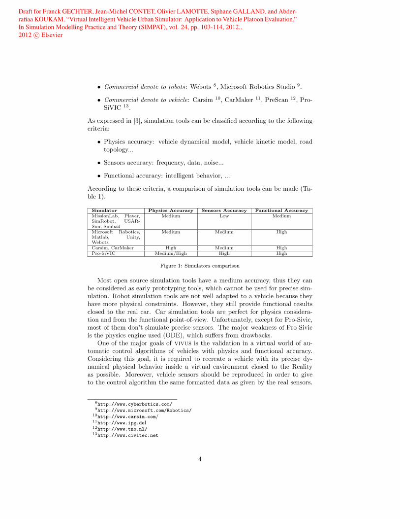
According to these criteria, a comparison of simulation tools can be made (Ta-ble 1).

Simulator Physics Accuracy Sensors Accuracy Functional AccuracyMissionLab, Player,SimRobot, USAR-Sim, Simbad

Medium Low Medium

Microsoft Robotics,Matlab, Unity,Webots

Medium Medium High

Carsim, CarMaker High Medium HighPro-SiVIC Medium/High High High

Figure 1: Simulators comparison

Most open source simulation tools have a medium accuracy, thus they canbe considered as early prototyping tools, which cannot be used for precise sim-ulation. Robot simulation tools are not well adapted to a vehicle because theyhave more physical constraints. However, they still provide functional resultsclosed to the real car. Car simulation tools are perfect for physics considera-tion and from the functional point-of-view. Unfortunately, except for Pro-Sivic,most of them don’t simulate precise sensors. The major weakness of Pro-Sivicis the physics engine used (ODE), which suffers from drawbacks.

One of the major goals of vivus is the validation in a virtual world of au-tomatic control algorithms of vehicles with physics and functional accuracy.Considering this goal, it is required to recreate a vehicle with its precise dy-namical physical behavior inside a virtual environment closed to the Realityas possible. Moreover, vehicle sensors should be reproduced in order to giveto the control algorithm the same formatted data as given by the real sensors.

8http://www.cyberbotics.com/9http://www.microsoft.com/Robotics/

10http://www.carsim.com/11http://www.ipg.del12http://www.tno.nl/13http://www.civitec.net

4


Additionally, vivus must run under real time constraints because the controlalgorithms are the one used with the real vehicles. Physics simulation is handledby the PHYSX software, which allows to apply forces to the different vehiclecomponents (dampers, motors...). All these components are also 3D objects onwhich physic-based relationship are applied.

3. Simulator Model

This part presents the simulator model. After a global overview of both thesimulator architecture and running process, this section will focus on specificcomponents such as the physics model and the sensor models.

3.1. Global Overview

The following subsections discuss the simulator architecture, execution andits implementation.

3.1.1. Simulator Architecture

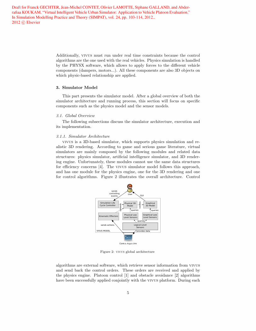
vivus is a 3D-based simulator, which supports physics simulation and re-alistic 3D rendering. According to game and serious game literature, virtualsimulators are mainly composed by the following modules and related datastructures: physics simulator, artificial intelligence simulator, and 3D render-ing engine. Unfortunately, these modules cannot use the same data structuresfor efficiency concerns [4]. The vivus simulator model follows this approach,and has one module for the physics engine, one for the 3D rendering and onefor control algorithms. Figure 2 illustrates the overall architecture. Control

Physical 3D

Model

Graphical

3D Model

Physical Low

Level Sensors

Graphical Low

Level Sensors

Logical Level

Sensors

Kinematic Effectors

Simulation Life

Cycle Controller

Control Algorithm

VIVUS MODEL

User

queries

queries queries

provides data

sends actions

update

s

sends

controlling

events

noti

fies

GUI

Figure 2: vivus global architecture

algorithms are external software, which retrieve sensor information from vivusand send back the control orders. These orders are received and applied bythe physics engine. Platoon control [1] and obstacle avoidance [2] algorithmshave been successfully applied conjointly with the vivus platform. During each

5


simulation step, the physics model notifies the graphical 3D model about eachchange. This last model then applies the newly received position and orienta-tion on the displayed objects. According to our model-separation assumption,the graphical-model data structure is based on classical 3D scenegraph.

3.1.2. Simulation Execution

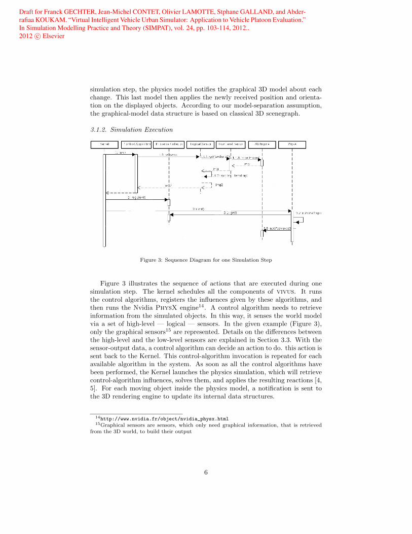
Figure 3: Sequence Diagram for one Simulation Step

Figure 3 illustrates the sequence of actions that are executed during onesimulation step. The kernel schedules all the components of vivus. It runsthe control algorithms, registers the influences given by these algorithms, andthen runs the Nvidia PhysX engine14. A control algorithm needs to retrieveinformation from the simulated objects. In this way, it senses the world modelvia a set of high-level — logical — sensors. In the given example (Figure 3),only the graphical sensors15 are represented. Details on the differences betweenthe high-level and the low-level sensors are explained in Section 3.3. With thesensor-output data, a control algorithm can decide an action to do. this action issent back to the Kernel. This control-algorithm invocation is repeated for eachavailable algorithm in the system. As soon as all the control algorithms havebeen performed, the Kernel launches the physics simulation, which will retrievecontrol-algorithm influences, solves them, and applies the resulting reactions [4,5]. For each moving object inside the physics model, a notification is sent tothe 3D rendering engine to update its internal data structures.

14http://www.nvidia.fr/object/nvidia_physx.html15Graphical sensors are sensors, which only need graphical information, that is retrieved

from the 3D world, to build their output

6


3.2. Physics Model

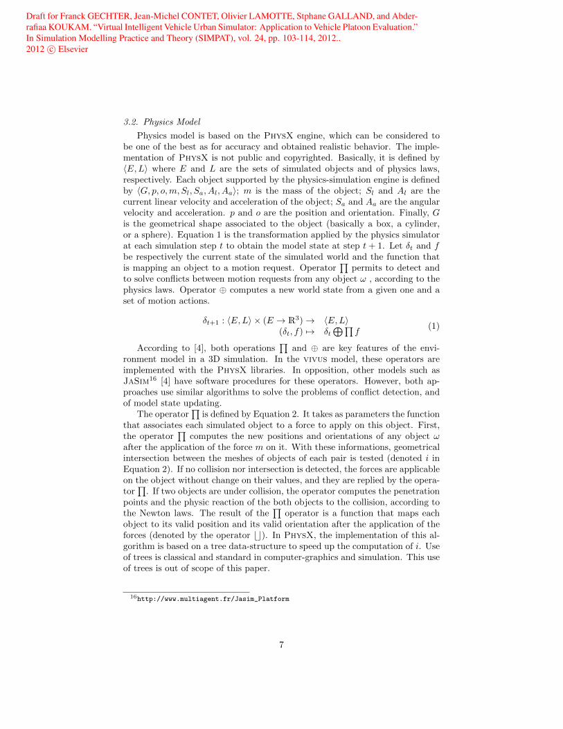
Physics model is based on the PhysX engine, which can be considered tobe one of the best as for accuracy and obtained realistic behavior. The imple-mentation of PhysX is not public and copyrighted. Basically, it is defined by〈E,L〉 where E and L are the sets of simulated objects and of physics laws,respectively. Each object supported by the physics-simulation engine is definedby 〈G, p, o,m, Sl, Sa, Al, Aa〉; m is the mass of the object; Sl and Al are thecurrent linear velocity and acceleration of the object; Sa and Aa are the angularvelocity and acceleration. p and o are the position and orientation. Finally, Gis the geometrical shape associated to the object (basically a box, a cylinder,or a sphere). Equation 1 is the transformation applied by the physics simulatorat each simulation step t to obtain the model state at step t+ 1. Let δt and fbe respectively the current state of the simulated world and the function thatis mapping an object to a motion request. Operator

∏permits to detect and

to solve conflicts between motion requests from any object ω , according to thephysics laws. Operator ⊕ computes a new world state from a given one and aset of motion actions.

δt+1 : 〈E,L〉 × (E → R3)→ 〈E,L〉(δt, f) 7→ δt

⊕∏f

(1)

According to [4], both operations∏

and ⊕ are key features of the envi-ronment model in a 3D simulation. In the vivus model, these operators areimplemented with the PhysX libraries. In opposition, other models such asJaSim16 [4] have software procedures for these operators. However, both ap-proaches use similar algorithms to solve the problems of conflict detection, andof model state updating.

The operator∏

is defined by Equation 2. It takes as parameters the functionthat associates each simulated object to a force to apply on this object. First,the operator

∏computes the new positions and orientations of any object ω

after the application of the force m on it. With these informations, geometricalintersection between the meshes of objects of each pair is tested (denoted i inEquation 2). If no collision nor intersection is detected, the forces are applicableon the object without change on their values, and they are replied by the opera-tor

∏. If two objects are under collision, the operator computes the penetration

points and the physic reaction of the both objects to the collision, according tothe Newton laws. The result of the

∏operator is a function that maps each

object to its valid position and its valid orientation after the application of theforces (denoted by the operator bc). In PhysX, the implementation of this al-gorithm is based on a tree data-structure to speed up the computation of i. Useof trees is classical and standard in computer-graphics and simulation. This useof trees is out of scope of this paper.

16http://www.multiagent.fr/Jasim_Platform

7


∏: (E → R3)→ (E → 〈R3,H〉)

(f := ω 7→ m) 7→

{ω 7→ (σp(ω) +m,σo(ω) +m) if i = ∅∏

(f ∩ {e 7→ bf(e)c|(e, b) ∈ i}) else

i := {a ∈ E|a 6= ω ∧ σG(a) + f(a) ∩ σG(ω) +m}

(2)

The operator ⊕ is defined by Equation 3. It loops on all the objects inthe world state δt, and it applies the motion vectors and quaternions to them.This operation is linear in time complexity. In PhysX, this operator is directlyinvoked on all the objects after the collision reactions were computed.

⊕ : 〈E,L〉 × (E → 〈R3,H〉)→ 〈E,L〉(δt, f) 7→ 〈{e+ f(e)|e ∈ σ1(δt)} , σ2(δt)〉

(3)

Equations 2 and 3 are coded in Algorithm 1, which illustrates the physicssimulation loop. First, the algorithm computes the new positions and orienta-tions G′(o) of all the objects at line 3. Function applyForce(s, t, f) applies theNewton forces to the shape given by G(o). The second step of Algorithm 1 isthe collision detection. The penetration points between objects of each pair arecomputed at line 9. If these points exist, the forces that led to the collision areclipped to avoid it. Finally, after all the collisions have been discarded, Algo-rithm 1 moves the objects and computes their kinematic attributes at line 18.

3.2.1. Implementation Notes

Modules illustrated by Figure 2 are implemented in C++; except the 3Drendering engine and its associated model, and the graphical low-level sensors,which are written in Java. These two parts of the code are connected throughsockets or a Java Native Interface. The control algorithm and the user areexternal actors of the system. They are connected with a network interfaceto the simulator. The rendering engine is based on Java3D and its scenegraph.The low-level graphical sensors are Java3D cameras inside this scenegraph. Theyare executed inside renderer threads at fixed rate to capture the pictures of thescene. These pictures are replied to the logical-level sensors for applying somenoises. The physics 3D model is written in PhysX. The kinematic effectorsare functions that change the positions of the physics-simulated objects. Thephysics level-level sensors are based on the query functions of PhysX (ray-cast,box intersection, etc.)

3.3. Sensor Architecture

Real vehicles are using a set of sensors for immediate environment percep-tion: laser rangefinder, Lidar, sonar, GPS, mono or stereo video camera, etc.One of the first steps for designing vivus is to identify the different types of sen-sors to simulate. They are classified according to the type of data they produceand to the data they need from the environment.

8


Algorithm 1 Physics Simulation Algorithm

1: procedure SimulatePhysics(objects, t, forces)2: repeat . Equivalent to

∏operator

3: for {o ∈ objects} do4: G′(o)← applyForce(G(o), t, forces(o))5: end for6: hasCollision← false7: for {o1 ∈ objects} do8: for {o2 ∈ objects|o2 6= o1} do9: p← computeCollisionPoint(G′(o1), G′(o2))

10: if p 6= ∅ then11: forces(o1)← min (clipForce(G(o1), p, forces(o1)), forces(o1))12: forces(o2)← min (clipForce(G(o2), p, forces(o1)), forces(o2))13: hasCollision← true14: end if15: end for16: end for17: until hasCollision = false18: for {o ∈ objects} do . Equivalent to ⊕ operator19: G(o)← G′(o)

20: v ← G′(o)−G(o)t

21: acceleration(o)← v−velocity(o)t

22: velocity(o)← v23: end for24: end procedure

9


• Image sensors produce a bitmap; needs the 3D world.

• Video sensors produce a sequence of bitmaps; needs the 3D world.

• Geometry sensors produce intersection information on a predefined set ofrays, or between objects; needs the physics world.

• Location sensors produce the vehicle positions and orientations; needs thephysics world.

• State sensors produce the states of the vehicles or one of their components(communication, engine, etc.), or the states of the simulated environmentcomponents such as weather reports; needs both the 3D and the physicsworld.

These sensors handle the recovery of data from the universe. However, sensordata is directly used by the control algorithms. It has been decided, for develop-ment issues, that control algorithms have to be the same in the virtual vehicleand in the physical vehicle. Then, sensor algorithms must provide the sameoutput data as the real sensors: same data format, frequency and data quality.For avoiding the creation of several almost identical sensors in each category,each virtual sensor is decomposed into two parts: the low-level sensor to collectdata from the virtual universe (3D, physics or both), and the high-level sensorto organize data from the lower level so that it meets the exact specifications ofthe real sensor. According to this structure, it is possible to connect a low-levelsensor to many high-level sensors.

3.3.1. Low-Level Sensors

For creating various low level sensors, the universe has been decomposedinto three parts: the physics part, the graphical part, and the logical part. Thisdecomposition is the basis of the overall architecture implementation of the sim-ulation tool. According to the type of the required data, the sensor is connectedto one of the universe parts. vivus does not reproduce the internal physics ofthe sensors, in opposite with specific commercial offers (Pro-CIVIC, etc.) thatalready support physics and accurate simulation of such sensors. Sensor algo-rithms implement simple models, which have the same output properties as thereal sensors. This choice of simplicity is due to the real-time constraint, whichis required by the global simulator. The physics part of the environment issupported by the PhysX engine. The graphical environment is supported bythe rendering engine. The logical part is supported by dedicated modules of thevivus simulator. The following items describe all the low-level sensors definedin vivus.

Geometry and Location Sensor. The geometry and location sensor uses thephysics and/or graphical parts of the environment to compute the possible col-lisions between objects and to measure the distance between them. Physicsenvironment depends on the physical attributes of simulated vehicles (shock,acceleration, braking, etc.) on one hand. On the other hand, it also depends on

10


computations based on environment 3D geometry. Given the laser rangefinder,for instance, the geometric sensor needs that PhysX computes the intersectionsbetween the 3D objects and the line segments representing the rays, which arespreading out by the laser rangefinder.

Image Sensor. The image sensor and video sensor use graphic images fromthe 3D projections, computed from significant points of view, with a specificresolution and frequency. For a stereoscopic camera, two bitmaps from thepoints of view of the two cameras are generated using the 3D rendering engine.For performance concern, the computed images are not directly displayed buttransmitted to the high-level sensors.

State Sensor. State sensor takes global information, like the weather, from thevivus state or from one or more of the low-level sensors. Then, data is formattedand filtered by the state sensor. For example, GPS sensor takes global positionand orientation of the vehicle from the PhysX object, and translates them intolongitude-latitude pairs.

3.3.2. High-Level Sensors

The main goal of the high-level sensors is to format data, acquired from thelow-level sensors, in order to fit the real sensor output format, and to integratesome noises at the same time. For example, let consider virtual cameras, the3D rendering engine produces very precise bitmaps without visual default. Thehigh-level camera introduces some defaults (radial distortion, chromatic aber-ration, low-pass filter, etc.) Organization of sensors allows to apply differentfilters on perfect initial information to match the real sensor’s characteristics.Another important aspect is the ability of vivus for simulating specific failuresof the sensors, such as partial data sending, GPS accuracy discontinuity (real-time or following a specific scenario), etc. Let take an example of a ray-basedsensor: the Laser Range Finder (LFR) LMS200 from SICK. This sensor is basedon a collection of 180 horizontal infrared rays fired from the front of the vehicle.Each time a ray is cut by an obstacle; the LRF sensor replies the distance to theintersection point. The LRF sensor implementation is based on the ray-objectintersection algorithm from PhysX. Unfortunately, the PhysX’s intersectionalgorithm provides precise values computed from the virtual world. A real-lifeLRF sensor is mostly influenced by environmental noises such as the position ofthe Sun, material on which the infrared rays are reflected, etc. To reproduce asaccurate as possible the behavior of the real LRF sensors; the results from theintersection algorithm should be noised. Let take a second example: the GeneralPosition System (GPS) sensor. It returns the global position of the vehicle onEarth. The low-level GPS sensor is simple: from the Euclidian coordinates givenby the PhysX engine, it computes the equivalent longitude-latitude position.

As for the LRF sensor, the GPS position is perfect. Real GPS receivers havean error from 4 to 1 meters [6, 7], according to several environmental constraintsaround the vehicle, such as the ionosphere or buildings. GPS perturbation isintroduced with equations on the GPS error estimation, that could be found inliterature.

11


4. Comparison Methodology and Application Presentation

4.1. Comparison Methodology

As expressed in the introduction the main goal of our project is to developa reliable simulation tool able to test new intelligent vehicle algorithm and toperform impossible scenario (crash, extreme tyre/road contact conditions,...).In order to validate the choices made in this simulator, we compare the resultsobtained in simulation with those obtained with real car. To that way, we takeas an example an application well-known in our Laboratory and for which resultshave already been published in [1], [8], and [? ].

Since the 3D models are geo-referenced, it is possible to record trajectorieswith centimeter precision. These trajectories may be replayed. Moreover, theinterface between the control algorithms and the simulator has been developedto fit the same specifications as for the interface between these control algorithmsand the physical vehicle.

The comparison protocol is then the following: (i) perform the tests withreal vehicles at a specific place recording each vehicle trajectory; (ii) performthe same test in simulation at the same virtual place (geo-localized reference)and record each virtual vehicle trajectory; (iii) compare results obtained.

Before exposing the results obtained in Section 5, next paragraph presentsan overview of the chosen application.

4.2. Application Presentation

Platoon systems can be defined as sets of vehicles that navigate accordingto a trajectory, while maintaining a predefined configuration [9]. Many appli-cations, such as transportation, land farming, search-and-rescue and militarysurveillance, can benefit from platoon system capabilities. The platoon controlmodel used in this paper is based on a local approach (i.e. each vehicle is onlyable to perceive its preceding). Thus, each vehicle determines its trajectoryrelatively to a preceding vehicle. The behavior of each vehicle bases exclu-sively on local perceptions. Other approaches [10] base on centralized servicessuch as geo-localization or communication with an infra-structure. Local anddecentralized approaches are simpler, because a locally determined behaviorsabstract from global details. Local approaches also possess a greater reliabil-ity, as operation does not depend on central components with specific roles.They are less expensive, as they do not require any road infra-structure. Inthis model, controls are enabled by forces, which are computed from a virtualphysical link. The virtual link is made by a classical spring-damper model asshown in Figure 4. Let consider the point of view of the platoon vehicle Vi. Inthis approach, operation of Vi bases on its perception of the preceding vehicle,Vi−1 in the train. The local model is based on forces. They are not materi-ally exerted but computed from a virtual physical interaction device relatingthe vehicles Vi and Vi−1. This virtual link connection is made by a bendingspring damper (Figure 4). The spring force attracts the vehicle Vi to the vehicleVi−1. The damping force, related to the spring force, avoids oscillations. Thetorsion force bends the spring damper system (Figure 4). Acceleration value

12


AccelerationPerceptiondistance

Ø

A

B

Vi1

Vi

Figure 4: Virtual link between vehicle

can be computed using Newton’s second law. By discrete integration, speedand vehicle state (position and orientation) and then the command law can bedetermined. In this case, command law consists in vehicle direction and speed.The choice of a command law takes into account the characteristics of the testvehicle used in our Laboratory.

The use of Physics inspired forces in the local platoon model enables aneasier tuning of the interaction model parameters and the adaptation to anykind of vehicle. Besides, the physics model has been used to prove platoonstability, by using classic physical proof method: energy analysis. By the sameway, another stability proof has been realized following a transfer-function ap-proach [1]. A verification has been realized to validate a condition for safeoperation and passengers integrity, i.e., the impossibility of inter-vehicular colli-sion during train operation. This verification is performed using a compositionalverification method [8] dedicated to this application. This verification exhibitsthe validity of safety properties during platoon evolution.

5. Experiments

On a linear platoon application, this section presents a comparison betweena vehicle simulation and a real experimentation.

5.1. Simulation and Experimental Protocol

Based on the algorithm described in the previous section, simulation and ex-perimentation scenarios are designed and performed to check platoon evolutionduring the lateral displacement situations and a set of safety conditions.

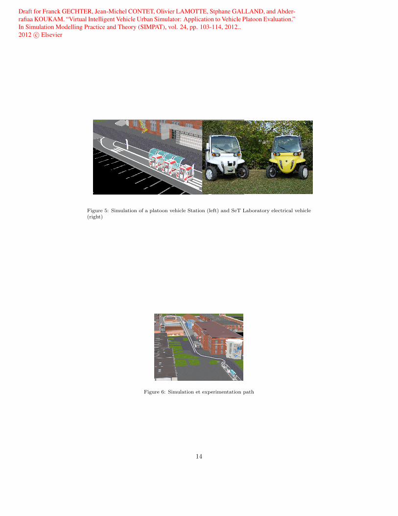
Simulations are realized with vivus simulator (Figure 5 (left)) presentedin this paper. The second platform is composed of GEM electrical vehiclesmodified by the ”Systemes et Transports” Laboratory (Figure 5 (right)). Thesevehicles have been automated and can be controlled by an onboard system.

Experiments were conducted on the Belfort’s Techno-park site. The simu-lations were performed on a 3D geo-localized model of the same site built fromGeographical Information Sources and topological data.

13


Figure 5: Simulation of a platoon vehicle Station (left) and SeT Laboratory electrical vehicle(right)

Figure 6: Simulation et experimentation path

14


Figure 6 shows the path (white curve) used for the simulation and experi-mentation. This path allows to move the train on a long distance in an urbanenvironment using a trajectory with different curve radius. To compare thesimulation and experimentation results, parameters were the same on simula-tion and real experiments. Thus, the perception of each vehicle is made by asimulated laser range finder having the same characteristics (range, angle, errorrate, etc.) as the vehicle real sensor. The distance and angle from one vehicleto the preceding are computed thanks to this sensor. The algorithm used is thesame for both simulations and real experiments. Moreover, the program runson the same computer. Indeed, a great attention has been paid on the factthat simulated vehicles should have the same communication interface as thereal ones. Thus, passing from the simulation to the real vehicle relies only onunplugging the artificial intelligence computer from the simulator and pluggingit on the real vehicle. However, experiments were performed with a more im-portant regular distance in order to avoid collision that can lead to irreversibledamage for vehicles. The distance has been established to 4 meters and thesafety distance to 1.5 meters.

5.2. Vehicle Physics Model

In order to obtain simulation results as near as possible from the reality, acomplete physics model of vehicles has been made. This section presents thedynamical model of the SeT Laboratory vehicle platform.

This model has been designed to suit the PhysX engine requirements. Mod-els designed for it are based on composition of PhysX elementary objects. Newcomponents can also be defined using these PhysX requirements. Vehicle dy-namical modeling is a common task in simulation. The SeT-car vehicle is thenconsidered as a rectangular chassis with four engine/wheel components. Thischoice can be considered to be realistic, the chassis being made as a rectan-gular un-deformable shape. The following parts describe all the parametersdetermined and/or computed for the vehicle.

5.2.1. Chassis ModelChassis is modeled as a rectangular shape with a size denoted C, a mass

denoted Mc and a gravity center Gc. Considering vehicle design, the followingpropositions can be exposed:

C =

Lc

lchc

Gc =

00

hzs

(4)

Gravity center position Gc of the chassis has been computed taking into ac-count gravity center of the body, gravity center of each component of the chas-sis, i.e., battery, embedded electronic card and components, etc. Wheel/enginecomponents are not included in this computation.

15


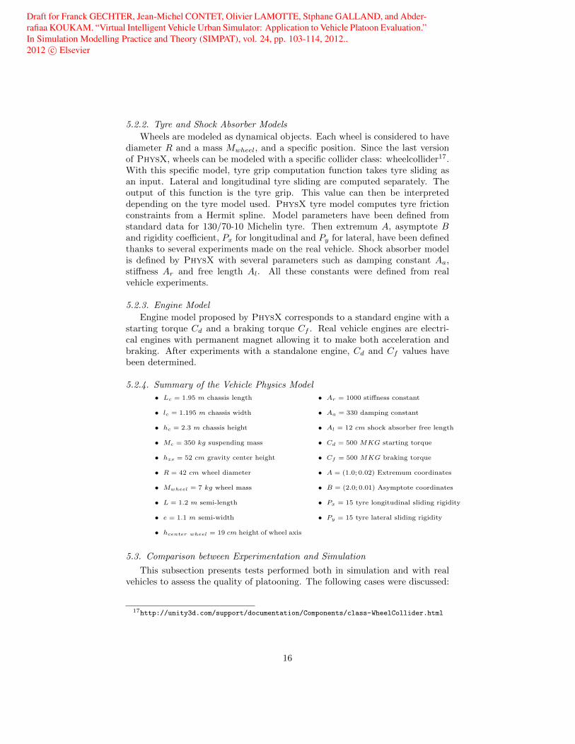
5.2.2. Tyre and Shock Absorber Models

Wheels are modeled as dynamical objects. Each wheel is considered to havediameter R and a mass Mwheel, and a specific position. Since the last versionof PhysX, wheels can be modeled with a specific collider class: wheelcollider17.With this specific model, tyre grip computation function takes tyre sliding asan input. Lateral and longitudinal tyre sliding are computed separately. Theoutput of this function is the tyre grip. This value can then be interpreteddepending on the tyre model used. PhysX tyre model computes tyre frictionconstraints from a Hermit spline. Model parameters have been defined fromstandard data for 130/70-10 Michelin tyre. Then extremum A, asymptote Band rigidity coefficient, Px for longitudinal and Py for lateral, have been definedthanks to several experiments made on the real vehicle. Shock absorber modelis defined by PhysX with several parameters such as damping constant Aa,stiffness Ar and free length Al. All these constants were defined from realvehicle experiments.

5.2.3. Engine Model

Engine model proposed by PhysX corresponds to a standard engine with astarting torque Cd and a braking torque Cf . Real vehicle engines are electri-cal engines with permanent magnet allowing it to make both acceleration andbraking. After experiments with a standalone engine, Cd and Cf values havebeen determined.

5.2.4. Summary of the Vehicle Physics Model

• Lc = 1.95 m chassis length

• lc = 1.195 m chassis width

• hc = 2.3 m chassis height

• Mc = 350 kg suspending mass

• hzs = 52 cm gravity center height

• R = 42 cm wheel diameter

• Mwheel = 7 kg wheel mass

• L = 1.2 m semi-length

• e = 1.1 m semi-width

• hcenter wheel = 19 cm height of wheel axis

• Ar = 1000 stiffness constant

• Aa = 330 damping constant

• Al = 12 cm shock absorber free length

• Cd = 500 MKG starting torque

• Cf = 500 MKG braking torque

• A = (1.0; 0.02) Extremum coordinates

• B = (2.0; 0.01) Asymptote coordinates

• Px = 15 tyre longitudinal sliding rigidity

• Py = 15 tyre lateral sliding rigidity

5.3. Comparison between Experimentation and Simulation

This subsection presents tests performed both in simulation and with realvehicles to assess the quality of platooning. The following cases were discussed:

17http://unity3d.com/support/documentation/Components/class-WheelCollider.html

16


• Evaluation of inter-vehicle distance: measuring the distance between twofollowing vehicles, compared to the desired regular inter-vehicle distanceduring platoon evolution (Figure 7).

• Evaluation of lateral deviation: measuring the distance between the tra-jectories of the geometric center of a vehicle relative to the same pathof his predecessor (Figure 7). For the measurement, points on the firstvehicle trajectory were selected. Then, the normal trace of these points isdrawn and a measure of the distance between the selected point and thepoint of intersection with the trajectory of its predecessor is made.

Longitudinal error

Regular distance Lateral error

Preceding vehicle path

Following vehicle path

Figure 7: Longitudinal error (left) Lateral error (right)

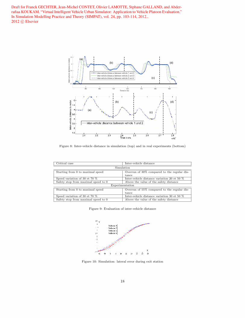
5.3.1. Evaluation of Inter-Vehicle Distance

To evaluate the inter-vehicle distance, the train is submitted to critical op-erations such as starting, emergency braking and quick change of speed of thefirst vehicle. Figure 8 (top) shows the distance variations between vehicles inrelation to quick changes of first vehicle speed. Figure 8 (bottom) shows thedistance evolution between two electric vehicles during the experiment. Figure 9gives an overview of the inter-vehicle distance variation. One can observe thatdespite the very sudden changes in first vehicle speed, this value is above thesafety distance and stabilizes rapidly to the regular distance. Figure 8 (top andbottom) present the same inter-vehicle variation.

5.3.2. Evaluation of Lateral Deviation

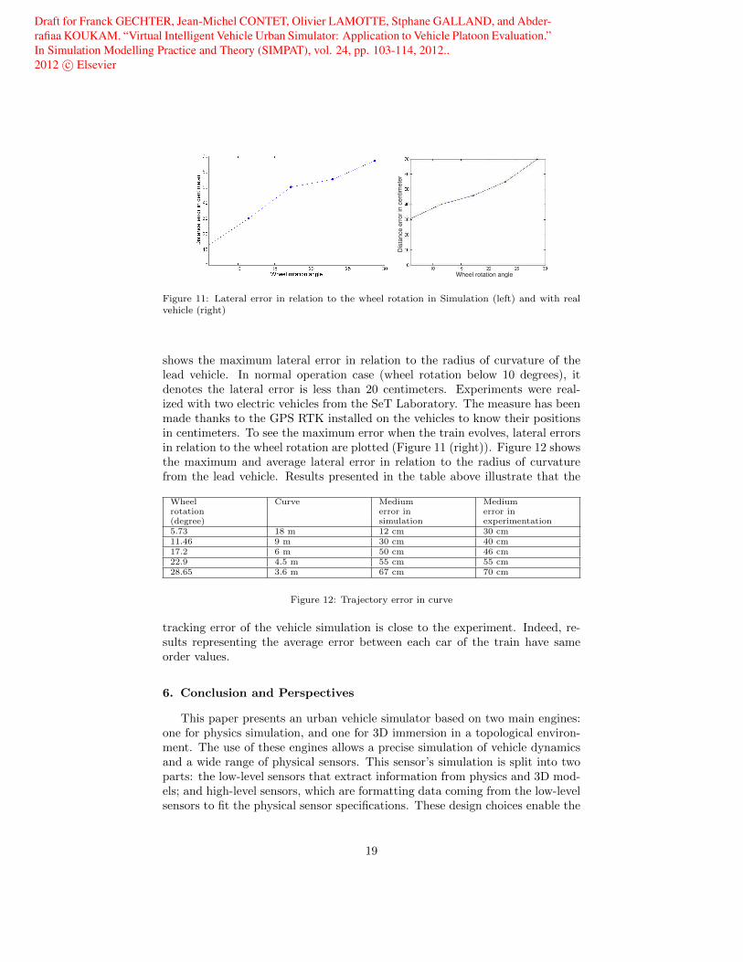
The distance between the trajectories of the vehicle geometric center rel-atively to the same path of its predecessor has also been evaluated. Lateraldeviation may cause problems in curves such as collision with vehicles in theopposite direction. Simulations were performed with a train of four vehicles.Figure 10 presents the tracks of vehicles to measure the lateral error betweeneach vehicle. To see the maximum error when the train evolves, lateral errorsin relation to the wheel rotation are plotted (Figure 11 (left)). Figure 11 (left)

17


(a) (b)

(c)

(d)

(a)

(b)

(c)

(d)

Figure 8: Inter-vehicle distance in simulation (top) and in real experiments (bottom)

Critical case Inter-vehicle distance

Simulation

Starting from 0 to maximal speed Overrun of 30% compared to the regular dis-tance

Speed variation of 30 et 70 % Inter-vehicle distance variation 20 et 50 %Safety stop from maximal speed to 0 Above the value of the safety distance

Experimentation

Starting from 0 to maximal speed Overrun of 55% compared to the regular dis-tance

Speed variation of 30 et 70 % Inter-vehicle distance variation 30 et 50 %Safety stop from maximal speed to 0 Above the value of the safety distance

Figure 9: Evaluation of inter-vehicle distance

X

Y

Figure 10: Simulation: lateral error during exit station

18


Wheel rotation angle

Dis

tanc

e er

ror i

n ce

ntim

eter

Figure 11: Lateral error in relation to the wheel rotation in Simulation (left) and with realvehicle (right)

shows the maximum lateral error in relation to the radius of curvature of thelead vehicle. In normal operation case (wheel rotation below 10 degrees), itdenotes the lateral error is less than 20 centimeters. Experiments were real-ized with two electric vehicles from the SeT Laboratory. The measure has beenmade thanks to the GPS RTK installed on the vehicles to know their positionsin centimeters. To see the maximum error when the train evolves, lateral errorsin relation to the wheel rotation are plotted (Figure 11 (right)). Figure 12 showsthe maximum and average lateral error in relation to the radius of curvaturefrom the lead vehicle. Results presented in the table above illustrate that the

Wheel Curve Medium Mediumrotation error in error in(degree) simulation experimentation5.73 18 m 12 cm 30 cm11.46 9 m 30 cm 40 cm17.2 6 m 50 cm 46 cm22.9 4.5 m 55 cm 55 cm28.65 3.6 m 67 cm 70 cm

Figure 12: Trajectory error in curve

tracking error of the vehicle simulation is close to the experiment. Indeed, re-sults representing the average error between each car of the train have sameorder values.

6. Conclusion and Perspectives

This paper presents an urban vehicle simulator based on two main engines:one for physics simulation, and one for 3D immersion in a topological environ-ment. The use of these engines allows a precise simulation of vehicle dynamicsand a wide range of physical sensors. This sensor’s simulation is split into twoparts: the low-level sensors that extract information from physics and 3D mod-els; and high-level sensors, which are formatting data coming from the low-levelsensors to fit the physical sensor specifications. These design choices enable the

19


test of control algorithms, as if they were run on a real vehicle. Indeed, thesealgorithms obtain the same sensor inputs with the simulator and the physicalvehicle. Thus, going from simulation to the real car relies only on an unplug-ging and replugging operations. This simulator has been successfully used as aprototyping tool for sensor designing and positioning. It is also a test bed forthe developers of artificial intelligence algorithms. Experiments exposed in thispaper shows simulation results closed to the Reality. The differences with thereal conditions are essentially due to the precision of the world topology, andthe model choose for the wheel/road contact. From this day forwards, we aimedat improving this simulator on the 3D level by changing the 3D engine. Indeed,the actual engine based on Java3d doesn’t allow to easily deal with climatic sim-ulation, shadows, lens flare, etc. The change of this engine will provide bettersimulation for image based sensors. We work on the vehicle physics model torefine several elements, and introduce new relevant components, which influenceglobal vehicle behavior. Moreover, we are also designing a new physics modelfor partner vehicles in the context of Safe-platoon project18.

References

[1] J.-M. Contet, F. Gechter, P. Gruer, A. Koukam, Bending virtual spring-damper : a solution to improve local platoon control, Lecture Notes inComputer Science 5544.

[2] F. Gechter, J.-M. Contet, P. Gruer, A. Koukam, Car-driving assistanceusing organization measurement of reactive multi-agent system, in: Inter-national Conference on Computational Science 2010 (ICCS 2010), Amster-dam, 2010.

[3] J. Craighead, R. Murphy, J. Burke, B. Goldiez, A survey of commercial andopen source unmanned vehicle simulators, IEEE International Conferenceon Robotics and Automation (2007) 852–857.

[4] S. Galland, N. Gaud, J. Demange, A. Koukam, Environment Model forMultiagent-Based Simulation of 3D Urban Systems, in: the 7th EuropeanWorkshop on Multi-Agent Systems (EUMAS09), Ayia Napa, Cyprus, 2009.

[5] F. Michel, The IRM4S model: the influence/reaction principle for mul-tiagent based simulation, in: Sixth International Joint Conference onAutonomous Agents and Multiagent Systems (AAMAS07), ACM, 2007.doi:http://doi.acm.org/10.1145/1329125.1329289.

[6] D. A. Grejner-Brzezinska, R. Da, C. Toth, Gps error modeling and otfambiguity resolution for high-accuracy gps/ins integrated system, Journal

18Safe-platoon is a project labeled by the National French Research Agency (ANR) http:

//safeplatoon.utbm.fr

20


of Geodesy 72 (1998) 626–638, 10.1007/s001900050202.URL http://dx.doi.org/10.1007/s001900050202

[7] B. W. Parkinson, GPS Error Analysis, Global Positioning System: Theoryand applications 1 (A96-20837 04-17) (1996) 469–483.

[8] J.-M. Contet, F. Gechter, P. Gruer, A. Koukam, An approach to compo-sitional verification of reactive multiagent systems, Working Notes of theTwenty-Fourth AAAI Conference on Artificial Intelligence (AAAI), Work-shop on Model Checking and Artificial Intelligence, Atlanta, Georgia, USA,July 11-12, 2010.

[9] J. Hedrick, M. Tomizuka, P. Varaiya, Control issues in automated highwaysystems, IEEE Control Systems Magazine 14 (6) (1994) 21 – 32.

[10] P. Martinet, B. Thuilot, J. Bom, Autonomous navigation and platoon-ing using a sensory memory, International IEEE Conference on IntelligentRobots and Systems, IROS’06, Beijing, China, 0ctober 2006.

21

Gechtercontetlamottegallandkoukam2012

Documents

Transcript of Gechtercontetlamottegallandkoukam2012