Artificial Intelligence 99 (1998) 1-19

Artificial Intelligence

GAS, a concept on modeling species in genetic algorithms ’

MGrk Jelasity a**, J6zsef Dombi b*2 a Research Group of Artificial Intelligence, Jdzsef Attila University and the Hungarian Academy of Sciences,

Aradi Vertanuk tere 1, H-6701 Szeged, Hungary b Department of Applied Informatics, .I&sef Attila University, Szeged, Hungary

Received April 1996; revised December 1996

Abstract

This paper introduces a niching technique called GAS (S stands for species) which dynamically creates a su.bpopulation structure (taxonomic chart) using a radius function instead of a single radius, and a “cooling” method similar to simulated annealing. GAS offers a solution to the niche radius prob:lem with the help of these techniques. A method based on the speed of species is presented for determining the radius function. Speed functions are given for both real and binary domains. We also discuss the sphere packing problem on binary domains using some tools of coding theory to make it possible to evaluate the output of the system. Finally two problems are examined empirically. The first is a difficult test function with unevenly spread local optima. The second is a-n NP-complete combinatorial optimization task, where a comparison is presented to the traditional genetic algorithm. @ 1998 Elsevier Science B.V.

Keywords: Multimodal optimalization; Niching; Niche radius problem; Genetic algorithms

1. Introduction

In recent years much work has been done with the aim of extending genetic algorithms (GAS) to make it possible to find more than one local optimum of a function and so to reduce the probability of missing the global optimum. The techniques developed for this purpose are known as niching techniques. Besides the greater probability of the success

* Corresponsling author. Email: jelasity@inf.u-szeged.hu. http://www.inf.u-szeged.hu/Njelasity.

’ This work was supported by the OTKA grant TO20150 and the MKM grant 220.

* Email: dombi@inf.u-szeged.hu.

0004-3702/98/$19.00 @ 1998 Elsevier Science B.V. All rights reserved.

PIISOOO4-3702(97)00071-4

2 M. Jelasity, J. Dombi/Artifcial Intelligence 99 (1998) I-19

of the algorithm and a significantly better performance on GA-hard problems (see [ 1 ] ) , niche techniques provide the user with more information on the problem, which is very useful in a wide range of applications (decision making, several designing tasks, etc.).

1.1. Best-known approaches

Simple iteration runs the simple GA several times to the same problem, and collects the results of the particular runs. Fitness sharing has been introduced by Goldberg and Richardson [ 61. The fitness of an individual is reduced if there are many other individuals near it and so the GA is forced to maintain diversity in the population. Subpopulations can also be maintained in parallel, usually with the allowance of some kind of communication between them (see, for example, [4]). The GAS method has developed from this approach. The sequential niche technique is described in [ 11. The GA (or any other optimizing procedure) is run many times on the same problem, but after every run the optimized function is modified (multiplied by a derating function) so that the optimum just found will not be located again.

1.2. Problems

These techniques yield good results from several viewpoints, but mention should be made of some of their drawbacks, which do not arise in the case of our method, GAS.

Simple iteration is unintelligent; if the optima are not of the same value relatively bad

local optima are found with low probability, while good optima are located several times which is highly unnecessary. Fitness sharing needs 0( n2) distance evaluations in every step, besides the evaluation of the fitness function. It cannot distinguish local optima that are much closer to each other than the niche radius (a parameter of the method); in other words, it is assumed that the local optima are approximately evenly spread

throughout the search space. This latter problem is known as the niche radius problem. The sequential niche technique also involves the niche radius problem. The complexity of the optimized function increases after every iteration due to the additional derating functions. Since the function is modified many times, “false” optima too are found.

The method seems difficult to use for combinatorial problems or structural optimization tasks, which are the most promising fields of GA applications.

GAS offers a solution to these problems including the niche radius problem, which

is the most important drawback of all of the methods mentioned earlier.

1.3. Outline of the paper

In Section 2 we give a brief description of GAS that is needed for an understanding of the following part of the paper. The reader who is interested in more details should refer to the Appendix on how to obtain more information or GAS itself.

In Section 4 we give a possible solution to the niche radius problem with the help of the GAS system. Both real and binary problem domains are discussed.

In Section 5 we present experimental results. Two problems are examined. The first demonstrates how GAS handles the uneven distribution of the local optima of the

M. Jelasity, J. Dombi/Art$cial Intelligence 99 (1998) 1-19 3

optimized function. The second is an NP-complete combinatorial problem, where a comparison is presented to the traditional GA.

2. Species and GAS

2.1. Basic ideas and motivations

The motivation of this work was to tackle the problem of finding unevenly spread optima of multimodal optimization problems. For this purpose, a subpopulation approach seemed to be the best choice.

The obvious drawback of subpopulation approaches is that managing subpopulations need special algorithms and the system is relatively difficult to understand and maybe to use as well. There are considerable advantages, however. Every subpopulation may have its own attributes that make it possible for them to adapt to the different regions of the fitness landscape. The subpopulations perform effective local search due to the mating restrictions that usually allow breeding only inside of a subpopulation, and the different subpopulations can even communicate with each other.

In our method GAS, every subpopulation (or species) is intended to occupy a local

maximizer of the fitness function. Thus, new species are created when it is likely that the parents are on different hills, and species have to be fused when they are thought to climb the same hill (heuristics will be given later). To shed some light on the way GAS copes with unevenly spread optima, it is natural to use a terminology that is well known from the field of simulated annealing. Thus, when illustrating our definitions and methods, we will talk about the “temperature” of species, the ability of escaping from local optima. In our system, we made the “temperature” an explicit attribute of every species (it is the attraction of species, see Definition 5). This allowed us to offer an algorithm that “cools down” the system while species of different “temperatures” are allowed to exist at the same time. The basic idea of the algorithm is that “warmer” species are allowed to create “cooler” species autonomously discovering their own local are of attraction.

Finally, llet us mention that due to our theoretical results, the large number of param-

eters of GAS can be reduced to a couple of easy-to-understand ones (see Section 4).

2.2. Basic dejinitions

Using the notations in the Introduction of [ 121, let D be the problem domain, f : D + W the fitness function and g : (0, 1)” --+ D for some m E {2,3,. . .} the coding function. ((GAS searches for the maxima of f!)

Let us assume that a distance function d : D x D + R and term section (section : D x D + .P( D), where P(D) is the power set of D) are defined.

Example 1. D C Em, D is convex.

section(x,y) = {z 1 z = n + t(y -x), t E [O,l]}.

4 M. Jelasity. J. Dombi/Art@cial Intelligence 99 (1998) I-19

(a) (b)

Fig. 1. (a) A possible radius function. (b) Terms related to species.

Example2. D={O,l}” (soif~~Dthenn=(xr,...,x,)).

section( x, y) = {Z 1 if Xj = yj then zj = xi}.

Defmition 3. R : N -+ R is a radius function over D if it is monotonic decreasing,

positive, R(0) = max{ d(el,ez) 1 el,e2 E D} and

lim R(n) = 0. “‘CC

Fig. 1 (a) exemplifies these properties. The radius function will be used to control the speed of “cooling”. In fact, it gives the “temperature” of the system in a given step (see Section 3). This sheds some light on the special requirements we made in Definition 3.

Let us fix a radius function R.

Definition 4. A species s over D is given by the triplet (0, I, S) (notation: s = (0, 1, S) ), where S is a population over D and the members of S are the individu-

als of s; o( E S) is the center of s and is such that f(o) = max f(S) ; l( E IV) is the radius index or the level of s, and so the radius of s is R(l). Recall that in GAS a population is a multiset (or bag) of individuals (e.g. S = (xi, x1, x2)).

Definition 5. s = (0, I, S) is a species. Let A(s) = {u E D 1 d(a, o) < R(I)} be the attraction of s.

Fig. 1 (b) illustrates the terms defined above. Species with small attraction behave as they were “cooler”; they discover a relatively

small area, their motion in the space is slower but they can differentiate between local optima that are relatively close to each other. Note that for a species s = (0, I, S), o is “almost” determined by S. If the maximal number of different maximizers in a population would be one, Definition 4 would be redundant. Also note that it is not necessary that S G A(s) .

M. Jelasify, J. Dombi/Art$cial Intelligence 99 (1998) 1-19 5

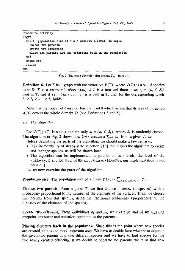
procedure activity begin

while (population size of T-n < maximum allowed) do begin choose two parents create two off spring place the parents and the offspring back in the population

end dying-off fusion

end

Fig. 2. The basic algorithm that creates If,+, from Tn.

Definition 6. Let T be a graph with the vertex set V(T), where V(T) is a set of species over D. T is a fuxonomic chart (t.c.) if T is a tree and there is an s, = (or, 0, S,) root in T, and if ( sr =)so, ~1, . . . , s, is a path in T, then for the corresponding levels la < 1, < . . . < 1, holds.

Note that the root sr of every t.c. has the level 0 which means that its area of attraction A (s) covers the whole domain D (see Definitions 3 and 5).

2.3. The algorithm

Let V( TO) (TO is a t.c.) contain only sr = (o,., 0, S,.), where S, is randomly chosen. The algorithm in Fig. 2 shows how GAS creates a Tn+l t.c. from a given T, t.c.

Before describing the parts of the algorithm, we should make a few remarks. l It is ,the flexibility of steady state selection [ 131 that allows the algorithm to create

and manage species, as will be shown later. l The algorithm can be implemented in parallel on two levels: the level of the

while cycle and the level of the procedure. (However, our implementation is not

parallel.) Let us now examine the parts of the algorithm.

Populatialn size. The population size of a given T t.c. is ~s=~o,~,S~EV~T~ (S].

Choose two parents. From a given T, we first choose a vertex (a species) with a probability proportional to the number of the elements of the vertices. Then, we choose

two parents from this species, using the traditional probability (proportional to the fitnesses of the elements of the species).

Create two offspring. From individuals p1 and ~2, we create pi and pi by applying onepoint crossover and mutation operators to the parents.

Placing elements back in the population. Since this is the point where new species are created, this is the most important step. We have to decide here whether to separate the given two parents into two different species and we have to find species for the two newly created offspring. If we decide to separate the parents, we must find new

6 M. Jelasity, J. Dombi/Arttj%ial Intelligence 99 (1998) I-19

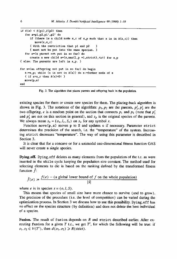
if f(e) < f(pl),f(p2) then for x=pl,p2,pi',p2' do

if (there is a child node s-c of s-p such that x is in A(s_c)) then move(x,s_c)

{ With the restriction that pi end p2 1

I must not be put into the same species. 1 for x=(a parent not put in so far) do

create a new child s=(x,maxIl_p +i,strict>,<x>) for s-p C else: The parents are left in s-p. )

for x=(an offspring not put in so far) do begin s:=s_p; while (x is not in A(s)) do s:-father node of s { if s=s_r then A(s)=D! )

move(p,s) end

Fig. 3. The algorithm that places parents and offspring back in the population.

existing species for them or create new species for them. The placing-back algorithm is

shown in Fig. 3. The notations of the algorithm: pi ,p2 are the parents, pi,pG are the

two offspring, e is a random point on the section that connects pt and p2 (note that pi and pi are not on this section in general), and s,, is the original species of the parents.

We always mean s, = (ox, 1,, S,) on s, for any symbol X. Function move(p, s> moves p to S and updates o if necessary. Parameter strict

determines the precision of the search, i.e. the “temperature” of the system. Increas- ing strict decreases “temperature”. The way of using this parameter is described in Section 3.

It is clear that for a concave or for a unimodal one-dimensional fitness function GAS

will never create a single species.

Dying-off. Dying-off deletes as many elements from the population of the t.c. as were

inserted in the while cycle keeping the population size constant. The method used for selecting elements to die is based on the ranking defined by the transformed fitness

function p:

f^(e) .= f(e) - (a global lower bound of f on the whole population)

ISI

where e is in species s = (0, 1, S). This means that species of small size have more chance to survive (and to grow).

The precision of the procedure (i.e. the level of competition) can be varied during the optimization process. In Section 3 we discuss how to use this possibility. Dying-off has no effect on the species structure (by definition) and does not delete the best individual of a species.

Fusion. The result of fusion depends on R and strict described earlier. After ex- ecuting fusion for a given T t.c., we get T’, for which the following will be true: if si,s2 E V(T’), then d(oi,02) 2 R(strict).

M. Jelasity, J. Dotnbi/Artijicial Intelligence 99 (1998) I-19

create a starting t.c. T-0 for strict:=1 to ST-m ( 0 < ST_m(=strict_max) < 8 1

new species evolution { evolution is the folloving macro: 1

stabilize C for i=l to IO do activity 1 iterate evolution until reaching I immigration 1 x-strict function evaluations I for i=l to 5 do activity 1

Fig. 4. The high-level test algorithm.

Fusion simply unites species of T that are too close to each other, and strict tells it what is too close. If s1 and sz are united, the result species is s = (0, min{ll , Zz}, S1 u&), where f(c)) = max{f(q), f(02)) and o is 01 or 02. In view of the tree structure, the species with the lower level absorbs the other. If the species have the same level, either of them may absorb the other.

3. Optimization with GAS

For global optimization with GAS, we suggest the algorithm shown in Fig. 4. For

determination of the vector of evaluation numbers x and the radius function R, we

suggest a method in Section 4 based on the speed of species with a given radius in a given domain.

The main for cycle performs the “cooling” operation. Increasing strict results in new species with smaller radii (see Fig. 3). The basic philosophy is to increase diversity at the beginning of every cycle and then perform optimization of the newly discovered areas. This kind of oscillation can be observed in biological systems as well.

We now describe the species-level genetic operators, used in the algorithm shown in

Fig. 4.

Immigration. For every species s = (0,1, S) in a given t.c., IS]/2 randomly generated new individuals are inserted from A(s). Immigration refreshes the genetic material of the species and makes their motion faster. It has a kind of greasing effect.

New speciies. This switch alters the state of the system towards managing species cre-

ation. It randomizes dying-off and relaxes competition by decreasing the lower bound

of the fitness function, and so decreases the relative differences between individuals. According to some biologists [ 31, species are born when the competition decreases; our experiments support this opinion.

Stabilize. The effect of this is the contrary of new species. It prohibits the creation of new species and increases competition.

As a summary, we give here some heuristical arguments that support the subpopulation structure approach and use a radius function instead of a single radius.

8 M. Jelasity, J. Dombi/Artificial Intelligence 99 (1998) I-19

l The number of distance calculations grows with the size of the t.c. instead of the size of the population.

l Application of species-level operators (e.g. fusion, immigration) becomes possible.

l Lower-level (closer to root) species manage to create new species in their attraction. l The advantages of the technique based on the radius function and increasing strict

(see Fig. 4) are similar to those of the “cooling” technique in the simulated

annealing method. Finally, to make our discussion more rigorous, we give the definitions of stability of

species and t.c. These definitions are not really necessary for the present discussion in the sense that will not be used in any strict mathematical environment. However, when stability is mentioned, it is meant in this sense. The impatient reader is free to skip these

definitions.

Definition 7. W C D. Species s is stable in W if o E W, and if or, 02, . . . is a series of new centers inserted by GAS to s during running then it is impossible that for some i

0; sf w.

Example 8. It is clear that s is stable in W = {e E D 1 f(e) > f(o)}.

Definition 9. eo E D, eo is a local optimum (with respect to d) of f, s is stable around

eo if, for every ot,o2, . . . series of new centers inserted by GAS to s during running,

o,, -+ ea (n -+ co) with probability 1.

Example 10. W G D, eo E W. If s is stable in W and eo is the global optimum of f in W (i.e. es is a local optimum of D or else s could not be stable in W) and there are no more optima of f in W, then s is stable around eo. This example would need a proof but we do not give it here because it is marginal from the viewpoint of the paper.

Definition 11. T is a t.c. T is stable if every species of T is stable around distinct local

optima of f.

Definition 12. T is a t.c. T is complete if T is stable and there is exactly one stable species around every local optimum of f.

4. Theoretical results

In this section we discuss the theoretical tools and new terms that can be used due to the exact definition of the t.c. data structure and GAS algorithm.

4. I. Speed of species

We do not assume that the optima of the fitness function are evenly spread; we create species instead that “live their own lives” and can move in the search space and find the niche on which they are stable. It can be seen that from this point of view determining

M. Jelasity, J. Dombi/Artifcial Intelligence 99 (1998) 1-19 9

the radius function R depends more upon the speed of the species than on the number of spheres (niches) of a given radius that can be packed into the space. The speed of a given species s = (0, I, S) will depend on its radius R( 1). The larger the radius is the faster the !;pecies can move towards its stable state so the fewer the number of iterations

it needs to become stable. This idea will be used when simultaneously dividing the available number of function evaluations among the species and setting the values of

the radius function R. The solution of the sphere packing problem mentioned above is the base of setting

the niche radius parameter of the methods mentioned in the Introduction. This value is useful when evaluating the output of the system since it tells us what percentage of

the possible number of optima we have found. In Section 4.3 we discuss such packing

problems in the case of binary domains.

4.1.1. Real domains In real domains we have D 2 R” for some n E N. Let us fix a dimension number

n and a species s = (0, 1, S) and let us denote the radius of s by I (i.e. r = R(l)). (Recall, that for a species s = (0, 1, S) the center of s, o, is an n-dimensional real vector:

o= (01,. .,. ,oa).) The following suggestion for the definition of speed is an approximation. It is assumed

that the fitness function f is the projection f(x) = XI and GAS simply selects new individuals from the attraction of s, A(s), randomly with a uniform distribution instead

of generating them using parents and genetic operators and drops them into the species one by one. The speed for a radius r and a dimension II will be the average step size towards the better region.

Definition 13. The speed u(r) of s is (cl - ot)/2, where c E B” is the center of

gravity of the set

S,,, == A(s) II {x E B” 1 x1 > ol}.

In other words, let us choose a random element x* = (x7,. . . , x;) from A(s) with a uniform dlistribution. Let ,$ = ot - x; if 01 > x7, and 5 = 0 otherwise. Than M(r) (the

expected value of 6) is u(r) . This means that o(r) is given by the equation

where V( &) is the volume of S,,,. (Recall that if 6 = 0 then the center of s o is not changed by GAS.) It can be proved that

(2)

holds. In the general case (if n is even) (2), is defined with the help of the function r( t + l), the continuous extension of t!. r( t + 1) = &” x’e-’ dx, r( l/2 + 1) = fi/2 and r(t -t 2) = (t + l)r(t + 1).

10 M. klasity, J. Dombi/Ar@cial Intelligence 99 (1998) l-19

4

3.5

3

1

2.5

2

1.5

1

nc

Empirical Speed of Species in Binary Domains 1 I I I I I

sqIt(x)‘3.0/11 .o -

n=l50

I 1 I “..s

0 20 40 60 80 100 r (radius)

120 140 160 180 200

Fig. 5. Speed in binary domains.

4.1.2. Binary domains

Let D = (0, 1)“. Let us fix a dimension number n and a species s = (o,l, S) and let us denote the radius of s by r (i.e. r = R( 1)). We give a definition of speed similar to Definition 13. Like in the case of real domains, an approximation is used. It is assumed that the fitness of an individual x E D is given by the number of 1s in it, and GAS

works as described in the case of real domains. As in the binary case, the speed for a radius r and a dimension n will be the average size of the first step of o after receiving

one random individual. The difference is that in the case of binary domains, the starting center has to be fixed too since the average step sizes change as the center changes. Let e E D such that the number of OS is equal to or greater by one than the number of 1s. Let e be the fixed starting center. Let

Sri,,, = {e’ E D 1 d(e’, e) 6 r}

where d is the Hamming distance (the sum of the bit differences). Let us choose a random e* from S,,, with a uniform distribution and let 5 = d(e*, e) if there are more 1s in e*, and let 5 = 0 otherwise.

Definition 14. Let u(r) = M(t) be the speed of species s in D if the radius of s is r.

We performed experiments to determine u(r) (Fig. 5). It can be seen if it > r, then the equation

hf. Jela& J. Dombi/Artificial Intelligence 99 (1998) 1-19 11

seems to describe the speed. If r approaches n, the growing of the speed becomes slower than (3) would indicate.

4.2. Determining R and x

We use the notations of Fig. 4 here. Recall that ST,,, is the number of steps in the “cooling” procedure, the maximal value of strict, and xi denotes the number of function evaluations at step i. Let us assume that the evaluation number N, the domain type and the corresponding speed function u are given. We know that

ST”,

c ;t~~ = N. (4) i=l

We suggest a setting for which the system of equations

u(R(i))xi=C (i= l,...,ST,,) (5)

holds where C is a constant (independent of i) . This simply means that the species of the different levels receive an equal chance to become stabilized. From (4) and (5) it follows that

(6)

We note that C is the distance that a species of level i is expected to crosses during xi iterations.

In GAS, the upper bound M of the number of species can be set. By default M = [population size/4]. Now we can give the value of C:

C = R(O)Mv. (7)

Recall that R(0) is the diameter of the domain we examine.

v is a threshold value. Setting Y = 1 means that every species receives at least sufficient function evaluations for crossing the whole space, which makes the probability of creating a stable t.c. very high. In Section 5 we examine the effect of several different settings of V. Finally let

R(i) = R(O)$ (i = 1,. . . ,ST,, /I E (0,l)). (8)

Then, R is a valid radius function and subproblems defined by the species will be similar in view of the radii.

Using (6), (7) and (S), we can write

(P E (0, I)), (9)

where everything is given except /I.

12 M. Jelasiry, J. Dombi/Artgicial Intelligence 99 (1998) I-19

Since v is monotonous, the right-hand side of (9) monotonically decreases as p increases and so reaches its minimum if p = 1. Using this fact, the feasibility condition of (9) is

N

R(O)Mv > ST,,

v(R(O) > * t 10)

If ( 10) holds, (9) has exactly one solution. This property allows us to use effective numeric methods for approximating p.

In Section 5.1 we discuss the parameters that have to be set in GAS.

4.3. Evaluating the output

We based the setting of the parameters of GAS on the speed function. However, it is important to know the maximal possible size of a t.c. for a given radius function R (assuming an arbitrary large evaluation number and population size) since it tells us what percentage of the maximal possible number of optima we have found.

The problem leads to the general sphere packing problem and this has been solved neither for binary nor for real sets in the general case.

Real case In n-dimensional real domains Deb’s method [5] can be used.

fi” P= Yjy- y ( >

where r is the species radius, the domain is [ 0, I]” and p is the number of optima, assuming that they are evenly spread. We note that this is only an approximation.

Binary case Results of coding theory can be used to solve the packing problem in binary domains

since it is one of the central problems of this field. We will need the definition of binary codes.

Definition 15. d,n E W, d < n. C C (0, 1)” is a (n, ICI, d) binary code if V/cl, cz E C: dist(ci, ~2) 2 d. (The function “dist” is the Hamming distance, the sum of the bit differences.)

Definition 16. d,n E IV. A(n,d) := max{jC] 1 C is a (n, ICl,d) binary code}.

A(n, d) has not yet been calculated in the general case; only lower and upper bounds are known. Such bounds can be found for example in [ 151, [ 1 l] or [ lo]. One of these is the Plotkin bound:

Theorem 17 (Plotkin bound). For d, n E N, we have

d Atn,d) 6 -

d- ;n ifdakn.

M. Jelasity, J. Dombi/Art@cial Intelligence 99 (1998) I-19 13

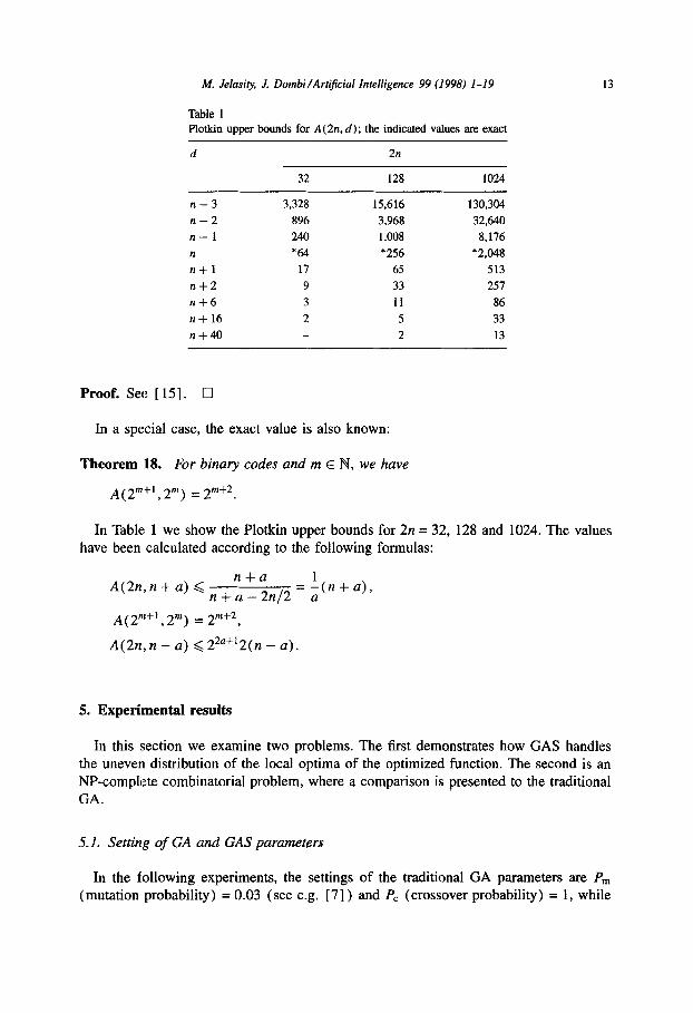
Table 1

Plotkin upper bounds for A( 2n, d); the indicated values are exact

d 2n

32 128 1024

n-3

n-2 n-l

n

n+l

n+2 n+6 n-t 16

n+40

3,328

896

240

*64

17

9

3

2

15,616 130,304

3,968 32,640

1,008 8,176

‘256 *2&M

65 513

33 257

11 86

5 33

2 13

Proof. See [ 151. 0

In a special case, the exact value is also known:

Theorem 18. For binary codes and m E N, we have

A( 2m+‘, 2”‘) = 2”‘+*.

In Table 1 we show the Plotkin upper bounds for 2n = 32, 128 and 1024. The values have been calculated according to the following formulas:

A(2n, n + a) 6 n+a

n + a - 2n/2 = i(n+a),

A(2”‘+’ ,,,I) = p+*,

A(2n,n - a) < 2*O+‘2(n - a).

5. Experimental results

In this section we examine two problems. The first demonstrates how GAS handles the uneven distribution of the local optima of the optimized function. The second is an NP-complete combinatorial problem, where a comparison is presented to the traditional

GA.

5.1. Setting of GA and GAS parameters

In the following experiments, the settings of the traditional GA parameters are Pm (mutation probability) = 0.03 (see e.g. [ 71) and PC (crossover probability) = 1, while

14 M. Jelasity, J. Dombi/ArtiJkial Intelligence 99 (1998) 1-19

the population size = 100. In the while cycle of the basic algorithm (shown in Fig. 2), the maximum allowed population size is 110. For continuous domains, we used Gray coding as suggested in [ 21.

The settings of the specific GAS parameters are the following:

l R (radius function) and x (evaluation numbers) can be determined using the method described in Section 4.

l M (maximal number of species in the t.c.) is set to M = (pop. size) /4. Setting a larger value is not recommended since too many small species could be created.

l N (CET xi) depends on the available time and computational resources. We used

N = 104. l Y (treshold) and ST, (maximal strict level) are the parameters we tested so we

used several values (see the descriptions of the experiments). For simplicity, we run evolution only once after new species (see Fig. 4) but

we note that increasing that number can significantly improve the performance in some cases. The cost of one evolution is 275 evaluations after new species, and 200 after stabilize at the above settings.

5.2. A function with unevenly spread optimas

The problem domain D is [ 0, lo]. The fitness function .f : D + Iw.

a=

3.040

1.098

0.674

3.537

6.173

8.679

4.503

3.328

6.937

0.700

10

, k=

2.983

2.378

2.439

1.168

2.406

1.236

2.868

1.378

2.348

2.268

1 f(x) = c

j=l (k(x-ai)12+ci’

, c=

0.140

0.127

0.132

0.125

0.189

0.187

0.171

0.188

0.176,

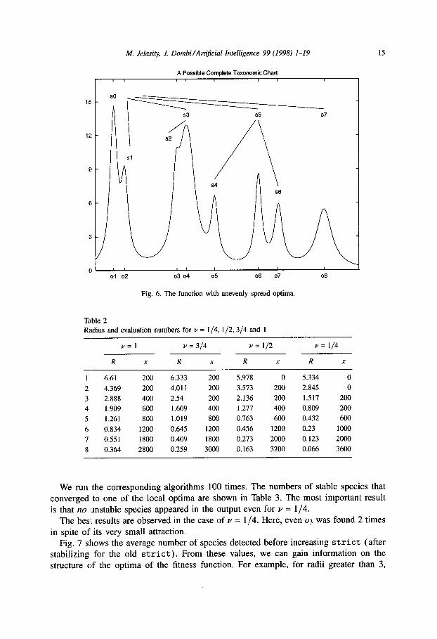
f (shown in Fig. 6) is a test function for global optimization procedures suggested in [14].

We have determined R and x for v = l/4,1/2,3/4 and 1 (see Table 2). ST,,, is 8 in every case. Recall that according to the algorithm in Fig. 4 the elements of x must be

divisible by 200 (the cost of evolution after stabilize) and the sum of them must be lo4 -ST,. 275.

M. Jelasity, J. Dombi/Artifcial Intelligence 99 (1998) l-19

A Possible Complete Taxonomic Chart I I

Fig. 6. The function with unevenly spread optima.

Table 2

Radius and evaluation numbers for Y = l/4, l/2,3/4 and 1

v=l V = 314 v= l/2 V= l/4

R x R x R x R x

1 6.61 200 6.333 200 5.978 0 5.334 0

2 4.369 200 4.011 200 3.573 200 2.845 0

3 2.888 400 2.54 200 2.136 200 1.517 200

4 1.909 600 1.609 400 I.217 400 0.809 200

5 1.261 800 1.019 800 0.763 600 0.432 600

6 0.834 1200 0.645 1200 0.456 1200 0.23 1000

I 0.551 1800 0.409 1800 0.273 2000 0.123 2000

8 0.364 2800 0.259 3000 0.163 3200 0.066 3600

15

We run the corresponding algorithms 100 times. The numbers of stable species that converged to one of the local optima are shown in Table 3. The most important result is that no unstable species appeared in the output even for v = l/4.

The best results are observed in the case of v = l/4. Here, even 03 was found 2 times in spite of its very small attraction.

Fig. 7 shows the average number of species detected before increasing strict (after stabilizing for the old strict). From these values, we can gain information on the structure of the optima of the fitness function. For example, for radii greater than 3,

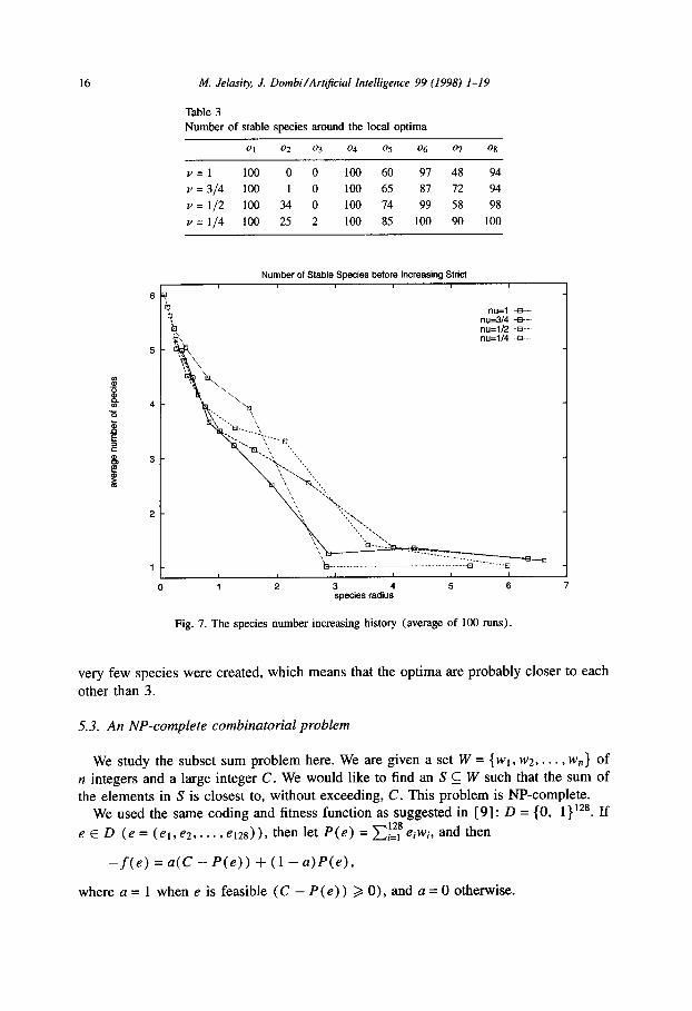
16 A4. Jelasity J. Dombi/Art@cial Intelligence 99 (1998) l-19

Table 3 Number of stable species around the local optima

01 02 03 04 OS 06 07 08

v=l 100 0 0 100 60 97 48 94

v = 314 100 1 0 100 65 87 72 94

v= 112 100 34 0 100 74 99 58 98

v = 114 100 25 2 100 85 100 90 100

Number of Stable Species before Increasing Strict

6’f 6 $ nw1 -

nu=3/4 a-- w nu=1/2 -0.- ‘.. h-p. nu=l/4 --B---.

5-

2-

b ..,......... _ .._._............................_..................... q

I 1 2 3 4 5 6 7

species radius

Fig. 7. The species number increasing history (average of 100 runs).

very few species were created, which means that the optima are probably closer to each

other than 3.

5.3. An NP-complete combinatorial problem

We study the subset sum problem here. We are given a set W = {WI, ~2,. . . , w,} of n integers and a large integer C. We would like to find an S c W such that the sum of the elements in S is closest to, without exceeding, C. This problem is NP-complete.

We used the same coding and fitness function as suggested in [9]: D = (0, 1}12*. If

e E D (e= (el,ez,..., elzg)), then let P(e) = C;zF eiwi, and then

-f(e) = a(C -P(e)) + (1 - a)P(e>,

where a = 1 when e is feasible (C - P(e) ) 2 0), and a = 0 otherwise.

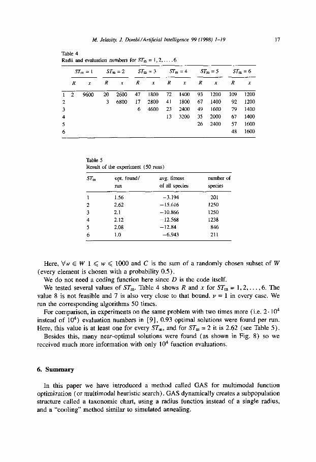
M. Jelasity, J. Dombi/Artijicial Intelligence 99 (1998) 1-19 17

Table 4 Ra.dii and evaluation numbers for ST, = 1,2,. ,6 -

ST,,, = 1 ST,,, = 2 ST, = 3 ST,,, =4 ST, = 5 ST, = 6

R x R x R x R n R x R x

T2 9600 20 2600 47 1800 72 1400 93 1200 109 1200

2 3 6800 17 2800 41 1800 67 1400 92 1200

3 6 4600 23 2400 49 1600 79 1400

4 13 3200 35 2000 67 1400

5 26 2400 57 1600

6 48 1600

Table 5

Result of the experiment (50 runs)

ST,

1

2

3

4

5

6

opt. found/ avg. fitness number of

run of all species species

1.56 -3.194 201

2.62 -15.616 1250

2.1 -10.866 1250

2.12 -12.568 1238

2.08 -12.84 846

1.0 -6.943 211

Here, ‘J-w E W 1 6 w < 1000 and C is the sum of a randomly chosen subset of W

(every element is chosen with a probability 0.5). We do not need a coding function here since D is the code itself. We tested several values of ST,. Table 4 shows R and x for ST, = 1,2, . . . ,6. The

value 8 is not feasible and 7 is also very close to that bound. v = 1 in every case. We run the corresponding algorithms 50 times.

For comparison, in experiments on the same problem with two times more (i.e. 2. lo4 instead of 104) evaluation numbers in [9], 0.93 optimal solutions were found per run. Here, this value is at least one for every ST,,,, and for ST, = 2 it is 2.62 (see Table 5).

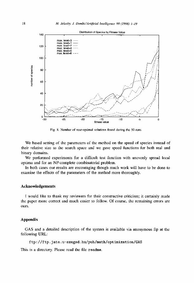
Besides this, many near-optimal solutions were found (as shown in Fig. 8) so we

received much more information with only lo4 function evaluations.

6. Summary

In this paper we have introduced a method called GAS for multimodal function optimization (or multimodal heuristic search). GAS dynamically creates a subpopulation structure called a taxonomic chart, using a radius function instead of a single radius,

and a “cooling” method similar to simulated annealing.

140

120

100

60

60

40

20

‘,.

b :.

0

M. Jelasity J. Dotnbi/Art@cial Intelligence 99 (1998) l-19

Distribution of Species by Fitness Value 1

max. level=3 - max. level=1 ----. mar. level=2 ----- max. level=4 .. ....... max. level=5 - -.- max. level=6 -.-.-

-30 -25 -20 -15 -10 -5 0 fitness value

Fig. 8. Number of near-optimal solutions found during the 50 runs

We based setting of the parameters of the method on the speed of species instead of their relative size to the search space and we gave speed functions for both real and binary domains.

We performed experiments for a difficult test function with unevenly spread local optima and for an NP-complete combinatorial problem.

In both cases our results are encouraging though much work will have to be done to examine the effects of the parameters of the method more thoroughly.

Acknowledgements

I would like to thank my reviewers for their constructive criticism; it certainly made the paper more correct and much easier to follow. Of course, the remaining errors are ours.

Appendix

GAS and a detailed description of the system is available via anonymous ftp at the following URL:

ftp://ftp.jate.u-szeged.hu/pub/math/optimization/GAS

This is a directory. Please read the file readme.

M. Jelasity, J. Dombi/Arhjkial Intelligence 99 (1998) 1-19 19

The authors would highly appreciate it if you informed them about any problems regarding GAS (compiling, using, etc.).

References

[l] D. Beasley, D.R. Bull, R.R. Martin, A sequential niche technique for multimodal function optimization,

Evolutionary Computation 1 (2) (1993) 101-125. ]2] R.A. Caruana, J.D. Schaffer, Representation and hidden bias: Gray vs. binary coding for genetic

algorithms, in: J. Laird, ed., Proceedings Fifth International Conference on Machine Learning, Ann

Arbor, MI, 1988, pp. 153-161.

[3] V. Csrlnyi, General Theory of Evolution, Publ. House of the Hung. Acad. Sci., Budapest, 1982.

[4] Y. DavIdor, A naturally occurring niche and species phenomenon: the model and first results, in:

Proceedings Fourth ICGA, Morgan Kaufmann, San Mateo, CA, 1991, pp. 257-263.

[ 51 K. Deb, Genetic algorithms in multimodal function optimization, Master’s Thesis, TCGA Report No.

89002, Department of Engineering mechanics, The University of Alabama, 1989.

[ 61 K. Deb, D.E. Goldberg, An investigation of niche and species formation in genetic function optimization,

in: Proceedings Third ICGA, Morgan Kaufmann, San Mateo, CA, 1989, pp. 42-50.

[7] D.E. Goldberg, Genetic Algorithms in Search, Optimization and Machine Learning, Addison-Wesley,

Reading, MA, 1989, ISBN o-201-15767-5.

[ 81 M. Jelasity, J. Dombi, GAS, an approach to a solution of the niche radius problem, in: Proceedings

GALESIA’95, 1995.

[9] S. Khtni, T. Back, J. Heitkiitter, An evolutionary approach to combinatorial optimization problems, in:

Proceedings CSC’94, 1993.

[lo] F.J. MacWilliams, N.J.A. Sloan, The Theory of Error-Correcting Codes, North-Holland, Amsterdam,

1977.

[ 111 R.J. McEliece, The Theory of Information and Coding, Addison-Wesley, Reading, MA, 1977.

[ 121 G.J.E. Rawlins, ed., Foundations of Genetic Algorithms, Morgan Kaufmann, San Mateo, CA, 1991.

[ 131 G. Syswerda, A study of reproduction in generational and steady state genetic algorithms, in: G.J.E.

Rawlinr, ed., Foundations of Genetic Algorithms Morgan Kaufmann, San Mateo, CA, 1991.

[ 141 A. Tom, A. iilinskas, Global optimization, in: Lecture Notes in Computer Science, Vol. 350, Springer,

Berlin, 1989.

[ 151 J.H. van Lint, Introduction to Coding Theory, Springer, Berlin, 1992.