Fuzzy Rule Based Models Modification by New Data: Application to Flood Flow Forecasting

Water Resour Manage (2009) 23:2491–2504DOI 10.1007/s11269-008-9392-z

Fuzzy Rule Based Models Modification by New Data:Application to Flood Flow Forecasting

M. Akbari · A. Afshar · M. Rezaei Sadrabadi

Received: 13 November 2007 / Accepted: 12 December 2008 /Published online: 13 January 2009© Springer Science + Business Media B.V. 2009

Abstract Reconstruction and/or modification of an already existing fuzzy modelwith new data may improve system performances. As new data become available,adjusting the existing fuzzy rule-based model may present a challenging alternativeto full model reconstruction. In this paper a fuzzy rule-based control model usinga Takagi–Sugeno fuzzy system is presented and a model modification algorithm isdeveloped which improves the performance of the initial model as new data becomeavailable. Proposed approach is applied to a flood flow forecasting case exampleand the results are compared with those forecasted using initially available andreconstructed models. Results show that the modified model outperforms the initialFRB model. Reconstructed model performs slightly better than the modified model;however, the reconstruction may not be justified in a real time flood forecastingsystem, considering the limitations on the available lead time.

Keywords Fuzzy modeling · Knowledge · Modification · Flood forecasting

1 Introduction

Fuzzy modeling, as an important branch in fuzzy systems theory, has successfullybeen employed to describe systems with nonlinear properties. Fuzzy model is adata-driven model which extracts relationships from input–output data without

M. Akbari (B) · A. AfsharCivil Engineering Department, Iran University of Science & Technology, Tehran, Irane-mail: [email protected]

A. Afshare-mail: [email protected]

M. R. SadrabadiDepartment of Mathematics and Science, Eindhoven University of Technology,5600 MB, Eindhoven, The Netherlandse-mail: [email protected]

2492 M. Akbari et al.

demanding the complete physical knowledge of the system. Fuzzy models may forman alternative to process-based models in applications where computational speedand reduction of simulation time is critical, and/or the underlying relationships arepoorly understood. In the fields of hydrology and water resources engineering, fuzzymodels have extensively been applied to rainfall, runoff and water level fluctuationforecasting (Aquil et al. 2006; Chau et al. 2005; Deka and Chandramouli 2005; Stüberet al. 2000; Yu et al. 2000), water quality parameters estimation (Maier et al. 2000) aswell as reservoir operation (Dubrovin et al. 2002; Karaboga et al. 2004; Mehta andJain 2008; Pinthong et al. 2008; Russell and Campbell 1996; Shrestha et al. 1996).

River flow forecasting has always been one of the most important issues inhydrology. It is particularly required in a flood-prone region for the issuance ofdisaster warning, regulating reservoir outflows and other schemes for flood control.In recent years, data-driven models, in particular fuzzy logic approaches, have beenpropagated actively in solving flood forecasting problems. This special attention ispartially due to tremendous data requirement and the associated long computationtime for model calibration in analytical approaches, specifically for real-time fore-casting (Chau et al. 2005).

Stüber et al. (2000) introduced an automatic generator of fuzzy rainfall–runoffmodel such that fuzzy rules were generated with an iterative and step by stepalgorithm. Deka and Chandramouli (2005) used fuzzy neural network model topredict river flow in terms of discharges at the upper gauging stations. Fuzzy rulesmay be developed based on physical understanding of the systems. Nayak et al.(2005) showed high ability of the adaptive neural fuzzy inference system (ANFIS) forriver flow forecasting on the basis of rainfall and runoff data, particularly at longerlead times, as compared to the artificial neural network (ANN) and fuzzy inferencesystems (FIS). Chau et al. (2005) compared genetic algorithm-based artificial neuralnetwork (ANN-GA) and ANFIS and linear regression model for water level fore-casting in a channel reach of Yangtze River in China. Aquil et al. (2006) appliedan algorithm for real-time prediction of river stage dynamic using a Takagi–Sugenofuzzy system and showed its superiority to the multiple linear regression approach.

In a data driven model, the governing physical principles of the system areusually extracted using the available data. These physical principles are commonlyreferred to as “knowledge of the system”. When a fuzzy model is constructed basedon the available data, partial knowledge of the system appears in the form offuzzy rules. With limited data, however precise knowledge of the complex systemscannot be acquired. In a real system, as operation proceeds, new data may beobtained. Applying the new data to the present fuzzy rules can extend the acquiredknowledge of the system. As the main body of the rules has already been developed,reconstruction of the rules may not be justified. In such situation, adjusting the initialFRB model in accordance with new data may present a challenging alternative tomodel reconstruction.

This research presents a fuzzy rule-based model modification algorithm whichimproves the performance of the model as new data becomes available. Proposedapproach is applied to a flood flow forecasting case example and the results arecompared with those forecasted using the original and the reconstructed model.The work uses MATLAB software to generate the fuzzy rules from available data.Computer codes are provided in visual basic language for modifying the providedmodel by new data and simulation requirements.

Fuzzy rule based models modification by new data: application to. . . 2493

The paper is organized as follows. In Section 2 fuzzy model of Takagi & Sugenotype is described. Section 3 describes a method for modifying the initial model bynew data. Section 4 illustrates the performance of the model in forecasting flood flowand the method of modification. Finally, conclusion appears in Section 5.

2 Generating Fuzzy Models from Numerical Data

Fuzzy logic control which is based on Zadeh’ theory of fuzzy sets may be regarded asmathematical model controlled by fuzzy rules. Primary advantages of fuzzy modelinginclude: (a) the facility for the explicit knowledge representation in the form ofIF–THEN rules, (b) the mechanism of human-like reasoning in linguistic terms, and(c) the ability to approximate complicated non-linear functions with simpler models(Chen and Linkens 2004). Every fuzzy rule is made up of sets of input variables orpremises in the form of fuzzy sets and a fuzzy consequence (Mamdani controller)or crisp function (Takagi and Sugeno controller). Many applications of both modeltypes have been presented in engineering problems (Aquil et al. 2006; Deka andChandramouli 2005). Since Sugeno system is computationally more efficient thanMamdani system, this study employs the former one.

Takagi–Sugeno fuzzy rules for any system are in the form of the followingequation (Takagi and Sugeno 1985).

Ri : If x1 is Ai1 and x2 is A12 and . . . xm is Aim

Then yi = ai1x1 + ai2x2 + . . . + aimxm + ai0 (i = 1, 2, . . . c) (1)

Where Ri denotes the ith fuzzy rule, x j is jth input (antecedent) variable, yi isoutput (consequent)variable of ith rule, Aij is fuzzy set of jth input variable and ithrule, and aij is the model output parameters that have to be determined in a givendata set.

Degree of fulfillment of the ith fuzzy rule for a given input crisp vector X = (x1,

x2, . . . , xm)T can be defined by Eq. 2 using product conjunction operator.

wi = μAi1 (x1) .μAi2 (x2) . . . μAim (xm) (2)

Where μAij

(x j

)is membership degree of x j in the fuzzy set Aij.

Output of the model is computed by taking the weighted average of the yi (Takagiand Sugeno 1985):

y =

c∑

i=1wi yi

c∑

i=1wi

(3)

Takagi and Sugeno (TS) fuzzy model approximates nonlinear system with acombination of several linear systems by fuzzy decomposition of the entire inputspace into several sub-spaces and representing each input/output space with a linearequation (Kim et al. 1997).


In the first step of identification of Takagi and Sugeno (TS) fuzzy model, inputvariables with significant operational impacts should be identified. In the secondstep, input/output (I/O) space is partitioned and the numbers of rules are identified.The antecedent membership functions of the fuzzy sets and parameters in theconsequences of each rule are determined. For construction of the model, a givendata set is used. Unknowns are determined such that output of the model matchesas much as possible with the observation data.. The procedure of developing afuzzy inference system using the framework of adaptive neural networks is calledan adaptive neurofuzzy inference system (ANFIS) (Deka and Chandramouli 2005).ANFIS makes use of a combination of back propagation and least mean squareestimation to learn the premise parameters and to determine the consequent parame-ters, respectively (Deka and Chandramouli 2005). Before applying ANFIS, trainingdata set is clustered with subtractive clustering algorithm. Subtractive clustering asa clustering algorithm does not require any priori knowledge about the number ofclusters. In this algorithm, each data point forms a potential cluster center, and iscalculated based on the density of surrounding data points. The algorithm selects thedatum point with the highest potential to be the first cluster center. To facilitate theemergence of the new cluster center, the data points in the vicinity of the previouscluster center are removed. The process of acquiring new cluster centers proceedsbased on potential value in relation to the acceptance and rejection thresholds. Ifthresholds limitation does not hold, the algorithm terminates.

This algorithm generates an FIS with the minimum number rules required todistinguish the fuzzy qualities associated with each of the clusters. The number ofrules (c) is the same as number of generated clusters.

Since different dimensions of the data can be of different scales, a suitable methodfor scaling the data must be applied before clustering. The data in this paper areinterval data which can be scaled as follows:

z j = x j

xmax(4)

Where xmax is maximum value of jth input or output variable.Concentration of this paper is on the alteration of a TSFRB. Details associated

with construction of the model may be found elsewhere (Takagi and Sugeno 1985).

3 Model Modification with New Data

Fuzzy modeling stores some knowledge of the system in the form of IF–THEN rules.This knowledge will be more complete provided collected data set would be morecomprehensive.

The purpose of fuzzy modeling is exploration of the knowledge of system as existsin the form of data set. Archiving data set is often costly and may even be impossiblefor some systems. As new data becomes available, one may either reconstruct themodel or modify the initial model with new data set. Even though it is possible toreconstruct the initial model, yet, it may not sound logical as the knowledge of thesystem has previously been derived. At this paper a method is presented to modifythe initial fuzzy model instead of its reconstruction.


Kim et al. (1997) introduced an approach to fuzzy modeling which composedof two steps: coarse tuning and fine tuning. For coarse tuning, FCRM clusteringalgorithm was proposed as fuzzy rules in the form of Eq. 1 were determined roughly.For fine tuning, parameter adjusting equations were derived by gradient descentalgorithm. In this study roughly tuned model has been developed utilizing ANFISapproach. Borrowing the basic idea for model modification from Kim et al. (1997),precise model is constructed using new data by means of gradient descent algorithmmethod. In other words the rough model is the one that has been developed with olddata where some knowledge of the system appears in the form of IF–THEN rules.Error associated with employing new datum in initial model may be estimated as:

e = ydes − y = ydes −

c∑

i=1wi yi

c∑

i=1wi

(5)

Where ydes is a desired output and y is an output of the rough fuzzy model.At this study a Gaussian function is chosen as the membership function, i.e.

μAij

(x j

) = exp

⎧⎨

⎩−1

2

(x j − p1

ij

p2ij

)2⎫⎬

⎭(6)

Where p1ij and p2

ij are center and width of the jth input variable and ith rulerespectively.

Gradient descent algorithm is employed to decrease the squared error e2 for anynew datum. In fact, gradient descent algorithm is employed to improve forecastingerror in the following single step for every new datum. Presented modificationformulation doesn’t minimize overall forecasting error for the new data set. Thegradient descent algorithm is used to reduce the forecasting error in the followingcomputational step. Improvement severity of error depends on the number of dataused for model construction. Therefore the premise parameters and the consequentparameters may be modified to reduce the squared error e2 (Kim et al. 1997), i.e.

�aij = −η∂

∂aij

(e2

2

)(7)

�pkij = −η

∂

∂pkij

(e2

2

)(8)

Where �aij and �pkij denote the modified amounts of parameters and η is a

learning rate. In fact η is representative of modification severity. Basically as thenumber of data used for model construction increases, the rate of changes ofparameters in model modification will decrease. Realizing that in the modificationprocess, number of available data increases. A rough estimation of η may follow as:

η = 1

n + 1(9)

Where n is the number of data used earlier for construction or modification of themodel.


Using the above relations, the parameter adjusting algorithm may be derived asfollows:

(a) For premise parameters:

�aij = −η∂

∂aij

(e2

2

)= −ηe

∂e∂aij

= ηe∂ y∂aij

= ηe∂

∂aij

⎛

⎜⎜⎝

c∑

i=1wi yi

c∑

i=1wi

⎞

⎟⎟⎠ = ηe

1c∑

i=1wi

∂

(c∑

i=1wi

m∑

j=1aijx j

)

∂aij

= ηewix jc∑

i=1wi

(10)

(b) For consequent parameters:

�pkij = −η

∂

∂pkij

(e2

2

)=−ηe

∂e

∂pkij

=−ηe∂

(ydes− y

)

∂pkij

=−ηe∂

∂pkij

⎛

⎜⎜⎝ydes− wix j

c∑

i=1wi

⎞

⎟⎟⎠

= ηe

{∂

∂pkij

(c∑

i=1wi yi

)×

c∑

i=1wi−

c∑

i=1wi yi × ∂

∂pkij

(c∑

i=1wi

)}

(c∑

i=1wi

)2

= ηe

∂wi

∂pkij

yi ×c∑

i=1wi−

c∑

i=1wi yi × ∂wi

∂pkij

(c∑

i=1wi

)2

= ηe∂wi

∂pkij

.yi − y

c∑

i=1wi

(11)

Where

∂wi

∂p1ij

= ∂

∂p1ij

exp

⎧⎨

⎩−1

2

m∑

j=1

(x j − p1

ij

p2ij

)2⎫⎬

⎭

= x j − p1ij

(p2

ij

)2 exp

⎧⎨

⎩−1

2

m∑

j=1

(x j − p1

ij

p2ij

)2⎫⎬

⎭= x j − p1

ij(

p2ij

)2 wi (12)


∂wi

∂p2ij

= ∂

∂p2ij

exp

⎧⎨

⎩−1

2

m∑

j=1

(x j − p1

ij

p2ij

)2⎫⎬

⎭

=(

x j − p1ij

)2

(p2

ij

)3 exp

⎧⎨

⎩−1

2

m∑

j=1

(x j − p1

ij

p2ij

)2⎫⎬

⎭=

(x j − p1

ij

)2

(p2

ij

)3 wi (13)

Therefore:

�p1ij = ηe

(yi − y

) wic∑

i=1wi

x j − p1ij

(p2

ij

)2 (14)

�p2ij = ηe

(yi − y

) wic∑

i=1wi

(x j − p1

ij

)2

(p2

ij

)3 (15)

4 Model Application

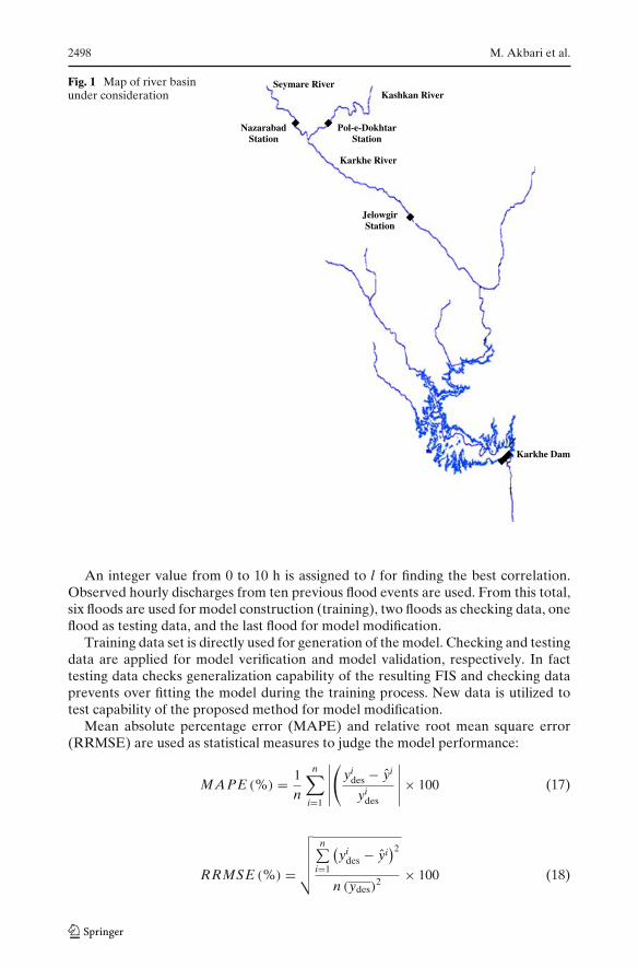
In order to demonstrate the effectiveness of the fuzzy modeling and proposedmodel modification method, a data set from Karkhe River in Iran is used (Fig. 1).Flood forecasting at Jelowgyr (J) control station is desired. This station is located atdownstream of Nazarabad (N) and Pol-e-Dokhtar (P) stations and immediately up-stream of Karkhe Dam, one of the major reservoirs in Iran. For reservoir operationpurposes flood forecasting at the named station is very important. The first step toconstruct a fuzzy rule base, is identification of the potentially effective variables onthe output of the system. There is no systematic way to identify these variables.Presumably, the experts’ knowledge may help nominating these effective variables.Nevertheless, there are some systematic, chiefly mathematical methods to elicitthe best combination of effective variables from a predetermined set of potentialvariables. From the experts’ point of view, the most probable effective variables onthe discharge at Jelowgyr station are the discharges at Nazarabad and Pol-e-Dokhtarstations. Furthermore, the experts believe that the lag time of the waves from uppertwo stations to Jelowgyr station is about 5 to 6 h, which may be estimated based onthe distance between stations and the flood flow velocity.

One may develop a correlation between discharges at any time at two upstreamstations and discharges at the control station considering different lag times. Lagtimes can be interpreted as lead times for discharge forecasting at Jelowgyr station.Mathematically this relation takes the following form:

QJ (t + l) = f(QN (t) , QP (t)

)(16)

Where QJ(t + l) is discharge at time period t + l at Jelowgyr station, QN(t) andQP(t) are discharges at time period t at Nazarabad and Pol-e-Dokhtar stationsrespectively.


Fig. 1 Map of river basinunder consideration Kashkan River

Seymare River

Karkhe River

Karkhe Dam

Pol-e-DokhtarStation

JelowgirStation

NazarabadStation

An integer value from 0 to 10 h is assigned to l for finding the best correlation.Observed hourly discharges from ten previous flood events are used. From this total,six floods are used for model construction (training), two floods as checking data, oneflood as testing data, and the last flood for model modification.

Training data set is directly used for generation of the model. Checking and testingdata are applied for model verification and model validation, respectively. In facttesting data checks generalization capability of the resulting FIS and checking dataprevents over fitting the model during the training process. New data is utilized totest capability of the proposed method for model modification.

Mean absolute percentage error (MAPE) and relative root mean square error(RRMSE) are used as statistical measures to judge the model performance:

MAPE (%) = 1

n

n∑

i=1

∣∣∣∣∣

(yi

des − yi

yides

∣∣∣∣∣× 100 (17)

RRMSE (%) =

√√√√√

n∑

i=1

(yi

des − yi)2

n (ydes)2 × 100 (18)


In which yides, yi, ydes, y and n refer to observed discharge for ith data point,

forecasted discharge for ith data point, mean of the observed discharge data points,mean of the forecasted discharge data points, and number of data points of data setrespectively.

Therefore, in this study, for every lead time (l), pairs of input–output data fromthe existing record are extracted and formatted according to relation (16). Model isthen constructed to forecast discharges at Jelowgyr station l hour in advance.

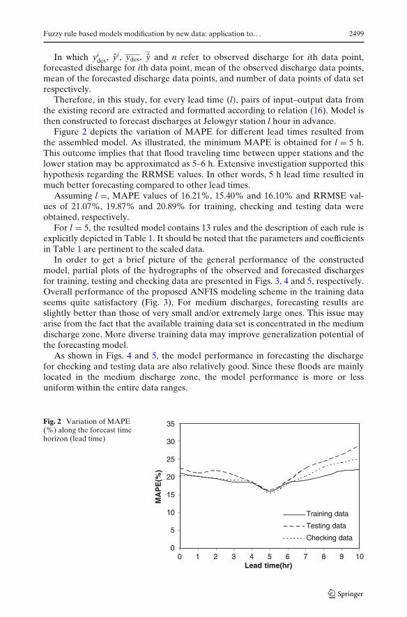
Figure 2 depicts the variation of MAPE for different lead times resulted fromthe assembled model. As illustrated, the minimum MAPE is obtained for l = 5 h.This outcome implies that that flood traveling time between upper stations and thelower station may be approximated as 5–6 h. Extensive investigation supported thishypothesis regarding the RRMSE values. In other words, 5 h lead time resulted inmuch better forecasting compared to other lead times.

Assuming l =, MAPE values of 16.21%, 15.40% and 16.10% and RRMSE val-ues of 21.07%, 19.87% and 20.89% for training, checking and testing data wereobtained, respectively.

For l = 5, the resulted model contains 13 rules and the description of each rule isexplicitly depicted in Table 1. It should be noted that the parameters and coefficientsin Table 1 are pertinent to the scaled data.

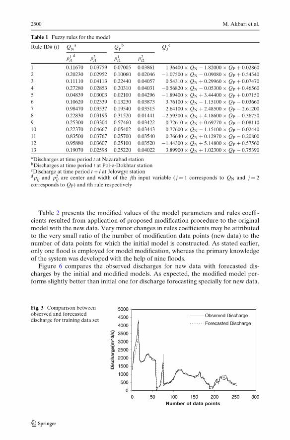
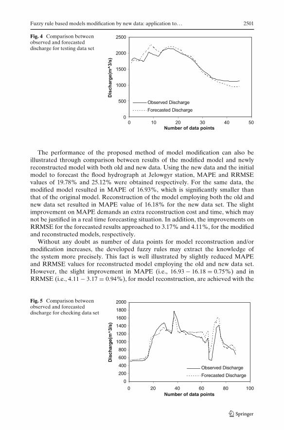
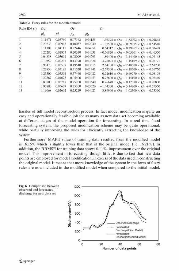
In order to get a brief picture of the general performance of the constructedmodel, partial plots of the hydrographs of the observed and forecasted dischargesfor training, testing and checking data are presented in Figs. 3, 4 and 5, respectively.Overall performance of the proposed ANFIS modeling scheme in the training dataseems quite satisfactory (Fig. 3), For medium discharges, forecasting results areslightly better than those of very small and/or extremely large ones. This issue mayarise from the fact that the available training data set is concentrated in the mediumdischarge zone. More diverse training data may improve generalization potential ofthe forecasting model.

As shown in Figs. 4 and 5, the model performance in forecasting the dischargefor checking and testing data are also relatively good. Since these floods are mainlylocated in the medium discharge zone, the model performance is more or lessuniform within the entire data ranges.

Fig. 2 Variation of MAPE(%) along the forecast timehorizon (lead time)

0

5

10

15

20

25

30

35

0 2 5 9 10Lead time(hr)

MA

PE

(%)

Training data

Testing data

Checking data

876431


Table 1 Fuzzy rules for the model

Rule ID# (i) QNa QP

b QJc

p1i1

dp2

i1 p1i2 p2

i2

1 0.11670 0.03759 0.07005 0.03861 1.36400 × QN − 1.82000 × QP + 0.028602 0.20230 0.02952 0.10060 0.02046 −1.07500 × QN − 0.09080 × QP + 0.545403 0.11110 0.04113 0.22440 0.04057 0.54310 × QN + 0.29960 × QP + 0.074704 0.27280 0.02853 0.20310 0.04031 −0.56820 × QN − 0.05300 × QP + 0.465605 0.04839 0.03003 0.02100 0.04296 −1.89400 × QN + 3.44400 × QP + 0.071506 0.10620 0.02339 0.13230 0.03873 3.76100 × QN − 1.15100 × QP − 0.036607 0.98470 0.03537 0.19540 0.03515 2.64100 × QN + 2.48500 × QP − 2.612008 0.22830 0.03195 0.31520 0.01441 −2.59300 × QN + 4.18600 × QP − 0.367509 0.25300 0.03304 0.57460 0.03422 0.72610 × QN + 0.69770 × QP − 0.0811010 0.22370 0.04667 0.05402 0.03443 0.77600 × QN − 1.15100 × QP − 0.0244011 0.83500 0.03767 0.25700 0.03540 0.76640 × QN + 0.12970 × QP − 0.2080012 0.95880 0.03607 0.25100 0.03520 −1.44300 × QN + 5.14800 × QP + 0.5756013 0.19070 0.02598 0.25220 0.04022 3.89900 × QN + 1.02300 × QP − 0.75390

aDischarges at time period t at Nazarabad stationbDischarges at time period t at Pol-e-Dokhtar stationcDischarge at time period t + l at Jelowgyr stationd p1

ij and p2ij are center and width of the jth input variable ( j = 1 corresponds to QN and j = 2

corresponds to QP) and ith rule respectively

Table 2 presents the modified values of the model parameters and rules coeffi-cients resulted from application of proposed modification procedure to the originalmodel with the new data. Very minor changes in rules coefficients may be attributedto the very small ratio of the number of modification data points (new data) to thenumber of data points for which the initial model is constructed. As stated earlier,only one flood is employed for model modification, whereas the primary knowledgeof the system was developed with the help of nine floods.

Figure 6 compares the observed discharges for new data with forecasted dis-charges by the initial and modified models. As expected, the modified model per-forms slightly better than initial one for discharge forecasting specially for new data.

Fig. 3 Comparison betweenobserved and forecasteddischarge for training data set

0

500

1000

1500

2000

2500

3000

3500

4000

4500

5000

0 50 100 150 200 250 300Number of data points

Dis

char

ge(m

^3/s

)

Observed Discharge

Forecasted Discharge


Fig. 4 Comparison betweenobserved and forecasteddischarge for testing data set

0

500

1000

1500

2000

2500

0 10 20 30 40 50Number of data points

Dis

ch

arg

e(m

^3

/s)

Observed Discharge


The performance of the proposed method of model modification can also beillustrated through comparison between results of the modified model and newlyreconstructed model with both old and new data. Using the new data and the initialmodel to forecast the flood hydrograph at Jelowgyr station, MAPE and RRMSEvalues of 19.78% and 25.12% were obtained respectively. For the same data, themodified model resulted in MAPE of 16.93%, which is significantly smaller thanthat of the original model. Reconstruction of the model employing both the old andnew data set resulted in MAPE value of 16.18% for the new data set. The slightimprovement on MAPE demands an extra reconstruction cost and time, which maynot be justified in a real time forecasting situation. In addition, the improvements onRRMSE for the forecasted results approached to 3.17% and 4.11%, for the modifiedand reconstructed models, respectively.

Without any doubt as number of data points for model reconstruction and/ormodification increases, the developed fuzzy rules may extract the knowledge ofthe system more precisely. This fact is well illustrated by slightly reduced MAPEand RRMSE values for reconstructed model employing the old and new data set.However, the slight improvement in MAPE (i.e., 16.93 − 16.18 = 0.75%) and inRRMSE (i.e., 4.11 − 3.17 = 0.94%), for model reconstruction, are achieved with the

Fig. 5 Comparison betweenobserved and forecasteddischarge for checking data set

0

200

400

600

800

1000

1200

1400

1600

1800

2000

0 20 40 60 80 100Number of data points

Dis

char

ge(

m^3

/s)

Observed Discharge



Table 2 Fuzzy rules for the modified model

Rule ID# (i) QN QP QJ

p1i1 p2

i1 p1i2 p2

i2

1 0.11671 0.03760 0.07162 0.04155 1.36398 × QN − 1.82002 × QP + 0.028482 0.20233 0.02943 0.10057 0.02040 −1.07500 × QN − 0.09075 × QP + 0.545403 0.11107 0.04115 0.22446 0.04051 0.54312 × QN + 0.29967 × QP + 0.074984 0.27280 0.02853 0.20310 0.04031 −0.56820 × QN − 0.05301 × QP + 0.465605 0.04838 0.03001 0.02099 0.04293 −1.89400 × QN + 3.44400 × QP + 0.071456 0.10559 0.02297 0.13190 0.03824 3.76093 × QN − 1.15109 × QP − 0.037217 0.98470 0.03537 0.19540 0.03515 2.64100 × QN + 2.48500 × QP − 2.612008 0.22830 0.03195 0.31520 0.01441 −2.59300 × QN + 4.18600 × QP − 0.367509 0.25300 0.03304 0.57460 0.03422 0.72610 × QN + 0.69770 × QP − 0.0810810 0.22367 0.04673 0.05406 0.03453 0.77600 × QN − 1.15100 × QP − 0.0244011 0.83500 0.03767 0.25700 0.03540 0.76640 × QN + 0.12970 × QP − 0.2080012 0.95880 0.03607 0.25100 0.03520 −1.44300 × QN + 5.14800 × QP + 0.5756013 0.19068 0.02602 0.25219 0.04025 3.89900 × QN + 1.02300 × QP − 0.75390

hassles of full model reconstruction process. In fact model modification is quite aneasy and operationally feasible job for as many as new data set becoming availableat different stages of the model operation for forecasting. In a real time floodforecasting system, the proposed modification scheme may be quite operational,while partially improving the rules for efficiently extracting the knowledge of thesystem.

Furthermore, MAPE value of training data resulted from the modified modelis 16.15% which is slightly lower than that of the original model (i.e. 16.21%). Inaddition, the RRMSE for training data shows 0.11%. improvement over the originalmodel. This improvement in forecasting, though little, is due to fact that new datapoints are employed for model modification, in excess of the data used in constructingthe original model. It means that more knowledge of the system in the form of fuzzyrules are now included in the modified model when compared to the initial model.

Fig. 6 Comparison betweenobserved and forecasteddischarge for new data set

0

200

400

600

800

1000

1200

0 20 40 60 80Number of data points

Dis

char

ge(

m^3

/s)

Observed Discharge

Forecasted Discharge(Initial Model)ForecastedDischarge(Modified Model)


Very little improvement in modified model may be related to the very small ratio ofthe number of new data to the total number of data points.

5 Conclusion

As new data become available, an already existing fuzzy model may be reconstructed,modified or used as is. Use of the new data for model reconstruction and/ormodification may extend the acquired knowledge of the system. When the mainbody of the rules has already been developed, reconstruction of the rules may notseem to be logical. Utilizing the existing data, an ANFIS model was employed toconstruct a fuzzy model to forecast flood flow in a branched river reach providedthat flood flows at upstream stations are known in advance. The fuzzy model wasthen modified with a Gradient Descent Algorithm. The modified model providedmore precise forecast compared to the initial (original) model. Performance of thereconstructed model with combination of both new and old data was slightly betterthan the modified model. However, in a real time flood forecasting, the proposedmodification approach was shown to be quite easy and operationally feasible job asnew data become available at different stages of flood forecasting process. Modelapplication to a real world case example showed that the proposed modificationapproach could partially improve the fuzzy rules by efficiently extracting some moreknowledge of the system. Also results shows, reconstructed model utilizing both theold and new data is slightly more accurate than modified model. Nevertheless thisimprovement at accuracy was not significant considering the hassles of the modelreconstruction.

References

Aquil M, Kita I, Yano A, Nishiyama S (2006) A Takagi–Sugeno fuzzy system for the prediction ofriver stage dynamics. JARQ 40(4):369–378

Chau KW, Wu CL, Li YS (2005) Comparison of several flood forecasting models in Yangtze River.J Hydrol Eng 10(6):485–491. doi:10.1061/(ASCE)1084-0699(2005)10:6(485)

Chen MY, Linkens DA (2004) Rule-base self-generation and simplification for data-driven fuzzymodels. J Fuzzy Sets Syst 142:243–265. doi:10.1016/S0165-0114(03)00160-X

Deka P, Chandramouli V (2005) Fuzzy neural network model for hydrologic flow routing. J HydrolEng 10(4):302–314. doi:10.1061/(ASCE)1084-0699(2005)10:4(302)

Dubrovin T, Jolma A, Turunen E (2002) Fuzzy model for real time reservoir operation. J WaterResour Plan Manage 128(1):66–73

Karaboga D, Bagis A, Haktanir T (2004) Fuzzy logic based operation of spillway gates of reservoirsduring floods. J Hydrol Eng 9(6):544–549. doi:10.1061/(ASCE)1084-0699(2004)9:6(544)

Kim E, Park M, Ji S, Park M (1997) A new approach to fuzzy modeling. J IEEE Trans Fuzzy Syst5(3):328–337. doi:10.1109/91.618271

Maier HR, Sayed T, Lence BJ (2000) Forecasting cyanobacterial concentrations using B-splinenetworks. J Comput Civ Eng 14(3):183–189. doi:10.1061/(ASCE)0887-3801(2000)14:3(183)

Mehta R, Jain SK (2008) Optimal operation of a multi-purpose reservoir using neuro-fuzzy tech-nique. J Water Resour Manage. doi:10.1007/s11269-008-9286-0

Nayak PC, Sudheer KP, Rangan DM, Ramasastri KS (2005) Short-term flood forecasting with aneurofuzzy model. J Water Resour Res 41:1–16

Pinthong P, Das Gupta A, Singh Babel M, Weesakul S (2008) Improved reservoir operation usinghybrid genetic algorithm and neurofuzzy computing. J Water Resour Manage. doi:10.1007/s11269-008-9295-z

http://dx.doi.org/10.1061/(ASCE)1084-0699(2005)10:6(485)

http://dx.doi.org/10.1016/S0165-0114(03)00160-X



http://dx.doi.org/10.1109/91.618271


http://dx.doi.org/10.1007/s11269-008-9286-0

http://dx.doi.org/10.1007/s11269-008-9295-z

http://dx.doi.org/10.1007/s11269-008-9295-z


Russell SO, Campbell PF (1996) Reservoir operating rules with fuzzy programming. J Water ResourPlan Manage 122(3):165–170. doi:10.1061/(ASCE)0733-9496(1996)122:3(165)

Shrestha BP, Duckstein L, Stakhiv EZ (1996) Fuzzy rule based modeling of reservoir operation.J Water Resour Plan Manage 122(4):262–269. doi:10.1061/(ASCE)0733-9496(1996)122:4(262)

Stüber M, Gemmar P, Greving M (2000) Machine supported development of fuzzy-flood forecastsystems. Proc Eur Conf Advances Flood Research 2:504–515

Takagi T, Sugeno M (1985) Fuzzy identification of systems and its applications to modeling andcontrol. J IEEE Trans Syst Man Cybern 15:116–132

Yu PS, Chen CJ, Chen SJ (2000) Application of gray and fuzzy methods for rainfall forecasting.J Hydrol Eng 5(4):339–345. doi:10.1061/(ASCE)1084-0699(2000)5:4(339)




Fuzzy Rule Based Models Modification by New Data: Application to Flood Flow Forecasting

Documents

Transcript of Fuzzy Rule Based Models Modification by New Data: Application to Flood Flow Forecasting