Fuzzy prototypes: From a cognitive view to a

machine learning principle

Marie-Jeanne Lesot1, Maria Rifqi1, and Bernadette Bouchon-Meunier1

Universite Pierre et Marie Curie-Paris6, CNRS, UMR 7606, LIP6, 8, rue duCapitaine Scott, Paris, F-75015, France{marie-jeanne.lesot,maria.rifqi,bernadette.bouchon-meunier}@lip6.fr

M.-J. Lesot, M. Rifqi et B. Bouchon-Meunier. Fuzzy prototypes: From a cognitive

view to a machine learning principle. In H. Bustince, F. Herrera and J. Montero

editors, Fuzzy Sets and Their Extensions: Representation, Aggregation and Models,

(pp. 431-452). Springer. 2007.

Abstract. Cognitive psychology works have shown that the cognitive representa-tion of categories is based on a typicality notion: all objects of a category do nothave the same representativeness, some are more characteristic or more typical thanothers, and better exemplify their category. Categories are then defined in terms ofprototypes, i.e. in terms of their most typical elements. Furthermore, these worksshowed that an object is all the more typical of its category as it shares many fea-tures with the other members of the category and few features with the members ofother categories.

In this paper, we propose to profit from these principles in a machine learningframework: a formalization of the previous cognitive notions is presented, leading toa prototype building method that makes it possible to characterize data sets takinginto account both common and discriminative features. Algorithms exploiting theseprototypes to perform tasks such as classification or clustering are then presented.

The formalization is based on the computation of typicality degrees that measurethe representativeness of each data point. These typicality degrees are then exploitedto define fuzzy prototypes: in adequacy with human-like description of categories, weconsider a prototype as an intrinsically imprecise notion. The fuzzy logic frameworkmakes it possible to model sets with unsharp boundaries or vague and approximateconcepts, and appears most appropriate to model prototypes.

We then exploit the computed typicality degrees and the built fuzzy prototypesto perform machine learning tasks such as classification and clustering. We presentseveral algorithms, justifying in each case the chosen parameters. We illustrate theresults obtained on several data sets corresponding both to crisp and fuzzy data.

1 Introduction

Prototypes are elements representing categories, structuring and summarizingthem, underlining their most important characteristics and their specificity asopposed to other categories. From a cognitive point of view, they are the basisfor the categorization task, process that aims at considering as equivalentobjects that are distinct but similar: cognitive science works [31,32] showed

2 Marie-Jeanne Lesot, Maria Rifqi, and Bernadette Bouchon-Meunier

that natural categories are organized around the notion of prototype and therelated notion of typicality.

In this paper, we propose to transpose the cognitive view of prototypes toa machine learning principle to extract knowledge from data. More precisely,we propose to characterize data sets through the construction of prototypesthat realize the cognitive approach. The core of our motivation is the factthat, through this notion of prototype, a data subset (a category for instance)is characterized both from an internal and an external point of view: the pro-totype underlines both what is common to the subset members and what isspecific to them in opposition to the other data. Using these two complemen-tary components leads to context-dependent representatives that are morerelevant than classic representatives that actually exploit only the internalview. Furthermore, the method makes it possible to determine the extent towhich the prototype should be a central or a discriminative element, i.e. itallows to rule the relative importance of common and discriminative features,leading to a flexible prototype building method.

Another concern of our approach is the adequacy with human-like descrip-tions that are usually based on imprecise linguistic expressions. To that aim,the construction method we propose builds fuzzy prototypes : the fuzzy logicframework makes it possible to model sets with unsharp boundaries or vagueand approximate concepts, as occur in this framework.

The paper is organized as follows: in Section 2, the cognitive definitions oftypicality and prototypes are introduced. In Section 3, these principles are for-malized to a prototype building method that makes it possible to characterizenumerical data sets. These prototypes are then exploited both for supervisedand unsupervised learning: Section 4 presents prototype-based classificationmethods and Section 5 describes a typicality-based clustering algorithm.

2 Cognitive definition of prototype

The cognitive definition of prototype was first proposed in the 70’s [27] andpopularized by E. Rosch [31,32], in the context of the study of cognitive con-cept organization. Previously, a crisp relationship between objects and catego-ries was assumed, based on the existence of necessary and sufficient propertiesto determine membership: according to this model, an object belongs to a ca-tegory if it possesses the properties, interpreted as necessary and sufficientconditions; otherwise, it is not a member of the category. Now in the case ofnatural categories, it is often the case that no feature is common to all thecategory members: as modeled in the family resemblance model of Wittgen-stein [36], each object shares different common features with other membersof the category, but no globally shared feature can be identified.

The prototype view of concept organization [27,31,32] models categoriesas organized around a center, the prototype, that is described by means ofproperties that are characteristic, typical of the category members. Indeed, all

Fuzzy prototypes: From a cognitive view to a machine learning principle 3

objects in a category are not equivalent: some are better examples and morecharacteristic of the category than others. For instance, in the case of themammal category, the dog is considered as a better example than a platypus.Thus, objects are spread over a scale, or a gradient of typicality; the prototypeis then related to the individuals that maximize this gradient.

Rosch and her colleagues [31,32] studied this typicality notion and showedit depends on two complementary components: an object is all the more ty-pical of its category as it shares many features with the other members ofthe category and few features with the members of other categories. This canfor instance be illustrated by platypuses and whales in the case of mammals:platypuses are atypical mainly because they have too few features in commonwith other mammals, whereas whales are atypical mainly because they havetoo many common features with members of the fish category. Due to thistypicality definition, prototypes underline both the common features of thecategory members and their discriminative features as opposed to other ca-tegories: they characterize the category both internally and in opposition toother categories.

3 Realization of the prototype view

3.1 Principle

To construct a fuzzy prototype in agreement with the previous cognitive pro-totype view, we consider that the degree of typicality of an object dependspositively on its total resemblance to others objects of its class (internal re-semblance) and on its total dissimilarity to objects of other classes (externaldissimilarity). This makes it possible to consider both the common featuresof the category members, and their distinctive features as opposed to othercategories. More precisely, the fuzzy prototype construction principle consistsin three steps [29]:

Step 1 Compute the internal resemblance degree of an object with the othermembers of its category and its external dissimilarity degree with themembers of the outside categories.

Step 2 Aggregate the internal resemblance and the external dissimilarity de-grees to obtain the typicality degree of the considered object.

Step 3 Aggregate the objects that are typical ”enough”, i.e. with a typicalitydegree higher than a predefined threshold to obtain the fuzzy prototype.

Internal resemblance and external dissimilarity

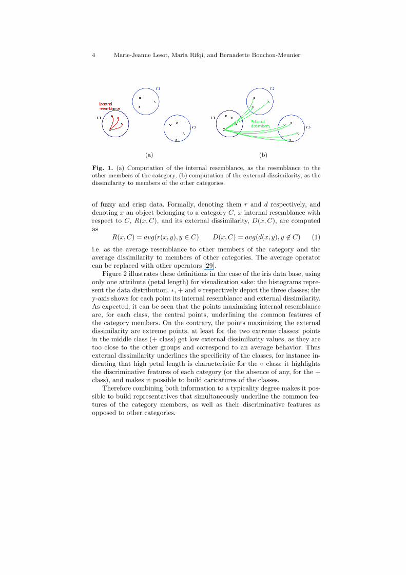
Step 1, that is illustrated on figure 1, requires the choice of a resemblancemeasure and a dissimilarity measure to compare the objects. These measuresdepend on the data nature and are detailed in Sections 3.3 and 3.4 in the case

4 Marie-Jeanne Lesot, Maria Rifqi, and Bernadette Bouchon-Meunier

(a) (b)

Fig. 1. (a) Computation of the internal resemblance, as the resemblance to theother members of the category, (b) computation of the external dissimilarity, as thedissimilarity to members of the other categories.

of fuzzy and crisp data. Formally, denoting them r and d respectively, anddenoting x an object belonging to a category C, x internal resemblance withrespect to C, R(x,C), and its external dissimilarity, D(x,C), are computedas

R(x,C) = avg(r(x, y), y ∈ C) D(x,C) = avg(d(x, y), y 6∈ C) (1)

i.e. as the average resemblance to other members of the category and theaverage dissimilarity to members of other categories. The average operatorcan be replaced with other operators [29].

Figure 2 illustrates these definitions in the case of the iris data base, usingonly one attribute (petal length) for visualization sake: the histograms repre-sent the data distribution, ∗, + and ◦ respectively depict the three classes; they-axis shows for each point its internal resemblance and external dissimilarity.As expected, it can be seen that the points maximizing internal resemblanceare, for each class, the central points, underlining the common features ofthe category members. On the contrary, the points maximizing the externaldissimilarity are extreme points, at least for the two extreme classes: pointsin the middle class (+ class) get low external dissimilarity values, as they aretoo close to the other groups and correspond to an average behavior. Thusexternal dissimilarity underlines the specificity of the classes, for instance in-dicating that high petal length is characteristic for the ◦ class: it highlightsthe discriminative features of each category (or the absence of any, for the +class), and makes it possible to build caricatures of the classes.

Therefore combining both information to a typicality degree makes it pos-sible to build representatives that simultaneously underline the common fea-tures of the category members, as well as their discriminative features asopposed to other categories.

Fuzzy prototypes: From a cognitive view to a machine learning principle 5

1 2 3 4 5 6 70

0.1

0.2

0.3

0.4

0.5

0.6

0.7

0.8

0.9

1

1 2 3 4 5 6 70

0.1

0.2

0.3

0.4

0.5

0.6

0.7

0.8

0.9

1

(a) (b)

Fig. 2. (a) Internal resemblance, (b) external dissimilarity, for the iris data set,considering only the petal length attribute [23].

Aggregation to a typicality degree

Step 2 requires the choice of an aggregation operator to express the depen-dence of typicality on internal resemblance and external dissimilarity, that isformally written

T (x,C) = ϕ(R(x,C), D(x,C)) (2)

where ϕ denotes the aggregation operator. It makes it possible to rule thesemantics of typicality and thus that of the prototypes, determining the extentto which the prototype should be a central or a discriminative element [23].

Figure 3 illustrates the typicality degrees obtained from the internal resem-blance and external dissimilarity of figure 2 for four operators: the minimum(see fig. 3a) is a conjunctive operator that requires both R and D to be highfor a point to be typical, leading to rather small typicality degrees on average.On the contrary, for the maximum (see fig. 3b), as any disjunctive operator,if either R or D is high, a point is considered as typical. This leads to highervalues but to non-convex distributions, reflecting a double semantics for ty-picality: central points as well as extreme points are typical, but for differentreasons.

Trade-off operators, such as the weighted mean (fig. 3c), offer a compen-sation property: low R values can be compensated for by high D. This isillustrated by the leftmost point on fig. 3c, whose typicality is higher thanwith the min operator, because its external dissimilarity compensates for itsinternal resemblance. The weights used in the weighted mean determine theextent to which compensation can take place, and rule the relative impor-tance of internal resemblance and external dissimilarity, leading to more orless discriminative prototypes, underlying more the common or the distinctivefeatures of the categories.

Lastly, variable behavior operators, such as the mica operator [17] (seefig. 3d) or the symmetric sum [33], are conjunctive, disjunctive or trade-offoperators, depending on the values to be aggregated. They offer a reinforce-ment property: if both R and D are high, they reinforce each other to give an

6 Marie-Jeanne Lesot, Maria Rifqi, and Bernadette Bouchon-Meunier

1 2 3 4 5 6 70

0.1

0.2

0.3

0.4

0.5

0.6

0.7

0.8

0.9

1

1 2 3 4 5 6 70

0.1

0.2

0.3

0.4

0.5

0.6

0.7

0.8

0.9

1

(a) (b)

1 2 3 4 5 6 70

0.1

0.2

0.3

0.4

0.5

0.6

0.7

0.8

0.9

1

1 2 3 4 5 6 70

0.1

0.2

0.3

0.4

0.5

0.6

0.7

0.8

0.9

1

(c) (d)

Fig. 3. Typicality degrees obtained from the internal resemblance and the exter-nal dissimilarity shown on fig. 2 using different aggregation operators: (a) T =min(R,D), (b) T = max(R,D), (c) T = 0.6R + 0.4D, (d) T =mica(R,D) [17].

even higher typicality (see class ∗), if both are low, they penalize each otherto give an even smaller value (see the leftmost point of the ◦ class).

Therefore, the aggregation operator determines the semantics of typicality,and rules the relative influence played by internal resemblance and externaldissimilarity.

Aggregation to a prototype

Lastly step 3 builds the prototype of a category itself, as the aggregation of themost typical objects of the category: the prototype for category C is definedin a general form as

p(C) = ψ({x/T (x,C) > τ}) (3)

where τ is the typicality threshold and ψ the aggregation operator. The lattercan still depend on the typicality degrees associated to the selected points,taking for instance the form of a weighted mean. Its actual definition dependson the data nature, it is detailed in Sections 3.3 and 3.4 in the case of fuzzyand crisp data.

Remarks

It is to be underlined that prototype can be built either from the typicalitydegrees of objects, as presented above, but also in an attribute per attribute

Fuzzy prototypes: From a cognitive view to a machine learning principle 7

approach: the global approach makes it possible to take into account attributecorrelation, but it can also be interesting to enhance the typical values of thedifferent properties used to describe the objects, without considering an objectas an indivisible whole. This means, all the values of a property are consideredsimultaneously, without taking into account the objects they describe. Forinstance, if the objects are represented by means of a color, a size and aweight, the fuzzy prototype of the category of these objects is the union oftypical values for the color, the size and the weight. It means that instead ofcomputing internal resemblance, external dissimilarity and typicality degreesfor each object, these quantities are computed for each attribute value. Thisapproach is in particular applied in the case of fuzzy data, as described inSection 3.3.

3.2 Related works

There exist many works to summarize data sets, or build significant repre-sentatives. A first approach, taking the average as starting point, consistsin defining more sophisticated variants to overcome the average’s drawbacks,in particular its sensitivity to outliers (see for instance [11]). Among thesevariants, one can mention the Most Typical Value [11] or the representativesproposed in [26] or [37]. In all these cases, the obtained value is computed asa weighted mean, the difference comes from the ways the weights are defined.

Besides, a second approach, more concerned with interpretability, doesnot reduce the representative to a single precise value but builds so-calledlinguistic summaries [16,15]. The latter identify significant trends in the dataand represent them in the form “Q B’s are A” where Q is a linguistic quantifierand A and B are fuzzy sets; for example, “most important experts are young”.

Yet, both approaches build internal representatives that take into accountthe common characteristics of the data, but not their specificity. More pre-cisely, they focus only on the data to be summarized, and do not depend ontheir context, which prevents them from identifying their particularity. On thecontrary, the cognitive view highlights the discriminative features: the dataare also characterized in opposition to the other categories.

Furthermore, the proposed realization of the cognitive approach describedin Section 3.1 makes it possible to rule the relative importance common anddiscriminative features play and the trade-off between them through the choiceof the aggregation operator, leading to a flexible method. As illustrated in Sec-tion 4 and 5, the choice of the aggregation operator depends on the considereduse of the prototype.

3.3 Fuzzy data case

In this section, we consider the case of fuzzy data, i.e. data whose attributestake as values fuzzy sets: formally, denoting F(R) the set of fuzzy subsets de-fined on the real line, the input space is F(R)p where p denotes the number of

8 Marie-Jeanne Lesot, Maria Rifqi, and Bernadette Bouchon-Meunier

attributes. We describe the instantiation of the previous prototype construc-tion method, discussing comparison measures for such data and aggregationoperators to construct the prototypes from the most typical values. We thenpresent an application in a medical domain, to mammographies.

Comparison measures

In the case of fuzzy data, the framework used to compute the internal resem-blance as well as the external dissimilarity is the one defined in [4] generalizingthe Tversky’s ”contrast model” [35].

In this framework a measure of resemblance comparing two fuzzy sets Aand B is a function of three arguments: M(A ∩ B) (the common features),M(A − B) and M(B − A) (the distinctive features), where M is fuzzy setmeasure [9] like the fuzzy cardinality for instance. More formally [4]:

Definition 1 A measure of resemblance r is

– non decreasing in M(A∩B), non increasing in M(A−B) and M(B−A)– reflexive: ∀A, r(A,A) = 1– symmetrical: ∀A,B, r(A,B) = r(B,A)

An example of measure of resemblance, proposed by [8], generalizing theJacccard measure to fuzzy sets, is the following:

r(A,B) =M(A ∩B)/M(A ∪B)

forM such that : M(A ∪B) =M(A ∩B) +M(A−B) +M(B −A).We also refer to this framework to choose a dissmilarity measure:

Definition 2 A measure of dissimilarity d is:

– independent of M(A∩B) and non decreasing in M(A−B) and M(B−A)– minimal: ∀A, d(A,A) = 0

An example of measure of dissimilarity, based on the generalizedMinkowski’sdistance, is the following:

d(A,B) =

(

1

Z

(∫

|fA(x) − fB(x)|ndx

))1/n

where Z is a normalizing factor, n an integer and fX denotes the membershipfunction of the fuzzy set X .

It is to be noticed that a dissimilarity measure is not necessarily deducedfrom a resemblance measure and vice versa because the purpose is to havedifferent information when comparing two objects, the dissimilarity measurefocusing on distinctive features.

Fuzzy prototypes: From a cognitive view to a machine learning principle 9

Aggregation into a fuzzy prototype

In the last step of the fuzzy prototype construction, fuzzy values of an at-tribute that are typical ”enough” have to be aggregated in order to obtain atypical value for the considered attribute. An aggregation operator must bechosen among numerous existing operators, deeply studied by several authorslike Mizumoto [24], [25], Detyniecki [7] or Calvo and her colleagues [5].

Application to mammography

Nowadays, mammography is the primary diagnostic procedure for the earlydetection of breast cancer. Microcalcification1 clusters are an important el-ement in the detection of breast cancer. This kind of finding is the directexpression of pathologies which may be benign or malignant. The descrip-tion of microcalcifications is not an easy task, even for an expert. If someof them are easy to detect and to identify, some others are more ambigu-ous. The texture of the image, the small size of objects to be detected (lessthan one millimeter), the various aspects they have, the radiological noise, areparameters which impact the detection and the characterization tasks.

More generally, mammographic images present two kinds of ambiguity: im-

precision and uncertainty. The imprecision on the contour of an object comesfrom the fuzzy aspect of the borders: the expert can define approximately thecontour but certainly not with a high spatial precision. The uncertainty comesfrom the microcalcification superimpositions: because objects are built fromthe superimpositions of several 3D structures on a single image, we may havea doubt about the contour position.

The first step consists in finding automatically the contours of microcalci-fications. This segmentation is also realized thanks to a fuzzy representationof imprecision and uncertainty (more details can be found in [28]). Each mi-crocalcification is then described by means of 5 fuzzy attributes computedfrom its fuzzy contour. These attributes enable us to describe more precisely:

• the shape (3 attributes): elongation (minimal diameter/maximal diame-ter), compactness1, compactness2.

• the dimension (2 attributes): surface, perimeter.

Figure 4 shows an example of the membership functions of the valuestaken by a detected microcalcification. One can notice that the membershipfunctions are not ”standard” in the sense that they are not triangular ortrapezoidal (as it is often the case in the literature) and this is because ofthe automatic generation of fuzzy values (we will not go into details here,interested readers may refer to [3]).

Experts have categorized microcalcifications into 2 classes: round micro-calcifications and not round ones, because this property is important to qualify

1 The microcalcifications are small depositions of radiologically very opaque mate-rials which can be seen on mammography exams as small bright spots.

10 Marie-Jeanne Lesot, Maria Rifqi, and Bernadette Bouchon-Meunier

0

0.2

0.4

0.6

0.8

1

1.2

0 10 20 30 40 50 60 70 80

Mem

bers

hip

degr

ee

Surface

0

0.2

0.4

0.6

0.8

1

1.2

140 160 180 200 220 240 260 280 300

Mem

bers

hip

degr

ee

Elongation

0

0.2

0.4

0.6

0.8

1

1.2

100 120 140 160 180 200 220 240

Mem

bers

hip

degr

ee

Compactness1

0

0.2

0.4

0.6

0.8

1

1.2

0 2 4 6 8 10 12 14

Mem

bers

hip

degr

ee

Compactness2

0

0.2

0.4

0.6

0.8

1

1.2

0 10 20 30 40 50

Mem

bers

hip

degr

ee

Perimeter

Fig. 4. Description of a microcalcification by means of fuzzy values of its 5 at-tributes.

the malignancy of the microcalcifications. The aim is then to build the fuzzyprototypes of the classes round and not round. Figure 5 gives the obtainedfuzzy prototypes with the internal resemblance and external dissimilarity com-puted using as aggregator the median (replacing the average in equation (1)by the median). The typicality degrees are obtained by the probabilistic t-conorm (ϕ(x, y) = x+ y− x · y in equation (2)). Lastly, the fuzzy values withmaximal typicality degree are aggregated through the max-union operator todefine the fuzzy prototype value of the corresponding attribute.

It can be seen that on the attributes elongation, compactness1 or com-

pactness2, the typical values of the two classes round and not round, are quitedifferent: the intersection between them is low. This can be interpreted in thefollowing way: a round microcalcification typically has an elongation approx-

imately between 100 and 150 whereas a not round microcalcification typically

has an elongation approximately between 150 and 200, etc. For the attributessurface and perimeter, contrary to the previous attributes, the typical values

Fuzzy prototypes: From a cognitive view to a machine learning principle 11

ROUND NOT ROUND

0

0.2

0.4

0.6

0.8

1

1.2

0 10 20 30 40 50

Mem

bers

hip

degr

ee

Surface

0

0.2

0.4

0.6

0.8

1

1.2

0 10 20 30 40 50

Mem

bers

hip

degr

ee

Surface

0

0.2

0.4

0.6

0.8

1

1.2

100 150 200 250 300

Mem

bers

hip

degr

ee

Elongation

0

0.2

0.4

0.6

0.8

1

1.2

100 150 200 250 300

Mem

bers

hip

degr

eeElongation

0

0.2

0.4

0.6

0.8

1

1.2

50 100 150 200 250

Mem

bers

hip

degr

ee

Compactness1

0

0.2

0.4

0.6

0.8

1

1.2

50 100 150 200 250

Mem

bers

hip

degr

ee

Compactness1

0

0.2

0.4

0.6

0.8

1

1.2

0 5 10 15 20

Mem

bers

hip

degr

ee

Compactness2

0

0.2

0.4

0.6

0.8

1

1.2

0 5 10 15 20

Mem

bers

hip

degr

ee

Compactness2

0

0.2

0.4

0.6

0.8

1

1.2

0 5 10 15 20 25 30

Mem

bers

hip

degr

ee

Perimeter

0

0.2

0.4

0.6

0.8

1

1.2

0 5 10 15 20 25 30

Mem

bers

hip

degr

ee

Perimeter

Fig. 5. Prototypes of the classes round and not round.

12 Marie-Jeanne Lesot, Maria Rifqi, and Bernadette Bouchon-Meunier

of the two classes are superimposed, it means that these attributes are nottypical.

3.4 Crisp data case

In this section, we consider the case of crisp numerical data, i.e. data repre-sented as real vectors: the input space is Rp, where p denotes the number ofattributes. We describe the comparison measures that can be considered inthis case, and the aggregation operator that builds prototypes from the mosttypical data; lastly we illustrate the results obtained on a real data set.

Comparison measures

Contrary to the previous fuzzy data, for crisp data, the relative position oftwo data cannot be characterized by their common and distinct elements re-spectively represented as their intersection and their set differences: the infor-mation is reduced, and depends on a single quantity, expressed as a distanceor a scalar product of the two vectors.

Thus dissimilarity is simply defined as a normalized distance [19]

d(x, y) = max

(

min

(

δ(x, y)− dmdM − dm

, 1

)

, 0

)

(4)

where δ is a distance, for instance chosen among the Euclidean, the weightedEuclidean, the Mahalanobis or the Manhattan distances, depending on the de-sired properties (e.g. robustness, derivability). The parameters dm and dM arethe normalization parameters, that can for instance be chosen as dm = 0 anddM the maximum observed distance. More generally, dm can be interpretedas a tolerance threshold, indicating the distance below which the dissimilarityis considered as 0, i.e. no distinction is made between the two data points; dMcorresponds to a saturation threshold, indicating the distance from which thetwo points are considered as totally dissimilar.

Regarding resemblance measures, two definitions can be considered. Theycan first be deduced from scalar products as the latter are related to the anglebetween the two vectors to be compared and are maximal when the two vectorsare identical; they must be normalized too to define a resemblance measure.Besides, similarity can be defined as a decreasing function of dissimilarity, asfor instance

r(x, y) = 1− d(x, y) or r(x, y) =1

1 + d(x, y)γ(5)

where γ is a user-defined parameter. Indeed, if dissimilarity is total, resem-blance is 0 and reciprocally. The Cauchy function on the right expresses anonlinear dependency between resemblance and dissimilarity, and in particu-lar makes it possible to rule the discrimination power of the measure [30,19].

Fuzzy prototypes: From a cognitive view to a machine learning principle 13

It is to be noticed that, as in the case of fuzzy data, the resemblance mea-sure is not necessarily the complement to 1 of the dissimilarity measure: thenormalization parameters defining dissimilarity can be different from thoseused to define the dissimilarity from which the resemblance is deduced. In-deed, resemblance is used to compare data points belonging to the same ca-tegory, whereas dissimilarity compares points from different categories. Thusit is expected that they apply to different distance scales, requiring differentnormalization schemes.

Aggregation into a fuzzy prototype

After the typicality degrees have been computed, the prototype is defined asthe aggregation of the most typical data. In the case of numerical data, onecan for instance define the prototype as the weighted average of the data,using the typicality degrees as weights. Yet this reduces the prototype to asingle precise value, which is not in adequacy with human-like descriptionof categories: considering for instance data describing the height of personsfrom different countries, one would rather say that ”the typical French personis around 1.70m tall” instead of ”the typical French person is 1.6834m tall”(fictitious value): the prototype is not described with a single numerical value,but with a linguistic expression, ”around 1.70m”, which is imprecise. This isbetter modeled in the fuzzy set framework, that makes it possible to representsuch unclear boundaries.

Therefore we propose to aggregate the most typical data in a fuzzy set[23]. To that aim, two thresholds are defined, respectively indicating the mi-nimum typicality degree required to belong to the prototype kernel and itssupport; in-between, a linear interpolation is performed. In our experiments,the thresholds are set to high values (respectively 0.9 and 0.7), because theprototype aim is to characterize the data set, and extract its most represen-tative components, and not to describe it as a whole.

Application to student characterization

As an example, we consider a data set describing results obtained by 150students to two exams [23]. It was decomposed into 5 categories by the fuzzy c-means [10,2]: the central group corresponds to students having average resultsfor both exams, the 4 peripheral clusters correspond to the 4 combinationssuccess/failure for the two exams. Prototypes are built to characterize these5 categories. The comparison measures are based on normalized Euclideandistances (with different normalization factors for the dissimilarity and theresemblance). The typicality degrees are derived from internal resemblanceand external dissimilarity using the symmetric sum operator [33]. Lastly theprototype is derived from the most typical data points using the methoddescribed in the previous paragraph.

14 Marie-Jeanne Lesot, Maria Rifqi, and Bernadette Bouchon-Meunier

0 5 10 15 20

0

2

4

6

8

10

12

14

16

18

20

0.1

0.2

0.3

0.4

0.5

0.6

0.7

0.8

0.9

1

Fig. 6. Level lines of the 5 fuzzy prototypes characterizing students described bytheir results on two exams [23].

Figure 6 represents the level lines of the obtained prototypes and showsthey provide much richer information than a single numerical value: theymodel the unclear boundaries of the prototypes. They also underline the dif-ference between the central group and the peripheral ones: no point totallybelongs to the prototype of the central group, because it has no real specificityas opposed to the other categories, as it corresponds to an average behavior.

In all cases, the fuzzy prototypes characterize the subgroups, capturingtheir semantics: they are approximately centered around the group meansbut take into account the discriminative features of the clusters and underlinetheir specificity. For instance, for the lower left cluster, the student havingtwice the mark 0 totally belongs to the prototype, which corresponds to thegroup interpretation as students having failed at both exams and underlineits specificity. It is to be noticed that this results from the chosen aggrega-tion operator (symmetric sum [33]) that gives a high influence for externaldissimilarity: it can be the case that such an extreme case should have a lowermembership degree, which can be obtained changing the aggregation operator.

4 Extension to supervised learning: classification

In this section, we exploit the previous formalization of the typicality degreesas well as the fuzzy prototype notion to perform a supervised learning taskof classification. It is true that the major interest of a prototype comes fromits power of description thanks to its synthetic view of the database. But, asZadeh underlined [38], a fuzzy prototype can be seen as a schema for gener-ating a set of objects. Thus, in a classification task, when a new object has tobe classified, it can be compared to each fuzzy prototype and classified in the

Fuzzy prototypes: From a cognitive view to a machine learning principle 15

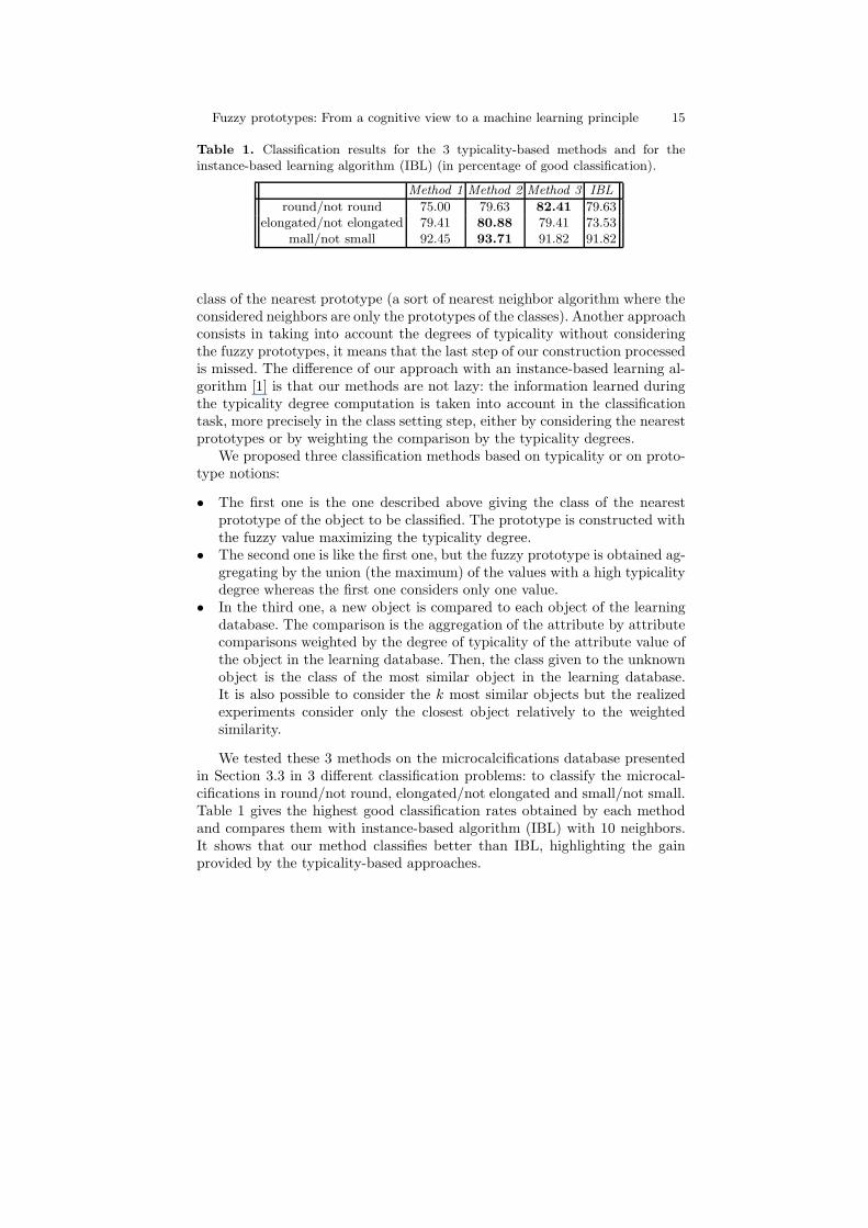
Table 1. Classification results for the 3 typicality-based methods and for theinstance-based learning algorithm (IBL) (in percentage of good classification).

Method 1 Method 2 Method 3 IBL

round/not round 75.00 79.63 82.41 79.63elongated/not elongated 79.41 80.88 79.41 73.53

mall/not small 92.45 93.71 91.82 91.82

class of the nearest prototype (a sort of nearest neighbor algorithm where theconsidered neighbors are only the prototypes of the classes). Another approachconsists in taking into account the degrees of typicality without consideringthe fuzzy prototypes, it means that the last step of our construction processedis missed. The difference of our approach with an instance-based learning al-gorithm [1] is that our methods are not lazy: the information learned duringthe typicality degree computation is taken into account in the classificationtask, more precisely in the class setting step, either by considering the nearestprototypes or by weighting the comparison by the typicality degrees.

We proposed three classification methods based on typicality or on proto-type notions:

• The first one is the one described above giving the class of the nearestprototype of the object to be classified. The prototype is constructed withthe fuzzy value maximizing the typicality degree.

• The second one is like the first one, but the fuzzy prototype is obtained ag-gregating by the union (the maximum) of the values with a high typicalitydegree whereas the first one considers only one value.

• In the third one, a new object is compared to each object of the learningdatabase. The comparison is the aggregation of the attribute by attributecomparisons weighted by the degree of typicality of the attribute value ofthe object in the learning database. Then, the class given to the unknownobject is the class of the most similar object in the learning database.It is also possible to consider the k most similar objects but the realizedexperiments consider only the closest object relatively to the weightedsimilarity.

We tested these 3 methods on the microcalcifications database presentedin Section 3.3 in 3 different classification problems: to classify the microcal-cifications in round/not round, elongated/not elongated and small/not small.Table 1 gives the highest good classification rates obtained by each methodand compares them with instance-based algorithm (IBL) with 10 neighbors.It shows that our method classifies better than IBL, highlighting the gainprovided by the typicality-based approaches.

16 Marie-Jeanne Lesot, Maria Rifqi, and Bernadette Bouchon-Meunier

5 Extension to unsupervised learning: clustering

In this section, we further exploit the notion of prototype as a machine learningprinciple, considering the unsupervised learning case and more precisely theclustering task.

5.1 Motivation

Clustering [14] aims at decomposing a data set into subgroups, or clusters,that are both homogeneous and distinct: the fact that the subgroups are ho-mogeneous (their compactness) implies that points assigned to the same clus-ter indeed resemble one another, which justifies their grouping. The fact thatthey are distinct (their separability) implies that points assigned to differentsubgroups are dissimilar one from another, which justifies their non-groupingand the individual existence of each cluster. Thus the cluster decompositionprovides a simplified representation of the data set, that summarizes it andhighlights its underlying structure.

Now these compactness and separability properties can be matched withthe properties on which typicality degrees rely, namely internal resemblanceand external dissimilarity: a cluster is compact if all its members resembleone another, which is equivalent to their having a high internal resemblance.Likewise, clusters are separable, if all their members are dissimilar from otherclusters members, i.e. if they have a high external dissimilarity. Thus a clusterdecomposition has a high quality if all points have a high typicality degree forthe cluster they are assigned to.

This is illustrated using the artificial two-dimensional data set shown onfigure 7a. Figures 7b and 7d present two data decompositions into 2 subgroups,respectively depicted with + and ⊳. Figures 7c and 7e show their associatedtypicality degree distribution: for each point, represented by its identificationnumber as indicated on figure 7a, its typicality degrees for the two clusters areindicated, the plain line corresponding to the + cluster, the dashed one to the⊳ cluster. It can be seen that typicality degrees take significantly higher valuesfor the data partition of figure 7d than for the partition of figure 7b that iscounter-intuitive and does not correspond to the expected decomposition: themost satisfying decomposition is the one for which each point is more typicalof the cluster it belongs to.

Thus we propose to exploit the typicality degree framework to performclustering: the typicality-based clustering algorithm (TBC) [20] looks for adecomposition such that each point is most typical of the cluster it is assignedto, and aims at maximizing the typicality degrees.

5.2 Typicality-based clustering algorithm

Following the motivations described above, the typicality-based clustering al-gorithm consists in alternating two steps:

Fuzzy prototypes: From a cognitive view to a machine learning principle 17

−2 −1 0 1 2−2

−1

0

1

2

1 2

3 4 5

8 9

10 11 12

13 1476

−2 −1 0 1 2−2

−1

0

1

2

0 5 100

0.2

0.4

0.6

0.8

1

(a) (b) (c)

−2 −1 0 1 2−2

−1

0

1

2

0 5 100

0.2

0.4

0.6

0.8

1

(d) (e)

Fig. 7. Motivation of the typicality-based clustering algorithm. (a) Considered dataset and data point numbering. (b) Counter-intuitive decomposition into 2 clusters,respectively depicted with + and ⊳, (c) associated typicality degrees with respectto the 2 clusters, for all data points represented by their identification number; theplain line indicates the typicality degree with respect to the + cluster, the dashed onefor the ⊳ cluster. (d) Decomposition into the 2 expected clusters and (e) associatedtypicality degrees.

1. Assuming a data partition, compute typicality degrees with respect to theclusters,

2. Assuming typicality degrees, modify the data partition so that each pointbecomes more typical of the cluster it is assigned to.

This means, one reduces to the supervised case considering the candi-date categories provided by the data decomposition, and one then evaluatesthese candidates using the computed typicality degrees. According to empiri-cal tests, this alternated process converges very rapidly to a stable partition,that corresponds to the desired partition [20].

Among the expected advantages of this approach are robustness to outliersand ability to avoid cluster overlapping areas: both outliers and points locatedin overlapping areas can be identified easily, as they have low typicality degrees(respectively because of low internal resemblance and low external dissimila-rity), leading to clusters that are indeed compact and separable. Moreover,after the algorithm has converged, the final typicality degree distribution canbe exploited to build fuzzy prototypes characterizing the obtained clusters,offering an interpretable representation of the clusters.

Regarding the typicality computation step, two differences are to be un-derlined as compared to the supervised case described in Section 3. First, inthe supervised learning framework, typicality is only considered for the cate-

18 Marie-Jeanne Lesot, Maria Rifqi, and Bernadette Bouchon-Meunier

gory a point belongs to, and equals 0 for the other categories. In the clusteringcase, clusters are to be identified, and different assignments must be consid-ered, thus typicality degrees are computed for all points and all clusters. Thecandidate partition is only used to determine which points must be takeninto account for the computation of internal resemblance and external dissi-milarity: for instance, for a given point, when its typicality with respect tocluster C is computed, internal resemblance is based on points assigned to Caccording to the candidate partition.

A second difference between supervised and unsupervised learning regardsthe choice of the aggregation operator defining typicality degrees from internalresemblance and external dissimilarity: it cannot be chosen as freely in bothcases. Indeed, in the supervised case, on may be interested in discriminativeprototypes (e.g. in classification tasks), thus a high importance may be givento external dissimilarity. In clustering, both internal resemblance and externaldissimilarity must be influential, otherwise, outliers may be considered ashighly typical of any cluster, distorting the clustering results. This means theaggregation operator must be a conjunctive operator or a variable behavioroperator [20].

5.3 Experimental results

In order to illustrate the properties of the typicality-based clustering algorithm(TBC), its results on the artificial two-dimensional data set shown on figure 8aare presented. The latter is made of 3 Gaussian clusters and a small outlyinggroup in the upper left corner.

Typicality-based clustering algorithm

Figures 8b and 8c represent the level lines of the obtained typicality degreedistribution and the associated fuzzy prototypes, when 3 clusters are searchedfor. Each symbol depicts a different cluster, the stars represent points assignedto the fictitious cluster that represents outliers and points in overlapping areas(more precisely, this cluster groups points with low typicality degrees [20]).Figure 8b shows that the expected clusters are identified, as well as the out-liers. These results show the method indeed takes into account both internalresemblance and external dissimilarity.

The effect of these two components can also be seen in the typicalitydistribution: on the one hand, the distributions are approximately centeredaround the group center, due to the internal resemblance constraint. On theother hand, the distribution of the upper cluster for instance is more spreadon the x-axis than on the y-axis: the overlap with the two other clusters leadsto reduced typicality degrees, due to the external dissimilarity constraint.

The associated fuzzy prototypes shown on figure 8c provide relevant sum-maries of the clusters: they have small support, and characterize the clusters.Indeed, they are concentrated on the central part of the clusters, but also

Fuzzy prototypes: From a cognitive view to a machine learning principle 19

−2 0 2 4 6

−2

−1

0

1

2

3

4

5

−2 0 2 4 6

−2

−1

0

1

2

3

4

5

0

0.1

0.2

0.3

0.4

0.5

0.6

0.7

0.8

0.9

1

−2 0 2 4 6

−2

−1

0

1

2

3

4

5

0

0.1

0.2

0.3

0.4

0.5

0.6

0.7

0.8

0.9

1

(a) (b) (c)

−2 0 2 4 6

−2

−1

0

1

2

3

4

5

0

0.1

0.2

0.3

0.4

0.5

0.6

0.7

0.8

0.9

1

−2 0 2 4 6

−2

−1

0

1

2

3

4

5

0

0.1

0.2

0.3

0.4

0.5

0.6

0.7

0.8

0.9

1

(d) (e)

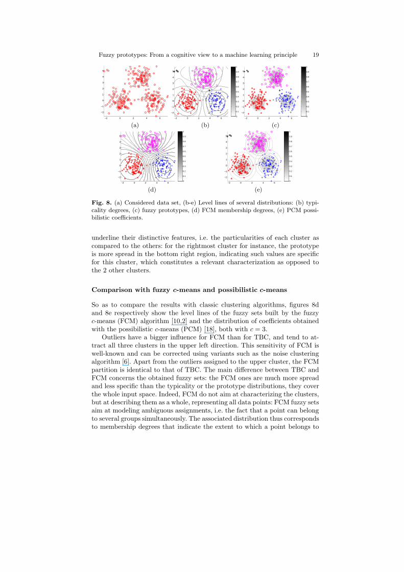
Fig. 8. (a) Considered data set, (b-e) Level lines of several distributions: (b) typi-cality degrees, (c) fuzzy prototypes, (d) FCM membership degrees, (e) PCM possi-bilistic coefficients.

underline their distinctive features, i.e. the particularities of each cluster ascompared to the others: for the rightmost cluster for instance, the prototypeis more spread in the bottom right region, indicating such values are specificfor this cluster, which constitutes a relevant characterization as opposed tothe 2 other clusters.

Comparison with fuzzy c-means and possibilistic c-means

So as to compare the results with classic clustering algorithms, figures 8dand 8e respectively show the level lines of the fuzzy sets built by the fuzzyc-means (FCM) algorithm [10,2] and the distribution of coefficients obtainedwith the possibilistic c-means (PCM) [18], both with c = 3.

Outliers have a bigger influence for FCM than for TBC, and tend to at-tract all three clusters in the upper left direction. This sensitivity of FCM iswell-known and can be corrected using variants such as the noise clusteringalgorithm [6]. Apart from the outliers assigned to the upper cluster, the FCMpartition is identical to that of TBC. The main difference between TBC andFCM concerns the obtained fuzzy sets: the FCM ones are much more spreadand less specific than the typicality or the prototype distributions, they coverthe whole input space. Indeed, FCM do not aim at characterizing the clusters,but at describing them as a whole, representing all data points: FCM fuzzy setsaim at modeling ambiguous assignments, i.e. the fact that a point can belongto several groups simultaneously. The associated distribution thus correspondsto membership degrees that indicate the extent to which a point belongs to

20 Marie-Jeanne Lesot, Maria Rifqi, and Bernadette Bouchon-Meunier

each cluster. Fuzzy prototypes only represent the most typical points, theycorrespond to fuzzy sets that characterize each cluster, indicating the extentto which a point belongs to the representative description of the cluster.

The PCM coefficients (see fig. 8e) correspond to a third semantics. It can beobserved that their distributions are spherical for all 3 clusters: the underlyingfunctions are indeed decreasing functions of the distance to the cluster center.This implies they are to be interpreted as internal resemblances, not takinginto account any external dissimilarity component. Thus, contrary to FCM,PCM are not sensitive to outliers, the latter are indeed identified as such andnot assigned to any of the three clusters. Yet due this weight definition PCMsuffer from convergence problems: they sometime fail to detect the expectedclusters and identify several times the same cluster [13]. To avoid this effect,Timm and Kruse [34] introduce in the PCM cost function a cluster repulsionterm, so as to force clusters apart. The proposed typicality-based approachcan be seen as another solution to this problem: the external dissimilaritycomponent also leads to a cluster repulsion effect. The latter is incorporatedin the coefficient definition itself and not only in the cluster center expression,enriching the coefficient semantics.

5.4 Algorithm extensions

The previous typicality-based clustering mechanism can be extended to adaptto specific data or cluster constraints, we briefly mention here two extensions.

TBC does not depend on the data points themselves, but only on theircomparison through resemblance and dissimilarity measures: contrary to FCMor PCM, it does not require the computation of data means and in the courseof the optimization process, clusters are only represented by the set of theirmembers, and not cluster centers. This implies that the algorithm is indepen-dent of the data nature, and makes it possible to extend it to other distances[21]: on the one hand, non-Euclidean distances can be used, in particular toidentify non-convex clusters; on the other hand, non-vectorial data, such assequences, trees or graphs can be handled.

Another extension concerns the use of typicality degrees in a Gustafson-Kessel manner: the Gustafson-Kessel algorithm [12] is a variant of FCM thatmakes it possible to identify ellipsoidal clusters, whereas FCM restrict tospherical clusters, through the automatic extraction of the cluster covariancematrices: contrary to the previous methods, the appropriate distance functionis not determined at the beginning of the algorithm, but is automaticallylearned from the data. The Gustafson-Kessel-like typicality-based clusteringalgorithm [22] modifies the optimization scheme presented in Section 5.2 toestimate cluster centers and cluster covariance matrices, using as weights thetypicality degrees. As TBC, it is robust with respect to outliers and ableto avoid overlapping areas between clusters, leading to both compact andseparable clusters [22].

Fuzzy prototypes: From a cognitive view to a machine learning principle 21

6 Conclusion

In this paper, we considered the cognitive definition of prototype and ty-picality and proposed to extend them to machine learning and data miningtasks. First, these notions make it possible to characterize data categories,underlining both the common features of the category members and their dis-criminative features, i.e. the category specificity, leading to an interpretabledata summarization; they can be applied both to crisp and fuzzy data. Fur-thermore, these notions can be extended to extract knowledge from the data,both in supervised and unsupervised learning frameworks, to perform classi-fication and clustering.

Perspectives of this work include the extension of the typicality notionto other machine learning tasks, and in particular to feature selection: whenapplied attribute by attribute, typicality makes it possible to identify pro-perties that have no typical values for categories, and are thus not relevantfor the category description. This approach has the advantage of defininglocal feature selection, insofar as attribute relevance is not defined for thewhole data set, but locally for each category (or each cluster in unsupervisedlearning). Links with other feature selection methods, and particular entropy-based approaches are to be studied in details.

References

1.D. W. Aha, D. Kibler, and M. K. Albert. Instance-based learning algorithms.Machine Learning, 6:37–66, 1991.

2.J. Bezdek. Fuzzy mathematics in pattern classification. PhD thesis, Applied Math-ematical Center, Cornell University, 1973.

3.S. Bothorel, B. Bouchon-Meunier, and S. Muller. Fuzzy logic-based approach forsemiological analysis of microcalcification in mammographic images. Interna-

tional Journ. of Intelligent Systems, 12:814–843, 1997.4.B. Bouchon-Meunier, M. Rifqi, and S. Bothorel. Towards general measures of

comparison of objects. Fuzzy Sets and Systems, 84(2):143–153, 1996.5.T. Calvo, A. Kolesarova, M. Komornikova, and R. Mesiar. Aggregation operators:

properties, classes and construction methods. In Aggregation operators: new

trends and applications, pages 3–104. Physica-Verlag, 2002.6.R. Dave. Characterization and detection of noise in clustering. Pattern Recognition

Letters, 12:657–664, 1991.7.M. Detyniecki. Mathematical Aggregation Operators and their Application to Video

Querying. PhD thesis, University of Pierre and Marie Curie, 2000.8.D. Dubois and H. Prade. Fuzzy Sets and Systems, Theory and Applications. Aca-

demic Press, New York, 1980.9.D. Dubois and H. Prade. A unifying view of comparison indices in a fuzzy set-

theoretic framework. In R. R. Yager, editor, Fuzzy set and possibility theory,pages 3–13. Pergamon Press, 1982.

10.J.C. Dunn. A fuzzy relative of the isodata process and its use in detecting compactwell-separated clusters. Journ. of Cybernetics, 3:32–57, 1973.

22 Marie-Jeanne Lesot, Maria Rifqi, and Bernadette Bouchon-Meunier

11.M. Friedman, M. Ming, and A. Kandel. On the theory of typicality. Int. Journ.of Uncertainty, Fuzziness and Knowledge-Based Systems, 3(2):127–142, 1995.

12.E. Gustafson and W. Kessel. Fuzzy clustering with a fuzzy covariance matrix. InProc. of IEEE CDC, pages 761–766, 1979.

13.F. Hoppner, F. Klawonn, R. Kruse, and T. Runkler. Fuzzy Cluster Analysis,

Methods for classification, data analysis and image recognition. Wiley, 2000.14.A. Jain, M. Murty, and P. Flynn. Data clustering: a review. ACM Computing

survey, 31(3):264–323, 1999.15.J. Kacprzyk and R. Yager. Linguistic summaries of data using fuzzy logic. Int.

Journ. of General Systems, 30:133–154, 2001.16.J. Kacprzyk, R. Yager, and S. Zadrozny. A fuzzy logic based approach to linguistic

summaries of databases. Int. Journ. of Applied Mathematics and Computer

Science, 10:813–834, 2000.17.A. Kelman and R. Yager. On the application of a class of mica operators.

Int. Journ. of Uncertainty, Fuzziness and Knowledge-Based Systems, 7:113–126, 1995.

18.R. Krishnapuram and J. Keller. A possibilistic approach to clustering. IEEE

Transactions on fuzzy systems, 1:98–110, 1993.19.M.-J. Lesot. Similarity, typicality and fuzzy prototypes for numerical data. In

6th European Congress on Systems Science, Workshop ”Similarity and resem-

blance”, 2005.20.M.-J. Lesot. Typicality-based clustering. Int. Journ. of Information Technology

and Intelligent Computing, 2006.21.M.-J. Lesot and R. Kruse. Data summarisation by typicality-based clustering for

vectorial data and nonvectorial data. In Proc. of the IEEE Int. Conf. on Fuzzy

Systems, Fuzz-IEEE’06, pages 3011–3018, 2006.22.M.-J. Lesot and R. Kruse. Gustafson-Kessel-like clustering algorithm based on

typicality degrees. In Proc. of IPMU’06, 2006.23.M.-J. Lesot, L. Mouillet, and B. Bouchon-Meunier. Fuzzy prototypes based on

typicality degrees. In B. Reusch, editor, Proc. of the 8th Fuzzy Days 2004,Advances in Soft Computing, pages 125–138. Springer, 2005.

24.M. Mizumoto. Pictorial representations of fuzzy connectives, part I: Cases of t-norms, t-conorms and averaging operators. Fuzzy Sets and Systems, 31(2):217–242, 1989.

25.M. Mizumoto. Pictorial representations of fuzzy connectives, part II: Casesof compensatory operators and self-dual operators. Fuzzy Sets and Systems,32(1):45–79, 1989.

26.N. Pal, K. Pal, and J. Bezdek. A mixed c-means clustering model. In Proc. of

the IEEE Int. Conf. on Fuzzy Systems, Fuzz-IEEE’97, pages 11–21, 1997.27.M.I. Posner and S.W. Keele. On the genesis of abstract ideas. Journ. of Experi-

mental Psychology, 77:353–363, 1968.28.A. Rick, S. Bothorel, B. Bouchon-Meunier, S. Muller, and M. Rifqi. Fuzzy tech-

niques in mammographic image processing. In Etienne Kerre and Mike Nachte-gael, editors, Fuzzy Techniques in Image Processing, Studies in Fuzziness andSoft Computing, pages 308–336. Springer Verlag, 2000.

29.M. Rifqi. Constructing prototypes from large databases. In Proc. of IPMU’96,pages 301–306, 1996.

30.M. Rifqi, V. Berger, and B. Bouchon-Meunier. Discrimination power of measuresof comparison. Fuzzy sets and systems, 110:189–196, 2000.

Fuzzy prototypes: From a cognitive view to a machine learning principle 23

31.E. Rosch. Principles of categorization. In E. Rosch and B. Lloyd, editors, Cog-nition and categorization, pages 27–48. Lawrence Erlbaum associates, 1978.

32.E. Rosch and C. Mervis. Family resemblance: studies of the internal structure ofcategories. Cognitive psychology, 7:573–605, 1975.

33.W. Silvert. Symmetric summation: a class of operations on fuzzy sets. IEEE

Transactions on Systems, Man and Cybernetics, 9:659–667, 1979.34.H. Timm and R. Kruse. A modification to improve possibilistic fuzzy cluster

analysis. In Proc. of the IEEE Int. Conf. on Fuzzy Systems, Fuzz-IEEE’02,2002.

35.A. Tversky. Features of similarity. Psychological Review, 84:327–352, 1977.36.L. Wittgenstein. Philosophical investigations. Macmillan, 1953.37.R. Yager. A human directed approach for data summarization. In Proc. of the

IEEE Int. Conf. on Fuzzy Systems, Fuzz-IEEE’06, pages 3604–3609, 2006.38.L. A. Zadeh. A note on prototype theory and fuzzy sets. Cognition, 12:291–297,

1982.