Fusion of magnetic resonance and ultrasound images for ...
203
En vue de l'obtention du DOCTORAT DE L'UNIVERSITÉ DE TOULOUSE Délivré par : Institut National Polytechnique de Toulouse (Toulouse INP) Discipline ou spécialité : Signal, Image, Acoustique et Optimisation Présentée et soutenue par : Mme OUMAIMA EL MANSOURI le lundi 7 décembre 2020 Titre : Unité de recherche : Ecole doctorale : Fusion of magnetic resonance and ultrasound images for endometriosis detection Mathématiques, Informatique, Télécommunications de Toulouse (MITT) Institut de Recherche en Informatique de Toulouse ( IRIT) Directeur(s) de Thèse : M. ADRIAN BASARAB M. JEAN-YVES TOURNERET Rapporteurs : Mme MIREILLE GARREAU, UNIVERSITE RENNES 1 M. PHILIPPE CIUCIU, CEA SACLAY Membre(s) du jury : M. JEAN-PHILIPPE THIRAN, ECOLE POLYTECHNIQUE FEDERALE DE LAUSANNE, Président M. ADRIAN BASARAB, UNIVERSITE PAUL SABATIER, Membre M. DENIS KOUAME, UNIVERSITE PAUL SABATIER, Membre M. JEAN-YVES TOURNERET, TOULOUSE INP, Membre M. MARIO FIGUEIREDO, INSTITUTO SUPERIOR TECNICO LISBONNE, Membre M. XAVIER PENNEC, INRIA SOPHIA ANTIPOLIS, Membre M. DENIS KOUAME
-
Upload
khangminh22 -
Category
Documents
-
view
0 -
download
0
Transcript of Fusion of magnetic resonance and ultrasound images for ...
En vue de l'obtention du
DOCTORAT DE L'UNIVERSITÉ DE TOULOUSEDélivré par :
Institut National Polytechnique de Toulouse (Toulouse INP)Discipline ou spécialité :
Signal, Image, Acoustique et Optimisation
Présentée et soutenue par :Mme OUMAIMA EL MANSOURI
le lundi 7 décembre 2020
Titre :
Unité de recherche :
Ecole doctorale :
Fusion of magnetic resonance and ultrasound images for endometriosisdetection
Mathématiques, Informatique, Télécommunications de Toulouse (MITT)
Institut de Recherche en Informatique de Toulouse ( IRIT)Directeur(s) de Thèse :
M. ADRIAN BASARABM. JEAN-YVES TOURNERET
Rapporteurs :Mme MIREILLE GARREAU, UNIVERSITE RENNES 1
M. PHILIPPE CIUCIU, CEA SACLAY
Membre(s) du jury :M. JEAN-PHILIPPE THIRAN, ECOLE POLYTECHNIQUE FEDERALE DE LAUSANNE, Président
M. ADRIAN BASARAB, UNIVERSITE PAUL SABATIER, MembreM. DENIS KOUAME, UNIVERSITE PAUL SABATIER, Membre
M. JEAN-YVES TOURNERET, TOULOUSE INP, MembreM. MARIO FIGUEIREDO, INSTITUTO SUPERIOR TECNICO LISBONNE, Membre
M. XAVIER PENNEC, INRIA SOPHIA ANTIPOLIS, Membre
M. DENIS KOUAME

ii
Acknowledgements
I would like firstly to express my sincere gratitude to my supervisors Professors Adrian Basarab, Denis
Kouamé, and Jean-Yves Tourneret, they convincingly guided and encouraged me to be professional
and do the right thing even when the road got tough. I am very grateful to all of them for their
scientific advice, the insightful discussions that we had. I would like to thank you for encouraging
my research and for allowing me to grow as a research scientist. I would like to thank the surgeon
gynecologist Fabien Vidal from CHU Toulouse, you have been there to support this Ph.D. in many
ways: your phantom enable us to validate our fusion method and your comments help us to improve
the quality of the proposed method, thank you.
I also have to thank the members of my Ph.D. committee, Professors Jean-Philippe Thiran,
Mireille Garreau, Philippe Ciuciu, Mario Figueiredo, and Xavier Pennec for serving as my committee
members. I also want to thank you for letting my defense be an enjoyable moment, and for your
brilliant comments and suggestions, thanks to you.
I thank all the former and present members of the IRIT lab especially my great office mate who
has been supportive in every way (thank you Mohamad Hourani and good luck). I would like also to
thank my second family in the TéSA lab. I shared unforgettable moments with you. I will cherish
these memories for the rest of my life. A special thanks to Corinne Mailhes. You are the nicest
person I’ve ever met.
A special thanks to my family. Words can not express how thankful I am to my mother, father,
and brothers (Hamid, Soufyan, Oussama El Manssouri, and Saida Ech-charyfy). My parents have
sacrificed their lives for me and provided unconditional care and love. I truly love them so much,
iii

and I would not have made it this far without them. I would also like to thank my beloved husband
Yacine Khoya for his support, he was by my side in bad and good moments. I love you my darling. I
am also grateful to my family in law (Hammadi, Mariam, Mohamed, Ilias, Asmaa, Inasse, Wissam,
and Marwa Khoya). They are my new family who supported and encouraged me during this PhD.
I would also like to thank my best friends and sisters (Salma, Nadia, Sabrina [and Adem], Aicha,
Maki, and Hanene). You have been great supporters during my bad and good moments.
These past three years have not been an easy ride, both personally and academically. I truly
thank you all for staying by my side, even when I was irritable.
iv
Résumé
L’endométriose est un trouble gynécologique qui touche généralement les femmes en âge de pro-
créer et qui est associé à des douleurs pelviennes chroniques et à l’infertilité. L’endométriose est
un exemple typique de pathologie qui nécessite l’utilisation de l’imagerie à résonance magnétique
(IRM) et l’imagerie ultrasonore (US) (appelée aussi échographie) pour le diagnostic préopératoire et
la chirurgie guidée. Ces modalités sont utilisées conjointement car elles contiennent des informations
complémentaires. Cependant, le fait qu’elles aient des résolutions, des champs de vue et des con-
trastes différents et qu’elles soient corrompues par des bruits de differentes natures rend la collecte
d’informations à partir de ces modalités difficile pour les radiologues. Ainsi, la fusion des images IRM
et l’échographie peut faciliter la tâche des experts médicaux et améliorer le diagnostic préopératoire
et le plan de l’intervention chirurgicale.
L’objet de cette thèse de doctorat est de proposer une nouvelle méthode de fusion automatique
des images IRM et US. Tout d’abord, nous supposons que les images IRM et US à fusionner sont
alignées, c’est-à-dire qu’il n’y a pas de déformation géométrique entre elles. Nous proposons alors dans
ce contexte idéal des méthodes de fusion pour ces deux images, qui visent à combiner les avantages
de chaque modalité, c’est-à-dire un bon contraste et un bon rapport signal/bruit pour l’IRM et
une bonne résolution spatiale pour l’échographie. L’algorithme proposé est basé sur un problème
inverse, réalisant une super-résolution de l’image IRM et un débruitage de l’image US. Des fonctions
polynomiales sont introduites pour modéliser les relations entre les niveaux de gris des images IRM
et US. Cependant, la méthode de fusion proposée est très sensible aux erreurs de recalage. C’est
pourquoi, dans un deuxième temps, nous proposons une méthode conjointe de fusion et de recalage
v
pour ces deux modalités. La fusion d’images IRM/US proposée permet d’obtenir conjointement une
super-résolution de l’image IRM et un débruitage de l’image US, et peut automatiquement prendre
en compte les erreurs de recalage. Une fonction polynomiale est utilisée pour relier les images
ultrasonores et IRM dans le processus de fusion, tandis qu’une mesure de similarité appropriée est
introduite pour traiter le problème de recalage. Le recalage proposé est basé sur une transformation
non rigide contenant un modèle élastique local de B-spline et une transformation affine globale.
Les opérations de fusion et de recalage sont effectuées alternativement, ce qui simplifie le problème
d’optimisation sous-jacent. L’intérêt de la fusion et du recalage conjoints est analysé à l’aide des
images synthétiques et expérimentales.
vi
Abstract
Endometriosis is a gynecologic disorder that typically affects women in their reproductive age and
is associated with chronic pelvic pain and infertility. In the context of pre-operative diagnosis and
guided surgery, endometriosis is a typical example of pathology that requires the use of both magnetic
resonance (MR) and ultrasound (US) modalities. These modalities are used side by side because they
contain complementary information. However, MRI and US images have different spatial resolutions,
fields of view and contrasts and are corrupted by different kinds of noise, which results in important
challenges related to their analysis by radiologists. The fusion of MR and US images is a way of
facilitating the task of medical experts and improve the pre-operative diagnosis and the surgery
mapping.
The object of this PhD thesis is to propose a new automatic fusion method for MRI and US
images. First, we assume that the MR and US images to be fused are aligned, i.e., there is no
geometric distortion between these images. We propose a fusion method for MR and US images,
which aims at combining the advantages of each modality, i.e., good contrast and signal to noise ratio
for the MR image and good spatial resolution for the US image. The proposed algorithm is based
on an inverse problem, performing a super-resolution of the MR image and a denoising of the US
image. A polynomial function is introduced to model the relationships between the gray levels of the
MR and US images. However, the proposed fusion method is very sensitive to registration errors.
Thus, in a second step, we introduce a joint fusion and registration method for MR and US images.
Registration is a complicated task in practical applications. The proposed MR/US image fusion
performs jointly super-resolution of the MR image and despeckling of the US image, and is able to
vii

automatically account for registration errors. A polynomial function is used to link ultrasound and
MR images in the fusion process while an appropriate similarity measure is introduced to handle the
registration problem. The proposed registration is based on a non-rigid transformation containing a
local elastic B-spline model and a global affine transformation. The fusion and registration operations
are performed alternatively simplifying the underlying optimization problem. The interest of the joint
fusion and registration is analyzed using synthetic and experimental phantom images.
viii
Acronyms
ADMM Alternating Direction Method of Multipliers
ANN Artificial Neural Networks
BCCB Block Circulant matrix of Circulant Blocks
CC Cross-Correlation
CNR Contrast-to-Noise Ratio
CT Computed Tomography
CVT Curvelet Transform
DICOM Digital Imaging and Communication in Medicine
DSC Dice Similarity Coefficient
DWT Discrete Wavelet Transform
EM Expectation-maximization
EN Entropy
FF Fusion Factor
FSIM Feature similarity index metric
GGD Generalized Gaussian Distribution
HR High Resolution
ix
ICP Iterative Closest Point
INPT Institut national polytechnique de Toulouse
IRIT Institut de Recherche en Informatique de Toulouse
ISNR Improvement in Signal-to-Noise Ratio
i.i.d independent and identically distributed
LC Local Correlation
LC2 Linear Correlation of Linear Combination
LPT Laplacian Pyramid Transform
LR Low Resolution
NMR Nuclear Magnetic Resonance
MI Mutual Information
MMSE Minimum Mean Square Error
MRI Magnetic Resonance Imaging
MSSIM Mean Structural Similarity Index Measure
NMI Normalized Mutual Information
NMSE Normalized Mean Square Error
NRMSE Normalized Root Mean Square Error
PALM Proximal Alternating Linearized Minimization
PCA Principal Component Analysis
PET Positron Emission Tomography
PSNR Peak Signal-to-Noise Ratio
PVA Polyvinyl Acid
RBF Radial Basis Functions
RF radio-frequencyx
RMSE Root Mean Square Error
SNR Signal-to-Noise Ratio
RF Radio-Frequency
RMSE Root Mean Square Error
SNR Signal-to-Noise Ratio
SPECT Single-Photon Emission Computed Tomography
SR Super Resolution
SSD Sum of Squared intensity Differences
SSIM Structural Similarity Index Measure
STD Standard Deviation
TPS Thin-Plate Splines
TRE Target Registration Error
TRF Tissue Reflectivity Function
TV Total Variation
TRUS Transrectal Ultrasound
TVUS Transvaginal Ultrasound
UIQI Universal Image Quality Indexing
US Ultrasound
xi

xii
Contents
Acknowledgements iii
Résumé v
Abstract vii
Acronyms ix
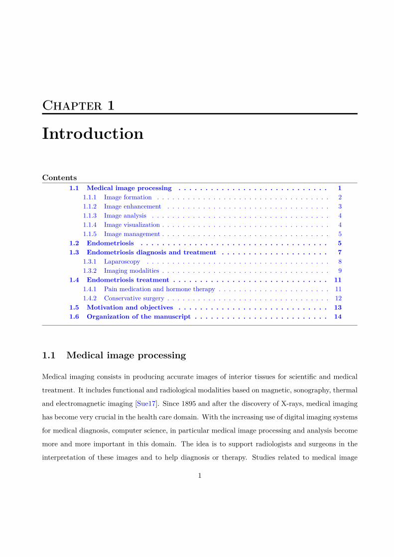
Chapter 1 Introduction 1
1.1 Medical image processing . . . . . . . . . . . . . . . . . . . . . . . . . . . . . . . . . . 1
1.1.1 Image formation . . . . . . . . . . . . . . . . . . . . . . . . . . . . . . . . . . . 2
1.1.2 Image enhancement . . . . . . . . . . . . . . . . . . . . . . . . . . . . . . . . . 3
1.1.3 Image analysis . . . . . . . . . . . . . . . . . . . . . . . . . . . . . . . . . . . . 4
1.1.4 Image visualization . . . . . . . . . . . . . . . . . . . . . . . . . . . . . . . . . . 4
1.1.5 Image management . . . . . . . . . . . . . . . . . . . . . . . . . . . . . . . . . . 5
1.2 Endometriosis . . . . . . . . . . . . . . . . . . . . . . . . . . . . . . . . . . . . . . . . . 5
1.3 Endometriosis diagnosis and treatment . . . . . . . . . . . . . . . . . . . . . . . . . . . 7
1.3.1 Laparoscopy . . . . . . . . . . . . . . . . . . . . . . . . . . . . . . . . . . . . . 8
1.3.2 Imaging modalities . . . . . . . . . . . . . . . . . . . . . . . . . . . . . . . . . . 9
1.4 Endometriosis treatment . . . . . . . . . . . . . . . . . . . . . . . . . . . . . . . . . . . 11
1.4.1 Pain medication and hormone therapy . . . . . . . . . . . . . . . . . . . . . . . 11
1.4.2 Conservative surgery . . . . . . . . . . . . . . . . . . . . . . . . . . . . . . . . . 12
xiii
1.5 Motivation and objectives . . . . . . . . . . . . . . . . . . . . . . . . . . . . . . . . . . 13
1.6 Organization of the manuscript . . . . . . . . . . . . . . . . . . . . . . . . . . . . . . . 14
List of publications 17
Chapter 2 MRI and Ultrasound imaging 19
2.1 MR image formation . . . . . . . . . . . . . . . . . . . . . . . . . . . . . . . . . . . . . 19
2.1.1 Nuclear spin and magnets . . . . . . . . . . . . . . . . . . . . . . . . . . . . . . 20
2.1.2 Relaxation . . . . . . . . . . . . . . . . . . . . . . . . . . . . . . . . . . . . . . 21
2.1.3 Spatial encoding in MR images . . . . . . . . . . . . . . . . . . . . . . . . . . . 23
2.2 MR super-resolution . . . . . . . . . . . . . . . . . . . . . . . . . . . . . . . . . . . . . 24
2.3 US image formation . . . . . . . . . . . . . . . . . . . . . . . . . . . . . . . . . . . . . 25
2.3.1 US propagation . . . . . . . . . . . . . . . . . . . . . . . . . . . . . . . . . . . . 26
2.3.2 US transducer . . . . . . . . . . . . . . . . . . . . . . . . . . . . . . . . . . . . 29
2.3.3 US data . . . . . . . . . . . . . . . . . . . . . . . . . . . . . . . . . . . . . . . . 29
2.4 Speckle reduction for US imaging . . . . . . . . . . . . . . . . . . . . . . . . . . . . . . 31
2.4.1 Other medical imaging modalities . . . . . . . . . . . . . . . . . . . . . . . . . 33
2.5 Conclusion . . . . . . . . . . . . . . . . . . . . . . . . . . . . . . . . . . . . . . . . . . 34
Chapter 3 Fusion and Registration in Medical Imaging 37
3.1 Introduction . . . . . . . . . . . . . . . . . . . . . . . . . . . . . . . . . . . . . . . . . . 37
3.2 Medical image fusion . . . . . . . . . . . . . . . . . . . . . . . . . . . . . . . . . . . . 39
3.2.1 Multi-modal image fusion methods . . . . . . . . . . . . . . . . . . . . . . . . . 41
3.2.2 Conclusion . . . . . . . . . . . . . . . . . . . . . . . . . . . . . . . . . . . . . . 56
3.3 Medical image registration . . . . . . . . . . . . . . . . . . . . . . . . . . . . . . . . . 57
3.3.1 Image similarity measure . . . . . . . . . . . . . . . . . . . . . . . . . . . . . . 59
3.3.2 Transformation models . . . . . . . . . . . . . . . . . . . . . . . . . . . . . . . . 63
3.3.3 Regularization in deformable registration . . . . . . . . . . . . . . . . . . . . . 67
3.3.4 Optimization . . . . . . . . . . . . . . . . . . . . . . . . . . . . . . . . . . . . . 69
xiv
3.3.5 Image registration metrics . . . . . . . . . . . . . . . . . . . . . . . . . . . . . . 70
3.4 MR and US registration: state of art . . . . . . . . . . . . . . . . . . . . . . . . . . . . 71
3.4.1 Intensity-based methods . . . . . . . . . . . . . . . . . . . . . . . . . . . . . . . 72
3.4.2 Feature-based methods . . . . . . . . . . . . . . . . . . . . . . . . . . . . . . . 74
3.4.3 Other approach . . . . . . . . . . . . . . . . . . . . . . . . . . . . . . . . . . . . 75
3.4.4 Conclusion . . . . . . . . . . . . . . . . . . . . . . . . . . . . . . . . . . . . . . 75
3.5 Global Conclusions . . . . . . . . . . . . . . . . . . . . . . . . . . . . . . . . . . . . . . 75
Chapter 4 Fusion of MRI and US images 77
4.1 Introduction . . . . . . . . . . . . . . . . . . . . . . . . . . . . . . . . . . . . . . . . . 77
4.2 MR/US fusion using a global polynomial function . . . . . . . . . . . . . . . . . . . . . 78
4.2.1 A statistical model for the fusion of MRI and US images . . . . . . . . . . . . 78
4.2.2 Algorithm for MR/US fusion . . . . . . . . . . . . . . . . . . . . . . . . . . . . 83
4.2.3 Simulation results . . . . . . . . . . . . . . . . . . . . . . . . . . . . . . . . . . 89
4.3 MR/US images fusion using a patch-wise polynomial . . . . . . . . . . . . . . . . . . . 109
4.3.1 Estimation of the polynomial functions fp . . . . . . . . . . . . . . . . . . . . . 109
4.3.2 Experimental results using a patch-wise polynomial function . . . . . . . . . . 110
4.4 Conclusion . . . . . . . . . . . . . . . . . . . . . . . . . . . . . . . . . . . . . . . . . . 114
Chapter 5 Joint registration and fusion of MRI and ultrasound images 115
5.1 Introduction . . . . . . . . . . . . . . . . . . . . . . . . . . . . . . . . . . . . . . . . . 115
5.2 MR/US image fusion and registration . . . . . . . . . . . . . . . . . . . . . . . . . . . 116
5.2.1 Observation models . . . . . . . . . . . . . . . . . . . . . . . . . . . . . . . . . 116
5.2.2 US/MR dependence model . . . . . . . . . . . . . . . . . . . . . . . . . . . . . 117
5.2.3 Proposed inverse problem . . . . . . . . . . . . . . . . . . . . . . . . . . . . . . 119
5.3 Proposed registration . . . . . . . . . . . . . . . . . . . . . . . . . . . . . . . . . . . . 120
5.3.1 Similarity measure . . . . . . . . . . . . . . . . . . . . . . . . . . . . . . . . . . 120
5.3.2 Spatial transformation . . . . . . . . . . . . . . . . . . . . . . . . . . . . . . . 121
5.3.3 Regularization . . . . . . . . . . . . . . . . . . . . . . . . . . . . . . . . . . . . 123
xv
5.4 Optimization algorithm for joint fusion and registration . . . . . . . . . . . . . . . . . 123
5.4.1 Estimation of the fused image for known (Tc) . . . . . . . . . . . . . . . . . . 124
5.4.2 Estimation of the spatial transformation . . . . . . . . . . . . . . . . . . . . . 126
5.4.3 Estimation of the polynomial function . . . . . . . . . . . . . . . . . . . . . . . 127
5.4.4 Proposed algorithm . . . . . . . . . . . . . . . . . . . . . . . . . . . . . . . . . 127
5.4.5 Performance measures . . . . . . . . . . . . . . . . . . . . . . . . . . . . . . . . 127
5.4.6 Simulation results on synthetic data . . . . . . . . . . . . . . . . . . . . . . . . 129
5.4.7 Experimental results on phantom data . . . . . . . . . . . . . . . . . . . . . . . 131
5.4.8 Hyperparameters . . . . . . . . . . . . . . . . . . . . . . . . . . . . . . . . . . . 137
5.5 Conclusions . . . . . . . . . . . . . . . . . . . . . . . . . . . . . . . . . . . . . . . . . . 137
Chapter 6 Conclusions and perspectives 141
Conclusions and perspectives 141
6.1 Conclusions . . . . . . . . . . . . . . . . . . . . . . . . . . . . . . . . . . . . . . . . . . 141
6.2 Future work . . . . . . . . . . . . . . . . . . . . . . . . . . . . . . . . . . . . . . . . . . 142
6.2.1 Short-term perspectives . . . . . . . . . . . . . . . . . . . . . . . . . . . . . . . 142
6.2.2 Long-term perspectives . . . . . . . . . . . . . . . . . . . . . . . . . . . . . . . 143
Appendices 145
Appendix A Design of a pelvic phantom for MR/US fusion . . . . . . . . . . . . . . . . . 147
A.1 Phantom design . . . . . . . . . . . . . . . . . . . . . . . . . . . . . . . . . . . . . . . . 147
A.2 Imaging techniques . . . . . . . . . . . . . . . . . . . . . . . . . . . . . . . . . . . . . . 148
A.3 Imaging results . . . . . . . . . . . . . . . . . . . . . . . . . . . . . . . . . . . . . . . . 149
Bibliography 187
xvi
Chapter 1
Introduction
Contents1.1 Medical image processing . . . . . . . . . . . . . . . . . . . . . . . . . . . . 1
1.1.1 Image formation . . . . . . . . . . . . . . . . . . . . . . . . . . . . . . . . . . 21.1.2 Image enhancement . . . . . . . . . . . . . . . . . . . . . . . . . . . . . . . . 31.1.3 Image analysis . . . . . . . . . . . . . . . . . . . . . . . . . . . . . . . . . . . 41.1.4 Image visualization . . . . . . . . . . . . . . . . . . . . . . . . . . . . . . . . . 41.1.5 Image management . . . . . . . . . . . . . . . . . . . . . . . . . . . . . . . . . 5
1.2 Endometriosis . . . . . . . . . . . . . . . . . . . . . . . . . . . . . . . . . . . 51.3 Endometriosis diagnosis and treatment . . . . . . . . . . . . . . . . . . . . 7
1.3.1 Laparoscopy . . . . . . . . . . . . . . . . . . . . . . . . . . . . . . . . . . . . 81.3.2 Imaging modalities . . . . . . . . . . . . . . . . . . . . . . . . . . . . . . . . . 9
1.4 Endometriosis treatment . . . . . . . . . . . . . . . . . . . . . . . . . . . . . 111.4.1 Pain medication and hormone therapy . . . . . . . . . . . . . . . . . . . . . . 111.4.2 Conservative surgery . . . . . . . . . . . . . . . . . . . . . . . . . . . . . . . . 12
1.5 Motivation and objectives . . . . . . . . . . . . . . . . . . . . . . . . . . . . 131.6 Organization of the manuscript . . . . . . . . . . . . . . . . . . . . . . . . . 14
1.1 Medical image processing
Medical imaging consists in producing accurate images of interior tissues for scientific and medical
treatment. It includes functional and radiological modalities based on magnetic, sonography, thermal
and electromagnetic imaging [Sue17]. Since 1895 and after the discovery of X-rays, medical imaging
has become very crucial in the health care domain. With the increasing use of digital imaging systems
for medical diagnosis, computer science, in particular medical image processing and analysis become
more and more important in this domain. The idea is to support radiologists and surgeons in the
interpretation of these images and to help diagnosis or therapy. Studies related to medical image
1
2 Chapter 1 - Introduction
processing reveal that these methods can not only improve the accuracy of the radiologist diagnosis
but also help to overcome the increasing data volume that challenges radiologist time. Also, the
decisions of radiologists can be affected by many factors like fatigue, distraction and experience
which is not the case of machines. There are several areas in which image processing techniques are
used to identify abnormalities or tumors in brain, heart, chest, lung, breast, prostate, colon, skeletal,
liver or vascular system [Ban08].
In the early 1980s, large-scale research on computer-aided diagnosis (CAD) started to take place
in the health care field [Doi07]. In 1982, M. Ishida [IKDF82] investigated the development of a
new digital radiographic image processing system. In 1985, M. L. Giger [GD85] examined the basic
imaging properties in digital radiography such as the effect of pixel size on signal to noise ratio (SNR)
and threshold contrast. In 1986, K. R.Hoffmann [HDC+86] proposed an automated tracking of the
vascular tree in digital subtraction angiography images using a double-square-box region-of-search
algorithm. In addition to these pioneer works, several studies have been conducted in order to help
radiologist in various clinical applications [IFDL83, IDLL84, GD84, LDM85, FDG85, GDF86]. The
concept of CAD was established in the 1960s [LHS+63, MNJB+64] but it was not effective until the
1980s due to the fact that computers were not sufficiently powerful.
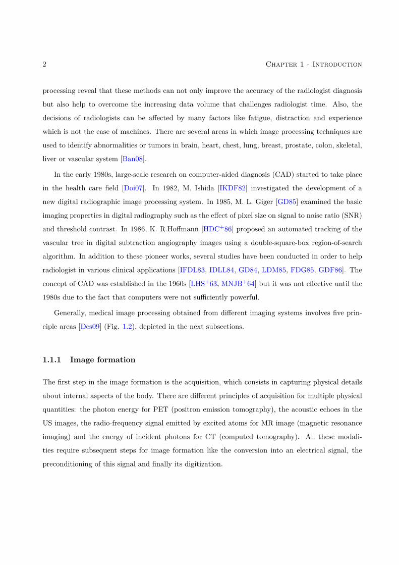
Generally, medical image processing obtained from different imaging systems involves five prin-
ciple areas [Des09] (Fig. 1.2), depicted in the next subsections.
1.1.1 Image formation
The first step in the image formation is the acquisition, which consists in capturing physical details
about internal aspects of the body. There are different principles of acquisition for multiple physical
quantities: the photon energy for PET (positron emission tomography), the acoustic echoes in the
US images, the radio-frequency signal emitted by excited atoms for MR image (magnetic resonance
imaging) and the energy of incident photons for CT (computed tomography). All these modali-
ties require subsequent steps for image formation like the conversion into an electrical signal, the
preconditioning of this signal and finally its digitization.
1.1 - Medical image processing 3
Figure 1.1: Medical image processing. Globally, image processing involves five major steps: imageformation, image enhancement, visualization, image analysis and management [Des09].
1.1.2 Image enhancement
The aim of medical image enhancement is to improve the interpretability of the information contained
in the image by applying an appropriate transformation to the image. Classical transformations are
defined in the spatial or frequency domains [MA10].
In the spatial domain, transforms are applied directly on image pixels, which is often used for
contrast optimization [KK16]. These methods generally rely on histogram [ATL14], logarithmic
[HAY10] and power law transforms [SS10]. In the frequency domain, standard methods capture the
spectral information contained in the image [YSS10], through filters [MM08], which can be used
to smooth or sharpen the images. These techniques allow for noise, artifacts and blur reduction,
enhancement of edges, contrast optimization and improvement of other fundamental properties that
4 Chapter 1 - Introduction
are important for an accurate interpretation.
1.1.3 Image analysis
Image analysis is an important step in image processing [DA00], it has several objectives such as:
image segmentation, image registration and image fusion.
Image segmentation is considered as an important step in CAD since it helps radiologists to
extract regions of interest (ROI) based on automatic or semi-automatic methods. It is the process
of dividing an image into homogeneous parts using specific attributes. Generally, the purpose of
segmentation is border detection, tumor detection and mass detection [PXP00].
Image fusion refers to assembling all the important information from multiple images and
including them in fewer images, e.g., in a single image. The purpose of image fusion is to reduce
the number of images and to build an enhanced image that is informative [JD14a], comprehensible
and accurate for the operator. The fusion of medical images is used for several studies of pathologies
and generally grants better medical decisions in clinical studies. Medical images that can be fused
efficiently include MR and single-photon emission computed tomography (SPECT) images [PHS+96],
MR and computed tomography (CT) [WB08], or positron emission tomography (PET) and CT
[VOB+04].
Image registration creates a common geometric reference frame across two or more image
datasets [OT14a]. It is a required task for the fusion and the comparison between images obtained
at different times or using different imaging modalities.
1.1.4 Image visualization
Image visualization refers to all types of matrix manipulations, resulting in an optimized output of
the image. Many applications require visualization and analysis of three-dimensional (3D) objects.
The aim of image visualization is to gain insight into the collected data through the process of
transforming, mapping, and view the collected data as images with high quality. This technology
provides crucial devices for diagnosis, research and instruction where the human body is interactively
explored. In order to visualize volumes, it is important not only to collect different viewpoints but
1.2 - Endometriosis 5
also to respect subtle variations in density and opacity while displaying them. Extensive researches
are done in this field especially in 3D reconstruction [NTCO12].
1.1.5 Image management
Image management deals with all the tools that provide practiced storage (servers, clouds), commu-
nication, sharing, archiving, backup, and access to image data [RP04]. Medical images use DICOM
(Digital Imaging and Communication in Medicine) for storage, which may require several megabytes
of storage capacity, and compression techniques. Also, techniques used in telemedicine/telehealth
are part of image management [TKO96, MLM+01].
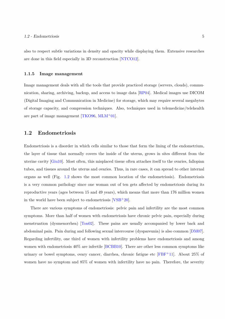
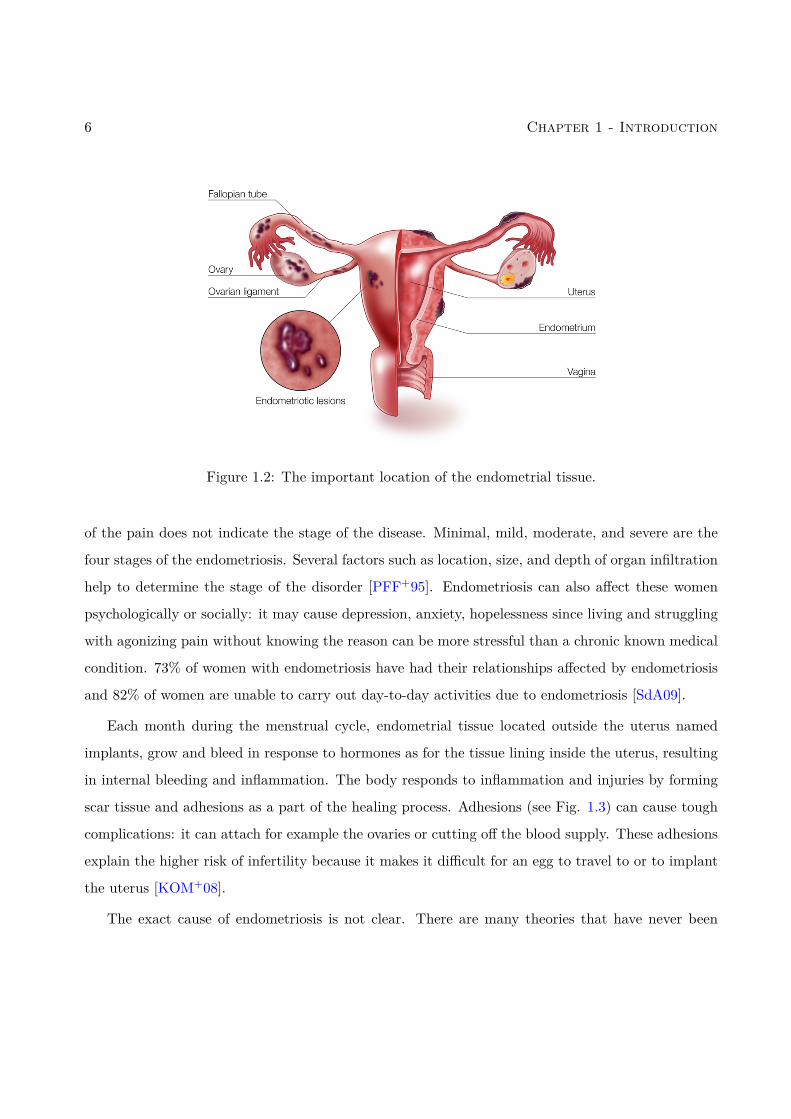
1.2 Endometriosis
Endometriosis is a disorder in which cells similar to those that form the lining of the endometrium,
the layer of tissue that normally covers the inside of the uterus, grows in sites different from the
uterine cavity [Giu10]. Most often, this misplaced tissue often attaches itself to the ovaries, fallopian
tubes, and tissues around the uterus and ovaries. Thus, in rare cases, it can spread to other internal
organs as well (Fig. 1.2 shows the most common location of the endometriosis). Endometriosis
is a very common pathology since one woman out of ten gets affected by endometriosis during its
reproductive years (ages between 15 and 49 years), which means that more than 176 million women
in the world have been subject to endometriosis [VSB+20].
There are various symptoms of endometriosis: pelvic pain and infertility are the most common
symptoms. More than half of women with endometriosis have chronic pelvic pain, especially during
menstruation (dysmenorrhea) [Ton02]. These pains are usually accompanied by lower back and
abdominal pain. Pain during and following sexual intercourse (dyspareunia) is also common [DM07].
Regarding infertility, one third of women with infertility problems have endometriosis and among
women with endometriosis 40% are infertile [BCBB10]. There are other less common symptoms like
urinary or bowel symptoms, ovary cancer, diarrhea, chronic fatigue etc [FBF+11]. About 25% of
women have no symptom and 85% of women with infertility have no pain. Therefore, the severity
6 Chapter 1 - Introduction
Figure 1.2: The important location of the endometrial tissue.
of the pain does not indicate the stage of the disease. Minimal, mild, moderate, and severe are the
four stages of the endometriosis. Several factors such as location, size, and depth of organ infiltration
help to determine the stage of the disorder [PFF+95]. Endometriosis can also affect these women
psychologically or socially: it may cause depression, anxiety, hopelessness since living and struggling
with agonizing pain without knowing the reason can be more stressful than a chronic known medical
condition. 73% of women with endometriosis have had their relationships affected by endometriosis
and 82% of women are unable to carry out day-to-day activities due to endometriosis [SdA09].
Each month during the menstrual cycle, endometrial tissue located outside the uterus named
implants, grow and bleed in response to hormones as for the tissue lining inside the uterus, resulting
in internal bleeding and inflammation. The body responds to inflammation and injuries by forming
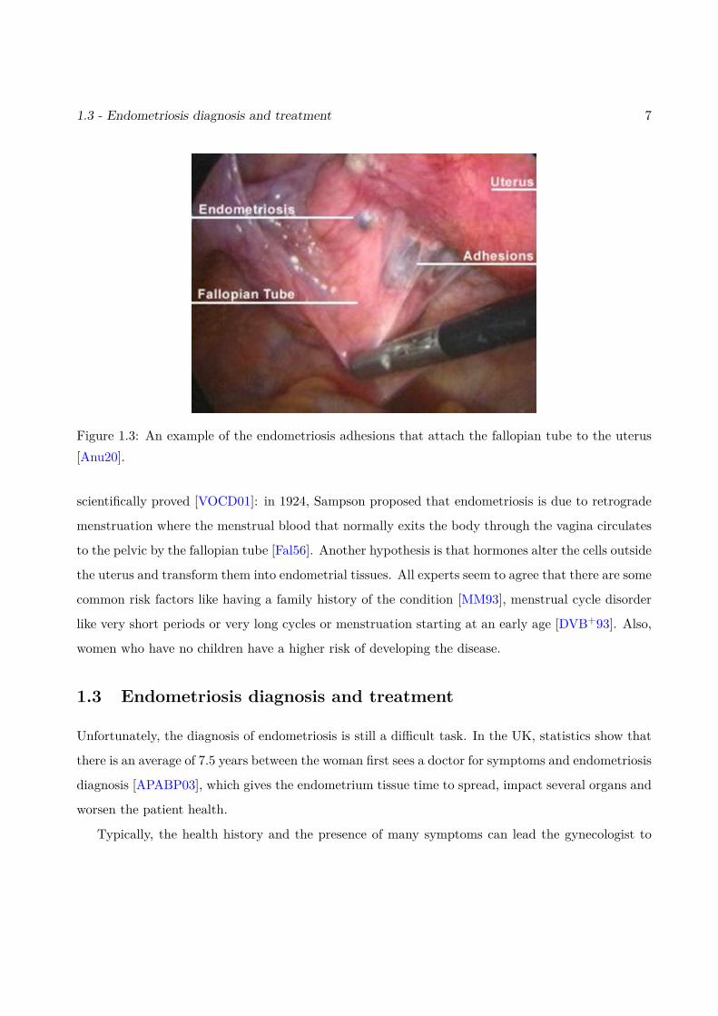
scar tissue and adhesions as a part of the healing process. Adhesions (see Fig. 1.3) can cause tough
complications: it can attach for example the ovaries or cutting off the blood supply. These adhesions
explain the higher risk of infertility because it makes it difficult for an egg to travel to or to implant
the uterus [KOM+08].
The exact cause of endometriosis is not clear. There are many theories that have never been
1.3 - Endometriosis diagnosis and treatment 7
Figure 1.3: An example of the endometriosis adhesions that attach the fallopian tube to the uterus[Anu20].
scientifically proved [VOCD01]: in 1924, Sampson proposed that endometriosis is due to retrograde
menstruation where the menstrual blood that normally exits the body through the vagina circulates
to the pelvic by the fallopian tube [Fal56]. Another hypothesis is that hormones alter the cells outside
the uterus and transform them into endometrial tissues. All experts seem to agree that there are some
common risk factors like having a family history of the condition [MM93], menstrual cycle disorder
like very short periods or very long cycles or menstruation starting at an early age [DVB+93]. Also,
women who have no children have a higher risk of developing the disease.
1.3 Endometriosis diagnosis and treatment
Unfortunately, the diagnosis of endometriosis is still a difficult task. In the UK, statistics show that
there is an average of 7.5 years between the woman first sees a doctor for symptoms and endometriosis
diagnosis [APABP03], which gives the endometrium tissue time to spread, impact several organs and
worsen the patient health.
Typically, the health history and the presence of many symptoms can lead the gynecologist to
8 Chapter 1 - Introduction
suspect endometriosis. Doctors generally start with a pelvic physical examination by feeling and
palpating the pelvis for abnormalities like cysts [BLR+09]. However, this technique is unable to
detect small areas with endometriosis and implants that are note located in the cervix, the vagina,
and the vulva.
Visual examination using laparoscopy [JRH+13] and different medical image modalities such as
transvaginal ultrasound (TVUS) [SBHU91] and magnetic resonance imaging (MRI) [ZDFZB03] are
the standard for the diagnosis of endometriosis. There is no consensus on the use of CT scanning
images due to a lack of contrast resolution [WJLS98].
Since there is no effective treatment, hormonal medication is used to decrease the pain in periods
and intercourse. However, depending on the disease stage, laparoscopic surgery reveals to be the
unique effective pain-relief [JDB+10]. TVUS and magnetic resonance (MR) images, besides being
used for diagnosis, are used to identify endometriosis and its depth of infiltration in organs before
performing surgery.
1.3.1 Laparoscopy
Laparoscopy (minimally invasive surgery) is an operation procedure performed in the pelvis and the
abdomen using tiny cuts (0.5cm-1cm) and a camera to look inside the abdominal cavity. Laparoscopy
is the most common way to officially diagnose endometriosis. A careful investigation of the pelvic
during laparoscopy permits lesion visualization. Sometimes a biopsy can be taken to confirm the
diagnosis. During a laparoscopy, various procedures can be performed in order to destroy or remove
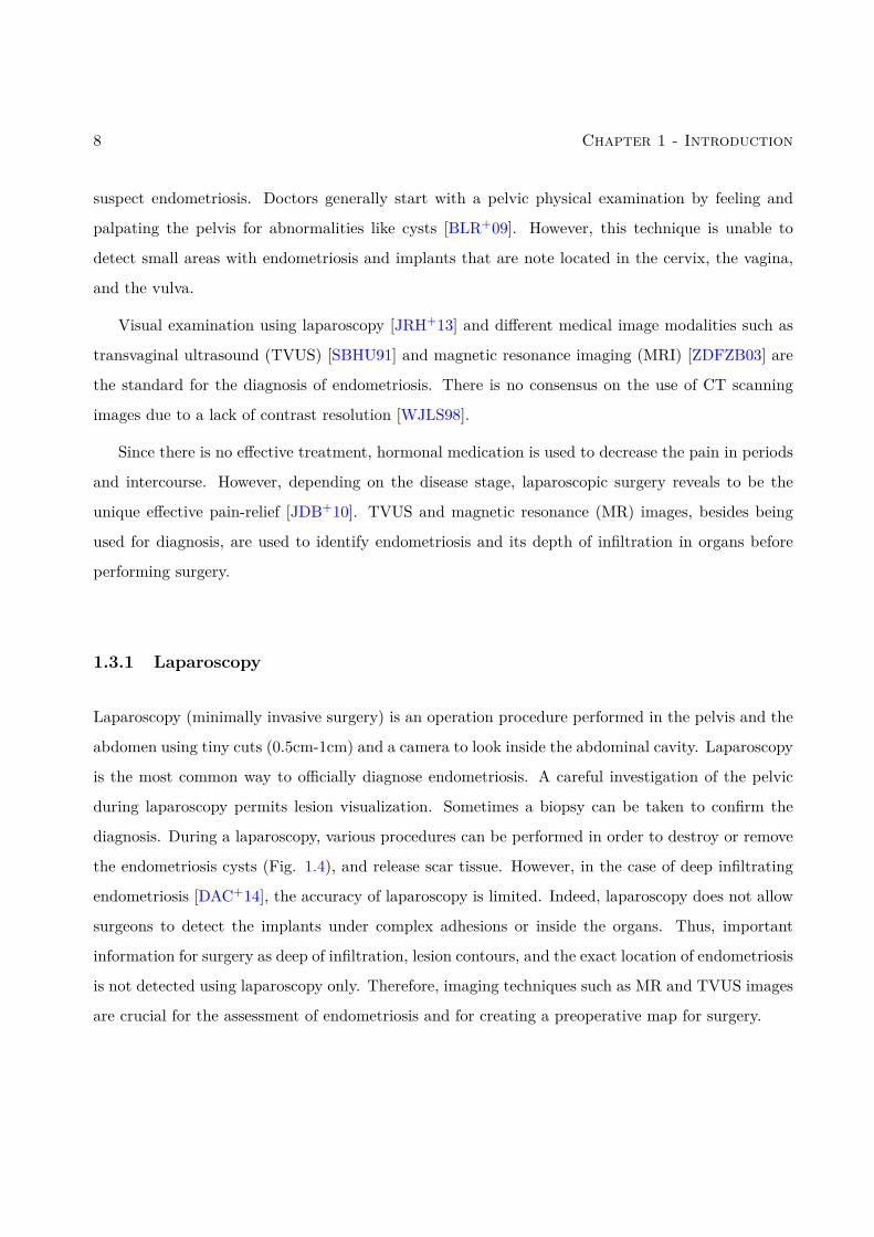
the endometriosis cysts (Fig. 1.4), and release scar tissue. However, in the case of deep infiltrating
endometriosis [DAC+14], the accuracy of laparoscopy is limited. Indeed, laparoscopy does not allow
surgeons to detect the implants under complex adhesions or inside the organs. Thus, important
information for surgery as deep of infiltration, lesion contours, and the exact location of endometriosis
is not detected using laparoscopy only. Therefore, imaging techniques such as MR and TVUS images
are crucial for the assessment of endometriosis and for creating a preoperative map for surgery.
1.3 - Endometriosis diagnosis and treatment 9
Figure 1.4: Inspecting the pelvic cavity for severe endometriosis location and excision [Gyn15].
1.3.2 Imaging modalities
Diagnosing endometriosis requires a reliable diagnostic imaging exam. Additionally, preoperative
images such as MR and TVUS images are crucial for identifying the different locations of deep
endometriosis because in certain sites, such as the intestine or bladder, the surgery is particularly
difficult and carries greater risk.
1.3.2.1 Transvaginal ultrasound (TVUS)
Transvaginal ultrasound or endovaginal ultrasound, is an internal examination of the reproductive
female organs as the uterus, fallopian tubes, ovaries and cervix by introducing gently a high-frequency
transducer probe (10MHz) into the vagina, and exploring the pelvic cavity.
Vaginal ultrasound has clinical value in the diagnosis of the endometrioma (endometriosis cysts)
and before operating for deep endometriosis. This concerns the identification of the spread of disease
in women with well-established clinical suspicion of endometriosis. Vaginal ultrasound is inexpen-
sive, easily accessible, has no counter-argument, and requires no preparation. Experts conducting
ultrasound examinations need to be experienced. The sonographer can evaluate and look for deep
infiltrating endometriosis adhesions (Fig. 1.5) and implants noting the size, location, and if applica-
ble, the distance from the anus [HET+11]. TVUS images have also some limitations which are the
10 Chapter 1 - Introduction
huge amount of speckle reducing the signal to noise ratio, and also their limited field of view and
low contrast. An improvement in sonographic detection of deep infiltrating endometriosis would not
only reduce the number of diagnostic laparoscopies, but it will also guide management and enhance
the quality of life.
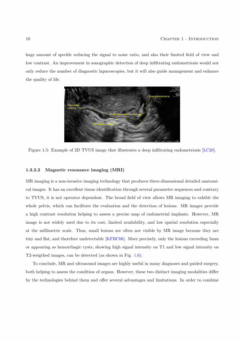
Figure 1.5: Example of 2D TVUS image that illustrates a deep infiltrating endometriosis [LC20].
1.3.2.2 Magnetic resonance imaging (MRI)
MR imaging is a non-invasive imaging technology that produces three-dimensional detailed anatomi-
cal images. It has an excellent tissue identification through several parameter sequences and contrary
to TVUS, it is not operator dependent. The broad field of view allows MR imaging to exhibit the
whole pelvis, which can facilitate the evaluation and the detection of lesions. MR images provide
a high contrast resolution helping to assess a precise map of endometrial implants. However, MR
image is not widely used due to its cost, limited availability, and low spatial resolution especially
at the millimetric scale. Thus, small lesions are often not visible by MR image because they are
tiny and flat, and therefore undetectable [KFBC06]. More precisely, only the lesions exceeding 5mm
or appearing as hemorrhagic cysts, showing high signal intensity on T1 and low signal intensity on
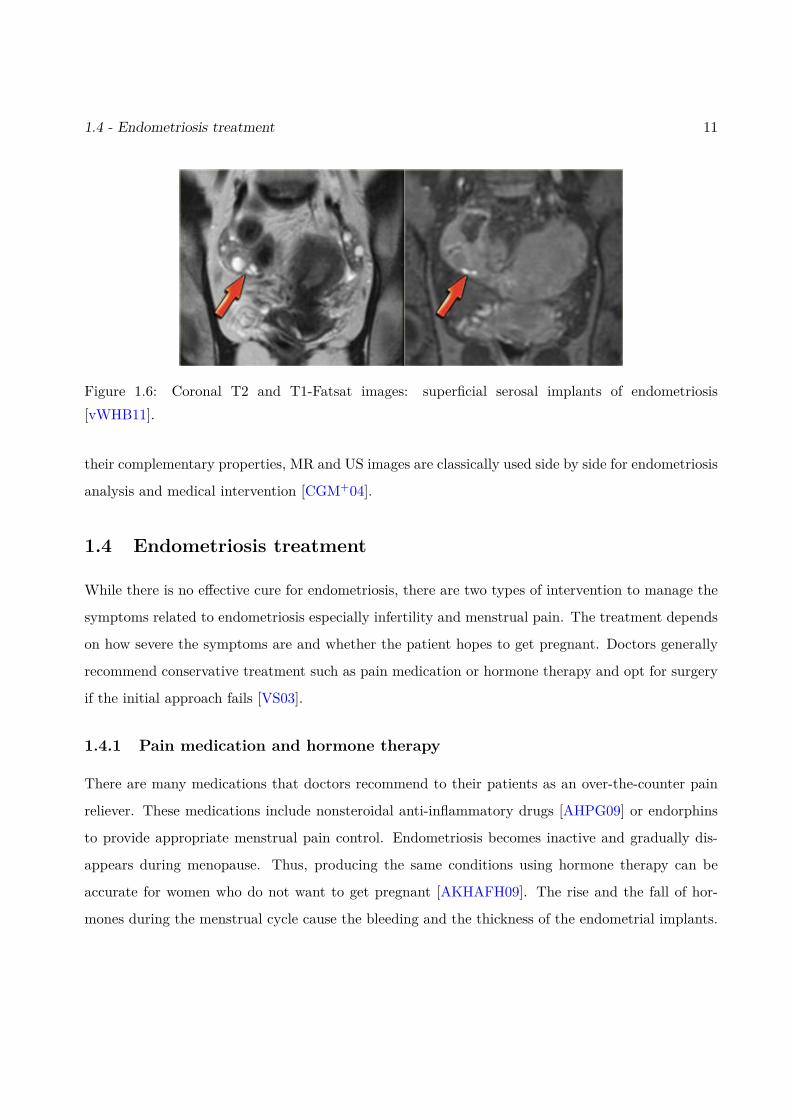
T2-weigthed images, can be detected (as shown in Fig. 1.6).
To conclude, MR and ultrasound images are highly useful in many diagnoses and guided surgery,
both helping to assess the condition of organs. However, these two distinct imaging modalities differ
by the technologies behind them and offer several advantages and limitations. In order to combine
1.4 - Endometriosis treatment 11
Figure 1.6: Coronal T2 and T1-Fatsat images: superficial serosal implants of endometriosis[vWHB11].
their complementary properties, MR and US images are classically used side by side for endometriosis
analysis and medical intervention [CGM+04].
1.4 Endometriosis treatment
While there is no effective cure for endometriosis, there are two types of intervention to manage the
symptoms related to endometriosis especially infertility and menstrual pain. The treatment depends
on how severe the symptoms are and whether the patient hopes to get pregnant. Doctors generally
recommend conservative treatment such as pain medication or hormone therapy and opt for surgery
if the initial approach fails [VS03].
1.4.1 Pain medication and hormone therapy
There are many medications that doctors recommend to their patients as an over-the-counter pain
reliever. These medications include nonsteroidal anti-inflammatory drugs [AHPG09] or endorphins
to provide appropriate menstrual pain control. Endometriosis becomes inactive and gradually dis-
appears during menopause. Thus, producing the same conditions using hormone therapy can be
accurate for women who do not want to get pregnant [AKHAFH09]. The rise and the fall of hor-
mones during the menstrual cycle cause the bleeding and the thickness of the endometrial implants.
12 Chapter 1 - Introduction
Stabilizing hormones may stop or slow its growth and prevent new adhesions. Combined estrogen-
progestogen birth control (hormonal contraception) is a gold standard hormone therapy [VPDG+05]
because it can be used during long periods, is inexpensive, and easy to use. Other hormonal medica-
tions can be used as danazol [HCM+88] and gestrinone [DNPCR90] but their use is limited because of
their side effect: excessive hair growth, voice changes and masculinization, etc. Generally, hormone
therapy is combined with pain medication for a conservative treatment. However, these approaches
are not a permanent fix or a cure for endometriosis since patients can experience pain recurrence
after stopping treatment and they are not adapted for women who want to get pregnant.
1.4.2 Conservative surgery
After an accurate diagnosis that indicates the existence of endometriosis, the exact location of im-
plants, their size, and their depth of infiltration, a surgical plan is defined to remove or incise this
endometrial tissue. This procedure is usually done using laparoscopy surgery because it is considered
as minimally invasive [DAC+14, NCG86]: the surgeon inserts a laparoscope with an attached cam-
era (a viewing instrument) through a small incision and inserts through another incisions surgical
instruments for the ablation or the excision of the implants, the adhesions, the endometriomas in
order to restore the pelvic anatomy as normal as possible. The precision of this surgery depends on
the accuracy of the diagnosis which is difficult using the current imaging techniques. Thus, 21.5% of
patients at 2 years and 40−50% at 5 years experience endometriosis recurrence [Guo09], which is due
to part of implants that have not been removed during surgery because of their deep infiltration or
defective surgical planning. Laparoscopy helps to preserve ovaries and the uterus (which is important
for women who want to get pregnant) and reduces the probability of developing adhesions. However,
laparoscopy increases the risk of recurrence.
In many cases, hysterectomy (removal of the uterus) is considered as a cure of endometriosis for
women who do not want to conceive. However, it must be accompanied by endometriosis excision or
the pain will persist if the endometriosis is located in other sites [NHG+95].
1.5 - Motivation and objectives 13
1.5 Motivation and objectives
As explained previously, endometriosis is a typical example of pathology that requires the use of MR
and US modalities in conventional clinical practice. Endometriotic lesions can be either superficial or
deeply infiltrating. Surgery is a cornerstone for endometriosis since disease removal positively impacts
quality of life and fertility [RCLB+18]. First line radiological assessment uses MR and pelvic US
imaging. MR image displays a higher sensitivity for endometriosis diagnosis compared to pelvic US
(0.94 versus 0.79) [NBF+16]. In contrast, pelvic US with transvaginal or transrectal route provides a
better specificity (0.94 versus 0.77) and is more accurate in the evaluation of infiltration depth when
compared to MR images. Considering the benignant nature of the disease and its high recurrence
rate, conservative management treatment involving limited invasive measurements is preferable to
surgery whenever feasible [DR17]. In the setting of deep infiltrating endometriosis, fusing the two
imaging techniques thus appears particularly promising. Indeed, the presence of information coming
from both US and MR modalities in a single image is expected to improve preoperative disease
mapping and subsequent definition of surgical modalities.
The fusion of MR and ultrasound (US) images is a challenging task because the two imaging
modalities have different resolutions and contrasts and are corrupted by different kinds of noise. To
the best of our knowledge, the fusion of MR and US images for endometriosis diagnosis has rarely
been considered in the literature. The primary goal of this work is to propose a fusion method that
considers MR and US image limitations and enhances image quality while gathering the information
from both of them. The US image can also show some deformations under certain conditions.
Introducing the transvaginal probe inside the vagina, full bladder, bowel, or gas inside the rectum
can deform the pelvic organs. Moreover, since the fusion method is very sensitive to the misalignment
between these two images, a joint registration and fusion method for MR and US images is interesting,
which is the second objective of this PhD thesis.
14 Chapter 1 - Introduction
1.6 Organization of the manuscript
The remaining of this thesis consists of 4 chapters and 2 appendices that are described below.
• Chapter 2: This chapter reminds the basic principles related to MR and US image forma-
tion. Moreover, MR and US advantages and limitations are reported and some post-processing
techniques are introduced with a brief state-of-art on MR super-resolution and US despeckling
techniques.
• Chapter 3: Since there is no existing method to fuse MR and US images, this chapter gives a
general review of medical image fusion, summarizing the most known and used medical image
fusion methods, which are classified into pixel-level image fusion and transform-based image
fusion. This chapter also introduces some metrics for performance evaluation that will be
used to evaluate the quality of image fusion. The chapter continues by introducing the image
registration framework and its components with a general survey in medical image registration.
The chapter is concluded by a state-of-the-art on the registration of MR and US images.
Main Contributions
The main contributions of this thesis are as follows.
• Chapter 4: This chapter introduces a new fusion method for magnetic resonance (MR) and
ultrasound (US) images [MBV+19, EMVB+20], which aims at combining the advantages of
each modality, i.e., good contrast and signal to noise ratio for the MR image and good spatial
resolution for the US image. The proposed algorithm is based on an inverse problem, performing
a super-resolution of the MR image and a denoising of the US image. A polynomial function
is introduced to model the relationships between the gray levels of the MR and US images.
The resulting inverse problem is solved using a proximal alternating linearized minimization
algorithm. The accuracy and the interest of the fusion algorithm are shown quantitatively and
qualitatively via evaluations on synthetic and experimental phantom data.
1.6 - Organization of the manuscript 15
• Chapter 5: This chapter introduces a joint fusion and registration method for magnetic res-
onance images (MR) and ultrasound (US) images. Fusion allows complementary information
from these two modalities to be captured, i.e., the good spatial resolution of US images and
the good signal to noise ratio of MR images. However, a good image fusion method requires
images to be registered, which is generally a complicated task in practical applications. The
proposed approach is based on two inverse problems, performing a super-resolution of the MR
image and a despeckling of the US image, and accounting for registration errors. A polynomial
function is used to link US and MR images in the fusion process while an appropriate similarity
measure is introduced to handle the registration problem. This measure is based on a non-rigid
transformation containing a local term based on B-splines and a global term based on an affine
transformation. The fusion and registration operations are performed alternatively simplify-
ing the underlying optimization problem. The interest of the joint fusion and registration is
analyzed quantitatively and qualitatively via synthetic and experimental phantom data.
Appendices
• Appendix A: This appendix presents an unexpensive and easy to make multi-modality
phantom for MR/US image fusion validated by Dr. Vidal. This phantom shows very similar
characteristics to an uterus infiltrated by endometrial tissue.

16 Chapter 1 - Introduction
List of publications
International Journal papers
1. O. El Mansouri, F. Vidal, A. Basarab, P. Payoux, D. Kouame and J.-Y. Tourneret, Fusion
of Magnetic Resonance and Ultrasound Images for Endometriosis Detection, IEEE
Trans. Image Process., 5324-5335, 2020, vol. 29, p. 5324-5335.
Conference papers with proceedings
1. O. El Mansouri, A. Basarab, M. A. T. Figueiredo, D. Kouame and J.-Y. Tourneret,Ultrasound
and magnetic resonance image fusion using a patch-wise polynomial model, in Proc.
IEEE Int. Conf. Image Processing (ICIP), Abu Dhabi, United Arab Emirates, Oct. 2020.
2. O. El Mansouri, F. Vidal, A. Basarab, D. Kouame and J.-Y. Tourneret, Magnetic Resonance
and Ultrasound Image Fusion Using a PALM Algorithm, in Proc. Workshop on signal
processing with Adaptative Sparse Structured Representations (SPARS), Toulouse, France, jul.
2019.
3. O. El Mansouri, F. Vidal, A. Basarab, D. Kouame and J.-Y. Tourneret, Fusion of Magnetic
Resonance and Ultrasound Images: A preliminary study towards endometriosis
detection, in Proc. IEEE Int. Conf. Symposium on Biomedical Imaging: From Nano to
Macro (ISBI), Venice, Italy, Apr. 2018.
17
18 List of publications
Conference papers without proceedings
1. O. El Mansouri, F. Vidal, A. Basarab, D. Kouame and J.-Y. Tourneret, Joint Fusion and
Registration of Magnetic Resonance and Ultrasound Images, IEEE Int. Ultrason.
Symp., Las Vegas, USA, jul. 2019.
2. O. El Mansouri, F. Vidal, A. Basarab, D. Kouame and J.-Y. Tourneret, Fusion of Magnetic
Resonance and Ultrasound Images for Endometriosis Detection, IEEE Int. Ultrason.
Symp., Glasgow, Scotland, UK, sept. 2019.
Chapter 2
MRI and Ultrasound imaging
Contents2.1 MR image formation . . . . . . . . . . . . . . . . . . . . . . . . . . . . . . . 19
2.1.1 Nuclear spin and magnets . . . . . . . . . . . . . . . . . . . . . . . . . . . . . 202.1.2 Relaxation . . . . . . . . . . . . . . . . . . . . . . . . . . . . . . . . . . . . . 212.1.3 Spatial encoding in MR images . . . . . . . . . . . . . . . . . . . . . . . . . . 23
2.2 MR super-resolution . . . . . . . . . . . . . . . . . . . . . . . . . . . . . . . 242.3 US image formation . . . . . . . . . . . . . . . . . . . . . . . . . . . . . . . 25
2.3.1 US propagation . . . . . . . . . . . . . . . . . . . . . . . . . . . . . . . . . . . 262.3.2 US transducer . . . . . . . . . . . . . . . . . . . . . . . . . . . . . . . . . . . 292.3.3 US data . . . . . . . . . . . . . . . . . . . . . . . . . . . . . . . . . . . . . . . 29
2.4 Speckle reduction for US imaging . . . . . . . . . . . . . . . . . . . . . . . 312.4.1 Other medical imaging modalities . . . . . . . . . . . . . . . . . . . . . . . . 33
2.5 Conclusion . . . . . . . . . . . . . . . . . . . . . . . . . . . . . . . . . . . . . 34
2.1 MR image formation
MR image is a medical imaging technique used in diagnosis of several pathologies related to blood
vessels, heart, brain or spinal cord. The principle of MR is based on the nuclear magnetic resonance
(NMR) phenomenon, i.e., the coupling between the magnetic moment of the nucleus of atoms (pro-
tons) and the external magnetic field [MS18], described by Felix Bloch and Edward Mills Purcell in
1946,which made them obtain the Nobel prize in 1952. At the beginning of the 1970s, numerous
developments in NMR, particularly in spectroscopy, suggested new applications for this technique.
In this context, Raymond Vahan Damadian proposed in 1969 to use NMR for medical purposes
and supported his proposal with the demonstration that NMR spectroscopy allows the detection of
tumors [KD15].
19
20 Chapter 2 - MRI and Ultrasound imaging
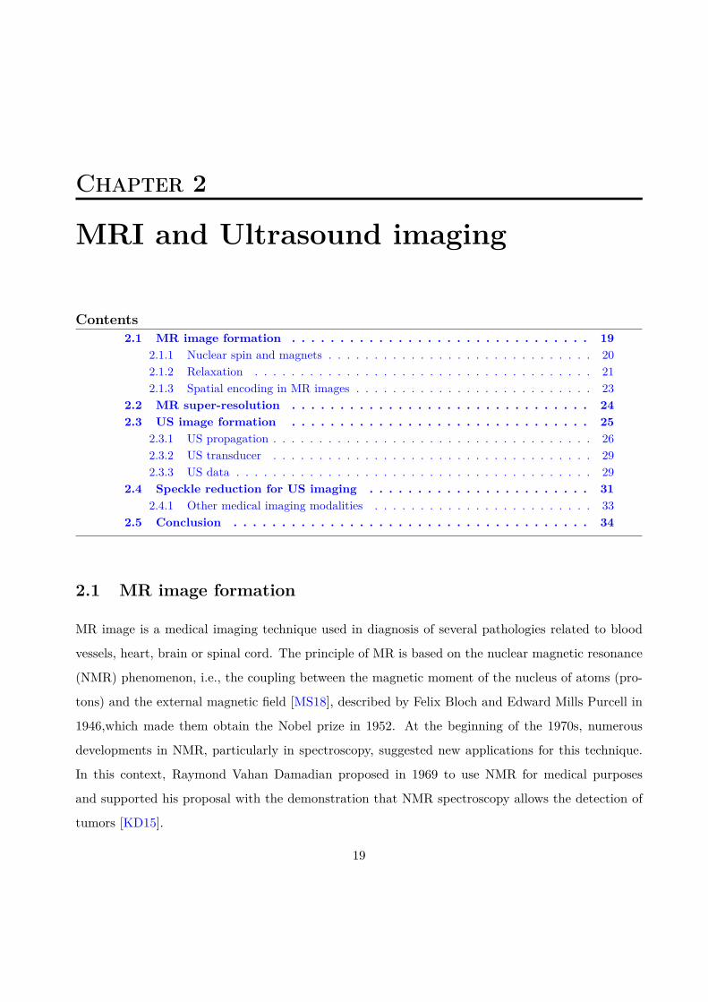
Figure 2.1: MR machine.
NMR is based on the spin magnetic moment caused by the nuclei of atomic isotopes such as
hydrogen (H); Hydrogen is found in large quantities in the human body via the water (H2O) contained
by the tissues and the organic molecules.
2.1.1 Nuclear spin and magnets
All nucleons (neutrons and protons) have the quantum property of spin quantified by the spin angular
momentum ~S. The spin depends on the number of neutrons and protons in the atom (in the case of
hydrogen, there is only one proton, thus the spin of this proton is the spin of the atom). A non-null
spin ~S is associated with a magnetic moment ~µ via the relation
~µ = γ~S (2.1)
where γ is the gyromagnetic ratio.
The hydrogen has two independent spin states: spin-up and spin-down. In the absence of magnetic
field, the numbers of nucleons in these two states are the same since these states are degenerated.
In this case, no magnetic moment can be detected. For the construction of MRI images, the atoms
2.1 - MR image formation 21
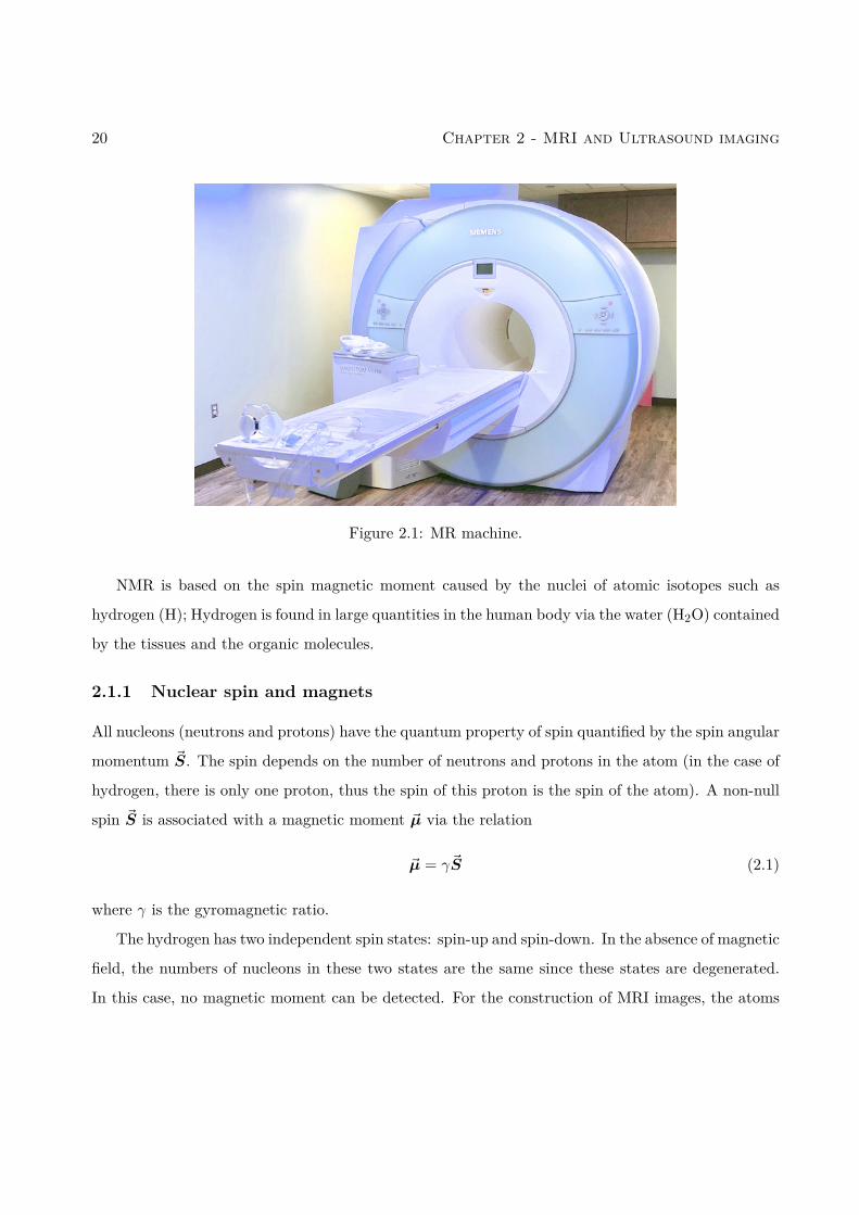
are placed in a large constant magnetic field (0.5 - 4.5T) created by a superconducting magnet (see
Fig. 2.1) and denoted as B0. The interaction between the nuclear magnetic dipole moment and the
external magnetic field results in Larmor precession, a rotation of the nucleons on themselves around
their axis with a rapid precession movement around the axis of the magnetic field. The angular
frequency of this rotation can be writing as follows:
ω0 = γB0. (2.2)
When exposed to magnetic fields, the magnetic dipole moments of protons can either align with the
direction of the external magnetic field B0 (the low energy state) or align with the opposite direction
of B0 (high-energy state). The magnetic field M0 produced by the entire volume is non-null and
represents a longitudinal magnetization aligned with the external magnetization because the slight
majority of protons align in the same direction as B0 (this mechanism is described in Fig. 2.2) as
predicted by Boltzmann theory. Note that the Larmor precession of a proton creates a magnetic
moment that has a non-zero component in the z direction and in the xy plane but considering the
volume, no magnetization is detected in the xy plane as the protons precess out of phase.
The M0 magnetization created by protons cannot form the MR image as B0 masks it. Indeed,
it is impossible to detect the magnetization M0 and produce the MR image as B0 is very large and
masks easily M0. The solution is to flip the magnetization M0 from the z-axis to the xy-plane, which
can be done by a precise excitation with radio-frequency pulses via an external coil. Note that this
excitation brings also protons into phase [MS18].
2.1.2 Relaxation
The following description occurs in a the classical xyz coordinates. After an excitation via RF pulses,
the longitudinal momentM0 flips to a certain angle and thus leads to both a momentMz in the z -axis
and a a transverse moment Mxy in the xy-plane. When the RF pulse is turned down, the protons
relax and begin to lose their energy and return to their states M0 before excitation (z-direction).
This phenomena is called relaxation. The main mechanisms of relaxation are T1 recovery and T2
decay [WMB+11]:
22 Chapter 2 - MRI and Ultrasound imaging
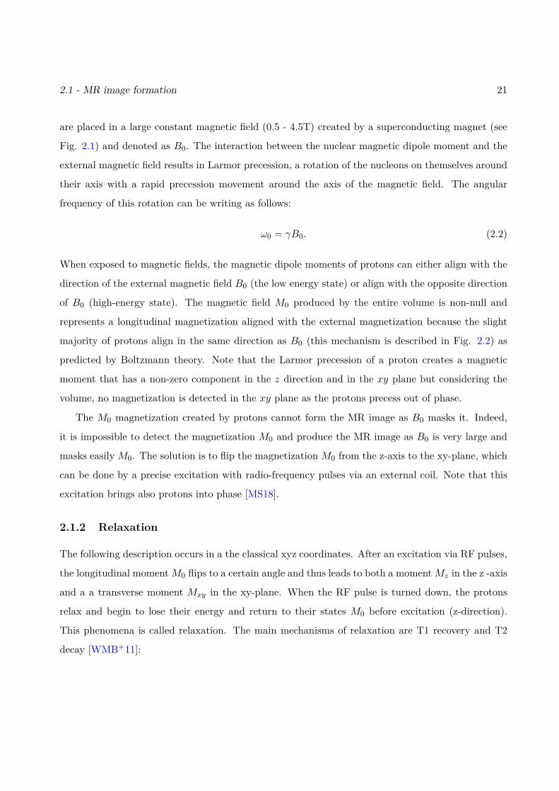
Figure 2.2: (A) the spin moment of a proton ~µ, (B) The spin moments of protons ~µ are randomlyoriented, thus, the global moment is null, (C) when placed in external magnetic field, protons aligntheir spin in the direction or in the opposite of B0 and then, produced a global longitudinal momentalign with B0 [BB11].
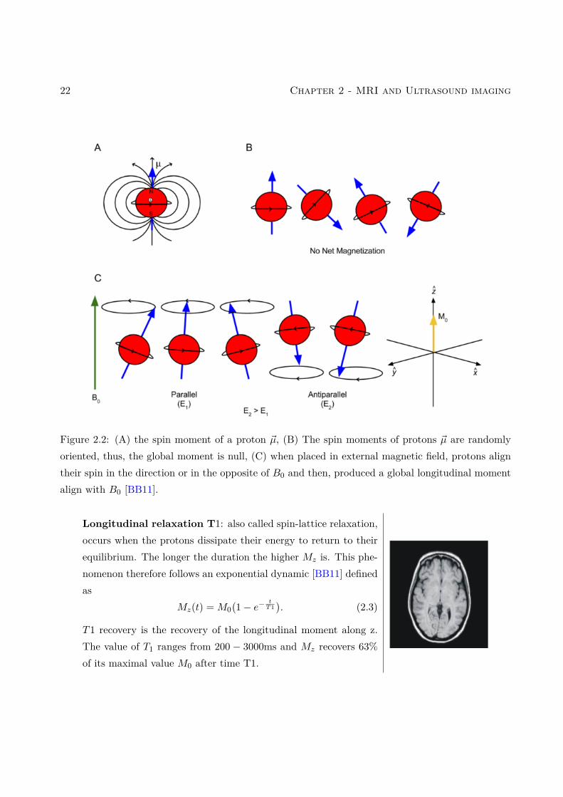
Longitudinal relaxation T1: also called spin-lattice relaxation,occurs when the protons dissipate their energy to return to theirequilibrium. The longer the duration the higher Mz is. This phe-nomenon therefore follows an exponential dynamic [BB11] definedas
Mz(t) = M0(1− e−
tT1). (2.3)
T1 recovery is the recovery of the longitudinal moment along z.The value of T1 ranges from 200 − 3000ms and Mz recovers 63%of its maximal value M0 after time T1.
2.1 - MR image formation 23
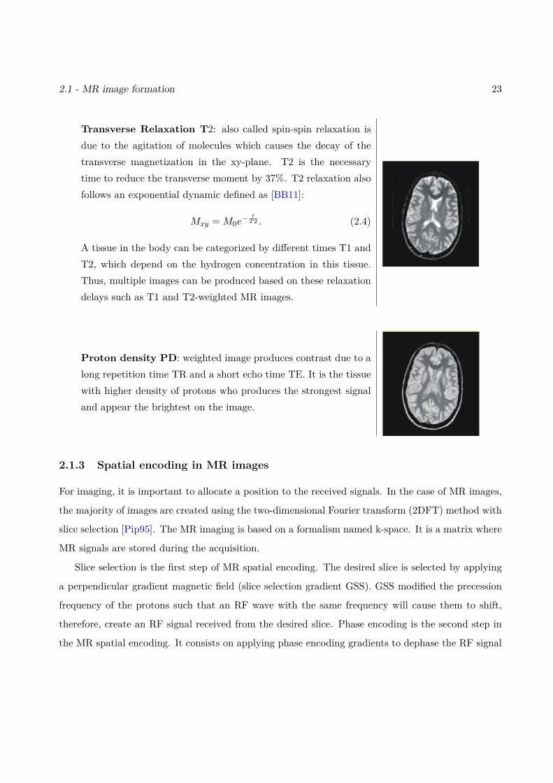
Transverse Relaxation T2: also called spin-spin relaxation isdue to the agitation of molecules which causes the decay of thetransverse magnetization in the xy-plane. T2 is the necessarytime to reduce the transverse moment by 37%. T2 relaxation alsofollows an exponential dynamic defined as [BB11]:
Mxy = M0e− tT2 . (2.4)
A tissue in the body can be categorized by different times T1 andT2, which depend on the hydrogen concentration in this tissue.Thus, multiple images can be produced based on these relaxationdelays such as T1 and T2-weighted MR images.
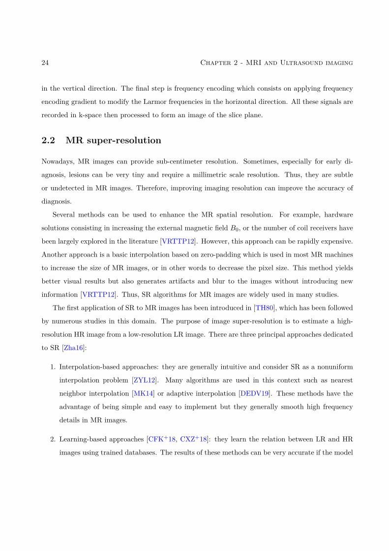
Proton density PD: weighted image produces contrast due to along repetition time TR and a short echo time TE. It is the tissuewith higher density of protons who produces the strongest signaland appear the brightest on the image.
2.1.3 Spatial encoding in MR images
For imaging, it is important to allocate a position to the received signals. In the case of MR images,
the majority of images are created using the two-dimensional Fourier transform (2DFT) method with
slice selection [Pip95]. The MR imaging is based on a formalism named k-space. It is a matrix where
MR signals are stored during the acquisition.
Slice selection is the first step of MR spatial encoding. The desired slice is selected by applying
a perpendicular gradient magnetic field (slice selection gradient GSS). GSS modified the precession
frequency of the protons such that an RF wave with the same frequency will cause them to shift,
therefore, create an RF signal received from the desired slice. Phase encoding is the second step in
the MR spatial encoding. It consists on applying phase encoding gradients to dephase the RF signal
24 Chapter 2 - MRI and Ultrasound imaging
in the vertical direction. The final step is frequency encoding which consists on applying frequency
encoding gradient to modify the Larmor frequencies in the horizontal direction. All these signals are
recorded in k-space then processed to form an image of the slice plane.
2.2 MR super-resolution
Nowadays, MR images can provide sub-centimeter resolution. Sometimes, especially for early di-
agnosis, lesions can be very tiny and require a millimetric scale resolution. Thus, they are subtle
or undetected in MR images. Therefore, improving imaging resolution can improve the accuracy of
diagnosis.
Several methods can be used to enhance the MR spatial resolution. For example, hardware
solutions consisting in increasing the external magnetic field B0, or the number of coil receivers have
been largely explored in the literature [VRTTP12]. However, this approach can be rapidly expensive.
Another approach is a basic interpolation based on zero-padding which is used in most MR machines
to increase the size of MR images, or in other words to decrease the pixel size. This method yields
better visual results but also generates artifacts and blur to the images without introducing new
information [VRTTP12]. Thus, SR algorithms for MR images are widely used in many studies.
The first application of SR to MR images has been introduced in [TH80], which has been followed
by numerous studies in this domain. The purpose of image super-resolution is to estimate a high-
resolution HR image from a low-resolution LR image. There are three principal approaches dedicated
to SR [Zha16]:
1. Interpolation-based approaches: they are generally intuitive and consider SR as a nonuniform
interpolation problem [ZYL12]. Many algorithms are used in this context such as nearest
neighbor interpolation [MK14] or adaptive interpolation [DEDV19]. These methods have the
advantage of being simple and easy to implement but they generally smooth high frequency
details in MR images.
2. Learning-based approaches [CFK+18, CXZ+18]: they learn the relation between LR and HR
images using trained databases. The results of these methods can be very accurate if the model
2.3 - US image formation 25
is well-trained.
3. Reconstruction-based approaches [Zha16, GEW10, GPOK02]: they use a data fidelity term
and a prior knowledge to model a relationship between the HR and LR images. The observed
LR image denoted as ymr can be modeled as a decimated and blurred version of the HR image
xmr contaminated by an additive Gaussian noise nmr:
ymr = SCxmr + nmr. (2.5)
Recovering the high-resolution MR image from its low-resolution counterpart is an ill-posed
problem. In order to obtain a realistic solution, many regularization φ can be added (i.e.,
gradient [Zha16] and self-similarity [MCB+10a] to name a few). The inverse problem considered
for these approaches can be defined as
minxmr
12‖ymr − SCxmr‖22 + τ1φ(xmr) (2.6)
where φ is the regularization function.
There are many algorithms that have been proposed to optimize this kind of functions, for
example: gradient-based methods, soft thresholding algorithms, alternating direction method
of multipliers (ADMM) and the split Bregman (SB) methods.
This thesis will consider a reconstruction-based approach applied to a single image to enhance the
MR image during the fusion because of its adaptability with the proposed fusion model.
2.3 US image formation
A sound wave is a vibration that propagates by longitudinal motion as an acoustic wave. Its prop-
agation is caused by the variation of pressure (repeating oscillation between high and low pressure)
in a medium such as liquids or gas. The wavelength λ can be described as the distance over which
the wave shape repeats, i.e.,
λ = c
f(2.7)
26 Chapter 2 - MRI and Ultrasound imaging
where f is the wave frequency and c is the speed of sound. Note that c depends on the medium
through which the sound wave propagates and can be defined as
c = 1√ρκ
(2.8)
where ρ and κ are the density and the compressibility of the medium. Thus, the speed of sound is
higher in materials where the density and the compressibility is lower. Here are some examples of
propagation velocities: air (330 m/s), fat (1450 m/s), water (1480 m/s), liver (1550 m/s), kidney
(1560 m/s), blood (1570 m/s), muscle (1580 m/s) and bone (4080 m/s). An average value in human
tissues is c = 1540 m/s. Another more precise way to characterize the medium through which the
US wave propagates is to study the acoustic impedance Z defined as
Z = ρc. (2.9)
US imaging is a high-frequency sound wave-based modality. The used frequencies are higher than the
audible sound > 20000 Hz and range, in standard applications, from 0 to 50 MHz for most of medical
applications. US imaging helps radiologists to see through the body by detecting the reflected echos
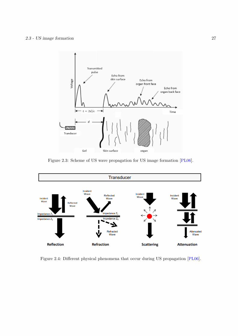
of the emitted pulses using a US probe (as shown in Fig. 2.3).
US images are used in different fields: some examples of clinical applications that involve US
images include cardiology, obstetrics, emergency medicine, colorectal surgery and pelvic surgery.
2.3.1 US propagation
The US image is formed by transmitting pulses into the body and detecting the reflected echoes.
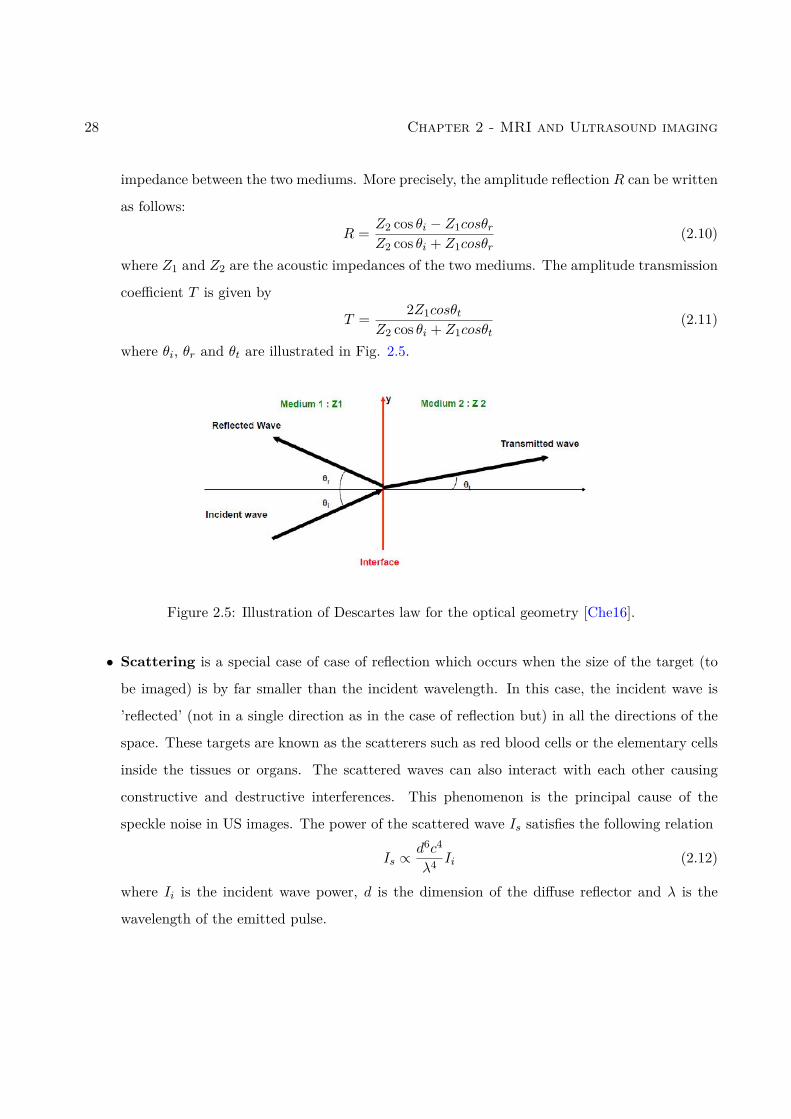
Other phenomena can occur during the US propagation such as scattering, refraction or attenuation
(shown by Fig. 2.4), which can contaminate the image by heavy speckle noise and artifacts. The
information that US images contain is due to the reflection and scattering of the emitted waves.
• Reflection: when the US wave passes between two mediums with different acoustic impedances
Z, a fraction of the wave is reflected which helps the image formation and highlights the organ
boundaries. The amplitude of the reflected wave depends on the difference between the acoustic
2.3 - US image formation 27
Figure 2.3: Scheme of US wave propagation for US image formation [PL06].
Figure 2.4: Different physical phenomena that occur during US propagation [PL06].
28 Chapter 2 - MRI and Ultrasound imaging
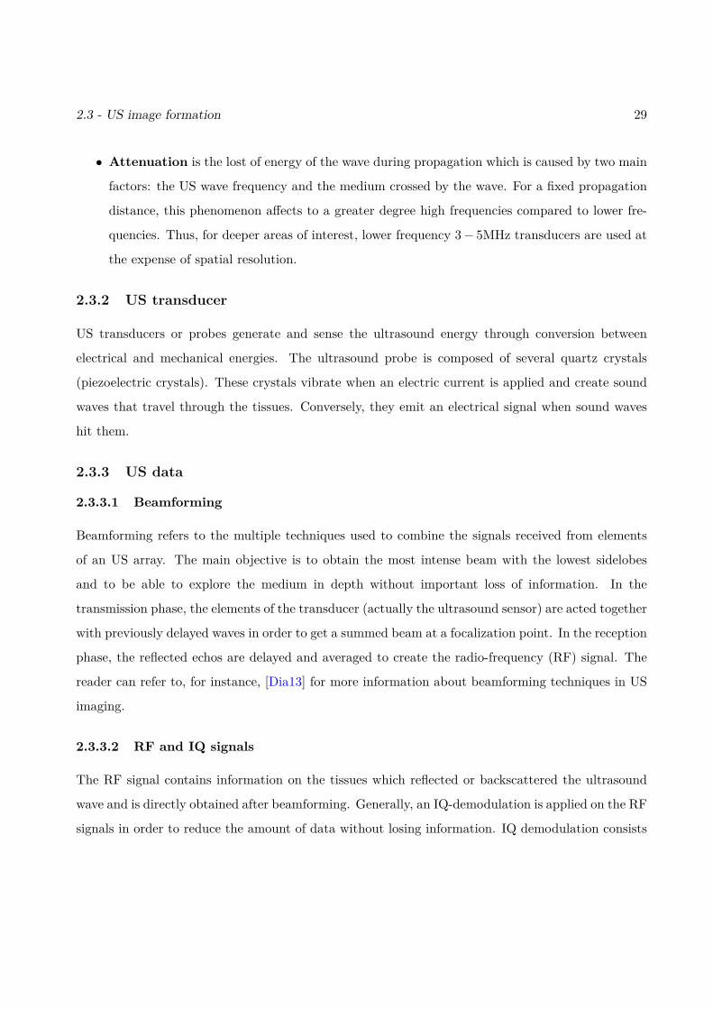
impedance between the two mediums. More precisely, the amplitude reflection R can be written
as follows:
R = Z2 cos θi − Z1cosθrZ2 cos θi + Z1cosθr
(2.10)
where Z1 and Z2 are the acoustic impedances of the two mediums. The amplitude transmission
coefficient T is given by
T = 2Z1cosθtZ2 cos θi + Z1cosθt
(2.11)
where θi, θr and θt are illustrated in Fig. 2.5.
Figure 2.5: Illustration of Descartes law for the optical geometry [Che16].
• Scattering is a special case of case of reflection which occurs when the size of the target (to
be imaged) is by far smaller than the incident wavelength. In this case, the incident wave is
’reflected’ (not in a single direction as in the case of reflection but) in all the directions of the
space. These targets are known as the scatterers such as red blood cells or the elementary cells
inside the tissues or organs. The scattered waves can also interact with each other causing
constructive and destructive interferences. This phenomenon is the principal cause of the
speckle noise in US images. The power of the scattered wave Is satisfies the following relation
Is ∝d6c4
λ4 Ii (2.12)
where Ii is the incident wave power, d is the dimension of the diffuse reflector and λ is the
wavelength of the emitted pulse.
2.3 - US image formation 29
• Attenuation is the lost of energy of the wave during propagation which is caused by two main
factors: the US wave frequency and the medium crossed by the wave. For a fixed propagation
distance, this phenomenon affects to a greater degree high frequencies compared to lower fre-
quencies. Thus, for deeper areas of interest, lower frequency 3− 5MHz transducers are used at
the expense of spatial resolution.
2.3.2 US transducer
US transducers or probes generate and sense the ultrasound energy through conversion between
electrical and mechanical energies. The ultrasound probe is composed of several quartz crystals
(piezoelectric crystals). These crystals vibrate when an electric current is applied and create sound
waves that travel through the tissues. Conversely, they emit an electrical signal when sound waves
hit them.
2.3.3 US data
2.3.3.1 Beamforming
Beamforming refers to the multiple techniques used to combine the signals received from elements
of an US array. The main objective is to obtain the most intense beam with the lowest sidelobes
and to be able to explore the medium in depth without important loss of information. In the
transmission phase, the elements of the transducer (actually the ultrasound sensor) are acted together
with previously delayed waves in order to get a summed beam at a focalization point. In the reception
phase, the reflected echos are delayed and averaged to create the radio-frequency (RF) signal. The
reader can refer to, for instance, [Dia13] for more information about beamforming techniques in US
imaging.
2.3.3.2 RF and IQ signals
The RF signal contains information on the tissues which reflected or backscattered the ultrasound
wave and is directly obtained after beamforming. Generally, an IQ-demodulation is applied on the RF
signals in order to reduce the amount of data without losing information. IQ demodulation consists
30 Chapter 2 - MRI and Ultrasound imaging
of 3 main steps: downmixing, low-pass filtering and decimation. Finally, the IQ signal denoted as
rIQ (phase and quadrature signal) can be computed as follows [Zha16]:
rIQ =(rRF − iH(rRF)
)e−iω0t, (2.13)
where rRF is the RF signal, H is the Hilbert transform and ω0 is the central frequency of the US
probe and i2 = −1.
2.3.3.3 US image modes
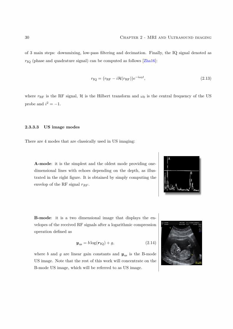
There are 4 modes that are classically used in US imaging:
A-mode: it is the simplest and the oldest mode providing one-dimensional lines with echoes depending on the depth, as illus-trated in the right figure. It is obtained by simply computing theenvelop of the RF signal rRF .
B-mode: it is a two dimensional image that displays the en-velopes of the received RF signals after a logarithmic compressionoperation defined as
yus = b log(rIQ) + g, (2.14)
where b and g are linear gain constants and yus is the B-modeUS image. Note that the rest of this work will concentrate on theB-mode US image, which will be referred to as US image.
2.4 - Speckle reduction for US imaging 31
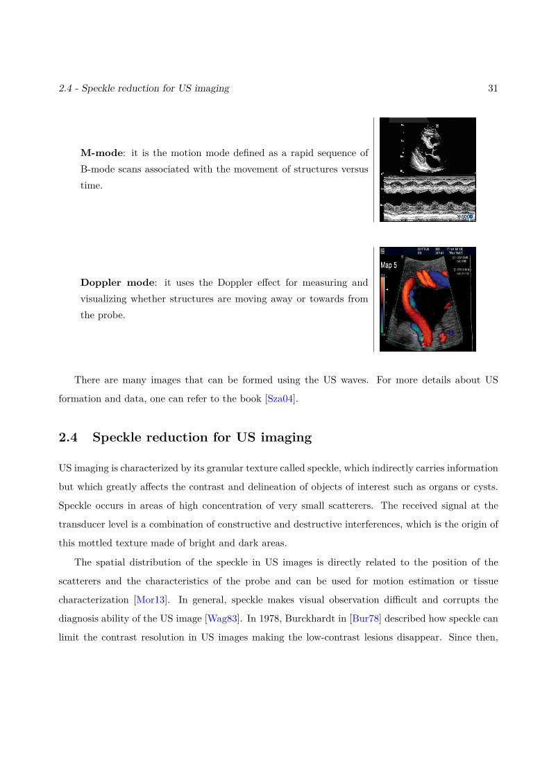
M-mode: it is the motion mode defined as a rapid sequence ofB-mode scans associated with the movement of structures versustime.
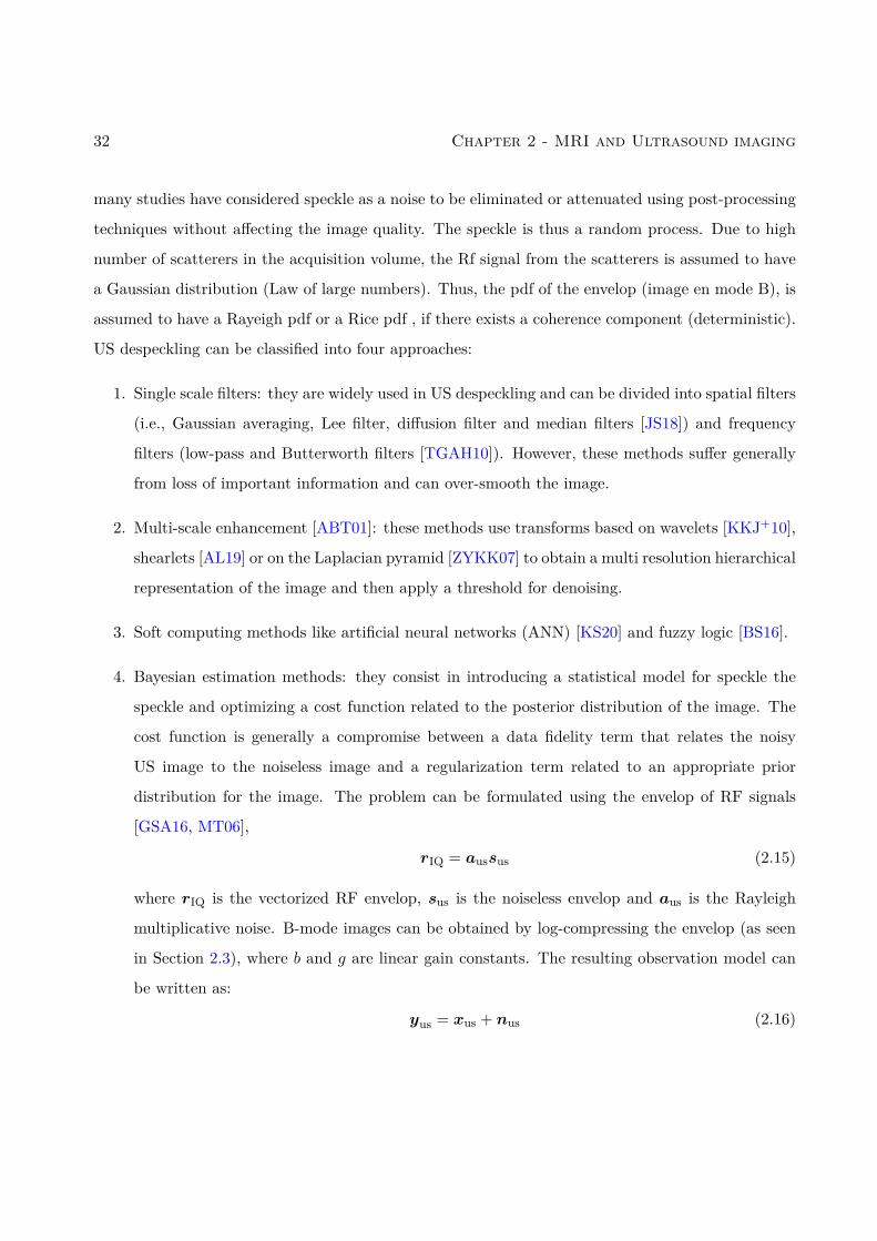
Doppler mode: it uses the Doppler effect for measuring andvisualizing whether structures are moving away or towards fromthe probe.
There are many images that can be formed using the US waves. For more details about US
formation and data, one can refer to the book [Sza04].
2.4 Speckle reduction for US imaging
US imaging is characterized by its granular texture called speckle, which indirectly carries information
but which greatly affects the contrast and delineation of objects of interest such as organs or cysts.
Speckle occurs in areas of high concentration of very small scatterers. The received signal at the
transducer level is a combination of constructive and destructive interferences, which is the origin of
this mottled texture made of bright and dark areas.
The spatial distribution of the speckle in US images is directly related to the position of the
scatterers and the characteristics of the probe and can be used for motion estimation or tissue
characterization [Mor13]. In general, speckle makes visual observation difficult and corrupts the
diagnosis ability of the US image [Wag83]. In 1978, Burckhardt in [Bur78] described how speckle can
limit the contrast resolution in US images making the low-contrast lesions disappear. Since then,
32 Chapter 2 - MRI and Ultrasound imaging
many studies have considered speckle as a noise to be eliminated or attenuated using post-processing
techniques without affecting the image quality. The speckle is thus a random process. Due to high
number of scatterers in the acquisition volume, the Rf signal from the scatterers is assumed to have
a Gaussian distribution (Law of large numbers). Thus, the pdf of the envelop (image en mode B), is
assumed to have a Rayeigh pdf or a Rice pdf , if there exists a coherence component (deterministic).
US despeckling can be classified into four approaches:
1. Single scale filters: they are widely used in US despeckling and can be divided into spatial filters
(i.e., Gaussian averaging, Lee filter, diffusion filter and median filters [JS18]) and frequency
filters (low-pass and Butterworth filters [TGAH10]). However, these methods suffer generally
from loss of important information and can over-smooth the image.
2. Multi-scale enhancement [ABT01]: these methods use transforms based on wavelets [KKJ+10],
shearlets [AL19] or on the Laplacian pyramid [ZYKK07] to obtain a multi resolution hierarchical
representation of the image and then apply a threshold for denoising.
3. Soft computing methods like artificial neural networks (ANN) [KS20] and fuzzy logic [BS16].
4. Bayesian estimation methods: they consist in introducing a statistical model for speckle the
speckle and optimizing a cost function related to the posterior distribution of the image. The
cost function is generally a compromise between a data fidelity term that relates the noisy
US image to the noiseless image and a regularization term related to an appropriate prior
distribution for the image. The problem can be formulated using the envelop of RF signals
[GSA16, MT06],
rIQ = aussus (2.15)
where rIQ is the vectorized RF envelop, sus is the noiseless envelop and aus is the Rayleigh
multiplicative noise. B-mode images can be obtained by log-compressing the envelop (as seen
in Section 2.3), where b and g are linear gain constants. The resulting observation model can
be written as:
yus = xus + nus (2.16)
2.4 - Speckle reduction for US imaging 33
where yus is the observed B-mode image, xus is the noiseless B-mode image and nus is an
additive noise, generally assumed to be independent from xus and distributed according to a
log-Rayleigh distribution.
2.4.1 Other medical imaging modalities
There are several types of medical images that are available for diagnosis and surgery treatment
and that are generally fused. Some examples include magnetic resonance imaging (MR), comput-
erized tomography (CT), positron emission tomography (PET), single-photon emission computed
tomography (SPECT) and US (US) imaging.
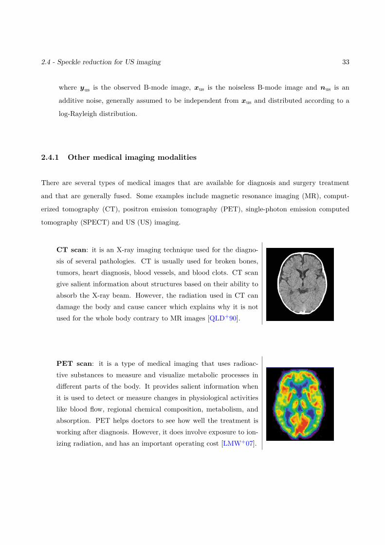
CT scan: it is an X-ray imaging technique used for the diagno-sis of several pathologies. CT is usually used for broken bones,tumors, heart diagnosis, blood vessels, and blood clots. CT scangive salient information about structures based on their ability toabsorb the X-ray beam. However, the radiation used in CT candamage the body and cause cancer which explains why it is notused for the whole body contrary to MR images [QLD+90].
PET scan: it is a type of medical imaging that uses radioac-tive substances to measure and visualize metabolic processes indifferent parts of the body. It provides salient information whenit is used to detect or measure changes in physiological activitieslike blood flow, regional chemical composition, metabolism, andabsorption. PET helps doctors to see how well the treatment isworking after diagnosis. However, it does involve exposure to ion-izing radiation, and has an important operating cost [LMW+07].
34 Chapter 2 - MRI and Ultrasound imaging
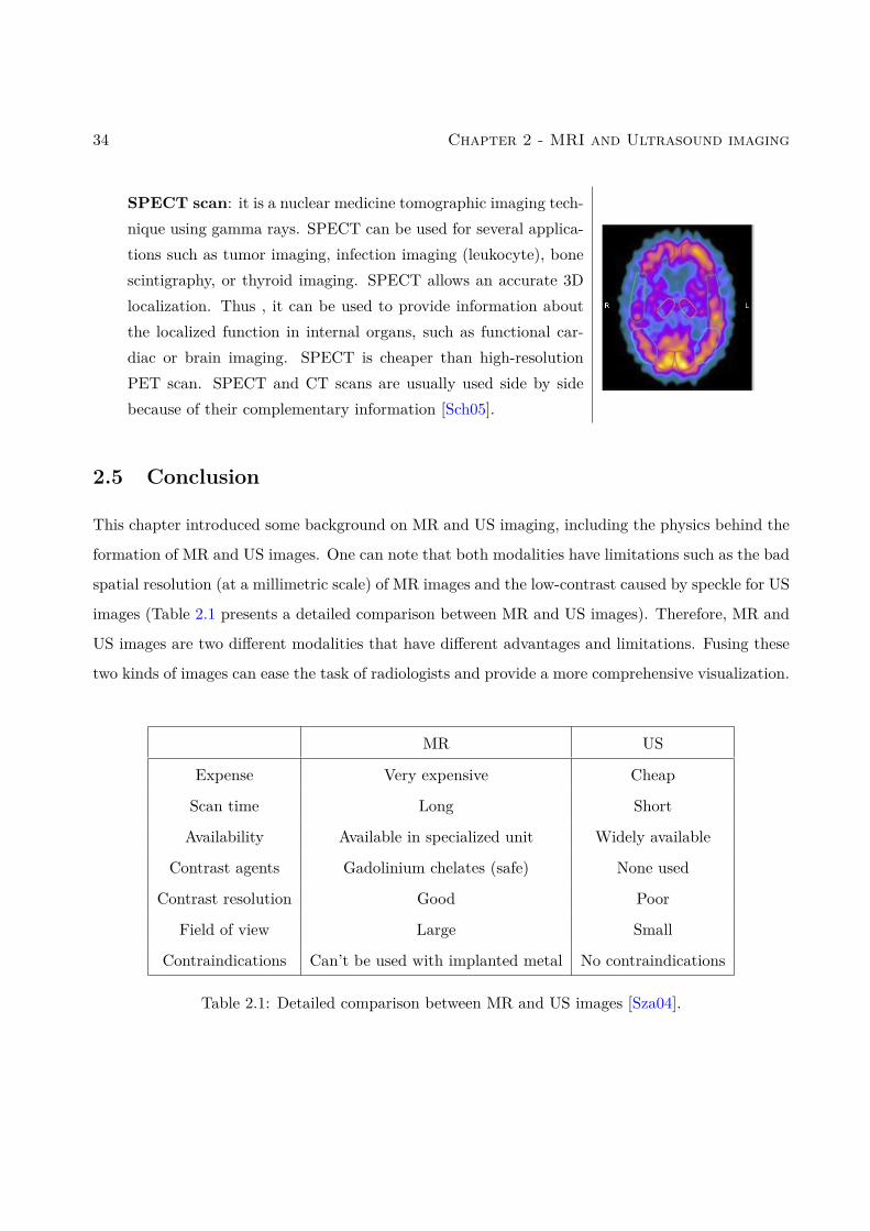
SPECT scan: it is a nuclear medicine tomographic imaging tech-nique using gamma rays. SPECT can be used for several applica-tions such as tumor imaging, infection imaging (leukocyte), bonescintigraphy, or thyroid imaging. SPECT allows an accurate 3Dlocalization. Thus , it can be used to provide information aboutthe localized function in internal organs, such as functional car-diac or brain imaging. SPECT is cheaper than high-resolutionPET scan. SPECT and CT scans are usually used side by sidebecause of their complementary information [Sch05].
2.5 Conclusion
This chapter introduced some background on MR and US imaging, including the physics behind the
formation of MR and US images. One can note that both modalities have limitations such as the bad
spatial resolution (at a millimetric scale) of MR images and the low-contrast caused by speckle for US
images (Table 2.1 presents a detailed comparison between MR and US images). Therefore, MR and
US images are two different modalities that have different advantages and limitations. Fusing these
two kinds of images can ease the task of radiologists and provide a more comprehensive visualization.
MR US
Expense Very expensive Cheap
Scan time Long Short
Availability Available in specialized unit Widely available
Contrast agents Gadolinium chelates (safe) None used
Contrast resolution Good Poor
Field of view Large Small
Contraindications Can’t be used with implanted metal No contraindications
Table 2.1: Detailed comparison between MR and US images [Sza04].
2.5 - Conclusion 35
Some post-processing techniques used for these images are also discussed. These techniques
include super-resolution for MR images and US despeckling. At this point, it is interesting to note
that the aim of image fusion is not only to gather information from the MR and US imaging modalities
but also to enhance them during the same process.
Generally, the diagnosis and the plan of surgery of endometriosis during the clinical routine are
based on:
• The B-mode transvaginal ultrasound image (TVUS): it is a pelvic scan that is performed by
a sonographer who records the static images and video clips. The information on the type
of machine used varies greatly and the only criteria to adopt the image is the “satisfactory”
quality stated by the radiologist and the gynecologist.
• MRI image: the state-of-art MR imaging protocol includes T2 and fat suppressed T1-weighted
sequences. The T2-weighted sequences without fat-suppression are assumed to be the best
sequences for detecting pelvic endometriosis [BBH+17]. Note that a detailed MRI protocol for
endometriosis detection was presented in [FFP+18].

36 Chapter 2 - MRI and Ultrasound imaging
Chapter 3
Fusion and Registration in MedicalImaging
Contents3.1 Introduction . . . . . . . . . . . . . . . . . . . . . . . . . . . . . . . . . . . . 373.2 Medical image fusion . . . . . . . . . . . . . . . . . . . . . . . . . . . . . . . 39
3.2.1 Multi-modal image fusion methods . . . . . . . . . . . . . . . . . . . . . . . . 413.2.2 Conclusion . . . . . . . . . . . . . . . . . . . . . . . . . . . . . . . . . . . . . 56
3.3 Medical image registration . . . . . . . . . . . . . . . . . . . . . . . . . . . 573.3.1 Image similarity measure . . . . . . . . . . . . . . . . . . . . . . . . . . . . . 593.3.2 Transformation models . . . . . . . . . . . . . . . . . . . . . . . . . . . . . . . 633.3.3 Regularization in deformable registration . . . . . . . . . . . . . . . . . . . . 673.3.4 Optimization . . . . . . . . . . . . . . . . . . . . . . . . . . . . . . . . . . . . 693.3.5 Image registration metrics . . . . . . . . . . . . . . . . . . . . . . . . . . . . . 70
3.4 MR and US registration: state of art . . . . . . . . . . . . . . . . . . . . . 713.4.1 Intensity-based methods . . . . . . . . . . . . . . . . . . . . . . . . . . . . . . 723.4.2 Feature-based methods . . . . . . . . . . . . . . . . . . . . . . . . . . . . . . 743.4.3 Other approach . . . . . . . . . . . . . . . . . . . . . . . . . . . . . . . . . . . 753.4.4 Conclusion . . . . . . . . . . . . . . . . . . . . . . . . . . . . . . . . . . . . . 75
3.5 Global Conclusions . . . . . . . . . . . . . . . . . . . . . . . . . . . . . . . . 75
3.1 Introduction
Image fusion has received much attention in the literature, in particular for medical imaging appli-
cations. These applications include diagnosis and imaging-guided surgery for which the efficiency of
experts can be improved for producing an unbiased and objective decision in a short time. However,
given the diversity of medical images, it is difficult to find a fusion method adapted to all medical
modalities.
37
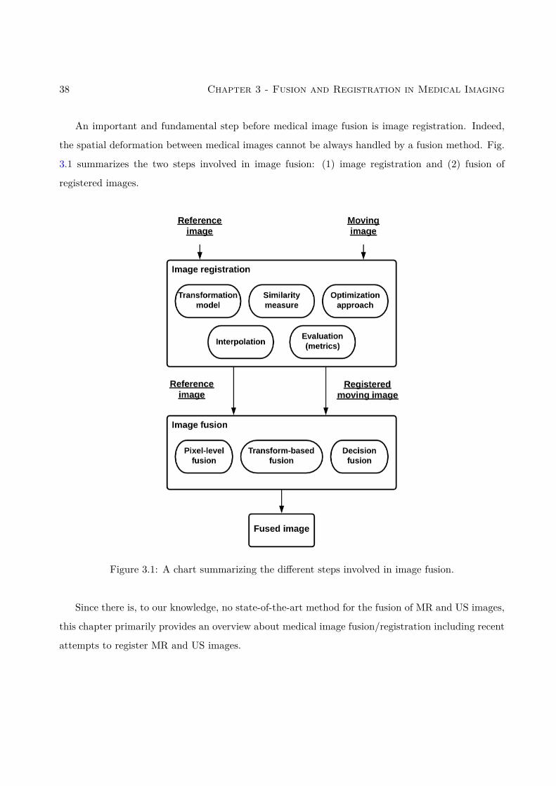
38 Chapter 3 - Fusion and Registration in Medical Imaging
An important and fundamental step before medical image fusion is image registration. Indeed,
the spatial deformation between medical images cannot be always handled by a fusion method. Fig.
3.1 summarizes the two steps involved in image fusion: (1) image registration and (2) fusion of
registered images.
Figure 3.1: A chart summarizing the different steps involved in image fusion.
Since there is, to our knowledge, no state-of-the-art method for the fusion of MR and US images,
this chapter primarily provides an overview about medical image fusion/registration including recent
attempts to register MR and US images.
3.2 - Medical image fusion 39
3.2 Medical image fusion
Image fusion can be defined as gathering all the important information from multiple images and
including them into a fewer number of images, e.g., into one single image. This single image is usually
more informative than the images before fusion and contains all the necessary information for the
application of interest [ANA18]. Thus, the purpose of image fusion is to build an enhanced image
that is informative, comprehensible and accurate for the human. The fusion of medical images is
becoming very common for the study of a given pathology and generally allows for better medical
decisions in clinical studies. This problem requires solving several technical challenges because of
the limitations imposed by specific imaging modalities. A large and growing body of literature has
investigated techniques addressing these challenges [JD14b, LBCA10].
Medical image fusion can be mainly classified into three categories: pixel-level fusion, feature
level fusion, and decision level fusion. Pixel-level fusion has the advantage of preserving most of the
pertinent information in the fused image. Feature-level fusion extracts features from images, such
as edges, textures and builds a fusion method using these features. Decision-level fusion refers to
methods first segmenting the images of interest into homogeneous regions and use this segmentation
to define the fusion method. Medical fusion methods have their own advantages and limitations that
are summarized in Table 3.1. The aim of this section is to provide a global view of image fusion in
the medical field.
Considering the nature of input images to be fused, medical image fusion can be classified into
three main categories: multi-view fusion, multi-temporal fusion and multi-modal fusion (see Table
3.2). Note that multi-modal fusion is very complex and challenging compared to the other categories
because it deals with completely different images which makes it difficult to find a relation between
the image of interest and the observed images, especially when considering pixel-level fusion.
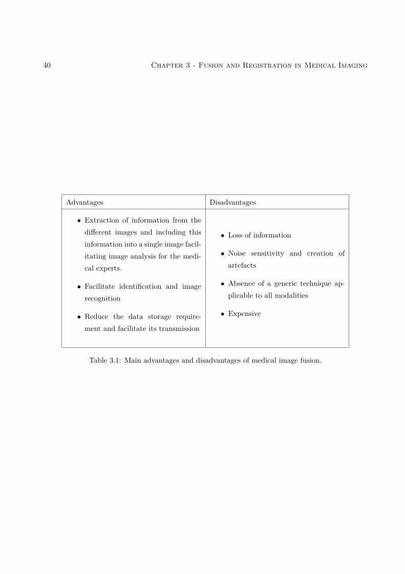
40 Chapter 3 - Fusion and Registration in Medical Imaging
Advantages Disadvantages
• Extraction of information from thedifferent images and including thisinformation into a single image facil-itating image analysis for the medi-cal experts.
• Facilitate identification and imagerecognition
• Reduce the data storage require-ment and facilitate its transmission
• Loss of information
• Noise sensitivity and creation ofartefacts
• Absence of a generic technique ap-plicable to all modalities
• Expensive
Table 3.1: Main advantages and disadvantages of medical image fusion.
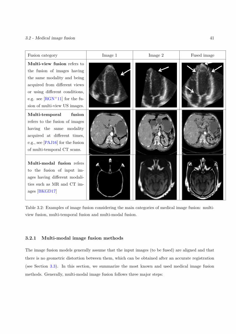
3.2 - Medical image fusion 41
Fusion category Image 1 Image 2 Fused image
Multi-view fusion refers tothe fusion of images havingthe same modality and beingacquired from different viewsor using different conditions,e.g. see [RGN+11] for the fu-sion of multi-view US images.
Multi-temporal fusionrefers to the fusion of imageshaving the same modalityacquired at different times,e.g., see [PAJ16] for the fusionof multi-temporal CT scans.
Multi-modal fusion refersto the fusion of input im-ages having different modali-ties such as MR and CT im-ages [BKGD17]
Table 3.2: Examples of image fusion considering the main categories of medical image fusion: multi-view fusion, multi-temporal fusion and multi-modal fusion.
3.2.1 Multi-modal image fusion methods
The image fusion models generally assume that the input images (to be fused) are aligned and that
there is no geometric distortion between them, which can be obtained after an accurate registration
(see Section 3.3). In this section, we summarize the most known and used medical image fusion
methods. Generally, multi-modal image fusion follows three major steps:
42 Chapter 3 - Fusion and Registration in Medical Imaging
1. Input images are decomposed into sub-images or features using image decomposition algo-
rithms.
2. Fusion rules are used to combine information from these sub-images into fused sub-images.
3. The fused image is reconstructed from the fused sub-images using image reconstruction algo-
rithms.
Finally, quality measures are used to evaluate the quality of fused images. Fig. 3.2 summarizes
the stages of multimodal image fusion and illustrates each stage with examples of algorithms and
methods.
3.2.1.1 Image decomposition and reconstruction
Multi-resolution analysis has been extensively considered for the fusion of medical images. Several
decomposition and reconstruction algorithms have been introduced in the literature. In this section,
we introduce three different key methodologies that are widely used in medical image fusion: 1)
discrete wavelet transform, 2) Laplacian pyramid transform and 3) sparse representation.
Discrete Wavelet Transform (DWT)
The discrete wavelet transform is the most common transform used in image fusion. The image
X goes through two filters (with lowpass and highpass impulse responses) in both horizontal and
vertical directions whose outputs are decimated by 2 (dyadic decomposition). This process is repeated
depending on the desired decomposition level (as illustrated in Fig. 3.3). Generally, the level of
decomposition should depend on the input image resolution: images with high resolution require
higher level of decomposition than low resolution images. The filtering operation can be defined as
the convolution of the vectorized image and the impulse response l:
Y [n] = (X ∗ l)[n] =∞∑
k=−∞X[k]l[n− k]. (3.1)
where l ∈ h, g, h and g are the low and the high pass filters.
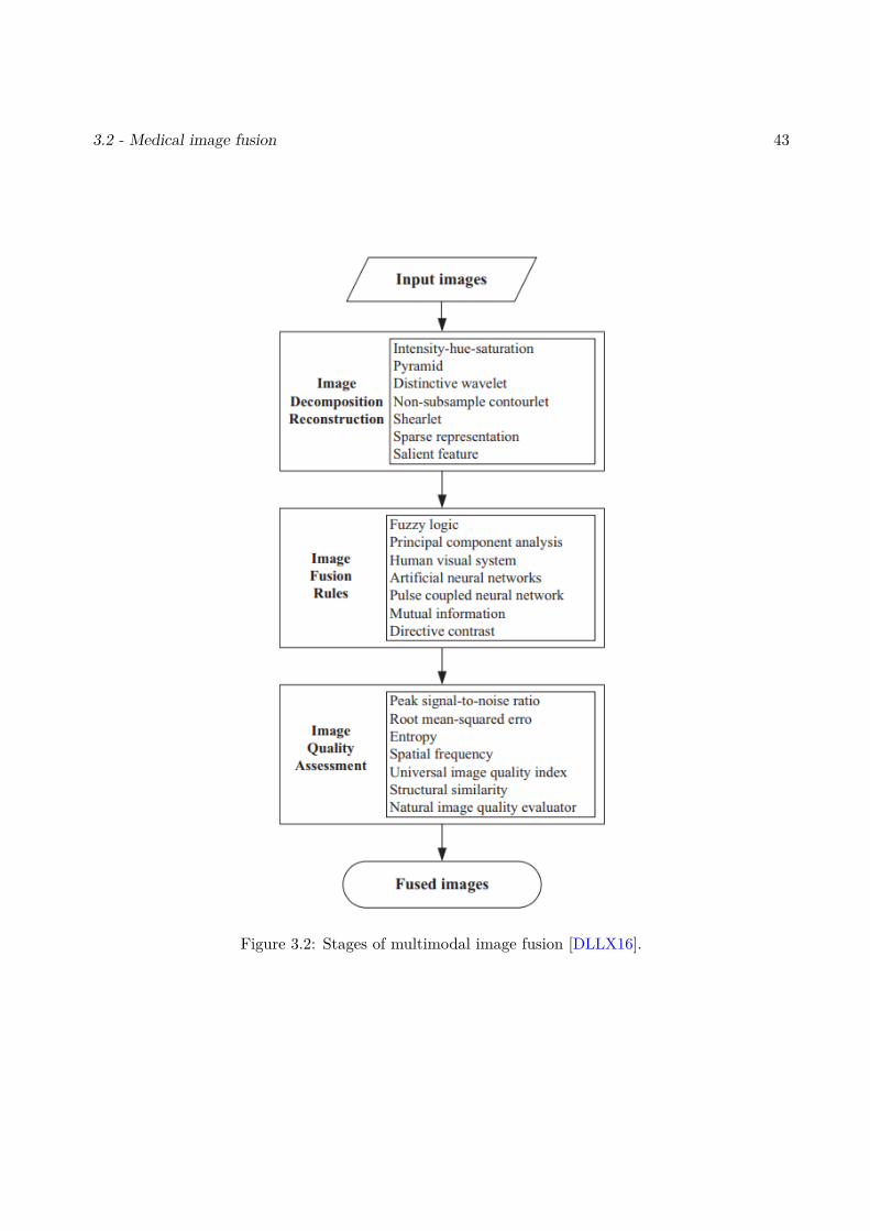
3.2 - Medical image fusion 43
Figure 3.2: Stages of multimodal image fusion [DLLX16].
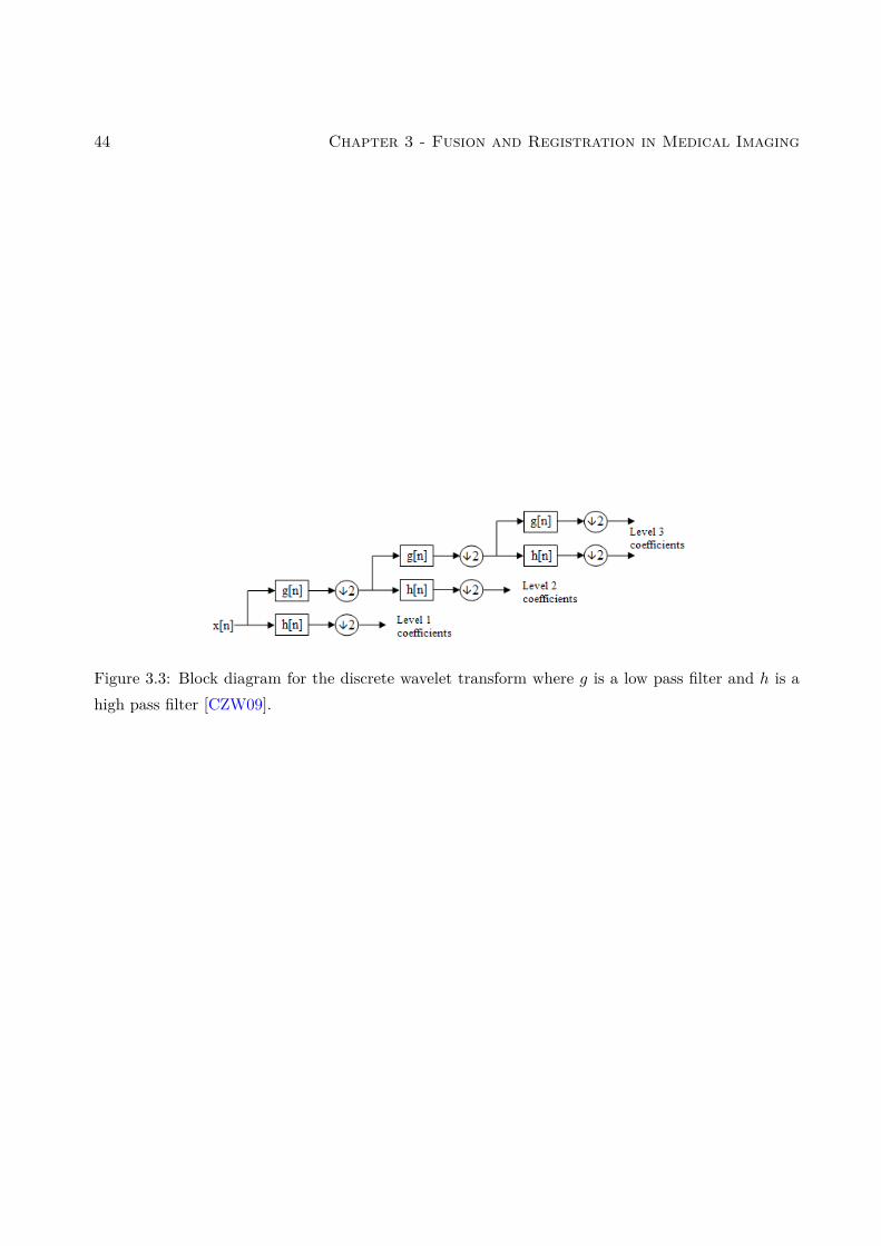
44 Chapter 3 - Fusion and Registration in Medical Imaging
Figure 3.3: Block diagram for the discrete wavelet transform where g is a low pass filter and h is ahigh pass filter [CZW09].
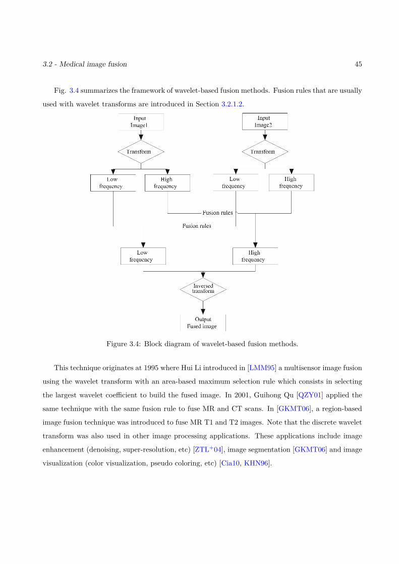
3.2 - Medical image fusion 45
Fig. 3.4 summarizes the framework of wavelet-based fusion methods. Fusion rules that are usually
used with wavelet transforms are introduced in Section 3.2.1.2.
Figure 3.4: Block diagram of wavelet-based fusion methods.
This technique originates at 1995 where Hui Li introduced in [LMM95] a multisensor image fusion
using the wavelet transform with an area-based maximum selection rule which consists in selecting
the largest wavelet coefficient to build the fused image. In 2001, Guihong Qu [QZY01] applied the
same technique with the same fusion rule to fuse MR and CT scans. In [GKMT06], a region-based
image fusion technique was introduced to fuse MR T1 and T2 images. Note that the discrete wavelet
transform was also used in other image processing applications. These applications include image
enhancement (denoising, super-resolution, etc) [ZTL+04], image segmentation [GKMT06] and image
visualization (color visualization, pseudo coloring, etc) [Cia10, KHN96].
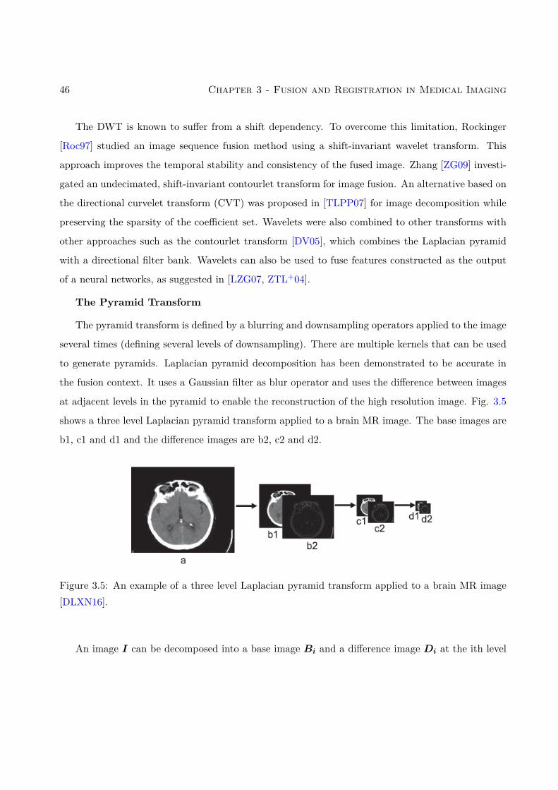
46 Chapter 3 - Fusion and Registration in Medical Imaging
The DWT is known to suffer from a shift dependency. To overcome this limitation, Rockinger
[Roc97] studied an image sequence fusion method using a shift-invariant wavelet transform. This
approach improves the temporal stability and consistency of the fused image. Zhang [ZG09] investi-
gated an undecimated, shift-invariant contourlet transform for image fusion. An alternative based on
the directional curvelet transform (CVT) was proposed in [TLPP07] for image decomposition while
preserving the sparsity of the coefficient set. Wavelets were also combined to other transforms with
other approaches such as the contourlet transform [DV05], which combines the Laplacian pyramid
with a directional filter bank. Wavelets can also be used to fuse features constructed as the output
of a neural networks, as suggested in [LZG07, ZTL+04].
The Pyramid Transform
The pyramid transform is defined by a blurring and downsampling operators applied to the image
several times (defining several levels of downsampling). There are multiple kernels that can be used
to generate pyramids. Laplacian pyramid decomposition has been demonstrated to be accurate in
the fusion context. It uses a Gaussian filter as blur operator and uses the difference between images
at adjacent levels in the pyramid to enable the reconstruction of the high resolution image. Fig. 3.5
shows a three level Laplacian pyramid transform applied to a brain MR image. The base images are
b1, c1 and d1 and the difference images are b2, c2 and d2.
Figure 3.5: An example of a three level Laplacian pyramid transform applied to a brain MR image[DLXN16].
An image I can be decomposed into a base image Bi and a difference image Di at the ith level
3.2 - Medical image fusion 47
using the following convolutions:
Bi = h ∗Li
Di = g ∗Li(3.2)
where h and g are respectively low and high pass filters, and Li can be written as
Li =
I if i = 0
s ∗Li−1 otherwise(3.3)
where s is a smooth Gaussian kernel with a downsampling operator.
Laplacian pyramid fusion consists of three phases (displayed in Fig. 3.6): image decomposition,
image fusion using accurate fusion rules and reconstruction of the fused image using inverse Laplacian
pyramid transform. One of the most common fusion rules in Laplacian pyramid fusion is the average
scheme for the base images and the maximum for the difference images as shown is Eq. (3.4)
Bfi = B1
i +B2i
2Dfi = max
(D1i ,D
2i
) (3.4)
where .f denotes the fused image, .1 and .2 are the images to fuse. Section 3.2.1.2 presents other
fusion rules that are used with the pyramid methods. Finally, the reconstruction of the fused image
is implemented using the inverse Laplacian pyramid transform.
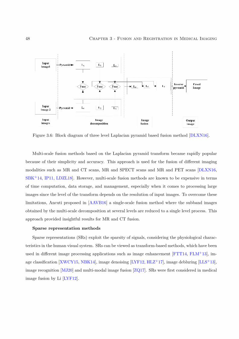
48 Chapter 3 - Fusion and Registration in Medical Imaging
Figure 3.6: Block diagram of three level Laplacian pyramid based fusion method [DLXN16].
Multi-scale fusion methods based on the Laplacian pyramid transform became rapidly popular
because of their simplicity and accuracy. This approach is used for the fusion of different imaging
modalities such as MR and CT scans, MR and SPECT scans and MR and PET scans [DLXN16,
SBK+14, IP11, LDZL18]. However, multi-scale fusion methods are known to be expensive in terms
of time computation, data storage, and management, especially when it comes to processing large
images since the level of the transform depends on the resolution of input images. To overcome these
limitations, Ancuti proposed in [AAVB16] a single-scale fusion method where the subband images
obtained by the multi-scale decomposition at several levels are reduced to a single level process. This
approach provided insightful results for MR and CT fusion.
Sparse representation methods
Sparse representations (SRs) exploit the sparsity of signals, considering the physiological charac-
teristics in the human visual system. SRs can be viewed as transform-based methods, which have been
used in different image processing applications such as image enhancement [FTT14, FLM+13], im-
age classification [XWCY15, NBK14], image denoising [LYF12, HLZ+17], image debluring [LLS+13],
image recognition [MJ20] and multi-modal image fusion [ZQ17]. SRs were first considered in medical
image fusion by Li [LYF12].
3.2 - Medical image fusion 49
Different from the other transform-based fusion methods, SRs make the assumption that the
high and the low frequency images share the same set of sparse coefficients [YLF13, DLLX16]. The
procedure of SR fusion can be summarized as follows:
1. Vectorization of the input images I1 and I2.
2. Decomposition of the two images using an overcomplete dictionary D. The K-SVD method
is a classical dictionary learning method, which has been used intensively for image fusion
[ZFLZ13]. The decompositions of the two images I1 and I2 are defined as
I1 = DS1
I2 = DS2,
where S1 and S2 are the sparse representations of I1 and I2 and D is the common dictionary
for the two images.
3. Combination of the sparse coefficients using an appropriate fusion rule
Sf = f(S1,S2),
where Sf contains sparse coefficients (see Section 3.2.1.2 for examples of fusion rules).
4. Reconstruction of the fused image using the overcomplete dictionary D:
If = DSf .
However, the conventional sparse representations have two major limitations: 1) details, struc-
tures, and edges in the input images are often smoothed and 2) the fused image can suffer from
an important loss of information if the dictionary has not been constructed properly. In the few
past years, many studies considered a combination of multi-scale approaches and SR techniques to
overcome their limitations and to robustify the fusion method [LSH+18, Yin15, LLW15]. In partic-
ular Yu Liu studied in [LLW15] a fusion framework where the multi-scale transform is first applied
on the pre-registered input images to obtain low-frequency and high-frequency images. In a second
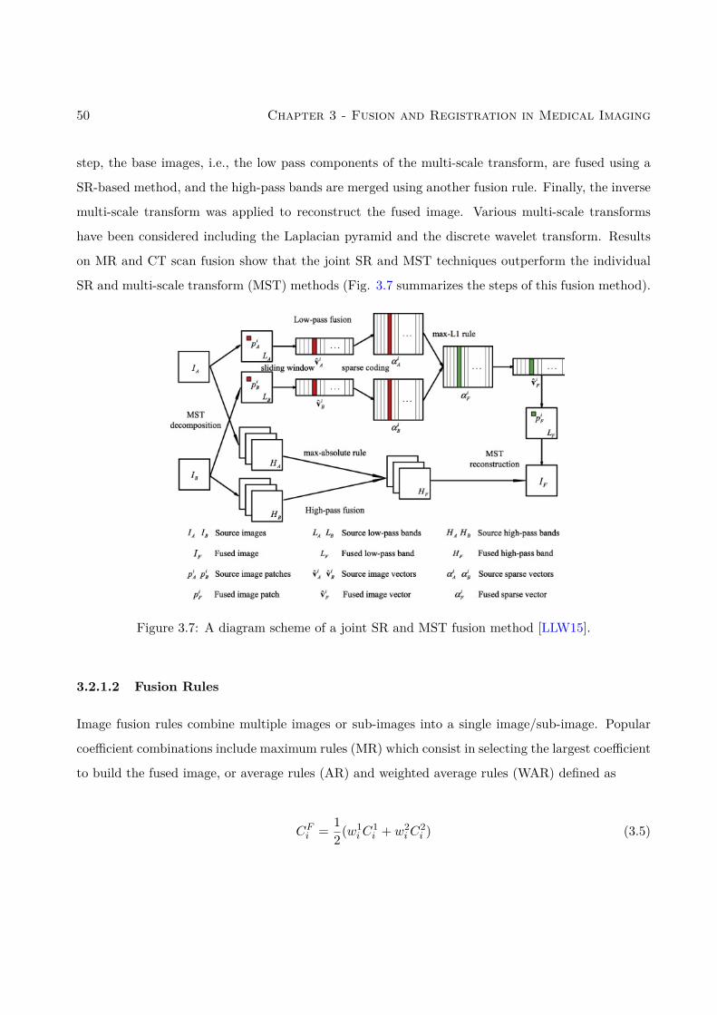
50 Chapter 3 - Fusion and Registration in Medical Imaging
step, the base images, i.e., the low pass components of the multi-scale transform, are fused using a
SR-based method, and the high-pass bands are merged using another fusion rule. Finally, the inverse
multi-scale transform was applied to reconstruct the fused image. Various multi-scale transforms
have been considered including the Laplacian pyramid and the discrete wavelet transform. Results
on MR and CT scan fusion show that the joint SR and MST techniques outperform the individual
SR and multi-scale transform (MST) methods (Fig. 3.7 summarizes the steps of this fusion method).
Figure 3.7: A diagram scheme of a joint SR and MST fusion method [LLW15].
3.2.1.2 Fusion Rules
Image fusion rules combine multiple images or sub-images into a single image/sub-image. Popular
coefficient combinations include maximum rules (MR) which consist in selecting the largest coefficient
to build the fused image, or average rules (AR) and weighted average rules (WAR) defined as
CFi = 12(w1
iC1i + w2
iC2i ) (3.5)
3.2 - Medical image fusion 51
where CFi is the fused coefficient, C1i and C2
i are the coefficients of the input images and w1i and w2
i
are appropriate weights.
In the following, image fusion rules that are widely combined with image decomposition methods
(Section 3.2.1.1) are introduced. Note that these fusion rules can be applied directly on image pixels
instead of the coefficients obtained after image decomposition as in [PM11, WMG10].
Principal Component Analysis
Principal component analysis (PCA) consists in transforming correlated variables into new decor-
related variables referred to as “principal components”. PCA allows the number of variables to be
reduced, which makes the information less redundant. The PCA fusion rule is a weighted average
rule where the weights (w1, w2) are computed by the eigenvalues (v1, v2) of the covariance matrice
cov(C1,C2), where C1 and C2 denote the vectorized coefficients of input images, i.e.,
w1 = v1v1 + v2
w2 = v2v1 + v2
.
Finally, the vectorized fused coefficients can be written as follows:
CF = w1C1 + w2C2.
Other fusion techniques based on PCA have been investigated in [WX09, AASAI09, HLLW10]. PCA
can be used side by side with other techniques for medical image fusion such as wavelet transforms
[CZW09]. Another fusion method is based on Hidden Markov Trees (HMT) [JLY, WLT14] which
assumes that the coefficients resulting from an HMT model come from a mixture of two Gaussian
distributions associated with the intra-coefficients and a quad-tree model for the inter-coefficients.
Visibility
The visibility is a human visual system that simulates the human process of image recognition to
evaluate the quality of an image. It is used in several studies as a fusion rule [AA15]. Fusion methods
based on the visibility provide better details that are conform to the human observer and reduce the
blurriness of the fused image. The visibility of an image denoted as vi can be expressed as:
vi = 1N
N∑j=1
|Ci(j)− µi(j)|(µi(j))α+1 i ∈ 1, 2 (3.6)
52 Chapter 3 - Fusion and Registration in Medical Imaging
where C1 and C2 are the vectorized coefficients of the input images, N is the size of the vectors Ci,
µi is the mean vector of Ci and α is a constant that ranges from 0.6 to 0.7.
The fused coefficients can be written as:
CF = w1C1 + w2C2 (3.7)
where
w1 = v1v1 + v2
w2 = v2v1 + v2
Artificial neural networks
Artificial neural networks (ANN) are inspired by the human brain, where neuron nodes are
interconnected like a web. The human brain has hundreds of billions of cells called neurons, each
neuron being responsible for information processing. Similar to the human brain, an ANN needs a
set of learning rules called backward propagation of error for processing features and making global
decisions. An ANN goes through a training step where it learns to recognize patterns in data, which
can be oral, visual or textual. During this supervised step, the network compares its produced output
with the ground truth (the desired output). The difference between these outcomes is corrected using
backward propagation of errors. The basic ANN works backward, starting with the output unit and
goes to the input units to adapt the connection weights between the units in order to reduce the
difference between the output of the network and the desired output.
An example of ANN models that is usually used as a fusion rule is the pulse-coupled neural
network (PCNN). It is a feedback network composed by several neurons. Each neuron is composed
by branching trees, linking-field model and pulse generators. For more details, the reader can refer
to the detailed review [WWZM16]. Authors introduced the basis of statistical analysis and some
modified PCNN models.
An ANN is able to analyze, predict, and infer information from a given data without going
through rigorous mathematical models, which is an important advantage especially for image fusion.
This makes the neural network attractive for image fusion.
The ANN have been used successfully for several applications of medical imaging including breast
3.2 - Medical image fusion 53
cancer detection [LZW+11, WWN+06, WHMA04], medical image classification [HAA17, LF98], can-
cer diagnosis [SGD04, SKH+03] and micro-calcification diagnosis [SKH+03]. However, a fusion image
technique based on neural networks is limited by the quality of the training data and the convergence
rate of the algorithm. To overcome this limitation, ANN fusion can be combined with other strategies
such as the wavelet transform [ZTL+04, LZG07], fuzzy logic [WDLL07, TWZW10, MM09], support
vector machines, Gaussian mixtures [LZW+11] and the Laplacian pyramid transform [DK12].
3.2.1.3 Image fusion metrics
The assessment of image fusion quality is fundamental in multi-modal image fusion because it helps
to design the best algorithm. Metrics from several image processing fields can be used for medical
image fusion such as: root-mean square error (RMSE), mutual information (MI), structural similarity
(SSIM), image entropy (EN), peak signal to noise ratio (PSNR) and standard deviation (STD).
Some performance measures have also been specifically designed to assess the performance of image
fusion method such as: the universal image quality indexing (UIQI), the fusion factor (FF), the
feature similarity index metric (FSIM), Xydeas and Petrovic metrics. All these quality measures are
regrouped in this section.
3.2.1.4 Root-mean square error (RMSE)
RMSE [CD14] are based on arithmetic theory and quantify the difference between the fused image
and the reference image:
RMSE =
√√√√( M∑i=1
N∑j=1
[I(i, j)− If ]2)
(3.8)
where I ∈ RM×N and If ∈ RM×N are the reference and fused images.
3.2.1.5 Peak signal to noise ratio (PSNR)
PSNR [KY12] is the ratio between the maximum possible power of a signal and the power of the
corrupting noise. It can be used in image fusion as an objective quality measurement. PSNR can be
54 Chapter 3 - Fusion and Registration in Medical Imaging
computed as follows:
PSNR = 20 log(max(I, If ))− 10 log(RMSE). (3.9)
3.2.1.6 Mutual information (MI)
The mutual information (MI) [CCB06] measures the mutual dependence between two variables. In
image fusion, MI quantifies the amount of information transferred from the input images to the fused
image using the following definition:
MI(I, If ) = H(I) +H(If )−H(I, If ) (3.10)
where H(I) and H(If ) are the marginal entropies of I and If and H(I, If ) is the joint entropy of
the pair (I, If ).
The normalized mutual information (NMI) [MVR+10] is also widely used to compare image fusion
methods and is defined by
NMI = 2(
MI(I1, If )H(I1) +H(If ) + MI(I2, If )
H(I2) +H(If )
)(3.11)
where I1 and I2 are the two observed images.
3.2.1.7 Structural similarity index measure (SSIM)
SSIM [DY11] is another type of metric, which measures how well the salient information is transferred
from the input image to the fused image. SSIM is based on three quantities based on: luminance,
contrast and structure (denoted as l, c and s):
SSIM(I, If ) =(l(I, If )
)α(c(I, If )
)β(s(I, If )
)γ(3.12)
where α, β, γ are weights chosen with respect to the application.
An advanced form of SSIM has been used in image fusion and is referred to as mean structural
similarity index measure (MSSIM) [KHC08]. MSSIM calculates the mean of the SSIM values over
small patches extracted form the input images which helps to reduce the loss of information about
3.2 - Medical image fusion 55
the local structure that can caused while applying SSIM to the whole image. MSSIM is defined as:
MSSIM = 1M
M∑m=1
SSIM(Im, Imf ) (3.13)
where the index .m indicates a patch extracted from the corresponding images and M is the number
of patches.
3.2.1.8 Image entropy (EN)
The Shannon entropy or information entropy for image processing [GP13] represents the average
level of information contained in the image and is defined as:
EN(I) = −∑x
pxlnpx (3.14)
where px is the number of pixels whose values are equal to x divided by the total number of pixels. In
image fusion, some metrics based on image entropy are widely used such as the difference of entropy
between images (DEN)
DEN = |EN(I)− EN(If )|. (3.15)
3.2.1.9 Universal image quality indexing (UIQI)
Universal image quality indexing (UIQI) [BLCL08] is based on the structural information in the
image. It combines the loss of correlation, luminance distortion and contrast distortion between
images. It can be mathematically writing as follows:
UIQI =σIIfσIσIf
×µIIf
(µIµIf )2 ×σIσIf
(σI)2 + (σIf )2 . (3.16)
where µ and σ denote the mean and the standard deviation of images.
3.2.1.10 Fusion factor (FF)
The fusion factor [CLBC] is an operator based on the mutual information defined as:
FF = MI(I1, If ) + MI(I2, If ) (3.17)
56 Chapter 3 - Fusion and Registration in Medical Imaging
where I1, I2 and If are the input images and the fused image. Large value of FF means that the
fused image contains a lot of amount of information from the input images.
Th fusion symmetry factor can also be calculated to indicates the degree of symmetry in the
information content from input images
FS = | MI(I1, If )MI(I1, If ) + MI(I2, If ) − 0.5| (3.18)
where |.| is the absolute value. A low value of FS indicates a good symmetry in the fused image.
3.2.1.11 Feature similarity index metric (FSIM)
The feature similarity index metric (FSIM) [ZZMZ11] quantifies the feature similarity (e.g., for edges)
between the fused and input images. It can be computed as follows:
FSIM =∑x∈Ω SL(x)PCm(x)∑
x∈Ω PCm(x) (3.19)
where Ω is the image domain, Sl is the total similarity and PCm is the congruency value [ZZMZ11].
3.2.1.12 Petrovic metric
The Petrovic metric [CP00] associates the visual information to the edge information in each pixel.
Thus, a measure of fusion performance is obtained by evaluating the amount of edge information
that is transferred from the reference image to the fused image:
QI1I2/Ifp =
∑Nn=1
∑Mm=1Q
I1If (n,m)wI1(n,m) +QI2If (n,m)wI2(n,m)∑Nn=1
∑Mm=1w
I1(n,m) + wI2(n,m)(3.20)
where QI1If , QI2If are the edge preservation values weighted respectively by wI1and wI1 .
3.2.2 Conclusion
The fusion of MR and US images is a complex problem considering the different image formation
models, noises, resolutions, contrasts and also the nature of US images which can be seen as gradient
images due to their sensitivity to acoustic impedance changes between neighbouring structures. Thus,
transform-based methods are not specifically appropriate for the fusion of MR and US images. In
3.3 - Medical image registration 57
Chapter 4, we will consider a wavelet-based method with an average weighted rule as in [LBCA10]
and a Laplacian-based method as in [AAVB16] for the fusion of MR and US images. Our results will
show the sensitivity of these methods to the presence of speckle noise: for low SNR, the multi-scale
fused image and the wavelet fused image contain distracting halos artefacts, especially in the regions
containing strong transitions between organs.
Note that the ANN-based fusion methods are difficult to apply to our fusion problem since
registered MR and US images are very hard to acquire which makes difficult the construction of a
rich training database.
3.3 Medical image registration
This section provides an overview of image registration methods that have been studied in the lit-
erature. Medical image registration can be defined as the task of estimating the optimal spatial
transformation in order to bring two medical images (reference image and moving image) into spatial
alignment. Image registration is a crucial phase for multiple image analysis problems that combine
information from different sources. The images to be registered may come from the same modal-
ity (same sensor), acquired at different times or from multiple modalities associated with different
sensors. Medical image registration has been used in several applications. These applications include:
• Multi-temporal image analysis, where images of the same scene are captured at different times
with different conditions. Registration of these images allows clinicians to follow disease pro-
gression.
• Multi-modal image fusion, where images acquired with different sensors are aligned to apply
image fusion techniques and improve the clinical diagnosis.
• Construction of atlases: an atlas refers to a specific model for a population of images with
parameters that are learned from a training dataset. This dataset generally requires to be
registered.
• Dynamic image sequence analysis: it is used to capture and quantify motion of an anatomy
58 Chapter 3 - Fusion and Registration in Medical Imaging
such as the cardiac cycle of the heart or the motion of lungs.
Image registration methods can be classified into two main approaches: (1) intensity-based meth-
ods and (2) feature-based methods. Intensity-based methods compare the intensity of pixels/voxels,
the intensity of gradients or statistical information related to the intensity of pixels/voxels. Con-
versely, feature-based methods compare structures extracted from images such as contours, edges,
surfaces, set of points, graphs and volumes.
Any registration algorithm requires the following ingredients (see Fig. 3.8).
1. Cost function: it is defined as an image similarity measure that quantifies the degree of
similarity between the two images to be registered and a regularization term to use in the op-
timization process. The regularization is necessary since the similarity measure term generally
leads to an ill-posed problem according to Hadamard’s definition1. If F is the cost function,
Fs the similarity term and Rs the regularization term, the following relation is obtained
F (T, Ir, Im) = Fs(T, Ir, Im) + τRs(T ) (3.21)
where τ is a regularization parameter, Im denotes the moving image, Ir is the reference image,
T : Ωr → Ωm is the geometric transformation, Ωr and Ωm are the reference and the moving
image domains.
2. A model for the geometric transform T , which can be linear (e.g., affine) or non-rigid (also
called elastic) enabling images to be registered with local geometric differences.
3. An optimization technique that minimizes/maximizes the cost function (3.21) in order to
estimate the optimum transformation that aligns the images to be registered.
4. Interpolation: applying a geometric transform in images requires to construct new data points
within the range of a discrete set of known data points in the image.
1Hadamard believes that mathematical models of physical phenomena are well posed problems if :• a solution exists,• the solution is unique,• and the solution behaviour changes continuously with the initial conditions.
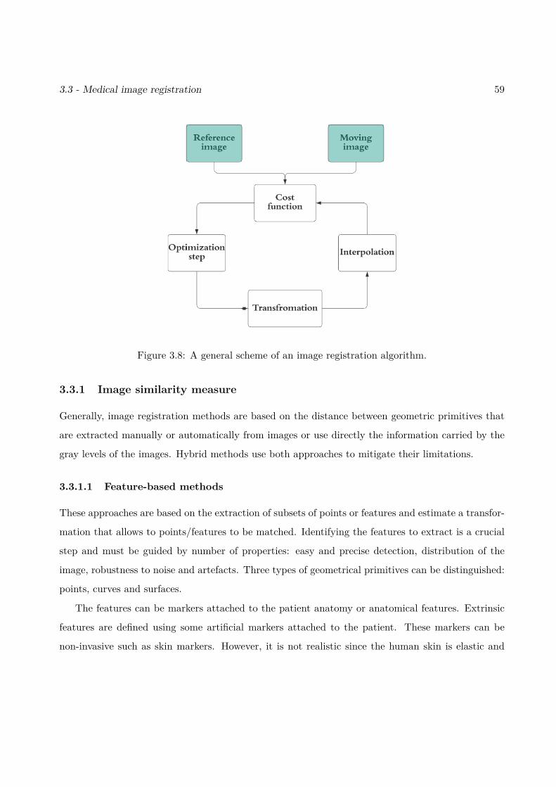
3.3 - Medical image registration 59
Figure 3.8: A general scheme of an image registration algorithm.
3.3.1 Image similarity measure
Generally, image registration methods are based on the distance between geometric primitives that
are extracted manually or automatically from images or use directly the information carried by the
gray levels of the images. Hybrid methods use both approaches to mitigate their limitations.
3.3.1.1 Feature-based methods
These approaches are based on the extraction of subsets of points or features and estimate a transfor-
mation that allows to points/features to be matched. Identifying the features to extract is a crucial
step and must be guided by number of properties: easy and precise detection, distribution of the
image, robustness to noise and artefacts. Three types of geometrical primitives can be distinguished:
points, curves and surfaces.
The features can be markers attached to the patient anatomy or anatomical features. Extrinsic
features are defined using some artificial markers attached to the patient. These markers can be
non-invasive such as skin markers. However, it is not realistic since the human skin is elastic and
60 Chapter 3 - Fusion and Registration in Medical Imaging
can be deformed easily. The non invasive markers such as stereotactic frames allow a robust and
accurate registration and are automatically detectable in images. However, they are uncomfortable
for patients and are difficult to be attached. Intrinsic features refer to points, curves or surfaces
extracted manually by experts or detected automatically using a feature detection algorithm. The
accuracy of this approach depends on the precision of these features and the salient information that
they carry. Alam and Rahman introduced two articles: the first one [AR16] is a detailed review
about the existing techniques for intrinsic image registration in a comprehensive manner and the
second one summarizes the extrinsic registration techniques existing in the literature for medical
images [ARU+16].
Several criteria and distances have been proposed in the literature for matching these extracted
features:
• To measure the distance between paired points, the standard Euclidean is classically used.
Thanks to its analytical properties, in the case of rigid or affine registration, it leads to an
analytical solution for the estimation of the transformed parameters:
Fs(T, Ir, Im) =∑i
‖pi − T (qi)‖2 (3.22)
where p and q are the two extracted sets of points.
• To measure the distance between two curves, two surfaces or two volumes, several approaches
are possible. ICP (iterative closest point) is the most frequently used algorithm: for each
point or a selection of points in the point cloud of the moving image, ICP matches the closest
point in the point cloud of the reference image. Then, it estimates the least square rigid
transformation relating these sets of points and continue until convergence to a local optimum.
Generally, ICP is applicable when a relatively good starting point for the initialization of the
algorithm is available. Otherwise, it will be trapped into the first local minimum and the
solution will not be reliable. ICP was introduced for the fist time for image registration by Besl
and McKay in [BM92]. Then, many studies have proposed variants of ICP such as EM-ICP
[GP02], fuzzy ICP [KSK96] and GO-ICP [YLCJ15]. The ICP algorithm has been used for the
3.3 - Medical image registration 61
registration of multiple modalities: MR/US images [FAS+12, MJF+12], MR/mammography
images [KEBH13], MR/CT scans [SKHB18], CT/PET scans [MCS+07] and CT/SPECT scans
[KDM+02].
The major disadvantage of these approaches is that they are very depending on the precision
with which the features have been extracted. Another limit concerns the accuracy of the resulting
registration, which is guaranteed only in the vicinity of the features. Finally, the main problem with
these approaches is that the extraction of features is operator dependent. Note that many automatic
and semi-automatic methods have been investigated in the literature [KZW+12, MOM+10].
3.3.1.2 Intensity-based methods
Contrary to feature-based approaches, the intensity-based approaches do not use a preliminary data
reduction step. They use the dense information carried by all the pixels/voxels of the image, either
by directly comparing the intensity levels or by associating to each pixel/voxel a value determined
from gray levels and comparing these sets of values. It is possible to consider differences of pixel
intensities such as gradients. Thus, registration can be achieved automatically. Similarity measures
allow for the comparison of information carried by the gray level intensities of the image. Each
criterion makes an assumption about the relationship that link these intensities. One of the basic
alignment measures is the sum of squared intensity differences (SSD) between images defined as:
SSD =∑x
[Ir(x)− Im(T (x))]2 (3.23)
where x is a pixel/voxel coordinate. SSD is typically used for mono-modal image registration [RA10]
because it is very sensitive to the contrast difference that may exist between multi-modal images.
Another measure is the cross-correlation alignment [AEGG08], which assumes that there is an
affine relationship between the intensities of the moving and the reference images:
CC = 1NσIrσIm
∑x
(Ir(x)− µIr
)(Im(T (x))− µIm
)(3.24)
where σIr , σIm are the standard deviation of the reference and moving images and µIr , µIm are the
mean of the reference and moving images. CC = 0 means that the two images are realizations of
62 Chapter 3 - Fusion and Registration in Medical Imaging
uncorrelated random variables and therefore are impossible to register. In the other cases, registration
can be obtained by maximizing CC. CC can be used for multi-modal registration such as MR and
CT scan registration for brain diagnosis [VdEMPV95, Sam09]. One of the well-known variant form
of cross-correlation is the local correlation (LC):
LC =
√√√√ 1Ns
(∑sj
CC2(sj))
(3.25)
where sj is the jth extracted patch from both images, CC2 is the square cross-correlation, Ns is
the number of extracted patchs. LC has been used successfully for rigid and non-rigid multimodal
registration [ZF03, WRN+99].
A common assumption is to consider that there is a functional relationship between the reference
and the moving images. Woods [WGH+98] has proposed an original criterion which proved itself to
be efficient for matching PET with MR defined as:
Woods =∑i
piσIr|jµIr|j
(3.26)
where σIr|j and µIr|j are respectively the standard variation and the mean of the intensities observed
in the reference image Ir that corresponds to the pixels/voxels in the moving image Im with intensities
equal to j. Roche proposed in [RPMA01] another functional relationship between images for image
registration: the bivariate correlation ratio, which assumes that an unknown polynomial function
can link MR and US images.
A completely different approach is to consider a statistical dependency between images. The
mutual information was first introduced in [VWI97, CMD+95] to measure the dependency between
images. It has been widely used for image registration [MCV+97]. Based on Shannon definition, MI
can be written as follows:
MI =∑i,j
pi,j log pi,jpipj
(3.27)
where pi, pj are respectively the probability of a pixel/voxel in Ir to have an intensity equal to i and
a pixel/voxel in Im(T ) to have an intensity equal to j and pi,j is the joint probability. Note also that
the transformation parameter can be estimated by maximizing the mutual information. Note that a
robust variant of the mutual information is the normalized mutual information (NMI) [XCT+08].
3.3 - Medical image registration 63
3.3.2 Transformation models
After defining a similarity measure, a transformation model can be constructed. It should transform
the moving image to be superimposed to the reference image. The choice of a transformation model
depends on the assumed geometric deformation introduced during the image acquisition, and on the
required accuracy of registration. Transformation models can be divided into two main categories
based on global models and deformable or local models.
3.3.2.1 Global models
Global models include rigid, affine, similarity, and perspective transformations [OT14b]. A rigid
transformation can register objects that are related by a rotation (φ) and a translation (tx, ty):
u = x cos(φ)− y sin(φ) + tx
v = x sin(φ) + y cos(φ) + ty,(3.28)
where x, y are the coordinate of a pixel i in the moving image before registration and u, v are the
coordinate of the same pixel after registration. A rigid transformation preserves distances between
all the pixel pairs in the image. It is one of the simplest transforms, which has mainly be used in
the context of medical imaging to register images of the same person acquired at different times or
in different imaging modalities. The number of degrees of freedom equals 3 for 2D images and 6 for
3D images.
Similarity models are built using a translation (tx, ty), a rotation (φ), and a scaling (s), i.e.,
u = s(x cos(φ)− y sin(φ)) + tx
v = s(x sin(φ) + y cos(φ)) + ty,(3.29)
A similarity model is generally called shape-preserving because it preserves angles and curvatures.
The number of degrees degree of freedom is 4 for 2D images and 7 for 3D images.
An affine transformation is a linear combination of translation, rotation, scaling, and shearing
defined as:
u = a0 + a1x+ a2y
v = b0 + b1x+ b2y.(3.30)
64 Chapter 3 - Fusion and Registration in Medical Imaging
An affine transformation preserves the parallelism of straight lines in the image. This model is
generally used in the context of medical imaging for inter-individual registration. However, its low
degree of freedom does not allow to accurately capture inter-individual anatomical variability. The
number of degrees of freedom is 6 for 2D images and 12 for 3D images.
The perspective transformation can be written as
u = a0 + a1x+ a2y
1 + c1x+ c2y
v = b0 + b1x+ b2y
1 + c1x+ c2y.
(3.31)
It does not keep the parallelism but imposes that the image of a straight line is a straight line.
This type of transformation can be used in the context of medical imaging for the registration of
radiological images (for this problem, the radiation from a point source interacts with the object to
be imaged to form a projection image in a plane) or in virtual reality applications.
3.3.2.2 Non-linear models
Linear models allow only a small number of degrees of freedom and are therefore poorly adapted
to capture inter-subject anatomical variability or the morphological variability of certain organs. In
many applications, such as brain or abdominal organ registration, it is necessary to use transforma-
tions with a large number of degrees of freedom, capable of modifying the overall shape of structures.
For this purpose, different non-linear models (called also non-rigid models) can be considered.
Polynomials
A polynomial representation can be used to model the deformation field between the two images.
Polynomials of order 2 to 5 have been considered [RPMA01]. Beyond this order, significant oscil-
lations appear, which reduces the interest of this model. A disadvantage of polynomial models is
related to their field of application, which is global, making them unsuitable for taking into account
local variations in shape. This limitation can be overcome by using polynomial models piecewisely.
Radial basis functions
A radial basis function (RBF) is a function ψ : Rn → R whose value depends on the input and
m fixed points called the centers ci (where i ∈ J1,mK) that can be used as control points for
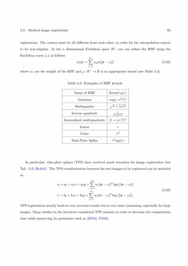
3.3 - Medical image registration 65
registration. The centers must be all different from each other, in order for the interpolation matrix
to be non-singular. In the n dimensional Euclidean space Rn, one can define the RBF using the
Euclidean norm ‖.‖ as follows
ψ(x) =m∑i=1
wiρ(‖x− ci‖) (3.32)
where wi are the weight of the RBF and ρ : R+ → R is an appropriate kernel (see Table 3.3).
Table 3.3: Examples of RBF kernels.
Name of RBF Kernel ρ(r)
Gaussian exp(−ε2r2)
Multiquadric√
1 + (εr)2
Inverse quadratic 11+(εr)2
Generalized multiquadratic (1 + (εr)2)β
Linear r
Cubic r3
Thin-Plate Spline r2 log(r)
In particulat, thin-plate splines (TPS) have received much attention for image registration (see
Tab. 3.3) [Roh01]. The TPS transformation between the two images to be registered can be modeled
as
u = a0 + a1x+ a2y +m∑i=1
wi‖x− ci‖2 log(‖x− ci‖
)v = b0 + b1x+ b2y +
m∑i=1
wi‖x− ci‖2 log(‖x− ci‖
).
(3.33)
TPS registration usually leads to very accurate results but is very time consuming, especially for large
images. Many studies in the literature considered TPS variants in order to decrease the computation
time while preserving its pertinence such as [BN92, PD92].
66 Chapter 3 - Fusion and Registration in Medical Imaging
Cubic B-spline
Another function from the spline family that is used for image registration is the cubic B-spline.
A spline can be defined as a piecewise polynomial function defined by knots (the points where the
polynomials meet) ki. The B-spline is a particular spline function that has minimal support with
respect to a given degree, smoothness, and domain partition. Cubic B-splines are B-splines of degree
3, which provide good compromise between simplicity and accuracy.
Denote as Ω = (x, y) | 0 ≤ x < N, 0 ≤ y < M the domain of the image-plane and consider an
nx × ny mesh of control points φij with identical spacing δ, denoted as Φ. The cubic B-spline local
transformation is defined as:
Tφ(x, y) =3∑
m=0
3∑n=0
Bm( xnx
)Bl( yny
)φix+m,jy+n, (3.34)
where ix = b x/nxc − 1, jy = by/nyc − 1 and b.c is used for the integer part. The cubic B-spline
uniform functions are defined as:
B0(u) = (1− u)3
6
B1(u) = 3u3 − 6u2 + 46
B2(u) = −3u3 + 3u2 + 3u+ 16
B3(u) = u3
6 .
(3.35)
Once the grid of the B-spline has been constructed, it is used to deform the local neighborhood of
every control point in the moving image. Once the moving image has been deformed, it is compared
to the reference image using the similarity measure. The cubic B-spline model has been used for
different applications in medical imaging such as registration of CT scan and MR image of heart
[KSP07] and motion estimation applied to MR images of the brain [VHS+98].
Elastic body models
Another registration approach is a non-parametric deformation model. In this technique, the
object being deformed is modeled as an elastic body. This idea has been introduced by Bajcsy in
[BK89]. The image is considered as a rubber sheet where external and internal forces are applied to
3.3 - Medical image registration 67
align images with minimum amount of bending and stretching. The spatial transformation T satisfies
the partial differential equation (the Navier Cauchy PDE):
µ∇2T + (µ+ λ)∇(∇T ) = S(T ) (3.36)
with certain boundary conditions such as T (z) = 0 for z located on the image boundary. S(T ) is the
body force that drives the registration (some examples of the body forces are given in [WS98]), ∇ is
the gradient, β and α are the Lamé coefficients. Elastic body models are simple to implement but
they are limited by their inability to model large and global deformation.
Viscous fluid Flow models
Viscous fluid Flow models are non-parametric models. The purpose of fluid registration is to
imitate a flow of fluid. Fluid registration has been used successfully in medical applications such as
brain image registration [DMVS03]. This kind of approach does not assume small deformations and
thus is able to model large and smooth deformations while maintaining continuity. The motion of
this transformation v is modeled by the Navier-Stokes equation and can be written as:
µ∇2v + (µ+ λ)∇(∇v) = S(v) (3.37)
where µ and λ are are the viscosity constants. The relationship between the transformation T and
the velocity v is given by
∂T (x, t)∂t
= v(x, t) +∇T (x, t)v(x, t). (3.38)
Even if this model is interesting, it cannot be used in images containing non-fluid objects.
Other examples of non parametric models used for image registration are diffusion models [HS81]
and curvative models [FM04]. The diffusion models handle object contours and features, and estimate
the smoothness of the deformation field rather than mimicking physical properties as fluid and elastic
models.
3.3.3 Regularization in deformable registration
A regularization can be introduced to a transformation model in order to avoid discontinuities in
the estimated transformation. For instance, the estimated transformation can be constrained based
68 Chapter 3 - Fusion and Registration in Medical Imaging
on prior knowledge about image acquisition, physical conditions, Cartesian coordinate changes, spa-
tial distortion, etc. Two kinds of regularizations have been considered for image registration: (1)
competitive regularization, (2) iterative filtering approaches.
3.3.3.1 Competitive regularization
Competitive approaches consist in considering a cost function composed of a data fidelity term based
on the similarity measure (see section 3.3.1) Fs and a regularization term Rs that penalizes abrupt
variations in the deformation field. The solution obtained by minimizing Fs(T ) + τRs(T ) satisfies
a compromise between the data attachment and the regularity of the solution. The regularization
parameter τ make it possible to satisfy this compromise. The regularization term prevents the
appearance of small unrealistic deformations which would cause only a slight decrease in the similarity
criterion. Different regularization energies have been proposed in the literature, many of them having
an interpretation related to material or fluid mechanics. An example of regularization in 2D is
Rs(T ) =∫
Ω
[∂2T
∂x2 + ∂2T
∂y2 + ∂2T
∂x∂y
]dxdy. (3.39)
In practice, the integral (3.39) is approximated by standard numerical integration [RSH+99].
3.3.3.2 Iterative filtering approaches
Iterative filtering approaches [PHF+14] are based on two steps: the first step estimates the trans-
formation T without regularization and the second step is smoothing the estimated deformation
using filters. These two steps are repeated several times until convergence. Several filters have been
proposed in order to smooth transformations such as Gaussian or adaptive filters. The main disad-
vantage of these methods is that they do not take into account the information carried by the image
during the regularization step, which can lead to smoothing areas containing pertinent information.
To overcome this limitation, the filtering can be constrained by a map of weights in order to consider
the information in the image. These weights are generally computed using the norm of the gradient
image.
3.3 - Medical image registration 69
3.3.4 Optimization
The aim of optimization is to estimate the optimal transformation that best aligns the reference and
source images according to a cost function defined using a data fidelity term (similarity measure)
and a regularization term. The choice of an optimization method can impact directly the quality of
the estimated transformation. Two categories of optimization methods were considered in [SDP13]
depending on the nature of the transformation T : (1) continuous methods and (2) discrete methods.
3.3.4.1 Continuous optimization
Continuous methods deal with variables that take real values and cost functions that are differ-
entiable. Generally, these methods update the unknown parameters (to be estimated) using the
following equation:
θk+1 = θk + αkgk(θk) (3.40)
where θ contains the parameters of the transformation, k is the iteration number, αk is the step size
at iteration k and gk is the corresponding search direction. The function gk depends on the similarity
measures and the regularization terms. The stepsize αk can be constant or may change during the
iterations via a line search that satisfies the Wolfe conditions or using the Barzilai–Borwein method.
The search direction can use the first order information such as the gradient descent method,
which is based on the negative gradient:
gk(θ) = −∇Es(θ) (3.41)
where Es(θ) = Fs(Tθ) + τRs(Tθ). Gradient descent methods are widely used in image registration.
They are used for different similarity measures and transformation models. Beg considered the
gradient descent method to register brain images using a least square distance as similarity measure
and the diffeomorphic model for the transformation [BMTY05], Klein used this method to register
images using mutual information and B-spline transformation [KSP07] and Huang proposed a shape
registration based on information theory and free form deformations [HPM06].
Conjugate gradient methods have better rates of convergence than the gradient descent. The
70 Chapter 3 - Fusion and Registration in Medical Imaging
search function conjugates the gradient to the previous direction using the following equation:
gk(θ) = −∇Es(θ) + βgk−1(θ). (3.42)
Some studies that use the conjugate gradient for image registration are [GVM04, PZF08, JSTL07].
Other continuous methods used in medical image registration are: Powell’s conjugate direction
method [PMV04], quasi-Newton methods [KSP07], Gauss-Newton methods [VPPA07], Levenberg-
Marquardt [GTN03] and stochastic gradient descent methods [BGSW07]. All these methods solve
unconstrained optimization problems. Constrained methods can be used when it is necessary such
as the log-barrier method [HM07].
3.3.4.2 Discrete optimization
Discrete optimization methods are used when the variables to estimate take discrete values. They can
be classified into three categories: (1) graph based methods [GPS89], (2) belief propagation methods
[YWA10] and (3) linear programming approaches [GKT+08].
A very comprehensive and detailed survey, presented by Klein, is available in [KSP07]. It com-
pares optimization techniques for image registration using mutual information as a similarity measure
and a B-spline transformation as a regularization.
3.3.5 Image registration metrics
The evaluation and comparison of registration methods, especially non-rigid registration methods,
are challenging problems due to the lack of ground truth. It is indeed difficult for experts to find a
consensus on what should be the transformation allowing the best matching of two images. The notion
of optimality of the registration seems to be closely linked to the application. The oldest method of
registration accuracy is based on visual assessment and is still used at least as complement of some
quantitative measures. Global linear registration methods can be evaluated using the mean square
error (MSE) [CEA00];
MSE = 1N
N∑i=1‖T (pm,i)− pr,i‖ (3.43)
3.4 - MR and US registration: state of art 71
where pm and pr are points extracted from the moving and the reference image and N is the number
of extracted points. The lower the MSE, the more accurate the registration.
The Dice Similarity Coefficient (DSC) is also a metric used for global registration. It was devel-
oped by Thorvald Sørensen and Lee Raymond Dice in 1948 [WCH+17]. It can be written as follows:
DSC = 2a2a+ b+ c
. (3.44)
where a is the number of pixels shared by the moving and the reference images, b and c are the
number of pixels unique to the reference and the moving images. A high value of DSC indicates a
good overlap between images, thus, an accurate registration.
Concerning local image registration, a common quantitative metric is the target registration
error (TRE) [KKM+09]. It uses two sets of landmarks identified by clinical experts2 denoted as
pm = pm,1, ..., pm,s and pr = pr,1, ..., pr,s leading to the following measure:
TRE = 1s
s∑i=1‖T (pm,i)− pr,i‖. (3.45)
A low TRE corresponds to a good local registration accuracy.
In some studies, the cross correlation CC and the median-absolute deviation metrics are used for
a quantitative evaluation of local/global registration methods.
3.4 MR and US registration: state of art
Because of the diversity of images to be registered and the complex deformations affecting medical
images, it is very difficult to design a general method that is adapted to all registration problems.
In the previous sections, we exposed some fusion and registration methods that have been used for
different medical imaging modalities. This section concentrates on the registration of MR and US
images, which can be considered under two angles (1) intensity-based methods and (2) feature-based
methods.2These sets must not be used in estimating the deformation, which can be challenging
72 Chapter 3 - Fusion and Registration in Medical Imaging
3.4.1 Intensity-based methods
The registration of MR and US images using the intensities of these images is a very challenging task.
Indeed, US and MR images are very different modalities: a US image can be seen as an image of
tissue boundaries contaminated by speckle noise with a small field of view and MR is a large field of
view image that provides information on the tissue density (see Chapter 2). For these reasons, basic
similarity measures such as the mutual information MI, the cross-correlation ratio (CCR) and the
sum of squared distances cannot be used easily to align MR and US images [HHR+05]. Therefore,
more complex similarity measures have been proposed for MR and US images; which are summarized
in this section.
Roche et al. in [RPMA01] presented an automatic method to rigidly register US and MR im-
ages. The similarity measure, used in their work, is based on a bivariate version of the generalized
correlation ratio [RMPA98]. In addition, the similarity measure relies on a polynomial function that
correlates the US image to the MR and the gradient of MR images in order to model the intensity
variations in tissue boundaries. Powell’s optimization algorithm was used to implement the bivariate
CCR. This approach outperforms the classical CCR and the mutual information. This technique
has been designed for image-guided neurosurgery and applied to brain images, which explains the
accuracy of a rigid transformation, since the brain is mostly rigid.
Arbel et al. in [AAM+04] proposed an automatic non-linear registration for the same application
as Roche et al. (image guided neurosurgery). The technique first predicts the appearance of the US
image based on a segmented MR image, providing a so-called pseudo US image. Once a pseudo-
US has been generated, the system computes a nonrigid registration based on a piecewise linear
deformation using the ANIMAL algorithm [CE97]. This method provided some insightful results for
the recovery of deformations due to brain shift and operative manipulations.
Craene et al. in [DCdBdM+04] studied a non-rigid MR/US registration algorithm based on a finite
element elastic deformation model to capture the deformation in the liver ablation and the prostate
biopsy. The similarity measure used in this study was a mix between mutual information and linear
elastic energy. The optimization was performed using a new method referred to as Perturbation
Stochastic Approximation (PSA). The use of volumetric meshes applied to the surfaces of organs to
3.4 - MR and US registration: state of art 73
build the deformation showed promising results.
Mitra et al. in [MMO+12] proposed a 2D deformable registration that aligns a pre-biopsy MR
image and a transrectal ultrasound image (TRUS). TRUS imaging is used to guide prostate biopsy.
A combination with pre-biopsy MR may help to improve the detection of early stage malignancy.
The method studied in [MMO+12] involves B-spline free-form deformations and a similarity measure
based on the normalized mutual information between the two images. Their main contribution was
to compute the NMI from the texture images obtained from the amplitude responses of directional
quadrature filters. The entropy between MR and TRUS intensity images is more than the entropy
between texture images because of the variations of gray levels. Using the texture images helps
NMI to better catch the (dis)similarities between MR and TRUS images. The optimization of the
resulting cost function was performed with a quasi-Newton algorithm. The results clearly outperform
a B-spline registration relying on NMI based on gray level intensities.
A different approach is based on the modality neighborhood descriptor (MIND) [HJB+12] and
its variant based on a self-similarity context (SSC) [HJP+13, RKC14]. These methods do not rely on
global intensity relations but use the difference of pre-defined neighborhood maps. [RKC14] proposes
a self similarity α-MI (SeSaMI) metric as a similarity measure to deal with B-spline MR and US
registration. This method showed robustness against signal nonstationarity and intensity distortions
and yielded insightful results for image-guided neurosurgery.
Fuerst et al. proposed in [FWMN14] another similarity measure to deal with MR and US regis-
tration. A linear correlation of linear combination (LC2) was first designed to register the US image
and a CT scan [WBK+08]. Fuerst et al. adapted this idea to MR-US registration. They assumed
that the US intensity is either correlated with the MR intensity or with the gradient of MR which
leads to a first order polynomial function that relates the US image to the MR image and its gradient.
A free-form deformation based on cubic B-splines was used to build the transformation between the
two images. This technique showed some accurate results for image guided neurosurgery using 14
clinical cases.
74 Chapter 3 - Fusion and Registration in Medical Imaging
3.4.2 Feature-based methods
The registration of MR and US images using feature-based methods can be very accurate, easy to
implement and not expensive. This kind of registration generally relies on data reduction performed
by an expert and segmentation. However, if MR image can be automatically segmented and features
can be easily extracted from these images, it is more difficult for US images because they are highly
contaminated by speckle noise. Thus, generating an automatic feature-based registration of MR/US
images is very difficult.
Singh et al. proposed in [SKX+08] a manual registration method for real-time transrectal ultra-
sonography (TRUS) and previously acquired MR image to guide prostate biopsies. The sequence
of MR images was registered manually to the US using custom software for real-time navigation
and feedback. However, this approach relies significantly on the pertinence of the choice of control
points and their correspondence in both images. In order to decrease user interaction, automatic and
semi-automatic methods were also presented in [KZW+12].
Kadoury et al. investigated in [KZW+12] an approach to rigidly register the preoperative MR and
the intraoperative US to allow pertinent needle placement during the ablation of liver metastases.
Their contribution consists of training a deformable model for unsupervised segmentation of the
liver in the MR image and extracting automatically the liver boundaries from the US image. The
registration was performed using a weighted ICP algorithm with internal energy as a penalization.
Yavariabdi et al. considered in [YSB+13] a variational approach to map endometrial implants
from transvaginal ultrasound (TVUS) and MR images. Images were first segmented by experts.
A novel variational one-step deformable ICP method was used to estimate the deformation. This
variant of ICP was then used to compute the deformation field based on a curative transformation
and also to establish point correspondences automatically. Thus, it allows one to decrease the expert
error and the interaction time while selecting manually point correspondences.
Mitra et al. presented in [MOM+10] an automatic deformable method for MR and US registration
for prostate biopsy. The deformation model was based on radial basis functions, more specificaly
on a thin-plate spline TPS. One contribution was to estimate the spline knots using a triangulation
technique with the axes of the segmented prostate in MR and TRUS images. The two images
3.5 - Global Conclusions 75
were segmented using the method of [GOM+10]. A Shepard interpolation was used to overcome
interpolation artefacts caused by the inverse TPS transform.
3.4.3 Other approach
Atehortúa et al. presented in [AGS+20] a novel 3D multimodal registration strategy to fuse 3D
real-time echocardiography images with cardiac cine MRI images. This alignment was performed
in a saliency space, which was designed to maximize similarity between the two imaging modalities.
This fusion improves the quality of the available information. The used method performs in two
steps: temporal and spatial registrations. A temporal alignment was firstly achieved by non linearly
matching pairs of correspondences between the two modalities using a dynamic time warping. A
temporal registration was then carried out by applying nonrigid transformations in a common saliency
space where normalized cross correlation between temporal pairs of salient volumes was maximized.
3.4.4 Conclusion
In our joint fusion and registration method presented in Chapter 5, we will consider a registration
step in order to correct registration errors during the fusion process. We will adopt the intensity-
based approach with a polynomial function fc as a similarity measure. We choose this similarity
measure because it is also used in the fusion process to match the pixel intensities from MR and
US images. The adopted transformation model is composed of a global transformation based on an
affine operator and a local transformation based on B-splines, since free form B-spline have been
widely used for non-rigid MR/US registration.
3.5 Global Conclusions
Since there is, to our knowledge, no state-of-the-art method for the fusion of MR and US images, this
chapter proposed basic survey of medical image fusion. We can note that medical image fusion is a
hard task and the challenging part is to estimate the link relating medical images especially when
using multiple modalities. Transforms or feature extraction may be used to overcome this challenge
but they are limited and sensitive to the low SNR of input images.

76 Chapter 3 - Fusion and Registration in Medical Imaging
The second part of this chapter presented the image registration framework and its components
with a general survey on medical image registration . This chapter was concluded by a state-of-the-
art on MR and US registration. Note that intensity-based and feature-based registration methods
have their own limitations and challenges. Intensity-based methods require to find an appropriate
similarity measure that links information in images whereas feature-based methods are operator-
dependent and rely excessively on the pertinence of features extracted by medical experts . At this
point, we would like to mention that the few automatic studies in MR/US feature-based registration
cannot handle important deformation between the images to be registered.
Chapter 4
Fusion of MRI and US images
Part of this chapter has been adapted from the journal paper [EMVB+20]
Contents4.1 Introduction . . . . . . . . . . . . . . . . . . . . . . . . . . . . . . . . . . . . 774.2 MR/US fusion using a global polynomial function . . . . . . . . . . . . . 78
4.2.1 A statistical model for the fusion of MRI and US images . . . . . . . . . . . 784.2.2 Algorithm for MR/US fusion . . . . . . . . . . . . . . . . . . . . . . . . . . . 834.2.3 Simulation results . . . . . . . . . . . . . . . . . . . . . . . . . . . . . . . . . 89
4.3 MR/US images fusion using a patch-wise polynomial . . . . . . . . . . . . 1094.3.1 Estimation of the polynomial functions fp . . . . . . . . . . . . . . . . . . . . 1094.3.2 Experimental results using a patch-wise polynomial function . . . . . . . . . 110
4.4 Conclusion . . . . . . . . . . . . . . . . . . . . . . . . . . . . . . . . . . . . . 114
4.1 Introduction
This chapter studies a new fusion method for MR and US images, based on two image formation
models gathering the advantages and drawbacks of each modality. More precisely, the MR image
formation model accounts for the low spatial resolution of the observed image using a standard
linear model with blurring and downsampling operators. The US image formation model takes into
consideration the high amount of speckle noise, which is assumed to be Rayleigh-distributed as in
many works including [AB07a, GCS05a, GSP05]. Given the different physical phenomena involved
in each imaging modality, we propose to model the correspondence between gray levels of MR and
US images using a polynomial function. This polynomial model can be theoretically motivated by
the Weierstrass approximation theorem, which states that any continuous function on a closed and
bounded interval can be uniformly approximated on that interval by polynomials with any degree of
77
78 Chapter 4 - Fusion of MRI and US images
accuracy [MS00]. A more practical reason for using this kind of relationship between MR and US
images is its successfull application to MR and US image registration [RPMA01]. Another variant to
link MRI and US images, based on a patch-wise polynomial model, is also presented. The non-linear
cost function considered to solve the fusion problem is constructed using the observation models
associated with the MR and US images and the polynomial transformation relating the two images.
Its minimization is challenging and is handled by a proximal alternating linearized minimization
(PALM) algorithm. The proposed image fusion method is evaluated on simulated data with available
ground truth, and on experimental data acquired on a phantom with imaging characteristics close
to endometriosis. Both qualitative and quantitative results show the interest of fusing MR and US
images, compared to restoring independently the images with each modality.
The remainder of this chapter is organized as follows: Section 4.2 introduces the statistical models
for MR and US image fusion including a non-linear relation between the two modalities. The different
steps of the proposed MR/US image fusion algorithm are detailed. Results obtained on simulated
data and on an experimental allow the performance of the proposed method to be evaluated. Section
4.3 proposes a patch-wise polynomial model to link MRI and ultrasound images and compares results
with the global polynomial function of Section 4.2. Conclusions are reported in Section 4.4.
4.2 MR/US fusion using a global polynomial function
4.2.1 A statistical model for the fusion of MRI and US images
The image fusion model introduced in this section assumes that the MR and US images to be
fused are aligned, i.e., there is no geometric distortion between them, which can be obtained after
an appropriate pre-registration. Thus, the registration potentially required in practical applications
(see Chapter 3, Section 3.4) is considered herein as a pre-processing step and the possible registration
errors are ignored hereafter. Note that despite this hypothesis, the fusion task is challenging because
the two imaging modalities have different resolutions and contrasts and are corrupted by different
kinds of noise.
4.2 - MR/US fusion using a global polynomial function 79
4.2.1.1 Observation models
As stated in Chapter 2, MRI has the advantage of acquiring images with a large field of view, at
the expense of a relatively low spatial resolution. In contrast to MRI, depending on the choice
of the central frequency of the probe, US imaging can offer well-resolved images. However, US
images are contaminated by a high level of speckle noise and have a reduced field of view. Based on
these observations, many existing works aimed at improving independently the quality of MR and US
images. In the case of MRI, the loss of resolution is classically modelled by a downsampling operation
and a low pass filter [SCW+15]. In US imaging, speckle noise is usually considered as additive when
considering the log-compressed envelope mode (also called B-mode) with a log-Rayleigh distribution
[KR05, TSP88a]. This study assumes that the US noise sequence is independent and identically
distributed (i.i.d) as in [C+02, BNB03]. Note that modelling the spatial correlation of noise samples
would increase the complexity of the fusion method and is left for future work. These observations
lead to the following image formation models
ym = SCxm + nm
yu = xu + nu
(4.1)
where xm ∈ RN is the non-observable high-resolution vectorized MR image, ym ∈ RM is the observed
low-resolution vectorized MR image and nm ∈ RN is the independent and identically distributed
(i.i.d.) noise vector corrupting the MR image, assumed to be Gaussian as in [GP95]. Note that
C ∈ RN×N is a block circulant with circulant blocks matrix modelling the blurring effect of the MRI
by a point spread function (PSF) and that S ∈ RM×N (with N = s2M) is a decimation operator
with a decimation factor s. On the other hand, yu ∈ RN is the observed vectorized B-mode US
image, xu ∈ RN is the noise-free vectorized US image and nu ∈ RN is an i.i.d. additive log-Rayleigh
noise with localization parameter γ. Note that the speckle noise affecting US images is mainly
caused by diffusion, i.e., by the constructive and destructive interferences between echoes originated
by small (with respect to the US wavelength) point targets called scatterers. Note also that all
the vectors in (4.1) are obtained by vectorizing the corresponding images using the lexicographical
order. Finally, we assume that xm and xu have the same spatial sampling, which can be obtained in
80 Chapter 4 - Fusion of MRI and US images
practical applications by adjusting the decimation factor d in the MRI model, so that pixels in the
super-resolved MR and US images have the same size.
4.2.1.2 Relation between US and MR images
MR and US imaging systems exploit different physical phenomena. Consequently, when imaging the
same tissues, even in the virtual case of a perfect acquisition (without noise) allowing xm and xu to
be directly observable, these two systems would not provide the same measurements. Thus, images
xm and xu in (4.1) are not equal, even if they correspond to the same tissue. For solving the fusion
task, we propose to link these two images by a parametric model. More precisely, we adopt the model
originally proposed in [RPMA01] for MR/US image registration. This model is motivated by the
fact that US image formation is essentially based on the gradient of the acoustic impedance between
neighbouring tissues and is thus able to highlight the interfaces between anatomical structures. For
US imaging, US waves (short pulses) are transmitted by the transducer, propagate through the
tissues, and return to the transducer as reflected echoes. The reflected echoes correspond to US
wave reflection at the interfaces between tissues with different acoustic impedances. Thus, the most
important features in US images correspond to regions with gradient of impedance. The noise-free
US envelope image (after amplitude demodulation of beamformed RF signals) can be expressed as
au = ∇ZHu (4.2)
where au is the speckle-free US envelope image, Z is the acoustic impedance map, u is the scan
direction, H stands for Hermitian transpose and ∇ is the discrete gradient operator. The B-mode or
log envelop of au, denoted by xu in (4.1) is
xu = b log[∇ZHu] + g (4.3)
where b and g are linear gains.
Exploiting the previous US image model relating US and MR pixel amplitudes turns out to finding
a relationship between the MRI amplitude and the acoustic impedance Z, denoted by φ such that
Z = φ[xm]. (4.4)
4.2 - MR/US fusion using a global polynomial function 81
Computing the gradient of (4.4) leads to
∇Z = φ′[xm]∇xm (4.5)
where φ′ is the derivative of the unknown function φ. By plugging (4.5) into (4.3), the following
relation between the US and MR images is obtained
xu = b log[φ′(xm)∇xHmu
]+ g (4.6)
where b and g are constants. Note that the amplitude of one pixel in xu not only depends on the
value of its counterpart in xm, but also on the gradient of the MR image. To simplify the notations,
this functional mapping between the US and MR images is defined as
xu = f(xm,∇xHmu) (4.7)
where f : RN × RN → RN is an unknown function and ∇xHmu ∈ RN contains in its ith line the inner
product between the ith local gradient xm and the US scan direction u.
We propose in this thesis to approximate the unknown function f in (4.7) by a polynomial (as in
[RPMA01]) such that
xu,i =∑
p+q≤dcpqx
pm,i(∇xHmu)qi (4.8)
where cpq are the unknown polynomial coefficients, index i stands for the ith coefficient of a vector
and d is the degree of the polynomial.
Remark 1. For simplicity, one might consider that the unknown function f can be approximated by alinear function that links directly the US image to the MRI and the gradient of MRI (see [MBV+19]).However, due to the complex relation between MRI and US gray-level intensities, a linear function isnot sufficient to model this relationship.
4.2.1.3 A Bayesian approach for MR and US image fusion
Using the relationship between MR and US images in (4.7), the image formation models in (4.1) can
be rewritten as
ym = SCx+ nm
yu = f(x,∇xHu) + nu
(4.9)
82 Chapter 4 - Fusion of MRI and US images
where x ∈ RN is the unknown image to be estimated, containing relevant information from both
MR and US data. The conditional distributions of ym and yu can be determined using the noise
distributions
ym|x ∼ N (SCx, σ2mIN )
yu|x ∼ LR(γ)(4.10)
where N (µ,Σ) denotes the normal distribution with mean vector µ and covariance matrix Σ, and
LR(γ) is the log-Rayleigh distribution with parameter γ1. Using Bayes rule and the independence
between the noise vectors nm and nu, the posterior distribution of x can be computed
p(x|ym,yu) ∝ p(ym|x)p(yu|x)p(x) (4.11)
where p(x) is the prior probability distribution of x and ∝ means “proportional to”. Finally, the
log-posterior distribution can be written as
− log p(x|ym,yu) = K + 12‖ym − SCx‖
2︸ ︷︷ ︸MRI data fidelity
− log [p(x)]︸ ︷︷ ︸regularization
+N∑i=1
[exp(yu,i − fi(x,∇xHu))− γ(yu,i − fi(x,∇xHu))
]︸ ︷︷ ︸
US data fidelity
(4.12)
where yu,i and fi(x,∇xHu) are the ith components of yu and f(x,∇xHu) and K is a constant.
Different prior distributions p(x) have been considered in the literature to solve ill-posed problems.
In this study, we propose to use the classical total variation (TV) promoting piece-wise constant fused
images. Estimating x in the sense of the maximum a posteriori principle using this TV regularization
leads to the following minimization problem
x = argminx
12‖ym − SCx‖
2 + τ1‖∇x‖2 + τ3‖∇f(x,∇xHu)‖2+
τ2
N∑i=1
[exp(yu,i − fi(x,∇xHu))− γ(yu,i − fi(x,∇xHu))
] (4.13)
1The probability density function (pdf) of a variable distributed according to a log-Rayleigh distribution denoted asz ∼ LR(γ) is p(z) = (ez)2
γexp[− (ez)2
2γ
]IR+ (z), where IR+ is the indicator on R+.
4.2 - MR/US fusion using a global polynomial function 83
where τ1, τ3 and τ2 are hyperparameters balancing the weights of the data fidelity and TV regu-
larization terms. Note that the cost function in (4.13) depends on the polynomial parameters cpqrelating US and MR pixel amplitudes, that need to be estimated before solving (4.13).
4.2.2 Algorithm for MR/US fusion
This section studies an optimization algorithm dedicated to solve (4.13). The presence of the non-
linear polynomial function f in (4.13) prevents the use of algorithms based on the alternate direction
method of multipliers (ADMM) [BPC+11] (as in [MBV+19]). Consequently, we propose hereafter an
algorithm based on the proximal alternating linearized minimization (PALM), adapted to nonconvex
and nonsmooth functions [BST14].
4.2.2.1 PALM summary
The PALM algorithm was originally designed to minimize functions of two vectors x and v that can
be decomposed as
minx,v
ψ(x,v) := l(x) + g(v) +H(x,v) (4.14)
where l and g are continuous convex functions and H may be non-linear. Moreover, these three
functions must respect the following conditions to fit the PALM framework [BST14]
1. l and g are inf-bounded(infRN
(f)> −∞ and infRN
(g)> −∞
).
2. For any fixed v, the function x 7→ H(x,v) is C1,1, and the partial gradient ∇xH(x,v) is
globally Lipschitz.
3. For any fixed x, the function v 7→ H(x,v) is C1,1, and the partial gradient ∇vH(x,v) is
globally Lipschitz.
4. ∇H is Lipschitz continuous on bounded subsets of the image domain.
PALM can be viewed as a minimization of the sum of the two functions l and g with a linearization
of H around a given point xk. The alternate minimization with respect to the two blocks x and v
proposed in [BST14] generates a sequence (xk,vk)k∈N using the following steps
84 Chapter 4 - Fusion of MRI and US images
Step 1: Choose γ1 > 1, set ck = γ1Lx(vk) and update xk as follows
xk+1 = proxlck(xk − 1
ck∇xH(xk,vk)
)= argmin
x(x− xk)H∇xH(xk,vk) + ck
2 ‖x− xk‖2 + l(x)
where Lx(vk) is the Lipschitz constant of x 7→ ∇xH(x,vk) and vk is the value of v at iteration #k.
Step 2 : Choose γ2 > 1, set dk = γ2Lv(xk) and update vk as folllows
vk+1 = proxgdk(vk − 1
dk∇vH(xk,vk)
)= argmin
v(v − vk)H∇vH(xk,vk) + dk
2 ‖v − vk‖2 + g(v)
where Lv(xk) is the Lipschitz constant of v 7→ ∇vH(xk,v) and xk is the value of x at iteration #k.
Note that this iterative scheme requires to compute the Lipschitz constants Lx(vk) and Lv(xk).
4.2.2.2 PALM for MR/US fusion
In order to respect the constraints mentioned above and to adapt our image fusion minimization
problem to the PALM framework, we propose the following parametrization
l(x) = 12‖ym − SCx‖
22 + τ1‖∇x‖2 (4.15)
g(v) = τ2∑i
[exp(yu,i − vi)− γ(yu,i − vi)] + τ3‖∇v‖2 (4.16)
H(x,v) = τ4
N∑i=1
(vi −
∑p+q≤3
cpqxpi (∇xHu)qi
)(4.17)
where
v = f(x,∇xHu).
Remark 2. With this choice of functions l, g and h, the four assumptions stated previously aresatisfied, as explained hereafter.
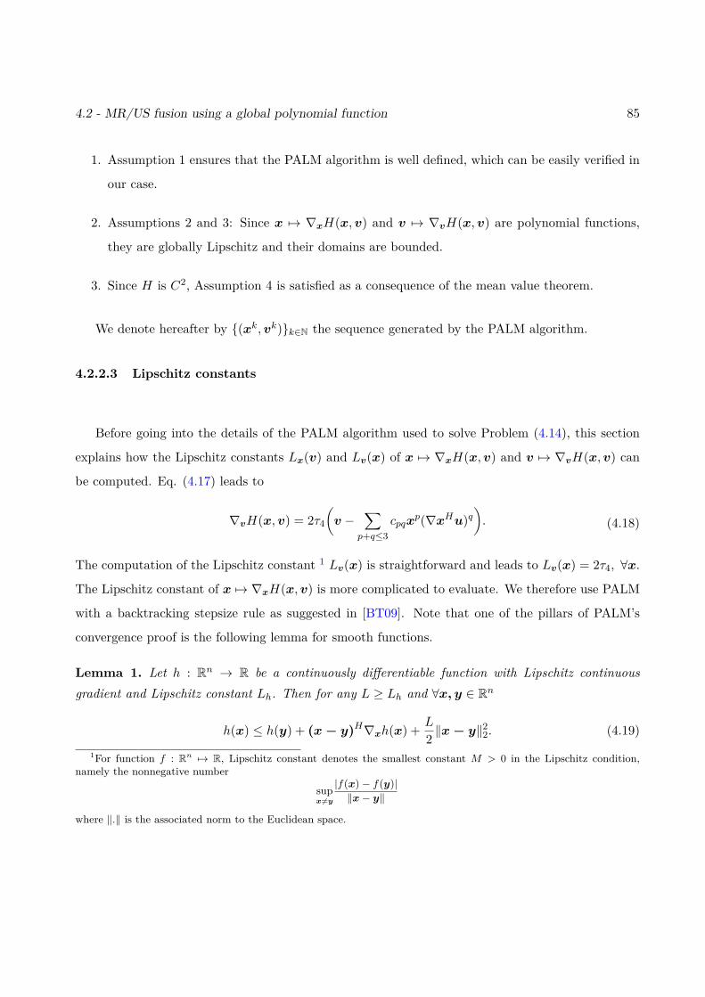
4.2 - MR/US fusion using a global polynomial function 85
1. Assumption 1 ensures that the PALM algorithm is well defined, which can be easily verified in
our case.
2. Assumptions 2 and 3: Since x 7→ ∇xH(x,v) and v 7→ ∇vH(x,v) are polynomial functions,
they are globally Lipschitz and their domains are bounded.
3. Since H is C2, Assumption 4 is satisfied as a consequence of the mean value theorem.
We denote hereafter by (xk,vk)k∈N the sequence generated by the PALM algorithm.
4.2.2.3 Lipschitz constants
Before going into the details of the PALM algorithm used to solve Problem (4.14), this section
explains how the Lipschitz constants Lx(v) and Lv(x) of x 7→ ∇xH(x,v) and v 7→ ∇vH(x,v) can
be computed. Eq. (4.17) leads to
∇vH(x,v) = 2τ4
(v −
∑p+q≤3
cpqxp(∇xHu)q
). (4.18)
The computation of the Lipschitz constant 1 Lv(x) is straightforward and leads to Lv(x) = 2τ4, ∀x.
The Lipschitz constant of x 7→ ∇xH(x,v) is more complicated to evaluate. We therefore use PALM
with a backtracking stepsize rule as suggested in [BT09]. Note that one of the pillars of PALM’s
convergence proof is the following lemma for smooth functions.
Lemma 1. Let h : Rn → R be a continuously differentiable function with Lipschitz continuousgradient and Lipschitz constant Lh. Then for any L ≥ Lh and ∀x, y ∈ Rn
h(x) ≤ h(y) + (x− y)H∇xh(x) + L
2 ‖x− y‖22. (4.19)1For function f : Rn 7→ R, Lipschitz constant denotes the smallest constant M > 0 in the Lipschitz condition,
namely the nonnegative number
supx 6=y
|f(x)− f(y)|‖x− y‖
where ‖.‖ is the associated norm to the Euclidean space.
86 Chapter 4 - Fusion of MRI and US images
Using simple algebra, one can show that the function ψ defined in (4.14) satisfies the following relation
ψ(x,v) ≤ QL(x, y, v) (4.20)
where
QL(x, y, v) = l(x) + g(v) +H(y, v) + (x− y)H∇xH(y, v) + L
2 ‖x− y‖2.
In order to ensure the convergence of the PALM algorithm, the backtracking rule consists of verifying
that the inequality (4.20) is satisfied at every step. To estimate the Lipschitz constant, at each
iteration k, we search for the smallest nonnegative integers ik such that Lk+1 = λikLk verifies
ψ(pL(xk),vk) ≤ QL(pL(xk),xk,vk)
with
pL(xk) = proxlLk+1
(xk − 1
Lk+1∇xH(xk,vk)
).
Remark 3. The sequence of values ψ(xk,vk) computed by PALM is decreasing for all xk and vk.The proof is straightforward. For every k ≥ 1
ψ(xk+1,vk) ≤ QLk+1(xk+1,xk,vk)
andQLk+1(xk+1,xk,vk) ≤ QLk+1(xk,xk,vk) = ψ(xk,vk).
Thusψ(xk+1,vk) ≤ ψ(xk,vk)
andψ(xk,vk+1) ≤ ψ(xk,vk)
which concludes the proof.
Remark 4. Since inequality (4.20) is satisfied for L ≥ Lx(v), ∀v, where Lx(v) is the Lipschitzconstant of x→ ∇xH(x, v), the following inequalities can be obtained
Lx(vk) ≤ Lk+1 ≤ λLH(vk). (4.21)
4.2 - MR/US fusion using a global polynomial function 87
Note that the inequality Lx(vk) ≤ Lk+1 is sufficient to ensure the convergence of PALM. However,the second inequality Lk+1 ≤ λLH(vk) allows the convergence rate to be controlled by an appropriatechoice of λ.
In the following subsections, the updates of each variable within PALM algorithm are described in
details.
4.2.2.4 Update of x
The update of x is achieved by minimizing the sum of quadratic functions, leading to
xk+1 = proxlLk+1
(xk − 1
Lk+1∇xH(xk,vk)
)= argmin
x
12‖SCx− ym‖2 + τ1‖∇x‖2 + Lk+1
2 ‖x− (xk − 1Lk+1
∇xH(xk,vk))‖2
where l is defined in (4.15) and Lk+1 is the Lipschitz constant at iteration k + 1. This minimization
problem admits an analytical solution, which can be computed efficiently in the Fourier domain.
The practical tractability of this solution is possible for large images using the decomposition of the
decimation matrix S proposed in [ZWB+16b], since the convolution operator is diagonalizable in the
Fourier domain. The update of x at the (k + 1)th iteration is then obtained as follows
xk+1 =[CHSHSC + 2
(τ1D + Lk+1
2 IN)]−1
R (4.22)
with
R = CHSHym + 2Lk+1
(xk − 1
Lk+1∇xH(xk,vk)
)D = DH
h Dh +DHv Dv
where Dh and Dv are the horizontal and vertical finite difference operators.
The direct computation of the solution (4.22) requires the inversion of high dimensional matrices.
To overcome this problem, we adopt herein the solution proposed in [ZWB+16b], which is recalled
hereafter. Based on the circulant boundary conditions, the blurring matrix C is a block circulant
with circulant blocks matrix (BCCB) that can be decomposed as
C = FHΛF
88 Chapter 4 - Fusion of MRI and US images
where F and FH are 2D Fourier and 2D inverse Fourier operators, Λ = diag(Fh), with h the first
column of the matrix C. Taking into account this property and using the Woodbury inverse formula
[ZWB+16b], the update of x can be rewritten as
xk+1 = 1τ1Lk+1
FHψFr − 1τ1Lk+1
FHψΛH(2τ1sIN + ΛψΛH)−1ΛψFr (4.23)
where
r = CHSHym + Lk+1
(xk − 1
Lk+1∇xH(xk,vk)
)
and the matrix Λ is a block diagonal matrix denoted as
Λ = [Λ1, ...,Λd]
where the blocks Λi are the diagonal matrices of Λ, and where
ψ = F (τ1(DHh Dh +DH
v Dv) + Lk+12 IN )−1FH .
4.2.2.5 Update of v
The vector v is updated using a gradient descent algorithm with backtracking line search, given
that the function to minimize in this step is differentiable and convex. More precisely, the following
update has ben considered
vk+1 = argminv
τ2∑i
[exp(yu,i − vi)− γ(yu,i − vi)]
+ τ3‖∇v‖2 + dk2 ‖v − (vk − 1
dk∇vH(xk+1,vk))‖2
= proxgdk(vk − 1
dk∇vH(xk+1,vk)
) (4.24)
where g is defined in (4.16) and dk = Lv(xk) is the Lipschitz constant of ∇vH at iteration k.
4.2 - MR/US fusion using a global polynomial function 89
4.2.2.6 Estimation of the global polynomial function
For a given order d, the unknown polynomial function f relating xm to xu is defined by Nd =
(d + 1)(d + 2)/2 coefficients gathered in the vector cd = cpq | p + q ≤ d. To estimate these
coefficients, we assume that the observed MR and US images are related as follows
yu,i =∑
p+q≤3cpqy
pm,i(∇yHmu)qi + εi i = 1, ..., N
or equivalently, in algebraic form
yu = Amcd + ε (4.25)
where Am ∈ RN×Nd is a matrix whose elements are ypm,i(∇yHmu)qi for p+ q ≤ d and ε = (ε1, ..., εN )T .
The least-squares estimator of cd (which is also the maximum likelihood estimator for i.i.d.
Gaussian errors εi) is defined by
cd = A†myu (4.26)
where A†m = (ATmAm)−1AT
m is the pseudo-inverse of the matrix Am. This estimator will be used
to estimate the coefficients of the polynomial function f in our experiments.
4.2.2.7 Algorithm summary
Algo. 1 summarizes all the steps of the proposed MR/US image fusion method.
4.2.3 Simulation results
4.2.3.1 Simulation setup
This section demonstrates the efficiency of the proposed MRI/US fusion method using two sets of
synthetic images with controlled ground truth. The observed MR images were generated from the
high resolution MR images displayed in Figs. 4.1(a) and 4.2(a), after blurring, decimation and
contamination by an additive i.i.d. white Gaussian noise leading to Figs. 4.1(c) and 4.2(c). The
blurring kernel was a 2D Gaussian filter of size 9× 9 with variance σ2m = 4. The decimation factors
were set to s = 4 for the first dataset and s = 2 for the second dataset. A Gaussian noise was finally
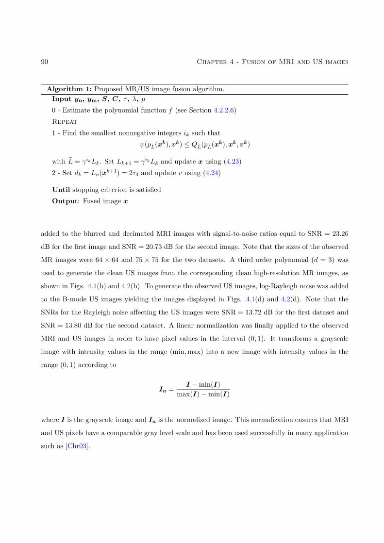
90 Chapter 4 - Fusion of MRI and US images
Algorithm 1: Proposed MR/US image fusion algorithm.Input yu, ym, S, C, τ , λ, µ0 - Estimate the polynomial function f (see Section 4.2.2.6)Repeat1 - Find the smallest nonnegative integers ik such that
ψ(pL(xk),vk) ≤ QL(pL(xk),xk,vk)
with L = γikLk. Set Lk+1 = γikLk and update x using (4.23)2 - Set dk = Lv(xk+1) = 2τ4 and update v using (4.24)
Until stopping criterion is satisfiedOutput: Fused image x
added to the blurred and decimated MRI images with signal-to-noise ratios equal to SNR = 23.26
dB for the first image and SNR = 20.73 dB for the second image. Note that the sizes of the observed
MR images were 64 × 64 and 75 × 75 for the two datasets. A third order polynomial (d = 3) was
used to generate the clean US images from the corresponding clean high-resolution MR images, as
shown in Figs. 4.1(b) and 4.2(b). To generate the observed US images, log-Rayleigh noise was added
to the B-mode US images yielding the images displayed in Figs. 4.1(d) and 4.2(d). Note that the
SNRs for the Rayleigh noise affecting the US images were SNR = 13.72 dB for the first dataset and
SNR = 13.80 dB for the second dataset. A linear normalization was finally applied to the observed
MRI and US images in order to have pixel values in the interval (0, 1). It transforms a grayscale
image with intensity values in the range (min,max) into a new image with intensity values in the
range (0, 1) according to
In = I −min(I)max(I)−min(I)
where I is the grayscale image and In is the normalized image. This normalization ensures that MRI
and US pixels have a comparable gray level scale and has been used successfully in many application
such as [Chr03].
4.2 - MR/US fusion using a global polynomial function 91
4.2.3.2 Performance evaluation
The performance of the proposed fusion algorithm was evaluated for synthetic data using four quan-
titative metrics: the root mean square error (RMSE), the peak signal to noise ratio (PSNR), the
improved signal-to-noise ratio (ISNR) and the mean structural similarity (MSSIM) [HZ10]. These
metrics are defined explicitely in (4.27), where x denotes the ground truth image, x is the estimated
image and y is the bicubic interpolated MR image:
RMSE =√
1N‖x− x‖22
PSNR = 20 log10max(x,x)RMSE
ISNR = 10 log10‖y − x‖‖x− x‖2
MSSIM = 1M
M∑j=1
SSIM(xj , xj). (4.27)
The metric MSSIM is implemented blockwise, where M is the number of local windows, xj and xjare local regions extracted from x and x and SSIM is the structural similarity index computed for
each window as in [WBSS04]. Note that the different metrics were computed using the fused image
and the US and MRI ground truth images. The proposed algorithm was compared to two existing
image restoration algorithms:
• An MR restoration algorithm proposed in [ZWB+16b] to estimate a high-resolution MR image
from the observed low resolution MR image.
• A denoising algorithm adapted to US images proposed in [GSA16].
4.2.3.3 Simulation results
The fused images obtained using the proposed algorithm are displayed in Figs. 4.1(g) and 4.2(g).
The first interesting result is that for both datasets, the fused image contains information from
both MR and US modalities in an enhanced image compared to the two observed MRI and US
images. The fused images are compared visually in Figs. 4.1 and 4.2 to the despeckled US image
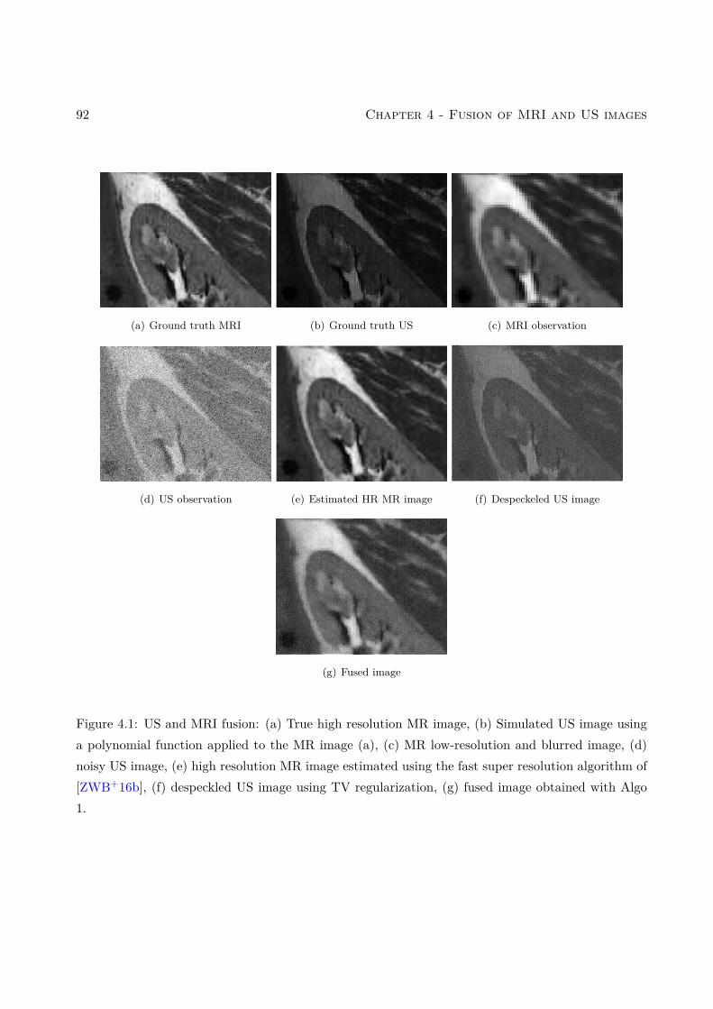
92 Chapter 4 - Fusion of MRI and US images
(a) Ground truth MRI (b) Ground truth US (c) MRI observation
(d) US observation (e) Estimated HR MR image (f) Despeckeled US image
(g) Fused image
Figure 4.1: US and MRI fusion: (a) True high resolution MR image, (b) Simulated US image usinga polynomial function applied to the MR image (a), (c) MR low-resolution and blurred image, (d)noisy US image, (e) high resolution MR image estimated using the fast super resolution algorithm of[ZWB+16b], (f) despeckled US image using TV regularization, (g) fused image obtained with Algo1.
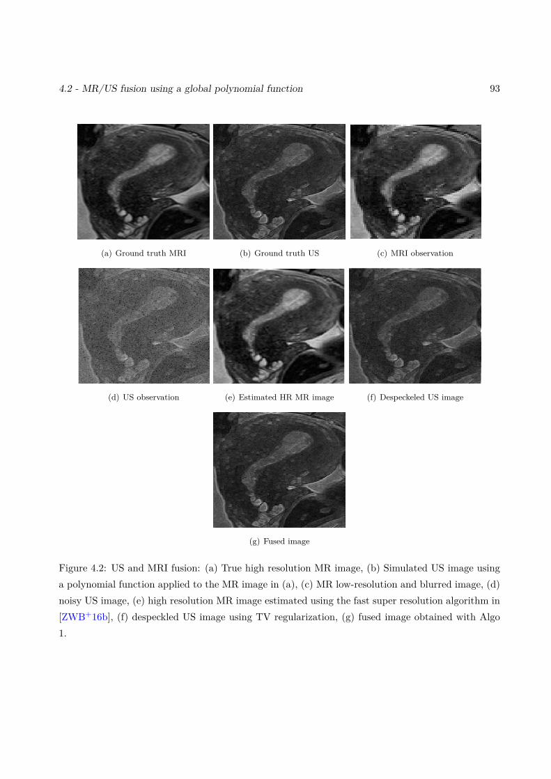
4.2 - MR/US fusion using a global polynomial function 93
(a) Ground truth MRI (b) Ground truth US (c) MRI observation
(d) US observation (e) Estimated HR MR image (f) Despeckeled US image
(g) Fused image
Figure 4.2: US and MRI fusion: (a) True high resolution MR image, (b) Simulated US image usinga polynomial function applied to the MR image in (a), (c) MR low-resolution and blurred image, (d)noisy US image, (e) high resolution MR image estimated using the fast super resolution algorithm in[ZWB+16b], (f) despeckled US image using TV regularization, (g) fused image obtained with Algo1.
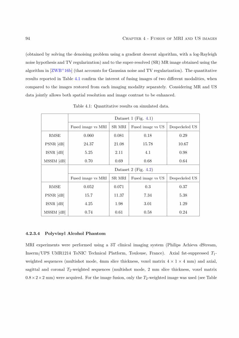
94 Chapter 4 - Fusion of MRI and US images
(obtained by solving the denoising problem using a gradient descent algorithm, with a log-Rayleigh
noise hypothesis and TV regularization) and to the super-resolved (SR) MR image obtained using the
algorithm in [ZWB+16b] (that accounts for Gaussian noise and TV regularization). The quantitative
results reported in Table 4.1 confirm the interest of fusing images of two different modalities, when
compared to the images restored from each imaging modality separately. Considering MR and US
data jointly allows both spatial resolution and image contrast to be enhanced.
Table 4.1: Quantitative results on simulated data.
Dataset 1 (Fig. 4.1)
Fused image vs MRI SR MRI Fused image vs US Despeckeled US
RMSE 0.060 0.081 0.18 0.29
PSNR [dB] 24.37 21.08 15.78 10.67
ISNR [dB] 5.25 2.11 4.1 0.98
MSSIM [dB] 0.70 0.69 0.68 0.64
Dataset 2 (Fig. 4.2)
Fused image vs MRI SR MRI Fused image vs US Despeckeled US
RMSE 0.052 0.071 0.3 0.37
PSNR [dB] 15.7 11.37 7.34 5.38
ISNR [dB] 4.25 1.98 3.01 1.29
MSSIM [dB] 0.74 0.61 0.58 0.24
4.2.3.4 Polyvinyl Alcohol Phantom
MRI experiments were performed using a 3T clinical imaging system (Philips Achieva dStream,
Inserm/UPS UMR1214 ToNIC Technical Platform, Toulouse, France). Axial fat-suppressed T1-
weighted sequences (multishot mode, 4mm slice thickness, voxel matrix 4 × 1 × 4 mm) and axial,
sagittal and coronal T2-weighted sequences (multishot mode, 2 mm slice thickness, voxel matrix
0.8×2×2 mm) were acquired. For the image fusion, only the T2-weighted image was used (see Table
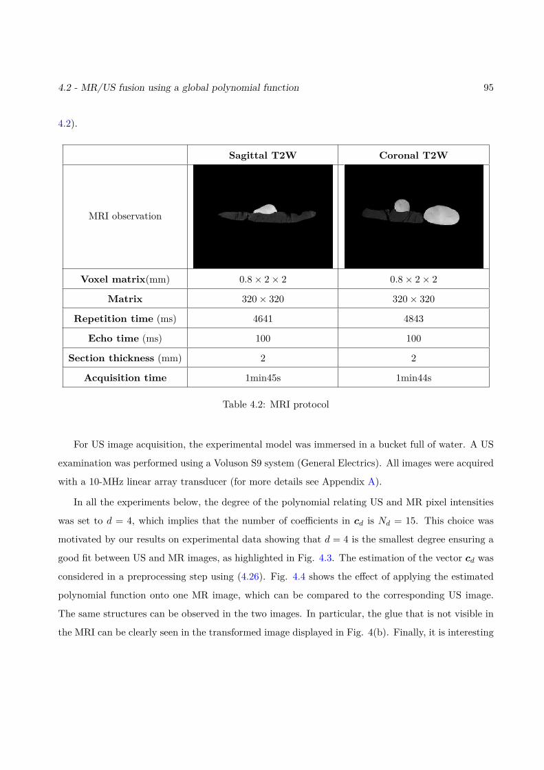
4.2 - MR/US fusion using a global polynomial function 95
4.2).
Sagittal T2W Coronal T2W
MRI observation
Voxel matrix(mm) 0.8× 2× 2 0.8× 2× 2
Matrix 320× 320 320× 320
Repetition time (ms) 4641 4843
Echo time (ms) 100 100
Section thickness (mm) 2 2
Acquisition time 1min45s 1min44s
Table 4.2: MRI protocol
For US image acquisition, the experimental model was immersed in a bucket full of water. A US
examination was performed using a Voluson S9 system (General Electrics). All images were acquired
with a 10-MHz linear array transducer (for more details see Appendix A).
In all the experiments below, the degree of the polynomial relating US and MR pixel intensities
was set to d = 4, which implies that the number of coefficients in cd is Nd = 15. This choice was
motivated by our results on experimental data showing that d = 4 is the smallest degree ensuring a
good fit between US and MR images, as highlighted in Fig. 4.3. The estimation of the vector cd was
considered in a preprocessing step using (4.26). Fig. 4.4 shows the effect of applying the estimated
polynomial function onto one MR image, which can be compared to the corresponding US image.
The same structures can be observed in the two images. In particular, the glue that is not visible in
the MRI can be clearly seen in the transformed image displayed in Fig. 4(b). Finally, it is interesting
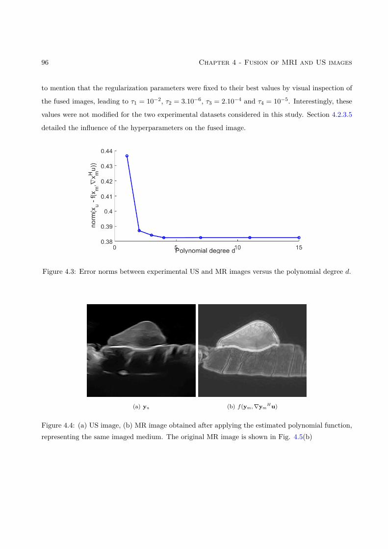
96 Chapter 4 - Fusion of MRI and US images
to mention that the regularization parameters were fixed to their best values by visual inspection of
the fused images, leading to τ1 = 10−2, τ2 = 3.10−6, τ3 = 2.10−4 and τ4 = 10−5. Interestingly, these
values were not modified for the two experimental datasets considered in this study. Section 4.2.3.5
detailed the influence of the hyperparameters on the fused image.
Figure 4.3: Error norms between experimental US and MR images versus the polynomial degree d.
(a) yu (b) f(ym,∇ymHu)
Figure 4.4: (a) US image, (b) MR image obtained after applying the estimated polynomial function,representing the same imaged medium. The original MR image is shown in Fig. 4.5(b)
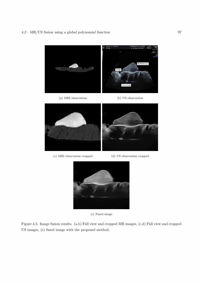
4.2 - MR/US fusion using a global polynomial function 97
(a) MRI observation (b) US observation
(c) MRI observation cropped (d) US observation cropped
(e) Fused image
Figure 4.5: Image fusion results. (a,b) Full view and cropped MR images, (c,d) Full view and croppedUS images, (e) fused image with the proposed method.
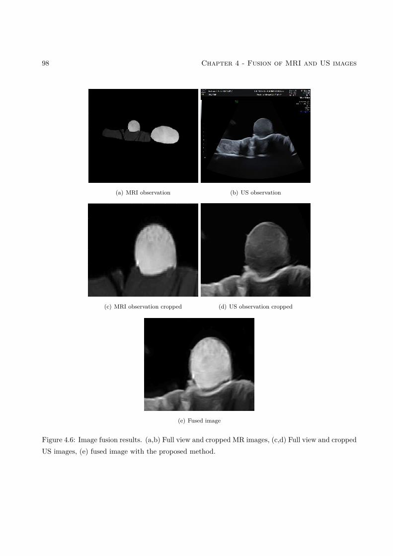
98 Chapter 4 - Fusion of MRI and US images
(a) MRI observation (b) US observation
(c) MRI observation cropped (d) US observation cropped
(e) Fused image
Figure 4.6: Image fusion results. (a,b) Full view and cropped MR images, (c,d) Full view and croppedUS images, (e) fused image with the proposed method.
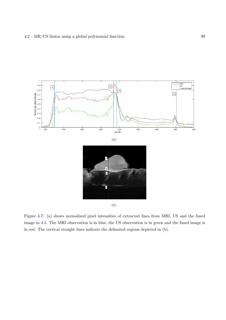
4.2 - MR/US fusion using a global polynomial function 99
(a)
(b)
Figure 4.7: (a) shows normalized pixel intensities of extracted lines from MRI, US and the fusedimage in 4.5. The MRI observation is in blue, the US observation is in green and the fused image isin red. The vertical straight lines indicate the delimited regions depicted in (b).
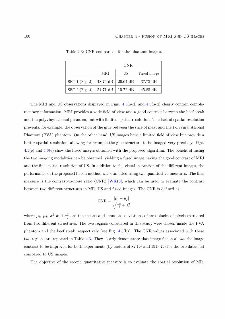
100 Chapter 4 - Fusion of MRI and US images
Table 4.3: CNR comparison for the phantom images.
CNR
MRI US Fused image
SET 1 (Fig. 3) 48.76 dB 20.64 dB 37.73 dB
SET 2 (Fig. 4) 54.71 dB 15.72 dB 45.85 dB
The MRI and US observations displayed in Figs. 4.5(a-d) and 4.5(a-d) clearly contain comple-
mentary information. MRI provides a wide field of view and a good contrast between the beef steak
and the polyvinyl alcohol phantom, but with limited spatial resolution. The lack of spatial resolution
prevents, for example, the observation of the glue between the slice of meat and the Polyvinyl Alcohol
Phantom (PVA) phantom. On the other hand, US images have a limited field of view but provide a
better spatial resolution, allowing for example the glue structure to be imaged very precisely. Figs.
4.5(e) and 4.6(e) show the fused images obtained with the proposed algorithm. The benefit of fusing
the two imaging modalities can be observed, yielding a fused image having the good contrast of MRI
and the fine spatial resolution of US. In addition to the visual inspection of the different images, the
performance of the proposed fusion method was evaluated using two quantitative measures. The first
measure is the contrast-to-noise ratio (CNR) [WR13], which can be used to evaluate the contrast
between two different structures in MR, US and fused images. The CNR is defined as
CNR = |µi − µj |√σ2i + σ2
j
where µi, µj , σ2i and σ2
j are the means and standard deviations of two blocks of pixels extracted
from two different structures. The two regions considered in this study were chosen inside the PVA
phantom and the beef steak, respectively (see Fig. 4.5(b)). The CNR values associated with these
two regions are reported in Table 4.3. They clearly demonstrate that image fusion allows the image
contrast to be improved for both experiments (by factors of 82.1% and 191.67% for the two datasets)
compared to US images.
The objective of the second quantitative measure is to evaluate the spatial resolution of MR,
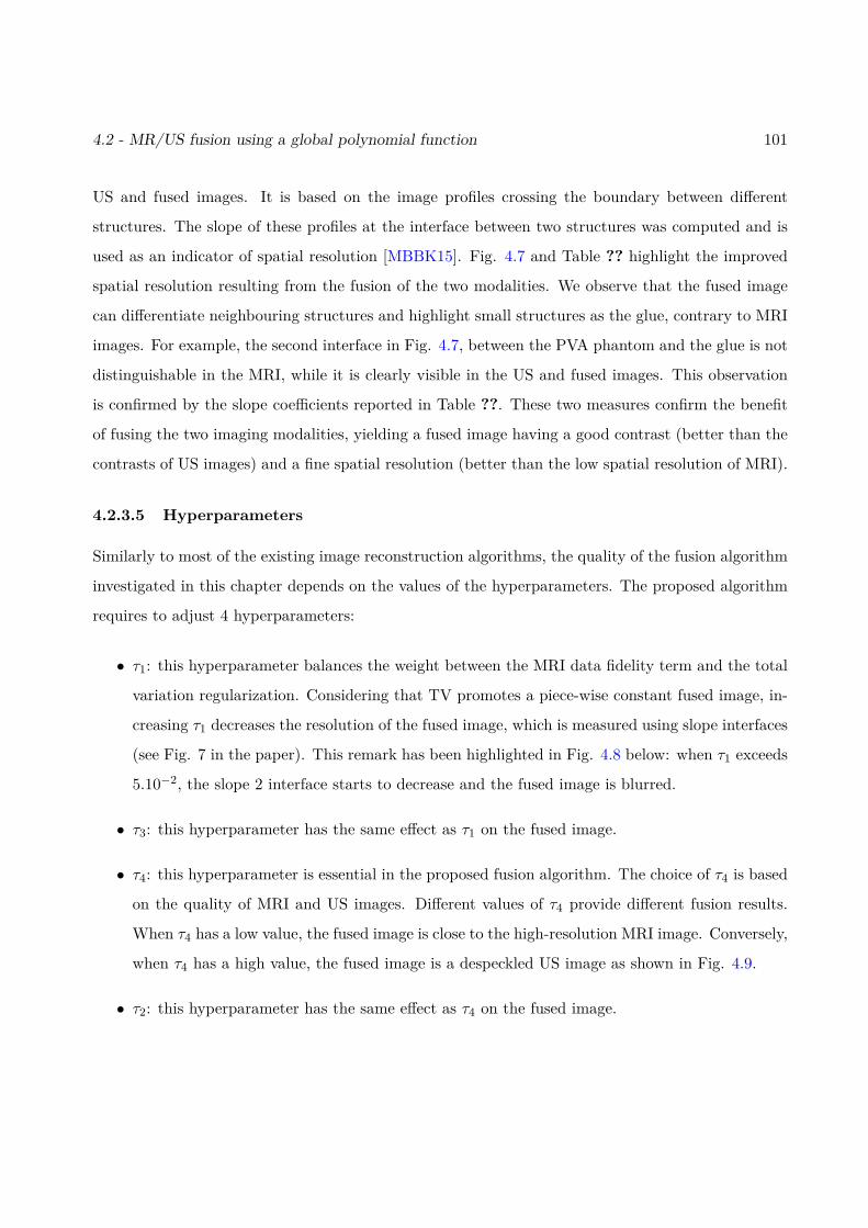
4.2 - MR/US fusion using a global polynomial function 101
US and fused images. It is based on the image profiles crossing the boundary between different
structures. The slope of these profiles at the interface between two structures was computed and is
used as an indicator of spatial resolution [MBBK15]. Fig. 4.7 and Table ?? highlight the improved
spatial resolution resulting from the fusion of the two modalities. We observe that the fused image
can differentiate neighbouring structures and highlight small structures as the glue, contrary to MRI
images. For example, the second interface in Fig. 4.7, between the PVA phantom and the glue is not
distinguishable in the MRI, while it is clearly visible in the US and fused images. This observation
is confirmed by the slope coefficients reported in Table ??. These two measures confirm the benefit
of fusing the two imaging modalities, yielding a fused image having a good contrast (better than the
contrasts of US images) and a fine spatial resolution (better than the low spatial resolution of MRI).
4.2.3.5 Hyperparameters
Similarly to most of the existing image reconstruction algorithms, the quality of the fusion algorithm
investigated in this chapter depends on the values of the hyperparameters. The proposed algorithm
requires to adjust 4 hyperparameters:
• τ1: this hyperparameter balances the weight between the MRI data fidelity term and the total
variation regularization. Considering that TV promotes a piece-wise constant fused image, in-
creasing τ1 decreases the resolution of the fused image, which is measured using slope interfaces
(see Fig. 7 in the paper). This remark has been highlighted in Fig. 4.8 below: when τ1 exceeds
5.10−2, the slope 2 interface starts to decrease and the fused image is blurred.
• τ3: this hyperparameter has the same effect as τ1 on the fused image.
• τ4: this hyperparameter is essential in the proposed fusion algorithm. The choice of τ4 is based
on the quality of MRI and US images. Different values of τ4 provide different fusion results.
When τ4 has a low value, the fused image is close to the high-resolution MRI image. Conversely,
when τ4 has a high value, the fused image is a despeckled US image as shown in Fig. 4.9.
• τ2: this hyperparameter has the same effect as τ4 on the fused image.
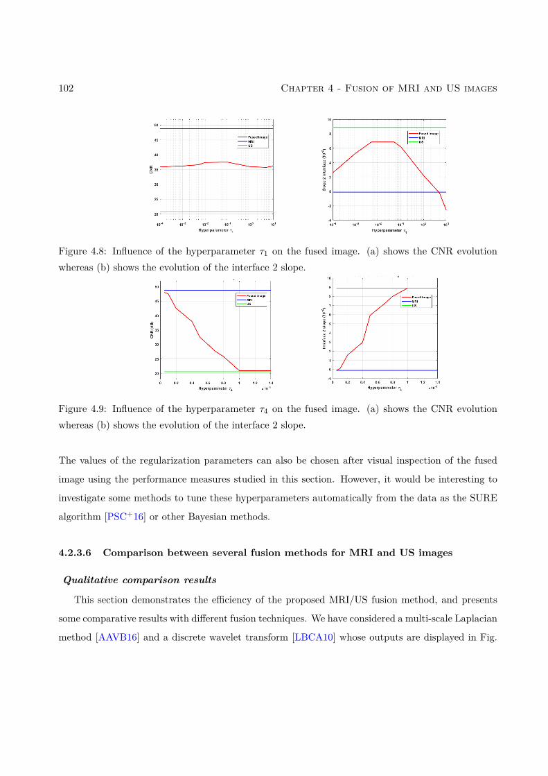
102 Chapter 4 - Fusion of MRI and US images
Figure 4.8: Influence of the hyperparameter τ1 on the fused image. (a) shows the CNR evolutionwhereas (b) shows the evolution of the interface 2 slope.
Figure 4.9: Influence of the hyperparameter τ4 on the fused image. (a) shows the CNR evolutionwhereas (b) shows the evolution of the interface 2 slope.
The values of the regularization parameters can also be chosen after visual inspection of the fused
image using the performance measures studied in this section. However, it would be interesting to
investigate some methods to tune these hyperparameters automatically from the data as the SURE
algorithm [PSC+16] or other Bayesian methods.
4.2.3.6 Comparison between several fusion methods for MRI and US images
Qualitative comparison results
This section demonstrates the efficiency of the proposed MRI/US fusion method, and presents
some comparative results with different fusion techniques. We have considered a multi-scale Laplacian
method [AAVB16] and a discrete wavelet transform [LBCA10] whose outputs are displayed in Fig.
4.2 - MR/US fusion using a global polynomial function 103
4.10 (for more details about these fusion techniques, see Chapter 3). In order to make a more fair
comparison, we have denoised the US image before fusion since our proposed strategy also performs
denoising. The figures displayed below show the effect of noise on the fused image. For low SNR,
the multi-scale fused image and the wavelet fused image contain distracting artifacts, especially in
the regions containing strong transitions between organs.
Quantitative comparison results
The performance of the proposed fusion algorithm was evaluated using a quantitative metric,
namely the Petrovic fusion metric [Pet07]. This metric associates important visual information with
the edge information in each pixel. Thus, a measure of fusion performance is obtained by evaluating
the amount of edge information that is transferred from input images to the fuse image. Fig. 4.11
clearly demonstrates that for higher noise levels the fusion becomes more complicated.
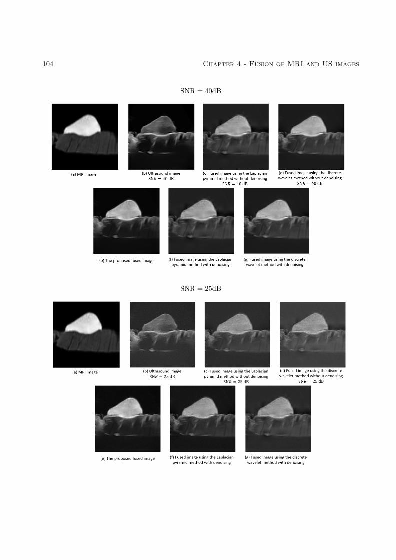
104 Chapter 4 - Fusion of MRI and US images
SNR = 40dB
SNR = 25dB
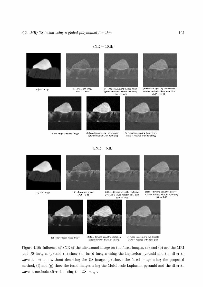
4.2 - MR/US fusion using a global polynomial function 105
SNR = 10dB
SNR = 5dB
Figure 4.10: Influence of SNR of the ultrasound image on the fused images, (a) and (b) are the MRIand US images, (c) and (d) show the fused images using the Laplacian pyramid and the discretewavelet methods without denoising the US image, (e) shows the fused image using the proposedmethod, (f) and (g) show the fused images using the Multi-scale Laplacian pyramid and the discretewavelet methods after denoising the US image.
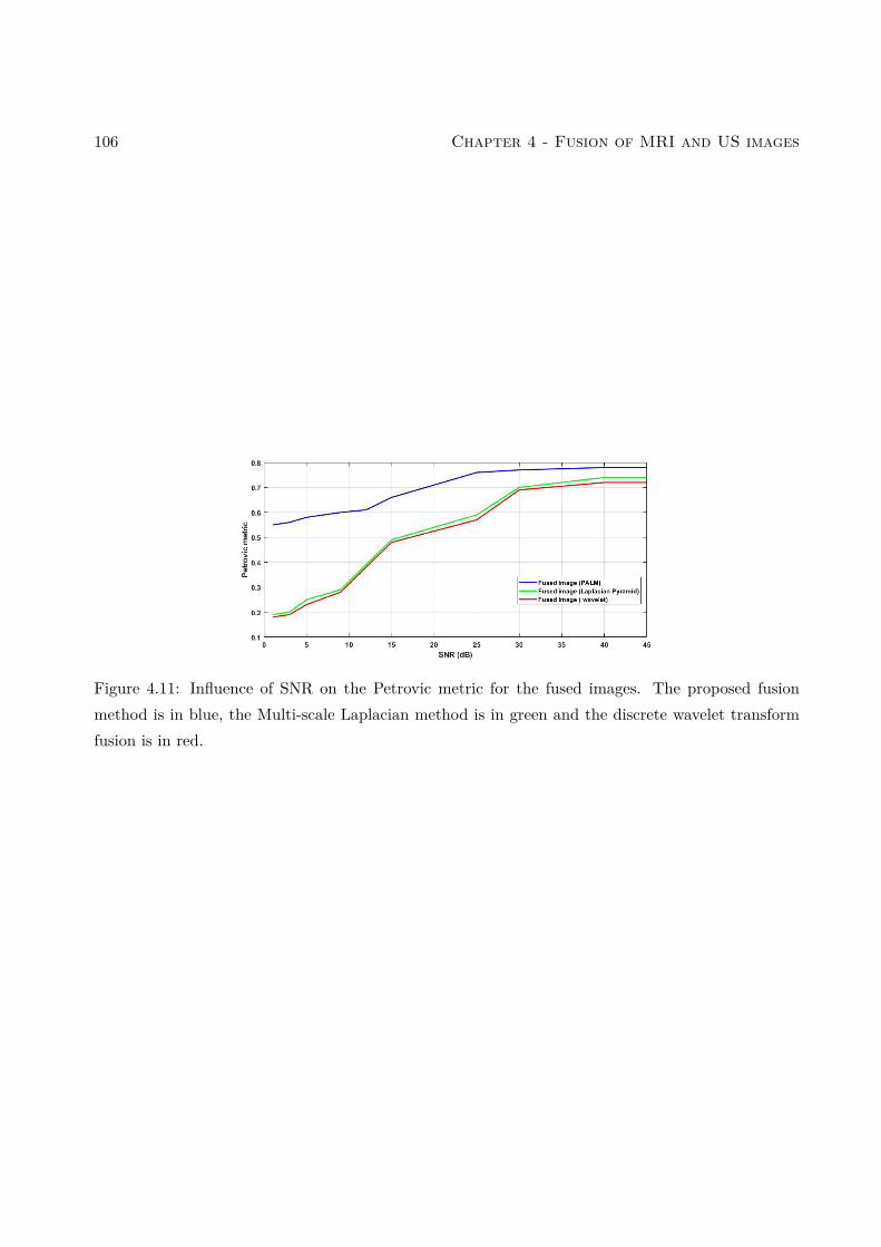
106 Chapter 4 - Fusion of MRI and US images
Figure 4.11: Influence of SNR on the Petrovic metric for the fused images. The proposed fusionmethod is in blue, the Multi-scale Laplacian method is in green and the discrete wavelet transformfusion is in red.
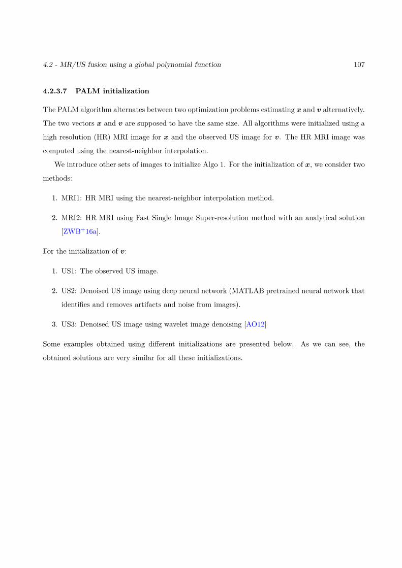
4.2 - MR/US fusion using a global polynomial function 107
4.2.3.7 PALM initialization
The PALM algorithm alternates between two optimization problems estimating x and v alternatively.
The two vectors x and v are supposed to have the same size. All algorithms were initialized using a
high resolution (HR) MRI image for x and the observed US image for v. The HR MRI image was
computed using the nearest-neighbor interpolation.
We introduce other sets of images to initialize Algo 1. For the initialization of x, we consider two
methods:
1. MRI1: HR MRI using the nearest-neighbor interpolation method.
2. MRI2: HR MRI using Fast Single Image Super-resolution method with an analytical solution
[ZWB+16a].
For the initialization of v:
1. US1: The observed US image.
2. US2: Denoised US image using deep neural network (MATLAB pretrained neural network that
identifies and removes artifacts and noise from images).
3. US3: Denoised US image using wavelet image denoising [AO12]
Some examples obtained using different initializations are presented below. As we can see, the
obtained solutions are very similar for all these initializations.
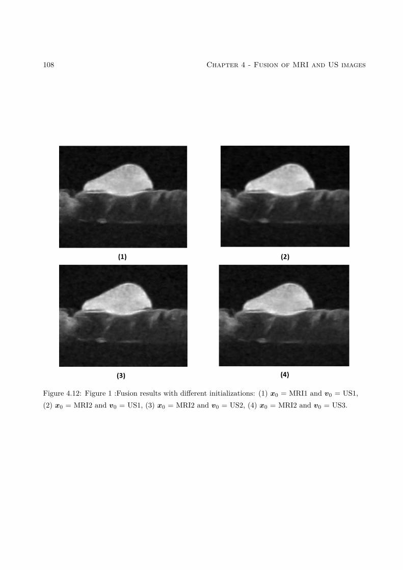
108 Chapter 4 - Fusion of MRI and US images
Figure 4.12: Figure 1 :Fusion results with different initializations: (1) x0 = MRI1 and v0 = US1,(2) x0 = MRI2 and v0 = US1, (3) x0 = MRI2 and v0 = US2, (4) x0 = MRI2 and v0 = US3.
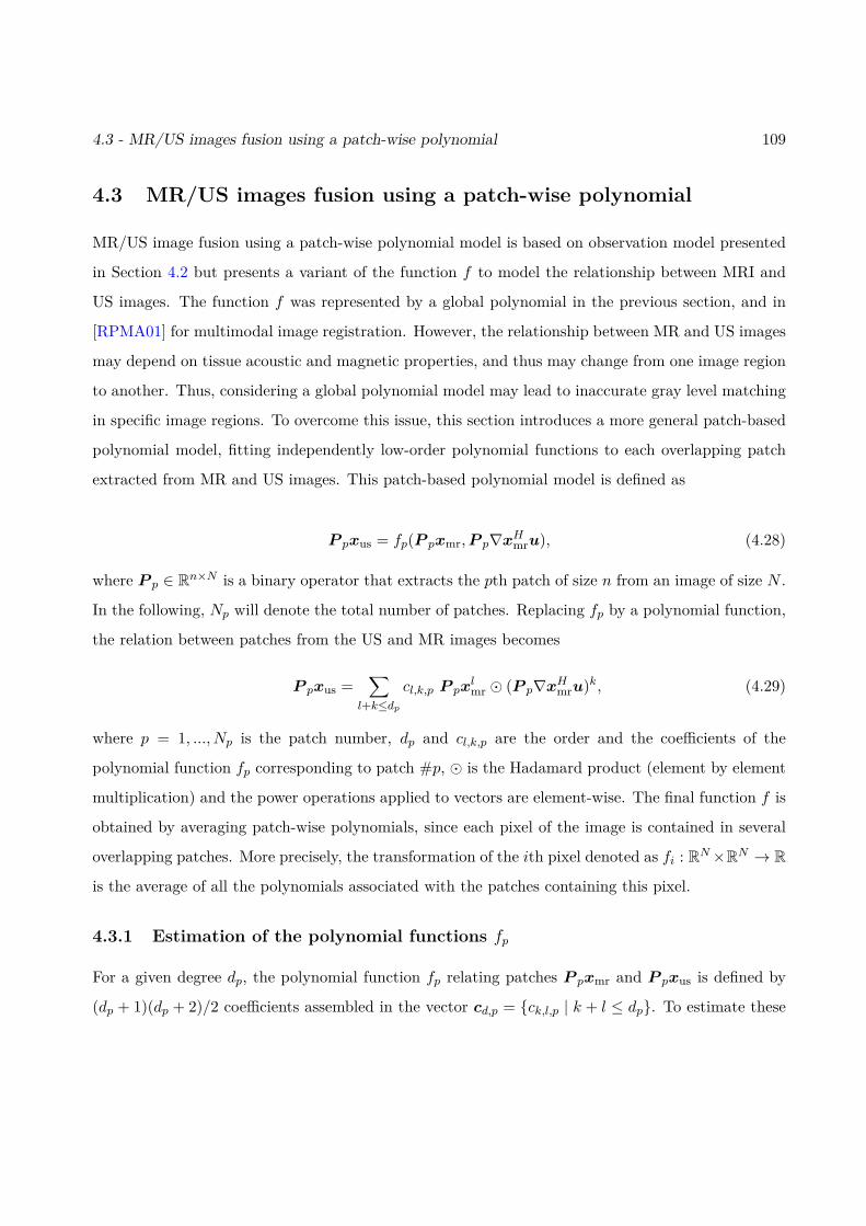
4.3 - MR/US images fusion using a patch-wise polynomial 109
4.3 MR/US images fusion using a patch-wise polynomial
MR/US image fusion using a patch-wise polynomial model is based on observation model presented
in Section 4.2 but presents a variant of the function f to model the relationship between MRI and
US images. The function f was represented by a global polynomial in the previous section, and in
[RPMA01] for multimodal image registration. However, the relationship between MR and US images
may depend on tissue acoustic and magnetic properties, and thus may change from one image region
to another. Thus, considering a global polynomial model may lead to inaccurate gray level matching
in specific image regions. To overcome this issue, this section introduces a more general patch-based
polynomial model, fitting independently low-order polynomial functions to each overlapping patch
extracted from MR and US images. This patch-based polynomial model is defined as
P pxus = fp(P pxmr,P p∇xHmru), (4.28)
where P p ∈ Rn×N is a binary operator that extracts the pth patch of size n from an image of size N .
In the following, Np will denote the total number of patches. Replacing fp by a polynomial function,
the relation between patches from the US and MR images becomes
P pxus =∑
l+k≤dpcl,k,p P px
lmr (P p∇xHmru)k, (4.29)
where p = 1, ..., Np is the patch number, dp and cl,k,p are the order and the coefficients of the
polynomial function fp corresponding to patch #p, is the Hadamard product (element by element
multiplication) and the power operations applied to vectors are element-wise. The final function f is
obtained by averaging patch-wise polynomials, since each pixel of the image is contained in several
overlapping patches. More precisely, the transformation of the ith pixel denoted as fi : RN×RN → R
is the average of all the polynomials associated with the patches containing this pixel.
4.3.1 Estimation of the polynomial functions fp
For a given degree dp, the polynomial function fp relating patches P pxmr and P pxus is defined by
(dp + 1)(dp + 2)/2 coefficients assembled in the vector cd,p = ck,l,p | k + l ≤ dp. To estimate these
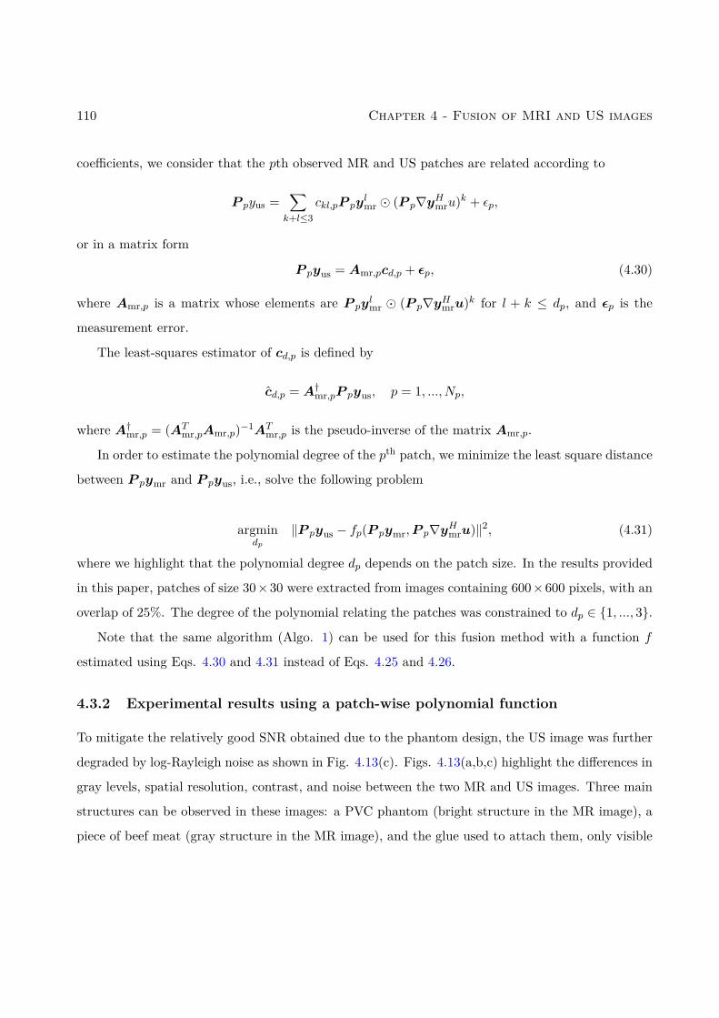
110 Chapter 4 - Fusion of MRI and US images
coefficients, we consider that the pth observed MR and US patches are related according to
P pyus =∑k+l≤3
ckl,pP pylmr (P p∇yHmru)k + εp,
or in a matrix form
P pyus = Amr,pcd,p + εp, (4.30)
where Amr,p is a matrix whose elements are P pylmr (P p∇yHmru)k for l + k ≤ dp, and εp is the
measurement error.
The least-squares estimator of cd,p is defined by
cd,p = A†mr,pP pyus, p = 1, ..., Np,
where A†mr,p = (ATmr,pAmr,p)−1AT
mr,p is the pseudo-inverse of the matrix Amr,p.
In order to estimate the polynomial degree of the pth patch, we minimize the least square distance
between P pymr and P pyus, i.e., solve the following problem
argmindp
‖P pyus − fp(P pymr,P p∇yHmru)‖2, (4.31)
where we highlight that the polynomial degree dp depends on the patch size. In the results provided
in this paper, patches of size 30×30 were extracted from images containing 600×600 pixels, with an
overlap of 25%. The degree of the polynomial relating the patches was constrained to dp ∈ 1, ..., 3.
Note that the same algorithm (Algo. 1) can be used for this fusion method with a function f
estimated using Eqs. 4.30 and 4.31 instead of Eqs. 4.25 and 4.26.
4.3.2 Experimental results using a patch-wise polynomial function
To mitigate the relatively good SNR obtained due to the phantom design, the US image was further
degraded by log-Rayleigh noise as shown in Fig. 4.13(c). Figs. 4.13(a,b,c) highlight the differences in
gray levels, spatial resolution, contrast, and noise between the two MR and US images. Three main
structures can be observed in these images: a PVC phantom (bright structure in the MR image), a
piece of beef meat (gray structure in the MR image), and the glue used to attach them, only visible
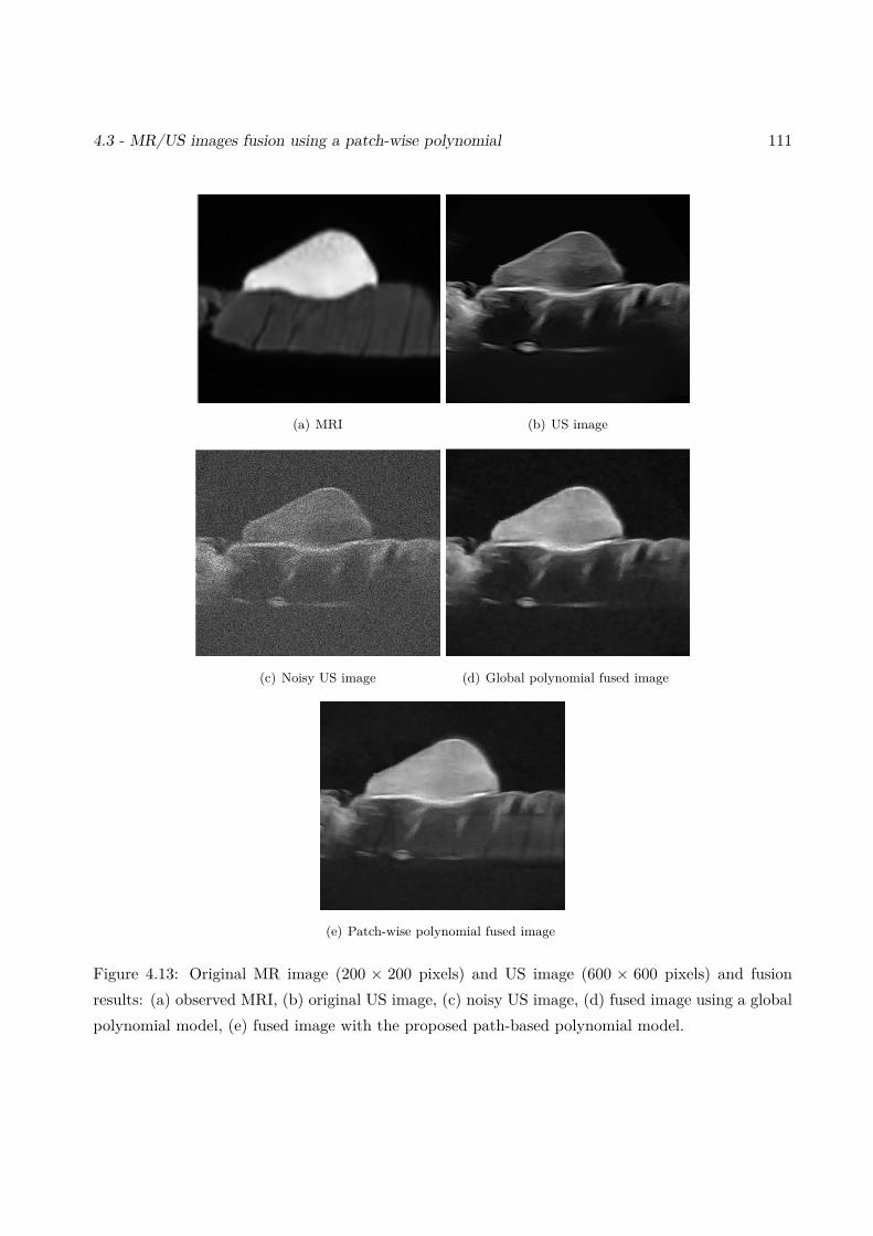
4.3 - MR/US images fusion using a patch-wise polynomial 111
(a) MRI (b) US image
(c) Noisy US image (d) Global polynomial fused image
(e) Patch-wise polynomial fused image
Figure 4.13: Original MR image (200 × 200 pixels) and US image (600 × 600 pixels) and fusionresults: (a) observed MRI, (b) original US image, (c) noisy US image, (d) fused image using a globalpolynomial model, (e) fused image with the proposed path-based polynomial model.
112 Chapter 4 - Fusion of MRI and US images
(a) (b)
(c)Figure 4.14: (a) and (c) show normalized pixel intensities of extracted lines from the MR, US andfused images (using the global polynomial fusion and the proposed patch-based fusion). (a) showsthe vertical straight lines in (b) whereas (c) displays the horizontal straight lines in (b).
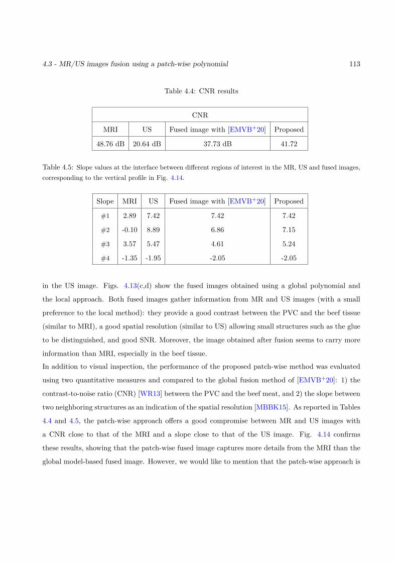
4.3 - MR/US images fusion using a patch-wise polynomial 113
Table 4.4: CNR results
CNR
MRI US Fused image with [EMVB+20] Proposed
48.76 dB 20.64 dB 37.73 dB 41.72
Table 4.5: Slope values at the interface between different regions of interest in the MR, US and fused images,corresponding to the vertical profile in Fig. 4.14.
Slope MRI US Fused image with [EMVB+20] Proposed
#1 2.89 7.42 7.42 7.42
#2 -0.10 8.89 6.86 7.15
#3 3.57 5.47 4.61 5.24
#4 -1.35 -1.95 -2.05 -2.05
in the US image. Figs. 4.13(c,d) show the fused images obtained using a global polynomial and
the local approach. Both fused images gather information from MR and US images (with a small
preference to the local method): they provide a good contrast between the PVC and the beef tissue
(similar to MRI), a good spatial resolution (similar to US) allowing small structures such as the glue
to be distinguished, and good SNR. Moreover, the image obtained after fusion seems to carry more
information than MRI, especially in the beef tissue.
In addition to visual inspection, the performance of the proposed patch-wise method was evaluated
using two quantitative measures and compared to the global fusion method of [EMVB+20]: 1) the
contrast-to-noise ratio (CNR) [WR13] between the PVC and the beef meat, and 2) the slope between
two neighboring structures as an indication of the spatial resolution [MBBK15]. As reported in Tables
4.4 and 4.5, the patch-wise approach offers a good compromise between MR and US images with
a CNR close to that of the MRI and a slope close to that of the US image. Fig. 4.14 confirms
these results, showing that the patch-wise fused image captures more details from the MRI than the
global model-based fused image. However, we would like to mention that the patch-wise approach is
114 Chapter 4 - Fusion of MRI and US images
more time consuming compared to the global polynomial. Thus, the choice of the adapted method
depends on the application.
4.4 Conclusion
This chapter studied new fusion methods for magnetic resonance (MR) and ultrasound (US) images.
The proposed methods were able to reconstruct a fused image containing information from both
observations, by solving a super-resolution inverse problem for MRI and a despeckling problem for
US images. These two problems were solved jointly by using appropriate statistical models and
polynomial relationships between the images of interest. A PALM algorithm was finally investigated
to solve the resulting fusion problem. Results obtained on simulated and real images clearly showed
the interest of combining the information contained in these two imaging modalities, instead of
restoring them independently.
To the best of our knowledge, this work is a first attempt for fusing MR and US images. It
opens several interesting perspectives. A natural progression of this work is to combine the proposed
framework with multimodal image registration, which would allow the proposed MR/US image fusion
to be robustified, which is the aim of the next chapter.
Chapter 5
Joint registration and fusion of MRIand ultrasound images
Contents5.1 Introduction . . . . . . . . . . . . . . . . . . . . . . . . . . . . . . . . . . . . 1155.2 MR/US image fusion and registration . . . . . . . . . . . . . . . . . . . . 116
5.2.1 Observation models . . . . . . . . . . . . . . . . . . . . . . . . . . . . . . . . 1165.2.2 US/MR dependence model . . . . . . . . . . . . . . . . . . . . . . . . . . . . 1175.2.3 Proposed inverse problem . . . . . . . . . . . . . . . . . . . . . . . . . . . . . 119
5.3 Proposed registration . . . . . . . . . . . . . . . . . . . . . . . . . . . . . . 1205.3.1 Similarity measure . . . . . . . . . . . . . . . . . . . . . . . . . . . . . . . . . 1205.3.2 Spatial transformation . . . . . . . . . . . . . . . . . . . . . . . . . . . . . . 1215.3.3 Regularization . . . . . . . . . . . . . . . . . . . . . . . . . . . . . . . . . . . 123
5.4 Optimization algorithm for joint fusion and registration . . . . . . . . . 1235.4.1 Estimation of the fused image for known (Tc) . . . . . . . . . . . . . . . . . 1245.4.2 Estimation of the spatial transformation . . . . . . . . . . . . . . . . . . . . 1265.4.3 Estimation of the polynomial function . . . . . . . . . . . . . . . . . . . . . . 1275.4.4 Proposed algorithm . . . . . . . . . . . . . . . . . . . . . . . . . . . . . . . . 1275.4.5 Performance measures . . . . . . . . . . . . . . . . . . . . . . . . . . . . . . . 1275.4.6 Simulation results on synthetic data . . . . . . . . . . . . . . . . . . . . . . . 1295.4.7 Experimental results on phantom data . . . . . . . . . . . . . . . . . . . . . . 1315.4.8 Hyperparameters . . . . . . . . . . . . . . . . . . . . . . . . . . . . . . . . . . 137
5.5 Conclusions . . . . . . . . . . . . . . . . . . . . . . . . . . . . . . . . . . . . . 137
5.1 Introduction
This chapter presents a joint registration and fusion method for MR and US images. Considering the
limitations of each modality, we have constructed in the previous chapter two observation models to
115
116 Chapter 5 - Joint registration and fusion of MRI and ultrasound images
enhance the quality (in terms of resolution and contrast) of both images. A first model is introduced
for the MR image based on a linear model formed by blurring and downsampling matrices. This
model has been used for super-resolution in several studies [GEW10, GPOK02, MCB+10b]. A
denoising model is considered for the US image in order to mitigate the effect of speckle noise
[AB07b, TSP88b, GCS05b]. Since US and MR modalities are different by their nature and content,
there is no simple correspondence between gray levels in these images. A polynomial function was
used in [RPMA01, EMVB+20] and in the previous chapter to link intensities of MR and US images.
However, in order to consider the possible misalignment between MR and US images, we consider
an MR/US registration step in order to estimate the non-linear transformation relating these two
images. This transformation is composed of a local transformation based on B-splines and a global
transformation based on an affine operator. This leads to a sophisticated and complex optimization
problem, which is handled via a PALM algorithm [BST14]. The main contribution of this chapter
with respect to Chapter 4 is a fusion algorithm able to mitigate the mis-registration errors between
the MR and US images. The possibility of handling mis-registration errors is essential for clinical
applications since MR and US images are not aligned because of the differences in acquisition setups,
while their alignment is a crucial requirement for the fusion process. Simulated data with controlled
ground truth are used to evaluate the proposed fusion/registration method. Experimental data
collected on a phantom with some similar characteristics to endometriosis are then considered.
5.2 MR/US image fusion and registration
5.2.1 Observation models
As explained previously, MR and US images are two medical modalities that have their specific
strengths and weaknesses. The main purpose of obtaining a fused image from these two modalities
is to take benefit from their strengths and mitigate their weaknesses. In the following, ym ∈ RM
and yu ∈ RN denote the observed MR and US images, which are the inputs of the proposed fusion
algorithm. Both observed images are related to the ideal fused image through two models accounting
for the degradation affecting the two modalities. In particular, the limited spatial resolution of the
5.2 - MR/US image fusion and registration 117
MR image is classically modelled using a blur, a down-sampling operator and additive white Gaussian
noise [GEW10, GPOK02, MCB+10b]. The speckle noise contaminating the US image is modelled as
an additive log-Rayleigh noise [AB07b, TSP88b, GCS05b]. The resulting joint observation models
associated with the MR and US images (introduced in Chapter 4) are:
ym = SCxm + nm
yu = xu + nu,(5.1)
where xm ∈ RN is the MR high-resolution image and xu ∈ RN is the despeckled US image,C ∈ RN×N
is a BCCB matrix (block circulant with circulant blocks) that models the blur in the MR image and
S ∈ RM×N (with N = s2M) is a decimation matrix (with a decimation factor of s in each spatial
direction). The two observation equations in (5.1) are used to estimate the fused image of interest
by taking benefit from both MR and US measurements. The first equation in (5.1) has been used
in many super-resolution methods to recover the high-resolution MR image xm from its noisy low-
resolution counterpart ym [GEW10, GPOK02, MCB+10b]. The second equation in (5.1) has been
considered in denoising methods for US images [AB07b, TSP88b, GCS05b]. The proposed approach
combines both observation equations to improve the resolution of the MR image and denoise the US
image. An additional model, detailed in the next section, is also considered to link xm and xu that
are different even in the ideal noiseless case, because of the different physical phenomena behind each
imaging modality.
5.2.2 US/MR dependence model
The proposed joint fusion and registration method is a pure intensity-based approach that does not
require any feature extraction. It relies on the assumption that the differences between xm and xuare due to two properties: i) the MR and US images are not perfectly aligned. This misalignment is
modelled by a geometric transform denoted as T , and ii) the relation between the pixel intensities
in the two images can be well approximated by a deterministic non-linear function denoted as fc.
Combining these two properties, the principle of the proposed algorithm is to search for a spatial
transformation T and an intensity mapping fc, in order to match xu to T (xm). Note that the
118 Chapter 5 - Joint registration and fusion of MRI and ultrasound images
function fc does not relate the pixel intensities from the two images directly, but it uses the fact that
the US image is mainly sensitive to interfaces between anatomical surfaces with different acoustic
impedances. As explained in the previous chapter, the mapping fc relates the US gray levels to the
gray levels and the gradients of the MR image calculated in the direction of US wave propagation
(see [RPMA01] for more details). Plugging T and fc into (5.1) results into the following observation
models:
ym = SCx+ nm
yu = fc(T (x),∇T (x)Hu) + nu,(5.2)
where x ∈ RN is the fused image to be estimated, which contains information from both MR and US
modalities. The function fc : RN×RN → RN allows the gray level intensities of MR and US images to
be matched, and T (.) is a geometric transformation due to possible mis-registration. Note that the
ith component of ∇T (x)Hu ∈ RN contains the inner product between the ith local gradient of T (x)
and the US scan direction u. Note also that the proposed fusion model (5.2) reduces to the model
investigated in the previous chapter when T (x) = x, which corresponds to the ideal case where the
MR and US images are perfectly aligned.
As shown in [RPMA01, EMVB+20], the unknown function fc in (5.2) can be efficiently approxi-
mated by a polynomial of order d. This approximation consists of decomposing the ith component
of xu = fc(T,xm,u) as:
xu,i =∑
p+q≤dcpqT (xpm,i)(∇T (xm)Hu)qi , (5.3)
where c is a vector containing all the unknown polynomial coefficients cpq and the index i ∈ 1, ..., N
is used for the ith coefficient of a vector. From the observation model (5.2) and the polynomial model
(5.3), the objective of the proposed algorithm is to estimate the fused image x (with better spatial
resolution, contrast and signal-to-noise ratio (SNR) than the original images xm and xu, the geometric
transform T (accounting for a possible mis-registration between the MR and US images) and the
polynomial coefficients cpq from the MR and US images (ym,yu) associated with the same tissue.
5.2 - MR/US image fusion and registration 119
5.2.3 Proposed inverse problem
Based on some noise assumptions, i.e., additive Gaussian and additive log-Rayleigh noises for the
MR and US images, an inverse problem was introduced in [EMVB+20] for the fusion of registered
MR and US images. This problem was defined as
x = argminx
12‖ym − SCx‖
2︸ ︷︷ ︸MR data fidelity
+ τ2
N∑i=1
exp [yu,i − fi(x,u)− γ(yu,i − fi(x,u))]︸ ︷︷ ︸US data fidelity
+ τ1‖∇x‖2 + τ3‖∇f(x,∇xHu)‖2︸ ︷︷ ︸regularization
,
(5.4)
where τ1, τ2 and τ3 are hyperparameters that balance the weights of the total variation (TV) regular-
ization and the data fidelity term, and yu,i, fi(x,u) are the ith components of yu and f(x,∇xHu).
Note that the two regularizations in (5.4) ensure some smoothness in the MR and US terms.
The fusion method based on (5.4) requires an accurate registration between MR and US images, as
well as the knowledge of the pixel intensity mapping function fc. Of course, in practical applications,
these two geometric and gray level transformations are not known and have to be estimated jointly
with the fused image x from the data. Note that the perfect alignment between MR and US images is
an important requirement for the success of most fusion algorithms. Thus considering the estimation
of the geometric transform T jointly with the fused image is still an important challenge. This chapter
proposes to tackle the joint fusion and registration problem by solving the following optimization
problem
(x, T , c) = argminx,T,c
12‖ym − SCx‖
2︸ ︷︷ ︸MR data fidelity
+ τ2
N∑i=1
exp [yu,i − fc,i(T,x,u)− γ(yu,i − fc,i(T,x,u))]︸ ︷︷ ︸US data fidelity
+ τ1‖∇x‖2 + τ3‖∇fc(T,x,u)‖2 + τ5Rs(T )︸ ︷︷ ︸regularization
,
(5.5)
120 Chapter 5 - Joint registration and fusion of MRI and ultrasound images
where the optimization is conducted with respect to the transformation T , the polynomial coefficient
vector c and the image of interest x, fc,i(T,x,u) is the ith component of fc(T,x,u) and Rs(T ) is
an additional regularization whose objective is to constrain the geometric transform T , as explained
in the next section.
5.3 Proposed registration
5.3.1 Similarity measure
Most of the existing image registration methods can be classified into two categories: area-based and
feature-based methods. In this chapter, it is more accurate to use an intensity-based technique be-
cause MR and US images are two distinct modalities from which it is difficult to extract automatically
the same features. In general, any registration algorithm requires the following ingredients:
• An image similarity measure that quantifies the degree of similarity between the two images
to be registered. The most common similarity measures (in particular for multi-modal image
registration) are the mutual information (MI), the normalized mutual information (NMI) and
the cross-correlation (CC). However, the mapping defined by the function fc in (5.5) that
matches the pixel intensities from the two image modalities was shown to be more appropriate
to MR and US images in [RPMA01] and in the previous chapter. The proposed fusion algorithm
estimates the function fc, which allows us to take advantage of this polynomial mapping
xu = fc(T (xm),∇T (xm)Hu) (5.6)
• A model for the geometric transform T , which can be linear (e.g., affine) or non-rigid (also
called elastic) enabling images to be registered with local geometric differences. Non-rigid
registration, which is preferred in medical applications, can be defined using radial basis func-
tions (thin-plate or surface splines, multiquadrics, and compactly-supported transformations
[CR03, CHH04, RSH+99]), physical continuum models, and large deformation models (diffeo-
morphisms) [RVW+11]. The model used in this work is detailed in the next section.
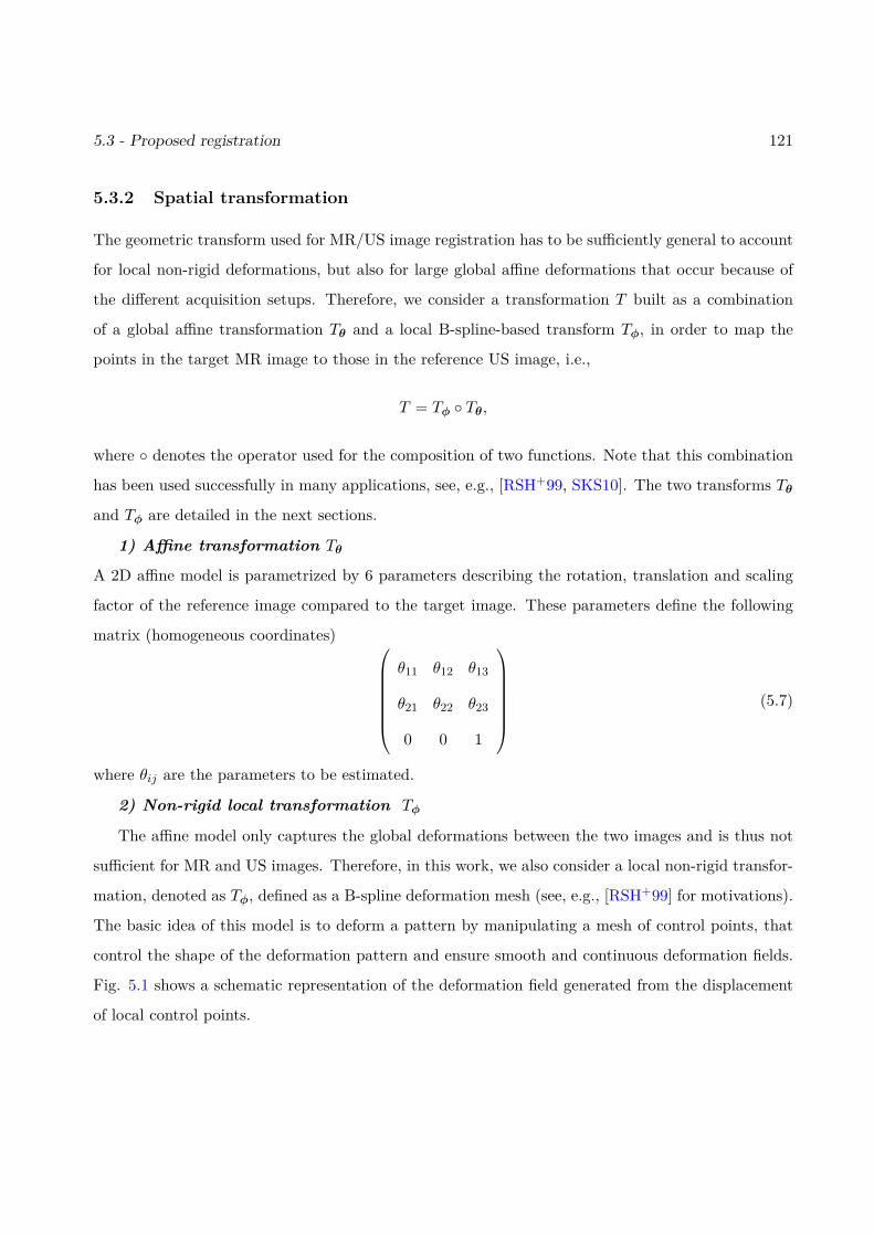
5.3 - Proposed registration 121
5.3.2 Spatial transformation
The geometric transform used for MR/US image registration has to be sufficiently general to account
for local non-rigid deformations, but also for large global affine deformations that occur because of
the different acquisition setups. Therefore, we consider a transformation T built as a combination
of a global affine transformation Tθ and a local B-spline-based transform Tφ, in order to map the
points in the target MR image to those in the reference US image, i.e.,
T = Tφ Tθ,
where denotes the operator used for the composition of two functions. Note that this combination
has been used successfully in many applications, see, e.g., [RSH+99, SKS10]. The two transforms Tθand Tφ are detailed in the next sections.
1) Affine transformation Tθ
A 2D affine model is parametrized by 6 parameters describing the rotation, translation and scaling
factor of the reference image compared to the target image. These parameters define the following
matrix (homogeneous coordinates) θ11 θ12 θ13
θ21 θ22 θ23
0 0 1
(5.7)
where θij are the parameters to be estimated.
2) Non-rigid local transformation Tφ
The affine model only captures the global deformations between the two images and is thus not
sufficient for MR and US images. Therefore, in this work, we also consider a local non-rigid transfor-
mation, denoted as Tφ, defined as a B-spline deformation mesh (see, e.g., [RSH+99] for motivations).
The basic idea of this model is to deform a pattern by manipulating a mesh of control points, that
control the shape of the deformation pattern and ensure smooth and continuous deformation fields.
Fig. 5.1 shows a schematic representation of the deformation field generated from the displacement
of local control points.
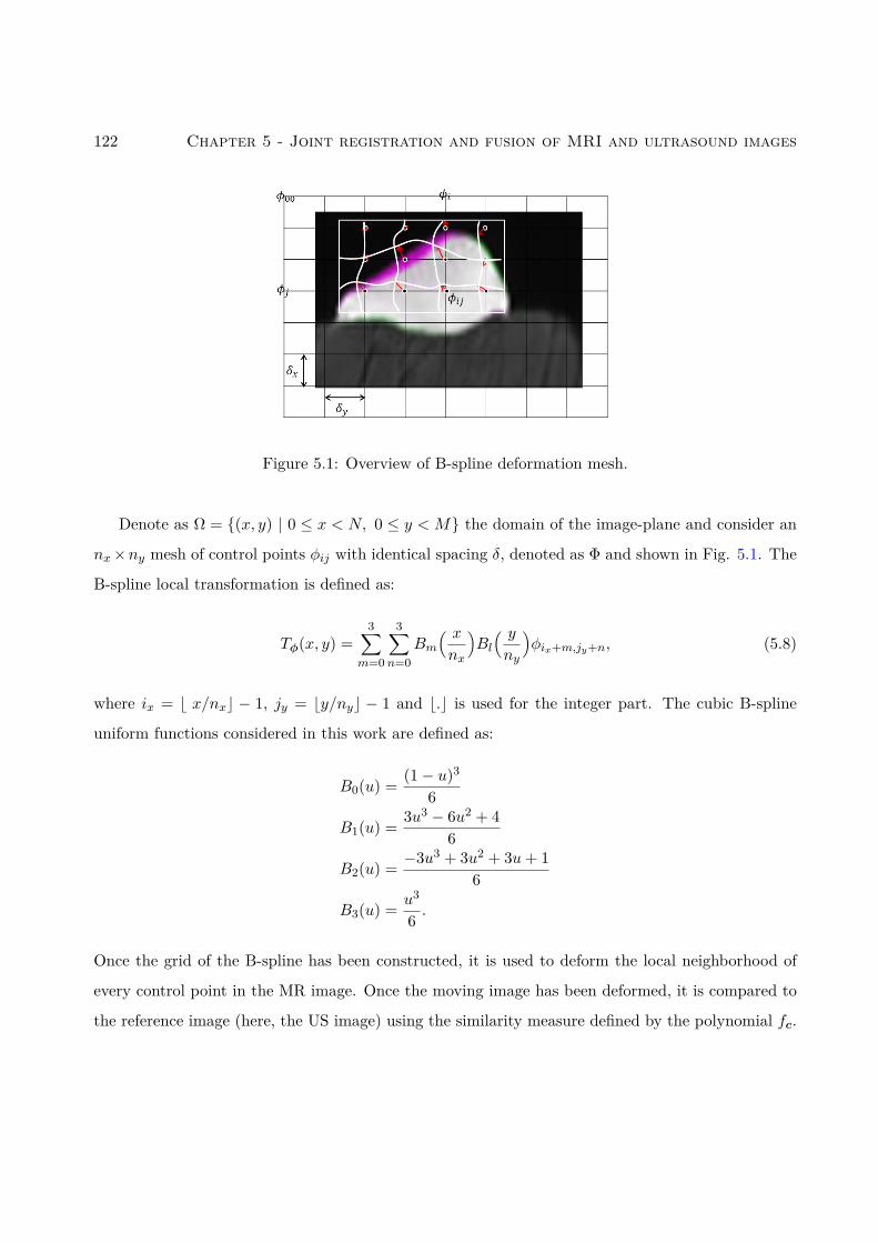
122 Chapter 5 - Joint registration and fusion of MRI and ultrasound images
Figure 5.1: Overview of B-spline deformation mesh.
Denote as Ω = (x, y) | 0 ≤ x < N, 0 ≤ y < M the domain of the image-plane and consider an
nx×ny mesh of control points φij with identical spacing δ, denoted as Φ and shown in Fig. 5.1. The
B-spline local transformation is defined as:
Tφ(x, y) =3∑
m=0
3∑n=0
Bm( xnx
)Bl( yny
)φix+m,jy+n, (5.8)
where ix = b x/nxc − 1, jy = by/nyc − 1 and b.c is used for the integer part. The cubic B-spline
uniform functions considered in this work are defined as:
B0(u) = (1− u)3
6
B1(u) = 3u3 − 6u2 + 46
B2(u) = −3u3 + 3u2 + 3u+ 16
B3(u) = u3
6 .
Once the grid of the B-spline has been constructed, it is used to deform the local neighborhood of
every control point in the MR image. Once the moving image has been deformed, it is compared to
the reference image (here, the US image) using the similarity measure defined by the polynomial fc.
5.4 - Optimization algorithm for joint fusion and registration 123
5.3.3 Regularization
This work considers a regularization to smooth the estimated transformation Tφ. Indeed, since the
registration of MR and US images requires a small spacing mesh, it may lead to B-spline functions
that are not sufficiently smooth. The regularization considered in this work is composed of second-
order derivatives of Tφ:
Rs(Tφ) =∫
Ω
[∂2Tφ∂x2 + ∂2Tφ
∂y2 + ∂2Tφ∂x∂y
]dxdy. (5.9)
In practice, the integral (5.9) (a scalar) is approximated by standard numerical integration providing
a discrete time regularization, which will be used in this chapter.
Note that there is no need to regularize the global transform Tθ and that the regularization (5.9)
reduces to zero for an affine transformation, therefore, penalizing only non-affine transformations.
5.4 Optimization algorithm for joint fusion and registration
This section details the proposed optimization algorithm used to minimize the cost function (5.5).
For a fixed transformation T and a fixed vector c, this minimization is clearly easier and can be
solved using an algorithm similar to the one developed in Chapter 4. Thus, in order to decouple
the optimizations with respect to x and (T, c), we introduce a latent vector v = (v1, ..., vN )T =
f(T (x,∇T (x)Hu
)leading to the following optimization problem equivalent to (5.5):
(x, T , c, v) = argminx,T,c,v
12‖ym − SCx‖
2
+ τ2
N∑i=1
[exp(yu,i − vi)− γ(yu,i − vi)]
+ τ1‖∇x‖2 + τ3‖∇v‖2 + τ5Rs(T )
+ τ4‖v − fc(T,x,u)‖2,
(5.10)
where τ4 is an additional hyperparameter. The proposed algorithm alternates between optimizations
with respect to the fused image x, the geometric transformation T and the polynomial coefficient
vector c, which are summarized below and detailed in the following sections.
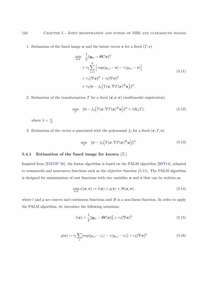
124 Chapter 5 - Joint registration and fusion of MRI and ultrasound images
1. Estimation of the fused image x and the latent vector v for a fixed (T, c)
minx,v
12‖ym − SCx‖
2
+ τ2
N∑i=1
[exp(yu,i − v)− γ(yu,i − v)
]+ τ1‖∇x‖2 + τ3‖∇v‖2
+ τ4‖v − fc(T (x,∇T (x)Hu
)‖2.
(5.11)
2. Estimation of the transformation T for a fixed (x, c,v) (multimodal registration)
minT
‖v − fc(T (x,∇T (x)Hu
)‖2 + λRs(T ). (5.12)
where λ = τ5τ4
3. Estimation of the vector c associated with the polynomial fc for a fixed (x, T,v)
minc
‖v − fc(T (x,∇T (x)Hu
)‖2. (5.13)
5.4.1 Estimation of the fused image for known (Tc)
Inspired from [EMVB+20], the fusion algorithm is based on the PALM algorithm [BST14], adapted
to nonsmooth and nonconvex functions such as the objective function (5.11). The PALM algorithm
is designed for minimization of cost functions with two variables x and v that can be written as:
minx,v
ψ(x,v) := l(x) + g(v) +H(x,v), (5.14)
where l and g are convex and continuous functions and H is a non-linear function. In order to apply
the PALM algorithm, we introduce the following notations:
l(x) = 12‖ym − SCx‖
22 + τ1‖∇x‖2 (5.15)
g(v) = τ2∑i
[exp(yu,i − vi)− γ(yu,i − vi)] + τ3‖∇v‖2 (5.16)
5.4 - Optimization algorithm for joint fusion and registration 125
H(x,v) = τ4
N∑i=1
(vi −
∑p+q≤3
cpqT (xpi )(∇T (x)Hu)qi). (5.17)
Note that this choice of functions fulfills all the assumptions required by PALM [BST14]:
1. l and g are bounded(infRN
(f)> −∞ and infRN
(g)> −∞
).
2. For any fixed v, the function x 7→ H(x,v) is C1,1, and the partial gradient ∇xH(x,v) is
globally Lipschitz.
3. For any fixed x, the function v 7→ H(x,v) is C1,1, and the partial gradient ∇vH(x,v) is
globally Lipschitz.
4. ∇H is Lipschitz continuous function in the image domain.
The alternate optimization with respect to the two vectors x and v proposed in [BST14] generates
a sequence (xk,vk)k∈N using the following steps:
Step 1: Choose γ1 > 1, set ck = γ1Lx(vk) and update xk
xk+1 = proxlck(xk − 1
ck∇xH(xk,vk)
), (5.18)
where Lx(vk) is the Lipschitz constant of x 7→ ∇xH(x,vk) and vk is the value of v at iteration #k.
The proximal operator providing xk+1 in (5.18) can be computed using straightforward computations
(minimization of the sum of quadratic functions), that is,
xk+1 = argminx
12‖SCx− ym‖2 + τ1‖∇x‖2 + Lk+1
2 ‖x− (xk − 1Lk+1
∇xH(xk,vk))‖2, (5.19)
where l has been defined in (5.15) and Lk+1 is the Lipschitz constant of x 7→ ∇xH(x,vk+1) at
iteration #(k+ 1). This minimization problem can be solved using an analytical solution, computed
in the Fourier domain.
Step 2 : Choose γ2 > 1, set dk = γ2Lv(xk) and update vk as follows
vk+1 = proxgdk(vk − 1
dk∇vH(xk,vk)
),
126 Chapter 5 - Joint registration and fusion of MRI and ultrasound images
where Lv(xk) is the Lipschitz constant of v 7→ ∇vH(xk,v) and xk is the value of x at iteration #k.
A gradient descent algorithm with backtracking line search is used to update v, since the function
to minimize is convex and differentiable. More precisely, vk+1 comes:
vk+1 = argminv
τ2∑i
[exp(yu,i − vi)− γ(yu,i − vi)]
+ τ3‖∇v‖2 + dk2 ‖v − (vk − 1
dk∇vH(xk+1,vk))‖2,
(5.20)
where g has been defined in (5.16) and dk = Lv(xk) is the Lipschitz constant of ∇vH at iteration
#k. Note that the hyperparameter τ4 has been included in the function H.
5.4.2 Estimation of the spatial transformation
The estimation of the parameters defining the transformations Tθ and Tφ in (5.7) and (5.8) (multi-
modal registration) is achieved by minimizing the cost function (5.12) in two steps:
1. In the first step, the local transform Tφ is assumed to be the identity and we estimate the 6
parameters of the global affine transformation Tθ by solving the following optimization problem
(with respect to θ) with respect to θ:
θ = argminθ
‖vk − fc(Tθ(xk),∇Tθ(xk)Hu
)‖2. (5.21)
2. Once the global transform Tθ has been estimated, the second step estimates the local transfor-
mation Tφ by solving the following problem (with respect to φ):
φ = argminφ
‖vk − fc(Tφ Tθ(xk),∇Tφ Tθ(xk)Hu
)‖2 + λRs(Tφ). (5.22)
Both optimizations are conducted using the Broyden-Fletcher-Goldfarb-Shanno (BFGS) algo-
rithm [HZ85] (a quasi-Newton method using an approximation of the Hessian matrix).
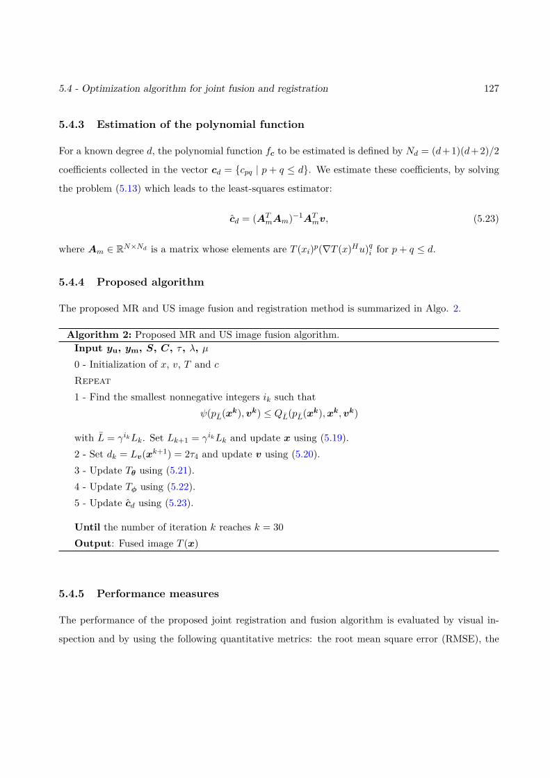
5.4 - Optimization algorithm for joint fusion and registration 127
5.4.3 Estimation of the polynomial function
For a known degree d, the polynomial function fc to be estimated is defined by Nd = (d+1)(d+2)/2
coefficients collected in the vector cd = cpq | p + q ≤ d. We estimate these coefficients, by solving
the problem (5.13) which leads to the least-squares estimator:
cd = (ATmAm)−1AT
mv, (5.23)
where Am ∈ RN×Nd is a matrix whose elements are T (xi)p(∇T (x)Hu)qi for p+ q ≤ d.
5.4.4 Proposed algorithm
The proposed MR and US image fusion and registration method is summarized in Algo. 2.
Algorithm 2: Proposed MR and US image fusion algorithm.Input yu, ym, S, C, τ , λ, µ0 - Initialization of x, v, T and cRepeat1 - Find the smallest nonnegative integers ik such that
ψ(pL(xk),vk) ≤ QL(pL(xk),xk,vk)
with L = γikLk. Set Lk+1 = γikLk and update x using (5.19).2 - Set dk = Lv(xk+1) = 2τ4 and update v using (5.20).3 - Update Tθ using (5.21).4 - Update Tφ using (5.22).5 - Update cd using (5.23).
Until the number of iteration k reaches k = 30Output: Fused image T (x)
5.4.5 Performance measures
The performance of the proposed joint registration and fusion algorithm is evaluated by visual in-
spection and by using the following quantitative metrics: the root mean square error (RMSE), the
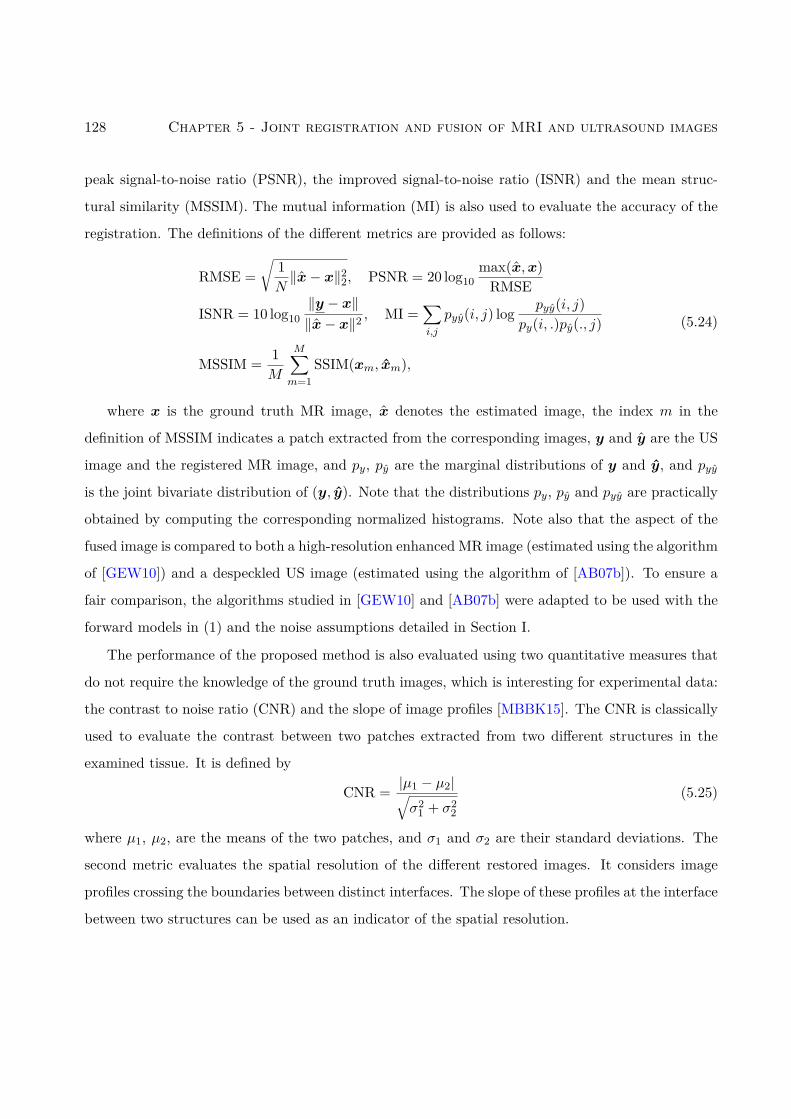
128 Chapter 5 - Joint registration and fusion of MRI and ultrasound images
peak signal-to-noise ratio (PSNR), the improved signal-to-noise ratio (ISNR) and the mean struc-
tural similarity (MSSIM). The mutual information (MI) is also used to evaluate the accuracy of the
registration. The definitions of the different metrics are provided as follows:
RMSE =√
1N‖x− x‖22, PSNR = 20 log10
max(x,x)RMSE
ISNR = 10 log10‖y − x‖‖x− x‖2
, MI =∑i,j
pyy(i, j) log pyy(i, j)py(i, .)py(., j)
MSSIM = 1M
M∑m=1
SSIM(xm, xm),
(5.24)
where x is the ground truth MR image, x denotes the estimated image, the index m in the
definition of MSSIM indicates a patch extracted from the corresponding images, y and y are the US
image and the registered MR image, and py, py are the marginal distributions of y and y, and pyyis the joint bivariate distribution of (y, y). Note that the distributions py, py and pyy are practically
obtained by computing the corresponding normalized histograms. Note also that the aspect of the
fused image is compared to both a high-resolution enhanced MR image (estimated using the algorithm
of [GEW10]) and a despeckled US image (estimated using the algorithm of [AB07b]). To ensure a
fair comparison, the algorithms studied in [GEW10] and [AB07b] were adapted to be used with the
forward models in (1) and the noise assumptions detailed in Section I.
The performance of the proposed method is also evaluated using two quantitative measures that
do not require the knowledge of the ground truth images, which is interesting for experimental data:
the contrast to noise ratio (CNR) and the slope of image profiles [MBBK15]. The CNR is classically
used to evaluate the contrast between two patches extracted from two different structures in the
examined tissue. It is defined by
CNR = |µ1 − µ2|√σ2
1 + σ22
(5.25)
where µ1, µ2, are the means of the two patches, and σ1 and σ2 are their standard deviations. The
second metric evaluates the spatial resolution of the different restored images. It considers image
profiles crossing the boundaries between distinct interfaces. The slope of these profiles at the interface
between two structures can be used as an indicator of the spatial resolution.
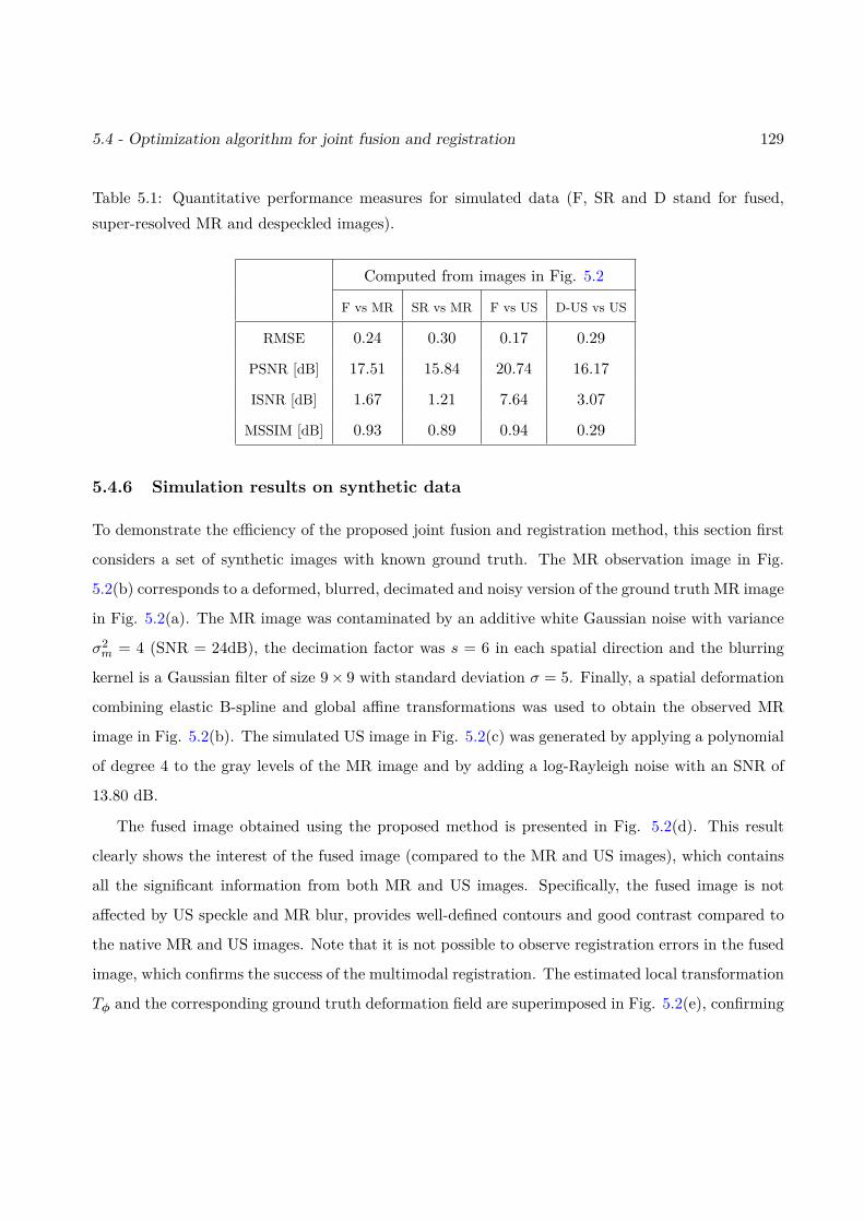
5.4 - Optimization algorithm for joint fusion and registration 129
Table 5.1: Quantitative performance measures for simulated data (F, SR and D stand for fused,super-resolved MR and despeckled images).
Computed from images in Fig. 5.2
F vs MR SR vs MR F vs US D-US vs US
RMSE 0.24 0.30 0.17 0.29
PSNR [dB] 17.51 15.84 20.74 16.17
ISNR [dB] 1.67 1.21 7.64 3.07
MSSIM [dB] 0.93 0.89 0.94 0.29
5.4.6 Simulation results on synthetic data
To demonstrate the efficiency of the proposed joint fusion and registration method, this section first
considers a set of synthetic images with known ground truth. The MR observation image in Fig.
5.2(b) corresponds to a deformed, blurred, decimated and noisy version of the ground truth MR image
in Fig. 5.2(a). The MR image was contaminated by an additive white Gaussian noise with variance
σ2m = 4 (SNR = 24dB), the decimation factor was s = 6 in each spatial direction and the blurring
kernel is a Gaussian filter of size 9× 9 with standard deviation σ = 5. Finally, a spatial deformation
combining elastic B-spline and global affine transformations was used to obtain the observed MR
image in Fig. 5.2(b). The simulated US image in Fig. 5.2(c) was generated by applying a polynomial
of degree 4 to the gray levels of the MR image and by adding a log-Rayleigh noise with an SNR of
13.80 dB.
The fused image obtained using the proposed method is presented in Fig. 5.2(d). This result
clearly shows the interest of the fused image (compared to the MR and US images), which contains
all the significant information from both MR and US images. Specifically, the fused image is not
affected by US speckle and MR blur, provides well-defined contours and good contrast compared to
the native MR and US images. Note that it is not possible to observe registration errors in the fused
image, which confirms the success of the multimodal registration. The estimated local transformation
Tφ and the corresponding ground truth deformation field are superimposed in Fig. 5.2(e), confirming
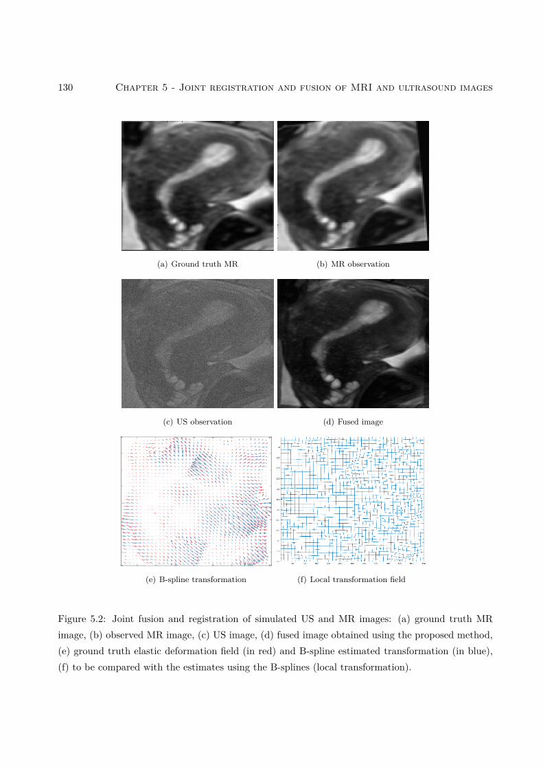
130 Chapter 5 - Joint registration and fusion of MRI and ultrasound images
(a) Ground truth MR (b) MR observation
(c) US observation (d) Fused image
(e) B-spline transformation (f) Local transformation field
Figure 5.2: Joint fusion and registration of simulated US and MR images: (a) ground truth MRimage, (b) observed MR image, (c) US image, (d) fused image obtained using the proposed method,(e) ground truth elastic deformation field (in red) and B-spline estimated transformation (in blue),(f) to be compared with the estimates using the B-splines (local transformation).
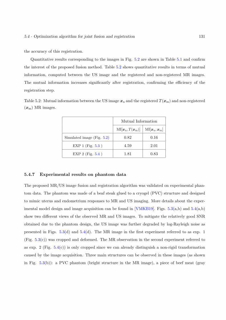
5.4 - Optimization algorithm for joint fusion and registration 131
the accuracy of this registration.
Quantitative results corresponding to the images in Fig. 5.2 are shown in Table 5.1 and confirm
the interest of the proposed fusion method. Table 5.2 shows quantitative results in terms of mutual
information, computed between the US image and the registered and non-registered MR images.
The mutual information increases significantly after registration, confirming the efficiency of the
registration step.
Table 5.2: Mutual information between the US image xu and the registered T (xm) and non-registered(xm) MR images.
Mutual Information
MI[xu, T (xm)] MI[xu,xm]
Simulated image (Fig. 5.2) 0.82 0.16
EXP 1 (Fig. 5.3 ) 4.59 2.01
EXP 2 (Fig. 5.4 ) 1.81 0.83
5.4.7 Experimental results on phantom data
The proposed MR/US image fusion and registration algorithm was validated on experimental phan-
tom data. The phantom was made of a beaf steak glued to a cryogel (PVC) structure and designed
to mimic uterus and endometrium responses to MR and US imaging. More details about the exper-
imental model design and image acquisition can be found in [VMKB19]. Figs. 5.3(a,b) and 5.4(a,b)
show two different views of the observed MR and US images. To mitigate the relatively good SNR
obtained due to the phantom design, the US image was further degraded by log-Rayleigh noise as
presented in Figs. 5.3(d) and 5.4(d). The MR image in the first experiment referred to as exp. 1
(Fig. 5.3(c)) was cropped and deformed. The MR observation in the second experiment referred to
as exp. 2 (Fig. 5.4(c)) is only cropped since we can already distinguish a non-rigid transformation
caused by the image acquisition. Three main structures can be observed in these images (as shown
in Fig. 5.3(b)): a PVC phantom (bright structure in the MR image), a piece of beef meat (gray
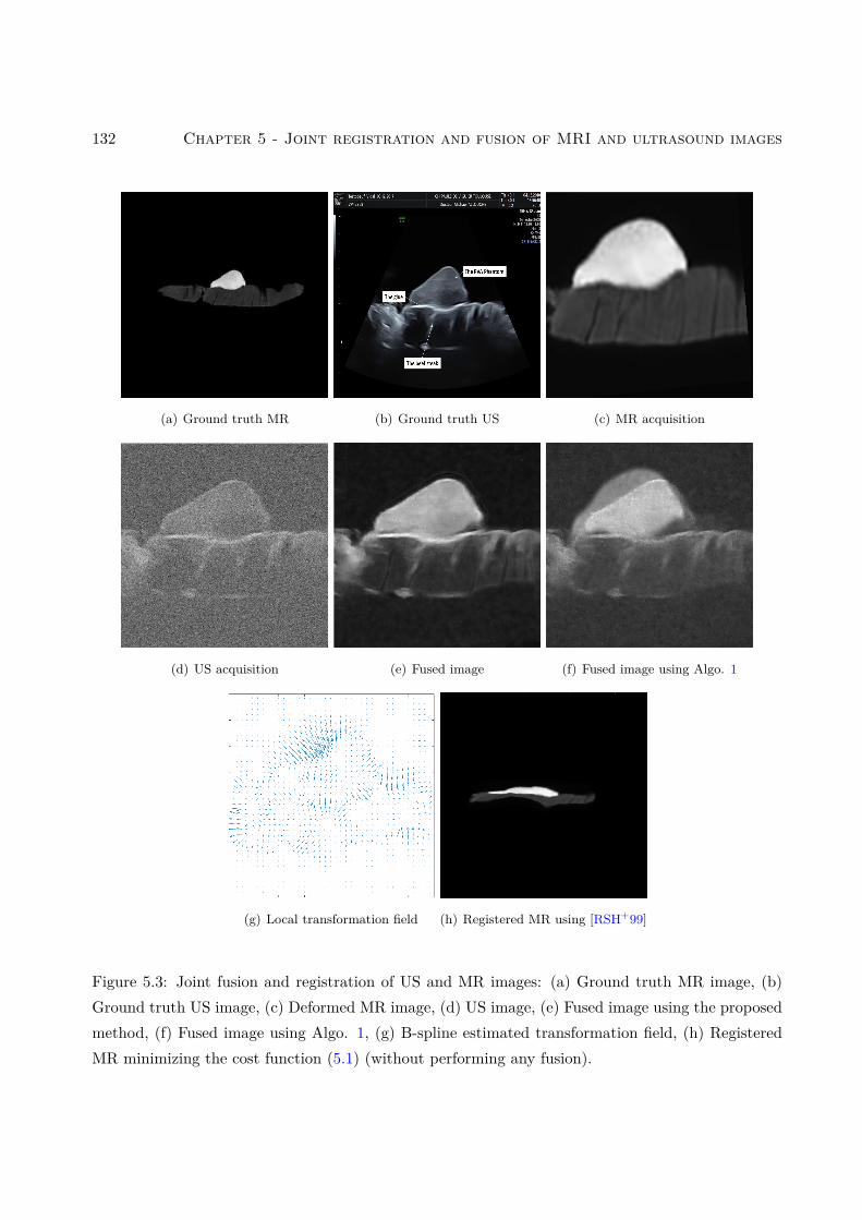
132 Chapter 5 - Joint registration and fusion of MRI and ultrasound images
(a) Ground truth MR (b) Ground truth US (c) MR acquisition
(d) US acquisition (e) Fused image (f) Fused image using Algo. 1
(g) Local transformation field (h) Registered MR using [RSH+99]
Figure 5.3: Joint fusion and registration of US and MR images: (a) Ground truth MR image, (b)Ground truth US image, (c) Deformed MR image, (d) US image, (e) Fused image using the proposedmethod, (f) Fused image using Algo. 1, (g) B-spline estimated transformation field, (h) RegisteredMR minimizing the cost function (5.1) (without performing any fusion).
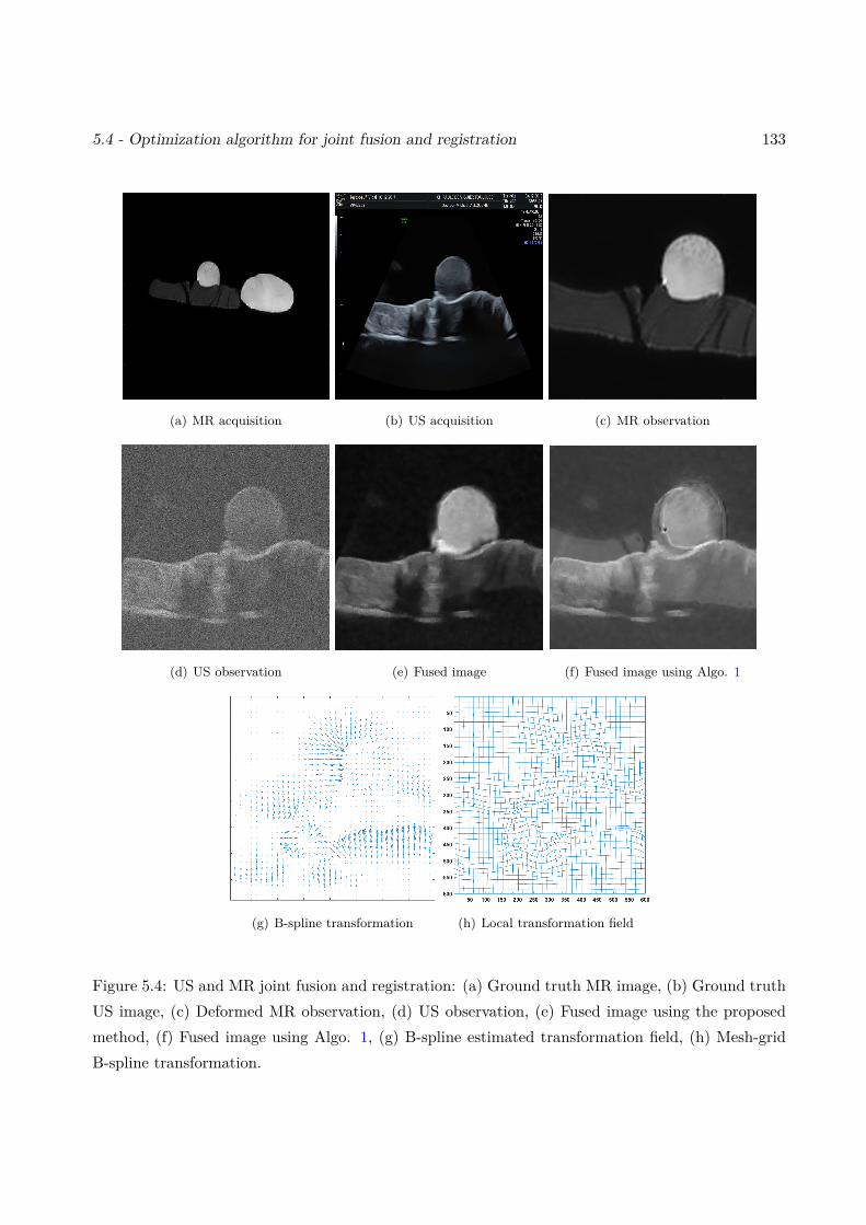
5.4 - Optimization algorithm for joint fusion and registration 133
(a) MR acquisition (b) US acquisition (c) MR observation
(d) US observation (e) Fused image (f) Fused image using Algo. 1
(g) B-spline transformation (h) Local transformation field
Figure 5.4: US and MR joint fusion and registration: (a) Ground truth MR image, (b) Ground truthUS image, (c) Deformed MR observation, (d) US observation, (e) Fused image using the proposedmethod, (f) Fused image using Algo. 1, (g) B-spline estimated transformation field, (h) Mesh-gridB-spline transformation.
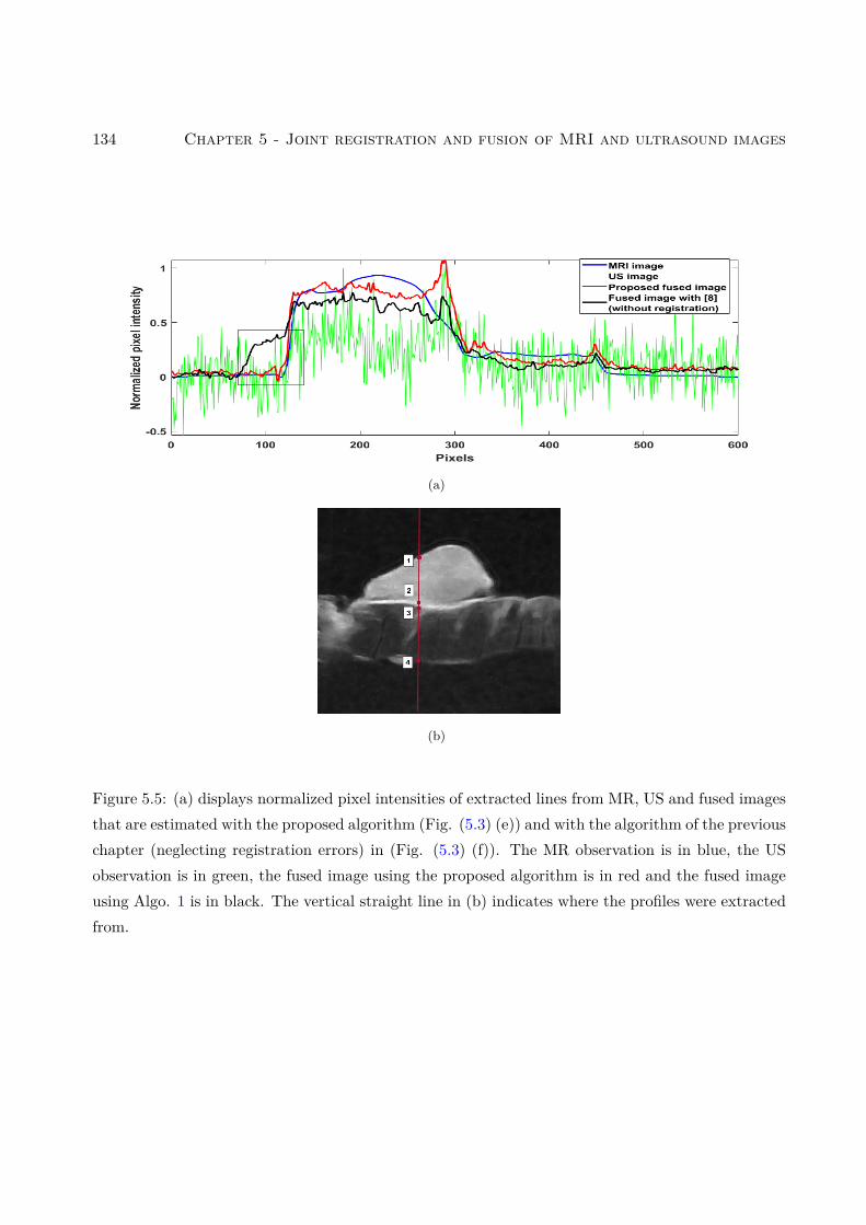
134 Chapter 5 - Joint registration and fusion of MRI and ultrasound images
(a)
(b)
Figure 5.5: (a) displays normalized pixel intensities of extracted lines from MR, US and fused imagesthat are estimated with the proposed algorithm (Fig. (5.3) (e)) and with the algorithm of the previouschapter (neglecting registration errors) in (Fig. (5.3) (f)). The MR observation is in blue, the USobservation is in green, the fused image using the proposed algorithm is in red and the fused imageusing Algo. 1 is in black. The vertical straight line in (b) indicates where the profiles were extractedfrom.
5.4 - Optimization algorithm for joint fusion and registration 135
structure in the MR image), and the glue used to attach them, only visible in the US image (thin
bright structure).
Figs. 5.3(e,f) and 5.4(e,f) show the fused images obtained using the proposed method and the
algorithm in Chapter 4 (Algo. 1). The fused images in Figs. 5.3(e) and 5.4(e) gather information
from MR and US images: they provide a good contrast between the PVC and the beef tissue (similar
to MR), a good spatial resolution (similar to US) allowing small structures such as the glue to be
distinguished, and good SNR. Moreover, registration errors are significantly reduced in the fused and
registered images when compared to the fused and unregistered images of Figs. 5.3(f) and 5.4(f)
obtained using the Algo. 1 . The performance of the proposed algorithm compared to Algo. 1
confirms the interest of a joint fusion and registration. Figs. 5.3(g) and 5.4(g) display the estimated
B-spline local transformation, which has been compensated in the proposed algorithm. Fig. 5.3(h)
was obtained using the same multimodal registration algorithm as the one embedded in the proposed
method. It clearly fails to register MR to the US image, because of its sensitivity to noise and to
mismatching between the gray levels in the two imaging modalities. Finally, the efficiency of the
registration step included in the proposed algorithm is confirmed by the values of MI shown in Table
5.2. Figs 5.3(a-d) and 5.4(a-d) show the MR and US observations, which clearly highlight the
complementarity between the two imaging modalities: MR has a large field of view with excellent
contrast between the polyvinyl alcohol and the beef steak with a limited spatial resolution especially
at millimetric scale (it is impossible to observe the glue among the steak and the PVA). On the other
hand, the US image has a good resolution that allows the glue to be imaged very precisely (mimicking
the endomotrium depth of inflitration), but has a reduced field of view. The fused images obtained
using Algo. 2 are presented in Figs. 5.3(e) and 5.4(e). The interest of fusing the two images can be
appreciated, in particular the ability of the fused image to gather the good contrast of MR and the
good spatial resolution of US. In addition to the visual examination of the different images, CNR
was used to assess the contrast between two different structures of the images. The two patches
considered to compute the CNR are extracted from the PVA phantom and the beef steak. Table 5.3
clearly demonstrates that the joint registration/fusion process improves the image contrast in both
experiments compared to US images.
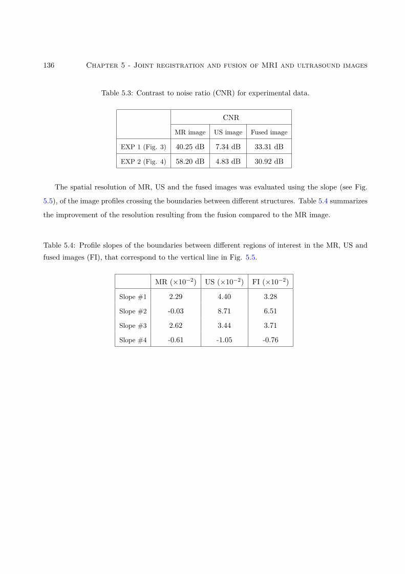
136 Chapter 5 - Joint registration and fusion of MRI and ultrasound images
Table 5.3: Contrast to noise ratio (CNR) for experimental data.
CNR
MR image US image Fused image
EXP 1 (Fig. 3) 40.25 dB 7.34 dB 33.31 dB
EXP 2 (Fig. 4) 58.20 dB 4.83 dB 30.92 dB
The spatial resolution of MR, US and the fused images was evaluated using the slope (see Fig.
5.5), of the image profiles crossing the boundaries between different structures. Table 5.4 summarizes
the improvement of the resolution resulting from the fusion compared to the MR image.
Table 5.4: Profile slopes of the boundaries between different regions of interest in the MR, US andfused images (FI), that correspond to the vertical line in Fig. 5.5.
MR (×10−2) US (×10−2) FI (×10−2)
Slope #1 2.29 4.40 3.28
Slope #2 -0.03 8.71 6.51
Slope #3 2.62 3.44 3.71
Slope #4 -0.61 -1.05 -0.76
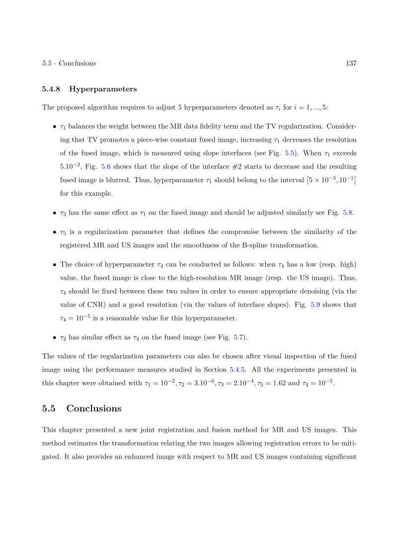
5.5 - Conclusions 137
5.4.8 Hyperparameters
The proposed algorithm requires to adjust 5 hyperparameters denoted as τi for i = 1, ..., 5:
• τ1 balances the weight between the MR data fidelity term and the TV regularization. Consider-
ing that TV promotes a piece-wise constant fused image, increasing τ1 decreases the resolution
of the fused image, which is measured using slope interfaces (see Fig. 5.5). When τ1 exceeds
5.10−2, Fig. 5.6 shows that the slope of the interface #2 starts to decrease and the resulting
fused image is blurred. Thus, hyperparameter τ1 should belong to the interval[5× 10⁻³, 10−1]
for this example.
• τ3 has the same effect as τ1 on the fused image and should be adjusted similarly see Fig. 5.8.
• τ5 is a regularization parameter that defines the compromise between the similarity of the
registered MR and US images and the smoothness of the B-spline transformation.
• The choice of hyperparameter τ4 can be conducted as follows: when τ4 has a low (resp. high)
value, the fused image is close to the high-resolution MR image (resp. the US image). Thus,
τ4 should be fixed between these two values in order to ensure appropriate denoising (via the
value of CNR) and a good resolution (via the values of interface slopes). Fig. 5.9 shows that
τ4 = 10−5 is a reasonable value for this hyperparameter.
• τ2 has similar effect as τ4 on the fused image (see Fig. 5.7).
The values of the regularization parameters can also be chosen after visual inspection of the fused
image using the performance measures studied in Section 5.4.5. All the experiments presented in
this chapter were obtained with τ1 = 10−2, τ2 = 3.10−6, τ3 = 2.10−4, τ5 = 1.62 and τ4 = 10−5.
5.5 Conclusions
This chapter presented a new joint registration and fusion method for MR and US images. This
method estimates the transformation relating the two images allowing registration errors to be miti-
gated. It also provides an enhanced image with respect to MR and US images containing significant
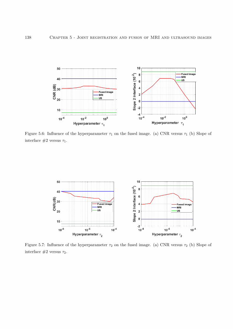
138 Chapter 5 - Joint registration and fusion of MRI and ultrasound images
Figure 5.6: Influence of the hyperparameter τ1 on the fused image. (a) CNR versus τ1 (b) Slope ofinterface #2 versus τ1.
Figure 5.7: Influence of the hyperparameter τ2 on the fused image. (a) CNR versus τ2 (b) Slope ofinterface #2 versus τ2.
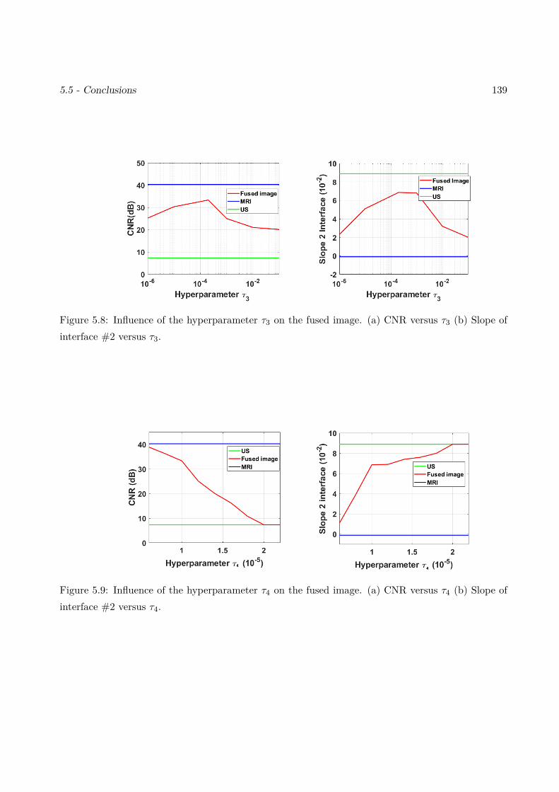
5.5 - Conclusions 139
Figure 5.8: Influence of the hyperparameter τ3 on the fused image. (a) CNR versus τ3 (b) Slope ofinterface #2 versus τ3.
Figure 5.9: Influence of the hyperparameter τ4 on the fused image. (a) CNR versus τ4 (b) Slope ofinterface #2 versus τ4.
140 Chapter 5 - Joint registration and fusion of MRI and ultrasound images
information from both modalities. The key ingredients of the proposed method include the resolution
of two inverse problems, ensuring a despeckling of the US image and a super-resolution of the MR,
the use of a polynomial function relating the noiseless US and MR images and the consideration of
local and global transformations in order to correct the registration errors. All these ingredients are
incorporated in PALM algorithm, allowing the joint fusion and registration problem to be solved.
Quantitative and qualitative results obtained with different datasets show very promising results for
synthetic and phantom data. Future work will be dedicated to confirm the encouraging phantom
results on in vivo data.
Chapter 6
Conclusions and perspectives
6.1 Conclusions
The objective of this PhD thesis was to investigate algorithms for the fusion of MRI and ultrasound
images for the pre-operative diagnosis and the imaging guided-surgery of endometriosis. This fusion
is a difficult task since MRI and US images are very different modalities that are contaminated by
different kinds of noises. Our main contributions concerning the fusion of MRI and US images are
summarized below:
The first work studied in Chapter 4 proposed a new fusion method for registered magnetic res-
onance (MR) and ultrasound (US) images. The proposed method was able to reconstruct a fused
image containing information from both observations, by solving a super-resolution inverse problem
for MRI and a despeckling problem for US images. These two problems were solved jointly by using
appropriate statistical models and a polynomial relationship between the images of interest. The
relation between MR and US images was modeled locally by two types of polynomial functions : a
global polynomial function and a low-order polynomial functions associated with the image patches.
A PALM algorithm was finally investigated to solve the resulting fusion problem. Results obtained
on simulated and real images clearly showed the interest of combining the information contained in
these two imaging modalities, instead of restoring them independently.
Results show that the patch-wise fusion method captures more details than the global polynomial
fusion. However, it is more time consuming. Thus, the choice of the adapted method depends on
the application. We would like to mention that these methods suppose that MRI and US images
are perfectly registered, otherwise it is necessary to use the algorithm of Chapter 5 which is more
efficient but at the price of a higher computational cost.
141
142 Conclusions and Perspectives
Chapter 5 presented a new joint registration and fusion method for MR and ultrasound images.
This method estimates the transformation relating the two images allowing registration errors to be
mitigated. It also provides an enhanced image with respect to MR and ultrasound images containing
significant information from both modalities. The key ingredients of the proposed method include also
the resolution of two inverse problems, ensuring a despeckling of the US image and a super-resolution
of the MRI, the use of a polynomial function relating the noiseless ultrasound and MR images and
the consideration of local and global transformations in order to correct the registration errors. All
these ingredients are incorporated in PALM algorithm, allowing the joint fusion and registration
problem to be solved. Quantitative and qualitative results obtained with different datasets show
very promising results for synthetic and phantom data.
6.2 Future work
To the best of our knowledge, this work is a first attempt for fusing MR and US images. It opens
several interesting perspectives.
6.2.1 Short-term perspectives
• Observation models: As a matter of simplicity and since the fusion is a complex and non-
linear task, we choose the hypothesis of an independent identically distributed noise in both
MRI and US images. A natural progression of this work is to take into account the possible
correlation of noise samples especially for the US image, to take into account the presence of
potential artifacts and to adapt the algorithm to not-fully developed speckle as in [DJ08].
• Regularizations: It is well known that inverse problems are ill-posed, which is a reason why
we proposed to use an l2-TV regularization to smooth MRI and US images. Other regularizers
have been proposed in the literature that might improve the proposed fusion: [BEGR09] intro-
duced a novel regularization adapted to MRI that combines an l1-TV and Gaussian mixture
regularization, [JB18] proposed a non-local total bounded variational (TBV) regularization to
restore US images corrupted with data-correlated speckles and linear blurring artifacts. Such
6.2 - Future work 143
regularizations may lead to significant improvement of edge definition for the fused image com-
pared to l2-TV regularization that can over-smooth the edges.
• Hyperparameters: As explain in Chapters 4 and 5, hyperparameters play an important role
in the obtained fused images. The choice of hyperparameters was done manually based on
visual inspection of images and using appropriate metrics. However, it would be interesting to
investigate some methods to tune these hyperparameters automatically from the data as the
SURE algorithm [PSC+16] or other Bayesian methods.
• MRI and US relationship: The key of an accurate image fusion is the choice of an adapted
function that can model a realistic relationship between images. In this work, we choose global
or patch-wise polynomial functions to link MRI and US images. An interesting prospect would
be to introduce more general transformations resulting for instance from kernel methods (see
[MZY15] for an example on point clouds) or to learn the functional dependence between MR
and US images using machine learning algorithms as in [KS19].
• 3D image fusion and registration: All the methods studied ion this work are restricted
to 2D images. In order to use these techniques clinically would be important to adapt these
methods for the fusion of 3D-MRI and 2D/3D US images.
6.2.2 Long-term perspectives
• Augmented reality: The fusion of 2D MRI and US images is a first step in a long study that
aims to create a virtual navigator based on augmented reality for endometriosis surgery. The
purpose of this study is to combine the fused MRI/US images that can provide a see-through
organs and the videos collected during laparoscopy using a small camera that shows only the
wall of organs. Combining these information can help to build an augmented reality of real-time
organ states. Augmented reality can help surgeons to become more efficient and would change
the life of many women.
• Other medical applications: There are other applications that use MRI and US images such
as prostate biopsy [NKS+09], tumor detection in the liver [KZW+12] and brain shift correction

144 Conclusions and Perspectives
[GLP01]. It would be interesting to investigate the potential use of the methods studied in this
PhD thesis to these new applications.

Appendices
145

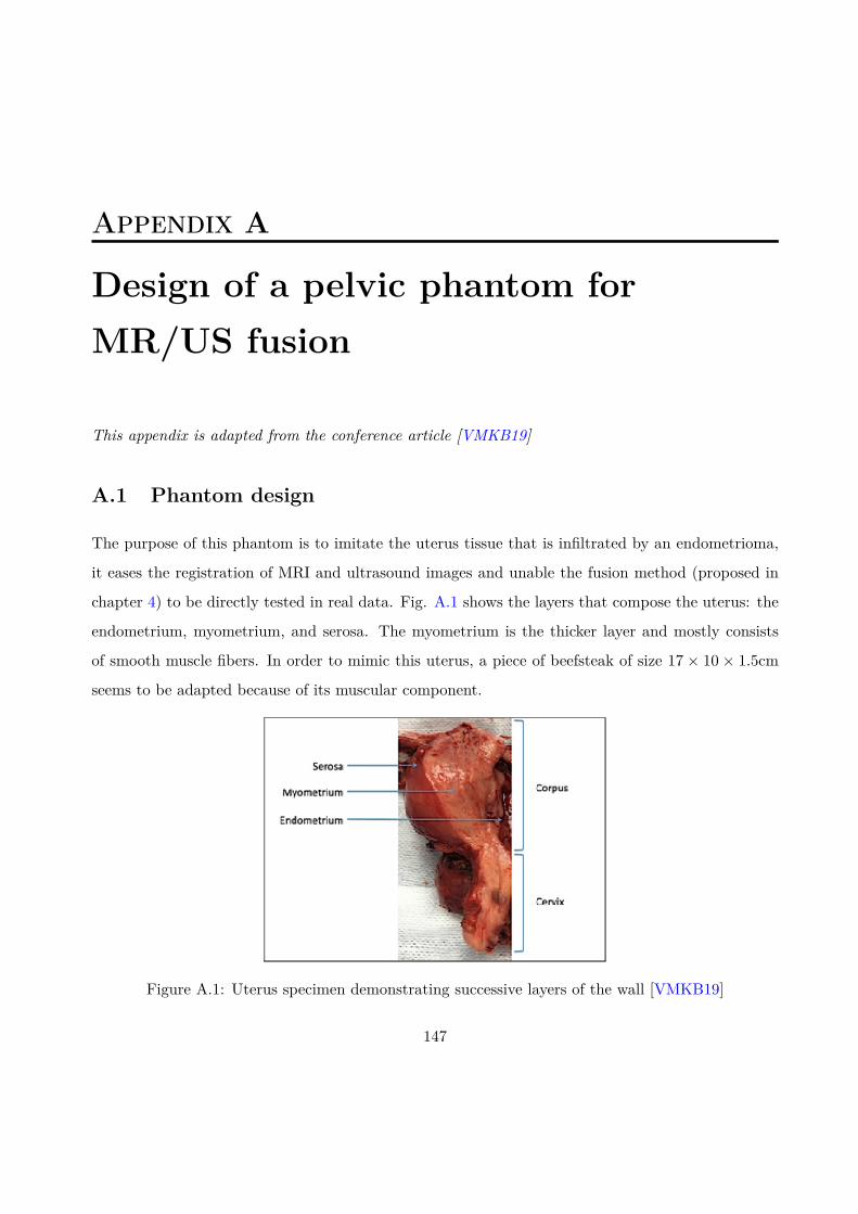
Appendix A
Design of a pelvic phantom forMR/US fusion
This appendix is adapted from the conference article [VMKB19]
A.1 Phantom design
The purpose of this phantom is to imitate the uterus tissue that is infiltrated by an endometrioma,
it eases the registration of MRI and ultrasound images and unable the fusion method (proposed in
chapter 4) to be directly tested in real data. Fig. A.1 shows the layers that compose the uterus: the
endometrium, myometrium, and serosa. The myometrium is the thicker layer and mostly consists
of smooth muscle fibers. In order to mimic this uterus, a piece of beefsteak of size 17 × 10 × 1.5cm
seems to be adapted because of its muscular component.
Figure A.1: Uterus specimen demonstrating successive layers of the wall [VMKB19]
147
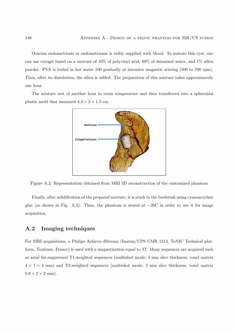
148 Appendix A - Design of a pelvic phantom for MR/US fusion
Ovarian endometriosis or endometrioma is richly supplied with blood. To imitate this cyst, one
can use cryogel based on a mixture of 10% of polyvinyl acid, 89% of deionized water, and 1% silica
powder. PVA is boiled in hot water 100 gradually at intensive magnetic stirring (500 to 700 rpm).
Then, after its dissolution, the silica is added. The preparation of this mixture takes approximately
one hour.
The mixture rest of another hour in room temperature and then transferred into a spheroidal
plastic mold that measures 4.3× 3× 1.5 cm.
Figure A.2: Representation obtained from MRI 3D reconstruction of the customized phantom
Finally, after solidification of the prepared mixture, it is stuck to the beefsteak using cyanoacrylate
glue (as shown in Fig. A.2). Then, the phantom is stored at −20C in order to use it for image
acquisition.
A.2 Imaging techniques
For MRI acquisitions, a Philips Achieva dStream (Inserm/UPS UMR 1214, ToNIC Technical plat-
form, Toulouse, France) is used with a magnetization equal to 3T. Many sequences are acquired such
as axial fat-suppressed T1-weighted sequences (multishot mode; 4 mm slice thickness; voxel matrix
4 × 1 × 4 mm) and T2-weighted sequences (multishot mode; 2 mm slice thickness; voxel matrix
0.8× 2× 2 mm).
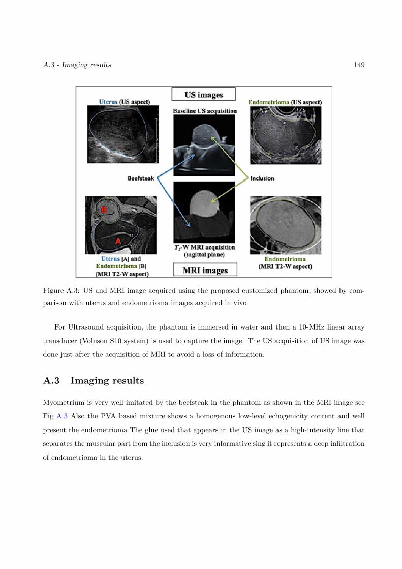
A.3 - Imaging results 149
Figure A.3: US and MRI image acquired using the proposed customized phantom, showed by com-parison with uterus and endometrioma images acquired in vivo
For Ultrasound acquisition, the phantom is immersed in water and then a 10-MHz linear array
transducer (Voluson S10 system) is used to capture the image. The US acquisition of US image was
done just after the acquisition of MRI to avoid a loss of information.
A.3 Imaging results
Myometrium is very well imitated by the beefsteak in the phantom as shown in the MRI image see
Fig A.3 Also the PVA based mixture shows a homogenous low-level echogenicity content and well
present the endometrioma The glue used that appears in the US image as a high-intensity line that
separates the muscular part from the inclusion is very informative sing it represents a deep infiltration
of endometrioma in the uterus.

150
Bibliography
[AA15] Nemir Ahmed Al-Azzawi. Medical image fusion based on shearlets and human feature
visibility. International Journal of Computer Applications, 125(12):1–12, 2015.
[AAM+04] Tal Arbel, Tal Arbel, Xavier Morandi, Roch M Comeau, and D Louis Collins. Au-
tomatic non-linear MRI-ultrasound registration for the correction of intra-operative
brain deformations. Computer Aided Surgery, 9(4):123–136, 2004.
[AASAI09] Nemir Al-Azzawi, Harsa Amylia Mat Sakim, Ahmed K Wan Abdullah, and Haidi
Ibrahim. Medical image fusion scheme using complex contourlet transform based on
PCA. In Proc. 2009 Annual International Conference of the IEEE Engineering in
Medicine and Biology Society, pages 5813–5816, Minneapolis, MN, 2009.
[AAVB16] Codruta O Ancuti, Cosmin Ancuti, Christophe De Vleeschouwer, and Alan C Bovik.
Single-scale fusion: An effective approach to merging images. IEEE Trans. Image
Processing, 26(1):65–78, 2016.
[AB07a] Tuncer C Aysal and Kenneth E Barner. Rayleigh-maximum-likelihood filtering for
speckle reduction of ultrasound images. IEEE Trans. Med. Imag., 26(5):712–727,
2007.
[AB07b] Tuncer C Aysal and Kenneth E Barner. Rayleigh-maximum-likelihood filtering for
speckle reduction of ultrasound images. IEEE Trans. Med. Imag., 26(5):712–727,
2007.
151
152 BIBLIOGRAPHY
[ABT01] Alin Achim, Anastasios Bezerianos, and Panagiotis Tsakalides. Novel bayesian mul-
tiscale method for speckle removal in medical ultrasound images. IEEE transactions
on medical imaging, 20(8):772–783, 2001.
[AEGG08] Brian B Avants, Charles L Epstein, Murray Grossman, and James C Gee. Symmetric
diffeomorphic image registration with cross-correlation: evaluating automated label-
ing of elderly and neurodegenerative brain. Medical image analysis, 12(1):26–41,
2008.
[AGS+20] Angélica Atehortúa, Mireille Garreau, Antoine Simon, Erwan Donal, Mathieu Led-
erlin, and Eduardo Romero. Fusion of 3D real-time echocardiography and cine MRI
using a saliency analysis. Computer Assisted Radiology and Surgery, 15(2):277–285,
2020.
[AHPG09] Claire Allen, Sally Hopewell, Andrew Prentice, and Daisy Gregory. Nonsteroidal
anti-inflammatory drugs for pain in women with endometriosis. Cochrane Database
of Systematic Reviews, (2), 2009.
[AKHAFH09] Hanan Al Kadri, Samar Hassan, Haya M Al-Fozan, and Ali Hajeer. Hormone therapy
for endometriosis and surgical menopause. Cochrane Database of Systematic Reviews,
(1), 2009.
[AL19] Reza Abazari and Mehrdad Lakestani. Non-subsampled shearlet transform and
log-transform methods for despeckling of medical ultrasound images. Informatica,
30(1):1–19, 2019.
[ANA18] M. Amin-Naji and A. Aghagolzadeh. Multi-focus image fusion in DCT domain using
variance and energy of Laplacian and correlation coefficient for visual sensor networks.
Journal of AI and Data Mining, 6:233–250, 2018.
[Anu20] Treatment of endometriosis. http://www.safertility.co.uk/Treatment_of_
endometriosis, 2020.
BIBLIOGRAPHY 153
[AO12] Anestis Antoniadis and Georges Oppenheim. Wavelets and statistics, volume 103.
2012.
[APABP03] MS Arruda, Carlos A Petta, Mauricio S Abrão, and Cristina L Benetti-Pinto. Time
elapsed from onset of symptoms to diagnosis of endometriosis in a cohort study of
Brazilian women. Human reproduction, 18(4):756–759, 2003.
[AR16] Fakhre Alam and Sami Ur Rahman. Intrinsic registration techniques for medical im-
ages: A state-of-the-art review. Journal of Postgraduate Medical Institute (Peshawar-
Pakistan), 30(2), 2016.
[ARU+16] F Alam, SU Rahman, S Ullah, A Khalil, and A Uddin. A review on extrinsic reg-
istration methods for medical images. Tech. J. Univ. Engineering Technol. Taxila,
21:110–9, 2016.
[ATL14] Tarun Kumar Agarwal, Mayank Tiwari, and Subir Singh Lamba. Modified histogram
based contrast enhancement using homomorphic filtering for medical images. In Proc.
2014 IEEE International Advance Computing Conference (IACC), Chicago, Illinois,
2014.
[Ban08] Isaac Bankman. Handbook of medical image processing and analysis. Elsevier, 2008.
[BB11] Jerrold T Bushberg and John M Boone. The essential physics of medical imaging.
Lippincott Williams & Wilkins, 2011.
[BBH+17] Marc Bazot, Nishat Bharwani, Cyrille Huchon, K Kinkel, Teresa Margarida Cunha,
Algesira Guerra, Lucia Manganaro, Laura Bunesch, Aki Kido, Kaori Togashi, et al.
European society of urogenital radiology (ESUR) guidelines: MR imaging of pelvic
endometriosis. European radiology, 27(7):2765–2775, 2017.
[BCBB10] Carlo Bulletti, Maria Elisabetta Coccia, Silvia Battistoni, and Andrea Borini. En-
dometriosis and infertility. Journal of assisted reproduction and genetics, 27(8):441–
447, 2010.
154 BIBLIOGRAPHY
[BEGR09] Avraham Ben-Ezra, Hayit Greenspan, and Yossi Rubner. Regularized super-
resolution of brain MRI. In Proc 2009 IEEE International Symposium on Biomedical
Imaging: From Nano to Macro, pages 254–257, Boston, MA, 2009.
[BGSW07] Serdar K Balci, Polina Golland, Martha Elizabeth Shenton, and William Mercer
Wells. Free-form B-spline deformation model for groupwise registration. Med. Imag.
Comput. Assist. Interv., 10:23–30, 2007.
[BK89] Ruzena Bajcsy and Stane Kovačič. Multiresolution elastic matching. Computer
vision, graphics, and image processing, 46(1):1–21, 1989.
[BKGD17] Durga Prasad Bavirisetti, Vijayakumar Kollu, Xiao Gang, and Ravindra Dhuli. Fu-
sion of MRI and CT images using guided image filter and image statistics. Interna-
tional journal of Imaging systems and Technology, 27(3):227–237, 2017.
[BLCL08] Erik Blasch, Xiaokun Li, Genshe Chen, and Wenhua Li. Image quality assessment for
performance evaluation of image fusion. In Proc. 2008 11th International Conference
on Information Fusion, pages 1–6, Cologne, 2008.
[BLR+09] Marc Bazot, Clarisse Lafont, Roman Rouzier, Gilles Roseau, Isabelle Thomassin-
Naggara, and Emile Daraï. Diagnostic accuracy of physical examination, transvaginal
sonography, rectal endoscopic sonography, and magnetic resonance imaging to diag-
nose deep infiltrating endometriosis. Fertility and sterility, 92(6):1825–1833, 2009.
[BM92] Paul J Besl and Neil D McKay. Method for registration of 3-D shapes. In Sensor fu-
sion IV: control paradigms and data structures, volume 1611, pages 586–606, Boston,
MA, United States, 1992.
[BMTY05] M Faisal Beg, Michael I Miller, Alain Trouvé, and Laurent Younes. Computing large
deformation metric mappings via geodesic flows of diffeomorphisms. International
journal of computer vision, 61(2):139–157, 2005.
BIBLIOGRAPHY 155
[BN92] Richard K Beatson and Garry N Newsam. Fast evaluation of radial basis functions.
Computers & Mathematics with Applications, 24(12):7–19, 1992.
[BNB03] Djamal Boukerroui, J Alison Noble, and Michael Brady. Velocity estimation in ul-
trasound images: A block matching approach. In Information Processing in Medical
Imaging, pages 586–598, Heidelberg, Germany, 2003.
[BPC+11] Stephen Boyd, Neal Parikh, Eric Chu, Borja Peleato, Jonathan Eckstein, et al. Dis-
tributed optimization and statistical learning via the alternating direction method of
multipliers. Foundations and Trends in Machine learning, 3(1):1–122, 2011.
[BS16] Jayachandran Jai Jaganath Babu and Gnanou Florence Sudha. Adaptive speckle
reduction in ultrasound images using fuzzy logic on coefficient of variation. Biomedical
Signal Processing and Control, 23:93–103, 2016.
[BST14] Jérôme Bolte, Shoham Sabach, and Marc Teboulle. Proximal alternating linearized
minimization or nonconvex and nonsmooth problems. Mathematical Programming,
146(1-2):459–494, 2014.
[BT09] Amir Beck and Marc Teboulle. A fast iterative shrinkage-thresholding algorithm for
linear inverse problems. SIAM journal on imaging sciences, 2(1):183–202, 2009.
[Bur78] Christoph B Burckhardt. Speckle in ultrasound B-mode scans. IEEE Transactions
on Sonics and ultrasonics, 25(1):1–6, 1978.
[C+02] Boaz Cohen et al. New maximum likelihood motion estimation schemes for noisy
ultrasound images. Pattern Recognition, 35(2):455–463, 2002.
[CCB06] N Cvejic, CN Canagarajah, and DR Bull. Image fusion metric based on mutual
information and Tsallis entropy. Electronics letters, 42(11):626–627, 2006.
[CD14] Tianfeng Chai and Roland R Draxler. Root mean square error (RMSE) or mean ab-
solute error (MAE)?–arguments against avoiding rmse in the literature. Geoscientific
model development, 7(3):1247–1250, 2014.
156 BIBLIOGRAPHY
[CE97] D. Louis Collins and Alan C. Evans. Animal: validation and applications of nonlinear
registration-based segmentation. International journal of pattern recognition and
artificial intelligence, 11(08):1271–1294, 1997.
[CEA00] SuChin Chen Coutre, MW Evens, and SG Armato. Performance evaluation of image
registration. In Proc. International Conference of the IEEE Engineering in Medicine
and Biology Society (Cat. No. 00CH37143), volume 4, pages 3140–3143, Chicago,
USA, 2000.
[CFK+18] Akshay S Chaudhari, Zhongnan Fang, Feliks Kogan, Jeff Wood, Kathryn J Stevens,
Eric K Gibbons, Jin Hyung Lee, Garry E Gold, and Brian A Hargreaves. Super-
resolution musculoskeletal MRI using deep learning. Magnetic resonance in medicine,
80(5):2139–2154, 2018.
[CGM+04] G Carbognin, A Guarise, L Minelli, I Vitale, R Malagó, G Zamboni, and C Procacci.
Pelvic endometriosis: US and MRI features. Abdominal imaging, 29(5):609, 2004.
[Che16] Zhouye Chen. Reconstruction of enhanced ultrasound images from compressed mea-
surements. PhD thesis, 2016.
[CHH04] William R Crum, Thomas Hartkens, and DLG Hill. Non-rigid image registration:
theory and practice. The British journal of radiology, 77(2):S140–S153, 2004.
[Chr03] James D Christensen. Normalization of brain magnetic resonance images using his-
togram even-order derivative analysis. Magnetic resonance imaging, 21(7):817–820,
2003.
[Cia10] Mario Ciampi. Medical image fusion for color visualization via 3D RDWT. In Proc.
10th IEEE International Conference on Information Technology and Applications in
Biomedicine, pages 1–6, Corfu, Greece, 2010.
[CLBC] Nedeljko Cvejic, Artur Loza, David Bull, and Nishan Canagarajah. A similarity
BIBLIOGRAPHY 157
metric for assessment of image fusion algorithms. International journal of signal
processing, 2(3):178–182.
[CMD+95] André Collignon, Frederik Maes, Dominique Delaere, Dirk Vandermeulen, Paul
Suetens, and Guy Marchal. Automated multi-modality image registration based on
information theory. In Information processing in medical imaging, volume 3, pages
263–274, Leuven, Belgium, 1995.
[CP00] Xydeas CS, , and Vladimir Petrovic. Objective image fusion performance measure.
Electronics letters, 36(4):308–309, 2000.
[CR03] Haili Chui and Anand Rangarajan. A new point matching algorithm for non-rigid
registration. Computer Vision and Image Understanding, 89(2-3):114–141, 2003.
[CXZ+18] Yuhua Chen, Yibin Xie, Zhengwei Zhou, Feng Shi, Anthony G Christodoulou, and
Debiao Li. Brain MRI super resolution using 3D deep densely connected neural
networks. In Proc. IEEE Int. Symp. Biomed. Imaging (ISBI), pages 739–742, Wash-
ington, DC, 2018.
[CZW09] Zhiming Cui, Guangming Zhang, and Jian Wu. Medical image fusion based on
wavelet transform and independent component analysis. In Proc. 2009 International
Joint Conference on Artificial Intelligence, pages 480–483, Hainan Island, 2009.
[DA00] James S Duncan and Nicholas Ayache. Medical image analysis: Progress over two
decades and the challenges ahead. IEEE Trans. Pattern Anal. and machine intelli-
gence, 22(1):85–106, 2000.
[DAC+14] James MN Duffy, Kirana Arambage, Frederico JS Correa, David Olive, Cindy Far-
quhar, Ray Garry, David H Barlow, and Tal Z Jacobson. Laparoscopic surgery for
endometriosis. Cochrane Database of Systematic Reviews, (4), 2014.
[DCdBdM+04] Mathieu De Craene, Aloys du Bois d’Aische, Benoît Macq, Florian Kipfmueller, Neil
Weisenfeld, Steven Haker, and Simon K Warfield. Multimodal nonrigid registration
158 BIBLIOGRAPHY
using a stochastic gradient approximation. In Proc. International Symposium on
Biomedical Imaging: Nano to Macro, pages 1459–1462, Arlington, VA, USA, 2004.
[DEDV19] Leandro Morera Delfin, Raul Pinto Elias, Humberto de Jesús Ochoa Domínguez, and
Osslan Osiris Overgara Villegas. Auto-regularized gradients of adaptive interpolation
for MRI super-resolution. Journal of Signal Processing Systems, 91(8):885–898, 2019.
[Des09] T Deserno. Medical image processing. Optipedia, SPIE Press, Bellingham, WA,
2009.
[Dia13] Bakary Diarra. Study and optimization of 2D matrix arrays for 3D ultrasound imag-
ing. PhD thesis, Université Claude Bernard - Lyon I, 2013.
[DJ08] Jihad S Daba and Philip Jreije. Advanced stochastic models for partially developed
speckle. World Academy of Science, Engineering and Technology, 41:566–570, 2008.
[DK12] Sudeb Das and Malay Kumar Kundu. NSCT-based multimodal medical image fu-
sion using pulse-coupled neural network and modified spatial frequency. Medical &
biological engineering & computing, 50(10):1105–1114, 2012.
[DLLX16] Jiao Du, Weisheng Li, Ke Lu, and Bin Xiao. An overview of multi-modal medical
image fusion. Neurocomputing, 215:3–20, 2016.
[DLXN16] Jiao Du, Weisheng Li, Bin Xiao, and Qamar Nawaz. Union Laplacian pyramid with
multiple features for medical image fusion. Neurocomputing, 194:326–339, 2016.
[DM07] Elaine Denny and Christopher H Mann. Endometriosis-associated dyspareunia: the
impact on women’s lives. BMJ Sexual & Reproductive Health, 33(3):189–193, 2007.
[DMVS03] Emiliano D’agostino, Frederik Maes, Dirk Vandermeulen, and Paul Suetens. A vis-
cous fluid model for multimodal non-rigid image registration using mutual informa-
tion. Medical image analysis, 7(4):565–575, 2003.
BIBLIOGRAPHY 159
[DNPCR90] Jacques Donnez, M Nisolle-Pochet, and F Casanas-Roux. Endometriosis-associated
infertility: evaluation of preoperative use of danazol, gestrinone, and buserelin. In-
ternational Journal of Fertility, 35(5):297–301, 1990.
[Doi07] Kunio Doi. Computer-aided diagnosis in medical imaging: historical review, current
status and future potential. Computerized medical imaging and graphics, 31(4-5):198–
211, 2007.
[DR17] Olivier Donnez and Horace Roman. Choosing the right surgical technique for deep
endometriosis: shaving, disc excision, or bowel resection? Fertility and sterility,
108(6):931–942, 2017.
[DV05] Minh N Do and Martin Vetterli. The contourlet transform: an efficient directional
multiresolution image representation. IEEE Trans. imag. process., 14(12):2091–2106,
2005.
[DVB+93] Sherri L Darrow, John E Vena, Ronald E Batt, Maria A Zielezny, Arthur M Michalek,
and Sharon Selman. Menstrual cycle characteristics and the risk of endometriosis.
Epidemiology, pages 135–142, 1993.
[DY11] Richard Dosselmann and Xue Dong Yang. A comprehensive assessment of the struc-
tural similarity index. Signal, Image and Video Processing, 5(1):81–91, 2011.
[EMVB+20] Oumaima El Mansouri, Fabien Vidal, Adrian Basarab, Pierre Payoux, Denis Kouamé,
and Jean-Yves Tourneret. Fusion of magnetic resonance and ultrasound images for
endometriosis detection. IEEE Trans. Image Process., 29:5324–5335, 2020.
[Fal56] Roy E Fallas. Endometriosis demonstration for the Sampson theory by a human
anomaly. American Journal of Obstetrics & Gynecology, 72(3):557–561, 1956.
[FAS+12] Parastoo Farnia, Alireza Ahmadian, Mahdi Sedighpoor, Alireza Khoshnevisan, and
Meysam Siyah Mansoory. On the performance of improved ICP algorithms for reg-
istration of intra-ultrasound with pre-MR images; a phantom study. In Proc. 2012
160 BIBLIOGRAPHY
Annual International Conference of the IEEE Engineering in Medicine and Biology
Society, pages 4390–4393, San Diego, CA, 2012.
[FBF+11] Jessica Fourquet, Lorna Báez, Michelle Figueroa, Iván Iriarte, and Idhaliz Flores.
Quantification of the impact of endometriosis symptoms on health-related quality of
life and work productivity. Fertility and sterility, 96(1):107–112, 2011.
[FDG85] Hiroshi Fujita, Kunio Doi, and Maryellen Lissak Giger. Investigation of basic imag-
ing properties in digital radiography. 6. MTFs of digital imaging systems. Medical
physics, 12(6):713–720, 1985.
[FFP+18] Pietro Valerio Foti, Renato Farina, Stefano Palmucci, Ilenia Anna Agata Vizzini,
Norma Libertini, Maria Coronella, Saveria Spadola, Rosario Caltabiano, Marco Iraci,
Antonio Basile, et al. Endometriosis: clinical features, MR imaging findings and
pathologic correlation. Insights into imaging, 9(2):149–172, 2018.
[FLM+13] Leyuan Fang, Shutao Li, Ryan P McNabb, Qing Nie, Anthony N Kuo, Cynthia A
Toth, Joseph A Izatt, and Sina Farsiu. Fast acquisition and reconstruction of optical
coherence tomography images via sparse representation. IEEE Trans. Med. Imag.,
32(11):2034–2049, 2013.
[FM04] Bernd Fischer and Jan Modersitzki. A unified approach to fast image registration and
a new curvature based registration technique. Linear Algebra and its applications,
380:107–124, 2004.
[FTT14] Konstantina Fotiadou, Grigorios Tsagkatakis, and Panagiotis Tsakalides. Low light
image enhancement via sparse representations. In Proc. Int. Conference on Image
Analysis and Recognition, pages 84–93, Vilamoura, Algarve, Portugal, 2014.
[FWMN14] Bernhard Fuerst, Wolfgang Wein, Markus Müller, and Nassir Navab. Automatic
ultrasound-MRI registration for neurosurgery using the 2D and 3D LC2 metric. Med-
ical image analysis, 18(8):1312–1319, 2014.
BIBLIOGRAPHY 161
[GCS05a] Savita Gupta, Ramesh Chand Chauhan, and Sweta Chaman Saxena. Locally adap-
tive wavelet domain Bayesian processor for denoising medical ultrasound images us-
ing speckle modelling based on Rayleigh distribution. IEE Proc. Vis. Image Signal
Process., 152(1):129–135, 2005.
[GCS05b] Savita Gupta, Ramesh Chand Chauhan, and Sweta Chaman Saxena. Locally adap-
tive wavelet domain bayesian processor for denoising medical ultrasound images using
speckle modelling based on Rayleigh distribution. IEE Proc. Vis. Image Signal Pro-
cess., 152(1):129–135, 2005.
[GD84] Maryellen Lissak Giger and Kunio Doi. Investigation of basic imaging properties in
digital radiography. i. modulation transfer function. Medical Physics, 11(3):287–295,
1984.
[GD85] Maryellen Lissak Giger and Kunio Doi. Investigation of basic imaging properties in
digital radiography. 3. effect of pixel size on SNR and threshold contrast. Medical
physics, 12(2):201–208, 1985.
[GDF86] Maryellen Lissak Giger, Kunio Doi, and Hiroshi Fujita. Investigation of basic imaging
properties in digital radiography. 7. noise wiener spectra of ii–tv digital imaging
systems. Medical physics, 13(2):131–138, 1986.
[GEW10] Ali Gholipour, Judy A Estroff, and Simon K Warfield. Robust super-resolution
volume reconstruction from slice acquisitions: application to fetal brain MRI. IEEE
Trans. Med. Imag., 29(10):1739–1758, 2010.
[Giu10] Linda C Giudice. Endometriosis. New England Journal of Medicine, 362(25):2389–
2398, 2010.
[GKMT06] Shruti Garg, K Ushah Kiran, Ram Mohan, and US Tiwary. Multilevel medical
image fusion using segmented image by level set evolution with region competition.
162 BIBLIOGRAPHY
In Proc. IEEE Engineering in Medicine and Biology 27th Annual Conference, pages
7680–7683, Shanghai, China, 2006.
[GKT+08] Ben Glocker, Nikos Komodakis, Georgios Tziritas, Nassir Navab, and Nikos Paragios.
Dense image registration through MRFs and efficient linear programming. Medical
image analysis, 12(6):731–741, 2008.
[GLP01] David G Gobbi, Belinda KH Lee, and Terence M Peters. Correlation of preoperative
mri and intraoperative 3d ultrasound to measure brain tissue shift. In Proc. Medical
Imaging: Visualization, Display, and Image-Guided Procedures, volume 4319, pages
264–271, 2001.
[GOM+10] Soumya Ghose, Arnau Oliver, Robert Martí, Xavier Lladó, Jordi Freixenet, Joan Vi-
lanova, and Fabrice Meriaudeau. Texture guided active appearance model propaga-
tion for prostate segmentation. In Proc. Int. Workshop on Prostate Cancer Imaging,
pages 111–120, Berlin, Heidelberg, 2010.
[GP95] Hákon Gudbjartsson and Samuel Patz. The Rician distribution of noisy MRI data.
Magnetic resonance in medicine, 34(6):910–914, 1995.
[GP02] Sébastien Granger and Xavier Pennec. Multi-scale EM-ICP: A fast and robust ap-
proach for surface registration. In Proc. European Conference on Computer Vision,
pages 418–432, Berlin, Heidelberg, 2002.
[GP13] Ashwini Galande and Ratna Patil. The art of medical image fusion: A survey. In
Proc. Int. Conference on Advances in Computing, Communications and Informatics
(ICACCI), pages 400–405, Mysore, 2013.
[GPOK02] Hayit Greenspan, Sharon Peled, Gal Oz, and Nahum Kiryati. MRI inter-slice recon-
struction using super-resolution. Magnetic resonance imaging, 20(5):437–446, 2002.
BIBLIOGRAPHY 163
[GPS89] Dorothy M Greig, Bruce T Porteous, and Allan H Seheult. Exact maximum a pos-
teriori estimation for binary images. Journal of the Royal Statistical Society: Series
B (Methodological), 51(2):271–279, 1989.
[GSA16] Nidhi Gupta, AP Shukla, and Suneeta Agarwal. Despeckling of medical ultrasound
images: a technical review. International Journal of Information Engineering and
Electronic Business, 8(3):11, 2016.
[GSP05] Nikhil Gupta, M N S Swamy, and Eugene Plotkin. Despeckling of medical ultrasound
images using data and rate adaptive lossy compression. IEEE Trans. Med. Imag.,
24(6):743–754, 2005.
[GTN03] Smadar Gefen, Oleh Tretiak, and Jonathan Nissanov. Elastic 3-D alignment of rat
brain histological images. IEEE Trans. Med. Imag., 22(11):1480–1489, 2003.
[Guo09] Sun-Wei Guo. Recurrence of endometriosis and its control. Human reproduction
update, 15(4):441–461, 2009.
[GVM04] Joan Glaunès, Marc Vaillant, and Michael I Miller. Landmark matching via large
deformation diffeomorphisms on the sphere. Journal of mathematical imaging and
vision, 20(1-2):179–200, 2004.
[Gyn15] WA GynaeScope. Laparoscopic surgery for endometriosis. https://www.
wagynaescope.com.au/laparoscopic-surgery-for-endometriosis, 2015.
[HAA17] Jude D Hemanth, J Anitha, and Bernadetta Kwintiana Ane. Fusion of artificial
neural networks for learning capability enhancement: Application to medical image
classification. Expert Systems, 34(6):e12225, 2017.
[HAY10] Md Foisal Hossain, Mohammad Reza Alsharif, and Katsumi Yamashita. Medical
image enhancement based on nonlinear technique and logarithmic transform coeffi-
cient histogram matching. In Proc. International Conference on Complex Medical
Engineering, pages 58–62, Gold Coast, Queensland, Australia, 2010.
164 BIBLIOGRAPHY
[HCM+88] Milan R Henzl, Stephen L Corson, Kamran Moghissi, Veasy C Buttram, Christer
Berqvist, and Jan Jacobson. Administration of nasal nafarelin as compared with oral
danazol for endometriosis. New England Journal of Medicine, 318(8):485–489, 1988.
[HDC+86] Kenneth R Hoffmann, Kunio Doi, Heang-Ping Chan, Laura Fencil, Hiroshi Fujita,
and Alan Muraki. Automated tracking of the vascular tree in DSA images using a
double-square-box region-of-search algorithm. In Application of Optical Instrumen-
tation in Medicine XIV and Picture Archiving and Communication Systems, volume
626, pages 326–333, Newport Beach, CA, United States, 1986.
[HET+11] Gernot Hudelist, James English, Alan Thomas, Andrea Tinelli, Christian Singer,
and Joerg Keckstein. Diagnostic accuracy of transvaginal ultrasound for non-invasive
diagnosis of bowel endometriosis: systematic review and meta-analysis. Ultrasound
in obstetrics & gynecology, 37(3):257–263, 2011.
[HHR+05] Xishi Huang, Nicholas Hill, Jing Ren, Gerard Guiraudon, Derek Boughner, and
Terry M Peters. Dynamic 3D ultrasound and MR image registration of the beat-
ing heart. In Proc. International Conference on Medical Image Computing and
Computer-Assisted Intervention, pages 171–178, Berlin, Heidelberg, 2005.
[HJB+12] Mattias Heinrich, Mark Jenkinson, Manav Bhushan, Tahreema Matin, Fergus Glee-
son, Michael Brady, and Julia A Schnabel. MIND: Modality independent neighbour-
hood descriptor for multi-modal deformable registration. Medical image analysis,
16(7):1423–1435, 2012.
[HJP+13] Mattias Paul Heinrich, Mark Jenkinson, Bartlomiej W Papież, Michael Brady, and
Julia A Schnabel. Towards realtime multimodal fusion for image-guided interventions
using self-similarities. In Proc. International conference on medical image computing
and computer-assisted intervention, pages 187–194, Berlin, Heidelberg, 2013.
[HLLW10] Changtao He, Quanxi Liu, Hongliang Li, and Haixu Wang. Multimodal medical
image fusion based on IHS and PCA. Procedia Engineering, 7:280–285, 2010.
BIBLIOGRAPHY 165
[HLZ+17] Zhenghua Huang, Qian Li, Tianxu Zhang, Nong Sang, and Hanyu Hong. Iterative
weighted sparse representation for x-ray cardiovascular angiogram image denoising
over learned dictionary. IET Image Processing, 12(2):254–261, 2017.
[HM07] Eldad Haber and Jan Modersitzki. Image registration with guaranteed displacement
regularity. International journal of computer vision, 71(3):361–372, 2007.
[HPM06] Xiaolei Huang, Nikos Paragios, and Dimitris N Metaxas. Shape registration in im-
plicit spaces using information theory and free form deformations. IEEE transactions
on pattern analysis and machine intelligence, 28(8):1303–1318, 2006.
[HS81] Berthold KP Horn and Brian G Schunck. Determining optical flow. In Techniques
and Applications of Image Understanding, volume 281, pages 319–331. International
Society for Optics and Photonics, 1981.
[HZ85] John D Head and Michael C Zerner. A Broyden—Fletcher—Goldfarb—Shanno op-
timization procedure for molecular geometries. Chemical physics letters, 122(3):264–
270, 1985.
[HZ10] Alain Hore and Djemel Ziou. Image quality metrics: PSNR vs. SSIM. In Proc. ICPR,
pages 2366–2369, Istanbul, Turkey, 2010.
[IDLL84] Masamitsu Ishida, Koichiro Doi, Lina Loo, and James Lehr. Digital image processing:
effect on detectability of simulated low-contrast radiographic patterns. Radiology,
150(2):569–575, 1984.
[IFDL83] Masamitsu Ishida, Paul Frank, Kunio Doi, and James Lehr. High quality digital
radiographic images: improved detection of low-contrast objects and preliminary
clinical studies. Radiographics, 3(2):325–338, 1983.
[IKDF82] Masamitsu Ishida, Hisatoyo Kato, Kunio Doi, and Paul Frank. Development of a
166 BIBLIOGRAPHY
new digital radiographic image processing system. In Proc. Application of Optical In-
strumentation in Medicine X, volume 347, pages 42–48, New Orleans, United States,
1982.
[IP11] N Indhumadhi and G Padmavathi. Enhanced image fusion algorithm using Laplacian
pyramid and spatial frequency based wavelet algorithm. Int. J. Comput. Sci. Eng,
1(5):298–303, 2011.
[JB18] P Jidesh and Balaji Banothu. Image despeckling with non-local total bounded vari-
ation regularization. Computers & Electrical Engineering, 70:631–646, 2018.
[JD14a] Alex Pappachen James and Belur Dasarathy. Medical image fusion: A survey of the
state of the art. Information fusion, 19:4–19, 2014.
[JD14b] Alex Pappachen James and Belur Dasarathy. Medical image fusion: A survey of the
state of the art. Information Fusion, 19:4–19, 2014.
[JDB+10] Tal Jacobson, James Duffy, David Barlow, Cindy Farquhar, Philippe Koninckx, and
David Olive. Laparoscopic surgery for subfertility associated with endometriosis.
Cochrane Database of Systematic Reviews, (1), 2010.
[JLY] Wei Jin, Jin-xiang Li, and Rener Yang. Medical image fusion using HMT model in
aliasing-free contourlet domain [j]. Journal of image and graphics, 2.
[JRH+13] EB Janssen, ACM Rijkers, Karel Hoppenbrouwers, Christel Meuleman, and
TM d’Hooghe. Prevalence of endometriosis diagnosed by laparoscopy in adolescents
with dysmenorrhea or chronic pelvic pain: a systematic review. Human reproduction
update, 19(5):570–582, 2013.
[JS18] Taylor Joel and Raghupathy Sivakumar. An extensive review on despeckling of med-
ical ultrasound images using various transformation techniques. Applied Acoustics,
138:18–27, 2018.
BIBLIOGRAPHY 167
[JSTL07] Anand A Joshi, David W Shattuck, Paul M Thompson, and Richard M Leahy.
Surface-constrained volumetric brain registration using harmonic mappings. IEEE
Trans. Med. Imag., 26(12):1657–1669, 2007.
[KD15] Jeff Kinley and Raymond Damadian. Gifted Mind: The Dr. Raymond Damadian
Story, Inventor of the MRI. New Leaf Publishing Group, 2015.
[KDM+02] George C Kagadis, Konstantinos K Delibasis, George K Matsopoulos, Nikolaos A
Mouravliansky, Pantelis A Asvestas, and George C Nikiforidis. A comparative study
of surface-and volume-based techniques for the automatic registration between CT
and SPECT brain images. Medical Physics, 29(2):201–213, 2002.
[KEBH13] Julia Krüger, Jan Ehrhardt, Arpad Bischof, and Heinz Handels. Breast compres-
sion simulation using ICP-based B-spline deformation for correspondence analysis
in mammography and MRI datasets. In Medical Imaging 2013: Image Processing,
volume 8669, page 86691D, Florida, United States, 2013.
[KFBC06] Karen Kinkel, Kathrin A Frei, Corinne Balleyguier, and Charles Chapron. Diagnosis
of endometriosis with imaging: a review. European radiology, 16(2):285–298, 2006.
[KHC08] Srivatsan Kandadai, Joseph Hardin, and Charles Creusere. Audio quality assessment
using the mean structural similarity measure. In Proc. IEEE International Con-
ference on Acoustics, Speech and Signal Processing, pages 221–224, Las Vegas, NV,
2008.
[KHN96] Chi-Wah Kok, Yui Hui, and Thuc-Quyen Nguyen. Medical image pseudo coloring
by wavelet fusion. In Proc. International Conference of the IEEE Engineering in
Medicine and Biology Society, volume 2, pages 648–649, Amsterdam, Netherlands,
1996.
[KK16] Randeep Kaur and Sandeep Kaur. Comparison of contrast enhancement techniques
168 BIBLIOGRAPHY
for medical image. In Proc. conference on emerging devices and smart systems
(ICEDSS), pages 155–159, Namakkal, 2016.
[KKJ+10] Ashish Khare, Manish Khare, Yongyeon Jeong, Hongkook Kim, and Moongu Jeon.
Despeckling of medical ultrasound images using Daubechies complex wavelet trans-
form. Signal Processing, 90(2):428–439, 2010.
[KKM+09] Sven Kabus, Tobias Klinder, Keelin Murphy, Bram van Ginneken, Cristian Lorenz,
and Josien PW Pluim. Evaluation of 4D-CT lung registration. In Proc. International
Conference on Medical Image Computing and Computer-Assisted Intervention, pages
747–754, Berlin, Heidelberg, 2009.
[KOM+08] Cleophas Kyama, Lutgart Overbergh, Attila Mihalyi, Christel Meuleman, Jason
Mwenda, Chantal Mathieu, and Thomas D’Hooghe. Endometrial and peritoneal ex-
pression of aromatase, cytokines, and adhesion factors in women with endometriosis.
Fertility and sterility, 89(2):301–310, 2008.
[KR05] Debasis Kundu and Mohammad Raqab. Generalized Rayleigh distribution: different
methods of estimations. Computational statistics & data analysis, 49(1):187–200,
2005.
[KS19] Manjit Kaur and Dilbag Singh. Fusion of medical images using deep belief networks.
Cluster Computing, pages 1–15, 2019.
[KS20] Priyanka Kokil and S Sudharson. Despeckling of clinical ultrasound images using deep
residual learning. Computer Methods and Programs in Biomedicine, page 105477,
2020.
[KSK96] Björn Krebs, Peter Sieverding, and Bernd Korn. A fuzzy ICP algorithm for 3D free-
form object recognition. In Proceedings of 13th International Conference on Pattern
Recognition, volume 1, pages 539–543, Vienna, Austria, 1996.
BIBLIOGRAPHY 169
[KSP07] Stefan Klein, Marius Staring, and Josien PW Pluim. Evaluation of optimization
methods for nonrigid medical image registration using mutual information and B-
splines. IEEE Trans. Image Process., 16(12):2879–2890, 2007.
[KY12] Jari Korhonen and Junyong You. Peak signal-to-noise ratio revisited: Is simple
beautiful? In Proc. International Workshop on Quality of Multimedia Experience,
pages 37–38, Yarra Valley, VIC, 2012.
[KZW+12] Samuel Kadoury, Lyubomir Zagorchev, Bradford J Wood, Aradhana Venkatesan,
Jürgen Weese, J Jago, and Jochen Kruecker. A model-based registration approach
of preoperative MRI with 3D ultrasound of the liver for interventional guidance
procedures. In Proc. IEEE Int. Symp. Biomed. Imaging (ISBI), pages 952–955,
Barcelona, Spain, 2012.
[LBCA10] Artur Loza, David Bull, Nishan Canagarajah, and Alin Achim. Non-Gaussian model-
based fusion of noisy images in the wavelet domain. Computer Vision and Image
Understanding, 114(1):54–65, 2010.
[LC20] Mathew Leonardi and George Condous. Noninvasive ultrasound di-
agnosis of endometriosis. https://www.contemporaryobgyn.net/view/
noninvasive-ultrasound-diagnosis-endometriosis, 2020.
[LDM85] Leh-Nien Loo, Kunio Doi, and Charles Metz. Investigation of basic imaging properties
in digital radiography. 4. effect of unsharp masking on the detectability of simple
patterns. Medical physics, 12(2):209–214, 1985.
[LDZL18] Weisheng Li, Jiao Du, Zhengmin Zhao, and Jinyi Long. Fusion of medical sensors
using adaptive cloud model in local Laplacian pyramid domain. IEEE Trans. Biomed.
Engineering, 66(4):1172–1183, 2018.
[LF98] Shang-Hong Lai and Ming Fang. Adaptive medical image visualization based on hier-
archical neural networks and intelligent decision fusion. In Neural Networks for Signal
170 BIBLIOGRAPHY
Processing VIII. Proceedings of the 1998 IEEE Signal Processing Society Workshop
(Cat. No. 98TH8378), pages 438–447, Cambridge, 1998.
[LHS+63] Gwilym Lodwick, Cosmo Haun, Walton Smith, Roy Keller, and Eddie Robertson.
Computer diagnosis of primary bone tumors: A preliminary report. Radiology,
80(2):273–275, 1963.
[LLS+13] Qiegen Liu, Dong Liang, Ying Song, Jianhua Luo, Yuemin Zhu, and Wenshu Li.
Augmented lagrangian-based sparse representation method with dictionary updating
for image deblurring. SIAM Journal on Imaging Sciences, 6(3):1689–1718, 2013.
[LLW15] Yu Liu, Shuping Liu, and Zengfu Wang. A general framework for image fusion based
on multi-scale transform and sparse representation. Information fusion, 24:147–164,
2015.
[LMM95] Hui Li, Bangalore Manjunath, and Sanjit Mitra. Multisensor image fusion using the
wavelet transform. Graphical models and image processing, 57(3):235–245, 1995.
[LMW+07] Marc Levivier, Nicolas Massager, David Wikler, Daniel Devriendt, and Serge Gold-
man. Integration of functional imaging in radiosurgery: the example of PET scan.
In Radiosurgery and pathological fundamentals, volume 20, pages 68–81. 2007.
[LSH+18] Yuanyuan Li, Yanjing Sun, Xinhua Huang, Guanqiu Qi, Mingyao Zheng, and Zhiqin
Zhu. An image fusion method based on sparse representation and sum modified-
Laplacian in NSCT domain. Entropy, 20(7):522, 2018.
[LYF12] Shutao Li, Haitao Yin, and Leyuan Fang. Group-sparse representation with dic-
tionary learning for medical image denoising and fusion. IEEE Transactions on
biomedical engineering, 59(12):3450–3459, 2012.
[LZG07] Xiaoqi Lu, Baohua Zhang, and Yong Gu. Medical image fusion algorithm based on
clustering neural network. In Proc. International Conference on Bioinformatics and
Biomedical Engineering, pages 637–640, Wuhan, China, 2007.
BIBLIOGRAPHY 171
[LZW+11] Dror Lederman, Bin Zheng, Xingwei Wang, Xiao Hui Wang, and David Gur. Improv-
ing breast cancer risk stratification using resonance-frequency electrical impedance
spectroscopy through fusion of multiple classifiers. Annals of biomedical engineering,
39(3):931–945, 2011.
[MA10] Raman Maini and Himanshu Aggarwal. A comprehensive review of image enhance-
ment techniques. arXiv:1003.4053, 2010.
[MBBK15] Renaud Morin, Adrian Basarab, Stéphanie Bidon, and Denis Kouamé. Motion
estimation-based image enhancement in ultrasound imaging. Ultrasonics, 60:19–26,
2015.
[MBV+19] Oumaima El Mansouri, Adrian Basarab, Fabien Vidal, Denis Kouamé, and Jean-
Yves Tourneret. Fusion of magnetic resonance and ultrasound images: A preliminary
study on simulated data. In Proc. IEEE Int. Symp. Biomed. Imaging (ISBI), pages
1733–1736, Venice, Italy, 2019.
[MCB+10a] José Manjón, Pierrick Coupé, Antonio Buades, Louis Collins, and Montserrat Robles.
MRI superresolution using self-similarity and image priors. International journal of
biomedical imaging, 2010:11, 2010.
[MCB+10b] José Manjón, Pierrick Coupé, Antonio Buades, Louis Collins, and Montserrat Robles.
MRI superresolution using self-similarity and image priors. Int. J. Biomed. Imaging,
2010:11, 2010.
[MCS+07] Antonio Moreno, Sylvie Chambon, Anand P Santhanam, Roberta Brocardo, Patrick
Kupelian, Jannick P Rolland, Elsa Angelini, and Isabelle Bloch. Thoracic CT-PET
registration using a 3D breathing model. In Proc. International Conference on Med-
ical Image Computing and Computer-Assisted Intervention, pages 626–633, Berlin,
Heidelberg, 2007.
[MCV+97] Frederik Maes, Andre Collignon, Dirk Vandermeulen, Guy Marchal, and Paul
172 BIBLIOGRAPHY
Suetens. Multimodality image registration by maximization of mutual information.
IEEE Trans. Med. Imag., 16(2):187–198, 1997.
[MJ20] Sarmad Maqsood and Umer Javed. Multi-modal medical image fusion based on two-
scale image decomposition and sparse representation. Biomedical Signal Processing
and Control, 57:101810, 2020.
[MJF+12] Mehdi Moradi, Firdaus Janoos, Andriy Fedorov, Petter Risholm, Tina Kapur, Lu-
ciant Wolfsberger, Paul Nguyen, Clare Tempany, and William Wells. Two solutions
for registration of ultrasound to MRI for image-guided prostate interventions. In
Proc. International Conference of the IEEE Engineering in Medicine and Biology
Society, pages 1129–1132, San Diego, CA, 2012.
[MK14] Amir Pasha Mahmoudzadeh and Nasser H Kashou. Interpolation-based super-
resolution reconstruction: effects of slice thickness. Journal of Medical Imaging,
1(3):034007, 2014.
[MLM+01] Matthew McAuliffe, Francois Lalonde, Delia McGarry, William Gandler, Karl Csaky,
and Benes Trus. Medical image processing, analysis and visualization in clinical
research. In Proc. IEEE Symposium on Computer-Based Medical Systems. CBMS
2001, pages 381–386, Bethesda, MD, USA, 2001.
[MM93] Mette Moen and Per Magnus. The familial risk of endometriosis. Acta obstetricia et
gynecologica Scandinavica, 72(7):560–564, 1993.
[MM08] Tarek Mahmoud and Stephen Marshall. Medical image enhancement using thresh-
old decomposition driven adaptive morphological filter. In Proc. European Signal
Processing Conference, pages 1–5, Lausanne, 2008.
[MM09] Francesco Masulli and Sushmita Mitra. Natural computing methods in bioinformat-
ics: A survey. Information Fusion, 10(3):211–216, 2009.
BIBLIOGRAPHY 173
[MMO+12] Jhimli Mitra, Robert Martí, Arnau Oliver, Xavier Lladó, Soumya Ghose, Joan Vi-
lanova, and Fabrice Meriaudeau. Prostate multimodality image registration based
on B-splines and quadrature local energy. International journal of computer assisted
radiology and surgery, 7(3):445–454, 2012.
[MNJB+64] Phillip Meyers, Charles Nice Jr, Hal Becker, Wilson Nettleton, James Sweeney, and
George Meckstroth. Automated computer analysis of radiographic images. Radiology,
83(6):1029–1034, 1964.
[MOM+10] Jhimli Mitra, Arnau Oliver, Robert Marti, Xavier Lladó, Joan Vilanova, and Fabrice
Meriaudeau. Multimodal prostate registration using thin-plate splines from auto-
matic correspondences. In Proc. International Conference on Digital Image Comput-
ing: Techniques and Applications, pages 587–592, Sydney, Australia, 2010.
[Mor13] Renaud Morin. Amélioration de la résolution en imagerie ultrasonore. PhD thesis,
Université de Toulouse, Université Toulouse III-Paul Sabatier, 2013.
[MS00] John Mathews and Giovanni Sicuranza. Polynomial signal processing. John Wiley
& Sons, Inc., 2000.
[MS18] Shaine Morris and Timothy Slesnick. Magnetic resonance imaging. Visual Guide to
Neonatal Cardiology, pages 104–108, 2018.
[MT06] Oleg Michailovich and Allen Tannenbaum. Despeckling of medical ultrasound images.
IEEE transactions on ultrasonics, ferroelectrics, and frequency control, 53(1):64–78,
2006.
[MVR+10] Marc Modat, Tom Vercauteren, Gerard R Ridgway, David J Hawkes, Nick C Fox,
and Sébastien Ourselin. Diffeomorphic demons using normalized mutual informa-
tion, evaluation on multimodal brain MR images. In Medical Imaging 2010: Image
Processing, volume 7623, page 76232K, California, United States, 2010.
174 BIBLIOGRAPHY
[MZY15] Jiayi Ma, Ji Zhao, and Alan L Yuille. Non-rigid point set registration by preserving
global and local structures. IEEE Trans. imag. Process., 25(1):53–64, 2015.
[NBF+16] Vicki Nisenblat, Patrick Bossuyt, Cindy Farquhar, Neil Johnson, and Louise Hull.
Imaging modalities for the non-invasive diagnosis of endometriosis. Cochrane
Database of Systematic Reviews, 7(2):CD009591, 2016.
[NBK14] Muhammad Nasir, Asim Baig, and Aasia Khanum. Brain tumor classification in
MRI scans using sparse representation. In Proc. International Conference on Image
and Signal Processing, pages 629–637, Normandy, France, 2014.
[NCG86] Camran Nezhat, Scott Crowgey, and Charles Garrison. Surgical treatment of en-
dometriosis via laser laparoscopy. Fertility and Sterility, 45(6):778–783, 1986.
[NHG+95] Anne Namnoum, Timothy Hickman, Sandra Goodman, Dan Gehlbach, and John
Rock. Incidence of symptom recurrence after hysterectomy for endometriosis. Fertility
and sterility, 64(5):898–902, 1995.
[NKS+09] Ramkrishnan Narayanan, John Kurhanewicz, Katsuto Shinohara, E David Crawford,
Anne Simoneau, and Jasjit S Suri. MRI-ultrasound registration for targeted prostate
biopsy. In Proc. IEEE Int. Symp. Biomed. Imaging (ISBI), pages 991–994, Boston,
MA, USA, 2009.
[NTCO12] Binh P Nguyen, Wei-Liang Tay, Chee-Kong Chui, and Sim-Heng Ong. A clustering-
based system to automate transfer function design for medical image visualization.
The Visual Computer, 28(2):181–191, 2012.
[OT14a] Francisco PM Oliveira and Joao Manuel RS Tavares. Medical image registration: a
review. Computer methods in biomechanics and biomedical engineering, 17(2):73–93,
2014.
[OT14b] Francisco PM Oliveira and Joao Manuel RS Tavares. Medical image registration: a
BIBLIOGRAPHY 175
review. Computer methods in biomechanics and biomedical engineering, 17(2):73–93,
2014.
[PAJ16] B Lakshmi Priya, S Joshi Adaikalamarie, and K Jayanthi. Multi-temporal fusion
of abdominal CT images for effective liver cancer diagnosis. In Proc. International
Conference on Wireless Communications, Signal Processing and Networking (WiSP-
NET), pages 1452–1457, Chennai, India, 2016.
[PD92] Michael Powell and James David. Tabulation of thin plate splines on a very fine
two-dimensional grid. In Numerical methods in approximation theory, Vol. 9, pages
221–244. 1992.
[Pet07] Vladimir Petrović. Subjective tests for image fusion evaluation and objective metric
validation. Information Fusion, 8(2):208–216, 2007.
[PFF+95] Fabio Parazzini, Monica Ferraroni, Luigi Fedele, Luca Bocciolone, Sabrina Rubessa,
and Aldo Riccardi. Pelvic endometriosis: reproductive and menstrual risk factors at
different stages in lombardy, northern italy. Journal of Epidemiology & Community
Health, 49(1):61–64, 1995.
[PHF+14] Bartłomiej W Papież, Mattias P Heinrich, Jérome Fehrenbach, Laurent Risser, and
Julia A Schnabel. An implicit sliding-motion preserving regularisation via bilateral
filtering for deformable image registration. Medical image analysis, 18(8):1299–1311,
2014.
[PHS+96] Uwe Pietrzyk, Karl Herholz, Alexander Schuster, Hans-Martin v Stockhausen, Hel-
mut Lucht, and Wolf-Dieter Heiss. Clinical applications of registration and fusion of
multimodality brain images from PET, SPECT, CT, and MRI. European journal of
radiology, 21(3):174–182, 1996.
[Pip95] James G Pipe. Spatial encoding and reconstruction in mri with quadratic phase
profiles. Magnetic resonance in medicine, 33(1):24–33, 1995.
176 BIBLIOGRAPHY
[PL06] Jerry Prince and Jonathan Links. Medical imaging signals and systems. 2006.
[PM11] Ujwala Patil and Uma Mudengudi. Image fusion using hierarchical pca. In In In-
ternational Conference on Image Information Processing, pages 1–6, Shimla, India,
2011.
[PMV04] Josien Pluim, Antoine Maintz, and Max Viergever. F-information measures in med-
ical image registration. IEEE Trans. Med. Imag., 23(12):1508–1516, 2004.
[PSC+16] Marcelo Pereyra, Philip Schniter, Emilie Chouzenoux, Jean-Christophe Pesquet,
Jean-Yves Tourneret, Alfred O Hero, and Steve McLaughlin. A survey of stochastic
simulation and optimization methods in signal processing. IEEE J. Sel. Topics Signal
Process., 10(2):224–241, 2016.
[PXP00] Dzung Pham, Chenyang Xu, and Jerry Prince. Current methods in medical image
segmentation. Annual review of biomedical engineering, 2(1):315–337, 2000.
[PZF08] Gheorghe Postelnicu, Lilla Zollei, and Bruce Fischl. Combined volumetric and surface
registration. IEEE Trans. Med. Imag., 28(4):508–522, 2008.
[QLD+90] Marc Quirynen, Yves Lamoral, Christel Dekeyser, Patrik Peene, Daniel van Steen-
berghe, Jan Bonte, and Albert L Baert. The CT scan standard reconstruction tech-
nique for reliable jaw bone volume determination. International Journal of Oral &
Maxillofacial Implants, 5(4), 1990.
[QZY01] Guihong Qu, Dali Zhang, and Pingfan Yan. Medical image fusion by wavelet trans-
form modulus maxima. Optics Express, 9(4):184–190, 2001.
[RA10] Daniel Rueckert and Paul Aljabar. Nonrigid registration of medical images: Theory,
methods, and applications [applications corner]. IEEE Signal Processing Magazine,
27(4):113–119, 2010.
[RCLB+18] Horace Roman, Isabella Chanavaz-Lacheray, Marcos Ballester, Sofiane Bendifallah,
Salma Touleimat, Jean-Jacques Tuech, Marilena Farella, and Benjamin Merlot. High
BIBLIOGRAPHY 177
postoperative fertility rate following surgical management of colorectal endometriosis.
Human Reproduction, 33(9):1669–1676, 2018.
[RGN+11] Kashif Rajpoot, Vicente Grau, Alison Noble, Harald Becher, and Cezary Szmigiel-
ski. The evaluation of single-view and multi-view fusion 3D echocardiography using
image-driven segmentation and tracking. Medical image analysis, 15(4):514–528,
2011.
[RKC14] Hassan Rivaz, Zahra Karimaghaloo, and Louis Collins. Self-similarity weighted mu-
tual information: a new nonrigid image registration metric. Medical image analysis,
18(2):343–358, 2014.
[RMPA98] Alexis Roche, Grégoire Malandain, Xavier Pennec, and Nicholas Ayache. The corre-
lation ratio as a new similarity measure for multimodal image registration. In Proc.
International Conference on Medical Image Computing and Computer-Assisted In-
tervention, pages 1115–1124, Berlin, Heidelberg, 1998.
[Roc97] Oliver Rockinger. Image sequence fusion using a shift-invariant wavelet transform. In
Proc. international conference on image processing, volume 3, pages 288–291, Santa
Barbara, CA, 1997.
[Roh01] Karl Rohr. Landmark-based image analysis: using geometric and intensity models,
volume 21. Springer Science & Business Media, 2001.
[RP04] Peter Alden Rothschild and Vijendra Guru Raaj Prasad. Medical image management
system and method, Jan. 13 2004. US Patent 6,678,703.
[RPMA01] Alexis Roche, Xavier Pennec, Grégoire Malandain, and Nicholas Ayache. Rigid regis-
tration of 3D ultrasound with MR images: a new approach combining intensity and
gradient information. IEEE Trans. Med. Imaging, 20(10):1038–1049, 2001.
[RSH+99] Daniel Rueckert, Luke Sonoda, Carmel Hayes, Derek Hill, Martin Leach, and David
178 BIBLIOGRAPHY
Hawkes. Nonrigid registration using free-form deformations: application to breast
MR images. IEEE Trans. Med. Imag., 18(8):712–721, 1999.
[RVW+11] Laurent Risser, François-Xavier Vialard, Robin Wolz, Maria Murgasova, Darryl D
Holm, and Daniel Rueckert. Simultaneous multi-scale registration using large defor-
mation diffeomorphic metric mapping. IEEE Trans. Med. Imag., 30(10):1746–1759,
2011.
[Sam09] Navid Samavati. Deformable multi-modality image registration based on finite element
modeling and moving least squares. PhD thesis, McMaster university, 2009.
[SBHU91] Peter Smith, Oddvar Bakos, Gun Heimer, and Ulf Ulmsten. Transvaginal ultrasound
for identifying endometrial abnormality. Acta obstetricia et gynecologica Scandinav-
ica, 70(7-8):591–594, 1991.
[SBK+14] Akanksha Sahu, Vikrant Bhateja, Abhinav Krishn, et al. Medical image fusion with
Laplacian pyramids. In Proc. International Conference on Medical Imaging, m-Health
and Emerging Communication Systems (MedCom), pages 448–453, Greater Noida,
2014.
[Sch05] Orazio Schillaci. Hybrid SPECT/CT: a new era for SPECT imaging?, 2005.
[SCW+15] Feng Shi, Jian Cheng, Li Wang, Pew-Thian Yap, and Dinggang Shen. LRTV: MR im-
age super-resolution with low-rank and total variation regularizations. IEEE Trans.
Med. Imaging, 34:2459–2466, 2015.
[SdA09] Rodrigo de P Sepulcri and Vivian F do Amaral. Depressive symptoms, anxiety, and
quality of life in women with pelvic endometriosis. European Journal of Obstetrics
& Gynecology and Reproductive Biology, 142(1):53–56, 2009.
[SDP13] Aristeidis Sotiras, Christos Davatzikos, and Nikos Paragios. Deformable medical
image registration: A survey. IEEE Trans. Med. Imag., 32(7):1153–1190, 2013.
BIBLIOGRAPHY 179
[SGD04] Muhammad Shoaib Sehgal, Iqbal Gondal, and Laurence Dooley. Support vector
machine and generalized regression neural network based classification fusion models
for cancer diagnosis. In Proc. International Conference on Hybrid Intelligent Systems
(HIS’04), pages 49–54, Kitakyushu, Japan, 2004.
[SKH+03] Harold Szu, Ivica Kopriva, Philip Hoekstra, Nicholas Diakides, Mary Diakides, James
Buss, and Jasper Lupo. Early tumor detection by multiple infrared unsupervised
neural nets fusion. In Proc. International Conference of the IEEE Engineering in
Medicine and Biology Society (IEEE Cat. No. 03CH37439), volume 2, pages 1133–
1136, Cancun, Mexico, 2003.
[SKHB18] Martin Sinko, Patrik Kamencay, Robert Hudec, and Miroslav Benco. 3D registration
of the point cloud data using ICP algorithm in medical image analysis. In Proc.
Elektro, pages 1–6, Mikulov, 2018.
[SKS10] James Shackleford, Nagarajan Kandasamy, and GC Sharp. On developing B-spline
registration algorithms for multi-core processors. Physics in Medicine & Biology,
55(21):6329, 2010.
[SKX+08] Anurag Singh, Jochen Kruecker, Sheng Xu, Neil Glossop, Peter Guion, Karen Ull-
man, Peter Choyke, and Bradford J Wood. Initial clinical experience with real-
time transrectal ultrasonography-magnetic resonance imaging fusion-guided prostate
biopsy. BJU international, 101(7):841–845, 2008.
[SS10] Romen Singh and Manglem Singh. Image enhancement by adaptive power-law trans-
formations. Bahria University Journal of Information & Communication Technolo-
gies (BUJICT), 3(1), 2010.
[Sue17] Paul Suetens. Fundamentals of medical imaging. Cambridge university press, 2017.
[Sza04] Thomas L Szabo. Diagnostic ultrasound imaging: inside out. Academic Press, 2004.
180 BIBLIOGRAPHY
[TGAH10] Peter Tay, Christopher Garson, Scott Acton, and John Hossack. Ultrasound despeck-
ling for contrast enhancement. IEEE Transactions on Image Processing, 19(7):1847–
1860, 2010.
[TH80] Roger Tsai and Thomas Huang. Moving image restoration and registration. In Proc.
International Conference on Acoustics, Speech, and Signal Processing, volume 5,
pages 418–421, Colorado, USA, 1980.
[TKO96] Manolis Tsiknakis, Dimitrios Katehakis, and Stelios Orphanoudakis. Intelligent im-
age management in a distributed PACS and telemedicine environment. IEEE Com-
munications Magazine, 34(7):36–45, 1996.
[TLPP07] Linda Tessens, Alessandro Ledda, Aleksandra Pizurica, and Wilfried Philips. Ex-
tending the depth of field in microscopy through curvelet-based frequency-adaptive
image fusion. In Proc. International Conference on Acoustics, Speech and Signal
Processing, volume 1, pages I–861, Honolulu, HI, 2007.
[Ton02] Giuseppe Tonini. Dysmenorrhea, endometriosis and premenstrual syndrome. Min-
erva pediatrica, 54(6):525, 2002.
[TSP88a] Theresa Tuthill, Robert Sperry, and Karen Parker. Deviations from Rayleigh statis-
tics in ultrasonic speckle. Ultrasonic imaging, 10(2):81–89, 1988.
[TSP88b] Theresa Tuthill, Robert Sperry, and Karen Parker. Deviations from Rayleigh statis-
tics in ultrasonic speckle. Ultrason. imaging, 10(2):81–89, 1988.
[TWZW10] Jionghua Teng, Suhuan Wang, Jingzhou Zhang, and Xue Wang. Neuro-fuzzy logic
based fusion algorithm of medical images. In Proc. International Congress on Image
and Signal Processing, volume 4, pages 1552–1556, Yantai, China, 2010.
[VdEMPV95] Petra Van den Elsen, Antoine Maintz, E-JD Pol, and Max Viergever. Automatic
registration of CT and MR brain images using correlation of geometrical features.
IEEE Trans. Med. Imag., 14(2):384–396, 1995.
BIBLIOGRAPHY 181
[VHS+98] Baba Vemuri, Shuangying Huang, Sartaj Sahni, Christiana Leonard, Cecile Mohr,
Robin Gilmore, and Jeffrey Fitzsimmons. An efficient motion estimator with appli-
cation to medical image registration. Medical Image Analysis, 2(1):79–98, 1998.
[VMKB19] Fabien Vidal, Oumaima El Mansouri, Denis Kouamé, and Adrian Basarab. On the
design of a pelvic phantom for magentic resononance and utltrasound image fusion. In
Proc. International Ultrasonics Symposium (IUS), pages 2400–2403, Glasgow, Scot-
land, 2019.
[VOB+04] Wouter Vogel, Wim Oyen, Jelle Barentsz, Jham Kaanders, and Franz Corstens.
PET/CT: panacea, redundancy, or something in between? Journal of Nuclear
Medicine, 45(1):15S, 2004.
[VOCD01] Denis Vinatier, Géraldine Orazi, Michael Cosson, and Philippe Dufour. Theories
of endometriosis. European Journal of Obstetrics & Gynecology and Reproductive
Biology, 96(1):21–34, 2001.
[VPDG+05] Paolo Vercellini, Giuliana Pietropaolo, Olga De Giorgi, Roberta Pasin, Annalisa
Chiodini, and Pier Giorgio Crosignani. Treatment of symptomatic rectovaginal en-
dometriosis with an estrogen–progestogen combination versus low-dose norethindrone
acetate. Fertility and sterility, 84(5):1375–1387, 2005.
[VPPA07] Tom Vercauteren, Xavier Pennec, Aymeric Perchant, and Nicholas Ayache. Non-
parametric diffeomorphic image registration with the demons algorithm. In Proc.
International Conference on Medical Image Computing and Computer-Assisted In-
tervention, pages 319–326, Brisbane, Australia, 2007.
[VRTTP12] Eric Van Reeth, Ivan Tham, Cher Heng Tan, and Chueh Loo Poh. Super-resolution
in magnetic resonance imaging: a review. Concepts in Magnetic Resonance Part A,
40(6):306–325, 2012.
182 BIBLIOGRAPHY
[VS03] Rafael F Valle and John Sciarra. Endometriosis: treatment strategies. Annals of the
New York Academy of Sciences, 997(1):229–239, 2003.
[VSB+20] Paolo Vercellini, Greta Sergenti, Laura Buggio, Maria Pina Frattaruolo, Dhouha
Dridi, and Nicola Berlanda. Advances in the medical management of bowel en-
dometriosis. Best Practice & Research Clinical Obstetrics & Gynaecology, 2020.
[vWHB11] Jan Hein van Waesberghe, Marieke Hazewinkel, and Milou Busard. MRI
detection of endometriosis. http://rad.desk.nl/en/p4da490c32edcc/
mri-detection-of-endometriosis.html, 2011.
[VWI97] Paul Viola and William Wells III. Alignment by maximization of mutual information.
International journal of computer vision, 24(2):137–154, 1997.
[Wag83] Robert Wagner. Statistics of speckle in ultrasound B-scans. IEEE Trans. Sonics &
Ultrason., 30(3):156–163, 1983.
[WB08] Alexander Wong and William Bishop. Efficient least squares fusion of MRI and CT
images using a phase congruency model. Pattern Recognition Letters, 29(3):173–180,
2008.
[WBK+08] Wolfgang Wein, Shelby Brunke, Ali Khamene, Matthew Callstrom, and Nassir
Navab. Automatic CT-ultrasound registration for diagnostic imaging and image-
guided intervention. Medical image analysis, 12(5):577–585, 2008.
[WBSS04] Zhou Wang, Alan Bovik, Hamid Sheikh, and Eero Simoncelli. Image quality as-
sessment: from error visibility to structural similarity. IEEE Trans. Image Process.,
13:600–612, 2004.
[WCH+17] Andrew Woerner, Mehee Choi, Matthew Harkenrider, John Roeske, and Murat
Surucu. Evaluation of deformable image registration-based contour propagation
from planning CT to cone-beam CT. Technology in cancer research & treatment,
16(6):801–810, 2017.
BIBLIOGRAPHY 183
[WDLL07] Yang-Ping Wang, Jian-Wu Dang, Qiang Li, and Sha Li. Multimodal medical im-
age fusion using fuzzy radial basis function neural networks. In Proc. International
Conference on Wavelet Analysis and Pattern Recognition, volume 2, pages 778–782,
Beijing, China, 2007.
[WGH+98] Roger Woods, Scott Grafton, Colin Holmes, Simon Cherry, and John Mazziotta.
Automated image registration: I. general methods and intrasubject, intramodality
validation. Journal of computer assisted tomography, 22(1):139–152, 1998.
[WHMA04] Yunfeng Wu, Jingjing He, Yi Man, and Juan Ignacio Arribas. Neural network fu-
sion strategies for identifying breast masses. In Proc. International Joint Conference
on Neural Networks (IEEE Cat. No. 04CH37541), volume 3, pages 2437–2442, Bu-
dapest, Hungaria, 2004.
[WJLS98] Robert Weinfeld, Sterling Johnson, Ce Lucas, and Faysal Saksouk. CT diagnosis
of perihepatic endometriosis complicated by malignant transformation. Abdominal
imaging, 23(2):183–184, 1998.
[WLT14] Lei Wang, Bin Li, and Lian-Fang Tian. Multi-modal medical image fusion using
the inter-scale and intra-scale dependencies between image shift-invariant shearlet
coefficients. Information Fusion, 19:20–28, 2014.
[WMB+11] Caroline Wright, David M Morris, Philip N Baker, Ian P Crocker, Penny A Gowland,
Geoff J Parker, and Colin P Sibley. Magnetic resonance imaging relaxation time
measurements of the placenta at 1.5 T. Placenta, 32(12):1010–1015, 2011.
[WMG10] Zhaobin Wang, Yide Ma, and Jason Gu. Multi-focus image fusion using pcnn. Pattern
Recognition, 43(6):2003–2016, 2010.
[WR13] Marijke Welvaert and Yves Rosseel. On the definition of signal-to-noise ratio and
contrast-to-noise ratio for fMRI data. PloS one, 8(11):e77089, 2013.
184 BIBLIOGRAPHY
[WRN+99] Jürgen Weese, Peter Rösch, Thomas Netsch, Thomas Blaffert, and Marcel Quist.
Gray-value based registration of CT and MR images by maximization of local correla-
tion. In Proc. International Conference on Medical Image Computing and Computer-
Assisted Intervention, pages 656–663, 1999.
[WS98] Yongmei Wang and Lawrence H Staib. Elastic model based non-rigid registration
incorporating statistical shape information. In Proc. International Conference on
Medical Image Computing and Computer-Assisted Intervention, pages 1162–1173,
1998.
[WWN+06] YunfengWu, CongWang, Sin Chun Ng, Anant Madabhushi, and Yixin Zhong. Breast
cancer diagnosis using neural-based linear fusion strategies. In Proc. International
Conference on Neural Information Processing, pages 165–175, Berlin, Heidelberg,
2006.
[WWZM16] Zhaobin Wang, Shuai Wang, Ying Zhu, and Yide Ma. Review of image fusion based
on pulse-coupled neural network. Archives of Computational Methods in Engineering,
23(4):659–671, 2016.
[WX09] Hao-quan Wang and Hao Xing. Multi-mode medical image fusion algorithm based
on principal component analysis. In 2009 International Symposium on Computer
Network and Multimedia Technology, pages 1–4, Wuhan, China, 2009.
[XCT+08] Rui Xu, Yen-Wei Chen, Song-Yuan Tang, Shigehiro Morikawa, and Yoshimasa Ku-
rumi. Parzen-window based normalized mutual information for medical image regis-
tration. IEICE transactions on information and systems, 91(1):132–144, 2008.
[XWCY15] Lele Xu, Xia Wu, Kewei Chen, and Li Yao. Multi-modality sparse representation-
based classification for alzheimer’s disease and mild cognitive impairment. Computer
methods and programs in biomedicine, 122(2):182–190, 2015.
BIBLIOGRAPHY 185
[Yin15] Haitao Yin. Sparse representation with learned multiscale dictionary for image fusion.
Neurocomputing, 148:600–610, 2015.
[YLCJ15] Jiaolong Yang, Hongdong Li, Dylan Campbell, and Yunde Jia. Go-ICP: A globally
optimal solution to 3D ICP point-set registration. IEEE transactions on pattern
analysis and machine intelligence, 38(11):2241–2254, 2015.
[YLF13] Haitao Yin, Shutao Li, and Leyuan Fang. Simultaneous image fusion and super-
resolution using sparse representation. Information Fusion, 14(3):229–240, 2013.
[YSB+13] Amir Yavariabdi, Chafik Samir, Adrien Bartoli, David Da Ines, and Nicolas Bour-
del. Contour-based TVUS-MR image registration for mapping small endometrial
implants. In Proc. International MICCAI Workshop on Computational and Clinical
Challenges in Abdominal Imaging, pages 145–154, 2013.
[YSS10] Yi Yang, Zhengwei Su, and L Sun. Medical image enhancement algorithm based on
wavelet transform. Electronics letters, 46(2):120–121, 2010.
[YWA10] Qingxiong Yang, Liang Wang, and Narendra Ahuja. A constant-space belief prop-
agation algorithm for stereo matching. In Proc. Computer Society Conference on
Computer Vision and Pattern Recognition, pages 1458–1465, San Francisco, CA,
2010.
[ZDFZB03] Raffaella Zanardi, Chiara Del Frate, Chiara Zuiani, and Massimo Bazzocchi. Stag-
ing of pelvic endometriosis based on MRI findings versus laparoscopic classification
according to the American Fertility Society. Abdominal imaging, 28(5):733–742, 2003.
[ZF03] Barbara Zitova and Jan Flusser. Image registration methods: a survey. Image and
vision computing, 21(11):977–1000, 2003.
[ZFLZ13] Qiheng Zhang, Yuli Fu, Haifeng Li, and Jian Zou. Dictionary learning method for
joint sparse representation-based image fusion. Optical Engineering, 52(5):057006,
2013.
186 BIBLIOGRAPHY
[ZG09] Qiang Zhang and Bao-long Guo. Multifocus image fusion using the nonsubsampled
contourlet transform. Signal processing, 89(7):1334–1346, 2009.
[Zha16] Ningning Zhao. Inverse problems in medical ultrasound images-applications to im-
age deconvolution, segmentation and super-resolution. PhD thesis, University of
Toulouse, France, 2016.
[ZQ17] Jing-jing Zong and Tian-shuang Qiu. Medical image fusion based on sparse rep-
resentation of classified image patches. Biomedical Signal Processing and Control,
34:195–205, 2017.
[ZTL+04] Qing-Ping Zhang, Wei-Jen Tang, Loi Lei Lai, Wai Ching Sun, and Kit PoWong. Med-
ical diagnostic image data fusion based on wavelet transformation and self-organising
features mapping neural networks. In Proc. International Conference on Machine
Learning and Cybernetics, volume 5, pages 2708–2712, Shanghai, China, 2004.
[ZWB+16a] Ningning Zhao, Qi Wei, Adrian Basarab, Nicolas Dobigeon, Denis Kouamé, and Jean-
Yves Tourneret. Fast single image super-resolution using a new analytical solution
for `2 − `2 problems. IEEE Trans. Med. Imag., 25(8):3683–3697, 2016.
[ZWB+16b] Ningning Zhao, Qi Wei, Adrian Basarab, Nicolas Dobigeon, Denis Kouamé, and Jean-
Yves Tourneret. Fast single image super-resolution using a new analytical solution
for l2-l2 problems. IEEE Trans. Image Process., 25:3683–3697, 2016.
[ZYKK07] Fan Zhang, Yang Mo Yoo, Liang Mong Koh, and Yongmin Kim. Nonlinear diffusion
in Laplacian pyramid domain for ultrasonic speckle reduction. IEEE trans. med.
imag., 26(2):200–211, 2007.
[ZYL12] Fei Zhou, Wenming Yang, and Qingmin Liao. Interpolation-based image super-
resolution using multisurface fitting. IEEE Transactions on Image Processing,
21(7):3312–3318, 2012.

BIBLIOGRAPHY 187
[ZZMZ11] Lin Zhang, Lei Zhang, Xuanqin Mou, and David Zhang. FSIM: A feature similarity
index for image quality assessment. IEEE trans. Imag. Processing, 20(8):2378–2386,
2011.
————-