From oscillatory transcranial current stimulation to scalp EEG changes: a biophysical and...

From Oscillatory Transcranial Current Stimulation toScalp EEG Changes: A Biophysical and PhysiologicalModeling StudyIsabelle Merlet1,2*, Gwenael Birot1,2, Ricardo Salvador3, Behnam Molaee-Ardekani1,2, Abeye Mekonnen3,

Aureli Soria-Frish4, Giulio Ruffini4, Pedro C. Miranda3,5, Fabrice Wendling1,2

1 INSERM, U1099, Rennes, France, 2 Universite de Rennes 1, LTSI, Rennes, France, 3 Institute of Biophysics and Biomedical Engineering, Faculty of Science, University of

Lisbon, Lisbon, Portugal, 4 Starlab Barcelona, Barcelona, Spain, 5 Neuroelectrics Barcelona, Barcelona, Spain

Abstract

Both biophysical and neurophysiological aspects need to be considered to assess the impact of electric fields induced bytranscranial current stimulation (tCS) on the cerebral cortex and the subsequent effects occurring on scalp EEG. Theobjective of this work was to elaborate a global model allowing for the simulation of scalp EEG signals under tCS. In ourintegrated modeling approach, realistic meshes of the head tissues and of the stimulation electrodes were first built to mapthe generated electric field distribution on the cortical surface. Secondly, source activities at various cortical macro-regionswere generated by means of a computational model of neuronal populations. The model parameters were adjusted so thatpopulations generated an oscillating activity around 10 Hz resembling typical EEG alpha activity. In order to account for tCSeffects and following current biophysical models, the calculated component of the electric field normal to the cortex wasused to locally influence the activity of neuronal populations. Lastly, EEG under both spontaneous and tACS-stimulated(transcranial sinunoidal tCS from 4 to 16 Hz) brain activity was simulated at the level of scalp electrodes by solving theforward problem in the aforementioned realistic head model. Under the 10 Hz-tACS condition, a significant increase inalpha power occurred in simulated scalp EEG signals as compared to the no-stimulation condition. This increase involvedmost channels bilaterally, was more pronounced on posterior electrodes and was only significant for tACS frequencies from8 to 12 Hz. The immediate effects of tACS in the model agreed with the post-tACS results previously reported in realsubjects. Moreover, additional information was also brought by the model at other electrode positions or stimulationfrequency. This suggests that our modeling approach can be used to compare, interpret and predict changes occurring onEEG with respect to parameters used in specific stimulation configurations.

Citation: Merlet I, Birot G, Salvador R, Molaee-Ardekani B, Mekonnen A, et al. (2013) From Oscillatory Transcranial Current Stimulation to Scalp EEG Changes: ABiophysical and Physiological Modeling Study. PLoS ONE 8(2): e57330. doi:10.1371/journal.pone.0057330

Editor: Gareth Robert Barnes, University College of London - Institute of Neurology, United Kingdom

Received September 17, 2012; Accepted January 21, 2013; Published February 28, 2013

Copyright: � 2013 Merlet et al. This is an open-access article distributed under the terms of the Creative Commons Attribution License, which permitsunrestricted use, distribution, and reproduction in any medium, provided the original author and source are credited.

Funding: This work was supported by the Seventh Framework Program for Research of the European Commission, Future and Emerging Technologies (FET)program, FET-Open grant number: 222079 (http://hive-eu.org/). The funders had no role in study design, data collection and analysis, decision to publish, orpreparation of the manuscript.

Competing Interests: Three of the authors (GR, ASF and PCM) are employed by a commercial company (Starlab Barcelona, 08022 Barcelona, Spain, andNeuroelectrics Barcelona, 08022 Barcelona, Spain). Products using the mapping of field distribution are in development in this Company. There are no otherproducts in development, marketed products, or financial support from this company to declare. This does not alter the authors’ adherence to all the PLOS ONEpolicies on sharing data and materials.

* E-mail: [email protected]

Introduction

Over the past 10 years, transcranial current stimulation (tCS)

has emerged as a very popular tool for non-invasive brain

stimulation as witnessed by its increasing use in the fields of

cognitive neuroscience, neuropsychology and clinical neurology

(for recent reviews see [1,2]. It is now well established that tCS

either with direct (tDCS) or alternating (tACS) current can induce

both immediate and long-lasting effects on brain activity, in a

polarity- and frequency-dependent manner.

To quantify these effects in humans, EEG is an ideal tool

especially when stimulation is expected to interact with on-going

brain rhythms. Recent human studies have shown that tACS

applied at low frequency during sleep [3] or wakefulness [4]

improved memory consolidation or encoding, while EEG delta

activity was increased. In addition, an increase in EEG alpha

power was reported after tACS was applied over the occipital

cortex at individual alpha peak frequency [5]. Similarly, tACS

applied transorbitally at alpha frequency in patients with partial

blindness succeeded in restoring visual function and concomitantly

increased the alpha power on EEG posterior electrodes [6].

Nevertheless, the relationship between changes in EEG and the

biophysical and physiological aspects involved during tCS needs to

be better understood. A first step is to determine the spatial

distribution of the electric field generated in the brain when the

transcranial induced currents flow through head tissues. This

estimation is complex and relies on the physical and geometrical

properties of the electrodes and of the different head tissues [7,8].

Another step in understanding the effects of tCS relates to the

impact of electric fields on the activity of neuronal populations

within the cerebral cortex. These effects depend on many

stimulation parameters such as the intensity or duration of the

PLOS ONE | www.plosone.org 1 February 2013 | Volume 8 | Issue 2 | e57330

current, but also on the orientation of the pyramidal cells in the

cortical layers [9,10].

Computational models have recently brought insight into the

manner in which electrical fields affect the activity of a neuronal

assembly and its response, as observed in local field potentials

(LFPs), and how these effects relate to the applied electric field

parameters [11,12]. The demand for integrating these aspects into

a global modeling approach is high, as it would foster a link

between tCS parameters and the effects of stimulation on cerebral

activity.

In the present paper, we propose a model of EEG generation

that integrates the effect of tCS on brain activity. Our modeling

pipeline combines (1) the construction of physical models for

current propagation in the brain in order to account for a realistic

distribution of the electrical field on the cortex, (2) the use of

neurophysiological mean field models to describe the local effect of

applied currents on the activity of cortical populations of neurons

(as reflected in local field potentials) and (3) the subsequent forward

calculation in the realistic head model in order to reconstruct scalp

EEG activity that reflects the global effects of tCS on brain

neurodynamics.

After reporting the entire pipeline from stimulation configura-

tion (head model, electrode size and position, current stimulation

parameters) to generation of scalp EEG signals, we initially

evaluate the face value of the model by attempting to reproduce

the results of one of the studies mentioned earlier [5] and,

secondly, question the predictive validity of our simulation

approach.

Materials and Methods

Model of Neocortical ActivityModel description. In order to simulate signals generated in

the cerebral cortex either spontaneously or under the influence of

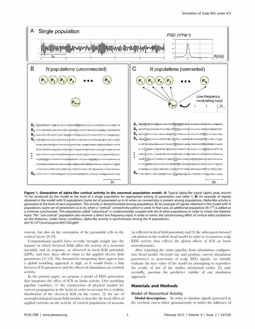
Figure 1. Generation of alpha-like cortical activity in the neuronal population model. A: Typical alpha-like signal (alpha peak around10 Hz) produced by the model at the level of a single population for appropriate setting of parameters (see table 1) B: An example of signalsobtained in the model with N populations (same set of parameters as in A) when no connectivity is present among populations. Alpha-like activity isgenerated at the level of each population. This activity is desynchronized among populations. C: An example of signals obtained in the model with Npopulations (same set of parameters as in A), when a ‘‘vertical’’ connectivity pattern is used. In that case, an additional population (N+1th) is added asa common synchronizer. This population called ‘‘subcortical’’ is unidirectionally coupled with the N other populations in order to mimic the thalamicinput. The ‘‘sub-cortical’’ population also receives a direct low frequency input in order to mimic the synchronizing effect of cortical delta oscillationson the thalamus. Under these conditions, alpha-like activity is synchronized among the N populations.doi:10.1371/journal.pone.0057330.g001

Simulation of Scalp EEG under tCS


an externally-applied electrical field, we used a physiologically-

plausible computational model recently developed in our team

[12]. The level of modeling we used is that of the neuronal

assembly. This model is composed of three subpopulations of cells

(principal pyramidal cells and two types of interneurons) which

interact via excitatory and inhibitory synaptic connections. The

model accounts for the main types of cells present in the cerebral

cortex, namely: i) Pyramidal cells which are identified as type P sub-

population in the model, ii) Axon-, soma- and proximal dendrite-

targeting cells (basket cells and chandelier cells) that mediate

GABAA,fast currents on type P cells and that are identified as type I

interneurons, and iii) Dendrite-targeting cells (bitufted, bipolar and

double bouquet cells) that mediate GABAA,slow currents on type P

cells and that are identified as type I9 interneurons. Interactions

between the three sub-populations are characterized by the

connectivity constants CPP, CPI , CIP, CPI ’, CI ’P, CII ’, and CI ’I

which account for the average number of synaptic contacts (or

‘‘connection strengths’’) between sub-populations. The temporal

dynamics of the model signal output directly compare with those

reflected in real signals (local field potentials or LFPs) recorded

with macro-electrodes located in the cerebral cortex.

Neuronal population models were originally developed to study

the mechanisms underlying the generation of alpha activity in the

cortex [13]. It is well-known that these models can easily reach an

oscillating behaviour after appropriate setting of i) connectivity

parameters and ii) rise and decay times of excitatory (glutamater-

gic) and inhibitory (GABAergic) average post-synaptic potentials

(PSPs). In particular, at the level of a single population, when these

parameters are properly adjusted, oscillations around 10 Hz

become prominent in the model signal output [14]. These

oscillations closely resemble real alpha activity (Figure 1A).

Model parameters used to simulate this alpha-like activity are

provided in Table 1. Besides parameters controlling the kinetics of

PSPs, the ratios between connectivity parameters (average number

of synaptic contacts between sub-populations) were set according

to physiology. In brief, the number of synaptic contacts among

pyramidal cells and from pyramidal cells to interneurons was set to

be greater than the number of synaptic contacts among

interneurons and from interneurons to pyramidal cells. Readers

may refer to appendix A of [15] for a literature review about the

cellular organization of cerebral cortex with special emphasis on

synaptic connections among pyramidal cells and interneurons.

As reported in [16,17], a number N of neuronal populations can

be coupled to model the activity over N interconnected brain

structures. We followed this approach to obtain a ‘‘realistic’’ (i.e.

relatively correlated) alpha-like activity over the entire neocortex

(see Section 1.4 for practical details). Indeed, in the absence of any

connectivity pattern, we could verify as expected that the N

populations of the model generate uncorrelated alpha activity

(Figure 1B) which is not compatible with real data. A way to

overcome this difficulty is to account for the influence of the

thalamic system which intervenes both in the generation and the

control of alpha/spindles observed in EEG signals [18,19]. It is

noteworthy that our intent was not to develop a complex thalamo-

cortical model but instead, to increase the ‘‘realism’’ of the

simulated alpha-like neocortical activity. To proceed, in the

model, we introduced an N+1th population, referred to as the

‘‘sub-cortical population’’, that was unidirectionally connected to

the N neocortical populations. Using this ‘‘vertical connectivity’’-

pattern, the model could include a common input (mimicking, to

some extent, the thalamic input) to neocortical populations. In

order to also account for the periodicity of alpha bursts, a direct

glutamatergic input was added to the sub-cortical population

(periodic trapezoid pulse, 2.5 s period, i.e. 0.4 Hz). Under these

conditions, we could qualitatively verify that the model generates

‘‘more realistic’’ alpha-like activity, as illustrated in Figure 1C.

Effect of tCS at neuronal population level. Neurons are

sensitive to externally-applied electric fields in a geometry-

dependent manner [10,20,21]. Their response depends on the

orientation of the electric field with respect to the somato-dendritic

axis on neuronal cells. More particularly, the field effects are

maximal when the field orientation is parallel to the cells’ main

axis. Conversely, field effects are null for orthogonal orientation.

In addition to the orientation, it has been shown that the direction

is also an essential factor. A field aligned with the orthodromic

direction (dendritic tuft to axon) would result in a positive

(depolarizing or excitatory) perturbation of the membrane

potential at the soma. Conversely, a field in the antidromic

direction would have a negative influence (hyperpolarizing or

inhibitory). In accordance with these considerations, the influence

of tCS was represented in the neuronal population model of as a

perturbation on the mean membrane potential. Two main

assumptions were made at this level. First, based on results

reported in [10], it can be reasonably hypothesized that this

perturbation is linear and direction-dependent within a certain

range of magnitude. Second, we recently showed that the electric

field induced by tCS has an impact on both pyramidal cells and

interneurons [12]. Nevertheless, for the purpose of this study and

in order to limit the number of free parameters, we neglected the

field effects on interneurons since the impact is lower compared

that on pyramidal cells [12].

Formally, we added a DC-offset voltage vtDCSX to the mean

membrane potential vX where X[fP,I ,I ’g. This DC-offset may

have either a depolarizing or a hyperpolarizing effect on the sub-

population of pyramidal cells, depending on its polarity. As a

consequence, the firing rate of the corresponding sub-population

described by the wave-to-pulse sigmoid function directly increases

or decreases accordingly. It is worth mentioning that this effect on

the firing rate is also consistent with results reported experimen-

tally [10], as the applied field also modifies the action potential

threshold.

Physical Model for Current PropagationIn order to map the spatial distribution of the electric field on

the cortical surface, we built a physical model for current

propagation using a three-step approach.

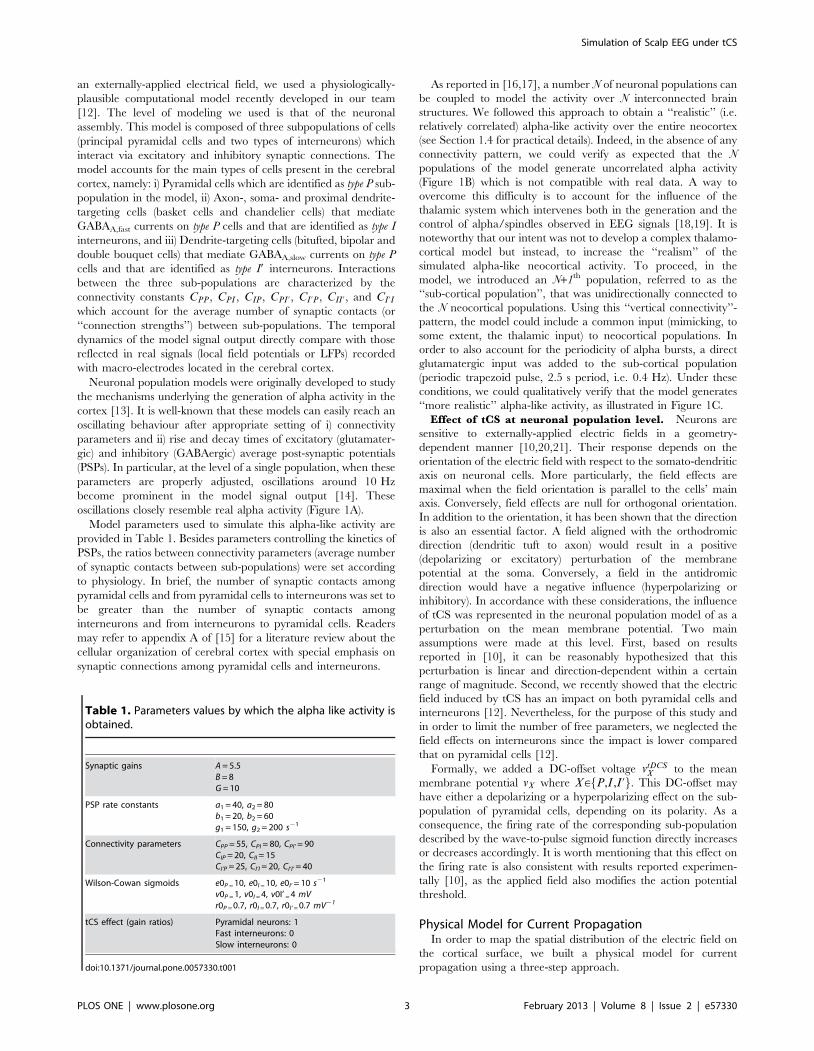
Table 1. Parameters values by which the alpha like activity isobtained.

Synaptic gains A = 5.5B = 8G = 10

PSP rate constants a1 = 40, a2 = 80b1 = 20, b2 = 60g1 = 150, g2 = 200 s21

Connectivity parameters CPP = 55, CPI = 80, CPI’ = 90CIP = 20, CII = 15CI’P = 25, CI’I = 20, CI’I’ = 40

Wilson-Cowan sigmoids e0P = 10, e0I = 10, e0I’ = 10 s21

v0P = 1, v0I = 4, v0I’ = 4 mVr0P = 0.7, r0I = 0.7, r0I’ = 0.7 mV21

tCS effect (gain ratios) Pyramidal neurons: 1Fast interneurons: 0Slow interneurons: 0

doi:10.1371/journal.pone.0057330.t001



First MR images were segmented. For this purpose we used T1

and Proton Density (PD) phantom images based on the Colin27

template (http://www.bic.mni.mcgill.ca/brainweb). Segmentation

was performed using the BrainSuite software (http://www.loni.

ucla.edu/Software/BrainSuite, [22–25]). White matter (WM),

gray matter (GM) and cerebrospinal fluid (CSF) were segmented

from the T1 images whereas the skull and scalp were obtained

from the PD images. The resulting masks were used to generate

surface meshes representing the boundaries between the different

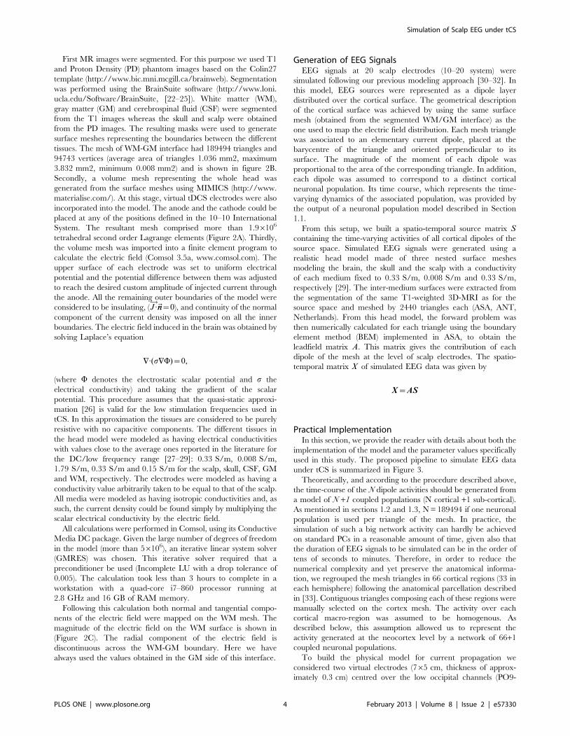
tissues. The mesh of WM-GM interface had 189494 triangles and

94743 vertices (average area of triangles 1.036 mm2, maximum

3.832 mm2, minimum 0.008 mm2) and is shown in figure 2B.

Secondly, a volume mesh representing the whole head was

generated from the surface meshes using MIMICS (http://www.

materialise.com/). At this stage, virtual tDCS electrodes were also

incorporated into the model. The anode and the cathode could be

placed at any of the positions defined in the 10–10 International

System. The resultant mesh comprised more than 1.96106

tetrahedral second order Lagrange elements (Figure 2A). Thirdly,

the volume mesh was imported into a finite element program to

calculate the electric field (Comsol 3.5a, www.comsol.com). The

upper surface of each electrode was set to uniform electrical

potential and the potential difference between them was adjusted

to reach the desired custom amplitude of injected current through

the anode. All the remaining outer boundaries of the model were

considered to be insulating, (J:!~nn~0), and continuity of the normal

component of the current density was imposed on all the inner

boundaries. The electric field induced in the brain was obtained by

solving Laplace’s equation

+:(s+W)~0,

(where W denotes the electrostatic scalar potential and s the

electrical conductivity) and taking the gradient of the scalar

potential. This procedure assumes that the quasi-static approxi-

mation [26] is valid for the low stimulation frequencies used in

tCS. In this approximation the tissues are considered to be purely

resistive with no capacitive components. The different tissues in

the head model were modeled as having electrical conductivities

with values close to the average ones reported in the literature for

the DC/low frequency range [27–29]: 0.33 S/m, 0.008 S/m,

1.79 S/m, 0.33 S/m and 0.15 S/m for the scalp, skull, CSF, GM

and WM, respectively. The electrodes were modeled as having a

conductivity value arbitrarily taken to be equal to that of the scalp.

All media were modeled as having isotropic conductivities and, as

such, the current density could be found simply by multiplying the

scalar electrical conductivity by the electric field.

All calculations were performed in Comsol, using its Conductive

Media DC package. Given the large number of degrees of freedom

in the model (more than 56106), an iterative linear system solver

(GMRES) was chosen. This iterative solver required that a

preconditioner be used (Incomplete LU with a drop tolerance of

0.005). The calculation took less than 3 hours to complete in a

workstation with a quad-core i7–860 processor running at

2.8 GHz and 16 GB of RAM memory.

Following this calculation both normal and tangential compo-

nents of the electric field were mapped on the WM mesh. The

magnitude of the electric field on the WM surface is shown in

(Figure 2C). The radial component of the electric field is

discontinuous across the WM-GM boundary. Here we have

always used the values obtained in the GM side of this interface.

Generation of EEG SignalsEEG signals at 20 scalp electrodes (10–20 system) were

simulated following our previous modeling approach [30–32]. In

this model, EEG sources were represented as a dipole layer

distributed over the cortical surface. The geometrical description

of the cortical surface was achieved by using the same surface

mesh (obtained from the segmented WM/GM interface) as the

one used to map the electric field distribution. Each mesh triangle

was associated to an elementary current dipole, placed at the

barycentre of the triangle and oriented perpendicular to its

surface. The magnitude of the moment of each dipole was

proportional to the area of the corresponding triangle. In addition,

each dipole was assumed to correspond to a distinct cortical

neuronal population. Its time course, which represents the time-

varying dynamics of the associated population, was provided by

the output of a neuronal population model described in Section

1.1.

From this setup, we built a spatio-temporal source matrix Scontaining the time-varying activities of all cortical dipoles of the

source space. Simulated EEG signals were generated using a

realistic head model made of three nested surface meshes

modeling the brain, the skull and the scalp with a conductivity

of each medium fixed to 0.33 S/m, 0.008 S/m and 0.33 S/m,

respectively [29]. The inter-medium surfaces were extracted from

the segmentation of the same T1-weighted 3D-MRI as for the

source space and meshed by 2440 triangles each (ASA, ANT,

Netherlands). From this head model, the forward problem was

then numerically calculated for each triangle using the boundary

element method (BEM) implemented in ASA, to obtain the

leadfield matrix A. This matrix gives the contribution of each

dipole of the mesh at the level of scalp electrodes. The spatio-

temporal matrix X of simulated EEG data was given by

X~AS

Practical ImplementationIn this section, we provide the reader with details about both the

implementation of the model and the parameter values specifically

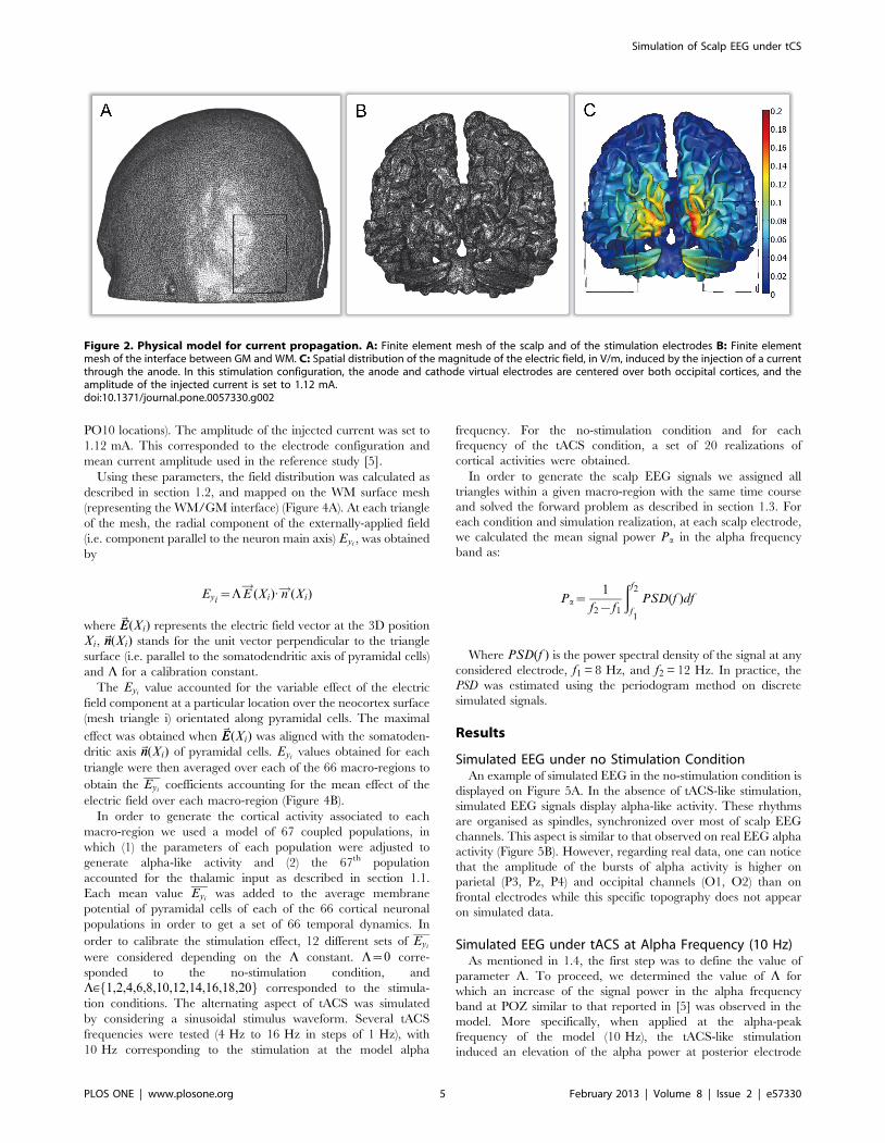
used in this study. The proposed pipeline to simulate EEG data

under tCS is summarized in Figure 3.

Theoretically, and according to the procedure described above,

the time-course of the N dipole activities should be generated from

a model of N +1 coupled populations (N cortical +1 sub-cortical).

As mentioned in sections 1.2 and 1.3, N = 189494 if one neuronal

population is used per triangle of the mesh. In practice, the

simulation of such a big network activity can hardly be achieved

on standard PCs in a reasonable amount of time, given also that

the duration of EEG signals to be simulated can be in the order of

tens of seconds to minutes. Therefore, in order to reduce the

numerical complexity and yet preserve the anatomical informa-

tion, we regrouped the mesh triangles in 66 cortical regions (33 in

each hemisphere) following the anatomical parcellation described

in [33]. Contiguous triangles composing each of these regions were

manually selected on the cortex mesh. The activity over each

cortical macro-region was assumed to be homogenous. As

described below, this assumption allowed us to represent the

activity generated at the neocortex level by a network of 66+1

coupled neuronal populations.

To build the physical model for current propagation we

considered two virtual electrodes (765 cm, thickness of approx-

imately 0.3 cm) centred over the low occipital channels (PO9-



PO10 locations). The amplitude of the injected current was set to

1.12 mA. This corresponded to the electrode configuration and

mean current amplitude used in the reference study [5].

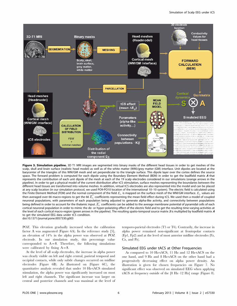
Using these parameters, the field distribution was calculated as

described in section 1.2, and mapped on the WM surface mesh

(representing the WM/GM interface) (Figure 4A). At each triangle

of the mesh, the radial component of the externally-applied field

(i.e. component parallel to the neuron main axis) Eyi, was obtained

by

Eyi~LE!

(Xi): n!(Xi)

where ~EE(Xi) represents the electric field vector at the 3D position

Xi, ~nn(Xi) stands for the unit vector perpendicular to the triangle

surface (i.e. parallel to the somatodendritic axis of pyramidal cells)

and L for a calibration constant.

The Eyivalue accounted for the variable effect of the electric

field component at a particular location over the neocortex surface

(mesh triangle i) orientated along pyramidal cells. The maximal

effect was obtained when ~EE(Xi) was aligned with the somatoden-

dritic axis ~nn(Xi) of pyramidal cells. Eyivalues obtained for each

triangle were then averaged over each of the 66 macro-regions to

obtain the Eyicoefficients accounting for the mean effect of the

electric field over each macro-region (Figure 4B).

In order to generate the cortical activity associated to each

macro-region we used a model of 67 coupled populations, in

which (1) the parameters of each population were adjusted to

generate alpha-like activity and (2) the 67th population

accounted for the thalamic input as described in section 1.1.

Each mean value Eyiwas added to the average membrane

potential of pyramidal cells of each of the 66 cortical neuronal

populations in order to get a set of 66 temporal dynamics. In

order to calibrate the stimulation effect, 12 different sets of Eyi

were considered depending on the L constant. L~0 corre-

sponded to the no-stimulation condition, and

L[f1,2,4,6,8,10,12,14,16,18,20g corresponded to the stimula-

tion conditions. The alternating aspect of tACS was simulated

by considering a sinusoidal stimulus waveform. Several tACS

frequencies were tested (4 Hz to 16 Hz in steps of 1 Hz), with

10 Hz corresponding to the stimulation at the model alpha

frequency. For the no-stimulation condition and for each

frequency of the tACS condition, a set of 20 realizations of

cortical activities were obtained.

In order to generate the scalp EEG signals we assigned all

triangles within a given macro-region with the same time course

and solved the forward problem as described in section 1.3. For

each condition and simulation realization, at each scalp electrode,

we calculated the mean signal power Pa in the alpha frequency

band as:

Pa~1

f2{f1

ðf2

f1

PSD(f )df

Where PSD(f ) is the power spectral density of the signal at any

considered electrode, f1 = 8 Hz, and f2 = 12 Hz. In practice, the

PSD was estimated using the periodogram method on discrete

simulated signals.

Results

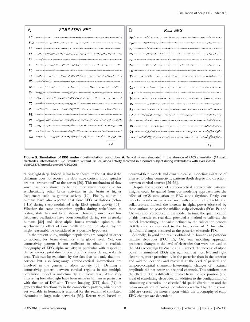
Simulated EEG under no Stimulation ConditionAn example of simulated EEG in the no-stimulation condition is

displayed on Figure 5A. In the absence of tACS-like stimulation,

simulated EEG signals display alpha-like activity. These rhythms

are organised as spindles, synchronized over most of scalp EEG

channels. This aspect is similar to that observed on real EEG alpha

activity (Figure 5B). However, regarding real data, one can notice

that the amplitude of the bursts of alpha activity is higher on

parietal (P3, Pz, P4) and occipital channels (O1, O2) than on

frontal electrodes while this specific topography does not appear

on simulated data.

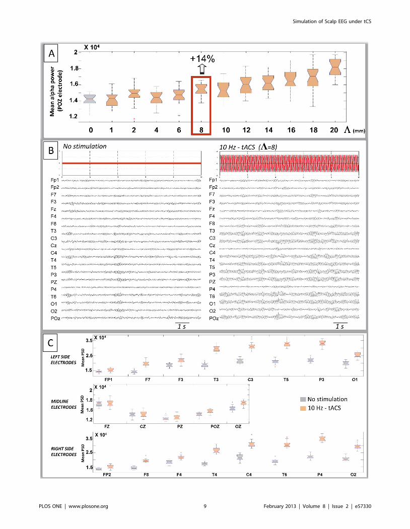
Simulated EEG under tACS at Alpha Frequency (10 Hz)As mentioned in 1.4, the first step was to define the value of

parameter L. To proceed, we determined the value of L for

which an increase of the signal power in the alpha frequency

band at POZ similar to that reported in [5] was observed in the

model. More specifically, when applied at the alpha-peak

frequency of the model (10 Hz), the tACS-like stimulation

induced an elevation of the alpha power at posterior electrode

Figure 2. Physical model for current propagation. A: Finite element mesh of the scalp and of the stimulation electrodes B: Finite elementmesh of the interface between GM and WM. C: Spatial distribution of the magnitude of the electric field, in V/m, induced by the injection of a currentthrough the anode. In this stimulation configuration, the anode and cathode virtual electrodes are centered over both occipital cortices, and theamplitude of the injected current is set to 1.12 mA.doi:10.1371/journal.pone.0057330.g002



POZ. This elevation gradually increased when the calibration

factor L was augmented (Figure 6A). In the reference study [5],

an elevation of 14% in the alpha power was observed at POZ

electrode. In our simulation study, this percentage value

corresponded to L~8. Therefore, the following simulations

were calibrated by fixing L~8.

At the level of all scalp electrodes, the increase in alpha power

was clearly visible on left and right central, parietal temporal and

occipital contacts, while only subtle changes occurred on midline

electrodes (Figure 6B). As illustrated on (Figure 6C), the

quantitative analysis revealed that under 10 Hz-tACS simulated

stimulation, the alpha power was significantly increased on most

left and right channels. The significant increase was larger on

central and posterior channels and was maximal at the level of

temporo-parietal electrodes (T5 or T6). Contrarily, the increase in

alpha power remained non-significant at frontopolar contacts

(Fp1, Fp2) and at the level of most anterior midline electrodes (Fz,

Cz, and Pz).

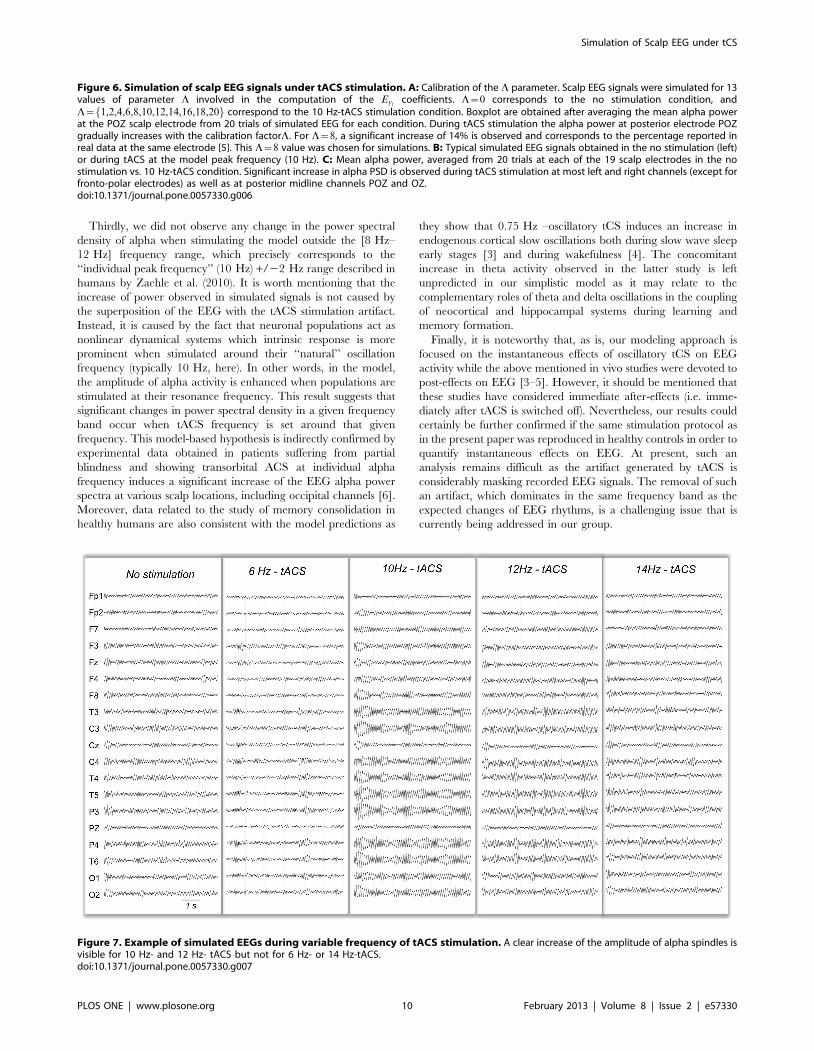
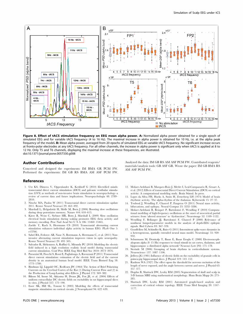
Simulated EEG under tACS at Other FrequenciesAs compared to 10 Hz-tACS, 11 Hz and 12 Hz-tACS on the

one hand, and 9 Hz and 8 Hz-tACS on the other hand had a

progressively decreasing effect on alpha power density. An

illustration is given for chosen frequencies on Figure 7. No

significant effect was observed on simulated EEG when applying

tACS at frequency outside of the [8 Hz–12 Hz] range (Figure 8).

Figure 3. Simulation pipeline. 3D T1 MRI images are segmented into binary masks of the different head tissues in order to get meshes of thescalp, skull and brain surface (realistic head model) as well as of the white matter (WM)/grey matter (GM) interface. Unit dipoles are located at thebarycenter of the triangles of this WM/GM mesh and set perpendicular to the triangle surface. This dipole layer over the cortex defines the sourcespace. The forward problem is computed for each dipole using the Boundary Element Method (BEM) in order to get the leadfield matrix A thatrepresents the contribution of each unit dipole of the mesh at each of the 19 scalp electrodes considered in our simulations (orange arrows in thepipeline). In order to get a physical model of the current distribution after tCS stimulation, surface meshes representing the boundaries between thedifferent head tissues are transformed into volume meshes. In addition, virtual tCS electrodes are also represented into the model and can be placedat any scalp location (in our simulation protocol, we used PO9-PO10 location of the international 10–10 system). The electric field is calculated usingthe Finite Element Method (FEM) and the normal component of the field Eyi

is mapped on the surface mesh of the WM/GM interface. Eyivalues are

then averaged over 66 macro-regions to get the 66 Eyicoefficients representing the mean field effect during tCS. We used then a model of coupled

neuronal populations, with parameters of each population being adjusted to generate alpha-like activity, and connectivity between populations

being defined in order to account for the thalamic input. Eyicoefficients can be added to the average membrane potential of pyramidal cells of each

cortical neuronal population in order to mimic the de- or hyper-polarizing effect of the electric field and to get the resulting time-varying activities atthe level of each cortical macro-region (green arrows in the pipeline). The resulting spatio-temporal source matrix S is multiplied by leadfield matrix Ato get the simulated EEG data under tCS condition.doi:10.1371/journal.pone.0057330.g003



Discussion

The past years have witnessed significant advances in the use of

tCS as a non-invasive tool for interacting with brain activity, not

only in various brain disorders [34–38] but also during cognitive

function [1,39]. Among the many techniques that can be used to

assess and quantify tCS effects, electroencephalography still

occupies a central position, due to its excellent temporal

resolution, reasonably good spatial resolution and relative ease of

use. However, the interpretation of changes observed in EEG

signals obtained under stimulation conditions is a challenging

issue. In this study, a general modeling framework is put forward

to progress in this interpretation. A complete pipeline is proposed

to allow for the simulation of EEG signals based on i) a realistic

description of the volume conductor features, ii) an accurate

representation of the distribution of the electric field inside this

volume conductor and iii) a model of the field effects on neuronal

assemblies in the neocortex. To the best of our knowledge, the use

of such a pipeline has not previously been proposed.

In order to evaluate the approach, we chose to start from a

recent study conducted in humans that examined the effects of

tACS on the alpha EEG activity [5]. This choice was motivated by

both the low number of studies reporting quantified EEG changes

in response to tACS and the relative ease with which oscillations in

the alpha frequency band can be simulated with neural mass

models. Using a physiologically-plausible neural mass model of

coupled neocortical populations recently proposed by our team

[12], we generated realistic signals of both cortical and related

scalp EEG alpha activity. These signals were obtained using a very

simple description of the interaction between neocortical macro-

regions and a subcortical structure whose activity is simply

described by a neuronal population model. Since the 709s, this

type of model has been widely used to reproduce physiological or

pathological rhythms at the level of a single neuronal assembly

[13,40–42] or in a small networks of coupled assemblies [16,43–

46]. For simplicity reasons, we implemented an unsophisticated

model for the thalamo-cortical interaction, as compared to those

already available from the literature [47–49]. Indeed, we just used

an extra neuronal population to provide common excitatory input

to those accounting for neocortical activity. This helped

pacemaking synchronized alpha oscillations over multiple cortical

regions. Then, for the periodicity of alpha bursts, this sub-cortical

population received itself a periodic excitatory input (periodic

trapezoid ‘‘ramp up’’, constant and ‘‘ramp down’’ function). One

rationalization for this slow periodic excitatory input comes from

findings that have emerged from the study of spindle oscillations

Figure 4. Spatial distribution of the externally-applied electric field and subsequent field effects. A: Spatial distribution of themagnitude of the electric field using two virtual electrodes over the occipital regions and after applying a 1.12 mA current through the anode. Theamplitude of the electric field is mapped on a mesh of the WM/GM interface. B: Mean field effect. The effect of the electric field depending on theorientation of pyramidal cells within the neocortex, is accounted for by calculating the radial component of the applied field Eyi

(scalar productbetween the electric field and the unit vector parallel to the pyramidal cell main axis) at each triangle of the mesh of the WM/GM interface. Eyi

values

obtained for each triangle are then averaged over each of the 66 anatomical macro-regions manually outlined according to [35]. The resulting Eyi

coefficients represent the mean effect of the electric field over each macro-region.doi:10.1371/journal.pone.0057330.g004



during light sleep. Indeed, is has been shown, in the cat, that if the

thalamus does not receive the slow wave cortical input, spindles

are not ‘‘transmitted’’ to the cortex [50]. This mechanism of slow

wave has been shown to be the mechanism responsible for

synchronizing other brain activities in the brain at higher

frequencies such as gamma activity [19]. Finally, studies in

humans have also reported that slow EEG oscillations (below

1 Hz) during sleep modulated scalp EEG spindle activity [51].

Whether the same mechanism applies during wakefulness at

resting state has not been shown. However, since very low

frequency oscillations have been identified during rest in awake

humans [52] and since alpha bursts resemble spindles, the

synchronizing effect of slow oscillations on the alpha rhythm

might reasonably be considered as a possible hypothesis.

In the present study, multiple populations are coupled in order

to account for brain dynamics at a global level. Yet, our

connectivity pattern is not sufficient to obtain a realistic

topography of EEG alpha activity; in particular with respect to

the parieto-occipital distribution of alpha waves during wakeful-

ness. This can be explained by the fact that not only thalomo-

cortical but also long-range cortico-cortical interactions are

involved in the genesis of alpha activity [53]. Defining a

connectivity pattern between cortical regions in our multiple

population model is unfortunately a difficult task. While very

interesting breakthroughs have been made in humans in particular

with the use of Diffusion Tensor Imaging (DTI) data [54], it

appears that directionality in the connectivity pattern, which is not

yet available in humans, is essential for the realism of simulated

dynamics in large-scale networks [55]. Recent work based on

neuronal field models and dynamic causal modeling might be of

interest to define connectivity patterns (both degree and direction)

between cortical sources [56–58].

Despite the absence of cortico-cortical connectivity patterns,

insights could be gained from our modeling approach into the

effect of tACS stimulation on EEG alpha rhythms. Firstly, our

modeled results are in accordance with the study by Zaehle and

collaborators. Indeed, the increase in alpha power observed by

these authors on posterior midline scalp electrodes (POz, Pz and

Oz) was also reproduced in the model. In turn, the quantification

of this increase on real data provided a method to calibrate the

model. Interestingly, the value defined by the calibration process

(L= 8) also corresponded to the first value of L for which

significant changes occurred at the posterior electrode POz.

Secondly, beyond the results obtained in humans at posterior

midline electrodes (POz, Pz, Oz), our modeling approach

predicted changes at the level of electrodes that were not used in

the EEG recordings by Zaehle et al. Indeed, the increase of alpha

power in simulated EEGs was significant at most left and right

electrodes, more prominently in the posterior than in the anterior

and midline locations and maximal at the level of parietal and

temporo-occipital channels. Interestingly, changes of maximal

amplitude did not occur on occipital channels. This confirms that

the effect of tCS is difficult to predict from the sole position (and

area) of stimulating electrodes. In addition to the configuration of

stimulating electrodes, the electric field spatial distribution and the

mean orientation of cortical populations reached by the maximal

field are crucial parameters upon which the topography of scalp

EEG changes are dependent.

Figure 5. Simulation of EEG under no-stimulation condition. A: Typical signals simulated in the absence of tACS stimulation (19 scalpelectrodes, international 10–20 standard system). B: Real alpha activity recorded in a normal subject during wakefulness with eyes closed.doi:10.1371/journal.pone.0057330.g005



Thirdly, we did not observe any change in the power spectral

density of alpha when stimulating the model outside the [8 Hz–

12 Hz] frequency range, which precisely corresponds to the

‘‘individual peak frequency’’ (10 Hz) +/22 Hz range described in

humans by Zaehle et al. (2010). It is worth mentioning that the

increase of power observed in simulated signals is not caused by

the superposition of the EEG with the tACS stimulation artifact.

Instead, it is caused by the fact that neuronal populations act as

nonlinear dynamical systems which intrinsic response is more

prominent when stimulated around their ‘‘natural’’ oscillation

frequency (typically 10 Hz, here). In other words, in the model,

the amplitude of alpha activity is enhanced when populations are

stimulated at their resonance frequency. This result suggests that

significant changes in power spectral density in a given frequency

band occur when tACS frequency is set around that given

frequency. This model-based hypothesis is indirectly confirmed by

experimental data obtained in patients suffering from partial

blindness and showing transorbital ACS at individual alpha

frequency induces a significant increase of the EEG alpha power

spectra at various scalp locations, including occipital channels [6].

Moreover, data related to the study of memory consolidation in

healthy humans are also consistent with the model predictions as

they show that 0.75 Hz –oscillatory tCS induces an increase in

endogenous cortical slow oscillations both during slow wave sleep

early stages [3] and during wakefulness [4]. The concomitant

increase in theta activity observed in the latter study is left

unpredicted in our simplistic model as it may relate to the

complementary roles of theta and delta oscillations in the coupling

of neocortical and hippocampal systems during learning and

memory formation.

Finally, it is noteworthy that, as is, our modeling approach is

focused on the instantaneous effects of oscillatory tCS on EEG

activity while the above mentioned in vivo studies were devoted to

post-effects on EEG [3–5]. However, it should be mentioned that

these studies have considered immediate after-effects (i.e. imme-

diately after tACS is switched off). Nevertheless, our results could

certainly be further confirmed if the same stimulation protocol as

in the present paper was reproduced in healthy controls in order to

quantify instantaneous effects on EEG. At present, such an

analysis remains difficult as the artifact generated by tACS is

considerably masking recorded EEG signals. The removal of such

an artifact, which dominates in the same frequency band as the

expected changes of EEG rhythms, is a challenging issue that is

currently being addressed in our group.

Figure 6. Simulation of scalp EEG signals under tACS stimulation. A: Calibration of the L parameter. Scalp EEG signals were simulated for 13values of parameter L involved in the computation of the Eyi

coefficients. L~0 corresponds to the no stimulation condition, andL~f1,2,4,6,8,10,12,14,16,18,20g correspond to the 10 Hz-tACS stimulation condition. Boxplot are obtained after averaging the mean alpha powerat the POZ scalp electrode from 20 trials of simulated EEG for each condition. During tACS stimulation the alpha power at posterior electrode POZgradually increases with the calibration factorL. For L~8, a significant increase of 14% is observed and corresponds to the percentage reported inreal data at the same electrode [5]. This L~8 value was chosen for simulations. B: Typical simulated EEG signals obtained in the no stimulation (left)or during tACS at the model peak frequency (10 Hz). C: Mean alpha power, averaged from 20 trials at each of the 19 scalp electrodes in the nostimulation vs. 10 Hz-tACS condition. Significant increase in alpha PSD is observed during tACS stimulation at most left and right channels (except forfronto-polar electrodes) as well as at posterior midline channels POZ and OZ.doi:10.1371/journal.pone.0057330.g006

Figure 7. Example of simulated EEGs during variable frequency of tACS stimulation. A clear increase of the amplitude of alpha spindles isvisible for 10 Hz- and 12 Hz- tACS but not for 6 Hz- or 14 Hz-tACS.doi:10.1371/journal.pone.0057330.g007



Author Contributions

Conceived and designed the experiments: IM BMA GR PCM FW.

Performed the experiments: IM GB RS BMA AM ASF PCM FW.

Analyzed the data: IM GB RS AM ASF PCM FW. Contributed reagents/

materials/analysis tools: GB ASF GR. Wrote the paper: IM GB BMA RS

AM ASF PCM FW.

References

1. Utz KS, Dimova V, Oppenlander K, Kerkhoff G (2010) Electrified minds:

transcranial direct current stimulation (tDCS) and galvanic vestibular stimula-tion (GVS) as methods of non-invasive brain stimulation in neuropsychology–a

review of current data and future implications. Neuropsychologia 48: 2789–2810.

2. Nitsche MA, Paulus W (2011) Transcranial direct current stimulation–update

2011. Restor Neurol Neurosci 29: 463–492.

3. Marshall L, Helgadottir H, Molle M, Born J (2006) Boosting slow oscillationsduring sleep potentiates memory. Nature 444: 610–613.

4. Kirov R, Weiss C, Siebner HR, Born J, Marshall L (2009) Slow oscillationelectrical brain stimulation during waking promotes EEG theta activity and

memory encoding. Proc Natl Acad Sci U S A 106: 15460–15465.

5. Zaehle T, Rach S, Herrmann CS (2010) Transcranial alternating currentstimulation enhances individual alpha activity in human EEG. PLoS One 5:

e13766.

6. Sabel BA, Fedorov AB, Naue N, Borrmann A, Herrmann C, et al. (2011) Non-invasive alternating current stimulation improves vision in optic neuropathy.

Restor Neurol Neurosci 29: 493–505.

7. Salvador R, Mekonnen A, Ruffini G, Miranda PC (2010) Modeling the electricfield induced in a high resolution realistic head model during transcranial

current stimulation. Conf Proc IEEE Eng Med Biol Soc 2010: 2073–2076.

8. Parazzini M, Fiocchi S, Rossi E, Paglialonga A, Ravazzani P (2011) Transcranialdirect current stimulation: estimation of the electric field and of the current

density in an anatomical human head model. IEEE Trans Biomed Eng 58:1773–1780.

9. Bindman LJ, Lippold OC, Redfearn JW (1964) The Action of Brief Polarizing

Currents on the Cerebral Cortex of the Rat (1) During Current Flow and (2) inthe Production of Long-Lasting after-Effects. J Physiol 172: 369–382.

10. Bikson M, Inoue M, Akiyama H, Deans JK, Fox JE, et al. (2004) Effects of

uniform extracellular DC electric fields on excitability in rat hippocampal slicesin vitro. J Physiol 557: 175–190.

11. Esser SK, Hill SL, Tononi G (2005) Modeling the effects of transcranial

magnetic stimulation on cortical circuits. J Neurophysiol 94: 622–639.

12. Molaee-Ardekani B, Marquez-Ruiz J, Merlet I, Leal-Campanario R, Gruart A,

et al. (2012) Effects of transcranial Direct Current Stimulation (tDCS) on cortical

activity: A computational modeling study. Brain Stimul. In press.

13. Lopes da Silva FH, Hoeks A, Smits H, Zetterberg LH (1974) Model of brain

rhythmic activity. The alpha-rhythm of the thalamus. Kybernetik 15: 27–37.

14. Touboul J, Wendling F, Chauvel P, Faugeras O (2011) Neural mass activity,

bifurcations, and epilepsy. Neural Comput 23: 3232–3286.

15. Molaee-Ardekani B, Benquet P, Bartolomei F, Wendling F (2010) Computa-

tional modeling of high-frequency oscillations at the onset of neocortical partial

seizures: from ‘altered structure’ to ‘dysfunction’. Neuroimage 52: 1109–1122.

16. Wendling F, Bellanger JJ, Bartolomei F, Chauvel P (2000) Relevance of

nonlinear lumped-parameter models in the analysis of depth-EEG epileptic

signals. Biol Cybern 83: 367–378.

17. Goodfellow M, Schindler K, Baier G (2011) Intermittent spike-wave dynamics in

a heterogeneous, spatially extended neural mass model. Neuroimage 55: 920–

932.

18. Schurmann M, Demiralp T, Basar E, Basar Eroglu C (2000) Electroenceph-

alogram alpha (8–15 Hz) responses to visual stimuli in cat cortex, thalamus, and

hippocampus: a distributed alpha network? Neurosci Lett 292: 175–178.

19. Steriade M (2006) Grouping of brain rhythms in corticothalamic systems.

Neuroscience 137: 1087–1106.

20. Jefferys JG (1981) Influence of electric fields on the excitability of granule cells in

guinea-pig hippocampal slices. J Physiol 319: 143–152.

21. Rushton WA (1927) The effect upon the threshold for nervous excitation of the

length of nerve exposed, and the angle between current and nerve. J Physiol 63:

357–377.

22. Dogdas B, Shattuck DW, Leahy RM (2005) Segmentation of skull and scalp in

3-D human MRI using mathematical morphology. Hum Brain Mapp 26: 273–

285.

23. Shattuck DW, Leahy RM (2001) Automated graph-based analysis and

correction of cortical volume topology. IEEE Trans Med Imaging 20: 1167–

1177.

Figure 8. Effect of tACS stimulation frequency on EEG mean alpha power. A: Normalized alpha power obtained for a single epoch ofsimulated EEG and for variable tACS frequency (4 to 16 Hz). The maximal increase in alpha power is obtained for 10 Hz, i.e. at the alpha peakfrequency of the model. B: Mean alpha power, averaged from 20 epochs of simulated EEG at variable tACS frequency. No significant increase occursat fronto-polar electrodes at any tACS frequency. For all other channels, the increase in alpha power is significant only when tACS is applied at 8 to12 Hz. Only T5 and T6 channels, displaying the maximal increase at these frequencies, are illustrated.doi:10.1371/journal.pone.0057330.g008



24. Shattuck DW, Leahy RM (2002) BrainSuite: an automated cortical surface

identification tool. Med Image Anal 6: 129–142.25. Shattuck DW, Sandor-Leahy SR, Schaper KA, Rottenberg DA, Leahy RM

(2001) Magnetic resonance image tissue classification using a partial volume

model. Neuroimage 13: 856–876.26. Plonsey R, Heppner DB (1967) Considerations of quasi-stationarity in

electrophysiological systems. Bull Math Biophys 29: 657–664.27. Nicholson PW (1965) Specific impedance of cerebral white matter. Exp Neurol

13: 386–401.

28. Baumann SB, Wozny DR, Kelly SK, Meno FM (1997) The electricalconductivity of human cerebrospinal fluid at body temperature. IEEE Trans

Biomed Eng 44: 220–223.29. Goncalves SI, de Munck JC, Verbunt JP, Bijma F, Heethaar RM, et al. (2003) In

vivo measurement of the brain and skull resistivities using an EIT-based methodand realistic models for the head. IEEE Trans Biomed Eng 50: 754–767.

30. Cosandier-Rimele D, Badier JM, Chauvel P, Wendling F (2007) A physiolog-

ically plausible spatio-temporal model for EEG signals recorded withintracerebral electrodes in human partial epilepsy. IEEE Trans Biomed Eng

54: 380–388.31. Cosandier-Rimele D, Merlet I, Badier JM, Chauvel P, Wendling F (2008) The

neuronal sources of EEG: modeling of simultaneous scalp and intracerebral

recordings in epilepsy. Neuroimage 42: 135–146.32. Cosandier-Rimele D, Merlet I, Bartolomei F, Badier JM, Wendling F (2010)

Computational modeling of epileptic activity: from cortical sources to EEGsignals. J Clin Neurophysiol 27: 465–470.

33. Desikan RS, Segonne F, Fischl B, Quinn BT, Dickerson BC, et al. (2006) Anautomated labeling system for subdividing the human cerebral cortex on MRI

scans into gyral based regions of interest. Neuroimage 31: 968–980.

34. Boggio PS, Ferrucci R, Rigonatti SP, Covre P, Nitsche M, et al. (2006) Effects oftranscranial direct current stimulation on working memory in patients with

Parkinson’s disease. J Neurol Sci 249: 31–38.35. Fregni F, Boggio PS, Nitsche MA, Rigonatti SP, Pascual-Leone A (2006)

Cognitive effects of repeated sessions of transcranial direct current stimulation in

patients with depression. Depress Anxiety 23: 482–484.36. Fregni F, Thome-Souza S, Nitsche MA, Freedman SD, Valente KD, et al.

(2006) A controlled clinical trial of cathodal DC polarization in patients withrefractory epilepsy. Epilepsia 47: 335–342.

37. Nitsche MA, Cohen LG, Wassermann EM, Priori A, Lang N, et al. (2008)Transcranial direct current stimulation: State of the art 2008. Brain Stim 1: 206–

223.

38. Fregni F, Boggio PS, Lima MC, Ferreira MJ, Wagner T, et al. (2006) A sham-controlled, phase II trial of transcranial direct current stimulation for the

treatment of central pain in traumatic spinal cord injury. Pain 122: 197–209.39. Reis J, Robertson EM, Krakauer JW, Rothwell J, Marshall L, et al. (2008)

Consensus: Can transcranial direct current stimulation and transcranial

magnetic stimulation enhance motor learning and memory formation? BrainStimul 1: 363–369.

40. Wilson HR, Cowan JD (1972) Excitatory and inhibitory interactions in localizedpopulations of model neurons. Biophys J 12: 1–24.

41. Freeman WJ (1978) Models of the dynamics of neural populations. Electro-

encephalogr Clin Neurophysiol Suppl: 9–18.

42. Kim JW, Robinson PA (2007) Compact dynamical model of brain activity. Phys

Rev E Stat Nonlin Soft Matter Phys 75: 031907.

43. David O, Friston KJ (2003) A neural mass model for MEG/EEG: coupling and

neuronal dynamics. Neuroimage 20: 1743–1755.

44. Jansen BH, Rit VG (1995) Electroencephalogram and visual evoked potential

generation in a mathematical model of coupled cortical columns. Biol Cybern

73: 357–366.

45. Freeman WJ (1987) Simulation of chaotic EEG patterns with a dynamic model

of the olfactory system. Biol Cybern 56: 139–150.

46. Robinson PA (2005) Propagator theory of brain dynamics. Phys Rev E Stat

Nonlin Soft Matter Phys 72: 011904.

47. Suffczynski P, Kalitzin S, Pfurtscheller G, Lopes da Silva FH (2001)

Computational model of thalamo-cortical networks: dynamical control of alpha

rhythms in relation to focal attention. Int J Psychophysiol 43: 25–40.

48. Breakspear M, Roberts JA, Terry JR, Rodrigues S, Mahant N, et al. (2006) A

unifying explanation of primary generalized seizures through nonlinear brain

modeling and bifurcation analysis. Cereb Cortex 16: 1296–1313.

49. Roberts JA, Robinson PA (2008) Modeling absence seizure dynamics:

implications for basic mechanisms and measurement of thalamocortical and

corticothalamic latencies. J Theor Biol 253: 189–201.

50. Contreras D, Destexhe A, Sejnowski TJ, Steriade M (1996) Control of

spatiotemporal coherence of a thalamic oscillation by corticothalamic feedback.

Science 274: 771–774.

51. Fell J, Elfadil H, Roschke J, Burr W, Klaver P, et al. (2002) Human scalp

recorded sigma activity is modulated by slow EEG oscillations during deep sleep.

Int J Neurosci 112: 893–900.

52. Demanuele C, Broyd SJ, Sonuga-Barke EJ, James C (2012) Neuronal oscillations

in the EEG under varying cognitive load: A comparative study between slow

waves and faster oscillations. Clin Neurophysiol 124(2): 247–262.

53. Steriade M, Gloor P, Llinas RR, Lopes de Silva FH, Mesulam MM (1990)

Report of IFCN Committee on Basic Mechanisms. Basic mechanisms of

cerebral rhythmic activities. Electroencephalogr clin Neurophysiol 76: 481–508.

54. Hagmann P, Cammoun L, Gigandet X, Meuli R, Honey CJ, et al. (2008)

Mapping the structural core of human cerebral cortex. PLoS Biol 6: e159.

55. Knock SA, McIntosh AR, Sporns O, Kotter R, Hagmann P, et al. (2009) The

effects of physiologically plausible connectivity structure on local and global

dynamics in large scale brain models. J Neurosci Methods 183: 86–94.

56. Chen CC, Henson RN, Stephan KE, Kilner JM, Friston KJ (2009) Forward and

backward connections in the brain: a DCM study of functional asymmetries.

Neuroimage 45: 453–462.

57. Pinotsis DA, Schwarzkopf DS, Litvak V, Rees G, Barnes G, et al. (2012)

Dynamic causal modelling of lateral interactions in the visual cortex. Neuro-

image 66C: 563–576.

58. Pinotsis DA, Moran RJ, Friston KJ (2012) Dynamic causal modeling with neural

fields. Neuroimage 59: 1261–1274.



From oscillatory transcranial current stimulation to scalp EEG changes: a biophysical and...

Documents

Transcript of From oscillatory transcranial current stimulation to scalp EEG changes: a biophysical and...