Frequency of Solar-like Systems and of Ice and Gas Giants Beyond the Snow Line from...

arX

iv:1

001.

0572

v1 [

astr

o-ph

.EP]

5 J

an 2

010

Frequency of Solar-Like Systems and of Ice and Gas Giants

Beyond the Snow Line from High-Magnification Microlensing

Events in 2005-2008

A. Gould1,2, Subo Dong1,3,4, B.S. Gaudi1,2, A. Udalski5,6, I.A. Bond7,8, J. Greenhill9,10,

R.A. Street11,12,13, M. Dominik9,11,14,15,16, T. Sumi7,17, M.K. Szymanski5,6, C. Han1,18,

and

W. Allen19, G. Bolt20, M. Bos21, G.W. Christie22, D.L. DePoy23, J. Drummond24,

J.D. Eastman2, A. Gal-Yam25, D. Higgins26, J. Janczak2, S. Kaspi27,28, S. Koz lowski2,

C.-U. Lee29, F. Mallia30, A. Maury30, D. Maoz27, J. McCormick31, L.A.G. Monard32,

D. Moorhouse33, N. Morgan2, T. Natusch34, E.O. Ofek35,36, B.-G. Park29, R.W. Pogge2,

D. Polishook27, R. Santallo37, A. Shporer27, O. Spector27, G. Thornley33, J.C. Yee2

(The µFUN Collaboration),

and

M. Kubiak6, G. Pietrzynski6,38, I. Soszynski6, O. Szewczyk38, L. Wyrzykowski39, K.

Ulaczyk6, R. Poleski6

(The OGLE Collaboration),

and

F. Abe17, D.P. Bennett40,9, C.S. Botzler41, D. Douchin41, M. Freeman41, A. Fukui17,

K. Furusawa17, J.B. Hearnshaw42, S. Hosaka17, Y. Itow17, K. Kamiya17, P.M. Kilmartin43,

A. Korpela44, W. Lin8, C.H. Ling8, S. Makita17, K. Masuda17, Y. Matsubara17,

N. Miyake17, Y. Muraki45, M. Nagaya17, K. Nishimoto17 K. Ohnishi46, T. Okumura17,

Y.C. Perrott41, L. Philpott41, N. Rattenbury41,11, To. Saito47, T. Sako17, D.J. Sullivan44,

W.L. Sweatman8, P.J. Tristram43, E. von Seggern41, P.C.M. Yock41

(The MOA Collaboration),

and

M. Albrow42, V. Batista48, J.P. Beaulieu48, S. Brillant49, J. Caldwell50, J.J. Calitz51,

A. Cassan48, A. Cole10, K. Cook52, C. Coutures53, S. Dieters48, D. Dominis Prester54,

J. Donatowicz55, P. Fouque56, K. Hill10, M. Hoffman51, F. Jablonski57, S.R. Kane58,

N. Kains15,11, D. Kubas49, J.-B. Marquette48, R. Martin59, E. Martioli57, P. Meintjes51,

J. Menzies60, E. Pedretti15, K. Pollard42, K.C. Sahu61, C. Vinter62, J. Wambsganss63,14,

R. Watson10, A. Williams59, M. Zub63,64

(The PLANET Collaboration),

and

A. Allan65, M.F. Bode66, D.M. Bramich67,9, M.J. Burgdorf68,69,14, N. Clay66, S. Fraser66,

E. Hawkins12, K. Horne15,9, E. Kerins70, T.A. Lister12, C. Mottram66, E.S. Saunders12,65,

C. Snodgrass49,71,14, I.A. Steele66, Y. Tsapras12,72,9

(The RoboNet Collaboration),

http://arxiv.org/abs/1001.0572v1

– 2 –

and

U. G. Jørgensen62,73,9, T. Anguita63,74, V. Bozza75,76, S. Calchi Novati75,76, K. Harpsøe62, T.

C. Hinse62,77, M. Hundertmark78, P. Kjærgaard62, C. Liebig15,63, L. Mancini75,76, G. Masi79,

M. Mathiasen62, S. Rahvar80, D. Ricci81, G. Scarpetta75,76, J. Southworth82, J. Surdej81, C.

C. Thone62,83

(The MiNDSTEp Consortium)

– 3 –

1Microlensing Follow Up Network (µFUN)

2Department of Astronomy, Ohio State University, 140 W. 18th Ave., Columbus, OH 43210, USA;

gould,gaudi,jdeast,jyee,pogge,[email protected], [email protected]

3Institute for Advanced Study, Einstein Drive, Princeton, NJ 08540, USA; [email protected]

4Sagan Fellow

5Optical Gravitational Lens Experiment (OGLE)

6Warsaw University Observatory, Al. Ujazdowskie 4, 00-478 Warszawa, Poland; e-mail: udalski, msz,

mk, pietrzyn, soszynsk, kulaczyk, [email protected]

7Microlensing Observations in Astrophysics (MOA)

8Institute of Information and Mathematical Sciences, Massey University, Private Bag 102-904, North

Shore Mail Centre, Auckland, New Zealand; i.a.bond,l.skuljan,w.lin,c.h.ling,[email protected]

9Probing Lensing Anomalies NETwork (PLANET)

10University of Tasmania, School of Mathematics and Physics, Private Bag 37, GPO Hobart, Tas 7001,

Australia; John.Greenhill,[email protected]

11RoboNet

12Las Cumbres Observatory Global Telescope network, 6740 Cortona Drive, suite 102, Goleta, CA 93117,

USA

13Dept. of Physics, Broida Hall, University of California, Santa Barbara CA 93106-9530, USA

14Microlensing Network for the Detection of Small Terrestrial Exoplanets (MiNDSTEp)

15SUPA School of Physics and Astronomy, Univ. of St Andrews, Scotland KY16 9SS, United Kingdom;

md35,nk87,ep41,[email protected]

16Royal Society University Research Fellow

17Solar-Terrestrial Environment Laboratory, Nagoya University, Nagoya, 464-8601, Japan;

sumi,abe,afukui,furusawa,itow,kkamiya,kmasuda,ymatsu,nmiyake,mnagaya,okumurat,[email protected]

u.ac.jp

18Department of Physics, Institute for Basic Science Research, Chungbuk National University, Chongju

361-763, Korea; [email protected]

19Vintage Lane Observatory, Blenheim, New Zealand; [email protected]

20Perth, Australia; [email protected]

21Molehill Astronomical Observatory, Auckland, New Zealand; [email protected]

22Auckland Observatory, Auckland, New Zealand; [email protected]

23Department of Physics and Astronomy, Texas A&M University, College Station, TX, USA; de-

[email protected]

– 4 –

24Possum Observatory, Patutahi, New Zealand; john [email protected]

25Department of Particle Physics and Astrophysics, Weizmann Institute of Science, 76100 Rehovot, Israel;

[email protected]

26Hunters Hill Observatory, Canberra, Australia; [email protected]

27School of Physics and Astronomy and Wise Observatory, Tel-Aviv University, Tel-Aviv 69978, Israel;

shai,dani,david,shporer,[email protected]

28Department of Physics, Technion, Haifa 32000, Israel

29Korea Astronomy and Space Science Institute, Daejon 305-348, Korea; leecu,[email protected]

30Campo Catino Austral Observatory, San Pedro de Atacama, Chile; francoma-

[email protected],[email protected]

31Farm Cove Observatory, Centre for Backyard Astrophysics, Pakuranga, Auckland, New Zealand; farm-

[email protected]

32Bronberg Observatory, Centre for Backyard Astrophysics, Pretoria, South Africa; [email protected]

33Kumeu Observatory, Kumeu, New Zealand; [email protected],[email protected]

34AUT University, Auckland, New Zealand; [email protected]

35Palomar Observatory, California, USA; [email protected]

36Einstein Fellow

37Southern Stars Observatory, Faaa, Tahiti, French Polynesia; [email protected]

38Universidad de Concepcion, Departamento de Fisica, Casilla 160–C, Concepcion, Chile; e-mail:

[email protected]

39Institute of Astronomy, University of Cambridge, Madingley Road, CB3 0HA Cambridge, United King-

dom; e-mail: [email protected]

40University of Notre Dame, Department of Physics, 225 Nieuwland Science Hall, Notre Dame, IN 46556-

5670 USA; [email protected]

41Department of Physics, University of Auckland, Private Bag 92019, Auckland, New Zealand;

c.botzler,[email protected],[email protected]

42University of Canterbury, Department of Physics and Astronomy, Private Bag 4800, Christchurch 8020,

New Zealand

43Mt. John Observatory, P.O. Box 56, Lake Tekapo 8780, New Zealand

44School of Chemical and Physical Sciences, Victoria University, Wellington, New Zealand;

[email protected],[email protected]

45Department of Physics, Konan University, Nishiokamoto 8-9-1, Kobe 658-8501, Japan

46Nagano National College of Technology, Nagano 381-8550, Japan

– 5 –

47Tokyo Metropolitan College of Industrial Technology, Tokyo 116-8523, Japan

48Institut d’Astrophysique de Paris, Universite Pierre et Marie Curie, CNRS UMR7095, 98bis Boulevard

Arago, 75014 Paris, France; beaulieu,[email protected]

49European Southern Observatory, Casilla 19001, Santiago 19, Chile; sbrillan,[email protected]

50McDonald Observatory, 16120 St Hwy Spur 78 #2, Fort Davis, TX 79734 USA; cald-

[email protected]

51University of the Free State, Faculty of Natural and Agricultural Sciences, Department of Physics, PO

Box 339, Bloemfontein 9300, South Africa; [email protected]

52Lawrence Livermore National Laboratory, Institute of Geophysics and Planetary Physics, P.O. Box 808,

Livermore, CA 94551-0808 USA; [email protected]

53CEA/Saclay, 91191 Gif-sur-Yvette cedex, France; [email protected]

54Department of Physics, University of Rijeka, Omladinska 14, 51000 Rijeka, Croatia

55Technische Universitaet Wien, Wieder Hauptst. 8-10, A-1040Wienna, Austria; [email protected]

56LATT, Universite de Toulouse, CNRS, France; [email protected]

57Instituto Nacional de Pesquisas Espaciais, Sao Jose dos Campos, SP, Brazil

58NASA Exoplanet Science Institute, Caltech, MS 100-22, 770 south Wilson Avenue, Pasadena, CA 91125,

USA; [email protected]

59Perth Observatory, Walnut Road, Bickley, Perth 6076, WA, Australia;

rmartin,[email protected]

60South African Astronomical Observatory, PO box 9, Observatory 7935, South Africa

61Space Telescope Science Institute, 3700 San Martin Drive, Baltimore, MD 21218, USA

62Niels Bohr Institutet, Københavns Universitet, Juliane Maries Vej 30, 2100 København Ø, Denmark

63Astronomisches Rechen-Institut, Zentrum fur Astronomie der Universitat Heidelberg (ZAH),

Monchhofstr. 12-14, 69120 Heidelberg, Germany

64Institute of Astronomy, University of Zielona Gora, Lubuska st. 2, 66-265 Zielona Gora, Poland

65School of Physics, University of Exeter, Stocker Road, Exeter EX4 4QL, United Kingdom

66Astrophysics Research Institute, Liverpool John Moores University, Liverpool CH41 1LD, United King-

dom

67European Southern Observatory, Karl-Schwarzschild-Straße 2, 85748 Garching bei Munchen, Germany

68Deutsches SOFIA Institut, Universitat Stuttgart, Pfaffenwaldring 31, 70569 Stuttgart, Germany

69SOFIA Science Center, NASA Ames Research Center, Mail Stop N211-3, Moffett Field CA 94035, USA

70Jodrell Bank Centre for Astrophysics, The University of Manchester, Oxford Road, Manchester M13

– 6 –

ABSTRACT

We present the first measurement of the planet frequency beyond the “snow

line”, for the planet-to-star mass-ratio interval −4.5 < log q < −2, corresponding

to the range of ice giants to gas giants. We find

d2Npl

d log q d log s= (0.36 ± 0.15) dex−2

at mean mass ratio q = 5×10−4 with no discernible deviation from a flat (Opik’s

Law) distribution in log projected separation s. The determination is based on

a sample of 6 planets detected from intensive follow-up observations of high-

magnification (A > 200) microlensing events during 2005-2008. The sampled

host stars have a typical mass Mhost ∼ 0.5M⊙, and detection is sensitive to

planets over a range of planet-star projected separations (s−1maxRE, smaxRE), where

RE ∼ 3.5 AU (Mhost/M⊙)1/2 is the Einstein radius and smax ∼ (q/10−4.3)2/3.

This corresponds to deprojected separations roughly 3 times the “snow line”.

9PL, United Kingdom; [email protected]

71Max Planck Institute for Solar System Research, Max-Planck-Str. 2, 37191 Katlenburg-Lindau, Germany

72Astronomy Unit, School of Mathematical Sciences, Queen Mary, University of London, Mile End Road,

London, E1 4NS, United Kingdom

73Centre for Star and Planet Formation, Københavns Universitet, Øster Voldgade 5-7, 1350 København

Ø, Denmark

74Departamento de Astronomıa y Astrofısica, Pontificia Universidad Catolica de Chile, Santiago, Chile

75Universita degli Studi di Salerno, Dipartimento di Fisica “E.R. Caianiello”, Via Ponte Don Melillo, 84085

Fisciano (SA), Italy

76INFN, Gruppo Collegato di Salerno, Sezione di Napoli, Italy

77Armagh Observatory, College Hill, Armagh, BT61 9DG, United Kingdom

78Institut fur Astrophysik, Georg-August-Universitat, Friedrich-Hund-Platz 1, 37077 Gottingen, Germany

79Bellatrix Astronomical Observatory, Via Madonna de Loco 47, 03023 Ceccano (FR), Italy

80Department of Physics, Sharif University of Technology, P. O. Box 11155–9161, Tehran, Iran

81Institut d’Astrophysique et de Geophysique, Allee du 6 Aout 17, Sart Tilman, Bat. B5c, 4000 Liege,

Belgium

82Astrophysics Group, Keele University, Staffordshire, ST5 5BG, United Kingdom

83INAF, Osservatorio Astronomico di Brera, 23806 Merate (LC), Italy

– 7 –

Despite the frenetic nature of these observations, we show that they have the

properties of a “controlled experiment”, which is what permits measurement of

absolute planet frequency. High-magnification events are rare, but the survey-

plus-followup high-magnification channel is very efficient: half of all high-mag

events were successfully monitored and half of these yielded planet detections.

The planet frequency derived from microlensing is a factor 7 larger than the

one derived from Doppler studies at factor ∼ 25 smaller star-planet separations

[i.e., periods 2 – 2000 days]. However, this difference is basically consistent with

the gradient derived from Doppler studies (when extrapolated well beyond the

separations from which it is measured). This suggests a universal separation

distribution across 2 dex in planet-star separation, 2 dex in mass ratio, and

0.3 dex in host mass. Finally, if all planetary systems were “analogs” of the

Solar System, our sample would have yielded 18.2 planets (11.4 “Jupiters”, 6.4

“Saturns”, 0.3 “Uranuses”, 0.2 “Neptunes”) including 6.1 systems with 2 or more

planet detections. This compares to 6 planets including one two-planet system in

the actual sample, implying a first estimate of 1/6 for the frequency of solar-like

systems.

Subject headings: gravitational lensing – planetary systems

1. Introduction

To date, 10 microlensing-planet discoveries have been published, which permits, at least

in principle, a measurement of planet parameter distribution functions. Of course, the size

of this sample is small, both absolutely and relative to the dozens of planets that have been

discovered from transit surveys and the hundreds from Doppler (radial velocity, hereafter

RV) surveys. However, microlensing probes a substantially different part of parameter space

from these other methods. The majority of RV planets, and the overwhelming majority of

transiting planets are believed to have reached their present locations, generally well within

the “snow line”, by migrating by a factor & 10 inward from their birthplace. By contrast,

microlensing planets are generally found beyond the snow line, where gas giants (analogs of

Jupiter and Saturn) and ice giants (analogs of Uranus and Neptune) are thought to form.

Thus it would be of substantial interest to compare the properties of microlensing planets,

which have not suffered major migrations, to other planets that have.

In the present incarnations of microlensing experiments, planet detection occurs through

several different routes, with various degrees of “human intervention”. At one extreme, plan-

ets can be detected simply on the basis of survey data, without even the knowledge that a

– 8 –

planet was present until after the event is over. This is the plan for so-called second gener-

ation microlensing planet surveys, which will permit rigorous, particle-physics-like objective

analysis of a “controlled experiment”. In fact, Tsapras et al. (2003) and Snodgrass et al.

(2004) have already carried out such analyses of first-generation survey-only data. How-

ever, to date only one secure microlensing planet has been discovered from survey-only data,

MOA-2007-BLG-192Lb (Bennett et al. 2008).

Rather, most microlensing planet detections have taken place through a complex inter-

play of survey and followup observations. Only a year after the first microlensing events were

discovered, the MACHO collaboration issued an IAU circular urging follow-up observations

of a microlensing event, and the OGLE collaboration initiated its Early Warning System

(EWS) (Udalski et al. 1994; Udalski 2003), which regularly issued “alerts” of ongoing mi-

crolensing events, usually well before peak, as soon as they were reliably detected. EWS,

together with a similar program soon initiated by the MACHO collaboration (Alcock et al.

1996) with their much larger camera, enabled the formation in 1995 of the first microlensing

follow-up teams, PLANET (Albrow et al. 1998) and MACHO/GMAN (Alcock et al. 1997),

and soon thereafter, MPS (Rhie et al. 1999). The EROS team issued only a few alerts, but

one of these led to the first mass measurement of an unseen object (An et al. 2002), and the

first spatially resolved high-resolution spectrum of another star (Castro et al. 2001). OGLE-

II inaugurated wide-field observations as well in 1998. In order to cover large areas of the sky

(even with wide-field cameras), the survey teams would generally obtain only ∼ 1 point per

night per field. Since typical planetary deviations from “normal” (point lens) microlensing

light curves last only of order a day or less, this was not generally adequate to detect a

planet. Hence, Gould & Loeb (1992) already advocated the formation of follow-up teams

that would choose several favorable events to monitor more frequently, using telescopes on

several continents to permit 24-hour coverage. In 2000, MACHO ceased operations, but a

new survey group, MOA, had already begun survey observations.

Once this synergy between survey and follow-up teams was established, it evolved

quickly on both sides. Both types of teams developed the capacity for “internal alerts”,

whereby real-time photometry was quickly analyzed to find hints of an anomaly. If these

hints were regarded as sufficiently interesting, they would trigger additional observations by

the team. The first such alert was by MACHO/GMAN in 1996 and several followed the next

year from PLANET. In 2003, OGLE developed the Early EWS, which automatically alerted

the observer to possible anomalies, who then would make additional observations and, if

these were confirming, publicize them to the community. OGLE also pioneered making their

data publicly available, which greatly facilitated follow-up work. These developments gener-

ally evolved into a system of mutual alerts, open transfer of data between teams, and active

ongoing email discussion of developing events.

– 9 –

The first secure microlensing planet, OGLE-2003-BLG-235Lb (Bond et al. 2004) was

discovered by means of such an internal alert. The MOA team noticed deviations in their

data, and initiated intensive follow-up of this event. In retrospect, one can see that even

without this internal alert, the combined OGLE and MOA data would have been sufficient

to show that the star had a companion. However, the normal survey data would not have

permitted one to tell whether this companion was a planet or a low-mass star (or possibly a

brown dwarf).

Detections of this type are at the opposite extreme from the pure-survey detection,

which can be modeled as a controlled experiment. Without understanding the efficiency at

which the observers issue their real time alerts, one cannot measure the absolute rate of

planets from observations that are triggered by the presence of the planet itself. Another

planet, OGLE-2007-BLG-368Lb (Sumi et al. 2010) falls partly into this category. In this

case, the alert was triggered by ARTEMIS (Dominik et al. 2008), whose ultimate goal is

to communicate such alerts directly to the followup telescopes without human interference

(and so bring such alerts into the fold of “rigorous controlled experiments”), although at this

stage ARTEMIS alerts were still vetted by humans. A further anomaly was soon detected

by the MOA observer. But even without followup observations triggered by these alerts,

this companion probably could have been constrained to be planetary, although with larger

errors, so this detection could still be integrated into the “controlled experiment” framework

even without trying to model the alert process.

However, if follow-up observations are carried out without being significantly influenced

by the possible presence of a planet, then these also can be treated as a controlled experi-

ment, and absolute rates can be derived using either the method of Gaudi & Sackett (2000)

or of Rhie et al. (2000). Such an analysis was carried out for the first 43 events monitored by

the PLANET Collaboration (Albrow et al. 2001; Gaudi et al. 2002). In particular, since no

planets were detected (and so only upper limits obtained), there was no possibility of recog-

nition of a possible planet playing any role in the observation strategy. But, as emphasized

above, once planets started to be discovered, the situation became more nuanced.

One path toward obtaining followup observations that are triggered on potentially plan-

etary anomalies, without compromising the “controlled experiment” ideal, is to establish

robotic triggering programs that communicate directly to robotic telescopes. This has been

the goal of the RoboNet Collaboration since its inception in 2004 (Tsapras et al. 2009). Al-

gorithms for detecting anomalies in robotically acquired real-time data (Dominik et al. 2007,

2008) and directing robotic telescopes (Horne et al. 2009) have been devised and are being

further developed, and will expand their scope as the Las Cumbres Observatory Global

Telescope Network (LCOGT) itself expands. But to date, the most effective RoboNET

– 10 –

observations have been “hand triggered” (e.g., for OGLE-2007-BLG-349Lb).

In spite of this nuanced situation, Sumi et al. (2010) were nevertheless able to extract

relative frequencies of planets from the ensemble of all 10 microlensing planets. They argued

that each of these planet detections was characterized by a sensitivity g(q) ∝ qm, where

q is the planet/star mass ratio. While m varies from event to event, they argued that

m = 0.6± 0.1 was an appropriate average value. They then fit the ensemble of detections to

a power-law mass distribution f(q)d log q ∝ qnd log q and found n = −0.68 ± 0.20. But they

did not attempt to extract absolute frequencies from their sample.

Here, we analyze an important subclass of microlensing planet searches: high-magnification

events that are intensively monitored over the peak. The observations of these events are

always frenetic, sometimes even comical, so it may seem surprising that they nevertheless

constitute a “controlled experiment”, or very nearly so, and hence are subject to rigorous

analysis.

More than a decade ago Griest & Safizadeh (1998) pointed out that high-mag events are

much more sensitive to planets than their far more common cousins, the low-magnification

events. The reason is fairly simple. For point-lens/point-source microlensing, the magnifi-

cation is very nearly A → u−1 for u . 1/3, where u is the source-lens separation normalized

to the Einstein radius. “High-magnification” (Amax ≫ 1) therefore implies impact param-

eter u0 = A−1max ≪ 1, i.e., that the source is projected very close to the lensing star. If the

lensing star has a planet, the planet’s gravitational field will perturb the otherwise circularly

symmetric gravitational field of the star, and so induce a tiny “central caustic” (contour of

infinite magnification) around it. If the source passes over or near this caustic, the lightcurve

is perturbed, revealing the planet’s presence. The key point is that the planet can be at a

broad range of separations and at virtually any angle relative to the source trajectory and

still create a caustic that will perturb the light curve.

However, following this seminal paper, microlensing follow-up monitoring groups con-

tinued to focus primarily on garden variety microlensing events, which are only sensitive to

so-called “planetary caustics”. These are formed by the action of the primary-star grav-

itational field on the planet gravitational field, and as such are bigger and so have larger

cross sections than central caustics. At first sight, this makes them more favorable targets,

but this conclusion only holds if one has unlimited telescope time for monitoring. Then

one would monitor all available events (and hence primarily low-mag events) and would find

most planets in these events (just because the caustics have a larger cross section). But

if observing resources are limited, then one should focus these on high-mag events because

these can be predicted (at least in principle) from the pre-peak part of the light curve and

have individually higher sensitivity to planets. By contrast, there is no way to predict that

– 11 –

a source is approaching a planetary caustic.

Nevertheless, within the context of continued focus on planetary caustics in normal

events, there were significant efforts to take advantage of high-mag events as well. In 1998

MPS issued the first high-mag alert for MACHO-98-BLG-35, which received an enthusiastic

response from the MOA group, leading to the possible detection of a planet (Rhie et al. 2000;

Bond et al. 2002b), but with too-low significance to be confident. From the inception of its

survey, MOA made real-time alerts of high magnification events a priority and attempted

to organize follow-up from other continents, with 10 such alerts the first year (Bond et al.

2002a). The most spectacular success of this program was MOA-2003-BLG-32/OGLE-2003-

BLG-219, which was densely sampled over its Amax = 520 peak by the Wise observatory in

Israel after such an alert, and which yielded the best upper limits on planetary companions to

a lens to that date (Abe et al. 2004). Theoretical work was also done to optimize observations

of high-mag events for planet sensitivity (Rattenbury et al. 2002).

When the Microlensing Follow Up Network (µFUN) began operations in 2001, it followed

the already-established model of follow-up observations, which did include high-mag events

(Yoo et al. 2003), but did not emphasize them. However, three things happened to change its

orientation toward concentrating on high-mag events. First, the OGLE-III survey came on

line in 2002 with a discovery rate of 350 events per year, moving up to 600 events per year in

2004. This compared with 40–80 events per year discovered by OGLE-II in 1998–2000. The

number of events alerted per year has a direct impact on whether or not one is in the regime

of “limited” or “unlimited” resources. Before 2002, if one restricted oneself to high-mag

events, one would mostly be sitting on one’s hands. For example, when Albrow et al. (2001)

and Gaudi et al. (2002) analyzed 5 years of PLANET collaboration data, they reported only

two events with Amax > 100. OGLE-III dramatically changed that situation. More recently,

the MOA collaboration inaugurated MOA-II (2007 first full season), which has had the net

effect of increasing the total rate of reported events by about 50%.

Second, µFUN began attracting the intrinsically “limited” observing resources of ama-

teur astronomers. These contrast with the larger dedicated professional observatories in two

key ways. First, the observers generally cannot observe all night, every night, or they will

be unable to keep their day jobs. Second, the smaller apertures of their telescopes restrict

them to relatively brighter targets. Both “limitations” naturally drive amateurs to high-mag

events, which have a bigger chance of science payoff and are brighter (because highly mag-

nified). Moreover, there is one crucial dimension in which amateurs are not limited: they

have completely free and almost instantaneous access to their telescopes at any time. Thus,

while dedicated follow-up telescopes are typically operated only in the 3-4 month core of the

season (when microlensing targets are observable for at least half the night), amateurs can

– 12 –

react to alerts deep into the wings of the season, close to doubling the number of high-mag

events that can be monitored. In 2004, one amateur began observing µFUN targets on her

own initiative. She requested regular alerts and began organizing other amateurs to join in,

who in turn self-organized a network. About half of the µFUN authors of this paper are

amateurs.

Third, µFUN had to become aware of this changed situation, i.e., that it had moved from

the domain of unlimited to limited resources. This transition was partly aided by the fact that

µFUN access to two of its professional telescopes (Wise and SMARTS CTIO) was limited

by their being shared resources. But throughout 2003-2004, µFUN “straddled two horses”,

focusing on high-mag events when available, but trying to keep to the old planetary-caustic

strategy most of the time. Preparations for the 2005 season were significantly influenced by

preliminary work (ultimately, Dong et al. 2006) showing that unless high-mag events were

intensively monitored over their peak, much of their sensitivity to planets is compromised.

Then in April 2005, µFUN intensively followed the (by those days’ standards) high-

mag event OGLE-2005-BLG-071, which resulted in the detection of the second microlensing

planet (Udalski et al. 2005). This detection led to µFUN consciously changing its orientation,

procedures, recruitment, etc., with the aim of focusing primarily on high-mag events.

From 2005 onwards, considerable effort has gone into identifying potential high-mag

events, and in some cases obtaining additional data to improve the prediction of Amax. If an

event is deemed a plausible high-mag candidate, then observers are notified by email, without

necessarily being urged to observe, just to put them on alert. Once high magnification

seems probable, observations are requested with various degrees of urgency. The urgency is

conditioned by the fact that peak sensitivity is usually less than a day (the normal human

cycle time) but more than a few hours (so requiring observations from multiple continents).

Many factors enter into the quality of the final light curve, including weather conditions on 6

continents plus Pacific Islands, observer availability, communication problems, etc. Indeed,

it is difficult to convey the level of chaos during one of these events.

Despite (and also because of) this chaos, the resulting data stream generally retains the

character of a “controlled experiment”. In the “ideal incarnation” of this search mode, the

event is recognized (with greater or lesser certainty) to be approaching a high-magnification

peak, and an alert is issued to interested observers urging them to observe it intensively over

the predicted peak. The observations take place regardless of whether the planet is present or

not. The very chaos, remoteness of observing locations and communication problems make

it difficult to gain knowledge of planetary perturbations until after the key observations are

over. In Section 2, we discuss how well the real events conform to this ideal, but assuming

for the moment that they do, the ensemble of high-magnification events with and without

– 13 –

detections can be analyzed in exactly the same way as can be done for the “pure survey”

mode. In Section 3, we derive an analytic expression for the sensitivity of an ensemble of

high magnification events monitored densely over their peak, and in Section 4, we calculate

numerical sensitivities and use these to measure the frequency of ice giants and gas giants

beyond the snow line. Finally, in Section 5, we discuss some implications of our results.

2. Selection Criteria and Data

We begin by designing criteria for selecting events and planets to be included in the

analysis that enable the detections and non-detections to be analyzed on the same footing.

This is essential to the goal of defining a data sample that can be treated as a “controlled

experiment”.

2.1. Selection Criteria for Events

E1) High-cadence (< 10 min) µFUN data over some portion of the peak

E2) High-cadence data covering at least one wing of the peak, |t− t0| < teff , with no major

gaps

E3) High signal-to-noise ratio (S/N) data (∑

i σ−2i > 50000) covering the other wing, where

the σi are the data-point errors in magnitudes

E4) Light-curve is not dominated by binary (non-planetary) features

We define teff ≡ u0tE for point-lens/point-source events, where tE is the Einstein crossing

time. For point-lens events that suffer finite-source effects, we generalize this definition to

the time interval during which the magnification is within√

2 of the peak. And for planetary

events, we further generalize it to the time interval that the magnification would have been

within√

2 of the peak if the lensing star had lacked planets.

We now justify these criteria.

In addition to reflecting the fact that we are summarizing µFUN work, criterion (E1)

ensures that we can rigorously review the available data on ∼ 3000 events discovered during

2005-2008, and reduce them to a manageable subset of “only” 315 that can be investigated

using µFUN files. These 315 were then quickly pared down to a few dozen events that are

consistent with high-magnification and actually meet criterion (E1).

Criteria (E2) and (E3) should be considered together. Our underlying requirement

is to have enough coverage of the event so that planetary deviations that give rise to a

∆χ2 = 500 deviation (for the rereduced data set), have a high probability of yielding a

– 14 –

unique scientific interpretation. See criterion (P2), below. These two criteria are basically

derived from the experience analyzing the event OGLE-2005-BLG-169 (Gould et al. 2006),

which does somewhat better than barely satisfy both. The analysis of this event was already

fairly difficult because of the multiple χ2 minima and would have been quite degenerate if,

for example, it lacked high S/N data on the rising side. Hence it would not have led to a

publishable planet with a reasonably well-defined mass ratio.

Criterion (E4) is adopted for two reasons. First, in contrast to point-lens events, most

binary events are not modeled with sufficient precision to measure the u0 parameter well

enough to construct a well-defined sample of events with maximum magnification greater

than some threshold Amax. Second, the problem of detecting planets in the presence of light-

curve features dominated by a binary is not well-understood. Hence, the results we derive

here really apply to stars not giving rise to strong binary features, which excludes roughly

3–6% of all stars (Alcock et al. 2000; Jaroszynski 2006).

Table 1 lists all events from 2005-2008 that satisfy these four criteria and that had

peak magnifications Amax > 100. Column 1 is the event name, column 2 is the maximum

magnification, column 3 is the time of closest approach between the source and lens t0,

column 4 is the Einstein timescale tE, column 5 gives the mass of the lens star for cases that

it is known, and column 6 gives the method by which it is derived. These lens masses and

methods are discussed in Section 4.2. The events are listed in inverse order of Amax.

Figure 1 shows the cumulative distribution A−1max for the 15 events in Table 1. It displays

a clear break at Amax = 200. Below this value, the distribution is uniform in A−1max, which

is the expected behavior for a complete sample (ignoring finite source effects), i.e., uniform

in u0, which is the impact parameter in units of the Einstein radius. The dashed line, with

slope of dNev/dA−1max = 2600 is a good match to the Amax > 200 data. Cohen et al. (2010)

found such uniformity for the underlying sample of OGLE events in 2008, with a slope of

dNev/du0 = 1080 for u0 < 0.05. From this comparison, we learn two things. First, µFUN was

aggressive enough to achieve a uniform subsample only for events with Amax > 200. Second

µFUN was able to intensively monitor half of all events in the Amax > 200 subsample.

That is, assuming that OGLE found similar numbers of high-mag events in 2005-2007, and

accounting for the fact that MOA found 50% more events (not found by OGLE) in 2007-

2008, the full sample of high-mag events was about dNev/du0 ∼ 5 × 1080 = 5400, of which

µFUN effectively monitored about 48%.

Although it may not be immediately obvious, Figure 1 implies that we must impose a

fifth criterion.

– 15 –

E5) Amax > 200

Figure 1 demonstrates that µFUN was substantially less enthusiastic about events

Amax < 200 than Amax > 200, whether because it simply did not act on events known

in advance to be in the former category or just became less enthusiastic about observations

once these events were recognized near peak not to be extremely magnified. This bias is

a natural consequence of µFUN’s limited observing resources (as discussed in Section 1):

there are 4 times as many events with Amax > 50 as Amax > 200 and their duration of peak,

2 teff ∼ 2 tEA−1max lasts 4 times as long, so 16 times more observing resources would be required

to follow them all. Hence, if an event proved midway to be one that the objective evidence

demonstrates µFUN cared less about, there would be a tendency on the part of observers

to slacken efforts (whether or not the internal alert was officially called off). Then the event

would have less chance of meeting the selection criteria. But if a planet were detected during

the peak observations (and there is a greater chance of recognizing a planet in real time for

lower Amax because the peak lasts longer) then observations would not slacken, but rather

intensify. Since this bias cannot be rigorously quantified, planets and non-detections from

Amax < 200 events must both be excluded from the sample.

2.2. Selection Criteria for Planets

P1) Planet must be discovered in an event that satisfies (E1)-(E5)

P2) Planetary fit yields improvement ∆χ2 > 500

P3) Planet-star mass ratio q must lie in the range

q− < q < q+, q− = 10−4.5, q− = 10−2. (1)

Criterion (P1) is self-evident but is stated explicitly for completeness and emphasis.

Criterion (P2) may appear at first sight somewhat draconian, but it is realistic. To explain

this, we first note that among the six planets listed in in Table 2, the “weakest” detection

is ∆χ2 = 880, which is for MOA-2008-BLG-310Lb (Dong et al. 2009b). Now, it is certainly

possible to recognize systematic residuals from a point-lens fits “by eye” at a much lower

level, even ∆χ2 = 100. Indeed, Batista et al. (2009) argued that no systematic residuals

were present in the fit to OGLE=2007-BLG-050 at a much lower level, ∆χ2 = 60. But

if such deviations had been observed in an event, this would not have necessarily enabled

discovery of a planet, where “discovery” here means “publication”. First, ∆χ2 = 100 in the

final, rereduced and carefully cleaned data implies something like ∆χ2 = 50 in the standard

pipeline data, and systematic deviations due to a planet at this level would probably not be

recognized as significant, i.e., clearly distinguishable from systematics that appear in dozens

of other events, and which just reflect instrumental, weather, or data-reduction problems.

– 16 –

But more to the point, even if the unrereduced-data were ∆χ2 = 100, triggering strenuous

efforts to clean and rereduce the dataset, resulting in, say, a ∆χ2 = 200 improvement, it

is far from clear that this deviation (even if strongly believed to be real) would lead to a

publishable planet detection. This is because, in addition to obtaining an acceptable fit to

the data, such a paper would have to demonstrate that there could be no acceptable fits

to the data to non-planetary solutions. We have already designed criteria (E2) and (E3)

to eliminate those events for which very high ∆χ2 is possible without leading to a unique

interpretation (due to incomplete coverage of the deviation). But we still must set the

threshold high enough so that if an anomalous event survives criteria (E2), (E3), and (P2),

it has a small chance of being ambiguous in its interpretation. Our best estimate of this,

from experience fitting events, is ∆χ2 = 500. However, we regard other values in the range

350-700 as also being plausible candidates for this threshold. We will show in Section 4 that

our basic conclusions are robust to changes within this range.

The upper boundary in Equation (1), Criterion (P3), is necessary because at high mass

ratios q, one cannot be confident that the event will not be rejected (consciously or un-

consciously) as a “brown dwarf” or “low-mass-star”, and therefore not be monitored as

intensively as it might be [and so not pass criteria (E2) and (E3).] To illustrate this, we

review how OGLE-2008-BLG-513Lb (Yee et al., in preparation) was “almost rejected” as a

binary, even though it is probably a planet. This event has a large, strong, resonant caustic,

that was initially mistaken for a binary. During the long intra-caustic period, it was realized

that the companion might be a planet, and that intensive observations of the caustic exit

would be necessary to resolve this question. Such observations were obtained, and from these

we know that the impact parameter was u0 ∼ 0.027, so Amax ∼ 37, which means that the

event fails criterion (E5) and so is excluded from our sample. But if these data had not been

obtained, then u0 for this event would not be known, and it would not be known whether

the event was in the sample or not, and if it were, whether the companion was a planet or

not.

Why does this example then not just prove that the whole concept of “controlled exper-

iment” is unviable? The answer is given by Figures 2 and 3, below. One sees from these that

at high mass ratios, q ∼ 10−2, there is an extremely wide range of s for which the planet is

“detectable”. Only a small fraction of these “detectable” events have s ∼ 1, which produce

large resonant caustics that might be mistaken for binaries. Hence, while in principle some

of these “detections” might be lost to this confusion, the great majority would not cause

any confusion. The reason that planets like OB08513Lb make their way into the detections

at all, despite their relative rarity, is that the caustics are so large that they are detectable

over a wide range of u0, only a small fraction of which would pass the “high-mag” criteria

of Section 2.1. Nevertheless, as q grows, this potential problem grows with it. We adopt

– 17 –

log q+ = −2, but recognize that values ranging from −2.3 to −1.8 might also have been

plausible choices.

The lower boundary q− = 10−4.5 is established because of concerns of the real “de-

tectability” of low mass planets in the presence of higher mass planets in the same system.

In the method of Rhie et al. (2000), which we employ in Section 4.1, planet sensitivity is de-

termined by fitting simulated star-planet light curves that are constructed to have the same

error properties as the actual data, to point-lens models. If the best such model increases χ2

by more than a given threshold (say ∆χ2 > 500), then the planet is said to be detectable.

Since this method directly mimics the process of planet detection for single-planet systems,

it is a good way to characterize the detectability of such systems. But high-magnification

events are particularly sensitive to multiple planets (Gaudi et al. 1998) and why should this

approach tell us anything about the detectability of a second planet in a system already

containing one planet? As first shown by Bozza et al. (1999), the net perturbations of such

two-planet high-magnification lightcurves usually “factor” into the sum of perturbations in-

duced by each planet separately. For example, the only published two-planet system has this

property (Gaudi et al. 2008; Bennett et al. 2010). Of course, the factoring is not perfect, but

in this real case (and in many simulated cases), once the dominant-planet perturbation is

removed, the secondary perturbation is easily recognized, leading to an excellent starting

point for a combined fit to both planets simultaneously. For reasonably comparable planet

mass ratios, the only exception to this is if the planet-star axes are closely (within . 20◦)

aligned (Rattenbury et al. 2002; Han 2005). In this case, the single-planet fit still fails, but

the residuals to this fit are not easily recognizable. While such difficulties might impede

recognition of the second planet, the required alignment is so close, that such cases would

be a small minority of two planet systems.

However, this factoring has only been studied in detail for planets with relatively com-

parable masses (Han 2005). The situation may not be as simple when the mass ratio of the

two planets is extreme. Based on analysis of the events listed in Table 2, below, we cannot

be confident of excluding all “second planets” with q < 10−5. To be “conservative”, we have

moved the boundary to q− = 10−4.5.

Because both q− and q+ have some uncertainty, we must ask how robust our conclusions

are to changes in these parameters within a reasonable range. We show in Section 4 that

our basic conclusions about planet frequency are not seriously affected by uncertainty in q−and q+. However, these uncertainties will prevent us from deriving a slope of the mass-ratio

function.

Six planets satisfy criteria (P1)-(P3). Table 2 displays their characteristics. Columns

2–5 are the parameters (u0, ρ, q, | log s|) measured from the event, where ρ is the source

– 18 –

radius in units of the angular Einstein radius θE. In several cases, there is an unresolved

s ↔ s−1 degeneracy, which is irrelevant to the current study, so we just display the absolute

value of the log. The final column is the maximum detectable value of | log s| according to

calculations reported in Section 4.1.

2.3. Were Discovery Observation Cadences Really Independent of the Planet?

Were the observations that led to the discovery of the six planets in fact carried out

independent of the presence of the planet? For three of these, OGLE-2005-BLG-169Lb

(Gould et al. 2006), MOA-2007-BLG-400Lb (Dong et al. 2009b), and MOA-2008-BLG-310Lb

(Janczak et al. 2010), the planet was not recognized until after the event had returned to

baseline. OGLE-2007-BLG-349 (Dong et al., in preparation) was recognized to have a sig-

nificant deviation possibly due to a planet based on observations in Chile, 36 hours after the

call for intensive observations based on its high-mag trajectory, and roughly 7 hours after

observations had begun in South Africa. While it is true that reports of this potential planet

heightened excitement, and may perhaps have increased the commitment of observers to get

observations, the density of observations (from 4 continents plus Oceania) did not qualita-

tively change from before till after the potentially-planetary anomaly was recognized. This is

the only one of the six planets in our sample that is not yet published. The reason is that the

system contains a third body, which has proven difficult to fully characterize. However, the

characteristics of OGLE-2007-BLG-349Lb are very well established, and the third body is

certainly not in the mass range being probed in the current analysis. Hence we feel confident

including this planet in the sample.

The two planets OGLE-2006-BLG-109Lb,c (Gaudi et al. 2008; Bennett et al. 2010) re-

quire closer examination. OGLE-2006-BLG-109 was recognized to be an interesting event

almost 10 days prior to peak due to detection of what turned out to be the resonant caustic

of OGLE-2006-BLG-109Lc, the Saturn mass-ratio planet in this system. This anomaly did

indeed trigger some additional observations, which did help characterize this planet. But

a review of email communications that initiated follow-up observations during the event

shows that far more intensive observations were triggered several days later, after the event

had appeared to return to “normal” (point-lens-like) microlensing, exactly by its high-mag

trajectory. Although these emails remark on the possible presence of a planet, they place

primary emphasis on this being an otherwise “normal” microlensing event that was reaching

extreme magnification. (Note that the appearance of extreme magnification was not itself

an artifact of the presence of planets(s), but was simply due to low source-lens impact pa-

rameter.) It was the intensive observations from New Zealand, triggered by these emails,

that captured the “central structure” of the caustic due to OGLE-2006-BLG-109c. These

would have enabled basic characterization of this planet even without the flurry of followup

– 19 –

observations 10 days earlier. Moreover, it was the same email that triggered intensive ob-

servations from two widely separated locations (Israel and Chile), that enabled detection of

the “central caustic” due to OGLE-2006-BLG-109Lb, the Jupiter mass-ratio planet. Thus,

all detections were in reasonable accord with the “controlled experiment” ideal.

3. Analytic Treatment

3.1. Triangle Diagrams

Batista et al. (2009) and Yee et al. (2009) recently analyzed the sensitivity to planets

of two events in our sample from Table 1, OGLE-2007-BLG-050 and OGLE-2008-BLG-279

respectively. Figures 2 and 3 are versions of their results, but with the detection thresh-

old used in this paper, ∆χ2 = 500. In contrast to the wide range of detection-sensitivity

morphologies shown in Figure 8 Gaudi et al. (2002), both of these diagrams have a simple

triangular appearance, which is basically described by a two-parameter equation,

| log s|max(q) = η logq

qmin

, (2)

where q is the planet/star mass ratio, s is the planet-star projected separation in units of the

Einstein radius, η is the slope of the triangle, and qmin defines the “bottom” of the triangle.

Planets lying inside the triangle are detected with 100% efficiency and those lying outside

are undetectable. The boundary region is quite narrow. In principle, planet detection is

a function not only of (s, q), but also α, the angle of the source-lens trajectory relative

to the planet-star axis. The narrowness of the boundary reflects that detection is almost

independent of α. See Batista et al. (2009) and Yee et al. (2009) for concrete illustrations.

It is also striking that the slopes η ∼ 0.32 and η ∼ 0.35 are nearly the same for the

two diagrams, leading to the conjecture that η is very nearly constant for well-monitored

high-magnification events. Indeed, of the 43 events analyzed by Albrow et al. (2001) and

Gaudi et al. (2002), two are relatively high-mag (Amax > 100) and both have the same tri-

angular appearance and very similar slope η, as does the extreme Amax = 3000 event OGLE-

BLG-2004-343 with simulated coverage analyzed by Dong et al. (2006). If truly generic,

this would mean that high-mag event sensitivities have an extremely simple triangular form

characterized by a single parameter, qmin.

Moreover, while qmin, i.e. the depth of the triangles in Figures 2 and 3, obviously depends

on the intensity, quality, and uniformity of coverage, one expects the fundamental scaling to

be

qmin = ξA−1max, (3)

where ξ is a parameter that depends on the data quality, etc. The reason for this expected

scaling is that the size of the central caustic is proportional to q, and A−1max measures how

– 20 –

closely the source probes the center, which is roughly the maximum of the impact parameter

u0 and the source size ρ (Han & Kim 2009; Batista et al. 2009)

Hence, armed with an empirical estimate of ξ, one can quickly gage the sensitivity of one

event or an ensemble of events to planets, which is quite useful both to guide observations and

as a check on “black-box” simulations of event sensitivity. Indeed as we will show below, one

can approximately “read off” the frequency of planets by just counting the number detected

and the number of high-mag events surveyed.

Based on this handful of published analyses, we estimated ξ ∼ 1/70 for a ∆χ2 =

500 threshold. Since these analyses (naturally) focused on events with better-than-average

coverage, we estimate that ξ ∼ 1/50 is more appropriate for a sample such as ours.

3.2. Analytic Estimate From Triangles

We now assume that planets are distributed uniformly in log s [Opik’s law (Opik 1924)]

in the neighborhood of the Einstein ring1. We will show further below that this assumption

is consistent with current microlensing data. Then, assuming η = 0.32 to be universal, we

have

Pi(q)d log q = 2ηfi(q) logq

qmin,i

Θ(q − qmin,i)d log q (4)

where f(q) is the number of planets per dex of projected separation per dex of mass ratio,

and Θ is a step function. The expected number of planets detected in high-mag events is

then just the sum of Equation (4) over all high-mag events with good coverage

dNpl

d log q=

Nev∑

i=1

Pi(q). (5)

Figure 1 demonstrates that the µFUN sample is uniform for 0 < A−1max < ǫ, where ǫ = 0.005.

Hence, we can turn this sum into an integral,

dNpl

d log q=

Nev∑

i=1

Pi(q) → Nev

ǫ

∫ ǫ

0

PAmax(q)dA−1

max = 2ηf(q)Nev

ǫ

∫ ǫ

0

log[q/(ξ/Amax)]Θ(q−ξ/Amax)])dA−1max

=2η

ξf(q)

Nev

ǫ

∫ ξǫ

0

log(q/qmin)Θ(q − qmin)dqmin =2η

ξ ln 10f(q)

Nev

ǫ

∫ min(q,ξǫ)

0

ln(q/qmin)dqmin,

(6)

1 If in fact planets are distributed dN/d log s ∝ sp, then Eq. (4) is in error by sinhx/x with x =

ηp ln q/qmin. For η = 0.32, p = 0.4 and q/qmin = 100, this is still only a factor 1.06.

– 21 –

which may be evaluated,dNpl

d log q=

2ηNev

ln 10g(q)f(q) (7)

g(q) =q

qthr(q < ξǫ); g(q) = 1 + ln

q

qthr(q > ξǫ) (8)

where qthr ≡ ξǫ. Below this threshold, detection efficiency falls linearly with q. Above

the threshold, it rises logarithmically with q. Note that the appearance of “ln 10” in these

formulae is an artifact of our having chosen to express the density of planets in units of dex

of separation, rather than the “natural unit” of an e-folding.

Both the break at qthr in the normalized survey sensitivity g(q) and the functional forms

of g(q) on either side of this break are easily understood from the triangular form of the

individual-event sensitivity diagrams. For q > qthr, all Nev events contribute sensitivity. If

we compare two mass ratios, log q and log q+d log q, the latter is sensitive to a log-separation

interval on the triangle that is larger by exactly 2ηd log q for each individual event, so the

sensitivity of the ensemble of events is simply 2η log q+const. On the other hand, for q < qthr,

only a fraction q/qthr of the events contribute, which breaks the logarithmic form of g(q).

Note that our estimate ξ = 1/50 implies that our Amax < ǫ−1 = 200 survey has

qthr = ǫξ = 10−4, (9)

i.e., twice the mass ratio of Neptune. We discuss the implications of this threshold in

Section 5.

4. Numerical Evaluation

4.1. Sensitivities for the Full Sample

To more accurately determine the sensitivity of our survey and to infer the frequency

of planets, we carry out a detailed sensitivity analysis of all 13 of the Amax > 200 events in

Table 1 (except the two that were already done). We use the method of Rhie et al. (2000)

(outlined in Section 2.2) except that we take full account of finite source effects (Dong et al.

2006), which are much more important for the present sample of events because of their

higher magnification. For the last three events above the cut in Table 1, θE (and hence

ρ ≡ θ∗/θE) is not well measured. For these, we follow the procedure of Gaudi et al. (2002)

and adopt ρ = θ∗/(µtyptE), where θ∗ is determined from the instrumental color-magnitude

diagram in the standard way (Yoo et al. 2004), tE is the measured Einstein timescale, and

µtyp = 4 mas yr−1 is the typical source-lens proper motion toward the Galactic bulge. Figure

– 22 –

4 is a “portrait album” of the resulting triangle diagrams (only one side shown to conserve

space) and Figure 5 shows the integrated sensitivity of each event as a function of mass ratio

q. That is, it is the integral of the sensitivity (in Figs. 2, 3, and 4) over horizontal slices.

Hence, if the sensitivity were truly a triangle, the curves in Figure 5 would be perfectly

straight lines, with slope 2η (illustrated by the bold black line segment) and x-intercepts at

qmin. Most of the curves do have this behavior over the range −4 . log q . −2, which is the

main range of sensitivity of this technique and also where the planets in Table 2 are located.

Moreover, the inferred intercepts of the straight-line portion of these curves do generally

reach to lower mass ratio qmin for higher Amax events, although with considerable scatter.

However, while some events (like OGLE-2008-BLG-279) are almost perfectly straight down

to zero, others (like OGLE-2005-BLG-169 and OGLE-2006-BLG-109) show a sharp flattening

toward lower mass ratios. There are two reasons for this. Events like OGLE-2005-BLG-169

have non-uniform coverage over peak, which makes detectability a strong function of angle.

The contours in the triangle diagram separate, so that while the 50%-sensitivity contour is

fairly straight, there is still substantial sensitivity below qmin, which is defined by where the

two 50% contours meet, creating a long tail of sensitivity below this threshold. Events like

OGLE-2006-BLG-109 have very small source size relative to impact parameter, ρ/u0 ≪ 1,

which enables detection of small mass-ratio planets that are very close to Einstein ring

because the relatively large, but very weak, caustics of these planets are then not “washed

out” as they would be for larger ρ (Bennett & Rhie 1996). Hence the entire “triangle” has

a curved appearance, although the contours are tightly packed together.

The black bold dashed curve in Figure 5 is the combined sensitivity, i.e., the sum of the

sensitivities for all 13 events (divided by 10, so it fits on the same plot), which we call G(q).

The curves in Figure 5 allow us to compare the observed log projected separation s,

with the maximum detectable separation. See Table 2. Because some planets suffer from the

s ↔ s−1 degeneracy, we only show the absolute value of log s. The cumulative distribution

of the ratios of these quantities is shown in Figure 6. The separations are consistent with

being uniform in log s, with Kolmogorov-Smirnov probability of 20%. (Moreover, in general,

the high-magnification events with the greatest values of | log s| – and so the greatest po-

tential leverage for probing the distribution as a function of s – are also the most severely

affected by the s ↔ s−1 degeneracy. This applies, for example, to MOA-2007-BLG-400Lb.

Thus the dependence on s will be much better explored using “planetary caustics” in low-

magnification events, for which the s ↔ s−1 degeneracy is easily resolved. Gould & Loeb

1992; Gaudi & Gould 1997)

4.2. Masses of Host Stars

Now, f(q) may in principle be a function of the host mass M (and perhaps other

– 23 –

variables as well). With only six detections, we are obviously in no position to subdivide

our sample. Nevertheless, it is important to assess what host mass range we are actually

probing. There do exist mass estimates or limits for all 5 hosts of the planets that have

been detected, and there are also mass estimates for 5 of the 8 lensing stars in the sample

for which no planet was detected, which are given in Table 1 together with the method

of estimation. For 5 of the events, both the angular Einstein radius θE and the “microlens

parallax” πE are measured, which together permits a mass measurement M = θE/κπE, where

κ ≡ 4G/(c2AU) ∼ 8.1 masM−1⊙ (Gould 2000b). The measurement for OGLE-2007-BLG-349

is preliminary (Dong et al., in preparation) but the others are secure. For four of the events,

there is a measurement of θE =√κMπrel, where πrel is the source-lens relative parallax,

but not πE. This measurement of the product of M and πrel combined with the lens-source

relative proper motion µ = θE/tE and a Galactic model (GM) permit a Bayesian estimate

of M . Finally there are two events for which adaptive optics (AO) observations provide

information on the host. For OGLE-2006-BLG-109, AO resolution of the host confirms the

microlensing mass determination from θE and πE. For MOA-2008-BLG-310, AO observations

detect excess light (not due to the source) but it is not known whether this excess is due to

the lens or another star. So only an upper limit on the mass is obtained.

Seven of these 10 measurements are in the range of middle M to middle K stars, while

one is a brown dwarf and another is likely to be a late M dwarf. They cover a fairly broad

range approximately centered on 0.5M⊙, with a tail toward lower mass. Of course, there are

also 3 lenses in the Amax > 200 sample for which there is no mass measurement or estimate.

These have timescales tE of 10, 26, and 59 days, which is much more typical of microlensing

events than the sample having mass measurements (with 3 events having tE > 100 days). If

these are otherwise typical events, then the lenses probably lie mostly in the Galactic bulge

(Kiraga & Paczynski 1994), in which case their mean mass is roughly 0.4M⊙ (Gould 2000a).

Given that this is a minority of the sample, that the information about this minority is far

less secure, and that the difference from the sample with harder information is not very large,

we adopt

M ∼ 0.5M⊙ (10)

for the typical mass of the sample. However, we note that the implications discussed in

Section 5 would not be greatly affected if we had adopted M ∼ 0.4M⊙.

4.3. Likelihood Analysis

To evaluate the mass-ratio distribution function f(q) = Aqn, we maximize the likelihood:

L = −Nexp +

Nobs∑

i=1

lnG(qi)f(qi); Nexp =

∫ q+

q−

dqG(q)f(q) (11)

– 24 –

and find

f(q) =dNev

d log q d log s= (0.36 ± 0.15) ×

( q

5 × 10−4

)−0.60±0.20

dex−2. (12)

However, as we now argue, while the normalization of Equation (12) is robust, the slope is

not.

In Section 2.2, we summarized why there must be some boundaries q± beyond which

the experiment is seriously degraded, but argued that there is no “impartial algorithm” for

deciding exactly where those boundaries should be. We find that if we vary q+ between

−2.3 and −2., and we vary q− between −5 and −4.5, that the normalization in Equation

(12) varies by only ±10%, which is much smaller than the statistical errors. However, the

power-law index varies between −0.6 and −0.2. If we had a much larger sample of planets,

then we could set the boundaries at various places within the range of our detections, thereby

simultaneously reducing both the number of detections and Nexp in Equation (11). For an

infinite sample, such a procedure should lead to no variation in either slope or normalization.

For a finite sample, the variation would provide an estimate of the error in these quantities

due to the uncertainty in knowledge of these boundaries. However, when we apply this

procedure to our small sample, we find quite wild variations, implying that we cannot derive

a reliable slope from these data.

In Section 2.2 we mentioned that the threshold value ∆χ2 > 500 also had some intrinsic

uncertainty. However, in this case the effect is very small. For example, if we decrease the

threshold to ∆χ2 > 350, then the normalization in Equation (12) decreases by only 7%,

much less than the Poisson error. Given that the normalization in Equation (12) is robust

but the slope is not, we give our final result as:

dNev

d log q d log s= (0.36 ± 0.15) dex−2 at q ∼ 5 × 10−4 (13)

Figure 7 summarizes the principal inputs to the modeling. The top panel shows the

cumulative distribution of the detections. The bottom panel shows the sensitivity of the

survey as function of planet mass, both the analytic approximation derived in Section 3.2

and the numerical determination derived in Section 4.1. These hardly differ.

The density given in Equation (13), can be obtained by a very simple argument. The

“triangle” for each event has sensitivity to (1/2 base × height) = η[log(0.01Amax/ξ)]2 ∼1.7[1+0.42 log(Amax/400)]2 dex2 of planet parameter space. We observed N = 13 events and

– 25 –

found six planets, so 6/(13 × 1.7) ∼ 0.27 dex−2, i.e. correct within the statistical error.

5. Discussion

We have presented the first measurement of the absolute frequency of planets beyond

the snow line over the mass-ratio range −4.5 . log q . −2. The resulting planet frequency,

Equation (13), can be understood directly from the data and the “triangle” sensitivity dia-

grams. The result is applicable to a range of host masses centered near M ∼ 0.5M⊙. The

distribution is consistent with being flat in log projected separation s.

5.1. Comparison with Previous Microlensing Results

Gould et al. (2006) had earlier concluded that “cool Neptunes are common” based on

one of the planets analyzed here (OGLE-2005-BLG-169Lb) and another planet with similar

mass ratio, OGLE-2005-BLG-390Lb (Beaulieu et al. 2006), which had been detected through

another channel: followup observations of low magnification events. OGLE-2005-BLG-390Lb

was actually recognized as a possible planetary event during the planetary deviation, but

detailed review of these communications and their impact on the observing schedule shows

that this “feedback” was not critical to robust detection. Moreover, at that time there

had been no other detections through this channel, so the Beaulieu et al. (2006) detection

could also be treated as a “controlled experiment”. These could then be combined to obtain

an absolute rate for “cool Neptunes”, albeit with large errors. However, with only two

detections, Gould et al. (2006) were not able to specify the mass range of “cool Neptunes”

and hence were not able to express their results in units of dex−2 as we have done here. If

we nevertheless, somewhat arbitrarily, say that the Beaulieu et al. (2006) and Gould et al.

(2006) result applies to 1 dex in log q, centered at the q = 8 × 10−5 of their two detections,

and adopt their 0.4 dex interval in log s, their estimated density of cool Neptunes can be

translated to 0.95+0.77−0.55 dex−2 (1σ). To make a fair comparison with Equation (13), it is

necessary to adopt some slope for the mass function in order to account for the factor ∼ 6

difference in mass. If we adopt the Sumi et al. (2010) slope of n = −0.68 from microlensing,

then our prediction for this mass range would be 1.25 dex−2. If we adopt the Cumming et al.

(2008) slope of n = −0.31 from RV, it would be 0.64 dex−2. Either way, these are consistent.

Sumi et al. (2010) analyzed all 10 published microlensing planets, including the 5 that

we analyze here. They approximated the sensitivity functions of this heterogeneous sample

by a single power law (∝ qm, m = 0.6±0.1) and derived a power-law mass-ratio distribution

dNpl/d log q ∼ qn, n = −0.68 ± 0.2. Since we are unable to derive a slope from our analysis,

– 26 –

and they do not derive a normalization, there can be no direct comparison of results.

5.2. Comparison with Radial Velocity Results

Based on an analysis of RV planets, Cumming et al. (2008) derive a normalization of

0.035 dex−2, a factor 10 ± 4 smaller than the one found here. A factor (5 × 10−4/1.66 ×10−3)−0.31 = 1.5 of this difference is due to the fact that they normalize at higher mass

ratio. The remaining factor 7 ± 3 difference is most likely due to the different star-planet

separations probed by current microlensing and RV experiments. The Cumming et al. (2008)

study targets stars with periods of 2–2000 days, corresponding to a mean semi-major-axis of

a = 0.31 AU. Microlensing probes a factor ∼ 3 beyond the snow line (Fig. 8 from Sumi et al.

2010)2. To make contact between microlensing observations of primarily lower mass stars

with RV observations of typically solar type stars, we should consider planets in similar

physical conditions, which we choose to normalize by the snow line. That is, we should

compare to G-star planets at 3 “snow-line radii”, i.e., a ∼ 8 AU. Hence, the inferred slope

between the RV and microlensing measurements is d lnN/d ln a = log(7 ± 3)/ log(8/0.31) =

0.56 ± 0.16, which is consistent with the slope of d lnN/d ln a = 0.39 ± 0.15 derived by

Cumming et al. (2008) for RV stars within their period range. Thus, simple extrapolation

of the RV density profile derived from planets thought to have migrated large distances,

adequately predicts the microlensing results based on planets beyond the snow line that are

believed to have migrated much less. See Figure 8. Figure 9 compares microlensing and RV

detections as a function of mass ratio q.

5.3. Prospects for Sensitivity to Very Low Mass Planets

Equation (8) and Figure 5 show a break in sensitivity at qthr ≃ 10−4. For a power-law

mass-ratio distribution, the ratio of planets expected above and below this threshold is

Npl(q > qthr)

Npl(q < qthr)=

n + 1

n

[

zn ln(z) +(n− 1

n

)

(zn − 1)]

, (14)

where z ≡ 0.01/qthr. This ratio is an extremely strong function of the adopted slope of

the mass function, n. For n = −0.68 (Sumi et al. 2010), it is 1.0, whereas for n = −0.31

2 Just as RV measurements respond to a projected stellar velocities, and so measure m sin i of the planet

which is always less than or equal to the planet mass m, so microlensing observations measure the projected

separation s, which for circular orbits is related to the semi-major axis by REs = a sin γ where γ is the angle

between the star-planet axis and the line of sight. The statistical distribution sin γ is exactly the same as for

sin i in RV. Hence, except for rare cases when the orbit is constrained by higher-order effects (Dong et al.

2009a; Bennett et al. 2010), a must be statistically estimated from s (and RE), which is what is done in Fig.

8 of Sumi et al. (2010).

– 27 –

(Cumming et al. 2008), it is 4.7. The fraction of planets within the lower domain that lies

below q is simply qn+1. Hence, while several authors have shown that individual planets

at or near Earth mass ratio are detectable in high-magnification events (Abe et al. 2004;

Dong et al. 2006; Yee et al. 2009; Batista et al. 2009), the actual rate of detection will be

strongly influenced by the actual value of n. As discussed in Section 2.2, probing to lower

masses will require technical advances to robustly identify low mass planets in the presence

of higher mass planets. But it will also require increasing the number of events that are

monitored.

There is some potential to do this. First, as shown in Section 4, only about half of

events that are announced by search teams are intensively monitored. Hence, there is room

to double the rate by more aggressive monitoring. This will be aided by inauguration of

OGLE-IV, which will have much higher time sampling and so will permit more accurate

prediction of high-mag events. Second, it is possible that the more intensive OGLE-IV

survey will increase the underlying sample of high-mag events. Finally, systematic analysis

of high-mag events could bring down the effective ∆χ2 threshold from 500 to, say, 200,

which would decrease ξ (and so qthr) by a factor (500/200)2/3 ∼ 1.8. This would bring only a

modest (logarithmic) increase in the sensitivity in the range q > qthr but would aid linearly

for q < qthr.

5.4. Constraints on Migration Scenarios

We showed in Section 5.2 that the planet density derived here, dNpl/d log qd log s =

0.36 dex−2 is consistent with the density derived from RV studies, if the latter are extrap-

olated to ∼ 25 times the semi-major axis where the measurement is made. Regardless of

the details of this comparison, the fact that the density of planets beyond the snow line is

7 times higher than that at 0.3 AU, indicates that most giant planets do not migrate very

far. Moreover, the fact that the slope found in RV studies at small s adequately predicts the

density at large s, would seem to imply that whatever is governing the amount of migration

is a continuous parameter. That is, it is not the case that there are two classes of planetary

systems: those with migration and those without. Rather, all systems have migration, but

by a continuously varying amount. This picture would be in accord with the evolving view

of the Solar System, that even though the giant planets are in the general area of their birth

“beyond the snow line”, they have migrated to a modest degree.

5.5. Comparison to Solar System

Another interesting point of comparison is to the planet density in the Solar System,

where there are 4 planets in the mass-separation regime that microlensing currently ex-

plores, Jupiter, Saturn, Uranus, and Neptune. How common are “Solar-System analogs”,

– 28 –

i.e., systems with several giant planets out beyond the snow line?

To address this question, we ask what the result of our study would have been if every

microlensed star possessed a “scaled version” of our own Solar System in the following sense:

4 planets with the same planet-to-star mass ratios and same ratios of semi-major axes as the

outer Solar-System planets, but with the overall scale determined by the “snow line”. While

there is observational evidence from the asteroid belt that the Solar-System snow line is

near Rsnow,⊙ = 2.7 AU (Morbidelli et al. 2000), there is considerable uncertainty on how this

scales with stellar mass (Sasselov & Lecar 2000; Kennedy & Kenyon 2008). We therefore

parametrize this relation by

Rsnow(M) = Rsnow,⊙

( M

M⊙

)ν

, (15)

and consider a range 0.5 < ν < 2, adopting ν = 1 for our fiducial value. We consider that

the typical Einstein radius is RE = 3.5 AU (M/M⊙)1/2 and the typical lensed star is M =

0.5M⊙. Then scaling down the semi-major axis of a Jupiter analog so aJup−analog/Rsnow =

aJup/Rsnow,⊙ impliesaJup−analog

RE

=aJup

3.5 AU

( M

M⊙

)ν−0.5

, (16)

and similarly for the other 3 planets. We then imagine that these systems are viewed at

random orientations, with the individual planets in random phases. From a Monte Carlo

simulation, we find that we would then have expected (for our fiducial ν = 1) to have detected

18.2 planets (11.4 “Jupiters”, 6.4 “Saturns”, 0.3 “Uranuses”, 0.2 “Neptunes”) including 6.1

systems with 2 or more planet detections. See Figure 10. For 1 < ν < 2, the planet totals and

multi-planet detections barely change. However they fall somewhat for smaller ν, reaching

15.3 planets and 3.8 two-planet systems at ν = 0.5.

These results compare to 6 planets including 1 two-planet system in the actual sample.

Hence, our Solar System appears to be 3 times richer in planets than other stars along

the line of sight toward the Galactic bulge. The single detection of a multi-planet sys-

tem (Gaudi et al. 2008) allows the first estimate of the frequency of stars with “solar-like

systems”, defined as having multiple giants in the snow zone: 1/6, albeit with large errors.

Work by AG was supported in part by NSF grant AST 0757888 and in part by NASA

grant 1277721 issued by JPL/Caltech. Work by SD was performed under contract with the

California Institute of Technology (Caltech) funded by NASA through the Sagan Fellowship

Program. This work was supported in part by an allocation of computing time from the

– 29 –

Ohio Supercomputer Center. The OGLE project is partially supported by the Polish MNiSW

grant N20303032/4275 to AU.The MOA collaboration was supported by the Marsden Fund

of New Zealand. The MOA collaboration and a part of authors are supported by the Grant-

in-Aid for Scientific Research, JSPS Research fellowships and the Global COE Program

”Quest for Fundamental Principles in the Universe” from JSPS and MEXT of Japan. TS

acknowledges support from grants JSPS18749004, JSPS20740104, and MEXT19015005. The

RoboNet project acknowledges support from PPARC (Particle Physics and Astronomy Re-

search Council) and STFC (Science and Technology Facilities Council). CH was supported

by Creative Research Initiative Program (2009-0081561) of National Research Foundation

of Korea. AGY’s activity is supported by a Marie Curie IRG grant from the EU, and by

the Minerva Foundation, Benoziyo Center for Astrophysics, a research grant from Peter and

Patricia Gruber Awards, and the William Z. and Eda Bess Novick New Scientists Fund at

the Weizmann Institute. DPB was supported by grants AST-0708890 from the NSF and

NNX07AL71G from NASA. Work by SK was supported at the Technion by the Kitzman

Fellowship and by a grant from the Israel-Niedersachsen collaboration program. Mt Canopus

observatory is financially supported by Dr David Warren.

REFERENCES

Abe, F. et al. 2004, Science, 305, 1264

Albrow, M. et al. 1998, ApJ, 509, 687

Albrow, M. et al. 2001, ApJ, 556, L113

Alcock, C. et al. 1996, ApJ, 463, L67

Alcock, C. et al. 1997, ApJ, 491, 436

Alcock, C. et al. 2000, ApJ, 541, 270

An, J. et al. 2002, ApJ, 572, 521

Batista, V. et al. 2009, A&A, 508, 467

Beaulieu, J.-P. et al. 2006, Nature, 439, 437

Bennett, D.P. & Rhie, S.-H. ApJ, 472, 660

Bennett, D.P. et al., 2008, ApJ, 684, 663

Bennett, D.P. et al., 2010, ApJ, submitted arXiv:0911.2706

Bond, I.A., et al. 2002, MNRAS, 331, L19

http://arxiv.org/abs/0911.2706

– 30 –

Bond, I.A., et al. 2002, MNRAS, 333, 71

Bond, I.A., et al. 2004, ApJ, 606, L155

Bozza, V. 1999, MNRAS, A&A, 348 311

Castro, S., Pogge, R.W., Rich, R.M., DePoy, D.L., & Gould, A. 2001, ApJ, 548, L197

Cohen, J. et al. 2010, ApJ, submitted, arXiv:0911.5081

Cumming, A., Butler, R.P., Marcy, G.W., Vogt, S.S., Wright, J.T., & Fischer, D.A. 2008,

PASP, 120, 531

Dominik, M., et al. 2007, MNRAS, 307, 792

Dominik, M., et al. 2008, Astronomische Nachrichten, 329, 248

Dong, S., et al. 2006, ApJ, 642, 842

Dong, S., et al. 2009a, ApJ, 695, 442

Dong, S., et al. 2009b, ApJ, 698, 1826

Gaudi, B.S. & Gould, A. 1997 ApJ, 486, 85

Gaudi, B.S., Naber, R.M. & Sackett, P.D. 1998 ApJ, 502, L33

Gaudi, B.S. & Sackett, P.D. 2000 ApJ, 528, 56

Gaudi, B.S. et al. 2002, ApJ, 566, 463

Gaudi, B. S., et al. 2008, Science, 319, 927

Gould, A., & Loeb, A. 1992, ApJ, 396, 104

Gould, A., et al. 2000, ApJ, 535, 920

Gould, A., et al. 2000, ApJ, 542, 785

Gould, A., et al. 2006, ApJ, 644, L37

Griest, K. & Safizadeh, N. 1998, ApJ, 500, 37

Han, C. 2005, ApJ, 629, 1102

Han, C. & Kim, D. 2009, ApJ, 693, 1835


– 31 –

Horne, K., Tsapras, Y., & Snodgrass, C. 2009, MNRAS, 396, 208

Janczak, J. et al. 2010, ApJ, submitted arXiv:0908.0529

Jaroszynski, J., et al. 2006, Acta Astron. 56, 307

Johnson, J.A. et al. 2010 PASP, in press, arXiv:0912.2730

Kennedy, G.M. & Kenyon, S.J. 2008, ApJ, 673, 502

Kiraga, M. & Paczynski, B. 1994, ApJ, 430, L101

Mayor, M., 2009, A&A, 493, 639

Morbidelli, A., Chambers, J.. Lunine, J.I., Petit, J.M., Robert, F., Valsecchi, G.B., & Cyr,

K.E. 2000, Meteoritics and Planetary Science, 35, 1309

Opik, E. 1924 Pulications de L’Observatoire Astronomique de l’Universite de Tartu, vol 25,

no. 6.

Rattenbury, N.J., Bond, I.A., Skuljan, J., & Yock, P.C.M. 2002, MNRAS, 335, 159

Rhie, S.H.,Becker, A.C., Bennett, D.P., Fragile, P.C., Johnson, B.R., King, L.J., Peterson,

B.A., & Quinn, J. 1999, ApJ, 522, 1037

Rhie, S.H. et al 2000, ApJ, 533, 378

Sasselov, D.D. & Lecar, M. 2000, ApJ, 528, 995

Snodgrass, C., Horne, K., & Tsapras, Y. 2004, MNRAS, 351, 967

Sumi, T. et al. 2010, ApJ, in press arXiv:0912.1171

Tsapras, Y., Horne, K., Kane, S., & Carson, R. 2003, MNRAS, 343, 1131

Tsapras, Y., et al. 2009, Astronomische Nachrichten, 330, 4

Udalski, A., et al. 2005, ApJ, 628, L109

Yee, J.C. et al. 2009, ApJ, ApJ, 703, 2082

Yoo, J. et al. 2004, ApJ, 616, 1204

Yoo, J. et al. 2004, ApJ, 603, 139




– 32 –

Udalski, A.,Szymanski, M., Kaluzny, J., Kubiak, M., Mateo, M., Krzeminski, W., & Paczyn-

ski, B. 1994, Acta Astron., 44, 317

Udalski, A. 2003, Acta Astron., 53, 291

This preprint was prepared with the AAS LATEX macros v5.2.

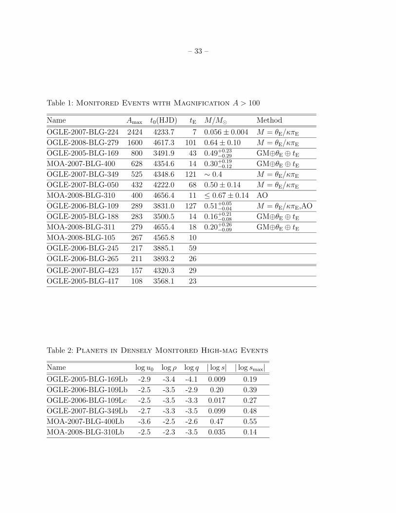
– 33 –

Table 1: Monitored Events with Magnification A > 100

Name Amax t0(HJD) tE M/M⊙ Method

OGLE-2007-BLG-224 2424 4233.7 7 0.056 ± 0.004 M = θE/κπE

OGLE-2008-BLG-279 1600 4617.3 101 0.64 ± 0.10 M = θE/κπE

OGLE-2005-BLG-169 800 3491.9 43 0.49+0.23−0.29 GM⊕θE ⊕ tE

MOA-2007-BLG-400 628 4354.6 14 0.30+0.19−0.12 GM⊕θE ⊕ tE

OGLE-2007-BLG-349 525 4348.6 121 ∼ 0.4 M = θE/κπE

OGLE-2007-BLG-050 432 4222.0 68 0.50 ± 0.14 M = θE/κπE

MOA-2008-BLG-310 400 4656.4 11 ≤ 0.67 ± 0.14 AO

OGLE-2006-BLG-109 289 3831.0 127 0.51+0.05−0.04 M = θE/κπE,AO

OGLE-2005-BLG-188 283 3500.5 14 0.16+0.21−0.08 GM⊕θE ⊕ tE

MOA-2008-BLG-311 279 4655.4 18 0.20+0.26−0.09 GM⊕θE ⊕ tE

MOA-2008-BLG-105 267 4565.8 10

OGLE-2006-BLG-245 217 3885.1 59

OGLE-2006-BLG-265 211 3893.2 26

OGLE-2007-BLG-423 157 4320.3 29

OGLE-2005-BLG-417 108 3568.1 23

Table 2: Planets in Densely Monitored High-mag Events

Name log u0 log ρ log q | log s| | log smax|OGLE-2005-BLG-169Lb -2.9 -3.4 -4.1 0.009 0.19

OGLE-2006-BLG-109Lb -2.5 -3.5 -2.9 0.20 0.39

OGLE-2006-BLG-109Lc -2.5 -3.5 -3.3 0.017 0.27

OGLE-2007-BLG-349Lb -2.7 -3.3 -3.5 0.099 0.48

MOA-2007-BLG-400Lb -3.6 -2.5 -2.6 0.47 0.55

MOA-2008-BLG-310Lb -2.5 -2.3 -3.5 0.035 0.14

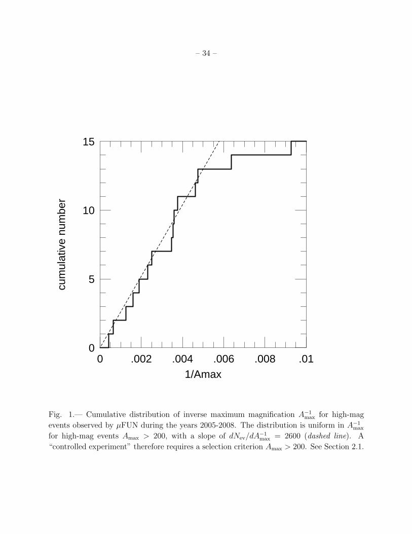
– 34 –

1/Amax

cum

ulat

ive

num

ber

0 .002 .004 .006 .008 .010

5

10

15

Fig. 1.— Cumulative distribution of inverse maximum magnification A−1max for high-mag

events observed by µFUN during the years 2005-2008. The distribution is uniform in A−1max

for high-mag events Amax > 200, with a slope of dNev/dA−1max = 2600 (dashed line). A

“controlled experiment” therefore requires a selection criterion Amax > 200. See Section 2.1.

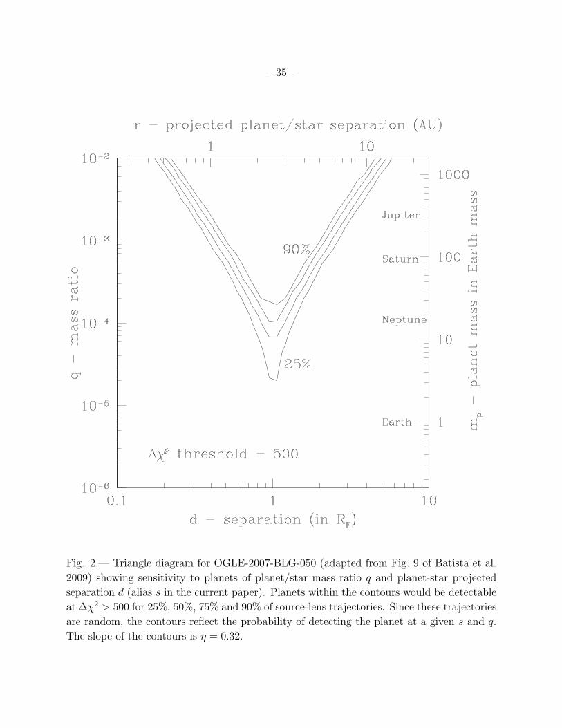
– 35 –

Fig. 2.— Triangle diagram for OGLE-2007-BLG-050 (adapted from Fig. 9 of Batista et al.

2009) showing sensitivity to planets of planet/star mass ratio q and planet-star projected

separation d (alias s in the current paper). Planets within the contours would be detectable

at ∆χ2 > 500 for 25%, 50%, 75% and 90% of source-lens trajectories. Since these trajectories

are random, the contours reflect the probability of detecting the planet at a given s and q.

The slope of the contours is η = 0.32.

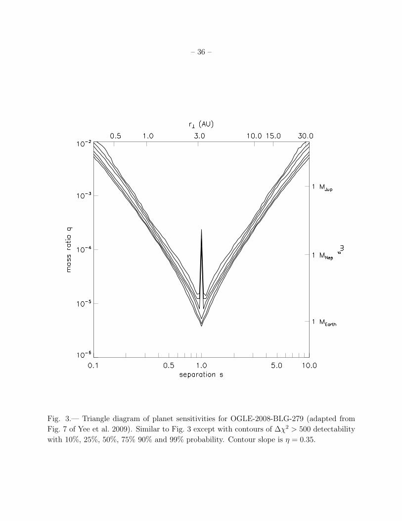
– 36 –

Fig. 3.— Triangle diagram of planet sensitivities for OGLE-2008-BLG-279 (adapted from

Fig. 7 of Yee et al. 2009). Similar to Fig. 3 except with contours of ∆χ2 > 500 detectability

with 10%, 25%, 50%, 75% 90% and 99% probability. Contour slope is η = 0.35.

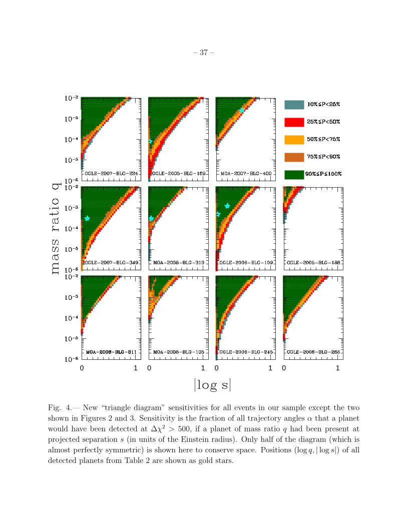
– 37 –

0 1 0 1 0 1 0 1

Fig. 4.— New “triangle diagram” sensitivities for all events in our sample except the two

shown in Figures 2 and 3. Sensitivity is the fraction of all trajectory angles α that a planet

would have been detected at ∆χ2 > 500, if a planet of mass ratio q had been present at

projected separation s (in units of the Einstein radius). Only half of the diagram (which is

almost perfectly symmetric) is shown here to conserve space. Positions (log q, | log s|) of all

detected planets from Table 2 are shown as gold stars.

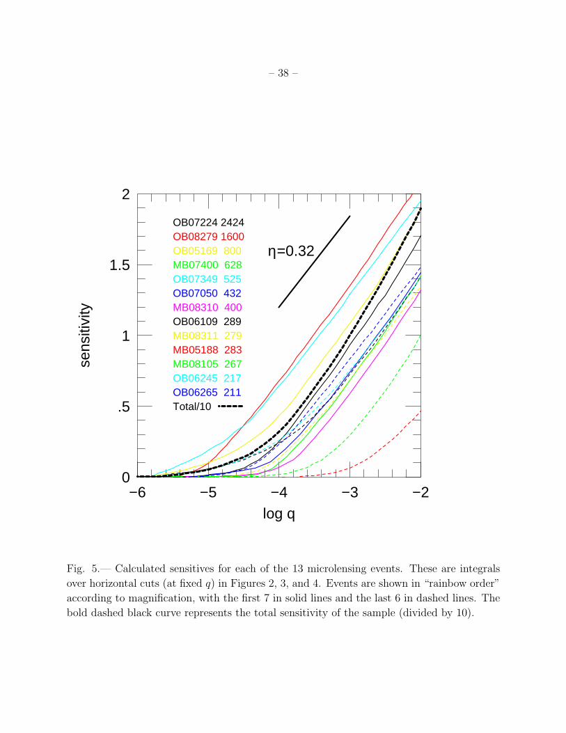
– 38 –

log q

sens

itivi

ty

−6 −5 −4 −3 −20

.5

1

1.5

2

OB07224 2424OB08279 1600OB05169 800MB07400 628OB07349 525OB07050 432MB08310 400OB06109 289

MB05188 283MB08311 279

MB08105 267OB06245 217OB06265 211Total/10

η=0.32

Fig. 5.— Calculated sensitives for each of the 13 microlensing events. These are integrals

over horizontal cuts (at fixed q) in Figures 2, 3, and 4. Events are shown in “rainbow order”

according to magnification, with the first 7 in solid lines and the last 6 in dashed lines. The

bold dashed black curve represents the total sensitivity of the sample (divided by 10).

– 39 –

|log s|/|log s|max

cum

ulat

ive

num

ber

0 .2 .4 .6 .8 10

2

4

6

Fig. 6.— Cumulative distribution of the (absolute value of the log of the) measured projected

separation, | log s|, in units of the maximum value of this parameter, derived in Section 4.1

The observed distribution is consistent with planets being distributed uniformly in log s,

with Kolmogorov-Smirnov probability of 20%.

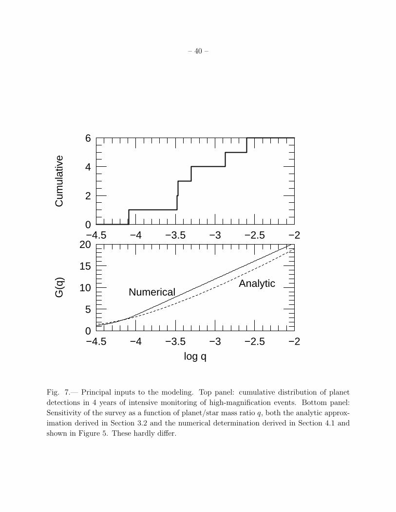
– 40 –C

umul

ativ

e

−4.5 −4 −3.5 −3 −2.5 −20

2

4

6

log q

G(q

)

−4.5 −4 −3.5 −3 −2.5 −20

5

10

15

20

NumericalAnalytic

Fig. 7.— Principal inputs to the modeling. Top panel: cumulative distribution of planet

detections in 4 years of intensive monitoring of high-magnification events. Bottom panel:

Sensitivity of the survey as a function of planet/star mass ratio q, both the analytic approx-

imation derived in Section 3.2 and the numerical determination derived in Section 4.1 and

shown in Figure 5. These hardly differ.

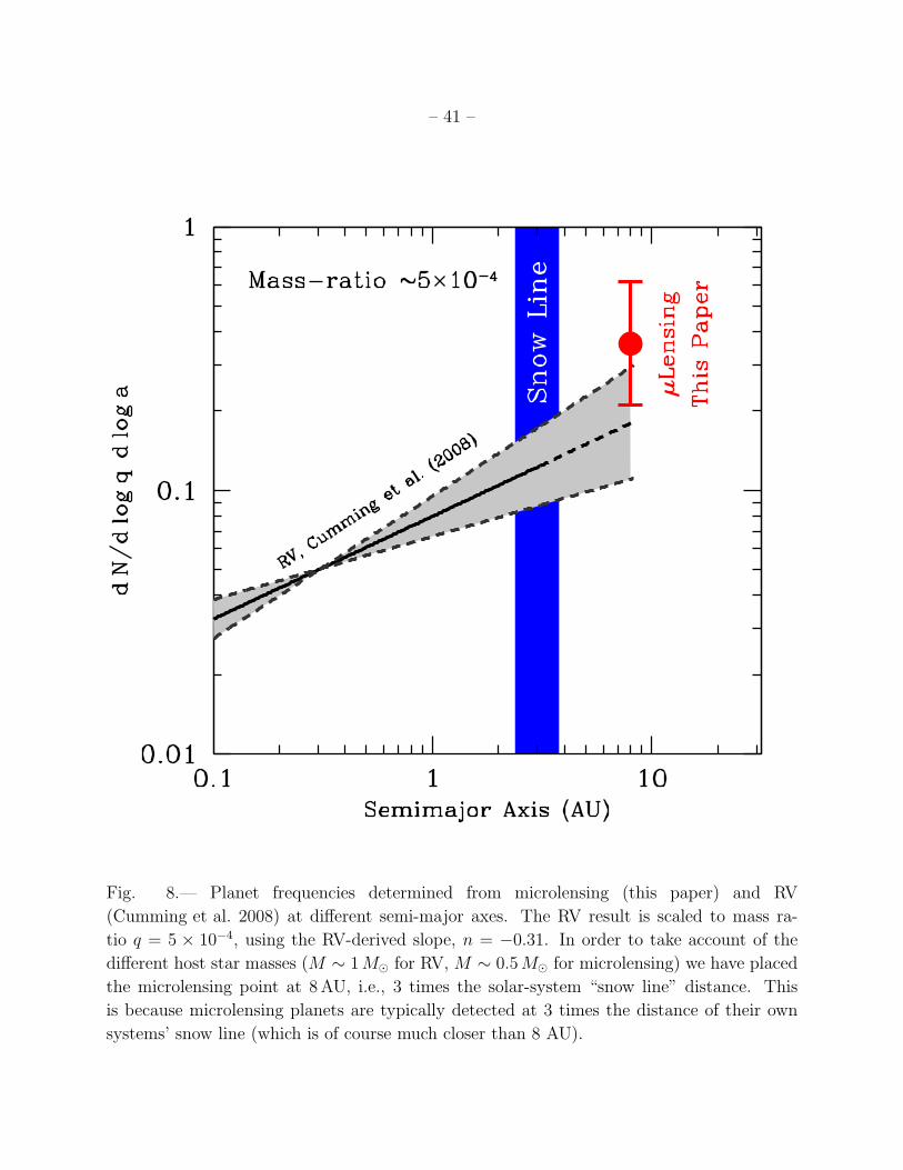
– 41 –

Fig. 8.— Planet frequencies determined from microlensing (this paper) and RV

(Cumming et al. 2008) at different semi-major axes. The RV result is scaled to mass ra-

tio q = 5 × 10−4, using the RV-derived slope, n = −0.31. In order to take account of the

different host star masses (M ∼ 1M⊙ for RV, M ∼ 0.5M⊙ for microlensing) we have placed

the microlensing point at 8 AU, i.e., 3 times the solar-system “snow line” distance. This

is because microlensing planets are typically detected at 3 times the distance of their own

systems’ snow line (which is of course much closer than 8 AU).

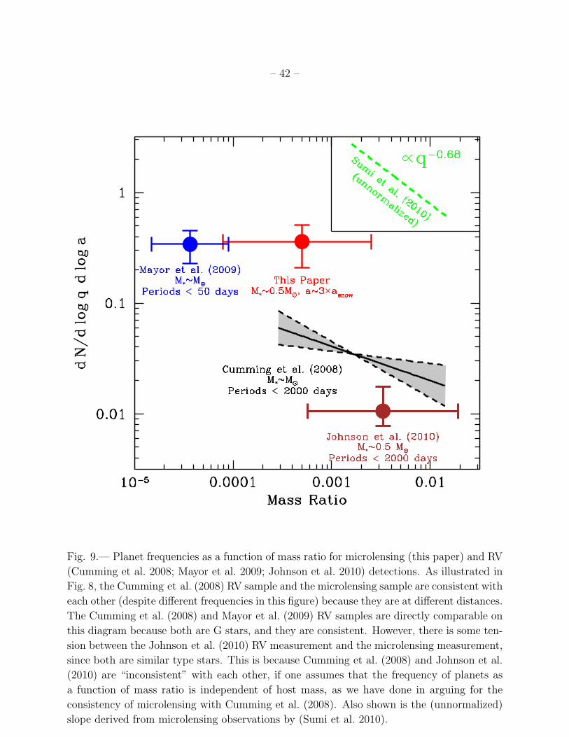
– 42 –

Fig. 9.— Planet frequencies as a function of mass ratio for microlensing (this paper) and RV

(Cumming et al. 2008; Mayor et al. 2009; Johnson et al. 2010) detections. As illustrated in

Fig. 8, the Cumming et al. (2008) RV sample and the microlensing sample are consistent with

each other (despite different frequencies in this figure) because they are at different distances.

The Cumming et al. (2008) and Mayor et al. (2009) RV samples are directly comparable on

this diagram because both are G stars, and they are consistent. However, there is some ten-

sion between the Johnson et al. (2010) RV measurement and the microlensing measurement,

since both are similar type stars. This is because Cumming et al. (2008) and Johnson et al.

(2010) are “inconsistent” with each other, if one assumes that the frequency of planets as

a function of mass ratio is independent of host mass, as we have done in arguing for the

consistency of microlensing with Cumming et al. (2008). Also shown is the (unnormalized)

slope derived from microlensing observations by (Sumi et al. 2010).

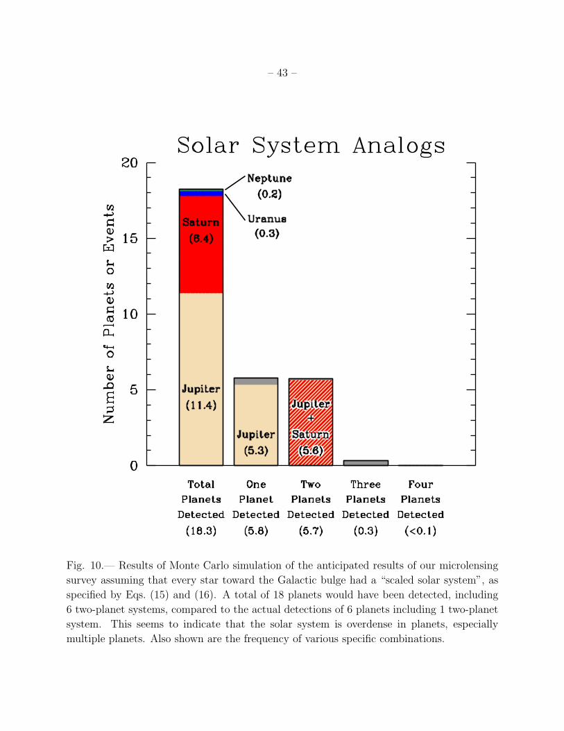
– 43 –

Fig. 10.— Results of Monte Carlo simulation of the anticipated results of our microlensing

survey assuming that every star toward the Galactic bulge had a “scaled solar system”, as

specified by Eqs. (15) and (16). A total of 18 planets would have been detected, including

6 two-planet systems, compared to the actual detections of 6 planets including 1 two-planet

system. This seems to indicate that the solar system is overdense in planets, especially

multiple planets. Also shown are the frequency of various specific combinations.

Frequency of Solar-like Systems and of Ice and Gas Giants Beyond the Snow Line from...

Documents

Transcript of Frequency of Solar-like Systems and of Ice and Gas Giants Beyond the Snow Line from...