arX

iv:a

stro

-ph/

0404

394v

1 2

0 A

pr 2

004

OGLE-2003-BLG-238:Microlensing Mass Estimate of an Isolated

Star ∗

Guangfei Jiang1, D.L. DePoy1, A. Gal-Yam2,3, B.S. Gaudi4, A. Gould1, C. Han5, Y.

Lipkin6, D. Maoz6, E.O. Ofek6, B.-G. Park7, and R.W. Pogge1

(The µFUN Collaboration),

A. Udalski8, M. Kubiak8, M. K. Szymanski8, O. Szewczyk8, K. Zebrun8,

L. Wyrzykowski6,8, I. Soszynski8, and G. Pietrzynski8,9

(The OGLE Collaboration)

and

M. D. Albrow10, J.-P. Beaulieu11, J. A. R. Caldwell12, A. Cassan11, C. Coutures11,13,

M. Dominik14, J. Donatowicz15, P. Fouque16, J. Greenhill17, K. Hill17, K. Horne14,

S.F. Jørgensen18, U. G. Jørgensen18, S. Kane14, D. Kubas19, R. Martin20,

J. Menzies21, K. R. Pollard10, K. C. Sahu12, J. Wambsganss18,

R. Watson17, and A. Williams20

(The PLANET Collaboration22)

– 2 –

1Department of Astronomy, The Ohio State University, 140 West 18th Avenue, Columbus, OH 43210;

jiang, depoy, gould, pogge@astronomy.ohio-state.edu

2Department of Astronomy, California Institute of Technology, Pasadena, CA 91025

avishay@astro.caltech.edu

3Hubble Fellow

4Harvard-Smithsonian Center for Astrophysics, Cambridge, MA 02138; sgaudi@cfa.harvard.edu

5Department of Physics, Institute for Basic Science Research, Chungbuk National University, Chongju

361-763, Korea; cheongho@astroph.chungbuk.ac.kr

6School of Physics and Astronomy and Wise Observatory, Tel-Aviv University, Tel Aviv 69978, Israel;

avishay, yiftah, dani, eran@wise.tau.ac.il

7Korea Astronomy Observatory 61-1, Whaam-Dong, Youseong-Gu, Daejeon 305-348, Korea; bg-

park@boao.re.kr

8Warsaw University Observatory, Al. Ujazdowskie 4, 00-478 Warszawa, Poland; udalski, soszynsk,

wyrzykow, mk, msz, pietrzyn, szewczyk, zebrun@astrouw.edu.pl

9Universidad de Concepcion, Departmento de Fisica, Casilla 160-C, Concepcion, Chile;

pietrzyn@hubble.cfm.udec.cl

10University of Canterbury, Department of Physics & Astronomy, Private Bag 4800, Christchurch, New

Zealand

11Institut d’Astrophysique de Paris, 98bis Boulevard Arago, 75014 Paris, France

12Space Telescope Science Institute, 3700 San Martin Drive, Baltimore, MD 21218, USA

13DSM/DAPNIA, CEA Saclay, 91191 Gif-sur-Yvette cedex, France

14University of St Andrews, School of Physics & Astronomy, North Haugh, St Andrews, KY16 9SS, United

Kingdom

15Technical University of Vienna, Dept. of Computing, Wiedner Hauptstrasse 10, Vienna, Austria

16Observatoire Midi-Pyrenees, UMR 5572, 14, avenue Edouard Belin, F-31400 Toulouse, France

17University of Tasmania, School of Maths and Physics, University of Tasmania, Private bag, Hobart,

Tasmania, 7001, Australia

18Niels Bohr Institute, Astronomical Observatory, Juliane Maries Vej 30, DK-2100 Copenhagen, Denmark

19Universitat Potsdam, Astrophysik, Am Neuen Palais 10, D-14469 Potsdam, Germany

20Perth Observatory, Walnut Road, Bickley, Perth 6076, Australia

21South African Astronomical Observatory, P.O. Box 9 Observatory 7935, South Africa

22e-mail address: planetmembers@anu.edu.au; sfj@astro.ku.dk

*Based in part on observations obtained with the 1.3 m Warsaw Telescope at the Las Campanas Obser-

– 3 –

ABSTRACT

Microlensing is the only known direct method to measure the masses of stars

that lack visible companions. In terms of microlensing observables, the mass

is given by M = (c2/4G)rEθE and so requires the measurement of both the

angular Einstein radius, θE, and the projected Einstein radius, rE. Simultaneous

measurement of these two parameters is extremely rare. Here we analyze OGLE-

2003-BLG-238, a spectacularly bright (Imin = 10.3), high-magnification (Amax =

170) microlensing event. Pronounced finite source effects permit a measurement

of θE = 650µas. Although the timescale of the event is only tE = 38 days, one

can still obtain weak constraints on the microlens parallax: 4.4 AU < rE < 18 AU

at the 1 σ level. Together these two parameter measurements yield a range for

the lens mass of 0.36M⊙ < M < 1.48M⊙. As was the case for MACHO-LMC-5,

the only other single star (apart from the Sun) whose mass has been determined

from its gravitational effects, this estimate is rather crude. It does, however,

demonstrate the viability of the technique. We also discuss future prospects for

single-lens mass measurements.

Subject headings: gravitational lensing — parallax

1. Introduction

When microlensing experiments were first proposed (Paczynski 1986) and implemented

(Alcock et al. 1993; Aubourg et al. 1993; Udalski et al. 1993), it was not expected to be

possible to measure the masses and distances of individual microlenses. The only microlens-

ing parameter that depends on the mass and that is routinely measured is the Einstein

timescale tE, which is a degenerate combination of the lens mass M , and the lens-source

relative parallax, πrel, and proper motion, µrel. Specifically,

tE =θEµrel

, θE =√

κMπrel, κ ≡4G

c2 AU≃ 8.14

mas

M⊙, (1)

where θE is the angular Einstein radius. However, Gould (1992) showed that if both θE and

the microlens parallax,

πE =

√

πrel

κM, (2)

vatory of the Carnegie Institution of Washington; and the Danish 1.54m telescope at ESO, La Silla, Chile,

operated by IJAF and financed by SNF.

– 4 –

could be measured, then the mass and lens-source relative parallax could both be determined,

M =θEκπE

, πrel = πEθE. (3)

Nevertheless, of the roughly 2000 microlensing events detected to date, there have been

only of order a dozen for which θE has been measured and a dozen for which πE has been

measured. Moreover, there is only one event, EROS-BLG-2000-5, with measurements of both

parameters, and so for which the microlens mass and distance have been reliably determined

(An et al. 2002). Since this one event was a binary, and since all the other stars with directly

measured masses are components of binaries, it remains the case today that the only single

star with a directly measured mass is the Sun.

The one partial exception is the microlens in MACHO-LMC-5. Alcock et al. (2001) were

able to measure both θE and πE for this event and so measure the mass and distance. These

estimates were completely inconsistent with photometry-based estimates of these quantities,

but Gould (2004) resolved this puzzle by showing that the πE measurement was subject to a

discrete degeneracy for this event and that the alternate solution was consistent at the few

σ level with the photometric evidence. Nevertheless, since the error in the mass estimate is

about 35%, this mass determination must be regarded as very approximate.

Here we analyze OGLE-2003-BLG-238, the brightest microlensing event ever observed

and only the fourth reported point-lens (i.e., non-binary) event with pronounced finite-source

effects. As with the other three such events (Alcock et al. 1997; Smith, Mao & Wozniak

2003; Yoo et al. 2004), these finite-source effects allow one to measure θE with reasonably

good (∼ 10%) precision, where the error is typically dominated by the modeling of the source

rather than the microlensing event. Hence, if πE could also be measured, it would be possible

to determine M .

Despite the event’s short duration, it is still possible to detect parallax effects in OGLE-

2003-BLG-238 because of its bright source and high magnification. For short events like

this one, the Earth’s acceleration can be approximated as uniform during the event. Gould,

Miralda-Escude & Bahcall (1994) showed that under these conditions, the parallax effect

reduces to a simple asymmetry in the lightcurve around the peak. The high magnification of

OGLE-2003-BLG-238 permits a very accurate measurement of the peak time of the event,

which in turn makes the fitting process very sensitive to this small asymmetry. The brightness

of the source allows high precision photometric measurements even in the wings of the

event, which enable detection of these subtle deviations. Unfortunately, as also shown by

Gould et al. (1994), the simplicity of the parallax effect for short events implies that only 1-

dimensional parallax information can be effectively extracted, whereas the microlens parallax

is intrinsically a 2-dimensional vector πE. That is, while one component of the vector parallax

– 5 –

is well determined, the scalar parallax πE is not well determined, and this degrades the mass

determination through equation (3). Nevertheless, this is still only the second single star

(other than the Sun) for which any direct mass measurement at all can be made.

2. Observational Data

The microlensing event OGLE-2003-BLG-238 was identified by the OGLE-III Early

Warning System (EWS) (Udalski 2003) on 2003 June 22. It peaked on HJD′ ≡ HJD−2450000 =

2878.38 (Aug 26.88) over South Africa. OGLE-III observations were carried out in I band

using the 1.3-m Warsaw telescope at the Las Campanas Observatory, Chile, which is op-

erated by the Carnegie Institution of Washington. While OGLE-III normally operates in

survey mode, cycling through the observed fields typically once per two nights during the

main part of the bulge season, it can switch rapidly to follow-up mode if an event is of partic-

ular interest and requires dense sampling. The high magnification of OGLE-2003-BLG-238,

which was predicted while the event was developing, and possible deviations from a single-

point-mass microlensing lightcurve profile were the main reasons that OGLE observed this

event in follow-up mode.

The OGLE-III data comprise a total of 205 observations in I band, including 144 during

the 2003 season and 61 in the two previous seasons, 2001 and 2002. The exposures were

generally the standard 120 s, except for three nights (HJD′ 2877.5–2879.7) around the maxi-

mum when the star was too bright for the standard exposure time. The time of exposure was

adjusted then to the current brightness of the lens and seeing conditions to avoid saturation

of images and was as short as 10 s on the night of maximum. Photometry was obtained

with the OGLE-III image subtraction technique data pipeline Udalski (2003) based in part

on the Wozniak (2000) DIA implementation.

Following the alert, the event was monitored by the Microlensing Follow-Up Network

(µFUN, Yoo et al. 2004) from sites in Chile and Israel, and by the Probing Lensing Anomalies

Network (PLANET, Albrow et al. 1998) from sites in Chile and Tasmania. The µFUN Chile

observations were carried out at the 1.3m (ex-2MASS) telescope at Cerro Tololo InterAmer-

ican Observatory, using the ANDICAM camera, which simultaneously images at optical and

infrared wavelengths (DePoy et al. 2003). There were a total 203 images in I from HJD′

2870.5 (eight days before peak) until HJD′ 2950.5 at the end of the season. The exposures

were generally 300 s, but were shortened to 120 s for 81 exposures over the peak. The

exposures should have been further shortened on the night of the peak but, due to human

error, this did not happen. Hence, all 19 of these images were saturated. µFUN obtained 12

points in V , primarily to determine the source color. This includes one saturated point over

– 6 –

the peak. All saturated images were discarded.

The µFUN Israel observations were carried out in I band using the Wise 1m telescope at

Mitzpe Ramon, 200 km south of Tel-Aviv. There were 14 observations in total, all restricted

to the peak of the event, 2877.3 < HJD′ < 2883.3. The exposures (all 240 s) were obtained

using the Wise Tektronix 1K CCD camera. All µFUN photometry was extracted using

DoPhot (Schechter, Mateo & Saha 1993).

The PLANET Chile observations were carried out in R band using the Danish 1.54m

telescope at the European Southern Observatory in La Silla, Chile. There were a total of

68 observations from HJD′ 2874.6 to HJD′ 2883.7. The exposure times ranged from 2 to 80

seconds. The PLANET Tasmania observations were carried out in I band using the Canopus

1m telescope near Hobart, Tasmania with 52 observations from HJD′ 2877.9 to HJD′ 2903.9.

The exposure times ranged from 60 to 300 seconds. During the first night in Tasmania the

data were taken despite significant cloud cover by observing through “holes” in the cloudy

sky. This proved feasible only because of the extreme brightness (I ∼ 11) of the source

and demonstrates the importance of carefully monitoring events in real time to determine

whether they should be observed despite truly awful conditions.

The position of the source is R.A. = 17h45m50s.34, decl. = −22◦40′58.′′1 (J2000) (l, b =

5.72, 2.60), and so was accessible for most of the night near peak from Chile and Tasmania,

but for only a few hours from Israel. The combined data sets are shown in Figure 1.

3. Finite-Source Effects

In general, the fluxes, Fi(t), observed during a microlensing event by i = 1, . . . , n obser-

vatory/filter combinations are fit to the form,

Fi(t) = Fs,iA(t) + Fb,i (4)

where Fs,i is the flux of the unmagnified source star as seen by the ith observatory and Fb,i

is any background flux that lies in the aperture but is not participating in the microlensing

event. (The one exception would be a binary-source event, in which case two source-star

terms and two magnification functions would be required.)

In most cases, the lensed star can be fairly approximated as a point source. The mag-

nification is then given by (Paczynski 1986),

A(u) =u2 + 2

u(u2 + 4)1/2, (5)

– 7 –

where u is the angular source-lens separation in units of the angular Einstein radius θE.

However, this approximation breaks down for u . ρ, where,

ρ ≡θ∗θE, (6)

is the angular source size θ∗ normalized to θE. Finite-source effects then dominate. An

appropriate formalism for incorporating these effects is given by Yoo et al. (2004). Here we

summarize the essentials. If limb darkening is neglected, the total magnification becomes

(Gould 1994; Witt & Mao 1994; Yoo et al. 2004),

Auni(u|ρ) ≃ A(u)B0(u/ρ), B0(z) ≡4

πzE(k, z), (7)

where E is the elliptic integral of the second kind and k = min(z−1, 1). This formula is

accurate to O(ρ2/8) (Yoo et al. 2004), and hence it applies whenever (as in the present case)

ρ≪ 1. Note from Figure 1 that the finite-source fit passes first above the point-source curve

and then moves below it. This transition occurs when B0(z) = 1, which (from fig. 3 of Yoo et

al. 2004) occurs at z ∼ 0.54. By contrast, for MACHO-95-30 (Alcock et al. 1997) and OGLE-

2003-BLG-262 (Yoo et al. 2004), the finite-source fits remain above the point-source curves

throughout because in those cases the minimum source-lens separation (impact parameters)

were u0 ∼ 0.7ρ and u0 ∼ 0.6ρ, respectively.

To include the effects of limb darkening, we model the source profile Sλ at each wave-

length λ by,

Sλ(ϑ) = Sλ[1 − Γλ(1 −3

2cosϑ)], (8)

where Γλ is the linear limb-darkening coefficient and ϑ is the angle between the normal to

the stellar surface and the line of sight. The magnification is then given by,

Ald(u|ρ) = A(u)[B0(z) − ΓB1(z)], (9)

where B1(z) is a function described by equation (16) and figure 3 of Yoo et al. (2004).

4. Parallax Effect

If the motions of the source, lens, and observer can all be approximated as rectilinear,

the source-lens separation, u, in equation (5), can be written,

u(t) =√

[τ(t)]2 + [β(t)]2, (10)

– 8 –

where,

τ(t) =t− t0tE

, β(t) = u0. (11)

The simplest point-source fit to a microlensing event requires five parameters, the source

flux Fs, the background flux Fb, the time of closest approach t0, the Einstein time scale tE,

and impact parameter u0.

However, even if the source and lens can be assumed to be in rectilinear motion, the

Earth is not. Especially for the long events (tE ≥ yr/2π), the Earth parallax effect must be

taken into account. The event OGLE-2003-BLG-238 lasted only 38 days, and hence parallax

effects would be negligible if the source were not very bright and highly magnified, both of

which facilitate detection of the very subtle parallax effect. Moreover, after it was realized

that finite-source effects had been detected, both OGLE and µFUN intensified observations

of the event in the hope of measuring the parallax and so combining the result with the

source-size measurement to determine a mass.

Historically, parallax fits were carried out in the heliocentric frame. That is, u0 was

adopted as the point of closest approach to the Sun, and t0 was the time at which this

approach occurred. When, as in the present case, parallax is only weakly detected, the

trajectory relative to the Sun is poorly determined, so t0 and u0 have very large errors that

are highly correlated with the parallax parameters. In the geocentric frame, by contrast,

t0 and u0 are directly determined from the time and height of the peak of the light curve

(Dominik 1998). Gould (2004) further refined the geocentric frame by subtracting out the

Earth-Sun relative velocity as well as their positional offset. This frame is appropriate for the

analysis of OGLE-2003-BLG-238. Hence, we follow the Gould (2004) formalism for modeling

parallax in the geocentric frame.

The parallax effect is parameterized by a vector πE whose magnitude gives the ratio of

the Earth’s orbit (1 AU) to the size of the Einstein ring projected onto the observer plane

(rE) and whose direction is that of the lens-source relative motion as seen from the Earth at

the peak of the event. Explicitly, πE ≡ AU/rE. Equation (11) is then replaced by,

τ(t) =t− t0tE

+ δτ, β(t) = u0 + δβ, (12)

where,

(δτ, δβ) = πE∆s = (πE · ∆s,πE × ∆s), (13)

and ∆s is the apparent position of the Sun relative to what it would be if the Earth remained

in rectilinear motion with the velocity it had at the peak of the event. See equations (4)-(6)

of Gould (2004). More explicitly,

(δτ, δβ) = [∆sN (t)πE,N + ∆sE(t)πE,E ,−∆sN(t)πE,E + ∆sE(t)πE,N ], (14)

– 9 –

where the subscripts N and E refer to components projected on the sky in north and east

celestial coordinates.

A major advantage of this formalism is that the parameters t0, u0, and tE are virtually

the same for the parallax and non-parallax solutions and, especially important in the present

case, when the parallax solution is varied in the πE plane to obtain likelihood contours.

4.1. Nonparallax Fit

As we will show in § 4.2, the parallax effect is quite subtle and so can, to a first

approximation, be ignored. On the other hand, the finite-source effects are quite severe

(see Fig. 1). We therefore begin by fitting the lightcurve by taking into account finite-

source effects (including linear limb darkening) but not parallax. The fit therefore contains

6 geometric parameters (t0, u0, tE, ρ,ΓI ,ΓR) as well as 12 flux parameters (two for each

observatory/filter combination). The results are listed in Table 1 and plotted in Figure 1.

Also shown in Figure 1 is the lightcurve that would have been generated by the same event

but assuming that the source had been a point of light. As discussed in § 3 this remains

below the finite-source curve until z ≡ u/ρ = 0.54, and then rises dramatically above it.

4.2. Parallax Fit

To find the best-fit parallax πE and the error ellipse around it, we conduct a grid

search over the πE plane. That is, we minimize χ2 by holding each trial parameter pair

πE ≡ (πE,N , πE,E) fixed, while allowing the remaining 18 parameters (see § 4.1) to vary.

After finding the best fit πE, we hold this fixed and renormalize the errors so that χ2 per

degree of freedom is unity. We eliminate the largest outlier point and repeat the process

until there are no 3 σ outliers. Of course, we first eliminate the 19 saturated points in µFUN

Chile I and 1 saturated point in µFUN V . We find that this procedure removes 5 points

from the OGLE data, an additional 17 points from the µFUN Chile I data, 7 points from

the PLANET R data, 2 points from the PLANET I data, and none from the other data

sets. The final renormalization factors are 1.96, 0.87, 2.2 and 1.4 for OGLE, µFUN Chile

I, PLANET Tasmania I and PLANET Chile R data, respectively. The other two data

sets, µFUN Chile V and µFUN Israel I, do not require renormalization. This cleaned and

renormalization data set is used in all fits reported in this paper and is shown in Figure 1.

It contains 200 points from OGLE I, 167 from µFUN Chile I, 14 from µFUN Israel I, 11

from µFUN Chile V , 50 from PLANET Tasmania I, and 61 from PLANET Chile R.

– 10 –

Figure 2 shows the resulting likelihood contours in the πE plane. The best fit is at

(πE,E, πE,N) = (0.0664,−0.0205). The contours are extremely elongated with their major

axes almost perfectly aligned with the North-South axis. Gould et al. (1994) showed that

short events would yield essentially 1-dimensional parallax information because the Earth’s

acceleration vector is basically constant over the duration of the event. Hence, only a single

parallax parameter can be measured robustly, namely the magnitude of the asymmetry of

the lightcurve. This yields information about the component of the projected lens-source

relative velocity parallel to the Earth’s acceleration (projected onto the plane of the sky) but

not the perpendicular component. At the peak of the event, the position of the Sun (pro-

jected onto the plane of the sky – see eq. [6] of Gould 2004) is (sE , sN) = (−0.930, 0.028)AU,

which means that the Earth is accelerating in the same direction. Hence, one expects the

direction of maximum sensitivity (minor axis of the error ellipse) to be at a postition angle

tan−1(−0.930/0.028) = 91◦.725 (north through east), which agrees quite well with the ori-

entation (91◦.769) shown in Figure 2. The event MOA-2003-BLG-37, which was also short

(tE ∼ 42 days) shows similar highly elongated parallax-error contours (Park et al. 2004).

Figures 1 and 2 both illustrate that the parallax effect in OGLE-2003-BLG-238 is weak.

The residuals in Figure 1, which shows the fit without parallax, demonstrate that the asym-

metry is quite subtle. Figure 2 shows that the error contours extend almost to the origin.

That is, from Table 1, the addition of two parallax parameters reduces χ2 from 510.6 to

478.3, a 5.5 σ effect.

4.3. Check for Parallax Degeneracies

Gould (2004) showed that microlensing events, particularly those with short timescales

(tE . yr/2π), could be subject to a discrete four-fold degeneracy. One pair of degener-

ate solutions, which was previously discovered by Smith, Mao & Paczynski (2003), takes

u0 → −u0. The remaining parameters are then similar to the original parameters, with

the differences being proportional to u0. Since in the present case u0 is extremely small,

u0 = 2 × 10−3, one expects that these two solutions would be virtually identical, and this

proves to be the case.

The other pair of solutions arises from the jerk-parallax degeneracy, which predicts that

if πE = (πE,‖, πE,⊥) is a solution, then π′E = (π′

E,‖, π′E,⊥) is also a solution, with

π′E,‖ = πE,‖, π′

E,⊥ = −(πE,⊥ + πj,⊥), (15)

– 11 –

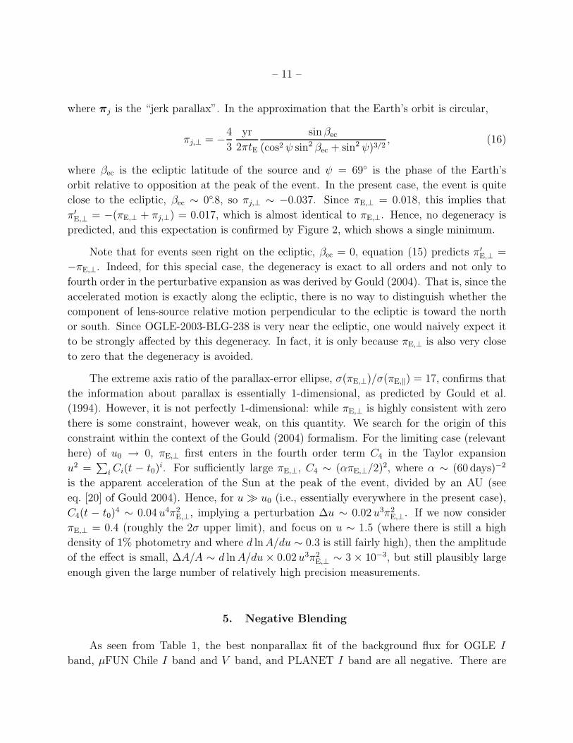
where πj is the “jerk parallax”. In the approximation that the Earth’s orbit is circular,

πj,⊥ = −4

3

yr

2πtE

sin βec

(cos2 ψ sin2 βec + sin2 ψ)3/2, (16)

where βec is the ecliptic latitude of the source and ψ = 69◦ is the phase of the Earth’s

orbit relative to opposition at the peak of the event. In the present case, the event is quite

close to the ecliptic, βec ∼ 0◦.8, so πj,⊥ ∼ −0.037. Since πE,⊥ = 0.018, this implies that

π′E,⊥ = −(πE,⊥ + πj,⊥) = 0.017, which is almost identical to πE,⊥. Hence, no degeneracy is

predicted, and this expectation is confirmed by Figure 2, which shows a single minimum.

Note that for events seen right on the ecliptic, βec = 0, equation (15) predicts π′E,⊥ =

−πE,⊥. Indeed, for this special case, the degeneracy is exact to all orders and not only to

fourth order in the perturbative expansion as was derived by Gould (2004). That is, since the

accelerated motion is exactly along the ecliptic, there is no way to distinguish whether the

component of lens-source relative motion perpendicular to the ecliptic is toward the north

or south. Since OGLE-2003-BLG-238 is very near the ecliptic, one would naively expect it

to be strongly affected by this degeneracy. In fact, it is only because πE,⊥ is also very close

to zero that the degeneracy is avoided.

The extreme axis ratio of the parallax-error ellipse, σ(πE,⊥)/σ(πE,‖) = 17, confirms that

the information about parallax is essentially 1-dimensional, as predicted by Gould et al.

(1994). However, it is not perfectly 1-dimensional: while πE,⊥ is highly consistent with zero

there is some constraint, however weak, on this quantity. We search for the origin of this

constraint within the context of the Gould (2004) formalism. For the limiting case (relevant

here) of u0 → 0, πE,⊥ first enters in the fourth order term C4 in the Taylor expansion

u2 =∑

i Ci(t − t0)i. For sufficiently large πE,⊥, C4 ∼ (απE,⊥/2)2, where α ∼ (60 days)−2

is the apparent acceleration of the Sun at the peak of the event, divided by an AU (see

eq. [20] of Gould 2004). Hence, for u ≫ u0 (i.e., essentially everywhere in the present case),

C4(t − t0)4 ∼ 0.04 u4π2

E,⊥, implying a perturbation ∆u ∼ 0.02 u3π2E,⊥. If we now consider

πE,⊥ = 0.4 (roughly the 2σ upper limit), and focus on u ∼ 1.5 (where there is still a high

density of 1% photometry and where d lnA/du ∼ 0.3 is still fairly high), then the amplitude

of the effect is small, ∆A/A ∼ d lnA/du × 0.02 u3π2E,⊥ ∼ 3 × 10−3, but still plausibly large

enough given the large number of relatively high precision measurements.

5. Negative Blending

As seen from Table 1, the best nonparallax fit of the background flux for OGLE I

band, µFUN Chile I band and V band, and PLANET I band are all negative. There are

– 12 –

three potential reasons for such negative background fluxes: systematic photometry errors,

unmodeled effects in the lightcurve that are absorbed by the blended flux parameter, and

“negative flux” from unlensed sources. The first possibility is virtually ruled out by the fact

that the negative background flux appears in so many unassociated lightcurves. The last

possibility is not as ridiculous as it might first appear because the dense Galactic bulge fields

have a mottled background of turnoff and main-sequence stars. If the source happens to lie in

a hole in this background, it will appear as negative Fb (Park et al. 2004). The Fb/Fs = −5%

from the OGLE photometry (which has the most extensive baseline), would require a “hole”

corresponding to a star 20 times fainter than the source i.e, I0,“hole′′ ∼ 17.6 (see Fig. 3). This

is a plausible brightness for a hole in the unresolved turnoff stars. Combining this value

with the Fb/Fs = −17% measurement from PLANET R, yields a color difference between

the “hole” and the source,

∆(R − I) ≡ (R− I)“hole′′ − (R− I)s = −1.25 ± 0.20, (17)

whereas the expected value (given the source position in Fig. 3) is about ∆(R− I) ∼ −0.5.

Hence this explanation is not completely self-consistent.

Because the effect of the blending parameter is even about the peak, it can absorb effects

of other even parameters including Fs, ρ, u0, and tE. Since all of these are taken into account

in the nonparallax fit (and its errors) these cannot be the cause. However, as pointed out

by Smith et al. (2003) microlens parallax can also mimic blending. Within the formalism of

Gould (2004), the blending fraction is correlated with πE,⊥ which is also an even parameter

(see Park et al. 2004).

The best-fit parallax solution still contains negative background fluxes, although these

are slightly reduced in magnitude relative to the nonparallax fit, while the errors are some-

what increased. The reduction reflects the absorption of some of the negative blending into

πE,⊥, while the larger errors reflect the covariance between Fb and πE,⊥. However, since the

negative blending is still detected with substantial significance, parallax cannot be the whole

story. A “hole” in the mottled bulge background of turnoff stars remains the most plausible

explanation for the negative blending, although as discussed above, this explanation is not

perfect.

6. Error Determination

We use Newton’s method to find the minimum χ2 with respect to the 18 parameters of

the nonparallax model. This procedure utilizes the Fischer matrix, and therefore automati-

cally generates a covariance matrix and so linearized error estimates for all the parameters.

– 13 –

We find, however, that Newton’s method fails when we add the two parallax parameters,

probably because the effect is too subtle to withstand the numerical noise induced by nu-

merical differentiation of the finite source effects. We therefore hold πE fixed at a grid of

values and, at each one, minimize χ2 with respect to the remaining 18 parameters. The re-

sulting contours are shown in Figure 2. To estimate the errors we use the method of “hybrid

statistical errors” given in Appendix D of An et al. (2002). First, Newton’s method auto-

matically yields cij, the covariance matrix of the model parameters (collectively ai) with the

two parameters πE held fixed at their best-fit values. Next we evaluate the two-dimensional

covariance matrix cmn, where m,n range over the parameters (πE,N , πE,E), by fitting the

contours in Figure 2 to a parabola. Third we evaluate ∂ai/∂am, the change in the best-fit

model parameter ai as one of the parallax parameters is varied over the grid. Finally, we

evaluate the covariance matrix cij by,

cij = cij +∑

m,n=πE,N ,πE,E

cmn∂ai

∂am

∂aj

∂an

. (18)

7. Estimates of Mass and Distance

7.1. Measurement of θE

We determine the angular size of the source θ∗ from the instrumental color-magnitude

diagram (CMD), using the method developed by Albrow et al. (2000b) and references therein,

which is concisely summarized by Yoo et al. (2004). We measure the offsets in color and

magnitude between the unmagnified source star and the center of the clump giants, ∆I =

Is − Iclump = −0.02, ∆(V − I) = (V − I)s − (V − I)clump = 0.22. For the dereddened color

and magnitude of the clump center, we adopt [(V − I)0, I0]clump = (1.00, 14.32) (Yoo et al.

2004), then transform from (V − I)0 to (V − K)0 using the color-color relation of Bessell

& Brett (1988). We obtain [(V − I)0, I0]s = (1.22, 14.30). Finally, using the color/surface-

brightness relation of van Belle (1999), we obtain θ∗ = 8.35 ± 0.72µas, where the error is

dominated by the 8.7% scatter in the van Belle (1999) relation.

From the best-fit value ρ = 0.0128, we then obtain,

θE = 652 ± 56µas, µrel = 6.20 ± 0.54 mas yr−1 = 29.4 ± 2.6 km s−1 kpc−1. (19)

– 14 –

7.2. Mass and Distance Estimates

The best parallax fit for the event is πE = 0.0695, which when combined with equa-

tions (3) and (19) yields,

M = 1.15M⊙ (best fit). (20)

However, the errors are quite large. Figure 2 shows that at the 1 σ level, πE lies in the range

0.2256 > πE > 0.0552, which implies

0.36 < M/M⊙ < 1.48 (1 σ). (21)

The same microlens parallax estimates lead (through eq. [3]) to a best relative parallax

estimate of πrel = 45µas and a 1 σ range of 147µas > πrel > 35µas. If one adopts a source

distance of Ds = 8 kpc, this corresponds to a distance range 3.6 kpc < Dl < 6.3 kpc.

At the 2σ level, 0.4180 > πE > 0.0434, which leads to a mass range 0.19 < M/M⊙ < 1.86

and a relative parallax range 273µas > πrel > 28µas, corresponding to 2.5 kpc < Dl <

6.5 kpc. Therefore, the 2 σ interval is consistent with most of the stellar range, but it does

not provide any “new” information about the lens other than ruling out stellar-mass black

holes and very late-type M dwarfs and brown dwarfs. On the other hand, it does serve

as a basic consistency check on the viability of the microlens mass measurements, since if

the method were plagued by strong systematic errors one would not necessarily expect the

estimated mass to lie in the stellar range.

7.3. A Single Star?

As noted in § 1, part of the motivation for microlensing mass measurements is that

this is the only known way to directly measure the mass of single stars. But how confident

can we be that OGLE-2003-BLG-238 is a single star? In a future paper, we will analyze

the lightcurve for the presence of all types of companions to the lens, particularly planetary

companions. However, by simple inspection of the lightcurve, it is possible to place rough

limits on stellar-mass companions, i.e., those with mass ratios q > 0.1. No such companions

are possible with separations (in units of θE of the observed lens) of d ∼ 1, since there would

be clearly visible caustic crossings.

As the separation is increased, the magnification pattern approaches a Chang-Refsdal

lens with shear γ = qw/d2w (Chang & Refsdal 1979, 1984). The width of the Chang-Refsdal

caustic in the limit of γ ≪ 1 is ℓ ∼ 4γ. From inspection of the lightcurve and the fact that

u0 ∼ ρ/6 (see Table 1), we can say that such a caustic would certainly have been noticed if

ℓ > ρ/2. This implies a limit dw > (8qw/ρ)1/2 = 25q1/2w .

– 15 –

According to the so-called d → d−1 duality discovered by Dominik (1999) and further

elaborated by Albrow et al. (2002), the central caustics of extremely close binaries mimic

those of wide binaries. Keeping to the convention that the observed Einstein radius cor-

reponds to the mass near the observed peak in the lightcurve (i.e., the combined mass of

the binary in the close case but just the mass one star in the wide case), one finds that

γ = d2cqc/(1 + qc)

2. Thus, by the same argument as above, dc < 0.04(1 + qc)q−1/2c . Combin-

ing these two arguments and making use of equation (19), implies that the entire range of

companion projected separations r⊥,

0.2 AU (q1/2c + q−1/2

c )Dl

R0

< r⊥ < 85 AU q1/2w

Dl

R0

(excluded companions), (22)

is excluded. Here Dl is the distance to the lens and R0 = 8 kpc. Hence, if the lens has a

stellar companion, it is either extremely close or very far away.

8. Future Prospects

To date, microlensing mass measurements of single stars have depended on very rare

combinations of circumstances. The problem is somewhat more severe than was outlined in

§ 1. There we noted that πE and θE were separately measured only infrequently, so combined

measurements are even more infrequent. However, for single stars, the events most likely

to show the parallax effects from which one could measure πE are also the least likely to

show the finite-source effects from which one could measure θE. That is, microlens parallax

measurements generally require long events, tE & yr/2π, which tends to favor large masses,

since tE ∝ M1/2. But the probability of significant finite-source effects (i.e., u0 . ρ) scales

as ρ = θ∗/θE, which favors small masses, since θE ∝M1/2. The combination of large tE and

small θE implies low relative proper motion µrel = θE/tE.

Actually, neither of the two single-star events with microlens mass measurements meets

this criterion. OGLE-2003-BLG-238 has µ ∼ 6 mas yr−1, which is a typical value for disk

lenses seen against the bulge and is substantially higher than the proper motions expected

for bulge-bulge events. MACHO-LMC-5 has µ ∼ 20 mas yr−1, which of course is extremely

fast. What can be learned about the future prospects for single-star mass measurements

from the failure of both of these events to “fit the mold”?

OGLE-2003-BLG-238 was not long enough to obtain a good microlens parallax mea-

surement. That is, only the πE,‖ component of the microlens parallax vector πE can really

be said to have been “measured”. The other (πE,⊥) component was only grossly constrained.

Regarding MACHO-LMC-5, it was neither long enough for a very accurate measurement

of πE, nor did it exhibit the finite source effects that are normally required to measure θE.

– 16 –

The fact is that auxiliary, non-microlensing, data were needed to measure θE for this event.

That is, the source and lens were separately resolved six years after the event, and from the

measurement of their separation, Alcock et al. (2001) were able to deduce µrel, which when

combined with microlensing data yielded θE.

This experience with MACHO-LMC-5 points to one future route to microlens mass

measurements: give up altogether on measuring θE from the microlensing events; just focus

on long events with good parallax measurements and measure θE from post-event astrometry.

Han & Chang (2003) estimated that 22% of disk-bulge events could be resolved 10 years after

the event, assuming a resolution of 50 mas.

Alcock et al. (2001) proposed a second route to measuring the mass of MACHO-LMC-5:

use the fact that the source was already resolved to measure both the lens-source relative

parallax πrel and the lens-source relative proper motion µrel. One sees directly from equa-

tion (1) that if these two measurements are combined with a measurement of tE, one obtains

the lens mass M . Indeed, this would be a variant of the original idea of Refsdal (1964) to

determine single-star masses by first finding nearby stars passing close to the line of sight of

more distant stars and by then obtaining πrel, and the angular deflection ∆θrel at the impact

parameter b = u0θe, all from astrometry. The only difference being that for these nearby

lenses, which generally pass well outside the Einstein ring (u0 ≫ 1), θE = (b∆θrel)1/2 is

determined directly from astrometry, rather than from the combination of astrometric (µrel)

and photometric (tE) parameters employed by Alcock et al. (2001).

Yet a third route is suggested by the experience of OGLE-2003-BLG-238. In spite of

its short duration, the microlens parallax is well measured in one direction. If the lens

could be resolved by post-event imaging, this would not only yield the magnitude of the

proper motion µrel, but also its direction. Since the directions of µrel and πE are the same,

the proper motion measurement would at the same time resolve the parallax degeneracy.

It may prove difficult to apply this method to OGLE-2003-BLG-238 itself because (from

Table 1), the source is so much brighter than the lens. However, Ghosh et al. (2004) argue

that another event, OGLE-2003-BLG-175/MOA-2003-BLG-45, shows excellent promise for

yielding a mass with this method.

Finally, a fourth route has been proposed by Agol et al. (2002). For very massive lenses,

primarily black holes, the events will generally be long enough to measure πE, while θE may

be large enough to measure it using precise astrometry from the deviation of the centroid

of lensed light relative to the source position. F. Delplancke (2004, private communication)

expects that she and her team at the Very Large Telescope will achieve the required high

precision for K < 11, 13, and 16 sources in 2004, 2005, and 2006, respectively.

– 17 –

In the longer term, it should be possible to measure single-star masses using the Space

Interferometry Mission (SIM) in two distinct ways. First, SIM’s high (4µas) precision will

allow one to carry out the original Refsdal (1964) proposal, provided appropriate lens-source

pairs can be found (Paczynski 1998; Gould 2000; Salim & Gould 2000). Second, for mi-

crolensing events generated by distant lenses (whether luminous or not) and for sufficiently

bright sources, it will be possible for SIM to routinely measure θE from the centroid dis-

placement discussed above (Boden, Shao & Van Buren 1998; Paczynski 1998). On the other

hand, since SIM will be in solar orbit, comparison of SIM and ground-based photometry

of the event will yield microlens parallaxes according to the method of Refsdal (1966) and

Gould (1995). Of order 200 such measurements should be feasible with the 1500 hours of

SIM time that has been allocated to this project (Gould & Salim 1999).

Work at OSU was supported by grants AST 02-01266 from the NSF and NAG 5-

10678 from NASA. B.S.G. was supported by a Menzel Fellowship from the Harvard College

Observatory. C.H. was supported by the Astrophysical Research Center for the Structure and

Evolution of the Cosmos (ARCSEC”) of Korea Science & Engineering Foundation (KOSEF)

through Science Research Program (SRC) program. A.G.-Y. acknowledges surpport by

NASA through Hubble Fellowship grant HST-HF-01158.01-A awarded by STScI, which is

operated by AURA, Inc., for NASA, under contract NAS 5-26555. Partial support to the

OGLE project was provided with the NSF grant AST-0204908 and NASA grant NAG5-

12212 to B. Paczynski and the Polish KBN grant 2P03D02124 to A. Udalski. A.U., I.S. and

K.Z. also acknowledge support from the grant “Subsydium Profesorskie” of the Foundation

for Polish Science. M.D. acknowledges postdoctoral support on the PPARC rolling grant

PPA/G/O/2001/00475.

REFERENCES

Albrow, M. D., et al. 1998, ApJ, 509, 687

Albrow, M. D., et al. 1999, ApJ, 522, 1011

Albrow, M. D., et al. 2000b, ApJ, 535, 176

Albrow, M., et al. 2002, ApJ, 572, 1031

Alcock, C., et al. 1993, Nature, 365, 621

Alcock, C. et al., 1997 ApJ, 491, 436

– 18 –

Alcock, C., et al. 2001, Nature, 414, 617

Agol, E., Kamionkowski, M., Koopmans, L.V.E., & Blandford, R.D. 2002 ApJ, 576, L131

An, J.H., et al. 2002, ApJ, 572, 521

Aubourg, E., et al. 1993, Nature, 365, 623

Bessell, M. S., & Brett, J. M. 1988, PASP, 100, 1134

Boden, A.F., Shao, M., & Van Buren, D. 1998 ApJ, 502, 538

Chang, K. & Refsdal, S. 1979, Nature, 282, 561

Chang, K. & Refsdal, S. 1984, A&A, 130, 157

DePoy, D. L. et al., 2003, SPIE, 4841, 827

Dominik, M. 1998, A&A, 329, 361

Dominik, M. 1999, A&A, 349, 108

Ghosh, H., et al. 2004, in preparation

Gould, A. 1992, ApJ, 392, 442

Gould, A. 1994, ApJ, 421, L71

Gould, A. 1995, 441, L21

Gould, A. 2000, ApJ, 535, 928

Gould, A. 2000, 532, 936

Gould, A. 2004, ApJ, in press (astro-ph/0311548)

Gould, A., Miralda-Escude, J., & Bahcall, J. N., 1994 ApJ, 423, L105

Gould, A. & Salim, S., 1999, 524, 804

Han, C. & Chang, H.-Y. 2003, MNRAS, 338, 637

Paczynski, B. 1986, ApJ, 304, 1

Paczynski, B. 1998 ApJ, 494, L23

Park, B.G., et al. 2004, in press (astro-ph/0401250)

– 19 –

Refsdal, S. 1964, MNRAS, 128, 295

Refsdal, S. 1966, MNRAS, 134, 315

Salim, S.& Gould, A. 2000, ApJ, 539, 241

Schechter, P.L., Mateo, M. & Saha, A. 1993, PASP, 105 1342

Schneider, P., Ehlers, J., & Falco, E.E. 1992, Gravitational Lenses (Berlin: Springer)

Smith, M., Mao, S., & Paczynski, B., 2003, MNRAS, 339, 925

Smith, M., Mao, S., & Wozniak, P., 2003, ApJ, 585, L65

Udalski, A., et al. 1993, Acta Astron., 43, 289

Udalski, A., 2003, Acta Astron., 53, 291

van Belle, G. T. 1999, PASP, 111, 1515

Witt, H., & Mao, S., 1994, ApJ, 430, 505

Wozniak, P.R. 2000, Acta Astron., 50, 421

Yoo, J. et al., 2004, ApJ, 603, 139

This preprint was prepared with the AAS LATEX macros v5.2.

– 20 –

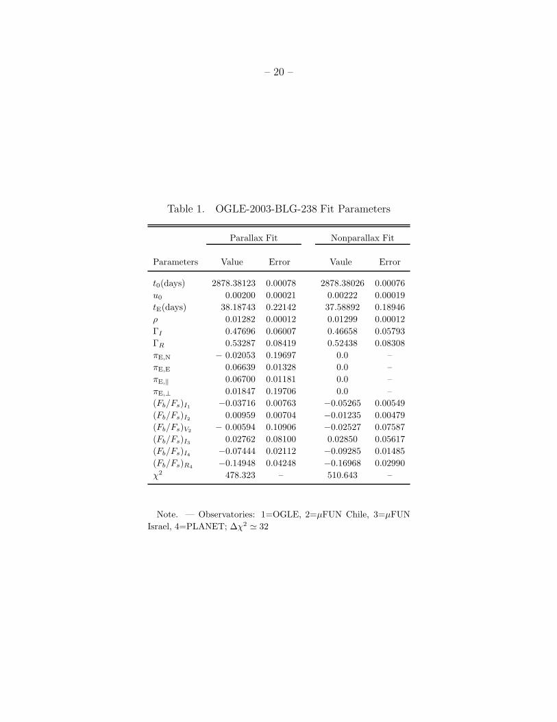
Table 1. OGLE-2003-BLG-238 Fit Parameters

Parallax Fit Nonparallax Fit

Parameters Value Error Vaule Error

t0(days) 2878.38123 0.00078 2878.38026 0.00076

u0 0.00200 0.00021 0.00222 0.00019

tE(days) 38.18743 0.22142 37.58892 0.18946

ρ 0.01282 0.00012 0.01299 0.00012

ΓI 0.47696 0.06007 0.46658 0.05793

ΓR 0.53287 0.08419 0.52438 0.08308

πE,N − 0.02053 0.19697 0.0 –

πE,E 0.06639 0.01328 0.0 –

πE,‖ 0.06700 0.01181 0.0 –

πE,⊥ 0.01847 0.19706 0.0 –

(Fb/Fs)I1 −0.03716 0.00763 −0.05265 0.00549

(Fb/Fs)I2 0.00959 0.00704 −0.01235 0.00479

(Fb/Fs)V2− 0.00594 0.10906 −0.02527 0.07587

(Fb/Fs)I3 0.02762 0.08100 0.02850 0.05617

(Fb/Fs)I4 −0.07444 0.02112 −0.09285 0.01485

(Fb/Fs)R4−0.14948 0.04248 −0.16968 0.02990

χ2 478.323 – 510.643 –

Note. — Observatories: 1=OGLE, 2=µFUN Chile, 3=µFUN

Israel, 4=PLANET; ∆χ2 ≃ 32

– 21 –

I(O

GLE

)

2870 2880 289015

14

13

12

11

10

77 78 79 8013

12

11

10

HJD−2,450,000

resi

dual

2870 2880 2890.1

.05

0

−.05

−.1

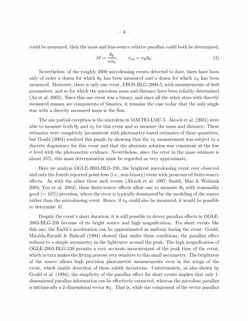
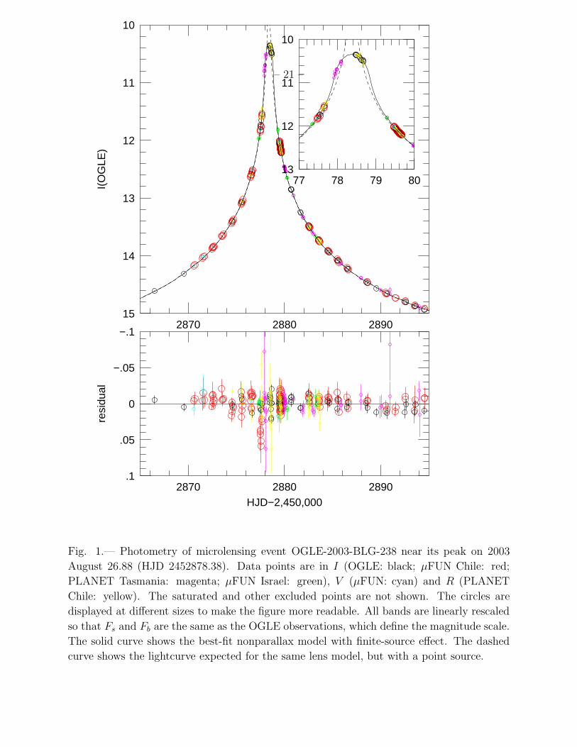
Fig. 1.— Photometry of microlensing event OGLE-2003-BLG-238 near its peak on 2003

August 26.88 (HJD 2452878.38). Data points are in I (OGLE: black; µFUN Chile: red;

PLANET Tasmania: magenta; µFUN Israel: green), V (µFUN: cyan) and R (PLANET

Chile: yellow). The saturated and other excluded points are not shown. The circles are

displayed at different sizes to make the figure more readable. All bands are linearly rescaled

so that Fs and Fb are the same as the OGLE observations, which define the magnitude scale.

The solid curve shows the best-fit nonparallax model with finite-source effect. The dashed

curve shows the lightcurve expected for the same lens model, but with a point source.

– 22 –

0.2 0-1

-0.5

0

0.5

1

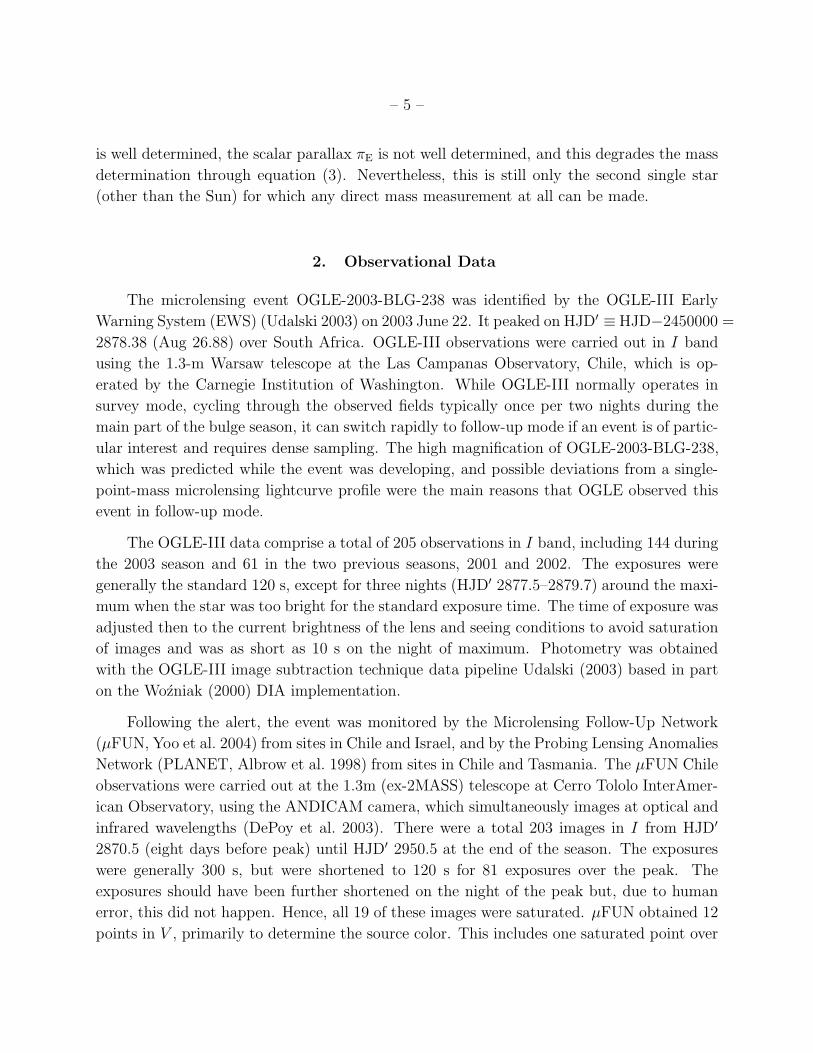
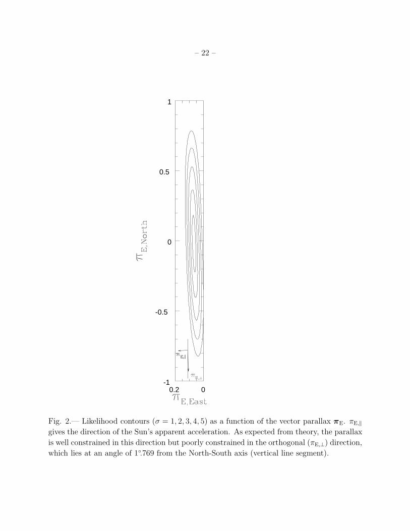
Fig. 2.— Likelihood contours (σ = 1, 2, 3, 4, 5) as a function of the vector parallax πE. πE,‖

gives the direction of the Sun’s apparent acceleration. As expected from theory, the parallax

is well constrained in this direction but poorly constrained in the orthogonal (πE,⊥) direction,

which lies at an angle of 1◦.769 from the North-South axis (vertical line segment).

– 23 –

(V−I)0

I 0

0 .5 1 1.518

17

16

15

14

13

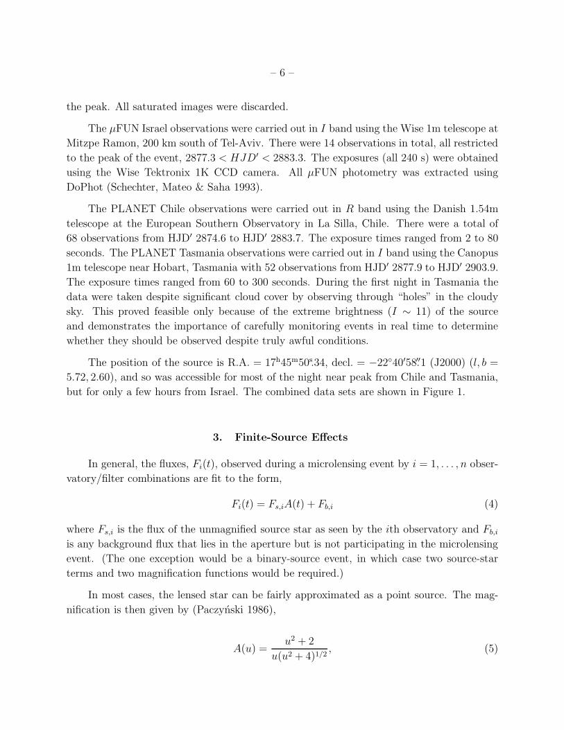
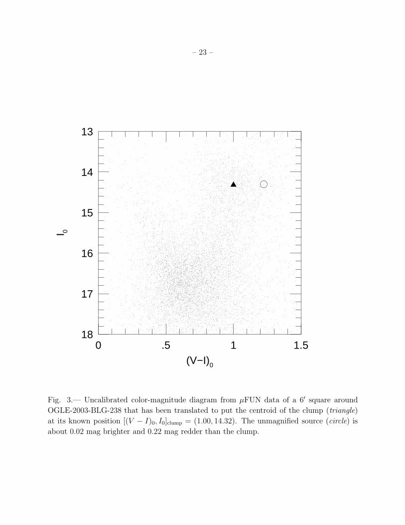
Fig. 3.— Uncalibrated color-magnitude diagram from µFUN data of a 6′ square around

OGLE-2003-BLG-238 that has been translated to put the centroid of the clump (triangle)

at its known position [(V − I)0, I0]clump = (1.00, 14.32). The unmagnified source (circle) is

about 0.02 mag brighter and 0.22 mag redder than the clump.