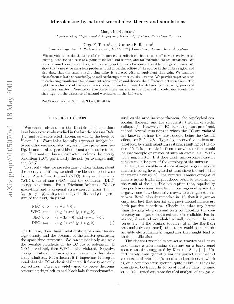
arX

iv:g

r-qc

/010

5070

v1 1

8 M

ay 2

001

Microlensing by natural wormholes: theory and simulations

Margarita Safonova∗

Department of Physics and Astrophysics, University of Delhi, New Delhi–7, India

Diego F. Torres† and Gustavo E. Romero‡

Instituto Argentino de Radioastronomıa, C.C.5, 1894 Villa Elisa, Buenos Aires, Argentina

We provide an in depth study of the theoretical peculiarities that arise in effective negative masslensing, both for the case of a point mass lens and source, and for extended source situations. Wedescribe novel observational signatures arising in the case of a source lensed by a negative mass. Weshow that a negative mass lens produces total or partial eclipse of the source in the umbra region andalso show that the usual Shapiro time delay is replaced with an equivalent time gain. We describethese features both theoretically, as well as through numerical simulations. We provide negative massmicrolensing simulations for various intensity profiles and discuss the differences between them. Thelight curves for microlensing events are presented and contrasted with those due to lensing producedby normal matter. Presence or absence of these features in the observed microlensing events canshed light on the existence of natural wormholes in the Universe.

PACS numbers: 95.30.Sf, 98.90.+s, 04.20.Gz

I. INTRODUCTION

Wormhole solutions to the Einstein field equationshave been extensively studied in the last decade (see Refs.[1,2] and references cited therein, as well as the book byVisser [3]). Wormholes basically represent bridges be-tween otherwise separated regions of the space-time (seeFig. 1) and need a special kind of matter in order to ex-ist. This matter, known as exotic, violates the energyconditions (EC), particularly the null (or averaged null)one [3,6,7].

To specify what we are referring to when talking aboutthe energy conditions, we shall provide their point-wiseform. Apart from the null (NEC), they are the weak(WEC), the strong (SEC), and the dominant (DEC)energy conditions. For a Friedman-Robertson-Walkerspace-time and a diagonal stress-energy tensor Tµν =(ρ,−p,−p,−p) with ρ the energy density and p the pres-sure of the fluid, they read:

NEC ⇐⇒ (ρ+ p ≥ 0),

WEC ⇐⇒ (ρ ≥ 0) and (ρ+ p ≥ 0),

SEC ⇐⇒ (ρ+ 3p ≥ 0) and (ρ+ p ≥ 0),

DEC ⇐⇒ (ρ ≥ 0) and (ρ± p ≥ 0). (1)

The EC are, then, linear relationships between the en-ergy density and the pressure of the matter generatingthe space-time curvature. We can immediately see whythe possible violations of the EC are so polemical. IfNEC is violated, then WEC is also violated. Negativeenergy densities—and so negative masses—are thus phys-ically admitted. Nevertheless, it is important to keep inmind that the EC of classical General Relativity are onlyconjectures. They are widely used to prove theoremsconcerning singularities and black hole thermodynamics,

such as the area increase theorem, the topological cen-sorship theorem, and the singularity theorem of stellarcollapse [3]. However, all EC lack a rigorous proof and,indeed, several situations in which the EC are violatedare known; perhaps the most quoted being the Casimireffect, see Refs. [2,8]. Typically, observed violations areproduced by small quantum systems, resulting of the or-der of h. It is currently far from clear whether there couldbe macroscopic quantities of such an exotic, e.g. WEC-violating, matter. If it does exist, macroscopic negativemasses could be part of the ontology of the universe.

In fact, the possible existence of negative gravitationalmasses is being investigated at least since the end of thenineteenth century [9]. The empirical absence of negativemasses in the Earth neighborhood could be explained asthe result of the plausible assumption that, repelled bythe positive masses prevalent in our region of space, thenegative ones have been driven away to extragalactic dis-tances. Bondi already remarked in [10] that it is just anempirical fact that inertial and gravitational masses areboth positive quantities. Clearly, no other way betterthan devising observational tests for deciding the con-troversy on negative mass existence is available. For in-stance, if natural wormholes actually exist in the uni-verse (e.g. if the original topology after the Big-Bangwas multiply connected), then there could be some ob-servable electromagnetic signatures that might lead totheir identification.

The idea that wormholes can act as gravitational lensesand induce a microlensing signature on a backgroundsource was first suggested by Kim and Sung [11]. Un-fortunately, their geometry was of a perfect alignment ofa source, both wormhole’s mouths and an observer, whichis, on a common sense ground, quite unlikely. They alsoconsidered both mouths to be of positive mass. Crameret al. [12] carried out more detailed analysis of a negative

1

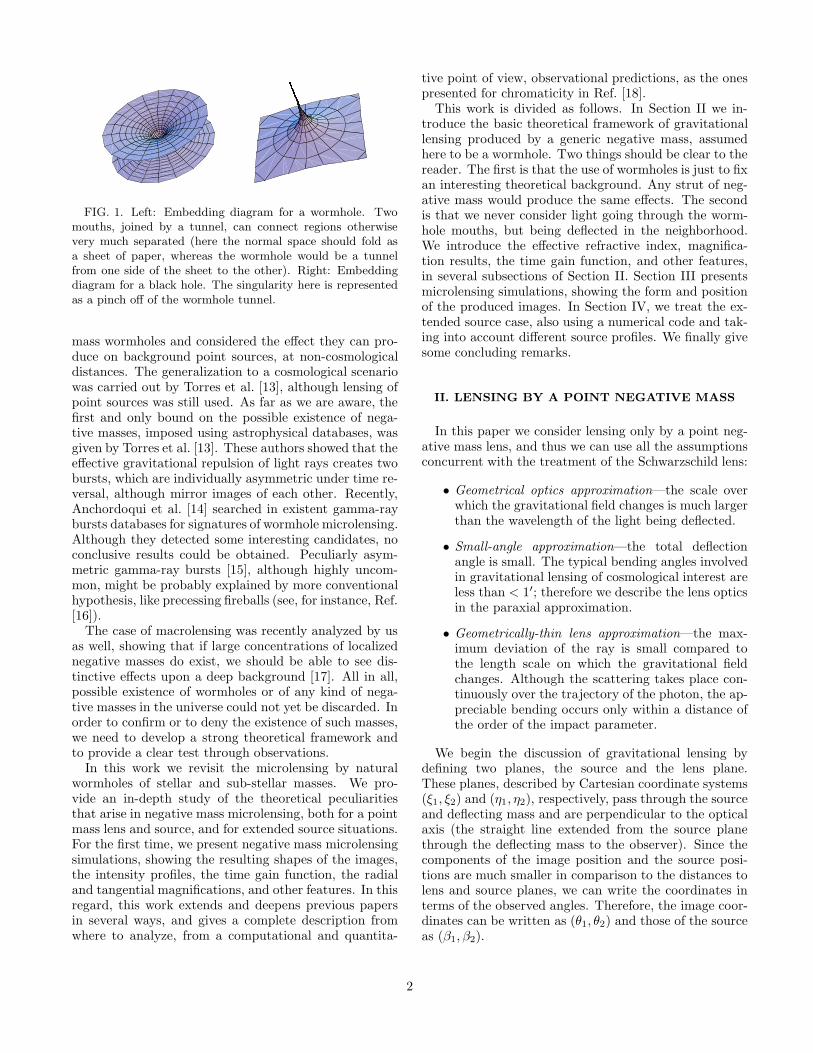
FIG. 1. Left: Embedding diagram for a wormhole. Twomouths, joined by a tunnel, can connect regions otherwisevery much separated (here the normal space should fold asa sheet of paper, whereas the wormhole would be a tunnelfrom one side of the sheet to the other). Right: Embeddingdiagram for a black hole. The singularity here is representedas a pinch off of the wormhole tunnel.

mass wormholes and considered the effect they can pro-duce on background point sources, at non-cosmologicaldistances. The generalization to a cosmological scenariowas carried out by Torres et al. [13], although lensing ofpoint sources was still used. As far as we are aware, thefirst and only bound on the possible existence of nega-tive masses, imposed using astrophysical databases, wasgiven by Torres et al. [13]. These authors showed that theeffective gravitational repulsion of light rays creates twobursts, which are individually asymmetric under time re-versal, although mirror images of each other. Recently,Anchordoqui et al. [14] searched in existent gamma-raybursts databases for signatures of wormhole microlensing.Although they detected some interesting candidates, noconclusive results could be obtained. Peculiarly asym-metric gamma-ray bursts [15], although highly uncom-mon, might be probably explained by more conventionalhypothesis, like precessing fireballs (see, for instance, Ref.[16]).

The case of macrolensing was recently analyzed by usas well, showing that if large concentrations of localizednegative masses do exist, we should be able to see dis-tinctive effects upon a deep background [17]. All in all,possible existence of wormholes or of any kind of nega-tive masses in the universe could not yet be discarded. Inorder to confirm or to deny the existence of such masses,we need to develop a strong theoretical framework andto provide a clear test through observations.

In this work we revisit the microlensing by naturalwormholes of stellar and sub-stellar masses. We pro-vide an in-depth study of the theoretical peculiaritiesthat arise in negative mass microlensing, both for a pointmass lens and source, and for extended source situations.For the first time, we present negative mass microlensingsimulations, showing the resulting shapes of the images,the intensity profiles, the time gain function, the radialand tangential magnifications, and other features. In thisregard, this work extends and deepens previous papersin several ways, and gives a complete description fromwhere to analyze, from a computational and quantita-

tive point of view, observational predictions, as the onespresented for chromaticity in Ref. [18].

This work is divided as follows. In Section II we in-troduce the basic theoretical framework of gravitationallensing produced by a generic negative mass, assumedhere to be a wormhole. Two things should be clear to thereader. The first is that the use of wormholes is just to fixan interesting theoretical background. Any strut of neg-ative mass would produce the same effects. The secondis that we never consider light going through the worm-hole mouths, but being deflected in the neighborhood.We introduce the effective refractive index, magnifica-tion results, the time gain function, and other features,in several subsections of Section II. Section III presentsmicrolensing simulations, showing the form and positionof the produced images. In Section IV, we treat the ex-tended source case, also using a numerical code and tak-ing into account different source profiles. We finally givesome concluding remarks.

II. LENSING BY A POINT NEGATIVE MASS

In this paper we consider lensing only by a point neg-ative mass lens, and thus we can use all the assumptionsconcurrent with the treatment of the Schwarzschild lens:

• Geometrical optics approximation—the scale overwhich the gravitational field changes is much largerthan the wavelength of the light being deflected.

• Small-angle approximation—the total deflectionangle is small. The typical bending angles involvedin gravitational lensing of cosmological interest areless than < 1′; therefore we describe the lens opticsin the paraxial approximation.

• Geometrically-thin lens approximation—the max-imum deviation of the ray is small compared tothe length scale on which the gravitational fieldchanges. Although the scattering takes place con-tinuously over the trajectory of the photon, the ap-preciable bending occurs only within a distance ofthe order of the impact parameter.

We begin the discussion of gravitational lensing bydefining two planes, the source and the lens plane.These planes, described by Cartesian coordinate systems(ξ1, ξ2) and (η1, η2), respectively, pass through the sourceand deflecting mass and are perpendicular to the opticalaxis (the straight line extended from the source planethrough the deflecting mass to the observer). Since thecomponents of the image position and the source posi-tions are much smaller in comparison to the distances tolens and source planes, we can write the coordinates interms of the observed angles. Therefore, the image coor-dinates can be written as (θ1, θ2) and those of the sourceas (β1, β2).

2

A. Effective refractive index of the gravitational

field of a negative mass and the deflection angle

The ‘Newtonian’ potential of a negative point masslens is given by

Φ(ξ, z) =G|M |

(b2 + z2)1/2, (2)

where b is the impact parameter of the unperturbed lightray and z is the distance along the unperturbed lightray from the point of closest approach. We have usedthe term Newtonian in quotation marks since it is, inprinciple, different from the usual one. Here the poten-tial is positive defined and approaching zero at infinity[3]. In view of the assumptions stated above, we candescribe light propagation close to the lens in a locallyMinkowskian space-time perturbed by the positive grav-itational potential of the lens to first post-Newtonian or-der. In this weak field limit, we describe the metric of thenegative mass body in orthonormal coordinates x0 = ct,x = (xi) by

ds2 ≈(

1 +2Φ

c2

)

c2dt2 −(

1 − 2Φ

c2

)

dl2, (3)

where dl = |x| denotes Euclidean arc length. The ef-fect of the space-time curvature on the propagation oflight can be expressed in terms of an effective index ofrefraction neff [19], which is given by

neff = 1 − 2

c2Φ . (4)

Thus, the effective speed of light in the field of a negativemass is

veff = c/neff ≈ c+2

cΦ . (5)

Because of the increase in the effective speed of lightin the gravitational field of a negative mass, light rayswould arrive faster than those following a similar pathin vacuum. This leads to a very interesting effect whencompared with the propagation of a light signal in thegravitational field of a positive mass. In that case, lightrays are delayed relative to propagation in vacuum—thewell known Shapiro time delay. In the case of a negativemass lensing, this effect is replaced by a new one, whichwe shall call time gain. We will describe this effect inmore detail in the following subsections.

Defining the deflection angle as the difference of theinitial and final ray direction

α := ein − eout, (6)

where e := dx/dl is the unit tangent vector of a ray x(l),we obtain the deflection angle as the integral along thelight path of the gradient of the gravitational potential

α =2

c2

∫

∇⊥Φdl , (7)

where ∇⊥Φ denotes the projection of ∇Φ onto the planeorthogonal to the direction e of the ray. We find

∇⊥Φ(b, z) = − G|M |b(b2 + z2)3/2

. (8)

Eq. 7 then yields the deflection angle

α = −4G|M |bc2b2

. (9)

It is interesting to point out that in the case of the neg-ative mass lensing, the term ‘deflection’ has its rightfulmeaning—the light is deflected away from the mass, un-like in the positive mass lensing, where it is bent towardsthe mass.

B. Lensing geometry and lens equation

b

O

W

SI

DD

Dl

ls s

1

α

β

β

β

θ

^

~

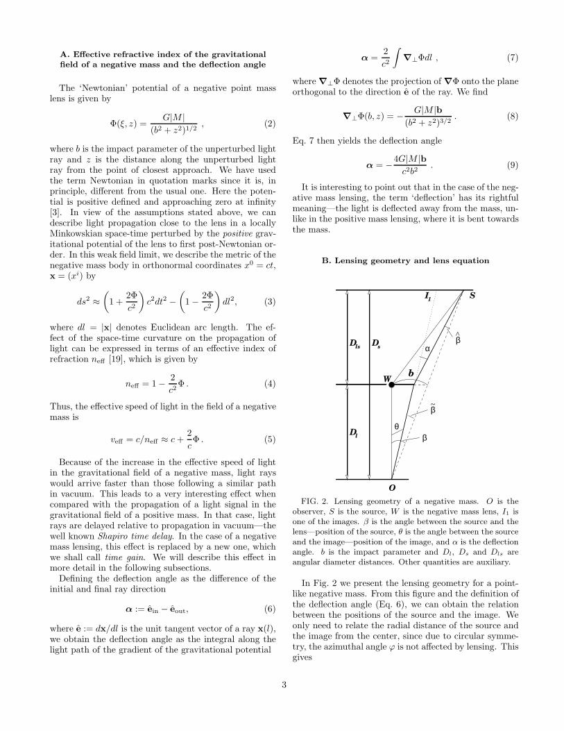
FIG. 2. Lensing geometry of a negative mass. O is theobserver, S is the source, W is the negative mass lens, I1 isone of the images. β is the angle between the source and thelens—position of the source, θ is the angle between the sourceand the image—position of the image, and α is the deflectionangle. b is the impact parameter and Dl, Ds and Dls areangular diameter distances. Other quantities are auxiliary.

In Fig. 2 we present the lensing geometry for a point-like negative mass. From this figure and the definition ofthe deflection angle (Eq. 6), we can obtain the relationbetween the positions of the source and the image. Weonly need to relate the radial distance of the source andthe image from the center, since due to circular symme-try, the azimuthal angle ϕ is not affected by lensing. Thisgives

3

(β − θ)Ds = −αDls (10)

or

β = θ − Dls

Ds

α . (11)

With the deflection angle (Eq. 9), we can write the lensequation as

β = θ +4G|M |c2ξ

Dls

Ds= θ +

4G|M |c2

Dls

DsDl

1

θ. (12)

C. Einstein radius and the formation of images

A natural angular scale in this problem is given by thequantity

θ2E =4G|M |c2

Dls

DsDl

, (13)

which is called the Einstein angle. In the case of apositive point mass lens, this corresponds to the angleat which the Einstein ring is formed, happening whensource, lens and observer are perfectly aligned. As wewill see later in this section, this does not happen if themass of the lens is negative. There are other differencesas well. A typical angular separation of images is of or-der 2 θE for a positive mass lens. Sources which are closerthan about θE to the optical axis are significantly magni-fied, whereas sources which are located well outside theEinstein ring are magnified very little. All this is differentwith a negative mass lens, but nonetheless, the Einsteinangle remains a useful scale for the description of the var-ious regimes in the present case and, therefore, we shalluse the same nomenclature for its definition.

The Einstein angle corresponds to the Einstein radiusin the linear scale (in the lens plane):

RE = θEDl =

√

4GM

c2DlsDl

Ds

. (14)

In terms of Einstein angle the lens equation takes theform

β = θ +θ2Eθ, (15)

which can be solved to obtain two solutions for the imageposition θ:

θ1,2 =1

2

(

β ±√

β2 − 4θ2E

)

. (16)

Unlike in the lensing due to positive masses, we find thatthere are three distinct regimes here and, thus, can clas-sify the lensing phenomenon as follows:

I: β < 2θE There is no real solution for the lensequation. It means that there are no images whenthe source is inside twice the Einstein angle.

II: β > 2θE There are two solutions, corresponding totwo images both on the same side of the lens andbetween the source and the lens. One is always in-side the Einstein angle, the other is always outsideit.

III: β = 2 θE This is a degenerate case, θ1,2 = θE;two images merge at the Einstein angular radius,forming the radial arc (see § II E).

We also obtain two important scales, one is the Ein-stein angle (θE)—the angular radius of the radial criticalcurve, the other is twice the Einstein angle (2 θE)—theangular radius of the caustic. Thus, we have two images,one is always inside the θE, one is always outside; and asa source approaches the caustic (2 θE) from the positiveside, two images coming closer and closer together, andnearer and the critical curve, thereby brightening. Whenthe source crosses the caustic, the two images merge onthe critical curve (θE) and disappear.

D. Time Gain and Time-Offset Function

Following [20], we define a scalar potential, ψ(θ), whichis the appropriately scaled projected Newtonian potentialof the lens,

ψ(θ) =Dls

DlDs

2

c2

∫

Φ(Dlθ, z)dz . (17)

For a negative point mass lens it is

ψ(θ) =Dls

DlDs

4G|M |c2

ln |θ| . (18)

The derivative of ψ with respect to θ is the deflectionangle

∇θψ = Dl∇bψ =2

c2Dls

Ds

∫

∇⊥Φdz = α . (19)

Thus, the deflection angle is the gradient of ψ—the de-flection potential

α(θ) = ∇θψ . (20)

¿From this fact and the lens equation (11) we obtain

(θ − β) + ∇θψ(θ) = 0 . (21)

This equation can be written as a gradient,

∇θ

[

1

2(θ − β)2 + ψ(θ)

]

= 0 . (22)

If we compare this equation with that for the Fermat’sprinciple [20]

4

∇θ t(θ) = 0 , (23)

we see that we can define the time-offset function (oppo-site to time-delay function in the case of positive masslens) as

t(θ) =(1 + zl)

c

DlDs

Dls

[

1

2(θ − β)2 + ψ(θ)

]

= tgeom + tpot,

(24)

where tgeom is the geometrical time delay due to the ex-tra path length of the deflected light ray relative to theunperturbed one. It remains the same as in the positivecase—increase of light-travel-time relative to an unbentray. The coefficient in front of the square brackets en-sures that the quantity corresponds to the time offset asmeasured by the observer. The second term tpot is thetime gain a ray experiences as it traverses the deflectionpotential ψ(θ), with an extra factor (1 + zl) for the cos-mological ‘redshifting’. Thus, cosmological geometricaltime delay is

tgeom =(1 + zl)

c

DlDs

Dls

1

2(θ − β)2 , (25)

and cosmological potential time gain is

tpot =(1 + zl)

c

DlDs

Dls

ψ(θ) . (26)

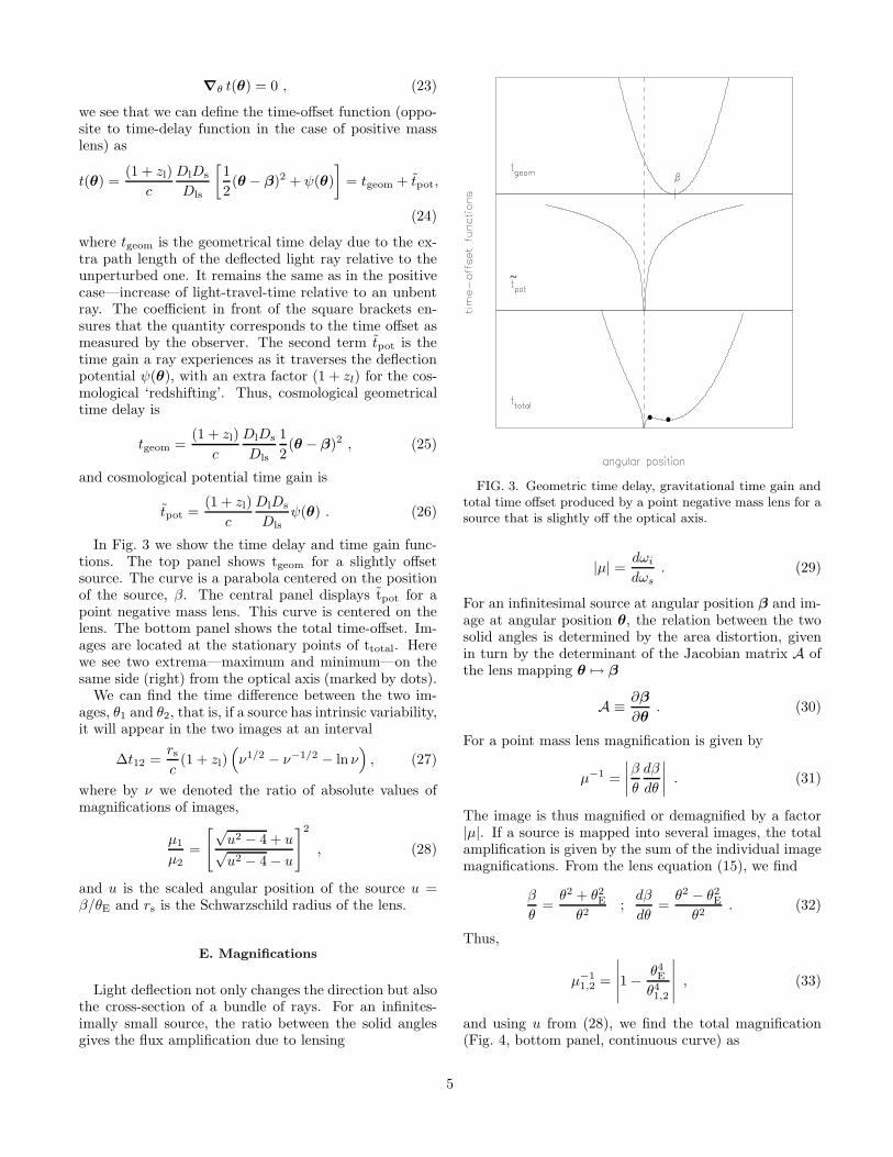
In Fig. 3 we show the time delay and time gain func-tions. The top panel shows tgeom for a slightly offsetsource. The curve is a parabola centered on the positionof the source, β. The central panel displays tpot for apoint negative mass lens. This curve is centered on thelens. The bottom panel shows the total time-offset. Im-ages are located at the stationary points of ttotal. Herewe see two extrema—maximum and minimum—on thesame side (right) from the optical axis (marked by dots).

We can find the time difference between the two im-ages, θ1 and θ2, that is, if a source has intrinsic variability,it will appear in the two images at an interval

∆t12 =rsc

(1 + zl)(

ν1/2 − ν−1/2 − ln ν)

, (27)

where by ν we denoted the ratio of absolute values ofmagnifications of images,

µ1

µ2

=

[√u2 − 4 + u√u2 − 4 − u

]2

, (28)

and u is the scaled angular position of the source u =β/θE and rs is the Schwarzschild radius of the lens.

E. Magnifications

Light deflection not only changes the direction but alsothe cross-section of a bundle of rays. For an infinites-imally small source, the ratio between the solid anglesgives the flux amplification due to lensing

~

FIG. 3. Geometric time delay, gravitational time gain andtotal time offset produced by a point negative mass lens for asource that is slightly off the optical axis.

|µ| =dωi

dωs. (29)

For an infinitesimal source at angular position β and im-age at angular position θ, the relation between the twosolid angles is determined by the area distortion, givenin turn by the determinant of the Jacobian matrix A ofthe lens mapping θ 7→ β

A ≡ ∂β

∂θ. (30)

For a point mass lens magnification is given by

µ−1 =

∣

∣

∣

∣

β

θ

dβ

dθ

∣

∣

∣

∣

. (31)

The image is thus magnified or demagnified by a factor|µ|. If a source is mapped into several images, the totalamplification is given by the sum of the individual imagemagnifications. From the lens equation (15), we find

β

θ=θ2 + θ2Eθ2

;dβ

dθ=θ2 − θ2Eθ2

. (32)

Thus,

µ−11,2 =

∣

∣

∣

∣

∣

1 − θ4Eθ41,2

∣

∣

∣

∣

∣

, (33)

and using u from (28), we find the total magnification(Fig. 4, bottom panel, continuous curve) as

5

µtot = |µ1| + |µ2| =u2 − 2

u√u2 − 4

. (34)

The tangential and radial critical curves follow fromthe singularities in

µtan =

∣

∣

∣

∣

β

θ

∣

∣

∣

∣

−1

=θ2

θ2 + θ2E(35)

and

µrad =

∣

∣

∣

∣

dβ

dθ

∣

∣

∣

∣

−1

=θ2

θ2 − θ2E. (36)

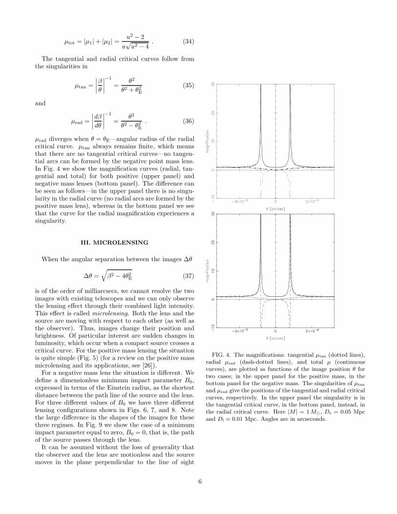
µrad diverges when θ = θE—angular radius of the radialcritical curve. µtan always remains finite, which meansthat there are no tangential critical curves—no tangen-tial arcs can be formed by the negative point mass lens.In Fig. 4 we show the magnification curves (radial, tan-gential and total) for both positive (upper panel) andnegative mass lenses (bottom panel). The difference canbe seen as follows—in the upper panel there is no singu-larity in the radial curve (no radial arcs are formed by thepositive mass lens), whereas in the bottom panel we seethat the curve for the radial magnification experiences asingularity.

III. MICROLENSING

When the angular separation between the images ∆θ

∆θ =√

β2 − 4θ2E (37)

is of the order of milliarcsecs, we cannot resolve the twoimages with existing telescopes and we can only observethe lensing effect through their combined light intensity.This effect is called microlensing. Both the lens and thesource are moving with respect to each other (as well asthe observer). Thus, images change their position andbrightness. Of particular interest are sudden changes inluminosity, which occur when a compact source crosses acritical curve. For the positive mass lensing the situationis quite simple (Fig. 5) (for a review on the positive massmicrolensing and its applications, see [26]).

For a negative mass lens the situation is different. Wedefine a dimensionless minimum impact parameter B0,expressed in terms of the Einstein radius, as the shortestdistance between the path line of the source and the lens.For three different values of B0 we have three differentlensing configurations shown in Figs. 6, 7, and 8. Notethe large difference in the shapes of the images for thesethree regimes. In Fig. 9 we show the case of a minimumimpact parameter equal to zero, B0 = 0, that is, the pathof the source passes through the lens.

It can be assumed without the loss of generality thatthe observer and the lens are motionless and the sourcemoves in the plane perpendicular to the line of sight

FIG. 4. The magnifications: tangential µtan (dotted lines),radial µrad (dash-dotted lines), and total µ (continuouscurves), are plotted as functions of the image position θ fortwo cases; in the upper panel for the positive mass, in thebottom panel for the negative mass. The singularities of µtan

and µrad give the positions of the tangential and radial criticalcurves, respectively. In the upper panel the singularity is inthe tangential critical curve, in the bottom panel, instead, inthe radial critical curve. Here |M | = 1 M⊙, Ds = 0.05 Mpcand Dl = 0.01 Mpc. Angles are in arcseconds.

6

FIG. 5. Schematic representation of the geometry of thepositive mass lensing due to the motion of the source, lens andthe observer (in this case we can consider only the motion ofthe source in the plane perpendicular to the optical axis). Thelens is indicated with a dot at the center of the Einstein ring,which is marked with a dashed line. The positions of thesource center are shown with a series of small open circles.The locations and the shapes of the two images are shownwith a series of dark ellipses. At any instant, the two images,the source and the lens are all on a single line, as shown inthe figure for one particular instant.

FIG. 6. True motion of the source and apparent motion ofthe images for B0 > 2. The inner dashed circle is the Einsteinring, the outer dashed circle is twice the Einstein ring. Therest is as in Fig. 5.

FIG. 7. True motion of the source and apparent motion ofthe images for B0 = 2. The inner dashed circle is the Einsteinring, the outer dashed circle is twice the Einstein ring. Therest is as in Fig. 5.

FIG. 8. True motion of the source and apparent motion ofthe images for B0 < 2. The inner dashed circle is the Einsteinring, the outer dashed circle is twice the Einstein ring. Therest is as in Fig. 5.

7

FIG. 9. True motion of the source and apparent motionof the images for B0 = 0. The inner dashed circle is theEinstein ring, the outer dashed circle is twice the Einsteinring. Images here are shown with the shaded ellipses. Therest is as in Fig. 5.

(therefore, changing its position in the source plane). Weadopt the treatment given in [21] for the velocity V , andconsider effective transverse velocity of the source rela-tive to the critical curve (see Appendix A). We define thetime scale of the microlensing event as the time it takesthe source to move across the Einstein radius, projectedonto the source plane, ξ0 = θEDs,

tv =ξ0V. (38)

Angle β changes with time according to

β(t) =

√

(

V t

Ds

)2

+ β20 . (39)

Here the moment t = 0 corresponds to the smallest an-gular distance β0 between the lens and the source. Nor-malizing (39) to θE ,

u(t) =

√

(

V t

θEDs

)2

+

(

β0

θE

)2

, (40)

where dimensionless impact parameter u is defined in(28). Including the time scale tv and defining

B0 =β0

θE, (41)

we obtain

u(t) =

√

B20 +

(

t

tv

)2

. (42)

Finally, the total amplification as a function of time isgiven by

A(t) =u(t)2 − 2

u(t)√

u(t)2 − 4. (43)

Comparing this analysis with that of Cramer et al. [12],we must note that they wrote the equation for the timedependent dimensionless impact parameter as (cf. ourEq. 42)

B(t) = B0

√

1 +

(

t

T0

)2

,

and defined the time scale for the microlensing event asthe time it takes to cross the minimum impact parameter(cf. our Eq. 38)

T0 =b0V,

where b0 is the minimum impact parameter and othervariables carry the same meanings as in our paper. Whilethere is no mistake in using such definitions, there is adefinite disadvantage in doing so. Using Eq. 10 of [12] forB(t) we cannot build the light curve for the case of theminimum impact parameter B0 = 0. In this case theirEq. 8 diverges, although there is nothing wrong with thisvalue of B0 (see our Figs. 9 and 10). In the same way,their definition of a time scale does not give much infor-mation on the light curves. With our definition (Eq. 38)we can see in Fig. 10 that in the extreme case of B0 = 0the separation between the half-events is exactly 2θE; itis always less than that with any other value of B0.

In Fig. 10 we show the light curves for the point sourcefor four source trajectories with different minimum im-pact parametersB0. As can be seen from the light curves,when the distance from the point mass to the source tra-jectory is larger than 2θE, the light curve is identical tothat of a positive mass lens light curve. However, whenthe distance is less than 2θE (or in other terms, B0 ≤ 2.0),the light curve shows significant differences. Such eventsare characterized by the asymmetrical light curves, whichoccur when a compact source crosses a critical curve. Avery interesting, eclipse-like, phenomenon occurs here; azero intensity region (disappearance of images) with anangular radius θ0

θ0 =√

4θ2E − β20 , (44)

or in terms of normalized unit θE,

∆ =√

4 −B20 . (45)

In the next Section we shall see how these features getaffected by the presence of an extended source.

IV. EXTENDED SOURCE

In the previous sections we considered magnificationsand light curves for point sources. However, sources are

8

FIG. 10. Light curves for the negative mass lensing of apoint source. ¿From the center of the graph towards the cor-ners the curves correspond to B0 = 2.5, 2.0, 1.5, 0.0. The timescale here is ξ0 divided by the effective transverse velocity ofthe source.

extended, and although their size may be small comparedto the relevant length scales of a lensing event, this exten-sion definitely has an impact on the light curves, as willbe demonstrated below. From variability arguments, theoptical and X-ray continuum emitting regions of quasarsare assumed to be much less than 1 pc [22], whereas thebroad-line emission probably has a radius as small as 0.1pc [23]. The high energy gamma-spheres have a typicalradius of 1015 cm [24]. Hence, one has to consider a fairlybroad range of source sizes.

We define here the dimensionless source radius, R, as

R =ρ

θE=R

ξ0, (46)

where ρ and R is the angular and the linear physical sizeof the source, respectively, and ξ0 is the the length unitin the source plane (see Eq. 38).

A. Comments on numerical method and simulations

It is convenient to write the lens equation in the scaledscalar form

y = x+1

x, (47)

where we normalized the coordinates to the Einstein an-gle: 1

x =θ

θE; y =

β

θE. (48)

The lens equation can be solved analytically for anysource position. The amplification factor, and thus thetotal amplification, can be readily calculated for pointsources. However, as we are interested in extendedsources, this amplification has to be integrated over thesource (Eq. 49), and furthermore, as we want to buildthe light curves, the total amplification for an extendedsource has to be calculated for many source positions.The amplification A of an extended source with surfacebrightness profile I(y) is given by

A =

∫

d2yI(y)A0(y)∫

d2yI(y), (49)

where A0(y) is the amplification of a point source atposition y. We have used the numerical method first de-scribed in [25]. We cover the lens plane with a uniformgrid. Each pixel on this grid is mapped, using Eq. 47,into the source plane. The step width (5000 × 5000) ischosen according the desired accuracy (i.e. the observ-able brightness). For a given source position (y01, y02)we calculate the squared deviation function (SDF)

S2 = (y10 − y1(x1, x2))2 + (y20 − y2(x1, x2))

2 . (50)

The solutions of the lens equation (Eq. 48) are given bythe zeroes of the SDF. Besides, Eq. 50 describes circleswith radii S around (y10, y20) in the source plane. Thus,the lines S = const are just the image shapes of a sourcewith radius S, which we plot using standard plotting soft-ware. Therefore, image points where SDF has value S2

correspond to those points of the circular source whichare at a distance S from the center. The surface bright-ness is preserved along the ray and if I(R0) = I0 for thesource, then the same intensity is given to those pixelswhere SDF= R2

0. In this way an intensity profile is cre-ated in the image plane and integrating over it we canobtain the total intensity of an image. Thus, we obtainthe approximate value of the total magnification by esti-mating the total intensity of all the images and dividingit by that of the unlensed source, according to the corre-sponding brightness profile of the source (see AppendixB). For a source with the constant surface brightness theluminosity of the images is proportional to the area en-closed by the line S = const. And the total magnificationis obtained by estimating the total area of all images and

1Note, that for the case in which x and y are expressedin length units, we obtain a different normalization in eachplane, which is not always convenient.

9

dividing it by that of the unlensed source. For calcula-tions of light curves we used a circular source which isdisplaced along a straight line in the source plane withsteps equal to 0.01 of the Einstein angular radius.

B. Results

In Figs. 11 and 12 we show four projected sourceand image positions, critical curves/caustics in thelens/source plane and representative light curves for dif-ferent normalized source sizes. The sources are taken tobe circular disks with constant surface brightness. In or-der to get absolute source radii and real light curves weneed the value of θE, the normalized angular unit, thedistance to the source, as well as the velocity V of thesource relative to the critical curves in the source plane(see Appendix A). We have used M = M⊙, H0 = 100km s−1 Mpc−1 and a standard cosmological model withzero cosmological constant. Here and in all subsequentsimulations the redshift of the source is zs = 0.5 and theredshift of the lens is zl = 0.1.

We display two cases for two different impact param-eters. It must be noted here that the minimum impactparameter B0 defines now the shortest distance betweenthe line of path of the center of the source and the lens.For each one of B0, the dimensionless radius of the sourceR increases from 0.01 to 2.0 in normalized units of θE.The shape of produced images changes notably with theincrease of the source size, as can be seen in the bottomright panel of Figs. 11 and 12. At the same time thesmaller the source the greater the magnification, sincewhen the source radius is greater than the Einstein ra-dius of the lens, the exterior parts, which are amplified,compete with the interior ones, which are demagnified.

It can be noted that, despite the noise in some of thesimulated light curves, the sharp peaks which occur whenthe source is crossing the critical line are well definedeven for the smallest source. Note that all infinities arereplaced now by finite amplifications, and that the curvesare softened; all these effects being generated by the fi-nite size of the source. Indeed, while the impressive dropto zero in the light curve is maintained, the divergence toinfinity, that happens for a point source, is very much re-duced. Note, that in cases of a large size of the source themagnification is very small. If we would like to see big-ger enhancement than that, we should consider sourcesof smaller sizes, approaching the point source situation(cf. Fig. 11, upper left plot).

It is also interesting to note here that for the im-pact parameter B0 = 2.0 the light curve of a small ex-tended source, though approaching the point source pat-tern (Fig. 10), still differs considerably from it (Fig. 12,upper left plot).

In Figs. 13 and 14 we show the images of an extendedsource with a Gaussian brightness distribution for twoeffective dimensionless source radii (Appendix B), RS,

FIG. 11. Four sets of lens-source configurations (upper pan-els) and corresponding amplification as a function of source’scenter position (bottom panels) are shown for four differentvalues of the dimensionless source radius R (0.01, 0.5, 1.0,2.0, in normalized units, θE). Each of the four upper panelsdisplay the time dependent position of the source’s center, theshapes of images (shaded ellipses) and critical curves (dashedcircles). The series of open small circles show the path ofthe source center. The lens is marked by the central cross.Minimum impact parameter B0 = 0. By replacing ξ withξθEDsV

−1 = ξtv we get corresponding time depending lightcurve.

10

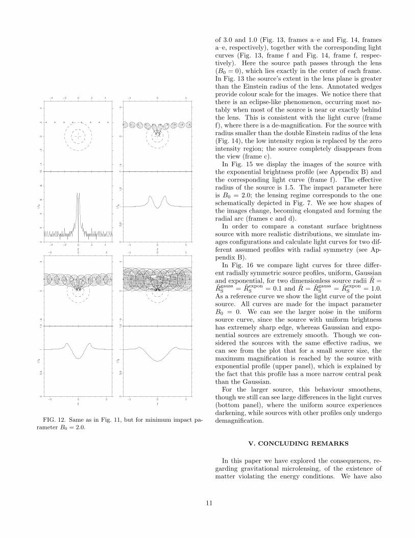
FIG. 12. Same as in Fig. 11, but for minimum impact pa-rameter B0 = 2.0.

of 3.0 and 1.0 (Fig. 13, frames a–e and Fig. 14, framesa–e, respectively), together with the corresponding lightcurves (Fig. 13, frame f and Fig. 14, frame f, respec-tively). Here the source path passes through the lens(B0 = 0), which lies exactly in the center of each frame.In Fig. 13 the source’s extent in the lens plane is greaterthan the Einstein radius of the lens. Annotated wedgesprovide colour scale for the images. We notice there thatthere is an eclipse-like phenomenon, occurring most no-tably when most of the source is near or exactly behindthe lens. This is consistent with the light curve (framef), where there is a de-magnification. For the source withradius smaller than the double Einstein radius of the lens(Fig. 14), the low intensity region is replaced by the zerointensity region; the source completely disappears fromthe view (frame c).

In Fig. 15 we display the images of the source withthe exponential brightness profile (see Appendix B) andthe corresponding light curve (frame f). The effectiveradius of the source is 1.5. The impact parameter hereis B0 = 2.0; the lensing regime corresponds to the oneschematically depicted in Fig. 7. We see how shapes ofthe images change, becoming elongated and forming theradial arc (frames c and d).

In order to compare a constant surface brightnesssource with more realistic distributions, we simulate im-ages configurations and calculate light curves for two dif-ferent assumed profiles with radial symmetry (see Ap-pendix B).

In Fig. 16 we compare light curves for three differ-ent radially symmetric source profiles, uniform, Gaussianand exponential, for two dimensionless source radii R =Rgauss

S = RexponS = 0.1 and R = Rgauss

S = RexponS = 1.0.

As a reference curve we show the light curve of the pointsource. All curves are made for the impact parameterB0 = 0. We can see the larger noise in the uniformsource curve, since the source with uniform brightnesshas extremely sharp edge, whereas Gaussian and expo-nential sources are extremely smooth. Though we con-sidered the sources with the same effective radius, wecan see from the plot that for a small source size, themaximum magnification is reached by the source withexponential profile (upper panel), which is explained bythe fact that this profile has a more narrow central peakthan the Gaussian.

For the larger source, this behaviour smoothens,though we still can see large differences in the light curves(bottom panel), where the uniform source experiencesdarkening, while sources with other profiles only undergodemagnification.

V. CONCLUDING REMARKS

In this paper we have explored the consequences, re-garding gravitational microlensing, of the existence ofmatter violating the energy conditions. We have also

11

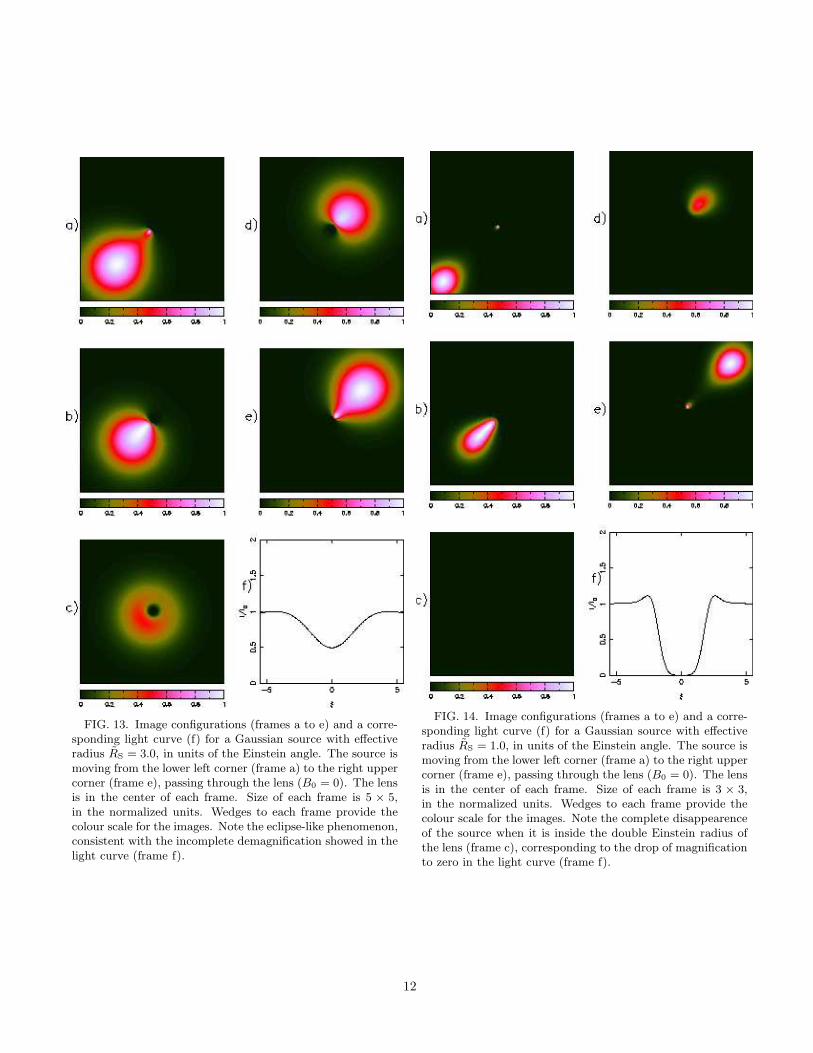
FIG. 13. Image configurations (frames a to e) and a corre-sponding light curve (f) for a Gaussian source with effectiveradius RS = 3.0, in units of the Einstein angle. The source ismoving from the lower left corner (frame a) to the right uppercorner (frame e), passing through the lens (B0 = 0). The lensis in the center of each frame. Size of each frame is 5 × 5,in the normalized units. Wedges to each frame provide thecolour scale for the images. Note the eclipse-like phenomenon,consistent with the incomplete demagnification showed in thelight curve (frame f).

FIG. 14. Image configurations (frames a to e) and a corre-sponding light curve (f) for a Gaussian source with effectiveradius RS = 1.0, in units of the Einstein angle. The source ismoving from the lower left corner (frame a) to the right uppercorner (frame e), passing through the lens (B0 = 0). The lensis in the center of each frame. Size of each frame is 3 × 3,in the normalized units. Wedges to each frame provide thecolour scale for the images. Note the complete disappearenceof the source when it is inside the double Einstein radius ofthe lens (frame c), corresponding to the drop of magnificationto zero in the light curve (frame f).

12

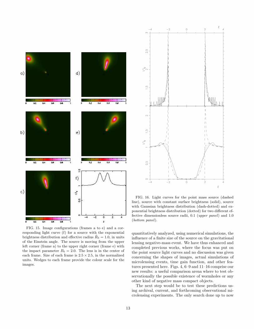
FIG. 15. Image configurations (frames a to e) and a cor-responding light curve (f) for a source with the exponentialbrightness distribution and effective radius RS = 1.0, in unitsof the Einstein angle. The source is moving from the upperleft corner (frame a) to the upper right corner (frame e) withthe impact parameter B0 = 2.0. The lens is in the center ofeach frame. Size of each frame is 2.5× 2.5, in the normalizedunits. Wedges to each frame provide the colour scale for theimages.

FIG. 16. Light curves for the point mass source (dashedline), source with constant surface brightness (solid), sourcewith Gaussian brightness distribution (dash-dotted) and ex-ponential brightness distribution (dotted) for two different ef-fective dimensionless source radii, 0.1 (upper panel) and 1.0(bottom panel).

quantitatively analyzed, using numerical simulations, theinfluence of a finite size of the source on the gravitationallensing negative-mass event. We have thus enhanced andcompleted previous works, where the focus was put onthe point source light curves and no discussion was givenconcerning the shapes of images, actual simulations ofmicrolensing events, time gain function, and other fea-tures presented here. Figs. 4, 6–9 and 11–16 comprise ournew results: a useful comparison arena where to test ob-servationally the possible existence of wormholes or anyother kind of negative mass compact objects.

The next step would be to test these predictions us-ing archival, current, and forthcoming observational mi-crolensing experiments. The only search done up to now

13

included the BATSE database of gamma-ray bursts, butthere is still much unexplored territory in the gravita-tional microlensing archives. We suggest to adapt thealert systems of these experiments in order to include thepossible effects of negative masses as well. This, perhaps,would not imply a burdensome work, but there could bea whole new world of discoveries.

ACKNOWLEDGMENTS

MS is supported by a ICCR scholarship (Indo-RussianExchange programme) and acknowledges the hospitalityof IUCAA, Pune. We would like to deeply thank TarunDeep Saini for his invaluable help with the programmingand Prof. Daksh Lohiya and Prof. M. V. Sazhin foruseful discussions. This work has also been supportedby CONICET (PIP 0430/98, GER), ANPCT (PICT 98No. 03-04881, GER) and Fundacion Antorchas (throughseparate grants to DFT and GER). D.F.T. especially ac-knowledges I. Andruchow for her continuing support.

APPENDIX A: VELOCITIES AND TIME SCALES

Let the source have a transverse velocity vs measuredin the source plane, the lens a transverse velocity vl mea-sured in the lens plane, and the observer a transverse ve-locity vobs measured in the observer plane. The effectivetransverse velocity of the source relative to the criticalcurves with time measured by the observer is

V =1

1 + zsvs −

1

1 + zl

Ds

Dl

vl +1

1 + zl

Dls

Dl

vobs , (A1)

where this effective velocity is such that for a stationaryobserver and lens, the position of the source will changein time according to δξ = V∆t.

We basically have two time scales of interest here. Thefirst one is the typical rise time to a peak in the ampli-fication. We can estimate that it corresponds to a dis-placement of ∆y ∼ R of the source across a critical line;the corresponding time scale τ1 is

τ1 = tvR , (A2)

where tv is given by (38), or in terms of the physical

source size R = ξ0R,

τ1 =R

V, (A3)

where effective transverse velocity of the source V is givenby (A1). The second time scale of interest is the timebetween two peaks τ2. For a point source we can estimateit as

τ2 = tv∆ , (A4)

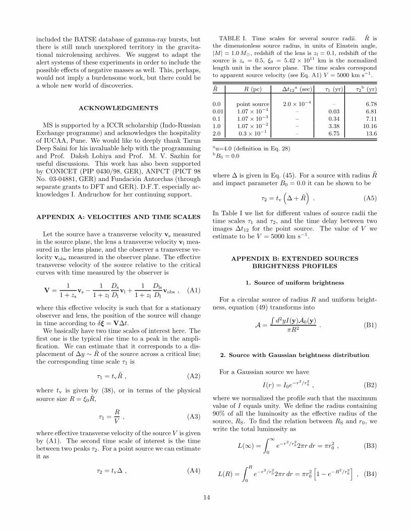
TABLE I. Time scales for several source radii. R isthe dimensionless source radius, in units of Einstein angle,|M | = 1.0 M⊙, redshift of the lens is zl = 0.1, redshift of thesource is zs = 0.5, ξ0 = 5.42 × 1011 km is the normalizedlength unit in the source plane. The time scales correspondto apparent source velocity (see Eq. A1) V = 5000 km s−1.

R R (pc) ∆t12a (sec) τ1 (yr) τ2

b (yr)

0.0 point source 2.0 × 10−4 – 6.780.01 1.07 × 10−4 – 0.03 6.810.1 1.07 × 10−3 – 0.34 7.111.0 1.07 × 10−2 – 3.38 10.162.0 0.3 × 10−1 – 6.75 13.6

au=4.0 (definition in Eq. 28)bB0 = 0.0

where ∆ is given in Eq. (45). For a source with radius Rand impact parameter B0 = 0.0 it can be shown to be

τ2 = tv

(

∆ + R)

. (A5)

In Table I we list for different values of source radii thetime scales τ1 and τ2, and the time delay between twoimages ∆t12 for the point source. The value of V weestimate to be V = 5000 km s−1.

APPENDIX B: EXTENDED SOURCES

BRIGHTNESS PROFILES

1. Source of uniform brightness

For a circular source of radius R and uniform bright-ness, equation (49) transforms into

A =

∫

d2yI(y)A0(y)

πR2. (B1)

2. Source with Gaussian brightness distribution

For a Gaussian source we have

I(r) = I0e−r2/r2

0 , (B2)

where we normalized the profile such that the maximumvalue of I equals unity. We define the radius containing90% of all the luminosity as the effective radius of thesource, RS. To find the relation between RS and r0, wewrite the total luminosity as

L(∞) =

∫ ∞

0

e−r2/r2

02πr dr = πr20 , (B3)

L(R) =

∫ R

0

e−r2/r2

02πr dr = πr20

[

1 − e−R2/r2

0

]

, (B4)

14

then

L(RS)

L(∞)= 0.9 =

[

1 − e−R2

S/r2

0

]

. (B5)

Thus, effective radius relates to the parameter r0 as

RS

r0=

√ln 10 . (B6)

3. Source with exponential brightness distribution

We have

I(r) = I0e−r/r0 . (B7)

In the same manner as above, RS is defined as radius,containing 90% of total luminosity. In the same way asabove, total luminosity

L(∞) =

∫ ∞

0

e−r/r02πr dr = 2πr20 , (B8)

then

L(R) =

∫ R

0

e−r/r02πr dr = 2π[

r20 −(

Rr0 + r20)

e−R/r0

]

,

(B9)

and

L(RS)

L(∞)= 0.9 . (B10)

From where we find that effective radius relates to theparameter r0 as

e−RS/r0

(

1 +RS

r0

)

= 0.1 . (B11)

Solution to this equation gives RS/r0 ≈ 3.89. This pro-file is also normalized such that the maximum value of Iequals unity.

∗ E-mail: rita@iucaa.ernet.in† E-mail: dtorres@venus.fisica.unlp.edu.ar‡ E-mail: romero@irma.iar.unlp.edu.ar[1] M. S. Morris & K. S. Thorne, Am. J. Phys. 56, 395

(1988).[2] L. A. Anchordoqui, S. E. Perez Bergliaffa & D. F. Torres,

Phys. Rev. D 55, 5226 (1997); A. DeBenedictis and A.Das [gr-qc/0009072]; S. E. Perez Bergliaffa and K. E. Hi-bberd, Phys. Rev. D 62, 044045 (2000); C. Barcelo and

M. Visser, Nucl. Phys. B584, 415 (2000); L. A. Anchor-doqui and S. E. Perez Bergliaffa, Phys. Rev. D 62, 067502(2000); D. Hochberg, A. Popov, and S. V. Sushkov, Phys.Rev. Lett. 78, 2050 (1997); S. Kim and H. Lee, Phys.Lett. B 458, 245 (1999); S. Krasnikov, Phys. Rev. D 62,084028 (2000); D. Hochberg and M. Visser, Phys. Rev.D 56, 4745 (1997).

[3] M. Visser, Lorentzian Wormholes (AIP, New York, 1996).[4] M. S. Morris, K. S. Thorne, and U. Yurtsever, Phys. Rev.

Lett. 61, 1446 (1988); V. Frolov and I. D. Novikov, Phys.Rev. D 42, 1057 (1990).

[5] S. W. Hawking, Phys. Rev. D 46, 603 (1992).[6] D. Hochberg and M. Visser, Phys. Rev. Lett. 81, 746

(1998).[7] D. Hochberg and M. Visser, Phys. Rev. D58, 044021

(1998).[8] C. Barcelo and M. Visser, Phys. Lett. B 466, 127 (1999);

M. Visser, talk at the Marcel Grossman Meeting, Rome,July 2000; C. Barcelo and M. Visser, Class. Quant. Grav.17, 3843, (2000).

[9] M. Jammer, Concepts of mass (Dover, New York, 1997).[10] H. Bondi, Rev. Mod. Phys. 29, 423 (1957).[11] S.-W. Kim and Y. M. Cho, in Evolution of the Universe

and its Observational Quest (Universal Academy Press,Inc. and Yamada Science Foundation, 1994), p. 353.

[12] J. Cramer, R. Forward, M. Morris, M. Visser, G. Benford,and G. Landis, Phys. Rev. D 51, 3117 (1995).

[13] D. F. Torres, G. E. Romero, and L. A. Anchordoqui,Phys. Rev. D 58, 123001 (1998); D. F. Torres, G. E.Romero, and L. A. Anchordoqui, (Honorable Mention,Gravity Foundation Research Awards 1998), Mod. Phys.Lett. A13, 1575 (1998).

[14] L. Anchordoqui, G. E. Romero, D. F. Torres, and I. An-druchow, Mod. Phys. Lett. A14, 791 (1999).

[15] G. E. Romero, D. F. Torres, I. Andruchow, L. A. An-chordoqui, and B. Link, Mon. Not. R. Astron. Soc. 308,799 (1999).

[16] S. F. Portegies Zwart, C-H. Lee, and H.K. Lee, Astro-phys. J. 520, 666 (1999).

[17] M. Safonova, D. F. Torres, and G. E. Romero, Mod.Phys. Lett. A16, 153 (2001).

[18] E. Eiroa, G. E. Romero, and D. F. Torres, Chromaticityeffects in wormhole microlensing, Mod. Phys. Lett. A (tobe published, 2001), gr-qc/0104076

[19] P. Schneider, J. Ehlers, and E. E. Falco, GravitationalLenses (Springer-Verlag Berlin Heidelberg New York,1992).

[20] R. Narayan and M. Bartelmann, in Formation of Struc-ture in the Universe, edited by A. Dekel and J. P. Ostriker(Cambridge, Cambridge University Press, 1999), p.360.

[21] R. Kayser, S. Refsdal, and R. Stabell, Astron. Astrophys.166, 36 (1986).

[22] P. Schneider and A. Weiss, Astron. Astrophys. 171, 49(1987).

[23] D. E. Osterbrock, A. T. Koski, and M. M. Phillips, As-trophys. J. 206, 898 (1976).

[24] R. D. Blanford and A. Levinson, Astrophys. J. 441, 79(1995).

[25] T. Schramm and R. Kayser, Astron. Astrophys. 174, 361(1987).

15

[26] M. V. Sazhin and A. F. Zakharov, Usp. Fiz. Nauk [Sov.Phys.–Usp], 168, 1041 (1998).

16