SOFTWARE Open Access

Snazer: the simulations and networks analyzerTommaso Mazza1*, Gennaro Iaccarino1, Corrado Priami1,2

Abstract

Background: Networks are widely recognized as key determinants of structure and function in systems that spanthe biological, physical, and social sciences. They are static pictures of the interactions among the components ofcomplex systems. Often, much effort is required to identify networks as part of particular patterns as well as tovisualize and interpret them.From a pure dynamical perspective, simulation represents a relevant way-out. Many simulator tools capitalized onthe “noisy” behavior of some systems and used formal models to represent cellular activities as temporal trajec-tories. Statistical methods have been applied to a fairly large number of replicated trajectories in order to inferknowledge.A tool which both graphically manipulates reactive models and deals with sets of simulation time-course data byaggregation, interpretation and statistical analysis is missing and could add value to simulators.

Results: We designed and implemented Snazer, the simulations and networks analyzer. Its goal is to aid theprocesses of visualizing and manipulating reactive models, as well as to share and interpret time-course dataproduced by stochastic simulators or by any other means.

Conclusions: Snazer is a solid prototype that integrates biological network and simulation time-course dataanalysis techniques.

BackgroundProteins and genes play fundamental roles in mostorganic functions. They cooperate to keep the entireorganism’s machinery working and prevent breakdowns.Globally, their social relationships give rise to minutelyorganized networks, currently the target of meticulousstudies [1]. Genetic Regulatory Networks (GRNs) [2,3]and Protein-to-Protein Interaction networks (PPIs) arethe most representative classes of biological networks.GRNs represent collections of DNA segments which

functionally interact with each other as well as with thechemicals that govern the transcription of genes intoRNA sequences. From another perspective, GRNs canbe seen as input-output machineries which produce anoutput (i.e. the expression level of a gene) by a com-bined application of basic functions to input stimuli.PPIs are comprised of proteins that form chains inwhich each protein reacts to a stimulus of its predeces-sor to produce a signal directed to its successor. Reac-tions in such chains are usually seen as directionallyoriented because often they are not reversible. A

reaction chain acts as a connector of a triggering eventto a final physiological response and then sets up acomplex (and often cyclic) collaborative network.Both kinds of networks have been collected into sev-

eral data banks spread throughout the WWW [4] andmodeled in a computerized fashion by means of someunambiguous and artificial formalisms. The most com-mon one makes use of coupled Ordinary DifferentialEquations (ODEs) [5]. Alternatively, several other pro-mising modeling techniques have been employed:(including) Boolean networks [6], Petri nets [7], Bayesiannetworks [8], graphical Gaussian models [9], ProcessCalculi [10,11] and Automata Theory [12]. Standard lan-guages, xml- (SBML [13], CellML [14]) or graphical-(SBGN [15], BlenX4Bio [16]) based, have been furtherproposed to allow knowledge sharing. All of them are(roughly) connected to graph theory, since a commonsimple principle holds: interacting agents (e.g. genes,proteins, enzymes, etc.) are represented as the graphvertices whereas interactions (e.g dimerization, phos-phorylation, collision, etc.) constitute the graph edges.Moreover, strength of connections (if any) is usuallymodeled by weighing the edges (e.g. to quantitatively* Correspondence: mazza@cosbi.eu

1The Microsoft Research University of Trento, CoSBi, Trento, Italy

Mazza et al. BMC Systems Biology 2010, 4:1http://www.biomedcentral.com/1752-0509/4/1

© 2010 Mazza et al; licensee BioMed Central Ltd. This is an Open Access article distributed under the terms of the Creative CommonsAttribution License (http://creativecommons.org/licenses/by/2.0), which permits unrestricted use, distribution, and reproduction inany medium, provided the original work is properly cited.

represent fluxes in metabolic networks). Protein-to-pro-tein interaction networks, chemical structures, gene co-expression and contact graphs for protein structures areall examples of undirected graphs, whereas experimentalprotocols and taxonomies of species and traditional reg-ulatory networks are examples of directed graphs. Otherexamples include: DNA, RNA or protein sequences (lin-ear graphs), sequence fragment overlap graphs (intervalgraphs) for shotgun sequence assembly, genetic mapsand multiple sequence alignments (partial orders). Ontop of them, a myriad of graphical- and textual- basedtools has been developed with the aim to simultaneouslymake the process of networks design increasingly moreintuitive and to speed up their functional description. InSec. 2, we itemize the most representative tools and givesome concise explanations of them.Once a network is defined by its constituents and

interactions, it is common practice to simulate the net-work by means of deterministic/stochastic solvers. Thedeterministic solvers cope with interlocking sets of dif-ferential or difference equations and require the specifi-cation of some initial conditions. Its response (y) isfixed, given the values of its input variables (xi), andimplies that var(y|xi) = 0. This property distinguishesdeterministic models from real-life experiments [17].Stochastic solvers use pseudorandom numbers (treatedas if they were random numbers distributed uniformlyand indpendently) to produce different y values, startingfrom the same initial parameters. Hence, the response yis a random variable with var(y|xi) = g(xi), usually esti-mated through replication and fed with different ran-dom numbers. A user-defined accuracy level determineshow many simulation runs are needed [18]. A stochastictrajectory or trace (corresponding to the output of asimulation run) is a sequence of temporal observationsof the copy-number of the species in the state space.Traces are curves generally made by double precision

(64-bit) floating-point numbers sampled over time. Theysketch the trend of some system variables that are chan-ging because of a predefined set of mathematical rules.Based on the continuous or discrete nature of suchrules, the traces format changes accordingly. Continuoustraces exhibit smooth trends of variables regularlyobserved at continuous time-scales. The solution of anODE-based biological system gives the trend of the con-centration of their variables within a desired time inter-val. Therefore, variables change continuously accordingto a mathematical function which solves the ODE’s set.Discrete traces only differ because of their non-homoge-neous temporal sampling. They are evaluated at uneventime instants that are calculated at run-time. Usually,biological discrete systems deal with chemicals popula-tions (in place of chemicals concentrations) and, conse-quently, Markovian trajectories are made of streams of

integer numbers. Sharing both kinds of simulationresults is, to a great extent, hindered by the use of avariety of data formats by the existing simulation soft-ware packages. In fact, most of them output traces deco-rated by proprietary meta-information that containsprivate, not human-readable simulator settings. Fewstandard formats exist, but although some of them seemto be very well-suited and complete, their general-pur-pose nature makes them little versatile for our needs.That is why Snazer has been equipped with an ad-hocand lightweight internal data format.The rest of the paper is organized as follows: Sec. 2

describes all the features of our tool compared to thoseof similar existing tools. Particularly, in Sec. 2.2 thegraph layout algorithms and the analysis features of Sna-zer are presented, whereas in Sec. 2.3 we describe theimplemented statistics routines. In Sec. 2.4, we presentthe internal data format together with the compressionpolicy employed to enhance the storing of data. In Sec.3 we test Snazer on a real case-study with the aim ofhighlighting features and strength points. Then, we per-form some benchmark tests on its compression capabil-ity and show the results. In Sec. 4 we conclude thepaper and present future works.

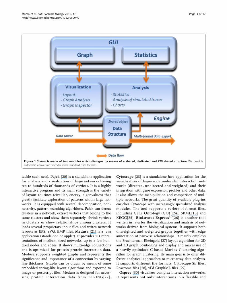
ImplementationSnazer is a software prototype whose aim is threefold: (i)manipulating biological networks, (ii) providingadvanced statistical analysis routines for simulated tracesand (iii) improving the traces sharing and storing pro-cesses. Snazer can also be considered as a viewer pack-age of Beta Workbench (BWB) [19]. By parsing itsoutput files, Snazer imports two relevant pieces of infor-mation inherently bound to the modeled systems: thegraphs of the simulated reactions and the simulatedtraces. It encloses them in a compact XML data struc-ture, designed to work as an interchange data source/sink. Through this, networks and simulation data looktightly coupled.The overall architectural skeleton draws inspiration

from the Model-View-Controller software architecturaldesign pattern and is made up of two parts: the reactiongraph (Sec. 2.2) and the statistics (Sec. 2.3) modules,that deal with visualization of the system interactionsand with calculation of statistics outcomes of simulatedtraces, respectively (see fig. 1). Both modules share theoptimized floating object compliant with the SnazerXML-schema previously mentioned and discussed inSec. 2.4 (cf. Additional Files 1).2.1 State of the artThe rationale behind Snazer comes directly from thescientific community, which needs to manage togetherthe biological models and their simulation results in acoherent manner. Several tools exist that unilaterally

Mazza et al. BMC Systems Biology 2010, 4:1http://www.biomedcentral.com/1752-0509/4/1

Page 2 of 17

tackle such need. Pajek [20] is a standalone applicationfor analysis and visualization of large networks havingten to hundreds of thousands of vertices. It is a highlyinteractive program and its main strength is the varietyof layout routines (circular, energy, eigenvalues) thatgreatly facilitate exploration of patterns within large net-works. It is equipped with several decomposition, con-nectivity, pattern searching algorithms. Pajek can detectclusters in a network, extract vertices that belong to thesame clusters and show them separately, shrink verticesin clusters or show relationships among clusters. Itloads several proprietary input files and writes networklayouts as EPS, SVG, BMP files. Medusa [21] is a Javaapplication (standalone or applet). It provides 2D repre-sentations of medium-sized networks, up to a few hun-dred nodes and edges. It shows multi-edge connectionsand is optimized for protein-protein interaction data.Medusa supports weighted graphs and represents thesignificance and importance of a connection by varyingline thickness. Graphs can be drawn by means of someembedded spring-like layout algorithms and exported toimage or postscript files. Medusa is designed for acces-sing protein interaction data from STRING[22].

Cytoscape [23] is a standalone Java application for thevisualization of large-scale molecular interaction net-works (directed, undirected and weighted) and theirintegration with gene expression profiles and other data.It also allows the manipulation and comparison of mul-tiple networks. The great quantity of available plug-insenriches Cytoscape with increasingly specialized analysismodules. The tool supports a variety of format files,including Gene Ontology (GO) [24], SBML[13] andKEGG[25]. BioLayout Express3D[26] is another toolwritten in Java for the visualization and analysis of net-works derived from biological systems. It supports bothunweighted and weighted graphs together with edgeannotation of pairwise relationships. It mainly employsthe Fruchterman-Rheingold [27] layout algorithm for 2Dand 3D graph positioning and display and makes use ofa heavily optimized C-based Markov Clustering algo-rithm for graph clustering. Its main goal is to offer dif-ferent analytical approaches to microarray data analysis.It supports different file formats: Cytoscape Sif files,Reactome files [28], yEd GraphML files [29].Osprey [30] visualizes complex interaction networks.

It represents not only interactions in a flexible and

Figure 1 Snazer is made of two modules which dialogue by means of a shared, dedicated and XML-based structure. We provideautomatic conversion from/to some standard data formats.

Mazza et al. BMC Systems Biology 2010, 4:1http://www.biomedcentral.com/1752-0509/4/1

Page 3 of 17

rapidly expandable graphical format, but also providesoptions for functional comparisons between data sets.Osprey uses the General Repository for InteractionDatasets as a database (BioGRID) [31], from which theuser can rapidly build interaction networks. Networkscan be saved as tab-delimited text files for future manip-ulation or exported as JPEG, PNG, and SVG. ProViz[32] is a standalone open source application developedfor the visualization of protein-protein interaction net-works. It provides facilities for navigating large graphsand exploring biologically relevant features. It has aplug-in library with dozens of layout algorithms. Basi-cally, they belong to three families: force-based, hier-archical and geometric layout (only circular). ProVizadopts emerging standards such as GO and PSI-MI[33].BiologicalNetworks [34] models whole cell biochemicalpathways and gene regulatory networks. It uses a specia-lized graph visualization engine to represent biologicalpathways, gene regulation networks and protein-proteininteraction maps for intuitive exploration and predic-tion. The tool can handle a variety of tasks, includinggraphic drawing and layout optimization, data filteringand pathway expansion, and classification and prioritiza-tion of proteins. BiologicalNetworks uses a proprietaryfile format (BNX) that stores information pertaining tothe model and the corresponding simulation environ-ment. It supports import and export of models fromSBML, SIF and GML file formats. Finally, Tulip [35] isone of the forerunners of drawing packages for biologi-cal networks. It allows the visualization, drawing andediting of graphs up to a million elements. Such a visua-lization system allows navigation through geometricoperations as well as extraction of subgraphs andenhancement of the results obtained by filtering. Itsmost interesting property is the underlying data struc-ture used to inspect huge graph attributes. Tulip imple-ments the well-known “flyweight” and “chain ofresponsibility” patterns to access graphs through views.The real advantage is enabling a real sharing of the ele-ments between graphs with a good memory manage-ment. All this software improve and obscure the first-generation tools from which they have drawn inspira-tion: Otter [36], a general-purpose network visualizationtool; Negopy [37], a discrete, linkage-based program forthe analysis of networks; KrackPlot [38], a networkvisualization tool intended for social networks; Multi-Net [39], a Windows-based computer program designedfor exploratory data analysis of social and other net-works. Other tools exist that aim at providing advancedstatistics routines for biological traces. Traviando [40] isa backend trace visualizer and analyzer. It interfaces theXML output file of Möbius, a multi-paradigm multi-solution framework for the performance and depend-ability assessment of systems, to investigate the details

of what happened in a simulation of a model. It verifiesthat certain events happen in a trace, that particularstates are frequently reached or that certain conditionshold throughout a simulation. It further analyzes thecyclic behavior with graphics that show if states arerepeatedly visited or how the length of the trace evolvesif cycles are removed. Traviando also supports variousstatistics on traces as well as the model checking of atrace with respect to LTL formulas. SimWiz [41] is anold but still interesting project. It is a collection of Javatools that aims at visualizing data resulting from differ-ent kinds of biochemical simulation processes. Itimports STODE[42] and COPASI[43] simulation outputfiles as well as the relative reaction graphs as SBMLfiles. Its main feature is animating the network graphthrough the information coming from the simulatedtraces. VANTED [44] loads and edits graphs, whichmay represent biological pathways or functional hierar-chies. It allows the mapping of experimental data setsonto the graph elements and visualizes time series dataor data of different genotypes or environmental condi-tions in the context of the underlying biological pro-cesses. Built-in statistic functions allow a fast evaluationof the data (e.g. t-Test or correlation analysis). Pop-Tools [45] is a versatile add-in for Microsoft Excel thatfacilitates analysis of matrix population models andsimulation of stochastic processes. Together with rou-tines for iterating and resampling, this allows the calcu-lation of bootstrap and other statistics for stochasticprocesses. Routines that facilitate calculation of somesimple maximum likelihood and resampling statisticsare supported as well.Snazer addresses many of these issues, but additionally

offers a solid framework that couples networks and tracesanalysis frameworks. It provides the user with the possibi-lity both of browsing, dissecting and analyzing the net-works components and of performing statistics on theinspected components. Snazer has been equipped with anefficient compression system to make huge amount ofdata manageable and treatable as well as to store andshare them. Compared to the existing tools, it covers mostof the network visualization layout routines. In addition, itimplements Temporal-Circuit (see Sec. 2.2), an originalalgorithm to layout networks according to the informationcoming from simulation. It is not as well equipped withdecomposition and connectivity algorithms as Pajek andBioLayout Express3D, because we mainly focused on origi-nal (e.g. ColorBlind filter and standard annotation inspec-tion - see Sec. 2.2.2) rather than existing functionalities.Snazer is cross-platform, being implemented in Java (likeMedusa, Cytoscape and BioLayout Express3D). It struc-tures input data in XML files (as BiologicalNetworks does)and makes use of an internal data structure to improvedata access (like Tulip). At the best of our knowledge,

Mazza et al. BMC Systems Biology 2010, 4:1http://www.biomedcentral.com/1752-0509/4/1

Page 4 of 17

Snazer is the only tool that provides data compression(Sec. 2.4). It supports some standard input data formats(as Medusa, Cytoscape, BioLayout Express3D, ProViz andBiologicalNetworks) to be fully compatible with all theorbiting software packages. Moreover, Snazer offers somenew trace analysis routines that deeply differ from thoseimplemented in the presented softwares. In fact, VANTEDfills network nodes with information coming from biologi-cal experiments (like microarray, proteomics, etc) to statis-tically analyze them. But it does not provide any means toanalyze simulated traces. SimWiz, instead, makes use oftraces to animate the related networks, but it does notprovide any functionality in support of simulation. Tra-viando analyzes individual traces by using classical model-checking methods, but lacks of any support for group-traces. PopTools, offers some statistical facilities for wet-data (as VANTED) and stochastic processes, but disre-gards any group-traces issue as well. Contrarily, Snazercovers these lacks by offering new analysis algorithms cen-tered on multi-traces analysis.All these features are built-in in Snazer and make it a

unique tool.2.2 The reaction graph perspectiveThe focus of network-level analysis in general is onproperties of networks as a whole. These may reflect, e.g. typical or atypical traits relative to an applicationdomain or similarities occurring in networks of entirelydifferent origin. Both from a global and a local view,quantitative analyses have been conducted on networksto investigate these traits. Snazer provides the user withsome clever layout algorithms to firstly give a globalinsight of a network, and with a centrality ranker indexto highlight vertex importance.2.2.1 Layout analysisGraph layout methods are core techniques for applica-tions based on graph-like network diagrams. Since sucha perspective is becoming more and more pervasive, andsince Snazer visualizes part of the data sets as reactiongraphs, we equipped it with the fastest and most flexiblelayout algorithms. Most of them belong to the force-based (or force-directed) class of algorithms. They areeasy to use, since they do not require special knowledgeabout the graph theory, and often their results look verygood. They mainly assign forces to networks as if thenodes were electrically charged particles and the edgeswere springs. Thus, layouts are arranged according toreal physical principles (e.g. Coulomb’s law, Hooke’slaw, etc). As a result, forces repetitively applied to nodespush and pull them further apart in order to minimizethe overall energy of the networks. When an equilibriumstate is reached, the graph is drawn.Such algorithms enjoy several strength-points: uniform

nodes distribution, symmetry, flexibility, simplicity, strongtheoretical foundations, but suffer from some drawbacks:

high running time (equivalent to O(V 3)) and poor localminima. Spring is the simplest force-based layout algo-rithm. Basically, nodes try to get as far of each other aspossible, but edges pull nodes near each other, merelyaccording to their weights. The energy of the system isminimized by iteratively arranging the nodes (fig. 2d). Itenjoys all the strength-points as well as it suffers fromall the drawbacks just mentioned.In particular, the task of bringing under control the

problem of poor local minima raised the interest ofmany scientists. Such issue is based on the fact that theobtained minimum system energy could be considerablyworse than a global minimum. Since such issue becomesmore and more important as the number of vertices ofthe graph increases and, hence, that the overall qualityof the drawing could result lower and lower, somescientists focused on the initial layout sub-problem tosolve it. They conjectured that any outcome of anyforce-based algorithms results to be strongly influencedby the initial layout, that in most cases is randomlygenerated.The Kamada-Kawai (KKLayout) algorithm represents

the first attempt to solve this problem. It was designedwith the aim to quickly generate advantageous initialconfigurations. Nodes are represented by steel rings andthe edges are springs between them. The attractive forceis analogous to the spring force and the repulsive one isanalogous to the electrical force. The energy minimiza-tion in this algorithm is achieved by obtaining the deri-vative of the force equations. At the minimum energy,the derivatives of the force equations are zero. Sincethese equations are not independent, they cannot beindependently brought to zero, and therefore, only thenode that has the maximum gradient value is moved.This process is repeated until the total energy is mini-mized (fig. 2a).A combined application of KKLayout with the Fruch-

terman-Reingold (FRLayout) algorithm represents todayone of the most successful layout solutions. FRLayoutcontributes in meaningfully placing the neighborednodes. It works with unweighted, undirected graphs,where attractive forces occur between adjacent nodesonly, and repulsive forces occur between every pair ofnodes. The movement of nodes is also function of thesystem temperature registered at each iteration. Gener-ally, temperature decreases through successive iterationswhile nodes occupy their place (fig. 2f).Some alternative ways of approaching this problem lie

in searching more directly for the energy minimum,either instead of or in conjunction with physical simula-tion. Among such procedures, we consider a competitivelearning method: the ISOM layout (ISOMLayout), whichextends the Kohonen’s self-organizing map. It evenly fillsthe space with vertices and lets them take place because

Mazza et al. BMC Systems Biology 2010, 4:1http://www.biomedcentral.com/1752-0509/4/1

Page 5 of 17

Figure 2 a) Kamada-Kawai, b) Circle, c) ISOM, d) Spring, e) Temporal Circuit, f) Fruchterman-Reingold.

Mazza et al. BMC Systems Biology 2010, 4:1http://www.biomedcentral.com/1752-0509/4/1

Page 6 of 17

of an heuristic function rather than of attracting forces.The algorithm selects a random point in the graph areaand picks the closest vertex to that point. This vertex ismoved toward that point as well as all vertices con-nected to that initial vertex by up to a set number ofedge steps. The amount by which the vertices aremoved decreases the greater the number of edges in theshortest path between the current and initial vertices.The initial number of edge steps is decreased during thelayout process so that the later steps form local clustersof connected vertices (fig. 2c).Unfortunately, such methodologies do not properly

work with huge networks, where problems like node-node or node-edge clashes are often encountered. Inthese cases, simple algorithms like the Circle layout areemployed with the aim to evenly space vertices on ageometric (circular, in this case) trajectory, irrespectiveof the network size. Circle attempts to minimize asmany overlapping vertices as it can, by placing verticesnext to each other that are adjacent in the graph. It is afast algorithm, essentially because it is not optimal. Thatis, it does not resolve the problem of edge intersection,but propose a more familiar way to visualize the net-work. It does not undergo sequential arrangement sinceit is a static layout (fig. 2b). All the described layouts aregeneral purpose and have been widely employed in het-erogeneous scientific areas. We designed and implemen-ted Temporal-Circuit, an original and ad-hoc layoutalgorithm, aimed at drawing simulated biological net-works. It locates network elements in an electric circuit.Nodes and reactions take progressively place into tabu-lar spots from left to right. In particular, the speciesinitially present into the system and the reactions whichinvolve them are drawn on the leftmost. Afterward, ifnew species are created somewhere and somehow intothe system (e.g. because of some synthesis reactions),they are depicted on the immediate right, together withthe reactions which implicate them. This process pro-gressively continues until any new species is placed.Therefore, the species that come last into the systemoccupy the rightmost side (fig. 2e). Since such a layoutencodes and visualizes both the network and simulationinformation, it works only if both the graph of reactionsand the simulated traces are provided by the user.2.2.2 Quantitative analysesThe determination of important elements, group of ele-ments or evident treats of networks is collectivelyknown as quantitative analysis [46]. Since the 1950s,along with some global topological indices, many vertexcentrality indices were introduced. These were to quan-tify an intuitive feeling that in most networks some ver-tices and edges are more central than other. In practice,they were to evaluate the ‘reachability’ of a vertex.

Given any network, these measures rank the verticesaccording to the number of neighbors or to the cost ittakes to reach all the other vertices from it. These cen-tralities are directly based on the notion of distanceswithin a graph, or on the notion of neighborhood, as inthe case of the degree centrality. Degree, eccentricity, clo-seness, centroid are only some among the most knownand simple existing centrality indices. On their basis,several structural properties have been studied, e.g. thegraph center, defined as the set of all the vertices ofminimum eccentricity; the median graph, an undirectedgraph in which any three vertices a, b, and c have aunique median: a vertex m(a, b, c) that belongs to short-est paths between any two of a, b, and c.Based on the set of shortest path in a graph, some

other centrality indices are worth being mentioned:stress centrality, that is based on the enumeration ofshortest paths; shortest-path betweenness centrality is akind of stress centrality that accounts for the fraction ofshortest paths between two nodes that contain a thirdnode.Vitality measures have been further used to determine

the importance of vertices or edges in a graph. Given anarbitrary real-valued function on a graph, a vitality mea-sure quantifies the difference between the value on thegraph with or without the vertex or the edge. In particu-lar, flow betweenness vitality is a measure for max-flownetworks which is similar to the shortest-path between-ness, but that aims at measuring the degree that themaximum flow depends on a particular vertex; closenessvitality denotes instead how much the transport cost inan all-to-all communication will increase if a vertex isremoved from the graph.These and all the other existing local methods try to

answer to questions like: which are the most centralmembers of a network and which the most peripheral?Which connections are crucial for the functioning of asubnetwork?Snazer contributes to answer to these questions by

providing a little set of interactive tools. Mainly, a degreeranker is implemented with the aim to highlight central-ity of nodes within graphs. Ranks are calculated accord-ing to the corresponding nodes degree and, then, nodescolor tonalities are tuned accordingly: the more a nodeis central, the darker will be its color tonality. Degreecentrality is meant as the number of links incident upona node (i.e., the number of ties that a node has). Degreeis often interpreted in terms of the immediate risk ofnode for catching whatever is flowing through the net-work (such as a virus, or some information). If the net-work is directed (meaning that ties have direction), thenwe usually define two separate measures of degree cen-trality, namely indegree and outdegree. Indegree is a

Mazza et al. BMC Systems Biology 2010, 4:1http://www.biomedcentral.com/1752-0509/4/1

Page 7 of 17

count of the number of ties directed to the node, andoutdegree is the number of ties that the node directs toothers. For positive relations such as friendship oradvice, we normally interpret indegree as a form ofpopularity, and outdegree as gregariousness.Mathematically, for a graph G with n vertices, the

degree centrality CD(v) for a vertex v is defined as:

C v deg v nD( ) ( ) / ( ). 1 (1)

Each graph drawn by Snazer is fully interactive. Theycan be graphically modified by stretching, translating andgrouping nodes and can be saved as standard GraphMLfiles. Snazer provides users with the possibility to dis-cover any information embedded into nodes and edges. Ifencoded in a standard manner, nodes hold data sourceinformation in the form of MIRIAM annotations [47]. Bythem, any detail (official name and synonyms, root URI,pattern of identifiers, documentation, etc.) refers to a cat-alog of data types through URIs and to their physicallocations through URLs. On the contrary, edges carryinformation about the nature of the reactions that they

represent (e.g. monomolecular, bimolecular, degradation,etc.). An example is reported in fig. 3.Another important feature is the support for color-

blind users. Snazer takes care of the most commoncolor vision deficiencies (protanopy and deuteranopy)that affect the 8% of the male and the 2% of the femalepopulations [48]. The set of the graph colors can betuned on-demand by means of our own procedure,referred to as ColorBlind filter [48]. It provides userswith a sufficient color contrast between nodes and theforeground/background, by changing the hue, saturationand lightness values of each color in a proportional way.In any case, nodes can be visited and highlighted by

the intuitive relationships of neighborhood, or by userselection. Selected nodes can be sent to the analysismodule to be further analyzed.2.3 Statistical perspectiveMany features have been ascribed to simulation tracesover the years: (i) the trend component, namely the longterm underlying direction (an upward or downward ten-dency) and rate of change; (ii) the irregular component(or ‘noise’), namely the component that is left over

Figure 3 An example of MIRIAM annotations (top-left) and of reaction information (bottom-left).

Mazza et al. BMC Systems Biology 2010, 4:1http://www.biomedcentral.com/1752-0509/4/1

Page 8 of 17

when the other components of the series have beenaccounted for; (iii) the autocorrelation, namely the rela-tionship between members of a time series of observa-tions and the same values at a fixed time interval later.Some scientists make use of specialized algorithms tolook for these and others properties in sets of traces,obtained by repetitive simulation of the same models. Intheir most basic form, multiple traces analysis algo-rithms treat all variables symmetrically without makingreference to the issue of dependence versus indepen-dence and permit causality testing of all variables simul-taneously. This is a major advantage of such algorithmscompared to the multivariate time series algorithms. Onthe basis of these algorithms, we equipped Snazer with7 analyzers, dealing with isolated as well as groupedtime series, each with its own specific parameters.They all tackle the common problem of dealing with

differently sampled traces. This problem is essentiallydue to the mathematics behind the generation of thetime vector. Indeed, whenever a Gillespie-inspired algo-rithm for simulating a model is used, the time evolutionof a well-stirred set {S1, ..., SN} of biochemical speciesreacting through M ≥ 1 reaction channels (reactions thehereafter) {R1, ..., RM} depends on:

• the probability aj(x )dt that, given

X t x( ) , one

reaction Rj will occur in the next infinitesimal inter-val [t, t + dt). N.b. aj(

x ) is a function of the number

of possible active instances of reaction Rj. Consider areaction R : S1 ® S2, then a(

x ) = cx1, where x1 is

the number of active R in the current state x , and cis a constant that depends on the physical character-istics of S1;• the change vji of the number of molecules of thespecie Si produced or consumed by a reaction Rj.

Given aj(x ), the evolution of a biochemical network is

described by the next reaction density function p(τ, j|x ,

t), which represents the probability, given X t x( ) , that

the next reaction in the system will occur in the infinite-simal time interval [t + τ, t + τ + dt) and will be onchannel Rj.

p j x t a x eja x( , | , ) ( ) ,( )

0 (2)

where a a xjj

M0 1 ( )

. By conditional probability, Eq.

2 can be rewritten asp j x t p x t p j x t( , | , ) ( | , ) ( | , , )

1 2 where

p x t a x e a x1 0

0 0( | , ) ( ) ( )( ) (3)

p j x ta j x

a x20

( | , , )( )

( ),

(4)

where τ is a sample from an exponential random vari-able with rate a0(

x ), and the selected reaction j is inde-

pendently taken from a discrete random variable withvalues in [1,M] and probabilities

a j x

a x

( )

( )

0. By the Eq. 4

and Eq. 3, the next reaction and the instant of timewhen it will fire are then chosen. In particular, the repe-titive calculation of the Eq. 3 provides the time vector ofa simulation, whose sampling is strongly dependentupon the initial seed of the generated stream of τ values.Thus, in the context of a MRiP simulation [49,50], dif-ferent initial seeds are carefully chosen and used toavoid the cross-correlation that would naturally existbetween any pair of traces. However, although this doesnot represent a problem from a graphical point of view,traces with different sizes and different time scaleswould result difficultly comparable from an analyticalperspective. E.g., in the case of two traces with differentsamplings (as in fig. 4), a slightly warping effect mightbe noticed at a certain point in their time scales. Thismeans that it might happen that some correspondingpoints might be plotted on shifted temporal locationsand, hence, that even the simplest analysis task mightfail on them.Our analysis routines overcome this issue. They all are

equipped with an embedded pre-processing functionalitythat prepares traces for analysis. It takes a set of tracesand applies an alignment procedure called binning[51-54], which has a twofold effect. It re-samples tracesand meaningfully reduces their sizes. Binning is one of

Figure 4 Often stochastic traces obtained by MRiP calculationsexhibit different sizes and warped time vectors. Alignmentprocedures, like binning, are widely used to re-sample traces andalign the corresponding values.

Mazza et al. BMC Systems Biology 2010, 4:1http://www.biomedcentral.com/1752-0509/4/1

Page 9 of 17

the most used pre-processing technique in the area ofsignal analysis. It groups adjacent points into bins andelects a representative member for each group. In parti-cular, it takes a subset of N points from a generic signal,represented by the couples [(v1,t1), (v2,t2) ..., (vN,tN)], andsubstitutes them with an unique point (v*, t), whosevalue v* is an aggregate function of the N original values(e.g. their sum), and the time t is usually chosen amongthe original times (e.g. as the median time, or the timecorresponding to the maximum value). Such basicoperations are conducted by scanning all the signalthrough a sort of sliding window (of fixed width) chosenby the user (Here, it should be noted from fig. 4, a con-stant window could contain a variable number of pointsalong a signal).This technique has been successfully used in the area

of Mass Spectrometry time course analysis, where thetime warping problem equally exists.2.3.1 Analysis routines

• Series allows the application of a plethora of statis-tical calculations to traces. It elaborates an outputdata point for each timestamp present in any of theinput traces and produces a time series as output,one for each selected statistical routine and for eachselected chemical. The available statistical calcula-tions are: mean, root mean square, variance, stan-dard deviation, standard error, geometric mean,harmonic mean, skew and kurtosis.• The first hitting analyzer works like series. How-ever, it samples traces only whenever a (user-defined) boolean condition becomes true. Indeed, foreach run, it searches for the first timestamp wherethe condition is satisfied and performs the requestedstatistics on the selected species. Finally, it outputsthe result as points on 2D charts, where time runson the X axis.• Pointwise is a uniform analyzer which differs fromseries only because it performs whatever chosen sta-tistics at regular, user-defined, intervals.• The steady state analyzer is applied to systemscharacterized by initial transient behaviors. Underthe assumption that the chance of entering whateverpossible state of the system after a transient periodis time-independent, this analyzer chooses a randomtimestamp (after the transient time) from each run,and performs there the requested statistics.• The cumulative analyzer calculates the maximum,minimum and mean (as the integral of a tracedivided by the total time) values for each selectedspecies within all the time intervals that verify a pre-defined boolean condition. In other words, it givesthe possibility of performing statistics only withinsome limited slices of traces.

• The time analyzer measures the duration of thetime intervals that verify a user-defined condition.We call “front” the timestamp when a conditionbecomes true (or vice-versa). Fronts can ascend ordescend, whenever the related conditions flip fromfalse to true (and vice-versa). Thus, this analyzerperforms statistics between any two consecutivefronts. Other than the usual statistics, it can furtherperform time-duration and time-sum calculations.• The raw data analyzer displays data on the 2Dchart, as they are.

Snazer gives the user the possibility to alternativelydisplay results in the chart panel at run-time or toexport them in SVG file format.2.4 Data boxingAs quickly introduced above, Snazer makes use of aninternal data representation. Before choosing it as ourfavorite data structure, we examined the three majoralternatives:

• HDF (Hierarchical Data Format [55]) is designedto assist users in the storage and manipulation ofscientific data across diverse operating systems andmachines. It is generally employed for managingvery large (and complex) data sets with very fastaccess requirements. Its main aim is to standardizethe format and descriptions of many types of com-monly used data sets (such as computerized imagesand scientific data). It allows self description of dataand accommodation for symbolic, numerical andgraphical information. It is platform independent.• NetCDF (Network Common Data Form [56]) is adata format made for managing array-oriented scien-tific data. As HDF, it is a standard, platform-inde-pendent format which allows self description of dataand efficient information retrieving. It makes use ofHDF to enhance managing of much larger files andmultiple unlimited dimensions.• SBRML (Systems Biology Result Markup Language[57]) is a proposal for a new markup languagewhose aim is to give structure to the results of typi-cal operations performed on SBML models. SBRMLcaptures and describes operations, type of operationsand the algorithms used to perform such operations.It is currently structured on three levels: (i) ontologyterms, (ii) software, algorithm and result informationand (iii) content of the result.

Unfortunately, all three data formats did not properlysuite our aims. The first two are very general-purposeand too complex for us. In fact, we only need to effi-ciently store/retrieve time course data and

Mazza et al. BMC Systems Biology 2010, 4:1http://www.biomedcentral.com/1752-0509/4/1

Page 10 of 17

simultaneously keep them linked with the correspondingbiological models. SBRML could work, but because it isstill a proposal and it lacks of guidelines, it has neverbeen adopted on concrete case-studies. Consequently,we discarded it as well.2.4.1 The internal data formatThe internal data format is a trade-off between simpli-city and functionality. It is ad-hoc made and it has notbeen meant to compete with the existing data formats.It makes the dialogue between both the visualizationand the analysis modules possible. It is an intermediateand XML-encoded data structure (cf. Additional File 1).To be coherent with the content of both modules, it islogically structured in two tightly coupled sub-parts.The former takes inspiration from SBML in both inher-iting and specializing some of its constructs. Thus, sinceSnazer agrees on the same policies of annotation andidentification, the SBase and SId elements are inheritedas-they-are. Furthermore, whichever biological system isspecified by a model entity and by a list of reactions,each containing a list of reactants, of products and oftheir chemical kinetics rates. Differently from SBML,each reaction is categorized by a type tag. Reactants andproducts reference three types of chemicals: entities,complexes and variables. The first two types allowrepresentation of structured elementary or complexreactive chemicals. Variables are destructured elementswhich express scalar measurements (mass, temperature,density, volume, etc.) evolving over time.The remaining part of the schema captures the infor-

mation concerning the simulated traces and time. Inparticular, a (de)structured chemicals is here referencedand annotated by means of the tstart attribute, whichspecifies the time when it enters into the system, and ofthe structure attribute, which records its internal beha-vior (if any). Finally, streams of simulated timesteps are

compressed and recorded together with the informationabout the first, last simulated timesteps and the overallnumber of timesteps. Traces are equally sampled overtime.2.4.2 The compression policyCompression is one of Snazer’s strength points. Tracesof both integer (entities or complexes populationchanges) and decimal (variables changes) numbersstreams are compressed by applying a pipeline ofsemantic and structural compressors. The simplesemantic compressor takes in input a stream of num-bers and outputs a stream of tuples (value, persistence’+’ increment*), where value is the placeholder for anynumber of the input stream, persistence counts thesimulated instants of time where value stays constantand increment stands for a list of (relative) changes fromvalue, for each number of the input stream subsequentto value. A new tuple is produced whenever one of thenumbers of the input stream stays constant. The overallstream of tuples flows into a structural compressorwhere it is further compressed by the gzip algorithm. Asa result, an ultra-optimized binary stream is produced.With the final aim to write it to file, it is transformedinto a printable (MIME) Base64 string (see fig. 5).

ResultsWe successfully used Snazer to analyze many real case-studies (some of them are enclosed in the AdditionalFile 2). Here we make use of a couple of them to showsome of its functionalities. They are the cell cycle [58]and the circadian clock [59] mammalian models. Theformer is a complex network of biochemical phenomenathat controls the duplication of cells. Such process ismacroscopically subdivided into four phases which cycli-cally alternate because of some cyclin-dependent proteinkinases (CDKs). When bound to specific cyclin partners,

Figure 5 (From left to right) A flow of integer or decimal numbers is given in input. A stream of textual tuples is generated by a semanticcompressor. Then, it flows in input to a structural compressor based on the gzip algorithm which further compresses and transforms the textualstream into a binary one. It is finally encoded into a printable Base64 stream of characters to be recorded into a XML file.

Mazza et al. BMC Systems Biology 2010, 4:1http://www.biomedcentral.com/1752-0509/4/1

Page 11 of 17

CDKs promote cellular progression along the cellularlife-cycle. The latter model reproduces periodic criticaltriggering signals in charge to control the cellular sizeduring the cell cycle. Merged together, they give raise toa very interesting model [60].By applying the Kamada-Kawai layout algorithm (cf.

Sec. 2.2 and see fig. 6), the modular feature of this net-work looks very evident. A fair chunk of it shows thecell cycle part (on the left side). The other accounts forthe circadian clock part. Both are not explicitly linked,but they are dependent because of the influencing activ-ity of the S_TF clock component on S_Wee1. The usedlayout algorithm manages to catch this aspect. Oncedrawn the network, we estimate the importance of thenodes by running a degree ranker. As a result, it changesthe nodes color tonalities as follows: the lower the nodeshue, the lower their importance within the network.Finally, we list all the reactions which S_CP2 (the

rightmost orange component in the figure) is involvedin. By just a click on it, its neighbor nodes and theirconnecting edges get highlighted (i.e. their bordersbecome thicker) and selected. The selected nodes can befurther analyzed or passed to the statistics panel.The statistics panel turns on whenever at least one

trace (with chemicals labels matching the networknodes labels) is imported. We used three different soft-ware packages to perform multiple simulations of themodel: BWB [19], Cyto-Sim [61] and COPASI [43].Initially, we import their traces and adopt the time

analyzer. This is usually used whenever the user wantsto count the number of oscillation periods (of the con-centration or population size) of a species, or to esti-mate the regularity of the cycles, or to measure theduration of the time intervals when a species is over/under a threshold. One can specify an (even complex)condition to be satisfied by one or more species. For

Figure 6 The graph is composed by two sub-graphs. On the left is the cell cycle model, on the right the circadian clock one. Both areconnected by 2 (logical) links. By applying a node importance ranker routine, S_CP is found to be one of the most central nodes within thegraph. We list all the reactions in which it is involved (top-left).

Mazza et al. BMC Systems Biology 2010, 4:1http://www.biomedcentral.com/1752-0509/4/1

Page 12 of 17

each species, one can specify the front type (cf. Sec. 2.3)and the x-axis point where to print the results. Since bymeans of the raw data analyzer we have verified inadvance that S_TF oscillates around the value 600, weare able to quantify the duration of its period by mea-suring the time intervals between two consecutive values600 (e.g. ascending fronts). In fig. 7a, the number ofdetected periods and their durations are shown in red.Instead, the duration of any interval between two conse-cutive ascending and descending fronts is shown in blueand green. In this case, we measure the time intervalduring which S_WEE1 and S_CP are below the specifiedthreshold.Another example lies in calculating a particular statis-

tics (e.g. mean and standard deviation) exactly and onlywhen a condition becomes verified (we make use of thevariance bars to highlight the stochastic differenceamong all the simulated traces, see fig. 8). To this aim,we use the first hitting analyzer and we define a two-

values condition that imposes that a molecule quantity(S_CP) is less than another (S_TF). Hence, by applyingthe analyzer, one of the mentioned statistics is com-puted on the selected species whenever the conditionbecomes verified (fig. 7b).3.1 Benchmark testsWe performed some benchmark tests about the Snazer’sability to compress input data. We also tested the mem-ory allocation due to the XML-encapsulation process.Results are shown in Table 1. We simulated some biolo-gical models and saved their traces as CSV files. Subse-quently, we inflated them using our compressionpipeline and saved them in XML format.The compression routine results to be more effective

the larger the model and the data set. In particular, itworks fine on stochastic and integer traces, essentiallybecause any sequential and stochastic framework sche-dules always only one reaction to occur at a time, whileall the others stay unchanged. Thus, since reactions

Figure 7 The time analyzer applied on the case-study.

Mazza et al. BMC Systems Biology 2010, 4:1http://www.biomedcentral.com/1752-0509/4/1

Page 13 of 17

occur because of their own propensity functions, somewill fire more frequently than others and, hence, modelswith many reactions will generate some frequently chan-ging traces and some rarely changing traces. Moreover,the probability for a reaction to stay unchanged gener-ally increases with the number of the reactions, irrespec-tive of its propensity function.The semantic compressor defined in Sec. 2.4 works

fine when reactions do not change frequently, since allthe consecutive stationary values are embodied by justone persistence value. Moreover, the best case occurswhen traces are made of integer numbers. In that case,the increment part of the tuple will be always made upof a few figures (stochastic frameworks based on SSAdeal with molecular reactions which involve few species)and the resulting compressed string will be the shortest.Contrarily, traces of decimal numbers would see the

increment value always made of as many figures as thenumbers precision.Therefore, the resulting compressed string will be

longer than one of the same length, but made of inte-gers. Generally, we detected a slight increase in terms ofmemory usage due to the fixed overhead introduced bythe XML structure. However, the larger the data set, themore negligible its overhead. This is shown in fig. 9b,where we depicted the ratio between the (fixed) memoryallocated to perform the boxing process and the physicalinput file sizes. The curve goes significantly down withthe increasing of the input file sizes.

ConclusionsWe implemented Snazer to help visualize biological net-works and to handle and store their simulation traces.In particular, Snazer has been equipped with two main

Figure 8 We have applied the series analyzer to three multi-simulations of the cell cycle - circadian clock coupled model. We set theplotting range between 0 and 500 and have picked up S_TF, S_WEE1 and S_CP as the species of which performing the mean and the standarddeviation statistics. We have requested the plotting of the variance bars as well.

Table 1

Xml-incapsulation routine benchmarks

Name BWB XML (compression %) Allocated memory

CC(1) 55.619 7.974 (85.66%) 398.248

UAT(1) 68.276 20.486 (70.00%) 403.136

CC(2) 102.870 19.875 (80.68%) 503.344

UAT(2) 106.271 21.100 (80.15%) 480.448

MAPKc 577.962 50.618 (91.24%) 1.721.616

Bycc(1) 909.064 172.266 (81.05%) 2.038.944

Gpc-RS 8.293.036 190.131 (97.71%) 21.790.768

Bycc(2) 130.821.452 3.735.872 (97.14%) 241.635.920

Bycc(3) 136.219.582 3.913.680 (97.13%) 191.823.072

Bycc(4) 148.322.373 4.318.744 (97.09%) 192.881.840

Data set names have been shortened in: CC (Circadian Clock) [59], UAT (Unpacked antagonistic toggle switch in budding yeast cell cycle) [62], MAPKc (MAPKcascade), Gpc-RS (G-protein-coupled receptor signaling) [63] and Bycc (Budding yeast cell cycle) [64]. Measurements are expressed in KByte. We list the names ofthe models in the first column. The second one identifies the traces files size generated by BWB. The third one holds the sizes of the corresponding compressedXML files (in percentage). The last one lists the quantity of memory allocated (in KBytes) for the compression and conversion routines from BWB to XML formats.

Mazza et al. BMC Systems Biology 2010, 4:1http://www.biomedcentral.com/1752-0509/4/1

Page 14 of 17

categories of tools. The visualization tools are in chargeof drawing graphs according to some well-known aswell as new layout algorithms. The new Circuit layouthas been presented in this context. Furthermore, somequantitative analyses routines have been implemented toallow the user to investigate some common traits of thebiological graphs as (e.g.) node centrality and nodeimportance. On the other hand, Snazer has been sup-plied with a set of statistics routines with the aim toanalyze the time course files obtained by simulation.Finally, Snazer relies on a very efficient compressionroutine that allows for comfortable storing and sharingof the simulation results. We plan to extend Snazer withfurther capabilities, such as remote database interfacingfor data collection, more sophisticated graph centralitycalculations and analysis routines (e.g. Fast Fourier

Transform). We finally aim at increasing compatibilitywith other standard languages (e.g. CellML) and I/Odata formats.

Availability and requirementsProject name: Snazer; Project home page: https://www.cosbi.eu/index.php/research/prototypes/snazer; Operat-ing system(s): Platform independent; Programming lan-guage: Java; Other requirements: Java 1.6 or higher,libSBML 3.3.1 or higher; Upon acceptance of the CoSBi-SSLA license, Snazer is freely available for non commer-cial purposes.

Additional file 1: Snazer XML schema. The XSD file and twoexplicative JPG and HTML files. (snazer.zip)Click here for file

Figure 9 a) Benchmark tests of Snazer’s ability to compress simulated traces (see also Table 1), b) Ratio between the memoryallocated because of the fixed overhead of the internal XML format and the effective size of each model.

Mazza et al. BMC Systems Biology 2010, 4:1http://www.biomedcentral.com/1752-0509/4/1

Page 15 of 17

[ http://www.biomedcentral.com/content/supplementary/1752-0509-4-1-S1.zip ]

Additional file 2: Example models. Some example models. (examples.zip)Click here for file[ http://www.biomedcentral.com/content/supplementary/1752-0509-4-1-S2.zip ]

AcknowledgementsThe authors thank Alida Palmisano and Alessandro Romanel for theirprecious suggestions and the CoSBi team.

Author details1The Microsoft Research University of Trento, CoSBi, Trento, Italy. 2DISI -University of Trento, Trento, Italy.

Authors’ contributionsTM conceived of the study, supervised its implementation and drafted themanuscript. GI implemented the most parts of Snazer. CP participated in thecoordination of the study. All authors read and approved the finalmanuscript.

Received: 24 April 2009Accepted: 7 January 2010 Published: 7 January 2010

References1. De Silva E, Stumpf M: Complex networks and simple models in biology. J

R Soc Interface 2005, 2:419-430.2. Kauffman S: The origins of Order USA: Oxford University Press 1993.3. Dougherty E, Akutsu T, Cristea P: Genetic Regulatory Networks Hindawi

Publishing Corporation 2007.4. Schaefer C: Pathway Databases. Annals of New York Academy of Sciences

2004, 1020:77-91.5. Hartman P: Ordinary Differential Equations New York: Society for Industrial

Mathematics, 2 2002.6. Kauffman SA: Metabolic stability and epigenesis in randomly constructed

genetic nets. Journal of Theoretical Biology 1969, 22(3):437-467.7. Peterson J: Petri Nets. ACM Computing Surveys 1977, 9(3):223-252.8. Ben-Gal I: Bayesian Networks. Encyclopedia of Statistics in Quality and

Reliability Sons JW 2007.9. Neumann A: Graphical Gaussian Shape Models and Their Application to

Image Segmentation. IEEE Transactions on Pattern Analysis and MachineIntelligence 2003, 25(3):316-329.

10. Milner R: A Calculus of Communicating Systems Springer Verlag 1982.11. Dematté L, Priami C, Romanel A: The BlenX Language: A Tutorial. SFM

LNCS, Springer-Verlag 2008, 313-365.12. Hopcroft JE, Motwani R, Ullman JD: Introduction to Automata Theory,

Languages, and Computation Addison-Wesley, 3 2006.13. Hucka M, Finney A, M SH, Bolouri H, Doyle JC, Kitano H, Arkin AP,

Bornstein BJ, Bray D, Cornish-Bowden A, Cuellar AA, Dronov S, Gilles ED,Ginkel M, Gor V, Goryanin II, Hedley WJ, Hodgman TC, Hofmeyr JH,Hunter PJ, Juty NS, Kasberger JL, Kremling A, Kummer U, Le Novére N,Loew LM, Lucio D, Mendes P, Minch E, Mjolsness ED, Nakayama Y,Nelson MR, Nielsen PF, Sakurada T, Schaff JC, Shapiro BE, Shimizu TS,Spence HD, Stelling J, Takahashi K, Tomita M, Wagner J, Wang J: Thesystems biology markup language (SBML): a medium for representationand exchange of biochemical network models. Bioinformatics 2003,19(4):524-531.

14. Cuellar AA, Lloyd CM, Nielsen PF, Bullivant DP, Nickerson DP, Hunter P: AnOverview of CellML 1.1, a Biological Model Description Language.SIMULATION: Transactions of The Society for Modeling and SimulationInternational 2003, 79(12):740-747.

15. SBGN website. http://sbgn.org/.16. Priami C, Ballarini P, Quaglia P: BlenX4Bio – BlenX for Biologists. CMSB ‘09:

Proceedings of the 7th International Conference on Computational Methods inSystems Biology Berlin, Heidelberg: Springer-Verlag 2009, 26-51.

17. Raj A, van Oudenaarden A: Nature, Nurture, or Chance: Stochastic GeneExpression and Its Consequences. Cell 2008, 135(2):216-226.

18. Ballarini P, Forlin M, Mazza T, Prandi D: Efficient Parallel Statistical ModelChecking of Biochemical Networks. Parallel and Distributed Methods inverifiCation (PDMC 09), EPTCS 2009, 47-61.

19. Dematté L, Priami C, Romanel A: The Beta Workbench: a computationaltool to study the dynamics of biological systems. Briefings inBioinformatics 2008, 9(5):437-449.

20. Douglas R, Batagelj V, Mrvar A: Analyzing Large Kinship and MarriageNetworks With Pgraph and Pajek. Social Science Computer Review 1999,17(3):245-274.

21. Hooper S, Bork P: Medusa: a simple tool for interaction graph analysis.Bioinformatics 2005, 21(24):4432-4433.

22. STRING - Known and Predicted Protein-Protein Interactions. http://string.embl.de/.

23. Shannon P, Markiel A, Ozier O, Baliga N, Wang J, Ramage D, Amin N,Schwikowski B, Ideker T: Cytoscape: a software environment forintegrated models of biomolecular interaction networks. GenomeResearch 2003, 13(11):2498-2504.

24. Consortium TGO: Gene ontology: tool for the unification of biology. NatGenet 2000, 25:25-29.

25. Pavlopoulos G, Wegener A, Schneider R: A survey of visualization tools forbiological network analysis. BioData Mining 2008, 1:1-12.

26. Freeman T, Goldovsky L, Brosch M, van Dongen S, Maziere P, Grocock R,Freilich S, Thornton J, Enright A: Construction, visualisation, and clusteringof transcription networks from microarray expression data. PLoScomputational biology 2007, 3(10):2032-2042.

27. Fruchterman T, Reingold E: Graph Drawing by Force-Directed Placement.Software, Practice and Experience 1991, 21:1129-1164.

28. Reactome - a curated knowledgebase of biological pathways. http://www.reactome.org/.

29. The GraphML File Format. http://graphml.graphdrawing.org/.30. Breitkreutz B, Stark C, Tyers M: Osprey: a network visualization system.

Genome Biology 2003, 4(3):1-4.31. General Repository for Interaction Datasets. http://www.thebiogrid.org/.32. Iragne F, Nikolski M, Mathieu B, Auber D, Sherman D: ProViz: protein

interaction visualization and exploration. Bioinformatics 2005, 21(2):272-274.

33. Hermjakob H, Montecchi-Palazzi L, Bader G, Wojcik J, Salwinski L, Ceol A,Moore S, Orchard S, Sarkans U, von Mering C, Roechert B, Poux S, Jung E,Mersch H, Kersey P, Lappe M, Li Y, Zeng R, Rana D, Nikolski M, Husi H,Brun C, Shanker K, Grant S, Sander C, Bork P, Zhu W, Pandey A, Brazma A,Jacq B, Vidal M, Sherman D, Legrain P, Cesareni G, Xenarios I, Eisenberg D,Steipe B, Hogue C, Apweiler R: The HUPO PSI’s molecular interactionformat-a community standard for the representation of proteininteraction data. Nat Biotechnol 2004, 22:177-183.

34. Baitaluk M, Sedova M, Ray A, Gupta A: BiologicalNetworks: visualizationand analysis tool for systems biology. Nucleic Acids Research 2006, 34:W466-W471.

35. Auber D: Tulip: A huge graph visualisation framework. Graph DrawingSoftwares, Mathematics and Visualization Springer-VerlagMutzel P, Jünger M2003, 105-126.

36. Claffy K, Huffaker B, Nemeth E: Otter: A general-purpose networkvisualization tool. International Networking Conference (INET99) 1999.

37. Kim J, Palmore J: Personal networks and the adoption of family planningin rural Korea. Journal of population and health studies 1984, 4(2):125-145.

38. Krackhardt D, Blythe J, McGrath C: KrackPlot 3.0: An Improved NetworkDrawing Program. Connections 1994, 17(2):53-55.

39. Seary A: Network Analysis with MultiNet. International Network for SocialNetwork Analysis 2002, 1:1-11.

40. Lamprecht R, Kemper P: Möbius Trace Analysis with Traviando. FifthInternational Conference on Quantitative Evaluation of Systems, IEEE ComputerSociety 2008, 41-42.

41. SimWiz. http://projects.villa-bosch.de/bcb/software/software/Ulla/SimWiz/.42. Van Gend K, Kummer U: Stode–automatic stochastic simulation of

systems described by differential equations. Second InternationalConference on Systems Biology Omnipress, MD, USAYi TM, Hucka M,Morohasi M, Kitano H 2001.

43. COPASI: Complex Pathway Simulator. http://www.copasi.org.44. Junker B, Klukas C, Schreiber F: VANTED: A system for advanced data

analysis and visualization in the context of biological networks. BMCBioinformatics 2006, 7(109).

45. Poptools. http://www.cse.csiro.au/poptools/.

Mazza et al. BMC Systems Biology 2010, 4:1http://www.biomedcentral.com/1752-0509/4/1

Page 16 of 17

46. Brandes U, Erlebach T: Network Analysis. Methodological Foundations NewYork: Springer Berlin/Heidelberg 2005.

47. Laibe C, Le Novère N: MIRIAM Resources: tools to generate and resolverobust cross-references in Systems Biology. BMC Systems Biology 2007,1(58).

48. Erra U, Iaccarino G, Malandrino D, Scarano V: Personalizable edge servicesfor Web accessibility. Universal Access in the Information Society 2007,6(3):285-306.

49. Ballarini P, Guido R, Mazza T, Prandi D: Taming the complexity ofbiological pathways through parallel computing. Briefings in Bioinformatics2009, 10(3):278-288.

50. Dematté L, Mazza T: On Parallel Stochastic Simulation of DiffusiveSystems. 6th International Conference on Computational Methods in SystemsBiology (CMSB 2008) 2008, 5307:191-210.

51. Cannataro M, Guzzi PH, Mazza T, Tradigo G, Veltri P: Preprocessing of MassSpectrometry Proteomics Data on the Grid. IEEE International Symposiumon Computer-Based Medical Systems (CBMS05) 2005, 549-554.

52. Cannataro M, Guzzi PH, Mazza T, Veltri P: Using Ontologies forPreprocessing and Mining Spectra Data on the Grid. Future GenerationComputer System 2007, 23:55-60.

53. Cannataro C, Guzzi PH, Mazza T, Tradigo G, Veltri P: On the Preprocessingof Mass Spectrometry Protemics Data. XV Italian Workshop on NeuralNetworks (WIRN 2005), LNCS, Volume 3931/2006 Springer Berlin/Heidelberg2006, 127-131.

54. Baudi F, Cannataro M, Casadonte R, Costanzo FS, Cuda G, Faniello C,Gaspari M, Guzzi PH, Mazza T, Quaresima B, Tagliaferri P, Tradigo G, Veltri P,Venuta S: Mass Spectrometry Data Analysis for Early Detection ofInherited Breast Cancer. Biological and Artificial Intelligence Environments15th Italian Workshop on Neural Nets, WIRN VIETRI 2004 SpringerNetherlandsApolloni B, Marinaro M, Tagliaferri R 2004, 21-28.

55. HDF website. http://www.hdfgroup.org/.56. NetCDF website. http://www.unidata.ucar.edu/software/netcdf/.57. SBRML website. http://www.comp-sys-bio.org/tiki-index.php?page=SBRML/.58. Novak B, Tyson J: A model for restriction point control of the mammalian

cell cycle. J Theor Biol 2004, 230(4):563-579.59. Zámborszky J, Hong C, Csikasz Nagy A: Computational Analysis of

Mammalian Cell Division Gated by a Circadian Clock: Quantized CellCycles and Cell Size Control. Journal of Biological Rhythms 2007, 22:542.

60. Romanel A, Ballarini P, Jordán F, Larcher R, Lecca P, Mazza T, Mura I,Palmisano A, Sedwards S, Zámborszky J, Csikász-Nagy A, Tradigo G:Analyzing the effect of noise on various models of Circadian Clock andCell Cycle coupling. International Modeling Competition at Leibniz-Zentrum für Informatik, Germany’s Schloss (Dagstuhl) 2007.

61. Sedwards S, Mazza T: Cyto-Sim: A Formal Language Model and StochasticSimulator of Membrane-Enclosed Biochemical Processes. Bioinformatics2007, 23(20):2800-2802.

62. Sabouri-Ghomi M, Ciliberto A, Kar S, Novak B, Tyson JJ: Antagonism andbistability in protein interaction networks. J Theor Biol 2008, 250:209-218.

63. Katanaev VL, Chornomorets M: Kinetic diversity in G-protein-coupledreceptor signalling. Biochem J 2007, 401(2):485-495.

64. Tyson J, Novak B: Cell Cycle Controls. Origins of Plastids Springer Verlag2003, 261-284.

doi:10.1186/1752-0509-4-1Cite this article as: Mazza et al.: Snazer: the simulations and networksanalyzer. BMC Systems Biology 2010 4:1.

Publish with BioMed Central and every scientist can read your work free of charge

"BioMed Central will be the most significant development for disseminating the results of biomedical research in our lifetime."

Sir Paul Nurse, Cancer Research UK

Your research papers will be:

available free of charge to the entire biomedical community

peer reviewed and published immediately upon acceptance

cited in PubMed and archived on PubMed Central

yours — you keep the copyright

Submit your manuscript here:http://www.biomedcentral.com/info/publishing_adv.asp

BioMedcentral

Mazza et al. BMC Systems Biology 2010, 4:1http://www.biomedcentral.com/1752-0509/4/1

Page 17 of 17