A scalar damage measure for seismic reliability analysis of RC frames
Upload
khangminh22Category
view
0download
0
Framework for Seismic Vulnerability
Assessment of RC High-rise Wall Buildings
A thesis submitted for the degree of Doctor of Philosophy
in the Faculty of Engineering of the University of Sheffield
By
Wael Alwaeli
(B.Sc. Civil Engineering, M.Sc. Structural Engineering)
Earthquake Engineering Group (EEG)
Department of Civil & Structural Engineering
The University of Sheffield
June 2019

This page is intentionally left in blank

I
ABSTRACT
With population growth and urbanization, the number of high-rise buildings is rapidly
growing worldwide resulting in increased exposure to multiple-scenario earthquakes and
associated risks. The wide range in the frequency content of expected ground motions
impacts the seismic response and vulnerability of this class of structures. While the seismic
vulnerability of some high-rise building classes has been evaluated, the vulnerability of
these structures under multiple earthquake scenarios is not fully understood, highlighting
the pressing need for the development of a framework to address this complex issue.
This study aims to establish a refined framework to assess the seismic vulnerability of RC
high-rise wall buildings in multiple-scenario earthquake-prone regions. A deeper
understanding of the responsive nature of these structures under different seismic scenarios
is developed as a tool to build the framework. The framework is concluded with
analytically-driven sets of Seismic Scenario-Structure-Based (SSSB) fragility relations.
Different nonlinear modelling approaches, software, and key parameters contributing to the
nonlinear analytical models of RC high-rise wall structures are investigated and verified
against full-scale shake table tests through a multi-level nonlinear modelling verification
scheme. The study reveals the superior performance of 4-noded fibre-based wall/shell
element modelling approach in accounting for the 3D effects and deformation
compatibility. A fundamental mode damping value in the range of 0.5% is found sufficient
to capture the inelastic response when initial stiffness-based damping matrix is employed.
A 30-storey reference wall building located in the multiple-scenario earthquake-prone city
of Dubai (UAE) is fully designed and numerically modelled as a case study to illustrate the
proposed framework. A total of 40 real earthquake records, representing severe distant and
moderate near-field seismic scenarios, are used in the Multi-Record Incremental Dynamic
Analyses (MRIDAs) along with a new scalar intensity measure.
A methodology is proposed to obtain reliable SSSB definitions of limit state criteria for RC
high-rise wall buildings. The local response of the reference building is mapped using Net
Inter-Storey Drift (NISD) as a global damage measure. The study reveals that for this class
of structures, higher modes shift the shear wall response from flexure-controlled under
severe distant earthquakes to shear-controlled under moderate near-field events. A
numerical parametric study employing seven RC high-rise wall buildings with varying
height is conducted to investigate the effect of total height on the local damage-drift
relation. The study reveals that, for buildings with varying heights and similar structural
system, NISD is better linked to the building response and well correlated to structural
member damage, which indicates that only one set of SSSB limit state criteria is necessary
for a range of buildings.
The study concludes with finalising the layout of the proposed refined framework to assess
the seismic vulnerability of RC high-rise wall buildings under multiple earthquake
scenarios. A methodology to develop refined fragility relations is presented where the
derived fragility curves are analysed, compared, and correlated to varying states of damage.
Finally, a methodology to develop Cheaper (simplified) Fragility Curves (CFC) using the
defined limit state criteria with a lower number of records is proposed along with a new
record selection criterion and fragility curve acceptance procedure. It is concluded that
fairly reliable CFCs can be achieved with 5 to 6 earthquake records only.

II
ACKNOWLEDGEMENTS
This work would not have been possible nor achievable without the guidance and support of
several people. People, who in many ways, did not hesitate to generously extend their
valuable assistance both physically and mentally with the preparation and completion of
this thesis.
Firstly, I must express my genuine gratitude and sincere regards to my supervisors and dear
friends, Prof. Kypros Pilakoutas and Associate Prof. Aman Mwafy. Your guidance,
profound intellect, keen eye and continuous encouragement have all made this thesis
possible. I am deeply and wholeheartedly thankful to Dr. Maurizio Guadagnini for his co-
supervision, advice, and invaluable friendship.
Thank you to all my colleagues in rooms E110 and E110a, substantially to Dr. Kamaran
Ismail, Dr. Reyes Garcia, and Dr. Bestun. It was the utmost pleasure to work with you.
Notable thanks to Archt. Yousuf Al Muhaideb (chairman of AREX Consultant, Dubai,
UAE), my dearest Eng. Huda al Mashhadani, the late Dr. Hameed Al Roba’I, my close
friend and brother Eng. Ahmed K. Alsharbati for their absolute and distinct support and
understanding during my research years.
My heart goes out to my late father, Qahtan Alwaeli, for planting the seed of belief and
determination in me. To my mother, Salwa Almusawi, for assuring this grand dream of
mine came true with constant prayers and insurmountable love. To my brother Samar, my
brother-in-law Ali, and my sisters, Awael, Sana’, and Rosul for their endless support and
devotion throughout this journey.
To my beloved family; my wife Yusra, who has been my confidant and shoulder to rest on
in times of need. My children, Tiba, Awael, Hassan and Ahmed, for their never-ending
adoration and encouragement. They have been there for me when I was not able to be there
for myself. Without them, I would have never amounted to where I am today.
I would like to sincerely thank Prof. Andreas Kappos and Dr. Iman Hajirasouliha (the
examiners) for their time and effort spent in reviewing the thesis. Their comments and
suggestions during and post the Viva have notably enhanced the thesis material both on the
technical and writing levels.
Thanks to Allah swt, for helping the little wounded ant summit this mighty mountain.

III
LIST OF PUBLICATIONS
Published:
Alwaeli, W., Mwafy, A., Pilakoutas, K., & Guadagnini, M. (2017). A methodology for
defining seismic scenario‐structure‐based limit state criteria for RC high‐rise wall
buildings using net drift. Earthquake Engineering & Structural Dynamics, 46(8),
1325-1344.
Alwaeli, W., Mwafy, A., Pilakoutas, K., & Guadagnini, M. (2017). Multi-level
nonlinear modelling verification scheme of RC high-rise wall buildings. Bulletin of
Earthquake Engineering, 15(5), 2035-2053.
Alwaeli, W., Mwafy, A., Pilakoutas, K., & Guadagnini, M. (2016) Performance
criteria for RC high-rise wall buildings exposed to varied seismic scenarios. 16th
World Conference on Earthquake Engineering (16WCEE), Santiago, Chile.
Alwaeli, W., Mwafy, A., Pilakoutas, K., & Guadagnini, M. (2015). Seismic scenario-
structure-based performance criteria for RC high-rise wall buildings. Third EAGE
International Conference on Engineering Geophysics, Al Ain, UAE.
Alwaeli, W., Mwafy, A., Pilakoutas, K., & Guadagnini, M. (2014). Framework for
developing fragility relations of high-rise RC wall buildings based on verified
modelling approach. Second European Conference on Earthquake Engineering and
Seismology (2ECEES), Istanbul, Turkey.
Alwaeli, W., Mwafy, A., Pilakoutas, K., & Guadagnini, M. (2013). Seismic loss
assessment framework for RC high-rise wall buildings: Dubai case study. Second
EAGE International Conference on Engineering Geophysics, Al Ain, UAE.
Submitted (under the first round of review):
Alwaeli, W., Mwafy, A., Pilakoutas, K., & Guadagnini, M. (October 2019). Rigorous
versus less-demanding fragility relations for RC high-rise buildings, Bulletin of
Earthquake Engineering.
Under preparation:
Alwaeli, W., Mwafy, A., Pilakoutas, K., & Guadagnini, M. (2020). Seismic
vulnerability of high-rise wall buildings: Problem definition and framework.

IV
LIST OF NOTATIONS
Ag cross-sectional gross area
cov coefficient of variation for the MRIDAs
D dead load
DisV vertical displacement at the wall segment node
Drms variable to verify the spectral compatibility of a selected record with the target
spectrum
E modulus of elasticity
Ec concrete modulus of elasticity
fc’
cylindrical compressive strength of concrete
fi frequency of the i-th mode
fy yield strength of reinforcing steel bars
f1 frequency of the first mode
hi height of the ith storey
hw wall height
i mode of vibration number
Ig cross-sectional gross moment of inertia
L live load
Lcb length of the coupling beam
Lw (lw) wall length
MPRi mass participation ratio corresponded to the ith mode of vibration
Mu ultimate moment
N number of periods at which the spectral shape is specified
n number of sample data demand points; cycle number
NISDi net inter-storey drift of the ith storey
NOR number of records used to develop the fragility curve
NVDispi net vertical inter-story displacement of the ith storey
P axial load
PGAs zero-period anchor point of the target spectrum
PGA0 peak ground acceleration of the selected record
Plower lower end point of the confidence interval for the mean of a log-normal
distribution
PLSi ith performance limit state
POE(PLSi|IM) probability of exceeding the ith
performance limit state given the IM value
Pupper upper end point of the confidence interval for the mean of a log-normal
distribution
V
Sa spectral acceleration
Sai spectral acceleration ordinate corresponded to the time period of the ith mode
Sa(T1) spectral acceleration at the fundamental period of the structure
Sa(wa) spectral acceleration at weighted-average period
(Sa)NORNOR+1 absolute of the difference ratio between Sa
NOR+1@50%POE and
SaNOR@50%POE
SaR spectral acceleration value of the record at the specified time period
SaUHS spectral acceleration value of the UHS at the specified time period
Sa(0.2s) spectral acceleration at 0.2 second time period
Sa(1s) spectral acceleration at 1 second time period
s2 standard error of the demand DM data
Sαs(Ti) target spectral acceleration at period Ti
Sα0(Ti) spectral acceleration of the selected record at period Ti
Taverage(mi,j) arithmetic mean of the ith and jth mode periods
TDP difference in the damage probability
TFC fragility curve tolerance factor
THDispi total lateral (horizontal) inter-storey displacement of the ith storey
Tmi building equivalent inelastic time period of the ith mode
TR record tolerance factor
Twa weighted-average period
Twa(mi,j) building weighted-average period of the ith and j
th modes
vn wall nominal shear strength from ACI code
Vu ultimate shear force
W confidence interval relative width
Yk observed median DM given the IM value
Yp power law estimated median DM given the IM value
α angle of the diagonal reinforcement in the coupling beam
α(DM|IM) natural logarithm of the calculated median demand DM given the IM value
α(DM|PLSi) natural logarithm of the median DM capacity for the ith performance limit state
β(DM|IM) demand uncertainty given the IM value
β(DM|PLSi) capacity uncertainty for the i
th performance limit state
βm
modelling uncertainty
γ constant, equals 1.2 for RC buildings
δθ equivalent displacement in the coupling beam at rotation θ
ε axial strain in walls

VI
θ coupling beam rotation in radians
θi tangent angle at the bottom end of the ith storey
ξi damping ratio of the i-th mode
𝜉1 damping ratio at the first mode
σ standard deviation of the sample mean
σNOR standard deviation of the Sa(wa) values at the (NOR) fragility curve
corresponding to POE levels of 16%, 50%, and 84%
σNOR+1 standard deviation of the Sa(wa) values at the (NOR+1) fragility curve
corresponding to POE levels of 16%, 50%, and 84%
σNORNOR+1 absolute of the difference ratio between σNOR+1 and σNOR
φ wall curvature; standard normal distribution function
φy wall yield curvature

VII
LIST OF ABBREVIATIONS
a/v acceleration to velocity ratio
C/D capacity to demand ratio
CFC cheaper fragility curve
CP collapse prevention
CQC complete quadratic combination
DBE designed-based earthquake
DI damage index
DM damage measure
DPO dynamic pushover
DSHA deterministic seismic hazard assessment
EDP engineering demand parameter
ELFP equivalent lateral force procedure
ERA earthquake risk assessment
FC fragility curve
F-D force-deformation relation
FFM free-field motion
FFT fast fourier transform
FIM foundation input motion
GIS geographic information system
GMPE ground motion prediction equation
HDSIs high definition satellite images
IDA incremental dynamic analysis
IM intensity measure
IO immediate occupancy
IOC impaired occupancy
IPO input-process-output
ISD inter-storey drift
LS life safety
M earthquake magnitude
MCE maximum considered earthquake
MDOF multidegree-of-freedom
MLNMVS multi-level nonlinear modelling verification scheme
MPR mass participation ratio
MRIDA multi-record incremental dynamic analysis
MRSA modal response spectrum analysis
VIII
M/V moment to shear ratio
MVLE multi vertical line element
NISD net inter-storey drift
NRHA nonlinear response history analysis
PGA peak ground acceleration
PLS performance limit state
POE probability of exceedance
PSHA probabilistic seismic hazard assessment
R earthquake site-to-source distance
RBM rigid body motion
RBMISD rigid body motion inter-storey drift component
RPLSC reference performance limit state criteria
RSC record selection criterion
S soil profile
SC structural collapse
SD structural damage
SDC seismic design category
SDOF single-degree-of-freedom
SF scale factor
SLE serviceability level earthquake
SPLSC specified performance limit state criteria
SRIDA single-record incremental dynamic analysis
SSI soil-structure interaction
SSSB seismic scenario-structure-based
TISD total inter-storey drift
UHS uniform hazard spectrum (spectra)
UOC unimpaired occupancy

IX
TABLE OF CONTENTS
ABSTRACT I
ACKNOWLEDGEMENTS II
LIST OF PUBLICATIONS III
LIST OF NOTATIONS IV
LIST OF ABBREVIATIONS VII
TABLE OF CONTENTS IX
LIST OF FIGURES XII
LIST OF TABLES XXI
CHAPTER 1. INTRODUCTION 23
1.1 PROBLEM DEFINITION AND SIGNIFICANCE 23 1.2 RESEARCH AIMS AND OBJECTIVES 26 1.3 THESIS LAYOUT 28
CHAPTER 2. PROBLEM DEFINITION 31
2.1 TERM DEFINITIONS 32 2.2 IPO MODEL 34
2.2.1 Structure 34 2.2.1.1 High-rise building definition 35 2.2.1.2 Building inventory 37
2.2.1.2.1 Structural systems of RC high-rise buildings 42 2.2.1.2.2 Performance of seismic-resistant RC high-rise buildings 43
2.2.2 Seismicity 45 2.2.2.1 Seismic hazard assessment 46 2.2.2.2 Hazard curves and UHS 46 2.2.2.3 Seismic scenarios through disaggregation of PSHA results 48 2.2.2.4 Input ground motions 49
2.2.2.4.1 Artificial spectrum-matched accelerograms 50 2.2.2.4.2 Synthetic accelerograms based on seismological source models 51 2.2.2.4.3 Scenario-based real accelerograms 51
2.2.3 Simulation 55 2.2.3.1 Element discretisation 56
2.2.3.1.1 RC Walls 57 2.2.3.1.2 Coupling beams 63 2.2.3.1.3 Flooring system 66 2.2.3.1.4 Coupling beam/Slab/Wall connection 68
2.2.3.2 Material constitutive models 69 2.2.3.3 Damping 73 2.2.3.4 Numerical solution 79 2.2.3.5 Model verification 80
2.2.4 Soil-Structure Interaction 81 2.2.4.1 SSI effects on the performance of mid- and high-rise buildings under past
earthquakes 81 2.2.4.2 Overview of SSI 82 2.2.4.3 Literature on the SSI effects in high-rises and wall buildings 84
2.2.5 Uncertainty modelling 88 2.2.5.1 Uncertainty in the seismic demand 89
2.2.5.1.1 Input motions 89 2.2.5.1.2 Building response 90
2.2.5.2 Uncertainty in the system capacity 90

X
2.2.5.2.1 Material properties 90 2.2.5.2.2 Member capacity 91 2.2.5.2.3 Performance criteria 91
2.2.6 Demands 91 2.2.6.1 Multi-Record Incremental Dynamic Analysis (MRIDA) 92
2.2.6.1.1 Intensity Measure (IM) 93 2.2.6.1.2 Damage Measure (DM) 93 2.2.6.1.3 Scaling algorithm 94
2.2.7 Damage Indices (DIs) 95 2.2.8 Performance criteria 96
2.2.8.1 Selection of performance limit states 98 2.2.8.2 Conceptual definitions of performance limit states 98 2.2.8.3 Quantitative definitions of performance limit states 99
2.2.9 Fragility/Vulnerability 101
CHAPTER 3. MULTI-LEVEL NONLINEAR MODELLING VERIFICATION
SCHEME OF RC HIGH-RISE WALL BUILDINGS 105
3.1 INTRODUCTION 106 3.2 ANALYTICAL TOOLS 108
3.2.1 ZEUS-NL 109 3.2.1.1 Cross-sections 109 3.2.1.2 Element formulations 110 3.2.1.3 Material Models 113 3.2.1.4 Numerical Strategy 115
3.2.2 PERFORM-3D 115 3.2.2.1 Cross-sections 116 3.2.2.2 Element formulations 117 3.2.2.3 Material Models 119 3.2.2.4 Numerical Strategy 120
3.3 DESCRIPTION OF THE TEST STRUCTURE 120 3.4 INPUT GROUND MOTIONS 124 3.5 ANALYTICAL MODELS AND RESULTS 126
3.5.1 Analytical model “Z-Model” 126 3.5.2 Analytical Model “IZ-Model” 132 3.5.3 Analytical Model “P-Model” 135
3.6 SUMMARY AND CONCLUSIONS 140
CHAPTER 4. CASE STUDY 143
4.1 SEISMICITY OF THE STUDY REGION 144 4.1.1 Earthquake data, faulting structures and seismic source models 145 4.1.2 Ground motion prediction equations 147 4.1.3 Results of PSHA studies on the region 150 4.1.4 Site conditions 153 4.1.5 Earthquake Scenarios 154
4.2 INPUT GROUND MOTIONS 155 4.3 SELECTION AND DESIGN OF THE 30-STOREY REFERENCE BUILDING 159
4.3.1 General properties and loading of the reference building 159 4.3.2 Analysis and design of the reference building 161
4.4 NONLINEAR MODELLING OF THE REFERENCE BUILDING 166 4.4.1 Modelling of piers and core wall segments 168 4.4.2 Modelling of coupling beams 169 4.4.3 Modelling of floor slabs 171 4.4.4 Damping 171
4.5 CONCLUDING REMARKS 172
XI
CHAPTER 5. SEISMIC SCENARIO-STRUCTURE-BASED LIMIT STATE
CRITERIA FOR RC HIGH-RISE WALL BUILDINGS USING NET
INTER-STOREY DRIFT 173
5.1 INTRODUCTION 174 5.2 MULTI-RECORD INCREMENTAL DYNAMIC ANALYSIS 176 5.3 MAPPING OF SEISMIC SCENARIO-BASED BUILDING LOCAL RESPONSE 185
5.3.1 Strains in concrete and reinforcing steel bars 185 5.3.2 Rotation in coupling beams and wall segments 187 5.3.3 Shear capacity in wall segments 187
5.4 RELATING SEISMIC SCENARIO-BASED BUILDING LOCAL RESPONSE TO GROUND MOTION
CHARACTERISTICS 208 5.5 LINKING LOCAL TO GLOBAL RESPONSE 219 5.6 DEFINITION OF PERFORMANCE LIMIT STATE CRITERIA 231
5.6.1 Limit states for severe distant earthquake scenario 234 5.6.2 Limit states for moderate near-field earthquake scenario 235
5.7 SUMMARY AND CONCLUDING REMARKS 243
CHAPTER 6. FRAGILITY RELATIONS: DEVELOPMENT, ASSESSMENT, AND
SIMPLIFIED METHODOLOGY 245
6.1 DEVELOPMENT OF THE FRAGILITY RELATIONS 246 6.2 ASSESSMENT AND COMPARISON OF THE FRAGILITY RELATIONS 255 6.3 SIMPLIFIED METHODOLOGY TO DEVELOP FRAGILITY RELATIONS FOR RC HIGH-RISE WALL
BUILDINGS 268 6.3.1 Record selection criterion (RSC) and record acceptance tolerance (TR) 273 6.3.2 Development of CFCs and calculation of fragility curve tolerance (TFC) 277
6.4 CONSISTENCY OF DEVELOPED FRAGILITY CURVES FOR BUILDINGS WITH VARYING HEIGHT 298 6.5 SUMMARY AND CONCLUDING REMARKS 309
CHAPTER 7. SUMMARY, CONCLUSIONS, AND RECOMMENDATIONS FOR
FUTURE WORK 313
7.1 SUMMARY 313 7.2 CONCLUSIONS 316
7.2.1 Nonlinear modelling 316 7.2.2 MRIDAs, seismic response mapping, and the definition of seismic scenario-based
limit state criteria 317 7.2.3 Development of refined and cheaper fragility relations 319
7.3 RECOMMENDATIONS FOR FUTURE WORK 321
REFERENCES 323
APPENDIX A. STRUCTURAL SYSTEMS IN RC HIGH-RISE BUILDINGS 347
A.1 INTERIOR STRUCTURAL SYSTEMS 347 A.1.1 Moment-resisting frame system 347 A.1.2 Shear wall system 347 A.1.3 Shear wall-Frame system 348 A.1.4 Core-supported outrigger system 348
A.2 EXTERIOR STRUCTURAL SYSTEMS 349 A.2.1 Tubular system 349 A.2.2 Exoskeleton system 351
A.3 HYBRID STRUCTURAL SYSTEMS 351

XII
LIST OF FIGURES
CHAPTER 2
Figure 2.1. Input-Process-Output (IPO) model to the engineering problem of seismic vulnerability
assessment of high-rise buildings ............................................................................................ 36
Figure 2.2. Collapsing chart for the “Structure” component in the IPO model .......................................... 37
Figure 2.3. Structural systems classification for high-rise buildings by Fazlur Khan: above for
steel; below for concrete (after Ali and Moon, 2007) ............................................................. 42
Figure 2.4. Study scales for the seismic hazard assessment (after Hays, 1994) ......................................... 45
Figure 2.5. Collapsing chart for the “Seismicity” component in the IPO model ........................................ 46
Figure 2.6. An example of combining hazard curves from individual periods to develop a UHS for
a site in Los Angeles (after Baker, 2013): (a) Hazed curve for SA(0.3s); (b) Hazard curve
for SA(1s); and (c) UHS for a set of spectral periods like those in (a) and (b) ........................... 47
Figure 2.7. Disaggregation results for the PSHA of Dubai, UAE (500-year return period) presented
in PGA and spectral accelerations of 0.2, 1, and 3s (after Aldama-Bustos et al., 2009) ......... 49
Figure 2.8. Collapsing chart for the “Simulation” component in the IPO model ....................................... 56
Figure 2.9. 2010 Chile MW 8.8 Earthquake: Typical wall damage (after Wallace, 2012) .......................... 57
Figure 2.10. 2010 Chile MW 8.8 Earthquake: Wall lateral buckling (after Wallace, 2012) ........................ 58
Figure 2.11. 2011 Christchurch, New Zealand ML 6.3 Earthquake: Typical wall damage (after
Wallace, 2012) ......................................................................................................................... 59
Figure 2.12. Test results for specimen RW2: (a) model results; and (b) bilinear fit for 0.5E*Ig and
Mn (after Orakcal and Wallace, 2006) ..................................................................................... 61
Figure 2.13. RW2-Wall average strain at wall base (after Orakcal and Wallace, 2006) ............................ 61
Figure 2.14. Response sensitivity to model parameters: (a) load-top displacement relation; and (b)
wall critical strain (after Orakcal and Wallace, 2006) ............................................................. 62
Figure 2.15. Nonlinear wall modelling - Combined flexure and shear behaviour: Load versus
lateral displacement (after Orakcal and Wallace, 2006) .......................................................... 63
Figure 2.16. Cyclic load-deformation relations: (a) CB24F versus CB24D; and (b) CB33F versus
CB33D (Naish et al., 2009) ..................................................................................................... 65
Figure 2.17. Imbedded element for coupling beam/slab-wall connection (after CSI, 2011) ...................... 68
Figure 2.18. Typical formation of an initial backbone curve for a material constitutive relation ............... 70
Figure 2.19. Samples of hysteresis characteristics: (a) bilinear; (b) peak oriented; and (c) pinching
(after Medina and Krawinkler, 2003, Medina and Krawinkler, 2004) .................................... 70
Figure 2.20. Degradation modes illustrated for a peak oriented model (after Ibarra and Krawinkler,
2005) ........................................................................................................................................ 71
Figure 2.21. Measured damping ratio for a number of high-rise buildings (after Smith and
Willford, 2007) ........................................................................................................................ 78
Figure 2.22. Collapsing chart for the “Uncertainty” component in the IPO model .................................... 89
Figure 2.23. Collapsing chart for the “Demands” component in the IPO model ........................................ 92
Figure 2.24. Collapsing chart for the DIs component in the IPO model ..................................................... 96
XIII
Figure 2.25. Collapsing chart for the “Performance” component in the IPO model .................................. 98
Figure 2.26. Characteristics of a fragility curve, (after Wen et al., 2004) ................................................ 101
Figure 2.27. A typical presentation of a vulnerability relation (after Yamin et al., 2017) ....................... 103
Figure 2.28. Collapsing chart for the “Vulnerability” component in the IPO model ............................... 103
CHAPTER 3
Figure 3.1. Cross-sections from ZEUS-NL library .................................................................................. 111
Figure 3.2. ZEUS-NL: Forces and displacements of cubic formulation .................................................. 111
Figure 3.3. ZEUS-NL: Location of the two Gauss sections ..................................................................... 111
Figure 3.4. ZEUS-NL: Forces and degrees of freedom for the 3D Joint element .................................... 112
Figure 3.5. ZEUS-NL: Force-Deformation relations for 3D Joint element .............................................. 112
Figure 3.6. ZEUS-NL: Element formulation: (a) lumped mass element; and (b) Rayleigh damping
element .................................................................................................................................. 113
Figure 3.7. Typical stress-strain relation for concrete material under cyclic loading ............................... 114
Figure 3.8. ZEUS-NL: Stress-strain laws for steel material: (a) Menegotto-Pinto steel model; and
(b) linear elastic steel model ................................................................................................. 115
Figure 3.9. PERFORM-3D: Modelling approach of RC cross-sections................................................... 117
Figure 3.10. PERFORM-3D: Deformation gauge elements: (a) strain gauge over two wall
elements; and (b) rotation gauge over two beam elements ................................................... 118
Figure 3.11. PERFORM-3D: 4-noded rotation gauge element ................................................................ 119
Figure 3.12. PERFORM-3D: 4-noded shear strain gauge element .......................................................... 119
Figure 3.13. PERFORM-3D: Trilinear and four linear F-D relations ...................................................... 120
Figure 3.14. Prototype building and test structure used in modelling verification: (a) Residential
floor plan; (b) Parking floor plan; and (c) Perspective view of the test structure
(Panagiotou et al., 2007a) ..................................................................................................... 121
Figure 3.15. Test structure used in modelling verification: (a) Elevation; (b) Floor plan view; and
(c) Foundation plan view ...................................................................................................... 123
Figure 3.16. Reinforcement details for the test structure: (a) web and flange walls at first level; and
(b) web and flange walls at levels 2-6; and (c) floor and link slabs at all levels ................... 124
Figure 3.17. Most intense 30s-time histories and response spectra of recorded table ground
motions for the test structure used in modelling verification ................................................ 125
Figure 3.18. Schematic diagrams of developed models for the test structure used in modelling
verification: (a) Z-Model; (b) IZ-Model; and (c) P-Model ................................................... 126
Figure 3.19. Z-Model: measured versus computed top relative displacement under the four Input
motions .................................................................................................................................. 130
Figure 3.20. Z-Model: measured versus computed envelopes: (a) relative displacement; (b) inter-
storey drift; (c) storey shear; and (d) storey overturning moment ......................................... 131
Figure 3.21. IZ-Model: measured versus computed envelopes: (a) storey shear; and (b) storey
moment ................................................................................................................................. 133
Figure 3.22. IZ-Model: evolution of modal characteristics during the four input motions: (a)
frequency spectra; and (b) structure periods ......................................................................... 134

XIV
Figure 3.23. IZ-Model: tensile strain of ST2 reinforcing bar over the height of first level under
EQ4 ........................................................................................................................................ 135
Figure 3.24. P-Model: measured versus computed top relative displacement under the four input
motions .................................................................................................................................. 137
Figure 3.25. P-Model: measured versus computed envelopes: (a) relative displacement; (b) inter-
storey drift; (c) shear force; and (d) storey overturning moment ........................................... 138
Figure 3.26. P-Model: evolution of modal characteristics during the four input motions: (a)
frequency spectra; and (b) structure periods .......................................................................... 139
Figure 3.27. P-Model: tensile strain of ST2 reinforcing bar over the height of the first level under
EQ4 ........................................................................................................................................ 139
CHAPTER 4
Figure 4.1. General tectonic setting around UAE (after Khan et al., 2013).............................................. 144
Figure 4.2. Seismic source zones defined for the PSHA studies of the region by (a) Al-Haddad et
al. (1994); (b) Abdulla and Al-Homoud (2004); (c) Aldama-Bustos et al. (2009); (d)
Khan et al. (Khan et al., 2013); and (e) Sigbjornsson and Elnashai (2006) ........................... 148
Figure 4.3. Seismic hazard curves (or data) for Dubai from some of the reviewed hazard studies .......... 152
Figure 4.4. UHS for Dubai from some of the reviewed hazard studies: (a) 10% POE in 50/Y; and
(b) 2% POE in 50/Y .............................................................................................................. 152
Figure 4.5. Dubai design spectra for site class B, C and D using 0.2s and 1.0s spectral acceleration
values adopted in the present study and site coefficient of ASCE/SEI 7-16 (2017) .............. 154
Figure 4.6. Response spectra of the 40 selected records with mean spectra, design spectra and 10%
POE in 50Y-UHS for the study region: (a) Record Set#1 and (b) Record Set#2
representing moderate near-field earthquake scenario .......................................................... 156
Figure 4.7. Reference building: (a) typical floor layout; and (b) 3D rendering of structure from
ETABS model ....................................................................................................................... 160
Figure 4.8. Typical cross-section detailing of Core 1, Pier P1, and coupling beams in the reference
building .................................................................................................................................. 164
Figure 4.9. Views of the structural model for the reference building in PERFORM-3D ......................... 167
Figure 4.10. General force-deformation relations for the RC walls: (a) confined concrete; (b)
reinforcing steel; and (c) wall inelastic shear behaviour........................................................ 170
Figure 4.11. Typical coupling beam modelling in PERFORM-3D .......................................................... 170
Figure 4.12. Shear displacement hinge backbone curve alongside cyclic degradation parameters .......... 171
CHAPTER 5
Figure 5.1. Flowchart for obtaining the proposed SSSB limit state criteria for RC high-rise wall
buildings ................................................................................................................................ 176
Figure 5.2. Seven-storey test structure: 1st mode period propagation ....................................................... 180
Figure 5.3. 30-storey reference building: 1st mode period propagation under R#5 of Record Set #1 ....... 181
Figure 5.4. Proposed improved scalar IM: (a) calculation of weighted-average period (Twa); (b)
response spectra for Record Set#1 anchored to the proposed IM; and (c) response
spectra for Record Set#2 anchored to the proposed IM ......................................................... 182
XV
Figure 5.5. IDA curves of the reference building along with their 16%, 50%, 84% fractile curves
and selected records to represent the 50% fractile: (a) under Record Set#1; and (b)
under Record Set#2 ............................................................................................................... 183
Figure 5.6. R#5 of Record Set#1: Anchored ground acceleration, ground velocity, and ground
displacement time histories ................................................................................................... 184
Figure 5.7. R#3 of Record Set#2: Anchored ground acceleration, ground velocity, and ground
displacement time histories ................................................................................................... 184
Figure 5.8. Elevation view of the deformed wall segment ....................................................................... 186
Figure 5.9. Shear failure criterion for structural walls from previous tests (Tuna, 2012) ........................ 188
Figure 5.10. Storey labelling for the reference building ........................................................................... 189
Figure 5.11. Rebar yielding in slabs under R#5 of Record Set#1 (IO): (a) TISD time history at
event level; (b) slab rebar tensile strain time history at event level; and (c) relative
lateral and vertical displacement envelopes in slab ends over building height at the
time of event occurrence ....................................................................................................... 192
Figure 5.12. Rebar yielding in walls under R#5 of Record Set#1 (IO): (a) rebar strain envelope in
the wall segment over building height at the time of event occurrence; (b) rotation
envelope in the wall segment over building height at the time of event occurrence; (c)
relative lateral displacement envelope in the wall segment over building height at the
time of event occurrence; (d) TISD time history in the wall segment at event level; and
(e) rebar strain time history in the wall segment at event level ............................................. 193
Figure 5.13. Rotation in walls under R#5 of Record Set#1 (LS): (a) rotation envelope in the wall
segment over building height at the time of event occurrence; (b) strain envelope in the
wall segment over building height at the time of event occurrence; (c) relative lateral
displacement envelope in the wall segment over building height at the time of event
occurrence; (d) TISD time history in the wall segment at event level; and (e) rotation
time history in the wall segment at event level ..................................................................... 194
Figure 5.14. Rotation in walls under R#5 of Record Set#1 (CP): (a) rotation envelope in the wall
segment over building height at the time of event occurrence; (b) strain envelope in the
wall segment over building height at the time of event occurrence; (c) relative lateral
displacement envelope in the wall segment over building height at the time of event
occurrence; (d) TISD time history in the wall segment at event level; and (e) rotation
time history in the wall segment at event level ..................................................................... 195
Figure 5.15. Rebar buckling in walls under R#5 of Record Set#1 (CP): (a) rebar strain envelope in
the wall segment over building height at the time of event occurrence; (b) rotation
envelope in the wall segment over building height at the time of event occurrence; (c)
relative lateral displacement envelope in the wall segment over building height at the
time of event occurrence; (d) TISD time history in the wall segment at event level; and
(e) rebar strain time history in the wall segment at event level ............................................. 196
Figure 5.16. Concrete crushing in walls under R#5 of Record Set#1 (CP): (a) concrete strain
envelope in the wall segment over building height at the time of event occurrence; (b)
rotation envelope in the wall segment over building height at the time of event
occurrence; (c) relative lateral displacement envelope in the wall segment over
building height at the time of event occurrence; (d) TISD time history in the wall
segment at event level; and (e) concrete strain time history in the wall segment at event
level ....................................................................................................................................... 197
Figure 5.17. Shear capacity exceedance in walls under R#5 of Record Set#1 (CP): (a) shear force
envelope in the wall segment over building height at the time of event occurrence; (b)
concrete strain envelope in the wall segment over building height at the time of event

XVI
occurrence; (c) relative lateral displacement envelope in the wall segment over
building height at the time of event occurrence; (d) TISD time history in the wall
segment at event level; and (e) shear force time history in the wall segment at event
level ....................................................................................................................................... 198
Figure 5.18. Time history of normalised shear force and curvature ductility pairs in walls under
R#5 of Record Set#1 (CP): (a) 1st storey; and (b) 2
nd storey ................................................. 199
Figure 5.19. Rebar yielding in slabs under R#3 of Record Set#2 (IO): (a) TISD time history at
event level; (b) slab rebar tensile strain time history at event level; and (c) relative
lateral and vertical displacement envelopes in slab ends over building height at the
time of event occurrence ........................................................................................................ 200
Figure 5.20. Rebar yielding in walls under R#3 of Record Set#2 (IO): (a) rebar strain envelope in
the wall segment over building height at the time of event occurrence; (b) rotation
envelope in the wall segment over building height at the time of event occurrence; (c)
relative lateral displacement envelope in the wall segment over building height at the
time of event occurrence; (d) TISD time history in the wall segment at event level; and
(e) rebar strain time history in the wall segment at event level ............................................. 201
Figure 5.21. Rotation in walls under R#3 of Record Set#2 (LS): (a) rotation envelope in the wall
segment over building height at the time of event occurrence; (b) strain envelope in the
wall segment over building height at the time of event occurrence; (c) relative lateral
displacement envelope in the wall segment over building height at the time of event
occurrence; (d) TISD time history in the wall segment at event level; and (e) rotation
time history in the wall segment at event level ...................................................................... 202
Figure 5.22. Rotation in walls under R#3 of Record Set#2 (CP): (a) rotation envelope in the wall
segment over building height at the time of event occurrence; (b) strain envelope in the
wall segment over building height at the time of event occurrence; (c) relative lateral
displacement envelope in the wall segment over building height at the time of event
occurrence; (d) TISD time history in the wall segment at event level; and (e) rotation
time history in the wall segment at event level ...................................................................... 203
Figure 5.23. Rebar buckling in walls under R#3 of Record Set#2 (CP): (a) rebar strain envelope in
the wall segment over building height at the time of event occurrence; (b) rotation
envelope in the wall segment over building height at the time of event occurrence; (c)
relative lateral displacement envelope in the wall segment over building height at the
time of event occurrence; (d) TISD time history in the wall segment at event level; and
(e) rebar strain time history in the wall segment at event level ............................................. 204
Figure 5.24. Concrete crushing in walls under R#3 of Record Set#2 (CP): (a) concrete strain
envelope in the wall segment over building height at the time of event occurrence; (b)
rotation envelope in the wall segment over building height at the time of event
occurrence; (c) relative lateral displacement envelope in the wall segment over
building height at the time of event occurrence; (d) TISD time history in the wall
segment at event level; and (e) concrete strain time history in the wall segment at event
level ....................................................................................................................................... 205
Figure 5.25. Shear capacity exceedance in walls under R#3 of Record Set#2 (CP): (a) shear force
envelope in the wall segment over building height at the time of event occurrence; (b)
concrete strain envelope in the wall segment over building height at the time of event
occurrence; (c) relative lateral displacement envelope in the wall segment over
building height at the time of event occurrence; (d) TISD time history in the wall
segment at event level; and (e) shear force time history in the wall segment at event
level ....................................................................................................................................... 206
Figure 5.26. Time history of normalised shear force and curvature ductility pairs in walls under
R#3 of Record Set#2 (CP): (a) 1st storey; and (b) 3
rd storey .................................................. 207
XVII
Figure 5.27. Coupling beam rotation envelope at different intensity levels: (a) R#5; and (b) R#3 .......... 208
Figure 5.28. R#5 of Record Set#1: Anchored ground motion time histories at the onset of rebar
yielding in slabs .................................................................................................................... 211
Figure 5.29. R#5 of Record Set#1: Anchored ground motion time histories at the onset of rebar
yielding in walls .................................................................................................................... 211
Figure 5.30. R#5 of Record Set#1: Anchored ground motion time histories at the onset of
exceeding (LS) rotation limit in walls ................................................................................... 212
Figure 5.31. R#5 of Record Set#1: Anchored ground motion time histories at the onset of rebar
buckling in walls ................................................................................................................... 212
Figure 5.32. R#5 of Record Set#1: Anchored ground motion time histories at the onset of
exceeding (CP) rotation limit in walls ................................................................................... 213
Figure 5.33. R#5 of Record Set#1: Anchored ground motion time histories at the onset of
exceeding shear capacity in walls ......................................................................................... 213
Figure 5.34. R#3 of Record Set#2: Anchored ground motion time histories at the onset of rebar
yielding in slabs .................................................................................................................... 214
Figure 5.35. R#3 of Record Set#2: Anchored ground motion time histories at the onset of rebar
yielding in walls .................................................................................................................... 214
Figure 5.36. R#3 of Record Set#2: Anchored ground motion time histories at the onset of
exceeding (LS) rotation limit in walls ................................................................................... 215
Figure 5.37. R#3 of Record Set#2: Anchored ground motion time histories at the onset of rebar
buckling in walls ................................................................................................................... 215
Figure 5.38. R#3 of Record Set#2: Anchored ground motion time histories at the onset of
exceeding (CP) rotation limit in walls ................................................................................... 216
Figure 5.39. R#3 of Record Set#2: Anchored ground motion time histories at the onset of
exceeding shear capacity in walls ......................................................................................... 216
Figure 5.40. Response spectra with regions of the first 3 translational modes of vibration in the
transverse direction of the reference building under R#5 of Record Set#1: (a)
acceleration response spectrum; (b) velocity response spectrum; and (c) displacement
response spectrum ................................................................................................................. 217
Figure 5.41. Response spectra with regions of the first 3 translational modes of vibration in the
transverse direction of the reference building under R#3 of Record Set#2: (a)
acceleration response spectrum; (b) velocity response spectrum; and (c) displacement
response spectrum ................................................................................................................. 218
Figure 5.42. Member deformation shape for calculation of NISD ........................................................... 220
Figure 5.43. Reference building response at selected seismic intensity levels under R#5 and R#3:
(a) TISD vs NISD envelopes; and (b) Ratio of RBMISD to TISD envelopes ...................... 223
Figure 5.44. R#5 of Record Set#1: TISD vs NISD over height of reference building at the onset of
local damage events: (a) rebar yield in slabs; (b) rebar yield in walls; (c) IO wall
rotation limit; (d) LS wall rotation limit; (figure continues in the next page) ....................... 224
Figure 5.45. R#3 of Record Set#2: TISD vs NISD over height of reference building at the onset of
local damage events: (a) rebar yield in slabs; (b) rebar yield in walls; (c) IO wall
rotation limit; (d) LS wall rotation limit; (figure continues in the next page) ....................... 226
Figure 5.46. R#5 of Record Set#1: Global response of buildings with different heights at seismic
intensity levels corresponded to the onset of damage events: (a) TISD; and (b) NISD ........ 230
XVIII
Figure 5.47. R#3 of Record Set#2: Global response of buildings with different heights at seismic
intensity levels corresponded to the onset of damage events: (a) TISD; and (b) NISD ......... 230
Figure 5.48. 50% fractile of NISDs associated with selected local damage events obtained from
MRIDAs of the reference building under Record Set#1: (a) rebar yield in slabs; (b)
rebar yield in walls; (c) exceedance of (LS) rotation limit in walls; (d) all CP-related
local damage events excluding shear capacity exceedance; and (e) all CP-related local
damage events including shear capacity exceedance ............................................................. 232
Figure 5.49. 50% fractile of NISDs associated with selected local damage events obtained from
MRIDAs of the reference building under Record Set#2: (a) rebar yield in slabs; (b)
rebar yield in walls; (c) exceedance of (LS) rotation limit in walls; (d) all CP-related
local damage events excluding shear capacity exceedance; and (e) all CP-related local
damage events including shear capacity exceedance ............................................................. 233
Figure 5.50. Relative lateral displacement over the height of reference building at the onset of
selected local damage events: (a) under R#5 of Record Set#1; and (b) under R#3 of
Record Set#2 ......................................................................................................................... 236
Figure 5.51. Propagation of local damage events in the reference building: (a) under R#5 of
Record Set#1; and (b) under R#3 of Record Set#2................................................................ 237
Figure 5.52. Bending moment and shear force demand time histories in the core wall segments of
the reference building at the onset of shear capacity exceedance: (a) under R#5 of
Record Set#1; and (b) under R#3 of Record Set#2................................................................ 238
Figure 5.53. Reference building PGA and Sa(wa) vs base shear under R#5 of Record Set#1 and R#3
of Record Set#2 at different intensity levels .......................................................................... 241
Figure 5.54. Reference building max NISD vs base shear under R#5 of Record Set#1 and R#3 of
Record Set#2 at different intensity levels .............................................................................. 241
CHAPTER 6
Figure 6.1. Schematic presentation for developing fragility relations ...................................................... 248
Figure 6.2. Record Set #1: Selected MRIDA results along with best-fit power-law line and NISD
values at limit states threshold ............................................................................................... 250
Figure 6.3. Record Set #2: Selected MRIDA results along with best-fit power-law line and NISD
values at limit states threshold ............................................................................................... 250
Figure 6.4. Record Set #1 - Reference building fragility curves with different βm values (0.2, 0.3,
and 0.4): (a) IO limit state; (b) LS limit state; and (c) CP limit state ..................................... 253
Figure 6.5. Record Set #2 - Reference building fragility curves with different βm values (0.2, 0.3,
and 0.4): (a) IO limit state; (b) LS limit state; and (c) CP limit state ..................................... 254
Figure 6.6. Reference building 50% fractile fragility curves for the adopted limit states (IO, LS,
and CP) under Record Set #1................................................................................................. 258
Figure 6.7. Reference building 50% fractile fragility curves for the adopted limit states (IO, LS,
and CP) under Record Set #2................................................................................................. 259
Figure 6.8. Record Set #1 - Reference building fragility curves with 16%, 50%, and 84% fractiles:
(a) IO limit state; (b) LS limit state; and (c) CP limit state .................................................... 261
Figure 6.9. Record Set #2 - Reference building fragility curves with 16%, 50%, and 84% fractiles:
(a) IO limit state; (b) LS limit state; and (c) CP limit state .................................................... 262
Figure 6.10. Reference building 50% fractile fragility curves for the adopted limit states (IO, LS,
and CP) under Record Set #1 and Record Set #2 .................................................................. 263

XIX
Figure 6.11. Reference building (LS) 16%, 50%, and 84% fractile fragility curves using the drift
recommendations of both ASCE/SEI 41-06 and ASCE/SEI 41-17 ...................................... 263
Figure 6.12. Relationship between the probability of limit states and damage states .............................. 264
Figure 6.13. Reference building damage state probabilities for different earthquake intensity levels
under Record Set #1 .............................................................................................................. 267
Figure 6.14. Reference building damage state probabilities for different earthquake intensity levels
under Record Set #2 .............................................................................................................. 267
Figure 6.15. Flowchart combining the steps for developing refined and cheaper fragility relations ....... 272
Figure 6.16. Schematic for the record tolerance (TR) calculation procedure ............................................ 275
Figure 6.17. Record Set #1: Acceleration response spectra of records #11, #4, #19, #5, #17, #2,
and #8 along with 10% POE in 50-years UHS of the study region at zone of effective
periods ................................................................................................................................... 275
Figure 6.18. Record Set #2: Acceleration response spectra of records #1, #7, #3, #11, #19, #10,
and #14 along with 10% POE in 50-years UHS of the study region at zone of effective
periods ................................................................................................................................... 276
Figure 6.19. Schematic for the calculation procedure of acceptance tolerance TFC
................................ 278
Figure 6.20. CFCs correspond to different number of applied records under severe distant
earthquake scenario: (a) @ IO limit state; (b) @ LS limit state; and (c) CP limit state ........ 283
Figure 6.21. CFCs correspond to different number of applied records under moderate near-field
earthquake scenario: (a) @ IO limit state; (b) @ LS limit state; and (c) CP limit state ........ 284
Figure 6.22. IO Limit State: CFCs developed using different number of records combined with the
refined, 20 records-based fragility curves for the reference building under severe
distant earthquake scenario: (a) 2 records; (b) 3 records; (c) 4 records; and (d) 5
records. .................................................................................................................................. 287
Figure 6.23. LS Limit State: CFCs developed using different number of records combined with the
refined, 20 records-based fragility curves for the reference building under severe
distant earthquake scenario: (a) 2 records; (b) 3 records; (c) 4 records; and (d) 5
records. .................................................................................................................................. 288
Figure 6.24. CP Limit State: CFCs developed using different number of records combined with the
refined, 20 records-based fragility curves for the reference building under severe
distant earthquake scenario: (a) 2 records; (b) 3 records; (c) 4 records; and (d) 5
records. .................................................................................................................................. 289
Figure 6.25. IO Limit State: CFCs developed using different number of records combined with the
refined, 20 records-based fragility curves for the reference building under moderate
near-field earthquake scenario: (a) 3 records; (b) 4 records; (c) 5 records; and (d) 6
records. .................................................................................................................................. 290
Figure 6.26. LS Limit State: CFCs developed using different number of records combined with the
refined, 20 records-based fragility curves for the reference building under moderate
near-field earthquake scenario: (a) 3 records; (b) 4 records; (c) 5 records; and (d) 6
records. .................................................................................................................................. 291
Figure 6.27. CP Limit State: CFCs developed using different number of records combined with the
refined, 20 records-based fragility curves for the reference building under moderate
near-field earthquake scenario: (a) 3 records; (b) 4 records; (c) 5 records; and (d) 6
records. .................................................................................................................................. 292
XX
Figure 6.28. Satisfactory CFCs at IO, LS, and CP limit states plotted against the refined fragility
curves of the reference building: (a) severe distant earthquake scenario; and (b)
moderate near-field earthquake scenario ............................................................................... 293
Figure 6.29. Schematic for the calculation procedure of the difference in the damage probability
(TDP
)....................................................................................................................................... 293
Figure 6.30. Comparison between satisfactory CFCs and the refined FCs of the reference building
in terms of damage state probability at different intensity levels under severe distant
earthquake scenario: (a) @ SLE; (b) @ DBE; (c) @ MCE; (d) @ Sa(wa) = 0.4 g; (e) @
Sa(wa) = 0.6 g; and (f) @ Sa(wa) = 0.8 g .................................................................................... 296
Figure 6.31. Comparison between satisfactory CFCs and the refined FCs of the reference building
in terms of damage state probability at different intensity levels under moderate near-
field earthquake scenario: (a) @ SLE; (b) @ DBE; (c) @ MCE; (d) @ Sa(wa) = 0.04 g;
(e) @ Sa(wa) = 0.08 g; and (f) @ Sa(wa) = 0.12 g ...................................................................... 297
Figure 6.32. Record Set #1-CFCs of 20S, 30S, 40S, and 50S buildings along with the rigorous
20R-based FCs of the 30S reference building: (a) IO; (b) LS; and (c) CP ............................ 302
Figure 6.33. Record Set #2-CFCs of 20S, 30S, 40S, and 50S buildings along with the rigorous
20R-based FCs of the 30S reference building: (a) IO; (b) LS; and (c) CP ............................ 303
XXI
LIST OF TABLES
CHAPTER 3
Table 3.1. Peak recorded values of selected response parameters for the test structure (Panagiotou
et al., 2010) ........................................................................................................................... 125
CHAPTER 4
Table 4.1. GMPEs for the reviewed studies alongside their references ................................................... 149
Table 4.2. Results for Dubai from reviewed hazard studies in PGA at 475 and 2475 return periods ...... 150
Table 4.3. Identification and characteristics for input ground motions in Record Set#1 ......................... 157
Table 4.4. Identification and characteristics for input ground motions in Record Set#2 ......................... 158
Table 4.5. General building properties ..................................................................................................... 159
Table 4.6. Load criteria ............................................................................................................................ 159
Table 4.7. Stiffness assumptions (Ghodsi and Ruiz, 2010, Tuna, 2012) .................................................. 162
Table 4.8. Adopted design parametersA ................................................................................................... 163
Table 4.9. Building vibration mode periods and mass participation summary ........................................ 163
Table 4.10. Design summary for Pier P1 and Core 1 in the reference building ....................................... 165
Table 4.11. Comparison of equivalent inelastic and uncracked periods in the transverse direction
between the entire reference building and the modelled 3D-slice ......................................... 167
CHAPTER 5
Table 5.1. Local DIs adopted in the mapping of the reference building response ................................... 185
Table 5.2. Predominant mode periods and design proportions of the six additional buildings for the
parametric study .................................................................................................................... 228
Table 5.3. Conceptual definitions of adopted limit state criteria for the reference building .................... 231
Table 5.4. Mapped and recommended limit state criteria for the reference building ............................... 242
CHAPTER 6
Table 6.1. Reference building derived NISD properties at the threshold of performance limit states
under Record Set #1 .............................................................................................................. 251
Table 6.2. Reference building derived NISD properties at the threshold of performance limit states
under Record Set #2 .............................................................................................................. 251
Table 6.3. Function parameters for the fragility curves of the reference building under Record Set
#1 and Record Set #2 ............................................................................................................ 251
Table 6.4. Derived log-normal distribution function properties for the fragility curves of the
reference building under Record Set #1 ................................................................................ 260
Table 6.5. Derived log-normal distribution function properties for the fragility curves of the
reference building under Record Set #2 ................................................................................ 260
Table 6.6. Reference building limit state and damage state probabilities for different earthquake
intensity levels under Record Set #1 and Record Set #2 ....................................................... 266
Table 6.7. Record Set #1: Parameters for the acceleration response spectra of the seven selected
records at the zone of effective periods ................................................................................. 276
XXII
Table 6.8. Record Set #2: Parameters for the acceleration response spectra of the seven selected
records at the zone of effective periods ................................................................................. 277
Table 6.9. Calculated values of TFC for different number of applied records under severe distant
earthquake scenario ............................................................................................................... 281
Table 6.10. Calculated values of TFC for different number of applied records under moderate near-
field earthquake scenario ....................................................................................................... 282
Table 6.11. Comparison between satisfactory CFCs and the refined FCs of the reference building
in terms of damage state probability at different intensity levels under severe distant
earthquake scenario ............................................................................................................... 294
Table 6.12. Comparison between satisfactory CFCs and the refined FCs of the reference building
in terms of damage state probability at different intensity levels under moderate near-
field earthquake scenario ....................................................................................................... 295
Table 6.13. Performance limit state criteria for 20S, 30S, 40S, and 50S using 5R and 6R along
with limit state criteria for 30S reference building based on 20R.......................................... 298
Table 6.14. 5R-based damage state probabilities of 20S, 40S, and 50S buildings and their
differences with reference to the 20R-based damage state probabilities of the reference
building under severe distant earthquake scenario ................................................................ 304
Table 6.15. 6R-based damage state probabilities of 20S, 40S, and 50S buildings and their
differences with reference to the 20R-based damage state probabilities of the reference
building under moderate near-field earthquake scenario ....................................................... 306
Table 6.16. Maximum difference summary of the 5R-based damage state probabilities of 20S, 30S,
40S, and 50S buildings with reference to the 20R-based damage state probabilities of
the reference building under severe distant and moderate near-field earthquake
scenarios ................................................................................................................................ 308
APPENDIX A
Table A1. Building examples, gains, and drawbacks of different structural systems in high-rise
buildings (Ali and Moon, 2007, Taranath, 2016, CTBUH, 2019) ......................................... 352

23
CHAPTER 1. Introduction
1.1 Problem definition and significance
With changing socioeconomic conditions, rapid population growth and urbanization,
many cities all over the world have expanded rapidly in recent years. This expansion
has led to a massive increase in high-rise buildings and to the spread of cities to
multiple-scenario earthquake-prone regions. This increases the exposure to seismic risk
and consequently, the concern for the seismic performance of this class of structures,
especially following the extensive damages caused by strong earthquakes that occurred
in the last three decades (e.g. Kobe 1995; Kocaeli, 1999; Chi-Chi, 1999; Tohoku, 2011).
The quantification and mitigation of seismic risk require a deep understanding of the
hazard and vulnerability (e.g. Pilakoutas, 1990, Kappos et al., 2010, Hajirasouliha and
Pilakoutas, 2012, Mwafy, 2012a).
High-rise buildings are at most risk from earthquake events since they represent a high
level of financial investment and population densities. The majority of high-rise
buildings in most countries employ RC walls and cores as the primary lateral-force-
Chapter 1. Introduction
24
resisting system due to their effectiveness in providing the strength, stiffness, and
deformation capacity needed to meet the seismic demand. The trend to increasingly use
RC in high-rise buildings is expected to continue due to the development of commercial
high-strength concrete and new advances in construction technologies (Ali and Moon,
2007). The broad range of frequency content in real strong ground motions,
representative of different seismic scenarios such as distant and near-field earthquakes,
can impose different levels of excitation on both fundamental and higher modes in RC
high-rise wall structures. This will result in more complex, seismic scenario-based
inelastic response.
Earthquake-resistant buildings are designed and detailed to respond inelastically under
the Design and Maximum Considered Earthquakes (DBE and MCE). In RC high-rise
buildings, well designed and proportioned RC slender shear walls ensure the adequate
performance of the building in the “service”, “ultimate”, and “collapse prevention” limit
states. Various aspects of nonlinear modelling, such as element discretisation, material
force-deformation relationships, and assumptions on the modelling of damping are
essential in defining the level of model accuracy for predicting the global and local
seismic response of a structure. Despite the ability of sophisticated wall micro-scale
models (i.e. continuum FE models) to provide a refined and detailed definition of the
local response with a high level of flexibility and accuracy, the associated
computational effort and time demands render these models forbiddingly expensive
especially when Multi-Record Incremental Dynamic Analysis (MRIDA) techniques are
adopted. Alternatively, the meso-scale fibre-based element modelling approach is
commonly used for RC shear walls (Wallace, 2007, Wallace, 2012). Given the
limitation in experimental data for RC structural wall systems subjected to cycling
loading as most tests conducted are on isolated wall elements, limited (shake table test
results-based) analytical verification attempts have been previously conducted with an
extended verification scheme that covers and compare different nonlinear modelling
aspects in the same verification attempt. These modelling aspects are namely: (i) wall
modelling approaches, i.e. frame (2-noded) and shell (4-noded) fibre-based elements;
(ii) different approaches in modelling of key parameters such as material and damping;
and (iii) three-dimensional interaction effects. Hence, there is still a need for an
extended verification scheme of building response for such structures which is essential
for assessing their seismic vulnerability and risk. (Ji et al., 2007a, Martinelli and
Filippou, 2009, PEER/ATC, 2010).

Chapter 1. Introduction
25
Quantitative definitions of limit state criteria form the spine of seismic vulnerability
assessment. These definitions require mathematical representations of local damage
indices, such as deformations, forces, or energy based on designated structural response
levels. Therefore, suitable damage measures need to be adapted to sufficiently correlate
local damage (events) in the building to its global response. There are several factors
affecting failure modes in this class of structures including building height, axial force
levels, supplementary regulations introduced by local authorities, as well as local trends
in design and construction. When the building response is dominated by the
fundamental mode, the taller the building, the larger is the expected Total Inter-Storey
Drift (TISD) due to the rigid body motion phenomenon. This is not necessarily
associated with seismic demand and level of damage at the lower floors in the building.
Hence, reliable definitions of limit state criteria corresponding to predefined
performance levels for RC high-rise wall buildings is another significant research issue.
For RC high-rise building inventory, even small errors in the derived sets of fragility
relations may have a significant impact on the estimated regional losses and associated
cost (in the fold of hundreds of millions or even billions of dollars). Hence, the key
parameters that control the resultant fragility curves need to be accurately decided and
calculated, including:
i. Uncertainties in input ground motions, controlled by the record selection criteria.
ii. Building seismic response, characterised by the two main measures that are
shaping the MRIDAs, namely the Intensity Measure (IM) and the Damage
Measure (DM).
iii. Building seismic performance capacity, represented by the seismic scenario-
based limit state criteria.
In MRIDA using real input ground motions, the seismic scenario-based record selection
criteria mainly include magnitude, distance, and site conditions without an explicit
reflection of structural characteristics of the building(s) under investigation (Iervolino
and Cornell, 2005, Mwafy et al., 2006, Mwafy, 2012a). This way of record selection
requires the calculation of seismic response for all ground motion records representative
of an earthquake scenario. It would, therefore, be useful to add another criterion to the
record selection in such a way that the selected records are the best representatives for
the prediction of the seismic response of the investigated structures. By adding this
element to the framework for deriving fragility relations of high-rise buildings, a
Chapter 1. Introduction
26
significant decrease in the number of ground motion records needed for the sufficiently
accurate prediction of seismic response and fragility relations with a predefined
acceptance level may be achieved.
1.2 Research aims and objectives
This study aims to establish a refined framework to assess the seismic vulnerability of
RC high-rise wall buildings in multiple-scenario earthquake-prone regions. The
framework is to be concluded with analytically-driven sets of seismic scenario-
structure-based (SSSB) fragility relations that can be developed using either a refined or
a simplified methodology.
The specific objectives of this research are:
(A) Establish a literature review-based problem definition.
A.1. Define the research problem through an Input-Process-Output (IPO)
model that presents the general framework to assess the seismic
vulnerability of RC high-rise wall building(s).
A.2. Critical review of the relevant literature on the key parameters and
variables that control each component in the framework.
(B) Investigate nonlinear modelling approaches, nonlinear modelling tools, and
modelling key parameters.
B.1. Investigate different nonlinear modelling approaches, tools, and
modelling key parameters to verify their effectiveness in simulating the
seismic response of RC high-rise wall structures.
B.2. Conduct a multi-level nonlinear modelling verification scheme
(MLNMVS) to verify the nonlinear modelling approach, tool, and
modelling key parameters to be adopted in the present study. The
MLNMVS involves the simulation of the shake table seismic response of
a full-scale multi-storey RC wall building.
(C) Build a case study to implement and verify the presented framework.
C.1. Select a study region, represented by the multiple-scenario earthquake-
prone Emirate of Dubai (United Arab Emirates). Dubai is worldwide

Chapter 1. Introduction
27
known for its escalating number of modern RC high-rise buildings and
skyscrapers.
C.2. Study the seismic hazard of the selected region to identify the seismic
scenarios, Uniform Hazard Spectrum (UHS) and site classification.
C.3. Utilise the available earthquake databases to assemble seismic scenario-
based real input ground motions to represent the seismic hazard of the
study region. For this purpose, a record selection criterion is to be set.
C.4. Choose, fully design, and idealise a reference (sample) building for the
case study.
(D) Set a methodology to derive new sets of SSSB limit state criteria for RC high-rise
wall buildings.
D.1. Investigate and propose new IM that best represents the seismic response
of the class of structures under investigation.
D.2. Investigate and propose new DM that best correlate local to global
damage of the class of structures under investigation.
D.3. Investigate the behaviour of the reference building under different
seismic scenarios to identify the modes of failure that control the seismic
response and the building performance.
(E) Set a methodology to derive refined SSSB analytically-driven fragility relations for
RC high-rise wall buildings.
E.1. Derive new sets of refined fragility relations for the reference building to
demonstrate the efficiency of the refined methodology.
E.2. Assess and compare the derived fragility relations to give insight into the
differences in the vulnerability of RC high-rise wall buildings under
multiple earthquake scenarios.
(F) Set a simplified methodology to derive less demanding (Cheaper) Fragility Curves
(CFC) for RC high-rise wall buildings.
F.1. Propose a new criterion for the record selection process to better link the
selected records to the structural characteristics of the investigated
Chapter 1. Introduction
28
building(s) and consequently reduce the total number of input ground
motions to be used in MRIDA.
F.2. Propose a new acceptance tolerance factor to set the desired accuracy
level of the developed CFCs.
F.3. Verify the proposed record selection criterion and the acceptance
tolerance factor used to derive the CFCs. The verification is through
applying the simplified methodology on the reference building (and three
other buildings with varying total height) and comparing the derived
CFCs with the refined ones.
1.3 Thesis layout
This thesis is organised into seven chapters and one appendix, written following the
“traditional” thesis format. A brief overview of each chapter is given below.
CHAPTER 2 presents the problem definition. In Section 2.1, a list of defined terms is
established, to be used throughout this thesis. In Section 2.2, an IPO model is presented
to best define the problem of assessing the seismic vulnerability of a building or
building stock. In this section, the relevant literature on the key parameters and
variables shaping the problem are critically reviewed.
CHAPTER 3 discusses the verification of nonlinear modelling of RC high-rise wall
structures. The chapter is divided into six sections. Following the chapter introduction
in Section 3.1, Section 3.2 presents the key features of the utilised analytical tools,
including cross-sections, element formulation, material models and numerical strategy.
A brief description of the University of California San Diego (USCD) shake table test
program and the test structure are given in Section 3.3. Section 3.4 discusses the four
input ground motions used in the tests. The analytical models created in the current
study along with the comparison of their results with experimental data are detailed in
Section 3.5. The chapter concludes with a summary of the work, findings, and
modelling recommendations (Section 3.6).
CHAPTER 4 presents the case study utilised in the current work. It consists of five
main sections. Section 4.1 presents the seismicity of the study region (Dubai). Hazard
studies on the region are critically reviewed and appropriate seismic characteristics are
selected for the subsequent seismic vulnerability assessment. Section 4.2 discusses the
Chapter 1. Introduction
29
criteria for the selection of input ground motions, where forty real records are selected
to represent two seismic scenarios. Section 4.3 discusses the selection, analysis, and
design of a 30-storey RC building that is utilised as the reference structure for the
current study. Section 4.4 details the nonlinear modelling of the 30-storey reference
building using the modelling approach and key parameters presented in CHAPTER 3.
The chapter concludes with a summary of the work (Section 4.5).
CHAPTER 5, dealing with the SSSB limit state criteria of RC high-rise buildings, is
divided into seven sections. Following the chapter introduction in Section 5.1,
Section 5.2 presents the results of the MRIDAs conducted on the reference building
using the two sets of seismic scenario-based records (20 records in each set). In this
section, a new scalar IM is proposed. In Section 5.3, the local response of the reference
building is mapped using a total of seven local Damage Indices (DIs) and two
representative records. Furthermore, the adopted DIs are discussed in detail. In
Section 5.4, the seismic scenario-based local response of the reference building is
mapped against and correlated to the acceleration, velocity and displacement time
histories of the two records used in Section 5.2 5.3. In Section 5.5, a new global DM is
proposed to be used in defining seismic scenario-based limit state criteria for the
reference building. In this section, a numerical parametric study is conducted, utilising
seven RC high-rise buildings with varying height, to investigate the effect of building
total height on the relationship between local damage events and drifts. In Section 5.6,
new sets of seismic scenario-based limit state criteria are defined for the three adopted
performance levels (Immediate Occupancy “IO”, Life Safety “LS”, and Collapse
Prevention “CP”). Furthermore, the reference building response and thus the defined
limit state criteria are discussed in detail for each of the two investigated seismic
scenarios. Section 5.7 presents the summary and concluding remarks of the chapter.
CHAPTER 6 deals with the development of fragility relations for RC high-rise wall
buildings. It contains five sections. Section 6.1 comprises the development of the
seismic scenario-based refined fragility relations for the reference building. This
represents the concluding step in the proposed framework for the seismic vulnerability
assessment of RC high-rise wall buildings. In Section 6.2, the refined fragility relations
are examined at selected earthquake intensity levels to assess their accuracy.
Furthermore, the characteristics of the developed fragility relations under the two
investigated seismic scenarios are analysed and compared. This section is concluded

Chapter 1. Introduction
30
with correlating the refined fragility relations with four states of damage in the reference
building, that are unimpaired occupancy “UOC”, impaired occupancy “IOC”, structural
damage “SD”, and structural collapse “SC”. In Section 6.3, a simplified methodology
towards developing fragility relations with less computational effort is proposed. By
utilising this methodology, the fragility curves of reinforced concrete high-rise buildings
related to a certain seismic scenario can be generated with a much lower number of
input ground motions compared to those needed to derive the refined fragility curves in
Section 6.1. Section 6.4 presents the developed fragility curves for three out of the six
additional buildings employed in the parametric study that was presented in CHAPTER
5. Section 6.4 6.5 presents the summary and concluding remarks of the chapter.
CHAPTER 7 summarises the research work, draws general conclusions and gives
recommendations for future work.
Appendix A discusses the different structural systems in RC high-rise buildings.

31
CHAPTER 2. Problem definition
The seismic vulnerability assessment of multiple-scenario earthquake-prone RC high-
rise wall buildings is a challenging and ongoing task for researchers. Considering this
task as an engineering problem, addressing it involves several components. The
objective of the first section of this chapter (Section 2.1) is to establish a list of key
terms that will be used throughout this document with a clear definition to each of them.
The terms will be listed in alphabetical order. In Section 2.2, an IPO model is presented
to best define the problem of assessing the seismic vulnerability of a building or a
building stock. In this section, the relevant literature on the key parameters and
variables shaping the problem are critically reviewed.

Chapter 2. Problem definition
32
2.1 Term definitions
A list of key term definitions is constructed hereafter in alphabetical order.
Building Inventory: Is a class of buildings often defined by structural material, height
range, lateral force-resisting system, occupancy, period of construction, and physical
condition for a specific region or country.
Seismic Damage Measure (DM): Is a structural state variable represented by a non-
negative scalar that signifies the additional response of the structural model as a result
of a predefined seismic loading.
Engineering Demand Parameter (EDP): Is the structural response variable of interest.
This can be either a global response such as peak inter-storey drift of any given storey
and peak floor acceleration, or a local response such as structural member force,
deformation, or energy dissipation.
Fragility (Vulnerability): Fragility is a probability-valued function of an Engineering
Demand Parameter (EDP) or an IM. Component fragility can be defined as the
cumulative distribution function of the EDP capacity of a building structural or non-
structural component to resist a specific damage state. Despite being varied by
component, the damage states are generally defined in terms of objective physical
damage linked to a particular repair cost. Fundamentally, the component fragility is a
function that outputs the probability of exceeding a predefined damage state of a
component for input values of a specified EDP. In structural component fragility
functions, different EDPs could be used as the argument such as member deformation,
force, and or hysteretic energy dissipation.
In the field of Earthquake Risk Assessment (ERA), researchers are commonly
implementing the fragility function approach in defining damage states for a whole
storey in a building (storey fragility function) or even for an entire building (building
fragility function). Storey or building fragility is defined exactly the same way as for the
component fragility; except for using IM as the argument and the damage state is being
for the entire storey or building. In developing building-based fragility relations, it is
essential to use a proper DM that is able to well correlate the building global response to
the local damage at the component level.
Chapter 2. Problem definition
33
The term “fragility” is commonly used interchangeably with the term “vulnerability”,
considering the two offer an exact same meaning. It can be defined as the probabilistic
vulnerability function (e.g. Kappos and Panagopoulos, 2010, Stefanidou et al., 2017).
What is common between fragility and vulnerability though is that they are both
functions whose only argument is a single scalar value of seismic intensity or structural
response. The seismic intensity is generally described by the IM while the structural
response variable of interest is referred to as the EDP. The main difference between the
two terms, on the other hand, is at their output value. Vulnerability is a loss-valued
function for an entire storey or a building. The vulnerability function establishes the
relation between the IM and the Mean Damage Ratio (MDR), which is the
repair/reconstruction cost. In the present study though, the term “vulnerability” refers to
the fragility of the entire structure.
Incremental Dynamic Analysis (IDA) curve: Is a plot of a predefined DM recorded in
an IDA study of a given structural model versus one IM or more that parameterized the
applied scaled ground motion accelerogram.
Intensity Measure (IM): Is a non-negative scalar (or vector) that constitutes a function
of the scaled accelerogram. It refers to the unscaled accelerogram and is increasing or
decreasing monotonically with a predefined scaling algorithm.
Multi-Record Incremental Dynamic Analysis (MRIDA): Is an assembly of SRIDA
studies for a specific structural model under multiple accelerograms. As a result of such
a study, a set of IDA curves is produced, which by sharing the same DM and a common
selection of IM variables, can be plotted on one graph.
Scaled Accelerogram: Is an accelerogram scaled with a non-negative scale factor (SF).
The SF establishes a one-to-one mapping from the unscaled (original) accelerogram to
all its scaled images. A value of SF = 1 indicates the natural accelerogram, SF > 1 is a
scaled-up accelerogram, while SF < 1 corresponds to a scaled-down one. A scaling
algorithm is used to estimate the intervals of the SF.
Scaling Algorithm: Is an algorithm intended to select an optimum grid of distinct
intensity measure values that will deliver the desired coverage of building seismic
response with the objectives of achieving a minimum number of runs, high demand
resolution, and high capacity resolution.

Chapter 2. Problem definition
34
Seismic Hazard: Is the probability of reaching or exceeding certain ground shaking
intensity (e.g. magnitude, acceleration, velocity, or displacement) for a given area and a
reference time period.
Single-Record Incremental Dynamic Analysis (SRIDA): Also known as Incremental
Dynamic Analysis (IDA) or simply a Dynamic Pushover (DPO). It is a dynamic
analysis study of specific structural model characterised by the SF of a given single
ground motion accelerogram.
The IDA involves a series of nonlinear dynamic runs performed using an accelerogram
with multiple scaled images, whereby the IMs are selected to cover the whole response
range from elastic to nonlinear all the way to the collapse state of the studied structure.
The intention is to monitor and record the DMs of the structural model at each IM level
of the scaled accelerogram. The results, DM response values against IM levels, are often
plotted as a continuous IDA curve.
Soil-Structure Interaction (SSI) analysis: Is the analysis that evaluates the collective
seismic response of the structure, foundation, and the surrounding/underlying soil, to
given free-field ground motion.
2.2 IPO model
Similar to any other engineering problem, the seismic vulnerability assessment of a
building (or a building inventory) can be presented using the Input-Process-Output
(IPO) model. Figure 2.1 illustrates the IPO model of the seismic vulnerability
assessment problem using the aforementioned concept. In the succeeding sub-sections,
each of the components in the three main blocks of the IPO model is further broken
down into its sub-components, whose critical literature reviewing is presented.
2.2.1 Structure
A building (or a building inventory) forms the input in this problem, in which all other
components of the IPO model are applied to, processed off, or resulted from. Figure 2.2
shows the collapsing chart for the “Structure” component of the IPO model. In the last
few decades, the developments of RC tall buildings have been rapidly increasing
worldwide. Varies factors drive these developments including but not limited to
Chapter 2. Problem definition
35
economics, politics, aesthetics, advancing in construction and material technology, and
municipal regulations. As a result of the pressing demand, sometimes desire, for taller
and taller buildings, combined with the revolution in architectural styles, the
development of the structural systems utilised in high-rise RC buildings has been a
continuously evolving process. The next subsections provide a brief discussion on high-
rise building definitions, the topic of building inventory, structural systems used in RC
high-rise buildings, and special provisions for the seismic design and performance of
this class of structures.
2.2.1.1 High-rise building definition
To the author’s knowledge, there is no consensus on the definition of a “Tall building”,
equivalent to a “High-rise building” used herein, where a clear height cutoff between
high-rise and low-to-mid-rise buildings is established. The Council of Tall Buildings
and Urban Habitat (CTBUH) describe a high-rise building as “A building whose height
creates different conditions in the design, construction, and use than those that exists in
common buildings of a certain region and period”.(CTBUH, 2008). Moehle (2007)
defined high-rise buildings as those with a height of 73 m (240 feet) or taller. Other
studies defined the cutoff height as approximately 49m (160feet), where the height is
measured from the building ground level (e.g. PEER/ATC, 2010, LATBSDC, 2011). In
the Pacific Earthquake Engineering Research Centre (PEER) guidelines for
performance-based seismic design of tall buildings (PEER, 2010), the definition of
high-rise buildings is those with unique seismic response characteristics in terms of the
fundamental translational period of vibration, mass participation in higher modes, and
the predominance of axial deformation of the vertical structural members (walls and/or
columns) in the lateral drift of the building.
For the current work, the reference structure utilised to illustrate the proposed
methodology of assessing the seismic vulnerability of RC high-rise buildings satisfies
all the aforementioned definitions. It is a 30-storey bearing wall RC building with an
above ground level-height of 89.6m. The total height of the building including the two
subterranean levels is 97.3m.
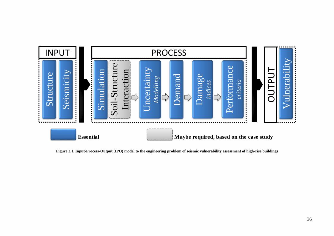
36
Figure 2.1. Input-Process-Output (IPO) model to the engineering problem of seismic vulnerability assessment of high-rise buildings
Essential Maybe required, based on the case study
Sei
smic
ity
Str
uct
ure
Soil
-Str
uct
ure
Inte
ract
ion
Sim
ula
tion
INPUT
Dem
and
Dam
age
in
dic
es
Per
form
ance
cr
iter
ia
PROCESS
Vuln
erab
ilit
y
OU
TPU
T
Unce
rtai
nty
Mo
del
ling

Chapter 2. Problem definition
37
Figure 2.2. Collapsingchartforthe“Structure”componentin the IPO model
2.2.1.2 Building inventory
Recalling the definition in Section 2.1, building inventory (stock) is a class of buildings
often defined by structural material, height range, lateral force-resisting system,
occupancy, period of construction, and physical condition for a specific region or
country. Since vulnerable building stocks remain the main cause of concern among the
factors that contribute to heavy casualties from significant earthquakes (e.g. Coburn and
Spence, 2003, Yepes-Estrada et al., 2017), limitations in inventory data significantly
impact the outcomes of earthquake loss and risk estimation studies (e.g. Rojahn and
Sharpe, 1985a, Coburn et al., 1992, Shakhramanian et al., 2000, Bommer et al., 2002,
FEMA, 2019). Different sources can be utilised to obtain building inventory in a
country or a region, among these are population census, field inspection, and technical
documentation. With the advancements in satellite technology, researchers have
developed other approaches to estimate building inventories. Some characteristics of the
building stock such as the height and the structural system estimation through the
geometries of building footprints may be obtained from satellite imageries (e.g. French
and Muthukumar, 2006, Rafi et al., 2016, Moya et al., 2018). Although the field
inventory data are the most accurate compared to data from other sources, the relatively
high cost and long period associated with field inspections render inventories for
earthquake loss studies mostly based on data from the other above-stated sources.
Hereafter, each of the classification criteria forming the building inventory definition is
briefly discussed, followed by literature on building inventory and data sources.
Str
uct
ure
Str
uct
ure
Def
init
ion
(Hig
h-r
ise B
uil
din
gs)
Bu
ild
ing I
nv
ento
ry
Structural Material(reinforced concrete)
Height Range
Structural System(shear walls)
Physical Condition
Period of Construction
Occupancy

Chapter 2. Problem definition
38
Structural material: Buildings are to be grouped according to their
construction material, mainly as: reinforced concrete (RC), masonry, steel,
wood, and composite.
Height range: Building height is one of the most significant parameters to be
considered when creating a building inventory. It reflects the dynamic
characteristics and seismic response of the buildings under study. Previous
studies on past earthquakes have shown that, depending on other factors such as
site classification and ground motion characteristics, damage can be
concentrated in buildings with a specific height range (Sucuoglu and Yazgan,
2003, Sucuoglu et al., 2007). With the continuous advancement in reinforced
concrete material and construction technologies, high-rise RC buildings are
getting higher and higher. This presses for a more detailed height classification
for building inventory.
Structural system: The lateral force-resisting structural system (or systems) in
a high-rise building identifies its seismic response and consequently the
vulnerability and loss due to earthquakes. With the wide range of structural
systems that can be employed in RC high-rise buildings, the lateral force-
resisting structural system stands as an important building classification
parameter for the establishment of building inventory for this class of structures.
Upon the availability of more detailed data, buildings may further be classified
according to some structural system-related aspects such as the presence of soft
and or weak storeys, short columns, long-span cantilevers, and pounding (Inel
et al., 2008). More details with regards to the classification of structural systems
used in RC high-rise buildings are given in Section 2.2.1.2.1 and Appendix A.
Occupancy: The occupancy type of a building or a building stock is a crucial
classification parameter for the estimation of casualties in earthquake risk and
mitigation studies. It also dictates the performance level assigned to the
structure for the purpose of vulnerability assessments. ASCE/SEI 7-16 (2017)
classifies buildings into four categories based on their use or occupancy:
Category I: Buildings that represent a low risk to human life in the event of
failure; Category II: All buildings except those listed in Categories I, III, and
IV; Category III: Buildings of which the failure could pose a substantial risk to
human life, a substantial economic impact, and industrial buildings containing

Chapter 2. Problem definition
39
toxic/explosive substances sufficient to pose a threat to the public if released;
and Category IV: Buildings designated as essential facilities, buildings of which
the failure could pose a substantial hazard to the community, industrial
buildings containing toxic/explosive substances sufficient to be dangerous to
the public if released, and buildings required to maintain the functionality after
an earthquake event. For high-rise buildings, the occupancy classification can
be subdivided to residential, commercial, and mixed-use buildings. Such sub-
classification is essential in estimating the potential level of casualties caused
by an earthquake event at different timing (day or night).
Period of construction: Building age is a key factor in determining the design
code in practice, the quality of construction material, and the detailing/
construction quality control level. Different regions in the world have different
dates that distinguish between the so-called pre-code and seismically-designed
buildings (Inel et al., 2008, Mwafy, 2012b). Furthermore, the construction era
implicitly defines the strength of the material utilised in the construction as well
as the construction techniques available at the time. All of which, contribute to
the response and consequently the seismic vulnerability of the building stock
under study.
Physical condition: the physical appearance of a building often reflects the
level of care given to its maintenance. Again, this may have an impact on the
performance of the building during an earthquake event. Structures that are
well-maintained against corrosion, rust, and other environmental and time-
dependent factors are expected to perform better in general and specifically
under cyclic loading such that from an earthquake. Classification of building
inventory using the physical condition parameter often involves a scale, say 1-
10, where a scale value is assigned to the building.
There have been various loss estimation methodologies developed in the past at both
national and regional levels. Inventory data used in those methodologies were prepared
with a primary focus on the economic impact assessment of an earthquake. It is worth
noting that the development of building inventory at a country or regional level involves
extensive efforts both in terms of identification and data assembling. In many countries
over the world, the basic inventory material requisite for completion of an earthquake
loss database either does not exist or is inaccessible.

Chapter 2. Problem definition
40
In 1983, Petrovski used a questionnaire-based technique to estimate the building type
classification in several Middle Eastern regions in an attempt to assess the associated
vulnerability in the studied countries (Petrovski, 1983). The information gathered
through questionnaires was very limited as no corresponding data were practically
available on the building structural systems.
In the ATC-13 project (1985b), the inventory model developed by the Applied
Technology Council (ATC) and incorporated by the Federal Emergency Management
Agency (FEMA) in the database of HAZUS loss assessment software (FEMA, 2019)
uses a consensus-based approach. In this model, the building stock is classified based on
the structural system and occupancy with three-level data entry.
The Early Post-Earthquake Damage Assessment Tool (EPEDAT) developed in 1997 to
estimate the casualties and regional damage for southern California used inventory data
from housing census, employment data, and county assessors’ records for buildings
(Eguchi et al., 1997). The inventory database of EPEDAT includes building age,
location, height, structural system, and occupancy. However, the methods used for the
building type classification, determination of day and night time population distribution,
and building occupancy have not been discussed in detail by the authors.
In the EXTREMUM computer tool developed by Shakhramanian et al. (2000), the
earthquake consequence forecasting model uses inventory data extracted from
population and building documentation in 89 regions in the Russian Federation. Neither
the procedure used in developing the inventory data nor whether the data have been
field validated were discussed in detail by the authors. QUAKELOSS, a newer version
of EXTREMUM, is created by the staff of the Extreme Situations Research Centre in
Moscow. QUAKELOSS is currently used by the World Agency of Planetary
Monitoring and Earthquake Risk Reduction (WAPMEER) to provide a near-real-time
assessment of injuries and death due to earthquakes anywhere in the world. The
building inventory incorporated in QUAKELOSS is reportedly covering two million
territories throughout the world.
In 2002, KOERILOSS, a scenario-based building loss and casualty estimation tool for
four cities in Turkey (Istanbul, Izmir, Bishkek, and Tashkent) was developed by
Bogazici University (Erdik and Aydinoglu, 2002, Erdik et al., 2003, Erdik and Fahjan,
2006). The building inventory for this program, utilising information from the State
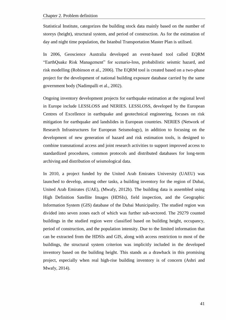
Chapter 2. Problem definition
41
Statistical Institute, categorizes the building stock data mainly based on the number of
storeys (height), structural system, and period of construction. As for the estimation of
day and night time population, the Istanbul Transportation Master Plan is utilised.
In 2006, Geoscience Australia developed an event-based tool called EQRM
“EarthQuake Risk Management” for scenario-loss, probabilistic seismic hazard, and
risk modelling (Robinson et al., 2006). The EQRM tool is created based on a two-phase
project for the development of national building exposure database carried by the same
government body (Nadimpalli et al., 2002).
Ongoing inventory development projects for earthquake estimation at the regional level
in Europe include LESSLOSS and NERIES. LESSLOSS, developed by the European
Centres of Excellence in earthquake and geotechnical engineering, focuses on risk
mitigation for earthquake and landslides in European countries. NERIES (Network of
Research Infrastructures for European Seismology), in addition to focusing on the
development of new generation of hazard and risk estimation tools, is designed to
combine transnational access and joint research activities to support improved access to
standardized procedures, common protocols and distributed databases for long-term
archiving and distribution of seismological data.
In 2010, a project funded by the United Arab Emirates University (UAEU) was
launched to develop, among other tasks, a building inventory for the region of Dubai,
United Arab Emirates (UAE), (Mwafy, 2012b). The building data is assembled using
High Definition Satellite Images (HDSIs), field inspection, and the Geographic
Information System (GIS) database of the Dubai Municipality. The studied region was
divided into seven zones each of which was further sub-sectored. The 29279 counted
buildings in the studied region were classified based on building height, occupancy,
period of construction, and the population intensity. Due to the limited information that
can be extracted from the HDSIs and GIS, along with access restriction to most of the
buildings, the structural system criterion was implicitly included in the developed
inventory based on the building height. This stands as a drawback in this promising
project, especially when real high-rise building inventory is of concern (Ashri and
Mwafy, 2014).

Chapter 2. Problem definition
42
2.2.1.2.1 Structural systems of RC high-rise buildings
One of the earliest efforts to classify structural systems of high-rise buildings according
to building height and system efficiency was that of Fazlur Khan in 1969 for steel
structures (Khan, 1969). This classification manifested the beginning of a new era of tall
buildings revolution utilising multiple structural systems. A few years later, Khan
upgraded his classifications by developing schemes for both steel and concrete (Khan,
1972, Khan, 1973) as shown in Figure 2.3, taken after Ali and Moon (2007).
Figure 2.3. Structural systems classification for high-rise buildings by Fazlur Khan: above for steel;
below for concrete (after Ali and Moon, 2007)
The shear wall-rigid frame interaction design approach first introduced by Khan and
Sbarounis (1964) has played a significant role in shaping the structural systems of
modern high-rise structures. The combination of the two structural forms leads to a

Chapter 2. Problem definition
43
highly efficient system, allowing a highly competitive design of 20- to 40-storey
buildings constructed either fully of reinforced concrete or composite with steel. In
1980, Khan and Rankine proposed yet another significant innovation in high-rises
(Khan and Rankine, 1980). They proposed, as it is called now, the exterior perforated or
framed tube system, where the exterior perimeter of the building is made of a system of
deep spandrels and closely-spaced columns forming a hollow thin-walled tube with
punched holes. For the sake of brevity, the classification and examples of the structural
systems in RC high-rise buildings are given in Appendix A.
2.2.1.2.2 Performance of seismic-resistant RC high-rise buildings
During earthquake events, the structural characteristics of the previously-described
structural systems determine the performance and stability of RC high-rise buildings.
For many decades now, internationally-recognised building codes have been developed
and maintained for seismic design of buildings. Among these codes are the late Uniform
Building Code (UBC) and the International Building Code (IBC) with their
incorporated national reference standards including the ACI 318 and the ASCE/SEI 7-
16 (UBC, 1997, ACI, 2014, IBC, 2015, ASCE/SEI-7, 2017). In these codes, however,
the seismic design provisions are based primarily on an understanding of the expected
behaviour of low- to mid-rise buildings. In order to extrapolate the design and detailing
provisions for use in high-rise structures, height limits were set for each of the identified
structural systems with some systems not permitted under certain seismic design
categories.
The recent developments in high-rise buildings, including innovative structural systems,
advanced material, and high-tech construction methods, have raised questions regarding
the applicability of prescriptive code provisions to the structural systems used in tall
buildings. As a result, performance-based, as well as consequence-based design
approaches using nonlinear analyses, have emerged as alternatives to the code-adopted
traditional strength-based design (e.g. PEER, 2010, PEER/ATC, 2010, LATBSDC,
2011). Hereafter, the major engineering, scientific, and regulatory issues specific to the
seismic design of high-rise buildings are addressed.
Structural systems and materials: Revolutionary developments in the
architectural and functional requirements for high-rise buildings have resulted in

Chapter 2. Problem definition
44
new structural systems and building materials that do not necessarily satisfy the
prescriptive provisions and requirements of currently-enforced building codes.
Hazard and performance objectives: As a result of the increasing demand for
high occupancy along with the interest in continued occupancy following the
earthquake event, the performance objectives and ground shaking levels for the
seismic design of high-rise buildings are to be reconsidered. Hence, new
initiatives in the analysis, design, and performance of high-rise buildings start to
emerge to the surface (e.g. PEER, 2010). Tall buildings, as a minimum, must be
collapse-prevented under long-return period earthquakes and significant
aftershocks, while serviceability criteria are to be met in more frequent events.
Input ground motions: The results of the nonlinear response history analysis of
high-rise buildings are significantly influenced by the selection, scaling, and
spectral alteration of input ground motions. Proper seismological methods are to
be implemented in the assembly of the seismic record sets to correctly represent
the duration and energy content required in the seismic design of high-rise
buildings.
Simulation, analysis, and acceptance criteria: In current codes, the seismic
design provisions do not specify appropriate simulation (modelling), analysis
methods, and acceptance criteria explicitly for high-rise buildings. Safety,
reliability, functionality, and re-occupancy criteria are therefore needed for this
class of buildings. Recently, there has been some effort to overcome these
shortcomings via pre-standards that are focusing on high-rise structures (e.g.
PEER, 2010, PEER/ATC, 2010, LATBSDC, 2011)
SSI for high-rise buildings with subterranean levels: High-rise buildings are
commonly constructed with several underground levels. Interaction between
soil, foundation, and structure can significantly alter the characteristics of the
input ground motion and consequently the response of the structure.
Local supplementary regulations in design and construction practices: Peer
reviewers and building authorities around the world often have their own design
and construction regulations specific to high-rise buildings as supplementary to
the seismic provisions. These regulations may have an impact on the
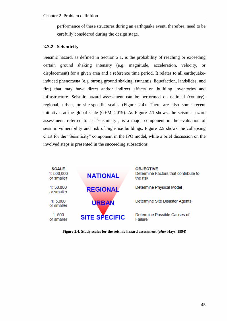
Chapter 2. Problem definition
45
performance of these structures during an earthquake event, therefore, need to be
carefully considered during the design stage.
2.2.2 Seismicity
Seismic hazard, as defined in Section 2.1, is the probability of reaching or exceeding
certain ground shaking intensity (e.g. magnitude, acceleration, velocity, or
displacement) for a given area and a reference time period. It relates to all earthquake-
induced phenomena (e.g. strong ground shaking, tsunamis, liquefaction, landslides, and
fire) that may have direct and/or indirect effects on building inventories and
infrastructure. Seismic hazard assessment can be performed on national (country),
regional, urban, or site-specific scales (Figure 2.4). There are also some recent
initiatives at the global scale (GEM, 2019). As Figure 2.1 shows, the seismic hazard
assessment, referred to as “seismicity”, is a major component in the evaluation of
seismic vulnerability and risk of high-rise buildings. Figure 2.5 shows the collapsing
chart for the “Seismicity” component in the IPO model, while a brief discussion on the
involved steps is presented in the succeeding subsections
Figure 2.4. Study scales for the seismic hazard assessment (after Hays, 1994)
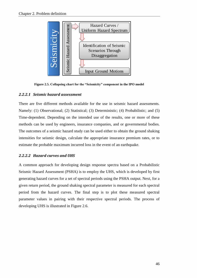
Chapter 2. Problem definition
46
Figure 2.5.Collapsingchartforthe“Seismicity”componentin the IPO model
2.2.2.1 Seismic hazard assessment
There are five different methods available for the use in seismic hazard assessments.
Namely: (1) Observational; (2) Statistical; (3) Deterministic; (4) Probabilistic; and (5)
Time-dependent. Depending on the intended use of the results, one or more of these
methods can be used by engineers, insurance companies, and or governmental bodies.
The outcomes of a seismic hazard study can be used either to obtain the ground shaking
intensities for seismic design, calculate the appropriate insurance premium rates, or to
estimate the probable maximum incurred loss in the event of an earthquake.
2.2.2.2 Hazard curves and UHS
A common approach for developing design response spectra based on a Probabilistic
Seismic Hazard Assessment (PSHA) is to employ the UHS, which is developed by first
generating hazard curves for a set of spectral periods using the PSHA output. Next, for a
given return period, the ground shaking spectral parameter is measured for each spectral
period from the hazard curves. The final step is to plot these measured spectral
parameter values in pairing with their respective spectral periods. The process of
developing UHS is illustrated in Figure 2.6.
Sei
smic
ity
Sei
smic
Haz
ard
Ass
essm
ent Hazard Curves /
Uniform Hazard Spectrum
Input Ground Motions
Identification of Seismic
Scenarios Through
Disaggregation
Chapter 2. Problem definition
47
Figure 2.6. An example of combining hazard curves from individual periods to develop a UHS for a
site in Los Angeles (after Baker, 2013): (a) Hazed curve for SA(0.3s); (b) Hazard curve for SA(1s); and
(c) UHS for a set of spectral periods like those in (a) and (b)
The term “uniform hazard spectrum” came from the fact that every ordinate in the UHS
has an equal probability of being exceeded. It should be clear that since the hazard
curves are independently computed for each spectral period in the set, the UHS does not
represent the spectrum of any single earthquake. It is common in a UHS to find that the
spectral acceleration values in the high-frequency zone (T < 0.2s) are controlled by
near-field moderate earthquakes, whereas, the values in the long period zone (T > 1s)
are controlled by distant strong events. The UHS is the only step in the PSHA that
combines the ground shaking parameters from multiple earthquakes.
The mixing of events in the UHS is sometimes cited for criticising the entire PSHA
approach. It is essential to recognize though that the UHS is merely a way to present the
output of a PSHA. No step in the PSHA requires the use of a UHS. Therefore, it is
totally possible to conduct a PSHA and productively use its results without ever
developing a UHS. This can be achieved by employing the disaggregation concept to
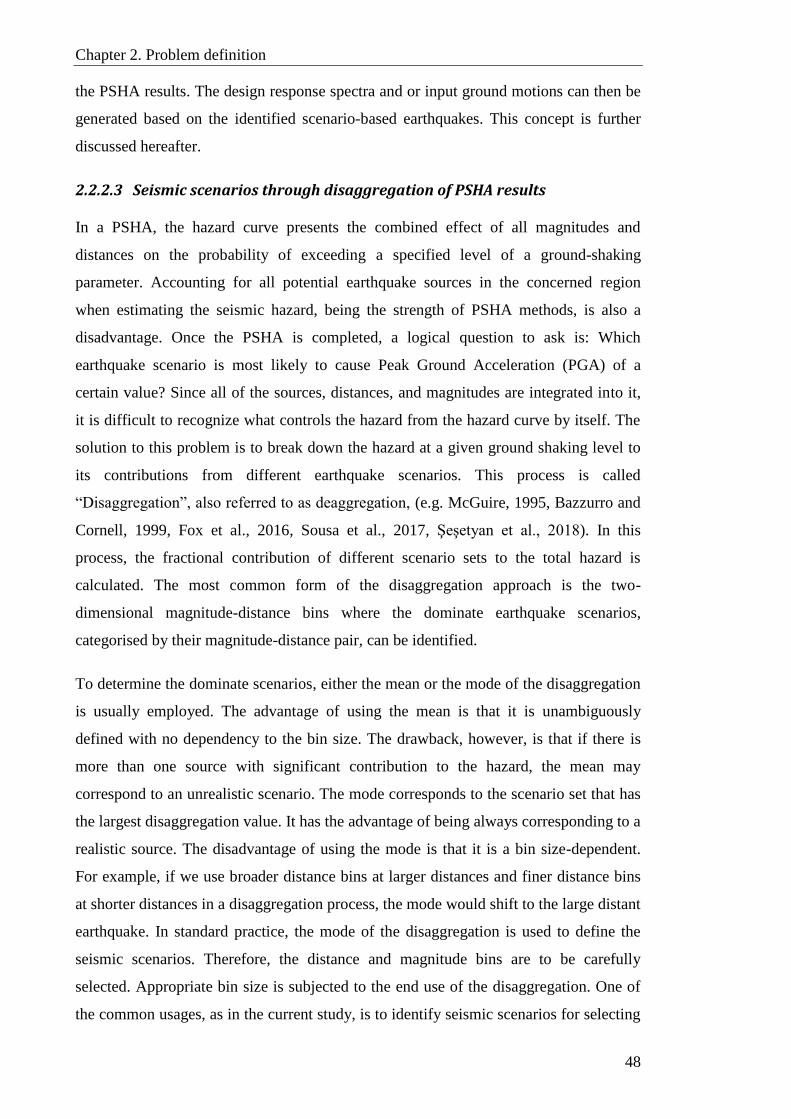
Chapter 2. Problem definition
48
the PSHA results. The design response spectra and or input ground motions can then be
generated based on the identified scenario-based earthquakes. This concept is further
discussed hereafter.
2.2.2.3 Seismic scenarios through disaggregation of PSHA results
In a PSHA, the hazard curve presents the combined effect of all magnitudes and
distances on the probability of exceeding a specified level of a ground-shaking
parameter. Accounting for all potential earthquake sources in the concerned region
when estimating the seismic hazard, being the strength of PSHA methods, is also a
disadvantage. Once the PSHA is completed, a logical question to ask is: Which
earthquake scenario is most likely to cause Peak Ground Acceleration (PGA) of a
certain value? Since all of the sources, distances, and magnitudes are integrated into it,
it is difficult to recognize what controls the hazard from the hazard curve by itself. The
solution to this problem is to break down the hazard at a given ground shaking level to
its contributions from different earthquake scenarios. This process is called
“Disaggregation”, also referred to as deaggregation, (e.g. McGuire, 1995, Bazzurro and
Cornell, 1999, Fox et al., 2016, Sousa et al., 2017, Şeşetyan et al., 2018). In this
process, the fractional contribution of different scenario sets to the total hazard is
calculated. The most common form of the disaggregation approach is the two-
dimensional magnitude-distance bins where the dominate earthquake scenarios,
categorised by their magnitude-distance pair, can be identified.
To determine the dominate scenarios, either the mean or the mode of the disaggregation
is usually employed. The advantage of using the mean is that it is unambiguously
defined with no dependency to the bin size. The drawback, however, is that if there is
more than one source with significant contribution to the hazard, the mean may
correspond to an unrealistic scenario. The mode corresponds to the scenario set that has
the largest disaggregation value. It has the advantage of being always corresponding to a
realistic source. The disadvantage of using the mode is that it is a bin size-dependent.
For example, if we use broader distance bins at larger distances and finer distance bins
at shorter distances in a disaggregation process, the mode would shift to the large distant
earthquake. In standard practice, the mode of the disaggregation is used to define the
seismic scenarios. Therefore, the distance and magnitude bins are to be carefully
selected. Appropriate bin size is subjected to the end use of the disaggregation. One of
the common usages, as in the current study, is to identify seismic scenarios for selecting
Chapter 2. Problem definition
49
time histories to be used in nonlinear analysis. Here, the change in the characteristics of
the time histories (e.g. duration, pulses, and spectral shape), and consequently the
seismic response of the building under study, alongside the magnitude and distance will
control the appropriate bin size. As an alternative, the mean magnitude and mean
distance for each controlling scenario is calculated. This is a robust approach in that it is
insensitive to the bin size, however, can be quite complicated if the controlling
scenarios overlap. In conclusion, there is not a unique optimum bin size for all projects
thus the hazard analyst needs to consider the end use of the disaggregation results when
deciding the bin sizes.
Figure 2.7 shows a sample of the disaggregation results for the Dubai region based on
the PSHA conducted by Aldama-Bustos et al. (2009). The results in the figure are for a
500-year return period, presented in terms of PGA and spectral accelerations.
Figure 2.7. Disaggregation results for the PSHA of Dubai, UAE (500-year return period) presented
in PGA and spectral accelerations of 0.2, 1, and 3s (after Aldama-Bustos et al., 2009)
2.2.2.4 Input ground motions
Due to the rapidly increasing computational power and the evolution of engineering
software during the last two decades, time-history analysis has been made feasible to
complex structures. As a result, time-domain analysis is prescribed for high-rise
structures in modern seismic codes. On the other hand, previous studies have shown that
among all uncertainty sources, input ground motions are the most unpredictable and
Chapter 2. Problem definition
50
carry a significant impact on the variability in the predicted structural response (e.g.
Elnashai and Izzuddin, 1993b, Padgett and DesRoches, 2007, Kappos, 2014,
Mangalathu et al., 2017, Kowsari et al., 2019). Ground motions appear random in time
and space due to the complex path that seismic waves follow from the source through
bedrock (Papageorgiou and Aki, 1983) and then through soil layers to reach the
structure foundation level (Manolis, 2002). Despite the above-discussed uncertainty,
ground motion record selection provisions in current codes are considered rather
simplified compared to the potential impact of the selection procedure on the analysis
results.
Selected input ground motions should represent the seismicity of the region under study
and must comply with design-based (or expected) earthquakes. In other words, the
selected records have to fulfil the earthquake scenarios that are identified through the
disaggregation process of PSHA results discussed in the previous section. In terms of
obtaining acceleration time-series, among the available approaches are (i) artificial
spectrum-matched accelerograms; (ii) synthetic accelerograms based on seismological
source models; and (iii) real earthquake accelerograms using scenario-based magnitude
and distance bins. These approaches are further discussed hereafter.
2.2.2.4.1 Artificial spectrum-matched accelerograms
Specialised software packages are employed to generate artificial spectrum-compatible
accelerograms for the use in the time-history analysis. This approach starts with
generating power spectral density function out of the smoothed response spectrum,
followed by deriving sinusoidal signals of random amplitudes and phase angles. These
signals are then summed to generate the accelerograms where an iterative procedure is
used to improve the match with the target response spectrum.
This approach is obviously attractive in such that one can generate as many acceleration
time-series as desired, all of which almost completely compatible with the target
spectrum. Nevertheless, it is now broadly not recommended to use artificial records
because they generally have an excessive number of strong-motion cycles and as a
result carry unreasonably high energy content (e.g. Seifried and Baker, 2016, Bani-Hani
and Malkawi, 2017). Gascot and Montejo (2016) evaluated three different
methodologies for the generation of spectrum compatible records: (i) wavelet-based
modification of real records; (ii) real record adjustment based on the Continuous

Chapter 2. Problem definition
51
Wavelet Transform; and (iii) synthetic record generation in the frequency domain. The
study concluded that even though the three methodologies are capable of generating
compatible records with an acceptable level of match, the records generated using the
frequency domain approach exhibit unrealistic strong motion characteristics. In the case
of methodologies based on the modification of real earthquake records, it was found
that when the real records are selected based on their initial compatibility with the target
spectrum, the resultant compatible records not only retain better the original
characteristic of the records but also reducing the variability in the structural response.
Matching artificial records to the entire target response spectrum, which is usually either
a UHS obtained from the PSHA or a UHS-based design spectrum, is neither reasonable
nor realistic (Naeim and Lew, 1995). This is certainly the case when the UHS is an
envelope of more than one earthquake scenario as for the study region in the current
work, where spectrum-matched artificial records will tend to be effectively unrealistic.
2.2.2.4.2 Synthetic accelerograms based on seismological source models
Synthetic acceleration time-series that account for path and site effect can be generated
from seismological source models. These models range from point sources, finite
sources, all the way to fully dynamic models of stress release. Software packages for
generating such synthetic records are freely available (e.g. Boore, 2003). Their
application, however, in terms of the definition of the parameters required to describe
the earthquake source generally requires the engagement of a seismologist. There is a
high degree of invariably- carried uncertainty in the determination of the source
parameters for past earthquakes. As for future earthquakes, the definition of these
parameters, to which the resulting synthetic records can be highly sensitive, normally
involves a substantial degree of expert judgment (e.g. Bommer and Acevedo, 2004,
Tang et al., 2016, Fahjan et al., 2017, Ghosh and Chakraborty, 2017).
2.2.2.4.3 Scenario-based real accelerograms
The third approach for obtaining time-series to be used in the time-history analysis is
real accelerograms recorded during past earthquakes. By definition, real records are free
of the issues associated with artificial spectrum-matched records. Among the selection
criteria, the earthquake magnitude (M) and source-to-site distance (R) bins that

Chapter 2. Problem definition
52
characterise the dominate earthquake scenarios in the area of interest are the most
common parameters used in the selection of real records.
Along this line, Shome et al. (1998) formed a bin of records using four different M-R
pairs to assess the seismic response of a five-storey building. Furthermore, Youngs and
his group (2006) and established the Design Ground Motion Library; an electronic
library of recorded accelerograms suitable for use in the time-history analysis of
structures. The total number of the record sets in the developed library was 26. In the
study of Wang et al. (Wang et al., 2015), a Design Ground Motion Library (DGML) is
presented for selecting earthquake ground motion time histories based on contemporary
knowledge and engineering practice. The library was created from a ground motion
database that consists of 3,182 records from shallow crustal earthquakes in active
tectonic regions rotated to fault-normal and fault-parallel directions. The DGML
enables users to construct design response spectra based on Next-Generation
Attenuation (NGA) relationships, including conditional mean spectra, code spectra, and
user specified spectra. Several studies (e.g. Stewart et al., 2002, Bommer and Acevedo,
2004, Ha and Han, 2016, Baker and Lee, 2018) also considered magnitude as an
important parameter in the selection of real records, arguing that when the magnitude
search window is kept as narrow as possible, the range for the source-to-site distance
can be widened.
Other studies, on the other hand, have examined the dependency of the inelastic seismic
response of structures on the M-R parameter pair used in the record selection (e.g.
Bazzurro and Cornell, 1994a, Bazzurro and Cornell, 1994b, Shome and Cornell, 1998,
Carballo and Cornel, 2000, Luco et al., 2002, Jalayer, 2003, Medina and Krawinkler,
2004, Baker and Cornell, 2005, Iervolino and Cornell, 2005, Vlachos et al., 2018). In
sum, these studies have concluded that deformation-based response has less dependency
on the M-R parameter pair when compared with the cumulative energy-based response.
They also verified the general independency of inelastic structural displacements to the
source-to-distance parameter R. Nevertheless, the conclusions drawn from these studies
may not be valid in the case of high-rise buildings. In this class of structures, the
duration of the selected records, which is a seismic scenario -dependent, plays an
essential role in the influence and contribution level of higher modes to the building
nonlinear response (e.g. Samanta and Pandey, 2018).

Chapter 2. Problem definition
53
Following the initial selection of real accelerograms based on the M-R parameter pair,
spectral matching is usually considered as a second-level selection criterion. In this
exercise, the response spectra of the selected records are to be modified in order to be
compatible with the corresponding target spectrum (UHS or design response spectrum).
It must be clarified here that spectral matching of real records is not to be confused with
the generation of spectral-matched artificial accelerograms discussed in
Section 2.2.2.4.1. Through the European strong-motion databank, Ambraseys et al.
(2004) proposed an Eqn. (2.1) to verify the spectral compatibility of a selected record
with the target spectrum.
Drms =1
N√∑ [
Sα0(Ti)
PGA0 −
Sαs(Ti)
PGAs]
2N
i=1
(2.1)
Where N is the number of periods at which the spectral shape is specified, Sα0(Ti) is the
spectral acceleration of the selected record at period Ti, Sαs(Ti) is the target spectral
acceleration at the same period, PGA0 is the peak ground acceleration of the selected
record, and PGAs is the zero-period anchor point of the target spectrum. Closer
matching between the shapes of the selected record and target spectra is indicated by a
small value of Drms.
It is important to recall that different M-R-based developed records are corresponding to
different earthquake scenarios, and that target spectrum is an envelope of all dominate
earthquake scenarios. Hence, the shapes of the record spectra in each record set are only
to be compatible with the part of the target spectrum that relates to the seismic scenario
employed in the developing of that set. Furthermore, when the seismic vulnerability
assessment of existing and new structures is the target of the study, obtaining a very
small value of Drms would not be that important. This is so because the selected real
records in each set will be subjected to a scaling scheme to cover the entire range of the
building response from elastic all the way to collapse. More insight on this matter is
given in CHAPTER 5.
Along with the discussed M-R pair and spectral-match selection criteria, there are three
additional complementary criteria that can be used in the real records selection process,
namely: (i) soil profile; (ii) strong motion duration; and (iii) acceleration to velocity
ratio (a/v). A brief discussion of each is bulleted hereafter.

Chapter 2. Problem definition
54
Soil profile: The actual soil profile (S) at the site of interest can be added to both
the earthquake magnitude and distance in the search window, leading to (M-R-
S) record bins (e.g. Kurama and Farrow, 2003, Youngs et al., 2006, Mwafy,
2012a, Mwafy et al., 2015b). The soil profile is known to influence ground
motions by altering both their amplitude and the calculated response spectra
(e.g. Bommer and Acevedo, 2004, Pandey et al., 2016, Trifunac, 2016, Barani
and Spallarossa, 2017). In general, the shear-wave velocity at the top 30m layer
of soil (VS,30) is a suitable measure to be used for site classification.
Alternatively, the site can be classified according to the well-established soil
categorization schemes included in seismic codes. Previous studies have
concluded that (M-R-S) selection approach may significantly reduce the number
of qualified records compared to the simpler (M-R) approach (e.g. Bommer and
Scott, 2000). Notwithstanding the restrictions implied to the selection process,
consideration of soil profile remains an important selection criterion.
Duration of ground motion: The duration of ground motion constitutes another
complementary parameter for the selection of real accelerograms. The ground-
shaking duration is typically controlled by the duration of the fault rupture,
which in turn is a function of the earthquake magnitude. Different types of
structural DIs are affected by ground motion duration in different ways. To be
specific, peak response-type DIs are independent of duration, while energy-
based DIs such as fatigue and absorbed hysteretic energy are interrelated to this
parameter (e.g. Shome et al., 1998, Iervolino et al., 2006, Chandramohan et al.,
2016a, Chandramohan et al., 2016b, Barbosa et al., 2017). In a study by
Hankock and Bommer (2006), the dependency of the abovementioned
phenomenon on the structural model itself is highlighted. Indeed, structures
modelled to exhibit stiffness and/or strength degradation under cyclic loading
are more sensitive to the number of cycles in the earthquake record and hence to
the shaking duration.
Acceleration to velocity ratio (a/v): As a complementary criterion for the record
selection process, the ground motion a/v forms an important measure of the
magnitude, frequency content and site-to-source distance of the earthquake event
(e.g. Tso et al., 1992, Carlton and Tokimatsu, 2016, Kohrangi et al., 2017,
Macedo and Castro, 2017). High a/v ratios (>1.2g/m/s) signify events with high

Chapter 2. Problem definition
55
dominant frequencies, medium-to-small magnitudes, short site-to-source
distances and short duration periods. Low a/v ratios (<0.8g/m/s), on the other
hand, represent earthquakes with low dominant frequencies, high-to-medium
magnitudes, long site-to-source distances and long duration periods. Examples
of studies that have considered the a/v criterion in the real records selection
process are the ones by Mwafy (2012a) and Ilyas et al. (2018).
2.2.3 Simulation
Based on modern seismic codes, earthquake-resistant RC buildings are designed and
detailed to respond well beyond the elastic range under DBE level ground motions.
Hence, verified nonlinear simulation, referred to hereafter as modelling, for building
response is essential in assessing the vulnerability of such structures. It is always easy to
forget that when a structure is analysed, the analysis is actually conducted on the model
of the structure and not the structure itself. In other words, the analytical model is an
approximation of the actual structure.
For RC high-rise wall buildings, Nonlinear Response History Analysis (NRHA) stands
as the most realistic tool currently available for predicting building response at different
levels of ground motion intensity. In NRHA, the accuracy of the nonlinear model is
measured by its sufficiency in capturing significant modes of deformation and
deterioration in the analysed structure from the onset of damage all the way to collapse.
Various aspects of nonlinear modelling such as element discretisation, material force-
deformation (also referred to as stress-strain) relations, and assumptions on modelling
of viscous damping and structural mass are essential in defining the level of accuracy a
model can have in predicting the seismic global and local response of the structure.
Figure 2.8 illustrates the collapsing chart for the “Simulation” component in the IPO
model, while the aforementioned modelling aspects are briefly discussed in the
succeeding subsections.

Chapter 2. Problem definition
56
Figure 2.8.Collapsingchartforthe“Simulation”componentin the IPO model
2.2.3.1 Element discretisation
Inelastic structural component models can generally be differentiated by the degree of
idealization in the model. In other words, the way plasticity is distributed through the
structural member cross-sections and along its length (Powell, 2010). Several model
types are available with the most detailed continuum finite element model at one
extreme and the lumped plasticity (concentrated hinge) model at the other. These
modelling types can also be used in modelling other types of structural members such as
slabs, braces and flexural walls.
In RC high-rise wall buildings, the fibre-based element is the most common modelling
approach used to model the structural walls which are expected to undergo inelastic
behaviour during the analysis (Wallace, 2007). This approach supports a proper
description of the wall geometry and the detailing of steel reinforcing bars and material
behaviour. It accounts for key response features including (i) relocation (shifting) of the
neutral axis along the cross-section of the wall during loading and unloading phases; (ii)
interaction with the other components connecting the walls/cores in the structure both in
and out of the wall’s plane such as the gravity frames and coupling beams; and (iii) the
impact of variation of axial load on wall flexural strength and stiffness.
Giving the above, fibre-based modelling approach will be adopted in the current study
for the RC walls as well as for the flooring system (flat plate) of the reference structure.
Coupling beams, on the other hand, will be modelled using a combination of elastic
elements and nonlinear hinges. Literature, key parameters, and modelling issues for the
said structural members are discussed in the following subsections.
Sim
ula
tion
Element Discretisation
Material
Constitutive Models
Model
Ver
ific
atio
n
Damping
Numerical Solution
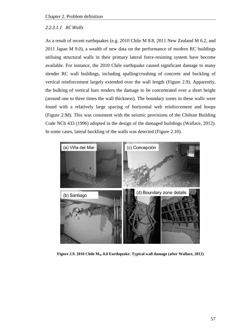
Chapter 2. Problem definition
57
2.2.3.1.1 RC Walls
As a result of recent earthquakes (e.g. 2010 Chile M 8.8, 2011 New Zealand M 6.2, and
2011 Japan M 9.0), a wealth of new data on the performance of modern RC buildings
utilising structural walls in their primary lateral force-resisting system have become
available. For instance, the 2010 Chile earthquake caused significant damage to many
slender RC wall buildings, including spalling/crushing of concrete and buckling of
vertical reinforcement largely extended over the wall length (Figure 2.9). Apparently,
the bulking of vertical bars renders the damage to be concentrated over a short height
(around one to three times the wall thickness). The boundary zones in these walls were
found with a relatively large spacing of horizontal web reinforcement and hoops
(Figure 2.9d). This was consistent with the seismic provisions of the Chilean Building
Code NCh 433 (1996) adopted in the design of the damaged buildings (Wallace, 2012).
In some cases, lateral buckling of the walls was detected (Figure 2.10).
Figure 2.9. 2010 Chile MW 8.8 Earthquake: Typical wall damage (after Wallace, 2012)
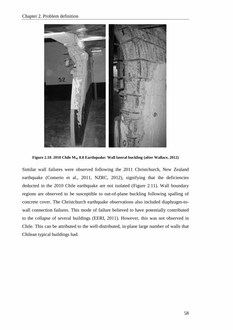
Chapter 2. Problem definition
58
Figure 2.10. 2010 Chile MW 8.8 Earthquake: Wall lateral buckling (after Wallace, 2012)
Similar wall failures were observed following the 2011 Christchurch, New Zealand
earthquake (Comerio et al., 2011, NZRC, 2012), signifying that the deficiencies
deducted in the 2010 Chile earthquake are not isolated (Figure 2.11). Wall boundary
regions are observed to be susceptible to out-of-plane buckling following spalling of
concrete cover. The Christchurch earthquake observations also included diaphragm-to-
wall connection failures. This mode of failure believed to have potentially contributed
to the collapse of several buildings (EERI, 2011). However, this was not observed in
Chile. This can be attributed to the well-distributed, in-plane large number of walls that
Chilean typical buildings had.
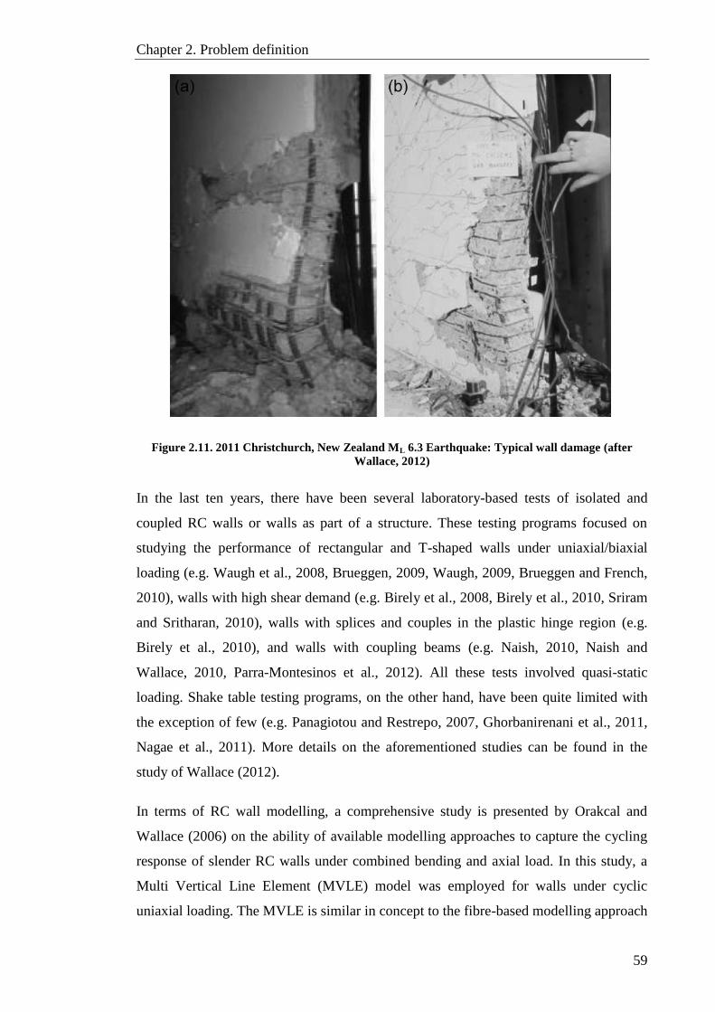
Chapter 2. Problem definition
59
Figure 2.11. 2011 Christchurch, New Zealand ML 6.3 Earthquake: Typical wall damage (after
Wallace, 2012)
In the last ten years, there have been several laboratory-based tests of isolated and
coupled RC walls or walls as part of a structure. These testing programs focused on
studying the performance of rectangular and T-shaped walls under uniaxial/biaxial
loading (e.g. Waugh et al., 2008, Brueggen, 2009, Waugh, 2009, Brueggen and French,
2010), walls with high shear demand (e.g. Birely et al., 2008, Birely et al., 2010, Sriram
and Sritharan, 2010), walls with splices and couples in the plastic hinge region (e.g.
Birely et al., 2010), and walls with coupling beams (e.g. Naish, 2010, Naish and
Wallace, 2010, Parra-Montesinos et al., 2012). All these tests involved quasi-static
loading. Shake table testing programs, on the other hand, have been quite limited with
the exception of few (e.g. Panagiotou and Restrepo, 2007, Ghorbanirenani et al., 2011,
Nagae et al., 2011). More details on the aforementioned studies can be found in the
study of Wallace (2012).
In terms of RC wall modelling, a comprehensive study is presented by Orakcal and
Wallace (2006) on the ability of available modelling approaches to capture the cycling
response of slender RC walls under combined bending and axial load. In this study, a
Multi Vertical Line Element (MVLE) model was employed for walls under cyclic
uniaxial loading. The MVLE is similar in concept to the fibre-based modelling approach

Chapter 2. Problem definition
60
embedded in some computer packages such as PERFORM-3D (CSI, 2011). The overall
modelling process presented in Orakcal and Wallace study (2006) includes: (i)
subdividing the wall cross-section into reinforcement fibres, confined concrete fibres,
and unconfined concrete fibres; (ii) employing suitable material constitutive relations;
(iii) dividing the wall height into a specified number of elements (components); (iv)
defining boundary conditions; and (v) applying a predefined load/displacement history.
The test walls were around one-fourth scale models, proportioned using the UBC-91
(Thomsen and Wallace, 1995, Thomsen and Wallace, 2004).
Key observations gleaned from the study of Orakcal and Wallace (2006) are bullet-
pointed below.
The effective elastic (linear) stiffness to the yield point is very close to the value
commonly used in design, that is 0.5E*Ig (Figure 2.12b). The results of the shake
table test of a full-scale, 7-storey RC building slice (Panagiotou and Restrepo,
2007) suggested a lower effective stiffness of 0.2E*Ig (Maffei, 2007). However,
it is important to note that the tension reinforcement ratio in the RC walls of the
shake table test was less than one-half of that used by Thomsen and Wallace
(2004). Indeed, that was the objective of the shake table test, to demonstrate that
adequate lateral load resistance of RC walls can be achieved by using just one-
half of the longitudinal reinforcement normally required by codes that were
enforced at the time of the testing program (e.g. UBC, 1997, IBC, 2003). The
use of significantly lower longitudinal reinforcement is expected to substantially
reduce the effective stiffness at yield since the yield curvature is mainly a
function of the wall length (Wallace and Moehle, 1992). Therefore, a reduction
in the yield moment strength by a factor of two renders the effective stiffness to
be reduced almost equally. Given that, the 0.2E*Ig reported in the shake table
testing program is not inconsistent with the 0.5E*Ig value recommended by
Orakcal and Wallace (2006). Accordingly, an effective yield stiffness of 0.5E*Ig
is considered appropriate for RC walls with code-compliant strength and axial
stress level up to 0.15Ag*fc’. it is worth noting that when fibre-based modelling
approach is used, the effective stiffness is automatically calculated based on the
adopted material constitutive relations, level of axial stress, and the analysis
current state.
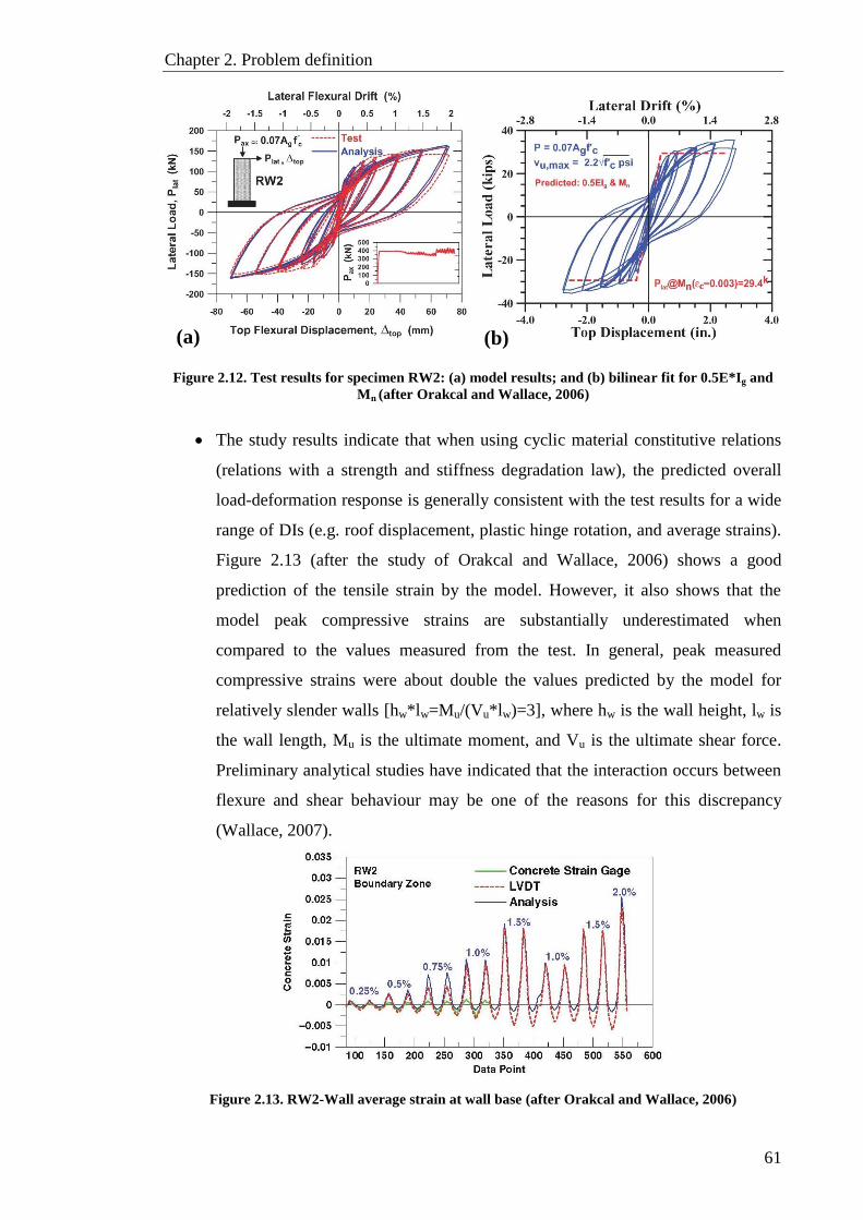
Chapter 2. Problem definition
61
Figure 2.12. Test results for specimen RW2: (a) model results; and (b) bilinear fit for 0.5E*Ig and
Mn (after Orakcal and Wallace, 2006)
The study results indicate that when using cyclic material constitutive relations
(relations with a strength and stiffness degradation law), the predicted overall
load-deformation response is generally consistent with the test results for a wide
range of DIs (e.g. roof displacement, plastic hinge rotation, and average strains).
Figure 2.13 (after the study of Orakcal and Wallace, 2006) shows a good
prediction of the tensile strain by the model. However, it also shows that the
model peak compressive strains are substantially underestimated when
compared to the values measured from the test. In general, peak measured
compressive strains were about double the values predicted by the model for
relatively slender walls [hw*lw=Mu/(Vu*lw)=3], where hw is the wall height, lw is
the wall length, Mu is the ultimate moment, and Vu is the ultimate shear force.
Preliminary analytical studies have indicated that the interaction occurs between
flexure and shear behaviour may be one of the reasons for this discrepancy
(Wallace, 2007).
Figure 2.13. RW2-Wall average strain at wall base (after Orakcal and Wallace, 2006)
(b) (a)
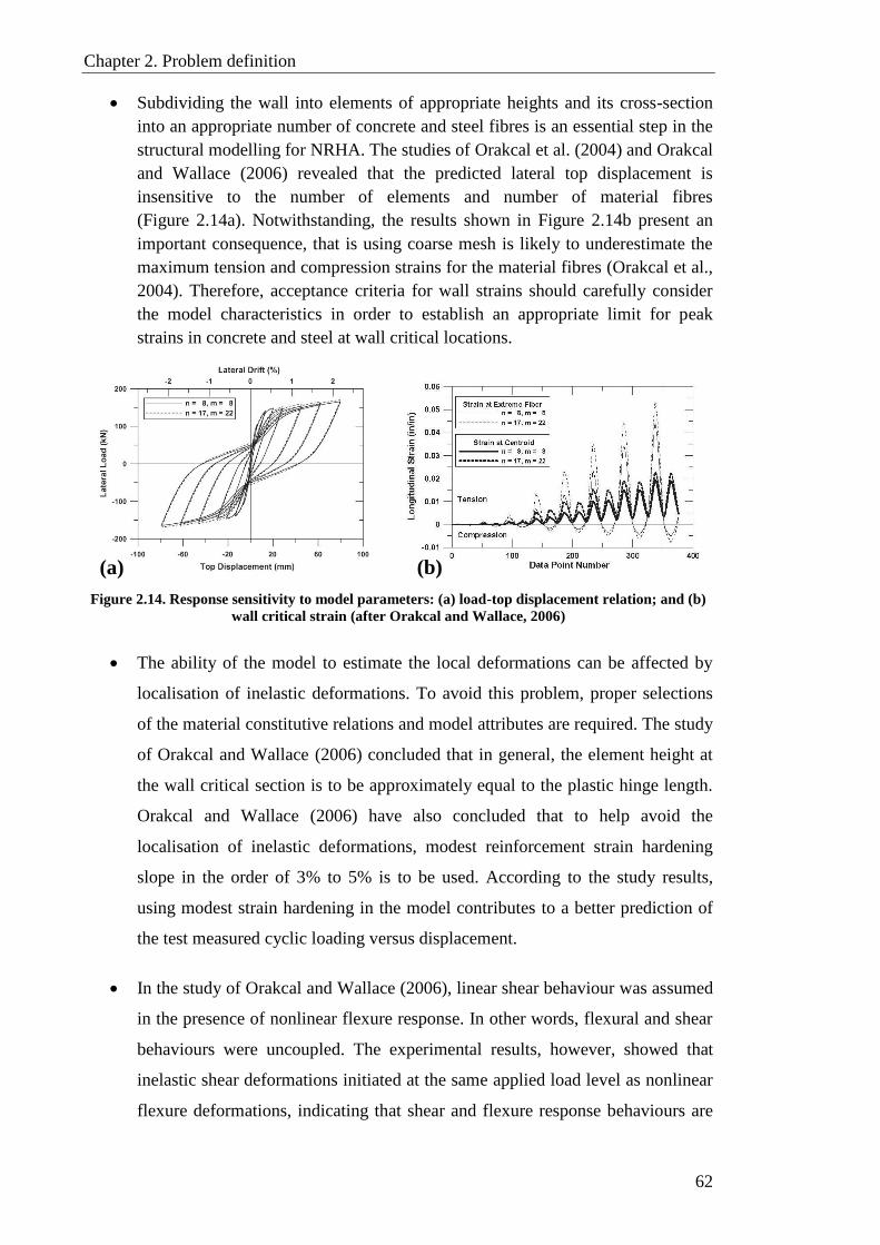
Chapter 2. Problem definition
62
Subdividing the wall into elements of appropriate heights and its cross-section
into an appropriate number of concrete and steel fibres is an essential step in the
structural modelling for NRHA. The studies of Orakcal et al. (2004) and Orakcal
and Wallace (2006) revealed that the predicted lateral top displacement is
insensitive to the number of elements and number of material fibres
(Figure 2.14a). Notwithstanding, the results shown in Figure 2.14b present an
important consequence, that is using coarse mesh is likely to underestimate the
maximum tension and compression strains for the material fibres (Orakcal et al.,
2004). Therefore, acceptance criteria for wall strains should carefully consider
the model characteristics in order to establish an appropriate limit for peak
strains in concrete and steel at wall critical locations.
Figure 2.14. Response sensitivity to model parameters: (a) load-top displacement relation; and (b)
wall critical strain (after Orakcal and Wallace, 2006)
The ability of the model to estimate the local deformations can be affected by
localisation of inelastic deformations. To avoid this problem, proper selections
of the material constitutive relations and model attributes are required. The study
of Orakcal and Wallace (2006) concluded that in general, the element height at
the wall critical section is to be approximately equal to the plastic hinge length.
Orakcal and Wallace (2006) have also concluded that to help avoid the
localisation of inelastic deformations, modest reinforcement strain hardening
slope in the order of 3% to 5% is to be used. According to the study results,
using modest strain hardening in the model contributes to a better prediction of
the test measured cyclic loading versus displacement.
In the study of Orakcal and Wallace (2006), linear shear behaviour was assumed
in the presence of nonlinear flexure response. In other words, flexural and shear
behaviours were uncoupled. The experimental results, however, showed that
inelastic shear deformations initiated at the same applied load level as nonlinear
flexure deformations, indicating that shear and flexure response behaviours are
(a) (b)

Chapter 2. Problem definition
63
indeed coupled. To account for the shear-flexure interaction, a coupled model
can be employed as shown in Figure 2.15 (e.g. Massone, 2006, Orakcal et al.,
2006, Kolozvari, 2013, Kolozvari et al., 2014a, Kolozvari et al., 2014b, Massone
et al., 2015). However, such coupled models are not yet available in
commercially-available computer packages since the development of coupled
cyclic material models remains a major research challenge. Given these
limitations, a simplified uncoupled modelling approach can be used to
reasonably capture the shear-flexure interaction behaviour of slender walls. An
example of such modelling approaches is the use of nonlinear shear spring
similar to that recommended by ASCE/SEI 41-06 (2007) and ASCE/SEI 41-16
(2017). The shear force-deformation relation required to define the shear spring
can be based on test results by Thomsen and Wallace (2004), calibration studies
by Gogus (2010), and modification to the post-cracking slope suggested by
Massone (2006). More details on this model approach are given in CHAPTER 3
of this thesis.
Figure 2.15. Nonlinear wall modelling - Combined flexure and shear behaviour: Load versus lateral
displacement (after Orakcal and Wallace, 2006)
2.2.3.1.2 Coupling beams
Reinforced concrete walls are usually coupled with beams to create openings to access
elevators, stairwells, and other systems. Those coupling beams are subjected to double
curvature and intended to yield under lateral loading. The shear demands resulting in the
beams are transferred to the coupled walls as axial tension and compression loads. As
the use of NRHA and performance-based design have become more common for high-
rise wall buildings, attention to the nonlinear modelling of coupling beams continues to
Chapter 2. Problem definition
64
increase. Modelling parameters of particular interest are the effective flexural stiffness
at yield and the allowable inelastic rotation prior to significant lateral strength
degradation. Test programs in this field were conducted either on coupling beams as
individual elements or on coupled-wall as a complete system. Historically, most of the
tests belonged to the former category with only a few large-scale tests dealing with the
latter. A detailed review of previous studies related to coupling beam seismic behaviour
and design was given by Mohr (2007), while Turgeon (2011) provided a thorough
review of experimental test programs of coupled-wall system.
Recent tests have been conducted using eight one-half-scaled RC coupling beams to
assess the modelling parameters alongside the detailing and configurations common for
both residential and office buildings, including the influence of post-tensioned and
reinforced slab flooring systems (Naish et al., 2009, Naish, 2010, Naish and Wallace,
2010, Wallace, 2012). In these tests, 2.4 and 3.33 aspect ratios (beam net length to depth
ratio) were adopted for beams representing residential and office buildings, respectively.
Tested beams were reinforced diagonally with transverse reinforcement placed either
around the bundles of diagonal bars (labelled as CB24D and CB33D in the tests) or
around the entire beam cross-section (labelled CB24F and CB33F in the tests) following
the provisions of the ACI 318 code used in the design stage.
The main conclusions of the above-mentioned studies are bullet-pointed hereafter.
The load-deformation relations of the 2.4 aspect ratio-beams with both
transverse reinforcement arrangements (CB24D and CB24F) were quite similar
over the entire range of applied rotations (Figure 2.16a). Similar results were
observed for the 3.33 aspect ratio-beams (Figure 2.16b).
Tested beams with a 2.4 aspect ratio obtained large rotation in the range of 8%
before any significant degradation in lateral load resistance occurred.
Furthermore, shear strengths in the range of 1.17 and 1.25 times the ACI 318
nominal strength were achieved by test beams with transverse reinforcement
placed around the diagonal bars and around the entire cross-section,
respectively.
Additional beams with a 2.4 aspect ratio were tested to evaluate the slab impact
(post-tensioned or RC) on the load-deformation relations. The tests revealed that

Chapter 2. Problem definition
65
the shear strength of the coupling beams increases by the existence of the slab.
This strength increase can be accounted for by considering the nominal moment
capacity increase in the beams due to the presence of the prestress and the slab.
The axial growth in the coupling beams prior to yield is restrained by the
presence of a flooring system (RC or PT slab), leading to slightly higher
stiffness. However, the secant stiffness for beams with and without slabs
following yield was very similar, where significant strength degradation
occurred at around the same rotation (8%).
Tests conducted on 3.33 aspect ratio-beams with longitudinal flexure
reinforcement instead of diagonal bars indicated that total rotation greater than
4% could be achieved prior to significant strength degradation. It is also
observed that the load-deformation relations for beams with longitudinal
reinforcement experience more pinching when compared to the diagonally-
reinforced beams, indicating less energy dissipation. Nevertheless, given the less
construction complexity, coupling beams with longitudinal reinforcement are
still appropriate to use in high-rise buildings when shear stress and rotation
demands are modest.
Figure 2.16. Cyclic load-deformation relations: (a) CB24F versus CB24D; and (b) CB33F versus
CB33D (Naish et al., 2009)
To model a coupling beam for NRHA, two nonlinear modelling approaches are
commonly used: (a) moment-hinge approach, consisting of an elastic cross-section
beam with rotational springs at beam ends to account for nonlinear flexure (and
slip/extension) deformation; and (b) shear-hinge approach, consisting of an elastic
cross-section beam with a nonlinear shear spring at beam mid-span.
(a) (b)

Chapter 2. Problem definition
66
Previous studies (e.g. Naish et al., 2009, Naish, 2010, Naish and Wallace, 2010)
investigated the two modelling approaches using full-scale-modified linearised
backbone relation for normalised shear versus rotation and effective stiffnesses resulted
from the testing program. The studies concluded that despite the better representation of
the unloading characteristics by the moment-hinge model, both models accurately
capture the overall load-rotation response of the member. Since the unloading
characteristics of the load-deformation relation have no significant impact on the current
work objective, it is decided to use the nonlinear shear-hinge approach in modelling the
coupling beams in the case study building. It is worth noting that a number of previous
studies dealing with the vulnerability assessment of RC high-rise wall structures have
adopted this nonlinear shear-hinge approach in the modelling of coupling beams (e.g.
Ghodsi and Ruiz, 2010, Tuna, 2012). More details of the shear-hinge modelling
approach and the parameter used to define the force-deformation relation assigned to the
coupling beams in the model of the reference structure are given in CHAPTER 4.
2.2.3.1.3 Flooring system
For high-rise wall buildings, the most common flooring system is flat plate slabs, either
of reinforced or post-tensioned concrete. This system is a preference to both architects
and mechanical engineers as it allows for more floor-to-floor clear height for the former
and more flexibility in running the mechanical services for the latter. Three main
modelling approaches are available to model flat plate slabs in high-rise wall buildings,
namely: (1) omitting the slab from the model and assigning diaphragm constraints to the
RC piers and core walls at each floor level; (2) modelling the slab using elastic,
equivalent slab-beam or shell elements; and (3) modelling the slab using inelastic fibre-
based elements. A brief discussion of each of the three abovementioned modelling
approaches is given below.
Modelling approach-1: The advantage of this approach obviously lies in the
saving of computational effort and time by dropping the slab from the model.
Given that slabs typically have high in-plane stiffness, rigid diaphragm
constraints are assigned to the wall ends at floor level in each storey for lateral
load analysis. In this modelling approach, all constrained nodal joints in the
same floor are slaved to one another hence they undertake similar in-plain
deformations. Several researches have implemented this approach in their
Chapter 2. Problem definition
67
modelling of high-rise wall buildings (e.g. Ghodsi and Ruiz, 2010, Tuna,
2012).
This approach, however, comes with a major drawback, that is not accounting
for the influence of the 3-dimensional interaction between the flooring system
and the walls on the overall lateral performance of the building. The shear
forces in the slab developed under lateral loading are transferred to the
connected walls in the form of axial forces (tension and compression), which
intern contribute either positively or negatively to the walls lateral force
resistance and ductility. This issue has been confirmed by previous studies (e.g.
Panagiotou and Restrepo, 2006).
Modelling approach-2: In this approach, the slab is modelled using either an
elastic, equivalent slab-beam element or an elastic shell element. An equivalent
slab-beam is an elastic flexural element having a rectangular section with its
depth and width dimensions representing the total slab thickness and its
effective width, respectively (Allen and Darvall, 1977, Grossman, 1997,
Hwang and Moehle, 2000, Kang and Wallace, 2005, Kang, 2006, Kang and
Wallace, 2006, Elwood et al., 2007, Kang et al., 2009, Waugh and Sritharan,
2010). Elastic shell element is a 4-node element with in-plane (membrane) and
out-of-plane (bending) plate elastic stiffnesses. The element is available in
several computer packages such as PERFORM-3D (CSI, 2011).
Using the equivalent slab beam and shell elements will obviously overcome the
drawback associated with the modelling approach-1. The shortcoming of using
these types of elements, on the other hand, is that they both can only be used to
model floor slabs that are expected to remain elastic throughout the earthquake
excitation. For slabs that are expected to crack and yield, the inelastic element
should be used, where the slab deformation can be accurately calculated along
with its impact on the additional axial forces induced in the walls. Furthermore,
using elastic element to model slabs that are expected to undergo plastic
deformation will hinder the use of these deformations as a damage index in the
process of estimating performance state criteria for the building.
Modelling approach-3: Using nonlinear fibre-based beam element in
modelling floor slabs is considered the most realistic of the three approaches

Chapter 2. Problem definition
68
listed herein since it overcomes the shortcomings in the modelling approach 1
and 2. Using this approach, the total width of the slab panel can be utilised
since the cracking and yielding events in the slab are automatically taken into
account through the fibre-based model.
In the current work, the third modelling approach (fibre-based beam element) is utilised
in modelling the RC flat slabs of the reference structure due to its effectiveness and
ability to overcome the shortcomings in other modelling approaches.
2.2.3.1.4 Coupling beam/Slab/Wall connection
In a 4-noded fibre-based shear wall element, the nodes have no in-plane rotational
stiffness. Therefore, when connecting an element that represents a coupling beam or a
slab to a shear wall, the connection is pinned. To specify moment-resisting connections
between a wall and a beam or a slab, an embedded element in the wall is to be added to
the model as shown in Figure 2.17. The embedded element must have a very stiff
section in bending in the plane of the wall to provide a stiff connection between the wall
and the coupling beam or the slab. On the other hand, it should obtain very small axial,
torsional, and out-of-plane bending stiffnesses to avoid adding artificial stiffness to the
wall elements.
Figure 2.17. Imbedded element for coupling beam/slab-wall connection (after CSI, 2011)

Chapter 2. Problem definition
69
In reality, there may be significant local deformation where the coupling beam or the
slab connects to the wall. The rotational stiffness of the elastic connection component in
the embedded element can be selected to provide an appropriate amount of fixity. It is
worth noting that the degree of fixity between the coupling beams or the slabs and the
walls may have an impact on the overall elastic stiffness of the structure. However, after
the coupling beam or the slab yields, the amount of end fixity is expected to have little
effect. As an alternative, inelastic moment connection component rather than elastic
release component may be used with the embedded element so that the beam- or slab-
to-wall connection is nonlinear.
2.2.3.2 Material constitutive models
Given the Bernoulli beam assumption that plane section remains plane after
deformation, uniaxial stress-strain constitutive laws are sufficient to model the steel and
concrete materials of RC members with fibre-discretized cross-sections. The main
objective of seismic vulnerability assessment studies of high-rise RC buildings is to
evaluate the performance of the structure at different seismic hazard levels. This
necessitates the use of hysteretic models that incorporate all key properties of steel and
concrete materials contributing to demand estimation as the building approaches
collapse. Furthermore, NRHA models should be based on expected material properties
rather than minimum specified properties. The term “expected” refers to properties that
are characterised based on median values from a large population of materials. The
definition of a typical hysteretic model comprises three steps:
A backbone curve, which is a force-deformation relation that sets the bounds
within which the hysteretic response of the member (component) is confined,
A set of rules defining hysteretic behaviour between the bounds defined by the
backbone curves, and
A set of rules defining various modes of degradation with reference to the
backbone curve. Degradation rules are based on the hysteretic energy
dissipation in the member (component) as it is subjected to cyclic loading.
The initial backbone curve defines the monotonically increasing deformation in the
material constitutive relation. Generally, the initial backbone curve is defined by the
following parameters: initial (elastic) stiffness, yield strength, post-capping stiffness,
strength cap and associated deformation, post-capping stiffness and deformation range,
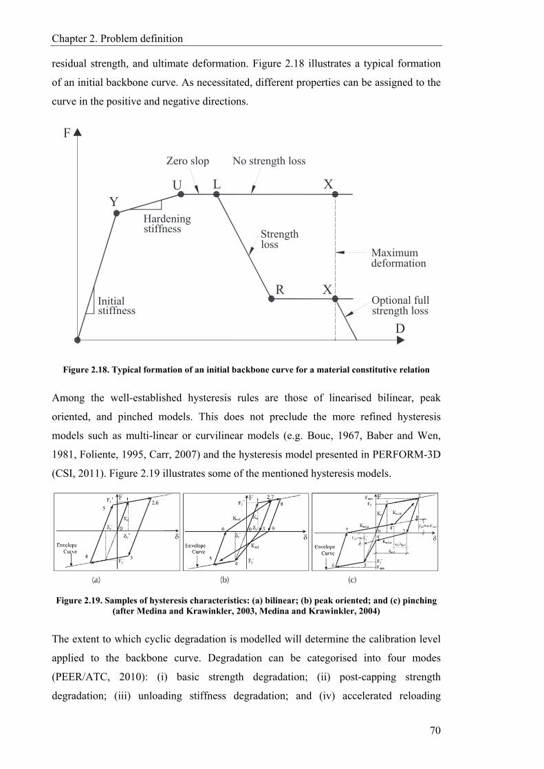
Chapter 2. Problem definition
70
residual strength, and ultimate deformation. Figure 2.18 illustrates a typical formation
of an initial backbone curve. As necessitated, different properties can be assigned to the
curve in the positive and negative directions.
Figure 2.18. Typical formation of an initial backbone curve for a material constitutive relation
Among the well-established hysteresis rules are those of linearised bilinear, peak
oriented, and pinched models. This does not preclude the more refined hysteresis
models such as multi-linear or curvilinear models (e.g. Bouc, 1967, Baber and Wen,
1981, Foliente, 1995, Carr, 2007) and the hysteresis model presented in PERFORM-3D
(CSI, 2011). Figure 2.19 illustrates some of the mentioned hysteresis models.
Figure 2.19. Samples of hysteresis characteristics: (a) bilinear; (b) peak oriented; and (c) pinching (after Medina and Krawinkler, 2003, Medina and Krawinkler, 2004)
The extent to which cyclic degradation is modelled will determine the calibration level
applied to the backbone curve. Degradation can be categorised into four modes
(PEER/ATC, 2010): (i) basic strength degradation; (ii) post-capping strength
degradation; (iii) unloading stiffness degradation; and (iv) accelerated reloading
UY
Zero slop
X
XR
stiffnessInitial
stiffnessHardening
Dstrength lossOptional full
deformationMaximum
lossStrength
No strength loss
F
L
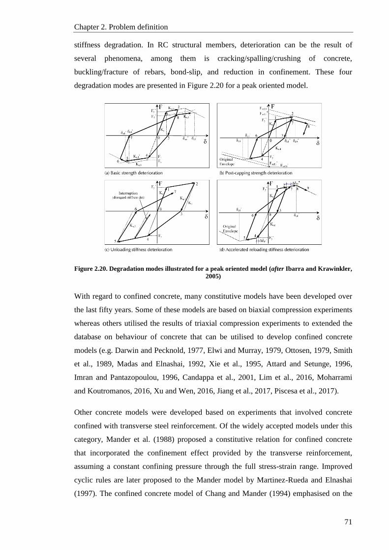
Chapter 2. Problem definition
71
stiffness degradation. In RC structural members, deterioration can be the result of
several phenomena, among them is cracking/spalling/crushing of concrete,
buckling/fracture of rebars, bond-slip, and reduction in confinement. These four
degradation modes are presented in Figure 2.20 for a peak oriented model.
Figure 2.20. Degradation modes illustrated for a peak oriented model (after Ibarra and Krawinkler,
2005)
With regard to confined concrete, many constitutive models have been developed over
the last fifty years. Some of these models are based on biaxial compression experiments
whereas others utilised the results of triaxial compression experiments to extended the
database on behaviour of concrete that can be utilised to develop confined concrete
models (e.g. Darwin and Pecknold, 1977, Elwi and Murray, 1979, Ottosen, 1979, Smith
et al., 1989, Madas and Elnashai, 1992, Xie et al., 1995, Attard and Setunge, 1996,
Imran and Pantazopoulou, 1996, Candappa et al., 2001, Lim et al., 2016, Moharrami
and Koutromanos, 2016, Xu and Wen, 2016, Jiang et al., 2017, Piscesa et al., 2017).
Other concrete models were developed based on experiments that involved concrete
confined with transverse steel reinforcement. Of the widely accepted models under this
category, Mander et al. (1988) proposed a constitutive relation for confined concrete
that incorporated the confinement effect provided by the transverse reinforcement,
assuming a constant confining pressure through the full stress-strain range. Improved
cyclic rules are later proposed to the Mander model by Martinez-Rueda and Elnashai
(1997). The confined concrete model of Chang and Mander (1994) emphasised on the
Chapter 2. Problem definition
72
transition of the stress-strain relation at the opening and closure of cracks. In this model,
the concrete in tension was modelled with cyclic behaviour. The model envelopes for
tension and compression have control on the slope at the origin as well as on the shape
of both pre-peak and post-peak zones of the stress-strain relation. Other examples of
transverse reinforcement-confined concrete are (Sheikh and Uzumeri, 1980, Scott et al.,
1982, Sheikh and Uzumeri, 1982).
For high-strength concrete, there are many confinement models proposed by researchers
(e.g. Fafitis and Shah, 1985, Yong et al., 1988, Bjerkeli et al., 1990, Nagashima et al.,
1992, Cusson and Paultre, 1993, Muguruma, 1993, Sun and Sakino, 1993, Li, 1994,
Ibrahim and MacGregor, 1996, Diniz and Frangopol, 1997, Kappos and Konstantinidis,
1999, Konstantinidis et al., 2007, Akiyama et al., 2010). The uniaxial, nonlinear
constant confinement constitutive for the high-strength concrete model of Kappos and
Konstantinidis (1999) has been embedded in some nonlinear analysis computer
packages such as SeismoStruct (SeismoSoft, 2019). In this model, the confinement
effect delivered by the transverse reinforcement were accounted for through the
modified Sheikh and Uzumeri factor (1982).
For steel reinforcement, among the widely used stress-strain models is the Menegotto-
Pinto relation (Menegotto and Pinto, 1973), coupled with isotropic hardening rules
introduced by Filippou et al. (1983). This model has been embedded in several research
software packages such as OpenSees (Mazzoni et al., 2006, McKenna and Fenves,
2006, McKenna, 2011), ZEUS-NL (Elnashai et al., 2012), and SeismoStruct
(SeismoSoft, 2019). Another commonly used model is the one proposed by Dodd and
Restrepo (1995). It accounts for the reduction in the unloading modulus with the plastic
strain, whereas the ultimate tensile strain reduction is taken exclusively as a function of
the maximum compressive strain.
In the present study, the modified Mander model (Martínez-Rueda and Elnashai, 1997)
and the Menegotto-Pinto relation (Menegotto and Pinto, 1973), coupled with isotropic
hardening rules proposed by Filippou et al. (1983) are utilised to present the stress-
strain relations of confined concrete and reinforcing steel, respectively. More details on
the used material models are given in CHAPTER 4.

Chapter 2. Problem definition
73
2.2.3.3 Damping
Damping is generally associated with the reduction in dynamic response due to energy
dissipation in the building. Depending on the physical contributors to damping, it can be
mathematically modelled in a variety of forms, including viscous damping, hysteretic
damping, or friction damping. Proper modelling of damping requires an appreciation for
its physical sources, and how these sources may vary in their contribution from one
building to another based on the building geometry and its dynamic characteristics. This
is especially true for tall buildings, where the structural systems, foundations, and non-
structural components can be quite different from those in conventional low- to mid-rise
construction. Damping in structures due to earthquake-induced motions can generally
be attributed to three main sources: (1) structural components; (2) nonstructural
components; and (3) the soil-structure interaction.
Viscous damping (also called inherent damping, initial elastic damping, or simply
elastic damping) in NRHA is necessary to account for damping prior to the onset of
hysteretic response (Priestley and Grant, 2005, Smyrou et al., 2011, Paulay and
Priestley, 2013). Some researchers (e.g. Priestley and Grant, 2005, Smyrou et al., 2011)
stated that viscous damping is not needed in the post-yield phase except during elastic
loading/unloading. Nevertheless, for certain constitutive relations that lead to vanishing
effective damping ratios at large amplitudes, some degree of viscous damping is
believed necessary to avoid unstable inelastic response computation (Luco and Lanzi,
2017a).
While the effect of damping in the linear stage of response is typically small except at
resonance condition, the mathematical modelling and details of viscous damping for the
inelastic stage have significant effects on the seismic response of high-rise buildings,
particularly, on the estimated damping forces in the equation of motion. Currently,
proper modelling and key parameters to represent viscous damping are still a topic of
argument between researchers. A number of different mathematical models involving
Rayleigh, Caughey, and modal viscous damping matrices based either on initial or
effective stiffnesses have been proposed. In the meantime, warnings about the
unintended problems that may be encountered from using (or misusing) these options
have been risen for the last three decades by a number of researchers (e.g. Chrisp, 1980,
Shing and Mahin, 1987, Léger and Dussault, 1992, Bernal, 1994, Carr, 1997, Hall,
1998, Carr, 2005, Hall, 2006, Carr, 2007, Charney, 2008, Ryan and Polanco, 2008,
Chapter 2. Problem definition
74
Zareian and Medina, 2010, Jehel et al., 2014, Hardyniec and Charney, 2015, Chopra
and McKenna, 2016a, Chopra and McKenna, 2016b, Hall, 2016). some studies
suggested to abandon altogether using conventional viscous damping model and replace
it with nonlinear hysteretic mechanism (e.g. Charney, 2008) or by a capped viscous
model (e.g. Hall, 1998, Hall, 2006, Hall, 2016). Other studies (e.g. Kausel, 2014)
recommended abandoning, when necessary, the classical or orthogonal damping matrix
assumption.
In the process of developing a damping model, two conflicting objectives must be
considered, these are: (1) arriving at a proper mechanical or physical representation of
the damping model while keeping the computational efficiency in mind; and (2)
respecting the limitation in experimental data available for damping of buildings at full
scale. Viscous damping in high-rise buildings represents a variety of damping sources
including internal friction in structural material, hysteresis response in nonstructural
elements, external friction between structural and nonstructural members, and radiation
into the surrounding soil. Mainly due to the computational convenience, viscous
damping models, in which nodal damping forces and nodal velocities are connected
together through a damping matrix, are ubiquitous. This is despite the extensive data on
material damping (Lazan, 1968) suggesting that linear hysteretic damping models
would be adequate for this particular damping component and that friction between
structural and nonstructural elements can be best represented by a Coulomb model
(Luco and Lanzi, 2017a). Strict obedience to the physical interpretation would
necessitate the assembly of the global damping matrix from the damping properties of
each of the structural elements in the building in correspondence to the process of
assembling the global stiffness matrix based on elastic and inelastic properties of the
structural elements. Notwithstanding the availability of damping information for
different structural members (e.g. Lazan, 1968), this approach is considered unrealistic,
and the damping matrix is conventionally formed on the bases of more global aspects.
The damping matrix is usually assumed orthogonal (classical), although this is not
necessary for step-by-step nonlinear analysis. This assumption enables continuity with
elastic analysis and taking advantage of experimental data that is usually presented in
the form of modal damping ratios. Orthogonal damping matrix is usually presented in
the form of Rayleigh damping (originally proposed by John W. Strutt, aka Lord
Rayleigh in 1877), Caughey damping (O'Kelly and Caughey, 1965), or modal damping
Chapter 2. Problem definition
75
(Wilson and Penzien, 1972). Again, for firm adherence to physical representation,
implying that damping forces at a given structural node should only be contingent on
the velocities at the adjacent nodes, limits the formation of classical damping matrix to
only a stiffness-proportional matrix and excludes the mass-proportional terms. The
choice of stiffness-proportional damping leads to modal damping ratios that increase
with frequency. This contradicts some of the experimental results as well as reduced
response in nonlinear analysis. Hall (1998, 2006) proposed a remedy to this issue
involving capping the nodal damping forces using certain rules. A comprehensive
discussion of Hall’s approach can be found in the studies of Chopra and McKenna
(2016a, 2016b).
Lesser concerns to the physical representation of the terms forming the damping matrix
have emerged as a more promising approach. This approach focuses more on the global
aspects, such as a more proper frequency-dependency of modal damping ratios and the
elimination of unjustifiably large nodal damping forces. The said approach, supported
by Carr (2007), requires shifting away from the conventional Rayleigh damping to non-
banded damping matrices based on modal or Caughey damping approaches. Variation
of modal damping ratios with frequency can be more realistically achieved by the use of
either modal damping matrix (Carr, 2007, Chopra and McKenna, 2016a) or Caughey
model with optimised coefficients (Lanzi and Luco, 2017, Luco and Lanzi, 2017b).
These two mathematical models also allow for the exclusion of the mass-proportional
term from the damping matrix, a term which can lead to unrealistic results in high-rise
and base-isolated buildings (Hall, 2006, Ryan and Polanco, 2008). Furthermore, moving
beyond Rayleigh damping is also epitomised by the need to limit the spurious, large
damping forces at massless degrees of freedom identified by Bernal (1994). It was
concluded in the latter study that these large spurious damping forces can be eradicated
primarily by condensation of the massless nodes, and secondarily by the use of Caughey
damping series along with negative powers assigned to the stiffness matrix. It is noted
later that the modal damping matrix attains the same results (Carr, 2007, Chopra and
McKenna, 2016a). According to the study of Hall (2016), however, these strategies do
not eliminate all sources of spurious, large damping forces.
Another source of uncertainty in viscous damping modelling, independently of the
mathematical approach used in forming the damping matrix, is the need to decide
whether to use initial or tangent (degraded) stiffness in the formation of the damping

Chapter 2. Problem definition
76
matrix. Despite the increase of related experimental data (e.g. Takayanagi and
Schnobrich, 1979, Otani, 1980, Celebi, 1996, Satake et al., 2003, Rodriguez et al., 2006,
Petrini et al., 2008, Papagiannopoulos and Beskos, 2012), the issue has not been fully
settled. One of the reasons is the difficulty in distinguishing between the viscous
damping from the hysteretic damping associated with nonlinear response and the
contribution of SSI (e.g. Celebi, 1996). Most of the aforementioned experimental
studies, however, suggested that tangent stiffness-based damping models seem to fit the
experimental data better than those based on initial stiffness. Studies like the one by
Carr (2007) indicated that using tangent stiffness in the damping matrix is one of the
ways to compensate for the large damping forces resulting from a conventional
Rayleigh model. Other studies (e.g. Chopra and McKenna, 2016a), on the other hand,
have passionately argued for utilising initial stiffness in the damping matrix. Some
research structural analysis packages allow for using tangent stiffness in the formation
of the damping matrix while others neither allow nor recommend it (Charney, 2008). It
is worth mentioning that the PERFORM-3D (CSI, 2011) commercial nonlinear analysis
package gives no allowance for using the tangent stiffness in modelling the viscous
damping.
Studies involving damping of higher modes of vibration in high-rise buildings are
limited. Yokoo and Akiyama (1972) gathered damping data from a total of 17, 4 to 40-
storey steel and RC buildings. It was concluded that damping ratios from higher modes
were larger than those associated with the fundamental mode. The results, however,
were insufficient to draw the overall frequency-damping ratio trend. Hart and
Vasudevan (1975) utilised the accelerograms recorded during the 1971 San Fernando
earthquake to study the damping ratio of 12 instrumented buildings using the amplitude
of the roof-to-basement transfer function at modal frequencies. No substantial
differences were found between the damping ratio of higher modes and those of the first
mode. The results of this study were the base of several others that recommended using
the same damping ratio for all modes of vibration (e.g. O'Rourke, 1976, Chopra, 2016).
Cruz and Miranda (2017) highlighted that the method used in the study of Hart and
Vasudevan (1975) produces systematic bias toward damping overestimation, similar to
the half-power bandwidth method, therefore not reliable in estimating damping of
structures. Specifically, Stagner (1972) concluded that many factors (such as spectral
frequency resolution, noise, Fourier amplitude spectrum smoothing, and zero paddings)
affect the shape and amplitudes of the peaks in the transform functions thus influencing
Chapter 2. Problem definition
77
the damping computation. The same conclusion was drawn by several other studies (e.g.
Jeary, 1986, Anderson et al., 1991, Miranda, 1992), that is the use of the half-power
bandwidth or the peak of the transfer function method renders the computed damping
ratio systematically overestimated.
In the study of O'Rourke (1976), damping data reported by eight investigations were
analysed. Most of the data came from ambient and forced vibrations, with some from
the 1971 San Fernando earthquake. The study revealed that in 61% of the cases, the
damping ratio associated with the second mode was higher than the one associated with
the fundamental mode and that the damping ratio allied to the third mode was higher
than the one to the second in 53% of the cases. Kareem (1981) suggested a stiffness-
proportional equation to calculate the modal damping using a normalised frequency
ratio. The proposed equation was tested by Kareem and Gurley (1996) against new
experimental data from Tamura et al. (1994) and other sources. Satake et al. (2003)
investigated the damping ratio of 205 buildings in Japan. The study concluded that the
damping ratio increases with frequency in different rates according to the material
forming the structural system of the building. For RC buildings, the proposed increase
rate is ξi= 1.4ξ
i−1, where ξi is the damping ratio of the i-th mode. Recently, a similar
study was conducted by Cruz and Miranda (2017). This time, a total of 24 buildings in
the range of 7 to 54 storeys, located in California, USA, were the studied material,
where 119 seismic response recorded during 46 earthquake events are investigated. The
proposed equation for the mean damping ratio of higher modes is: ξi= ξ
1[1 +
γ (fi
f1− 1)], where ξ
i is the damping ratio for the i-th mode, 𝜉1 is the damping ratio at
the first mode, fi is the frequency of the i-th mode, f1 is the frequency of the first mode,
and γ can be taken as 1.2 for RC buildings.
For the viscous damping ratios to be used in NRHA of high-rise RC buildings, scattered
values, in the range of 0.75% to 2.5%, have been proposed in different seismic
guidelines and previous studies (e.g. CTBUH, 2008, PEER, 2010, Mwafy, 2012a). It is
important to keep in mind, as discussed earlier, that the value of the damping ratio to be
used is largely affected by the analysis method and the adopted damping matrix
properties. Different analysis methods (i.e. elastic response spectrum analysis, elastic
response history analysis, and nonlinear response history analysis) necessitate a
different range of viscous damping ratios. A key aspect of defining a proper viscous

Chapter 2. Problem definition
78
damping ratio is the stiffness assumed in the model of the structure. The 5%, commonly
adopted in code seismic provisions (e.g. ASCE/SEI-7, 2017) when using the elastic
analysis corresponds to secant stiffness conditions at yield. The same ratio (5%) was
adopted by Priestley (1993, 1999) using the displacement-based design method in
which secant stiffness at target (design) displacement was utilised. On the other hand,
when NRHA accompanied with fibre-based models are adopted, either initial or tangent
(degraded) stiffness is used in the formation of the damping matrix. The initial stiffness-
proportional damping, adopted in the current study, assumes initially uncracked
concrete and hence the model would only match dynamic test results if very low
viscous damping ratio is assumed.
This considerable scattering in the experimental damping data is highlighted by the
study of Smith and Willford (2007) which was based on the damping data of tall
buildings gathered from the work of different researchers (Figure 2.21). The figure
depicts that for RC buildings with 100m height, for instance, an elastic damping ratio of
approximately 1% is measured with the damping value decreases as the building height
increases.
Figure 2.21. Measured damping ratio for a number of high-rise buildings (after Smith and
Willford, 2007)
The shake table testing program of a full-scale 7-storey RC wall building conducted by
Panagiotou et al. (2007a, 2007b, 2010) at the University of California, San Diego stands
as a great opportunity to investigate the appropriate viscous damping values to be used
in nonlinear simulation of the test structure and accordingly for RC wall buildings. The
estimated viscous dumping ratios by those researchers were in the range of 0.3% to
1.0%, using different mathematical damping models and damping matrix properties

Chapter 2. Problem definition
79
(e.g. Panagiotou and Restrepo, 2006, Martinelli and Filippou, 2009, Waugh and
Sritharan, 2010).
2.2.3.4 Numerical solution
Nonlinear analysis of earthquake-excited structures requires the use of robust and
efficient computational methods to accurately estimate the demands and response.
Compared to linear static or linear dynamic problems, the solution of the nonlinear
dynamic equation of motion involves numerical difficulties and demands that increase
the computational effort. In the second half of the last century, the solution of highly
nonlinear problems went through significant progress by developing several robust
solution algorithms These algorithms have the capability to trace equilibrium paths of
nonlinear problems that involve limit points in the type of snap-through and snap-back.
When examining the seismic response of buildings, the equilibrium path usually
consists of an upper limit point (snap-through) followed by a post-yield branch of often
a negative slope (snap-back). The softening is usually the result of material constitutive
relations or other sources such as connection fracture in steel buildings.
Nonlinear response history analysis is considered the most realistic method of analysis
and often provides a reference to other analysis methods (linear dynamic, linear static,
and nonlinear static). On the other hand, it is the analysis method with the most time-
consuming and computational effort. Although Newton-Raphson is still needed in every
time step, the computational treatment of nonlinearities using the NRHA method is less
problematic considering the favourable effect of the mass term in the stiffness matrix. In
the seismic analysis, implicit integration algorithms, such as the Newmark integration
(Newmark, 1959) and the Hilber-Hughes-Taylor integration (Hilber et al., 1977), are
almost always preferred. These algorithms allow relatively large time step in the
inelastic stage, especially when the building response is dominated by the first or few
modes of vibration. Given that ground motion accelerograms are classically discretized
in time steps of 0.005 or 0.01 seconds, using an explicit integration scheme that
demands a very dense time step for stability assurance would be inefficient.
The achievement of a stable, accurate, and solution convergence in NRHA is always a
big challenge that requires a great amount of knowledge and judgment. Slow
convergence or even divergence of the solution to the equation of motion is commonly
encountered for this kind of problems (Bathe and Cimento, 1980). Divergence is
Chapter 2. Problem definition
80
normally taking place when softening/stiffening of the force-deformation relation
occurs. One of the solutions to this problem is to restart the analysis from the last
converged time step using a smaller time step. Another solution is to use more refined
energy-conserving integration algorithms (e.g. Armero, 2006). The solution algorithms,
integration schemes, and divergence treatment employed in the present work are
detailed in CHAPTER 3.
2.2.3.5 Model verification
For RC high-rise wall buildings, NRHA is the most suitable analysis method for
predicting building response at different levels of ground motion intensity. The
accuracy of the nonlinear model is assessed by its capability of capturing the significant
modes of failure from within the elastic and inelastic building response. Various aspects
of nonlinear modelling, such as element discretisation, material constitutive laws, and
assumptions on modelling of viscous damping, are essential in defining the level of
accuracy a model can have in predicting the seismic response of the structure both at
global and local levels.
The high cost and lack of facilities render shake table full or large-scale testing
programs of wall structures that can be used for model verification process very limited
(e.g. Panagiotou et al., 2007a, Panagiotou et al., 2007b, Nagae et al., 2011).
Consequently, most of the conducted testing programs involve isolated wall elements or
coupled walls system (e.g. Ji et al., 2007a, Wallace, 2007, Beyer et al., 2008, Wallace
and Moehle, 2012, Lehman et al., 2013). Hence, there is still a need for a verified
nonlinear modelling approach which is essential for assessing the seismic vulnerability
and estimating the seismic risk of such structures (Ji et al., 2007a, Martinelli and
Filippou, 2009, PEER/ATC, 2010).
Different nonlinear analysis computer packages offer different modelling approaches in
terms of element discretisation, material models, damping, and mass representation.
Therefore, it is essential to investigate various modelling approaches in order to
understand the consequences of using one analytical tool over. In the present work, a
comprehensive MLNMVS is presented in CHAPTER 3.

Chapter 2. Problem definition
81
2.2.4 Soil-Structure Interaction
The structural response of a building to earthquake ground shaking is the result of the
interaction between three interrelated systems: the structure, the foundation, and the
surrounding/underlying soil (e.g. FEMA, 2015). The collective response of these
systems to given free-field ground motion is evaluated using Soil-Foundation-Structure
Interaction (SFSI) analysis or simply referred to as SSI analysis. Conventionally,
engineering practice ignores the SSI effects when evaluating the seismic response of
buildings based on the perception that inclusion of SSI effects will reduce the demands
on the structure, therefore, ignoring it will lead to a conservative analysis and design.
However, previous studies have shown that this is not always the case (e.g. Givens,
2013). Furthermore, conventional engineering practice is force-based, normally
intending to achieve a single performance (life safety). Seismic vulnerability assessment
of buildings, on the other hand, is a performance-based approach where the evaluation
of the building response under increasing seismic intensities is intended. Therefore,
depending on the characteristics of the building, the foundation, and the
surrounding/underlying geological media, the consideration of SSI may be important for
a reliable seismic vulnerability assessment of buildings.
2.2.4.1 SSI effects on the performance of mid- and high-rise buildings under
past earthquakes
The seismic performance of mid- and high-rise buildings (normally pile-supported)
under past earthquakes is a good illustration of the SSI effects. A summary of varying
studies on past earthquakes-induced damage on pile-supported mid- and high-rise
buildings is given by (Meymand, 1998). The main outcomes of this study are briefly
presented hereafter.
The 7.3M, 1964 Niigata (Japan) earthquake had caused liquefaction-related damage and
failures to a widespread of pile-supported buildings. The damage modes in those
buildings include losing of pile bearing capacity, broken piles, and differential
settlement of buildings.
The 8.1M, 1985 Mexico City (Mexico) earthquake, triggered over 400 km away from
the city centre, caused enormous damage to the mid- and high-rise buildings in the Lake
Zone of the city as a result of convergence site response factors. The travelling distance
along with the deep soft clay deposits in the Lake Zone had effectively filtered the
Chapter 2. Problem definition
82
seismic waves to a long period motion in the range of approximately 2 seconds. This
amplified long period motion came into resonance with many buildings of similar
fundamental period, resulting in different modes of failure in these buildings including
failure of piles, large settlement, and tilting (Girault, 1986, Mendoza and Romo, 1989).
Another example of SSI effects on mid- and high-rise buildings is the damage observed
due to the 7.2M, 1995 Kobe (Japan) earthquake. The ground-shaking duration of this
earthquake was 20 seconds, causing over 5500 casualties and more than 200,000
damaged housing units. Studies on damage patterns caused by the Kobe earthquake
have recognised different failure modes including separation between piles and pile
caps, damage of or near the pile head and at deeper levels of piles, and settlement/tilting
of buildings (Mizuno et al., 1996, Tokimatsu et al., 1998, Hayashi and Takahashi,
2004).
The last example presented in this literature review is the 7.6M, 1999 Chi-Chi (Taiwan)
earthquake and its subsequent aftershocks, four of them with a magnitude of larger than
6.5. This catastrophic event had induced heavy damage in the centre counties of Nantou,
Yunlin, and Taichung. Losses presented in over 2,400 dead, over 10,000 injured, and
around 15,000 buildings either completely destroyed or seriously damaged. Many of the
mid- and high-rise buildings were settled or even collapsed during the temporary loss in
foundation soil strength due to the earthquake-induced widespread liquefaction
problems. This was despite the deep raft foundation or raft foundation with large
diameter piles commonly found in this class of buildings in Taiwan (Hsieh, 2000).
The aforementioned examples emphasise the significance of the SSI effects when
assessing the vulnerability of high-rise buildings in regions prone to liquefaction and
other problems associated with soft underlying soil.
2.2.4.2 Overview of SSI
In the definition of SSI analysis, the term free-field refers to a ground motion that is not
affected by the vibration of the structure or the waves scattering around and or at the
foundation. In the theoretical scenario of a rigid foundation supported on a rigid soil
(rigid base condition), SSI effects do not exist. Hence, SSI accounts for the difference
between the structure actual response and the theoretical response of the rigid base
condition. SSI effects can be classified into three components (e.g. NEHRP, 2012,
FEMA, 2015): (1) inertial interaction effects; (ii) kinematic interaction effects; and (iii)
Chapter 2. Problem definition
83
soil-foundation flexibility effects. The first to introduce the terms inertial and kinematic
interaction was Robert Whitman in 1975 (Kausel, 2010). Engineering-wise, these three
components are related to the following parameters and or actions:
Inertial interaction effects: in a vibrating structure, the developed inertia causes
moment, torsion, and base shear. These demands produce displacements and
rotation at the soil-foundation interface as a consequence of the flexibility in the
soil-foundation system. Furthermore, these displacements cause energy
dissipation in the form of radiation damping and hysteretic soil damping
(material damping). These inertial interaction effects, called so since they are
rooted in structural inertia, can significantly affect overall system flexibility and
damping.
Kinematic interaction effects: A free-field ground motion can vary from a
foundation input motion due to: (1) base slab averaging related to foundation
geometry, wave scattering, and embedment effects in the absence of the
structure inertial response; and (2) relative rotations and displacements between
the foundation system and the free-field allied with the foundation and structure
inertia.
Foundation deformation effects: The structural foundation elements are
subjected to axial, flexural, and shear deformations as a result of displacements
and forces induced by the superstructure and the surrounding/underlying soil.
These demands, of which the foundation elements should be designed, could be
important, especially in flexible foundation systems such as piles.
The analysis approaches that can be utilised to evaluate the SSI effects can be classified
as direct, substructure, and hybrid (NEHRP, 2012, Givens, 2013). In the direct
approach, the soil and structure are analysed as a complete system by including them in
the same model. In the substructure approach, the problem is divided into discrete parts
that are eventually combined to form the complete solution. In the hybrid approach, the
former two approaches are used in a combination. The concepts behind these three
approaches are given hereafter.
Chapter 2. Problem definition
84
2.2.4.3 Literature on the SSI effects in high-rises and wall buildings
The effects of the SSI on high-rises and wall buildings were the subject of several
studies in the last half-century or so. A brief presentation of some of these studies is
given hereafter.
Ukaji (1975) studied the SSI effects on mid- and high-rise buildings during earthquakes
using a two-dimensional coupled model. Studying the response of three buildings (5,
10, and 20-storey), he investigated the effects of soil properties, soil depth, ground
motion characteristics, building characteristics, and foundation system properties among
other parameters. The study concluded that when the natural period ratio between the
underlying soil and the building is unity, the base shear tends to maximum for a given
soil damping ratio and that base shear value decreases when soil damping increases. It
was also concluded that the best approach for the study of the ground motion effect
should be statistical-based since the results of the base shear amplification factor from
the three past earthquakes considered in the study were widely scattered without any
sort of correlation. As far as flexible structures are concerned (such as most of the high-
rise buildings), the study revealed that the response of the foundation system and the
soil deposit to the bed-rock motion is almost independent of the building characteristics.
Using the substructure approach, Han and Cathro (1997) analysed a pile-supported, 20-
storey building under different scenarios: rigid base, linear soil-foundation system, and
nonlinear soil-foundation system. The conclusions of the study were: (1) the seismic
behaviour of pile-supported high-rise buildings is different from those with rigid base or
shallow foundation; (2) the effects of the SSI on pile-supported high-rises is complex,
therefore the substructure approach is a realistic method of analysis; (3) the nonlinear
response of a pile foundation system can be approximately considered by a boundary
zone model with non-reflective interface; and (4) for the seismic response of high-rise
buildings, the group effect and nonlinearity of pile-soil-pile interaction are important
factors.
Shiming and Gang (1998) used the substructure analysis approach to present a three-
dimensional SSI and corresponding analysis software. The analyses were conducted on
a 12-storey building with two types of structural systems (frame and frame-wall) and
two types of foundations (raft with and without piles). Some of the conclusions drawn
from the study were: (1) the building natural period of each mode with SSI is greater in

Chapter 2. Problem definition
85
varying percentage than that without SSI. The softer the soil and the stiffer the structure,
the greater is the increase in the natural period of the system; (2) the increase in natural
period is smaller for a pile-supported foundation than that without piles; and (3) the
seismic response of high-rise buildings considering the SSI effects depend on the soil
stiffness, foundation type, and spectral characteristics of the input motion.
Inaba et al. (2000) investigated the nonlinear response of the NTT Kobe Ekimae
building and the surface soil in the site including the SSI during the 1995 Kobe
earthquake. The building, built in 1972, is a steel-RC frame structure with a total of 11
storeys (8 above ground and 3 subterranean levels) with a raft foundation. In this study,
two-dimensional finite element method was used to model the soil and the building. The
base of the building was set as a stiff basement in the model, whereas the boundary
surface was modelled as viscous. Among the conclusions of the study are: (1)
significant nonlinearity of the soil deposit occurred at the foundation corner for both
vertical compressive and shear stress-strain; (2) the maximum displacement due to
foundation rocking observed at the top floor of the building was in the range of 15-18%
of the total displacement.
Hayashi and Takahashi (2004) studied the raft foundation uplift and the separation
between the underground exterior walls and soil through the modelling of a 9-storey
building under the 1995 Kobe earthquake using 2-dimensional finite element approach.
Linear springs were used to model the building, while equivalent linear and viscous
models were adopted to simulate the soil and the boundary surface, respectively. The
study revealed that the rotation of the raft foundation significantly increased in the uplift
case. Hence, inter-storey drifts in the building reduced with the increases of the
foundation rotational angle. The results estimated that the uplifting effect could be the
main reason why high-rise buildings in the affected area rarely suffered structural
damage during the Kobe earthquake.
In the study of Nghiem (2009), one of the main objectives was to investigate the SSI
effect on acceleration, top displacement, and base shear of high-rise buildings under
strong ground motions. In this study, SSI3D computer code was developed to
investigate the seismic response of two 20-storey hypothetical buildings and one 30-
storey actual (existing) building. The first hypothetical structure was a 75.6m tall RC
office building with a lateral force-resisting system comprised of RC shear walls and
moment frames. The second hypothetical structure was an 82.2m tall office tower with a

Chapter 2. Problem definition
86
perimeter steel moment frame representing the lateral force-resisting system. The
existing Y-shaped, 30-storey building (total height was not stated in the study)
comprised of RC ductile moment frames with RC shear walls presented in the central
core. All three building were supported by deep piles with raft or pile caps. Different
site conditions and soil profiles were considered in the analyses of the above-mentioned
buildings including reclaimed soil, weathered bed-rock underlying surficial clayey silts
and sands, and very stiff-to-hard sandy clays and silty sand. Different modelling
approaches were employed to reflect the way SSI effects were included. These are rigid
base, flexible base with linear foundation springs, flexible base with linear soil, flexible
base with nonlinear foundation springs, and flexible base with nonlinear soil. With
numerous analyses conducted on the three reference buildings, the study concluded that
the inclusion of the SSI effects increases the building base flexibility and hence
increases the building natural period and decreases the base shear.
Tang (2009) assessed the SSI effects on the response of shear wall structures using two-
and three-dimensional analyses with pulse motion as input. In this study, the SSI effects
on shear wall structures were investigated by conducting probabilistic seismic demand
analyses with the nonlinear hysteretic behaviour of the foundations and the shear walls.
The study results indicated that although a number of discrete cases exist where SSI
increases the structural response, in general, the inclusion of the SSI effects tends to
lower the vulnerability of shear walls and hence shear wall structures.
Givens (2013) investigated the SSI effects on a 13-storey RC moment frame building
with 2-basement levels and a 10-storey RC wall building with no basements. The
foundation system comprised bored piles, grade beams, and pile caps for the former
building, whereas the foundation system for the latter building contained spread footing,
drilled piles, and raft elements. The substructure approach was utilised to perform the
SSI analysis in this study considering different model configurations (three-dimensional
baseline model; flexible structure with rigid basement/soil model; flexible
structure/basement with rigid soil model; flexible structure/basement/soil model; and
bathtub model). In the bathtub approach, vertical and horizontal soil springs are used to
support the subterranean floors with these springs fixed at their ends to a rigid bathtub.
The bathtub is excited with either a horizontal FIM or a FFM. The conclusion of the
study was that the bathtub model provides a good estimation of the superstructure
response given the baseline model as a reference. In general, the study suggested that

Chapter 2. Problem definition
87
the substructure approach is practical to incorporate the SSI effects into realistic
response history analyses of buildings. Several other studies had similar conclusions to
the ones discussed above (e.g. Tang and Zhang, 2011, Balkaya et al., 2012, NEHRP,
2012, Pitilakis et al., 2014).
In the study of Li et al. (2014), the substructure approach is utilised to investigate the
influence of the SSI on the seismic resistance of supper tall structures with the Shanghai
Tower (632m total height) as a study building. A refined Finite Element model of the
superstructure along with a simplified model of the foundation and the surrounding soil
are created to collapse process and modes of failure of the tower considering the SSI
effect. The study main conclusions were: (i) the SSI effect extends the periods of the
lower order modes of vibration, particularly the 1st mode period, while the effect has a
minor impact on the translational modal shape vectors; (ii) the SSI effect improves the
collapse resistance capacity by increasing the collapse margin ratio; and (iii) under
extremely strong earthquakes, the SSI effect has some impact on the failure sequence of
the study building but a negligible impact on the final failure modes.
Lu et al. (2016) conducted a parametric study to investigate the seismic performance of
multi-storey shear wall buildings (1, 5, 10, 15, and 20-storey) considering SSI. The
investigated structures were subjected to 3-sets of synthetic spectrum-compatible
earthquakes. Among the investigated parameters were site condition, soil stiffness,
design lateral load pattern, fundamental period, structure slenderness ratio, and the
number of storeys. The results indicated that, generally, SSI may reduce the strength
and ductility demands of mid- and high-rise buildings up to 60%., especially those with
low ductility demands.
In the study of Bagheri et al. (2018), Soil-Pile-Structure Interaction (SPSI) effect was
investigated on two 15- and 30-story moment-resisting steel frame buildings with total
heights of 45 and 90 m, respectively. Numerical analyses were performed to investigate
the different factors affecting seismic response, including building configuration, pile
length, building height, and input ground motion characteristics. The structural and soil
elements were modelled as inelastic and elastic-plastic continuum materials. Among
other findings by the study, SPSI was found to have a favourable effect in reducing the
amount and trend of shear forces in the superstructure. The reduction level is found to
be influenced by the pile diameter, length, and configuration.
Chapter 2. Problem definition
88
Considering the very dense (or stiff) soil and soft rock underlying deposits of Dubai’s
sites (the case study region in the current work), liquefaction and or other soft
underlying soil-associated problems are unlikely to be encountered. When consulting
the above-detailed literature, the SSI is likely to have insignificant adverse if not
favourable effects on the seismic response of the study case buildings in the present
work, namely: (i) extending the fundamental period of the structure (Shiming and Gang,
1998, Nghiem, 2009, Li et al., 2014); (ii) reducing base shear and hence storey shear
(Nghiem, 2009, Bagheri et al., 2018); (iii) reducing inter-storey drift due to the
foundation system rotation (Hayashi and Takahashi, 2004); and (iv) reducing strength
and ductility demands in the lateral force-resisting system hence reducing the
vulnerability and improving the collapse resistance capacity of shear walls and shear
wall structures (Tang, 2009, Li et al., 2014, Lu et al., 2016). It is worth noting that SSI
effect on buildings response is a huge field of ongoing research, normally handled as a
main topic in post-graduate researches where the full time of the study is dedicated to
the topic. Moreover, investigating the effect of SSI on building response would require
the use of special analytical software with features that allow for proper and realistic
modelling of all involved components (i.e. superstructure, foundation, and soil). The
PERFORM-3D commercial package utilised in the present work, despite its
advancement in the nonlinear fibre-based modelling of the superstructure, has very
limited capabilities in modelling the stiffness and damping of the surrounding soil.
Taking all the above arguments into account, it is decided not to include the SSI effects
in the current work. Meantime, it is recommended for future work to investigate these
effects on the seismic vulnerability assessment of RC high-rise wall structures located
in areas with less favourable site conditions.
2.2.5 Uncertainty modelling
For the development of reliable fragility relations, it is essential to account for the
uncertainties in the seismic demands and the system capacity. Some of these
uncertainties are inherently random (aleatoric) while others are due to errors arising
from lack of knowledge (epistemic), (Wen et al., 2003). Typically, simulation methods
such as the Monte Carlo and the Latin Hypercube are used to account for demand and
capacity uncertainties. However, for large structures such as high-rise buildings,
applying these techniques renders a large number of computationally demanding
NRHAs. Hence, it is more efficient to focus on the uncertainty sources that impact the

Chapter 2. Problem definition
89
probabilistic response, while consulting previous studies in estimating the influence of
others. Uncertainties in the seismic demands and the system capacity, forming the
collapsing chart for the “Uncertainty” component in the IPO model (Figure 2.22), are
briefly discussed hereafter.
Figure 2.22.Collapsingchartforthe“Uncertainty”componentin the IPO model
2.2.5.1 Uncertainty in the seismic demand
Two main sources can be identified for the seismic demand uncertainty: (i) input
motions; and (ii) building response. These two sources are briefly discussed hereafter.
2.2.5.1.1 Input motions
Among all other demand and capacity uncertainties, the input motion characteristics
have the most significant impact on the fragility curves (Elnashai and Izzuddin, 1993b,
Wen et al., 2003, Wen et al., 2004, Kwon and Elnashai, 2006, Soltangharaei et al.,
2016, Abdelnaby, 2018). A wide range of frequency content and seismic energy levels
must be included in the selection of the input motions in order to account for this source
of uncertainty in the vulnerability assessment of high-rise buildings. To achieve that, the
combination of the following three main parameters is to be considered (e.g. Kwon and
Elnashai, 2006, Mwafy et al., 2006, Mwafy, 2012a):
Source mechanisms: Frequency content and inherent energy are controlled by
random source mechanisms,
Path: Different paths of wave propagation lead to different attenuation effects,
and
Unce
rtai
nty
Model
ling
Cap
acit
yD
eman
d
Material Properties
Member Capacity
Performance Criteria
Input Motions
Building Response
Chapter 2. Problem definition
90
Site condition: The seismic response can be amplified or mitigated as a result of
the soil interference at the site.
In the present study, the above-mentioned parameters are considered in the selection of
a total of 40 seismic scenario-based input ground motions (two sets of 20 records each).
More insight on the record selection criteria is given in Section 2.2.2 and CHAPTER 4.
2.2.5.1.2 Building response
Accounting for the uncertainty associated with the building response to seismic
excitations is a challenging task, especially in the case of high-rise structures when the
response can be highly inelastic. The most effective approach to deal with this source of
uncertainty is to use the NRHA method to predict the response. Probabilistic structural
demands can be attained using sampling techniques. Alternatively, regression analyses
with the best fit power-law expression (Vamvatsikos and Cornell, 2002, Luco and
Cornell, 2007) through MRIDAs can be employed to establish functional relations
between the adopted IM and DM.
In the present study, the method of analysis and the approach used to estimate the
probabilistic structural demands in the reference building are the most effective for
deriving fragility relations for high-rise structures, which intern contribute to the
reduction of the uncertainty in seismic demands.
2.2.5.2 Uncertainty in the system capacity
Uncertainty in the system capacity can be traced back to three main sources: (i) material
properties; (ii) member capacity; and (iii) performance criteria. These sources are
briefly discussed hereafter.
2.2.5.2.1 Material properties
The strength of reinforcing steel and concrete is inherently variable. However, when
compared to the variability of ground motions, the uncertainty associated to the material
properties is proven to have little impact on the structural response with even lesser
impact at high ground motion intensities (e.g. Kappos, 1986, Kappos and Penelis, 1986,
Wen et al., 2003, Kwon and Elnashai, 2006, Mwafy et al., 2015b). Accordingly,
material properties are considered deterministic in the present study, set to their mean
(expected) values.
Chapter 2. Problem definition
91
2.2.5.2.2 Member capacity
The capacity of a structural member is the maximum force or deformation that the
member can endure before reaching a predefined damage state. The main keys
controlling the member capacity are the modelling approach of the member
component(s) and the force-deformation relation assigned to the member materials.
In the present study, the uncertainty in the member capacity is accounted for by
adopting the fibre-based modelling approach along with force-deformation material
relations that incorporate hysteresis rules as well as strength and stiffness degradation.
The adopted modelling approach and modelling key parameters are verified against
shake table experimental results from a full-scale 7-storey RC wall building (Panagiotou
et al., 2007a, Panagiotou et al., 2007b, Panagiotou et al., 2010). More details on the
verification process are given in CHAPTER 3.
2.2.5.2.3 Performance criteria
The damage states and the global DM to be used in the definition of the performance
limit states for the structure of interest can be considered as one of the sources of
uncertainty in assessing the seismic vulnerability. The uncertainty level, therefore,
varies according to the attention given to the selection and definition of the local DIs
and the global DM.
In the present study, the uncertainty in the performance criteria is accounted for by the
definition and selection of seven local DIs for the reference building. These DIs are
examined, mapped, and correlated to one another. Additionally, a new global DM is
proposed to be used in defining the performance criteria and in the development of the
vulnerability relations. More details on this topic are given in CHAPTER 5.
2.2.6 Demands
Given that NRHA is the most suitable method of analysis available for high-rise
buildings, MRIDA has been emerged and evolved during the past four decades to
become the most preferred method for thoroughly estimating the structural demands
(response) of a building under seismic loads. The method involves applying multiple
input ground motions to a structural model, each of which is scaled to multiple intensity
levels, hence producing multiple response curves, parameterized against a predefined
intensity level.
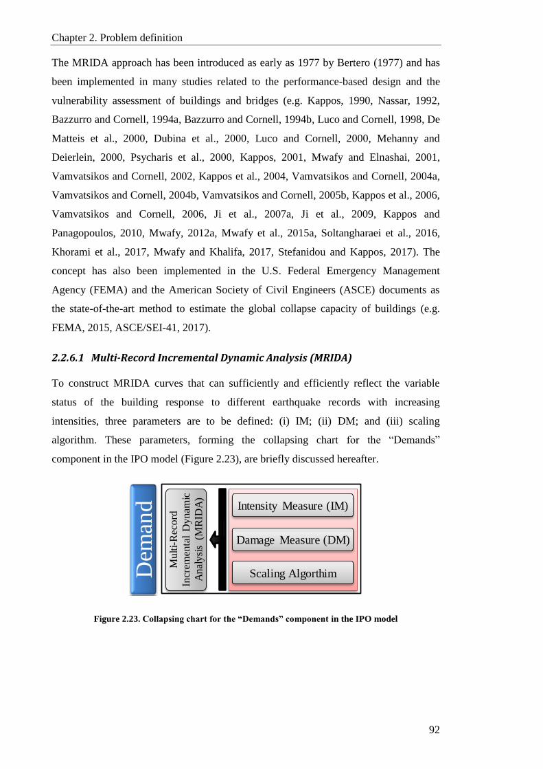
Chapter 2. Problem definition
92
The MRIDA approach has been introduced as early as 1977 by Bertero (1977) and has
been implemented in many studies related to the performance-based design and the
vulnerability assessment of buildings and bridges (e.g. Kappos, 1990, Nassar, 1992,
Bazzurro and Cornell, 1994a, Bazzurro and Cornell, 1994b, Luco and Cornell, 1998, De
Matteis et al., 2000, Dubina et al., 2000, Luco and Cornell, 2000, Mehanny and
Deierlein, 2000, Psycharis et al., 2000, Kappos, 2001, Mwafy and Elnashai, 2001,
Vamvatsikos and Cornell, 2002, Kappos et al., 2004, Vamvatsikos and Cornell, 2004a,
Vamvatsikos and Cornell, 2004b, Vamvatsikos and Cornell, 2005b, Kappos et al., 2006,
Vamvatsikos and Cornell, 2006, Ji et al., 2007a, Ji et al., 2009, Kappos and
Panagopoulos, 2010, Mwafy, 2012a, Mwafy et al., 2015a, Soltangharaei et al., 2016,
Khorami et al., 2017, Mwafy and Khalifa, 2017, Stefanidou and Kappos, 2017). The
concept has also been implemented in the U.S. Federal Emergency Management
Agency (FEMA) and the American Society of Civil Engineers (ASCE) documents as
the state-of-the-art method to estimate the global collapse capacity of buildings (e.g.
FEMA, 2015, ASCE/SEI-41, 2017).
2.2.6.1 Multi-Record Incremental Dynamic Analysis (MRIDA)
To construct MRIDA curves that can sufficiently and efficiently reflect the variable
status of the building response to different earthquake records with increasing
intensities, three parameters are to be defined: (i) IM; (ii) DM; and (iii) scaling
algorithm. These parameters, forming the collapsing chart for the “Demands”
component in the IPO model (Figure 2.23), are briefly discussed hereafter.
Figure 2.23.Collapsingchartforthe“Demands”componentin the IPO model
Dem
and Intensity Measure (IM)
Damage Measure (DM)
Scaling Algorthim
Mu
lti-
Rec
ord
Incr
emen
tal
Dy
nam
ic
Anal
ysi
s (M
RID
A)

Chapter 2. Problem definition
93
2.2.6.1.1 Intensity Measure (IM)
The IM, as defined in Section 2.1, is a non-negative scalar (or vector) that constitutes a
function of the scaled accelerogram. It refers to the unscaled accelerogram and is
increasing or decreasing monotonically with a predefined scaling algorithm.
In the past, PGA used to be the most preferred intensity measure. In recent years,
however, the elastic spectral acceleration at the fundamental period of the structure,
Sa(T1) or Sa in short, has been found to be more efficient, since it is structure-dependent,
and became a frequently used intensity measure for short buildings. However, Sa is
shown to be neither efficient nor sufficient to be used with tall buildings (Shome, 1999,
Vamvatsikos and Cornell, 2002) and for structures subjected to near-source earthquakes
(Luco and Cornell, 2007). Other intensity measures have been proposed in the literature
to overcome the major shortcomings of Sa, namely discounting the contribution of the
higher modes and fundamental period lengthening of the structure associated with
stiffness degradation (Shome, 1999, Carballo and Cornel, 2000, Cordova et al., 2000).
New approaches have led to other kinds of intensity measures such as inelastic spectral
value-based scalar intensity measures (e.g. Luco and Cornell, 2007) and vector-valued
intensity measures (Bazzurro and Cornell, 2002, Conte et al., 2003, Baker and Cornell,
2005). These approaches, although promising, are not easy to apply since they require
probabilistic seismic hazard assessment based on custom-made attenuation laws to
obtain the joint hazard curve. In the present study, a new scalar intensity measure
termed spectral acceleration at weighted-average period Sa(wa), is proposed. More insight
about this IM is given in CHAPTER 5.
2.2.6.1.2 Damage Measure (DM)
The DM, as defined in Section 2.1, is a structural state variable represented by a non-
negative scalar that signifies the additional response of the structural model as a result
of a predefined seismic loading. In other words, a DM is a quantitative parameter that
forms a part of the output of the corresponding NRHA.
Different DMs can be selected depending on the application and the assessed structure
itself. They can be categorised as: (i) demand-based; (ii) deformation-based; (iii) force-
based; (iv) energy-based; and (v) stability-based. For the structural damage of buildings,
the deformation-based maximum total peak inter-storey drift is a strong DM candidate.

Chapter 2. Problem definition
94
It is found to well relate to the member rotation and both local and global storey
collapse. Hence, this DM is adopted in many loss estimation programs such as HAZUS
(FEMA, 2019, Kircher et al., 2006), seismic code provisions (e.g. PEER/ATC, 2010,
FEMA, 2015, ASCE/SEI-41, 2017), and previous studies (e.g. Vamvatsikos and
Cornell, 2002, 2004a, Mwafy, 2012a, Yamin et al., 2017). For high-rise buildings,
however, the maximum net (effective) peak inter-storey drift, accounting for the rigid
body motion effects, is argued to be a more reliable DM (e.g. Ji et al., 2009). More
insight on this DM is given in CHAPTER 5.
2.2.6.1.3 Scaling algorithm
Performing a MRIDA can be quite intensive in terms of computational efforts and
resources. Although an almost continuous representation of the IDA curves is preferred,
the high cost associated with each NRHA run for a high-rise building necessitates the
employment of a scaling algorithm. As defined in Section 2.1, scaling algorithm is an
algorithm intended to select an optimum grid of distinct intensity measure values that
will deliver the desired coverage of the building seismic response with the objectives of
achieving a minimum number of runs, high demand resolution, and high capacity
resolution. In a MRIDA study, a different scaling algorithm can be designed for each
record set separately. The results obtained from the first record in the set can be utilised
to define the scaling algorithm to be used on the rest of the records in that set. The
simplest form of scaling algorithms is the so-called stepping algorithm, where a
constant step is adopted to increase the IM from zero to collapse level. The end result is
IM-uniformly spaced grid of points where only a pre-defined step value and a run-
stopping rule are required. The quality of this type of scaling algorithm is principally
dependent on the selected IM step. A version of this form is detailed in Yun et al.
(2002) and is used in the FEMA guidelines (e.g. FEMA, 2015).
A more advanced technique that can be adopted is the hunt and fill tracing algorithm.
This technique was discussed in detail by Vamvatsikos and Cornell (2004b). In this
algorithm, the first routine, also called the hunting part, involves increasing the step
interval until all damage states associated with the collapse prevention performance
level are bracketed with the means of only a few runs. Step interval increasing can be
achieved by applying either a constant, resulting in a quadratic series of IMs, or a factor,
producing a geometric series. To improve upon capacity resolution of the IDA curve, a
step reducing (second routine) is to be added to the algorithm once the first damage

Chapter 2. Problem definition
95
associated with collapse prevention state is detected. The third and final routine in this
algorithm is to fill in the gaps created by the enlarged step intervals introduced in the
first routine. This will enhance the demand resolution in the IDA curve. The hunt and
fill tracing algorithm require the definition of an initial step, a run-stopping rule, a step
interval increasing function, and capacity and demand resolutions. The hunt and fill
tracing algorithm are adopted in the present study in which the step interval increasing
function and capacity and demand resolutions are selected so that a predefined number
of runs (fourteen) is performed on each of the 40 used records.
2.2.7 Damage Indices (DIs)
Earthquakes with varying scenarios are expected to impose different excitation levels to
different modes of vibration in high-rise buildings. Furthermore, it may impose different
nature of excitation on an individual structural element such as a structural wall or a
coupling beam. Therefore, a wide range of DIs is to be considered for a proper
vulnerability assessment study of this class of structures. As highlighted in
Section 2.2.6.1.2, DIs can be categorised as:
Demand-based: Such as peak floor acceleration. This DI is widely used if the
damage of non-structural contents or sensitive equipment in a multi-storey
building is to be assessed.
Deformation-based: Such as strains (tensile and compressive) in reinforcing
steel and concrete materials, shear strain in walls, rotations in structural
members, peak storey ductilities, total peak roof drift, and maximum total peak
inter-storey drift.
Force-based: Such as base shears, base overturning moments, and capacities of
structural members in shear/axial/bending.
Energy-based: Such as the global Park-Ang index (Park and Ang, 1985).
Stability-based: Such as the stability index proposed by Mehanny and Deierlein
(2000).
For the definition of reliable performance criteria of high-rise buildings, local DIs (such
as strains and rotations) and global DIs (such as drifts) are to be selected,
mathematically defined in the model, mapped, and linked to one another. Mapping of
the local damages resulting from the MRIDA on a building provides insight into the
nature of the building response under varying earthquake scenarios. This enables
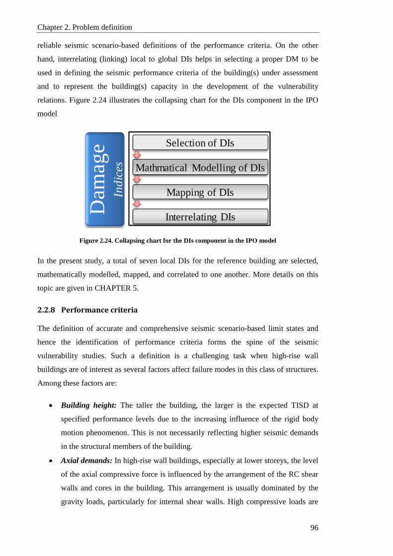
Chapter 2. Problem definition
96
reliable seismic scenario-based definitions of the performance criteria. On the other
hand, interrelating (linking) local to global DIs helps in selecting a proper DM to be
used in defining the seismic performance criteria of the building(s) under assessment
and to represent the building(s) capacity in the development of the vulnerability
relations. Figure 2.24 illustrates the collapsing chart for the DIs component in the IPO
model
Figure 2.24. Collapsing chart for the DIs component in the IPO model
In the present study, a total of seven local DIs for the reference building are selected,
mathematically modelled, mapped, and correlated to one another. More details on this
topic are given in CHAPTER 5.
2.2.8 Performance criteria
The definition of accurate and comprehensive seismic scenario-based limit states and
hence the identification of performance criteria forms the spine of the seismic
vulnerability studies. Such a definition is a challenging task when high-rise wall
buildings are of interest as several factors affect failure modes in this class of structures.
Among these factors are:
Building height: The taller the building, the larger is the expected TISD at
specified performance levels due to the increasing influence of the rigid body
motion phenomenon. This is not necessarily reflecting higher seismic demands
in the structural members of the building.
Axial demands: In high-rise wall buildings, especially at lower storeys, the level
of the axial compressive force is influenced by the arrangement of the RC shear
walls and cores in the building. This arrangement is usually dominated by the
gravity loads, particularly for internal shear walls. High compressive loads are
Dam
age
Ind
ices
Selection of DIs
Mathmatical Modelling of DIs
Mapping of DIs
Interrelating DIs

Chapter 2. Problem definition
97
expected to delay the onset of the initial cracking and yielding in vertical
elements but can decrease ductility and hence the TISD at which concrete core
crushing and rebar buckling occur.
Supplementary regulations and construction trends: The supplementary
regulations of local authorities, as well as trends adopted by both consultants and
contractors, may impact the design and hence the seismic performance of high-
rise buildings. For instance, the minimum steel ratio in vertical elements may
exceed the value that is stated in the code provisions.
Limit states present propagating points on a continuous scale of damage states of the
structure, therefore, described with potential and tolerable losses such as the structural
and non-structural damage, the number of casualties, the facility non-operational time,
repair cost and others. There are two different approaches for defining the limit states
for a building or a building inventory. These are:
I. Qualitative approach: This approach, where the limit states are defined through
the description of the structure’s damage state, is the most used in building
regulations and seismic codes (e.g. ASCE/SEI-41, 2017, FEMA, 2019). For
instance, in a study by Rossetto and Elnashai (2003), this approach is utilised to
define seven limit sates based on post-earthquakes observed damage data on
buildings.
II. Quantitative approach: The definition of limit states based on this approach
requires mathematical representations of local DIs (such as deformations, forces,
and energy) based on designated building performance levels. This necessitates
the adoption of a suitable DM to sufficiently correlate local damage events in the
building to its global response. Several researchers have adopted this approach
in their definitions of limit states (e.g. Kappos, 1991, Kappos and
Dimitrakopoulos, 2008, Ji et al., 2009, Kappos et al., 2010, Mwafy, 2012a,
Pejovic and Jankovic, 2016)
Due to the lack of sufficient post-earthquake data in the case of RC high-rise wall
buildings, the qualitative approach would not be suitable for defining the performance
criteria for this building class. Nevertheless, the limit states defined in previous studies
and seismic codes using qualitative approaches can serve as references (e.g. Ji et al.,
2007b).
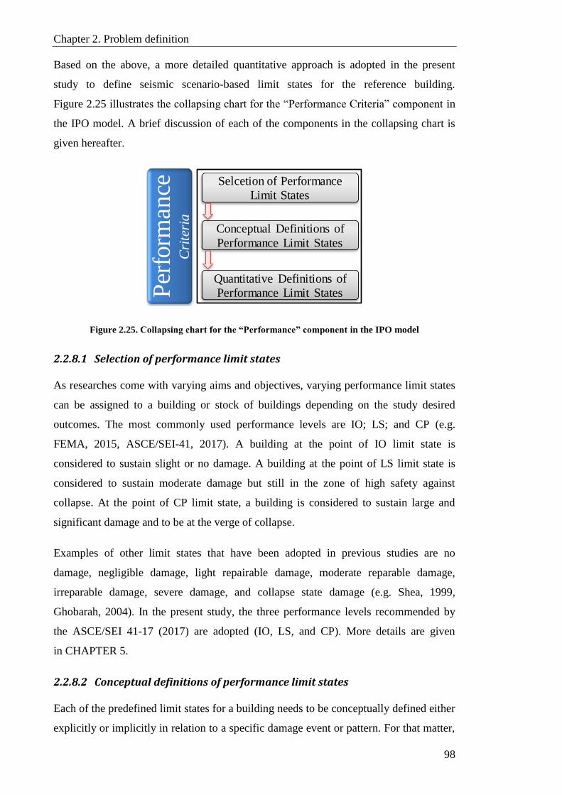
Chapter 2. Problem definition
98
Based on the above, a more detailed quantitative approach is adopted in the present
study to define seismic scenario-based limit states for the reference building.
Figure 2.25 illustrates the collapsing chart for the “Performance Criteria” component in
the IPO model. A brief discussion of each of the components in the collapsing chart is
given hereafter.
Figure 2.25.Collapsingchartforthe“Performance”componentin the IPO model
2.2.8.1 Selection of performance limit states
As researches come with varying aims and objectives, varying performance limit states
can be assigned to a building or stock of buildings depending on the study desired
outcomes. The most commonly used performance levels are IO; LS; and CP (e.g.
FEMA, 2015, ASCE/SEI-41, 2017). A building at the point of IO limit state is
considered to sustain slight or no damage. A building at the point of LS limit state is
considered to sustain moderate damage but still in the zone of high safety against
collapse. At the point of CP limit state, a building is considered to sustain large and
significant damage and to be at the verge of collapse.
Examples of other limit states that have been adopted in previous studies are no
damage, negligible damage, light repairable damage, moderate reparable damage,
irreparable damage, severe damage, and collapse state damage (e.g. Shea, 1999,
Ghobarah, 2004). In the present study, the three performance levels recommended by
the ASCE/SEI 41-17 (2017) are adopted (IO, LS, and CP). More details are given
in CHAPTER 5.
2.2.8.2 Conceptual definitions of performance limit states
Each of the predefined limit states for a building needs to be conceptually defined either
explicitly or implicitly in relation to a specific damage event or pattern. For that matter,
Per
form
ance
Cri
teri
aSelcetion of Performance
Limit States
Conceptual Definitions of
Performance Limit States
Quantitative Definitions of
Performance Limit States
Chapter 2. Problem definition
99
different approaches have been adopted in seismic codes and previous studies. In the
study of Vamvatsikos and Cornell (2004a) on steel moment-resisting frame buildings,
the characteristics of the IDA curves were utilised to conceptually define the CP and
collapse limit states. The former was linked to the “80% reduction in slope” point on the
curve while the latter was associated with reaching the flatness zone (global dynamic
instability). In the ASCE/SEI 41-06 standard (2007), specific rotation values in RC
walls and coupling beams are associated to each of the three predefined limit states (IO,
LS, and CP) for the primary and secondary components controlled by the flexural
response. In the study of Ji et al. (2007b) which involved a 54-storey RC high-rise wall
building, pushover and time-history analyses were performed to conceptually define the
three selected limit states (Serviceability, Damage Control, and CP). The Serviceability
limit state was linked to the initiation of minor cracks in main resisting members. The
Damage Control limit state was linked to the first yielding in longitudinal reinforcement
or to the occurrence of the first plastic hinge (whichever happens first). The CP limit
state was linked to the reach of the ultimate capacity in the main resisting members and
to the start of the descending zone in the capacity curve.
Another example is the study of Mwafy (2012a) that involved pushover and incremental
dynamic analyses on the nonlinear models of six reference RC wall buildings with
varying heights (10 to 60 storeys). In this study, the CP limit state was selected based on
the recommendation of previous studies. The LS limit state was linked to the global
yielding point of the building, which was estimated from the capacity curve using the
elastic-perfectly plastic idealization concept. The IO limit state was associated with the
most conservative first yielding values obtained from pushover analysis and median
IDA results of 20 earthquake records. A more recent study by Mwafy and Khalifa
(Mwafy and Khalifa, 2017) on vertically irregular high-rise buildings estimated the
limit states from IDA by linking local response to TISD.
In the present study, seven local DIs are used to conceptually define the adopted
performance limit states for the reference building. More details are given in CHAPTER
5.
2.2.8.3 Quantitative definitions of performance limit states
Using TISD as a DM, seismic guidelines and previous studies have adopted a wide
range of quantitative values to define limit state criteria associated with different

Chapter 2. Problem definition
100
performance levels of RC shear walls and wall structures. The SEAOC blue book
(1999) proposed TISDs of 0.4%, 0.9%, 1.4% and 2.1% for RC shear walls at
performance levels SP1 (negligible damage), SP2 (minor to moderate reparable
damage), SP3 (moderate to major irreparable damage) and SP4 (collapse performance
level), respectively. In ASCE/SEI 41-06 (2007), TISDs of 0.5%, 1%, and 2.0% are
assigned to the IO, LS and CP performance levels, respectively. In a study involving
post-earthquakes observed damage data on RC wall buildings, Rossetto and Elnashai
(2003) suggested TISD values of 0.00, 0.026, 0.34, 0.72, 1.54, 2.56, and > 3.31 for the
damage states of none, slight, light, moderate, extensive, partial collapse, and collapse,
respectively. For ductile RC walls, Ghobarah (2004) recommended TISDs of <0.2%,
0.4%, <0.8%, >0.8%, 1.5% and >2.5% corresponded to damage levels of none, light
reparable, moderate reparable, irreparable, severe (or life safe) and collapse,
respectively. In contrast, Ji et al. (2007a) suggested conservative TISDs to define three
performance limit states obtained from inelastic pushover and time history analyses for
a 54-storey RC wall building. The proposed TISDs were 0.2%, 0.52% and 1.1% for
serviceability, damage control, and collapse prevention limit states, respectively. In a
study of RC wall buildings with a number of storeys ranging between 10 to 60, Mwafy
(2012a) suggested a TISD value of 2.5% for CP, while height-dependent TISDs were
proposed for IO (0.32% to 0.83%) and LS (0.81% to 1.35%). In the study of Jeong et al.
(2012), TISDs of 0.4% to 0.7%, 1.5%, and 2.5% were associated to the limit states of
IO, LS, and CP, respectively, for 8-storey wall-frame buildings with different ductility
and input ground motion intensity levels. More recently, a study conducted by Pejovic
and Jankovic (2016), involving RC high-rise wall buildings (10-, 30-, and 40-storey)
located in the southern Euro-Mediterranean zone, suggested TISD values of 0.25%,
0.53%, 0.95%, and 1.64% for the limit states of slight damage, moderate damage,
extensive damage, and collapse, respectively.
It is essential to highlight that all the above-mentioned recommendations of TISDs, as
quantitative definitions to the performance limit states of RC wall buildings, have not
taken into consideration the need for seismic scenario-based limit state definitions. The
broad range of frequency content in real strong ground motions, representative of
different seismic scenarios (i.e. distant and near-field earthquakes), can impose a
different level of excitation on both fundamental and higher modes in the RC high-rise
wall structures and consequently different nature of response. Therefore, for an accurate
vulnerability and seismic risk assessment studies on this class of buildings, seismic
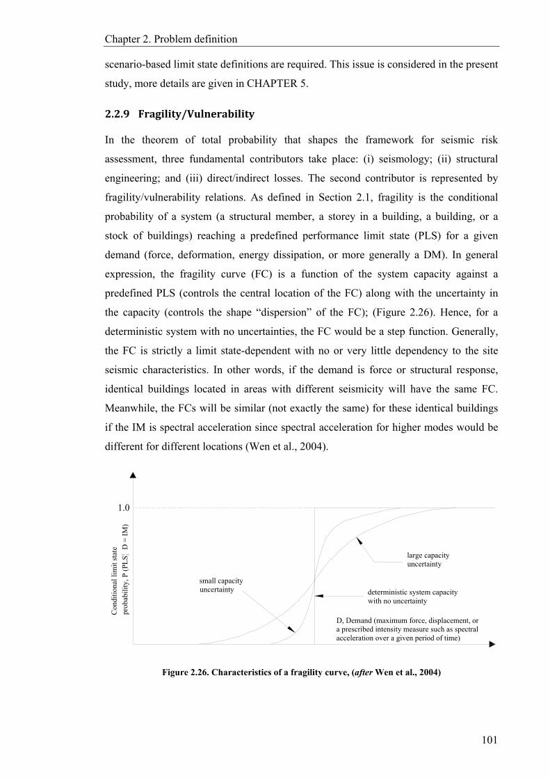
Chapter 2. Problem definition
101
scenario-based limit state definitions are required. This issue is considered in the present
study, more details are given in CHAPTER 5.
2.2.9 Fragility/Vulnerability
In the theorem of total probability that shapes the framework for seismic risk
assessment, three fundamental contributors take place: (i) seismology; (ii) structural
engineering; and (iii) direct/indirect losses. The second contributor is represented by
fragility/vulnerability relations. As defined in Section 2.1, fragility is the conditional
probability of a system (a structural member, a storey in a building, a building, or a
stock of buildings) reaching a predefined performance limit state (PLS) for a given
demand (force, deformation, energy dissipation, or more generally a DM). In general
expression, the fragility curve (FC) is a function of the system capacity against a
predefined PLS (controls the central location of the FC) along with the uncertainty in
the capacity (controls the shape “dispersion” of the FC); (Figure 2.26). Hence, for a
deterministic system with no uncertainties, the FC would be a step function. Generally,
the FC is strictly a limit state-dependent with no or very little dependency to the site
seismic characteristics. In other words, if the demand is force or structural response,
identical buildings located in areas with different seismicity will have the same FC.
Meanwhile, the FCs will be similar (not exactly the same) for these identical buildings
if the IM is spectral acceleration since spectral acceleration for higher modes would be
different for different locations (Wen et al., 2004).
Figure 2.26. Characteristics of a fragility curve, (after Wen et al., 2004)
large capacityuncertainty
small capacityuncertainty deterministic system capacity
with no uncertainty
Con
diti
onal
lim
it st
ate
prob
abil
ity,
P (
PLS
¦D
= I
M)
1.0
D, Demand (maximum force, displacement, ora prescribed intensity measure such as spectralacceleration over a given period of time)

Chapter 2. Problem definition
102
To generate a fragility/vulnerability curve, the following order-wise steps are needed:
1. Defining the PLSs of interest and the IM. In the present study, the defined
performance limit states are IO, LS, and CP (more details are given in
Section 2.2.8 and CHAPTER 5). The proposed IM is the spectral acceleration at
weighted-average period Sa(wa) (more details are given in Section 2.2.6.1.1
and CHAPTER 5).
2. Performing regression analysis on the limit states-related building response as a
function of the IM (MRIDAs results). Considering the nonlinear nature of the
problem and the record-to-record response variation, nonlinear regression
analysis in the power-law form is recommended (Vamvatsikos and Cornell,
2002, Luco and Cornell, 2007, Mwafy, 2012a, Mwafy and Elkholy, 2017).
Other nonlinear regression analysis may be implemented if found to better fit the
LSs-IM relation.
3. Accounting for the uncertainties in the FC development process. These
uncertainties can be categorised as (i) demand uncertainty; capacity uncertainty;
and modelling uncertainty. Details on the estimation of these uncertainties are
given in CHAPTER 6.
4. Generating the FCs using a proper distribution function. Generally, a lognormal
cumulative distribution function provides a good fit (Wen et al., 2004) therefore
adopted in the present study. More details on the components of the FC function
are given in CHAPTER 6.
5. The probabilistic earthquake risk assessment for a building or a building stock
may be expressed in terms of a probability distribution function of economic
losses (vulnerability curves) by further processing the FCs. An example of such
a presentation is shown in Figure 2.27. Several methods have been proposed by
previous studies to develop the vulnerability functions (e.g. Scholl, 1980, Kustu
et al., 1982, Kustu and Miller, 1984, Singhal and Kiremidjian, 1996, Porter et
al., 2001, D’ayala et al., 2014, Yamin et al., 2014a, Yamin et al., 2014b, Yamin
et al., 2017). Those methods have been imbedded in earthquake risk assessment
platforms such as CAPRA (ERN-CAPRA, 2011), HAZUS (FEMA, 2019,
Kircher et al., 2006), Risk-UE (RISK-UE, 2001-2004), and other recently
developed platforms (e.g. GEM, 2019). To develop the vulnerability relations,
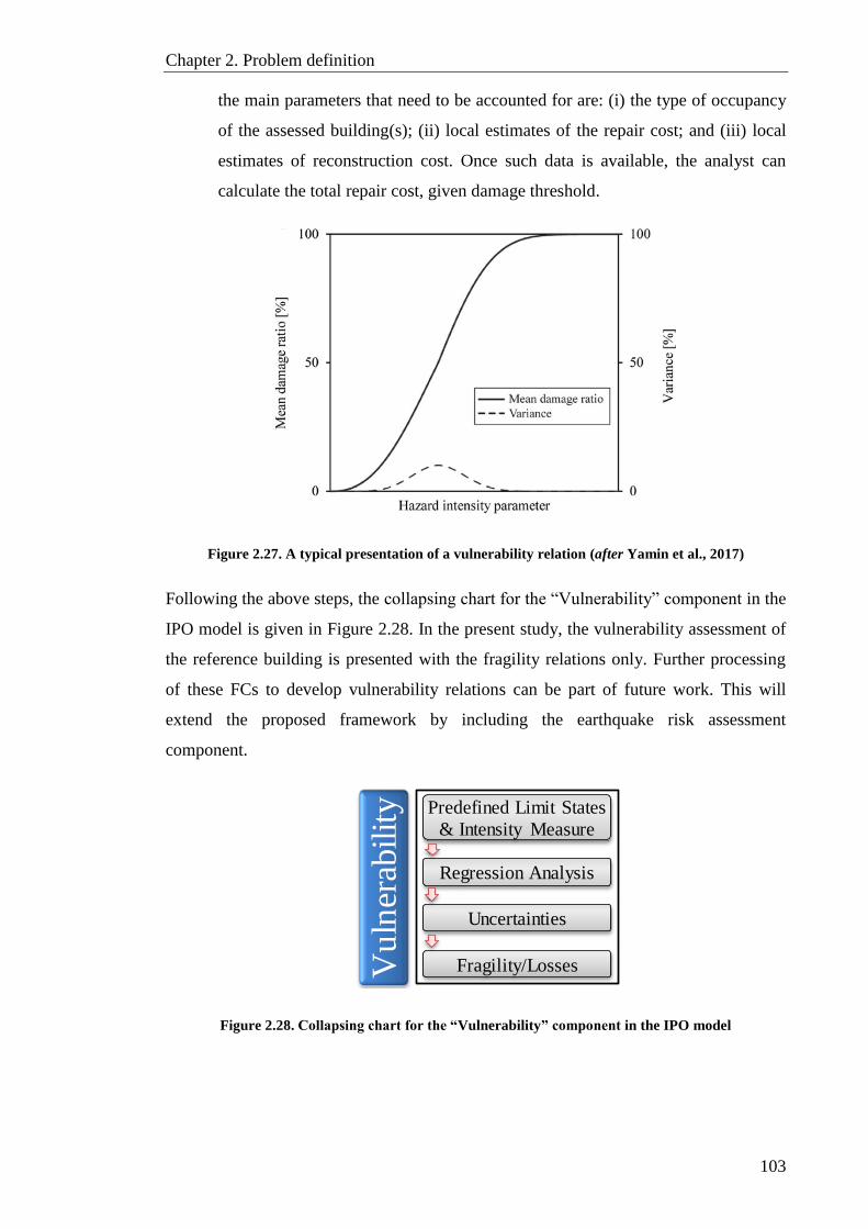
Chapter 2. Problem definition
103
the main parameters that need to be accounted for are: (i) the type of occupancy
of the assessed building(s); (ii) local estimates of the repair cost; and (iii) local
estimates of reconstruction cost. Once such data is available, the analyst can
calculate the total repair cost, given damage threshold.
Figure 2.27. A typical presentation of a vulnerability relation (after Yamin et al., 2017)
Following the above steps, the collapsing chart for the “Vulnerability” component in the
IPO model is given in Figure 2.28. In the present study, the vulnerability assessment of
the reference building is presented with the fragility relations only. Further processing
of these FCs to develop vulnerability relations can be part of future work. This will
extend the proposed framework by including the earthquake risk assessment
component.
Figure 2.28.Collapsingchartforthe“Vulnerability”componentin the IPO model
Vu
lner
abilit
y Predefined Limit States
& Intensity Measure
Regression Analysis
Uncertainties
Fragility/Losses

104
This page is intentionally left in blank

Chapter 3. Multi-level nonlinear modelling verification scheme
105
CHAPTER 3. Multi-level nonlinear
modelling verification
scheme of RC high-rise wall
buildings
Earthquake-resistant structures are designed and detailed to respond well beyond the
elastic range under the DBE. However, in terms of analysis, RC walls are often treated
as linear elements despite their considerable depth ignoring the effect of deformation
compatibility. Due to the limited number of comprehensive experimental studies on RC
structural wall systems subjected to cyclic loading, few in-depth analytical verification
studies have been conducted. Motivated by the increasing need for more accurate
seismic risk assessment of high-rise buildings adopting RC shear walls as the lateral
force-resisting system, a MLNMVS is developed in this chapter to investigate two
different nonlinear modelling techniques for shear walls (i.e. 2- and 4-noded fibre-based
elements). The investigated modelling approaches and their key parameters are verified
against the results of Phase-I of shake table specimen tests for a seven-storey full-scale

Chapter 3. Multi-level nonlinear modelling verification scheme
106
RC shear wall structure. The test structure was subjected to base excitations
representing four earthquake records of increasing intensities. The uniaxial shake table
tests were performed at the University of California, San Diego (Panagiotou et al.,
2007a, Panagiotou et al., 2007b). In the established MLNMVS, three analytical models
are developed using two different software (ZEUS-NL and PERFORM-3D). The results
obtained from the analytical models are compared with the experimental results both on
the global and local response levels (top displacement, inter-storey drift, storey shear
force, storey bending moment, period elongation and rebar tensile strain). The study
reveals the superior performance of 4-noded fibre-based wall/shell element modelling
approach in accounting for the 3D effects of deformation compatibility between lateral
and gravity-force-resisting systems. The study also highlights the sensitivity of attained
results to the stiffnesses assigned to the rigid links and 3D joints required to connect the
shear walls to neighbouring elements when a 2-noded element is used.
3.1 Introduction
With increasing concern for the seismic performance of RC buildings following
extensive damage caused by recent strong earthquakes (e.g. Kobe 1995; Kocaeli, 1999;
Chi-Chi, 1999; and Tohoku, 2011), the use of RC shear walls in medium- to high-rise
buildings is favoured in earthquake-prone regions. Shear walls can be found either as
single elements coupled with moment-resisting frames, or in the shape of L, T, U, or
tubular cross-sections. Based on modern seismic codes, earthquake-resistant buildings
are designed and detailed to respond inelastically under the DBE and MCE. In RC high-
rise buildings, well designed and proportioned RC slender shear walls can provide the
required strength, stiffness and deformation ductility to ensure the adequate
performance of the structure in the “service”, “ultimate”, and “collapse prevention”
limit states. Nonetheless, RC shear walls are often modelled as linear elements during
the analysis for simplicity despite their considerably large depth (PEER, 2010,
PEER/ATC, 2010). This can lead to a considerable underestimation of the deformed
shape and compatibility issues between shear and flexural lateral resisting mechanisms,
as well as, of local high deformation demand issues. Furthermore, due to high costs and
lack of availability of large scale testing facilities, there are few reliable and
comprehensive studies on the cyclic behaviour of RC wall buildings that could have
been used for verification purposes (Ji et al., 2007a, Wallace, 2007, Beyer et al., 2008,
Wallace and Moehle, 2012). Hence, there is still a need for a verified nonlinear
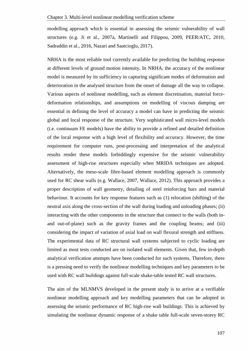
Chapter 3. Multi-level nonlinear modelling verification scheme
107
modelling approach which is essential in assessing the seismic vulnerability of wall
structures (e.g. Ji et al., 2007a, Martinelli and Filippou, 2009, PEER/ATC, 2010,
Sadraddin et al., 2016, Nazari and Saatcioglu, 2017).
NRHA is the most reliable tool currently available for predicting the building response
at different levels of ground motion intensity. In NRHA, the accuracy of the nonlinear
model is measured by its sufficiency in capturing significant modes of deformation and
deterioration in the analysed structure from the onset of damage all the way to collapse.
Various aspects of nonlinear modelling, such as element discretisation, material force-
deformation relationships, and assumptions on modelling of viscous damping are
essential in defining the level of accuracy a model can have in predicting the seismic
global and local response of the structure. Very sophisticated wall micro-level models
(i.e. continuum FE models) have the ability to provide a refined and detailed definition
of the local response with a high level of flexibility and accuracy. However, the time
requirement for computer runs, post-processing and interpretation of the analytical
results render these models forbiddingly expensive for the seismic vulnerability
assessment of high-rise structures especially when MRIDA techniques are adopted.
Alternatively, the meso-scale fibre-based element modelling approach is commonly
used for RC shear walls (e.g. Wallace, 2007, Wallace, 2012). This approach provides a
proper description of wall geometry, detailing of steel reinforcing bars and material
behaviour. It accounts for key response features such as (1) relocation (shifting) of the
neutral axis along the cross-section of the wall during loading and unloading phases; (ii)
interacting with the other components in the structure that connect to the walls (both in-
and out-of-plane) such as the gravity frames and the coupling beams; and (iii)
considering the impact of variation of axial load on wall flexural strength and stiffness.
The experimental data of RC structural wall systems subjected to cyclic loading are
limited as most tests conducted are on isolated wall elements. Given that, few in-depth
analytical verification attempts have been conducted for such systems. Therefore, there
is a pressing need to verify the nonlinear modelling techniques and key parameters to be
used with RC wall buildings against full-scale shake-table tested RC wall structures.
The aim of the MLNMVS developed in the present study is to arrive at a verifiable
nonlinear modelling approach and key modelling parameters that can be adopted in
assessing the seismic performance of RC high-rise wall buildings. This is achieved by
simulating the nonlinear dynamic response of a shake table full-scale seven-storey RC

Chapter 3. Multi-level nonlinear modelling verification scheme
108
wall building slice. This building was tested under base excitations representing four
earthquake records of increasing intensities on the Large high-performance outdoor
shake table at the University of California, San Diego (Panagiotou et al., 2007a,
Panagiotou et al., 2007b, Panagiotou et al., 2010). To model the shear walls in the tested
structure, two fibre-based modelling approaches are investigated: (i) 2-noded beam-
column line element (also called wide-column element), where an equivalent column at
the wall centroidal axis with wide cross-section is used to model the property of the
wall; and (ii) 4-noded wall element, a modelling approach conceptually similar to the
Multiple-Vertical-Line-Element model (Wallace, 2007, Wallace, 2010). ZEUS-NL
analytical software (Elnashai et al., 2012) is utilised to implement the former modelling
approach, while PERFORM-3D (CSI, 2011) is chosen to investigate the latter.
In Section 3.2 of this chapter, key features of the utilised analytical software are
presented, including cross-sections, element formulation, material models and
numerical strategy. A brief description of the shake table test program and the test
structure are given in Sections 3.3. Section 3.4 discusses the four input ground motions
used in the tests. The analytical models created in the current study along with the
comparison of their results with the experimental data are detailed in Section 3.5. The
chapter concludes with a summary of the work, findings, and modelling
recommendations (Section 3.6).
3.2 Analytical Tools
There is a wide variety of finite element (FE) structural software available to
researchers that are capable of performing fibre element-based nonlinear analysis.
Among these packages are DRAIN-3DX (Prakash et al., 1994), OpenSees (Mazzoni et
al., 2006, McKenna and Fenves, 2006, McKenna, 2011), ZEUS-NL (Elnashai et al.,
2012) and PERFORM-3D (CSI, 2011). Depending on the geometry of the structure, the
purpose of the analysis, and the efficiency of the software to perform the required tasks,
one tool may be selected over the others. The first three packages are essentially frame
element analysis software with mostly comparable elements and capabilities.
In the current study, ZEUS-NL and PERFORM-3D analytical software are utilised in
the MLNMVS. The main capabilities of both packages are summarised below:
Chapter 3. Multi-level nonlinear modelling verification scheme
109
Predicting the response of RC, steel and composite structures under static and
dynamic loading, taking into account the effects of both material and geometric
nonlinearities.
The applied load can be constant or variable forces, displacements and or
accelerations.
The ability to perform different methods of analysis such as eigenvalue,
pushover, and response histories.
The ability to model different concrete and steel material relations, with the
option of including hysteresis loops of strength and stiffness degradation.
Built-in Library of elements and components that can be used with a wide range
of concrete, steel and composite cross-sectional configurations.
A detailed description of the utilised software is beyond the scope of this study. Only
the cross-sections, element formulations, material models and numerical strategies that
relate to the present work are briefly presented in the succeeding sub-sections. Further
information regarding the software is available in the ZEUS-NL user manual (Elnashai
et al., 2012) and its counterpart for PERFORM-3D (CSI, 2011).
3.2.1 ZEUS-NL
ZEUS-NL is a fibre-based nonlinear analysis platform developed at Imperial College
London, UK and the University of Illinois at Urbana-Champaign, U.S., and has been
verified against experimental tests of steel and concrete frame elements and structures in
Europe and the U.S. (e.g. Elnashai and Elghazouli, 1993, Elnashai and Izzuddin, 1993a,
Elnashai et al., 2012, Izzuddin, 2016). The package is employed in several research
projects in Europe, the U.S. and the Middle East (e.g. Elnashai, 2006, Kim and
Elnashai, 2008, Ji et al., 2009, Mwafy, 2012a, Mwafy et al., 2015a).
3.2.1.1 Cross-sections
A large number of cross-section configurations is available in ZEUS-NL library.
General use sections include solid rectangular; symmetrical hollow-I-T, Asymmetric L-
C, and fully/partially-encased composite I. For RC elements, there are specific sections
available in the library such as rectangular/circular column section, T-beam section, and

Chapter 3. Multi-level nonlinear modelling verification scheme
110
rectangular flexural wall section. Figure 3.1 illustrates some of the above-mentioned
cross-sections.
3.2.1.2 Element formulations
ZEUS-NL library contains a set of elements that can be utilised to model the elasto-
plastic structural behaviour, the dynamic characteristics of the model, and the boundary
conditions. Among the element types used in the current study are cubic elasto-plastic
beam-column element, 3D joint element, lumped mass element, and Rayleigh damping
element.
For the cubic elasto-plastic element, the classical displacement-based FE formulation is
employed (Hellesland and Scordelis, 1981, Mari, 1984). A cubic-shape function is used
for calculating transverse displacement v(x). This function is given by Eqn. ( 3.1), where
all the equation symbols are graphically defined in Figure 3.2. The formulation of this
element represents the inelastic cyclic response of RC members, accounting for
geometrical and material nonlinearities. The axial strain is assumed constant along the
element length in this formulation and hence a refined discretisation, typically three or
more elements per structural member, is required to achieve a reasonable accuracy in
the inelastic modelling. The expected length of the plastic hinge is another factor to be
considered when deciding the number of elements in a structural member. This issue is
further investigated in the model verification process. Cross-section behaviour is
represented using the fibre approach, where element cross-sections are divided into a
number of fibres (layers). An appropriate material model is assigned to each fibre where
strains and stresses are monitored. The sectional stress-strain state is then obtained
through the integration of the nonlinear stress-strain response of the individual fibres.
Two controlling (Gauss) sections along each element are used for the numerical
integration of the governing equations in the element formulation (Figure 3.3).
v(x) = (θ1 + θ2
L2) x3 − (
2θ1 + θ2L
) x2 + θ1. x ( 3.1)
In the cubic elasto-plastic element formulation, the cross-section fibres have no ability
to deal with shear stress. Hence, the shear deformation is not calculated at the section
level and the effect of shear-flexure interaction on the element’s ductility is not
accounted for. To determine the shear deformation in a member, a displacement-type
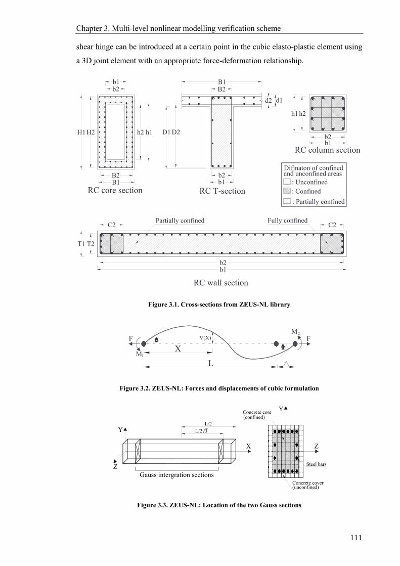
Chapter 3. Multi-level nonlinear modelling verification scheme
111
shear hinge can be introduced at a certain point in the cubic elasto-plastic element using
a 3D joint element with an appropriate force-deformation relationship.
Figure 3.1. Cross-sections from ZEUS-NL library
Figure 3.2. ZEUS-NL: Forces and displacements of cubic formulation
Figure 3.3. ZEUS-NL: Location of the two Gauss sections
RC column section
h2h1
b2b1
b2b1
D2D1
B2B1
RC T-section
Difinaton of confinedand unconfined areas
T1 T2
b1b2
Partially confined Fully confinedC2
RC wall section
: Unconfined: Confined
: Partially confined
d2 d1
H1 H2
b1b2
h1h2
B1B2
RC core section
C2
M1
F V(X)
X
L
1
M2
2
F
Y
Z
X
Concrete core Y
Z
Steel bars
Concrete cover
Gauss intergration sections
L/2 3
L/2 (confined)
(unconfined)
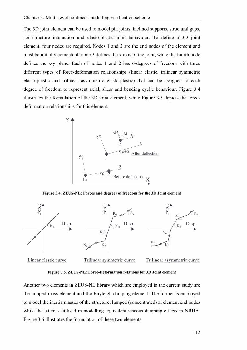
Chapter 3. Multi-level nonlinear modelling verification scheme
112
The 3D joint element can be used to model pin joints, inclined supports, structural gaps,
soil-structure interaction and elasto-plastic joint behaviour. To define a 3D joint
element, four nodes are required. Nodes 1 and 2 are the end nodes of the element and
must be initially coincident; node 3 defines the x-axis of the joint, while the fourth node
defines the x-y plane. Each of nodes 1 and 2 has 6-degrees of freedom with three
different types of force-deformation relationships (linear elastic, trilinear symmetric
elasto-plastic and trilinear asymmetric elasto-plastic) that can be assigned to each
degree of freedom to represent axial, shear and bending cyclic behaviour. Figure 3.4
illustrates the formulation of the 3D joint element, while Figure 3.5 depicts the force-
deformation relationships for this element.
Figure 3.4. ZEUS-NL: Forces and degrees of freedom for the 3D Joint element
Figure 3.5. ZEUS-NL: Force-Deformation relations for 3D Joint element
Another two elements in ZEUS-NL library which are employed in the current study are
the lumped mass element and the Rayleigh damping element. The former is employed
to model the inertia masses of the structure, lumped (concentrated) at element end nodes
while the latter is utilised in modelling equivalent viscous damping effects in NRHA.
Figure 3.6 illustrates the formulation of these two elements.
Y
X1,23
1
2
M
After deflection
Before deflection
K
Linear elastic curve Trilinear symmetric curve Trilinear asymmetric curve
K+2
Disp.
K1K2
K0Disp. Disp.K0
K0
K1K2
+1
K+0
K-0
K-1
K-2
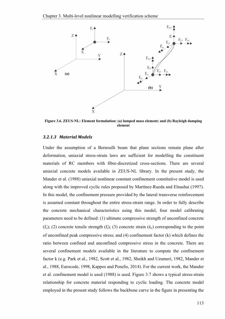
Chapter 3. Multi-level nonlinear modelling verification scheme
113
Figure 3.6. ZEUS-NL: Element formulation: (a) lumped mass element; and (b) Rayleigh damping element
3.2.1.3 MaterialModels
Under the assumption of a Bernoulli beam that plane sections remain plane after
deformation, uniaxial stress-strain laws are sufficient for modelling the constituent
materials of RC members with fibre-discretized cross-sections. There are several
uniaxial concrete models available in ZEUS-NL library. In the present study, the
Mander et al. (1988) uniaxial nonlinear constant confinement constitutive model is used
along with the improved cyclic rules proposed by Martínez-Rueda and Elnashai (1997).
In this model, the confinement pressure provided by the lateral transverse reinforcement
is assumed constant throughout the entire stress-strain range. In order to fully describe
the concrete mechanical characteristics using this model, four model calibrating
parameters need to be defined: (1) ultimate compressive strength of unconfined concrete
(fc); (2) concrete tensile strength (ft); (3) concrete strain (εc) corresponding to the point
of unconfined peak compressive stress; and (4) confinement factor (k) which defines the
ratio between confined and unconfined compressive stress in the concrete. There are
several confinement models available in the literature to compute the confinement
factor k (e.g. Park et al., 1982, Scott et al., 1982, Sheikh and Uzumeri, 1982, Mander et
al., 1988, Eurocode, 1998, Kappos and Penelis, 2014). For the current work, the Mander
et al. confinement model is used (1988) is used. Figure 3.7 shows a typical stress-strain
relationship for concrete material responding to cyclic loading. The concrete model
employed in the present study follows the backbone curve in the figure in presenting the
Fz
Fy
FxY
Z
X
z1F
zz2F
yyFy2Fx2F
zF
Z
Y
X
xxF
zz1F
yyFy1Fx1F
xxF(a)
(b)

Chapter 3. Multi-level nonlinear modelling verification scheme
114
response under compressive load histories. When compressive stress is decreased and
increased again, the unloading and reloading curves are followed, respectively.
Figure 3.7. Typical stress-strain relation for concrete material under cyclic loading
To model steel material, two uniaxial stress-strain laws are utilised of the four available
in ZEUS-NL library: (1) The Menegotto and Pinto uniaxial steel model (1973) coupled
with the isotropic hardening rules proposed by (Filippou et al., 1983); and (2) Uniaxial
elastic model with symmetric behaviour in tension and compression. The Menegotto-
Pinto steel model is a well-known nonlinear relationship in modelling of reinforcing
steel in RC structures, particularly those subjected to complex loading histories where
significant load reversals might occur. When there is a need to model steel structural
members that are expected to remain elastic during the analysis, the elastic model is
used. Figure 3.8 shows the stress-strain relationship for the two adopted uniaxial steel
models. In Figure 3.8a, Eo is the initial elastic modulus of steel, E1 is the strain-
hardening modulus, Ro is a parameter defining the initial loading curvature, a1 to a4 are
experimental-based parameters that control the curvature and isotropic strain hardening
in subsequent load cycles.
Reloading curveUnloading curveEnvelope curve
c
cf

Chapter 3. Multi-level nonlinear modelling verification scheme
115
Figure 3.8. ZEUS-NL: Stress-strain laws for steel material: (a) Menegotto-Pinto steel model; and (b) linear elastic steel model
3.2.1.4 NumericalStrategy
In ZEUS-NL package, solving the system of equations of motion in NRHA can be
carried out by the means of two different numerical direct integration schemes; (1) the
Newmark integration scheme (Newmark, 1959); and (2) the Hilber-Hughes-Taylor
integration scheme (Hilber et al., 1977). The solution algorithm allows the employment
of either Newton-Raphson or modified Newton-Raphson iterative procedures, where
convergence is defined based on either displacement-rotation or force-moment criteria.
The efficient Lanczos algorithm (Hughes, 2012) is used by default for the evaluation of
structural natural frequencies and mode shapes. However, the Jacobi algorithm with
Ritz transformation is also available as another option to the user.
3.2.2 PERFORM‐3D
PERFORM-3D (CSI, 2011) is a structural-engineering nonlinear analysis software
developed by Dr. Graham H. Powell (Professor Emeritus, University of California at
Berkeley) for Computers & Structures, Inc. In recent years, this software has been
utilised in many studies and research programs to assess the seismic performance of RC
high-rise wall structures and buildings utilising other structural systems (e.g. Ghodsi
and Ruiz, 2010, PEER, 2011, Tuna, 2012). The 4-noded fibre-based wall element
implemented in PERFORM-3D is conceptually the same as the MVLE model, a model
that has previously been validated using experimental results from seismic tests at the
component level (e.g. Orakcal and Wallace, 2006, Wallace, 2007, Wallace, 2012).
E1
R0
E0
y
0 1 2
y
, ,
E
(a) (b)
Chapter 3. Multi-level nonlinear modelling verification scheme
116
3.2.2.1 Cross-sections
The cross-sections available in PERFORM-3D library can be divided into two
categories: (i) elastic sections to be used with linear analysis such as general,
symmetric-I, rectangular and membrane/shell RC and steel sections; and (ii) inelastic
(fibre) sections to be assigned to beams, columns and shear walls expected to
experience inelastic behaviour. Inelastic fibre section for beams, columns and shear
walls can be discretized to a maximum of 12, 60 and 16 fibres, respectively. Beam
sections use fibre properties for axial and in-plane bending (with P-M interaction) only
and are elastic for out-of-plane bending, while for column sections, fibre properties for
bending about both axes are used with biaxial bending and P-M-M interaction. Beam
and column fibre sections are both assumed to be elastic in shear. When inelastic shear
is to be considered, the shear hinge component is to be added.
The fibres in a shear wall section account for the vertical axial, vertical in-plane bending
and their interaction. The section is assumed elastic for the out-of-plane bending as well
as for horizontal axial/bending. Shear properties (elastic or inelastic) are not assigned to
the cross-section itself, but rather to the shear wall compound component, where
uncoupled shear deformation and compressive strain in concrete due to shear can be
determined. Figure 3.9 shows the modelling approach of some fibre-based cross-
sections in PERFORM-3D.
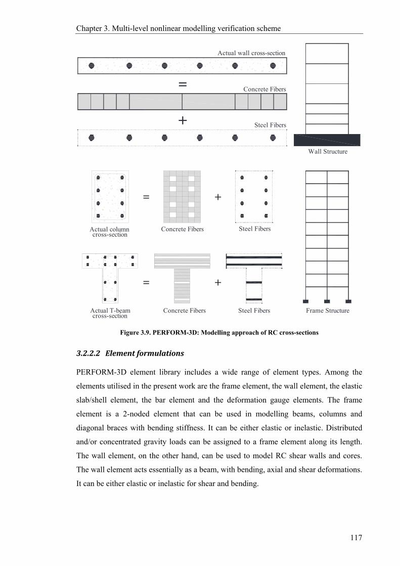
Chapter 3. Multi-level nonlinear modelling verification scheme
117
Figure 3.9. PERFORM-3D: Modelling approach of RC cross-sections
3.2.2.2 Elementformulations
PERFORM-3D element library includes a wide range of element types. Among the
elements utilised in the present work are the frame element, the wall element, the elastic
slab/shell element, the bar element and the deformation gauge elements. The frame
element is a 2-noded element that can be used in modelling beams, columns and
diagonal braces with bending stiffness. It can be either elastic or inelastic. Distributed
and/or concentrated gravity loads can be assigned to a frame element along its length.
The wall element, on the other hand, can be used to model RC shear walls and cores.
The wall element acts essentially as a beam, with bending, axial and shear deformations.
It can be either elastic or inelastic for shear and bending.
Actual wall cross-section
Concrete Fibers
Steel Fibers
=
+
+=
+=
Actual column Concrete Fibers Steel Fibers
Actual T-beam Concrete Fibers Steel Fibers
cross-section
cross-sectionFrame Structure
Wall Structure
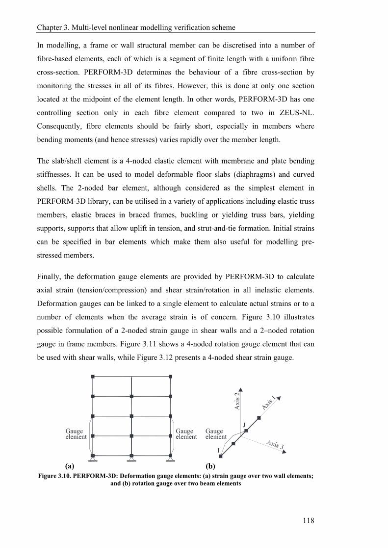
Chapter 3. Multi-level nonlinear modelling verification scheme
118
In modelling, a frame or wall structural member can be discretised into a number of
fibre-based elements, each of which is a segment of finite length with a uniform fibre
cross-section. PERFORM-3D determines the behaviour of a fibre cross-section by
monitoring the stresses in all of its fibres. However, this is done at only one section
located at the midpoint of the element length. In other words, PERFORM-3D has one
controlling section only in each fibre element compared to two in ZEUS-NL.
Consequently, fibre elements should be fairly short, especially in members where
bending moments (and hence stresses) varies rapidly over the member length.
The slab/shell element is a 4-noded elastic element with membrane and plate bending
stiffnesses. It can be used to model deformable floor slabs (diaphragms) and curved
shells. The 2-noded bar element, although considered as the simplest element in
PERFORM-3D library, can be utilised in a variety of applications including elastic truss
members, elastic braces in braced frames, buckling or yielding truss bars, yielding
supports, supports that allow uplift in tension, and strut-and-tie formation. Initial strains
can be specified in bar elements which make them also useful for modelling pre-
stressed members.
Finally, the deformation gauge elements are provided by PERFORM-3D to calculate
axial strain (tension/compression) and shear strain/rotation in all inelastic elements.
Deformation gauges can be linked to a single element to calculate actual strains or to a
number of elements when the average strain is of concern. Figure 3.10 illustrates
possible formulation of a 2-noded strain gauge in shear walls and a 2–noded rotation
gauge in frame members. Figure 3.11 shows a 4-noded rotation gauge element that can
be used with shear walls, while Figure 3.12 presents a 4-noded shear strain gauge.
Figure 3.10. PERFORM-3D: Deformation gauge elements: (a) strain gauge over two wall elements; and (b) rotation gauge over two beam elements
Gaugeelement
I
JGaugeelement
Gaugeelement
(a) (b)

Chapter 3. Multi-level nonlinear modelling verification scheme
119
Figure 3.11. PERFORM-3D: 4-noded rotation gauge element
Figure 3.12. PERFORM-3D: 4-noded shear strain gauge element
3.2.2.3 MaterialModels
In PERFORM-3D, the relations that describe actions (force, moment, stress, etc.) and
corresponding deformations (deflection, rotation, strain, etc.) in any material (steel or
concrete) are called Force-Deformation (F-D) relation. Linear and nonlinear F-D
relations are used to model elastic and inelastic materials, respectively. For inelastic
materials, PERFORM-3D offers trilinear and four-linear F-D relations as shown in
Figure 3.13. Cyclic degradation and strength loss are optional and can be defined when
required. In Figure 3.13, Y is the first yield point, U is the ultimate strength point, L is
the ductile limit point where significant strength loss begins, R is the residual strength
point and X is a point to specify a deformation value at which the analysis is to be
stopped. F-D relation can be unsymmetrical, where positive and negative deformations
are different.
K
I
L
J
Gauge element
K
I
L
J
K'
L'
Rotation (solid lines)
Wall elements(dashed lines)
K
I
L
J
Gauge element
Positive
(solid lines)
shear strain
Wall elements(dashed lines)
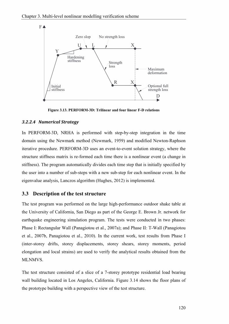
Chapter 3. Multi-level nonlinear modelling verification scheme
120
Figure 3.13. PERFORM-3D: Trilinear and four linear F-D relations
3.2.2.4 NumericalStrategy
In PERFORM-3D, NRHA is performed with step-by-step integration in the time
domain using the Newmark method (Newmark, 1959) and modified Newton-Raphson
iterative procedure. PERFORM-3D uses an event-to-event solution strategy, where the
structure stiffness matrix is re-formed each time there is a nonlinear event (a change in
stiffness). The program automatically divides each time step that is initially specified by
the user into a number of sub-steps with a new sub-step for each nonlinear event. In the
eigenvalue analysis, Lanczos algorithm (Hughes, 2012) is implemented.
3.3 Description of the test structure
The test program was performed on the large high-performance outdoor shake table at
the University of California, San Diego as part of the George E. Brown Jr. network for
earthquake engineering simulation program. The tests were conducted in two phases:
Phase I: Rectangular Wall (Panagiotou et al., 2007a); and Phase II: T-Wall (Panagiotou
et al., 2007b, Panagiotou et al., 2010). In the current work, test results from Phase I
(inter-storey drifts, storey displacements, storey shears, storey moments, period
elongation and local strains) are used to verify the analytical results obtained from the
MLNMVS.
The test structure consisted of a slice of a 7-storey prototype residential load bearing
wall building located in Los Angeles, California. Figure 3.14 shows the floor plans of
the prototype building with a perspective view of the test structure.
UY
Zero slop
X
XR
stiffnessInitial
stiffnessHardening
Dstrength lossOptional full
deformationMaximum
lossStrength
No strength loss
F
L

Chapter 3. Multi-level nonlinear modelling verification scheme
121
Figure 3.14. Prototype building and test structure used in modelling verification: (a) Residential floor plan; (b) Parking floor plan; and (c) Perspective view of the test structure (Panagiotou et al.,
2007a)
In Phase I of the test, resistance to lateral forces was provided by a 3.66m long load-
bearing RC rectangular wall, hereafter referred to as “web wall”. The web wall was
directed East-West (loading direction) and provided support to seven 200mm thick RC
slabs spaced at 2.74m. Two transverse walls were built to provide lateral and torsional
stability; the East RC wall, hereafter referred to as “flange wall” and the West precast,
prestressed segmental wall. The test structure height, starting from the top of the
foundation, was 19.20m with total mass (excluding the foundation) of around 210tons.
8 spaces @ 8.53m= 68.28m
Residential Unit
Test Structure
4.88
m4.
88m
4.88
m4.
88m
19.5
mStructural Wall (Transverse)
8 spaces @ 8.53m= 68.28m
Parking stall
Test Structure
203mm thick slab19
.5m
Shear Wall (Transverse)
(a)
(b)
(c)
Chapter 3. Multi-level nonlinear modelling verification scheme
122
Web and flange walls were linked with a 610mm wide slab. The link slab had two,
140mm deep by 51mm wide, slots on both ends. These pin-pin connections had the
capability of transferring in-plane diaphragm shear, moment, and axial forces but had a
reduced capacity to transfer out-of-plane actions during phase I of the test. The North
and South ends of the RC floor slabs were supported on four pin-ends gravity columns
designed and detailed to carry axial tension and compression only. Concrete with a
target 27.6MPa specified compressive strength and Grade-60 steel reinforcement were
used in the test structure. The measured average concrete compressive strength at the
day of the final test was 37.9MPa, while the average measured reinforcing steel yield
strength was 455MPa. The footings under the web and flange walls were longitudinally
prestressed and designed to remain elastic during testing. The geometry of the test
structure and the reinforcement details for the web wall, flange wall, and slabs are given
in Figure 3.15 and Figure 3.16, respectively. More details about the test structure can be
found in Panagiotou et al. (2007a, 2010).

Chapter 3. Multi-level nonlinear modelling verification scheme
123
Figure 3.15. Test structure used in modelling verification: (a) Elevation; (b) Floor plan view; and (c) Foundation plan view
North
Loa
ding
Dire
ctio
n
E
W
++
+
+
++
++
++
+ +
+ +
+ +
+ + + +
+
+
++
++ ++
+++ +
North
. ...
++
Flange wall
Web wall
Detail A
(a)
(b)
(c)

Chapter 3. Multi-level nonlinear modelling verification scheme
124
Figure 3.16. Reinforcement details for the test structure: (a) web and flange walls at first level; and (b) web and flange walls at levels 2-6; and (c) floor and link slabs at all levels
3.4 Input ground motions
Phase I of the test program investigated the response of the cantilever web wall to four
levels of excitation with increasing intensities (EQ1-EQ4), representing four historical
earthquakes recorded in Southern California. Prior to and between the earthquake tests,
the structure was subjected to long-duration ambient vibration tests and long-duration
low-amplitude white noise tests for system damage identification (Moaveni et al.,
2010). The low-intensity input motion EQ1 was the VNUY longitudinal component
from the 1971 Mw 6.6 San Fernando earthquake. The two medium intensity input
motions EQ2 and EQ3 were the VNUY transverse component record from the 1971 Mw
6.6 San Fernando earthquake and the WHOX longitudinal component from the 1994
Mw 6.7 Northridge earthquake, respectively. The large intensity input motion EQ4 was
Ø12 @ 20390° standard
90° standardØ12 @ 305
Ø12 @ 20390° standard
Ø12 @ 203 90° standardØ12 @ 305
51x140 slot2Ø12x4775@305 T&B
7Ø16x8026@152 T&B
13Ø12x8026@305 T&B
12Ø12x3048@305 T
N
(a) (b)
(c)
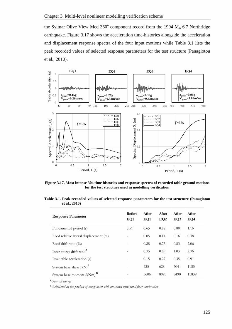
Chapter 3. Multi-level nonlinear modelling verification scheme
125
the Sylmar Olive View Med 360o component record from the 1994 Mw 6.7 Northridge
earthquake. Figure 3.17 shows the acceleration time-histories alongside the acceleration
and displacement response spectra of the four input motions while Table 3.1 lists the
peak recorded values of selected response parameters for the test structure (Panagiotou
et al., 2010).
Figure 3.17. Most intense 30s-time histories and response spectra of recorded table ground motions
for the test structure used in modelling verification
Table 3.1. Peak recorded values of selected response parameters for the test structure (Panagiotou
et al., 2010)
Response Parameter Before
EQ1
After
EQ1
After
EQ2
After
EQ3
After
EQ4
Fundamental period (s) 0.51 0.65 0.82 0.88 1.16
Roof relative lateral displacement (m) - 0.05 0.14 0.16 0.38
Roof drift ratio (%) - 0.28 0.75 0.83 2.06
Inter-storey drift ratioA - 0.35 0.89 1.03 2.36
Peak table acceleration (g) - 0.15 0.27 0.35 0.91
System base shear (kN)B - 425 628 704 1185
System base moment (kNm) B - 5606 8093 8490 11839
AOver all storeys
BCalculated as the product of storey mass with measured horizontal floor acceleration
-1
-0.5
0
0.5
1
40 50 60 70
EQ1
agmax=0.15g
Vgmax=0.26m/sec
185 195 205 215
EQ2
agmax=0.27g
Vgmax=0.32m/sec
325 335 345 355
EQ3
agmax=0.35g
Vgmax=0.43m/sec
455 465 475 485
EQ4
agmax=0.91g
Vgmax=1.02m/sec
0
1
2
3
0 0.5 1 1.5 2
Sp
ectr
al A
ccel
erat
ion S
a(g
)
Period, T (s)
EQ1EQ2EQ3EQ4=5%
0
0.2
0.4
0.6
0 0.5 1 1.5 2
Sp
ectr
al D
isp
lace
men
t S
d(m
)
Period, T (s)
EQ1EQ2EQ3EQ4
=5%
Tab
le A
ccel
erat
ion (
g)
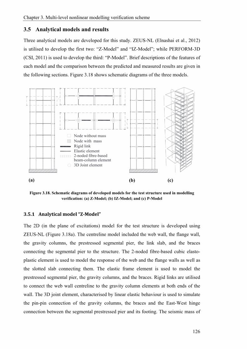
Chapter 3. Multi-level nonlinear modelling verification scheme
126
3.5 Analytical models and results
Three analytical models are developed for this study. ZEUS-NL (Elnashai et al., 2012)
is utilised to develop the first two: “Z-Model” and “IZ-Model”; while PERFORM-3D
(CSI, 2011) is used to develop the third: “P-Model”. Brief descriptions of the features of
each model and the comparison between the predicted and measured results are given in
the following sections. Figure 3.18 shows schematic diagrams of the three models.
Figure 3.18. Schematic diagrams of developed models for the test structure used in modelling verification: (a) Z-Model; (b) IZ-Model; and (c) P-Model
3.5.1 Analyticalmodel“Z‐Model”
The 2D (in the plane of excitations) model for the test structure is developed using
ZEUS-NL (Figure 3.18a). The centreline model included the web wall, the flange wall,
the gravity columns, the prestressed segmental pier, the link slab, and the braces
connecting the segmental pier to the structure. The 2-noded fibre-based cubic elasto-
plastic element is used to model the response of the web and the flange walls as well as
the slotted slab connecting them. The elastic frame element is used to model the
prestressed segmental pier, the gravity columns, and the braces. Rigid links are utilised
to connect the web wall centreline to the gravity column elements at both ends of the
wall. The 3D joint element, characterised by linear elastic behaviour is used to simulate
the pin-pin connection of the gravity columns, the braces and the East-West hinge
connection between the segmental prestressed pier and its footing. The seismic mass of
Node without massNode with massRigid linkElastic element 2-noded fibre-based
3D Joint elementbeam-column element
(a) (b) (c)

Chapter 3. Multi-level nonlinear modelling verification scheme
127
the test structure is lumped at floor levels to simplify the analytical model. The weight
of the structure is also applied as nodal loads to account for the gravity and the P-∆
effects during NRHA.
The uniaxial nonlinear constant confinement constitutive model of Mander et al. (1988)
with improved cyclic rules proposed by Martínez-Rueda and Elnashai (1997) is used to
calculate the properties of the confined concrete and assigned to the corresponding
fibres in the web and the flange walls’ cross-section at the first storey (Figure 3.7). The
concrete in the upper storeys had no confinement reinforcement and thus modelled
using unconfined concrete fibres. In both cases, the tensile strength of concrete is
neglected. The F-D behaviour of the steel reinforcing bars in the test structure is
idealised using the uniaxial steel model of Menegotto and Pinto (1973) coupled with the
isotropic hardening rules proposed by Filippou et al. (1983), as shown in Figure 3.8a. In
this figure, Eo is the initial elastic modulus of steel, E1 is the strain-hardening modulus,
Ro is a parameter defining the initial loading curvature, and a1 to a4 are experimental-
based parameters that control the curvature and isotropic strain hardening in the
subsequent load cycles, taken as 20, 18.5, 0.15, 0.01 and 7, respectively (Elnashai et al.,
2012). Previous studies indicated that shear deformation may have a significant
contribution to the lateral displacement of walls especially at lower storeys, even in
walls that are categorised as flexure-dominated (e.g. Thomsen and Wallace, 1995). In
ZEUS-NL, the fibres in the cubic elasto-plastic element used to model the web wall
have zero resistance to transverse forces, and hence shear deformation cannot be
determined at the section level. It can be, however, explicitly modelled by introducing
shear springs to the wall element. Justified by the fact that the experimental results for
the test structure evidenced almost exclusively flexural cracking at the web wall base
(Panagiotou et al., 2007a, Martinelli and Filippou, 2009), shear deformation is not
considered in this analytical model.
ZEUS-NL includes Rayleigh damping as the only option to account for the effects of
the viscous damping during dynamic analysis. The mathematical model of Rayleigh
damping in this package is based on the initial stiffness in calculating the damping
matrix. When the use of tangent stiffness-proportional damping is not an available
option, previous studies recommended lowering the first mode initial stiffness-
proportional damping value (e.g. Hall, 2006, Smyrou et al., 2011). The use of the mass-
proportional damping term in the damping matrix is discouraged by several researchers.

Chapter 3. Multi-level nonlinear modelling verification scheme
128
For an instant, Priestley and Grant (2005) showed that including the mass-proportional
term in the damping equation can heavily weight the mass matrix, leading to a nearly
constant damping matrix during the post-elastic response of the structure regardless of
stiffness degradation. Hall (2006) suggested that the presence of mass-proportional
damping will generate extraneous damping forces due to the rigid body motion
component involved in the formulation of earthquake analysis that is based on total
motion. It is worth noting that rigid body motion phenomena become more significant
in the analysis of tall buildings. For the test structure, previous studies have adopted
different approaches and values to model viscous damping. For instance, Panagiotou
and Restrepo (2006) used a damping ratio of 0.3% for the first longitudinal mode to
accurately simulate the response to earthquake input motions; Martinelli and Filippou
(2009) used Rayleigh damping with mass and initial stiffness-proportional damping
matrix and a 1.0% damping ratio for the first two flexural modes; while Waugh and
Sritharan (2010) used tangent stiffness-proportional viscous damping corresponded to
0.5% and 0.8% damping ratios for the first and third uncracked mode periods,
respectively. The use of such a low damping ratio in modelling the test structure can be
attributed, in addition to the discussion included in Section 2.2.3.3, to the absence of
non-structural elements and also to the fact that flexural cracking was largely limited to
the lower part of the structure as a consequence of the low ratio of the longitudinal
reinforcements led to by the design approach of the building (i.e. displacement-based
design). Based on the above, an initial stiffness-proportional viscous damping
corresponding to 0.5% damping ratio in the first longitudinal mode is used in the Z-
Model, while the mass-proportional damping term is set to zero.
The input motions shown in Figure 3.17 are applied to the base of the Z-Model in the
East-West direction parallel to the web wall. Using the Newmark integration scheme,
NRHA is conducted at a time step of 1/60s. The four input motions, EQ1 to EQ4, are
concatenated to account for the accumulated structural damage on the response of the
test structure. Six seconds of zero-base acceleration is added in between the earthquake
records to allow the structure to come to rest prior to being subjected to the next record.
The applied concatenated base motion record is 523s long in total.
The capability of the Z-Model in predicting the global response of the test structure
during the most intense 30s of each of the four earthquake input motions is assessed by
comparing the analytical results with measured data for top-floor relative displacement
Chapter 3. Multi-level nonlinear modelling verification scheme
129
time histories (Figure 3.19), response envelopes of storey displacement, inter-storey
drift (ISD), storey shear force and storey overturning moment (Figure 3.20). Figure 3.19
shows that the model well captures all the significant peak relative displacements
recorded during EQ1, EQ2 and EQ4. The relatively poor prediction of the last part of
the peak displacement histories in Figure 3.19 can be attributed to the assumptions
made in the modelling of viscous damping. The peak displacements on EQ3 are
underpredicted by as much as 25%, the discrepancies in the computed response under
EQ3 have also been recorded in other studies (e.g. Kelly, 2007, Waugh and Sritharan,
2010). This is mainly attributed to the similarity in the earthquake intensity between
EQ2 and EQ3 input motions. As a consequence of these two records having comparable
intensities, the unloading and reloading paths of the material models rather than their
envelopes have a big influence on the analytical response under EQ3. Accurate
representation of the unloading and reloading behaviour of material models becomes
more important when the structure does not move into virgin territory, as during
aftershocks for example. Figure 3.20a shows very good agreement between predicted
and measured displacement envelopes at floor-levels (storey displacement). As
expected, the displacements under EQ3 are under predicted. The maximum calculated
roof drift ratios are found to be 0.30% under EQ1, 0.75% under EQ2 and 2.05% under
EQ4, compared to their corresponding measured values of 0.28%, 0.75% and 2.06%,
respectively. While for the response under EQ3, the obtained and measured maximum
roof drifts are 0.78% and 0.83%, respectively. ISD is typically considered as a key
parameter in defining performance limit states for seismic vulnerability assessment of
buildings and hence it is essential to have this parameter accurately predicted. As shown
in Figure 3.20(b), the ISD envelopes are well predicted by the analysis under EQ1, EQ2
and EQ4, while under EQ3 it is within 30% of the experimental values for the same
reasons discussed above.

Chapter 3. Multi-level nonlinear modelling verification scheme
130
Figure 3.19. Z-Model: measured versus computed top relative displacement under the four Input
motions
-0.1
-0.05
0
0.05
0.1
40 45 50 55 60 65 70
Dis
pla
cem
ent
(m)
Time (s)
Exp. Ana.
Z-Model
EQ1
-0.2
-0.1
0
0.1
0.2
185 190 195 200 205 210 215
Dis
pla
cem
ent
(m)
Time (s)
Exp. Ana.
Z-Model
EQ2
-0.2
-0.1
0
0.1
0.2
325 330 335 340 345 350 355
Dis
pla
cem
ent
(m)
Time (s)
Exp. Ana.
Z-Model
EQ3
-0.5
-0.25
0
0.25
0.5
455 460 465 470 475 480 485
Dis
pla
cem
ent
(m)
Time (s)
Exp. Ana.
EQ4
Z-Model
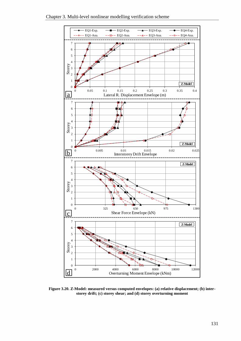
Chapter 3. Multi-level nonlinear modelling verification scheme
131
Figure 3.20. Z-Model: measured versus computed envelopes: (a) relative displacement; (b) inter-
storey drift; (c) storey shear; and (d) storey overturning moment
70
215
355
485
0
1
2
3
4
5
6
7
0 0.05 0.1 0.15 0.2 0.25 0.3 0.35 0.4
Sto
rey
Lateral R. Displacement Envelope (m)
Z-Model
0
1
2
3
4
5
6
7
0 0.005 0.01 0.015 0.02 0.025
Sto
rey
Interstorey Drift Envelope
Z-Model
0
1
2
3
4
5
6
7
0 325 650 975 1300
Sto
rey
Shear Force Envelope (kN)
Z-Model
0
1
2
3
4
5
6
7
0 0.05 0.1 0.15 0.2 0.25 0.3 0.35 0.4
Sto
ry
Lateral R. Displacement Envelope (m)
EQ1-Exp. EQ2-Exp. EQ3-Exp. EQ4-Exp.
EQ1-Ana. EQ2-Ana. EQ3-Ana. EQ4-Ana.
Z-Model
0
1
2
3
4
5
6
7
0 2000 4000 6000 8000 10000 12000
Sto
rey
Overturning Moment Envelope (kNm)
Z-Model
0
1
2
3
4
5
6
7
0 0.05 0.1 0.15 0.2 0.25 0.3 0.35 0.4
Sto
ry
Lateral R. Displacement Envelope (m)
EQ1-Exp. EQ2-Exp. EQ3-Exp. EQ4-Exp.
EQ1-Ana. EQ2-Ana. EQ3-Ana. EQ4-Ana.
Z-Model
a
b
c
d
Chapter 3. Multi-level nonlinear modelling verification scheme
132
Despite the good agreement between predicted and measured response values of top
displacement time histories, storey displacement and ISD envelopes discussed above,
the Z-Model underestimates the storey shear and consequently storey moment
envelopes of the test structure. Especially when the structure behaves inelastically
(Figure 3.20c and Figure 3.20d). The discrepancies between the reported and the
analytical storey shear and moment values can be attributed to the influence of the 3D
interaction between the gravity columns, the floor slabs and the web wall on the overall
lateral capacity of the test structure. The significant contribution of this interaction to
the lateral force resistance of the test building was confirmed by Panagiotou and
Restrepo (2006) using pushover analysis. The main reason for this influence is that, due
to their interaction with the floor slab, the gravity columns developed significant axial
strains during testing. Consequently, the columns near the tension side of the web wall
were experiencing tensile forces and those closer to the compression side were
subjected to compression forces. Given the 3.05m span between the columns, the
tension and compression forces enabled a large moment to be developed and effectively
increased the lateral force resistance of the test structure.
3.5.2 Analytical Model “IZ-Model”
To address the shortcomings of the Z-Model, IZ-Model is developed as an improved 2-
noded fibre-based model to introduce the 3D slab-columns-web wall interaction effect.
In the IZ-Model, 3D joint elements are introduced at both ends of the rigid link that
connects the web wall centreline to the gravity columns at each floor level
(Figure 3.18b). A bilinear asymmetric moment-curvature relation is assigned to those
elements to simulate the out-of-plane flexural rigidity of the slab. Figure 3.21 shows the
storey shear and moment envelopes predicted using the IZ-Model under EQ1 to EQ4,
where significant improvement can be seen. This exercise highlights the importance of
taking into account the 3D interaction effect of all structural members in the building to
accurately predict the seismic response.
To assess the capability of the IZ-Model to capture the damage evolution of the test
structure under the four input motions, the frequency spectra of the top relative
displacement time-histories using the Fast Fourier Transform (FFT) method and the
structure periods of the first two modes are plotted under EQ1 to EQ4 in Figure 3.22. It
is worth noting that the measured fundamental frequency of the test structure changed
from 1.96Hz before testing to 0.86Hz at the end of EQ4, with corresponding
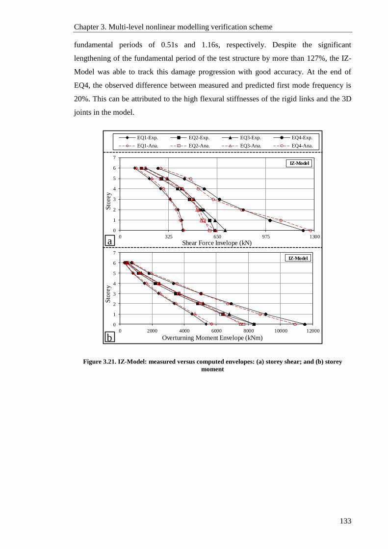
Chapter 3. Multi-level nonlinear modelling verification scheme
133
fundamental periods of 0.51s and 1.16s, respectively. Despite the significant
lengthening of the fundamental period of the test structure by more than 127%, the IZ-
Model was able to track this damage progression with good accuracy. At the end of
EQ4, the observed difference between measured and predicted first mode frequency is
20%. This can be attributed to the high flexural stiffnesses of the rigid links and the 3D
joints in the model.
Figure 3.21. IZ-Model: measured versus computed envelopes: (a) storey shear; and (b) storey
moment
0
1
2
3
4
5
6
7
0 325 650 975 1300
Sto
rey
Shear Force Invelope (kN)
IZ-Model
0
1
2
3
4
5
6
7
0 2000 4000 6000 8000 10000 12000
Sto
rey
Overturning Moment Envelope (kNm)
IZ-Model
0
1
2
3
4
5
6
7
0 0.05 0.1 0.15 0.2 0.25 0.3 0.35 0.4
Sto
ry
Lateral R. Displacement Envelope (m)
EQ1-Exp. EQ2-Exp. EQ3-Exp. EQ4-Exp.
EQ1-Ana. EQ2-Ana. EQ3-Ana. EQ4-Ana.
Z-Model
b
a

Chapter 3. Multi-level nonlinear modelling verification scheme
134
Figure 3.22. IZ-Model: evolution of modal characteristics during the four input motions: (a)
frequency spectra; and (b) structure periods
Another measure of the capability of the analytical model is the determination of the
local damage. Figure 3.23 depicts the tensile strain envelope of an outer reinforcing bar
located in the web wall (marked as ST2 in the tests) over the height of the first level
under EQ4 input motion. It should be noted that computed strains can be mesh-
sensitive, especially at zones of concentrated plasticity. To investigate the influence of
the mesh size on the computed stains, the web wall member in the first level of the
building is modelled using four different meshes: One Element-mesh (1E); Two
Element-mesh (2E); Three Element-mesh (3E); and Six Element-mesh (6E). The results
presented in Figure 3.23 show that the IZ-Model with 2E predicted the tensile strain
envelops of ST2 reinforcing bar with good accuracy. It is worth mentioning that the 2E
needed an element length of 1321mm, which is close to the expected plastic hinge
length at the web wall base (0.5 times the flexural depth of the wall=1830mm) as
proposed by ASCE/SEI 41-06 (2007). Hence, mesh size not exceeding the expected
0
0.5
1
0 0.5 1 1.5 2
No
rmal
ized A
mpli
tude
Frequency (Hz)
End of EQ1-Ana.End of EQ2-Ana.End of EQ3-Ana.End of EQ4-Ana.
1.6
0
1.1
4
1.2
5
1.0
3Measured Frq. (Hz):
After EQ1: 1.53After EQ2: 1.23
After EQ3: 1.11After EQ4: 0.86
IZ-Model
Before EQ1 After EQ1 After EQ2 After EQ3 After EQ4
0
0.2
0.4
0.6
0.8
1
1.2
Peri
od, T
(s)
1ST Mode-Exp.1ST Mode-Ana.2ND Mode-Exp.2ND Mode-Ana.
IZ-Model
b
b
a

Chapter 3. Multi-level nonlinear modelling verification scheme
135
plastic zone length is confirmed as being suitable for fibre-based modelling of RC shear
walls.
Figure 3.23. IZ-Model: tensile strain of ST2 reinforcing bar over the height of first level under EQ4
3.5.3 Analytical Model “P-Model”
To evaluate the capability of the 4-noded element modelling approach in predicting the
response of the test structure, the P-Model is developed using PERFORM-3D (CSI,
2011). To model the web and the flange walls, the 4-noded fibre-based shear wall
element is used with nonlinear vertical fibres to represent the behaviour of concrete and
reinforcing steel. Based on the outcome of the element mesh sensitivity study conducted
on the IZ-Model in Section 3.5.2, the web wall in the first level is represented with two
vertical elements “1E Mesh”, as shown in Figure 3.18c. The link slab is modelled using
the 2-noded fibre-based frame element. An elastic frame element with specified cross-
section properties is used to model the prestressed segmental pier, while the elastic bar
element is utilised to model the pin-pin end braces and gravity columns. Finally, the
elastic 4-noded slab element is used to represent the floor slabs. For the sake of
comparison, the same principles used in Z-Model and IZ-Model for modelling the
seismic mass of the test structure are followed.
The four-linear segment F-D relation is used to approximate the concrete stress-strain
relationship based on the modified Mander model (Figure 3.13). For the reinforcing
steel material model, a similar relation is used with the post-yield stiffness and cyclic
degradation parameters defined following the adjustments described by Orakcal and
Wallace (2006). The linear stress-strain relation is used to model the materials of the
prestressed segmental pier, floor slabs, braces and gravity columns. In PERFORM-3D,
viscous damping can be modelled using modal damping, a more preferred viscous
0
1
2
3
4
0 0.005 0.01 0.015 0.02 0.025 0.03
Heig
ht
(m)
ST2-Rebar Tensile Strain
EQ4-Exp.EQ4-Ana.-1E MeshEQ4-Ana.-2E MeshEQ4-Ana.-3E MeshEQ4-Ana.-6E Mesh
IZ-Model
Chapter 3. Multi-level nonlinear modelling verification scheme
136
damping modelling approach (CSI, 2011). However, for consistency, the same
assumptions and procedures used in the ZEUS-NL models for the viscous damping,
input motion application, and numerical strategy are adopted in this model.
The shear deformation in the web wall is accounted for in the P-Model by assigning a
trilinear relation to the wall element similar to the one recommended by ASCE/SEI 41-
06 (2007) and ASCE/SEI 41-16 (ASCE/SEI-41, 2017). to represent the nonlinear shear
behaviour of the wall. Test results by Thomsen and Wallace (2004) and the follow-up
calibration study by Gogus (2010) are used to define the shear F-D relation. In the used
trilinear relation, the uncracked shear modulus is taken as 0.4Ec and diagonal (shear)
cracking is assumed to start at 0.25√fc′ ≤ 0.5vn, where vn is the wall nominal shear
strength from ACI 318 (2014). The post-cracking slope is reduced to 0.01Ec to account
for the nonlinear shear deformations due to shear-flexure interaction (Massone, 2006).
Following the same sequence used in the previous section, Figure 3.24 to Figure 3.27
show predicted versus measured top-floor relative displacement time-histories, response
envelopes, the evolution of modal characteristics and ST2 steel rebar tensile strain,
respectively. Good agreement can be seen for all predicted response except the ones
under EQ3, where, for the same reasons discussed earlier, predicted response of the test
structure have some discrepancies when compared with measured values.
While the data measured from the shake table test confirmed the accuracy of the
investigated modelling approaches and key parameters in predicting global response and
local damage induced by the seismic demands on slender wall structures, some
limitations became apparent in the 2-noded fibre-based modelling approach (e.g.
accounting for 3D compatibility effects). The study reveals the superior ability of the 4-
noded fibre-based wall/shell element to account for the 3D effects of deformation
compatibility between lateral and gravity-force-resisting systems. The study also
addresses the sensitivity of attained results to the stiffnesses assigned to the rigid links
and the 3D joints required to connect the shear walls to neighbouring elements when the
2-noded fibre-based element modelling approach is used.

Chapter 3. Multi-level nonlinear modelling verification scheme
137
Figure 3.24. P-Model: measured versus computed top relative displacement under the four input
motions
-0.1
-0.05
0
0.05
0.1
40 45 50 55 60 65 70
Dis
pla
cem
ent
(m)
Time (s)
Exp. Ana.
EQ1
P-Model
-0.2
-0.1
0
0.1
0.2
185 190 195 200 205 210 215
Dis
pla
cem
ent
(m)
Time (s)
Exp. Ana.
EQ2
P-Model
-0.2
-0.1
0
0.1
0.2
325 330 335 340 345 350 355
Dis
pla
cem
ent
(m)
Time (s)
Exp. Ana.
EQ3
P-Model
-0.4
-0.2
0
0.2
0.4
455 460 465 470 475 480 485
Dis
pla
cem
ent
(m)
Time (s)
Exp. Ana.
P-Model
EQ4

Chapter 3. Multi-level nonlinear modelling verification scheme
138
Figure 3.25. P-Model: measured versus computed envelopes: (a) relative displacement; (b) inter-
storey drift; (c) shear force; and (d) storey overturning moment
215
355
0
1
2
3
4
5
6
7
0 0.05 0.1 0.15 0.2 0.25 0.3 0.35 0.4
Sto
rey
Lateral R. Displacement Envelope (m)
P-Model
0
1
2
3
4
5
6
7
0 0.005 0.01 0.015 0.02 0.025
Sto
rey
Interstorey Drift Envelope
P-Model
0
1
2
3
4
5
6
7
0 325 650 975 1300
Sto
rey
Shear Force Envelope (kN)
P-Model
485
0
1
2
3
4
5
6
7
0 0.05 0.1 0.15 0.2 0.25 0.3 0.35 0.4
Sto
ry
Lateral R. Displacement Envelope (m)
EQ1-Exp. EQ2-Exp. EQ3-Exp. EQ4-Exp.
EQ1-Ana. EQ2-Ana. EQ3-Ana. EQ4-Ana.
Z-Model
0
1
2
3
4
5
6
7
0 2000 4000 6000 8000 10000 12000
Sto
rey
Overturning Moment Envelope (kNm)
P-Model
a
b
c
d
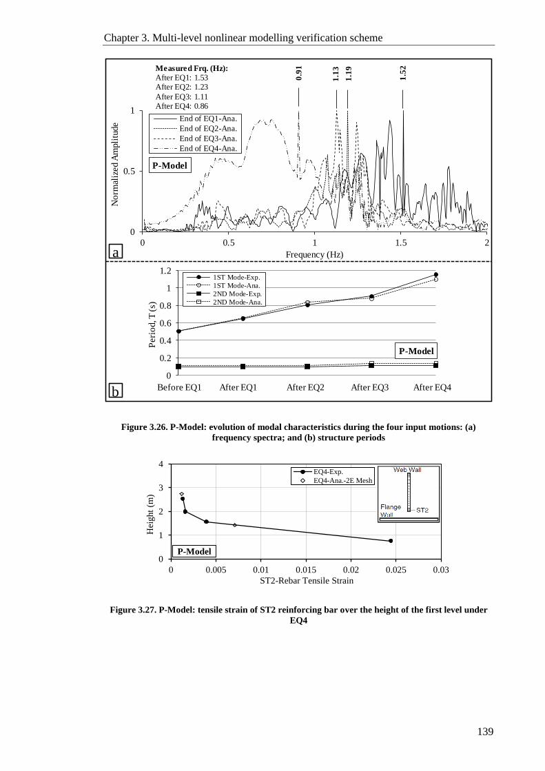
Chapter 3. Multi-level nonlinear modelling verification scheme
139
Figure 3.26. P-Model: evolution of modal characteristics during the four input motions: (a)
frequency spectra; and (b) structure periods
Figure 3.27. P-Model: tensile strain of ST2 reinforcing bar over the height of the first level under
EQ4
0
0.5
1
0 0.5 1 1.5 2
No
rmal
ized A
mpli
tude
Frequency (Hz)
End of EQ1-Ana.
End of EQ2-Ana.
End of EQ3-Ana.
End of EQ4-Ana.
1.5
2
1.1
3
1.1
9
0.9
1Measured Frq. (Hz):
After EQ1: 1.53After EQ2: 1.23
After EQ3: 1.11After EQ4: 0.86
P-Model
Before EQ1 After EQ1 After EQ2 After EQ3 After EQ4
0
0.2
0.4
0.6
0.8
1
1.2
Peri
od, T
(s)
1ST Mode-Exp.
1ST Mode-Ana.
2ND Mode-Exp.
2ND Mode-Ana.
P-Model
b
a
0
1
2
3
4
0 0.005 0.01 0.015 0.02 0.025 0.03
Hei
ght
(m)
ST2-Rebar Tensile Strain
EQ4-Exp.
EQ4-Ana.-2E Mesh
P-Model

Chapter 3. Multi-level nonlinear modelling verification scheme
140
3.6 Summary and conclusions
In this chapter, the results from Phase I of the shake table tests undertaken at the
University of California, San Diego of a full-scale slice of a seven-storey RC wall
building are employed to conduct a MLNMVS. The scheme verifies different
approaches and key parameters in modelling RC slender shear walls forming the lateral
force-resisting system in RC high-rise wall buildings. Three analytical models are
created to simulate the nonlinear response of the test structure under four consecutive
table excitations. The excitations represent real earthquake motions with increasing
maximum acceleration from 0.15g to 0.91g. The 2-noded fibre-based beam-column
element approach is adopted to model the web and the flange walls of the test structure
in 2D centreline models using ZEUS-NL tool. PERFORM-3D package is utilised to
create the third (3D) model using the 4-noded fibre-based wall/shell element. The main
conclusions drawn from this study are:
With appropriate care in the modelling of the geometry, both investigated
nonlinear modelling approaches (2- and 4-noded fibre-based elements) are
sufficient to predict global deformation response (storey lateral displacement
and ISD) of RC wall buildings with relatively good accuracy.
The study reveals the supremacy of the 4-noded fibre-based wall/shell element
in accounting for the 3D effects of deformation compatibility between lateral
and gravity-force-resisting systems. The 3D interaction between the gravity
columns, the floor slabs, and the web wall significantly contributed to the
overall lateral capacity of the test structure.
When initial stiffness is used in constructing the damping matrix for RC wall
buildings with no or well-isolated non-structural elements, low damping ratio
(0.5% for the test structure) is suitable for assessing their seismic performance.
The observed difference between the predicted and the measured response of
the test structure under the two consecutive input motions with comparable
intensities (EQ2 and EQ3) highlights the importance of accurate representation
of the unloading/reloading paths of the material models. This is especially true
when assessing the performance of buildings under earthquake motions that do
not considerably take the structure into virgin territory.

Chapter 3. Multi-level nonlinear modelling verification scheme
141
No noticeable change is observed in the analytical response of the test structure
when shear deformation was accounted for in the P-Model compared to the
results obtained from the IZ-Model. This is justified by the test results that
demonstrated almost exclusively flexural cracking at the web wall base.
However, shear deformation may still make a significant contribution to the
lateral displacement of walls, even in walls categorised as slender and or
flexure-dominated. Hence, considering the shear deformation either implicitly
(coupled model) or explicitly (uncoupled model) is recommended.

142
This page is intentionally left in blank
143
CHAPTER 4. Case study
To demonstrate the proposed framework for assessing the seismic vulnerability of RC
high-rise wall buildings under different earthquake scenarios, the city of Dubai (UAE)
is chosen in the present work as a case study for two main reasons: (i) due to the
unprecedented level of growth in property development in recent years. In this growth,
high-rise buildings are forming the biggest share of the new construction. This class of
buildings represents high levels of financial investment and population density increase
which significantly increases exposure; and (ii) the multi-scenario earthquakes under
which the region is vulnerable, where high-rise buildings are expected to respond to in
different ways.
This chapter consists of four main sections. Section 4.1 presents the seismicity of Dubai
city. Hazard studies on the region are critically reviewed and appropriate seismic
characteristics are selected for the subsequent seismic vulnerability assessment. The
criteria for selecting the input ground motions are discussed in Section 4.2, where forty
real records are selected to represent two seismic scenarios. Section 4.3 discusses the
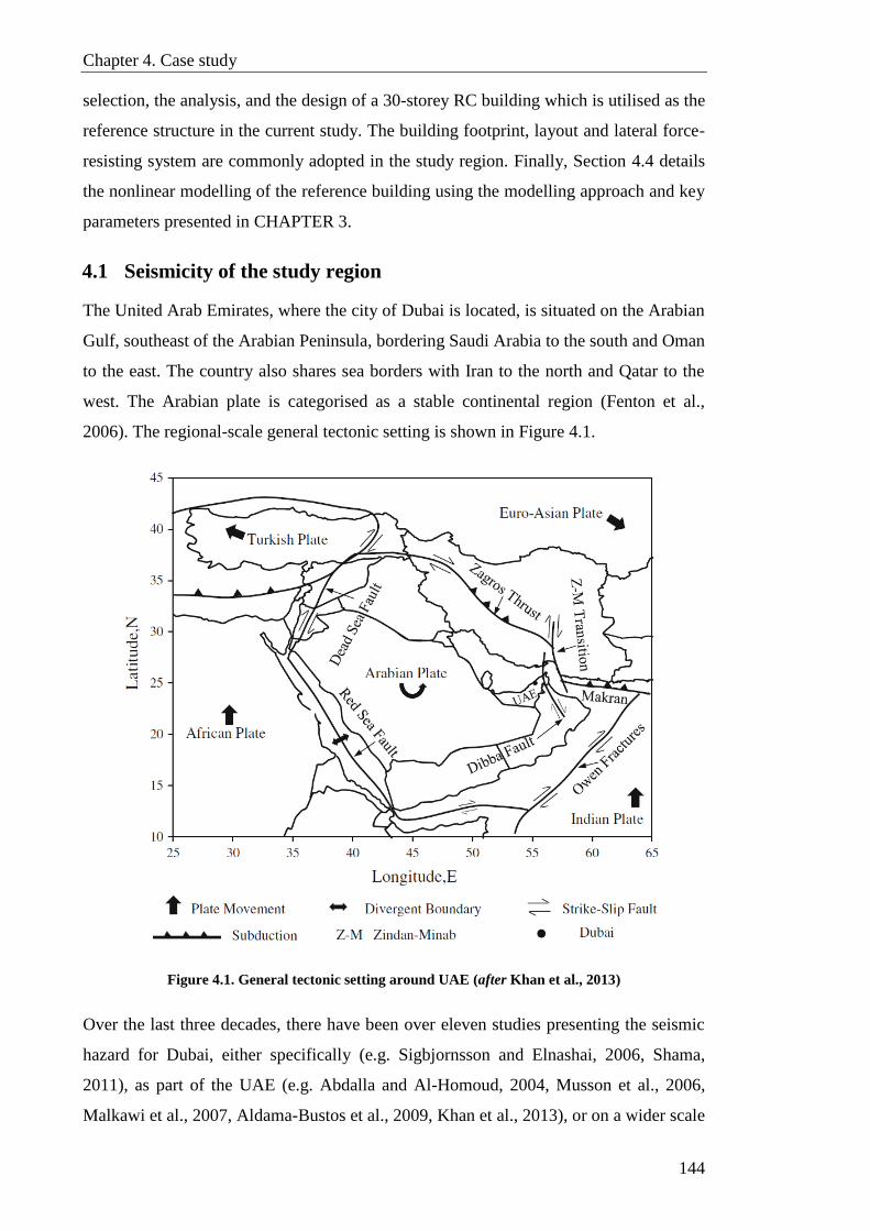
Chapter 4. Case study
144
selection, the analysis, and the design of a 30-storey RC building which is utilised as the
reference structure in the current study. The building footprint, layout and lateral force-
resisting system are commonly adopted in the study region. Finally, Section 4.4 details
the nonlinear modelling of the reference building using the modelling approach and key
parameters presented in CHAPTER 3.
4.1 Seismicity of the study region
The United Arab Emirates, where the city of Dubai is located, is situated on the Arabian
Gulf, southeast of the Arabian Peninsula, bordering Saudi Arabia to the south and Oman
to the east. The country also shares sea borders with Iran to the north and Qatar to the
west. The Arabian plate is categorised as a stable continental region (Fenton et al.,
2006). The regional-scale general tectonic setting is shown in Figure 4.1.
Figure 4.1. General tectonic setting around UAE (after Khan et al., 2013)
Over the last three decades, there have been over eleven studies presenting the seismic
hazard for Dubai, either specifically (e.g. Sigbjornsson and Elnashai, 2006, Shama,
2011), as part of the UAE (e.g. Abdalla and Al-Homoud, 2004, Musson et al., 2006,
Malkawi et al., 2007, Aldama-Bustos et al., 2009, Khan et al., 2013), or on a wider scale
Chapter 4. Case study
145
that covers most of the Arabian Peninsula (e.g. Al-Haddad et al., 1994, Grünthal et al.,
1999, Peiris et al., 2006, Pasucci et al., 2008). The conclusions drawn by these studies
are quite different with regard to the level of seismicity in Dubai and the UAE as a
whole, with estimates of the PGA in Dubai ranging from less than 0.05g to 0.32g for a
return period of 475 years.
The work of Peiris et al. (2006), Musson et al. (2006), Malkawi et al. (2007), and
Pasucci et al. (2008) have less impact as the former two are published in conference
proceedings and the latter two as international and technical reports, respectively. It is
worth mentioning though that the outcome for Dubai (PGA for a return period of 475
years) in the above-mentioned studies by Peiris et al., Musson et al., and Pasucci et al.
(0.06g, 0.06g and 0.05g, respectively) is very close to the result obtained by Aldama-
Bustos et al. (2009). On the other hand, the study by Malkawi et al. reported a PGA
value greater than 0.2g.
The work of Grünthal et al. (1999) basically aimed to fill in the blank areas left in the
global hazard map produced by the Global Seismic Hazard Assessment Project
(GSHAP), of which the northeast corner of the Arabian Peninsula was not covered in
any of its regional sub-projects. The UAE hazard was mapped by simulating the
attenuated effect of the seismic activity in the Dead Sea fault area and in Zagros
province of Iran, without performing actual seismic hazard analysis for sites in UAE.
Therefore, the estimates of Grünthal et al. are disregarded in the current study.
With the exception of the latter work, the above-mentioned studies have implemented
the PSHA methodology, based essentially on Poisson Model framework (Cornell,
1968). In a PSHA framework, there are several key input parameters. These parameters
are highlighted below with a critical review on their impact on the concluded results of
some of the aforementioned studies.
4.1.1 Earthquake data, faulting structures and seismic source models
To compile an appropriate seismic source model for the use within a PSHA study, it is
essential to identify the individual faulting structures both on the local and the regional
levels. The faulting structures to be identified are the ones which have the potential to
generate earthquakes that could affect Dubai and other sites within the UAE. Based on
the tectonic setting of the region, four main seismic sources can be identified: (i) Zagros
fold-thrust; (ii) Zendan-Minab-Palami fault system; (iii) Makran subduction zone; and

Chapter 4. Case study
146
(iv) local crustal faults including Oman mountains, Dibba line, Wadi Ham, Wadi El-
Fay, Wadi Shimal and the controversial West Cost Fault (WCF), (Johnson, 1998).
Defining the seismic source zones, in terms of covered area, assigned faults, and
seismicity (recurrence parameters) has a major impact on the output of the PSHA.
In the study of Al-Haddad et al. (1994), UAE region has not been included in any of the
considered seismic source zones. The closest considered source was the one that
combines the western edge of the Makran subduction zone and the southernmost part of
Zagros fold-thrust (Figure 4.2a). In this study, international earthquake data bank
sources alongside Saudi Arabian Earthquake Data File (SAEDF) were utilised to
assemble the earthquake catalogue used with the PSHA. The study was based on
instrumented and historic events covering a time span from 2150 BC to 1990 AD and a
geographic region bounded by 10o N to 35
o N and 30
o E to 60
o E.
The first PSHA conducted specifically for the UAE was presented by Abdulla and Al-
Homoud (2004). The seismic source zones defined in this study are similar to those of
Al-Haddad et al. (1994), with the exception of two additional small zones. The two
added zones are effectively linking the stable UAE with the active areas of Makran and
Zagros regions (Figure 4.2b). These source zones have contributed to inflating the
seismic hazard within the UAE. The earthquake data were based on the catalogue of the
International Institute for Earthquake Engineering and Seismology (IIEES, 2019) and
the work of Farahbod and Arkhani (2002). The employed time span was between 1008
AD to 2002 AD and the covered area bounded by 20o N to 30
o N and 50
o E to 60
o E.
Sigbjornsson and Elnashai (2006) conducted a hazard study focusing only on Dubai
(Figure 4.2e). The study indicated that the seismic source zonation is based on the work
of Tavakoli and Ghafory-Ashtiany (1999), but also included the Dibba and West Coast
faults. The earthquake data for the study area of 20o N to 30
o N and 50
o E to 60
o E and
for the period of 734 AD to 1996 AD were extracted from three main sources: (i)
Ambraseys and Melville (2005); (ii) Ambraseys and Srbulov (1994); and (iii) GSHAP
data (2004). USGS data (2019) were also used to include additional events up to 2004.
The study of Aldama-Bustos et al. (2009) concentrated on the major cities of Abu
Dhabi, Dubai, and Ras Al Khaymah in the UAE. Twenty distinct seismic sources were
included within the seismic source model, mainly related to the Zagros fold and thrust
belts using the work of Berberian (1995) to partition this overall region into sub-sources
Chapter 4. Case study
147
(Figure 4.2c). The stable carton consisting most of the Arabian Peninsula was treated as
a background source. Earthquake data were gathered from several sources (e.g.
Ambraseys and Srbulov, 1994, Ambraseys and Melville, 2005, IIEES, 2019, ISC, 2019,
USGS, 2019). The spatial study region spanned 21o N to 31
o N and 47
o E to 66
o E and
covered the period from 3000 BC up to 2003 AD.
In the study of Shama (2011), a PSHA was performed to establish the hazard spectrum
for a site located at Dubai Creek on the west coast of the UAE where a new bridge was
proposed. A definite number and borders for the seismic source zones were not
reported. However, the study provided details of the characteristics of four seismic
sources: Zagros fault-thrust region, Zendann-Minab-Palami fault system, Makran
subduction zone, and local faults in the UAE (including the WCF). The effect of
background seismicity was not included in this study. The covered area spanned 22o N
to 31o N and 49
o E to 67
o E, and the earthquake catalogue was mainly based on IRIS
(2019) and (IIEES, 2019).
One of the most recent studies in this field was conducted by Khan et al. (2013). In this
study, seven distinct seismic sources are included (Figure 4.2d), based primarily on the
work of Berberian (1995), Engdahl et al. (2006), and Aldama-Bustos et al. (2009). The
USGS, the National Geosciences of Iran (NGI), and the National Centre of Meteorology
and Seismology of UAE (NCMS-UAE) were used as sources to assemble the
earthquake catalogue for the study region with covered area of 18o N to 32
o N and 45
o E
to 70o E. Events dated between 1900 AD and 2010 AD were used.
4.1.2 Ground motion prediction equations
Ground Motion Prediction Equations (GMPEs) are normally developed using statistical
regression on data of the observed ground motion intensities. These models are used to
predict the probability distribution of ground motion intensity as a function of variables
such as event magnitude, distance, faulting mechanism, site conditions, and directivity
effect.
It is always preferable to use ground motion prediction models which are based on
strong-motion recordings from the study areas. There were no seismograph networks in
UAE until recently when one was set up by the governments of Abu Dhabi and Dubai in
2010 (Khan et al., 2013). Hence, the data available for this region is very limited to
drive site-specific equations. For that reason, all above-mentioned studies used GMPEs

Chapter 4. Case study
148
developed for other geographical regions, with the choice of such equations in recent
studies often based on guidelines proposed by Cotton et al. (2006). Table 4.1 lists the
GMPEs used in the aforementioned studies alongside their references.
Figure 4.2. Seismic source zones defined for the PSHA studies of the region by (a) Al-Haddad et al. (1994); (b) Abdulla and Al-Homoud (2004); (c) Aldama-Bustos et al. (2009); (d) Khan et al. (Khan
et al., 2013); and (e) Sigbjornsson and Elnashai (2006)
IRAN
UAE
OMAN
31°
30°
29°
28°
27°
26°
25°
24°
23°
22°
21°49° 50° 51° 52° 53° 54° 55° 56° 57° 58° 59° 60° 61°
Lat
itud
e
Longitude
2
1
IRAN5
1
2
3
UAE
OMAN
4
67
Zone I
Zone IIZone III
15
WCF
17
5
14
4
2
7
6 13
8
13
20
12
10
11
9
1819
16
IRAN
UAE
OMAN
IRAN
UAE
OMAN
3
45
6
2
1
49° 50° 51° 52° 53° 54° 55° 56° 57° 58° 59° 60° 61° 62°
Longitude
IRAN
UAE
914
8
1113
1210
2
5
3
1
7 64
OMAN
31°
30°
29°
28°
27°
26°
25°
24°
32°
33°
34°
35°
36°
51° 52° 53° 54° 55° 56° 57° 58° 59° 60° 61° 62° 63°50°49°48°47°46°45°44°43°42° 64°
Lat
itud
e
Longitude
31°
30°
29°
28°
27°
26°
25°
24°
23°
22°
21°L
atit
ude
49° 50° 51° 52° 53° 54° 55° 56° 57° 58° 59° 60° 61°Longitude
31°
30°
29°
28°
27°
26°
25°
24°
23°
22°
21°
Lat
itud
e
31°
30°
29°
28°
27°
26°
25°
24°
23°
22°
21°
Lat
itud
e
49° 50° 51° 52° 53° 54° 55° 56° 57° 58° 59° 60° 61° 62°
Longitude
a b
c d
e

149
Table 4.1. GMPEs for the reviewed studies alongside their references
Reviewed study GMPE #
Al-Haddad et al. (1994) 1
Abdalla and Al-Homoud (2004) 2
Sigbjornsson and Elnashai (2006) 3, 4
Peiris et al. (2006) 3, 5, 6, 7, 8
Musson et al. (2006) 3, 9
Malkawi et al. (2007) 7
Pasucci et al. (2008) 6, 10, 11, 12, 13
Aldama-Bustos et al. (2009) 10, 11, 13, 14, 15, 16, 17
Shama (2011) 3, 10, 14, 18, 19, 20, 21
Khan et al. (2013) 10, 13, 14, 16, 22, 23, 24
GMPE # Reference study GMPE # Reference study
1 Campbell (Campbell, 1985) 13 Atkinson and Boore (Atkinson and Boore, 2006)
2 Zare (Zare, 2002) 14 Abrahamson and Silva (Abrahamson and Silva, 1997)
3 Ambraseys et al.(Ambraseys et al., 1996) 15 Ambraseys et al. (Ambraseys et al., 2005)
4 Simpson (Simpson, 1996) 16 Atkinson and Boore (Atkinson and Boore, 2003)
5 Sadigh et al. (Sadigh et al., 1997) 17 Boore (Atkinson and Boore, 2007)
6 Spudich et al.(Spudich et al., 1999) 18 Boore et al. (Boore et al., 1997)
7 Atkinson and Boore (Atkinson and Boore, 1997) 19 Gregor et al. (Gregor et al., 2002)
8 (Dahle et al., 1990) 20 Campbell (Campbell, 2003)
9 Dahle et al. (Ambraseys, 1995) 21 Campbell and Bozorgnia (Campbell and Bozorgnia, 2003)
10 Youngs et al. (Youngs et al., 1997) 22 *Boore and Atkinson (Boore and Atkinson, 2008)
11 Akkar and Bommer (Akkar and Bommer, 2007) 23 *Abrahamson and Silva (Abrahamson and Silva, 2008)
12 Campbell and Bozorgnia (Campbell and Bozorgnia, 2007) 24 *Campbell and Bozorgnia (Campbell and Bozorgnia, 2008)
*New Generation Attenuation (NGA) equation
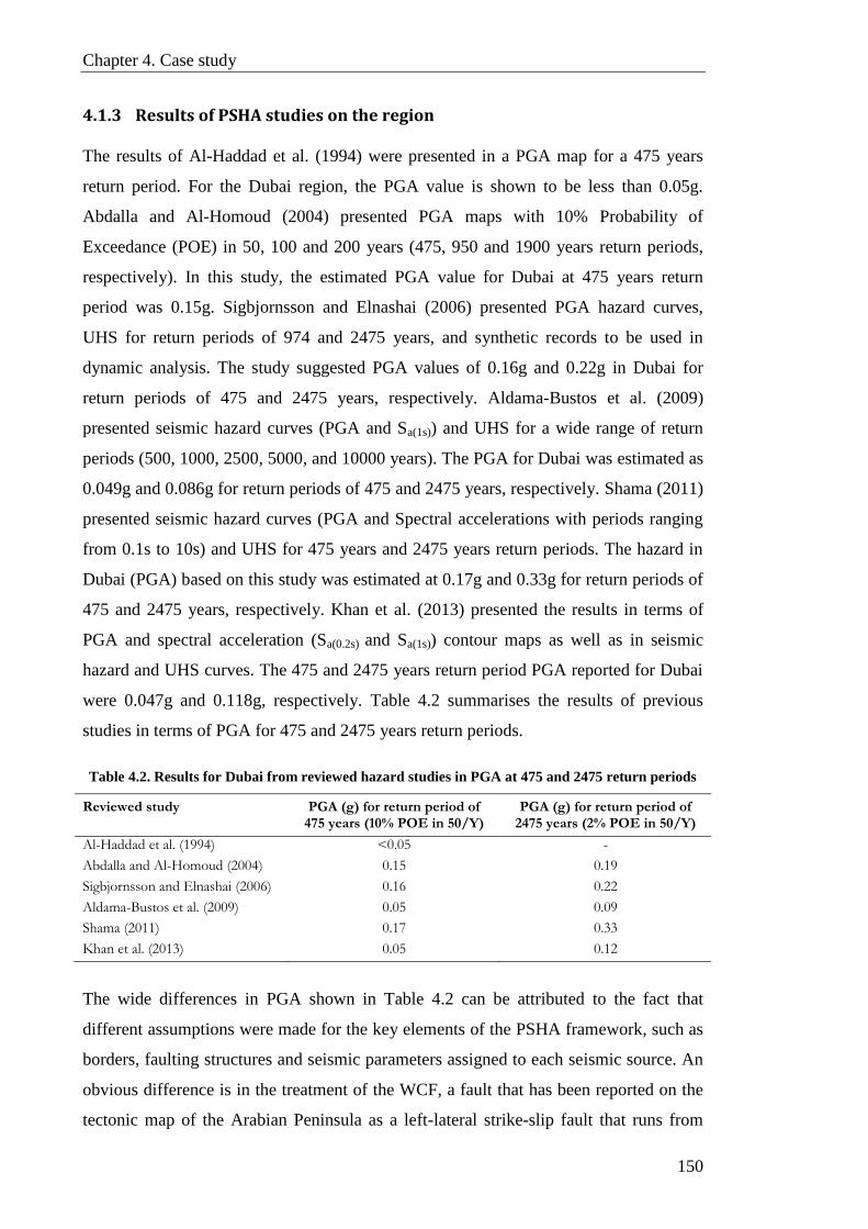
Chapter 4. Case study
150
4.1.3 Results of PSHA studies on the region
The results of Al-Haddad et al. (1994) were presented in a PGA map for a 475 years
return period. For the Dubai region, the PGA value is shown to be less than 0.05g.
Abdalla and Al-Homoud (2004) presented PGA maps with 10% Probability of
Exceedance (POE) in 50, 100 and 200 years (475, 950 and 1900 years return periods,
respectively). In this study, the estimated PGA value for Dubai at 475 years return
period was 0.15g. Sigbjornsson and Elnashai (2006) presented PGA hazard curves,
UHS for return periods of 974 and 2475 years, and synthetic records to be used in
dynamic analysis. The study suggested PGA values of 0.16g and 0.22g in Dubai for
return periods of 475 and 2475 years, respectively. Aldama-Bustos et al. (2009)
presented seismic hazard curves (PGA and Sa(1s)) and UHS for a wide range of return
periods (500, 1000, 2500, 5000, and 10000 years). The PGA for Dubai was estimated as
0.049g and 0.086g for return periods of 475 and 2475 years, respectively. Shama (2011)
presented seismic hazard curves (PGA and Spectral accelerations with periods ranging
from 0.1s to 10s) and UHS for 475 years and 2475 years return periods. The hazard in
Dubai (PGA) based on this study was estimated at 0.17g and 0.33g for return periods of
475 and 2475 years, respectively. Khan et al. (2013) presented the results in terms of
PGA and spectral acceleration (Sa(0.2s) and Sa(1s)) contour maps as well as in seismic
hazard and UHS curves. The 475 and 2475 years return period PGA reported for Dubai
were 0.047g and 0.118g, respectively. Table 4.2 summarises the results of previous
studies in terms of PGA for 475 and 2475 years return periods.
Table 4.2. Results for Dubai from reviewed hazard studies in PGA at 475 and 2475 return periods
Reviewed study PGA (g) for return period of 475 years (10% POE in 50/Y)
PGA (g) for return period of 2475 years (2% POE in 50/Y)
Al-Haddad et al. (1994) <0.05 -
Abdalla and Al-Homoud (2004) 0.15 0.19
Sigbjornsson and Elnashai (2006) 0.16 0.22
Aldama-Bustos et al. (2009) 0.05 0.09
Shama (2011) 0.17 0.33
Khan et al. (2013) 0.05 0.12
The wide differences in PGA shown in Table 4.2 can be attributed to the fact that
different assumptions were made for the key elements of the PSHA framework, such as
borders, faulting structures and seismic parameters assigned to each seismic source. An
obvious difference is in the treatment of the WCF, a fault that has been reported on the
tectonic map of the Arabian Peninsula as a left-lateral strike-slip fault that runs from

Chapter 4. Case study
151
Abu Dhabi through Dubai and Sharjah to Ras Al Khaimah, parallel to the west coast of
UAE (Brown, 1972, Johnson, 1998). The existence and activity level of this fault has
been the focus of ongoing debate, with some of the studies considering it as a major
active source (Sigbjornsson and Elnashai, 2006, Shama, 2011) while others (e.g.
Aldama-Bustos et al., 2009, Khan et al., 2013) excluding it from their source model.
Notwithstanding the currently weak evidence for its existence, if the WCF was shown to
exist with a proven degree of activity (using geomorphic indicators and paleo
seismological investigation), the implication on the PSHA would be serious (Aldama-
Bustos et al., 2009). Other elements like the type and number of GMPEs used with each
seismic source and the definition of the horizontal component of motion could also have
a considerable effect on the outcome of the PSHA.
Considering the level of detail and assumptions made in the discussed studies, the study
of Aldama-Bustos et al. (2009) represents a comprehensive investigation. However, and
since the objective of the current work is to assess the seismic vulnerability of RC high-
rise wall buildings, it is reasonable to lean towards studies with reasonably conservative
outcomes that are in line with the seismic design criteria currently enforced in the UAE.
Among these are the peer-reviewed works of Abdalla and Al-Homoud (2004),
Sigbjornsson and Elnashai (2006), and Shama (2011). In these three studies, the PGA in
Dubai ranges between 0.15g to 0.17g for a return period of 475 years and 0.19g to 0.33g
for 2475 years return period. For the spectral acceleration, the values for 0.2s and 1.0s
from the 2475 years return period UHS curves are given as 0.8g and 0.28g in (Shama,
2011), 0.72g and 0.58g in (Sigbjornsson and Elnashai, 2006). These spectral
acceleration values are taken as 0.85g and 0.26g in the seismic maps included in the
Abu Dhabi International Building Code “ADIBC”, (DMA, 2013) based on the study of
Abdalla and Al-Homoud (2004). The high spectral accelerations in long periods from
Sigbjornsson and Elnashai are hard to justify even by accounting for the possible use of
GMPEs that are based on the larger horizontal component (Aldama-Bustos et al., 2009).
In conclusion, the hazard values in terms of PGA at 475 years return period and spectral
accelerations for 2475 years return period at 0.2s and 1.0s adopted for Dubai in the
current work are 0.16g, 0.80g and 0.24g, respectively. These are consistent with the
design values approved by the Dubai Municipality; the legal body responsible for
reviewing and approving all civil and structural designs in Dubai. Figure 4.3 and

Chapter 4. Case study
152
Figure 4.4 show a comparison of the results obtained by some of the discussed studies
in terms of seismic hazard curves (or data) and UHS, respectively.
Figure 4.3. Seismic hazard curves (or data) for Dubai from some of the reviewed hazard studies
Figure 4.4. UHS for Dubai from some of the reviewed hazard studies: (a) 10% POE in 50/Y; and
(b) 2% POE in 50/Y
0.0001
0.001
0.01
0.1
0 0.05 0.1 0.15 0.2 0.25 0.3 0.35
PGA (g)
Sigbjornsson & Elnashai (2006)
Aldama-Bustos et al. (2009)
Shama (2011)
Khan et al. (2012)
Abdalla & Al Homoud (2004) - 475 years
Abdalla & Al Homoud (2004) - 2475 years
Annual
Fre
quency o
f E
xceedan
ce (
1/Y
)
475 Years
2475 Years
0
0.2
0.4
0.6
0.8
0 0.5 1 1.5 2 2.5 3 3.5 4
Spectr
al A
ccele
rati
on (
g)
Period (s)
Sigbjornsson & Elnashai (2006)Aldama-Bustos et al. (2009)Shama (2011)Khan et al. (2012)
0
0.3
0.6
0.9
1.2
0 0.5 1 1.5 2 2.5 3 3.5 4
Spectr
al A
ccele
rati
on (
g)
Period (s)
Sigbjornsson & Elnashai (2006)Aldama-Bustos et al. (2009)Shama (2011)Khan et al. (2012)
2% POE in 50/Y (2475 years return period)
10% POE in 50/Y (475 years return period)
a
b
Chapter 4. Case study
153
4.1.4 Site conditions
In all the studies listed in Table 4.1, the site condition used is bedrock except for
Sigbjornsson and Elnashai (2006) where the assumed site classification adopted in the
attenuation relationships has not been specified explicitly. However, Sigbjornsson and
Elnashai compared the results directly with the work of Abdalla and Al-Homoud
(2004), suggesting that the site condition considered in their work is also bedrock.
Amplification of site response due to the effect of surface soil deposits of a particular
site has been demonstrated in many previous events. Among others, are the Mexico
earthquake in 1985 and the Bam earthquake in 2003. The seismic waves at site surface
have been amplified by 5-fold the ground motion at bedrock level in the former (Celebi
et al., 1987), while the ground surface motion was significantly altered in the latter
(Rayhani et al., 2008). The level of response amplification caused by site condition
depends on, among other factors, the properties of soil deposits and the characteristics
of bedrock motion (e.g. Day, 2002).
Based on the author’s personal experience from working as a senior structural designer
in Dubai and related studies (e.g. Irfan et al., 2012), the near-surface soil in most of the
Dubai region can be classified as “Class C: very dense soil and soft rock” with a small
portion classified as “Class D: stiff soil”. This classification is based on the average
shear wave velocity for the top 30m, following site classification system of ASCE/SEI
7-16 (2017) and FEMA P-1050 (2015). The classification of Dubai soil may
considerably amplify ground motions generated by low-to-moderate near-field and
strong distant earthquakes, which in turn, impacts the seismic response of RC high-rise
buildings with long fundamental periods and short higher mode periods.
For a site condition like the one in Dubai (very dense or stiff soil overlaying bedrock),
site response amplification can be estimated either by (a) developing the response
spectrum at the ground surface directly from the region hazard study using attenuation
equations that are driven specifically for computing stiff soil-site response spectra
(instead of bedrock response spectra); (b) using code-provided site coefficients to adjust
the response spectrum values for the stiff soil overburden; or (c) region hazard study
followed by dynamic site response analysis, (e.g. FEMA, 2015, ASCE/SEI-7, 2017).
Although dynamic nonlinear (or equivalent linear) site response analysis is a more
accurate, yet complicated, method to account for the site response amplification,

Chapter 4. Case study
154
approach (b) is adopted in the current work for the design of the case study high-rise
building. For the vulnerability study, real input ground motions recorded on similar soil
classes as those known in Dubai were adopted, as discussed hereafter. Figure 4.5
presents a comparison of 475 years return period code spectra of Dubai for site class B
(bedrock), C (very dense soil and soft rock) and D (stiff soil), based on the 0.2s and 1.0s
spectral accelerations adopted in the current study and site coefficients of ASCE/SEI 7-
16 (2017).
Figure 4.5. Dubai design spectra for site class B, C and D using 0.2s and 1.0s spectral acceleration
values adopted in the present study and site coefficient of ASCE/SEI 7-16 (2017)
4.1.5 Earthquake Scenarios
The UHS represent the envelope (aggregation) of the effect of all earthquakes
contributing to the study region with different combinations of magnitudes and
distances. However, at a given time, a building will normally undergo only one
earthquake as far as design is concerned. Hence, disaggregation of the rate of
occurrence associated with the level of ground motion corresponding to selected return
periods is required in order to identify the magnitude-distance scenarios most
significantly contributing to the hazard (Bazzurro and Cornell, 1999)
Mwafy et al. (2006) demonstrated the characteristic difference in response induced by
earthquakes due to strong distant and moderate near-field events, especially for high-
rise buildings with long fundamental periods. The disaggregation process in the work of
Aldama-Bustos et al. (2009) clearly showed that for spectral accelerations at longer
response periods, larger magnitude earthquakes located at greater distances are the main
contributor to risk. It also illustrated that as one moves towards the north part of the
0
0.1
0.2
0.3
0.4
0.5
0.6
0.7
0 0.5 1 1.5 2 2.5 3 3.5 4
Sp
ectr
al A
ccel
erat
ion
(g)
Period (s)
Dubai design spectrum: Site Class BDubai design spectrum: Site Class CDubai design spectrum: Site Class D

Chapter 4. Case study
155
UAE (from Abu Dhabi to Dubai and Ras Al-Khaimah), the contributions of the Makran
and Zagros regions to the hazard at short response periods relatively increases. Similar
findings were reported by Mwafy et al. (2006), Shama (2011), and Khan (2013).
Based on the disaggregation process in the above-mentioned studies, two main
scenarios can be identified: (i) 5-6 magnitude earthquake at 10-60km epicentral distance
generated by local faults (Dibba fault and WCF); and (ii) 7-8 magnitude earthquake at
100-200km epicentral distance that could be triggered at the Makran subduction zone.
The selected response spectra of the input ground motions that represent the
aforementioned earthquake scenarios are expected to match different parts of the code
spectra for the study region (Figure 4.5) according to the earthquake scenario they
represent. These records will be used in the nonlinear dynamic analyses of the reference
building in CHAPTER 5.
4.2 Input ground motions
Ground excitation induced by different earthquake scenarios is a major source of
uncertainty in determining seismic demands. To account for this uncertainty, the two
aforementioned earthquake scenarios are represented in the current study by two sets
with 20 natural earthquake records in each set (total of 40 records). Record Set#1
contains the input motions representing the severe distant earthquake scenario, while
Record Set#2 represents the moderate near-field scenario. The European Strong-motion
(Ambraseys et al., 2004) and the Pacific Earthquake Engineering Research Centre
(PEER, 2019) databases are used to select the earthquake records due to the insufficient
number of recorded events within the study region. Four parameters are considered in
the selection criteria of the 40 records; (i) event magnitude (M); (ii) distance to source
(R); (iii) site soil condition (S); and (iv) ground motion acceleration to velocity (a/v)
ratio.
Earthquakes with larger magnitudes come with significantly longer effective durations
and more significant peaks compared to smaller ones. The site-to-source distance
generally affects the ground motion at the site through path attenuation and high-
frequency filtration. Depending on the characteristics of the site soil strata, the seismic
wave is either amplified or dissipated while travelling from the bedrock to the ground
level. This modification in the seismic wave impacts the dynamic behaviour of wide
frequency-sensitive high-rise buildings. The a/v ratio forms an important measure to
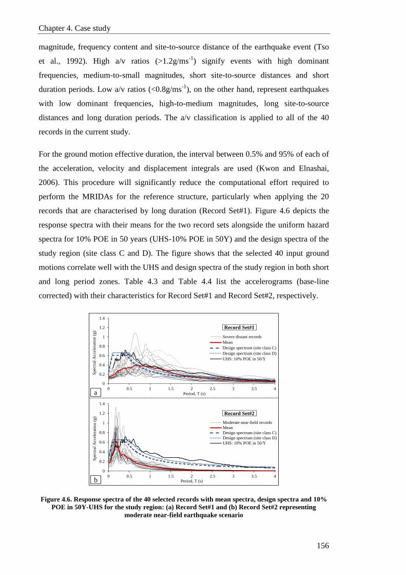
Chapter 4. Case study
156
magnitude, frequency content and site-to-source distance of the earthquake event (Tso
et al., 1992). High a/v ratios (>1.2g/ms-1
) signify events with high dominant
frequencies, medium-to-small magnitudes, short site-to-source distances and short
duration periods. Low a/v ratios (<0.8g/ms-1
), on the other hand, represent earthquakes
with low dominant frequencies, high-to-medium magnitudes, long site-to-source
distances and long duration periods. The a/v classification is applied to all of the 40
records in the current study.
For the ground motion effective duration, the interval between 0.5% and 95% of each of
the acceleration, velocity and displacement integrals are used (Kwon and Elnashai,
2006). This procedure will significantly reduce the computational effort required to
perform the MRIDAs for the reference structure, particularly when applying the 20
records that are characterised by long duration (Record Set#1). Figure 4.6 depicts the
response spectra with their means for the two record sets alongside the uniform hazard
spectra for 10% POE in 50 years (UHS-10% POE in 50Y) and the design spectra of the
study region (site class C and D). The figure shows that the selected 40 input ground
motions correlate well with the UHS and design spectra of the study region in both short
and long period zones. Table 4.3 and Table 4.4 list the accelerograms (base-line
corrected) with their characteristics for Record Set#1 and Record Set#2, respectively.
Figure 4.6. Response spectra of the 40 selected records with mean spectra, design spectra and 10%
POE in 50Y-UHS for the study region: (a) Record Set#1 and (b) Record Set#2 representing
moderate near-field earthquake scenario
0
0.2
0.4
0.6
0.8
1
1.2
1.4
0 0.5 1 1.5 2 2.5 3 3.5 4
Sp
ectr
al A
ccel
erat
ion (
g)
Period, T (s)
Moderate near-field records
Mean
Design spectrum (site class C)
Design spectrum (site class D)
UHS: 10% POE in 50/Y
0
0.2
0.4
0.6
0.8
1
1.2
1.4
0 0.5 1 1.5 2 2.5 3 3.5 4
Sp
ectr
al A
ccel
erat
ion (
g)
Period, T (s)
Severe distant records
Mean
Design spectrum (site class C)
Design spectrum (site class D)
UHS: 10% POE in 50/Y
a
b
Record Set#1
Record Set#2

157
Table 4.3. Identification and characteristics for input ground motions in Record Set#1
Record
ID
Earthquake Station Component Date Magnitude
(Mw)
Site
class
Epicentral
Distance (km)
Duration
(sec)
Sample Step (s)
PGA
(g)
(a/v)
g/ms-1
(a/v)
Class
R1 Bucharest Building res. Institute EW 04-03-1977 7.53 D 161 18 0.005 0.176 0.60
LOW
R2 Chi-Chi CWB 99999 ILA013 EW 20-09-1999 7.62 C 135 60 0.004 0.139 0.52
R3 Loma Prieta Emeryville 260 18-10-1989 6.93 C 96.5 28 0.01 0.250 0.57
R4 Loma Prieta Golden Gate Bridge 270 18-10-1989 6.93 C 100 28 0.005 0.233 0.61
R5 Hector Mine Indio - Coachella Canal 0 16-10-1999 7.13 D 99 60 0.02 0.092 0.70
R6 Izmit Ambarli-Termik EW 17-08-1999 7.64 D 113 50 0.005 0.183 0.60
R7 Izmit Istanbul-Zeytinburnu NS 17-08-1999 7.64 D 96 96 0.01 0.110 0.77
R8 Kocaeli Bursa Tofas E 17-08-1999 7.51 D 95 70 0.005 0.108 0.49
R9 Kocaeli Hava Alani 90 17-08-1999 7.51 C 102 90 0.005 0.094 0.46
R10 Loma Prieta Alameda Naval Air Stn Hanger 270 18-10-1989 6.93 D 91 29 0.005 0.244 0.73
R11 Loma Prieta Berkeley LBL 90 18-10-1989 6.93 C 98 39 0.005 0.117 0.65
R12 Loma Prieta Oakland-Outer Harbor Wharf 0 18-10-1989 6.93 D 94 40 0.02 0.280 0.67
R13 Manjil Abhar N57E 20-06-1990 7.42 D 91 29 0.01 0.133 0.62
R14 Manjil Tonekabun N132 20-06-1990 7.42 C 131 40 0.005 0.124 0.76
R15 Chi-Chi TAP005 E 20-09-1999 7.62 D 156 60 0.005 0.137 0.49
R16 Chi-Chi TAP010 E 20-09-1999 7.62 D 151 60 0.005 0.121 0.50
R17 Chi-Chi TAP021 E 20-09-1999 7.62 D 151 60 0.005 0.117 0.47
R18 Chi-Chi TAP032 N 20-09-1999 7.62 C 144 60 0.005 0.115 0.64
R19 Chi-Chi TAP090 E 20-09-1999 7.62 D 156 60 0.005 0.130 0.41
R20 Chi-Chi TAP095 N 20-09-1999 7.62 D 158 60 0.005 0.098 0.52
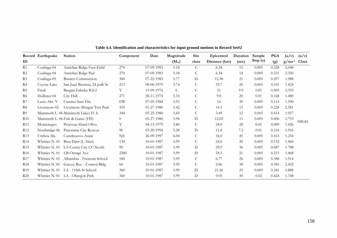
158
Table 4.4. Identification and characteristics for input ground motions in Record Set#2
Record
ID
Earthquake Station Component Date Magnitude
(Mw)
Site
class
Epicentral
Distance (km)
Duration
(sec)
Sample Step (s)
PGA
(g)
(a/v)
g/ms-1
(a/v)
Class
R1 Coalinga-04 Anticline Ridge Free-Field 270 07-09-1983 5.18 C 6.34 15 0.005 0.328 2.048
HIGH
R2 Coalinga-04 Anticline Ridge Pad 270 07-09-1983 5.18 C 6.34 14 0.005 0.331 2.350
R3 Coalinga-05 Burnett Construction 360 07-22-1983 5.77 D 12.38 21 0.005 0.297 1.988
R4 Coyote Lake San Juan Bautista, 24 polk St 213 08-06-1979 5.74 C 19.7 26 0.005 0.101 1.424
R5 Friuli Breginj-Fabrika IGLI Y 15-09-1976 6 C 21 9.9 0.01 0.505 2.333
R6 Hollister-04 City Hall 271 28-11-1974 5.14 C 9.8 20 0.01 0.168 1.480
R7 Lazio Abr. Y Cassino-Sant Elia EW 07-05-1984 5.93 C 16 30 0.005 0.114 1.590
R8 Livermore-02 Livermore-Morgan Terr Park 355 01-27-1980 5.42 C 14.1 15 0.005 0.228 2.581
R9 Mammoth L. 06 Mammoth Lakes H. S. 344 05-25-1980 5.69 C 3.49 12 0.005 0.414 1.957
R10 Mammoth L. 06 Fish & Game (FIS) 0 05-27-1980 5.94 D 12.02 11 0.005 0.406 2.753
R11 Montenegro Petrovac-Hotel Oliva Y 04-15-1979 5.80 C 24.0 28 0.01 0.089 1.426
R12 Northridge-06 Panorama City-Roscoe 90 03-20-1994 5.28 D 11.8 7.2 0.01 0.116 1.916
R13 Umbria Ma. Castelnuovo-Assisi NE 26-09-1997 6.04 C 16.0 45 0.005 0.163 1.254
R14 Whittier N. 01 Brea Dam (L Abut) 130 10-01-1987 5.99 C 24.0 20 0.005 0.132 1.460
R15 Whittier N. 01 LA-Centry City CC North 90 10-01-1987 5.99 D 29.9 30 0.005 0.087 1.788
R16 Whittier N. 01 LB-Orange Ave 2280 10-01-1987 5.99 D 24.5 21 0.005 0.215 1.468
R17 Whittier N. 01 Alhambra - Fremont School 180 10-01-1987 5.99 C 6.77 26 0.005 0.388 1.514
R18 Whittier N. 01 Garvey Res. - Control Bldg 60 10-01-1987 5.99 C 2.86 38 0.005 0.385 2.432
R19 Whittier N. 01 LA - 116th St School 360 10-01-1987 5.99 D 21.26 25 0.005 0.341 1.888
R20 Whittier N. 01 LA - Obregon Park 360 10-01-1987 5.99 D 9.05 30 0.02 0.424 1.748
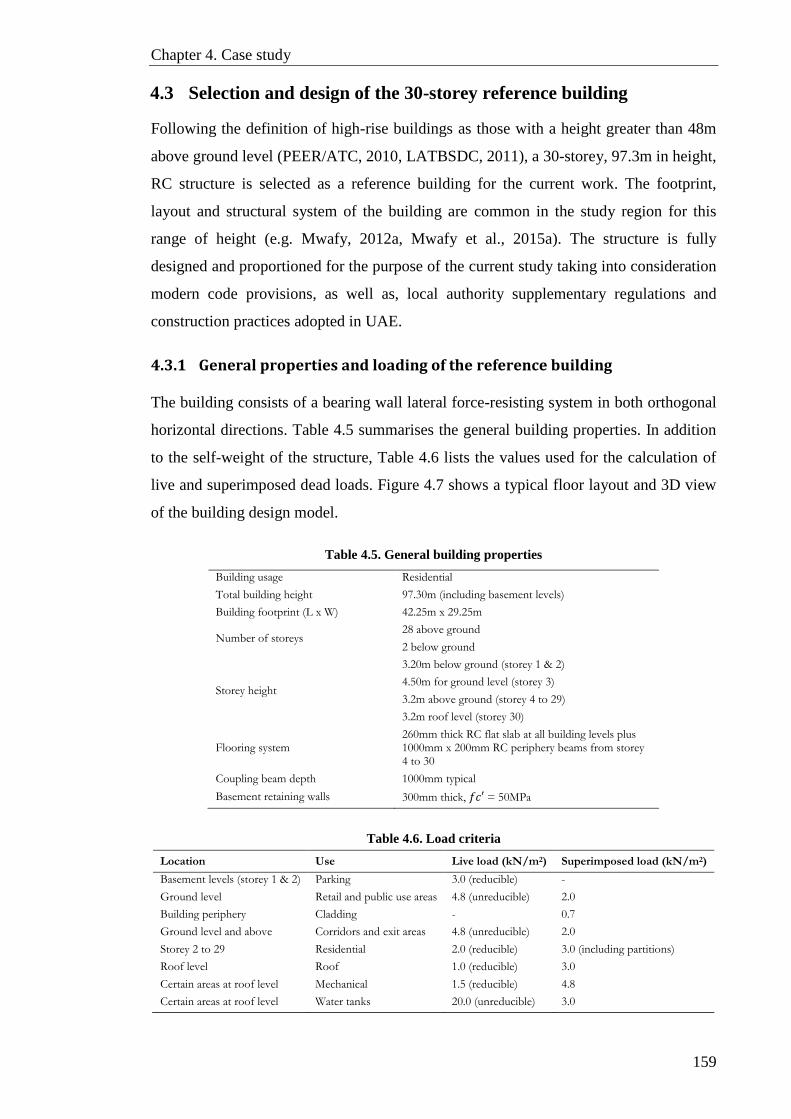
Chapter 4. Case study
159
4.3 Selection and design of the 30-storey reference building
Following the definition of high-rise buildings as those with a height greater than 48m
above ground level (PEER/ATC, 2010, LATBSDC, 2011), a 30-storey, 97.3m in height,
RC structure is selected as a reference building for the current work. The footprint,
layout and structural system of the building are common in the study region for this
range of height (e.g. Mwafy, 2012a, Mwafy et al., 2015a). The structure is fully
designed and proportioned for the purpose of the current study taking into consideration
modern code provisions, as well as, local authority supplementary regulations and
construction practices adopted in UAE.
4.3.1 General properties and loading of the reference building
The building consists of a bearing wall lateral force-resisting system in both orthogonal
horizontal directions. Table 4.5 summarises the general building properties. In addition
to the self-weight of the structure, Table 4.6 lists the values used for the calculation of
live and superimposed dead loads. Figure 4.7 shows a typical floor layout and 3D view
of the building design model.
Table 4.5. General building properties
Building usage Residential
Total building height 97.30m (including basement levels)
Building footprint (L x W) 42.25m x 29.25m
Number of storeys 28 above ground
2 below ground
Storey height
3.20m below ground (storey 1 & 2)
4.50m for ground level (storey 3)
3.2m above ground (storey 4 to 29)
3.2m roof level (storey 30)
Flooring system 260mm thick RC flat slab at all building levels plus 1000mm x 200mm RC periphery beams from storey 4 to 30
Coupling beam depth 1000mm typical
Basement retaining walls 300mm thick, 𝑓𝑐′ = 50MPa
Table 4.6. Load criteria
Location Use Live load (kN/m2) Superimposed load (kN/m2)
Basement levels (storey 1 & 2) Parking 3.0 (reducible) -
Ground level Retail and public use areas 4.8 (unreducible) 2.0
Building periphery Cladding - 0.7
Ground level and above Corridors and exit areas 4.8 (unreducible) 2.0
Storey 2 to 29 Residential 2.0 (reducible) 3.0 (including partitions)
Roof level Roof 1.0 (reducible) 3.0
Certain areas at roof level Mechanical 1.5 (reducible) 4.8
Certain areas at roof level Water tanks 20.0 (unreducible) 3.0
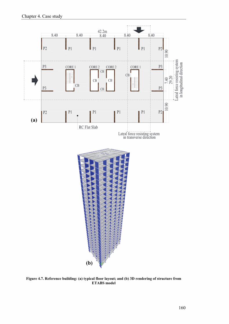
Chapter 4. Case study
160
Figure 4.7. Reference building: (a) typical floor layout; and (b) 3D rendering of structure from ETABS model
(a)
(b)

Chapter 4. Case study
161
A basic wind speed of 45m/s with an importance factor of 1.0 and exposure type C are
considered in estimating wind loads using the ASCE/SEI 7-05 (2005). Following the
discussion in Section 4.1.3, the seismic design loads are calculated using mapped
spectral response accelerations of 0.80g and 0.24g at 0.2s and 1.0s, respectively. Site
class SC (very dense soil and soft rock) is considered in the seismic analysis.
4.3.2 Analysis and design of the reference building
ETABS (CSI, 2015), a commercial structural analysis and design software for high-rise
buildings, is utilised to model the reference building in 3D. For the analysis and design
of the flooring system, The SAFE flooring analysis and design software is used (CSI,
2014). Shell elements are used to model shear walls and floor slabs, while frame
elements are adopted in modelling periphery and coupling beams. In the analysis,
seismic demand is estimated using both Equivalent Lateral Force Procedure (ELFP) and
Modal Response Spectrum Analysis (MRSA). A sufficient number of modes were
included in the analysis to obtain combined modal mass participation of at least 90% of
the actual mass in each of the orthogonal directions (ASCE/SEI-7, 2017). The combined
response of the model base shear from MRSA is scaled up to a minimum of 85% of the
base shear calculated from ELFP (ASCE/SEI-7, 2017). Complete Quadratic
Combination (CQC) method and Ritz-vector procedure are used for the MRSA. Critical
viscous damping of 5% is considered for all modes of vibration. Eccentricity ratios of
5% are considered for the diaphragm centre of rigidity in both orthogonal directions to
account for accidental torsional effects on the building. P-Δ effects are also accounted
for in the analysis.
The design of the building is performed in general compliance with the IBC (2015),
which requires the use of the ASCE/SEI 7-10 (2010) and ACI 318 (2014). ASTM 706
reinforcing steel is used with a specified yielding strength of 460MPa. The specified
concrete strengths used in the flooring system, retaining walls at basements, piers, cores
and coupling beams range between 40MPa and 50MPa. Cross-sections and
corresponding reinforcement of piers and cores vary over the building height. Cast-in-
situ RC flat slabs of 0.26m thickness with periphery beams are adopted for the flooring
system, also serving as a rigid diaphragm to transfer lateral forces to the vertical
structural elements at each floor. The flooring system is subjected to special design
requirements, including punching shear, so as to resist the combination of seismic
deformations and gravity loads. The stiffness assumptions given in Table 4.7 are used to
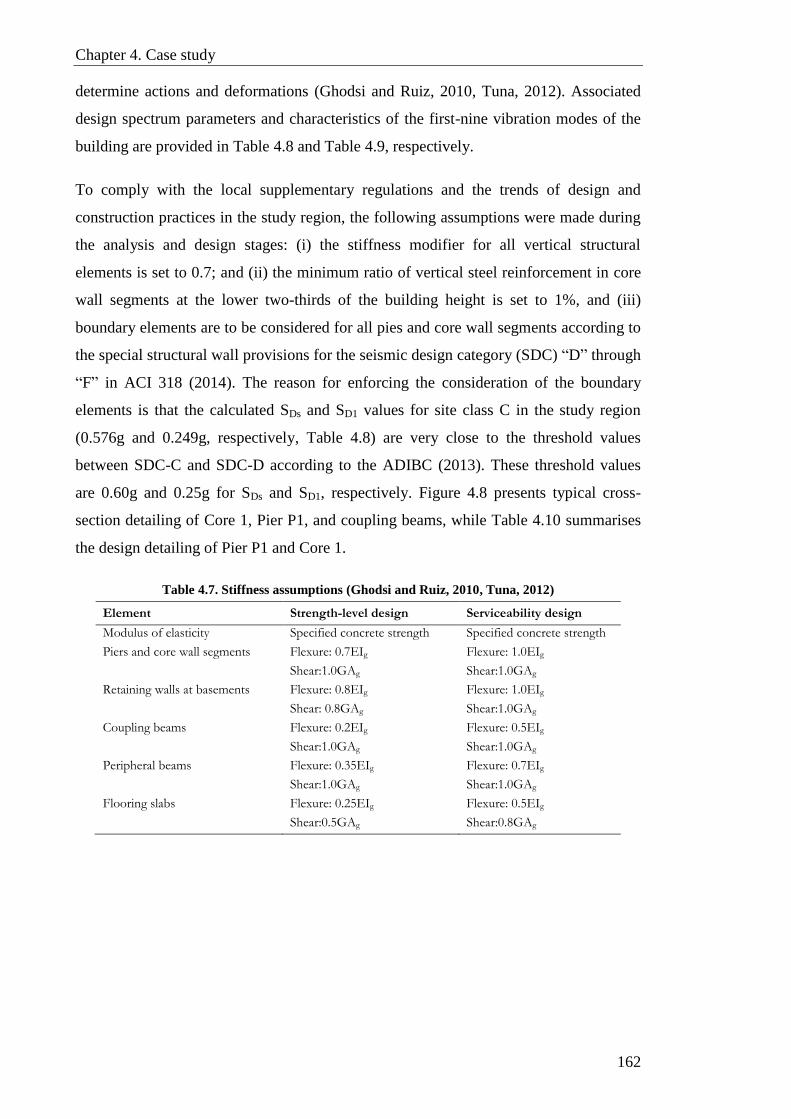
Chapter 4. Case study
162
determine actions and deformations (Ghodsi and Ruiz, 2010, Tuna, 2012). Associated
design spectrum parameters and characteristics of the first-nine vibration modes of the
building are provided in Table 4.8 and Table 4.9, respectively.
To comply with the local supplementary regulations and the trends of design and
construction practices in the study region, the following assumptions were made during
the analysis and design stages: (i) the stiffness modifier for all vertical structural
elements is set to 0.7; and (ii) the minimum ratio of vertical steel reinforcement in core
wall segments at the lower two-thirds of the building height is set to 1%, and (iii)
boundary elements are to be considered for all pies and core wall segments according to
the special structural wall provisions for the seismic design category (SDC) “D” through
“F” in ACI 318 (2014). The reason for enforcing the consideration of the boundary
elements is that the calculated SDs and SD1 values for site class C in the study region
(0.576g and 0.249g, respectively, Table 4.8) are very close to the threshold values
between SDC-C and SDC-D according to the ADIBC (2013). These threshold values
are 0.60g and 0.25g for SDs and SD1, respectively. Figure 4.8 presents typical cross-
section detailing of Core 1, Pier P1, and coupling beams, while Table 4.10 summarises
the design detailing of Pier P1 and Core 1.
Table 4.7. Stiffness assumptions (Ghodsi and Ruiz, 2010, Tuna, 2012)
Element Strength-level design Serviceability design
Modulus of elasticity Specified concrete strength Specified concrete strength
Piers and core wall segments Flexure: 0.7EIg
Shear:1.0GAg
Flexure: 1.0EIg
Shear:1.0GAg
Retaining walls at basements Flexure: 0.8EIg
Shear: 0.8GAg
Flexure: 1.0EIg
Shear:1.0GAg
Coupling beams Flexure: 0.2EIg
Shear:1.0GAg
Flexure: 0.5EIg
Shear:1.0GAg
Peripheral beams Flexure: 0.35EIg
Shear:1.0GAg
Flexure: 0.7EIg
Shear:1.0GAg
Flooring slabs Flexure: 0.25EIg
Shear:0.5GAg
Flexure: 0.5EIg
Shear:0.8GAg

Chapter 4. Case study
163
Table 4.8. Adopted design parametersA
Ss(0.2s) 0.80g
S1(1.0s) 0.24g
Site class C
Fa 1.08
Fv 1.56
SMs 0.864g
SM1 0.374g
SDs 0.576g
SD1 0.249g
SDC (DMA, 2013) C
Risk category I
Seismic importance factor 1.0
R 4.0
Cd 4.0
Seismic weight (W) 466696kN (47590t)
Modal combination method Complete quadratic combination (CQC)
Redundancy factor (ρ)B 1.0
Accidental eccentricity 5%
Viscous damping 5%
Modal base shear 11299kNC
ARefer to ASCE/SEI 7-10 for the definition of table parameters BThe redundancy factor = 1, the structure complies with 12.3.4.1 of ASCE/SEI 7-10 CPer Section 12.9.4 of ASCE/SEI 7-10, for strength design, the modal analyses are scaled to match 0.85V = 11299kN
Table 4.9. Building vibration mode periods and mass participation summary
Vibration mode #
Uncracked period (s)
Equivalent inelastic
period (s)
Mode dominate direction Mass participation (%)
1 3.44 5.30 Translation mode on X direction (H1) 71
2 3.21 4.46 Translation mode on Y direction (H2) 66
3 3.03 3.96 Torsional mode 72
4 1.03 1.43 Translation mode on X direction (H1) 14
5 0.91 1.09 Torsional mode 13
6 0.82 0.96 Translation mode on Y direction (H2) 18
7 0.52 0.65 Translation mode on X direction (H1) 6
8 0.36 0.40 Torsional mode 5.5
9 0.32 0.39 Translation mode on Y direction (H2) 6.5

164
Figure 4.8. Typical cross-section detailing of Core 1, Pier P1, and coupling beams in the reference building
Coupling beam typical detailing
CORE 1
AS
6
Pier1 (1 S-10 S)
L1
AS5AS4AS5AS5
AS5AS4AS5AS5
Pier1 (11 S-30 S)
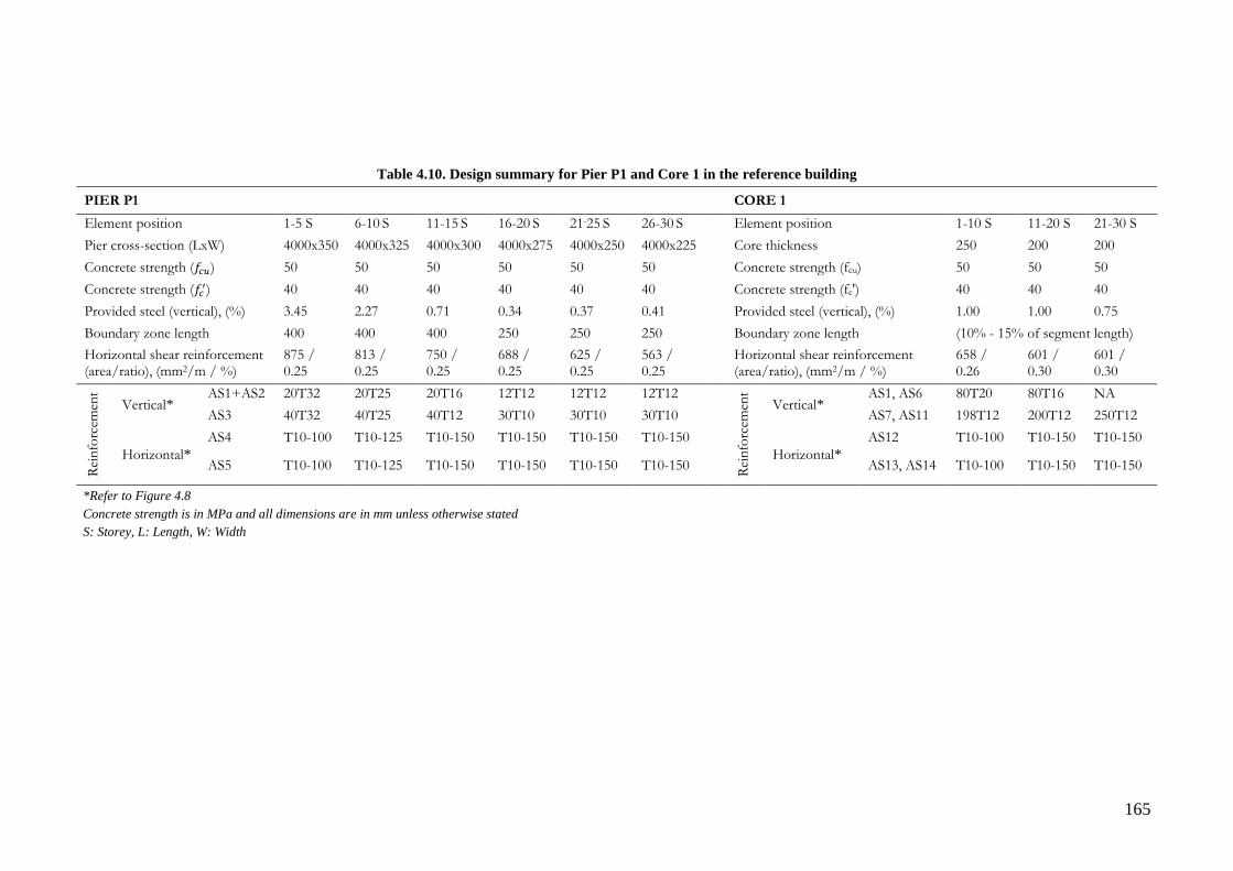
165
Table 4.10. Design summary for Pier P1 and Core 1 in the reference building
PIER P1 CORE 1
Element position 1-5 S 6-10 S 11-15 S 16-20 S 21-25 S 26-30 S
Element position 1-10 S 11-20 S 21-30 S
Pier cross-section (LxW) 4000x350 4000x325 4000x300 4000x275 4000x250 4000x225
Core thickness 250 200 200
Concrete strength (𝑓𝑐𝑢) 50 50 50 50 50 50
Concrete strength (fcu) 50 50 50
Concrete strength (𝑓𝑐′) 40 40 40 40 40 40
Concrete strength (fc') 40 40 40
Provided steel (vertical), (%) 3.45 2.27 0.71 0.34 0.37 0.41
Provided steel (vertical), (%) 1.00 1.00 0.75
Boundary zone length 400 400 400 250 250 250
Boundary zone length (10% - 15% of segment length)
Horizontal shear reinforcement (area/ratio), (mm2/m / %)
875 / 0.25
813 / 0.25
750 / 0.25
688 / 0.25
625 / 0.25
563 / 0.25
Horizontal shear reinforcement (area/ratio), (mm2/m / %)
658 / 0.26
601 / 0.30
601 / 0.30
Rei
nfo
rcem
ent
Vertical* AS1+AS2 20T32 20T25 20T16 12T12 12T12 12T12
Rei
nfo
rcem
ent
Vertical* AS1, AS6 80T20 80T16 NA
AS3 40T32 40T25 40T12 30T10 30T10 30T10
AS7, AS11 198T12 200T12 250T12
Horizontal*
AS4 T10-100 T10-125 T10-150 T10-150 T10-150 T10-150
Horizontal*
AS12 T10-100 T10-150 T10-150
AS5 T10-100 T10-125 T10-150 T10-150 T10-150 T10-150 AS13, AS14 T10-100 T10-150 T10-150
*Refer to Figure 4.8
Concrete strength is in MPa and all dimensions are in mm unless otherwise stated
S: Storey, L: Length, W: Width

Chapter 4. Case study
166
4.4 Nonlinear modelling of the reference building
PERFORM-3D analytical tool (CSI, 2011) is utilised to create the nonlinear model of
the reference building. The selection of the tool, modelling approach and key modelling
parameters are based on the MLNMVS presented in CHAPTER 3 of this thesis
Although PERFORM-3D is an efficient 3D modelling package, it is computationally
demanding to execute a large number of NRHAs for a 3D model of an entire high-rise
structure, particularly when a wide range of input ground motions is employed. A 3D-
slice idealization is therefore adopted to develop the nonlinear model of the reference
building. The lateral force-resisting system of the building in the transverse direction is
assumed to consist of four framing bays. Each of these, carrying 25% of the total mass
of the building, consisted of two external piers (P1) and an internal core, as shown in
Figure 4.7a. Conservatively, the two framing bays at the right and left edges of the
building are assumed not to form part of the lateral force-resisting system and only
carry gravity load. In the longitudinal direction, the lateral forces are resisted by a single
framing system which consists of all the internal cores and piers P3. Other piers (P2 and
P1) are assumed not to be participating in resisting lateral forces in the longitudinal
direction. The results from the free vibration analysis conducted on the entire building
using the ETABS 3D model indicate a comparable lateral capacity in the two
orthogonal directions with the fundamental mode uncracked periods of 3.44s and 3.21s
in the longitudinal and transverse directions (H1 and H2), respectively. Vindicated by
this fact, the number of MRIDAs, and thus the computational effort, can be significantly
reduced by focusing only on one direction of the building. As a result, the 3D-slice
representing the lateral force-resisting system in the transverse direction of the reference
building is modelled and employed in the next chapter to define the performance limit
states. To confirm the suitability of the 3D-slice model in representing the transverse
direction of the reference building, Table 4.11 lists the equivalent inelastic and
uncracked periods of the first three modes in the transverse direction of both the
reference building and the modelled 3D-slice. As the table depicts, these periods are
very close, mostly identical. The maximum difference in the equivalent inelastic periods
of modes 1, 2, and 3 between the entire building and the 3D-slice transverse direction is
0.30s (6.7%), 0.00s (0.0%), and 0.00s (0.0%), respectively. These small-to-no
differences, are attributed to the minor contribution of the two framing bays at the right
and left edges of the building to the overall lateral stiffness in the transverse direction.
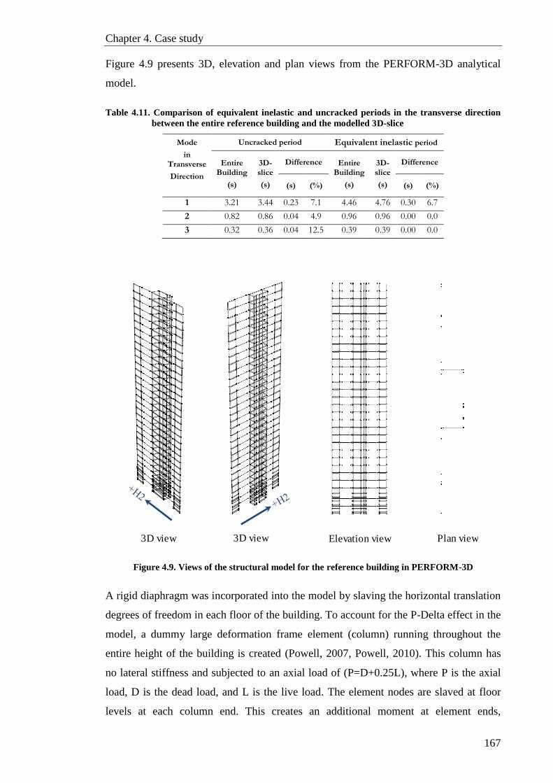
Chapter 4. Case study
167
Figure 4.9 presents 3D, elevation and plan views from the PERFORM-3D analytical
model.
Table 4.11. Comparison of equivalent inelastic and uncracked periods in the transverse direction
between the entire reference building and the modelled 3D-slice
Mode
in Transverse
Direction
Uncracked period Equivalent inelastic period
Entire Building
(s)
3D-slice
(s)
Difference Entire Building
(s)
3D-slice
(s)
Difference
(s) (%) (s) (%)
1 3.21 3.44 0.23 7.1 4.46 4.76 0.30 6.7
2 0.82 0.86 0.04 4.9 0.96 0.96 0.00 0.0
3 0.32 0.36 0.04 12.5 0.39 0.39 0.00 0.0
Figure 4.9. Views of the structural model for the reference building in PERFORM-3D
A rigid diaphragm was incorporated into the model by slaving the horizontal translation
degrees of freedom in each floor of the building. To account for the P-Delta effect in the
model, a dummy large deformation frame element (column) running throughout the
entire height of the building is created (Powell, 2007, Powell, 2010). This column has
no lateral stiffness and subjected to an axial load of (P=D+0.25L), where P is the axial
load, D is the dead load, and L is the live load. The element nodes are slaved at floor
levels at each column end. This creates an additional moment at element ends,
3D view 3D view Elevation view Plan view

Chapter 4. Case study
168
proportional to the lateral displacement. The seismic masses are assigned to the nodes at
each storey level in terms of dead load. The base of the structure is rigidly modelled
using vertical supports at the top-of-foundation level.
4.4.1 Modelling of piers and core wall segments
The 4-noded fibre-based shear wall element is utilised to model the piers and core wall
segments. Only confined concrete is modelled, i.e., the unconfined concrete cover is
neglected. Expected strengths of 1.3fc’and 1.17fy are used for concrete and reinforcing
steel, respectively (LATBSDC, 2011).
The four-linear segment relation (Figure 4.10a) is used to model the concrete stress-
strain relation based on the modified Mander model (Martínez-Rueda and Elnashai,
1997). Having the piers and core wall segments modelled using fibre elements; the
effective bending stiffness is not assigned explicitly to the concrete material model as it
is the product of the assumed stress-strain relations. Therefore, the effective bending
stiffness decreases with increasing fibre strains.
For the steel in tension, the post-yield stiffness and cyclic degradation parameters are
defined following adjustments described by Orakcal and Wallace (2006). In
compression, buckling of steel rebars is modelled based on experimental results and
analytical models from previous studies (e.g. Rodriguez et al., 1999, Bae et al., 2005,
Cosenza and Prota, 2006, Tuna, 2012). Reinforcing steel stress-strain relation is shown
in Figure 4.10b.
As adopted and verified in CHAPTER 3, the inelastic shear deformation in piers and
core wall segments is accounted for by assigning a trilinear relation (Figure 4.10c)
similar to the one recommended by ASCE/SEI 41-06 (2007) and ASCE/SEI 41-16
(ASCE/SEI-41, 2017). Test results by Thomsen and Wallace (2004) and calibration
study by Gogus (2010) are used to define the shear F-D relation. In the used trilinear
relation, the uncracked shear modulus is taken as 0.4Ec and diagonal (shear) cracking is
assumed to start at 0.25√fc′ ≤ 0.5vn, where vn is the wall nominal shear strength from
the ACI 318 (2014) and fc′ is the concrete expected compressive strength in MPa. The
post-cracking slope is reduced to 0.01Ec to account for the nonlinear shear deformations
due to shear-flexure interaction (Massone, 2006).

Chapter 4. Case study
169
4.4.2 Modelling of coupling beams
The coupling beams between the core wall segments are modelled as elastic beam
elements with nonlinear displacement shear hinge at mid-span (Figure 4.11), based on
test results by Naish et al. (Naish and Wallace, 2010). For obtaining the nominal
expected shear capacity, the angle of the diagonal reinforcement in the coupling beam
(α) is calculated based on 125mm distance from the centre of gravity of the diagonal
reinforcement bundle to the face of the coupling beam.
To define the behaviour of the displacement shear hinge in PERFORM-3D, the
displacement of the coupling beam is related to its rotation as described in Eqn. ( 4.1).
δθ = θ x Lcb ( 4.1)
Where θ is the coupling beam rotation in radians, Lcb is the length of the coupling beam
and δθ is the equivalent displacement at rotation θ. Figure 4.12 illustrates the backbone
parameters alongside the cyclic energy dissipation factors (degradation parameters)
used to model the shear displacement hinges for the coupling beams in the reference
building.
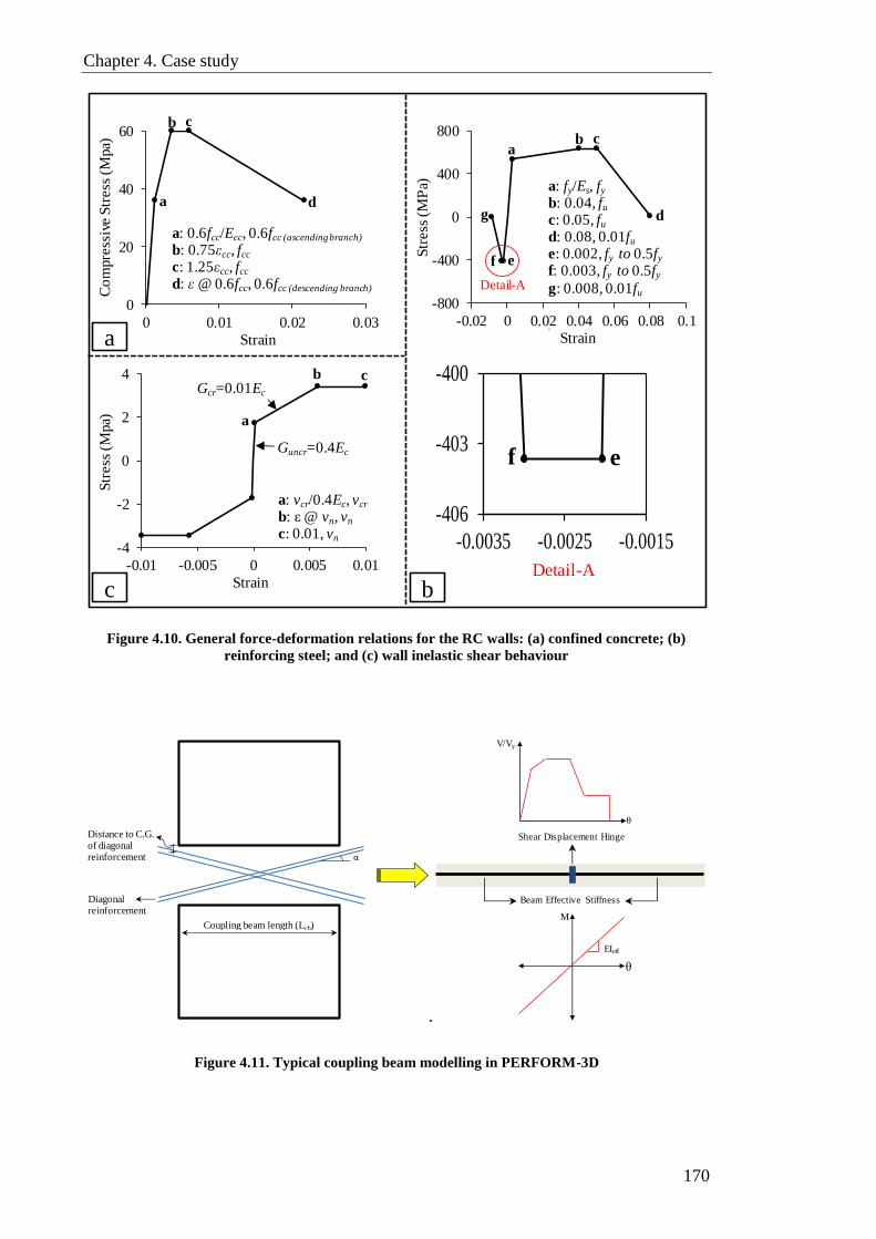
Chapter 4. Case study
170
Figure 4.10. General force-deformation relations for the RC walls: (a) confined concrete; (b)
reinforcing steel; and (c) wall inelastic shear behaviour
.
Figure 4.11. Typical coupling beam modelling in PERFORM-3D
a: fy/Es, fy
b: 0.04, fu
c: 0.05, fu
d: 0.08, 0.01fu
e: 0.002, fy to 0.5fy
f: 0.003, fy to 0.5fy
g: 0.008, 0.01fu
.
-800
-400
0
400
800
-0.02 0 0.02 0.04 0.06 0.08 0.1
Str
ess
(M
Pa)
Strain
ab c
d
ef
g
-4
-2
0
2
4
-0.01 -0.005 0 0.005 0.01
Str
ess
(M
pa)
Strain
a
b c
a: vcr/0.4Ec, vcr
b: ε @ vn, vn
c: 0.01, vn
Gcr=0.01Ec
Guncr=0.4Ec
0
20
40
60
0 0.01 0.02 0.03
Co
mpre
ssiv
e S
tress
(M
pa)
Strain
a: 0.6fcc/Ecc, 0.6fcc (ascending branch)
b: 0.75εcc, fcc
c: 1.25εcc, fcc
d: ε @ 0.6fcc, 0.6fcc (descending branch)
a
b c
d
-406
-403
-400
-0.0035 -0.0025 -0.0015
f e
Detail-A
Detail-A
a
bc
α
Distance to C.G.of diagonal reinforcement
Coupling beam length (Lcb)
Diagonal reinforcement
θ
M
EIeff
Beam Effective Stiffness
Shear Displacement Hinge
θ
V/Vy
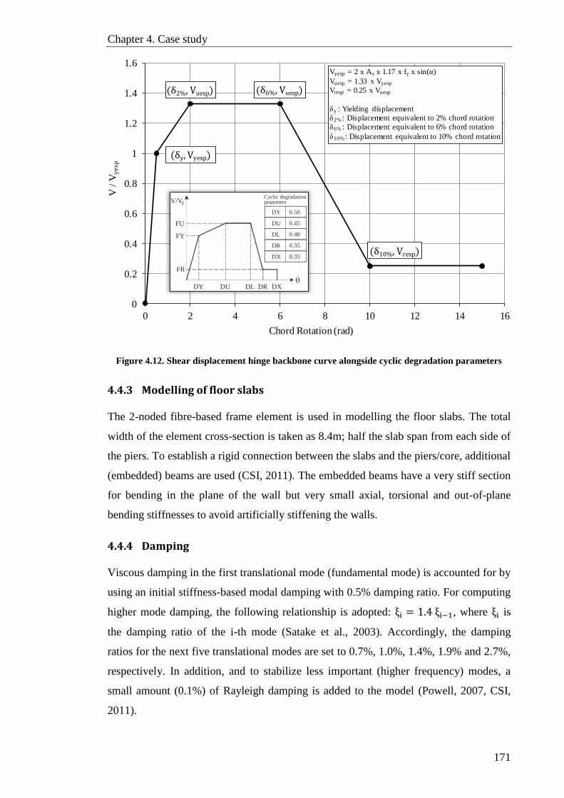
Chapter 4. Case study
171
Figure 4.12. Shear displacement hinge backbone curve alongside cyclic degradation parameters
4.4.3 Modelling of floor slabs
The 2-noded fibre-based frame element is used in modelling the floor slabs. The total
width of the element cross-section is taken as 8.4m; half the slab span from each side of
the piers. To establish a rigid connection between the slabs and the piers/core, additional
(embedded) beams are used (CSI, 2011). The embedded beams have a very stiff section
for bending in the plane of the wall but very small axial, torsional and out-of-plane
bending stiffnesses to avoid artificially stiffening the walls.
4.4.4 Damping
Viscous damping in the first translational mode (fundamental mode) is accounted for by
using an initial stiffness-based modal damping with 0.5% damping ratio. For computing
higher mode damping, the following relationship is adopted: ξi = 1.4 ξi−1, where ξi is
the damping ratio of the i-th mode (Satake et al., 2003). Accordingly, the damping
ratios for the next five translational modes are set to 0.7%, 1.0%, 1.4%, 1.9% and 2.7%,
respectively. In addition, and to stabilize less important (higher frequency) modes, a
small amount (0.1%) of Rayleigh damping is added to the model (Powell, 2007, CSI,
2011).
0
0.2
0.4
0.6
0.8
1
1.2
1.4
1.6
0 2 4 6 8 10 12 14 16
V /
Vy
exp
Chord Rotation (rad)
(δy, Vyexp)
(δ2%, Vuexp) (δ6%, Vuexp)
(δ10%, Vrexp)
Vyexp = 2 x As x 1.17 x fy x sin(α)
Vuexp = 1.33 x Vyexp
Vrexp = 0.25 x Vuexp
δy : Yielding displacement
δ2% : Displacement equivalent to 2% chord rotation
δ6% : Displacement equivalent to 6% chord rotation
δ10% : Displacement equivalent to 10% chord rotation
DY
DU
DL
DR
DX
0.50
0.45
0.40
0.35
0.35
V/V
FU
FY
FR
DY DU DL DR DX
Cyclic degradation prametersy

Chapter 4. Case study
172
4.5 Concluding remarks
This chapter provided all the input data for the analysis of a case study high-rise RC
building in Dubai (UAE), a region that is vulnerable to different earthquake scenarios.
The results of the analysis will be used in the subsequent chapters to
develop/demonstrate the framework for the seismic vulnerability assessment of RC
high-rise wall buildings.

173
CHAPTER 5. Seismic scenario-structure-
based limit state criteria for
RC high-rise wall buildings
using net inter-storey drift
As a result of population growth and consequent urbanisation, the number of high-rise
buildings is rapidly growing worldwide resulting in increased exposure to multiple-
scenario earthquakes and associated risk. The wide range in frequency contents of
possible strong ground motions can have an impact on the seismic response,
vulnerability and limit state criteria definitions of such structures. In this chapter, new,
reliable SSSB definitions of limit state criteria for RC high-rise wall buildings are
proposed. The 30-storey reference building is utilised to illustrate the methodology for
defining the limit state criteria. The building is designed following modern seismic code
provisions and then modelled with PERFORM-3D using the nonlinear fibre-based
approach as discussed in CHAPTER 3. Uncertainty in ground motions is accounted for
by the selection of forty real earthquake records representing the two seismic scenarios
Chapter 5. Seismic scenario-structure-based limit state criteria using NISD
174
in which the study region is vulnerable to (CHAPTER 4). Seismic scenario-based
building local response at increasing earthquake intensities is mapped using MRIDAs
with an improved scalar IM. NISD is selected as a global DM based on the outcome of
the mapping process and a parametric study involving seven buildings ranging from 20-
50 storeys. This DM is used to link local damage events, including shear, in the
reference building to global response under different seismic scenarios. While the study
concludes by proposing SSSB limit state criteria for the reference building, the
proposed limit state criteria are applicable to comparable RC high-rise wall buildings
and seismic regions.
5.1 Introduction
With changing socioeconomic conditions, rapid population growth and urbanisation,
many cities all over the world have expanded rapidly in recent years. This expansion
has led to a massive increase in high-rise buildings and to the spread of cities to
multiple-scenario earthquake-prone regions. This increases exposure to seismic risk. A
risk which to quantify and mitigate, a better understanding of the hazard and
vulnerability is required.
The majority of high-rise buildings in most countries employ RC piers and core walls as
the primary lateral force-resisting system due to their effectiveness in providing the
strength, stiffness and deformation capacity needed to meet the seismic demand. The
trend to increasingly use RC in high-rise buildings is expected to continue due to the
development of commercial high-strength concrete and new advances in construction
technologies (Ali and Moon, 2007). Quantitative definitions of limit state criteria form
the spine to seismic vulnerability assessment and consequently to the seismic risk
analysis and mitigation for RC high-rise wall buildings. These definitions require
mathematical representations of local DIs, such as deformations, forces or energy,
corresponding to designated structural response levels. Therefore, a suitable DM needs
to be adopted to sufficiently correlate local damages (events) in the building to its
global response.
The broad range of frequency content in real strong ground motions, representative of
different seismic scenarios such as distant and near-field earthquakes, can impose
different levels of excitation on both fundamental and higher modes in RC high-rise
wall structures. This can result in more complex, seismic scenario-based inelastic
Chapter 5. Seismic scenario-structure-based limit state criteria using NISD
175
response. Another special issue in RC high-rise wall buildings is the definition of limit
state criteria corresponding to predefined performance levels since there are several
factors affecting the failure modes. Among these factors are building height, axial force
levels, supplementary regulations introduced by local authorities, and local trends in
design and construction. For buildings with fundamental mode-dominated response, the
taller the building, the larger is the expected TISD at specified performance levels. For
high-rise wall buildings, especially at lower storeys, axial compressive force levels are
influenced by the arrangement of the RC shear walls and cores in the building. This
arrangement is usually dominated by gravity loads, particularly for internal shear walls.
High compressive loads are expected to delay the onset of initial cracking and yielding
in vertical elements but can decrease ductility and hence the TISD at which concrete
core crushing and rebar buckling occur. Finally, the supplementary regulations of local
authorities, as well as the trends adopted by both consultants and contractors, may
impact the design and hence the seismic performance. For instance, the minimum steel
ratio in vertical elements may exceed the value that is stated in code provisions.
Adopting the methodology presented in CHAPTER 2, new, reliable SSSB definitions of
performance limit state criteria for RC high-rise wall buildings are proposed in this
chapter. Following a brief introduction, this chapter presents in detail: (i) a discussion
on the main parameters of the conducted MRIDAs including a proposition for an
improved scalar IM; (ii) the mapping of seismic scenario-based building local response;
(iii) relating local response to the ground motion characteristics; (iv) the selection of a
suitable DM to correlate local to global response; (v) the proposal for new SSSB
performance limit state criteria for the reference building and RC high-rise wall
buildings in similar seismic regions. This chapter ends with a summary of the work and
concluding remarks. Figure 5.1 summarises pictorially the flowchart for obtaining the
SSSB limit state criteria proposed in the current work.

Chapter 5. Seismic scenario-structure-based limit state criteria using NISD
176
Figure 5.1. Flowchart for obtaining the proposed SSSB limit state criteria for RC high-rise wall
buildings
5.2 Multi-record incremental dynamic analysis
For the purpose of defining SSSB performance limit state criteria for the reference
building, MRIDAs are performed using the two sets of records assembled in CHAPTER
4. To construct IDA curves that can sufficiently and efficiently represent the variable
states of the response of the structure to different earthquake records with increasing
intensities, a suitable ground motion intensity measure needs to be defined. PGA was
used to be the most accepted intensity measure. The elastic spectral acceleration at the
fundamental period of the structure, Sa(T1), or Sa in short, has been found to be more
efficient since it is structure-dependent and become a frequently used intensity measure
for low- to mid-rise buildings. However, Sa is neither suited for tall buildings (Shome,
Alternate path.
START
SELECTION OF REFERENCE
STRUCTURES REPRESENTATIVE
OF BUILDING INVENTORY
Designing reference
structures following codes
and construction practice
adopted in the study region
Collecting of existing
structural drawings &
design data (if available)
(Chapter 4)
Verified nonlinear 3D modelling includingflexure-axial-shear interaction effects
(Chapters 3, 4)
Adopting suitable Intensity Measure (IM) to be used with
Multi-Record Incremental Dynamic Analyses (MRIDAs)
(Chapter 5)
(MRIDAs)
ENSEMBLE OF SCENARIO-
BASED REAL INPUT
GROUND MOTIONS
Record selection criteria:
• Magnitude (M)
• Distance to source (R)
• Site soil condition (S)
• Acceleration to velocity ratio (a/v)
END
(Chapter 4)
Mapping of seismic scenario-based building
local response
Correlating local to global response through
suitable Damage Measure (DM)
Definition of seismic scenario-structure based (SSSB) limit
state criteria to be used in seismic vulnerability & risk
assessment
(Chapter 5)
(Chapter 5)(Chapter 5)
(Chapter 5)

Chapter 5. Seismic scenario-structure-based limit state criteria using NISD
177
1999, Vamvatsikos and Cornell, 2002) nor for structures subjected to near-source
earthquakes (Luco and Cornell, 2007). Other intensity measures have been proposed in
the literature in an attempt to overcome the major shortcomings of Sa, namely
discounting the contribution of the higher modes and fundamental period lengthening
associated with stiffness degradation in the structure (Shome, 1999, Carballo and
Cornel, 2000, Cordova et al., 2000). New approaches have led to other kinds of
intensity measures such as inelastic spectral value-based scalar intensity measures (e.g.
Luco and Cornell, 2007) and vector-valued intensity measures (Bazzurro and Cornell,
2002, Conte et al., 2003, Baker and Cornell, 2005). These approaches, though
promising, are not easy to apply since they require probabilistic seismic hazard
assessment based on custom-made attenuation laws to obtain the joint hazard curve.
In a comprehensive study by Kappos and Kyriakakis (2000), the problem of reducing
scatter in the seismic response calculated using NRHA with natural records was
reevaluated. In this study, a total of seven IMs were investigated, namely: PGA, PGV,
Arias Intensity, (Root-Mean Square) Acceleration “RMS Acceleration”, Spectrum
Intensity (i.e. area under the pseudo-velocity spectrum), Root-Mean Square
Acceleration “RMSA”, and the Fajfar et al. (1990) PGV-duration combined IM “Iv”.
Two sets of ground motions were used, representing two different seismotectonic
environments (Greece and California). The study comprised two parts, the first focused
on the scaling effect on both strength and displacement spectra, while the second part
addressed the problem in the context of response variability in MDOF systems with a
focus on multistorey frames. The first part of the study concluded that in the
intermediate and long period ranges, any of the three velocity-related IMs (PGV, SI, and
Iv) can be adopted to good effect. In case of systems with ductility factor >1, it is
concluded that the use of SI scaling along with entire period range leads to a reasonably
low scattering in both strength and displacement spectra, with the coefficient of
variation (COV) hardly exceeding 0.5 within any zone of practical interest. In the
second part of the study, an alternative scaling method (narrow-band spectrum
intensities calculated on the basis of elastic and inelastic pseudo-velocity spectra) was
proposed. The study revealed that, from the practical point of view, both proposals
based on the narrow-band SI concept lead to COV values between 0.1 and 0.4 in the
calculated drifts and member ductilities.
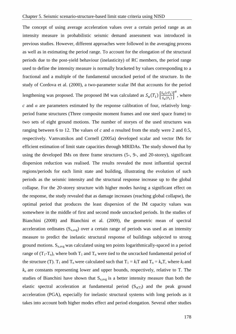
Chapter 5. Seismic scenario-structure-based limit state criteria using NISD
178
The concept of using average acceleration values over a certain period range as an
intensity measure in probabilistic seismic demand assessment was introduced in
previous studies. However, different approaches were followed in the averaging process
as well as in estimating the period range. To account for the elongation of the structural
periods due to the post-yield behaviour (inelasticity) of RC members, the period range
used to define the intensity measure is normally bracketed by values corresponding to a
fractional and a multiple of the fundamental uncracked period of the structure. In the
study of Cordova et al. (2000), a two-parameter scalar IM that accounts for the period
lengthening was proposed. The proposed IM was calculated as 𝑆𝑎(𝑇1) [𝑆𝑎(𝑐𝑇1)
𝑆𝑎(𝑇1)]𝛼
, where
c and α are parameters estimated by the response calibration of four, relatively long-
period frame structures (Three composite moment frames and one steel space frame) to
two sets of eight ground motions. The number of storyes of the used structures was
ranging between 6 to 12. The values of c and α resulted from the study were 2 and 0.5,
respectively. Vamvatsikos and Cornell (2005a) developed scalar and vector IMs for
efficient estimation of limit state capacities through MRIDAs. The study showed that by
using the developed IMs on three frame structures (5-, 9-, and 20-storey), significant
dispersion reduction was realised. The results revealed the most influential spectral
regions/periods for each limit state and building, illustrating the evolution of such
periods as the seismic intensity and the structural response increase up to the global
collapse. For the 20-storey structure with higher modes having a significant effect on
the response, the study revealed that as damage increases (reaching global collapse), the
optimal period that produces the least dispersion of the IM capacity values was
somewhere in the middle of first and second mode uncracked periods. In the studies of
Bianchini (2008) and Bianchini et al. (2009), the geometric mean of spectral
acceleration ordinates (Sa,avg) over a certain range of periods was used as an intensity
measure to predict the inelastic structural response of buildings subjected to strong
ground motions. Sa,avg was calculated using ten points logarithmically-spaced in a period
range of (T1-Tn), where both T1 and Tn were tied to the uncracked fundamental period of
the structure (T). T1 and Tn were calculated such that T1 = klT and Tn = kuT, where kl and
ku are constants representing lower and upper bounds, respectively, relative to T. The
studies of Bianchini have shown that Sa,avg is a better intensity measure than both the
elastic spectral acceleration at fundamental period (Sa(T)) and the peak ground
acceleration (PGA), especially for inelastic structural systems with long periods as it
takes into account both higher modes effect and period elongation. Several other studies
Chapter 5. Seismic scenario-structure-based limit state criteria using NISD
179
related to spectral acceleration-based IMs are available in the literature (e.g. Kurama
and Farrow, 2003, Baker and Cornell, 2004, Mehanny, 2009, Bojórquez and Iervolino,
2011).
In the present study, an improved scalar intensity measure termed spectral acceleration
at weighted-average period Sa(wa), is proposed. Using the 10% POE in 50-years UHS for
the study region, the weighted-average period (Twa) is the period linked to the spectral
acceleration value that represents the average of the spectral acceleration ordinates
pinned to the equivalent inelastic period of the first three modes of vibration weighted
by their corresponding mass participation ratios (MPR). The procedure of calculating
the Sa(wa) of the reference building is illustrated in Figure 5.4a. Sa(wa) is calculated using
Eqn. ( 5.1) below:
Sa(wa) =∑(Sai ∗ MPRi)
∑MPRi ( 5.1)
Where i is the mode of vibration number (i = 1 to 3), Sai is the spectral acceleration
ordinate corresponded to the equivalent inelastic period of the ith
mode of vibration, and
MPRi is the mass participation ratio corresponding to the ith
mode of vibration. The
proposed intensity measure follows the average spectral acceleration concept discussed
above, yet with a different technique in bracketing the period interval and defining the
points within the chosen range of periods. The 1st mode equivalent inelastic period
(around 1.40 of the uncracked fundamental period), calculated using the reduced
stiffnesses given in Table 4.7, is employed as a bracket to account for the elongation
due to the post-yield behaviour (stiffness degradation) of the reference building.
To illustrate the suitability of the 1st mode equivalent inelastic period to account for the
period elongation of the structure at the post-yield zone, two examples are given
hereunder. The first example (Figure 5.2) shows the 1st mode period propagation of the
shake table-tested seven-storey full-scale RC wall structure utilised in the MLNMVS
in CHAPTER 3, while the second (Figure 5.3) illustrates the 1st mode period
propagation of the 30-stoery reference building. It is worth noting that the detailed
mapping of the 30-stoery reference structure is presented in Section 5.3 hereafter. In
Figure 5.2, the uncracked fundamental period of the test structure was measured as
0.51s (Table 3.1) and estimated as 0.50s from the PERFORM-3D model (Figure 3.26).
The equivalent inelastic 1st mode period of the test structure is calculated as 0.84s using

Chapter 5. Seismic scenario-structure-based limit state criteria using NISD
180
the reduced stiffnesses presented in Table 4.7, while the 1st mode cracked period at
yield, considered to be corresponding to the seismic intensity where the first yield at the
tested web wall occurred, is calculated as 0.67s using the Fourier Transformation
Analysis (FTA). To arrive at this seismic intensity, EQ3 shake table input motion is
down-scaled by a scale factor of 0.65. In the second example (30-storey reference
building), the uncracked fundamental period (Period #1 in Figure 5.3) is calculated as
3.21s (Table 4.9). Using FTA, the cracked period at first yield in core walls (Period #2
in Figure 5.3) and the period corresponding to the CP-related 1st steel buckling in core
walls (Period #4 in Figure 5.3) are calculated as 4.13s and 4.87s, respectively. The
equivalent inelastic period (Period #3 in Figure 5.3) is calculated as 4.46s (Table 4.9)
using the reduced stiffnesses in Table 4.7. In both examples, the calculated equivalent
inelastic period falls between the cracked period at yield and the CP-related period.
The structural characteristics of the building are not only represented by the equivalent
inelastic fundamental period but also with the equivalent inelastic periods of higher
modes (2nd
and 3rd
). Furthermore, the dynamic characteristics of the building are
accounted for by weighting the spectral acceleration values that are corresponding to the
first three modes’ equivalent inelastic periods to their respective mass participation
factors. It is noteworthy that the weighted-average period (Twa) estimated in the current
work is in-line with what was proposed in previous studies for long-period structures
(e.g. Vamvatsikos and Cornell, 2005a).
Figure 5.2. Seven-storey test structure: 1st mode period propagation
Before EQ1
After EQ1
After EQ2
After EQ3
After EQ4
2.13
3.27
1
Before EQ1 After EQ1 After EQ2 After EQ3 After EQ4
0.0
0.2
0.4
0.6
0.8
1.0
1.2
Peri
od, T
(s)
1st mode periods measured from the shake table test
Uncracked fundamental period
Cracked period at yield: At 1st yield in wall (Fourier Transformation)
Equivalent inelastic period
0.67 s
0.84 s
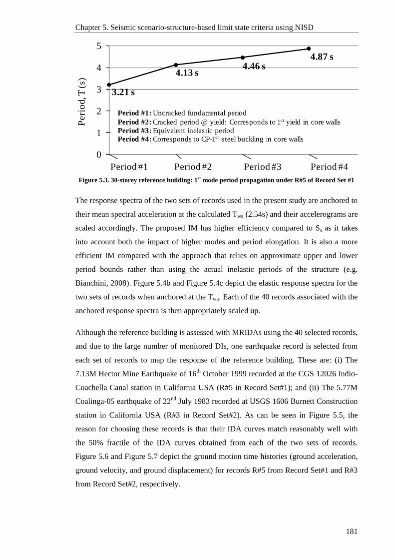
Chapter 5. Seismic scenario-structure-based limit state criteria using NISD
181
Figure 5.3. 30-storey reference building: 1st mode period propagation under R#5 of Record Set #1
The response spectra of the two sets of records used in the present study are anchored to
their mean spectral acceleration at the calculated Twa (2.54s) and their accelerograms are
scaled accordingly. The proposed IM has higher efficiency compared to Sa as it takes
into account both the impact of higher modes and period elongation. It is also a more
efficient IM compared with the approach that relies on approximate upper and lower
period bounds rather than using the actual inelastic periods of the structure (e.g.
Bianchini, 2008). Figure 5.4b and Figure 5.4c depict the elastic response spectra for the
two sets of records when anchored at the Twa. Each of the 40 records associated with the
anchored response spectra is then appropriately scaled up.
Although the reference building is assessed with MRIDAs using the 40 selected records,
and due to the large number of monitored DIs, one earthquake record is selected from
each set of records to map the response of the reference building. These are: (i) The
7.13M Hector Mine Earthquake of 16th
October 1999 recorded at the CGS 12026 Indio-
Coachella Canal station in California USA (R#5 in Record Set#1); and (ii) The 5.77M
Coalinga-05 earthquake of 22nd
July 1983 recorded at USGS 1606 Burnett Construction
station in California USA (R#3 in Record Set#2). As can be seen in Figure 5.5, the
reason for choosing these records is that their IDA curves match reasonably well with
the 50% fractile of the IDA curves obtained from each of the two sets of records.
Figure 5.6 and Figure 5.7 depict the ground motion time histories (ground acceleration,
ground velocity, and ground displacement) for records R#5 from Record Set#1 and R#3
from Record Set#2, respectively.
1st mode
Uncracked fundamental period
Period at 1st yield in core walls
Equivalent inelastic period
Period #1 Period #2 Period #3 Period #4
0
1
2
3
4
5
Peri
od, T
(s)
4.13 s4.46 s
3.21 s
4.87 s
Period #1: Uncracked fundamental period
Period #2: Cracked period @ yield: Corresponds to 1st yield in core walls
Period #3: Equivalent inelastic period
Period #4: Corresponds to CP-1st steel buckling in core walls

Chapter 5. Seismic scenario-structure-based limit state criteria using NISD
182
Figure 5.4. Proposed improved scalar IM: (a) calculation of weighted-average period (Twa); (b)
response spectra for Record Set#1 anchored to the proposed IM; and (c) response spectra for
Record Set#2 anchored to the proposed IM
0
0.3
0.6
0.9
1.2
0 1 2 3 4 5
Spectr
al A
ccele
rati
on (
g)
Period, T (s)
Response spectra of Set #1 recordsMean
Tw
a=
2.5
4 s
Sa
(wa
)=
0.1
05
g
0
0.3
0.6
0.9
1.2
1.5
1.8
0 1 2 3 4 5
Spectr
al A
ccele
rati
on (
g)
Period, T (s)
Response spectra of Set #2 recordsMean
Tw
a=
2.5
4 s
Sa
(wa
)=
0.0
11
g0
0.1
0.2
0.3
0.4
0.5
0.6
0.7
0.8
0 1 2 3 4 5
Spectr
al A
ccele
rati
on (
g)
Period, T (s)
3rd Mode:
Period (T3) = 0.39sSpectral acceleration (Sa3) = 0.64gMass participation ratio (MPR3) = 6.5%
2nd Mode:
T2 = 0.96sSa2 = 0.39gMPR2 = 17.9%
1st Mode:T1 = 4.46sSa1 = 0.06gMPR1 = 65.8%
10% POE in 50 Y (UHS) for study region
Sa(wa) = 0.17g
Twa = 2.54s
a
b
c
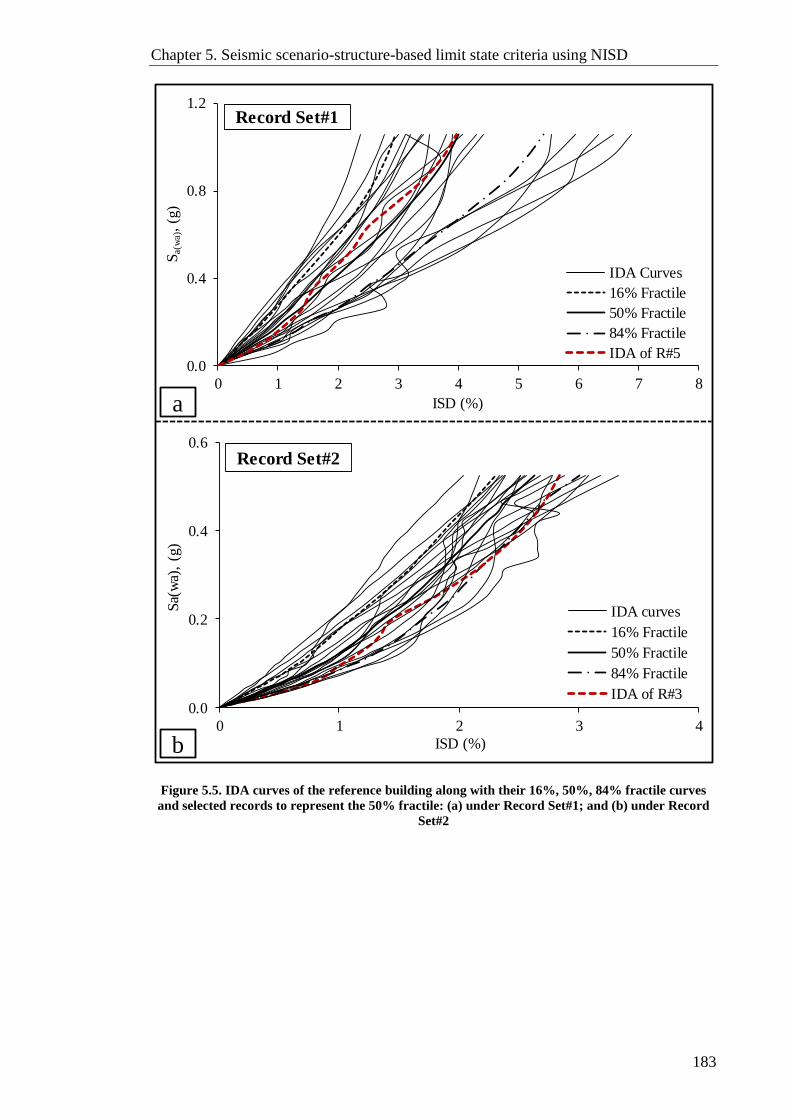
Chapter 5. Seismic scenario-structure-based limit state criteria using NISD
183
Figure 5.5. IDA curves of the reference building along with their 16%, 50%, 84% fractile curves
and selected records to represent the 50% fractile: (a) under Record Set#1; and (b) under Record
Set#2
0.0
0.2
0.4
0.6
0 1 2 3 4
Sa(
wa)
, (g
)
ISD (%)
IDA curves
16% Fractile
50% Fractile
84% Fractile
IDA of R#3
Record Set#2
0.0
0.4
0.8
1.2
0 1 2 3 4 5 6 7 8
Sa(w
a), (
g)
ISD (%)
IDA Curves
16% Fractile
50% Fractile
84% Fractile
IDA of R#5
Record Set#1
a
b
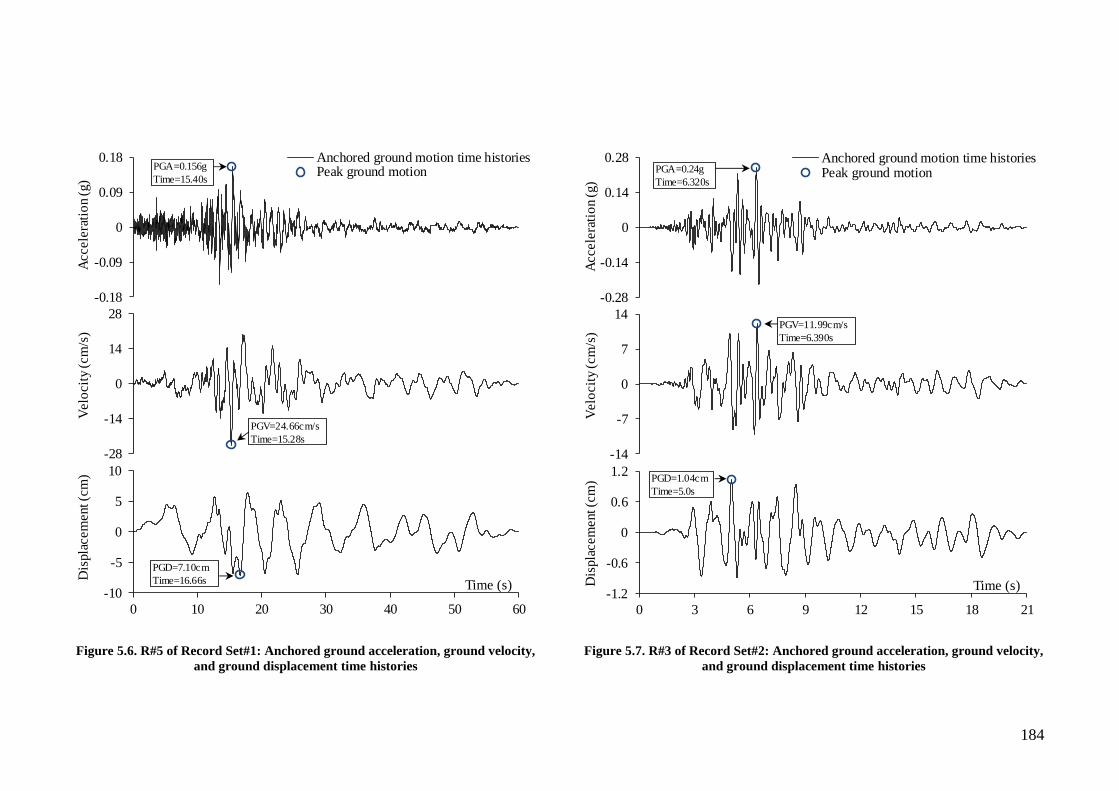
184
Figure 5.6. R#5 of Record Set#1: Anchored ground acceleration, ground velocity,
and ground displacement time histories
Figure 5.7. R#3 of Record Set#2: Anchored ground acceleration, ground velocity,
and ground displacement time histories
Event
LS-WR
Time
Time
Time
-0.18
-0.09
0
0.09
0.18
Accele
rati
on (
g)
Anchored ground motion time historiesPeak ground motion
-28
-14
0
14
28
Velo
cit
y (
cm
/s)
-10
-5
0
5
10
0 10 20 30 40 50 60
Dis
pla
cem
ent (c
m)
Time (s)
PGA=0.156g
Time=15.40s
PGV=24.66cm/s
Time=15.28s
PGD=7.10cm
Time=16.66s
-0.28
-0.14
0
0.14
0.28
Accele
rati
on (
g)
Anchored ground motion time historiesPeak ground motion
-14
-7
0
7
14
Velo
cit
y (
cm
/s)
-1.2
-0.6
0
0.6
1.2
0 3 6 9 12 15 18 21
Dis
pla
cem
ent (c
m)
Time (s)
PGA=0.24g
Time=6.320s
PGV=11.99cm/s
Time=6.390s
PGD=1.04cm
Time=5.0s
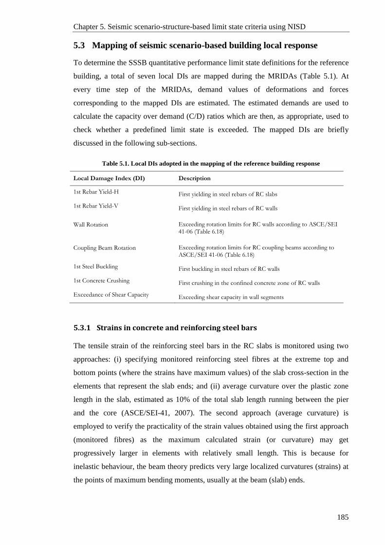
Chapter 5. Seismic scenario-structure-based limit state criteria using NISD
185
5.3 Mapping of seismic scenario-based building local response
To determine the SSSB quantitative performance limit state definitions for the reference
building, a total of seven local DIs are mapped during the MRIDAs (Table 5.1). At
every time step of the MRIDAs, demand values of deformations and forces
corresponding to the mapped DIs are estimated. The estimated demands are used to
calculate the capacity over demand (C/D) ratios which are then, as appropriate, used to
check whether a predefined limit state is exceeded. The mapped DIs are briefly
discussed in the following sub-sections.
Table 5.1. Local DIs adopted in the mapping of the reference building response
Local Damage Index (DI) Description
1st Rebar Yield-H First yielding in steel rebars of RC slabs
1st Rebar Yield-V First yielding in steel rebars of RC walls
Wall Rotation Exceeding rotation limits for RC walls according to ASCE/SEI 41-06 (Table 6.18)
Coupling Beam Rotation Exceeding rotation limits for RC coupling beams according to ASCE/SEI 41-06 (Table 6.18)
1st Steel Buckling First buckling in steel rebars of RC walls
1st Concrete Crushing First crushing in the confined concrete zone of RC walls
Exceedance of Shear Capacity Exceeding shear capacity in wall segments
5.3.1 Strains in concrete and reinforcing steel bars
The tensile strain of the reinforcing steel bars in the RC slabs is monitored using two
approaches: (i) specifying monitored reinforcing steel fibres at the extreme top and
bottom points (where the strains have maximum values) of the slab cross-section in the
elements that represent the slab ends; and (ii) average curvature over the plastic zone
length in the slab, estimated as 10% of the total slab length running between the pier
and the core (ASCE/SEI-41, 2007). The second approach (average curvature) is
employed to verify the practicality of the strain values obtained using the first approach
(monitored fibres) as the maximum calculated strain (or curvature) may get
progressively larger in elements with relatively small length. This is because for
inelastic behaviour, the beam theory predicts very large localized curvatures (strains) at
the points of maximum bending moments, usually at the beam (slab) ends.
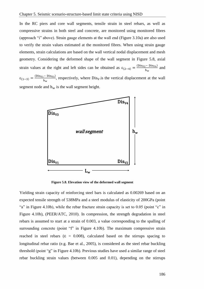
Chapter 5. Seismic scenario-structure-based limit state criteria using NISD
186
In the RC piers and core wall segments, tensile strain in steel rebars, as well as
compressive strains in both steel and concrete, are monitored using monitored fibres
(approach “i” above). Strain gauge elements at the wall end (Figure 3.10a) are also used
to verify the strain values estimated at the monitored fibres. When using strain gauge
elements, strain calculations are based on the wall vertical nodal displacement and mesh
geometry. Considering the deformed shape of the wall segment in Figure 5.8, axial
strain values at the right and left sides can be obtained as ε(2−4) =(DisV2− DisV4)
hw and
ε(1−3) =(DisV1− DisV3)
hw, respectively, where DisV.is the vertical displacement at the wall
segment node and hw is the wall segment height.
Figure 5.8. Elevation view of the deformed wall segment
Yielding strain capacity of reinforcing steel bars is calculated as 0.00269 based on an
expected tensile strength of 538MPa and a steel modulus of elasticity of 200GPa (point
“a” in Figure 4.10b), while the rebar fracture strain capacity is set to 0.05 (point “c” in
Figure 4.10b), (PEER/ATC, 2010). In compression, the strength degradation in steel
rebars is assumed to start at a strain of 0.003, a value corresponding to the spalling of
surrounding concrete (point “f” in Figure 4.10b). The maximum compressive strain
reached in steel rebars (ε = 0.008), calculated based on the stirrups spacing to
longitudinal rebar ratio (e.g. Bae et al., 2005), is considered as the steel rebar buckling
threshold (point “g” in Figure 4.10b). Previous studies have used a similar range of steel
rebar buckling strain values (between 0.005 and 0.01), depending on the stirrups
DisV2
DisV3
DisV1
DisV4
hw
Lw
wall segment
Chapter 5. Seismic scenario-structure-based limit state criteria using NISD
187
spacing to longitudinal rebar ratio (e.g. Ghodsi and Ruiz, 2010, Tuna, 2012). Finally,
the crushing strain of confined concrete is taken as the strain value at 60% of the peak
confined concrete strength on the descending branch of the Mander stress-strain curve
(point “d” in Figure 4.10a).
5.3.2 Rotation in coupling beams and wall segments
Rotation in coupling beams is estimated using the 2-noded rotation gauge element. The
rotation demand is calculated as the rotation at End J of the beam element minus the
rotation at End I (Figure 3.10b). Like the beam element, the 2-noded rotation gauge has
local axes 1, 2 and 3, where the calculated rotation is about axis-3. A positive rotation
corresponds to a positive moment about axis-3 in the coupling beam element. In the
wall segments, the rotation is calculated using the 4-noded rotation gauge element
shown in Figure 3.11. The gauge rotation is the rotation of the side KL minus the
rotation of the side IJ, where side rotation is positive clockwise. Hence, positive gauge
rotation corresponds to tension on the side IK and compression on the side JL. It is
worth noting that all deformation (strain and rotation) gauge elements in PERFORM-3D
do not add any stiffness or strength to the structure.
For each predefined performance limit state, the rotation capacity of the coupling beams
and wall segments in the reference structure is set following table 6-18 of ASCE/SEI
41-06 (2007). In the wall segments, Table 6-18 of ASCE/SEI 41-06 relates the rotation
capacity to the shear and axial force demands in the wall. Since the wall rotation gauge
in the adopted version of PERFORM-3D has constant rotation capacities that are
unrelated to the axial and shear demands, a post-processor was created for this study to
monitor the axial and shear demand levels in each wall segment at every time step of the
MRIDAs, where the rotation capacity is adjusted accordingly.
5.3.3 Shear capacity in wall segments
Using the “structural section” feature in PERFORM-3D, the shear capacity in piers and
core wall segments of the reference building is assessed throughout the MRIDAs taking
into account the shear strength degradation depending on the level of nonlinear flexural
deformation (Wallace, 2010, Tuna, 2012). Pairs of normalised shear demand and
curvature ductility in wall segments are pinned at each time step and checked against a
trilinear trend line and a flat line as predefined envelopes. The trilinear trend line shown
in Figure 5.9, representing the median shear strength of structural walls from a previous
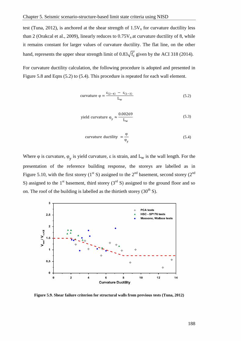
Chapter 5. Seismic scenario-structure-based limit state criteria using NISD
188
test (Tuna, 2012), is anchored at the shear strength of 1.5Vn for curvature ductility less
than 2 (Orakcal et al., 2009), linearly reduces to 0.75Vn at curvature ductility of 8, while
it remains constant for larger values of curvature ductility. The flat line, on the other
hand, represents the upper shear strength limit of 0.83√fc′ given by the ACI 318 (2014).
For curvature ductility calculation, the following procedure is adopted and presented in
Figure 5.8 and Eqns ( 5.2) to ( 5.4). This procedure is repeated for each wall element.
curvature φ =ε(2−4) − ε(1−3)
Lw ( 5.2)
yield curvature φy≈0.00269
Lw ( 5.3)
curvature ductility =φ
φy
( 5.4)
Where φ is curvature, φy is yield curvature, ε is strain, and Lw is the wall length. For the
presentation of the reference building response, the storeys are labelled as in
Figure 5.10, with the first storey (1st S) assigned to the 2
nd basement, second storey (2
nd
S) assigned to the 1st basement, third storey (3
rd S) assigned to the ground floor and so
on. The roof of the building is labelled as the thirtieth storey (30th
S).
Figure 5.9. Shear failure criterion for structural walls from previous tests (Tuna, 2012)
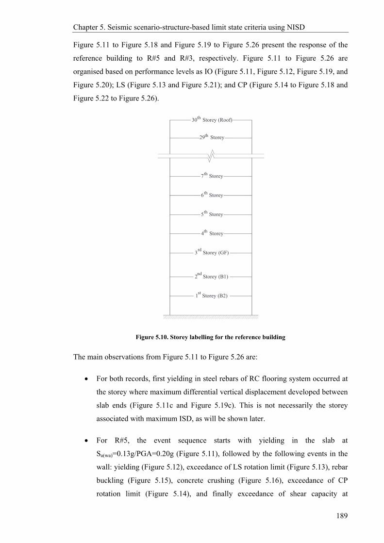
Chapter 5. Seismic scenario-structure-based limit state criteria using NISD
189
Figure 5.11 to Figure 5.18 and Figure 5.19 to Figure 5.26 present the response of the
reference building to R#5 and R#3, respectively. Figure 5.11 to Figure 5.26 are
organised based on performance levels as IO (Figure 5.11, Figure 5.12, Figure 5.19, and
Figure 5.20); LS (Figure 5.13 and Figure 5.21); and CP (Figure 5.14 to Figure 5.18 and
Figure 5.22 to Figure 5.26).
Figure 5.10. Storey labelling for the reference building
The main observations from Figure 5.11 to Figure 5.26 are:
For both records, first yielding in steel rebars of RC flooring system occurred at
the storey where maximum differential vertical displacement developed between
slab ends (Figure 5.11c and Figure 5.19c). This is not necessarily the storey
associated with maximum ISD, as will be shown later.
For R#5, the event sequence starts with yielding in the slab at
Sa(wa)=0.13g/PGA=0.20g (Figure 5.11), followed by the following events in the
wall: yielding (Figure 5.12), exceedance of LS rotation limit (Figure 5.13), rebar
buckling (Figure 5.15), concrete crushing (Figure 5.16), exceedance of CP
rotation limit (Figure 5.14), and finally exceedance of shear capacity at
1 Storey (B2) st
4 Storey th
2 Storey (B1) nd
3 Storey (GF) rd
5 Storey th
6 Storey th
7 Storey th
29 Storey th
30 Storey (Roof) th

Chapter 5. Seismic scenario-structure-based limit state criteria using NISD
190
Sa(wa)=0.84g/PGA=1.25g (Figure 5.17). All events occurred within the lower
five storeys of the building except for the slab yielding which occurred at the
24th
storey. As above, the event sequence for R#3 starts with yielding in the slab
at Sa(wa)=0.06g/PGA=1.43g (Figure 5.19) followed by yielding in the wall
(Figure 5.20). However, the sequence of the other events in the wall
conspicuously differs with exceedance of shear capacity next (Figure 5.25),
followed by rebar buckling (Figure 5.23), exceedance of LS rotation limit
(Figure 5.21), concrete crushing (Figure 5.24), and ends with exceedance of CP
rotation limit at Sa(wa)=0.34g/PGA=7.64g (Figure 5.22). In R#3, the yielding
events in slab and wall occurred at higher storeys; 28th
storey and 21st storey,
respectively, while all other events occurred within the lower five storeys of the
building.
For R#5, the shape of the relative lateral displacement plot at the onset of the
sequence of events indicates a first mode-dominated response (Figure 5.11c to
Figure 5.16c). However, the second mode appears responsible for the
exceedance of the wall shear capacity event (Figure 5.17c). On the contrary, for
R#3, the shape of the relative lateral displacement plots indicate that the building
response is controlled by the second mode (Figure 5.19c and Figure 5.21c to
Figure 5.24c) except for wall yielding and shear capacity exceedance where the
response is dominated by the third mode (Figure 5.20c and Figure 5.25c). This is
further discussed in Section 5.5.
By post-processing the time history results, it is observed that the potential
failure in wall segments when shear capacity is exceeded under the two records
differs in nature. The time history of normalised shear demand and curvature
ductility curves for the concerned wall segment at the 1st storey and the storey
where the shear capacity is exceeded under R#5 and R#3 are plotted in
Figure 5.18 and Figure 5.26, respectively. Under both records, the maximum
shear demand has occurred at very low curvature ductility; 0.61/0.41 in 1st
storey/2nd
storey under R#5, and 0.059/0.055 in 1st storey/3
rd storey under R#3.
Notwithstanding, the walls in the 1st and 2
nd storeys under R#5 developed a
considerable amount of curvature ductility (4.64 and 1.80, respectively) prior to
the exceedance of shear capacity, while under R#3, the maximum curvature
ductility in the walls at the 1st and 3
rd storeys was less than 1.0 (0.44 and 0.25,
Chapter 5. Seismic scenario-structure-based limit state criteria using NISD
191
respectively). This indicates that under R#5, shear failure is preceded by flexural
yielding in walls, giving the chance to flexure-related damages (strains and or
rotations) to occur first. While under R#3, wall segments in the concerned
storeys remain elastic (curvature ductility < 1) over the entire time history of the
record at the seismic intensity level corresponding to shear failure. This
observation is further analysed in Section 5.5.
For both seismic scenarios, at the onset of each of the damage events in the
walls, seismic demands (strain/rotation/shear) reduce with building height,
diminishing at the top five storeys (Figure 5.12(a, b) to Figure 5.17(a, b) and
Figure 5.19(a, b) to Figure 5.25(a, b)). This trend is inconsistent with the fact
that these top storeys are showing maximum overall TISDs during the damage
sequence. This is examined further in the next section.
As one of the considered DIs in the current study, the overall nonlinear rotation of the
coupling beams is monitored throughout the entire range of the adopted seismic
intensity levels under both R#5 and R#3. Figure 5.27a shows that under R#5, the beam
rotation exceeded the ASCE/SEI 41-06 limit for IO limit state (0.006 rad) at higher
seismic intensity level (PGA=0.55, Sa(wa)=0.37g) compared to the ones corresponding to
other IO DIs such as first yield in slabs (PGA=0.20g, Sa(wa)=0.13g) and first yield in
walls (PGA=0.31g, Sa(wa)=0.21g). Under this record, the ASCE/SEI 41-06 rotation
limits for LS and CP limit state (0.018rad and 0.03rad, respectively) were not reached
even at the highest considered seismic intensity level in the current study (PGA=1.87g,
Sa(wa)=1.27g). Similar results are observed under R#3 (Figure 5.27b), with beam rotation
exceeding IO and LS limits at higher intensity levels compared to the intensities
marking the exceedance of other related DIs. Under this record, the rotation limit
associated with CP has never been reached even at the highest considered seismic
intensity level.
The above indicates that, for diagonally-reinforced coupling beams such as the ones
used in the reference building, potential damage due to earthquakes is insignificant to
have any influence on the definition of limit state criteria. Similar conclusions were also
drawn from previous studies (Tuna, 2012). It is noteworthy that in the case study
building, the coupling beams only connected core walls. The rotation may be higher for
coupling beams connecting shear walls.

Chapter 5. Seismic scenario-structure-based limit state criteria using NISD
192
Figure 5.11. Rebar yielding in slabs under R#5 of Record Set#1 (IO): (a) TISD time history at event
level; (b) slab rebar tensile strain time history at event level; and (c) relative lateral and vertical
displacement envelopes in slab ends over building height at the time of event occurrence
-1
-0.5
0
0.5
1
0 10 20 30 40 50 60
TIS
D (
%)
Time (s)
24th S: TISD Time HistoryYield St Excdd (L)Max Tensile St (L)Max TISD
0 30 60
0
5
10
15
20
25
30
0
5
10
15
20
25
30
-1000 -500 0
Sto
rey
Rtv Disp24th S: Yield St ExcddV-Rtv Disp @ Slab Ends24th S: Yield St Excdd
Rtv Disp @ Excdd of Yield St (mm)
V-Rtv Disp @ Excdd of Yield St (mm)
Event coincided with max. V-Rtv Disp
c
b
a
0
0.0012
0.0024
0.0036
0 10 20 30 40 50 60
Str
ain
Time (s)
24th S: Tensile St Time HistoryRebar Yielding StYield St Excdd

193
Figure 5.12. Rebar yielding in walls under R#5 of Record Set#1 (IO): (a) rebar strain envelope in the wall segment over building height at the time of event occurrence; (b)
rotation envelope in the wall segment over building height at the time of event occurrence; (c) relative lateral displacement envelope in the wall segment over building
height at the time of event occurrence; (d) TISD time history in the wall segment at event level; and (e) rebar strain time history in the wall segment at event level
0
5
10
15
20
25
30
-0.03 -0.015 0 0.015
Sto
rey
Strain
Concrete Crush StRebar St (L)1st S: Yield St ExcddRebar Yielding StRebar Buck St
Left
Right
0
5
10
15
20
25
30
-1000 -500 0
Sto
rey
Rtv Disp1st S: Yield St Excdd
Rtv Disp @ Excdd of Yield St (mm)
-0.2
0
0.2
0 10 20 30 40 50 60
TIS
D (
%)
Time (s)
1st S: TISD Time HistoryYield St Excdd (L)Max Tensile St (L)Max TISD
-0.004
0
0.004
0 10 20 30 40 50 60
Str
ain
Time (s)
1st S (L): St Time HistoryRebar Yielding StYield St Excdd
Str
ain d
em
and a
ppro
achin
g z
ero
@ u
pper
sto
ries
0
5
10
15
20
25
30
-0.008 0 0.008
Sto
rey
Rotation (rad)
Wall RtWall Rt Lmt (ASCE 41-07)1st S: Yield St Excdd
Ro
tati
on d
em
and a
ppro
achin
g z
ero
@ u
pper
sto
ries
Resp
onse
do
min
ated b
y 1
stm
ode
a b c d
e
Left
Right
Left
Right
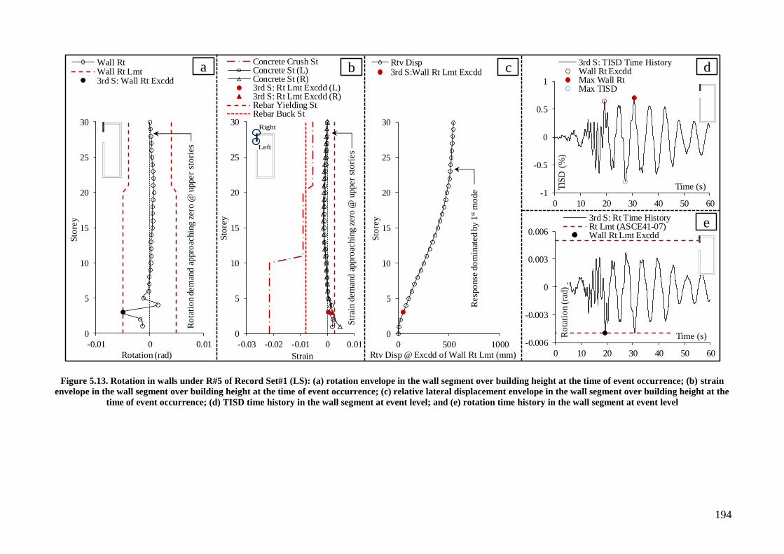
194
Figure 5.13. Rotation in walls under R#5 of Record Set#1 (LS): (a) rotation envelope in the wall segment over building height at the time of event occurrence; (b) strain
envelope in the wall segment over building height at the time of event occurrence; (c) relative lateral displacement envelope in the wall segment over building height at the
time of event occurrence; (d) TISD time history in the wall segment at event level; and (e) rotation time history in the wall segment at event level
0
5
10
15
20
25
30
-0.01 0 0.01
Sto
rey
Rotation (rad)
Wall RtWall Rt Lmt3rd S: Wall Rt Excdd
0
5
10
15
20
25
30
0 500 1000
Sto
rey
Rtv Disp3rd S:Wall Rt Lmt Excdd
Ro
tati
on d
em
and a
ppro
achin
g z
ero
@ u
pper
sto
ries
0
5
10
15
20
25
30
-0.03 -0.02 -0.01 0 0.01
Sto
rey
Strain
Concrete Crush StConcrete St (L)Concrete St (R)3rd S: Rt Lmt Excdd (L)3rd S: Rt Lmt Excdd (R)Rebar Yielding StRebar Buck St
Left
Right
-1
-0.5
0
0.5
1
0 10 20 30 40 50 60
TIS
D (
%)
Time (s)
3rd S: TISD Time HistoryWall Rt ExcddMax Wall RtMax TISD
-0.006
-0.003
0
0.003
0.006
0 10 20 30 40 50 60
Ro
tati
on (
rad)
Time (s)
3rd S: Rt Time HistoryRt Lmt (ASCE41-07)Wall Rt Lmt Excdd
Str
ain d
em
and a
ppro
achin
g z
ero
@ u
pper
sto
ries
Resp
onse
do
min
ated b
y 1
stm
ode
Rtv Disp @ Excdd of Wall Rt Lmt (mm)
a b c d
e
Sa(
wa)
= 0
.37
g, P
GA
=0
.55
g
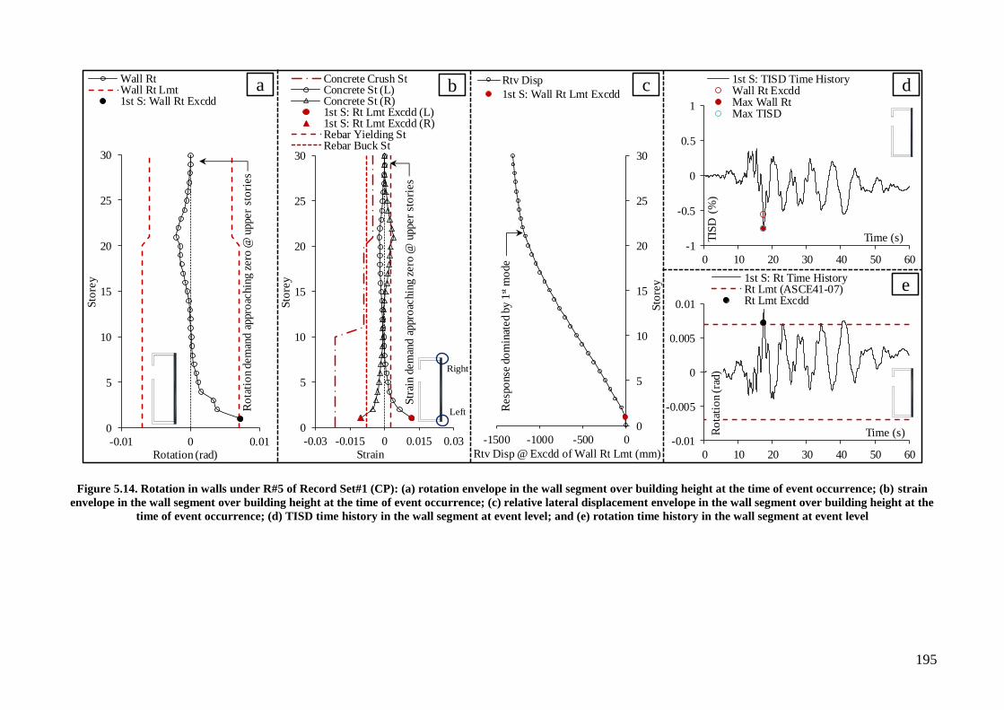
195
Figure 5.14. Rotation in walls under R#5 of Record Set#1 (CP): (a) rotation envelope in the wall segment over building height at the time of event occurrence; (b) strain
envelope in the wall segment over building height at the time of event occurrence; (c) relative lateral displacement envelope in the wall segment over building height at the
time of event occurrence; (d) TISD time history in the wall segment at event level; and (e) rotation time history in the wall segment at event level
0
5
10
15
20
25
30
-0.01 0 0.01
Sto
rey
Rotation (rad)
Wall RtWall Rt Lmt1st S: Wall Rt Excdd
0
5
10
15
20
25
30
-1500 -1000 -500 0
Sto
rey
Rtv Disp
1st S: Wall Rt Lmt Excdd
-1
-0.5
0
0.5
1
0 10 20 30 40 50 60
TIS
D (
%)
Time (s)
1st S: TISD Time HistoryWall Rt ExcddMax Wall RtMax TISD
-0.01
-0.005
0
0.005
0.01
0 10 20 30 40 50 60
Ro
tati
on (
rad)
Time (s)
1st S: Rt Time HistoryRt Lmt (ASCE41-07)Rt Lmt Excdd
0
5
10
15
20
25
30
-0.03 -0.015 0 0.015 0.03
Sto
rey
Strain
Concrete Crush StConcrete St (L)Concrete St (R)1st S: Rt Lmt Excdd (L)1st S: Rt Lmt Excdd (R)Rebar Yielding StRebar Buck St
Left
Right
Rtv Disp @ Excdd of Wall Rt Lmt (mm)
Ro
tati
on d
em
and a
ppro
achin
g z
ero
@ u
pper
sto
ries
Str
ain d
em
and a
ppro
achin
g z
ero
@ u
pper
sto
ries
Resp
onse
do
min
ated b
y 1
stm
ode
a b c d
e

196
Figure 5.15. Rebar buckling in walls under R#5 of Record Set#1 (CP): (a) rebar strain envelope in the wall segment over building height at the time of event occurrence;
(b) rotation envelope in the wall segment over building height at the time of event occurrence; (c) relative lateral displacement envelope in the wall segment over building
height at the time of event occurrence; (d) TISD time history in the wall segment at event level; and (e) rebar strain time history in the wall segment at event level
-0.5
0
0.5
0 10 20 30 40 50 60
TIS
D (
%)
Time (s)
1st S: TISD Time HistoryBuck St Excdd (R)Max Comp St (R)Max TISD
-0.012
-0.006
0
0.006
0.012
0 10 20 30 40 50 60
Str
ain
Time (s)
1st S (R): Rebar St Time HistoryRebar Buck StBuck St Excdd
Left
Right
0
5
10
15
20
25
30
-0.012 0 0.012
Sto
rey
Rotation (rad)
Wall RtWall Rt Lmt (ASCE 41-07)1st S: Buck St Excdd
0
5
10
15
20
25
30
-0.03 -0.015 0 0.015
Sto
rey
Strain
Concrete Crush StRebar St (R)1st S: Buck St ExcddRebar Yielding StRebar Buck St
0
5
10
15
20
25
30
-1000 -500 0
Sto
rey
Rtv Disp1st S: Buck St Excdd
Rtv Disp @ Excdd of Buckling St (mm)
Str
ain d
em
and a
ppro
achin
g z
ero
@ u
pper
sto
ries
Left
Right
Left
Right
Resp
onse
do
min
ated b
y 1
stm
ode
Ro
tati
on d
em
and a
ppro
achin
g z
ero
@ u
pper
sto
ries
Left
Right
a b c d
e
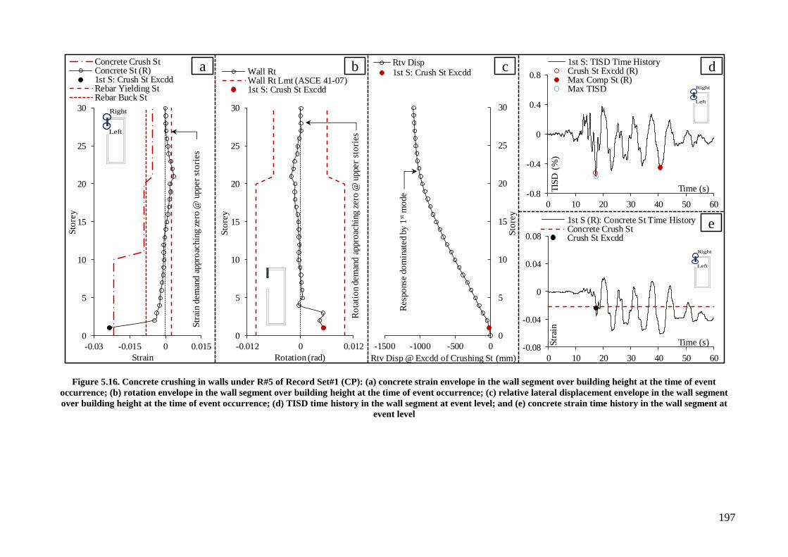
197
Figure 5.16. Concrete crushing in walls under R#5 of Record Set#1 (CP): (a) concrete strain envelope in the wall segment over building height at the time of event
occurrence; (b) rotation envelope in the wall segment over building height at the time of event occurrence; (c) relative lateral displacement envelope in the wall segment
over building height at the time of event occurrence; (d) TISD time history in the wall segment at event level; and (e) concrete strain time history in the wall segment at
event level
0
5
10
15
20
25
30
-0.03 -0.015 0 0.015
Sto
rey
Strain
Concrete Crush StConcrete St (R)1st S: Crush St ExcddRebar Yielding StRebar Buck St
Str
ain d
em
and a
ppro
achin
g z
ero
@ u
pper
sto
ries
0
5
10
15
20
25
30
-1500 -1000 -500 0
Sto
rey
Rtv Disp1st S: Crush St Excdd
Rtv Disp @ Excdd of Crushing St (mm)
-0.8
-0.4
0
0.4
0.8
0 10 20 30 40 50 60
TIS
D (
%)
Time (s)
1st S: TISD Time HistoryCrush St Excdd (R)Max Comp St (R)Max TISD
-0.08
-0.04
0
0.04
0.08
0 10 20 30 40 50 60
Str
ain
Time (s)
1st S (R): Concrete St Time HistoryConcrete Crush StCrush St Excdd
0
5
10
15
20
25
30
-0.012 0 0.012
Sto
rey
Rotation (rad)
Wall RtWall Rt Lmt (ASCE 41-07)1st S: Crush St Excdd
Left
Right
Ro
tati
on d
em
and a
ppro
achin
g z
ero
@ u
pper
sto
ries
Resp
onse
do
min
ated b
y 1
stm
ode
Left
Right
Left
Right
a b c d
e
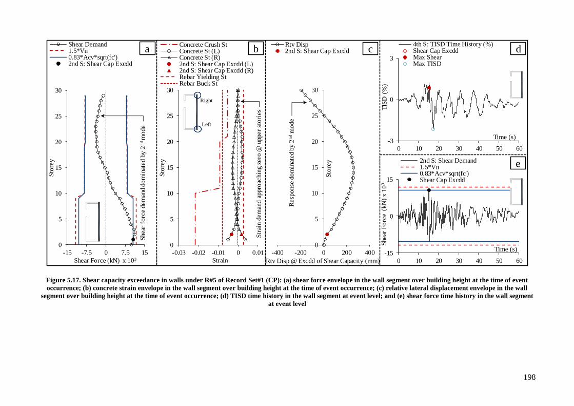
198
Figure 5.17. Shear capacity exceedance in walls under R#5 of Record Set#1 (CP): (a) shear force envelope in the wall segment over building height at the time of event
occurrence; (b) concrete strain envelope in the wall segment over building height at the time of event occurrence; (c) relative lateral displacement envelope in the wall
segment over building height at the time of event occurrence; (d) TISD time history in the wall segment at event level; and (e) shear force time history in the wall segment
at event level
0
5
10
15
20
25
30
-15 -7.5 0 7.5 15
Sto
rey
Shear Force (kN) x 103
Shear Demand1.5*Vn0.83*Acv*sqrt(fc')2nd S: Shear Cap Excdd
0
5
10
15
20
25
30
-0.03 -0.02 -0.01 0 0.01
Sto
rey
Strain
Concrete Crush StConcrete St (L)Concrete St (R)2nd S: Shear Cap Excdd (L)2nd S: Shear Cap Excdd (R)Rebar Yielding StRebar Buck St
0
5
10
15
20
25
30
-400 -200 0 200 400
Sto
rey
Rtv Disp2nd S: Shear Cap Excdd
-15
0
15
0 10 20 30 40 50 60
Shear
Fo
rce (
kN
)x 1
03
Time (s)
2nd S: Shear Demand1.5*Vn0.83*Acv*sqrt(fc')Shear Cap Excdd
-3
0
3
0 10 20 30 40 50 60
TIS
D (
%)
Time (s)
4th S: TISD Time History (%)Shear Cap ExcddMax ShearMax TISD
Shear
fo
rce d
em
and d
om
inat
ed b
y 2
ndm
ode Left
Right
Str
ain d
em
and a
ppro
achin
g z
ero
@ u
pper
sto
ries
Resp
onse
do
min
ated b
y 2
nd
mo
de
a b c d
e
Rtv Disp @ Excdd of Shear Capacity (mm)

199
Figure 5.18. Time history of normalised shear force and curvature ductility pairs in walls under R#5 of Record Set#1 (CP): (a) 1st storey; and (b) 2
nd storey
CP-WR
0.00
0.37
0.75
1.12
0
0.25
0.5
0.75
1
1.25
1.5
0 1 2 3 4 5 6 7 8 9 10
Shea
r F
orc
e R
atio
VD/A
CI
Up
per
Lim
it
She
ar F
orc
e R
atio
VD/V
n
Curvature Ductility
Normalized VD & CD pairs Time History(1.5*Vn) Failure EnvelopeShear Cap Upper Limit (ACI)Max Shear DemandMax Curvature Ductility
0.00
0.37
0.75
1.12
0
0.25
0.5
0.75
1
1.25
1.5
0 1 2 3 4 5 6 7 8 9 10
Shea
r F
orc
e R
atio
VD/A
CI
Up
per
Lim
it
She
ar F
orc
e R
atio
VD/V
n
Curvature Ductility
Normalized VD & CD Pairs Time History(1.5*Vn) Failure EnvelopeShear Cap Upper Limit (ACI)Max Shear DemandMax Curvature Ductility
11796 kN 11796 kN
10504 kN 10504 kN
VDmax= 9989 kN
VD @ CD(max) = 1873 kN
CDmax = 4.64
CD @ VDmax = 0.61
1st S
a b
2nd S
VDmax= 10621 kN
VD @ CD(max) = 6354 kN
CDmax = 1.8
CD @ VDmax = 0.41
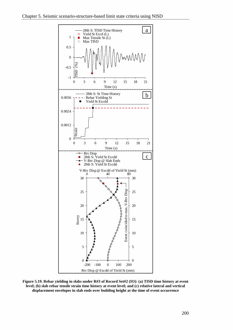
Chapter 5. Seismic scenario-structure-based limit state criteria using NISD
200
Figure 5.19. Rebar yielding in slabs under R#3 of Record Set#2 (IO): (a) TISD time history at event
level; (b) slab rebar tensile strain time history at event level; and (c) relative lateral and vertical
displacement envelopes in slab ends over building height at the time of event occurrence
-1
-0.5
0
0.5
1
0 3 6 9 12 15 18 21
TIS
D
(%)
Time (s)
28th S: TISD Time HistoryYield St Excd (L)Max Tensile St (L)Max TISD
0
0.0012
0.0024
0.0036
0 3 6 9 12 15 18 21
Str
ain
Time (s)
28th S: St Time HistoryRebar Yielding StYield St Excdd
0 40 80
0
5
10
15
20
25
30
0
5
10
15
20
25
30
-200 -100 0 100 200
Sto
rey
Rtv Disp28th S: Yield St ExcddV-Rtv Disp @ Slab Ends28th S: Yield St Excdd
V-Rtv Disp @ Excdd of Yield St (mm)
Rtv Disp @ Excdd of Yield St (mm)
Eve
nt
co
incid
ed to
max
. V
-Rtv
Dis
p
c
b
a
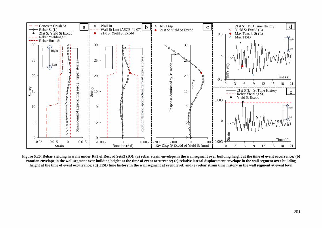
201
Figure 5.20. Rebar yielding in walls under R#3 of Record Set#2 (IO): (a) rebar strain envelope in the wall segment over building height at the time of event occurrence; (b)
rotation envelope in the wall segment over building height at the time of event occurrence; (c) relative lateral displacement envelope in the wall segment over building
height at the time of event occurrence; (d) TISD time history in the wall segment at event level; and (e) rebar strain time history in the wall segment at event level
0
5
10
15
20
25
30
-0.03 -0.015 0 0.015
Sto
rey
Strain
Concrete Crush StRebar St (L)21st S: Yield St ExcddRebar Yielding StRebar Buck St
0
5
10
15
20
25
30
-200 -100 0 100
Sto
rey
Rtv Disp21st S: Yield St Excdd
Rtv Disp @ Excdd of Yield St (mm)
-0.6
0
0.6
0 3 6 9 12 15 18 21
TIS
D
(%)
Time (s)
21st S: TISD Time HistoryYield St Excdd (L)Max Tensile St (L)Max TISD
-0.003
0
0.003
0 3 6 9 12 15 18 21
Str
ain
Time (s)
21st S (L): St Time HistoryRebar Yielding StYield St Excdd
Left
Right
0
5
10
15
20
25
30
-0.005 0 0.005
Sto
rey
Rotation (rad)
Wall RtWall Rt Lmt (ASCE 41-07)21st S: Yield St Excdd
Str
ain d
em
and a
ppro
achin
g z
ero
@ u
pper
sto
ries
Ro
tati
on d
em
and a
ppro
achin
g z
ero
@ u
pper
sto
ries
Resp
onse
do
min
ated b
y 3
rdm
odeLeft
RightLeft
Right
a b c d
e
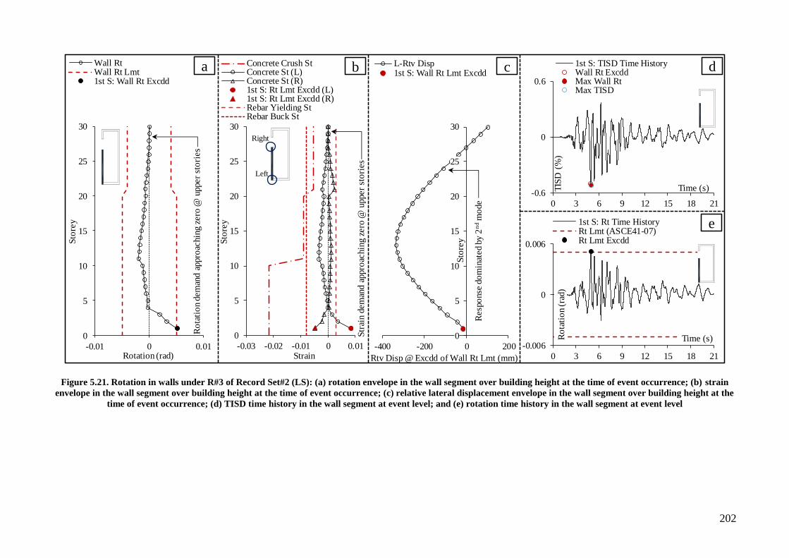
202
Figure 5.21. Rotation in walls under R#3 of Record Set#2 (LS): (a) rotation envelope in the wall segment over building height at the time of event occurrence; (b) strain
envelope in the wall segment over building height at the time of event occurrence; (c) relative lateral displacement envelope in the wall segment over building height at the
time of event occurrence; (d) TISD time history in the wall segment at event level; and (e) rotation time history in the wall segment at event level
0
5
10
15
20
25
30
-0.01 0 0.01
Sto
rey
Rotation (rad)
Wall RtWall Rt Lmt1st S: Wall Rt Excdd
0
5
10
15
20
25
30
-400 -200 0 200
Sto
rey
L-Rtv Disp1st S: Wall Rt Lmt Excdd
Rtv Disp @ Excdd of Wall Rt Lmt (mm)
-0.6
0
0.6
0 3 6 9 12 15 18 21
TIS
D (
%)
Time (s)
1st S: TISD Time HistoryWall Rt ExcddMax Wall RtMax TISD
-0.006
0
0.006
0 3 6 9 12 15 18 21
Ro
tati
on (
rad)
Time (s)
1st S: Rt Time HistoryRt Lmt (ASCE41-07)Rt Lmt Excdd
0
5
10
15
20
25
30
-0.03 -0.02 -0.01 0 0.01
Sto
rey
Strain
Concrete Crush StConcrete St (L)Concrete St (R)1st S: Rt Lmt Excdd (L)1st S: Rt Lmt Excdd (R)Rebar Yielding StRebar Buck St
Left
Right
Ro
tati
on d
em
and a
ppro
achin
g z
ero
@ u
pper
sto
ries
Str
ain d
em
and a
ppro
achin
g z
ero
@ u
pper
sto
ries
Resp
onse
do
min
ated b
y 2
nd
mo
de
a b c d
e
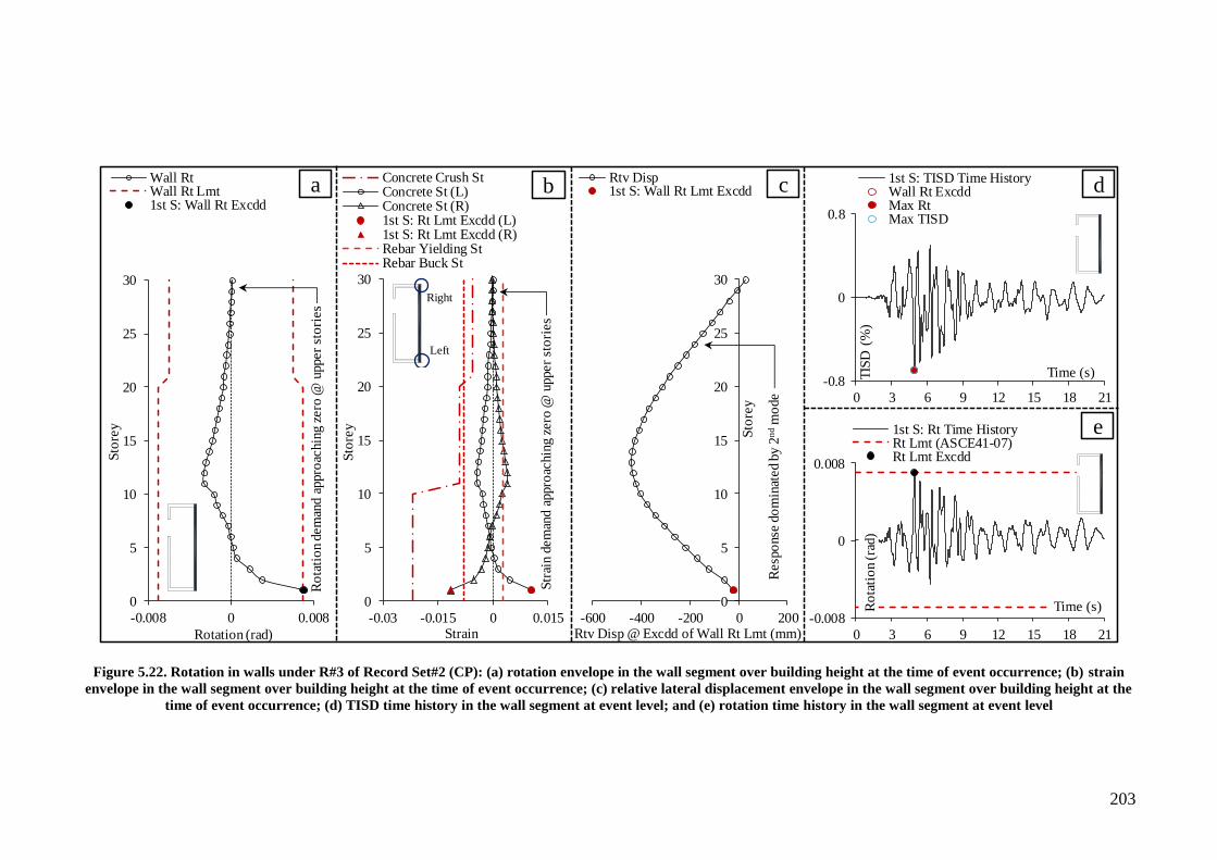
203
Figure 5.22. Rotation in walls under R#3 of Record Set#2 (CP): (a) rotation envelope in the wall segment over building height at the time of event occurrence; (b) strain
envelope in the wall segment over building height at the time of event occurrence; (c) relative lateral displacement envelope in the wall segment over building height at the
time of event occurrence; (d) TISD time history in the wall segment at event level; and (e) rotation time history in the wall segment at event level
0
5
10
15
20
25
30
-600 -400 -200 0 200
Sto
rey
Rtv Disp1st S: Wall Rt Lmt Excdd
0
5
10
15
20
25
30
-0.008 0 0.008
Sto
rey
Rotation (rad)
Wall RtWall Rt Lmt1st S: Wall Rt Excdd
-0.8
0
0.8
0 3 6 9 12 15 18 21
TIS
D (
%)
Time (s)
1st S: TISD Time HistoryWall Rt ExcddMax RtMax TISD
-0.008
0
0.008
0 3 6 9 12 15 18 21
Ro
tati
on (
rad)
Time (s)
1st S: Rt Time HistoryRt Lmt (ASCE41-07)Rt Lmt Excdd
0
5
10
15
20
25
30
-0.03 -0.015 0 0.015
Sto
rey
Strain
Concrete Crush StConcrete St (L)Concrete St (R)1st S: Rt Lmt Excdd (L)1st S: Rt Lmt Excdd (R)Rebar Yielding StRebar Buck St
Rtv Disp @ Excdd of Wall Rt Lmt (mm)
Left
Right
Ro
tati
on d
em
and a
ppro
achin
g z
ero
@ u
pper
sto
ries
Str
ain d
em
and a
ppro
achin
g z
ero
@ u
pper
sto
ries
Resp
onse
do
min
ated b
y 2
nd
mo
de
a b c d
e

204
Figure 5.23. Rebar buckling in walls under R#3 of Record Set#2 (CP): (a) rebar strain envelope in the wall segment over building height at the time of event occurrence;
(b) rotation envelope in the wall segment over building height at the time of event occurrence; (c) relative lateral displacement envelope in the wall segment over building
height at the time of event occurrence; (d) TISD time history in the wall segment at event level; and (e) rebar strain time history in the wall segment at event level
0
5
10
15
20
25
30
-400 -200 0 200
Sto
rey
Rtv Disp1st S: Buck St Excdd
0
5
10
15
20
25
30
-0.03 -0.015 0 0.015
Sto
rey
Strain
Concrete Crush StRebar St (R)1st S: Buck St ExcddRebar Yielding StRebar Buck St
-0.6
0
0.6
0 3 6 9 12 15 18 21
TIS
D (
%)
Time (s)
1st S: TISD Time HistoryBuck St Excdd (R)Max Comp St (R)Max TISD
-0.012
0
0.012
0 3 6 9 12 15 18 21
Str
ain
Time (s)
1st S (R): Rebar St Time HistoryRebar Buck StBuck St Excdd
0
5
10
15
20
25
30
-0.01 0 0.01
Sto
rey
Rotation (rad)
Wall RtWall Rt Lmt (ASCE 41-07)B2: Buck St Excdd
Rtv Disp @ Excdd of Buckling Strain (mm)
Left
Right
Left
Right
Left
Right
Str
ain d
em
and a
ppro
achin
g z
ero
@ u
pper
sto
ries
Ro
tati
on d
em
and a
ppro
achin
g z
ero
@ u
pper
sto
ries
Resp
onse
do
min
ated b
y 2
nd
mo
de
a b c d
e

205
Figure 5.24. Concrete crushing in walls under R#3 of Record Set#2 (CP): (a) concrete strain envelope in the wall segment over building height at the time of event
occurrence; (b) rotation envelope in the wall segment over building height at the time of event occurrence; (c) relative lateral displacement envelope in the wall segment
over building height at the time of event occurrence; (d) TISD time history in the wall segment at event level; and (e) concrete strain time history in the wall segment at
event level
0
5
10
15
20
25
30
-300 -200 -100 0 100
Sto
rey
Rtv Disp1st S: Crush St Excdd
0
5
10
15
20
25
30
-0.03 -0.015 0 0.015
Sto
rey
Strain
Concrete Crush StConcrete St (R)1st S: Crush St ExcddRebar Yielding StRebar Buckling St
-0.8
0
0.8
0 3 6 9 12 15 18 21
TIS
D (
%)
Time (s)
1st S: TISD Time HistoryCrsh St Excd (R)Max Comp St (R)Max TISD
-0.03
-0.02
-0.01
0
0.01
0 3 6 9 12 15 18 21
Str
ain
Time (s)
1st S (R): Concrete St Time HistoryConcrete Crsh StCrsh St Excd
0
5
10
15
20
25
30
-0.012 0 0.012
Sto
rey
Rotation (rad)
Wall RtWall Rt Lmt (ASCE 41-07)B2: Crush St Excdd
Rtv Disp @ Excdd of Crushing St (mm)
Left
Right
Left
Right
Left
Right
Str
ain d
em
and a
ppro
achin
g z
ero
@ u
pper
sto
ries
Ro
tati
on d
em
and a
ppro
achin
g z
ero
@ u
pper
sto
ries
Resp
onse
do
min
ated b
y 2
nd
mo
de
a b c d
e
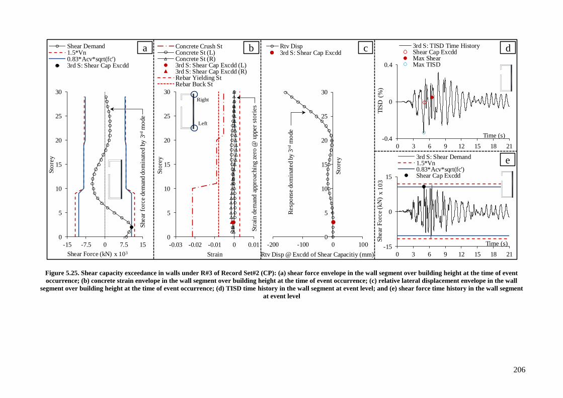
206
Figure 5.25. Shear capacity exceedance in walls under R#3 of Record Set#2 (CP): (a) shear force envelope in the wall segment over building height at the time of event
occurrence; (b) concrete strain envelope in the wall segment over building height at the time of event occurrence; (c) relative lateral displacement envelope in the wall
segment over building height at the time of event occurrence; (d) TISD time history in the wall segment at event level; and (e) shear force time history in the wall segment
at event level
0
5
10
15
20
25
30
-15 -7.5 0 7.5 15
Sto
rey
Shear Force (kN) x 103
Shear Demand1.5*Vn0.83*Acv*sqrt(fc')3rd S: Shear Cap Excdd
0
5
10
15
20
25
30
-0.03 -0.02 -0.01 0 0.01
Sto
rey
Strain
Concrete Crush StConcrete St (L)Concrete St (R)3rd S: Shear Cap Excdd (L)3rd S: Shear Cap Excdd (R)Rebar Yielding StRebar Buck St
0
5
10
15
20
25
30
-200 -100 0 100
Sto
rey
Rtv Disp3rd S: Shear Cap Excdd
-0.4
0
0.4
0 3 6 9 12 15 18 21
TIS
D (
%)
Time (s)
3rd S: TISD Time HistoryShear Cap ExcddMax ShearMax TISD
-15
0
15
0 3 6 9 12 15 18 21
Shear
Fo
rce (
kN
)x 1
03
Time (s)
3rd S: Shear Demand1.5*Vn0.83*Acv*sqrt(fc')Shear Cap Excdd
Rtv Disp @ Excdd of Shear Capacitiy (mm)
Shear
fo
rce d
em
and d
om
inat
ed b
y 3
rdm
ode
Left
Right
Str
ain d
em
and a
ppro
achin
g z
ero
@ u
pper
sto
ries
Resp
onse
do
min
ated b
y 3
rdm
ode
a b c d
e
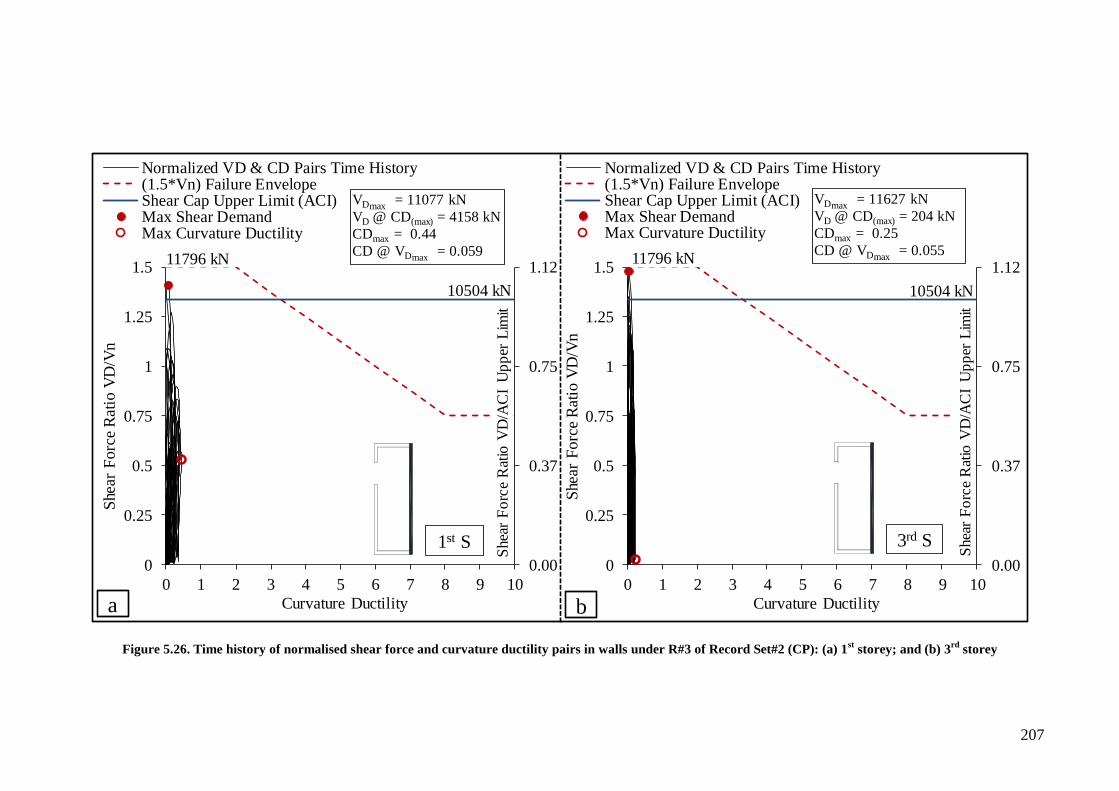
207
Figure 5.26. Time history of normalised shear force and curvature ductility pairs in walls under R#3 of Record Set#2 (CP): (a) 1st storey; and (b) 3
rd storey
0.00
0.37
0.75
1.12
0
0.25
0.5
0.75
1
1.25
1.5
0 1 2 3 4 5 6 7 8 9 10
Shea
r F
orc
e R
atio
VD
/AC
I U
pp
er L
imit
She
ar F
orc
e R
atio
VD
/Vn
Curvature Ductility
Normalized VD & CD Pairs Time History(1.5*Vn) Failure EnvelopeShear Cap Upper Limit (ACI)Max Shear DemandMax Curvature Ductility
0.00
0.37
0.75
1.12
0
0.25
0.5
0.75
1
1.25
1.5
0 1 2 3 4 5 6 7 8 9 10
Shea
r F
orc
e R
atio
VD
/AC
I U
pp
er L
imit
She
ar F
orc
e R
atio
VD
/Vn
Curvature Ductility
Normalized VD & CD Pairs Time History(1.5*Vn) Failure EnvelopeShear Cap Upper Limit (ACI)Max Shear DemandMax Curvature Ductility
11796 kN 11796 kN
10504 kN 10504 kN
VDmax= 11077 kN
VD @ CD(max) = 4158 kN
CDmax = 0.44
CD @ VDmax = 0.059
1st S 3rd S
a b
VDmax= 11627 kN
VD @ CD(max) = 204 kN
CDmax = 0.25
CD @ VDmax = 0.055
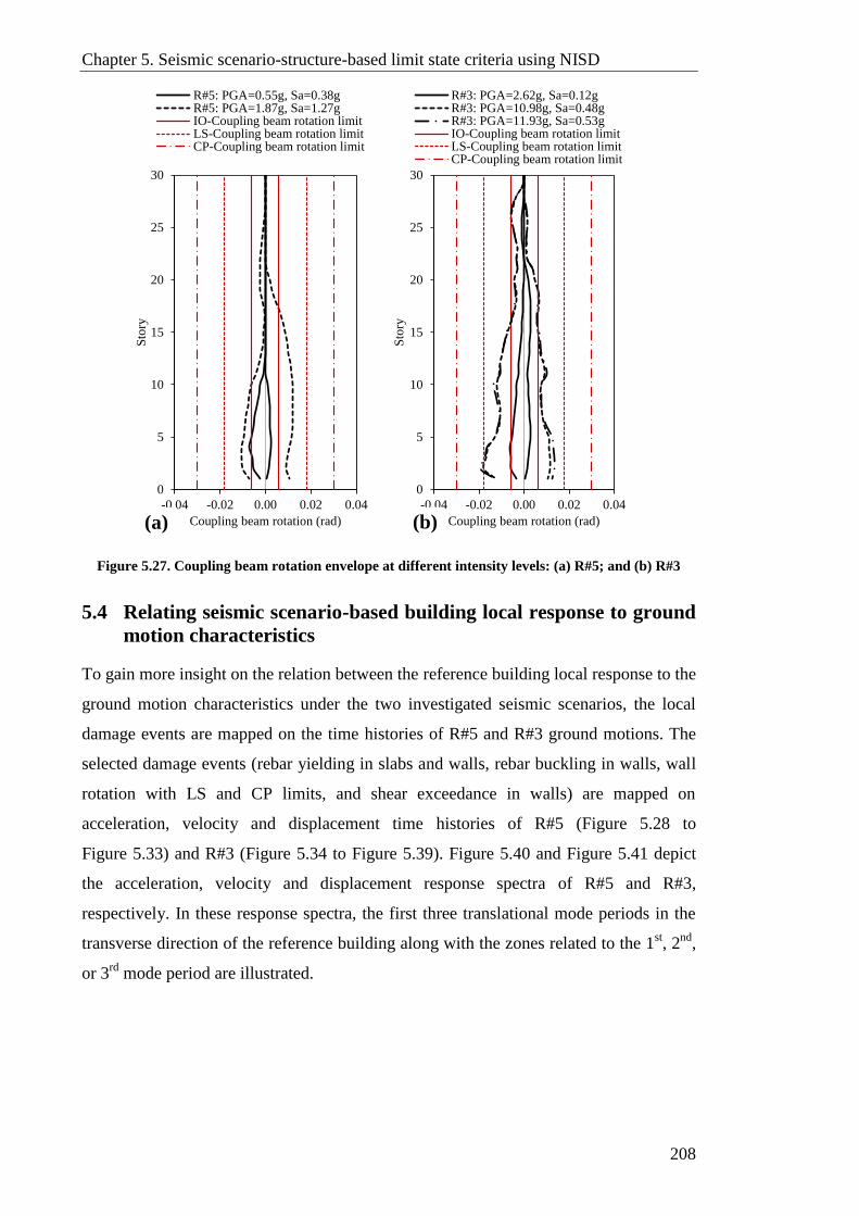
Chapter 5. Seismic scenario-structure-based limit state criteria using NISD
208
Figure 5.27. Coupling beam rotation envelope at different intensity levels: (a) R#5; and (b) R#3
5.4 Relating seismic scenario-based building local response to ground
motion characteristics
To gain more insight on the relation between the reference building local response to the
ground motion characteristics under the two investigated seismic scenarios, the local
damage events are mapped on the time histories of R#5 and R#3 ground motions. The
selected damage events (rebar yielding in slabs and walls, rebar buckling in walls, wall
rotation with LS and CP limits, and shear exceedance in walls) are mapped on
acceleration, velocity and displacement time histories of R#5 (Figure 5.28 to
Figure 5.33) and R#3 (Figure 5.34 to Figure 5.39). Figure 5.40 and Figure 5.41 depict
the acceleration, velocity and displacement response spectra of R#5 and R#3,
respectively. In these response spectra, the first three translational mode periods in the
transverse direction of the reference building along with the zones related to the 1st, 2
nd,
or 3rd
mode period are illustrated.
0
5
10
15
20
25
30
-0.04 -0.02 0.00 0.02 0.04
Sto
ry
Coupling beam rotation (rad)
R#3: PGA=2.62g, Sa=0.12gR#3: PGA=10.98g, Sa=0.48gR#3: PGA=11.93g, Sa=0.53gIO-Coupling beam rotation limitLS-Coupling beam rotation limitCP-Coupling beam rotation limit
0
5
10
15
20
25
30
-0.04 -0.02 0.00 0.02 0.04
Sto
ry
Coupling beam rotation (rad)
R#5: PGA=0.55g, Sa=0.38gR#5: PGA=1.87g, Sa=1.27gIO-Coupling beam rotation limitLS-Coupling beam rotation limitCP-Coupling beam rotation limit
(a) (b)

Chapter 5. Seismic scenario-structure-based limit state criteria using NISD
209
The following can be concluded from the aforementioned figures:
Under R#5, the IO and LS deformation-related damage events, which
correspond to the 1st mode of vibration, are associated with ground displacement
or ground displacement spikes which are close in value to the peak ground
displacement. While for the CP deformation-related damage events, they are
associated with either ground displacement and velocity peaks or spikes which
are close in value to the ground peaks. For the shear exceedance in walls, the
event is associated with both peak ground velocity and ground acceleration
spike.
Under R#3, the pattern for the local damage events does not correlate well to the
record ground motion time histories as under R#5. The deformation-related
damage events are found to be associated with peaks or with spikes close to the
peaks of ground displacement, velocity, and or acceleration with more obvious
correlation to ground velocity peaks (or spikes). This illustrates the effect of
higher mode on building response, having in mind that all deformation-related
damage events under R#3 correspond to the 2nd
mode of vibration, except for
rebar yielding in walls which corresponds to the 3rd
mode. For the shear
exceedance in walls (which corresponds to the 3rd
mode), failure is associated
with spikes in all ground motion time histories (displacement, velocity and
acceleration). This again illustrates the importance of higher modes.
Under R#5 (Figure 5.40c), it can be seen that the maximum spectral
displacement is found in the region of the 1st mode period. The maximum
spectral velocity (Figure 5.40b) and moderate spectral acceleration
(Figure 5.40a) correspond to the region of the 2nd
mode period.
Under R#3, the maximum spectral displacement is correlated to the 2nd
mode
period (Figure 5.41c). While maximum spectral velocity (Figure 5.41b) and
maximum spectral acceleration (Figure 5.41a) are correlated to the 3rd
mode
period.
The abovementioned observations indicate the following:
To minimise the dispersion of the MRIDAs results, it might be more appropriate
to use the displacement and velocity uniform hazard spectra as references when

Chapter 5. Seismic scenario-structure-based limit state criteria using NISD
210
selecting, scaling and anchoring real ground motions to be used in the NRHAs
under strong distant and moderate near-field earthquake scenarios, respectively.
When the performance-based design is adopted, the building seismic
performance may be further optimised by avoiding critical frequency range
associated with response spectral amplifications.
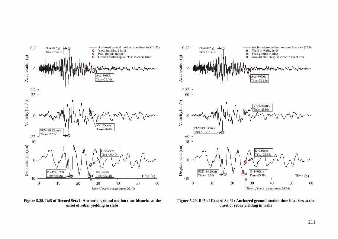
211
Figure 5.28. R#5 of Record Set#1: Anchored ground motion time histories at the
onset of rebar yielding in slabs
Figure 5.29. R#5 of Record Set#1: Anchored ground motion time histories at the
onset of rebar yielding in walls
-0.2
0
0.2
Accele
rati
on (
g)
Anchored ground motion time histories (*1.25)Yield in slabs, 24th SPeak ground motionGround motion spike close to event time
-32
0
32
Velo
cit
y (
cm
/s)
-10
0
10
0 10 20 30 40 50 60
Dis
pla
cem
ent (c
m)
Time (s)
PGA=0.20g
Time=15.40s
Acc=0.013g
Time=26.40s
PGV=30.83cm/s
Time=15.28s
V=1.75cm/s
Time=26.40s
D=2.58cm
Time=26.40s
PGD=8.87cm
Time=16.66s
D=8.76cm
Time=25.58s
Time of event occurrance: 26.40s
Time-0.32
0
0.32
Accele
rati
on (
g)
Anchored ground motion time histories (*2.0)Yield in walls, 1st SPeak ground motionGround motion spike close to event time
-60
0
60
Velo
cit
y (
cm
/s)
-18
0
18
0 10 20 30 40 50 60D
ispla
cem
ent (c
m)
Time (s)
PGA=0.20g
Time=15.40s
Acc=0.006g
Time=26.96s
PGV=49.33cm/s
Time=15.28s
V=10.48cm/s
Time=26.96s
D=1.92cm
Time=26.96s
PGD=14.20cm
Time=16.66s
D=14.02cm
Time=25.58s
Time of event occurrance: 26.96s
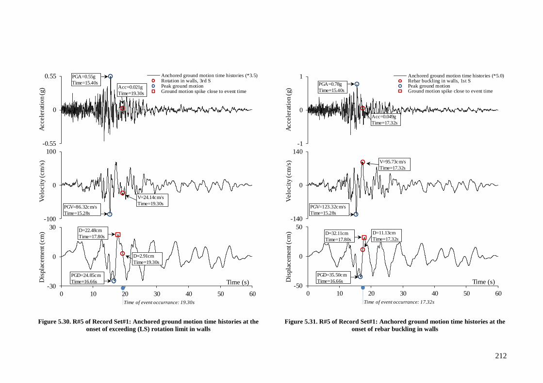
212
Figure 5.30. R#5 of Record Set#1: Anchored ground motion time histories at the
onset of exceeding (LS) rotation limit in walls
Figure 5.31. R#5 of Record Set#1: Anchored ground motion time histories at the
onset of rebar buckling in walls
Event
LS-WR
Time
Time
Time
-0.55
0
0.55
Accele
rati
on (
g)
Anchored ground motion time histories (*3.5)Rotation in walls, 3rd SPeak ground motionGround motion spike close to event time
-100
0
100
Velo
cit
y (
cm
/s)
-30
0
30
0 10 20 30 40 50 60
Dis
pla
cem
ent (c
m)
Time (s)
PGA=0.55g
Time=15.40sAcc=0.021g
Time=19.30s
PGV=86.32cm/s
Time=15.28s
V=24.14cm/s
Time=19.30s
D=2.91cm
Time=19.30s
PGD=24.85cm
Time=16.66s
D=22.48cm
Time=17.80s
Time of event occurrance: 19.30s
CP-SB
Time
Time
Time
-1
0
1
Accele
rati
on (
g)
Anchored ground motion time histories (*5.0)Rebar buckling in walls, 1st SPeak ground motionGround motion spike close to event time
-140
0
140
Velo
cit
y (
cm
/s)
-50
0
50
0 10 20 30 40 50 60D
ispla
cem
ent (c
m)
Time (s)
PGA=0.78g
Time=15.40s
Acc=0.049g
Time=17.32s
PGV=123.32cm/s
Time=15.28s
V=95.73cm/s
Time=17.32s
D=11.13cm
Time=17.32s
PGD=35.50cm
Time=16.66s
D=32.11cm
Time=17.80s
Time of event occurrance: 17.32s
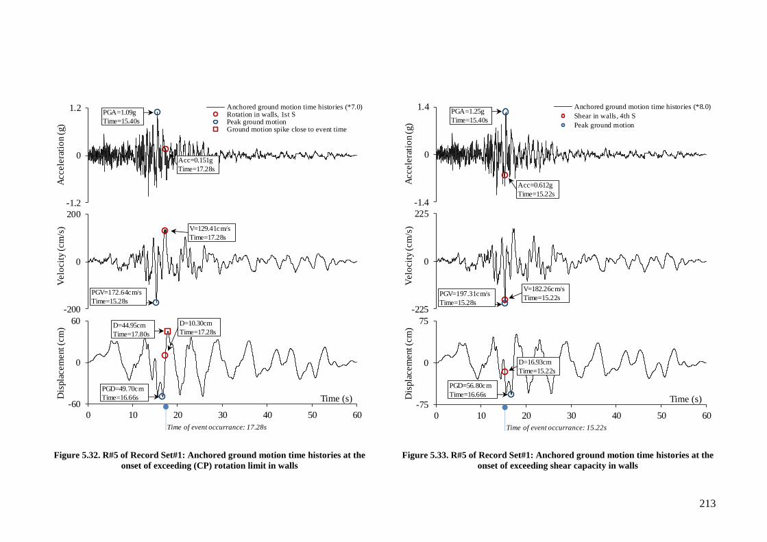
213
Figure 5.32. R#5 of Record Set#1: Anchored ground motion time histories at the
onset of exceeding (CP) rotation limit in walls
Figure 5.33. R#5 of Record Set#1: Anchored ground motion time histories at the
onset of exceeding shear capacity in walls
Event
CP-WR
Time
Time
Time
-1.2
0
1.2
Accele
rati
on (
g)
Anchored ground motion time histories (*7.0)Rotation in walls, 1st SPeak ground motionGround motion spike close to event time
-200
0
200
Velo
cit
y (
cm
/s)
-60
0
60
0 10 20 30 40 50 60
Dis
pla
cem
ent (c
m)
Time (s)
PGA=1.09g
Time=15.40s
Acc=0.151g
Time=17.28s
PGV=172.64cm/s
Time=15.28s
V=129.41cm/s
Time=17.28s
D=10.30cm
Time=17.28s
PGD=49.70cm
Time=16.66s
D=44.95cm
Time=17.80s
Time of event occurrance: 17.28s
Event
CP-SH
Time
Time
Time
4.995
-1.4
0
1.4
Accele
rati
on (
g)
Anchored ground motion time histories (*8.0)
Shear in walls, 4th S
Peak ground motion
-225
0
225
Velo
cit
y (
cm
/s)
-75
0
75
0 10 20 30 40 50 60D
ispla
cem
ent (c
m)
Time (s)
PGA=1.25g
Time=15.40s
Acc=0.612g
Time=15.22s
PGV=197.31cm/s
Time=15.28s
V=182.26cm/s
Time=15.22s
D=16.93cm
Time=15.22s
PGD=56.80cm
Time=16.66s
Time of event occurrance: 15.22s

214
Figure 5.34. R#3 of Record Set#2: Anchored ground motion time histories at the
onset of rebar yielding in slabs
Figure 5.35. R#3 of Record Set#2: Anchored ground motion time histories at the
onset of rebar yielding in walls
-1.6
0
1.6
Accele
rati
on (
g)
Anchored ground motion time histories (*6)
Yield in slabs, 28th S
Peak ground motion
-90
0
90
Velo
cit
y (
cm
/s)
-10
0
10
0 3 6 9 12 15 18 21
Dis
pla
cem
ent (c
m)
Time (s)
PGA=1.43g
Time=6.320s
Acc=1.12g
Time=5.325s
PGV=71.93cm/s
Time=6.390sV=25.82cm/s
Time=5.325s
D=5.05cm
Time=5.325s
PGD=6.23cm
Time=5.0s
Time of event occurrance: 5.325s
Time
-1.9
0
1.9
Accele
rati
on (
g)
Anchored ground motion time histories (*7)Yield in walls, 21st SPeak ground motionGround motion spike close to event time
-100
0
100
Velo
cit
y (
cm
/s)
-10
0
10
0 3 6 9 12 15 18 21D
ispla
cem
ent (c
m)
Time (s)
PGA=1.67g
Time=6.320s
Acc=1.26g
Time=5.425s
PGV=83.92cm/s
Time=6.390s
V=37.04cm/s
Time=5.425s
D=0.16cm
Time=5.425s
PGD=7.27cm
Time=5.0s
Time of event occurrance: 5.425s
V=70.43cm/s
Time=5.375s

215
Figure 5.36. R#3 of Record Set#2: Anchored ground motion time histories at the
onset of exceeding (LS) rotation limit in walls
Figure 5.37. R#3 of Record Set#2: Anchored ground motion time histories at the
onset of rebar buckling in walls
-6
0
6
Accele
rati
on (
g)
Anchored ground motion time histories (*24)Rotation in Walls, 1st SPeak ground motionGround motion spike close to event time
-320
0
320
Velo
cit
y (
cm
/s)
-28
0
28
0 3 6 9 12 15 18 21
Dis
pla
cem
ent (c
m)
Time (s)
PGA=5.73g
Time=6.320s
Acc=1.30g
Time=4.930s
PGV=287.74cm/s
Time=6.390sV=229.58cm/s
Time=4.930s
D=15.72cm
Time=4.930s
PGD=24.92cm
Time=5.0s
D=15.69cm
Time=4.70s
Time of event occurrance: 4.930s
-5
0
5
Accele
rati
on (
g)
Anchored ground motion time histories (*20)Rebar buckling in Walls, 1st SPeak ground motionGround motion spike close to event time
-260
0
260
Velo
cit
y (
cm
/s)
-24
0
24
0 3 6 9 12 15 18 21D
ispla
cem
ent (c
m)
Time (s)
PGA=4.77g
Time=6.320s
Acc=0.26g
Time=4.915s
PGV=239.78cm/s
Time=6.390sV=200.88cm/s
Time=4.915s
D=10.14cm
Time=4.915s
PGD=20.77cm
Time=5.0s
D=13.07cm
Time=4.70s
Time of event occurrance: 4.915s
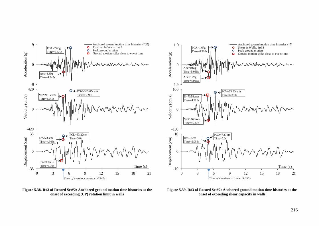
216
Figure 5.38. R#3 of Record Set#2: Anchored ground motion time histories at the
onset of exceeding (CP) rotation limit in walls
Figure 5.39. R#3 of Record Set#2: Anchored ground motion time histories at the
onset of exceeding shear capacity in walls
-9
0
9
Accele
rati
on (
g)
Anchored ground motion time histories (*32)Rotation in Walls, 1st SPeak ground motionGround motion spike close to event time
-420
0
420
Velo
cit
y (
cm
/s)
-38
0
38
0 3 6 9 12 15 18 21
Dis
pla
cem
ent (c
m)
Time (s)
PGA=7.63g
Time=6.320s
Acc=3.30g
Time=4.945s
PGV=383.65cm/s
Time=6.390sV=269.15cm/s
Time=4.945s
D=25.30cm
Time=4.945s
PGD=33.22cm
Time=5.0s
D=20.92cm
Time=4.70s
Time of event occurrance: 4.945s
4.995
-1.9
0
1.9
Accele
rati
on (
g)
Anchored ground motion time histories (*7)Shear in Walls, 3rd SPeak ground motionGround motion spike close to event time
-100
0
100
Velo
cit
y (
cm
/s)
-10
0
10
0 3 6 9 12 15 18 21D
ispla
cem
ent (c
m)
Time (s)
PGA=1.67g
Time=6.320s
Acc=0.69g
Time=5.055s
PGV=83.92cm/s
Time=6.390s
V=55.66cm/s
Time=5.055s
D=5.61cm
Time=5.055s
PGD=7.27cm
Time=5.0s
D=70.58cm/s
Time=4.910s
Time of event occurrance: 5.055s
Acc=1.23g
Time=4.995s
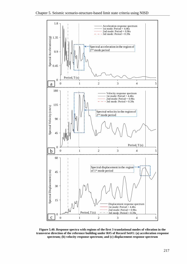
Chapter 5. Seismic scenario-structure-based limit state criteria using NISD
217
Figure 5.40. Response spectra with regions of the first 3 translational modes of vibration in the
transverse direction of the reference building under R#5 of Record Set#1: (a) acceleration response
spectrum; (b) velocity response spectrum; and (c) displacement response spectrum
Time
0
0.45
0.9
1.35
1.8
0 1 2 3 4 5
Spectr
al A
ccele
rati
on (
g)
Period, T (s)
Acceleration response spectrum1st mode: Period = 4.46s2nd mode: Period = 0.96s3rd mode: Period = 0.39s
Spectral acceleration in the region of 2nd mode period
0
45
90
135
180
0 1 2 3 4 5
Spectr
al V
elo
cit
y (
cm
/s)
Period, T (s)
Velocity response spectrum1st mode: Period = 4.46s2nd mode: Period = 0.96s3rd mode: Period = 0.39s
0
15
30
45
60
0 1 2 3 4 5
Spectr
al D
ispla
cem
ent (c
m)
Period, T (s)
Displacement response spectrum1st mode: Period = 4.46s2nd mode: Period = 0.96s3rd mode: Period = 0.39s
Spectral velocity in the region of 2nd mode period
Spectral displacement in the region of 1st mode period
a
b
c
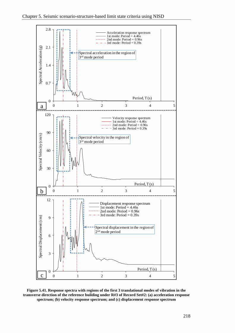
Chapter 5. Seismic scenario-structure-based limit state criteria using NISD
218
Figure 5.41. Response spectra with regions of the first 3 translational modes of vibration in the
transverse direction of the reference building under R#3 of Record Set#2: (a) acceleration response
spectrum; (b) velocity response spectrum; and (c) displacement response spectrum
Time
0
0.7
1.4
2.1
2.8
0 1 2 3 4 5
Spectr
al A
ccele
rati
on (
g)
Period, T (s)
Acceleration response spectrum1st mode: Period = 4.46s2nd mode: Period = 0.96s3rd mode: Period = 0.39s
0
30
60
90
120
0 1 2 3 4 5
Spectr
al V
elo
cit
y (
cm
/s)
Period, T (s)
Velocity response spectrum1st mode: Period = 4.46s2nd mode: Period = 0.96s3rd mode: Period = 0.39s
0
3
6
9
12
0 1 2 3 4 5
Spectr
al D
ispla
cem
ent (c
m)
Period, T (s)
Displacement response spectrum1st mode: Period = 4.46s2nd mode: Period = 0.96s3rd mode: Period = 0.39s
Spectral acceleration in the region of 3rd mode period
Spectral velocity in the region of 3rd mode period
Spectral displacement in the region of 2nd mode period
a
b
c

Chapter 5. Seismic scenario-structure-based limit state criteria using NISD
219
5.5 Linking local to global response
To quantitatively define the performance limit states, DMs need to be adapted to link
local-to-global response. The selection of a DM depends primarily on the structural
characteristics of the assessed building and its usage. DMs include: (i) deformation-
based DMs such as roof drift and TISD; (ii) force-based DMs such as base shear; and
(iii) energy-based DMs such as the global Park-Ang index (Park and Ang, 1985). TISD
has been frequently used as a global DM in previous studies since it is adopted by most
of the seismic design and assessment code provisions and can be easily calibrated
against experimental data available in the literature.
Using TISD, seismic guidelines and previous researches have proposed a wide range of
limit state criteria associated with different performance levels of RC shear walls and
wall structures. In ASCE/SEI 41-06 (2007), TISDs of 0.5%, 1% and 2.0% are assigned
to the IO, LS, and CP performance levels, respectively. The SEAOC blue book (1999)
proposed TISDs of 0.4%, 0.9%, 1.4% and 2.1% for RC shear walls at performance
levels SP1 (negligible damage), SP2 (minor to moderate reparable damage), SP3
(moderate to major irreparable damage), and SP4 (collapse performance level). Seismic
codes tend to lean to the conservative side, but less conservative TISDs have been
recommended in the literature based on experimental and analytical results. For ductile
RC walls, Ghobarah (2004) recommended TISDs of <0.2%, 0.4%, <0.8%, >0.8%, 1.5%
and >2.5% corresponded to damage levels of none, light reparable, moderate reparable,
irreparable, severe (or life safe), and collapse, respectively. In another study of RC wall
buildings with a number of storeys ranging between 10 to 60, Mwafy (2012a) suggested
a TISD value of 2.5% for CP, while height-dependent TISDs were proposed for IO
(0.32% to 0.83%) and LS (0.81% to 1.35%). In contrast, Ji et al. (2009) suggested
conservative TISDs to define three performance limit states obtained from inelastic
pushover and time history analyses for a 54-storey RC wall building. The proposed
TISDs were 0.2%, 0.52% and 1.1% for serviceability, damage control and collapse
prevention limit states, respectively. Bearing the above in mind, reliable definitions of
performance limit state criteria for RC high-rise wall structures remain a significant
research issue.
TISD at any storey is a combination of two major components: (i) lateral net drift
caused by shear and flexure deformation, referred to hereafter as NISD; and (ii) drift
from rigid body motion (RBM) caused by the rotation in the lower storey, referred to
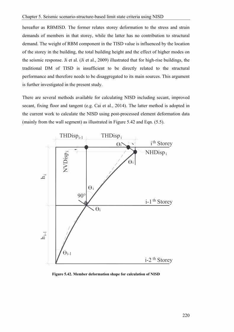
Chapter 5. Seismic scenario-structure-based limit state criteria using NISD
220
hereafter as RBMISD. The former relates storey deformation to the stress and strain
demands of members in that storey, while the latter has no contribution to structural
demand. The weight of RBM component in the TISD value is influenced by the location
of the storey in the building, the total building height and the effect of higher modes on
the seismic response. Ji et al. (Ji et al., 2009) illustrated that for high-rise buildings, the
traditional DM of TISD is insufficient to be directly related to the structural
performance and therefore needs to be disaggregated to its main sources. This argument
is further investigated in the present study.
There are several methods available for calculating NISD including secant, improved
secant, fixing floor and tangent (e.g. Cai et al., 2014). The latter method is adopted in
the current work to calculate the NISD using post-processed element deformation data
(mainly from the wall segment) as illustrated in Figure 5.42 and Eqn. ( 5.5).
Figure 5.42. Member deformation shape for calculation of NISD
hi-
1h
i
THDispi-1 THDispi
NV
Dis
pi
i-1
i
i
i
i
NHDisp i
i Storeyth
i-1 Storeyth
i-2 Storeyth
90°
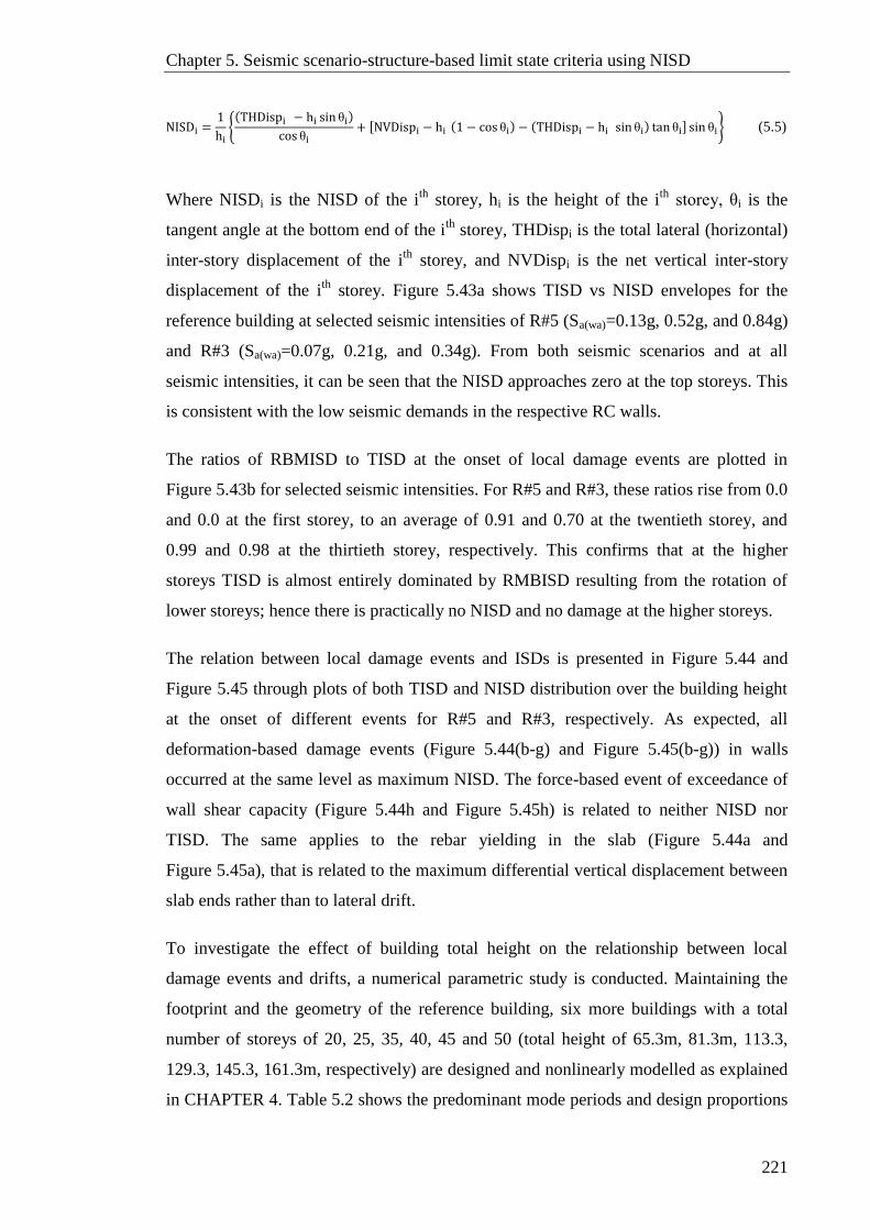
Chapter 5. Seismic scenario-structure-based limit state criteria using NISD
221
NISDi =1
hi{(THDispi − hi sin θi)
cos θi+ [NVDispi − hi (1 − cos θi) − (THDispi − hi sin θi) tan θi] sin θi} (5.5)
Where NISDi is the NISD of the ith
storey, hi is the height of the ith
storey, θi is the
tangent angle at the bottom end of the ith
storey, THDispi is the total lateral (horizontal)
inter-story displacement of the ith
storey, and NVDispi is the net vertical inter-story
displacement of the ith
storey. Figure 5.43a shows TISD vs NISD envelopes for the
reference building at selected seismic intensities of R#5 (Sa(wa)=0.13g, 0.52g, and 0.84g)
and R#3 (Sa(wa)=0.07g, 0.21g, and 0.34g). From both seismic scenarios and at all
seismic intensities, it can be seen that the NISD approaches zero at the top storeys. This
is consistent with the low seismic demands in the respective RC walls.
The ratios of RBMISD to TISD at the onset of local damage events are plotted in
Figure 5.43b for selected seismic intensities. For R#5 and R#3, these ratios rise from 0.0
and 0.0 at the first storey, to an average of 0.91 and 0.70 at the twentieth storey, and
0.99 and 0.98 at the thirtieth storey, respectively. This confirms that at the higher
storeys TISD is almost entirely dominated by RMBISD resulting from the rotation of
lower storeys; hence there is practically no NISD and no damage at the higher storeys.
The relation between local damage events and ISDs is presented in Figure 5.44 and
Figure 5.45 through plots of both TISD and NISD distribution over the building height
at the onset of different events for R#5 and R#3, respectively. As expected, all
deformation-based damage events (Figure 5.44(b-g) and Figure 5.45(b-g)) in walls
occurred at the same level as maximum NISD. The force-based event of exceedance of
wall shear capacity (Figure 5.44h and Figure 5.45h) is related to neither NISD nor
TISD. The same applies to the rebar yielding in the slab (Figure 5.44a and
Figure 5.45a), that is related to the maximum differential vertical displacement between
slab ends rather than to lateral drift.
To investigate the effect of building total height on the relationship between local
damage events and drifts, a numerical parametric study is conducted. Maintaining the
footprint and the geometry of the reference building, six more buildings with a total
number of storeys of 20, 25, 35, 40, 45 and 50 (total height of 65.3m, 81.3m, 113.3,
129.3, 145.3, 161.3m, respectively) are designed and nonlinearly modelled as explained
in CHAPTER 4. Table 5.2 shows the predominant mode periods and design proportions

Chapter 5. Seismic scenario-structure-based limit state criteria using NISD
222
of the six additional buildings, while Figure 5.46 and Figure 5.47 depict NISD and
TISD at the onset of local damage events against building total height when subjected to
R#5 and R#3, respectively. Under R#5, nearly all events, except the exceedance of wall
shear capacity occur at a similar NISD for all building heights. The NISD results under
R#3 show higher variability and this can be attributed again to the bigger impact of
higher modes on the response of such buildings to moderate near-field earthquakes.
TISD can be responsible for non-structural damage in tall buildings and inconvenience
to the occupants, hence is important at least when evaluating the performance of high-
rise buildings at serviceability level. However, the above discussion confirms the
superiority of NISD over TISD as a global DM for the vulnerability assessment of high-
rise buildings due to its structural significance, its correlation with local response and its
consistency in buildings with varying heights. Thus, it is decided to use the NISD as the
global DM in the present study.
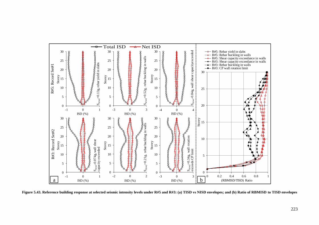
223
Figure 5.43. Reference building response at selected seismic intensity levels under R#5 and R#3: (a) TISD vs NISD envelopes; and (b) Ratio of RBMISD to TISD envelopes
0
5
10
15
20
25
30
-4 0 4
Sto
rey
ISD (%)
0
5
10
15
20
25
30
-3 0 3
Sto
rey
ISD (%)
0
5
10
15
20
25
30
-1 0 1
Sto
rey
ISD (%)
0
5
10
15
20
25
30
-3 0 3
Sto
rey
ISD (%)
0
5
10
15
20
25
30
-2 0 2
Sto
rey
ISD (%)
0
5
10
15
20
25
30
-1 0 1
Sto
rey
ISD (%)
R#5:
Rec
ord
Set
#1
Sa(
wa)
=0
.13
g, r
ebar
yie
ld i
n s
labs
Sa(w
a)=
0.5
2g,
rebar
buckli
ng i
n w
alls
Sa(
wa
)=0
.84
g, w
all
shear
cap
acit
yexceeded
0
5
10
15
20
25
30
0 0.2 0.4 0.6 0.8 1
Sto
rey
(RBMISD/TISD) Ratio
R#5: Rebar yield in slabsR#5: Rebar buckling in wallsR#5: Shear capacity exceedance in wallsR#3: Shear capacity exceedance in wallsR#3: Rebar buckling in wallsR#3: CP wall rotation limit
R#3
: R
ecord
Set
#2
0
5
10
15
20
25
30
-1 0 1
Sto
ry
ISD (%)
Total ISD Net ISD
Sa(
wa
)=0
.07
4g, w
all
shear
cap
acit
y e
xceeded
Sa(
wa)
=0
.21
g,
rebar
buckli
ng i
n w
alls
Sa(
wa)
=0
.34
g,
wal
lro
tati
on
exceeds
CP
lim
it
a b
(a) (b)
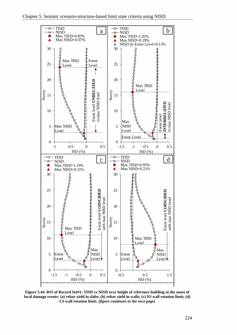
Chapter 5. Seismic scenario-structure-based limit state criteria using NISD
224
Figure 5.44. R#5 of Record Set#1: TISD vs NISD over height of reference building at the onset of
local damage events: (a) rebar yield in slabs; (b) rebar yield in walls; (c) IO wall rotation limit; (d)
LS wall rotation limit; (figure continues in the next page)
0
5
10
15
20
25
30
-1 -0.5 0 0.5
Sto
rey
ISD (%)
TISDNISDMax TISD=0.83%Max NISD=0.07%
Max TISDLevel
EventLevel
Max NISDLevel
a
Eve
nt
leve
lU
NR
EL
AT
ED
to m
ax N
ISD
leve
l
0
5
10
15
20
25
30
-1.5 -1 -0.5 0 0.5
Sto
rey
ISD (%)
TISDNISDMax TISD=1.02%Max NISD=0.19%NISD @ Event Level=0.13%
Max TISDLevel
Event Level
Max NISDLevel E
vent
leve
lIN
TE
RR
EL
AT
ED
to m
ax N
ISD
leve
l
b
0
5
10
15
20
25
30
-0.5 0.5 1.5
Sto
rey
ISD (%)
TISDNISDMax TISD=0.93%Max NISD=0.21%
0
5
10
15
20
25
30
-1.5 -1 -0.5 0 0.5
Sto
rey
ISD (%)
TISDNISDMax TISD=1.19%Max NISD=0.21%
Max TISDLevel
EventLevel
Max NISDLevel
Max TISDLevel
EventLevel
Max NISDLevel
Eve
nt
leve
lC
OIN
CID
ED
wit
h m
ax N
ISD
leve
l
Eve
nt
leve
lC
OIN
CID
ED
wit
h m
ax N
ISD
leve
l
c d
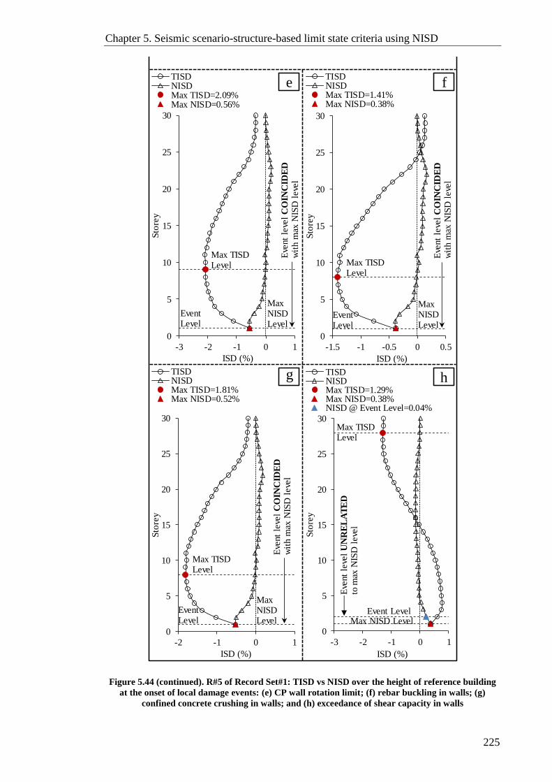
Chapter 5. Seismic scenario-structure-based limit state criteria using NISD
225
Figure 5.44 (continued). R#5 of Record Set#1: TISD vs NISD over the height of reference building
at the onset of local damage events: (e) CP wall rotation limit; (f) rebar buckling in walls; (g)
confined concrete crushing in walls; and (h) exceedance of shear capacity in walls
0
5
10
15
20
25
30
-1.5 -1 -0.5 0 0.5
Sto
rey
ISD (%)
TISDNISDMax TISD=1.41%Max NISD=0.38%
0
5
10
15
20
25
30
-3 -2 -1 0 1
Sto
rey
ISD (%)
TISDNISDMax TISD=2.09%Max NISD=0.56%
Max TISDLevel
EventLevel
Max NISDLevel
Eve
nt
leve
lC
OIN
CID
ED
wit
h m
ax N
ISD
leve
l
Max TISDLevel
EventLevel
Max NISDLevel
Eve
nt
leve
lC
OIN
CID
ED
wit
h m
ax N
ISD
leve
l
e f
0
5
10
15
20
25
30
-2 -1 0 1
Sto
rey
ISD (%)
TISDNISDMax TISD=1.81%Max NISD=0.52%
0
5
10
15
20
25
30
-3 -2 -1 0 1
Sto
rey
ISD (%)
TISDNISDMax TISD=1.29%Max NISD=0.38%NISD @ Event Level=0.04%
Max TISDLevel
EventLevel
Max NISDLevel
Max TISDLevel
Event LevelMax NISD Level
Eve
nt
leve
lC
OIN
CID
ED
wit
h m
ax N
ISD
leve
l
Eve
nt
leve
lU
NR
EL
AT
ED
to m
ax N
ISD
leve
l
g h

Chapter 5. Seismic scenario-structure-based limit state criteria using NISD
226
Figure 5.45. R#3 of Record Set#2: TISD vs NISD over height of reference building at the onset of
local damage events: (a) rebar yield in slabs; (b) rebar yield in walls; (c) IO wall rotation limit; (d)
LS wall rotation limit; (figure continues in the next page)
0
5
10
15
20
25
30
-1 -0.5 0 0.5
Sto
rey
ISD (%)
TISDNISDMax TISD=0.86%Max NISD=0.15%NISD @ Event Level=0.14%
0
5
10
15
20
25
30
-0.2 -0.1 0 0.1 0.2
Sto
rey
ISD (%)
TISDNISDMax TISD=0.18%Max NISD=0.11%NISD @ Event Level=0.006%
Max TISDLevel
EventLevel
Max NISDLevel
Max TISDLevel
EventLevel
Max NISDLevel
Eve
nt
leve
lU
NR
EL
AT
ED
to m
ax N
ISD
leve
l
Eve
nt
leve
lIN
TE
RR
EL
AT
ED
to m
ax N
ISD
leve
l
0
5
10
15
20
25
30
-2 -1 0 1 2
Sto
rey
ISD (%)
TISDNISDMax TISD=1.12%Max NISD=0.50%
0
5
10
15
20
25
30
-1 -0.5 0 0.5
Sto
rey
ISD (%)
TISDNISDMax TISD=0.89%Max NISD=0.14%NISD @ Event Level=0.14%
Max TISDLevel
Max NISDLevelEvent
Level
Max TISDLevelMax
NISDLevel
EventLevel
Eve
nt
leve
lIN
TE
RR
EL
AT
ED
to m
ax N
ISD
leve
l
Eve
nt
leve
lC
OIN
CID
ED
wit
h m
ax N
ISD
leve
l
a b
c d
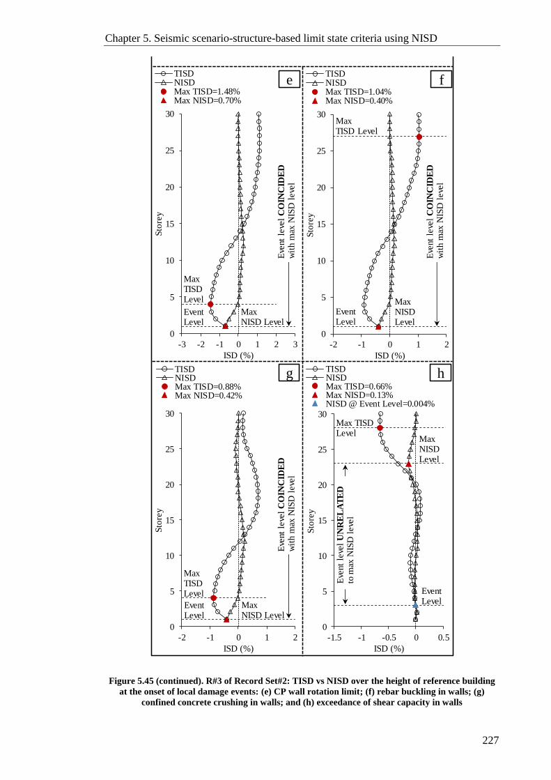
Chapter 5. Seismic scenario-structure-based limit state criteria using NISD
227
Figure 5.45 (continued). R#3 of Record Set#2: TISD vs NISD over the height of reference building
at the onset of local damage events: (e) CP wall rotation limit; (f) rebar buckling in walls; (g)
confined concrete crushing in walls; and (h) exceedance of shear capacity in walls
0
5
10
15
20
25
30
-2 -1 0 1 2
Sto
rey
ISD (%)
TISDNISDMax TISD=1.04%Max NISD=0.40%
0
5
10
15
20
25
30
-3 -2 -1 0 1 2 3
Sto
rey
ISD (%)
TISDNISDMax TISD=1.48%Max NISD=0.70%
Max TISDLevel
Max TISD Level
EventLevel
Max NISD Level
Max NISDLevel
EventLevel
Eve
nt
leve
lC
OIN
CID
ED
wit
h m
ax N
ISD
leve
l
Eve
nt
leve
lC
OIN
CID
ED
wit
h m
ax N
ISD
leve
l
e f
0
5
10
15
20
25
30
-1.5 -1 -0.5 0 0.5
Sto
rey
ISD (%)
TISDNISDMax TISD=0.66%Max NISD=0.13%NISD @ Event Level=0.004%
0
5
10
15
20
25
30
-2 -1 0 1 2
Sto
rey
ISD (%)
TISDNISDMax TISD=0.88%Max NISD=0.42%
Max TISDLevel
Max NISD Level
EventLevel
Max TISDLevel
Max NISD Level
EventLevel
Eve
nt
leve
lC
OIN
CID
ED
wit
h m
ax N
ISD
leve
l
Eve
nt
leve
lU
NR
EL
AT
ED
to m
ax N
ISD
leve
l
g h

228
Table 5.2. Predominant mode periods and design proportions of the six additional buildings for the parametric study
Building Mode periods in the transverse direction (s) Member Proportion Storey
1-5 6-10 11-15 16-20 21-25 26-30 31-35 36-40 41-45 46-50
20-Stories
Uncracked Equivalent inelastic
Core 1
Thickness 225 225 200 200
fc’ 40 40 40 40
1st 1.83 1st 2.29 V. Reinf. 2.30 1.00 1.00 0.80
H. Reinf. 0.80 0.91 0.74 0.61
2nd 0.42 2nd 0.47
Pier 1
Thickness 275 250 225 200
fc’ 40 40 40 40
3rd 0.17 3rd 0.19 V. Reinf. 0.87 0.75 0.90 1.86
H. Reinf. 0.25 0.25 0.28 0.25
25-Stories
Uncracked Equivalent inelastic
Core 1
Thickness 225 225 200 200 200
fc’ 40 40 40 40 40
1st 2.45 1st 3.29 V. Reinf. 2.15 1.00 1.00 0.85 0.76
H. Reinf. 1.08 0.92 0.82 0.63 0.63
2nd 0.60 2nd 0.69
Pier 1
Thickness 300 275 250 225 200
fc’ 40 40 40 40 40
3rd 0.26 3rd 0.28 V. Reinf. 2.43 0.62 0.89 0.93 2.01
H. Reinf. 0.25 0.25 0.25 0.25 0.25
35-Stories
Uncracked Equivalent inelastic
Core 1
Thickness 300 300 300 250 250 200 200
fc’ 40 40 40 40 40 40 40
1st 3.71 1st 5.16 V. Reinf. 4.56 1.24 1.16 1.00 1.00 0.80 0.68
H. Reinf. 0.83 0.67 0.54 0.54 0.54 0.61 0.66
2nd 0.95 2nd 1.12
Pier 1
Thickness 450 425 400 375 350 325 300
fc’ 40 40 40 40 40 40 40
3rd 0.37 3rd 0.44 V. Reinf. 5.85 4.31 4.09 2.67 1.54 0.95 1.38
H. Reinf. 0.25 0.25 0.25 0.25 0.25 0.25 0.25
Concretecompressivestrength(fc’)isinMPa;“Pier1”lengthis4000mm,allreinforcementisgivenin(%);alldimensionsare in mm.

229
Table 5.2 (continued). Predominant mode periods and design proportions of the six additional buildings for the parametric study
Building Mode periods in the
transverse direction (s) Member Proportion
Storey
1-5 6-10 11-15 16-20 21-25 26-30 31-35 36-40 41-45 46-50
40-Stories
Uncracked Equivalent
inelastic Core 1
Thickness 375 375 375 325 325 325 275 275
fc’ 48 48 48 48 48 48 48 48
1st 4.23 1st 5.96 V. Reinf. 5.48 2.31 2.52 1.00 1.00 0.69 0.62 0.49
H. Reinf. 0.74 0.58 0.46 0.49 0.49 0.47 0.45 0.50
2nd 1.08 2nd 1.29
Pier 1
Thickness 600 575 550 525 500 450 425 400
fc’ 48 48 48 48 48 48 48 48
3rd 0.42 3rd 0.50 V. Reinf. 6.50 5.18 5.01 3.64 2.65 1.57 0.55 0.83
H. Reinf. 0.25 0.25 0.25 0.25 0.25 0.25 0.25 0.25
45-Stories
Uncracked Equivalent
inelastic Core 1
Thickness 475 475 475 475 425 425 425 375 375
fc’ 48 48 48 48 48 48 48 48 48
1st 4.92 1st 6.94 V. Reinf. 5.97 3.06 3.41 2.17 1.49 1.00 0.32 0.41 0.26
H. Reinf. 0.63 0.58 0.42 0.40 0.48 0.44 0.35 0.38 0.43
2nd 1.19 2nd 1.48
Pier 1
Thickness 700 675 650 625 600 575 550 525 500
fc’ 48 48 48 48 48 48 48 48 48
3rd 0.47 3rd 0.57 V. Reinf. 7.05 6.12 6.08 4.80 3.78 2.78 0.75 0.73 1.01
H. Reinf. 0.25 0.25 0.25 0.25 0.25 0.25 0.25 0.25 0.25
50-Stories
Uncracked Equivalent
inelastic Core 1
Thickness 600 600 600 600 525 525 525 525 450 450
fc’ 48 48 48 48 48 48 48 48 48 48
1st 5.63 1st 8.00 V. Reinf. 6.89 4.36 4.19 3.06 2.48 1.47 1.00 0.41 0.58 0.25
H. Reinf. 0.65 0.67 0.45 0.42 0.49 0.48 0.40 0.34 0.35 0.45
2nd 1.32 2nd 1.70
Pier 1
Thickness 850 825 800 775 750 725 700 650 600 550
fc’ 48 48 48 48 48 48 48 48 48 48
3rd 0.54 3rd 0.66 V. Reinf. 7.25 6.52 6.58 5.57 4.54 3.57 0.61 0.45 0.42 1.86
H. Reinf. 0.25 0.25 0.25 0.25 0.25 0.25 0.25 0.25 0.25 0.25
Concretecompressivestrength(fc’)isinMPa;“Pier1”lengthis4000mm,allreinforcementisgivenin(%);alldimensionsare in mm.

230
Figure 5.46. R#5 of Record Set#1: Global response of buildings with different heights at seismic intensity levels corresponded to the onset of damage events: (a) TISD; and
(b) NISD
Figure 5.47. R#3 of Record Set#2: Global response of buildings with different heights at seismic intensity levels corresponded to the onset of damage events: (a) TISD; and
(b) NISD
60
90
120
150
180
0 0.5 1 1.5 2 2.5 3 3.5
Bui
ldin
g T
ota
l H
eigh
t (m
)
TISD (%)
R#5: Record Set#1
60
90
120
150
180
0 0.5 1 1.5 2 2.5 3 3.5
Bui
ldin
g T
ota
l H
eigh
t (m
)
NISD (%)
Rebar yield in slabsRebar yield in wallsIO wall rotation limitLS wall rotation limitCP wall rotation limitRebar buckling in wallsConcrete crushing in wallsWall shear capacity exceedance
R#5: Record Set#1
a b
60
90
120
150
180
0 0.5 1 1.5 2 2.5 3 3.5
Buil
din
g T
ota
l T
eight
(m)
TISD (%)
R#3: Record Set#2
60
90
120
150
180
0 0.5 1 1.5 2 2.5 3 3.5
Buil
din
g T
ota
l H
eight
(m)
NISD (%)
Rebar yield in slabsRebar yield in wallsIO wall rotation limitLS wall rotation limitCP wall rotation limitRebar buckling in wallsConcrete crushing in wallsWall shear capacity exceedance
R#3: Record Set#2
a b

Chapter 5. Seismic scenario-structure-based limit state criteria using NISD
231
5.6 Definition of performance limit state criteria
The three commonly used performance levels (IO, LS, and CP) are adopted in the
present study. New SSSB limit state criteria are proposed using the MRIDAs results
from the 40 selected records and the mapping/linking of predefined local damage
discussed in Sections 5.3 and 5.5 of this chapter. Table 5.3 summarises the conceptual
definitions of the proposed limit state criteria, while Figure 5.48 and Figure 5.49 depict
the 50% fractile of the NISDs related to selected local damage events (or combination
of events) in the reference building under R#5 and R#3, respectively. The proposed
limit state criteria associated with the two investigated seismic scenarios are discussed
in the succeeding sub-sections.
Table 5.3. Conceptual definitions of adopted limit state criteria for the reference building
Limit State Wall response Definition
Immediate Occupancy (IO)
Wall response controlled by flexure
The onset of the first yield of reinforcing steel in all vertical/horizontal elements or the (IO) ASCE/SEI 41-06 rotation limits in shear walls/core system/coupling beams, whichever comes first.
Wall response controlled by shear
NISD corresponding to values in Table 6-19 (ASCE/SEI 41-06).
Life
Safety (LS)
Wall response controlled by flexure
The onset of the (LS) ASCE/SEI 41-06 rotation limits in shear walls/core system/coupling beams or 50% of CP-related NISD from all deformation-based DIs combined, whichever comes first.
Wall response controlled by shear
NISD corresponding to values in Table 6-19 (ASCE/SEI 41-06).
Collapse Prevention (CP)
Wall response controlled by flexure
The onset of buckling/fracture of reinforcing steel, crushing of concrete core, the (CP) ASCE/SEI 41-06 rotation limits in shear walls/core system/coupling beams or the exceedance of shear capacity in shear walls/core system, whichever comes first.
Wall response controlled by shear
The onset of exceedance of shear capacity in shear walls/core system or NISD corresponding to values in Table 6-19 (ASCE/SEI 41-06), whichever comes first.
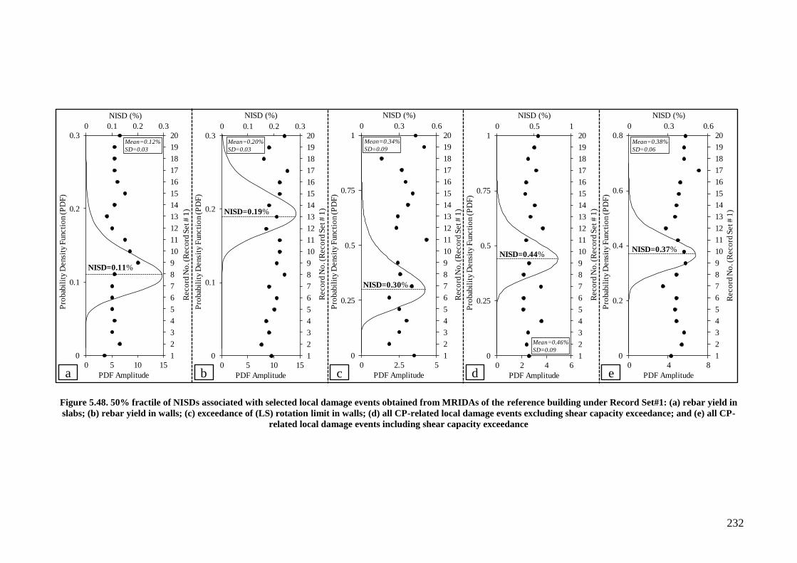
232
Figure 5.48. 50% fractile of NISDs associated with selected local damage events obtained from MRIDAs of the reference building under Record Set#1: (a) rebar yield in
slabs; (b) rebar yield in walls; (c) exceedance of (LS) rotation limit in walls; (d) all CP-related local damage events excluding shear capacity exceedance; and (e) all CP-
related local damage events including shear capacity exceedance
0 0.1 0.2 0.3
1
2
3
4
5
6
7
8
9
10
11
12
13
14
15
16
17
18
19
20
0
0.1
0.2
0.3
0 5 10 15
Reco
rd N
o. (
Reco
rd S
et #
1)
Pro
bab
ilit
y D
ensi
ty F
uncti
on (
PD
F)
PDF Amplitude
NISD (%)
0 0.3 0.6
1
2
3
4
5
6
7
8
9
10
11
12
13
14
15
16
17
18
19
20
0
0.25
0.5
0.75
1
0 2.5 5
NISD (%)
Reco
rd N
o. (
Reco
rd S
et #
1)
Pro
bab
ilit
y D
ensi
ty F
uncti
on (
PD
F)
PDF Amplitude
0 0.3 0.6
1
2
3
4
5
6
7
8
9
10
11
12
13
14
15
16
17
18
19
20
0
0.2
0.4
0.6
0.8
0 4 8
NISD (%)
Reco
rd N
o. (
Reco
rd S
et #
1)
Pro
bab
ilit
y D
ensi
ty F
uncti
on (
PD
F)
PDF Amplitude
0 0.5 1
1
2
3
4
5
6
7
8
9
10
11
12
13
14
15
16
17
18
19
20
0
0.25
0.5
0.75
1
0 2 4 6
NISD (%)
Reco
rd N
o. (
Reco
rd S
et #
1)
Pro
bab
ilit
y D
ensi
ty F
uncti
on (
PD
F)
PDF Amplitude
0 0.1 0.2 0.3
1
2
3
4
5
6
7
8
9
10
11
12
13
14
15
16
17
18
19
20
0
0.1
0.2
0.3
0 5 10 15
NISD (%)
Reco
rd N
o. (
Reco
rd S
et #
1)
Pro
bab
ilit
y D
ensi
ty F
uncti
on (
PD
F)
PDF Amplitude
NISD=0.11%
NISD=0.19%
NISD=0.30%
NISD=0.44%NISD=0.37%
a b c d e
Mean=0.12%
SD=0.03
Mean=0.20%
SD=0.03
Mean=0.34%
SD=0.09
Mean=0.46%
SD=0.09
Mean=0.38%
SD=0.06
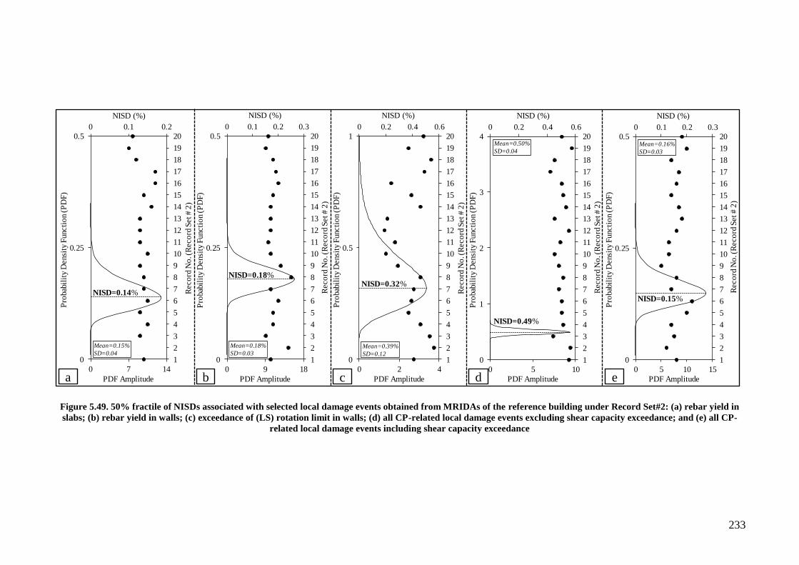
233
Figure 5.49. 50% fractile of NISDs associated with selected local damage events obtained from MRIDAs of the reference building under Record Set#2: (a) rebar yield in
slabs; (b) rebar yield in walls; (c) exceedance of (LS) rotation limit in walls; (d) all CP-related local damage events excluding shear capacity exceedance; and (e) all CP-
related local damage events including shear capacity exceedance
0 0.2 0.4 0.6
1
2
3
4
5
6
7
8
9
10
11
12
13
14
15
16
17
18
19
20
0
0.5
1
0 2 4
NISD (%)
Reco
rd N
o. (
Reco
rd S
et #
2)
Pro
bab
ilit
y D
ensi
ty F
uncti
on (
PD
F)
PDF Amplitude
0 0.1 0.2 0.3
1
2
3
4
5
6
7
8
9
10
11
12
13
14
15
16
17
18
19
20
0
0.25
0.5
0 5 10 15
NISD (%)
Reco
rd N
o. (
Reco
rd S
et #
2)
Pro
bab
ilit
y D
ensi
ty F
uncti
on (
PD
F)
PDF Amplitude
0 0.2 0.4 0.6
1
2
3
4
5
6
7
8
9
10
11
12
13
14
15
16
17
18
19
20
0
1
2
3
4
0 5 10
NISD (%)
Reco
rd N
o. (
Reco
rd S
et #
2)
Pro
bab
ilit
y D
ensi
ty F
uncti
on (
PD
F)
PDF Amplitude
0 0.1 0.2 0.3
1
2
3
4
5
6
7
8
9
10
11
12
13
14
15
16
17
18
19
20
0
0.25
0.5
0 9 18
NISD (%)
Reco
rd N
o. (
Reco
rd S
et #
2)
Pro
bab
ilit
y D
ensi
ty F
uncti
on (
PD
F)
PDF Amplitude
0 0.1 0.2
1
2
3
4
5
6
7
8
9
10
11
12
13
14
15
16
17
18
19
20
0
0.25
0.5
0 7 14
Reco
rd N
o. (
Reco
rd S
et #
2)
Pro
bab
ilit
y D
ensi
ty F
uncti
on (
PD
F)
PDF Amplitude
NISD (%)
NISD=0.14%
NISD=0.18%NISD=0.32%
NISD=0.49%
NISD=0.15%
Mean=0.15%
SD=0.04
Mean=0.18%
SD=0.03Mean=0.39%
SD=0.12
Mean=0.50%
SD=0.04Mean=0.16%
SD=0.03
a b c d e
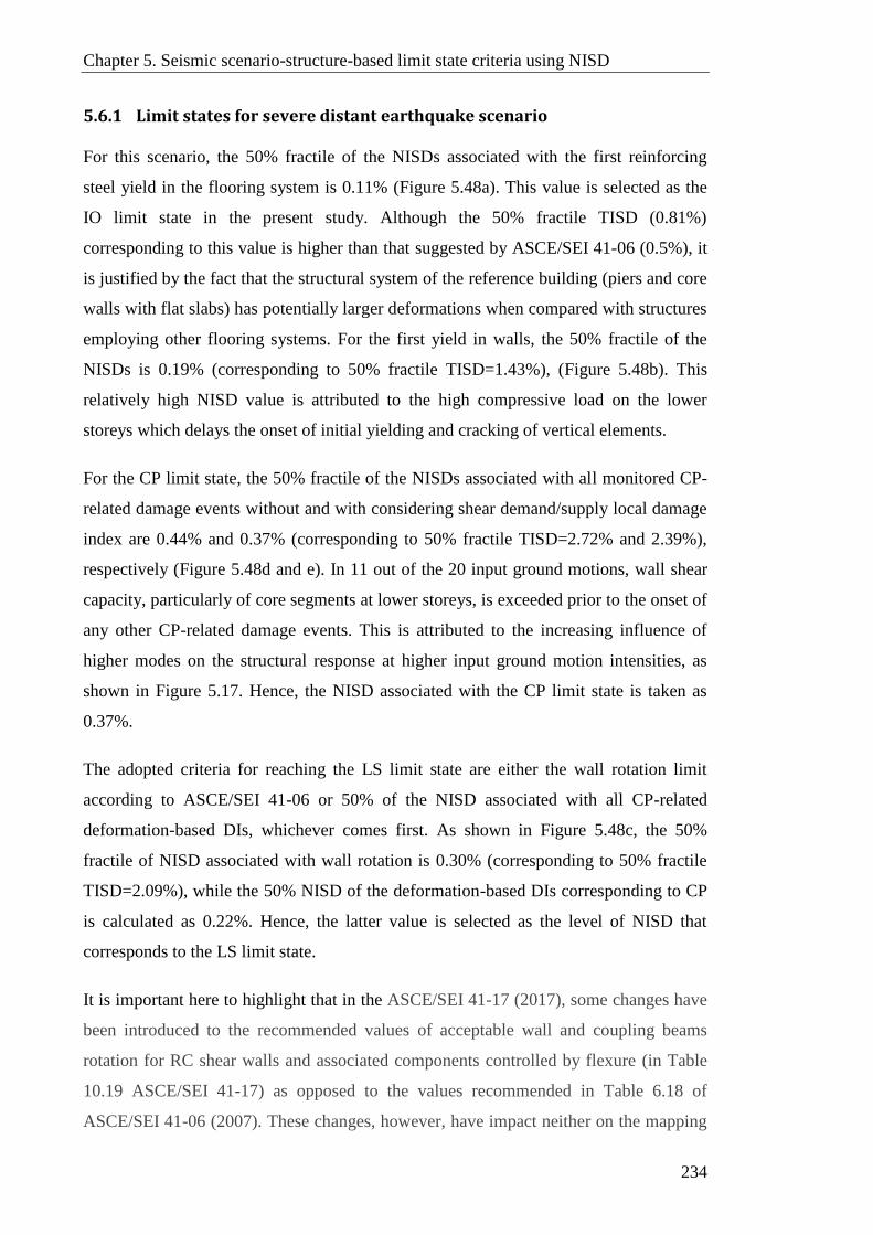
Chapter 5. Seismic scenario-structure-based limit state criteria using NISD
234
5.6.1 Limit states for severe distant earthquake scenario
For this scenario, the 50% fractile of the NISDs associated with the first reinforcing
steel yield in the flooring system is 0.11% (Figure 5.48a). This value is selected as the
IO limit state in the present study. Although the 50% fractile TISD (0.81%)
corresponding to this value is higher than that suggested by ASCE/SEI 41-06 (0.5%), it
is justified by the fact that the structural system of the reference building (piers and core
walls with flat slabs) has potentially larger deformations when compared with structures
employing other flooring systems. For the first yield in walls, the 50% fractile of the
NISDs is 0.19% (corresponding to 50% fractile TISD=1.43%), (Figure 5.48b). This
relatively high NISD value is attributed to the high compressive load on the lower
storeys which delays the onset of initial yielding and cracking of vertical elements.
For the CP limit state, the 50% fractile of the NISDs associated with all monitored CP-
related damage events without and with considering shear demand/supply local damage
index are 0.44% and 0.37% (corresponding to 50% fractile TISD=2.72% and 2.39%),
respectively (Figure 5.48d and e). In 11 out of the 20 input ground motions, wall shear
capacity, particularly of core segments at lower storeys, is exceeded prior to the onset of
any other CP-related damage events. This is attributed to the increasing influence of
higher modes on the structural response at higher input ground motion intensities, as
shown in Figure 5.17. Hence, the NISD associated with the CP limit state is taken as
0.37%.
The adopted criteria for reaching the LS limit state are either the wall rotation limit
according to ASCE/SEI 41-06 or 50% of the NISD associated with all CP-related
deformation-based DIs, whichever comes first. As shown in Figure 5.48c, the 50%
fractile of NISD associated with wall rotation is 0.30% (corresponding to 50% fractile
TISD=2.09%), while the 50% NISD of the deformation-based DIs corresponding to CP
is calculated as 0.22%. Hence, the latter value is selected as the level of NISD that
corresponds to the LS limit state.
It is important here to highlight that in the ASCE/SEI 41-17 (2017), some changes have
been introduced to the recommended values of acceptable wall and coupling beams
rotation for RC shear walls and associated components controlled by flexure (in Table
10.19 ASCE/SEI 41-17) as opposed to the values recommended in Table 6.18 of
ASCE/SEI 41-06 (2007). These changes, however, have impact neither on the mapping
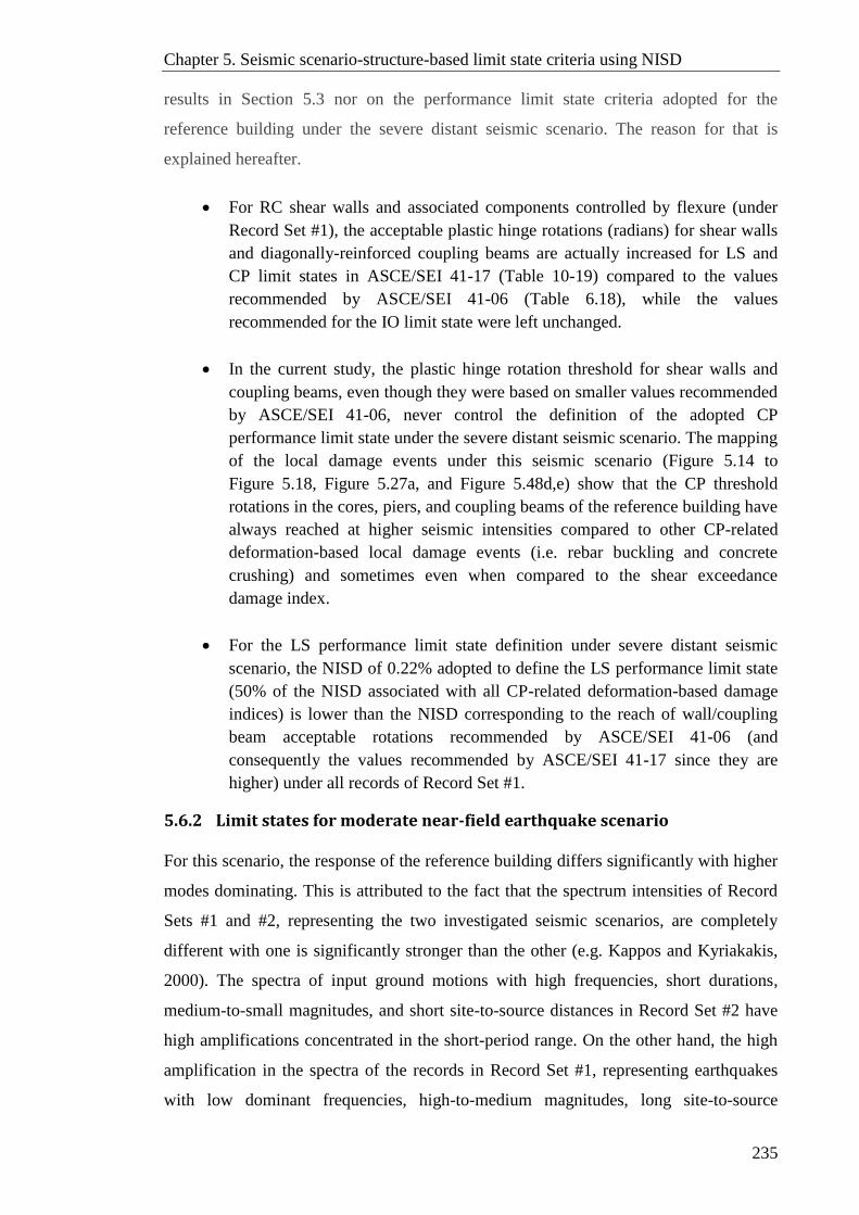
Chapter 5. Seismic scenario-structure-based limit state criteria using NISD
235
results in Section 5.3 nor on the performance limit state criteria adopted for the
reference building under the severe distant seismic scenario. The reason for that is
explained hereafter.
For RC shear walls and associated components controlled by flexure (under
Record Set #1), the acceptable plastic hinge rotations (radians) for shear walls
and diagonally-reinforced coupling beams are actually increased for LS and
CP limit states in ASCE/SEI 41-17 (Table 10-19) compared to the values
recommended by ASCE/SEI 41-06 (Table 6.18), while the values
recommended for the IO limit state were left unchanged.
In the current study, the plastic hinge rotation threshold for shear walls and
coupling beams, even though they were based on smaller values recommended
by ASCE/SEI 41-06, never control the definition of the adopted CP
performance limit state under the severe distant seismic scenario. The mapping
of the local damage events under this seismic scenario (Figure 5.14 to
Figure 5.18, Figure 5.27a, and Figure 5.48d,e) show that the CP threshold
rotations in the cores, piers, and coupling beams of the reference building have
always reached at higher seismic intensities compared to other CP-related
deformation-based local damage events (i.e. rebar buckling and concrete
crushing) and sometimes even when compared to the shear exceedance
damage index.
For the LS performance limit state definition under severe distant seismic
scenario, the NISD of 0.22% adopted to define the LS performance limit state
(50% of the NISD associated with all CP-related deformation-based damage
indices) is lower than the NISD corresponding to the reach of wall/coupling
beam acceptable rotations recommended by ASCE/SEI 41-06 (and
consequently the values recommended by ASCE/SEI 41-17 since they are
higher) under all records of Record Set #1.
5.6.2 Limit states for moderate near-field earthquake scenario
For this scenario, the response of the reference building differs significantly with higher
modes dominating. This is attributed to the fact that the spectrum intensities of Record
Sets #1 and #2, representing the two investigated seismic scenarios, are completely
different with one is significantly stronger than the other (e.g. Kappos and Kyriakakis,
2000). The spectra of input ground motions with high frequencies, short durations,
medium-to-small magnitudes, and short site-to-source distances in Record Set #2 have
high amplifications concentrated in the short-period range. On the other hand, the high
amplification in the spectra of the records in Record Set #1, representing earthquakes
with low dominant frequencies, high-to-medium magnitudes, long site-to-source
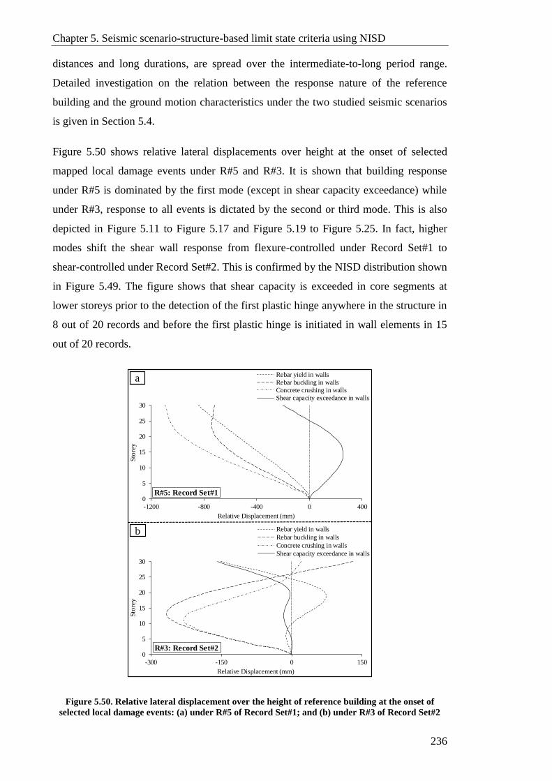
Chapter 5. Seismic scenario-structure-based limit state criteria using NISD
236
distances and long durations, are spread over the intermediate-to-long period range.
Detailed investigation on the relation between the response nature of the reference
building and the ground motion characteristics under the two studied seismic scenarios
is given in Section 5.4.
Figure 5.50 shows relative lateral displacements over height at the onset of selected
mapped local damage events under R#5 and R#3. It is shown that building response
under R#5 is dominated by the first mode (except in shear capacity exceedance) while
under R#3, response to all events is dictated by the second or third mode. This is also
depicted in Figure 5.11 to Figure 5.17 and Figure 5.19 to Figure 5.25. In fact, higher
modes shift the shear wall response from flexure-controlled under Record Set#1 to
shear-controlled under Record Set#2. This is confirmed by the NISD distribution shown
in Figure 5.49. The figure shows that shear capacity is exceeded in core segments at
lower storeys prior to the detection of the first plastic hinge anywhere in the structure in
8 out of 20 records and before the first plastic hinge is initiated in wall elements in 15
out of 20 records.
Figure 5.50. Relative lateral displacement over the height of reference building at the onset of
selected local damage events: (a) under R#5 of Record Set#1; and (b) under R#3 of Record Set#2
0
5
10
15
20
25
30
-1200 -800 -400 0 400
Sto
rey
Relative Displacement (mm)
Rebar yield in walls
Rebar buckling in walls
Concrete crushing in walls
Shear capacity exceedance in walls
0
5
10
15
20
25
30
-300 -150 0 150
Sto
rey
Relative Displacement (mm)
Rebar yield in walls
Rebar buckling in walls
Concrete crushing in walls
Shear capacity exceedance in walls
R#5: Record Set#1
R#3: Record Set#2
a
b

Chapter 5. Seismic scenario-structure-based limit state criteria using NISD
237
The same can also be concluded from the propagation of local damage events under
R#5 and R#3, shown in Figure 5.51. Under R#5, the building responds with rebar
yielding in the flooring system, followed by wall rebar yielding, rebar buckling,
concrete crushing, and finally with exceedance of shear capacity (Figure 5.51a).
Building response to R#3 (Figure 5.51b), on the other hand, differs as the exceedance of
shear capacity occurs at the same seismic intensity scale associated with rebar yielding
in walls and just after rebar yielding in the flooring system. As shown in Figure 5.49e,
the calculated 50% fractile NISD associated with the shear capacity damage index is
0.15%. This value corresponds to 50% fractile TISD=0.79%; a value close to the TISD
suggested by ASCE/SEI 41-06 for walls with shear-controlled response at CP (0.75%).
Figure 5.51. Propagation of local damage events in the reference building: (a) under R#5 of Record
Set#1; and (b) under R#3 of Record Set#2
0.0
0.4
0.9
1.3
1.8
0
0.3
0.6
0.9
1.2
0 0.25 0.5 0.75 1 1.25
PG
A (
g)
Sa(
wa)
, (g
)
NISD (%)
IDA curveRebar yield in slabsRebar yield in wallsRebar buckling in wallsConcrete crushing in wallsShear capacity exceedance in walls
0.0
2.3
4.5
6.8
9.1
11.4
13.6
0
0.1
0.2
0.3
0.4
0.5
0 0.25 0.5 0.75 1 1.25
PG
A (
g)
Sa(
wa)
, (g
)
NISD (%)
IDA curve
Rebar yield in slabs
Rebar yield in walls
Rebar buckling in walls
Concrete crushing in walls
Shear capacity exceedance in walls
R#5: Record Set#1
R#3: Record Set#2
a
b
Chapter 5. Seismic scenario-structure-based limit state criteria using NISD
238
To add to the above discussion, the bending moment and shear demand histories in the
core wall segments at the time bracketing the onset of exceeding the shear capacity
under R#5 and R#3 are plotted in Figure 5.52. Under R#5 (Figure 5.52a), the high
bending moment-to-shear ratio (M/V=1.72) corresponds to flexure-controlled
behaviour. On the other hand, the low bending moment-to-shear ratio (M/V=0.72)
under R#3 (Figure 5.52b) warrants the shear-controlled classification for the response of
the reference building.
Figure 5.52. Bending moment and shear force demand time histories in the core wall segments of
the reference building at the onset of shear capacity exceedance: (a) under R#5 of Record Set#1;
and (b) under R#3 of Record Set#2
As another way of analysing the seismic scenario-based shear response of the reference
building, the base shear at increasing seismic intensities is plotted in Figure 5.53 and
Figure 5.54. In Figure 5.53, the horizontal axes present the ground motion intensity in
-80
-40
0
40
80
14 14.5 15 15.5 16
Time (s)
Shear force demand history
Bending moment demand history
Bending moment=18.2MN-m
Shear force=10.6MN
Bendin
g M
om
ent &
Shear
Fo
rce D
em
ands
(MN
, m
)
-80
-40
0
40
80
4 4.5 5 5.5 6
Time (s)
Shear force demand history
Bending moment demand history
Bending moment=7.7 MN-m
Shear force=10.6 MN
Bendin
g M
om
ent &
Shear
Fo
rce D
em
ands
(MN
, m
)
R#5, Record Set#1, Sa(wa)=0.84g, PGA=1.25g: 2nd Storey: M/V=1.72
R#3, Record Set#2, Sa(wa)=0.074g, PGA=1.67g: 3rd Storey: M/V=0.72
@ 5
.055
s
@ 1
5.2
20
s
a
b
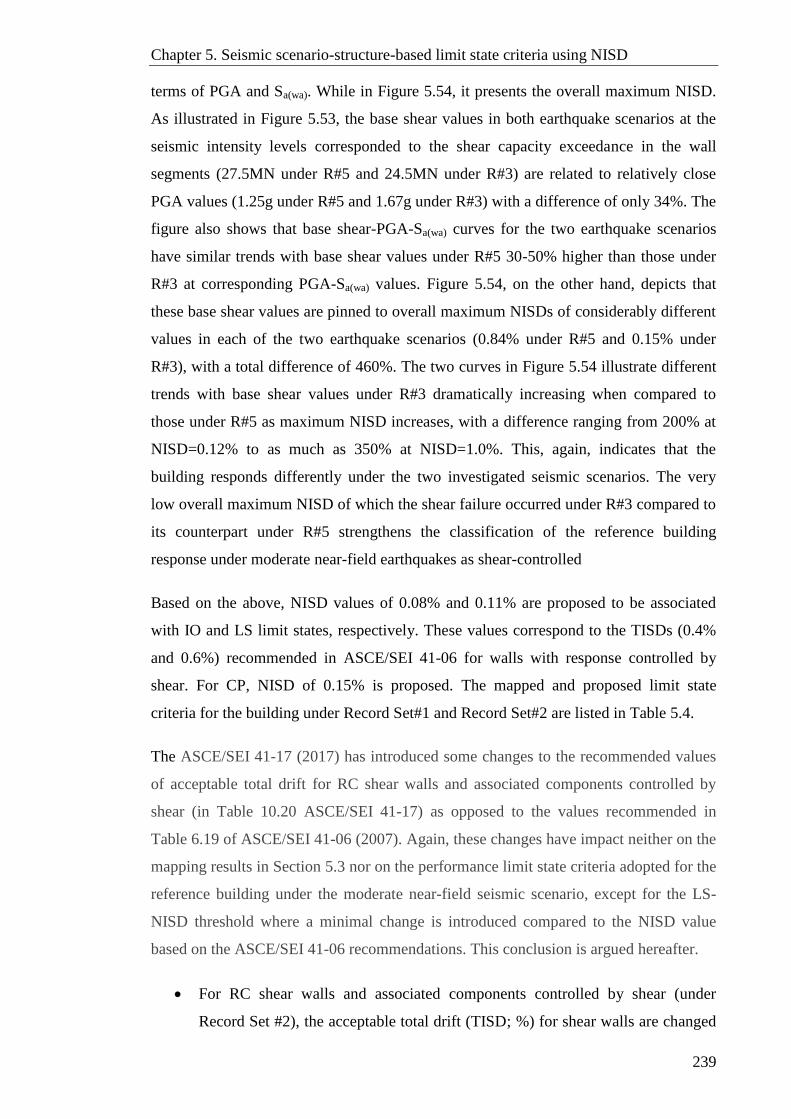
Chapter 5. Seismic scenario-structure-based limit state criteria using NISD
239
terms of PGA and Sa(wa). While in Figure 5.54, it presents the overall maximum NISD.
As illustrated in Figure 5.53, the base shear values in both earthquake scenarios at the
seismic intensity levels corresponded to the shear capacity exceedance in the wall
segments (27.5MN under R#5 and 24.5MN under R#3) are related to relatively close
PGA values (1.25g under R#5 and 1.67g under R#3) with a difference of only 34%. The
figure also shows that base shear-PGA-Sa(wa) curves for the two earthquake scenarios
have similar trends with base shear values under R#5 30-50% higher than those under
R#3 at corresponding PGA-Sa(wa) values. Figure 5.54, on the other hand, depicts that
these base shear values are pinned to overall maximum NISDs of considerably different
values in each of the two earthquake scenarios (0.84% under R#5 and 0.15% under
R#3), with a total difference of 460%. The two curves in Figure 5.54 illustrate different
trends with base shear values under R#3 dramatically increasing when compared to
those under R#5 as maximum NISD increases, with a difference ranging from 200% at
NISD=0.12% to as much as 350% at NISD=1.0%. This, again, indicates that the
building responds differently under the two investigated seismic scenarios. The very
low overall maximum NISD of which the shear failure occurred under R#3 compared to
its counterpart under R#5 strengthens the classification of the reference building
response under moderate near-field earthquakes as shear-controlled
Based on the above, NISD values of 0.08% and 0.11% are proposed to be associated
with IO and LS limit states, respectively. These values correspond to the TISDs (0.4%
and 0.6%) recommended in ASCE/SEI 41-06 for walls with response controlled by
shear. For CP, NISD of 0.15% is proposed. The mapped and proposed limit state
criteria for the building under Record Set#1 and Record Set#2 are listed in Table 5.4.
The ASCE/SEI 41-17 (2017) has introduced some changes to the recommended values
of acceptable total drift for RC shear walls and associated components controlled by
shear (in Table 10.20 ASCE/SEI 41-17) as opposed to the values recommended in
Table 6.19 of ASCE/SEI 41-06 (2007). Again, these changes have impact neither on the
mapping results in Section 5.3 nor on the performance limit state criteria adopted for the
reference building under the moderate near-field seismic scenario, except for the LS-
NISD threshold where a minimal change is introduced compared to the NISD value
based on the ASCE/SEI 41-06 recommendations. This conclusion is argued hereafter.
For RC shear walls and associated components controlled by shear (under
Record Set #2), the acceptable total drift (TISD; %) for shear walls are changed

Chapter 5. Seismic scenario-structure-based limit state criteria using NISD
240
in ASCE/SEI 41-17 (Table 10-20) to 0.75% and 1.00% (under axial force ratio >
0.05) for LS and CP limit states, respectively, compared to the 0.60% and 0.75%
values recommended by ASCE/SEI 41-06 (Table 6.19), while the values
recommended for the IO limit state were left unchanged (0.40%).
For the definition of the CP performance limit state criteria in the current study,
the drift value recommended by ASCE/SEI 41-06 is not been utilized. The NISD
value of 0.15% (corresponding to TISD = 0.79%) adopted in the definition of
the CP performance limit state under moderate near-field seismic scenario is
based on the mapping of all the adopted CP-related damage indices (Figure 5.22
to Figure 5.26, Figure 5.27b, and Figure 5.49d,e). It is important to emphasize
here that, due to the response nature of the reference building under moderate
near-field earthquakes, the CP limit state definition is controlled by the shear
exceedance damage index for all records in Record Set #2.
For the definition of the LS performance limit state criteria in the current study,
the NISD value of 0.11% adopted in the definition of the LS performance limit
state under moderate near-field seismic scenario corresponds to the TISD value
of 0.60% recommended by ASCE/SEI 41-06 (Table 6.19). The NISD value
corresponding to the new TISD of 0.75% recommended by ASCE/SEI 41-17
(Table 10-20) is 0.117%, that is only 6% higher. It is worth noting that due to
the rigid body motion component (RBM), a certain percentage of increase in the
TISD value renders a much small percentage of increase in the corresponding
NISD.

Chapter 5. Seismic scenario-structure-based limit state criteria using NISD
241
Figure 5.53. Reference building PGA and Sa(wa) vs base shear under R#5 of Record Set#1 and R#3
of Record Set#2 at different intensity levels
Figure 5.54. Reference building max NISD vs base shear under R#5 of Record Set#1 and R#3 of
Record Set#2 at different intensity levels
0.00 0.34 0.68 1.01 1.35
0
10
20
30
40
0 0.25 0.5 0.75 1 1.25 1.5 1.75 2
Bas
e S
hear
(B
S),
(M
N)
PGA (g)
R#5: Record Set#1R#3: Record Set#2
0.00 0.02 0.04 0.07 0.09
R#5: Sa(wa), (g)
R#3: Sa(wa), (g)
BS = 27.5MN
BS = 24.5MN
PG
A=
1.2
5g
PG
A=
1.6
7g
Sa(wa)=0.84g
Sa(wa)=0.074g
Difference=34%
0
20
40
60
80
100
0 0.2 0.4 0.6 0.8 1
Bas
e S
hear
(B
S),
(M
N)
Max. NISD (%)
R#5: Record Set#1R#3: Record Set#2
BS=27.5MN
BS=24.5MN
NISD=0.15% NISD=0.84%
Difference=460%
242
Table 5.4. Mapped and recommended limit state criteria for the reference building
Limit state Damage Index (DI)
NISD (%)
Record Set#1
(Far-field)
Record Set#2
(Near-field)
Mapped Proposed Mapped Proposed
IO
1st rebar yield in slabs 0.11
0.11
0.14
0.08
1st rebar yield in walls 0.19 0.18
Wall rotation limit (ASCE/SEI 41-06) 0.19 0.17
All IO-related deformation-based DIs (combined) 0.11 0.14
NISD corresponds to value in Table 6-19 of ASCE/SEI 41-06 for RC shear walls controlled by shear N/A 0.08
LS
Wall rotation (ASCE/SEI 41-06) 0.30
0.22
0.32
0.11 50% of NISD from all CP-related deformation-based DIs (combined) 0.22 0.25
NISD corresponding to the value in Table 6-19 of ASCE/SEI 41-06 for RC shear walls controlled by shear N/A 0.11
CP
1st rebar buckling in walls 0.44
0.37
0.49
0.15
1st concrete crushing in walls 0.59 0.67
Wall rotation (ASCE/SEI 41-06) 0.51 0.71
Shear capacity exceedance 0.37 0.15
All CP-related deformation-based DIs (combined) 0.44 0.49
All CP-related DIs inclusive of shear capacity (combined) 0.37 0.15
NISD corresponds to the value in Table 6-19 of ASCE/SEI 41-06 for RC shear walls controlled by shear N/A 0.14

Chapter 5. Seismic scenario-structure-based limit state criteria using NISD
243
5.7 Summary and concluding remarks
In this chapter, the methodology for proposing reliable Seismic Scenario-Structure-
Based (SSSB) definitions of performance limit state criteria for high-rise RC wall
buildings is illustrated on the 30-storey RC wall reference building located in Dubai
(study region). Multi-Record Incremental Dynamic Analyses (MRIDAs) with new
intensity measure are conducted to assess building local response to two different
seismic scenarios. Seismic scenario-based local damage events, presented with a range
of deformation and capacity-based damage indices (DIs), are mapped and linked to
building global response. The relation between those local DIs and the input ground
motion characteristics are also discussed. Finally, a new set of SSSB limit state criteria
is proposed for the reference structure.
A parametric study involving the reference 30-storey structure in addition to six other
buildings with different heights shows that, for such buildings, Net Inter-Storey Drift
(NISD) is better than Total Inter-Storey Drift (TISD) as a global damage measure (DM)
in defining limit state criteria. NISD is better linked with the local response over the
height of the building and well correlated to deformation-based local damage events for
buildings with varying heights. The study concludes that structural system, arrangement
and geometry of vertical elements, and axial force level in the lower storeys influence
the seismic intensity and deformation levels that are related to local damage events. It is
found that moderate near-field earthquake events can shift the seismic response from
flexure-controlled to shear-controlled. This leads to the conclusion that the response of
RC high-rise wall buildings and consequently the definition of limit state criteria for
designated performance levels are strongly influenced by both the structure and the
seismic scenario. As a result, new SSSB limit state criteria are proposed for RC high-
rise wall buildings with similar characteristics and subjected to similar seismic
scenarios.

244
This page is intentionally left in blank

245
CHAPTER 6. Fragility relations:
Development, assessment,
and simplified methodology
Chapter 6 contains four main sections. Section 6.1 involves the development of the
seismic scenario-based fragility relations for the reference building. This represents the
concluding step in the proposed framework for the seismic vulnerability assessment of
RC high-rise wall buildings (the reader is referred to the IPO model presented
in CHAPTER 2). In Section 6.2, the developed fragility relations are examined at
selected earthquake intensity levels to assess their accuracy. Furthermore, the
characteristics of the developed fragility relations under the two investigated seismic
scenarios are analysed and compared. 6.2 is concluded by correlating the developed
fragility relations with four states of damage in the reference building, that is
unimpaired occupancy, impaired occupancy, structural damage, and structural collapse.

Chapter 6. Fragility relations: Development, assessment, and simplified methodology
246
In Section 6.3, a simplified methodology towards developing fragility relations with less
computational effort is proposed. Utilising this methodology, the fragility curves of
reinforced concrete high-rise buildings can be generated with a much lower number of
input ground motions compared to the original number of records adopted in the current
study (i.e. twenty records in each set). Using a lower number of records results in a
dramatic reduction in time and effort, especially when a big building inventory is under
investigation. Accordingly, the fragility curves developed using this simplified
methodology are called hereafter Cheaper Fragility Curves (CFC). The chapter is
concluded with Section 6.4, where the summary and concluding remarks are presented.
6.1 Development of the fragility relations
In this section, seismic scenario-based fragility relations for the reference building are
developed. Furthermore, the efficiency of the proposed damage measure (NISD) is
investigated using the confidence interval relative width statistics. The fragility curves
are developed using the following equation (Wen et al., 2004):
POE(PLSi|IM) = 1 − φ
(
α(DM|PLSi) − α(DM|IM)
√β(DM|IM)2 + β(DM|PLSi)
2 + βm2
)
(6.1)
Where POE(PLSi|IM) is the probability of exceeding a predefined performance limit
state (PLSi) given the IM value, φ is the standard normal cumulative distribution
function, α(DM|PLSi) = ln (median of the DM capacity for PLSi), α(DM|IM) = ln (calculated
median demand DM given the IM value from the regression analysis best-fit power-law
line), and β(DM|IM), β(DM|PLSi), and β
m are demand, capacity, and modelling
uncertainties, respectively, given in the following equations:
β(DM|IM) = √ln(1 + s2) , s2 =∑(ln(Yk) − ln(Yp))
2
/(n − 2) (6.2)
β(DM|PLSi)= √ln(1 + cov2) (6.3)
βm= 0.2 to 0.4 (6.4)
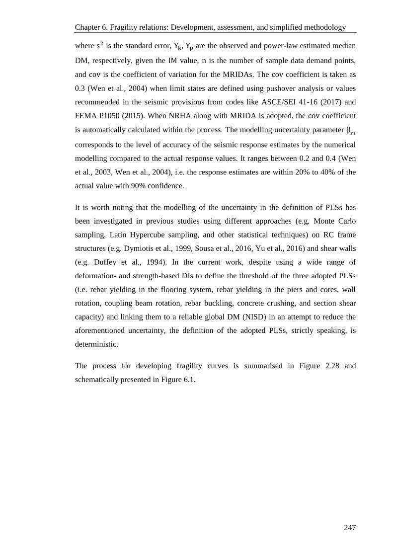
Chapter 6. Fragility relations: Development, assessment, and simplified methodology
247
where s2 is the standard error, Yk, Yp are the observed and power-law estimated median
DM, respectively, given the IM value, n is the number of sample data demand points,
and cov is the coefficient of variation for the MRIDAs. The cov coefficient is taken as
0.3 (Wen et al., 2004) when limit states are defined using pushover analysis or values
recommended in the seismic provisions from codes like ASCE/SEI 41-16 (2017) and
FEMA P1050 (2015). When NRHA along with MRIDA is adopted, the cov coefficient
is automatically calculated within the process. The modelling uncertainty parameter βm
corresponds to the level of accuracy of the seismic response estimates by the numerical
modelling compared to the actual response values. It ranges between 0.2 and 0.4 (Wen
et al., 2003, Wen et al., 2004), i.e. the response estimates are within 20% to 40% of the
actual value with 90% confidence.
It is worth noting that the modelling of the uncertainty in the definition of PLSs has
been investigated in previous studies using different approaches (e.g. Monte Carlo
sampling, Latin Hypercube sampling, and other statistical techniques) on RC frame
structures (e.g. Dymiotis et al., 1999, Sousa et al., 2016, Yu et al., 2016) and shear walls
(e.g. Duffey et al., 1994). In the current work, despite using a wide range of
deformation- and strength-based DIs to define the threshold of the three adopted PLSs
(i.e. rebar yielding in the flooring system, rebar yielding in the piers and cores, wall
rotation, coupling beam rotation, rebar buckling, concrete crushing, and section shear
capacity) and linking them to a reliable global DM (NISD) in an attempt to reduce the
aforementioned uncertainty, the definition of the adopted PLSs, strictly speaking, is
deterministic.
The process for developing fragility curves is summarised in Figure 2.28 and
schematically presented in Figure 6.1.
Chapter 6. Fragility relations: Development, assessment, and simplified methodology
248
Figure 6.1. Schematic presentation for developing fragility relations
The results of the MRIDAs performed on the reference building ( CHAPTER 5) in terms
of Sa(wa)-NISD pair points along with best-fit power-law line and NISD values at limit
state threshold for Record Set #1 and #2 are presented in Figure 6.2 and Figure 6.3,
respectively. The shown regression lines represent the mean of the random variable
(NISD/Sa(wa)), that is the value at which the random variable has 50% probability of
being equal to or less than. In these figures, the high values of the coefficient of
determination (R2 = 0.69 for Record Set #1 and 0.85 for Record Set #2) and the
coefficient of correlation ((R2)0.5
= 0.83 for Record Set #1 and 0.92 for Record Set #2)
show strong mathematical correlation between the adopted damage and intensity
measures. Furthermore, small values of dispersion (σNISD|Sa(wa)
) are obtained (0.33 for
Record Set #1 and 0.15 for Record Set #2). Given that NISD values correspond to log-
normal distribution, σNISD|Sa(wa) is defined as the natural logarithms of the residuals
NISD data from the regression line.
The 16%, 50% (mean), and 84% fractile NISD values at the threshold of adopted limit
states for the reference building under Record Set #1 and Record Set #2 are listed in
Table 6.1 and Table 6.2, respectively. In addition, these tables show the standard
DM
0.0
0.2
0.4
0.6
0.8
1.0
0.0
0.2
0.4
0.6
0.8
1.0
DM PLSi
IMIMj
[IMj , POE(PLSi)]
Fragility Curve
POE(PLSi IM)
IMIM
POE(PLSi IMj)
IMj
Dotted Fragility Diagram *Using lognormal Cumulative Distribution Function (CDF)*Accounting for uncertainty
PO
E
PO
E
DM PLSi

Chapter 6. Fragility relations: Development, assessment, and simplified methodology
249
deviation (σ), the confidence intervals (Plower, Pupper), and the confidence interval relative
width (W) for each limit state. In these tables, the relatively high difference in the 16%,
50%, and 84% fractile NISD values corresponding to a predefined limit state is
attributed to the more accurate (hence more sensitive) approach in calculating the DM
(NISD) compared to the TISD, resulting from the elimination of the RBM component.
The confidence interval is a statistical value (expressed by the probability) that validates
the closeness of the estimated mean value to the population mean value. The plus-minus
one-σ confidence interval, corresponds to the probability of 84%, along with its relative
width are calculated by the following equations:
Plower, upper = η ∗ e±
σ
√n (6.5)
W (%) = 100 ∗ Pupper − Plower
η
(6.6)
Where Plower and Pupper are lower and upper-end points of the confidence interval for the
mean of a log-normal distribution, η is the sample mean value for the random variable,
σ/√n is the standard error of the mean, σ is the standard deviation of the sample mean,
and n is the number of sample data demand points.
In analytical practice, the acceptable confidence interval relative width is in the range of
10% (e.g. Pejovic and Jankovic, 2016). For the obtained NISD values at the threshold of
the adopted limit states under the two investigated seismic scenarios, the calculated 84%
confidence interval relative width is between 1.89 and 2.90 (Table 6.1 and Table 6.2).
These small values indicate a high level of accuracy in calculating the random variables
which can be attributed to the efficiency of the proposed damage measure (NISD).

Chapter 6. Fragility relations: Development, assessment, and simplified methodology
250
Figure 6.2. Record Set #1: Selected MRIDA results along with best-fit power-law line and NISD
values at limit states threshold
Figure 6.3. Record Set #2: Selected MRIDA results along with best-fit power-law line and NISD
values at limit states threshold
State
IO
LS
CP
0.0
0.5
1.0
1.5
0 0.15 0.3 0.45 0.6 0.75 0.9
NIS
D (
%)
Sa(wa), (g)
(DM, IM) pair points NISD (IO): 0.11%NISD (LS): 0.22% NISD (CP): 0.37%
Record Set#1
y = 0.826x 0.977
R2 = 0.69
σ=0.33
0.0
0.3
0.5
0.8
1.0
0.0 0.1 0.2 0.3 0.4 0.5
NIS
D (
%)
Sa(wa), (g)
(DM, IM) pair points NISD (IO): 0.08%NISD (LS): 0.11% NISD (CP): 0.15%
Record Set#2
y = 1.819x 1.013
R2 = 0.85
σ=0.15
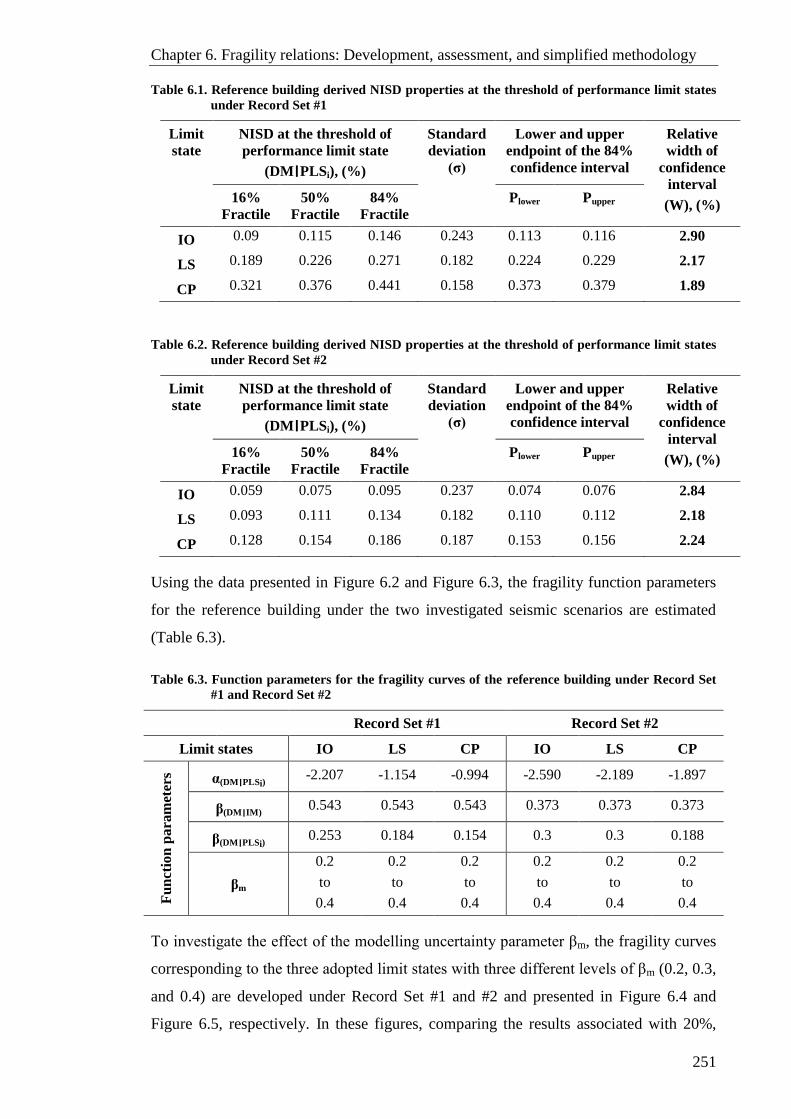
Chapter 6. Fragility relations: Development, assessment, and simplified methodology
251
Table 6.1. Reference building derived NISD properties at the threshold of performance limit states
under Record Set #1
Limit
state
NISD at the threshold of
performance limit state
(DM׀PLSi), (%)
Standard
deviation
(σ)
Lower and upper
endpoint of the 84%
confidence interval
Relative
width of
confidence
interval
(W), (%) 16%
Fractile
50%
Fractile
84%
Fractile
Plower Pupper
IO 0.09 0.115 0.146 0.243 0.113 0.116 2.90
LS 0.189 0.226 0.271 0.182 0.224 0.229 2.17
CP 0.321 0.376 0.441 0.158 0.373 0.379 1.89
Table 6.2. Reference building derived NISD properties at the threshold of performance limit states
under Record Set #2
Limit
state
NISD at the threshold of
performance limit state
(DM׀PLSi), (%)
Standard
deviation
(σ)
Lower and upper
endpoint of the 84%
confidence interval
Relative
width of
confidence
interval
(W), (%) 16%
Fractile
50%
Fractile
84%
Fractile
Plower Pupper
IO 0.059 0.075 0.095 0.237 0.074 0.076 2.84
LS 0.093 0.111 0.134 0.182 0.110 0.112 2.18
CP 0.128 0.154 0.186 0.187 0.153 0.156 2.24
Using the data presented in Figure 6.2 and Figure 6.3, the fragility function parameters
for the reference building under the two investigated seismic scenarios are estimated
(Table 6.3).
Table 6.3. Function parameters for the fragility curves of the reference building under Record Set
#1 and Record Set #2
Record Set #1 Record Set #2
Limit states IO LS CP IO LS CP
Fu
nct
ion
pa
ram
eter
s α(DM׀PLSi) -2.207 -1.154 -0.994 -2.590 -2.189 -1.897
β(DM׀IM) 0.543 0.543 0.543 0.373 0.373 0.373
β(DM׀PLSi) 0.253 0.184 0.154 0.3 0.3 0.188
βm
0.2
to
0.4
0.2
to
0.4
0.2
to
0.4
0.2
to
0.4
0.2
to
0.4
0.2
to
0.4
To investigate the effect of the modelling uncertainty parameter βm, the fragility curves
corresponding to the three adopted limit states with three different levels of βm (0.2, 0.3,
and 0.4) are developed under Record Set #1 and #2 and presented in Figure 6.4 and
Figure 6.5, respectively. In these figures, comparing the results associated with 20%,

Chapter 6. Fragility relations: Development, assessment, and simplified methodology
252
30%, and 40% modelling uncertainty, it can be concluded that the value assigned to βm
has a relatively insignificant effect on the slope for the entire range of the developed
fragility functions. On the other hand, Figure 6.4 and Figure 6.5 indicate that beyond the
curve central point, the value of βm = 0.2 resulting in a slightly higher probability for
any of the adopted limit states to be reached or exceeded at any given Sa(wa). The upper
zone of the fragility curve corresponds to higher seismic intensity levels, therefore,
more critical to the vulnerability assessment of a building or a building stock. Giving
that, the value of βm = 0.2 is adopted for developing all further fragility relations
discussed in the present work.
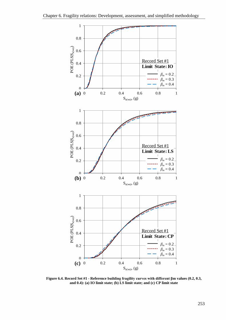
Chapter 6. Fragility relations: Development, assessment, and simplified methodology
253
Figure 6.4. Record Set #1 - Reference buildingfragilitycurveswithdifferentβmvalues (0.2, 0.3,
and 0.4): (a) IO limit state; (b) LS limit state; and (c) CP limit state
0
0.2
0.4
0.6
0.8
1
0 0.2 0.4 0.6 0.8 1
PO
E (
PL
S|S
a(w
a))
Sa(wa), (g)
βm = 0.2
βm = 0.3
βm = 0.4
Record Set #1
Limit State: IO
0
0.2
0.4
0.6
0.8
1
0 0.2 0.4 0.6 0.8 1
PO
E (
PL
S|S
a(w
a))
Sa(wa), (g)
βm = 0.2
βm = 0.3
βm = 0.4
Record Set #1
Limit State: LS
0
0.2
0.4
0.6
0.8
1
0 0.2 0.4 0.6 0.8 1
PO
E (
PL
S|S
a(w
a))
Sa(wa), (g)
βm = 0.2
βm = 0.3
βm = 0.4
Record Set #1
Limit State: CP
PO
E (
PL
S|S
a(w
a))
PO
E (
PL
S|S
a(w
a))
PO
E (
PL
S|S
a(w
a))
(a)
(b)
(c)
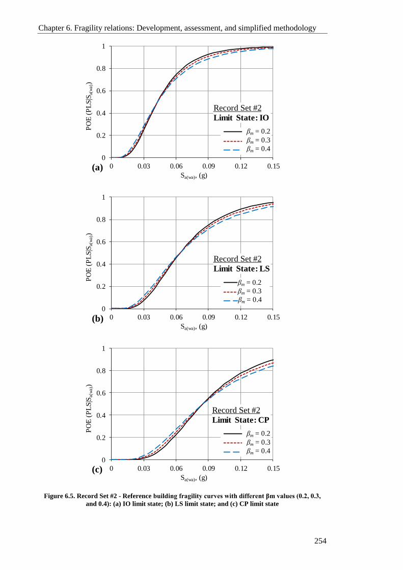
Chapter 6. Fragility relations: Development, assessment, and simplified methodology
254
Figure 6.5. Record Set #2 - Reference buildingfragilitycurveswithdifferentβmvalues(0.2,0.3,
and 0.4): (a) IO limit state; (b) LS limit state; and (c) CP limit state
0
0.2
0.4
0.6
0.8
1
0 0.03 0.06 0.09 0.12 0.15
PO
E (
PL
S|S
a(w
a))
Sa(wa), (g)
βm = 0.2
βm = 0.3
βm = 0.4
Record Set #2
Limit State: IO
0
0.2
0.4
0.6
0.8
1
0 0.03 0.06 0.09 0.12 0.15
PO
E (
PL
S|S
a(w
a))
Sa(wa), (g)
βm = 0.2
βm = 0.3
βm = 0.4
Record Set #2
Limit State: LS
0
0.2
0.4
0.6
0.8
1
0 0.03 0.06 0.09 0.12 0.15
PO
E (
PL
S|S
a(w
a))
Sa(wa), (g)
βm = 0.2
βm = 0.3
βm = 0.4
Record Set #2
Limit State: CP
(a)
(b)
(c)
Chapter 6. Fragility relations: Development, assessment, and simplified methodology
255
6.2 Assessment and comparison of the fragility relations
The developed fragility curves under the two investigated seismic scenarios are assessed
and compared in this section to shed more light upon the differences in the vulnerability
of RC high-rise wall buildings under multiple earthquake scenarios. Using the intensity
measure of Sa(wa) and the mean (50% fractile) values of the DM (NISD) used to define
the three adopted limit states, the fragility relations of the reference building under
Record Set #1 and Record Set #2 are given in Figure 6.6 and Figure 6.7, respectively. In
these figures, zoom in to the part of interest of the fragility curves is also shown. These
parts of interest cover the Sa(wa) values (and their corresponding POE) associated with
three selected earthquake intensity levels: (i) Serviceability Level Earthquake (SLE)
with 50% POE in 30 years (43-year return period); (ii) DBE with 10% POE in 50 years
(475-year return period); and MCE with 2% POE in 50 years (2475-year return period).
The Twa of the reference building (2.54s) falls within the region design spectra zone that
envelopes the severe distant seismic scenario. Accordingly, the Sa(wa) values associated
with the DBE and MCE under this scenario are calculated using the corresponding
design spectra of the study region (Figure 4.5). These design spectra are generated using
the procedure given in the ASCE/SEI 7-16 (2017) and the IBC (IBC, 2015). These
values are 0.105g and 0.158g, respectively. It is worth noting that as per the procedure
of the aforementioned codes, the spectral acceleration values associated with the MCE
are 1.5 times their DBE counterparts. It can be seen that the calculated Sa(wa) value of
0.105g (associated with DBE) is matching with the corresponding Sa(wa) value from the
mean of the response spectra for Record Set #1 (Figure 4.6a). For the moderate near-
field seismic scenario, the Sa(wa) value associated with the DBE is estimated from the
mean of the response spectra for Record Set #2 as 0.011g (Figure 4.6b). For this seismic
scenario, the value associated with the MCE is taken as 0.0165g (1.5 times 0.011 g).
As for estimating the Sa(wa) values associated with the SLE under the two investigated
seismic scenarios, there are no probabilistic seismic hazard assessment studies available
on the study region for this earthquake intensity level. Consulting previous studies (e.g.
Ghodsi and Ruiz, 2010, Tuna, 2012), it was decided to take the Sa(wa) value associated
with the SLE as 0.5 times the DBE-associated value. Accordingly, the Sa(wa) values
corresponding to the SLE under the severe distant and moderate near-field seismic
scenarios are taken as 0.0525g and 0.0053g, respectively.
Chapter 6. Fragility relations: Development, assessment, and simplified methodology
256
Again, the 84% confidence interval of the fragility curve for each limit state along with
its relative width is calculated under Record Set #1 and Record Set #2 using Eqn (6.5)
and (6.6) and listed in Table 6.4 and Table 6.5, respectively. For example, Table 6.4
shows that the mean value of Sa(wa) for limit state IO is 0.127g, representing the mean
value of IM at which the reference building reaches the threshold of the limit state IO
under Record Set #1. In other words, it means that by the probability of 50% for the
Sa(wa) value of 0.127g, the threshold of the damage state IO under Record Set #1 is
reached (i.e. first rebar yield in flooring system). The 16% percentile of Sa(wa) value at
the threshold of limit state IO under Record Set #1 is 0.067g while the 84% percentile is
0.240g. For the mean value of Sa(wa) corresponding to the limit state IO under Record
Set #1, the plus-minus one-σ confidence interval is calculated as [Plower, Pupper] =
[0.122g, 0.132g], returning a relative width value of 7.63. It is important to emphasise
that in Table 6.4 and Table 6.5, the presented 16%, 50%, and 84% fractile values are for
the Sa(wa) at the threshold of different performance limit states, not NISD (response)
values. The significant difference in the 16%, 50%, and 84% fractiles of these Sa(wa)
values corresponding to a specific limit state reflects the variability in the input ground
motion characteristics from one record to another in the record set, not to the response
(NISD) at different limit states/fractiles. Therefore, for Table 6.4 and Table 6.5, the
relative width of confidence interval (W, %) represents a more suitable measure of the
accuracy of the developed fragility curves. For the fragility relations of the reference
building under the two investigated seismic scenarios, the relative width of confidence
interval for all adopted limit states is lower than 10% (between 5.43 and 7.63). This
indicates the high accuracy of the obtained fragility curves and the possibility of
implementing them for RC high-rise wall buildings with similar structural
characteristics and seismicity.
The fragility curves shown in Figure 6.6 and Figure 6.7 are developed using the mean
value (50% fractile) of NISDs at the threshold of a given limit state. Given that the
seismic vulnerability analysis is probabilistic, the fragility relations based on the 16%
and 84% fractiles of the adopted PLSs are developed under Record Set #1 and Record
Set #2 and shown in Figure 6.8 and Figure 6.9, respectively. To facilitate the assessment
and comparison between the developed fragility relations of the reference building
under the two investigated seismic scenarios, Figure 6.10 depicts the compiled fragility
relations (50% fractile) under both Record Set #1 and Record Set #2. In this figure, the
Chapter 6. Fragility relations: Development, assessment, and simplified methodology
257
POE is given in percentage to better link the data with those in Table 6.6 (will be
discussed later).
By analysing the data in Figure 6.10, it can be seen that for the developed fragility
relations under the severe distant seismic scenario, the steepness of the curves increases
as the limit states shifts from CP to IO. The steep slope of the IO limit state curve is
attributed to the high lateral stiffness of the reference building in the elastic range,
which significantly decreases the dispersions in the NISD values from different records
at the threshold of the limit state. Figure 6.10 also shows that the three fragility curves
developed under the moderate near-field earthquake scenario have almost the same
steepness. As previously explained, this is due to the fact that, under almost all the
records in Record Set #2, the three limit states (IO, LS, and CP) are reached while the
structure is still in the elastic zone (Table 5.4).
The latest recommendations in ASCE/SEI 41-17 (2017) for the TISD associated with
LS performance limit state (discussed in Section 5.6.2) introduces a minimal change to
the LS limit state fragility curves of the reference building under the moderate near-field
seismic scenario. Figure 6.11 shows 16%, 50%, and 84% fractile (LS) fragility curves
using the drift recommendations of both ASCE/SEI 41-06 and ASCE/SEI 41-17. The
difference in the POE (LS|Sa(wa)) along the entire range of the three curves is limited to
1%-4% only. These results further support the argument on the negligible effect the new
recommendations in ASCE/SEI 41-17 have on the framework, methodologies and
outcome of the current work.
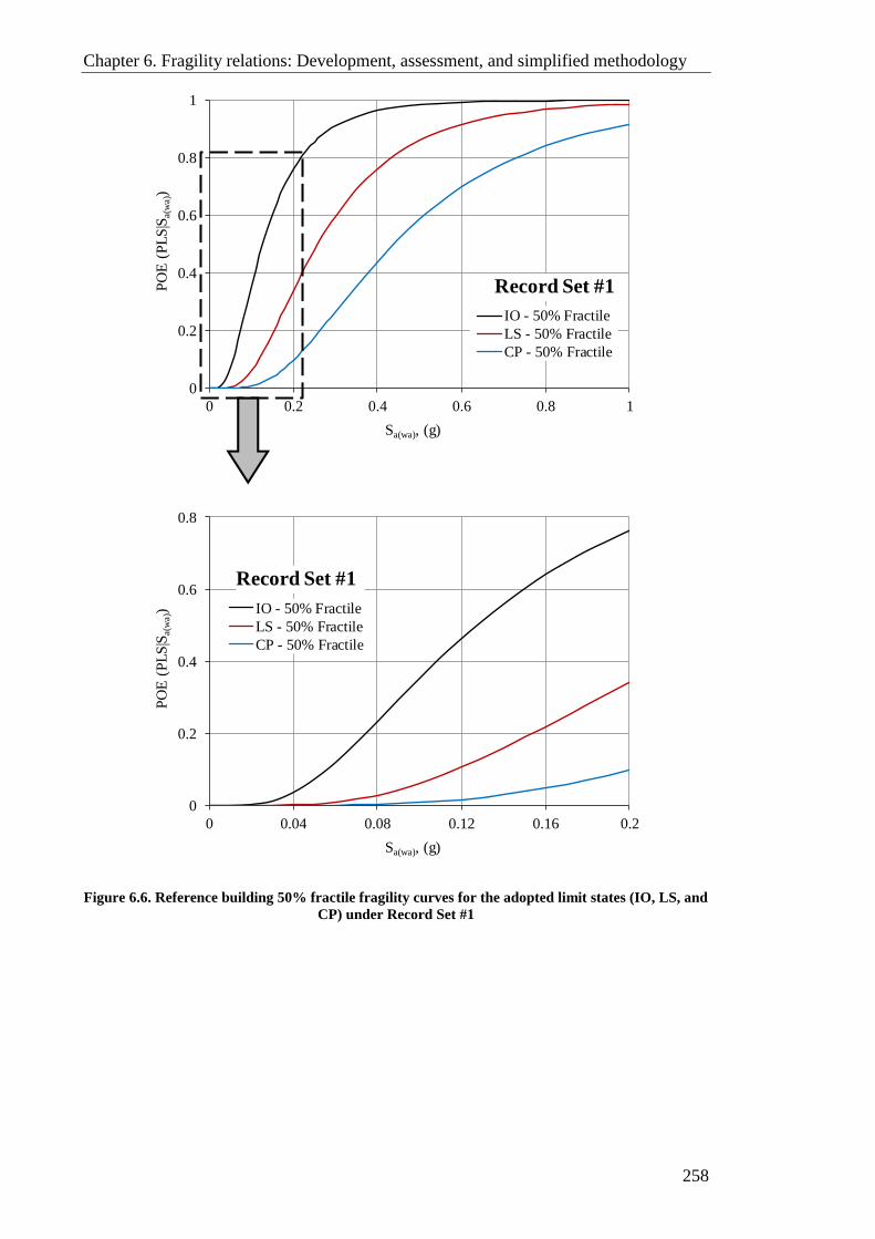
Chapter 6. Fragility relations: Development, assessment, and simplified methodology
258
Figure 6.6. Reference building 50% fractile fragility curves for the adopted limit states (IO, LS, and
CP) under Record Set #1
0
0.2
0.4
0.6
0.8
1
0 0.2 0.4 0.6 0.8 1
PO
E (
PL
S|S
a(w
a))
Sa(wa), (g)
IO - 50% Fractile
LS - 50% Fractile
CP - 50% Fractile
Record Set #1
0.2
0.4
0.6
0.8
PO
E (
LS
|Sa(w
a))
0
0.2
0.4
0.6
0.8
0 0.04 0.08 0.12 0.16 0.2
PO
E (
PL
S|S
a(w
a))
Sa(wa), (g)
IO - 50% Fractile
LS - 50% Fractile
CP - 50% Fractile
Record Set #1
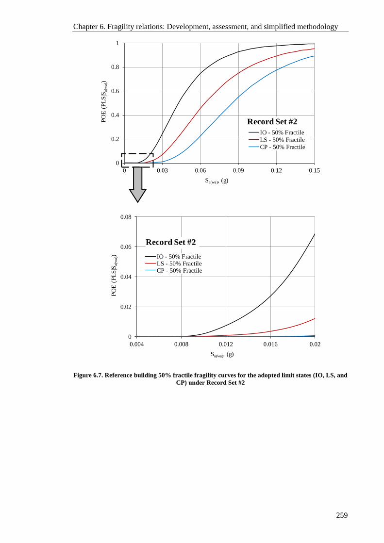
Chapter 6. Fragility relations: Development, assessment, and simplified methodology
259
Figure 6.7. Reference building 50% fractile fragility curves for the adopted limit states (IO, LS, and
CP) under Record Set #2
0
0.2
0.4
0.6
0.8
1
0 0.03 0.06 0.09 0.12 0.15
PO
E (
PL
S|S
a(w
a))
Sa(wa), (g)
IO - 50% Fractile
LS - 50% Fractile
CP - 50% Fractile
Record Set #2
0
0.02
0.04
0.06
0.08
0.004 0.008 0.012 0.016 0.02
PO
E (
PL
S|S
a(w
a))
Sa(wa), (g)
IO - 50% FractileLS - 50% FractileCP - 50% Fractile
Record Set #2
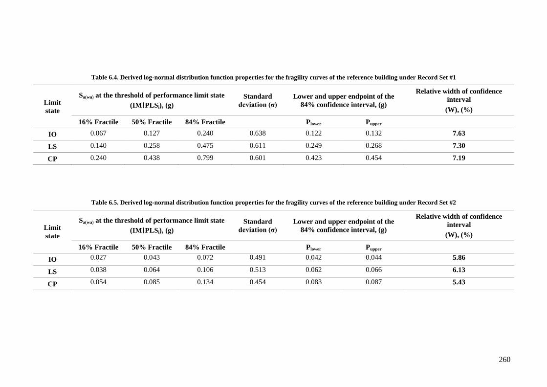
260
Table 6.4. Derived log-normal distribution function properties for the fragility curves of the reference building under Record Set #1
Limit
state
Sa(wa) at the threshold of performance limit state
(IM׀PLSi), (g)
Standard
deviation(σ)
Lower and upper endpoint of the
84% confidence interval, (g)
Relative width of confidence
interval
(W), (%)
16% Fractile 50% Fractile 84% Fractile Plower Pupper
IO 0.067 0.127 0.240 0.638 0.122 0.132 7.63
LS 0.140 0.258 0.475 0.611 0.249 0.268 7.30
CP 0.240 0.438 0.799 0.601 0.423 0.454 7.19
Table 6.5. Derived log-normal distribution function properties for the fragility curves of the reference building under Record Set #2
Limit
state
Sa(wa) at the threshold of performance limit state
(IM׀PLSi), (g)
Standard
deviation(σ)
Lower and upper endpoint of the
84% confidence interval, (g)
Relative width of confidence
interval
(W), (%)
16% Fractile 50% Fractile 84% Fractile Plower Pupper
IO 0.027 0.043 0.072 0.491 0.042 0.044 5.86
LS 0.038 0.064 0.106 0.513 0.062 0.066 6.13
CP 0.054 0.085 0.134 0.454 0.083 0.087 5.43

Chapter 6. Fragility relations: Development, assessment, and simplified methodology
261
Figure 6.8. Record Set #1 - Reference building fragility curves with 16%, 50%, and 84% fractiles:
(a) IO limit state; (b) LS limit state; and (c) CP limit state
0
0.2
0.4
0.6
0.8
1
0 0.2 0.4 0.6 0.8 1
PO
E (
PL
S|S
a(w
a))
Sa(wa), (g)
16% Fractile50% Fractile84% Fractile
Record Set #1
Limit State: IO
0
0.2
0.4
0.6
0.8
1
0 0.2 0.4 0.6 0.8 1
PO
E (
PL
S|S
a(w
a))
Sa(wa), (g)
16% Fractile50% Fractile84% Fractile
Record Set #1
Limit State: LS
0
0.2
0.4
0.6
0.8
1
0 0.2 0.4 0.6 0.8 1
PO
E (
PL
S|S
a(w
a))
Sa(wa), (g)
16% Fractile50% Fractile84% Fractile
Record Set #1
Limit State: CP
PO
E (
PL
S|S
a(w
a))
PO
E (
PL
S|S
a(w
a))
PO
E (
PL
S|S
a(w
a))
(a)
(c)
(b)
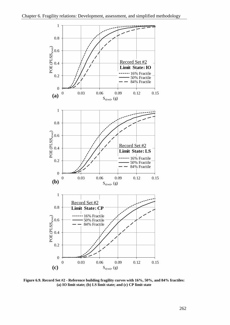
Chapter 6. Fragility relations: Development, assessment, and simplified methodology
262
Figure 6.9. Record Set #2 - Reference building fragility curves with 16%, 50%, and 84% fractiles:
(a) IO limit state; (b) LS limit state; and (c) CP limit state
1
16% Fractile50% Fractile84% Fractile
Record Set #1
State: IO
1
16% Fractile50% Fractile84% Fractile
Record Set #1
State: LS
1
16% Fractile50% Fractile84% Fractile
Record Set #1
State: CP
0
0.2
0.4
0.6
0.8
1
0 0.03 0.06 0.09 0.12 0.15
PO
E (
PL
S|S
a(w
a))
Sa(wa), (g)
16% Fractile50% Fractile84% Fractile
Record Set #2
Limit State: IO
0
0.2
0.4
0.6
0.8
1
0 0.03 0.06 0.09 0.12 0.15
PO
E (
PL
S|S
a(w
a))
Sa(wa), (g)
16% Fractile50% Fractile84% Fractile
Record Set #2
Limit State: LS
0
0.2
0.4
0.6
0.8
1
0 0.03 0.06 0.09 0.12 0.15
PO
E (
PL
S|S
a(w
a))
Sa(wa), (g)
16% Fractile50% Fractile84% Fractile
Record Set #2
Limit State: CP
(a)
(b)
(c)
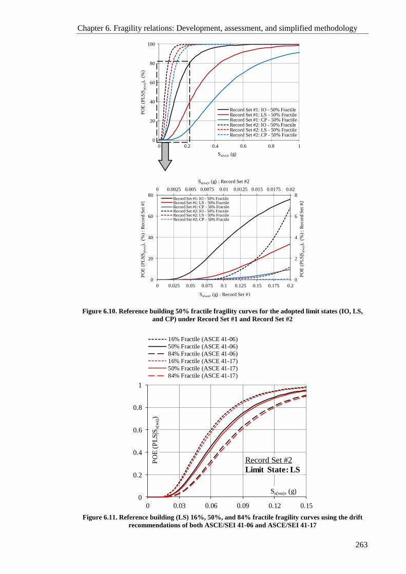
Chapter 6. Fragility relations: Development, assessment, and simplified methodology
263
Figure 6.10. Reference building 50% fractile fragility curves for the adopted limit states (IO, LS,
and CP) under Record Set #1 and Record Set #2
Figure 6.11. Reference building (LS) 16%, 50%, and 84% fractile fragility curves using the drift
recommendations of both ASCE/SEI 41-06 and ASCE/SEI 41-17
0
20
40
60
80
100
0 0.2 0.4 0.6 0.8 1P
OE
(P
LS
|Sa(w
a))
, (%
)
Sa(wa), (g)
Record Set #1: IO - 50% FractileRecord Set #1: LS - 50% FractileRecord Set #1: CP - 50% FractileRecord Set #2: IO - 50% FractileRecord Set #2: LS - 50% FractileRecord Set #2: CP - 50% Fractile
0 0.0025 0.005 0.0075 0.01 0.0125 0.015 0.0175 0.02
0
2
4
6
8
0
20
40
60
80
0 0.025 0.05 0.075 0.1 0.125 0.15 0.175 0.2
Sa(wa), (g) : Record Set #2
PO
E (
PL
S|S
a(w
a))
, (%
) :
Rec
ord
Set
#2
PO
E (
PL
S|S
a(w
a))
, (%
) :
Rec
ord
Set
#1
Sa(wa), (g) : Record Set #1
Record Set #1: IO - 50% FractileRecord Set #1: LS - 50% FractileRecord Set #1: CP - 50% FractileRecord Set #2: IO - 50% FractileRecord Set #2: LS - 50% FractileRecord Set #2: CP - 50% Fractile
Seismic scenario Earthquake
intensity level
Limit state probability (%) Damage state probability (%)
IO LS CP Unimpaired
Occupancy
Impaired
Occupancy
Structural
damage
Structural
collapse
Strong distant
earthquakes
(Record Set #1)
@ Sa(wa) = 0.053 g (SLE) 8.3 0.5 0.0 91.7 7.8 0.4 0.0
@ Sa(wa) = 0.105 g (DBE) 38.2 7.1 0.9 61.8 31.1 6.2 0.9
@ Sa(wa) = 0.158 g (MCE) 63.4 21.2 4.6 36.6 42.1 16.7 4.6
@ Sa(wa) = 0.4 g 96.4 76.4 44.0 3.6 20.0 32.2 44.0
@ Sa(wa) = 0.6 g 99.3 91.6 69.9 0.7 7.6 21.7 69.9
@ Sa(wa) = 0.8 g 99.8 96.8 84.1 0.2 3.0 12.7 84.1
Moderate near-
field earthquakes
(Record Set #2)
@ Sa(wa) = 0.006 g (SLE) 0.0 0.0 0.0 100.0 0.0 0.0 0.0
@ Sa(wa) = 0.011 g (DBE) 0.4 0.0 0.0 99.6 0.4 0.0 0.0
@ Sa(wa) = 0.017 g (MCE) 3.6 0.5 0.0 96.4 3.1 0.5 0.0
@ Sa(wa) = 0.04 g 44.6 18.2 5.0 55.4 26.4 13.2 5.0
@ Sa(wa) = 0.08 g 88.8 67.1 44.4 11.2 21.7 22.4 44.7
@ Sa(wa) = 0.12 g 97.8 89.2 77.4 2.2 8.6 11.7 77.4
0
0.2
0.4
0.6
0.8
1
0 0.03 0.06 0.09 0.12 0.15
PO
E (
PL
S|S
a(w
a))
Sa(wa), (g)
16% Fractile (ASCE 41-06)
50% Fractile (ASCE 41-06)
84% Fractile (ASCE 41-06)
16% Fractile (ASCE 41-17)
50% Fractile (ASCE 41-17)
84% Fractile (ASCE 41-17)
Record Set #2
Limit State: LS

Chapter 6. Fragility relations: Development, assessment, and simplified methodology
264
To correlate the developed fragility relations with the state of damage in the reference
building, the three adopted limit states are considered to be the threshold response
quantities for the following damage states: (i) unimpaired occupancy (UOC); (ii)
impaired occupancy (IOC); (iii) structural damage (SD); and (iv) structural collapse
(SC). Damage state is a function of a specified measure of earthquake ground motion
intensity but also is required for estimating expected or maximum probable losses.
Similar damage state definitions have been adopted for seismic vulnerability
assessments in previous studies (e.g. Ellingwood et al., 2007, Celik and Ellingwood,
2010, Jeong et al., 2012). When compared to the damage state definitions adopted in
HAZUS (Kircher et al., 2006), the equivalence of UOC, IOC, SD, and SC is “no
damage”, “slight-to-moderate damage”, “extensive damage”, and “complete damage”,
respectively. The damage state probabilities of the reference building are determined by
the differences between limit state probabilities. Figure 6.12 schematically illustrates
the relationship between the limit states and the damage states, while the calculated
damage state probabilities for the three selected earthquake intensity levels (SLE, DBE,
and MCE) under the two investigated seismic scenarios are listed in Table 6.6 and
graphically illustrated in Figure 6.13 and Figure 6.14.
Figure 6.12. Relationship between the probability of limit states and damage states
(1.0 - PIO)
(PIO - PLS)
(PLS - PCP)
1.0
PIO
PLS
PCP
0
(PCP)
IO LS CP Limit states
Unimpairedoccupancy
Impairedoccupancy
Structuraldamage
StructuralCollapse
Damage states
Pro
ba
bil
ity
(P
)
Demand
Probability of limit state
Probability of damage state
PIO : Probability of IO limit statePLS : Probability of LS limit state PCP : Probability of CP limit state
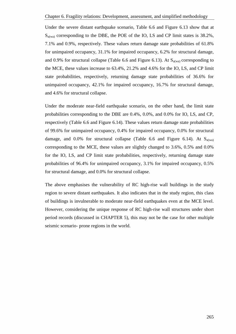
Chapter 6. Fragility relations: Development, assessment, and simplified methodology
265
Under the severe distant earthquake scenario, Table 6.6 and Figure 6.13 show that at
Sa(wa) corresponding to the DBE, the POE of the IO, LS and CP limit states is 38.2%,
7.1% and 0.9%, respectively. These values return damage state probabilities of 61.8%
for unimpaired occupancy, 31.1% for impaired occupancy, 6.2% for structural damage,
and 0.9% for structural collapse (Table 6.6 and Figure 6.13). At Sa(wa) corresponding to
the MCE, these values increase to 63.4%, 21.2% and 4.6% for the IO, LS, and CP limit
state probabilities, respectively, returning damage state probabilities of 36.6% for
unimpaired occupancy, 42.1% for impaired occupancy, 16.7% for structural damage,
and 4.6% for structural collapse.
Under the moderate near-field earthquake scenario, on the other hand, the limit state
probabilities corresponding to the DBE are 0.4%, 0.0%, and 0.0% for IO, LS, and CP,
respectively (Table 6.6 and Figure 6.14). These values return damage state probabilities
of 99.6% for unimpaired occupancy, 0.4% for impaired occupancy, 0.0% for structural
damage, and 0.0% for structural collapse (Table 6.6 and Figure 6.14). At Sa(wa)
corresponding to the MCE, these values are slightly changed to 3.6%, 0.5% and 0.0%
for the IO, LS, and CP limit state probabilities, respectively, returning damage state
probabilities of 96.4% for unimpaired occupancy, 3.1% for impaired occupancy, 0.5%
for structural damage, and 0.0% for structural collapse.
The above emphasises the vulnerability of RC high-rise wall buildings in the study
region to severe distant earthquakes. It also indicates that in the study region, this class
of buildings is invulnerable to moderate near-field earthquakes even at the MCE level.
However, considering the unique response of RC high-rise wall structures under short
period records (discussed in CHAPTER 5), this may not be the case for other multiple
seismic scenario- prone regions in the world.
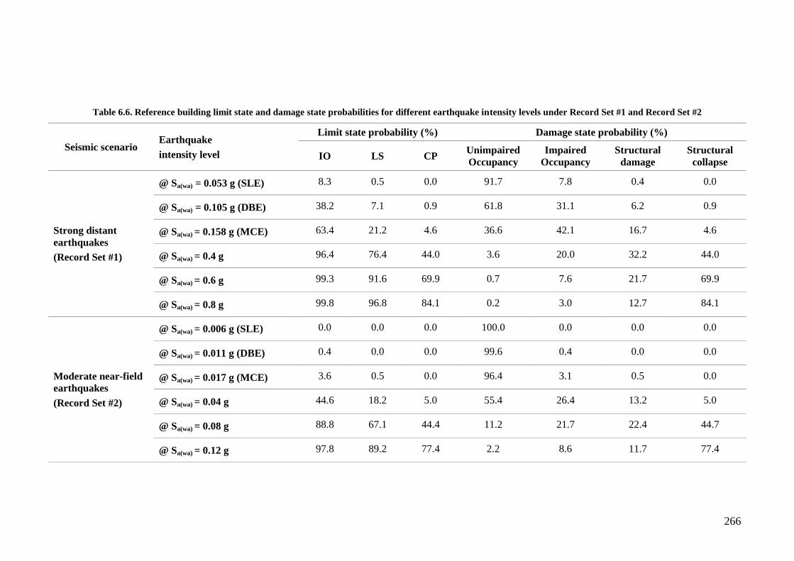
266
Table 6.6. Reference building limit state and damage state probabilities for different earthquake intensity levels under Record Set #1 and Record Set #2
Seismic scenario Earthquake
intensity level
Limit state probability (%) Damage state probability (%)
IO LS CP Unimpaired
Occupancy
Impaired
Occupancy
Structural
damage
Structural
collapse
Strong distant
earthquakes
(Record Set #1)
@ Sa(wa) = 0.053 g (SLE) 8.3 0.5 0.0 91.7 7.8 0.4 0.0
@ Sa(wa) = 0.105 g (DBE) 38.2 7.1 0.9 61.8 31.1 6.2 0.9
@ Sa(wa) = 0.158 g (MCE) 63.4 21.2 4.6 36.6 42.1 16.7 4.6
@ Sa(wa) = 0.4 g 96.4 76.4 44.0 3.6 20.0 32.2 44.0
@ Sa(wa) = 0.6 g 99.3 91.6 69.9 0.7 7.6 21.7 69.9
@ Sa(wa) = 0.8 g 99.8 96.8 84.1 0.2 3.0 12.7 84.1
Moderate near-field
earthquakes
(Record Set #2)
@ Sa(wa) = 0.006 g (SLE) 0.0 0.0 0.0 100.0 0.0 0.0 0.0
@ Sa(wa) = 0.011 g (DBE) 0.4 0.0 0.0 99.6 0.4 0.0 0.0
@ Sa(wa) = 0.017 g (MCE) 3.6 0.5 0.0 96.4 3.1 0.5 0.0
@ Sa(wa) = 0.04 g 44.6 18.2 5.0 55.4 26.4 13.2 5.0
@ Sa(wa) = 0.08 g 88.8 67.1 44.4 11.2 21.7 22.4 44.7
@ Sa(wa) = 0.12 g 97.8 89.2 77.4 2.2 8.6 11.7 77.4
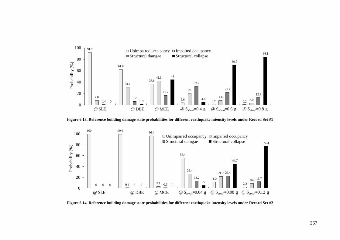
267
Figure 6.13. Reference building damage state probabilities for different earthquake intensity levels under Record Set #1
Figure 6.14. Reference building damage state probabilities for different earthquake intensity levels under Record Set #2
91.7
61.8
36.6
3.60.7 0.2
7.8
31.1
42.1
20
7.63.0
0.46.2
16.7
32.2
21.7
12.7
0 0.9
44
4.6
69.9
84.1
0
20
40
60
80
100
Pro
bab
ilit
y (%
)
Unimpaired occupancy Impaired occupancy
Structural damgae Structural collapse
@ SLE @ DBE @ MCE @ Sa(wa)=0.4 g @ Sa(wa)=0.6 g @ Sa(wa)=0.8 g
100 99.696.4
55.4
11.2
2.20 0.4 3.1
26.421.7
8.6
0 0 0.5
13.2
22.4
11.7
0 0 05
44.7
77.4
0
20
40
60
80
100
Pro
bab
ilit
y (%
)
Unimpaired occupancy Impaired occupancy
Structural damgae Structural collapse
@ SLE @ DBE @ MCE @ Sa(wa)=0.04 g @ Sa(wa)=0.08 g @ Sa(wa)=0.12 g

Chapter 6. Fragility relations: Development, assessment, and simplified methodology
268
6.3 Simplified methodology to develop fragility relations for RC high-
rise wall buildings
In this final part of CHAPTER 6, a simplified methodology towards developing fragility
relations for high-rise buildings is proposed. The fragility curves generated using the
proposed methodology is referred to hereafter as Cheaper Fragility Curves (CFC). The
terminology reflects the considerable reduction in time and effort that can be achieved
utilising this simplified methodology. The methodology is centred on developing a set
of CFCs with a predefined acceptance (tolerance) level for each seismic scenario under
investigation using a lower number of earthquake records.
Given that MRIDA is the core and spine of any framework that ends with the
development of fragility relations, a number of different methods have previously been
proposed either to simplify or to approximate the process of conducting these analyses.
Approximate methods for IDAs involved the replacement of dynamic nonlinear analysis
by a combination of pushover analysis of a multi-degree-of-freedom (MDOF) model
and dynamic nonlinear analysis of single-degree-of-freedom (SDOF) model (e.g.
Vamvatsikos and Cornell, 2005b, Han and Chopra, 2006, Vamvatsikos and Cornell,
2006). Other researchers have attempted to simplify the procedure by reducing the
dispersion in IDA results (e.g. Shome, 1999, Carballo and Cornel, 2000). Typically, a
reduction in dispersion by a factor of two means that four times fewer records are
needed to gain the same confidence (Vamvatsikos and Cornell, 2004a).
The selection criteria of real ground motion records for seismic scenario-based MRIDA
mainly include magnitude, distance, and site conditions (e.g. Iervolino and Cornell,
2005) without an explicit reflection of structural characteristics of the building(s) under
investigation. This way of record selection requires the calculation of seismic response
for all ground motion records representative of an earthquake scenario. It would,
therefore, be useful to add another criterion to the record selection, such that the
selected records are the best representatives for the prediction of the seismic response of
the investigated structures. By adding this element to the framework for deriving
fragility relations for high-rise buildings, a significant decrease in the number of ground
motion records needed for the sufficiently accurate prediction of seismic response and
fragility relations at a predefined acceptance level can be achieved.
The acceptance level for the developed CFCs is subjective; therefore, the accepted
tolerances can be decided depending on the objectives behind the vulnerability study

Chapter 6. Fragility relations: Development, assessment, and simplified methodology
269
and how the outcomes will be utilised. As pictorially illustrated in Figure 2.1, the
characteristics of a fragility curve (the output in the IPO model) are mainly determined
by the following variables: (i) uncertainties in input ground motions; (ii) building
seismic demand (response); and (iii) building seismic performance (capacity).
The building seismic response is characterised by the two main measures that are
shaping the MRIDAs, namely the IM and the DM. The scalar IM of Sa(wa) proposed in
the current study is shown to be efficient for high-rise buildings with varying height
range. It takes into account both the impact of higher modes and period elongation and
utilises the actual inelastic periods of the structure. As for the damage measure, the
numerical parametric study conducted in Section 5.5 revealed the consistency of NISD
as a global DM for the vulnerability assessment of high-rise buildings with varying
heights.
In multi scenario-seismic-prone regions, the seismic capacity of a building is
represented by the seismic scenario-based limit state criteria ( CHAPTER 5). The
conceptual definitions of the proposed limit state criteria (Table 5.3) is based on the
detailed mapping of the seismic scenario-based local response (Section 5.3), utilising
the comprehensive list of adopted DIs (Table 5.1). The proposed global DM (NISD)
eliminates the RBM-induced artificial component of the TISD, a component that has no
contribution to structural demand. The weight of RBM-induced component in the TISD
is influenced by the location of the storey in the building, the total building height and
the effect of higher modes on the seismic response (e.g. Ji et al., 2009). Accordingly,
removing this component (i.e. using NISD rather TISD as a global DM) eliminates the
variation in the seismic scenario-based limit state criteria for high-rise buildings with
varying heights. As a result, it is fairly acceptable to conclude that adopting the
methodology for determining the seismic scenario-based limit state criteria proposed
in CHAPTER 5 for RC high-rise buildings with varying structural systems and a wider
height range is adequate to return reliable fragility relations.
Based on the above discussion, and to take into account the “uncertainties in input
ground motions” variable, a new Record Selection Criterion (RSC) is proposed
hereafter as part of the simplified methodology. By adopting the proposed RSC, a
considerably lower number of records will be required to develop CFCs for RC high-
rise buildings of varying heights.
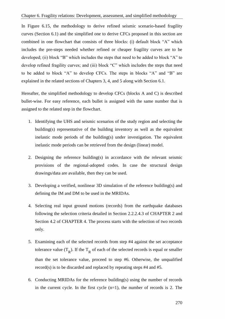
Chapter 6. Fragility relations: Development, assessment, and simplified methodology
270
In Figure 6.15, the methodology to derive refined seismic scenario-based fragility
curves (Section 6.1) and the simplified one to derive CFCs proposed in this section are
combined in one flowchart that consists of three blocks: (i) default block “A” which
includes the pre-steps needed whether refined or cheaper fragility curves are to be
developed; (ii) block “B” which includes the steps that need to be added to block “A” to
develop refined fragility curves; and (iii) block “C” which includes the steps that need
to be added to block “A” to develop CFCs. The steps in blocks “A” and “B” are
explained in the related sections of Chapters 3, 4, and 5 along with Section 6.1.
Hereafter, the simplified methodology to develop CFCs (blocks A and C) is described
bullet-wise. For easy reference, each bullet is assigned with the same number that is
assigned to the related step in the flowchart.
1. Identifying the UHS and seismic scenarios of the study region and selecting the
building(s) representative of the building inventory as well as the equivalent
inelastic mode periods of the building(s) under investigation. The equivalent
inelastic mode periods can be retrieved from the design (linear) model.
2. Designing the reference building(s) in accordance with the relevant seismic
provisions of the regional-adopted codes. In case the structural design
drawings/data are available, then they can be used.
3. Developing a verified, nonlinear 3D simulation of the reference building(s) and
defining the IM and DM to be used in the MRIDAs.
4. Selecting real input ground motions (records) from the earthquake databases
following the selection criteria detailed in Section 2.2.2.4.3 of CHAPTER 2 and
Section 4.2 of CHAPTER 4. The process starts with the selection of two records
only.
5. Examining each of the selected records from step #4 against the set acceptance
tolerance value (TR
). If the TR
of each of the selected records is equal or smaller
than the set tolerance value, proceed to step #6. Otherwise, the unqualified
record(s) is to be discarded and replaced by repeating steps #4 and #5.
6. Conducting MRIDAs for the reference building(s) using the number of records
in the current cycle. In the first cycle (n=1), the number of records is 2. The
Chapter 6. Fragility relations: Development, assessment, and simplified methodology
271
MRIDAs results are to be mapped, where local building response is correlated to
its global response using the adopted global DM (the reader is referred
to CHAPTER 5 for more details).
7. Defining seismic scenario-based limit state criteria for the reference building(s)
(the reader is referred to CHAPTER 5 for more details).
8. Developing the cheaper fragility curves (CFCs) based on the output of steps #6
and #7.
9. The developed CFCs are to be examined against the set acceptance tolerance
value (TFC). If the TFC values of the developed CFCs from two successive cycles
(n and n-1) are equal or smaller than the set tolerance value, proceed to step #10.
Otherwise, steps #5 to #8 are to be repeated with one more record added to the
related set of records.
10. The developed CFCs from the cycle (n-1) is to be adopted for the reference
building(s) and used for further seismic hazard assessment and mitigation
studies.
In the succeeding sections ( 6.3.1 and 6.3.2), the simplified methodology is further
explained by employing it to the reference building. To verify the simplified
methodology outcome, the developed CFCs for the reference building are compared
with the refined fragility relations generated in Section 6.1.
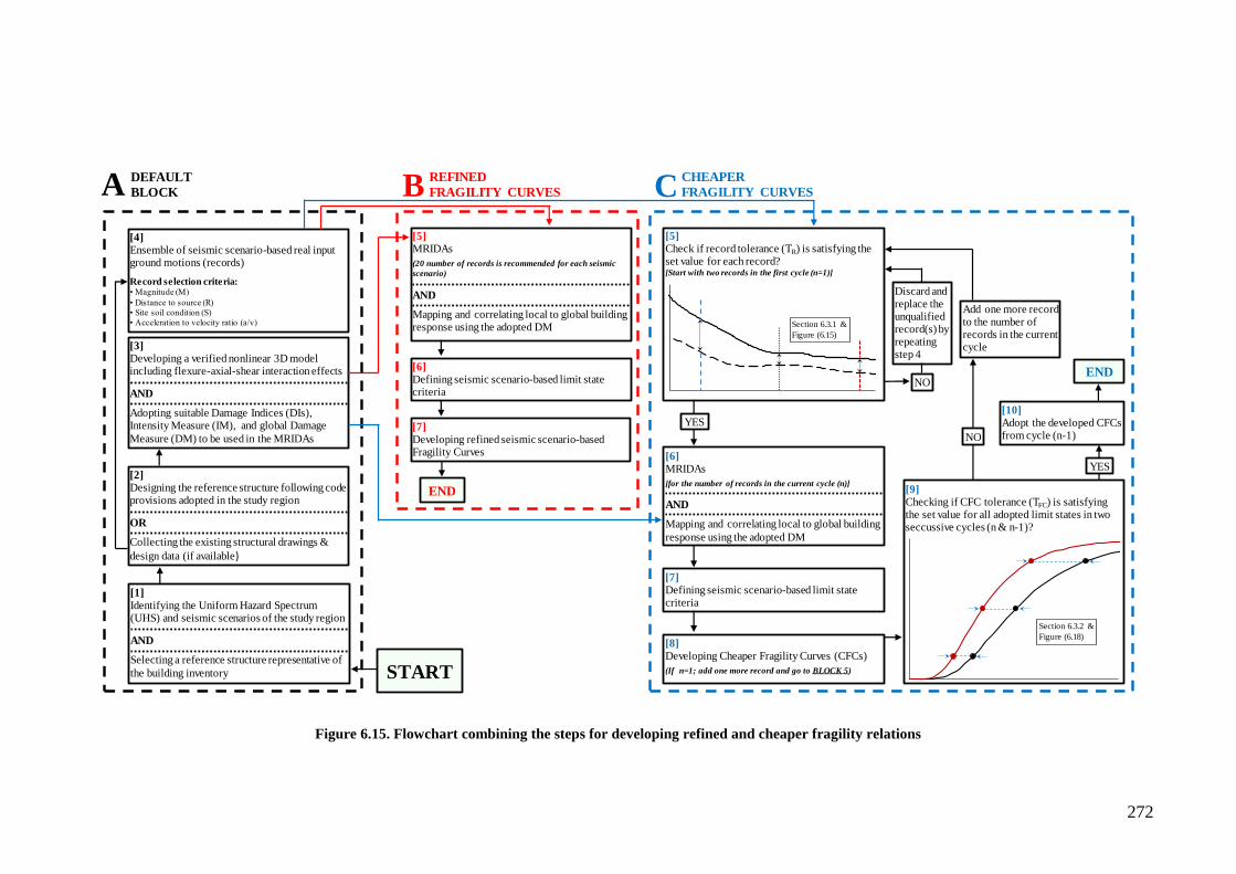
272
Figure 6.15. Flowchart combining the steps for developing refined and cheaper fragility relations
START
[1]Identifying the Uniform Hazard Spectrum(UHS) and seismic scenarios of the study region
AND
Selecting a reference structure representative of
the building inventory
[2]Designing the reference structure following code provisions adopted in the study region
OR
Collecting the existing structural drawings &
design data (if available)
[3]Developing a verified nonlinear 3D model including flexure-axial-shear interaction effects
AND
Adopting suitable Damage Indices (DIs), Intensity Measure (IM), and global Damage
Measure (DM) to be used in the MRIDAs
[4]
Ensemble of seismic scenario-based real input ground motions (records)
Record selection criteria:• Magnitude (M)
• Distance to source (R)
• Site soil condition (S)
• Acceleration to velocity ratio (a/v)
REFINED
FRAGILITY CURVES
[5]
MRIDAs
(20 number of records is recommended for each seismic
scenario)
AND
Mapping and correlating local to global building response using the adopted DM
[6]
Defining seismic scenario-based limit state criteria
[7]
Developing refined seismic scenario-based Fragility Curves
END
[5]Check if record tolerance (TR) is satisfying the set value for each record?[Start with two records in the first cycle (n=1)]
Section 6.3.1 &
Figure (6.15)
YES
[6]
MRIDAs
[for the number of records in the current cycle (n)]
AND
Mapping and correlating local to global building
response using the adopted DM
NO
Discard and replace the unqualified record(s) by repeating step 4
CHEAPER
FRAGILITY CURVES
[7]
Defining seismic scenario-based limit state criteria
[8]
Developing Cheaper Fragility Curves (CFCs)
(If n=1; add one more record and go to BLOCK 5)
[9]
Checking if CFC tolerance (TFC) is satisfying the set value for all adopted limit states in two seccussive cycles (n & n-1)?
YES
[10]Adopt the developed CFCs from cycle (n-1)NO
END
Section 6.3.2 &
Figure (6.18)
Add one more record to the number of records in the current cycle
DEFAULT
BLOCKA B C
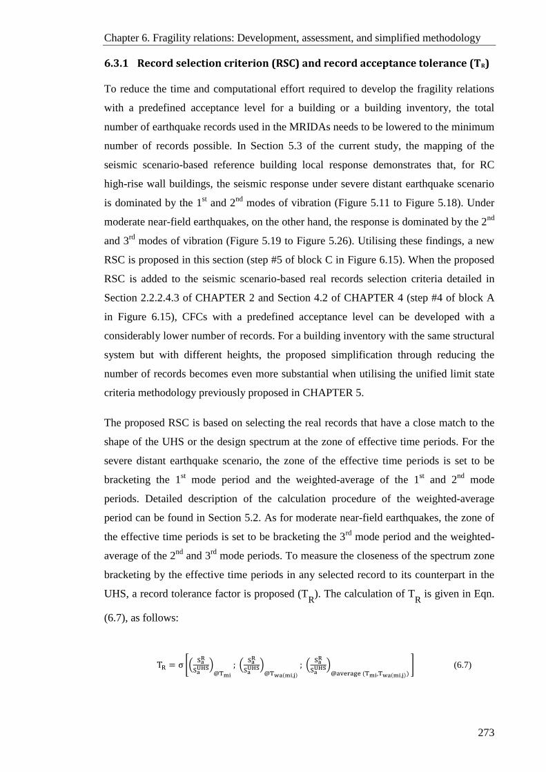
Chapter 6. Fragility relations: Development, assessment, and simplified methodology
273
6.3.1 Record selection criterion (RSC) and record acceptance tolerance (TR)
To reduce the time and computational effort required to develop the fragility relations
with a predefined acceptance level for a building or a building inventory, the total
number of earthquake records used in the MRIDAs needs to be lowered to the minimum
number of records possible. In Section 5.3 of the current study, the mapping of the
seismic scenario-based reference building local response demonstrates that, for RC
high-rise wall buildings, the seismic response under severe distant earthquake scenario
is dominated by the 1st and 2
nd modes of vibration (Figure 5.11 to Figure 5.18). Under
moderate near-field earthquakes, on the other hand, the response is dominated by the 2nd
and 3rd
modes of vibration (Figure 5.19 to Figure 5.26). Utilising these findings, a new
RSC is proposed in this section (step #5 of block C in Figure 6.15). When the proposed
RSC is added to the seismic scenario-based real records selection criteria detailed in
Section 2.2.2.4.3 of CHAPTER 2 and Section 4.2 of CHAPTER 4 (step #4 of block A
in Figure 6.15), CFCs with a predefined acceptance level can be developed with a
considerably lower number of records. For a building inventory with the same structural
system but with different heights, the proposed simplification through reducing the
number of records becomes even more substantial when utilising the unified limit state
criteria methodology previously proposed in CHAPTER 5.
The proposed RSC is based on selecting the real records that have a close match to the
shape of the UHS or the design spectrum at the zone of effective time periods. For the
severe distant earthquake scenario, the zone of the effective time periods is set to be
bracketing the 1st mode period and the weighted-average of the 1
st and 2
nd mode
periods. Detailed description of the calculation procedure of the weighted-average
period can be found in Section 5.2. As for moderate near-field earthquakes, the zone of
the effective time periods is set to be bracketing the 3rd
mode period and the weighted-
average of the 2nd
and 3rd
mode periods. To measure the closeness of the spectrum zone
bracketing by the effective time periods in any selected record to its counterpart in the
UHS, a record tolerance factor is proposed (TR
). The calculation of TR
is given in Eqn.
( 6.7), as follows:
TR = σ [(SaR
SaUHS)
@Tmi
; (SaR
SaUHS)
@Twa(mi,j)
; (SaR
SaUHS)
@average (Tmi,Twa(mi,j)) ] ( 6.7)

Chapter 6. Fragility relations: Development, assessment, and simplified methodology
274
Where TR
is the record tolerance factor, σ is the standard deviation, SaR is the spectral
acceleration value of the record at the specified time period, SaUHS is the spectral
acceleration value of the UHS at the specified time period, Tmi is the building
equivalent inelastic time period of mode i, Twa(mi,j) is the building weighted-average
period of modes i and j, and average (Tmi, Twa(mi,j)) is the arithmetic mean of Tmi and
Twa(mi,j).
The smaller the TR
value, the closer is the matching of the selected record to the shape
of the UHS (or the design spectrum) at the zone of effective mode periods and
consequently, the lesser impact the ground motion uncertainties have on the derived
fragility relations. In the current study, the acceptance value of TR
is set to 10%. This
upper bound will later be shown to be sufficient. Although the proposed methodology
requires a minimum of two records for each seismic scenario as a start, seven records
are selected hereafter from each of the two sets of records. It is important to state that
TR
upper bound can be set to any other value as long as the acceptance level for the
CFCs is achieved.
Figure 6.16 shows the schematic for the calculation procedure of TR
, while Figure 6.17
and Figure 6.18 depict the seven records selected for each seismic scenario along with
the UHS of the region at the zone of effective time periods. Table 6.7 and Table 6.8 give
the parameters for the acceleration response spectra of the selected records at the zone
of effective periods from Record Sets #1 and #2, respectively.
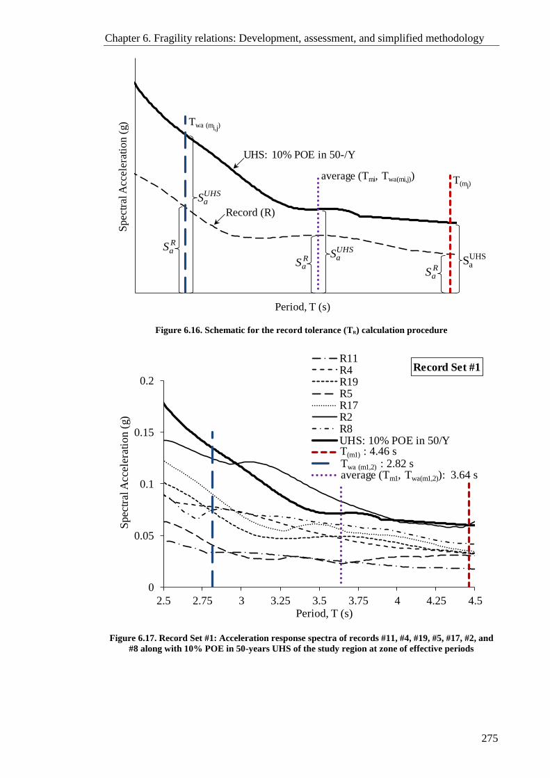
Chapter 6. Fragility relations: Development, assessment, and simplified methodology
275
Figure 6.16. Schematic for the record tolerance (TR) calculation procedure
Figure 6.17. Record Set #1: Acceleration response spectra of records #11, #4, #19, #5, #17, #2, and
#8 along with 10% POE in 50-years UHS of the study region at zone of effective periods
0
0.05
0.1
0.15
0.2
2.5 2.75 3 3.25 3.5 3.75 4 4.25 4.5
Spec
tral
Acc
eler
atio
n (g
)
Period, T (s)
Twa (mi,j)
average (Tmi, Twa(mi,j)) T(mi)
Record (R)
UHS: 10% POE in 50-/Y
RaS
UHSaSR
aS
UHSaS
RaS
UHSaS
0
0.05
0.1
0.15
0.2
2.5 2.75 3 3.25 3.5 3.75 4 4.25 4.5
Spec
tral
Acc
eler
atio
n (g
)
Period, T (s)
R11R4R19R5R17R2R8UHS: 10% POE in 50/YT of mode (1): 4.46 s
Series5
Record Set #1
Twa (m1,2) : 2.82 saverage (Tm1, Twa(m1,2)): 3.64 s
T(m1) : 4.46 s
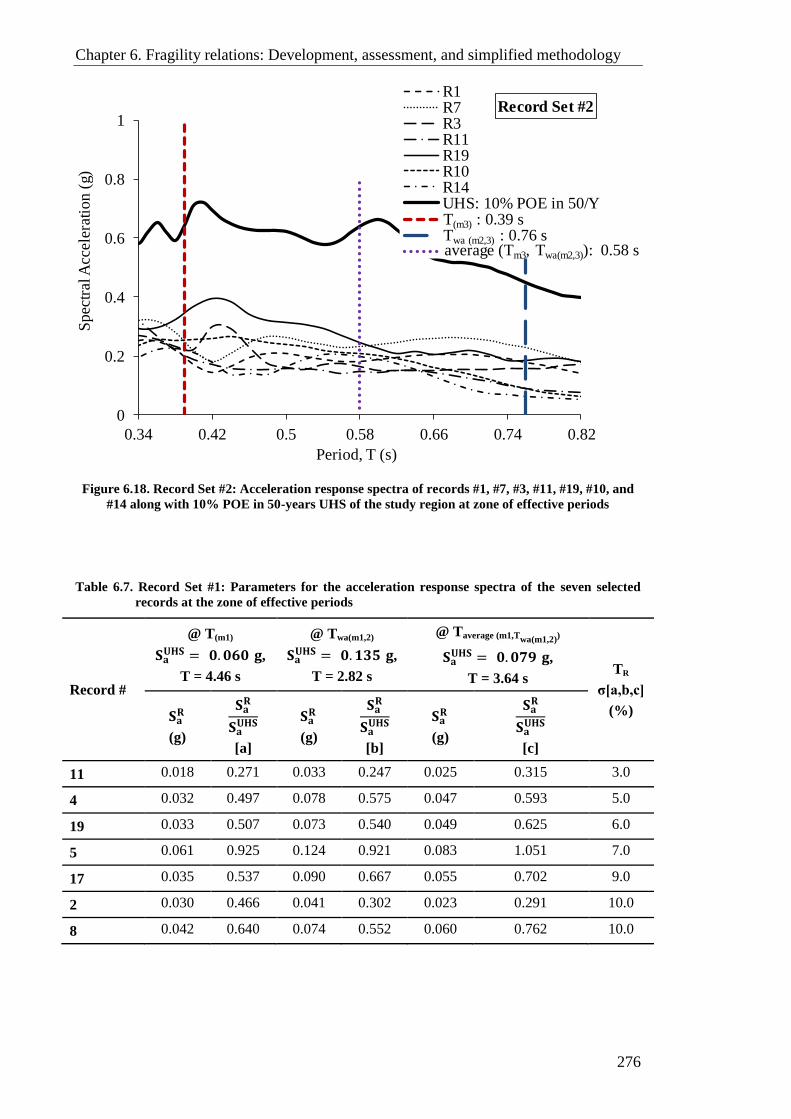
Chapter 6. Fragility relations: Development, assessment, and simplified methodology
276
Figure 6.18. Record Set #2: Acceleration response spectra of records #1, #7, #3, #11, #19, #10, and
#14 along with 10% POE in 50-years UHS of the study region at zone of effective periods
Table 6.7. Record Set #1: Parameters for the acceleration response spectra of the seven selected
records at the zone of effective periods
Record #
@ T(m1)
𝐒𝐚𝐔𝐇𝐒 = 𝟎. 𝟎𝟔𝟎 𝐠,
T = 4.46 s
@ Twa(m1,2)
𝐒𝐚𝐔𝐇𝐒 = 𝟎. 𝟏𝟑𝟓 𝐠,
T = 2.82 s
@ Taverage (m1,Twa(m1,2))
𝐒𝐚𝐔𝐇𝐒 = 𝟎. 𝟎𝟕𝟗 𝐠,
T = 3.64 s TR
σ[a,b,c]
(%) 𝐒𝐚 𝐑
(g)
𝐒𝐚𝐑
𝐒𝐚𝐔𝐇𝐒
[a]
𝐒𝐚 𝐑
(g)
𝐒𝐚𝐑
𝐒𝐚𝐔𝐇𝐒
[b]
𝐒𝐚 𝐑
(g)
𝐒𝐚𝐑
𝐒𝐚𝐔𝐇𝐒
[c]
11 0.018 0.271 0.033 0.247 0.025 0.315 3.0
4 0.032 0.497 0.078 0.575 0.047 0.593 5.0
19 0.033 0.507 0.073 0.540 0.049 0.625 6.0
5 0.061 0.925 0.124 0.921 0.083 1.051 7.0
17 0.035 0.537 0.090 0.667 0.055 0.702 9.0
2 0.030 0.466 0.041 0.302 0.023 0.291 10.0
8 0.042 0.640 0.074 0.552 0.060 0.762 10.0
0
0.2
0.4
0.6
0.8
1
0.34 0.42 0.5 0.58 0.66 0.74 0.82
Sp
ectr
al A
ccel
erat
ion
(g)
Period, T (s)
R1R7R3R11R19R10R14UHS: 10% POE in 50/YT of mode (3): 0.39 s
Series3
Record Set #2
Twa (m2,3) : 0.76 saverage (Tm3, Twa(m2,3)): 0.58 s
T(m3) : 0.39 s

Chapter 6. Fragility relations: Development, assessment, and simplified methodology
277
Table 6.8. Record Set #2: Parameters for the acceleration response spectra of the seven selected
records at the zone of effective periods
Record #
@ T(m3)
𝐒𝐚𝐔𝐇𝐒 = 𝟎. 𝟔𝟒𝟑 𝐠,
T = 0.39 s
@ Twa(m2,3)
𝐒𝐚𝐔𝐇𝐒 = 𝟎. 𝟒𝟗𝟗 𝐠,
T = 0.76 s
@ Taverage (m3,Twa(m2,3))
𝐒𝐚𝐔𝐇𝐒 = 𝟎. 𝟔𝟑𝟗 𝐠,
T = 0.58 s TR
σ[a,b,c]
(%) 𝐒𝐚 𝐑
(g)
𝐒𝐚𝐑
𝐒𝐚𝐔𝐇𝐒
[a]
𝐒𝐚 𝐑
(g)
𝐒𝐚𝐑
𝐒𝐚𝐔𝐇𝐒
[b]
𝐒𝐚 𝐑
(g)
𝐒𝐚𝐑
𝐒𝐚𝐔𝐇𝐒
[c]
1 0.202 0.314 0.182 0.364 0.182 0.285 4.0
7 0.256 0.398 0.230 0.462 0.231 0.361 5.0
3 0.228 0.354 0.157 0.314 0.163 0.255 5.0
11 0.207 0.321 0.093 0.186 0.148 0.232 7.0
19 0.342 0.531 0.185 0.370 0.247 0.386 9.0
10 0.253 0.393 0.092 0.184 0.208 0.326 9.0
14 0.220 0.342 0.065 0.130 0.197 0.309 10.0
6.3.2 Development of CFCs and calculation of fragility curve tolerance (TFC)
Using the proposed simplified methodology, the first set of CFCs can be developed
using two records only for each seismic scenario. The number of records used to
develop the fragility curve is referred to as NOR. The records are selected according to
the procedure described in Section 6.3.1. To decide whether the accuracy level for the
developed CFCs is acceptable, a tolerance factor denoted TFC
is proposed. the
calculation of TFC
is given in below set of equations:
TFC = [0.25xσNORNOR+1 + 0.75x(Sa)NOR
NOR+1] (6.8)
σNOR+1 = σ[(SaNOR+1@16%POE); (Sa
NOR+1@50%POE); (SaNOR+1@84%POE)] (6.9)
σNOR = σ[(SaNOR@16%POE); (Sa
NOR@50%POE); (SaNOR@84%POE)] (6.10)
σNORNOR+1 = ABS (
σNOR+1−σNOR
σNOR) (6.11)

Chapter 6. Fragility relations: Development, assessment, and simplified methodology
278
(Sa)NORNOR+1 = ABS [
(SaNOR+1@50%POE)−(Sa
NOR@50%POE)
(SaNOR@50%POE)
] (6.12)
Where TFC is the fragility curve tolerance factor, σNOR+1 is the standard deviation of the
Sa(wa) values at the (NOR+1) fragility curve corresponding to POE levels of 16%, 50%,
and 84%, σNOR is the standard deviation of the Sa(wa) values at the (NOR) fragility curve
corresponding to POE levels of 16%, 50%, and 84%, σNORNOR+1 is the absolute of the
difference ratio between σNOR+1 and σNOR, and (Sa)NORNOR+1 is the absolute of the
difference ratio between SaNOR+1@50%POE and Sa
NOR@50%POE. The calculation of TFC
is
pictorially illustrated in Figure 6.19.
Figure 6.19. Schematic for the calculation procedure of acceptance tolerance TFC
In the TFC
equation, the values of σNOR+1and σNOR define the slope of the fragility
curves developed NOR+1 and NOR, respectively. Accordingly, the resulting σNORNOR+1 is
a measure of the congruence in the slope of the two fragility curves. The (Sa)NORNOR+1, on
the other hand, measures how close the two fragility curves are in terms of the Sa(wa)
value corresponding to the 50% POE. The two aforementioned measures are weighed
0.03144
0.052526
0.087466
0.045656
0.076094
0.126719
0 0.03 0.06 0.09 0.12 0.15
0
0.25
0.5
0.75
1
0 0.03 0.06 0.09 0.12 0.15
Sa(wa), (g)
PO
E (
PL
S|S
a(w
a))
Sa(wa), (g)
16% POE
50% POE
84% POE
σNOR+1
SaNOR+1@84%POESa
NOR+1@16%POE SaNOR+1@50%POE
SaR+1@ 16% POE Sa
R@ 16% POE σRR+1 = ABS (
σR+1−σR
σR)
SaR+1@ 50% POE Sa
R@ 50% POE (Sa)RR+1 = ABS [
SaR+1(@50% POE)−Sa
R(@50% POE)
SaR(@50% POE)
]
SaR+1@ 84% POE Sa
R@ 84% POE TFC = [0.25xσRR+1 + 0.75x(Sa)R
R+1]
σR+1 σR
0 0.03 0.06 0.09 0.12 0.15
00.250.5
0.751
0 0.03 0.06 0.09 0.12 0.15
Sa(wa), (g)
PO
E (
LS
|Sa
(wa
))
Sa(wa), (g)
Fragility curve based on a number of records = NOR
Fragility curve based on a number of records = NOR+1
16% POE
50% POE
84% POE
SaR+1@ 16% POE Sa
R@ 16% POE σRR+1 = ABS (
σR+1−σR
σR)
SaR+1@ 50% POE Sa
R@ 50% POE (Sa)RR+1 = ABS [
SaR+1(@50% POE)−Sa
R(@50% POE)
SaR(@50% POE)
]
SaR+1@ 84% POE Sa
R@ 84% POE TFC = [0.25xσRR+1 + 0.75x(Sa)R
R+1]
σR+1 σR
SaR+1@ 16% POE Sa
R@ 16% POE σRR+1 = ABS (
σR+1−σR
σR)
SaR+1@ 50% POE Sa
R@ 50% POE (Sa)RR+1 = ABS [
SaR+1(@50% POE)−Sa
R(@50% POE)
SaR(@50% POE)
]
SaR+1@ 84% POE Sa
R@ 84% POE TFC = [0.25xσRR+1 + 0.75x(Sa)R
R+1]
σR+1 σR
SaR+1@ 16% POE Sa
R@ 16% POE σRR+1 = ABS (
σR+1−σR
σR)
SaR+1@ 50% POE Sa
R@ 50% POE (Sa)RR+1 = ABS [
SaR+1(@50% POE)−Sa
R(@50% POE)
SaR(@50% POE)
]
SaR+1@ 84% POE Sa
R@ 84% POE TFC = [0.25xσRR+1 + 0.75x(Sa)R
R+1]
σR+1 σR
SaR+1@ 16% POE Sa
R@ 16% POE σRR+1 = ABS (
σR+1−σR
σR)
SaR+1@ 50% POE Sa
R@ 50% POE (Sa)RR+1 = ABS [
SaR+1(@50% POE)−Sa
R(@50% POE)
SaR(@50% POE)
]
SaR+1@ 84% POE Sa
R@ 84% POE TFC = [0.25xσRR+1 + 0.75x(Sa)R
R+1]
σR+1 σR
SaR+1@ 16% POE Sa
R@ 16% POE σRR+1 = ABS (
σR+1−σR
σR)
SaR+1@ 50% POE Sa
R@ 50% POE (Sa)RR+1 = ABS [
SaR+1(@50% POE)−Sa
R(@50% POE)
SaR(@50% POE)
]
SaR+1@ 84% POE Sa
R@ 84% POE TFC = [0.25xσRR+1 + 0.75x(Sa)R
R+1]
σR+1 σR
SaR+1@ 16% POE Sa
R@ 16% POE σRR+1 = ABS (
σR+1−σR
σR)
SaR+1@ 50% POE Sa
R@ 50% POE (Sa)RR+1 = ABS [
SaR+1(@50% POE)−Sa
R(@50% POE)
SaR(@50% POE)
]
SaR+1@ 84% POE Sa
R@ 84% POE TFC = [0.25xσRR+1 + 0.75x(Sa)R
R+1]
σR+1 σR
SaR+1@ 16% POE Sa
R@ 16% POE σRR+1 = ABS (
σR+1−σR
σR)
SaR+1@ 50% POE Sa
R@ 50% POE (Sa)RR+1 = ABS [
SaR+1(@50% POE)−Sa
R(@50% POE)
SaR(@50% POE)
]
SaR+1@ 84% POE Sa
R@ 84% POE TFC = [0.25xσRR+1 + 0.75x(Sa)R
R+1]
σR+1 σR
SaR+1@ 16% POE Sa
R@ 16% POE σRR+1 = ABS (
σR+1−σR
σR)
SaR+1@ 50% POE Sa
R@ 50% POE (Sa)RR+1 = ABS [
SaR+1(@50% POE)−Sa
R(@50% POE)
SaR(@50% POE)
]
SaR+1@ 84% POE Sa
R@ 84% POE TFC = [0.25xσRR+1 + 0.75x(Sa)R
R+1]
σR+1 σR
SaR+1@ 16% POE Sa
R@ 16% POE σRR+1 = ABS (
σR+1−σR
σR)
SaR+1@ 50% POE Sa
R@ 50% POE (Sa)RR+1 = ABS [
SaR+1(@50% POE)−Sa
R(@50% POE)
SaR(@50% POE)
]
SaR+1@ 84% POE Sa
R@ 84% POE TFC = [0.25xσRR+1 + 0.75x(Sa)R
R+1]
σR+1 σR
SaR+1@ 16% POE Sa
R@ 16% POE σRR+1 = ABS (
σR+1−σR
σR)
SaR+1@ 50% POE Sa
R@ 50% POE (Sa)RR+1 = ABS [
SaR+1(@50% POE)−Sa
R(@50% POE)
SaR(@50% POE)
]
SaR+1@ 84% POE Sa
R@ 84% POE TFC = [0.25xσRR+1 + 0.75x(Sa)R
R+1]
σR+1 σR
SaR+1@ 16% POE Sa
R@ 16% POE σRR+1 = ABS (
σR+1−σR
σR)
SaR+1@ 50% POE Sa
R@ 50% POE (Sa)RR+1 = ABS [
SaR+1(@50% POE)−Sa
R(@50% POE)
SaR(@50% POE)
]
SaR+1@ 84% POE Sa
R@ 84% POE TFC = [0.25xσRR+1 + 0.75x(Sa)R
R+1]
σR+1 σR
σNOR
SaNOR@16%POE Sa
NOR@50%POE SaNOR@84%POE
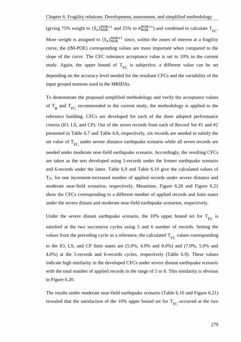
Chapter 6. Fragility relations: Development, assessment, and simplified methodology
279
(giving 75% weight to (Sa)NORNOR+1 and 25% to σNOR
NOR+1) and combined to calculate TFC
.
More weight is assigned to (Sa)NORNOR+1 since, within the zones of interest at a fragility
curve, the (IM-POE) corresponding values are more important when compared to the
slope of the curve. The CFC tolerance acceptance value is set to 10% in the current
study. Again, the upper bound of TFC
is subjective, a different value can be set
depending on the accuracy level needed for the resultant CFCs and the variability of the
input ground motions used in the MRIDAs.
To demonstrate the proposed simplified methodology and verify the acceptance values
of TR
and TFC
recommended in the current study, the methodology is applied to the
reference building. CFCs are developed for each of the three adopted performance
criteria (IO, LS, and CP). Out of the seven records from each of Record Set #1 and #2
presented in Table 6.7 and Table 6.8, respectively, six records are needed to satisfy the
set value of TFC
under severe distance earthquake scenario while all seven records are
needed under moderate near-field earthquake scenario. Accordingly, the resulting CFCs
are taken as the sets developed using 5-records under the former earthquake scenario
and 6-records under the latter. Table 6.9 and Table 6.10 give the calculated values of
TFC for one increment-increased number of applied records under severe distance and
moderate near-field scenarios, respectively. Meantime, Figure 6.20 and Figure 6.21
show the CFCs corresponding to a different number of applied records and limit states
under the severe distant and moderate near-field earthquake scenarios, respectively.
Under the severe distant earthquake scenario, the 10% upper bound set for TFC
is
satisfied at the two successive cycles using 5 and 6 number of records. Setting the
values from the preceding cycle as a reference, the calculated TFC
values corresponding
to the IO, LS, and CP limit states are (5.0%, 4.0% and 8.0%) and (7.0%, 5.0% and
4.0%) at the 5-records and 6-records cycles, respectively (Table 6.9). These values
indicate high similarity in the developed CFCs under severe distant earthquake scenario
with the total number of applied records in the range of 5 to 6. This similarity is obvious
in Figure 6.20.
The results under moderate near-field earthquake scenario (Table 6.10 and Figure 6.21)
revealed that the satisfaction of the 10% upper bound set for TFC
occurred at the two

Chapter 6. Fragility relations: Development, assessment, and simplified methodology
280
successive cycles using 6 and 7 number of records. The calculated TFC
values
corresponding to the IO, LS, and CP limit states are (7.0%, 5.0% and 6.0%) and (2.0%,
5.0% and 3.0%) at the 6-records and 7-records cycles, respectively. Again, these values
indicate high similarity in the developed CFCs under moderate near-field earthquake
scenario with the total number of applied records in the range of 6 to 7. This similarity
is clearly illustrated in Figure 6.21.

281
Table 6.9. Calculated values of TFC for different number of applied records under severe distant earthquake scenario
No. of
records
(NOR)
Limit state
(PLSi)
Sa(wa) at 16%, 50%, and 84% POE of
performance limit state (IM׀PLSi), (g) Standard
deviation
(σ)
𝛔𝐍𝐎𝐑𝐍𝐎𝐑+𝟏 (𝐒𝐚)𝐍𝐎𝐑
𝐍𝐎𝐑+𝟏 TFC
(%) @ 16% @ 50% @ 84%
2
IO 0.076 0.092 0.134 0.289 0 0 0
LS 0.132 0.184 0.257 0.333 0 0 0
CP 0.234 0.290 0.361 0.217 0 0 0
3
IO 0.073 0.103 0.145 0.343 0.19 0.12 14.0
LS 0.140 0.198 0.239 0.271 0.19 0.08 10.0
CP 0.281 0.324 0.438 0.227 0.05 0.12 10.0
4
IO 0.072 0.110 0.168 0.424 0.23 0.07 11.0
LS 0.140 0.219 0.343 0.448 0.65 0.11 24.0
CP 0.246 0.369 0.550 0.402 0.78 0.14 30.0
5
IO 0.073 0.103 0.145 0.343 0.02 0.05 5.0
LS 0.145 0.228 0.361 0.456 0.02 0.04 4.0
CP 0.253 0.405 0.571 0.409 0.02 0.1 8.0
6
IO 0.76 0.109 0.168 0.397 0.08 0.06 7.0
LS 0.149 0.215 0.375 0.465 0.02 0.06 5.0
CP 0.244 0.415 0.580 0.437 0.07 0.02 4.0
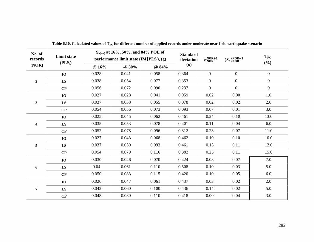
282
Table 6.10. Calculated values of TFC for different number of applied records under moderate near-field earthquake scenario
No. of
records
(NOR)
Limit state
(PLSi)
Sa(wa) at 16%, 50%, and 84% POE of
performance limit state (IM׀PLSi), (g) Standard
deviation
(σ) 𝛔𝐍𝐎𝐑𝐍𝐎𝐑+𝟏 (𝐒𝐚)𝐍𝐎𝐑
𝐍𝐎𝐑+𝟏 TFC
(%) @ 16% @ 50% @ 84%
2
IO 0.028 0.041 0.058 0.364 0 0 0
LS 0.038 0.054 0.077 0.353 0 0 0
CP 0.056 0.072 0.090 0.237 0 0 0
3
IO 0.027 0.028 0.041 0.059 0.02 0.00 1.0
LS 0.037 0.038 0.055 0.078 0.02 0.02 2.0
CP 0.054 0.056 0.073 0.093 0.07 0.01 3.0
4
IO 0.025 0.045 0.062 0.461 0.24 0.10 13.0
LS 0.035 0.053 0.078 0.401 0.11 0.04 6.0
CP 0.052 0.078 0.096 0.312 0.23 0.07 11.0
5
IO 0.027 0.043 0.068 0.462 0.10 0.10 10.0
LS 0.037 0.059 0.093 0.461 0.15 0.11 12.0
CP 0.054 0.079 0.116 0.382 0.25 0.11 15.0
6
IO 0.030 0.046 0.070 0.424 0.08 0.07 7.0
LS 0.04 0.061 0.110 0.508 0.10 0.03 5.0
CP 0.050 0.083 0.115 0.420 0.10 0.05 6.0
7
IO 0.026 0.047 0.061 0.437 0.03 0.02 2.0
LS 0.042 0.060 0.100 0.436 0.14 0.02 5.0
CP 0.048 0.080 0.110 0.418 0.00 0.04 3.0
Chapter 6. Fragility relations: Development, assessment, and simplified methodology
283
Figure 6.20. CFCs correspond to different number of applied records under severe distant earthquake
scenario: (a) @ IO limit state; (b) @ LS limit state; and (c) CP limit state
0
0.2
0.4
0.6
0.8
1
0 0.2 0.4 0.6 0.8 1
PO
E (
PL
S|S
a(w
a))
Sa(wa), (g)
2-Records3-Records4-Records5-Records6-Records
Record Set #1:
CFCs (50% Fractile)
Limit State: IO
0
0.2
0.4
0.6
0.8
1
0 0.2 0.4 0.6 0.8 1
PO
E (
PL
S|S
a(w
a))
Sa(wa), (g)
2-Records3-Records4-Records5-Records6-Records
0
0.2
0.4
0.6
0.8
1
0 0.2 0.4 0.6 0.8 1
PO
E (
PL
S|S
a(w
a))
Sa(wa), (g)
2-Records3-Records4-Records5-Records6-Records
Record Set #1:
CFCs (50% Fractile)
Limit State: LS
Record Set #1:
CFCs (50% Fractile)
Limit State: CP

Chapter 6. Fragility relations: Development, assessment, and simplified methodology
284
Figure 6.21. CFCs correspond to different number of applied records under moderate near-field earthquake
scenario: (a) @ IO limit state; (b) @ LS limit state; and (c) CP limit state
0
0.2
0.4
0.6
0.8
1
0 0.03 0.06 0.09 0.12 0.15
PO
E (
PL
S|S
a(w
a))
Sa(wa), (g)
3-Records4-Records5-Records6-Records7-Records
Record Set #2:
CFCs (50% Fractile)
Limit State: IO
0
0.2
0.4
0.6
0.8
1
0 0.03 0.06 0.09 0.12 0.15
PO
E (
PL
S|S
a(w
a))
Sa(wa), (g)
3-Records4-Records5-Records6-Records7-Records
Record Set #2:
CFCs (50% Fractile)
Limit State: LS
0
0.2
0.4
0.6
0.8
1
0 0.03 0.06 0.09 0.12 0.15
PO
E (
PL
S|S
a(w
a))
Sa(wa), (g)
3-Records4-Records5-Records6-Records7-Records
Record Set #2:
CFCs (50% Fractile)
Limit State: CP

Chapter 6. Fragility relations: Development, assessment, and simplified methodology
285
To verify the recommended upper bound value for TFC
, the CFCs developed for the reference
building at a different number of applied records are plotted against their refined counterparts
that were developed in Section 6.1. Figure 6.22 to Figure 6.24 show the CFCs correspond to the
IO, LS, and CP limit states under severe distant earthquake scenario, while Figure 6.25 to
Figure 6.27 show the same under the moderate near-field scenario. In Figure 6.28, satisfactory
CFCs at IO, LS, and CP limit states are plotted against the refined fragility curves of the
reference building under both investigated seismic scenarios.
The results presented in Figure 6.22 to Figure 6.28 show that the CFCs developed for the
reference building are closer to the refined fragility curves under moderate near-field scenario
compared to the ones under severe distant scenario. Under severe distant seismic scenario, the
maximum POE difference between the satisfactory CFCs and the refined ones is (4.8% @ IO,
2.7% @ LS, and 1.0% @ CP) at DBE, (13.4% @ IO, 0.1% @ LS, and 3.1% @ CP) at MCE, and
(13.0% @ IO, 13.0% @ LS, and 17.0% @ CP) at any intensity level within the range of
Figure 6.28a. Under moderate near-field seismic scenario, the maximum POE difference
between the satisfactory CFCs and the refined ones is (0.2% @ IO, 0.2% @ LS, and 0.0% @
CP) at DBE, (0.4% @ IO, 0.3% @ LS, and 0.0% @ CP) at MCE, and (7.0% @ IO, 4.0% @ LS,
and 6.0% @ CP) at any intensity level within the range of Figure 6.28b.
The higher differences in POEs under severe distant seismic scenario can be attributed to the
high nonlinearity that shapes high-rise buildings’ complex response subjected to long-period
records. The characteristics of long-period records may vary considerably from one record to
another and at different period spans in the same record in terms of record intensity, number of
peaks, and peak amplitudes, causing higher uncertainties in the input ground motions. As a
result, different applied records may trigger different local damage indices, causing the building
to respond differently. This issue does not present in the building response under moderate near-
field earthquake scenario (Table 6.10), considering the almost elastic, shear-controlled nature of
response of the building under this seismic scenario as discussed in details in CHAPTER 5.
Despite the differences between the CFCs and the refined set of fragility curves subjected to
severe distant earthquake scenario compared with the ones under the moderate near-field
scenario, the relatively small differences from both scenarios reflect the soundness of the

Chapter 6. Fragility relations: Development, assessment, and simplified methodology
286
proposed simplified methodology to develop reliable sets of fragility curves with considerably
less time and computational effort.
As another form of comparison, which is more convenient for the seismic hazard assessment and
mitigation studies, the probabilities of the damage states referred to in Section 6.2 (UOC, IOC,
SD, and SC) are calculated and compared at different earthquake intensity levels using the
satisfactory CFCs and the refined ones for the reference building under both investigated seismic
scenarios. The procedure to calculate the difference between these values at a given earthquake
intensity level (TDP) is schematically presented in Figure 6.29. The results are presented in a
tabulated format (Table 6.11 and Table 6.12) as well as in bar charts (Figure 6.30 and
Figure 6.31). The results show that between the satisfactory CFCs and the refined ones, the
maximum difference in the damage state probability at any seismic intensity level is 7% @
UOC, 7% @ IOC, 4% @ SD, and 5% @ SC under moderate near-field seismic scenario
(Table 6.12 and Figure 6.31). Under severe distant scenario, the values are 14% @ UOC, 13% @
IOC, 10% @ SD, and 17% @ SC (Table 6.11 and Figure 6.30). Again, these differences are
smaller at the DBE and MCE intensity levels for both seismic scenarios.
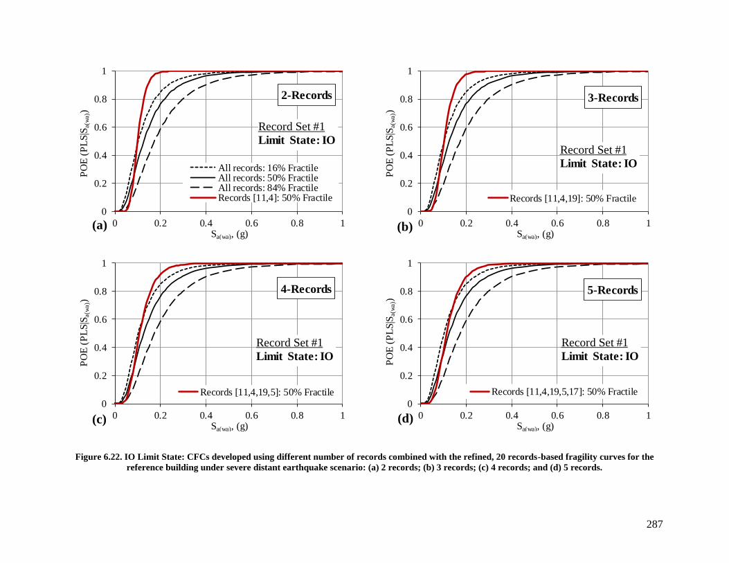
287
Figure 6.22. IO Limit State: CFCs developed using different number of records combined with the refined, 20 records-based fragility curves for the
reference building under severe distant earthquake scenario: (a) 2 records; (b) 3 records; (c) 4 records; and (d) 5 records.
0
0.2
0.4
0.6
0.8
1
0 0.2 0.4 0.6 0.8 1
PO
E (
PL
S|S
a(w
a))
Sa(wa), (g)
All records: 16% FractileAll records: 50% FractileAll records: 84% FractileRecords [11,4]: 50% Fractile
Record Set #1
Limit State: IO
0
0.2
0.4
0.6
0.8
1
0 0.2 0.4 0.6 0.8 1
PO
E (
PL
S|S
a(w
a))
Sa(wa), (g)
Records [11,4,19]: 50% Fractile
Record Set #1
Limit State: IO
0
0.2
0.4
0.6
0.8
1
0 0.2 0.4 0.6 0.8 1
PO
E (
PL
S|S
a(w
a))
Sa(wa), (g)
Records [11,4,19,5]: 50% Fractile
Record Set #1
Limit State: IO
0
0.2
0.4
0.6
0.8
1
0 0.2 0.4 0.6 0.8 1
PO
E (
PL
S|S
a(w
a))
Sa(wa), (g)
Records [11,4,19,5,17]: 50% Fractile
Record Set #1
Limit State: IO
2-Records 3-Records
4-Records 5-Records
(a) (b)
(c) (d)

288
Figure 6.23. LS Limit State: CFCs developed using different number of records combined with the refined, 20 records-based fragility curves for the
reference building under severe distant earthquake scenario: (a) 2 records; (b) 3 records; (c) 4 records; and (d) 5 records.
Difference (%)
IO
13
0
0.2
0.4
0.6
0.8
1
0 0.2 0.4 0.6 0.8 1
PO
E (
PL
S|S
a(w
a))
Sa(wa), (g)
All records: 16% FractileAll records: 50% FractileAll records: 84% FractileSeries4
Record Set #1
Limit State: LS
Records [11,4]: 50% Fractile
0
0.2
0.4
0.6
0.8
1
0 0.2 0.4 0.6 0.8 1
PO
E (
PL
S|S
a(w
a))
Sa(wa), (g)
Records [11,4,19]: 50% Fractile
Record Set #1
Limit State: LS
0
0.2
0.4
0.6
0.8
1
0 0.2 0.4 0.6 0.8 1
PO
E (
PL
S|S
a(w
a))
Sa(wa), (g)
Records [11,4,19,5]: 50% Fractile
Record Set #1
Limit State: LS
0
0.2
0.4
0.6
0.8
1
0 0.2 0.4 0.6 0.8 1
PO
E (
PL
S|S
a(w
a))
Sa(wa), (g)
Records [11,4,19,5,17]: 50% Fractile
Record Set #1
Limit State: LS
2-Records 3-Records
4-Records 5-Records
(a) (b)
(c) (d)
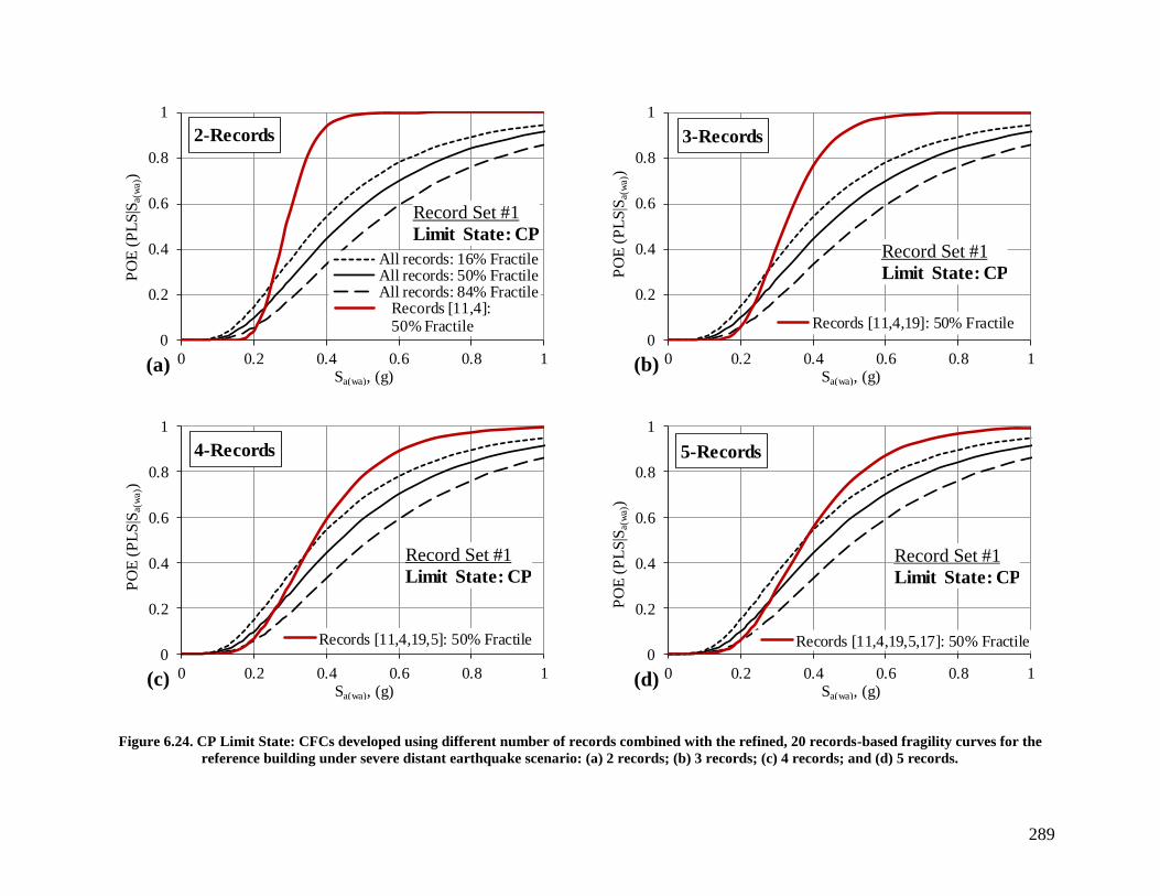
289
Figure 6.24. CP Limit State: CFCs developed using different number of records combined with the refined, 20 records-based fragility curves for the
reference building under severe distant earthquake scenario: (a) 2 records; (b) 3 records; (c) 4 records; and (d) 5 records.
0
0.2
0.4
0.6
0.8
1
0 0.2 0.4 0.6 0.8 1
PO
E (
PL
S|S
a(w
a))
Sa(wa), (g)
All records: 16% FractileAll records: 50% FractileAll records: 84% Fractile
Record Set #1
Limit State: CP
Records [11,4]: 50% Fractile
0
0.2
0.4
0.6
0.8
1
0 0.2 0.4 0.6 0.8 1
PO
E (
PL
S|S
a(w
a))
Sa(wa), (g)
Records [11,4,19]: 50% Fractile
Record Set #1
Limit State: CP
0
0.2
0.4
0.6
0.8
1
0 0.2 0.4 0.6 0.8 1
PO
E (
PL
S|S
a(w
a))
Sa(wa), (g)
Records [11,4,19,5]: 50% Fractile
Record Set #1
Limit State: CP
0
0.2
0.4
0.6
0.8
1
0 0.2 0.4 0.6 0.8 1
PO
E (
PL
S|S
a(w
a))
Sa(wa), (g)
Records [11,4,19,5,17]: 50% Fractile
Record Set #1
Limit State: CP
2-Records 3-Records
4-Records 5-Records
(a) (b)
(c) (d)

290
Figure 6.25. IO Limit State: CFCs developed using different number of records combined with the refined, 20 records-based fragility curves for the
reference building under moderate near-field earthquake scenario: (a) 3 records; (b) 4 records; (c) 5 records; and (d) 6 records.
0
0.2
0.4
0.6
0.8
1
0 0.03 0.06 0.09 0.12 0.15
PO
E (
PL
S|S
a(w
a))
Sa(wa), (g)
All records: 16% FractileAll records: 50% FractileAll records: 84% FractileRecords [1,7,3]: 50% Fractile
Record Set #2
Limit State: IO
0
0.2
0.4
0.6
0.8
1
0 0.03 0.06 0.09 0.12 0.15
PO
E (
PL
S|S
a(w
a))
Sa(wa), (g)
Records [1,7,3,11]: 50% Fractile
Record Set #2
Limit State: IO
0
0.2
0.4
0.6
0.8
1
0 0.03 0.06 0.09 0.12 0.15
PO
E (
PL
S|S
a(w
a))
Sa(wa), (g)
Records [1,7,3,11,19]: 50% Fractile
Record Set #2
Limit State: IO
0
0.2
0.4
0.6
0.8
1
0 0.03 0.06 0.09 0.12 0.15
PO
E (
PL
S|S
a(w
a))
Sa(wa), (g)
Records [1,7,3,11,19,10]: 50% Fractile
Record Set #2
Limit State: IO
3-Records 4-Records
5-Records 6-Records
(a) (b)
(d) (c)
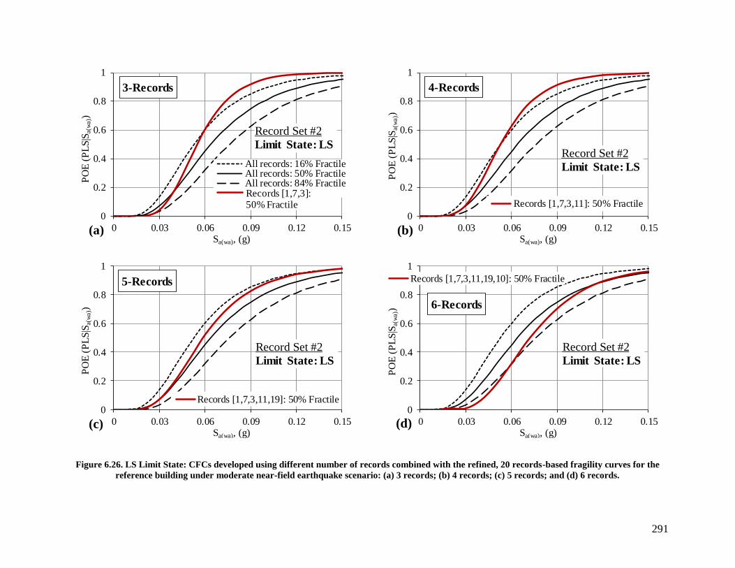
291
Figure 6.26. LS Limit State: CFCs developed using different number of records combined with the refined, 20 records-based fragility curves for the
reference building under moderate near-field earthquake scenario: (a) 3 records; (b) 4 records; (c) 5 records; and (d) 6 records.
0
0.2
0.4
0.6
0.8
1
0 0.03 0.06 0.09 0.12 0.15
PO
E (
PL
S|S
a(w
a))
Sa(wa), (g)
All records: 16% FractileAll records: 50% FractileAll records: 84% Fractile
Record Set #2
Limit State: LS
Records [1,7,3]:50% Fractile
0
0.2
0.4
0.6
0.8
1
0 0.03 0.06 0.09 0.12 0.15
PO
E (
PL
S|S
a(w
a))
Sa(wa), (g)
Records [1,7,3,11]: 50% Fractile
Record Set #2
Limit State: LS
0
0.2
0.4
0.6
0.8
1
0 0.03 0.06 0.09 0.12 0.15
PO
E (
PL
S|S
a(w
a))
Sa(wa), (g)
Records [1,7,3,11,19]: 50% Fractile
Record Set #2
Limit State: LS
0
0.2
0.4
0.6
0.8
1
0 0.03 0.06 0.09 0.12 0.15
PO
E (
PL
S|S
a(w
a))
Sa(wa), (g)
Records [1,7,3,11,19,10]: 50% Fractile
Record Set #2
Limit State: LS
3-Records 4-Records
5-Records
6-Records
(a)
(d) (c)
(b)
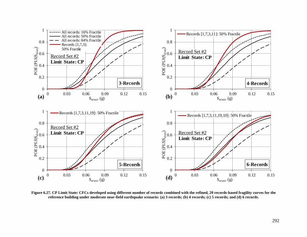
292
Figure 6.27. CP Limit State: CFCs developed using different number of records combined with the refined, 20 records-based fragility curves for the
reference building under moderate near-field earthquake scenario: (a) 3 records; (b) 4 records; (c) 5 records; and (d) 6 records.
R11R4 Record Set #1
0
0.2
0.4
0.6
0.8
1
0 0.03 0.06 0.09 0.12 0.15
PO
E (
PL
S|S
a(w
a))
Sa(wa), (g)
All records: 16% FractileAll records: 50% FractileAll records: 84% Fractile
Record Set #2
Limit State: CP
Records [1,7,3]:50% Fractile
0
0.2
0.4
0.6
0.8
1
0 0.03 0.06 0.09 0.12 0.15
PO
E (
PL
S|S
a(w
a))
Sa(wa), (g)
Records [1,7,3,11]: 50% Fractile
Record Set #2
Limit State: CP
0
0.2
0.4
0.6
0.8
1
0 0.03 0.06 0.09 0.12 0.15
PO
E (
PL
S|S
a(w
a))
Sa(wa), (g)
Records [1,7,3,11,19]: 50% Fractile
Record Set #2
Limit State: CP
0
0.2
0.4
0.6
0.8
1
0 0.03 0.06 0.09 0.12 0.15
PO
E (
PL
S|S
a(w
a))
Sa(wa), (g)
Records [1,7,3,11,19,10]: 50% Fractile
Record Set #2
Limit State: CP
3-Records 4-Records
5-Records 6-Records
(a) (b)
(c) (d)
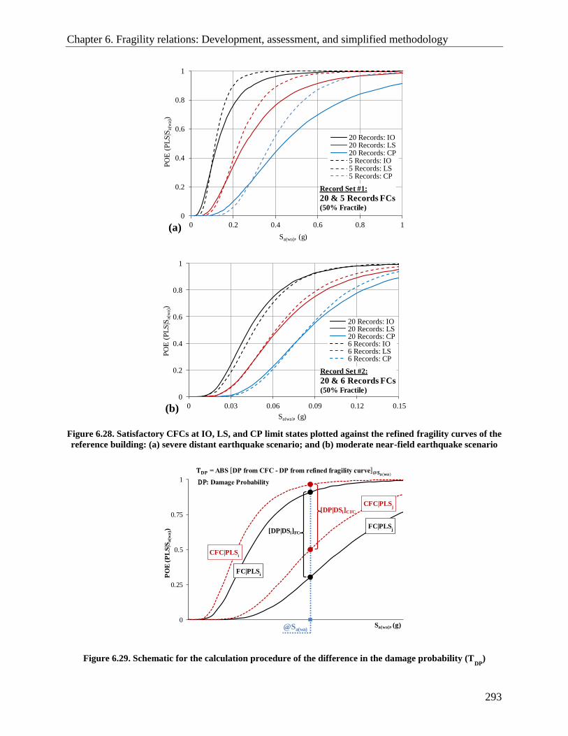
Chapter 6. Fragility relations: Development, assessment, and simplified methodology
293
Figure 6.28. Satisfactory CFCs at IO, LS, and CP limit states plotted against the refined fragility curves of the
reference building: (a) severe distant earthquake scenario; and (b) moderate near-field earthquake scenario
Figure 6.29. Schematic for the calculation procedure of the difference in the damage probability (TDP
)
0
0.2
0.4
0.6
0.8
1
0 0.2 0.4 0.6 0.8 1
PO
E (
PL
S|S
a(w
a))
Sa(wa), (g)
20 Records: IO20 Records: LS20 Records: CP5 Records: IO5 Records: LS5 Records: CP
0
0.2
0.4
0.6
0.8
1
0 0.03 0.06 0.09 0.12 0.15
PO
E (
PL
S|S
a(w
a))
Sa(wa), (g)
20 Records: IO20 Records: LS20 Records: CP6 Records: IO6 Records: LS6 Records: CP
Record Set #1:
20 & 5 Records FCs(50% Fractile)
Record Set #2:
20 & 6 Records FCs(50% Fractile)
0.085
0.085
0.085
0
0.25
0.5
0.75
1
0 0.03 0.06 0.09 0.12 0.15
PO
E (
PL
S|S
a(w
a))
Sa(wa), (g)@Sa(wa)
CFC|PLSi
CFC|PLSj
FC|PLSi
FC|PLSj[DP|DSi]FC
[DP|DSi]CFC
S DPfromC C DPfromrefinedfragilitycurve @𝐒𝐚( 𝐚)
DP DamageProbability
(a)
(b)

294
Table 6.11. Comparison between satisfactory CFCs and the refined FCs of the reference building in terms of damage state probability at different
intensity levels under severe distant earthquake scenario
Earthquake
intensity level
No. of
records
Damage state probability
Unimpaired
Occupancy
+TDP
(%)
Impaired
Occupancy
+TDP
(%)
Structural
damage
+TDP
(%)
Structural
collapse
+TDP
(%)
@ Sa(wa)
= 0.053 g (SLE)
20 0.92
5.0
0.08
5.0
0.00
0.0
0.00
0.0
5 0.97 0.03 0.00 0.00
@ Sa(wa)
= 0.105 g (DBE)
20 0.62
3.0
0.31
6.0
0.06
2.0
0.01
1.0
5 0.59 0.37 0.04 0.00
@ Sa(wa)
= 0.158 g (MCE)
20 0.37
14.0
0.42
13.0
0.17
3.0
0.04
2.0
5 0.23 0.55 0.20 0.02
@ Sa(wa)
= 0.4 g
20 0.04
4.0
0.20
9.0
0.32
2.0
0.44
11.0
5 0.00 0.11 0.34 0.55
@ Sa(wa)
= 0.6 g
20 0.01
1.0
0.08
6.0
0.22
10.0
0.70
17.0
5 0.00 0.02 0.11 0.87
@ Sa(wa)
= 0.8 g
20 0.00
0.0
0.03
3.0
0.13
10.0
0.84
13.0
5 0.00 0.00 0.03 0.97
+TDP
: Difference in the Damage Probability = ABS [(5 records damage state probability – 20 records damage state probability], (%)

295
Table 6.12. Comparison between satisfactory CFCs and the refined FCs of the reference building in terms of damage state probability at different
intensity levels under moderate near-field earthquake scenario
Earthquake
intensity level
No. of
records
Damage state probability
Unimpaired
Occupancy
+TDP
(%)
Impaired
Occupancy
+TDP
(%)
Structural
damage
+TDP
(%)
Structural
collapse
+TDP
(%)
@ Sa(wa)
= 0.006 g (SLE)
20 1.00
0.0
0.00
0.0
0.00
0.0
0.00
0.0
6 1.00 0.00 0.00 0.00
@ Sa(wa)
= 0.011g (DBE)
20 1.00
0.0
0.00
0.0
0.00
0.0
0.00
0.0
6 1.00 0.00 0.00 0.00
@ Sa(wa)
= 0.017 g (MCE)
20 0.97
0.0
0.03
1.0
0.00
1.0
0.00
0.0
6 0.97 0.02 0.01 0.00
@ Sa(wa)
= 0.04 g
20 0.56
7.0
0.26
7.0
0.13
1.0
0.05
1.0
6 0.63 0.19 0.14 0.04
@ Sa(wa)
= 0.08 g
20 0.11
1.0
0.22
5.0
0.22
4.0
0.45
0.0
6 0.12 0.17 0.26 0.45
@ Sa(wa)
= 0.12 g
20 0.02
0.0
0.09
3.0
0.12
2.0
0.77
5.0
6 0.02 0.06 0.10 0.82
+TDP
: Difference in the Damage Probability = ABS [(6 records damage state probability – 20 records damage state probability], (%)

296
Figure 6.30. Comparison between satisfactory CFCs and the refined FCs of the reference building in terms of damage state probability at different
intensity levels under severe distant earthquake scenario: (a) @ SLE; (b) @ DBE; (c) @ MCE; (d) @ Sa(wa) = 0.4 g; (e) @ Sa(wa) = 0.6 g; and (f) @ Sa(wa) =
0.8 g
0.00
0.25
0.50
0.75
1.000.97
0.03 0.00 0.00
0.92
0.080.00 0.00
5 Records
20 Records
UOC: Unimpaired Occupancy IOC: Impaired Occupancy
SD: Structural Damage SC: Structural Collapse
Dam
ag
e p
rob
ab
ilit
y
Damage
0.00
0.25
0.50
0.75
1.00
0.59
0.37
0.04 0.00
0.62
0.31
0.060.01
0.00
0.25
0.50
0.75
1.00
0.23
0.55
0.20
0.02
0.370.42
0.170.04
0.00
0.25
0.50
0.75
1.00
0.000.11
0.34
0.55
0.04
0.200.32
0.44
0.00
0.25
0.50
0.75
1.00
0.00 0.020.11
0.87
0.010.08
0.21
0.70
0.00
0.25
0.50
0.75
1.00
0.00 0.00 0.03
0.97
0.00 0.030.13
0.84
Dam
ag
e p
rob
ab
ilit
y
Damage
(a) (b) (c)
(d) (e) (f)
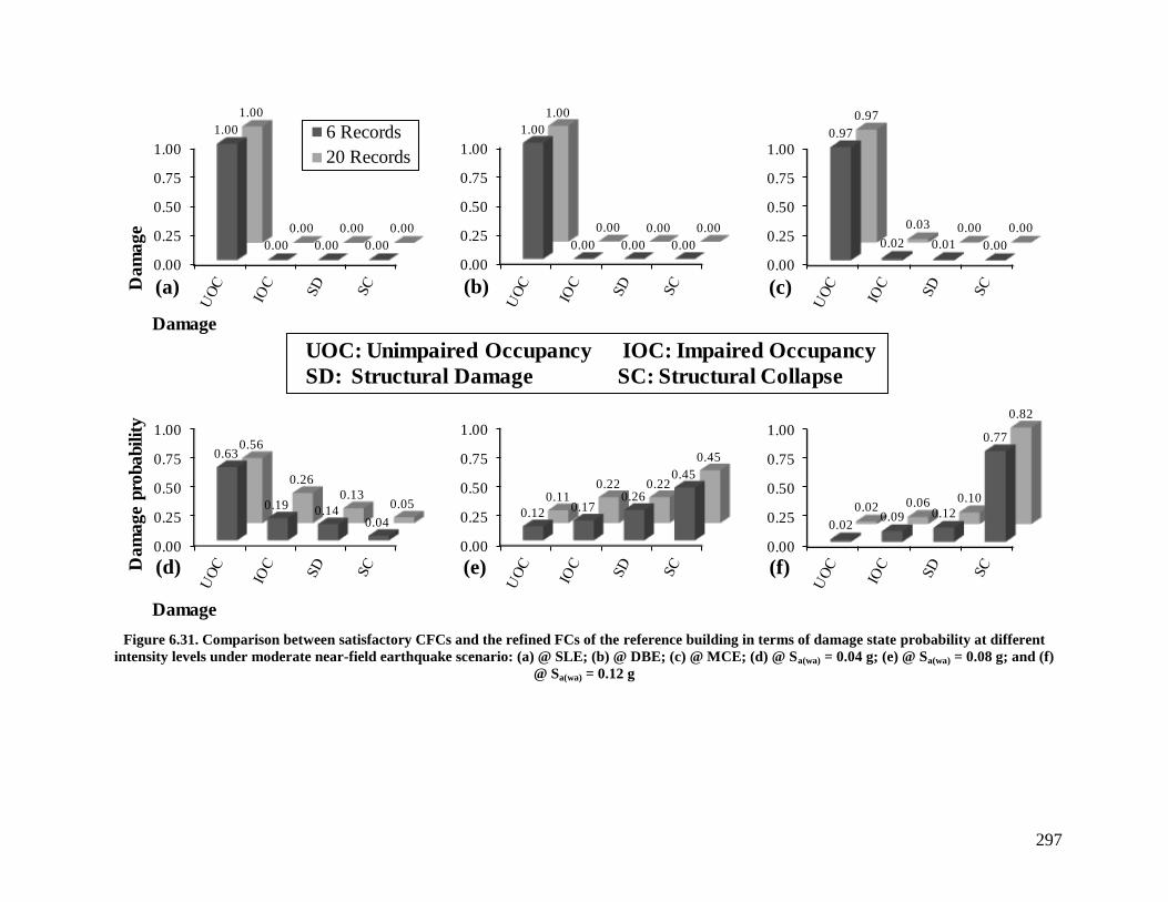
297
Figure 6.31. Comparison between satisfactory CFCs and the refined FCs of the reference building in terms of damage state probability at different
intensity levels under moderate near-field earthquake scenario: (a) @ SLE; (b) @ DBE; (c) @ MCE; (d) @ Sa(wa) = 0.04 g; (e) @ Sa(wa) = 0.08 g; and (f)
@ Sa(wa) = 0.12 g
0.00
0.25
0.50
0.75
1.00
1.00
0.00 0.00 0.00
1.00
0.00 0.00 0.00
6 Records
20 Records
Da
ma
ge
Damage
0.00
0.25
0.50
0.75
1.00
1.00
0.00 0.00 0.00
1.00
0.00 0.00 0.00
0.00
0.25
0.50
0.75
1.000.97
0.02 0.01 0.00
0.97
0.03 0.00 0.00
0.00
0.25
0.50
0.75
1.00
0.63
0.19 0.140.04
0.56
0.26
0.130.05
0.00
0.25
0.50
0.75
1.00
0.12 0.170.26
0.45
0.110.22 0.22
0.45
0.00
0.25
0.50
0.75
1.00
0.020.09 0.12
0.77
0.02 0.06 0.10
0.82
Da
ma
ge
pro
ba
bil
ity
Damage
UOC: Unimpaired Occupancy IOC: Impaired Occupancy
SD: Structural Damage SC: Structural Collapse
(a) (b) (c)
(d) (e) (f)

Chapter 6. Fragility relations: Development, assessment, and simplified methodology
298
6.4 Consistency of developed fragility curves for buildings with
varying height
In Section 5.5, a parametric study, employing six additional buildings, is conducted to
investigate the effect of building total height (number of storeys) on the consistency of
the adopted global DM (NISD) corresponding to the mapped DIs. The predominant
mode periods (uncracked and equivalent inelastic) along with the design proportions of
these additional buildings are given in Table 5.2. To take the parametric study one step
further, CFCs for three out of the six additional buildings are developed in this section.
The three selected buildings are 20-storeys (20S), 40-storeys (40S), and 50-storeys
(50S). the same input ground motions from Section 6.3 (5-Records “5R” representing
the severe distant seismic scenario and 6-Records “6R” representing the moderate near-
field seismic scenario) are utilized to develop CFCs for the aforementioned buildings.
Following the methodology presented in CHAPTER 5, performance limit state criteria,
with NISD as DM, under both seismic scenarios are specified for each of the three
selected buildings (along with the 30S reference building) using the 5R and 6R,
respectively. Table 6.13 lists the “specified” PLS criteria for the 20S, 30S, 40S, and 50S
based on the 5R and 6R (referred to hereafter as SPLSC) along the adopted “reference”
PLS criteria for the 30S building using the twenty records (20R) in each set of records
(referred to hereafter as RPLSC).
Table 6.13. Performance limit state criteria for 20S, 30S, 40S, and 50S using 5R and 6R along with
limit state criteria for 30S reference building based on 20R
Record Set
Limit State
NISD associated to limit state (%)
Building
20S 30S 40S 50S 30S (20R)
#1
(5R)
IO 0.15 0.12 0.11 0.06 0.11
LS 0.25 0.23 0.23 0.12 0.22
CP 0.46 0.40 0.38 0.19 0.37
#2
(6R)
IO 0.11 0.08 0.08 0.06 0.08
LS 0.14 0.10 0.10 0.09 0.11
CP 0.18 0.14 0.12 0.11 0.15
Using the SPLSC listed in Table 6.13, the CFCs for the 20S, 30S, 40S, and 50S
buildings along with the RPLSC-based rigorous FCs of the 30S reference building
(developed in 6.1) under severe distant and moderate near-field seismic scenarios are
presented in Figure 6.32 and Figure 6.33, respectively. The results in these figures are
utilised to evaluate the capability of the presented framework and methodologies of

Chapter 6. Fragility relations: Development, assessment, and simplified methodology
299
developing one set of fragility curves that can represent RC high-rise buildings with
varying total height. To make it more convenient and easier to compare, the results in
Figure 6.32 and Figure 6.33 are presented in the form of damage state probabilities in
Table 6.14 and Table 6.15, respectively. These tables summarise the probabilities of
UO, IO, SD, and SC damage states for the 20S, 40S, and 50S buildings at different
earthquake intensity levels under the two investigated seismic scenarios. Furthermore,
the tables are listing the difference in damage state probabilities for these three
buildings with reference to the rigorous FC-based values calculated for the 30S
reference building. Table 6.16 summarises the maximum values of the CFC-based
damage state probability difference of all studied buildings (20S, 30S, 40S, and 50S) in
reference to the rigorous FC-based damage state probabilities of the 3S reference
building.
By analysing the aforementioned figures and tables, the following remarks can be
withdrawn.
1. Under the severe distant seismic scenario, Figure 6.32 shows that as the building
goes taller (from 20S up to 50S), it becomes less vulnerable. This is attributed to
the fact that for the investigated buildings, the lateral stiffness of the piers and
cores at lower floors (in the direction of the seismic excitation) increases as the
building goes taller. This renders taller buildings needing a higher seismic
intensity to reach a predefined NISD value (limit state criteria). This observation
is consistent for all PLSs under severe distant seismic scenario except for the IO-
CFC of the 20S building and the CP-CFC of the 50S building.
2. The IO-CFC of the 20S building under severe distant seismic scenario indicates
a slightly lower vulnerability at Sa(wa) > 0.15g when compared to the next
building in terms of total height (30S). This may be attributed to the increasing
contribution of the first mode of vibration to the IO-related building response at
higher seismic intensities as the building total height becomes lower,
approaching the height of first mode-dominated structures. For the 50S building
under the severe distant seismic scenario, on the other hand, the CP-CFC is close
to the 40S CP-CFC at seismic intensities between 0.60g and 0.80g. This is
attributed to the shear-controlled CP limit state definition of the 50S building at
these high seismic intensities as opposed to the deformation-based definition at
lower intensities.

Chapter 6. Fragility relations: Development, assessment, and simplified methodology
300
3. The observation discussed in the above points is not applicable to the fragility
curves presented in Figure 6.33 (under moderate near-field seismic scenario).
This is obviously due to the shear-controlled response of all investigated
buildings under this seismic scenario. A lengthy discussion on the characteristics
of such a response nature is given in CHAPTER 5.
4. The developed CFCs for the investigated buildings under moderate near-field
seismic scenario (Figure 6.33) showing lesser dispersion (curves are closer to
each other) compared to the CFCs under sever distant seismic scenario
(Figure 6.32). Again, this is attributed to elastic nature of the shear-controlled
response of the lateral force-resisting system (piers and cores) in the investigated
buildings under Record Set #2 as opposed to the high nonlinearity accompanies
the flexure-controlled response of these buildings under Record Set #1.
5. Comparing any CFC-based damage state probability (UOC, IOC, SD, or SC)
calculated for the investigated buildings to the rigorous FC-based values for the
30S reference building, the minimum and maximum differences (TDP) under
severe distant seismic scenario are 9.0% (40S & 50S: SC) and 32% (50S: UOC),
respectively (Table 6.16). Under the moderate near-field seismic scenario, the
minimum and maximum differences are 2.0% (50S: IOC) and 17% (40S: UOC),
respectively (Table 6.16). Depending on the study purpose and the intended use
for the final product (fragility set), the dispersion in the TDP under severe distant
seismic scenario can be reduced by tightening the acceptance values of TR and
TFC (i.e. increasing the number of records to be used in developing the CFCs).
In conclusion, the TDP differences reported in point #6 above may still be a reasonable
compromise considering the massive saving in effort and computational time when only
one set of seismic scenario-based PLS criteria and CFCs are used for an inventory of
high-rise buildings with a wide range of total building height. This is especially true for
vulnerability assessment studies on the regional or global scale, where the end product
is intended for clients such as insurance companies and hazard mitigation/planning
governmental and non-governmental bodies.
It is important to emphasise here that these TDP calculated differences are the sum of
two components, the first is related to the use of CFC methodology rather than the
refined (rigorous) approach in developing the SPLSC-based fragility curves for the 20S,

Chapter 6. Fragility relations: Development, assessment, and simplified methodology
301
40S, and 50S buildings in this parametric study, while the second component is related
to the variation in the building total height. Considering the TDP related to the 30S
reference building (comprises of the first component only), the maximum difference in
TDP for the other investigated buildings is expected to drop by more than 50% when
eliminating the first component (assuming that the fragility curves for all the
investigated buildings were developed using the rigorous approach). This further
supports the supremacy of the adopted NISD as DM, Sa(wa) as IM, along with all other
components and methodologies of the framework proposed in the current work in terms
of the ability to develop one set of seismic scenario-based fragility relations that suits a
group of RC high-rise buildings with varying height.
To close, it is emphasised that, notwithstanding the number of records employed for the
derivation of the refined fragility relations, the rigour of the nonlinear modelling of the
reference building and the additional six buildings used in the parametric study, the
comprehensive methodology to quantitatively estimate the adopted performance limit
state criteria, and the thorough verification of the methodology to derive the CFCs, the
conclusions of the parametric study are, strictly speaking, applicable to the buildings’
configuration and the seismic scenarios investigated. However, considering the level of
detail put in the framework for developing both rigorous and CFCs, some generality to
the applicability of the parametric study results for RC high-rise buildings with different
configurations and seismicity may fairly be claimed.
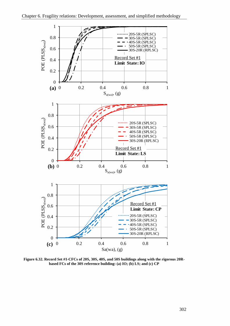
Chapter 6. Fragility relations: Development, assessment, and simplified methodology
302
Figure 6.32. Record Set #1-CFCs of 20S, 30S, 40S, and 50S buildings along with the rigorous 20R-
based FCs of the 30S reference building: (a) IO; (b) LS; and (c) CP
0
0.2
0.4
0.6
0.8
1
0 0.2 0.4 0.6 0.8 1
PO
E (
PL
S|S
a(w
a))
Sa(wa), (g)
20S-5R (SPLSC)30S-5R (SPLSC)40S-5R (SPLSC)50S-5R (SPLSC)30S-20R (RPLSC)
0
0.2
0.4
0.6
0.8
1
0 0.2 0.4 0.6 0.8 1
PO
E (
PL
S|S
a(w
a))
Sa(wa), (g)
20S-5R (SPLSC)30S-5R (SPLSC)40S-5R (SPLSC)50S-5R (SPLSC)30S-20R (RPLSC)
0
0.2
0.4
0.6
0.8
1
0 0.2 0.4 0.6 0.8 1
PO
E (
PL
S|S
a(w
a))
Sa(wa), (g)
20S-5R (SPLSC)30S-5R (SPLSC)40S-5R (SPLSC)50S-5R (SPLSC)30S-20R (RPLSC)
Record Set #1
Limit State: IO
Record Set #1
Limit State: LS
Record Set #1
Limit State: CP
(a)
(c)
(b)
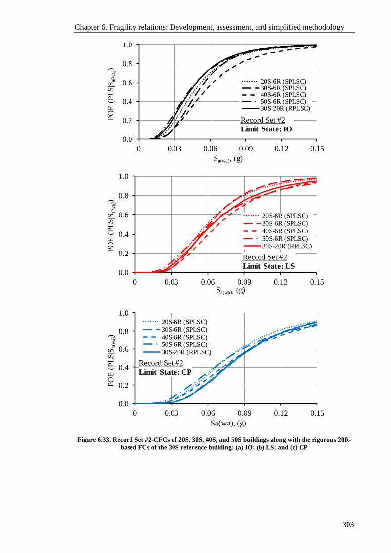
Chapter 6. Fragility relations: Development, assessment, and simplified methodology
303
Figure 6.33. Record Set #2-CFCs of 20S, 30S, 40S, and 50S buildings along with the rigorous 20R-
based FCs of the 30S reference building: (a) IO; (b) LS; and (c) CP
0.0
0.2
0.4
0.6
0.8
1.0
0 0.03 0.06 0.09 0.12 0.15
PO
E (
PL
S|S
a(w
a))
Sa(wa), (g)
20S-6R (SPLSC)30S-6R (SPLSC)40S-6R (SPLSC)50S-6R (SPLSC)30S-20R (RPLSC)
0.0
0.2
0.4
0.6
0.8
1.0
0 0.03 0.06 0.09 0.12 0.15
PO
E (
PL
S|S
a(w
a))
Sa(wa), (g)
20S-6R (SPLSC)30S-6R (SPLSC)40S-6R (SPLSC)50S-6R (SPLSC)30S-20R (RPLSC)
0.0
0.2
0.4
0.6
0.8
1.0
0 0.03 0.06 0.09 0.12 0.15
PO
E (
PL
S|S
a(w
a))
Sa(wa), (g)
20S-6R (SPLSC)30S-6R (SPLSC)40S-6R (SPLSC)50S-6R (SPLSC)30S-20R (RPLSC)
Record Set #2
Limit State: IO
Record Set #2
Limit State: LS
Record Set #2
Limit State: CP

304
Table 6.14. 5R-based damage state probabilities of 20S, 40S, and 50S buildings and their differences with reference to the 20R-based damage state probabilities of the
reference building under severe distant earthquake scenario
Earthquake
intensity level Building
Damage state probability
Unimpaired Occupancy +T
DP
(%) Impaired Occupancy
+TDP
(%) Structural damage
+TDP
(%) Structural collapse
+TDP
(%)
@ Sa(wa)
= 0.053 g (SLE)
20S 0.99 7.0 0.01 7.0 0.00 0.0 0.00 0.0
40S 0.98 6.0 0.02 6.0 0.00 0.0 0.00 0.0
50S 1.00 8.0 0.00 8.0 0.00 0.0 0.00 0.0
@ Sa(wa)
= 0.105 g (DBE)
20S 0.74 12.0 0.22 9.0 0.04 2.0 0.00 1.0
40S 0.72 10.0 0.27 4.0 0.01 5.0 0.00 1.0
50S 0.94 32.0 0.06 25.0 0.00 6.0 0.00 1.0
@ Sa(wa)
= 0.158 g (MCE)
20S 0.32 5.0 0.41 1.0 0.24 7.0 0.03 1.0
40S 0.34 3.0 0.57 15.0 0.08 9.0 0.01 3.0
50S 0.62 25.0 0.33 9.0 0.05 12.0 0.00 4.0
+TDP
: Difference in the Damage Probability = ABS [(5R damage probability of concerned building – 20R damage probability of 30S reference Building], (%)
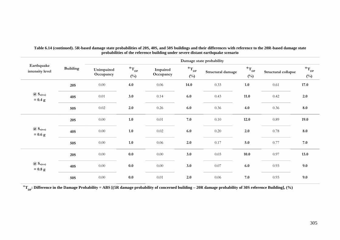
305
Table 6.14 (continued). 5R-based damage state probabilities of 20S, 40S, and 50S buildings and their differences with reference to the 20R-based damage state
probabilities of the reference building under severe distant earthquake scenario
Earthquake
intensity level Building
Damage state probability
Unimpaired Occupancy
+TDP
(%)
Impaired Occupancy
+TDP
(%) Structural damage
+TDP
(%) Structural collapse
+TDP
(%)
@ Sa(wa)
= 0.4 g
20S 0.00 4.0 0.06 14.0 0.33 1.0 0.61 17.0
40S 0.01 3.0 0.14 6.0 0.43 11.0 0.42 2.0
50S 0.02 2.0 0.26 6.0 0.36 4.0 0.36 8.0
@ Sa(wa)
= 0.6 g
20S 0.00 1.0 0.01 7.0 0.10 12.0 0.89 19.0
40S 0.00 1.0 0.02 6.0 0.20 2.0 0.78 8.0
50S 0.00 1.0 0.06 2.0 0.17 5.0 0.77 7.0
@ Sa(wa)
= 0.8 g
20S 0.00 0.0 0.00 3.0 0.03 10.0 0.97 13.0
40S 0.00 0.0 0.00 3.0 0.07 6.0 0.93 9.0
50S 0.00 0.0 0.01 2.0 0.06 7.0 0.93 9.0
+TDP
: Difference in the Damage Probability = ABS [(5R damage probability of concerned building – 20R damage probability of 30S reference Building], (%)
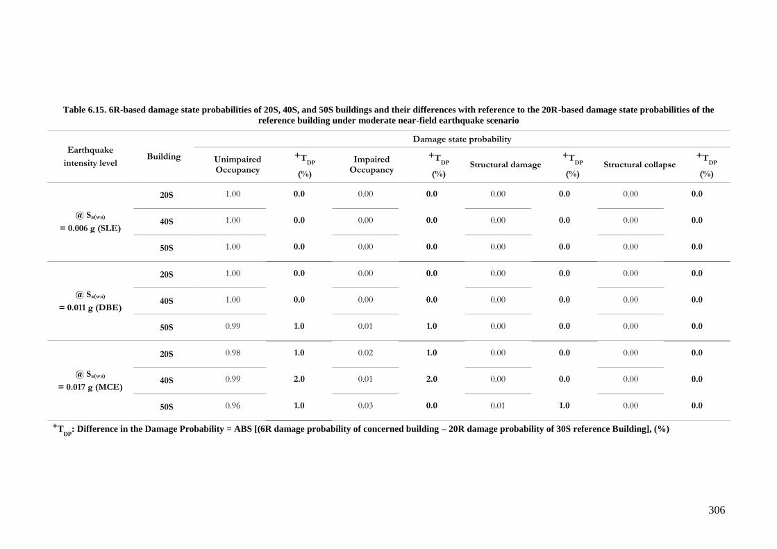
306
Table 6.15. 6R-based damage state probabilities of 20S, 40S, and 50S buildings and their differences with reference to the 20R-based damage state probabilities of the
reference building under moderate near-field earthquake scenario
Earthquake
intensity level Building
Damage state probability
Unimpaired Occupancy
+TDP
(%)
Impaired Occupancy
+TDP
(%) Structural damage
+TDP
(%) Structural collapse
+TDP
(%)
@ Sa(wa)
= 0.006 g (SLE)
20S 1.00 0.0 0.00 0.0 0.00 0.0 0.00 0.0
40S 1.00 0.0 0.00 0.0 0.00 0.0 0.00 0.0
50S 1.00 0.0 0.00 0.0 0.00 0.0 0.00 0.0
@ Sa(wa)
= 0.011 g (DBE)
20S 1.00 0.0 0.00 0.0 0.00 0.0 0.00 0.0
40S 1.00 0.0 0.00 0.0 0.00 0.0 0.00 0.0
50S 0.99 1.0 0.01 1.0 0.00 0.0 0.00 0.0
@ Sa(wa)
= 0.017 g (MCE)
20S 0.98 1.0 0.02 1.0 0.00 0.0 0.00 0.0
40S 0.99 2.0 0.01 2.0 0.00 0.0 0.00 0.0
50S 0.96 1.0 0.03 0.0 0.01 1.0 0.00 0.0
+TDP
: Difference in the Damage Probability = ABS [(6R damage probability of concerned building – 20R damage probability of 30S reference Building], (%)

307
Table 6.15 (continued). 6R-based damage state probabilities of 20S, 40S, and 50S buildings and their differences with reference to the 20R-based damage state
probabilities of the reference building under moderate near-field earthquake scenario
Earthquake
intensity level Building
Damage state probability
Unimpaired Occupancy
+TDP
(%)
Impaired Occupancy
+TDP
(%) Structural damage
+TDP
(%) Structural collapse
+TDP
(%)
@ Sa(wa)
= 0.04 g
20S 0.62 6.0 0.17 9.0 0.11 2.0 0.10 5.0
40S 0.73 17.0 0.13 13.0 0.05 8.0 0.09 4.0
50S 0.53 3.0 0.24 2.0 0.09 4.0 0.14 9.0
@ Sa(wa)
= 0.08 g
20S 0.14 3.0 0.13 9.0 0.19 3.0 0.54 9.0
40S 0.23 12.0 0.15 7.0 0.14 8.0 0.48 3.0
50S 0.012 1.0 0.22 0.0 0.13 9.0 0.53 8.0
@ Sa(wa)
= 0.12 g
20S 0.03 1.0 0.05 4.0 0.11 1.0 0.81 4.0
40S 0.06 4.0 0.07 2.0 0.11 1.0 0.76 1.0
50S 0.03 1.0 0.11 2.0 0.09 3.0 0.77 0.0
+TDP
: Difference in the Damage Probability = ABS [(6R damage probability of concerned building – 20R damage probability of 30S reference Building], (%)
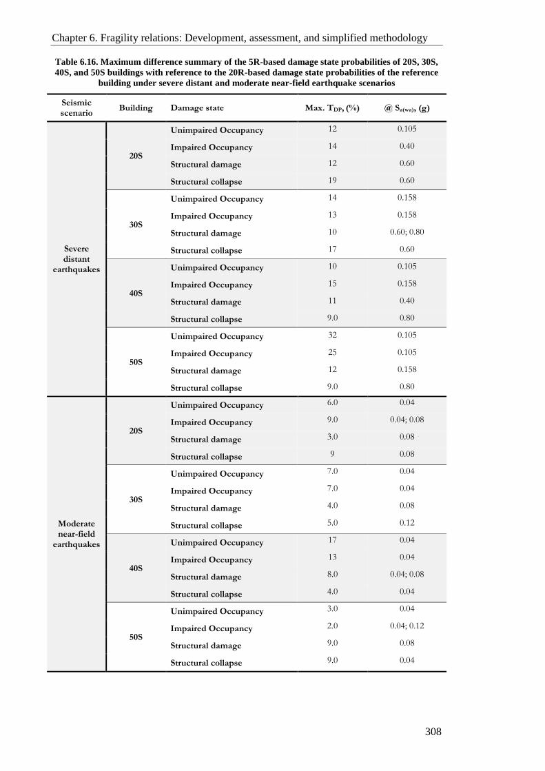
Chapter 6. Fragility relations: Development, assessment, and simplified methodology
308
Table 6.16. Maximum difference summary of the 5R-based damage state probabilities of 20S, 30S,
40S, and 50S buildings with reference to the 20R-based damage state probabilities of the reference
building under severe distant and moderate near-field earthquake scenarios
Seismic scenario
Building Damage state Max. TDP, (%) @ Sa(wa), (g)
Severe distant
earthquakes
20S
Unimpaired Occupancy 12 0.105
Impaired Occupancy 14 0.40
Structural damage 12 0.60
Structural collapse 19 0.60
30S
Unimpaired Occupancy 14 0.158
Impaired Occupancy 13 0.158
Structural damage 10 0.60; 0.80
Structural collapse 17 0.60
40S
Unimpaired Occupancy 10 0.105
Impaired Occupancy 15 0.158
Structural damage 11 0.40
Structural collapse 9.0 0.80
50S
Unimpaired Occupancy 32 0.105
Impaired Occupancy 25 0.105
Structural damage 12 0.158
Structural collapse 9.0 0.80
Moderate near-field
earthquakes
20S
Unimpaired Occupancy 6.0 0.04
Impaired Occupancy 9.0 0.04; 0.08
Structural damage 3.0 0.08
Structural collapse 9 0.08
30S
Unimpaired Occupancy 7.0 0.04
Impaired Occupancy 7.0 0.04
Structural damage 4.0 0.08
Structural collapse 5.0 0.12
40S
Unimpaired Occupancy 17 0.04
Impaired Occupancy 13 0.04
Structural damage 8.0 0.04; 0.08
Structural collapse 4.0 0.04
50S
Unimpaired Occupancy 3.0 0.04
Impaired Occupancy 2.0 0.04; 0.12
Structural damage 9.0 0.08
Structural collapse 9.0 0.04
Chapter 6. Fragility relations: Development, assessment, and simplified methodology
309
6.5 Summary and concluding remarks
CHAPTER 6 is divided into four main parts. Besides this fourth part (Section 6.4), the
first part (Section 6.1) comprises the procedure for developing seismic scenario-based
fragility relations for RC high-rise buildings with an application on the reference
building. This represents the concluding step in the proposed framework for the seismic
vulnerability assessment of RC high-rise buildings. The second part of the chapter
(Section 6.2) deals with examining the developed fragility relations at selected
earthquake intensity levels to assess their accuracy, study their characteristics, and
compare them at different levels. This part of the chapter is concluded with correlating
the developed fragility relations with four states of damage in the reference building,
that is unimpaired occupancy, impaired occupancy, structural damage, and structural
collapse.
In the third part of the chapter (Section 6.3), a simplified methodology is proposed to
develop Cheaper Fragility Curves (CFCs), with lesser number of input ground motions
compared to the number of records needed for developing the refined fragility curves.
Utilising this methodology, the fragility curves of RC high-rise buildings under a
specific seismic scenario can be developed with a substantial reduction in time and
computational effort, especially when a big building inventory is under investigation. In
the proposed methodology, a new Record Selection Criterion (RCS) is proposed with a
recommendation for the selected records’ acceptance tolerance (TR
). Additionally, a
procedure to verify the developed CFCs against a recommended acceptance level (TFC
)
is proposed. Finally, the developed CFCs are compared with the refined fragility curves
from Section 6.1 to verify the proposed simplified methodology.
In Section 6.4, CFCs are developed for three out of the six additional buildings which
were employed in the parametric study presented in Section 5.5. The three selected
buildings are 20-storeys (20S), 40-storeys (40S), and 50-storeys (50S). The same
number of records used in Section 6.3 are utilized to develop CFCs for the
aforementioned buildings. The developed CFCs are analysed to confirm the suitability
of the refined framework proposed in the current study for developing one set of
seismic scenario-based fragility relations that suits an inventory of RC high-rise
buildings with varying height.
Chapter 6. Fragility relations: Development, assessment, and simplified methodology
310
The main conclusions drawn in this chapter are bullet-pointed below:
For the reference building under severe distant earthquakes, the steepness of the
fragility curves increases as the limit state shifts from CP to IO. This is
attributed to the fact that the building is moving from the inelastic to the elastic
zone as the limit state shifts towards IO. When the building responds elastically,
the dispersions in the NISD values from different records at the threshold of the
limit state significantly decreases. On the contrary, the fragility curves
developed under the moderate near-field earthquake scenario have almost the
same; steep slopes. This is attributed to the shear-controlled response nature of
RC high-rise wall buildings under this seismic scenario, where all three limit
states (IO, LS, and CP) may be reached while the structure is still in the elastic
zone.
The developed fragility relations in Section 6.1 emphasises the vulnerability of
RC high-rise wall buildings in the study region to severe distant earthquakes. It
also reveals the invulnerability of this class of buildings to moderate near-field
earthquakes even at the MCE level. This may not necessarily be the case for
other multiple seismic scenario-prone regions in the world considering the
unique response of RC high-rise wall structures under short period records.
It is concluded that when utilising the simplified methodology proposed in this
chapter, fairly reliable seismic scenario-based fragility curves can be developed
for RC high-rise buildings with a total number of input ground motions ranging
between 5 and 6.
Depending on the purpose of the study and the way the resultant fragility curves
are employed, the acceptance values for the record selection tolerance (TR
) and
the fragility curve tolerance (TFC
) can be adjusted. Another factor that
influences the decided acceptance values for TR
and TFC
is the variability of the
input ground motions used in the MRIDAs. This is clear in the resultant CFCs
for the reference building under the severe distant seismic scenario, where

Chapter 6. Fragility relations: Development, assessment, and simplified methodology
311
adopting a smaller value of TR
, TFC
, or both may render CFCs that have better
matching with the refined set of fragility curves.
The methodology to derive refined seismic scenario-based fragility curves
(Section 6.1) and the simplified one to derive CFCs proposed in this section are
combined in one flowchart in Figure 6.15.
The parametric study results presented in Section 6.4 further supports the
supremacy of the adopted NISD as DM, Sa(wa) as IM, along with all other
components and methodologies of the framework proposed in the current work
in terms of the capability for developing only one set of seismic scenario-based
PLS criteria and fragility relations which can suit RC high-rise buildings with a
wide range of total building height.
The latest recommendations of ASCE/SEI 41-17 (2017) for the TISD associated
with LS performance limit state introduce a minimal change to the LS limit state
fragility curves of the reference building under moderate near-field seismic
scenario when compared to their counterpart results based on the
recommendations of ASCE/SEI 41-06 (2007). The difference in the POE
(LS|Sa(wa)) along the entire range of the 16%, 50%, and 84% curves is limited to
1%-4% only. These results further support the argument on the negligible effect
the latest recommendations of ASCE/SEI 41-17 have on the framework,
methodologies and outcome of the current work.

312
This page is intentionally left in blank

313
CHAPTER 7. Summary, conclusions, and
recommendations for future
work
7.1 Summary
The aim of this study was to establish a refined framework to assess the seismic
vulnerability of RC high-rise wall buildings in multiple-scenario earthquake-prone
regions. The framework’s output comprises analytically-driven sets of seismic scenario-
structure-based (SSSB) fragility relations that can be developed using either a refined or
a simplified methodology.
The brief introduction provided in CHAPTER 1 was followed by the problem definition
in CHAPTER 2. This Chapter included a list of some of the main terms that are used
throughout this thesis along with their definition. Furthermore, an Input-Process-Output
(IPO) model is presented as a general framework for assessing the seismic vulnerability
of a building or building inventory, with a critical review of the relevant literature on the
key parameters and variables shaping the problem.

Chapter 7. Summary, conclusions, and recommendations for future work
314
CHAPTER 3 summarised a detailed study conducted to investigate different nonlinear
modelling approaches, software, and key parameters contributing to the nonlinear
analytical models. Three numerical models were created using two different software
(ZEUS-NL and PERFORM-3D). The investigated nonlinear modelling techniques and
their key parameters were verified against the results of Phase I of the uniaxial shaking
table specimen tests (performed at the University of California, San Diego) on a seven-
storey full-scale RC shear wall structure. The test structure was subjected to base
excitations representing four earthquake records of increasing intensities. The results
obtained from the numerical models, along with their comparison to the experimental
data both on the global and local response, were employed in a Multi-Level Nonlinear
Modelling Verification Scheme (MLNMVS). The conducted MLNMVS aims to verify
different approaches and key parameters in the modelling of RC slender shear walls that
are forming the lateral-force-resisting system in RC high-rise wall buildings. The
chapter was concluded with recommendations for the nonlinear modelling approach,
software and key parameters to be employed in the current work.
CHAPTER 4 presented a case study that was designed to be used in the current work.
To demonstrate the refined framework for seismic vulnerability assessment of RC high-
rise wall buildings under multiple earthquake scenarios, the city of Dubai (UAE) was
chosen for the case study for two main reasons. The first is due to the unprecedented
level of growth in property development in recent years, with high-rise buildings
forming the biggest share of new construction, and consequently, representing high
levels of financial investment and population density increase which significantly
increase exposure. The second reason is the multi earthquake scenarios that the region is
vulnerable to, where high-rise structures are expected to return different seismic
response. The seismicity of the study region was presented through critical reviewing of
the related seismic hazard studies and the selection of appropriate seismic
characteristics for use with the proposed refined framework. The criteria for the
selection of input ground motions were proposed and discussed. Forty real records were
selected to represent the two seismic scenarios which the study region is vulnerable to
(severe distant and moderate near-field earthquakes). Furthermore, a 30-storey, 97.3m
in height, RC wall structure was selected as a reference building for the current work.
The footprint, layout and structural system of the building are common in the study
region for this range of height. The reference building was fully designed and
proportioned for the purpose of this study taking into consideration modern code
Chapter 7. Summary, conclusions, and recommendations for future work
315
provisions. Finally, PERFORM-3D analytical software was utilised to create the
nonlinear model of the reference building. The selection of the software, modelling
approach and key modelling parameters were based on the MLNMVS presented
in CHAPTER 3.
In CHAPTER 5, a methodology was proposed to obtain reliable SSSB definitions of
limit state criteria for RC high-rise wall buildings. The reference 30-storey building was
utilised to illustrate the proposed methodology along with its nonlinear model and the
seismic scenario-based sets of real records presented in CHAPTER 4. The Building
local response at increasing earthquake intensities was mapped to better understand the
response nature of this class of structures under different seismic scenarios. In this
mapping, a total of seven local Damage Indices (DIs) were employed. Multi-Record
Incremental Dynamic Analyses (MRIDAs) were conducted on the reference building
using a total of 40 records (20 records for each of the two investigated seismic
scenarios). New scalar intensity measure (spectral acceleration at weighted-average
period) and global damage measure (net inter-storey drift) were proposed and used with
the MRIDAs. Finally, a numerical parametric study was conducted to investigate the
effect of building total height on the relation between local damage events and drifts.
Maintaining the footprint and the geometry of the reference building, six more buildings
with a total number of storeys of 20, 25, 35, 40, 45 and 50 were designed and
nonlinearly modelled for the purpose of the parametric study. The chapter was
concluded with proposing two sets of SSSB limit state criteria for shear wall high-rise
buildings with a similar structural system to that adopted for the reference building. The
proposed limit state criteria correspond to the three adopted performance levels:
Immediate Occupancy (IO), Life Safety (LS), and Collapse Prevention (CP).
In CHAPTER 6, the current study was concluded with presenting the final layout of the
proposed refined framework to assess the seismic vulnerability of RC high-rise wall
buildings under multiple earthquake scenarios. A methodology to develop refined
fragility relations was presented with an application on the reference building. The
refined fragility relations were analysed at selected earthquake intensity levels to
correlate them to the mapped response of the reference building. The characteristics of
the refined fragility relations under the two investigated seismic scenarios were
analysed, compared, and correlated to the four states of damage adopted in the current
work, namely unimpaired occupancy, impaired occupancy, structural damage, and

Chapter 7. Summary, conclusions, and recommendations for future work
316
structural collapse. Furthermore, a simplified methodology towards developing fragility
relations with less computational effort was proposed. The developed fragility curves
using this approach were termed Cheaper Fragility Curves (CFC). Utilising this
methodology with the proposed approach for selecting limit states, CFCs for RC high-
rise buildings related to a specific seismic scenario can be generated with a considerably
lower number of input ground motions compared to those needed to derive the refined
fragility curves. As a tool to arrive at the proposed simplified methodology, a new
selection criterion for the input ground motions was proposed. The CFCs developed for
the reference building were compared with the refined sets to verify the proposed
simplified methodology and the recommended acceptance values for the tolerance
factors. Finally, CFCs are developed for three out of the six additional buildings which
were employed in the parametric study presented in Section 5.5. The three selected
buildings are 20-storeys (20S), 40-storeys (40S), and 50-storeys (50S). The developed
CFCs are analysed to confirm the suitability of the refined framework proposed in the
current study for developing one set of seismic scenario-based fragility relations that
suits an inventory of RC high-rise buildings with varying height.
7.2 Conclusions
The primary conclusions drawn from the current study are categorised into three main
topics that form the core of the presented refined framework. These topics are (i)
nonlinear modelling; (ii) MRIDAs, seismic response mapping, and the definition of
seismic scenario-based limit state criteria; and (iii) development of refined and cheaper
fragility relations. These conclusions are presented below.
7.2.1 Nonlinear modelling
1. With appropriate care in the modelling of the geometry, both investigated
nonlinear modelling approaches (2- and 4-noded fibre-based elements) are
sufficient to predict global deformation response (storey lateral displacement
and interstorey drift) of RC wall buildings with relatively good accuracy.
2. The 4-noded fibre-based wall/shell element best accounted for the 3D effects of
deformation compatibility between the lateral and the gravity load-resisting
systems. In high-rise wall buildings, the 3D interaction between the gravity
columns, floor slabs, and shear walls/cores significantly contributes to the
overall lateral capacity.
Chapter 7. Summary, conclusions, and recommendations for future work
317
3. When the 2-noded fibre-based element modelling approach is used, the study
revealed the sensitivity of the results to the stiffnesses assigned to the rigid links
and 3D joints required to connect the shear walls to the neighbouring elements.
4. When initial stiffness is employed in constructing the damping matrix for RC
wall buildings with no or well-isolated non-structural elements, low modal
damping ratio (in the range of 0.5%) assigned to the fundamental mode of
vibration is suitable for assessing the seismic performance of such buildings. For
the next few higher modes, this value should be increased. In addition, and to
stabilize less important (higher frequency) modes, a small amount (in the range
of 0.1%) of Rayleigh damping is recommended to be added to the model
(Powell, 2007, CSI, 2011).
5. The observed difference between predicted and measured response of the test
structure in CHAPTER 3 under the two consecutive input motions with
comparable intensities (EQ2 and EQ3) highlights the importance of accurate
representation of the unloading/reloading paths of the material models. This is
particularly true when assessing the performance of buildings under earthquake
motions that do not move the structure into a virgin territory (i.e. past previous
deformations).
6. No noticeable change is observed in the numerical response of the test structure
( CHAPTER 3) when shear deformation is accounted for in the nonlinear model.
This is justified by the test results that demonstrated almost exclusively flexural
cracking at the web wall base. However, shear deformation may still contribute
to the lateral displacement of walls in tall buildings, even in walls categorised as
slender and/or flexure-dominated. Hence, considering the shear deformation
either implicitly (coupled model) or explicitly (uncoupled model) is
recommended.
7.2.2 MRIDAs, seismic response mapping, and the definition of seismic
scenario-based limit state criteria
1. For high-rise buildings, the introduction of an intensity measure that can take
into account both the impact of higher modes and period elongation is essential.
Accordingly, a new scalar intensity measure termed spectral acceleration at the
weighted-average period (Sa(wa)) was proposed in the present study.

Chapter 7. Summary, conclusions, and recommendations for future work
318
2. The study shows that structural system, arrangement and geometry of vertical
structural elements, and axial force level in the lower storeys influence the
seismic intensity and deformation levels that correspond to the local damage
events. This leads to the conclusion that the response of RC high-rise wall
buildings and consequently the definition of limit state criteria for designated
performance levels are strongly influenced by both the structure and the seismic
scenario.
3. Under both investigated seismic scenarios, almost all damage events that
occurred in the walls/cores of the reference building (i.e. rebar yielding and
buckling, concrete crushing, wall rotation, and shear strength exceedance) took
place in the lower five storeys or one-sixth of the height. Notwithstanding, the
event propagation and sequence substantially differ under the two scenarios.
This highlights the different nature of the response of RC high-rise wall
buildings under different earthquake scenarios.
4. The mapping of the reference building response shows that under both
investigated seismic scenarios, coupling beam rotation has not reached the code
limits throughout the entire range of intensity levels. This shows that, for
diagonally-reinforced coupling beams, potential damage due to earthquakes is
too minor to have any influence in the definition of the limit state criteria. It is
noteworthy that in the case study building, the coupling beams only connected
core walls. The rotation may be higher for coupling beams connecting shear
walls.
5. Under the moderate near-field seismic scenario, the high frequencies and short
durations of the input ground motions render higher modes dominate the high-
rise buildings response. The response mapping results presented in CHAPTER 5
showed that, in RC high-rise wall buildings, higher modes shift the shear wall
response from flexure-controlled under severe distant earthquake scenario to
shear-controlled under the moderate near-field scenario.
6. The mapping of the building local and global response showed that when
comparing between two events occurring at different seismic intensity levels, the
event corresponding to the higher intensity level does not necessarily associate
with the maximum overall lateral displacement (and consequently maximum
Chapter 7. Summary, conclusions, and recommendations for future work
319
overall TISD). It is also shown that, at the onset of an event, the storey at which
maximum overall lateral displacement (global response) is observed is generally
not associated with the one where the event (local response) has taken place.
This confirms that TISD is not an appropriate damage measure for high-rise
buildings.
7. TISD can be responsible for non-structural damage in tall buildings and
inconvenience to the occupants, hence is important at least when evaluating the
performance of high-rise buildings at serviceability level. However, the current
study confirmed the superiority of NISD over TISD as a global DM for the
vulnerability assessment of high-rise buildings. NISD is better linked with the
local response over the height of the building and well correlated to
deformation-based local damage events for buildings with varying heights.
Accordingly, when NISD is adopted as the global DM, one set of seismic-
scenario-based limit state criteria need to be defined for high-rise buildings with
varying height but with the similar structural system.
7.2.3 Development of refined and cheaper fragility relations
1. When RC high-rise wall buildings respond within the elastic range, the
dispersion in the NISD values from different records at the threshold of the IO
and, with less extent, LS limit states significantly decrease. Consequently, the
steepness of the fragility curves increases as the limit state shifts from CP to IO
under severe distant earthquakes. On the contrary, the shear-controlled response
nature of RC high-rise wall buildings renders the fragility curves associated with
the moderate near-field earthquake scenario have almost the same; steep slopes.
This is because all three limit states (IO, LS, and CP) may be reached under this
seismic scenario while the structure is still in the elastic zone.
2. The developed refined fragility relations emphasised the vulnerability of RC
high-rise wall buildings in the study region to severe distant earthquakes. It also
revealed the invulnerability of this class of buildings to moderate near-field
earthquakes even at the MCE level. This may not necessarily be the case for
other multiple-scenario earthquake-prone regions in the world considering the
unique response of RC high-rise wall structures under short period records.
Chapter 7. Summary, conclusions, and recommendations for future work
320
3. The ASCE/SEI 41-17 (2017) latest recommendations for the LS performance
limit state-associated TISD introduce a minimal change to the LS limit state
fragility curves of the reference building under moderate near-field seismic
scenario compared to their corresponding results based on the recommendations
of ASCE/SEI 41-06 (2007). The difference in the POE (LS|Sa(wa)) along the
entire range of the 16%, 50%, and 84% curves is limited to 1%-4% only. These
results emphasise the negligible effect the ASCE/SEI 41-17 latest
recommendations have on the framework, methodologies and outcome of the
current work.
4. It is concluded that when utilising the simplified methodology proposed
in CHAPTER 6, fairly reliable seismic scenario-based fragility curves can be
developed for RC high-rise buildings with a considerably lower number of input
ground motions ranging between 5 to 6.
5. Depending on the study purpose and the way the resultant fragility curves are
employed, the acceptance values for the proposed record selection tolerance
factor (TR) and the fragility curve tolerance factor (TFC) can be adjusted.
Another factor that influences the decided acceptance values for TR and TFC is
the variability of the input ground motions used in the MRIDAs. This was
shown in the resultant CFCs for the reference building under the severe distant
seismic scenario, where adopting a smaller acceptance value of TR, TFC, or both
may yield CFCs that have a better match with the refined set of fragility curves.
In the present work, 10% is the recommended acceptance value for both TR and
TFC.
6. The methodology to derive refined seismic scenario-based fragility curves and
the simplified one to derive CFCs proposed in the current study were depicted in
a combined flowchart in Figure 6.15.
7. The parametric study results presented in Section 6.4 further supports the
supremacy of the adopted NISD as DM, Sa(wa) as IM, along with all other
components and methodologies of the framework proposed in the current work
in terms of the capability for developing only one set of seismic scenario-based
PLS criteria and fragility relations which can suit RC high-rise buildings with a
wide range of total building height. It is worth noting that the conclusions of the

Chapter 7. Summary, conclusions, and recommendations for future work
321
conducted parametric study are, strictly speaking, applicable to the buildings’
configuration and the seismic scenarios investigated. However, considering the
level of detail put in the framework for developing both rigorous and CFCs,
some generality to the applicability of the parametric study results for RC high-
rise buildings with different configurations and seismicity may fairly be claimed.
7.3 Recommendations for future work
The present study utilised a 30-storey RC wall building as a case study. Further
research is needed to apply the proposed framework on RC high-rise buildings
with different structural systems and total height range.
In future research, parametric studies may be conducted to verify the efficiency
of the new scalar intensity measure proposed in this study Sa(wa). Future studies
may investigate the impact of this intensity measure on reducing the dispersion
in the incremental dynamic analysis curves and on the number of input ground
motions required in the proposed simplified methodology to derive fragility
relations.
In this study, only the horizontal components of the input ground motions were
used. Further research is required to evaluate the effects of the vertical
component of input ground motions on the fragility relations of RC high-rise
wall buildings, particularly under near-field earthquake scenario.
Future research is needed to investigate the effects of plan and vertical
irregularities in buildings on the consistency of the proposed global damage
measure (NISD) and consequently the definition of the limit state criteria.
Encouraged by the observations and conclusions drawn from the mapping of the
reference building response using NISD, future research is required to back the
proposition of adopting this DM in seismic code provisions related to the design
and analysis of high-rise buildings.
The Soil-Structure Interaction (SSI) was not included in the present study.
Future research may investigate the impact of this component for different case
studies on the proposed framework.
Chapter 7. Summary, conclusions, and recommendations for future work
322
In the present work, the acceleration uniform hazard spectrum is adopted as a
reference when selecting, scaling and anchoring real ground motions. In future
studies, the possibilities of using the displacement and velocity uniform hazard
spectra as references to minimise the dispersion of the MRIDAs results may be
investigated.
Future research is required to study the effects of considering the local
authorities’ supplementary regulations and the local construction practices on
the seismic response of existing RC high-rise wall buildings.
Future research is needed to study the possibilities of extending the developed
framework to assess the earthquake risk of high-rise buildings in the case study
region and embedding the framework in the seismic risk assessment platforms.
323
REFERENCES
A ABDALLA, J. A. & AL-HOMOUD, A. S., 2004. "Seismic hazard assessment of United Arab Emirates
and its surroundings". Journal of Earthquake Engineering, 8 (6), pp. 817-837.
ABDELNABY, A. E., 2018. "Fragility curves for RC frames subjected to Tohoku mainshock-aftershocks
sequences". Journal of Earthquake Engineering, 22 (5), pp. 902-920.
ABRAHAMSON, N. A. & SILVA, W. J., 1997. "Empirical response spectral attenuation relations for
shallow crustal earthquakes". Seismological Research Letters, 68 (1), pp. 94-127.
ABRAHAMSON, N. A. & SILVA, W. J., 2008. "Summary of the Abrahamson & Silva NGA ground-
motion relations". Earthquake Spectra, 24 (1), pp. 67-97.
ACI, 2014. "Building code requirements for structural concrete (ACI 318-14) and Commentary".
Farmington Hills, MI: American Concrete Institute Committee 318.
AKIYAMA, M., SUZUKI, M. & FRANGOPOL, D. M., 2010. "Stress-averaged strain model for
confined high-strength concrete". ACI Structural Journal, 107 (2), pp. 179-188.
AKKAR, S. & BOMMER, J. J., 2007. "Prediction of elastic displacement response spectra in Europe and
the Middle East". Earthquake engineering & structural dynamics, 36 (10), pp. 1275-1301.
AL-HADDAD, M., SIDDIQI, G. H., AL-ZAID, R., ARAFAH, A., NECIOGLU, A. & TURKELLI, N.,
1994. "A basis for evaluation of seismic hazard and design criteria for Saudi Arabia".
Earthquake Spectra, 10 (2), pp. 231-258.
ALDAMA-BUSTOS, G., BOMMER, J. J., FENTON, C. H. & STAFFORD, P. J., 2009. "Probabilistic
seismic hazard analysis for rock sites in the cities of Abu Dhabi, Dubai and Ra's Al Khaymah,
United Arab Emirates". Georisk, 3 (1), pp. 1-29.

References
324
ALI, M. M. & MOON, K. S., 2007. "Structural developments in tall buildings: current trends and future
prospects". Architectural Science Review, 50 (3), pp. 205-223.
ALLEN, F. & DARVALL, P., 1977. "Lateral load equivalent frame". ACI Journal Proceedings.
AMBRASEYS, N. N., 1995. "The prediction of earthquake peak ground acceleration in Europe".
Earthquake Engineering & Structural Dynamics, 24 (4), pp. 467-490.
AMBRASEYS, N. N., DOUGLAS, J., SARMA, S. K. & SMIT, P. M., 2005. "Equations for the
estimation of strong ground motions from shallow crustal earthquakes using data from Europe
and the Middle East: Horizontal peak ground acceleration and spectral acceleration". Bulletin of
Earthquake Engineering, 3 (1), pp. 1-53.
AMBRASEYS, N. N., DOUGLAS, J., SIGBJÖRNSSON, R., BERGE‐THIERRY, C., SUHADOLC, P.,
COSTA, G. & SMIT, M. P., 2004. "Dissemination of European strong-motion data, Volume 2,
using strong-motion dataspace navigator, CD ROM collection". Engineering and Physical
Sciences Research Council, UK.
AMBRASEYS, N. N. & MELVILLE, C. P., 2005. "A history of Persian earthquakes", Cambridge, UK.
AMBRASEYS, N. N., SIMPSON, K. U. & BOMMER, J. J., 1996. "Prediction of horizontal response
spectra in Europe". Earthquake Engineering & Structural Dynamics, 25 (4), pp. 371-400.
AMBRASEYS, N. N. & SRBULOV, M., 1994. "Attenuation of earthquake‐induced ground
displacements". Earthquake Engineering & Structural Dynamics, 23 (5), pp. 467-487.
ANDERSON, J. C., MIRANDA, E. & BERTERO, V. V., 1991. "Evaluation of the seismic performance
of a thirty-story RC building", University of California, Berkeley, CA, Earthquake Engineering
Research Center.
ARMERO, F., 2006. "Energy-dissipative momentum-conserving time-stepping algorithms for finite
strain multiplicative plasticity". Computer Methods in Applied Mechanics and Engineering, 195
(37), pp. 4862-4889.
ASCE/SEI-7, 2005. "Minimum design loads for buildings and other structures, ASCE Standard
ASCE/SEI 7-05 ". Reston, VA: American Society of Civil Engineers.
ASCE/SEI-7, 2010. "Minimum design loads for buildings and other structures, ASCE Standard
ASCE/SEI 7-10". Reston, VA: American Society of Civil Engineers.
ASCE/SEI-7, 2017. "Minimum design loads for buildings and other structures, ASCE Standard
ASCE/SEI 7-16", Reston, VA, American Society of Civil Engineers.
ASCE/SEI-41, 2007. "Seismic rehabilitation of existing buildings, ASCE Standard ASCE/SEI 41-06",
Reston, VA, American Society of Civil Engineers.
ASCE/SEI-41, 2017. "Seismic evaluation and retrofit of existing buildings, ASCE Standard ASCE/SEI
41-17". Reston, VA: American Society of Civil Engineers.
ASHRI, A. & MWAFY, A., 2014. "3D vulnerability functions for contemporary buildings with varying
structural systems and heights". Second European Conference on Earthquake Engineering and
Seismology (2ECEES). Istanbul, Turkey.
ATKINSON, G. M. & BOORE, D. M., 1997. "Some comparisons between recent ground-motion
relations". Seismological Research Letters, 68 (1), pp. 24-40.
ATKINSON, G. M. & BOORE, D. M., 2003. "Empirical ground-motion relations for subduction-zone
earthquakes and their application to Cascadia and other regions". Bulletin of the Seismological
Society of America, 93 (4), pp. 1703-1729.
ATKINSON, G. M. & BOORE, D. M., 2006. "Earthquake ground-motion prediction equations for
eastern North America". Bulletin of the Seismological Society of America, 96 (6), pp. 2181-2205.
ATKINSON, G. M. & BOORE, D. M., 2007. "Boore-Atkinson NGA ground motion relations for the
geometric mean horizontal component of peak and spectral ground motion parameters". Pacific
Earthquake Engineering Research Center (PEER).
ATTARD, M. M. & SETUNGE, S., 1996. "Stress-strain relationship of confined and unconfined
concrete". Materials Journal, 93 (5), pp. 432-442.

References
325
B BABER, T. T. & WEN, Y. K., 1981. "Random vibration hysteretic, degrading systems". Journal of the
Engineering Mechanics Division, 107 (6), pp. 1069-1087.
BAE, S., MIESES, A. M. & BAYRAK, O., 2005. "Inelastic buckling of reinforcing bars". Journal of
Structural Engineering, 131 (2), pp. 314-321.
BAGHERI, M., JAMKHANEH, M. E. & SAMALI, B., 2018. "Effect of Seismic Soil–Pile–Structure
Interaction on Mid-and High-Rise Steel Buildings Resting on a Group of Pile Foundations".
International Journal of Geomechanics, 18 (9), pp. 04018103: 1-27.
BAKER, J. W., 2013. An introduction to probabilistic seismic hazard analysis. White Paper Version 2.0,
79 pp.
BAKER, J. W. & CORNELL, C. A.: Choice of a vector of ground motion intensity measures for seismic
demand hazard analysis". 13th World Conference on Earthquake Engineering, 2004.
BAKER, J. W. & CORNELL, C. A., 2005. "A vector‐valued ground motion intensity measure consisting
of spectral acceleration and epsilon". Earthquake Engineering & Structural Dynamics, 34 (10),
pp. 1193-1217.
BAKER, J. W. & LEE, C., 2018. "An improved algorithm for selecting ground motions to match a
conditional spectrum". Journal of Earthquake Engineering, 22 (4), pp. 708-723.
BAKER, W. F., 2017. "Building the world's tallest skyscraper, the Burj Khalifa". In: ATLAS, N. (ed.).
BALKAYA, C., YUKSEL, S. B. & DERINOZ, O., 2012. "Soil‐structure interaction effects on the
fundamental periods of the shear‐wall dominant buildings". The Structural Design of Tall and
Special Buildings, 21 (6), pp. 416-430.
BANI-HANI, K. A. & MALKAWI, A. I., 2017. "A Multi-step approach to generate response-spectrum-
compatible artificial earthquake accelerograms". Soil Dynamics and Earthquake Engineering, 97
117-132.
BARANI, S. & SPALLAROSSA, D., 2017. "Soil amplification in probabilistic ground motion hazard
analysis". Bulletin of Earthquake Engineering, 15 (6), pp. 2525-2545.
BARBOSA, A. R., RIBEIRO, F. L. A. & NEVES, L. A. C., 2017. "Influence of earthquake ground‐motion duration on damage estimation: application to steel moment resisting frames".
Earthquake Engineering & Structural Dynamics, 46 (1), pp. 27-49.
BATHE, K. J. & CIMENTO, A. P., 1980. "Some practical procedures for the solution of nonlinear finite
element equations". Computer Methods in Applied Mechanics and Engineering, 22 (1), pp. 59-
85.
BAZZURRO, P. & CORNELL, C. A., 1994a. "Seismic hazard analysis of nonlinear structures. I:
Methodology". Journal of Structural Engineering, 120 (11), pp. 3320-3344.
BAZZURRO, P. & CORNELL, C. A., 1994b. "Seismic hazard analysis of nonlinear structures. II:
Applications". Journal of Structural Engineering, 120 (11), pp. 3345-3365.
BAZZURRO, P. & CORNELL, C. A., 1999. "Disaggregation of seismic hazard". Bulletin of the
Seismological Society of America, 89 (2), pp. 501-520.
BAZZURRO, P. & CORNELL, C. A., 2002. "Vector-valued probabilistic seismic hazard analysis
(VPSHA)". 7th US National Conference on Earthquake Engineering. Boston, MA.
BERBERIAN, M., 1995. "Master “blind” thrust faults hidden under the Zagros folds: Active basement
tectonics and surface morphotectonics". Tectonophysics, 241 (3), pp. 193-224.
BERNAL, D., 1994. "Viscous damping in inelastic structural response". Journal of structural
engineering, 120 (4), pp. 1240-1254.
BERTERO, V. V., 1977. "Strength and deformation capacities of buildings under extreme environments".
Structural Engineering and Structural Mechanics, 53 (1), pp. 29-79.
BEYER, K., DAZIO, A. & PRIESTLEY, M. J. N., 2008. "Quasi-static cyclic tests of two U-shaped
reinforced concrete walls". Journal of Earthquake Engineering, 12 (7), pp. 1023-1053.
References
326
BIANCHINI, M., 2008. "Improved ground motion intensity measures for reliability-based demand
analysis of structures". Doctoral dissertation, University of Bologna.
BIANCHINI, M., DIOTALLEVI, P. & BAKER, J.: Prediction of inelastic structural response using an
average of spectral accelerations". Proc. of the 10th International Conference on Structural
Safety and Reliability (ICOSSAR09), Osaka, Japan, 2009. 13-17.
BIRELY, A., LEHMAN, D., LOWES, L., KUCHMA, D., HART, C. & MARLEY, K., 2008.
"Investigation of the seismic behavior and analysis of reinforced concrete structural walls". 14th
World Conference on Earthquake Engineering (WCEE14). Beijing, China.
BIRELY, A., LEHMAN, D., LOWES, L., KUCHMA, D., HART, C. & MARLEY, K., 2010.
"Investigation of the Seismic Response of Planer Concrete Walls". 9th U.S. National Conference
and 10th Canadian Conference on Earthquake Engineering. Ontario, Canada.
BJERKELI, L., TOMASZEWICZ, A. & JENSEN, J. J., 1990. "Deformation properties and ductility of
high-strength concrete". 2nd International Conference on Utilization of High Strength Concrete.
Berkeley, CA.
BOJÓRQUEZ, E. & IERVOLINO, I., 2011. "Spectral shape proxies and nonlinear structural response".
Soil Dynamics and Earthquake Engineering, 31 (7), pp. 996-1008.
BOMMER, J. J. & ACEVEDO, A. B., 2004. "The use of real earthquake accelerograms as input to
dynamic analysis". Journal of Earthquake Engineering, 8 (1), pp. 43-91.
BOMMER, J. J. & SCOTT, S. G., 2000. The feasibility of using real accelerograms for seismic design.
Implications of recent earthquakes on seismic risk.
BOMMER, J. J., SPENCE, R., ERDIK, M., TABUCHI, S., AYDINOGLU, N., BOOTH, E., DEL RE, D.
& PETERKEN, O., 2002. "Development of an earthquake loss model for Turkish catastrophe
insurance". Journal of Seismology, 6 (3), pp. 431-446.
BOORE, D. M., 2003. "Simulation of ground motion using the stochastic method". Pure and Applied
Geophysics, 160 (3-4), pp. 635-676.
BOORE, D. M. & ATKINSON, G. M., 2008. "Ground-motion prediction equations for the average
horizontal component of PGA, PGV, and 5%-damped PSA at spectral periods between 0.01 s
and 10.0 s". Earthquake Spectra, 24 (1), pp. 99-138.
BOORE, D. M., JOYNER, W. B. & FUMAL, T. E., 1997. "Equations for estimating horizontal response
spectra and peak acceleration from western North American earthquakes: A summary of recent
work". Seismological Research Letters, 68 (1), pp. 128-153.
BOUC, R., 1967. "Forced vibration of mechanical systems with hysteresis". 4th Conference on Nonlinear
Oscillations. Prague.
BROWN, G. G. 1972. Tectonic Map of the Arabian Peninsula. Saudi Arabian Dir. Gen. Miner. Res.
Geol. Map AP-2, at, 1(4,000,000).
BRUEGGEN, B. L., 2009. "Performance of T-shaped reinforced concrete structural walls under multi-
directional loading". Doctoral dissertation, Department of Civil Engineering, University of
Minnesota.
BRUEGGEN, B. L. & FRENCH, C. W., 2010. "Simplified modeling of non-rectangular RC structural
walls". 9th U.S. National Conference and 10th Canadian Conference on Earthquake
Engineering, including Papers from the 4th International Tsunami Symposium. Ontario, Canada.
C CAI, J., BU, G., YANG, C., CHEN, Q. & ZUO, Z., 2014. "Calculation methods for inter-story drifts of
building structures". Advances in Structural Engineering, 17 (5), pp. 735-745.
CAMPBELL, K. W., 1985. "Strong motion attenuation relations: A ten-year perspective". Earthquake
Spectra, 1 (4), pp. 759-804.
CAMPBELL, K. W., 2003. "Prediction of strong ground motion using the hybrid empirical method and
its use in the development of ground-motion (attenuation) relations in eastern North America".
Bulletin of the Seismological Society of America, 93 (3), pp. 1012-1033.

References
327
CAMPBELL, K. W. & BOZORGNIA, Y., 2003. "Updated near-source ground-motion (attenuation)
relations for the horizontal and vertical components of peak ground acceleration and acceleration
response spectra". Bulletin of the Seismological Society of America, 93 (1), pp. 314-331.
CAMPBELL, K. W. & BOZORGNIA, Y., 2007. "Campbell-Bozorgnia NGA ground motion relations for
the geometric mean horizontal component of peak and spectral ground motion parameters".
Pacific Earthquake Engineering Research Center Report (PEER).
CAMPBELL, K. W. & BOZORGNIA, Y., 2008. "NGA ground motion model for the geometric mean
horizontal component of PGA, PGV, PGD and 5% damped linear elastic response spectra for
periods ranging from 0.01 to 10 s". Earthquake Spectra, 24 (1), pp. 139-171.
CANDAPPA, D. C., SANJAYAN, J. G. & SETUNGE, S., 2001. "Complete triaxial stress-strain curves
of high-strength concrete". Journal of Materials in Civil Engineering, 13 (3), pp. 209-215.
CARBALLO, J. E. & CORNEL, C. A., 2000. "Probabilistic seismic demand analysis: spectrum matching
and design". Reliability of Marine Structures Program. Stanford, CA: Department of Civil and
Environmental Engineering, Stanford University.
CARLTON, B. & TOKIMATSU, K., 2016. "Comparison of equivalent linear and nonlinear site response
analysis results and model to estimate maximum shear strain". Earthquake Spectra, 32 (3), pp.
1867-1887.
CARR, A. J., 1997. "Damping models for inelastic structures". Asia-Pacific Vibration Conference.
Kyongiu, South Korea.
CARR, A. J., 2005. "Damping models for time-history structural analyses". Asia-Pacific Vibration
Conference. Langkawi, Malaysia.
CARR, A. J., 2007. "RUAUMOKO Manual (Volume 1: Theory)". University of Canterbury,
Chirstchurch, New Zealand.
CELEBI, M., 1996. "Comparison of damping in buildings under low-amplitude and strong motions".
Journal of Wind Engineering and Industrial Aerodynamics, 59 (2-3), pp. 309-323.
CELEBI, M., DIETEL, C., PRINCE, J., ONATE, M. & CHAVEZ, G., 1987. "Site amplification in
Mexico City (determined from 19 September 1985 strong-motion records and from recordings of
weak motions)". In Developments in Geotechnical Engineering 44 141-151.
CELIK, O. C. & ELLINGWOOD, B. R., 2010. "Seismic fragilities for non-ductile reinforced concrete
frames–Role of aleatoric and epistemic uncertainties". Structural Safety, 32 (1), pp. 1-12.
CHANDRAMOHAN, R., BAKER, J. W. & DEIERLEIN, G. G., 2016a. "Impact of hazard‐consistent
ground motion duration in structural collapse risk assessment". Earthquake Engineering &
Structural Dynamics, 45 (8), pp. 1357-1379.
CHANDRAMOHAN, R., BAKER, J. W. & DEIERLEIN, G. G., 2016b. "Quantifying the influence of
ground motion duration on structural collapse capacity using spectrally equivalent records".
Earthquake Spectra, 32 (2), pp. 927-950.
CHANG, G. A. & MANDER, J. B., 1994. "Seismic energy based fatigue damage analysis of bridge
columns: Part 1-Evaluation of seismic capacity". NCEER Technical (Report No. NCEER-94-
0006): State University of New York, Buffalo, NY.
CHARNEY, F. A., 2008. "Unintended consequences of modeling damping in structures". Journal of
Structural Engineering, 134 (4), pp. 581-592.
CHOPRA, A. K., 2016. "Dynamics of structures: Theory and applications to earthquake engineering",
Prentice-hall International Series I Civil Engineering and Engineering Mechanics.
CHOPRA, A. K. & MCKENNA, F., 2016a. "Modeling viscous damping in nonlinear response history
analysis of buildings for earthquake excitation". Earthquake Engineering & Structural
Dynamics, 45 (2), pp. 193-211.
CHOPRA, A. K. & MCKENNA, F., 2016b. "Response to John Hall's Discussion (EQE‐16‐0008) to
Chopra and McKenna's paper,‘Modeling viscous damping in nonlinear response history analysis
of buildings for earthquake excitation’". Earthquake Engineering & Structural Dynamics, 45
(13), pp. 2235-2238.
CHRISP, D., 1980. "Damping models for inelastic structures". Ph.D., University of Canterbury,
Christchurch, New Zealand.

References
328
COBURN, A. W. & SPENCE, R. J., 2003. "Earthquake protection", John Wiley & Sons.
COBURN, A. W., SPENCE, R. J. & POMONIS, A., 1992. "Factors determining human casualty levels in
earthquakes: Mortality prediction in building collapse". First International Forum on Earthquake
related Casualties. Madrid, Spain.
COMERIO, M., ELWOOD, K., BERKOWITZ, R., BRUNEAU, M., DISMUKE, J., GAVIN, H.,
GOULD, K. J. & T., K., 2011. "The M 6.3 Christchurch, New Zealand, Earthquake of February
22, 2011. EERI special earthquake report". Oakland, New Zealand: Earthquake Engineering
Research Institute (EERI).
CONTE, J. P., PANDIT, H., STEWART, J. P. & WALLACE, J. W., 2003. "Ground motion intensity
measures for performance-based earthquake engineering". In Applications of Statistics and
Probability in Civil Engineering: 9th International Conference. San Francisco, CA.
CORDOVA, P. P., DEIERLEIN, G. G., MEHANNY, S. S. & CORNELL, C. A., 2000. "Development of
a two-parameter seismic intensity measure and probabilistic assessment procedure". The Second
US-Japan Workshop on Performance-Based Earthquake Engineering Methodology for
Reinforced Concrete Building Structures. Sapporo, Hokkaido, Japan.
CORNELL, C. A., 1968. "Engineering seismic risk analysis". Bulletin of the Seismological Society of
America, 58 (5), pp. 1583-1606.
COSENZA, E. & PROTA, A., 2006. "Experimental behaviour and numerical modelling of smooth steel
bars under compression". Journal of Earthquake Engineering, 10 (3), pp. 313-329.
COTTON, F., SCHERBAUM, F., BOMMER, J. J. & BUNGUM, H., 2006. "Criteria for selecting and
adjusting ground-motion models for specific target regions: Application to Central Europe and
rock sites". Journal of Seismology, 10 (2), pp. 137-156.
CRUZ, C. & MIRANDA, E., 2017. "Evaluation of the Rayleigh damping model for buildings".
Engineering Structures, 138 324-336.
CSI, 2011. "PERFORM-3D V5: Nonlinear analysis and performance assessment for 3D structures: User
Manual", Berkeley, CA, Computer and Structures, Inc. (CSI).
CSI, 2014. "SAFE: Slab analysis by finite element method", Berkeley, CA, Computer and Structures, Inc.
(CSI).
CSI, 2015. "ETABS: Extended 3D Analysis of Building Systems", Berkeley, CA, Computer and
Structures, Inc. (CSI).
CTBUH, 2008. "Recommendations for the Seismic Design of High-rise Buildings". Chicago, Illinois.:
Consensus Document. Report for the Working Group on the Seismic Design of Tall Buildings,
for the Council on Tall Buildings and Urban Habitat (CTBUH).
CTBUH, 2019. "The Council on Tall Buildings and Urban Habitat " [Online]. Available:
http://www.ctbuh.org [Accessed April 2014].
CUSSON, D. & PAULTRE, P., 1993. "Confinement model for high-strength concrete tied columns".
Report No. SMS-9302. Department of Civil Engineering, University of Sherbrooke, Quebec,
Canada.
D D’AYALA, D., MESLEM, A., VAMVATSIKOS, D., PORTER, K., ROSSETTO, T., CROWLEY, H. &
SILVA, V., 2014. "Guidelines for analytical vulnerability assessment of low/mid-rise Buildings-
Methodology". Report produced in the context of the Vulnerability Global Component Project.
GEM Foundation.
DAHLE, A., BUNGUM, H. & KVAMME, L. B., 1990. "Attenuation models inferred from intraplate
earthquake recordings". Earthquake Engineering & Structural Dynamics, 19 (8), pp. 1125-1141.
DARWIN, D. & PECKNOLD, D. A., 1977. "Nonlinear biaxial stress-strain law for concrete". Journal of
Engineering Mechanics Devision, 103 (2), pp. 229-241.
DAY, R. W., 2002. "Geotechnical earthquake engineering handbook", New York, NY, McGraw-Hill
Professional.
References
329
DE MATTEIS, G., LANDOLFO, R., DUBINA, D. & STRATAN, A., 2000. Influence of the structural
typology on the seismic performance of steel framed buildings. Moment resistant connections of
steel frames in seismic areas: Design and reliability. CRC Press.
DINIZ, S. M. & FRANGOPOL, D. M., 1997. "Strength and ductility simulation of high-strength concrete
columns". Journal of Structural Engineering, 123 (10), pp. 1365-1374.
DMA, 2013. "Abu Dhabi International Building Code". Department of Municipal Affairs, Abu Dhabi,
UAE.
DODD, L. L. & RESTREPO-POSADA, J. I., 1995. "Model for predicting cyclic behavior of reinforcing
steel". Journal of Structural Engineering, 121 (3), pp. 433-445.
DUBINA, D., CIUTINA, A., STRATAN, A. & DINU, F., 2000. Ductility demand for semi-rigid joint
frames. Moment resistant connections of steel frames in seismic areas. CRC Press.
DUFFEY, T. A., FARRAR, C. R. & GOLDMAN, A., 1994. "Low-rise shear wall ultimate drift limits".
Earthquake Spectra, 10 (4), pp. 655-674.
DYMIOTIS, C., KAPPOS, A. J. & CHRYSSANTHOPOULOS, M. K., 1999. "Seismic reliability of RC
frames with uncertain drift and member capacity". Journal of Structural Engineering, 125 (9),
pp. 1038-1047.
E EERI, 2011. "Christchurch Clearinghouse" [Online]. Available: http://www.eqclearinghouse.org/2011-
02-22/christchurch/ [Accessed May 2015].
EGUCHI, R. T., GOLTZ, J. D., SELIGSON, H. A., FLORES, P. J., BLAIS, N. C., HEATON, T. H. &
BORTUGNO, E., 1997. "Real-time loss estimation as an emergency response decision support
system: the early post-earthquake damage assessment tool (EPEDAT)". Earthquake Spectra, 13
(4), pp. 815-833.
ELLINGWOOD, B. R., CELIK, O. C. & KINALI, K., 2007. "Fragility assessment of building structural
systems in Mid‐America". Earthquake Engineering & Structural Dynamics, 36 (13), pp. 1935-
1952.
ELNASHAI, A. S., 2006. "Assessment of seismic vulnerability of structures". Journal of Constructional
Steel Research, 62 (11), pp. 1134-1147.
ELNASHAI, A. S. & ELGHAZOULI, A. Y., 1993. "Performance of composite steel/concrete members
under earthquake loading. Part I: Analytical model". Earthquake Engineering & Structural
Dynamics, 22 (4), pp. 315-345.
ELNASHAI, A. S. & IZZUDDIN, B. A., 1993a. "Modelling of material nonlinearities in steel structures
subjected to transient dynamic loading". Earthquake Engineering & Structural Dynamics, 22
(6), pp. 509-532.
ELNASHAI, A. S. & IZZUDDIN, B. A., 1993b. "Sources of uncertainty and future research requirements
in seismic analysis of structures". Nuclear Energy, 32 (4), pp. 213-220.
ELNASHAI, A. S., PAPANIKOLAOU, V. K. & LEE, D., 2012. "Zeus-NL: A system for inelastic
analysis of structures-User Manual ", Mid-America Earthquake Center, University of Illinois at
Urbana-Champaign, Urbana, IL.
ELWI, A. A. & MURRAY, D. W., 1979. "A 3D hypoelastic concrete constitutive relationship". Journal
of the Engineering Mechanics Division, 105 (4), pp. 623-641.
ELWOOD, K. J., MATAMOROS, A. B., WALLACE, J. W., LEHMAN, D. E., HEINTZ, J. A.,
MITCHELL, A. D., MOORE, M. A., VALLEY, M. T., LOWES, L. N. & COMARTIN, C. D.,
2007. "Update to ASCE/SEI 41 concrete provisions". Earthquake Spectra, 23 (3), pp. 493-523.
ENGDAHL, E. R., JACKSON, J. A., MYERS, S. C., BERGMAN, E. A. & PRIESTLEY, K., 2006.
"Relocation and assessment of seismicity in the Iran region". Geophysical Journal International,
167 (2), pp. 761-778.
ERDIK, M. & AYDINOGLU, N., 2002. "Earthquake performance and vulnerability of buildings in
Turkey". Disaster Management Facility. Washington, DC: The World Bank Group

References
330
ERDIK, M., AYDINOGLU, N., FAHJAN, Y., SESETYAN, K., DEMIRCIOGLU, M., SIYAHI, B.,
DURUKAL, E., OZBEY, C., BIRO, Y., AKMAN, H. & YUZUGULLU, O., 2003. "Earthquake
risk assessment for Istanbul metropolitan area". Earthquake Engineering and Engineering
Vibration, 2 (1), pp. 1-23.
ERDIK, M. & FAHJAN, Y., 2006. "Damage scenarios and damage evaluation, assessing and managing
earthquake risk heo-scientific and engineering knowledge for earthquake risk mitigation:
Developments, tools, techniques".
ERN-CAPRA, 2011. "Metodología de modelación probabilista de riesgos naturales ERN-CAPRA-T1".
Consorcio Evaluación de Riesgos Naturales-América.
EUROCODE, 1998. "EN1998-Eurocode 8: Design of structures for earthquake resistance". Part 1:
General rules, seismic actions and rules for buildings. Bruxelles, Belgium Comité Européen de
Normalisation.
F FAFITIS, A. & SHAH, S. P., 1985. "Lateral reinforcement for high-strength concrete columns". ACI
Special Publication. Detroit, MI.
FAHJAN, Y. M., KARA, F. İ. & MERT, A., 2017. Selection and Scaling Time History Records for
Performance-Based Design. Performance-Based Seismic Design of Concrete Structures and
Infrastructures. IGI Global.
FAJFAR, P., VIDIC, T. & FISCHINGER, M., 1990. "A measure of earthquake motion capacity to
damage medium-period structures". Soil Dynamics and Earthquake Engineering, 9 (5), pp. 236-
242.
FARAHBOD, A. M. & ARKHANI, M., 2002. "Seismicity Catalog of Iran (1900–2000) for moderate and
strong earthquakes: An overview and revision". International Institute of Earthquake
Engineering and Seismology.
FEMA, 2015. "NEHRP recommended seismic provisions for new buildings and other structures, FEMA
P-1050, Part 1: Provisions and Part 2: Commentary". Federal Emergency Management Agency,
Washington, D.C.
FEMA, 2019. "HAZUS-MH 4.2.2 User Release Notes. ". Federal Emergency Management Agency,
Washington, D.C.
FENTON, C. H., ADAMS, J. & HALCHUK, S., 2006. "Seismic hazards assessment for radioactive waste
disposal sites in regions of low seismic activity". Geotechnical & Geological Engineering, 24
(3), pp. 579-592.
FILIPPOU, F. C., BERTERO, V. V. & POPOV, E. P., 1983. "Effects of bond deterioration on hysteretic
behavior of reinforced concrete joints". Berkeley, CA: University of California.
FOLIENTE, G. C., 1995. "Hysteresis modeling of wood joints and structural systems". Journal of
Structural Engineering, 121 (6), pp. 1013-1022.
FOX, M. J., STAFFORD, P. J. & SULLIVAN, T. J., 2016. "Seismic hazard disaggregation in
performance‐based earthquake engineering: occurrence or exceedance?". Earthquake
Engineering & Structural Dynamics, 45 (5), pp. 835-842.
FRENCH, S. P. & MUTHUKUMAR, S., 2006. "Advanced technologies for earthquake risk inventories".
Journal of Earthquake Engineering, 10 (2), pp. 207-236.
G GASCOT, R. L. & MONTEJO, L. A., 2016. "Spectrum-compatible earthquake records and their
influence on the seismic response of reinforced concrete structures". Earthquake Spectra, 32 (1),
pp. 101-123.
GEM, 2019. "Global Earthquake Model Foundation" [Online]. Available:
https://www.globalquakemodel.org/ [Accessed March 2018].
References
331
GHOBARAH, A., 2004. "On drift limits associated with different damage levels". Performance-Based
Seismic Design Concepts and Implementation: Proceedings of the International Workshop. Bled,
Slovenia.
GHODSI, T. & RUIZ, J. A. F., 2010. "Pacific earthquake engineering research/seismic safety
commission tall building design case study 2". The Structural Design of Tall and Special
Buildings, 19 (1‐2), pp. 197-256.
GHORBANIRENANI, I., TREMBLAY, R., LÉGER, P. & LECLERC, M., 2011. "Shake table testing of
slender RC shear walls subjected to eastern North America seismic ground motions". Journal of
Structural Engineering, 138 (12), pp. 1515-1529.
GHOSH, S. & CHAKRABORTY, S., 2017. "Probabilistic seismic hazard analysis and synthetic ground
motion generation for seismic risk assessment of structures in the Northeast India". International
Journal of Geotechnical Earthquake Engineering (IJGEE), 8 (2), pp. 39-59.
GIRAULT, P. D., 1986. "Analysis of foundation failures ". International Conference on the Mexico
Earthquake-1985: Factors Involved and Lessons Learned. American Society of Civil Engineers
(ASCE), New York, NY.
GIVENS, M. J., 2013. "Dynamic soil-structure interaction of instrumented buildings and test structures".
Doctoral dissertation, University of California, Los Angeles, CA.
GOGUS, A., 2010. "Structural wall systems-nonlinear modeling and collapse assessment of shear walls
and slab-column frames". Doctoral dissertation, University of California, Los Angeles, CA.
GREGOR, N. J., SILVA, W. J., WONG, I. G. & YOUNGS, R. R., 2002. "Ground-motion attenuation
relationships for Cascadia subduction zone megathrust earthquakes based on a stochastic finite-
fault model". Bulletin of the Seismological Society of America, 92 (5), pp. 1923-1932.
GROSSMAN, J. S., 1997. "Verification of proposed design methodologies for effective width of slabs in
slab-column frames". Structural Journal, 94 (2), pp. 181-196.
GRÜNTHAL, G., BOSSE, C., SELLAMI, S., MAYER-ROSA, D. & GIARDINI, D., 1999. "Compilation
of the GSHAP regional seismic hazard for Europe, Africa and the Middle East". Annali di
Geofisica, 42 (6), pp. 1215-1223.
GSHAP, 2004. "Global Seismic Hazard Assessment Program " [Online]. Available:
http://www.seismo.ethz.ch/GSHAP/index.html [Accessed January 2015].
H HA, S. J. & HAN, S. W., 2016. "An efficient method for selecting and scaling ground motions matching
target response spectrum mean and variance". Earthquake Engineering & Structural Dynamics,
45 (8), pp.
HAJIRASOULIHA, I. & PILAKOUTAS, K., 2012. "General seismic load distribution for optimum
performance-based design of shear-buildings". Journal of Earthquake Engineering, 16 (4), pp.
443-462.
HALL, J. F., 1998. "Seismic response of steel frame buildings to near-source ground motions".
Earthquake Engineering and Structural Dynamics, 27 (12), pp. 1445-1464.
HALL, J. F., 2006. "Problems encountered from the use (or misuse) of Rayleigh damping". Earthquake
Engineering & Structural Dynamics, 35 (5), pp. 525-545.
HALL, J. F., 2016. "Discussion of ‘Modelling viscous damping in nonlinear response history analysis of
buildings for earthquake excitation’ by Anil K. Chopra and Frank McKenna". Earthquake
Engineering & Structural Dynamics, 45 (13), pp. 2229-2233.
HAN, S. W. & CHOPRA, A. K., 2006. "Approximate incremental dynamic analysis using the modal
pushover analysis procedure". Earthquake Engineering & Structural Dynamics, 35 (15), pp.
1853-1873.
HAN, Y. & CATHRO, D., 1997. "Seismic behavior of tall buildings supported on pile foundations".
Seismic Analysis and Design for Soil-Pile-Structure Interactions Geotechnical Special
Publication No. 70, American Society of Civil Engineers.

References
332
HANCOCK, J. & BOMMER, J. J., 2006. "A state-of-knowledge review of the influence of strong-motion
duration on structural damage". Earthquake Spectra, 22 (3), pp. 827-845.
HARDYNIEC, A. & CHARNEY, F. A., 2015. "An investigation into the effects of damping and
nonlinear geometry models in earthquake engineering analysis". Earthquake Engineering &
Structural Dynamics, 44 (15), pp. 2695-2715.
HART, G. C. & VASUDEVAN, R., 1975. "Earthquake design of buildings: Damping". Journal of the
Structural Division, 101 (1), pp. 11-30.
HAYASHI, Y. & TAKAHASHI, I., 2004. "Soil-structure interaction effects on building response in
recent earthquakes". Third UJNR Workshop on Soil-Structure Interaction. Vallombrosa Center,
Menlo Park, CA.
HAYS, W. W., 1994. "Assessment and management of earthquake risk in urban areas". First Cairo
Earthquake Engineering Symposium on Seismic Risk Assessment, Cairo 1994.
HELLESLAND, J. & SCORDELIS, A., 1981. "Analysis of RC bridge columns under imposed
deformations". IABSE colloquium. Delft, the Netherlands.
HILBER, H. M., HUGHES, T. J. & TAYLOR, R. L., 1977. "Improved numerical dissipation for time
integration algorithms in structural dynamics". Earthquake Engineering & Structural Dynamics,
5 (3), pp. 283-292.
HSIEH, H. S., 2000. "Building Foundation Types in Taiwan". International Training Programs for
Seismic Design of Building Structures. Hosted by National Center for Research on Earthquake
Engineering. Sponsored by Department of International Program, National Science Council.
HUGHES, T. J., 2012. "The finite element method: Linear static and dynamic finite element analysis",
Dover Publications, Kindle edition
HWANG, S. J. & MOEHLE, J. P., 2000. "Models for laterally loaded slab-column frames". Structural
Journal, 97 (2), pp. 345-352.
I IBARRA, L. F. & KRAWINKLER, H., 2005. "Global collapse of frame structures under seismic
excitations". Johm Blume Earthquake Engineering Center, Department of Civil Engineering,
Stanford University, Stanford, CA.
IBC, 2003. "International building code (IBC-2003)". International Code Council (ICC). Washington,
DC.
IBC, 2015. "Inernational Building Code (IBC-2015)". Washington, DC: International Code Council
(ICC).
IBRAHIM, H. H. & MACGREGOR, J. G., 1996. "Flexural behavior of laterally reinforced high-strength
concrete sections". Structural Journal, 93 (6), pp. 674-684.
IERVOLINO, I. & CORNELL, C. A., 2005. "Record selection for nonlinear seismic analysis of
structures". Earthquake Spectra, 21 (3), pp. 685-713.
IERVOLINO, I., MANFREDI, G. & COSENZA, E., 2006. "Ground motion duration effects on nonlinear
seismic response". Earthquake Engineering & Structural Dynamics, 35 (1), pp. 21-38.
IIEES, 2019. "Earthquake data bank" [Online]. Tahran, Iran.: International Institute for Earthquake
Engineering and Seismology (IIEES). Available: http://www.iiees.ac.ir [Accessed January
2012].
ILYAS, A., AZEEM, M. A. & MOHIUDDIN, H., 2018. "Seismic Response of Reinforced Concrete
Buildings under Mainshock-Aftershock Earthquake Sequence". International Journal of Civil
Engineering and Technology, 9 (4), pp. 647-659.
IMRAN, I. & PANTAZOPOULOU, S. J., 1996. "Experimental study of plain concrete under triaxial
stress". ACI Materials Journal-American Concrete Institute, 93 (6), pp. 589-601.
INABA, T., DOHI, H., OKUTA, K., SATO, T. & AKAGI, H., 2000. "Nonlinear response of surface soil
and NTT building due to soil–structure interaction during the 1995 Hyogo-ken Nanbu (Kobe)
earthquake". Soil Dynamics and Earthquake Engineering, 20 (5-8), pp. 289-300.
References
333
INEL, M., SENEL, S. M., TOPRAK, S. & MANAV, Y., 2008. "Seismic risk assessment of buildings in
urban areas: A case study for Denizli, Turkey". Natural Hazards, 46 (3), pp. 265-285.
IRFAN, M., EL-EMAM, M., KHAN, Z. & ABDALLA, J., 2012. "Local Site Effects on Seismic Ground
Response of Dubai-Sharjah Metropolitan Area". GeoCongress 2012. Oakland, CA: Geo-Institute
of ASCE.
IRIS, 2019. "IRIS Earthquake Browser (IEB)" [Online]. Washington, DC: Incorporated Research
Institution for Seismology (IRIS). Available: http://www.iris.edu [Accessed January 2012].
ISC, 2019. "ISC Online Bulletin" [Online]. Thatcham, UK: International Seismology Centre. Available:
http://www.isc.ac.uk [Accessed January 2012].
IZZUDDIN, B. A., 2016. "ADAPTIC User Manual ", Department of Civil and Environmental
Engineering, Imperial College, UK.
J JALAYER, F., 2003. "Direct probabilistic seismic analysis: Implementing non-linear dynamic
assessments". Doctoral dissertation, Stanford University, CA.
JEARY, A. P., 1986. "Damping in tall buildings-a mechanism and a predictor". Earthquake Engineering
& Structural Dynamics, 14 (5), pp. 733-750.
JEHEL, P., LÉGER, P. & IBRAHIMBEGOVIC, A., 2014. "Initial versus tangent stiffness‐based
Rayleigh damping in inelastic time history seismic analyses". Earthquake Engineering &
Structural Dynamics, 43 (3), pp. 467-484.
JEONG, S.-H., MWAFY, A. & ELNASHAI, A., 2012. "Probabilistic seismic performance assessment of
code-compliant multi-story RC buildings". Engineering Structures, 34 527-537.
JI, J., ELNASHAI, A. S. & KUCHMA, D. A., 2007a. "An analytical framework for seismic fragility
analysis of RC high-rise buildings". Engineering Structures, 29 (12), pp. 3197-3209.
JI, J., ELNASHAI, A. S. & KUCHMA, D. A., 2007b. "Seismic fragility assessment for reinforced
concrete high-rise buildings". Mid-America Earthquake Center (MAE). Universty of Illinois at
Urbana-Champaign, IL.
JI, J., ELNASHAI, A. S. & KUCHMA, D. A., 2009. "Seismic fragility relationships of reinforced
concrete high‐rise buildings". The Structural Design of Tall and Special Buildings, 18 (3), pp.
259-277.
JIANG, J., XIAO, P. & LI, B., 2017. "True-triaxial compressive behaviour of concrete under passive
confinement". Construction and Building Materials, 156 584-598.
JOHNSON, P. R., 1998. "Tectonic map of Saudi Arabia and adjacent areas". Technical Report USGS-
TR-98-3. Deputy Ministry for Mineral Resources.
K KANG, T. H., 2006. "Dynamic tests and modeling of RC and PT slab-column connections". 8th US
National Conference on Earthquake Engineering. San Francisco, CA.
KANG, T. H. & WALLACE, J. W., 2005. "Dynamic responses of flat plate systems with shear
reinforcement". ACI Structural Journal, 102 (5), pp. 763.
KANG, T. H. & WALLACE, J. W., 2006. "Punching of reinforced and post-tensioned concrete slab-
column connections". Structural Journal, 103 (4), pp. 531-540.
KANG, T. H., WALLACE, J. W. & ELWOOD, K. J., 2009. "Nonlinear modeling of flat-plate systems".
Journal of structural engineering, 135 (2), pp. 147-158.
KAPPOS, A. J.: Input parameters for inelastic seismic analysis of R/C frame structures". Proceedings of
8th European Conference on Earthquake Engineering, LNEC, Lisbon, Portugal, 1986. 33-40.
KAPPOS, A. J.: Problems in using inelastic dynamic analysis to estimate seismic response modification
factors of R/C buildings". 9th Eur Conf Earthq Eng, 1990. 20-29.

References
334
KAPPOS, A. J., 1991. "Analytical prediction of the collapse earthquake for R/C buildings: Suggested
methodology". Earthquake Engineering & Structural Dynamics, 20 (2), pp. 167-176.
KAPPOS, A. J., 2001. "Seismic vulnerability assessment of existing buildings in Southern Europe".
Keynote lecture, Convegno Nazionale ‘L’Ingegneria Sismica in Italia’ (Potenza/Matera, Italy),
CD ROM Proceedings.
KAPPOS, A. J., 2014. "Dynamic loading and design of structures", CRC Press.
KAPPOS, A. J. & DIMITRAKOPOULOS, E. G., 2008. "Feasibility of pre-earthquake strengthening of
buildings based on cost-benefit and life-cycle cost analysis, with the aid of fragility curves".
Natural Hazards, 45 (1), pp. 33-54.
KAPPOS, A. J. & KONSTANTINIDIS, D., 1999. "Statistical analysis of confined high strength
concrete". Materials and Structures, 32 (10), pp. 734-748.
KAPPOS, A. J. & KYRIAKAKIS, P., 2000. "A re-evaluation of scaling techniques for natural records".
Soil Dynamics and Earthquake Engineering, 20 (1-4), pp. 111-123.
KAPPOS, A. J., PANAGIOTOPOULOS, C. & PANAGOPOULOS, G.: Derivation of fragility curves
using inelastic time-history analysis and damage statistics". Proceedings, ICCE‘04,Madeira,
Portugal, 2004. 665-672.
KAPPOS, A. J. & PANAGOPOULOS, G., 2010. "Fragility curves for reinforced concrete buildings in
Greece". Structure and Infrastructure Engineering, 6 (1-2), pp. 39-53.
KAPPOS, A. J., PANAGOPOULOS, G., PANAGIOTOPOULOS, C. & PENELIS, G. G., 2006. "A
hybrid method for the vulnerability assessment of R/C and URM buildings". Bulletin of
Earthquake Engineering, 4 (4), pp. 391-413.
KAPPOS, A. J., PANAGOPOULOS, G., SEXTOS, A., PAPANIKOLAOU, V. K. & STYLIANIDIS, K.
C., 2010. "Development of comprehensive earthquake loss scenarios for a Greek and a Turkish
city-Structural aspects". Earthquakes and Structures, 1 (2), pp. 197-214.
KAPPOS, A. J. & PENELIS, G. G., 1986. "Influence of concrete and steel properties on calculated
inelastic seismic response of reinforced-concrete frames". Journal of the American Concrete
Institute 83 (1), pp. 167-169.
KAPPOS, A. J. & PENELIS, G. G., 2014. "Earthquake resistant concrete structures", CRC Press.
KAREEM, A., 1981. "Wind-excited response of buildings in higher modes". Journal of the Structural
Division, 107 (4), pp. 701-706.
KAREEM, A. & GURLEY, K., 1996. "Damping in structures: Its evaluation and treatment of
uncertainty". Journal of Wind Engineering and Industrial Aerodynamics, 59 (2-3), pp. 131-157.
KAUSEL, E., 2010. "Early history of soil-structure interaction". Soil Dynamics and Earthquake
Engineering, 30 (9), pp. 822-832.
KAUSEL, E., 2014. "Damping matrices revisited". Journal of Engineering Mechanics, 140 (8), pp.
04014055 (1-4).
KELLY, T., 2007. "A blind prediction test of nonlinear analysis procedures for reinforced concrete shear
walls". Bulletin of the New Zealand Society for Earthquake Engineering, 40 (3), pp. 142-159.
KHAN, F. R., 1967. "John Hancock Center". Civil Engineering, 37 (10), pp. 38.
KHAN, F. R., 1969. "Recent structural systems in steel for high-rise buildings". British Constructional
Steelwork Association Conference on Steel in Architecture London, UK.
KHAN, F. R., 1972. "Influence of design criteria on selection of structural systems for tall buildings".
Canadian Structural Engineering Conference. Montreal, Canada.
KHAN, F. R., 1973. "Evolution of structural systems for high-rise buildings in steel and concrete". 10th
Regional Conference on Tall Buildings Bratislava, Czech Republic.
KHAN, F. R. & RANKINE, J., 1980. "Structural Systems and concepts". Tall Building Systems and
Concepts Council on Tall Buildings and Urban Habitat (CTBUH) & American Society of Civil
Engineers (ASCE).
KHAN, F. R. & SBAROUNIS, J. A., 1964. "Interaction of shear walls and frames ". Journal of the
Structural Division, 90 (3), pp. 285-338.
References
335
KHAN, Z., EL-EMAM, M., IRFAN, M. & ABDALLA, J., 2013. "Probabilistic seismic hazard analysis
and spectral accelerations for United Arab Emirates". Natural Hazards, 67 (2), pp. 569-589.
KHORAMI, M., ALVANSAZYAZDI, M., SHARIATI, M., ZANDI, Y., JALALI, A. & TAHIR, M.,
2017. "Seismic performance evaluation of buckling restrained braced frames (BRBF) using
incremental nonlinear dynamic analysis method (IDA)". Earthquakes and Structures, 13 (6), pp.
KIM, S. J. & ELNASHAI, A. S., 2008. "Seismic assessment of RC structures considering vertical ground
motion". University of Ellinios at Urbana Champaign, IL: Mid-America Earthquake Center,
Depaertment of Civil and Environmental Engineering.
KIRCHER, C. A., WHITMAN, R. V. & HOLMES, W. T., 2006. "HAZUS earthquake loss estimation
methods ". Natural Hazards Review, 7 (2), pp. 45-59.
KOHRANGI, M., BAZZURRO, P., VAMVATSIKOS, D. & SPILLATURA, A., 2017. "Conditional
spectrum‐based ground motion record selection using average spectral acceleration". Earthquake
Engineering & Structural Dynamics, 46 (10), pp. 1667-1685.
KOLOZVARI, K., 2013. "Analytical modeling of cyclic shear-flexure interaction in reinforced concrete
structural walls". Doctoral dissertation, UCLA, Los Angeles, CA.
KOLOZVARI, K., ORAKCAL, K. & WALLACE, J. W., 2014a. "Modeling of cyclic shear-flexure
interaction in reinforced concrete structural walls. I: Theory". Journal of Structural Engineering,
141 (5), pp. 04014135 (1-10).
KOLOZVARI, K., TRAN, T. A., ORAKCAL, K. & WALLACE, J. W., 2014b. "Modeling of cyclic
shear-flexure interaction in reinforced concrete structural walls. II: experimental validation".
Journal of Structural Engineering, 141 (5), pp. 04014136 (1-12).
KONSTANTINIDIS, D. K., KAPPOS, A. J. & IZZUDDIN, B. A., 2007. "Analytical stress–strain model
for high-strength concrete members under cyclic loading". Journal of Structural Engineering,
133 (4), pp. 484-494.
KOWSARI, M., GHASEMI, S., FARAJPOUR, Z. & ZARE, M., 2019. "Capturing epistemic uncertainty
in the Iranian strong-motion data on the basis of backbone ground motion models". Journal of
Seismology, 1-13.
KURAMA, Y. C. & FARROW, K. T., 2003. "Ground motion scaling methods for different site
conditions and structure characteristics". Earthquake Engineering & Structural Dynamics, 32
(15), pp. 2425-2450.
KUSTU, O. & MILLER, D. D., 1984. "A rational methodology for predicting earthquake losses in urban
areas". 8th World Conference on Earthquake Engineering (8WCEE). San Francisco, CA.
KUSTU, O., MILLER, D. D. & BROKKEN, S. T., 1982. "Development of damage functions for high-
rise building components". San Francisco, CA: URS/John A. Blume and Associates.
KWON, O. S. & ELNASHAI, A. S., 2006. "The effect of material and ground motion uncertainty on the
seismic vulnerability curves of RC structure". Engineering Structures, 28 (2), pp. 289-303.
L LANZI, A. & LUCO, J. E., 2017. "Caughey damping series in terms of products of the flexibility matrix".
Journal of Engineering Mechanics, 143 (9), pp. 04017089 (1-9).
LATBSDC, 2011. "An alternative procedure for seismic analysis and design of tall buildings located in
the Los Angeles region". Los Angeles, CA: Los Angeles Tall Buildings Structural Design
Council.
LAZAN, B. J., 1968. "Damping of materials and members in structural mechanics", Oxford, UK,
Pergamon Press
LÉGER, P. & DUSSAULT, S., 1992. "Seismic-energy dissipation in MDOF structures". Journal of
Structural Engineering, 118 (5), pp. 1251-1269.
LEHMAN, D. E., TURGEON, J. A., BIRELY, A. C., HART, C. R., MARLEY, K. P., KUCHMA, D. A.
& LOWES, L. N., 2013. "Seismic behavior of a modern concrete coupled wall". Journal of
Structural Engineering, 139 (8), pp. 1371-1381.
References
336
LI, B., 1994. "Strength and ductility of reinforced concrete members and frames constructed using high
strength concrete". Doctoral dissertation, Department of Civil Engineering, University of
Canterbury, Christchurch, New Zealand.
LI, M., LU, X., LU, X. & YE, L., 2014. "Influence of soil-structure interaction on seismic collapse
resistance of super-tall buildings". Journal of Rock Mechanics and Geotechnical Engineering, 6
(5), pp. 477-485.
LIM, J. C., OZBAKKALOGLU, T., GHOLAMPOUR, A., BENNETT, T. & SADEGHI, R., 2016.
"Finite-element modeling of actively confined normal-strength and high-strength concrete under
uniaxial, biaxial, and triaxial compression". Journal of Structural Engineering, 142 (11), pp.
04016113.
LU, Y., HAJIRASOULIHA, I. & MARSHALL, A. M., 2016. "Performance-based seismic design of
flexible-base multi-storey buildings considering soil-structure interaction". Engineering
Structures, 108 90-103.
LUCO, J. E. & LANZI, A., 2017a. "A new inherent damping model for inelastic time‐history analyses".
Earthquake Engineering & Structural Dynamics, 46 (12), pp. 1919-1939.
LUCO, J. E. & LANZI, A., 2017b. "Optimal Caughey series representation of classical damping
matrices". Soil Dynamics and Earthquake Engineering, 92 253-265.
LUCO, N. & CORNELL, C. A., 1998. "Effects of Random Connection Fractures on the Demands and
Reliability for 3-Story Pre-Northridge SMRF Structure". 6th USA National Conference on
Earthquake Engineering. Seattle, WA.
LUCO, N. & CORNELL, C. A., 2000. "Effects of connection fractures on SMRF seismic drift demands".
Journal of Structural Engineering, 126 (1), pp. 127-136.
LUCO, N. & CORNELL, C. A., 2007. "Structure-specific scalar intensity measures for near-source and
ordinary earthquake ground motions". Earthquake Spectra, 23 (2), pp. 357-392.
LUCO, N., MAI, P. M., CORNELL, C. A. & BEROZA, G. C., 2002. "Probabilistic seismic demand
analysis, SMRF connection fractures, and near-source effects". 7th U.S. National Conference on
Earthquake Engineering. Boston, MA.
M MACEDO, L. & CASTRO, J. M., 2017. "SelEQ: an advanced ground motion record selection and scaling
framework". Advances in Engineering Software, 114 32-47.
MADAS, P. & ELNASHAI, A. S., 1992. "A new passive confinement model for the analysis of concrete
structures subjected to cyclic and transient dynamic loading". Earthquake Engineering &
Structural Dynamics, 21 (5), pp. 409-431.
MAFFEI, J., 2007. "UCSD building slice test". PEER Tall Buildings Workshop, Task 7 (presentation)
San Francisco, CA.
MALKAWI, A. I. H., BARAKAT, S., SHANABLEH, A., AL BDOUR, W., OMAR, M. & ALTOUBAT,
S., 2007. "Seismic hazard assessment and mitigation of earthquake risk in United Arab
Emirates". Sharjah, UAE: Published jointly by Jordan University of Science and Technology,
Aman, Jordan and the Deanship of Research and Higher Studies, University of Sharjah, UAE.
MANDER, J. B., PRIESTLEY, M. J. & PARK, R., 1988. "Theoretical stress-strain model for confined
concrete". Journal of Structural Engineering, 114 (8), pp. 1804-1826.
MANGALATHU, S., SOLEIMANI, F., JIANG, J., DESROCHES, R. & PADGETT, J. E.: Sensitivity of
fragility curves to parameter uncertainty using Lasso regression". Proceedings of the 16th world
conference on earthquake engineering, Santiago de Chile, Chile, Paper, 2017.
MANOLIS, G. D., 2002. "Stochastic soil dynamics". Soil Dynamics and Earthquake Engineering, 22 (1),
pp. 3-15.
MARI, A. R., 1984. "Nonlinear geometric material and time dependent analysis of three dimensional
reinforced and prestressed concrete frames". Berkeley, CA: Department of Civil Engineering,
University of California.

References
337
MARTINELLI, P. & FILIPPOU, F. C., 2009. "Simulation of the shaking table test of a seven-story shear
wall building". Earthquake Engineering & Structural Dynamics, 38 (5), pp. 587-607.
MARTÍNEZ-RUEDA, J. E. & ELNASHAI, A. S., 1997. "Confined concrete model under cyclic load".
Materials and Structures, 30 (3), pp. 139-147.
MASSONE, L. M., 2006. "RC wall shear–flexure interaction: Analytical and experimental responses".
Doctoral dissertation, University of California.
MASSONE, L. M., ORAKCAL, K. & WALLACE, J. W., 2015. Modeling flexural/shear interaction in
RC walls. ACI-SP-236: Deformation Capacity and Shear Strength of Reinforced Concrete
Members under Cyclic Loadings. Farmington Hills, MI: American Concrete Institute (ACI).
MAZZONI, S., MCKENNA, F., SCOTT, M. H. & FENVES, G. L., 2006. "OpenSees command language
manual". Pacific Earthquake Engineering Research (PEER) Center.
MCGUIRE, R. K., 1995. "Probabilistic seismic hazard analysis and design earthquakes: Closing the
loop". Bulletin of the Seismological Society of America, 85 (5), pp. 1275-1284.
MCKENNA, F., 2011. "OpenSees: A framework for earthquake engineering simulation". Computing in
Science & Engineering, 13 (4), pp. 58-66.
MCKENNA, F. & FENVES, G. L., 2006. "OpenSees: Open system for earthquake engineering
simulation", Berkeley, CA, Pacific Earthquake Engineering Research Center (PEER)
MEDINA, R. & KRAWINKLER, H., 2003. "Seismic demands for nondeteriorating frame structures and
their dependence on ground motions". Report No. TR144, John Blume Earthquake Engineering
Center, Department of Civil Engineering, Stanford University, Stanford, California, and PEER
Report 2003/15, Pacific Earthquake Engineering Research Center, University of California,
Berkeley, California.
MEDINA, R. A. & KRAWINKLER, H., 2004. "Seismic demands for nondeteriorating frame structures
and their dependence on ground motions". PEER Project 3011999: Seismic demands for
performance-based design. Stanford, CA: The John A. Blume Earthquake Engineering Center,
Department of Civil and Environmental Engineering, Stanford University.
MEHANNY, S. S., 2009. "A broad-range power-law form scalar-based seismic intensity measure".
Engineering Structures, 31 (7), pp. 1354-1368.
MEHANNY, S. S. F. & DEIERLEIN, G. G., 2000. "Modeling and assessment of seismic performance of
composite frames with reinforced concrete columns and steel beams". Stanford, Stanford, CA:
The John A. Blume Earthquake Engineering Center, Department of Civil and Environmental
Engineering, , Stanford University.
MENDOZA, M. & ROMO, M., 1989. "Behavior of building foundations in Mexico City during the 1985
Earthquake: Second stage". U.S.-Mexico Workshop on 1985 Mexico Earthquake Research in
Lessons Learned from the 1985 Mexico Earthquake. Mexico City, Mexico: Earthquake
Engineering Research Institute (EERI).
MENEGOTTO, M. & PINTO, P., 1973. "Method of analysis for cyclically loaded reinforced concrete
plane frames including changes in geometry and non-elastic behavior of elements under
combined normal force and bending". IABSE Symposium on the resistance and ultimate
deformability of structures acted on by well-defined repeated loads. Lisbon, Portugal.
MEYMAND, P. J., 1998. "Shaking table scale model tests of nonlinear soil-pile-superstructure
interaction in soft clay". Doctoral Dissertation, Civil Engineering Graduate Division, University
of California.
MIRANDA, E., 1992. "Seismic evaluation and upgrading of existing buildings". Doctoral Dissertation,
Civil Engineering Graduate Division, University of California.
MIZUNO, H., IIBA, M. & HIRADE, T., 1996. "Pile damage during the 1995 Hyogoken-Nanbu
earthquake in Japan". 11th World Conference on Earthquake Engineering (11WCEE). Acapulco,
Mexico.
MOAVENI, B., HE, X., CONTE, J. P. & RESTREPO, J. I., 2010. "Damage identification study of a
seven-story full-scale building slice tested on the UCSD-NEES shake table". Structural Safety,
32 (5), pp. 347-356.
References
338
MOEHLE, J. P., 2007. "The tall buildings initiative for alternative seismic design". The Structural Design
of Tall and Special Buildings, 16 (5), pp. 559-567.
MOHARRAMI, M. & KOUTROMANOS, I., 2016. "Triaxial constitutive model for concrete under
cyclic loading". Journal of Structural Engineering, 142 (7), pp. 04016039.
MOHR, D. S., 2007. "Nonlinear analysis and performance based design methods for reinforced concrete
coupled shear walls". Doctoral Dissertation, University of Washington.
MOON, K. S., 2005. "Dynamic interrelationship between technology and architecture in tall buildings".
Doctoral Dissertation, Massachusetts Institute of Technology (MIT).
MOYA, L., MAS, E., ADRIANO, B., KOSHIMURA, S., YAMAZAKI, F. & LIU, W., 2018. "An
integrated method to extract collapsed buildings from satellite imagery, hazard distribution and
fragility curves". International journal of disaster risk reduction, 31 1374-1384.
MUGURUMA, H., 1993. "Stress-strain curve model for concrete with a wide-range of compressive
strength". 3rd International conference on utilization of high-strength concrete. Lillehammer,
Norway.
MUSSON, R. M., NORTHMORE, K., SARGEANT, S., PHILLIPS, E., BOON, D., LONG, D., MCCUE,
K. & AMBRASEYS, N. N., 2006. "The geology and geophysics of the United Arab Emirates.
Vol. 4: Geological hazards". British Geological Survey, Keyworth.
MWAFY, A., 2012a. "Analytically derived fragility relationships for the modern high‐rise buildings in
the UAE". The Structural Design of Tall and Special Buildings, 21 (11), pp. 824-843.
MWAFY, A., 2012b. "Classification and idealization of the building stock in the UAE for earthquake loss
estimation". 15th world conference on earthquake engineering. Lisbon, Portugal
MWAFY, A. & ELKHOLY, S., 2017. "Performance assessment and prioritization of mitigation
approaches for pre-seismic code structures". Advances in Structural Engineering, 20 (6), pp.
917-939.
MWAFY, A. & ELNASHAI, A. S., 2001. "Static pushover versus dynamic collapse analysis of RC
buildings". Engineering Structures, 23 (5), pp. 407-424.
MWAFY, A., ELNASHAI, A. S., SIGBJÖRNSSON, R. & SALAMA, A., 2006. "Significance of severe
distant and moderate close earthquakes on design and behavior of tall buildings". The Structural
Design of Tall and Special Buildings, 15 (4), pp. 391-416.
MWAFY, A., HUSSAIN, N. & EL-SAWY, K., 2015a. "Assessment of material strength implications on
seismic design of tall buildings through collapse analysis". Advances in Structural Engineering,
18 (12), pp. 2017-2033.
MWAFY, A., HUSSAIN, N. & EL‐SAWY, K., 2015b. "Seismic performance and cost‐effectiveness of
high‐rise buildings with increasing concrete strength". The Structural Design of Tall and Special
Buildings, 24 (4), pp. 257-279.
MWAFY, A. & KHALIFA, S., 2017. "Effect of vertical structural irregularity on seismic design of tall
buildings ". The Structural Design of Tall and Special Buildings, 26 (18), pp. e1399 (1-22).
N NADIMPALLI, K., CORNISH, L. & KAZEMI, S., 2002. "National Exposure Information System
(NEXIS) ". Geoscience Australia.
NAEIM, F. & LEW, M., 1995. "On the use of design spectrum compatible time histories". Earthquake
Spectra, 11 (1), pp. 111-127.
NAGAE, T., TAHARA, K., MATSUMORI, T., SHIOHARA, H., KABEYASAWA, T., KONO, S.,
NISHIYAMA, M., WALLACE, J. W., GHANNOUM, W., MOEHLE, J. P., SAUSE, R.,
KELLER, W. & TUNA, Z., 2011. "Design and instrumentation of the 2010 E-Defense four-
story reinforced concrete and post-tensioned concrete buildings". Department of Civil and
Environmental Engineering, University of California, Berkeley, CA: Pacific Earthquake
Engineering Research Center (PEER).

References
339
NAGASHIMA, T., SUGANO, S., KIMURA, H. & ICHIKAWA, A., 1992. "Monotonic axial
compression test on ultra-high-strength concrete tied columns". 10th World conference on
earthquake engineering (10WCEE). Madrid, Spain.
NAISH, D. A. B., 2010. "Testing and modeling of reinforced concrete coupling beams". Doctoral
Dissertation, University of California.
NAISH, D. A. B., FRY, J. A., KLEMENCIC, R. & WALLACE, J. W., 2009. "Experimental evaluation
and analytical modeling of ACI 318-05/08 reinforced concrete coupling beams subjected to
reversed cyclic loading". Report No. UCLA-SGEL 6, 2009. University of California, Los
Angeles, CA.
NAISH, D. A. B. & WALLACE, J. W., 2010. "Testing and modeling of diagonally-reinforced reinforced
concrete coupling beams". 9th US National Conference on Earthquake Engineering. Toronto,
Canada.
NASSAR, A., 1992. "Seismic demands for SDOF and MDOF systems". Stanford, CA: John A. Blume
Earthquake Engineering Center, Department of Civil Engineering, Stanford University.
NAZARI, Y. R. & SAATCIOGLU, M., 2017. "Seismic vulnerability assessment of concrete shear wall
buildings through fragility analysis". Journal of Building Engineering, 12 202-209.
NCH-433, 1996. "Official Chilean Code 433-96 : Seismic Design of Buildings ". Santiago, Chile:
Nacional de Normalizacion.
NEHRP, 2012. "Soil-Structure Interaction for Building Structures". Redwood, CA: NEHRP Consultants
Joint Venture (a partnership of the Applied Technology Council and the Consortium of
Universities for Research in Earthquake Engineering).
NEWMARK, N. M., 1959. "A method of computation for structural dynamics". Journal of the
Engineering Mechanics Division, 85 (3), pp. 67-94.
NGHIEM, H. M., 2009. "Soil-pile-structure interaction effects on high rises under seismic shaking".
Doctoral Dissertation, University of Colorado, Department of Civil Engineering, Denver.
NZRC, 2012. "Canterbury Earthquake Royal Commission - Final Report". Wellington, New Zealand.
O O'KELLY, M. E. J. & CAUGHEY, T. K., 1965. "Classical normal modes in damped linear dynamic
systems". Journal of Applied Mechanics, 32 (3), pp. 583-588.
O'ROURKE, M. J., 1976. "Discussion of response to stochastic wind of N-degree tall buildings by
William E. Saul, Alain H. Peyrot and P. Jayachandran". Journal of the Structural Division, 102
(12), pp. 2401-2403.
ORAKCAL, K., MASSONE, L. M. & WALLACE, J. W., 2006. "Analytical modeling of reinforced
concrete walls for predicting flexural and coupled-shear-flexural responses". Berkeley, CA:
Pacific Earthquake Engineering Research (PEER) Center, College of Engineering, University of
California.
ORAKCAL, K., MASSONE, L. M. & WALLACE, J. W., 2009. "Shear strength of lightly reinforced wall
piers and spandrels". ACI Structural Journal, 106 (4), pp. 455-465.
ORAKCAL, K. & WALLACE, J. W., 2006. "Flexural Modeling of Reinforced Concrete Walls-
Experimental Verification". ACI Structural Journal, 103 (2), pp. 196-206.
ORAKCAL, K., WALLACE, J. W. & CONTE, J. P., 2004. "Flexural modeling of reinforced concrete
walls-model attributes". ACI Structural Journal, 101 (5), pp. 688-698.
OTANI, S., 1980. "Nonlinear dynamic analysis of reinforced concrete building structures". Canadian
Journal of Civil Engineering, 7 (2), pp. 333-344.
OTTOSEN, N. S., 1979. "Constitutive model for short-time loading of concrete". Journal of the
Engineering Mechanics Division ASCE, 105 (2), pp. 127-141.

References
340
P PADGETT, J. E. & DESROCHES, R., 2007. "Sensitivity of seismic response and fragility to parameter
uncertainty". Journal of Structural Engineering, 133 (12), pp. 1710-1718.
PANAGIOTOU, M. & RESTREPO, J. I., 2006. "Model calibration for the UCSD 7-story building slice".
NEES-UCSD Workshop on the Analytical Model of Reinforced Concrete Walls for Earthquake
Resistance. San Diego, CA.
PANAGIOTOU, M. & RESTREPO, J. I., 2007. "Practical lessons learned from the full-scale 7-story
building shake table test at UC San Diego". 2007 SEAOC Convention. Squaw Creek, CA.
PANAGIOTOU, M., RESTREPO, J. I. & CONTE, J. P., 2007a. "Shake table test of a 7 story full scale
reinforced concrete structural wall building slice phase I: Rectangular wall section". San Diego,
CA: Department of Structural Engineering, University of California.
PANAGIOTOU, M., RESTREPO, J. I. & CONTE, J. P., 2007b. "Shake table test of a 7 story full scale
reinforced concrete structural wall building slice phase II: T-Wall section". San Diego, CA:
Department of Structural Engineering, University of California.
PANAGIOTOU, M., RESTREPO, J. I. & CONTE, J. P., 2010. "Shake-table test of a full-scale 7-story
building slice. Phase I: Rectangular wall". Journal of Structural Engineering, 137 (6), pp. 691-
704.
PANDEY, B., JAKKA, R. S. & KUMAR, A., 2016. "Influence of local site conditions on strong ground
motion characteristics at Tarai region of Uttarakhand, India". Natural Hazards, 81 (2), pp. 1073-
1089.
PAPAGEORGIOU, A. S. & AKI, K., 1983. "A specific barrier model for the quantitative description of
inhomogeneous faulting and the prediction of strong ground motion. I: Description of the
model". Bulletin of the Seismological Society of America, 73 (3), pp. 693-722.
PAPAGIANNOPOULOS, G. & BESKOS, D., 2012. "Damping identification for building structures
subjected to earthquakes: A Review". Journal of the Serbian Society for Computational
Mechanics, 6 (1), pp. 129-147.
PARK, R., PRIESTLEY, M. & GILL, W. D., 1982. "Ductility of square-confined concrete columns".
Journal of the Structural Division, 108 (4), pp. 929-950.
PARK, Y. J. & ANG, A. H. S., 1985. "Mechanistic seismic damage model for reinforced concrete".
Journal of Structural Engineering, 111 (4), pp. 722-739.
PARRA-MONTESINOS, G. J., WIGHT, J. K., LEQUESNE, R. D. & SETKIT, M., 2012. A summary of
ten years of research on HPFRC coupling beams. High Performance Fiber Reinforced Cement
Composites 6. RILEM State of the Art Reports Springer, Dordrecht.
PASUCCI, V., FREE, M. W. & LUBKOWSKI, Z. A., 2008. "Seismic hazard and seismic design
requirements for the Arabian Peninsula region". 14th World Conference on Earthquake
Engineering (14WCEE). Beijing, China.
PAULAY, T. & PRIESTLEY, M. J. N., 2013. "Seismic design of reinforced concrete and masonry
buildings", John Wiley and Sons Inc.
PEER, 2010. "Guidelines for performance-based seismic design of tall buildings". College of
Engineering, University of California, Berkeley, CA: Pacific Earthquake Engineering Research
(PEER) Center.
PEER, 2011. "Case studies of the seismic performance of tall buildings designed by alternative means:
Task 12 report for the Tall Buildings Initiative (TBI)". College of Engineering, University of
California, Berkeley, CA: Pacific Earthquake Engineering Research (PEER) Center.
PEER, 2019. "Ground motion Database" [Online]. Berkeley, CA: Pacific Earthquake Engineering
Research (PEER) Center. Available: http://peer.berkeley.edu/ [Accessed January 01 2019].
PEER/ATC, 2010. "Modeling and acceptance criteria for seismic design and analysis of tall buildings".
Redwood City, CA: By Applied Technology Council (ATC) for the Pacific Earthquake
Engineering Research (PEER) Center.

References
341
PEIRIS, N., FREE, M. W., LUBKOWSKI, Z. A. & HUSSEIN, A. T., 2006. "Seismic hazard and seismic
design requirements for the Arabian Gulf region". First European Conference on Earthquake
Engineering and Seismology (1ECEES). Geneva, Switzerland.
PEJOVIC, J. & JANKOVIC, S., 2016. "Seismic fragility assessment for reinforced concrete high-rise
buildings in Southern Euro-Mediterranean zone". Bulletin of Earthquake Engineering, 14 (1),
pp. 185-212.
PETRINI, L., MAGGI, C., PRIESTLEY, M. J. N. & CALVI, G. M., 2008. "Experimental verification of
viscous damping modeling for inelastic time history analyzes". Journal of Earthquake
Engineering, 12 (S1), pp. 125-145.
PETROVSKI, J., 1983. Engineering measures for earthquake risk reduction in the Arab countries.
Cidlinsky, K., and Rouhban, B.M. eds.: Assessment and mitigation of earthquake risk in the
Arab region: Prepared by UNESCO for the Arab Fund for Economic and Social Development.
PILAKOUTAS, K., 1990. "Earthquake resistant design of reinforced concrete walls". Doctoral
Dissertation, Imperial College of Science Technology and Medicine.
PISCESA, B., ATTARD, M. M., SAMANI, A. K. & TANGARAMVONG, S., 2017. "Plasticity
Constitutive Model for Stress-Strain Relationship of Confined Concrete". ACI Structural
Journal, 114 (2), pp.
PITILAKIS, K. D., KARAPETROU, S. T. & FOTOPOULOU, S. D., 2014. "Consideration of ageing and
SSI effects on seismic vulnerability assessment of RC buildings". Bulletin of Earthquake
Engineering, 12 (4), pp. 1755-1776.
PORTER, K. A., KIREMIDJIAN, A. S. & LEGRUE, J. S., 2001. "Assembly-based vulnerability of
buildings and its use in performance evaluation". Earthquake Spectra, 17 (2), pp. 291-312.
POWELL, G. H., 2007. "Detailed example of a tall shear wall building using CSI's Perform 3D nonlinear
dynamic analysis", University Avenue, Berkeley, CA, Computers & Structures Educational
Services.
POWELL, G. H., 2010. "Modeling for structural analysis: Behavior and basics", University Avenue,
Berkeley, CA, Computers & Structures Educational Services.
PRAKASH, V., POWELL, G. H. & CAMPBELL, S., 1994. "Drain-3DX: Base program description and
user guide: Version 1.10", Berkeley, CA, Department of Civil Engineering, University of
California.
PRIESTLEY, M. J. N., 1993. "Myths and fallacies in earthquake engineering-conflicts between design
and reality". Bulletin of the New Zealand National Society for Earthquake Engineering, 26 (3),
pp. 329-341.
PRIESTLEY, M. J. N.: Displacement-based approaches to rational limit states design of new structures".
Proc. 11th Eur. Conf. Earthquake Eng.: Invited Lectures, 1999. 317-335.
PRIESTLEY, M. J. N. & GRANT, D. N., 2005. "Viscous damping in seismic design and analysis".
Journal of Earthquake Engineering, 9 (2), pp. 229-255.
PSYCHARIS, I. N., PAPASTAMATIOU, D. Y. & ALEXANDRIS, A. P., 2000. "Parametric
investigation of the stability of classical columns under harmonic and earthquake excitations".
Earthquake Engineering and Structural Dynamics, 29 (8), pp. 1093-1109.
R RAFI, M. M., LODI, S. H., AHMED, M., KUMAR, A. & VERJEE, F., 2016. "Development of building
inventory for northern Pakistan for seismic risk reduction". International Journal of Disaster
Resilience in the Built Environment, 7 (5), pp. 501-520.
RAYHANI, M. H. T., EL NAGGAR, M. H. & TABATABAEI, S. H., 2008. "Nonlinear analysis of local
site effects on seismic ground response in the Bam earthquake". Geotechnical and Geological
Engineering, 26 (1), pp. 91-100.
RISK-UE, 2001-2004. "An advanced approach to earthquake risk scenarios, with applications to different
European cities. Projet Europen Risk-UE".
References
342
ROBINSON, D., FULFORD, G. & DHU, T., 2006. "EQRM: Geoscience Australia's Earthquake Risk
Model: Technical Manual Version 3.0", Geoscience Australia.
RODRIGUEZ, M. E., BOTERO, J. C. & VILLA, J., 1999. "Cyclic stress-strain behavior of reinforcing
steel including effect of buckling". Journal of Structural Engineering, 125 (6), pp. 605-612.
RODRIGUEZ, M. E., RESTREPO, J. I. & BLANDÓN, J. J., 2006. "Shaking table tests of a four-story
miniature steel building-model validation". Earthquake Spectra, 22 (3), pp. 755-780.
ROJAHN, C. & SHARPE, R. L., 1985a. "Earthquake damage evaluation data for California", Applied
technology council.
ROJAHN, C. & SHARPE, R. L., 1985b. "Earthquake damage evaluation data for California". Redwood
City, CA: Applied Technology Council (ATC).
ROSSETTO, T. & ELNASHAI, A. S., 2003. "Derivation of vulnerability functions for European-type RC
structures based on observational data". Engineering Structures, 25 (10), pp. 1241-1263.
RYAN, K. L. & POLANCO, J., 2008. "Problems with Rayleigh damping in base-isolated buildings".
Journal of Structural Engineering, 134 (11), pp. 1780-1784.
S SADIGH, K., CHANG, C. Y., EGAN, J. A., MAKDISI, F. & YOUNGS, R. R., 1997. "Attenuation
relationships for shallow crustal earthquakes based on California strong motion data".
Seismological Research Letters, 68 (1), pp. 180-189.
SADRADDIN, H. L., SHAO, X. & HU, Y., 2016. "Fragility assessment of high‐rise reinforced concrete
buildings considering the effects of shear wall contributions". The Structural Design of Tall and
Special Buildings, 25 (18), pp. 1089-1102.
SAMANTA, A. & PANDEY, P., 2018. "Effects of ground motion modification methods and ground
motion duration on seismic performance of a 15-storied building". Journal of Building
Engineering, 15 14-25.
SATAKE, N., SUDA, K. I., ARAKAWA, T., SASAKI, A. & TAMURA, Y., 2003. "Damping evaluation
using full-scale data of buildings in Japan". Journal of Structural Engineering, 129 (4), pp. 470-
477.
SCHOLL, R. E., 1980. "Seismic damage assessment for high-rise buildings: Annual technical report".
California, CA: URS/John A. Blume & Associates, Engineers.
SCOTT, B. D., PARK, R. & PRIESTLEY, M. J. N., 1982. "Stress-strain behavior of concrete confined by
overlapping hoops at low and high strain rates". Journal Proceedings, 79 (1), pp. 13-27.
SEIFRIED, A. E. & BAKER, J. W., 2016. "Spectral variability and its relationship to structural response
estimated from scaled and spectrum-matched ground motions". Earthquake Spectra, 32 (4), pp.
2191-2205.
SEISMOSOFT, 2019. "SeismoStruct: A computer program for static and dynamic nonlinear analysis of
framed structures".
ŞEŞETYAN, K., DANCIU, L., TÜMSA, M. B. D., GIARDINI, D., ERDIK, M., AKKAR, S., GÜLEN,
L., ZARE, M., ADAMIA, S. & ANSARI, A., 2018. "The 2014 seismic hazard model of the
Middle East: overview and results". Bulletin of Earthquake Engineering, 16 (8), pp. 3535-3566.
SHAKHRAMANIAN, M. A., LARIONOV, V. I., NIGMETOV, G. M. & SUTSCHEV, S. P., 2000.
"Assessment of the seismic risk and forecasting consequences of earthquakes while solving
problems on population rescue (theory and practice)". Russian Civil Defense and Disaster
Management Research Institute.
SHAMA, A. A., 2011. "Site specific probabilistic seismic hazard analysis at Dubai Creek on the west
coast of UAE". Earthquake Engineering and Engineering Vibration, 10 (1), pp. 143-152.
SHEA, G. H., 1999. "Recommended Lateral Force Requirements and Commentary", Sacramento, CA,
Seismology Committee, Structural Engineers Association of California (SEAOC).
SHEIKH, S. A. & UZUMERI, S. M., 1980. "Strength and ductility of tied concrete columns". Journal of
the Structures Division, 106 (5), pp. 1079-1112.
References
343
SHEIKH, S. A. & UZUMERI, S. M., 1982. "Analytical model for concrete confinement in tied columns".
Journal of the Structural Division, 108 (12), pp. 2703-2722.
SHIMING, W. & GANG, G., 1998. Dynamic soil-structure interaction for high-rise buildings.
Developments in Geotechnical Engineering.
SHING, P. S. B. & MAHIN, S. A., 1987. "Elimination of spurious higher‐mode response in
pseudodynamic tests". Earthquake Engineering & Structural Dynamics, 15 (4), pp. 425-445.
SHOME, N., 1999. "Probabilistic seismic demand analysis of nonlinear structures". Doctoral
Dissertation, Stanford University.
SHOME, N. & CORNELL, C. A., 1998. "Normalization and scaling accelerograms for nonlinear
structural analysis". 6th US National Conference on Earthquake Engineering. Seattle, WA.
SHOME, N., CORNELL, C. A., BAZZURRO, P. & CARBALLO, J. E., 1998. "Earthquakes, records,
and nonlinear responses". Earthquake Spectra, 14 (3), pp. 469-500.
SIGBJORNSSON, R. & ELNASHAI, A. S., 2006. "Hazard assessment of Dubai, United Arab Emirates,
for close and distant earthquakes". Journal of Earthquake Engineering, 10 (5), pp. 749-773.
SIMPSON, K. A., 1996. "Attenuation of strong ground-motion incorporating near-surface foundation
conditions". Doctoral Dissertation, Imperial College London (University of London).
SINGHAL, A. & KIREMIDJIAN, A. S., 1996. "Method for probabilistic evaluation of seismic structural
damage". Journal of Structural Engineering, 122 (12), pp. 1459-1467.
SMITH, R. J. & WILLFORD, M. R., 2007. "The damped outrigger concept for tall buildings". The
Structural Design of Tall and Special Buildings, 16 (4), pp. 501-517.
SMITH, S. S., WILLAM, K. J., GERSTLE, K. H. & STURE, S., 1989. "Concrete over the top-or, is there
life after peak?". ACI Materials Journal, 86 (5), pp. 491-497.
SMYROU, E., PRIESTLEY, M. J. N. & CARR, A. J., 2011. "Modelling of elastic damping in nonlinear
time-history analyses of cantilever RC walls". Bulletin of Earthquake Engineering, 9 (5), pp.
1559-1578.
SOLTANGHARAEI, V., RAZI, M. & VAHDANI, R., 2016. "Seismic fragility of lateral force resisting
systems under near and far-fault ground motions". International Journal of Structural
Engineering, 7 (3), pp. 291-303.
SOUSA, L., MARQUES, M., SILVA, V. & VARUM, H., 2017. "Hazard disaggregation and record
selection for fragility analysis and earthquake loss estimation". Earthquake Spectra, 33 (2), pp.
529-549.
SOUSA, L., SILVA, V., MARQUES, M. & CROWLEY, H., 2016. "On the treatment of uncertainties in
the development of fragility functions for earthquake loss estimation of building portfolios".
Earthquake Engineering & Structural Dynamics, 45 (12), pp. 1955-1976.
SPUDICH, P., JOYNER, W. B., LINDH, A. G., BOORE, D. M., MARGARIS, B. U. & FLETCHER, J.
B., 1999. "SEA99: a revised ground motion prediction relation for use in extensional tectonic
regimes". Bulletin of the Seismological Society of America, 89 (5), pp. 1156-1170.
SRIRAM, A. & SRITHARAN, S., 2010. "Nonlinear Fiber-Based Analysis of Rectangular Concrete Walls
Designed with Different Anchorage Details". 9th U.S. National Conference and 10th Canadian
Conference on Earthquake Engineering. Ontario, Canada.
STAGNER, J. R., 1972. "Damping estimation and digital filtering applied to structural motions".
Doctoral Dissertation, University of California.
STEFANIDOU, S., SEXTOS, A. G., KOTSOGLOU, A. N., LESGIDIS, N. & KAPPOS, A. J., 2017.
"Soil-structure interaction effects in analysis of seismic fragility of bridges using an intensity-
based ground motion selection procedure". Engineering Structures, 151 366-380.
STEFANIDOU, S. P. & KAPPOS, A. J., 2017. "Methodology for the development of bridge‐specific
fragility curves". Earthquake Engineering & Structural Dynamics, 46 (1), pp. 73-93.
STEWART, J. P., CHIOU, S. J., BRAY, J. D., GRAVES, R. W., SOMERVILLE, P. G. &
ABRAHAMSON, N. A., 2002. "Ground motion evaluation procedures for performance-based
design". Soil Dynamics and Earthquake Engineering, 22 (9-12), pp. 765-772.

References
344
SUCUOGLU, H. & YAZGAN, U., 2003. Simple survey procedures for seismic risk assessment in urban
building stocks. Seismic assessment and rehabilitation of existing buildings. Dordrecht:
Springer.
SUCUOGLU, H., YAZGAN, U. & YAKUT, A., 2007. "A screening procedure for seismic risk
assessment in urban building stocks". Earthquake Spectra, 23 (2), pp. 441-458.
SUN, Y. P. & SAKINO, K., 1993. "Ductility improvement of reinforced concrete columns with high
strength materials". Transactions of the Japan Concrete Institute (JCI), 15 455-462.
T TAKAYANAGI, T. & SCHNOBRICH, W. C., 1979. "Non‐linear analysis of coupled wall systems".
Earthquake Engineering & Structural Dynamics, 7 (1), pp. 1-22.
TAMURA, Y., YAMADA, M. & YOKOTA, H., 1994. "Estimation of structural damping of buildings".
Structures Congress XII. Atlanta, USA: ASCE.
TANG, Y., 2009. "Soil-structure interaction and its roles in performance-based seismic analysis of shear
wall structures". Doctoral Dissertation, University of California.
TANG, Y., LAM, N., LUMANTARNA, E. & TSANG, H. H.: Generation of synthetic earthquake
accelerograms based on up-to-date seismological ground motion models". The Australian
Earthquake Engineering Society 2016 Conference, 2016.
TANG, Y. & ZHANG, J., 2011. "Probabilistic seismic demand analysis of a slender RC shear wall
considering soil-structure interaction effects". Engineering Structures, 33 (1), pp. 218-229.
TARANATH, B. S., 2004. "Wind and earthquake resistant buildings: Structural analysis and design",
CRC press.
TARANATH, B. S., 2009. "Reinforced concrete design of tall buildings", CRC Press.
TARANATH, B. S., 2016. "Tall building design: Steel, concrete, and composite systems", CRC Press.
TAVAKOLI, B. & GHAFORY-ASHTIANY, M., 1999. "Seismic hazard assessment of Iran". Annals of
Geophysics, 42 (6), pp. 1013-1021.
THOMSEN, J. H. & WALLACE, J. W., 1995. "Displacement based design of reinforced concrete
structural walls: An experimental investigation of walls with rectangular and t-shaped cross-
sections: A dissertation". Doctoral Dissertation, Clarkson University.
THOMSEN, J. H. & WALLACE, J. W., 2004. "Displacement-based design of slender reinforced
concrete structural walls-experimental verification". Journal of Structural Engineering, 130 (4),
pp. 618-630.
TOKIMATSU, K., OH-OKA, H., SATAKE, K., SHAMOTO, Y. & ASAKA, Y., 1998. "Effects of lateral
ground movements on failure patterns of piles in the 1995 Hyogoken-Nambu earthquake".
Proceeding of a Speciality Conference, Geotechnical Earthquake Engineering and Soil
Dynamics III. Seattle, WA: ASCE.
TRIFUNAC, M. D., 2016. "Site conditions and earthquake ground motion–A review". Soil dynamics and
earthquake engineering, 90 88-100.
TSO, W. K., ZHU, T. J. & HEIDEBRECHT, A. C., 1992. "Engineering implication of ground motion
A/V ratio". Soil Dynamics and Earthquake Engineering, 11 (3), pp. 133-144.
TUNA, Z., 2012. "Seismic performance, modeling, and failure assessment of RC shear wall buildings".
Doctoral Dissertation, University of California.
TURGEON, J. A., 2011. "The seismic performance of coupled reinforced concrete walls". Master of
Science, University of Washington.
U UBC, 1997. "UBC-97 Uniform Building Code v. 2: Structural Engineering Design Provisions". Whittier,
CA: International Conference of Building Officials.
References
345
UKAJI, K., 1975. "Analysis of soil-foundation-structure interaction during earthquakes". Doctoral
Dissertation, Stanford University.
USGS, 2019. "United State Geological Survey-National Earthquake Information Centre (NEIC)". U.S.
V VAMVATSIKOS, D. & CORNELL, C. A., 2002. "Incremental dynamic analysis". Earthquake
Engineering & Structural Dynamics, 31 (3), pp. 491-514.
VAMVATSIKOS, D. & CORNELL, C. A., 2004a. "Applied incremental dynamic analysis". Earthquake
Spectra, 20 (2), pp. 523-553.
VAMVATSIKOS, D. & CORNELL, C. A., 2004b. "Tracing and post-processing of IDA curves: Theory
and software implementation". Stanford, CA: RMS Program, Stanford University.
VAMVATSIKOS, D. & CORNELL, C. A., 2005a. "Developing efficient scalar and vector intensity
measures for IDA capacity estimation by incorporating elastic spectral shape information".
Earthquake engineering & structural dynamics, 34 (13), pp. 1573-1600.
VAMVATSIKOS, D. & CORNELL, C. A., 2005b. "Direct estimation of seismic demand and capacity of
multidegree-of-freedom systems through incremental dynamic analysis of single-degree-of-
freedom approximation". Journal of Structural Engineering, 131 (4), pp. 589-599.
VAMVATSIKOS, D. & CORNELL, C. A., 2006. "Direct estimation of the seismic demand and capacity
of oscillators with multi‐linear static pushovers through IDA". Earthquake Engineering &
Structural Dynamics, 35 (9), pp. 1097-1117.
VLACHOS, C., PAPAKONSTANTINOU, K. G. & DEODATIS, G., 2018. "Predictive model for site
specific simulation of ground motions based on earthquake scenarios". Earthquake Engineering
& Structural Dynamics, 47 (1), pp. 195-218.
W WALLACE, J. W., 2007. "Modelling issues for tall reinforced concrete core wall buildings". The
Structural Design of Tall and Special Buildings, 16 (5), pp. 615-632.
WALLACE, J. W., 2010. Performance-based design of tall reinforced concrete core wall buildings.
Earthquake Engineering in Europe. Netherlands: Springer.
WALLACE, J. W., 2012. "Behavior, design, and modeling of structural walls and coupling beams-
Lessons from recent laboratory tests and earthquakes". International Journal of Concrete
Structures and Materials, 6 (1), pp. 3-18.
WALLACE, J. W. & MOEHLE, J. P., 1992. "Ductility and detailing requirements of bearing wall
buildings". Journal of Structural Engineering, 118 (6), pp. 1625-1644.
WALLACE, J. W. & MOEHLE, J. P., 2012. "Behavior and design of structural walls–lessons from recent
laboratory tests & earthquakes". International Symposium on Engineering Lessons Learned from
the 2011 Great East Japan Earthquake. Tokyo, Japan.
WANG, G., YOUNGS, R. R., POWER, M. & LI, Z., 2015. "Design ground motion library: an interactive
tool for selecting earthquake ground motions". Earthquake Spectra, 31 (2), pp. 617-635.
WAUGH, J. D., 2009. "Nonlinear analysis of T-shaped concrete walls subjected to multi-directional
loading". Doctoral Dissertation, Iowa State University.
WAUGH, J. D., AALETI, S., SRITHARAN, S. & ZHAO, J., 2008. "Nonlinear analysis of rectangular
and T-shaped concrete walls". Ames, IA: Department of Civil, Construction and Environmental
Engineering, Iowa State University.
WAUGH, J. D. & SRITHARAN, S., 2010. "Lessons learned from seismic analysis of a seven-story
concrete test building". Journal of Earthquake Engineering, 14 (3), pp. 448-469.
WEN, Y. K., ELLINGWOOD, B. R. & BRACCI, J. M., 2004. "Vulnerability function framework for
consequence-based engineering". MAE Center Project. Champaign, IL: University of Illinois at
Urbana-Champaign.

References
346
WEN, Y. K., ELLINGWOOD, B. R., VENEZIANO, D. & BRACCI, J. M., 2003. "Uncertainty modeling
in earthquake engineering". MAE Center Project. Champaign, IL: University of Illinois at
Urbana-Champaign.
WILSON, E. & PENZIEN, J. O., 1972. "Evaluation of orthogonal damping matrices". International
Journal for Numerical Methods in Engineering, 4 (1), pp. 5-10.
X XIE, J., ELWI, A. E. & MACGREGOR, J. G., 1995. "Mechanical properties of three high-strength
concretes containing silica fume". Materials Journal, 92 (2), pp. 135-145.
XU, H. & WEN, H. M., 2016. "A computational constitutive model for concrete subjected to dynamic
loadings". International Journal of Impact Engineering, 91 116-125.
Y YAMIN, L. E., HURTADO, A. I., BARBAT, A. H. & CARDONA, O. D., 2014a. "Seismic and wind
vulnerability assessment for the GAR-13 global risk assessment". International Journal of
Disaster Risk Reduction, 10 452-460.
YAMIN, L. E., HURTADO, A. I., RINCON, R., BARBAT, A. H. & REYES, J. C., 2014b. "Use of non-
linear dynamic analysis in the assessment of seismic vulnerability of buildings". Second
European Conference on Earthquake Engineering and Seismology (2ECEES). Istanbul, Turkey.
YAMIN, L. E., HURTADO, A. I., RINCON, R., DORADO, J. F. & REYES, J. C., 2017. "Probabilistic
seismic vulnerability assessment of buildings in terms of economic losses". Engineering
Structures, 138 308-323.
YEPES-ESTRADA, C., SILVA, V., VALCÁRCEL, J., ACEVEDO, A. B., TARQUE, N., HUBE, M. A.,
CORONEL, G. & MARÍA, H., 2017. "Modeling the residential building inventory in South
America for seismic risk assessment". Earthquake Spectra, 33 (1), pp. 299-322.
YOKOO, Y. & AKIYAMA, H., 1972. "Lateral vibration and damping due to wind and earthquake
effects". The International Conference on Planning and Design of Tall Buildings. NY, U.S.
YONG, Y. K., NOUR, M. G. & NAWY, E. G., 1988. "Behavior of laterally confined high-strength
concrete under axial loads". Journal of Structural Engineering, 114 (2), pp. 332-351.
YOUNGS, R. R., CHIOU, S. J., SILVA, W. J. & HUMPHREY, J. R., 1997. "Strong ground motion
attenuation relationships for subduction zone earthquakes". Seismological Research Letters, 68
(1), pp. 58-73.
YOUNGS, R. R., POWER, M. & CHIN, C., 2006. "Design ground motion library". 8th National
Conference on Earthquake Engineering. San Francisco, CA.
YU, X., LU, D. & LI, B., 2016. "Estimating uncertainty in limit state capacities for reinforced concrete
frame structures through pushover analysis". Earthquakes and Structures, 10 (1), pp. 141-161.
YUN, S. Y., HAMBURGER, R. O., CORNELL, C. A. & FOUTCH, D. A., 2002. "Seismic performance
evaluation for steel moment frames". Journal of Structural Engineering, 128 (4), pp. 534-545.
Z ZARE, M., 2002. "Attenuation relation and coefficients of movement in Iran". Iran: International Institute
of Earthquake Engineering and Seismology.
ZAREIAN, F. & MEDINA, R. A., 2010. "A practical method for proper modeling of structural damping
in inelastic plane structural systems". Computers & Structures, 88 (1-2), pp. 45-53.
347
Appendix A. Structural systems in RC high-
rise buildings
Based on the distribution of the primary components of the lateral load-resisting system
in the building, structural systems in RC high-rise buildings can be classified under
three broad categories: interior systems, exterior systems, and hybrid system (e.g
Taranath, 2004, Ali and Moon, 2007, Taranath, 2009, Taranath, 2016, CTBUH, 2019).
Table A1 summarises the system types under each category, while a brief definition of
each category and the structural systems falling under it is given hereafter.
A.1 Interior structural systems
In this structural system, the major part of the lateral load-resisting system is located
within the interior zone of the building. Among the well-established structural forms
under this category are the rigid frame, shear walls and/or cores, shear wall-rigid frame,
and core-supported outrigger.
A.1.1 Moment-resisting frame system
It is a system that comprises of vertical (column) and horizontal (beam) members
connected together in a planar grid form by rigid (moment-resisting) joints. The formed
planar rigid frames resist lateral loads principally through the flexural stiffness of their
members. Frame stiffness resisting the lateral sway of the building is the factor
controlling the size of beams. The size of the columns, on the other hand, is largely
controlled by gravity loads, leading to progressively larger column sizes towards the
base of the structure. In low-to-medium seismic regions, the frame action may be used
for lateral resistance of RC buildings up to 15- to 20-storeys except when the building is
very slender. An example of a rigid frame system in RC buildings is the 12-storey, 45m
Warqaa Residential in Dubai, UAE.
A.1.2 Shear wall system
This system comprises either of RC planar/coupled shear walls, RC core walls, or a
combination of the two, have been on the most prevalent lateral load-resisting system in
high-rise buildings. In a simplified form, the system is a resemblance of vertical
cantilever fixed to the base of the building. When two or more shear walls in the same
Appendix A. Structural systems in RC high-rise buildings
348
planar grid are linked by horizontal members such as slabs or beams, the formed system
is called coupled shear walls. The overall lateral stiffness of this system far exceeds the
sum of the stiffnesses of the walls forming it. The reason is that the flooring system
renders the shear walls acting as coupled. In many tall buildings, the sold single or
multiple RC cores located around the building main utility shafts, stairwells, and
elevators can alone be sufficient to stabilize the structure against lateral forces. The RC
Wave tower in Dubai, UAE with its 28-storeys and 101m of total height stands as a
good example of using a combination of planar and coupled shear walls along with core
walls.
A.1.3 Shear wall-Frame system
This structural system resulted from the interaction of rigid frame system and shear/core
walls system when combined together. Above a certain building height, rigid frame
system alone becomes insufficient because of the excessive building sway. Similarly,
the shear/core walls system has its limitation in providing lateral resistance to buildings
above a certain number of storeys depending on the system height-to-width ratio. In the
shear wall-rigid frame system, the horizontal deflection compatibility generates
interaction between the two sub-systems. When combining the linear shear-type sway
profile of the rigid frame with the parabolic bending-type sway mode of the shear wall,
the lateral rigidity of the building enhances. This is so because the shear wall is
restrained by the rigid frame at the upper levels while it restrains the frame at the lower
levels of the building. This system is applicable for buildings in the range of 50 to 80
storeys. There are, however, examples of this system in buildings of over 100 storeys.
The 60-storey, 220m Stella Maris tower located in Dubai, UAE is an example of
buildings utilising the shear wall-rigid frame system.
A.1.4 Core-supported outrigger system
This system is a modification of the shear wall-rigid frame system, consisting of an RC
core and 1- to 2-storey-high horizontal outriggers in the form of steel trusses or RC
walls that connect the core to the perimeter columns. Normally, the core is centrally
located with outriggers spreading on both sides of the buildings. In some cases,
however, the core may be located at one side of the building with outriggers extending
to the perimeter columns on the other side. The outriggers effectively act as stiff caps
tending to reverse the bending curvature of the RC core by inducing tension-
compression couple in perimeter columns. Furthermore, the system often includes

Appendix A. Structural systems in RC high-rise buildings
349
exterior belt girders (or trusses) that interconnect the perimeter columns. The function
of the belt girders is to efficiently distribute the compressive and tensile forces between
the perimeter columns, which in turn, help to minimise the differential shortening and
elongation of those columns. To reduce the obstruction to the view and occupiable
space that outriggers create, they often positioned at mechanical and power equipment
floors. Core-supported outrigger systems enable the construction of buildings with great
height potential up to 150 storeys and more (Taranath, 2016). An excellent example of
buildings utilising the system is the 101-storey, 509m famous Taipei 101 tower in
Taipei, Taiwan.
A.2 Exterior structural systems
In this structural system, the major part of the lateral load-resisting system is located at
the building perimeter. Among the main structural systems falling under this category
are the tubular, with its different forms, and the exoskeleton.
A.2.1 Tubular system
The tubular system is one of the most typical exterior structural systems with the
earliest application attributed to Fazlur Khan in the design of the 43-storey DeEitt-
Chestnut building in Chicago USA (Ali and Moon, 2007). It is a three-dimensional
system utilising the entire depth of the building to resist lateral loads. According to the
building height and their structural efficiency, there are several types of the tubular
system.
Framed tube: Is the basic of tubular forms, consisting of closed spaced columns
rigidly connected to deep spandrel beams throughout the exterior perimeter of the
building. In this system, the axial forces resisted by the corner columns are much
greater compared to those carried by the middle columns for both the flange frame
(frame perpendicular to the direction of lateral load) and the web frame (frame
parallel to the direction of lateral load). This is known as the shear lag phenomenon
whose effect, for an optimal framed tube design, is to be limited to the lowest and
substituted with more of cantilever-type behaviour.
Braced tube: The concept of this system is to replace the closely spaced perimeter
columns with widely spaced columns stiffened by diagonal braces to attain a wall-
Appendix A. Structural systems in RC high-rise buildings
350
like structural characteristics. An early example of this system is the John Hanckok
Centre of Chicago, USA (Taranath, 2016)
framed tube system becomes increasingly inefficient as the web frame starts to act
similar to a conventional rigid frame. Consequently, the size of the columns and
beams become larger since their designs are then controlled by bending. The braced
tube system overcomes this issue as the perimeter frames are braced in their own
planes with diagonals that are connected to the columns at each joint. This
arrangement effectively eliminates shear lag effects. As a result, the columns can be
spaced more widely and, along with the spandrel beams, have smaller sizes than in
the framed tube system (Khan, 1967).
Tube-in-tube: In this tubular form, the core in the building is utilised as an inner
tube alongside the exterior framed tube to enhance the overall lateral stiffness. The
lateral load is transferred to both tubes through the floor diaphragm connecting the
core to the perimeter columns/spandrels system. An example of this tubular system
is the 64-storey Al-Hekma Tower located in Dubai, UAE. Depending on the
building height and complexity, the tube-in-tube system may have more than one
inner tube connected to the perimeter framed tube.
Diagrid tube: The diagrid tube -as a portmanteau of diagonal grid tube- is another
tubular form of which almost all vertical columns in the conventional perimeter
braced frame system are eliminated. The diagrid system consists of perimeter
diagonals arranged in a triangulated configuration, carrying lateral forces as well as
gravity loads in a distributive manner. Compared to the framed tube system, this
tubular form is greatly more effective in minimising shear deformation as it carries
shear by axial action of the diagonal members rather than by bending of the
spandrel beams and vertical columns forming the exterior framed tube (Moon,
2005). Good examples of RC high-rise buildings built using the diagrid tube system
are the O-14 building in Dubai, UAE (23-storey above ground, 102 m) and the
COR building in Miami, USA (25-storey above ground, 116 m).
Modular tube: Also known as “Bundled Tube”, is a system of which the
underlying principle is to connect two or more widely spaced columns-individual
tubes in a vertical modular form with the main objective being to decrease the shear
lag effect. The cluster of tubes is interconnected with common interior panels to

Appendix A. Structural systems in RC high-rise buildings
351
generate a multicellular tube. The supremacy of the modular tube system over the
single framed/braced tube becomes evident when building dimensions increase in
both width and height. The best example of this system in action is the Burj Khalifa
tower in Dubai, UAE, standing as the tallest RC building in the world with 828 m
of total architectural height and 165 above-ground storeys. It is noteworthy that this
structural system of Burj Khalifa is combined with another system termed
buttressed core, in which each of the building wings is buttressed down to provide
more stiffness (Baker, 2017).
A.2.2 Exoskeleton system
In this structural form, the lateral load-resisting system is positioned outside the
building boundary lines of the building away from its façades. The system normally acts
as the primary building identifier due to its compositional characteristics. Although
fireproofing of the exoskeleton system is not a challenging issue, its thermal expansion-
contraction and systematic thermal bridges should be carefully looked into during the
design stage. An example of the system is the 44-storey, 154 m Hotel De Artes in
Barcelona, Spain.
A.3 Hybrid structural systems
The hybrid system is a complex yet efficient system often formed by the combination of
exterior and interior structural forms thereby referred to as “hybrid”. With this type of
structural systems, mega tall structures can be achieved. A good example is the
structural systems of the 93-storey, 452m Petronas Twin Towers in Kuala Lumpur,
Malaysia. The building utilised RC core walls, a framed tube with high strength ring
beams, and a composite deck flooring for faster construction.

352
Table A1. Building examples, gains, and drawbacks of different structural systems in high-rise buildings (Ali and Moon, 2007, Taranath, 2016, CTBUH, 2019)
Bro
ad
Cate
gory
Str
uct
ura
l
Syst
em
Sub-Category
Common
Height
Range (m)
Gains drawbacks Building example
Inte
rior
Rig
id
Fra
mes
- 40-70 Flexibility in interior space planning
Drop beams affecting floor-to-floor
clear height and MEP services
Slow construction
Warqaa Residential,
Dubai, UAE (12-storey,
45m)
Sh
ear
Wal
ls
and
/or
Co
re
Wal
ls
- 70-150
Shear walls and cores effectively resist
lateral loads
Fast construction
The existence of shear walls and
cores limits interior space planning
Wave Tower, Dubai,
UAE (28-storey, 101m)
Sh
ear
wal
l-
Rig
id F
ram
e
- 150-250 The shear wall-rigid frame interacting
system effectively resist lateral loads
The existence of shear walls and
cores limits interior space planning
Stella Maris Tower,
Dubai, UAE (60-storey,
220m)
Co
re-
sup
po
rted
Ou
trig
ger
- > 300
Minimise lateral deformation of the
interior core
Exterior columns connected to the
interior core through extended outriggers
effectively resists bending
The 1- to 2-storey depth of outriggers
obstruct the use of the storeys of
which they are positioned
Taipei 101, Taipei,
Taiwan (101-storey,
509m)

353
Table A1 (continued). Building examples, gains, and drawbacks of different structural systems in high-rise buildings
Bro
ad
Cate
gory
Str
uct
ura
l
Syst
em
Sub-Category
Common
Height
Range (m)
Gains drawbacks Building example
Exte
rior Tu
be
Framed Tube 175-250
Efficient resistance to lateral load
Interior floor plan relatively free
Closely spaced perimeter columns
hinder the view
Optimum tubular behaviour hindered
by shear lag
Water Tower Place,
Chicago, USA (78-
storey, 262m)
Braced Tube 250-350
Diagonal members effectively carry
lateral shear forces through axial
tension/compression
Wider spacing between perimeter
columns compared with framed tube
system
View obstruction by bracings
Onterie Center Chicago,
USA (60-storey, 170m)
Tube-in-Tube 200-300 The interior core tube-exterior framed
tube interaction system efficiently
resisting lateral loads
The existence of shear core limits
interior space planning
Hekma Tower, Dubai,
UAE (64-storey, 282m)
Diagrid Tube 250-350 Diagonal members effectively carry
lateral shear forces through axial
tension/compression
Complicated formwork
Expensive construction
View obstruction by diagonal
members
O-14, Dubai, UAE (23-
storey, 102m)
Modular Tube >400 Reducing lateral shear lag effects Bundled tube configuration may
limit interior space planning
Burj Khalifa, Dubai,
UAE (165-storey, 828m)
Ex
o-
skel
eto
n
- 250-350 Column-free interior
Thermal bridging
Thermal expansion/contraction of the
system
Hotel De Artes,
Barcelona, Spain (44-
storey, 154m)
Hyb
rid
Co
mb
inat
ion
of
Ex
teri
or/
Inte
rio
r
Sy
stem
s
- > 400 Applicable for supertall buildings Building form depends greatly on the
implemented structural systems
Petronas Towers, Kuala
Lumpur, Malaysia (93-
storey, 452m)
Copyright © 2022 FDOKUMEN