A scalar damage measure for seismic reliability analysis of RC frames

EARTHQUAKE ENGINEERING AND STRUCTURAL DYNAMICSEarthquake Engng Struct. Dyn. 2007; 36:2059–2079Published online 14 June 2007 in Wiley InterScience (www.interscience.wiley.com). DOI: 10.1002/eqe.704

A scalar damage measure for seismic reliability analysisof RC frames

F. Jalayer, P. Franchin and P. E. Pinto∗,†

Department of Structural and Geotechnical Engineering, University of Rome ‘La Sapienza’, Rome, Italy

SUMMARY

A scalar damage measure (DM) for probabilistic performance assessment of structures can be expressedas the critical demand-to-capacity ratio corresponding to the component or mechanism that leads thestructure closest to failure at the onset of which, the DM assumes the value of one. This DM can beemployed to make probabilistic performance assessments taking into account the uncertainty in the groundmotion, in the structural modelling parameters, and also in the model(s) used for determining componentscapacity. Nonlinear dynamic analysis methods can be used to estimate this DM in two ways: (a) applyinga (small-size) set of un-scaled ground motion records to the structure and (b) using incremental dynamicanalysis. Case (a) is suitable for making performance assessments based on demand and capacity factordesign format and case (b) is suitable for estimating directly the probability of failure using numericalintegration. Performance assessments using this DM are described in a case study of a RC frame in whichthe critical demand-to-capacity ratio is determined by taking into account various modes of failure forthe limit state of collapse, such as weak storey mechanisms, shear failure in the columns, and ultimatedeformations in the columns. Copyright q 2007 John Wiley & Sons, Ltd.

Received 31 July 2006; Revised 19 February 2007; Accepted 22 March 2007

KEYWORDS: probabilistic performance-based design; seismic assessment; reinforced concrete structures;collapse

1. INTRODUCTION

Modern performance-based design is characterized by quantifiable performance objectives. Theuncertainty in the ground motion that is expected to happen at a site and the uncertainty in themodel and the corresponding parameters used to represent the structure lead to probabilistic seismic

∗Correspondence to: P. E. Pinto, Department of Structural and Geotechnical Engineering, University of Rome ‘LaSapienza’, Via A. Gramsci N 53, Rome, 00197, Italy.

†E-mail: [email protected]

Contract/grant sponsor: European Commission; contract/grant number: GOCE-CT-2003-505488Contract/grant sponsor: European Union

Copyright q 2007 John Wiley & Sons, Ltd.

2060 F. JALAYER, P. FRANCHIN AND P. E. PINTO

performance assessment objectives. A probabilistic performance objective can be expressed—interms of structural response parameters—by ensuring that the mean annual frequency �LS ofstructural demand D reaching or exceeding structural capacity CLS for a limit state is smaller thanor equal to a tolerable annual frequency P0:

�LS = �(D>CLS)�P0 (1)

where �LS is also referred to, more briefly, as the limit state probability and/or failure probability.‡ Itshould be noted that the demand and capacity terms appearing in the performance objective areglobal (system) variables (scalar or vector). For instance, maximum inter-storey drift ratio, denotedby �max, which is the (absolute) maximum storey drift ratio over time history and structural height,is a scalar system demand parameter. The value for �max that corresponds to the threshold of thelimit state identifies maximum inter-storey drift capacity, denoted by �CLS .

Evaluation of the performance objective in Equation (1) inherits the challenges involved in theevaluation of system demand and capacity. As it concerns the seismic demand to the structure, ifit is based on time-history structural analyses, one is faced with the questions of which and howmany ground motion records to choose in order to obtain an estimate for structural demand whichreflects well the ground motion uncertainty.

The issue of structural capacity, which is the main focus of this work, is more complex. The‘system behaviour’ of the structure, i.e. the interaction of its members to determine the overallresponse up to failure, is an outcome of the matrix structural analysis, that is, a by-product ofthe structural connectivity. Ideally, if available finite-element models were capable of reliablydescribing all interacting aspects of nonlinear response in the large displacement regime, onecould rely entirely on numerical analysis to detect structural failure. The current situation isdifferent. In the specific case of reinforce concrete (RC) frame structures, a general-purposemodel that describes satisfactorily the three-dimensional interaction between axial force, bendingmoments, shear forces, and torsion—while accounting for phenomena such as bond-slip and barbuckling, under cyclic loading conditions—is not yet available. Therefore, there is still the need toresort to (code-based) capacity formulas in order to describe the capacity of structural members.These formulas are mostly of semi-empirical nature, blending mechanical considerations withexperimental results. Since, however, these capacity formulas are defined at the member level ratherthan at the system level, it is the component state that can be determined directly and one needs arobust general procedure to express the global state of the structure as a function of its components’states. These practical limitations call for a procedure that can exploit both capabilities of finite-element model for evaluating system performance and information provided by component capacityformulas.

In this work, a scalar variable referred to as the ‘critical demand-to-capacity ratio’ is used as aglobal damage measure (DM) for performance assessment of a RC frame structure. The systemreliability concept of the ‘cut-sets’ [1] is employed to arrive at such a single system variable.It is shown that this variable can offer a concise way of aggregating both demand and capacityinformation, various failure mechanisms, and also code-based semi-empirical component capacityformulas.

‡For events with a very small probability of occurrence—such as strong earthquakes—the numerical values of (mean)annual frequency of occurrence and of the probability of occurrence (in one year) are very close.

Copyright q 2007 John Wiley & Sons, Ltd. Earthquake Engng Struct. Dyn. 2007; 36:2059–2079DOI: 10.1002/eqe

A SCALAR DAMAGE MEASURE FOR SEISMIC RELIABILITY ANALYSIS OF RC FRAMES 2061

2. METHODOLOGY

2.1. Critical demand-to-capacity ratio as damage measure for probabilistic performanceobjectives

It is desirable to express the performance objective in terms of a (scalar) system DV which reflectshow far the structure is from the threshold of the limit state, namely

�LS = �(DM>1)�P0 (2)

For example, the DM can be defined as ratio of system demand D to system capacity CLS (e.g.�max/�CLS) or it can be a function of component demand and capacities, which is equal to one atonset of failure. This latter formulation is the one adopted here.

In this work, the scalar system DM, denoted by Y , is defined as demand-to-capacity ratio ofthe critical component, i.e. the component that brings the system closer to failure:

Y = Nmechmaxl=1

Nlminj=1

Djl

C jl(3)

where Nmech is the number of considered potential failure mechanisms and Nl the number ofcomponents taking part in the lth mechanism. This corresponds to the system reliability conceptof ‘cut-set’ [1], defined as any set of components whose joint failure, Yl = minNl

j=1 Djl/C jl > 1,

implies failure of the system, Y = maxNmechl=1 Yl > 1. This way of describing system behaviour in

terms of its components has been also used in [2–4].

2.2. Probabilistic performance assessment using the proposed damage measure

There are alternative methods for taking into account ground motion uncertainty [5, 6].A probabilistic representation of the entire ground motion time history can be constructed

based on a stochastic model that depends on ground motion source, path, and site parameters.Alternatively, the uncertainty in the ground motion can be represented by adopting a parameter,known as the intensity measure, that represents the dominant features of ground shaking. Inthis approach, structural performance assessment is broken down into two stages; namely, thestructure-specific stage requiring performance assessment for a given value of the IM, and the site-specific stage requiring estimation of the likelihood that an earthquake event with a given value ofintensity measure takes place [7, 8]. This work adopts the spectral acceleration at small-amplitudefundamental period T1 of the structure, denoted by Sa(T1) (or, more briefly, Sa), as the intensitymeasure IM. The mean annual frequency of failure can then be formulated as

�LS =∫ ∞

0P(Y>1|Sa) · |d�Sa(Sa)| (4)

where P(Y>1|Sa) is the conditional probability of failure given Sa which is also known asthe fragility curve and �Sa(Sa) is the mean annual frequency that an earthquake with a spectralacceleration larger than Sa takes place at the site under consideration, also known as the spectralacceleration hazard curve.

The integral in Equation (4) can be evaluated either numerically or, by making some simplifyingassumptions, through an analytical closed-form solution. The two alternatives are illustrated below.



2.2.1. Numerical integration: structural fragility. The fragility function P(Y>1|Sa) can be calcu-lated by making the common assumption that the (conditional) distribution of critical demand-to-capacity ratio Y for a given level of Sa is described by a lognormal distribution, namely

P(Y>1|Sa) = 1 − �

(ln 1 − ln �Y |Sa

�Y |Sa

)= 1 − �

(− ln �Y |Sa�Y |Sa

)(5)

In application, however, a problem often arises with the estimation of the parameters �Y |Sa and�Y |Sa . Since structural response is evaluated by means of nonlinear time-history analyses, it isnot uncommon to encounter numerical instabilities (i.e. cases where divergence results in un-realistically large demand-to-capacity ratios denoted by L) which erroneously affect the parametersestimation. In these cases, the fragility function can be calculated as follows [9]:

P(Y>1|Sa) = P(Y>1|Sa,NL) · (1 − P(L|Sa)) + P(L|Sa) (6)

where P(L|Sa) is the probability of having very large Y values for a given Sa and P(Y>1|Sa,NL)

is the fragility given that no very large Y values are encountered (denoted by NL), which can beassumed to be described by a Lognormal distribution:

P(Y>1|Sa,NL) = 1 − �

(− ln �Y |Sa,NL�Y |Sa,NL

)(7)

where �Y |Sa,NL and �Y |Sa,NL are median and fractional standard deviation of Y given Sa and NL.Use of Equation (6) allows accounting separately for ‘converged’ and ‘non-converged’ values. Itis important to stress that the validity of Equation (6) rests on the assumption that all numericalnon-convergence cases are triggered by structural failure.

A more effective alternative to evaluate the fragility function makes use of SY=1a , the spectral

acceleration that corresponds to a unit value for Y (i.e. to failure). This approach, used in [4, 8],is based on the following assumption:

P(Y>1|Sa) = P(SY=1a �Sa) (8)

Assuming that SY=1a is an uncertain variable described by a Lognormal distribution with median

�SY=1a

and fractional standard deviation �SY=1a

, the structural fragility can be calculated as theLognormal cumulative distribution function (CDF):

P(SY=1a �Sa) =�

(ln Sa − ln �SY=1

a

�SY=1a

)(9)

This approach has two advantages. The first is that, since SY=1a results to be almost insensitive to the

occurrence of very large values of Y , there is no need to separate ‘converged’ from ‘non-converged’cases as in Equation (6). The second is that it requires a comparatively reduced computationaleffort with respect to Equation (5) or (6)–(7), since only the region of the Sa − Y relationship inthe neighbourhood of Y = 1 needs to be determined. For the above reasons, whenever calculatingfragility hereafter in the text, reference is made to Equation (9).



2.2.2. Closed-form solution: demand and capacity-factored design (DCFD). Demand and capacity-factored design (DCFD) is a family of closed-form analytic probabilistic performance-based as-sessment formats in which—after making a set of simplifying assumptions explained in detail in[8, 10]—the performance objective in Equation (1) is represented in the following form:

FD(P0)�FC (10)

where, similar to load and resistance factor design procedures, FD(P0) is the factored demand atthe allowable probability level P0 and FC is the factored capacity. A closed-form analytic formatsimilar to DCFD in terms of the critical demand-to-capacity ratio Y , in which the performanceobjective is expressed as

FY(P0)�1 (11)

can be derived under the assumptions that (1) the spectral acceleration hazard is described as apower-law function of the spectral acceleration level:

�Sa(Sa) = k0 · S−ka (12)

and (2) that the critical demand-to-capacity ratio can be expressed as

Y = �Y |Sa · �Y |Sa (13)

where it is assumed that the median is a power-law function of spectral acceleration level(�Y |Sa = a · Sba ) and that �Y |Sa is described by a unit-median Lognormal PDF with fractionalstandard deviation equal to �Y |Sa . Based on this set of simplifying assumptions,§ the performanceobjective in Equation (11) can be derived as

�Y |SP0a · e(1/2)(k/b)�2

Y |SP0a �1 (14)

where �Y |SP0a and �

Y |SP0a are median and fractional standard deviation of the critical demand-

to-capacity ratio at a spectral acceleration equal to SP0a which has mean annual frequency of

exceedance equal to P0. The performance objective in Equation (14) compares the factored criticaldemand-to-capacity ratio at allowable probability P0 against unity.

It can be observed that this offers a concise criterion for assessment of the structural performance.The fractional standard deviation �

Y |SP0a in Equation (14) can represent the uncertainty in the critical

demand-to-capacity ratio due to ground motion prediction and structural modelling. Finally, basedon the same set of assumptions, a similar closed-form solution can be found for the integral inEquation (4):

�LS = �Sa

(1b√a

)· e(1/2)(k2/b2)�2Y |Sa (15)

where 1/ b√a is the spectral acceleration that corresponds to a median Y value equal to unity.

§Validity of some of these assumptions are further investigated in a conference article written by the authors [11].



2.2.3. Using alternative nonlinear dynamic analysis methods to construct a probabilistic modelfor DV. Alternative strategies can be followed when using nonlinear dynamic analyses to build aprobabilistic model for Y and/or SY=1

a . One procedure, also known as the ‘Cloud Analysis’ [12],is a convenient choice (though not the most accurate) when making assessments using DCFDformat in Equations (14) and/or (15), with a (relatively) small number of structural analyses. Anadvantage of this method is that it is based on the ground motions as they are recorded and doesnot require scaling. The procedure consists of applying a suite of ground motion records (in theorder of 10–30 records) to the structure and to calculate the critical demand-to-capacity ratios Y .Then, by performing a simple linear regression of the logarithm of Y against the logarithm of Sa,one can calculate parameters a, b and �Y |Sa .

An alternative, also known as incremental dynamic analysis (IDA) [9, 13], is a nonlinear dy-namic analysis procedure in which a suite of ground motion records are scaled to subsequentlyincreasing spectral acceleration levels and applied to the structure. The critical demand-to-capacityratios Y calculated for the suite of records at each Sa level can then be used to obtain either:(1) parameters �Y |Sa,NL, �Y |Sa,NL and P(L|Sa) or (2) parameters �SY=1

aand �SY=1

a.¶ IDA is a suit-

able choice for calculating fragilities in Equation (4) when minimizing the number of structuralanalyses is not a primary concern.

2.2.4. The uncertainty in the component capacities. Component capacities are usually obtainedfrom code-based empirical or semi-empirical component capacity models, such as, e.g. thoseproposed in [14] (for a wider critical over-view see the fib guidelines [15]). There is usually asignificant amount of modelling uncertainty associated with the mean estimates provided by thesemodels (e.g. coefficients of variation up to 40%). Thus, modelling uncertainty is an important con-tributor to probability of failure and performance objectives. Moreover, predicting the mechanicalparameters entering the capacity formulas is also subject to uncertainty, adding to the uncertainty indetermining the value of Y . All these sources of uncertainty could be dealt with as described below.

Fragility formulation: In the presence of structural modelling uncertainty, the fragility functionin Equation (5) can be expanded as follows:

P(Y>1|Sa) = P(SY=1a �Sa) =

∫P(SY=1

a �Sa|eUC) · p(eUC) · deUC (16)

where eUC is a vector of parameters representing the uncertainty in the component capacity models.The integral in Equation (16) cannot be solved analytically in the general case. However, one canuse simulations in order to solve the integral numerically. This involves calculation of structuralfragility for a number of realizations of eUC.

One more effective alternative is to consider a single scalar variable �UC representing the (global)effect of component modelling uncertainties on the fragility curve. If �UC is assumed to be Log-normal with unit median and fractional standard deviation �UC, the integral in Equation (16) canhave a closed-form solution. Assuming that the median SY=1

a for a given value of �UC is expressedas follows:

�SY=1a |�UC = �SY=1

a |�UC = 1 · �UC (17)

¶Note that those simplifying assumptions regarding the functional form of median and standard deviation for uncertainvariable Y as a function of Sa are released.



while �SY=1a |�UC = �SY=1

a, it can be proved (using a technique similar to the one described in [8]

Appendix A) that the integral in Equation (16) can be solved analytically as

P(SY=1a �Sa) =�

⎛⎝ ln Sa − ln(�SY=1

a |�UC=1)√�2SY=1

a+ �2UC

⎞⎠ (18)

which shows that the presence of modelling uncertainties inflates the dispersion in SY=1a .

DCFD formulation: An extended formulation of the DCFD format in the presence of structuralmodelling uncertainties can be derived by assuming that the median critical demand-to-capacityratio can be expressed as follows:

�Y |Sa = �Y |Sa,�UC=1 · �UC (19)

where �Y |Sa,�UC=1 is the median critical demand-to-capacity ratio for a given Sa and under theassumption that there is no capacity modelling uncertainty. Note that here it is assumed that theuncertain variable �UC representing the global effect of modelling uncertainty is independent ofthe Sa level. The DCFD performance objective in terms of the critical demand-to-capacity ratio inthe presence of capacity modelling uncertainty can be derived as [8]

�Y |SP0a ,�UC = 1

· e(1/2)(k/b)�2Y |SP0a · e(1/2)(k/b)�2UC�1 (20)

The next section illustrates a method for estimating the dispersion of random variable �UC.

2.2.5. Evaluation of global capacity uncertainty parameter �UC. As it can be observed in Equa-tions (18) and (20), the effect of the capacity modelling uncertainty represents itself in terms ofthe fractional standard deviation for the global uncertain parameter �UC. However, the problem ofrelating modelling uncertainties at the component level to the uncertain parameter �UC at systemlevel remains to be solved.

The procedures for estimating the value of �UC normally involve sampling of the componentcapacities from their corresponding PDF. These can be simulated assuming they are Lognormalvariables, with median given by the capacity formulas and coefficient of variation estimated bythe standard error of regression for the corresponding formula. In sampling, one has to account forpossible correlations between component capacities. This correlation arises from two main sources.First, capacity formulas share a number of material properties which are uncertain and spatiallydistributed over the structure. Second, even in the case of deterministic and spatially homogeneousmaterial properties, one has to consider that the formulas providing the member capacities areaffected by a model error.

One can think of this error as the sum of two terms, one accounting for factors not included inthe formulas and affecting groups of elements (e.g. quality of workmanship, curing of concrete,etc.), the other accounting for factors not included in the formulas and affecting individual ele-ments (e.g. missing variables that might take on different values for nominally identical members).The actual correlation between the component capacities depends on the relative importance ofthese two terms, one leading towards complete correlation, and the other towards lack of it. How-ever, a full treatment of the problem along the above lines is not only disproportionately onerousbut also difficult to support with experimental data. As a way of approximation, one possibil-ity is to assume that component capacities for each mechanism (e.g. shear failure, yield chord



rotations, etc.) are fully correlated, whereas component capacities for different mechanisms areassumed to be un-correlated. Based on this assumption, the value for critical demand-to-capacityratio in the presence of component capacity uncertainty can be calculated as follows:

Y = Nmechmaxl=1

[�−1UCl

·Nlminj=1

Djl

C jl

](21)

where �UCl is the uncertain variable representing component capacity uncertainty for mechanism l,assumed to be described by a unit-median (in the absence of bias) Lognormal PDF with a fractionalstandard deviation equal to �UCl

.In order to emulate the situation where a set of observed Y values are available, one can simulate

the component capacities based on their probability distributions for a suite of ground motionrecords (one capacity sample per record) and calculate the resulting Yi ’s using Equation (21).These Y values can be treated as observed data in order to obtain a parameter estimate for �UCby following a Bayesian updating approach according to the equation:

p(�UC|D) = p(D|�UC)

p(D)p(�UC) = c−1 p(D|�UC)p(�UC) (22)

where D denotes the observed data, i.e. here the simulated Yi values, p(D|�UC) is the probabilityof having the set of Yi ’s for a known value of �UC (the likelihood function), p(�UC) is the (prior)probability distribution for �UC, p(�UC|D) is the updated (posterior) probability distribution for�UC given the set of Y values, and c is a normalizing factor ensuring that the PDF p(�UC|D)

sums up to unity. The mode of the resulting probability distribution can be used as a maximumlikelihood estimate (given data D) for �UC.

For the purpose of evaluation of �UC in DCFD formulation, the likelihood function p(D|�UC)

can be expressed as the product of lognormal PDFs for the set of Yi ’s:

p(D|�UC) =N∏i=1

1

Yi · �T�

(ln Yi − ln a · Sba,i

�T

)(23)

where �T =√

�2Y |Sa + �2UC. For the purpose of evaluation of the �UC in the fragility formulation in

Equation (18), the likelihood function p(D|�UC) can be expressed as the product of the lognormalPDF’s for the set of SY = 1

a values:

p(D|�UC) =N∏i=1

1

SY=1a,i · �T

�

(ln SY = 1

a,i − ln �SY=1a |�UC=1

�T

)(24)

where �T =√

�2SY=1a

+ �2UC. In the case where very little (close to nothing) is known about �UC,

one has to resort to choosing a non-informative prior PDF. It can be shown [16] that—having aGaussian PDF inside the likelihood function p(D|�UC)—a non-formative prior distribution is onethat is uniform for the logarithm of the standard deviation of the Gaussian, i.e. ln �T = const. Thisresults in the following prior PDF for �UC:

p(�UC) ∝ �UC�2T

(25)



3. EXAMPLE APPLICATION

In this section a numerical example of performance assessment using the critical demand-to-capacity ratio as the DM is presented. Two different allowable frequency levels of 10 and 25%in 50 years, which correspond to average annual frequencies equal to 2× 10−3 and 5× 10−3, areassumed in the statement of performance objective in Equation (1).

3.1. Case study structure

A generic 8-storey RC structure (Figure 1) is employed to illustrate the use of the proposedDM. The frame is designed according to an ‘old’ seismic code (i.e. conventional equivalent staticforces and no beam-to-column capacity design requirements) and modelled using OPENSEES[17]. Frame elements are modelled using a fibre section, distributed plasticity, displacement-basedbeam–column element [18]. This element is based on a uniaxial Kent–Scott–Park concrete modelwith degrading linear un-loading/re-loading stiffness [19] and no tensile strength, and a Giuffre–Menegotto–Pinto steel model with isotropic strain hardening [20]. Small-amplitude first-modeperiod is computed to be 1.5 s. Mass-proportional damping is assumed and set equal to 5% ofcritical damping in the fundamental mode of vibration.

∆

∆ ∆

(a)

(b) (c)

Figure 1. The 8-storey case-study RC frame and its idealized yield mechanisms.



Table I. Ground-motion records for 6.5�M�7.0 and 15�r�30 km selected from Silva Catalog.

ID Earthquake Station and Comp M r Mech Sa(T1)

1 Loma Prieta 10/18/89 Agnews State Hospital, 090 6.9 28.2 RO 0.232 Northridge 01/17/94 LA—Baldwin Hill, 090 6.7 31.3 RN 0.253 Imperial Valley 10/15/79 Compuertas, 285 6.5 32.6 SS 0.0814 Imperial Valley 10/15/79 Plaster City, 135 6.5 31.7 SS 0.065 Loma Prieta 10/18/89 Hollister Diff Array, 255 6.9 25.8 RO 0.676 San Fernando 02/09/71 LA—Hollywood Stor Lot, 180 6.6 21.2 RN 0.147 Loma Prieta 10/18/89 Anderson Dam (Downst), 270 6.9 21.4 RO 0.298 Loma Prieta 10/18/89 Coyote Lake Dam (Downst), 285 6.9 22.3 RO 0.299 Imperial Valley 10/15/79 El Centro Array #12, 140 6.5 18.2 SS 0.18

10 Imperial Valley 10/15/79 Cucapah, 085 6.5 23.6 SS 0.4011 Northridge 01/17/94 LA, Hollywood Stor FF, 360 6.7 25.5 RN 0.6112 Loma Prieta 10/18/89 Sunnyvale, Colton Ave, 270 6.9 28.8 RO 0.3613 Loma Prieta 10/18/89 Anderson Dam (Downst), 360 6.9 21.4 RO 0.3114 Imperial Valley 10/15/79 Chihuahua, 012 6.5 28.7 SS 0.5115 Imperial Valley 10/15/79 El Centro Array #13, 140 6.5 21.9 SS 0.1316 Imperial Valley 10/15/79 Westmorland Fire Station, 090 6.5 15.1 SS 0.1017 Loma Prieta 10/18/89 Hollister South & Pine, 000 6.9 28.8 RO 1.0218 Loma Prieta 10/18/89 Sunnyvale, Colton Ave., 360 6.9 28.8 RO 0.2519 Superstition Hills(B) 11/24/87 Wildlife Liquefaction Array, 090 6.7 24.4 SS 0.2620 Imperial Valley 10/15/79 Chihuahua, 282 6.5 28.7 SS 0.6321 Imperial Valley 10/15/79 El Centro Array #13, 230 6.5 21.9 SS 0.1122 Imperial Valley 10/15/79 Westmorland Fire Station, 180 6.5 15.1 SS 0.1323 Loma Prieta 10/18/89 Halls Valley, 090 6.9 31.6 RO 0.2224 Loma Prieta 10/18/89 Waho, 000 6.9 16.9 RO 0.8025 Superstition Hills 11/24/87 Wildlife Liquefaction Array, 360 6.7 24.4 SS 0.5326 Imperial Valley 10/15/79 Compuertas, 015 6.5 32.6 SS 0.1627 Imperial Valley 10/15/79 Plaster City, 045 6.5 31.7 SS 0.0328 Loma Prieta 10/18/89 Hollister Diff Array, 165 6.9 25.8 RO 0.6729 San Fernando 02/09/71 LA—Hollywood Stor Lot, 090 6.6 21.2 RN 0.3030 Loma Prieta 10/18/89 Waho, 090 6.9 16.9 RO 0.72

Soil type: C, D (geo-matrix); r: closest distance to fault rupture; M: moment magnitude; SS: strike slip; RN:reverse thrust; RO:reverse-oblique.

3.2. Ground motion record selection

Nonlinear dynamic analyses are performed using a suite of 30 real ground motion records selectedfrom a catalog of California records on stiff soil from a magnitude range of 6.5�M�7 and source-to-site distances of 15�r�30 km (see Table I). The spectra of the records are shown in Figure 2.Also, the histogram of the Sa(T1) values at T1 = 1.5 are shown in Figure 3.

3.3. Probabilistic model for Sa (spectral acceleration hazard)

Mean annual frequency of exceeding a given value of spectral acceleration is calculated using aprobabilistic seismic hazard analysis (PSHA, [21]) performed at Sa(T1 = 1.5 s) for a site located inSouthern California (see [9] for more details). The resulting hazard curve for spectral accelerationis plotted in Figure 4. Consistent with the assumptions that lead to the derivation of Equation (14),a line is fitted to the hazard curve close to the allowable annual frequency 2× 10−3. The fittedstraight line in logarithmic scale (a power-law curve as in Equation (12) in arithmetic scale) has



0 0.5 1 1.5 20

0.5

1

1.5

T period

Sa(

T)

Figure 2. Pseudo-acceleration spectra for ground-motion recordings, Table I.

0 0.05 0.1 0.15 0.2 0.25 0.3 0.35 0.4 0.45 0.50

2

4

6

8

10

12

Sa(T1=1.5)

Figure 3. Histogram for Sa(T1) for the suite of 30 ground-motion recordings in Table I.



10−4

10−2 10−1 100 101

10−3

10−2

10−1

100

Sa(T1=1.5)

PSHA: Based on Abrahamson and Silva (1997)Empirical Attenuation Relation for Firm Soil

P0

=2× 10

(10% in 50yrs)

Sa5 × 10 =0.5 g

k=3

P0

=5× 10

(25% in 50yrs)

Sa2x10 =0.65 g

Figure 4. Mean annual frequency of exceeding Sa(T1).

a slope k equal to 3.0. Spectral acceleration values corresponding to P0 = 2× 10−3 and 5× 10−3,denoted by SP0

a , are also shown in the figure and are equal to 0.65g and 0.50g, respectively.

3.4. The failure mechanisms

The formulation of critical demand-to-capacity ratio in Equation (3) is general with respect tothe failure mechanisms considered. In this work, three different types of failure mechanisms areconsidered, namely yield mechanisms, ultimate column deformation mechanisms, and shear failuremechanisms.

A yield mechanism is defined herein as the yielding of a set of elements (generally subjectedto different inelastic demands) such that the overall lateral stiffness of the structure is signifi-cantly reduced. Depending on the structural design, and in particular on relative beam-to-columncapacities, three different types of yield mechanisms can be developed [15]:

(a) Single-storey mechanisms: These mechanisms are identified by concentrated yielding incolumns’ ends in a single storey (Figure 1(a)); they tend to occur when beams are strongerthan columns.

(b) Full-beam mechanisms: These mechanisms are identified by distributed yielding in beams’ends over the entire height (Figure 1(b)); they tend to occur when columns are stronger thanbeams.

(c) Partial-beam mechanisms: These mechanisms are identified by distribution of yielding inbeams over part of the height of the structure (Figure 1(c)).

As far as ultimate deformation and shear mechanisms are concerned, it is assumed that thesefailure mechanisms develop either when one of the side columns reaches ultimate deformationcapacity/shear capacity, or when both of the middle columns reach ultimate capacity/shear capacity.



3.5. Probabilistic models for component capacities

Component capacities are modelled as the product of a semi-empirical formula times a unit-medianLognormal variable accounting for variability of capacity centred around the median provided bythe formula, according to the general format

Ci = Ci · �Ci (26)

The expressions for median capacities corresponding to the considered mechanisms are givenbelow.

The formula for (median) yield chord rotation capacity �y of (non-seismically detailed) RCmembers is taken from a regression study in [14] on a database of specimens representative ofvarious types of RC members:

�y =�yLs

3+ 0.0025 + 0.25�ydb fy

(d − d ′)√

fc(27)

where �y is the yield curvature, Ls = M/V is the shear span, �y is the steel yield strain, fc is theconcrete strength (MPa), fy is the steel yield stress (MPa), (d − d ′) is the distance between thetension and compression reinforcement, and db is the bar diameter. The first term in Equation (28)reflects part of the yield chord rotation that is caused by flexural deformations; the third termreflects fixed end rotation due to bar pull-out and the second term is a constant that takes intoaccount the (average) shear distortion of shear span at flexural yielding. It is assumed that �C,yieldcan be modelled by a unit-median Lognormal variable with a fractional standard deviation �C,yieldequal to 36% based on [22].

The formula for the (median) ultimate chord rotation capacity �u of a RC member is also takenfrom [14] and has the following expression:

�u = 0.00992 · 0.3� · 5

√max(0.01,�′)max(0.01,�)

·(Ls

h

)0.425

· 25(sxfyhfc

) (28)

where � = N/Ac fc is the normalized axial force, � and �′ are the tension and compression steelreinforcement ratios, sx = Asx/bwsh is the ratio of transverse steel parallel to the direction ofloading, fyh is the yield stress of the transverse steel, and is the confinement effectiveness ratio.It is assumed that �C,ult can be modelled by a unit-median Lognormal variable with a fractionalstandard deviation �C,ult equal to 47% based on the statistics provided in [14].

Finally, the formula for (median) ultimate shear capacity in the components is taken from [22]and can be expressed as

V = k(Vst + Vc) (29)

Vst = Ast fyhd

s(30)

Vc = 0.50√

fc

(d

Ls

√1 + N

0.50√

fcAc

)· Ac (31)



where Vst is the contribution of the transverse steel reinforcement (ties), Ast is the total area oftransverse shear reinforcement, and s is the distance between the ties; Vc is the contribution ofconcrete, N is the axial force, Ac is the cross-sectional area, and 0.5

√fc is the concrete tensile

strength. Moreover, it is assumed that �C,shear can be modelled by a unit-median Lognormalvariable with a fractional standard deviation �C,shear equal to 40% and that the value of k is equalto 0.80.

3.6. Performance assessment

Performance assessments for the structure are carried out for the two alternative strategies recalledin Section 2.2.3, i.e. cloud analysis and IDA.

3.6.1. DCFD using cloud analysis. As explained in Section 2.2.3, regression on Sa of Y valuesobtained for the set of ground motion records in Table I is employed to obtain parameter esti-mates for Equations (14) and (15). Performance is assessed both considering and disregarding theuncertainty in component capacity models.

No capacity modelling uncertainty: The set of ground motion records described in Section 3.2is applied (un-scaled) to the structural model and the critical demand-to-capacity ratios Yi arecalculated for each ground motion. Figure 5 illustrates the Y values for each record on thehorizontal axis against the corresponding Sa(T1) values on the vertical axis. Onset of failure ismarked by Y = 1. It can be seen that two of the ground motions (two different recordings ofLoma Prieta Earthquake with Sa(T1) equal to 0.18g and 0.49g, respectively) produce a criticaldemand-to-capacity ratio equal to or greater than unity.

A straight line is fitted—using linear regression in logarithmic scale—to data in order to estimatethe parameters a, b, and �Y |Sa in Equation (14). The fitted line is also shown in the figure, dashedafter it intersects the value of Y = 1 which marks structural failure.

0 0.2 0.4 0.6 0.8 1 1.2 1.40

0.1

0.2

0.3

0.4

0.5

0.6

0.7

Critical Demand to Capacity Ratio, Y

Sa(

T1=

1.5)

ηY=a ⋅ Sab

a=1.3748b=0.64

βY|S

=0.33

SaP0=0.50 g

SaP0=0.65 g

Figure 5. Critical demand-to-capacity ratio for the set of records in Table I.



0 0.2 0.4 0.6 0.8 10

0.005

0.010

0.015

0.020

0.025

0.030

0.035

0.040

0.045

0.050

βUC

Pro

babi

lity

Mas

s F

unct

ion

Maximum likelihood βUC= 0.22

Posterior PDF

Prior PDF

Figure 6. Evaluating global modelling uncertainty parameter �UC.

It can be observed from the figure that for the allowable frequency of P0 = 2×10−3, SP0a = 0.65g

already falls within the failure region, indicating that the structure does not meet the perfor-mance objective (Equation (2)). For the allowable frequency of P0 = 5× 10−3, the factored criticaldemand-to-capacity ratio FY(P0) is calculated from Equation (14) using estimated parameters:

�Y |SP0a · e(1/2)(k/b)�2

Y |SP0a = 0.88× e(1/2)(3/0.64)(0.33)2 = 0.88× 1.29= 1.135≮ 1 (32)

It can be observed that the factor exp(1/2)(k/b)�2Y |SP0a

magnifies the median critical demand-to-

capacity ratio so that the resulting FY(P0) = 1.135 is larger than unity.Mean annual frequency �LS of exceeding limit state threshold LS as given in the closed-form

expression given by Equation (15) is equal to

�LS = �Sa

(1

0.64√1.375

)· e(1/2)(32/0.642)0.332 = 3× 10−3 × 3.30= 0.0099 (33)

which is larger than both allowable annual frequency levels 2× 10−3 and 5× 10−3.Taking into account component capacity modelling uncertainties: Following the approach dis-

cussed in Section 2.2.5, a (maximum likelihood) estimate for value of �UC, which representsthe global effect of component capacity modelling uncertainties in the statement of performanceobjectives in Equation (20), can be obtained. As a prior estimate, the non-informative PDF for�UC given in Equation (25) is chosen in the interval between zero and one, zero corresponding tothe case where there is no capacity uncertainty in Equation (22) and one being an assumed upperbound for �UC. This prior PDF is plotted as a dashed line in Figure 6. For obtaining the critical



demand-to-capacity ratios Yi for the set of ground motion records in the presence of modellingcapacity uncertainty, the component capacities are simulated as explained in Section 2.2.5. As itis seen from Equation (21), the critical demand-to-capacity ratios (for the suite of ground motionrecords) can be re-calculated without redoing the structural analyses. The resulting updated PDFp(�UC|D) is calculated from Equation (22) and shown in Figure 6. The maximum likelihoodestimate for �UC, i.e. the value with maximum probability density, is also marked in the figureand is equal to 0.22.

It may be of interest to note that, since the Bayesian approach starts from a non-informativeprior distribution, its results are essentially dependent on the data. Hence, the estimate for �UCobtained by following the Bayesian approach is expected to be quite close to that obtained bya simple linear regression on the new set of Y values (data D). This latter results in a standarderror of regression equal to 38% which is close to the maximum likelihood estimate for �T whichis equal to 0.38 and reflects the combined effect of �Y |Sa = 0.33 representing record-to-recordvariability and �UC = 0.22 representing modelling uncertainty.

The factored critical demand-to-capacity ratio FY(P0) in the presence of capacity modellinguncertainty can be calculated from Equation (20) based on the estimated parameters:

�Y |SP0a · e(1/2)(k/b)�2

Y |SP0a · e(1/2)(k/b)�2UC = 0.88× 1.29× 1.12= 1.27≮ 1 (34)

As expected, the presence of modelling uncertainty results in a larger factored critical demand-to-capacity ratio (�LS = 0.0099× e(1/2)(32/0.642)0.222 = 0.0168).

3.6.2. Numerical integration employing incremental dynamic analysis. For comparison purposes,the fragility function has been evaluated using both approaches illustrated in Section 2.2.3, i.e.Equations (6) and (7) and Equation (9). Critical demand-to-capacity ratios Yi are calculated byscaling the set of ground motion records described in Table I to several Sa levels. Resulting record-by-record Y values are plotted in Figure 7. As it can be seen, with increasing Sa, there are quite afew cases of numerical instability which result in very large Y values. As before the value of Y = 1is marked in the figure as the onset of structural failure. The thick curves represent 16th, 50th(median) and 84th percentiles of data (conditional on non-occurrence of numerical instability) as afunction of Sa, from which �Y |Sa,NL and �Y |Sa,NL and P(L|Sa) can be evaluated. Moreover, spectralacceleration values SY=1

a,i for each record are marked on the figure with stars. It is apparent that if

instead of looking at Y values conditional on Sa, one considers the SY=1a,i values, the problem of

having to handle non-converged values is substantially diminished. From these values, parameters�SY=1

aand �SY=1

aare evaluated and the resulting Lognormal PDF is also shown in the figure. The

fragilities computed according to both criteria are plotted together in Figure 8. The curves areessentially equivalent.‖

The mean annual frequency of failure calculated by integrating fragility (Equations (5) and (6))and spectral acceleration hazard in Equation (4), is equal to �LS = 0.0116. This value of �LS,calculated using IDA and based on 30× (number of Sa levels) structural analyses, is close to

‖In the case where fragility is defined as the CDF of spectral acceleration at Y = 1 (continuous line), it is restrictedto be a monotonically increasing function. However, in the case where fragility is defined as the probability thatY�1 for a given Sa (dots connected by lines), it is not subjected to the monotonically increasing restriction, as itcan be observed in the figure.



0 0.2 0.4 0.6 0.8 1 1.2 1.4 1.6 1.8 20

0.1

0.2

0.3

0.4

0.5

0.6

0.7

0.8

0.9

1

Critical Demand to Capacity Ratio Y

Sa(

T1=

1.5)

Figure 7. Incremental dynamic analysis on ground motion records in Table I.

0 0.2 0.4 0.6 0.8 10

0.1

0.2

0.3

0.4

0.5

0.6

0.7

0.8

0.9

1

Sa(T1=1.5)

P(Y

>1|

Sa)

using Y values

using SaY=1 values

Figure 8. Alternative methods for evaluation of the fragility curve.



0 0.2 0.4 0.6 0.8 10

0.005

0.01

0.015

0.02

0.025

0.03

0.035

0.04

βUC

Pro

babi

lity

Den

sity

PriorPosterior

Maximum likelihood βUC=0.30

Figure 9. Evaluation of the fragility parameters representing component capacity uncertainties.

the value calculated following the method based on linear regression (�LS = 0.0099), which wasobtained based on only 30 structural analyses.

Taking into account component capacity modelling uncertainties: The approach discussed inSection 2.2.5 is applied to obtain maximum likelihood estimate for �UC from Equations (22)and (24).

In order to obtain a set of SY=1a values as observed data for Bayesian updating, each IDA

curve corresponding to a ground motion record is associated with a single realization of vectorof component capacity uncertainties. These component capacities and the resulting Y valuesare calculated as described in Equation (21) of Section 2.2.5. Figure 9 shows in dashed linethe chosen non-informative prior distribution for �UC from Equation (25), in thick continuousline the updated PDF for �UC based on the set of SY=1

a values, and the maximum likelihoodestimate for �UC which is equal to 0.30. The fragility curves calculated from Equation (9) andcorresponding to different realizations of component capacity uncertainties are shown as thin dashedlines in Figure 10,∗∗ where the thick continuous line is the fragility curve obtained disregarding theuncertainty in the component capacities and the thick dashed line is the fragility curve calculatedfrom Equation (18) and based on the maximum likelihood estimate for �UC. It can be observedthat the overall effect of uncertainty in component capacities results in a slight increase in thedispersion of SY=1

a , which leads to a mean annual frequency of limit state exceedance equal to�LS = 0.0147, close enough to the corresponding one evaluated by cloud analysis �LS = 0.0168.

∗∗Note that for carrying out different realizations of capacity uncertainty on the same set of records, one can performone set of structural analyses to get the IDA curves and use the same analyses paired with different realizationsof component capacities.



0 0.1 0.2 0.3 0.4 0.5 0.6 0.7 0.8 0.9 10

0.1

0.2

0.3

0.4

0.5

0.6

0.7

0.8

0.9

1

Sa(T1=1.5) [g]

P(Y

>1|

Sa)

Prior Fragility

Posterior Fragility

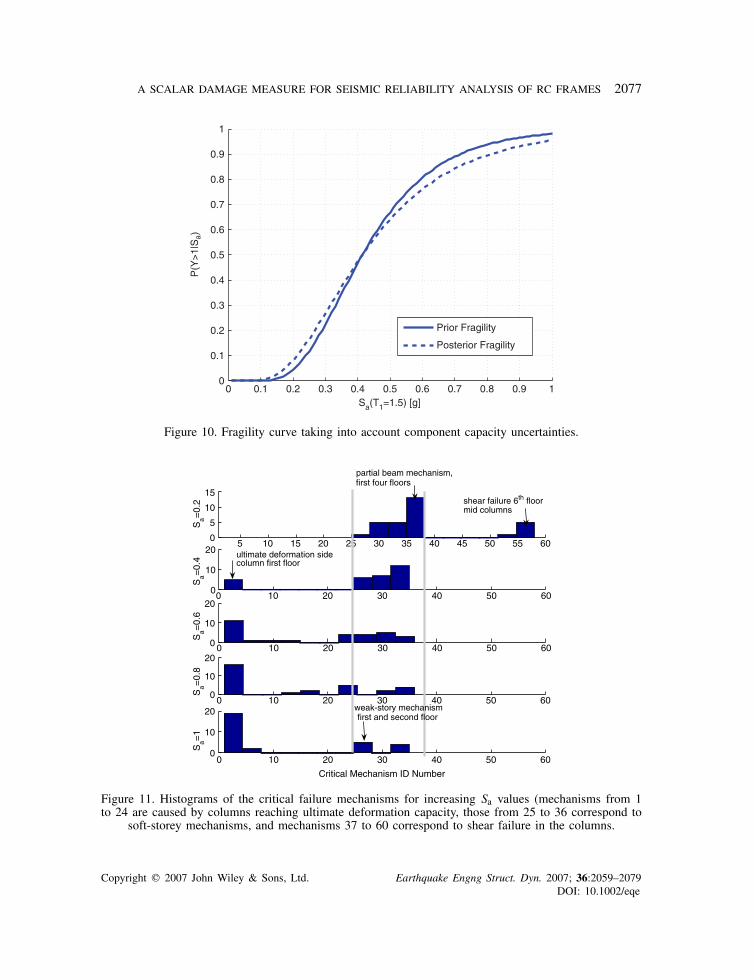
Figure 10. Fragility curve taking into account component capacity uncertainties.

5 10 15 20 25 30 35 40 45 50 55 60

0 10 20 30 40 50 60

0 10 20 30 40 50 60

0 10 20 30 40 50 60

0 10 20 30 40 50 60

Critical Mechanism ID Number

partial beam mechanism,first four floors

shear failure 6th floormid columns

ultimate deformation sidecolumn first floor

first and second floorweak-story mechanism

Sa=

0.2

Sa=

0.4

Sa=

0.6

Sa=

0.8

Sa=

1

0

5

10

15

0

10

20

0

10

20

0

10

20

0

10

20

Figure 11. Histograms of the critical failure mechanisms for increasing Sa values (mechanisms from 1to 24 are caused by columns reaching ultimate deformation capacity, those from 25 to 36 correspond to

soft-storey mechanisms, and mechanisms 37 to 60 correspond to shear failure in the columns.



Analysis of failure: The results of IDA allow to visualize the shift in critical failure mech-anism(s) with increasing spectral acceleration level. Figure 11 shows the histogram of criticalfailure mechanisms at each Sa level. There are three distinct zones on the histogram, the one tothe left corresponding to ultimate deformation mechanisms in the columns, the one in the middlecorresponding to yield mechanisms, and the one to the right corresponding to shear mechanisms.It can be observed that for the lowest Sa level, shear failure in the corner columns of the sixth floorand partial beam mechanism in first four floors are dominant, whereas for intermediate Sa levelsweak storey mechanisms become more critical. For higher levels of Sa, ultimate deformation infirst floor columns is the critical failure mechanism.

4. SUMMARY AND CONCLUSIONS

The scalar system-level DM used in this paper for probabilistic performance assessment of struc-tures is the critical demand-to-capacity ratio, defined as ratio of demand to capacity for thecomponent that leads the system closer to failure. This DM relies on a cut-set description of thestructure/system to aggregate the state of its components into the global structural state.

It allows for incorporation of information coming from response analysis and from experimen-tally based member capacity formulas in performance assessment, consideration of the uncertaintyinduced by the ground motion, as well as the uncertainty associated with the definition of capacity.Correlations existing within demands and within capacities of different components, and betweendemands and capacities, are also accounted for.

With reference to a generic RC frame structure, the probabilistic evaluation of this DM has beenpursued in parallel by using two nonlinear dynamic analysis approaches, the so-called ‘cloud’ and‘incremental dynamic analyses’. The former has been employed to assess the limit-state exceedancefrequency �LS directly using a well-established closed-form approximation, while the latter hasbeen used to obtain the fragility function, from which �LS follows numerical integration with thehazard function.

Particular consideration has been devoted to assess the effect of the modelling uncertaintyin member capacity models. A Bayesian approach has been employed to express this effectwith a single, system-level random variable, which reflects the number and types of mechanismsconsidered. As expected, given the relatively large dispersion of member capacity models, theyhave been found to be an influential factor on the final result.

ACKNOWLEDGEMENTS

This work was supported in part by the LESSLOSS Project funded by the European Commission—under Award Number GOCE-CT-2003-505488. This support is gratefully acknowledged. Any opinions,findings, and conclusions or recommendations expressed in this material are those of the authors and donot necessarily reflect those of the funding body. The first author also acknowledges the support fromthe Masters in Earthquake Engineering and Engineering Seismology Program (MEEES) by the EuropeanUnion.

REFERENCES

1. Ditlevsen O, Masden HO. Structural Reliability Methods. Wiley: New York, 1996.2. Au SK, Beck JL. Subset simulation and its application to seismic risk based on dynamic analysis. Journal of

Engineering Mechanics 2003; 129(8):901–917.



3. Lupoi G, Franchin P, Lupoi A, Pinto PE. Seismic fragility analysis of structural systems. Journal of EngineeringMechanics (ASCE) 2006; 132(4):385–395.

4. Schotanus MIJ, Franchin P. Seismic reliability analysis using response surface: a simplified approach. Proceedingsof 2nd ASRANet Colloquium, Barcelona, Spain, 2004.

5. Pinto PE, Giannini R, Franchin P. Seismic Reliability Analysis of Structures. IUSS Press: Pavia, 2004.www.iusspress.it

6. Jalayer F, Beck JL. Effects of alternative representations of ground motion uncertainty on seismic risk assessmentof structures. Earthquake Engineering and Structural Dynamics 2006, accepted.

7. Luco N, Cornell CA. Structure-specific scalar intensity measures for near-source and ordinary earthquake groundmotions. Earthquake Spectra 2006, submitted.

8. Jalayer F, Cornell CA. A technical framework for probability-based demand and capacity factor design (DCFD)seismic formats. Pacific Earthquake Engineering Research Center Report, vol. 08, 2003.

9. Jalayer F, Cornell CA. Alternative non-linear demand estimation methods for probability-based seismicassessments—Part I: wide range methods. Earthquake Spectra 2006, submitted.

10. Cornell CA, Jalayer F, Hamburger RO, Foutch DA. The probabilistic basis for the 2000 SAC/FEMA steelmoment frame guidelines. Journal of Structural Engineering (ASCE) 2002; 128(4):526–533.

11. Jalayer F, Franchin P, Pinto PE. Structural modelling uncertainty in seismic reliability analysis of RC frames: theuse of advanced simulation methods. Computational Methods in Structural Dynamics and Earthquake Engineering,COMPDYN2007, Crete, Greece, June 2007.

12. Jalayer F, Cornell CA. Alternative non-linear demand estimation methods for probability-based seismicassessments—Part II: reducing the analysis effort. Earthquake Spectra 2006, submitted.

13. Vamvatsikos V, Cornell CA. Incremental dynamic analysis. Earthquake Engineering and Structural Dynamics2002; 31(3):491–514.

14. Panagiotakos TB, Fardis MN. Deformations of reinforced concrete members at yielding and ultimate. ACIStructural Journal 2001; 98(2):135–148.

15. Seismic Assessment and Retrofit of Reinforced Concrete Buildings. Federation International du Beton ( fib) Stateof the Art Report, vol. 24, 2003.

16. Box GEP, Tiao GC. Bayesian Inference in Statistical Analysis. Wiley Classics Library, Wiley: New York, 1992.17. McKenna F, Fenves GL, Jeremic B, Scott MH. Open System for Earthquake Engineering Simulation, 2000.

http://opensees.berekely.edu18. Neuenhofer A, Filippou FC. Evaluation of non-linear frame finite element models. Journal of Structural

Engineering (ASCE) 1997; 123:958–966.19. Karsan ID, Jirsa JO. Behaviour of concrete under compressive loading. Journal of Structural Division (ASCE)

1969; 95(12):2543–2563.20. Menegotto M, Pinto PE. Method of analysis for cyclically loaded reinforced concrete plane frames including

changes in geometry and non-elastic behaviour of elements under combined normal force and bending. Proceedingsof IABSE Symposium on Resistance and Ultimate Deformability of Structures Acted on by Well Defined RepeatedLoads, Lisbon, 1973; 15–22.

21. McGuire RK. Seismic Hazard and Risk Analysis. Monograph, Earthquake Engineering Research Institute, 2004.22. Martın-Perez B, Pantazopoulos SJ. Mechanics of concrete participation in cyclic shear resistance of reinforced

concert. Journal of Structural Engineering (ASCE) 1998; 124(6):633–641.


A scalar damage measure for seismic reliability analysis of RC frames

Documents

Transcript of A scalar damage measure for seismic reliability analysis of RC frames