Fourier analysis of an equal-order incompressible flow solver stabilized by pressure gradient...

INTERNATIONAL JOURNAL FOR NUMERICAL METHODS IN FLUIDSInt. J. Numer. Meth. Fluids 2000; 34: 65–92

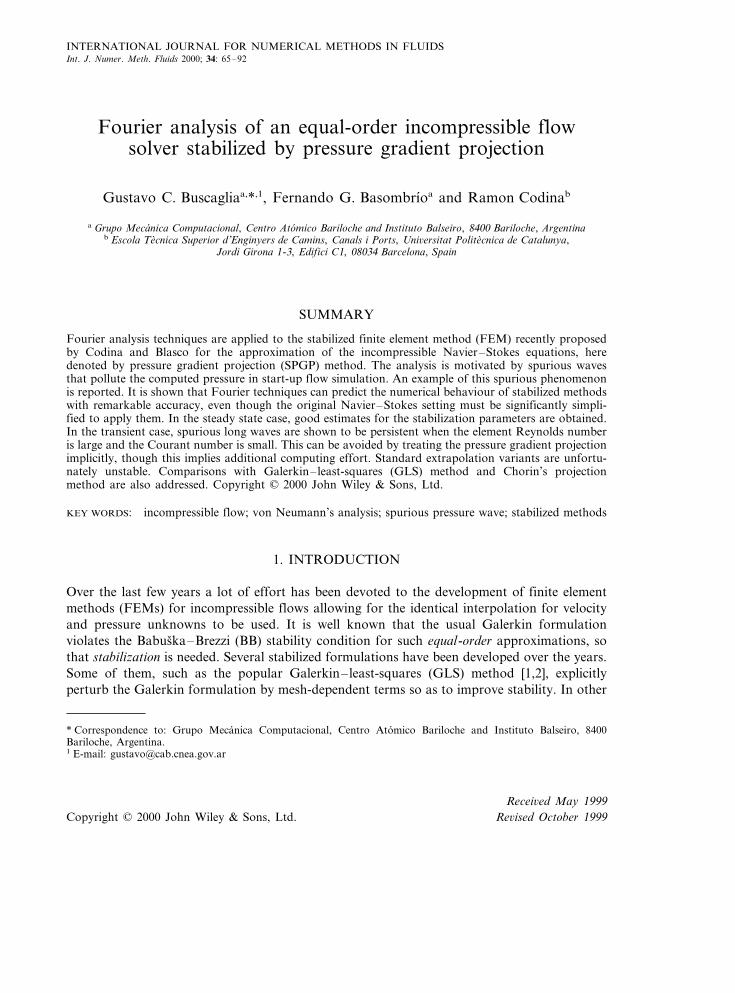
Fourier analysis of an equal-order incompressible flowsolver stabilized by pressure gradient projection

Gustavo C. Buscagliaa,*,1, Fernando G. Basombrıoa and Ramon Codinab

a Grupo Mecanica Computacional, Centro Atomico Bariloche and Instituto Balseiro, 8400 Bariloche, Argentinab Escola Tecnica Superior d’Enginyers de Camins, Canals i Ports, Uni6ersitat Politecnica de Catalunya,

Jordi Girona 1-3, Edifici C1, 08034 Barcelona, Spain

SUMMARY

Fourier analysis techniques are applied to the stabilized finite element method (FEM) recently proposedby Codina and Blasco for the approximation of the incompressible Navier–Stokes equations, heredenoted by pressure gradient projection (SPGP) method. The analysis is motivated by spurious wavesthat pollute the computed pressure in start-up flow simulation. An example of this spurious phenomenonis reported. It is shown that Fourier techniques can predict the numerical behaviour of stabilized methodswith remarkable accuracy, even though the original Navier–Stokes setting must be significantly simpli-fied to apply them. In the steady state case, good estimates for the stabilization parameters are obtained.In the transient case, spurious long waves are shown to be persistent when the element Reynolds numberis large and the Courant number is small. This can be avoided by treating the pressure gradient projectionimplicitly, though this implies additional computing effort. Standard extrapolation variants are unfortu-nately unstable. Comparisons with Galerkin–least-squares (GLS) method and Chorin’s projectionmethod are also addressed. Copyright © 2000 John Wiley & Sons, Ltd.

KEY WORDS: incompressible flow; von Neumann’s analysis; spurious pressure wave; stabilized methods

1. INTRODUCTION

Over the last few years a lot of effort has been devoted to the development of finite elementmethods (FEMs) for incompressible flows allowing for the identical interpolation for velocityand pressure unknowns to be used. It is well known that the usual Galerkin formulationviolates the Babuska–Brezzi (BB) stability condition for such equal-order approximations, sothat stabilization is needed. Several stabilized formulations have been developed over the years.Some of them, such as the popular Galerkin–least-squares (GLS) method [1,2], explicitlyperturb the Galerkin formulation by mesh-dependent terms so as to improve stability. In other

* Correspondence to: Grupo Mecanica Computacional, Centro Atomico Bariloche and Instituto Balseiro, 8400Bariloche, Argentina.1 E-mail: [email protected]

Copyright © 2000 John Wiley & Sons, Ltd.Recei6ed May 1999

Re6ised October 1999

G. C. BUSCAGLIA, F. G. BASOMBRIO AND R. CODINA66

formulations, the stabilization terms are implicit within a fractional step algorithm. This is thecase, for example, of projection methods based on the early ideas of Chorin [3] and Temam [4](see, e.g. References [5–11]).

The equal-order method analysed in this article combines, in some sense, the two stabiliza-tion procedures mentioned above. An explicit stabilization term is incorporated, which in turnmimics the effect of fractional step methods. To our knowledge, the first precedent of thismethod was proposed by Habashi et al. [12] as the following modification of the zero-divergence constraint:

div u−l92p= −l div g (1)

where g=9p and l is a small parameter. Although at the continuous level the termscontaining l cancel exactly, upon finite element discretization, cancellation no longer occursand these terms in fact stabilize the formulation. Equivalent terms in the finite elementequations were later identified by Zienkiewicz and Codina [13] as explaining the goodbehaviour of an equal-order fractional step method (in their scheme, l was in fact the timestep). Finally, Codina and Blasco [14–16] formulated and analysed theoretically an equal-order method based on these ideas. From the convergence analysis, an elementwise estimatel�h2 (for h being small) was derived, and optimal convergence rates obtained. We will referto this method hereafter as the stabilized by pressure gradient projection (SPGP) method.Recent work by Codina [17] has shown a link between this method and the sub-grid scales(SGS) method [18].

From the computational point of view, the main drawback of the SPGP method is theintroduction of the projection of the pressure gradient as a new unknown of the problem, thusincreasing substantially the number of nodal unknowns of the final discrete system. However,iterative strategies may be devised to make the method efficient, with a computational costsimilar to that of other stabilized methods. On the other hand, when the transient Navier–Stokes equations are discretized using a finite difference scheme, the projection of the pressuregradient can be treated explicitly; that is to say, evaluated at the previous time step. In thiscase, the increase of cost of the formulation with respect to the standard Galerkin method isvery low. First, a stabilization matrix must be built up, and at the end of each time step thepressure gradient must be projected. This leads to a linear system of equations with a Grammsystem matrix, which can be solved by simple Jacobi iterations or approximated by a diagonalsystem (lumped form). The number of unknowns is not increased.

Many numerical tests have recently been performed to the SPGP method, involving steadyand transient, two- and three-dimensional flows [Buscaglia G, Carrica P. Unpublished results;19], with quite good results. A turbulent code based on the SPGP method also exhibits goodbehaviour [Lew A, Buscaglia G, Carrica P. A robust equal-order finite element formulation forthe k-epsilon turbulence model. Submitted]. Most of these tests deal with the pressure gradientprojection explicitly. Comparing the SPGP and GLS methods, it was found that the formerleads to better conditioning of the system matrix and smoother temporal behaviour of thepressure field in transients. As a drawback, spurious long-wave pressure transients in stronglyaccelerated flows (such as start-up flows) were detected. One of these cases is reported below.These spurious transients do not affect the velocity field, but render the pressure field useless

Copyright © 2000 John Wiley & Sons, Ltd. Int. J. Numer. Meth. Fluids 2000; 34: 65–92

EQUAL-ORDER INCOMPRESSIBLE FLOW SOLVER 67

until their extinction. Fortunately, no such phenomenon occurs in smooth flows (such asvortex shedding flows).

Summarizing, its overall performance makes the SPGP method attractive for equal-orderfinite element treatment of incompressible flows, mainly transient ones, and further work isneeded to understand and improve its properties. Stabilized methods are prone to introducespurious pressure wave perturbations. This is a price to be paid for avoiding the BB condition.

In this paper, Fourier analysis techniques are applied to the SPGP method and some of itsvariants. Several simplifications are introduced to render this analysis feasible. First, aone-dimensional model problem that mimics the Navier–Stokes equations is introduced anddiscretized. Second, the domain is assumed to be (−�, +�), so that all nodes areequivalent. Finally, the convective non-linear term is linearized. From the Fourier analysis ofthe discrete equations, appropriate choices of stabilization coefficients are obtained. In thetransient case (classical von Neumann’s analysis) stability is discussed. Moreover, a spuriousoscillatory behaviour is identified, which explains (both qualitatively and quantitatively)two-dimensional numerical results for start-up flow around a circular cylinder at a Reynoldsnumber of 3000. In particular, it is shown that the explicit treatment of the pressure gradientprojection activates this spurious behaviour and that a high-Reynolds number stabilizationcoefficient improves the results. Comparisons with the GLS and Chorin’s methods are alsoaddressed. Numerical results of the one-dimensional model problem in a bounded domainwithout linearizing the convective term show that the conclusions from Fourier analysis applyin more realistic situations.

2. DESCRIPTION OF THE NUMERICAL METHOD

The governing equations correspond to an incompressible, constant viscosity flow, i.e.

r(u(t

+r(u ·9)u−div(2mDu)+9p= f (2)

div u=0 (3)

where u is the velocity field; r is the density; m is the dynamic viscosity; D is the symmetricgradient operator, i.e. (Du)ij= (ui, j+uj,i)/2; p is the pressure; and f is the volumetric forces.These equations are assumed to hold in a bounded domain V, with initial solenoidal conditionsfor u in V, imposed velocities on the Dirichlet boundary GD, and imposed tractions on theNeumann boundary GN (GD@GN=(V, GDSGN=¥).

u(x, 0)=u0(x), x�V (4)

u(x, t)=g(x, t), x�GD (5)

(−p1+2mDu) ·n=F, x�GN (6)



Now, let Th be a finite element partition of V, and let Vh¦H1(V)nsd be an associated finiteelement space to approximate the velocity field, where nsd is the number of space dimensions.We assume that Vh consists of piecewise linear, bilinear or trilinear vector fields. We define, asusual,

VhD={6h�Vh, 6h=g on GD} (7)

Vh0={6h�Vh, 6h=0 on GD} (8)

and let Qh¦L2(V) be a finite element space for the pressure. Of most interest to us is the casewhen the interpolants for the pressure coincide with those used for each component of thevelocity field. Finally, let Gh be another vector finite element space, which we take to begenerally coincident with Vh (no boundary conditions imposed). The SPGP method consideredthus reads [15]

Find (uhn, ph

n, ghn)�VhD×Qh×Gh such that

�r

uhn−uh

n−1

Dt+r(uh* ·9)uh

n, 6h�

+a(uhn, 6h)− (ph

n, div 6h)− ( f n, 6h)−&

GN

Fn ·6h dG

+ %K�Th

�r

uhn−uh

n−1

Dt+r(uh* ·9)uh

n+9phn− f,

tu

r[r(uh* ·9)6h ]

�K

=0 (9)

(qh, div uhn)+ %

K�Th

�9ph

n−ghn−1+b,

tp

r9qh

�K

=0 (10)

(−9phn+gh

n, jh)=0 (11)

for all (6h, qh, jh)�Vh0×Qh×Gh.In Equation (9), a( · , · ) is the viscous bilinear form, uh* can be taken as uh

n or uhn−1, the latter

corresponding to the standard linearized treatment of convection, and tu is the SUPG intrinsictime

tu=a(ReK)hK

2�un−1� (12)

ReK=r �un−1�hK

12m(13)

a(ReK)=min(1, ReK) (14)

and tp is a second intrinsic time. In Reference [15], the value rhK2 /(12m), differing just by a

factor of two from the low-Reynolds number formula for tu, is adopted. In practice, this valueis slightly too large for high-Reynolds number computations, a better choice being tp=tu.



Simpler formulae for the stabilization parameters, justified by a convergence analysis, wererecently proposed by Codina [20]. Notice that the previous formulation is of the backwardEuler kind, except for the appearance of gh

n−1+b if bB1. For the algorithmic cost to becompetitive, the choice b=0 is mandatory.

The matrix formulation of Equations (9)–(11) is

1Dt

MU(Un−Un−1)+ (A+K)Un−B0 Pn=F (15)

BTUn+1r

LPn−1r

DTGn−1+b=0 (16)

−CPn+MGn=0 (17)

where Un, Pn and Gn are the vectors containing the unknowns, MU, A and K are the matricesarising from the temporal derivative, convective and viscous terms respectively (including thestabilization terms), and

BIJ=&

VMJ div NI dV (18)

B0 IJ=BIJ−&

Vtu9MJ ·(uh

n ·9)NI dV (19)

DIJ=&

Vtp9MJ ·NI dV (20)

CIJ=&

V9MJ ·NI dV (21)

LIJ=&

Vtp9MJ ·9MI dV (22)

MIJ=&

VMJMI dV (23)

MI and NI being respectively, the Ith basis function for pressure and velocity (NI is, thus,vectorial). The mass matrix M can be used in consistent form or lumped form. No significantdifference was found using linear elements, so that the lumped form is adopted.



3. FOURIER ANALYSIS OF THE STEADY STATE

To perform the Fourier analysis, a model one-dimensional problem is introduced that retainsthe main characteristics of the Navier–Stokes equations. We keep the notation u and p for theunknowns to make the analogy evident. The proposed equations are

r(u(t

+ru(u(x

−2m(2u(x2+

(p(x

= f (24)

(u(x

=0 (25)

Let us begin omitting the SUPG terms (tu=0). Let us also linearize the problem replacing thenon-linear term ru((u/(x) by rc((u/(x). The SPGP method, with M lumped and assuming fis continuous and piecewise linear, leads to the following stencil:

r

6Dt(Ui−1

n +4Uin+Ui+1

n −Ui−1n−1−4Ui

n−1−Ui+1n−1)+rc

Ui+1n −Ui−1

n

2h

−2mUi+1

n −2Uin+Ui−1

n

h2 +Pi+1

n −Pi−1n

2h=

Fi−1n +4Fi

n+Fi+1n

6(26)

Ui+1n −Ui−1

n

2h−

tp

r

Pi+1n −2Pi

n+Pi−1n

h2 = −tp

r

Pi+2n−1+b−2Pi

n−1+b+Pi−2n−1+b

4h2 (27)

where h is the (uniform) mesh size and capital letters denote nodal values of the unknowns.If tu\0, Equation (26) must be modified by adding

−tu!rcDt

Ui+1n −Ui−1

n −Ui+1n−1+Ui−1

n−1

2h+rc2 Ui+1

n −2Uin+Ui−1

n

h2

+cPi+1

n −2Pin+Pi−1

n

h2

"to the left-hand side, and

−tucFi+1−Fi−1

2h

to the right-hand side.The Fourier analysis of the steady state, which is restricted to Stokes flow (r=0), roughly

follows the lines of Reference [21]. Let us consider the following stencil:

− (2m+n)Ui+1−2Ui+Ui−1

h2 +Pi+1−Pi−1

2h=

Fi−1+Fi+Fi+1

6(28)



Ui+1−Ui−1

2h−a

Pi+1−2Pi+Pi−1

h2 +gPi+2−2Pi+Pi−2

4h2 = −dFi+1−Fi−1

2h(29)

This stencil, with suitable values for the constants n, a, g and d, corresponds to the steady stateformulation of the SPGP method (Ui

n=Uin−1=Ui, Pi

n=Pin−1=Pi). It also allows for the

comparison of the SPGP method (d=0, a=g) with the GLS method (d=a, g=0). Now, let

m %=2m+n, a=am %

h2 , g=gm %

h2 , d0 =dm %

h2

and defining

V=Um %

h2 , Gi+1/2=Pi+1−Pi

h

the stencil becomes

− (Vi+1−2Vi+Vi−1)+12

(Gi+1/2+Gi−1/2)=Fi+1+4Fi+Fi−1

6(30)

Vi+1−Vi−1

2− a(Gi+1/2−Gi−1/2)+

g

4(Gi+3/2+Gi+1/2−Gi−1/2−Gi−3/2)

= −d02

(Fi+1−Fi−1) (31)

Assuming now that i runs from −� to +� and inserting Fourier modes

Vi�V. e−Iikh, Gi�G. e−Iikh, Fi�F. e−Iikh

with k the Fourier variable and I=−1, and denoting u=kh/2, the following system isobtained:

4 sin2 uV. +cos uG. =�1−

23

sin2 u�

F. (32)

cos uV. + (g cos2 u− a)G. = −d0 cos uF. (33)

Symbolic manipulation [20] was used to get V. and G. . Its expansions around u=0 read

SV�V.F. = a−d0 − g+

�−4a2−

23

g(−1+6d0 +6g)+ a�1

3+4d0 +8g

�nu2+O(u4) (34)

SG�G.F. =1+

�−

16+4(− a+d0 + g)

nu2+O(u4) (35)



Notice that the exact dependencies (if u"0) are V. =0, G. =F. , or, in other terms, SV=0 andSG=1. For the scheme to coincide with these exact expressions at u�0, the only condition is

a− g−d0 =0 (36)

Both the GLS and SPGP methods satisfy this condition. Let us impose thus g= a−d0 . In thiscase

SV=�

a−23

d0 �u2+O(u4) (37)

SG=1−u2

6+O(u4) (38)

From this we learn, on the one hand, that asymptotic accuracy (as kh�0) cannot be improvedbeyond second order (which is the expected spatial accuracy), as SG is second-order accuratefor any choice of a and d0 . On the other hand, accuracy in the velocity could be improved bychoosing a linear combination of the GLS and SPGP methods, namely a=2

3d0 (implyingg= −1

3d0 ). The gain is, however, not significant, as, in general, accuracy in velocity is muchhigher than in pressure.

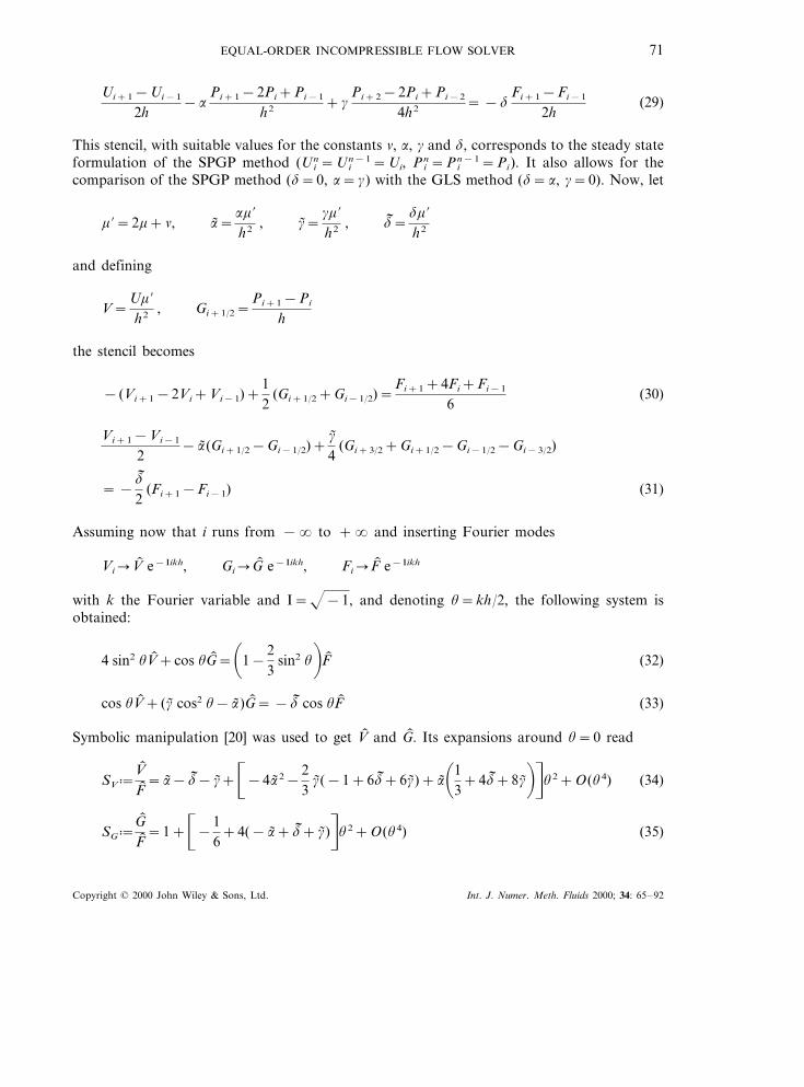
The selection of a and d0 must be made examining the accuracy when kh is far from zero, asthe behaviour in the vicinity of zero does not depend on these parameters. We have focusedon two cases: GLS (a=r, d0 =r, g=0) and SPGP (a=r, g=r, d0 =0). Comparison is made forr=10−1, 10−2 and 10−3. Plots of SG versus u can be seen in Figures 1 and 2.

By direct inspection of Figures 1 and 2 it becomes clear that, for both the SPGP and GLSmethods, r=10−2 is the best choice. For r=10−1, SG is significantly lower than the exact

Figure 1. SG versus u for the GLS method with r=10−1, 10−2 and 10−3.



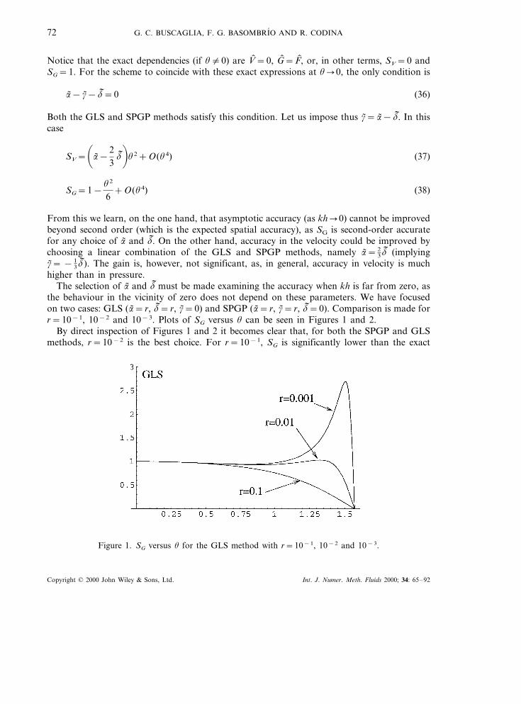
Figure 2. SG versus u for the SPGP method with r=10−1, 10−2 and 10−3.

value of 1, for u as low as 0.75. For r=10−3, SG exhibits a peak near the mesh mode(u=p/2), proving that the spurious mode of the Galerkin formulation is not properlystabilized. From the observation that r (and thus a) must roughly be equal to 10−2, as

tp

r=a=

ah2

m %

it follows that a good choice for tp/r is

tp

r=

h2

100m %(39)

for both methods, which is consistent with usual adopted formulae for GLS [2].

RemarkAnother possibility, by inspection of Equation (35), is to put g+d0 − a= 1

24. This sets thesecond-order term in SG to zero, leaving a zeroth-order term in SV. Though no furtherinvestigation has yet been performed, the increase in accuracy for the most sensitive variable(the pressure) may prove useful. (Accuracy of order eight in G is obtained choosing g= a−d0 + 1

24, d0 =2a− 148 and a= 1

32!!!)



4. START-UP FLOW AROUND A CYLINDER: SPURIOUS PRESSURE WAVE

To motivate the von Neumann’s analysis of the next section, we briefly report here on anumerical test. The problem consists of the start-up flow around a circular cylinder atRe=3000, defined as Re=rU�D/m, U� being the unperturbed flow velocity and D thecylinder’s diameter. The domain is V= (−5, 15)× (−5, 5)¯C, with C being the cylinder ofunit diameter centred at the origin. This problem has been studied both experimentally [23]and numerically (by the GSMAC method [24]). Starting from rest, U� is impulsively modifiedto U�=1, with D=1, r=3000 and m=1. Attempts to simulate this flow starting from restsystematically failed. Success was attained using as initial condition the inviscid solution, asdiscussed by Gresho [25], i.e.

u1=1−x1

2−x22

4r4 , u2= −x1x2

2r4 , p=r(x1

2−x22−1

8)2r4 (40)

where r2=x12+x2

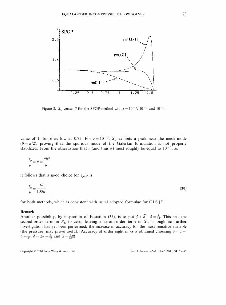
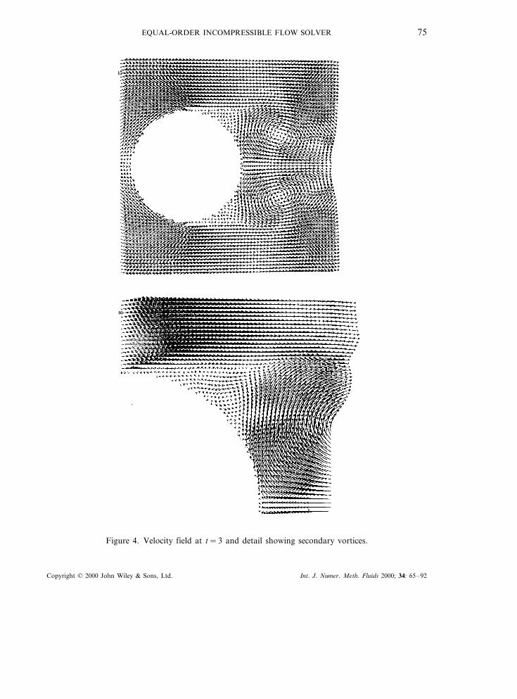
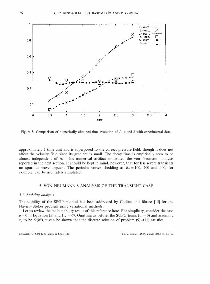
2. The flow is characterized by the formation and growth of two mainsymmetric vortices downstream of the cylinder, with some secondary vortices also appearing(see Figure 3). The simulation time is 3 units, with a time step of Dt=0.001. We do not intendto give detailed results here. The numerical parameters were tu according to Equation (12),tp=tu, b=0. The mesh consisted of 11518 P1 triangles, refined near the cylinder. The mainfact is that the velocity field is accurately predicted. A snapshot of the velocity field at t=3can be seen in Figure 4, which compares well with experimental data. In Figure 5, aquantitative comparison of the time evolution of the flow characteristic lengths a, b and L (seeFigure 3) with the experiment is shown.

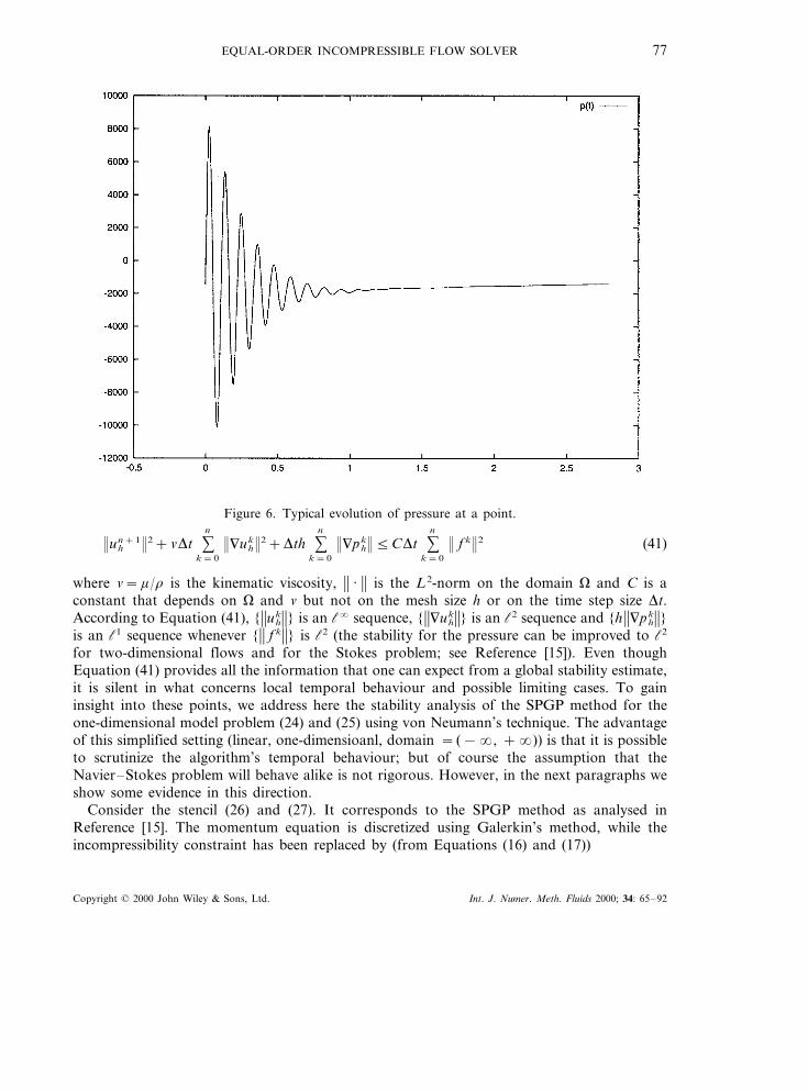
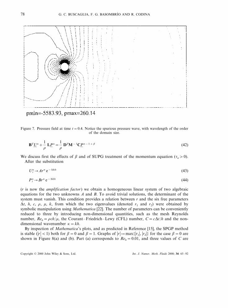
The behaviour of the pressure is quite unexpected. A typical evolution of the pressure at apoint in the domain is shown in Figure 6. A spurious oscillation is observed; roughly asinusoidal function with decaying amplitude. This is associated with a long wavelength,quasi-one-dimensional wave, which is shown in Figure 7 at time t=0.4. This wave persists for

Figure 3. Problem geometry and definition of a, b and L.



Figure 4. Velocity field at t=3 and detail showing secondary vortices.



Figure 5. Comparison of numerically obtained time evolution of L, a and b with experimental data.

approximately 1 time unit and is superposed to the correct pressure field, though it does notaffect the velocity field since its gradient is small. The decay time is empirically seen to bealmost independent of Dt. This numerical artifact motivated the von Neumann analysisreported in the next section. It should be kept in mind, however, that for less severe transientsno spurious wave appears. The periodic vortex shedding at Re=100, 200 and 400, forexample, can be accurately simulated.

5. VON NEUMANN’S ANALYSIS OF THE TRANSIENT CASE

5.1. Stability analysis

The stability of the SPGP method has been addressed by Codina and Blasco [15] for theNavier–Stokes problem using variational methods.

Let us review the main stability result of this reference here. For simplicity, consider the caseg=0 in Equation (5) and GN=¥. Omitting as before, the SUPG terms (tu=0) and assumingtp to be O(h2), it can be shown that the discrete solution of problem (9)–(11) satisfies



Figure 6. Typical evolution of pressure at a point.

uhn+1 2+nDt %

n

k=0

9uhk 2+Dth %

n

k=0

9phk 5CDt %

n

k=0

f k 2 (41)

where n=m/r is the kinematic viscosity, �� · �� is the L2-norm on the domain V and C is aconstant that depends on V and n but not on the mesh size h or on the time step size Dt.According to Equation (41), {��uh

k��} is an l� sequence, {��9uhk��} is an l2 sequence and {h ��9ph

k��}is an l1 sequence whenever {�� f k��} is l2 (the stability for the pressure can be improved to l2

for two-dimensional flows and for the Stokes problem; see Reference [15]). Even thoughEquation (41) provides all the information that one can expect from a global stability estimate,it is silent in what concerns local temporal behaviour and possible limiting cases. To gaininsight into these points, we address here the stability analysis of the SPGP method for theone-dimensional model problem (24) and (25) using von Neumann’s technique. The advantageof this simplified setting (linear, one-dimensioanl, domain = (−�, +�)) is that it is possibleto scrutinize the algorithm’s temporal behaviour; but of course the assumption that theNavier–Stokes problem will behave alike is not rigorous. However, in the next paragraphs weshow some evidence in this direction.

Consider the stencil (26) and (27). It corresponds to the SPGP method as analysed inReference [15]. The momentum equation is discretized using Galerkin’s method, while theincompressibility constraint has been replaced by (from Equations (16) and (17))



Figure 7. Pressure field at time t=0.4. Notice the spurious pressure wave, with wavelength of the orderof the domain size.

BTUn+1r

LPn=1r

DTM−1CPn−1+b (42)

We discuss first the effects of b and of SUPG treatment of the momentum equation (tu\0).After the substitution

Uin�Arn e−Iikh (43)

Pin�Brn e−Iikh (44)

(r is now the amplification factor) we obtain a homogeneous linear system of two algebraicequations for the two unknowns A and B. To avoid trivial solutions, the determinant of thesystem must vanish. This condition provides a relation between r and the six free parametersDt, h, c, r, m, k, from which the two eigenvalues (denoted r1 and r2) were obtained bysymbolic manipulation using Mathematica [22]. The number of parameters can be convenientlyreduced to three by introducing non-dimensional quantities, such as the mesh Reynoldsnumber, Reh=rch/m, the Courant–Friedrich–Lewy (CFL) number, C=cDt/h and the non-dimensional wavenumber k=kh.

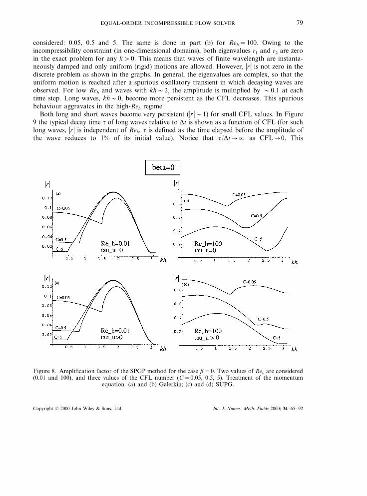
By inspection of Mathematica ’s plots, and as predicted in Reference [15], the SPGP methodis stable (�r �B1) both for b=0 and b=1. Graphs of �r ��max{�r1�, �r2�} for the case b=0 areshown in Figure 8(a) and (b). Part (a) corresponds to Reh=0.01, and three values of C are



considered: 0.05, 0.5 and 5. The same is done in part (b) for Reh=100. Owing to theincompressibility constraint (in one-dimensional domains), both eigenvalues r1 and r2 are zeroin the exact problem for any k\0. This means that waves of finite wavelength are instanta-neously damped and only uniform (rigid) motions are allowed. However, �r � is not zero in thediscrete problem as shown in the graphs. In general, the eigenvalues are complex, so that theuniform motion is reached after a spurious oscillatory transient in which decaying waves areobserved. For low Reh and waves with kh�2, the amplitude is multiplied by �0.1 at eachtime step. Long waves, kh�0, become more persistent as the CFL decreases. This spuriousbehaviour aggravates in the high-Reh regime.

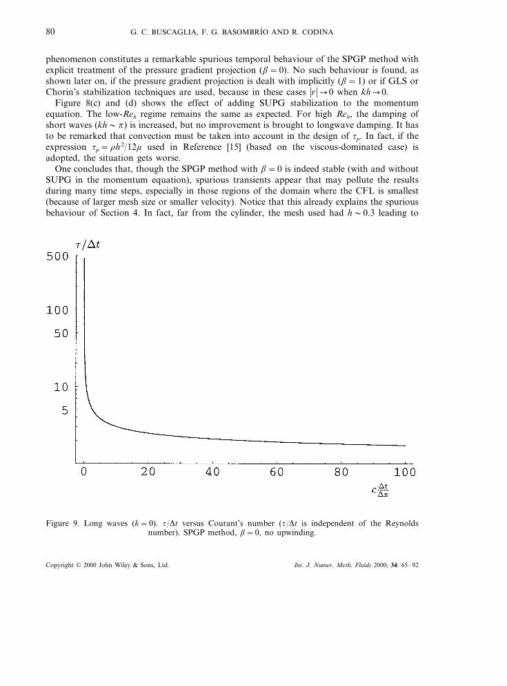
Both long and short waves become very persistent (�r ��1) for small CFL values. In Figure9 the typical decay time t of long waves relative to Dt is shown as a function of CFL (for suchlong waves, �r � is independent of Reh, t is defined as the time elapsed before the amplitude ofthe wave reduces to 1% of its initial value). Notice that t/Dt�� as CFL�0. This

Figure 8. Amplification factor of the SPGP method for the case b=0. Two values of Reh are considered(0.01 and 100), and three values of the CFL number (C=0.05, 0.5, 5). Treatment of the momentum

equation: (a) and (b) Galerkin; (c) and (d) SUPG.



phenomenon constitutes a remarkable spurious temporal behaviour of the SPGP method withexplicit treatment of the pressure gradient projection (b=0). No such behaviour is found, asshown later on, if the pressure gradient projection is dealt with implicitly (b=1) or if GLS orChorin’s stabilization techniques are used, because in these cases �r ��0 when kh�0.

Figure 8(c) and (d) shows the effect of adding SUPG stabilization to the momentumequation. The low-Reh regime remains the same as expected. For high Reh, the damping ofshort waves (kh�p) is increased, but no improvement is brought to longwave damping. It hasto be remarked that convection must be taken into account in the design of tp. In fact, if theexpression tp=rh2/12m used in Reference [15] (based on the viscous-dominated case) isadopted, the situation gets worse.

One concludes that, though the SPGP method with b=0 is indeed stable (with and withoutSUPG in the momentum equation), spurious transients appear that may pollute the resultsduring many time steps, especially in those regions of the domain where the CFL is smallest(because of larger mesh size or smaller velocity). Notice that this already explains the spuriousbehaviour of Section 4. In fact, far from the cylinder, the mesh used had h�0.3 leading to

Figure 9. Long waves (k=0). t/Dt versus Courant’s number (t/Dt is independent of the Reynoldsnumber). SPGP method, b=0, no upwinding.



Reh�900 and C�0.003, values that fall well within the expected range of longwavepersistance.

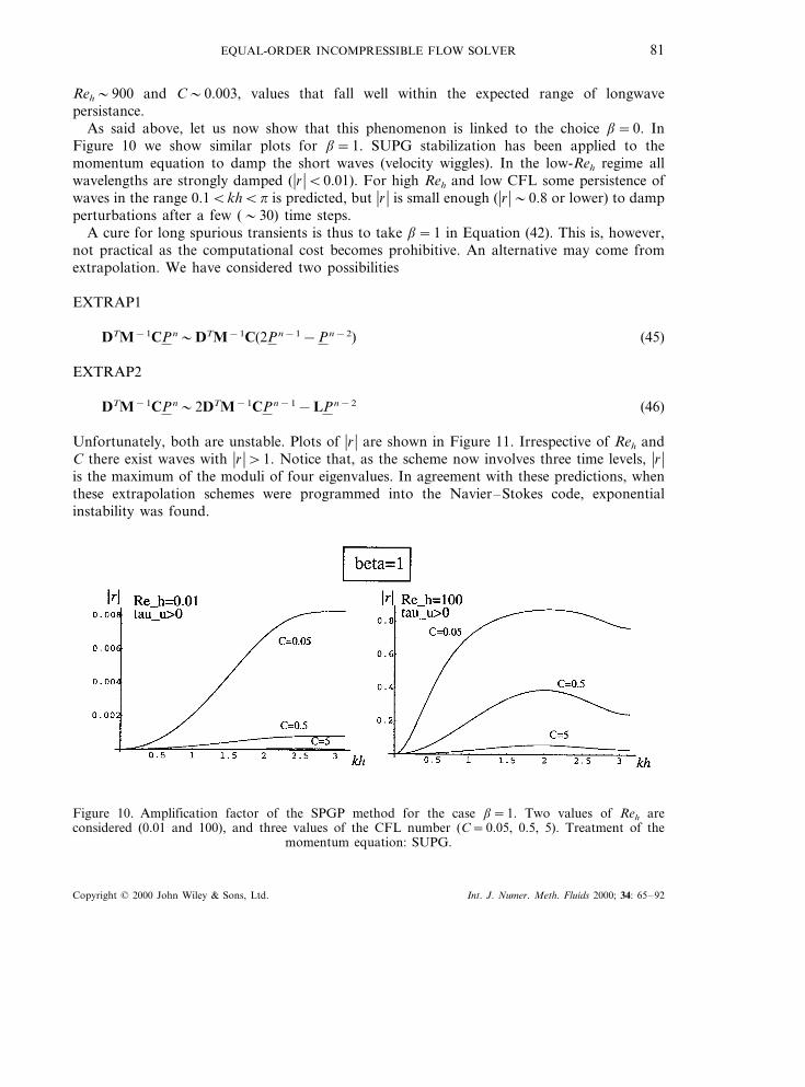
As said above, let us now show that this phenomenon is linked to the choice b=0. InFigure 10 we show similar plots for b=1. SUPG stabilization has been applied to themomentum equation to damp the short waves (velocity wiggles). In the low-Reh regime allwavelengths are strongly damped (�r �B0.01). For high Reh and low CFL some persistence ofwaves in the range 0.1BkhBp is predicted, but �r � is small enough (�r ��0.8 or lower) to dampperturbations after a few (�30) time steps.

A cure for long spurious transients is thus to take b=1 in Equation (42). This is, however,not practical as the computational cost becomes prohibitive. An alternative may come fromextrapolation. We have considered two possibilities

EXTRAP1

DTM−1CPn�DTM−1C(2Pn−1−Pn−2) (45)

EXTRAP2

DTM−1CPn�2DTM−1CPn−1−LPn−2 (46)

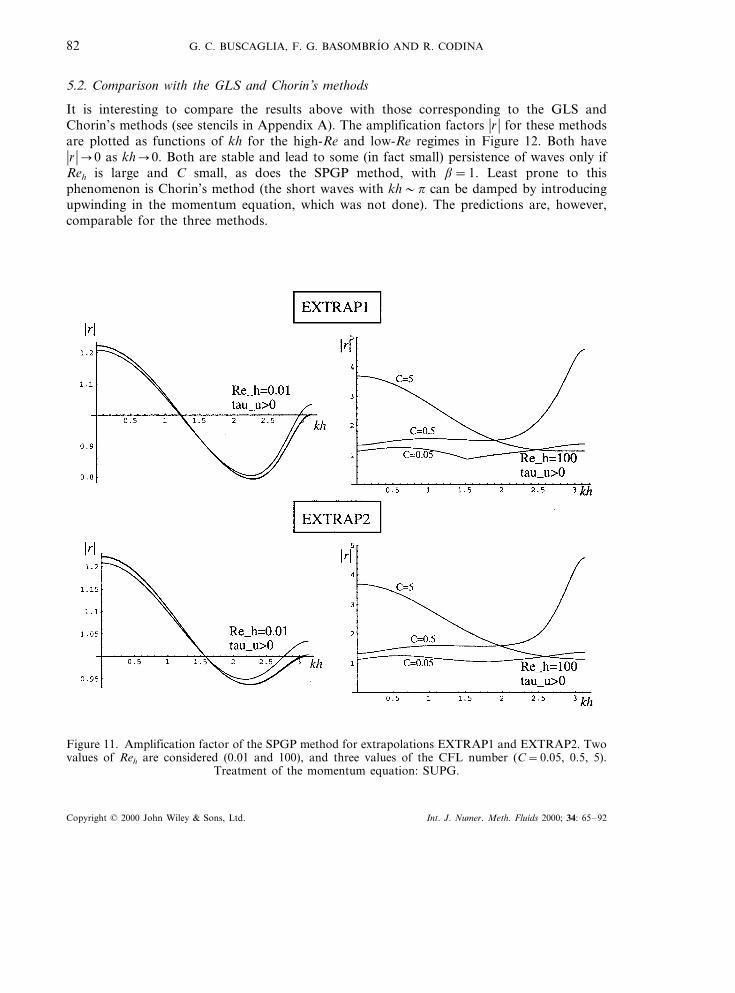
Unfortunately, both are unstable. Plots of �r � are shown in Figure 11. Irrespective of Reh andC there exist waves with �r �\1. Notice that, as the scheme now involves three time levels, �r �is the maximum of the moduli of four eigenvalues. In agreement with these predictions, whenthese extrapolation schemes were programmed into the Navier–Stokes code, exponentialinstability was found.

Figure 10. Amplification factor of the SPGP method for the case b=1. Two values of Reh areconsidered (0.01 and 100), and three values of the CFL number (C=0.05, 0.5, 5). Treatment of the

momentum equation: SUPG.



5.2. Comparison with the GLS and Chorin’s methods

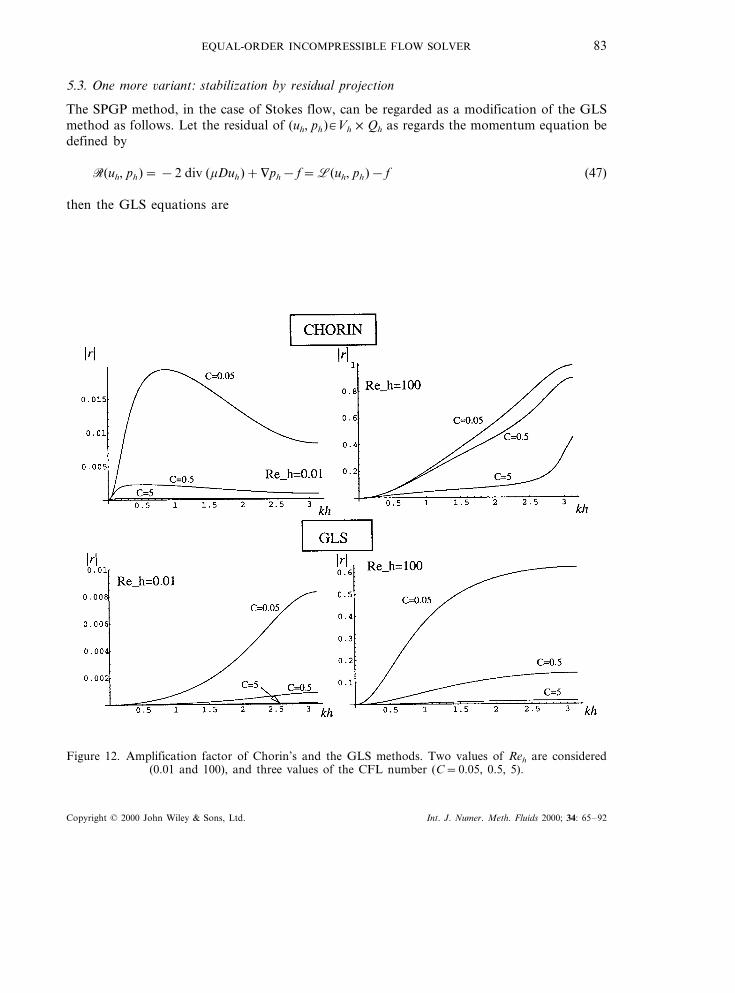
It is interesting to compare the results above with those corresponding to the GLS andChorin’s methods (see stencils in Appendix A). The amplification factors �r � for these methodsare plotted as functions of kh for the high-Re and low-Re regimes in Figure 12. Both have�r ��0 as kh�0. Both are stable and lead to some (in fact small) persistence of waves only ifReh is large and C small, as does the SPGP method, with b=1. Least prone to thisphenomenon is Chorin’s method (the short waves with kh�p can be damped by introducingupwinding in the momentum equation, which was not done). The predictions are, however,comparable for the three methods.

Figure 11. Amplification factor of the SPGP method for extrapolations EXTRAP1 and EXTRAP2. Twovalues of Reh are considered (0.01 and 100), and three values of the CFL number (C=0.05, 0.5, 5).

Treatment of the momentum equation: SUPG.



5.3. One more 6ariant: stabilization by residual projection

The SPGP method, in the case of Stokes flow, can be regarded as a modification of the GLSmethod as follows. Let the residual of (uh, ph)�Vh×Qh as regards the momentum equation bedefined by

R(uh, ph)= −2 div (mDuh)+9ph− f=L(uh, ph)− f (47)

then the GLS equations are

Figure 12. Amplification factor of Chorin’s and the GLS methods. Two values of Reh are considered(0.01 and 100), and three values of the CFL number (C=0.05, 0.5, 5).



a(uh, 6h)− (ph, div 6h)− ( f, 6h)−&

GN

F ·6h dG+ (qh, div uh)

+ %K�Th

�R(uh, ph),

tu

rL(6h, qh)

�K

=0 (48)

On the other hand, for linear elements, piecewise linear f and Stokes flow, the SPGP methodcan be written as

a(uh, 6h)− (ph, div 6h)− ( f, 6h)−&

GN

F ·6h dG+ (qh, div uh)

+ %K�Th

�R(uh, ph)−PhR(uh, ph),

t

rL(6h, qh)

�K

=0 (49)

It is evident that the only difference with the GLS equations is that the projection of theresidual, PhR, onto Vh has been subtracted from the residual itself within the stabilizationterm. Consistency has not been lost, since for the exact solution the residual vanishes. Withthis interpretation one could proceed analogously for the transient Navier–Stokes problem,arriving at a variant of the SPGP method. In this case, the residual is

R(uh, ph)=r(uh

(t+r(uh ·9)uh−2 div(mDuh)+9ph− f (50)

For non-zero Re, the residual of the incompressibility constraint also enters the GLSformulation [1], times a mesh-dependent constant

dK=r �uh �2tu (51)

and thus, assuming linear elements, the stabilization terms are

%K�Th

�(r(uh ·9)uh+9ph)−Ph(r(uh ·9)uh+9ph),

tu

r(r(uh ·9)6h+9qh)

�K

+ %K�Th

dK(div uh−Ph div uh, div 6h)K (52)

An almost equivalent formulation is proposed in Codina [17], where it is shown that it is infact a SGS method [18] with a particular choice for the space of sub-scales.

von Neumann’s analysis of this method yields results that resemble those of the SPGPmethod. In this case, the possibility also appears of dealing with the residual projection eitherimplicitly (b=1 in the SPGP method) or explicitly (b=0), and again the only reasonablechoice (from the computational point of view) is the latter. The results are shown in Figure 13.



Figure 13. Amplification factor of full-residual projection variant of the SPGP method. Two values ofReh are considered (0.01 and 100), and three values of the CFL number (C=0.05, 0.5, 5).

6. NUMERICAL TESTS

The predictions of the previous section are based on the linearized version of the modelproblem (24) and (25), and disregarding boundary effects. It is important to check that theconclusions are not overruled as soon as these simplifying hypotheses are dropped.

6.1. Comparison for a one-dimensional model problem

Considering first the full (non-linear) one-dimensional model problem (24) and (25), to besolved for t\0 in V= (0, 1) with f=0 and initial and boundary conditions

u(x, t=0)=0, u(0, t\0)=1, p(1, t\0)=0 (53)

the exact solution is

u(x, t)=1 (54)

p(x, t)=0 (55)

A series of numerical experiments on this problem were performed using the SPGP method.Linear one-dimensional finite elements were used. Experiences were made with r=1, m=1/45000, for different values of h and Dt. The computed pressure is seen to oscillate aroundzero with an amplitude that decays to zero. This is a spurious pressure transient that isactivated by the sudden imposition of u=1 on the left boundary. The period of theoscillations, and the decay behaviour, are not predictable a priori due to the non-linearity ofthe problem. Our aim here is to compare them with the predictions from von Neumann’sanalysis (which rigorously apply just to the linearized model with no boundary).



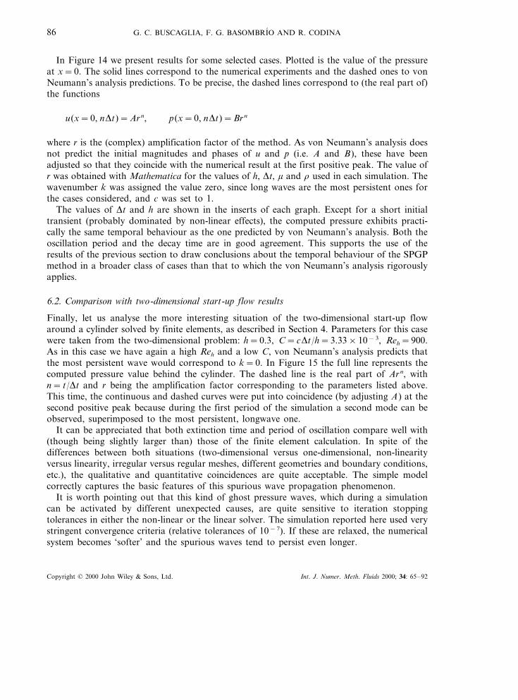
In Figure 14 we present results for some selected cases. Plotted is the value of the pressureat x=0. The solid lines correspond to the numerical experiments and the dashed ones to vonNeumann’s analysis predictions. To be precise, the dashed lines correspond to (the real part of)the functions

u(x=0, nDt)=Arn, p(x=0, nDt)=Brn

where r is the (complex) amplification factor of the method. As von Neumann’s analysis doesnot predict the initial magnitudes and phases of u and p (i.e. A and B), these have beenadjusted so that they coincide with the numerical result at the first positive peak. The value ofr was obtained with Mathematica for the values of h, Dt, m and r used in each simulation. Thewavenumber k was assigned the value zero, since long waves are the most persistent ones forthe cases considered, and c was set to 1.

The values of Dt and h are shown in the inserts of each graph. Except for a short initialtransient (probably dominated by non-linear effects), the computed pressure exhibits practi-cally the same temporal behaviour as the one predicted by von Neumann’s analysis. Both theoscillation period and the decay time are in good agreement. This supports the use of theresults of the previous section to draw conclusions about the temporal behaviour of the SPGPmethod in a broader class of cases than that to which the von Neumann’s analysis rigorouslyapplies.

6.2. Comparison with two-dimensional start-up flow results

Finally, let us analyse the more interesting situation of the two-dimensional start-up flowaround a cylinder solved by finite elements, as described in Section 4. Parameters for this casewere taken from the two-dimensional problem: h=0.3, C=cDt/h=3.33×10−3, Reh=900.As in this case we have again a high Reh and a low C, von Neumann’s analysis predicts thatthe most persistent wave would correspond to k=0. In Figure 15 the full line represents thecomputed pressure value behind the cylinder. The dashed line is the real part of Arn, withn= t/Dt and r being the amplification factor corresponding to the parameters listed above.This time, the continuous and dashed curves were put into coincidence (by adjusting A) at thesecond positive peak because during the first period of the simulation a second mode can beobserved, superimposed to the most persistent, longwave one.

It can be appreciated that both extinction time and period of oscillation compare well with(though being slightly larger than) those of the finite element calculation. In spite of thedifferences between both situations (two-dimensional versus one-dimensional, non-linearityversus linearity, irregular versus regular meshes, different geometries and boundary conditions,etc.), the qualitative and quantitative coincidences are quite acceptable. The simple modelcorrectly captures the basic features of this spurious wave propagation phenomenon.

It is worth pointing out that this kind of ghost pressure waves, which during a simulationcan be activated by different unexpected causes, are quite sensitive to iteration stoppingtolerances in either the non-linear or the linear solver. The simulation reported here used verystringent convergence criteria (relative tolerances of 10−7). If these are relaxed, the numericalsystem becomes ‘softer’ and the spurious waves tend to persist even longer.



Figure 14. Pressure at x=0 versus time. Numerical experiments with the explicit SPGP method in theunit one-dimensional interval (r=c=1, m=45000). Solid line: numerical experiment; dashed line:

theoretical prediction. Both curves have been made to coincide near the first positive peak.



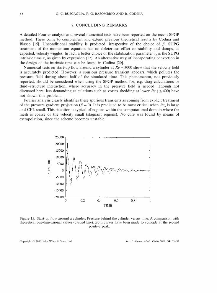
7. CONCLUDING REMARKS

A detailed Fourier analysis and several numerical tests have been reported on the recent SPGPmethod. These come to complement and extend previous theoretical results by Codina andBlasco [15]. Unconditional stability is predicted, irrespective of the choice of b. SUPGtreatment of the momentum equation has no deleterious effect on stability and damps, asexpected, velocity wiggles. In fact, a better choice of the stabilization parameter tp is the SUPGintrinsic time tu as given by expression (12). An alternative way of incorporating convection inthe design of the intrinsic time can be found in Codina [20].

Numerical tests on start-up flow around a cylinder at Re=3000 show that the velocity fieldis accurately predicted. However, a spurious pressure transient appears, which pollutes thepressure field during about half of the simulated time. This phenomenon, not previouslyreported, should be considered when using the SPGP method for, e.g. drag calculations orfluid–structure interaction, where accuracy in the pressure field is needed. Though notdiscussed here, less demanding calculations such as vortex shedding at lower Re (5400) havenot shown this problem.

Fourier analysis clearly identifies these spurious transients as coming from explicit treatmentof the pressure gradient projection (b=0). It is predicted to be most critical when Reh is largeand CFL small. This situation is typical of regions within the computational domain where themesh is coarse or the velocity small (stagnant regions). No cure was found by means ofextrapolation, since the scheme becomes unstable.

Figure 15. Start-up flow around a cylinder. Pressure behind the cylinder versus time. A comparison withtheoretical one-dimensional values (dashed line). Both curves have been made to coincide at the second

positive peak.



Finally, it should be remarked that all predictions coming from Fourier analysis made abovedo not account for finite domain size and boundary conditions. Notice that trigonometricfunctions are not eigenfunctions of the exact problem in bounded domains unless periodicityis assumed. Heuristically, our approach has been to draw conclusions from the infinite-domaincase and consider them applicable to more realistic situations. The numerical tests reported inthe previous sections (especially those in Figure 14) support our approach, as remarkablecoincidences between the predictions from von Neumann’s analysis and actual computationshave been obtained.

ACKNOWLEDGMENTS

This work was partially supported by Agencia Nacional de Promocion Cientıfica y Tecnologica throughgrants PICT97 No. 12-00000-00982 and PMT-PICT 0392, BID 802/OC.

APPENDIX A

A.1. Stencil of GLS method

r

6Dt(Ui−1

n +4Uin+Ui+1



Ui+1n −Ui−1

n

2h

− (2m+turc2)Ui+1

n −2Uin+Ui−1

n

h2 +Pi+1

n −Pi−1n

2h−

rtucDt

Ui+1n −Ui+1

n−1−Ui−1n +Ui−1

n−1

2h

−tucPi+1

n −2Pin+Pi−1

n

h2 =0 (56)

Ui+1n −Ui−1

n

2h−

tu

DtUi+1

n −Ui+1n−1−Ui−1

n +Ui−1n−1

2h−tuc

Ui+1n −2Ui

n+Ui−1n

h2

−tu

r

Pi+1n −2Pi

n+Pi−1n

h2 =0 (57)

A.2. Stencil of Chorin’s method

This is the usual decoupled projection method, with the intermediate velocity eliminatedthrough lumping of the velocity mass matrix

r

6Dt(Ui−1

n +4Uin+Ui+1



Ui+1n −Ui−1

n

2h

−2mUi+1

n −2Uin+Ui−1

n

h2 +Pi+1

n −Pi−1n

2h+cDt

Pi+2n −2Pi

n+Pi−2n

(2h)2

+mDt

r

Pi−2n −2Pi−1

n +2Pi+1n −Pi+2

n

h3 =0 (58)



Ui+1n −Ui−1

n

2h+

Dtr

�Pi+2n −2Pi

n+Pi−2n

(2h)2 −Pi+1

n −2Pin+Pi−1

n

h2

�=0 (59)

APPENDIX B

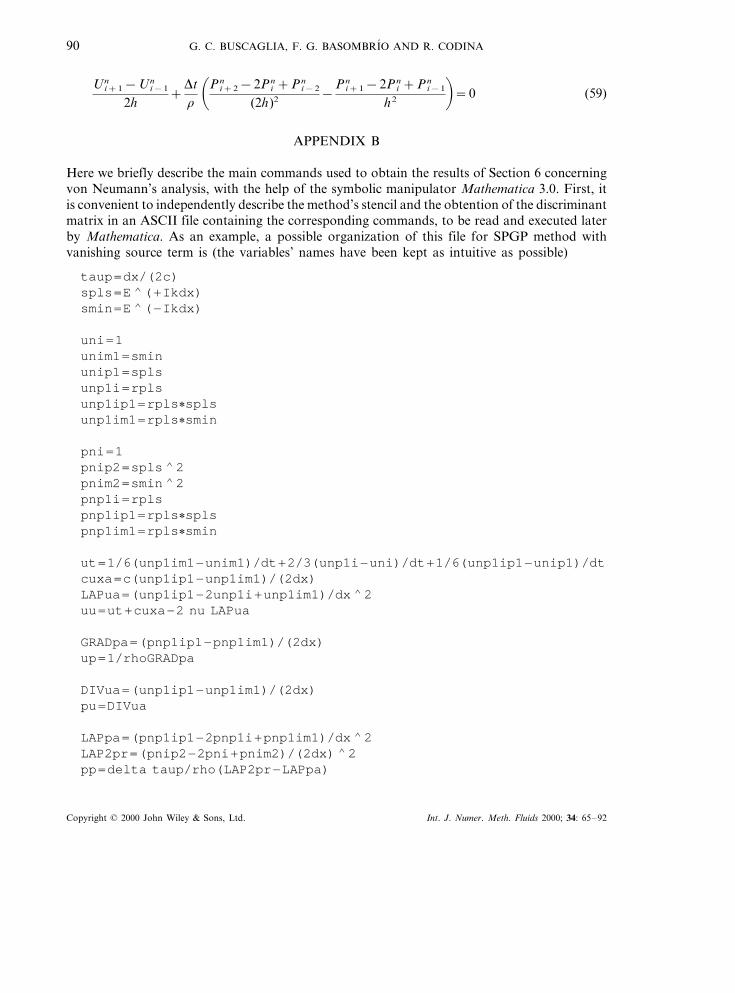
Here we briefly describe the main commands used to obtain the results of Section 6 concerningvon Neumann’s analysis, with the help of the symbolic manipulator Mathematica 3.0. First, itis convenient to independently describe the method’s stencil and the obtention of the discriminantmatrix in an ASCII file containing the corresponding commands, to be read and executed laterby Mathematica. As an example, a possible organization of this file for SPGP method withvanishing source term is (the variables’ names have been kept as intuitive as possible)

taup=dx/(2c)spls=E � (+Ikdx)smin=E � (−Ikdx)

uni=1unim1=sminunip1=splsunp1i=rplsunp1ip1=rpls �splsunp1im1=rpls �smin

pni=1pnip2=spls �2pnim2=smin �2pnp1i=rplspnp1ip1=rpls �splspnp1im1=rpls �smin

ut=1/6(unp1im1−unim1)/dt+2/3(unp1i−uni)/dt+1/6(unp1ip1−unip1)/dtcuxa=c(unp1ip1−unp1im1)/(2dx)LAPua=(unp1ip1−2unp1i+unp1im1)/dx �2uu=ut+cuxa−2 nu LAPua

GRADpa=(pnp1ip1−pnp1im1)/(2dx)up=1/rhoGRADpa

DIVua=(unp1ip1−unp1im1)/(2dx)pu=DIVua

LAPpa=(pnp1ip1−2pnp1i+pnp1im1)/dx �2LAP2pr=(pnip2−2pni+pnim2)/(2dx) �2pp=delta taup/rho(LAP2pr−LAPpa)



Let the name of this file be spgp.mat. Then, the essential commands for Mathematica ’s sessiondefining all the necessary explicit functions are

BB ‘‘spgp.mat’’matr={{uu,up},{pu,pp}}det=Det[matr]/.{nu− \1/Reynolds,c− \1,rho− \1,dx− \DX,dt− \C}roots=rpls/.Solve[det= =0,rpls]omega[n – ,delt – ,Rey – ,kk – ,dx – ,dt – ] �

I/dtLog[root[[n]]/.{delta− \delt,Reynolds− \Rey,k− \kk,DX− \dx,C− \dt}]romega[n –,delt –,Rey – ,kk – ,dx – ,dt – ] �Re[omega[n,delt,Rey,kk,dx,dt]]iomega[n –,delt –,Rey – ,kk – ,dx – ,dt – ] �Im[omega[n,delt,Rey,kk,dx,dt]]period[n –,delt –,Rey –,kk –,dx –,dt – ] �2Pi/romega[n,delt,Rey,kk,dx,dt]perrel[n –,delt –,Rey – ,kk – ,dx – ,dt – ] �period[n,delt,Rey,kk,dx,dt]/dttau [n – ,delt – ,Rey – ,kk – ,dx – ,dt – ] �−4.6/iomega[n,delt,Rey,kk,dx,dt]taurel[n – ,delt – ,Rey – ,kk – ,dx – ,dt – ] � tau[n,delt,Rey,kk,dx,dt]/dt

For the preceding commands, n=1, 2 stands for root’s number. ‘omega’ (v) is defined byr=e−IvDt.

REFERENCES

1. Franca L, Frey S. Stabilized finite element methods: II. The incompressible Navier–Stokes equations. ComputerMethods in Applied Mechanics and Engineering 1992; 99: 209–233.

2. Franca L, Hughes T, Stenberg R. Stabilized finite element methods. In Incompressible Computational FluidDynamics, Gunzburger M, Nicolaides R (eds). Cambridge University Press: Cambridge, 1993; 87–107.

3. Chorin AJ. Numerical solution of the Navier–Stokes equations. Mathematics of Computation 1968; 22: 745–762.4. Temam R. Sur l’approximation de la solution des equations de Navier–Stokes par la methode des pas

fractionnaires (I). Archi6e of Rational Mechanics and Analysis 1969; 32: 135–153.5. Colella P, Puckett EG. Modern numerical methods for fluid flow. http://patzek.berkeley.edu/PE/modern–

numerical–methods–for–flu.htm, 1994.6. Daniels H, Peters A. Solving large incompressible time-dependent flow problems on scalable parallel systems. In

Solution Techniques for Large-Scale CFD Problems, Habashi WG (ed.). Wiley: New York, 1995; 27–40.7. Guermond J-L, Quartapelle L. Calculation of incompressible viscous flows by an unconditionally stable projection

FEM. Journal of Computational Physics 1997; 132: 12–33.8. Guermond J-L, Quartapelle L. On stability and convergence of projection methods based on pressure Poisson

equation. International Journal for Numerical Methods in Fluids 1998; 26: 1039–1053.9. Nonino C, Comini G. An equal-order velocity–pressure algorithm for incompressible thermal flows. Part 1:

formulation. Numerical Heat Transfer 1997; B32: 1–15.10. Nonino C, Comini G. An equal-order velocity–pressure algorithm for incompressible thermal flows. Part 2:

validation. Numerical Heat Transfer 1997; B32: 17–35.11. Simo JC, Armero F. Unconditional stability and long-term behavior of transient algorithms for the incompressible

Navier–Stokes and Euler equations. Computer Methods in Applied Mechanics and Engineering 1994; 111: 111–154.12. Habashi W, Peeters M, Robichaud M, Nguyen V-N. A fully-coupled finite element algorithm, using direct and

iterative solvers, for the incompressible Navier–Stokes equations. In Incompressible Computational Fluid Dynam-ics, Gunzburger M, Nicolaides R (eds). Cambridge University Press: Cambridge, 1993.

13. Zienkiewicz OC, Codina R. A general algorithm for compressible and incompressible flow—part I. The split,characteristic-based scheme. International Journal for Numerical Methods in Fluids 1995; 20: 869–885.

14. Codina R, Blasco J. A finite element formulation for the Stokes problem allowing equal velocity–pressureinterpolation. Computer Methods in Applied Mechanics and Engineering 1997; 143: 373–391.

15. Codina R, Blasco J. Stabilized finite element method for the transient Navier–Stokes equations based on apressure gradient projection. Computer Methods in Applied Mechanics and Engineering 2000; 182: 277–300.



16. Codina R, Blasco J. Analysis of a finite element approximation of the stationary Navier–Stokes equations usingequal velocity–pressure interpolation. Numerische Mathematik, in press.

17. Codina R. Stabilization of incompressibility and convection through orthogonal sub-scales in finite elementmethods. Computer Methods in Applied Mechanics and Engineering, in press.

18. Hughes T. Multiscale phenomena: Green’s function, the Dirichlet-to-Neumann formulation, subgrid scale models,bubbles and the origins of stabilized formulations. Computer Methods in Applied Mechanics and Engineering 1995;127: 387–401.

19. Lew A. El metodo de elemento finitos en entornos computacionales de alta performance. Master’s thesis, InstitutoBalseiro, 1998.

20. Codina R. A stabilized finite element method for generalized stationary incompressible flows. Computer Methodsin Applied Mechanics and Engineering, in press.

21. Idelsohn S, Storti M, Nigro N. Stability analysis of mixed finite element formulations with special mention ofequal-order interpolations. International Journal for Numerical Methods in Fluids 1995; 20: 1003–1022.

22. Wolfram S. Mathematica (2nd edn). Addison-Wesley: Reading, MA, 1991.23. Bouard R, Coutanceau M. The early stage of development of the wake behind an impulsively started cylinder for

40BReB104. Journal of Fluid Mechanics 1980; 101: 583–607.24. Tanahashi T, Okanaga H. GSMAC finite element method for unsteady incompressible Navier–Stokes equations

at high Reynolds numbers. International Journal for Numerical Methods in Fluids 1990; 11: 479–499.25. Gresho P. Incompressible fluid dynamics: some fundamental formulation issues. Annual Re6iew of Fluid Mechanics

1991; 23: 423–453.


Fourier analysis of an equal-order incompressible flow solver stabilized by pressure gradient...

Documents

Transcript of Fourier analysis of an equal-order incompressible flow solver stabilized by pressure gradient...